Master of Science Thesis

Aerodynamic performance of a wind-turbine rotor

by means of OpenFOAM

by

Evangelos Giannopoulos

November 2016

KTH Royal Institute of Technology

Department of Mechanics

SE-100 44Stockholm, Sweden

2

TITLE: Aerodynamic performance of a wind-

turbine rotor by means of OpenFOAM

AUTHOR: Evangelos Giannopoulos

SUPERVISOR: Dr. Antonio Segalini

PARTNER: KTH Royal Institute of Technology

INSTITUTION: Department of Mechanics

INDUSTRIAL PARTNER: Vattenfall AB (YRLF)

INDUSTRIAL SUPERVISOR: Eric Lillberg

NUMBER OF PAGES: v, 43

i

Abstract

In order for wind-farm operators to deal with challenges regarding their fleet

management, it is useful for them to estimate their units’ performance for

different conditions. To perform such estimations, Computational Fluid

Dynamics (CFD) may be used.

This project focuses on the development of a CFD model for the aerodynamic

analysis of wind turbine rotors, depending on their surface roughness. The work

has been carried out in collaboration with the KTH Royal Institute of Technology

and the Vattenfall AB R&D department.

The open-source software OpenFOAM has been used to develop the desired

model. A rigid body incompressible steady state, Reynolds-Averaged Navier-

Stokes equations, k – ω SST CFD case has been set up. The NREL 5-MW rotor

geometry has been used and the effect of four different surface roughness height

values {1mm, 0.5mm, 100 μm, 30 μm} on its aerodynamic performance has

been investigated for an incoming wind velocity of 10m/s. The referred

roughness height values have been applied on the whole rotor surface. A 120°

wedge type computational domain of unstructured mesh has been developed for

the present simulations.

The results indicate that a roughness-height increase leads to earlier flow

separation over the blade suction side and increases the turbulent area of the

boundary layer. That leads to a decrease for the extracted Torque and the Thrust

force on the wind turbine rotor. Moreover, it is concluded that the rotor

aerodynamic performance is more sensitive to low roughness heights rather than

to high ones.

Key words: wind turbine, rotor, performance, CFD model, boundary layer,

roughness

ii

Acknowledgements

At this point I would like to thank my supervisors, Dr. Antonio Segalini from the

Mechanics department of the KTH Royal Institute of Technology and Eric

Lillberg from the Vattenfall AB R&D department. I appreciate their patience and

the guidance that they have both offered me throughout this work.

I would also like to thank the colleagues from Vattenfall AB for creating a

motivating but also relaxed working environment for me throughout this project.

Special thanks to Panos Jagalos from the Vattenfall AB Wind team for his

unconventional support and professional guidance.

Thanks to Prof. Vasilis Riziotis and Dr. Dimitris Manolas from the Fluids

department of the National Technical University of Athens Mechanical

Engineering school for their support throughout this work.

Thanks to Hugo Olivares Espinosa, from the Earth Science department of the

Uppsala University, for sharing parts of his work.

Last but not least, thanks to all my friends and family members for their support

throughout every step of my life. It was only with your help that I have managed

to carry out this effort.

iii

Contents

1. INTRODUCTION ........................................................................................... 1

1.1 Motivation and Objectives .......................................................................................... 4

1.2 Thesis layout ............................................................................................................... 7

2. THEORY AND BACKGROUND ....................................................................... 9

2.1 Wind Turbine Aerodynamics ....................................................................................... 9 2.1.1 2D Aerodynamics ....................................................................................................... 11 2.1.2 Boundary Layer and Separation ................................................................................. 12 2.1.3 Skin Friction Drag ....................................................................................................... 13 2.1.4 Pressure Drag ............................................................................................................. 14 2.1.5 The effect of roughness .............................................................................................. 14

2.2 The Reynolds-Averaged Navier-Stokes equations ......................................................14

2.3 Using Computational Fluid Dynamics .........................................................................17

2.4 Related studies done .................................................................................................18 2.4.1 The NREL 5MW wind turbine ..................................................................................... 18 2.4.2 Studies on roughness ................................................................................................. 19

3. PREPROCESSING ....................................................................................... 21

3.1 Mesh .........................................................................................................................21

3.2 Boundary conditions and numerical schemes ............................................................24

3.3 Wall function .............................................................................................................25

3.4 The Multiple Reference Frame approach ...................................................................26

4. RESULTS AND DISCUSSION ........................................................................ 28

4.1 Smooth surface results ..............................................................................................28 4.1.1 Relative velocity around the blade ............................................................................. 28 4.1.2 The wake behind the rotor ......................................................................................... 30

4.2 The effect of roughness .............................................................................................35

5. CONCLUSION AND OUTLOOK .................................................................... 39

5.1 Thesis outcome ..........................................................................................................39

5.2 Future work ...............................................................................................................40

APPENDIX A. OPENFOAM FVSCHEMES FILE ....................................................... 41

APPENDIX B. ROUGHNESS EFFECT ON BL AND K ............................................... 42

REFERENCES ...................................................................................................... 45

iv

Nomenclature

BC Boundary Condition(s)

CFD Computational Fluid Dynamics

CV Control Volume

DNS Direct Numerical Simulations

HAWT Horizontal Axis Wind Turbine

k Turbulent kinetic energy

LES Large Eddy Simulations

MRF Multi Reference Frame

NREL National Renewable Energy Laboratory

nut Kinematic turbulence viscosity

PDE Partial Diferential Equations

r Radial distance from the axis of rotation

RANS Reynols Averaged Navier Stokes

Re Reynolds number

RET Renewable Energy Technology

SST Shear Stress Transport

TSR Tip Speed Ratio

u flow velocity

Urel Relative velocity

VAWT Vertical Axis Wind Turbine

WT Wind Turbine

WTs Wind Turbines

2D Two dimensional

δ Boundary Layer thickness

ω Turbulence dissipation rate

ρ Fluid density

v

List of Figures

Figure 1.1. OECD electricity generation from renewables: 1971-2014 [3] .................1 Figure 1.2. CO2 emissions per kWh of electricity generation [3] ................................1

Figure 1.3. Increase in the global installed wind capacity [5] ......................................2 Figure 1.4. Electricity production wind capacity in Sweden ........................................2 Figure 1.5. Vattenfall's Wind Power Generation since 2011 [8] ...................................3 Figure 1.6. Main components of a HAWT [11] ............................................................4 Figure 1.7. Schematic 2-D representation of surface roughness [13] ...........................5 Figure 1.8. Different roughness sources [14] ................................................................5 Figure 1.9. Vortex generators on WT blades [15], [16] ................................................6 Figure 1.10. Work flow chart of the thesis' main core ..................................................7 Figure 2.1. Schematic representation of the distribution of axial velocity and pressure

along the rotor axis [17] ..............................................................................................10

Figure 2.2. Schematic representation of the aerodynamic forces generated by an airfoil

..................................................................................................................................... 11 Figure 2.3. Generic profile of the BL over a flat plate [21] ........................................12

Figure 2.4. Attached (a) and separated flow (b) around an airfoil [24] ......................13 Figure 3.1. Domain’s boundaries ................................................................................22 Figure 3.2. Mesh refinement close to the blade, r/R=0.71 ..........................................22 Figure 3.3. Layering around the blade ........................................................................23

Figure 3.4. A zoom in the layers around the blade ......................................................23 Figure 3.5. Blade along with spinner ..........................................................................24

Figure 3.6. Rotational (red) and stationary (grey) regions ..........................................26 Figure 3.7. Air modeled to rotate around the blade in the rotating region ..................27 Figure 4.1. relative velocity distribution, r/R=0.08 ....................................................28

Figure 4.2. relative velocity distribution, r/R=0.16 ....................................................29

Figure 4.3. Relative velocity distribution, r/R=0.48 ...................................................29 Figure 4.4. relative velocity distribution, r/R=0.71 ....................................................29 Figure 4.5. Streamlined representation of the relative velocity field, r/R=0.71 .........30

Figure 4.6. Velocity wake behind the blade, plane in the direction normal to the blade

motion, domain of ~13M cells ....................................................................................31

Figure 4.7. Velocity wake behind the blade, plane in the direction normal to the blade

motion, domain of ~24M cells ....................................................................................31

Figure 4.8.Velocity wake behind the blade, plane in the direction normal to the blade

motion, domain of ~33M cells ....................................................................................32 Figure 4.9.Velocity wake behind the blade, blade cross sectional plane at 40m height,

view from above, blade motion from bottom to top, domain of ~13M cells ..............32

Figure 4.10. Velocity wake behind the blade, blade cross sectional plane at 40m height,

view from above, blade motion from bottom to top, domain of ~24M cells ..............32 Figure 4.11. Velocity wake behind the blade, blade cross sectional plane at 40m height,

view from above, blade motion from bottom to top, domain of ~33M cells ..............33 Figure 4.12.Rotor power predictions for different incoming wind velocities ............34 Figure 4.13. Rotor Thrust for different incoming wind velocities ..............................35 Figure 4.14. Relative velocity around a smooth and a rough blade, at r/R=0.71,

TSR=7.53, rotor diameter=126m ................................................................................36

Figure 4.15. Streamlined relative velocity around a smooth and a rough blade, at

r/R=0.71, TSR=7.53, rotor diameter=126m ................................................................36 Figure 4.16. Roughness effect on Torque ...................................................................37 Figure 4.17. Roughness effect on Thrust ....................................................................37

1

1. Introduction

Over the past decades there has been a growing concern about the world’s climate

change. Mitigation of carbon dioxide (CO2) emissions has been high in the agenda of

the Paris climate conference (COP21) in December 2015. The final agreement focuses

on limiting the world average temperature increase below 2°C as well as the need for

global emissions to peak as soon as possible. The EU has approved the April-2016-

Paris agreement putting it in force since 4 November 2016 [1]. According to the

International Energy Agency (IEA) 2016 World Energy Outlook [2], although the CO2

emissions for 2015 have stalled, the current reduction rates are not enough to support

limiting global warming by less than 2 °C. Based on the same report and the IEA 2040

scenario, the estimated continuous growth in energy-related CO2 emissions by 2040

means that we are far from keeping close to the Paris Agreement’s goal to reach a peak

in emissions as soon as possible.

Securing further CO2-emissions-free energy sources seems necessary in order to

develop a sustainable society. Renewable Energy Technology (RET) has already been

playing a key role to that and the relevant power production has increased its world

share over the past years. The IEA has reported a significant growth of electricity

generation from renewables across the OECD countries over the past 20 years, as may

be seen in Figure 1.1. That growth goes with a total reduction rate in the carbon

intensity of electricity generation, which is stronger for the European part of the OECD

countries, as shown in Figure 2.1. [3]

Figure 1.1. OECD electricity generation from renewables: 1971-2014 [3]

Figure 1.2. CO2 emissions per kWh of electricity generation [3]

2

Wind power generation, in particular, has been showing an average annual growth rate

of 22.1% for the period 1990-2015, within the OECD countries [4]. As reported from

the Global Wind Energy Council and shown in Figure 1.3, since 2000, the global annual

installed wind capacity has been growing steadily, with the exception of year 2013.

Especially after 2006, it seems that there has been a boost in the added wind capacity

worldwide [5].

Figure 1.3. Increase in the global installed wind capacity [5]

Sweden has been following the same trend while increasing its existent wind capacity

from almost 0.3 GW in 2006 to over 6 GW in 2015, as reported from the Wind Energy

Market Intelligence [6]. Figure 1.4 tracks the Swedish growth back to 1997.

Figure 1.4. Electricity production wind capacity in Sweden

The Swedish state-owned power producer Vattenfall AB, shifting its strategy towards

Wind Energy, has been steadily increasing its wind power generation since 2011. The

increase has been dramatic in 2015 as shown in Figure 1.5. [7], [8]

3

Figure 1.5. Vattenfall's Wind Power Generation since 2011 [8]

The figures above indicate that wind will possibly be among the main energy sources

of the upcoming years. Thus, a deep interest arises on the efficiency of wind power

units throughout their lifecycle. In order for Wind Energy to be economically viable,

the overall costs per power unit produced need to decrease.

Although new WT designs and innovative control systems have continuously been

developed, old units’ performance should not be neglected. According to the

International Renewable Energy Agency, a lifecycle cost breakdown for wind power in

seven countries has shown that Operation and Maintenance (O&M) costs account for

11% – 30% of the total Levelized Cost Of Energy of onshore units [9].

In order for a wind-farm operator to keep down the O&M costs, it is important to know

how to use the available equipment in the optimum way. To this end, it is crucial to be

updated on each unit’s components condition and expected performance. This way,

activities related to repairing, ordering new parts or not changing the status of a wind

unit can be better scheduled. The above process is summarized by the term fleet

management.

A key part of fleet management is estimating the performance of a wind turbine’s rotor

according to several parameters affecting it. Prior to getting into details of its

performance, it is worth describing what a wind turbine (WT) is as well as highlighting

its basic components.

Wind turbines (WTs) are machines designed to interact with the wind in a way that they

extract part of its kinetic energy converting it to useful mechanical energy. For most

WTs, this mechanical energy is used to rotate a moving component which, in turn,

induces rotation to a shaft mounted on a power generator. In other words, part of the

wind’s kinetic energy is transformed to shaft rotational speed necessary for a generator

to produce power. Depending on the direction of the shaft’s axis of rotation, such WTs

may be categorized in Horizontal Axis Wind Turbines (HAWTs) and Vertical Axis

Wind Turbines (VAWT) [10]. HAWTs dominate the share of installed wind power

3.4 3.63.9 4.1

5.8

0.8 0.7 0.6 0.7 0.9

0

1

2

3

4

5

6

7

2011 2012 2013 2014 2015

Win

d P

ow

er G

ener

atio

n [

TWh

]

Year

Vattenfall Wind Power Generation

Total Generation Generation in Sweden

4

capacity worldwide. The dominance of HAWT over VAWT also applies for the

activities of Vattenfall AB in collaboration with which this thesis has been carried out.

For this reason, the present work has been focused solely on the performance of

HAWTs.

The basic components of a HWAT are illustrated in Figure 1.6 and briefly described

below.

Figure 1.6. Main components of a HAWT [11]

Rotor: consists of the blades (or wings) and the spinner that is the connection between

the blades and the rotating shaft. Through the rotor, kinetic energy is extracted from the

wind so as to induce torque to the generator shaft.

Nacelle: hosts the gearbox and the power generator. The gearbox is placed between the

rotor and the generator. The rotor is not straightly connected to the shaft that is mounted

on the generator but rather to a larger low-speed shaft, able to stand big loads. The role

of the gearbox is to transform the low rotational speed of the large shaft to a high

rotational speed of the shaft mounted on the generator. The generator, is the actual

power-producing part of a WT.

Tower: it is where the nacelle-rotor system is based. It used to keep the rotor part on a

height that would let it experience higher wind velocities [10].

1.1 Motivation and Objectives

As mentioned earlier, the rotor performance is of high importance and its analysis is a

key part of the fleet management. Depending on the specific interest of the analysis,

performance may be measured in various ways. In this thesis performance is measured

5

in terms of Torque, Mechanical Power and Thrust that are analyzed in the next chapter.

What should be stressed is that the rotor performance is a result of various parameters,

the effect of which cannot be measured just by a change in the WT power output. A

way to overcome this obstacle and study the effect of a single parameter on the rotor

performance is by developing a model. The latter is by definition an approximation of

reality, where certain parameters affecting the investigated final result are kept constant

while the rest (variables) are given a degree of freedom. In this way, it is possible to

investigate the relationship among variables or their effect on the final result.

A parameter affecting the rotor performance is its surface roughness or simply

roughness. The latter refers to the variations in the height of the surface relative to a

reference plane [12]. Even for the smoothest surface, a very close look would reveal a

pattern qualitatively similar to the one in Figure 1.7 (two dimensional representation),

in which the mentioned reference plane is denoted as Mean Line.

Figure 1.7. Schematic 2-D representation of surface roughness [13]

For a WT rotor, roughness is an undesired characteristic that acts against its optimum

performance causing Mechanical Power output loss. Roughness may be caused by

various reasons such as dust particles transported within the wind, icing, insects hitting

the blades or erosion of the surface material as shown in Figure 1.8.

Figure 1.8. Different roughness sources [14]

A more detailed explanation on how roughness influences the performance of a WT

rotor is given in the relevant section of chapter 2. What is more important to understand

at this stage is how a WT operator may utilize information on the rotor’s surface

roughness to estimate its performance.

Although roughness is something that a WT operator may observe physically, it cannot

be straightly linked to a specific range change in the rotor’s performance. Based on

what has been explained above, a model can help in developing such a link. In other

6

words, a model may serve as a tool for an operator to translate the observed roughness

into an estimated change in the performance.

Taking a step further, different parameters may act in favor of the performance. A slight

change on the blades geometries by means of passive aerodynamic add-ons may be

considered as such. Passive aerodynamic add-ons are devices that are mounted on the

blades of a WT in order to help the rotor better react with the incoming wind flow and

extract more energy from it. An example of such add-ons is vortex generators (VGs)

that are shown in Figure 1.9. The left hand side of Figure 1.9 shows a real example of

VGs mounted on a blade section while the right hand side of the figure is a

representation of how VGs are placed on a WT rotor. In certain cases, VGs may be used

to recover some of the lost Mechanical Power due to the existence of roughness. They

can be incorporated in a model and act as another variable in the estimated performance

output.

Figure 1.9. Vortex generators on WT blades [15], [16]

The main objective of this work is to study the effect of roughness on the rotor

performance by means of Computational Fluid Dynamics (CFD). The latter allows to

model the flow around a WT rotor and estimate its performance by changing the desired

variables. It should be stressed that the actual focus is on capturing the change that

roughness induces in an estimated rotor performance rather than the accuracy of the

estimated performance itself.

A side goal is to develop a CFD tool that may serve as the basis for future parametric

studies on the performance of WT rotor, such as the one related to the influence of

VGs on it.

This project may also serve as a feasibility study, used to evaluate whether or not it is

worthy for an operator to further investigate on the above and move towards the

development of a highly accurate model.

An extra interest is on checking what it takes for such a tool to be developed by means

of the software OpenFOAM. The main reason for that is that OpenFOAM is an open-

source software, free of license-costs. Although a detailed manual is not available and

it takes some time for a beginner to become familiar with its use, it still seems to be a

sustainable investment, in the long run, for an organization to train its engineers on the

use of a simple software like that rather taking on high costs for more user-friendly

ones. Moreover, OpenFOAM allows a lot of interaction with the user giving the

freedom to manually set the equations and parameters describing a case.

7

1.2 Thesis layout

During the main core of this work, two main steps have been followed:

(a) The development of a CFD model for the simulation of a smooth surface rotor

(b) The study of the roughness effect on the performance of the same rotor

The above becomes clearer in a work flow chart representation made through Figure

1.10 below.

Figure 1.10. Work flow chart of the thesis' main core

It should be clarified that only the rotor of the selected WT is examined, without any

interaction with other WT components.

The biggest challenge is to create the initial model for a rotor with a smooth surface.

Once this is done, then the roughness performance effects investigation come as a faster

process.

The present report consists of four main sections. Starting with Chapter 2, the theory

behind the intended model development is described. At first, the basic principles of

WT aerodynamics are presented. What follows is an explanation of how the flow

boundary layer (BL) develops around a WT blade. Based on the latter, a description of

the Lift and Drag forces generation is made. It is, then, discussed how roughness is

expected to affect the aerodynamic performance of a WT rotor. Following to that we

show how we may move from a qualitative description of the wind flow around a WT

rotor to a quantitative one. To this end, the Navier-Stokes equations are presented along

with the way in which a Reynolds-Averaged Navier-Stokes model of two supporting

equations is developed after introducing turbulence to the problem. The need of

computer power for solving such problems is then stressed out. Finally, we highlight

similar studies done on smooth rotors and studies done on the effect of roughness on

the aerodynamic performance of rotors and airfoils.

In Chapter 3, a description of the CFD case setup is made. The characteristics of the

computational domain are defined as well as the boundary conditions of the problem.

We close the chapter by describing how the flow is solved in OpenFOAM by applying

the Multiple Reference Frame approach.

Chapter 4 is dedicated to the model output. At first, it is shown that a boundary layer

may be captured with the chosen case setup. We then present the CFD model’s output

for a smooth rotor in section 4.2, as shown in Figure 1.10. Before moving further, we

8

examine the effect of the near wake grid resolution on the developed model. After it is

checked that the physical meaning of the produced flow field is acceptable, we compare

the performance results of four different incoming wind velocities with other studies

done on the same rotor and with similar methods. Moving to section 4.3, the lightest

case version of the tried near wake grid resolutions, in terms of computational cost, is

selected and four different roughness heights are tried in the model for an incoming

wind velocity of 10m/s. The resulting trend is, then, compared with similar studies on

different rotors as well as with relevant observations made on airfoils’ performance.

We close the report with Chapter 5 where the main conclusions of the study are

summarized and recommendations for future work are made.

9

2. Theory and Background

In order to better understand and assess the results of the developed model, it is

necessary that the basic theory behind the investigated phenomena and the used method

is mentioned. The chapter starts with a description of basic principles related to WT

rotor aerodynamics and the forces acting on its blades. A closer look is, then, taken on

how the wind flow moves at a close distance around the blades’ surface, creating the

so called boundary layer (BL), as well as on the way that the latter is related to the

generated aerodynamic forces on the blades. In addition, the effect of roughness on the

aerodynamic forces acting on the rotor, changing its performance, is explained.

After a qualitative analysis of the examined phenomena, the need for a quantitative

description of the above is stressed. To this end, the use of Computational Fluid

Dynamics and the need of computing power are mentioned. What is described in

particular, are the Reynolds-Averaged Navier-Stokes equations along with the k – ω

SST turbulence model that completes them.

Finally, the main outcome of the most interesting studies examined during the project’s

literature review is highlighted and summarized in the chapter’s last section.

2.1 Wind Turbine Aerodynamics

As briefly explained in Chapter 1, a wind turbine extracts kinetic energy from the wind

and converts it to mechanical energy used to increase the rotational speed of a shaft.

Moreover, using the first law of thermodynamics and considering an isothermal flow,

which is usually the case for flows around WTs, we may end to the following relation

(eq. 2-1):

�̇� (𝑈2

2

2−

𝑈12

2) = −�̇�

(2-1)

which states that the change of kinetic energy of the flow in a streamtube equals to the

rate of work done by the system.

Taking into account the above, an incoming wind flow of velocity 𝑈∞ hitting a WT

rotor (simply rotor from now on) will be slowed down. The reduction of the wind flow

velocity is related to the kinetic energy extracted from it. At a specific snapshot of the

phenomenon, one may observe that the fluid particles that exchange energy with the

rotor affect the ones that have not yet reached it and so on. Furthermore, the particles

that have already exchanged energy with the WT rotor have been decelerated up to a

certain asymptotic value 𝑈𝑤. This becomes clearer in Figure 2.1.a that is a simplified

version of a top view of a rotor. The particles that are on the cross line defined by the

rotor have a velocity of 𝑈𝑑.

In addition, using Bernoulli’s theorem, for a steady flow, the compressibility and

viscosity of which are negligible, and for which the there is no change in the

gravitational potential energy occurs, pressure (p) and velocity (U) are related through

the following expression (eq. 2-2):

10

Figure 2.1. Schematic representation of the distribution of axial velocity and pressure along

the rotor axis [17]

𝑝

𝜌+

𝑈2

2= 𝑐𝑜𝑛𝑠𝑡𝑎𝑛𝑡

(2-2)

where ρ is the fluid (air for this study) density.

Since the wind velocity decreases in the way described above when hitting a rotor and

taking into consideration eq. 2-2, the pressure of the wind flow is expected to increase

from a free-stream point value 𝑝∞ to a value 𝑝𝑢 right before the rotor, drop drastically

right after the rotor to a value of 𝑝𝑑 and start increasing again till reaching the free-

stream value 𝑝∞. The above becomes clearer in Figure 2.1.b.

The wind applies a total force on a rotor of a diameter (d) that may be expressed as (eq.

2-3):

𝑇 = (𝑝𝑢 − 𝑝𝑑)𝐴𝑑 (2-3)

where 𝐴𝑑 is the rotor swept area (𝐴𝑑 = 𝜋𝑑2

4).

The T force is not equally distributed along the rotor blades. We call Thrust the

integrated T component in the direction of the rotor axis. In a similar way, the

integrated cross product of the local T components in the direction of the blade motion

with the local distance from the rotor axis (r) is called Torque. A clearer explanation

of Thrust and Torque is provided in section 2.1.1.

The Torque multiplied by the rotational speed of the shaft attached to the rotor gives

the mechanical power (Power in this report) of the latter.

The ratio of the Power to the available power in the wind (1

2𝜌𝐴𝑑𝑈∞

3 ) is defined as

power coefficient 𝐶𝑃.

Based on the Actuator Disk theory, it may be shown that for the power coefficient

there is a maximum of: 𝐶𝑃,𝑚𝑎𝑥 =16

27≈ 0.593

11

The above maximum is also called the Betz limit and it is an important note to be made

in order to understand that there is a maximum in the power that can be extracted from

the wind [17].

2.1.1 2D Aerodynamics

A clear way to understand how energy may be extracted from the wind and be

converted into mechanical power of the rotor is by looking at the forces acting on a

blade cross section (airfoil)1. This lead us to a two dimensional (2D) analysis as in

Figure 2.2 below.

Figure 2.2. Schematic representation of the aerodynamic forces generated by an airfoil

The point that first faces the flow is called leading edge while the point last being in

touch with it is called trailing edge. The chord is the line section connecting the leading

edge and the trailing edge. The angle of attack (α) is the angle between the Urel vector

and the chord. The upper-curved side of the airfoil is called the suction side and it is

the side where low pressure occurs for the flow, while the opposite side is the pressure

side where the flow pressure is higher than the one over the suction side [17].

The relative velocity 𝑈𝑟𝑒𝑙 is the actual flow velocity that the airfoil experiences. Its

vector is composed by adding the vector of the incoming wind velocity (𝑈∞) to the

vector of the blade cross section’s tangential velocity (𝑈𝑡𝑎𝑛𝑔 = 𝜔𝑟). The total

aerodynamic force acting on the airfoil is denoted by R. The composing vectors for R

is D (Drag) in the direction of the 𝑈𝑟𝑒𝑙 and L (Lift) in the direction perpendicular to the

direction of the 𝑈𝑟𝑒𝑙 [18], [19]. Low air pressure is generated on the suction side of the

airfoil, while high air pressure is developed on the pressure side. That pressure

difference induces the Lift force. Drag force may be understood as the force of the wind

opposing to the airfoil’s motion through it. Lift and Drag may be analyzed into their

1 A blade cross section may be perceived as a very thin airfoil

12

composing vectors in the direction of the airfoil motion (Y) and the direction of the

rotor axis (X) [20]. These components add up to the total aerodynamic force component

in the Y direction (𝑅𝑌) and the X direction (𝑅𝑋) respectively. The cross product of 𝑅𝑌

with the distance from the rotor axis r, gives the local Torque for this very thin airfoil

section of the blade. The sum of the local Torques of every blade section, multiplied by

the number of the rotor blades, gives the total Torque as described earlier. In the same

way, the sum of all local 𝑅𝑋 forces, multiplied by the number of the rotor blades, gives

the total Thrust.

The pressure forces around the airfoil also generate an aerodynamic torque M.

2.1.2 Boundary Layer and Separation

Far from the blade, the inertia effect is larger than the viscous one on the fluid particles.

However, very close to the blade, viscosity plays an important role for the flow. Due to

viscous forces, the air flow right on the blade surface has a zero velocity relative to the

latter (no-slip condition). As we move farther from the surface the velocity increases

till it reaches the so called free-stream velocity value, at a point after which viscous

forces do not influence the flow significantly. The region close to the surface, where

viscosity cannot be neglected, till the point where the flow reaches the free-stream

velocity is called boundary layer (BL). The distance between the surface and the point

where the flow reaches 99% of the free-stream velocity is called boundary layer

thickness (δ) [17].

In order to better understand the flow in a BL, a flat pate case may initially be analyzed.

Before the leading edge, the flow velocity profile is uniform. At the leading edge, right

on the surface, the flow velocity is zero. The no-slip condition leads the boundary layer

to grow, as shown in Figure 2.3 [17].

Figure 2.3. Generic profile of the BL over a flat plate [21]

A flow characteristic is the ratio of the inertia forces that act between its particles to the

viscous ones. This ratio is represented by the Reynolds number (Re) which is defined

as: 𝑅𝑒 =𝜌𝑈𝐿

𝜇 , where: μ is the dynamic viscosity of the fluid which is used to relate

13

the stresses applied on a fluid particle to its linear deformation and L is the characteristic

length that in the case of the flat plate is the horizontal distance from the leading edge.

A low Re indicates that viscous forces play an important role in the flow [22]. A

relatively stable flow, of low Re, which fluid particles follow a streamlined motion

without large fluctuations, is called laminar. Above a critical Re, inertia forces govern

over the viscous ones and the flow moves towards the so called turbulent regime where

its characteristics change to: unstable movement of fluid particles, chaotic fluctuations

in space and time, a wide spectrum of scales of swirling flow structures (eddies), high

diffusivity and dissipation of kinetic energy into heat [23]. In the turbulent regime, there

is mixing of fluid particles of high and low momentum and the flow BL is more

homogeneous than a laminar one. Moreover, a turbulent BL is thicker than a laminar

one, as shown in Figure 2.3. Before becoming turbulent, the flow passes from a

transition stage of a 𝑅𝑒 ≈ 5 ∙ 105 [17].

The transition region is not the same for every surface. When trying to estimate the

flow around another surface such as an airfoil, it may be easier to assume a turbulent

BL right from the stagnation point. The BL may then be estimated by using wall

functions which are models that set the average velocity of a turbulent flow at a certain

distance from the surface. In Chapter 3, where the pre-processing of this thesis work is

described, the specific wall function used for the project’s application is mentioned.

The flow is slower the closer we get to the surface. A favorable pressure gradient would

accelerate the fluid particles in the main flow direction. On the contrary, an adverse

pressure gradient decelerates the fluid in the opposite direction. At a certain point, the

pressure gradient might be strong enough to lead to a separation of flow. That point is

called the separation point. Figure 2.4 shows an attached and a separate flow around

an airfoil.

Downstream of the separation point, the fluid particles experience shear stresses from

the flow layers that still move forward and shear stresses in the opposite direction from

the boundary. In addition, an adverse pressure gradient pushes the flow backwards. As

a consequence, a flow recirculation, that is often seen as a recirculation bubble, might

occur in this region.

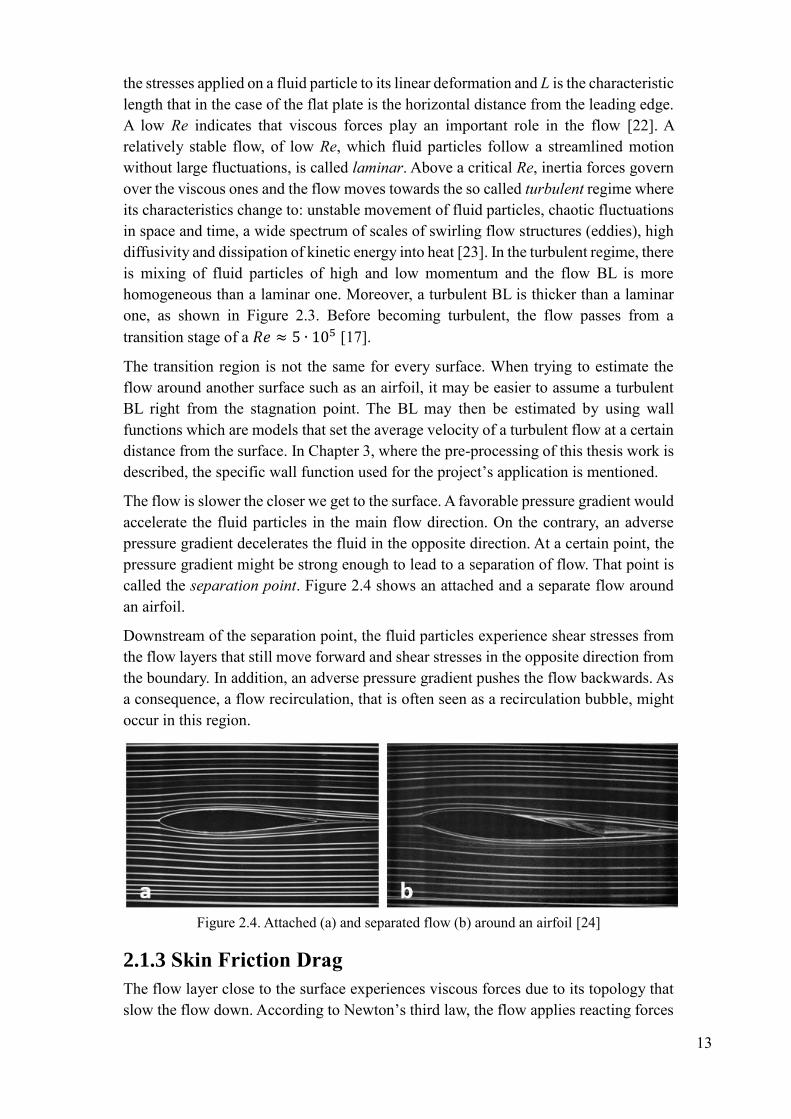
Figure 2.4. Attached (a) and separated flow (b) around an airfoil [24]

2.1.3 Skin Friction Drag

The flow layer close to the surface experiences viscous forces due to its topology that

slow the flow down. According to Newton’s third law, the flow applies reacting forces

14

on the surface, opposing an object through it. The sum of these reacting forces is called

skin friction drag.

Due to viscous effects within the fluid, the layer closest to the boundary slows the layer

right above it by imposing shear stresses on it. The slowing-down effect travels to the

upper levels of the flow. In a turbulent regime, it takes longer for this effect to be

diminished as we move farther from the boundary. That indicates that the BL gets

thicker. In other words, increase of the skin friction drag leads to higher turbulence and

thicker turbulent BL.

2.1.4 Pressure Drag

An object exposed in a flow usually experiences a pressure difference between the side

facing the flow and the side where the flow leaves the object. Such pressure difference,

generates a force in the direction of the incoming flow that opposes the motion of the

object through it. This force is called pressure drag. In case of a streamlined object,

where no flow separation occurs, there is no such pressure difference and thus no

pressure drag. On the contrary, when flow separation occurs, the pressure after the

separation point remains approximately equal to the static pressure on the separation

point which is lower than the pressure on the leading edge of the object [17]. Thus,

pressure drag is applied on the object. Similarly, in the case of an airfoil, when flow

separation occurs, the pressure distribution on it is such that pressure drag is generated.

2.1.5 The effect of roughness

More intense roughness is translated to stronger forces between the fluid and the

boundary. That, in turn, means that skin friction drag over the surface is increased.

Moreover, in the turbulent regime, roughness increase is expected to lead to an increase

of the BL thickness. A thicker BL is, in turn, easier to separate from the surface. Thus,

when roughness increases, separation may occur or appear earlier if already occurred.

That, in turn, means that the pressure drag increases. In addition, for an airfoil, if the

separation occurs very close to its maximum thickness point, a large wake will develop

after the separation point. That wake redistributes the flow over the rest of the surface

which may reduce the generated Lift on the airfoil. This condition is known as

aerodynamic stall [25].

To sum up, for an airfoil and a WT rotor blade, roughness increase is expected to lead

to an increase of both skin friction drag and pressure drag as well as to a decrease of

Lift.

2.2 The Reynolds-Averaged Navier-Stokes equations

The above analysis of WT aerodynamics is helpful in order to understand the main

phenomena taking place in the examined WT rotor application qualitatively. However,

this is not enough to make quantitative estimations of a rotor performance. To this end,

the flow should be described mathematically and a system of equations representing its

field should be solved.

15

A fluid flow is governed by three basic principles: (a) mass conservation, (b) the sum

of the forces on a fluid particle equals the rate of change of its momentum (Newton’s

second law) and (c) the sum of the rate of heat addition to a fluid particle and the rate

of work done on it is equal to the rate of change of its energy [26], [27].

The terms fluid element and fluid particle are used in the description of the above

principles. A fluid element may be considered as the smallest control volume (CV) for

which the assumption of the fluid as a continuum is valid. A fluid element is a fixed

volume in space and does not move with the fluid. A fluid particle is a moving CV that

follows the fluid flow and it experiences two rates of changes: one due to the change

of flow field in time and one because it moves to different locations within the flow

field where the conditions are different from each other. [28]

The mass conservation principle is expressed through the continuity equation (eq. 2-

4):

𝜕𝜌

𝜕𝑡+ 𝑑𝑖𝑣(𝜌𝐮) = 0

(2-4)

where 𝑑𝑖𝑣(𝜌𝒖) = 𝜕(𝜌𝑢)

𝜕𝑥+

𝜕(𝜌𝑣)

𝜕𝑦+

𝜕(𝜌𝑤)

𝜕𝑧 and {u, v, w} are the fluid velocity

components in the {x, y, z} Cartesian directions respectively.

Considering a Newtonian2 fluid, the momentum principle, is expressed through the

Navier-Stokes equations {eq. (2-5), (2-6), (2-7)}:

𝜕(𝑢)

𝜕𝑡+ 𝑑𝑖𝑣(𝑢𝐮) = −

1

𝜌

𝜕𝑝

𝜕𝑥+ ν 𝑑𝑖𝑣( 𝑔𝑟𝑎𝑑(𝑢)) + 𝑆

(2-5)

𝜕(𝑣)

𝜕𝑡+ 𝑑𝑖𝑣(𝑣𝐮) = −

1

𝜌

𝜕𝑝

𝜕𝑦+ ν 𝑑𝑖𝑣( 𝑔𝑟𝑎𝑑(𝑣)) + 𝑆

(2-6)

𝜕(𝑤)

𝜕𝑡+ 𝑑𝑖𝑣(𝑤𝐮) = −

1

𝜌

𝜕𝑝

𝜕𝑧+ ν 𝑑𝑖𝑣( 𝑔𝑟𝑎𝑑(𝑤)) + 𝑆

(2-7)

where ν is the kinematic viscosity of the fluid which is defined as the ratio of its

dynamic viscosity to its density (ν =𝜇

𝜌) and S is a denotation for a source term. A

source term expresses a body force3 contribution.

The system of the equations (2-4) – (2-7) may be solved given enough initial conditions

(boundary conditions).

If there is no heat transfer involved in the problem, the energy equation does not need

to be solved, thus, the energy balance principle is out of the scope of this study [26].

The properties of a turbulent flow are decomposed into a mean value and a fluctuating

2 A Newtonian fluid is a fluid for which a fluid particle’s viscous stresses are proportional to its rates of deformation 3 Forces on a fluid particle are categorized in two types: the surface forces {pressure, viscous} and the body forces

{gravity, centrifugal, Coriolis, electromagnetic}

16

component superimposed on it. The mean value is denoted with a capital letter while

the fluctuating component with a lower case letter stressed. For example, the flow

velocity, at a certain point, is written as 𝑢(𝑡) = 𝑈(𝑡) + 𝑢′(𝑡). This type of expressing

a property is called the Reynolds decomposition.

Considering the Reynolds decomposition for an incompressible turbulent flow (such as

the one of the examined flow around a WT rotor), the continuity equation is

transformed to the continuity equation for the mean flow (eq. 2-8):

𝑑𝑖𝑣𝐔 = 0

(2-8)

With the same considerations, the Navier-Stokes equations are transformed to the so

called Reynolds-Averaged Navier-Stokes (RANS) equations {eq. (2-9), (2-10), (2-

11)}:

𝜕(𝑈)

𝜕𝑡+ 𝑑𝑖𝑣(𝑈𝐔) = −

1

𝜌

𝜕𝑃

𝜕𝑥+ ν 𝑑𝑖𝑣( 𝑔𝑟𝑎𝑑(𝑈))

+1

𝜌[𝜕(−𝜌𝑢′2̅̅ ̅̅ )

𝜕𝑥+

𝜕(−𝜌𝑢′𝑣′̅̅ ̅̅ ̅̅ )

𝜕𝑦+

𝜕(−𝜌𝑢′𝑤′̅̅ ̅̅ ̅̅ )

𝜕𝑧]

(2-9)

𝜕(𝑉)

𝜕𝑡+ 𝑑𝑖𝑣(𝑉𝐔) = −

1

𝜌

𝜕𝑃

𝜕𝑦+ ν 𝑑𝑖𝑣( 𝑔𝑟𝑎𝑑(𝑉))

+1

𝜌[𝜕(−𝜌𝑢′𝑣′̅̅ ̅̅ ̅̅ )

𝜕𝑥+

𝜕(−𝜌𝑣′2̅̅ ̅̅ )

𝜕𝑦+

𝜕(−𝜌𝑣′𝑤′̅̅ ̅̅ ̅̅ )

𝜕𝑧]

(2-10)

𝜕(𝑊)

𝜕𝑡+ 𝑑𝑖𝑣(𝑊𝐔) = −

1

𝜌

𝜕𝑃

𝜕𝑧+ ν 𝑑𝑖𝑣( 𝑔𝑟𝑎𝑑(𝑊))

+1

𝜌[𝜕(−𝜌𝑢′𝑤′̅̅ ̅̅ ̅̅ )

𝜕𝑥+

𝜕(−𝜌𝑣′𝑤′̅̅ ̅̅ ̅̅ )

𝜕𝑦+

𝜕(−𝜌𝑤′2̅̅ ̅̅ ̅)

𝜕𝑧]

(2-11)

Compared to the laminar Navier-Stokes equations, the RANS equations include six additional

stresses. Three normal stresses: 𝜏𝑥𝑥 = −𝜌𝑢′2̅̅ ̅̅ , 𝜏𝑦𝑦 = −𝜌𝑣′2̅̅ ̅̅ , 𝜏𝑧𝑧 = −𝜌𝑤′2̅̅ ̅̅̅ and three shear

stresses: 𝜏𝑥𝑦 = 𝜏𝑦𝑥 = −𝜌𝑢′𝑣′̅̅ ̅̅ ̅, 𝜏𝑥𝑧 = 𝜏𝑧𝑥 = −𝜌𝑢′𝑤′̅̅ ̅̅ ̅̅ , 𝜏𝑦𝑧 = 𝜏𝑧𝑦 = −𝜌𝑣′𝑤′̅̅ ̅̅ ̅̅ . These

additional turbulent stresses are called Reynolds stresses. The Reynolds stresses are

related to the momentum exchange among the fluid particles due to convective

transport by the eddies, which causes the faster moving fluid layers to be decelerated

and the slower moving layers to be accelerated [26].

The system of equations (2-8) – (2-11) is not closed even if boundary conditions (BC)

are provided. In order to close the system, there have been several turbulence models

developed. One them is the two-equations-based k – ω SST (Shear Stress Transport)

model that relates the turbulent kinetic energy (k) with its specific dissipation rate (ω).

17

The model is appropriate for external aerodynamic applications and it has been, thus,

selected as the proper model to be used for this study. An extra reason for selecting the

k – ω SST turbulence model is that, according to Sagol et al. [14], it seems to be the

most accurate model when it comes to capturing the effect of WT blades’ surface

roughness on the flow. Details on the included equations of the model may be found in

(Versteeg and Malalasekera) [26].

The RANS equations focus on the mean flow and the effect of turbulence to its

properties. It should be noted that RANS equations are able to resolve large eddies

(Integral scale) but model the effect of smaller eddies to the flow field rather than

compute their exact formation. Different approaches may resolve the eddies and thus

the whole flow with higher accuracy. The Large Eddy Simulations (LES) and the Direct

Numerical Simulations (DNS) are used for that purpose. Large Eddy Simulations are

able to compute the formation of eddies up to a certain filter scale within a turbulent

flow but model the effect of the smaller ones like in the RANS method. Direct

Numerical Simulations resolve the formation of all eddies [26], [29].

Although the LES and DNS approach lead to higher accuracy, the computational cost

is high as well. For the present study, where it is not necessary to resolve the turbulent

fluctuations in detail and the interest is about the time-averaged properties of the flow,

the RANS equations constitute a method that is expected to give satisfactory results.

2.3 Using Computational Fluid Dynamics

In the previous section, the need for a quantitative approach of the flow description was

stressed. That, in turn, led to the development of a system of equations describing the

flow mathematically. However, in order to get an estimation of the flow properties in

space and time, the above system of equations needs to be solved. To this end, the

Computational Fluid Dynamics (CFD) method is used. CFD is the process of solving

the partial differential equations describing a flow in order to obtain a description of

the complete flow field of interest in space and time [27].

A CFD problem is defined within certain geometrical boundaries. A set of closed

boundaries defines the region in which the flow properties are going to be computed.

This region is called computational domain. A computational domain is split to a

number of control volumes (CV) cells that, in turn, define the so called computational

mesh (or simply mesh). The process of splitting the computational domain in several

cells is called meshing. In order to simulate a flow within a certain domain, the fluid

properties in each and every cell should be computed.

Since certain similarities may be observed among the equations describing the flow, a

single form of all of them may be introduced:

𝜕(𝜌𝛷)

𝜕𝑡+ 𝑑𝑖𝑣(𝜌𝛷𝒖) = 𝑑𝑖𝑣(𝛤𝑔𝑟𝑎𝑑𝛷) + 𝑆𝛷

(2-12)

where Φ is a general variable that can be replaced with each flow variable, Γ is the

diffusion coefficient and 𝑆𝛷 the source term for the property Φ. Equation (2-12) is

18

called a transport equation.

The 𝑑𝑖𝑣(𝜌𝛷𝒖) part is called convective term, while 𝑑𝑖𝑣(𝛤𝑔𝑟𝑎𝑑𝛷) is called diffusive

term.

Integrating equation (2-12) over a three dimensional CV leads to the expression below

(eq. 2-13):

∫𝜕(𝜌𝛷)

𝜕𝑡

𝐶𝑉

𝑑𝑉 + ∫ 𝑑𝑖𝑣(𝜌𝛷𝒖)𝑑𝑉

𝐶𝑉

= ∫ 𝑑𝑖𝑣(𝛤𝑔𝑟𝑎𝑑𝛷)𝑑𝑉

𝐶𝑉

+ ∫ 𝑆𝛷

𝐶𝑉

𝑑𝑉

(2-13)

Solving the transport equation over the cells of an entire domain, provides the way that

the fluid properties change in space and time. This approach is called the finite volume

method.

The more control volumes a domain is split to, the more accurate flow solution may be

achieved. Depending on the resolution, a computational mesh may be characterized

either as fine or coarse.

A mesh should not, necessarily, be of the same resolution in every region of a domain.

For instance, in the case of simulating the air flow around a WT rotor, a higher mesh

resolution is needed close to the blade where the flow changes are more intense, while

a lower mesh resolution may be enough far from the blade. Last but not least, in order

for a stable CFD solution to be achieved, the mesh should obey several quality

requirements such as cells’ skewness close to zero, cells’ aspect ratio close to 1 and

smoothness in the change of the cells’ size between neighboring mesh zones [26].

A CFD solution for a complex problem, such as studying the flow around a WT rotor,

would not be possible without the use of modern computers or clusters of them that can

handle big computational costs.

2.4 Related studies done

2.4.1 The NREL 5MW wind turbine

The United States National Renewable Energy Laboratory (NREL) has released a study

on a 5MW rated power WT, the geometry of which has been defined by the NREL

itself. An aerodynamic analysis, based on the NREL in-built tool FAST, has been

carried out as a part of the same study [30]. The NREL 5MW WT geometry as well as

the results from its aerodynamic analysis have been a validation reference for various

works aiming to study the flow around wind turbines.

Chow and van Dam [31] have developed the OVERFLOW2 numerical simulation

model to solve RANS equations with a k – ω SST turbulence model regarding the

NREL 5MW rotor. One of their goals has been to show that flow separation over the

inboard part of a WT leads to significant power loss and investigate possible solutions

to recover part of it. However, for this thesis, the most important outcome of their study

is related to the near wake region mesh resolution. What they have shown is that low

mesh resolution for the near wake region leads to over-prediction of the total rotor

19

Torque and Thrust.

Dose et al. [32] have carried out an OpenFOAM based CFD study on the effect of blade

deflection on the aerodynamic performance of WT rotors. They have also developed a

k – ω SST turbulent model around the NREL 5MW rotor. Their study shows that there

is an increase of around 1% and around 4% for Power and Thrust respectively

when blade deflection is taken into account compared to cases where rigid blades

are examined. That power increase may be explained by an increase in the blade’s

angle of attack activated by a torsion deformation on the region closer to its tip. It

should be noted, though, that in the present thesis blade deflections have not been taken

into account.

2.4.2 Studies on roughness

Sagol et al. [14], have reviewed the effect of blades’ roughness on the flow field and

the power generation performance of a WT as well as the ability of various numerical

models to capture it. Various types of roughness elements4 have been investigated as

well as various intensities and locations of it. Their study outcome show that roughness

causes early transition from laminar to turbulent flow around the WT blades. It also

shows that the extent of the transition flow is longer and the turbulence intensity close

to the blades is increased. Furthermore, it is concluded that a WT tends to

underperform as its surface roughness elements’ size and density increases. In

addition, the blade’s leading edge region seems to be most sensitive to roughness, while

the latter shows little influence on the flow for the region close to the trailing edge.

Finally, the k – ω SST turbulence model has been selected as the most accurate

one, when it comes to capturing the effect of roughness on the flow around a wind

turbine.

Van Rooij and Timmer [33] have examined the effect of roughness on airfoils of

different thickness and structure, trying to relate its effect on their performance. The

RFOIL code has been used to represent the effect of blade rotation to the flow. As it is

concluded, “results from this code indicate that rotational effects dramatically

reduce roughness sensitivity effects at inboard5 locations of a blade”. As an extra

conclusion, it is stated that vortex generators on an airfoil reduce its sensitivity to

roughness, leading to better overall airfoil aerodynamic performance.

Huang et al. [34] have evaluated the roughness sensitivity indicators for different blade

airfoil sections in the spanwise direction for a pitch-regulated WT. The study focuses

on the two dimensional aerodynamics of an airfoil. It is pointed out that the Drag force

has little effect on the middle and inboard sections of the blade but significant one on

the outboard part where most of the wind energy is extracted. It is also concluded that

the generated Lift force decreases when the surface roughness increases, especially

when that increase is in the leading edge region.

Ren and Ou [35] have investigated the effect of roughness on the flow over the

NACA63-430 airfoil, which is widely used in the mid-sections of WT blades. Their

4 By the term roughness elements, types of roughness like dirt, ice, etc. are meant 5 Inboard indicates the region closer to the root of a blade while outboard indicates the region close to the blade tip

20

work has been based on RANS with a k – ω SST model. Their model has been first

validated against experimental data for a smooth case and a good agreement has been

observed. Different roughness heights have been tried on the tested airfoil. The results

indicate that airfoil aerodynamic performance is more sensitive to roughness

heights lower than 0.3mm and less for greater than 0.3mm ones. It is also

concluded that roughness has greater effect in the front 50% chord span of an airfoil

rather than in the back 50% of it.

21

3. Preprocessing

An OpenFOAM-software based CFD model has been developed for the scope of this

thesis. It has been attempted that solutions of low computational cost are achieved. The

goal is to create a model that is able to capture the effect of roughness on a WT three-

blade rotor aerodynamic performance.

The acceptable accuracy has been set as the one enough to show a certain trend for the

above. To this end, RANS type calculations have been performed on a computational

domain of moderate mesh refinement. The k – ω SST turbulence model has been

applied for reasons explained in section 2.4.3. The study focus has been on the total

Torque and total Thrust forces of the examined WT rotor. The total Torque and Thrust

are calculated as the sum of pressure and viscous forces for each blade point in the

direction of motion (Cartesian Y-axis in this model) and the direction of the undisturbed

wind (Cartesian Z-axis in this model) respectively.

Since the study focus has been on the region around the blade, less importance has been

given to the domain regions far from it. As it will be shown in Chapter 4, a mesh

refinement extending farther from the blade may improve the wake predictions which,

in turn, may affect the forces around the rotor. However, since this work may be

considered as a feasibility study for the goals stated in the first paragraph and since a

light solution model is to be developed in order to see whether or not a relevant trend

can be captured, a lower mesh resolution has been applied.

3.1 Mesh

In order to reduce the computational cost, the rotor has not entirely been considered in

the computational domain. Taking advantage of the fact that that – without the presence

of any other WT component – there is a 120° periodicity in the rotor geometry and the

flow around it, just one third of the rotor has been included in the model preprocessing

stage. The effect on the flow around a single blade from the other two is computed by

considering the so called cyclic boundary conditions (BC) as it is explained in the

following section. A rough illustration of how the computational domain looks like is

offered in Figure 3.1 below.

It should be noted that there is no actual rotor boundary but this imaginary patch is

used to show the interface between two regions: the rotating and the stationary one (see

section 3.3).

In order to avoid any computation disruption or influence of the outer boundary

(symmetrySide) to the blade, a distance of 9 ∙ (𝑏𝑙𝑎𝑑𝑒 𝑟𝑎𝑑𝑖𝑢𝑠) is kept between the two

patches. For the same reason, a distance of 2 ∙ (𝑏𝑙𝑎𝑑𝑒 𝑟𝑎𝑑𝑖𝑢𝑠) and 5 ∙ (𝑏𝑙𝑎𝑑𝑒 𝑟𝑎𝑑𝑖𝑢𝑠)

from the blade is kept for the inlet and the outlet patches respectively.

22

Figure 3.1. Domain’s boundaries

An unstructured mesh of ~13M cells has been used. Since the region around the blade

is the main focus of the study as explained above, the highest level of refinement has

been around the blade while the mesh gets coarser towards the surrounding boundaries.

Figure 3.2 shows how the mesh gets finer as we move closer to the blade, on a plane

normal to the blade spanwise direction at a height of 45m (r/R=0.71).

Figure 3.2. Mesh refinement close to the blade, r/R=0.71

In order for the aerodynamic forces to be properly calculated and the effect of

roughness on them to be better captured, the boundary layers around the blade surface

should be better estimated. To this end, an extra type of refinement – called layering –

has been applied around the blade boundary. This refinement is shown in Figure 3.3

and Figure 3.4 which actually provide a closer look of the Figure 3.2 above.

23

Figure 3.3. Layering around the blade

Figure 3.4. A zoom in the layers around the blade

The computational mesh has been generated using the OpenFOAM in-built meshing

snappyHexMesh utility. It is necessary that surface meshes are provided to

snappyHexMesh for every boundary patch included in the computational domain. The

corresponding surfaces have been designed and meshed by using the SALOME

software. The most challenging part has been the surface meshing process of the blade.

For this project, blade is considered as the WT blade itself along with one third of the

rotating component – called spinner – where actually the blades stand. This is

illustrated in Figure 3.5 below. It should be noted that the blade’s geometry is as

defined by NREL in the relevant report [30], while the spinner is not based on any

official document but rather designed to resemble an actual spinner. Since the main

wind energy extraction is expected to take place towards the outboard section of the

blade, the spinner should not play a key role in the examined rotor aerodynamics. The

rotor diameter is 126 m. Its performance has been tested for four incoming velocities

{8, 9, 10 and 11.4 m/s} with respective tip-speed ratio (TSR) of {7.54, 7.54, 7.53 and

6.93}. For this velocity range, the same pitch angle has been taken into consideration

as indicated in the NREL report [30]. The comparisons regarding roughness have been

performed for an incoming velocity of 10m/s.

24

Figure 3.5. Blade along with spinner

3.2 Boundary conditions and numerical schemes

The computational domain includes six boundaries, as in Figure 3.1: {blade, inlet,

outlet, symmetryUp, symmetryDown, symmetrySide}. It is reminded that there is no

rotor boundary included in the computational domain, but this patch is used to indicate

the interface between two different regions within the same domain.

The inlet and outlet boundaries are self-explained. Regarding the symmetryUp and

symmetryDown boundaries, those are considered to be neighboring with each other. In

other words, the flux going out of the symmetryDown boundary is seen as an incoming

flux for the symmetryUp one and vice versa. The BC condition best describing such a

neighboring relationship is the cyclic one.

The symmetrySide boundary resembles the region very far from the rotor, where wind

velocity and pressure may be considered same as the ones of the inlet. This boundary

may be physically considered as the sky in this model.

In the followed approach (see section 3.4), instead of a rotating blade, a stationary blade

with a rotating flow around it, is considered. That explains why a zero velocity BC has

been assigned for the blade.

The BC used for the velocity and pressure fields for every patch are summarized in

Table 3.1 below.

25

Table 3.1. Velocity and pressure conditions assigned on boundaries

boundary velocity pressure6

inlet 10 m/s zeroGradient

outlet 10 m/s 0 [m2/s2]

blade 0 m/s zeroGradient

symmetrySide 10 m/s zeroGradient

symmetryUp &

symmetryDown cyclic cyclic

The OpenFOAM simpleFoam utility for incompressible flows has been used for

solving this problem. The applied finite volume numerical schemes are defined in the

system/fvScheme file as in the Appendix A. More about the finite volume schemes

theory as well as the available OpenFOAM choices on them may be found in Versteeg

and Malalasekera [26] and the OpenFoam user guide [36] respectively.

3.3 Wall function

As mentioned in section 2.1.2, the BL may be estimated by using wall functions which

are models that set the average velocity of a turbulent flow at a certain distance from

the surface. The specific wall function used for the project’s application is given by eq.

3-1 below. It is reminded that by using wall functions, it is assumed that the BL is by

default in the turbulent regime.

𝑢𝑃𝐶𝜇

14⁄

𝑘1

2⁄

𝜏𝑤

𝜌

=1

𝜅ln (𝐸

𝜌

𝜇𝐶𝜇

14⁄

𝑘1

2⁄ 𝑦𝑃) −1

𝜅ln (1 + 𝐶𝑠

𝜌

𝜇𝐶𝜇

14⁄

𝑘1

2⁄ 𝐾𝑠)

(3-1)

𝒖𝑷: is the mean velocity of the fluid at point P

𝒚𝑷: is the distance from the point P to the wall

𝑪𝝁: is a constant related to the turbulence model and is equal to 0.09

𝒌: ss the turbulent kinetic energy

𝝉𝒘: is the wall shear stress

𝝆: is the fluid density

𝜿: is the von Karman constant, equal to 0.4187

𝑬: is an empirical constant, equal to 9.793

𝝁: is the dynamic viscosity of the fluid

𝑪𝒔: is the roughness constant that indicates the roughness distribution along the

surface. A value of 0.5 indicates an even distribution

𝑲𝒔: is the actual roughness height (e.g. for a sand grain type roughness, 𝐾𝑠 is the

actual height of a sand grain) and it is the parameter for which different values

have been tried out in this project.

6 For an incompressible problem, such as the examined one, OpenFOAM solves for the normalized-by-density static

pressure 𝑝∗ = 𝑝/𝜌.

26

3.4 The Multiple Reference Frame approach

As mentioned in the introduction, a steady-state approach has been applied on the

developed incompressible flow model. For steady-state incompressible solutions,

where rotation of boundaries and torque forces are investigated, OpenFOAM offers

certain approaches. For computational cost reasons, the Multi Reference Frame (MRF)

one has been selected for this case.

In the MRF approach and for the specific problem, two regions have been defined in

the computational domain. A rotating and a stationary one, as shown in Figure 3.6. The

red-shaded one is the rotating region and the grey-shaded one is the stationary region.

As stated earlier, in the first one, a rotating flow around the blade is considered rather

than a rotating blade. The axis of rotation is the axis of the whole rotor geometry

symmetry. In other words, a tangential velocity is imposed on the cells centers within

the rotating region. The cells in the stationary region may see the effect of the rotation

of the cells that belong to the rotating region. However, there is no rotational velocity

imposed on the cell centers of the stationary region.

The above is demonstrated in Figure 3.7. In the rotating region, the Coriolis force is

added as a source term in the governing equations. Moreover, for the cells belonging

to it, the tangential component is taken into account when computing for the velocity

which is taken as: 𝑈𝑟𝑒𝑙 = 𝑈𝑎𝑏𝑠 + 𝜔 ∗ 𝑟 .

Figure 3.6. Rotational (red) and stationary (grey) regions

27

Figure 3.7. Air modeled to rotate around the blade in the rotating region

28

4. Results and Discussion

The main focus of this chapter is to show how close the developed model stands in

respect to the initial expectations. It is, thus, important to take into account the lessons

learned from previous studies, as in Chapter 2, while judging on the specific model’s

outcome.

4.1 Smooth surface results

4.1.1 Relative velocity around the blade

Since the aerodynamic forces around the blades are the main scope of this thesis, the

relative velocity (Urel) distribution around it should also be examined. Such an

examination reveals the regions where flow separation is most expected to occur. This

can be done by observing the Urel around various blade cross sections along the blade.

Figure 4.1 – Figure 4.4 show the Urel for four selected representative cross sections: at

r/R=0.08, r/R=0.16, r/R=0.48 and r/R=0.71 respectively. Figure 4.5 is a streamlined

representation of Urel at r/R=0.71. The Cartesian X, Y and Z axes are assigned to the

undisturbed wind direction, the direction of the blade motion and the blade spanwise

direction respectively. With dark blue, Urel values equal to the minimum value stated

on the figures are represented, while with dark red, values equal to the maximum one

are represented.

From the figures, it may be observed that, in the blade inboard sections, early flow

separation occurs for incoming wind of 10m/s. It is reminded that the rotor diameter is

126m and the tip-speed ratio for that case is 7.53. The separation point is further

downstream, along the chord span, for the middle and outboard sections.

Figure 4.1. relative velocity distribution, r/R=0.08

29

Figure 4.2. relative velocity distribution, r/R=0.16

Figure 4.3. Relative velocity distribution, r/R=0.48

Figure 4.4. relative velocity distribution, r/R=0.71

30

Figure 4.5. Streamlined representation of the relative velocity field, r/R=0.71

4.1.2 The wake behind the rotor

Although the main focus is around the blade, the fact that the rotor’s velocity wake may

affect the blade region should not be neglected either. Due to the vortices developed in

the rotor’s wake, the latter may induce backward wind velocity as well. That would

slow down the incoming wind velocity seen by the rotor. It is, thus, important to

sufficiently resolve the wake up to a certain distance downstream the rotor.

In order for that to be supported, extra mesh refinement, extending in the region of

interest, is necessary. Figures 4.6 – 4.8 show the wake behind the blade in the examined

domain, as seen on a plane on the blade translation axis, for three different mesh

refinement extensions around the blade. In the first case (Figure 4.6), the mesh is

moderately refined up to a distance of 0.024R away from the blade in all directions,

leading to a domain of ~13M cells (case 1). In the second case (Figure 4.7), the mesh

is moderately refined within a cylinder of r = 1.59R extending from -0.095R upstream

the rotor till R downstream the rotor, on the axis of rotation, leading to a domain of

~24M cells (case 2). In the third case (Figure 4.8), the mesh is moderately refined

within a similar cylinder like the one of case two, with the same radius, but this time

extending from -R upstream the rotor till 2R downstream the rotor, on the axis of

rotation, leading to ~33M cells (case 3).

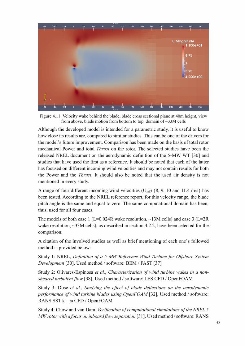
In Figures 4.9 – 4.11 the wakes of the same cases are illustrated on a blade cross

sectional plane at r/R=0.63. The view is as if an observer looks down the blade. The

blade motion direction is from the bottom to the top of the figures. The dark red values

refer to the region close to the leading edge, on the suction side. It should be stressed

that the figures show the field for U, not for Urel.

The results suggest that, for case 2 (~24M cells), there is a decrease of around -4% and

-2% for the total Torque and total Thrust respectively, compared to case 1 (~13M cells).

For case 3 (~33M cells), the decrease in the total Torque and Thrust is around -9.6%

and -3.9% respectively, compared to case 1 (~13Mcells). There is a clear over-

prediction of both Torque and Thrust as the wake region moves towards lower

31

resolution. This is in agreement with the study results of Chow and van Dam [31], as

mentioned in section 2.4.1.

On the other hand, a higher mesh resolution allows for better capturing the physics of

the problem. The wake can be better resolved when the refinement extends in a larger

region. That, however, increases the computational cost dramatically.

Since the purpose of developing this model is to check if a certain trend in the

aerodynamic performance due to roughness can be captured, a model of lower

refinement may be used. Consequently, the one that is computationally cheaper (first

case with low resolved wake) has been selected to carry out this study.

Figure 4.6. Velocity wake behind the blade, plane in the direction normal to the blade motion,

domain of ~13M cells

Figure 4.7. Velocity wake behind the blade, plane in the direction normal to the blade motion,

domain of ~24M cells

32

Figure 4.8.Velocity wake behind the blade, plane in the direction normal to the blade motion,

domain of ~33M cells

Figure 4.9.Velocity wake behind the blade, blade cross sectional plane at 40m height, view

from above, blade motion from bottom to top, domain of ~13M cells

Figure 4.10. Velocity wake behind the blade, blade cross sectional plane at 40m height, view

from above, blade motion from bottom to top, domain of ~24M cells

33

Figure 4.11. Velocity wake behind the blade, blade cross sectional plane at 40m height, view

from above, blade motion from bottom to top, domain of ~33M cells

Although the developed model is intended for a parametric study, it is useful to know

how close its results are, compared to similar studies. This can be one of the drivers for

the model’s future improvement. Comparison has been made on the basis of total rotor

mechanical Power and total Thrust on the rotor. The selected studies have been the

released NREL document on the aerodynamic definition of the 5-MW WT [30] and

studies that have used the first as a reference. It should be noted that each of the latter

has focused on different incoming wind velocities and may not contain results for both

the Power and the Thrust. It should also be noted that the used air density is not

mentioned in every study.

A range of four different incoming wind velocities (Uinf) {8, 9, 10 and 11.4 m/s} has

been tested. According to the NREL reference report, for this velocity range, the blade

pitch angle is the same and equal to zero. The same computational domain has been,

thus, used for all four cases.

The models of both case 1 (L=0.024R wake resolution, ~13M cells) and case 3 (L=2R

wake resolution, ~33M cells), as described in section 4.2.2, have been selected for the

comparison.

A citation of the involved studies as well as brief mentioning of each one’s followed

method is provided below:

Study 1: NREL, Definition of a 5-MW Reference Wind Turbine for Offshore System

Development [30]. Used method / software: BEM / FAST [37]

Study 2: Olivares-Espinosa et al., Characterization of wind turbine wakes in a non-

sheared turbulent flow [38]. Used method / software: LES CFD / OpenFOAM

Study 3: Dose et al., Studying the effect of blade deflections on the aerodynamic

performance of wind turbine blades using OpenFOAM [32], Used method / software:

RANS SST k – ω CFD / OpenFOAM

Study 4: Chow and van Dam, Verification of computational simulations of the NREL 5

MW rotor with a focus on inboard flow separation [31]. Used method / software: RANS

34

SST k – ω CFD / OVERFLOW2

Study 5: Zhao et al., Computational Aerodynamic Analysis of Offshore Upwind and

Downwind Turbines [39], Used method / software: RANS / U2NCLE [39]

Figure 4.12 and Figure 4.13 show where the present study stands in terms of predicted

rotor total Power and total Thrust, compared to the studies mentioned above.

The comparison suggests that both of the examined cases of the developed model have

the lowest Power prediction for all incoming wind velocities. The Thrust estimation

seems to be in closer agreement with other studies. Further investigation is needed to

understand the reasons of such discrepancies.

Although a low wake resolution model is not able to capture the wake physics correctly,

it can still be used for a comparative study on the blade region.

Figure 4.12.Rotor power predictions for different incoming wind velocities

1500

2000

2500

3000

3500

4000

4500

5000

5500

6000

7 7 . 5 8 8 . 5 9 9 . 5 1 0 1 0 . 5 1 1 1 1 . 5 1 2

Ro

tor

Po

we

r [k

W]

Incoming wind velocity [m/s]

Power vs U inf

present study 13M cells present study 33M cells NREL

Olivares-Espinosa et al. Dose et al. Chow and van Dam

Zhao et al.

35

Figure 4.13. Rotor Thrust for different incoming wind velocities

4.2 The effect of roughness

In this study, since roughness has been applied through wall functions, its intensity has

been considered as uniformly distributed on the blade surface. However, reality might

be different and roughness would rather be more intense in certain regions such as the

leading edge.

Four different roughness height values have been selected to be compared with a case

of smooth blade surface: 30μm, 100μm, 0.5mm and 1mm. They all refer to the exact

same case set up, in which roughness height is the only parameter that changes. The

driver for the selection of the above values has been the possible reasons leading to

blade degrading (erosion, mosquitos, dust, icing). Since this is a feasibility study, a

rough estimation has been performed to assign the specific roughness heights to the

respective roughness sources.

An incoming wind velocity of 10m/s has been applied for the comparisons.

The light low-wake-resolution version of the developed model (case 1, 13M cells) has

350

400

450

500

550

600

650

700

750

800

850

900

7 8 9 1 0 1 1 1 2

Ro

tor

Thru

st [

kN]

Incoming wind velocity [m/s]

Thrust vs U inf

present study 13M cells present study 33M cells NREL

Olivares-Espinosa et al. Dose et al. Chow and van Dam

36

been used. In the following figures, a comparison between a smooth blade case and a

case of 0.5mm roughness height has been selected as a representative one for

demonstrating the effect of roughness on the aerodynamic performance. Figure 4.14

provides a close look of the Urel distribution around the blade, at r/R=0.71. The effect

of roughness on the flow closer to the trailing edge may be detected. This becomes

clearer at Figure 4.15 which is a streamlined representation of Figure 4.14. Here it

becomes more obvious that roughness leads to earlier flow separation, as actually

expected. The same trend has been detected throughout the whole blade span but

r/R=0.71 has been selected for demonstration, since at the middle and outboard regions

is where the largest wind energy extraction is expected to take place.

The turbulence increase generated by the addition of roughness on the blade is

demonstrated in Appendix B, where plots of the BL development and turbulent kinetic

energy in it are presented for different x/c points of the blade suction side, at r/R=0.71.

Figure 4.14. Relative velocity around a smooth and a rough blade, at r/R=0.71, TSR=7.53,

rotor diameter=126m

Figure 4.15. Streamlined relative velocity around a smooth and a rough blade, at r/R=0.71,

TSR=7.53, rotor diameter=126m

37

The overall results indicate a that, in respect to the smooth surface case, there is a

Torque decrease of around -1%, -5%, -18% and -25% for the 30μm, 100μm, 0.5mm

and 1mm roughness height cases respectively. However, there is a decreasing trend for

the Thrust as well, with the respective figures being -0.5%, -2%, -8% and -11% for the

four cases.

Figure 4.16 illustrates the estimated Torque for each of the examined cases, while

Figure 4.17 shows the estimated Thrust for the same cases. By looking at the relative

changes, what can be drawn as a conclusion is that, both Torque and Thrust wise, the

rotor is more sensitive to small rather than large roughness heights. This follows the

trend indicated for an airfoil level by Ren and Ou [35], as mentioned in section 2.4.2.

Figure 4.16. Roughness effect on Torque

Figure 4.17. Roughness effect on Thrust

The recorded Torque loss for the rough cases may be explained by the fact that the

separation point moves towards the blade leading edge as the roughness height

increases and there is, thus, lower Lift generation.

2000

2100

2200

2300

2400

2500

2600

2700

2800

2900

3000

0 0.1 0.2 0.3 0.4 0.5 0.6 0.7 0.8 0.9 1 1.1

Torque

[kN

m]

roughness height [mm]

Torque vs roughness height

smooth

1mm

0.5 mm

100μm

30μm

560

570

580

590

600

610

620

630

640

650

660

0 0.1 0.2 0.3 0.4 0.5 0.6 0.7 0.8 0.9 1 1.1

Thrust

[kN

]

roughness height [mm]

Thrust vs roughness height

smooth

1mm

0.5mm

100μm

30μm

38

Regarding the Thrust decrease, this may be explained by the total decrease of its Lift

component due earlier flow separation.

39

5. Conclusion and Outlook

Estimating the aerodynamic performance of WT rotors may be of great importance for

wind farm operators in order to carry out a more efficient fleet management. Various

parameters may be taken into account when making such estimations. As such, surface

roughness seems to be a well-known problem for a rotor’s performance. It could be,

thus, useful for an operator to have a cost-effective tool for monitoring the effect of

surface roughness intensity on the aerodynamic performance of WT rotors. For the

development of such a tool, Computational Fluid Dynamics may be used.

This thesis deals with the development of a cost effective CFD model that may be used

as a tool for parametric studies on a WT rotor. The investigated parameter, in this work,

is blade surface roughness. The OpenFOAM open-source software has been used to

develop the desired model. A rigid body steady state RANS, k – ω SST CFD case has

been set up. The NREL 5-MW rotor geometry has been examined for this case. The

effect of four different surface roughness intensities – expressed through four

roughness height values {30 μm, 100 μm, 0.5 mm, 1 mm} respectively – on its

aerodynamic performance have been investigated, for an incoming wind velocity of

10m/s. The referred roughness height values have been applied on the whole rotor

surface. A 120° wedge type computational domain of an unstructured mesh has been

developed for the case.

The main focus of the solution has been the change that roughness induces in a

given/estimated rotor performance rather than the accuracy of the estimated

performance itself.

5.1 Thesis outcome

The main outcome of the model indicates that a roughness height increase leads to

earlier flow separation over the blade suction side. That leads to a decrease for the

Thrust force on the rotor and the extracted Toque by the latter. Moreover, it is concluded

that the rotor aerodynamic performance is more sensitive to low roughness heights

rather than to higher ones.

More specifically, in respect to a smooth surface case, there is a Torque decrease of 1%,

5%, 18% and 25% for the 30μm, 100μm, 0.5mm and 1mm roughness height cases

respectively. There is a decreasing trend for the Thrust as well, with the respective

figures being 0.5%, 2%, 8% and 11% for the four cases.

40

5.2 Future work

From the figures mentioned above, it may be concluded that the roughness effect on a

WT rotor’s performance can be captured with the present model and it may motivate

further parametric studies.

To this end, a more accurate model should be developed.

A mesh improvement could be the starting point. More specifically, a higher wake

region resolution, a better layering and a longer computational domain may be

considered.

Different incoming wind velocities as well as non-uniform roughness distribution could

also be tried out.

Finally, an investigation of vortex generators or other means that could possibly lead to

a Torque recovery are yet to be tried as well.

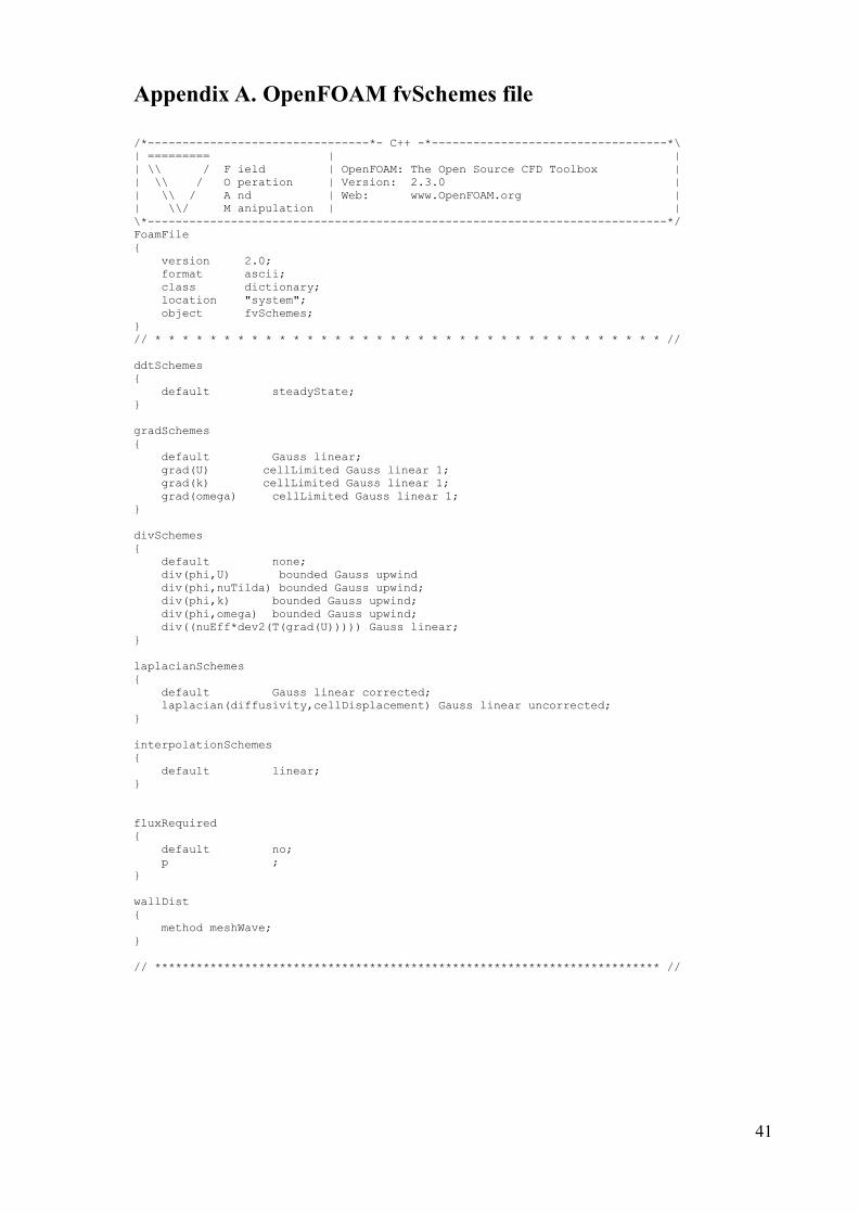
41

Appendix A. OpenFOAM fvSchemes file

/*--------------------------------*- C++ -*----------------------------------*\

| ========= | |

| \\ / F ield | OpenFOAM: The Open Source CFD Toolbox |

| \\ / O peration | Version: 2.3.0 |

| \\ / A nd | Web: www.OpenFOAM.org |

| \\/ M anipulation | |

\*---------------------------------------------------------------------------*/

FoamFile

{

version 2.0;

format ascii;

class dictionary;

location "system";

object fvSchemes;

}

// * * * * * * * * * * * * * * * * * * * * * * * * * * * * * * * * * * * * * //

ddtSchemes

{

default steadyState;

}

gradSchemes

{

default Gauss linear;

grad(U) cellLimited Gauss linear 1;

grad(k) cellLimited Gauss linear 1;

grad(omega) cellLimited Gauss linear 1;

}

divSchemes

{

default none;

div(phi,U) bounded Gauss upwind

div(phi,nuTilda) bounded Gauss upwind;

div(phi,k) bounded Gauss upwind;

div(phi,omega) bounded Gauss upwind;

div((nuEff*dev2(T(grad(U))))) Gauss linear;

}

laplacianSchemes

{

default Gauss linear corrected;

laplacian(diffusivity,cellDisplacement) Gauss linear uncorrected;

}

interpolationSchemes

{

default linear;

}

fluxRequired

{

default no;

p ;

}

wallDist

{

method meshWave;

}

// ************************************************************************* //

42

Appendix B. Roughness effect on BL and k

Below, there is a demonstration of plots of the BL and turbulent kinetic energy for

different x/c points {0.22, 0.43, 0.73} of the blade suction side, at r/R=0.71. Such plots

have been useful to ensure that the model moves towards the right direction when it

comes to estimating the turbulence increase in the BL around the blade. The same trend

is recorded across the whole blade span. The specific r/R height has been selected as a

representative one.

0

10

20

30

40

50

60

70

0 20 40 60 80 100

No

rmal

-to

-su

rfac

e d

ista

nce

[m

m]

Urel [m/s]

suction side BL profile (r/R = 0.71, x/c = 0.22)

smooth

0.5mm

0

10

20

30

40

50

60

70

0 20 40 60

No

rmal

-to

-su

rfac

e d

ista

nce

[m

m]

k [m2/s2]

suction side turbulence kinetic energy (k) profile (r/R = 0.71, x/c = 0.22)

smooth

0.5mm

43

0

10

20

30

40

50

60

70

0 20 40 60 80

No

rmal

-to

-su

rfac

e d

ista

nce

[m

m]

Urel [m/s]

suction side BL profile (r/R = 0.71, x/c = 0.43)

smooth

0.5mm

0

10

20

30

40

50

60

70

0 10 20 30 40 50

No

rmal

-to

-su

rfac

e d

ista

nce

[m

m]

k [m2/s2]

suction side turbulence kinetic energy (k) profile (r/R = 0.71, x/c = 0.43)

smooth

0.5mm

44

0

10

20

30

40

50

60

70

0 20 40 60

No

rmal

-to

-su

rfac

e d

ista

nce

[m

m]

Urel [m/s]

suction side BL profile (r/R = 0.71, x/c = 0.73)

smooth

0.5mm

0

10

20

30

40

50

60

70

0 10 20 30 40

No

rmal

-to

-su

rfac

e d

ista

nce

[m

m]

k [m2/s2]

suction side turbulence kinetic energy (k) profile (r/R = 0.71, x/c = 0.73)

smooth

0.5mm

45

References

[1] “European Comission, Climate Action,” 2017. [Online]. Available:

http://ec.europa.eu/clima/policies/international/negotiations/paris_en.

[2] International Energy Agency, “World Energy Outlook 2016,” 2016.

[3] International Energy Agency, “Recent trends in the OECD: energy and CO2

emissions,” 2016.

[4] International Energy Agency, “Renewable energy continuing to increase market share,”

2016. [Online]. Available: http://www.iea.org/newsroom/news/2016/july/renewable-

energy-continuing-to-increase-market-share.html. [Accessed: 01-Jan-2016].

[5] Global Wind Energy Council, “Global Wind Statistics 2015,” 2016.

[6] “The Wind Power.” [Online]. Available:

http://www.thewindpower.net/country_en_17_sweden.php.

[7] “Vattenfall Annual and Sustainability report 2015,” 2015.

[8] “Vattenfall.” [Online]. Available: https://corporate.vattenfall.com/about-

vattenfall/vattenfall-in-brief/.

[9] International Renweable Energy Agency, “RENEWABLE ENERGY

TECHNOLOGIES: COST ANALYSIS SERIES, Wind Power,” 2012.

[10] F. D. Bianchi, H. De Battista, and R. J. Mantz, “The Wind and Wind Turbines,” in Wind

Turbine Control Systems, 2007, pp. 7–28.

[11] “National Renewable Energy laboratory, Wind Energy Basics.” [Online]. Available:

https://www.nrel.gov/workingwithus/re-wind.html.

[12] B. Bhushan, “Surface Roughness Analysis and Measurement Techniques,” 2001.

[13] “The Home Of Surface Measurement.” [Online]. Available:

http://www.rubert.co.uk/faqs/roughness-parameters/.

[14] E. Sagol, M. Reggio, and A. Ilinca, “Issues concerning roughness on wind turbine

blades,” Renew. Sustain. Energy Rev., vol. 23, pp. 514–525, 2013.

[15] “Smart Blade, Performance Improvement for Wind Turbines.” [Online]. Available:

http://smart-blade.com/products-services/vortex-generators.html.

[16] “SENVION wind energy, Retrofits.” [Online]. Available:

https://www.senvion.com/global/en/wind-energy-solutions/service/retrofits/.

[17] A. Segalini, Wind Turbine Aerodynamics, Lecture notes. 2016.

[18] J. Gary L., “Wind Turbine Power,” in Wind Energy Systems, 2001, p. 4.1-4.55.

[19] Gurit, “Aerodynamics and Loads,” in Wind Energy Handbook, 2016.

[20] N. Hall, “National Aeronautics and Space Administration,” What is Drag. [Online].

Available: https://www.grc.nasa.gov/www/k-12/airplane/drag1.html.

[21] “VISCOUS INCOMPRESSIBLE FLOW, lecture 7.” [Online]. Available:

46

http://nptel.ac.in/courses/101103004/module5/lec7/3.html.

[22] C. von Ossietzky, “Viscosity and Reynolds Numbers.”

[23] A. . Johansson and S. Wallin, Turbulence lecture notes. Stockholm, 2012.

[24] M. van Dyke, An Album of Fluid Motion. Department of Mechanical Engineering,

Stanford University.

[25] “Boundary Layer Separation and Pressure Drag,” Aerospace Engineering, 2016.

[Online]. Available: http://aerospaceengineeringblog.com/boundary-layer-separation-

and-pressure-drag/.

[26] H. K. Versteeg and W. Malalasekera, An Introduction to Computational Fluid

Dynamics. 2004.

[27] J. F. Wendt et al., Computational Fluid Dynamics, AN INTRODUCTION, Third.

Springer.

[28] R. Fakhrai, “Conservation Equations, lecture notes.” 2015.

[29] R. Fakhrai, “Turbulence, lecture notes.” 2015.

[30] J. Jonkman, S. Butterfield, W. Musial, and G. Scott, “Definition of a 5-MW reference

wind turbine for offshore system development,” 2009.

[31] R. Chow and C. P. van Dam, “Verification of computational simulations of the NREL

5 MW rotor with a focus on inboard flow separation,” Wind Energy, 2012.

[32] B. Dose, B. Stoevesandt, and J. Peinke, “Studying the effect of blade deflections on the

aerodynamic performance of wind turbine blades using OpenFOAM.” pp. 2–5.

[33] R. P. J. O. M. van Rooij and W. A. Timmer, “Roughness Sensitivity Considerations for

Thick Rotor Blade Airfoils,” 2003.

[34] C. Huang, K. Yang, Q. Liu, L. Zhang, J. Bai, and J. Xu, “A study on performance

influences of airfoil aerodynamic parameters and evaluation indicators for the

roughness sensitivity on wind turbine blade,” Sci. China Technol. Sci., vol. 54, no. 11,

pp. 2993–2998, 2011.

[35] N. Ren and J. Ou, “Dust Effect on the Performance of Wind Turbine Airfoils,” J.

Electromagn. Anal. Appl., vol. 1, no. June, pp. 102–107, 2009.

[36] C. J. Greenshields, “OpenFOAM User Guide,” no. December. 2015.

[37] J. Jonkman, “FAST, An aeroelastic computer-aided engineering (CAE) tool for

horizontal axis wind turbines.” [Online]. Available: https://nwtc.nrel.gov/FAST.

[38] H. Olivares-Espinosa and S. Breton, “Characterization of wind turbine wakes in a non-

sheared turbulent flow,” in International Conference on Aerodynamics of Offshore

Wind Energy Systems and Wakes (ICOWES2013), 2013, no. June, pp. 435–449.

[39] Q. Zhao, C. Sheng, and A. Afjeh, “Computational Aerodynamic Analysis of Offshore

Upwind and Downwind Turbines,” J. Aerodyn., vol. 2014, 2014.