aerodynamic control of nasp-type.vehicles through … · nasa contractor report 177626 aerodynamic...
TRANSCRIPT

NASA Contractor Report 177626
-_J i:LC---"//y -
Aerodynamic Control of
NASP-Type.Vehicles ThroughVortex Manipulation
Volume IV
SimulationBrooke C. Smith, Carlos J. Su&rez, William M. Porada, and Gerald N. Malcolm
CONTRACT NAS2-13196September 1993
National Aeronautics andSpace Administration
(NASA-CR-17762b-Vo]-4) AERODYNAMICCONTROL 0F NASP-TYPE VEHICLES
THEOUGH VORTEX MANIPULATION, VOLUME
4 (Ei_etics International) 151 p
N96-15720
Unclas
G310Z 0190879
https://ntrs.nasa.gov/search.jsp?R=19940011247 2018-06-06T18:29:46+00:00Z

NASA Contractor Report 177626
Aerodynamic Control ofNASP-Type Vehicles ThroughVortex Manipulation
Volume IV
SimulationBrooke C. Smith, Carlos J. Su&rez, William M. Porada, and Gerald N. Malcolm
Eidetics International, Inc.
3415 Lomita Blvd.
Torrance, CA 90505
Prepared forAmes Research CenterCONTRACT NAS2-13196
September 1993
N/_ANational Aeronautics andSpace Administration
Ames Research CenterMoffett Field, California 94035-1000


TABLE OF (_ONTENT$
NOMENCLATURE ..................................................................................................................... viLIST OF FIGURES ..................................................................................................................... viiSUMMARY .................................................................................................................................. 1
1.02.03.0
4.05.06.0
7.08.0
9.010.0
11.012.0
PURPOSE ......................................................................................................................... 2REVIEW OF PNEUMATIC VORTEX CONTROL ......................................................... 2FULL SCALE AIRCRAFT DESCRIPTION ................................................................... 33.1. Characteristic Dimensions ................................................................................. 4OBJECTIVES .................................................................................................................... 4APPROACH ...................................................................................................................... 4TASKS ............................................................................................................................... 46.1 Static Aero Model From Wind Tunnel Tests ................................................... 4
6.2 Conventional and Pneumatic Control Modeling ............................................ 46.3 Develop Simple Control Laws With and Without Pneumatic Controls ...... 56.4 Pilot-In-The-Loop Simulation And Evaluation ................................................ 5WIND TUNNEL MODEL DESCRIPTION ..................................................................... 5STATIC AERODYNAMIC MODEL ................................................................................ 6
8.1 Static Aerodynamics ........................................................................................... 68.1.1 Longitudinal Aerodynamics ................................................................... 68.1.2 Lateral - Directional Aerodynamics ...................................................... 6
8.2 Conventional Controls ........................................................................................ 78.3 Pneumatic Controls, Static Effects .................................................................... 7
8.3.1 Yaw Moment Effects ................................................................................ 88.3.2 Computer Model Formulation ................................................................ 88.3.3 Roll Moment Effects ................................................................................. 8
8.3.4 Pneumatic Control Time Lag ................................................................. 9DYNAMIC AERODYNAMICS ........................................................................................ 9WIND TUNNEL WING ROCK RESPONSE ............................................................... 1010.1 Time Histories ..................................................................................................... 1010.2 Phase Plane Plots ............................................................................................. 1010.3 Summary Behavior And Dominant Trends ................................................... 11ONE-DEGREE-OF-FREEDOM WING ROCK SIMULATION ................................... 11WING ROCK LATERAL AERODYNAMICS ............................................................... 1112.1 Wind Tunnel Model Mass Moment of Inertia Estimation ............................ 1 1
12.2 Wing Rock Aerodynamic Models .................................................................... 1212.2.1 Absolute Value Model (First Order) ........................................ 13
12.2.1.1 Development of Model ........................................................ 1312.2.1.2 Evaluation of First Order Model Results .......................... 14
12.2.2 Parabolic Model (Second Order) ............................................ 1412.2.2.1 Evaluation of Second Order Model Results .................... 14
12.2.3 Higher Order Model (nth Order) .............................................. 1512.2.4 Remarks ....................................................................................... 15
12.3 Pneumatic Controls, Dynamic effects ............................................................ 1512.3.1 One Side Blowing ...................................................................... 16
12.3.1.1 CIo Effect ............................................................................... 1612.3.1.2 Damping Effect, CIp ............................................................. 17
III
PRECEENNG PAGE BLANK NOT FN.MED
13.0
14.0
15.0
16.0
12.3.2 Model Description ...................................................................... 1712.3.2.1 Model Validation Via Comparison With Wind
Tunnel Tests ......................................................................... 1712.3.3 Combined Blowing .................................................................... 1812.3.4 Pulsed Blowing .......................................................................... 18
FULL SCALE MASS PROPERTIES ........................................................................... 1813.1 Estimation Techniques ..................................................................................... 181DOF SIMULATION, SCALE EFFECTS ................................................................... 1914.1 Nondimensional Inertias, Dynamic Similitude ............................................. 20FULL SCALE CONTROL SYSTEM DEVELOPMENT ............................................ 2115.1 Methodology and Approach ............................................................................ 2115.2 Design Flight Condition .................................................................................... 2115.3 Design Criteria ................................................................................................... 2115.4 Longitudinal Flight Control System ................................................................ 2215.5 Lateral - Directional Flight Control System ................................................... 2315.6 Control Mixing Methodology ............................................................................ 2515.7 Static Trim Requirements ................................................................................. 2515.8 Pneumatic Control Implementation Schemes .............................................. 26
15.8.1 Non-Active Controls: Wing Rock Suppression .................... 2615.8.1.1 Steady Simultaneous Blowing .......................................... 2615.8.1.2 Pulsed Alternating Blowing ................................................ 27
15.8.2 Active Controls ........................................................................... 2715.8.2.1 Dithered Control ................................................................... 2715.8.2.2 Scheduled Proportion of Commanded Control ............. 2815.8.2.3 High Frequency / Low Frequency Mix ............................. 28
15.8.3 Implementations for Further Study ......................................... 2915.8.4 Demonstration Testbeds .......................................................... 29
MANNED SIMULATION ............................................................................................... 2916.1 ARENA Description ........................................................................................... 2916.2 Implementation ................................................................................................... 30
16.2.1 Winds, Turbulence ..................................................................... 3016.2.2 Instrumentation ........................................................................... 30
16.3 Evaluation Tasks ................................................................................................ 31
16.3.1 Glideslope and Localizer tracking .......................................... 3116.3.2 Bank-to-Bank Loaded Rolls ..................................................... 3116.3.3 Cross Wind Takeoff ................................................................... 32
16.4 Evaluation Matrix ............................................................................................... 3216.5 Results and Discussion .................................................................................... 32
16.5.1 Pilot Control Inputs .................................................................... 3316.5.1.1 Conventional Control Surfaces ......................................... 33
16.5.1.2 Forebody Blowing ................................................................ 3416.5.2 Landing Approach ..................................................................... 34
16.5.2.1 Partially Augmented, No Blowing ..................................... 3516.5.2.2 Partially Augmented With Pulsed Blowing ...................... 3516.5.2.3 Partially Augmented With Proportional Blowing ............ 3616.5.2.4 Fully Augmented, No Blowing ........................................... 3716.5.2.5 Fully Augmented With Proportional Blowing .................. 3816.5.2.6 Advantages Of Forebody Blowing With And Without
Full FCS Augmentation ...................................................... 39
iv

17.0
18.019.020.0
16.5.3 Loaded Roll ................................................................................. 39
16.5.4 Cross Wind Capability .............................................................. 4116.5.5 Handling Qualities ..................................................................... 42
JET BLOWING SYSTEM REQUIREMENTS ............................................................. 42
17.1 Blowing Coefficient And Blowing Sources ................................................... 4217.2 Potential Sources For High-Pressure Gas .................................................... 4517.3 Design Guidelines For Blowing System ........................................................ 4617.4 Utility Of Jet Blowing For Forebody Vortex Control ..................................... 47CONCLUSIONS ....................................................................................................... 49ACKNOWLEDGMENTS ............................................................................................... 49REFERENCES ............................................................................................................... 50
FIGURES ............................................................................................................... ,..................... 52
V

NOMENOLATURE
ArefbC
L
C_
rnjqV
vj(_, AOA
(t)
Phidot, pPhiddotP
Be
(_r
8e, I
iT)e,rIxxCNCmCnCICyCLACnt_CICp
Cnl3CIl
CIp
reference wing areawing spanwing chordreference length = total length of the model
momentum coefficient of blowing = rhj Vj / q Aref
mass flow rate of the blowing jetfree-stream dynamic pressurefree-stream velocityaverage exit velocity of the blowing jet
angle of attack
sideslip angle
roll angle
velocity vector roll angle
azimuth angle (from the windward meridian)roll rate, body axisroll acceleration, body axisperiod of wing rock oscillation
elevator deflection (+ down)
rudder deflection (+ right)
left elevon deflection
right elevon deflectionMoment of inertianormal force coefficientpitching moment coefficientyawing moment coefficientrolling moment coefficientside force coefficient
stability axis lift coefficientyawing moment incrementrolling moment incrementpressure coefficient
directional stability derivative
lateral stability derivative
roll moment rate derivative -aCI
oq(pb/2V)
vi

Figure 1 -
Figure 2 -
Figure 3 -
Figure 4 -
Figure 5 -
Figure 6 -
Figure 7 -
Figure 8 -
Figure 9 -
Figure 10 -
Figure 11 -
Figure 12-
Figure 13-
Figure 14-
Figure 15 -
Figure 16-
LIST OF FIGURES
Schematics of Wind Tunnel Model ..................................................... 53
Photos of Wind Tunnel Model ............................................................. 54
Schematics of Different Blowing Schemes ....................................... 55
Static Aerodynamic Model (Longitudinal Characteristics)a) CN, b) Cm ........................................................................................... 56
Static Aerodynamic Model (Longitudinal Characteristics)a) Static Stability, b) Static Margin ..................................................... 57
Static Aerodynamic ModelBasic Drag Polar (from DATCOM) ...................................................... 58
Drag Coefficient Increment due to LandingGear Extension ....................................................................................... 58
Static Aerodynamic Model (Directional Characteristics)Directional Aerodynamics and Conventional Control Effectson Yawing Moment ................................................................................ 59
Static Aerodynamic Model (Lateral Characteristics)Lateral Aerodynamics and Conventional Control Effectson Rolling Moment ................................................................................. 61
Aerodynamic Model of Pneumatic ControlEffect on Yawing Moment ..................................................................... 64
Aerodynamic Model of Pneumatic ControlEffect on Rolling Moment ...................................................................... 65
Roll Angle History of Wing Rock at Various Anglesof Attack (Wind Tunnel Test) ................................................................ 66
Phase Plots at (z = 25 ° (q = 958 Pa, Tail-On)(Wind Tunnel Test) ................................................................................ 67
Reduced Frequency of Wing Rock Motion (q = 958 Pa) ................. 68
Maximum Peak-to-Peak Amplitude of Wing Rock(q = 958 Pa) ............................................................................................ 68
Wing Rock Mathematical ModelRelationship between Damping Term and Roll Angle .................... 69
vii

Figure 17 -
Figure 18 -
Figure 19 -
Figure 20 -
Figure 21 -
Figure 22 -
Figure 23 -
Figure 24 -
Figure 25 -
Figure 26 -
Figure 27 -
Figure 28 -
Figure 29 -
Figure 30 -
Wing Rock Build-up at (z= 25° (q = 958 Pa, Tail-On)(Wind Tunnel Test) ................................................................................ 70
Results of First Order Wing Rock Model at (_ = 30 °a) Roll Angle History, b) Phase Plot ................................................... 71
Phase Plots at (z = 30 ° (q = 958 Pa, Tail-On)
(Wind Tunnel Test) ................................................................................ 72
Angular Velocity and Acceleration at e_= 30 °(Wind Tunnel Test) ................................................................................ 73
Results of Second Order Wing Rock Model at (z = 30 °a) Roll Angle History, b) Phase Plot ................................................... 74
Results of Second Order Wing Rock Model at (z = 25 °Wing Rock Build-up for a) t = 0 to 2 sec., b) t = 2 to 4 sec ............... 75
Phase Plots at (z = 25 ° for the Motion Shown in
Figure 22 (Part b) ................................................................................... 76
Results of nth Order Wing Rock Model at (z = 30 °Phase Plot ............................................................................................... 77
Effect of Aft Blowing on Wing Rock at (z = 30 °
(Wind Tunnel Test, Tail-On, CI_ = 0.0037)
a) Left Nozzle, b) Right Nozzle, c) Simultaneous Blowing ............. 78
Effect of Aft Blowing on Wing Rock at o_= 25 °(Wind Tunnel Test, Tail-On)
a) Right Nozzle, CI_ = 0.0028; b) Right Nozzle, Cp. = 0.0037 ........ 79
Results of Second Order Wing Rock Model at (z = 30 °
Wing Rock Suppression, CI.[ = 0.0037 ............................................... 80
Non-Dimensional Inertias for Three Example Aircraft .................... 81
Comparison of Wind Tunnel Model and Full ScaleConfiguration (Wing Rock Build-up)a)-b) Roll Angle, c)-d) Phase Plots ..................................................... 82
Comparison of Wind Tunnel Model and Full ScaleConfiguration (Steady Wing Rock)a)-b) Roll Angle, c)-d) Phase Plots ..................................................... 84
Jlo
VIII

Figure 31 -
Figure 32 -
Figure 33 -
Figure 34 -
Figure 35 -
Figure 36 -
Figure 37 -
Figure 38 -
Comparison of Wind Tunnel Model and Full Scale
Configuration (Wing Rock Suppression, CI_ = 0.0037)a)-b) Roll Angle, c)-d) Phase Plots ..................................................... 86
Longitudinal Flight Control System .................................................... 88
Lateral-Directional Flight Control System ......................................... 89
Arena Hardware Configuration ........................................................... 92
Profiles of Mean Wind Velocity over Level Terrains ofDifferent Roughness (from Ref. 27) .................................................... 93
Approach and Landing Simulation for the NASP-typeConfiguration with Partially Augmented Flight ControlSystem (No Forebody Blowing); a) Variation in Altitude (-Z) andHorizontal Excursions (Y), b) Cross-Track and Altitude Errors,c) Angles of Attack and Sideslip, d) Angles of Attack and Roll,e) Angles of Attack and Roll, f) Angles of Attack and Roll,g) Roll Angle and Roll Rate, h) Roll Angle and Roll Rate,i) Flight Velocity and Mach Number, j) Dynamic Pressure,k) Rudder Deflection Angle, I) Aileron Deflection Angle ................. 94
Approach and Landing Simulation for the NASP-typeConfiguration with Partially Augmented Flight ControlSystem and Pulsed Forebody Blowing; a) Variation inAltitude (-Z) and Horizontal Excursions (Y), b) Cross-Trackand Altitude Errors, c) Angles of Attack and Sideslip,d) Angles of Attack and Roll, e) Flight Velocity and MachNumber, f) Dynamic Pressure, g) Rudder Deflection Angle,h) Aileron Deflection Angle, i) Blowing Coefficient (LeftNozzle), j) Blowing Coefficient (Right Nozzle), k) AccumulativeTotal Mass Flow Requirements (Left), I) Accumulative TotalMass Flow Requirements (Right) ...................................................... 100
Approach and Landing Simulation for the NASP-typeConfiguration with Partially Augmented Flight ControlSystem and Proportional Forebody Blowing; a) Variation inAltitude (-Z) and Horizontal Excursions (Y), b) Cross-Trackand Altitude Errors, c) Angles of Attack and Sideslip,d) Angles of Attack and Roll, e) Flight Velocity and MachNumber, f) Dynamic Pressure, g) Rudder Deflection Angle,h) Aileron Deflection Angle, i) Blowing Coefficient (Left Nozzle),j) Blowing Coefficient (Right Nozzle), k) Blowing Coefficient(Expanded Time Scale), I) Mass Flow Rate (Left Nozzle),m) Mass Flow Rate (Right Nozzle), n) Accumulative TotalMass Flow Requirements (Left and Right) ...................................... 106
ix

Figure 39 -
Figure 40 -
Figure 41 -
Figure 42 -
Figure 43 -
Figure 44 -
Figure 45 -
Figure 46 -
Approach and Landing Simulation for the NASP-typeConfiguration with Fully Augmented Flight Control System(No Forebody Blowing); a) Variation in Altitude (-Z) andHorizontal Excursions (Y), b) Cross-Track and Altitude Errors,c) Angles of Attack and Sideslip, d) Roll Angle, e) FlightVelocity and Mach Number, f) Dynamic Pressure, g) RudderDeflection Angle, h) Aileron Deflection Angle ................................ 113
Approach and Landing Simulation for the NASP-typeConfiguration with Fully Augmented Flight ControlSystem and Proportional Forebody Blowing; a) Variation inAltitude (-Z) and Horizontal Excursions (Y), b) Cross-Trackand Altitude Errors, c) Angles of Attack and Sideslip, d) RollAngle, e) Flight Velocity and Mach Number, f) DynamicPressure, g) Rudder Deflection Angle, h) Aileron DeflectionAngle, i) Blowing Coefficient (Left Nozzle), j) BlowingCoefficient (Right Nozzle), k) Mass Flow Rate (Left Nozzle),I) Mass Flow Rate (Right Nozzle), m) Accumulative Total MassFlow Requirements (Left), n) Accumulative Total Mass FlowRequirements (Right) .......................................................................... 117
Loaded Roll Simulation for the NASP-type Configurationwith Fully Augmented Flight Control System (No ForebodyBlowing); a) Velocity Vector Roll Angle, b) Cross-Track(Y-Coordinate), c) Altitude (-Z), d) Angle of Attack, e) RudderDeflection Angle, f) Aileron Deflection Angle, g) Body-AxisRoll Rate, h) Body-Axis Yaw Rate ..................................................... 124
Loaded Roll Simulation for the NASP-type Configurationwith Fully Augmented Flight Control System and ProportionalForebody Blowing; a) Velocity Vector Roll Angle, b) Cross-Track(Y-Coordinate), c) Altitude (-Z), d) Angle of Attack, e) RudderDeflection Angle, f) Aileron Deflection Angle, g) Body-AxisRoll Rate, h) Body-Axis Yaw Rate, i) Blowing Coefficient,h) Mass Flow Rate, j) Accumulative Total Mass Requirements... 128
Comparison Between Velocity Vector Roll Rate forthe Non-Blowing and Blowing Cases .............................................. 133
Nozzle Total Pressure Requirements vs. Nozzle Diameterfor Stated Reference Conditions ....................................................... 134
Variation in Altitude and Lateral Excursions from Extended
Vertical Plane Centered on the Runway for SimulatedApproach and Landing Task With Fully Augmented ControlSystem Including Proportional Forebody Blowing ........................ 134
Deviation from the Flight Path for Example Approach andLanding Task Described in Fig. 2 ..................................................... 135

Figure 47 - Variation in Dynamic Pressure for Example Approach andLanding Task Shown in Fig. 2 ........................................................... 135
Figure 48 - Variation in Vehicle Attitude with Time for Example Approachand Landing Task Shown in Fig. 2; a) Roll Angle,b) Angles of Attack and Sideslip ....................................................... 136
Figure 49 - Variation in Blowing Momentum Coefficient with Time forExample Approach and Landing Task Shown in Fig. 2a) Left Nozzle, b) Right Nozzle ......................................................... 137
Figure 50 - Variation in Jet Nozzle Mass Flow Rate with Time forExample Approach and Landing Task Shown in Fig. 2a) Left Nozzle, b) Right Nozzle ......................................................... 138
Figure 51 - Accumulative Total Mass Flow Requirements Integratedover the Total Time for Example Approach and LandingTask Shown in Fig. 2; a) Left Nozzle, b) Right Nozzle ................ 139
Figure 52 - Mass Flow Variation with Stagnation Temperature of the Airat the Nozzle Exit for the Reference Conditions Shown ............... 140
xi

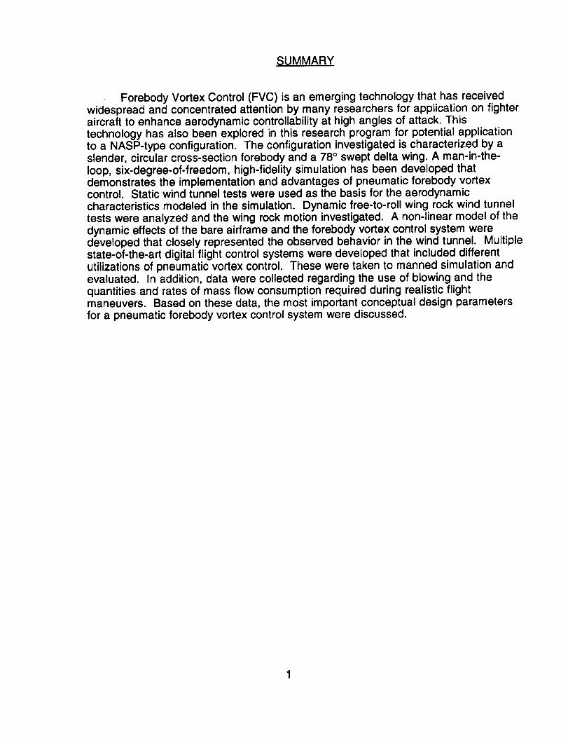
SUMMARY
Forebody Vortex Control (FVC) is an emerging technology that has receivedwidespread and concentrated attention by many researchers for application on fighteraircraft to enhance aerodynamic controllability at high angles of attack. Thistechnology has also been explored in this research program for potential applicationto a NASP-type configuration. The configuration investigated is characterized by aslender, circular cross-section forebody and a 78 ° swept delta wing. A man-in-the-loop, six-degree-of-freedom, high-fidelity simulation has been developed thatdemonstrates the implementation and advantages of pneumatic forebody vortexcontrol. Static wind tunnel tests were used as the basis for the aerodynamiccharacteristics modeled in the simulation. Dynamic free-to-roll wing rock wind tunneltests were analyzed and the wing rock motion investigated. A non-linear model of thedynamic effects of the bare airframe and the forebody vortex control system weredeveloped that closely represented the observed behavior in the wind tunnel. Multiplestate-of-the-art digital flight control systems were developed that included differentutilizations of pneumatic vortex control. These were taken to manned simulation andevaluated. In addition, data were collected regarding the use of blowing and thequantities and rates of mass flow consumption required during realistic flightmaneuvers. Based on these data, the most important conceptual design parametersfor a pneumatic forebody vortex control system were discussed.

AERODYNAMIC CONTROL OF NASP-TYPE VEHICLESTHROUGH VORTEX MANIPULATION
VOLUME IV: SIMULATION
1.0 B.U.B.P_Q,_E
The purpose of the simulation task is to demonstrate the feasibility andimplementation of pneumatic forebody vortex control on an advanced aircraftconfiguration. The aircraft is geometrically similar to the configuration tested inwater tunnel and low-speed wind tunnel tests. The flight regime to be explored ishigh angle of attack (i.e., low speed) where other similar designs have difficultydue to reduced stability and control power (e.g., max gross weight return tolanding and cross wind take-off).
Water tunnel and wind tunnel static tests are discussed in Volumes I and II,respectively. Volume III summarizes the results of the wing rock experimentsperformed first in the Eidetics water tunnel and later in the NASA Ames ResearchCenter 7 x 10 ft wind tunnel. This volume of the Final Report presents thedevelopment of a man-in-the-loop simulation that includes the static and dynamicaerodynamic behavior presented in the preceding volumes.
2.0 REVIEW OF PNEUMATIC VORTEX CONTROl
One of the most significant and ambitious programs of the aerospace industry inthe near future will be the development and eventual flight test of the National Aero-Space Plane (NASP, X-30). Much of the technological research now being conductedto support the development of a NASP concentrates on the hypersonic regime. Inaddition to excellent hypersonic performance, however, high-quality low-speed flightmust also be achieved. Conceivably, configurations optimized for hypersonic flightmay experience adverse low-speed aerodynamic phenomena dominated byseparated and vortex flows, such as wing rock or non-zero yawing moments at zerosideslip, which could complicate the effort of attaining good handling qualities duringthe takeoff and the approach and landing phases. Using conventional controleffectors such as rudder or aileron to overcome the effects of these adverse
phenomena and satisfy low-speed flight quality criteria may result in excess weightover that if hypersonic flight quality was the only concern. Use of non-conventionalvortex control effectors, on the other hand, may potentially satisfy low-speed flightquality criteria with a substantially lower weight penalty. The principal mechanism toaccomplish a saving in weight is with fluid amplification, where a small fluidic input,such as surface blowing in the forebody region, results in large output control forcesand moments to the airframe by influencing the vortex flow field.
Powerful forebody vortices are a principal cause of aircraft instabilities at highangles of attack. An effective means of suppressing the instabilities in this flightregime is, therefore, to directly control these vortices. Recent research efforts on
2

fighter-type aircraft indicate that some of the most promising methods for ForebodyVortex Control (FVC) are movable forebody strakes, rotatable nose-tip and nose-boomdevices, and blowing on the forebody surface. The use of symmetrically deployedforebody strakes has been shown to be effective in forcing naturally occurringasymmetric vortices at high angles of attack to be symmetric. The large forebody sideforces and resulting yawing moments at zero sideslip are therefore reduced oreliminated. The use of asymmetrically deployed forebody strakes has been
investigated for the possible application of controlling the yawing moment 1,2.Rotatable nose-tip devices have also been found to be effective in controlling the
forebody flow. These devices are in the forms of a small cylinder attached to the tip 3,
machined flats 3, elliptic tips 4, and small vortex generators 5. Miniature, rotatablestrakes attached to the nose-boom of an F-16 also influence the forebody vortex flow
field, creating forces and moments that can be used for additional control 6. Due inpart to the concern about strakes and mechanical surfaces interfering with forebodyradar operation, various forebody blowing techniques to control the forebody vortexorientations have also been investigated as alternatives to mechanical devices. Twomain forms of blowing have been studied: (1) blowing from a localized jet2,7, 8, and
(2) blowing from a tangential slot2,8-12o In both forms, blowing was highly effective incontrolling the vortex orientation.
The Phase I technical results 13 show that it is potentially feasible to utilizevortex manipulation with blowing to provide the necessary control forces for a NASP-type configuration, as well as fighter configurations, at low speeds and high angles ofattack. The mass flow requirements for blowing scaled to a full-size NASP based onsub-scale experiments appear to be low, well within practical limits of acquiring therequired mass flow through engine bleed or similar sources. The resulting controlmoments, based on wind tunnel studies of fighter configurations, can be greater thanthose generated by a typical rudder. The vertical tail area and structural weight maybe reduced, and thus, potentially lead to an improvement in the hypersonic dragperformance. Preliminary tests in this Phase II investigation also show that blowingcan produce sizable forces and moments at angles of attack between 20 ° and 30 ° .
3.0 FULL SCALE AIRCRAFT DESCRIPTION
It is important to note that at the time the research contract with NASA wasawarded, a specific design for the NASP had not been selected. The models used inthe Phase I study and in this investigation are based on drawings of a generic,preliminary NASP configuration provided by the duPont Aerospace Co., Inc. Theconfiguration that now appears from the consolidated NASP design team, however, issignificantly different. Even though it still has highly swept wings, the fuselage has ablunt forebody, so the lateral-directional stability problems will be different. This by nomeans diminishes the value of this research program; the general results obtained inthis study may be applicable to similar configurations, such as the High Speed CivilTransport (HSCT) or any other supersonic/hypersonic advanced configuration. Also,the basic fluid mechanics associated with blowing will be better understood from thisstudy. Despite the dissimilarity between the current NASP and the configurations
3

used in this investigation, the models will still be referred to as NASP-typeconfigurations.
3.1 Characteristic Dimensions
Despite not representing the current design for NASP, the model tested in thewind tunnel is similar to other aircraft concepts under consideration, such as ahypersonic interceptor. The manned simulation study and the pneumatic systemsizing and preliminary design were based partly on the geometry of one of theseconfigurations. The overall length of the conceptual interceptor is 75 feet and thegross weight is 100,000 pounds. Conveniently, the wind tunnel model is a 1/15 scaleof this size vehicle.
4.0
Many different forebody vortex control schemes have been examined in windtunnel tests and have demonstrated their potentials as additional sources of controlpower. The next step in the process of advancing forebody vortex controlmethodology out of the laboratory and into flight is exploration of the implementationand use of the system in an aircraft. The objectives of the present tasks were toperform manned simulation and define some of the requirements for developing aconceptual forebody blowing system. This required the development of anaerodynamic model of a vehicle that could employ pneumatic forebody vortex controland to demonstrate the implementation, use, and potential benefits.
5.0 APPROACH
The approach was to develop a simple control system that captured thesignificant aspects of pneumatic vortex control and allowed the behavior of the controlsystem to be examined. Simple flight tasks were developed to allow the evaluation ofthe benefits of blowing and to determine some of the system requirements, such asduty cycles, blowing capacity and rates required, tolerable lag time in the response,etc.
6.0 TASKS
6.1 Static Aero Model From Wind Tunnel Tests
The baseline static aerodynamic model was developed from the static windtunnel test described in Volume II of this report. Effects of the vertical tail wereincluded as separate increments to the basic data so that the tail effectiveness couldbe easily varied.
6.2 Conventional and Pneumatic Control Modeling
Conventional control effects were determined directly from the static wind tunneltests. The pneumatic control characteristics were improved from those demonstratedin the current wind tunnel test and were based partially on the results of additional,
4

more extensive, test programs where the full potential of pneumatic forebody vortexcontrol was developed. This 'optimization" of the pneumatic control data wasacceptable, realizing that incorporation of the "first-cut" system from the test waspremature.
6.3 Develop Simole Control Laws With and Without Pneumatic Controls
A number of different control schemes incorporating different forms of blowingcontrol were evaluated and compared. In addition to the baseline conventional controlsystem, five alternatives for pneumatic forebody vortex control were examined. Theseimplementations ranged in sophistication from simple open-loop steady blowing forwing rock suppression to a fully active complementary filtered frequency mix ofconventional and pneumatic controls. Three control schemes were selected for furtherevaluation with the manned simulation. The controls were integrated with two distinctflight control systems, one representative of a modern fully augmented fly-by-wireaircraft, and the other modeling a simplified, partially augmented system that highlightsthe differences between the control techniques.
6.4 Pilot-In-The-Loop Simulation And Evaluation
Manned simulations evaluated the relative performance benefits of the differentcontrol schemes. Evaluation tasks were developed to explore regions of the flightenvelope where pneumatic controls are effective, namely at high angles of attackduring the landing approach and during maneuvering flight. High angles of attack arealso attained during take-off. The application of pneumatic control during take-off wasevaluated.
7.0 WIND TUNNEL MODEL DE$(_,RIPTION
The model used in the wind tunnel test can be seen in Figs. 1 and 2. Theforebody has a length-to-base diameter ratio of 6, and is circular in cross-section. Thewing is a sharp-edge delta with a 78 ° sweep. This NASP-type configurationpossesses characteristics that are similar to certain forebody/leading-edge extension(LEX) and missile forebody/canard combinations. Surface mounted transducersmonitored the pressure changes produced by blowing and provided useful time lagdata. An internal 6-component sting balance was used to acquire force and momentdata.
The experiments were conducted in the NASA Ames Research Center 7 x 10Foot Wind Tunnel. Most of the static wind tunnel tests, reported in Volume II, wereperformed at a dynamic pressure q = 1915 Pa (40 psf), which corresponds to a freestream velocity of 55 m/sec (180 ft/sec), and a Reynolds number of 570,000 based onthe body diameter. The tests were performed for an angle of attack range from 0 ° to30 ° and for a sideslip angle range from -10 ° to 10°.
The blowing ports were located at two longitudinal positions and at • = 150 °radially, as seen in Fig. 2b. The total pressure and temperature at the nozzle exits
were measured to determine the mass flow rate and the blowing coefficient C_. The
5

flow was choked at the nozzle exit for all test conditions. The different blowingtechniques investigated, which are illustrated in Fig. 3, include aft blowing from theforward location, aft blowing at an angle, forward blowing from the aft and forwardlocations, and combined blowing. Aft blowing jets were selected as the configurationfor the simulator study.
8.0 STATIC AERODYNAMIC MODEL
The static aerodynamic model was developed directly from the results of thestatic wind tunnel tests described in Volume I1. Only low-speed aerodynamiccharacteristics are included. Aerodynamic asymmetries discovered in the bareairframe were retained as representative of those expected in a full size aircraft.Conventional control effectiveness increments were broken out separately to facilitatesizing studies. The static effects of pneumatic controls were modified to represent thebehavior expected of a "developed" system.
8.1 Static Aerodynamics
The longitudinal and lateral-directional aerodynamic models, with the exceptionof the drag component, were developed directly from the experimental data. Thematrix of angles of attack and sideslip tested in the wind tunnel were extrapolated
slightly to range from -4 ° to 34 ° AOA and sideslip angles to +10 °. The wind tunneldata were fitted with smooth curves in both angle of attack and sideslip andinterpolated at 2 ° increments. The moment reference center for these plots is thesame as was used during the static wind tunnel test, namely at 67% of the body lengthor 30% mean aerodynamic chord. The aerodynamic math model is expressed in bodyaxes coefficients.
8.1.1 Longitudinal Aerodvnami;_
Plots of CN and Cm are shown in Figs. 4a and 4b for _ = 0 °. Sideslip variationup to 10 ° had little effect on the normal force and pitching moment. Static stability andstatic margin are shown as functions of angle of attack in Figs. 5a and 5b. Included inthese plots are the effects of full up and down elevator deflections.
The basic drag polar shown in Fig. 6 was determined from DATCOM 14 for theclean configuration. The drag increment due to the landing gear extension was scaled
from data of a similar configuration 15 and is plotted in Fig. 7.
8.1.2 Lateral- Directional Aerodvnami;_
Typically, configurations with high fineness ratio fuselages and forebodiesexhibit asymmetric aerodynamic behavior at high angles of attack. Over some rangeof AOA, many wind tunnel tests of these configurations have shown significant yawingand rolling moments developed at zero sideslip. Many studies attribute this behavior tosmall, unavoidable imperfections of the forebody, which trigger the highly sensitiveforebody vortices to assume an asymmetric orientation. The wind tunnel test resultsfrom this research were no exception.
6

It is assumed that these asymmetries will exist in any full size aircraft of thisconfiguration and the flight control system will be required to compensate for them.The asymmetric behavior was represented by an additional component build-upparameter with a separate scaling factor. The factor allows the amount of asymmetrypresent in the aerodynamic model to be easily varied.
The static lateral-directional aerodynamic coefficients are modeled in a build-upform where the individual contributions of the vertical tail, control deflections andasymmetries are tabulated separately. The mathematical form of the yaw momentbuild-up equation is shown for illustration below:
Cn= Cn(a.l_t,,.t,,_.+ k_ACn(a.#)t_;
+ koACno(a)l=iZo# + koklACno(a)l_._
This allows maximum flexibility in modifying the data base to represent differentconfigurations. For example, if the effects of smaller vertical tails were to be explored,the factor kl would be set to a value smaller than 1. Similarly, values of k0 less than 1include smaller amounts of the asymmetric moments.
8.2 Conventional Controls
The NASP configuration in this study has three independent conventionalcontrol surfaces. A single rudder is the primary yaw control surface. Full span controlsurfaces at the trailing edge of the wing (elevons) are deflected together for pitchcontrol and differentially for roll control.
The conventional control effects are added onto the basic static aerodynamicbuild-up equations in a similar manner as described above. Continuing with the yawmoment build-up equation as an illustration, two additional terms are added on torepresent the contributions of the aileron and rudder deflections.
Cn = Cn( a,l_=ito#+ klACn(a,_)l_ait
+ koACno(a)l_oH + kok_ACno(a)l_
+ ACn(a,&_) + knACn(a,&)
Plots of the individual components used in the build-up equations of the lateral-directional aerodynamic coefficients are shown in Figs. 8a through 8e for yaw momentand Figs 9a through 9d for roll moment. In general, rudder deflections produced yawmoment without causing a roll moment. Aileron deflections, i.e., differential elevondeflection, caused a significant amount of yaw moment along with the desired rollmoment.
8.3 Pneumatic Controls. Static Effects
The static wind tunnel tests revealed that pneumatic forebody vortex control waseffectively uncoupled from the longitudinal aerodynamics and did not significantlyalter the pitch moment or lift characteristics of the aircraft. The pneumatic control didexhibit large effects in yaw and roll moments at high angles of attack. The side forceeffect was small and not modeled for the simulation.
7

8.3.1 Yaw Moment Effects
The concepts tested in the wind tunnel established the ability of pneumatictechniques to provide yaw moment control. However, the particular configurations
were not as well behaved as other nozzle configurations7, 8 that have been more fullydeveloped. Since the purpose of the simulation exercise was to provide a preliminarylook at how pneumatic control might be integrated into an aircraft flight control system,the results from the wind tunnel were modified to represent an "optimized" blowingsystem. The pneumatic yaw control characteristics were based on a combination of X-
297, F-16C 8, and generic fighter test results 16, tempered by the behavior observed inthe wind tunnel.
8.3.2 Computer Model Formulation
The yaw moment control effectiveness of forebody vortex control by pneumatic
jets is a function of mass flow rate and the aerodynamic angles, (_ and I_. When asideslip condition exists, the effectiveness also depends on whether the blowing jet ison the windward or leeward side of the forebody. The following equation wasdeveloped to include these effects individually:
Ao,l,,,,h, = k,,<o,)k s,,,,,)
A
The terms in the equation are non-linear functions and are evaluated by tablelook-up. Figure 10 shows plots of each term in the yawing moment increment due to
pneumatic control equation. The k(z term shows that the pneumatic control does not
become effective until the angle of attack is greater than 10°, at which point theeffectiveness rapidly grows. The beta term shows the observed trend that blowing onthe windward side provides a larger restoring moment than is produced by blowing onthe leeward side. Interestingly, this characteristic results in an increase in the staticyaw stability with steady blowing simultaneously on both sides. The change in sign of
kl_ indicates that at a sideslip angle greater than 7 ° the effect of lee side blowing
becomes stabilizing and provides a restoring moment. The C!1 term shows adeadband until the mass flow coefficient increases above 0.001, followed by a levelingof the curve at high flow rates.
8.3.3 Roll Moment Effects
The computer formulation of the roll control due to forebody blowing is similar tothat used for the yaw control. The static effects of pneumatic control on the roll momentat small blowing rates were determined from the static wind tunnel test results. Thebehavior at larger blowing rates was determined from the wing rock tests and will bediscussed later. The static roll moment effects of pneumatic control are presented inFig. 11. The characteristics of the dependencies are similar to the yaw moment effectsdiscussed above with the exception of the angle of attack term. This term includes thereversal in effectiveness that was consistently observed during the NASP wind tunneltest series.
8

In addition to the static control effects, the pneumatic control has a largeinfluence on the dynamic behavior of the roll aerodynamics. These effects will beestablished through the use of a simple one-degree-of-freedom simulation that isdescribed in a later section of this report.
8.3.4 Pneumatic Control Time Laa
Time histories of the surface pressures shown in Volume II show that the timelag after the onset of blowing and before the response is seen is nearly equal to thetime required for the freestream flow to travel the same distance. Based on thisobservation, the time constant for the yaw and roll moment effects were nominally setas a fraction of the body length divided by the freestream velocity. The distance fromthe pneumatic control nozzle exit to the wing aerodynamic center (48.31 feet for thefull-scale aircraft) was used as the characteristic length.
The manned simulation used a first order lag to model the time delay assketched in the block diagram below:
ts+l
9.0 DYNAMIC AERODYNAMICS
With the exception of the large amplitude lateral aerodynamics, the ratedependent aerodynamic characteristics were estimated by handbook methods andcomparison with similar configurations. Handbook methods, such as DATCOM 14, arebased on compilations of a large number of aircraft and generally do a poor jobestimating specific characteristics of unconventional configurations. Published studies
of two recent high-speed aircraft configurations15,17-20 were also used as a basis forestimations of the NASP dynamic derivatives. It is recognized that an active "fly-by-wire" flight control system will be needed for this class of aircraft, and, given sufficientcontrol power, the bare airframe stability and damping characteristics will becompletely overshadowed by the artificial effects of the flight control system.Consequently, only approximate values for the aerodynamic rate derivatives arerequired to meet the objectives of this study.
The primary aerodynamic dynamic derivatives that are included in thesimulation model are:
Cm_,(ot), Cm,(a)
Cnp(a), Cn,(a)
Clp(a,_),Cl,(a)
9

The roll moment due to roll rate was established through the use of a one-degree-of-freedom simulation of the wing rock motion observed in the wind tunnel.The process of determining the non-linear behavior of the roll damping is described inthe following sections.
10.0 WIND TUNNEL WING ROCK RESPONSE
The wing rock phenomena experienced during the wind tunnel test has beenthoroughly documented in Volume III of this report. Some examples of the wing rocklimit cycle behavior will be presented in this section along with a brief summary of thesignificant results.
10.1 Time Histories
In general, the wing rock behavior began at (x = 22°; for angles of attack below
22 °, the model either rolled to a static and dynamically stable position, or experienceda very irregular motion. Roll angle histories at various angles of attack are shown inFig. 12. The oscillatory behavior was established within the first cycle, but it took 4 to 6cycles for the motion to reach its maximum amplitude. The wing rock frequency was
approximately 3 Hz at the wind tunnel test conditions, or _O/O,_= 0.1.V"v)
10.2 Phase Plane Plots
The high quality of the recorded values of roll angle during the wing rockexperiments allows them to be numerically differentiated twice to determine the rollangular accelerations. The simple one-degree-of-freedom equation of motion showsthat the total aerodynamic rolling moment is proportional to the angular acceleration.
Plots of _' vs. (1)reveal the energy balance of the limit cycle behavior as discussed inVolume II1.
Phase plane plots for a single cycle of wing rock at c¢= 25 ° are shown in Fig. 13.
The cycle begins at $ = 0 ° with the model moving right-wing down at the maximum
angular velocity. The model decelerates until the velocity is zero and the roll angle isa maximum. The motion then reverses direction and the velocity increases negativelyas the model approaches the zero roll position. The second half of the cycle continues
in a similar fashion. The roll acceleration, _', produces typical wing rock hystersis
ioops21,22 when plotted as a function of roll angle. In this graph, a clockwise loopdenotes an area where energy is being added to the system, i.e., the oscillations arebeing driven and are growing in amplitude. Counter-clockwise loops near themaximum roll angles represent areas where the system is consuming energy andtherefore the motion is damped. In Fig. 13, the areas enclosed by the two destabilizingloops and the single stabilizing loop are roughly equal, indicating an energy balancewhich yields the stable limit cycle motion of wing rock. The crossing points of the loopsindicate the points in the cycle where the damping changes sign from undamped todamped.
10

10.3 Summary_ Behavior And Dominant Trends
The reduced frequency of the limit cycle oscillation shows a slight increase withangle of attack as shown in Fig. 14. As discussed below, the wing rock frequencylargely depends upon the static roll moment due to sideslip, which displays a similarvariation with angle of attack. Figure 15 shows that the maximum peak-to-peakamplitude of the oscillation increases rapidly once the motion becomes wellestablished above 22 ° angle of attack. Between 24 ° and 28 ° , the amplitude increases
more slowly, reaching a maximum of +42 °. The limit cycle amplitude decreasedslightly at 30 ° angle of attack. These characteristics will be reproduced in the mannedsimulation, but in preparation, a simple one-degree-of-freedom (1DOF) simulation willbe presented.
11.0 ONE-DEGREE-OF-FREEDOM WING ROCK SIMULATION
A simple one degree of freedom simulation was created to develop the wingrock aerodynamic model. The purpose was to isolate and identify the contributions ofthe various aerodynamic inputs to the wing rock behavior. The wing rock response ofvarious aerodynamic models was compared to the behavior witnessed in the windtunnel to evaluate the adequacy of the mathematical model to capture the significantaspects of the aerodynamics.
The specific objectives of the 1-DOF simulation exercise were:
1. Develop an aerodynamic model and simulation that closely reproducesthe observed behavior from the free-to-roll wing rock wind tunnel test.
2. Identify the significant parameters of the aerodynamic model bycomparison of the simulation with the experimental results.
3. Determine the dynamic effects of the pneumatic forebody vortex controland develop a model for the manned simulation.
Reference 23 presents the results of a non-linear simulation using values of CIpdetermined from rotary balance and forced oscillation wind tunnel tests. The purposeof this investigation was to determine the significant characteristics of CIp fromcomparison of a simple simulation with the observed behavior from the free-to-rollwing rock wind tunnel test.
12.0 WING ROCK LATERAL AERODYNAMICS
12.1 Wind Tunnel Model Mass Moment of Inertia Estimation
Crucial to the successful simulation of any dynamic motion is an accurateestimation of the system's mass and inertia. Due to its prominent role in the wing rockequations of motion, the roll moment of inertia of the wind tunnel model needed to beestimated. Two methods were used to estimate the roll inertia. First, the roll inertia
11

was directly estimated from the weights of individual components of the model alongwith the geometry and relative positioning of the components. This value of Ixx for thewind tunnel model was 0.0312 slug-ft 2. The second method was used to validate theestimation. As will be discussed below, the frequency of the wing rock oscillation isstrongly dependent upon the model's roll moment due to sideslip, CII_, and the rollmoment of inertia, Ixx. Independently, CII] can be determined from the static wind
tunnel test results. Together, the values of Cll3/Ixx from each test condition where themodel wing rocked and the values of CII3 from the static test give multiple estimationsof Ixx. These estimates verified the accuracy of the moment of inertia value.
12.2 Wing Rock Aerodynamic Models
Nguyen, et. al. 23 express the equation of motion for the one-degree-of-freedomsimulation as:
_o q Aref b= Ixx CI
where Cl = fcn( 0¢,_, _, p, etc.)
Note: The aerodynamic angles, e¢and 13,and the wind tunnel sting pitch and
roll angles, 0 and _, are related by the following equations:
tan (z = tan e cos
sin 13= sin e sin
COSe = COSor,COS
tan $ = tan I_/ sin o_
Nguyen et al. compared the results of their non-linear simulation with anapproximate analytic solution based on small angle assumptions and a simplifiedmodel of the roll moment behavior. Their simplified model is presented as:
pbCl = CII313+ (Clpo + ClPl3 1131)2V
or using the small roll angle assumption 13-- sin(e ) _,
pbCl = CIi] sin(O) _ + (Clpo + CIp I] sin(e )1 _1) 2V
After substituting this form into the equation of motion, they present the followingapproximate solution for the limit-cycle amplitude and period of oscillation:
-3_ Clpo
4sin(0) Clp_
12
2/_P=
"_-Cl_ cl Aref b sin(8)Ix)(
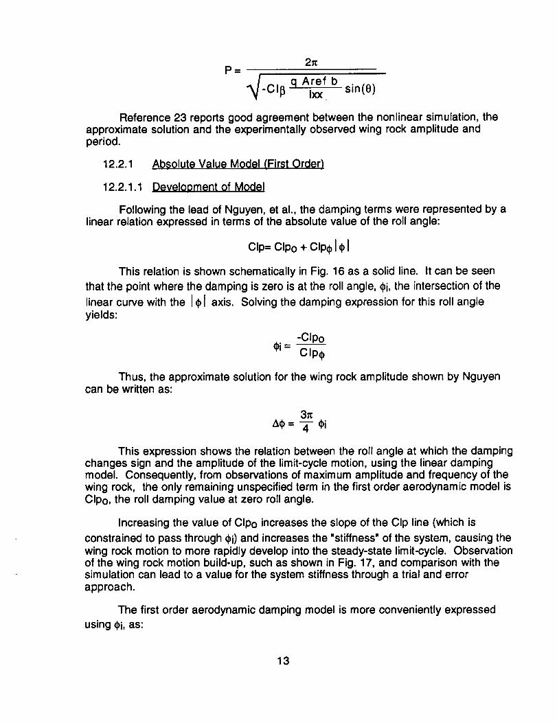
Reference 23 reports good agreement between the nonlinear simulation, theapproximate solution and the experimentally observed wing rock amplitude andperiod.
12.2.1 Absolute Value Model (First Order)
12.2.1.1 Develo_Dment of Model
Following the lead of Nguyen, et al., the damping terms were represented by alinear relation expressed in terms of the absolute value of the roll angle:
CIp= Clpo + CIp I$1
This relation is shown schematically in Fig. 16 as a solid line. It can be seen
that the point where the damping is zero is at the roll angle, ¢i, the intersection of the
linear curve with the I¢1 axis. Solving the damping expression for this roll angleyields:
-Clpo
¢i- CIp¢
Thus, the approximate solution for the wing rock amplitude shown by Nguyencan be written as:
This expression shows the relation between the roll angle at which the dampingchanges sign and the amplitude of the limit-cycle motion, using the linear dampingmodel. Consequently, from observations of maximum amplitude and frequency of thewing rock, the only remaining unspecified term in the first order aerodynamic model isClpo, the roll damping value at zero roll angle.
Increasing the value of Clpo increases the slope of the CIp line (which is
constrained to pass through _i) and increases the "stiffness" of the system, causing thewing rock motion to more rapidly develop into the steady-state limit-cycle. Observationof the wing rock motion build-up, such as shown in Fig. 17, and comparison with thesimulation can lead to a value for the system stiffness through a trial and errorapproach.
The first order aerodynamic damping model is more conveniently expressed
using ¢i, as:
13

CIp= Clpo /1 Iml" _i /
12.2.1.2 Evaluation of First Order Model Re_;ults
As an example of the first order model, the wing rock behavior at a sting angle
e = 30 ° will be simulated. Figure 18 shows a time history and phase plot after the wingrock motion has reached the limit-cycle. Comparison of these plots with theexperimental results shown in Figs. 19 and 20, show the strengths and weaknesses ofthe first order model. As expected, the frequency, maximum amplitude, and maximumangular accelerations of the simulated motion agree quite well with the experiment.
However, the character of the value of _' variation with roll is not reproduced well.
Since _' is proportional to the aerodynamic moment (see the equation of motion), thismeans the damping model is not an accurate representation of the actual behavior.Specifically, the abrupt slope change at zero roll angle shown by the simulationcorrelates directly to the slope change in CIp as the roll angle changes sign.
In addition, the roll angle where the curve crosses over itself does not agree
with the experiment. This angle is the point where the damping changes sign, _i in the
notation above. According to the development of the first order model, the ratio of (N/,_(I)
is 4/3= (or 0.424). The experimental results of Fig. 19 show this ratio to beapproximately 0.544.
12.2.2 Parabolic Model (_Second Order)
Observation of the behavior of the first order model and comparisons with theexperimental results led to the development of a second order model for theaerodynamic damping. This model is formulated below.
Clpo / /.I (1)" (1)bias I/2 /CIp= 2 1 - (I)i
The second order model is depicted in Fig. 16 as a dotted line. The additional
_bias term in this model is an adjustment to reproduce the asymmetric behavior of the
(l)i points seen in the experimental results.
The frequency behavior of this model is the same as the first order model
discussed above, so the value used for CII3 is also the same. Also, the value of CIp,used to set the growth rate, is the same for the two models.
12.2.2.1 Evaluation of Second Order Model Results
Figure 21a shows the limit-cycle behavior of the second order model at a 30 °
pitch angle corresponding to the experimental results shown in Figs. 19 and 20.Again, just as with the first order model, the maximum amplitude and frequency of theoscillation agree closely with the experiments. The general shape of the phase plot
14

(Fig. 21b) agrees more closely with the experiment, showing the improvement in the
damping model around zero roll angle. The ratio of _i/A<_ for the second order model is0.5, which also is closer to the experimental observations.
As a further example of the second order model, the build-up of the wing rock
behavior at 8 = 25 ° will be simulated. Figure 22a shows the time history of roll anglewhen the simulation is started with an initial roll angle of 6 °. Figure 22b shows thenext 2 seconds of wing rock as the limit-cycle is reached. These plots show goodagreement with the build-up shown previously in Fig. 17. Figure 23 shows the phaseplots corresponding to the final 2 seconds shown in the previous figure.
12.2.3 Higher Order Model (nth Order)
To further increase the accuracy of the simulation, the order of the model was
allowed to vary to match the experimental observation of the ¢i/A¢ ratio. The nth ordermodel was formulated as:
c0o/ /,°°0ia'in/CIp= _ 1 - $i
It was found that a value of n equal to 2.84 produced a $i/A¢ ratio equal to the0.544 value observed in the wind tunnel. The resulting phase plot is shown in Fig. 24.Again, the frequency, amplitude, and maximum angular acceleration all matched theexperimental results closely.
12.2.4 Remarks
First, second and n th order models for the aerodynamic damping weredeveloped and examined with a one degree of freedom simulation. Very goodagreement with the observed behavior from the wind tunnel tests was obtained. Thewing rock growth rate, the maximum amplitude, frequency and maximum angularacceleration of the limit-cycle behavior were all closely reproduced by the simulation.
12.3 Pneumatic Controls. Dynamic Effects
The one-degree-of-freedom simulation was also used to explore the dynamiceffects of pneumatic forebody vortex control. Comparison of the time historiesobtained in the wing rock wind tunnel test with the output of the simulation programallowed different modeling schemes to be tested. The final aerodynamic model forpneumatic forebody vortex control closely reproduced the observed behavior in thewind tunnel.
The static wind tunnel test revealed that blowing from a jet located on theforebody generated roll and yaw moments by affecting the formation and interaction ofthe forebody vortices with the wing and LEX vortices. In addition, the wing rock tests
15
show the dynamic effects on the vehicle's lateral aerodynamics. The major effects ofblowing from forebody jets are:
• a yaw moment increment• a roll moment increment• an increase in roll damping
The different pneumatic control schemes tested during the wing rock tests were:steady blowing on one side, combined blowing simultaneously on both sides, andpulsed blowing rapidly alternating between sides. The overall effects of the differentmethods will be presented below along with the results of modeling the effects in theone-degree-of-freedom simulation. More detailed discussion of the pneumatic controleffects on the wing rock behavior can be found in Volume III of this report.
12.3.1 One Side Blowing
Initiation of blowing from a jet located on one side of the forebody during anestablished wing rock oscillation caused the motion to damp out, provided the blowingmass flow rate was sufficient. When the motion stopped, the model was not in awings-level attitude. This creates a trimmed condition with a non-zero sideslip angle,
or in other words, the blowing caused an increment in the zero _ roll moment (L_CIo).This is consistent with the observations from the static wind tunnel test.
12.3.1.1
The roll moment model was presented earlier when the static yaw controleffectiveness was discussed. However, at that time, the determination of the rollmoment characteristics at large blowing rates was not explained.
The maximum value of the blowing momentum coefficient examined during the
static wind tunnel tests was CI_ = 0.0015. Subsequently, this level of blowing was
found to be ineffective in alleviating the wing rock. Blowing levels of Cp = 0.0028 and0.0037 were used during the dynamic wind tunnel tests. Due to the lack of overlap
between the two test series, ,_CIo effect of the higher momentum rates had to beestimated from the final trim roll angle of the model after the wing rock had beendamped.
The equation for the one-degree-of-freedom roll moment developed in anearlier section, when solved for trimmed, static conditions appears as:
CI = CI_ sin((] ) Sss = 0 for trim conditions
From this relation, the value of CIj3 can be determined easily for the differentsting pitch angles and blowing rates tested. These values were then appended to theresults of the static wind tunnel test to provide an aerodynamic model valid over theentire range of blowing coefficients.
16

12.3.1.2 DamDing Effect. CI_
Time histories of the wing rock oscillation and the blowing pressure signal are
shown in Fig. 25. At the larger blowing rate of Cp = 0.0037, blowing on the left or right
sides caused a shift in the mean value of the oscillation (the ACIo effect), and
smoothly damped the oscillation. The slight differences observed in the damping dueto blowing with the left or right jets is related to the natural asymmetry of the vortex flowpattern as explained in Volume III of this report. For the purpose of the simulationmodel, the asymmetric damping effect is of lesser importance and will not be modeled.
Figure 26 compares the responses at two different blowing rates, CI_ = 0.0028and 0.0037, at an angle of attack of 25 ° . The small blowing rate was not as effective indamping the wing rock oscillation; rather, it only reduced the amplitude. Blowing ratesless than 0.0028 were unable to eliminate the oscillation. The blowing effectiveness
was approximately the same at (z = 25 ° and 30 ° for the same value of Cl.t. In general,the damping contribution of pneumatic forebody vortex control jets appears to beproportional to the blowing rate and shows angle of attack sensitivity similar to thestatic control effectiveness.
12.3.2 Model Description
The computer formulation of the static roll moment control effectiveness due topneumatic forebody vortex control was identical in form to the yaw control model andwas presented earlier in Section 8.3.3 covering static aerodynamic controls. The rollcontrol system similarly included a first order lag, but with provisions for a longercharacteristic length yielding a greater time delay in response.
Pneumatic forebody vortex control has a major effect on the dynamicaerodynamic characteristics. The additional roll damping provided by forebody jetsblowing on one side individually was modeled in the computer simulations by thefollowing equation:
A Cll_,k,,,,=, = -Clp o (oJ C.llBt''m )_c/l_,=o.oo_
This formulation keys the additional damping contribution to the amount ofdynamic instability present in the bare airframe at the current flight condition, yielding aconsistent damped response with the activation of forebody blowing. The magnitudeof the damping increment is also scaled with the static roll control power provided bythe blowing system, thus including the effects of varying blowing rates.
12.3.2.1 Model Validation Via Comparison With Wind Tunnel Tests
Proof of the appropriateness of the dynamic blowing model was obtainedthrough comparison of the experimentally observed response to the predictions of theone-degree-of-freedom simulation. Results of the experiment at an angle of attack of
o_= 30 ° were presented earlier in Fig. 25. The results of the simulation at the sameconditions are shown in Fig 27. The wing rock limit cycle was fully established at the
17

beginning of the plot (time = 0). Steady blowing on the right side was initiated at 0.1seconds at CI_= 0.0037. The wing rock damped in approximately 5 oscillations,establishing a steady trimmed roll offset of 10°. The agreement demonstrated by thisexample is typical of comparisons made over the entire range tested in the windtunnel. Differences noted in specific comparisons fell well within the run-to-runvariations observed during the wind tunnel tests, and therefore the computerformulation is judged to be an adequate representation of the static and dynamicaerodynamic behavior of pneumatic forebody vortex control.
12.3.3 Combined Blowing
Combined blowing simultaneously on both sides of the forebody was tested inthe wind tunnel. This was very effective in damping the wing rock oscillation andproduced very little residual roll moment compared to blowing on one side alone. Thecomputer modeling of combined blowing was a simple addition of the left and rightblowing models. The result is a canceling of the static roll moment effect at zerosideslip, though a net roll moment exists at non-zero sideslip due to the differingeffectiveness of blowing on the windward and leeward sides. The damping incrementof the two sides sum to produce a larger damping effect than that from single sideblowing. The justification for this simple summation of the single effects can be seenby again referring to Fig. 25. The experiment clearly showed a more rapid damping toa steady state roll angle closer to zero than in the case of single side blowing.
12.3.4 Pulsed Blowing
As discussed earlier, concern for the mass flow required for simultaneouscombined blowing led to the testing of rapidly pulsed blowing alternating between theleft and right sides. The computer model of this technique is a combination of the twosingle side blowing models. The frequency and duty cycle of the pulses could bevaried. At a sufficiently high pulsing frequency, the airframe does not respond to theroll and yaw moment perturbations due to the blowing, yielding a time-averagedmoment cancellation and symmetry. However, the additional roll damping producedby blowing on each side is of the same sign, so the time-averaged response is anincrease in the level of damping similar to that obtained from blowing steadily on oneside. The experimentally observed behavior will be reproduced by this computerformulation.
13.0 FULL SCALE MASS PROPERTIES
13.1 Estimation Techniaue{;
Basic aircraft design handbooks 15,24 were consulted for methods to estimatethe component weights, cg's, and moments of inertia. Not surprisingly, due to theunconventional nature of this configuration, the different empirical methods gavewidely varying estimates for the mass properties. Based on the geometry of thevarious components and comparison of weight fractions of similar aircraft, thefollowing weight build-up was estimated:
18

Structural Section Wei_lht (Ibs !
Win_l 8,500Vertical Stab 1,000
28,000Fuselage + PayloadEnginesFuel
Total
8,00054,500
100,000
Recognizing the difficulty of accurately estimating mass moments of inertia, thevalues obtained from the empirical methods were compared with those of other aircraftof similar design and flight regime. Of course, there are not too many of those in
existence, but using scaling techniques suggested by Raymer 24, the principalmoments of inertia for the XB-70, A-12 (SR-71), and the paper study aircraftdesignated AST-105-1 were reduced to a non-dimensional form and compared. Thefinal values for the mass properties used in this study are based on the average of thenon-dimensional mass properties of these three aircraft.
Bar charts comparing the non-dimensional inertias of these 3 example aircraftand the average value used for the NASP configuration are shown in Fig. 28 for thefull fuel gross weight condition and the empty fuel condition. The mass propertiesused in the full-scale control system development and manned simulation are shownin the table below.
Weight (Ibs)
Ixx (slug-ft 2)
lyy (slug-ft2)
Izz (slug-ft 2)
Ixy (slug-ft 2)
I FuII FuelCondition
100,00026,554
669,415
540,904
0
I Empty FuelCondition
45,00015,367
378,697
308,4660
14.0 1DOF SIMULATION. SCALE EFFECTS
The one-degree-of-freedom simulation closely reproduced the limit cyclemotion as observed during the wing rock wind tunnel test. In preparation for the man-in-the-loop simulation, the full scale aircraft dimensions and mass properties wereinput into the one-degree-of-freedom simulation. The model scale conditions werethose of the wind tunnel test. The full scale conditions were set at 30% fuel weight,200 KIAS at sea level, standard day conditions. These are tabulated below.
19

q (psf)v (us)b(ft)s (ft2)Ixx (slug-ft 2)
I Model Scale21.0
Full Scale
135.59132.84 337.56
17._12 259:5/12335/144 75375/144
0.0312 18723.
Figure 29 compares the two simulation results at an angle of attack o_= 30 °.The plots are presented in pairs, with the model scale and full scale results at similarconditions shown together. Note that the time scales are different. The series of plotsbegin with the roll time histories during the build-up of the oscillation after being
released from an initial roll angle of _ = 6 °, followed by the phase plane plots coveringthe same period. The next set, Fig. 30, continues from the final conditions of theprevious set and shows the development of the limit cycle. The final set, Fig. 31,shows the effects of initiating steady forebody blowing on the right side at a rate of
CI_ = 0.0037. The blowing begins 0.2 seconds into the simulation of the model scaleand at 1.0 seconds for the full scale example.
It is apparent from the comparisons that the overall character of the wing rockbehavior is similar between the model scale and the full scale with the exception of thetime scale. The frequency of the oscillations were 2.91 Hz for the model scale and0.554 Hz for the full scale aircraft at these conditions. The amplitude of bothoscillations grew at approximately the same percentage each cycle and the maximumamplitude of limit cycle was the same. Moreover, the response to forebody blowingwas similar for both configurations.
14.1 Nondimensional Inertias. Dynami_ Similitude
The reduced frequencies of the wing rock limit cycles are shown in the tablebelow. The similarity of the values shows that the wind tunnel model and testconditions were close to being dynamically scaled for the assumed full scale flightconditions. Had this wind tunnel test been intended as a proper dynamic test of aspecific aircraft, the non-dimensional mass moment of inertias would have been
matched to those of the full scale aircraft and flight conditions 25. The relative massmoment of inertia values for the wind tunnel test and flight conditions are shown in thetable:
Reduced
Frequency
ReducedInertia
r 2 Ixx "_
_p Aref b 3 )
ModelScale
0.0992
3.766
FullScale
0.1115
2.976
20

The dynamic scaling is significant because it indicates that the aerodynamicphenomena observed in the wind tunnel correspond to conditions likely to be seen infull scale flight. In fact, variations of the assumed full scale parameters can createconditions where exact dynamic similitude with the wind tunnel test exists. Forexample, if the altitude were increased to 7800 ft or the fuel load increased to 74% ofmaximum, then the reduced inertia values for the full scale aircraft would exactly matchthose of the wind tunnel test model.
15.0 FULL SCALE CONTROL SYSTEM DEVELOPMENT
15.1 Methodology and Aooroach
The basic requirements for the flight control system are to provide adequatehandling qualities such that the aircraft becomes flyable. The bare airframe as testedin the wind tunnel has severe cross-coupling of the control effects and inadequatedamping in all axes. The longitudinal flight control system combines an angle of attackcommand system (at low speeds) with a load factor, nz, command system (at highspeed). The lateral-directional control system will consist of roll rate and sideslipcommands. Lateral movement of the pilot's control stick commands the flight controlsystem to execute a pure, uncoupled velocity-vector roll. Similarly, depressing therudder pedals produces a stability axis yaw command resulting in a pure, uncoupledsideslip maneuver.
Each axis has available feedbacks of aerodynamic and flight path angles andrates. A fully augmented flight control system will be implemented that is similar to thatfound in a state-of-the-art high performance aircraft. This design is representative of asystem that would be expected, or even required, for a flight vehicle of this class. Inaddition, a partial-augmentation flight control system will be modeled. This system hasthe rate feedback paths in the lateral and directional axes disconnected, resulting inno artificial damping supplementing the bare airframe in these axes. The purpose ofincluding this unrealistic flight control system is to highlight the effects of variouspneumatic forebody vortex control schemes.
15.2 Design Flight Condition
The flight control system synthesis was done for low speed and high speedflight conditions; however, a great part of the development concentrated on theapproach to landing configuration. The landing configuration studied was 30% fuelweight, 200 to 300 knots airspeed, and altitudes from sea level to 10,000 feet. Full fuelweights and inertias were used to represent the take-off condition.
15.3 Design Criteria
The criteria chosen for the flight control system (FCS) was per MIL-F-8785C.
Longitudinal short period characteristics were augmented so as to be within the o_spvs. nz boundaries for Class IV airplanes. Lateral-directional modes were alsoaugmented so as to meet the frequency and damping requirements of thespecification.
21
Attention was also given to handling qualities. Longitudinal motion was tuned
so as to meet Gibson's criteria 28 (i.e., pitch angle dropback for pitch pulse inputs).Lateral motion was tuned to have zero sideslip and sideslip rate during rollmaneuvers. The control system also provided a "pure decoupling" between each axis.
15.4 Longitudinal Flight Control System
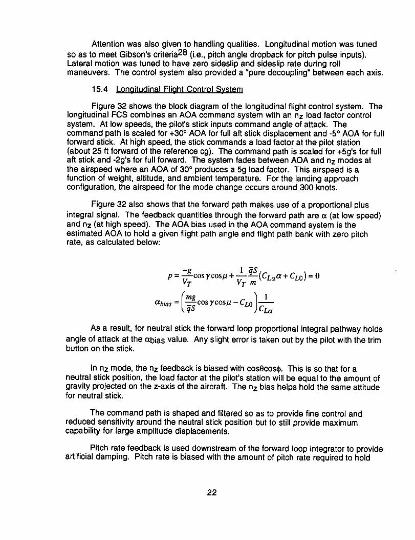
Figure 32 shows the block diagram of the longitudinal flight control system. Thelongitudinal FCS combines an AOA command system with an nz load factor controlsystem. At low speeds, the pilot's stick inputs command angle of attack. Thecommand path is scaled for +30 ° AOA for full aft stick displacement and -5 ° AOA for fullforward stick. At high speed, the stick commands a load factor at the pilot station(about 25 ft forward of the reference cg). The command path is scaled for +5g's for fullaft stick and -2g's for full forward. The system fades between AOA and nz modes atthe airspeed where an AOA of 30 ° produces a 5g load factor. This airspeed is afunction of weight, altitude, and ambient temperature. For the landing approachconfiguration, the airspeed for the mode change occurs around 300 knots.
Figure 32 also shows that the forward path makes use of a proportional plus
integral signal. The feedback quantities through the forward path are e¢(at low speed)and nz (at high speed). The AOA bias used in the AOA command system is theestimated AOA to hold a given flight path angle and flight path bank with zero pitchrate, as calculated below:
p = -g y¢o,v + tCL. +CLO)=0Vr Vr m"
Otbias = Cm_g cos_fcosll-CLo] 1\ q_ CLa
As a result, for neutral stick the forward loop proportional integral pathway holds
angle of attack at the e_bias value. Any slight error is taken out by the pilot with the trimbutton on the stick.
In nz mode, the nz feedback is biased with cos0cos_. This is so that for aneutral stick position, the load factor at the pilot's station will be equal to the amount ofgravity projected on the z-axis of the aircraft. The nz bias helps hold the same attitudefor neutral stick.
The command path is shaped and filtered so as to provide fine control andreduced sensitivity around the neutral stick position but to still provide maximumcapability for large amplitude displacements.
Pitch rate feedback is used downstream of the forward loop integrator to provideartificial damping. Pitch rate is biased with the amount of pitch rate required to hold
22

zero &. This helps eliminate angle of attack excursions due to kinematic coupling and
changes in projected gravity during rolls and/or sideslips. The Qbias value is given by:
Q_. = tanfl(Pcost_ + Rsin o0 - _rrCOS ycos//
Pitch rate feedback is also filtered through a lead-lag to provide good pitchresponses and proper frequency and damping characteristics.
A lead term is incorporated downstream of the forward loop integrator labeled fiin the block diagram. This accounts for the pitching moment produced by the time rateof change of the projection of the gravity vector and the time rate of change of the
kinematic coupling terms in the & equation. The value of h is given by:
h = tanfl(Pcosa+ Rsin oO + &(Rcos a - Psin oO
1
- ]3(Pcos a + Rsin a) cos2
+ g(f3tanflcosycosla_pw.,acosysinp_Q_siny ) 1V cos3
This feedback also helps in reducing angle of attack excursions during rolls andsideslips. The "dumbbell effect" during high AOA velocity vector rolls is eliminated bythe use of P.R inertial coupling as shown in the block diagram.
The gains in the pitch axis FCS were obtained at every point in the flightenvelope. The gains are scheduled as a function of Mach number and static pressurelevels. Synthesis and analysis of the FCS was accomplished using the Boeing controlsystem analysis program EASY5.
15.5 Lateral - Directional Flioht Control System
Figures 33a to 33c represent the lateral-directional control system design.Lateral movement of the pilot's control stick commands the stability axis roll rate. This
command is then transformed into body axis roll and yaw rates through coso_ and sine¢.Sideslip is commanded by rudder pedal deflections and its error signal goes through aproportional-integral path. The output from the proportional-integral path commands
stability axis yaw rate, and it also goes through the coso_ and sins transformation to get
body axis roll and yaw rates. The rate commands from both command channels aresummed to get the total body axes rate commands.
The roll axis command path is scheduled as a function of dynamic pressure andangle of attack. The roll rate command is set by computing the maximum availablecontrol power at each flight condition assuming a stability axis roll. The control powercomputation takes into account inertial coupling, airframe roll/yaw damping, andcontrol power for stability augmentation. Approximately 15% of the maximumavailable control power is reserved for transients. The roll axis is shaped and filtered
23
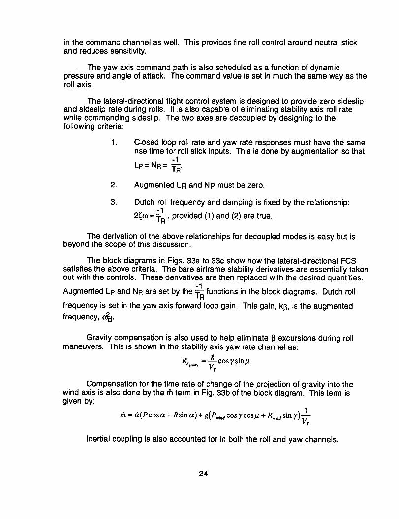
in the command channel as well. This provides fine roll control around neutral stickand reduces sensitivity.
The yaw axis command path is also scheduled as a function of dynamicpressure and angle of attack. The command value is set in much the same way as theroll axis.
The lateral-directional flight control system is designed to provide zero sideslipand sideslip rate during rolls. It is also capable of eliminating stability axis roll ratewhile commanding sideslip. The two axes are decoupled by designing to thefollowing criteria:
. Closed loop roll rate and yaw rate responses must have the samerise time for roll stick inputs. This is done by augmentation so that
-1Lp= NR= _RR"
2. Augmented LR and Np must be zero.
. Dutch roll frequency and damping is fixed by the relationship:-1
2_0) = _RR' provided (1) and (2) are true.
The derivation of the above relationships for decoupled modes is easy but isbeyond the scope of this discussion.
The block diagrams in Figs. 33a to 33c show how the lateral-directional FCSsatisfies the above criteria. The bare airframe stability derivatives are essentially takenout with the controls. These derivatives are then replaced with the desired quantities.
-1Augmented Lp and NR are set by the _-_ functions in the block diagrams. Dutch roll
frequency is set in the yaw axis forward loop gain. This gain, k,8, is the augmented
frequency, _d"
Gravity compensation is also used to help eliminate 13excursions during rollmaneuvers. This is shown in the stability axis yaw rate channel as:
Rs,,.,,, = ug---cos 7sinp"r
Compensation for the time rate of change of the projection of gravity into thewind axis is also done by the rh term in Fig. 33b of the block diagram. This term isgiven by:
th = a(Pcosa + Rsin o0 + g(P.._ cos ycosp + R_ sin 7)-;--1,Vr
Inertial coupling is also accounted for in both the roll and yaw channels.
24

15.6 Control Mixing Methodology
The NASP configuration uses elevons at the trailing edge of the wing asprimary control surfaces for both pitch and roll control. The lateral-directional flightcontrol system produces a set of moment commands that are passed through a mixing
algorithm and results in a differential elevon command, _A, and rudder command, _SR.
A collective elevon command, $E, is computed by the pitch axis FCS. The collectiveand differential elevon commands are combined to determine the individual left and
right elevon deflections by the following relations:
&_.L = (&E- &A) &_,R= (&E+ &A)
Due to the use of this mixing, one elevon will generally reach its deflection limitbefore the other one. At that point, any additional deflection commanded by the flightcontrol system can no longer be delivered and a compromise must be made. Becausethis investigation primarily involves a landing task and maneuvering in close proximityto the ground, the control limiting scheme gives preference to the pitch command.That is, if both a large elevator and a large aileron deflection are commanded by theflight control system, the elevons will deflect to give the full commanded value ofelevator deflection at the expense of aileron.
15.7 St0ti¢ Trim ReQuirements
As a simple example of the benefits of pneumatic forebody vortex control, thecontrol deflections required for a trim flight condition will be presented. The flightcondition is 5,000 ft altitude, standard day, Mach = 0.365 (400 if/s). The aircraft istrimmed, wings level, in a 15 ° glide at its empty fuel weight. Trim is defined in this caseas a condition of zero angular and linear accelerations. Airframe asymmetries, asmeasured in the wind tunnel, are included in the basic aerodynamics, producingtrimmed flight with a steady state sideslip.
The aircraft trims under these conditions at an angle of attack o_= 17.455 ° and
sideslip _ = 3.855 °. The use of forebody blowing relieves the conventional controlsystem of some of the burden of supplying trimming moments as shown in thefollowing table of required control deflections:
C_ used Trim 5R Trim 5EIL Trim _EvR0 -13.898 -3.129 -28.8180.00155 -7.015 -3.129 -28.8180.00185 -2.732 -3.129 -28.8180.00216 -0.425 -3.129 -28.818
Large differential elevon deflections are required to trim the roll moment due tosideslip and the basic airframe asymmetries. At this angle of attack, the blowingsystem does not contribute to the rolling moment, so variation of the blowing rate doesnot effect the elevator or aileron deflection requirements. The rudder trim resultsclearly illustrates the ability of pneumatic forebody vortex control to provide significantcontrol moments to supplement the conventional control system.
25

15.8 Pneumatic Control Implementation Schemes
The wind tunnel tests show that pneumatic forebody vortex manipulation offerssome potential for use as a supplemental control system. In general, pneumatictechniques have the following major strengths that could be advantageouslyincorporated into an aircraft's control system:
• Large yaw moment generation at high AOA• Increased roll damping
Five schemes for implementation of the pneumatic control will be discussedbelow in order of increasing sophistication. Two of the methods are =non-active,"meaning the implementation is not a primary control method but rather is a simpleon/off device. The last three discussed use the pneumatic control in concert with theconventional control system.
15.8.1 Non-Active Controls: Wing Rock SuporessioFl
The first two control schemes utilize the demonstrated ability of pneumaticforebody vortex control to increase the natural roll damping of the aircraft. The majoradvantage of using forebody vortex control to provide roll damping is that it frees theprimary flight control surfaces for their primary task, i.e., controlling the aircraft. Thishas the benefits of increasing the available control power, simplifying the primarycontrol system, and reducing the overall system requirements.
The pneumatic systems are basically simple on/off implementations that areautomatically activated by the aircraft angle of attack. The implementations areclassified as non-active controls because the systems are not used in the direct controlof the aircraft and do not use feedback of the aircraft state (except for angle of attack) toregulate the amount of control.
15.8.1.1 Steady Simultaneous Blowing
The simplest use of pneumatic control is simultaneous blowing on both sides ofthe forebody. As discussed in Volume III of this report, this was found to be an effectivemeans of reducing the wing rock oscillation. The system would begin blowing as theangle of attack increased into the range where the bare airframe lacks roll damping.Steady blowing reduces the de-stabilizing interaction of the forebody and wing vortexsystems, thereby increasing the roll damping.
However, there are some drawbacks to this implementation. The airframe'snatural asymmetric yaw and roll moments at zero sideslip are still present, and insome cases are reinforced by the blowing. The mass flow requirements are thelargest of any of the implementations, and other pneumatic control techniques showedgreater increases in roll damping.
26

15.8.1.2 Pulsed Alternating Blowing
A non-active pneumatic forebody vortex control implementation that does notshare the undesirable side effects of steady simultaneous blowing is pulsed blowing.In this implementation, the blowing is rapidly alternated between the left and rightsides. The wind tunnel test demonstrated that if the switching frequency isapproximately twice the wing rock frequency, the beneficial supplement to rolldamping is retained without the accompanying asymmetric moments. The naturalfrequency of the airframe is low enough that the airframe cannot respond significantlyto the alternating moments. As a result, it appears to the airframe as if the time-averaged yaw and roll moment due to the pneumatic control is zero and the forebodyvortex flow is stabilized into an effectively symmetric configuration. Additionally, thetotal mass flow requirements of this control system should be roughly half of that for theimplementation of steady simultaneous blowing on both sides, if the blowingalternates sides with no overlap or pause between pulses.
15.8.2 Active Controls
Three methods of incorporating pneumatic forebody vortex control into theprimary flight control system will be discussed. The pneumatic control is treated asanother source of yaw moment, similar to the conventional rudder control, but withdifferent characteristics. In each of these concepts, the use of the pneumatic controlincreases with angle of attack as the pneumatic control power increases and theconventional control loses effectiveness. The three techniques generally increase insophistication in the order presented, but each method has specific characteristics thatwould be advantageous in different conditions.
15.8.2.1 Dithered Control
As shown in an earlier section, the yaw moment due to blowing is not a linear
function of CI_; rather, there is a deadband below which blowing has little effect,followed by a rapid increase in yaw moment increment, then a leveling of the curveshowing the effectiveness is reducing. A highly nonlinear control gradient causes anaircraft to have poor handling qualities and to be difficult (or impossible) to fly. Atechnique to create linear behavior from a nonlinear control response is throughcontrol dithering. The degree of nonlinearity exhibited by this configuration was notsevere, but would require compensation from the control system and would causemore difficulty in implementation.
Dithering can be thought of as an extension of the pulsed alternating blowingpreviously described. The blowing will switch rapidly back and forth between the leftand right sides at a frequency greater than the airframe natural frequency. However,the duty cycle, that is, the relative time spent blowing on each side, will be varied inproportion to the commanded yaw moment. In this manner, the resultant net control
gradient is linear and the effects of the deadband and the nonlinear response to CI_are reduced or eliminated.
27

The advantages and disadvantages of the dithered control system are similar tothe pulsed blowing. Roll damping is automatically increased whenever the pneumaticsystem is operating. Undesirable asymmetric forebody vortex flow is eliminated in atime-average sense. Also, the same drawback of dithered control is that, like thepulsed blowing, the mass flow requirements are high because the system iscontinuously blowing on one side or the other at high angles of attack.
15.8.2.2 Scheduled Proportion of Commanded Control
This approach treats the pneumatic controls as just another source for yawmoment. In response to a requirement for control moment, the control logic divides therequirement between all available controls by a specified mix. For example, the flightcontrol system interprets a pedal input as a yaw rate command requiring yaw moment.The flight control system divides the requirement between the yaw moment sources, inthis case the rudder and forebody vortex control. Each control provides a percentageof the total requirement. An early version of this control scheme used a fixed ratiosplitting the work between the conventional and pneumatic control systems. A moresophisticated version, used in the manned simulation, divided the demand accordingto the ratio of maximum control power available from each system. At low angles ofattack the rudder provided 100% of the yaw moment. As the angle of attack wasincreased above 20 ° , the pneumatic control system became active and satisfied largeramounts of the yaw requirement.
This control implementation has smaller total mass flow requirements than theprevious schemes because blowing is only active when needed. While the jet blowingis actually taking place, the level of roll damping will be increased; however, duringother times, the damping will have to be artificially augmented by the conventionalcontrols.
15.8.2.3 High Freauency / Low Freauency Mix
Some configurations of forebody vortex control may exhibit significant time lagsbetween a control actuation and the resultant force or moment generation. A controlimplementation that addresses this problem would use complementary filtering toproduce a high-frequency / low-frequency control mix. The rudder, the high frequencycontrol, would deflect to satisfy the yaw rate requirement onset and then wash-out asthe pneumatic system, the low frequency system, becomes effective. This then returnsthe rudder to a neutral position, restoring its full control capacity. Another way to lookat this implementation is the pneumatic system as the coarse control with theconventional controls functioning as the fine tuning (providing that the conventialcontrol is still effective at that flight condition).
The response time of the aerodynamics after the initiation of blowing wasestimated from the pressure measurement time histories from the wind tunnel test
described in Volume I1. The delay in pressure rise was determined to be only the timerequired for the freestream flow to transverse from the blowing jet location to thepressure sensor. The distance from the nose to the wing reference center is 48 feet onthe full scale aircraft. At a minimum flight speed of 200 knots, the control power wouldtake only 0.14 seconds to fully develop. The control system as implemented for this
28

study runs at 20 Hz, or in other words, with a time between updates of 0.05 seconds.The control lag for this configuration was not a critical issue.
15.8.3 Implementations for Further Study
In addition to the conventional control baseline, two pneumatic control systemswere selected for further development and study. The first is the non-active pulsedblowing to explore the advantages of a simple implementation. The wind tunnel testindicated that the time lags of the pneumatic control effectiveness were small enoughnot to be an issue in this configuration, so the proportional technique was chosen asthe active control implementation.
15.8.4 Demonstration Testbeds
The three control concepts (one conventional and two pneumatic) were eachincorporated into two distinct system architectures. The first system, a partial-augmentation system, handles control system mixing logic and produces uncoupledresponses to control commands. This minimal system does not use rate feedbacks inthe lateral-directional axes so the airframe damping is not artificially enhanced. Thesecond system, a fully augmented system, is representative of a modern digital fly-by-wire system with full augmentation in all axes. This control system has position, stateand rate feedbacks available and schedules gains such that good flying qualities areproduced. The minimal system highlights the differences in the aircraft behavior withthe different control systems, i.e., without blowing, with pulsed blowing, and withproportional blowing. The three control systems in the fully augmented aircraft appearsimilar to the pilot, unless maximum performance maneuvers are performed. In total,five different control systems were evaluated in the manned simulation. (Thecombination of pulsed blowing and a fully augmented flight control system wasdeemed of little value.)
16.0 MANNED SIMULATION
The static and dynamic aerodynamic model and control systems wereincorporated into a manned simulation for the purpose of evaluating the use andbenefits of pneumatic forebody vortex control in a flight vehicle. The flight tests wereperformed with a high-fidelity six-degree-of-freedom simulator. The evaluation pilotwas qualified and regularly flies high performance, supersonic fighter aircraft.Evaluation tasks were designed to require a high degree of piloting skill and aircraftperformance in the flight regimes where forebody vortex control is effective.
16.1 ARENA DescriDtion
The ARENA simulator 26 is a low-cost, man-in-the-loop, real time air combatsimulator that provides high-fidelity flight mechanics, avionics and controls. It hasbeen successfully used in studies of close-in air combat and in ground attackscenarios. The fixed base (non-motion) simulator has a large rear projection screen
29

providing out-the-window views forward. It features a glass cockpit that is easilyreconfigured to represent other aircraft or different avionics. A battle manager stationcontrols test set-up and real-time monitoring of the simulation, in addition to collectingdata for post-flight analysis. A sketch of the ARENA hardware configuration is shownin Fig. 34.
16.2 Implementation
Adaptation of the ARENA manned simulation cockpit to the NASP configurationwas relatively straight-forward. The aerodynamic model described above wassupplemented with generic models of engine performance (suitably scaled), speedbrakes, and landing gear. The cockpit layout is typical of a modern fighter aircraftusing the HOTAS (hands on throttle and stick) philosophy. Existing switches on thecontrol stick were reprogrammed to function as pitch trim control.
16.2.1 Winds. Turbulence
Provisions were added to allow for atmospheric disturbances to affect theaircraft. Steady horizontal inertial winds were input with an altitude variation
representative of the Earth's boundary layer profile as described by Etkin 27. Themiddle profile shown in Fig. 35 corresponds to a surface roughness expected in opencountry and is assumed to be appropriate for the regions surrounding an airport.
Atmospheric disturbances were incorporated in the simulation following theguidelines of MIL-STD-1797 "Flying Qualities of Piloted Vehicles" (Ref. 28). TheDryden form of turbulent velocity spectra with a low-altitude disturbance model wasused. The Dryden model is a convenient spectral form based on an exponentialautocorrelation function for the axial component. The other components of turbulenceintensity are based on the axial component. Turbulence intensity was variable on ascale of 1 to 10 with 1 corresponding to light turbulence and 10 representing severeturbulence. In the simulated landing tasks a turbulence level of 5 (moderate) wasused.
16.2.2 Instrumentation
The ARENA cockpit used in the manned simulation incorporates a Head UpDisplay (HUD) and out-of-window displays, but due to the aircraft attitude during thehigh angle of attack approach and the inability of the pilot to see anything but sky, theywere of limited utility. The primary instruments used during the simulation tasks were:an attitude indicator with glideslope and Iocalizer bars, angle of attack meter, airspeedindicator, vertical velocity indicator, and horizontal situation display including gyrocompass and DME (distance measuring equipment). No special instrumentationbeyond what is found in a typical state-of-the-art cockpit was used.
30

16.3 Evaluation Tasks
Evaluation tasks were identified that would explore the use of pneumaticforebody vortex control. As suggested earlier, the principal advantages of this controlsystem are increased roll and yaw control power and greater roll damping at highangles of attack. Three maneuvers were selected that involve high angle of attackmaneuvering:
• Landing Approach. A low-speed precision tracking task that requiresgood handling qualities and smooth control response.
• Loaded Roll. A high agility maneuver that requires maximum controlpower and response.
• Cross Wind Take-Off. Requires control power in sideslip and crossedcontrol conditions.
These maneuvers are described individually in the following paragraphs.
16.3.1 Glideslooe and Localizer Trackina
A standard FAR landing approach scenario was designed to test the pilot'sability to execute a precision tracking task. The standard 3 ° glideslope was used. Thepiloting task began at a trimmed flight condition at 0.6 Mach, 5,000 ft altitude,100,000 ft uprange from the runway center, and offset 8,000 ft to the side of the runwaycenterline. The pilot was asked to fly a 30 ° course to the Iocalizer and tum to smoothlyintersect the runway heading, while simultaneously transitioning to the glideslope.
The pilot was instructed to maintain a constant airspeed and aircraftconfiguration once established on the glideslope. The approach airspeed was fixed at200 kts which required 25 ° angle of attack to maintain a trimmed flight condition. Thepilot's workload at this condition was extremely high due to: poor handling qualities ofthe aircraft, the extreme body attitude which did not allow "out-the-window" sight of theground, and the large effect of thrust on the flight path and trim. Adding to the pilot'sworkload was the presence of atmospheric turbulence which precluded theestablishment of a steady trimmed descent attitude.
16.3.2 B_.nk-t0-B_.nk Loaded Rolls
To illustrate the maneuverability advantages of pneumatic forebody vortexcontrol, a series of loaded rolls were performed. A loaded roll is a roll about thevelocity vector performed with a constant angle of attack or load factor.Aerodynamically, this maneuver is very similar to a departure and spin but control isretained throughout. This requires good handling qualities and a large amount ofcontrol power in roll and yaw.
The evaluation maneuvers each began at the same altitude and airspeed
(5,000 ft and 300 knots). The pilot rolled to approximately ¢ = -90 °, stabilized the roll
angle, increased angle of attack to a prescribed value, and rolled 180 ° to _ = +90 °
31

while trying to maintain a constant angle of attack and airspeed. He was not requiredto hold sideslip to zero. The pilot was allowed to use any combination of control inputsto minimize the time required to complete the roll maneuver.
16.3.3 Cross Wind Takeoff
An inherent characteristic of this class of long slender aircraft with highly sweptwings and high wing Ioadings is a limitation in allowable cross-wind capability duringtake.off16. This is due to the low speed and high gross weight conditions, requiringhigh angles of attack after rotation. In the high angle of attack regime, many of theseconfigurations suffer from low directional stability and reduced directional controlpower.
16.4 Evaluation M_trix
The implementation of the aerodynamic and control system models in themanned simulation includes provisions for exploring the effects of varying turbulencelevels, inertial winds including shear layers, reduced control size control surfaces,airframe asymmetries, reduced longitudinal and lateral-directional stability, pneumaticcontrol time lag effects, etc. With the limited resources available in this contract, theevaluation matrix was limited to the five control systems described above in thelanding approach task and the two fully augmented control systems in the bank-to-bank loaded roll. The landing tasks were performed with a single turbulence level andno wind. The loaded rolls included no atmospheric disturbances.
16.5 Results and Discussion
The following section shows comparisons between various flight parameters forthe five different flight control system schemes described above. The flights selectedfor analysis represent typical simulation results obtained from multiple tests with eachconfiguration. The purpose is to compare the appropriate flight parameters and drawsome conclusions regarding the advantages and disadvantages of using forebodyblowing with flight control systems using partial or full augmentation to contribute to theoverall improvements in the flying qualities for the different flight tasks.
Results from the manned simulation will be shown and evaluated. As statedearlier, the purpose of the manned simulation was to fly the vehicle with severaldifferent control systems performing specific flight tasks. The primary flight tasks werea Landing A00roach and a J..O.o,.c[._i_LB..o_at high angles of attack. The control systemsconsisted of five different combinations of conventional and forebody vortex controls.These are categorized as:
1) Partial augmentation, no blowing; conventional control surfaces only areused for stability and control. Pitch damping and pitch controls to compensate forpitch/roll/yaw coupling are included and are automatic. There are no artificiallateral/directional damping inputs from the control system.
32

2) Pertial augmentation with 0ulsed blowing: the control system is the same asNo. 1 except that pulsed blowing is automatically activated (open loop, no feedbackexcept angle of attack) on the forebody to suppress wing rock above a specified angleof attack, set here at 20 ° .
3) Partial augmentation with orooortional blowinQ: the control system is thesame as No. 1 except that the flight control system chooses the proportional mix offorebody blowing control input and the conventional aft-body control surface input tomeet the control input demand from the pilot. The proportionality is based on theangle of attack and the respective control power that is available from the forebodyand the conventional surface at that angle of attack. The proportionality scheme wasdescribed earlier in Section 15.8.2.2.
4) Full augmentation, no blowing: the control system is configured to provideartificial damping in all axes, including lateral/directional, by utilizing whatever controlsurfaces are required. The full augmentation means full utilization of all controlsurfaces as needed to maintain good handling qualities throughout the flight regime,to the extent possible with the available control power from the conventional surfaces.No inputs from forebody blowing are available.
5) Full augmentation with proportional blowing: the control system is the sameas No. 4 except that forebody blowing is also available to contribute control forces andmoments. The integration of the forebody blowing with the conventional surfaces isaccomplished through proportional control logic as in No. 3. The principal differencefrom No. 4 is that the blowing system can also be used along with conventionalsurfaces for full augmentation to provide good handling qualities through artificialdamping, etc.
16.5.1 Pilot Control InPuts
Control inputs from the pilot with a fully augmented flight control system producecommands to the control effectors, where the proportion of conventional and blowingcontributions are determined by the flight control system based on a prescribedproportionality scheme.
16.5.1.1 Conventional Control Surfaces
Longitudinal stick - pure pitch (Nz command at speeds above "corner" speed, angleof attack command at speeds below corner speed), requiressimultaneous movement of elevons
Lateral stick - velocity vector roll rate, requires rudder (for yaw) and differentialelevons (for roll), simultaneous elevons (nose-down for pitchcoupling) to produce a pure velocity vector roll
Rudder petals - sideslip angle command, similar to lateral stick input, i.e., rudderand simultaneous elevons for roll/pitch control to produce a purestability-axis yaw motion
33

16.5.1.2 Forebody Blowing
Longitudinal stick - no forebody input
Lateral stick - blowing from one jet only, determined by stick deflection and at alevel determined by proportionality formula for required staticmoment, and to provide sufficient roll/yaw damping with feedbackfrom velocity vector roll rate and roll direction
Rudder pedals - similar to lateral stick except blowing on left/right sides as requiredto produce a pure stability-axis yaw motion
16.5.2 Landing Approach
The landing approach task was described earlier in Section 16.3.1. Thelanding approach originates 100,000 ft in the -X-direction from the center point of therunway and 8000 ft in the -Y-direction from the airport runway centerline. The desiredflight path is from the starting point at a 30 ° angle to the intersection with the approachpath (extended vertical plane running through the center of the runway) and then turns30 ° for final approach. Desired touchdown is on the centerline of the runway 4000 ftprior to the reference center point of the runway. This results in the starting point being96,000 ft in the -X-direction from the touchdown point. With a 3 ° glideslope to thetouchdown point the altitude at a distance of 96,000 ft would be 5031 ft. Since theinitial altitude is 5000 ft, the pilot is to fly at constant altitude until he intersects theplane for the 3 ° glideslope to the touchdown point (a distance of 591 ft for an altitudedifference of 31 ft). A perfect landing would touch down on the center line of therunway at a distance of -4000 ft from the center point of the runway.
The following five groups of figures (Figs. 36 through 40) show comparisonsbetween several flight parameters that have been chosen to illustrate the relativemerits of the various flight control schemes. Parameters that have been chosen(where appropriate) for comparison include the following:
a) Variation in altitude (-Z) and horizontal excursions (Y) from an extendedvertical plane through the centerline of the runway along the ground track, X
b) Cross-track and altitude errors, (horizontally, AY and vertically, AZ), deviation(desired minus actual) of the aircraft cg from the desired approach flight pathalong the ground track, X
c) Angle of attack vs. timed) Angle of sideslip vs. timee) Roll angle vs. timef) Roll rate vs. timeg) Flight velocity vs. timeh) Dynamic pressure vs. timei) Rudder deflection angle vs. timej) Aileron deflection, (left elevon - right elevon)/2 vs. timek) Blowing coefficient (left and right nozzles) vs. timeI) Mass flow rate (left and right nozzles) vs. time
Discussion of the results of the five test cases are intended primarily to illustratethe benefits of forebody blowing, where appropriate, to both the partially augmented
34

flight control system and the fully augmented flight control system. The evaluation ofthe relative merits will be based on examining some of the flight parameters in Figs. 36through 40.
16.5.2.1 Partially Augmented. No Blowina
Figure 36 represents the case for a partially augmented flight control systemwith no forebody blowing available. Figure 36a shows the flight path leading to anattempted touchdown point (X=-4000, Z=0, Y=0). The obvious result is that the targetwas not reached, i.e., Z=0 at X=-30,000 ft (crashed). The deviation of the actual flightpath from the desired flight path is shown in Fig. 36b. The obvious errors are adescent in altitude that is much too steep, and some difficulty in holding lateral flightpath. The variations in angles of attack, sideslip and roll angle are much morerevealing in terms of the difficulty in flying this configuration. These are shown in Figs.36c and 36d. In order to hold the velocity to 200 KIAS and to keep from droppingaltitude too rapidly, a high angle of attack must be flown in order to provide adequatelift and drag.
These curves show angles of attack consistently in the range of 20 ° to 27 ° ,angles where there are severe directional stability deficiencies and wing rock (lateraldynamic instability). The large oscillations in roll (phi) and sideslip (beta) are evidenceof the difficulty of maintaining control in these modes. These instabilities are ultimatelywhat led to the "crash". The angular excursions become uncontrollable after about120 seconds into the flight. Figures 36e-36h show an expanded scale to illustrate thedetailed time history of angle of attack, roll and roll rate. The buildup in roll angleoscillations and rate to a limit cycle motion are significant and the motion cannot beovercome by the pilot. The wing rock frequency is approximately 0.5 Hz.
Figures 36i and 36j show the time history of the velocity, Mach number, anddynamic pressure. The task was to decrease the initial velocity from M=0.6 to M=0.33(approximately 200 KIAS) and hold this velocity until touchdown. This was virtuallyimpossible to accomplish, as can be seen. Figures 36k and 361 show the time historyof the rudder and aileron (differential elevon) deflections. Both of these arecommanded by the pilot in an open loop fashion, i.e., there are no automatic or closed-loop rudder and aileron inputs from the flight control system to improve the handlingqualities. The difficulty for the pilot is that since the stability is so poor in both roll andyaw axes, it is difficult to coordinate all the proper control movements to counteract thelarge amplitude motions at the frequencies that are being experienced.
16.5.2.2 Partially Augmented With Pulsed Blowina
Figure 37 has the same control system but with the addition of an open loopblowing system that acts as an automatic wing rock suppression system at high anglesof attack. The pulsed blowing system is initiated at angles of attack greater than 20 °with the mass flow increasing linearly with angle of attack until reaching a specifiedmaximum level. The period of the pulsing was set equal to the pneumatic control timeconstant. This represents a greater frequency than was possible in the wind tunneldue to experimental limitations and produces smaller roll and yaw disturbances to theairframe. The pulsing frequency is approximately 6Hz, or approximately 12 times thenatural wing rock frequency (the pulsing nozzle flow suppresses the roll moment
35
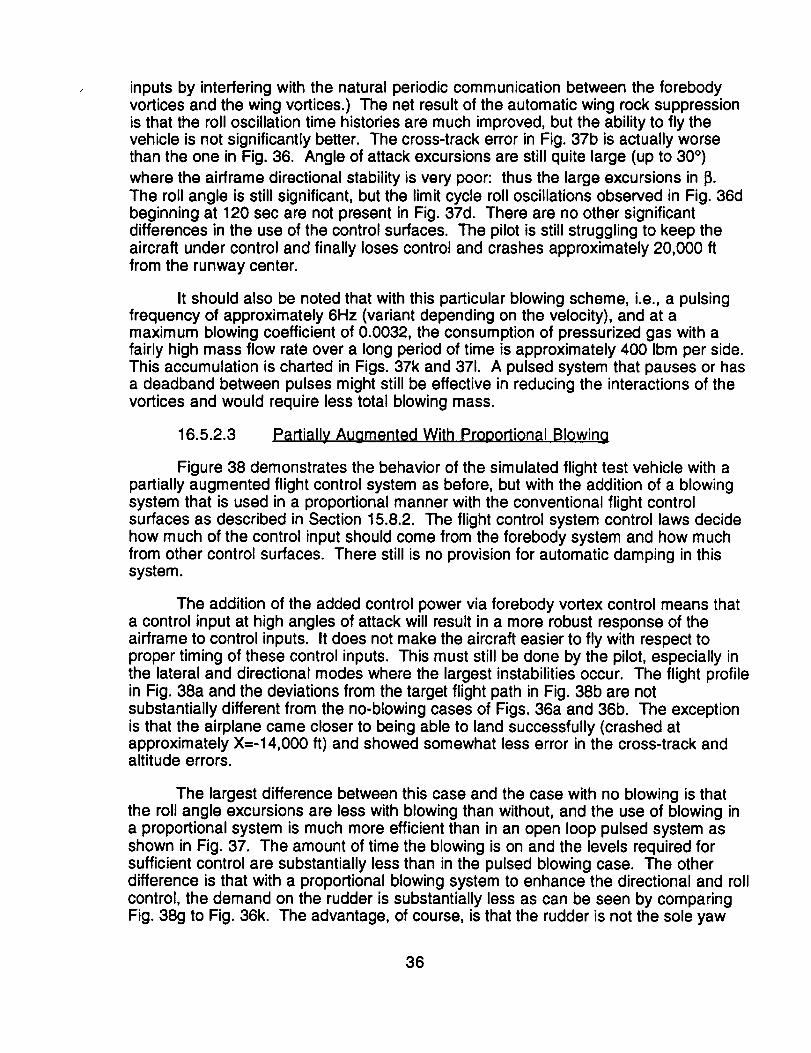
inputs by interfering with the natural periodic communication between the forebodyvortices and the wing vortices.) The net result of the automatic wing rock suppressionis that the roll oscillation time histories are much improved, but the ability to fly thevehicle is not significantly better. The cross-track error in Fig. 37b is actually worsethan the one in Fig. 36. Angle of attack excursions are still quite large (up to 30 °)
where the airframe directional stability is very poor: thus the large excursions in _.The roll angle is still significant, but the limit cycle roll oscillations observed in Fig. 36dbeginning at 120 sec are not present in Fig. 37d. There are no other significantdifferences in the use of the control surfaces. The pilot is still struggling to keep theaircraft under control and finally loses control and crashes approximately 20,000 ftfrom the runway center.
It should also be noted that with this particular blowing scheme, i.e., a pulsingfrequency of approximately 6Hz (variant depending on the velocity), and at amaximum blowing coefficient of 0.0032, the consumption of pressurized gas with afairly high mass flow rate over a long period of time is approximately 400 Ibm per side.This accumulation is charted in Figs. 37k and 371. A pulsed system that pauses or hasa deadband between pulses might still be effective in reducing the interactions of thevortices and would require less total blowing mass.
16.5.2.3 Partially Augmented With Prooortional Blowing
Figure 38 demonstrates the behavior of the simulated flight test vehicle with apartially augmented flight control system as before, but with the addition of a blowingsystem that is used in a proportional manner with the conventional flight controlsurfaces as described in Section 15.8.2. The flight control system control laws decidehow much of the control input should come from the forebody system and how muchfrom other control surfaces. There still is no provision for automatic damping in thissystem.
The addition of the added control power via forebody vortex control means thata control input at high angles of attack will result in a more robust response of theairframe to control inputs. It does not make the aircraft easier to fly with respect toproper timing of these control inputs. This must still be done by the pilot, especially inthe lateral and directional modes where the largest instabilities occur. The flight profilein Fig. 38a and the deviations from the target flight path in Fig. 38b are notsubstantially different from the no-blowing cases of Figs. 36a and 36b. The exceptionis that the airplane came closer to being able to land successfully (crashed atapproximately X=-14,000 ft) and showed somewhat less error in the cross-track andaltitude errors.
The largest difference between this case and the case with no blowing is thatthe roll angle excursions are less with blowing than without, and the use of blowing ina proportional system is much more efficient than in an open loop pulsed system asshown in Fig. 37. The amount of time the blowing is on and the levels required forsufficient control are substantially less than in the pulsed blowing case. The otherdifference is that with a proportional blowing system to enhance the directional and rollcontrol, the demand on the rudder is substantially less as can be seen by comparingFig. 38g to Fig. 36k. The advantage, of course, is that the rudder is not the sole yaw
36

control, and there is a substantial amount of control power remaining for controlpurposes, if so demanded.
It is interesting to note that there is not much difference in the use of the aileronswith and without blowing, comparing Fig. 361 to Fig. 38h. In both control systems thepilot is attempting to counteract the wing rock motion with well-timed rudder andaileron inputs (phasing is critical). But since the wing rock is suppressed only with thesystem that has blowing, the rudder and aileron inputs do not have much benefit.Aileron inputs are only effective in the wing rock suppression mode if they are timedprecisely with the motion that needs to be suppressed. If the timing is off, the inputscan substantially enhance the motion (pilot-induced-oscillations). The blowingprovides roll damping (wing-rock suppression) simply by being on, even withoutproper phasing with the motion. Effectiveness is improved if the blowing is in theproper phase relationship with the wing rock motion, but it is not essential. Blowing onone side does have the effect of creating a small offset in roll angle which must betaken out by the pilot or the flight control system with ailerons and possibly somerudder. The aileron usage is only slightly increased compared to Fig. 36, whichperhaps reflects this. The variation in blowing coefficient on left and right nozzles andthe corresponding mass flow requirements are shown in Figs. 38i-38n. The usage issubstantially less than that for the pulsed system in Fig. 37.
16.5.2.4 Fully A_gmented. No Blowing
Figure 39 illustrates the case for a fully augmented conventional flight controlsystem with no blowing inputs from the forebody. If the flight path and thedisplacement errors from the flight path (Figs. 39a and 39b) are compared to thepartially augmented without blowing case in Figs. 36a and 36b, there is an obviousimprovement in the ability to track the desired flight path for the fully augmentedsystem, as one would expect. The aircraft has small deviations from the target flightpath, and the pilot was able to land the aircraft at the proper location. In Fig. 39c theexcursions in sideslip angle are significantly less in than in Fig. 36c. The angle ofattack still varies over the entire range of 0 to 30 ° in order to maintain the properaltitude and velocity, but the aircraft is controllable. The rudder is very active (Fig. 39g)in order to maintain small sideslip angles due to the weak natural airframe directionalstability at high angles of attack. But with the automatic control system, the pilot workload is significantly less.
Aileron deflections are not significantly different between these two cases,despite the fact that the partially augmented system experienced uncontrollable wingrock motions and the fully augmented case shows virtually no wing rock. Theconclusion might be that the aileron deflection that was commanded was much moreeffective in the fully augmented case because it was timed much better with the motionit was trying to damp compared to what the pilot can do on his own. It may also be thatthe pilot simply did not choose or was unable to command aileron to suppress the rolloscillation and relied more heavily on the rudder to try to maintain control laterally aswell as directionally. Even with the flight control system in command in the fullyaugmented case, the ailerons were used much less than the rudder. There are somesignificant excursions in roll angle (Fig. 39d), but no evidence of wing rock. The abilityto maintain small sideslip by proper use of the rudder has undoubtedly benefited the
37

stability in the lateral mode as well because of the coupling between the directionaland lateral modes of motion.
A comparison of Fig. 39 with Fig. 38 will provide some insight into the relativemerits of the fully augmented conventional system with the partially augmented systemwith blowing available in an open-loop but proportionally-controlled mode.Comparing the flight path displacement errors would suggest that the fully augmentedsystem is somewhat better than the partially augmented system, even though morecontrol power is available at the higher angles of attack for the blowing case. Theimprovements gained from the full augmentation can also be seen by comparing thevariations in roll and sideslip angles between the two cases. The partially augmentedcontrol system cannot effectively dampen the wing rock tendency as well as the fullyaugmented system. The control power is available with blowing, but without anintelligent flight control system to provide the blowing command based on feedback ofroll and roll rate, it is difficult to use it properly.
It is also interesting to note the differences in the usage of the rudder. Withpartial augmentation, the rudder is not being utilized much when blowing is available.This is undoubtedly due to the proportional control system that provides a blend ofrudder and forebody blowing for directional control. The pilot is working hard tomaintain low sideslip angles, and a rudder command will result in more forebodycontrol input at high angles of attack than rudder, thus a reduction in the rudderdeflections. This graphically demonstrates the advantage of having the blowingavailable, but it also demonstrates that the use of the blowing must be carefullyintegrated into the flight control system with the benefits of motion feedback to use it tobest advantage.
16.5.2.5 Fully Augmented With Prqporl;iqn_l Blqwing
Having shown that the fully augmented system with conventional controlsurfaces only is superior to the partially augmented system with blowing available, anobvious question is: what are the advantages of having blowing available in a fullyaugmented system? Figure 40 illustrates the flight parameters for this particular caseand is best evaluated by comparison to Fig. 39 for the fully augmented case withoutblowing. A comparison of the performance in terms of the flight path deviation (Figs.39b and 40b) show no significant difference. The pilot was able to maintain thedesired flight path and land successfully in both cases. There is some improvementfor the blowing case in the early part of the flight in cross-track error but it is not ofmajor importance.
The time histories of roll angle and sideslip angle are similar in terms ofmaximum amplitude and the suppression of wing rock. This indicates that theconventional control system has enough control power through the use of the rudderand the ailerons to suppress wing rock without having to resort to forebody blowing,provided that there is a flight control system that can use it intelligently, as discussed inthe previous section. The primary advantage in the use of forebody blowing for thisparticular aircraft is in the difference in the duty cycle of the rudder. Because of thecapability to derive control power from the forebody and blend it properly with therudder, there is a significant reduction in the use of the rudder to maintain good lateral-directional stability. This can be seen by comparing Figs. 39g and 40g. The benefit is
38

that the rudder is not operating near saturation just to maintain stability and is,therefore, available for more robust control inputs. The additional control power of theforebody may also allow the vertical tail and rudder area to be reduced, saving weightand reducing drag. There will also be cases where the basic airframe cannot provideadequate directional and lateral stability, and the addition of blowing that is well-controlled by the flight control system will be essential to fly the aircraft.
16.5.2.6 Advantages of Forebodv Blowing With And Without Full FCS
Although the comparison of the partially augmented system with blowing to thefully augmented system with blowing (Figs. 38 and 40) can be made by comparingeach with the fully augmented system without blowing (Fig. 39), a direct comparison isuseful to highlight the differences and explain what they mean.
In both cases, blowing is available as a proportional control input. That is, it isblended in a prescribed manner with the rudder and ailerons, depending on angle ofattack, in order to maximize the control forces that are available. The key difference is
the ability of the flight control system to use it properly, primarily in terms of when touse it with respect to the aircraft motion. With the partially augmented system, the pilotis deciding when to input the controls to maintain directional and lateral stability, adifficult task with an aircraft that is directionally unstable and is prone to violent wingrock at medium to high angles of attack. In order to fly the desired landing approachprofile, high angles of attack are a necessity, meaning that the pilot needs as muchhelp as possible to provide acceptable handling qualities.
For this aircraft, it is virtually impossible to fly with acceptable excursions insideslip and roll without the use of an automatic and fully augmented flight controlsystem. This can be seen clearly by comparing Figs. 38c and 38d with Figs. 40c and40d, where the excursions in sideslip and roll angle are significantly less for the fullyaugmented system. An automatic flight control system with full augmentation for allaxes will be even more important in an aircraft where the conventional control surfacesare inadequate on their own and are supplemented from other sources such asforebody blowing. This blending must be managed effectively and efficiently by theflight control system.
16.5.3
In addition to the landing approach task, a maneuvering task was alsoevaluated. Forebody vortex control has been promoted as an effective method ofproviding robust yaw/roll control for fighter aircraft at high angles of attack where theconventional aft-fuselage control surfaces such as rudder and differential tail havebeen shown to be severely reduced in effectiveness because of the immersion ofthese surfaces in the wakes of the wing, fuselage, etc. In particular, for a velocityvector roll, which is an important capability for an enhanced-agility fighter, the forebodycan produce significant forces to provide the required moment around the velocityvector, essentially a yawing moment with coordinated roll moment. Although thisaircraft configuration is not specifically designed for high maneuverability, it is judgedworthwhile to evaluate the capability for performing such a maneuver.
39

The description of the loaded roll maneuver for this simulation task wasprovided in Section 16.3.2. The pilot is attempting to roll around the velocity vector asrapidly as possible at 300 knots starting at 5000 feet altitude for a total of 180 ° (from-90 ° to +90 °) at a fixed angle of attack. He was allowed to use any combination ofcontrol inputs he desired to maintain angle of attack and minimize the time required toperform the 180 ° roll. The maneuver was performed with two of the five designatedflight control systems described earlier for the landing approach task. The two systemsare (1) Fully augmented without blowing and (2) Fully augmented with proportionalblowing. Each was evaluated at three conditions, i.e., trying to hold angles of attack of20 ° , 25 ° and 30 °. Five trials were run for each condition.
The first example to be discussed is the fully augmented case with no blowingand trying to hold 25 ° AOA. Figure 41 illustrates this case. The time history of the
velocity vector roll angle, mu (it), is shown in Fig. 41a. The motion starts at _ = -90 °
and progresses to 11= + 90 ° and stops shortly thereafter (or the simulation run wasterminated). The run numbers represent the five trials. The important parameter to
observe is the time to roll the 180 °, or the slope of the curve between I1 = -90 ° and+90 °. The first run (41) was the slowest and the remaining were fairly equal. Theexception to the pattern is run 47 which starts very slowly at first and then buildsrapidly to a rate nearly equal to the other three runs (44, 50, and 53). Note the loss inaltitude (-Z) in Fig. 41c, which is a result of losing the lift vector in the vertical planebecause of the roll.
Angle of attack (Fig. 41d) is held reasonably close to 25 ° for the duration of theroll (from approximately t=10 to t=20 seconds), although there is wide variationapproaching and departing from 25 ° AOA with time. Recall that the fully augmentedflight control system is supposed to produce a velocity vector roll with only a lateralstick input by using whatever surfaces are available, including rudder, elevons andailerons (differential elevons). The test pilot did not fly the maneuver with "feet on thefloor" causing the resulting maneuver to deviate from a zero-sideslip velocity vectorroll. Referring to Figs. 41e and 41f, the roll is produced primarily from a rudderdeflection, with only a small input from the ailerons to help stabilize the aircraft.Figures 41g and 41h show the response of the aircraft in terms of body-axis roll (p)and yaw (r) rates.
For comparison, the same maneuver is performed with full augmentationincluding proportional blowing, again attempting to hold 25 ° AOA. This case is
documented in Fig. 42. The variation of the velocity vector roll angle I_ with time in Fig.42a shows more consistency than in the previous case, very linear and all nearlyequal in slope. The roll rate also appears to be higher than the case where blowingwas not available (rates are compared later). There is still approximately the sameloss in altitude during the maneuver (Fig. 42c) but less variation from run to run. Theability to hold 25 ° AOA does not appear to be substantially better for the blowing case.This capability depends primarily on the ability of the control surfaces to provide pitchcontrol to counteract the inertial pitchup effects of rolling at angle of attack. Since thereis no control power in pitch provided by forebody blowing, it is not surprising to seelittle difference between the two cases.
40

The rudder deflection is substantially less for the blowing case (Fig. 42e) thanfor the non-blowing case (Fig. 41e), primarily because the forebody blowing providesa substantial portion of the yawing moment (or velocity vector roll moment) to producethe commanded velocity vector roll rate. Interestingly, when blowing is contributing tovelocity vector roll through a body-axis yaw moment, one nozzle is blowing on the sidein the direction in which the nose is moving, causing a body-axis rolling moment thatmust be countered with the ailerons in order to maintain the commanded roll and yawrates.
The aileron activity was increased because of the need to provide an adequateroll input to complement the roll moment produced by the blowing forebody. This doesnot detract from the advantages of using blowing. It shows clearly that the properbalance between the conventional and forebody blowing control inputs chosen byappropriate flight control system laws can result in an improved flight vehicle.
Similar runs were made for angles of attack at 20 ° and 30 °, and comparisonswere made between the achievable velocity vector roll rates with and withoutproportional forebody blowing. A summary of these data is shown in Fig. 43. Thiscomparison was developed by averaging the observed velocity vector roll rates
between I_ = !"90° for each of the cases (3 angles of attack and blowing vs. noblowing). The highest and lowest roll rates were eliminated from each set of runsbefore the average was calculated. The average roll rates are shown for the threeangles of attack investigated with and without blowing.
There is a clear advantage in the cases with blowing, as one would expect,because the blowing adds additional control power at the higher angles of attack. Itappears that, if used properly in an automatic flight control system, blowing not onlyprovides the control power, but also provides it in a manner that can be used toenhance loaded roll agility performance.
16.5.4 Cross Wind Capability
The additional cross-wind take-off capability afforded by the use of pneumaticforebody vortex control has been estimated by examining the steady state trimcapabilities of the aircraft. Generally, aircraft of this class suffer from a low value ofmaximum trimmable sideslip which limits the cross-wind take-off capability. Anadditional source of yaw moment control would increase the level of cross-wind thatcould be tolerated. However, the configuration investigated in this study does notshow this advantage for two reasons. First, the rudder area was scaled for aconventionally controlled aircraft and is quite large. As discussed earlier, one of thebenefits of forebody vortex control is the potential for reducing the tail size. The largerudder remained very effective throughout the angle of attack range, allowing largesideslip angles to be trimmed with conventional controls alone. The second unusualfeature of the current configuration is the reversal in leeside blowing effectivenessbeyond 7 ° sideslip. In other words, at sideslip greater than 7 °, blowing on either sideproduces a restoring moment that decreases the sideslip. (See Section 8.3.2 and Fig.10.) This characteristic increases the stability level of the airframe, but limits the levelof trimmable sideslip to 7°.
41
16.5.5 H_ndlin9 Qualities
As evidenced by the ground tracks and by the evaluation pilot's comments, thethree configurations with only partially augmented flight control systems were virtuallyunflyable. However, the use of pneumatic controls did improve the handling qualitiessomewhat due to the added damping provided when the pneumatic control wasactivated. The two configurations with full-augmentation flight control systemsappeared quite similar to the pilot with a slight preference expressed for the aircraftwith the pneumatic control system due to its increased maneuver performance.
17.0 JET BLOWING SYSTEM REQUIREMENTS
17.1 Blowing Coefficient And Blowing Sources
The parameter typically used to quantify jet blowing in a forebody vortex controlsystem is a non-dimensional "momentum coefficient" expressed as:
where the numerator is equivalent to a force or "thrust" produced by the momentum ofthe jet, and the denominator has the usual terms to non-dimensionalize aerodynamicforces for coefficients, i.e.:
m =
vj --
qoo =
Aref =
mass flow rate from the jetvelocity of the jet streamflight or freestream dynamic pressureconfiguration reference area, usually wing area
A mass flow rate corresponding to C_ of practical effectiveness for forebody jet
blowing usually requires a nozzle pressure ratio resulting in choked flow (i.e., Po/Pj >1.893), thereby establishing vj equal to the speed of sound at the exit. The jet velocityis therefore a function of only the temperature of the jet at the exit and will be constantregardless of the pressure. The mass flow rate then is increased by increasing thedensity of the jet flow or by increasing the pressure. For a typical example thetemperature can be assumed to be near ambient conditions unless the source of thejet air supply is heated or cooled.
Since r_ = pjvjAj where
pj = density of the jet flowsonic velocityarea of the jet
42

then r_ is a function of the local total temperature (To) and pressure (Po) of the supplyair source for the blowing system. Therefore, for a specific temperature, To, the
requirements for r_ are dictated by the area (or diameter, dj) of the jet nozzle and thelevel of the supply pressure, Po.
The following derivation will illustrate the appropriate equations to define the
relationships between d" and Po, and r_, Po, and dj. These are the perfect gasirelations for a compressible, isentropic, adiabatic gas.
C_
Vj '--"
m =
where
t
p =
m vjqoo Aref
et
V -- a
(1 7-1 )-1/'y-1 2 ) lty'l 2 )1/7-1 Po+T Po po RTo
V a = Y-1 )-1/2 1/2(,_)1/2 (T*) 1/2 = (,_)1/2 (1 + _ T O
2 )1/2 1/2= ('YR) 1/2 ( _ To
so then from r_ = p v* Aj
• Pom =
qYo
m
CI1 m
2 ) y+ 1/y-1
2 7+1/y.1 1/2
Aj Po
I_I2
(p*Aj)qooAref
Aj
43

C_
P°2To ("--_) ( 7+12 ) 7+II'y-I A j2
Po 2 ) 117-IRTo ( 7+1 Aj q=Aref
2 )1'/7-1 Po Aj(7) (7+1 qoo
2 )7/7"1 Po /t;dj 2(7) (7+1 q_Tref 4
C!1 _7 i__2 )17"1 Po dj 24 _'7+ 1 q_%t_ref
Therefore:
dj4 2 -',17"1
Po Aref C_ ]112
m =2 _,+1/7"1 1/2 /_d2j] , Po
For air"
7 = 1.4
R = 1716 ff2/sec2°R.
With the following units for the various parameters,
dj = ft, Po = Ibs/ft2, To = °R, qoo =lbs/ft 2, Aref = ft2
then
Cp = 0.5806 Po d2j / qoo Aref
Po = 1.7214 q=o Aref CI,L/d2j
44

= ]1/2 1/2dj 1.312[-_--_ Aref Cp.
m = 0.01298 d2j Po/To 1/2
With the establishment of a typical flight envelope and performance
requirements for a specific vehicle and with knowledge of the maximum level of Cp. for
a desired level of aerodynamic control power, Aref, qmax, and C_max can be chosen.Once chosen, the designer's choice for a blowing system requires an evaluation of thetrade-off between nozzle size and the pressure available from various potentialsources. The size of the nozzle will be influenced by a desire to keep the nozzlessmall and to integrate them into the upper surface of the forebody as much aspossible, minimizing the projection above the surface. However, as the equation
shows, smaller jets require higher supply pressure to obtain an equivalent C_ level.
17.2 potential Sources For High-Pressure Gas
The blowing can be provided by a number of potential sources:
1) Engine bleed air
2) Stored pressurized gas
3) Regenerative stored gas supply
4) Combustible or reactant gas system
5) Non-engine related high pressure gas source
The choice of potential sources for supplying adequate gas (air) supply for theblowing system will depend on several parameters. The primary ones are:
1) Duty cycle requirements
a) Frequency of jet-on commandsb) Mass flow rate required during jet-on statec) Maximum length of time for each jet-on conditiond) Maximum total time for jet-on condition for typical flight mission
2) Capacity for high pressure gas storage or generation
a) Engine bleed capacityb) Capacity for on-board high-pressure canistersc) Regeneration of high pressure gas with power take-off from engined) Chemical reactant or combustion source
45

3) Plumbing constraints
a) Volume required for stored gas containersb) Volume for piping hot gas from engine to forebodyc) Problems associated with high temperatures and pressures (safety,
etc.)
The demand for blowing for any given time in a flight mission in terms of massflow rate and the duration of the jet-on state will play a significant role in determiningwhether the rate and duration must be met by a continuous supply of high pressuregas, as from engine bleed, or whether the demand can be met by a stored gas supply,which can be regenerated at times in the flight mission when blowing is not required.The requirement for a specific pressure level to acquire the desired mass flow rate willalso influence the choice of pressure sources. Using engine bleed, one also mustconsider the plumbing requirements to move hot air from the rear of the aircraft to thefront, etc. If adequate on-board storage can be provided, it may be possible topressurize high pressure bottles on the ground prior to flight and to replenish them onlanding, provided that the storage capacity is sufficient for an entire flight mission. Itmay also be possible to regenerate the high pressure reservoir in flight if a power take-off from the engine can drive a compressor at a time when the forebody blowingsystem is not needed. If the system is needed only for approach and landing, thestorage capacity could be renewed on the ground before each flight. If the system isneeded throughout the flight envelope, then a regenerative system, or a continuoussupply of gas from engine bleed would be required.
17.3 Design Guidelines For Blowing System
The following discussion of design guidelines is based on a configuration andan example approach and landing task discussed earlier in this report in Section16.5.2.5. The configuration has a fully augmented flight control system andproportional forebody blowing.
The plot in Fig. 44 illustrates the relationship between the jet diameter and the
supply pressure required for a maximum CI_ of 0.002, and a maximum q associatedwith the example landing task of qmax = 250 psf. The time-history records of some ofthe flight parameters of interest for this example are shown in the next few figures.Figure 45 shows the variation in altitude (-Z) and horizontal excursions (Y) from anextended vertical plane through the center of the runway. The deviation of the aircraftposition from the desired flight path, discussed earlier in Section 16.3.1, is shown inFig. 46. Figure 47 shows the variation in dynamic pressure, and Fig. 48 shows thevariation in roll angle and angles of attack and sideslip over the flight history. In
addition to these flight parameters, there is a plot of C_ vs. t (Fig. 49), mass flow rate r_
vs. t (Fig. 50), and integrated r_ or cumulative mass requirements with time (Fig. 51).This demonstrates the usage of the blowing system to meet the control demands ofthe flight control system in this particular landing task.
For a flight vehicle of the size used in this simulation study, a practical jet
diameter would probably be in the range of 1.0 to 2.0 inches. With the CI_ and q_
46

requirements as noted, i.e., CI_ = 0.002 and qoo = 250 psf, the range of pressure levelsrequired at the nozzle would be (referring to Fig. 44) approximately 500 psi to 150 psicorresponding to the nozzle diameters of 1.0 to 2.0 inches. If the available pressurewere in the range of 1000 psi, for example, the jets could be reduced to 0.7 inches.
Once a jet diameter and related supply pressure, Po, are chosen (see Fig. 44), itcan be determined what the resulting range of required mass flow rates must be,assuming a temperature a reservoir To.
From the mass flow rate equation shown earlier:
m = 0.012982 Po dj2/To 1/2
where
dj 1.312 _ Aref) 1/2 Cp,1/2
Substituting this equation for dj into the r_ equation:
m .022346 q_ Aref Cl,d/'l"o 1/2
For this example case:
where CI1 = 0.002, qoo = 250 psf, and Aref = 523.4,
m = (.022346) (250) (523.4) (.O02)/To 1/2
m 5.8479/'1"o 1/2 slugs/sec or 188.302/ro 1/2 Ibm/sec
The plot of r_ vs. To for this example is shown in Fig. 52.
For the illustrated example, if we choose a nozzle diameter of 1 inch, referring toFig. 44, the required maximum pressure Po will be 500 psi and with a total temperatureof 530 ° R (70°F), the corresponding mass flow would be (see Fig. 52) approximately8.1 Ibm/sec. From the simulation example, the mass flow requirements during thelanding task varied from 0 to approximately 8 Ibm/sec, resulting in the total mass ofblowing air required over the 265 second time span of the landing task of mtotal =274.8 Ibm for the left nozzle and 261.7 Ibm for the right nozzle for a total of 536.5 Ibm.
17.4 Utility Of Jet Blowing For Forebody Vortex Control
The designer has an option to either obtain this quantity of air from stored gas orto provide a continuously replenished pressurized air system either by direct enginebleed from the compressor by-pass air or possibly by repressurizing high-pressure
47
bottles or containers on board at a rate consistent with the r_ demands. Thisregeneration could possibly be derived from a power take-off compressor driven bythe engine in some fashion.
If this represents the blowing requirements for a typical landing task, i.e., amaximum required r_ = 8.1 Ibm/sec and with a duty cycle as shown in this example,what are the practical alternatives for supplying the required mass flow?
Without knowing the specific engine characteristics of a proposed engine, it isdifficult to decide whether using bleed air from the engine compressor is possible ornot. From information on typical fighter configurations, an assessment has been madeto determine whether bleed air from a fighter aircraft propulsion system can beconsidered. It is known that the level of total engine bleed air of today's typical twinengine fighter aircraft is in the range up to 8 Ibm/sec, depending on altitude andthrottle setting etc. That is not to say that all of the engine bleed would be availablefrom these presently configured engines for a forebody control system, but it is not outof the question to consider engine bleed as a source, particularly if the duty cycle overthe normal range of maneuvers is not high. If the design of a vehicle was expected toinclude sufficient bleed air for a pneumatic forebody blowing system, it is possible thatthe design of the engine and other related systems could take this into account early inthe design.
An accurate assessment of the duty cycle for any particular vehicle woulddepend on the requirement for enhanced control and the frequency with which itwould be employed in a typical flight mission. Trade-off studies comparing theadvantages and disadvantages of a blowing system to an enhanced conventionalcontrol system would have to be made using extensive simulation evaluation todetermine the complexity of a blowing system, including the hardware requirements interms of weight, cost, volume, etc., as well as the control system requirements andenhancement of conventional control surfaces.
For example, to solve a directional stability problem at medium to high angles ofattack, the vertical tail (and rudder) could be enlarged in order to be more effective, orone could consider using an active control system on the forebody, which is moreeffective in producing yawing moments, and integrate the control actuation into theflight control system. The advantage could be reduced tail height, which means lessweight and less drag at all conditions including, particularly, cruise conditions wherethe enlarged tail is not necessary. However, the penalties for providing vortex controlwould also have to be evaluated, such as weight, requirements for more enginecapacity, complexity of the active control system, fail-safe operation, engine outlimitations, etc.
There could also be a system which relies on storable high pressure air forshort duty cycles that would not depend on real-time generation of the high-pressuregas source. This would have an impact on safety considerations and efficientscheduling of the use of blowing nozzles so that the demand for replenishment of thehigh pressure gas source could be met efficiently at a time when the blowing system isnot required.
48
Serious consideration of forebody vortex control with pneumatic jets and therelated hardware and flight control system software will require careful analysis andevaluation of tradeoffs. For some vehicles it may not be practical. For others it may bethe answer to providing a high-gain, highly-effective control input source that cannotbe obtained in any other practical way. The result of this study shows that it is at leastpossible to consider a forebody pneumatic control system as a candidate for high-attitude aerodynamic control.
18.0 CONCLUSIONS
Data from the static wind tunnel test described in Volume II were smoothed,
interpolated and incorporated into a six-degree-of-freedom simulation data base. Thedatabase included the static aerodynamic effects of pneumatic forebody vortex control.The free-to-roll wind tunnel test revealed a wing rock limit cycle oscillation at highangles of attack, as expected.
The non-linear aerodynamics causing the wing rock limit cycle were closelymodeled by a second-order expression. The formula had three terms that wereincluded as functions of angle of attack. The role in the limit cycle motion played byeach of the terms was determined, allowing the observed motion from the wind tunnelto be quickly and easily reproduced. A non-linear, one-degree-of-freedom simulationwas used in this part of the study.
For the manned simulation, a representative hypersonic aircraft was sized andmass properties were estimated based on other similar configurations and aircraftpreliminary design methods. The aircraft had an overall length of 75 ft and a maximumgross weight of 100,000 Ibs. The resultant high wing loading forced the angle of attackto be very large in low-speed flight conditions. The wind tunnel model and testconditions were a near-perfect dynamically scaled test of this hypothetical aircraft.
Different forms of pneumatic forebody vortex control were investigated and twosystems, in addition to a conventionally control system, were selected for further studyin the manned simulation. A landing and approach task and high angle of attackloaded rolls were used to evaluate the control systems. The simulation clearlydemonstrated the utility of blowing control in a properly designed flight control system.
Mass flow rates and total mass requirements from the flight maneuvers wereused as basis for a discussion of the design of a jet blowing system. Potential sourcesfor the high pressure gas supply were identified and design guidelines werediscussed.
19.0 A(_KNOWLED(_MENT$
Support for this work is provided by NASA-Ames Research Center undercontract NAS2-12989. The technical monitor is Mr. Larry Meyn of the Fixed-WingAerodynamics Branch. We would also like to acknowledge the support of Eideticspersonnel who were instrumental in the simulation exercise: Don Farmer, Bill Clarkand Jim Cobasko.
49

20.0 REFERENCES
1. Murri, D. G. and Rao, D. M., "Exploratory Studies of Actuated ForebodyStrakes for Yaw Control at High Angles of Attack," AIAA-87-2557-CP, August 1987.
2. Malcolm, G. N., Ng, T. T., Lewis, L. C., and Murri, D. G., "Development ofNon-Conventional Control Methods for High Angle of Attack Flight Using VortexManipulation," AIAA-89-2192, July 31, August 1-2, 1989.
3. Zilliac, G., Degani, D., and M. Tobak, "Asymmetric Vortices on a SlenderBody of Revolution," AIAA-90-0388, January 1990.
4. Moskovitz, C., Hall, R., and DeJarnette, F., "Experimental Investigation ofa New Device to Control the Asymmetric Flowfield on Forebodies at Large Angles ofAttack," AIAA-90-0068, January 1990.
5. Ng, T. T. and Malcolm, G. N., "Aerodynamic Control Using ForebodyStrakes," AIAA-91-0618, January 1991.
6. Su_rez, C. J., Malcolm, G. N., and Ng, T. T., "Forebody Vortex Controlwith Miniature, Rotatable Nose-Boom Strakes", AIAA-92-0022, January 1992.
7. Guyton, R. W., and Maerki, G., "X-29 Forebody Jet Blowing", AIAA-92-0017, January 1992.
8. LeMay, S. P., Sewall, W. G., and Henderson, J. F., "Forebody Vortex FlowControl on the F-16C Using Tangential Slot and Jet Nozzle Blowing", AIAA-92-0019,January 1992.
9. Tavella, D. A., Schiff, L. B., and Cummings, R. M., "Pneumatic VorticalFlow Control at High Angles of Attack," AIAA-90-0098, January 1990.
10. Rosen, B. and Davis, W., "Numerical Study of Asymmetric Air Injection toControl High Angle-of-Attack Forebody Vortices on the X-29 Aircraft," AIAA-90-3004,August 1990.
11. Ng, T. T. and Malcolm, G. N., "Aerodynamic Control Using ForebodyBlowing and Suction," AIAA-91-0619, January 1991.
12. Ng, T. T., Su_rez, C. J., and Malcolm, G. N., "Forebody Vortex ControlUsing Slot Blowing," AIAA-91-3254, September 1991.
13. Ng, T. T., "Aerodynamic Control of NASP-type Vehicles through VortexManipulation", Eidetics International TR89-009, 1989.
14. Hoak, D. E., and Carlson, J. W., "USAF Stability and Control DATCOM,"Air Force Flight Dynamics Laboratory, Wright-Patterson AFB, OH.
50
15. Baber, H. T. Jr., "Characteristics of the Advanced Supersonic TechnologyAST-105-1 Configured for Transpacific Range with Pratt and Whitney Aircraft VariableStream Engines", NASA-TM-78818, March 1979.
16. Malcolm, G. N., and Ng, T. T., "Forebody Vortex Manipulation forAerodynamic Control of Aircraft Methods at High Angles of Attack," SAE TP-892220,September 1989.
17. Grantham, W. D., Smith, P. M., and Deal, P. L., "A Simulator Study for theDevelopment and Evaluation of Operating Procedures on a Supersonic CruiseResearch Transport to Minimize Airport-Community Noise", NASA-TP-1742,November 1980.
18. Fox, C. H. Jr., Luckring, J. M., Morgan, H. L. Jr., and Huffman, J. K.,"Subsonic Longitudinal and Lateral-Directional Static Aerodynamic Characteristics ofa Slender Wing-Body Configuration", NASA TM-1011, February 1988.
19. Hahne, D. E., Luckring, J. M., Covell, P. F., Phillips, W. P., Gatlin, G. M.,Shaughnessy, J. D., and Nguyen, L. T., "Stability Characteristics of a ConicalAerospace Plane Concept", SAE TP-892313, September 1989.
20. Hahne, D. E., Riebe, G. D., Riley, D. R., and Pegg, R. J., "ExploratoryWind-Tunnel Investigation of the Low-Speed Aerodynamic Characteristics of aConical Aerospace Plane Concept", NASA TP-2860, January 1989.
21. Levin, D., and Katz, J., "Self-Induced Roll Oscillations of Low-AspectRatio Rectangular Wings", AIAA-90-2811, August 1990.
22 Levin, D., and Katz, J., "Dynamic Load Measurements with Delta WingsUndergoing Self-Induced Roll-Oscillations", AIAA-82-1320, 1982.
23. Nguyen, L. T., Yip, L., and Chambers, J. R., • Self-Induced Wing Rock ofSlender Delta Wings", AIAA-81-1883, August 1981.
24. Raymer, D. P., Aircraft Design: A Conceotual ADoroach, AIAA EducationSeries, Washington, DC, 1989.
25. Wolowicz, C. H., Bowman, J. S. Jr., and Gilbert, W. P., "SimilitudeRequirements and Scaling Relationships as Applied to Model Testing", NASA TP-1435, August 1979.
26. Mosher, S. M., and Skow, A. M., "ARENA II. Man In The Loop, Multi-Mission Air Combat Simulation", Eidetics International S91-010, Torrance, CA, 1991.
27. Etkin, B., Dynamics of Atmospheric Flight. John Wiley and Sons, NewYork, NY, 1972.
28. Authors unknown, "Flying Qualities of Piloted Aircraft', MIL-STD-1797(USAF), 1987.
51

FIGURES
52

('3
m_)
0
_)t-r-
F-
°_
0(no
E(])
o
t
LL.
53

N
c-c
"0c_
0_)0
0
!
oJ
LL
54

AFT BLOWING
A B301N
--_._.I3.2 cm
I
i.i°
OMBINED BLOWI
B30OUT
I
Figure 3 - Schematics of Different Blowing Schemes
55

CN
Cm
1.5
0.5
0
-0.5
0.1
0.05
0
-0.O5
-0.1
-0.15
Static Long Stability
.... I .... I .... I .... I .... I .... I .... I ....
I ---.---- CN ,_"I-- []-- _°_°,_°°r ,_:._.o
.................t ...................i...................- ...................i....................i............:_r-!........_:.-_ .................': ! ! ! i ,_ i , i
i i i :: .or _'i !i i i i_ i ," :. !i :: :, .2ri i .o" i i........:........i....................i..................._.._. , ,. , _ -
i i ._'i __i ..°_ i ::_Er i,,,,f i.o" ::
i ._ i :: o :: i
._" i _ o"! i ::
; o_°'
i .,0"
! °I t t l I (
-5 0 5 10 15 20 25 30 35
ALPHA (deg.)
Static Long Stability
<_.' ' ' } .... I .... I .... I .... I .... I .... I ....
"O : O.i I
"x>. --------- Cmi °'0, i
- ! - - E3- - i5e=30°I, 30°r
................. "..:'.............. "":'i"£':':"0"" - '_':': ............................. -'"o-'-5e=-30°l,-30°r ....
i :'o: i "¢,.i "¢o! i i °o
.......... -_................... i .................... :................... _ ................... ,.......... :-:- ---................... ,.................i i i i i _'i_ ii i i ! i i "'_ i
i i i i i i i"o.
[] i ! i i i i ._
................_, .......................................................i................................__-" ....................................._3 r-4
! I=I"
N_N. E].la J'E]':
-5 0 5 10 15 20 25 30 35
ALPHA (deg.)
a)
b)
Figure 4 - Static Aerodynamic Model (Longitudinal Characteristics)a) CN, b) Cm
56

CN
1.5
0.5
Se=30°l, 30°r
Static Long Stability --o--5e=-30Ol,-30°,r
I I I ....i io, !
J _..........................,............................i................................................i !,o i ) i _i ,_ i /i %i ,°'i i /' i _
..........................i...............:-_........i............................iS ..............._......................_i p i i r_
_,..- t io0= i
i I i i. i i | i i i i I I i i i i i i
0.05 0 -0.05 -0.1 -0.15Cm
a)
J¢
¢-
o
P
on-
O
0m
¢=I=,
IL
-0.3
-0.2
-0.1
0
0.1
0.2
Static Margln
.... I .... I .... l'",'l''"i .... I .... J ....
' ! I ii i _ static margin
_.;--_,,"-i.--.-_........i.........................................--"- _°°l' 3°°r"", ', i l"°'" _,=-_O',.._O°r
...... t ...............:J"_':'-'_-" _ ='_'_'.......
• : <_. -e , , =_ ! j
...............;................i-i_ i_.]_!_.ii. 2-;............_..,i.................$................;............... !i................il...............
....................................................._:._ _._._:-- o.,_._:.__.......
.... _I.... _I ........ il .... ='_'I ...... ='
-5 0 5 10 15 20 25 30 35
ALPHA
b)
Figure 5 - Static Aerodynamic Model (Longitudinal Characteristics)a) Static Stability, b) Static Margin
57
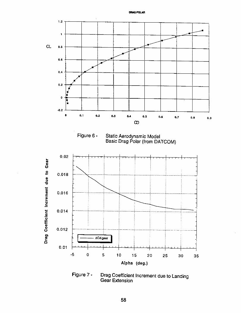
DI_kG POU_
CL
1.2
0.8
0.6
0.4
=1
0.2 J
,(
0 m
-0.2
J
......--.=J
0 0.1 0,2 0,3 0,4 0.5 0=6 0,7 0.8 0.9
Figure 6- Static Aerodynamic ModelBasic Drag Polar (from DATCOM)
O
O
"O
¢.-
E
¢-
oOo
0.02
0.018
0.016
0.014
0.012
0.01
.... I .... I .... .... I .... J .... I .... J ....
-5 0 5 10 15 20 25 30 35
Alpha (deg.)
Figure 7 - Drag Coefficient Increment due to LandingGear Extension
58

A
(:=_.
O
oI
t-O
0.1 -
0.045 -
-0.01 -
-0.065 -
I o ACn tail off (13=0°)
i---o -- ACn tail off (13=+2°)
.._,-- __ _ AC nI tail off (I3=+4°)" I
: - - -x- - - &C n tail off (13=+6°)I
" " -'t- " "
--1 ACn tail off (13=+8°)
I q" -- ACn tail off (13=+1 0°)
Ac ,(_,13)n tail o f
I
" _ _ l"% t'_ : .,"_ _ t_, _ f"_ : f_ _ ¢'_ _ ¢'_ : I._, t-_ _ f"_
_-_--._ _ ..............__£1-_e-_--e- _a,_,,e_o
._ :_ -_ -x- -x-i-x-* -_- _- -_.-i-x.-o_,-o-_.___,_c.= -+ -+ i-+ -+ -'1" . " i-+ _< _ .K-__/_'- _,x, ! "-,
............... i',\+....................................................................................T,T_ .......
X -I-, \
i _ -
-0.12 I I I t I I l-5 0 5 10 15 20 25 30 35
ALPHA
a)
I o c I ACo,_,_0.1 - -- no(tailoff) II
oo4 ................................i..............................................................................................................°-0.01
(b-<1
-0.065 -
-0.12
-5I I I t I I I
0 5 10 15 20 25 30 35ALPHA
b)
Figure 8 - Static Aerodynamic Model (Directional Characteristics)Directional Aerodynamics and Conventional Control Effectson Yawing Moment
59

-0 oO ACnAtail(__ )
--4" o---_ -- ACnAtail( _- 2 )O
_ ._ _ ACnAtail(_-+4 )
6v
-X- --4" °.... a_CnAtail(_,- 6 )
__4. o---+ " ACnAtail(_- 8 )
-- t, -- ACnAtail(_=+10 o)
natal
II
-0.065 -
_- _ _ _ ",,_. ,/-0.045 _-_:_-"__ ....................*:.........-_-.----i...................-._..---.+-.--_--_---_-
I;-+ ++ +i-+-:'_ ! / ._ + +ix-'<'_" .__F_ ->_ -_- -x- -x-i-x- -x- ":t: "_..... L& .+" i x'_ o--.-o"- i 0/-I-o--o--_--o--o-f,o--o-..o..., -.+- _- __o;_ _.._ -IB---_ B--B- B-+-B-_ _---T_-_'_:--_ : : .
-- F0 o 0 0 0 o O ,9 ,-, ,.,:,=, v,.-_'_'-'*'_-_---"_"-_ O;O C ,_, O 0"0.01 .......................................i..............:.....................................................................i......................................
.<1
o : i
-0.12 t ' I I I I I t-5 0 5 10 15 20 25 30 35
c)
ALPHA
o ACn(Sr=0O ) ---+-- &Cn(Sr=+20o )
-- Z_Cn(Sr=+5o ) --_- _ 6Cn(Sr=+25o )A C n( 0_,8r )
-- ._ - 6Cn(Br=+10:)-- o-- &Cn(Sr=+30° )
0"1 f-j ---x--ACn:'r=+15)" _ii -)t
..................i....................:................i..................._..................:,......................-,_.........:._:..-..._..-.___Io. 2 ;- j2T
_: -0 01 .................................................................................................................................................................t-
O
-0.065 -
-0.12 -
-5 0 5 10 15 20 25 30 35
d)
ALPHA
Figure 8 - Continued
6O

o ACn(Sa=0O) ---+-- ACn(Sa=+40o )
-- ACn(Sa=+l 0 °) --_- _ &Cn05a=+50o )
0.1 - - _ - ACn(Sa=+2°°)- e-- ACn(Sa=+60o ) JI---_-
................... T!..................... -::......................",=!......................_'-Lx_"- L'_ -................ .:._:.._..................... T!......................TI/;...... ',f>_";_.....0.045 -,_.-_- _ _ _r -'_x ,_
_-_ _-- 0-- _-- 0.--0--_ _>--0--- _-- _r-- i _m---o'v : _ _ J,_/O _-.o--.e- _ a-i-e- o--e- O---E_-::_ _ "--'_.-'f-.,#Z-_'_-."
g -0.01 ..............................................................................................................................................................................t-
O<3
-0.065 ............................................................................................................................................................................
-0.12 - -
-5 0 5 10 15 20 25 30 35
AC (o_,Sa)n
e)
ALPHA
Figure 8 - Concluded
0.06 -
0.04 -
_" 0.02 -g
v
o 0
o< -0.02
-0.04
Figure 9 -
o AC
-- AC
- -_ - Z_C
- --x-- -AC
- "-+ " -AC
--z_ -- AC
tail off (13=0°)
tail off (13=+2°)
tail off (j3=+4°)
tail off (13=+6°)
tail off (13=+8°)
tail off (B=+I 0°)
AC I tail off (0(''_)
I 1
i !
" " "":'i O._. i ./O i . ._ i _.
i _r.--A _"
I I i i I I0 5 10 15 20 25
ALPHA
Static Aerodynamic Model (Lateral Characteristics)Lateral Aerodynamics and Conventional Control Effects
on Rolling Moment61
.,%
30 35
a)

I o ACIotail off I AC (O.)
0.06 -_-
0
o<_
0.04 -
0.02 -
m
-0.02 -
-0.04 -
-0.06 -
-5 0 5 10 15 20 25 30 35ALPHA
b)
O B O
&CiAtail(15-0 )
___ __ &CiAtail(l_=+2o ) A ClAtail OC'l_)
0.06- - _ - ACIAtail(l_=+4°) I {
---x--- &Ciz_tail(13=+6o ) i
0.04- "+ " &Ciz_tail(l_+8°) ii i i
i '_z, -- ACiAtail(13=+10o ) i f'-i i '
0.02- .... i i i ! ! i i _.-
-_--_ -:_'-_ -_-'r_ i "_, +. _ o D--_,.,_ z
o i_ i ', i i i"& -_ " "-_' -<-0.02 i i i t ' ', , i+ _i
_ i ! _'-_ i: ! ! i,-7i
-0.04 .... i
-0 06q I t 1 l _ _ I
-5 0 5 10 15 20 25 30ALPHA
Figure 9 - Continued
35
c)
62

0.05
0.04
0.03
0.02
0.01
-0.01
-----e--- ,.,Cl(Sa=O=) - --o--- &Cj(Sa=+40=)
----B- ,_C1(8a==+10='}---x- - ACI(Sa=+50=)
--- _-- &Cl(Sa=+20,,)- -o- . &Cl(Sa=+60o)
_.. _... &Cl(Sa=+30=)
-.,-_ ,=,,,,,,=f==,,_=,_
ACl(Sa)
. _" -Oo ._.
s.
-...,. o •
/_-'"-=_ _-_-"_-...................................................• ......._.....................i........-".........." .............._ ...........................................
/ . _-x .L.x" i "x_ __ _-x-X
° : _ .' d : %341 _. __ O- 0 • . .
-_---.,-x.----':---.-......... ,_-._..................!.....................i.....................".....................i...........t...-.._.._._..=.m_e. -e" "" i _.._ i _'" _'"""'_.i
o- ! .,,.--,,"i" ..... ""-,,-_'" i '.."",, i.._-'_" " i i "'_.. "
"" i _ _ "_ ""-""" -,',
. i -o--.o--_-....................i..........._;-:'---$:':-:-o_-'_-:-_._..........................................
- ,=,...o-" $" "¢"--o- : "-c,...0. =...-o'" "o.
: i
;-
-5 0 5 10 15 20 25 30 35
ALPHA
d)
Figure 9 - Concluded
63

,5
O.l
0.09
0.08
0.07
0.08
0.05
0.04
0.03
0.02
0.01
0
i__i__1-11I
/i/I/lj
./-I--I--l--I_ i i 4
0 0.001 0.002 0.003 0.004 0.005
Crnu
lg
1
0.9
0.8
0.7
0.6
0.5
0.4
0.3
0.2
-5 0
/n.--- i-- i-- n .--i-- i .... n
-- I--I-4- I--I--I _ i _ i _ q
5 10 15 20 25 30 35
ALPHA (deg.)
J_
I
-10
1.2
) _n _ n. u \!
f I 0 I ,it
-5 -0.2 (_ 5 1 0
-0.4
-0.6
-0.8
BETA (dog.)
Figure 10- Aerodynamic Model of Pneumatic ControlEffect on Yawing Moment
64

0.025
0.02
0.015
0.01
0.005
0
_ • _U _m--lmml--41 -- n_ N- -m_m_ m
_m--N- •- • -m
-m -,_r'N11 ¢ ¢ p o (
0 0.001 0.002 0.003 0.004 0.005
Cmu
1
0.8
0.6
0.4
0.2
_-m--m O-i
-5 -0.2
-0.4
-0.6
-0.8
--m--am--+-m---m-- m....._m , l // , ,
ALPHA (dog.)
I
35
.O
I
-10 S
/
1.2
0.8
0.6
0.4
0.2
-5 -0.2
-0.4
-0.6
-0.8
.f.........m_ m_U_m \I
I -I
5 10
BETA (dog.)
Figure 11 - Aerodynamic Model of Pneumatic ControlEffect on Rolling Moment
65

II
I!
: i
::
0
o<
!
66

I000
800
_00
u 400
• 200
I-0 0o
-200
-40O
-600
.BOO
-1OOO
WING ROCK AT ALPIIA = 25 °
TAIL ON
--,-----_-F-,-,-_t-,--,--,-_---t_,, I .... I,,,-F,-,-,-,-F--,-_-F _-,-,-
..............._....................................................o._-.___, .....................J................i..............................
...............i................i...... i..............._...............i........... i................_..............
...............i............_ ..........i...............i................_................i................_................,.._,..........._..............
i i i i i i i i..............i............7...............T..............."..............T...............?................i................i.............i..............
...............!............. i ...............:!..............._................!........... : : "......i..............
...............}............ ...............i...............i................................! :
.............................. _ i ! ..
!
.... i .... I .... I .... 4_"i .... I .... _.... _.... _.... mI I I
-50 -40 -30 -20 -I0 0 I0 20 30 40 50
ROLL ANGLE [sec.]
a)
O
et
"U
I-0
O.
20000
IO000
12000
8000
4OO0
0
-4000
-8000
-12000
-16000
-20000
WING ROCK AT ALPHA = 25 °
TAIL ON
_'! .... I .... I .... I ....
..............I................i................i...............i..............................!
..............._................_................_...............T..............._..............._...............................I...............
! ...............
!
I! I
i -,k4 I
! : , . I I
............... _................ _................ ; ................................ ,_............... _............... i .......... t..............
' ! 1' i t°
!
-50 -40 -30 -'20 -10 0 10 20 30 40 50
ROLL ANGLE [see]
b)
Figure 13 - Phase Plots at (z = 25 ° (q = 958 Pa, Tail-On)
(Wind Tunnel Test)
67

0.15
0.14
0.13,v,
>" 0.12UZuJ=:)0 0.11UJ¢EEL
0.1
UJUD o.ogQWCE
0.08
0.07
0.06
0.05
WING ROCK FREQUENCY
! ,
............... !.................................. !.................................................................... .:................. ,...............................
..............i___;,;_o_j.............._................!................................I................................................
.............. .............................}.................................j.................ii ! : :
............................. _.......................................... : ............... _.............. _ ............... _............. i...............
, i i i
i _ IRRE(3UI_ARMOTION
i t i ! ,,
.................................................. ! ................. i .................................
i ' 1.... I .... i ......... i.........
10 12 14 16 18 20
J
i i
................ i ................. 4................. I ...............
i
22 24 26 28 30
AtIGLE OF ATTACK Ideg.]
Figure 14 - Reduced Frequency of Wing Rock Motion (q = 958 Pa)
100
"T
wo 80
n_ 70
_ 60
w
6 soD.-
_ 40
• 30
x
10
0
WING ROCK AMPLITUDE
I
t i i
II
................. i .......t
lI
i I
................ i ...............................
lI!
I
10 12
Figure 15-
14 16 t8 gO 22 24 26 28 30
ANOL8 OF ATTACK |deg. I
Maximum Peak-to-Peak Amplitude of Wing Rock (q = 958 Pa)
68

clp/_C,po
,/' I \_ ,_._-Clpo
Figure 16- Wing Rock Mathematical Model
Relationship between Damping Term and Roll Angle
69

d,l#
"O
u,I,.,,J(32:<[
,.,J_JoG:
OiU
ul.J(.,;1Z
,,,J,,,.JOrr-
5O
4O
3O
2O
10
0
-10
-20
-30
-40
-50
5O
40
3O
2O
10
0
-10
-20
-30
-40
-50
WING ROCK BUll.D-UP AT ALPHA = 25 °
TAIL ON
! _ ! ! .... I.Cycle 1 Cycle 2 nycl_ 3 Cycle _ Cycle 5 iCyclo 6 Cycle. 7
.........................i..........................i...................................................i...........................i........t P,.......
AJ".........................;..........................;..........................!.......................................... :...I .....
......... i ....... 4 .......
iiiiiiiii .....................u..°
I
RUN 60181i
........................................................ > ............................ 4 ......................................................... ) ...........................
1i ! I i ___ I i i I I l I I __-L I I I i I ! I I I f I I
0.5 1 1.5 2 2.5 3
TIME [sec.]
WING ROCK AT ALPHA = 25 °CYCLE # 3 & 4 -- TAIL ON
titIN_ (a)
tt
{
t • PIll3 I
Pill SMOOTH 3........................... PHI 4 .......
• • PHI _MOOTH 4 II
................;................_................._.................i...............
i z i................ i................. ;.................................. _................ • ................ _ ................ ;................. |................. _...............
' : ! ,,.'"'"o%1 I
i \'a i i+'i -• ;* t •
.............. ,....................................................................................................... _................. _.,.............. !....._ _-
i %.,,...,..
ii
!
Ii
0.9 0.97 !.04 1. I I 1.18 1.25 1.32 1.39 1.46 1.$3 1,6
TIME [see.}
Figure 17 - Wing Rock Build-up at e_= 25 ° (q = 958 Pa, Tail-On)(Wind Tunnel Test)
70

E,<
on-
4O
3O
2O
10
0
-1o
-2O
-30
-4O
MODEL SCALE WING ROCK AT
Clp -- Op__1--_(phi--bio')/phi il}
I/I
V L V
0.2 0.4 0.6 0.8 1 1.2
Time (sec.)
ALPHA = 50 °
/ / /V \
1.4 1.6 1.8 2
a)
on b
-rEL
1E
12
I¢'
E,
4
2
t_v
-2
-4
-I_
-I¢'
-12
-14
-I{:,
I
Roll Angle (deg.)
b)
Figure 18 - Results of First Order Wing Rock Model at e¢= 30 °
a) Roll Angle History, b) Phase Plot
71

o
m
"u
I--00O
1000
800
6O0
.-?.o 400g
• 200
I-0 0Q
_ -200
-400
-6O0
-8OO
-1OO0
20000
16000
12000
8OO0
4000
0
-4000
-8000
-12OOO
-16000
-20000
WING FLOCKAT ALPIIA = 30°TAIL ON
.... J.... I .... ! .... t. ....... ! .... I .... ' .... _ '
...............i...............i = ..,..!..............i...............i......... J.............................-, : : : ]
...............i.............................i................i..............._...............i................i................i..............i.............c= : : i ! ! z .
...............l............... i...............i..............._.............. 1............._.
ii iiiiiiiiiiiiiiiiiiiiiii;iiii,;iiiii;iiiii127}Iii............................... ;...............; ...............1............................
i i i : i i i =...............I......................................;..............._...............i.................................. !..............
_-___ __.__-i ........., ................ ;................ ;............... $ ........ _.............. _................ , ........ ;................ , ................ , ..............
i _= i i i i i i l :
• I--e-- l_IfOOT SM
_-_ ........ ' ........ , .... i .... ' .... i ......t__L.,._L i I- I I
-50 -40 -30 -20 -I0 0 10 70 30 40 SO
Roll Angle (deg.)
WING ROCK AT ALPHA = 30"TAIL ON
i tii................1
I | I
I
-50 -40 -30 -20 -I0 0 10 20 30 40 50
Roll Angle (deg.)
Figure 19 - Phase Plots at {z = 30 ° (q = 958 Pa, Tail-On)(Wind Tunnel Test)
a)
b)
72

5O
4O
30
20,..?
10
ILl
0 0z<
-10o
-20
WING ROCK AT ALPHA = 30 °
TAIL ON
0.75 0.8 0.85 0.9 0.95 1 1.05 1.1
TIME [sec.]
1000
8OO
600
400
Z
20000
0
?-200
n
-400
-6OO
-800
-10OO
a)
50
40
30
20
._. 10
W
J
0 0z
__ -100
-20
-30
WING ROCK AT ALPHA = 30 °
TAIL ON
I
-40
-50
0.7 0.75 0.8 0.85 0.9 0.95 1 1.05 1.1
TIME [see.]
200OO
16000
12000
8OO0 ._
4OO0 00
o "_ID
-4000 B
0
-8000 ""
-12OO0
-16000
-2O000
b)
Figure 20 - Angular Velocity and Acceleration at o_= 30 °(Wind Tunnel Test)
73

MODEL ,30 °
"o
t,-,,(
orr
4O
3O
20
10
0
-10
-2O
-3O
-4O
h
I
I
SCALE WING ROCK AT ALPHA =CJp- CIp_i[t--_(phi--blos>/ph;_i_^2]/2
/_ _ AI
I /, /I I, / /!
1//'l/ 1/ / / / /V L V L V L
/i
o o.= 0.4 o.s 0.8 _ _.2 _.A _.s _.8 2
Time (sec.)
a)
oQ)
&
I- o0m om
v
"1-
14
12
10
8
6
4
2
0
--2
-4
-6
--8
-10
-12
--14
MODEL SCALE WING ROCK AT ALPHA - ,30"CIp - CIp i[1--1(l#ni--bla,,,)/phi_il^2_J2
I I I I
--40 --20 0 20 40
Roll Angle (deg.)
b)
Figure 21 - Results of Second Order Wing Rock Model at cz = 30 °a) Roll Angle History, b) Phase Plot
74

25
MODEL SCALE WING ROCK AT ALPHA = 25 °
Clp- Clp_;[1--1(phi--bia_>/phi_;_'2]/'2
m
v
.<
0rr
- f,,o ;_ il II 1s _ /'\ t
o \ t/ / / 1_: ,/tlkl ,
_' t. tl i/ /-15
-20
o 0.2 o.4 0.6 0.8 _ _.2 _.4 ;.s _.a
Time(s_.)
a)
4O
MODEL SCALE WING ROCK AT ALPHA = 25"Clp - Cip_(1-1(phi-I.,ia,,,)/l_i_it^2]/2
@
o
,o f ,,,o A i'_ / t t _,o /_ /! / 't 1
/ '/1 ' /t/o / ' / t
__o 1 l/ t/'/ I'--20 i
" _ 1 k/ /-30 v
--4O I
0 0.2 0.4 0.6 O.B 1 1.2 1.4 1.6 1.8 2
Time(sec.)
b)
Figure 22 - Results of Second Order Wing Rock Model at o: = 25 °
Wing Rock Build-up for a) t = 0 to 2 sec., b) t = 2 to 4 sec.
75

60O
MODEL SCALE WING ROCK AT ALPHA = 25"
op - Ctp__[1-1(p.l-bio,>/PhL;l^2]/2
o
I"-
0Cl
"r
5OO
400
300
200
100
0
-100
-200
-300
-400
-500
-600I
--40
t=4.
I I I I ,,, I I
-20 0 20
Roll Angle (deg.)
I
4O
o4
=_ ,;,"0 c
0
o1::3
"1"0.
MODEL SCALE WING ROCK AT ALPHA = 25"C'Ip -- OFl_i[1-_(Flhi-bia',,)/phi_il^2]/2
10
9 -
8 -
7 -
6 -
5 -
4. -
3 -
2 -
1
0
-1
-2
-3
-4
-5
-6
-7
-8
-9
-10 I ,J I I
--4O --20
%
1 t 1
0 20
Roll Angle (deg.)
I
4_
Figure 23 - Phase Plots at o_= 25 ° for the Motion Shown inFigure 22 (Part b)
76

C:"
Im
L__3
II "7
.___3 -'_-_
II-- -z
. °_
I
',LJ 2_-2J g
(_b c._
Z
//
/ t
///
//
I ,/
/
,-./-,i-/
_°t
C;"
I'.1
C_ _._o
e-
0
0C',lI
0
oCO
II
0
O0
C°I
$
0c-
C
"4- OO_
rrl_
I
0
u_
--4-I
_"_pur.,,_n oqL)
(i_oes/fieP) J.OClC] IHd
77
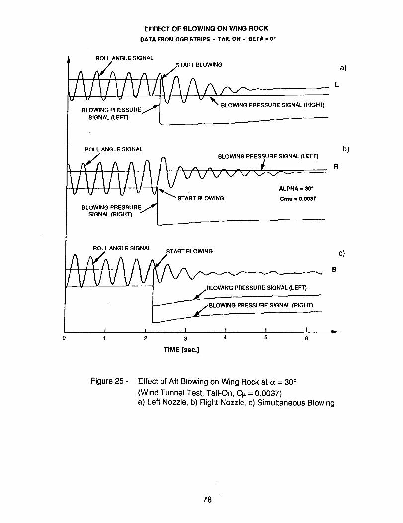
EFFECT OF BLOWING ON WING ROCK
DATA FROM OGR STRIPS - TAIL ON - BETA ,, 0_
ROLL ANGLE SIGNAL
BLOWING PRESSURE 7
SIGNAL (LEFT)
START BLOWING
V V _t_ BLOWING PRESSURE SIGNAL (FLIGHT)
a)
L
ROLL ANGLE SIGNAL
f V V V vvvl/I/l/I/lll ,<,.,.=.U U U U V I_START_ BLOWING Cmu 0.0037IB
BLOWING PRESSURE/SIGNAL (RIGHT)
b)
R
ROLL ANGLE SIGNALSTART BLOWING
A AIR A A A.GIt/t/vvt/!
/BLOWlNG PRESSURE SIGNAL (RIGHT)
I I I I I I
1 2 3 4 5 6
TIME [sec.]
c)
B
v
Figure 25 - Effect of Aft Blowing on Wing Rock at (z = 30 °
(Wind Tunnel Test, Tail-On, CI_ = 0.0037)a) Left Nozzle, b) Right Nozzle, c) Simultaneous Blowing
78

EFFECT OF BLOWING ON WING ROCK
DATA FROM OGR STRIPS - TAIL ON - BETA = 0°
ROLL ANGLE SIGNAL
A /f_ n BLOW,NGPRESSURES,GNAL(LEFT)?A A A A _,A..Z ...... _.,
V V V V V V _ START BLOWING ALPHA = 25°
Cmu = 0.0028BLOWING PRESSURE.,_
SIGNAL (RIGHT)
a)
A
! V tJ tJ IJ tJ IJ _"----_ START BLOWING
ROLL ANGLE SIGNAL
A_ BLOWING PRESSURE SIGNAL (LEFT)A AAA_^ _/_ .V Vv-v_-_-- - '
BLOWING PRESSURE _SIGNAL (RIGHT)
ALPHA = 25°
Cmu = 0.0037
I I I I I I ._1 2 3 4 5 6
TIME [sec.]
b)
Figure 26 - Effect of Aft Blowing on Wing Rock at (z = 25 °(Wind Tunnel Test, Tail-On)
a) Right Nozzle, CI1 = 0.0028; b) Right Nozzle, CI_ = 0.0037
79

Q
CD_D
II
7-
Q___]
F--_<_ '-I
_Bt-
Y_
Q_v
©TZ
I
__J<_0O0
__JW
(D
0
J
fJ
Jf
0 0 0 oto ol ,--
m
.=-
o_:_Dc_
°° {J_
a)
oZ
mm
0 0 0 0
I I I I
GO
0
A
m Ecl _-
0
cy0
0
0
0cOII
0
o 00 0rrci
c
_ 0
(_'-"o_c _
o
0 o0
m c
!
b-
U_
('Bep) el6UV IIOH
80

II
'2
II
II
½
II
I I I I I Io
c-
O
Ii
I,
13..E
IJJ
o°_
O..Ex
IJJ
t-l--
m_
(Dr-
eOc,or-
E°m
a!
cOz
!
cOOJ
°_
Ii
NOIIVI::IAO 90 llaVl::l 7VNOISN:IIAIIO-NON
81
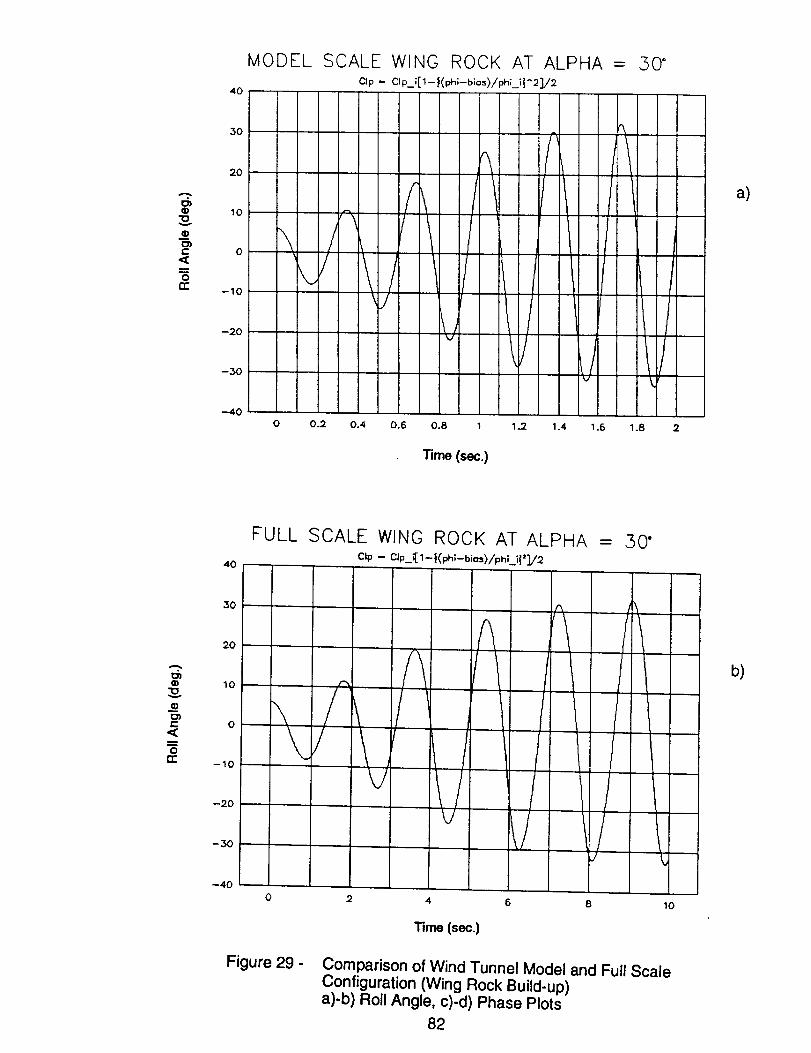
Q)"Ov
e,,,<
or,r
4o
3o
2o
lo
-lO
-2o
-3o
MODEL
%
SCALE WING ROCK AT ALPHA =C|p- Clp_i[1--_(_;--blas)/__i_^2_/2
/\ /' //
tJ v l,J
50 =
a)
--4Oo o.2 o., 0.6 0.8 _ _.2 _.4 _._ _.8
Time (sec.)
_D
_me-,<o
rr"
4O
30
2O
10
-10
-20
-30
FULL SCALE WING ROCK AT ALPHAc_p- clp_:.[_-i(ph;-b_,=,)/p_,L;_']/2
= ..%0"
i , /
/\/1 1/1
b)
--400
Figure 29 -
2 4 6 8 10
Time(sec.)
Comparison of Wind Tunnel Model and Full ScaleConfiguration (Wing Rock Build-up)a)-b) Roll Angle, c)-d) Phase Plots
82
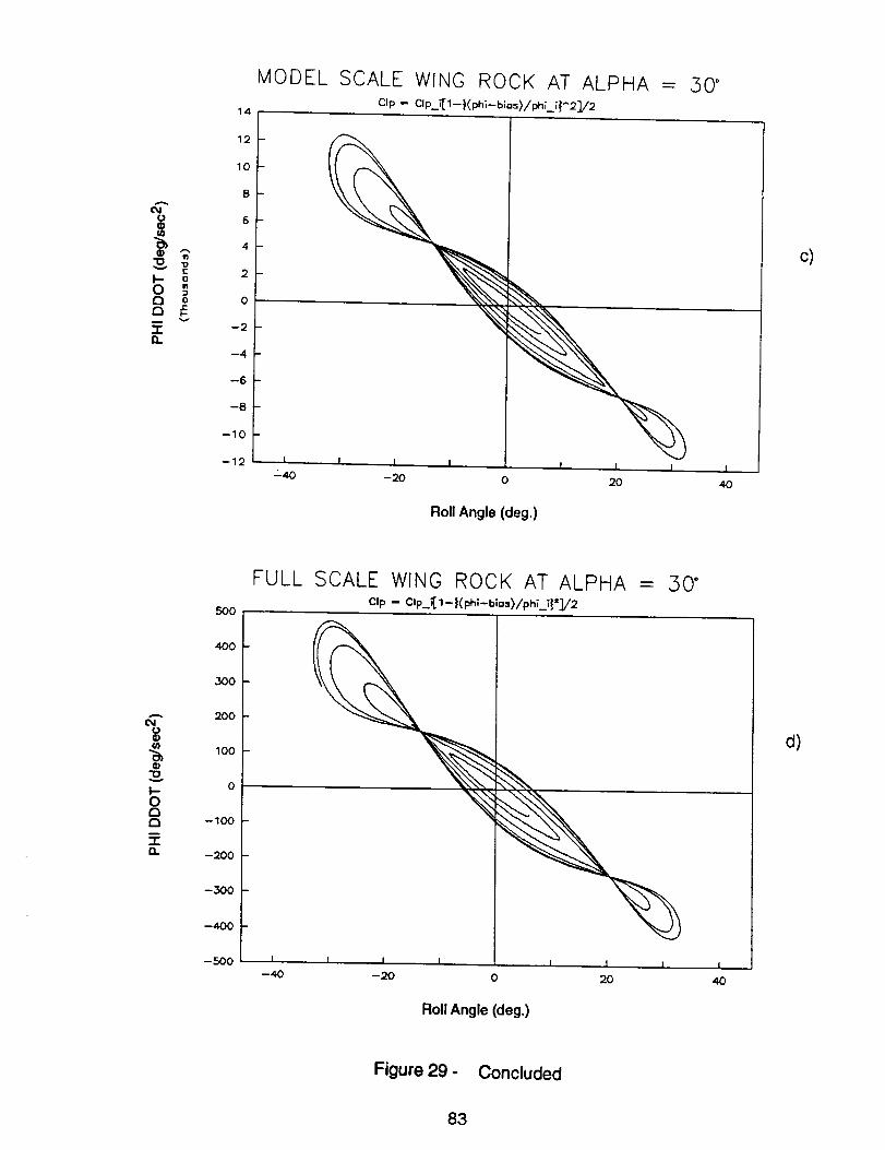
14
MODEL SCALE WING ROCK AT ALPHA = 30 °CIp- tip i[1--t(phl--bi,",s}/phi_i_^2]//2
A
"D 'ot"
I-- oo0 or..,
vm
,1-im
12
10
B
6
4
2
0
--2
--4
--6
-8
--10
--12 I , !
--40 --20 0 20
Roll Angle (deg.)
40
c)
"D
I--o
-rel
50o
4oo
:3oo
2OO
100
0
--100
--200
--300
--400
--500
FULL SCALE WING ROCK AT ALPHA = 50 °CIp -- CIp_(1--_(phl-blas)/phi..._'_/2
I
--40
I I I 1 i 1
-2O 0 20 40
Roll Angle (deg.)
d)
Figure 29 - Concluded
83

t-
Orr
4O
3O
20
10
0
--10
-20
-3O
--4O
MODEL SCALE WING ROCK AT ALPHA = .30"op- C_pj[1--t(ph_--b_os>/phUP2]/2
0 0.2 0.4 0.6 0.8 1 1_ 1.4 1.6 1.6 2
Time (sec.)
a)
t_
"I0
_0
t-
Orr
4o
30
2O
10
0
--10
-20
--30
--40
FULL SCALE WING ROCK AT ALPHA = ,30"Clp -- tip i[1--t(phi--bios)/phi_il']/2
0 2 4 6 8 10
Figure 30 -
Time (sec.)
Comparison of Wind Tunnel Model and Full Scale
Configuration (Steady Wing Rock)a)-b) Roll Angle, c)-d) Phase Plots
b)
84

14
MODEL SCALE WING ROCK AT ALPHA = 50"CIp-- CIp_i[1--_(ph;--bias)/phi_i_^2],/2
"0 ,-v 0
0 o
D
"1"
12
10
8
6
4
2
0
--2
--4
--6
-8
-10
--12
--14 1 I I I
--40 --20 0 20 40
Roll Angle (deg.)
c)
Ao,,I
e3
I--o0
"r13.
6O0
500
4O0
300
200
100
0
--100
-200
--300
-400
-500
FULL SCALE WING ROCK AT ALPHA = ,30 °Clp -- CIp__ 1--_(phi--bia,,,)//phi_ii'I/2
I I I , ,I I I I
--40 -20 0 20 40
Roll Angle (deg.)
d)
Figure 30 - Concluded
85

4O
MODEL SCALE WING ROCK AT ALPHACIp -- CIp_i[1--{(ph;--bia=>/phi_i_^2_/2
= 50"
"13
¢-
0rr
3O
20
10
0
--10
f',t
fl
L.,/;
j Note: Blowing
starts at *
a)
"I3v
0rr"
-4O
4O
,.30
2O
10
-10
-2O
-3O
-40
0 0.2 0.4 0.6 0.8 1 1.2 1.4 1.6 1,8 2
Time (sec.)
FULL SCALE WING ROCK AT ALPHA = 30 °C,p - Clp_i[1--l(ph;-bia..)/r, hLil']/2
Note: Blowingstarts at *
I I I0 2 4 6 8
Time (sec.)
lO
b)
Figure 31 - Comparison of Wind Tunnel Model and Full Scale
Configuration (Wing Rock Suppression, Cp. = 0.0037)a)-b) Roll Angle, c)-d) Phase Plots
86

AO4
CD"O
I--Ot-tE3
"l-Q.
t-O
O
9
8
7
6
5
4
3
2
1
0
-I
-2
-3
-4
--5
--6
--7
-8
-9
--10
--11
-12
MODEL SCALE WING ROCK AT ALPHA = 50 °
clp- Clp_;[1--{(ph;-bio_>/r,h;_i}_2]/2
--'- t=0.__,_
INote: Blowingstarts at * I
I l . I
--40 --20
I I I
0 2O
I
4O
Roll Angle (deg.)
c)
o@
G)"ID
t-O
E3-r-
6O0
5O0
4O0
30O
2O0
100
0
--100
-200
--300
--4O0
-500
FULL SCALE WING ROCK AT ALPHA = ,30"
clp - clp_,'['_-t(_;-Uio,,>/ph;_iF'3/2
INote: Blowing Istarts at * t = 0., I
--40 --20 0 20
Roll Angle (deg.)
| ,
4O
d)
Figure 31 - Concluded
87

er"
Q:E
I
+
:e
rl
' vL__rl _L_
0
D.
vl "
Q.r,O
(3 <m
0
U <
4.
mf_
E.,-.p(/):>,,
C).m-.,c-O
t-C_
U..
r-
"O
C_
O.-J
!
(,-j
:3
LJ-
88

W
]
0>- Z
" 8
c:o.
J
L
0
c,-c_
Ii
c0
£,_0,)
£:::)
I,...
0,)(0
J
|
t-
U.
89

oE
t_J
(D
co_
0
|
C_jC_
LL
90

5r,o
n"mmmX
0
m
..J0
I--Z00--I
Z0!,-0LUa:
LLII--
_1
8
z
00
eO.
E_o
DZ
0U
eQ:
0Z
oo
_E
"O_D
Oc-O
O
!
_D
C_
u.
91

In
IJR
l-
lIJ
nm
Z
o
oo5_
ILl
t-O
r-Oo
m
!
,q._0
g2

0
Ill
"_ rr0
-Or
°_
r-
.._rr0...,
_.121
!
L,.
93

A
>.
-8000
-6000
-4000
-2000
RUN 35
2000
-120000
Partially augmented, no blowing
:,
I, zl
-100000 -80000 -60000 -40000 -20000 0
X (ft.)
a) Variation in Altitude (-Z) and Horizontal Excursions (Y)
-5000
-4O00
-3O00
-2O00
-1000
N
E
ED.O
v
>.
0
n-UJ
0,¢n-I--d_
0
0
-4000
-3000
-2000
-1000
0
1000
2000
3000
4000
Partially augmented, no blowingB
i i i r i i i i i _ i i i i i I i i ,I
................................................................................................O!,aZIi .
RUN 35i l i i i 1 i _ i J i J i i i J J l
-2OOO
-1500
-1000
-500
5OO
1000
1500
2000
I'-
-IC
mm:o=00
DN
-120000 -100000 -80000 -60000 -40000 -20000 0
x (..)
Figure 36 -
b) Cross-Track and Altitude Errors
Approach and Landing Simulation for the NASP-typeConfiguration with Partially Augmented Flight Control System
(No Forebody Blowing)
94

"o
io,,E
40
30
20
10
-10
Partially augmented, no blowing
RUN35
i
i
alpha
0 40 80 120 160 200
Time (sec.)
c) Angles of Attack and Sideslip
10
8
6
4
2
0
-2
-4
-6
-8
-10
Co=_=;
A
o.o
(a
40
30
A
o_ 20o'1o
(0,J¢Q.
-- 10
0
-10
Partially augmented, no blowing
i .......... ! ...... A 1. _o_ y _ _,_.ai _,- i...............r! _1 i
--- _/;.tl'- "_-_ i........ ......................................i....................! -.............. i
' ' ' I ' ' ' , , , j , , , I , , ,40 80 120 160 200
Time (sec.)
d) Angles of Attack and Roll
100
80
60
4O
20
0
-20
-40
-60
-80
-100
i
A
o
Figure 36- Continued
95

A
o
a
4O
30
20
10
0
-10
Partially augmented, no blowing
f, -,,- ,1.... I .... I .... t .... t ....: I
i phi 80RUN 35 i _ :
j °2O
0
-20
-40
-60
-80
t,,, I'''' I ' ' ' ' ' ' ' ' ' ' ' ' -100
100 110 120 130 140 150
Time (sec.)
e) Angles of Attack and Roll
Q.O
v
A
o"ov
e=f-_L
<
4O
3O
20
10
"10
Partially augmented, no blowing
...... I,,'l'''t''' ,oo] i :
I_ II I soRUN 35 _ alpha i i phi
! ! i 40
0
.............................................................................................. 20
-40
.................................................................................... i ............................. _ ........................... "60i i''' i''' l''' I''' ''' -loo
132 134 136 138 140130
Time (sec.)
f) Angles of Attack and Roll
=rm
Q.O
v
Figure 36- Continued
96
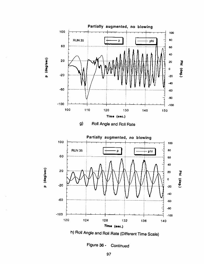
A
Oom
@"O
100
60
20
-20
-60
-100
100
Partially augmented, no blowing
110 120 130 140 150
Time (sec.)
g) Roll Angle and Roll Rate
lOO
80
60
4o
20
o
-20
-40
-60
-80
-lOO
'IVE
A
¢¢o
v
A
uow
o
100
60
2O
-20
-60
-100
120
Partially augmented, no blowing
......
_ ............ 200
-20
-40
.........................................................- ......................................................................................-60
' '' ' '' I''' I''' '''124 128 132 136 140
Time (sec.)
h) Roll Angle and Roll Rate (Different Time Scale)
lOO
80
60
4o
-80
-100
"I0
A
otj_v
Figure 36 - Continued
97
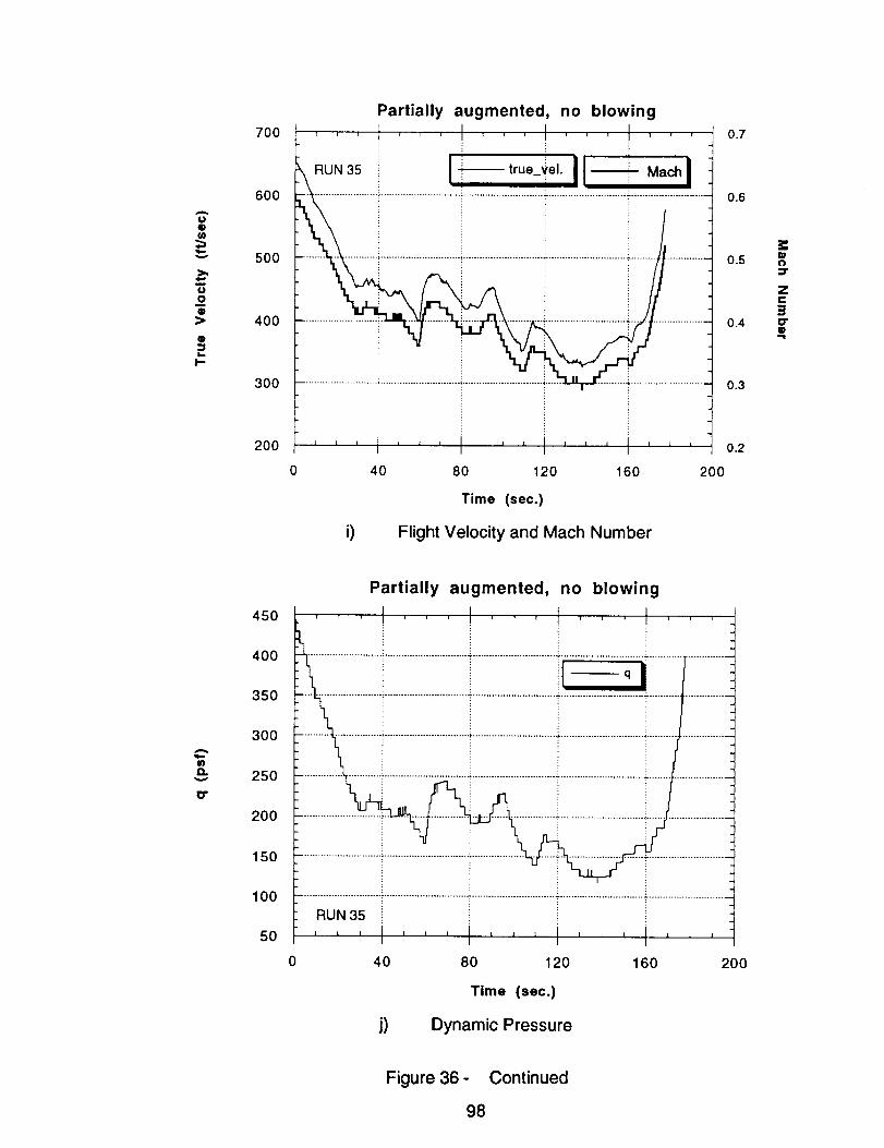
ow
.>,
Om
Q>
@=1I,.
I-
700
6OO
5O0
400
300
200
RUN 35
0 40 80
i)
Partially augmented, no blowing
• , ,I,,,I,,,: E
-_-- true_ el _ Maci " iI
I120 160
Time (sec.)
Flight Velocity and Mach Number
0.7
0.6
0.3
0.2
2OO
¢)
z
3O"
A
v
O"
450
400
350
300
250
200
150
100
50
0
RUN 35
, I I I ,
40 80 120
Time (sec.)
j) Dynamic Pressure
160 200
Figure 36- Continued
98

30
Partially augmented, no blowing
2OA
oqD
"" 10¢:
ou
0o
-lO"0'10
mr
-20
-3O
0 40 80 120
Time (sec.)
k) Rudder Deflection Angle
160 200
A
O)O
'tOv
¢..O
m
o
c_
i-
oo
m
,<
3O
2O
10
-10
-2O
-30
Partially augmented, no blowing
RUN 35
0Ill I I J I I I i _ l i I i A i
40 80 120 160
Time (sec.)
Aileron Deflection Angle
200
Figure 36 - Concluded
99

A
>.
-8000
-6000
-4000
-2000
0
RUN 15
2000
-120000
a)
Partially augmented + pulsed blowing
!--z
0
0
-5000
-100000 -80000 -60000 -40000 -20000
X (ft.)
Variation in Altitude (-Z) and Horizontal Excursions (Y)
-4000
N
-3000
-2000
-1000
>.
n-On-n-
v0,<n-I-
090n-(.)
-4000
-3000
-2000
-1000
0
1000
2000
3000
4000
-120000
Partially augmented + pulsed blowing
....... .......i_.i'_lo_,_z____________________i________________________________._.________i____.._______`_..______i.......................i....................I1
............................................. •;...................................... _...................... i ......................
RUN15 ) i i --iDeltaY II I _ J J J
-100000 -80000 -60000 -40000 -20000
-2000
-1500
>-1000 r
c-500 o
m
m0
O
500
N
1000
1500
2OOO
0
b)x (ft.)
Cross-Track and Altitude Errors
Figure 37 - Approach and Landing Simulation for the NASP-typeConfiguration with Partially Augmented Flight Control Systemand Pulsed Forebody Blowing
100

olo
"10v
(=J=o.
n
,,¢
40
30
2O
10
-10
Partially augmented + pulsed blowing
........ I .... I .... I .... J
JRUN 15 i
4
• - - alpha i - -beta ;_
10
8
6
4
2
0
-2
-4
-6
-8
-10
50 100 150 200 250
Time (sec.)
c) Angles of Attack and Sideslip
@
=)
A
e(av
o
v
m,,1=o.
40
30
20
10
0
-10
Partially augmented + pulsed blowing
.... t ........ I .... I ....i E
RUN 15 : :
0 50 100 150
Time (sec.)
100
80
60
40
o _-20 _..
-40
-60
-80
-100
200 250
d) Angles of Attack and Roll
Figure 37- Continued
101

A
Qt_
q,..v
_>,uo
>
@
I=
I--
700
600
50O
400
300
200
Partially augmented + pulsed blowing
, . . JI r = 1 J J J r i _ i
RUN 15
0 50 100 150 200
Time (see.)
0.7
0,6
0.3
0.2
25O
l=mN=r
e-3o"o
e) Flight Velocity and Mach Number
A
D.v
O"
450
400
350
300
250
200
150
100
50
RUN 15
0
Partially augmented + pulsed blowing
40 80 120
Time (sec.)
f) Dynamic Pressure
160 200
Figure 37- Continued
102

A
o"I3v
O
o
@c_
'10'10
n,-
o
v
¢,...O
m
¢,.}Q
,e.=
oC_
cO
Omm
30
20
10
0
-10
-20
-30
30
20
10
0
-10
-20
-3O
Partially augmented ÷ pulsed blowing
0 40 80 120 160 200
Time (see.)
g) Rudder Deflection Angle
Partially augmented + pulsed blowing
. I I Ii i ! i i i f I _ i i i i l i
RUN 15 i :
l I I I I I I I I I I I
40 80 120
Time (sec.)
h) Aileron Deflection Angle
160
I I I
200
Figure 37- Continued
103

A
-oU_
o,-Iv
(P
¢:4)Oo
I¢
Oi
m
Partially augmented + pulsed blowing
0.0035 i ........ . .... .... . ....
RUN 15
0.003
0.0025
0.002
0.0015
0.001
0.0005
A
@1D
m
U_
m
m
o
OO(JO1¢-
O
0
0.0035
0.003
0.0025
0.002
0.0015
0.001
0.0005
0 50
i)
100 150 200
Time (see.)
Blowing Coefficient (Left Nozzle)
J)
50 100 150 200
Time (sec.)
Blowing Coefficient (Right Nozzle)
250
250
Figure 37 - Continued
104

A
E-=
==-o
.J
el
1-oE==
D"O
tr-
elelca
=EI==
m
P
3=oIZl
500
400
300
200
100
0
Partially augmented + pulsed blowing
........ ' .... I .... I ....RUN 15
50 100 150 200 250
Time (sec.)
k) Accumulative Total Mass Flow Requirements (Left)
A
E,,Q
el
r"OEmi-.
m
D"og:
elel
i._n
¢7)f,.
o
500
400
300
200
100
0
i)
Partially augmented + pulsed blowing
! i i i _ i J J i ! ! _ _ _ I i i i r i
RUN 15 i i
............................. _............................... _.............................. _............................. _.............................
............................. _............................... '_............................ _............................... _ ............................
50 100 150 200 250
Time (sec.)
Accumulative Total Mass Flow Requirements (Right)
Figure 37 - Concluded
105

A
=::
>-
-8000
-6000
-4000
-2000
RUN 24
Partially augmented +
20OO
-120000
proportional blowing
' I
!_z
a)
- 100000 -80000 -60000 -40000 -20000 0
X (ft.)
Variation in Altitude (-Z) and Horizontal Excursions (Y)
-5000
-4000
-3000
-2000
-1000
N
m
Eo.
9
::1=v
A
v
)-
n-o
w
o
n-
_n0n-O
-4000
-3000
-2000
-1000
0
1000
2000
3000
4000 L i _ _ A ,
"120000 "100000
RUN 24
I I I I I I I I I l I I
-80000 -60000 -40000 -20000 0
X (ft.)
-2000
-1500
>
-1000
C-500 O
m
m0 m
O
50O
N
iooo
1500
20OO
Figure 38 -
b) Cross-Track and Altitude Errors
Approach and Landing Simulation for the NASP-typeConfiguration with Partially Augmented Flight Control Systemand Proportional Forebody Blowing
106

"O
J¢Q.
m
<
40
3O
20
10
-I0
0
Partially augmented + proportional blowing
" ....... ! .... ! .... ! .... t
RUN24 !--alphai! ! .... beta ! 1
10
8
6
50 100 150 200
2
0
-2
- -4
...... -6
Time (sec.)
c) Angles of Attack and Sideslip
-8
-10
250
m
m
A
D.O
A
O}@
"O
40
30
2O
a,¢
--:" 10
-I0
Partially augmented + proportional blowing
........ i .... t .... I .... tRUN 24 : alpha : - - - ,hi
t o .._
V "'_t
..................................................................................................................... i ..........................
I I I I I I 1 J I I I i I I l I l I I I
t
0 50 100 150 200 250
100
80
60
40
20
0
-20
-40
-60
-80
-100
Time (sec.)
"I0
@(O
d) Angles of Attack and Roll
Figure 38 - Continued
107

A
@
v
oo@
o
.=I--
7OO
6OO
500
400
300
200
RUN 24
Partially augmented + proportional blowing
J I I I I
I
_ true_vel.
e)
50 100 150 200
Time (see.)
Flight Velocity and Math Number
0.2
250
o_r
Z¢,-3D"O"=1
A
W
O"
450
400
350
300
250
200
150
100
50
Partially augmented + proportional blowing
• I I •i
RUN 24
40 80 120
Time (sec.)
f) Dynamic Pressure
Figure 38 - Continued108
160 2O0
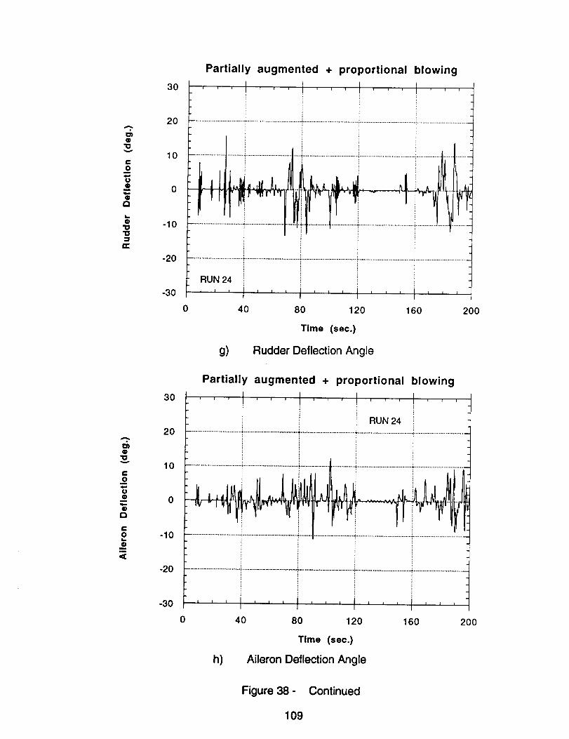
o
c
.9oo@
mit,.
O
'ID'ID
n-
A
o'tO
cO
uo
mb
o
¢=
,9°Q
mm
Partially augmented + proportional blowing
30 , ..... I .........
0 ........................................................... "_............................................................................................
.... i-10 " "
-20 .........................................................................................................................................................
RUN 24
"30 = J i I A I 1 I I _ i I I i i
0 40 80 120 160 200
Time (sec.)
g) Rudder Deflection Angle
Partially augmented + proportional blowing
3o ....... I t I
i RUN 24
0 ............................................................. _ ..........................................................................................
10 ......................................................................................................................................................
-10 "..............
-20 ........................................................................................................................................................
"30 l = i = i i I I t I = J t = =
0 40 80 120 160 200
h)
Time (see.)
Aileron Deflection Angle
Figure 38 - Continued
109

A
q)-o(/)
q}.J
6o
QO
O
I¢
O
m
0.0035
0.003
0.0025
0.002
0.0015
0.001
0.0005
Partially augmented + proportional blowing
RUN 24 - - -CmuJett i
0 50 100 150 200 250
Time (sec.)
i) Blowing Coefficient (Left Nozzle)
A
o'lO
U)
m
n,.
t-oo
:8:::OOo
I¢
om
0.0035
0.003
0.0025
0.002
0.0015
0.001
0.0005
0
Partially augmented + proportional blowing
• I
.......... i,
RUN 24
i iiil50 100 150
Time (sec.)
2OO
J) Blowing Coefficient (Right Nozzle)
250
Figure 38 - Continued
110

0.0035
0.003
0.0025Q
U
• 0.002Oo
m 0.0015
m 0.001
0.0005
Partially augmented + proportional blowing
............ I .... t ....
RUN24 I _ Crnuleft I................................................................................ _ _'nu r_ht
50 60 70 80 90 100
Time (sec.)
k) Blowing Coefficient (Expanded Time Scale)
oOM
E,,Q
e
ffl
0,,J
=a
o
i1
w
m
10
8
6
4
2
Partially augmented + proportional blowing
RUN 24
S = 523.4 ft2
Vj = 1116 ft/secm = 304.9 Ibm
0 50 100
i)
E
I
150
Time (sec.)
Mass Flow Rate (Left Nozzle)
Figure 38 - Continued
111
200
;
rndolleft
250

A
uo
E.a
m
,,c_=
QI=*
n-
o
It.
m=E
10
8
6
4
2
0
Partially augmented + proportional blowing
l
RUN 24
0
.... I .... I
S = 523.4 ft2
Vj = 11 16 Wsec
m = 237.8 Ibm
ili200
Time (sec.)
m) Mass Flow Rate (Right Nozzle)
J°
J
I
I I
250
A
E,,Qm
o&_
"5O"Q
nr"
=Et-
,<
3=O
(ZI
350
3OO
250
20O
150
100
5O
0
-50
n)
Partially augmented + proportional blowing
..................................................................... _ RIGHT ................................... ,.,.c..
0 50 100 150 200 250
TOTAL MASS
INTEGRATION543_m
Time (sec.)
Accumulative Total Mass Flow Requirements (Left and Right)
Figure 38 - Concluded
112

A
q..,.v
>.
-8000
-6000
-4000
-2000
0
RUN 18
2000
-120000
Fully augmented, no blowing
-100000 -80000 -60000 -40000 -20000 0
-50OO
-40OO
NA
-3000 &
e,.
a.
-2000
-1000
0
X (ft.)
a) Variation in Altitude (-Z) and Horizontal Excursions (Y)
A
v
>-"<3
O
IJJ
vto
n-I--
U)O
tO
-4000
-3000
-2000
-1000
0
1000
2000
3000
4000
Fully augmented, no blowing
,,,I,,,I,,,I,,,I,,,I,,,
...................... i ......................................................................... i
! ¢ ........
........................................ _..................................................i........................._......................
i i = l I I | I I l l l I I | i I I
-120000 -100000 -80000 -60000 -40000 -20000 0
-2000
-1500
-1000
-500
0
500
1000
1500
2000
Figure 39 -
x (ft.)b) Cross-Track and Altitude Errors
Approach and Landing Simulation for the NASP-typeConfiguration with Fully Augmented Flight Control System(No Forebody Blowing)
113
I-.-i'-4CC)m
m-n-n0-n

o_
"o
Q.
4O
30
20
10
0
-10
Fully augmented, no blowing
.... I .... I ........ t .... I .... 31o
i [--------_alpha I I!! beia J i 8i : . ! •
0
-. -8
L I I h I I I I I I I I I I I I I I I L I I I I 1
i
i 1 0
50 100 150 200 250 300
Time (sec.)
c) Angles of Attack and Sideslip
m
D
A
a.(D
v
3O
2O
10
Q
0
a.
-lO
-20
-3O
0
Time (sec.)
d) Roll Angle
Figure 39- Continued
114

A
U0m
_o0
0
I"
700
600
5OO
400
300
2O0
RUN 18
5O
e)
Fully augmented, no blowing
irue_veL _ Mach
100 150
Time (sec.)
200 250
Flight Velocity and Mach Number
3OO
0.7
0.6
0.3
0.2
=lO
Z¢:3O"¢D-ql
A
D.
O"
450
400
350
300
250
200
150
100
50
Fully augmented, no blowing
RUN 18
5O
f)
100 150
Time (sec.)
Dynamic Pressure
2OO 250 3O0
Figure 39- Continued
115

3O
Fully augmented, no blowing
2O
O_
O1o
10c-
Om
O
= 0Q
"_ -10
n-
-2O
-30
0 50 100 150 200
Tlme (sec.)
g) Rudder Deflection Angle
250 300
3O
2O
610
e.
o
0
-= o6
r_
c-
O -10o
-2O
-30
Fully augmented, no blowing
RUN 18 i
i i l ! i _ = l _ i l L 1 i 1 i I I _ I 1 i 1 ]
50 100 150 200
Tlme (sec.)
h) Aileron Deflection Angle
250 3OO
Figure 39 - Concluded
116

A
v
-8000
-6000
-4000
-2000
0
2000
RUN 30
-120000
a)
Fully augmented + proportional blowing
-100000 -80000 -60000 -40000 -20000
X (ft.)
-5ooo
-4ooo
-lOOO
o
0
Variation in Altitude (-Z) and Horizontal Excursions (Y)
NA
e,-a.O
A
n-On-trI,g
vtO
trI-
t_On-tO
-4000
-3000
-2000
-1000
0
1000
2000
3000
4000
Figure 40 -
-120000 -100000
Fully augmented + proportional blowing
,,,t ...... i,,, i ,, , I, ,,]
....................... ' ........................ ¢....... °.. ....
iiiiiiiiiiiiiiiiii
i i i i i i ' ' I I I I I I I I I I I
-80000 -60000 -40000 -20000 0
b)x (ft.)
Cross-Track and Altitude Errors
-2000
-1500
-1000
-500
0
500
1000
1500
2000
Approach and Landing Simulation for the NASP-typeConfiguration with Fully Augmented Flight Control Systemand Proportional Forebody Blowing
117
r-
c
m
m_D
O
E>N

¢3=
e-
40
30
2O
10
0
-10
Fully augmented + proportional blowing
RUN 30
50 100 150 200 250
Time (sec.)
c) Angles of Attack and Sideslip
10
6
4
2
0
-2
-4
-6
-8J
-10
3O0
CO
I
A
Q.O
.¢=v
3O
20
10
UiQ
"-" 0
.1=Q.
-10
-20
-30
0
Fully augmented + proportional blowingA
i ! _ i 1 i ! i J | r u i i i r = i = | | ' r r u r I
_l_i _ RUN30 _"4
-4
-I
"4
i .
-4
-I
,.4
J i I t i x i i i I I A n ! i I | i J i i I I I ¢
50 100 150 200 250 300
Time (sec.)
d) Roll Angle
Figure 40- Continued
118

700Fully augmented + proportional blowing
0.7
v
0
o0
>
(P
&.I--
600
500
400
300
0.6
0.3
mo_r
ze-
30"0
200
50
e)
100 150 200 250
Time (sec.)
Flight Velocity and Mach Number
300
0.2
IIo
mv
450
400
350
300
250
200
150
1 O0
50
0 5O
f)
100 150 200
Time (sec.)
Dynamic Pressure
Figure 40- Continued
250 300
119

A
ololo
co
uo
or-t
"ID"lO
IZ
3O
2O
10
0
-10
-20
-3O
Fully augmented + proportional blowing
RUN 30
50 100 150 200
Time (sec.)
g) Rudder Deflection Angle
I
250 300
A
o_o
"ID
CO
o@
oQ
o4)
ii
30
2O
10
-10
-20
-30
Fully augmented + proportional blowing
i = i i J w i _ , i i J _ i _ 1 f i i _ = J i i J
JRUN 30
................................................. ........................................................................................................ "1
/
1 L i J I I I I i _ I I I L A t i i i I I I i i i
I ; I
50 100 150 200 250 300
Time (see.)
h) Aileron Deflection Angle
Figure 40- Continued
120

-o¢/)
Q
,.I
¢P
u
o0
z=om
0.0035
0.003
0.0025
0.002
0.0015
0.001
0.0005
0
50 1 O0 150 200 250 300
Time (see.)
Blowing Coefficient (Left Nozzle)
-ou)
Z-u
n-
_e_u:1=oo0
z=om
Fully augmented + proportional blowing
0.0035 _ J ........i ! , ! _ ! = i T I | | I = I I !
!' iiii iiiiiii iiiiiiiiiiii i iiiiiiiiiillo.oo_....._).._ I .............................................................................
0.0025 .....................................................................................................
0.002 ......................•..............................................•..............................
0.0015 .............. _................................................................
O00it t/i/0.0005
0
0 50 100 150 200 250 300
Time (sec.)
j) Blowing Coefficient (Right Nozzle)
Figure 40- Continued
121

Eel
=--o
¢P-J
.=rt,-
]=oI.I.
gco
10
8
6
4
2
0
Fully augmented + proportional blowing
.... I .... I .... t .... t .... t ....: i
I- _'+w=l i i _°_°
i
50 100 150 200 250 300
Time (sec.)
k) Mass Flow Rate (Left Nozzle)
E
="
O9
Z-.?n-
¢=
]=o14.
m
10
Fully augmented + proportional blowing
50 , 100 150 200 250 300
Time (see.)
Mass Flow Rate (Right Nozzle)I)
Figure 40- Continued
122

AEJ_
@
(/7
=::O
--I
"O
.=
¢TQ
m=E
C
om
300
250
200
150
100
50
0
RUN 30
Fully augmented + proportional blowing
S = 523.4 ft 2
Vj = 1116 ft/sec
m = 274.8 Ibm
m)
50 100 150 200 250 300
Time (sec.)
Accumulative Total Mass Flow Requirements (Left)
AE
J_
O-of_
E:O)
n-
"O
,.!O"O
mmm=E
<CO_C
om
300
250
200
150
1O0
50
Fully augmented + proportional blowing
............ I ........ I ....
i ! ! _ I vj=1116.Js_c/.........................-........................._..........................:........_......!.....1 _=_,._,_,[
....................... ;-.................... i ......................... $......................... _.......................... _.......................
i/i! I
0 50 100 150 200 250 300
Time (sec.)
n) Accumulative Total Mass Flow Requirements (Right)
Figure 40 - Concluded
123
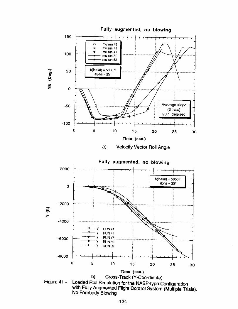
Qo
150
100
5O
=E 0
-50
-100
Fully augmented, no blowing
---e--- mu run41mu run 44mu run 47mu run 50mu run 53
.......... h(initial) = 5000 ftalpha= 25°
Average slope
(3 trials)
20.1 deg/sec
5 10 15 20 25
Time (see.)
a) Velocity Vector Roll Angle
3O
2OO0
0
-2000
-4000
-6000
-800O
Figure 41 -
Fully augmented, no blowing
........ { ...... ,,I .... I ....
I Ii I alpha= 25 |
---_-- y RuN4_ ! i _,_"--.._:'_y : i ! :....... _ Y _.B.UN..4_.X_-'_...__ ......................_y RuNs0 \_L
----'--- Y RUNS3k i 1 t I I J A _ I I I 1 I I _ I _ I I J I l_,¢
0 5 10 15 20 25 30
Time (sec.)
b) Cross-Track (Y-Coordinate)
Loaded Roll Simulation for the NASP-type Configurationwith Fully Augmented Flight Control System (Multiple Trials).No Forebody Blowing
124

A
¢=
e""10
N
-6O00
-5000
-4000
-3000
-2000
-1000
0
0
Fully augmented, no blowing
h(initial) = 5000 flalpha = 25°
5
c)
10 15
Time (see.)
Altitude (-Z)
20 25 30
A
o"O
¢=
a.
3O
25
2O
15
10
Fully augmented, no blowing
h(initial) = 5000 I1alpha = 25°
+ alpha RUN 41alpha RUN 44
+ alpha "_U_147alpha RUN 50alpha RUN'53
10 15 20
Time (see.)
d) Angle of Attack
Figure 41 - Continued
25 3O
125

A
01Q10
e-O
"6Q
m
"O10
30
2O
10
-10
-2O
-3O
Fully augmented, no blowing
h(initial) = 5000 ft
alpha = 25 °
rudder_clef RUN 41
rudder_clef RUN_A
----e--- rudder_def RUN 47
------=--- rudder_def "'RUIq_
rudder_clef RUN 53
0 5 10 15 20 25
Time (see.)
e) Rudder Deflection Angle
O1o
10V
O
Qm
c-
oo
mu
Fully augmented, no blowing
30 ........ I .... 4 ............
il h(initial) = 5000 ftlalpha = 25 °
20 ...................................
10 ...................................................i.....................................................................................................
.... _../_ . _ _ i ..................0 ..... _ _- - i i i /
-10 .......................................................................................................aileron def RUN 41
aileron def RUN 44
---e----- aileron def RUN47
-20 ............... ---4---- aileron def "'R0I_'5(J ........................................................................
aileron_clef RUN 53
_ _ ._
-30 .... i
0 5 10 15 20 25
f)Time (see.)
Aileron Deflection Angle
Figure41 - Continued
126
30

A
(.1Qw
O)Q
"0
30
20
10
0
-10
-20
-30
Fully augmented, no blowing
h(initial) = 5000 ftalpha = 25°
t I I
P RUN 41P RUN 44P RUN 47
P RUN 50P RUN53
0 5 10 15 20 25
Time (see.)
g) Body-Axis Roll Rate
30
A
oO
O)O
"O
L_
30
20
Fully augmented, no blowing
fl' hlinitiaalpha':)1==500025°.... ft I ............................................................................................ 4- .......................
10
0
-10
-20
-30
0 5 10 15 20 25 30
Time (sec.)
h) Body-Axis Yaw Rate
Figure 41 - Concluded
127

olQ
O
:l=E
150
100
5O
0
-50
-100
-150
Fully augmented + proportional blowing
mu run 60
----e---- mu run 61
mu run 62
-----iE--- mu run 63
mu run 64
h(initial) = 5000 ft
alpha = 25 °
Average slope(3 trials)
28.1 deg/sec
0 5 10 15 20 25 30
Time (see.)
a) Velocity Vector Roll Angle
A
>-
2000
0
-2000
-4000
-6000
-8000
Figure 42 -
Fully augmented + proportional blowing
........ t ............ J ....
i h(initial) = 5000 ft
i alpha = 25 °
---e---- y RUN 60----e---- y RUN61
.........----e---- y -RU-N62...................................................................................................----=---- Y RUN63
y RUN64
I A ' ' _ ' J = ] I J l J l I I I I I I I _ t I t t
I I I
0 5 10 15 20 25 30
Time (sec.)
b) Cross-Track (Y-Coordinate)
Loaded Roll Simulation for the NASP4ype Configurationwith Fully Augmented Flight Control System and ProportionalForebody Blowing (Multiple Trials)
128

A
o"10
me.e
i
,=
N
-6000
-5000
-4000
-3000
-2000
-1000
0
0
Fully augmented + proportional blowing
h(initial) = 5000 ftalpha = 25°
----e---- z RUN 60
----e--- z RUN 61
RUN 62 L_....._...----e---- z FrdN7 (_3 .................................................
Z RUN 64
5 10 15 20
Time (sec.)
c) Altitude (-Z)
25 3O
A
O1o
"O
m
Q.m
3O
25
20
15
10
5
0
Fully augmented + proportional blowing
h(initial) = 5000 ftalpha = 25°
alpha RUN 60---e---- alpha RUN 61
alpha 'RUN 62 .........alpha RUN 63alpha RUN 64
5 10 15 20
Time (sec.)
d) Angle of Attack
Figure 42 - Continued
25 30
129

A
"O
r"
o
om
q)¢3
"O"lO
n-
30
20
10
-10
-2O
-30
Fully augmented + proportional blowing
t I t S t
i i n u _ w t F n I I T V I U _ _ n _ r n T
........................ ; .......................... i..........................
0 5 10
................... °.,i .......................
rudder_def RUN 60
rudder_def RUN 61
rudder_def RUN 62
---m--- rudder_clef "1_N63 ..........
rudder_def RUN 64
i
I I I I I I I l ' Ji I I I I
15 20 25 30
Time (sec.)
e) Rudder Deflection Angle
Q
O
O
OO
¢,,.OL_
Om
30
20
10
0
-10
-20
-30
Fully augmented + proportional blowing
.... t ........ I .... t .... I ....
-----e---- aileron_def RUN 60 i
_ _ aileron_def RUN61 i I alpha=25° -
---o--- aileron_de| RUN 62
aileron_de! RUN 63
aileron_def RUN 64
a I I L J I I J I J _ = I J I I J J I I I I * t a L
I I
5 10 15 20 25
Tlme (see.)
f) Aileron Deflection Angle
Figure 42 - Continued
130
30

A
@
@"O
Q.
40
30
20
10
0
-10
-20
-30
-40
0
Fully augmented
h(initial) = 5000 ft
alpha = 25 °
+ proportional blowing
----e--- p RUN60
p RUN 62
P RUN 63
p RUN 64
_ :
5 10 15 20 25 30
Time (sec.)
g) Body-Axis Roll Rate
30
2O
10A
o@
• 0"Ov
L_
-10
-2O
-30
0
Fully augmented + proportional blowing
.... ! .... ! .... ! .... i .... _....
alpha= 25° ...........................................................................
........................'................................. iiiiiiiiiiiiiill...........................---e-_ r ....1_1_60................
---e--- r RU_61----o--- r RUN 62
............................................................................................_ r ....RUR'6_................r RU_
E
............ ''"1''"i'"'5 10 15 20 25 30
Time (sec.)
h) Body-Axis Yaw Rate
Figure 42 - Continued
131

Qm
oqk--
o0(3
I"m
3=0
{0
0,0035
0.003
0.0025
0.002
0.0015
0.001
0.0005
0
RUN 63
Fully augmented + proportional blowing
r i _ i i i I r _ i i i _ i i i r i r t i 1 i
Cmu leftCmu right h(initial) = 5000 ft
............................... ! alpha = 25°
.............................................................................. r .......................
... ' .......................... _......
0 5 10
il
.........................iii.........iii-I
15 20 25
Time (sec.)
i) Blowing Coefficient
3O
A
oo
.QV
@
¢1(Z
toI.i.
¢/I
t_=E
20
16
12
8
4
Fully augmented + proportional blowing
mass flow left
mass flow right
RUN 63
................... : .......................... ! ...... 1l ................. :'
0 5 10
.... I ' 1
I
h(initial) = 5000 ftalpha = 25°
IIII Illl
15 20 25 30
Time (sec.)
h) Mass Flow Rate
Figure 42 - Continued
132

A
EJ_u
¢,..oE
O"o
n-
¢0
=EL-
m
,¢O1e.
Oi
m
A
f,.to
01o
10
o,e.e
¢un-
On-
O01
Q>
,¢
100
80
60
40
20
0
Fully augmented + proportional blowing
.... i .... I ........ t .... I_,,,:
left i
_ :ight (I h(initial) = 5000 ft J........................ _.......................... i ................................................... alpha = 25 °
RUN 63
........................i.............................................................................;.......................
5 10 15 20 25 30
J)Time (sec.)
Accumulative Total Mass Requirements
Figure 42 - Concluded
35
3o
25
20
15
10
0
Fully augmented
vrr ell nut ill u'nl flu unl
.................... i..................... L._2 ..................... ;...................... _....................
............................................................ I_ BLOWINGNOBLOWING I .....................................
I I I I k I I 1 I I ! I t ! I I I I | t I
18 20 22 24 26 28 30 32
Alpha (deg.)
Figure 43 - Comparison Between Velocity Vector Roll Rate for
the Non-Blowing and Blowing Cases
133

o.
O
2000
1600
1200
8OO
400
0
.... l; .... I .... i{ ..............
i/ :i Cmu(max) = 0.002 1
............................'if............................_............................_(max):2_o_,,I..........i
iI I I I ] I I 1 l t I I I I l I I I i 1 I
0 0.5 1 1.5 2 2.5
Figure 44 -
dj (in.)
Nozzle Total Pressure Requirements vs. Nozzle Diameterfor Stated Reference Conditions
A
v
-8000
-6000
-4000
-2000
0
RUN 30
2000
-120000
Figure 45 -
I
l zl
-100000 -80000 -60000 -40000 -20000 0
-5000
-4000
NA
-3000
o-2000
-1000
X (ft.)
Variation in Altitude and Lateral Excursions from Extended
Vertical Plane Centered on the Runway for Simulated Approachand Landing Task With Fully Augmented Control SystemIncluding Proportional Forebody Blowing
134

A
0n-n-LU
n-I--
0
U
5000
4000
3000
2000
1000
0
-1000
-2000
-3000
-4000
-5000
! I I 'i i ! i ! i i i • I ! i i . I ! i i i l ! , , i !
RUN 18 . ..................................................i....... _ ..t.........................:=.......................
i IJ ii. i, i
.......................!........................._.........................!.........................,.................................................; _ 0
• _ _ _
• . . . _ _
................... |.........................i.........................L........................_........................._.......................
.................... "I..................... .i.........................i..........................i,........................._-.........................• _ ,: _ •
: l ............ _ ................................
j ii t = = ..........= 1 t l
i i i ii i i • i a I , I l ! i l I i i i I i i I I i a a |
I I
4000
3000
2000
1000
0
-1000
0 50 100 150 200 250 300
Time (see.)
Figure 46 - Deviation from the Flight Path for Example Approach andLanding Task Described in Fig. 45
>r"
-Ic
i11
1112J2J02J
I>N
v
W
(2"
450
400
350
300
250
200
150
100
50
0
Figure 47 -
RUN 30
50 100 150 200 250 300
Time (see.)
Variation in Dynamic Pressure for Example Approach andLanding Task Shown in Fig. 45
135

A
o}o
D.
3O
2O
10
0
-10
-20
-3O
1 ]I I
I
.........................a)
i*11 iiii llJl illJ J,JJ tJJ=
0 50 100 150 200 250 300
Time (see.)
a) Roll Angle
o"IDv
m
=--
D.
4O
3O
2O
10
0
-10
RUN 30
,. 10
- 8
6
4
.................
- 0
-2I
°
- -4o
................ -6
°
)) - 8-10
0 50 100 150 200 250 300
b)
Time (see.)
Angles of Attack and Sideslip
Figure 48 - Variation in Vehicle Attitude with Time for Example Approachand Landing Task Shown in Fig. 45
mo
el
A
Q.QOlD
136

A
m"o
J
(3
ofO
e.,
o
co
0.0035
0.003
0.0025
0.002
0.0015
0.001
0.0005
0
I I ICmu_ i
...!..j ......... I i RUN30
a)t * i L
0 250 30050 100 150 200
Time (sec.)
a) Left Nozzle
A
o"o
o)
n-
U
-$o
(J
olp.
3:o
m
0.0035
0.003
0.0025
0.002
0.0015
0.001
0.0005
Figure 49 -
0 50 100 150 200 250 300
Time ($ec.)
b) Right Nozzle
Variation in Blowing Momentum Coefficient with Time forExample Approach and Landing Task Shown in Fig. 45
137

10 I ....
W
.Qi
6
.J
G)
4t1"
O
@l= 2
RUN 30
5O 100
a)
150
Time (se¢.)
Left Nozzle
200 250 300
10
E 8
"O
Or)6
.T=t_
n-
¢= 4n-
oEL
a 2f,oM
0
0 50 100 150 200 250 300
Time (see.)
b) Right Nozzle
Figure 50 - Variation in Jet Nozzle Mass Flow Rate with Time forExample Approach and Landing Task Shown in Fig. 45
138

E
"IDN
.J
P
mw113
c-
o
300
250
200
150
100
5O
RUN 30LEFT I
50 100 150 200 250
Time (see.)
a) Left Nozzle
S = 523.4 ft 2
Vj = 1116 Wsecrn = 274.8 Ibm
a)
300
Em
=;-oo0
ot
"o2
o"
CC
rha=E
II.w
<
e,..
i=o
rn
30O
250
200
150
100
50
Figure 51 -
.... I .... I .... I ........ i ....
IRUN 30 _ RIGHT
1
0 50 100 150 200 250 300
Time ($ec.)
b) Right Nozzle
Accumulative Total Mass Flow Requirements Integratedover the Total Time for Example Approach and LandingTask Shown in Fig. 45
139

A
,,amv
o
_oU.
m=E
14 I ' ' '
12
10
6
4
200
I r ,I
Cmu(max) = 0.002
q (max) = 250 psf
S = 523.4 ft 2
400 600 800 1000 1200 1400 1600
To (°R)
Figure 52 - Mass Flow Variation with Stagnation Temperature of the Air at the NozzleExit for the Reference Conditions Shown
140


Form Approved
REPORT DOCUMENTATION PAGE OMSNo.ozo4-ola8Public reporting burden for this collection of information is estimated to average 1 hour par response, including Me time for reviewing instructions, leerching existing data source=;,
gathering and maintaining the date needed, and completing end reviewing the collection of information. Send comments regarding this burden estimate or any other aspect of this
collection of information, including suggestions for reducing this burden, to Washington Headquarters Services, Directorate for information Operations and Reports, 1215 Jefferson
Davis Highway, Suite 1204, Arlington, VA 22202.4302, and to the Office of Management and Budget, Paperwork Reduction Proiect (0704-0188), Washington, DC 20503.
1. AGENCY USE ONLY (Leave blank) 2. REPORT DATE 3. REPORT TYPE AND DATES COVERED
September 1993 Contractor Report4. TITLE AND SUBTITLE 5. FUNDING NUMBERS
Aerodynamic Control of NASP-Type Vehicles Through Vortex
Manipulation, Volume IV" Simulation
a. AUTHOR(S) NAS2-13196
Brooke C. Smith, Carlos Su_irez, William M. Porada, andGerald N. Malcolm
7. PERFORMING ORGANIZATION NAME(S) AND ADDRESS(ES) 8. PERFORMING ORGANIZATION
REPORT NUMBER
Eidetics International, Inc.
3415 Lomita Blvd. A-93138
Torrance, CA 90505
9. SPONSORING/MONITORING AGENCY NAME(S) AND ADORESS(ES) 10. SPONSORING/MONITORING
AGENCY REPORT NUMBER
National Aeronautics and Space Administration
Washington, DC 20546-0001 NASA CR-177626
11. SUPPLEMENTARY NOTES
Point of Contact: Larry Meyn, Ames Research Center, MS 247-2, Moffett Field, CA 94035-1000(415) 604-5038
12a. DISTRIBUTION/AVAILABILITY STATEMENT
Unclassified-Unlimited
Subject Category - 02
12b. DISTRIBUTION CODE
13. ABSTRACT (Maximum 200 words)
Forebody Vortex Control (FVC) is an emerging technology that has received widespread and concentrated
attention by many researchers for application on fighter aircraft to enhance aerodynamic controllability at high
angles of attack. This research explores potential application of FVC to a NASP-type configuration. The
configuration investigated is characterized by a slender, circular cross-section forebody and a 78 ° swept delta
wing. Aman-in-the-loop, six-degress-of-freedom, high-fidelity simulation has been developed that demonstratesthe implementation and advantages of pneumatic forebody vortex control. Static wind tunnel tests were used as
the basis for the aerodynamic characteristics modeled in the simulation. Dynamic free-to-roll wind tunnel tests
were analyzed and the wing rock motion investigated. A non-linear model of the dynamic effects of the bare
airframe and the forebody vortex control system were developed that closely represented the observed behavior.
Multiple state-of-the-air digital flight control systems were developed that included different utilizations of
pneumatic vortex control. These were evaluated through manned simulation. Design parameters for a pneumatic
forebody vortex control system were based on data collected regarding the use of blowing and the mass flowrequired during realistic flight maneuvers.
14. SUBJECT TERMS
Generic hypersonic configuration, Forebody vortex control, Wing rock
suppression, Experimental/simulation, Aerodynamic control
17. SECURITY CLASSIFICATION 18. SECURITY CLASSIFICATION 19. SECURITY CLASSIFICATION
OF REPORT OF THIS PAGE OF ABSTRACT
Unclassified Unclassified
NSN 7540-01-280-5500
15. NUMBER OF PAGES
15216. PRICE CODE
A0820. LIMITATION OF ABSTRACT
Standard Form 298 (Rev. 2-89)Prescribed by ANSI Std. Z3g-18
298-102