BBAA VI International Colloquium on: Bluff Bodies Aerodynamics & Applications

Milano, Italy, July, 20-24 2008

AERODYNAMIC CALCULATIONS OF CROSSWIND STABILITY OF A

HIGH-SPEED TRAIN USING CONTROL VOLUMES OF ARBITRARY

POLYHEDRAL SHAPE

Ben Diedrichs

KTH Aeronautical and Vehicle Engineering. Div. of Rail Vehicles

SE−10044 Stockholm, Sweden Bombardier Transportation. Department of Aero- and Thermodynamics

SE−72173 Västerås, Sweden

Keywords: Train aerodynamics, crosswind stability, train overturning, CFD, wind tunnel testing, ICE 2, ATM.

Abstract. This paper presents additional aerodynamic results of crosswind stability

obtained numerically and experimentally for the leading control unit (class 808) of Deutsche

Bahn AG’s high-speed train Inter-City Express 2. The realistic vehicle model includes bogies

that are partially covered with bogie skirts, inter-car gap and a plough. Model is mounted

according to the flat ground scenario of the European code for interoperable trains, known as

the TSI provisions. In addition, results are obtained for a similar but smooth vehicle

(Aerodynamic Train Model), which is without bogies and plough.

The objectives of the study are to explore the predictive accuracy that typical steady state

CFD-RANS methods (industry standard) return using arbitrary polyhedral cells that are

suitable for complex geometries and variable flow field conditions (calculation of different yaw

angles). Computational meshes are generated with the automatic mesh tool of CCM+ from

CD-Adapco that requires little manual effort. Results of both hi- and low-Reynolds number

(Re) meshes are investigated. Results are also calculated with a trimmed hexahedral hi-Re

mesh generated with the same tool. Further, a very fine mesh based on exclusively hexahedral

cells, which is built manually, is included in the study. Calculations are carried out with the

commercial code STAR-CD, for yaw angles of 20°, 30°, 40°, 50° and 60°, all at a Re of

1.4×106, which is similar to that of the wind tunnel experiment.

Calculated results show fair and in some cases remarkable agreement with the experiments.

However, all calculations for 30 to 60° under estimate the lift force. Therefore, a compilation

of previously calculated results (using technologies of RANS, DES and LES) of the ATM is

made for the flow case of 30°. These results conclusively indicate a lower lift force compared to

the experiments and show fair mutual agreement.

Ben Diedrichs

2

1 INTRODUCTION

The understanding of crosswind stability for rail vehicles, which is a topic that is recognized to be a safety issue, has matured considerably in the railway community during the last two decades. This is partly thanks to the work with the European legislations on Technical Specifications for Interoperability (TSI) Ref. [7], which has triggered several research projects where some are mentioned below. Further, the ecological aspects for a sustainable development will continue to put crosswind stability of various vehicle types into the focus, as reduction of energy consumption hinges on the ability to reduce the stabilizing vehicle weight.

Crosswind stability is a multidisciplinary topic of mechanical engineering that combines aerodynamics and vehicle dynamics, where the latter involves the mechanical properties and weight distribution. Currently, approval of conventional rail vehicles with Computational Fluid Dynamics (CFD) is discussed for the Euopean standard prEN 14067−6 [9]. It is assumed that particularly Reynolds Average Navier Stokes (RANS) modelling will continue to be an important technology to assess the flow fields and crucial vehicle load distributions. The strongest reason is that a dozen of flow calculations (yaw angles, see Fig. 1 for its definition) must be evaluated to fully understand the stability of a vehicle. Currently, this limitation may exclude cumbersome unsteady numerical methods such as Large Eddy Simulations (LES) and Detached Eddy Simulations (DES), where wind tunnel testing is still economically viable by comparison.

Examples of recent studies of crosswind stability using CFD are found in Khier et al. 2000, 2002 [16, 17], TRANSAERO project [11, 17], Diedrichs 2003 [4], Eisenlauer et al. 2003 [10], Gautier et al. 2003 [12], Cléon et al. 2004 [3], Wu 2004 [27], Rolén et al. 2004 [24], Hemida 2006 [14] and Diedrichs et al. 2007 [5].

Amongst these investigators, Eisenlauer et al., Wu, Rolén et al. and Hemida used a slender model of the leading control unit of the ICE 2 train, where the bogies were omitted and the studies were confined to yaw angles of typically ≤ 30°. The model is known as the Aerodynamic Train Model (ATM) and is further discussed in sections 3 and 9. Recall that the front-end of a railway car is usually subjected to the largest aerodynamic loads per unit length, which explains why leading cars of high-speed trains are often the most critical to crosswind stability.

The objective of the present study is to investigate the more realistic shape of the leading car of the ICE 2 train (cf. Refs [4, 6]) that includes bogies with adherent wheel-sets, partial bogie skirts, plough underneath the front-end and inter-car gap. Results of high, intermediate and low cruising speeds that may correspond to the yaw angles of 20 to 60° are studied. The additional geometrical features puts more emphasize on the mesh generation where automatic meshing tools are favorable. To this end, results are here derived with meshes based on arbitrary polyhedral control volumes (APCV) for both hi- and low-Reynolds number (Re) modelling approaches. Results are compared with a traditionally built very fine hexahedral mesh, and a trimmed hexahedral mesh. Moreover, results are compared with a reference wind tunnel test carried out by Bombardier Transportation, Ref. [28], where the comparison includes the static surface pressure, pressure field adjacent to the car body and aerodynamic integral loads. Further, wind tunnel test results obtained by Politechnical Institute of Milano (cf. Ref. [2]) are also included in the comparison. The latter experiments are carried out at a Re that is five times less than the reference measurements.

Ben Diedrichs

3

2 DEFINITIONS

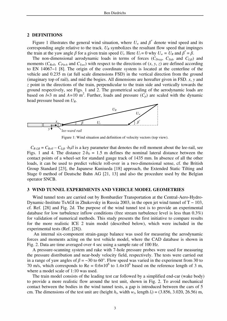
Figure 1 illustrates the general wind situation, where Uw and β* denote wind speed and its

corresponding angle relative to the track. UR symbolizes the resultant flow speed that impinges the train at the yaw angle β for a given train speed Ut. Here Ut = 0 why Uw = UR and β

* = β. The non-dimensional aerodynamic loads in terms of forces (CDrag, CSide and CLift) and

moments (CRoll, CPitch and CYaw) with respect to the directions of (x, y, z) are defined according to EN 14067−1 [8]. The origin of the coordinate system is located at the centerline of the vehicle and 0.235 m (at full scale dimensions FSD) in the vertical direction from the ground (imaginary top of rail), and mid the bogies. All dimensions are hereafter given in FSD. x, y and z point in the directions of the train, perpendicular to the train side and vertically towards the ground respectively, see Figs. 1 and 2. The geometrical scaling of the aerodynamic loads are based on l=3 m and A=10 m2. Further, loads and pressure (Cp) are scaled with the dynamic head pressure based on UR.

Uw UR

β β*

Ut

x

y lee-ward rail

Figure 1: Wind situation and definition of velocity vectors (top view). CR-LR = CRoll – CLift ·b0/l is a key parameter that denotes the roll moment about the lee-rail, see Figs. 1 and 4. The distance 2·b0 = 1.5 m defines the nominal lateral distance between the contact points of a wheel-set for standard gauge track of 1435 mm. In absence of all the other loads, it can be used to predict vehicle roll-over in a two-dimensional sense, cf. the British Group Standard [23], the Japanese Kuniueda [18] approach, the Extended Static Tilting and Stage 0 method of Deutsche Bahn AG [21, 13] and also the procedure used by the Belgian operator SNCB. 3 WIND TUNNEL EXPERIMENTS AND VEHICLE MODEL GEOMETRIES

Wind tunnel tests are carried out by Bombardier Transportation at the Central-Aero-Hydro-Dynamic-Institute TsAGI in Zhukovsky in Russia 2003, in the open jet wind tunnel of T − 103, cf. Ref. [28] and Fig. 2d. The purpose of the wind tunnel test is to provide an experimental database for low turbulence inflow conditions (free stream turbulence level is less than 0.3%) for validation of numerical methods. This study presents the first initiative to compare results for the more realistic ICE 2 train model (described below), which were included in the experimental tests (Ref. [28]).

An internal six-component strain-gauge balance was used for measuring the aerodynamic forces and moments acting on the test vehicle model, where the CAD database is shown in Fig. 2. Data are time averaged over 4 sec using a sample rate of 100 Hz.

A pressure-scanning system and rake with 7-hole pressure probes were used for measuring the pressure distribution and near-body velocity field, respectively. The tests were carried out in a range of yaw angles of β = −30 to 60°. Flow speed was varied in the experiment from 30 to 70 m/s, which corresponds to Re = 0.6×106 to 1.4×106 based on the reference length of 3 m, where a model scale of 1:10 was used.

The train model consists of the leading test car followed by a simplified end-car (wake body) to provide a more realistic flow around the test unit, shown in Fig. 2. To avoid mechanical contact between the bodies in the wind tunnel tests, a gap is introduced between the cars of 5 cm. The dimensions of the test unit are (height ht, width wt, length lt) = (3.856, 3.020, 26.56) m,

Ben Diedrichs

4

where the car body length is measured from the nose to centre of the inter-car gap. An imaginary top of rail (TOR) is located 0.235 m above the elliptic ground plate, where the total vertical distance from the ground to the underbelly of the vehicle is 0.503 m. The set-up reflects the TSI provisions Ref. [7].

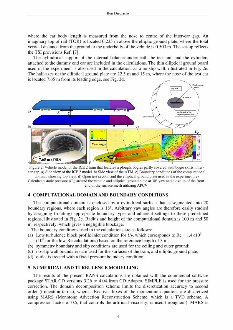
The cylindrical support of the internal balance underneath the test unit and the cylinders attached to the dummy end car are included in the calculations. The thin elliptical ground board used in the experiment is also used in the calculation, as a no-slip wall, illustrated in Fig. 2e. The half-axes of the elliptical ground plate are 22.5 m and 15 m, where the nose of the test car is located 7.65 m from its leading edge, see Fig. 2d.

a)

b) c)

d) e) Figure 2: Vehicle model of the ICE 2 train that features a plough, bogies partly covered with bogie skirts, inter-

car gap. a) Side view of the ICE 2 model. b) Side view of the ATM. c) Boundary conditions of the computational domain, showing top view. d) Open test section and the elliptical ground plate used in the experiment. e)

Calculated static pressure (Cp) around the vehicle and elliptical ground plate at 30° yaw and close up of the front-end of the surface mesh utilizing APCV.

4 COMPUTATIONAL DOMAIN AND BOUNDARY CONDITIONS

The computational domain is enclosed by a cylindrical surface that is segmented into 20 boundary regions, where each region is 18°. Arbitrary yaw angles are therefore easily studied by assigning (rotating) appropriate boundary types and adherent settings to these predefined regions, illustrated in Fig. 2c. Radius and height of the computational domain is 100 m and 50 m, respectively, which gives a negligible blockage. The boundary conditions used in the calculations are as follows: (a) Low turbulence block profile inlet condition for UR, which corresponds to Re = 1.4×106

(106 for the low-Re calculations) based on the reference length of 3 m; (b) symmetry boundary and slip conditions are used for the ceiling and outer ground; (c) no-slip wall boundaries are used for the surfaces of the train, and elliptic ground plate; (d) outlet is treated with a fixed pressure boundary condition. 5 NUMERICAL AND TURBULENCE MODELLING

The results of the present RANS calculations are obtained with the commercial software package STAR-CD versions 3.26 to 4.04 from CD-Adapco. SIMPLE is used for the pressure correction. The domain decomposition scheme limits the discretization accuracy to second order (truncation terms), where advective fluxes of the momentum equations are discretized using MARS (Monotone Advection Reconstruction Scheme, which is a TVD scheme. A compression factor of 0.5, that controls the artificial viscosity, is used throughout). MARS is

x z

R = 100 m

Uniform inlet

Fixed pressure

outlet

No-slip wall of the

elliptical ground plate

Slip wall

Yaw angle

Wind 7.65 m (FSD)

Cp

Ben Diedrichs

5

second order accurate on a uniform mesh. Hi-Re turbulence closure is achieved with the linear and quadratic nonlinear eddy-viscosity

models (NLEVM) of Launder and Spalding 1974 [19] and Shih et al. 1993 [25], respectively. Both models use k and ε that denote turbulent kinetic energy and dissipation of turbulent energy, which provide the basic time and length scales of the turbulence model. The nonlinearity pertains to the constitutive relationship between the Reynolds stresses and shear strains of the mean flow. In comparison to the linear model the NLEVM provides inequality of normal stresses, can predict some effects of streamline curvature via a different response to rotational and irrotational strains and henceforth also obey basic realizability constraints (ensure the positivity of normal stresses). Low-Re turbulence closure is achieved with the k−ω SST model of Menter 1992 [22], which blends automatically between the Wilcox k–ω [26] and the standard Jones and Launder k–ε [15] turbulence models in the inner and outer part of the boundary layer, respectively. In addition, the quadratic k–ε low-Re model of Lien et al. 1996 [20] is used. In the low-Re and hi-Re meshes the first cells adjacent to the walls of the train are adjusted to meet the requirements of y+

< 2 and 30 < y+ < 150. Mesh properties are described

next.

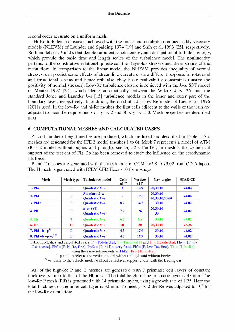
6 COMPUTATIONAL MESHES AND CALCULATED CASES

A total number of eight meshes are produced, which are listed and described in Table 1. Six meshes are generated for the ICE 2 model (meshes 1 to 6). Mesh 7 represents a model of ATM (ICE 2 model without bogies and plough), see Fig. 2b. Further, in mesh 8 the cylindrical support of the test car of Fig. 2b has been removed to study the influence on the aerodynamic lift force. P and T meshes are generated with the mesh tools of CCM+ v2.8 to v3.02 from CD-Adapco. The H mesh is generated with ICEM CFD Hexa v10 from Ansys.

Mesh Mesh type Turbulence model Cells ×106

Vertices ×106

Yaw angles STAR-CD

1. Phc P Quadratic k−ε 3 12.9 20,30,40 v4.02

Standard k−ε 20,30,40 2. Phf P

Quadratic k−ε 5 19.5

20,30,40,50,60 v4.04

3. Phf2 P Quadratic k−ε 8.2 34.2 30,40 v4.02

k−ω SST 20,30,40 4. Plf

P Quadratic k−ε

7.7 26 30

v4.02

5. Th T Quadratic k−ε 6.2 6.8 30,40 v4.02

6. Hh H Quadratic k−ε 20 20 20,30,40 v3.26

7. Phf −b −p1) P Quadratic k−ε 4.3 17.9 30,40 v4.02

8. Phf −b −p −c1,2) P Quadratic k−ε 4.3 17.9 30,40 v4.02

Table 1: Meshes and calculated cases. P = Polyhedral, T = Trimmed H and H = Hexahedral. Phc = [P, hi-Re, coarse], Phf = [P, hi-Re, fine], Phf2 = [P, hi-Re, very fine]. Plf = [P, low-Re, fine]. Th = [T, hi-Re]

using the same refinements as Phf2. Hh = [H, hi-Re]. 1) −p and −b refer to the vehicle model without plough and without bogies.

2) −c refers to the vehicle model without cylindrical support underneath the leading car.

All of the high-Re P and T meshes are generated with 7 prismatic cell layers of constant thickness, similar to that of the Hh mesh. The total height of the prismatic layer is 35 mm. The low-Re P mesh (Plf) is generated with 14 prismatic layers, using a growth rate of 1.25. Here the total thickness of the inner cell layer is 32 mm. To meet y+ < 2 the Re was adjusted to 106 for the low-Re calculations.

Ben Diedrichs

6

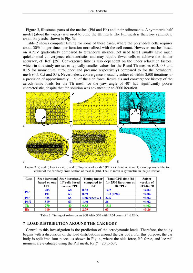
Figure 3, illustrates parts of the meshes (Phf and Hh) and their refinements. A symmetric half model (about the y-axis) was used to build the Hh mesh. The full mesh is therefore symmetric about the y-axis, shown in Fig. 3c. Table 2 shows computer timing for some of these cases, where the polyhedral cells requires about 30% longer times per iteration normalized with the cell count. However, meshes based on APCV (particularly compared to tetrahedral meshes, not used here) usually have much quicker total convergence characteristics and may require fewer cells to achieve the similar accuracy, cf. Ref. [29]. Convergence time is also dependent on the under relaxation factors, which in this study are set to typically smaller values for the P and Th meshes (0.3, 0.3 and 0.15 for momentum, turbulence and pressure respectively) compared to for the hexahedral mesh (0.5, 0.5 and 0.3). Nevertheless, convergence is usually achieved within 2500 iterations to a precision of approximately ±1% of the side force. Residuals and convergence history of the aerodynamic loads for the Th mesh for the yaw angle of 40° had significantly poorer characteristic, despite that the solution was advanced up to 8000 iteration.

a) b) e)

c) d) f)

Figure 3: a) and b) Front view, c) and d) Top view of mesh 3 (Phf). e) Front view and f) close up around the top corner of the car body cross section of mesh 6 (Hh). The Hh mesh is symmetric in the y-direction.

Case Sec / iteration based on one

CPU

Sec / iteration / 106 cells based

on one CPU

Timing factor compared to

Phf

Total CPU time [h] for 2500 iterations on

10 CPUs

Solver version of

STAR-CD

205 68 0.63 14.2 v4.02 Phc

191 63 0.59 13.3 (0.94) v4.04

Phf 325 65 Reference = 1 22.6 v4.02

Phf2 519 63 1.60 36 v4.02

Th 270 43 0.83 18.8 v4.02

Hh 910 45 2.79 63 v3.26

Table 2: Timing of solver on an SGI Altix 350 with IA64 cores of 1.6 GHz.

7 LOAD DISTRIBUTION AROUND THE CAR BODY

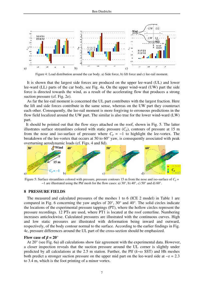
Central to this investigation is the prediction of the aerodynamic loads. Therefore, the study begins with a discussion of the load distributions around the car body. For this purpose, the car body is split into four pieces as shown in Fig. 4, where the side force, lift force, and lee-rail moment are evaluated using the Phf mesh, for β = 20 to 60°.

Ben Diedrichs

7

a) b) c)

Figure 4: Load distribution around the car body. a) Side force, b) lift force and c) lee-rail moment.

It is shown that the largest side forces are produced on the upper lee-ward (UL) and lower lee-ward (LL) parts of the car body, see Fig. 4a. On the upper wind-ward (UW) part the side force is directed towards the wind, as a result of the accelerating flow that produces a strong suction pressure (cf. Fig. 2e). As far the lee-rail moment is concerned the UL part contributes with the largest fraction. Here the lift and side forces contribute in the same sense, whereas on the UW part they counteract each other. Consequently, the lee-rail moment is more forgiving to erroneous predictions in the flow field localized around the UW part. The similar is also true for the lower wind-ward (LW) part. It should be pointed out that the flow stays attached on the roof, shown in Fig. 5. The latter illustrates surface streamlines colored with static pressure (Cp), contours of pressure at 15 m from the nose and iso-surface of pressure where Cp = −1 to highlight the lee-vortex. The breakdown of the lee-vortex that occurs at 50 to 60° yaw, is consequently associated with peak overturning aerodynamic loads (cf. Figs. 4 and 8d).

a) b) c) d)

Figure 5: Surface streamlines colored with pressure, pressure contours 15 m from the nose and iso-surface of Cp = −1 are illustrated using the Phf mesh for the flow cases: a) 30°, b) 40°, c) 50° and d) 60°.

8 PRESSURE FIELDS

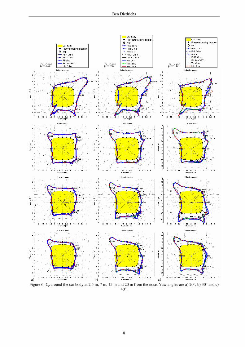
The measured and calculated pressures of the meshes 1 to 6 (ICE 2 model) in Table 1 are compared in Fig. 6 concerning the yaw angles of 20°, 30° and 40°. The solid circles indicate the locations of the experimental pressure tappings (PT), where the hollow circles represent the pressure recordings. 12 PTs are used, where PT1 is located at the roof centerline. Numbering increases anticlockwise. Calculated pressures are illustrated with the continuous curves. High and low static pressures are illustrated with deformation being inward and outward, respectively, of the body contour normal to the surface. According to the earlier findings in Fig. 4c, pressure differences around the UL part of the cross-section should be emphasized.

Flow case of β = 20° At 20° (see Fig. 6a) all calculations show fair agreement with the experimental data. However, a closer inspection reveals that the suction pressure around the UL corner is slightly under predicted by all calculations at the 2.5 m station. Further, the Plf (k−ω SST) and Hh meshes both predict a stronger suction pressure on the upper mid part on the lee-ward side at −z = 2.3 to 3.4 m, which is the foot printing of a minor vortex.

y

UW UL

LW LL

z

Wind

lee-rail

moment

y

UW UL

LW LL

z

Wind

lee-rail

moment

Cp

15 m

Cp = −1

30° 40° 50° 60°

Wind

Ben Diedrichs

8

Figure 6: Cp around the car body at 2.5 m, 7 m, 15 m and 20 m from the nose. Yaw angles are a) 20°, b) 30° and c)

40°.

β=20° β=30° β=40°

a) b) c)

Ben Diedrichs

9

a)

b)

c)

d)

e)

f)

g)

h)

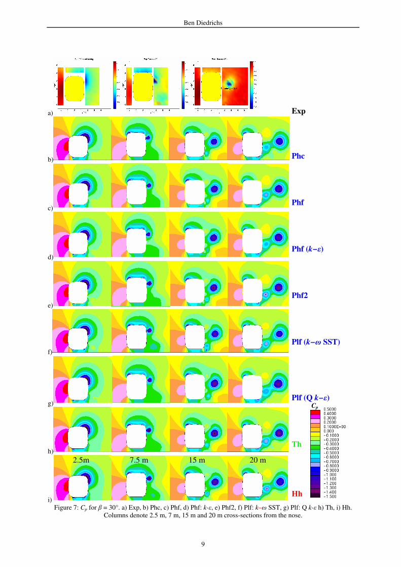
i) Figure 7: Cp for β = 30°. a) Exp, b) Phc, c) Phf, d) Phf: k-ε, e) Phf2, f) Plf: k−ω SST, g) Plf: Q k-ε h) Th, i) Hh.

Columns denote 2.5 m, 7 m, 15 m and 20 m cross-sections from the nose.

Exp

Phc

Phf

Phf (k−ε)

Phf2

Plf (k−ω SST)

Plf (Q k−ε)

Th

Hh

2.5m 7.5 m 15 m 20 m

Cp

Ben Diedrichs

10

At 7 m from the nose, all calculations predict a stronger suction pressure underneath the car. Again, the Hh mesh agrees best with the low pressure (Cp = −0.41) around the lee-vortex about UL part. However, further up (Cp = −0.32), the Hh mesh returns the largest deviation. At 15 m, the most pronounced differences are due to the Phf (standard k−ε), which are found around the LL part. Deviations in the pressure field around the LL corner have only a relatively small effect on the lee-rail moment, see Fig. 4c. At 20 m, the somewhat large differences in results between the coarse Phc (Q k−ε) and fine mesh Phf (Q k−ε) should be pointed out. Further, the coherent results of Phf (Q k−ε) and Hh meshes should be noticed, where the same turbulence model is used.

Flow case of β = 30° Pressures at 30° yaw are calculated for six meshes of the ICE 2 model, see Fig. 6b. Again, the overall impression is that the results of the calculations are fairly coherent. The largest deviations are found typically on the lee-ward side and underneath the car. Similar to the results at 20° yaw, the suction pressure is slightly under predicted about the UL corner at the 2.5 m station. Results of the low-Re mesh Plf (k−ω SST) indicate a stronger suction pressure about the UW part (−z ~ 3.4 m), which is the foot printing of a vortex. Plf (Q k−ε) gives the second strongest suction pressure about this location. The Hh mesh predicts stronger low pressure further down. As expected, the poorest resolution in this regard is predicted with the standard k−ε turbulence model. At 7 m, all calculations underestimates the suction pressure significantly compared to PT10 (Cp = −1.19). This is the case also for 50° but not for 60°, not shown here. At 20 m, the results of the Plf (k−ω SST) is different on the lower part of the lee-ward side, where it has the best agreement with the experimental data mid the vehicle (Cp = −0.23). In general, relatively large differences are found underneath the car, by comparison with the experimental results, where the calculations typically predict stronger suction pressure. This has implications on the aerodynamic lift force, which will be discussed further in section 9. Also, at β = 30° measured pressure fields at 2.5 m, 7 m and 15 m from the nose, are shown in Fig. 7a. 234 and 336 experimental grid points are used for the first two stations and 15 m, respectively. Unfortunately, the pressure field underneath the model is not measured, which would have been useful when trying to understand the discrepancies mentioned in connection to Fig. 6. In Figs. 7b to 7i the calculated static pressure fields of all our calculations are presented for comparative purposes. At 2.5 m (Fig. 7a), the resolution of the experimental grid is not fine enough around the UL part to confirm the presence of a vortex core (augmentation of suction pressure), which is indicated in the calculations of Fig. 6. At 7 m (Fig. 7), the largest differences are found adjacent to the ground, where the experimental data indicates a much higher pressure around y = 2 to 3 m. Further up at −z ~ 3.5 m a minor high pressure zone is discernable, which is considered to be erroneous. At 15 m, the presence of the lee-vortex is obvious, where the centre is located at y ~ −z ~ 2.7 m. The experimental results indicate a stronger vortex core (Cp = −1.89), in terms of suction pressure, compared to all the calculations. As far as the hi-Re P meshes are concerned, the finest grid returns the strongest suction pressure in the vortex core (Cp = −1.38). It is further noticed that the smaller in size vortex that detaches the vehicle near the ground, at about −z = 1 m, is stronger in all calculations. This is not confirmed by the results presented in Fig. 6, why the experimental data may not be consistent. In this regard, the largest deviation in pressure around the LL corner (15 m from the nose) is predicted with the low-Re mesh Plf (k−ω SST). Notice that the quadratic model Plf (Q k−ε) gives different results. In general, Fig. 7 illustrates fairly good agreement amongst all calculations. The most obvious differences are found adjacent to the ground and underbelly of the vehicle, which is seen already in Fig. 6. Earlier results, cf. Diedrichs 2003 and Rolén et al. 2004, where the

Ben Diedrichs

11

standard k−ε model were used, resulted in a much weaker lee-vortex compared to the quadratic version. In the present study, see Fig. 7d, the lee-vortex is comparable regarding the two turbulence models, which appears to be a significant improvement of using APCV.

Flow case of β = 40° Again, we turn to Fig. 6 and examine the pressures at the 40° yaw angle. At 2.5 m, the calculations agree quite well with the experimental data. Similar to the 20° and 30° cases the resolution of the calculations around the UW corner (−z ~ 3 m) show differences. Here the Hh mesh gives the strongest suction pressure due to the lee-vortex formation. Again the Plf (k−ω SST) predicts the pressure core of lee-vortex to be somewhat higher up, than all other calculations. At 15 m (adjacent to the cylindrical support) the most palpable discrepancies are found underneath, where Plf (k−ω SST) gives the best agreement with the experiment. At 20 m it is interesting to find that the calculations underneath the model agree much better with the experiments (compared to 15 m). Similar to the 30° case, the low-Re model Plf (k−ω SST) returns a lower suction pressure on the lee-ward side, where mid the cross-section it has the best agreement with the experimental reference point. In section 9, it is demonstrated that the integral side force in this particular case has the best agreement with the experiment.

9 AERODYNAMIC LOADS

As mentioned before, central to this study is the prediction of the integral aerodynamic loads of the test car. To this end, the loads for the ICE 2 model and ATM are presented here, with particular focus on the side force, lift force, roll moment and roll moment about the lee-rail. The comparison includes the wind tunnel data obtained at Polimi (Ref. [2]) for the ICE 2 model without plough and for the ATM. Recall that these tests are carried out at a five times lower Re (2.8×105) than the TsAGI reference tests (Ref. [28]). All loads are detailed in Fig. 8.

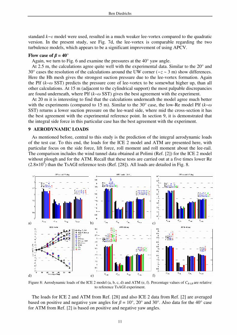
a) b) c)

d) e) f)

Figure 8: Aerodynamic loads of the ICE 2 model (a, b, c, d) and ATM (e, f). Percentage values of CR-LR are relative to reference TsAGI experiment.

The loads for ICE 2 and ATM from Ref. [28] and also ICE 2 data from Ref. [2] are averaged based on positive and negative yaw angles for β = 10°, 20° and 30°. Also data for the 40° case for ATM from Ref. [2] is based on positive and negative yaw angles.

Ben Diedrichs

12

9.1 ICE 2 model

At 20°, see Fig. 8a, the data confirms the previous findings of the surface pressure (see Fig. 6), that this flow case agrees quite well with the wind tunnel data. Further, the Phf mesh displays the best overall agreement, where the crucial lee-rail moment is predicted 0.2%. The corresponding difference for the Hh mesh is −0.3%, where the lift force indicates the largest difference of −14.4%. The loads of the Polimi experiment deviates significantly more than the calculations, where the five times lower Re and lacking plough should be kept in mind. At 30°, see Fig. 8b, the largest deviation of CR-LR is 3.8%, where the Polimi experiment differs by 6.9%. The most obvious discrepancy between the experiment and calculations is the lift force, which is consistently being under predicted in the range of −31.1 to −47.6%. Polimi results shows only a minor difference in the lift where the side force and roll moment are only slightly stronger than the reference experiment. It is interesting to notice that an increase in the side force is often balanced by a reduction of the lift force, which usually returns a lee-rail moment that agrees better than the two orthogonal loads. This is also observed in e.g. Diedrichs 2003 and Diedrichs et al. 2007, and could be explained by the results in Fig. 5. The current models are sensitive to the exact location and strength of the peak suction pressure at the upper wind ward corner. A difference in the location and strength may result in a larger uplift and consequently lower side force or vice versa. This altogether reduces the sensitivity of the crucial lee-rail moment. Further, in Fig. 5 it is shown that the largest part of the lee-rail moment is generated around the upper lee-ward corner, where the side and lift forces contribute in the same sense. The pronounced differences found near the ground around the lee-ward corner (Figs. 6c), are fortunately contributing less to the lee-rail moment as a consequence of a relatively small leverage. At 40°, see Fig. 8c, the similar trend to that of the 30° case is observed, where the side force in most of the calculations are over predicted and the lift force is under estimated in all of the calculations. Nonetheless, compared to the 30° case, the lee-rail moments agree remarkably well with the experimental data. The low-Re mesh Plf (k−ω SST) gives the largest difference and the Phf2 mesh gives zero difference. The Hh mesh returns a CR-LR that is 1% larger, despite the side force and roll moment mid the rail are about 10% greater than the experimental data. It is noticed that the discrepancies for 40° concerning the Hh mesh are very similar to those at 30°. Finally it is mentioned that at 50° and 60° yaw, CR-LR of Phf differs by 0.9% and 4.2%, respectively, see Fig. 8d. It should be pointed out that the qualitative trend for the highest yaw angle agrees well with the TsAGI experiment as opposed to the Polimi tests.

9.2 ATM

The issue with the significantly under predicted lift force is investigated further. To this end, additional results for the ATM are calculated and compared to results obtained in previous studies, described below. Our results concern meshes 7 and 8 (the latter without cylindrical support), see Table 1, for 30° and 40° yaw. The results of mesh 7 (Phf: –p –b), see Figs. 8e,f, confirm the issue with the lift force, which is found to be −19.2% and −51.6% at 30° and 40° yaw, respectively. At 30° all other loads are predicted with fair accuracy, where the lee-rail moment is −2.5% compared to the experiment. At 40° the relatively small lift force is clearly influencing the lee-rail moment that is predicted −8.5%. Additional results obtained by Rolén et al. 2004 [24], Wu 2004 [27] (RANS and DES), a study by Bombardier Aerospace (BA) Ref. [1] and the LES results of Hemida 2006 [14] are brought into the comparison. In the latter the friction forces are not taken into account in the integral loads. Friction for the 30° flow contributes with 1.1% and 0.7% (obtained with Phf: –p –b) to the side and lift forces, respectively. The vehicle models in the above studies are illustrated in Fig. 9. Notice that none of the numerical models fully agree with the reference

Ben Diedrichs

13

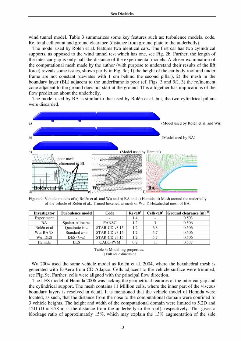
wind tunnel model. Table 3 summarizes some key features such as: turbulence models, code, Re, total cell count and ground clearance (distance from ground plate to the underbelly). The model used by Rolén et al. features two identical cars. The first car has two cylindrical supports, as opposed to the wind tunnel test which has one, see Fig. 2b. Further, the length of the inter-car gap is only half the distance of the experimental models. A closer examination of the computational mesh made by the author (with purpose to understand their results of the lift force) reveals some issues, shown partly in Fig. 9d; 1) the height of the car body roof and under frame are not constant (deviates with 1 cm behind the second pillar), 2) the mesh in the boundary layer (BL) adjacent to the underframe is poor (cf. Figs. 3 and 9f), 3) the refinement zone adjacent to the ground does not start at the ground. This altogether has implications of the flow prediction about the underbelly. The model used by BA is similar to that used by Rolén et al. but, the two cylindrical pillars were discarded.

a) (Model used by Rolén et al. and Wu)

b) (Model used by BA)

c) (Model used by Hemida)

d) e) f)

Figure 9: Vehicle models of a) Rolén et al. and Wu and b) BA and c) Hemida. d) Mesh around the underbelly of the vehicle of Rolén et al.. Trimed hexehedral mesh of Wu. f) Hexahedral mesh of BA.

Investigator Turbulence model Code Re×106 Cells×106 Ground clearance [m] 1)

Experiment - - 1.4 - 0.503

BA Spalart-Allmaras FANSC 1.2 3 0.506

Rolén et al Quadratic k−ε STAR-CD v3.15 1.2 6.3 0.506

Wu: RANS Standard k−ε STAR-CD v3.15 1.2 5.7 0.506

Wu: DES DES (k−ε) STAR-CD v3.15 1.2 5.7 0.506

Hemida LES CALC-PVM 0.2 11 0.537

Table 3: Modelling properties. 1) Full scale dimension

Wu 2004 used the same vehicle model as Rolén et al. 2004, where the hexahedral mesh is generated with EsAero from CD-Adapco. Cells adjacent to the vehicle surface were trimmed, see Fig. 9e. Further, cells were aligned with the principal flow direction.

The LES model of Hemida 2006 was lacking the geometrical features of the inter-car gap and the cylindrical support. The mesh contains 11 Million cells, where the inner part of the viscous boundary layers is resolved in detail. It is mentioned that the vehicle model of Hemida were located, as such, that the distance from the nose to the computational domain were confined to 3 vehicle heights. The height and width of the computational domain were limited to 5.2D and 12D (D = 3.58 m is the distance from the underbelly to the roof), respectively. This gives a blockage ratio of approximately 15%, which may explain the 13% augmentation of the side

poor mesh refinement in BL

Rolén et al Wu BA

Ben Diedrichs

14

force compared to the experiment. Notice also that the current model has the largest ground clearance, which could explain, under the circumstances, the relatively weak lift force. Further, it should be pointed out that the Re in the LES was confined to 0.2×106 for practical reasons. Figs. 8e,f show that, most of the results under estimate the lift force compared to the experiment, except the results of Rolén et al. These results are obviously different to the results of Wu who used the same vehicle model, but different turbulence models. A closer examination of the surface pressure in the underframe is made by the author (not shown here) that reveals significant differences. The issues of the mesh resolution and CAD, described above, may likely explain this. As far as the lee-rail moment is concerned, Figs. 8e,f show that the Polimi wind tunnel test results have the worst and best agreement at 30° and 40°, respectively. At 30°, mesh 8 (Phf: –p –b –c) and BA show fairer agreement than at 40°. Finally, the sensitivity of the cylindrical support is illustrated by the differences in the results of meshes 7 and 8. At 30° the lift force is reduced significantly (from –19 to –42%) when the support is removed. The reduction in the lift is caused by an increased flow underneath the vehicle, which lowers and increases the surface pressure about the underbelly and roof, respectively. At 40° the difference is much more subtle, where there is hardly any difference in the lee-rail moment concerning the two meshes.

10 CONCLUSIONS

The present study on crosswind aerodynamics has focused attention on the applicability of RANS to resolve the overturning loads under low turbulence conditions exemplified for a realistic high-speed train model with bogies. The calculations are compared to a wind tunnel experiment that used the exact same geometry and Re. As regards the computational models, the investigation has studied results obtained with arbitrary polyhedral meshes, a trimmed hexahedral mesh and a very fine exclusively hexahedral mesh. For this purpose a second order approximation of the advective momentum fluxes and a realizable second order eddy-viscosity closure that are used as the baseline numerical scheme. The investigation has also included a low-Re mesh, which resolves the stiff part of the inner viscous boundary layer adjacent to the wall of the train. The investigation can report the following conclusions:

• Automatic meshing utilizing APCV significantly reduces the pre-processing work compared to manual approaches (that requires a great deal of skills and effort for geometries like the present train model), mitigates the risk of human errors, and typically shortens the total solver time by generating meshes with fewer elements.

• Steady state RANS approaches appear justified in conjunction with the yaw angles investigated here, which may correspond to high, intermediate and low cruising speeds of 20 to 60° yaw. As far as the most crucial aerodynamic load component (lee-rail moment) is concerned, the calculations show that the most overall coherent results are obtained at 40° yaw (relative to 20° and 30°. Results for 50° and 60° yaw are calculated only for one mesh) in comparison with the experiments. Conversely, the results of the calculations at 40° yaw for the smoother ATM without bogies exhibits larger unsteadiness and less coherent results compared to the experiment.

• The low-Re approaches to represent the near-wall regime around the vehicle tested in this study do not seem favorable over the high-Re approaches.

• Lee-rail moment obtains its greatest contribution from the upper lee-ward part of the car body. Conversely, a relatively small contribution comes from the upper wind-ward part, where the current geometry is less sensitive to numerical issues (peak suction pressure).

• In comparison with the experiment, most of the calculations indicate a slightly stronger side force and under estimated lift force. This altogether, returns a lee-rail moment that

Ben Diedrichs

15

fortunately agrees well. Further, the experiment at 30° yaw suggests a stronger suction pressure of the lee-vortex core than all our calculations.

• A comparison of current and previous calculated results of the ATM (see Fig. 2b) show a consistent trend of under estimating the lift force, which is likely caused by flow differences of the boundary layer adjacent to the ground. For example, the current study has found the lift force to be sensitive to geometrical features underneath the train, such as the supporting pillar commonly used in experiments (more so for 30° yaw compared to 40°).

• A further wind tunnel study that validates the current wind tunnel experiment is welcome. It is suggested that future experiments are designed around the numerical issues. For example, it would be of interest to measure and compare loads of separate parts of the car body (see Fig. 4). Further, in our particular case, flow properties adjacent to the ground and additional pressure tappings on the upper part of the wind-ward corner and ground board would have been desirable.

The continuation of this study will investigate the response of unsteady wind gusts utilizing transient methods (variants of DES) for the currently used realistic train model of ICE 2. Also, the definition and study of a Regional Train Model exposed to crosswind is currently being discussed.

ACKNOWLEDGEMENT

This study is carried out as an integral part of the Vinnova Centre of Excellence for ECO2 Vehicle Design at the Royal Institute of Technology in Stockholm. Bombardier Transportation has contributed with experimental data and computer resources. Bombardier Aerospace is acknowledged for sharing their results of the ATM. Finally, Mindware Inc. is acknowledged for the support to generate the ICEM CFD hexahedral mesh.

REFERENCES

[1] Bombardier Aerospace. 2004. CFD FOR STABILTY AND CONTROL (III). Internal report issued by Dept. of Aerodynamics, Flight Performance, CFD.

[2] Cheli, F., Tomasini, G. and Rocchi, D. 2007. Polimi wind tunnel tests on Bombardier ATM vehicle. Technical Report, archived at Bombardier Transportation.

[3] Cléon, L.M., Gautier, P-E. and Sourget, F. 2004. Sécurité de la circulation des trains à grande vitesse vis-à-vis des vents latéraux: le programme DeuFraKo. Revue Générale des Chemins de fer – juillet-août 2004/7.

[4] Diedrichs, B. 2003. On computational fluid dynamics modeling of crosswind effects for high-speed rolling stock. Proc. Instn Mech. Engrs, Part F: J. Rail and Rapid Transit, 217(F3), pp. 203–226.

[5] Diedrichs, B. 2005. Computational Methods for Crosswind Stability of Railway Trains. A Literature Survey. Royal Institute of Technology (KTH), Stockholm, Sweden, TRITA AVE 2005:27. ISSN 1651-7660. ISRN KTH/AVE/RTR-05/27-SE.

[6] Diedrichs, B., Sima, M., Orellano, A., and Tengstrand, H. 2007. Crosswind stability of a high-speed train on a high embankment. Proc. Instn Mech. Engrs, Part F: J. Rail and Rapid Transit, 221(F2), pp. 205–225.

[7] Directive 96/48/EC. 2006. Interoperability of the trans-European high speed rail system.

[8] EN 14067−1. 2003. Railway Applications – Aerodynamics – Part 1: Symbols and units. European standard.

[9] prEN 14067−6. 2007. Railway Applications – Aerodynamics – Part 6: Requirements and test procedures for cross wind assessment. European standard.

[10] Eisenlauer, M., Matschke, G., Meri, A. and Heine, C. 2003. CFD calculation of aerodynamic forces and side wind behavior of railway vehicles. Parametric investigations and comparison with wind tunnel data. MIRA Conference.

Ben Diedrichs

16

[11] Fauchier, C., Le Dévéhat, E. and Grégoire, R. 2002. Numerical study of the turbulent flow around the reduced-scale model of an Inter-Regio. TRANSAERO ISBN 0179-9614, 61–74.

[12] Gautier, P-E., Tielkes, T., Sourget, F., Allain, E., Grab, M. and Heine, C. 2003. Strong wind risks in railways: the DEUFRAKO crosswind program. Proc. of WCRR’2003, 463–475.

[13] Heine, C. 2005. Sicherheitsnachweis bei Seitenwind. Konzernrichtlinie 807, Version 01.01.2005, Deutsche Bahn AG.

[14] Hemida, H. 2006. Large-Eddy Simulation of the Flow around Simplified High-Speed Trains under Side Wind Conditions. Thesis for licentiate of engineering no. 2006:06 Chalmers University, Sweden. ISSN 1652-8565.

[15] Jones, W. and Launder, B. 1972. The prediction of laminarization with a two-equation model of turbulence. Int. J. Heat Mass Transfer. Vol. 15, pp. 301–314.

[16] Khier, W., Breuer, M. and Durst, F. 2000. Flow structures around trains under side wind conditions: A numerical study. Int. J. Computers & Fluids, 29(2), 179–195.

[17] Khier, W., Breuer, M. and Durst. F. 2002. Numerical computation of 3-D turbulent flow around high-speed trains under side wind conditions. TRANSAERO ISBN 0179-9614., pp. 75–84.

[18] Kunieda, M. 1972. Railway Technical Research Report of Tokyo (in Japanese). No. 793.

[19] Launder, B.E. and Spalding, D.B. 1974. The numerical computation of turbulent flows. Comp. Meth. in Appl. Mech. and Eng., 3, pp. 269–289.

[20] Lien, F.S., Chen, W.L., and Leschziner, M.A. 1996. Low-Reynolds-Number Eddy-Viscosity Modelling Based on Non-Linear Stress-Strain/Vorticity Relations. Proc. 3rd Symp. on Engineering Turbulence Modelling and Measurements, Crete, Greece.

[21] Matschke, G. 2001. Sicherheitsnachweis bei Seitenwind. Konzernrichtlinie 401, Version 03.2001, Deutsche Bahn AG.

[22] Menter, F. M. 1992. Improved Two-Equation k−ω Turbulence Models for Aerodynamic Flows. NASA-TM-103975.

[23] Railtrack plc, 2000. Resistance of railway vehicles to roll-over in gales. GM/RT2142.

[24] Rolén, C., Rung, T. and Wu, D. 2004. Computational modelling of cross-wind stability of high speed trains. European Congress on Computational Methods in Applied Sciences and Engineering. ECCOMAS. P. Neittaanmäki, T. Rossi, S. Korotov, E. Oñate, J. Périaux, and D. Knörzer (eds.) Jyväskylä, 24–28 July.

[25] Shih, T-H., Zhu, J. and Lumley, J. L. 1993. A realizable Reynolds Stress Algebraic Equation Model. 9th

Symposium on Turbulence Shear Flows. Kyoto, Japan, August 10-18, 1993.

[26] Wilcox, DC. 1993. Turbulence Modeling for CFD. DWC Industries Inc., 5354 Palm Drive, La Canada, California 91011, USA.

[27] Wu, D. 2004. Predictive Prospects of Unsteady Detached-Eddy Simulations in Industrial External Aerodynamic Flow Simulations. Final Thesis. Lehrstuhl für Strömungslehre und Aerodynamishes Institute Aachen. Matriculation number: 219949.

[28] Orellano, A. and Schober, M. 2006. Aerodynamic Performance of a Typical High-Speed Train. WSEAS TRANSACTIONS on FLUID MECHANICS, Issue 5, Volume 1, ISSN 1790-5087, http://www.wseas.org.

[29] Peric', M. 2004. Flow Simulation using Control Volumes of Arbitrary Polyhedral Shape. Ercoftac Bulletin, pp. 62, 25-29.