aerodynamic and acoustic analysis of an optimized low

Aerodynamic and acoustic analysis of an optimizedlow Reynolds number rotorRonan Serre1*, Nicolas Gourdain1, Thierry Jardin1, Adrian Sabate Lopez1, Viswesh Sujjur Balaramraja1,Sylvain Belliot1, Marc C. Jacob1, Jean-Marc Mosche�a1

SYM

POSI

A

ON ROTATING MACHIN

ERY

ISROMAC 2017

InternationalSymposium on

Transport Phenomenaand

Dynamics of RotatingMachinery

Maui, Hawaii

December 16-21, 2017

Abstract�e demand in Micro–Air Vehicles (MAV) is increasing as well as their potential missions. Eitherfor discretion in military operations or noise pollution in civilian use, noise reduction of MAV is agoal to achieve. Aeroacoustic research has long been focusing on full scale rotorcra�s. At MAVscales however, the hierarchization of the numerous sources of noise is not straightforward, as aconsequence of the relatively low Reynolds number that ranges typically from 5,000 to 100,000. �isknowledge however, is crucial for aeroacoustic optimization. �is contribution brie�y describes alow–cost, numerical methodology to achieve noise reduction by optimization of MAV rotor bladegeometry. �at methodology is applied to reduce noise from a MAV developped at ISAE–Supaeroand a 8 dB(A) reduction on the acoustic power is found experimentally. �e innovative rotor bladegeometry allowing this noise reduction is then analyzed in detail using high–�delity numericalapproaches such as Unsteady Reynolds Averaged Navier–Stokes (URANS) simulation and VeryLarge Eddy Simulation using La�ice Boltzmann Method (VLES–LBM). �at strategy gives insightinto the �ow features around the optimized rotor and guidelines for the acoustic models used in alow–cost numerical optimization loop.KeywordsAeroacoustics — Low noise optimization — Micro–Air Vehicles1Department of Aerodynamics, Energetics and Propulsion (DAEP), ISAE–Supaero, Toulouse, France*Corresponding author: [email protected]

INTRODUCTIONDesigning a silent rotor goes through an aeroacoustic op-timization, which implies understanding the aerodynamicphenomena responsible for noise generation. Predicting thenoise generated aerodynamically is relatively straightfor-ward once detailed aerodynamics involved in the propulsionsystem are available through the use of direct noise computa-tion or hybrid prediction. Aeroacoustic optimization in thatframework is possible [1, 2] but demanding in terms of com-putational cost hence not realistic in an industrial context.To this aim, lower–�delity tools are needed. �e numericaltool discussed in the present paper is suited for engineeringpurposes. It contains an aerodynamic model, acoustic modelsfor tonal and broadband noise and optimization algorithms.A similar strategy has been followed by Wisniewsky et al. [3]and Zawodny et al. [4] with models based on empirical dataat relatively high Reynolds numbers and for symetrical pro-�le. �e present study proposes a more general methodology.�e optimization consists in a systematic scanning of the pa-rameters space de�ned by chord and twist laws as a functionof the blade radius and rotor rotation speed with constantthrust as objective. �e blade chord and twist laws are pa-rameterized by Bezier curves considering control points in 4sections along the blade span giving 8 variables. However,in order to ensure that li� at blade tip vanishes, which isrequired to minimize induced velocity, the twist at the fourthcontrol point is set to zero eventually giving 7 variables. Inthe combination method, each variable can take 4 values giv-

ing 47 individual evaluations. A multi–objective selection isapplied to express the pareto front according to lower powerconsumption and lower overall sound pressure level. �e nu-merical tool allows airfoil section optimization although thispaper focuses on investigating one optimized geometry pre-viously obtained. �e e�ect of the airfoil section optimizationhas been addressed in a companion paper [5] and will notbe discussed herea�er. For each set of parameters, the bladeloading is obtained using Blade Element and Momentum �e-ory (BEMT) as described by Winarto [6]. Distributions ofli� and drag and global thrust and torque are retrieved fromlocal li� and drag coe�cients of the blade element airfoil sec-tions. Knowledge of the aerodynamic polar of the consideredairfoil section is essential. �ree strategies may be employedto this end: experimental [7], high–�delity simulation [8]or low–�delity modeling [9]. �e last one is used in thepresent study for e�ectiveness. Li� and drag coe�cients areextracted from Xfoil open–source so�ware by Drela [9], aswell as boundary layer data. �at so�ware is based on poten-tial theory with viscosity models. It was shown in a previouspaper [5] that Xfoil provides results in agreement with ex-periments. For that reason, it is used herein to provide inputdata to the optimization tool. �e aerodynamic model basedon BEMT is fast and reliable but yields a steady loading onthe blades and that reduces a priori the ability to predict noiseradiation, for acoustics is intrinsically unsteady. However,because of the relative motion between the spinning bladesand a static observer, acoustic radiation can still be retrieved

Aerodynamic and acoustic analysis of an optimized low Reynolds number rotor — 2/9

from a steady loading but only the main tonal part from theperiodic excitation. Having access to unsteady aerodynamicswould enhance model predictions but dramatically increasescomputational cost in the optimization process. �e acous-tic spectrum radiated by rotors exhibits also a broadbandpart [10]. Low–�delity broadband models are added in theoptimization process to enrich the acoustic prediction. �eacoustic modeling is performed in two steps: i) an integralmethod based on the Ffowcs Williams and Hawkings [11](FWH) equation gives the tonal noise radiated by the rotorfrom the steady loading yielded by the BEMT and ii) ana-lytical models estimate the broadband part of the acousticspectrum based on the work of Roger and Moreau [12]. �eFWH equation is implemented in the time domain in theform known as Formulation 1A [13] and applied on the bladesurface. �e quadrupole term is removed from the FWHequation and since the integration surfaces correspond tothe blades, no quadrupole source is taken into account. �isis physically consistent with the low Mach number contextof the MAV rotors [14]. As a consequence, the FWH reducesto thickness and loading noise computation obtained fromthe two surface integrals. �e main input parameters arethe incoming �ow velocity at the blade element in�uenc-ing the thickness noise and the force distributions actingon the loading noise. In that steady loading framework, thela�er is found to be relatively small without signi�cantlycontributing to the overall noise while the former is foundto be dominant independently of the observer’s location. Inaddition, three sources of broadband noise are considered:the sca�ering of boundary layer disturbances as sound bythe trailing edge, the ingestion of turbulence at the leadingedge and the shedding of vortical eddies in the wake [12].�e �rst two models are active in the optimization tool a�erbeing calibrated with materials presented in this paper. �ethird model is le� for future work. �e main inputs for thetrailing edge noise model are the wall pressure spectrum andthe spanwise coherent length and both can be modelled fromboundary layer data. Boundary layer information is acces-sible from Xfoil so�ware and thus, the trailing edge noisemodel is the most straightforward. �e main input for theturbulence interaction noise model is turbulence statistics.It was then decided to run a �rst optimization with the soletrailing edge noise model and to investigate the optimized ge-ometry with higher �delity simulations to have access to suchturbulence statistics that could help calibrate the turbulenceinteraction noise model. �e broadband noise models areimplemented according to the formulations proposed by ref-erence [12], a slight correction that accounts for low–aspectratio wings from the strip theory framework notwithstand-ing. �e broadband noise models are then modi�ed by aDoppler shi� imposed by the relative motion between thesource and the observer and integrated over a rotation cy-cle [15]. During the optimization process, only one observerlocation is considered, located 45° above the rotor plane, 1 maway from the center of rotation.

1. OPTIMIZATIONRESULTSANDMEASURE-MENTS�e optimization tool is used at ISAE–Supaero to determinea low noise MAV blade geometry. Chord and twist distribu-tion laws were derived from a range of possibilities in thespanwise chord–twist space for several numbers of bladesper rotor at constant thrust of 2.85 N required for hovering�ight, allowing for rotational speed to adjust. �e airfoilsection is a thin, cambered Goe�ingen 265, suitable for lowReynolds number �ow. �e conventional rotor compared tothe optimized con�gurations is a two–blade commercial ro-tor with APC7x5 blades, mounted on the ISAE–Supaero MAV.Since the airfoil section of APC7x5 blades was unknown tothe authors, the conventional rotor and the best optimizedone are compared experimentally. �e optimized rotors aremanufactured using SLA technology on a 3D printer with a50 µm vertical resolution. �e measurements take place in

X

Z

Y

Figure 1. Schematic view of the experimental set–upfollowing the ISO 3746 : 1995 standard. �e source (orange)is surrounded by the measurement surface (blue) on whichthe microphones are positionned (red). �e axis areindicated in black and represent unit length. �e plane ofrotation is represented by the red circle.

a rectangular room, not acoustically treated of dimensions(l1 × l2 × l3) = (14.9× 4.5× 1.8) m3. �e aerodynamic forcesare retrieved from a �ve components balance. To ensure thevalidity of sound measurements in a room that is not acous-tically treated, the sound power level is computed accordingto ISO 3746 : 1995 standard with �ve measurement points1 m around the rotor as illustrated in �gure 1, on a Bruel& Kjær 1/2′′ free–�eld microphone and a Nexus frequencyanalyzer with a frequency resolution of 3.125 Hz. �e mi-crophones are in the acoustic far–�eld, the distance betweenthe source and the microphones approximately representing5 rotor diameters. Four of the microphones are on a merid-ian line parallel to the ground and centered on the axis ofrotation and a ��h microphone is located in the plane ofrotation. �e maximum noise reduction for the optimizedgeometries is achieved by the three–bladed con�gurationaccording to measurements. Its chord and twist distributionlaws are plo�ed in �gure 2 with those of the conventionalrotor. �e radial position is normalized by the tip radius


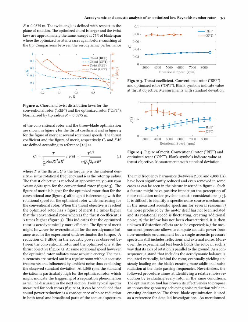
R = 0.0875 m. �e twist angle is de�ned with respect to theplane of rotation. �e optimized chord is larger and the twistlaws are approximately the same, except at 75% of blade spanwhere the optimized twist increases again before vanishing atthe tip. Comparisons between the aerodynamic performance

r/R0.2 0.4 0.6 0.8 1

c/R

0

0.2

0.4

0.6

0.8

1

t(deg.)

0

10

20

30

40

50

Chord (REF)Chord (OPT)Twist (REF)Twist (OPT)

Figure 2. Chord and twist distribution laws for theconventional rotor (“REF”) and the optimized rotor (“OPT”).Normalized by tip radius R = 0.0875 m.

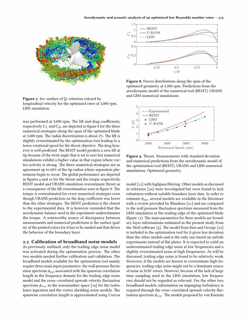
of the conventional rotor and the three–blade optimizationare shown in �gure 3 for the thrust coe�cient and in �gure 4for the �gure of merit at several rotational speeds. �e thrustcoe�cient and the �gure of merit, respectively Ct and FMare de�ned according to reference [16] as

Ct =T

12 ρ(ωR)2πR2

; FM =T3/2

ωQ√2ρπR2

(1)

where T is the thrust, Q is the torque, ρ is the ambient den-sity,ω is the rotational frequency and R is the rotor tip radius.�e thrust objective is reached at approximately 5,400 rpmversus 8,500 rpm for the conventional rotor (�gure 3). �e�gure of merit is higher for the optimized rotor than for theconventional one (�gure 4) although it is decreasing with therotational speed for the optimized rotor while increasing forthe conventional rotor. When the thrust objective is reachedthe optimized rotor has a �gure of merit 1.3 times higherthat the conventional rotor whereas the thrust coe�cient is3 times higher (�gure 3). �is indicates that the optimizedrotor is aerodynamically more e�cient. �e �gure of meritmight however be overestimated for the aerodynamic bal-ance used in the experiment underestimates the torque. Areduction of 8 dB(A) in the acoustic power is observed be-tween the conventional rotor and the optimized one at thethrust objective (�gure 5). At same rotational speed however,the optimized rotor radiates more acoustic energy. �e mea-surements are carried out in a regular room without acoustictreatments and in�uenced by ambient noise thus explainingthe observed standard deviation. At 4,500 rpm, the standarddeviation is particularly high for the optimized rotor whichmight indicate the triggering of a separation phenomenonas will be discussed in the next section. From typical spectrameasured for both rotors (�gure 6), it can be concluded thatsound power reduction is a consequence of noise reductionin both tonal and broadband parts of the acoustic spectrum.

Rotational Speed (rpm)

3000 4000 5000 6000 7000 8000

Ct

0

0.02

0.04

0.06

0.08

0.1

REF

OPT

Figure 3. �rust coe�cient. Conventional rotor (“REF”)and optimized rotor (“OPT”). Blank symbols indicate valueat thrust objective. Measurements with standard deviation.


3000 4000 5000 6000 7000 8000

FM

0

0.5

1

REF

OPT

Figure 4. Figure of merit. Conventional rotor (“REF”) andoptimized rotor (“OPT”). Blank symbols indicate value atthrust objective. Measurements with standard deviation.

�e mid frequency harmonics (between 2,000 and 6,000 Hz)have been signi�cantly reduced and even removed in somecases as can be seen in the picture inserted in �gure 6. Sucha feature might have positive impact on the perception ofnoise reduction under psycho–acoustic considerations [17].It is di�cult to identify a speci�c noise source mechanismin the measured acoustic spectrum for several reasons: i)the noise produced by the motor itself has not been isolatedand its rotational speed is �uctuating, creating additionalnoise; ii) the in�ow has not been characterized, it is thenunkown if distortion e�ects are to be expected; iii) the mea-surement procedure allows to compute acoustic power fromnon–anechoic environment but a single acoustic pressurespectrum still includes re�ections and external noise. More-over, the experimental test bench holds the rotor in such away that its axis of rotation is parallel to the ground. As a con-sequence, a stand that includes the aerodynamic balance ismounted vertically, behind the rotor, eventually yielding un-steady loading on the blades creating more additional noiseradiation at the blade passing frequencies. Nevertheless, thefollowed procedure aimes at identifying a relative noise re-duction by evaluating every rotor in the same conditions.�e optimization tool has proven its e�ectiveness to proposean innovative geometry achieving noise reduction while in-creasing endurance. �e three–blade optimization is usedas a reference for detailed investigations. As mentionned


in the introduction, at this early stage of development theoptimized rotor was obtained with only the trailing edgenoise model active in the optimization tool. It is expectedthat optimizations can be enhanced by taking into accountother broadband noise sources and by investigating the aero-dynamic �ow features around the optimized geometry. Ahigher level of noise reduction is expected.


4000 5000 6000 7000 8000

Acoustic

Pow

erdB(A

)

60

65

70

75

80

REF

OPT

Figure 5. Acoustic power. Conventional rotor (“REF”) andoptimized rotor (“OPT”). Blank symbols indicate value atthrust objective. Measurements with standard deviation.

Narrow Band Frequency Hz

0 2000 4000 6000 8000 10000

SoundPressure

Level

dB

0

20

40

60

80

100

REF

OPT

Background

Blade Passing Frequency

1 2 3 4 5 6 7 8 9 1020

40

60

Figure 6. Acoustic spectra for the conventional rotor(“REF”) and the optimized rotor (“OPT”) at the rotationalspeed of the thrust objective. �e spectra are averaged overmicrophone positions and measurement sessions. Close–upview with frequencies normalized by the blade passingfrequency.

2. AERODYNAMIC INVESTIGATION FROMHIGH FIDELITY METHODSTwo additional numerical strategies are used to analyze theaerodynamic and the acoustic characteristics of the optimizedrotor. Note that these two strategies simulated only the ro-tor without installations. A �rst strategy is based on theLa�ice–Boltzmann Method, referred to as LBM, and is usedto perform a Large–Eddy Simulation. Beyond computationalperformance, the main advantage of LBM is that the method

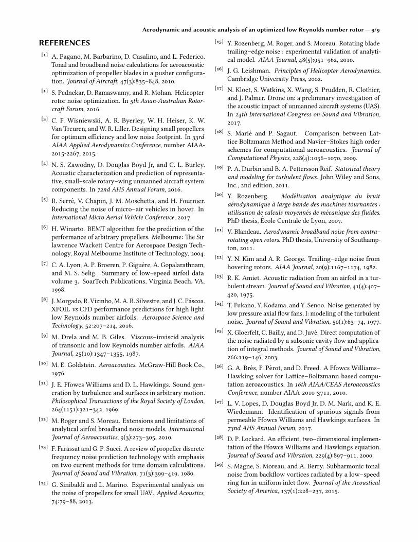
is stable without arti�cial dissipation, which makes it equiva-lent to solve the Navier–Stokes equations with a high–ordernumerical scheme [18]. �e present discretization of theequations ensures that the method is second–order accurateboth in time and space. �e LBM equations are solved usingthe open source so�ware Palabos (www.Palabos.org)on a cubic domain with an edge of about 45R. �e mesh ofthe rotor is composed of 249 million Cartesian cells. Bound-ary conditions are coupled with a bu�er layer of 1 m to avoidspurious re�ections. �e dimension of the �rst cell layerat the rotor wall is 350 µm to obtain an y+ of 50 in the tipregion. One rotor revolution is achieved in 250 time stepsand data are extracted a�er 8 revolutions. A second strategyresolves the three–dimensional incompressible Reynolds–Averaged Navier–Stokes (URANS) equations on a cylindricaldomain of diameter 20R and length 50R enclosing the ro-tor. Numerical resolution is achieved using a �nite volumeapproach by means of StarCCM+ commercial code. �e com-putational domain is discretized using 8 million polyhedralcells with a typical size in the vicinity of the rotor of R/176.�e boundary conditions upstream and downstream the rotorare implemented as pressure conditions while the peripheryof the domain is treated as a slip wall. �e blades are mod-elled as no–slip surfaces. A full rotation is dicretized into360 time steps and at least 35 rotations are needed to ensurethat initial transients have su�ciently decayed. Both spatialand temporal discretizations are achieved using second orderschemes. Finally, the k–ε model is employed for URANSturbulence closure with maximum y+ values below unity.Note that Spalart–Allmaras and k–ω SST models (with andwithout gamma–Re–theta transition model) were tested andyielded similar results to those obtained using the k–ε modelin terms of integrated loads. In addition, it was veri�ed thatthe results are converged with respect to the typical cell size.Analyzing the characteristics of the optimized geometry withhigh–�delity numerical simulations serves three objectives:i) validate the aerodynamic model in the optimization tool,ii) calibrate and validate the acoustic broadband models andiii) rank the noise sources in MAV rotors. Analyzing the LBMsimulation also provides informations on the �ow featuresaround the optimized rotor and helps identify speci�c charac-teristics such as stall phenomena or leading edge separationas can be seen in �gure 7. Such a phenomenon occurs around75% of the blade radius, where the twist angle increases again(�gure 2) suggesting that having an in�ection point on thetwist distribution law should be avoided. �e resulting �owthen merges with the tip vortex and impinges the follow-ing blade. It creates an interaction noise that is believed bythe authors to be the most dominant noise source in thiscon�guration.

2.1 Validation of the aerodynamic model�e rotational speed in U–RANS and LBM simulations wasset at 5,000 rpm as was predicted by BEMT to reach the thrustobjective. It was observed in the experiment to be underesti-mated as the actual rotation speed needed to reach the thrustobjective is around 5,400 rpm. An additional computation

www.Palabos.org


Figure 7. Iso–surface of Q–criterion colored bylongitudinal velocity for the optimized rotor at 5,000 rpm.LBM simulation.

was performed at 3,000 rpm. �e li� and drag coe�cients,respectively CL and CD , are depicted in �gure 8 for the threenumerical strategies along the span of the optimized bladeat 5,000 rpm. �e radial discretization is about 2%. �e li� isslightly overestimated by the optimization tool leading to alower rotational speed for the thrust objective. �e drag how-ever is well predicted. �e BEMT model predicts a zero li� attip because of the twist angle that is set to zero but numericalsimulations exhibit a higher value in that region where vor-tex activity is strong. �e three numerical strategies are inagreement up to 60% of the tip radius where separation phe-nomena begin to occur. �e global performance are depictedin �gures 9 and 10 for the thrust and the torque respectively.BEMT model and URANS simulation overestimate thrust asa consequence of the li� overestimation seen in �gure 8. �etorque is overestimated for every numerical strategies eventhough URANS prediction on the drag coe�cient was lowerthan the other strategies. �e BEMT prediction is the closestto the experimental data. It is however reminded that theaerodynamic balance used in the experiment underestimatesthe torque. A noteworthy source of discrepancy betweenmeasurements and numerical predictions is the surface qual-ity of the printed rotors for it has to be sanded and that drivesthe behavior of the boundary layer.

2.2 Calibration of broadband noise modelsAs previously outlined, only the trailing edge noise modelwas activated during the optimization process. �e othertwo models needed further calibration and validation. �ebroadband models available for the optimization tool mainlyrequire three main input parameters: the wall pressure �uctu-ation spectrum φpp associated with the spanwise correlationlength in the frequency domain for the trailing edge noisemodel and the cross–correlated upwash velocity �uctuationspectrum φww in the wavenumber space [19] for the turbu-lence ingestion and the vortex shedding noise models. �espanwise correlation length is approximated using Corcos

CL

0

0.5

1

1.5

BEMT

U-RANS

LBM

r/R

0.25 0.5 0.75 1

CD

0

0.2

0.4

Figure 8. Forces distributions along the span of theoptimized geometry at 5,000 rpm. Predictions from theaerodynamic model of the numerical tool (BEMT), URANSand LBM numerical simulations.


3000 4000 5000 6000

T(N

)

0

1

2

3

4

5

Experimental

BEMT

LBM

U–RANS

Figure 9. �rust. Measurements with standard deviationand numerical predictions from the aerodynamic model ofthe optimization tool (BEMT), URANS and LBM numericalsimulations. Optimized geometry.

model [12] with highpass �ltering. Other models as discussedin reference [20] were investigated but were found to lackrobustness without suitable boundary layer data. In order toestimate φpp , several models are available in the literaturewith a review provided by Blandeau [21] and are comparedto the wall pressure �uctuation spectrum measured from theLBM simulation at the trailing edge of the optimized blade(�gure 11). �e main parameters for these models are bound-ary layer informations estimated in the present study fromthe Xfoil so�ware [5]. �e model from Kim and George [22]is included in the optimization tool for it gives less deviationthan the other models and is the only one based on airfoilsexperiments instead of �at plates. It is expected to yield anunderestimated trailing edge noise at low frequencies and aslightly overestimated noise at high frequencies. As will bediscussed, trailing edge noise is found to be relatively weak.Moreover, if the models are known to overestimate high fre-quencies, trailing edge noise might not be a dominant sourceof noise in MAV rotors. However, because of the lack of largetime sampling used in the LBM simulation, low frequen-cies should not be regarded as relevant. For the other twobroadband models, information on impinging turbulence isrequired through the cross–correlated upwash velocity �uc-tuation spectrum φww . �e models proposed by von Karman



3000 4000 5000 6000

Q(N

.m)

0

0.02

0.04

0.06

0.08

Experimental

BEMT

LBM

U–RANS

Figure 10. Torque. Measurements with standard deviationand numerical predictions from the aerodynamic model ofthe optimization tool (BEMT), URANS and LBM numericalsimulations. Optimized geometry.

and Liepmann cited in reference [23] are compared to datafrom the LBM simulation just upstream of the leading edgeof one blade in the optimized rotor as shown in �gure 12 forkx = ω/U0, U0 being the uniform convection velocity underthe frozen–turbulence assumption and ky = 0. �e modelingof φww is expected to yield the right trend although it overes-timates the whole spectrum. It is worth noting that the orderof magnitude in the error of the estimated φpp or φww alsoimpacts the overall sound pressure level. �at is to say, if the�uctuation spectrum models are estimated 10 times higherthan the e�ective value, the overall sound pressure level is10 dB higher. �e von Karman and Liepmann models dependon the wavenumbers and two scales representative of theturbulence impinging the leading edge which in turn causesinteraction noise. �ese two scales are the intensity of thechordwise velocity �uctuation and the Taylor micro–scaleLµ as the turbulence length scale. �at turbulence lengthscale can be directly derived from the LBM simulation and isdepicted in �gure 13. �e turbulence appears to be relativelyhomogeneous both in the vertical direction (z/R) and in theradial direction (r/R) between 60% and 90% of the blade ra-dius. It is however necessary to approximate this quantity

Frequency (Hz)

102 103

φpp/(1 2ρU

2 0)

10−10

10−5

100

LBMChase-HoweGoodyWillmarth-Roos-AmietKim-George

Figure 11. Wall pressure �uctuation spectrum φpp at thetrailing edge, mid–span of the optimized blade from LBMsimulations and numerical models.

with data already available in the optimization tool. In the

kx

102 103

φww(k

x,0)

10−10

10−8

10−6

10−4

LBM

von Karman

Liepmann

Figure 12. Cross–correlated upwash velocity �uctuationspectrum φww upstream of the leading edge of theoptimized blade from LBM simulations and numericalmodels.

Figure 13. Taylor micro–scale Lµ upstream of the leadingedge of the optimized rotor normalized by maximum radius.LBM simulation.

context of a clean in�ow condition, the turbulence impingingthe leading edge is believed to be generated by the wakeof the trailing edge of the previous blade as it is believedto be stalled in this context. A similitude is then expectedto be found between leading edge turbulence and trailingedge wake. �e boundary layer informations from Xfoil areused to estimate the width of the wake near 90% of the chordaccording to the de�nition proposed in reference [24]:

D∗w = dAS + δ∗p + δ

∗s (2)

where dAS is the airfoil section thickness near the trailingedge and δ∗p and δ∗s are the boundary layer displacementthicknesses on pressure side and suction side respectively. Acomparison between the turbulence length scale measuredfrom the LBM simulation upstream of the leading edge and anestimate of the wake width from the numerical tool is plo�edin �gure 14. It is unknown whether that scaling is relevant inevery situations before further investigations are carried outbut helpful equivalence is observed. For the following opti-mizations, the turbulence length scale is estimated from theXfoil so�ware based on boundary layer data and equation (2)to feed the φww models. A way to scale the intensity of thechordwise velocity �uctuation is still under investigation.For the following computations, a value of 4 m/s is takenfrom LBM simulation, representing 10% of the tip speed.


r/R

0.5 0.6 0.7 0.8 0.9 1

Norm

alizedlength

scales

0

0.02

0.04Lµ/R (mean value ∼ 0.021)

D∗

w/R (mean value ∼ 0.020)

Figure 14. Comparison of length scales representative ofturbulence and wake. Lµ predicted from LBM simulationand D∗w predicted from the optimization tool. Normalizedby tip radius.

3. AEROACOUSTIC INVESTIGATION FROMHIGH FIDELITY METHODSAn aeroacoustic solver is developped to predict the noisefrom the LBM simulation. It solves the FWH equation in thefrequency domain [25] on a cartesian, permeable control sur-face surrounding the optimized rotor. �e permeable controlsurface is centered on the rotor and is two rotor diameterslong in the directions parallel to the rotor plane (axis e−→x ande−→y ) and one rotor diameter long in the direction parallel tothe axis of rotation (axis e−→z ). Aerodynamic data are extractedfor three rotor revolutions with a relatively high frequencyresolution (∼ 30 Hz). �e purpose is �rst to assess the abilityof LBM simulation to provide valuable information for wavepropagation methods [26]. It is believed that LBM simulationis a natural candidate for providing aerodynamic input toaeroacoustic analogies if care is taken to ensure that eddiesdo not cross the control surfaces. Although a promising �lter-ing procedure has been recently proposed in reference [27]to suppress spurious signal from permeable FWH solver, itdoes not appear mature. A weighting coe�cient is appliedon the multipole de�nitions as suggested by Lockard [28].�e acoustic prediction resulting from the LBM simulationis compared to the optimization tool predictions and mea-surements on the acoustic power computed according toISO 3746 : 1995 standard. Computations are run with theoptimization tool for two con�gurations: with the trailingedge noise model only (labelled “TE”) and in addition withthe turbulence interaction noise model (labelled “TE+TI”).Results are shown in �gure 15. Figure 15 indicates that turbu-lence interaction noise is dominant compared to trailing edgenoise and this may be a consequence of the large coherentstructures shed into the wake as observed in �gure 7 thatimpinge the following leading edge causing the interactionnoise. �e computations are now systematically carried outwith the interaction noise model in addition to the trailingedge noise model. �e acoustic powers at a rotational speedof 5,000 rpm are reported in table 1. �e corresponding soundpower levels are plo�ed in �gure 16 in third octave centeredfrequency bands according to ISO 3746 : 1995 standard. �eprediction from the optimization tool is in relative agree-


4000 5000 6000

Acoustic

Pow

erdB(A

)

10

20

30

40

50

60

70

80

Experimental

Optimization tool (TE+TI)

Optimization tool (TE)

LBM

Figure 15. Acoustic power from measurements withstandard deviation and numerical predictions from theoptimization tool and LBM simulation.

Table 1. Acoustic power for the optimized rotor at5,000 rpm according to ISO 3746 : 1995 standard.

Experimental 69.7 dB(A)Optimization tool 69.1 dB(A)FWH-LBM 73.9 dB(A)

ment with the measurements while the prediction from theLBM simulation is higher. �e power level of the BPF andsubharmonics observed in the measurement are higher thanthose predicted by the optimization tool and that is a conse-quence of installation e�ects and unsteady loading. Figure 16shows that most of the frequencies are overpredicted by theFWH solver and that overestimation is found again on theacoustic power (table 1). As previously mentionned, soundis propagated from aerodynamic data stored for three rotorrevolutions: this relatively large sampling might be the causeof the observed discrepancy. It is worth noting that turbulenteddies crossing the permeable control surfaces might also beresponsible for creating spurious noise [27]. Acoustic propa-

Third Octave Centered Frequency Band (Hz)

125 200 315 500 800 1250 2000 3150 5000SoundPow

erLevel

dB(A

)

20

40

60

80

Experimental Optimization tool FWH-LBM

Figure 16. Acoustic power spectra according to ISO3746 : 1995 standard between measurements, numericalprediction from the optimization tool and FWH propagationof LBM simulation.

gation is extracted from the LBM simulation and compared


with the predictions from the FWH–LBM tool. �at overes-timation of the blade passing frequency is observed on theacoustic power spectral density (PSD) plo�ed in �gure 17both from the FWH–LBM tool and the direct measurementsof the LBM simulation. �e signals are taken in the rotorplane, corresponding with one microphone position, approx-imately 1 m away from the rotor. Numerical predictionsobserved in �gure 17 are a preliminary result: the PSD seemshigher for every frequency than the measurements and thatmight be a consequence of the large frequency resolutionavailable from the LBM simulations. �e BPF is particularlyoverestimated. �e FWH–LBM tool proves its relevance athigher frequencies. In this domain, mesh discretization ofthe LBM simulation reaches the same order of magnitudethan the acoustic wavelength and a signi�cant dissipationoccurs. �e FWH solver is a numerical tool that can be used

Narrow Band Frequency Hz

0 1000 2000 3000 4000 5000

PSD

(dB/Hz)

0

20

40

60

Experimental LBM FWH–LBM

Figure 17. Acoustic power spectral density (PSD) frommeasurements and numerical predictions from LBMsimulation at one microphone position in the rotor plane.

to identify a hierarchy in the sources of noise. �e FWHequation is generally wri�en in a way that links mathemati-cal terms with physical meaning. �e corresponding acousticpressure for each of the terms in the FWH equation in theform of a directivity pa�ern centered on the rotor is shownin �gure 18 for the perpendicular plane of rotation. �e di-rectivity contours give insight into the acoustic radiationpa�ern around the MAV rotor. �e total acoustic radiationseems mostly equal in every direction, although the acousticintensity seems higher in the downwards direction as can beexpected. �e most striking feature of the directivity pa�ernsis the monopole term being dominant. It is consistant withobservation from �gure 17 where BPF is overestimated andmainly comes from the steady loading which the monopoleterm account for. However, loading noise, represented bythe dipole terms, is generally considered as dominant in low–Reynolds number fan [29] due to unsteady loading. Analysisof the broadband noise models also suggests that dipole termsare expected to be dominant for interaction noise, believed bythe authors to be the main noise source in this con�guration,is a consequence of unsteady loading. As previously observed(�gure 16), interaction noise in MAV rotors is a broadband,high–frequency component of the acoustic spectrum andit might not be resolved yet by the FWH tool addressed in

this contribution, as a result of the high frequency resolutionavailable at this early stage. As a consequence, the dipoleterms of the FWH equation might be underpredicted.

20

40

60

80

Up

Down

Left Right

Total

Monopole

Dipole e−→x

Dipole e−→y

Dipole e−→z

Figure 18. Directivity contour perpendicular to the plane ofrotation at r = 1 m away from the rotor. Correspondingacoustic pressure from multipole terms in the FWHequation [25]. Levels in dB. Rotor is not at scale.

4. DISCUSSION�e optimization has proven its e�ectiveness to reduce thenoise produced by MAV rotors in hover and increase en-durance. A reduction of 8 dB(A) in the acoustic power isobtained and experimentally observed from a protocol suit-able for non–treated rooms. High levels of noise reductionare expected in the future using the tools presented herein.However, the optimization presented in this contribution is�rst of all an aerodynamic optimization. Acoustic modelsin the optimization tool estimate noise levels from steadyloading but experiment and numerical simulations suggestthat unsteady aerodynamics induces most of the noise. Insuch a context, reducing the rotational speed or optimizingthe aerodynamic e�ciency will lead to lower noise levels asrotational speed is the driving parameter for the involvednoise mechanisms. Another source of noise is under investi-gation with implementation of vortex shedding broadbandnoise model [12]. �e dominant source of noise is foundto be produced by the interaction between turbulence andleading edge. �e turbulence impinging the leading edge isrelatively homogeneous, and if most of the noise is producedin the leading edge region, a speci�c design should be able tosigni�cantly reduce acoustic radiation by destroying homo-geneous turbulence or by allowing phase cancellation of theacoustic waves resulting from the sca�ering of turbulencewavelength by the leading edge.

ACKNOWLEDGMENTS�is research is supported by Direction Generale de l’Armement(DGA) from the French Ministry of Defense. �e authorsthank Remy Chanton from the technical team for the set–upof the aerodynamic balance.


REFERENCES[1] A. Pagano, M. Barbarino, D. Casalino, and L. Federico.

Tonal and broadband noise calculations for aeroacousticoptimization of propeller blades in a pusher con�gura-tion. Journal of Aircra�, 47(3):835–848, 2010.

[2] S. Pednekar, D. Ramaswamy, and R. Mohan. Helicopterrotor noise optimization. In 5th Asian-Australian Rotor-cra� Forum, 2016.

[3] C. F. Wisniewski, A. R. Byerley, W. H. Heiser, K. W.Van Treuren, and W. R. Liller. Designing small propellersfor optimum e�ciency and low noise footprint. In 33rdAIAA Applied Aerodynamics Conference, number AIAA-2015-2267, 2015.

[4] N. S. Zawodny, D. Douglas Boyd Jr, and C. L. Burley.Acoustic characterization and prediction of representa-tive, small–scale rotary–wing unmanned aircra� systemcomponents. In 72nd AHS Annual Forum, 2016.

[5] R. Serre, V. Chapin, J. M. Mosche�a, and H. Fournier.Reducing the noise of micro–air vehicles in hover. InInternational Micro Aerial Vehicle Conference, 2017.

[6] H. Winarto. BEMT algorithm for the prediction of theperformance of arbitrary propellers. Melbourne: �e Sirlawrence Wacke� Centre for Aerospace Design Tech-nology, Royal Melbourne Institute of Technology, 2004.

[7] C. A. Lyon, A. P. Broeren, P. Giguere, A. Gopalarathnam,and M. S. Selig. Summary of low–speed airfoil datavolume 3. SoarTech Publications, Virginia Beach, VA,1998.

[8] J. Morgado, R. Vizinho, M. A. R. Silvestre, and J. C. Pascoa.XFOIL vs CFD performance predictions for high lightlow Reynolds number airfoils. Aerospace Science andTechnology, 52:207–214, 2016.

[9] M. Drela and M. B. Giles. Viscous–inviscid analysisof transonic and low Reynolds number airfoils. AIAAJournal, 25(10):1347–1355, 1987.

[10] M. E. Goldstein. Aeroacoustics. McGraw-Hill Book Co.,1976.

[11] J. E. Ffowcs Williams and D. L. Hawkings. Sound gen-eration by turbulence and surfaces in arbitrary motion.Philosophical Transactions of the Royal Society of London,264(1151):321–342, 1969.

[12] M. Roger and S. Moreau. Extensions and limitations ofanalytical airfoil broadband noise models. InternationalJournal of Aeroacoustics, 9(3):273–305, 2010.

[13] F. Farassat and G. P. Succi. A review of propeller discretefrequency noise prediction technology with emphasison two current methods for time domain calculations.Journal of Sound and Vibration, 71(3):399–419, 1980.

[14] G. Sinibaldi and L. Marino. Experimental analysis onthe noise of propellers for small UAV. Applied Acoustics,74:79–88, 2013.

[15] Y. Rozenberg, M. Roger, and S. Moreau. Rotating bladetrailing–edge noise : experimental validation of analyti-cal model. AIAA Journal, 48(5):951–962, 2010.

[16] J. G. Leishman. Principles of Helicopter Aerodynamics.Cambridge University Press, 2002.

[17] N. Kloet, S. Watkins, X. Wang, S. Prudden, R. Clothier,and J. Palmer. Drone on: a preliminary investigation ofthe acoustic impact of unmanned aircra� systems (UAS).In 24th International Congress on Sound and Vibration,2017.

[18] S. Marie and P. Sagaut. Comparison between Lat-tice Boltzmann Method and Navier–Stokes high orderschemes for computational aeroacoustics. Journal ofComputational Physics, 228(4):1056–1070, 2009.

[19] P. A. Durbin and B. A. Pe�ersson Reif. Statistical theoryand modeling for turbulent �ows. John Wiley and Sons,Inc., 2nd edition, 2011.

[20] Y. Rozenberg. Modelisation analytique du bruitaerodynamique a large bande des machines tournantes :utilisation de calculs moyennes de mecanique des �uides.PhD thesis, Ecole Centrale de Lyon, 2007.

[21] V. Blandeau. Aerodynamic broadband noise from contra–rotating open rotors. PhD thesis, University of Southamp-ton, 2011.

[22] Y. N. Kim and A. R. George. Trailing–edge noise fromhovering rotors. AIAA Journal, 20(9):1167–1174, 1982.

[23] R. K. Amiet. Acoustic radiation from an airfoil in a tur-bulent stream. Journal of Sound and Vibration, 41(4):407–420, 1975.

[24] T. Fukano, Y. Kodama, and Y. Senoo. Noise generated bylow pressure axial �ow fans, I: modeling of the turbulentnoise. Journal of Sound and Vibration, 50(1):63–74, 1977.

[25] X. Gloerfelt, C. Bailly, and D. Juve. Direct computation ofthe noise radiated by a subsonic cavity �ow and applica-tion of integral methods. Journal of Sound and Vibration,266:119–146, 2003.

[26] G. A. Bres, F. Perot, and D. Freed. A Ffowcs Williams–Hawking solver for La�ice–Boltzmann based compu-tation aeroacoustics. In 16th AIAA/CEAS AeroacousticsConference, number AIAA-2010-3711, 2010.

[27] L. V. Lopes, D. Douglas Boyd Jr, D. M. Nark, and K. E.Wiedemann. Identi�cation of spurious signals frompermeable Ffowcs Williams and Hawkings surfaces. In73nd AHS Annual Forum, 2017.

[28] D. P. Lockard. An e�cient, two–dimensional implemen-tation of the Ffowcs Williams and Hawkings equation.Journal of Sound and Vibration, 229(4):897–911, 2000.

[29] S. Magne, S. Moreau, and A. Berry. Subharmonic tonalnoise from back�ow vortices radiated by a low–speedring fan in uniform inlet �ow. Journal of the AcousticalSociety of America, 137(1):228–237, 2015.

aerodynamic and acoustic analysis of an optimized low

Documents