aerodynamic analysis of low reynolds number flows
TRANSCRIPT
Universita degli Studi di Napoli Federico II
Dottorato di Ricerca in Ingegneria Aerospaziale,Navale e della Qualita (XXII ciclo)
Dipartimento di Ingegneria Aerospaziale
Aerodynamic Analysis of Low Reynolds
Number Flows
Tutore CandidatoCh.mo Prof. Renato Tognaccini Pietro Catalano
Anno Accademico 2009

ABSTRACT
An aerodynamic analysis of low-Reynolds number flows is presented. The
focus is placed on the laminar separation bubbles, a peculiar phenomenon of
these kind of flows. The only simulations techniques feasible to be applied to
complex configurations appear to be the methods based on the Reynolds Av-
eraged Navier Stokes equations. A critical point is the turbulence modelling.
In fact, the turbulence models are calibrated for flows at high Reynolds num-
ber with separation in the turbulent regime.
The flow over a flat plate with an imposed pressure gradient, and around
the Selig-Donavan 7003 airfoil is considered. Large eddy simulations have
also been performed and used as reference for the RANS results.
Laminar separation bubbles have been found by the Spalart-Allmaras
and the κ − ω SST turbulence models. The models have been used without
prescribing the transition location and assuming low values of the free-stream
turbulence.
The main results have been achieved for the κ−ω SST turbulence model.
This model is very reliable for transonic flows at high Reynolds number, but
has shown limits when applied to low-Reynolds number flows. A modification
of the model has been proposed. The modified model, named as κ− ω SST-
LR, has provided a correct simulation of the boundary layer in the tests
performed at low and high Reynolds numbers. The laminar separation bubble
arising of the SD 7003 airfoil has been well captured. The accuracy of the
new model is not reduced in transonic regime.
i

Nomenclature
∇ Nabla operator
B Constant in the logarithmic law of velocity
b Wing span
c Airfoil chord
CD Drag coefficient
CF Friction coefficient
CL Lift coefficient
CP Pressure coefficient
DES Detached eddy simulation
DNS Direct numerical simulation
e Energy (Internal + Kinetic) per unit mass
ILES Implicit large eddy simulation
L Length
LES Large eddy simulation
LSB Laminar separation bubble
p Static pressure
RANS Reynolds Averaged Navier Stokes
Re Reynolds number
RSM Reynolds Stress Model
SD Selig-Donovan
SST Shear Stress Transport
T Temperature
t Time
ii

tij Viscous stress tensor
u,v,w Velocity components in x,y,z directions
ui Velocity in tensor notation
uτ Friction velocity
V Module of the velocity
x,y,z Cartesian coordinates
xi Position vector in tensor notation
y+ Viscous coordinate in the wall-normal direction, uτ yν
Subscripts
∞ Free stream conditions
ref Reference
tr Transition
Symbols
α Angle of attack
δ∗ Displacement thickness
δij Kronecker delta
η Kolmogorov length scale
Self-similar coordinate
κ Turbulent kinetic energy
κa von Karman constant
λ Heat conduction coefficient
µ Molecular viscosity
µt Eddy viscosity
ν Kinematic viscosity, µρ
Ω Vorticity
ω Specific turbulent dissipation rate
ρ Density
τij Sub-grid stress tensor
Reynolds stress tensor
τw Surface shear stress
τxy Reynolds shear stress
iii

ν Working variable of the Spalart-Allmaras turbulence model
ε Turbulent dissipation rate
tη Kolmogorov time scale
uη Kolmogorov velocity scale
Superscripts
+ Viscous units
iv

Contents
1 Introduction 1
1.1 Aerodynamics of Low Reynolds Number Flows . . . . . . . . . 2
2 Physical and Mathematical Model 7
2.1 Large Eddy Simulation . . . . . . . . . . . . . . . . . . . . . . 10
2.1.1 Subgrid Modelling . . . . . . . . . . . . . . . . . . . . 10
2.1.2 Dynamic Models . . . . . . . . . . . . . . . . . . . . . 11
2.1.3 LASSIE Code . . . . . . . . . . . . . . . . . . . . . . . 12
2.1.3.1 Numerical method . . . . . . . . . . . . . . . 13
2.2 Reynolds Averaging of the Navier-Stokes Equations . . . . . . 14
2.2.1 The One-equation Spalart-Allmaras Turbulence Model 16
2.2.1.1 Free Shear Layer Flows . . . . . . . . . . . . 16
2.2.1.2 Wall Bounded Flows . . . . . . . . . . . . . . 17
2.2.2 The Two-equation Turbulence Models . . . . . . . . . 20
2.2.2.1 The κ-ω Wilcox model . . . . . . . . . . . . . 22
2.2.2.1.1 Free Shear Layer Fows . . . . . . . . 22
2.2.2.1.2 Boundary Layer Flows . . . . . . . . 23
2.2.2.1.2.1 The log layer . . . . . . . . . 23
2.2.2.1.2.2 The defect layer . . . . . . . . 24
2.2.2.1.2.3 The viscous sublayer . . . . . 25
2.2.2.1.3 Free-stream Dependency . . . . . . . 27
2.2.2.2 The κ-ω TNT model . . . . . . . . . . . . . . 28
2.2.2.3 The κ-ω SST turbulence model . . . . . . . . 30
v

Contents
2.2.3 ZEN Code . . . . . . . . . . . . . . . . . . . . . . . . . 33
2.2.3.1 Numerical definition . . . . . . . . . . . . . . 34
2.2.3.2 UZEN: the Time-accurate Version . . . . . . 36
2.3 Detached Eddy Simulation . . . . . . . . . . . . . . . . . . . . 37
2.3.1 SA-DES . . . . . . . . . . . . . . . . . . . . . . . . . . 37
2.3.2 SST-DES . . . . . . . . . . . . . . . . . . . . . . . . . 38
3 Laminar Separation Bubbles 39
3.1 Flow over a Flat Plate . . . . . . . . . . . . . . . . . . . . . . 40
3.1.1 Numerical Set-up . . . . . . . . . . . . . . . . . . . . . 40
3.1.2 Influence of free-stream Turbulence . . . . . . . . . . . 44
3.2 Flow around the SD 7003 Airfoil . . . . . . . . . . . . . . . . . 53
3.2.1 Grid Assessment . . . . . . . . . . . . . . . . . . . . . 53
3.2.2 Turbulence Models Assessment . . . . . . . . . . . . . 55
3.2.3 Results by κ-ω SST turbulence model . . . . . . . . . . 55
3.2.3.1 Main Characteristics of the Flow . . . . . . . 56
3.2.3.2 Large Eddy Simulations . . . . . . . . . . . . 57
3.2.3.3 RANS-LES Comparison . . . . . . . . . . . . 60
3.2.3.4 Flow at α = 4 . . . . . . . . . . . . . . . . . 62
4 Turbulence Modelling 65
4.1 Analysis of the the κ-ω SST model . . . . . . . . . . . . . . . 65
4.2 The κ-ω SST-LR model . . . . . . . . . . . . . . . . . . . . . 69
4.2.1 Analysis for Low Reynolds Number Flows . . . . . . . 72
4.3 Drag polar of the SD 7003 airfoil . . . . . . . . . . . . . . . . 80
4.3.1 Stall Characteristics . . . . . . . . . . . . . . . . . . . 83
5 Transonic Flows 86
5.1 RAE 2822 Airfoil . . . . . . . . . . . . . . . . . . . . . . . . . 86
5.1.1 Case 9 . . . . . . . . . . . . . . . . . . . . . . . . . . . 86
5.1.2 Case 10 . . . . . . . . . . . . . . . . . . . . . . . . . . 87
5.2 RAE M2155 Wing . . . . . . . . . . . . . . . . . . . . . . . . 89
vi

Contents
6 Conclusions 91
vii

Chapter 1
Introduction
Aerodynamic perfomances of aerial vehicles are largely influenced by the
Reynolds number. The different flow regimes occurring in a wide range of
Reynolds numbers are well described by Carmichael [1].
The regime at Reynolds number lower than 102 is of interest for devices
used to reduce the turbulence level of wind tunnels, but not for airfoil-like
machines.
The regime of Reynolds number up to 104 regards insects and small model
airplanes. The flow is strongly laminar and not able to sustain adverse pres-
sure gradients. Some interesting solutions are adopted in nature in order to
prevent the separation. The dragonfly has a saw tooth single surface airfoil.
It is thought that eddies are formed in the troughs and keep the flow at-
tached. The fly has a large number of fine hair-like elements that promote
an eddy-induced energy transfer and prevent separation.
The range of Reynolds number between 104 − 105 is typical of flying an-
imals and large model airplanes. At the lower end of this regime, natural
laminar regime is possible provided that the lift coefficient of the flying ma-
chine remains quite low (≈ 0.5). Higher lift coefficients would produce a flow
separation without re-attachment with a drop in lift and a rise of the drag
coefficient. Carmichael [1] has pointed out that, under natural laminar flow
separation, the distance betweeen the separation and the re-attachment point
expressed in terms of Reynolds number is about 50000. Thus, if a separation
occurs at Reynolds number lower than 50000, the distance to the trailing
edge is insufficient for the re-attachment of the flow. At higher Reynolds
1

1.1 Aerodynamics of Low Reynolds Number Flows
number re-attachement is possible, but the bubble is of significant length
with an important impact on the performance.
The next Reynolds number regime, up to 106, is of interest of large soaring
birds but also of large radio controlled model aircrafts, ultra-light gliders,
and human powered aircrafts. Airfoils for wind turbines also operate in this
regime. Extensive laminar flow is possible and the performances of the airfoils
are improved with respect to lower Reynolds numbers.
Large aircrafts fly at Reynolds numbers of order of magnitute 107−108. It
is still possible to obtain large regions of laminar flows. The flight altitude has
to be high in order to keep the Reynolds number per unit length reasonably
low. Favourable pressure gradients are necessary and are obtained through
a careful design of the wing sections. Devices to stabilize the boundary layer
are also used.
Reynolds numbers still higher are typically for large water-immersed ve-
hicles such as tankers and nuclear submarines.
1.1 Aerodynamics of Low Reynolds Number
Flows
The limit of the low Reynolds number regime is usually indicated to be 2×10⁵
[2, 3]. Below this limit, the drag polar of the airfoils present a decline of the
aerodynamic efficiency due to the presence of laminar separations.
The research in the field of the low Reynolds number flows is being pushed
by the the growing interest of the aerospace industries in unmanned and
micro-aerial vehicles (UAV and MAV). UAV wings typically operate at a
Reynolds number of 104 − 105. At these Reynolds numbers, the flow cannot
sustain strong adverse pressure gradients and often separates in the laminar
regime. The disturbances present in the laminar region are amplified inside
the separated shear layer and transiton to the turbulent regime occurs. The
turbulence developing inside the re-circulation region enhances the momen-
tum transport and the flow re-attaches.
2

1.1 Aerodynamics of Low Reynolds Number Flows
This phenomenon, the laminar separation bubble, is one of the main
critical aspects of flows at low Reynolds numbers and adversely affects the
performance of an airfoil. Thick bubbles change the effective contour of an
airofil. This results in an increase of the pressure drag. Suction is reduced
in the aft part and pressure recovery is decreased in the rear part of the
airfoil. Skin friction drag increases as well due to the rise of the turbulent
momentum. A more significant effect occurs when the turbulent transport
is not sufficient to close the bubble. The separated region extends up to the
trailing edge. This causes a loss of lift and an increase of drag with hysteresis
effects of the force coefficients with the angle of attack.
The only simulation techniques feasible to be applied to complex config-
urations such as High Altitude Long Endurance (HALE) unmanned vehicles
appear to be the methods based on the Reynolds Averaged Navier Stokes
equations. A critical point in applying the RANS approach to low Reynolds
number flows is the turbulence modelling. In fact the presence of separation
bubbles means that the separation is laminar and that the transition points
are very difficult to be set. The turbulence models are instead calibrated for
separation in the turbulent flow regime, and need the transition points to be
known a priori.
Spalart and Strelets [4] performed a direct numerical simulation (DNS) of
a separation bubble over a flat plate. They also applied the RANS equations
arguing that turbulence models should be able to deal with this kind of flow,
where the transition is due to the flow that re-circulating inside the separated
region brings turbulent fluid upstream in the laminar zone. They used a so-
called ”trip-less” approach consisting of setting non-zero turbulence inflow
values during the first iterations and then setting zero turbulence values until
a steady state is reached. The Spalart-Almars model [5] finds a bubble but
with a slow recovery and a re-attachment more downstream with respect to
DNS results. The κ−ω SST model [6] provides a separation only if modified
by a term derived from the Spalat-Allmras model.
The possibility of using the Reynolds Averaged Navier Stokes equations
for the numerical simulation of low Reynolds number flows and laminar sep-
3

1.1 Aerodynamics of Low Reynolds Number Flows
aration bubbles is addressed in several papers. Howard et al. [7] performed
RANS simulations of a laminar bubble over a flat plate using the κ−g model
[8] with and without fixing the transition point, and modified by using co-
efficients depending on the local turbulent Reynolds number as proposed by
Wilcox [9]. The model without any treatment of the transition provides a
very weak separation. The model with modified coefficients presents a bub-
ble with a re-attachment anticipated with respect to DNS. The κ− g model
not modified but applied with the transition point imposed returns a bubble.
The re-attachment point is located more downstream than DNS data.
The RANS approach, with some treatment to take into account the tran-
sition phenomenon, has been applied to the Selig-Donovan 7003 airfoil by
several researchers. This airfoil has been specifically designed for small model
gliders at Reynolds number below 105, and exhibits a relatively large laminar
bubble over a broad range of incidences at Reynolds number of 6×10⁴ . The
Selig-Donovan 7003 airfoil has been the subject of numerical and experimen-
tal investigations [3].
Windte [10], Radespiel [11], Yuan et al. [12] employed a RANS solver
coupled to a transition prediction method to simulate the flow around the
SD7003 airfoil at Re = 6 × 10⁴. Contour plots of Reynolds stresses are
presented. Some interesting results were achieved by the Menter BSL-two
layer model [6], the explicit algebraic Reynolds stress model by Wallin [13],
and the Wilcox RSM model [9]. The drag polar of the airfoil is computed with
a reasonable accuracy at low angle of attack. A systematic over-prediction of
the CL with respect to the experiments is however noted. Some dependence
of the results on the choice of the Ncrit is seen mainly at the high incidences.
An easier approach has been also tried. Tang [14] applied the RANS
equations without any particular treatment of the transition to the flow at
Re = 6 × 10⁴ around the SD 7003 airfoil. First a laminar simulation is
performed. The transition is considered to occur in the separated region at
the point where the flow reverses direction and moves downstream. Then, a
simulation with imposed transition point is performed. Results are presented
for the flow at α = 4 in terms of contour plot of the Reynolds stresses,
4

1.1 Aerodynamics of Low Reynolds Number Flows
pressure coefficient, and velocity contours with stream-lines. Good results
are achieved by the Spalart-Allmaras model. A too short bubble is instead
returned by the Menter BSL-two layer, and the Jones-Launder [15] κ − ε
models.
Large eddy simulations of low Reynolds number flows are becoming af-
fordable, at least for validating the results of the much faster RANS solvers.
Indeed, LES of the flow around the SD 7003 airfoil have been performed.
Yuan et al. [12] employed an incompressible solver using the SIMPLE al-
gorithm [16] for the pressure-velocity coupling. The static Smagorinsky and
the selective scale model by Lenormand et al. [17] have been used as sub-
grid closures of the Navier Stokes equations. The flow at Re = 6 × 10⁴, and
α = 4 has been computed. Differences with respect to RANS results in the
zone of the bubble in terms of pressure and friction coefficients are shown.
The importance of 3D fluid structures is discussed. Galbraith and Visbal
[18] applied an high-order implicit LES to compute the entire drag polar of
the SD7003 airfoil at Re = 6 × 10⁴. Good accuracy with the experimental
data is shown. The stall is well predicted. The CL compares well with the
experiments also at a post-stall angle, while the CD is over-predicted.
Rumsey and Spalart [19] have performed an analysis of the behaviour
of the Spalart-Allmaras and the κ-ω SST (modified adding sustaining terms
[20]) turbulence models in low Reynolds number regions of an aerodynamic
flow field. They tested the behaviour of the models over a flat plate with
decreasing values of the free-stream turbulence, and found that the κ-ω SST
exhibits a correct trend for the transition to turbulence. Rumsey and Spalart
[19] also considered the flow around the NACA 0012 airfoil at Reynolds
number 1 × 10⁵. The main conclusion of their article is that “these models
are intended for fully turbulent high Reynolds number computations, and
using them for transitional (e.g., low Reynolds number) or relaminarizing
flows is not appropriate. Competing models which fare better in these areas
have not been identified.”
The main aim of the activities reported in this thesis has been to give a
contribution to the numerical simulations of low Reynolds number flows.
5

1.1 Aerodynamics of Low Reynolds Number Flows
The physical and mathematical models adopted are described in the chap-
ter 2.
Chapter 3 deals with the phenomenon of the laminar separation bubbles.
A RANS method is applied by using several turbulence models to the incom-
pressible flow over a flat plate with an imposed pressure gradient and around
the Selig-Donovan 7003 airfoil. Large eddy simulations of the flow around
the SD 7003 airfoil have been also performed and used as a reference for the
results achieved by RANS. The laminar separation bubbles are reproduced
without specifying the location of the transition from the laminar to the tur-
bulent regime. The turbulence models are run assuming the flow turbulent
in all the flow field and adopting low values of the free-stream turbulence.
The chapter 4 focus on the κ-ω SST turbulence model, a model that,
despite of the limits shown in low Reynolds number applications, is very re-
liable for transonic flows, as pointed out by different authors (cfr. Catalano
and Amato [21, 22]). The limits of this model have been confirmed. How-
ever it is shown that they are not due to “design” problems of the model
but rather to its implementation. Indeed a modification of the SST for-
mulation is proposed. This allows for a very satisfactory simulation of the
laminar separation bubble when the transition point is prescribed. An ex-
cellent agreement with the LES results is obtained in terms of pressure and
skin friction distributions along the SD 7003 airfoil. The κ-ω SST model,
with low Reynolds modifications, has been applied to compute the drag po-
lar of the SD 7003 airfoil. The new turbulence model has shown results in
good agreement with both experimental and LES data. The angle and the
characteritics of the stall of the SD 7003 airfoil have been well predicted.
The “performance” of the new model is not reduced in transonic regime
at high Reynolds number. This is shown in chapter 5 where the flow around
typical transonic benchmark, such as the airfoil RAE 2822 and the wing RAE
M2155, is discussed.
The conlcusions are drawn in the chapter 6.
6

Chapter 2
Physical and Mathematical Model
The equations of the fluid dynamics are the well-known Navier-Stokes equa-
tions that come directly from the conservation laws of mass, momentum and
energy. These equations, under the hypothesis of continuum flow, no disso-
ciation, no real gas effects, fluid in a state of thermodynamic equilibrium,
neglegibility of body forces and heat sources, have the following form in a
cartesian coordinate system :
∂U
∂t+
∂F c1
∂x+
∂F c2
∂y+
∂F c3
∂z=
∂F ν1
∂x+
∂F ν2
∂y+
∂F ν3
∂z(2.1)
where
U =
ρ
ρu
ρv
ρw
ρe
(2.2)
is the vector of the unknown flow variables,
F c1 =
ρu
ρu2 + p
ρuv
ρuw
(ρe + p)u
F c2 =
ρv
ρvu
ρv2 + p
ρvw
(ρe + p)v
F c3 =
ρw
ρwu
ρwv
ρw2 + p
(ρe + p)w
(2.3)
7

Chapter 2. Physical and Mathematical Model
are the convective, and
F ν1 =
0
t11
t12
t13
ut11 + vt12 + wt13 − q1
F ν2 =
0
t21
t22
t23
ut21 + vt22 + wt23 − q2
F ν3 =
0
t31
t32
t33
ut31 + vt32 + wt33 − q3
(2.4)
the diffusive fluxes. The stress tensor tij is related to the strain tensor through
the molecular viscosity µ
tij = µ(∂ui
∂xj
+∂uj
∂xi
− 2
3
∂uk
∂xk
δij
)(2.5)
with i = 1..3, j = 1..3 and the convention on the summation of the repeated
indices is used. The heat flux qj is defined by the Fourier law as
qj = −λ∂T
∂xj
(2.6)
The equations (2.1) with the intial and boundary conditions are, for a lam-
inar flow regime, a closed system of equations once the dependence of the
molecular viscosity and thermal conducivity on the thermodynamic proper-
ties of the flow are specified. The relations µ = µ(p, T ), λ = λ(p, T ) together
with the state thermodynamic equation are the closures needed.
8

Chapter 2. Physical and Mathematical Model
In the turbulent regime, the scenario is different. The flow exhibits scales
with large variations in space and time. The direct resolution of all the
motion scales can be prohibitively expensive and depends on the Reynolds
number. Following the Kolmogorov hypotheses, the statistics of the smallest
scales of motion are uniquely determined by the molecular viscosity ν and by
the dissipation rate of the turbulent kinetic energy ε. The length, velocity
and time Kolmogorov scales are built on the basis of dimensional analysis as
η = (ν3/ε)1/4 uη = (νε)1/4 τη = (νε)1/2 (2.7)
with ε ≈ u3/L. The spatial resolution must to be of order of magnitude η
and the size of the computational domain has to be proportional to the most
energetic scale of the flow L. The number of points required to resolve the
Kolmogorov scales in the three computational directions is
N = N1 ∗ N2 ∗ N3 =(L
η
)3
= ©(Re9/4) (2.8)
The equations have to be resolved in time with a time step ∆t ≈ τη (without
taking into account numerical stability requirements) for a number of time
steps
NT =T
∆t≈ L
uτη
= ©(Re1/2) (2.9)
The cost of a simulation is proportional to N ∗ NT = ©(Re11/4) rapidly
growing with the Reynolds number.
The direct numerical simulation (DNS) of all the motion scales of a tur-
bulent flow is limited to flows at Re = ©(103,4). An averaging of the Navier
Stokes equations is performed in order to make affordable the numerical sim-
ulation of flows at higher Reynolds number. The results discussed in this
thesis have been achieved by numerical methods based on Large Eddy Simu-
lations (LES), and the Reynolds Averaged Navier Stokes equations (RANS),
based respectively on a spatial and time averaging of the (2.1).
9

2.1 Large Eddy Simulation
2.1 Large Eddy Simulation
A spatial filtering of the Navier-Stokes equations is introduced by the follow-
ing operation
f(x, t) =
∫
D
f(x′, t)G(x − x′,)dx′ (2.10)
where f is a fluid dynamic variable, G the filter function, the filter width,
and D stands for the computational domain. The filtered equations allow
to resolve the scale of the motion up a certain size, while the effect of the
unresolved scales needs to be modelled. The Large Eddy Simulation resolves
the large scales of motion; the scales that carry the energy, are dinamically
more important, and are characteritics of the flow. The small scales of the
motions; the scales where the dissipation of energy in heat takes place are
modelled. These scales are believed to be homogeneous, isotropic and not
dependent on the particular flow.
The unknown term, that takes into account the effect of the unresolved
scales on the resolved ones, is the subgrid stress tensor given by :
τij = uiuj − ui uj (2.11)
2.1.1 Subgrid Modelling
Many subgrid models make use of the ”eddy viscosity” concept relating the
subgrid stress tensor (2.11) to the resolved strain tensor through the subgrid
scale visosity νsgs as
τij −1
3δijτkk = −2νsgsSij = −νsgs
(∂ui
∂xj
+∂uj
∂xi
)(2.12)
The Smagorinsky model, the progenitor of most subgrid models, comes from
the equilibruim hypothesis. It is supposed that at the small scale level, the
production of the subgrid kinetic energy is balanced by the viscous dissipation
εν :
−τijSij = εν (2.13)
10

2.1 Large Eddy Simulation
The substitution of (2.11) into the (2.13) yields
−2νsgsSijSij ∝κ3
sgs
l(2.14)
where it has been considered that the viscous dissipation is proportional to
the subgrid kinetic energy κsgs and to a length scale l
ǫν ∝κ3
sgs
l(2.15)
Since ν ∝ κsgsl and l is proportional to the filter width , the subgrid kinetic
energy results
κsgs ∝ (2SijSij) = 2|S| (2.16)
Therefore, the subgrid viscosity is obtained as
νsgs = (CS)2|S| (2.17)
The Smagorinsky constant CS is real with an usual value between 0.1 and
0.2. In presence of solid boundaries, the length scale is modified by the Van
Driest damping function in order to take into account the reduced growth of
the small scale close to a wall. The (2.17) is modified to
νsgs =[CS(1 − e
−y+
25 )]2|S| (2.18)
2.1.2 Dynamic Models
In the dynamic models the Smagorinsky constant CS is not more assigned ”a
priori” but is computed during the numerical simulation. A new filter, the
test filter function G with a width > is introduced. The application of
the filter function G to the Navier Stokes equations gives rise to the filtered
quantities
f(x, t) =
∫
D
f(x′, t)G(x − x′, ,)dx′ (2.19)
and to subgrid stresses that read as
Tij = uiuj − ui uj (2.20)
11

2.1 Large Eddy Simulation
It is possible to consider the resolved turbulent stresses
Lij = ui uj − ui uj (2.21)
that represent the contribution to the Reynolds stresses of the scales whose
length is intermediate between the test filter and the filter . It is worth
noting that Lij are not unknown and can be computed explicitly. Instead,
an eddy viscosity model is assumed for both τij and Tij
τij −1
3δijτkk = −2C2|S|Sij (2.22)
Tij −1
3δijTkk = −2C2|S|Sij (2.23)
Equation (2.21) can be rearranged as
Lij = ui uj − ui uj + uiuj − uiuj = Tij − τij (2.24)
The subsitution of equations (2.22) and (2.23) into the (2.24) provides a re-
lation usable for the determination of C. Equation (2.24) cannot be satisfied
exactly because the stress tensors have been replaced by a model. Further-
more the system of equations (2.24) is overestimated since there are more
equations than unknowns. These issues are addressed by considering that
the error in resolving the (2.24)
eij = Lij −Tij + τij = Lij +2C(2|S|Sij −2|S|Sij
)= Lij +2CMij (2.25)
be minimized in a least-square sense
∂ < eijeij >
∂C= 2
⟨eij
∂eij
∂C
⟩= 2
⟨(Lij + 2CMij)Mij
⟩= 0 (2.26)
and
C = −1
2
< LijMij >
< MijMij >(2.27)
2.1.3 LASSIE Code
An incompressible flow solver of the Navier Stokes equations has ben used
for the large eddy simulations [23]. The code employs an energy-conservative
12

2.1 Large Eddy Simulation
numerical scheme. Second order central differences in stream-wise and wall-
normal directions, and Fourier collocations in the span-wise direction are
used. The code is written in body-fitted coordinates with a staggered ar-
rangement of the flow variables. The fractional step approach [24], in com-
bination with the Crank-Nicholson method for the viscous terms and the 3rd
order Runge-Kutta scheme is used for the time advancement. The continu-
ity constraint is imposed at each Runge-Kutta substep by solving a Poisson
equation for the pressure. The subgrid scale stress tensor is modelled by the
dynamic Smagorinsky model [25] in combination with a least-contraction and
span-wise averaging [26].
2.1.3.1 Numerical method
The momentum equation of the (2.1) is written for an incompressible flow as
∂uj
∂t+
∂uiuj
∂xj
= − ∂p
∂xj
+∂
∂xk
((ν + νSGS)
∂uj
∂xk
)(2.28)
The (2.28) is advanced in time with a time step ∆t in three stages (m = 1..3).
1. A velocity field is evaluated as
uj − unj
∆t+
(γmH(un
i ) + ζmH(un−1i )
)= −∂pn
∂xj
+
+(αmL(un
j ) + βmL(uj))
(2.29)
where H and L stand for the convective and diffusive operator.
2. The field uj is updated as
u∗j − uj
∆t=
(αm + βm
)∂pn
∂xj
(2.30)
3. The field u∗i is not divergence-free. The continuity is enforced by up-
grading the pressure solving
1
∆t
∂u∗j
∂xj
=(αm + βm
)∂pn+1
∂xj
(2.31)
13

2.2 Reynolds Averaging of the Navier-Stokes Equations
4. The solenoidal velocity field at the time level n + 1 is evaluated as
un+1j = u∗
j −(αm + βm
)∆t
∂pn+1
∂xj
(2.32)
The coefficients used are the following :
γ1 =1√3
γ2 =1
2√
3= γ3 = 1.0
ζ1 = 0 ζ2 =1
2− 1√
3ζ3 = −1
2− 1
2√
3αm = βm = γm + ζm (2.33)
It is worth noting that α1 + α2 + α3 = β1 + β2 + β3 = 0.5
2.2 Reynolds Averaging of the Navier-Stokes
Equations
A time averaging process of the (2.1) is performed. Instantaneous flow vari-
ables are considered as the sum of a mean and a fluctuating value :
f(x, t) = f(x, t) + f′
(x, t) (2.34)
The mean value is computed by averaging the variable over a time interval
∆T much larger than the period of the fluctuating part but smaller than the
time interval associated with the unsteady flow :
f(x, t) =1
∆T
∫ ∆T
0
f(x, t)dt (2.35)
Therefore :
f ′(x, t) = 0 , f(x, t) = f(x, t) (2.36)
but
f ′(x, t)g′(x, t) 6= 0 (2.37)
The time averaging of (2.1), performed by applying the (2.34 - 2.35) taking
into account the (2.36 - 2.37), leads to a system of equations for the mean
14
2.2 Reynolds Averaging of the Navier-Stokes Equations
value of the unknown flow variables (2.2). These equations, named Reynolds
Averaged Navier Stokes (RANS), are formally identical to (2.3-2.4) with the
exception of a new unknown term that comes from the convective fluxes. This
term, the Reynolds stress tensor, is constituted by the double corrrelation of
the turbulent velocity fluctuations :
τij = −ρu′
iu′
j (2.38)
A set of transport equations to directly compute the components of (2.38)
can be derived by multiplying the Navier Stokes equations by the velocity
fluctuations and then time-averaging. The resulting Reynolds stress equa-
tions read, for an incompressible flow, as:
∂τij
∂t+ uk
∂τij
∂xk
= −τik∂uj
∂xk
− τjk∂ui
∂xk
+ 2µ∂u
′
i
∂xk
∂u′
j
∂xk
+ p′
(∂u′
i
∂xj
+∂u
′
j
∂xi
)+
+∂
∂xk
[ν∂τij
∂xk
+ ρu′
iu′
ju′
k + p′u′
iδjk + p′u′
jδik
](2.39)
New unknows have been generated. Although equations for these terms could
be obtained, the non linearity of the Navier Stokes equations would generate
additional unknown terms. The usual approach is to relate the Reynolds
tensor to the resolved mean flow variables through a turbulence model.
The Reynolds tensor, in analogy to (2.5), is made proportional to the
mean flow strain tensor through the eddy viscosity :
τij = µt
(∂ui
∂xj
+∂uj
∂xi
− 2
3
∂uk
∂xk
δij
)− 2
3ρκδij (2.40)
where κ is the turbulent kinetic energy. The task on any turbulence model
is to close the RANS equations by computing the eddy viscosity µt that is
assumed to depend on the velocity and length scale of the turbulent eddies
µt ∝ κ1/2lα (2.41)
Several turbulence models, ranging from algebraic to Reynolds stress models,
have been developed and can be found in literature. In the algebraic mod-
els [27], the eddy viscosity is completely determined in terms of local flow
variables. These models are cheap and robust, but are not able to take into
account important effects of the flow history.
15

2.2 Reynolds Averaging of the Navier-Stokes Equations
2.2.1 The One-equation Spalart-Allmaras Turbulence
Model
In the one-equation models, only one or a combination of the turbulent scales
are computed by solving a transport equation.
Likely, the Spalart-Allmaras [5] is the most famous one-equation turbu-
lence model. In this model the eddy viscosity is computed by an intermediate
variable ν through the relation
µt = ρνt = ρνfv1(χ) (2.42)
where χ is the ratio between the model working variable ν and the molecular
kinematic viscosity, and fv1 is a damping function accounting for the wall
effects. The intermediate variable ν is computed by solving a differential
equation that can be written as:
Dν
Dt= Cb1
[1 − ft2
]Sν +
1
σ
[∇ · ((ν + ν)∇ν) + Cb2(∇ν)2
]
−[Cw1fw − Cb1
κa2ft2
][ν
d
]2
+ ft1∆U2 (2.43)
The physical meaning of each term of the (2.43), and the way the model
has been built are explained in the following sections.
2.2.1.1 Free Shear Layer Flows
The basic Spalart-Allmaras turbulence model is well suited for free shear
layer flows only, and constists of a transport equation, with a production
and a diffusive term, for the eddy viscosity itself
Dνt
Dt= Cb1Sνt +
1
σ
[∇ · (νT∇νt) + Cb2(∇νt)
2]
(2.44)
where S is assumed to be the flow vorticity |Ω|.Three constants need to be determined. A first idea for the order of
magnitude of Cb1 can be obtained considering an homogeneous shear layer
(S = |∂u∂y|). For this kind of flow, experimental and DNS data say that νT
16

2.2 Reynolds Averaging of the Navier-Stokes Equations
increases with a growth rate between 0.10 and 0.16, while the present model
yields an eddy viscosity that grows exponentially as eCb1St. This means that
Cb1 must be of order of magnitude 0.10.
On other hand the lack of a destruction term in the (2.44), gives an in-
consistency in case of an isotropic (S = 0) turbulent flow where the eddy
viscosity decreases with the time as t−15 , and generally for the class of shear
flows, such as an axisymmetric wake, in which νT decreases. Anyhow the
diffusion term of the (2.44) can eliminate this deficiency. In fact the diffu-
sion term can bring down the eddy viscosity if the quantity ν1+Cb2T does not
decrease. Considering an axisymmetric wake this condition is satisfied only
if Cb2 ≤ 1.
An upper limit for Cb2 is obtained from the behaviour of a turbulent front
which propagates into a non turbulent region. The solution provided by the
(2.44) is physically correct only if Cb2 > −1.
Two other constrains for the constants can be found by requiring that the
model provides correct levels of the shear stress in two dimensional mixing
layer and wakes.
After these calibrations a degree of freedom has still been left. Assuming
a value of the constant σ between 0.6 and 1 (the chosen value is 2/3), the
resulting model is better suited for wakes than for jet flows that are anyway
less relevant for aeronautical applications.
2.2.1.2 Wall Bounded Flows
In case of boudary layer flows, the equation (2.44) must be modified.
Three distinct regions, the sublayer, the log, and the defect layer, can be
discerned in a turbulent boundary layer. The log layer is the zone sufficiently
close to the wall where inertial terms can be neglected, but also sufficiently
far from the surface that the molecular stress is negligible with respect to the
Reynolds stress. The sublayer is the region closest to a solid surface where
the turbulence is negligible with respect to the molecular viscous effects.
The defect layer extends from the end of the log layer to the border of the
17

2.2 Reynolds Averaging of the Navier-Stokes Equations
boundary layer.
For the defect and log layers, the transport equation of the Spalart and
Allmaras turbulence model is the following
Dνt
Dt= Cb1Sνt +
1
σ
[∇ · (νt∇νt) + Cb2(∇νt)
2]− Cw1
[νt
d
]2
(2.45)
where d is the distance from the wall, and Cw1 a new constant. The adding
of this new term does not affect the values of Cb1, Cb2, and σ since the last
term of equation (2.45) becomes negligible for free shear flows (d ≫ δ).
The value of Cw1 is determined considering the log layer region of a tur-
bulent flow where
S =uτ
κadνt = uτκad (2.46)
where uτ =√
τw
ρis the friction velocity and τw = µ∂u
∂y
∣∣∣∣y=0
the wall shear
stress. The equilibrium between prodution, diffusion, and destruction terms
results in the following equation for Cw1:
Cw1 =Cb1
κ2a
+(1 + Cb2)
σ(2.47)
Nevertheless since the last term of the (2.45) decays too slowly in the outer
region of the boundary layer, it is multiplied by a function fw which, following
the algebraic models, can be considered dependent on the mixing length
l ≡√
νt/S. The function fw is defined in the following way
fw = g
[1 + C6
w3
g6 + C6w3
] 16
(2.48)
g = r + Cw2
(r6 − r
)
The variable r depends on the mixing length and on the distance from the
wall through the following relation
r =νt
Sκ2ad
2(2.49)
The new constants introduced are calibrated by matching the skin friction
coefficient on a flat plate.
18

2.2 Reynolds Averaging of the Navier-Stokes Equations
In order to deal with the sub-layer region of a turbulent flow, the eddy
viscosity needs to be computed in terms of a new variable through the intro-
duction of a damping function
νT = νfv1(χ) fv1 =χ3
χ3 + C3v1
(2.50)
where χ = ν/ν. All the variables of the (2.45) are reformulated in terms of
ν instead of νt, and S is replaced by
S = S +ν
κ2ad
2fv2 fv2 = 1 − χ
1 + χfv1
(2.51)
The functions fv1 and fv2 are constructed in such a way that the new variables
maintain their log layer behaviour through the boundary layer. The value of
the new constant Cv1 is 7.1, and has been chosen by Spalart and Allmaras
on the basis of their experience.
The final version of the model valid for free shear layer flows, and for
boundary layer flows is
Dν
Dt= Cb1Sν +
1
σ
[∇ · ((ν + ν)∇ν) + Cb2(∇ν)2
]− Cw1fw
[ν
d
]2
(2.52)
where also the diffusion term has been modified by the adding of a molecular
diffusion term.
In the equation (2.52) the transition is left free. In order to control the
flow parameters in the laminar region and to initiate the transition near the
specified points, so-called ”tripping” terms are added to the (2.52). With
these terms the transport equation of the model assumes the form of the
(2.43).
The production term of the (2.52) is multiplied by the function 1 − ft2,
with
ft2 = Ct3e−Ct4χ2
(2.53)
whose aim is to keep, in the laminar region, the working variable ν in the
range between 0 and its free stream value. The values, chosen on empirical
basis, for Ct3 and Ct4 are respectively 1.2 and 0.5. In the equation (2.43) ∆U
19

2.2 Reynolds Averaging of the Navier-Stokes Equations
represents the absolute value of the difference between the velocity at the
wall trip point (actually zero) and that at the considering field point. The
function ft1 is given by the following expression
ft1 = Ct1gte
(−Ct2
ω2t
∆U2 [d2+g2t dt2]
)(2.54)
with gt ≡ min(0.1, ∆U/ωt∆xt), and ωt the vorticity at the trip point, and
∆xt the grid spacing along the wall at the trip point. The function ft1 is of the
Gaussian type and is dependent on the grid spacing through the parameter
gt. This allows to keep the influence of the transition terms confined nearby
the trip point. Numerical experiments have shown that suitable values for
Ct1 and Ct2 are respectively 1 and 2.
2.2.2 The Two-equation Turbulence Models
The two-equation models, in the limits of the (2.40), are complete in the
sense that two transport equations for both the turbulent scales are solved,
and the Reynolds tensor can be completely determined from the local state
of the mean flow and of the mean turbulent quantities. The velocity scale
is chosen to be the square root of the turbulent kinetic energy κ, while the
length scale is usually determined from κ and an auxiliary variable ζ.
The transport equations for a generic two-equation turbulence model κ−ζ
[21], can be written, in a cartesian coordinate system, as :
∂Uκζ
∂t+
∂Eκζ
∂x+
∂F κζ
∂y+
∂Gκζ
∂z=
∂Eκζν
∂x+
∂F κζν
∂y+
∂Gκζν
∂z+ Hκζ (2.55)
where the the vector of the unkwnown variables is
Uκζ =
(ρκ
ρζ
)(2.56)
the convective fluxes are
Eκζ =
(ρuκ
ρuζ
)F κζ =
(ρvκ
ρvζ
)Gκζ =
(ρwκ
ρwζ
)(2.57)
20
2.2 Reynolds Averaging of the Navier-Stokes Equations
and the diffusive fluxes read as
Eκζν =
(µκ
∂κ∂x
µζ∂ζ∂x
)F κζ
ν =
(µκ
∂κ∂y
µζ∂ζ∂y
)Gκζ
ν =
(µκ
∂κ∂z
µζ∂ζ∂z
)(2.58)
with µκ and µζ the eddy diffusivities of the turbulent variables. The source
term is given by
Hκζ =
(Pκ − Dκ
Pζ − Dζ
)(2.59)
where Pκ,Dκ and Pζ ,Dζ stand for the production and destruction term of κ
and ζ respectively.
The terms of the transport equation of κ can be derived by considering the
equation (2.39) with i = j since τii = −ρu′
iu′
i = −2ρκ. The diffusive fluxes
take into account for the molecular diffusion of κ, the turbulent transport
and the pressure diffusion
µκ∂κ
∂xj
= µ∂κ
∂xj
− 1
2ρu
′
iu′
iu′
j − p′u′
j (2.60)
The production represents the rate at which the kinetic energy is transferred
from the mean flow to the turbulence
Pκ = τij∂ui
∂xj
(2.61)
and the destruction is equal to the dissipation, the rate at which the turbulent
kinetic energy is converted into thermal internal energy
Dκ = ε = ν∂u
′
i
∂xk
∂u′
i
∂xk
(2.62)
The equation for ζ can be derived from the Navier Stokes but results much
more complicated than (2.39) and involves many unknowns for which reliable
closures have not been found. The transport equation for ζ is obtained
from the transport equation of κ multiplyng by ζ/κ and calibrating the new
constants.
The most popular turbulence models make use, as second turbulent scale,
of the turbulent dissipation rate ε [15], or of the specific turbulent dissipation
21

2.2 Reynolds Averaging of the Navier-Stokes Equations
rate ω ∝ ε/κ [9]. The κ-ω models are less stiff and more accurate than κ-
ε models for boundary layers flows subject to adverse pressure gradients
[28, 29]. Neverthless, κ-ε models maintain their relaiability for wakes and in
the zones of the field far from the solid boundaries.
2.2.2.1 The κ-ω Wilcox model
The κ-ω turbulence models consist of two transport equations to determine
κ and ω, with the eddy viscosity computed as:
µt = γ∗ρκ
ω(2.63)
The constant γ∗ can be incorporated, with no loss of generality, in the defi-
nition of ω.
The transport equations for the standard κ-ω model as proposed by
Wilcox [30] are
∂(ρκ)
∂t+
∂(ρκuj)
∂xj
= τij∂ui
∂xj
− β∗ρωκ +∂
∂xj
[(µ + σkµt)
∂κ
∂xj
](2.64)
∂(ρω)
∂t+
∂(ρωuj)
∂xj
= γω
κτij
∂ui
∂xj
− βρω2 +∂
∂xj
[(µ + σωµt)
∂ω
∂xj
](2.65)
The constants present in the above equations have the following values
β∗ = 0.09 σκ = 0.5 β = 0.075 σω = 0.5 (2.66)
γ =β
β∗− σωκa
2
√β∗
(2.67)
and have been determined by calibrating the model for basic flows.
2.2.2.1.1 Free Shear Layer Fows A first indication for the values of
the constants can be achieved by evaluating the decaying process of the
homogeneous isotropic turbulence. The equations 2.64 - 2.65, in case of
homogeneous isotropic turbulence, simplify to:
∂κ
∂t= −β∗ωκ (2.68)
∂ω
∂t= −βω2 (2.69)
22
2.2 Reynolds Averaging of the Navier-Stokes Equations
from which the solution for κ is found to be:
κ ∝ t−β∗/β (2.70)
Experimental observations indicate that κ ∝ t−n with n = 1.25 ± 0.06 and
therefore the ratioβ∗
β=
6
5(2.71)
has been chosen.
2.2.2.1.2 Boundary Layer Flows Other information to determine the
constants, and the near wall behaviour of ω can be achieved by assessing the
model for the three regions (viscous, logarithmic and defect) of a turbulent
boundary layer.
2.2.2.1.2.1 The log layer is the portion of the boundary layer far
enough from the surface to make the molecular viscosity negligible with re-
spect to the eddy viscosity, but close enough to neglect the convection with
respect to the production and the diffusion of turbulence. In this zone the
logarithmic law of the velocity
u+ =1
κa
log y+ + B (2.72)
stands, the eddy viscosity varies linearly with the distance from the wall, and
the Reynolds shear stress
τxy = µt
(∂u
∂y+
∂v
∂x
)(2.73)
results to be constant.
The momentum equation, and the 2.64 - 2.65 reduce to
0 =∂
∂y
[νt
∂u
∂y
](2.74)
0 = νt
(∂u
∂y
)2
− β∗ωκ + σk∂
∂y
[νt
∂κ
∂y
](2.75)
0 = γ
(∂u
∂y
)2
− βω2 + σω∂
∂y
[νt
∂ω
∂y
](2.76)
23

2.2 Reynolds Averaging of the Navier-Stokes Equations
and yield the following solution:
u =uτ
κa
log y + constant κ =u2
τ√β∗
ω =uτ√
β∗κay(2.77)
with uτ =√
τw/ρ the friction velocity.
By sostistution of the above solution in the (2.64) or (2.65), the following
expression for the Karman constant is obtained
κa2 =
√β∗
(ββ∗
− γ)
σω
(2.78)
from which the (2.67) can be retrieved.
From the definiton of the friction velocity, follows that
τw = ρuτ2 =
√β∗ρκ (2.79)
Several experimental data indicate for the the ratio τ/κ in the log layer a
value of about 0.3; thus the value of 0.09 can be assigned to β∗.
2.2.2.1.2.2 The defect layer is the outer region of the boundary
layer where the molecular viscosity is negligible with respect to the eddy
viscosity. Wilcox [9] has analyzed the defect layer by using a perturbation
method. This has allowed to determine, by means of a numerical experimen-
tation, the values of the constants σκ and σω.
The perturbation expansion of the defect layer has been made in terms
of the ratio of the friction velocity to the Eulerian velocity Ue at the edge
of the boundary layer, and of dimensionless coordinates, ξ and η, defined as
follows
ξ =x
Lη =
y
∆∆ =
Ueδ∗
uτ
(2.80)
where δ∗ is the displacement thickness, and L is a characteristic streamwise
length scale supposed to be very large with respect to δ∗.
The velocity is expressed as
u(x, y)
Ue
= 1 −(
uτ
Ue
)U1(ξ, η) + ...... (2.81)
24

2.2 Reynolds Averaging of the Navier-Stokes Equations
where U1(ξ, η) is the solution of the first order transformed momentum equa-
tion with the following boundary conditions
η → ∞ U1 → 0 (2.82)
η → 0∂U1
∂η→ − 1
κaη(2.83)
The turbulent variables, κ and ω, can be expressed as:
κ =uτ
2
√β∗
[K0(η) + ....
](2.84)
ω =uτ√β∗∆
[W0(η) + ....
](2.85)
with K0 and W0 solution of the first order transformed turbulence equations
with the following boundary conditions
η → ∞ K0(η) → 0 W0(η) → 0 (2.86)
η → 0 K0(η) →[1 + κ1η log η + ....
]
W0(η) → 1
κaη
[1 + w1η log η + ....
](2.87)
where κ1 and w1 are given by
κ1 =βT /κa
σκκa2
2√
β∗− 1
(2.88)
w1 =σκκa
2/(2√
β∗)
1 − β/(γβ∗)κ1 (2.89)
and βT = δ∗
τw
dPdx
represents the pressure gradient in dimensionless form.
The defect layer analysis, by using the pertubation method briefly sum-
marized above, has been used by Wilcox to predict the boundary layer over
a flat plate in case of zero pressure gradient and for βT ranging from −0.5 to
9. The best matching between the numerical and experimental results has
been found using σκ = σω = 0.5, and therefore these are the values assigned
to the two constants.
2.2.2.1.2.3 The viscous sublayer is the region of the boundary
layer closest to the surface. In this zone the velocity varies linearly with
25

2.2 Reynolds Averaging of the Navier-Stokes Equations
the distance from the wall, and the molecular diffusion has to be taken into
account. Considering an incompressible pressure constant case and being the
convective terms negligible in the sublayer, the momentum equation and the
(2.64) - (2.65) reduce to
uτ2 =
(ν + νt
)∂u
∂y(2.90)
0 = νt
(∂u
∂y
)2
− β∗ωκ +∂
∂y
[(ν + σkνt
)∂κ
∂y
](2.91)
0 = γ
(∂u
∂y
)2
− βω2 +∂
∂y
[(ν + σωνt
)∂ω
∂y
](2.92)
Wilcox has shown that, for a perfectly smooth surface in the equation (2.92)
dissipation and molecular diffusion balance, and the following asymptotic
behaviour for ω can be retrieved
ω → 6ν(βy2
) y → 0 (2.93)
The above equation can be used to specify ω at the wall, and permits together
with the other boundary conditions
y+ → ∞ κ → uτ√β∗
ω → uτ√β∗κy
(2.94)
y+ → 0 u = κ = 0 (2.95)
to close the set of equations (2.90)-(2.92).
From the solution obtained it is possible to calculate the constant of the
logarithmic wall law (2.72) as
B = limy+→∞
[u+ − 1
κa
](2.96)
The standard Wilcox model yields B = 5.1, a value that falls well within the
scatter of the experimental data.
These results show that the model can be used without additional special
viscous damping terms.
26

2.2 Reynolds Averaging of the Navier-Stokes Equations
2.2.2.1.3 Free-stream Dependency Several applications of the Wilcox
κ-ω turbulence models to wall bounded flows can be found in literature [29,
28, 31, 8]. The model has always provided satisfactory results becoming
widely used for external transonic aerodynamics. The reason is the semplicity
of its formulation in the viscous sublayer. The model does not require the
use of damping functions and employs straightforward Dirichlet boundary
conditions resulting to be less stiff and more robust than other popular two
equation models (i.e. κ-ε).
However a dependency of the results on the free-stream value of ω has
been found. This free-stream dependency has been seen to be very strong for
free shear layer flows but is also significant for boundary layer flows. Menter
[32] has shown that a correct solution for high Reynolds number boundary
layer flows can be achieved if a lower limit on ω is imposed. Applying the
perturbation analysis of the defect layer the following estimate for this limit
is obtained
ωlim =1
β
1
δ∗d
dx
(Ueδ
∗)
= ©(
10U∞
L
)(2.97)
where L is a characteristic length in the streamwise direction. In practical
applications, however, ωlim could result to be too high with respect to the
free-stream values of the turbulent variables and therefore its use could be
not appropriate.
The κ-ε turbulence model generally does not show to have this free-stream
dependency, and since, by performing the change of variable ω → ε, it is
possible to see that the main difference between the two models is the so-
called cross diffusion term (∝ ∂κ∂xj
∂ω∂xj
), Menter has proposed to resolve this
drawback of the κ-ω models by taking into account this additional term in
the evaluation of ω.
Wilcox [33] has proposed a revised model with the inclusion of the cross-
diffusion term, and has shown that this term is effective in eliminating the
sensitivity to the free-stream value of ω but adversely affects the compressible
boundary layer predictions.
27

2.2 Reynolds Averaging of the Navier-Stokes Equations
2.2.2.2 The κ-ω TNT model
Kok has proposed the TNT κ-ω model [34]. The cross diffusion term is taken
into account only if positive, and therefore it is not effective in the near wall
region where the gradients of κ and ω have opposite signs. The computation
of distances from the wall is avoided. Thus the main advantages of the κ-ω
models are preserved.
The equations of the TNT model are
∂(ρκ)
∂t+
∂(ρκuj)
∂xj
= τij∂ui
∂xj
− β∗ρωκ +∂
∂xj
[(µ + σkµt)
∂κ
∂xj
](2.98)
∂(ρω)
∂t+
∂(ρωuj)
∂xj
= γω
κτij
∂ui
∂xj
− βρω2 +∂
∂xj
[(µ + σωµt)
∂ω
∂xj
]+ CD(2.99)
where
CD = σdρ
ωMax
[∂κ
∂xj
∂ω
∂xj
, 0
](2.100)
The constants are
β∗ = 0.09 σκ =2
3β = 0.075 σω = 0.5 σd = 0.5 (2.101)
and the (2.67) always stands for γ.
The values assigned to β and β∗ follow from the (2.71) and (2.79), the
value of σω has been chosen in order to try to minimize the impact in the
near-wall region, and γ always comes from the (2.78). The values of the
other two constants σκ and σd have a weak influence on the solution in the
inner boundary layer, and have been determined by Kok by performing an
analysis of the 1-dimensional diffusion problem:
∂u
∂t=
∂
∂y
[νt
∂u
∂y
](2.102)
∂κ
∂t=
∂
∂y
[σkνt
∂κ
∂y
](2.103)
∂ω
∂t=
∂
∂y
[σωνt
∂ω
∂y
]+ σd
1
ω
∂κ
∂y
∂ω
∂y(2.104)
28

2.2 Reynolds Averaging of the Navier-Stokes Equations
This set of equations admits a solution consisting of a front between a tur-
bulent and a non turbulent region moving with a velocity c in the positive y
direction
u = u0H(ct − y)|ct − y
δ0
|σκσω
σω−σκ+σd
(2.105)
κ = κ0H(ct − y)|ct − y
δ0
|σω
σω−σκ+σd
(2.106)
ω = ω0H(ct − y)|ct − y
δ0
|σκ−σd
σω−σκ+σd
(2.107)
where H is the Heaviside function, u0, κ0, ω0 are positive constants, and c is
given by
c =κ0
ω0δ0
σκσω
σω − σκ + σd
(2.108)
Cazalbou et al. [35] have studied the behaviour of the turbulence models at
the edges of a turbulent region and have shown that the (2.105)-(2.107) can
be considered as a local solution of the general mono dimensional problem at
y = ct if, in the (2.98)-(2.99), the source terms become negligible compared
to the diffusion terms when approaching the front. From (2.98) the diffusion,
the production, and dissipation terms result respectively
∂
∂y
[σkνt
∂κ
∂y
]∝ H(ct − y)|ct − y
δ0
|σκ−σd
σω−σκ+σd
(2.109)
νt
[∂
∂y
]2
∝ H(ct − y)|ct − y
δ0
|(2σκ−1)σω+σκ−σd
σω−σκ+σd
(2.110)
β∗κω ∝ H(ct − y)|ct − y
δ0
|σω+σκ−σdσω−σκ+σd
(2.111)
and requiring that the exponent in the production and dissipation terms be
larger than the one in the diffusion term, the following constraints
σκ > 0.5 σω > 0.0 (2.112)
are obtained. The same constraints can be obtained from the (2.99).
29

2.2 Reynolds Averaging of the Navier-Stokes Equations
Imposing that the transported variable (u, κ, ω) go to zero when approach-
ing the front, the following relations are obtained
σω − σκ + σd > 0.0 (2.113)
σκ − σd > 0.0 (2.114)
Examination of the (2.105) shows that the velocity profile could exhibit an
infinite slope at the edge of the front unless
σω − σκ + σd ≤ σκσω (2.115)
The (2.112) and (2.113) also ensure that the velocity of the front is positive
and therefore that the turbulent front moves into the non turbulent region.
The set of constants proposed by Kok satisfies all the contraints of the
turbulent non turbulent (TNT) analysis presented above, while neither the
standard Wilcox model nor the Wilcox model including the cross diffusion
term (σω = 0.6, σκ = 1.0, σd = 0.3) [33] respect the relation (2.113).
2.2.2.3 The κ-ω SST turbulence model
The Shear Stress Transport (SST) κ-ω turbulence model has been designed
by Menter [6] with the aim to retain the robust and accurate formulation
of the Wilcox model in the near wall region, and to take advantage of the
free-stream independence of the κ-ε model in the outer part of the boundary
layer and in the wakes. In order to achieve this, the constants of the model
and the cross diffusion term are multiplied by a blending function equal to
one in the near wall region and equal to zero away from the surface.
The transport equations of the SST κ-ω turbulence model read as
∂(ρκ)
∂t+
∂(ρκuj)
∂xj
= τij∂ui
∂xj
− β∗ρωκ +∂
∂xj
[(µ + σkµt)
∂κ
∂xj
](2.116)
∂(ρω)
∂t+
∂(ρωuj)
∂xj
= γρ
µt
τij∂ui
∂xj
− βρω2 +∂
∂xj
[(µ + σωµt)
∂ω
∂xj
](2.117)
+ 2(1 − F1)ρσω2
1
ω
∂κ
∂xj
∂ω
∂xj
30

2.2 Reynolds Averaging of the Navier-Stokes Equations
where each constant is calculated as
φ = F1φ1 + (1 − F1)φ2 (2.118)
The values of the constants are:
• for the inner zone (κ-ω type)
σκ1 = 0.85 σω1 = 0.5 β1 = 0.075 (2.119)
• for the outer zone (κ-ε type)
σκ2 = 1.0 σω2 = 0.856 β2 = 0.0828 (2.120)
and
β∗ = 0.09 γ1,2 =β1,2
β∗− σω1,2κa
2
√β∗
(2.121)
The blending function F1 is computed as
F1 = tanh(arg14) (2.122)
with
arg1 = Min
[Max
( √κ
0.09ωy,500ν
ωy2
),
4ρσω2κ
CDκωy2
](2.123)
and
CDκω = Max
[2ρσω2
1
ω
∂κ
∂xj
∂ω
∂xj
, 10−20
](2.124)
In the (2.123) the first argument represents the turbulent length scale Lt =√
κ/(β∗ω) divided by the shortest distance to the next surface, the second
term becomes important in the viscous sublayer and ensures that F1 does not
go to zero in that region, while the last term prevents a possible free stream
dependence of the κ-ω type solution.
In order to improve the simulation of adverse pressure gradient flows, the
effect of the tranport of the principal shear stress (τxy = −ρu′v′) has been
included in the definition of the eddy viscosity. Following the Bradshaw’s
31

2.2 Reynolds Averaging of the Navier-Stokes Equations
assumption, employed also by the Johnson-King model, τxy is assumed to be
proportional, in the boundary layer, to the turbulent kinetic energy
τxy = ρa1κ (2.125)
where a1 is a constant.
In a two equation model, the shear stress is usually computed by means
of the vorticity
τxy = µtΩ (2.126)
a relation that, if the eddy viscosity is expressed by the (2.63), can be also
written as
τxy = ρ
√Pκ
Dκ
a1κ (2.127)
where Pκ and Dκ represent the production and the destruction of κ respec-
tively.
The ratio Pκ/Dκ can be significantly greater than one in adverse pressure
gradient flows. Therefore, the equation (2.127) could lead to an overpredic-
tion of τxy unless the eddy viscosity is defined as follows
µt = ρa1κ
Ω(2.128)
However the following expression
µt = ρa1κ
Max(a1ω, Ω)(2.129)
is employed instead of the (2.128). In fact, the equation (2.128) cannot be
used in the complete flow field because there are points where Ω goes to zero.
The (2.129) guarantees the use of equation (2.128) for most of the adverse
pressure gradient regions where Ω > a1ω, and of equation (2.63) for the
rest of the boundary layer. Nevertheless, in order to recover the (2.63) for
free shear layer flows, where the relation (2.125) does not necessarly hold, a
blending function, that limites the use of Ω only to wall bounded flows, has
been included in the 2.129.
Finally the eddy viscosity is written as
µT =ρa1κ
Max(a1ω, ΩF2)(2.130)
32

2.2 Reynolds Averaging of the Navier-Stokes Equations
with a1 = 0.31, and the blending function F2 evaluated as
F2 = tanh(arg22) (2.131)
with
arg2 = Max
[2
√κ
0.09ωy,500ν
ωy2
](2.132)
The function F2 has been designed to be 1 close to solid boundaries and 0 in
the upper part of the logarithmic region of a turbulent boundary layer where
Eq. (2.125) should be recovered.
The κ-ω Shear Stress Transport (SST) model has been successively ap-
plied in a wide range of applications, and is regarded in the aeronautical
community as the best linear two equation model for compressible external
aerodynamics [36, 37].
2.2.3 ZEN Code
The flow solver adopted for the RANS simulations is a multi-block well as-
sessed tool for the analysis of complex configurations in the subsonic, tran-
sonic, and supersonic regimes [21, 38]. The equations are discretized by
means of a standard cell-centered finite volume scheme with blended self
adaptive second and fourth order artificial dissipation. The pseudo time-
marching advancement is performed by using the Runge-Kutta algorithm
with convergence accelerators such as the multi-grid and residual smoothing
techniques.
The turbulence equations are weakly coupled with the RANS equations
and solved only on the finest grid level of a multi-grid cycle. Algebraic,
one-equation, two-equations [39], and non linear eddy viscosity turbulence
models [40] are available.
33

2.2 Reynolds Averaging of the Navier-Stokes Equations
2.2.3.1 Numerical definition
The Navier-Stokes equations (2.1), after applying the Gauss theorem, are
written for each cell (i, j, k) of a computational domain as
d
dt
∫
Vijk
UijkdVijk +
∫
∂Vijk
(F c − F v)dSijk =
∫
Vijk
QdVijk (2.133)
where U is the vector of the unknown variabls, F c is the convective flux, F v
the viscous (physical and artificial) flux, and Q stands for the source term
(if any). The volume of the computational cell is Vijk.
The (2.133), by means of a cell centered finite volume approach, reduce
to
VijkdUijk
dt+ Rc
ijk − Rvijk − VijkQijk = 0 (2.134)
with Rc and Rv the total net fluxes ( convective and viscous respectively )
positive if outgoing from the volume Vijk.
The residual Rcijk is obtained as the sum of the fluxes across the six faces
of the cell (i, j, k)
Rcijk = fi+1/2 − fi−1/2 + fj+1/2 − fj−1/2 + fk+1/2 − fk−1/2 (2.135)
At the interface i+1/2 of the cell (i, j, k), the flux fi+1/2, positive if outgoing
from the volume Vijk, is evaluated as
fi+1/2 =
qi+1/2ρi+1/2
qi+1/2(ρu)i+1/2 + pi+1/2Ai+1/2
qi+1/2Hi+1/2
(2.136)
where ρi+1/2 is the density, pi+1/2 the termodynamic pressure, (ρu)i+1/2 the
momentum, and Hi+1/2 the enthalpy evaluated at the cell face by averaging
between the values at the centers of the cells (i, j, k) and (i + 1, j, k). The
volume flux qi+1/2 is computed as :
qi+1/2 =(ρu)i+1/2 · Ai+1/2
ρi+1/2
(2.137)
where Ai+1/2 is the area vector of the face (i + 1/2, j, k) pointing in the
positive i direction.
34

2.2 Reynolds Averaging of the Navier-Stokes Equations
The residual Rvijk is obtained as the sum of the fluxes across the six faces
of the cell (i, j, k)
Rvijk = gi+1/2 − gi−1/2 + gj+1/2 − gj−1/2 + gk+1/2 − gk−1/2 (2.138)
The generic flux gi+1/2 requires, for the momentum equation, the evaluation
of the velocities derivatives and of the heat flux for the energy equation.
The derivatives of the velocities are computed by integrating over a cell
volume and applying the Gauss theorem. The gradient of the generic velocity
component u is obtained as
(∇u)i,j,k =1
Vi,j,k
6∑
f=1
ufAf (2.139)
where uf is the value of u at the face center, and Af is the area vector of the
face. Thus the derivative of u in the xi direction results to be
∂u
∂xi
=1
Vi,j,k
((ui+1,j,k + ui,j,k)
2Axi
i+1/2,j,k −(ui,j,k + ui−1,j,k)
2Axi
i−1/2,j,k
+(ui,j+1,k + ui,j,k)
2Axi
i,j+1/2,k −(ui,j,k + ui,j−1,k)
2Axi
i,j−1/2,k (2.140)
+(ui,j,k+1 + ui,j,k)
2Axi
i,j,k+1/2 −(ui,j,k + ui,j,k−1)
2Axi
i,j,k−1/2
)
with Axi
i+1/2,j,k the xi-component of the area vector of the face (i + 1/2, j, k)
Axi
i+1/2,j,k = Ai+1/2,j,knxi
i+1/2,j,k (2.141)
where ni+1/2,j,k is the normal versor of the face.
The heat flux is computed as (λtot)i+1/2(∇iT )i+1/2 where
(λtot)i+1/2 =Cp µi+1/2
Pr+
Cp(µt)i+1/2
Prt
(2.142)
is the total heat conduction coefficient with µ the molecular and µt the turbu-
lent viscosity and Pr and Prt the Prandtl and the turbulent Prandtl number
respectively. The molecular and turbulent viscosity are computed by aver-
aging between the cells sharing the considered interface
µi+1/2 =µi,j,k + µi+1,j,k
2(2.143)
35
2.2 Reynolds Averaging of the Navier-Stokes Equations
(µt)i+1/2 =(µt)i,j,k + (µt)i+1,j,k
2(2.144)
The i component of the gradient of the temperature T is evaluated as
(∇iT )i+1/2 =Ti+1 − Ti
Li+1/2
(2.145)
where
Li+1/2 =Vi,j,k + Vi+1,j,k
2|Ai+1/2|(2.146)
with |Ai+1/2| the area of the face (i+1/2, j, k), and Vi+1,j,k the volume of the
cell (i + 1, j, k).
The equation (2.134) is advanced in time by using a Runge Kutta (RK)
algorithm. The m - stage formula, assuming that n is the known time level,
is
U(0)i,j,k = U
(n)i,j,k (2.147)
(U(k)i,j,k − U
(0)i,j,k) = αkti,j,k
[− 1
Vi,j,k
(Rci,j,k + Rv
i,j,k) + Qi,j,k
](2.148)
U(n+1)i,j,k = U
(m−1)i,j,k (2.149)
where αk is the RK coefficient and ti,j,k is the time step which is evaluated
for each grid cell separately. The convective residuals Rci,j,k are computed at
each stage of the procedure, while the terms Rvi,j,k and Qi,j,k are calculated
only at the first stage and then are frozen.
The use of a local time step does not influence the steady-state solu-
tion, and allows to have, where possible, larger time steps and thus to expel
disturbances faster.
2.2.3.2 UZEN: the Time-accurate Version
A time-accurate version of the flow solver has also been developed [41]. The
time integration is based on the dual-time stepping method [42] where a
pseudo steady-state problem is solved at each physical time step. The DTS
considers the residual equations in an implicit way. All the variables are
known at time level n, and the equations at the time level n + 1 become :
LtUn+1 = −R(Un+1) (2.150)
36

2.3 Detached Eddy Simulation
where Lt is the time derivative operator, and
R = RC + RV (2.151)
is the sum of the convective and viscous (physical and artificial) fluxes.
A second order backward difference formula is applied for the time dis-
cretization :
LtUn+1 =
3Un+1 − 4Un + Un−1
2 t(2.152)
At each physical time level, the DTS method considers a new residual :
R(U) = R(U) +3Un+1 − 4Un + Un−1
2 t(2.153)
and the following equation
dU
dτ= −R(U) (2.154)
is solved in the dual-time τ . The integration of equation (2.154) to its steady
state provides the solution of equation (2.152); the flow variables U at the
time level n + 1.
2.3 Detached Eddy Simulation
The detached eddy simulation belongs to the class of numerical techniques
named hybrid LES-RANS. The accuracy of LES is tried to be achieved at
a lower computational cost exploiting a RANS approach in the zone of the
flow field where the boundary layer is expected to stay attached to the body.
The LES approach should be applied only in the zone of saparated flow.
The detached eddy simulation based on the Spalart-Allmaras and κ-ω
SST models is implemented in the UZEN code [43]
2.3.1 SA-DES
The Detached Eddy Simulation was proposed by Shur and Spalart [44] by
re-defining the length scale of the Spalart Allmaras model (Eq. 2.43). The
37

2.3 Detached Eddy Simulation
equilibrium hypothesis applied to the model reads as
Cb1Sν = Cw1
( ν
d
)2
(2.155)
and hence
ν ≈ Sd2 (2.156)
The comparison of the above relation with the equation (2.17) shows that
a Smagorinky-like form of the model can be achieved by posing d = CS.
The DES version of the Spalart-Allmaras turbulence model is achieved by
defining a length scale as
d = Min(d, CDES) (2.157)
where d is the distance from a solid boundary, CDES = 0.65, and has to
be considered as the maximum local grid spacing
= Max(x,y,z) (2.158)
2.3.2 SST-DES
The DES approach consists of multiplying the dissipation term of equation
(2.64) by
FDES = Max
[Lt
CDES∆(1 − F2), 1
](2.159)
where Lt =√
κβ∗ω
is the turbulent length scale. The constant CDES is com-
puted, following equation (2.118), as
CDES = F1CκωDES + (1 − F1)C
κεDES (2.160)
with CκωDES = 0.78 and Cκε
DES = 0.61
38

Chapter 3
Laminar Separation Bubbles
Flows at low Reynolds number are not able to sustain strong adverse pressure
gradients and often separate in laminar flow regime. The turbulence develop-
ing inside the re-circulation region enhances the momentum transport, and
the flow re-attaches. A laminar separation bubble (LSB) is formed. A sketch
of the typical structure of a LSB is shown in figure 3.1. A large part of the
Figure 3.1: Structure of a laminar separation bubble, from Horton [45]
separated zone is characterized by a slow flow motion. This is named as
dead-air region. The last part of the bubble presents a strong re-circulation
vortex flow. Looking at the path of the dividing stream-line, it is clear that
a sudden pressure recovery leading to the re-attachment of the flow occurs
in this zone.
The capability of the RANS models to predict a laminar separation bub-
ble is discussed in this chapter. The presence in the flow field of laminar
separation bubbles means that the transition points cannot be set a pri-
ori. This is a critical point for the turbulence models that are calibrated for
39

3.1 Flow over a Flat Plate
separation in the turbulent flow regime, and need the transition points to be
known. This issue has been addressed perfoming numerical simulations with-
out specifying the transition location and using low values of the free-stream
turbulence [46].
The first test-case discussed is the flow over a flat plate with an imposed
pressure gradient. The results obtained by applying the ZEN code are com-
pared to experimental [47] and DNS [48] data found in literature. Then the
flow at Reynolds number 6.0 × 10⁴ around the Selig-Donovan 7003 is taken
into consideration. RANS and large eddy simulations have been performed
and compared to experimental [49] and other numerical results [18].
3.1 Flow over a Flat Plate
A flat plate is mounted in the laminar water tunnel of the Institute of Aero-
dynamics and Gasdynamics of University of Stuttgart [48, 47]. A pressure
gradient is imposed by means of a body located at the upper boundary of
the experimental apparatus. The free-stream velocity V∞ is 0.125 m/s, and
the viscosity ν is 1 × 10⁻⁶ m2/s. The resulting Reynolds number is about
1×10⁵. At the inflow, the measured velocity profile can be approximated by
a Falkner-Skan solution with a Reynolds number based on the displacement
thickness Reδ∗ of 900 and a Hartree parameter β of 0.13.
3.1.1 Numerical Set-up
A computational grid composed of 4 domains has been employed (figure
3.2a). The first and fourth block do not have any wall, while the second
and third block have a solid boundary. The second domain is adopted to
set up the velocity at the inflow of the third block that corresponds to the
experimental flat plate. A laminar boundary layer develops in the second
computational domain for a length
Lδ∗ =(Reδ∗
C1
)2 ν
V∞(3.1)
40

3.1 Flow over a Flat Plate
X
Z
•4 •3 •2 •1 0 10
0.1
0.2
0.3
0.4
0.5
41 2 3
137x12185x121 497x121 481x121
(a) Computational Domain for the LSB over
a Flat Plate. For each block the number of
points is reported
U/U∞
z/L
0 0.2 0.4 0.6 0.8 110•4
10•3
10•2 ZENFalkner•Skan β=0.13
LANG Test•CaseInflow Profile
(b) Stream-wise velocity profile at the inflow
boundary of the domain of interest
Figure 3.2: Numerical Set-up for the LSB over a Flat Plate.
obtained considering that
Reδ∗ = C1
√V∞
νLδ∗ C1 = 1.7208 (3.2)
The stream-wise velocity obtained numerically at the inflow of the domain
of interest matches the experimental data (figure 3.2b).
This numerical set-up has been verified by considering the flow over the
flat plate withuot an imposed pressure gradient. The ZEN code has been ap-
plied to simulate a laminar flow with a Reynolds number based on the length
of the second and third domain of 4.935× 10⁵. At the inflow boundary, free-
stream conditions are imposed for the velocity components and density while
the pressure is extrapolated from the interior. At the outflow boundary all the
fluid dynamic variables are extrapolated. The friction coefficient compares
very well with the Blasius curve [50] as shown in figure 3.3. The stream-wise
and normal-wise components of the velocity are presented as functions of the
self-similar coordinate η = z√
u∞
νxin figure 3.4. The velocities obtained at
different locations x/L collapse in an unique plot in excellent agreement with
the Blasius solution.
41

3.1 Flow over a Flat Plate
X/L
CF
10•4 10•3 10•2 10•1 10010•3
10•2
10•1 ZENCF=0.664/(Rex)
0.5
Reynolds Number = 4.935x10⁵
Figure 3.3: Laminar flow over a flat plate : Friction Coefficient
U/U∞
η
0 0.2 0.4 0.6 0.8 110•3
10•2
10•1
100
101
BlasiusX/L=0.30X/L=0.40X/L=0.50X/L=0.60X/L=0.80
Reynolds Number = 4.935x10⁵
(a) Stream-wise velocity
W/U∞SQRT(U
∞X/ν)
η
0 0.2 0.4 0.6 0.8 110•3
10•2
10•1
100
101
BlasiusX/L=0.30X/L=0.40X/L=0.50X/L=0.60X/L=0.80
Reynolds Number = 4.935x10⁵
(b) Normal-wise velocity
Figure 3.4: Laminar flow over a flat plate: Velocity profiles
The next step has been to increase the Reynolds number of an order of
magnitude and simulate the flow imposing the transition at x/L = 0.1. The
height of the wall-adjacent cells has been decreased with respect to the case
at Re = 4.935 × 10⁵. The Spalart-Allmaras and the κ-ω SST turbulence
models have been employed. The friction coefficient is shown in figure 3.5.
The Blasius laminar and Prandtl turbulent curves [50] are reproduced very
well.
The experiment performed at the University of Stuttgart [48, 47] has been
42

3.1 Flow over a Flat Plate
X/L
CF
10•3 10•2 10•1 10010•4
10•3
10•2
ZENCF=0.664/(Rex)
0.5
CF=0.0592*(Rex)•0.2
Reynols number = 4.935 x 10⁶Spalart• Allmaras Turbulence Model
(a) Spalart-Allmaras
X/L
CF
10•3 10•2 10•1 10010•4
10•3
10•2
ZENCF=0.664/(Rex)
0.5
CF=0.0592*(Rex)•0.2
Reynols number = 4.935 x 10⁶κ−ω SST Turbulence Model
(b) κ-ω SST
Figure 3.5: Transitional Flow over a flat plate: Friction Coefficient
X/L
W/U
∞
0 0.2 0.4 0.6 0.8 1•0.15
•0.1
•0.05
0
0.05
0.1
(a)
Figure 3.6: Normal-wise velocity profile at the top boundary of the domain
of interest
simulated by adopting the numerical set-up described above. A pressure
gradient is imposed at the top boundary of the 3rd computational domain
(figure 3.2a) by prescribing a normal-wise velocity as come out by DNS data
(figure 3.6). The following boundary condition has been implemented
w < 0 ⇒
u v w ρ imposed
p extrapolatedw > 0 ⇒
w imposed
u v ρ p extrapolated
43

3.1 Flow over a Flat Plate
X
CP
•0.5 0 0.5 1
•0.6
•0.5
•0.4
•0.3
•0.2
•0.1
0
DNS • CPFree Transit. • CPFixed Transit. • CP
Spalart•Allmaras Turbulence Model
(a) Spalart-Allmaras
X
CP
•0.5 0 0.5 1
•0.6
•0.5
•0.4
•0.3
•0.2
•0.1
0
DNS • CPFree Transit. • CPFixed Transit. • CP
SST κ−ω Turbulence Model
(b) κ-ω SST
Figure 3.7: LSB over a Flat Plate : Pressure Coefficient. Effect of imposing
transition point
3.1.2 Influence of free-stream Turbulence
The transition of the flow from the laminar to the turbulent regime is a
critical point in reproducing laminar separation bubbles. This is shown in
figures 3.7 and 3.8 where the pressure and friction coefficients achieved by
the Spalart-Allmaras and κ-ω SST turbulence models with standard inputs
are reported. It is clearly seen that only imposing the transiton point, the
flow separates and a laminar bubble is formed. No separation occurs if the
turbulence models are run in a ”fully turbulent” way without specifying the
transition location.
Some researchers have coupled transiton prediction methods to RANS
solvers in order to simulate laminar bubbles [10, 11, 12].
An other way has been tried [46]. Indeed laminar bubbles are found if
the turbulence models are run with low values of the free-stream turbulent
variables. No particular treatment of the transtion mechanism is employed.
The figures 3.9 and 3.10 show the pressure and friction coefficients achieved
by lowering the free-stream values of the turbulent variables (the ratio νν
for the Spalart Allmaras; µt
µ, and
√κ
Vfor the κ-ω SST). The RANS results
are compared to DNS [48] data in the laminar part of the bubble. The
44

3.1 Flow over a Flat Plate
X
CF
•0.5 0 0.5 1•0.004
•0.002
0
0.002
0.004
0.006
0.008
DNS • CFFree Transit. • CFFixed Transit. • CF
Spalart•Allmaras Turbulence Model
(a) Spalart-Allmaras
X
CF
•0.5 0 0.5 1•0.004
•0.002
0
0.002
0.004
0.006
0.008
DNS • CFFree Transit. • CFFixed Transit. • CF
SST κ−ω Turbulence Model
(b) κ-ω SST
Figure 3.8: LSB over a FLat Plate : Friction Coefficient. Effect of imposing
transition point
X
CP
•0.5 0 0.5 1
•0.6
•0.5
•0.4
•0.3
•0.2
•0.1
0
DNSFree Transition (1e•10)Free Transition (1e•15)Free Transition (1e•20)Free Transition (1e•30)
Spalart•Allmaras Turbulence Model
(a) Spalart-Allmaras
X
CP
•0.5 0 0.5 1
•0.6
•0.5
•0.4
•0.3
•0.2
•0.1
0
DNSFree Transit. • 1e•3Free Transit. • 1e•9
SST κ−ω Turbulence Model
(b) κ-ω SST
Figure 3.9: LSB over a Flat Plate : Pressure Coefficient. Effect of lowering
free-stream values of the turbulent variables; νν
(a); µt
µ(b)
re-attachment of the flow provided by the DNS is at x = 0.6.
The bubble is found if the free-stream values are sufficiently low. The
Spalart-Allmaras (figures 3.9a, and 3.10a) returns a bubble if νν|∞ ≤ 1×10⁻¹⁵
with the results obtained with νν|∞ = 1 × 10⁻²⁰ and ν
ν|∞ = 1 × 10⁻³⁰ almost
indistinguishable. All the simulations with bubble show the same separation
45

3.1 Flow over a Flat Plate
X
CF
•0.5 0 0.5 1•0.004
•0.002
0
0.002
0.004
0.006
0.008
DNSFree Transition (1e•10)Free Transition (1e•15)Free Transition (1e•20)Free Transition (1e•30)
Spalart•Allmaras Turbulence Model
(a) Spalart-Allmaras
X
CF
•0.5 0 0.5 1•0.004
•0.002
0
0.002
0.004
0.006
0.008
DNSFree Transit. • 1e•3Free Transit. • 1e•9
SST κ−ω Turbulence Model
(b) κ-ω SST
Figure 3.10: LSB over a Flat Plate : Friction Coefficient. Effect of lowering
free-stream values of the turbulent variables; νν
(a); µt
µ(b)
point as the DNS. The simulation with νν|∞ ≤ 1 × 10⁻¹⁵ follows better the
CF in the ”dead air” region but gives a re-attachment point located more
downstream than DNS data. The computation with νν|∞ ≤ 1×10⁻²⁰ provides
a dead-air region shorter with respect to DNS but the length of the bubble
is well reproduced.
The κ − ω SST model (figures 3.9b, and 3.10b), with difference to what
found by Spalart [4], finds a bubble when used with µt
µ|∞ = 1 × 10⁻⁹, and
√κ
V|∞ = 10−6. The separation point is well predicted, the transition antici-
pated and the re-attachment slightly posticipated with respect to DNS.
The effect of lowering the free-stream turbulence has been investigated in
more detail. The stream-wise velocity profiles at different locations achieved
by the κ-ω SST and Spalart-Allmaras turbulence models are shown in figure
3.11 and 3.12 respectively. Velocities have been obtained by considering
different conditions at the top boundary of the computational domain. Solid
curves refer to simulations performed by imposing a pressure gradient, as
reported in the previous section. The dashed-dot lines are for free-stream
condition applied at the top boundary.
Two ways of dealing with the transition phenomenon are reported. Black
46

3.1 Flow over a Flat Plate
U/U∞
Z
0 0.2 0.4 0.6 0.8 1 1.2 1.410•4
10•3
10•2
LaminarDNSFixed Transit. • NOPGFixed Transit. • PGFree Transit. • NOPGFree Transit. • PG•1e•1Free Transit. • PG•1e•3Free Transit. • PG•1e•9
x = • 0.15
(a) x = −0.15
U/U∞
Z
0 0.2 0.4 0.6 0.8 1 1.2 1.410•4
10•3
10•2
LaminarDNSFixed Transit. • NOPGFixed Transit. • PGFree Transit. • NOPGFree Transit. • PG •1e•1Free Transit. • PG •1e•3Free Transit. • PG •1e•9
x = 0.15
(b) x = 0.15
U/U∞
Z
0 0.2 0.4 0.6 0.8 1 1.2 1.410•4
10•3
10•2
LaminarDNSFixed Transit. • NOPGFixed Transit. • PGFree Transit. • NOPGFree Transit. • PG • 1e•1Free Transit. • PG • 1e•3Free Transit. • PG • 1e•9
x = 0.225
(c) x = 0.225
U/U∞
Z
0 0.2 0.4 0.6 0.8 1 1.2 1.410•4
10•3
10•2
LaminarDNSFixed Transit. • NOPGFixed Transit. • PGFree Transit. • NOPGFree Transit. • PG •1e•1Free Transit. • PG •1e•3Free Transit. • PG •1e•9
x = 0.39
(d) x = 0.39
U/U∞
Z
0 0.2 0.4 0.6 0.8 1 1.2 1.410•4
10•3
10•2
LaminarDNSFixed Transit. • NOPGFixed Transit. • PGFree Transit. • NOPGFree Transit. • PG •1e•1Free Transit. • PG •1e•3Free Transit. • PG •1e•9
x = 0.42
(e) x = 0.42
U/U∞
Z0 0.2 0.4 0.6 0.8 1 1.2 1.4
10•4
10•3
10•2
LaminarFixed Transit. • NOPGFixed Transit. • PGFree Transit. • NOPGFree Transit. • PG •1e•1Free Transit. • PG •1e•3Free Transit. • PG •1e•9
x = 0.50
(f) x = 0.50
U/U∞
Z
0 0.2 0.4 0.6 0.8 1 1.2 1.410•4
10•3
10•2
LaminarFixed Transit. • NOPGFixed Transit. • PGFree Transit. • NOPGFree Transit. • PG •1e•1Free Transit. • PG •1e•3Free Transit. • PG •1e•9
x = 0.60
(g) x = 0.60
U/U∞
Z
0 0.2 0.4 0.6 0.8 1 1.2 1.410•4
10•3
10•2
LaminarFixed Transit. • NOPGFixed Transit. • PGFree Transit. • NOPGFree Transit. • PG •1e•1Free Transit. • PG •1e•3Free Transit. • PG •1e•9
x = 0.75
(h) x = 0.75
U/U∞
Z
0 0.2 0.4 0.6 0.8 1 1.2 1.410•4
10•3
10•2
LaminarFixed Transit. • NOPGFixed Transit. • PGFree Transit. • NOPGFree Transit. • PG •1e•3Free Transit. • PG •1e•3Free Transit. • PG •1e•9
x = 1.0
(i) x = 1.0
Figure 3.11: LSB over a flat plate - κ − ω SST turbulence model: Influence
of free-stream tubulence on stream-wise velocity: —- Pressure gradient PG;
− · − No pressure gradient; NOPG
lines are for the runs carried out by prescribing the location of the transition
a priori, while the results achieved by fully turbulent simulations are shown
in coloured curves. Decreasing values of the free-stream tubulence are used.
The results obtained with free-stream conditions imposed at the top
boundary of the computational domain are compared to the velocities achieved
47
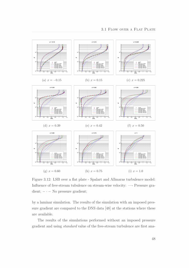
3.1 Flow over a Flat Plate
U/U∞
Z
0 0.2 0.4 0.6 0.8 1 1.2 1.410•4
10•3
10•2
LaminarDNSFixed Transit. • NOPGFixed Transit. • PGFree Transit. • NOPGFree Transit. • PG•1e•1Free Transit. • PG•1e•15Free Transit. • PG•1e•30
x = • 0.15
(a) x = −0.15
U/U∞
Z
0 0.2 0.4 0.6 0.8 1 1.2 1.410•4
10•3
10•2
LaminarDNSFixed Transit. • NOPGFixed Transit. • PGFree Transit. • NOPGFree Transit. • PG•1e•1Free Transit. • PG•1e•15Free Transit. • PG•1e•30
x = 0.15
(b) x = 0.15
U/U∞
Z
0 0.2 0.4 0.6 0.8 1 1.2 1.410•4
10•3
10•2
LaminarDNSFixed Transit. • NOPGFixed Transit. • PGFree Transit. • NOPGFree Transit. • PG•1e•1Free Transit. • PG•1e•15Free Transit. • PG•1e•30
x = 0.225
(c) x = 0.225
U/U∞
Z
0 0.2 0.4 0.6 0.8 1 1.2 1.410•4
10•3
10•2
LaminarDNSFixed Transit. • NOPGFixed Transit. • PGFree Transit. • NOPGFree Transit. • PG•1e•1Free Transit. • PG•1e•15Free Transit. • PG•1e•30
x = 0.39
(d) x = 0.39
U/U∞
Z
0 0.2 0.4 0.6 0.8 1 1.2 1.410•4
10•3
10•2
LaminarDNSFixed Transit. • NOPGFixed Transit. • PGFree Transit. • NOPGFree Transit. • PG•1e•1Free Transit. • PG•1e•15Free Transit. • PG•1e•30
x = 0.42
(e) x = 0.42
U/U∞
Z0 0.2 0.4 0.6 0.8 1 1.2 1.4
10•4
10•3
10•2
LaminarFixed Transit. • NOPGFixed Transit. • PGFree Transit. • NOPGFree Transit. • PG•1e•1Free Transit. • PG•1e•15Free Transit. • PG•1e•30
x = 0.50
(f) x = 0.50
U/U∞
Z
0 0.2 0.4 0.6 0.8 1 1.2 1.410•4
10•3
10•2
LaminarFixed Transit. • NOPGFixed Transit. • PGFree Transit. • NOPGFree Transit. • PG•1e•1Free Transit. • PG•1e•15Free Transit. • PG•1e•30
x = 0.60
(g) x = 0.60
U/U∞
Z
0 0.2 0.4 0.6 0.8 1 1.2 1.410•4
10•3
10•2
LaminarFixed Transit. • NOPGFixed Transit. • PGFree Transit. • NOPGFree Transit. • PG•1e•1Free Transit. • PG•1e•15Free Transit. • PG•1e•30
x = 0.75
(h) x = 0.75
U/U∞
Z
0 0.2 0.4 0.6 0.8 1 1.2 1.410•4
10•3
10•2
LaminarFixed Transit. • NOPGFixed Transit. • PGFree Transit. • NOPGFree Transit. • PG•1e•1Free Transit. • PG•1e•15Free Transit. • PG•1e•30
x = 1
(i) x = 1.0
Figure 3.12: LSB over a flat plate - Spalart and Allmaras turbulence model:
Influence of free-stream tubulence on stream-wise velocity: —- Pressure gra-
dient; − · − No pressure gradient;
by a laminar simulation. The results of the simulation with an imposed pres-
sure gradient are compared to the DNS data [48] at the stations where these
are available.
The results of the simulations performed without an imposed pressure
gradient and using standard value of the free-stream turbulence are first ana-
48

3.1 Flow over a Flat Plate
lyzed. Both the Spalart-Allmaras and the κ-ω SST turbulence models return
the same kind of results. The flow obtained in case of prescribed transition
location (at x = 0.42) remains in the laminar regime up to the transition
point. In fact, it is possible to note from both figure 3.11 and 3.12, how
the velocity profiles (black dash-dotted curves) compare with the laminar
solution (square symbols) very well. A turbulent flow develops only down-
stream the transition location. Instead in case of simulation without fixing
the transtion location, the velocity profiles (green dash-dotted curves) do not
follow the laminar solution (square symbol) showing a logarithmic turbulent
region already at x = 0.15.
The simulations with an imposed pressure gradient have been performed
by prescribing the transition location and by assuming the flow turbulent
everywhere with decreasing values of the free-stream turbulence.
Different solutions corresponding to the free-stream ratio µt
µhave been
computed by applying the κ-ω SST model as shown in figure 3.11. The results
obtained by imposing the transition (black solid curves) reproduce the DNS
data very well. At the first station (figure 3.11a), all the velocity profiles
achieved without fixing the transition location (coloured solid curves) follow
the DNS data. The situation changes as the flow develops along the flat plate.
Only the results achieved by using µt
µ|∞ = 1×10⁻⁹ (red solid curve) follow the
DNS data at x = 0.15 and provide a separation at x = 0.225. Downstream
the separation point, the velocity obtained by prescribing the transiton is
still in good agreement with the DNS data. Instead the simulation withµt
µ|∞ = 1× 10⁻⁹ shows a velocity with some disagreement and provides a re-
attachment anticipated with respect to the computation with the transition
point fixed. The other simulations return a flow that develops a turbulent
region upstream of the transition location and do not show any separation.
The results achieved by the Spalart-Allmaras turbulence model are re-
ported in figure 3.12. The solution with the pressure gradient and fully
turbulent conditions are obtained with decreasing value of the free-strem
ratio νν. The velocity corresponding to the value ν
ν|∞ = 0.1 shows a tur-
bulent flow and does not return a separation. The solution obtained with
49
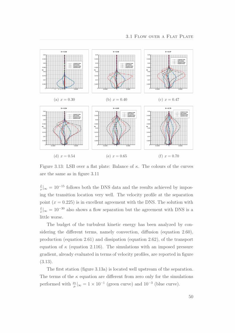
3.1 Flow over a Flat Plate
Z
•0.0005 0 0.00050
0.005
0.01
0.015
0.02
0.025
0.03
0.035
0.04
CONVECTIONDIFFUSIONPRODUCTIONDISSIPATION
X = 0.30
(a) x = 0.30
Z
•0.0005 0 0.00050
0.005
0.01
0.015
0.02
0.025
0.03
0.035
0.04
CONVECTIONDIFFUSIONPRODUCTIONDISSIPATION
X = 0.40
(b) x = 0.40
Z
•0.0005 0 0.00050
0.005
0.01
0.015
0.02
0.025
0.03
0.035
0.04
CONVECTIONDIFFUSIONPRODUCTIONDISSIPATION
X = 0.47
(c) x = 0.47
Z
•0.0005 0 0.00050
0.005
0.01
0.015
0.02
0.025
0.03
0.035
0.04
CONVECTIONDIFFUSIONPRODUCTIONDISSIPATION
X = 0.54
(d) x = 0.54
Z
•0.0005 0 0.00050
0.005
0.01
0.015
0.02
0.025
0.03
0.035
0.04CONVECTIONDIFFUSIONPRODUCTIONDISSIPATION
X = 0.65
(e) x = 0.65
Z•0.0005 0 0.0005
0
0.005
0.01
0.015
0.02
0.025
0.03
0.035
0.04 CONVECTIONDIFFUSIONPRODUCTIONDISSIPATION
X = 0.70
(f) x = 0.70
Figure 3.13: LSB over a flat plate: Balance of κ. The colours of the curves
are the same as in figure 3.11
νν|∞ = 10−15 follows both the DNS data and the results achieved by impos-
ing the transition location very well. The velocity profile at the separation
point (x = 0.225) is in excellent agreement with the DNS. The solution withνν|∞ = 10−30 also shows a flow separation but the agreement with DNS is a
little worse.
The budget of the turbulent kinetic energy has been analyzed by con-
sidering the different terms, namely convection, diffusion (equation 2.60),
production (equation 2.61) and dissipation (equation 2.62), of the transport
equation of κ (equation 2.116). The simulations with an imposed pressure
gradient, already evaluated in terms of velocity profiles, are reported in figure
(3.13).
The first station (figure 3.13a) is located well upstream of the separation.
The terms of the κ equation are different from zero only for the simulations
performed with µt
µ|∞ = 1 × 10⁻¹ (green curve) and 10−3 (blue curve).
50

3.1 Flow over a Flat Plate
At x = 0.40 (figure 3.13b), the flow is approaching the transition (oc-
curing at x = 0.42). The terms provided by the computation with µt
µ|∞ =
1×10⁻⁹ become active and result larger than the ones provided by the other
two simulations performed without imposing the transition location. At the
station x = 0.47 (figure 3.13c), located downstream the transition point, also
the simulation performed with the transition prescribed (black curve) has all
the terms that contribute to the balance of κ. The results of the computa-
tions with µt
µ|∞ = 1 × 10⁻¹ and 10−3 are quite similar. The production and
dissipation obtained by fixing the transtion point become larger (in absolute
value) than all the other simulations and resemble the ones obtained withµt
µ|∞ = 1 × 10⁻⁹. The convection achieved by fixing the transition is similar
to the convection obtained with µt
µ|∞ = 1 × 10⁻⁹ in the inner part of the
boundary layer while becomes larger in the outer part. Instead, the diffu-
sion, both molecular and turbulent, resulting by the two simulation is very
similar.
In all the simulations, the diffusion is positive close to the wall and in the
last part of the boundary layer, while gives a negative contribution in the
central region. Convection is first positive and then becomes negative. Pro-
duction and dissipation are the terms that mainly contribute to the budget
of κ in the outer part of the boundary layer.
The results reported in the figures (3.11)-(3.13) show that in case of sim-
ulations with the transtion point prescribed, the flow remain in the laminar
regime upstream of the transition and that the terms of the transport equa-
tion of κ are activated only downstream the transition. The use of low values
of free-stream turbulence do not reproduce exactly the results achieved by fix-
ing the transition a priori but allows to obtain a solution that resembles quite
well a laminar flow upstream the actual transition. The Spalart-Allmaras has
provided results better than the κ-ω SST turbulence model.
The analysis of the budget of the turbulent kinetic energy at different
stations along the flat plate, has highlighted that the production of κ re-
sulting from the computation with low value of µt
µ|∞ becomes different from
zero a little upstream of the transition point. However the terms concurring
51

3.1 Flow over a Flat Plate
ReX
Cf
104 105 106
0.002
0.004
0.006
0.008
0.01
0.664*Rex•0.50
0.0592*Rex•0.20
1.341e•91e•151e•201e•30
Spalart•Allmaras
(a) Spalart-Allmaras
ReX
Cf
104 105 106
0.002
0.004
0.006
0.008
0.01
0.664*Rex•0.50
0.0592*Rex•0.20
1e•31e•91e•201e•30
κ•ω SST Turbulence Model
(b) κ-ω SST
Figure 3.14: Incompressible flow over a flat plate : Friction Coefficient. Effect
of lowering free-stream values of the turbulent variables; νν
(a); µt
µ(b)
to the budget of κ obtained by fixing the transtion point are similar, also
from a quantitative point of view, to the ones resulting from the simulation
performed with low values of free-stream turbulence for all the length of the
flat plate.
The behaviour of the turbulence models when run with very low values of
the turbulent variables has been further investigated by simulating the flow
over a flat plate at ReL = 1 × 10⁶.
A sort of numerical transition is shown. The friction coefficient is reported
in figure 3.14 toghether with the Blasius and the Prandtl curves [50]. The
Spalart-Allmaras model provides a jump from the laminar to the Prandtl
curve if the ratio ( νν)|∞ is kept low. This jump occurs at higher Reynolds
number as this ratio decreases. A sort of convergence as the free-stream
values are lowered is instead shown by the κ-ω SST model. The jump occurs
at a Reynolds number of about 1×10⁵. Both the models slightly underpredict
the Prandtl curve.
52

3.2 Flow around the SD 7003 Airfoil
3.2 Flow around the SD 7003 Airfoil
The laminar separation bubble over an airfoil has been analyzed. The incom-
pressible flow around the Selig-Donovan (SD) 7003 airfoil presents interesting
characteristics. At Reynolds number 6×10⁴ a bubble is formed on the upper
surface of the airfoil. The bubble is located in the rear zone close to the
trailing edge at low incidences, and moves upstream as the angle of attack
increases.
This is a widely-used test case for which experimental [49] and numerical
[18] data are available in literature. RANS and large eddy simulations at
several angles of incidence have been performed. The main aim is to analyze
the limits of the RANS methods by comparison with LES results.
A first set of results have been obtained by running the turbulence models
without specifying the transition points (flows is assumed turbulent every-
where). Laminar separation bubbles are detected if the turbulence models
are robust enough to be run with very low values of free-stream turbulence.
An other set of results are presented by running the turbulence model with
the transition location fixed at a point retrieved by the LES data.
The NEC SX6 machine has been used. A RANS simulation has been
obtained in about 8 hours while a LES solution has required about 30 days
CPU of a single processor.
3.2.1 Grid Assessment
A C-topology grid with 768 (96 in the wake) cells in the stream-wise and 176
cells in the normal-wise direction has been employed. The far-field bound-
aries are located at a distance of 30 chords from the airfoil. The height of
the wall-adjacent cells in viscous coordinates remains less than one for all the
upper surface of the airfoil, as shown in Fig. 3.15a where the y+ obtained by
the RANS with the κ − ω SST turbulence model is presented.
The 2D mesh of the RANS computations has also been employed for
the large eddy simulations. The only difference is that the branch-cut line is
adapted with the angle of attack to follow the wake. The span-wise extension
53

3.2 Flow around the SD 7003 Airfoil
X/C
∆y+
0.2 0.4 0.6 0.80
0.2
0.4
0.6
0.8
1
SD 7003 AirfoilReynolds number = 6.0x10⁴
RANS at α=6
(a) RANS
X/C
∆y+
∆x+,∆z+
0.2 0.4 0.6 0.80
0.2
0.4
0.6
0.8
1
0
2
4
6
8
10
12
14
16
18
20
∆y+∆z+∆x+
SD 7003 ArifoilReynolds number = 6.0 x 10⁴
Large Eddy Simulation at α=6
(b) LES
Figure 3.15: SD7003 Airfoil, Re = 6×10⁴, α = 6. Size of wall-adjacent grid
cells; −−: ∆y+, —: ∆z+, − · −: ∆x+
X/C
CP
0 0.2 0.4 0.6 0.8 1
•1.5
•1
•0.5
0
0.5
1
96 x 22192 x 44384 x 88768 x 1761536 x 352
(a) Pressure Coefficient
X/C
CF
0.2 0.4 0.6 0.8•0.004
•0.002
0
0.002
0.004
0.006
0.008
0.01
96 x 22192 x 44384 x 88768 x 1761536 x 352
(b) Friction Coefficient
Figure 3.16: SD7003 Airfoil, Re = 6.0×10⁴, α = 4. Grid convergence study
of the RANS solution
of the computational domain is 0.1×c with 48 cells. The wall-adjacent cells in
viscous coordinates have size less than one in the wall-normal direction, and
order of magnitude 10 in the stream and span-wise directions (Fig. 3.15b).
A grid convergence study (Fig. 3.16) has been performed for the RANS
solutions. Five levels of the computational mesh are considered. The two
54
3.2 Flow around the SD 7003 Airfoil
coarsest grids provide a separated flow. The flow re-attaches in the three
finer meshes with the re-attachment point between the 50% and 60% of the
chord. Differences between the 4th and 5th level of the grid are negligible for
both pressure (Fig. 3.16a) and friction coefficient (Fig. 3.16b). Therefore 4
levels of the grid are considered sufficiently accurate, and have been used in
the simulations discussed in the following sections.
3.2.2 Turbulence Models Assessment
RANS simulations of the flow at Re = 6 × 10⁴ and α = 4 around the SD
7003 airfoil have been performed by using several turbulence models. The
transition is not specified and the flow is assumed to be turbulent everywhere.
The Spalart-Allmaras [5], the κ−ε Myong-Kasagi [51], and the κ−ω Wilcox
[30], TNT [34], BSL, and SST [6] are the models tested. The value of the
free-stream turbulence is decreased provided that a converged solution can
be achieved. The large eddy simulations by Galbraith and Visbal [18] are
taken as reference data.
All the RANS results show a different solution in terms of pressure (Fig.
3.17a and c) and friction coefficient (Fig. 3.17b and d) with respect to LES.
The differences are better appreciated looking at the friction coefficient on
the upper surface. The κ− ε does not provide a flow separation. A flow with
a separation and a re-attachment is returned by all the other turbulence
models. The κ − ω SST and the Spalart-Allmaras provide a qualitatively
good result. The CF presents the same shape as LES data although the
re-attachment point is anticipated. The κ−ω BSL yields a result in between
the TNT and SST models.
3.2.3 Results by κ-ω SST turbulence model
In the following, the focus is placed on the κ-ω SST turbulence model. This
model is very popular and reliable for transonic high-Reynolds number flows,
as pointed out by different authors (cfr. Catalano and Amato [21, 22], Bezard
et al. [37]), but its effectiveness for low-Reynolds number flows is doubtful
55

3.2 Flow around the SD 7003 Airfoil
X/C
CP
0 0.2 0.4 0.6 0.8 1
•1.5
•1
•0.5
0
0.5
1
ILES (Galbraith and Visbal)Spalart•Allmarasκ −ε MKκ −ω Wilcox
(a) Pressure Coefficient
X/C
CF
0.2 0.4 0.6 0.8•0.01
0
0.01
0.02
0.03
ILES (Galbraith and Visbal)Spalart•Allmarasκ −ε MKκ −ω Wilcox
(b) Friction Coefficient
X/C
CP
0 0.2 0.4 0.6 0.8 1
•1.5
•1
•0.5
0
0.5
1
ILES (Galbraith and Visbal)κ −ω TNTκ −ω SSTκ −ω BSL
(c) Pressure Coefficient
X/C
CF
0.2 0.4 0.6 0.8•0.01
0
0.01
0.02
0.03
ILES (Galbraith and Visbal)κ −ω TNTκ −ω SSTκ −ω BSL
(d) Friction Coefficient
Figure 3.17: SD7003 Airfoil, Re = 6.0 × 10⁴, α = 4. Results by several
turbulence models
(Catalano and Tognaccini [46], Rumsey and Spalart [19]).
3.2.3.1 Main Characteristics of the Flow
The model is applied at several angles of incidence with µt
µ|∞ = 1×10⁻⁹ and
√κ
U|∞ = 10−6. The friction and pressure coefficient as function of the angle
of attack are presented in Fig. 3.18. A bubble is predicted in the trailing
edge zone of the airfoil at α = 0 and then moves towards the leading edge
56

3.2 Flow around the SD 7003 Airfoil
X/C
CP
0 0.2 0.4 0.6 0.8 1
•3
•2.5
•2
•1.5
•1
•0.5
0
0.5
1
α=0α=2α=4α=6α=8
(a) Pressure Coefficient
X/C
CF
0.2 0.4 0.6 0.8•0.02
•0.01
0
0.01
0.02
0.03
α=0α=2α=4α=6α=8
(b) Friction Coefficient
Figure 3.18: SD7003 Airfoil, Re = 6.0×10⁴. RANS, κ−ω SST with laminar-
turbulent transition not prescribed: CP and CF over the airfoil at different
angles of attack.
as α increases.
The evolution of the laminar bubble as a function of the angle of incidence
is also presented in figure 3.19. The contour map of the turbulent kinetic
energy shows that the turbulence is formed inside the bubble. The airfoil
is stalled at α = 10. This is likely a combined stall due to the interaction
between the laminar bubble in the leading edge zone and a separated region
appearing in the rear part of the airfoil at the high incidences.
3.2.3.2 Large Eddy Simulations
Large eddy simulations of the flow around the SD 7003 airfoil have been
performed at several incidences. A RANS flow field has been used as initial
solution and the simulation has been advanced in time with a time step
t = 1.5 × 10⁻⁴. Figure 3.20 shows the three-dimensional turbulent flow
that develops in the rear part of the airfoil downsteam the separation. The
time history of the lift and drag coefficients for the case at α = 4 is shown
in figure 3.21a and 3.21b. The large eddy simulation has been advanced in
time for more than 20 characteristic times, and then the results have been
57

3.2 Flow around the SD 7003 Airfoil
X
Z
0 0.2 0.4 0.6 0.8 1•0.25
•0.2
•0.15
•0.1
•0.05
0
0.05
0.1
0.15
0.2
0.25
0.0E+00 6.3E•03 1.3E•02 1.9E•02 2.5E•02 3.2E•02 3.8E•02 4.4E•02 5.1E•02 5.7E•02κ/V
∞
2
(a) α = 0
X
Z
0 0.2 0.4 0.6 0.8 1•0.25
•0.2
•0.15
•0.1
•0.05
0
0.05
0.1
0.15
0.2
0.25
0.0E+00 6.3E•03 1.3E•02 1.9E•02 2.5E•02 3.2E•02 3.8E•02 4.4E•02 5.1E•02 5.7E•02κ/V
∞
2
(b) α = 2
X
Z
0 0.2 0.4 0.6 0.8 1•0.25
•0.2
•0.15
•0.1
•0.05
0
0.05
0.1
0.15
0.2
0.25
0.0E+00 6.3E•03 1.3E•02 1.9E•02 2.5E•02 3.2E•02 3.8E•02 4.4E•02 5.1E•02 5.7E•02κ/V
∞
2
(c) α = 4
X
Z
0 0.2 0.4 0.6 0.8 1•0.25
•0.2
•0.15
•0.1
•0.05
0
0.05
0.1
0.15
0.2
0.25
0.0E+00 6.3E•03 1.3E•02 1.9E•02 2.5E•02 3.2E•02 3.8E•02 4.4E•02 5.1E•02 5.7E•02κ/V
∞
2
(d) α = 6
X
Z
0 0.2 0.4 0.6 0.8 1•0.25
•0.2
•0.15
•0.1
•0.05
0
0.05
0.1
0.15
0.2
0.25
0.0E+00 6.3E•03 1.3E•02 1.9E•02 2.5E•02 3.2E•02 3.8E•02 4.4E•02 5.1E•02 5.7E•02κ/V
∞
2
(e) α = 8
X
Z
0 0.2 0.4 0.6 0.8 1•0.25
•0.2
•0.15
•0.1
•0.05
0
0.05
0.1
0.15
0.2
0.25
0.0E+00 6.3E•03 1.3E•02 1.9E•02 2.5E•02 3.2E•02 3.8E•02 4.4E•02 5.1E•02 5.7E•02κ/V
∞
2
(f) α = 10
Figure 3.19: SD7003 Airfoil : RANS. Evolution of the bubble with the angle
of attack. Contour map of k is shown
X/C
Z/C
0 0.5 1
•0.5
0
0.5•0.07 •0.06 •0.05 •0.04 •0.02 •0.01 0.00 0.02 0.03 0.04 0.05 0.06
(a) α = 0
X/C
Z/C
0 0.5 1
•0.5
0
0.5•0.13 •0.10 •0.08 •0.06 •0.04 •0.01 0.01 0.04 0.06 0.08 0.10 0.13
(b) α = 4
Figure 3.20: SD7003 Airfoil : Large Eddy Simulation. Contour map of the
instantaneous spanwise-averaged WV∞
58

3.2 Flow around the SD 7003 Airfoil
t*U∞/c
CL
0 5 10 15 200.45
0.5
0.55
0.6
0.65
0.7
(a) Lift Coefficient
t*U∞/c
CD
0 2 4 6 8 10 12 14 16 18 20 220.015
0.02
0.025
0.03
0.035
(b) Drag Coefficient
Figure 3.21: SD7003 Airfoil : Large Eddy Simulation at α = 4. Time
history of the aerodynamic coefficients.
x/c
CP
0 0.2 0.4 0.6 0.8 1
•1.5
•1
•0.5
0
0.5
1
T0 = 17.75T=T0+3.00T=T0+5.40
(a) Pressure Coefficient
x/c
CF
0.1 0.2 0.3 0.4 0.5 0.6 0.7 0.8 0.9•0.02
•0.01
0
0.01
0.02
0.03
T0 = 17.75T=T0+3.00T=T0+5.40
(b) Friction Coefficient
Figure 3.22: SD7003 Airfoil : Large Eddy Simulation at α = 4. Time
averaging of pressure and friction coefficient.
time-avergaed. Figure 3.22 shows the time-averaging process of the pressure
and friction coefficients. The solution achieved at a certain instant shows a
well-defined separation point, and a series of separation and re-attachment
points downstream the dear-air region. The bubble with one separation and
one re-attachment point is obtained only when the solution is averaged in
59

3.2 Flow around the SD 7003 Airfoil
X/C
CP
0 0.2 0.4 0.6 0.8 1
•1.5
•1
•0.5
0
0.5
1
ILES (Galbraith and Visbal)LES (Catalano and Tognaccini)κ−ωSST
(a) Pressure Coefficient
X/C
CF
0.1 0.2 0.3 0.4 0.5 0.6 0.7 0.8 0.9•0.01
0
0.01
0.02
0.03
ILES (Galbraith and Visbal)LES (Catalano and Tognaccini)κ−ω SST
(b) Friction Coefficient
Figure 3.23: SD7003 Airfoil, Re = 6.0 × 10⁴, α = 4. Pressure and friction
coefficient; ©: ILES (Galbraith and Visbal), : present LES , —–: RANS
κ − ω SST with laminar-turbulent transition not prescribed.
time for a significant period.
3.2.3.3 RANS-LES Comparison
The RANS solutions are compared in terms of pressure and friction coeffi-
cients to the large eddy simulations data by the authors and Galbraith and
Visbal [18] in the figures 3.23, 3.24, and 3.25 at α = 4, 6, and 8 respec-
tively. The pressure recovery in the zone of the bubble is much stronger in
LES than in RANS data, as can be seen in all the CP and CF plots. The
separation point is well predicted in the RANS simulations, but the RANS
provide a re-attachment anticipated with respect to LES results. Down-
stream the flow re-attachment, the RANS recover to a level of pressure lower
than LES.
The present large eddy simulations are in excellent agreement with the
ILES by Galbraith and Visbal [18] at α = 4 and 8. Some discrepancies can
be noted for the flow at α = 6.
The RANS simulations have been performed without an a priori knowl-
edge of the laminar-turbulent transition. It has been shown that a laminar
60
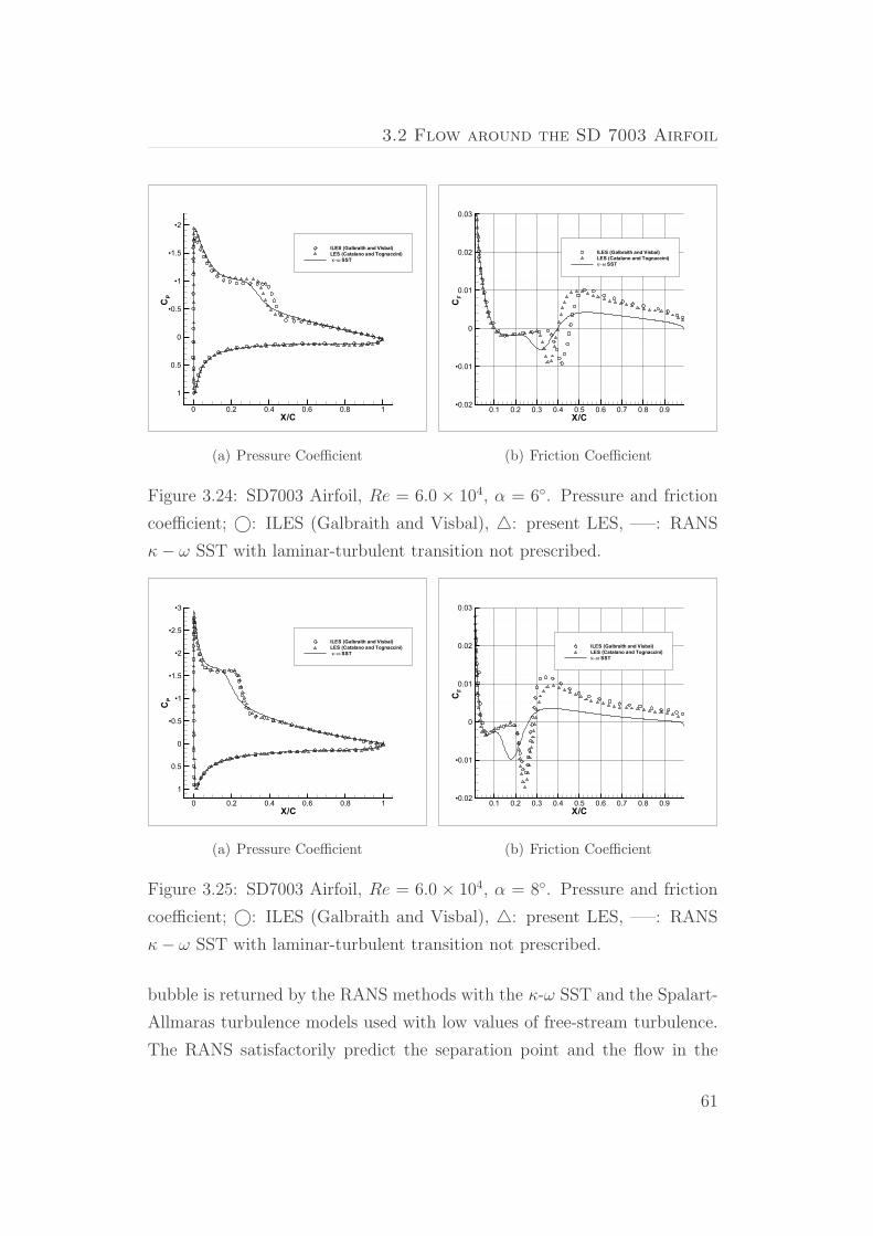
3.2 Flow around the SD 7003 Airfoil
X/C
CP
0 0.2 0.4 0.6 0.8 1
•2
•1.5
•1
•0.5
0
0.5
1
ILES (Galbraith and Visbal)LES (Catalano and Tognaccini)κ−ω SST
(a) Pressure Coefficient
X/C
CF
0.1 0.2 0.3 0.4 0.5 0.6 0.7 0.8 0.9•0.02
•0.01
0
0.01
0.02
0.03
ILES (Galbraith and Visbal)LES (Catalano and Tognaccini)κ−ω SST
(b) Friction Coefficient
Figure 3.24: SD7003 Airfoil, Re = 6.0 × 10⁴, α = 6. Pressure and friction
coefficient; ©: ILES (Galbraith and Visbal), : present LES, —–: RANS
κ − ω SST with laminar-turbulent transition not prescribed.
X/C
CP
0 0.2 0.4 0.6 0.8 1
•3
•2.5
•2
•1.5
•1
•0.5
0
0.5
1
ILES (Galbraith and Visbal)LES (Catalano and Tognaccini)κ−ω SST
(a) Pressure Coefficient
X/C
CF
0.1 0.2 0.3 0.4 0.5 0.6 0.7 0.8 0.9•0.02
•0.01
0
0.01
0.02
0.03
ILES (Galbraith and Visbal)LES (Catalano and Tognaccini)κ−ω SST
(b) Friction Coefficient
Figure 3.25: SD7003 Airfoil, Re = 6.0 × 10⁴, α = 8. Pressure and friction
coefficient; ©: ILES (Galbraith and Visbal), : present LES, —–: RANS
κ − ω SST with laminar-turbulent transition not prescribed.
bubble is returned by the RANS methods with the κ-ω SST and the Spalart-
Allmaras turbulence models used with low values of free-stream turbulence.
The RANS satisfactorily predict the separation point and the flow in the
61

3.2 Flow around the SD 7003 Airfoil
dead air region. A shorter bubble length and a weaker pressure recovery is
provided by RANS with respect to LES.
3.2.3.4 Flow at α = 4
A comparison between the bubble returned by the RANS and LES methods
at α = 4 is presented in Fig. 3.26. The stream-lines with the contour map
of the axial velocity and the pressure coefficient in the zone of the bubble
are presented. The LES results are averaged along the span direction and in
time for about 8 characteristic times. The structure of a laminar separation
bubble [45] (Fig. 3.1) can be recognized. A dead-air region is returned
by both RANS and LES. The zone of reverse flow lying below the dividing
stream-line is characterized by very low value of the U/U∞ for a large extent
of the bubble. The pressure recovery occurs in the zone where stronger
negative velocities are attained by the flow. A reverse flow vortex is seen in
the LES results while a more spread region of pressure recovery is returned
by the RANS method.
The flow has also been computed by imposing the transition location at
xtr/c = 0.53, a value retrieved by LES data. The results are expected to
improve when the turbulence models are run with the transition point fixed
at a reasonable location. This is shown in literature and has been verified
by the author [46] for the flow over a flat plate with an imposed pressure
gradient [48, 47].
The κ-ω BSL turbulence model [6] is also applied. The comparison be-
tween the friction and pressure coefficient achieved by applying the two mod-
els without and with the transition location fixed a priori is shown in Fig.
3.27. The two κ-ω models provide a similar result when used without fixing
the transition location. On the contrary, a large difference occurs when the
simulations are performed with the transition point fixed a priori. The κ-ω
BSL provides a pressure recovery closer to the LES data. On the contrary,
the κ-ω SST produces a too low turbulence and the flow does not reattach.
The Shear Stress Transport formulation should allow for a better charac-
62

3.2 Flow around the SD 7003 Airfoil
•0.05
0.00
0.00
0.06
0.11
0.16
0.16
0.21
0.21
0.270.32
0.37
0.37
0.420.47
0.47
0.53
0.530.58
0.58
0.63
0.63
0.68 0.730.79
0.79
0.84
0.84
0.89 0.89
0.94
1.00
1.00
1.05
1.10
1.10
X/C
Z/C
0.2 0.3 0.4 0.5 0.6
0.04
0.05
0.06
0.07
0.08•0.10 0.00 0.11 0.21 0.32 0.42 0.53 0.63 0.73 0.84 0.94 1.05
U/V∞
(a) RANS, κ − ω SST with laminar-
turbulent transition not prescribed: Stream-
lines and contour map of the axial velocity
•0.10
0.000.11 0.11
0.210.320.42
0.53
0.53
0.63
0.63
0.73
0.730.84
0.84
0.941.05
X/C
Z/C
0.2 0.3 0.4 0.5 0.6
0.04
0.05
0.06
0.07
0.08•0.10 0.00 0.11 0.21 0.32 0.42 0.53 0.63 0.73 0.84 0.94 1.05
U/V∞
(b) LES : Stream-lines and contour map of
the axial velocity
X/C
CP
0.2 0.3 0.4 0.5 0.6
•1
•0.5
0
0.5
(c) RANS, κ−ω SST with laminar-turbulent
transition not prescribed: Pressure Coeffi-
cient
X/C
CP
0.2 0.3 0.4 0.5 0.6
•1
•0.5
0
0.5
(d) LES : Pressure Coefficient
Figure 3.26: SD7003 Airfoil, Re = 6.0 × 10⁴, α = 4. Structure of the
Laminar bubble.
terization of flow separations and re-attachments. This has been verified for
typical transonic benchmarks, but, as shown by the present results, at low
Reynolds number seems to provide results even worse than the baseline BSL
model. This confirms the analysis performed by Rumsey and Spalart [19] on
63

3.2 Flow around the SD 7003 Airfoil
X/C
CP
0 0.2 0.4 0.6 0.8 1
•1.5
•1
•0.5
0
0.5
1
ILES (Galbraith and Visbal)LES (Catalano and Tognaccini)κ−ω BSL • No Trans.κ−ω SST • No Trans.κ−ω BSL • Trans. at X/C=0.53κ−ω SST • Trans. at X/C=0.53
(a) Pressure Coefficient
X/C
CF
0.2 0.4 0.6 0.8•0.01
0
0.01
0.02
0.03
ILES (Galbraith and Visbal)LES (Catalano and Tognaccini)κ−ω BSL • No Trans.κ−ω SST • No Trans.κ−ω BSL • Trans at X/C=0.53κ−ω SST • Trans at X/C=0.53
(b) Friction Coefficient
Figure 3.27: SD7003 Airfoil, Re = 6.0 × 10⁴, α = 4, Pressure and friction
coefficient; ©: ILES (Galbraith and Visbal), : present LES, − · −: RANS
κ − ω BSL, − − −: RANS κ − ω SST; red lines: transition not specified;
black lines: transition fixed (xtr/c = 0.53).
the poor accuracy of the κ-ω SST for low-Reynolds number flows.
64

Chapter 4
Turbulence Modelling
This chapter is devoted to the derivation and description of the κ-ω SST-LR
turbulence model. This consinst in some modifications apported to the κ-ω
SST model.
First the equations of the κ-ω SST are re-called, and some results achieved
by the model are critically revised. Some features of the model are analyzed
at decreasing Reynolds numbers. The implementation of the model will be
shown to become critical as the Reynolds number decreases [52].
Modifications of the κ-ω SST model are proposed and applied to flows at
low as well as high Reynolds number. The results obtained at low Reynolds
number are noticeably improved by this modified model, and the characterit-
ics at high Reynolds number are preserved [53].
4.1 Analysis of the the κ-ω SST model
The SST formulation accounts for computing the shear stress as
τ = a1κ (4.1)
in a suitable part of the boundary layer. This is obtained by considering that
for boundary layer flows
τ ≈ µtΩ (4.2)
where Ω is the vorticity. The eddy viscosity is computed by making use of a
switching between the specific turbulent dissipation ω and Ω
µt =ρa1κ
MAX(a1ω, F2Ω)(4.3)
65
4.1 Analysis of the the κ-ω SST model
where a1 = 0.3 and F2 is a blending function computed as
F2 = tanh(Arg22) (4.4)
where
Arg2 = max(Arg21, Arg22) (4.5)
with
Arg21 =2√
κ
β∗ωy, Arg22 =
500µ
ωy2(4.6)
The function F2 has been designed to be 1 close to solid boundaries and
zero in the upper part of the logarithmic region of a turbulent boundary
layer where Eq. (4.1) should be recovered. The presence and extension of
the logarithmic region depends on the Reynolds number. In particular, its
extension increases as the Reynolds number increases.
The flow around the SD 7003 airfoil has been analyzed at α = 0 and
Reynolds numbers 6.0×10⁶, 6.0×10⁵, and 6.0×10⁴. The turbulent intensity
has been set to 0.1% and the ratio between the free-stream turbulent and
molecular viscosity to 0.1. This numerical setting allows to concentrate on
the effect of the Reynolds number on the boundary layer because laminar
separation bubbles are not returned by any of the simulations. The spacing
of the first layers of cells has been adapted to the Reynolds number in such
a way to obtain a y+ of order of magnitude one for all the simulations.
The stream-wise velocity profiles at three stations along the upper surface
of the SD 7003 airfoil are shown in the Fig. 4.1. The curves u+ = y+
corresponding to the viscous sub-layer, and u+ = uuτ
= 1κa
log y+ + B (with
κa = 0.41, and B = 5.0) corresponding to the log-layer are also shown. The
flow at the highest Reynolds number (Fig. 4.1a, Fig. 4.1b, and Fig. 4.1c)
presents a well-defined logarithmic region in a large extent of the boundary
layer. At Reynolds number 6.0 × 10⁵ (Fig. 4.1d, Fig. 4.1e, and Fig. 4.1f),
the log-layer still exists, but both the thickness of the boundary layer and
the extension of the logarithmic region are reduced of an order of magnitude.
The numerical results follow fairly well either the linear and the log law of the
velocity at both the Reynolds numbers. On the contrary, at Re = 6.0 × 10⁴
66

4.1 Analysis of the the κ-ω SST model
y+
U+
100 101 102 103 1040
5
10
15
20
25
30
X/C = 0.40
U+=y+
U+=1/κaLog(y+)+B
(a) x/c = 0.40
y+
U+
100 101 102 103 1040
5
10
15
20
25
30
X/C = 0.60
U+=y+
U+=1/κaLog(y+)+B
(b) x/c = 0.60
y+
U+
100 101 102 103 1040
5
10
15
20
25
30
X/C = 0.90
U+=y+
U+=1/κaLog(y+)+B
(c) x/c = 0.90
Reynolds number = 6.0 × 10⁶
y+
U+
100 101 102 1030
5
10
15
20
25
X/C = 0.40
U+=y+
U+=1/κaLog(y+)+B
(d) x/c = 0.40
y+
U+
100 101 102 1030
5
10
15
20
25
X/C = 0.60
U+=y+
U+=1/κaLog(y+)+B
(e) x/c = 0.60
y+
U+
100 101 102 1030
5
10
15
20
25
30
X/C = 0.90
U+=y+
U+=1/κaLog(y+)+B
(f) x/c = 0.90
Reynolds number = 6.0 × 10⁵
y+
U+
100 101 1020
5
10
15
20
25
30
35
X/C = 0.40
U+=y+
U+=1/κaLog(y+)+B
(g) x/c = 0.40
y+
U+
100 101 1020
5
10
15
20
25
30
35
40
45
50
55
X/C = 0.60
U+=y+
U+=1/κaLog(y+)+B
(h) x/c = 0.60
y+
U+
100 101 1020
10
20
30
40
50
60
X/C = 0.90
U+=y+
U+=1/κaLog(y+)+B
(i) x/c = 0.90
Reynolds number = 6.0 × 10⁴
Figure 4.1: κ − ω SST. Velocity profiles on the SD 7003 Airfoil at three
Reynolds numbers, α = 0
(Fig. 4.1g, Fig. 4.1h, and Fig. 4.1i), the logarithmic region is totally absent
in the calculations. The stream-wise velocity has a linear behaviour with y+
for most of the boundary layer but does not follow the viscous law u+ =
y+. The velocity reaches higher values with respect to the other two lower
67

4.1 Analysis of the the κ-ω SST model
Reynolds numbers.
The eddy viscosity is shown in Fig. 4.2. The two quantities a1ω and
F2Ω at denominator of Eq. (4.3) are also reported as symbols, and their
maximum as a solid line. Similar results are obtained at Reynolds numbers
6.0 × 10⁶ (Fig. 4.2a, Fig. 4.2b, and Fig. 4.2c) and 6.0 × 10⁵ (Fig. 4.2d, Fig.
4.2e, and Fig. 4.2f). The eddy viscosity is computed as µt = ρκ/ω in most
of the boundary layer. F2Ω is greater than a1ω in a narrow region close to
the zone where µt/µ has reached its maximum and starts to decrease. In this
region, the eddy viscosity is computed as µt = a1κ/F2Ω.
At Reynolds number 6.0 × 10⁴ (Fig. 4.2g, Fig. 4.2h, and Fig. 4.2i), the
eddy viscosity µt/µ is lower than 0.01 at x/c = 0.40 and 0.1 at x/c = 0.60,
and greater than one only at the station x/c = 0.90. At this location,
F2Ω > a1ω in the region where µt/µ is maximum. The flow can be considered
turbulent only at x/c = 0.90.
The behaviour of the blending function F2 (Eq. 4.4) and its arguments
(Eq. 4.5 and Eq. 4.6) is presented in the Fig. 4.3. At Reynolds number
6.0 × 10⁶ (Fig. 4.3a, Fig. 4.3b, and Fig. 4.3c), the F2, as expected, is
computed as a function of the viscous quantity Arg22 in the sub-layer and
then as a function of the turbulent length scale Arg21 in the remaining part
of the boundary layer. It is worth noting that at the station x/c = 0.40, the
F2 presents a little jump. This can be seen also at Reynolds number 6.0×10⁵
(Fig. 4.3d, Fig. 4.3e, and Fig. 4.3f) at x/c = 0.40 and in a less pronounced
way at x/c = 0.60. This occurs in the upper part of the boundary layer when
the viscous argument Arg22 becomes greater than the turbulent argument
Arg21. At Reynolds number 6.0 × 10⁴ (Fig. 4.3g, Fig. 4.3h, and Fig. 4.3i),
the F2 shows a large oscillation. Indeed, in the outer part of the boundary
layer it again grows while it was expected to vanish in order to correctly
perform the switch in the eddy viscosity calculation.
68

4.2 The κ-ω SST-LR model
y+
µt/µ
a 1ω,F
2Ω
100 101 102 103 1040
30
60
90
120
150
100
101
102
103
µt/µa1ωF2ΩMax(a1ω,F2Ω)
X/C = 0.40
(a) x/c = 0.40
y+
µt/µ
a 1ω,F
2Ω
100 101 102 103 1040
50
100
150
200
100
101
102
103
µt/µa1ωF2ΩMax(a1ω,F2Ω)
X/C = 0.60
(b) x/c = 0.60
y+
µt/µ
a 1ω,F
2Ω
100 101 102 103 1040
50
100
150
200
250
300
350
100
101
102
103
µt/µa1ωF2ΩMax(a1ω,F2Ω)
X/C = 0.90
(c) x/c = 0.90
Reynolds number = 6.0 × 10⁶
y+
µt/µ
a 1ω,F
2Ω
100 101 102 1030
5
10
15
20
100
101
102
103
µt/µa1ωF2ΩMax(a1ω,F2Ω)
X/C = 0.40
(d) x/c = 0.40
y+
µt/µ
a 1ω,F
2Ω
100 101 102 1030
5
10
15
20
25
30
10•1
100
101
102
103
µt/µa1ωF2ΩMax(a1ω,F2Ω)
X/C = 0.60
(e) x/c = 0.60
y+
µt/µ
a 1ω,F
2Ω
100 101 102 1030
10
20
30
40
50
10•1
100
101
102
103
µt/µa1ωF2ΩMax(a1ω,F2Ω)
X/C = 0.90
(f) x/c = 0.90
Reynolds number = 6.0 × 10⁵
y+
µt/µ
a 1ω,F
2Ω
100 101 1020
0.002
0.004
0.006
0.008
0.01
10•1
100
101
102
103
µt/µa1ωF2ΩMax(a1ω,F2Ω)
X/C = 0.40
(g) x/c = 0.40
y+
µt/µ
a 1ω,F
2Ω
100 101 1020
0.02
0.04
0.06
0.08
0.1
10•1
100
101
102
103
µt/µa1ωF2ΩMax(a1ω,F2Ω)
X/C = 0.60
(h) x/c = 0.60
y+
µt/µ
a 1ω,F
2Ω
100 101 1020
1
2
3
4
10•1
100
101
102
103
µt/µa1ωF2ΩMax(a1ω,F2Ω)
X/C = 0.90
(i) x/c = 0.90
Reynolds number = 6.0 × 10⁴
Figure 4.2: κ−ω SST. Eddy viscosity profiles on the SD7003 airfoil at three
Reynolds numbers, α = 0; −·−: µt/µ, 2: a1ω, ∇: F2Ω, —–: max[a1ω, F2Ω]
4.2 The κ-ω SST-LR model
The computation of F2 in the standard SST formulation requires the calcu-
lation of the maximum between two arguments (Eq. 4.4). The first one is
69

4.2 The κ-ω SST-LR model
y+
Arg21,Arg22,Arg2
F 2
100 101 102 103 104•2
0
2
4
6
8
10
0
0.2
0.4
0.6
0.8
1
Arg21Arg22Arg2F2
X/C = 0.40
(a) x/c = 0.40
y+
Arg21,Arg22,Arg2
F 2
100 101 102 103 104•2
0
2
4
6
8
10
0
0.2
0.4
0.6
0.8
1
Arg21Arg22Arg2F2
X/C = 0.60
(b) x/c = 0.60
y+
Arg21,Arg22,Arg2
F 2
100 101 102 103 104•2
0
2
4
6
8
10
0
0.2
0.4
0.6
0.8
1
Arg21Arg22Arg2F2
X/C = 0.90
(c) x/c = 0.90
Reynolds number = 6.0 × 10⁶
y+
Arg21,Arg22,Arg2
F 2
100 101 102 103•2
0
2
4
6
8
10
0
0.2
0.4
0.6
0.8
1
Arg21Arg22Arg2F2
X/C = 0.40
(d) x/c = 0.40
y+
Arg21,Arg22,Arg2
F 2
100 101 102 103•2
0
2
4
6
8
10
0
0.2
0.4
0.6
0.8
1
Arg21Arg22Arg2F2
X/C = 0.60
(e) x/c = 0.60
y+
Arg21,Arg22,Arg2
F 2
100 101 102 103•2
0
2
4
6
8
10
0
0.2
0.4
0.6
0.8
1
Arg21Arg22Arg2F2
X/C = 0.90
(f) x/c = 0.90
Reynolds number = 6.0 × 10⁵
y+
Arg21,Arg22,Arg2
F 2
100 101 102•2
0
2
4
6
8
10
0
0.2
0.4
0.6
0.8
1
Arg21Arg22Arg2F2
X/C = 0.40
(g) x/c = 0.40
y+
Arg21,Arg22,Arg2
F 2
100 101 102•2
0
2
4
6
8
10
0
0.2
0.4
0.6
0.8
1
Arg21Arg22Arg2F2
X/C = 0.60
(h) x/c = 0.60
y+
Arg21,Arg22,Arg2
F 2
100 101 102•2
0
2
4
6
8
10
0
0.2
0.4
0.6
0.8
1
Arg21Arg22Arg2F2
X/C = 0.90
(i) x/c = 0.90
Reynolds number = 6.0 × 10⁴
Figure 4.3: κ− ω SST. Function F2 on the SD7003 airfoil at three Reynolds
numbers, α = 0; − · −: F2, ∇: Arg21, 2: Arg22, —–: max[Arg21, Arg22]
Arg21 (Eq. 4.6), the turbulent length scale divided by the distance from the
wall. Arg21 is zero at the body surface, reaches a maximum in the log-region,
and then vanishes in the upper part of the boundary layer. The second ar-
gument is Arg22 which depends on the molecular viscosity µ, the specific
70
4.2 The κ-ω SST-LR model
dissipation rate ω, and the square of the distance from the body surface.
The quantity Arg22 has a constant value close to a solid boundary since
ω ∝ 1
y2as y −→ 0 (4.7)
and behaves as y in the outer part of the boundary layer. Arg22 should
be important in the viscous sublayer, while Arg21 should play a role in the
logarithmic part of the boundary layer. This occurs at Re = 6 × 10⁶ (Fig.
4.3a, 4.3b, and 4.3c) and Re = 6 × 10⁵ (Fig. 4.3d, 4.3e, and 4.3f). In these
cases a log region can be clearly discerned in the boundary layer (Fig. 4.1a,
4.1b, 4.1c, and Fig. 4.1d, Fig. 4.1e, Fig. 4.1f). Arg21 should be small as
the Reynolds number decreases and the log layer tends to disappear, but this
is not true at Re = 6 × 10⁴. Indeed, the logarithmic region is absent (Fig.
4.1g, Fig. 4.1h, Fig. 4.1i), but Arg21 > Arg22 and F2 = tanh(Arg212) in a
significant part of the boundary layer at x/c = 0.90 (Fig. 4.3i).
A modification is here proposed in order to correctly apply the SST for-
mulation to low Reynolds number flows. F2 is again computed following Eq.
4.4, but Eq. 4.5 is modified as :
Arg2 = max(1/kf ∗ Arg21, Arg22) (4.8)
with
kf =∣∣∣ln
(kr/Re
)∣∣∣ kr = eB
2κ2a (4.9)
The coefficient kf is of order of magnitude one if Re ≈ 106, and greater than
one at lower Reynolds numbers. In this way Arg21 decreases in case of low
Reynolds numbers flows, but the original formulation is recovered for high
Reynolds number flows.
The analysis in the previous section has also highlighted some oscillations
of F2, more clear as the Reynolds number decreases. As recommended by
Menter [6], a limiter for the turbulent specific dissipation in the form
ω ≥ ωlim = kωU∞
Lref
, kω = 10 (4.10)
71

4.2 The κ-ω SST-LR model
has been used in the numerical simulations. This limiter does not properly
work as the Reynolds number decreases. It has been here updated as follows:
ω ≥ ωlim = kωU∞
Lref
∗ kf (4.11)
The modified model (equations 4.8, 4.9, and 4.11) is referenced as κ − ω
SST-LR in the following sections.
4.2.1 Analysis for Low Reynolds Number Flows
The simulations of the flow around the SD 7003 airfoil at α = 0 and Reynolds
numbers 6× 10⁶, 6× 10⁵, and 6× 10⁴ have been repeated by using the κ−ω
SST-LR model.
The velocity profiles are presented in the Fig. 4.4. There are negligible
differences with the velocities provided by the κ−ω SST at Reynolds numbers
6× 10⁶, and 6× 10⁵. Large differences are instead seen at Reynolds number
6 × 10⁴. Indeed a viscous region is now clearly identified in the boundary
layer. The velocity profiles follow the linear law u+ = y+ very well. The
levels of u+ remain of the same order of magnitude as at the higher Reynolds
numbers. It is interesting to compare in Fig. 4.1 and 4.4, the solutions
obtained at x/c = 0.90. The κ − ω SST-LR, with difference to the standard
SST, provides a boundary layer profile with a small visible log region, which
implies a significant turbulence.
The eddy viscosity is shown in Fig. 4.5. The results obtained by the κ−ω
SST-LR model at Reynolds number 6×10⁶ present the same behaviour as the
µt/µ provided by the κ−ω SST (Fig. 4.5) in terms of either maximum value
and zone where this maximum is attained. At Reynolds number 6× 10⁵, the
κ−ω SST-LR returns a slightly more turbulent flow than standard SST. The
eddy viscosity behaviour after the maximum is slightly more irregular than
standard SST. At Reynolds number 6 × 10⁴, the κ − ω SST-LR provides a
turbulent flow (µt/µ ≥ 1) also at x/c = 0.60. With difference to the SST
model (Fig. 4.2g, 4.2h, 4.2i), the eddy viscosity is computed as µt = ρκ/ω
in the entire boundary layer at both x/c = 0.60, and x/c = 0.90. The new
72

4.2 The κ-ω SST-LR model
y+
U+
100 101 102 103 1040
5
10
15
20
25
30
X/C = 0.40
U+=y+
U+=1/κaLog(y+)+B
(a) x/c = 0.40
y+
U+
100 101 102 103 1040
5
10
15
20
25
30
X/C = 0.60
U+=y+
U+=1/κaLog(y+)+B
(b) x/c = 0.60
y+
U+
100 101 102 103 1040
5
10
15
20
25
30
35
X/C = 0.90
U+=y+
U+=1/κaLog(y+)+B
(c) x/c = 0.90
Reynolds number = 6.0 × 10⁶
y+
U+
100 101 102 1030
5
10
15
20
25
X/C = 0.40
U+=y+
U+=1/κaLog(y+)+B
(d) x/c = 0.40
y+
U+
100 101 102 1030
5
10
15
20
25
X/C = 0.60
U+=y+
U+=1/κaLog(y+)+B
(e) x/c = 0.60
y+
U+
100 101 102 1030
5
10
15
20
25
30
X/C = 0.90
U+=y+
U+=1/κaLog(y+)+B
(f) x/c = 0.90
Reynolds number = 6.0 × 10⁵
y+
U+
100 101 1020
5
10
15
20
25
30
X/C = 0.40
U+=y+
U+=1/κaLog(y+)+B
(g) x/c = 0.40
y+
U+
100 101 1020
5
10
15
20
25
X/C = 0.60
U+=y+
U+=1/κaLog(y+)+B
(h) x/c = 0.60
y+
U+
100 101 1020
5
10
15
20
25
X/C = 0.90
U+=y+
U+=1/κaLog(y+)+B
(i) x/c = 0.90
Reynolds number = 6.0 × 10⁴
Figure 4.4: κ − ω SST-LR. Velocity Profiles on the SD7003 airfoil at three
Reynolds numbers, α = 0
limiter Eq. 4.11 increases significantly the value of a1ω at the edge of the
boundary layer.
The Fig. 4.6 shows the function F2 computed by equations 4.4, 4.8, and
4.9. There are not significant differences between the results obtained by the
73

4.2 The κ-ω SST-LR model
y+
µt/µ
a 1ω,F
2Ω
100 101 102 103 1040
30
60
90
120
150
100
101
102
103
µt/µa1ωF2ΩMax(a1ω,F2Ω)
X/C = 0.40
(a) x/c = 0.40
y+
µt/µ
a 1ω,F
2Ω
100 101 102 103 1040
50
100
150
200
100
101
102
103
µt/µa1ωF2ΩMax(a1ω,F2Ω)
X/C = 0.60
(b) x/c = 0.60
y+
µt/µ
a 1ω,F
2Ω
100 101 102 103 1040
50
100
150
200
250
300
350
100
101
102
103
µt/µa1ωF2ΩMax(a1ω,F2Ω)
X/C = 0.90
(c) x/c = 0.90
Reynolds number = 6.0 × 10⁶
y+
µt/µ
a 1ω,F
2Ω
100 101 102 1030
5
10
15
20
25
100
101
102
103
µt/µa1ωF2ΩMax(a1ω,F2Ω)
X/C = 0.40
(d) x/c = 0.40
y+
µt/µ
a 1ω,F
2Ω
100 101 102 1030
5
10
15
20
25
30
35
10•1
100
101
102
103
µt/µa1ωF2ΩMax(a1ω,F2Ω)
X/C = 0.60
(e) x/c = 0.60
y+
µt/µ
a 1ω,F
2Ω
100 101 102 1030
10
20
30
40
50
10•1
100
101
102
103
µt/µa1ωF2ΩMax(a1ω,F2Ω)
X/C = 0.90
(f) x/c = 0.90
Reynolds number = 6.0 × 10⁵
y+
µt/µ
a 1ω,F
2Ω
100 101 1020
0.05
0.1
0.15
0.2
10•1
100
101
102
103
µt/µa1ωF2ΩMax(a1ω,F2Ω)
X/C = 0.40
(g) x/c = 0.40
y+
µt/µ
a 1ω,F
2Ω
100 101 1020
1
2
3
4
10•1
100
101
102
103
µt/µa1ωF2ΩMax(a1ω,F2Ω)
X/C = 0.60
(h) x/c = 0.60
y+
µt/µ
a 1ω,F
2Ω
100 101 1020
1
2
3
4
5
6
7
8
9
10
10•1
100
101
102
103
µt/µa1ωF2ΩMax(a1ω,F2Ω)
X/C = 0.90
(i) x/c = 0.90
Reynolds number = 6.0 × 10⁴
Figure 4.5: κ − ω SST-LR. Eddy viscosity profiles on the SD7003 airfoil
at three Reynolds numbers, α = 0; − · −: µt/µ, 2: a1ω, ∇: F2Ω, —–:
max[a1ω, F2Ω]
κ−ω SST-LR and SST at all the three Reynolds numbers. The F2 obtained
by the κ − ω SST-LR has the same behaviour and goes to zero in the same
zone of the boundary layer as the results provided by κ − ω SST (Fig. 4.3).
74

4.2 The κ-ω SST-LR model
y+
Arg21,Arg22,Arg2
F 2
100 101 102 103 104•2
0
2
4
6
8
10
0
0.2
0.4
0.6
0.8
1
Arg21Arg22Arg2F2
X/C = 0.40
(a) x/c = 0.40
y+
Arg21,Arg22,Arg2
F 2
100 101 102 103 104•2
0
2
4
6
8
10
0
0.2
0.4
0.6
0.8
1
Arg21Arg22Arg2F2
X/C = 0.60
(b) x/c = 0.60
y+
Arg21,Arg22,Arg2
F 2
100 101 102 103 104•2
0
2
4
6
8
10
0
0.2
0.4
0.6
0.8
1
Arg21Arg22Arg2F2
X/C = 0.90
(c) x/c = 0.90
Reynolds number = 6.0 × 10⁶
y+
Arg21,Arg22,Arg2
F 2
100 101 102 103•2
0
2
4
6
8
10
0
0.2
0.4
0.6
0.8
1
Arg21Arg22Arg2F2
X/C = 0.40
(d) x/c = 0.40
y+
Arg21,Arg22,Arg2
F 2
100 101 102 103•2
0
2
4
6
8
10
0
0.2
0.4
0.6
0.8
1
Arg21Arg22Arg2F2
X/C = 0.60
(e) x/c = 0.60
y+
Arg21,Arg22,Arg2
F 2
100 101 102 103•2
0
2
4
6
8
10
0
0.2
0.4
0.6
0.8
1
Arg21Arg22Arg2F2
X/C = 0.90
(f) x/c = 0.90
Reynolds number = 6.0 × 10⁵
y+
Arg21,Arg22,Arg2
F 2
100 101 102•2
0
2
4
6
8
10
0
0.2
0.4
0.6
0.8
1
Arg21Arg22Arg2F2
X/C = 0.40
(g) x/c = 0.40
y+
Arg21,Arg22,Arg2
F 2
100 101 102•2
0
2
4
6
8
10
0
0.2
0.4
0.6
0.8
1
Arg21Arg22Arg2F2
X/C = 0.60
(h) x/c = 0.60
y+
Arg21,Arg22,Arg2
F 2
100 101 102•2
0
2
4
6
8
10
0
0.2
0.4
0.6
0.8
1
Arg21Arg22Arg2F2
X/C = 0.90
(i) x/c = 0.90
Reynolds number = 6.0 × 10⁴
Figure 4.6: κ − ω SST-LR. Function F2 on the SD7003 airfoil at three
Reynolds numbers, α = 0; − · −: F2, ∇: Arg21, 2: Arg22, —–:
max[Arg21, Arg22]
The oscillation in the F2 is still present but reduced. F2 depends on Arg22
close to the airfoil surface, and is F2 = tanh(Arg212) in the log-layer zone.
At Reynolds number 6 × 10⁴, F2 = tanh(Arg222) except in a very narrow
75

4.2 The κ-ω SST-LR model
zone at the station x/c = 0.90. This is consistent with the fact that the
κ− ω SST-LR provides at Re = 6× 10⁴ and x/c = 0.90 a turbulent solution
with a logarithmic region in the boundary layer. It is worth noting that
the discontinuous behaviour of the F2 at Reynolds number 6 × 10⁴ has no
effect on the solution since, as already seen, the eddy viscosity is computed
as µt = ρκ/ω in all the boundary layer.
In conclusions, the κ − ω SST-LR has returned the same results as the
κ − ω SST model at high Reynolds number and improved the results at
low Reynolds number. In particular at Reynolds number 6 × 10⁴, the flow
presents a well-defined viscous region and a developing turbulent logarithmic
zone.
The κ−ω SST-LR model has been applied to compute the flow at α = 4
and Reynolds number 6 × 10⁴ around the SD 7003 airfoil. The free-stream
values of the turbulence are lowered((
µt
µ
)∞
= 1 × 10⁻⁹ and(√
κU
)∞
=
10−6)
in such a way to obtain a laminar separation bubble. The model has
been employed with and without the transition imposed (same numerical
input as previous tests with the standard formulation). The new and some
previous results are presented together in Fig. 4.7. In case of simulation with
transition point fixed, the results obtained by the κ − ω SST-LR model are
significantly improved with respect to the standard SST. The κ − ω SST-
LR model has returned a flow more turbulent than the standard SST. This
has allowed the re-attachment of the flow and a pressure recovery in a far
better agreement with LES results. The results are also slightly improved
with respect to the κ− ω BSL, with a better agreement of the reattachment
point. The stream-lines and the countour map of the axial velocity achieved
by the κ − ω SST-LR are shown in Fig. 4.8. The structure of a laminar
separation bubble (Fig. 3.1) is well resembled. The height and the length
of the bubble are in good agreement with LES results (Fig. 3.26b), and
improved with respect to the κ − ω SST model (Fig. 3.26a).
In case of simulation without specification of the transition point, the
modifications of the results are not so dramatic, in particular the agreement
76

4.2 The κ-ω SST-LR model
X/C
CP
0 0.2 0.4 0.6 0.8 1
•1.5
•1
•0.5
0
0.5
1
ILES (Galbraith and Visbal)LES (Catalano and Tognaccini)κ−ω BSL • No Trans.κ−ω SST • No Trans.κ−ω SST•LR • No Trans.κ−ω BSL • Trans. at X/C=0.53κ−ω SST • Trans. at X/C=0.53κ−ω SST•LR • Trans. at X/C=0.53
(a) Pressure Coefficient
X/C
CF
0.2 0.4 0.6 0.8•0.01
0
0.01
0.02
0.03
ILES (Galbraith and Visbal)LES (Catalano and Tognaccini)κ−ω BSL • No Trans.κ−ω SST • No Trans.κ−ω SST•LR • No Trans.κ−ω BSL • Trans at X/C=0.53κ−ω SST • Trans at X/C=0.53κ−ω SST•LR • Trans at X/C=0.53
(b) Friction Coefficient
Figure 4.7: SD7003 Airfoil, Re = 6 × 10⁴, α = 4. Pressure and friction
coefficient; ©: ILES (Galbraith and Visbal), : present LES, − · −: RANS
κ− ω BSL, −−−: RANS κ− ω SST, —–: RANS κ− ω SST-LR; red lines:
transition not specified, black lines: transition fixed (xtr/c = 0.53).
•0.05
0.00
•0.05
0.00
•0.05
0.06
0.06
0.00
0.16
0.11
0.110.32
0.06
0.47
0.53
0.11
0.37
0.32
0.32 0.270.58
0.42
0.63
0.47
0.73
0.42
0.53
0.89
0.53
0.68
0.79
0.94
X/C
Z/C
0.2 0.3 0.4 0.5 0.6
0.04
0.05
0.06
0.07
0.08•0.10 0.00 0.11 0.21 0.32 0.42 0.53 0.63 0.73 0.84 0.94 1.05
U/V∞
Figure 4.8: SD7003 Airfoil, Re = 6.0 × 10⁴, α = 4. RANS κ − ω SST-LR,
transition fixed (xtr/c = 0.53): Structure of the Laminar bubble.
of the reattachment point with LES results remains poor.
A possible strategy to compute the flow at low Reynolds number around
an airfoil by the RANS approach can be the following. First, the presence of
77

4.2 The κ-ω SST-LR model
X/C
CP
0 0.2 0.4 0.6 0.8 1
•2
•1.5
•1
•0.5
0
0.5
1
ILES (Galbraith and Visbal)LES (Catalano and Tognaccini)κ−ω SST • No Trans.κ−ω SST•LR • No Trans.κ−ω SST • Trans. at X/C=0.33κ−ω SST•LR • Trans. at X/C=0.33
(a) Pressure Coefficient
X/C
CF
0.1 0.2 0.3 0.4 0.5 0.6 0.7 0.8 0.9•0.02
•0.01
0
0.01
0.02
0.03
ILES (Galbraith and Visbal)LES (Catalano and Tognaccini)κ−ω SST • No Trans.κ−ω SST•LR • No Trans.κ−ω SST • Trans. at X/C=0.33κ−ω SST•LR • Trans. at X/C=0.33
(b) Friction Coefficient
Figure 4.9: SD7003 Airfoil, Re = 6 × 10⁴, α = 6. Pressure and friction
coefficient; ©: ILES (Galbraith and Visbal), : present LES, −−−: RANS
κ − ω SST, —–: RANS κ − ω SST-LR; red lines: transition not specified,
black lines: transition fixed (xtr/c = 0.33).
laminar separation bubbles can be detected by a simulation with low values
of free-stream turbulence. Then, the results can be improved by imposing
the transition location. A reasonable point is downstream the X/C where
the friction coefficient is minimum. The flow at α = 6 has been computed
by this strategy and applying the κ-ω SST and SST-LR tubulence models.
The results are shown in figure 4.9. The transition location is fixed 10%
downstream the point of minimum CF . The pressure and friction coefficients
achieved by the κ − ω SST-LR in case of prescribed transition are in very
good agreement with the LES data. The κ-ω SST model returns a poor
result as for the flow at α = 4.
The same strategy has been applied also to the flow at α = 8 and 9. The
results are presented in the figures 4.10 and 4.11. The improvement in the
pressure and friction coefficients achieved by the κ − ω SST-LR model with
the transition point prescribed is evident. The κ− ω SST provides the same
kind of results as at the other angles of attack.
The very rough criterion used for imposing the transition could be im-
78
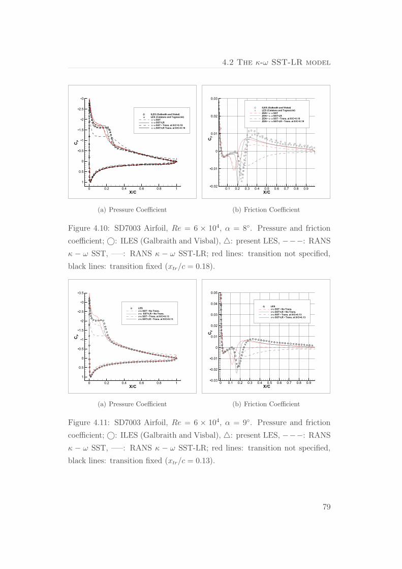
4.2 The κ-ω SST-LR model
X/C
CP
0 0.2 0.4 0.6 0.8 1
•3
•2.5
•2
•1.5
•1
•0.5
0
0.5
1
ILES (Galbraith and Visbal)LES (Catalano and Tognaccini)κ−ω SSTκ−ω SST•LRκ−ω SST • Trans. at X/C=0.18κ−ω SST•LR Trans. at X/C=0.18
(a) Pressure Coefficient
X/C
CF
0.1 0.2 0.3 0.4 0.5 0.6 0.7 0.8 0.9•0.02
•0.01
0
0.01
0.02
0.03
ILES (Galbraith and Visbal)LES (Catalano and Tognaccini)ZEN • κ−ω SSTZEN • κ−ω SST•LRZEN • κ−ω SST • Trans. at X/C=0.18ZEN • κ−ω SST•LR • Trans. at X/C=0.18
(b) Friction Coefficient
Figure 4.10: SD7003 Airfoil, Re = 6 × 10⁴, α = 8. Pressure and friction
coefficient; ©: ILES (Galbraith and Visbal), : present LES, −−−: RANS
κ − ω SST, —–: RANS κ − ω SST-LR; red lines: transition not specified,
black lines: transition fixed (xtr/c = 0.18).
X/C
CP
0 0.2 0.4 0.6 0.8 1
•3.5
•3
•2.5
•2
•1.5
•1
•0.5
0
0.5
1
LESκ•ω SST • No Trans.κ•ω SST•LR • No Trans.κ•ω SST • Trans. at X/C=0.13κ•ω SST•LR • Trans. at X/C=0.13
(a) Pressure Coefficient
X/C
CF
0 0.1 0.2 0.3 0.4 0.5 0.6 0.7 0.8 0.9•0.03
•0.02
•0.01
0
0.01
0.02
0.03
0.04
0.05
LESκ•ω SST • No Trans.κ•ω SST•LR • No Trans.κ•ω SST • Trans. at X/C=0.13κ•ω SST•LR • Trans. at X/C=0.13
(b) Friction Coefficient
Figure 4.11: SD7003 Airfoil, Re = 6 × 10⁴, α = 9. Pressure and friction
coefficient; ©: ILES (Galbraith and Visbal), : present LES, −−−: RANS
κ − ω SST, —–: RANS κ − ω SST-LR; red lines: transition not specified,
black lines: transition fixed (xtr/c = 0.13).
79

4.3 Drag polar of the SD 7003 airfoil
T*U∞/LREF
CL
CD
0 5 10 15 20 250
0.2
0.4
0.6
0.8
1
1.2
1.4
0
0.05
0.1
0.15
0.2
0.25
0.3
0.35
0.4
α=9α=10α=11α=12
(a) κ-ω SST-LR
T*U∞/LREF
CL
CD
0 5 10 15 20 25 30 350
0.2
0.4
0.6
0.8
1
1.2
1.4
0
0.05
0.1
0.15
0.2
0.25
0.3
0.35
0.4
α=9α=10α=11α=12
(b) κ-ω SST
Figure 4.12: URANS of the flow aorund the SD7003 airfoil: Time evolution
of lift and drag coefficients
proved by using methods able to estimate the transition location starting
from a pressure distribution [54].
4.3 Drag polar of the SD 7003 airfoil
The drag polar of the SD 7003 airfoil at Reynolds number 6.0×10⁴ has been
computed by the the κ-ω SST and SST-LR models [55]. RANS simulations
up to α = 9, and time-accurate URANS simulations from α = 10 to 12
have been performed. Three levels of the computational grid are used in the
time-accurate computations in order to limit the CPU time.
The evolution in time of the lift and drag coefficients are shown in figure
4.12. Steady state solutions are obtained in all the simulations. The κ-ω
SST-LR model (figure 4.12 a) provides solutions with a CL slightly increasing
with the angle of attack up to α = 11. A light decrease is seen for α = 12.
Instead, the κ-ω SST (figure 4.12 b) yields a drop of the lift coefficient when
α goes from 9 to 10. The drag coefficient increases with the angle of attack
for both the models. A large variation of CD occurs for the κ-ω SST model
bewteen α = 9 and 10.
80

4.3 Drag polar of the SD 7003 airfoil
T*U∞/LRef
CL C
D0 5 10 15
0.6
0.65
0.7
0.75
0.8
0.85
0.9
0.95
1
1.05
0.04
0.045
0.05
0.055
0.06
0.065
0.07
Time averaging
(a) α = 9
T*U∞/LRef
CL
CD
0 5 10 15 20 250.5
0.75
1
1.25
1.5
0.05
0.1
0.15
0.2
0.25
0.3
0.35
0.4Time Averaging
(b) α = 11
Figure 4.13: Large Eddy simulation of the flow aorund the SD 7003 airfoil:
Time evolution of lift and drag coefficients
Large eddy simulations have also been performed up to α = 11. The
span-wise extension ∆z of the computational domanin is 0.1 × c for α ≤ 9
and 0.2×c for α > 9. The number of cells used in the span-wise direciton is 48
for ∆z = 0.1, and 96 for ∆z = 0.2 The simulations are started from a RANS
flow field. The solution is first advanced in time with a fix Courant number
and a time step computed on the basis of numerical stability analysis. Then,
once the solution has started to develop, a constant time step ∆t = 0.5×10⁻⁴
is used. The evolution in time of the aerodynamic coefficients is presented in
figure 4.13 for α = 9 and 11. The behaviour of the aerodynamic coefficient
at α = 11 shows a large variation when the flow starts to separate on the
central region of the upper surface of the airfoil.
The lift and drag coefficients are compared (figure 4.14) to three sets
of experimental data, and to the numerical results obtained by the ILES
approach [18]. The measurements taken from Selig et al. [56] at University
of Princeton in 1989 , from Selig et al. [57] at University of Illinois in 1996,
and from Ol et al. [49] at the Horizontal Fee-Surface Wind Tunnel (HFWT)
of the Air Force Research Laboratory in 2005 are considered.
The differences in the lift coefficient (figure 4.14 a) are mainly seen at the
81
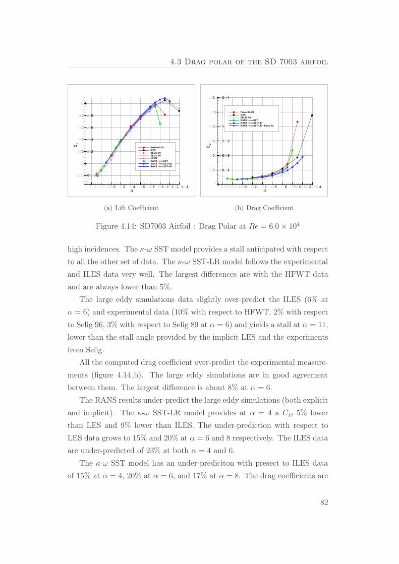
4.3 Drag polar of the SD 7003 airfoil
α
CL
•4 •2 0 2 4 6 8 10 12 14
•0.2
0
0.2
0.4
0.6
0.8
1
Present LESILESSELIG 89SELIG 96HFWTRANS • κ•ω SSTRANS • κ•ω SST•LRRANS • κ•ω SST•LR
(a) Lift Coefficient
α
CD
•4 •2 0 2 4 6 8 10 12 140
0.04
0.08
0.12
0.16
0.2
0.24
Present LESILESSELIG 96RANS • κ•ω SSTRANS • κ•ω SST•LRRANS • κ•ω SST•LR • Trans. fix.
(b) Drag Coefficient
Figure 4.14: SD7003 Airfoil : Drag Polar at Re = 6.0 × 10⁴
high incidences. The κ-ω SST model provides a stall anticipated with respect
to all the other set of data. The κ-ω SST-LR model follows the experimental
and ILES data very well. The largest differences are with the HFWT data
and are always lower than 5%.
The large eddy simulations data slightly over-predict the ILES (6% at
α = 6) and experimental data (10% with respect to HFWT, 2% with respect
to Selig 96, 3% with respect to Selig 89 at α = 6) and yields a stall at α = 11,
lower than the stall angle provided by the implicit LES and the experiments
from Selig.
All the computed drag coefficient over-predict the experimental measure-
ments (figure 4.14 b). The large eddy simulations are in good agreement
between them. The largest difference is about 8% at α = 6.
The RANS results under-predict the large eddy simulations (both explicit
and implicit). The κ-ω SST-LR model provides at α = 4 a CD 5% lower
than LES and 9% lower than ILES. The under-prediction with respect to
LES data grows to 15% and 20% at α = 6 and 8 respectively. The ILES data
are under-predicted of 23% at both α = 4 and 6.
The κ-ω SST model has an under-prediciton with presect to ILES data
of 15% at α = 4, 20% at α = 6, and 17% at α = 8. The drag coefficients are
82

4.3 Drag polar of the SD 7003 airfoil
α
X/C
CP
0 0.2 0.4 0.6 0.8 1
•4
•3
•2
•1
0
1
α=9α=10α=11α=12
(a) Pressure Coefficient
α
X/C
Cf
0.2 0.4 0.6 0.8
•0.02
0
0.02α=9α=10α=11α=12
(b) Friction Coefficient
Figure 4.15: SD7003 Airfoil : Evolution with α of the pressure and friction
coefficient. κ-ω SST-LR turbulence model - transition not specified.
lower than LES data of 18% at α = 4 and 8, 13% at α = 6.
The results at higher angles of incidence are close to the drag rise of the
stall and have not been analyzed from a quatitative point of view.
The comparison between LES and the RANS data obtained by fully tur-
bulent simulations is acceptable at low angles of attack. The CD and CL
achieved by the κ-ω SST-LR with an imposed transition point (also if with a
very rough criterion) are also shown in figure 4.14. The agreement with the
aerodynamic coefficients provided by the large eddy simulations improves.
The largest difference presented by the CD is 14%. This occurs at α = 6 for
the comparison with the explicit LES, and at α = 8 for the explicit LES.
4.3.1 Stall Characteristics
The evolution with the angle of attack of the pressure and friction coefficients
achieved by the κ-ω SST-LR turbulence model is presented in figure 4.15.
The bubble moves towards the leading edge of the airfoil as α increases from
9 to 10. Both the separation and re-attachment points do not change for
α = 11 but the recovery of the pressure is decreased. A separation zone
starts to develop in the trailing edge zone at α = 11. The flow at α = 12
83

4.3 Drag polar of the SD 7003 airfoil
X
Y
0 0.5 1
•0.5
0
0.5
•0.32 •0.27 •0.23 •0.18 •0.14 •0.10 •0.05 0.04 0.08 0.13 0.17 0.21W/V
∞
(a) T0
X
Y
0 0.5 1
•0.5
0
0.5
•0.32 •0.27 •0.23 •0.18 •0.14 •0.10 •0.05 0.04 0.08 0.13 0.17 0.21W/V
∞
(b) T0 + 0.36
X
Y
0 0.5 1
•0.5
0
0.5
•0.32 •0.27 •0.23 •0.18 •0.14 •0.10 •0.05 0.04 0.08 0.13 0.17 0.21W/V
∞
(c) T0 + 0.72
X
Y
0 0.5 1
•0.5
0
0.5
•0.32 •0.27 •0.23 •0.18 •0.14 •0.10 •0.05 0.04 0.08 0.13 0.17 0.21W/V
∞
(d) T0 + 1.08
X
Y
0 0.5 1
•0.5
0
0.5
•0.32 •0.27 •0.23 •0.18 •0.14 •0.10 •0.05 0.04 0.08 0.13 0.17 0.21W/V
∞
(e) T0 + 1.44
XY
0 0.5 1
•0.5
0
0.5
•0.32 •0.27 •0.23 •0.18 •0.14 •0.10 •0.05 0.04 0.08 0.13 0.17 0.21W/V
∞
(f) T0 + 1.80
Figure 4.16: SD7003 Airfoil : Large Eddy Simulation at high α. Instanta-
neous span-wise averaged w/v∞
re-attaches at a level of pressure significantly lower with respect to α = 11.
A large separated region is present on the upper surface of the airfoil. As α
still increases the flow is not more able to re-attach and the bubble joins with
the region of the separated flow forming on the upper surface of the airfoil.
Therefore a combined stall occurs.
This analysis is confirmed by LES results. Figure 4.16 shows the span-
wise velocity at high angle of attack. The w is averaged in the span direction
and is presented at six different instants of time. The bubble in the leading
edge zone can be discerned. Turbulent flow structures downstream the bubble
are also visible in some plots. A large region of separated flow is present in
the upper region of the airfoil.
The fluctuations originating in the zone of the bubble and the large zone
of separated flow are also visible in the pressure distribution (figure 4.17). A
re-circulating flow at low pressure is present on the upper region of the airfoil.
84

4.3 Drag polar of the SD 7003 airfoil
X
Y
0 0.5 1
•0.5
0
0.5
•2.10 •1.91 •1.72 •1.52 •1.33 •1.14 •0.95 •0.75 •0.56 •0.37 •0.18 0.02 0.21 0.40CP/2
(a) T0
X
Y
0 0.5 1
•0.5
0
0.5
•2.10 •1.91 •1.72 •1.52 •1.33 •1.14 •0.95 •0.75 •0.56 •0.37 •0.18 0.02 0.21 0.40CP/2
(b) T0 + 0.36
X
Y
0 0.5 1
•0.5
0
0.5
•2.10 •1.91 •1.72 •1.52 •1.33 •1.14 •0.95 •0.75 •0.56 •0.37 •0.18 0.02 0.21 0.40CP/2
(c) T0 + 0.72
X
Y
0 0.5 1
•0.5
0
0.5
•2.10 •1.91 •1.72 •1.52 •1.33 •1.14 •0.95 •0.75 •0.56 •0.37 •0.18 0.02 0.21 0.40CP/2
(d) T0 + 1.08
X
Y
0 0.5 1
•0.5
0
0.5
•2.10 •1.91 •1.72 •1.52 •1.33 •1.14 •0.95 •0.75 •0.56 •0.37 •0.18 0.02 0.21 0.40CP/2
(e) T0 + 1.44
XY
0 0.5 1
•0.5
0
0.5
•2.10 •1.91 •1.72 •1.52 •1.33 •1.14 •0.95 •0.75 •0.56 •0.37 •0.18 0.02 0.21 0.40CP/2
(f) T0 + 1.80
Figure 4.17: SD7003 Airfoil : Large Eddy Simulation at high α. Instanta-
neous span-wise averaged (P − P∞)/(ρ∞v∞2)
A second low-pressure re-circulating zone appears close to the trailimg-edge,
is fed by the upstream flow, and then is convected downstream in the wake.
85

Chapter 5
Transonic Flows
The κ-ω SST-LR is applied to tyipcal transonic benchmarks [22] in order
to verify that the accuracy and reliability of the original SST formulation
is recovered for transonic flows at high Reynolds number. The RAE 2822
airfoil and the wing RAE M2155 are considered.
5.1 RAE 2822 Airfoil
The flow around the RAE 2822 airfoil has been computed at the following
specifications named as case 9 and case 10 in literature [58].
Case 9 Case 10
Mach number = 0.734 0.754
Reynolds number = 6.5 × 10⁶ 6.2 × 10⁶
α = 2.79 2.54
The transition is fixed at X/C = 0.3 as in the experiments. The flow is
characterized by a strong shock boundar-layer interaction.
5.1.1 Case 9
The pressure and the friction coefficient achieved by the κ-ω BSL, SST, and
SST-LR turbulence models for the case 9 flow condition are compared to
the experimental data in figure 5.1. The friction coefficients on the lower
surface of the airfoil are reported as negative values. The agreement with
86

5.1 RAE 2822 Airfoil
X/C
CP
0 0.2 0.4 0.6 0.8 1
•1.5
•1
•0.5
0
0.5
1
Experimentalκ−ω BSLκ−ω SSTκ−ω SST•LR
RAE 2822 Airfoil • Case 9Mach=0.734, Re=6.5 x 10⁶, α=2.79
(a) Pressure Coefficient
X/C
CF
0.2 0.4 0.6 0.8
•0.004
•0.002
0
0.002
0.004
0.006
0.008
Experimentalκ−ω BSLκ−ω SSTκ−ω SST•LR
RAE 2822 Airfoil • Case 9Mach=0.734, Re=6.5 x 10⁶, α=2.79
(b) Friction Coefficient
Figure 5.1: RAE 2822 Airfoil, Case 9 flow condition: Pressure and friction
coefficient; symbols: experimental, − · −: RANS κ − ω BSL, −−−: RANS
κ − ω SST, —–: RANS κ − ω SST-LR;
the experimental data is good for all the three tubulence models. The SST
ans SST-LR provide a very similar pressure and friction coefficients and a
weak shock-induced separation. The BSL model shows a shock located more
downstream with respect to the other results.
5.1.2 Case 10
At the condition named as case 10, the flow is characterized by a shock-
induced separation followed by a pressure recovery and a re-attachment.
The pressure and the friction coefficients are shown in figure 5.2. Differences
between the turbulnce models are more evident with respect to the case 9
flow condition. The κ-ω SST and SST-LR return a shock-induced separa-
tion. The SST predicts the location of the shock better than the SST-LR,
and the SST-LR shows a pressure recovery in the region where the flow re-
attaches stronger than the SST. The κ-ω BSL provides a shock located too
downstream and does not present a separation.
The velocity profiles at three stations on the upper surface of the airfoil
are presented in figure 5.3. The first station is located upstream of the shock
87

5.1 RAE 2822 Airfoil
X/C
CP
0 0.2 0.4 0.6 0.8 1
•1.5
•1
•0.5
0
0.5
1
Experimentalκ−ω BSLκ−ω SSTκ−ω SST•LR
RAE 2822 Airfoil • Case 10Mach=0.754, Re=6.2 x 10⁶, α=2.57
(a) Pressure Coefficient
X/C
CF
0.2 0.4 0.6 0.8
•0.004
•0.002
0
0.002
0.004
0.006
Experimentalκ−ω BSLκ−ω SSTκ−ω SST•LR
RAE 2822 Airfoil • Case 10Mach=0.754, Re=6.2 x 10⁶, α=2.57
(b) Friction Coefficient
Figure 5.2: RAE 2822 Airfoil, Case 10 flow condition: Pressure and friction
coefficient; symbols: experimental, − · −: RANS κ − ω BSL, −−−: RANS
κ − ω SST, —–: RANS κ − ω SST-LR;
U/UE
Z/C
0.4 0.5 0.6 0.7 0.8 0.9 110•4
10•3
10•2
Experimentalκ−ω BSLκ−ω SSTκ−ω SST•LR
RAE 2022 Airfoil • Case 10Mach=0.754, Re=6.2 x 10⁶, α=2.57
(a) X/C = 0.40
U/UE
Z/C
0 0.2 0.4 0.6 0.8 10
0.01
0.02
0.03
Experimentalκ−ω BSLκ−ω SSTκ−ω SST•LR
RAE 2022 Airfoil • Case 10Mach=0.754, Re=6.2 x 10⁶, α=2.57
(b) X/C = 0.65
U/UE
Z/C
0.2 0.4 0.6 0.8 10
0.01
0.02
0.03
0.04
0.05
Experimentalκ−ω BSLκ−ω SSTκ−ω SST•LR
RAE 2022 Airfoil • Case 10Mach=0.754, Re=6.2 x 10⁶, α=2.57
(c) X/C = 0.90
Figure 5.3: RAE 2822 Airfoil, Case 10 flow condition: Velocity profiles;
symbols: experimental, − ·−: RANS κ− ω BSL, −−−: RANS κ− ω SST,
—–: RANS κ − ω SST-LR;
and all the three turbulence models provide a velocity profile in very good
agreement with the experimental data. The second station is very critical
because located just downstream the shock in the region of separated flow.
The agreement is not as good as at X/C = 0.40. However, the SST and SST-
LR models show a zone of negative velocity and a behaviour that resembles
the experimental data. The result of the BSL model is definitely worse. The
88

5.2 RAE M2155 Wing
last station is located in the region where the flow is re-attached. The κ-ω
SST provides a result better than the SST-LR and a good agreement with
the experimental data in the inner part of the boundary layer. The κ-ω BSL
model has provided a solution without separation, and the boundary layer
at X/C = 0.90 is significantly different with respect to the other solutions.
5.2 RAE M2155 Wing
The RAE M2155 wing placed is a transonic benchmark [59] for which the
κ − ω SST model has provided appreciable results [21].
The case 2 condition:
• Mach number = 0.806
• Reynolds number = 4.1 × 10⁶
• α = 2.50
is characterized by a quite complex shock topology [59]. The flow on the
upper surface of the wing is characterized by a triple shock wave system
from the root to about the 50% of the span, and by a single shock wave from
about the 50% to the tip. Inboard the 50% span, changes in the flow direction
occur in the region of the forward leg of the triple shock wave system and
in trailing edge zone but without flow separation. The flow separation starts
where the three shock waves join together and ends at about 90% of the
span. The separation extends for about 10% of the local chord.
A mesh with 35 blocks and about 1.2× 10⁶ cells has been employed. The
κ − ω SST, SST-LR, and BSL turbulence models are applied.
The results are shown in terms of pressure coefficient at several stations
along the span in Fig. 5.4. At the inboard span-wise stations, the interaction
between the shock wave system and the boundary layer is not very strong
and the three κ − ω models present the same pressure coefficients. At the
stations where the shock boundary-layer interaction becomes stronger and
89

5.2 RAE M2155 Wing
X/C
CP
0 0.2 0.4 0.6 0.8 1
•1.5
•1
•0.5
0
0.5
1
Experimentalκ−ω SSTκ−ω SST•LRκ−ω BSL
2y/b = 0.20
(a) y/2b = 0.20
X/C
CP
0 0.2 0.4 0.6 0.8 1
•1.5
•1
•0.5
0
0.5
1
Experimentalκ−ω SSTκ−ω SST•LRκ−ω BSL
2y/b = 0.40
(b) y/2b = 0.40
X/C
CP
0 0.2 0.4 0.6 0.8 1
•1.5
•1
•0.5
0
0.5
1
Experimentalκ−ω SSTκ−ω SST•LRκ−ω BSL
2y/b = 0.50
(c) y/2b = 0.50
X/C
CP
0 0.2 0.4 0.6 0.8 1
•1.5
•1
•0.5
0
0.5
1
Experimentalκ−ω SSTκ−ω SST•LRκ−ω BSL
2y/b = 0.60
(d) y/2b = 0.60
X/C
CP
0 0.2 0.4 0.6 0.8 1
•1.5
•1
•0.5
0
0.5
1
Experimentalκ−ω SSTκ−ω SST•LRκ−ω BSL
2y/b = 0.80
(e) y/2b = 0.80
X/CCP
0 0.2 0.4 0.6 0.8 1
•1.5
•1
•0.5
0
0.5
1
Experimentalκ−ω SSTκ−ω SST•LRκ−ω BSL
2y/b = 0.95
(f) y/2b = 0.95
Figure 5.4: Pressure coefficients over the RAE M2155 wing; •: experiment,
− − 2 − −: RANS κ − ω SST, —∆—: RANS κ − ω SST-LR, − · ∇ − ·:RANS κ − ω BSL
the flow separates the κ − ω SST-LR provides the same results as the SST
model and follows the experimental data better than the BSL model.
90

Chapter 6
Conclusions
A contribution to the numerical simulation of low-Reynolds number flows
has been given.
The focus has been placed on the methods based on the resolution of the
Reynolds Averaged Navier Stokes equations. The capability of the turbulence
models to return a laminar separation bubble has been investigated. The
incompressible flow over a flat plate with an imposed pressure gradient, and
around the SD 7003 airfoil have been considered. Large eddy simulations
have also been performed and used as a reference for the RANS results.
Laminar separation bubbles have been found by the Spalart-Allmaras and
the κ-ω SST turbulence models. The simulations have been performed using
very low values of the free-stream turbulence without an a priori knowledge
of the laminar-turbulent transition, and by prescribing the transition location
as retrieved by LES data. A satisfactory prediction of the flow characteristics
in the dead air region of the bubble is obtained. On the contrary, a poor
agreement has been provided by RANS with respect to LES in the zone of
pressure recovery. These discrepancies are essentially due to a too low level
of turbulence in the bubble.
The behaviour of the κ-ω SST turbulence model has been investigated
in detail. Simulations of the flow around the SD 7003 airfoil at Reynolds
numbers 6×10⁴, 6×10⁵, and 6×10⁶ have been performed. This model did not
predict correctly the viscous and logarithmic regions of the boundary layer at
the lowest Reynolds number. However, it has been shown that this is related
to the implementation at low Reynolds numbers, rather than to an intrinsic
91

Chapter 6. Conclusions
“design” limit of the model. Indeed, a modification has been proposed. The
modified model, the κ-ω SST-LR, has provided a correct simulation of the
viscous sublayer and logarithmic region in the tests performed at high and
low Reynolds numbers. The laminar separation bubble arising on the SD
7003 airfoil is well captured and the results of the RANS simulations are in
excellent agreement with the LES data. In addition, high Reynolds number
performances of the model do not deteriorate with respect to the standard
κ-ω SST as shown by the transonic tests around the RAE 2822 airfoil and
M2155 wing. The κ-ω SST-LR turbulence model ca be used in a wide range
of Reynolds numbers to simulate different flow aspects from the laminar
separation bubbles to the shock-boundary layer interaction.
92

Bibliography
[1] Carmichael, B. H., “Low Reynolds Number Airfoil,” Tech. Rep. NASA-
CR-165803, NASA, 1981.
[2] Lissaman, P. B. S., “Low Reynolds Number Airfoils,” Annual Review of
Fluid Mechanics , Vol. 39, 1983, pp. 223–239.
[3] Arina, R., Atkin, C., Hanff, E., Jones, K., Lekas, T., Oi, M., Khalid, M.,
McAuliffe, B., Paquet, J. B., Platzer, M., Rist, U., Windte, J., and Yuan,
W., “Experimental and Computational Investigations in Low Reynolds
Number Aerodynamics with Applications to Micro Air Vehicles,” RTO
Technical Report NATO-AVT-101, NATO, 2009.
[4] Spalart, P. R. and Strelets, M. K., “Mechanisms of Transition and Heat
Transfer in a Separation Bubble,” Journal of Fluid Mechanics , Vol. 30,
2000, pp. 329–349.
[5] Spalart, P. R. and Allmaras, S. R., “A one equation turbulence model
for aerodynamic flows,” 30th AIAA Aerospace Sciences Meeting and Ex-
hibit , Reno, NV, Jan. 1992, AIAA paper 92-0439.
[6] Menter, F. R., “Two-equation Eddy Viscosity Turbulence Models for
Engineering Applications,” Aerospace Science and Technology Journal ,
Vol. 32, No. 7, 1994, pp. 1598–1695.
93
Bibliography
[7] Howard, R. J. A., Alam, M., and Sandham, N. D., “Two-Equations
Turbulence Modelling of a Transitional Separation Bubble,” Flow Tur-
bulence and Combustion, Vol. 63, 1999, pp. 175–191.
[8] Kalitzin, G., Gould, A., and Benton, J., “Application of two-equation
turbulence models to aircraft design,” 34th AIAA Aerospace Sciences
Meeting and Exhibit , Reno, NV, 1996, AIAA paper 96-0327.
[9] Wilcox, D. C., Turbulence Modeling for CFD , DCW Industies inc., La
Canada, Los Angeles, California, 1994.
[10] Windte, J., Scholz, U., and Radespiel, R., “Validation of RANS Simu-
lation of Laminar Separation Bubbles on Airfoils,,” Aerospace Science
and Technology Journal , Vol. 10, No. 7, 2006, pp. 484–494.
[11] Radespiel, R., Windte, J., and Scholz, U., “Numerical and Experimental
Flow Analysis of Moving Airfoils with Laminar Separation Bubbles,”
44th AIAA Aerospace Sciences Meeting and Exhibit , Reno, NV, Jan.
3–Jan. 5 2006, AIAA paper 2006-0501.
[12] Yuan, W., Khalid, M., Windte, J., Scholz, U., and Radespiel, R., “An
Investigation of Low-Reynolds-Number Flows past Airfoils,” 23rd AIAA
Applied Aerodynamics Conference, Toronto, Canada, June 6–June 9
2005, AIAA paper 2005-4607.
[13] Wallin, S. and Johansson, A., “An Explicit Algebraic Reynolds Stress
Model for Incompressible and Compressible Turbulent Flows,” Journal
of Fluid Mechanics , Vol. 403, 2000, pp. 89–132.
[14] Tang, L., “RANS Simulation of Low-Reynolds-Number Airfoil Aerody-
namics,” 44th AIAA Aerospace Science Meetinf and Exhibit , Reno, NV,
Jan. 3–Jan. 5 2006, AIAA paper 2006-0249.
[15] Jones, W. P. and Launder, B. E., “The Prediciton of Laminarization
with a Two-Equation Model for Turbulence,” International Journal of
Heat and Mass Transfer , Vol. 15, 1972, pp. 301–314.
94
Bibliography
[16] Ferziger, J. H. and Peric, M., Computational Methods for Fluid Dynam-
ics , Springer-Verlag, Berlin & Heidelberg, 1996.
[17] Lenormand, E., Saguat, P., Phuoc, L., and Comte, P., “Subgrid-
Scale Models for Large Eddy Simulation of Compressible Wall Bounded
Flows,” AIAA Journal , Vol. 38, 2000, pp. 1340–1350.
[18] Galbraith, M. C. and M. R. Visbal, “Implicit Large Eddy Simulation
of Low Reynolds Number Flow past the SD 7003 Airfoil,” 46th AIAA
Aerospace Sciences Meeting and Exhibit , Reno, NV, Jan. 7 –Jan. 10
2008, AIAA paper 2008-225.
[19] Rumsey, C. L. and Spalart, P. R., “Turbulence Model Behavior in Low
Reynolds Number Regions of Aerodynamic Flow Fields,” AIAA Jour-
nal , Vol. 47, No. 4, 2009, pp. 982–993.
[20] Spalart, P. R. and Rumsey, C. L., “Effective Inflow Conditions for Tur-
bulence Models in Aerodynamic Calculations,” AIAA Journal , Vol. 45,
No. 10, 2007, pp. 2544–2553.
[21] Catalano, P. and Amato, M., “An Evaluation of RANS Turbulence Mod-
elling for Aerodynamic Applications,” Aerospace Science and Technology
Journal , Vol. 7, No. 7, 2003, pp. 493–509.
[22] Catalano, P. and Amato, M., “A Numerical Evaluation of 2-D and 3-D
Application Challenges of Transonic Aerodynamics,” QNET-CFD Net-
work Newsletter , Vol. 1, No. 7, 2001, pp. 25–28.
[23] Catalano, P., Wang, M., Iaccarino, G., and Moin, P., “Numerical Sim-
ulation of the Flow around a Circular Cylinder at High Reynolds Num-
bers,” Internatonal Journal of Heat and Fluid Flow , Vol. 24, 2003,
pp. 463–469.
[24] Kim, J. and Moin, P., “Application of a Fractional Step Method to
Incompressible Navier-Stokes Equations,” Journal of Computational
Physics , Vol. 59, 1985, pp. 308–323.
95

Bibliography
[25] Germano, M., Piomelli, U., Moin, P., and Cabot, W. H., “A Dynamic
Subgrid-scale Eddy Viscosity Model,” Physics of Fluids , Vol. 3, 1991,
pp. 1760–1765.
[26] Lilly, D. K., “A Proposed Modification of the Germano Subgrid Scale
Closure Method,” Physics of Fluids , Vol. 4, 1992, pp. 633–635.
[27] Baldwin, B. S. and Lomax, H., “Thin layer approximation and algebraic
model for separated turbulent flows,” American Institute of Aeronautics
and Astronautics (AIAA), 1978, AIAA Paper 78-257.
[28] Menter, F. R., “Performance of popular turbulence models for attached
and separated turbulent boundary layers,” AIAA Journal , Vol. 30,
No. 8, 1992, pp. 2066–2072.
[29] Wilocx, D. C., “A half-century historical review of the κ-ω model,”
AIAA Journal , Vol. 26, No. 11, 1988, pp. 1311–1320.
[30] Wilcox, D. C., “Reassessment of the scale-determining equation for
advanced turbulence models,” AIAA Journal , Vol. 26, No. 11, 1988,
pp. 1299–1310.
[31] Monsen, E., Rudnik, R., and Beeckle, H., “Flexibility and efficiency of a
transport equation turbulence model fro three-dimensional flows,” Notes
on Numerical Fluid Mechanics , Vol. 60, 1997, pp. 237–244.
[32] Menter, F. R., “Influence of free-stream values on κ-ω model prediction,”
AIAA Journal , Vol. 30, No. 6, 1991, pp. 1657–1659.
[33] Wilocx, D. C., “A two equations turbulence model for wall-bounded and
free-shear flows,” 24th Fluid Dynqamics Conference, American Institute
of Aeronautics and Astronautics (AIAA), Orlando, FL, July 6–9 1993.
[34] Kok, J., “Resolving the Dependence on Free-Stream Values for the κ-ω
Turbulence Model,” AIAA Journal , Vol. 38, No. 7, 2000, pp. 1292–1295.
96

Bibliography
[35] Cazalbou, J. B., Spalart, P. R., and Bradshaw, P., “On the behavior
of two equation models at the edge of a turbulent region,” Physics of
Fluids , Vol. 5, No. 5, 1994, pp. 1797–1804.
[36] Leschziner, M. A. and Loyau, H., “Numerical Investigation of three-
dimensioanl transonic flows with large separation,” ICAS 2000 Confer-
ence, Harrogate, UK, Aug. 28 –Sept. 1 2000.
[37] Bezard, H., Catalano, P., Courty, J. C., Kok, J., Krumbein, A., and
Wallin, S., “Progress in advanced turbulence and transition modelling
in the European project AVTAC,” 18th AIAA Applied Aerodynamics
Conference, Denver, CO, 2000, AIAA paper 2000-4511.
[38] Catalano, P., Marini, M., Nicoli, A., and Pizzicaroli, A., “CFD Contri-
bution to the Aerodynamic Data Set of the Vega Launcher,” Journal of
Spacecraft and Rockets , Vol. 44, No. 1, 2007, pp. 42–51.
[39] Catalano, P. and Amato, M., “Assessment of κ-ω turbulence modeling
in the CIRA flow solver ZEN,” ECCOMAS 2001 Conference, Swansea,
Wales, Sept.4–7 2001.
[40] Amato, M. and Catalano, P., “Non Linear κ-ε turbulence modeling for
industrial applications,” ICAS 2000 Congress , Harrogate, UK, Aug. 28
– Sept. 1 2000.
[41] Marongiu, C., Catalano, P., Amato, M., and Iaccarino, G., “U-ZEN : A
computational tool solving U-RANS equations for industrial unsteady
applications,” 34th AIAA Fluid Dynamics Conference, Portland (Or),
June 28 –July 1 2004, AIAA Paper 2004-2345.
[42] Jameson, A., “Time Dependent Calculations using Multigrid with Ap-
plication to Unsteady Flows past Airfoils and Wings,” June 24–26 1991,
AIAA Paper 1991-1596.
97

Bibliography
[43] Catalano, P., “Numerical Investigation of the Flow around the Ahmed
Model,” 18th AIAA Computational Fluid Dynamics Conference, Miami,
FL, June 25 –June 28 2007, AIAA paper 2007-4096.
[44] Shur, M., Spalart, P. R., Strelets, M., and Travin, A., “Detached-eddy
Simulation of an Airfoil at High Angle of Attack,” Engineering Turbu-
lence Modelling and Experiments - 4 , ETMM-4, Ajaccio, Corsica, FR,
May24–26 1999.
[45] Horton, H. P., Laminar Separation in two and three-dimensional incom-
pressible flow , PhD thesis, University of London, 1968.
[46] Catalano, P. and Tognaccini, R., “Influence of Free-stream Turbulence
on Simulations of Laminar Separation Bubbles,” 47th AIAA Aerospace
Sciences Meeting and Exhibit , Orlando, FL, Jan. 3 –Jan. 5 2009, AIAA
paper 2009-1471.
[47] Lang, M., Rist, U., and Wagner, S., “Investigation on Controlled Tran-
sition Development in a Laminar Separation Bubble by means of LDA
and PIV,” Experiments in Fluids , Vol. 36, 2004, pp. 43–52.
[48] Marxen, O., Lang, M., Rist, U., and Wagner, S., “A Combined Numer-
ical/Experimental Study of Unsteady Phenomena in a Laminar Separa-
tion Bubble,” Flow Turbulence and Combustion, Vol. 71, 2003, pp. 133–
146.
[49] Ol, M. V., McAuliffe, B. R., Hanff, E. S., Scholz, U., and Kalher, C.,
“Comparison of Laminar Separation Bubble Measurements on a Low
Reynolds Number Airfoil in Three Facilities,” 135th AIAA Fluid Dy-
namics Conference, Toronto, Canada, June 6–June 9 2005, AIAA paper
2005-5149.
[50] Schlichting, H., Boundary Layer Theory , McGraw-Hill Book
Company,7th Edition, 1978.
98
Bibliography
[51] Myong, H. and Kasagi, N., “A new Approach to the Improvement of the
κ-ε Turbulence Model for Wall-bounded Shear Flows,” JSME Interna-
tional Journal Series II , Vol. 33, No. 1, 1990, pp. 63–72.
[52] Catalano, P. and Tognaccini, R., “An Analysis of the Shear Stress Trans-
port Formulation for Low Reynolds Number Flows,” XX Congresso
Nazionale AIDAA, Milano, June29–July 3 2009.
[53] Catalano, P. and Tognaccini, R., “Turbulence Modelling for Low
Reynolds Numebr Flows,” AIAA Journal , under review for publication.
[54] Catalano, P., Iuliano, E., Donelli, R., and Paniza, A., “A Numerical
Procedure for Predicting Transition in a RANS Environment,” XX Con-
gresso Nazionale AIDAA, Milano, June29–July 3 2009.
[55] Catalano, P. and Tognaccini, R., “Numerical analysis of the Flow around
the SD 7003 Airfoil,” to be presented at 48th AIAA Aerospace Sciences
Meeting and Exhibit , Orlando, FL, Jan. 4 –Jan. 7 2010, AIAA paper
2010-68.
[56] Selig, M. S., Donovan, J. F., and Fraser, D. B., “Airfoils at Low Speeds,”
Soartech 8 , H. A. Stokely, Soartech publications, Virginia Beach, VA,
USA, 1989.
[57] Selig, M. S., Guglielmo, J. J., Groeren, A. P., and Giguere, P., “Sum-
mary of Low-Speed Airfoil Data,” H. A. Stokely, Soartech Aero publi-
cations, Virginia Beach, VA, USA, 1995.
[58] Haase, W., Bradsma, F., Elsholz, E., Leschziner, M., and Schwamborn,
D., “EUROVAL - An European initiative on validation of CFD codes,”
Notes on Numerical Fluid Mechanics , Vol. 42, 1992.
[59] Firmin, M. C. P. and McDonald, M. A., “Measuremnets of the Flow
over a Low Aspect-Ratio Wing in the Mach number range 0.6 to 0.87
99

Bibliography
for the Purpose of Validation of Computational methods,” Technical Re-
port DRA-TR-92016, DRA — Defence Research Agency, Farnborough,
Hampshire, UK, 1992.
100