1

Department of Pesticide Regulation Environmental Monitoring Branch

1001 I Street, P.O. Box 4015 Sacramento, CA 95812-4015

AERFUM: an integrated air dispersion modeling system for soil fumigants

Yuzhou Luo, Ph.D., Research Scientist IV

10/17/2019

1 Introduction

Gaussian plume models such as ISCST (Industrial Source Complex – Short Term) and AERMOD (American Meteorological Society/Environmental Protection Agency Regulatory Model) are used to predict air pollution levels for environmental and human health protection. Those models were originally developed for industrial and transportation sources. Pesticide applications present complexities in terms of intermittent sources characteristics. Due to the transient nature of these sources at regional scale, a modeling system is needed to consider the emissions from treated fields according to pesticide application amount, method, timing, and associated environmental conditions for appropriate exposure modeling.

The California Department of Pesticide Regulation (DPR) has developed a modeling system, AERFUM (Air Exposure and Risk model for Fumigants), for predicting ambient concentrations of soil fumigants. AERFUM employs AERMOD and ISCST3 as simulation engines, and provides pre- and post-processing functions specifically designed for regulatory purposes related to fumigations at various spatiotemporal scales. AERFUM is optimized for model applications in California by incorporating pesticide use data, meteorological data, and geographic information system (GIS) layers.

With the simulation engines and processors, two types of simulations are implemented in AERFUM: [1] Unit simulation, which evaluates a single application event for the potential air concentrations at field scale; and [2] Regional simulation, which continuously simulates reported pesticide uses at sub-regional scale, and the results could be compared to measured concentrations from air monitoring networks. The unit simulation function is used to determine critical values for mitigation efforts, such as buffer zone settings used to quantify the relationship between use and air concentrations by application conditions (method, season, and region). Regional simulation also supports scenario analysis for proposed management practices, e.g., the use limit of a pesticide. AEFRUM is developed with a Graphical User Interface (GUI), providing assistant functions throughout the modeling procedure and result interpretation. In summary, AERFUM is anticipated to facilitate air dispersion modeling and associated regulation and mitigation efforts for soil fumigants in California.

2

2 Review of previous relevant studies DPR has used air dispersion modeling for soil fumigants since the 1990s. The early version of the ISCST model was used to predict methyl bromide flux from area sources (Ross et al., 1996), and version 3 of the model (ISCST3) was later implemented in the determination of buffer zones for methyl bromide (Segawa, 1997; Segawa et al., 2000). Johnson (2001) introduced probability distributions in exposure analysis on soil fumigants, which required more advanced modeling systems to manage ISCST3 model runs and process the modeling results. Three modeling systems were developed for predicting a bystander’s exposure to soil fumigants emitted from treated agricultural fields: Fumigant Exposure Modeling System (FEMS) (Sullivan et al., 2004), Soil Fumigant Exposure Assessment (SOFEA) (Cryer, 2005), and Probabilistic Exposure and Risk Model for Fumigants (PERFUM) (Reiss and Griffin, 2006). The following reviews are only for the model versions used and evaluated by DPR, and do not reflect the latest updates. DPR compared the FEMS version 5.074 and PERFUM version 2 (PERFUM2), and concluded that there were features of the FEMS model that made it difficult to use to generate buffer zones (Barry, 2007). Therefore, PERFUM2 was used as the primary modeling system to develop buffer zones of soil fumigations, e.g., for methyl isothiocyanate (Barry, 2006) and chloropicrin (Barry, 2014). Two types of buffer zone lengths can be calculated by PERFUM2: the “maximum direction” and “whole field” (Reiss and Griffin, 2006). DPR has reviewed the two approaches and recommended the use of the maximum direction buffer zone (Barry and Johnson, 2007). One of the known limitations of PERFUM2 is that the upper limit of 1440 m is not sufficient for certain application methods and rates with large treated acreages (e.g., 40 acres) (Barry, 2006, 2007). In addition, PERFUM2 was developed by modifying the source codes of ISCST3, making it difficult to update the simulation engine from ISCST3 to AERMOD. SOFEA was proposed by Dow AgroSciences (DAS) to evaluate proposed township caps of 1,3-dichloropropene (1,3-D) (Cryer, 2005). With a proposed township cap value, hypothetical application data were randomly generated by SOFEA based on the probability distributions of application rate, acreage, and timing reported in past years. The 2nd version, SOFEA2 (van Wesenbeeck et al., 2013), also included the capability to utilize reported use data. SOFEA has been used by DPR for predicting 1,3-D concentrations since 2007 (Johnson, 2007a, b), but its modeling performance was not evaluated until monitoring data became available in 2012 (Rotondaro and van Wesenbeeck, 2012) for a 3×3 township area in Merced. Johnson (2014a) compared the observed and SOFEA2-predicted 72-hour concentrations at each monitoring site submitted by DAS (van Wesenbeeck et al., 2013). Results showed that SOFEA2 under-predicted the air concentrations as averages and higher percentiles when compared to the monitoring data in Merced. Independent SOFEA2 simulations were also conducted by DPR for model evaluation. Johnson (2014b) concluded that the model substantially under-predicted the measured average concentrations (even the predicted upper percentiles were below the observed averages). Later, DAS introduced adjustments on mixing heights, which reduced originally assumed mixing height (320 m) to smaller values of 1.6 - 31.9 m, varying by stability class. Barry (2015) tested

3

SOFEA2 with the adjusted meteorological data, and the results showed that the model over-predicted 6 out of the 9 monitoring sites (including 4 of them with prediction/observation ratio > 2). In addition, some significant issues of SOFEA2 on both pre- and post-processing for ISCST3 were also identified. A new program version, SOFEA 4.1beta, has been recently developed by DAS. 3 AERFUM overview Recently DPR switched to AERMOD for air dispersion modeling, starting with structural fumigation of sulfuryl fluoride (Tao, 2015) and followed by a series of studies on 1,3-D (Tao, 2018b, a; Luo, 2019; Tao, 2019). Similar to the ISCST3-based studies, a modeling system is needed to manage AERMOD runs to achieve a specific modeling purpose. Based on the previous experiences in model applications and evaluations, the following considerations are required in the development of the new system AERFUM (but not sufficiently implemented in the existing systems):

Flexibility to work with new data and new approaches. For example, the flux time series should not be limited by the built-in data, but the newly developed flux time series, e.g., those from HYDRUS modeling (Brown, 2018), can be easily incorporated into the system. Compatibility with different versions of air dispersion programs, e.g., upgrade from ISCST3 to AERMOD, or with a newer version of AERMOD. In other words, the functions provided in the modeling system are independent to the simulation engines. Extensibility to solve new problems with the provided functions. This requires modularized design, so users can build their own solutions in addition to those proposed at the time of system development. Consistency in model configurations over time (different years) and space (various locations in California).

Figure 1. Input data, programs, and outputs managed by AERFUM

4

AERFUM is developed as a hub to manage all inputs, outputs, and programs related to air dispersion modeling of soil fumigants (Figure 1). The modeling procedure is initiated by user-specified inputs and options, and conducted with dynamic data exchanges with the USEPA programs for air dispersion modeling. AERFUM uses AERMOD as the default simulation engine, and also provides the option for ISCST3 modeling. According to the USEPA (2005a) “Guideline on Air Quality Models”, AERMOD should be used as the preferred air dispersion model in place of ISC (both short term ISCST3 and long term ISCLT3). AERFUM compatibility with ISCST3 is only developed for the comparison with DPR’s previous modeling studies. AERFUM supports two types of simulations: unit simulation and regional simulation. Unit simulation evaluates a single application event for the potential air concentrations in the surrounding areas of the treated field. This function is used to determine critical values for mitigation efforts, such as buffer zones (DPR, 2017a) and application factors by application conditions (method, season, and region) (DPR, 2017b). Regional simulation continuously simulates reported pesticide uses at a larger spatial scale, and the results could be compared with measured concentrations at a monitoring site, or used to estimate the exposure level (e.g., annual average concentrations) over a specific region. To facilitate the model configurations, 8 functions are developed in AERFUM. Some functions are shared by the two simulation types, while others are specifically designed for regional simulations only (Table 1). More information is provided in Section 4 (for pre-processing functions) and Section 5 (for post processing). Table 1. Summary of AERFUM functions and related simulation type(s) Functions Description Unit

simulation Landscape simulation

Projection and coordinate systems

Define the simulation domain, and convert coordinates as needed between different projection systems

X

Meteorological data Prepare meteorological input data for AERMOD and ISCST3

X X

Pesticide use data and flux time series

Manage pesticide use data and associated flux time series

X [1] X

Source randomization

Locate a reported use within a section X

Source emission Calculate hourly emissions for all sources in the simulation domain

X

Receptors Generate receptors according to user-specified modeling options

X X

Terrain processing Prepare required inputs for model runs with either FLAT (flat) or ELEV (elevated) options

X X

Post processing Process the predicted hourly concentrations for final results

X X

Note: [1] Unit simulations use flux time series only

5

Spatially, AERFUM accepts a simulation domain from a fraction of a section (1×1 mi2) to multiple townships (6×6 mi2). Note that Gaussian air dispersion modeling is not recommended for a transport distance more than 50 km (or 31 mi) (USEPA, 2005b). Hourly simulations are conducted in AERFUM, and all input data are either organized in hourly time step or reference to an integer hour. For example, the meteorological data, flux time series, and intermediate predictions are presented in hourly format, and the start hours of sampling events and pesticide applications are rounded to the nearest hours. 4 AERFUM pre-processing functions 4.1 Projection and coordinate systems The primary coordinate system used in AERFUM is “NAD 1983 California (Teale) Albers (Meters)” (ESRI name: “NAD_1983_California_Teale_Albers”). This system is an adaptation of the Albers Conical Equal Area project as defined by the former State of California Teale Data Center GIS Solutions Group (CDFW, 2015). It is a California-specific projection optimized for area calculations, making it popular to map statewide resources. Coordinate values are in meters from the origin (X=0, Y=0) near the center of the state. DPR-provided GIS maps for Pesticide Use Reporting (PUR) data analysis are prepared in this coordinate system (DPR, 2018). Within the NAD 1983 California (Teale) Albers, townships and sections are generally in square shape following the orientation of the X/Y directions.

Figure 2. Coordinate system of “NAD 1983 California (Teale) Albers (Meters)” (CDFW, 2015) with the origin located approximately at (120W, 38N) In addition, the following two coordinate systems are used by some of the AERFUM functions:

6

Geographic coordinate system in World Geodetic System (WGS) 1984. Weather stations and monitoring sites are defined with latitudes and longitudes in decimal degrees. Universal Transverse Mercator (UTM) conformal projection, used to define the anchor point as a new origin for terrain processing.

Table 2 summarizes the use of the above three projections. Functions for coordinate system conversion and transformation are incorporated in AERFUM. The relevant equations and parameters are based on PROJ (https://proj4.org/). Table 2. Projections used in AERFUM Programs Projection Notes AERMET and AERSURFACE

WGS1984 Location of weather stations, user-specified

AERMAP WGS1984 Simulation domain, generated by AERFUM according to model settings

AERMAP UTM Anchor point, generated by AERFUM according to model settings

AERMOD NAD 1983 California (Teale) Albers (Meters)

Location of sources and receptors, adjusted to relative distance (meters) to the anchor point

Theoretically, absolute coordinate values in “NAD_1983_California_Teale_Albers” can be directly used in modeling. For example, DPR’s air monitoring site at Delhi is located at x = -68,778 m and y = -65,030 m. For more manageable parameterization, relative coordinate values can be defined with a new origin located within the area of interest. For this purpose, AERFUM first determines the spatial extent for the simulation domain based on the model settings, and extracts two reference points: the southwest and northeast corners of the domain. The southwest corner is selected as the new origin in AERFUM, and also used as the “anchor” in AERMAP after conversion to UTM (Table 2). For example, if the 3×3 township area surrounding the Delhi site is selected as the simulation domain (Figure 3), the southwest corner of the spatial extent of the simulation domain is (-81,611, -82,088). AERFUM uses this point as the new origin, so that all objects (sources, receptors, sites, etc.) in the subsequent modeling and data analysis processes would have relative coordinate values ranging from 0 to 28,968 m (or 18 miles), e.g., the Delhi site at (12,833, 17,058).

7

Figure 3. Relative coordinates used in AERFUM regional simulations 4.2 Meteorological data preparation A function to prepare meteorological input data has been incorporated in AERFUM, and also developed as a stand-alone program “MetProc”. This program automatically downloads and processes meteorological data in California and provides consistent inputs for air dispersion models (AERMOD and ISCST3). More information on the methodology and computer implementation are documented in a separate technical report (Luo, 2017). 4.3 Management for pesticide use data and flux time series Pesticide use data are managed by AERFUM in two ways: [1] dynamic connection with DPR’s PUR, or [2] user-provided data. AERFUM is connected to DPR’s internal Oracle database via Open Database Connectivity (ODBC), and automatically retrieves use data according to the modeling domain, period, and the fumigant of interest. In addition, static data tables, such as the processed 1,3-D use data from both the PUR and Agrian (Gonzalez, 2018), can be also used in AERFUM. Table 3 summarizes pesticide use data required by AERFUM. The data fields are named by following the PUR terminology. Application rate is not directly required by AERFUM, but internally calculated based on the application amount and treated acreage, and used in the preparation of emission input files (see Section 4.5).

8

Table 3. Data structure for pesticide use data Data field Descriptions Missing data

allowed? MTR Township, text, size=7 No SECTION Section , text, size=2 No COUNTY_CD County code. AERFUM also accepts county names in

the user-provided data, and will convert names to codes.

No

LBS_CHM_USED Applied mass by active ingredient, pound No ACRE_TREATED Treated acreage No APPLIC_DT Application date, “mm/dd/yyyy” No APPLIC_TIME Application time, “hhmm” Yes FUME_CD Field fumigation method (FFM) code, or any index

system linked with the provided flux time series Yes [1]

Note: [1] A default value should be specified by a user. In addition to pesticide use data, AERFUM also requires flux time series. A flux time series is an hourly time series of flux (μg/m2-s) for a fumigation method at the reference application rate. A flux time series is also associated with a start hour (01-24), so the flux values can be referenced in hourly modeling. Based on different modeling objectives, a flux time series could be: [1] a “full” time series for the period from the completion of an application event to the end of emission duration when negligible fluxes are observed/predicted, or [2] a “partial” flux time series for a sub-period (e.g., the highest N-hour flux used in buffer zone determination). Flux time series are linked with the use database by FUME_CD, i.e., one flux time series should be prepared for each FUME_CD or each group of FUME_CDs. Flux time series can be generated by field experiments or mathematical modeling. The HYDRUS-generated flux time series with a 21-d duration (Brown, 2018) are incorporated in the current version of AERFUM for 1,3-D modeling. An example of the flux time series is shown in Figure 4.

Figure 4. Example of the flux time series generated by HYDRUS, shown as one of the flux time series for FFM 1206 (Nontarpaulin/Deep/Broadcast) with a reference application rate of 100 lb/ac

9

With the use data and flux time series, the following data processing is conducted by AERFUM on the retrieved PUR data or user-provided use data:

Check missing data (Table 3); Remove records with zero applied mass or zero treated acreage; Fill the missing FUME_CD with the user-specified default value; For missing application time, replace with the start hour of the corresponding flux time series; and Round application time to the nearest integer hour.

4.4 Source location and randomization AERFUM prepares input data for sources (i.e., pesticide applications), including source size, location, and emission. AERFUM assumes each treated field is a square area source with the side length determined by the reported acreage (ACRE_TREATED, Table 3). The following paragraphs describe the AERFUM function to determine source locations, while the calculation of source emissions is presented in Section 4.5. An area source (as a square in AERFUM) is located based on its southwest corner. For unit simulations, the origin of the coordinate system is located at the center of the treated field, so the location of the corresponding source is (-SL/2, -SL/2) with SL denoting the side length of the treated field modeled as a square (Figure 5).

Figure 5. Relative coordinates used in AERFUM unit simulations For regional simulations, application events are reported at the spatial resolution of section (1×1 mi2) in the U.S. Public Land Survey System (PLSS), but the location of a treated field is not specified. To locate each application in the simulation domain, AERFUM randomly selects coordinates within the section where the application is reported (Figure 6). Sources are not allowed to overlap each other within a year. Land use is not considered for source randomization in the current version of AERFUM. One additional restriction is applied to model applications with monitoring data. In this case, a source is not allowed to overlap the monitoring site (mathematically, to re-randomize the source location if overlapping is observed).

10

Figure 6. Demonstration of source randomization within a section. The green, dotted rectangle indicates the potential area for placing a source (by its southwest corner). SL = the side length of the treated field (as a square) Source randomization will introduce uncertainty on air dispersion modeling. The potential impacts, listed below, vary by modeling purposes: For comparison between modeling predictions and monitoring data: since modeling

results are only reported at pre-defined locations of monitoring sites, source randomization may significantly affect model predictions especially for the sources within short distances to a monitoring site. Model evaluation with the use data and monitoring data of 1,3-D indicated that intensive 1,3-D uses in the same or adjacent townships of a monitoring site could result in over-predictions (Luo, 2019). At the same time, air dispersion models may not be able to capture some sampling results with extremely high concentrations values, which are usually related to applications near the monitoring site in upwind direction and require more accurate source information for modeling (Tao, 2018b).

For spatial variability and associated summary statistics (e.g., the 95th percentile over a certaint area) on air concentrations of fumigants: the effects of source randomization are less significant compared to monitoring site-specific modeling discussed above. In this case, the results are mainly determined by the concentration values predicted by air dispersion models, but not sensitive to the exact locations of the predictions.

To account for the uncertainty resulting from source randomization, AERFUM supports batch runs, where the model will be run multiple times and the average of their predictions are used for the subsequent data analysis. Each model run is the same except that source locations are re-randomized using the system clock as a random seed (a number used to initialize a pseudorandom number generator). 4.5 Source emission Unit simulations are based on a hypothetical continuous emission of 1.0 µg/m2-s, and flux time series are incorporated later during the post-processing of the predicted hourly concentrations. See Section 5.1 for more information.

11

For regional simulations, AERFUM prepares hourly emissions as an input file for air dispersion models, based on the use data and flux time series (introduced in Section 4.3). The data processing is summarized as follows:

Prepare an empty 2-D matrix as the container for hourly emissions to be calculated: E(K,N) where K is the total number of pesticide applications in the simulation domain and N is the total hours during the modeling period. For example, there were 2149 applications of 1,3-D in the 3×3 townships around the monitoring site at Watsonville during 2012-2017 (i.e., 2192 days or 52608 hours), resulting in a matrix with the size of (2149,52608). For the first application (k=1):

o

o

o

o

Retrieve its date/hour, method, and rate of application from the use database processed in Section 4.3; Convert the application date/hour to the relative hours from the beginning of the modeling period, and locate the application in E(K,N); Get the flux time series according to the application method, and adjust (i.e., multiply) the hourly fluxes in the time series by the ratio between the reported application rate and the reference rate of the flux time series; and Assign the adjusted hourly fluxes to E(K,N), starting from the cell located previously with the application date/time.

Using the above example (3×3 townships around the Watsonville site during 2012-2017) for demonstration:

o

o

o

o

The first 1,3-D application was reported at 11AM, 4/27/2012, with a rate of 157.5 lb/ac by FFM 1201 (“Nontarpaulin/Shallow/Broadcast or Bed”); This application is located at (1,2819) with 1 denoting the first application and 2819 as the relative hours between (11AM of 4/27/2012) and (1AM of 1/1/2012, or the first hour of the modeling period); With the HYDRUS-predicted flux time series for 1,3-D (Brown, 2018), for example, there are 504 hourly flux values for FFM 1201 with the reference rate of 100 lb/ac. All these values are multiplied by [reported rate]/[reference rate] = 157.5/100 = 1.575; The 504 values of adjusted hourly fluxes are assigned to the cells (1,2819:3322) of the flux matrix, where 2819 is the relative hours previously located for the application and “2819:3322” indicates the range of 504 subsequent hours after application.

Repeat above processes and update the matrix E(K,N) for all applications reported in the simulation domain (k=1 to K). Write the resultant matrix to a text file in the format required by air dispersion models, e.g., under the “SO HOUREMIS” keyword in AERMOD.

4.6 Configuration for receptors Receptors are defined by coordinates (x,y) and heights (z), where the air dispersion model will report predicted concentrations. Three types of receptors can be configured in AERFUM: [1] individual receptors at the location of each monitoring site, [2] Cartesian network, and [3] polar network. The built-in functions in air dispersion models for defining receptors are not used, such

12

as GRIDCART and GRIDPOLR in AERMOD. Instead, AERFUM will generate all input data for receptors, with options designed for model applications specific to soil fumigants. The height of a receptor is determined based on the modeling objective. Generally, if model-predicted concentrations are to be compared to monitoring data, the receptor height follows the inlet height of the corresponding monitoring site. In this case, monitoring data are required (Table 4). If the modeling results are used for exposure and risk assessments, otherwise, a 1.5-m receptor height above the ground surface is used as default value to mimic the breathing height of an adult. Table 4. Data structure for monitoring data Data field Description siteID Unique identifier for monitoring sites in the simulation domain,

consecutive integer starting from 1 lon Longitude of the site, decimal degree lat Latitude of the site, decimal degree height Inlet height of the site, meter starting_date Date when sampling is started starting_hour Hour when sampling is started, round to the nearest integer, 1-24 collection_hour Sampling duration, hours, round to the nearest integer observation Measured concentration, μg/m3

4.6.1 Receptors co-located with monitoring sites A receptor will be placed at each monitoring site at the same location and height. Monitoring data are required for this option (Table 4). 4.6.2 Receptors in a Cartesian network In this configuration, AERFUM will calculate the coordinates for each receptor with the interval (the same value is used for both x and y increments) specified by a user. Smaller intervals, and thus more receptors within the same domain, will better capture the spatial variability on predicted concentrations, but also increase the execution time of modeling. There is no guideline for choosing the interval, but some previously used values can be considered for reference. For example, gridded receptors are developed at an interval of 268 m in DPR’s modeling efforts for 1,3-D (Johnson and Powell, 2005; Johnson, 2007a, b; Barry and Kwok, 2016), resulting 36 receptors for each section (1×1 mi2), and a total of 1,296 receptors in each township (6×6 mi2). The following options are provided by AERFUM for generating receptors in Cartesian network:

Receptors over the whole simulation domain; Receptors over a user-specified township in the simulation domain; Receptors around each monitoring site. In addition to monitoring data (Table 4), for this option, a user should specify a distance “L”, and AERFUM will generate receptors centered at a site with the spatial extent of ±L in both x and y directions (Figure 7). Similar to the above option: receptors around the source in a unit simulation (Figure 7).

13

Figure 7. Receptors surrounding (a) a monitoring site, or (b) a treated field (unit simulation only) 4.6.3 Fenceline receptors This option is specifically designed for buffer zone determination with hybrid networks: Cartesian network from each side of the treated field, and polar network at the corners (Figure 8). The configuration was initially proposed in a DPR study for evaluating buffer zones for methyl bromide (Johnson, 2001), and later incorporated in PERFUM (Reiss and Griffin, 2006).

Figure 8. Receptors for buffer zone determination, showing only some spokes (arrow lines), rings (rounded rectangles), and receptors (dots) for demonstration purposes With a hypothetical treated field, receptors are defined by the intersection of spokes (lines originated from the edges or corners of the field) and rings (rounded rectangles surrounding the field at a specified distance). Therefore, three sets of parameters are used to characterize the receptors: [1] the distance (Δx) between the spokes on the sides of the field, [2] the angle (θ) between the spokes on the corners of the field, and [3] the spacing of the rings from the edges of the field. Following the settings in PERFUM, two options are provided in AERFUM for the placement of spokes: “coarse grid” (Δx=35 m, and θ=18º) or “fine grid” (Δx=9 m, and θ=5º). The spacing for rings can be specified by a user. A nested spacing is usually used with more rings near the field. For example, PERFUM (version 2) uses 28 rings with distances of 20-1440 m from the field, and the spacing increases from 10 m near the field to 120 m for outer rings.

14

4.7 Terrain processing Terrain processing is managed by AERFUM to incorporate elevation data in the characterization of sources (treated fields) and receptors. Unit simulations in AERFUM assume a flat terrain for all sources and receptors, so the input files prepared by AERFUM for sources and receptors can be used directly for the air dispersion model. For regional simulations, AERMAP (USEPA, 2018) is employed to retrieve and process elevation data for sources and receptors prepared by AERFUM. The National Elevation Dataset (NED) at the resolution of 1 arc-second (about 30 m) is used in this process. USGS provides NED data as individual images tiled in degree blocks (an area by 1º longitude and 1º latitude). Specifically, AERFUM prepares the following input data to AERMAP:

Simulation domain by the coordinates of the northeast and southwest corners, in decimal degree; Coordinates (relative to the southwest corner of the domain) for all sources and receptors. As mentioned before, the sources are located by the coordinates of their southwest corners; List of required NED images to cover the spatial extent of the simulation domain; and Anchor point: the southwest corner of the domain, in UTM Easting, Northing and Zone coordinates

AERMAP retrieves elevation values at the given coordinates of sources and receptors. For receptors, AERMAP also searches for the “hill height scale” with the terrain height and location that have the greatest influence on dispersion for each individual receptor. The hill height scale is used by AERMOD, but not accepted by ISCST3. Therefore, AERFUM will remove the data column for the hill height scale from the AERMAP outputs if ISCST3 is selected as the simulation engine for air dispersion modeling. 5 AERFUM post-processing functions AERMOD (or ISCST3) predicted hourly concentrations are considered as intermediate results in AERFUM and further processed according to user-specified modeling objectives. 5.1 (Unit simulations only) Incorporation of flux time series For unit simulations, hourly concentrations are predicted with a steady-state unit emission of 1.0 µg/m2-s (see Section 4.5). Flux time series are not considered in the simulations, but incorporated in the AERFUM post-processing by assuming the proportional change of concentrations with input flux. This proportionality is embodied in the Gaussian equations for air dispersion modeling. The other implied assumption is the proportional relationship between flux and application rate, which is justified in the development of flux time series (Brown, 2018). The following paragraphs describe the process to incorporate the hourly concentrations of a receptor with a flux time series on one day. The same process should be repeated for all receptors, all flux time series, and all days in the simulation period.

15

First, the start hour and flux duration are retrieved from the selected flux time series. A subset of the hourly concentrations is extracted from the model prediction, where the first value is predicted at the start hour on a simulation day, and the length of the subset is determined by the flux duration. For example, a flux time series is defined with a start hour of 12PM and a duration of 8 hours. By assuming the application is conducted on 1/1/2013, the resulting subset includes 8 values of hourly concentrations predicted for 12PM-7PM of 1/1/2013. The concentration values in the subset are multiplied by the flux values in the time series (the first concentration times the first flux, the 2nd concentration times the 2nd flux, etc., Figure 9) to generate an adjusted time series of concentrations based on the flux time series. The time series is indexed by the corresponding receptor, flux, and date, and used in the subsequent temporal averaging and spatial summary.

Figure 9. Incorporation of flux time series with predicted concentrations for unit simulations. Numerical values presented in the example are for demonstration purposes only. 5.2 Temporal averaging AERMOD and ISCST3 have built-in functions to summarize predicted concentrations over user-defined intervals (e.g., daily, annual), but some considerations specific for modeling fumigant applications are not sufficiently incorporated. For example, the built-in averaging algorithm only reports 24-hour averages over the 24 hours of each calendar day. To be comparable with monitoring data or a flux time series, the specific start hour should be considered. In addition, the required distance to an occupied structure and its duration for fumigant applications such as 1,3-D are not represented in the models. Therefore, all temporal averaging processes are conducted in AERFUM with customized functions to reflect all the requirements for soil fumigants. Hourly concentrations at a receptor may be averaged over a duration for the following purposes: [1] comparison with monitoring data representing average ambient concentrations for the sampling duration; [2] averages for the duration of flux time series to determine buffer zone settings; and [3] annual averages for risk assessment. For temporal averaging, two parameters are required by AERFUM: the start hour and averaging period (in hours) (Table 5). For example, a sample was started at 12PM 12/1/2006 for a duration of 24 hours and analyzed for 1,3-D concentration at the Parlier site. In this case, the 24 values of predicted hourly concentrations from “12PM 12/1/2006” to “11AM 12/2/2006” will be averaged and assigned to 12/1/2006 for comparison with the corresponding monitoring results.

16

Table 5. AERFUM settings for temporal averaging Objective Start hour Period (in hours) Comparison with monitoring data

On a sampling day: specified in the monitoring data (Table 4); On a day without sampling: default values specified by a user

Same as start hour

Average over the duration of a flux time series

Specified in a flux time series (Sections 4.3 and 5.1)

Same as start hour

Annual average 1 (the first hour of the year of simulation)

Total hours (8760 or 8784) of the year of simulation

Figure 10. Example of temporal averaging for comparison with monitoring data (CONC_O) in AERFUM. Numerical values presented in the example are for demonstration only. The general equation for temporal averaging is the sum of hourly concentrations during the averaging period divided by the period length (hour),

�̅�𝐶 = ∑𝐶𝐶(𝑡𝑡)𝑇𝑇

(1)

17

where C(t) is the hourly concentration (µg/m3) for each hour of the period, and T is the total hours in the period. The following three steps are implemented in AERFUM for the calculation of the average concentrations:

Retrieve C(t) and T according to the settings in Table 5; Adjust C(t) and/or T if necessary; and Calculate the average concentration with the adjusted C(t) and T.

Adjustment on T is related to the calm and missing hours during the average period. The period for short-term (≤ 24 hours) average is adjusted by the following equation as implemented in the subroutine “AVER” in AERMOD (in the source code “calc2.f”),

T' = max (int (T×75%+0.4), (non-missing, non-calm hours)) (2) where “int” is a function to round the provided number to the nearest integer. For example, for 24-hour average (T=24), if there are 5 hours in the period associated with either missing or calm conditions, the period length for averaging is adjusted as max(18, 24-5)=19 hours. For average period > 24 hours, the 75% limit in Eq. (2) is not applied, so T'= (total non-missing, no-calm hours) according to the subroutine “PERAVE” in AERMOD (“output.f”). For assessment with gridded receptors over a region (e.g., a township), model-predicted hourly concentrations at a receptor may be adjusted by considering the required distance to an occupied structure and re-entry period for 1,3-D applications. Taking 1,3-D as an example, DPR’s 2001 Enforcement Letter set a minimum no-treatment zone of 100 feet from the application perimeter for any occupied residences, schools, hospitals and other similar sites (DPR, 2001). It also set a restricted entry interval (REI) for all 1,3-D application methods at 7 day after the application. Mathematically, hourly concentrations, C(t), predicted within the specified distance of the application and duration for each application event are set to a missing value and thus not used in the calculation of averages. Finally, the C(t) and T adjusted according to meteorological conditions and application data, if applicable, are put back to Eq. (1) to calculate the average concentration for a specific period. For comparison with monitoring data, especially those as reported 24-hour averages, AERFUM provides options to calculate average predictions on sampling days only, or on all days in the modeling period regardless of the availability of monitoring data. The latter option is recommended for model evaluation, and the user is asked to provide default values for the start time and sampling duration (Table 5). For example, 1,3-D monitoring studies conducted by DPR and ARB are associated with a 24-hour sampling duration and a start hour usually between 10AM and 2PM. In a recent study (Luo, 2019), modeling performance for 1,3-D was evaluated by comparing the annual statistics between predictions on all days of a year (365 or 366 values) and approximately weekly observations. 5.3 Spatial summary

18

After temporal averaging, concentrations at receptors could be summarized within a certain area according to the modeling objective. In addition to average, other summary statistics are provided in AERFUM, including the maximum and the 95th percentile (Table 6). Table 6. AERFUM options for spatial summary Spatial extent Statistical measure(s) Example model application Surrounding area of a treated field

Average Average concentrations based on a single hypothetical application

Surrounding area of a treated field

Maximum Development of buffer zones

One township Average Average concentrations over a township based on reported pesticide uses

Surrounding area of a monitoring site

Average, maximum, or 95th percentile

Evaluation of modeling performance and associated uncertainties

A buffer zone is determined based on the maximum predicted concentrations, and presented as the maximum direction buffer zone length (m). On each day of the modeling period and for each flux time series, AERFUM reports the buffer estimate required to disperse the maximum concentration (on the spoke in the direction downwind of the field, Figure 8) to a concentration below the user-specified threshold. The buffer estimates by day and flux are organized in the form of a probability distribution to further determine buffer zone lengths with a given level of protection, e.g., 95% used by DPR in the development of chloropicrin buffer zones (Barry, 2014). 5.4 Summary of AERFUM outputs The output data and format by AERFUM are determined by the options selected for post-processing. With monitoring data provided, the output is a data table in ACCESS format with both measured and predicted concentrations organized by sampling/modeling date. Figure 12 shows an example of AERFUM output with the monitoring data at Parlier in 2006. Modeling results from the 1st model run (ConcP1) are predicted for all days, while samples were taken every week and the empty cells in “ConcO” indicate days without sampling. This data table is also used for time-series plotting between observations and predictions (see the section of “computer implementation”).

19

Figure 11. Example of AERFUM output showing observed (ConcO) and predicted (ConcP) 247-hour average concentrations for a monitoring site (with the user-specified start hour at 11AM) Other outputs are presented as text files in CSV (comma-separated value) format (Table 7), which can be easily imported to Microsoft Excel or other statistical programs. Figure 13 shows an example of AERFUM results of long-term monthly averages of 1,3-D concentrations for 15 field fumigation methods at one of the modeled locations. Table 7. AERFUM outputs in text files Output file(s) Description Data structure AERFUM.AFDAY and .AFMON

Average concentrations (µg/m3) over the simulation domain during the flux duration, presented as daily concentrations (.AFDAY) or long-term monthly averages (.AFMON)

Daily: Column=flux time series Row=days Monthly: Column=months Row=flux time series

AERFUM.RISK Annual average concentration (µg/m3) at each receptor in the user-specified township

Column=receptors Row=years and model runs

AERFUM.DMDB Daily maximum direction buffer zone length (m)

Column=flux time series Row=days

20

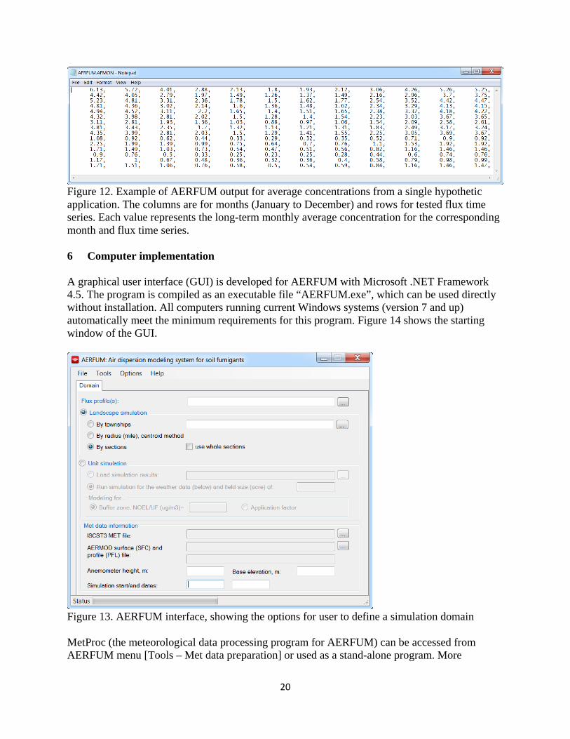
Figure 12. Example of AERFUM output for average concentrations from a single hypothetic application. The columns are for months (January to December) and rows for tested flux time series. Each value represents the long-term monthly average concentration for the corresponding month and flux time series. 6 Computer implementation A graphical user interface (GUI) is developed for AERFUM with Microsoft .NET Framework 4.5. The program is compiled as an executable file “AERFUM.exe”, which can be used directly without installation. All computers running current Windows systems (version 7 and up) automatically meet the minimum requirements for this program. Figure 14 shows the starting window of the GUI.

Figure 13. AERFUM interface, showing the options for user to define a simulation domain MetProc (the meteorological data processing program for AERFUM) can be accessed from AERFUM menu [Tools – Met data preparation] or used as a stand-alone program. More

21

information on the MetProc program and demonstrations are documented in another report (Luo, 2017). In addition to the executable file, supporting data and programs for AERFUM are required in the same folder:

1) USEPA programs, available from the website of USEPA Support Center for Regulatory Atmospheric Modeling (SCRAM, https://www.epa.gov/scram/air-quality-dispersion-modeling-preferred-and-recommended-models). AERFUM uses the latest versions (as of 8/9/2018): AERMET v18081, AERMINUTE v15272, AERSURFACE v13016, AERMAP v18081, AERMOD v18081, and ISCST3 v02035.

2) The National Elevation Dataset (NED) at the resolution of 1 arc-second, which can be obtained through the USGS Multi-Resolution Land Characteristics Consortium (https://www.mrlc.gov/). Downloaded images should be converted to GeoTIFF format to be read by AERMAP. See AERMAP document Section 2.2.1 for more information (USEPA, 2018).

For multi-year model runs, AERFUM supports parallel computation with up to 5 CPU threads (Figure 15). Given the popular PC configurations (8-thread CPU, as in most of DPR computers), the 5-thread parallel computation is the most efficient settings for the model applications with the most recent five years of consecutive meteorological data as recommended by USEPA (2015). When the five assigned CPUs are fully loaded for modeling, AERFUM takes about 80% of total CPU usage in an 8-thread computer.

Figure 14. AERFUM parallel computation for multi-year modeling (showing the modeling progress for 2011 simulated by the first assigned CPU)

22

For model applications with monitoring data, a simple plotting function is provided in AERFUM for graphically comparing the predicted and observed concentrations (Figure 16). A user can plot results for different sites and from different model runs (if batch runs are conducted). The modeling results for the concentration values are saved in a data table (see Section 5.4 for more information).

Figure 15. AERFUM predicted concentrations plotted with monitoring data 7 Model evaluation The modeling performance of AERFUM/AERMOD (AERFUM with AERMOD as the simulation engine) has been evaluated with the 1,3-D monitoring data collected by DPR, ARB, and DAS in 19 stations during 2006-2017 (Luo, 2019). Predicted and observed annual averages were compared in 52 data sets organized by monitoring site and year. The results indicated that AERFUM/AERMOD satisfactorily simulated the monitoring data. Most of predicted annual concentrations were within the factor of 2 of the measured values. In addition, no consistent over- or under-prediction was observed for each monitoring site during multi-year simulations. Some extremely high values of measurements were not captured by the model at the location of monitoring sites. Therefore, AERFUM was further tested as spatially distributed modeling with a Cartesian network of receptors; the results simulated the measured concentrations well in terms of numerical values and probability distributions over the monitoring area.

23

Acknowledgments

The author acknowledges Bruce Johnson, Jing Tao, Jazmin Gonzalez, Colin Brown, Maziar Kandelous, Minh Pham, Edgar Vidrio, Pam Wofford, Karen Morrison, and Randy Segawa for valuable discussions and critical reviews in the initialization and development of this study.

References

Barry, T. (2006). Development of methyl isothiocyanate buffer zones using the probabilistic exposure and risk model for fumigants version 2 (PERFUM2) (https://www.cdpr.ca.gov/docs/emon/pubs/ehapreps/analysis_memos/1776_andrews.pdf, 20 pages, accessed 3/12/2019). California Department of Pesticide Regulation, Sacramento, CA.

Barry, T. (2007). Development of additional methyl isothiocyanate buffer zones for the metam sodium mitigation proposal (https://www.cdpr.ca.gov/docs/emon/pubs/ehapreps/analysis_memos/1884_Andrws_MITC.pdf, 27 pages, accessed 3/12/2019). California Department of Pesticide Regulation,Sacramento, CA.

Barry, T. (2014). Development of Chloropicrin buffer zones - revised, 62 pages. California Department of Pesticide Regulation, Sacramento, CA.

Barry, T. (2015). Evaluation of the Air Dispersion Modeling Tool SOFEA2 (http://www.cdpr.ca.gov/docs/emon/pubs/ehapreps/analysis_memos/2543_sofea.pdf, 14 pages, accessed 3/12/2019). California Department of Pesticide Regulation, Sacramento, CA.

Barry, T. and B. Johnson (2007). Analysis of the relationship between percentiles of the whole field buffer zone distribution and the maximum direction buffer zone (https://www.cdpr.ca.gov/docs/emon/pubs/ehapreps/analysis_memos/1959_segawa.pdf, 48 pages, accessed 3/12/2019). California Department of Pesticide Regulation, Sacramento, CA.

Barry, T. and E. Kwok (2016). Updated (no December applications allowed) simulation of cancer risks associated with different township cap scenarios of Merced County for 1,3-dichloropropene (http://www.cdpr.ca.gov/docs/whs/pdf/1_3_d_cancer_risk_memo.pdf, 13 pages, accessed 3/12/2019). California Department of Pesticide Regulation, Sacramento, CA.

Brown, C. (2018). HYDRUS-simulated flux estimates of 1,3-Dichlorpropene max period-averaged flux and emission ratio for approved application methods (under review). California Department of Pesticide Regulation, Sacramento, CA.

CDFW (2015). CDFW Projection and Datum Guidelines (https://nrm.dfg.ca.gov/FileHandler.ashx?DocumentID=109326, 3 pages, accessed 3/12/2019). California Department of Fish and Wildlife, Sacramento, CA.

Cryer, S. (2005). Predicting Soil Fumigant Air Concentrations under Regional and Diverse Agronomic Conditions. Journal of Environmental Quality 34(6): 2197-2207.

DPR (2001). Suggested Permit Conditions for Using 1,3-Dichloropropene Pesticides (Fumigant), https://www.cdpr.ca.gov/docs/county/cacltrs/penfltrs/penf2001/2001031.pdf. California Department of Pesticide Regulation, Sacramento, CA.

24

DPR (2017a). Additional Labeling Requirements for Use of All Products Containing Chloropicrin as an Active Ingredient in California (https://www.cdpr.ca.gov/chloropicrin.htm). California Department of Pesticide Regulation, Sacramento, CA.

DPR (2017b). Appendix J: 1,3-Dichloropropene (Field Fumigant) Recommended Permit Conditions, in Pesticide Use Enforcement Program Standards Compendium, Volume 3, Restricted Materials and Permitting (http://www.cdpr.ca.gov/docs/enforce/compend/vol_3/rstrct_mat.htm). California Department of Pesticide Regulation, Sacramento, CA.

DPR (2018). Pesticide Use Reporting (PUR) (https://www.cdpr.ca.gov/docs/pur/purmain.htm). California Department of Pesticide Regulation, Sacramento, CA.

Gonzalez, J. (2018). Processing of Dow AgroSciences-submitted 1,3-Dichloropropene township cap tracking data (under review). California Department of Pesticide Regulation, Sacramento, CA.

Johnson, B. (2001). Evaluating the Effectiveness of Methyl Bromide Soil Buffer Zones in Maintaining Acute Exposures Below a Reference Air Concentration (https://www.cdpr.ca.gov/docs/emon/pubs/ehapreps/eh0010.pdf, 117 pages, accessed 3/12/2019). California Department of Pesticide Regulation, Sacramento, CA.

Johnson, B. (2007a). Simulation of concentrations and exposure associated with Dow AgroSciences-proposed township caps for Ventura County for 1,3-dichloropropene (http://www.cdpr.ca.gov/docs/emon/pubs/ehapreps/analysis_memos/ventur_telone.pdf, 22 pages, accessed 3/12/2019). California Department of Pesticide Regulation, Sacramento, CA.

Johnson, B. (2007b). Simulation of Concentrations and Exposure Associated with Dow Agrosciences-Proposed Township Caps for Merced County for 1,3-Dichloropropene (http://www.cdpr.ca.gov/docs/emon/pubs/ehapreps/analysis_memos/mercd_telone.pdf, 12 pages, accessed 3/12/2019). California Department of Pesticide Regulation, Sacramento, CA.

Johnson, B. (2014a). Registration evaluation report, tracking id #263794 (DPR internal webpage, http://em/localdocs/pubs/rr_revs/rr1458.pdf, 31 pages, accessed 3/12/2019). California Department of Pesticide Regulation, Sacramento, CA.

Johnson, B. (2014b). Comparison of One-Year Township Monitoring Results From Merced to SOFEA Simulation Results (http://www.cdpr.ca.gov/docs/emon/pubs/ehapreps/analysis_memos/2493_sofea-to-dasmonit.pdf, 17 pages, accessed 3/12/2019).

Johnson, B. and S. Powell (2005). Interim statewide caps analysis for 1,3-Dichloropropene, 55 pages. California Department of Pesticide Regulation, Sacramento, CA.

Luo, Y. (2017). Meteorological data processing for ISCST3 and AERMOD (http://www.cdpr.ca.gov/docs/emon/pubs/ehapreps/analysis_memos/metproc_final.pdf, 13 pages, accessed 3/12/2019). California Department of Pesticide Regulation, Sacramento, CA.

Luo, Y. (2019). Evaluating AERMOD for simulating ambient concentrations of 1,3-Dichloropropene. California Department of Pesticide Regulation, Sacramento, CA.

Reiss, R. and J. Griffin (2006). A probabilistic model for acute bystander exposure and risk assessment for soil fumigants. Atmospheric Environment 40(19): 3548-3560.

25

Ross, L. J., B. Johnson, K. D. Kim and J. Hsu (1996). Prediction of Methyl Bromide Flux from Area Sources Using the ISCST Model. Journal of Environmental Quality 25(4): 885-891.

Rotondaro, A. and I. van Wesenbeeck (2012). Montoring of Cis-and Trans-1,3Dichlorpopropene in air in 9 high 1,3-Dichlorpopropene use townships Merced County, California. Regulatory Sciences and Government Affairs – Indianapolis Lab. DowAgroSciences LLC. 9330 Zionville Road, Indianapolis, Indiana 46268-1054. Data volume50046-0220 parts 1 and 2.

Segawa, R. (1997). Description of computer modeling procedures for methyl bromide, 9 pages. California Department of Pesticide Regulation, Sacramento, CA.

Segawa, R., T. Barry and B. Johnson (2000). Recommendations for methyl bromide buffer zones for field fumigations (https://www.cdpr.ca.gov/docs/specproj/tribal/recsformebrbuffzones.pdf, 22 pages, accessed 3/12/2019). California Department of Pesticide Regulation, Sacramento, CA.

Sullivan, D. A., M. T. Holdsworth and D. J. Hlinka (2004). Monte Carlo-based dispersion modeling of off-gassing releases from the fumigant metam-sodium for determining distances to exposure endpoints. Atmospheric Environment 38(16): 2471-2481.

Tao, J. (2015). AERMOD Modeling for Two Air Monitoring Studies of Structural Fumigation With Sulfuryl Fluoride (http://www.cdpr.ca.gov/docs/emon/pubs/ehapreps/analysis_memos/tao_sulfuryl_fluoride.pdf, 27 pages, accessed 3/12/2019). California Department of Pesticide Regulation, Sacramento, CA.

Tao, J. (2018a). Modeling a 1,3-Dichloropropene Application at Shafter, CA on January 21, 2018 (https://www.cdpr.ca.gov/docs/emon/pubs/ehapreps/analysis_memos/modeling_1,3-d_shafter.pdf, 5 pages, accessed 3/12/2019). California Department of Pesticide Regulation, Sacramento, CA.

Tao, J. (2018b). Modeling a 1,3-Dichloropropene Application at Parlier, CA on September 19, 2017 (https://www.cdpr.ca.gov/docs/emon/pubs/ehapreps/analysis_memos/modeling_1,3-d_parlier.pdf, 6 pages, accessed 3/12/2019). California Department of Pesticide Regulation, Sacramento, CA.

Tao, J. (2019). Modeling 1,3-Dichloropropene Applications at Parlier, CA on October 9, 2018 (https://www.cdpr.ca.gov/docs/emon/pubs/ehapreps/analysis_memos/modeling_1,3-d_parlier_2019.pdf, 10 pages, accessed 3/18,2019). California Department of Pesticide Regulation, Sacramento, CA.

USEPA (2005a). 40 CFR Appendix W to Part 51, Guideline on Air Quality Models. USEPA (2005b). Revision to the guideline on air quality models: adoption of a preferred general

purpose (flat and complex terrain) dispersion model and other revisions; final rule. 40 CFR Part 51. United States Environmental Protection Agency, Washington, DC.

USEPA (2015). Guideline on Air Quality Models: Enhancements to AERMOD Dispersion Modeling System and Incorporation of Approaches to Address Ozone and Fine Particulate Matter (EPA-HQ-OAR-2015-0310-0154). U.S. Environmental Protection Agency, Office of Air Quality Planning and Standards, Research Triangle Park, NC.

USEPA (2018). User's Guide for the AERMOD Terrain Preprocessor (AERMAP), v18081 (EPA-454/B-18-004). U.S. Environmental Protection Agency, Office of Air Quality Planning and Standards, Research Triangle Park, NC.

26

van Wesenbeeck, I. J., S. A. Cryer and O. de Cirugeda Helle (2013). Validation of SOFEA2 with 1,3-Dichloropropene ambient monitoring data in Merced County California – REVISED report [revised March 2014]. Regulatory Science and Governnment Affairs, Dow AgroSciences LLC 9330 Zionsville Road, Indianapolis, Indiana 46268-1054. Lab Study ID 131271.