advisors and asset prices: a model of the origins of · pdf fileadvisors and asset prices: a...

NBER WORKING PAPER SERIES

ADVISORS AND ASSET PRICES:A MODEL OF THE ORIGINS OF BUBBLES

Harrison HongJose A. Scheinkman

Wei Xiong

Working Paper 13504http://www.nber.org/papers/w13504

NATIONAL BUREAU OF ECONOMIC RESEARCH1050 Massachusetts Avenue

Cambridge, MA 02138October 2007

We thank Kerry Back, Henry Cao, John Eatwell, Simon Gervais, Ming Huang, Robert Jarrow, MaureenO'Hara, Jacob Sagi, Robert Shiller, Sheridan Titman, Pietro Veronesi, and seminar participants at theBank of England, Cornell University, St. Louis Federal Reserve Bank, 2006 American Finance AssociationAnnual Meeting in Philadelphia, 12th Mitsui Life Symposium at University of Michigan, Cambridge-PrincetonConference on Finance, CEPR/Pompeu Fabra Bubble Conference, Duke-UNC Asset Pricing Conference,Financial Intermediation Research Society Conference in Shanghai and NBER Behavioral FinanceConference for helpful comments. We thank the National Science Foundation for financial supportunder grants SES0350770 and SES0718407. The views expressed herein are those of the author(s)and do not necessarily reflect the views of the National Bureau of Economic Research.

© 2007 by Harrison Hong, Jose A. Scheinkman, and Wei Xiong. All rights reserved. Short sectionsof text, not to exceed two paragraphs, may be quoted without explicit permission provided that fullcredit, including © notice, is given to the source.

Advisors and Asset Prices: A Model of the Origins of BubblesHarrison Hong, Jose A. Scheinkman, and Wei XiongNBER Working Paper No. 13504October 2007JEL No. G1,G14,G2

ABSTRACT

We develop a model of asset price bubbles based on the communication process between advisorsand investors. Advisors are well-intentioned and want to maximize the welfare of their advisees (likea parent treats a child). But only some advisors understand the new technology (the tech-savvies);others do not and can only make a downward-biased recommendation (the old-fogies). While smartinvestors recognize the heterogeneity in advisors, naive ones mistakenly take whatever is said at facevalue. Tech-savvies inflate their forecasts to signal that they are not old-fogies, since more accurateinformation about their type improves the welfare of investors in the future. A bubble arises for a widerange of parameters, and its size is maximized when there is a mix of smart and naive investors inthe economy. Our model suggests an alternative source for stock over-valuation in addition to investoroverreaction to news and sell-side bias.

Harrison HongBerndheim Center for FinancePrinceton University26 Prospect AvenuePrinceton, NJ [email protected]

Jose A. ScheinkmanDepartment of EconomicsPrinceton UniversityPrinceton, NJ 08544-1021and [email protected]

Wei XiongPrinceton UniversityDepartment of EconomicsBendheim Center for FinancePrinceton, NJ 08450and [email protected]

“To be against what is new is not to be modern. Not to be modern is to write

yourself out of the scene. Not to be in the scene is to be nowhere.” Tom Wolfe,

The Painted Word

1. Introduction

What are the origins of speculative asset price bubbles? This question remains unanswered

despite a large and growing literature on speculative trading and asset price bubbles in

economics. Motivated in part by the behavior of internet stocks during the late nineties, a

surge in new research has arrived at two conclusions. The first is that differences of opinion

among investors and short sales constraints are sufficient to generate a price bubble.1 The

second is that once a bubble begins, it is difficult for smart money to eliminate the mispricing

(i.e. there are limits of arbitrage).2 All these studies take as given that investors disagree

about asset values. But where does this divergence of opinion come from?

In this paper, we develop a model of the origins of bubbles. Two sets of stylized facts

motivate our analysis. The first is that asset price bubbles tend to occur during periods of

excitement about new technologies.3 In the U.S., speculative episodes have coincided with the

following major technological breakthroughs: (1) railroads, (2) electricity, (3) automobiles,

(4) radio, (5) micro-electronics, (6) personal computers, (7) biotechnology, and most recently

(8) the Internet.4 The second is that in the aftermath of the Internet bubble, the media and

regulators placed much of the blame on biased advisors for manipulating the expectations

of naive investors. While not directly related to the Internet experience, indirect evidence

from academic research in support of this view held by the media and regulators include:

(1) analyst incentives to generate biased, optimistic forecasts; (2) naive individual investors

who do not recognize that these biased recommendations are motivated by incentives to sell1See, e.g., Miller (1977), Harrison and Kreps (1978), Chen, Hong and Stein (2002), and Scheinkman and

Xiong (2003). Extensive empirical work confirming this premise include Diether, Malloy and Scherbina (2002),Lamont and Thaler (2003), and Ofek and Richardson (2003). This literature stands in contrast to the rationalbubble literature (see, e.g., Blanchard and Watson, 1982) in which these two ingredients are not crucial inan infinite horizon setting. However, Allen, Morris, and Postlewaite (1993) show that these two ingredientsemerge as relevant again to generate a rational bubble in a finite horizon setting.

2See, e.g., Shleifer and Vishny (1997), Abreu and Brunnermeier (2003).3See, e.g., Malkiel (2003), Nairn (2002), Shiller (2000).4See DeMarzo, Kaniel and Kremer (2006) and Pastor and Veronesi (2006) for rational explanations of high

stock prices for new technologies.

1

stocks; and (3) analysts’ optimistic forecasts have an impact on prices.5

We focus on the role of advisors and their communication process with investors in gen-

erating divergence of opinion and asset price bubbles. Building on the existing literature, we

assume that there are two types of investors, smart and naive, who are short sales constrained.

While smart investors recognize the heterogeneity in advisors, naive ones take whatever rec-

ommendations they receive at face value. Importantly, all advisors are well-intentioned in

that they care about the welfare of their advisees and want to honestly disclose their signals

to investors. We also assume that at times of technological innovation, only some advi-

sors understand the new technology (the tech-savvies); others do not and can only make

a downward-biased recommendation (the old-fogies). We also consider an alternative as-

sumption in which the old-fogies are replaced by dreamers who only issue upward-biased

recommendations. The divergence of opinion and price bias results do not depend on this as-

sumption but the old-fogey assumption is more theoretically interesting and there is evidence

that it is relevant at a minimum for the recent internet experience.6

A key contribution of our model is that it serves as a warning that even if a stock appears

over-valued, it may not be due to investors overreacting to news nor to sell-side bias. We

are not disclaiming the role of sell-side bias in the dot-com bubble—only that such bias is

not needed to generate asset price bubbles. Indeed, it is not clear that such bias can explain

bubbles that have occurred during earlier periods. We observe that during the dot-com

period, even so-called objective research firms with no investment-banking business, such as

Sanford and Bernstein, issued recommendations every bit as optimistic as investment banks5See, e.g., Lin and McNichols (1998), Hong and Kubik (2003) for evidence on analyst incentives, Malmendier

and Shantikumar (2004) for evidence on investor reaction to recommendations and Michaely and Womack(1999) for evidence on price impact.

6Throughout The Painted Word, from which our epigraph is drawn, Tom Wolfe describes the loss ofcredibility suffered by art critics who were perceived as not ”getting” the new pop art movement of the latefifties. There is ample anecdotal evidence suggesting that advisors during the dot-com bubble faced similarconcerns. For instance, Stanley Druckenmiller, a self-confessed old economy dinosaur and value investor,reversed course during the Internet boom period and declared that he understood the Internet after a meetingwith guru Andrew Grove (see Pacelle, 2000). Famous examples of old-fogies include Jonathan Cohen, asell-side analyst covering Internet stocks for Merrill Lynch who was fired for his skeptical reports about theInternet. In contrast, Mary Meeker, a vocal proponent of the Internet revolution, not only prospered duringthe Internet era but continues to be an influential voice in technology even after the bursting of the bubble.Finally, there also is evidence that young mutual fund managers were more aggressively holding technologystocks during the dot-com bubble as compared to their older counterparts (see, e.g. Greenwood and Nagel,2006).

2

(see, e.g., Cowen, Groysberg, and Healy, 2003).7 This suggests that there must exist other

causes of upward biased forecasts by advisors aside from the sell-side incentives of analysts.

Moreover, we think of our model as applying more broadly to other advisors such as buy-side

analysts who are likely to be a more important part of the market. In short, our paper is

an exploration of an alternative and potentially more theoretically interesting mechanism for

generating divergence of opinion as opposed to simply assuming investors overreact to news

or are overly exuberant.

More specifically, we consider an economy with a single asset, which we call the new

technology stock. There are three dates, 0, 1 and 2. At date 0, advisors are randomly

matched with investors (the advisees). Advisors also observe the terminal payoff (which is

realized at date 2) and can send signals about this payoff to their advisees at date 0. A tech-

savvy can send whatever signal he wants, while an old-fogey, who does not understand the

new technology, is limited to a downward-biased signal. The investor type is unknown to the

advisor, and the advisor type is unknown to the investor. The advisor-investor relationship

is similar to that of a parent and teenaged child, in which the smart teenager is not sure

whether dad is cool, and the cool dad tries to impress his teenaged child because he wants

his child to heed his advice in the future.

At date 1, these advisors are randomly matched with a new set of investors. These

investors can invest in a separate risky project requiring an initial fixed cost. Advisors

again receive information about this risky project, which pays off at date 2. Once again, a

tech-savvy can send whatever signal he wants, while an old-fogey is restricted to a downward-

biased signal. Each investor has access to the track record of his advisor, namely the signal

(or recommendation) that was sent by the latter at date 0. A smart investor can use this

information to update his belief about his advisor’s type.

To put this simple model into some context, think of the advisor at date 0 as a sell-side

analyst covering technology stocks, but (counterfactually) with only good intentions. Date

1 represents the future career opportunities of this analyst; for example, sell-side analysts

typically become advisors to hedge funds or corporations later in their careers. Importantly,7Moreover, Grosyberg et al. (2005) find that buy-side analysts (those working at mutual funds with-

out brokerage or investment banking relationships) issue even more optimistic forecasts than their sell-sidecounterparts.

3

what the advisor says at date 0 can be used for or against him at date 1. The updating of a

smart investor’s belief about his advisor’s type is a key driver of our model.

We first consider the equilibrium at date 1. Because of uncertainty about advisor type,

smart investors may end up making investments when they should not, since they are not

sure whether a negative signal (i.e., a signal value less than the fixed cost of investing) is

truly negative or if it just came from an old-fogey. We solve for a Bayesian-Nash equilibrium

in the reporting strategies of the advisors and the investment policies of the advisees. In

this equilibrium, tech-savvy advisors bias their signals downward over the set of states in

which it is not efficient for the advisee to invest. By downwardly biasing their signals over

these states, the tech-savvy advisors lead the smart advisees to conclude that a certain set

of negative signals cannot be generated by tech-savvy advisors. This signaling enables smart

investors to avoid at least some inefficient investments. However, it also imposes a dishonesty

cost upon the tech-savvy advisor, and this dishonesty cost is incurred per advisee.

As a result, the tech-savvy advisor has an incentive to establish a better reputation

at date 0 through his recommendation about the technology stock, since smart investors

subsequently will use his date 0 recommendation to update their beliefs on his type. The

stronger his reputation among smart investors becomes at date 1, the more easily he can

avoid dishonesty costs in inducing his advisees to make efficient investments in that period.

This reputational incentive leads the tech-savvy advisor to inflate his forecasts to signal his

type to smart investors. We show that such a Bayesian-Nash equilibrium exists at date 0.

While smart advisees properly deflate this upward bias, naive investors unfortunately take

what the advisor says at face value.

We show that a price bubble can arise as a result of this signaling equilibrium. It is im-

portant to note that the assumption about heterogeneity in advisor types (tech-savvies versus

old-fogies) does not bias the results in our favor. To the contrary, this assumption, in com-

bination with our assumption of investor heterogeneity, would tend to produce a downward

bias in prices since naive investors take whatever old-fogies say at face value. In other words,

the effect of optimistic signaling by well-intentioned tech-savvies has to be strong enough to

overcome this baseline downward bias. It is not clear ex ante that this need be the case.

However, we show that such a technology price bubble does exist when there is a sufficient

4

number of naive investors guided by tech-savvy advisors.

To develop intuition for the price bias, let’s consider two polar cases. First, suppose

that there are only smart investors in the economy. In equilibrium, tech-savvy advisors will

tend to bias their forecasts upward so as to distinguish themselves from old-fogies. However,

smart investors understand this and in equilibrium will adjust their beliefs accordingly. In

this case, price will be an unbiased signal of fundamentals. Next, suppose that there are only

naive investors in the economy. In equilibrium, tech-savvy advisors will honestly disclose

their signals since they do not worry about the ability of naive investors to infer their type.

In this case, however, price will typically contain a downward bias due to the pessimistic

recommendations of old-fogies, which the naive investors take at face value.

When both types of investors are present in the economy, the price could be upwardly

biased. Tech-savvy advisors will bias their messages upward, and the extent of this bias in-

creases with the fraction of smart investors. While smart investors can de-bias these messages,

naive investors are unable to do so. Due to short sales constraints, the price is determined by

the marginal buyer and is not affected by investors with a lower valuation. If the marginal

investor is a naive advisee of a tech-savvy, then price will be upwardly biased.

Our theory yields testable implications. For instance, unlike models such as Delong,

Shleifer, Summers and Waldmann (1990), the degree of mispricing in our model is largest

when there are both sets of investors in the economy. Furthermore, we consider a number of

robustness issues. We show that our main results survive when we loosen two assumptions:

(1) allow old-fogies to send biased messages at a cost just like tech-savvies and (2) allow an

investor at date 0 to observe the recommendations of other advisors as well. We also consider

a number of extensions. In our model, smart investors are worried about unduely pessimistic

advisors. However, due to short sales constraints, our pricing results would survive even when

smart investors are worried about unduely optimistic advisors (dreamers). Importantly, our

results are robust to allowing for both dreamers and old-fogeys to simultaneously be in the

economy (see Section 3.3).

Our model is technically about a price bias and not about bubbles. We intentionally

neglect the key element of speculative trading (i.e., buying in anticipation of capital gain)

modelled elsewhere to keep things simple. But it is similar in spirit to models of speculative

5

trading driven by heterogeneous beliefs and offers an important new rationale for investor

divergence of opinion.

Our theory is related to the literature on costly signaling (see, e.g., Kreps, 1990; Fudenberg

and Tirole, 1991). A key theme that this paper shares with earlier work is that concerns about

reputation can affect the actions of agents who try to shape their reputations (Holmstrom

and Ricart i Costa, 1986; Holmstrom, 1999). Previous studies have shown that reputational

incentives can lead agents to take perverse actions, such as saying the expected thing which

may lead to information loss (Scharfstein and Stein, 1990; Ottaviani and Sorensen, 2006),

adopting a standard of conformist behavior (Bernheim, 1994) or making politically correct

statements so as to not look racist (Morris, 2001). More specifically, our model, similar to

Morris (2001) but unlike the others, emphasizes the perverse reputational incentives of a well-

intentioned advisor: in our model, the well-intentioned tech-savvy advisor engages in costly

signaling at date 0 so as to better help future investors. This contrasts with career-concerns-

based models such as Scharfstein and Stein (1990) in which the advisor does not know his

own type and engages in signal jamming to achieve a better reputation for his own personal

gain. Our work departs from the existing literature on reputational signaling by focusing on

the interaction of sophisticated agents (tech-savvies and smart investors) and naive agents

(old-fogies and naive investors), in a model that is geared toward examining implications for

asset pricing.

Finally, our paper complements interesting recent work by Hirshleifer and Teoh (2003) on

the disclosure strategies of firms when some of their investors have limited attention. Like us,

they emphasize the importance of introducing boundedly rational agents in understanding

the effect of disclosures on asset prices. Unlike us, they focus on how the presentation of

information may lead to different results with inattentive investors and the resulting incentives

of managers to potentially manipulate earnings to fool inattentive investors.

Our paper is organized as follows. We present the model and discuss related empirical

implications in Section 2. We consider robustness and extensions in Section 3. In Section

4, we conclude with a reinterpretation of the events of the Internet period in light of our

findings. Proofs are presented in the Appendix.

6

2. Model

2.1. Set-up

We consider the pricing of a single traded asset, which we call the new technology or tech

stock. There are three dates, denoted by t = 0, 1, 2. The stock pays a liquidating dividend

at t = 2 given by

v = θ + ε, (1)

where θ is uniformly distributed on the interval [0, 1], and ε is normally distributed with a

mean of zero and a variance of σ2.

There are two types of advisors in the economy: those who are tech-savvy (with a mass of

π0 ∈ [0, 1] in the population) and those who are old-fogies (with a remaining mass of 1−π0).

Advisor type is unknown to investors. Tech-savvy advisors observe θ (i.e., they understand

the new technology) and send a report to investors at t = 0, denoted by sTS0 . We assume that

tech-savvy advisors are well-intentioned in two respects: they want to tell the truth, and they

also want to maximize the welfare of their advisees at t = 1. The truth-telling preference is

captured by an assumption that tech-savvies incur a dishonesty cost if they report a signal

different from the truth. This cost is given by

c(sTS0 − θ)2, (2)

where c > 0. As we shall see, a tech-savvy advisor may choose to incur some dishonesty

cost and strategically bias his report upward to improve the welfare of his future clients.8 In

contrast to the tech-savvy advisors, old-fogies do not understand the new technology and can

only send a report that is a downward-biased version of the truth. We assume that old-fogies

are not aware of their bias and truthfully report their common belief at t = 0:9

sOF0 = aθ, (3)

8 For simplicity, we assume that tech-savvy advisors have a dishonesty cost at t = 0 instead of explicitlyincorporating the welfare of the advisees at t = 0. Our results remain when incorporating their welfare butthe conditions are less transparent.

9We will relax this assumption in Subsection 3.2 by allowing old-fogies to inflate their signals by incurringa dishonesty cost. We will show that this extension does not affect our main results.

7

where a ∈ [0, 1). Thus, the report sent by the old-fogies will always be a fraction of the true

value.

There are also two types of investors at t = 0: smart ones (with a mass of ρ ∈ [0, 1] in

the population) and naive ones (with a remaining mass of 1 − ρ). Investor type is unknown

to advisors. Each investor is randomly matched with one advisor and only has access to

the report from this advisor.10 Smart investors are aware of the existence of old-fogies and

take into account the optimal reporting strategy of tech-savvy advisors in inferring their

advisors’ types from the messages sent by those advisors. Naive investors are not aware

of the heterogeneity in advisors and simply take the messages sent to them at their face

values.11 We assume that both smart and naive investors are risk neutral and take positions

to maximize their expected terminal wealth. We also assume that investors cannot short sell

shares and there is an upper bound to the number of shares an investor can hold, which we

denote by k.

At t = 1, the advisors are matched with a new set of investors. For simplicity, we assume

that these investors are risk neutral. Each of these investors has an opportunity to invest

in a different risky (new technology) project. The fixed cost of the project is I, which is a

constant between 0 and 1. The payoff of the project is f , which is uniformly distributed on

the interval [0, 1]. f is independent of θ. Tech-savvy advisors observe f and send a report to

investors at t = 1, denoted by sTS1 . They continue to want to maximize the welfare of their

new advisees and incur a dishonesty cost per advisee of

c(sTS1 − f)2, (4)

where c > 0, if their report differs from the truth. Old-fogies again do not understand this

new technology, and they send a signal at t = 1 given by

sOF1 = af, (5)

where a ∈ [0, 1). We impose a parameter restriction that a ≥ I. This restriction ensures that

at least in some states of the economy an old-fogey advisor would advise investors to invest10We will allow smart investors to access reports from other advisors in the extension to our main model

developed in Subsection 3.2.11This assumption fits with empirical evidence reported by Malmendier and Shantikumar (2004) about the

inability of individual investors to see through the incentives of sell-side analysts.

8

in the project. In addition, we assume that each advisor at t = 1 is randomly matched with

n advisees. Advisor type is unknown to investors.

At t = 1, investors again will rely on the single advisor with whom they are matched in

deciding whether to make an investment. Investors only receive information about the past

reports (at t = 0) of the individual advisors with whom they are matched. Again, there are

two types of investors at t = 1. The smart investor uses the past report from his advisor to

update his belief at t = 1 about his advisor’s type, which we denote by π1. Naive investors

again just take whatever their advisors tell them at face value.

The motivation for the t = 1 set-up is that it is a reduced-form model meant to capture

a stream of future advising engagements in an advisor’s career. More specifically, one can

think of the advisor as a sell-side analyst at date 0 who becomes a consultant to hedge funds

or corporations on other projects later in his career (date 1). Those client institutions at

date 1 have information regarding his track record as a sell-side analyst. The parameter n

captures the number of such future advising engagements. For simplicity, we have assumed

that each advisor interacts with the same number of advisees at t = 1. More realistically,

advisors with better reputations, i.e. higher π1’s, would attract a larger number of advisees

at date 1. This would only help to strengthen our results.

2.2. Equilibrium at t = 1

We begin by deriving a Bayesian-Nash equilibrium for the reporting strategy of the tech-savvy

advisors and the investment policies of investors at date 1. In characterizing this equilibrium,

we will take as given the following property of the date 0 equilibrium: π1, the probability

that the smart investor assigns to the tech-savvy advisor type at date 1, can only take three

values depending upon the report sent at t = 0: 0, πL (a constant) and 1. We will show

that this condition indeed characterizes the outcome from the game at t = 0 in the next

sub-section.

2.2.1. Smart investors have perfect information about advisor type: π1 = 1 or π1 = 0

We begin our analysis of the date 1 equilibrium with the case in which a smart investor knows

for sure whether his advisor is tech-savvy or an old-fogey. We will look for an equilibrium in

9

which the tech-savvy advisor tells the truth and investors follow the efficient investment rule

of investing when their expected values of f are greater than I (the fixed cost of investing).

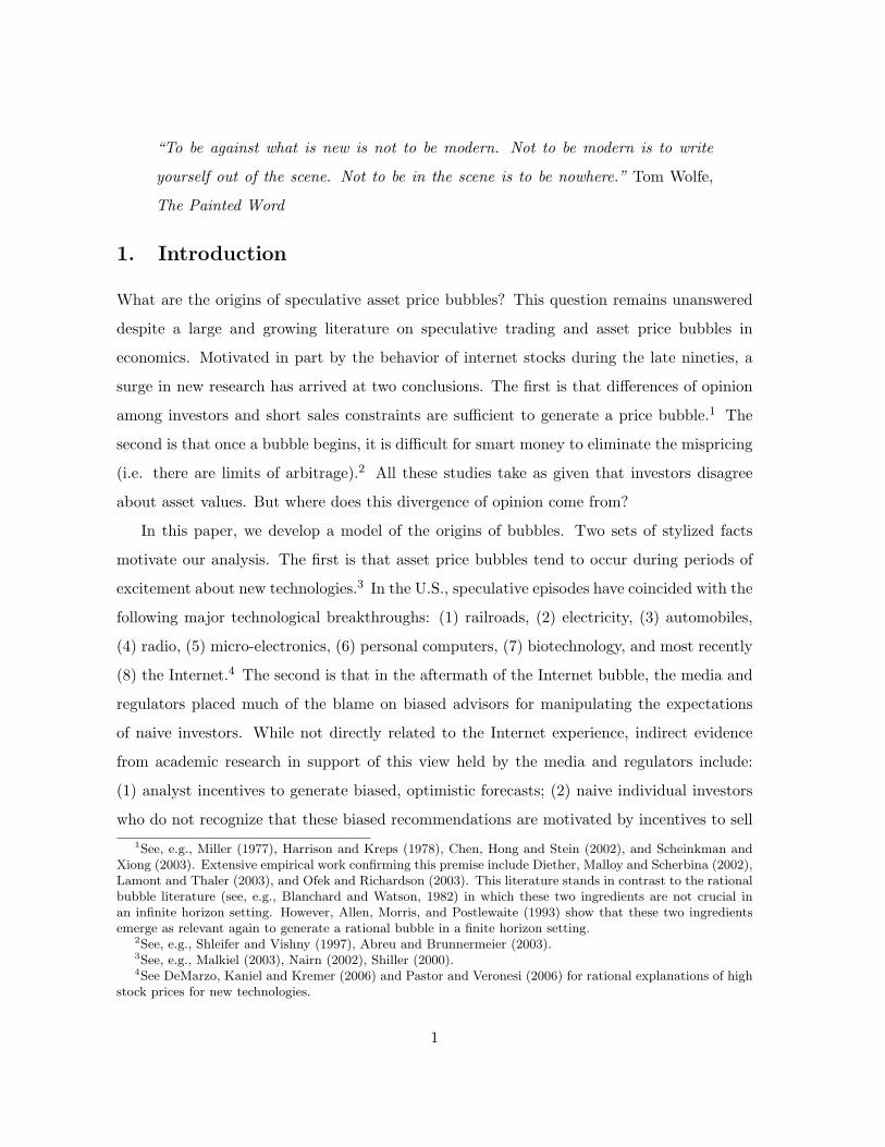
Proposition 1 Suppose that π1 = 1 or π1 = 0. A Bayesian-Nash equilibrium at t = 1

consists of the following profiles. The tech-savvy advisor truthfully reports his information,

i.e. sTS1 = f . The old-fogey reports sOF

1 = af by assumption. A smart investor is able to

deduce f from the message sent by his advisor, denoted by s1, and invests if f ≥ I and does

not invest if f < I. A naive investor invests if s1 ≥ I and does not invest if s1 < I.

I

f

s

0

1

1 I

Tech−savvies’ strategy

Old−fogies’ strategy

a

Figure 1: Advisors’ strategies at t = 1 when investors have perfect information about advisortype. The solid line plots tech-savvy advisors’ strategy for different values of f , while thedashed line plots old-fogey advisors’ strategy.

Fig. 1 illustrates the reporting strategies of tech-savvy and old-fogey advisors. Let’s

check that this is indeed a Bayesian-Nash equilibrium. Given the reporting strategies of the

two types of advisors and the perfect information about advisor type, the smart investor can

deduce f and hence employs the efficient investment rule: invest only if f ≥ I. His expected

gain is

E[max(f − I, 0)] =∫ 1

I(f − I)df =

12(1− I)2. (6)

10

There is nothing to check for the naive investors since we assume that they always listen to

whatever message is sent and invest only if s1 ≥ I. They make an efficient investment decision

if their advisor happens to be tech-savvy but may under-invest if their advisor happens to

be an old-fogey.

Given the investment strategies of the two types of investors, it is optimal for a tech-

savvy advisor to report the truth. He has nothing to gain from deviating from the truth

because the smart investor knows his type while the naive investor listens to whatever he

says. Furthermore, he would incur a dishonesty cost by lying. There is nothing to check for

old-fogies since we assume that they always report sOF1 = af . We therefore have proven that

the profiles described in Proposition 1 constitute a Bayesian-Nash equilibrium.

2.2.2. Smart investors have imperfect information about advisor type: π1 = πL

When smart investors have imperfect information about advisor type at date 1, i.e. π1 =

πL, then a tech-savvy advisor has an incentive to report a downward-biased signal of f for

realizations of f that are neither extremely high nor extremely low. Since a smart investor

does not have perfect information about his advisor’s type, he will infer that signals less than

I may be sent by old-fogies in situations where f ≥ I, which could lead him to invest when he

should not. A tech-savvy advisor can alleviate this problem by discretely biasing his message

downward so as to communicate to a smart advisee that his message must be coming from a

tech-savvy advisor. In doing so, however, the tech-savvy advisor incurs some dishonesty cost

in equilibrium. As we will show in the next subsection, the date 1 dishonesty penalty creates

an incentive for a tech-savvy advisor to incur some initial dishonesty cost at t = 0 so as to

convince future investors of his type.

We begin by formally constructing the Bayesian-Nash equilibrium of the t = 1 sub-game

when π1 = πL.

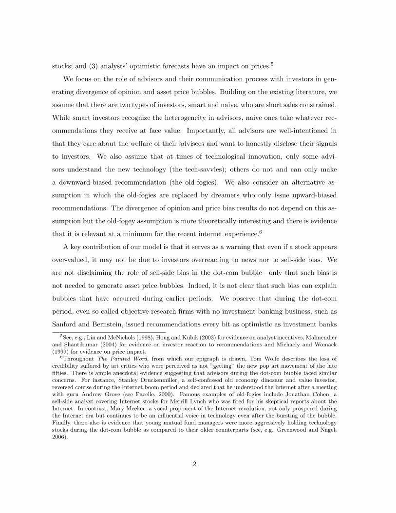
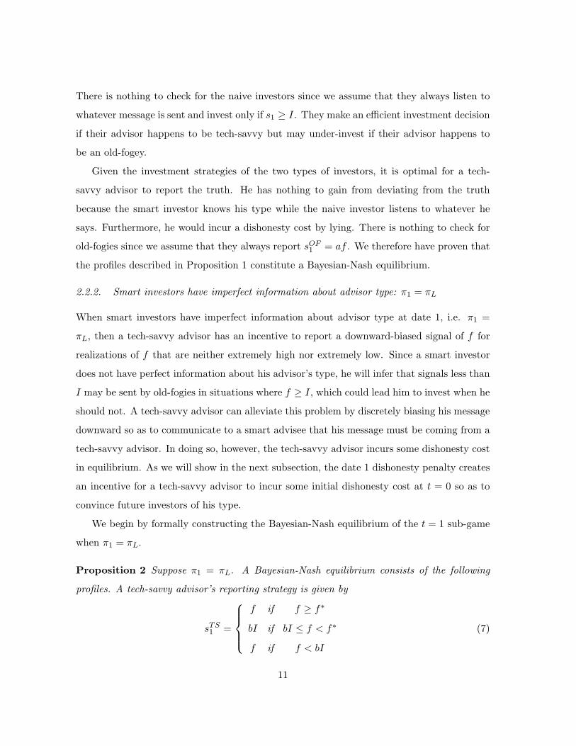
Proposition 2 Suppose π1 = πL. A Bayesian-Nash equilibrium consists of the following

profiles. A tech-savvy advisor’s reporting strategy is given by

sTS1 =

f if f ≥ f∗

bI if bI ≤ f < f∗

f if f < bI

(7)

11

where

b =1

πLL + (1− πLL)/a∈ (a, 1), (8)

with

πLL =πL

πL + (1− πL)/a< πL, (9)

and f∗ solves the equation

c(f∗ − bI)2 = ρ(I − f∗). (10)

The solution of this equation is given by

f∗ =12

√(ρ/c− 2bI)2 + 4(ρI/c− b2I2)− 1

2(ρ/c− 2bI), (11)

and bI < f∗ < I. The old-fogey reports sOF1 = af by assumption. After observing a signal

s1 sent by his advisor, a smart investor will invest if s1 > bI and does not invest if s1 ≤ bI.

A naive investor invests if s1 ≥ I and does not invest if s1 < I.

I

bI f

s

0

1

1 I

bI



f*

f*

a

Figure 2: Advisors’ strategies at t = 1 when investors have imperfect information aboutadvisor type. The solid line plots tech-savvy advisors’ strategy for different values of f , whilethe dashed line plots old-fogey advisors’ strategy.

12

The proof of this proposition is in the Appendix. Fig. 2 illustrates the tech-savvy advisor’s

reporting strategy described in Proposition 2. The tech-savvy advisor deflates his signal to

bI when the fundamental variable f is between bI and f∗ and truthfully reports his signal

when f is outside of this region. Note that (bI, I) is the region of fundamental value in which

smart investors might potentially confuse a truthful signal from a tech-savvy advisor with a

downward biased signal from an old-fogey advisor and make an inferior investment. To offset

this identification problem, the optimal reporting strategy is for the tech-savvy advisor to

downward bias his signal when f is between bIand f∗, where f∗ is a cut-off value given in

the proposition. Given the tech-savvy advisor’s reporting strategy, a smart investor advised

by the tech-savvy advisor avoids an inferior investment when f is between bI and f∗, but

still takes an inferior investment when f is between f∗ and I.

2.2.3. The gain from improved reputation for a tech-savvy advisor

Having characterized our Bayesian-Nash equilibrium across the varying states of informa-

tional completeness regarding advisor type, we now consider the value of the advisor’s rep-

utation from the perspective of a tech-savvy advisor. The advisor’s reputation will affect

the investment strategy of smart investors but has no effect on naive investors. If a tech-

savvy advisor has a perfect reputation, a smart investor’s welfare is given by the expression∫ 1I (f − I)df , which we presented earlier in equation (6). Accordingly, the value of a perfect

reputation to a tech-savvy advisor is

V1 = nρ

∫ 1

I(f − I)df, (12)

which is proportional to the number of advisees he has and the probability that each one is

smart.

If the tech-savvy advisor has an imperfect reputation, the expected investment profit to

a smart investor in our Bayesian-Nash equilibrium is∫ 1

f∗(f − I)df, (13)

since the investor will end up investing when the signal is above f∗. With an imperfect repu-

tation, the tech-savvy advisor incurs a dishonesty cost in equilibrium when the fundamental

13

variable is between bI and f∗. The expected cost per advisee of deflating his message in those

states is ∫ f∗

bIc(f − bI)2df. (14)

Since the tech-savvy advisor cares about both his own dishonesty cost and the smart investors’

gain from investment, the value he obtains from an imperfect reputation is given by

V2 = nρ

∫ 1

f∗(f − I)df −

∫ f∗

bInc(f − bI)2df. (15)

Hence, the incremental gain to the tech-savvy advisor from establishing a perfect reputa-

tion is

V1 − V2 = nρ

∫ I

f∗(I − f)df +

∫ f∗

bInc(f − bI)2df. (16)

The first term represents a gain from preventing smart investors from making inefficient

investments in inferior projects, and the second term represents a gain from avoiding the

dishonesty cost. We derive some simple comparative statics for this gain from a better

reputation.

Proposition 3 The tech-savvy advisor’s gain from improving his reputation, V1 − V2, in-

creases with the number of advisees (n) and the fraction of smart investors in the population

(ρ); and it decreases with the fraction of tech-savvy advisors (π0) and the degree to which

old-fogies behave like tech-savvies (a).

We relegate the proof of Proposition 3 to the Appendix since each of the comparative

statics results can be explained with simple intuition. First, as the number of advisees n at

t = 1 increases, the tech-savvy advisor has to incur more dishonesty costs. Hence, the greater

the number of future advisees, the larger is the gain to establishing a better reputation early

on. Similarly, having a better reputation only matters if there are smart investors around

to use it. The gain to a better reputation thus increases with ρ. On the other hand, the

better the initial reputation (π0), the less valuable is the gain from establishing a perfect

reputation, and hence we find that V1 − V2 decreases in π0. Finally, the larger is a, the more

old-fogies behave like tech-savvies. As the difference between old-fogies and tech-savvies

14

shrinks, investment decisions become more efficient, and the gain to a tech-savvy advisor

from improving his reputation diminishes.

One way to think of the signalling game at t = 1 is that of an advisor (an analyst,

consultant, CEO) without a technology background who is hired by the board of directors

of a technology company to work with the company. A specific example is Louis Gertsner

who took over IBM in the early nineties and is often credited with saving it. Gerstner’s

previous posts had been American Express and RJR Nabisco. He often describes having

to face a skeptical IBM culture in his bid to turnaround IBM (see Gertsner, 2002). In the

context of our model, the advisees are the engineers of IBM who are uncertain about the

quality of Gertsner (whether he is a tech-savvy or an old-fogey). Gertsner had to talk the

IBM engineers out of a number of investments (or changes). His uncertain reputation means

that he had to exaggerate the extent to which he was against an investment to thwart it. As

a result, there is a reward to developing a reputation as a tech-savvy as this will help lower

the cost of having to exaggerate associated with being of an uncertain quality. This is a quite

general point that transcends the specific context of analysts or CEOs.12

2.3. Equilibrium at t = 0

2.3.1. Tech-savvy advisor’s reporting strategy

As we discussed earlier, it is potentially useful for a tech-savvy advisor with good intentions

to develop a good reputation among smart investors, since such a reputation would lessen

the extent of inefficient investment by smart investors at t = 1 and also reduce the advisor’s

dishonesty cost in that period when he tries to minimize the investment inefficiency by biasing

his reports.

In this sub-section, we will construct a Bayesian-Nash equilibrium at t = 0 in which the

tech-savvy advisor biases his reports in an attempt to build a better reputation.

12Indeed, a second example that is less financially related is a professor in a department who might bethought of as being too tough (an old-fogey in terms of standards regarding hiring and not realizing thattimes have changed and there are more jobs now). Hence, he has to be really negative to convince hiscolleagues to not hire someone. A third example is a dad who might be thought of as being an old-fogeyby his kid. If the dad really wants the kid not to try something new, again he has to exaggerate and reallydisapprove to convince his kid.

15

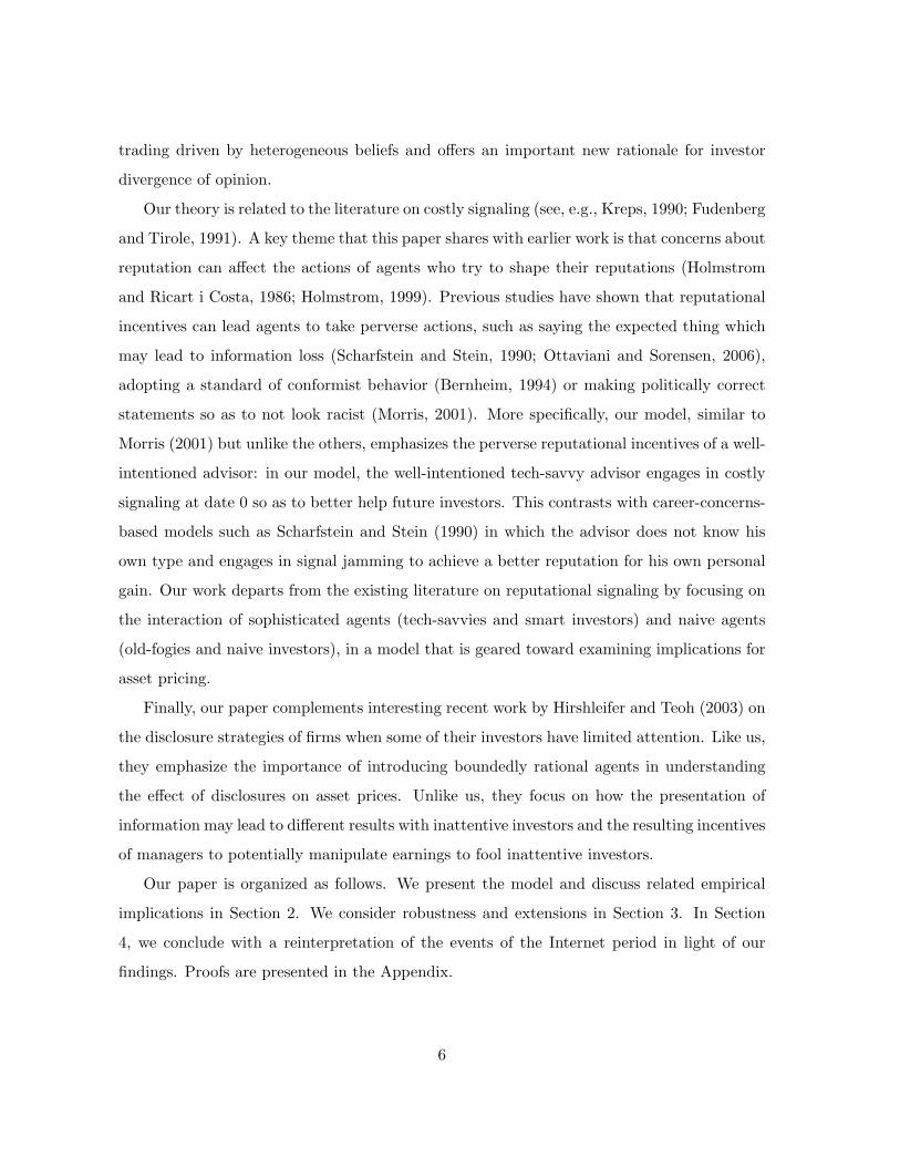
Theorem 1 A Bayesian Nash equilibrium at t = 0 consists of the following profiles. The

reporting strategy of a tech-savvy advisor is

sTS0 =

θ if θ ≥ a

a if θ∗ < θ < a

θ if θ ≤ θ∗

(17)

where θ∗ ∈ [0, a) is a constant determined by

θ∗ =

{a−

√V1−V2

c , if a−√

V1−V2c > 0

0, otherwise. (18)

An old-fogey reports sOF0 by assumption. After observing a signal s0 sent by his advisor, a

smart investor infers the advisor’s type according to the following rule: if s0 ≥ a, the advisor

is tech-savvy for sure (π1 = 1); if θ∗ < s0 < a, the advisor is an old-fogey for sure (π1 = 0);

if s0 ≤ θ∗, the advisor’s type remains unclear, and his reputation as a tech-savvy advisor is

πL =π0

π0 + (1− π0)/a, (19)

which is lower than the advisor’s initial reputation (π0).

a

θ* θ

s

0

1

1 a

θ*

Tech−savvys’ strategy


Figure 3: Advisors’ strategies at t = 0. The solid line plots tech-savvy advisors’ strategy fordifferent values of θ, while the dashed line plots old-fogey advisors’ strategy.

16

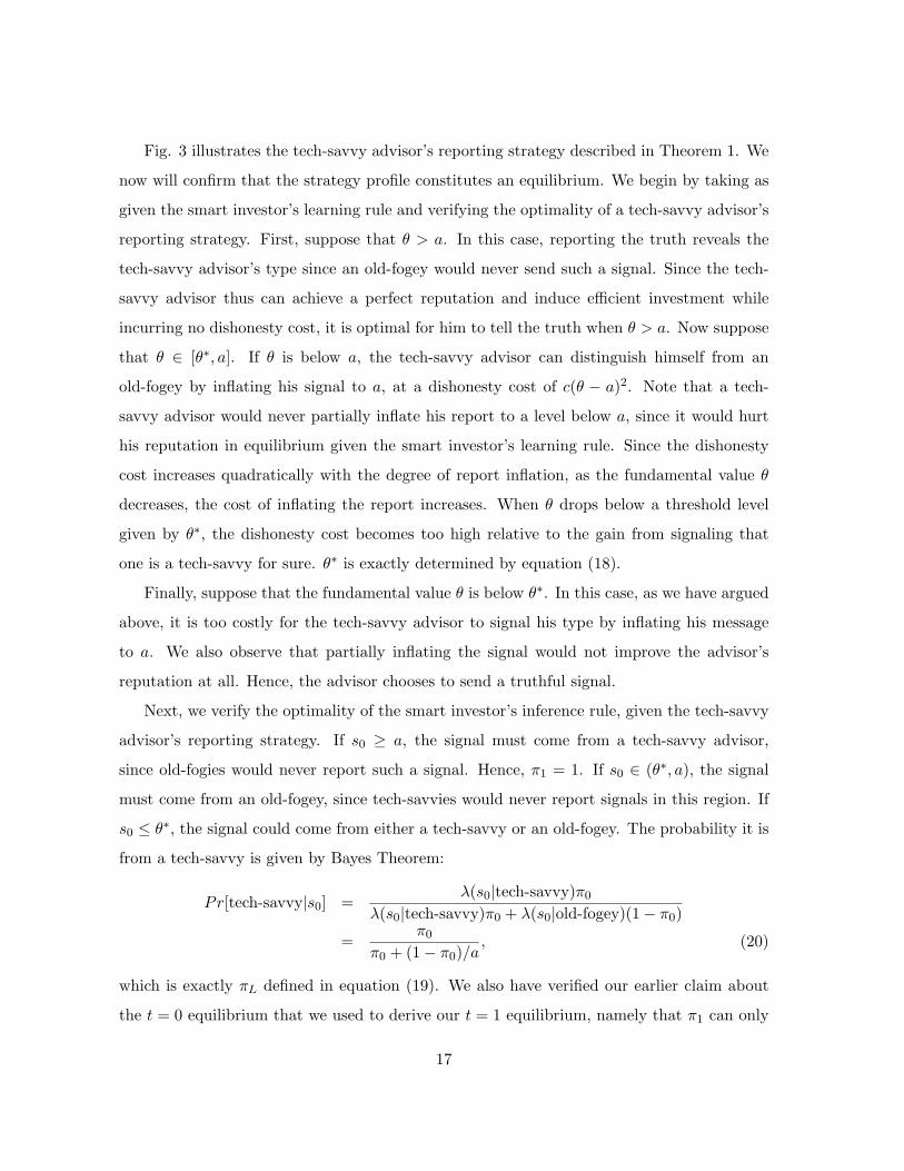
Fig. 3 illustrates the tech-savvy advisor’s reporting strategy described in Theorem 1. We

now will confirm that the strategy profile constitutes an equilibrium. We begin by taking as

given the smart investor’s learning rule and verifying the optimality of a tech-savvy advisor’s

reporting strategy. First, suppose that θ > a. In this case, reporting the truth reveals the

tech-savvy advisor’s type since an old-fogey would never send such a signal. Since the tech-

savvy advisor thus can achieve a perfect reputation and induce efficient investment while

incurring no dishonesty cost, it is optimal for him to tell the truth when θ > a. Now suppose

that θ ∈ [θ∗, a]. If θ is below a, the tech-savvy advisor can distinguish himself from an

old-fogey by inflating his signal to a, at a dishonesty cost of c(θ − a)2. Note that a tech-

savvy advisor would never partially inflate his report to a level below a, since it would hurt

his reputation in equilibrium given the smart investor’s learning rule. Since the dishonesty

cost increases quadratically with the degree of report inflation, as the fundamental value θ

decreases, the cost of inflating the report increases. When θ drops below a threshold level

given by θ∗, the dishonesty cost becomes too high relative to the gain from signaling that

one is a tech-savvy for sure. θ∗ is exactly determined by equation (18).

Finally, suppose that the fundamental value θ is below θ∗. In this case, as we have argued

above, it is too costly for the tech-savvy advisor to signal his type by inflating his message

to a. We also observe that partially inflating the signal would not improve the advisor’s

reputation at all. Hence, the advisor chooses to send a truthful signal.

Next, we verify the optimality of the smart investor’s inference rule, given the tech-savvy

advisor’s reporting strategy. If s0 ≥ a, the signal must come from a tech-savvy advisor,

since old-fogies would never report such a signal. Hence, π1 = 1. If s0 ∈ (θ∗, a), the signal

must come from an old-fogey, since tech-savvies would never report signals in this region. If

s0 ≤ θ∗, the signal could come from either a tech-savvy or an old-fogey. The probability it is

from a tech-savvy is given by Bayes Theorem:

Pr[tech-savvy|s0] =λ(s0|tech-savvy)π0

λ(s0|tech-savvy)π0 + λ(s0|old-fogey)(1− π0)

=π0

π0 + (1− π0)/a, (20)

which is exactly πL defined in equation (19). We also have verified our earlier claim about

the t = 0 equilibrium that we used to derive our t = 1 equilibrium, namely that π1 can only

17

take on one of three values—0, 1, and πL.

The cut-off value θ∗ captures the degree to which the tech-savvy advisor biases his report

in order to build a better reputation. The lower is θ∗, the greater the bias. The bias is

maximal when θ∗ = 0, since this implies that the tech-savvy advisor reports a over the

entire interval [0, a). Thus, a− θ∗ can be interpreted as a measure of the upward bias in the

tech-savvy’s reporting strategy.

Proposition 4 The upward bias of the tech-savvy advisor’s reporting strategy (as measured

by a − θ∗) increases with the number of advisees at t = 1 (n) and the fraction of smart

investors (ρ), and decreases with the fraction of tech-savvy advisors (π0).

The intuition for these comparative statics is similar to that underlying the behavior of

V1 − V2, since the upward bias in the initial report is driven by the incentive to gain a better

reputation.

2.3.2. Asset price at t = 0

We now derive the equilibrium price of the tech stock at t = 0. An individual investor i, who

observes a signal si,0 from his advisor and takes the asset price p as given, chooses his asset

holding xi (shares) to maximize his expected final wealth:

maxxi∈[0,k]

xi[Ei(θ|si,0)− p]. (21)

Note that the investor cannot short sell the asset and can only take a position smaller than

k.13 It is direct to solve the investor’s optimal position:

xi =

{0 if Ei(θ|si,0) < p

k if Ei(θ|si,0) ≥ p(22)

The investor will stay out of the market if the price is too high relative to his belief of the

asset fundamental and will take a maximum position k otherwise.

To derive the equilibrium asset price, we assume that the per capita supply of the asset is

x̄ shares. To make our discussion relevant, we require that k > x̄, i.e., investors in aggregate

can hold the net asset supply.13We could also impose an upper bound on each investor’s position measured in dollars. This would slightly

complicate the notation, but would not affect the qualitative results.

18

Since each investor is paired with a single advisor, there are four possible types of investor-

advisor pairs: smart investors advised by tech-savvy advisors, smart investors advised by old-

fogey advisors, naive investors advised by tech-savvy advisors, and naive investors advised by

old-fogey advisors, in proportions of ρπ0, ρ(1−π0), (1−ρ)π0 and (1−ρ)(1−π0), respectively.

To simplify our discussion, we assume that there are enough investors of each of these four

pairs so that in aggregate any single combination can hold the net asset supply. As a result,

the equilibrium asset price is determined by the highest belief among these classes of investors.

We divide the derivation of the equilibrium asset price into the following three cases.

• Case 1: θ > a. In this case, tech-savvy advisors send a message equal to θ, while

old-fogey advisors send a message equal to aθ. After observing the message from their

advisors, smart investors, irrespective of the type of their advisors, will able to exactly

back out the true fundamental value θ. Naive investors advised by tech-savvy advisors

will believe the asset fundamental is θ, while those advised by old-fogey advisors will

believe the fundamental is aθ. Thus, the asset price is θ, which is unbiased.

• Case 2: θ ∈ [θ∗, a]. In this case, tech-savvy advisors send a message equal to a, while

old-fogey advisors send a message equal to aθ. Then, among the investors, naive ones

advised by tech-savvy advisors will hold the highest belief about the asset fundamental,

a. Thus,the asset price is a, with an upward bias that equals a− θ.

• Case 3: θ < θ∗. In this case, the equilibrium asset price is unbiased—given by θ. First

note that tech-savvy advisors send a message equal to θ, while old-fogey advisors send

a message equal to aθ. Then, naive investors advised by tech-savvy advisors believe

the asset fundamental is θ, while naive investors advised by old-fogey advisors believe

that it is aθ. Smart investors cannot exactly identify whether their advisors are tech-

savvy or old-fogey and will assign a probability πL, given in equation (19), to their

advisors as tech-savvy. Then, if a smart investor receives a message θ from his advisor,

he knows that the actual asset fundamental is either θ or θ/a, with probabilities of πL

and 1 − πL, respectively. However, this smart investor would not bid a price equal to

the expected asset fundamental, πLθ + (1 − πL)θ/a, because of the winner’s curse. If

the asset fundamental is θ/a, then naive investors advised by tech-savvy advisors would

19

bid θ/a. Thus, if the smart investor bids πLθ + (1− πL)θ/a, he is cursed to receive the

asset because this implies that no one is bidding θ/a. Aware of this curse, any smart

investor receiving a message θ would only bid a price θ. Overall, the highest bid in the

market would be θ, and so is the asset price.

Summarizing the three cases discussed above, we obtain the following theorem regarding

the existence of a technology bubble.

Theorem 2 When there is a sufficient number of naive investors advised by tech-savvy ad-

visors, the equilibrium stock price is identical to the tech-savvy advisors’ signal:

p =

θ if θ ≥ a

a if θ∗ < θ < a

θ if θ ≤ θ∗

. (23)

Thus, tech-savvy advisors’ message inflation would directly lead to a price bubble, i.e., the

asset price is upward biased by a− θ for asset fundamental θ between θ∗ and a.

2.4. Empirical Implications

In this subsection, we develop some testable implications of our model in the following propo-

sition:

Proposition 5 The price bubble (bias) is maximized when there is a mix of naive and smart

investors. The recommendation bias on the part of the tech-savvy advisors increases with the

proportion of smart investors.

It is straightforward to prove this proposition. First note that when there are only smart

investors in the market, tech-savvy advisors would have the greatest incentive to signal their

type by inflating their signals, but smart investors understand this and will de-bias the signals

accordingly. Thus, there is no price bias on average. When there are only naive investors in

the market, tech-savvy advisors have no incentive to inflate their signals. As a result, there is

no price bias either. Taken together, the price bias is maximized when there is a mix of naive

and smart investors. Furthermore, the property of tech-savvy advisors’ recommendation bias

follows from Proposition 4.

20

The first prediction from Proposition 5 involves the relationship between price bias and

ρ. Suppose that we take the market-to-book ratio of a stock to be a proxy for over-valuation.

The caveat here is that the market-to-book ratio depends on risk and future returns. So

these other factors have to be controlled for to the extent possible. But lets assume that this

proxy picks up to some degree over-valuation and in addition that institutional investors are

smart and individual investors are naive. Then our model predicts that in a cross-section of

stocks, this ratio is non-linear in the heterogeneity of institutional and individual investors’

holdings in the stock. In other words, our model predicts that the market-to-book ratio will

be smaller when stock holders are exclusively retail or exclusively institutional and larger

when there is a mix of both. This strikes us as being a genuinely testable implication.

Nonetheless, this nonlinear pattern might also emerge in a standard asymmetric infor-

mation model in which institutional investors are (better) informed agents and individual

investors are uninformed (Grossman and Stiglitz, 1980). In this setting, the unconditional

equilibrium price is a non-linear function of the fraction of agents and in fact there are param-

eter values for which the pricing function is first increasing and then decreasing in the fraction

of informed agents.14 In other words, to distinguish between our model and alternatives, one

needs to simultaneously look at the second prediction from our comparative statics exercise

on ρ— that the recommendation bias is increasing in ρ. Using our previous interpretation

of institutional investors as smart and individual investors as naive, our model predicts that

we should see more optimistic recommendations issued by analysts on stocks in which the

investors are mostly institutional and less optimistic recommendations on stocks in which the

investors are mostly individuals.15

Ideally, we would obtain forecasts of buy-side analysts to conduct this test as we have

less confidence in the prospects for testing this prediction using sell-side analyst data since

their incentives are known to be influenced by investment banking and trading commis-

sions. In other words, they do not have the purely good intentions as do the advisors in our

model. Unfortunately, buy-side analyst data is harder to come by than data for the sell-side.

Nonetheless, if one were to control for these offsetting incentives to the greatest extent pos-14We thank the referee for pointing this out to us.15Here we are assuming that the distribution of advisor types is roughly the same across stocks of different

characteristics.

21

sible (perhaps by focusing on those sell-side analysts from purely objective research shops),

it would be interesting to see whether these two predictions simultaneously hold true in the

data.

We discuss below the case where investors are concerned about advisors being unduely

optimistic. We call such advisors dreamers. We show that if there are dreamers instead of old-

fogies, then the recommendation bias of tech-savvy decreases with ρ since tech-savvy advisors

will want to deflate their signals as we explain below. We think the old-fogey assumption

makes more sense for the Internet period. But in general, one could look at the relationship

between bias and the mix of investors to deduce which of these assumptions is valid.

3. Robustness

3.1. Other equilibria

In this paper, we construct an equilibrium at t = 0 in which a tech-savvy advisor biases his

message to a (or slightly above a) because there is no possibility that an old-fogey would

deliver such a message, given that an old-fogey’s message support is on the interval [0, a]

by assumption. Alternatively, one could attempt to construct an equilibrium in which the

tech-savvy advisor biases his message to some other value, say a0, where a0 < a. Such an

equilibrium would offer the advantage of lowering the dishonesty cost incurred by the tech-

savvy type. Suppose that the tech-savvy advisor commits to reporting a0 for realizations

of fundamental value θ around a0. If smart investors know that only tech-savvy advisors

say a0 with a high probability, then tech-savvy advisors may be able to signal their type

more cost-efficiently. However, this type of equilibrium requires more public information or

coordination between tech-savvy advisors and smart investors than the one in which messages

are biased all the way up to a, or slightly higher than a. Indeed, biasing reports to slightly

above a is a natural strategy for signaling by tech-savvy advisors, since it arises naturally out

of the non-overlapping support of old-fogies and smart investors at a. The strategy of biasing

to a0 would require more public knowledge, e.g. via a pre-game announcement that a0 is a

focal message for tech-savvy advisors. Consequently, we focus on the equilibrium centered

on a, though we acknowledge the possibility of other equilibria requiring more pre-game

coordination.

22

3.2. Alternative assumptions

Our results depend on two assumptions. First, old-fogies always report a downward-biased

signal. Second, each investor at t = 0 only observes the message sent by his advisor. What

happens if old-fogies are allowed to send biased messages at a cost, just like tech-savvies?

And what if an investor at t = 0 can observe the recommendations of other advisors as well?

In this subsection, we extend our model to relax these two assumptions. This extension

yields several new insights. Notably, old-fogies want to bias their recommendations upwards

at t = 0. However, tech-savvies still can separate themselves from old-fogies by inflating

their recommendations to a level that is too costly for old-fogies to mimic. Such separation is

feasible when tech-savvies’ true beliefs are sufficiently above those of old-fogies. Otherwise,

tech-savvies truthfully report their beliefs and are mimicked by old-fogies, resulting in a

pooling of the two types. Since naive investors take their advisors’ signals at face value, we

show that a bubble still can arise even when we relax these two key assumptions.

In order to solve the model in this more general setting, however, we need to make

additional assumptions related to the off-equilibrium beliefs of market participants. While

we think these assumptions are reasonable, other equilibria could arise under alternative

assumptions about their off-equilibrium beliefs, as is commonly the case with Bayesian-Nash

equilibria. In this sense, our solution here is more fragile than that of our benchmark model.

We adopt the same set-up as in Section 2.1. At t = 0, both tech-savvy and old-fogey

advisors form their beliefs about a new technology θ. While the tech-savvies’ belief is correct

(θ̂TS = θ), the old-fogies’ belief is biased downward (θ̂OF = aθ). Both types of advisors

report signals to their advisees based on their beliefs. Extending our basic model, we assume

that old-fogies, like tech-savvies, can choose to bias their signals (recommendations) relative

to their own beliefs, subject to a dishonesty cost:

c(sOF0 − θ̂OF )2. (24)

In addition, we assume that at t = 0 there are many advisors in the market covering the

same technology stock, and their signals are observable not only to their advisees, but also to

other smart investors. Consequently, smart investors can compare signals from all advisors

to infer the asset fundamental θ. We assume that a naive investor continues to use only his

23

advisor’s signal and accepts it at face value.

At t = 1, each advisor is matched with a new set of investors and assists them in deciding

whether to invest in a new project with random liquidation value f and fixed cost I. We now

assume that both tech-savvy and old-fogey advisors can choose to bias their signals, subject

to the dishonesty cost, to maximize their advisees’ welfare based on their heterogenous beliefs.

As before, when a tech-savvy advisor with an imperfect reputation at t = 1 believes that the

project’s liquidation value f is below the cost I, smart investors might choose to invest in

the project even if the advisor truthfully reports his pessimistic belief. This is because smart

investors attribute a positive probability to the advisor being an old-fogey.

We now characterize our equilibrium solution of this extended model. At t = 1, the opti-

mal communication strategy on the part of a tech-savvy advisor with an imperfect reputation

(i.e. probability of being tech-savvy) π ∈ (0, 1) is to bias his messages downward over some

beliefs so as to communicate to his smart advisee that certain messages could not be coming

from him. An old-fogey advisor with a reputation π ∈ (0, 1) also has the same incentive to

deflate his recommendation over the same belief region.

Proposition 6 summarizes the Bayesian-Nash equilibrium at t = 1, with the proof given

in the Appendix.

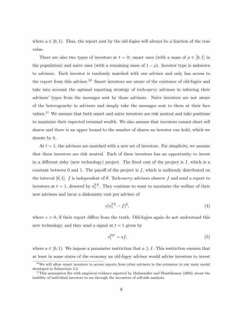
Proposition 6 A Bayesian-Nash equilibrium at t = 1 consists of the following profiles. The

reporting strategy of a tech-savvy advisor with a reputation of π ∈ [0, 1] of being tech-savvy,

is

sTS1 (f̂TS) =

f̂TS if f̂TS ≥ f∗

dI if dI ≤ f̂TS < f∗

f̂TS if f̂TS < dI

(25)

where f̂TS is the advisor’s belief about the project fundamental f . The parameters f∗ and d

are determined by the following equations:

nρ(I − f∗) = nc(f∗ − dI)2 (26)12(f∗ + dI) = b(π)I (27)

24

where

b(π) =1

π̂ + (1− π̂)/a, with π̂ =

π

π + (1− π)/a. (28)

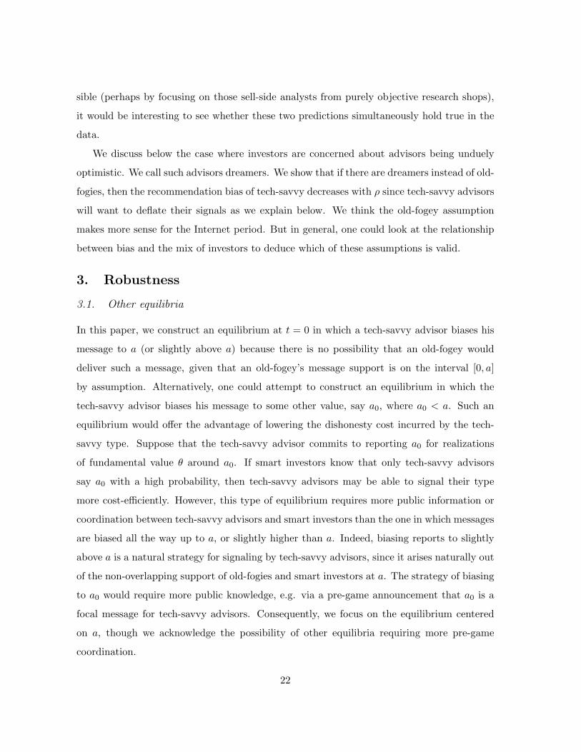
The reporting strategy of an old-fogey advisor with reputation π is the same as that of a

tech-savvy advisor with the same reputation:

sOF1 (f̂OF ) =

f̂OF if f̂OF ≥ f∗

dI if dI ≤ f̂OF < f∗

f̂OF if f̂OF < dI

(29)

where f̂OF is the advisor’s belief about the project fundamental f .

After observing the signal, a naive investor invests if and only if the signal is above I. A

smart investor does not invest if the signal is equal to or below dI and invests otherwise.

I

f

s

0

1

1

dI



f*

a

Figure 4: Advisors’ strategies at t = 1 with imperfect information about type. The solidline plots tech-savvy advisors’ strategy for different values of f , while the dashed line plotsold-fogey advisors’ strategy.

Proposition 6 shows that tech-savvy and old-fogey advisors who possess the same rep-

utation and the same belief about the project fundamental will choose to report the same

signal, as illustrated in Fig. 4. The proof of Proposition 6 is standard and is given in the

25

Appendix. We verify the optimality of advisors’ reporting strategies by taking the investors’

learning rules as given, and we subsequently verify the optimality of investors’ learning rules

by taking advisors’ reporting strategies as given. Since in equilibrium advisors do not report

signals in the region (dI, f∗), we need to specify an off-equilibrium belief for smart investors

if an advisor chooses to send a signal s1 ∈ (dI, f∗). In the proof, we assume that an investor

believes that such a signal could be from either a tech-savvy or an old-fogey with a belief

between s1 and f∗ and that the belief of each type of advisor is uniformly distributed on

(s1, f∗).16

According to Proposition 6, an imperfect reputation (π < 1) creates inefficiencies for

both types of advisors, as both tech-savvy and old-fogey advisors need to incur dishonesty

costs to avoid inefficient investment by their smart advisees when the advisors’ beliefs are in

(dI, f∗). Furthermore, the smart advisee makes an inefficient investment from the advisor’s

perspective if the advisor’s belief is in (f∗, I). Thus, for a benevolent tech-savvy advisor with

a reputation π, the expected inefficiency - equal to his dishonesty cost plus the investment

loss by his advisees - is

KTS(π) =∫ I

f∗nρ(I − f̂)df̂ +

∫ f∗

dInc(f̂ − dI)2df̂ . (30)

For a benevolent old-fogey advisor with a reputation π, the expected inefficiency is

KOF (π) =∫ I

f∗nρ(I − f̂)df̂/a +

∫ f∗

dInc(f̂ − dI)2df̂/a. (31)

Note that

KOF (π) = KTS(π)/a. (32)

Based upon the expressions for KTS and KOF , we can directly verify that they are mono-

tonically decreasing with the advisor’s reputation π, as stated in the following proposition.

Proposition 7 Both KTS(π) and KOF (π) decrease with π and are zero when π = 1.

Proposition 7 shows that both tech-savvy and old-fogey advisors can benefit from a good

reputation. Thus, at t = 0, tech-savvy advisors have incentives to separate themselves from16This assumption is reasonable because in the proposed equilibrium, no type of advisor ever inflates his

signal, but both types deflate their signals for some beliefs below f∗. Hence, a signal in (dI, f∗) could comefrom an advisor who is attempting to deflate his signal but does not deflate it enough to the optimal level dI.

26

old-fogey advisors by reporting an optimistic signal. At the same time, old-fogey advisors also

have the incentive to mix with tech-savvy advisors by inflating their signals as well. Due to

these incentives operating on both types, the equilibrium has two outcomes: (1) a separating

outcome in which tech-savvy advisors report an extremely optimistic signal that is too costly

for old-fogey advisors to match, when the fundamental is sufficiently high; and (2) a pooling

outcome, in which tech-savvy advisors truthfully report their belief, and old-fogey advisors

match such a recommendation, when the fundamental is not too high.

The following proposition summarizes the equilibrium, with the proof given in the Ap-

pendix.

Proposition 8 Under certain sufficient conditions, namely

1− a ≤√

KOF (0)/c (33)

[√

KOF (0)−√

KTS(π̂)]/a <√

KOF (0)−KOF (π̂) <√

c(1− a)/a (34)

where π̂ = π0π0+(1−π0)/a , we have the following Bayesian-Nash equilibrium at t = 0.

Given a tech-savvy advisor’s belief θ̂TS, which is equal to the true value θ, his reporting

strategy is

sTS0 (θ̂TS) =

{aθ̂TS + z if θ̂TS ≥ θ∗

θ̂TS if θ̂TS < θ∗,(35)

where

z =√

KOF (0)/c, (36)

and θ∗ ∈ (0, 1) is defined as

θ∗ =a

1− a

√[KOF (0)−KOF (π̂)]/c. (37)

Given an old-fogey advisor’s belief θ̂OF , which is equal to aθ, his reporting strategy is

sOF0 (θ̂OF ) =

{θ̂OF if θ̂OF ≥ aθ∗

θ̂OF /a if θ̂OF < aθ∗.(38)

A naive investor always takes the signal from his advisor at face value. When θ < θ∗,

the naive investor’s belief turns out to be correct; when θ ≥ θ∗, his belief is upward biased

27

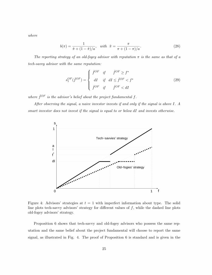
when he is matched with a tech-savvy advisor and downward biased when matched with an

old-fogey advisor.

Smart investors are always able to correctly infer the value of θ by comparing signals

available in the market. Furthermore, when θ ≥ θ∗, there is a separating outcome in which

tech-savvy advisors inflate their signal to aθ + z, while old-fogey advisors report aθ. Thus,

smart investors are able to identify their advisors’ types when θ is high. When θ < θ∗, there

is a pooling outcome in which all advisors send the same signal equal to θ. In this case, smart

investors attribute probability π̂ = π0π0+(1−π0)/a to their advisors being tech-savvy.

θ

s

0

1

1



a

a+z

θ*

Figure 5: Advisors’ strategies at t = 0. The solid line plots tech-savvy advisors’ strategy fordifferent values of θ, while the dashed line plots old-fogey advisors’ strategy.

As illustrated in Fig. 5, Proposition 8 shows that when the technology fundamental θ is

sufficiently high (θ ≥ θ∗), tech-savvy advisors are able to separate themselves from old-fogey

advisors by inflating their signal. It is too costly for old-fogey advisors to match the tech-

savvies’ signal because their belief is substantially below that of the tech-savvies. When θ is

small (θ < θ∗), tech-savvy and old-fogey advisors’ beliefs are close enough that it becomes

too costly for tech-savvy advisors to separate themselves, and consequently there is a pooling

equilibrium in which old-fogies inflate their signal to match the tech-savvies’ truthful report.

The proof of Proposition 8 is standard and is given in the Appendix. We again need

28

to specify certain assumptions for investors’ learning rules when they receive off-equilibrium

signals. These assumptions are similar in spirit to those used to derive the equilibrium at

t = 1.

Because of the short sales constraints, the asset price at t = 0 is determined by the highest

belief in the market. When the asset fundamental θ is above θ∗, the belief of those naive

investors advised by tech-savvy advisors is upward biased to aθ + z. As a result, the asset

price is upward biased to aθ + z as well, as long as these investors in aggregate can hold the

net asset supply. When θ is below θ∗, every investor holds the correct belief, thus the asset

price is unbiased.

Proposition 9 When there is a sufficient number of naive investors advised by tech-savvy

advisors, the asset price at t = 0 is determined by

p =

{aθ + z if θ > θ∗

θ if θ ≤ θ∗(39)

The asset price is upward-biased when θ ≥ θ∗ and is unbiased otherwise.

3.3. Extensions

We consider a number of extensions to our model. The first extension is to allow for inter-

mediate performance feedback. In our current model, the advisors are not judged on the

accuracy of their recommendations at t = 0. We can extend our model to allow for this

feedback. This feedback would weaken the incentive of the tech-savvy advisors to signal their

type, but the key results would not be overturned. As is the case with any type of signaling

model, we also could allow advisors to signal in other ways besides through their recommen-

dations. While the advisor might trade off different modes of signaling, the basic insights of

the model would remain unchanged.

The second extension is to replace old-fogies with dreamers, advisors who are instead

unduely optimistic. The model in this case is completely symmetric to our original set-up

except that tech-savvies deflate their signal to separate themselves from dreamers. However,

despite tech-savvy advisors’ signal deflation, the asset price would still be upward biased

as long as there are enough naive investors guided by dreamers. Although smart investors

29

recognize the overvaluation, they can only sit on the sideline because of the short sales

constraints. We omit the analysis of this case as it is subsumed by our next extension.

The third extension is to consider the equilibrium when there are both dreamer and old-

fogey advisors in the economy. Namely, we derive the equilibrium at t=0 when there are

both dreamers and old-fogies in the market, i.e. there are three type, dreamers, old-fogies

and tech-savvies. The upshot is that we are able to show that there is an equilibrium with

properties qualitatively similar to those in the paper and hence that our results will not fall

apart with three types in the market.

More specifically, we assume that dreamers can only send an upward-biased signal about

the new technology at t = 0:

sDR0 = b + (1− b)θ (40)

where b ∈ (0, 1). Note that as b increases, the dreamers’ signal becomes more optimistic. As

before, old-fogies can only send a downward-biased signal:

sOF0 = aθ, (41)

where a ∈ [0, 1). Tech-savvies have a correct belief about θ, but can choose to bias their

reports for the purpose of signalling. We denote the initial distribution of the three types of

advisors, dreamers, old-fogies, and tech-savvies, by πDR, πOF , and πTS , respectively (πDR +

πOF + πTS = 1).

It is difficult to analyze the tech-savvies’ reporting strategy in the most general case.

Instead, we focus on the case where dreamers’ and old-fogies’ signal spaces do not overlap,

i.e., the highest possible report from an old-fogey is still lower than the lowest possible

message from a dreamer, b > a. We need this assumption of non-overlapping signal spaces

for tractability.

For brevity, we focus on the t = 0 equilibrium and the reporting strategy of tech-savvies

during this period. We make some reduced form assumptions regarding the advisor’s contin-

uation value function at t = 1. Given the non-overlapping signal spaces, there are only three

possible outcomes regarding a tech-savvy’s reputation at t = 1 in equilibrium. The first is

that he has a perfect reputation as a tech-savvy. We denote his value function in this case

30

by VTS . The second is that he has an imperfect reputation as a possible old-fogey but is

for sure not a dreamer. We denote his value function in this case by VOF (π) with π as the

probability that smart investors assign to him as a tech-savvy. The third is that he has an

imperfect reputation as a possible dreamer but is for sure not an old-fogey. We denote his

value function in this case VDR(π) with π as the probability that smart investors assign to

him as a tech-savvy. It is natural to assume that both VOF (π) and VDR(π) increase with π

and are always less than VTS . Otherwise, there would be not value of signalling at t = 0.

Like before, we assume that if the tech-savvy biases his report, he suffers a dishonesty cost:

c(sTS1 − θ)2.

The equilibrium at t = 0 is summarized in the following theorem.

Theorem 3 A Bayesian Nash equilibrium at t = 0 consists of the following profiles. The

reporting strategy of a tech-savvy advisor is

sTS0 =

θ if θ ≥ θ∗2

b if b ≤ θ < θ∗2

θ if a ≤ θ < b

a if θ∗1 ≤ θ < a

θ if θ < a

(42)

where θ∗1 ∈ [0, a) is a constant determined

θ∗1 =

a−

√VTS−VOF

“πTS

πTS+πOF /a

”c , if a−

√VTS−VOF

“πTS

πTS+πOF /a

”c > 0

0, otherwise(43)

and θ∗2 ∈ (b, 1] is a constant determined

θ∗2 =

b +

√VTS−VDR

“πTS

πTS+πDR/(1−b)

”c , if b +

√VTS−VDR

“πTS

πTS+πDR/(1−b)

”c < 1

1, otherwise.(44)

After observing a signal s0 sent by his advisor, a smart investor infers the advisor’s type

according to the following rule: if s0 ≥ θ∗2, the advisor can either be a tech-savvy with a

probability of πTSπTS+πDR/(1−b) or a dreamer with a probability of πDR/(1−b)

πTS+πDR/(1−b) ; if b < s0 < θ∗2,

the advisor is a dreamer for sure; if a ≤ s0 ≤ b, the advisor is a tech-savvy for sure; if

31

θ∗1 ≤ s0 < a, the advisor is an old-fogey for sure; finally, if s0 ≤ θ∗1, the advisor can either be

a tech-savvy with a probability of πTSπTS+πOF /a or an old-fogey with a probability of πOF /a

πTS+πOF /a .

b

θ2* θ

s

0

1

1

a

θ1*


Dreamers’ strategy


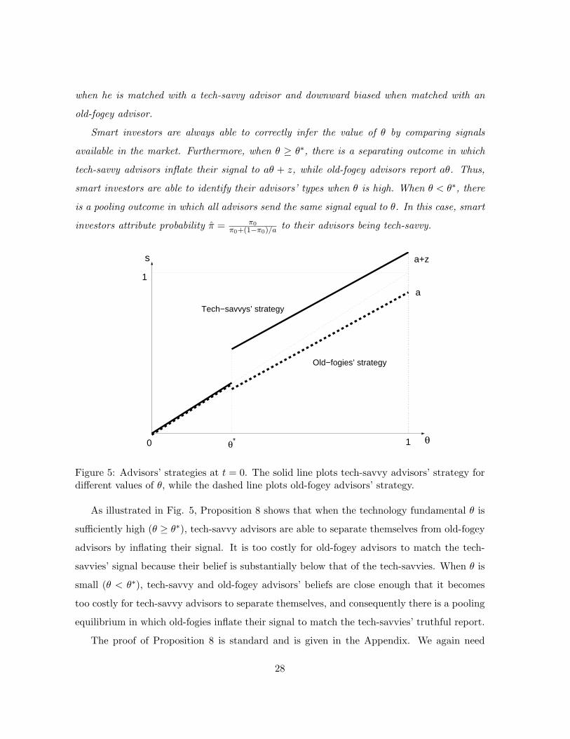
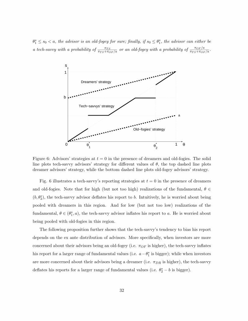
Figure 6: Advisors’ strategies at t = 0 in the presence of dreamers and old-fogies. The solidline plots tech-savvy advisors’ strategy for different values of θ, the top dashed line plotsdreamer advisors’ strategy, while the bottom dashed line plots old-fogey advisors’ strategy.

Fig. 6 illustrates a tech-savvy’s reporting strategies at t = 0 in the presence of dreamers

and old-fogies. Note that for high (but not too high) realizations of the fundamental, θ ∈

(b, θ∗2), the tech-savvy advisor deflates his report to b. Intuitively, he is worried about being

pooled with dreamers in this region. And for low (but not too low) realizations of the

fundamental, θ ∈ (θ∗1, a), the tech-savvy advisor inflates his report to a. He is worried about

being pooled with old-fogies in this region.

The following proposition further shows that the tech-savvy’s tendency to bias his report

depends on the ex ante distribution of advisors. More specifically, when investors are more

concerned about their advisors being an old-fogey (i.e. πOF is higher), the tech-savvy inflates

his report for a larger range of fundamental values (i.e. a−θ∗1 is bigger); while when investors

are more concerned about their advisors being a dreamer (i.e. πDR is higher), the tech-savvy

deflates his reports for a larger range of fundamental values (i.e. θ∗2 − b is bigger).

32

Proposition 10 Keeping πTS constant, an increase in πOF (which corresponds to a decrease

in πDR for the probabilities to sum up to one) would cause a− θ∗1 to rise and θ∗2 − b to fall.

Thus, our results remain with three types of advisors in the market in the sense that

there is more inflation when there is more concern about old-fogies and less inflation or

deflation when there is more concern about dreamers. Importantly, since there are short-

sales constraints, there will be an upward price bias and the bias is greater when there is

more concern about old-fogies.

4. Conclusion

We conclude by re-interpreting the events of the Internet period in light of our model. In the

aftermath of the Internet bubble, many have cited the role of biased advisors in manipulating

the expectations of naive investors. We agree with the focus on the role of advisors but observe

that there is something deeper in the communication process between advisors and investors

that can lead to an upward bias in prices during times of excitement about new technologies,

even absent any explicit incentives on the part of analysts to sell stocks.

Our model suggests that the Internet period was a time when investors were naturally

concerned about whether their advisors understood the new technology, i.e. were their ad-

visors old-fogies or tech-savvy? Investors do not want to listen to old-fogies. As a result,

well-intentioned advisors have an incentive to signal that they are tech-savvy by issuing opti-

mistic forecasts, and this incentive is based on their desire to be listened to by future advisees.

Unfortunately, naive investors do not understand the incentives of advisors to inflate their

forecasts, and consequently asset prices are biased upward.

This view is not totally without empirical support. In addition to the evidence cited in

the introduction, it is well known that the reports issued by sell-side analysts are typically

read only by institutional investors, who for the most part do a good job of de-biasing analyst

recommendations. Unfortunately, during the Internet period, many retail investors took the

positive, upbeat recommendations of analysts a bit too literally. Again, this is not to say

that analysts during this period were solely well-intentioned, but simply that when there are

naive investors, there can be a bubble during times of technological excitement even if all

33

analysts are well-intentioned.

5. Appendix

5.1. Proof of Proposition 2

To verify that the proposed strategies indeed constitute a Bayesian-Nash equilibrium, we

begin by taking as given the reporting strategies of the advisors and verifying the optimality

of the smart investor’s investment policy. First, suppose that s1 ≥ I. The message could be

from a tech-savvy or an old-fogey (if s1 ∈ [I, a]). In this case, however, it does not matter to

the smart investor which type of advisor sent such a signal, since the investor will infer that

f ≥ I given the reporting strategies of the two types of advisors. Thus, the investor invests

when s1 ≥ I.

Next, let’s suppose that s1 ∈ (f∗, I). For a signal sent in this region of the support, the

signal again could be from a tech-savvy or an old-fogey. Let πLL be the posterior probability

that a signal in this region came from a tech-savvy advisor, i.e.

πLL = Pr{tech-savvy|s1} (45)

with s1 ∈ (f∗, I). Then by Bayes Theorem, we have that

πLL =λ(s1|tech-savvy)πL

λ(s1|tech-savvy)πL + λ(s1|old-fogey)(1− πL), (46)

where λ denotes a probability density function. Given the tech-savvy advisor’s reporting

strategy, the probability density of his signal is

λ(s1|tech-savvy) =

1 if f ∈ [0, bI)

0 if f ∈ (bI, f∗)

1 if f ∈ [f∗, 1]

(47)

and Pr(s1 = bI|tech-savvy) = f∗ − bI. Note also that since the signal from an old-fogey has

uniform distribution over the interval [0, a],

λ(s1|old-fogey) = 1/a, ∀ s1 ∈ [0, a]. (48)

Thus, if s1 ∈ (f∗, I), then

πLL =πL

πL + (1− πL)/a< πL. (49)

34

Given such a signal, the smart investor’s inference of the project fundamental is

E[f |s1] = πLLs1 + (1− πLL)s1/a. (50)

Thus, the investor finds it optimal to invest in the project if

s1 >I

πLL + (1− πLL)/a= bI. (51)

Now suppose that s1 ∈ (bI, f∗]. In this case, the smart investor deduces that the signal

must be from an old-fogey since a tech-savvy advisor would never send a signal in this region.

Given such a signal, the smart investor’s inference of the project fundamental is

E[f |s1] = s1/a >bI

a=

I

1− (1− a)πLL> I. (52)

The smart investor therefore invests when s1 ∈ (bI, f∗].

If s1 = bI, then the signal must be from a tech-savvy advisor since the reporting strategy

of that type puts non-trivial mass on the signal bI. To see this, note that

Pr{s1 = bI|tech-savvy} = f∗ − bI, (53)

and

Pr{s1 = bI|old-fogey} = Pr{s1 ∈ (bI − ε, bI + ε)|old-fogey}ε→0 =2ε

a

∣∣∣∣ε→0

= 0. (54)

Thus, the conditional probability that such a signal comes from a tech-savvy is

Pr{tech-savvy|s1 = bI}

=Pr(s1 = bI|tech-savvy)πL

Pr(s1 = bI|tech-savvy)πL + Pr(s1 = bI|old-fogey)(1− πL)= 1 (55)

Given such an inference, the smart investor would not invest.

If s1 < bI, then the analysis is similar to the case in which s1 ∈ (f∗, I). πLL again is the

posterior probability that a signal in this region came from a tech-savvy advisor. Given such

a signal, the smart investor’s inference of the project fundamental is

E[f |s1] =s1

b. (56)

In this case, s1 < bI, so the smart investors do not invest. We thus have shown that the

postulated investment policy of the smart investors is indeed optimal given the proposed

35

reporting strategy of the tech-savvy advisors and the assumed reporting strategy of the old-

fogies.

We now will show that the tech-savvy advisor’s reporting strategy is optimal given the

investors’ investment policies. Suppose that f ≥ I, so that it is efficient for investors to invest.

Then it is optimal for the tech-savvy advisor to tell the truth. Suppose that f ∈ (f∗, I). In

this case, investment is not efficient. Under the proposed strategy of smart investors, however,

those investors will invest after observing a signal in this range. If the advisor tells the truth,

then the expected cost born by smart investors is nρ(I − f). If the advisor were to bias his

message, he would have to deflate it to bI to prevent smart investors from investing according

to the proposed investment rule. The dishonesty cost of deflating the message to bI across n

advisees is

nc(f − bI)2. (57)

Since f > f∗, we find that

nc(f − bI)2 > nc(f∗ − bI)2 = nρ(I − f∗) > nρ(I − f) (58)

using the definition of f∗ given in the proposition above. As a result, there is no incentive

for a tech-savvy advisor to under-report his signal in order to dissuade smart investors from

investing.

Suppose that f ∈ [bI, f∗]. Under the proposed equilibrium strategies, the smart investor

would not invest in this range of f , and the tech-savvy advisor incurs a dishonesty cost of

nc(f − bI)2. The tech-savvy advisor will not deviate to any signal lower than bI, since this

would increase his dishonesty cost while having no effect on the smart investor’s decision. If

the advisor deviates to any signal s1 > bI, this would induce the smart investor to invest,

and the cost to smart investors again would be given by nρ(I − f). If the advisor reports bI,

then the dishonesty cost incurred by the advisor is nc(f − bI)2. Note that when f ∈ [bI, f∗],

nc(f − bI)2 ≤ nc(f∗ − bI)2 = nρ(I − f∗) ≤ nρ(I − f), (59)

again from the definition of f∗. Thus, it is optimal for the tech-savvy advisor to report bI

when f ∈ [bI, f∗], since the cost of inefficient investment by smart investors outweighs the

36

maximum reduction of dishonesty cost that the tech-savvy advisor could achieve by telling

the truth.

Finally, if f < bI, then the advisor simply tells the truth since a truthful signal will lead

investors to make the efficient decision to not invest.


By integrating Eq. (16), we have

V1 − V2 =nρ

2(I − f∗)2 +

nc

3(f∗ − bI)3. (60)

By substituting in Eq. (10), we can transform the last Eq. into

V1 − V2 = nρ(I − f∗)[(

12− b

3

)I − f∗

6

]. (61)

This equation directly implies that V1 − V2 increases with ρ and decreases with f∗.

Eq. (10) implies that f∗ increases with b. Eq. (8) implies that b increases with πLL,

which also increases with π0. Thus, f∗ increases with π0, and V1 − V2 decreases with π0. Eq.

(8) also implies that b increases with a; therefore, f∗ increases with a, and V1 − V2 decreases

with a.


Proposition 3 implies that the gain from a good reputation, V1 − V2, increases with n and ρ,

and it decreases with π0. Then, Eq. (18) implies that θ∗ (weakly) decreases with n and ρ,

and it (weakly) increases with π0.


First, taking as given the tech-savvy and old-fogey advisors’ reporting strategies, we verify

the optimality of the smart investors’ investment rule based on the realization of s1.

1. s1 ∈ (a, 1]. This signal must be from a tech-savvy advisor, and the investment project’s

payoff f = s1 ≥ a ≥ I. Therefore, it is optimal for the smart investor to invest in the

project.

37

2. s1 ∈ [f∗, a]. This signal could be from a tech-savvy or an old-fogey. Given the prior

probability π that the advisor is tech-savvy, the updated probability is π̂ = ππ+(1−π)/a .

Accordingly, the expected project payoff is

E{f |s1 ∈ [f∗, a]} = π̂s1 + (1− π̂)s1/a = s1/b(π) =2s1

f∗ + dII > I. (62)

Hence the smart investor invests.

3. s1 ∈ (dI, f∗). Since neither tech-savvies nor old-fogies report signals in this range in

equilibrium, we need to specify a certain off-equilibrium belief for the investor in order

to derive her investment decision. We assume that after receiving a signal in (dI, f∗),

the investor believes that the signal could be from either a tech-savvy or an old-fogey

with a belief between s1 and f∗. We further assume that the smart investor views

the belief of each type of advisor to be uniformly distributed on (s1, f∗). Under these

assumptions, the smart investor’s updated expectation of the project payoff is

E[f |s1 ∈ (dI, f∗)] = [π̂ + (1− π̂)/a](s1 + f∗)

2

> [π̂ + (1− π̂)/a](dI + f∗)

2= [π̂ + (1− π̂)/a]b(π)I

= I. (63)

Consequently, the smart investor would choose to invest.

4. s1 = dI. Such a signal could be from either a tech-savvy or an old-fogey advisor with a

belief between dI and f∗. Given the prior probability π that the advisor is tech-savvy,

the smart investor’s updated probability is π̂. Then since advisors’ beliefs are uniformly

distributed, the smart investor’s expectation of the project payoff is

E[f |s1 = dI] = [π̂ + (1− π̂)/a](dI + f∗)

2= [π̂ + (1− π̂)/a]b(π)I

= I. (64)

Hence, the investor is indifferent between investing and not investing.

38

5. s1 ∈ [0, dI). Such a signal could be a truthful signal from either a tech-savvy or an

old-fogey. The smart investor’s expectation of the project payoff is

E[f |s1] = [π̂ + (1− π̂)/a]s1

< [π̂ + (1− π̂)/a]dI

< [π̂ + (1− π̂)/a]b(π)I

= I. (65)

Accordingly, the investor chooses not to invest.

Next, taking the smart investor’s investment strategy as given, we derive the optimal

reporting strategies for both the tech-savvy and old-fogey advisors. Both types of advisors

want to maximize their advisees’ investment profits and simultaneously minimize their dis-

honesty costs. Given this common objective, tech-savvy and old-fogey advisors have the same

optimal reporting strategy. Therefore, in the proof below, we do not differentiate them. We

denote f̂ as a given advisor’s belief about the project fundamental. Based on the realization

of f̂ , we have the following cases.

1. f̂ > I. The advisor will truthfully report her belief, because it is optimal to invest in

the project, and all investors will do so after receiving a truthful signal.

2. f̂ ∈ [f∗, I). The advisor believes that it is inefficient to invest in the project. If

she truthfully reports her belief in the signal, a naive advisee will take the signal at

face value and will choose not to invest. However, a smart advisee cannot distinguish

whether the signal is from a tech-savvy or old-fogey advisor and will choose to invest

according to his investment strategy. The advisor can prevent the inefficient investment

by her smart advisees by deflating the signal to dI. In doing so, the advisor has to incur

a dishonesty cost of

nc(f̂ − dI)2 ≥ nc(f∗ − dI)2 = nρ(I − f∗) > nρ(I − f̂), (66)

where the last expression equals the total investment losses that would be incurred by

her smart advisees if the advisor reports truthfully. Since the dishonesty cost outweighs

39

the avoided investment losses, it is not optimal for the advisor to deflate her signal to

dI. It also is not optimal to deflate her signal to a level higher than dI, since a smart

advisee still would invest after observing such a signal. Hence, the advisor will truthfully

report her belief.

3. f̂ ∈ (dI, f∗). Similar to the previous case, the advisor believes that it is inefficient

to invest in the project and faces the dilemma that her smart advisees would choose

to invest after observing a truthful signal from her. To avoid this outcome, it now is

optimal for the advisor to deflate her signal to dI, since her dishonesty cost is smaller

than her smart advisees’ potential investment losses:

nc(f̂ − dI)2 < nc(f∗ − dI)2 = nρ(I − f∗) < nρ(I − f̂). (67)

Again, note that the advisor will not deflate her signal to a level higher than dI since

her smart advisees still would choose to invest after receiving such a signal. Hence, it

is optimal for the advisor to deflate her signal to dI.

4. f̂ ∈ [0, dI]. The advisor will truthfully report her belief, since the advisor regards the

project as inferior, and all her advisees will avoid the project after receiving a truthful

signal.


Taking the advisors’ reporting strategies as given, it is straightforward to verify the optimality

of the smart investors’ learning rule. Accordingly, we will focus on the verifying the optimality

of an individual advisor’s reporting strategy, taking the smart investors’ learning rule and

other advisors’ reporting strategies as given.

First, we verify the optimality of a tech-savvy advisor’s reporting strategy. Depending on

the realization of her belief θ̂TS , which is equal to θ, we have the following cases.

1. θ̂TS ∈ [θ∗, 1]. The advisor knows that other tech-savvy advisors share her belief and will

report signals equal to aθ̂TS + z, and that old-fogey advisors will report signals equal

to their belief, aθ̂TS . The advisor can choose to inflate her signal to aθ̂TS + z, just

like other tech-savvies, and thus obtain a perfect reputation among smart investors.

40

The investor also could truthfully report her belief or inflate her signal to a level lower

than aθ̂TS + z. (Note that there are no incentives for the advisor to deflate her signal.)

Since these alternative signals do not appear in equilibrium, we need to specify an off-

equilibrium belief for smart investors in order to evaluate the advisor’s optimal choice.

We assume that if smart investors receive a signal in the region [θ̂TS , aθ̂TS + z), they

believe the signal could be from either tech-savvies or old-fogies, and therefore assign

the sender the probability π̂ = π0π0+(1−π0)/a of being tech-savvy. Given the investors’

learning rule, the feasible choices for the advisor are to truthfully report her belief or

to inflate the signal to aθ̂TS + z, which generate reputations of π̂ and 1, respectively.

The benefit of inflating the signal is KTS(π̂)−KTS(1) = KTS(π̂). The dishonesty cost

of inflating the signal is

c(aθ̂TS + z − θ̂TS)2 = c[z − (1− a)θ̂TS ]2. (68)

When θ̂TS > θ∗, the inequality conditions in (34) imply that the dishonesty cost is less

than KTS(π̂). Thus, the advisor’s optimal strategy is to inflate the signal to aθ̂TS + z.

2. θ̂TS ∈ [0, θ∗). In this region, tech-savvy and old-fogey advisors’ signals are pooled at the

same level θ̂TS . To verify the optimality of a tech-savvy advisor’s strategy, we assume

that if an advisor sends a signal above or equal to θ̂TS , smart investors assign her a

probability π̂ of being tech-savvy; and if the advisor sends a signal below θ̂TS , smart

investors assign her a probability zero of being tech-savvy. It then directly follows from

these assumptions that a tech-savvy advisor’s optimal choice is to truthfully report her

belief.

Next, we verify the optimality of an old-fogey advisor’s reporting strategy. Depending

upon the realization of the advisor’s belief θ̂OF , which is equal to aθ, we have the following

cases.

1. θ̂OF ∈ [aθ∗, a]. The advisor knows that other old-fogey advisors will report their belief

θ̂OF , while tech-savvy advisors will report θ̂OF + z. We need to show that the advisor’s

optimal choice is to truthfully report her belief and thus be identified as an old-fogey.

She could choose to inflate her signal to θ̂OF + z and thus be identified as tech-savvy.

41

The dishonesty cost that she would incur is cz2, while the benefit is KOF (0), which

is exactly cz2 by construction of z in Proposition 8. Hence, the advisor is indifferent

between truthfully reporting her belief or inflating the signal to θ̂OF +z. The advisor also

could inflate her signal to a level in [θ̂OF /a, θ̂OF + z). In equilibrium, no one actually

sends a signal in this region. Given our earlier assumption about smart investors’

off-equilibrium that they assign the sender a probability π̂ of being tech-savvy upon

receiving a signal in this region, the advisor would only inflate the signal to θ̂OF /a,

the minimum level needed to obtain the partial reputation π̂ as a tech-savvy. The

dishonesty cost incurred is

c(θ̂OF /a− θ̂OF )2 = c(1− a)2

a2ˆθOF 2 ≥ KOF (0)−KOF (π̂), ∀ θ̂OF > θ∗. (69)

Since KOF (0) − KOF (π̂) is the benefit of inflating the signal, it is not optimal for the

advisor to do so when her belief is above θ∗. Also note that the advisor would never

choose to inflate her signal to a level lower than θ̂OF /a, because a tech-savvy advisor

would never send out a signal in this region. Therefore, truthfully reporting the belief

θ̂OF is an optimal choice.

2. θ̂OF ∈ [0, aθ∗). The old-fogey advisor has two feasible choices. She can either obtain a

reputation π̂ by inflating her signal to θ̂OF /a, or she can identify herself as an old-fogey

by reporting her true belief θ̂OF . Since the cost of inflating the signal

c(θ̂OF /a− θ̂OF )2 = c(1− a)2

a2θ̂OF 2 ≤ KOF (0)−KOF (π̂), ∀ θ̂OF ≤ θ∗, (70)

the advisor’s optimal choice is to inflate the signal.

5.6. Proof of Theorem 3

We begin by taking as given the smart investor’s learning rule and verifying the optimality

of a tech-savvy’s reporting strategy, according to the following cases:

• First, suppose that θ ∈ (a, b). In this case, reporting the truth reveals the tech-savvy’s

type since neither an old-fogey nor a dreamer would ever send such a signal. The tech-

savvy thus can achieve a perfect reputation while incurring no dishonesty cost, it is

optimal for him to tell the truth when θ ∈ (a, b).

42

• Now, suppose that θ ∈ [θ∗1, a]. In this case, the tech-savvy does not need to be worried

about being identified as a dreamer since a dreamer will never report a signal in this

region. However, an old-fogey might. If θ is below a, the tech-savvy can distinguish

himself from an old-fogey by inflating his signal to a, at a dishonesty cost of c(θ − a)2.

Note that a tech-savvy would never partially inflate his report to a level below a, since it

would hurt his reputation given the smart investor’s learning rule. Since the dishonesty

cost increases quadratically with the degree of report inflation, as the fundamental

value θ decreases, the cost of inflating the report increases. When θ drops below a

threshold level given by θ∗1, the dishonesty cost becomes too high relative to the gain

from signaling that one is a tech-savvy for sure. θ∗1 is exactly determined by Eq. (43).

• Then, suppose that the fundamental value θ is below θ∗1. In this case, as we have argued

above, it is too costly for the tech-savvy to signal his type by inflating his message to

a. We also observe that partially inflating the signal would not improve the advisor’s

reputation at all. Hence, the advisor chooses to send a truthful signal.

• Next, suppose that θ ∈ [b, θ∗2]. In this case, the tech-savvy does not need to be worried

about being identified as an old-fogey since an old-fogey will never report a signal in

this region. However, a dreamer might. If θ is above b, the tech-savvy can distinguish

himself from a dreamer by deflating his signal to b, at a dishonesty cost of c(θ − b)2.

Note that a tech-savvy would never partially deflate his report to a level above b, since it

would hurt his reputation given the smart investor’s learning rule. Since the dishonesty

cost increases quadratically with the degree of report deflation, as the fundamental

value θ increases, the cost of deflating the report increases. When θ rises above a

threshold level given by θ∗2, the dishonesty cost becomes too high relative to the gain

from signaling that one is a tech-savvy for sure. θ∗2 is exactly determined by Eq. (44).

• Finally, suppose that the fundamental value θ is above θ∗2. In this case, as we have

argued above, it is too costly for the tech-savvy to signal his type by deflating his

message to b. We also observe that partially deflating the signal would not improve the

advisor’s reputation at all. Hence, the advisor chooses to send a truthful signal.

43

Next, we verify the optimality of the smart investor’s inference rule, given the tech-savvy’s

reporting strategy.

• If s0 ∈ [a, b], the signal must come from a tech-savvy, since neither old-fogies nor

dreamers would report such a signal.

• If s0 ∈ (θ∗1, a), the signal must come from an old-fogey, since neither tech-savvies nor

dreamers would report signals in this region.

• If s0 ≤ θ∗1, the signal could come from either a tech-savvy or an old-fogey, and the

probability it is from a tech-savvy is given by Bayes Theorem:

Pr[tech-savvy|s0] =λ(s0|tech-savvy)πTS

λ(s0|tech-savvy)πTS + λ(s0|old-fogey)πOF

=πTS

πTS + πOF /a. (71)

Consequently, the probability that the signal comes from an old-fogey is πOF /aπTS+πOF /a .

• If s0 ∈ (b, θ∗2), the signal must come from a dreamer, since neither tech-savvies nor

old-fogies would report signals in this region.

• If s0 ≥ θ∗2, the signal could come from either a tech-savvy or a dreamer, and the

probability it is from a tech-savvy is given by Bayes Theorem:

Pr[tech-savvy|s0] =λ(s0|tech-savvy)πTS

λ(s0|tech-savvy)πTS + λ(s0|dreamer)πDR

=πTS

πTS + πDR/(1− b). (72)

Consequently, the probability that the signal comes from a dreamer is πDR/(1−b)πTS+πDR/(1−b) .


It is direct to see that πTSπTS+πOF /a decreases with πOF . Thus, an increase in πOF would cause

VTS − VOF

(πTS

πTS+πOF /a

)to increase since VOF (·) is a monotonically increasing function.

Consequently, θ∗1 would decrease with πOF , as implied by Eq. (43). Similarly, we can prove

that θ∗2 increases with πDR, using Eq. (44).

44

References

Abreu, D., Brunnermeier, M., 2003. Bubbles and crashes. Econometrica 71, 173-204.

Allen, F., Morris, S., Postlewaite, A., 1993. Finite bubbles with short sale constraints andasymmetric information. Journal of Economic Theory 61, 206-229.

Bernheim, D., 1994. A theory of comformity. Journal of Political Economy 102, 841-877.

Blanchard, O., Watson, M., 1982. Bubbles, rational expectations and financial markets. In:Wachtel, P. (Ed.), Crisis in the Economic and Financial Structure: Bubbles, Bursts,and Shocks. Lexington Press, Lexington, MA.

Chen, J., Hong, H., Stein, J., 2002. Breadth of ownership and stock returns. Journal ofFinancial Economics 66, 171-205.

Cowen, A., Groysberg, B., Healy, P., 2003. Which types of analyst firms make more opti-mistic forecasts. Unpublished working paper, Harvard Business School.

DeLong, J. B., Shleifer, A., Summers, L., Waldmann, R., 1990. Noise trader risk in financialmarkets. Journal of Political Economy 98, 703-38.

DeMarzo, P., Kaniel, R., Kremer, I., 2006. Relative wealth concerns and financial bubbles.Review of Financial Studies, forthcoming.

Diether, K., Malloy, C., Scherbina, A., 2002. Differences of opinion and the cross section ofstock returns. Journal of Finance 52, 2113-2141.

Fudenberg, D., Tirole, J., 1991. Game Theory. MIT Press, Cambridge, MA.

Gerstner, L., 2002. Who Says Elephants Can’T Dance?: Leading A Great EnterpriseThrough Dramatic Change. Harper Collins, New York, NY.

Greenwood, R., Nagel, S., 2006. Inexperienced investors and bubbles. Unpublished workingpaper, Harvard Business School.

Grossman, S., Stiglitz, J., 1980. On the impossibility of informationally efficient markets.American Economic Review 70, 393-408.

Groysberg, B., Healy, P., Chapman, C., Gui, Y., 2005. Do buy-side analysts out-performthe sell-side? Unpublished working paper, Harvard Business School.

Harrison, J. M., Kreps, D., 1978. Speculative investor behavior in a stock market withheterogeneous expectations. Quarterly Journal of Economics 92, 323-36.

Hirshleifer, D., Teoh, S. H., 2003. Limited attention, information disclosure, and financialreporting. Journal of Accounting and Economics 36, 337-386.

Holmstrom, B., 1999, Managerial incentive problems: A dynamic perspective. Review ofEconomic Studies 66, 169-182.

Holmstrom, B., Ricart i Costa, J., 1986. Managerial incentives and capital management.Quarterly Journal of Economics 101, 835-860.

45

Hong, H., Kubik, J., 2003. Analyzing the analysts: Career concerns and biased earningsforecasts. Journal of Finance 58, 313-351.

Kreps, D., 1990. A Course in Microeconomic Theory. Princeton University Press, Prince-ton, NJ.

Lamont, O., Thaler, R., 2003. Can the market add and subtract? Mispricing in tech stockcarve-outs. Journal of Political Economy 111, 227-268.

Lin, H., McNichols, M., 1998. Underwriting relationships, analysts’ earnings forecasts andinvestment recommendations. Journal of Accounting and Economics 25, 101-127.

Malkiel, B., 2003. A Random Walk Down Wall Street. W.W. Norton and Company, NewYork, NY.

Malmenier, U., Shantikumar, D., 2004. Are investors naive about incentives? Journal ofFinancial Economics, forthcoming.

Michaely, R., Womack, K., 1999. Conflict of interest and the credibility of underwriteranalyst recommendations. Review of Financial Studies 12, 653-686.

Miller, E., 1977. Risk, uncertainty and divergence of opinion. Journal of Finance 32,1151-1168.

Morris, S., 2001. Political correctness. Journal of Political Economy 109, 231-265.

Nairn, A., 2002. Engines That Move Markets. John Wiley and Sons, Inc., New York, NY.

Ofek, E., Richardson, M., 2003. Dotcom mania: The rise and fall of internet stock prices.Journal of Finance 58, 1113-1137.

Ottaviani, M., Sorensen, P., 2006. Professional advice. Journal of Economic Theory 126,120142.

Pacelle, M., 2000. Soros’ Quantum Fund lost big on tech selloff. Smart Money Magazine,January 6, article available online at SmartMoney.com.

Pastor, L., Veronesi, P., 2006. Technological revolutions and stock prices. Unpublishedworking paper, University of Chicago.

Scharfstein, D., Stein, J., 1990. Herd behavior and investment. American Economic Review80, 465-479.

Scheinkman, J., Xiong, W., 2003. Overconfidence and speculative bubbles. Journal ofPolitical Economy 111, 1183-1219.

Shiller, R., 2000. Irrational Exuberance. Broadway Books, New York, NY.

Shleifer, A., Vishny, R., 1997. Limits of arbitrage. Journal of Finance 52, 35-55.

Wolfe, T., 1975. The Painted Word. Farrar, Straus and Giroux, New York, NY.

46

advisors and asset prices: a model of the origins of · pdf fileadvisors and asset prices: a...

Documents