advertiment advertencia · sales forecasting methodology of great practical implications . ......
TRANSCRIPT

ADVERTIMENT. Lʼaccés als continguts dʼaquesta tesi doctoral i la seva utilització ha de respectar els drets de lapersona autora. Pot ser utilitzada per a consulta o estudi personal, així com en activitats o materials dʼinvestigació idocència en els termes establerts a lʼart. 32 del Text Refós de la Llei de Propietat Intel·lectual (RDL 1/1996). Per altresutilitzacions es requereix lʼautorització prèvia i expressa de la persona autora. En qualsevol cas, en la utilització delsseus continguts caldrà indicar de forma clara el nom i cognoms de la persona autora i el títol de la tesi doctoral. Nosʼautoritza la seva reproducció o altres formes dʼexplotació efectuades amb finalitats de lucre ni la seva comunicaciópública des dʼun lloc aliè al servei TDX. Tampoc sʼautoritza la presentació del seu contingut en una finestra o marc alièa TDX (framing). Aquesta reserva de drets afecta tant als continguts de la tesi com als seus resums i índexs.
ADVERTENCIA. El acceso a los contenidos de esta tesis doctoral y su utilización debe respetar los derechos de lapersona autora. Puede ser utilizada para consulta o estudio personal, así como en actividades o materiales deinvestigación y docencia en los términos establecidos en el art. 32 del Texto Refundido de la Ley de PropiedadIntelectual (RDL 1/1996). Para otros usos se requiere la autorización previa y expresa de la persona autora. Encualquier caso, en la utilización de sus contenidos se deberá indicar de forma clara el nombre y apellidos de la personaautora y el título de la tesis doctoral. No se autoriza su reproducción u otras formas de explotación efectuadas con fineslucrativos ni su comunicación pública desde un sitio ajeno al servicio TDR. Tampoco se autoriza la presentación desu contenido en una ventana o marco ajeno a TDR (framing). Esta reserva de derechos afecta tanto al contenido dela tesis como a sus resúmenes e índices.
WARNING. The access to the contents of this doctoral thesis and its use must respect the rights of the author. It canbe used for reference or private study, as well as research and learning activities or materials in the terms establishedby the 32nd article of the Spanish Consolidated Copyright Act (RDL 1/1996). Express and previous authorization of theauthor is required for any other uses. In any case, when using its content, full name of the author and title of the thesismust be clearly indicated. Reproduction or other forms of for profit use or public communication from outside TDXservice is not allowed. Presentation of its content in a window or frame external to TDX (framing) is not authorized either.These rights affect both the content of the thesis and its abstracts and indexes.

Maya Dori Arbiv From Macro to Micro Doctorate Thesis Dissertation
i
Doctorate Thesis Dissertation
From Macro to Micro
A case of a successful implementation of a novel
sales forecasting methodology of great practical
implications
Maya Dori Arbiv
Ph. D. program in Economics, Management and Organization (DEMO)
Signed by the author, Maya Dori Arbiv .....................................................................................
Signed by the thesis director, Dr. Josep Rialp Criado…………………..……...................................
Thesis Director: Dr. Josep Rialp Criado
Facultat d'Economia i Empresa
Universitat Autònoma de Barcelona
2017

Maya Dori Arbiv From Macro to Micro Doctorate Thesis Dissertation
ii
COPYRIGHT Attention is drawn to the fact that copyright of this thesis rests with the author.
A copy of this thesis has been supplied on condition that anyone who consults it is understood
to recognize that its copyright rests with the author and that they must not copy it or use
material from it except as permitted by law or with the consent of the author.

Maya Dori Arbiv From Macro to Micro Doctorate Thesis Dissertation
iii
Table of Contents
Abstract ...................................................................................................................................... 1
Acknowledgements .................................................................................................................... 2
1 Introduction ........................................................................................................................ 3
1.1 The price of uncertainty .............................................................................................. 4
1.2 Why do managers need forecasting tools ................................................................... 6
1.3 A success story - The use of our forecasting models at Hewlett-Packard .................. 8
1.4 Does sample size matter? .......................................................................................... 13
1.5 Trying to improve our data sample size .................................................................... 18
2 The problem statements ................................................................................................... 24
2.1 Problem statement number 1: limited usage of the existing forecasting tools........ 24
2.2 Problem statement number 2: multinationals marketing strategy dilemma ........... 26
2.3 Problem statement number 3: product forecasting at different stages of the product
life cycle ................................................................................................................................ 28
2.4 Problem statement number 4: limited tools for product portfolio management .... 28
3 Literature Review .............................................................................................................. 31
3.1 Product forecasting ................................................................................................... 31
3.1.1 The ingredients of a good forecasting model recipe ......................................... 35
3.2 The Institutional Theory ............................................................................................ 39
3.3 Cultures as institutions .............................................................................................. 45
3.4 International Adaptation versus global Standardization........................................... 51
3.5 The forecasting model framework ............................................................................ 57
3.5.1 The Macro to Micro path ................................................................................... 58
3.6 Product life cycle ........................................................................................................ 60
3.6.1 The Bass model for product life cycle forecasting ............................................. 61
3.6.2 The Bass model as a forecasting method: limitations and improvements ........ 63
3.6.3 Technology generations and substitution .......................................................... 67
3.6.4 Does product adoption accelerate between different technologies? ............... 68
3.6.5 Does new product technology substitute the previous one? ............................ 70
3.7 Product portfolio managerial literature review ........................................................ 71

Maya Dori Arbiv From Macro to Micro Doctorate Thesis Dissertation
iv
3.8 The forecasting accuracy literature ........................................................................... 75
4 The research approach ..................................................................................................... 79
4.1.1 Introduction to empirical study number 1 ......................................................... 80
4.1.2 Introduction to empirical study number 2 ......................................................... 80
4.1.3 Introduction to empirical study number 3 ......................................................... 82
4.1.4 Introduction to empirical study number 4 ......................................................... 83
5 Empirical study number 1 ................................................................................................. 85
5.1 The product lines tested ............................................................................................ 85
5.2 The model set up ....................................................................................................... 86
5.3 The macroeconomic Indicators selection criteria ..................................................... 88
5.4 The rationale of the selection of the macroeconomic indicators ............................. 89
5.4.1 The macroeconomic indicators for the forecasting model of Product Line PLT 90
5.4.2 The macroeconomic indicators for the forecasting model of Product Line PLG 92
5.4.3 The macroeconomic indicators for the forecasting model of Product Line PLI . 93
5.5 Empirical study number 1 first attribute - explanatory capability ............................ 96
5.5.1 The explanatory capability of the forecasting model for PLT ............................ 97
5.5.2 The explanatory capability of the forecasting model for PLG .......................... 101
5.5.3 The explanatory capability of the forecasting model for PLI ........................... 104
5.6 Empirical study number 1 first attribute - Forecasting predictability ..................... 107
5.7 The singular relationship between the forecasting models and the macroeconomic
indicators selected .............................................................................................................. 110
5.7.1 The singular relationship between the forecasting model for PLT and its
macroeconomic indicators selected ............................................................................... 111
5.7.2 The singular relationship between the forecasting model for PLG and its
macroeconomic indicators selected ............................................................................... 114
5.7.3 The singular relationship between the forecasting model for PLI and its
macroeconomic indicators selected ............................................................................... 117
6 Empirical study number 2 ............................................................................................... 120
6.1 The model in 3 different geo-political countries ..................................................... 120
6.2 Conclusions from the localized model ..................................................................... 127
6.3 In a new search of best fitting local models ............................................................ 128
6.3.1 The UK economy´s characteristics ................................................................... 128
6.3.2 The German economy characteristics .............................................................. 130

Maya Dori Arbiv From Macro to Micro Doctorate Thesis Dissertation
v
7 Empirical study number 3 ............................................................................................... 136
7.1 Is the empirical test merely anecdotal? .................................................................. 137
7.2 Product A sales forecast and its PLC stages ............................................................. 138
7.3 Product B sales forecast and its PLC stages ............................................................. 142
8 Empirical study number 4 ............................................................................................... 146
8.1 Product B introduction in light of product A existence ........................................... 147
8.2 Portfolio decision making test #1: Product B from sales perspective ..................... 148
8.3 Portfolio decision making test #2: Product B from revenue perspective ............... 150
8.4 Portfolio decision making test #3: Product B from market perspective ................. 151
8.5 A Game changer product portfolio decision ........................................................... 152
8.6 The results of the new product launch .................................................................... 153
8.6.1 Portfolio decision making test #1: Product C from sales perspective ............. 153
8.6.2 Portfolio decision making test #2: Product C from revenue perspective ........ 156
8.6.3 Portfolio decision making test #3: Product C from market perspective .......... 157
8.7 Three generations under one roof: products dynamics .......................................... 158
9 The Thesis contributions and limitations ........................................................................ 160
10 Annex 1- The GLOBE country scores ............................................................................... 163
11 References ....................................................................................................................... 166
List of Figures
Figure 1 Hewlett-Packard split in 2015 .................................................................................... 12
Figure 2 Hewlett-Packard markets division after the split ....................................................... 13
Figure 3 The statistics results of our forecasting model using annual data points.................. 19
Figure 4 The statistics results of our forecasting model using quarterly data points .............. 20
Figure 5 The statistics results of our forecasting model using quarterly data points and
controlling for seasonality effect ............................................................................................. 22
Figure 6: The classification of forecasting methods ................................................................. 34
Figure 7: The relationship between the forecasting methods ................................................. 35
Figure 8: Coleman´s Diagram ................................................................................................... 43
Figure 9: Countries map based on Hofstede´s dimensions: Power Distance and uncertainty
avoidance ................................................................................................................................. 46

Maya Dori Arbiv From Macro to Micro Doctorate Thesis Dissertation
vi
Figure 10: The Countries clusters according to GLOBE. ........................................................... 49
Figure 11: The main benefits of Standardization ..................................................................... 54
Figure 12: The main benefits of Adaptation ............................................................................ 56
Figure 13: Our Macro to Micro Path ........................................................................................ 59
Figure 14: The relationship between the Macro and Micro components ............................... 60
Figure 15: Bass classical model ................................................................................................ 62
Figure 16: Bass classical product life cycle model .................................................................... 63
Figure 17: Potential turning points in the product life cycle ................................................... 66
Figure 18: Determination of Expected Commercial Value of a project ................................... 73
Figure 19: The empirical studies flow ...................................................................................... 79
Figure 20: The Coleman theorem ............................................................................................. 87
Figure 21 : The usage of the macroeconomic indicators ......................................................... 89
Figure 22: PLT units’ growth Vs. Construction CapEx growth and growth change .................. 92
Figure 23: PLG units’ growth Vs. Retail sales Growth and Retail sales speed ......................... 93
Figure 24: PLI units’ growth Vs. GDP growth and credit tightening......................................... 94
Figure 25: PLI model forecast units’ growth Vs. Actual units’ growth ..................................... 95
Figure 26: Model Forecast units Vs. Actual PLI units ............................................................... 95
Figure 27: PLT Model forecast .................................................................................................. 98
Figure 28: PLT Model forecast Vs. actual PLT units growth ..................................................... 99
Figure 29: PLT units: Model Vs. Actual ................................................................................... 100
Figure 30: PLG Model forecast Vs. Actual PLG units’ growth ................................................ 102
Figure 31: PLG Model forecast statistics results .................................................................... 102
Figure 32: PLG units: Model Vs. Actual PLG units .................................................................. 103
Figure 33: PLI model forecast units’ growth Vs. Actual units’ growth ................................... 105
Figure 34: PLI model forecast ................................................................................................. 105
Figure 35: Model Forecast units Vs. Actual PLI units ............................................................. 106
Figure 36: UK PLI units’ growth Vs. the European-based PLI model forecasted units’ growth
................................................................................................................................................ 125
Figure 37: Germany actual units’ growth Vs. Germany forecasted units growth based on the
European model ..................................................................................................................... 126
Figure 38: Spain units growth Vs. Spain forecasted units growth based on the European model
................................................................................................................................................ 126
Figure 39: UK model forecasted units’ growth Vs. UK actual units’ growth .......................... 129

Maya Dori Arbiv From Macro to Micro Doctorate Thesis Dissertation
vii
Figure 40: Germany units’ growth Vs. the UK-based model forecasted units’ growth ......... 130
Figure 41: Germany actual units’ growth Vs. Germany forecasted units growth based on the
German model ........................................................................................................................ 132
Figure 42: Spain units’ growth Vs. Spain forecasted units growth based on the UK model . 133
Figure 43: Spain units’ growth Vs. Spain forecasted units growth based on the German model
................................................................................................................................................ 133
Figure 44: Spain units’ growth Vs. Spain forecasted units growth based on the European model
................................................................................................................................................ 134
Figure 45: Spain units’ growth Vs. Spain forecasted units based on the European model ... 135
Figure 46: Total market units Vs. A and B units ..................................................................... 137
Figure 47: Product launches of the main technology players ................................................ 138
Figure 48: A quarterly view of the sales of product A ............................................................ 139
Figure 49: Product A forecasting model ................................................................................. 140
Figure 50: Product A forecasted units vs. units A sold ........................................................... 140
Figure 51: The coefficients of the sales of product A and the macroeconomic indicator ..... 141
Figure 52: A schematic view of the characteristics of product A and B ................................. 142
Figure 53: Product B sales results by quarter ........................................................................ 143
Figure 54: Product B sales forecast statistics results ............................................................. 144
Figure 55: Product B sales forecast vs the product B units’ sales .......................................... 144
Figure 56: Product B sales in 2008-2013 ................................................................................ 145
Figure 57: The sales of product A and Product B 2005-2013 ................................................. 148
Figure 58: products A and B units gain versus forecast ......................................................... 150
Figure 59: Market size growth ............................................................................................... 152
Figure 60: Product C units out of total units in the market ................................................... 154
Figure 61: The statistical results of forecasting the sales of product A and B as a function of a
macroeconomic indicator ...................................................................................................... 155
Figure 62: Product C contribution to products A and B sales ................................................ 156
Figure 63: Product C sales revenue out of the total revenue ................................................ 156
Figure 64: Market size growth................................................................................................ 158
Figure 65: Product B sales as a function of products C and A ................................................ 159

Maya Dori Arbiv From Macro to Micro Doctorate Thesis Dissertation
viii
List of Tables
Table 1: The dimensions index levels for the Germanic, Latin Europe and Anglo clusters at the
GLOBE research ........................................................................................................................ 49
Table 2: The dimensions of the index levels for Germany, Spain and United Kingdome at the
GLOBE research ........................................................................................................................ 51
Table 3: The main categories of the modifications on the Bass model ................................... 65
Table 4: The characteristics of the product lines tested .......................................................... 86
Table 5: The PLI model forecasting accuracy metrics results .................................................. 96
Table 6 : The PLT model forecasting accuracy metrics results............................................... 100
Table 7 : The PLG model forecasting accuracy metrics results .............................................. 104
Table 8 : The PLI model forecasting accuracy metrics results ............................................... 107
Table 9 : The 2012 forecast compared with Q1CY2011- Q1CY2012 growth ......................... 109
Table 10 : PLT forecast based on three different Macroeconomic Indicators sets ............... 112
Table 11 : The three PLT forecasting model accuracy metrics results ................................... 113
Table 12 : PLG forecast based on three different Macroeconomic Indicators sets ............... 115
Table 13 : The accuracy metrics results for the three PLG forecasting models ..................... 116
Table 14 : The PLI forecasts results based on three different Macroeconomic Indicators sets
................................................................................................................................................ 118
Table 15 : The accuracy metrics results for the three PLI forecasting models ...................... 119
Table 16: The worldwide tanking of the Retail sector size by GDP in % ................................ 121
Table 17: The worldwide ranking of the Consumer expenditure in Retail out of total
expenditure in % ..................................................................................................................... 122
Table 18: Ranking of the Retail sector size by GDP in % ........................................................ 123
Table 19: The accuracy metrics results of the PLI European localized model forecasting .... 125
Table 20: The accuracy matric results of the forecasting models for the UK ........................ 129
Table 21: The accuracy matric results of the three forecasting model for Germany ............ 132
Table 22: The three Spain´s forecasting model accuracy matric results ............................... 134

Maya Dori Arbiv From Macro to Micro Doctorate Thesis Dissertation
ix
List of Equations
Equation 1: The Normative Theory of Choice .......................................................................... 38
Equation 2: The utility equation under the normative theory of choice ................................. 38
Equation 3: The MAD formula .................................................................................................. 77
Equation 4: The MPE/MFE formula .......................................................................................... 77
Equation 5: The WMAPE formula ............................................................................................. 77
Equation 6: The FEQ formula ................................................................................................... 77
Equation 7: The MSE formula ................................................................................................... 78
Equation 8: The RMSE formula ................................................................................................ 78
Equation 9: PLT units ‘market forecasted growth equation .................................................... 97
Equation 10: PLT forecasted units ‘market quantity equation ................................................ 99
Equation 11: PLG units’ market forecasted growth equation ............................................... 101
Equation 12: PLG forecasted units ‘market quantity equation.............................................. 103
Equation 13: PLI units ‘market forecasted growth equation ................................................. 104
Equation 14: PLI forecasted units ‘market quantity equation ............................................... 106

Maya Dori Arbiv From Macro to Micro Doctorate Thesis Dissertation
1
Abstract
Our doctorate thesis offers a novel sales forecasting model in order to predict the sales of products in different market segments, cultures, stages of the product life cycles and in different intra-product portfolio dynamics. The four empirical studies of our thesis are driven by the identified need for a pragmatic, robust and accurate sale forecasting tool for companies and by the lack of literature and tools that can cover the entire width of our problem statements. The forecasting models are based on company´s external inputs (macroeconomic indicators) that allow us to overcome the challenge and the dependency of gathering the company y´s internal information for a sales forecast and on the other hand offers a new external perspective on the sales potential of the products and it also allow us to explore the role of macroeconomic model in the decision-making process at the micro company´s level. The forecasting models presented in this thesis were used in many of Hewlett–Packard´s high profile decision making processes ranging from market sizing, forecasting of the company´s revenue, establishing sales quotas for the sales force as well as R&D investment decisions in new products. The forecasting models show, through empirical study number 1 ,that to correctly capture the unique characteristics of each of the product lines, the set of macroeconomic indicators that are used as inputs needs to be singular and adapted to the drivers of the demand generation for the products. With these findings, empirical study number 1, sheds empirical light to the new institutional theoretical framework. Empirical study number 2 shows that in order to correctly capture the sales demand in a country or a culture one has to understand the culture´s characteristics and reflect them in the inputs used for the forecasting model. With these empirical study findings we provide support to the marketing adaptation school of thoughts. Empirical study number 3 proves that the models forecast accurately products regardless of their product life cycle stages which is an essential attribute to ensure the wider usability of the models in comparison to other forecasting methodologies described in the literature. Empirical study number 4 takes the individual forecast models of two products and compare them to the actual sales results of these products. The assumption of the analysis is that the deviations between the forecasted units and the real units sold of each of the product are explained by the portfolio dynamics between the two products and thus quantifies the portfolio dynamic. The introduction of a third product and its impact on the other two existing product is also discussed in empirical study number 4 leading to better understanding of the role of management in product portfolio decision making and contributing to the product portfolio management literature.
Keywords: Forecasting, sales forecasting, demand forecasting, institutional theory, Bass
model, product life cycle, marketing standardization, marketing adaptation, product portfolio,
product portfolio management, national culture, management decision making

Maya Dori Arbiv From Macro to Micro Doctorate Thesis Dissertation
2
Acknowledgements
When I was a primary school student in Israel, I often used to stay during the afterschool hours and teach myself science at the small school library. While I was there, every time I lifted my eyes from the books I could see in front of me on one of the walls the phrase “A man is not more than the mold of the landscapes of his homeland” (Shaul Tshernichovsky). More than 30 years have passed and many kilometers away in the new place I call now home, I still hold this sentence to be true.
I am not more than the mold of the landscapes of my homeland, to where my grandparents immigrated and established their new life starting all over again but writing their own book of life and giving hope for a better world after the Second World War.
I am not more than the mold of the landscapes of my homeland, as I’m the daughter of my parents and the older sister to my sister and brother. For all my parents’ love and efforts I would like to thank them deeply. My mother and father have big part in my achievements.
I am not more than the mold of the landscapes of my homeland, where I met and chose my soulmate to this voyage of life. One of the finest sons of my homeland with whom I share my values and to whom I owe so much of who am I today.
I am not more than the mold of the landscapes of my homeland, where beautiful flowers blossom making life joyful and giving meaning to life. I have three beautiful flowers in my garden, my children. For all they taught me, for all they transformed in me, you are my life and soul and I will always be part of yours.
I am not more than the mold of the landscapes of my homeland, in which people appear and initiate a spark that changes the course of my life. I’m grateful to all the people I met and in particular to my friends and extended family members whose souls touched mine and transformed me. I’m grateful to Professor Pedro Videla from IESE business school who’s Economics classes initiated the spark in me to peruse a PhD in this field.
I am not more than the mold of the landscapes of my homeland, which taught me the value of true friendship with people who believed in me and were there to help and guide me and for that I’m eternally grateful to my dear PhD director, Professor Josep Rialp Criado and to the head of the Economics department, Professor Miguel Ángel Garcia Cestona.
I am not more than the mold of the landscapes of my homeland, which thought me the value of team work though which great things are being built. I’m grateful to all my colleagues and managers at Hewlett-Packard. I learned greatly from each and every one of them. A special thank you to Mr. Gido Van Praag, Mr. Alon Bar Shany, Mr. Ronen Samuel and Mr. Raffi Kraus for supporting me each step of the way. My gratitude to Mr. Carles Magrinya who introduced me to the world of forecasting in Hewlett-Packard and a special thank you to Mr. Adir Ariel, my colleague and friend, whose wisdom and advice were always greatly appreciated.
I am not more than the mold of the landscapes of my homeland and as such, I hope for a better future for my children and for all the world’s children. I wish they will live in a safe, peaceful, healthy, respectful and prosperous world. A world that is worth live in even for the short while that we are here as the mold of the landscapes of our homelands.

Maya Dori Arbiv From Macro to Micro Doctorate Thesis Dissertation
3
1 Introduction
Our thesis offers a novel sales forecasting model for high tech products. It does so for various
market segments, cultures, stages of the product life cycles and for the different intra-product
portfolio dynamics that a product might have with other products in the same product line.
Our thesis is driven by the identified need for a pragmatic, robust and accurate sale forecasting
tool for companies such as Hewlett-Packard and by the lack of literature that covers the entire
width of our questions.
We are using macroeconomic indicators as a basis for sales forecasting. Our decision of not
using company´s internal data streams from the nature of this data. Internal information can
be either incomplete, missing, spread across various department or biased. This makes our
model, on the one hand, more accessible to firms and, on the other hand, more objective by
not including different departments´ likely biases. Apart from facilitating an accessible and
objective forecast, the use of external macroeconomic indicators also allows us to explore
their role in the decision-making process at the micro level. This special link between the
macro and the micro is at the core of our four empirical studies. Thus, the four empirical
studies detailed in our thesis represent a rare opportunity of connecting theoretical
frameworks with the empirical demonstration of the theories. Among the theories that are
being demonstrated empirically in our thesis there are the New Institutional theory, the Bass
model as a forecasting tool improvement, Product portfolio dynamic and the marketing
strategy debate for international companies, namely the Standardization vs. Adaptation.
Sales forecasting is an essential building block in many of the companies’ strategic decisions
such as defining the markets for products, analyzing products and product potential in
different markets, planning corporate strategies, defining distribution channels, product
pricing and determining profit and sales potential. In addition to being essential in companies´
strategic processes, sales forecasting is also key in many operational decisions such as,
developing sales quotas, determining the number and allocation of salespeople, product
production planning, constructing advertising and marketing budgets, determining inventory
standards and more. Inaccurate forecast, therefore, often leads to business losses evident in

Maya Dori Arbiv From Macro to Micro Doctorate Thesis Dissertation
4
both the cost of goods return and opportunity loss. This is especially the case in high value
products industries. Thus, the absence of solid forecasting models in companies’ strategic and
operational processes is the underlying motivation for our thesis.
Likewise, in their paper summarizing the Bass model research in the last 25 years, Meade and
Islam (2006) have identified forecasting with multinational models as one of the potentially
most interesting future research areas. The reason they gave for this identification was that
more and more multinational companies launch cross borders products and therefore, face
challenges in forecasting the sales in such a complex environment.
1.1 The price of uncertainty
Forecasting is considered by Chambers et al. (1971) as “the third rail of business”. In virtually
every decision they make, companies today consider some kind of sales/demand forecast.
Sound predictions of demands and trends are no longer luxury items, but a necessity, if
companies are to cope with sudden changes in demand levels and large swings of the
economy. Sales forecasting can help companies deal with these challenges as long as the
forecasting tools are accessible, accurate, simple and insightful.
The importance of accurate and accessible forecasting cannot be stressed enough and there
is an ample recognition in both the managerial and the academic literature of the importance
of sales/demand forecasting as key in many strategic planning and operational processes.
Mentzer and Bienstock (1998) and Makridakis and Hibon (2000) pointed that forecast of sales
influences numerous decisions at the organizational level. Agrawal and Schorling (1996) also
claimed that accurate demand forecasting plays an important role in profitable retail
operations. In the managerial literature we find numerous stories of companies and
sometimes even entire industries that have made grave strategic errors because of inaccurate
industrywide demand forecasts. Among the most known business stories we can find the
following:

Maya Dori Arbiv From Macro to Micro Doctorate Thesis Dissertation
5
In 1974, U.S. electric utilities made plans to double generating capacity by the mid-
1980s based on forecasts of a 7% annual growth in demand. Such forecasts are crucial
since companies must begin building new generating plants five to ten years before
they are to come on line. But during the 1975–1985 period, load actually grew at only
a 2% rate. Despite the postponement or cancellation of many projects, the excess
generating capacity has hurt the industry financial situation and led to an increase in
the electricity bills of the consumers.
The petroleum industry invested $500 billion worldwide in 1980 and 1981 because it
expected oil prices to rise 50% by 1985. The estimate was based on forecasts that the
market would grow from 52 million barrels of oil a day in 1979 to 60 million barrels in
1985. Instead, demand had fallen to 46 million barrels by 1985. Prices fell, creating
huge losses in drilling, production, refining, and shipping investments.
In 1983 and 1984, 67 new types of business personal computers were introduced to
the U.S. market, and most companies were expecting explosive growth. One industry
forecasting service projected an installed base of 27 million units by 1988; another
predicted 28 million units by 1987. In fact, only 15 million units had been shipped by
1986. By then, many manufacturers had abandoned the PC market or gone out of
business altogether.
The need for an accessible and an accurate forecasting methodology is even stronger for high
tech companies. These companies were defined by Clarke and Stough (2001) as any industry
having twice the number of technical employees and double the R&D outlays of the average
and also as companies that are engaged in the design, development, introduction of new
products and innovative manufacturing processes, or both, through the systematic application
of scientific and technical knowledge. Also considered to be high tech companies those who
participate in a business with high-tech characteristics: the business requires a strong
scientific/technical basis; new technology can obsolete old technology rapidly; and as new
technologies come on stream, the applications they create revolutionize demand. Anyway you
define it, a high-tech industry faces special challenges not encountered by other more stable
industries and, therefore, the need for demand forecasting that can help decide on the
technology R&D investments, sales channels, etc. is even stronger in high tech companies.

Maya Dori Arbiv From Macro to Micro Doctorate Thesis Dissertation
6
In spite of the critical role of sales/demand forecasting tools in the companies’ and especially
to high tech companies’ survival, only few companies are really good at forecasting, and there
can be big penalties for being wrong. In fact, a survey of more than 500 senior executives
completed by the world-known consulting firm, KPMG and that was cited by the Harvard
Business Review, Bartlow et al. (2016), shows that only 1% of companies hit their financial
forecast over three years, and only one forecast out of five are within 5% forecasting accuracy.
On average, according to the survey, companies forecasting was off by 13% and that
forecasting inaccuracy had a very big impact of the company’s shareholder value of not less
than 6%.
1.2 Why do managers need forecasting tools
We live in a world of uncertainty where an effective forecast could serve as a useful compass
helping management to navigate with informed intuition through the market turbulences.
Saffo (2007) stresses the importance of forecasting as a way of broadening management’s
understanding by revealing overlooked possibilities and exposing unexamined assumptions
regarding hoped-for outcomes. At the same time, it narrows the decision space within which
they must exercise their intuition. The forecaster’s job according to Saffo (2007) is to define
the range of possibilities in a manner that helps the decision maker exercise strategic
judgment. Saffo (2007) also makes a distinction between a “prediction” and a “forecast”.
According to this distinction, “prediction” is possible only in a world in which events are
preordained and no amount of action in the present can influence future outcomes. However,
the reality is quite different – little is certain and our current actions and decisions in the
present shape how things could turn out in the future. “Forecast” on the other hand, looks at
how hidden currents in the present signal possible changes in direction of markets. Thus, the
primary goal of forecasting is to identify the full range of possibilities in their various levels of
probabilities. Whether a specific forecast actually turns out to be accurate is only a part of the
picture. Unlike a prediction, a forecast must have logic to it. The forecaster must be able to
articulate and defend that logic. Moreover, Management, the end user of the sales forecast,
must understand enough of the forecast process and logic to make an independent
assessment of its quality and to properly account for the opportunities and risks it presents.
The wise end user of a forecast is not a trusting by stander but a participant and, above all, a

Maya Dori Arbiv From Macro to Micro Doctorate Thesis Dissertation
7
critic. We will validate through empirical study number 4 the power of managerial decisions
demonstrating that management has a key role in making decisions that can change the
business reality. Our forecasts models are not “predictions” but forecasting tools that
management can use in order to make decisions that can change the future of the company
and the market both in the short and the long term.
To cater to all these challenges management must have access to accurate and robust
forecasting technics. With “access” we refer to being able to have a forecast that will provide
him or her with the tools to make decisions. These tools should not be necessarily perfect from
the academic point of view but tools that adhere to some statistics minimum base lines and
that are accessible and simple for them to understand and trust. According to Georgodd and
Murdick (1986) improving a firm’s forecasting competence even a little can yield a competitive
advantage. A company that is right three times out of five on its judgment calls is going to have
an ever-increasing edge on a competitor that gets them right only twice out of five.
Managers are facing with numerous challenges from strategic to operational and they are paid
for and expected to ensure that the company is profitable. Sales/demand forecasting for the
company´s products is useful as it can help management make the numerous decisions at
every stage. At each stage of the life cycle of a product, from conception to steady-state sales,
the decisions that management must make are characteristically quite different, and they
require as accurate as possible forecasting to answer these challenges. For example, at the
product development stage the questions would be about the amount of development effort,
product design, business strategies, alternative growth opportunities to pursuing product X,
should the company enter these markets, how to allocate R&D efforts, how successful will
different product concepts be, how will product X fit into the markets five or ten years from
now and the like. Later on, at the early introduction of the product, the decisions are about
the optimal facility size, marketing strategies, distribution channels and pricing and when the
product is at rapid growth the questions are around facility expansion, marketing strategies,
production planning and sales coverage. Before a product can enter its (hopefully) rapid
penetration stage, the market potential must be tested out and the product must be
introduced and then more market testing may be advisable. At this stage, management needs
answers to these questions: what shall our marketing plan be? Which markets should we enter

Maya Dori Arbiv From Macro to Micro Doctorate Thesis Dissertation
8
and with what production quantities? How much manufacturing capacity will the early
production stages require? As demand grows, where should we build this capacity? How shall
we allocate our R&D resources over time? When the product is at a steady state the decisions
that must be made are around promotions, special pricing, production planning and inventory
management.
Each of the product life cycle stages represents a long chain of decisions and challenges for
the company’s management. So many decisions to be made and the risk in getting them wrong
is high and expensive to both the management and the company. To answer all these
important questions at every stage of the product life cycle, the company´s management will
need access to demand/sales forecasting tools.
1.3 A success story - The use of our forecasting models at Hewlett-
Packard
We offer a robust sales/demand forecasting tool to help companies make numerous strategic
and operational decisions regardless of the product line, product life cycle stage or geographic
coverage. Such a flexible and robust forecasting tool has countless implications to companies.
One company that already successfully tested and implemented our forecasting/demand
forecasting tool in its strategic and operational decisions making processes is Hewlett-Packard.
Hewlett-Packard is an important company of high tech products and like several other market
players it is characterized by the rapid development of science and technology, with
increasingly frequent products upgrades and with more products having shorter life cycle. The
short life cycle of the technology products is a result of science and technology updating faster,
commodities becoming more personalized and functional products being combined with
innovative products. In such a market where product life cycle is shorter, there is an increasing
need for management to have access to a robust sales forecast and so was the case for
Hewlett-Packard which faced many of these challenges in its forecasting activity. An article
called “Forecasting for short-lived product: Hewlett-Packard’s journey”, published by two
Hewlett-Packard’ s employees, Burruss and Kuettner (2003), recognized that “the forecasting
methods in use today are often poorly suited to the consumer electronics industry, because

Maya Dori Arbiv From Macro to Micro Doctorate Thesis Dissertation
9
they assume that products have a fairly long life cycle, which is often not the case in this
industry” and described how Hewlett-Packard’s Strategic Planning and Modeling group
(SPaM) consequently developed a forecasting methodology, called the Product Life Cycle
(PLC). The method is specifically designed to forecast products with high uncertainty, a steep
obsolescence curve, and a short life cycle. At the heart of this methodology from 2003 was the
use of forecasting by analogy before any demand is realized for new products mainly inkjet
Desktop printers. In general, until 2010 the forecasting methodology applied by most of the
departments of Hewlett-Packard was mainly based on extrapolation of previous year sales
results plus the estimated sales results of the new product launch sales that was estimated by
the product managers. This forecasting methodology often created frustration as after a good
sales year the bar was usually set higher, creating the sense that the sales people are becoming
“victims” of their own success. The worse was after an extremely good year followed by an
extremely bad year where the gap between the forecasted sales results and the actual sales
was the widest. In addition, the forecasting based on extrapolation also required the
collaboration of several departments within the company, the finance department had to
provide gross margin calculation for the products and currency level estimations, the strategic
marketing department had to provide products sales forecast for the coming year, the current
business department had to provide the year´s actual information of the units sold, the
product mix from every country, the sales pricing of each country as well as other information.
Such a forecasting exercise represents a challenge where most of the effort actually goes to
gathering the internal information rather than assessing how well the past year´s information
will serve as a good basis to the next year´s sales results.
In the last years, our forecasting models took an important part in several of Hewlett–
Packard´s high profile decision making processes ranging from market sizing, company’s
revenue forecasting, establishing the sales quota for the sales force and deciding which
products justify the investment required in R&D. Our sales/demand forecasting tool were
tested and used by Hewlett-Packard for several product lines in several countries and in
several stages of the product life cycle. Playing a critical role in the decision making processes
at Hewlett-Packard, in order to validate their accuracy, our models were compared to the
latest actual sales results. In addition to the forecasting accuracy requirement, our forecasting
models provided Hewlett-Packard with insights on the reasons for the expected market

Maya Dori Arbiv From Macro to Micro Doctorate Thesis Dissertation
10
demand changes. These insights are enabled in our forecasting model by the usage of the
macroeconomic indicators that best correlate to the market of the products. The
macroeconomic indicators that we chose were closely related to the sales enablers of the
products and therefore, the forecasted changes in the demand could always be explained by
the changes in the sales enablers as they were captured in the macroeconomic indicators.
Our forecasting models were used in numerous occasions during several years in Hewlett –
Packard. Between 2010 and 2012, in the midst of deep world economic crises, our forecasting
models were at the heart of tough decision making process for Hewlett-Packard R&D product
investments. Similar to any multinational company with several product lines, Hewlett-
Packard acts as an investment fund that carefully assesses its different products R&D
investments. In multinationals, different product lines are, in reality, competing with each
other for the company´s funding and each product division is therefore required to submit its
sales forecast to secure its future R&D funding. Our forecasting models provided a market size
forecast for future products reflecting the market potential for these products as well as their
revenue estimations based on additional parameters such as expected market share and
product pricing. The forecasting models were updated and reviewed every three months by
the company´s top managers and were used these models to assess the market potential and
the Return of Investment (ROI) of the products that often implied many millions of dollars.
From 2012 to 2014 our models were used by Hewlett-Packard´s European directors
extensively for other high profile decision making processes. One such process was
establishing the sales quotas and sales objectives for the different countries. It was an annual
process with a great impact on the entire sales force remuneration, as their salaries depended
on achieving the sales quotas that were establish based on our forecasting models. The risk in
wrongly setting the sales quota is double fold. If the company sets the sales quotas too high,
the sales goals will not be met and the commission-driven sales force will become less engaged
and may leave the company. If the company sets the sales quota too low, the sales force will
not sell more than the established sales quota leaving revenue in the market to be picked up
by competitors while their sales commission is fully paid for a job only partially done.
Therefore, our sales forecasting models had to be accurate and cultural adaptive in order to
correctly forecast the sales quota in the amalgam of countries that composes the sales region.

Maya Dori Arbiv From Macro to Micro Doctorate Thesis Dissertation
11
In parallel to establishing the sales quotas, from 2012 to 2014 the European managers of
Hewlett-Packard used our forecasting models to negotiate the sales targets that were given
by the Hewlett Packard ´s headquarters and to establish the sales and pricing strategy in order
to achieve these sales targets. Every year, Hewlett-Packard’s headquarters provide sales
revenue targets and financial guidelines. The regional managerial teams have to prepare their
own assumptions with regards to the sales forecast of their region and compare it to the
headquarters´ next year’s financial guidelines proposal before it becomes a commitment. It is
a though negotiation process where both sides have a lot at stake. If the region takes the
headquarters´ proposal and commits to it without a double check, the risk of not meeting the
financial commitment agreed implies multiple risks to the company’s employees and to the
company’s investors. To mitigate this risk, the regions´ management needs to provide solid
reasons, backed up with numbers, as to why the financial targets should be different than the
headquarters´ proposal in order to commit to an achievable financial target. In this tough and
complex negotiation process, completed every year in which, our forecasting models where
instrumental in helping the region commit to achievable sales and financial targets.
In 2014, our forecasting models were at the heart of another set of important decisions that
needed to be made about a new product introduction. The new product had to coexist with
several generations of products in the portfolio and the forecasting model helped the
management to quantify dynamics between the different products at the portfolio and decide
on the actions required to balance the new product mix. The fact that the company´s
managers were able to quantify in advance the dynamics between the several generations of
products enabled the management to provide clear guidelines to the new product
introduction as well as to the sales force. This resulted in one of the best product introductions
in this product line´s history.
From 2014 onwards, the Silicon Valley pioneer Hewlett-Packard, underwent a tectonic shifting
process. On November 2, 2015, the 76 years old company, has split into two companies, HP
Inc. (HPQ) and Hewlett Packard Enterprise (HPE). The shares of the two independent entities
started trading on the New York Stock Exchange on November 2, 2015. The market also
identified that the two new companies are indeed different and on the first day of trading, the

Maya Dori Arbiv From Macro to Micro Doctorate Thesis Dissertation
12
companies’ shares moved in opposite directions. HP Inc.’s shares rose 13% to close at $13.83
while Hewlett Packard Enterprise’s fell 1.6% to close at $14.49.
Figure 1 Hewlett-Packard split in 2015
Source: Market Realist Inc.
According to Market Realist Inc., the split of Hewlett-Packard was first announced on October
6, 2014, as part of the company’s five-year plan to turn around its business, which has been
hit by the emergence of cloud technology and continued softness in PC (personal computer)
shipments. HP Inc. will focus on PCs and printers, while Hewlett Packard Enterprise, or HPE,
will focus on servers, storage, the cloud, networking, services, and software. Meg Whitman
the former CEO of Hewlett-Packard (2011-2015) and the CEO of the Hewlett-Packard
Enterprise from 2015 said that “as two independent, industry-leading companies, Hewlett-
Packard Enterprise and HP Inc. can drive more focused business strategies, innovation
roadmaps, and go-to-market models. The separation will also present better choices for
investors by creating two distinct and attractive investment profiles.”

Maya Dori Arbiv From Macro to Micro Doctorate Thesis Dissertation
13
Figure 2 Hewlett-Packard markets division after the split
Source: Market Realist Inc.
The company´s split had a huge impact on all the business aspects of the two newly formed
companies. According to the market analyst, Market Realist, Hewlett-Packard has already
reduced its workforce by 80,000 to 85,000 during the process of the split, and expected to cut
around 30,000 more jobs in its enterprise segment in the following years. After the company’s
split, our forecasting model were not used.
In summary, between 2010 and the company’s split announcement in 2014, our forecasting
models proved time and time again to be reliable tool in several of the most strategic decisions
that Hewlett-Packard´s managers and executives had to make. The models helped the
company gain and save money in all these strategic decisions from product R&D investments
to correctly distributing the sales quotas to the countries and helping launch new products
while avoiding cannibalization of products in the company´s portfolio.
1.4 Does sample size matter?
The successful implementation of our sales/demand forecasting models at Hewlett-Packard
represent an important proof point for our forecasting model usefulness and need for
multinational companies such as Hewlett-Packard.

Maya Dori Arbiv From Macro to Micro Doctorate Thesis Dissertation
14
Hewlett-Packard´s management was looking for forecasting tools that comply with the base
rules of statistics and, at the same time, help its managers make tough decisions.
The company´s management was very satisfied with our models and acknowledged them to
be insightful and useful while the right balance between accuracy and accessibility.
One of our forecasting model´s constraints from a statistical point of view may be its limited
data points. Our models use between 4 to 9 data points representing between 4 and 9 years
of product history. This possible limitation, however, must be taken at its industry context of
the challenge of managing products with a short life cycle. In high tech markets a 4 year-old
technology is considered to be mature and at 9 years on the verge of becoming obsolete. The
short life cycle of most of the high tech products is an inherent limitation on our forecasting
models as it would be in any other fast moving industry from fashion to technology. Because
the life cycles of technology products are too short for standard time-series forecasting
methods (not longer than three-four years), one of the most important ways of overcoming
the challenges of managing supply chains for such products is to find appropriate forecasting
methodologies Fisher and Raman (1999). The standard forecasting methods require some
historical data, which are often unavailable at the time when the forecasts are being
performed for products with a short life cycle Lin (2005). The life cycle profiles for these
products are different from profiles of a standard life cycle. They have a high introduction
spike, a gradual leveling-off of sales in the maturity phase, and then a swift decline in sales
when a new generation of products is introduced e.g. Wu and Aytac, (2007).
We do not deny the valid economic reason behind having an optimal size of data sample. An
under-sized study can be a waste of resources for not having the capability to produce useful
results, while an over-sized one uses more resources than necessary. Sample size is beyond a
statistical theoretical discussion, especially in experiments involving human or animal subjects
where sample size is a pivotal issue for ethical reasons. An under-sized experiment exposes
the subjects to potentially harmful treatments without advancing knowledge. In an over-sized
experiment, an unnecessary number of subjects are exposed to a potentially harmful
treatment, or are denied a potentially beneficial one.

Maya Dori Arbiv From Macro to Micro Doctorate Thesis Dissertation
15
For such an important issue in life science and medical research, there is a surprisingly small
amount of published literature. Important general references include Mace (1964), Kraemer
and Thiemann (1987), Cohen (1988), Desu and Raghavarao (1990), Lipsey (1990) and Odeh
and Fox (1991). There are numerous articles, especially in biostatistics journals, concerning
sample-size determination for specific tests. Also of interest are studies of the extent to which
sample size is adequate or inadequate in published studies; see Freiman et al. (1986) and
Thornley and Adams (1998).
The theoretical statistical framework of the optimal sample size is the central limit theorem
that states that the mean of a sufficiently large number of independent random variables,
each with finite mean and variance, will be approximately normally distributed. The theorem
deliberately does not define what “large” means. If it could be proven that it is 30, or any other
number for that matter, the theorem would have said so. But it does not. If the central limit
theorem is silent about the meaning of “large,” where does the classical reverence for 30 as
the sample size come from? In reality, it comes from artificial computer simulation
experiments presented in introductory textbooks. These experiments take repeated idealized
computer samples (assuming no error component) from a normal distribution, sometimes
from skewed distributions. But we know that many attributes in real life are not normally
distributed. For example, consumer purchases follow a negative binomial distribution and not
a normal distribution. Admission in maternity wards will likely follow Poisson distribution
rather than a normal distribution. In a simulation exercise involving four different underlying
distributions (normal, uniform, beta and gamma) carried out by Professor Murtaza Haider of
the Ted Rogers School of Management, it took a sample of 4,500 (not 30) for the t-value to
converge precisely to the z-values needed for a normal distribution. This is after assuming
perfect random sampling, 100 per cent response rate, and no coverage error.
The central limit theorem is a very important theorem in statistics. It provides the basis for
much of our sampling procedures. The fact that even small samples can converge to normality
is interesting and has profound implications for marketing and social research. But it stretches
credulity to take an inductive leap and believe that, therefore, the number 30 has magical
properties and would work irrespective of the underlying distribution, irrespective of where
and how sample is chosen, irrespective of clustering, irrespective of non-randomness, and

Maya Dori Arbiv From Macro to Micro Doctorate Thesis Dissertation
16
irrespective of other non-sampling errors that accompany marketing research studies. The
central limit theorem simply does not say it, nor is there any empirical support for it.
The questions of small sample is more critical and more frequent at the pharmaceutical and
medical research. Studies with a small number of subjects have several very important
advantages as they can be quick to conduct with regard to enrolling patients, reviewing patient
records, performing biochemical analyses or asking subjects to complete study
questionnaires. Therefore, an obvious strength is that the research question can be addressed
in a relatively short space of time. Furthermore, small studies often only need to be conducted
over a few centers. Obtaining ethical and institutional approval is easier in small studies
compared with large multi-center studies. This is particularly true for international studies. It
is often better to test a new research hypothesis in a small number of subjects first. This avoids
spending too many resources, e.g. subjects, time and financial costs, on finding an association
between a factor and a disorder when there really is no effect.
Small studies can also make use of surrogate markers when examining associations, i.e. a
factor that can be used instead of a true outcome measure, but it may not have an obvious
impact that subjects are able to identify. For example, in lung cancer, the true end-point in a
clinical trial of a new intervention is overall survival: time until death from any cause. ‘‘Death’’
is clearly clinically meaningful to patients and clinicians, thus if the intervention increases
survival time this should provide sufficient justification to change practice.
Surrogate end-points are often associated with more events, which are observed relatively
soon after the intervention is administered; therefore, subjects may not require a long follow-
up period. Both of these characteristics allow a smaller study to be conducted in a short space
of time. Observing no change in the surrogate marker usually indicates there is unlikely to be
an effect on the true end-point, thus avoiding an unnecessary large study.
The small sample studies in the world of medical research are not rare events in spite of their
implications on the patients’ health a good example of that is that the editorial board of the
European Respiratory Journal often review very interesting studies but based on small sample
sizes. While the board encourages the best use of such data, editors must take into account
that small studies have their limitations.

Maya Dori Arbiv From Macro to Micro Doctorate Thesis Dissertation
17
In summary, we recognize that one of the theoretical limitations of our forecasting models
from an academic point of view lays at the small data sample that was used as a consequence
of the nature of the products. However, there are several facts that tilt the scale toward
accepting and embracing our forecasting models as great contribution to the managerial and
scholar literature in spite of their limitation. The first is the fact that in spite of the possible
limitation of small data sample size, our models were used by Hewlett-Packard to make
informed decisions. The second is the fact that the theoretical reason behind the ideal sample
size does not necessarily imply that 4-9 data points is not valid. The third is the fact that even
in clinical trials with human patients it is admitted to create new treatments and new drugs at
a “life or death” situations based on small sized sample research. The fourth reason is that the
forecasting models are not only useful at the managerial pragmatic level but also at the scholar
and academic level as they prove empirically, as it will be discussed at length in our thesis,
some of the most known theoretical frameworks in social science and marketing such as New
Institutional Theory, Standardization versus Adaptation as the best marketing strategy for the
company that looks for expanding its markets beyond its home country.
Last but not least, the fifth point is the fact we consulted with the Applied Statistics
Department - Servei d'Estadística Aplicada of the Universidad Autónoma of Barcelona about
the small sample size of our models that derives from the nature of the products. The Statistics
department stated several reasons for their approval of the small sample size of our
forecasting models. The first was that any empirical study has to use the sample data that is
available to it even if it means using only few data points. The second reason was directly
linked to our specific econometric models quality. Our models have high R^2s, the F tests
indicate that the R^2s are significantly different from 0, the coefficients of the explanatory
variables are significant and their standard errors are not high. The statistics departments
stated that the quality of our models, in spite of the small data sample, proves that our models
cannot be a result of a “random walk” and therefore concluded there was something profound
in our models that overcomes the limited sample size. Consequently, the statistics department
academic judgement was that our forecasting models are useful from a practitioner point of
view. All these five proof points give us the confidence to claim that the advantages of our
forecasting models outweigh the sample size theoretical limitation.

Maya Dori Arbiv From Macro to Micro Doctorate Thesis Dissertation
18
1.5 Trying to improve our data sample size
Even though the theory, academy and also the practice support the validity of our small sized
forecasting models, we made the effort of increasing the data points. These efforts and their
results are detailed in this section. Our models might be based on small sample data but they
do not ignore or violet the baseline rules of the statistics validity of our models. All our models
have an R^2 of above 80% with the dependent variables statistically significant and we looked
for even more ways to make our models more statistically valid. One of the theoretical options
to increase the number of data points could have been to use quarterly macro and sales data
instead of annual data that were used in the models and by that multiply our sample size by
four. Our models are originally created based on annual sales data and annual macroeconomic
indicators. We used annual data and not quarterly data that could have multiplied our
forecasting sample size by four, from 4 data points to 16, and make them more valid from
statistical point of view. We limited our models to annual sales and macro sample data for
several reasons. The first and the main reason for using annual data is directly related to the
decision making horizon. The types of decisions that require our forecasting models were
strategic ones such as R&D investments, setting sales quotas, new product launch, etc. These
decisions are related to structural and more profound currents of the markets and are best
reflected in annual data. As a proof point to that, we can highlight that the annual dependent
variables in our sales forecasting models were statistically significant. In the following figure
we demonstrate one of our forecasting model using only 4 annual data points and using as an
independent variable annual GDP growth rates.

Maya Dori Arbiv From Macro to Micro Doctorate Thesis Dissertation
19
Figure 3 The statistics results of our forecasting model using annual data points
As shown in the summary above of this model that is based on annual sales and
macroeconomic indicator which is annual GDP , the model shows and R square adjusted of
87.63% and the level of confidence of the model (1-α) set to 95.8% and the annual
independent variable “GDP growth” is statistically significant at 95.8% as well.
The second reason for not using quarterly data is also related to how the macroeconomic data
is gathered annually versus quarterly, making the annual data more accurate as usually
quarterly GDP for example is done with a smaller sample and has some estimations done
(often based on last year's data). Annual GDP on the other hand is usually the most accurate
measure with a larger sample and more revision time between collection of data and its
publication.
To support our claim that the annual macroeconomic indicators are different and more
accurate than the quarterly macroeconomic indicators we bring a quote from the OECD
publication “Quarterly National Accounts” that describes the sources and methods used by
OECD member countries in composing and reporting their macroeconomic indicators. In its

Maya Dori Arbiv From Macro to Micro Doctorate Thesis Dissertation
20
explanation, the OECD confirms that there are great differences between the aggregation of
quarterly data and annual data causing differences in the level of accuracy: "Although the
increased use of input-output techniques for quarterly accounts may give the impression that
exactly the same methodology is used for quarterly and annual accounts, this is seldom if ever
the case." (OECD P. 8). The OECD also admits that the quarterly macroeconomic indicators
are less accurate than the annual macroeconomic indicators. "While all national accounts
contain elements of unreliability, special uncertainties attach to quarterly national accounts
because the basic statistics from which they are derived tend to be less complete than those
used in preparing annual estimates.” (OECD P. 16)
In our forecasting models, it is also evident, as shown in the following figure, that the same
macroeconomic indicator that was statistically significate when it was taken at its annual form
becomes statistically irrelevant and does not contribute to a statistically meaningful
forecasting model. We would like to highlight that the model has not changed and the only
change is by introducing a higher frequency data from annual to quarterly and this change
created a model that stops being statistically significant or even valid.
Figure 4 The statistics results of our forecasting model using quarterly data points

Maya Dori Arbiv From Macro to Micro Doctorate Thesis Dissertation
21
As shown in the figure above, statistics summary of this model that is based on quarterly sales
and macroeconomic indicator which is quarterly GDP, the model shows and R^2 adjusted of -
6.93% and the level of confidence of the model (1-α) is set to 12.82% and the quarterly
independent variable “GDP growth” is non-statistically significant at 12.82% as well.
The third reason for not using the quarterly data in spite of its theoretical statistical advantage
was that quarterly data points are heavily subjected to seasonality effect related to short term
decisions that the middle management can make. Among these decisions that can change the
sales in the short term, we can find price promotions and competition moves. These decisions
require very close monitoring and fast decision making. This part of the quarterly decision
making is based on information that can usually discovered and covered by the company´s
sales calls. There is no advantage in using macroeconomic-indicators-based-forecasting model
for something that can be brought to the management attention by talking to the sales force.
We tested the seasonality effect at the quarterly data sample and added to the model dummy
independent variables representing each one of the 4 quarters and controlling for seasonality.
Adding the dummies to the quarterly forecasting model has improved substantially the model
in comparison to the quarterly model without the dummies but still it was far from the annual
forecasting model from the statistics point of view. The following figure summarizes the
statistics results of the quarterly model with the dummy variable reflecting the seasonality. As
shown in the following figure, the seasonality dummy values were statistically significant
variables at the quarterly models but none of the independent variables that were statistically
significant at the annual models was statistically significant at the quarterly forecasting
models.

Maya Dori Arbiv From Macro to Micro Doctorate Thesis Dissertation
22
Figure 5 The statistics results of our forecasting model using quarterly data points and controlling for seasonality effect
We show in the above figure the statistics summary of this model that is based on quarterly
sales and macroeconomic indicator which is quarterly GDP and controlled for seasonality by
the quarterly dummy variables. The model shows an R square adjusted of 52% and the level
of confidence of the model (1-α) set to 85.6%. One of the quarterly dummy variables, the one
that represents the first quarter of the year was statistically significant while the rest of the
independent variables including the “EMEA GDP growth” quarterly variable are non-
statistically significant. The reason that only the first quarter is statistically significant could be
that among the four quarters the first is the most representative of the entire year´s trend.
The reason for us to believe that the first quarter represents best the sales potential is due to
its proximity to the forecasting time.
The conclusion from this effort of increasing the sample size by using quarterly data instead
of annual data is that increasing the data points in itself does not improve the statistics validity
of the model in comparison to the original model which uses only 4 annual data points. It could
be that the quarterly data contains too much “noise” that do not allow the macroeconomic
indicators capture more structural currents that can be useful for the forecasting models.

Maya Dori Arbiv From Macro to Micro Doctorate Thesis Dissertation
23
There could be many other reasons for the quarterly data to be less valid for our model but
one thing from this experiment is very clear. It is evident that at least in our models, the smaller
but higher quality data samples contributed more to a statically valid model than the sample
size that was 4 times bigger.

Maya Dori Arbiv From Macro to Micro Doctorate Thesis Dissertation
24
2 The problem statements
Our doctorate thesis offers a novel forecasting model in order to predict the sales of products
in different market segments, cultures, stages of the product life cycles and in different intra-
product portfolio dynamics. The four empirical studies of our thesis are driven by the identified
need for a pragmatic, robust and accurate sale forecasting tool for companies and by the lack
of literature and tools that can cover the entire width of our questions. The forecasting models
are based on company´s external inputs (macroeconomic indicators) that allow us to explore
their role in the decision-making process at the micro company´s level. The forecasting models
presented in this thesis were used in many of Hewlett-Packard´s high profile decision making
processes ranging from market sizing, forecasting of the company´s revenue, establishing sales
quotas for the sales force as well as R&D investment decisions in new products.
2.1 Problem statement number 1: limited usage of the existing
forecasting tools
There are many forecasting methodologies suggested by both scholars and managerial
consultants such as Bass (1969), Heeler and Hustad (1980), Mahajan et al. (1990), Jain (1992),
Bass et al. (1994), Callen et al. (1996), Prybutok et al. (2000), Erdem et al. (2005), Chang et al.
(2005), Chang and Liu (2008), Tanaka (2010), Zliobaite et al. (2012) and many more.
However, in spite of the abundant forecasting methodologies in the literature, and the critical
role of the forecasting for the companies, none of the existing forecasting method has been
established itself as a standard forecasting method and most of the existing forecasting
methodologies are not part of the companies forecasting methodologies and the usage level
of the forecasting methodology among firms is very low. Armstrong and Pagell (2003) claim
that only 3% of the published papers about forecasting are found useful enough to be used in
practice.
It is intriguing to try and understand the huge gap between the need for forecasting tools for
strategic and operational decision making of the company and the extremely low usage of

Maya Dori Arbiv From Macro to Micro Doctorate Thesis Dissertation
25
forecasting tool in reality. The reason suggested for the very low usage of the forecasting tools
by firms by Hogarth (2006) is that companies need simpler forecasting models as simpler
models are also proven to be more accurate than complex ones in many situations. It seems
that the forecasting methodologies are perceived by the companies as too statistically
sophisticated and as those that would require resources that only few companies could afford.
Most of these forecasting methods require certain econometric and mathematical skills to
master and therefore are not within the reach of many companies and their managers. In
addition, many of these forecasting methods require ample data from the company that is
spread among different departments in different data bases and that each department acts
as a “gate keeper” for its information. Due to all of the above limitations it is not surprising
that not all academic forecasting methods and techniques are used in practice by the
companies.
Using macroeconomic indicators in our forecast model help overcome many of the forecasting
challenging for companies. First and foremost, macroeconomic indicators as inputs means
that our forecasting model does not require company´s internal data that can be either
incomplete, biased, missing or spread across various departments such as in the case of
Hewlett-Packard. The use of external data in the form of macroeconomic indicators, makes
our forecasting model more accessible to firms and more objective in its results as the
different departments´ natural biases are not reflected at the model´s results. It will also help
the companies adopt the forecasting model as it is not a result of one specific department´s
data.
In addition, we use linear regression in our model which mathematically is very simple, which
could help the forecast methodology more accessible for companies. Another advantage of
the linear regression is in its simplicity. The literature brings ample evidences that statistically
sophisticated or complex methods do not necessarily provide more accurate forecasts than
simpler ones (Makridakis et Al. (1982) and Makridakis and Hibon (2000)). Gigerenzer and
Goldstein (2002) also showed recently that simple statistical forecasting rules, which are
usually simplifications of classical models, have been shown to make better predictions than
more complex rules, especially when the future values of a criterion are highly uncertain.

Maya Dori Arbiv From Macro to Micro Doctorate Thesis Dissertation
26
In our forecasting model the simplification is manifested in the usage of a linear regression
and the small amount of macroeconomic indicators and data points used in the regression.
2.2 Problem statement number 2: multinationals marketing
strategy dilemma
Multinational companies are especially interested in understanding culture differences as it
affects their sales in the different countries. Different tastes and cultural nuances are very
important to take into account in order to sell the right products to the right people or package
and communicate the value of the same product in a different way to different people.
As the level of global trade increases, corporations around the world have a growing need for
establishing the right strategy to deal with the sales of products in very distinctive cultures e.g.
Elinder (1961), Diehl et al. (2005), Advertising Age, (2005). The marketing academic literature
is divided between those who favors replicating the methodology of the company at its base
country to other markets that it expands, called “Standardization” e.g. Fatt (1967), Buzzell
(1968), Levitt(1983), Kotabe(1990), Yip (1996), Friedman (2005) and those who believe that
each new market requires culture specific marketing tools from the company, called
“Adaptation” e.g. Jain (1989 ), Kashani (1989), Ruigrok and van Tulder (1995), Papavassiliou
and Stathakopoulos (1997), Czinkota and Ronkainen (1998), Paliwoda and Thomas (1999).
The impact of national culture has become one of the most important topics also in
management research e.g. Leung et al. (2005), Friedman (2005), Gelfand et al. (2007), Tsui et
al. (2007) and Triandis (2008) and Sirkin et al. (2008). Most of the efforts exerted by cross
cultural researchers have been directed towards uncovering and explaining e.g. Earley and
Singh (1995) and Chen et al. (2003) or finding better ways to uncover and explain cross-cultural
differences e.g. Kitayama, (2002), Brockner (2003), Von Glinow et al. (2004) and Tsui et al.
(2007). In parallel to the management research, there is literature that classifies the cultural
dimensions e.g. Hofstede (1980) and Triandis and Gelfand (1988) have ultimately supported

Maya Dori Arbiv From Macro to Micro Doctorate Thesis Dissertation
27
effects of national cultures. These studies did account for individuals’ differences in attitudes
within a nation and also made cross-cultural comparisons.
In our empirical study, we combine sales forecasting on the same product with selecting three
distinctively different cultures. We show that the best forecasting accuracy is reached when
the macroeconomic indicators are selected and treated based on the uniqueness of the
culture. This validates empirically that the cultures are in fact different and that affects the
sales patterns of each of the culture. It also proves that the best marketing strategy for
multinational companies lays in the adaptation of its marketing activities to the different
cultures.
Our empirical study number two tests the sales forecasting models created at the empirical
study number one and explores their behavior under different cultures. We offer in our thesis
a two-level test to the Adaptation-versus-Standardization debate. Our first hypothesis tests
whether a global sales forecasting model works at the same accuracy level at a geographically
aggregated level and at its sub-geography level. In case that the testing this hypothesis results
in that the global model does not work well at the sub levels, the standardization approach at
its extreme will be discarded.
Our second hypothesis will check the best forecasting model at a sub-regional level. By finding
a country specific sales forecasting model we will provide additional support to the adaptation
approach.
The novelty of our contribution to the adaptation-versus-standardization debate is of double
fold: the first contribution is by the fact that it provides strong empirical support to the
adaptation approach in the two hypotheses mentioned above and the second contribution is
by the methodology applied that uses external factors to the companies. Most of the literature
about standardization and adaptation that is mentioned in our literature review uses internal
factors related to the companies themselves such as pricing, resources etc. Our thesis
contributes to the debate by using forecasting models which are based on macroeconomic
indicators hence uses firms´ external factors to guide both management and scholars in this
decision.

Maya Dori Arbiv From Macro to Micro Doctorate Thesis Dissertation
28
2.3 Problem statement number 3: product forecasting at different
stages of the product life cycle
Bass (1969) sets the academic framework for product life cycle, where product´s life is divided
into five different segments. Nevertheless, the Bass model fails to serve as a forecasting tool.
Bass and many others have offered several studies that tried to improve Bass original model
e.g. Robinson and Lakhani (1975), Mahajan and Peterson (1985), Norton and Bass (1987),
Gatignon et al. (1989), Mahajan et al. (1990), Baptista (1999), Mahajan et al. (2000a,b) and
Meade and Islam (2001).
Our forecasting model offers an alternative to the Bass model as a method of forecasting. In
addition to being a forecasting alternative method, our thesis also proves to overcome some
of Bass´ most known forecasting limitations. The classic Bass model does not provide
explanation or forecasting capabilities to the product´s initial stage, the takeoff e.g. Golder
and Tellis (1997) nor the sales decrease right after the product take off, also known as, the
chasm e.g. Moore (1991) and later on was coined a “saddle” by Goldenberg at al. (2002).
Our model overcomes both the takeoff and the saddle challenges present in the Bass model
by the fact that it has proven to forecast well products in different stages of their life cycle.
2.4 Problem statement number 4: limited tools for product
portfolio management
Portfolio management for product innovation is one of the most important senior
management functions according to Roussel et al. (1991) and Cooper and Kleinschmidt (1996).
Faced with rapidly changing technologies, shorter product life cycles, and heightened global
competition, more than ever, how a business spends its technology dollars and resources is
paramount to its future prosperity and even its survival.
If we accept the fact that an innovation introduced into a market cannot remain isolated, we
have to accept the possibility that another innovation or existing product can both positively

Maya Dori Arbiv From Macro to Micro Doctorate Thesis Dissertation
29
or negatively influence its diffusion process. The market success of a given innovation may
even be aided by another product (multi-product interactions) or product generation
(successive generations).
The classical diffusion models such as Bass (1969), Kalish (1985) do not consider relationships
between different product categories; thus they do not take into account the fact that the
adoption of an innovation does complement, substitute, eliminate or enhance the adoption
of another product(s) (or vice versa). A later Bass paper, Norton and Bass (1987), takes into
account multiple generation products but the assumption of having a consistent coefficient
across generations that this paper is based upon has received criticism from Islam and Meade
(1997). In general, in spite of the fact the several generation of products coexisting is a very
common thing, there is relatively little attention to it from the academic literature, Shocker et
al. (2004).
Coexisting products could influence each other in several possible ways; they can create
acceleration of the product adoption as the technology develops and that could substitute
each other as new product generation takes the place of an old one. There is not a clear answer
to the question whether the diffusion accelerates across technology generations and
Stremersch et al. (2010) has been offering contradicting answers to this question.
Another product portfolio dynamic that raise the interest of the academic researchers is the
product substitution. Some of the diffusion models have threated the substitution questions
as upgrading e.g. Norton and Bass (1987, 1992) and Bass and Bass (2001, 2004) and
cannibalization e.g. Mahajan and Muller (1996). Our model quantifies the product
substitution/cannibalization/upgrade phenomenon and demonstrates that indeed as
Goldenberg and Oreg (2007) defined the “laggards”, we have also witnessed in our research
leapfrogging of the laggards’ users between the old generations of product to the newest
products.
Our model is using external data to the company in the form of macroeconomic indicators
which allows us to quantify the impacts of the intra-product portfolio synergies and
interaction. In particular, our empirical study number four shows indication of acceleration in

Maya Dori Arbiv From Macro to Micro Doctorate Thesis Dissertation
30
the adoption rates of the newer generations of products and these results support the analysis
of Van Bulte (2000, 2002) that also found conclusive evidence that such acceleration does
indeed occur.

Maya Dori Arbiv From Macro to Micro Doctorate Thesis Dissertation
31
3 Literature Review
3.1 Product forecasting
Our model is a product sales forecasting tool, a subject that can be found in many publications
in the marketing science literature. The breakthrough publication of product diffusion model
was the publication of "A new product growth model for consumer durables" by Frank Bass
(1969). The original Bass model is driven by the basic premise of diffusion theory, which
suggests that inter-personal communication significantly influences the diffusion process.
Therefore, sales, Y, are modeled as a function of the cumulative past sales by typically using
the differential equation form ( )dY
f Ydt
.
The basic Bass model assumes that marketing effects can be implicitly captured by the
diffusion parameters. This model is the conceptual basis of other diffusion models that have
been suggested in the past and it is currently and in the past used as a benchmark model in
the literature. But despite this popularity, its forecasting quality is not universally convincing,
especially prior to the sales peak (Boswijk and Franses (2005), Heeler and Hustad (1980) and
Mahajan et al. (1990)). To improve the performance of the Bass model, numerous extensions
have been proposed such as models that have explicit consideration of marketing variables,
in particular pricing. One of the most notable extensions was proposed by Jain (1992) and
integrates the Bass approach into the proportional hazard (PH) model. The PH model is
composed of a baseline hazard function that captures the longitudinal regularities in duration
time dynamics and an exponential function of covariates that proportionately adjusts the
baseline hazard up or down to reflect the effect of marketing variables . Jain used the hazard
function of the Bass model as the baseline hazard.
Another interesting extension is the Generalized Bass model (GB model) proposed by Bass et
al. (1994). The GB model reduces to the basic Bass model if the relative changes in the period-
to period values of the marketing variables are constant. Thus, the Bass model achieves
approximately the same fit as the GB model in the case of almost constant relative changes.
Like the PH model, it is able to explain the deviations of the actual data from the smooth and
symmetric curve of the basic Bass model when the causal effects of the marketing variables

Maya Dori Arbiv From Macro to Micro Doctorate Thesis Dissertation
32
are statistically significant. This, however, means that neither the PH model nor the GB model
captures the actual effect of price in the sense of democratization of innovation.
Bass et al. (2000) empirically compared the basic Bass model, the GB model and the PH model
in terms of forecasting accuracy and reported that the latter performs better than the GB
model, and the GB model performs better than the Bass model.
Tsai and Yiming (2011) use the Bass growth and the Lotka-Volterra equation to predict the
equilibrium between the different sizes of LCD TVs. The Lotka-Volterra model was developed
to model interaction between two competing species based on logistic curve offset by
Chakraborty et al. (2007) and Delgado and Suarez (2007) and extended to analyze
technological diffusion in competitive or collaborative markets suggested by Watanabe et al.
(2003), Tang and Zhang, (2005) and Castiaux, (2007). Zliobaite et al. (2012) offer a predictors-
based sales forecasting tool for the retail food business.
In parallel to the variances to the Bass diffusion approach, Decker and Gnibba-Yukawa (2010)
has developed a Utility-Based approach in successfully analyzing consumer behavior in high
tech markets. The utility based approach describes individual buy/no-buy decisions of
consumers from the utility-theoretic point of view and transform the utility from getting the
product to a purchase probability. In this case, the market development is explained by the
changing utility of an innovation over time.
There are two ways to consider the effect of interpersonal communication within the utility-
theoretic approach. One possibility is to use the Bayesian framework and explicitly model how
product quality perception and uncertainty about the product change after having obtained
new word-of-mouth information. Erdem et al. (2005) used this approach to investigate
information search and purchase behavior in the personal computer (PC) market. However,
since it requires extensive individual-level data, its applicability to the present sales forecasting
task is limited. The effect of interpersonal communication can also be modeled by using the
time since product introduction or by using the number of adopters as an independent
variable in the utility function. Jun and Park (1999) as well as Jun et al. (2002) followed this

Maya Dori Arbiv From Macro to Micro Doctorate Thesis Dissertation
33
idea and modeled purchase behavior regarding successive generations of technological
innovations.
In addition to the Bass and utility models and their derivatives, in the field of forecasting in
general the literature offers a prolific array of mathematical methods. The existing
quantitative approaches include heuristic methods such as time series decomposition and
exponential smoothing as well as time series regression and autoregressive and integrated
moving average (ARIMA) models. However, Chu and Zhang (2003) claimed that linear methods
have major limitations since users are unable to consider the complex relationships in the data
into those forecast except for seasonal analysis. There are, therefore, researches on nonlinear
modeling approach with neural networks. Interest in using artificial neural networks (ANNs)
for forecasting has led to a tremendous surge in research activities in the past decade. While
ANNs provide a great deal of promise, they also embody much uncertainty. Researchers to
date are still not certain about the effect of key factors on forecasting performance of ANNs.
Elkateb et al. (1998) proposed that neural network (NN) model in electric load forecasting
showed better performance than ARIMA models. Prybutok et al. (2000) also reported the
superiority of ANN method in forecasting ozone concentration. However, Callen et al. (1996),
Darbellay and Slama (2000), and Kirby et al. (1997) reported the opposite results. Their
findings revealed that neural network is not superior to the time series models even if the data
is nonlinear. In addition, Faraway and Chatfield (1998) reported that a neural network model
requires experimental efforts and traditional modeling skills in order to fix each product
forecast settings. These problems, thus, illustrate that ANN method is not the best forecasting
method for those industries with short life cycle or wide variety products.
However, some other trials for combining clustering technique and forecasting method have
been reported successful results e.g. Chang et al. (2006).
Tanaka (2010) proposes a forecast model for irregular and nonlinear sales items names an NM
method. This method predicts the future M day accumulated sales forecast based on the past
nth day accumulated sales results. Shah (2012) offers a fuzzy based method for non-stationary,
non-linear time series as an improved prediction for many different types of data such as
university enrolment, sales of chemical product and India´s GDP. Karniouchina (2011)

Maya Dori Arbiv From Macro to Micro Doctorate Thesis Dissertation
34
emphasize the predictive capabilities of the virtual stock markets for gestalt-like products
(movies, music records, theatrical plays etc.).
The various forecasting methods found in the literature can be expressed in the following
figure:
Figure 6: The classification of forecasting methods
Source: aggregated information by Maya Dori
Diffusion models
Bass Model
Proportional Hazard (PH)
Generalized Bass model (GB)
Utility models
Bayesian
communication effect
Judgmental methods
Composite forecasts
Statistical surveys
Delphi method
Scenario building
Technology forecasting
Forecast by analogy
Statistical- Time Series I
Moving avarages (simple and
wighted)
Autoregressive moving average
(ARMA)
Autoregressive integrated
moving average (ARIMA)
Exponential smoothing
Statistical Time Series II
Extrapolation
Last period demand
Growth Curve-Bass Model
Trend Estimation
Linear Prediction
Causal/Econometric
Theory Based -Underlying
factors
Artificial Intelligence
Artificial neural networks
Group method of data handling
Support vector machines
Other Methods
Simulation
Ensemble forecasting
Probabilistic forecasting
Prediction Market

Maya Dori Arbiv From Macro to Micro Doctorate Thesis Dissertation
35
These forecasting methods are rarely stand-alone methods and they are usually interlinked
and combined with each other. Figure 4 summarizes some of the observed connections
between the various forecasting methods. Such as between the causal method and Forecast
by analogy or between scenario building and simulation
Figure 7: The relationship between the forecasting methods
Source: aggregated information by Maya Dori
Presently, no method has been established as a standard forecasting method for those
nonlinear products and all of these methods require certain econometric and mathematical
skills to master and, therefore, they are not within the reach of many company managers.
3.1.1 The ingredients of a good forecasting model recipe
3.1.1.1 Keep it simple
We aim to propose a sales forecasting model that is simple and easy to implement in the high
tech industry. This is in line with the literature evidences in Makridakis et al. (1982) and
Makridakis and Hibon (2000) that statistically sophisticated or complex methods do not
necessarily provide more accurate forecasts than simpler ones. Gigerenzer and Goldstein
Diffusion models
Bass Model
Proportional Hazard (PH)
Generalized Bass model (GB)
Utility models
Bayesian
communication effect
Judgmental methods
Composite forecasts
Statistical surveys
Delphi method
Scenario building
Technology forecasting
Forecast by analogy
Statistical- Time Series I
Simple Moving avarages
WightedMoving avarages
Autoregressive moving average
(ARMA)
Autoregressive integrated
moving average (ARIMA)
Exponential smoothing
Statistical Time Series II
Extrapolation
Last period demand
Growth Curve-Bass Model
Trend Estimation
Linear Prediction
Causal/Econometric
Theory Based -Underlying
factors
Artificial Intelligence
Artificial neural networks
Group method of data handling
Support vector machines
Other Methods
Simulation
Ensemble forecasting
Probabilistic forecasting
Prediction Market

Maya Dori Arbiv From Macro to Micro Doctorate Thesis Dissertation
36
(2002) also showed recently that simple statistical forecasting rules, which are usually
simplifications of classical models, have been shown to make better predictions than more
complex rules, especially when the future values of a criterion are highly uncertain. In our
model the simplification is manifested in the usage of a linear regression and the small amount
of macroeconomic indicators used in the regression.
The most influential paper on empirical comparisons of alternative forecasting methods is that
of Makridakis, et al (1982) called the M-competition. The M-competition was followed by
other competitions, the most recent being the M3-Competition by Makridakis and Hibon
(2000). The three M competitions consisted of an invitation to predict thousands of time-
series drawn from various areas of economic activity and different forecast horizons by
volunteers’ researchers in any of the forecasting methods that the researchers desired. Then
these forecasts accuracy were compared and ranked. One of the main conclusions of all the
M-competitions was that statistically sophisticated or complex methods do not necessarily
provide more accurate forecasts than simpler ones. The possible reason given by Makridakis
and Hibon (2000) that simple methods can outperform, in certain cases, statistically
sophisticated ones, is that simple methods usually identify and extrapolate the trends and
other patterns in the data that are influenced by strong cycles of varying duration and lengths
whose turning points cannot be predicted, making them behave like a random walk.
3.1.1.2 Linear regression has some inherent advantages
Our suggested forecasting models are based on the widely spread regression analysis which
entered the social science in the 1870s with the pioneering work of Francis Galton. According
to Armstrong (2001), Grove and Meehl (1996) and Armstrong (2012), regression analysis
provides an objective and systematic way of analyzing data. As a result, decisions based on
regressions are less likely to be subject to bias, they are consistent, the basis for the decisions
can be fully explained, and they are generally useful. The gains are especially well documented
when compared to judgmental decisions made based on the same data
There are ample evidences in Armstrong (1985) and in Allen and Fildes (2001) indicating that
regression analysis often provides useful forecast. We chose regression analysis as an ideal
method for our forecasting model since the regression-based forecast is most effective when
dealing with small numbers of variables and when there are well established causal

Maya Dori Arbiv From Macro to Micro Doctorate Thesis Dissertation
37
relationships. The macroeconomic indicators that we chose for the linear regressions are the
actual drivers of the demand for the products sales—for example the demand for retail
catalogues for printing demand or the credit availability to purchase expensive printing
equipment.
3.1.1.3 Prior Meta-analysis
Regression analysis as a “per se” method is not better or worse than any of the known
forecasting methods. However, it can be very powerful if a prior Meta-analysis is done,
according to Cumming (2012) it can give better results than other more sophisticated
forecasting methods. Armstrong (1968 a,b), and Armstrong (2012) also agree with this claim.
It is also recommended to have a theory about the sales drivers of the product lines. Our
models are based on such meta-analysis that suggests which variables to include, specifying
the expected direction of the relationship and specifying the nature of the functional form,
ranges of magnitudes of relationships and the size of expected magnitudes of those
relationships. It is also important to determine the relationships that can be measured outside
of the model, based on either common knowledge (for example, adjusting for the indicators’
growth or transforming the data to a first derivative basis) or analyses of other data.
In 1974, Dawes and Corrigan reported the following interesting experiment: instead of using
weights in a linear model that have been determined by the least squares algorithm, they use
weights that were chosen at random (between 0 and 1) but subject to having the appropriate
sign. The results of this experiment were most surprising to scientists brought up in the
tradition of least-squares. The predictions of the quasi-random linear models were quite good
and, in fact, on four datasets, they exceeded the predictions made by human judges who had
been provided with the same data (i.e., values of the predictor variables). Dawes and Corrigan
outlined that one of the reasons for the success of their method was that in prediction, having
the appropriate variables in the equation may be more important than the precise form of the
function.
Therefore, a key to the model reliability would be the careful decision over the selection of
the macroeconomic indicator/s, the way of using them in the regression model and the

Maya Dori Arbiv From Macro to Micro Doctorate Thesis Dissertation
38
expected sign of the coefficient. The forecasters’ knowledge of the market could help them
choose the right indicators and discarding those that give unrealistic coefficients signs and
reducing in this way the amount of variables in the linear regression.
3.1.1.3.1 “Less” is “More”
Part of the simplicity and accuracy of our models arrives from the fact that we use very few
independent variables in the regressions model. This is in line with The Normative Theory of
Choice that provides numerous evidences that the less variables in the linear regression the
more accurate the model is. In the Normative Theory of Choice, the values of alternatives are
typically assessed by calculating a weighted sum of outcomes. Thus, in expected utility theory,
the utilities of outcomes are weighted by their probabilities of occurrence. Similarly, in the
additive form of multi-attribute utility theory, the utility of an alternative i 1 2Y ( , , )i i ikX X X
is determined by the function:
i
1
U(Y ) ( )k
j ij
j
W U X
Equation 1: The Normative Theory of Choice
Where U(.) denotes utility and the wj are weighting parameters subject to the constraint
1
k
j
j
W
=1
Equation 2: The utility equation under the normative theory of choice
Models such as the one in Keeney and Raiffa (1993) have a “gold standard” status in decision
making because they essentially define what is “optimal.” Moreover, they seem to make good
sense in that they consider all the information and weight it appropriately. But do people need
to consider all the information when they make a decision? Could they actually do “better” if
they ignore some information? One of the first researchers to examine this issue was
Thorngate (1980). Using simulations, Thorngate investigated how often various heuristic
strategies would select the highest expected value alternatives from different choices sets. In
short, the criterion was a weighted sum (i.e., similar to equation above) and the heuristic
models only used part of this information. For example, the most successful strategy in the
simulation was one that assumed all probabilities were equal. Thorngate’s results were

Maya Dori Arbiv From Macro to Micro Doctorate Thesis Dissertation
39
surprising in that the more successful models had success rates of 75% and more when
selecting the best from two to four alternatives. Clearly, for models to be effective, it was not
necessary to use all the information. However, would it be possible to remove this design
constraint and observe situations where “less” was “more”? Moreover, whereas one might
justify models that use less information by accepting an accuracy-effort tradeoff, are there
situations where one does not have to make this tradeoff? Gigerenzer and Goldstein (1996)
indicated two ways in which “less” might be “more.” Significantly, both involve the use of a
heuristic decision rule exploiting an environmental “niche” (or task) to which it is well adapted.
In our forecasting model we have selected the macroeconomic indicators for each product
line very carefully based on relevance criteria. The macroeconomic indicators chosen are the
most relevant to the reason of purchase of the products. Obviously it is a simplification but we
preferred to keep it simple and most relevant in order to avoid the usage of numerous factors
that will make the interpretation of the results more difficult to understand.
3.1.1.4 Use common sense which is not the most common of all senses
Likewise, there are evidences in Jorgensen (2007) and Berg et al. (2008) that the average
accuracy of expert-judgment based effort estimates is higher than the average accuracy of
software based models or that judgmental inputs into model increase its accuracy. Human
judgment can be demonstrated to provide a significant benefit to forecasting accuracy but it
can, according to Lawrence (2006), also be subject to many biases.
We apply judgment in our Meta-analysis by selecting the most adequate macroeconomic
indicators and their form of use for each of the market forecast. In addition, the models should
be revised to make sure that they still make sense in the fast changing market. Rising
competitive technology or major change in the rules of the game could easily make the model
irrelevant if it is not updated with these changes.
3.2 The Institutional Theory
In addition to the complexity of most forecasting methods, the Bass model and its extensions,
the diffusion models and their derivatives as well as the various quantitative approaches to

Maya Dori Arbiv From Macro to Micro Doctorate Thesis Dissertation
40
sales forecasting seems to ignore the business environment, the country or the area in which
the company is operating. We claim that economic environmental factors have major
influence on the firms’ results as they shape the company’s growth boundaries and often drive
the company’s strategy and actions. Even though companies in the same economic/cultural
regions may have very different business models to compete and thrive in their markets, they
are all, first and foremost influenced by the exogenous factors of the business macroeconomic
environment.
The theory that supports our claim that the environment shapes the company´s results is the
Institutional Theory and our proposed model steams from it. According to the Institutional
Theory, Institutions are made up of formal rules, informal norms and the enforcement
characteristics that determine economic performance. While the formal rules can be changed
overnight, the informal norms are strongly rooted in the culture and can change only gradually
over time. Thus, many of the environmental forces on organizations are typical to that
environment and are unlikely to change rapidly.
The institutional theory started with Veblen and other researchers such as John R.
Commons, Wesley C. Mitchell of the American school of institutional economics, who
described economic behavior as socially determined and saw economic organization as a
process of ongoing evolution. This evolution was driven by the human instincts of
emulation, predation, and workmanship, parental bent and idle curiosity. Veblen wanted
economists to grasp the effects of social and cultural change on economic changes. In The
Theory of the Leisure Class, Veblen (1899), the instincts of emulation and predation play a
major role. Veblen particularly strongly rejected any theory based on individual action or any
theory highlighting any factor of an inner personal motivation and considered such theories
as "unscientific."
The New Institutional Economics (NIE) as represented by Douglass North along with Ronald
Coase and Oliver Williamson is an attempt to incorporate a theory of institutions into
economics by arguing that what characterizes economies are not institutions, ideas or
ideologies but efficient markets-both economic and political. The new institutional economics
fits in with neo-classical theory as it begins with the scarcity hence competition postulate; it

Maya Dori Arbiv From Macro to Micro Doctorate Thesis Dissertation
41
views economics as a theory of choice subject to constraints; it employs price theory as an
essential part of the analysis of institutions; and it sees changes in relative prices as a major
force inducing change in institutions. The new institutional economics does not only fit to the
neo classical economy theory but it also modifies and extends it. In addition to modifying the
rationality postulate, it adds institutions as a critical constraint and analyzes the role of
transaction costs as the connection between institutions and costs of production. It extends
economic theory by incorporating ideas and ideologies into the analysis, modeling the political
process as a critical factor in the performance of economies, as the source of the diverse
performance of economies, and as the explanation for "inefficient" markets.
Our thesis will contribute to the Institutional theory and the New Institutional by showing a
strong connection between the High Tech products sales and the markets in which these
products are being sold as represented by several macroeconomic indicators. The New
Institutional Economics Theory establishes the type of connection between macro level
activities, which are exogenous to the firms, and the micro level which are the companies
themselves and their products. Institutions are a major factor in shaping economic outcomes.
Despite the diversity of the NIE´s views on the various definitions of institutions at least two
characteristics are recurring in these NIE discussions. First, theoretical analysis is often
embedded in a historical narrative or complemented with empirical case studies. Second, the
analysis is committed in providing an explanation which focuses on the micro-foundations of
the link between institutions and economic outcomes. Therefore, the NIE typically seeks to
provide micro-explanations often using the rational-choice-theory when explaining the role of
institutions. The work of Douglass North (1990) falls into that category. However, an
explanation based on the micro level only, such as that based on the rational choice theory, is
not complete according to Cyril (2012), and as it was already claimed in the early literature by
researchers such as Field (1981, 1984) that said that at least some macro structures or
institutions must be taken as exogenous in any micro explanation. Cyril (2012) explains it using
game theory and claiming that Institutions produce downward effects, shaping each agent’s
action in the game. Moreover, in a game-theoretic framework, macro-structures are
constitutive of individual agency since, without them, agents would often be unable to choose.
Our paper also demonstrates that these macro structures are essential for a better forecasting
model.

Maya Dori Arbiv From Macro to Micro Doctorate Thesis Dissertation
42
In spite of the fact that institutions are a critical pillar of the NIE in explaining the Macro to
Micro connection, there is not yet an accepted definition of “institutions” in economics. In the
one hand, North (1990) defined Institutions as “the rules of the game”. On the other hand,
Hodgson (2006 P. 18) defined institutions as “systems of established and embedded social
rules that structure social interactions” and as “social structure” he considered “all sets of
social relations, including the episodic and those without rules, as well as social institutions”,
Hodgson (2006 P. 17).The nature of an institution consists of observable and non-observable
components. Among the formal components are rules, norms and organizations while non-
observable ones are tacit beliefs, sentiments etc. According to Cyril (2012), economic studies
of the relationship between institutions and economic performance usually take only the
measurable, observable component of the institutions due to the fact that the informal
components are hard to measure or even to observe. However, unobservable institutional
components could be as powerful as observable ones and, therefore, we need to be taken
into consideration.
The NIE offers a connecting framework between the cultures at the macro level and business
results at the micro level. A key talisman in discussions about the relation between "macro"
and "micro" is a famous framework placed by James Coleman in his book Foundations of Social
Theory (1990). There, he describes graphically his theory about the relationship between the
macro and the micro structures in what is often referred to as "Coleman's Boat", “Coleman´s
Bathtub” or simply “Coleman´s Diagram”. The Coleman Diagram bellow is one of the most
useful expository vehicles for thinking about multi-level issues in social science research. The
diagram portrays macro-micro-micro-macro relations as a sort of rhombic figure with
causal relations going down from macro (e.g. institutions) to the conditions of individual
actions which then give rise to individual actions that in turn aggregate up to macro outcomes.

Maya Dori Arbiv From Macro to Micro Doctorate Thesis Dissertation
43
Figure 8: Coleman´s Diagram
The core of Coleman´s argument is that while social sciences are essentially committed to
providing explanations of the relation between two macro states (S(t) and S(t+1)) marked as
relation 4 in the diagram, they cannot do so directly because relation 4 is not causal but only
statistical. Therefore, Coleman claims that the explanation must engage with the micro-
elements in the original state (E(t)) and the final stage (E(t+1)) in relation 2. These micro
elements are responsible for the transition of the macro elements from their original state
(S(t)) to their final state (S(t+1)). The micro elements in social science are formed by
individual´s actions and their interaction. In our thesis we will refer to the micro elements as
the users of technology that can be individuals or small companies.
Relation 1 is the macro to micro relation which indicates how individuals’ actions are
influenced by the macro state of the system. The relationship described in arrow 1 in
Coleman´s table is crucial to define the type of link between macro and micro elements and it
is the foundation of our model. Relation 2 is the micro to micro relation through which the
micro elements act and interact. Relation 3 is the micro to macro relation which accounts for
the interaction between micro elements aggregate into their new patterns at the macro level.
The analytical branch of social science such as Hedstrom (2005), Hedstrom and Bearman
(2009) has developed the fundamental concept of social mechanisms to formalize the
processes behind relations 1, 2 and 3 and defined it as “a constellation of entities and activities
that are organized such that they regularly bring about a particular type of outcome (. . .) we
explain an observed outcome by referring to the mechanism by which such outcomes are

Maya Dori Arbiv From Macro to Micro Doctorate Thesis Dissertation
44
regularly brought about” , Hedstrom and Bearman (2009 P. 5). Following this definition,
Institutions are in fact a social outcome. Therefore, on Coleman´s diagram the state S(t) can
be defined as a set of norms, rules and organizations while the state S(t+1) is defined by the
aggregated behavior at the micro level.
At first glance this relationship might be perceived as a “cause and effect” one, however
Coleman and other rational-choice-oriented sociologists do not accept this definition in its
face value. In fact, they could offer a definition similar to Granovetter (1985) saying that the
individuals’ actions take place in network of relationships, occupations and opportunities. This
network of relationships proposes constraints on individual choice but they cannot be defined
as a cause to the individuals’ actions. This approach of recognizing that individual actions taken
place in a prior network of interactions and positions is the “Methodological individualism”.
When we add to the methodological individualism the non- random/structured component
we arrive to “structural individualism” that, according to Udehn (2001), could explain
Coleman´s diagram.
According to Udehn (2001) in the Structural Individualism the individuals occupy positions and
“they enter relations that depend upon these positions. The situations they face are
interdependent, or functional related, prior to any interaction. The result is a structural effect,
as distinguished from a mere interaction effect”, (Udehn; 2001 P. 304)
These interactions between agents are the non-random/structural components, which are an
essential part of the structural individualism. According to Hedstrom (2005) these interactions
do not possess any ontological power and hence relationship number 1 in Coleman´s diagram
does not represent a downward causation.
Therefore, the next question that should be asked is what is the nature of the relationship
between the macro structure and the micro structure if such relationship is not causal?
Some social scientists such as Abell et al. (2010) define this relationship as “supervenience”.
Supervenience is a functional relation between two levels of properties and it indicates that a
higher level property is defined by the lower level properties that constitute it. Macro
structures are constitutive of individual actions, independently of any claim regarding possible
causal relationship between institutions and individual actions.

Maya Dori Arbiv From Macro to Micro Doctorate Thesis Dissertation
45
Others, such as Cyril (2012), define this relationship as a correlated equilibrium by using
elements from game theory, and conclude that “whatever nature of the correlated device, we
can consider that the downward effect captured by the correlated equilibrium operates
through the formation of the players beliefs” , Cyril (2012 P. 338) . Hence, he proposes to call
this kind of downward effect triggered by institutions a belief-mediated downward effect. This
definition of institutions as correlated equilibrium can be used to demonstrate that the
relationships between institutions and individuals are constitutive relationships and helps to
constitute the common understanding of institutions which is a must to produce the
downward effect. Greif (2002, 2006) gives narratives related the formation of commercial
associations in the middle age mostly induced by the surrounding macroeconomic
circumstances reinforcing in a vivid historical example the importance of macro structures as
inputs in micro reactions explanations.
Based on the NIE it can be expected that different geo-political regions will behave differently.
They will be different at the micro level and therefore will be different at the macro level as
well. Therefore, we would explore next the possibility that cultures are institution based on
the definition of the NIE.
3.3 Cultures as institutions
Culture as institutions or as a reflection of Institution at the micro level, can be defined as “the
collective programming of the mind which distinguishes the member of one group or category
from those of another, Hofstede (1991). It comprises shared values, understandings,
assumptions and goals of this group resulting in large part in common attitudes, codes of
conduct, expectations and in practices that guide and control certain norms of behavior e.g.
Hofstede (1980). Cultural studies show that there are considerable differences in values and
attitudes around the world e.g. Hofstede (1991) and Schwartz (1994).
The impact of national culture has become one of the most important topics in management
research such as Gelfand et al. (2007), Leung et al. (2005), Triandis (2008), Tsui et al. (2007)
and also in the managerial practice such as Friedman (2005) and Sirkin et al. (2008). Most of
the efforts exerted by cross cultural researchers such as Earley and Singh (1995) and Chen et

Maya Dori Arbiv From Macro to Micro Doctorate Thesis Dissertation
46
al. (2003) have been directed towards uncovering and explaining, or finding better ways to
uncover and explain cross-cultural differences such as Brockner (2003), Kitayama, (2002), Tsui
et al., (2007) and Von Glinow et al. (2004). Since Hofstede (1980) proposed the cultural
dimension at the national level in the 1970´s, many scholars such as Triandis and Gelfand
(1988) have verified the effects of national cultures using his cultural dimensions. Although
some criticism surfaced that Hofstede (1980) ignored propensities of members in a nation, it
is worthwhile to note that Triandis et al. (1988) have ultimately supported effects of national
cultures by accounting for individuals’ differences in attitudes within a nation and by making
cross-cultural comparisons.
Figure 9: Countries map based on Hofstede´s dimensions: Power Distance and uncertainty avoidance
Source: Hofstede (1980)

Maya Dori Arbiv From Macro to Micro Doctorate Thesis Dissertation
47
As mentioned earlier, there are four cross-cultural classification systems exist which report
data from a large number of countries, allowing for cross-cultural comparisons. The first,
developed by Hofstede (1980), identifies five value dimensions based on fundamental
problems which all societies face. The second, based on Schwartz’s (1994) seminal work on
human values, outlines seven national-cultural domains. The third, a World Values Survey,
advanced by Inglehart (1997), reveals that a wide range of attitudes and values are reflected
in just two major dimensions – the polarization between traditional values and secular-
rational values; and the polarization between survival values and self-expression values. The
final framework – entitled GLOBE – offers a new alternative. Drawn from organizational and
management science, GLOBE outlines nine cultural dimensions and differentiates between
societal values and societal practices.
The name GLOBE refers to the Global Leadership and Organizational Behavior Effectiveness
Research Project. The Globe study, a global investigation program that analyzes the
relationship between national culture, organizational culture and leadership identifies 10
cultural clusters that are differing considerably in nine dimensions. GLOBE's major premise
and finding is that leader effectiveness is contextual, that is, it is embedded in the societal and
organizational norms, values, and beliefs of the people being led. In other words, to be seen
as effective, the time-tested adage continues to apply: "When in Rome do as the Romans do."
The cultural dimensions at the heart of the Globe study are:
1. Power Distance: The degree to which members of a collective expect power to be
distributed equally.
2. Uncertainty Avoidance: The extent to which a society, organization, or group relies on
social norms, rules, and procedures to alleviate unpredictability of future events.
3. Humane Orientation: The degree to which a collective encourages and rewards
individuals for being fair, altruistic, generous, caring, and kind to others.
4. Collectivism I (Institutional): The degree to which organizational and societal
institutional practices encourage and reward collective.
5. Collectivism II (In-Group): The degree to which individuals express pride, loyalty, and
cohesiveness in their organizations or families.

Maya Dori Arbiv From Macro to Micro Doctorate Thesis Dissertation
48
6. Assertiveness: The degree to which individuals are assertive, confrontational, and
aggressive in their relationships with others.
7. Gender Egalitarianism: The degree to which a collective minimizes gender inequality.
8. Future Orientation: The extent to which individuals engage in future-oriented
behaviors such as delaying gratification, planning, and investing in the future.
9. Performance Orientation: The degree to which a collective encourages and rewards
group members for performance improvement and excellence.
As a first step to gauge leader effectiveness across cultures, GLOBE empirically established
nine cultural dimensions that make it possible to capture the similarities and/or differences in
norms, values, beliefs –and practices—among societies. They build on findings by Hofstede
(1980), Schwartz (1994), Inglehart (1997), and others. This first step allowed GLOBE, as shown
in the figure bellow, to place 60 of the 62 countries into country clusters, similar to those by
Ronen and Shenkar (1985), Inglehart (1997), and Schwartz (1999).
The GLOBE culture clusters are:
Anglo: Australia, Canada, England, Ireland, New Zealand, South Africa and United States
Latin Europe: France, Israel, Italy, Portugal, Spain, Switzerland (French speaking part)
Nordic Europe: Denmark, Finland and Sweden.
Germanic Europe: Austria, Germany, Netherlands and Switzerland (German speaking part)
Eastern Europe: Albania, Georgia, Greece, Hungary, Kazakhstan, Poland, Russia and Slovenia.
Latin America: Argentina, Bolivia, Brazil, Colombia, Costa Rica, Ecuador, El Salvador,
Guatemala, Mexico and Venezuela
Sub-Saharan Africa: Namibia, Nigeria, Zambia and Zimbabwe.
Middle East: Egypt, Kuwait, Morocco, Qatar and Turkey.
Southern Asia: India, Indonesia, Iran, Malaysia, Philippines, Thailand.
Confucian Asia: China, Hong Kong, Japan, Singapore, South Korea and Taiwan.
Cultural similarity is greatest among societies that constitute a cluster; cultural difference
increases the farther clusters are apart. For example, the Nordic cluster is most dissimilar from
the Eastern European. The following figure represents the clusters and the distances closeness
of the clusters to each other.

Maya Dori Arbiv From Macro to Micro Doctorate Thesis Dissertation
49
Figure 10: The Countries clusters according to GLOBE.
Source: Adapted from House at Al. (2004)
In order to characterise three of the cultures used at the empirical part we took the Globe
country indexes for each of the 9 dimensions (Annex 1) and compared their values to the
median of the worldwide sample. Whenever the median of the culture was higher than that
of the total sample we marked it in H (= High) when it was equal or lower to the median of the
sample we marked it as L (= Low). The following table summarises these findings:
Germanic Latin Europe Anglo
Uncertainty Avoidance H L H
Power Distance L H L
Collectivism I (Institutional) L L H
Collectivism II (In-Group) L L L
Gender Egalitarianism L L L
Assertiveness H H H
Future orientation H L H
Performance orientation H L H
Humane Orientation L L H
Table 1: The dimensions index levels for the Germanic, Latin Europe and Anglo clusters at the
GLOBE research

Maya Dori Arbiv From Macro to Micro Doctorate Thesis Dissertation
50
The Germanic culture cluster, based on the above table, shows high practices scores for
Performance Orientation, Uncertainty Avoidance, Future Orientation and Assertiveness, but
low practices scores for Human Orientation, Institutional Collectivism, and In-Group
collectivism. In other words, societies in the Germanic Europe cluster rely on more assertive
and individualistic approaches which are futuristic, well defined, result oriented and often
harsh, reflecting the technocratic orientation of the Germanic societies.
The Anglo culture cluster, based on the above table, shows high practices scores for
Performance Orientation, Uncertainty Avoidance, Future Orientation, Institutional
collectivism, Humane Orientation and Assertiveness, but low practices scores for In-Group
collectivism and power distance. Put differently, societies in the Anglo cluster rely on more
assertive and individualistic futuristic approaches.
The Latin Europe cluster, based on the above table, is distinguished by weak practices scores
for uncertainty avoidance, Institutional Collectivism, In-group collectivism, performance
orientation and Humane Orientation, indicating the effective autonomy orientation and the
risk taking of the Latin European societies. The Latin European cluster on the other hand is
distinguished by high score for Assertiveness and power distance, indicating the desire of this
society to distribute evenly the power and the control of the country´s resources.
In the empirical study we have selected three countries representing three culture clusters
according to the Globe research: Germany, Spain and United Kingdom. The following table
summarises the characteristics of these countries according to the Globe research in
comparison to the world wide median score:
Germany Spain UK
Uncertainty Avoidance 5,19 3,97 4,65
Power Distance 5,395 5,52 5,15
Collectivism I (Institutional) 3,675 3,85 4,27
Collectivism II (In-Group) 4,27 5,45 4,08

Maya Dori Arbiv From Macro to Micro Doctorate Thesis Dissertation
51
Gender Egalitarianism 3,08 3,01 3,67
Assertiveness 4,64 4,42 4,15
future orientation 4,11 3,51 4,28
performance orientation 4,17 4,01 4,08
Humane Orientation 3,29 3,32 3,72
Table 2: The dimensions of the index levels for Germany, Spain and United Kingdome at the
GLOBE research
Even though both United Kingdom and Germany belong to culture clusters that are risk averse,
as shown in the table above, looking at the GLOBE data at the country level we observe
noticeable difference in their averseness degrees. Among the three countries the country with
the highest uncertainty avoidance score is Germany.
The way the individuals and firms interact with each other is driven by the norms (formal and
non-formal) and since these norms are culture specific we would expect these interaction to
be regional specific and that they cannot be found at the same way in other regions with
different culture characteristics and therefore, we would expect that the adoption of products
would be different in different cultures. The different behavior patterns reflecting the
different cultures should be noticeable in the sales forecasting in each market.
3.4 International Adaptation versus global Standardization
Cultural differences have also influence on the marketing strategy of multinational companies
and the field of international marketing literature often deals with the multinational
companies´ fundamental decision. Multinational companies have to decide on whether to use
a standardized marketing mix (product, price, place, promotion, people, process
management, etc.) with a single marketing strategy in all countries, a strategy known as
“Standardize” or to adjust the marketing mix to fit the unique dimensions of each potentially
unique local market, a strategy known as “Adaptation”.

Maya Dori Arbiv From Macro to Micro Doctorate Thesis Dissertation
52
As the level of global trade increases, corporations around the world have a growing need for
knowledge of foreign cultures and for the right strategy to deal with the sales of products in
very distinctive cultures. Diehl et al (2005) provides some eye opening data regarding the
importance of foreign business to multinational companies. According to their study, large
retail chains such as Netherland’s Ahold, Belgium‘s Delhaize Le Lion or Germany’s Metro sell
their products to consumers in 25 to 35 countries. For some of these chains, 80% of their sales
come from outside the home market. This trend is not unique to European companies;
McDonald’s sells nearly two-thirds of their burgers outside of the United States, while Toyota
sells more of its vehicles in the U.S. than it does in Japan. Because consumers are increasingly
found abroad, advertisers must devote an ever-rising percentage of their advertising budgets
to foreign markets. For example, the American company Procter and Gamble (P & G). P & G
spent 3.57 billion dollars (U.S) selling its products within the U.S., but 4.35 billion dollars
communicating with consumers around the rest of the globe (Advertising Age, 2005).
For such companies, a profound knowledge of foreign cultures is vital, in order to effectively
communicate and operate worldwide. When it comes to the right way to extract value of
foreign operations there is a debate over the extent of standardization or adaptation which
are the two extremes of the multinational operations pendulum within the field of
international marketing. This debate commenced as early as 1961, when Elinder (1961)
considered it with respect to worldwide advertising. Nearly half a century later, the debate on
standardizing marketing internationally, is ongoing (e.g. Vrontis and Kitchen (2005)). Even a
cursory review of the literature identifies two main approaches with remarkable longevity,
namely, adaptation and standardization of international marketing tactics.
Supporters of standardization such as Fatt (1967), Buzzell (1968), Levitt (1983) and Yip (1996),
viewed markets as increasingly homogeneous and global in scope and scale and believed that
the key for survival and growth is a multinational’s ability to standardize goods and services.
Supporters of standardization stipulate that consumers´ needs, wishes and requirements do
not vary significantly across markets or nations and that the world is becoming increasingly
similar in terms of environmental factors and customer requirements. Irrespectively of their
geographical locations, consumers have the same demands, in other words, that the world is
flat (Friedman, 2005). This view was echoed in Levitt´s paper (1983) arguing that
standardization of the marketing mix and the creation of a single strategy for the entire global

Maya Dori Arbiv From Macro to Micro Doctorate Thesis Dissertation
53
market offers economies of scale in production and marketing and moreover is consistent with
what he described as the “mobile consumer”.
Levitt (1983) asserted that well-managed companies moved from an emphasis on customizing
items, to offering globally standardized products that were advanced, functional, reliable and
low in price. In Levitt’s view, global companies will achieve long-term success by concentrating
on what everyone wants rather than worrying about the details of what everyone thinks they
might like. Papavassiliou and Stathakopoulos (1997) suggested four main reasons that make
Levitt’s thesis appealing. First, it allows multinational companies to maintain a consistent
image and brand identity on a global basis. Second, it minimizes confusion among buyers that
travel. Third, it allows the multinational company to develop a single tactical approach. And,
fourth, it enables the company to take advantage of economies of scale in production and
experience and learning curve effects. Therefore, standardization has been argued to have
several benefits and advantages across the various aspects of the marketing mix as also
concluded by others as Kotabe (1990) and Vrontis and Thrassou (2007). Some of these benefits
are economies of scale across the elements of the marketing mix, cost reduction and transfer
of expertise etc. Vrontis and Thrassou (2007) present in a study of companies in the United
Kingdom, a framework that highlights the advantages of standardization across the elements
of the marketing mix which the author believes is relevant for other companies in different
countries.
The following figure summarizes the main benefits of standardization as they described in the
literature:

Maya Dori Arbiv From Macro to Micro Doctorate Thesis Dissertation
54
Figure 11: The main benefits of Standardization
Source: “why companies standardize” Verontis et Al. (2007) as presented at Amuah H. (2012)
However, the standardize view at its extreme level remains in sharp contrast to what our sales
forecasting models suggest. Our models show that the evident culture differences lead to the
conclusion that a better strategy for multinational companies is to adapt their marketing mix
and go-to-market to the local culture or at least to take the culture differences into
consideration when forecasting the market potential of their new commercial frontier.
Therefore, we suggest to adopt an “adapt” strategy over “standardize” in their marketing
approach.
The adaptation advocates such as Kashani (1989) indicate difficulties in using a standardized
approach and therefore support market tailoring and adaptation to fit the “unique
dimensions” of different international markets as Thrassou and Vrontis (2006). More
specifically, supporters of the international adaptation school of thought such as Papavassiliou
and Stathakopoulos (1997) argue that there are insurmountable differences between

Maya Dori Arbiv From Macro to Micro Doctorate Thesis Dissertation
55
countries and even between regions in the same country. It is argued in Czinkota and
Ronkainen (1998) that marketers are subject to a number of macro-environmental factors,
such as climate, race, topography, occupations, taste, law, culture, technology and society.
Paliwoda and Thomas (1999) expand this list to include consumer tastes, disposable income,
taxation, nationalism, local labor costs, literacy and levels of education. Followers of this
school stipulate that multinational companies should find out how to adjust their marketing
strategy and tactics (marketing mix elements) in order to fit market requirements. Not only
that, supporters of adaptation declare that the assumptions underlining global
standardization philosophy are contradicted by the facts. “Standardization is at best difficult
and, at worst, impractical”, Jain (1989, P. 71). Globalization, according to Ruigrok and van
Tulder (1995) seems to be as much overstatement as it is an ideology. Ruigrok and van Tulder
(1995) went so far as to state that it is impossible to market effectively by using the same
marketing mix methods and marketing strategies everywhere. In addition, Helming (1982) and
Youovich (1982) challenge the basic assumption of the standardization approach and argue
that similar buying motives for consumers on an international basis may, at best, be simplistic
and at worst, dangerous. Thus, supporters of international adaptation argue that tailoring
marketing mix elements is essential and vital in meeting the needs and wants of target
markets. To them, marketing mix elements cannot be standardized, as international markets
are subject to differential macro and micro-environmental factors, constraints and conflicts.
In the same line of pro-adaptation thought, Lipman (1988) supports that for many the global-
marketing theory itself is bankrupt and bunk. In fact, the concept that once sent scores of
executives scrambling to reconfigure marketing strategies now has many feeling duped. Not
only are cultural and other differences very much still in the ascendancy, but marketing
products in the same way everywhere can scare off customers, alienate employees and
blindside businesses to their customers’ real needs.
The following figure summarizes the main benefits of adaptation as they described in the
literature:

Maya Dori Arbiv From Macro to Micro Doctorate Thesis Dissertation
56
Figure 12: The main benefits of Adaptation
Source: “why companies standartize” Verontis et Al. as presented at Amuah H. (2012)
Both schools of thought in themselves appear to be sensible, logical and coherent, highlighting
the advantages and benefits that a multinational company could gain by using any approach.
It is only when one focuses on the extreme position of either, such as in Kitchen (2003), Vrontis
(2003) and Soufani et al. (2006) that they often become impractical and incoherent. Marketing
reality for multinationals does not lie in either of these two polarized positions, as both
processes are likely to coexist, even within the same company, product line, or brand.

Maya Dori Arbiv From Macro to Micro Doctorate Thesis Dissertation
57
Literature quoting practical evidence suggests that companies make contingency choices,
which relate to key determinants in each circumstance (Vrontis et al., 2006).
The decision whether to standardize or adapt should not be a dichotomous one. Some
academics suggest that standardizing tactics combined with and adaptation tactics to different
market conditions is necessary e.g. Peebles et al. (1977), Quelch and Hoff (1986), Light (1990)
and Vrontis and Vronti (2004). For these authors, standardisation and adaptation is not an all-
or-nothing proposition, but a matter of degree. Heterogeneity among different countries does
not allow full standardisation. On the other hand, the huge costs involved in adaptation and
the benefits of standardisation, may not allow adaptation to be used extensively e.g. Vrontis
(2005). Nanda and Dickson (2007) concentrate on three factors to examine
standardisation/adaptation behavior: homogeneity of customer response to the marketing
mix, transferability of competitive advantage and similarities in the degree of economic
freedom. He notes that even in countries with similar cultures (e.g. across the European
Union) there are differences in customer needs and wants. Furthermore, they argue that
standardisation will be successful when the homogeneity of customer response and the
degree of similarity in economic freedom is high and competitive advantages are easily
transferable.
A good balance point between standardization and adaptation could be found in Hassan et al.
(2003) who suggest different ways of global market segmentation that are useful for decisions
on brand standardization versus adaptation. They specify three main segmentations: group of
countries demanding similar products, different countries with the same product and
universal segments that present in many or most countries. Moreover, macro (economic,
technological, geographic, political, etc.) and micro (lifestyles, attitudes, consumer tastes and
preferences) forces should be highly considered by multinational companies operating in the
global marketing arena.
3.5 The forecasting model framework
Our work shows that there is a strong link between macroeconomic conditions and
companies’ business environment that directly influence the company’s financial results. This

Maya Dori Arbiv From Macro to Micro Doctorate Thesis Dissertation
58
demonstrated relationship is strong evidence to the fact that companies in spite of their
different business models are above all submitted to the global market´s caprice supporting.
The suggested model is based on macroeconomic data; in fact, we will apply regression
analysis for estimating causal macroeconomic coefficients from historical data. Theory, prior
research and expert domain knowledge are used to specify relationships between a variable
to be forecasted and explanatory variables at the Meta-analysis stage.
The model offers a forecast for the future unit growth by selecting macroeconomic indicators
sets that are related to the product line and that show high correlation to the market product
sale and through extracting the coefficients between these indicators and hardware sales
growth. The selection of the macroeconomic indicators is not random. They are carefully
selected as indicators related to the reasons of purchase of the products. The way the
indicators are being used is part of the intelligence that the forecaster needs to put into it in
order to make it part of a decision tool.
The advantage of using macroeconomic indicators as a basis for the econometric forecasting
model is of threefold:
Macroeconomic indicators are widely available and most of them are
frequently updated.
They are exogenous and independent to management decision making.
Macroeconomic indicators’ limitation in forecasting unexpected events is well
known and this opens up the discussion on how decisions that are taken today
could influence a theoretical straight line future forecast.
3.5.1 The Macro to Micro path
The Macro to Micro path consists of macroeconomic indicators that are used to forecast the
market size units’ growth. The market forecasted units represent are the market opportunity
of the company. The Company´s market share is them multiplied by the units’ market amount
to establish the forecasted company´s units.

Maya Dori Arbiv From Macro to Micro Doctorate Thesis Dissertation
59
To establish the position that the company will have in the future market size the forecaster
takes the current market share of the company and adds or subtracts to that the future
products or the lack of product launches for the forecasted year. Once the forecaster has the
market size and the company´s estimated market share she obtains the forecasted amount of
units to be potentially sold by the company for that year. Then, in order to forecast the
revenue from this estimated amount of units, the forecaster needs to establish the selling
price of these units. She does so by taking into account the current units selling price, estimate
the future price erosion due to market share gain objectives and due to competitive pressure
(Nash Equilibrium), and so (ignoring product mix impact for simplification) have a forecast for
the company´s future year revenue. Our thesis details the models to forecast the market size
units’ growth. The following drawings summarize the path from the macro level to the micro
level. Where the macro level is the market opportunity calculated by the econometric models
based on macroeconomic indicators. To obtain the units that potentially will be sold in the
market in a certain year. Each of the market players obtain a certain share in the market that
leads to the number of units that a specific firm sell within this market. Then multiplied by the
estimated future selling price we obtain the company´s revenue.
Figure 13: Our Macro to Micro Path

Maya Dori Arbiv From Macro to Micro Doctorate Thesis Dissertation
60
Figure 14: The relationship between the Macro and Micro components
3.6 Product life cycle
Ever since Bass published his iconic, elegant and mathematically innovative diffusion of the
innovation model in Bass (1969), scholars have related to the Bass model and many have
connected his model with the product life cycle stages as a popular research topic such as in
Robinson and Lakhani (1975) and Gatignonet al. (1989).
However, in spite of the fact that the Bass model has been refined a number of times through
the years by Bass himself and others, his original forecasting caveats remain the same and in
many papers it was concluded that preparing a forecast by using the classic Bass model can be
still a very much inaccurate exercise. In our thesis we will discuss three of the caveats of the
classical Bass model and its derivatives, namely the Bass´ forecasting accuracy, its inability to
forecast based on few data points and its inability to fit to non-smooth sales results into the
product sales curve. In contrast to these Bass model caveats, our thesis is perfectly able to
reflect take offs, saddles, turning points and any other changes in the product sales that cannot
not be reflected in the Bass smooth product curve. In comparison to the proliferation of the
Bass model´s derivative papers, the diffusion modelling of multiple generation products has
received less attention, though the number of publications in this area is steadily growing
(Islam and Meade (2006)). The growing interest in this area can be attributed to reducing
lifecycles of products and dominance of high technology products in the market.
Our thesis will address the limitations of the Bass model in forecasting sales at a multi
generation´s environment and will answer two of the long-lasting academic literature

Maya Dori Arbiv From Macro to Micro Doctorate Thesis Dissertation
61
questions regarding multi-generations products: whether product adoption accelerates
between the products technology and whether the new product technology substitute the
previous one.
The spread of an innovation in a market is termed “diffusion”. Diffusion research seeks to
understand the spread of innovations by modeling their entire life cycle from the perspective
of communications and consumer interactions. Traditionally, the main thread of diffusion
models has been based on the framework developed by Bass (1969). The Bass model considers
the aggregate first-purchase growth of a category of a durable good introduced into a market
with potential m. The social network into which it diffuses is assumed to be fully connected
and homogenous. At each point in time, new adopters join the market as a result of two types
of influences: external influences (p), such as advertising and other communications initiated
by the firm, and internal market influences (q) that result from interactions among adopters
and potential adopters in the social system. The Bass model states that the probability that an
individual will adopt the innovation — given that the individual has not yet adopted it—is
linear with respect to the number of previous adopters. The model parameters (p, q, and m)
can be estimated from the actual adoption data. Parameter estimation issues are discussed in
Sultan et al. (1990), Van den Bulte and Lilien (1997), Lilien et al. (2000), Bulte and Stremersch
(2004), Van den Venkatesan et al. (2004), Boswijk and Franses (2005) and Jiang et al. (2006).
The proliferation of newly introduced information, entertainment, and communication
products and services and the development of market trends such as globalization and
increased competition have resulted in diffusion processes that go beyond the classical
scenario of a single market monopoly of durable goods in a homogenous, fully connected
social system. The diffusion modeling literature since 1990 has attempted to extend the Bass
framework to reflect the increasing complexity of new product growth in the context of the
multi-channel ways of product communication.
3.6.1 The Bass model for product life cycle forecasting
During the post-World War II period (1945-1960), sales of new consumer durables followed
an S-Shaped pattern over time (Bass, 1969). However, as new consumer electronic products
remained analog devices rather than digital ones, the pace of technological change was

Maya Dori Arbiv From Macro to Micro Doctorate Thesis Dissertation
62
relatively slow by today’s standards. Frank Bass, was the first to build a product life cycle model
for the consumer appliance industry. His model is known as the Bass Diffusion Model. With
that, he predicts initial household sales of consumer durable goods category by year.
The Bass´ product life cycle model separates consumers into five different segments;
Innovators, Early Adopters, Early Majority, Late Majority and Laggards. Innovators are the
consumers who seek new experience with technology. Through their experience and “word
of mouth,” early adopters drive the initial sales growth. Once the technology is accepted as
mainstream with the early majority group, growth begins to accelerate. When the late
majority adopts, the product enters into its mature phase with slower growth. Finally, the
laggard group, the only people on the block without the new technology, adopts, and then
the product life cycle is completed.
Figure 15: Bass classical model
Source: http://www.free-power-point-templates.com/articles/new-product-diffusion-curve-slide-for-
powerpoint/
These Bass five consumer segments are translated into four stages of the product life cycle:
Introduction, growth, maturity, and decline.
The introduction phase has a slower growth since at the initial state not enough advertising
budget is allocated, distribution channels are not well established and people who sell the
product are not yet fully trained

Maya Dori Arbiv From Macro to Micro Doctorate Thesis Dissertation
63
The growth phase reflects the highest rate of customers’ acceptance where the product is
being purchased at its most rapid phase.
The maturity phase the market saturation level for the product has been reached as most
potential buyers have already purchased.
The decline phase the product sales rate decelerates and eventually decreases.
These phases of the product life cycle can generate S shaped market diffusion over time
Figure 16: Bass classical product life cycle model
Source: Malakooti (2013)
3.6.2 The Bass model as a forecasting method: limitations and improvements
3.6.2.1 Limitation # 1: product forecasting accuracy
Although the Bass 1969 model was elegant and innovative from a mathematical perspective,
it was not quite so good for forecasting and therefore the original Bass model has been refined
a number of times through the years by Bass himself and others. The main modelling
developments in the period 1970 onwards have been in modifying the existing models by
adding greater flexibility to the underlying model in various ways. The main categories of these
modifications are listed in table 3, and in each case, the citations of a pioneering paper are
quoted as a proxy for research activity in this area.

Maya Dori Arbiv From Macro to Micro Doctorate Thesis Dissertation
64
However, in spite of the fact that, as it can be observed from the summary table 1 below, there
was an extensive work done to further develop and improve the Bass model, it is still relatively
easy to find applications where the Bass model validity is dubious.
The development on the original Bass model Authors and year
1. the introduction of marketing variables in the
parameterization of the models
Robinson and
Lakhani (1975)
2. generalizing the models to consider innovations at
different stages of diffusions in different countries
Gatignon et al. (1989)
3. generalizing the models to consider the diffusion of
successive generations of technology
Norton and
Bass (1987)
4. Reviews of diffusion models Mahajan and Peterson
(1985, 1993), Mahajan et al.
(2000a,b)
5. Bass diffusion model review from an economic
viewpoint; focuses on the diffusion of process between
firms and the roles that geography and inter-firm
networks play in knowledge transfer.
Baptista (1999)
6. Offer a research agenda for the development of a
sounder theory for diffusion in a marketing context and
more effective practice:
increasing the understanding of the diffusion process at the level of the individual exploiting developments in hazard models as a means of incorporating marketing mix variables
investigating the nature and effect of supply and distribution constraints modelling and predicting product take-off
Empirical comparisons with other sales forecasting models
Mahajan,
Muller and Bass (1990)
7. Improvements to the Bass model validity: The product should be adoptable rather than consumable (i.e. there should be an obvious upper bound to the saturation level).
Statistical validity: the estimation of model parameters should be subject to significance tests demonstrable.
Meade and Islam (2001)

Maya Dori Arbiv From Macro to Micro Doctorate Thesis Dissertation
65
Forecasting ability and validity: The forecast should be contextually plausible and the forecast should be accompanied by some measure of uncertainty, ideally a prediction interval
Table 3: The main categories of the modifications on the Bass model
To give a simple example of by how far the original Bass model was an inaccurate forecasting
method we give this example from the original Bass paper from 1969. In late 1966, the Bass
model predicted that U.S. color television sales would peak at 6.7 million units in 1968. But
color television sales first peaked in 1973 when more than 50% of U.S. households had a color
TV, and then again in 1994 when 24.7 million units were sold. The reason for its low forecast
accuracy might be because the model was based on annual data, and it took several years
after the launch to accumulate enough observations to estimate the model parameters with
any degree of confidence. Bass himself commented in his 1969 paper: “Some kind of estimate
is possible with only three (annual) observations… Any such estimate should be viewed with
some skepticism… The parameter estimates are very sensitive to small variations in three
observations. Before applying estimates obtained from a limited number of observations, the
plausibility of these estimates should be closely scrutinized.”(Bass (1969) page 222-223).
3.6.2.2 Limitation # 2 phenomena that do not fit the typical Bass model
In the past decade, a stream of literature has emerged to examine the turning points in the
product life cycle that are not included in the classic Bass model smooth-adoption curve (figure
13) such as takeoff, which occurs at the beginning and saddle, which occurs during early
growth. The classic Bass model starts with spontaneous adoption by an initial group of
adopters but does not provide explanations for the mechanisms that lead to this initial
adoption, or takeoff. Studies on takeoff focus on this initial stage and explore the market's
behavior and the interface between adoption and the start of communication interactions.

Maya Dori Arbiv From Macro to Micro Doctorate Thesis Dissertation
66
Figure 17: Potential turning points in the product life cycle
Source: Peres et al. (2010)
Golder and Tellis (1997) defined takeoff time as the time at which a dramatic increase in sales
occurs that distinguishes the cutoff point between the introduction and growth stage of the
product lifecycle. The importance of takeoff time to the firm is quite clear: a rapid increase in
sales requires substantial investments in production, distribution, and marketing, which most
often involve considerable lead time to put into place successfully. Golder and Tellis (1997)
found that the average time to takeoff for categories introduced after World War II was six
years and that average penetration at takeoff was 1.7% of market potential. Price at takeoff
was found to be 63% of the original price. Other studies have investigated factors that
influence time to takeoff. Accelerating factors are price reduction, product category (brown
goods such as CDs and television sets take off faster than white goods), and cultural factors
such as masculinity and a low level of uncertainty avoidance as studied in Foster et al. (2004)
and Tellis et al. (2003).
Following takeoff, diffusion models predict a monotonic increase in sales up to the peak of
growth. However, in some markets a sudden decrease in sales may follow an initial rise. This
decrease in sales was observed by Moore (1991), who denoted it as the chasm between the
early and main markets, and this concept was later formalized and explored by Mahajan and
Muller (1996); Goldenberg et al. (2002); Golder and Tellis (2004); Muller and Yogev (2006);
Van den Bulte and Joshi (2007); Vakratsas and Kolsarici (2008); and Libai et al. (2008).
Goldenberg et al. (2002) referred to the phenomenon as a “saddle” and defined it as a pattern

Maya Dori Arbiv From Macro to Micro Doctorate Thesis Dissertation
67
in which an initial peak arrives before a substantial depth and duration that is followed by
increased sales that eventually exceed the initial peak.
Saddles are turning points that can represent periods of exceptional opportunity or caution to
the company management and therefore it is very important for the manager to know
whether or not the forecasting technique anticipates these fundamental shifts.
While a saddle can be attributed to causes such as changes in technology and macroeconomic
events, it can also be explained by consumer interactions. Golder and Tellis (2004), as well as
Chandrasekaran et al. (2006), have claimed that the saddle phenomenon can be explained
using the informational cascade theory. Small shocks to the economic system such as a minor
recession can temporarily decrease the adoption rate, and the decrease is magnified through
the informational cascade. These findings regarding the takeoff and saddle demonstrate that
there are phenomena that do not fit the typical Bass model bell-shaped sales curve.
3.6.3 Technology generations and substitution
In theory, the basic diffusion process is terminated by a decay of the number of new adopters
and saturation of the market potential. In practice, however, products are often substituted
with newer generations of products with more advanced attributes. Since the pioneering work
of Fourt and Woodlock (1960) and Bass (1969) many marketing scientists have proposed sales
growth models to measure the effectiveness/success of a new idea or new product among
target populations. This high level of interest in measuring the diffusion of innovation has
resulted in a large body of publications (table 1). In comparison, the diffusion modelling of
multiple generation products have received less attention, though the number of publications
in this area is steadily growing (Islam and Meade (2010)). The growing interest in this area can
be attributed to reducing lifecycles of products and dominance of high technology products in
the market.
3.6.3.1 The limitations of the Bass model in multi-generation technology
The classical diffusion models as Bass (1969) and Kalish (1985) do not consider relationships
between different product categories; thus they do not take into account the fact that the
adoption of an innovation does complement, substitute, eliminate or enhance the adoption

Maya Dori Arbiv From Macro to Micro Doctorate Thesis Dissertation
68
of another product(s) (or vice versa). If we accept the fact that an innovation introduced into
a market cannot remain isolated, we have to accept the possibility that another innovation or
existing product can both positively or negatively influence its diffusion process. The market
success of a given innovation may even be aided by another product (multi-product
interactions) or product generation (successive generations).
Norton and Bass (1987) model is a classic example of multiple generation model, which is again
built upon the Bass model. In the model it is assumed that the coefficients of innovation and
imitation remain unchanged from generation to generation of technology. But many authors
have argued against this assumption. Islam and Meade (1997) have tested the hypothesis of
coefficient constancy across generation of Norton–Bass model. Their empirical work relaxed
the assumption of constant coefficient. They proposed that the coefficients of later generation
technology are constant increment/decrement over the coefficients of the first generation.
Mahajan and Muller (1996) proposed a model, which is again an extension of Bass model to
capture simultaneously both the substitution and diffusion patterns for each successive
generation of technological products. Speece and MacLachlan (1995), Danaher, Hardie and
Putsis (2001), developed a model in a different way by incorporating price as an explanatory
variable.
Shocker at al. (2004) point out the relatively little attention that multi-product growth models
have received compared to other topics dealing with the diffusion of new products. Therefore
the models of technology generations should be distinct and should identify the potential
market for each generation, the growth rate of consumer preference towards a generation
and repeat buying behaviors.
3.6.4 Does product adoption accelerate between different technologies?
New product growth across technology generations has generated a growing interest among
marketing scholars such as Bass and Bass (2001, 2004), Mahajan and Muller (1996), and
Norton and Bass (1987, 1992). A major issue examined by these researchers is whether
diffusion accelerates between technology generations. This question has practical importance
for forecasting as projections regarding the growth of advanced generations of a product must

Maya Dori Arbiv From Macro to Micro Doctorate Thesis Dissertation
69
often be made during the early stages of product penetration or before launch and are thus
based on using diffusion parameters from previous generations.
As Stremersch et al. (2010) pointed out; the literature offers contradicting answers to the
question of whether diffusion accelerates across technology generations. The key finding (or
assumption) of several studies across multiple product categories is that growth parameters
are constant across technology generations e.g.), Norton and Bass, (1987, 1992), Kim et al.
(2000), Mahajan and Muller (1996) and Bass and Bass (2004). Bayus (1994), for example, used
a proportional hazard model to analyze the diffusion of four generations of personal
computers and concluded that the average product lifespan did not decline over time. This
was true even when moderating variables (such as year of entry and technology used) were
included. Exceptions to this premise were provided by Islam and Meade (1997) and Pae and
Lehmann (2003), who demonstrated that the results can be an artifact of the difference in the
length of time covered by the data series used in the analysis; their findings were subject to
criticism by Van den Bulte (2004).
In a contradiction to the stability of growth parameters across generations, there is a great
body of evidence in Van den Bulte and Stremersch (2004, 2006) suggesting that the overall
temporal pattern of diffusion of innovation accelerates over time. A recent analysis by Van
den Bulte (2000, 2002) found conclusive evidence that such acceleration does indeed occur.
Van den Bulte investigated the issue of acceleration by adopting the Bass model with the
internal influence parameter (q) set to zero and running the model on 31 product categories
in consumer electronics and household products. The average annual acceleration between
1946 and 1980 was found to be around 2%. Exceptions to this generalized finding are rare
Bayus (1994) and contested on the grounds of estimation bias and invalid inference as in Van
den Bulte (2000).
These two research streams form an intriguing paradox: It seems that, in the same economy,
an acceleration of the diffusion of innovations over time should be reflected in an acceleration
of diffusion of technology generations that succeed one other; however, the diffusion rates of
sequential technology generations remain constant.

Maya Dori Arbiv From Macro to Micro Doctorate Thesis Dissertation
70
A resolution to the paradox was suggested recently by Stremersch et al. (2010), who noted
constant growth parameters across generations but a shorter time to takeoff for each
successive generation. They investigated whether the faster takeoff of successive generations
is due to the passage of time or to the generational effect. They defined technology generation
as a set of products similar in customer-perceived characteristics and technology vintage as
the year in which the first model of a specific technology generation was launched
commercially. Using a discrete proportional hazard model in 12 product categories,
Stremersch, Muller, and Peres (2010) found that acceleration in time to takeoff is due to the
passage of time and not to generational shifts. Thus, time indeed accelerates early growth,
whereas generational shifts do not.
3.6.5 Does new product technology substitute the previous one?
The issue of technological substitution has raised questions related to the heterogeneity in the
adopting population. Goldenberg and Oreg (2007) proposed a redefinition of the “laggards”
concept; they suggested that laggards from previous product generations may often become
innovators of the latest generation because of leapfrogging. Thus, for example, in the early
days of the MP3 revolution, an early adopter of MP3 could be a user of a Walkman cassette
player who did not adopt CD technology and decided to upgrade by leapfrogging to an MP3
player. Hence, early adopters of MP3 players were not necessarily innovative; some may have
been leapfrogging laggards from previous generations. Thus, firms should approach them with
the appropriate marketing mix tools and not treat them as innovators.
The entry of a new technology generation complicates the growth dynamics and generates
consumer-related processes that are not observed in single-generation diffusion. First, the
entry of a new generation is usually considered to increase the market potential. In addition,
customers can upgrade and replace an old technology with a new one. On the other hand,
individuals who belong to the increased market potential might decide eventually to adopt
the older generation of the product and, hence, cannibalize the new technology's potential. If
there are more than two generations, adopters can skip a generation and leapfrog to advanced
versions. This means that the entry of a new technology reveals heterogeneity in the adopting
population that was not realized in a single generation scenario.

Maya Dori Arbiv From Macro to Micro Doctorate Thesis Dissertation
71
Surprisingly, none of the diffusion models have yet offered a comprehensive treatment of
these dynamics. Studies so far have focused on one or two of these aspects, such as upgrading
as in Bass et al. (2001, 2004) and in Norton and Bass (1992) and on cannibalization as in
Mahajan et al. (1996).
Normative decisions are also influenced by intergenerational dynamics. Several papers,
Padmanabhan and Bass (1993), Danaher et al. (2001) and Lehmann and Esteban-Bravo (2006),
have investigated optimal pricing decisions under technological substitution. However, with
the exception of Lehmann and Esteban-Bravo (2006), these studies did not address the
dynamics of specific groups of adopters.
While models for the diffusion of technology generations have existed for a while, major
questions remain unanswered. According to traditional approaches, the new generation
eventually replaces the older generation; however, this is no longer the case. For many
products, old and new generations coexist for a long time. In the mobile phone industry, the
number of subscribers to analog phones continued to increase long after digital technologies
became available. Use of older handset types in emerging economies challenges
manufacturers to cope simultaneously with multiple technology generations. The two most
frequently cited models of technological substitution, developed by Norton and Bass (1987)
and Mahajan and Muller (1996), are restrictive in their treatment of the coexistence of
multiple generations. They also provide little insight into other substitution issues, such as
leapfrog behavior, and the differences between adopter groups (e.g. new customers joining
the category vs. upgraders).
3.7 Product portfolio managerial literature review
Portfolio management for product innovation is one of the most important senior
management functions e.g. Roussel at al. (1991) and Cooper and Kleinschmidt (1996). Faced
with rapidly changing technologies, shorter product life cycles, and heightened global
competition, more than ever, how a business spends its technology dollars and resources is
paramount to its future prosperity and even its survival. Indeed portfolio management is the
manifestation of a business’s strategy – it dictates where and how the company invests for the

Maya Dori Arbiv From Macro to Micro Doctorate Thesis Dissertation
72
future. It can be said that portfolio management treats R&D investments much like a fund
manager in the stock market treats financial investments.
According to the Product Development Institute (The PDI, co-founded by Dr. Scott J.
Edgett and Dr. Robert G. Cooper) , companies adopt portfolio management to establish a
dynamic design process that allows them to constantly consider and revise their new product
development projects from the following perspectives: evaluate, select and prioritize new
projects, accelerate, kill or de-prioritize existing projects, allocate and reallocate resources to
active projects. The portfolio decision process is characterized by uncertain information,
dynamic opportunities, multiple goals, project interdependence and multiple decision makers.
The portfolio decision process encompasses and sometime overlaps numerous decision-
making processes within a company’s business, including periodic reviews of all projects in the
total portfolio (i.e., examining all projects holistically, as well as evaluating them against each
other), making go/kill decisions about individual projects on an ongoing basis and developing
new product strategies for the business (complete with strategic resource allocation
decisions). In brief, where to focus, how to focus and what to measure are crucial factors in
influencing innovation success.
It deals with issues such as maximizing the value of the portfolio, hence the return on R&D
spending, an appropriately balanced portfolio and a portfolio investment strategy that is
aligned with the company’s overall business strategy.
Product portfolio management considers many unique aspects of the problem which makes it
one of the most challenging decision-making faced by business today: First, new product
portfolio management deals with future events and opportunities thus much of the
information required is either uncertain or unreliable. Second, the decision environment is a
very dynamic one: the status and prospects for projects in the portfolio are ever changing, as
new information becomes available. Third, the projects in the portfolio are at different stages
of completion, yet all projects compete against each other for resources, so that cost benefit
analysis to compare the projects must be done even though the level of information about
each project is different. Forth, the resources to be allocated across projects are limited and
therefore often there need to be made some painful tradeoffs between the projects.

Maya Dori Arbiv From Macro to Micro Doctorate Thesis Dissertation
73
Figure 18: Determination of Expected Commercial Value of a project
Source: Stage gate international ©
Ben Almojuela, the Associate Technical Fellow in Product Development at Boeing Commercial
Airplanes, offered a comprehensive definition for portfolio management as "a dynamic
decision process in which a set of active new product and R&D projects is regularly evaluated,
prioritized, and selected based on the goal of obtaining the greatest possible value from the
organization’s limited resources." Goldense (2005 P. 2). According to this definition, portfolio
management is composed of the following six elements: project evaluation, resource
allocation across projects, corporate resource allocation, strategizing, project prioritization
and project selection. Almojuela also outlined the benefits of portfolio management in ten key
areas:
1. Timing - Ensures that products and technology are delivered to market at the target
time.
2. Projects - Defines projects or sets of projects to address scenarios on the roadmaps in
accordance with strategic concepts. Focused on projects and project attributes that
affect portfolio management outcomes.
3. Resources - Aligns resources, work statement and resultant risk levels. Resource
allocation is a major goal.
4. Planning - Critical to long-range planning and execution of plans. Creates a framework
and helps collect data for further planning activities.

Maya Dori Arbiv From Macro to Micro Doctorate Thesis Dissertation
74
5. Decisions - Makes tactical (execution of the strategy) decisions. Strongly influences
strategic decisions. Decision-making systems embedded in the process.
6. Communication and Collaboration - Imposes a common nomenclature for stakeholders
to support critical decision-making. Facilitates structured discussions and dialogs.
7. Synergy - Critical macro-process for bringing ideas all the way to market. Strong
synergy with project management and technology planning.
8. Strategy - Uses strategy-related criteria to facilitate decision-making and aligning
product & technology development with corporate & product strategy.
9. Risk - Addresses risk in terms of multiple scenarios for product developments. Risk is
explicitly evaluated at each stage of gated process within portfolio development.
10. Alignment - Aligns work statement, resources for each project or set of projects within
the portfolio. Aligns development with decision-making process.
The importance of benchmarking and identifying the drivers of a new product introduction
success is huge for both companies and scholars.
According to a survey done by Cooper and Kleinschmidt (1996) there are several key factors
for successful products developments. One of the most notable conclusions in this best
practices survey is the importance of a strategic vision. According to the survey top performer
companies possess a product innovation strategy, driven by the leadership team and its
strategic vision for the business.
This innovation strategy consists of a number of elements, including the business’s goals for
product innovation for example, 3M’s goal of “percentage of sales from new products” has
been adopted by many firms, and how the business’s new product effort ties into its overall
business goals.
Part of the innovation strategy is the companies´ top management decision on where to focus
its R&D efforts along with how the business plans to win in each area. Successful companies
also may create an environment to foster the development of innovative new products for
example, P&G’s strategy of “connect and develop” or working with partners to develop new

Maya Dori Arbiv From Macro to Micro Doctorate Thesis Dissertation
75
products outside the corporation. The academic literature review has discussed extensively
the Bass model and its extension with a special focus on their limitations for product
forecasting, forecasting accuracy and the exclusion of turning points (takeoffs, and saddles)
which are typical phenomenon in products life cycle. Following, we have reviewed the
academic literature of sales forecasting in a multigenerational product environment which is
of a growing interest but nevertheless was not considered by the classical Bass model. Next
we have discussed the literature of products dynamics such as products acceleration,
substitution and cannibalization.
The managerial literature review has focused on product portfolio management which is one
of the most important senior management functions along with product development which
is key for any company’s success and survival. The literature review of the managerial
literature has covered the industry practice as well as providing examples from companies
such as Boeing, P&G, 3M and more about their product portfolio management and product
development.
3.8 The forecasting accuracy literature
In this section we will describe the forecasting accuracy measurements that are found in the
literature. We used these forecasting accuracy measurements in our empirical studies section
in order to calculate the in-series accuracy of the models.
In spite of the fact that most social scientist learn to identify the “Goodness” of the linear
regression model through using the least squares algorithm and conclude that when the
overall relationship is statistically significant (when R^2 is above a reasonable threshold) the
model is good, there are other factors that can influence even more the model´s “Goodness”.
In practice and also in the literature for example in Hanke and Reitsch (1995 P. 120) and
Bowerman et al. (2004 P. 18) forecast accuracy is typically measured using the Mean Absolute
Percent Error or MAPE and it was also the primary measure in the M-competition described
in Makridakis et al. (1982). However, Makridakis, Wheelwright and Hyndman (1998 P. 45)
warn against the use of the MAPE in some circumstances.

Maya Dori Arbiv From Macro to Micro Doctorate Thesis Dissertation
76
Additional accuracy measurements were also offered in the literature, Armstrong and Collopy
(1992) recommended the use of Geometric Mean Relative Absolute Error - GMRAE, Median
Relative Absolute Error - MdRAE and Symmetric Median Absolute Percentage Error - MdAPE.
Fildes (1992) recommended the use of MdAPE and GMRAE (although he described the latter
as the relative geometric root mean square error or GRMSE). Hyndman and Koehler (2005)
recommend using Mean Absolute Scaled Error – MASE and the Mean Absolute Erorr - MAE or
in its variant as Mean Absolute Deviation - MAD are both recommended as the primary
forecasting accuracy measure by Sanders. Statistically, MAPE is defined as the average of
percentage errors. Most practitioners, however, define and use the MAPE as the Mean
Absolute Deviation divided by Average units. This is in effect a volume weighted MAPE. This is
also referred to as the MAD/Mean ratio.
To quantify the in-series accuracy of the proposed models we will use the following accuracy
measurements:
Mean Absolute Deviation (MAD)
Mean Percent Error (MPE)/ Mean Forecasting Error (MFE)
Weighted Absolute Percent Error (WMAPE)
MAD-Mean Ratio
Forecasting Efficiency Quotient
R-Square
Mean Squared Error (MSE)
Root Mean Square Error (RMSE)
Median Absolute Percent Error (MdAPE)
Let tD denote the observation at time t and tF denote the forecast of tD . Then define tE the
forecast error t t tE D F .
Mean Absolute Deviation (MAD): The MAD is a measure of the average error size for the
forecasts and indicates the average deviation from historical demand. Because the MAD is

Maya Dori Arbiv From Macro to Micro Doctorate Thesis Dissertation
77
calculated with absolute values, it does not take into account the direction of those deviations
(i.e. whether they are above or below historical demand).
Equation 3: The MAD formula
Mean Percent Error (MPE)/Mean Forecasting Error (MFE): Measures average deviation of
forecast from historical data.
Equation 4: The MPE/MFE formula
Weighted Absolute Percent Error (WMAPE): Measures the weighted absolute deviation of
forecast from historical as a percentage of historical data.
Equation 5: The WMAPE formula
Forecasting Efficiency Quotient (FEQ): The FEQ measures the forecasting improvement over
the average as the baseline forecast
FEQ = (CV* – WMAPE)/CV*
CV* = Coefficient of Variation
Equation 6: The FEQ formula
Mean Squared Error (MSE): MSE is a risk function, corresponding to the expected value of
the squared error loss or quadratic loss. MSE measures the average of the squares of the

Maya Dori Arbiv From Macro to Micro Doctorate Thesis Dissertation
78
"errors." The error is the amount by which the value implied by the estimator differs from the
quantity to be estimated.
Equation 7: The MSE formula
Root Mean Square Error (RMSE): measure of the difference between values predicted by a
model and the values historically observed from the environment that is being modeled. These
individual differences are also called residuals, and the RMSE serves to aggregate them into a
single measure of predictive power.
Equation 8: The RMSE formula
Median Absolute Percent Error (MdAPE): The middle value of all the percentage errors for a
data set when the absolute values of the errors (negative signs are ignored) are ordered by
size.

Maya Dori Arbiv From Macro to Micro Doctorate Thesis Dissertation
79
4 The research approach
To answer the four problem statements described in section 2, we embarked on four empirical
studies. The empirical study that lays the foundations to the other three is empirical study
number one where we have designed and tested an innovative forecasting tool that uses
macroeconomic indicators as an input for the products sales output. Then in the following two
empirical studies we test the capabilities of the macroeconomic based forecasting model that
was created at empirical study number one. The forecasting model capabilities that were
tested in empirical study number two is the cultural adaptability, in other words, how the
macroeconomic-indicator-based forecasting model adapts to different business cultures and
forecasts accurately the sales in these local markets. The other forecasting model capabilities
that were tested in empirical study number three is the product life cycle adaptability, hence,
how the macroeconomic based forecasting model adapts to different product life cycle and
forecasts accurately the sales in the different product life cycle stages. After noticing that the
macroeconomic based forecasting model is adaptable to the product life cycle, we used this
important capability to quantify product portfolio dynamics which is at the heart of empirical
study number four.
Figure 19: The empirical studies flow

Maya Dori Arbiv From Macro to Micro Doctorate Thesis Dissertation
80
4.1.1 Introduction to empirical study number 1
Empirical study number 1 intent to provide a simple and robust tool for sales forecasting for
high tech products and to provide greater insight into how the institutional theory framework
represented by the macroeconomic indicators helps us obtain such a forecasting tool.
Empirical study number one discusses the connection between macroeconomic indicators
with the microeconomic sales forecast of three different high tech product families and
suggests accurate and robust sales forecasting econometric model for each of the three
product families based on the singular relationship between the macroeconomic indicators
and the products families. We focus on three different markets and, in particularly, we
examine the special relationship between specific sets of macroeconomic indicators and these
markets. We propose forecasting models based on these relationships between the product
lines and the macroeconomic indicators and we also quantify the model´s accuracy and fit by
using the widely used forecast accuracy measurements. We later find support for our
hypotheses that the relation between each product line and the suggested macroeconomic
indicators sets is unique and we show how replacing these sets with other macroeconomic
indicators results in worse off models. Furthermore, we also show that the suggested models
are robust enough to provide insights into the future growth forecast. Our results highlight
the importance of considering the different macroeconomic indicators due to differences in
markets of the product lines and its consequences on differences in product purchase drivers.
Finally, the empirical study shows a strong explanatory connection be provide an empiric proof
to the institutional theory.
4.1.2 Introduction to empirical study number 2
Empirical study number two tests the sales forecasting models created at the empirical study
number one and explores their behavior under different cultures. It discusses the adaptation
of the macroeconomic-indicators-based sales forecasting models to three very different geo-
political cultures and shows that our model adapts well to the cultural diversity and forecast
at a high level of accuracy the sales of high tech products in various geo-political markets. We
wanted to check whether the forecasting model tested in empirical study number one is
adaptable to different cultures and gives good forecasting results also under different cultures.
We wanted to provide an empiric proof for the best strategy for multinational companies

Maya Dori Arbiv From Macro to Micro Doctorate Thesis Dissertation
81
going abroad whether it is standardization of the processes or adaptation to the local markets.
Our forecasting model revealed the cultural differences when we applied them in different
geopolitical markets. Empirical study number two is exploring the link between business
culture differences and forecast accuracy. In particular, it shows how the culturally-adapted
model has higher forecast accuracy.
The theoretical framework of empirical study number two is the New Institutional Economics
theory that sees individuals, and in our case, firms, as part of a bigger framework that
influences them. In support to the New Institutional Economics theory, in our thesis we show
strong evidences that the underlying factors of the same market in different countries are
unique to each country. The New Institutional Economics Theory supports our approach that
effective forecasting must consider cultural features at the meta-analysis stage. Our model
proves the institutional theory´s premise that the individual level, and in our case, the product
industry, is subject to cultural and market idiosyncrasies.Therefore, the precise question to be
answered in empirical study number two is whether the same set of macroeconomic
indicators works in a similar way in several geopolitical markets and If that is not the case, we
explore the better set of macroeconomic indicators for a more accurate forecast.
In empirical study number 2 we show that when we take the same product line in three
countries representing different cultures, the macroeconomic indicator that better predicts
the sales of the product line is different. Thus we will demonstrate that the macroeconomic
indicators sets are unique to their geographical regions even for the same product line. This
finding supports the need to adapt the company’s marketing mix to each geo political region.
This approach is called “adapt” and it is one of the two possibilities established in the
marketing literature to companies’ marketing activity approach in different markets. The
other option is to standardize. Empirical study number two shows that since the set of macro
indicators is unique to the three geo political regions (even for the same product line),
standardizing the company’s marketing activities in global markets might result in not realizing
the full potential of these markets.

Maya Dori Arbiv From Macro to Micro Doctorate Thesis Dissertation
82
4.1.3 Introduction to empirical study number 3
Empirical study number three takes the model that was tested in empirical study number one
and check its behavior in different stages of the product life cycle. Identifying the exact stage
in of the product within the product life cycle is critical for designing the marketing efforts
needed to promote the product’s sales. It is also important to ensure that our model forecasts
accurately independently of the product life cycle stage of the products. Therefore, empirical
study number three is driven by the desire to extend the model in empirical study number one
to different stages of the product life cycle stages.
It is generally accepted that high-technology products follow a basic lifecycle (PLC) that
characterizes both the product’s development and the market’s reaction to this product. This
product lifecycle or technology adoption lifecycle indicates what stage of technology adoption
the product is in. Its creation is based on the fact that consumers tend to self-segregate
themselves along an axis of increasing risk (or risk tolerance), with the risk immune forming
the innovators. These factors influence the required strategy for the product, dictating
marketing, technology and pricing strategies. Moreover, the proper strategy “does not just
change as we move from stage to stage, it actually reverses the prior strategy,” as Geoffery
Moore states in his book “Inside the Tornado” (1995).Obviously, this reversal in the required
strategy presents great problems for the high-tech industry. Moore (1999) states that,
“significant marketing expenditure and risk ultimately hinge on a choice about where the
product is in the Technology Adoption Life Cycle” (“Inside the Tornado” chapter 6).
Unfortunately, however, it is not an easy task to determine what phase of the life cycle a
product is in. “In particular, it will be easy for some people to think we are in one stage of the
market, while others think we are in another. If this is allowed to persist, people will be
working at cross purposes - violently.”
Indeed, understanding the life cycle of a product is important to a business for a number of
reasons. One important reason is that understanding the stages of the PLC will help a business
to manage its cash flow. When the product is launched into the market the business incurs
significant costs in marketing and sales. Sales revenue in the introductory stage is unlikely to
cover costs. As the product moves into its growth phase, the cost of promoting the product

Maya Dori Arbiv From Macro to Micro Doctorate Thesis Dissertation
83
should decrease as cash flow from product sales increase and the business can see a profit.
Profits should continue through maturity until sales fall as the product begins to decline.
Knowing in which phase of the PLC that product is allows to determine the pricing strategies,
for example ‘buy one get one free’ offers or any other forms of discounts would be more
appropriate at the mature or decline PLC stage to encourage more sales. Other pricing
strategies can be used at appropriate stages of the PLC, for example a business can use price
skimming when the product is first launched by charging high prices. The aim of skimming is
to gain high profits in the early stages of the PLC. Skimming is successful when the product is
new and different so that consumers will pay a high price for being the first to have it. The
opposite strategy to skimming is termed penetration pricing, this means setting a low price
when the product first enters the market. The aim is to get the maximum possible market
share quickly and to shorten the launch stage of the PLC. Penetration pricing is appropriate
for a follower company that launches its first product that aims to compete with an existing
products of a market leader for example. Due to the importance of determining in which stage
of the PLC the product is encountered, our empirical study number three tests the
macroeconomic-indicators-based sales forecasting model in products in different life cycles.
4.1.4 Introduction to empirical study number 4
Empirical study number four considers three generations of products and uses the
macroeconomic-indicators-based forecasting model to assess the impact of the introduction
of the newer generation of products on the overall company´s performance.
Unlike more stable industries, high-tech firms must constantly be in a strategy development
phase and their flexibility and agility to react to the ever-changing market and technological
landscapes are crucial to their survival. These companies are in desperate need of assistance
in developing new products with the newer technology developments. This often means that
high technology products come in generations and that companies launch a continuous
innovation without withdrawing the earlier one(s) from the market. Hardware and software
components of computers are examples of such products. Thus a consumer can evaluate the
technologically enhanced product on the merit of earlier generations. This evaluation can be
based upon relative utility, price difference etc. A consumer goes through a more complex

Maya Dori Arbiv From Macro to Micro Doctorate Thesis Dissertation
84
decision making process as compared to products with only one generation. Thus the
modelling process for technology generations is somewhat different from the traditional
model of single generation product. When a new technology is introduced in the market, it
not only attracts first time purchasers but also previous buyers who would upgrade their
products. This factor adds more complexity to the modeling and has lately captured the
attention of researchers (Islam and Meade, 2006).
Having several product generations available at the same time means that the consumer can
evaluate the technologically-enhanced product, not only for their own merit, but also on the
merit of earlier generations. Those customers who decided not to buy the first product may
decide to do so now or those who already have the former product generation may decide to
trade up or trade in their products for the newer generation of products. Thus, a consumer
goes through a more complex decision making process as compared to products with only one
generation. Thus, multigenerational products could bring intra products portfolio dynamic
such as: cannibalization of one products sales by the newer product generation, faster price
erosions of both products and of course the competition may also react to the changes in the
product portfolio by launching its own products in market niches that the product portfolio of
the other company were left unattended. Therefore, the impact of the product portfolio
dynamics on sales makes it an important point to consider when one is offering a forecasting
model for high tech products. Empirical study number four considers three generations of
products and uses the macroeconomic-based forecasting model to assess the impact of the
introduction of the second generation of products on the overall company´s performance in
addition to quantifying the dynamics between the products and the influence they had on
each other. By using macroeconomic indicators which are external factors to the company´s
decisions and control to forecast the company´s sales we neutralize the impact of the products
dynamics and therefore we are able to quantify the dynamics between the products and how
they influence each other´s sales results.

Maya Dori Arbiv From Macro to Micro Doctorate Thesis Dissertation
85
5 Empirical study number 1
5.1 The product lines tested
The application of the New Institutional Theory is shown through the forecasting models of
hardware units’ sales of the following three different product lines:
1. PLI – A high value product line.
2. PLT – A large format product line.
3. PLG – A large format product line.
PLI is a product line of high value units. PLI´s average selling price range is between USD$ 300k
and USD $3M. PLI products are used for high quality catalogues of all kinds, marketing
collateral, Photographs, digital book publishing and trans-promotional printing. The
worldwide units’ market size is couple of thousands of units sold by various presses
manufacturers every year. This market exists for several years already but the technology
behind it was not widely accepted by the market until 2008. The market is a high-growth
competitive market.
PLT is a product line for technical drawings and for topographic maps. The PLT´s unit average
selling price range is USD$ 2k and USD$ 30K. The clients who purchase these plotters are
usually Architects, Engineering companies, Construction firms and reprography firms. The
market was redefined in 2007 by a technology breakthrough that allows the productivity
required in the market. The PLT market is of a flat growth.
PLG is a product line for professional photographs and Print Service providers. PLG´s units
average selling price range is between USD$5k and USD$30k. The clients of these units are
professional photographers, and professional service providers to retailors. The PLG market is
of a mild growth.

Maya Dori Arbiv From Macro to Micro Doctorate Thesis Dissertation
86
The three product lines are different as they represent different technologies, offering
different value proposition to their clients and this the clients’ typology is different for each of
the three product lines.
PLT PLG PLI
Product
description
A large format
product line
A large format
product line
A high value product line
HW Value
range
USD$ 2k and USD$
30K
USD$5k and USD$50k USD$ 300k and USD $3M
Market growth Flat growth Moderate growth High-growth
Competition
landscape
A duopoly but
mainly dominated
by one
manufacturer
largely dominated by
one manufacturer
A competitive market
with various players
Table 4: The characteristics of the product lines tested
5.2 The model set up
Empirical study number one takes the constitutive relationship between macro market
conditions and the sales of hardware units and uses macroeconomic indicators to forecast the
sales growth rate of the several product lines.
The PLI units’ growth forecasting model is based on two macroeconomic indicators: the GDP
growth rate and the credit availability and correlates it to the actual PLI units Year-over-Year
growth. This set of macroeconomic indicators was found to be better correlated as well as
they were good proxies to the demand drivers of the PLI units’ sales.
Using the Coleman´s diagram we could describe the PLI forecasting model in the following
graphical way:

Maya Dori Arbiv From Macro to Micro Doctorate Thesis Dissertation
87
Figure 20: The Coleman theorem
Relationship 1: the Macro to Micro relationship in time t and it was defined by Coleman as a
supervenience relationship. We quantify this relationship by using a multi-variant time series
analysis in order to obtain the correlations between the Macroeconomic indicators and the
PLI sales growth that constitute the micro level.
Relationship 2: the Micro to Micro dimension between time t to time t+1 reflects the firms
actions, decisions and performance that combined lead to the sales growth. However, the
activity of the firms is irrelevant to our models as our model does not take relationship 2 as an
input. The sales growth level at time t+1, micro t+1, is the output of our models that is not
calculated through relationship 2 but through relationship 1, 4 and 3. We first establish the
relationship between Macro t to Micro t (relationship 1). Then we use external forecasts to
establish the state at Macro t+1 (relationship 4). Then by using the correlation from
relationship 1 and the macro t+1 forecast, we calculate through relationship number 3 the
micro state at t+1.
Year t Year t+1
????
1
2
3
4
Macro dimension
Micro dimension

Maya Dori Arbiv From Macro to Micro Doctorate Thesis Dissertation
88
Relationship 3: The Micro to Macro relationship in time t+1. Our model revert the arrow
direction of the relationship of the Micro to macro. The reason for this is that we use the
Macro state at time t+1 in order to forecast the sales growth in time t+1 which is the micro
dimension. This is done by using a linear regression with the pre-established correlations from
relationship 1.
Relationship 4: The Macro to Macro relationship. In the original Coleman theorem this
relationship is unknown and the macro state at time t+1 is forecasted by aggregating all the
outputs of the activity at the micro level at time t+1. Our model´s objective is to forecast the
micro results in t+1. This is done by using the macro t to macro t+1 forecasts for the macro
economic indicator. The known relationship between the micro and the macro at time t
(relationship 1) and the third party economic outlook for the macro level at t+1, allows us to
forecast directly from the macro level at t+1 the micro level at t+1.
5.3 The macroeconomic Indicators selection criteria
The following Macroeconomic indicators were considered at the Meta-analysis stage for the
forecasting models of the three product lines:
1. Gross Domestic Product (GDP)
2. Retail Trade sales
3. Credit conditions and availability (Credit tightening)
4. Capital expenditure in the Construction Market
5. Equipment Depreciation in the Construction Market
6. Outdoor advertising
These macroeconomic indicators are provided by several data providers who publish historical
data and also forecasted future data for the markets in the different countries.
In our research we have used the data from March 2012 and July 2012 provided by the Global
Insight Company for the Retail Sales, Construction market and GDP. Outdoor advertising is
based on December 2011 data from Zenith Optimedia and Credit conditions was the data

Maya Dori Arbiv From Macro to Micro Doctorate Thesis Dissertation
89
published in June 2012 by the European Central Bank based on a survey of 192 European
banks. With the exception of the Credit tightening, all the data was on a country level, which
was aggregated when needed to a region level. It is important to mention, and later it will be
demonstrated, that the set of indicators used for each of the product lines´ forecasting models
is unique to the product line that it was chosen for. In the following section, we explain in great
details the rationale behind the specific selection of each of the macroeconomic indicators for
each of the product lines and empirical studies.
5.4 The rationale of the selection of the macroeconomic indicators
As shown, PLI, PLT and PLG are three different product lines and would potentially require,
according to the institutional theory, different sets of macroeconomic indicators as a basis for
their forecasting models. The first step for the selection of the macroeconomic indicator/s was
to have a theory in the meta-analysis stage on the markets of the products and the ways by
which these products are used.
The macroeconomic indicators (relationship 4) were used to forecast the micro level results
(line 2) of the company´s sales as described in the following Coleman diagram:
Figure 21 : The usage of the macroeconomic indicators

Maya Dori Arbiv From Macro to Micro Doctorate Thesis Dissertation
90
5.4.1 The macroeconomic indicators for the forecasting model of Product Line
PLT
The PLT products are sold mainly to Architects, Engineering companies, Construction firms and
Reprography firms (who sell them to the other three clients ‘groups). This led us to look for a
macroeconomic indicator that represents the market in which all these clients are operating
in and to which the prints outputs serve. We found this market to be the construction market
and the indicators that are related to the equipment purchase decisions in the Construction
market which are the Capital Expenditures and the Depreciation of equipment. The
construction Capital expenditures and the market depreciation indicators are the
quantification of investments and depreciation in the construction market in each country in
billions of Dollars. Since construction market is big part of the GDP of a country we also found
a positive correlation between the PLT product market sales and the GDP. Nevertheless, the
construction market is a much better proxy to the PLT market than GDP and therefore, in spite
of the positive correlation also found with GDP, we chose to use the construction market
indicators for the PLT model.
The decision to purchase a printer for the technical applications is related to Investment in the
Construction Market. The concept of investment is captured through the Capital Expenditure
(CapEx). Capital expenditure is a long-term investment process in which a firm purchases fixed
assets for manufacturing or operating activities. The firm generally uses capital assets for
several years. Capital expenditure levels are important because they provide insight into
senior management's confidence in future economic trends. The investment decisions in the
market are also captured through the Depreciation growth of the market. Depreciation is an
accounting method that helps a company allocates the cost of a fixed asset over several years.
A fixed asset, also known as capital asset, is a resource that a firm intends to use in operating
activities for more than 12 months. Examples include property, plants and equipment such
large format plotters to print the drawings and construction plans and maps.
We found that the PLT units growth correlates best with the growth of the Construction
market Depreciation and the changes in speed if the Capital Expenditure of the Construction

Maya Dori Arbiv From Macro to Micro Doctorate Thesis Dissertation
91
Market. The higher growth of Depreciation and growth speed of capital expenditure, the
higher PLT units’ growth.
It is important to mention that the form of construction CapEx that best fits the PLT market is
the first derivative of the construction CapEx. Meaning, that the PLT market is sensitive to
changes in the speed of investment in the Construction market and not only to the growth of
the Construction Capital Expenditure. That means that even if the construction market
continues to grow but the speed of the growth is decreasing, there will be a decrease in the
growth of the sales of the PLT units.
This phenomenon was observed after 2009 where the construction market dropped to never-
seen-before-levels. Until 2009 the construction market grew steadily and this sensitivity to its
growth speed was not observed. As of 2009 changes in speed of growth of the construction
CapEX (when the market declines less or grows more) can explain the peaks of recovery or
sudden drops in the PLT units’ growth between 2009 and 2011.
The following graph shows this change in paradigm. As of 2009 where the first derivative of
the construction CapEx growth is very similar to the PLT units growth and the construction
CapEx growth is no longer able to explain the PLT units growth.

Maya Dori Arbiv From Macro to Micro Doctorate Thesis Dissertation
92
Figure 22: PLT units’ growth Vs. Construction CapEx growth and growth change
5.4.2 The macroeconomic indicators for the forecasting model of Product Line
PLG
The second market in our research is PLG which its main applications are decoration, signage
and display. These applications are closely related to retail companies who often publish their
promotions and products information in their point of sales such as many signs you find in
your visit to the super market for example. The two macroeconomic indicators that were
found to better explain the PLG market growth were Retail sales and also outdoor advertising.
Outdoor advertising is an indicator that encompasses the advertising expenses of most of the
world´s countries for non-electronic advertising and non-magazines advertising. However, this
indicator does not work well in all the regions checked, perhaps due to difficulties in data
collection of this market in some countries, and therefore this indicator in most cases was
replaced by the retail sales indicator in our models.
4,205%-0,841%
-11,057%
-19,339%
14,432%
4,318%
13%
19%
0%
-32%
37%
1%
13% 13%
2%
-18%
-3%1%
2006 2007 2008 2009 2010 2011
PLT units’ growth Vs. Construction CapEx growth and growth change
EMEA Construction CapEx growth changes
EMEA PLT actual units growth
EMEA Construction CapEx growth

Maya Dori Arbiv From Macro to Micro Doctorate Thesis Dissertation
93
The PLG units´ growth shows a positive correlation to the Retail market sales growth and to
the changes in speed of the Retail market sales and thus the form of the Retail sales indicator
that follows the PLG market growth is the Retail sales growth and the Retail sales growth first
derivative.
The following graph shows a comparison between the PLG Year-over-Year growth of the units
sold and the retails sales growth speed. In the flowing graph, it can be appreciated that as of
2009, the first derivative of the retail sales follows best the PLG market units’ growth.
This actually makes sense if we take into account the retail market characteristics where
Inventory and promotions are planned ahead, anticipating any change in the consumption.
Figure 23: PLG units’ growth Vs. Retail sales Growth and Retail sales speed
5.4.3 The macroeconomic indicators for the forecasting model of Product Line
PLI
Our third product line, PLI, is very much related to the general economic activity of the market
and therefore its forecast is encompassed by the GDP. Also, in countries where the retail
industry drive these applications the PLI market is highly correlated also to the retails sales
3%
-8%
-12%
-30%
11%
-9%
2%-1% -2%
-5%
5%
0%2% 1%-1%
-3%0% -1%
2006 2007 2008 2009 2010 2011
PLG units’ growth Vs. Retail sales Growth and Retail sales first derivative
EMEA PLG units growth EMEA Retail sales growth change
EMEA Retail sales growth

Maya Dori Arbiv From Macro to Micro Doctorate Thesis Dissertation
94
indicator. The retail sales indicator is published by various data provider and captures the size
in Millions of dollars of the retails market of each country.
The PLI units are expensive equipment and their selling price is between 300k USD$ to 3M
USD$. We suspected and later on confirmed that the demand could be also influenced by the
availability of credit to purchase the PLI units. We added to the model the credit impact on
the PLI sales by using an indicator that represents the credit environment, Credit availability.
Credit availability captures the negative impact of the banks´ tightening credit conditions. This
data is an indicator published by the European Central bank that it is based on a survey of 192
banks in the European Union regarding the quarterly credit conditions and availability to small
and medium sized enterprises. We took item 1.2 in the CEB questionnaire that checked the
loan supply to small and medium size enterprises that is backwards looking three months data.
We converted it to annual data by looking for the yearly average. Then, the 2008 number was
set as a base to the following year´s credit availability data with each year´s average banks
response added to the previous year. As showed in the following graph, PLI´s year-over-year
growth pattern is very similar to that of GDP growth. However, GDP growth explains only part
of the growth of the PLI market growth. Due to the high value of the units their sales are also
sensitive to credit availability and not only to the rate of the economy growth. When credit
conditions are tightening like in the last couple of years, PLI´s growth is moderating in spite of
some positive changes of the GDP growth.
Figure 24: PLI units’ growth Vs. GDP growth and credit tightening
Source: IDC market report and European central bank
-30%
-20%
-10%
0%
10%
2008 2009 2010 2011
Units growth Vs. GDP growth
actual units growth
EMEA GDP growth0
10
20
30
40
50
60
70
80
90
100
2007 2008 2009 2010 2011
Credit Tightening

Maya Dori Arbiv From Macro to Micro Doctorate Thesis Dissertation
95
Applying the methodology previously described here, we determine the units’ growth based
on our forecasting model.
In order to evaluate the model´s forecasting capabilities we compared the model in-series
forecasted units with that of the actual units sold. This comparison shows that the model
forecasts the HW units’ growth very similar to the actual units’ growth thus, the model predicts
relatively well PLI units’ growth trend.
Figure 25: PLI model forecast units’ growth Vs. Actual units’ growth
The next step was to convert the forecasted unit´s annual growth rate to units’ annual amount
and compare this model forecasted units amount to the actual PLI annual units sold. The result
of this comparison is displayed in the following figure. Also in absolute units numbers, when
looking at the actual units sold and the units predicted to be sold through the model it is also
appreciated that the model explains well the historical trajectory of the PLI sales.
Figure 26: Model Forecast units Vs. Actual PLI units
-30%
-25%
-20%
-15%
-10%
-5%
0%
5%
10%
2008 2009 2010 2011 2012
PLI EMEA Actual HW units growth
PLl EMEA forecasted HW units growth
0
200
400
600
800
2008 2009 2010 2011
PLI EMEA Actual units
PLI Model Forecasted units (based of GDP&Credit)

Maya Dori Arbiv From Macro to Micro Doctorate Thesis Dissertation
96
Applying known accuracy tests on the model, we receive the following results as shown in the
following table:
Forecast Metrics
PLI model
based on GDP and Credit
availability
Mean Absolute Deviation (MAD) 0.97
Mean Percentage Error (MPE) 5%
Weighted Absolute Percentage Error
(WMAPE) -13%
MAD-Mean Ratio -0.13
Forecasting Efficiency Quotient 0.91
R-Square 99%
Mean Squared Error (MSE) 0.58
Root Mean Square Error (RMSE) 0.76
Median Absolute Percentage Error (MdAPE) -0.04
Table 5: The PLI model forecasting accuracy metrics results
5.5 Empirical study number 1 first attribute - explanatory
capability
By explanatory capability we refer to the ability of the models to project based on the historical
sales and using the sales enablers as dependent variables at a very good accuracy. This is also
the accuracy can be backward checked in reference to the historical sales known as in-series
forecasting capability. The explanatory capability of the models is a very important attribute
of these models to make them an insightful tool. We will demonstrate that the usage of
macroeconomic indicators representing the sales enablers as dependent variables in the
forecasting models can explain well the historical units’ sales growth. We will look at this
attribute from the three different product lines/markets perspectives.

Maya Dori Arbiv From Macro to Micro Doctorate Thesis Dissertation
97
5.5.1 The explanatory capability of the forecasting model for PLT
We structured a PLT units´ growth regression model based on the construction Depreciation
growth and the CapEx growth speed. The PLT forecasting model had an R^2 of 91% at a
confidence level of 93% (1-α). The model is based on the correlation between the yearly PLT
units’ sales growth and the construction Depreciation CapEx growth speed. One of the two
independent variables was statistically significant and the other one helped increase the
explanatory level of the models in comparison to other models and therefore we decided to
keep it as one of the two independent variables even though it was not statistically significant.
The equation that represents the relationship between the PLT units’ market growth and the
macroeconomic indicators is:
t 1 t 2 tY β β .A CapExGrowthChange Depr Growth
tY =PLT units’ growth rate at year t
A = Intercept
tCapExGrowthChange = Construction market capital expenditure growth rate change at year t
t t-1CapExGrowth CapExGrowth
t.Depr Growth = construction market depreciation growth rate
1β = PLT Units growth rate Coefficient with CapEx growth speed change
2β = PLT Units growth Coefficient with Depreciation growth rate
Equation 9: PLT units ‘market forecasted growth equation
This actually makes sense if we take into account the construction market itself. The
equipment purchase for construction planning and design are planned ahead, anticipating
changes in growth speed of construction.

Maya Dori Arbiv From Macro to Micro Doctorate Thesis Dissertation
98
Figure 27: PLT Model forecast
A comparison between the model forecasted units growth, using the construction CapEx
growth speed and the Construction market Depreciation Growth, and the actual units sold
shows that the units’ growth model forecast is very close to the actual units’ growth and
therefore, shows that the model predicts relatively well the growth trend. The fact that the
model is able to explain the past units growth gives assurance that the correlation between
the macroeconomic indicators and the product line is not a coincidence.

Maya Dori Arbiv From Macro to Micro Doctorate Thesis Dissertation
99
Figure 28: PLT Model forecast Vs. actual PLT units growth
The next step was to convert the forecasted unit´s annual growth rate to units’ annual amount
and compare this model forecasted units amount to the actual PLT annual units sold. The
relationship between the forecasted units’ growth and the annual forecasted units can be
described in the following equation:
t t-1 tU U (1 Y )
or alternatively
t t-1 1 t 2 tU U (1 β β . )A CapExGrowthChange Depr Growth
tU = PLT units at year t
t-1U = PLT units at year t-1
tY = PLT unit´s forecasted growth rate for year t
Equation 10: PLT forecasted units ‘market quantity equation
When looking at the actual units sold and the units predicted to be sold through the model as
displayed in the following graph it is appreciated that the model explains well the historical
trajectory of the PLT sales.
-40%
-20%
0%
20%
40%
60%
2007 2008 2009 2010 2011
PLT Model forecasted units growth ( based on Construction CapEx and Depreciation)
EMEA PLT actual units growth

Maya Dori Arbiv From Macro to Micro Doctorate Thesis Dissertation
100
Figure 29: PLT units: Model Vs. Actual
To quanitify the PLT model in-series forecasting accuracy, we show in the table bellow the
model´s results through some of the convetional forecasting accuracy measurment explained
in the previous subsections.
Forecast Metrics
PLT model based on the
Construction Market
Mean Absolute Deviation (MAD) 5.4
Mean Percent Error (MPE) 450%
Weighted Absolute Percent Error (WMAPE) 86%
MAD-Mean Ratio 0.9
Forecasting Efficiency Quotient 0.77
R-Square 91%
Mean Squared Error (MSE) 40.3
Root Mean Square Error (RMSE) 6.3
Median Absolute Percent Error (MdAPE) 0.45
Table 6 : The PLT model forecasting accuracy metrics results
-
50.000
100.000
2007 2008 2009 2010 2011
PLT Model forecasted units (based on Construction CapEx and Depreciation)
PLT Actual units

Maya Dori Arbiv From Macro to Micro Doctorate Thesis Dissertation
101
5.5.2 The explanatory capability of the forecasting model for PLG
The model´s aim is to forecast the following year PLG units’ growth. The model is based on the
correlation between the yearly PLG units’ sales growth, as reported by IDC, and the Retail
growth and the first derivative of the retails indicator. One of the independent variables is
statistically significant and the other one helped increase the explanatory level of the models
in comparison to other models and therefore we decided to keep it as one of the two
independent variables even though it was not statistically significant.
The equation that represents the relationship between the PLG units’ market growth and the
macroeconomic indicators is:
t 1 t 2 tY β Re β ReA tailSGrowth tailSGrowthChange
tY = Model forecasted PLG units’ growth rate at year t
tRe tailSGrowth = Retail sales growth rate at year t
tRe tailSGrowthChange = Retail sales growth rate speed change ( t t-1Re RetailSGrowth tailSGrowth )
1β = PLG Units growth rate Coefficient with Retail sales growth
2β = PLG Units growth Coefficient with Retail sales growth rate speed change
Equation 11: PLG units’ market forecasted growth equation
The comparison between the Retail sales growth and growth speed changes, and the actual
units sold shows that the model units forecast is very close to the actual PLG units’ growth
thus, the model predicts relatively well the growth trend which is very important for planning
purposes. The following graph shows the comparison between the forecasted PLG Year-over-
Year units’ growth and the actual PLG units’ growth rate.

Maya Dori Arbiv From Macro to Micro Doctorate Thesis Dissertation
102
Figure 30: PLG Model forecast Vs. Actual PLG units’ growth
Figure 31: PLG Model forecast statistics results
The next step was to convert the forecasted unit´s annual growth rate to units’ annual amount
and compare this model forecasted units amount to the actual PLG annual units sold.
-35%
-30%
-25%
-20%
-15%
-10%
-5%
0%
5%
10%
15%
2006 2007 2008 2009 2010 2011
EMEA PLG units growth
PLG Model forecasted units (Based on Retail growth and Retail growth changes)

Maya Dori Arbiv From Macro to Micro Doctorate Thesis Dissertation
103
The relationship between the forecasted units’ growth and the annual forecasted units can be
described in the following equation:
t t-1 t
t t-1 1 t 2 t
U U (1 Y )
U U (1 β Re β Re )A tailSGrowth tailSGrowthChange
tU = PLG units at year t
t-1U = PLG units at year t-1
tY = PLG unit´s growth rate forecasted for year t
Equation 12: PLG forecasted units ‘market quantity equation
When looking at the actual units sold and the units predicted to sold through the model it is
also appreciated that the model explains well the historical trajectory of the PLG sales as shows
in the following graph.
Figure 32: PLG units: Model Vs. Actual PLG units
To quanitify the PLG model in-series forecasting accuracy, we show in the table bellow the
model´s results through some of the convetional forecasting accuracy measurment explained
in the previous subsections.
0
10000
20000
30000
40000
50000
2006 2007 2008 2009 2010 2011EMA PLG Actual units
PLG Model forecasted units growth (Based on Retail growth and Retail growthchanges)

Maya Dori Arbiv From Macro to Micro Doctorate Thesis Dissertation
104
Forecast Metrics
PLG model based on the Retail
Market
Mean Absolute Deviation (MAD) 1.5
Mean Percent Error (MPE) 9%
Weighted Absolute Percent Error (WMAPE) -21%
MAD-Mean Ratio -0.2
Forecasting Efficiency Quotient 0.89
R-Square 98%
Mean Squared Error (MSE) 3.5
Root Mean Square Error (RMSE) 1.9
Median Absolute Percent Error (MdAPE) -0.06
Table 7 : The PLG model forecasting accuracy metrics results
5.5.3 The explanatory capability of the forecasting model for PLI
A model was constructed to forecast the PLI units’ growth based on the correlation between
the GDP growth and the credit availability of the region and the actual PLI units Year-over-Year
growth. The PLI forecasting model had an R^2 of 98% at a confidence level of 98% (1-α). The
model is based on the correlation between the yearly PLI units’ sales The GDP growth and the
credit tightening. Both independent variables are statistically significant.
The equation that represents the relationship between the PLI units’ market growth and the
macroeconomic indicators is:
t 1 t 2 tY β βA GDPGrowth CreditTight
tY = Model forecasted PLI units’ growth rate at year t
GDPGrowth = GDP growth rate at year t
tCreditTight = Credit conditions tightening at year t ( t-1 tCreditTight CreditTight )
1β = PLI Units growth rate Coefficient with GDP growth
2β = PLI Units growth Coefficient with Credit Condition tightening
Equation 13: PLI units ‘market forecasted growth equation

Maya Dori Arbiv From Macro to Micro Doctorate Thesis Dissertation
105
A comparison between the model forecasted units (using GDP growth and credit tightening)
and the actual units sold shows that the model units growth forecast shows that it is very close
to the actual units’ growth. The model predicts relatively well PLI units’ growth trend.
Figure 33: PLI model forecast units’ growth Vs. Actual units’ growth
Figure 34: PLI model forecast
-30%
-20%
-10%
0%
10%
2008 2009 2010 2011
PLI EMEA Actual units growth
Forecasted units growth based of GDP&Credit model

Maya Dori Arbiv From Macro to Micro Doctorate Thesis Dissertation
106
The next step was to convert the forecasted unit´s annual growth rate to units’ annual amount
and compare this model forecasted units amount to the actual PLI annual units sold.
The relationship between the forecasted units’ growth and the annual forecasted units can be
described in the following equation:
t t-1 t
t t-1 1 t 2 t
U U (1 Y )
U U (1 β β )A GDPGrowth CreditTight
tU = PLI units at year t
t-1U = PLI units at year t-1
tY = PLI unit´s growth rate forecasted for year t
Equation 14: PLI forecasted units ‘market quantity equation
Also in absolute units numbers, when looking at the actual units sold and the units predicted
to be sold through the model it is also appreciated that the model explains well the historical
trajectory of the PLI sales.
Figure 35: Model Forecast units Vs. Actual PLI units
To quanitify the PLI model in-series forecasting accuracy, we show in the table bellow the
model´s results through some of the convetional forecasting accuracy measurment explained
in the previous subsections.
0
200
400
600
800
2008 2009 2010 2011
PLI EMEA Actual units
PLI Model Forecasted units (based of GDP&Credit)

Maya Dori Arbiv From Macro to Micro Doctorate Thesis Dissertation
107
Forecast Metrics
PLI model based on GDP and Credit
tightening
Mean Absolute Deviation (MAD) 2.4
Mean Percent Error (MPE) -19%
Weighted Absolute Percent Error (WMAPE) -33%
MAD-Mean Ratio -0.3
Forecasting Efficiency Quotient 0.81
R-Square 93%
Mean Squared Error (MSE) 8.7
Root Mean Square Error (RMSE) 3.0
Median Absolute Percent Error (MdAPE) -0.45
Table 8 : The PLI model forecasting accuracy metrics results
5.6 Empirical study number 1 first attribute - Forecasting
predictability
The ability of the models to forecast the market demand is crucial for companies. A company
prepares its strategic and operational plans totally different depending if the market is
expected to grow, decline or stay flat. A growing market calls for recruiting of more employees,
increasing marketing and operating budgets, increase of manufacturing plans etc. While a
declining market calls for layoffs and shrinking marketing and operating budgets and reduced
manufacturing plans etc. Therefore it is critical that the market forecasts will give a reliable
indication as to where the market is going. The models in-series accuracy to the past sales was
demonstrated in the previous sub section of this thesis. In this subsection we wanted to
demonstrate the future forecasting predictability capability if the proposed models. In other
words, how well these models in the different markets predict the market growth trends.
In order to answer this question we have compared the models’ annual forecasted growth for
the following year with the growth results of the first quarter of the year. We have taken the
size of the market of the first quarter of Calendar Year 2012 (Q1CY12) and compared it to the
market size of the first quarter of the previous year 2011 (Q1CY11). This growth rates

Maya Dori Arbiv From Macro to Micro Doctorate Thesis Dissertation
108
comparison is therefore seasonality adjusted growth and gives an indication of by how much
the market grew or declined between the two years.
These quarter-over-quarter growth rates were compared to the models’ yearly forecasted
growth rate. This is of course not a “like-for-like” comparison since the model is forecasting
the yearly units’ growth rate while here we compare it to the first quarter growth between
the two years. However we truly believe that the comparison between the first quarters of
each of the two years could be compared to the model´s yearly forecast since the growth rate
of the first quarters could serve as a proxy to the year over year growth. And therefore this
comparison could be used to show the model´s robustness in predicating the market growth
trend.
The models’ forecasts give the following year’s growth rate. This forecasted annual growth
rate is in fact the compounded growth rate of the four quarters of the year and not the first
quarter growth rate in comparison to previous year last quarter of the first one and therefore
we do not expect the quarter over quarter growth to be identical to the models forecasted
annual growth rate. However, if the forecasted growth rate trend (positive, negative and order
of magnitudes) is similar to the quarter- over-quarter growth results it is a good indication for
the forecasting trend capabilities of the suggested models.
This comparison was repeated to all the regional models presented in this research:
The PLT market model’s annual growth rate forecast based on the forecasts of the
Construction market was a slight positive growth of 2%. The first quarter of the year in
comparison of the first quarter of the previous year shows a positive growth of 14%. Thus, we
can conclude that the model predicted the market positive growth trend. The PLG market
model’s annual growth rate forecast based on the forecasts of the Retail market was a
negative growth of -6%. The first quarter of the year in comparison of the first quarter of the
previous year shows a negative growth as well of -12%. Thus, the model predicted well the
market negative growth trend. The PLI market model’s annual growth rate forecast based on
the forecasts of the GDP and credit availability assumption of continuity of the 2011 conditions
was a negative growth of -12%. The first quarter of the year in comparison of the first quarter
of the previous year shows a negative growth as well of -33%. Thus, the model predicted well

Maya Dori Arbiv From Macro to Micro Doctorate Thesis Dissertation
109
the market negative growth trend. Thus, the three Macroeconomic indicators-based models
predicted the market trend well. These results are summarized in the following table.
Product line and region Q1CY2011 over Q1CY2012
growth
Model yearly forecasted
Units’ growth
PLT Market units growth 2% 14%
PLG Market units growth -12% -6%
PLI Market units growth -33% -12%
Table 9 : The 2012 forecast compared with Q1CY2011- Q1CY2012 growth
Even in this back-of-the-envelope comparison between the models and the actuals it is shown
that the models accurately forecast the direction of the expected growth, being negative or
positive. It seems like a trivial thing but for management forecasting the direction of the
growth is absolutely critical for decision making. In a growing market the company needs to
plan to have more resources such as sales people and technician to install and fix the
machines. The sooner the managers gets the forecast the better he/she can react to that as
all these people will need onboard trainings and will not be able to yield results within the first
6 months at least. A negative growth means that the market is decreasing and it is time to stop
hiring and optimize resources.

Maya Dori Arbiv From Macro to Micro Doctorate Thesis Dissertation
110
5.7 The singular relationship between the forecasting models and
the macroeconomic indicators selected
After being introduced to the markets and the macroeconomic indicators that are related to
them, the questions arise are whether it is a coincidence that all three market models using
macroeconomic indicators work relatively well and what will happen if we choose different
macroeconomic indicators. Would they work the same? As stated earlier, the macroeconomic
indicators that were chosen for each of the models were not random and we chose them since
they are related to the growth drivers of the applications that are the outputs of these
machines and therefore we do not expect the indicators to work well for other models but
theirs. The Institutional theory drives the intuition that since the forces shaping each of the
markets are unique to the environment in which the firm is operating in, the macroeconomic
indicators that relate to that market should be unique as well.
In order to resolve this doubt we have decided to check what happens to the models in-series
accuracy when other macroeconomic indicators are applied in the models. For simplicity
purposes and to ensure that the selection of the macroeconomic indicators is unbiased we
checked the three models using the other two models macroeconomic indicators. Therefore,
we structured for example a new PLT model based on the macroeconomic indicators of PLI
and PLG and the repeating a similar procedure for the other two markets.
The following step was to compare these two new models´ accuracy with the original model
results to see whether the usage of another set of indicators improves or not the performance
of the model with the original set of macroeconomic indicators. For convenience, at the end
of each model’s comparison there is a comparative table displaying the accuracy factors of the
three models: with the original set of indicators and with the indicators of the other two
product lines. Where the first column of the table shows the comparison between the product
line units’ growth and the indicators, the second column shows the model forecasted units’
growth and the actual units’ growth and the third column shows the model forecasted units
and the actual units in absolute numbers.

Maya Dori Arbiv From Macro to Micro Doctorate Thesis Dissertation
111
5.7.1 The singular relationship between the forecasting model for PLT and its
macroeconomic indicators selected
We showed that using construction CapEx growth speed change and the Depreciation growth
of the construction market the model explains well the historical PLT sales pattern. Will that
attribute also obtain using Retail sales growth and growth speed, which is at the base of the
PLG model, or GDP growth and credit tightening, which are at the core of the PLI model?
When the PLT model is constructed with the PLG’s indicators, by using the correlation
obtained between the PLT units’ growth and retail sales growth and speed changes, as can be
seen in the first column of the following comparative table, the retail sales growth speed fails
to describe the 2008 units’ growth drop. Consequently, as shows in the second column, when
the retails indicator is put in the model it fails in both forecasting the big units drop in 2008.
This flaw makes the Retail sales indicator unsuitable for the forecasting model of the PLT.
When the PLT model is constructed with the PLI’s macroeconomic indicators (Using the
correlation between the PLT units growth and the GDP growth and Credit tightening), as can
be seen in the first column of the following comparative table, GDP grow is similar to the PLT
units. This is not a surprise at all as the construction sector is highly correlated to GDP and the
construction sector itself is a big influencer to the GDP growth (and decline) in many regions.
Even if the construction sales are correlated to the GDP, the GDP growth is not the form of the
indicator which tracks well the PLT market. That form would be the GDP growth speed which
is the equivalent to the Construction CapEX growth speed that was at the core of the PLT
original model. In addition to that point of the GDP indicator’s form, the PLI model is not only
based on GDP growth but also on credit availability which is not relevant to the PLT market
since the units don’t cost as much. The PLT model using the GDP and credit tightening fails to
predict the 2010 PLT units’ growth rate and 2011’s drop in growth. Thus, we can conclude that
the Retail sales as one set of indicators and GDP and Credit tightening as another set of
indicators do not explain the PLT market as well as the Construction market indicators do. It
makes sense that the PLT model gives better results if is based on Construction market and
not on Retail sales as these products are hardly used in this space. In addition as explained,
credit availability is irrelevant for the PLT units

Maya Dori Arbiv From Macro to Micro Doctorate Thesis Dissertation
112
PLT units growth Vs.
macro indicator´s growth
Model forecast Vs. Actual
PLT units growth
Model Vs. Actual PLT
units
PLT Based
on the
Constructi
on Market
(PLT’s
original
model)
PLT Based
on Retail
sales
(PLG’s
model)
PLT Based
on GDP
and Credit
tightening
(PLI’s
model)
Table 10 : PLT forecast based on three different Macroeconomic Indicators sets
-40%
-20%
0%
20%
40%
60%
-30%
-20%
-10%
0%
10%
20%
2006 2007 2008 2009 2010 2011
EMEA Construction CapEx growthchanges
EMEA PLT actual units growth
-40%
-20%
0%
20%
40%
60%
2007 2008 2009 2010 2011
PLT Model forecasted unitsgrowth ( based on ConstructionCapEx and Depreciation)
EMEA PLT actual units growth
50.000
55.000
60.000
65.000
70.000
75.000
80.000
85.000
90.000
2007 2008 2009 2010 2011
PLT Model forecasted units(based on ConstructionCapEx and Depreciation)
PLT Actual units
-6%
-4%
-2%
0%
2%
4%
6%
-40%
-20%
0%
20%
40%
60%
2007 2008 2009 2010 2011
EMEA PLT actual unitsgrowth
EMEA Retail Growth change
-40%
-30%
-20%
-10%
0%
10%
20%
30%
40%
50%
2007 2008 2009 2010 2011
Forecasted units growth(Based on Retail model)
EMEA PLT actual units growth
50.000
70.000
90.000
110.000
2007 2008 2009 2010 2011
PLT Model forecasted units(Based on Retail Sales)
PLT Actual units
-40%
-30%
-20%
-10%
0%
10%
20%
30%
40%
50%
-6%
-4%
-2%
0%
2%
4%
6%
20
06
20
07
20
08
20
09
20
10
20
11
EMEA GDP growth
EMEA PLT actual units growth
-50%
0%
50%
2007 2008 2009 2010 2011
PLT Moel forecasted unitsgrowth (Based on GDP andCredit Tightening)
EMEA PLT actual units growth
50.000
55.000
60.000
65.000
70.000
75.000
80.000
85.000
90.000
95.000
20072008200920102011
PLT Moel forecasted units(Based on GDP and CreditTightening)
PLT Actual units

Maya Dori Arbiv From Macro to Micro Doctorate Thesis Dissertation
113
When the three PLT models are compared by their forecasting accuracy, it shows that the
majority of the forecasting accuracy factors support the Construction market-based model for
the PLT forecasting.
Forecast Metrics
PLT model based on the Construction Market
PLT model based on the Retail Market
PLT model based on GDP and Credit
Mean Absolute Deviation (MAD) 5.4 7.3 7.7
Mean Percent Error (MPE) 450% 203% -96%
Weighted Absolute Percent Error (WMAPE) 86% 115% 123%
MAD-Mean Ratio 0.9 1.2 1.2
Forecasting Efficiency Quotient 0.77 0.69 0.67
R-Square 91% 87% 75%
Mean Squared Error (MSE) 40.3 60.2 113.0
Root Mean Square Error (RMSE) 6.3 7.8 10.6
Median Absolute Percent Error (MdAPE) 0.45 0.69 0.47
Table 11 : The three PLT forecasting model accuracy metrics results

Maya Dori Arbiv From Macro to Micro Doctorate Thesis Dissertation
114
5.7.2 The singular relationship between the forecasting model for PLG and its
macroeconomic indicators selected
We showed in the previous section that the Retail sales growth and growth speed explains
well the PLG past sales pattern. Is that attribute could also be obtained using Construction
CapEx growth speed and the depreciation growth which at the base of the PLT model? or only
by GDP growth and credit tightening, which are at the core of the PLI model? When the PLG
model is reconstructed with the PLT’s model indicators (by using Construction CapEx growth
speed and the depreciation growth), as can be seen in the first column of the following
comparative table, the Construction market indicators fail to describe the 2008 units growth
and the 2007 units drop. Consequently, as shows in the second column, when the construction
indicator is put in the model it fails in both forecasting the units growth in 2007 and in 2008.
The Construction indicators predict positive units’ growth in 2011 which is absolutely not the
case for the PLG market in 2011. This makes the construction market based indicators
unsuitable for the forecasting model of the PLG. This result makes sense if we take into
account that the PLG units are not used for construction related drawings. When the PLG
model is reconstructed with the PLI’s (by using GDP growth and Credit tightening), as can be
seen in the first column of the following comparative table, GDP grow is similar to the PLG
units. When adding the credit tightening to the model, the model fails to explain the 2010
units’ growth and the 2011 units’ decline which makes it unsuitable for model forecasting of
PLG. This result makes sense if we take into account that the PLG units are at a very specific
market (professional photography) or for signage and display that are not directly linked to
the general economy as it is represented in the GDP. Hence, both intents to look for
correlation between the PLG units and the Construction sales and GDP growth and credit
tightening give worse off results. Therefore, the best suited indicator for the PLG market is the
Retail sales indicator.

Maya Dori Arbiv From Macro to Micro Doctorate Thesis Dissertation
115
PLG units growth
Vs. macro
indicator´s growth
Model forecast Vs. Actual PLG
units growth
Model Vs. Actual PLG
units
PLG Based
on the Retail
Market
(PLG’s
original
model)
PLG Based
on The
constructio
n Market
(PLT’s
model)
PLG Based
on GDP and
Credit
tightening
(PLI’s
model)
Table 12 : PLG forecast based on three different Macroeconomic Indicators sets
-6%
-4%
-2%
0%
2%
4%
6%
-40%
-30%
-20%
-10%
0%
10%
20%
20
06
20
07
20
08
20
09
20
10
20
11
EMEA PLG unitsgrowthEMEA Retail salesgrowth change
-40%
-30%
-20%
-10%
0%
10%
20%
2006 2007 2008 2009 2010 2011
EMEA PLG units growth
PLG Model forecasted units (Basedon Retail growth and Retail growthchanges)
0
10000
20000
30000
40000
50000
20
06
20
07
20
08
20
09
20
10
20
11
EMA PLG Actual units
-25%
-20%
-15%
-10%
-5%
0%
5%
10%
15%
20%
-35%
-30%
-25%
-20%
-15%
-10%
-5%
0%
5%
10%
15%
2006 2008 2010
EMEA PLG unitsgrowth
EMEA ConstructionCapEx growth changes
-40%
-30%
-20%
-10%
0%
10%
20%
2006 2007 2008 2009 2010 2011
EMEA PLG units growth
Forecasted units (Based onConstruction market)
0
10000
20000
30000
40000
50000
20
06
20
07
20
08
20
09
20
10
20
11
EMA PLG Actual units
Forecasted units(Based onConstruction market)
-6%
-4%
-2%
0%
2%
4%
6%
-40%
-30%
-20%
-10%
0%
10%
20%
2006 2008 2010
EMEA PLG unitsgrowth
EMEA GDP growth
-40%
-20%
0%
20%
EMEA PLG units growth
PLG Model forecasted unitsgrowth (Based on GDP andCredit Tightening)
0
10000
20000
30000
40000
50000
EMA PLG Actual units
PLG Model forecastedunits (Based on GDP andCredit Tightening)

Maya Dori Arbiv From Macro to Micro Doctorate Thesis Dissertation
116
When the three PLG models are compared by their forecasting accuracy, it shows that the
majority of the forecasting accuracy factors support the Retail market based model for the
PLG forecasting.
Forecast Metrics
PLG model
based on
the Retail
Market
PLG model
based on the
Construction
market
PLG model
based on
GDP and
credit
Mean Absolute Deviation (MAD) 1.5 3.4 5.3
Mean Percent Error (MPE) 9% 29% 68%
Weighted Absolute Percent Error (WMAPE) -21% -46% -72%
MAD-Mean Ratio -0.2 -0.5 -0.7
Forecasting Efficiency Quotient 0.89 0.76 0.62
R-Square 98% 91% 73%
Mean Squared Error (MSE) 3.5 14.1 43.6
Root Mean Square Error (RMSE) 1.9 3.8 6.6
Median Absolute Percent Error (MdAPE) -0.06 -0.22 -0.04
Table 13 : The accuracy metrics results for the three PLG forecasting models

Maya Dori Arbiv From Macro to Micro Doctorate Thesis Dissertation
117
5.7.3 The singular relationship between the forecasting model for PLI and its
macroeconomic indicators selected
We showed in the previous section that GDP growth and Credit tightening creates a model
that explains well the PLI past sales pattern. Will that attribute also be obtained using
Construction sales growth speed which is at the base of the PLT model? Or Retail sales growth
speed, which are at the core of the PLG model?
When the PLI model is restructured with the PLT’s indicators (by using the construction CapEx
and depreciation), as can be seen in the first column of the following comparative table, the
model fails to describe the 2008 units growth, the 2010 units drop and the 2011 units growth.
Consequently, as shows in the second column, when the construction indicator is put in the
model it fails to predict the units’ growth in 2008-2011. The construction growth indicator
predicts higher units’ growth in 2009 which is absolutely not the case for the PLI market in
2009. This makes the construction sales indicator unsuitable for the forecasting model of the
PLI. The reason for that is that the PLI market is being hardly used for construction related
prints since the PLI units are too expansive with printing quality that is not needed for
construction drawings. When the PLI model is restructured with the PLG’s indicators (by using
the retail sales growth and speed changes), as can be seen in the first column of the following
comparative table, the retail market indicators fails to describe the 2008 and the 2011 units
growth, consequently as shows in the second column, when the retails indicators is put in the
model it fails in both forecasting the big units growth in 2008 and the units’ growth in 2011.
This makes the retail market indicators unsuitable for the forecasting model of the PLI.
Hence, both intents to look for correlation between the PLI units and the Construction market
and Retail market give worse off results. Therefore, the best suited indicators for the PLI
market is the GDP growth and Credit tightening conditions.
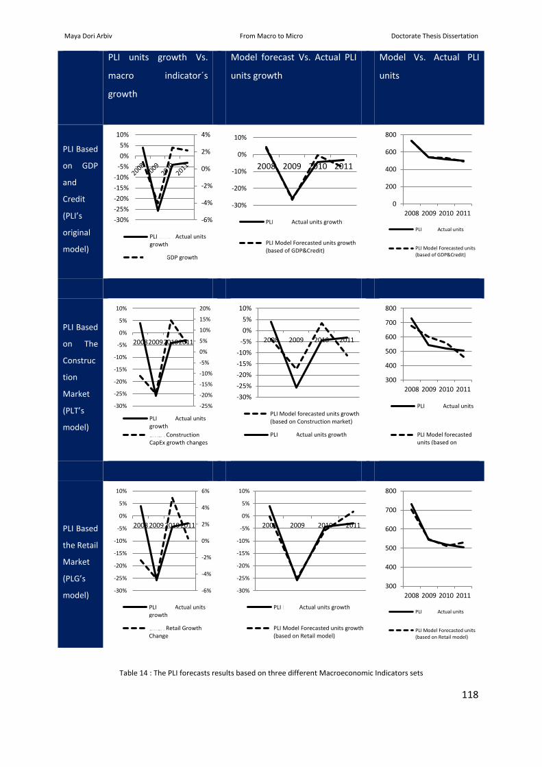
Maya Dori Arbiv From Macro to Micro Doctorate Thesis Dissertation
118
PLI units growth Vs.
macro indicator´s
growth
Model forecast Vs. Actual PLI
units growth
Model Vs. Actual PLI
units
PLI Based
on GDP
and
Credit
(PLI’s
original
model)
PLI Based
on The
Construc
tion
Market
(PLT’s
model)
PLI Based
the Retail
Market
(PLG’s
model)
Table 14 : The PLI forecasts results based on three different Macroeconomic Indicators sets
-6%
-4%
-2%
0%
2%
4%
-30%
-25%
-20%
-15%
-10%
-5%
0%
5%
10%
PLI EMEA Actual unitsgrowth
EMEA GDP growth
0
200
400
600
800
2008 2009 2010 2011
PLI EMEA Actual units
PLI Model Forecasted units(based of GDP&Credit)
-25%
-20%
-15%
-10%
-5%
0%
5%
10%
15%
20%
-30%
-25%
-20%
-15%
-10%
-5%
0%
5%
10%
2008200920102011
PLI EMEA Actual unitsgrowth
EMEA ConstructionCapEx growth changes
-30%
-25%
-20%
-15%
-10%
-5%
0%
5%
10%
2008 2009 2010 2011
PLI Model forecasted units growth(based on Construction market)
PLI EMEA Actual units growth
300
400
500
600
700
800
2008 2009 2010 2011
PLI EMEA Actual units
PLI Model forecastedunits (based onConstruction market)
-6%
-4%
-2%
0%
2%
4%
6%
-30%
-25%
-20%
-15%
-10%
-5%
0%
5%
10%
2008 2009 2010 2011
PLI EMEA Actual unitsgrowth
EMEA Retail GrowthChange
-30%
-25%
-20%
-15%
-10%
-5%
0%
5%
10%
2008 2009 2010 2011
PLI EMEA Actual units growth
PLI Model Forecasted units growth(based on Retail model)
300
400
500
600
700
800
2008 2009 2010 2011
PLI EMEA Actual units
PLI Model Forecasted units(based on Retail model)
-30%
-20%
-10%
0%
10%
2008 2009 2010 2011
PLI EMEA Actual units growth
PLI Model Forecasted units growth(based of GDP&Credit)

Maya Dori Arbiv From Macro to Micro Doctorate Thesis Dissertation
119
When the three PLI models are compared by their forecasting accuracy, it shows that the
majority of the forecasting accuracy factors support GDP and Credit based model for the PLI
forecasting.
Forecast Metrics
PLI model
based on
GDP &
Credit
PLI based on
the
Construction
market
PLI model
based on
Retail
Market
Mean Absolute Deviation (MAD) 2.4 7.9 2.8
Mean Percent Error (MPE) -19% 37% 58%
Weighted Absolute Percent Error (WMAPE) -33% -108% -38%
MAD-Mean Ratio -0.3 -1.1 -0.4
Forecasting Efficiency Quotient 0.81 0.38 0.78
R-Square 93% 49% 91%
Mean Squared Error (MSE) 8.7 62.3 10.6
Root Mean Square Error (RMSE) 3.0 7.9 3.3
Median Absolute Percent Error (MdAPE) -0.45 -1.05 -0.19
Table 15 : The accuracy metrics results for the three PLI forecasting models

Maya Dori Arbiv From Macro to Micro Doctorate Thesis Dissertation
120
6 Empirical study number 2
The empirical study tests the following two hypotheses:
1. The NIE suggests that the macro level activity is unique to each geo political area in
addition; the adaptation approach claims that regional differences are too big to be
ignored by the company´s activity. To test this claim of cultural difference of the NIE
and the international marketing adaptation approaches, we take a regional sales
forecasting model and test its forecasting capabilities in three of the countries that
constitute it. If the localized version of the regional model is capable of forecasting
well, it would mean that culture differences are big enough to be noticed by it. If the
localized regional model fails to forecast well it at the countries level it means that
these countries have some characteristics that should be taken into account by a better
forecasting model. This potential outcome would support the NIE and the adaptation
approach.
2. The international marketing literature debates for many decades on the best
marketing approach in firms expanding their activities beyond their home market. To
test if countries are in fact different in their sales drivers we search for country- specific
forecasting models. By providing country specific sales forecasting models we provide
additional support to the adaptation approach.
6.1 The model in 3 different geo-political countries
Once we have the model completed from empirical study number one, we are now ready to
check whether this model works the same in three different countries. As shown in the
previous sections, the sales were best explained by the GDP growth and the credit tightening
conditions. The question is: would that be the case for the three selected countries? We will
show that these are, without a doubt, three different markets where different drivers
influence the units’ sales. For the selection of the regions we have used the three regions types
described in the GLOBE research: United Kingdom as a representative of the Anglo culture
type, Germany as representative of the Germanic culture and Spain as a representative of the

Maya Dori Arbiv From Macro to Micro Doctorate Thesis Dissertation
121
Latin European culture. Each of the three cultures is also different in their countries’
economies characteristics.
One of the distinctive characteristics of the UK culture and therefore one of the pillars of the
UK economy is its retail sector. Retail is one of the biggest engines of its economy and Retails
consumer expenditures account for almost 37% of UK´s GDP as well as in worldwide relative
terms the UK retail sector is large as it is the 10th biggest in the world (Euromonitor, 2011). UK
also hosts one of the biggest retail companies in the world; The UK-based Tesco is the third-
largest retailer in the world measured by revenues after Wal-Mart Stores and Carrefour. In
addition, UK´s capital, London is a major retail center and in 2010 had the highest non-food
retail sales of any city in the world, with a total spend of around £64.2 billion (Euromonitor
2011). According to the British Retail consortium (BRC), In 2012 UK retail sales were over £311
billion which represented the sales revenue from 9% of all VAT-registered businesses in the
UK.
Table 16: The worldwide tanking of the Retail sector size by GDP in %
(Source: Euromonitor International from national statistics)
The consumers spending in the UK on retail products is also ranked among as the top 13th
place in the world:

Maya Dori Arbiv From Macro to Micro Doctorate Thesis Dissertation
122
Table 17: The worldwide ranking of the Consumer expenditure in Retail out of total expenditure in %
(Source: Euromonitor International from national statistics)
The German economy is characterized by its hardworking highly skilled labor force that
contributes to positioning Germany as the fifth largest economy in the world (in PPP terms).
Germany is also Europe's largest economy and it is a leading exporter of machinery, vehicles,
chemicals, and household equipment. When retail and manufacturing sectors are
encompassed together they represent the largest employer and the fourth-largest contributor
to value creation in Germany according to a Mckinsey´s report (2008). Germany is very open
to external markets as it is the second largest exporter and third largest importer of goods in
the world. Yet despite its close links and relationships with other nations around the globe, it
retains its own very distinct culture.

Maya Dori Arbiv From Macro to Micro Doctorate Thesis Dissertation
123
Table 18: Ranking of the Retail sector size by GDP in %
(Source: Euromonitor International from national statistics)
Long a largely agricultural country, Spain produces large crops and is the world's largest
producer of olive oil and Europe's largest producer of lemons, oranges, and strawberries. The
major Spanish industries produce textiles and apparel, foods and beverages, metals and metal
products, chemicals, ships, automobiles, machine tools, clay and refractory products,
footwear, pharmaceuticals, and medical equipment. Fishing is an important source of
livelihood, especially on the Atlantic coast, and fish canning is a major industry. Tourism is
Spain's greatest source of income.
Spain's greatest trade is with France, Germany, Italy, and Great Britain. Among the leading
exports are machinery; motor vehicles; fruit, wine, and other food products; and
pharmaceuticals. Major imports include machinery and equipment, fuels, chemicals,
manufactured goods, foodstuffs, and medical instruments.
Spain, Germany and the United Kingdome each represent large part of the European economy.

Maya Dori Arbiv From Macro to Micro Doctorate Thesis Dissertation
124
In 2012 Spain accounted for around 7% of EMEA´s GDP and roughly 10% of the European
Union economy UK´s GDP accounted for 14% of the EMEA economy and was second to
Germany. The German GDP in 2012 accounted for 16% of the EMEA economy making it the
largest economy in the whole EMEA economy. Being such an important part of EMEA region
we would a priori expect UK and Germany to respond well to the forecasting model produced
for the entire EMEA region and therefore, that the EMEA model (adapted to the local UK and
Germany’s data) would forecast well also the units sales in that region. We used a localized
version of a model that is based on EMEA´s data. Hence we used the GDP and credit tightening
variables of the central bank of Europe and England and generated new correlation figures to
represent the relationship between the PLI units sold in the local regions and the local
macroeconomic indicators, namely the local GDP growth and credit availability.
Due to the fact that the UK is not part of the Euro monetary union the credit availability data
was taken from the central bank of England. However, it did not improve the model to the
levels demonstrated at in the EMEA model. In another attempt to improve the UK localized
model we also introduced the European central bank credit availability data and this model
gave us worse of results than that of the model using the Central Bank of England credit
availability data. For the Spanish localized model we decided to use the European Central Bank
data on the credit availability. The reasons for the fact that we opted to use the central
European bank credit availability data instead of that provided by the central bank of Spain
were that the data provided by the central bank of Spain did not show to have any statistically
significant correlation with the sales of the PLI units sold in Spain while the credit availability
data provided by the central bank of Europe were statistically significant. The second reason
is the size of the Spanish banks within the European Union which is very significant and
therefore we felt confident, in that case, to take the European central bank credit availability
data as a proxy to the credit availability in Spain.
When the EMEA level GDP and Credit availability were used in the model for UK and Germany
the model only partially explained the historical units sales and gave poor in-series accuracy
of the UK and German sales as showed in the following graph and table below.

Maya Dori Arbiv From Macro to Micro Doctorate Thesis Dissertation
125
Forecast Metrics
European
model
European
localized models
UK Germany Spain
Mean Absolute Deviation (MAD) 0.97 13.46 12.4 6.0
Mean Percentage Error (MPE) 5% -103% 0,37 0,39
Weighted Absolute Percentage Error
(WMAPE) -13% -334% -5,93 -43%
MAD-Mean Ratio -0.13 -3.34 -5.9 -0.4
Forecasting Efficiency Quotient 0.91 0.09 0.31 0.33
R-Square 99% 60% 70% 87%
Mean Squared Error (MSE) 0.58 226.57 239.3 61.4
Root Mean Square Error (RMSE) 0.76 15.05 15.5 7.8
Median Absolute Percentage Error
(MdAPE) -0.04 -1.23 -0.2 0.5
Table 19: The accuracy metrics results of the PLI European localized model forecasting
Figure 36: UK PLI units’ growth Vs. the European-based PLI model forecasted units’ growth
-60%
-40%
-20%
0%
20%
40%
2008 2009 2010 2011
UK PLI Actual units growth
UK&I PLI forecasted units based GDP and credit availability (EMEA model)

Maya Dori Arbiv From Macro to Micro Doctorate Thesis Dissertation
126
Figure 37: Germany actual units’ growth Vs. Germany forecasted units growth based on the European model
These results show that two of the EMEA´s largest mature economies are not responding well
at all to the European forecasting model while the Spanish forecast model using the European
localized model works relatively well. Contrary to what we observed in UK and Germany’s case
there was a good correlation between the localized EMEA based model and the units sold in
Spain. Looking the correlation between the Spanish historical sales and GDP growth in Spain
and Credit availability in EMEA (which are both the EMEA level forecasting model indicators)
we find a model that explains much better the historical PLI units.
Figure 38: Spain units growth Vs. Spain forecasted units growth based on the European model
-100%
0%
100%
2008 2009 2010 2011
Germany forecast unit growth based on GDP growth and Credit tightening
Germany PLI Actual units growth
2008 2009 2010 2011
Spain units growth forecastbased on GDP and Credit
-41% -24% 1% 7%
Spain PLI Actual units growh -40% -23% -11% 19%
-100%
0%
100%
Gro
wth
rat
e
Spain actual units growth Vs. forecasted growth based on GDP and credit

Maya Dori Arbiv From Macro to Micro Doctorate Thesis Dissertation
127
This is a surprising result, raises questions and defiantly asking a further deep dive. Are there
other stronger factors in Germany and UK that better explain the sales in the local markets?
How come that the sales in Spain of all the three economies are actually explained well by the
European localized model? What would be the possible reasons for that? Can we find a specific
model for these regions that would forecast with accuracy the sales? In what this regional
specific model will be different than the European cross-regional model?
We will address these questions in our following section of this thesis.
6.2 Conclusions from the localized model
We demonstrated that in spite of the fact that the model works at the European regional level
it does not fit as well when it is localised and tested in its sub regions. The evidence is
conclusive “localisation” of a global model, in spite of the fact that the European global model
was proven to be very robust, surprisingly does not work as well even when we test it in the
number one and two economies comprising the EMEA economy, Germany and UK.
Our first conclusion from these results is that the intent of “one size fits all” in forecasting
might not be necessarily a good methodology for forecasting in local markets. So perhaps local
economies behaviours, reflecting the choices and the decision making processes of its agents
are not represented well in a model that is too insensitive to these nuances.
The second conclusion is that there might be specific characteristics to the local economies
that would require us to create a new model to better forecast the sales in these markets.
The intriguing results of the localised forecasting models have motivated us to look for models
that would work for these two economies better. Thus, leaving behind the failed intend to
localise a model and “force” it to work in the local economies level, in the next section we
embark on the search of a unique forecasting model for each of the regions.
We were curious to see what would be these local models and what would be the differences
between the local models and the “localised model” and what would be the differences
between the local model of one economy and the other local economy´s model. In other
words, could we put the cultural differences between the British, the Germans and the
Spaniards into mathematical formulas?

Maya Dori Arbiv From Macro to Micro Doctorate Thesis Dissertation
128
6.3 In a new search of best fitting local models
In this section we search for the forecasting model that gives the best in line accuracy with the
sales of the country.
6.3.1 The UK economy´s characteristics
As showed earlier, Retail sector occupies a big part and represents an important pillar of the
UK´s economy. In addition, the technology units forecasted are also used for retail-related
applications. These two important indications made us suspect that retail could be an
important potential contributor to the sales forecast of units in the UK. For that end, we have
used the UK retail index growth rates as a proxy for the retail sector as a macro structure
influencing the micro structure of the units’ sales.
We have considered the retail index as a macro level data since it is the aggregation of all the
retail micro level activities in the country. In fact, The Retail sales index is considered as key
economic indicator and one of the earliest measures of economic activity and it is used to
estimate consumer spending on retail goods and the output of the retail sector, both of which
are used in the compilation of the national accounts of the United Kingdome. The main output
measures include growth of the retail sector for in this year in comparison to that of the
previous year, mathematically represented by the first derivative of the retail index.
As mentioned earlier, the sales of the units in the UK were poorly forecasted by the localized
European model with GDP and credit availability. Due to the importance of the retail sector to
the British society and economy we have decided to check the correlation between the PLI
units sold in the UK and the retail sales index. Matching the early indications of the importance
of the retail sector, UK´s units sales is highly correlated to retail sales growth and the retail
market explains much better the historical sales than GDP and credit availability based
European model.
Looking at the correlation between the UK´s historical sales and Retail sales in the UK we find
a model that explains much better the historical PLI units in this region as can be observed in
the following graphs. Statistically this model gives R^2 adjusted of 86.46%, confidence level
(1- α) = 95.4% with Retail index as statistically significant.

Maya Dori Arbiv From Macro to Micro Doctorate Thesis Dissertation
129
Figure 39: UK model forecasted units’ growth Vs. UK actual units’ growth
Forecast Metrics European localized
– UK model
The local UK
Model
(based on Retail
sales)
Mean Absolute Deviation (MAD) 13.46 7.77
Mean Percentage Error (MPE) -103% 124%
Weighted Absolute Percentage Error (WMAPE) -334% -193%
MAD-Mean Ratio -3.34 -1.93
Forecasting Efficiency Quotient 0.09 0.22
R-Square 60% 86%
Mean Squared Error (MSE) 226.57 80.07
Root Mean Square Error (RMSE) 15.05 8.95
Median Absolute Percentage Error (MdAPE) -1.23 -1.00
Table 20: The accuracy matric results of the forecasting models for the UK
-60%
-40%
-20%
0%
20%
40%
2008 2009 2010 2011
UK&I forecasted units based on Retail sales growth
UK&I PLI Actual units growth

Maya Dori Arbiv From Macro to Micro Doctorate Thesis Dissertation
130
6.3.2 The German economy characteristics
Encouraged by the importance of the retail sector to the German economy and the forecasting
capabilities of the UK model based on the retail index, we tried to apply a retail sector based
model to forecast the units sold in the Germany. Since this model works well for the UK we
expected to work for the German market as well, however, as can be showed in the following
graph this model fails to explain the historical units growth in Germany. In addition,
statistically this model is far from being acceptable with R^2 adjusted: 0.36, confidence level
(1- α) =76%, the Retail growth indicator as not statistically significant.
Figure 40: Germany units’ growth Vs. the UK-based model forecasted units’ growth
The question that this result raises is why in spite of the fact that the retail sector is important
in Germany using the retail index gives non-conclusive forecasting results.
Therefore we started looking for other cultural and economic characteristics that could explain
this puzzling result. The first possible explanation to difference between the German and the
UK model is that the Germans are known to be risk averse and very prudent in their
investments spending as firms and as individuals and that the uncertainty caused by
unemployment means that export growth does not translate into domestic spending and
therefore both businesses and people tend to save for the rainy day rather than boost the
economy by spending. This claim is supported by Hofstede´s (1980) work and the GLOBE
research positioning Germany among the group of the most risk adverse cultures.
Still convinced in the relevance of the retail market on the sales of the PLI units in Germany,
we embarked on a search for a better way to reflect the German retail sales as a macro
-50%
0%
50%
2008 2009 2010 2011
Germany forecast unit growth based on Retail Sales growth (The UK&I model)
Germany PLI Actual units growth

Maya Dori Arbiv From Macro to Micro Doctorate Thesis Dissertation
131
structure that influences the micro structure of the units sales and that would reflect the
uniqueness of the German culture risk averseness, the savings “for a Rainey day” and the
Germany sensitivity to any early inflation signs. To reflect these culture characteristics we
decided to test the correlation between the units sold in Germany and the second derivative
of the retails sales growth in Germany. We assumed that using the second derivative of the
macroeconomic indicator would reflect the changes in growth rate that the Germans could be
so sensitive to. The second derivative is the mathematical representation of the changes in
speed of the growth of the economic activity captured by the macro economic indicator. A
negative reaction such as a decrease in sales induced by the decrease of the growth of the
economic activity will be considered as “prudency”/risk aversion. For example, assuming that
in time t the growth rate of the macro economic indicator is 4% and in time t+1 it is 2%. In
time t+1 there was a growth in the economic activity represented by the indicator however
for a prudent/risk adverse person it will be a bad sign since the speed of the growth was
reduced by half. A prudent person or culture who are educated to look for the “clouds before
the storm embarks at their door” like in Germany would perceive this decrease in speed as
bad news and will call for a halt in its investments and expenses rate.
The forecasting model based on the correlation of the PLI units sold in Germany and the Retail
sales growth difference calculated as the second derivative of the retail sales in Germany
results in a model that explains much better the historical PLI units’ growth, as shown in the
following graphs. In addition, contrary to the European model based on GDP growth and credit
availability this new model gives a good model fit with R^2 adjusted of 86.46%, confidence
level (1- α)=95.4% and with Retail sales statistically significant.
2008 2009 2010 2011
Germany PLI Forecastedunits based on retail
sales growth diff17% -39% 32% -18%
Germany PLI Actualunits growth
18% -38% 32% -20%
-50%
0%
50%
Gro
wth
rat
e

Maya Dori Arbiv From Macro to Micro Doctorate Thesis Dissertation
132
Figure 41: Germany actual units’ growth Vs. Germany forecasted units growth based on the German model
To summarize, Germany, similarly to the UK, is a market in which the units also correlate to
the retail sales but in a surprisingly different way. In Germany the units correlate best to the
second derivative of the Retail sales growth. This indicates a mature market that is hyper
sensitive to any change in the Retail market speed, in comparison to the UK market. It means
that the German market is over-reacting to any little change in the retail growth speed being
positive or a negative change.
Forecast Metrics Germany
European-
localized Model
Retail based
model
Second derivative
Retail Based
model
Mean Absolute Deviation (MAD) 12.4 15.3 1.0
Mean Percentage Error (MPE) 37% 72% 3%
Weighted Absolute Percentage Error (WMAPE) -593% -730% -46%
MAD-Mean Ratio -5.9 -7.3 -0.5
Forecasting Efficiency Quotient 0.31 0.28 0.22
R-Square 70% 58% 99.9%
Mean Squared Error (MSE) 239.3 337.0 1.1
Root Mean Square Error (RMSE) 15.5 18.4 1.1
Median Absolute Percentage Error (MdAPE) -0.2 1.4 1.2
Table 21: The accuracy matric results of the three forecasting model for Germany
The Spanish units correlated with a localized version of the European model that takes into
account the GDP growth and credit availability. Contrary to the other two geo-political regions,
UK and Germany, in the case of Spain, the localized model gave fairly good forecasting
accuracy results. In order to confirm that these results are not random we also applied the UK
model based on the retail macroeconomic indicators and then applied the German model
based on a variation of the retail based model. After testing these two models, we conclude
that both models do not work well for the Spain market, while that the Spanish model based
on the localized European model that takes the GDP growth and credit tightening indicators
matches well the Spain PLI market. Using the UK model based on retail sales growth results

Maya Dori Arbiv From Macro to Micro Doctorate Thesis Dissertation
133
only partially explains the historical sales, as showed in the following graph. In addition the
model’s fit “wellness” shows difficulties to the fit between Retail Sales growth and the Spain
PLI market with R^2 adjusted: -41.46%, confidence level (1- α)=23% and with Retail sales
growth indicator not significant statistically.
Figure 42: Spain units’ growth Vs. Spain forecasted units growth based on the UK model
Using the German model, based on retail sales growth speed (first derivative), only partially
explains the historical PLI sales, as shown in the following graph. In addition the model’s fit
“wellness” shows difficulties to the fit between Retail Sales first derivative and the Spain units
market with R^2 adjusted: -40%, confidence level (1- α)=24% , Retail sales growth speed
indicator not significant statistically.
Figure 43: Spain units’ growth Vs. Spain forecasted units growth based on the German model
-50%
0%
50%
2008 2009 2010 2011
Spain units growth forecast based on Retail Growth
Spain PLI Actual units growh
-50%
0%
50%
2008 2009 2010 2011
Spain units growth forecast based on Retail Growth Diff
Spain PLI Actual units growh

Maya Dori Arbiv From Macro to Micro Doctorate Thesis Dissertation
134
The comparison of the accuracy factors of the three models for the Spain units shows the clear
advantage of the Spain model over the other two models.
Forecast Metrics Spain based
on the
German
Model
Spain based
on the UK
Model
The Spain
Model based
on the
European
model
Mean Absolute Deviation (MAD) 17.4 16.7 6.0
Mean Percentage Error (MPE) 82% 76% 39%
Weighted Absolute Percentage Error
(WMAPE) -125% -120% -43%
MAD-Mean Ratio -1.3 -1.2 -0.4
Forecasting Efficiency Quotient 0.27 0.31 0.33
R-Square 6% 6% 87%
Mean Squared Error (MSE) 429.6 431.9 61.4
Root Mean Square Error (RMSE) 20.7 20.8 7.8
Median Absolute Percentage Error (MdAPE) -1.5 -1.5 0.5
Table 22: The three Spain´s forecasting model accuracy matric results
Figure 44: Spain units’ growth Vs. Spain forecasted units growth based on the European model
-50%
0%
50%
2008 2009 2010 2011
Spain units growth forecast based on GDP and Credit
Spain PLI Actual units growh

Maya Dori Arbiv From Macro to Micro Doctorate Thesis Dissertation
135
Figure 45: Spain units’ growth Vs. Spain forecasted units based on the European model
One possible explanation to it is that Retail market is less dominant in the Spanish economy in
comparison to the relevance of factors such as availability of credit in the Spanish market and
its dependency on credit availability in order to finance investments such as that of the PLI
products. The possible explanation for the credit dependency is that private equity and self-
funding are less common financing mechanisms than bank credit lines. In addition, these credit
lines were severely tightened in the years that are covered in this research which resulted in
limited financing tools. One of the potential reasons for the strong correlation between the
units’ growth and the credit availability in Spain is the dependency of Small and Medium
business which are the majority of the businesses in Spain and the majority of the clients of
the products on their banks credit lines as their business life-line. The high dependency on
banks financing could indicate that self-funding projects or private equity financing are not
common in the Spain business culture Spain- These last two points are worth further future
investigation.
20
25
30
35
40
45
50
2008 2009 2010 2011
Spain PLI Actual units Spain units forecast based on GDP and Credit

Maya Dori Arbiv From Macro to Micro Doctorate Thesis Dissertation
136
7 Empirical study number 3
In this empirical study we explore the life cycle of three products generations and show that
the model is able to forecast well the sales of the products at the different stages of their
product life cycles. Then, using the products sales forecasting models and comparing them to
the actual products sales, we analyze the different aspects of the introduction of a second
product and answer the question whether the introduction of that product, product B, was
successful and beneficial to the company while discussing some of the product portfolio
dynamics that were created from the two products coexistence. We then discuss the reasons
that made the company introduce a third product and the product portfolio dynamic between
the three generations of products.
As in the previous empirical study described in our thesis, Empirical study number 3 uses a
model that takes the constitutive relationship between macro market conditions and the sales
of units and uses macroeconomic indicators to forecast the sales growth rate of the one
product line. The forecasting model is based on one or two macroeconomic indicators: the
GDP growth rate and the credit availability. When the product capital investment is relatively
low, the credit availability indicator is less significant than the GDP growth and therefore for
the entry level product, product A, we have used only the GDP growth as a macroeconomic
indicator for the forecasting model. However, for product B a much substantial capital
investment is required and therefore, in addition to the GDP growth indicator we have used
the credit availability indicator in order to forecast the products sales growth correctly. The
GDP information is widely available and publically published by many entities. The data we
used in this thesis is taken from IHS data base. IHS is a global information company providing
market information and forecasts of many macroeconomic indicators. The credit availability
information is taken from the Central European bank survey of banks around Europe regarding
the credit policy applied to their customers. The part of the survey that is used in this thesis is
the loans conditions to small and medium size enterprises.
The empirical study will analyze three products of one product line manufactured and
designed by Hewlett Packard, named here as products A, B and C. We will compare their

Maya Dori Arbiv From Macro to Micro Doctorate Thesis Dissertation
137
product life cycles and highlight their product portfolio dynamic at the decisions made based
on these portfolio dynamics.
7.1 Is the empirical test merely anecdotal?
To refute the potential claim that using two products of one company is too firm-specific or
even an anecdotal case, we would like to clarify that products A and B represent the two main
products in the market. The market of which products A and B are big part of, contains other
technology firms such as Hewlett-Packard, Fuji-Xerox, Xerox and Kodak. This market and the
number of units sold from each of the players is closely monitored by the International Data
Corporation (IDC), an American market research, analysis and advisory firm, specializes in
information technology, telecommunications, and consumer technology. According to IDC,
these four main players represented 86% to 90% of the total market units in 2008 to 2013.
According to the same source, the total worldwide market size of all the products value was
estimated in 2010 to be 0.9 billion of USD dollars. Hewlett-Packard is the leader of this 1 Billion
USD$ market. According to industry analyst IDC, Hewlett-Packard is the world-wide market
leader with more than 50% percent of the market units sold between 2008 and 2013.
Consequently, as shown in the following graph, product A and B products sales trend is very
much similar to that of the entire market.
Figure 46: Total market units Vs. A and B units
Source: IDC market share report
0
200
400
600
800
2008 2009 2010 2011 2012 2013
Product A+B out of the total market
Product A and B Total Market

Maya Dori Arbiv From Macro to Micro Doctorate Thesis Dissertation
138
In Addition, as the market leader, Hewlett-Packard´s decisions and products launches tend to
be followed by other technology companies in the market. For example, after Hewlett-Packard
launched product B at the end of 2008, Kodak launched another product and upgrades for its
existing products in 2009. The following figure summarizes the product launches by the
technology players in the market, namely, Kodak, Xerox and Hewlett-Packard.
Y0=2005, Y1=2006, Y2=2007, Y3=2008, Y4=2009, Y5=2010, Y6=2011, Y7=2012
Figure 47: Product launches of the main technology players
Source: KODAK and Xerox web sites and IDC Q1CY2014 report
7.2 Product A sales forecast and its PLC stages
Product A was introduced by Hewlett-Packard in 2003 and represented the most advanced
technology of its time. Product A was at its “maturity” stage by the time we analyzed it for the
thesis. The following is a quarterly view of product´s A sales showing the sales results of
product A over time:

Maya Dori Arbiv From Macro to Micro Doctorate Thesis Dissertation
139
Y0=2005, Y1=2006, Y2=2007, Y3=2008, Y4=2009, Y5=2010, Y6=2011, Y7=2012, Y8=2013, Y9=2014
Figure 48: A quarterly view of the sales of product A
Source: IDC market reports
We have created a forecasting model that uses macroeconomic indicators to forecast the sales
of Product A based on the IDC market reports. After testing the model with several different
macroeconomic indicators, we have found that product A correlates better with GDP growth
and that its purchase was most probably self-financed as credit availability, measured by the
credit tightening factor, was not statically significant. The forecasting model resulted outcome
was R^2 adjusted of 70% at a confidence level of 99% (1-α). The depended variable, GDP was
statistically significant.
0
20
40
60
80
100
Y0Q1
Y0Q3
Y1Q1
Y1Q3
Y2Q1
Y2Q3
Y3Q1
Y3Q3
Y4Q1
Y4Q3
Y5Q1
Y5Q3
Y6Q1
Y6Q3
Y7Q1
Y7Q3
Y8Q1
Y8Q3
Y9Q1
Product A units sales over time
Product A 4 per. Mov. Avg. (Product A)

Maya Dori Arbiv From Macro to Micro Doctorate Thesis Dissertation
140
Figure 49: Product A forecasting model
The following graph describes the model forecast and the Product A units sold in an in-series
accuracy exercise. The model scores fairly close to the real product A units sales as well as the
upper and lower 95% product A sales model forecast. One of the main limitations of the Bass
model as a forecasting tool (1969) was its need for many data point to general a forecasting
model. Nevertheless, the model we designed for Product A used only nine data points (2005-
2013) for a model with high level of statistical accuracy forecasting results.
Y1=2006, Y2=2007, Y3=2008, Y4=2009, Y5=2010, Y6=2011, Y7=2012, Y8=2013
Figure 50: Product A forecasted units vs. units A sold
During the 9 years of product history, Product A passed through several stages of its product
life cycle as can be seen in the graph above. In spite of the very different product life cycle
stages, our forecasting model was able to forecast the sales of product A through its various
product life cycle stages with a great level of accuracy. It represents not only a contribution to
the Bass model and its extensions but also to the product life cycle literature as it does not
require to use any of the company´s internal information as selling prices.
It can be observed in the figure bellow that product A was passing through several of its
product life cycle stages. It also shown in the graph bellow that 2013 was a transition point
between two different life cycle stages of product A, the “maturity” and the “decline” phases.
0
100
200
300
400
Y1 Y2 Y3 Y4 Y5 Y6 Y7 Y8
Product A units
Product A units - model prediction
Units A- model prediction upper 95%
Units A- model prediction Lower 95%
Time
Units

Maya Dori Arbiv From Macro to Micro Doctorate Thesis Dissertation
141
Following product A life cycle stages, we have separated product A phases to “maturity” and
“decline” stages based on their sales growth and tested the coefficient (β) between product A
and the macroeconomic indicator GDP. The correlation between the macro indicator and the
product A sales growth was 10.75 higher at the “decline” stage of the product than at the
“maturity” stage which might indicate that product A is being sold to the late majority and to
the laggards customers. This insight tells us that the sales of product A at the decline stage are
more correlated to the macroeconomic climate than at the previous stages while the sales at
the early stages are less correlated to the macroeconomic indicator. It could be explained by
the characteristics of the “early adopters” and the “early majority” who buy the products at
the early stages of the product life cycle. These customers tend to have more risk taking
attitude than the customers who buy products at later stages of their product life cycle, who
are characterized by being more risk averse. In that case, the difference in the beta between
the macro indicator and the sales of a product are rightfully reflecting the type of customers
and the life cycle stage of the product.
Y1=2006, Y2=2007, Y3=2008, Y4=2009, Y5=2010, Y6=2011, Y7=2012, Y8=2013
Figure 51: The coefficients of the sales of product A and the macroeconomic indicator

Maya Dori Arbiv From Macro to Micro Doctorate Thesis Dissertation
142
7.3 Product B sales forecast and its PLC stages
At the second half of 2008, when Product A has reached its rock bottom growth rate levels,
Hewlett-Packard launched a new product, product B, with better product attributes than
product A. Due to its better product attributes it was also offered at a list price which was
double the price of Product A. This is a very common pricing strategy of new product launches
called “skimming pricing” where higher prices are charged for the new product as it allows to
recover the products research and development sunk costs as soon as possible before the
competition steps and lowers the market price. Product B had also unique attributes in
comparison to the competition and when it was launched there was no product in the market
that could match the productivity and quality of product B. In addition, products A and B had
different list prices and product attributed that helped the market distinct and choose
between them based on their needs and capital investment capacity. The following graph
describes product B attributes and list prices in comparison to the competition and product A.
Figure 52: A schematic view of the characteristics of product A and B
The sales level of product B was slowly but surely increasing right after the product was
launched and during the growth stage of the product.
Product A Product B
The competition
Price
Product
Attributes
600K$
300K$
450K$

Maya Dori Arbiv From Macro to Micro Doctorate Thesis Dissertation
143
Y3=2008, Y4=2009, Y5=2010, Y6=2011, Y7=2012, Y8=2013, Y9=2014
Figure 53: Product B sales results by quarter
(Source: IDC market report)
We have created a forecasting model that uses macroeconomic indicators to forecast the sales
of product B. After testing several macroeconomic indicators, we have found that product B
correlates better with the GDP growth and the credit availability. It looks that the sales of
product B required external financing due to product B list price. Since product B was a new
product in the market at the time of the analysis, we had only 4 data points representing the
years of the product since its launch and the time of our analysis. As shown in the following
figure capturing Nevertheless, with the 4 data point representing the 4 years of product annual
sales information, the forecasting model had an R^2 of 98% at a confidence level of 93% (1-
α). Both dependent variables were statistically significant.
0
10
20
30
40
50
Y3Q3
Y3Q4
Y4Q1
Y4Q2
Y4Q3
Y4Q4
Y5Q1
Y5Q2
Y5Q3
Y5Q4
Y6Q1
Y6Q2
Y6Q3
Y6Q4
Y7Q1
Y7Q2
Y7Q3
Y7Q4
Y8Q1
Y8Q2
Y8Q3
Y8Q4
Y9Q1
Product B Linear (Product B)
Units
Time

Maya Dori Arbiv From Macro to Micro Doctorate Thesis Dissertation
144
Figure 54: Product B sales forecast statistics results
The following graph shows the results of the in-series accuracy exercise of the forecasting
model. It shown that the model forecast is fairly close to the real product B units’ sales and
the upper and lower 95% forecast are close to the real product B sales.
Y4=2009, Y5=2010, Y6=2011, Y7=2012
Figure 55: Product B sales forecast vs the product B units’ sales
0
50
100
150
Y4 Y5 Y6 Y7
Product B units Product B units - model prediction
Units B- model prediction UPPER 95% Units B- model prediction LOWER 95%
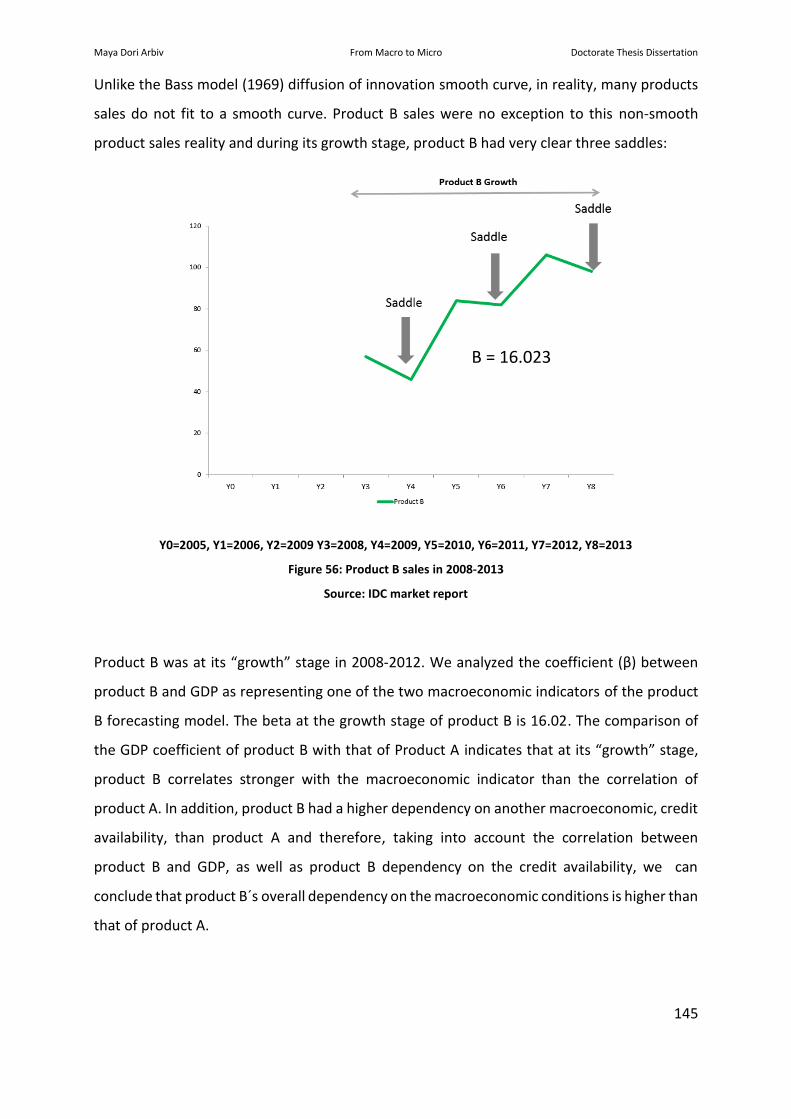
Maya Dori Arbiv From Macro to Micro Doctorate Thesis Dissertation
145
Unlike the Bass model (1969) diffusion of innovation smooth curve, in reality, many products
sales do not fit to a smooth curve. Product B sales were no exception to this non-smooth
product sales reality and during its growth stage, product B had very clear three saddles:
Y0=2005, Y1=2006, Y2=2009 Y3=2008, Y4=2009, Y5=2010, Y6=2011, Y7=2012, Y8=2013
Figure 56: Product B sales in 2008-2013
Source: IDC market report
Product B was at its “growth” stage in 2008-2012. We analyzed the coefficient (β) between
product B and GDP as representing one of the two macroeconomic indicators of the product
B forecasting model. The beta at the growth stage of product B is 16.02. The comparison of
the GDP coefficient of product B with that of Product A indicates that at its “growth” stage,
product B correlates stronger with the macroeconomic indicator than the correlation of
product A. In addition, product B had a higher dependency on another macroeconomic, credit
availability, than product A and therefore, taking into account the correlation between
product B and GDP, as well as product B dependency on the credit availability, we can
conclude that product B´s overall dependency on the macroeconomic conditions is higher than
that of product A.
Β = 16.023

Maya Dori Arbiv From Macro to Micro Doctorate Thesis Dissertation
146
8 Empirical study number 4
When one is looking at the empirical study in series accuracy levels, she can get the wrong
impression that “everything is already written in the stars” and that since the macroeconomic
indicators have such a significant level of explanatory capability they are also the sole and the
only driver of the sales of the products. This would be a confusion between “forecast” and
“prediction” that was mentioned in previous sections of the thesis. In empirical study number
4, we would like to refute the impression that management cannot influence the results of a
forecast by empirically showing that the strategic decisions of the management about the
product portfolio are critical components in shaping the outcome of the product portfolio
sales results.
Portfolio-related managerial decisions are divided into short term decisions and long term
decisions. The main difference between the short term managerial decisions and the long term
ones can be summarized by the understanding that the short term is reflected in “doing things
right”. In the short term the product is a “given” and the company´s management needs to
decide on the marketing activities to pull the demand for the products which often involves
the decision on the pricing strategy that depends on the products price elasticity could
increase the demand for a product. The long term decisions on the other hand, are reflected
in “doing the right things” meaning that the decisions are about which products to develop for
the identified market challenges or for new markets opportunity. The goals of the long term
product portfolio decision makings can be summarized in two main tasks:
The decision on the right mix of products in the product portfolio by determining which
product to launch and when and which product to remove from the company´s
portfolio.
The decisions on which market to approach with new products, solutions and often
with disruptive technologies.
Empirical study number 4 takes the individual forecast models of product A and B, created in
empirical study number 3 and compare them to the actual sales results of these products. This

Maya Dori Arbiv From Macro to Micro Doctorate Thesis Dissertation
147
comparison will give us the ability to separate between the expected sales growth from each
of the products based on their stand-alone ability in the market and the possible product
portfolio decisions and effects that may influence these results. In order to isolate the
potential effect of product B introduction on product A, product A forecasting model was
based on only three data points, years 2006, 2007, 2008, which are years where product B did
not exist or its sales were not yet reflected at the IDC market tracker report. Our model was
based on only external information of macroeconomic indicators and that allowed us to isolate
the impact of the product portfolio dynamics. The assumption of the analysis is that the
deviations between the forecasted units and the real units sold of each of the product are
explained by the portfolio dynamics between the two products. The separation of the two
source of impacts on sales, that of the product and that of product portfolio, could lead us to
answer the question whether the portfolio dynamics of the products was that of “substitution”
or “sales acceleration” and consequently we can answer another important question which is
whether the launch of product B increased the revenue of the company.
8.1 Product B introduction in light of product A existence
Product B was introduced at the end of 2008 and started its “introduction” and “growth”
product life cycle stages in parallel to product A´s “maturity” and the beginning of the
“decline” life cycle stages. The fact that the two products coexisted during the entire time line
covered in this thesis, gave us a unique opportunity to study and observe the dynamics
between the two products. As shown in the flowing figure representing the two products´
sales over the years, Product B units’ sales were slowly growing until it eventually matched
the sales levels of product A in 2012. In the following year, 2013, the sales levels of product B
surpassed the sales of product A for the first time.

Maya Dori Arbiv From Macro to Micro Doctorate Thesis Dissertation
148
Y0=2005, Y1=2006, Y2=2009 Y3=2008, Y4=2009, Y5=2010, Y6=2011, Y7=2012, Y8=2013
Figure 57: The sales of product A and Product B 2005-2013
Although product A´s sales were constantly decreasing during the “decline” stage of the
product, Product B was not able to outperform Product A units sales during first few years of
its existence, from 2008 to 2012. It shows that product B was clearly not substituting
completely product A. The longtime that was required for product B to reach the levels of
product A also raises the question whether the major R&D and the marketing efforts and
investments that were made in launching product B actually paid off for the company. In order
to answer these questions, in the empirical study number four we analyze the different
aspects of product B results.
8.2 Portfolio decision making test #1: Product B from sales
perspective
When the actual sales of products A and B are compared with the forecasts of these products
from 2009 to 2012, the total balance is positive as more units from product A and B were sold
Time
Units

Maya Dori Arbiv From Macro to Micro Doctorate Thesis Dissertation
149
than the forecasted ones. In total, both products contributed to a difference of 22 units
between the forecast and the real units sold as reported by IDC.
In 2009, just a few months after the introduction of product B, the sales of product A
outperformed the forecast by 38 units, according to IDC market report, meaning that the
existing product was outperforming the new product. The possible reasons for what could be
related to challenges in new product introduction are widely described in the academic
literature. The common wisdom among practitioners such as Morris at al. (1996), Stalk (1988)
and Wilson and Norton, (1989), is that the firm should introduce the product as soon as it is
available or at maturity of the old generation e.g. Mahajan and Muller (1996). In fact, the
decision on what is the right timing to introduce a new generation of a product represents a
clear tradeoff for the companies the time to market of introducing products as fast as possible
and the performance of their products e.g. Morris at al. (1996). Stalk (1988) coined the term
time-based competition to highlight the importance of quick time-to-market in today's
intensive competitive environment. Clark (1989) estimates that for a $10,000 car, each day of
delay in introducing a new model rep-resents a $1 million loss in profit. A recent McKinsey
study reports that, on average, companies lose 33% of after-tax profit when they ship products
six months late, as compared with losses of 3.5% when they overspend 50% on product
development. In their book “Developing Products in Half the Time”, Smith and Reinertsen
(1991) argue that it is necessary to adopt an incremental approach to product innovation in
order to reduce time to market. This is because incremental product innovation reduces the
amount of effort and learning that must be done and, consequently, the amount of time
needed to invest in the new product prior to its launch. Such a perspective has led many
companies to adopt time-to-market as their principal product development metric.
The difference between the sales forecast of product B and the actual sales of product B in
2010-2011 as reported by IDC, demonstrates that product B canalized 23 units of product A.
In other words, 23 units of product A were not sold due to the existence of product B.
However, in 2012, it looks that product B was not impacting the sales of product A as the two
forecasting models of product, that includes the product B impact on product A and the one
that excludes it, forecasted the same amount of units of product A to be sold that year. In
2012 product A sales outperformed the two (identical forecasts) by 8 units. When we isolate

Maya Dori Arbiv From Macro to Micro Doctorate Thesis Dissertation
150
the product B introduction results that are reflected in 2009, we can conclude that, in general,
the internal dynamics between the two products generations was that of cannibalization of
product A or substitution of product A with product B.
Y1=2006, Y2=2009 Y3=2008, Y4=2009, Y5=2010, Y6=2011, Y7=2012, Y8=2013
Figure 58: products A and B units gain versus forecast
Overall between 2009 and 2012 Product A units outperformed the forecast by 22 units and
product B underperformed the model by 2 units. In total products A and B outperformed the
forecasted units by 20 units. All these additional units came from product A which could
indicate that the introduction of product B did not substitute product A and might create
acceleration in the sales of product A.
8.3 Portfolio decision making test #2: Product B from revenue
perspective
As explained in the previous section, the mix of the products sold in 2009-2012 was skewed
toward product A as more of product A were sold than product B. Taking into account that
Time
Units

Maya Dori Arbiv From Macro to Micro Doctorate Thesis Dissertation
151
product A selling price was around half of that of product B, as reported by IDC, the company
gained several million dollars during years 2009 and 2012 from product B introduction. A single
digit million dollar figure in 4 years of sales of product B could be perceived as not such a bad
revenue result but If we take into account that the main contributor to this revenue upside
was Product A as well as the fact that this additional revenue is probably not covering the R&D
costs of developing product B, we find this result as a disappointing one. R&D investments are
not shared publically but in general those product investments tend to be more than a single
digit million dollar figure in the market of products A and B. Therefore a single digit revenue
figure would probably barely cover the investment involved in the development of the new
product. In summary, from revenue perspective, it looks that the introduction of product B
was a limited success.
8.4 Portfolio decision making test #3: Product B from market
perspective
According to the IDC market share reports, in 2009, shortly after product B was introduced,
the market in which product A and B were part of grew negatively and stood at -10% in
comparison to the previous year´s market growth. Hewlett-Packard´s units’ growth of
products A and B contributed to a positive growth of 23%, as reported by IDC. The competition
was lagging behind Hewlett-Packard´s product introduction success and their market growth
stood at -20%. The positive product introduction impact continued also in the following year,
in 2010 Hewlett-Packards´ units’ sales grew double the speed of the market growth speed with
55% and 27% respectively. The positive market growth was mainly attributed to Hewlett-
Packards´ product sales performance as the competition grew only 13% that year. 2011 was
equally bad to Hewlett-Packard as to it its competitors. In 2012, Hewlett-Packards surpassed,
once again, both the market and the competition growth with 11% units’ sales growth versus
the market’s growth of 5% and the competition growth of 1% that year. In summary, based
solely on IDC market report, from market perspective, product B helped defend Hewlett-
Packards´ position as the market leader, granting the company the privilege of growing faster
than its competitors and surpassing the total market growth in most of the years after the
introduction of product B. Hence, from market positioning perspective, the introduction of
product B was successful.

Maya Dori Arbiv From Macro to Micro Doctorate Thesis Dissertation
152
Y4=2009, Y5=2010, Y6=2011, Y7=2012
Figure 59: Market size growth
Source: IDC market report
8.5 A Game changer product portfolio decision
In 2013 that market of product A and B suffered from an adverse economic climate and
consequently their sales have declined. During this year product A was at its “decline” stage
for several years already and product B was in its “growth” stage that was temporarily
hampered by the macro economic conditions, representing a saddle in its growth attributed
mainly to the fact that the potential customers for product B could not access credit lines due
to the “financial drought”. The European banks have reported in the European central bank
survey that the credit availability in 2013 has declined by almost 60% between 2012 and 2013.
Consequently to the macro conditions headwinds, the market itself was undergoing a
significant market restructuring as many of the customers went out of business while others
were bought by other companies and struggled to grow their business and to invest in new
equipment. The adverse macroeconomic conditions as well as the market restructuring
directly influenced and reflected in the units sold in 2013. Using our methodology of analyzing
the forecast models with the real units sold as reported in the IDC market report, we clearly
-10%
27%
-18%
5%
23%
55%
-18%
11%
-20%
13%
-18%
1%
-40% -20% 0% 20% 40% 60%
Y4
Y5
Y6
Y7
Competition growth HP growth Market growth
Year-Over Year
(YoY) growth
Year

Maya Dori Arbiv From Macro to Micro Doctorate Thesis Dissertation
153
see that in 2013 the gap between the sales forecast and the actual sales was 90 units. 65 out
of the 90 units were Product B units that was forecasted to be sold but never did in 2013.
The forecasting models demonstrate that products A and B, suffered more than just
macroeconomic headwinds and that there might more needed to be done in order to ensure
the products sales in the long term. This decision required a change to the future product
portfolio and led the company to embark on intensive R&D efforts in order to introduce to
these new markets a true disruptive technology.
For several years the company had invested many resources in the creation of a new platform
of products for the new markets. These intensive R&D investments were fruitful and in 2013
Hewlett-Packard launched product C. The product was a first of its kind was designed to
several new markets that nor product neither A nor B could cater to in the past. The addition
of a new generation of products to the company´s portfolio aimed to reshape the market and
the company´s portfolio´s dynamic. In the following thesis´ subchapters we will quantify and
comment on these impacts.
8.6 The results of the new product launch
8.6.1 Portfolio decision making test #1: Product C from sales perspective
Product C sales acceptance was good. Soon after its launch in 2013, product C was already 4%
of the total units sold in the market according to IDC. The number of product C units sold was
growing each year and in 2014 it was already 6% of the total units sold which represents a
growth rate of 67%.

Maya Dori Arbiv From Macro to Micro Doctorate Thesis Dissertation
154
Figure 60: Product C units out of total units in the market
However, these positive sales results are not reveling the impact that product C launch had on
the other two products in the portfolio. An interesting question to be answered is whether the
introduction of product C helped Hewlett-Packard to outperform the sales forecast based on
the macroeconomic indicators. In other words, whether Hewlett-Packard was able to change
its “destiny” that was “written in the stars” with the huge investment made in the
development of product C. To answer this important question, we have prepared a
forecasting model based on empirical study number one and applied macroeconomic
indicators to predict the sales of products A and B together as reported by IDC. The forecasting
model is robust and accurate with R^2 of 87.6% and probability of 96% and the independent
variable, GDP growth, as statistically significant.
0%
20%
40%
60%
80%
100%
2012 2013 2014 2015
Product C out of total market
Other products in the market
Linear (Product C out of total market)

Maya Dori Arbiv From Macro to Micro Doctorate Thesis Dissertation
155
Figure 61: The statistical results of forecasting the sales of product A and B as a function of a macroeconomic
indicator
This model predicted that in 2013 and 2014 the sales of products A and B would be higher
than there actually were. The introduction of product C in 2013 resulted in reducing the gap
between the sales predictions and the actual sales due to the sales of the newly released
product C and in 2014 the three product together outperformed the sales forecast of product
A and B. Therefore, we can conclude that product C has contributed positively to the sales of
Hewlett-Packard and the evidence to it is by the reduction of the gap between the sales
forecast and the actual sales in 2013, as reported by IDC, and by the fact that the sales of
product A, B and C products outperformed the model sales forecast of product A and B.

Maya Dori Arbiv From Macro to Micro Doctorate Thesis Dissertation
156
Y7=2012, Y8=2013, Y9=2014
Figure 62: Product C contribution to products A and B sales
8.6.2 Portfolio decision making test #2: Product C from revenue perspective
According to the IDC reports, product C selling price was 4 times the price of product A and 2
the selling price of product B this fact combined with the increasing share of the product C in
the product mix resulted in a fast growing share of product C in the total revenue results.
According to IDC market share report, during the first year of its launch in 2013, the sales of
product C contributed to 18% of the total revenue that year and reached 25% in 2014.
Figure 63: Product C sales revenue out of the total revenue
Source: IDC market report
150
160
170
180
190
200
210
220
230
Y7 Y8 Y9
Product A+B Product A+B model prediction Products A+B+C
0%
50%
100%
2008 2009 2010 2011 2012 2013 2014
Product A Product B Product C
Product C
Contribution
Time
Units

Maya Dori Arbiv From Macro to Micro Doctorate Thesis Dissertation
157
8.6.3 Portfolio decision making test #3: Product C from market perspective
From market positioning perspective, the introduction of product C paid off for the company.
In 2013, shortly after product C was introduced, the market size growth stood at 1% in
comparison to the previous year´s size growth. Hewlett-Packard ´s products in that market,
products A, B and C, contributed to a positive growth of 2%., double the speed of the growth
of the market. The competition was lagging behind Hewlett-Packard´s product introduction
success and their market growth stood at 1%. The following year, 2014 was an equally bad
year for Hewlett-Packard and for Hewlett-Packard ´s competitors in this product segments.
Product C together with product A and B couldn’t outperform the market negative growth of
-6%. However, in the first quarter of the following year, 2015 Hewlett-Packard ´s products
outperformed the very negative market growth trend of -14% as Hewlett-Packard ́ s sales were
flat while the sales of the competition were -24% less than the equivalent sales of the first
quarter of the previous year. In summary, from market perspective, product C continued
helping to defend Hewlett-Packard ´s position as a market leader, granting the company the
privilege of growing faster than its competitors and surpassing the total market growth in most
of the years after the introduction of product C.

Maya Dori Arbiv From Macro to Micro Doctorate Thesis Dissertation
158
Y7=2012, Y8=2013, Y9=2014, Y10=2015
Figure 64: Market size growth
Source: IDC market report
8.7 Three generations under one roof: products dynamics
In order to quantify the intra-products relationships we have created a forecasting model for
product B based on the sales of product A and C. By doing so we wanted to analyze the impact
of the other products on the sales of product B. The model is based on the quarterly sales of
product A, B and C of five quarters from 2013 and 2014 as they reported by IDC. In spite of the
small amount of data points the model is robust with R^2 of 89.3% and probability of 89%.
While designing the forecasting model for product B, we have observed an interesting
phenomenon. The sales of product C of the next quarter had an impact on the sales of product
B of the running quarter. This indicates a lagging of the sales of press C and a cannibalization
of product B by product C. We found this phenomenon a very interesting one as not only it
showed a product substitution of product B with product C but also showed the impact of the
5%
1%
-6%
-14%
11%
2%
-6%
0%
1%
1%
-6%
-24%
-30% -25% -20% -15% -10% -5% 0% 5% 10% 15%
Y7
Y8
Y9
Y10 (QoQ)
Competition growth HP growth Market growth
Year
Year
over
Year
(YoY)
growth

Maya Dori Arbiv From Macro to Micro Doctorate Thesis Dissertation
159
sales force behavior. A closer look at 2013 sales shows that each sale of product C in 2013 was
at the expense of the sale of product B. To be more precise every sale of product C in the
following quarter was at the expense of 2.8 units of product B sales in the current quarter.
This phenomenon represents a cannibalization or a semi substitution of product B by product
C. Inter product portfolio cannibalization has many explanations and it is a result of the multi
generations of products where customers/“laggards” are now exposed to an improved
product and may decide to delay the purchase of the previous product generation or to
upgrade to the newer one e.g. Goldenberg and Oreg (2007). Product C was clearly not
replacing completely neither product A or B but was now being sold to customers who would
like to continue to innovate and would like to have the state of the art machines to be able to
do that and among new customers that could not be targeted with the previous products of
the product portfolio. This phenomenon is known as “leapfrogging” e.g. Goldenberg and Oreg
(2007).
Figure 65: Product B sales as a function of products C and A

Maya Dori Arbiv From Macro to Micro Doctorate Thesis Dissertation
160
9 The Thesis contributions and limitations
Our doctorate thesis offers a novel sales forecasting model in order to predict the sales of
products in different market segments, cultures, stages of the product life cycles and in
different intra-product portfolio dynamics. The four empirical studies of our thesis are driven
by the identified need for a pragmatic, robust and accurate sale forecasting tool for companies
and by the lack of literature and tools that can cover the entire width of our problem
statements. The forecasting models are based on company´s external inputs, macroeconomic
indicators, that allow us to overcome the challenge and the dependency of gathering the
company´s internal information for a sales forecast and, on the other hand, offers a new
external perspective on the sales potential of the products. In addition, it allows us to explore
the role of macroeconomic model in the decision-making process at the micro company´s
level. The forecasting models presented in this thesis were used in many of Hewlett–Packard´s
high profile decision making processes ranging from market sizing, forecasting of the
company´s revenue, establishing sales quotas for the sales force as well as R&D investment
decisions for new products.
The forecasting models show, through empirical study number 1, that to correctly capture the
unique characteristics of each of the product lines, the set of macroeconomic indicators that
are used as inputs needs to be singular and adapted to the drivers of the demand generation
for the products. With these findings, empirical study number 1, sheds empirical light to the
new institutional theoretical framework. Empirical study number 2 shows that in order to
correctly capture the sales demand in a country or a culture one has to understand the
culture´s characteristics and reflect them in the inputs used for the forecasting model. With
this empirical study findings, we provide support to the marketing adaptation school of
thoughts. Empirical study number 3 proves that the models forecast accurately products
regardless of their product life cycle stages which is an essential attribute to ensure the wider
usability of the models in comparison to other forecasting methodologies described in the
literature. Empirical study number 4 takes the individual forecast models of two products and
compare them to the actual sales results of these products. The assumption of the analysis is

Maya Dori Arbiv From Macro to Micro Doctorate Thesis Dissertation
161
that the deviations between the forecasted units and the real units sold of each of the product
are explained by the portfolio dynamics between the two products and thus, quantifies the
portfolio dynamic. The introduction of a third product and its impact on the other two existing
product is also discussed in empirical study number 4 leading to better understanding of the
role of management in product portfolio decision making and contributing to the product
portfolio management literature by providing a real life example.
Our thesis unlocks the combined power of the theoretical and the practical in international
commerce and has multilayer contributions. The first contribution of this thesis is by offering
a reliable, simple and robust sales forecasting which is critical for both strategic and
operational decision of firms. Secondly, the thesis discusses real-life example of the use of our
forecasting model in Hewlett-Packard. Thirdly, our forecasting model uses external data which
makes our forecasting model more accessible and objective to firms. Fourthly, the four
empirical studies detailed in our thesis represent a rare opportunity of connecting several
theoretical frameworks with their empirical demonstration. Among these theories are the
New Institutional theory, the marketing strategy debate for international companies, namely
the Standardization vs. Adaptation, product portfolio dynamics, product generations and Bass
model (1969) as a forecasting methodology. Fifthly, the models proved to be valid to predict
sales of products in different market segments, cultures, stages of the product life cycles and
in different intra-product portfolio dynamics. Sixthly, this thesis also represents an
improvement to some of the known pitfalls of the classical Bass model (1969) that is not able
to forecast accurately in fast moving high tech markets and also fails to forecast when only
limited amount of data points are available for the product forecasting and is unsuccessful to
adapt to a non-smooth product sales behaviors. Seventhly, our thesis provides a tool for
product portfolio dynamics quantification and discusses real-life examples of the impact,
consequences and managerial decisions made to tackle these important and common product
portfolio issues.
However, there are several limitations to our sales forecasting models. One an important
challenge is the number of observations used to estimate the models. This number is small
indeed. However, there are two sections in the introduction chapter of this dissertation
(sections 1.4 and 1.5) where we try to justify the utility of the models generated although the

Maya Dori Arbiv From Macro to Micro Doctorate Thesis Dissertation
162
number of observation used is really small. We want to thank the committee of the DEMO
program for providing the assessment of the dissertation and for their comments on this point.
Their comments motivated the introduction of these two sections in the introduction. In
addition to the small data sample limitation, the sales forecasting models are limited as any
other attempt to forecast the future. Forecasting always assumes the risk of unforeseen
events affecting the time-series involved which can and do occur from time to time. The
model by nature is a simplification of many factors that only part of them are known to the
forecaster. As a simplification, if any of these known or unknown factors are changing their
weight or trend over time, the model might not be robust enough to take it into account. Apart
from the inherent uncertainty attached to any forecast, our models, in addition, try to forecast
new and rapidly changing technology which are even harder to predict. Furthermore, the
markets subject to our research are in a dynamic competition landscape and therefore the
randomness in such series is high as competitive action and reaction cannot always be
accurately predicted. In addition, the model is highly depended on the macroeconomic
indicators´ own forecast which are limited to the quality and the rigor by which they were
done by the data provider. In addition, the macroeconomic indicators such as GDP and credit
availability could be very sensitive to the political environment especially in times of economic
turmoil. Therefore, the macroeconomic data itself could miss the influences unexpected
political dynamics. As a suggestion to future line of investigation, it could be challenging but
interesting to gather a robust model, not affected by changes in the weight of the factors or
trends over time, and valid for different industries. Another limitation of the forecasting model
lays in its dependency of a skilled forecaster to apply it properly. At the heart of the cross-
over-point between the micro level, the sales of the product, and the macro, the
macroeconomic indicators, lays the forecaster. The forecaster has to have enough familiarity
with the products and the customer’s behavior in order to choose the right macroeconomic
indicator to represent the purchasing dynamics of the products. This understanding level that
can be unique to the forecaster and it gives “craftsmanship” flavor to the forecasting model
methodology. Therefore, due to the potential singularity of the data and the uniqueness of
the forecaster’s knowledge, we believe that the main future line of investigation should be the
extrapolation of the forecasting model to other products in other markets and perhaps those
of a lower technology. This will give the thesis the external validity for its methodology and
forecasting capability.

Maya Dori Arbiv From Macro to Micro Doctorate Thesis Dissertation
163
10 Annex 1- The GLOBE country scores
Un
cert
ain
ty
Avo
idan
ce
Po
wer
Dis
tan
ce
Co
llect
ivis
m I
(In
stit
uti
on
al)
Co
llect
ivis
m II
(In
-
Gro
up
)
Gen
der
Egal
itar
ian
ism
asse
rtiv
ene
ss
futu
re o
rien
tati
on
per
form
ance
ori
enta
tio
n
Hu
man
Ori
enta
tio
n
German
Austria 5,16 4,95 4,3 4,85 3,09 4,62 4,46 4,44 3,72
Netherlands 4,7 4,11 4,46 3,7 3,5 4,32 4,61 4,32 3,86
Switzerland
(German
speaking)
5,37 4,9 4,06 3,97 2,97 4,6 4,73 4,94 3,6
Germany* 5,19 5,395 3,675 4,27 3,08 4,64 4,11 4,17 3,29
Latin
Europe
Israel 4,01 4,73 4,46 4,7 3,19 4,23 3,85 4,08 4,1
Italy 3,79 5,43 3,68 4,94 3,24 4,07 3,25 3,58 3,63
Switzerland
(French
speaking)
4,98 4,86 4,22 3,85 3,42 3,47 4,27 4,25 3,93
Spain 3,97 5,52 3,85 5,45 3,01 4,42 3,51 4,01 3,32
Portugal 3,91 5,44 3,92 5,51 3,66 3,65 3,71 3,6 3,91
France 4,43 5,28 3,93 4,37 3,64 4,13 3,48 4,11 3,4
Anglo
Canada 4,58 4,82 4,38 4,26 3,7 4,05 4,44 4,49 4,49
USA 4,15 4,88 4,2 4,25 3,34 4,55 4,15 4,49 4,17
Australia 4,39 4,74 4,29 4,17 3,4 4,28 4,09 4,36 4,28
Ireland 4,3 5,15 4,63 5,14 3,21 3,92 3,98 4,36 4,96
England 4,65 5,15 4,27 4,08 3,67 4,15 4,28 4,08 3,72
South Africa
(white) 4,09 5,16 4,62 4,5 3,27 4,6 4,13 4,11 3,49
New
Zealand 4,75 4,89 4,81 3,67 3,22 3,42 3,47 4,72 4,32
Nordic
Denmark 5,22 3,89 4,8 3,53 3,93 3,8 4,44 4,22 4,44
Finland 5,02 4,89 4,63 4,07 3,35 3,81 4,24 3,81 3,96
Sweden 5,32 4,85 5,22 3,66 3,84 3,38 4,39 3,72 4,1

Maya Dori Arbiv From Macro to Micro Doctorate Thesis Dissertation
164
Latin
America
Ecuador 3,68 5,6 3,9 5,81 3,07 4,09 3,74 4,2 4,65
El Salvador 3,62 5,68 3,71 5,35 3,16 4,62 3,8 3,72 3,71
Colombia 3,57 5,56 3,81 5,73 3,67 4,2 3,27 3,94 3,72
Bolivia 3,35 4,51 4,04 5,47 3,55 3,79 3,61 3,61 4,05
Brazil 3,6 5,33 3,83 5,18 3,31 4,2 3,81 4,04 3,65
Guatemala 3,3 5,6 3,7 5,63 3,02 3,89 3,24 3,81 3,89
Argentina 3,65 5,64 3,66 5,51 3,49 4,22 3,08 3,65 3,99
Venezuela 3,44 5,40 3,96 5,53 3,62 4,33 3,35 3,32 4,25
Mexico 4,18 5,22 4,06 5,71 3,64 4,45 3,97 4,1 3,98
Costa Rica 3,82 4,74 3,93 5,32 3,56 3,75 3,6 4,12 4,39
South
east Asian
Philippines 3,89 5,44 4,65 6,36 3,64 4,01 4,15 4,47 5,12
Indonesia 4,17 5,18 4,54 4,68 3,26 3,86 3,86 4,41 4,69
Malaysia 4,78 5,17 4,61 5,51 3,51 3,87 4,58 4,34 4,87
India 4,15 5,47 4,38 5,92 2,9 3,73 4,19 4,25 4,57
Thailand 3,93 5,63 4,03 5,79 3,35 3,64 3,43 3,93 4,81
Iran 3,67 5,43 3,88 6,03 2,99 4,04 3,7 4,58 4,23
Confucian
Asia
Singapore 5,31 4,99 4,9 5,64 3,7 4,17 5,07 4,9 3,49
Hong Kong 4,32 4,96 4,13 5,32 3,47 4,67 4,03 4,8 3,9
Taiwan 4,34 5,18 4,59 5,59 3,18 3,92 3,96 4,56 4,11
China 4,94 5,04 4,77 5,8 3,05 3,76 3,75 4,45 4,36
South Korea 3,55 5,61 5,2 5,54 2,5 4,4 3,97 4,55 3,81
Japan 4,07 5,11 5,19 4,63 3,19 3,59 4,29 4,22 4,3
Middle East
Turkey 3,63 5,57 4,03 5,88 2,89 4,53 3,74 3,83 3,94
Kuwait 4,21 5,12 4,49 5,8 2,58 3,63 3,26 3,95 4,52
Egypt 4,06 4,92 4,5 5,64 2,81 3,91 3,86 4,27 4,73
Morocco 3,65 5,8 3,87 5,87 2,84 4,52 3,26 3,99 4,19
Qatar 3,99 4,73 4,5 4,71 3,63 4,11 3,78 3,45 4,42
Eastern
Europe
Greece 3,39 5,4 3,25 5,27 3,48 4,58 3,4 3,2 3,34
Hungary 3,12 5,56 3,53 5,25 4,08 4,79 3,21 3,43 3,35
Albania 4,57 4,62 4,54 5,74 3,71 4,89 3,86 4,81 4,64
Slovenia 3,78 5,33 4,13 5,43 3,96 4 3,59 3,66 3,79

Maya Dori Arbiv From Macro to Micro Doctorate Thesis Dissertation
165
Poland 3,62 5,1 4,53 5,52 4,02 4,06 3,11 3,89 3,61
Russia 2,88 5,52 4,5 5,63 4,07 3,68 2,88 3,39 3,94
Georgia 3,5 5,22 4,03 6,19 3,55 4,18 3,41 3,88 4,18
Kazakhstan 3,66 5,31 4,29 5,26 3,94 4,46 3,57 3,57 3,99
Sub-
Saharan
Africa
Namibia 4,2 5,29 4,13 4,52 3,88 3,91 3,42 3,67 3,96
Nigeria 4,29 5,8 4,14 5,55 3,01 3,79 4,09 3,92 4,1
Zambia 4,1 5,31 4,61 5,84 2,86 4,07 3,62 4,16 5,23
Zimbabwe 4,15 5,67 4,12 5,57 3,04 4,06 3,77 4,24 4,45
An average of east and west Germany´s scores

Maya Dori Arbiv From Macro to Micro Doctorate Thesis Dissertation
166
11 References
Abell P., Felin T. and Foss N. J. (2010), ‘Causal and Constitutive Relations and the Squaring of Coleman's Diagram: Reply to Vromen’, Erkenntnis, 73 (3): 385–391.
Advertising Age, (2005) 19th Annual Global Market Report, November 14.
Agrawal, D., & Schorling, C. (1996). Market share forecasting: An empirical comparison
of artificial neural networks and multinomial logit model. Journal of Retailing, 72(4),
383–407.
Allen, P. G., & Fildes, R. (2001). Econometric forecasting. In J. S. Armstrong (Ed.),
Principles of forecasting. Boston: Kluwer Academic Publishers.
Amuah H. (2012) Market Standardization versus Localization as an international
market strategy and the role of the cultural patterns in a society and its impact on
consumption
Andrich, D. (1978), “A rating formulation for ordered response categories”,
Psychometrika, Vol. 43, pp. 357-74.
Armstrong J.S. (2012). Illusions in regression analysis. International Journal of
Forecasting 28 (2012) 689-694.
Armstrong, J. S. (1968a). Long-range forecasting for a consumer durable in an
international market. Ph.D. Thesis. MIT.
Armstrong, J. S. (1968b). Long-range forecasting for international markets: the use of
causal models. In R. L. King (Ed.), Marketing and the new science of planning. Chicago:
American Marketing Association. Available at: http://goo.gl/oKYUH.
Armstrong, J. S. (1985). Long-range forecasting. New York: John Wiley.
Armstrong, J. S. (2001). Judgmental bootstrapping: inferring experts’ rules for
forecasting. In J. S. Armstrong (Ed.), Principles of forecasting. Boston: Kluwer Academic
Publishers.
Armstrong, J. S. and Pagell, R., 2003. Reaping benefits from management research:
Lessons from the forecasting principles project. Interfaces 33 (6), 89-111.
Armstrong, J.S., and Collopy, F. (1992) Error measures for generalizing about
forecasting methods: empirical comparisons. International J Forecasting, 8, 69–80.
Athanasou, J. and Lamprianou, I. (2002), A Teacher’s Guide to Assessment, Social
Science Press, Sydney.
Backhaus, K. and van Doorn, J. (2007), “Consumer perceptions of advertising
standardization: a cross-country study of different advertising categories”,
International Management Review, Vol. 3 No. 4, p. 37.
Baptista, R. (1999). The diffusion of process innovations: A selective review. International
Journal of the Economics of Business, 6(1), 107-129.
Baptista, R. (2000). The diffusion of process innovations: A selective review.
International Journal of Industrial Organisation, 18, 515– 535.

Maya Dori Arbiv From Macro to Micro Doctorate Thesis Dissertation
167
Barnett W., Four Steps to Forecast Total Market Demand, Harvard Business Review, July 1988 issue
Barnett W., Four Steps to forecast total market demand, Harvard Business School July 1988 issue
Bartlow J., Joyce t., Yoon E., The Forecasting Sweet Spot Between Micro and Macro, Harvard Business Review, August 2016 issue
Bass, F. M., Krishnan, T., & Jain, D. (1994). Why the Bass model fits without decision
variables. Marketing Science, 13 (3), 203– 223.
Bass, F.M., Jain, D.C., and Krishnan, T.V. (2000). Modeling the Marketing-Mix Influence
in New-Product Diffusion. In: New-Product Diffusion Models, ed. V. Mahajan, E. Muller,
and Y. Wind. Boston: Kluwer, 99–122.
Bass, F.M., Krishnan, T.V., and Jain, D.C. (1994).Why the Bass Model Fits without
Decision Variables. Marketing Science 13(3):203–23.
Bass, Frank (1969). "A new product growth model for consumer durables".
Management Science 15 (5): p215–227.
Bass, P., & Bass, F. M. (2001). Diffusion of technology generations: A model of adoption
and repeat sales. Working paper: University of Texas at Dallas.
Bass, P., & Bass, F. M. (2004). IT waves: two completed generational diffusion models.
Working paper: University of Texas at Dallas.
Bayus, B. L. (1994). Are product life cycles really getting shorter? Journal of Product
Innovation Management, 11(4), 300−308.
Berg, J.E. ,Nelson, F.D., Rietz, T.A., Prediction market accuracy in the long run,
international-journal-of-forecasting Volume 24, Issue 2, April 2008, Pages 283-298
Bergman, E., Nicolaievsky, D., 2007. Investor protection and the Coasian view. Journal
of Financial Economics 84, 738–771
Birdee, A and Gilhooly,R (2011) ‘Changes to the Industrial analysis of loans and deposits
data’, Monetary and Financial Statistics, February 2011.
Boddewyn, J.J., Soehl, R. and Picard, J. (1986), “Standardization in international
marketing: is Ted Levitt in fact right?”, Business Horizons, Vol. 29, pp. 69-75.
Boswijk, H.P. and Franses, P.H. (2005). On the Econometrics of the Bass Diffusion
Model. Journal of Business & Economic Statistics 23(3):255–68.
Bowerman, B.L., O’connell, R.T., and Koehler, A.B. (2004) Forecasting, time series and
regression: an applied approach, Thomson Brooks/Cole: Belmont, CA.
Box, G. E. P., Jenkins, G. M., and Reinsel, G. C. (1994). Time Series Analysis, Forecasting
and Control, 3rd ed. Prentice Hall, Englewood Clifs, NJ.
Brocklebank, John C., and David A. Dickey. 2003. SAS® for Forecasting Time Series,
Second Edition. Cary, NC: SAS Institute Inc.
Brockner, J. (2003). Unpacking country effects: on the need to operationalize the
psychological determinants of cross-national differences. Research in Organizational
Behavior, 25, 333-

Maya Dori Arbiv From Macro to Micro Doctorate Thesis Dissertation
168
Burruss, J., & Kuettner, D. (2003). Forecasting for Short-Lived Products: Hewlett-
Packard's Journey. The Journal of Business Forecasting Methods & Systems, 21(4), 9.
Bushman, R., Piotroski, J., Smith, A., 2004. What determines corporate transparency?
Journal of Accounting Research 42, 207–252.
Bustamante S., Localization vs. Standardization: Global approaches to CSR
Management in multinational companies, working paper number 60, 3/2011 IMB
Institute of Management Berlin
Buzzell, R.D. (1968), “Can you standardize multinational marketing?”, Harvard Business
Review, Vol. 46, pp. 102-13.
Buzzell, R.D., Quelch, J.A. and Bartlett, C.A. (1995), Global Marketing Management,
Cases and Readings, 3rd ed., Addison-Wesley, New York, NY.
Calder, Alan. Corporate Governance: A Practical Guide to the Legal Frameworks and
International Codes of Practice. Kogan Page. © 2008.
Callen, J. L., Kwan, C. Y., Yip, C. Y., & Yuan, Y. (1996). Neural network forecasting of
quarterly accounting earnings. International Journal of Forecasting, 12, 255–267.
Castiaux, A. (2007) Radical innovation in established organizations: being a knowledge
predator, Journal of Engineering and Technology and Management, 24, 36–52.
Castro A., The Spaniards: An Introduction to Their History (tr. 1971, repr. 1980);
Central bank of England, Quarterly 3 month growth rate (annualised) of UK resident
monetary financial institutions' (excl. Central Bank) sterling M4 liabilities to Private
sector excluding intermediate OFCs in percent) not seasonally adjusted,
http://www.bankofengland.co.uk/
Chakraborty, A., Singh, M., Lucy, D. and Ridland, P. (2007) Predator–prey model with
prey-taxis and diffusion, Mathematical and Computer Modelling, 46, 482–98.
Chakrapani C., Statistical Reasoning vs. Magical Thinking, vue April 2011
Chambers John C., Mullick Satinder K. Smith , How to Choose the Right Forecasting Technique, Harvard Business Review, July 1971 issue
Chanda U., Bardhan A.K., Modelling innovation and imitation sales of products with multiple technological generations. Journal of High Technology Management Research 18 (2008) 173–190
Chandrasekaran, D., & Tellis, G. J. (2006). Getting a grip on the saddle: Cycles, chasms, or cascades? PDMA Research Forum, Atlanta, 21–22 October.
Chang, M. K., Cheung, W., & Lai, V. S. (2005). Literature derived reference models for the adoption of online shopping. Information & Management, 42(4), 543-559.
Chang, P. C., & Lai, C. Y. (2005). A hybrid system combining self-organizing maps with
case-based reasoning in wholesaler’s new-release book forecasting. Expert Systems
with Applications, 29, 183–192.
Chang, P. C., & Liao, W. (2006). Combining SOM and fuzzy rule base for flow time
prediction in semiconductor manufacturing factory. Applied Soft Computing, 6(2),
198–206.
Chang, P. C., & Liu, C. H. (2008). A TSK type fuzzy rule based system for stock price
prediction. Expert Systems with Applications, 34(1), 135–144.

Maya Dori Arbiv From Macro to Micro Doctorate Thesis Dissertation
169
Chang, P. C., Lai, C. Y., & Lai, K. R. (2006). A hybrid system by evolving case based
reasoning with genetic algorithm in wholesaler’s returning book forecasting. Decision
Support System, 42, 1715–1729.
Chen, Y., Manniz, E.A. & Okumura, T. (2003) The importance of who you meet: Effects
of self versus other-concerns among negotiators in the United States, the People’s
Republic of China, and Japan. Journal of Experimental Social Psychology, 39, 24-34.
Chhokar, J.S. et al (eds.), "Culture and Leadership across the World: The GLOBE Book
of In-Depth Studies of 25 Societies." Mahwah, NJ: Lawrence Erlbaum, 2007.
Choi, K.C. and Jarboe, T.B. (1996), “Mass customization in power plant design and
construction”, Power Engineering, Vol. 100 No. 1, pp. 33-6.
Chu, C.-W., & Zhang, G. P. (2003). A comparative study of linear and nonlinear models
for aggregate retail sales forecasting. International Journal of Production Economics,
86, 217–231.
Chung, H.F.L. (2007), “International marketing standardization strategies analysis: a
cross-national investigation”, Asia Pacific Journal of Marketing, Vol. 19 No. 2,pp. 145-
67.
Churchill, G.A. (1979), “A paradigm for developing better measures for marketing
constructs”, Journal of Marketing Research, Vol. 16 No. 1, pp. 64-73.
Clark, K., "Project Scope and Project Performance: The Effect of Parts Strategy and Supplier Involvement on Product Development," Management Sci., 35, 5 (1989), 1247-1263.
Clarke A., Stough R., Defining High Tech ACCRA Research Methods: Defining High Technology. A Summary of Presentations by: Dr. Audrey Clarke, Western Oregon University Dr. Roger R. Stough, George Mason University By: Alissa DeJonge, Research Analyst, CERC March 12-13, 2001
Cohen M., Eliashberg J., Ho T., New Product Development: The Performance and Time-to-Market Trade off. Management Science, Vol. 42, No. 2 (Feb., 1996), pp. 173-186
Cohen, J. (1988), Statistical Power Analysis for the Behavioral Sciences, Academic Press, New York, 2nd edn.
Coleman J.S., (1990), Foundations of Social Theory, Harvard University Press
Coleman, James S., Foundations of Social Theory, 1994, , Harvard University Press ISBN
0-674-31225-2
Cooper R. G., Scott J. E., Kleinschmidt E.J.,The Product Development Institute, 2000.
Cooper, R. G., & Kleinschmidt, E. J. (1996). Winning businesses in product
development: The critical success factors. Research-technology management, 39(4),
18-29.
Craig Doidgea, G. Andrew Karolyi, Rene´ M. Stulz (2007) Why do countries matter so
much for corporate governance?. Journal of Financial Economics 86 (2007) 1–39
Critical success factors”, Research-Technology Management, July-August 1996.
Crouch, S. and Housden, M. (1996), Marketing Research for Managers, 2nd ed.,
Butterworth-Heinemann, Oxford.

Maya Dori Arbiv From Macro to Micro Doctorate Thesis Dissertation
170
Cumming, G. (2012). Understanding the new statistics: effect sizes, confidence
intervals and meta-analysis. New York: Routledge.
Cyril H., (2012). Linking institutions to economic performance: the role of
macrostructures in micro explanations. Journal of Institutional Economics, 8, pp 327-
349
Czinkota, M. R., & Ronkainen, I. A. (1998). Internetional Marketing, Dryden Pres. Fort
Worth, etc, 427.
Czinkota, M.R. and Ronkainen, I.A. (1998), International Marketing, 5th ed., The
Dryden Press, London.
Danaher, P. J., Hardie, B. G. S., & Putsis, W. P. (2001). Marketing-mix variables and the diffusion of successive generations of technological innovation. International Journal
of Marketing Research, 38(4), 501−514.
Darbellay, G. A., & Slama, M. (2000). Forecasting consumers’ expenditure: A
comparison between econometric and neural network models. International Journal
of Forecasting, 12, 255–267.
Dawes, R.M., & Corrigan, B. (1974) Linear models in decision making, Psychological
Bulletin, 81, 95-106
Decker R., and Gnibba-Yukawa k., Sales Forecasting in High-Technology Markets: A
Utility-Based Approach, Journal of product innovation management 2010 VOl. 27: Page
115–129
Delgado, M. and Suarez, A. (2007) Age-dependent diffusive Lotka–Volterra type
systems, Mathematical and Computer Modelling, 45, 668–80.
Desu, M. M. and Raghavarao, D. (1990), Sample Size Methodology, Academic Press,
Boston.
Dicken, P. (1998), Global Shift, Transforming the World Economy, 3rd ed., Paul
Chapman, London.
Diehl S., Mueller B., Terlutter R., GLOBE study – applicability of a new typology of
cultural dimensions for cross-cultural marketing and advertising research, 2005
Djankov, S., LaPorta, R., Lopez-de-Silanes, F., Shleifer, A., 2006. The law and economics
of self-dealing. Journal of Financial Economics, forthcoming.
Dori, M. (2012). “From Macro to Micro: Using Macroeconomic Indicators to Forecast
Sales in High Tech Markets ". Doctorate thesis chapter, presented in DEMO workshop
in Mallorca, Spain September 2012.
Dori, M. (2013). “Business Cultures make the world round: Using culture-specific
Macroeconomic Indicators to Forecast Sales in High Tech Markets ". Doctorate thesis
chapter, presented in DEMO workshop in Mallorca, Spain September 2013.
Douglas, S.P. and Wind, Y. (1987), “The myth of globalization”, Columbia Journal of
World Business, Vol. 22, pp. 19-29.
Dyck, A., Zingales, L., 2004. Private benefits of control: an international comparison.
Journal of Finance 59, 537–600.

Maya Dori Arbiv From Macro to Micro Doctorate Thesis Dissertation
171
Earley, P. C., & Singh, H. (1995). International and intercultural management research: what's next?. Academy of Management Journal, 38(2), 327-340.
Economic Cycles: Their Law And Cause, Henry Ludwell Moore Columbia university,
1914
Economic Indicators for Print – by Applied Economics Research Institute University of
Cincinnati, 2011
Elinder, E. (1961), “How international can advertising be?”, International Advertiser
December, pp. 12-16.
Elkateb, M. M., Solaiman, K., & Al-Turki, Y. (1998). A comparative study of medium
weather- dependent load forecasting using enhanced artificial/fuzzy neural network
and statistical techniques. Neurocomputing, 23, 3–13.
Erdem, T., Keane, M.P., and Strebel, J. (2005). Learning about Computers: An Analysis
of Information Search and Technology Choice. Quantitative Marketing and Economics
3(3):207–47.
European Central Bank web site www.ecb.int
European Central bank, Euro area bank lending survey, http://www.ecb.europa.eu/stats/money/surveys/lend/html/index.en.html
Ewing, M.T., Salzberger, T. and Sinkovics, R.R. (2005), “An alternate approach to
assessing cross-cultural measurement equivalence in advertising research”, Journal of
Advertising, Vol. 34 No. 1, pp. 17-36.
Faraway, J., & Chatfield, C. (1998). Time series forecasting with neural networks: A
comparative study using the airline data. Applied Statistics, 47, 231–250.
Fatt, A. (1967), “The danger of local international advertising”, Journal of Marketing,
Vol. 31 No. 1, pp. 60-2.
Field, A. J. (1981), ‘The Problem with Neoclassical Institutional Economics’,
Explorations in Economic History, 18: 174–198.
Field, A. J. (1984), ‘Microeconomics, Norms, and Rationality’, Economic Development
and Cultural Change, 32(4): 683–711.
Fildes, R. (1992), The evaluation of extrapolative forecasting methods. International J.
Forecasting, 8, 81–98.
Fisher,M., Raman, A., 1999. Managing short life-cycle products. Ascet, 1, 4/15.
Foster, J. A., Golder, P. N., & Tellis, G. J. (2004). Predicting sales takeoff for Whirlpool's
new personal valet. Marketing Science, 23(2), 182−185.
Fourt, L. A., & Woodlock, J. W. (1960). Early prediction of market success for new
grocery products. Journal of Marketing, 25, 31−38.
Freiman, J. A., Chalmers, T. C., Smith, Jr., H., and Kuebler, R. R. (1986), “The Importance of Beta, the Type II Error, and Sample Size in the Design and Interpretation of the Randomized Controlled Trial: Survey of 71 “Negative” Trials,” in Medical Uses of Statistics, eds. J. C. Bailar III and F. Mosteller, chap. 14, pp. 289–304, NEJM Books, Waltham, Mass.
Friedman T., The World Is Flat: A Brief History of the Twenty-First Century, 2005, Farrar,
Straus and Giroux, 0-374-29288-4

Maya Dori Arbiv From Macro to Micro Doctorate Thesis Dissertation
172
Friedman, T. (2005). The world is flat: a brief history of the twenty-first century. NY:
Picador/Farrar, Straus and Giroux.
G.A. Moore, Inside the Tornado, 265. New York: Harper Business Books; 1999.
Gatignon, H., Eliashberg, J., & Robertson, T. S. (1989). Modeling multinational diffusion patterns: An efficient methodology. Marketing Science, 8(3), 231-247.
Gelfand, M.J., Erez, M., Aycan, Z. (2007). Cross-cultural organizational behavior. Annual
Review of Psychology, 58, 1-35.
Georgodd D., Murdick R., Manager’s guide to forecasting, Harvard Business School January 1986 issue
Ghoshal, S.,Bartlett, C. A.(1990); The multinational organization as an
Interorganizational Network, Academy of Management Review 1990, 15 (4), 603-625.
Gigerenzer, G. & Goldstein, D. G. (1996). Reasoning the fast and frugal way: Models of
bounded rationality. Psychological Review, 103, 650-669.
Golcher, R and Wall, S (2005), ‘A comparison of the industrial analysis of bank lending
to and deposits from UK residents and sectoral M4 and M4 lending’ Monetary and
Financial Statistics, January 2005, pages 9-12
Goldenberg, J., & Oreg, S. (2007). Laggards in disguise: Resistance to adopt and the
leapfrogging effect. Technological Forecasting and Social Change, 74(8), 1272−1281.
Goldenberg, J., Libai, B., & Muller, E. (2002). Riding the saddle: How cross-market
communications can create a major slump in sales. Journal of Marketing, 66(2), 1−16.
Goldense Group inc., www.goldensegroupinc.com/CompPub/Quotations/Q29.pdf
Goldense Bradford L. PORTFOLIO DECISION MAKING: A FRAMEWORK & OVERVIEW, Management Roundtable, Inc. 2005-2006
Golder, P. N., & Tellis, G. J. (1997). Will it ever fly? Modeling the takeoff of really new
consumer durables. Marketing Science, 16(3), 256−270.
Golder, P. N., & Tellis, G. J. (1998). Beyond diffusion: An affordability model of the
growth of new consumer durables. Journal of Forecasting, 17(3–4), 259−280.
Golder, P. N., & Tellis, G. J. (2004). Growing, growing, gone: Cascades, diffusion, and
turning points in the product life cycle. Marketing Science, 23(2), 207−218.
Goldstein, D. G. & Gigerenzer, G. (2002). Models of ecological rationality: The
recognition heuristic. Psychological Review, 109, 75-90.
Granovetter, M. (1985). Economic action and social structure: The problem of embeddedness. American journal of sociology, 91(3), 481-510.
Greif A., Institutions and impersonal exchange: from communal to individual responsibility, Journal of Institutional and Theoretical Economics JITE 158 (1), 168-204, 2002
Greif A., Institutions and the Path to the Modern Economy: Lessons from Medieval
Trade, Cambridge University press, 2006.
Grove, W. M., & Meehl, P. E. (1996). Comparative efficiency of informal (subjective,
impressionistic) and formal (mechanical, algorithmic) prediction procedures: the
clinical-statistical controversy. Psychology, Public Policy, and Law, 2, 293–323.
Guðmundsdóttir Svala, (2012): Does where you come from make a difference in the
cross-cultural adjustment in Iceland? , University of Iceland

Maya Dori Arbiv From Macro to Micro Doctorate Thesis Dissertation
173
H. Kamen, Empire: How Spain Became a World Power, 1492–1763 (2003);
H. Thomas, Rivers of Gold: The Rise of the Spanish Empire (2004)
Hackshaw A., Small studies: strengths and limitations, EUROPEAN RESPIRATORY JOURNAL, VOLUME 32 NUMBER 5, p. 1141-1143
Haider M., Spurr T., Nix S., The design and development of large scale traffic assignment models using geographic information systems.
Hanke, J.E., and Reitsch, A.G. (1995) Business forecasting, 5th ed., Prentice-Hall:
Englewood Cliffs, NJ.
Hassan, S.S., Craft, S. and Kortam, W. (2003), “Understanding the new bases for global
market segmentation”, Journal of Consumer Marketing, Vol. 20 No. 5, pp. 446-62.
Hedström, P. (1998). Social mechanisms: An analytical approach to social theory. Richard Swedberg, eds.
Hedstrom, P. (2005). Dissecting the social: On the principles of analytical sociology. Cambridge University Press.
Hedström, P., & Bearman, P. (2009). The Oxford handbook of analytical sociology. Oxford University Press.
Hedström, P., & Swedberg, R. (1998). Social mechanisms: An analytical approach to social theory. Cambridge University Press.
Heeler, R.M. and Hustad, T.P. (1980). Problems in Predicting New Product Growth for
Consumer Durables. Management Science 26(10):1007–20.
Helming, A. (1982), “Pitfalls lie waiting for unwary marketers”, Advertising Age, 17
May, p. M-8.
Hennessey, J. (2001), Global Marketing Strategies, 5th ed., Houghton Mifflin, Boston,
MA.
Hickson, D.J., & Pugh, D.S. (1995). Management Worldwide: The Impact of Societal
Culture onorganizations around the globe. Harmondsworth: Penguin.
Hodgson G., M., (2006). Economics in the Shadows of Darwin and Marx. Essays on
Institutional and Evolutionary Themes.
Hofstede, G. (1980). Culture’s consequences: Comparing Values, Behaviours,
institutions and organizations and Across Nations. Beverly Hills, CA: Sage.
Hofstede, G. (1991): Cultures and Organizations: Software of the Mind. London:
Macmillan.
Hofstede, G.H., Culture's Consequences: International Differences in Work-Related
Values. Thousand Oaks, CA: Sage, 1980 (revised and expanded in 2001).
Hogarth R.M, (2006) On ignoring scientific evidence: The bumpy road to
enlightenment. Working paper. ICREA & Universitat Pompeu Fabra, Barcelona
Hope, O.-K., 2003. Firm-level disclosures and the relative roles of culture and legal
origin. Journal of International Financial Management and Accounting 14, 218–248.
Hoppe Michael H., Culture and Leader Effectiveness: The GLOBE Study, 2007
Horsky, D., & Simon, L. S. (1983). Advertising and the diffusion of new products.
Marketing Science, 2(1), 1– 17.

Maya Dori Arbiv From Macro to Micro Doctorate Thesis Dissertation
174
House R.J. et al. (eds.), Culture, Leadership, and Organizations: The GLOBE Study of 62
Societies. Thousand Oaks, CA: Sage, 2004.
House, R.J., Hanges, P.J., Javidan, M., Dorfman, P. & Gupta, V. (2004). Culture,
Leadership, and Organizations: The GLOBE study of 62 societies. Thousand Oaks, CA:
Sage.
Hyndman, R. J. (1998). fma: Data sets from" Forecasting: methods and applications" by Makridakis. Wheelwright & Hyndman.
Hyndman, R.J., Koehler, A.B (2005) “Another look at measures of forecast accuracy",
Monash University.
Inglehart, R., (1997) Modernization and Post-Modernization: Cultural, Economic, and
Political Change in 43 Societies. Princeton, N.J.: Princeton University Press.
International Data Corporation (IDC) Digital presses market share report , published in the first quarter of calendar year 2013 (Q1CY2013), in the first quarter of calendar year 2014 (Q1CY 2014) and in the first quarter of calendar year 2015 (Q1CY 2015)
Islam, T., Meade, N. (1996). Forecasting the development of the market for business
telephones in the UK. Journal of the Operational Research Society, 47, 906–918.
Islam, T., Meade, N. (1997). The diffusion of successive generations of a technology: A
more general model. Technological Forecasting and Social Change, 56(1), 49−60.
Jae, H.P., Samiee, S. and Tai, S. (2002), “Global advertising strategy: the moderating
role of brand familiarity and execution style”, International Marketing Review, Vol. 19
No. 2, pp. 176-89.
Jain, D.C. (1992). Marketing Mix Effects on the Diffusion of Innovations. Working Paper,
Kellogg Graduate School of Management, Northwestern University.
Jain, S.C. (1989), “Standardization of international marketing strategy: some research
hypotheses”, Journal of Marketing, Vol. 53, pp. 70-9.
Janssen, N (2009), ‘Measures of M4 and M4 lending excluding intermediate other
financial corporations’, Monetary and Financial Statistics, May 2009, pages 1-4
Jiang, Z., Bass, F. M., & Bass, P. I. (2006). The virtual Bass model and the left-hand truncation bias in diffusion of innovation studies. International Journal of Research in
Marketing, 23(1), 93−106.
John Rogers Commons "Institutional Economics" American Economic Review, vol. 21
(1931), pp. 648–657
John Rogers Commons Institutional Economics. New York: Macmillan, 1934
Jørgensen, M., Forecasting of software development work effort: Evidence on expert
judgement and formal models , international-journal-of-forecasting, Volume 23, Issue
3, July 2007, Pages 449-462
Jun, D.B. and Park, Y.S. (1999). A Choice-Based Diffusion Model for Multiple
Generations of Products. Technological Forecasting and Social Change 61:45–58.
Jun, D.B., Kim, S.K., Park, Y.S., Park, M.H., and Wilson, A.R. (2002). Forecasting
Telecommunication Service Subscribers in Substitutive and Competitive Environments.
International Journal of Forecasting 18:561–81.

Maya Dori Arbiv From Macro to Micro Doctorate Thesis Dissertation
175
Kalish, S. (1985). A new product adoption model with pricing, advertising and
uncertainty. Management Science, 31, 1569−1585.
Kanso, A. and Kitchen, P.J. (2004), “Marketing consumer services internationally:
localization and standardization revisited”, Marketing Intelligence and Planning, Vol.
22 No. 2, pp. 87-94.
Karniouchina Ekaterina V. “Are Virtual Market Efficient Predictors of New Product
Success? The Case of the Hollywood Stock Exchange”. The Journal of Product
Innovation Management, Volume 28, Issue 4, pages 470–484, July 2011
Karshenas, M., & Stoneman, P. (1992). A flexible model of technological diffusion
incorporating economic factors with an application to the spread of colour television
ownership in the UK. Journal of Forecasting, 11, 577– 601.
Kashani, K. (1989), “Beware the pitfalls of global marketing”, Harvard Business Review
September/October, pp. 91-8.
Keegan, W.S. and Green, M.S. (2000), Global Marketing, 2nd ed., Prentice-Hall,
Englewood Cliffs, NJ.
Keeney, R. L., & Raiffa, H. (1993). Decisions with multiple objectives: Preferences and
value tradeoffs. Cambridge, UK: Cambridge University Press.
Kim, N., Chang, D. R., & Shocker, A. D. (2000). Modeling intercategory and generational dynamics for a growing information technology industry. Management Science, 46(4), 496-512.
Kim, W.C. and Mauborgne, R.A. (1987), “Cross-cultural strategies”, The Journal of
Business Strategy, Vol. 7, pp. 31-40.
Kirby, H. R., Watson, S. M., & Dougherty, M. S. (1997). Should we use neural networks
or statistical models for short-term motorway traffic forecasting? International Journal
of Forecasting, 12, 43–50.
Kitayama, S. (2002). Culture and basic psychological processes – toward a system view
of culture: comment on Oyserman et al. (2002). Psychological Bulletin, 128, 89-96.
Kitchen, P.J. (2003), the Rhetoric and Reality of Marketing: An International Managerial
Approach, Palgrave-Macmillan, Basingstoke.
Kitchen, P.J. and de Pelsmacker, P. (2004), Integrated Marketing Communications: A
Primer, Routledge, London.
Kotabe, M. (1990). Corporate Product Policy and Innovative Behaviour of European
and Japanese Multinationals: An Empirical Investigation. Journal of Marketing, 54(2),
19-33.
Kraemer, H. C. and Thiemann, S. (1987), How Many Subjects? Statistical Power Analysis in Research, Sage Publications, Newbury Park, CA.
La Porta, R., Lopez-De-Silanes, F., Shleifer, A., Vishny, R., 1998. Law and finance. Journal
of Political Economy 106, 1113–1155.
La Porta, R., Lopez-De-Silanes, F., Shleifer, A., Vishny, R., 2002. Investor protection and
corporate valuation. Journal of Finance 57, 1147–1170.

Maya Dori Arbiv From Macro to Micro Doctorate Thesis Dissertation
176
Lawrence M., Goodwin P., O'Connor M., Önkal D., Judgmental forecasting: A review
of progress over the last 25years, international-journal-of-forecasting 2006
Lehmann, D. R., & Esteban-Bravo, M. (2006). When giving some away makes sense to
jump-start the diffusion process. Marketing Letters, 17(4), 243−254.
Lehmann, D. R., & Esteban-Bravo, M. (2006). When giving some away makes sense to jump-start the diffusion process. Marketing Letters, 17(4), 243-254.
Lehmann, D. R., & Weinberg, C. B. (2000). Sale through sequential distribution
channels: an application to movies and videos. Journal of Marketing, 64(3), 18−33.
Lenth R.V, Some Practical Guidelines for Effective Sample-Size Determination, Department of Statistics University of Iowa, March 1, 2001
Leung, K., Bhagat, R. S., Buchan, N. R., Erez, M., & Gibson, C. B. (2005). Culture and
international business: Recent advances and their implications for future
research. Journal of International Business Studies, 36(4), 357-378.
Levitt, T. (1983), “The globalization of markets”, Harvard Business Review, Vol. 61, pp.
92-102.
Libai, B., Mahajan, V., & Muller, E. (2008). Can you see the chasm? Innovation diffusion according to Rogers, Bass and Moore. In N. Malhorta (Ed.), Review of Marketing Research. Armonk, NY: ME Sharpe Publications.
Light, L. (1990), “The changing advertising world”, Journal of Advertising Research, Vol.
30 No. 2, pp. 30-5.
Lilien, G. L., Rangaswamy, A., & Van den Bulte, C. (2000). Diffusion models: Managerial applications and software. In V. Mahajan, E. Muller, & Y. Wind (Eds.), New product diffusion models. New York: Kluwer Academic Publishers.
Lin Feng-Jenq, 2005. Forecasting telecommunication new service demand by analogy method and combined forecast. Yugoslav Journal of Operations Research, 15(1), 97–107.
Lipman, J. (1988), “Marketers turn sour on global sales pitch Harvard guru makes”, Wall
Street Journal, 12 May, p. 17.
Lipsey, M. W. (1990), Design Sensitivity: Statistical Power for Experimental Research, Sage Publications, Newbury Park, CA.
Mace, A. E. (1964), Sample-size determination, Reinhold, New York.
Mahajan Vijay ., Peterson R. A., (1985) Models for Innovation Diffusion (Quantitative Applications in the Social Sciences) 1st Edition, Sage publication
Mahajan, V., & Muller, E. (1996). Timing, diffusion, and substitution of successive generations of technological innovations: The IBM mainframe case. Technological
Forecasting and Social Change, 51(2), 109−132.
Mahajan, V., & Muller, E. (1998).When is it worthwhile targeting the majority instead of the innovators in a new product launch? Journal of Marketing Research, 35(3), 488
−495.
Mahajan, V., & Peterson, R. A. (1978). Innovation diffusion in a dynamic potential
adapter population. Management Science, 24, 1589–1597.
Mahajan, V., Muller, E., & Bass, F. M. (1990). New product diffusion models in
marketing: A review and directions for research. Journal of Marketing, 54(1), 1−26.

Maya Dori Arbiv From Macro to Micro Doctorate Thesis Dissertation
177
Mahajan, Vijay, Eitan Muller, and Yoram Wind. (2000a) “New Product Diffusion Models: From Theory to Practice.” In New Product Diffusion Models, ed. Mahajan, V., Eitan Muller, Yoram Wind, pp. 3–24, Boston: Kluwer Academic.
Mahajan, Vijay, Eitan Muller, and Yoram Wind. (2000b) New Product Diffusion Models. Boston: Kluwer Academic.
Main, J. (1989), “How to go global and why?”, Fortune, 28 August, pp. 54-8.
Makridakis, S., Andersen, A., Carbone, R., Fildes, R., Hibon, M., Lewandowski, R.,
Newton, J., Parzen, E., & Winkler, R. (1982). The accuracy of extrapolation (time series)
methods: results of a forecasting competition. Journal of Forecasting 1, 111–153.
Makridakis, S., Hibbon M. (2000). The M3-Competition: Results, conclusions and
implications. International Journal of Forecasting 16, 451-476.
Makridakis, S., Wheelwright, S., and Hyndman, R.J. (1998) Forecasting: methods and
applications, 3rd ed., JohnWiley & Sons: New York.
Malakooti, B. (2013). Operations and Production Systems with Multiple Objectives. John Wiley & Sons
Management Science, Vol. 42, No. 2 (Feb., 1996), pp. 173-186
Market Realist Inc. http://marketrealist.com/
Mckinsey & Company, Germany 2020. Future perspective for the German economy,
2008
Meade N., & Islam, T. (2001). Forecasting the diffusion of innovations: Implications for time-series extrapolation. In Principles of forecasting (pp. 577-595). Springer US.
Meade N., Islam T., Modelling and forecasting the diffusion of innovation – A 25-year review. International Journal of Forecasting 22 (2006) 519– 545.
Meade P., DEVELOPMENT OF A FRAMEWORK FOR MANAGING THE PRODUCT LIFE CYCLE USING CHAOS AND COMPLEXITY THEORIES. A dissertation submitted in partial fulfillment of the requirements for the degree of Doctor of Philosophy, of Central Florida,
Meade, N., & Islam, T. (2010). Modeling and Forecasting Diffusion. Gaining Momentum: Managing the Diffusion of Innovation, 376-426.
Meade, N., Islam, T. (2010). Using copulas to model repeat purchase behaviour–An exploratory analysis via a case study. European Journal of Operational Research, 200(3), 908-917.
Mentzer, John T., and Carol C. Bienstock. Sales Forecasting Management:
Understanding the Techniques, Systems, and Management of the Sales Forecasting
Process. Sage, 1998.
Miller, W.L. and Morris, L., 4th Generation R&D-Managing Knowledge, Technology, and Innovation, New York: John Wiley & Sons, Inc., 1999.
Moor D Haran U., A simple tool for making better forecasts, Harvard Business School May 2014 issue
Moore, G. A. (1991). Crossing the chasm. New York: Harper Business.
Moore, G. A. (1995) Inside the Tornado: Marketing Strategies from Silicon Valley’s Cutting Edge, HarperCollins © 1995
Morris A. Cohen, Eliasberg J,M Ho Teck-hua, The Performance and Time-to-Market Tradeoff , Management Science, Volume 42, Issue 2, 173-186, 1996.

Maya Dori Arbiv From Macro to Micro Doctorate Thesis Dissertation
178
Muller, E., & Yogev, G. (2006). When does the majority become a majority? Empirical analysis of the time at which main market adopters purchase the bulk of our sales.
Technological Forecasting and Social Change, 73(10), 1107−1120.
Nanda, K.V. and Dickson, P.R. (2007), “The fundamentals of standardizing global
marketing strategy”, International Marketing Review, Vol. 24 No. 1, pp. 46-63.
North D. C., The New Institutional Economics And Development, Washington
Univesity, St. Louis
North, D. C. (1990). Institutions, institutional change and economic performance. Cambridge university press.
North, Douglass and Robert Thomas. (1973). The Rise of the Western World: A New
Economic History. Cambridge: Cambridge University Press
Norton, J. A., & Bass, F. M. (1987). A diffusion theory model of adoption and substitution for successive generations of high-technology products. Management
Science, 33 (9), 1069−1086.
Norton, J. A., & Bass, F. M. (1992). The evolution of technological generations: The law
of capture. Sloan Management Review, 33(2), 66−77.
Nunnally, J.C. and Bernstein, I.H. (1994), Psychometric Theory, 3rd ed., McGraw-Hill,
New York, NY.
Odeh, R. E. and Fox, M. (1991), Sample Size Choice: Charts for Experiments with Linear Models, Marcel Dekker, New York, second edn.
OECD Quarterly National Accounts: sources and methods used by OECD member countries (http://www.oecd.org/std/na/1909562.pdf)
Okazaki, S. and Mueller, B. (2007), “Cross-cultural advertising research: where we have
been and where we need to go”, International Marketing Review, Vol. 24 No. 5, pp.
499-518.
Owladi, J (2010), ‘Statistical Reporting of Securitisations’, Monetary and Financial
Statistics, February 2010, pages 1-3.
Padmanabhan, V., & Bass, F. M. (1993). Optimal pricing of successive generations of
product advances. International Journal of Research in Marketing, 10(2), 185−207.
Pae, H. J., & Lehman, D. R. (2003). Multi generation innovation diffusion: The impact
of intergeneration time. Journal of the Academy of Marketing Science, 31(1), 36−45.
Paliwoda, S.J. and Thomas, M.J. (1999), International Marketing, 3rd ed.,Butterworth-
Heinemann, Oxford.
Papavassiliou, N. and Stathakopoulos, V. (1997), “Standardization versus adaptation of
international advertising strategies: towards a framework”, European Journal of
Marketing, Vol. 31 No. 7, pp. 504-27.
Payne, J. W., Bettman, J. R., & Johnson, E. J. (1993). The adaptive decision maker. New
York, NY: Cambridge University Press.
PDI, Product Development Institute Inc, http://www.prod-dev.com/index.php
Peebles, D.M., Ryans, J.K. Jr and Vernon, I.R. (1977), “A new perspective on advertising
standardization”, European Journal of Marketing, Vol. 11 No. 8, pp. 669-76.

Maya Dori Arbiv From Macro to Micro Doctorate Thesis Dissertation
179
Peres, R., Muller, E., Mahajan, V., “Innovation diffusion and new product growth models: A critical review and research directions“. Intern. J. of Research in Marketing 27 (2010) 91–106.
Pistor, K., Raiser, M., Gelfer, S., 2000. Law and finance in transition economies. The
Economics of Transition 8, 325–368.
PORTFOLIO DECISION MAKING: A FRAMEWORK & OVERVIEW, Management Roundtable, Inc. 2005-2006.
Potter Mark (16 February 2011). "Tesco to outpace growth at global rivals – study". Reuters. Retrieved 14 May 2011.
Prahalad, C.K. and Doz, Y. (1986), The Multinational Mission: Balancing Local Demands and Global Vision, The Free Press, New York, NY.
Prahalad, C.K., Doz, Y. (1987): The Multinational Mission: Balancing Local Demands and Global Vision, New York: The Free Press.
Prybutok, V. R., Yi J., & Mitchell, D. (2000). Comparison of neural network models with ARIMA and regression models for prediction of Huston’s daily maximum ozone concentration. European Journal of Operations Research, 122, 31–40.
Prybutok, V. R., Yi, J., & Mitchell, D. (2000). Comparison of neural network models with ARIMA and regression models for prediction of Huston’s daily maximum ozone concentration. European Journal of Operations Research, 122, 31–40.
Quelch, J.A. and Hoff, E.J. (1986), “Customising global marketing”, Harvard Business Review,Vol. 64, pp. 59-68.
Robinson, B., & Lakhani, C. (1975). Dynamic pricing models for new product planning. Management Science, 10, 1113– 1122.
Rogers, Everett M. (1962). Diffusion of Innovations. Glencoe: Free Press. ISBN 0-612-62843-4.
Ronen, S. and Shenkar, O., "Clustering Countries on Attitudinal Dimensions: A Review and Synthesis." Academy of Management Review, 1985, 10(3), 435-454.
Roussel, P., Saad, K.N. & Erickson, T.J. Third Generation R&D, Managing the Link to Corporate Strategy, Harvard Business School Press & Arthur D. Little Inc, 1991.
Ruigrok, W. and van Tulder, R. (1995), The Logic of International Restructuring, Routledge, London.
Ryans, J.K. Jr, Griffth, D.A. and White, D.S. (2003), “Standardization/adaptation of international strategy: necessary conditions for the advancement of knowledge”, International Marketing Review, Vol. 20 No. 6, pp. 588-603.
Saffo p., Managing for the long term- six rules for effective forecasting ,Harvard Business review July- August 2007
Salzberger, T. and Sinkovics, R.R. (2006), “Reconsidering the problem of data equivalence in international marketing research”, International Marketing Review, Vol. 23 No. 4, pp. 390-417.
Sanders, N. R. (1997). Measuring forecast accuracy: Some practical suggestions
Schultz, D.E. and Kitchen, P.J. (2000), Communicating Globally: An Integrated Marketing Approach, Palgrave, Basingstoke.
Schwartz, S. H., "Beyond Individualism/Collectivism: New Cultural Dimensions of
Values." In U. Kim et al. (eds.), Individualism and Collectivism: Theory, Methods, and
Applications. Thousand Oaks, CA: Sage, 1994.

Maya Dori Arbiv From Macro to Micro Doctorate Thesis Dissertation
180
Schwartz, S.H., "A Theory of Cultural Values and Some Implications for Work." Applied Psychology, 1999, 48(1), 23-47.
Shah M., Fuzzy based trend mapping and forecasting for time series data, Expert Systems with Applications 39 (2012) 6351–6358
Shocker, A. D., Bayus, B. L., & Kim, N. (2004). Product complements and substitutes in
the real world: The relevance of other products. Journal of Marketing, 68(1), 28−40.
Shuster, J. J. (1990), CRC Handbook of Sample Size Guidelines for Clinical Trials, CRC Press, Boca Raton.
Siemens, Portfolio management for the product lifecycle, Best Practice Brief, Siemens PLM Software
Sirkin, H.L., Hemerling, J.W., & Bhattacharya, A.K. (2008). Globality: Competing with everyone from everywhere for everything. NY: Business Plus.
Smith, P. G. and D. G. Reinertsen, "Developing New Products in Half the Time," Van Nostrand Reinhold Books, New York, NY, 1991.
Smith, P.B. and Peterson, M.F., "Beyond Value Comparisons: Sources Used to Give Meaning to Management Work Events in Twenty-Nine Countries." Paper presented at the annual meeting of the Academy of Management, Vancouver, Canada, August 1995.
Sood, A., James, G. A., & Tellis, G. J. (2009). Functional regression: A new model for
predicting market penetration of new products. Marketing Science, 28(1), 36−51.
Sorenson, R.I. and Wiechmann, U.E. (1975), “How multinationals view marketing standardization”, Harvard Business Review, Vol. 53, pp. 38-48.
Soufani, K., Vrontis, D. and Poutziouris, P. (2006), “Private equity for small firms: a conceptual model of adaptation versus standardization strategy”, International Journal of Entrepreneurship and Small Business, Vol. 3 Nos 3/4, pp. 498-515.
Soutar, G.N., Bell, R.C. and Wallis, Y.M. (1990), “Consumer acquisition patterns for durable goods: a Rasch analysis”, European Journal of Marketing, Vol. 24 No. 8, pp. 31-9.
Speece, M. W., & MacLachlan, D. L. (1995). Application of a multi-generation diffusion model to milk container technology. Technological Forecasting and Social Change, 49,
281−295.
Stage Gate - http://www.stage-gate.com/
Stalk, G., "Time-The Next Source of Competitive Advantage," Harvard Business Rev., July-August (1988), 41-51.
Stremersch, S., & Lemmens, A. (2009). Sales growth of new pharmaceuticals across the
globe: The role of regulatory regimes. Marketing Science, 28(4), 690−708.
Stremersch, S., Muller, E., & Peres, R. (2010). Does new product growth accelerate
across technology generations? Journal of Marketing, 21(2), 103−120.
Stulz, R., Williamson, R., 2003. Culture, openness, and finance. Journal of Financial Economics 70, 313–349.
Sultan, F., Farley, J. U., & Lehmann, D. R. (1990). A meta-analysis of applications of diffusion models. Journal of marketing research, 70-77.
Szozda N., Decision Making in Manufacturing and Services, Analogous Forecasting of Products with a Short Life Cycle. 2010 Vol. 4 , No. 1–2, pp. 71–85
Tanaka K., A sales forecasting model for new-released and nonlinear sales trend
products Expert Systems with Applications 37 (2010) 7387–7393

Maya Dori Arbiv From Macro to Micro Doctorate Thesis Dissertation
181
Tang, Y. and Zhang, J. W. (2005) A competition model for two CPU vendors, Physica A, 348, 465–80.
Tanner P., Why Did Hewlett-Packard Split Its Business? Market Realist November 3, 2015
Tanner, J. C. (1974). Forecasts of vehicles and traffic in Great Britain. TRRL laboratory report, vol. 650. UK7 Transport and Road Research Laboratory, Department of Transport.
Tellis, G. J., Stremersch, S., & Yin, E. (2003). The international takeoff of new products:the role of economics, culture, and country innovativeness. Marketing
Science, 22(2), 188−208.
Terpstra, V. and Sarathy, R. (1997), International Marketing, 7th ed., The Dryden Press, Fort Worth, TX.
The Informal Economy and Spanish Industrial Development (1990);
Thorngate, W. (1980). Efficient decision heuristics. Behavioral Science, 25, 219-225.
Thornley, B. and Adams, C. (1998), “Content and quality of 2000 controlled trials in schizophrenia over 50 years,” British Medical Journal, 317, 1181–1184.
Thrassou, A. and Vrontis, D. (2006), “A small services firm marketing communications model for SME-dominated environments”, Journal of Marketing Communications, Vol. 12 No. 3,pp. 183-202.
Triandis, H. C. (2008). Fooling ourselves: Self-deception in politics, religion, and terrorism. West Port, CT: Krieger Publishers.
Triandis, H.C. & Gelfand, M.J. (1988). Converging measurement of horizontal and vertical individualism and collectivism. Journal of Personality and Social Psychology, 74, 118-128.
Triandis, H.C. in the Foreward to the first GLOBE volume.
Tsai Bi-Huei & Yiming Li (2011): Modelling competition in global LCD TV industry, Applied Economics, 43:22, 2969-2981
Tsui, A.S., Nifadkar, S., & Ou, A.Y. (2007). Cross-national, cross-cultural organizational behavior: Advances, gaps, and recommendations. Journal of Management, 33, 426-478.
Udehn, L. (2001). Methodological individualism: Background, history and meaning. Routledge, London.
Vakratsas, D., & Kolsarici, C. (2008). A dual-market diffusion model for a new prescription pharmaceutical. International Journal of Research in Marketing, 25(4), 282
−293.
Van den Bulte, C. (2000). New product diffusion acceleration: Measurement and
analysis. Marketing Science, 19(4), 366−380.
Van den Bulte, C. (2002). Want to know how diffusion speed varies across countries
and products? Try using a Bass model. PDMA Visions, 26, 12−15.
Van den Bulte, C. (2004). Multigeneration innovation diffusion and intergeneration
time: A cautionary note. Journal of the Academy of Marketing Science, 32(3), 357−360.
Van den Bulte, C., & Joshi, Y. V. (2007). New product diffusion with influentials and
imitators. Marketing Science, 26(3), 400−421.
Van den Bulte, C., & Lilien, G. L. (1997). Bias and systematic change in the parameter
estimates of macro-level diffusion models. Marketing Science, 16(4), 338−353.

Maya Dori Arbiv From Macro to Micro Doctorate Thesis Dissertation
182
Van den Bulte, C., & Stremersch, S. (2004). Social contagion and income heterogeneity
in new product diffusion: A meta-analytic test. Marketing Science, 23, 530– 544.
Van den Bulte, C., & Stremersch, S. (2006). Contrasting early and late new product diffusion: speed across time, products, and countries. Working paper: Erasmus University.
Van Raij, W.F. (1997), “Globalisztion of marketing communication?” Journal of Economic Psychology, Vol. 18 Nos 2/3, pp. 259-70.
Veblen T. (1934), The Theory of the Leisure Class: An Economic Study of Institutions. Introduction by Stuart Chase. New York: The Modern Library.
Veblen T., Theory of the Leisure Class: An Economic Study of Institutions 1899.
Venkatesan, R., Krishnan, T. V., & Kumar, V. (2004). Evolutionary estimation of macro level diffusion models using genetic algorithms: An alternative to nonlinear least squares. Marketing Science, 23(3), 451–464.
Vignali, C. and Vrontis, D. (1999), An International Marketing Reader, The Manchester
Metropolitan University, Manchester.
Von Glinow, M.A., Shapiro, D.L., & Brett, J.M. (2004). Can we talk, and should we?
Managing emotional conflict in multicultural teams. Academy of Management Review,
29, 578-592.
Vrontis D., Thrassou A., Lamprianou I., International marketing adaptation versus
standartisation of multinational companies, International Marketing Review Vol. 26
Nos 4/5, 2009 477-500.
Vrontis, D. (2003), “Integrating adaptation and standardization in international
marketing, the AdaptStand modelling process”, Journal of Marketing Management,
Vol. 19 Nos 3/4, pp. 283-305.
Vrontis, D. (2005), “The creation of the adaptation process in international marketing”,
Journal of Innovative Marketing, Vol. 1 No. 2, pp. 7-21.
Vrontis, D. and Kitchen, P. (2005), “Entry methods and international marketing decision
making: an empirical investigation”, International Journal of Business Studies, Vol. 13
No. 1, pp. 87-110.
Vrontis, D. and Papasolomou, I. (2005), “The use of entry methods in identifying
multinational companies’ AdaptStand behaviour in foreign markets”, Review of
Business, Vol. 26 No. 1, pp. 13-20.
Vrontis, D. and Thrassou, A. (2007), “Adaptation vs standardization in international
marketing – the country-of-origin effect”, Journal of Innovative Marketing, Vol. 3 No.
4, pp. 7-21.
Vrontis, D. and Vronti, P. (2004), “LEVI STRAUSS. An international marketing
investigation”, Journal of Fashion Marketing & Management, Vol. 8 No. 4, pp. 389-98.
Vrontis, D., &, Thrassou, A. (2007). Adaptation vs. Standardization in International
Marketing: The Country-of-Origin Effect. Innovative Marketing, 3, 4.
Vrontis, D., Thrassou, A. and Vignali, C. (2006), “The country-of-origin effect, on the
purchase intention of apparel – opportunities and threats for small firms”,

Maya Dori Arbiv From Macro to Micro Doctorate Thesis Dissertation
183
International Journal of Entrepreneurship and Small Business, Vol. 3 Nos 3/4, pp. 459-
76.
Vrontis, D., Thrassou, A. Lamprianou I. (2009). International Marketing adaptation
versus standardisation of multinational companies. International marketing review
Vol. 26 Nos 4&5, 2009 PP 477/500.
W. Maltby, The Rise and Fall of the Spanish Empire (2009)
Wareham, J., Levy, A., & Shi, W. (2004). Wireless diffusion and mobile computing:
implications for the digital divide. Telecommunications policy, 28, 439–457.
Watanabe, C., Kondo, R. and Nagamatsu, A. (2003) Policy options for the diffusion orbit
of competitive innovations – an application of Lotka–Volterra equations to Japan’s
transition from analog to digital TV broadcasting, Technovation, 23, 437–45.
Wesley Clair Mitchell, Business Cycles, University of California Press, 1913. ISBN 978-
0-8337-2407-6
Westley, K (1999), 'The new industrial analysis of bank deposits and lending'
Monetary and Financial Statistics, January 1999, pages 1-5.
Wilson, O. L., & Norton, J. A. (1989). Optimal entry timing for a product line extension. Marketing Science, 8(1), 1–17.
Wolfe, E.W. and Smith, E.V. Jr (2007), “Instrument development tools and activities for
measure validation using Rasch models: part I – instrument development tools”,
Journal of Applied Measurement, Vol. 8 No. 1, pp. 97-123.
World 3.0: Global Prosperity and How to Achieve It. Harvard Business Press. © 2011.
Wu, S.D., Aytac, B., 2007. Characterization of demand for short life-cycle technology
products. Technical report, Lehigh University, Report No. 07T–005
Yip, G. (1996), “Toward a new global strategy”, Chief Executive Journal, Vol. 110, pp.
66-7.
Youovich, B.E. (1982), “Maintain a balance of planning”, Advertising Age, 17 May, p.
M-7.
Zellner A., Ando t. A direct Monte Carlo approach for Bayesian analysis of the
seemingly unrelated regression model, Journal of Econometrics 159 (2010) 33-45
Zliobaite I., Bakker J., Pechenizkiy M., Beating the baseline prediction in food sales: How intelligent an intelligent predictor is?, Expert Systems with Applications 39 (2012) 806–815