Adverse Selection & Renegotiation in Procurement

(The Review of Economic Studies 1990)

work of:

Jean-Jacques Laffont & Jean Tirolepresented by:

Deepak Hegde & Rob SeamansFebruary 6, 2006

1.0 Motivation and Outline• Optimal incentive scheme in a single-period trades off minimizing

information rent to the high type while providing incentives to reduce costs • Prior literature has dealt with multiple periods by using Long Term

contract (LT) or 2 Short Term contracts (ST.• Problem with LT: may not be conditionally optimal. In case first period

results in high costs, it may be better for both parties to agree to higher incentives to the agent to reduce cost in period -2.

• Problem with ST: need to compensate good type more to reveal type, and hence danger of bad type pretending to be good type and playing a “take the money and run” strategy.

• Laffont & Tirole offer a tradeoff between advantages of ex ante commitment not to renegotiate contract and ex post mutually beneficial renegotiation by offering two contracts, one LT and one ST, where renegotiation occurs in second period.

• Setup– Agent realizes a project for principal in each period– Project’s cost (common information) depends on agent’s type and cost-

reducing effort, payment to agent decreases with realized costs

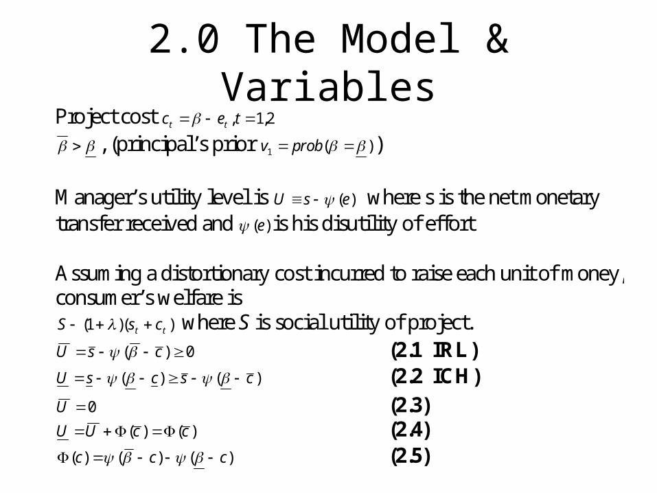
2.0 The Model & VariablesProject cost 2,1, tec tt

, (principal’s prior )(1 probv ) Manager’s utility level is )(esU where s is the net monetary transfer received and )(e is his disutility of effort Assuming a distortionary cost incurred to raise each unit of money, consumer’s welfare is

))(1( tt csS where S is social utility of project. 0)( csU (2.1 IRL)

)()( cscsU (2.2 ICH) 0U (2.3)

)()( ccUU (2.4) )()()( ccc (2.5)

2.1 The Basic Model under Incomplete Information

)})()(1)(1(

))]())()(1[({

1

1},{

ccv

cccvMin cc

)(I

*ec

)(')1)(1(

1)('1

1 cv

vc

)7.2(

)8.2(

Taking FOCs:

2.1 The Basic Model under Incomplete Information – cont’d

Proposition 1. The optimal (static or dynamic) commitment solution is characterized by:

*)( 1 evc

*)( 1 evc

01

dv

cd))(()( 11 vcvU

2.2 Optimal pooling allocationFrom P1, the principal never chooses to pick a single cost c for both types. But, if she did (this is to set up pooling equilibrium in the first period for the forthcoming renegotiation case) then, chooses c so as to solve

)}()])()(1())(()[1{(

)()])([()1{[(

111

1}{

cvccvccv

cvccEMin c

(2.9)

The solution to the strictly convex programme, lies between the two types’ socially optimal cost and decreases with the probability of the good type.

*,)(* 1 evce p & .01

dv

dc p

(2.10)

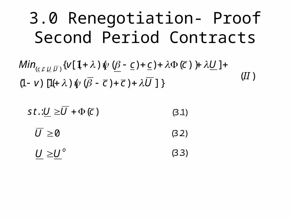
3.0 Renegotiation- Proof Second Period Contracts

]}))()(1)[(1(

]))())()(1[({},,,{

Uccv

UcccvMin UUcc

)(II

)(:.. cUUts

0U

oUU

)1.3(

)3.3(

)2.3(

3.0 Renegotiation- Proof Second Period Contracts – cont’d

)(III)]})()(1)[(1(

]*)*)()(1[({},{

ccv

UeevMin Uc

)(:.. cUts )4.3(

)5.3(oUU

)( 1

)( 2

3.0 Renegotiation- Proof Second Period Contracts – cont’d

)7.3()(')1)(1(

1)(' 1 cv

c

v 21 01 02 )8.3(

Taking FOCs:

3.2 Proposition 2

Normalizing 0U , renegotiation-proof contracts that keep both types in period two can be indexed by a single parameter, the good type’s rent U , with *)]()),(([ evcU 1. For ))(( vcU , it is the conditionally optimal contract:

*ec ; )(vcc 2. For *)())(( eUvc , it is a rent constrained contract: *ec ; )()(* 1 vcUce . 3. For *)(*)( eUe , it is a sell-out contract:

*ec ; *ec .

4.0 Characterization of Optimal Contract

4.0 Characterization of Optimal Contract – cont’d

• Theorem 1“The principal offers the agent a choice between two contracts in the first period. The first is picked by the good type only and yields the efficient cost in both periods. In the second contract, both types produce at the same cost level in the first period, and the second-period allocation is the conditionally optimal one given posterior beliefs v2 in [0,v1].”

• Theorem 2“The first period cost in the pooling branch c1(x) is independent of the discount factor (for a given x), and is an increasing function of the probability x that the good type separates in the first period. In a pooling equilibrium (x=0), c1(0) = cp(v1), and in a separating equilibrium (x=1), c1(1) = c-(v1).”

4.0 Characterization of Optimal Contract – cont’d

)(cU )4.3(

)5.3(o

UU

)( 1

)( 2

Remarks:

1. Rent given to good type in “commitment and renegotiation” is higherthan in case of commitment.

2. Principal essentially offers choice between a long term contractand a short term contract. Short term contract is followed by a conditionally optimal contract in the second period.

5.0 How much pooling?

(i) The good type’s probability of separation x is non-increasing with the discount factor (ii) There exists a 00 such that for all 0 , the optimal contract is a separating one (x=1). Intuition: If )1( x is the probability of pooling, the first-period loss in welfare due to pooling is proportional to , while the second period gain due to a reduction in the good-type’s rent is proportional to .

5.0 How much pooling? (continued)

(iii) When )( , the optimal contract tends towards a pooling contract )0( x . However, a pooling contract is never optimal

)0(x . Intuition: At the full pooling allocation, small changes in 2c have only second-order effects because the second-period allocation is the commitment one. A small decrease in 2c allows x to become positive without violating renegotiation-proofness, and the first period allocation is improved to the first order in x.

8.0 Summary

Appendix 1– Benchmark Case, Complete Information, Utilitarian Regulator

)}())(1({},{ ttttse esesSMaxtt

0)(:.. tt ests

*eet .2,1*),( test

*))*)()(1()(1( eeS

Optimal regulatory allocation:

Welfare:

Appendix 4.0 Characterization of Optimal Contract

Appendix 4.0 Characterization of Optimal Contract– cont’d

)(cU )4.3(

)5.3(o

UU

)( 1

)( 2

})])()(1(

*)*)(()[1[(

)]()])()(1(

))()1(*)*)(()[1{(

21221

1

11111

1111},,{ 221

Uvaav

eev

avaav

ccxveexvMin Uaa

)(:.. 22 aUts

)(* 22 vcae

)2.4(

)3.4(

)4.4(

)(IC

)(RNP

Solution strategy: Find out what binds, break into two parts and solve.

Appendix 4.0 Characterization of Optimal Contract– cont’d

)(cU )4.3(

)5.3(o

UU

)( 1

)( 2

)}()])()(1)(1{( 21221}{ 2avaavMin a

)(*:.. 22 vcaets

)5.4(

)6.4( )(same

4.3 binds because last period (Lemma 2)

Lemma 3: The optimal a2 equals c-(v2)

Proof: By Bayes rule, v2<v1 .

By Proposition 1, dc/dv>0, so c(v2)<c(v1). Equation 4.5 is strictly convex in a2, so optimal solution is c-(v2).

Appendix 4.0 Characterization of Optimal Contract– cont’d

)(cU )4.3(

)5.3(o

UU

)( 1

)( 2

)7.4(

Minimization of 4.2 with respect to a1 yields:

Note that we get the same pooling solution from earlier when x=0,and the result from Proposition 1 when x=1 (separating).

)](')('[)1)(1(

1

)1()1(

)(')1()(')1(

111

1

11

1111

aaxv

v

vxv

axvav

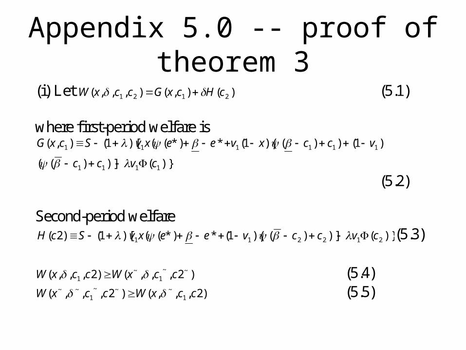
Appendix 5.0 -- proof of theorem 3

(i) Let )(),(),,,( 2121 cHcxGccxW (5.1) where first-period welfare is

)}()])((

)1())()(1(**)(()[1(),(

1111

111111

cvcc

vccxveexvScxG

(5.2) Second-period welfare

)}()])()(1(**)(()[1()2( 212211 cvccveexvScH (5.3)

)2,,,()2,,,( ~~1

~1 ccxWccxW (5.4)

)2,,,()2,,,( 1~~~

1~~ ccxWccxW (5.5)