Advancing Front Surface Mesh Generation in Parametric Space Using aRiemannian Surface Definition

Joseph R. Tristano, Steven J. Owen and Scott A. CanannANSYS, Inc.

275 Technology DriveCanonsburg, PA 15317

andCarnegie Mellon University

Department of Environmental and Civil EngineeringPittsburgh PA

{ joe.tristano, steve.owen, scott.canann }@ansys.com

Abstract

A method is presented for meshing 3D CAD surfaces in parametric space using an advancing frontapproach and a metric map to govern the size and shape of the triangles in the parametric space. Thecreation of the metric map will be discussed. The advancing front mesher generates triangles based on themetric map, stretching them in order to capture the change in parameterization of the surface. Thebenefits of this algorithm include better quality elements without having to do costly real spacecalculations.

Keywords: Triangulation, free surface meshing, Riemannian metric, CAE, finite elements

1. Introduction

1.1 Importance of work

The finite element method is a powerful tool for today’s engineering community. One of the barriers toautomating finite element analysis is robust automatic mesh generation on CAD surfaces. There are manymanual, semi-automatic, and automatic methods available today, and all have their own advantages anddrawbacks1. Current commercial codes tend to use either advancing front or Delaunay2 triangulation togenerate surface meshes. These methods, while very robust in two dimensions, are not as effective on 3-dimensional parametric surfaces, common in CAD models produced in industry. Direct three-dimensionalextensions of Delaunay3 and advancing front4 techniques have been proposed, but tend to be slower andless robust. For this reason, two dimensional methods are preferred, utilizing a parametric surfacemapping where appropriate. However, standard two-dimensional methods cannot be used directly sincethe mapping from parametric space to real space can produce distorted elements. A method is needed toplace anisotropic triangles in two dimensions that will map back to isotropic triangles in threedimensions. A metric map based on the first fundamental form of the surface can be used. While asignificant amount of research has gone into meshing surfaces using a metric map with Delaunay

triangulation5, little work has been done in the area of advancing front6,7. This paper proposes anexpanded use of the metric map for use in advancing front mesh generation.

1.2 Previous work

Previous work in this area has been done by George et al at INRIA5,8 and others9,10 who have investigatedthe use of the metric and metric map quite extensively with the use of a Delaunay kernel. Möller andHansbo investigated using a metric to define the shape of triangles in parametric space but did not proposean algorithm to produce the mesh6. Cuilière7 has also explored the use of a metric in meshing parametricsurfaces using advancing front. He explored the notion of an orthogonal vector in Riemannian space (seesection 3.4.3.3, equation 14) quite thoroughly.

1.3 Overview of paper

The blend of advancing front and a metric map is new since previous work with the advancing frontmethod has been in parametric space (either directly meshing the parametric space11or modifying thespace12) or directly on the 3D surface4.

This paper describes the details of generating a finite element mesh in the parametric space of a CADsurface using a Riemannian metric map. Section 2 presents the overall algorithm. Section 3 gives thedetails of the algorithm. Section 4 presents some results and comparison to other methods. Section 5draws conclusions and discusses a few areas where work is still needed.

2. Overall Algorithm

As with any advancing front method, the algorithm begins with a set of boundary loop segments, definedas the initial “front”. Triangles are constructed from the front segments and grow towards the interior ofthe domain, “advancing the front as it proceeds”. More specifically, the proposed algorithm involves thefollowing steps:

�• Discretize the boundary (section 3.2)�• Compute background mesh (section 3.3 )�• Orient the front segments (section 3.4.1)�• Initialize the fronts (section 3.4.2)�• Process the fronts (section 3.4.3)For each front:

�• Check metric of nodes on front to determine appropriate method for distancecalculation (section 3.4.3.1)

�• Check to see if the angle between adjacent fronts is below a threshold angle. If it is,see if the formation of a triangle is possible (section 3.4.3.2)

�• Determine the best location for a candidate node based on interpolation of thebackground mesh. (section 3.4.3.3)

�• Find all nearby nodes on the current front (section 3.4.3.4)�• See if any of the nearby nodes form an acceptable triangle (section 3.4.3.5)�• If all of the above methods fail, use a brute force method to go through all the

remaining nodes on the front and form the best triangle (section 3.4.3.6)�• Check boundary node normals (section 3.4.3.7)�• Form triangle

�• Update the front.

The proposed algorithm can be used for both flat and curved surfaces. While curved surfaces require theuse of a metric map, flat surfaces can use the identity matrix for the metric, provided an initialtransformation of the three dimensional boundary nodes to the x-y plane is first accomplished.

3. Details of the Algorithm

This section will define the metric and it’s uses. It will also describe the creation of the background meshand the surface mesh that utilize the metric.

3.1 Definition of the metric

For 3D surfaces with a parameterization denoted by there is a metric of the tangent plane at every pointP defined as:

[ ] =GFFE

M P [1]

where

22

21

11

=

=

=

GFE

[2]

and

),(),(

’2

’1

vu

vu

v

u

=

=[3]

where ),(’ vuu and ),(’ vuv are the gradient vectors at the point P on the surface.

The 3D distance between two points along the surface, A and B, as measured from point A can becomputed using their coordinates in parametric space and the metric at A:

22 )())((2)( ABAABABAABAMvvGvvuuFuuEAB

A++= [4]

This function only gives the distance with respect to the metric at A. The distance as computed from bothA and B is needed during the meshing process. For a well behaved surface the distance can be computedas the average of the distance measured from A and the distance measured from B:

2BA MM

ABABAB

+= [5]

Well behaved implies a minimal deviation of the surface derivatives over the surface. The behavior of thesurface is determined during the creation of the background mesh (section 3.3). When the surface is notwell behaved, numerical integration must be done using a finite number of integration points, N (typically5), along the line segment between A and B.

[ ]( )

[ ]( ) [ ] [ ]2

1

11

13

+

++

=

+=

=

=

iiiavg

iiiavgii

T

i

n

iiD

MMM

PPMPPd

dd

[6]

3.2 Discretization of the Boundary

The boundary loops of the surface must be discretized in such a way that well shaped elements can becreated. A method such as smart sizing13 can be used where the boundary is discretized and then refinedbased on the proximity and curvature of the lines in the model. This allows the mesher to capture thecurvature of the surface by putting more element divisions on highly curved boundaries.

3.3 Construction of metric & size map

The metric stated above is used to compute 3D distances in a 2D, parametric domain. Since 3D sizes arestored on the 2D domain, the metric allows for the creation of distortion free triangles while performingall of the meshing in 2D parametric space. This is accomplished by using the metric to distort thetriangles in the parametric space so they are distortion free when mapped back to real space.

For the sake of efficiency, a background mesh is defined to control element sizing and metric values. Thebackground mesh consists of selected points in the parametric domain where both size and metric areknown exactly. The mesher can utilize this information to interpolate local size and metric data as afunction of the parametric u,v coordinates. For example:

[ ] ),(),(vufM

vufsize=

=

P[7]

One of the benefits of computing the metric map and size map using the same background mesh is that allsizing information and metric information is stored in one place. A second benefit is that the metric of apoint in parametric space can be determined by a simple interpolation rather than a costly evaluation ofthe surface followed by the computation of the metric. An additional benefit is the ability to refine thebackground mesh based on size and metric values at the same time on the same mesh. This, as describedby Owen14, is a fast and convenient way to compute essentially two different maps on one mesh.

The initial background mesh is a Delaunay tesselation of a subset of the domain’s boundary nodes inparametric space. Boundary nodes are inserted into the background mesh only if their resultingcontribution to the size map would affect it significantly.

The parametric space does not need to be well behaved in order for this method to work well. As a matterof fact, one of the strengths of this method is its ability to handle surfaces that do not have a well behavedparametric space.

Once the background mesh is generated, the 3D sizes and metrics are stored at the nodes of the 2Dbackground mesh for later reference.

If the element size must change on the interior of the mesh due to surface curvature or due to the metricchanges caused by variations in the mapping between parametric space and global space, internal nodesmust be inserted into the background mesh so that an accurate representation of the size and metric can beproduced.

The internal nodes in the background mesh are placed by using a quadtree decomposition of theparametric space. The quadtree is initialized by evaluating the tangent vectors at each of the points in anNxN grid. A reasonable value for N is 10. New nodes are inserted as needed at the centroid of eachquadtree leaf. The quadtree leaves are refined based on the ratio the deviation of the mapping of thesurface from parametric space to real space. This ratio is defined as the maximum magnitude to theminimum magnitude of the tangent vectors at the four corners of the leaf. If this ratio exceeds themaximum slope ratio (1.5 seems to work well for most surfaces) the leaf is refined. If the leaves need to berefined, the surface is not considered to be locally well behaved. The level of refinement is limited to amaximum number of iterations as well as by the real world length of the diagonal of the smallest quadtreeleaf. If the diagonal length in real space is less than twice the minimum size then refinement of thebackground mesh is stopped. In addition to being inserted to fully capture transitions in the parametricmapping, nodes are also inserted to capture size transitions and surface curvature (as in Owen14).

Any interpolation method can be used to create and evaluate the background mesh, but Owen14 illustratesthat natural neighbor interpolation is an attractive method to use since it is C1 continuous at the nodes ofthe background mesh. This is important in representing the metric, since is undesirable to havediscontinuities in the metric map. The method also reduces the amount of “banding” i.e., bands ofunnecessarily small elements.

Figure 1 Background mesh before and after refinement

3.4 Advancing front algorithm using the metric map

After the background mesh has been created, the meshing process can begin. While the basic algorithmwas outlined in Section 2, the details will be presented here.

3.4.1 Orient front segments

A set of closed boundary loops (closed set of singly connected edges) made up of the initial front serves asinput to the advancing front mesher. Boundary loops are oriented such that the exterior loops follow acounter-clockwise direction and the interior loops follow a clockwise direction.

3.4.2 Initialize the fronts

The first step after the boundary has been discretized and the size/metric map has been computed is theinitialization of the front:

�• Sizes and metrics are interpolated from the background mesh and stored with the boundary nodes.The 3D front length is computed and stored in the front data structure using the distance calculationsfrom Section 3.1.

�• For each edge on the front, the equation of the line using the u,v coordinates of the edge’s nodes iscomputed for intersection calculations to be performed later.

�• Experience has shown that meshing smaller fronts first can be advantageous. To accomplish this, thefronts are hashed according to their 3D size. The fronts are stored in a collection of bins; each oneholding a specified range of sizes. Bin sizes are defined logarithmically, where the front size rangefor a bin containing small fronts is narrower than for larger fronts. During the meshing process,fronts are first processed from the bin containing the smallest fronts. It was found that sorting basedon 3D size is better than 2D size because of problems found with mapping the mesh back to 3D spacewhere the parametric space is highly distorted. Sorting based on 3D distances also helps to bettercapture size transitions in the mesh.

�• The final step in front initialization is to check for intersecting boundary segments. This step isperformed in order to check for erroneous or poor input. Each front segment is checked against anynon-adjacent front. If any of the boundary fronts intersect, the mesher returns an error code.

3.4.3 Process the fronts

The fronts are now processed from the smallest 3D sized front to the largest, as described in the followingsections.

3.4.3.1 Check metric of nodes on the front

Since distance measurement in Riemannian space varies from one location to another throughout theparametric space, special care must be taken where large size transitions occur, or where the parametricspace is locally not well behaved.

For each front, the mesher must ensure that the metrics at its end nodes do not exceed the maximum sloperatio defined during the creation of the background mesh. If the ratio is exceeded, distance calculationsmust be integrated to better approximate the true 3D distance. (Note that in further discussions of distancecalculations the ratio of the metrics must be checked in order to determine which distance calculationshould be used, i.e. averaging (equation 5) or integrating (equation 6)).

3.4.3.2 Check if the angle between adjacent fronts is below threshold angle

The first step in processing a front is checking the 3D angle it makes between its two adjacent fronts.Using the 3D lengths of the three sides, the law of cosines is used to compute the angle at the desired nodeas in the following:

+=

DD

DDDA ABCA

BCABCA

33

23

23

231

2cos [8]

If the angle is below the threshold angle of 75 degrees as shown in Figure 2, the triangle formed from A,B and C becomes a candidate triangle. Before forming triangle ABC, segment BC must first be checked toensure it does not intersect any other fronts. This can be done as outlined in section 3.4.3.5.

A B

C

currentfront

Adjacentfront

A= 75° in real space

Figure 2 Small angle triangle creation

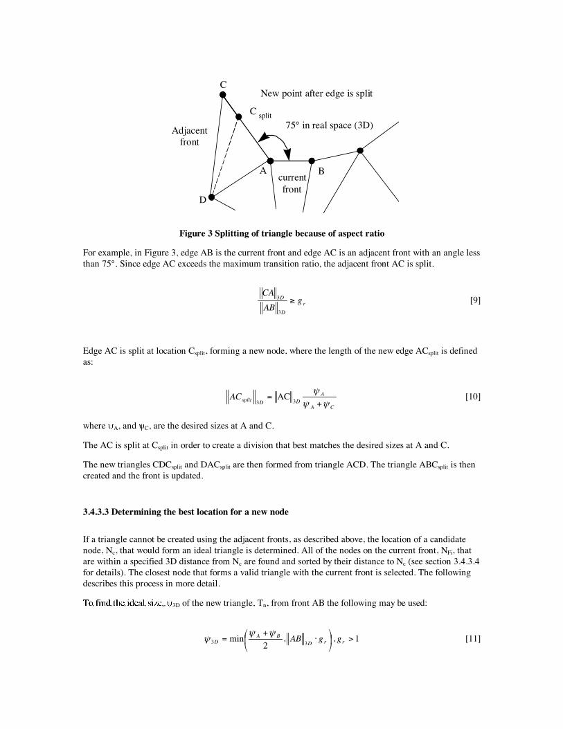
To ensure that high aspect ratio triangles are not created, an additional check is made before the triangleis created. If the aspect ratio of edge length to front length is more than twice the user controllable growthratio, gr, (usually 2.0) the adjacent edge will be split.

A B

C

currentfront

75° in real space (3D)

New point after edge is split

C split

Adjacentfront

D

Figure 3 Splitting of triangle because of aspect ratio

For example, in Figure 3, edge AB is the current front and edge AC is an adjacent front with an angle lessthan 75°. Since edge AC exceeds the maximum transition ratio, the adjacent front AC is split.

rD

D gABCA

3

3 [9]

Edge AC is split at location Csplit, forming a new node, where the length of the new edge ACsplit is definedas:

CA

ADDsplitAC

+=

33AC [10]

where A, and C, are the desired sizes at A and C.

The AC is split at Csplit in order to create a division that best matches the desired sizes at A and C.

The new triangles CDCsplit and DACsplit are then formed from triangle ACD. The triangle ABCsplit is thencreated and the front is updated.

3.4.3.3 Determining the best location for a new node

If a triangle cannot be created using the adjacent fronts, as described above, the location of a candidatenode, Nc, that would form an ideal triangle is determined. All of the nodes on the current front, NFi, thatare within a specified 3D distance from Nc are found and sorted by their distance to Nc (see section 3.4.3.4for details). The closest node that forms a valid triangle with the current front is selected. The followingdescribes this process in more detail.

3D of the new triangle, Tn, from front AB the following may be used:

1,,2

min33 >

+= rrD

BAD ggAB [11]

A, B are the 3D element sizes interpolated from the background mesh at A and B respectively andgr is a user defined maximum growth ratio.

For flat, non-parametric surfaces, the location of Nc can be constructed by forming an isosceles trianglewith front AB, where edge length DDcDc BNAN 333

== , and the height, h3D, of Tn is defined as:

4

232

33D

DD

ABh = [12]

Since most parametric mappings are not uniform, DcDc BNAN

22, even though

DcDc BNAN33

= .

However, Nc can be located by computing an equivalent h2D and normal vector, DN2 to front AB, asshown in Figure 4. For example let:

222 DD

ABABm +

= [13]

ABmm

mm

N

ND V

FEGF

vu

NABAB

ABAB

D

D

+

+==

)(

2

22 [14]

where ABV is a unit vector pointing from A to B and ABm is the midpoint of AB.

Finally, to locate Nc in parametric space, Nc2D, the following can be used:

DDABDc hNmN 222 += [15]

where

22

32

22222

DABDDABDAB NmNNmNm

DD

vGvuFuE

hh

++= [16]

A

90° in real space (3D)

B

Nc

current frontmAB

h2DDN2

Figure 4 Locating ideal node location

3.4.3.4 Find nearby nodes

It is not always necessary to create a new node at Nc. In many cases, there will be an existing node, NF,that is close enough to fulfill the local size requirements. A search radius, r3D defined as:

( ) 10,,min 33 <<= sfsr fDcD [17]

where c is the interpolated element size at Nc, and sf is a shrink factor limiting the radius of acceptablenodes, thereby limiting the size transition in the mesh and reducing the number of distance calculations.A typical range for sf is between .8 and .4.

Since the search radius is a 3D distance, an ellipse based on the metric at Nc must be used in parametricspace to calculate a bounding box to reduce the number of distance calculations. The major radius of thisellipse is used as the width of the bounding box.

22

32

2ccccccc NNNNNNN

DD

vGvuFuE

rr

++= [18]

Equation 18 is in the same form as an ellipse in polar coordinates centered about the origin. It can then betransformed into the general form of an ellipse in Cartesian coordinates.

022 =+++ FCxyByAx [19]

where:

ccccc NDNDDNNN vryurxrFFCGBEA 22

22

23 ,,,2,, ====== [20]

By rotating the ellipse to align with the Cartesian coordinate axis, equation 19 may be reduced and themajor radius defined as:

( )rotrot BAa

,min1

= [21]

where

CAB

where

FCABB

FCBAA

-rot

-rot

=

+=

++=

cot

22sinsincos

22sinsincos

122

122

[22]

The major radius can now be used as the parametric space bounding box width.

A bounding box with width 2a centered at Nc can be used to quickly filter nodes, NFi , on the front that donot fall within the ellipse. The distance equations mentioned in section 3.1 can be used to determine ifthey are actually within the search radius while not violating the maximum growth ratio ,gr.

3.4.3.5 Validity checks for candidate Triangles

There are three tests that a triangle must pass to be accepted: zero area test, internal node test, and frontintersection test.

The first triangle validity check determines if the triangle has zero area in parametric space. Zero areatriangles cannot be created.

If Tn passes the zero area test, it must be checked for nodes interior to it or nodes too close to the boundaryedges of nearby triangles. The nodes close to the triangle are checked with this same test, referred to asthe interior node test.

The area (barycentic) coordinates of a node on the front, NFi, which lies within the bounding box of thecurrent front are computed with respect to Tn (Figure 5). If any of these coordinates are less than aspecified empirical tolerance, Nc must be tested again using the approximate 3D area coordinates. The 3D

3D, can be defined from Heron’s formula as.

)CA-(s)BC-(s)AB-(ss3D3D3D3 =D [23]

where

2CA +BC + AB

=s 3D3D3D [24]

A B

Nc

NFi

Tn

Figure 5 Test for node inside triangle

If any of these area coordinates are algebraically less than an empirical tolerance (currently set to -0.0154321012) then the triangle passes the interior node test.

If the triangle passes the interior node test, the triangle then goes through the front intersection test. Thistest checks that the triangle does not intersect any of the current fronts. This intersection test is performedin parametric space.

3.4.3.6 Brute force method

If any of the candidate nodes (nearby nodes plus the ideal node Nc), Nci, fail to create a valid triangle, thenthe brute force method presented in this section is used to create a triangle. The brute force methodconsists of looping through all of the nodes on the front and finding the best shaped triangle. A distortionmetric15

as:

222

ˆ32

CC

CC

BNABANnBNAN

++

×= [25]

The directions vectors ANC and BNC 3D2,

3D,can be defined as:

23

23

23

23

3232

DCDDC

DD BNABAN ++

= [26]

The distortion metric alone is not always the best method to create the new triangle because size criterionmay be violated even though one triangle may be of better quality than another. It was found that the besttriangle is created by penalizing the distortion metric of the triangle based on a function of the ratio ofdesired triangle size and longest triangle edge length. This function is illustrated below:

<+

<<=

xxxe

xxxepenalty x

x

19

1091(5.0

10sin4.0)1(

)1(

[27]

where

( )( )

DCDC

BA

BNANx

33,max

2+= [28]

where A B are the desired sizes at A and B.

1 2 3 4 edglen

Interp size0.2

0.4

0.6

0.8

1

penalty

Figure 6 Penalty function for distortion metric

The new alpha then becomes:

penaltyDnew = 3 [29]

3.4.3.7 Checking boundary normals

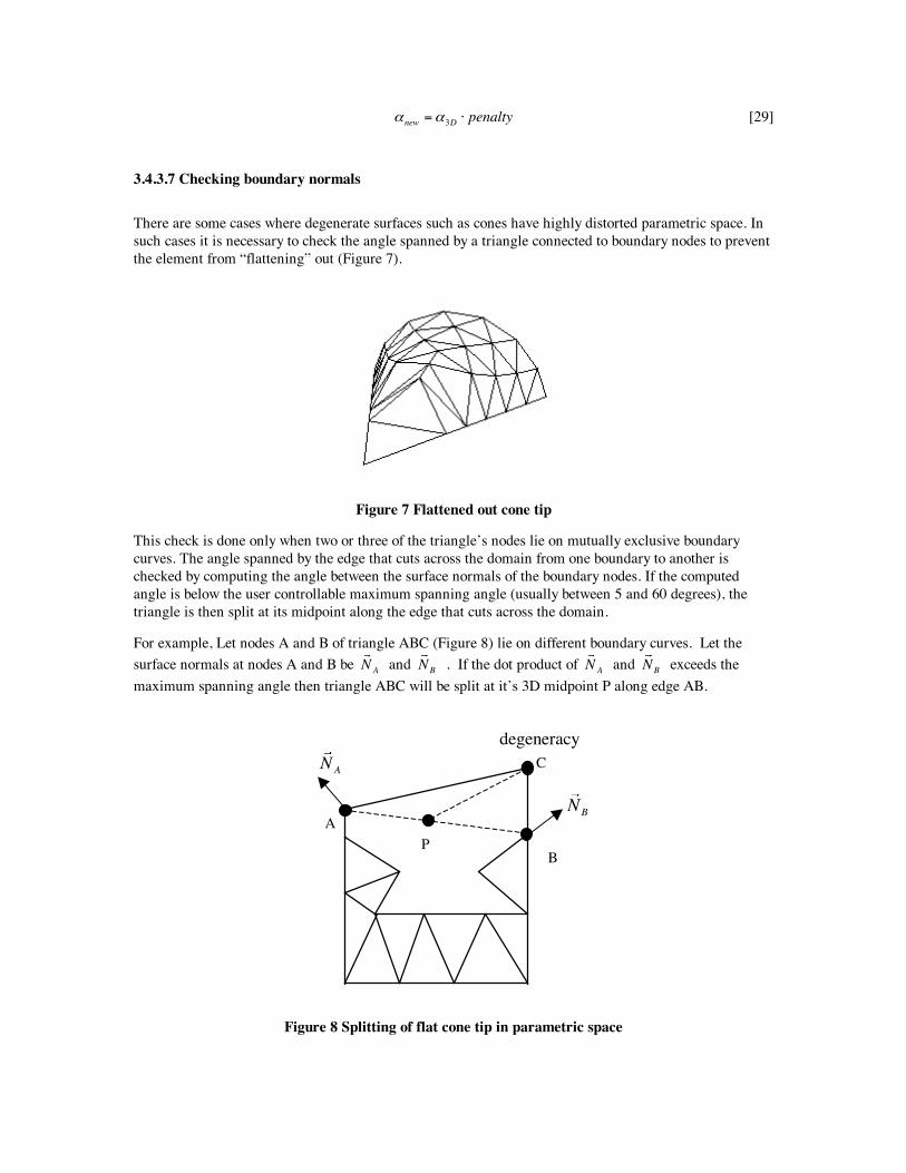
There are some cases where degenerate surfaces such as cones have highly distorted parametric space. Insuch cases it is necessary to check the angle spanned by a triangle connected to boundary nodes to preventthe element from “flattening” out (Figure 7).

Figure 7 Flattened out cone tip

This check is done only when two or three of the triangle’s nodes lie on mutually exclusive boundarycurves. The angle spanned by the edge that cuts across the domain from one boundary to another ischecked by computing the angle between the surface normals of the boundary nodes. If the computedangle is below the user controllable maximum spanning angle (usually between 5 and 60 degrees), thetriangle is then split at its midpoint along the edge that cuts across the domain.

For example, Let nodes A and B of triangle ABC (Figure 8) lie on different boundary curves. Let thesurface normals at nodes A and B be AN and BN . If the dot product of AN and BN exceeds themaximum spanning angle then triangle ABC will be split at it’s 3D midpoint P along edge AB.

degeneracy

A

B

C

P

AN

BN

Figure 8 Splitting of flat cone tip in parametric space

4. Results and Comparisons

In this section, the results of the Riemannian space advancing front mesher are compared against thewarped parametric space and direct 3D meshers available in the ANSYS program. The warpedparametric space mesher12 is a mesher in the ANSYS program that meshes parametric surfaces in adifferent manner. This method reparametrizes the surface selectively evaluating surface derivatives ( u,

v) over the domain and adjusting local u,v values to hold the magnitude of u, v roughly constant.Times presented in this section incorporate the total meshing time after boundary discretization. Thisincludes, projecting the 3D boundary nodes to 2D parametric space, background mesh creation, advancingfront meshing, cleanup and smoothing, mapping to 3D, and storage of elements to the ANSYS database.

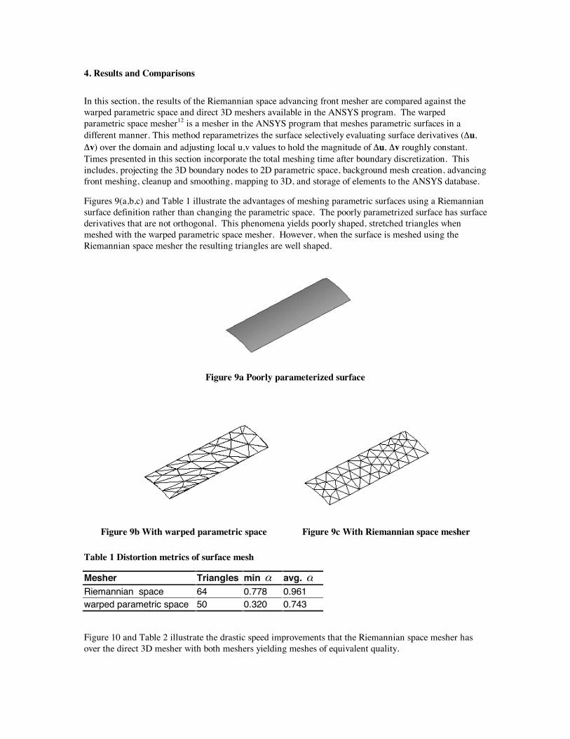
Figures 9(a,b,c) and Table 1 illustrate the advantages of meshing parametric surfaces using a Riemanniansurface definition rather than changing the parametric space. The poorly parametrized surface has surfacederivatives that are not orthogonal. This phenomena yields poorly shaped, stretched triangles whenmeshed with the warped parametric space mesher. However, when the surface is meshed using theRiemannian space mesher the resulting triangles are well shaped.

Figure 9a Poorly parameterized surface

Figure 9b With warped parametric space Figure 9c With Riemannian space mesher

Table 1 Distortion metrics of surface mesh

Mesher Triangles min avg. Riemannian space 64 0.778 0.961warped parametric space 50 0.320 0.743

Figure 10 and Table 2 illustrate the drastic speed improvements that the Riemannian space mesher hasover the direct 3D mesher with both meshers yielding meshes of equivalent quality.

Figure 10 Spring

Table 2 Spring statistics

Mesher Triangles min Avg. time elements/secRiemannian space 3336 0.489 0.923 9.93 335.95warped parametric space 4356 0.307 0.922 21.89 198.99direct 3D 3506 0.481 0.927 64.38 54.45

Figures 11(a,b,c) and Table 3 illustrate the overall quality and speed improvements over the warpedparametric space and direct 3D meshers for a general CAD surface. The stretched triangles in the warpedparametric space mesh are caused by non-orthogonal surface derivatives. The Riemannian space mesherresolves those problems. It also resolves the problems of costly real space calculations done by the direct3D mesher.

Figure 11a CAD Surface Figure 11b With Riemannian space mesher

Figure 11c With warped parametric space Figure 11d With direct 3D mesher

Table 3 CAD surface statistics

Mesher Triangles min Avg. time elements/secRiemannian space 121 0.650 0.910 0.36 336.11warped parametric space 115 0.409 0.821 0.29 396.55direct 3D 125 0.459 0.907 0.74 168.91

5. Conclusion

A method for meshing 3D parametric surfaces using the advancing front method with a Riemanniansurface definition was presented. The details of the creation of the metric map used to determine theamount of distortion of the elements in parametric space were given along with the details of anadvancing front algorithm that utilizes the metric map.

Meshing surfaces using an advancing front with a Riemannian surface definition proves to be a valuabletechnique for meshing surfaces common in CAE. This method overcomes anomalies found in the warpedparametric space and direct 3D methods currently used in the ANSYS program. Well shaped trianglesare produced by this method. Any of three of the methods compared robust and capable of creating highquality meshes for most geometries. However, having all three meshers available in the ANSYS programgreatly increases the likelihood of successfully meshing any arbitrary collection of surfaces and hence fullyautomated constrained tetrahedral meshing. Future areas of work may include the combination of awarped parametric space and Riemannian space mesher in order to create better mappings for high aspectratio surfaces.

6. References

1 Ho-Le, K., Finite element mesh generation methods: a review and classification, Computer AidedDesign, Vol 20(1) , 27-38, 1988.

2 Chen, H., and J. Bishop, Delaunay Triangulation for Curved Surfaces, 6th International MeshingRoundtable Proceedings, pp.115-127, 1997.

3 Chew, Paul L., Guaranteed-Quality Mesh Generation for Curved Surfaces, 9th Annual ComputationalGeometry, Vol 73, 1993.

4 Lohner,R., Extensions and Improvements of the Advancing Front Grid Generation Technique,Communications in Numerical Methods in Engineering, John Wiley & Sons, Ltd, Vol 12, pp.683-702,1996.

5 George P. L., and H. Borouchaki, Delaunay Triangulation and Meshing Application to FiniteElements, Editions HERMES, Paris, 1998.

6 Moller, P., and P Hansbo, On advancing front mesh generation in three dimensions, IJNME, Vol. 38,pp.3551-3569, 1995.

7 Cuilière, J. C., An adaptive method for the automatic triangulation of 3D parametric surfaces, ComputerAided Design, Vol 30(2), pp.139-149, 1998.

8 Castro Díaz, M. J., and F. Hect, Anisotropic Surface Mesh Generation, INRIA Research Report, No

2672, 1995.9 Shimada, K., Anisotropic Triangular Meshing of Parametric Surfaces via Close Packing of Ellipsoidal

Bubbles, 6th International Meshing Roundtable Proceedings, pp.63-74, 1996.10 Bossen, F. J., P. S. Heckbert, A Pliant Method fo Anisotropic Mesh Generation, 5th International

Meshing Roundtable Proceedings, pp.375-390, 1997.11 Lo, S.H., A new mesh generation scheme for arbitrary planar domains, IJNME, Vol. 21, pp1403-1426,

1985.12 Canann, S. A., Y. C. Liu and A. V. Mobley, Automatic 3D Surface Meshing to Address Today's

Industrial Needs, Finite Elements Anal. Des., Vol 25, pp.185-198, 1997.13 Cunha, A., S. A. Canann and S. Saigal, Automatic Boundary Sizing for 2D and 3D Meshes, AMD-Vol.

220 Trends in Unstructured Mesh Generation, ASME, pp.65-72, July 1997.14 Owen, S., Neighborhood-based element sizing control for finite element surface meshing, 6th

International Meshing Roundtable Proceedings, pp..43-154, 1997.15 Lo, S.H. and C.K. Lee, On Using Meshes of Mixed Element Types in Adaptive Finite Element

Analysis, Finite Elements in Analysis and Design, Elsevier, Vol 11, pp.307-336, 1992.