advances in markov chain monte carlo...
TRANSCRIPT

Advances in Markov chain
Monte Carlo methods
Iain MurrayM.A., M.Sci., Natural Sciences (Physics), University of Cambridge, UK (2002)
Gatsby Computational Neuroscience Unit
University College London
17 Queen Square
London WC1N 3AR, United Kingdom
THESIS
Submitted for the degree of
Doctor of Philosophy, University of London
2007

2
I, Iain Murray, confirm that the work presented in this thesis is my own. Whereinformation has been derived from other sources, I confirm that this has been indicatedin the thesis.
3
Abstract
Probability distributions over many variables occur frequently in Bayesian inference,statistical physics and simulation studies. Samples from distributions give insight intotheir typical behavior and can allow approximation of any quantity of interest, suchas expectations or normalizing constants. Markov chain Monte Carlo (MCMC), intro-duced by Metropolis et al. (1953), allows sampling from distributions with intractablenormalization, and remains one of most important tools for approximate computationwith probability distributions.
While not needed by MCMC, normalizers are key quantities: in Bayesian statisticsmarginal likelihoods are needed for model comparison; in statistical physics many phys-ical quantities relate to the partition function. In this thesis we propose and investigateseveral new Monte Carlo algorithms, both for evaluating normalizing constants and forimproved sampling of distributions.
Many MCMC correctness proofs rely on using reversible transition operators; oftenthese operators lead to slow diffusive motion resembling a random walk. After reviewingexisting MCMC algorithms, we develop a new framework for constructing non-reversibletransition operators that allow more persistent motion.
Next we explore and extend MCMC-based algorithms for computing normalizing con-stants. We compare annealing, multicanonical and nested sampling, giving recommen-dations for their use. We also develop a new MCMC operator and Nested Samplingapproach for the Potts model. This demonstrates that nested sampling is sometimesbetter than annealing methods at computing normalizing constants and drawing pos-terior samples.
Finally we consider “doubly-intractable” distributions with extra unknown normalizerterms that do not cancel in standard MCMC algorithms. We propose using severaldeterministic approximations for the unknown terms, and investigate their interactionwith sampling algorithms. We then develop novel exact-sampling-based MCMC meth-ods, the Exchange Algorithm and Latent Histories. For the first time these algorithmsdo not require separate approximation before sampling begins. Moreover, the ExchangeAlgorithm outperforms the only alternative sampling algorithm for doubly intractabledistributions.

4
Acknowledgments
I feel very fortunate to have been supervised by Zoubin Ghahramani. My traininghas benefited greatly from his expertise, enthusiasm and encouragement. I have beenequally fortunate to receive regular advice and ideas from David MacKay. Much of thisresearch would never have happened without these mentors and friends.
This work was carried out at the Gatsby computational neuroscience unit at UniversityCollege London. This is a first-class environment in which to conduct research, bothintellectually and socially. Peter Dayan, the director, is owed a lot of credit for this,as are all of Gatsby’s members and visitors, past and present. Several individuals haveoffered me their constant support, advice and good humor, in particular Angela Yu, EdSnelson, Katherine Heller and members of the Inference group in Cambridge. I’d alsolike to extend a special thanks to Alex Boss whose administrative help often extendedbeyond the call of duty.
Some of chapter 4 is a review of John Skilling’s nested sampling algorithm. John hasbeen generous with his advice and encouragement, which enabled me to pursue a studybased on his work. Thanks also to Radford Neal for comments on aspects of chapters 3and 5, Hyun-Chul Kim for mean-field code used in chapter 5 and Matthew Stephensfor encouraging me to work out the non-infinite explanation of the exchange algorithm.Thanks to my examiners Peter Green and Lorenz Wernisch for reviewing this work andcatching some mistakes. Of course I am solely responsible for any errors that remain.
I am enormously grateful to the Gatsby charitable foundation for funding my researchand providing travel money. Further travel monies were received from the PASCALnetwork of excellence, AUAI, the NIPS foundation and the Valencia Bayesian meeting.
Various items of free software have played a vital role in conducting this research: gcc,GNU/Linux, gnuplot, LATEX, METAPOST (Hobby, 1992), Octave, Valgrind (Sewardand Nethercote, 2005), Vim and many more. Projects in the public interest such asthese deserve considerable support.
Finally I would like to thank my family and friends for all their support and patience.
Contents
Front matter
Abstract . . . . . . . . . . . . . . . . . . . . . . . . . . . . . . . . . . . . . . . 3Acknowledgments . . . . . . . . . . . . . . . . . . . . . . . . . . . . . . . . . . 4Contents . . . . . . . . . . . . . . . . . . . . . . . . . . . . . . . . . . . . . . . 5List of algorithms . . . . . . . . . . . . . . . . . . . . . . . . . . . . . . . . . . 9List of figures . . . . . . . . . . . . . . . . . . . . . . . . . . . . . . . . . . . . 10List of tables . . . . . . . . . . . . . . . . . . . . . . . . . . . . . . . . . . . . 12Notes on notation . . . . . . . . . . . . . . . . . . . . . . . . . . . . . . . . . 13
1 Introduction 14
1.1 Graphical models . . . . . . . . . . . . . . . . . . . . . . . . . . . . . . . 141.1.1 Directed graphical models . . . . . . . . . . . . . . . . . . . . . . 151.1.2 Undirected graphical models . . . . . . . . . . . . . . . . . . . . 161.1.3 The Potts model . . . . . . . . . . . . . . . . . . . . . . . . . . . 171.1.4 Computations with graphs . . . . . . . . . . . . . . . . . . . . . 17
1.2 The role of summation . . . . . . . . . . . . . . . . . . . . . . . . . . . . 181.3 Simple Monte Carlo . . . . . . . . . . . . . . . . . . . . . . . . . . . . . 20
1.3.1 Sampling from distributions . . . . . . . . . . . . . . . . . . . . . 211.3.2 Importance sampling . . . . . . . . . . . . . . . . . . . . . . . . . 23
1.4 Markov chain Monte Carlo (MCMC) . . . . . . . . . . . . . . . . . . . . 241.5 Choice of method . . . . . . . . . . . . . . . . . . . . . . . . . . . . . . . 26
2 Markov chain Monte Carlo 27
2.1 Metropolis methods . . . . . . . . . . . . . . . . . . . . . . . . . . . . . 272.1.1 Generality of Metropolis–Hastings . . . . . . . . . . . . . . . . . 282.1.2 Gibbs sampling . . . . . . . . . . . . . . . . . . . . . . . . . . . . 302.1.3 A two stage acceptance rule . . . . . . . . . . . . . . . . . . . . . 30
2.2 Construction of estimators . . . . . . . . . . . . . . . . . . . . . . . . . . 312.2.1 Conditional estimators (“Rao-Blackwellization”) . . . . . . . . . 322.2.2 Waste recycling . . . . . . . . . . . . . . . . . . . . . . . . . . . . 34
2.3 Convergence . . . . . . . . . . . . . . . . . . . . . . . . . . . . . . . . . . 352.4 Auxiliary variable methods . . . . . . . . . . . . . . . . . . . . . . . . . 36
2.4.1 Swendsen–Wang . . . . . . . . . . . . . . . . . . . . . . . . . . . 36
CONTENTS 6
2.4.2 Slice Sampling . . . . . . . . . . . . . . . . . . . . . . . . . . . . 392.4.3 Hamiltonian Monte Carlo . . . . . . . . . . . . . . . . . . . . . . 41
2.5 Annealing methods . . . . . . . . . . . . . . . . . . . . . . . . . . . . . . 422.5.1 Simulated tempering / Expanded Ensembles . . . . . . . . . . . 432.5.2 Parallel tempering . . . . . . . . . . . . . . . . . . . . . . . . . . 442.5.3 Annealed importance sampling (AIS) . . . . . . . . . . . . . . . 452.5.4 Tempered transitions . . . . . . . . . . . . . . . . . . . . . . . . . 46
2.5.4.1 Generalization to only forward transitions . . . . . . . . 482.5.4.2 Generalization to a single pass . . . . . . . . . . . . . . 49
2.6 Multicanonical ensemble . . . . . . . . . . . . . . . . . . . . . . . . . . . 502.7 Exact sampling . . . . . . . . . . . . . . . . . . . . . . . . . . . . . . . . 52
2.7.1 Exact sampling example: the Ising model . . . . . . . . . . . . . 542.8 Discussion and Outlook . . . . . . . . . . . . . . . . . . . . . . . . . . . 55
3 Multiple proposals and non-reversible Markov chains 57
3.1 “Population Monte Carlo” . . . . . . . . . . . . . . . . . . . . . . . . . . 583.2 Multiple-Try Metropolis . . . . . . . . . . . . . . . . . . . . . . . . . . . 60
3.2.1 Efficiency of MTM . . . . . . . . . . . . . . . . . . . . . . . . . . 623.2.2 Multiple-Importance Try . . . . . . . . . . . . . . . . . . . . . . 653.2.3 Waste-recycled MTM . . . . . . . . . . . . . . . . . . . . . . . . 66
3.3 Ordered overrelaxation . . . . . . . . . . . . . . . . . . . . . . . . . . . . 683.3.1 Adapting K automatically . . . . . . . . . . . . . . . . . . . . . . 69
3.4 Pivot-based transitions . . . . . . . . . . . . . . . . . . . . . . . . . . . . 703.4.1 Ordered overrelaxation with pivot-based transitions . . . . . . . 723.4.2 Persistence with pivot states . . . . . . . . . . . . . . . . . . . . 73
3.5 Pivot-based Metropolis . . . . . . . . . . . . . . . . . . . . . . . . . . . . 773.6 Summary . . . . . . . . . . . . . . . . . . . . . . . . . . . . . . . . . . . 783.7 Related and future work . . . . . . . . . . . . . . . . . . . . . . . . . . . 79
4 Normalizing constants and nested sampling 81
4.1 Starting at the prior . . . . . . . . . . . . . . . . . . . . . . . . . . . . . 834.2 Bridging to the posterior . . . . . . . . . . . . . . . . . . . . . . . . . . . 85
4.2.1 Aside on the ‘prior’ factorization . . . . . . . . . . . . . . . . . . 864.2.2 Thermodynamic integration . . . . . . . . . . . . . . . . . . . . . 86
4.3 Multicanonical sampling . . . . . . . . . . . . . . . . . . . . . . . . . . . 884.4 Nested sampling . . . . . . . . . . . . . . . . . . . . . . . . . . . . . . . 88
4.4.1 A change of variables . . . . . . . . . . . . . . . . . . . . . . . . 894.4.2 Computations in the new representation . . . . . . . . . . . . . . 914.4.3 Nested sampling algorithms . . . . . . . . . . . . . . . . . . . . . 924.4.4 MCMC approximations . . . . . . . . . . . . . . . . . . . . . . . 944.4.5 Integrating out x . . . . . . . . . . . . . . . . . . . . . . . . . . . 954.4.6 Degenerate likelihoods . . . . . . . . . . . . . . . . . . . . . . . . 95
CONTENTS 7
4.5 Efficiency of the algorithms . . . . . . . . . . . . . . . . . . . . . . . . . 984.5.1 Nested sampling . . . . . . . . . . . . . . . . . . . . . . . . . . . 994.5.2 Multicanonical sampling . . . . . . . . . . . . . . . . . . . . . . . 1004.5.3 Importance sampling . . . . . . . . . . . . . . . . . . . . . . . . . 102
4.6 Constructing annealing schedules . . . . . . . . . . . . . . . . . . . . . . 1034.7 Markov chains for normalizing constants . . . . . . . . . . . . . . . . . . 105
4.7.1 Randomize operator orderings . . . . . . . . . . . . . . . . . . . 1054.7.2 Changes in length-scale and energy . . . . . . . . . . . . . . . . . 1064.7.3 A new version of Swendsen–Wang . . . . . . . . . . . . . . . . . 107
4.8 Experiments . . . . . . . . . . . . . . . . . . . . . . . . . . . . . . . . . . 1094.8.1 Description of slice sampling experiments . . . . . . . . . . . . . 1094.8.2 Discussion of slice sampling results . . . . . . . . . . . . . . . . . 1114.8.3 The Potts model . . . . . . . . . . . . . . . . . . . . . . . . . . . 116
4.9 Discussion and conclusions . . . . . . . . . . . . . . . . . . . . . . . . . . 1184.9.1 Summary . . . . . . . . . . . . . . . . . . . . . . . . . . . . . . . 1184.9.2 Related work . . . . . . . . . . . . . . . . . . . . . . . . . . . . . 1194.9.3 Philosophy . . . . . . . . . . . . . . . . . . . . . . . . . . . . . . 120
5 Doubly-intractable distributions 122
5.1 Bayesian learning of undirected models . . . . . . . . . . . . . . . . . . . 1235.1.1 Do we need Z(θ) for MCMC? . . . . . . . . . . . . . . . . . . . . 125
5.2 Approximation Schemes . . . . . . . . . . . . . . . . . . . . . . . . . . . 1275.2.1 Targets for MCMC approximation . . . . . . . . . . . . . . . . . 1285.2.2 Approximation algorithms . . . . . . . . . . . . . . . . . . . . . . 1295.2.3 Extension to hidden variables . . . . . . . . . . . . . . . . . . . . 1315.2.4 Experiments involving fully observed models . . . . . . . . . . . 1325.2.5 Experiment involving hidden variables . . . . . . . . . . . . . . . 1345.2.6 Discussion . . . . . . . . . . . . . . . . . . . . . . . . . . . . . . . 136
5.3 The Exchange Algorithm . . . . . . . . . . . . . . . . . . . . . . . . . . 1375.3.1 Product space interpretation . . . . . . . . . . . . . . . . . . . . 1395.3.2 Bridging Exchange Algorithm . . . . . . . . . . . . . . . . . . . . 1405.3.3 Details for proof of correctness . . . . . . . . . . . . . . . . . . . 143
5.4 The Single Auxiliary Variable Method . . . . . . . . . . . . . . . . . . . 1445.4.1 Reinterpreting SAVM . . . . . . . . . . . . . . . . . . . . . . . . 146
5.5 MAVM: a tempered-transitions refinement . . . . . . . . . . . . . . . . . 1465.6 Comparison of the exchange algorithm and MAVM . . . . . . . . . . . . 149
5.6.1 Ising model comparison . . . . . . . . . . . . . . . . . . . . . . . 1505.6.2 Discussion . . . . . . . . . . . . . . . . . . . . . . . . . . . . . . . 152
5.7 Latent History methods . . . . . . . . . . . . . . . . . . . . . . . . . . . 1535.7.1 Metropolis–Hastings algorithm . . . . . . . . . . . . . . . . . . . 1545.7.2 Performance . . . . . . . . . . . . . . . . . . . . . . . . . . . . . 155
5.8 Slice sampling doubly-intractable distributions . . . . . . . . . . . . . . 157

CONTENTS 8
5.8.1 Latent histories . . . . . . . . . . . . . . . . . . . . . . . . . . . . 1585.8.2 MAVM . . . . . . . . . . . . . . . . . . . . . . . . . . . . . . . . 158
5.9 Discussion . . . . . . . . . . . . . . . . . . . . . . . . . . . . . . . . . . . 159
6 Summary and future work 162
References 164
List of algorithms
1.1 Rejection sampling . . . . . . . . . . . . . . . . . . . . . . . . . . . . . . 232.1 Metropolis–Hastings . . . . . . . . . . . . . . . . . . . . . . . . . . . . . 272.2 A two stage acceptance rule . . . . . . . . . . . . . . . . . . . . . . . . . 313.1 “Population Monte Carlo” as in Cappe et al. (2004) . . . . . . . . . . . 593.2 A single step of the Multiple-Try Metropolis Markov chain . . . . . . . . 623.3 Self size-adjusting population for ordered overrelaxation . . . . . . . . . 703.4 The pivot-based transition . . . . . . . . . . . . . . . . . . . . . . . . . . 713.5 The pivot-based Metropolis operator . . . . . . . . . . . . . . . . . . . . 774.1 Single particle nested sampling . . . . . . . . . . . . . . . . . . . . . . . 924.2 Multiple particle nested sampling . . . . . . . . . . . . . . . . . . . . . . 924.3 Construction of an annealing schedule from nested sampling . . . . . . . 1054.4 Swendsen–Wang for weighted bond configurations . . . . . . . . . . . . 1085.1 Standard (but infeasible) Metropolis–Hastings . . . . . . . . . . . . . . . 1255.2 Exchange algorithm . . . . . . . . . . . . . . . . . . . . . . . . . . . . . 1385.3 Exchange algorithm with bridging . . . . . . . . . . . . . . . . . . . . . 1425.4 Multiple auxiliary variable method (MAVM) . . . . . . . . . . . . . . . 1475.5 Simple rejection sampling algorithm for θ ∼ p(θ|y) . . . . . . . . . . . . 1535.6 Template for a latent history sampler . . . . . . . . . . . . . . . . . . . . 1545.7 Metropolis–Hastings latent history sampler . . . . . . . . . . . . . . . . 156
List of figures
1.1 A selection of directed graphical models . . . . . . . . . . . . . . . . . . 151.2 Some graphical models over three variables . . . . . . . . . . . . . . . . 161.3 A grid of 100 binary variables . . . . . . . . . . . . . . . . . . . . . . . . 181.4 An intractable undirected graphical model? . . . . . . . . . . . . . . . . 191.5 Drawing samples from low-dimensional distributions . . . . . . . . . . . 22
2.1 Challenges for Markov chain exploration . . . . . . . . . . . . . . . . . . 352.2 The Swendsen–Wang algorithm . . . . . . . . . . . . . . . . . . . . . . . 382.3 Slice sampling . . . . . . . . . . . . . . . . . . . . . . . . . . . . . . . . . 392.4 The effect of annealing . . . . . . . . . . . . . . . . . . . . . . . . . . . . 432.5 Parallel tempering . . . . . . . . . . . . . . . . . . . . . . . . . . . . . . 442.6 Annealed importance sampling (AIS) . . . . . . . . . . . . . . . . . . . . 462.7 Tempered transitions . . . . . . . . . . . . . . . . . . . . . . . . . . . . . 482.8 Multicanonical ensemble example . . . . . . . . . . . . . . . . . . . . . . 512.9 Coupling from the past (CFTP) overview . . . . . . . . . . . . . . . . . 53
3.1 Metropolis and Population Monte Carlo on the “funnel” distribution . . 613.2 Multiple-Try Metropolis (MTM) . . . . . . . . . . . . . . . . . . . . . . 633.3 Performance of Multiple-Try Metropolis . . . . . . . . . . . . . . . . . . 643.4 The idea behind successive overrelaxation . . . . . . . . . . . . . . . . . 683.5 Illustration of the pivot-based transitions operator. . . . . . . . . . . . . 713.6 Ordered overrelaxation schemes applied to a bivariate Gaussian . . . . . 743.7 Using pivot states for persistent motion. . . . . . . . . . . . . . . . . . . 763.8 Example of persistent motion . . . . . . . . . . . . . . . . . . . . . . . . 763.9 Reflect move for discrete distributions. . . . . . . . . . . . . . . . . . . . 78
4.1 Views of the integral Z=∫
L(θ) π(θ)dθ . . . . . . . . . . . . . . . . . . 904.2 Nested sampling illustrations . . . . . . . . . . . . . . . . . . . . . . . . 914.3 The arithmetic and geometric means of nested sampling’s progress . . . 944.4 Errors in nested sampling approximations . . . . . . . . . . . . . . . . . 964.5 Empirical average behavior of AIS and nested sampling . . . . . . . . . 1154.6 Potts model states accessible by MCMC and nested sampling . . . . . . 118

LIST OF FIGURES 11
5.1 A simple illustration of the global nature of Z . . . . . . . . . . . . . . . 1265.2 Histograms of approximate samples for heart disease risk model . . . . . 1335.3 Quality of marginals from approximate MCMC methods . . . . . . . . . 1335.4 Toy semi-supervised problem with results from approximate samplers . 1355.5 The exchange algorithm’s augmented model . . . . . . . . . . . . . . . . 1375.6 A product space model motivating the exchange algorithm . . . . . . . . 1395.7 The proposed change in joint distribution under a bridged exchange . . 1425.8 Augmented model used by SAVM . . . . . . . . . . . . . . . . . . . . . . 1455.9 Joint model for MAVM . . . . . . . . . . . . . . . . . . . . . . . . . . . 1485.10 Comparison of MAVM and the exchange algorithm learning a precision 1515.11 Performance comparison of exchange and MAVM on an Ising model . . 1525.12 The latent history representation . . . . . . . . . . . . . . . . . . . . . . 154

List of tables
3.1 Equilibrium efficiency of MTM and Metropolis . . . . . . . . . . . . . . 643.2 Accuracy on t-distribution after 1000 proposals . . . . . . . . . . . . . . 67
4.1 A rough interpretation of the evidence scale . . . . . . . . . . . . . . . . 824.2 Nested sampling, AIS and multicanonical behavior with slice-sampling . 1124.3 Estimates of the deceptive distribution . . . . . . . . . . . . . . . . . . . 1164.4 Partition function results for 16×16 Potts systems . . . . . . . . . . . . 117
13
Notes on notation
Probability distributions
We have chosen to follow a fairly loose, but commonly-used notation for probabilities.
Occasionally we use P (X =x) to denote the probability that a random variable X takeson the value x. But as long as the meaning can be inferred from context we simplywrite P (x).
Often there is more than one probability distribution over the same variable. We simplywrite q(x) for the probability under distribution q and p(x) for the probability under p.
We never mention the space in which X lives, nor any measure theory unless it isactually used. We rarely need to distinguish between probability densities and discreteprobabilities. This loose notation is imprecise, but hopefully its simplicity will beappreciated by some readers.
Probability of a “given” b
We use several notations for distributions over variables that depend on other quantities:
• P (a|b) — This is the conditional probability of a given b. Bayes rule can beapplied to infer b from a: P (b|a) = P (a|b)P (b)/P (a).
• P (a; b) — The probability of a is a function depending on some parameter b. Oneshould not necessarily assume that Bayes rule holds for a and b.
• T (a←b) — T is a transition operator which gives a probability distribution overa new position a given a starting position b. One could also write T (a; b), thearrow is to provide a more obvious distinction from authors that use T (a, b) forthe probability of the transition a→ b. Transition operators do not necessarilysatisfy Bayes rule, known as “detailed balance”, so the notation T (a|b) is avoided.
• T (a←b; c) — This specifies parameters c in addition to starting location b.
Expectations
We use Ep(x)[f(x)] ≡∑
x p(x)f(x) for the expectation or average of f(x) under thedistribution p(x). A sum with no specified range should be taken to mean “over allvalues”. The variance of a quantity is given by varp[f ] ≡ Ep(x)
[f(x)2
]− Ep(x)[f(x)]2.
Chapter 1
Introduction
Probability distributions over many variables occur frequently in Bayesian inference,statistical physics and simulation studies. Computational methods for dealing withthese large and complex distributions remains an active area of research.
Graphical models (section 1.1) provide a powerful framework for representing thesedistributions. We use these to explain challenging probability distributions, and some-times the algorithms to deal with them. A surprising number of statistical problemsresult in the computation of averages, which we explain in section 1.2. Monte Carlotechniques (section 1.3) approximate these summations using random samples. Manyof these methods rely on the use of Markov chains (section 1.4). Extending Markovchain Monte Carlo (MCMC) techniques is the subject of this thesis.
1.1 Graphical models
Compact representations of high-dimensional probability distributions are essential fortheir interpretation, feasibility of learning and computational reasons. As a concreteexample consider a distribution over a vector of D binary variables x. For small D, e.g.two or three, an explicit table of counts for all possible joint settings could be maintainedand used for frequency-based estimates of the settings’ probabilities. Explicitly storingsuch a table becomes exponentially more costly as D grows. Even if the table is storedin a sparse data structure, the representation is not useful for learning probabilities:most cells will contain zero observations. Enforcing some structure is essential whenlearning from large multivariate distributions.
The simplest multivariate distributions assume that all of their component variables xd
are independent:
p(x) =D∏
d=1
p(xd). (1.1)
Graphical models 15
x1 x2 x3 x4 x5
c
(a) Naıve Bayes
x1 x2 x3 x4 x5
y
(b) Hidden causes
θ y
(c) Simple parametric model
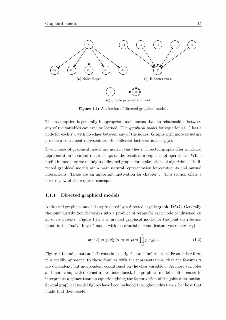
Figure 1.1: A selection of directed graphical models.
This assumption is generally inappropriate as it means that no relationships betweenany of the variables can ever be learned. The graphical model for equation (1.1) has anode for each xd, with no edges between any of the nodes. Graphs with more structureprovide a convenient representation for different factorizations of p(x).
Two classes of graphical model are used in this thesis. Directed graphs offer a naturalrepresentation of causal relationships or the result of a sequence of operations. Whileuseful in modeling we mainly use directed graphs for explanations of algorithms. Undi-rected graphical models are a more natural representation for constraints and mutualinteractions. These are an important motivation for chapter 5. This section offers abrief review of the required concepts.
1.1.1 Directed graphical models
A directed graphical model is represented by a directed acyclic graph (DAG). Generallythe joint distribution factorizes into a product of terms for each node conditioned onall of its parents. Figure 1.1a is a directed graphical model for the joint distributionfound in the “naıve Bayes” model with class variable c and feature vector x={xd},
p(c,x) = p(c)p(x|c) = p(c)D∏
d=1
p(xd|c). (1.2)
Figure 1.1a and equation (1.2) contain exactly the same information. From either formit is readily apparent, to those familiar with the representations, that the features x
are dependent, but independent conditioned on the class variable c. As more variablesand more complicated structure are introduced, the graphical model is often easier tointerpret at a glance than an equation giving the factorization of the joint distribution.Several graphical model figures have been included throughout this thesis for those thatmight find them useful.
Graphical models 16
x1 x2
x3
(a)
x1 x2
x3
fi
x1 x2
x3
(b)
x1 x2
x3
(c)
x1 x2x1
x3
x2
x3
x1 x2
x3
(d)
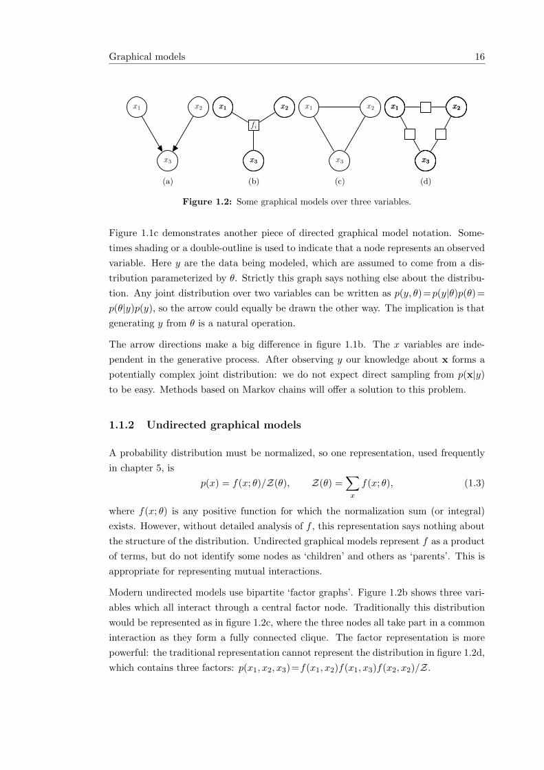
Figure 1.2: Some graphical models over three variables.
Figure 1.1c demonstrates another piece of directed graphical model notation. Some-times shading or a double-outline is used to indicate that a node represents an observedvariable. Here y are the data being modeled, which are assumed to come from a dis-tribution parameterized by θ. Strictly this graph says nothing else about the distribu-tion. Any joint distribution over two variables can be written as p(y, θ)=p(y|θ)p(θ)=p(θ|y)p(y), so the arrow could equally be drawn the other way. The implication is thatgenerating y from θ is a natural operation.
The arrow directions make a big difference in figure 1.1b. The x variables are inde-pendent in the generative process. After observing y our knowledge about x forms apotentially complex joint distribution: we do not expect direct sampling from p(x|y)to be easy. Methods based on Markov chains will offer a solution to this problem.
1.1.2 Undirected graphical models
A probability distribution must be normalized, so one representation, used frequentlyin chapter 5, is
p(x) = f(x; θ)/Z(θ), Z(θ) =∑
x
f(x; θ), (1.3)
where f(x; θ) is any positive function for which the normalization sum (or integral)exists. However, without detailed analysis of f , this representation says nothing aboutthe structure of the distribution. Undirected graphical models represent f as a productof terms, but do not identify some nodes as ‘children’ and others as ‘parents’. This isappropriate for representing mutual interactions.
Modern undirected models use bipartite ‘factor graphs’. Figure 1.2b shows three vari-ables which all interact through a central factor node. Traditionally this distributionwould be represented as in figure 1.2c, where the three nodes all take part in a commoninteraction as they form a fully connected clique. The factor representation is morepowerful: the traditional representation cannot represent the distribution in figure 1.2d,which contains three factors: p(x1, x2, x3)=f(x1, x2)f(x1, x3)f(x2, x2)/Z.
Graphical models 17
1.1.3 The Potts model
The Potts model is a widespread example of an undirected graphical model. Its prob-ability distribution is defined over discrete variables s, each taking on one of q distinctsettings or “colors”:
p(s|J, q) =1
ZP(J, q)exp( ∑
(ij)∈E
Jij(δsisj − 1))
. (1.4)
The variables exist as nodes on a graph where (ij)∈ E means that nodes i and j arelinked by an edge. The Kronecker delta, δsisj is one when si and sj are the same colorand zero otherwise. Neighboring nodes pay an “energy penalty” of Jij when they aredifferent colors. Often a single common coupling Jij =J is used. A common extensionallows biases to be put on the colors: an additional term
∑i hi(si) is put inside the
exponential. The Potts model with bias terms and q = 2 has several different names:the Boltzmann machine, the Ising model, binary Markov random fields or autologisticmodels.
1.1.4 Computations with graphs
Imagine a problem that involves summing over the settings of a binary Potts modelwith 100 variables. In general this seems impossible: there are 2100 possible states.For comparison the age of the universe is usually estimated to be about 298 picosec-onds, while most current processors take about 210 picoseconds to perform a singleinstruction.
If the model’s graph forms a chain, s1—s2—s3 · · · sN , the distribution can be factoredinto a product of functions involving each adjacent pair:
p(s|J) =1Z(J)
N∏n=2
fn(sn, sn−1;J). (1.5)
Now certain sums, such as the normalizer Z(J)=∑
s
∏fn(sn, sn−1;J) and expectations
of functions of variables Ep(s)[g(si)] are tractable. An example showing how the sumscan be decomposed is as follows:
∑s
g(si)N∏
n=2
fn(sn, sn−1) =∑
s1
∑s2
f2(s2, s1)∑
s3f3(s3, s2) · · ·∑
sifi(si, si−1)g(si)
∑si+1
fi+1(si+1, si) · · ·∑sN−1
fN−1(sN−1, sN−2)∑
sNfN (sN , sN−1).
(1.6)
Performing the sums right to left makes the computation O(qN) rather than O(qN ),where q=2 for binary variables.
The role of summation 18
(a) (b)
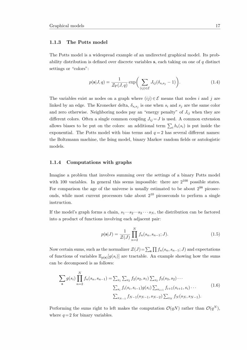
Figure 1.3: A “small” state space of 100 binary variables represented as (a) pixelsand (b) an undirected graphical model.
The above technique easily generalizes to tree-structured graphs, but other topologiesare common in applications. Figure 1.3 shows a grid of 100 binary variables. Arrays likethis are common in computer vision, spatial statistics and statistical physics. Treatingeach row of 10 pixels as a single variable makes a chain-structured graph with N =10variables each taking on 210 = 1024 states. Summing has changed from an operationthat takes orders of magnitude longer than the age of the universe to being almostinstantaneous. Advanced versions of this procedure exist for general graphical models,notably the junction tree algorithm (Lauritzen and Spiegelhalter, 1988). The cost ofthe algorithm is determined by the tree-width of a graph, which indicates the largestnumber of variables that need to be joined in order to form a tree structure.
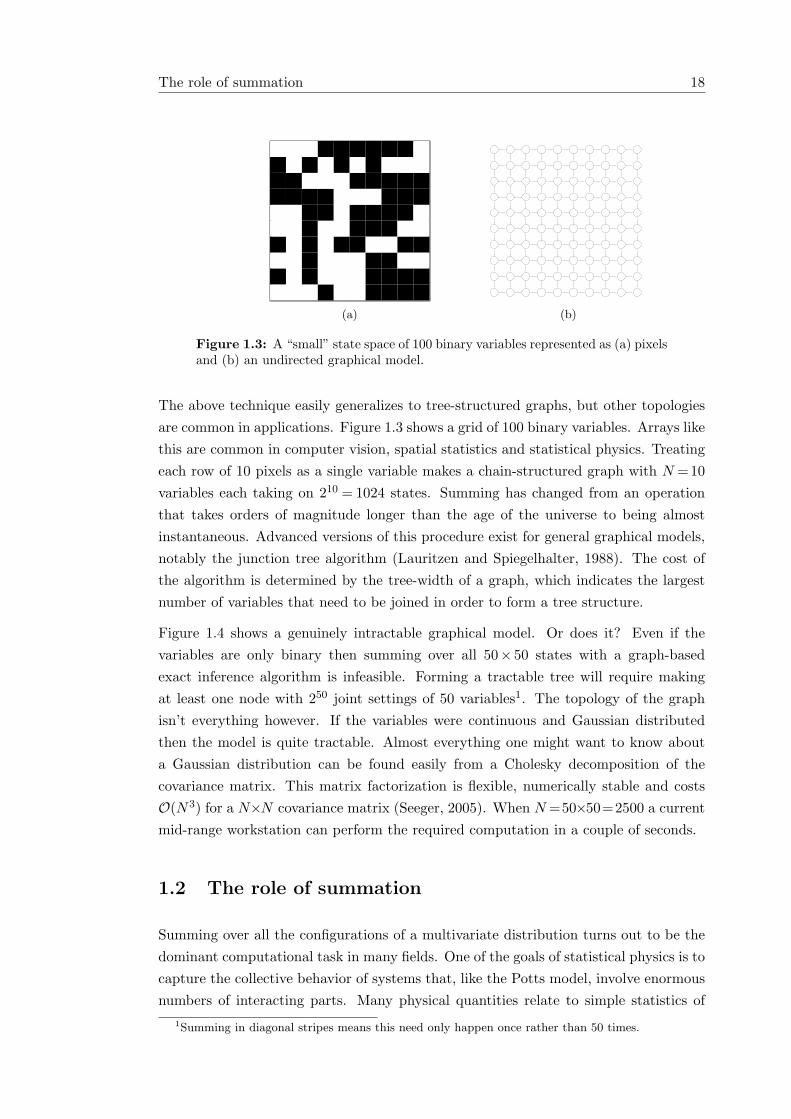
Figure 1.4 shows a genuinely intractable graphical model. Or does it? Even if thevariables are only binary then summing over all 50× 50 states with a graph-basedexact inference algorithm is infeasible. Forming a tractable tree will require makingat least one node with 250 joint settings of 50 variables1. The topology of the graphisn’t everything however. If the variables were continuous and Gaussian distributedthen the model is quite tractable. Almost everything one might want to know abouta Gaussian distribution can be found easily from a Cholesky decomposition of thecovariance matrix. This matrix factorization is flexible, numerically stable and costsO(N3) for a N×N covariance matrix (Seeger, 2005). When N =50×50=2500 a currentmid-range workstation can perform the required computation in a couple of seconds.
1.2 The role of summation
Summing over all the configurations of a multivariate distribution turns out to be thedominant computational task in many fields. One of the goals of statistical physics is tocapture the collective behavior of systems that, like the Potts model, involve enormousnumbers of interacting parts. Many physical quantities relate to simple statistics of
1Summing in diagonal stripes means this need only happen once rather than 50 times.
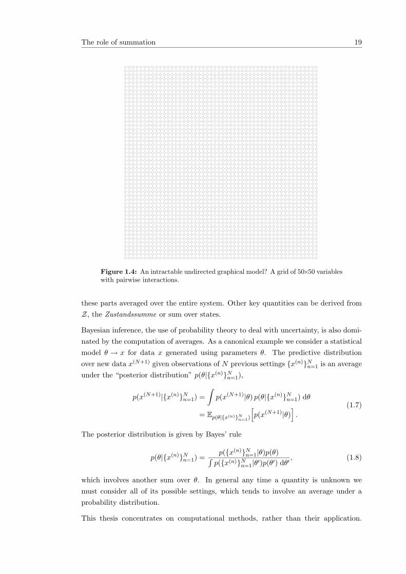
The role of summation 19
Figure 1.4: An intractable undirected graphical model? A grid of 50×50 variableswith pairwise interactions.
these parts averaged over the entire system. Other key quantities can be derived fromZ, the Zustandssumme or sum over states.
Bayesian inference, the use of probability theory to deal with uncertainty, is also domi-nated by the computation of averages. As a canonical example we consider a statisticalmodel θ → x for data x generated using parameters θ. The predictive distributionover new data x(N+1) given observations of N previous settings {x(n)}Nn=1 is an averageunder the “posterior distribution” p(θ|{x(n)}Nn=1),
p(x(N+1)|{x(n)}Nn=1) =∫
p(x(N+1)|θ) p(θ|{x(n)}Nn=1) dθ
= Ep(θ|{x(n)}Nn=1)
[p(x(N+1)|θ)
].
(1.7)
The posterior distribution is given by Bayes’ rule
p(θ|{x(n)}Nn=1) =p({x(n)}Nn=1|θ)p(θ)∫
p({x(n)}Nn=1|θ′)p(θ′) dθ′, (1.8)
which involves another sum over θ. In general any time a quantity is unknown wemust consider all of its possible settings, which tends to involve an average under aprobability distribution.
This thesis concentrates on computational methods, rather than their application.
Simple Monte Carlo 20
However, modeling and learning from data are a key motivation for this work, sowe briefly mention some more general references. “Bayesian inference” is named afterBayes (1763), although many of the ideas that currently fall under this banner camemuch later. For more on the philosophy a good start is a beautifully written paperby Cox (1946)2. Recent textbooks offer a broader view of probabilistic modeling andare available from the viewpoints of various communities, including statistics (Gelmanet al., 2003), machine learning (MacKay, 2003; Bishop, 2006) and the physical sciences(Sivia and Skilling, 2006).
1.3 Simple Monte Carlo
Many of the alleged difficulties with finding averages are unduly pessimistic. Imaginewe were interested in the average salary x of people p in the set of statisticians S.Formally this is a large, “intractable” sum over all of the |S| statisticians in the world:
Ep∈S [x(p)] ≡ 1|S|∑p∈S
x(p). (1.9)
But to claim that the question is unanswerable is absurd. We can clearly get a reason-able estimate of the answer by measuring just some statisticians,
Ep∈S [x(p)] ≈ 1S
S∑s=1
x(p(s)), for random survey of S people {p(s)} ∈ S. (1.10)
No reasonable application needs the exact answer, which in any case is constantlyfluctuating as individual statisticians are hired, promoted and retire. So for all practicalpurposes the problem is solved. Nearly. Conducting surveys that obtain a fair samplefrom a target population is difficult. But the technique is so useful we are prepared toinvest effort into good sampling methods.
This statistical sampling technique is directly relevant to solving difficult integrals instatistical inference. For example, what is the distribution over an unknown quantityx after observing data D from a distribution with unknown parameters θ?
p(x|D) =∫
p(x|θ,D)p(θ|D) dθ = Ep(θ|D)[p(x|θ,D)]
≈ 1S
S∑s=1
p(x|θ(s),D), θ(s) ∼ p(θ|D).(1.11)
We draw samples from the target distribution, which rather than the set of statisticiansis now p(θ|D). Approximating general averages by statistical sampling is known as“simple Monte Carlo”. The estimates are unbiased, which if not clear now is shown
2Cox’s work has been subject to some technical objections which are countered by Horn (2003).
Simple Monte Carlo 21
more generally in section 2.2. As long as variances are bounded appropriately the sumof independent terms will obey a central limit theorem; the estimator’s variance willscale like 1/S.
Having an estimator’s variance shrink only linearly with computational effort is oftenconsidered poor. Sokal (1996) begins a lecture course on Monte Carlo with the warning
“Monte Carlo is an extremely bad method; it should be used only when allalternative methods are worse.”
However, as Sokal goes on to acknowledge, Monte Carlo is also an extremely importantmethod. On some problems it might be the only way to obtain accurate answers.Metropolis (1987) describes how the physicist Enrico Fermi (1901–1954) used MonteCarlo before the development of electronic computers. When insomnia struck he wouldspend his nights predicting the results of complex neutron scattering experiments byperforming statistical sampling calculations with a mechanical adding machine. Asanalytically deriving the behavior of many neutrons seemed intractable, Fermi’s abilityto make accurate predictions astonished his colleagues.
Many problems in physics and statistics are complex and involve many variables. Nu-merical methods that scale exponentially with the dimensionality of the problem willnot work at all. In contrast, Monte Carlo is usually simple and its 1/
√S scaling of error
bars “independent of dimensionality” may be good enough. Even when more advanceddeterministic methods are available, Monte Carlo can be appropriate if today’s com-puters can return useful answers with less implementation effort than more complexmethods.
1.3.1 Sampling from distributions
Just as finding a fair sample from a population is difficult in surveys, sampling correctlyfrom arbitrary probability distributions is also hard. ‘Simple’ Monte Carlo is only aseasy to implement as the random variate generator for the entire joint distributioninvolved.
A graphical description of sampling from a probability distribution is given by fig-ure 1.5a. Points are drawn uniformly from the unit area underneath the probabilitydensity function and their corresponding value recorded. This correctly assigns eachelement of the input space dx with probability p(x)dx.
The probability mass to the left of each point, u(x), is distributed as Uniform[0, 1].To implement a sampler we can first draw u and then compute x(u) from the inversecumulative distribution. That is x(u) = Φ−1(u), where Φ(x) =
∫ x−∞ p(x′) dx′. Now the
difficulty of sampling from distributions with this general method becomes apparent.It is often infeasible to even normalize p, a single integral over the entire state space,whereas Φ(x) is a whole continuum of such integrals.
Simple Monte Carlo 22
p(x)
xx
(2)x
(3)x
(1)x
(4)
(a) Direct sampling
coptq∗(x)
p∗(x)
c q∗(x)
xx
(1)
(xj , hj)
(xi, hi)
(b) Rejection sampling
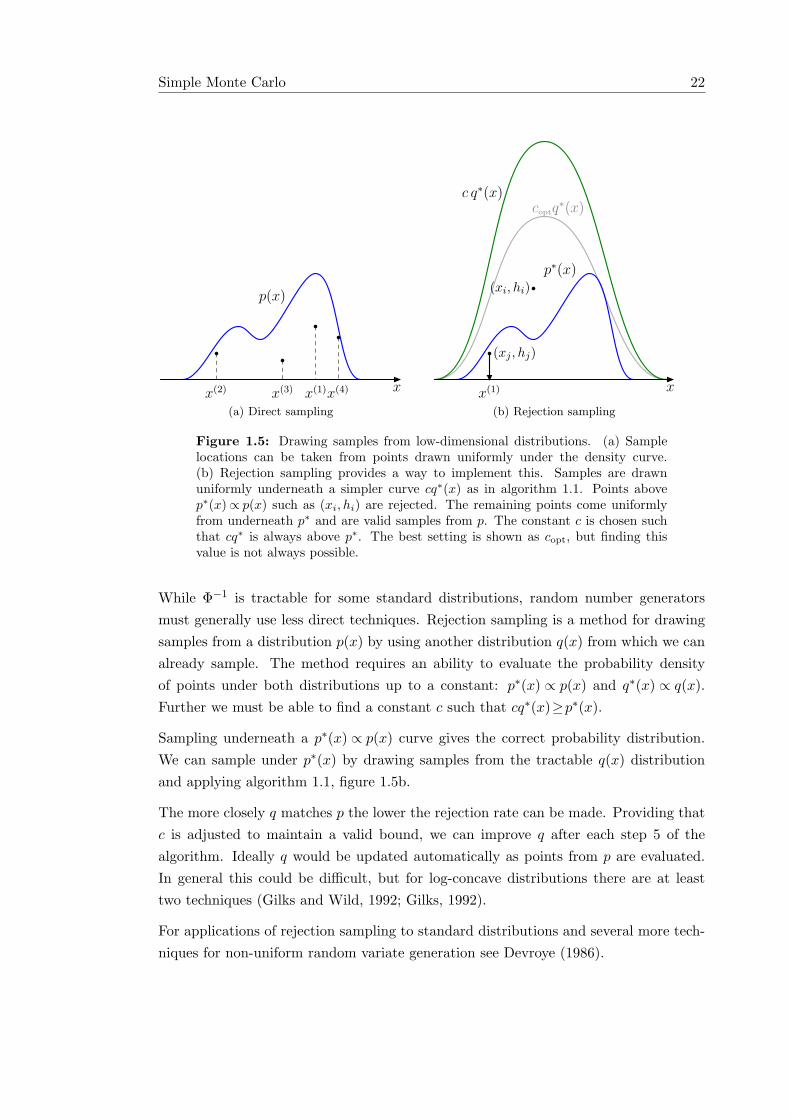
Figure 1.5: Drawing samples from low-dimensional distributions. (a) Samplelocations can be taken from points drawn uniformly under the density curve.(b) Rejection sampling provides a way to implement this. Samples are drawnuniformly underneath a simpler curve cq∗(x) as in algorithm 1.1. Points abovep∗(x)∝ p(x) such as (xi, hi) are rejected. The remaining points come uniformlyfrom underneath p∗ and are valid samples from p. The constant c is chosen suchthat cq∗ is always above p∗. The best setting is shown as copt, but finding thisvalue is not always possible.
While Φ−1 is tractable for some standard distributions, random number generatorsmust generally use less direct techniques. Rejection sampling is a method for drawingsamples from a distribution p(x) by using another distribution q(x) from which we canalready sample. The method requires an ability to evaluate the probability densityof points under both distributions up to a constant: p∗(x) ∝ p(x) and q∗(x) ∝ q(x).Further we must be able to find a constant c such that cq∗(x)≥p∗(x).
Sampling underneath a p∗(x) ∝ p(x) curve gives the correct probability distribution.We can sample under p∗(x) by drawing samples from the tractable q(x) distributionand applying algorithm 1.1, figure 1.5b.
The more closely q matches p the lower the rejection rate can be made. Providing thatc is adjusted to maintain a valid bound, we can improve q after each step 5 of thealgorithm. Ideally q would be updated automatically as points from p are evaluated.In general this could be difficult, but for log-concave distributions there are at leasttwo techniques (Gilks and Wild, 1992; Gilks, 1992).
For applications of rejection sampling to standard distributions and several more tech-niques for non-uniform random variate generation see Devroye (1986).
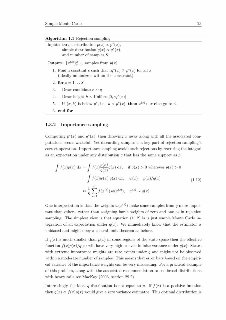
Simple Monte Carlo 23
Algorithm 1.1 Rejection samplingInputs: target distribution p(x) ∝ p∗(x),
simple distribution q(x) ∝ q∗(x),and number of samples S.
Outputs: {x(s)}Ss=1, samples from p(x)
1. Find a constant c such that cq∗(x) ≥ p∗(x) for all x(ideally minimize c within the constraint)
2. for s = 1 . . . S
3. Draw candidate x ∼ q
4. Draw height h ∼ Uniform[0, cq∗(x)]
5. if (x, h) is below p∗, i.e., h < p∗(x), then x(s)←x else go to 3.
6. end for
1.3.2 Importance sampling
Computing p∗(x) and q∗(x), then throwing x away along with all the associated com-putations seems wasteful. Yet discarding samples is a key part of rejection sampling’scorrect operation. Importance sampling avoids such rejections by rewriting the integralas an expectation under any distribution q that has the same support as p:∫
f(x)p(x) dx =∫
f(x)p(x)q(x)
q(x) dx, if q(x) > 0 wherever p(x) > 0
=∫
f(x)w(x) q(x) dx, w(x) = p(x)/q(x)
≈ 1S
S∑s=1
f(x(s)) w(x(s)), x(s) ∼ q(x).
(1.12)
One interpretation is that the weights w(x(s)) make some samples from q more impor-tant than others, rather than assigning harsh weights of zero and one as in rejectionsampling. The simplest view is that equation (1.12) is is just simple Monte Carlo in-tegration of an expectation under q(x). We immediately know that the estimator isunbiased and might obey a central limit theorem as before.
If q(x) is much smaller than p(x) in some regions of the state space then the effectivefunction f(x)p(x)/q(x) will have very high or even infinite variance under q(x). Stateswith extreme importance weights are rare events under q and might not be observedwithin a moderate number of samples. This means that error bars based on the empiri-cal variance of the importance weights can be very misleading. For a practical exampleof this problem, along with the associated recommendation to use broad distributionswith heavy tails see MacKay (2003, section 29.2).
Interestingly the ideal q distribution is not equal to p. If f(x) is a positive functionthen q(x) ∝ f(x)p(x) would give a zero variance estimator. This optimal distribution is
Markov chain Monte Carlo (MCMC) 24
unobtainable as evaluating q(x) requires the normalization Zq =∫
f(x)p(x) dx, the tar-get integral. But sometimes deliberate matches between q and p are useful in practice.For example when interested in gathering statistics about the tails of p.
Nothing about the importance sampling trick in equation (1.12) actually requires theoriginal integral to be an expectation. We can divide and multiply any integrand by aconvenient distribution to make it an expectation. Thus importance sampling allowsany integral to be approximated by Monte Carlo. As most of the integrals in dominantapplications are expectations, we still maintain p(x) in the equations throughout.
Evaluating the importance weights w(x) requires evaluating p(x) = p∗(x)/Zp, but of-ten Zp is unknown. In these cases the normalizing constant must be approximatedseparately as follows:
Zp
Zq=
1Zq
∫p∗(x) dx =
∫p∗(x)q∗(x)
q(x) dx
=∫
w∗(x) q(x) dx, w∗(x) = p∗(x)/q∗(x)
≈ 1S
S∑s=1
w∗(x(s)), x(s) ∼ q(x)
(1.13)
This gives an approximation for the importance weights
w(x) =p(x)q(x)
=Zq
Zp
p∗(x)q∗(x)
≈ w∗(x)1S
∑Ss=1 w∗(x(s))
,
(1.14)
which can be used within equation (1.12). The resulting estimator is biased but con-sistent when both estimators (1.12) and (1.13) have bounded variance.
1.4 Markov chain Monte Carlo (MCMC)
Both rejection sampling and importance sampling require a tractable surrogate distri-bution q(x). Neither method will perform well if maxx p(x)/q(x) is large: rejectionsampling will rarely return samples and importance sampling will have large variance.Markov chain Monte Carlo methods can be used to sample from p(x) distributionsthat are complex and have unknown normalization. This is achieved by relaxing therequirement that the samples should be independent.
A Markov chain generates a correlated sequence of states. Each step in the sequenceis drawn from a transition operator T (x′← x), which gives the probability of movingfrom state x to state x′. According to the Markov property, the transition probabilitiesdepend only on the current state, x. In particular, any free parameters σ, e.g. step
Markov chain Monte Carlo (MCMC) 25
sizes, in a family of transition operators, T (x′←x;σ), cannot be chosen based on thehistory of the chain.
A basic requirement for T is that given a sample from p(x), the marginal distributionover the next state in the chain is also the target distribution of interest p:
p(x′) =∑
x
T (x′←x) p(x) for all x′. (1.15)
By induction all subsequent steps of the chain will have the same marginal distribution.The transition operator is said to leave the target distribution p stationary. MCMCalgorithms often require operators that ensure the marginal distribution over a stateof the chain tends to p(x) regardless of starting state. This requires irreducibility : theability to reach any x where p(x) > 0 in a finite number of steps, and aperiodicity :no states are only accessible at certain regularly spaced times. For more details seeTierney (1994). For now we note that as long as a T satisfies equation (1.15) it can beuseful as the other conditions can be met through combinations with other operators.
Given that p(x) is a complicated distribution, it might seem unreasonable to expectthat we could find a transition operator T leaving it stationary. However, it is ofteneasy to construct a transition operator satisfying detailed balance:
T (x′←x) p(x) = T (x←x′) p(x′) for all x, x′. (1.16)
This states that a step starting at equilibrium and transitioning under T has the sameprobability “forwards” x→ x′ or “backwards” x′→ x. Proving detailed balance onlyrequires considering each pair of states in isolation, there is no sum over all statesas in equation (1.15). Having shown equation (1.16), summing over x on both sidesimmediately recovers the stationary distribution requirement (1.15). Thus detailedbalance is a useful property for deriving many MCMC methods; however it is not alwaysrequired or even desirable. Chapter 3 introduces some MCMC transition operators thatdo not satisfy equation (1.16).
Given any transition operator T satisfying the stationary condition, equation (1.15),we can construct a reverse operator T defined by
T (x←x′) ∝ T (x′←x) p(x) =T (x′←x) p(x)∑x T (x′←x) p(x)
=T (x′←x) p(x)
p(x′). (1.17)
A symmetric form of this relationship shows that an operator satisfying detailed balanceis its own reverse transition operator:
T (x′←x) p(x) = T (x←x′) p(x′) for all x, x′. (1.18)
Summing over x or x′ reveals that this mutual reversibility condition implies that thestationary condition, equation (1.15), holds for both T and T . Therefore constructing
Choice of method 26
a pair of mutually reversible transition distributions is an alternative strategy for con-structing MCMC operators. Detailed balance is a restricted case where a transitionoperator must be its own reverse operator.
1.5 Choice of method
In this introduction we described the importance of high-dimensional probability dis-tributions. Samples from these distributions capture their typical properties, which isthe basis of the Monte Carlo estimation of expectations such as
∫f(x)p(x) dx. We
assume or hope that extreme values under p(x) do not form a significant contributionto the integral. For expectations in many physical and statistical applications this is areasonable assumption.
In high-dimensional problems sampling from an interesting target distribution p(x)is often intractable. Methods such as rejection sampling fail because finding a close-matching simple distribution q(x) is not possible. For the same reason importancesampling estimators tend to have very high variance.
We described rejection sampling as it remains an important method when i.i.d. samplesfrom low-dimensional distributions are required. This occurs in some simulation work,and as part of some MCMC methods. Similarly while simple importance samplinghas problems in high dimensions, it provides the basis of more advanced methods thatare useful on some high-dimensional problems. We neglect much of the importancesampling literature, but will study some methods relating to Markov chains.
The focus of this thesis are methods that use Markov chains. These allow us to draw(correlated) samples from complex distributions and to perform Monte Carlo integra-tion in high-dimensional problems. The next chapter reviews several important algo-rithms based on Markov chains together with some new contributions. After this wewill be in a position to outline the remainder of the thesis.
Chapter 2
Markov chain Monte Carlo
This chapter reviews some important Markov chain Monte Carlo (MCMC) algorithms.Much of this material is standard and could be skipped by those already familiar withthe literature. However, some of the material in this chapter is, to the best of ourknowledge, novel. These contributions include generalizations of tempered transitionsin subsection 2.5.4 and the introduction of a slice-sampling version of the two stageacceptance rule (see sections 2.1.3 and 2.4.2). We also present some results in anunconventional way, which is designed to help with reading later chapters.
2.1 Metropolis methods
Algorithm 2.1 gives a procedure for simulating a Markov chain with stationary distri-bution p(x) due to Hastings (1970).
Algorithm 2.1 Metropolis–HastingsInput: initial setting x, number of iterations S
1. for s = 1 . . . S
2. Propose x′ ∼ q(x′←x)
3. Compute a =p(x′) q(x←x′)p(x) q(x′←x)
4. Set x = x′ with probability min(1, a), e.g.(a) Draw r ∼ Uniform[0, 1](b) if (r < a) then set x←x′.
5. end for
The setting of x at the end of each iteration is considered as a sample from the targetprobability distribution p(x). Adjacent samples are identical when the state is notupdated in step 4b), but every iteration must be recorded as part of the Markov chain.
Metropolis methods 28
It is straightforward to show that the Metropolis–Hastings algorithm satisfies detailedbalance:
T (x′←x) p(x) = min(
1,p(x′) q(x←x′)p(x) q(x′←x)
)q(x′←x) p(x)
= min(p(x) q(x′←x), p(x′) q(x←x′)
)= min
(1,
p(x) q(x′←x)p(x′) q(x←x′)
)q(x←x′) p(x′)
= T (x←x′) p(x′), as required.
(2.1)
Here the probability for a forwards transition x→ x′ was manipulated into the prob-ability of the reverse transition x′→x. However it would have been sufficient to stopafter the second line and note that the expression is symmetric in x and x′.
The algorithm is valid for any proposal distribution q. Ideal proposals would beconstructed for rapid exploration of the distribution of interest p. We could writeq(x′←x;D) to emphasize choices of proposal that are based on observed data D. Us-ing any fixed D is valid, but q cannot be based on the past history of the sampler assuch a chain would not be “Markov”.
Often proposals are not complicated data-based distributions. Simple perturbationssuch as a Gaussian with mean x are commonly chosen. The accept/reject step 4. inthe algorithm, corrects for the mismatch between the proposal and target distributions.When the proposal distribution is symmetric, i.e. q(x← x′) = q(x′← x) for all x, x′,the acceptance ratio in step 3. simplifies to a ratio under the distribution of interest,a = p(x′)/p(x). This is the original Metropolis algorithm (Metropolis et al., 1953).Some authors, e.g. MacKay (2003), prefer to drop such distinctions and simply refer toall Metropolis–Hastings algorithms as Metropolis methods. The next section suggestsanother justification of this view.
2.1.1 Generality of Metropolis–Hastings
Consider a MCMC algorithm that proposes a state from a distribution q(x′←x) andaccepts with probability pa(x′←x). Restricting attention to transition operators sat-isfying detailed balance,
pa(x′←x)q(x′←x) p(x) = pa(x←x′)q(x←x′) p(x′), for all x, x′, (2.2)
gives an equality constraint. We also have inequalities that must hold for probabilities:
0 ≤ pa(x′←x) ≤ 1 and 0 ≤ pa(x←x′) ≤ 1. (2.3)
Optimizing the average acceptance probability p(x)pa(x′← x)+p(x′)pa(x← x′) withrespect to a(x′←x) and a(x←x′) must saturate one or more of the inequalities (2.3), a
Metropolis methods 29
well known property of linear programming problems. Therefore, either pa(x′←x)=1or pa(x←x′)=1 and pa(x′←x) is given by equation (2.2). This gives the Metropolis–Hastings acceptance rule,
pa(x′←x) = min(
1,p(x′)q(x←x′)p(x)q(x′←x)
). (2.4)
According to the constraint of equation (2.2), a pair of valid acceptance probabilitiesmust have the same ratio pa(x′ ← x)/pa(x← x′) as any other valid pair. Thereforethey can be obtained by multiplying the Metropolis–Hastings probabilities by a con-stant less than one. This corresponds to mixing in some fraction of the “do nothing”transition operator, which leaves the chain in the current state, at those two sites. Italso corresponds to adjusting the proposal distribution q to suggest staying still moreoften. Staying still more often harms the asymptotic variance of the chain: in this sense(although not by all measures) using equation (2.4) is optimal (Peskun, 1973).
Given this result it is unsurprising that Metropolis–Hastings has become almost syn-onymous with MCMC. It is tempting to conclude that the only way to improve Markovchains for Monte Carlo is by researching domain-specific proposal distributions such asin the vision community’s “Data-driven MCMC” (Tu and Zhu, 2002). In fact a richvariety of more generic MCMC-based algorithms exist and continue to be developed.Many of these do satisfy detailed balance, but the corresponding M–H q(x′←x) distri-bution is often defined implicitly and would not be a natural description of the method.
To illustrate the limitations of claiming “all (reversible) MCMC is just Metropolis–Hastings” we show that “all (reversible) MCMC is just Metropolis”. This also demon-strates a methodology used throughout the thesis. We construct a new target distribu-tion p(x, x′)=q(x′←x) p(x), i.e. the joint distribution over a point x∼p and a point x′
proposed from that location. The marginal distribution over x is the original target p.Now consider the symmetric Metropolis proposal that swaps the values of x and x′
such that putatively x′ comes from p and x was proposed from it. The Metropolisacceptance probability for this swap proposal is
min(
1,p(x′, x)p(x, x′)
)= min
(1,
p(x′) q(x←x′)p(x) q(x′←x)
), (2.5)
i.e., the Metropolis–Hastings acceptance probability. In this sense only an algorithmwith symmetric proposals is needed. But this is not a very natural description of theMetropolis–Hastings algorithm. Similarly, while it is possible to describe all algorithmssatisfying detailed balance as Metropolis or Metropolis–Hastings algorithms, other de-scriptions may be more natural. However, we will find constructing joint distributionslike p(x, x′) a useful theoretical tool and one that suggests new Markov chain operators.
Metropolis methods 30
2.1.2 Gibbs sampling
Gibbs sampling (Geman and Geman, 1984) resamples each dimension xi of a mul-tivariate quantity x from their conditional distributions p(xi|xj 6=i). Any individualupdate maintains detailed balance, which is easily checked directly. Alternatively wecan write the Gibbs sampling update as a Metropolis–Hastings proposal: q(x′←x) =p(x′i|xj 6=i)I(x′{j 6=i}= x{j 6=i}), where I is an indicator function ensuring all componentsother than xi stay fixed. The acceptance probability for this proposal is identical toone, so need not be checked.
Gibbs sampling is often easy to implement. If the target distribution is discrete andeach variable takes on a small number of settings then the conditional distributions canbe explicitly computed,
p(xi|xj 6=i) ∝ p(xi,xj 6=i) =p(xi,xj 6=i)∑x′i
p(x′i,xj 6=i). (2.6)
On continuous problems the one-dimensional conditional distributions are usuallyamenable to standard sampling methods as mentioned in subsection 1.3.1.
A desirable feature of Gibbs sampling is that it has no free parameters and so can beapplied fairly automatically. Indeed the BUGS packages can create Gibbs samplers fora large variety of models specified using a simple description language (Spiegelhalteret al., 1996). There are actually some free choices regarding how the variables areupdated. “Block-Gibbs” sampling chooses groups of variables to update at once. Also,continuous distributions can be re-parameterized before Gibbs sampling — a basis inwhich the dimensions are independent would obviously be particularly effective.
Clifford et al. (1993) contains several interesting discussions regarding the nature andhistory of the Gibbs sampler. The method has often been regarded with a ratherundeserved special status amongst MCMC methods. It is just one of many ways toconstruct a Markov chain with a target stationary distribution. In particular there is noneed to approximate Gibbs sampling when sampling from conditionals is not tractableas in (Ritter and Tanner, 1992). Metropolis–Hastings updates of each dimension canbe used instead, and there is no need to call this method Metropolis-within-Gibbs.
2.1.3 A two stage acceptance rule
If the target distribution is factored into two terms, for example a prior and likelihoodp(x)∝π(x)L(x), a proposal can be accepted with probability
pa = min(
1,q(x←x′)π(x′)q(x′←x)π(x)
)min
(1,
L(x′)L(x)
). (2.7)

Construction of estimators 31
Straightforward checking shows that this satisfies detailed balance. We know fromprevious discussions that it will accept less often than standard Metropolis–Hastingsand is inferior according to Peskun (1973), but computationally it can be more efficient.Algorithm 2.2 is an acceptance rule that will accept proposals with probability pa. Ifπ(x′) is able to veto an a priori unreasonable proposal then L(x′) need not be computed.Factoring out a cheap “sanity-check” distribution π(x) may be worth a fall in acceptancerate in problems where likelihood evaluations are expensive.
Algorithm 2.2 A two stage acceptance ruleInput: initial setting x, proposed setting x′
1. Draw r1 ∼ Uniform[0, 1]
2. if r1 <q(x←x′)π(x′)q(x′←x)π(x)
3. Draw r2 ∼ Uniform[0, 1]
4. if r2 <L(x′)L(x)
Accept else Reject
5. else6. Reject
As with standard Metropolis–Hastings none of the probabilities need to be computedexactly. Bounding them sufficiently to make the accept/reject decision in step 2. or 4. isall that is required. In practice few Monte Carlo codes implement the required intervalarithmetic to make these savings. In contrast the two stage procedure is generallyapplicable and easy to implement.
Algorithm 2.2 is a special case of the “surrogate transitions method” (Liu, 2001,pp. 194–195) and also the (different) algorithm of Christen and Fox (2005). The two-stage method here is also equivalent to Dostert et al. (2006, Algorithm II), whichpresented it in the context of a particular choice for q(x′← x). This literature has arich variety of possible approximate distributions that can be used for π(x) in particularapplications. In a statistical application where p(x) depends on a data set a generalchoice would be to use a subset of the data to define π(x).
An obvious generalization is splitting the acceptance rule into more than two terms.Factoring the distribution into many terms could make the acceptance rate fall dra-matically, so there would need to be a specific computational benefit.
2.2 Construction of estimators
The output of an MCMC algorithm is a set of correlated samples drawn from a jointdistribution P ({x(s)}). At equilibrium every marginal p(x(s)) is the correct distribu-tion of interest. Using these equilibrium samples in the straightforward Monte Carlo
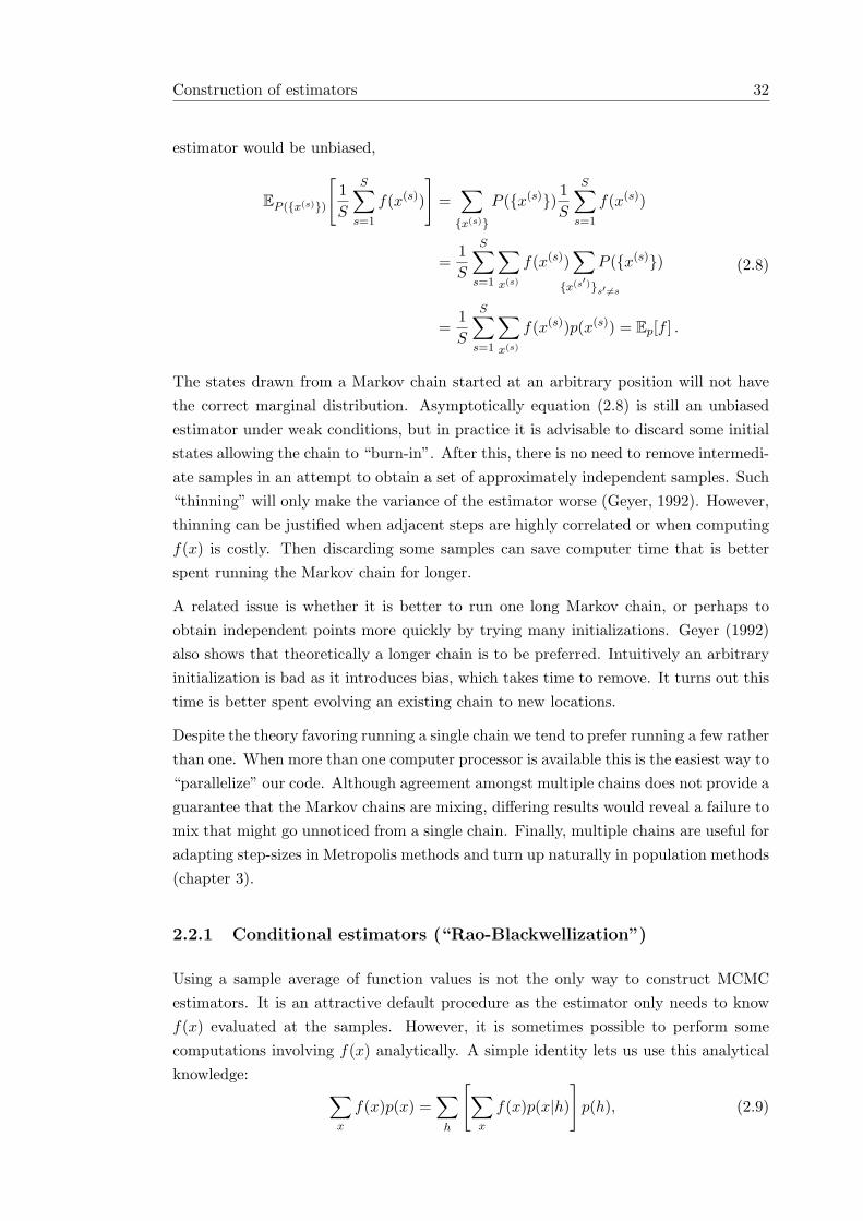
Construction of estimators 32
estimator would be unbiased,
EP ({x(s)})
[1S
S∑s=1
f(x(s))
]=∑{x(s)}
P ({x(s)}) 1S
S∑s=1
f(x(s))
=1S
S∑s=1
∑x(s)
f(x(s))∑
{x(s′)}s′ 6=s
P ({x(s)})
=1S
S∑s=1
∑x(s)
f(x(s))p(x(s)) = Ep[f ] .
(2.8)
The states drawn from a Markov chain started at an arbitrary position will not havethe correct marginal distribution. Asymptotically equation (2.8) is still an unbiasedestimator under weak conditions, but in practice it is advisable to discard some initialstates allowing the chain to “burn-in”. After this, there is no need to remove intermedi-ate samples in an attempt to obtain a set of approximately independent samples. Such“thinning” will only make the variance of the estimator worse (Geyer, 1992). However,thinning can be justified when adjacent steps are highly correlated or when computingf(x) is costly. Then discarding some samples can save computer time that is betterspent running the Markov chain for longer.
A related issue is whether it is better to run one long Markov chain, or perhaps toobtain independent points more quickly by trying many initializations. Geyer (1992)also shows that theoretically a longer chain is to be preferred. Intuitively an arbitraryinitialization is bad as it introduces bias, which takes time to remove. It turns out thistime is better spent evolving an existing chain to new locations.
Despite the theory favoring running a single chain we tend to prefer running a few ratherthan one. When more than one computer processor is available this is the easiest way to“parallelize” our code. Although agreement amongst multiple chains does not provide aguarantee that the Markov chains are mixing, differing results would reveal a failure tomix that might go unnoticed from a single chain. Finally, multiple chains are useful foradapting step-sizes in Metropolis methods and turn up naturally in population methods(chapter 3).
2.2.1 Conditional estimators (“Rao-Blackwellization”)
Using a sample average of function values is not the only way to construct MCMCestimators. It is an attractive default procedure as the estimator only needs to knowf(x) evaluated at the samples. However, it is sometimes possible to perform somecomputations involving f(x) analytically. A simple identity lets us use this analyticalknowledge: ∑
x
f(x)p(x) =∑
h
[∑x
f(x)p(x|h)
]p(h), (2.9)
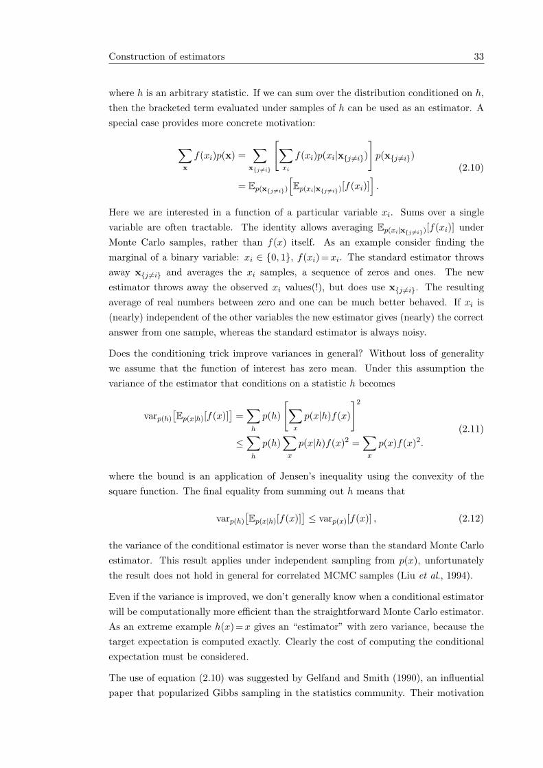
Construction of estimators 33
where h is an arbitrary statistic. If we can sum over the distribution conditioned on h,then the bracketed term evaluated under samples of h can be used as an estimator. Aspecial case provides more concrete motivation:
∑x
f(xi)p(x) =∑
x{j 6=i}
[∑xi
f(xi)p(xi|x{j 6=i})
]p(x{j 6=i})
= Ep(x{j 6=i})
[Ep(xi|x{j 6=i})[f(xi)]
].
(2.10)
Here we are interested in a function of a particular variable xi. Sums over a singlevariable are often tractable. The identity allows averaging Ep(xi|x{j 6=i})[f(xi)] underMonte Carlo samples, rather than f(x) itself. As an example consider finding themarginal of a binary variable: xi ∈ {0, 1}, f(xi)=xi. The standard estimator throwsaway x{j 6=i} and averages the xi samples, a sequence of zeros and ones. The newestimator throws away the observed xi values(!), but does use x{j 6=i}. The resultingaverage of real numbers between zero and one can be much better behaved. If xi is(nearly) independent of the other variables the new estimator gives (nearly) the correctanswer from one sample, whereas the standard estimator is always noisy.
Does the conditioning trick improve variances in general? Without loss of generalitywe assume that the function of interest has zero mean. Under this assumption thevariance of the estimator that conditions on a statistic h becomes
varp(h)
[Ep(x|h)[f(x)]
]=∑
h
p(h)
[∑x
p(x|h)f(x)
]2
≤∑
h
p(h)∑
x
p(x|h)f(x)2 =∑
x
p(x)f(x)2.(2.11)
where the bound is an application of Jensen’s inequality using the convexity of thesquare function. The final equality from summing out h means that
varp(h)
[Ep(x|h)[f(x)]
]≤ varp(x)[f(x)] , (2.12)
the variance of the conditional estimator is never worse than the standard Monte Carloestimator. This result applies under independent sampling from p(x), unfortunatelythe result does not hold in general for correlated MCMC samples (Liu et al., 1994).
Even if the variance is improved, we don’t generally know when a conditional estimatorwill be computationally more efficient than the straightforward Monte Carlo estimator.As an extreme example h(x)=x gives an “estimator” with zero variance, because thetarget expectation is computed exactly. Clearly the cost of computing the conditionalexpectation must be considered.
The use of equation (2.10) was suggested by Gelfand and Smith (1990), an influentialpaper that popularized Gibbs sampling in the statistics community. Their motivation
Construction of estimators 34
was essentially equation (2.11), cited as a version of the Rao-Blackwell theorem. Thebound’s requirement of independent samples was satisfied because the paper proposedrunning many independent Gibbs sampling runs. As this practice has fallen out of favor,it seems misleading to continue to call the method “Rao-Blackwellization”, althoughsome of the literature continues to do so. Despite the lack of Rao-Blackwell guaranteesthe estimator can often be justified empirically, as was done earlier by at least Pearl(1987).
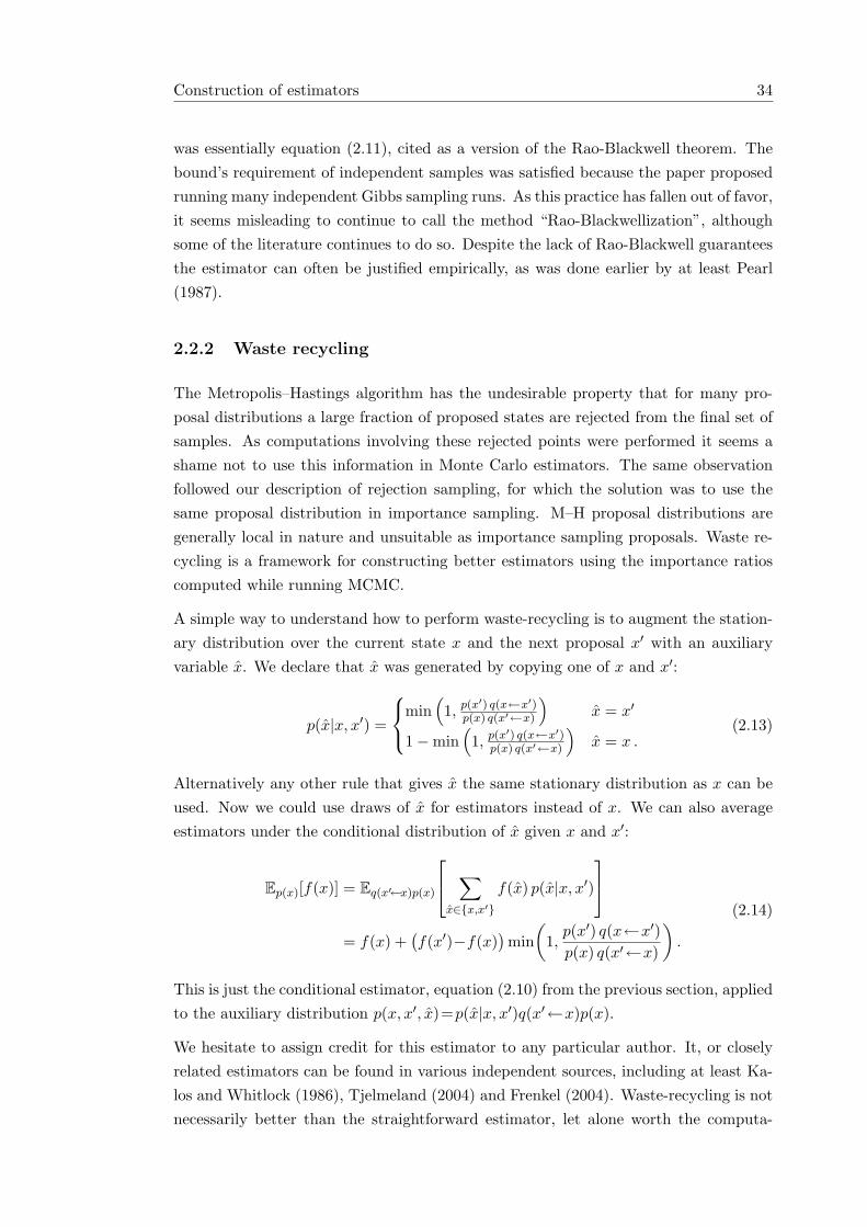
2.2.2 Waste recycling
The Metropolis–Hastings algorithm has the undesirable property that for many pro-posal distributions a large fraction of proposed states are rejected from the final set ofsamples. As computations involving these rejected points were performed it seems ashame not to use this information in Monte Carlo estimators. The same observationfollowed our description of rejection sampling, for which the solution was to use thesame proposal distribution in importance sampling. M–H proposal distributions aregenerally local in nature and unsuitable as importance sampling proposals. Waste re-cycling is a framework for constructing better estimators using the importance ratioscomputed while running MCMC.
A simple way to understand how to perform waste-recycling is to augment the station-ary distribution over the current state x and the next proposal x′ with an auxiliaryvariable x. We declare that x was generated by copying one of x and x′:
p(x|x, x′) =
min(1, p(x′) q(x←x′)
p(x) q(x′←x)
)x = x′
1−min(1, p(x′) q(x←x′)
p(x) q(x′←x)
)x = x .
(2.13)
Alternatively any other rule that gives x the same stationary distribution as x can beused. Now we could use draws of x for estimators instead of x. We can also averageestimators under the conditional distribution of x given x and x′:
Ep(x)[f(x)] = Eq(x′←x)p(x)
∑x∈{x,x′}
f(x) p(x|x, x′)
= f(x) +
(f(x′)−f(x)
)min
(1,
p(x′) q(x←x′)p(x) q(x′←x)
).
(2.14)
This is just the conditional estimator, equation (2.10) from the previous section, appliedto the auxiliary distribution p(x, x′, x)=p(x|x, x′)q(x′←x)p(x).
We hesitate to assign credit for this estimator to any particular author. It, or closelyrelated estimators can be found in various independent sources, including at least Ka-los and Whitlock (1986), Tjelmeland (2004) and Frenkel (2004). Waste-recycling is notnecessarily better than the straightforward estimator, let alone worth the computa-
Convergence 35
Q
P
L
(a) Slow diffusion (b) Burn-in and mode finding
0 a A
p1
p2
(c) Balancing density and volume
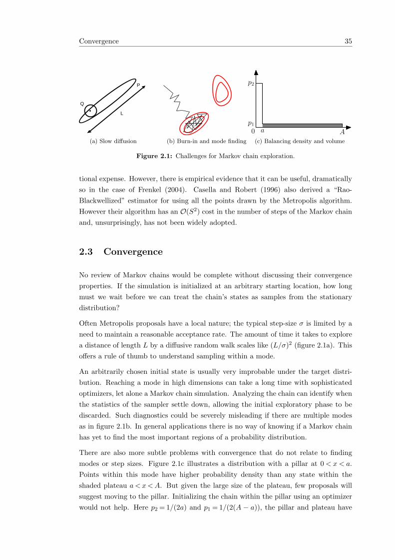
Figure 2.1: Challenges for Markov chain exploration.
tional expense. However, there is empirical evidence that it can be useful, dramaticallyso in the case of Frenkel (2004). Casella and Robert (1996) also derived a “Rao-Blackwellized” estimator for using all the points drawn by the Metropolis algorithm.However their algorithm has an O(S2) cost in the number of steps of the Markov chainand, unsurprisingly, has not been widely adopted.
2.3 Convergence
No review of Markov chains would be complete without discussing their convergenceproperties. If the simulation is initialized at an arbitrary starting location, how longmust we wait before we can treat the chain’s states as samples from the stationarydistribution?
Often Metropolis proposals have a local nature; the typical step-size σ is limited by aneed to maintain a reasonable acceptance rate. The amount of time it takes to explorea distance of length L by a diffusive random walk scales like (L/σ)2 (figure 2.1a). Thisoffers a rule of thumb to understand sampling within a mode.
An arbitrarily chosen initial state is usually very improbable under the target distri-bution. Reaching a mode in high dimensions can take a long time with sophisticatedoptimizers, let alone a Markov chain simulation. Analyzing the chain can identify whenthe statistics of the sampler settle down, allowing the initial exploratory phase to bediscarded. Such diagnostics could be severely misleading if there are multiple modesas in figure 2.1b. In general applications there is no way of knowing if a Markov chainhas yet to find the most important regions of a probability distribution.
There are also more subtle problems with convergence that do not relate to findingmodes or step sizes. Figure 2.1c illustrates a distribution with a pillar at 0 < x < a.Points within this mode have higher probability density than any state within theshaded plateau a < x < A. But given the large size of the plateau, few proposals willsuggest moving to the pillar. Initializing the chain within the pillar using an optimizerwould not help. Here p2 = 1/(2a) and p1 = 1/(2(A − a)), the pillar and plateau have
Auxiliary variable methods 36
equal probability mass, yet only a small fraction of proposals from the pillar to theplateau can be accepted — the acceptance rate is a/(A−a) for symmetric proposals.A proposal distribution that knew the probability masses involved (e.g. i.i.d. samplingq(x′ ← x) = p(x′)) would move rapidly between the modes; but this would involvealready having the knowledge that MCMC is being used to discover.
There is a theoretical literature on Markov chain convergence. But for general statisticalproblems it is difficult to prove much about the validity of any particular MCMC result.In later chapters we make occasional use of a standard diagnostic tool to compare theconvergence properties of chains. But in general we would also run the sampling code ona cut-down version of the problem where exact results are available or simple importancesampling will work. In inference problems it is a good idea to check that a sampleris consistent with ground truth when learning from synthetic data generated from theprior model. Geweke (2004)’s method for “getting it right” is a more advanced wayto check consistency between samplers for the prior and posterior. Such diagnosticsare also a guard against errors in the software implementation, a possibility consideredseriously even by experts (Kass et al., 1998).
2.4 Auxiliary variable methods
As emphasized in the introduction, Monte Carlo is usually best avoided when possible.In tractable problems computations based on analytical solutions will usually be farmore efficient. One would think this means we should analytically marginalize outvariables wherever possible.
Auxiliary variable methods turn this thinking on its head. Given a target distributionp(x), we introduce auxiliary variables z such that p(x) =
∫p(x, z) dz. We could just
sample from p(x), corresponding to analytically integrating out z from p(x, z). Instead,auxiliary variable methods instantiate the auxiliary variables in a Markov chain thatexplores the joint distribution. Surprisingly, this can result in a better Monte Carlomethod.
An alternative way of introducing extra variables is to make the target distribution aconditional of a joint distribution p(x) = p(x|β = 1). The whole p(x, β) distribution isexplored, but only samples where β=1 are retained. This seemingly wasteful procedurecan also yield better Monte Carlo estimates. An example is simulated tempering,discussed later in subsection 2.5.1.
2.4.1 Swendsen–Wang
The Swendsen–Wang algorithm (Swendsen and Wang, 1987) is a highly effective algo-rithm for sampling Potts models (subsection 1.1.3) with a small number of colors q. The
Auxiliary variable methods 37
algorithm is important in its own right (we use it in chapters 4 and 5) and as a signif-icant development in auxiliary variable methods. Edwards and Sokal (1988) provideda scheme for constructing similar auxiliary variable methods for a wider class of mod-els. They also identified the “Fortuin-Kasteleyn-Swendsen-Wang” (FKSW) auxiliaryvariable joint distribution that underlies the algorithm.
The FKSW joint distribution is over the original Potts color variables s= {si} on thenodes of a graph and binary bond variables d={dij ∈ {0, 1}} present on each edge:
p(s,d) =1
ZP(J, q)
∏(ij)∈E
[(1− pij)δdij ,0 + pijδdij ,1δsi,sj
], pij ≡ (1− e−Jij ). (2.15)
As long as all couplings Jij are positive the marginal distribution over s is the Pottsdistribution, equation (1.4). The marginal distribution over the bonds is the randomcluster model of Fortuin and Kasteleyn (1972):
p(d) =1
ZP(J, q)
∏(ij)∈E
pdij
ij (1− pij)1−dijqC(d), (2.16)
where C(d) is the number of connected components in a graph with edges whereverdij =1.
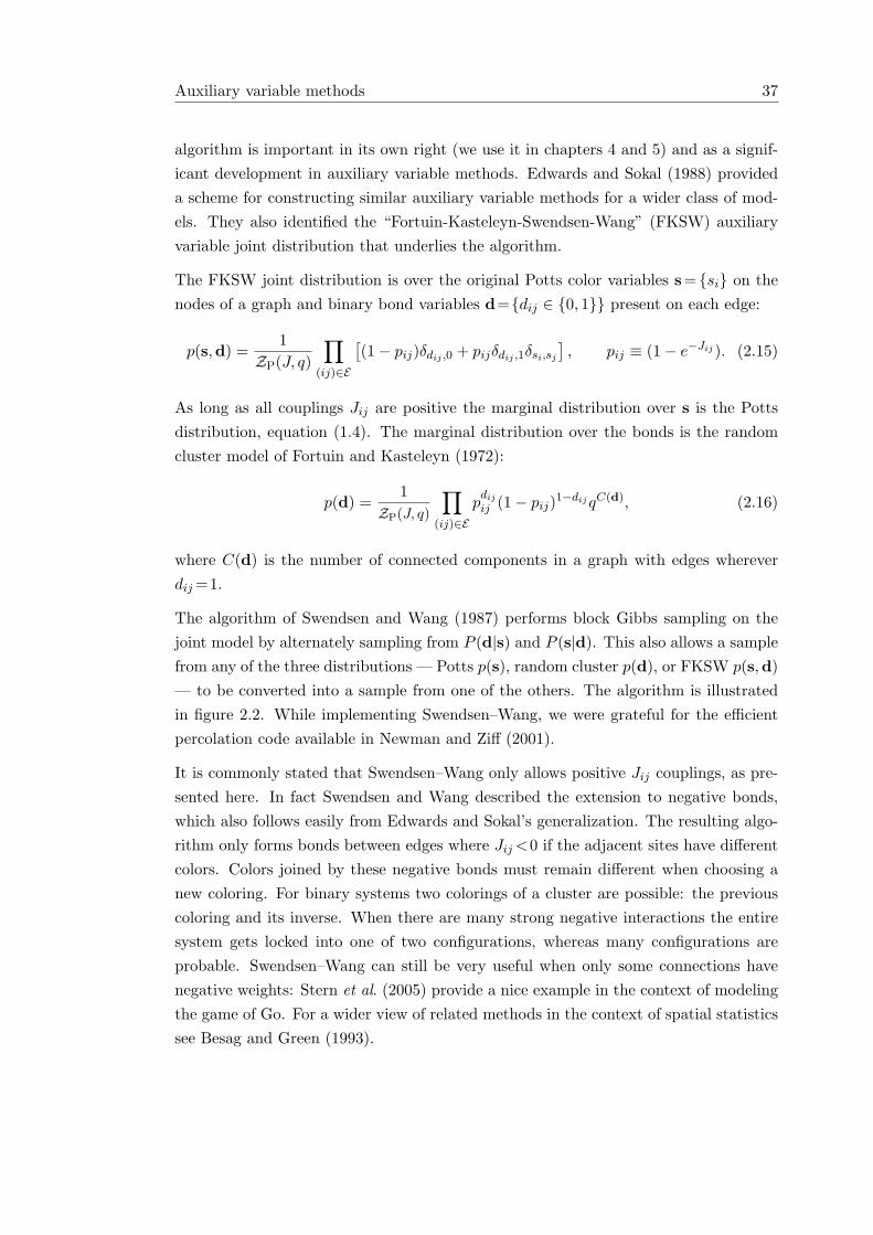
The algorithm of Swendsen and Wang (1987) performs block Gibbs sampling on thejoint model by alternately sampling from P (d|s) and P (s|d). This also allows a samplefrom any of the three distributions — Potts p(s), random cluster p(d), or FKSW p(s,d)— to be converted into a sample from one of the others. The algorithm is illustratedin figure 2.2. While implementing Swendsen–Wang, we were grateful for the efficientpercolation code available in Newman and Ziff (2001).
It is commonly stated that Swendsen–Wang only allows positive Jij couplings, as pre-sented here. In fact Swendsen and Wang described the extension to negative bonds,which also follows easily from Edwards and Sokal’s generalization. The resulting algo-rithm only forms bonds between edges where Jij <0 if the adjacent sites have differentcolors. Colors joined by these negative bonds must remain different when choosing anew coloring. For binary systems two colorings of a cluster are possible: the previouscoloring and its inverse. When there are many strong negative interactions the entiresystem gets locked into one of two configurations, whereas many configurations areprobable. Swendsen–Wang can still be very useful when only some connections havenegative weights: Stern et al. (2005) provide a nice example in the context of modelingthe game of Go. For a wider view of related methods in the context of spatial statisticssee Besag and Green (1993).
Auxiliary variable methods 38
(a) Potts state (b) FKSW state
(c) Random cluster state (d) New FKSW state
Figure 2.2: The Swendsen–Wang algorithm. (a) As an example we run thealgorithm on a binary Potts model on a square lattice. (b) Under the FKSWconditional p(d|s) bonds are placed down with probability pij =1 − e1−Jij wher-ever adjacent sites have the same color. (c) Discarding the colors gives a samplefrom the random cluster model. (d) Sampling from p(s|d) involves assigning eachconnected component or “cluster” a new color uniformly at random, giving a newFKSW state. Discarding the bonds gives a new setting of the Potts model. Thiscoloring is dramatically different from the previous one. In contrast a sweep ofsingle-site Gibbs sampling can only diffuse the boundaries of the red and blueregions by roughly the width of a single site.
Auxiliary variable methods 39
x
h
(x, h)
(a)
x
h
(x, h)
(b)
x
h
(x, h)
(c)
x
h
(x, h)
P∗(x)
(d)
x
h
(x, h)
P∗(x)
(e)
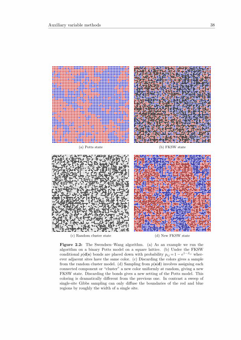
Figure 2.3: Slice sampling. (a)–(c) show a procedure for unimodal distributions:after sampling h from its conditional distribution an interval is found enclosing theregion where H(x)>h. Samples are drawn uniformly from this interval until oneunderneath the curve is found. Points outside the curve can be used to shrink theinterval, this is an adaptive rejection sampling method. (d) Sampling uniformlyfrom the slice is difficult for multi-modal distributions. (e) One valid procedureuses an initial bracket of width σ that encloses x but is centered uniformly atrandom. This bracket is extended in increments of σ until it sticks outside thecurve at both ends. This can cut off regions of the slice, but applying the previousadaptive rejection sampling procedure still leaves the uniform distribution on theslice invariant.
2.4.2 Slice Sampling
All Metropolis methods make use of a proposal distribution q(x′← x). In continuousspaces such distributions have step-size parameters that have to be set well. Almostall proposals are rejected if step-sizes are too large; overly small step-sizes lead to slowdiffusive exploration of the target distribution. In contrast, a self-tuning method, whichhas less-important or even no step-size parameters would be preferable.
Slice sampling (Neal, 1997, 2003) is a method with one auxiliary variable that fits intothe framework of Edwards and Sokal (1988). The auxiliary variable does not directlyhelp mixing but allows the use of relatively easy-to-implement algorithms that allowself-tuning while generating a valid Markov chain. Like Gibbs sampling a slice samplingchain has no rejections: it always moves when sampling a continuous distribution. Slicesampling works by stepping back to the view of figure 1.5a: sampling involves drawingpoints uniformly underneath a curve H(x) = p∗(x). Rather than drawing points i.i.d.as in rejection sampling, a Markov chain explores this uniform distribution over theoriginal variables x and a height variable 0<h<H(x).
Slice sampling algorithms alternate between updating h and one or more of the orig-inal variables. The height has a simple conditional distribution from which it can beresampled, h∼Uniform[0,H(x)]. Conditioned on h the stationary distribution over x
is uniform over the ‘slice’ that lies under the curve: H(x)≥h. When the distribution is
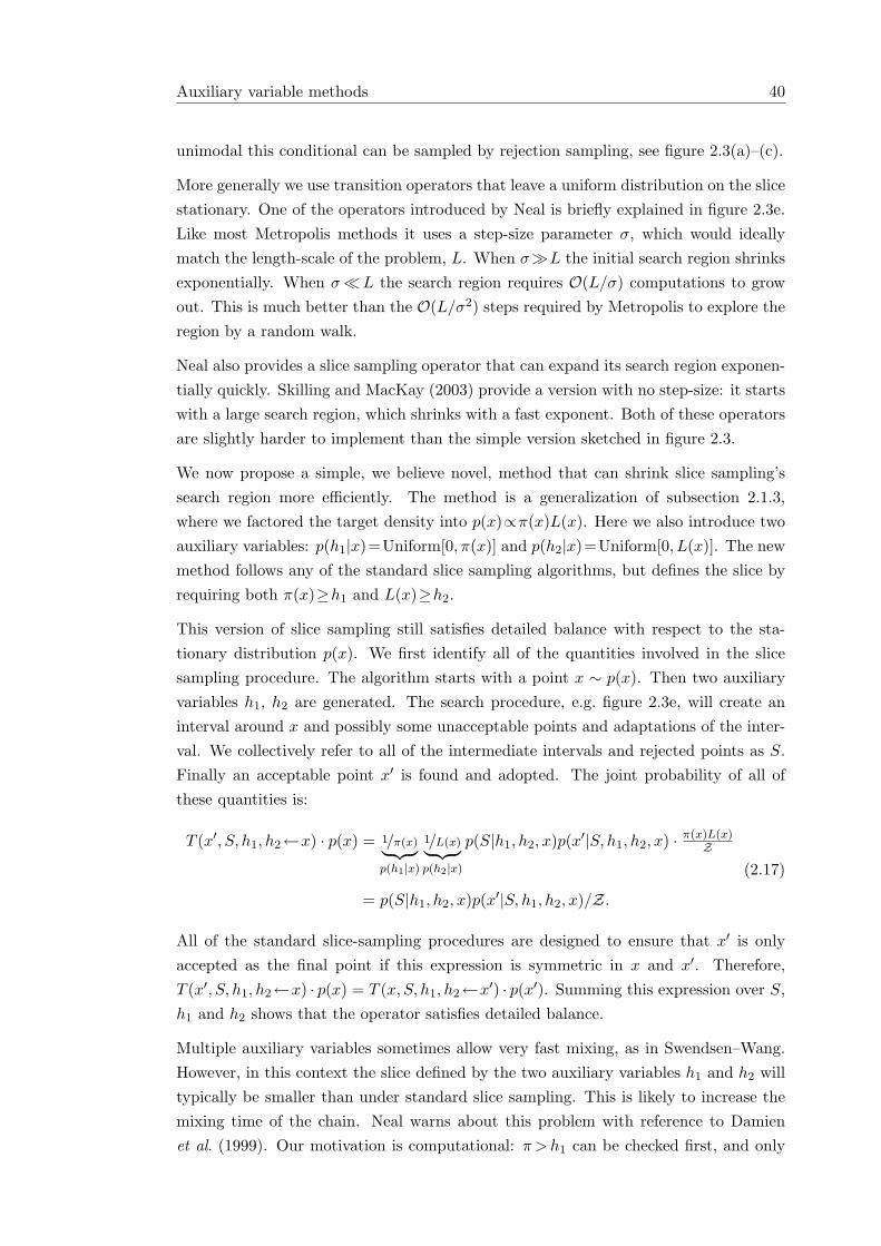
Auxiliary variable methods 40
unimodal this conditional can be sampled by rejection sampling, see figure 2.3(a)–(c).
More generally we use transition operators that leave a uniform distribution on the slicestationary. One of the operators introduced by Neal is briefly explained in figure 2.3e.Like most Metropolis methods it uses a step-size parameter σ, which would ideallymatch the length-scale of the problem, L. When σ�L the initial search region shrinksexponentially. When σ�L the search region requires O(L/σ) computations to growout. This is much better than the O(L/σ2) steps required by Metropolis to explore theregion by a random walk.
Neal also provides a slice sampling operator that can expand its search region exponen-tially quickly. Skilling and MacKay (2003) provide a version with no step-size: it startswith a large search region, which shrinks with a fast exponent. Both of these operatorsare slightly harder to implement than the simple version sketched in figure 2.3.
We now propose a simple, we believe novel, method that can shrink slice sampling’ssearch region more efficiently. The method is a generalization of subsection 2.1.3,where we factored the target density into p(x)∝π(x)L(x). Here we also introduce twoauxiliary variables: p(h1|x)=Uniform[0, π(x)] and p(h2|x)=Uniform[0, L(x)]. The newmethod follows any of the standard slice sampling algorithms, but defines the slice byrequiring both π(x)≥h1 and L(x)≥h2.
This version of slice sampling still satisfies detailed balance with respect to the sta-tionary distribution p(x). We first identify all of the quantities involved in the slicesampling procedure. The algorithm starts with a point x ∼ p(x). Then two auxiliaryvariables h1, h2 are generated. The search procedure, e.g. figure 2.3e, will create aninterval around x and possibly some unacceptable points and adaptations of the inter-val. We collectively refer to all of the intermediate intervals and rejected points as S.Finally an acceptable point x′ is found and adopted. The joint probability of all ofthese quantities is:
T (x′, S, h1, h2←x) · p(x) = 1/π(x)︸ ︷︷ ︸p(h1|x)
1/L(x)︸ ︷︷ ︸p(h2|x)
p(S|h1, h2, x)p(x′|S, h1, h2, x) · π(x)L(x)Z
= p(S|h1, h2, x)p(x′|S, h1, h2, x)/Z.
(2.17)
All of the standard slice-sampling procedures are designed to ensure that x′ is onlyaccepted as the final point if this expression is symmetric in x and x′. Therefore,T (x′, S, h1, h2←x) · p(x) = T (x, S, h1, h2←x′) · p(x′). Summing this expression over S,h1 and h2 shows that the operator satisfies detailed balance.
Multiple auxiliary variables sometimes allow very fast mixing, as in Swendsen–Wang.However, in this context the slice defined by the two auxiliary variables h1 and h2 willtypically be smaller than under standard slice sampling. This is likely to increase themixing time of the chain. Neal warns about this problem with reference to Damienet al. (1999). Our motivation is computational: π >h1 can be checked first, and only
Auxiliary variable methods 41
if it satisfies the slice constraint need L > h2 be checked. Thus schemes that startwith a large range and rapidly shrink a bracket around the slice can do so with lesscomputation if π(x) can reject some unreasonable points while being cheap to compute.
2.4.3 Hamiltonian Monte Carlo
Physical simulations often work by discretizing time and approximately computing theresult of following the Hamiltonian dynamics of the system being modeled. Thesedynamics exploit gradients of a target stationary probability density, not just point-wise evaluations as in the Metropolis algorithm. Theoretically, gradients only evercost a constant multiple of the computer time needed to evaluate a function (Bischofand Bucker, 2000), and are a much richer source of information. The difficulty withsimulation work is that inaccuracies accumulate rapidly unless time is discretized veryfinely, which has a large computational cost.
The Metropolis algorithm targets only an equilibrium distribution over states. Themethod doesn’t need this distribution to be the result of an underlying dynamical sys-tem. Instead the algorithm evolves according to a proposal distribution. The progressof the Metropolis algorithm often resembles a diffusive random walk. In contrast a par-ticle evolving under Hamiltonian dynamics will naturally move in persistent trajectoriesacross its state-space.
These two areas of physical simulation research were combined in Hybrid Monte Carlo(Duane et al., 1987). Hamiltonian dynamics are simulated approximately as a Metropo-lis proposal, which is accepted or rejected. This allows persistent, rapid motion acrossa state space without damaging the equilibrium distribution of the chain through dis-cretization errors. If the target probability distribution does not correspond to a Hamil-tonian system then auxiliary variables are introduced to create a fictitious system thatcan be simulated.
While Hamiltonian dynamics is time reversible, some care is required to ensure thediscretized version is also reversible. Neal (1993) reviews a variety of Hamiltonian basedMonte Carlo methods. See MacKay (2003) for another review with simple examplecode.
Hybrid Monte Carlo crossed into a statistical setting through work on Bayesian neuralnetworks (Neal, 1992, 1996b), where it is extremely successful. Hamiltonian MonteCarlo methods continue to appear in recent work, especially in Gaussian process mod-eling, although they could be adopted more widely.
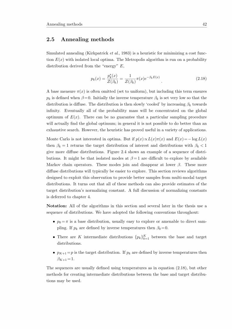
Annealing methods 42
2.5 Annealing methods
Simulated annealing (Kirkpatrick et al., 1983) is a heuristic for minimizing a cost func-tion E(x) with isolated local optima. The Metropolis algorithm is run on a probabilitydistribution derived from the “energy” E,
pk(x) =p∗k(x)Z(βk)
=1
Z(βk)π(x)e−βkE(x)
.(2.18)
A base measure π(x) is often omitted (set to uniform), but including this term ensurespk is defined when β=0. Initially the inverse temperature βk is set very low so that thedistribution is diffuse. The distribution is then slowly ‘cooled’ by increasing βk towardsinfinity. Eventually all of the probability mass will be concentrated on the globaloptimum of E(x). There can be no guarantee that a particular sampling procedurewill actually find the global optimum; in general it is not possible to do better than anexhaustive search. However, the heuristic has proved useful in a variety of applications.
Monte Carlo is not interested in optima. But if p(x)∝L(x)π(x) and E(x)=− log L(x)then βk = 1 returns the target distribution of interest and distributions with βk < 1give more diffuse distributions. Figure 2.4 shows an example of a sequence of distri-butions. It might be that isolated modes at β =1 are difficult to explore by availableMarkov chain operators. These modes join and disappear at lower β. These morediffuse distributions will typically be easier to explore. This section reviews algorithmsdesigned to exploit this observation to provide better samples from multi-modal targetdistributions. It turns out that all of these methods can also provide estimates of thetarget distribution’s normalizing constant. A full discussion of normalizing constantsis deferred to chapter 4.
Notation: All of the algorithms in this section and several later in the thesis use asequence of distributions. We have adopted the following conventions throughout:
• p0 =π is a base distribution, usually easy to explore or amenable to direct sam-pling. If pk are defined by inverse temperatures then β0 =0.
• There are K intermediate distributions {pk}Kk=1 between the base and targetdistributions.
• pK+1 =p is the target distribution. If pk are defined by inverse temperatures thenβK+1 =1.
The sequences are usually defined using temperatures as in equation (2.18), but othermethods for creating intermediate distributions between the base and target distribu-tions may be used.
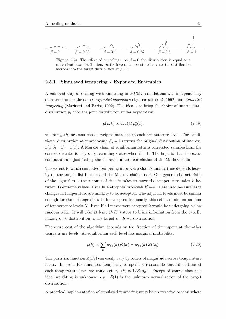
Annealing methods 43
β = 0 β = 0.03 β = 0.1 β = 0.25 β = 0.5 β = 1
Figure 2.4: The effect of annealing. At β = 0 the distribution is equal to aconvenient base distribution. As the inverse temperature increases the distributionmorphs into the target distribution at β=1.
2.5.1 Simulated tempering / Expanded Ensembles
A coherent way of dealing with annealing in MCMC simulations was independentlydiscovered under the names expanded ensembles (Lyubartsev et al., 1992) and simulatedtempering (Marinari and Parisi, 1992). The idea is to bring the choice of intermediatedistribution pk into the joint distribution under exploration:
p(x, k) ∝ wST(k) p∗k(x), (2.19)
where wST(k) are user-chosen weights attached to each temperature level. The condi-tional distribution at temperature βk = 1 returns the original distribution of interest:p(x|βk =1) = p(x). A Markov chain at equilibrium returns correlated samples from thecorrect distribution by only recording states when β = 1. The hope is that the extracomputation is justified by the decrease in auto-correlation of the Markov chain.
The extent to which simulated tempering improves a chain’s mixing time depends heav-ily on the target distribution and the Markov chains used. One general characteristicof the algorithm is the amount of time it takes to move the temperature index k be-tween its extreme values. Usually Metropolis proposals k′←k±1 are used because largechanges in temperature are unlikely to be accepted. The adjacent levels must be similarenough for these changes in k to be accepted frequently, this sets a minimum numberof temperature levels K. Even if all moves were accepted k would be undergoing a slowrandom walk. It will take at least O(K2) steps to bring information from the rapidlymixing k=0 distribution to the target k=K+1 distribution.
The extra cost of the algorithm depends on the fraction of time spent at the othertemperature levels. At equilibrium each level has marginal probability:
p(k) ∝∑
x
wST(k) p∗k(x) = wST(k)Z(βk). (2.20)
The partition function Z(βk) can easily vary by orders of magnitude across temperaturelevels. In order for simulated tempering to spend a reasonable amount of time ateach temperature level we could set wST(k) ≈ 1/Z(βk). Except of course that thisideal weighting is unknown: e.g., Z(1) is the unknown normalization of the targetdistribution.
A practical implementation of simulated tempering must be an iterative process where
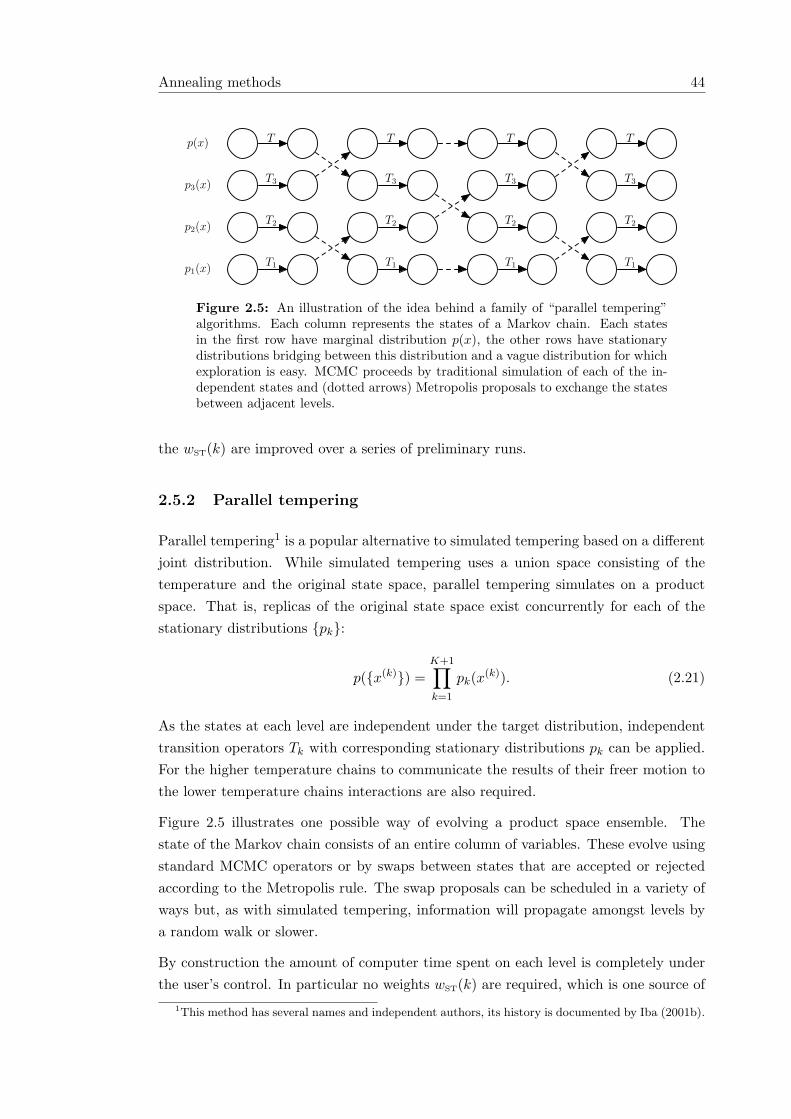
Annealing methods 44
p(x)
p3(x)
p2(x)
p1(x)
T
T3
T2
T1
T
T3
T2
T1
T
T3
T2
T1
T
T3
T2
T1
Figure 2.5: An illustration of the idea behind a family of “parallel tempering”algorithms. Each column represents the states of a Markov chain. Each statesin the first row have marginal distribution p(x), the other rows have stationarydistributions bridging between this distribution and a vague distribution for whichexploration is easy. MCMC proceeds by traditional simulation of each of the in-dependent states and (dotted arrows) Metropolis proposals to exchange the statesbetween adjacent levels.
the wST(k) are improved over a series of preliminary runs.
2.5.2 Parallel tempering
Parallel tempering1 is a popular alternative to simulated tempering based on a differentjoint distribution. While simulated tempering uses a union space consisting of thetemperature and the original state space, parallel tempering simulates on a productspace. That is, replicas of the original state space exist concurrently for each of thestationary distributions {pk}:
p({x(k)}) =K+1∏k=1
pk(x(k)). (2.21)
As the states at each level are independent under the target distribution, independenttransition operators Tk with corresponding stationary distributions pk can be applied.For the higher temperature chains to communicate the results of their freer motion tothe lower temperature chains interactions are also required.
Figure 2.5 illustrates one possible way of evolving a product space ensemble. Thestate of the Markov chain consists of an entire column of variables. These evolve usingstandard MCMC operators or by swaps between states that are accepted or rejectedaccording to the Metropolis rule. The swap proposals can be scheduled in a variety ofways but, as with simulated tempering, information will propagate amongst levels bya random walk or slower.
By construction the amount of computer time spent on each level is completely underthe user’s control. In particular no weights wST(k) are required, which is one source of
1This method has several names and independent authors, its history is documented by Iba (2001b).
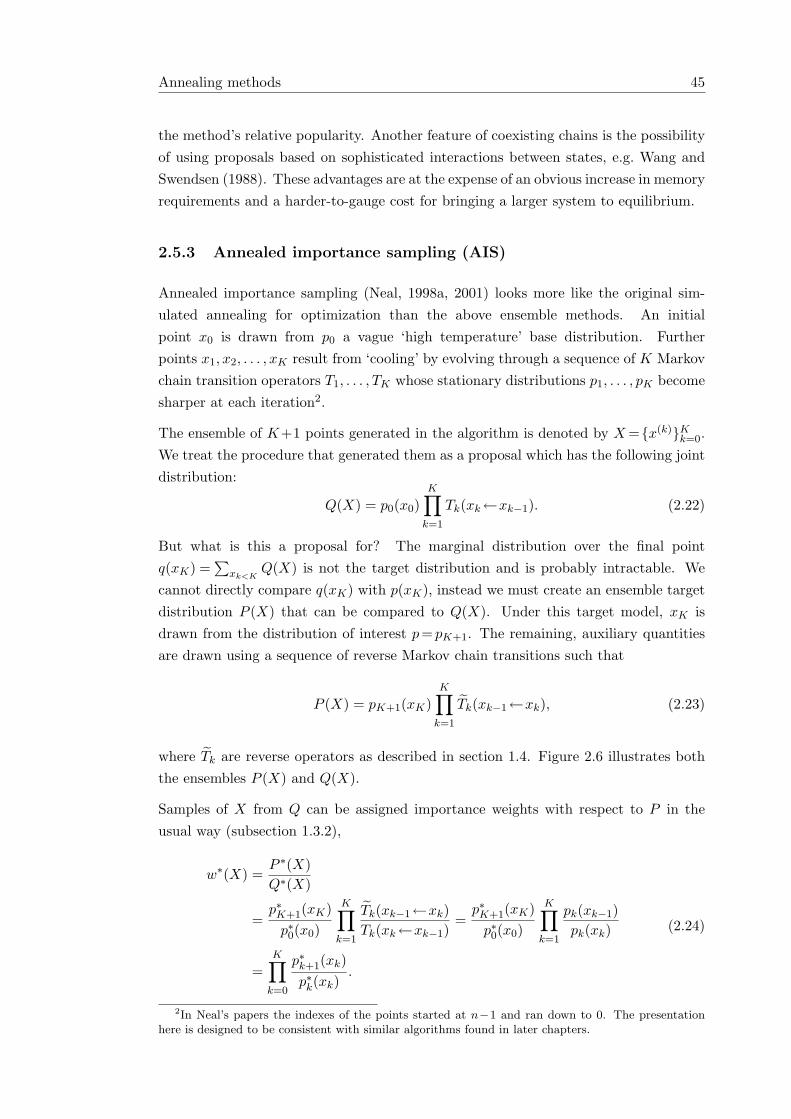
Annealing methods 45
the method’s relative popularity. Another feature of coexisting chains is the possibilityof using proposals based on sophisticated interactions between states, e.g. Wang andSwendsen (1988). These advantages are at the expense of an obvious increase in memoryrequirements and a harder-to-gauge cost for bringing a larger system to equilibrium.
2.5.3 Annealed importance sampling (AIS)
Annealed importance sampling (Neal, 1998a, 2001) looks more like the original sim-ulated annealing for optimization than the above ensemble methods. An initialpoint x0 is drawn from p0 a vague ‘high temperature’ base distribution. Furtherpoints x1, x2, . . . , xK result from ‘cooling’ by evolving through a sequence of K Markovchain transition operators T1, . . . , TK whose stationary distributions p1, . . . , pK becomesharper at each iteration2.
The ensemble of K+1 points generated in the algorithm is denoted by X ={x(k)}Kk=0.We treat the procedure that generated them as a proposal which has the following jointdistribution:
Q(X) = p0(x0)K∏
k=1
Tk(xk←xk−1). (2.22)
But what is this a proposal for? The marginal distribution over the final pointq(xK) =
∑xk<K
Q(X) is not the target distribution and is probably intractable. Wecannot directly compare q(xK) with p(xK), instead we must create an ensemble targetdistribution P (X) that can be compared to Q(X). Under this target model, xK isdrawn from the distribution of interest p= pK+1. The remaining, auxiliary quantitiesare drawn using a sequence of reverse Markov chain transitions such that
P (X) = pK+1(xK)K∏
k=1
Tk(xk−1←xk), (2.23)
where Tk are reverse operators as described in section 1.4. Figure 2.6 illustrates boththe ensembles P (X) and Q(X).
Samples of X from Q can be assigned importance weights with respect to P in theusual way (subsection 1.3.2),
w∗(X) =P ∗(X)Q∗(X)
=p∗K+1(xK)
p∗0(x0)
K∏k=1
Tk(xk−1←xk)Tk(xk←xk−1)
=p∗K+1(xK)
p∗0(x0)
K∏k=1
pk(xk−1)pk(xk)
=K∏
k=0
p∗k+1(xk)p∗k(xk)
.
(2.24)
2In Neal’s papers the indexes of the points started at n−1 and ran down to 0. The presentationhere is designed to be consistent with similar algorithms found in later chapters.
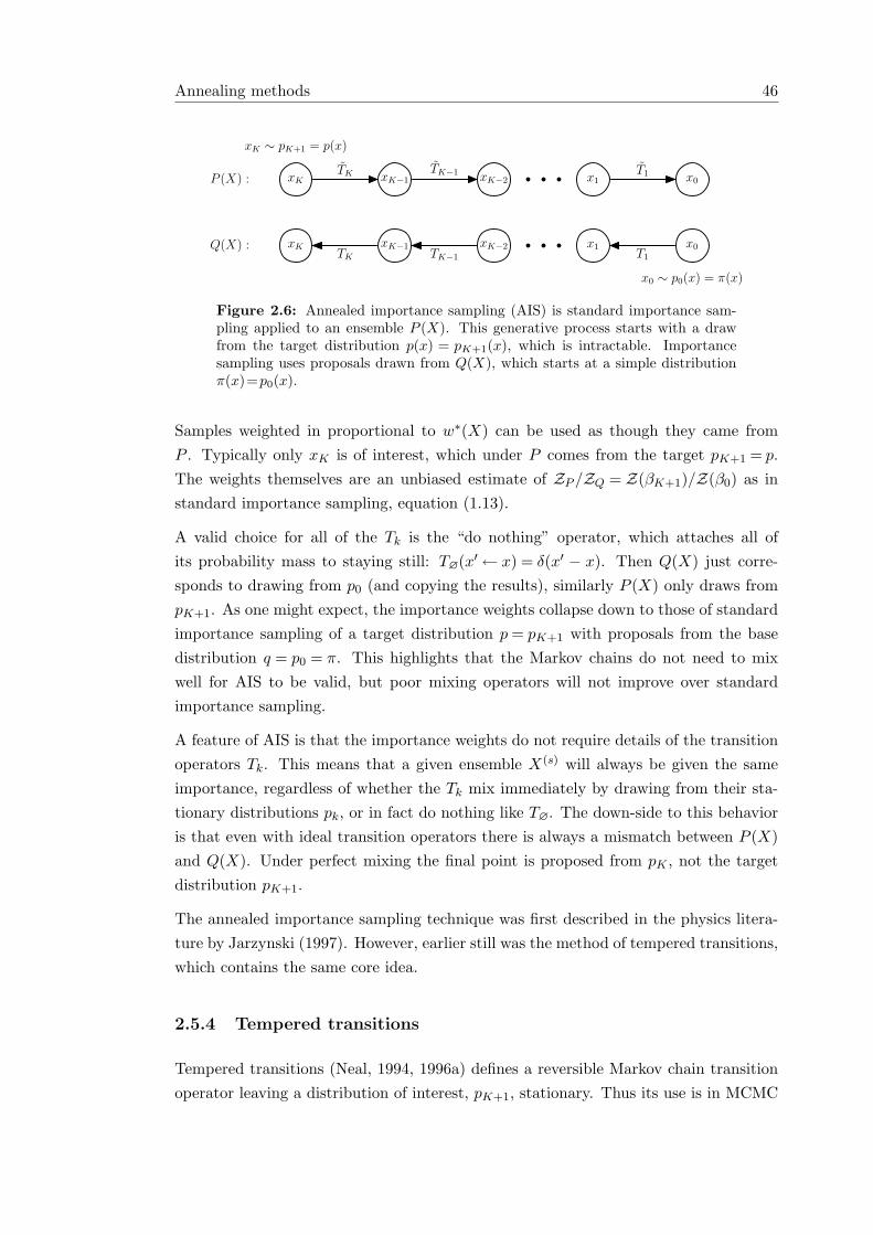
Annealing methods 46
xK ∼ pK+1 = p(x)
P (X) : xK xK−1 xK−2 x1 x0
TKTK−1 T1
x0 ∼ p0(x) = π(x)
Q(X) : xK xK−1 xK−2 x1 x0TK TK−1 T1
Figure 2.6: Annealed importance sampling (AIS) is standard importance sam-pling applied to an ensemble P (X). This generative process starts with a drawfrom the target distribution p(x) = pK+1(x), which is intractable. Importancesampling uses proposals drawn from Q(X), which starts at a simple distributionπ(x)=p0(x).
Samples weighted in proportional to w∗(X) can be used as though they came fromP . Typically only xK is of interest, which under P comes from the target pK+1 = p.The weights themselves are an unbiased estimate of ZP /ZQ = Z(βK+1)/Z(β0) as instandard importance sampling, equation (1.13).
A valid choice for all of the Tk is the “do nothing” operator, which attaches all ofits probability mass to staying still: T∅(x′← x) = δ(x′ − x). Then Q(X) just corre-sponds to drawing from p0 (and copying the results), similarly P (X) only draws frompK+1. As one might expect, the importance weights collapse down to those of standardimportance sampling of a target distribution p = pK+1 with proposals from the basedistribution q = p0 = π. This highlights that the Markov chains do not need to mixwell for AIS to be valid, but poor mixing operators will not improve over standardimportance sampling.
A feature of AIS is that the importance weights do not require details of the transitionoperators Tk. This means that a given ensemble X(s) will always be given the sameimportance, regardless of whether the Tk mix immediately by drawing from their sta-tionary distributions pk, or in fact do nothing like T∅. The down-side to this behavioris that even with ideal transition operators there is always a mismatch between P (X)and Q(X). Under perfect mixing the final point is proposed from pK , not the targetdistribution pK+1.
The annealed importance sampling technique was first described in the physics litera-ture by Jarzynski (1997). However, earlier still was the method of tempered transitions,which contains the same core idea.
2.5.4 Tempered transitions
Tempered transitions (Neal, 1994, 1996a) defines a reversible Markov chain transitionoperator leaving a distribution of interest, pK+1, stationary. Thus its use is in MCMC
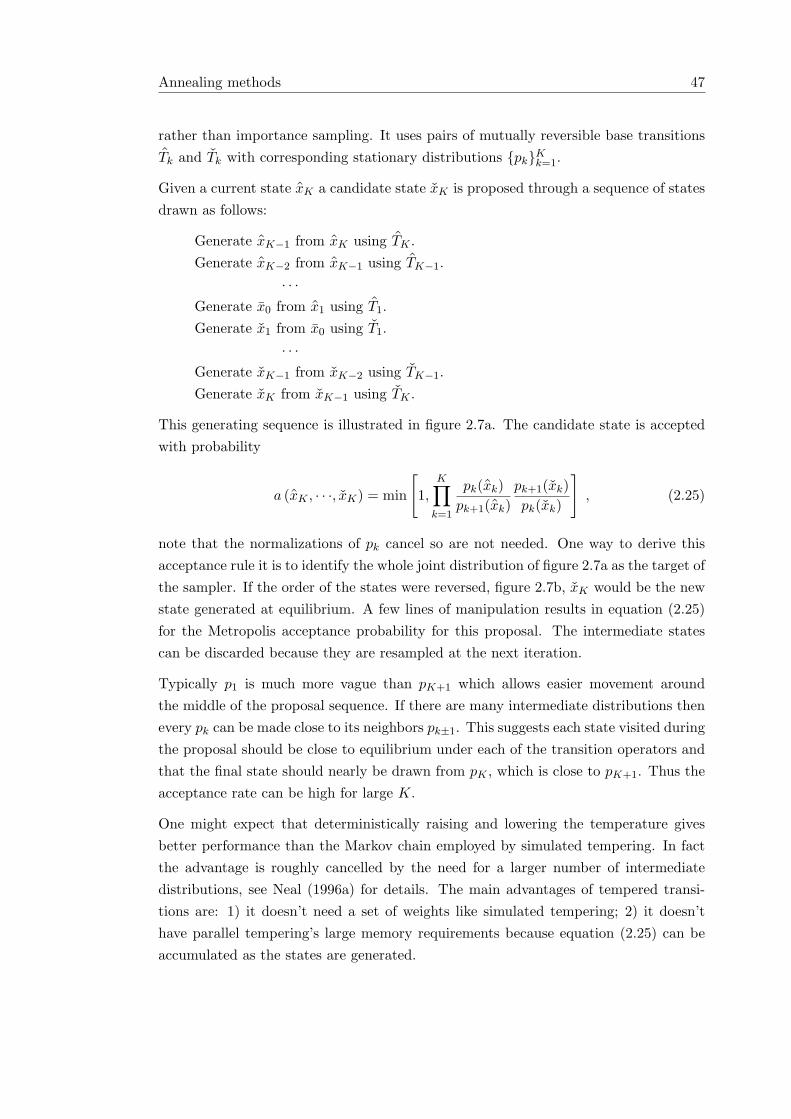
Annealing methods 47
rather than importance sampling. It uses pairs of mutually reversible base transitionsTk and Tk with corresponding stationary distributions {pk}Kk=1.
Given a current state xK a candidate state xK is proposed through a sequence of statesdrawn as follows:
Generate xK−1 from xK using TK .Generate xK−2 from xK−1 using TK−1.
· · ·Generate x0 from x1 using T1.Generate x1 from x0 using T1.
· · ·Generate xK−1 from xK−2 using TK−1.Generate xK from xK−1 using TK .
This generating sequence is illustrated in figure 2.7a. The candidate state is acceptedwith probability
a (xK , · · ·, xK) = min
[1,
K∏k=1
pk(xk)pk+1(xk)
pk+1(xk)pk(xk)
], (2.25)
note that the normalizations of pk cancel so are not needed. One way to derive thisacceptance rule it is to identify the whole joint distribution of figure 2.7a as the target ofthe sampler. If the order of the states were reversed, figure 2.7b, xK would be the newstate generated at equilibrium. A few lines of manipulation results in equation (2.25)for the Metropolis acceptance probability for this proposal. The intermediate statescan be discarded because they are resampled at the next iteration.
Typically p1 is much more vague than pK+1 which allows easier movement aroundthe middle of the proposal sequence. If there are many intermediate distributions thenevery pk can be made close to its neighbors pk±1. This suggests each state visited duringthe proposal should be close to equilibrium under each of the transition operators andthat the final state should nearly be drawn from pK , which is close to pK+1. Thus theacceptance rate can be high for large K.
One might expect that deterministically raising and lowering the temperature givesbetter performance than the Markov chain employed by simulated tempering. In factthe advantage is roughly cancelled by the need for a larger number of intermediatedistributions, see Neal (1996a) for details. The main advantages of tempered transi-tions are: 1) it doesn’t need a set of weights like simulated tempering; 2) it doesn’thave parallel tempering’s large memory requirements because equation (2.25) can beaccumulated as the states are generated.
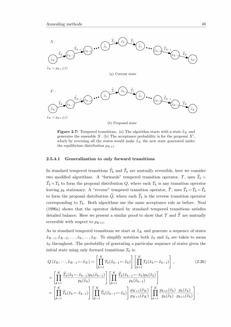
Annealing methods 48
xK ∼ pK+1(x)
X :
xK
xK−1
xK−2
x1
x0
x1
xK−2
xK−1
xK
TK
TK−1
T1 T1
TK−1
TK
(a) Current state
xK ∼ pK+1(x)
X ′ :
xK
xK−1
xK−2
x1
x0
x1
xK−2
xK−1
xK
TK
TK−1
T1 T1
TK−1
TK
(b) Proposed state
Figure 2.7: Tempered transitions. (a) The algorithm starts with a state xK andgenerates the ensemble X. (b) The acceptance probability is for the proposal X ′,which by reversing all the states would make xK the new state generated underthe equilibrium distribution pK+1.
2.5.4.1 Generalization to only forward transitions
In standard tempered transitions Tk and Tk are mutually reversible, here we considertwo modified algorithms. A “forwards” tempered transition operator, T , uses Tk =Tk =Tk to form the proposal distribution Q, where each Tk is any transition operatorleaving pk stationary. A “reverse” tempered transition operator, T , uses Tk = Tk = Tk
to form the proposal distribution Q, where each Tk is the reverse transition operatorcorresponding to Tk. Both algorithms use the same acceptance rule as before. Neal(1996a) shows that the operator defined by standard tempered transitions satisfiesdetailed balance. Here we present a similar proof to show that T and T are mutuallyreversible with respect to pK+1.
As in standard tempered transitions we start at xK and generate a sequence of statesxK−1, xK−2, . . . , x0, . . . , xK . To simplify notation both x0 and x0 are taken to meanx0 throughout. The probability of generating a particular sequence of states given theinitial state using only forward transitions Tk is:
Q (xK , · · ·, xK−1← xK) =
[K∏
k=1
Tk(xk−1← xk)
][K∏
k=1
Tk(xk← xk−1)
], (2.26)
=
[K∏
k=1
Tk(xk← xk−1)pk(xk−1)pk(xk)
][K∏
k=1
Tk(xk−1← xk)pk(xk)pk(xk−1)
]
=
[K∏
k=1
Tk(xk← xk−1)
][K∏
k=1
Tk(xk−1← xk)
]pK+1(xK)pK+1(xK)
[K∏
k=1
pk+1(xk)pk(xk)
pk(xk)pk+1(xk)
].
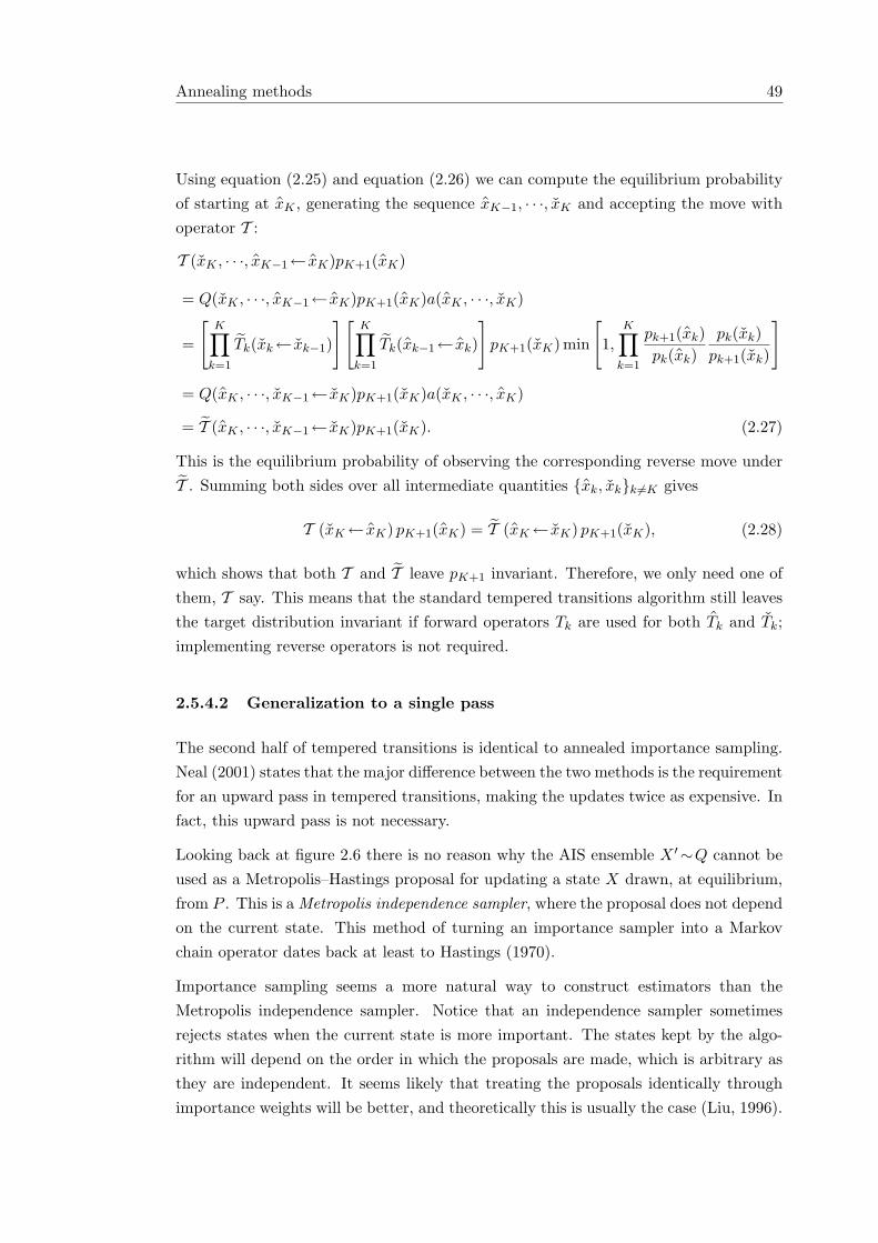
Annealing methods 49
Using equation (2.25) and equation (2.26) we can compute the equilibrium probabilityof starting at xK , generating the sequence xK−1, · · ·, xK and accepting the move withoperator T :
T (xK , · · ·, xK−1← xK)pK+1(xK)
= Q(xK , · · ·, xK−1← xK)pK+1(xK)a(xK , · · ·, xK)
=
[K∏
k=1
Tk(xk← xk−1)
][K∏
k=1
Tk(xk−1← xk)
]pK+1(xK) min
[1,
K∏k=1
pk+1(xk)pk(xk)
pk(xk)pk+1(xk)
]
= Q(xK , · · ·, xK−1← xK)pK+1(xK)a(xK , · · ·, xK)
= T (xK , · · ·, xK−1← xK)pK+1(xK). (2.27)
This is the equilibrium probability of observing the corresponding reverse move underT . Summing both sides over all intermediate quantities {xk, xk}k 6=K gives
T (xK← xK) pK+1(xK) = T (xK← xK) pK+1(xK), (2.28)
which shows that both T and T leave pK+1 invariant. Therefore, we only need one ofthem, T say. This means that the standard tempered transitions algorithm still leavesthe target distribution invariant if forward operators Tk are used for both Tk and Tk;implementing reverse operators is not required.
2.5.4.2 Generalization to a single pass
The second half of tempered transitions is identical to annealed importance sampling.Neal (2001) states that the major difference between the two methods is the requirementfor an upward pass in tempered transitions, making the updates twice as expensive. Infact, this upward pass is not necessary.
Looking back at figure 2.6 there is no reason why the AIS ensemble X ′∼Q cannot beused as a Metropolis–Hastings proposal for updating a state X drawn, at equilibrium,from P . This is a Metropolis independence sampler, where the proposal does not dependon the current state. This method of turning an importance sampler into a Markovchain operator dates back at least to Hastings (1970).
Importance sampling seems a more natural way to construct estimators than theMetropolis independence sampler. Notice that an independence sampler sometimesrejects states when the current state is more important. The states kept by the algo-rithm will depend on the order in which the proposals are made, which is arbitrary asthey are independent. It seems likely that treating the proposals identically throughimportance weights will be better, and theoretically this is usually the case (Liu, 1996).
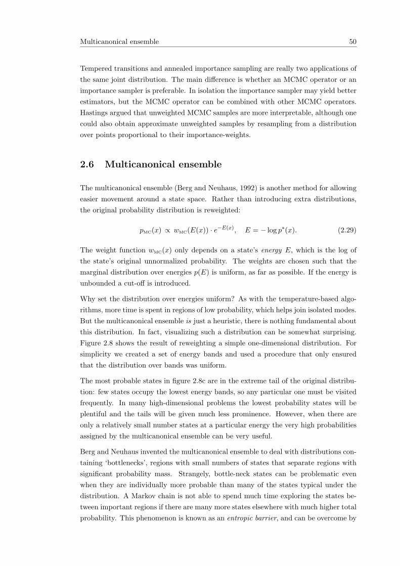
Multicanonical ensemble 50
Tempered transitions and annealed importance sampling are really two applications ofthe same joint distribution. The main difference is whether an MCMC operator or animportance sampler is preferable. In isolation the importance sampler may yield betterestimators, but the MCMC operator can be combined with other MCMC operators.Hastings argued that unweighted MCMC samples are more interpretable, although onecould also obtain approximate unweighted samples by resampling from a distributionover points proportional to their importance-weights.
2.6 Multicanonical ensemble
The multicanonical ensemble (Berg and Neuhaus, 1992) is another method for allowingeasier movement around a state space. Rather than introducing extra distributions,the original probability distribution is reweighted:
pMC(x) ∝ wMC(E(x)) · e−E(x), E = − log p∗(x). (2.29)
The weight function wMC(x) only depends on a state’s energy E, which is the log ofthe state’s original unnormalized probability. The weights are chosen such that themarginal distribution over energies p(E) is uniform, as far as possible. If the energy isunbounded a cut-off is introduced.
Why set the distribution over energies uniform? As with the temperature-based algo-rithms, more time is spent in regions of low probability, which helps join isolated modes.But the multicanonical ensemble is just a heuristic, there is nothing fundamental aboutthis distribution. In fact, visualizing such a distribution can be somewhat surprising.Figure 2.8 shows the result of reweighting a simple one-dimensional distribution. Forsimplicity we created a set of energy bands and used a procedure that only ensuredthat the distribution over bands was uniform.
The most probable states in figure 2.8c are in the extreme tail of the original distribu-tion: few states occupy the lowest energy bands, so any particular one must be visitedfrequently. In many high-dimensional problems the lowest probability states will beplentiful and the tails will be given much less prominence. However, when there areonly a relatively small number states at a particular energy the very high probabilitiesassigned by the multicanonical ensemble can be very useful.
Berg and Neuhaus invented the multicanonical ensemble to deal with distributions con-taining ‘bottlenecks’, regions with small numbers of states that separate regions withsignificant probability mass. Strangely, bottle-neck states can be problematic evenwhen they are individually more probable than many of the states typical under thedistribution. A Markov chain is not able to spend much time exploring the states be-tween important regions if there are many more states elsewhere with much higher totalprobability. This phenomenon is known as an entropic barrier, and can be overcome by
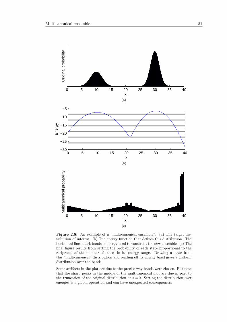
Multicanonical ensemble 51
0 5 10 15 20 25 30 35 40x
Orig
inal
pro
babi
lity
(a)
0 5 10 15 20 25 30 35 40−30
−25
−20
−15
−10
−5
x
Ene
rgy
(b)
0 5 10 15 20 25 30 35 40x
Mul
tican
onic
al p
roba
bilit
y
(c)
Figure 2.8: An example of a “multicanonical ensemble”. (a) The target dis-tribution of interest. (b) The energy function that defines this distribution. Thehorizontal lines mark bands of energy used to construct the new ensemble. (c) Thefinal figure results from setting the probability of each state proportional to thereciprocal of the number of states in its energy range. Drawing a state fromthis “multicanonical” distribution and reading off its energy band gives a uniformdistribution over the bands.
Some artifacts in the plot are due to the precise way bands were chosen. But notethat the sharp peaks in the middle of the multicanonical plot are due in part tothe truncation of the original distribution at x = 0. Setting the distribution overenergies is a global operation and can have unexpected consequences.
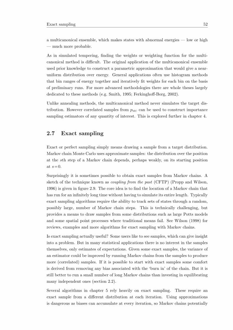
Exact sampling 52
a multicanonical ensemble, which makes states with abnormal energies — low or high— much more probable.
As in simulated tempering, finding the weights or weighting function for the multi-canonical method is difficult. The original application of the multicanonical ensembleused prior knowledge to construct a parametric approximation that would give a near-uniform distribution over energy. General applications often use histogram methodsthat bin ranges of energy together and iteratively fit weights for each bin on the basisof preliminary runs. For more advanced methodologies there are whole theses largelydedicated to these methods (e.g. Smith, 1995; Ferkinghoff-Borg, 2002).
Unlike annealing methods, the multicanonical method never simulates the target dis-tribution. However correlated samples from pMC can be used to construct importancesampling estimators of any quantity of interest. This is explored further in chapter 4.
2.7 Exact sampling
Exact or perfect sampling simply means drawing a sample from a target distribution.Markov chain Monte Carlo uses approximate samples: the distribution over the positionat the sth step of a Markov chain depends, perhaps weakly, on its starting positionat s=0.
Surprisingly it is sometimes possible to obtain exact samples from Markov chains. Asketch of the technique known as coupling from the past (CFTP) (Propp and Wilson,1996) is given in figure 2.9. The core idea is to find the location of a Markov chain thathas run for an infinitely long time without having to simulate its entire length. Typicallyexact sampling algorithms require the ability to track sets of states through a random,possibly large, number of Markov chain steps. This is technically challenging, butprovides a means to draw samples from some distributions such as large Potts modelsand some spatial point processes where traditional means fail. See Wilson (1998) forreviews, examples and more algorithms for exact sampling with Markov chains.
Is exact sampling actually useful? Some users like to see samples, which can give insightinto a problem. But in many statistical applications there is no interest in the samplesthemselves, only estimates of expectations. Given some exact samples, the variance ofan estimator could be improved by running Markov chains from the samples to producemore (correlated) samples. If it is possible to start with exact samples some comfortis derived from removing any bias associated with the ‘burn in’ of the chain. But it isstill better to run a small number of long Markov chains than investing in equilibratingmany independent ones (section 2.2).
Several algorithms in chapter 5 rely heavily on exact sampling. These require anexact sample from a different distribution at each iteration. Using approximationsis dangerous as biases can accumulate at every iteration, so Markov chains potentially
Exact sampling 53
x
time
−∞ 0
(a) A sample is at the end of an infinite chain.
x
time
−∞ 0−t1
?
(b) We try to find the end with a finite number of random numbers.
x
time
−∞ 0−t1−t1−t2
(c) Eventually, after a random amount of time, we find the sample
Figure 2.9: Coupling from the past (CFTP) overview. Each dash on the time axisrepresents a random number used by the chain. Everything must be consistentwith the infinite chain in (a). We try to locate the final state by looking at(drawing) just some of the random numbers. (b) Before time −t1 we know nothing,so the chain could be anywhere, we evolve a bound on the state space forward totime zero. At first this might only localize the sample. (c) We look at morerandom numbers further into the past until a bound collapses to a single state,we then follow it to the exact sample at time zero. It takes a random amount ofcomputation before the bound can be made tight.
Exact sampling 54
have to be run for a very long time. Exact sampling gives a stopping rule, and one thatguarantees zero bias.
2.7.1 Exact sampling example: the Ising model
Coupling from the past relies on being able to prove where the final state of a Markovchain lies without knowing the starting location. To demonstrate that this is sometimespossible we describe the summary state technique, following Childs et al. (2001). Themethod is originally due to Huber (1998), who uses the name bounding chains.
Our task is to find the setting of an Ising model, a Potts model (subsection 1.1.3) whereeach variable takes on q = 2 settings si ∈ {+1,−1}. We assume the system evolvedunder Gibbs sampling (subsection 2.1.2) from time t=−∞ to t=0. Each variable wasupdated in order at each time step according to the following algorithm:
ui,t ∼ Uniform[0, 1]
p+ = p(s(t)i =+1
∣∣ sj<i =s(t)j<i, sj>i =s
(t−1)j>i
)=
exp(∑
j∈Ei Jij(δ+1,sj − 1))∑
s′iexp
(∑j∈Ei Jij(δs′isj
− 1))
if ui,t < p+ then set s(t)i ←+1 else s
(t)i ←−1.
(2.30)
In general, the setting of variable i at time t depends on the random number ui,t andthe settings of its neighbors j ∈ Ei.
The summary states algorithm starts by drawing all the random numbers ui,t for somefinite range of time t =−T . . . 0. We don’t know what happened before time −T , sofor each variable we set s
(−T )i =?. We then follow the Gibbs sampling updates from
t=−T to t=0, setting the states to ?’s whenever the result of an update depends onthe settings of states we do not know:
ui,t ∼ Uniform[0, 1]
p+,max = maxsj :sj=?
p(s(t)i =+1
∣∣ sj<i =s(t)j<i, sj>i =s
(t−1)j>i
)p+,min = min
sj :sj=?p(s(t)i =+1
∣∣ sj<i =s(t)j<i, sj>i =s
(t−1)j>i
)if ui,t < p+,min then set s
(t)i ←+1
if ui,t > p+,max then set s(t)i ←−1
otherwise set s(t)i ←?.
(2.31)
If some of the s(0)i states are set to ? then we do not know the setting of our exact
sample. We draw more of the random numbers ui,t from time −T−1 back to time −2T
and start again from s(−2T ) =?. The hope is that eventually, after doubling the numberof Markov chain steps enough times, no ?’s will remain and we will know s(0).
Discussion and Outlook 55
More sophisticated versions of the algorithm have been developed for models with q>2and for tracking dependencies among unknown states. When the connection strengthsJ are large it won’t be possible to get rid of all the ?’s in practice. Better Markov chainsthan Gibbs sampling are required. While the details are considerably more involved,it is possible to bound the behavior of random-cluster samplers (Propp and Wilson,1996) and carefully implemented Swendsen–Wang samplers (Huber, 2002).
2.8 Discussion and Outlook
In this chapter we have reviewed a subset of the established literature on Markov chainMonte Carlo methods. Most MCMC algorithms are underpinned by proving detailedbalance, which is almost synonymous with the seminal algorithms of Metropolis et al.(1953) and Hastings (1970). Some choices still remain in the choice of acceptance ruleand the construction of estimators. We presented an interpretation of “waste-recycling”estimators, which we will apply in a new setting in chapter 3. We also reviewed a “two-stage” acceptance rule in subsection 2.1.3, which trades off statistical optimality to givecomputational savings. We extended this idea to slice sampling in subsection 2.4.2.
Algorithms and proposal distributions tuned for particular applications are clearly im-portant, but were beyond the scope of this review. Moreover, we did not discusstechniques that sample distributions with variable dimensionality (e.g. Green, 1995),or infinite dimensionality (e.g. Neal, 1998c). While important in some applications, oras a replacement for model selection techniques, they are not used by the remainderof the thesis. We do have a brief excursion into sampling from an infinite-dimensionaldistribution at the end of chapter 5, although this is more closely related to the workon exact sampling reviewed in the previous section.
Auxiliary variable methods have the potential to dramatically accelerate Markov chainexploration. Figure 2.2 demonstrated the large changes possible in a single step ofSwendsen–Wang. Slice sampling doesn’t make such dramatic moves, but it is an easy-to-apply method that we have found personally useful both in this thesis and in quicklytesting hypotheses in discussions with colleagues. Similarly Hamiltonian Monte Carlohas proved personally useful in work outside this thesis (Murray and Snelson, 2006),and we feel it should be used more widely.
The use of annealing methods appears somewhat mysterious — especially in a statisticalsetting. It seems strange to sample at a range of “temperatures” in applications outsideof physics. However, the annealing heuristic, figure 2.4, can be very effective in problemswith multiple modes. It is less clear whether these distributions need to be simulatedtogether as in parallel tempering or separately as in the other algorithms. We explorethe issue of populations of samples in the next chapter. This work leads us to construct
Discussion and Outlook 56
new algorithms for constructing non-reversible Markov chains, operators that do notsatisfy detailed balance.
Returning to annealing, chapter 4 explores the computation of normalizing constants.There we explore why standard MCMC is insufficient for solving this problem and theadvantages of using multiple distributions as in annealing. We then provide a criticaland comparative review of annealed importance sampling, the multicanonical ensembleand nested sampling, a new method by John Skilling. We will propose new proceduresfor running both nested sampling and annealed importance sampling.
Finally, all of the algorithms discussed so far rely on being able to evaluate a functionproportional to the target distribution, p∗(x)∝p(x). It turns out that this assumptionis not met by a class of statistical inference problems, which we label doubly-intractable.Chapter 5 is dedicated to constructing new algorithms for this problem. Their operationdraws on ideas from all areas of this review, including annealing and exact sampling.
Chapter 3
Multiple proposals and
non-reversible Markov chains
Markov chain Monte Carlo is ambitious: a huge amount is asked of a solitary pointdiffusing through the void of a complex high-dimensional space. The target station-ary distribution may have multiple modes, a representative sample of which must befound. Also, somehow, the mass of each mode is (implicitly) estimated so that thecorrect amount of time is spent in each one. Even navigating a single mode can bedifficult. A long standing idea is that multiple points evolving simultaneously shouldhelp. Communication amongst points might help find and explore the regions of highprobability mass.
The simplest way to introduce multiple points is to target a product model P (X) =∏Kk=1 p(xk). This is just like parallel tempering (subsection 2.5.2), except that each
of the independent distributions are the same. Although each of the xk variables areindependent, a Markov chain operator used to update one of them can depend on thesetting of the others at the same time step. This provides a limited but adapting sourceof information about length-scales in the problem and the positions of modes.
Adaptive Direction Sampling (ADS) is a name given to at least two algorithms. One ofthese updates a point by resampling from its conditional distribution (i.e. Gibbs sam-pling) along a direction suggested by another pair of points (Gilks et al., 1994). Thisallows coupled movement of highly correlated variables, which would be difficult understandard axis-aligned Gibbs sampling. Initial experiments with ADS highlighted theneed for many more particles than dimensions in order to equilibrate in all necessarydirections. Then the burden of bringing K points all to equilibrium simultaneouslyremoves the advantage. On the other hand some advantage is obtained with a smallnumber of points when combined with standard axis-aligned updates to ensure mix-ing in the full space. I have been able to produce very similar results using a slicesampling based version of ADS as suggested in MacKay (2003). Related ideas are
“Population Monte Carlo” 58
still being actively pursued in the literature (Ter Braak, 2006; Christen and Fox, 2006).While general theoretical results seem elusive, a small number of parallel chains is oftenempirically useful and seems advisable in general.
This chapter is dedicated to exploring other Monte Carlo algorithms that attempt toleverage an advantage from multiple points. The first of these, “Population MonteCarlo” as in Cappe et al. (2004), is an existing importance sampling method describedas a competitor to MCMC methods. We highlight some important differences withMCMC-based methods like ADS, not made apparent enough in the current literature.We then return to MCMC methods, looking at those not based on the ADS productmodel. These methods have a single Markov chain ‘backbone’, which branches to aset of points for consideration at each step. Ensembles of dependent points might al-low more thorough local exploration. Section 3.2 reviews and extends Multiple-TryMetropolis (MTM), an algorithm for making good use of expensive proposal mecha-nisms. Section 3.3 covers ordered over-relaxation an existing extension to Gibbs sam-pling, which draws multiple points to improve navigation of highly correlated variables.We extend ordered over-relaxation from just Gibbs sampling to arbitrary transition op-erators and multiple Metropolis proposals.
3.1 “Population Monte Carlo”
Many Monte Carlo algorithms could be described as population methods; Iba (2001a)provides a review of some of them. This section refers to a specific method withthe name “Population Monte Carlo” (PMC) as described by Cappe et al. (2004) andpopularized in Robert and Casella (2004). It is described as an algorithm which canbe iterated like MCMC, but unlike Markov methods can easily be adapted over time.Examples were presented in which replacing MCMC with PMC gave better results. Infact it is also easy to demonstrate the reverse. This section provides a critical reviewof PMC.
The template of a PMC method is given in algorithm 3.1. K particles are evolved inparallel. An arbitrary distribution qks is used to move each particle at each step. Thesedistributions can depend on all the particles’ entire histories. Unbiased estimates can beconstructed from the proposed points, {x(s)
k }, weighted by their importance weights.As usual (subsection 1.3.2) the weights are usually only available up to a constant.Consistent estimators are still available by using normalized weights.
The resampled points drawn in step 7 are a biased sample from the target distribu-tion for finite K. For example, K = 1 would just give a sample from the proposaldistribution. When K is large the points are approximately unbiased samples fromthe target distribution. It is hoped these will form a useful basis for constructing the
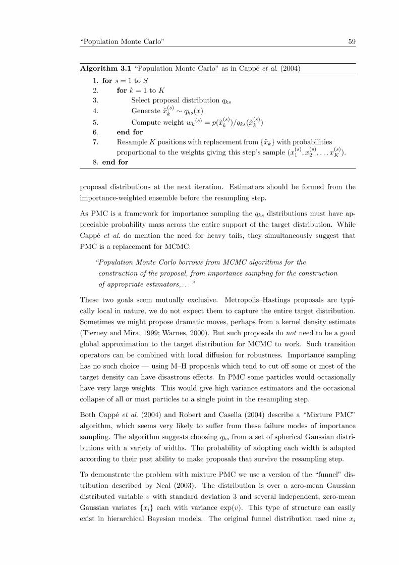
“Population Monte Carlo” 59
Algorithm 3.1 “Population Monte Carlo” as in Cappe et al. (2004)
1. for s = 1 to S
2. for k = 1 to K
3. Select proposal distribution qks
4. Generate x(s)k ∼ qks(x)
5. Compute weight wk(s) = p(x(s)
k )/qks(x(s)k )
6. end for7. Resample K positions with replacement from {xk} with probabilities
proportional to the weights giving this step’s sample (x(s)1 , x
(s)2 , . . . x
(s)K ).
8. end for
proposal distributions at the next iteration. Estimators should be formed from theimportance-weighted ensemble before the resampling step.
As PMC is a framework for importance sampling the qks distributions must have ap-preciable probability mass across the entire support of the target distribution. WhileCappe et al. do mention the need for heavy tails, they simultaneously suggest thatPMC is a replacement for MCMC:
“Population Monte Carlo borrows from MCMC algorithms for theconstruction of the proposal, from importance sampling for the constructionof appropriate estimators,. . . ”
These two goals seem mutually exclusive. Metropolis–Hastings proposals are typi-cally local in nature, we do not expect them to capture the entire target distribution.Sometimes we might propose dramatic moves, perhaps from a kernel density estimate(Tierney and Mira, 1999; Warnes, 2000). But such proposals do not need to be a goodglobal approximation to the target distribution for MCMC to work. Such transitionoperators can be combined with local diffusion for robustness. Importance samplinghas no such choice — using M–H proposals which tend to cut off some or most of thetarget density can have disastrous effects. In PMC some particles would occasionallyhave very large weights. This would give high variance estimators and the occasionalcollapse of all or most particles to a single point in the resampling step.
Both Cappe et al. (2004) and Robert and Casella (2004) describe a “Mixture PMC”algorithm, which seems very likely to suffer from these failure modes of importancesampling. The algorithm suggests choosing qks from a set of spherical Gaussian distri-butions with a variety of widths. The probability of adopting each width is adaptedaccording to their past ability to make proposals that survive the resampling step.
To demonstrate the problem with mixture PMC we use a version of the “funnel” dis-tribution described by Neal (2003). The distribution is over a zero-mean Gaussiandistributed variable v with standard deviation 3 and several independent, zero-meanGaussian variates {xi} each with variance exp(v). This type of structure can easilyexist in hierarchical Bayesian models. The original funnel distribution used nine xi
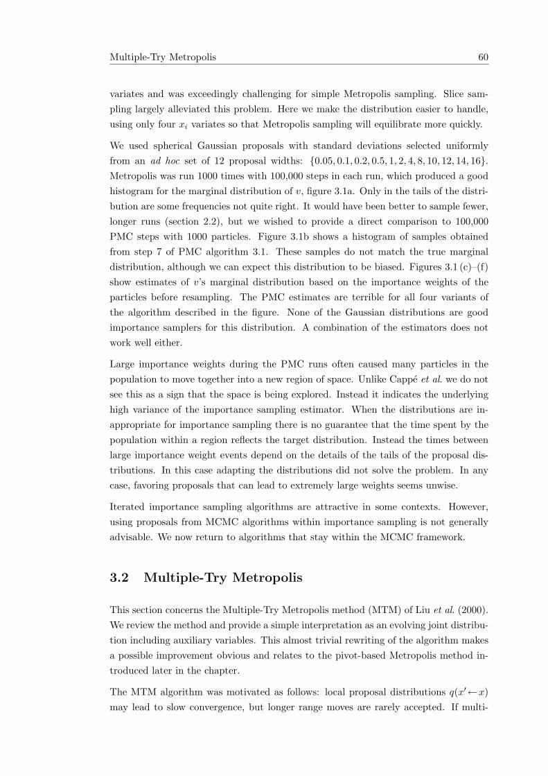
Multiple-Try Metropolis 60
variates and was exceedingly challenging for simple Metropolis sampling. Slice sam-pling largely alleviated this problem. Here we make the distribution easier to handle,using only four xi variates so that Metropolis sampling will equilibrate more quickly.
We used spherical Gaussian proposals with standard deviations selected uniformlyfrom an ad hoc set of 12 proposal widths: {0.05, 0.1, 0.2, 0.5, 1, 2, 4, 8, 10, 12, 14, 16}.Metropolis was run 1000 times with 100,000 steps in each run, which produced a goodhistogram for the marginal distribution of v, figure 3.1a. Only in the tails of the distri-bution are some frequencies not quite right. It would have been better to sample fewer,longer runs (section 2.2), but we wished to provide a direct comparison to 100,000PMC steps with 1000 particles. Figure 3.1b shows a histogram of samples obtainedfrom step 7 of PMC algorithm 3.1. These samples do not match the true marginaldistribution, although we can expect this distribution to be biased. Figures 3.1 (c)–(f)show estimates of v’s marginal distribution based on the importance weights of theparticles before resampling. The PMC estimates are terrible for all four variants ofthe algorithm described in the figure. None of the Gaussian distributions are goodimportance samplers for this distribution. A combination of the estimators does notwork well either.
Large importance weights during the PMC runs often caused many particles in thepopulation to move together into a new region of space. Unlike Cappe et al. we do notsee this as a sign that the space is being explored. Instead it indicates the underlyinghigh variance of the importance sampling estimator. When the distributions are in-appropriate for importance sampling there is no guarantee that the time spent by thepopulation within a region reflects the target distribution. Instead the times betweenlarge importance weight events depend on the details of the tails of the proposal dis-tributions. In this case adapting the distributions did not solve the problem. In anycase, favoring proposals that can lead to extremely large weights seems unwise.
Iterated importance sampling algorithms are attractive in some contexts. However,using proposals from MCMC algorithms within importance sampling is not generallyadvisable. We now return to algorithms that stay within the MCMC framework.
3.2 Multiple-Try Metropolis
This section concerns the Multiple-Try Metropolis method (MTM) of Liu et al. (2000).We review the method and provide a simple interpretation as an evolving joint distribu-tion including auxiliary variables. This almost trivial rewriting of the algorithm makesa possible improvement obvious and relates to the pivot-based Metropolis method in-troduced later in the chapter.
The MTM algorithm was motivated as follows: local proposal distributions q(x′←x)may lead to slow convergence, but longer range moves are rarely accepted. If multi-
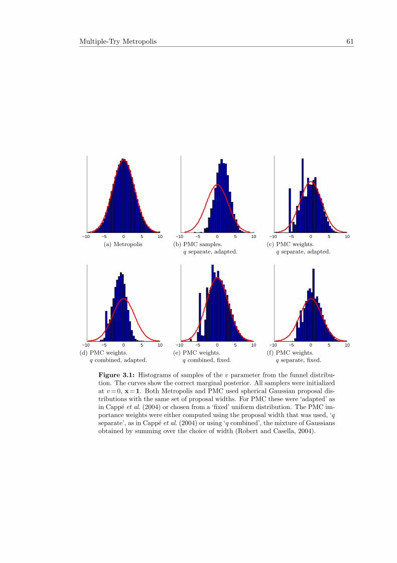
Multiple-Try Metropolis 61
−10 −5 0 5 10
(a) Metropolis
−10 −5 0 5 10
(b) PMC samples.q separate, adapted.
−10 −5 0 5 10
(c) PMC weights.q separate, adapted.
−10 −5 0 5 10
(d) PMC weights.q combined, adapted.
−10 −5 0 5 10
(e) PMC weights.q combined, fixed.
−10 −5 0 5 10
(f) PMC weights.q separate, fixed.
Figure 3.1: Histograms of samples of the v parameter from the funnel distribu-tion. The curves show the correct marginal posterior. All samplers were initializedat v =0, x=1. Both Metropolis and PMC used spherical Gaussian proposal dis-tributions with the same set of proposal widths. For PMC these were ‘adapted’ asin Cappe et al. (2004) or chosen from a ‘fixed’ uniform distribution. The PMC im-portance weights were either computed using the proposal width that was used, ‘qseparate’, as in Cappe et al. (2004) or using ‘q combined’, the mixture of Gaussiansobtained by summing over the choice of width (Robert and Casella, 2004).
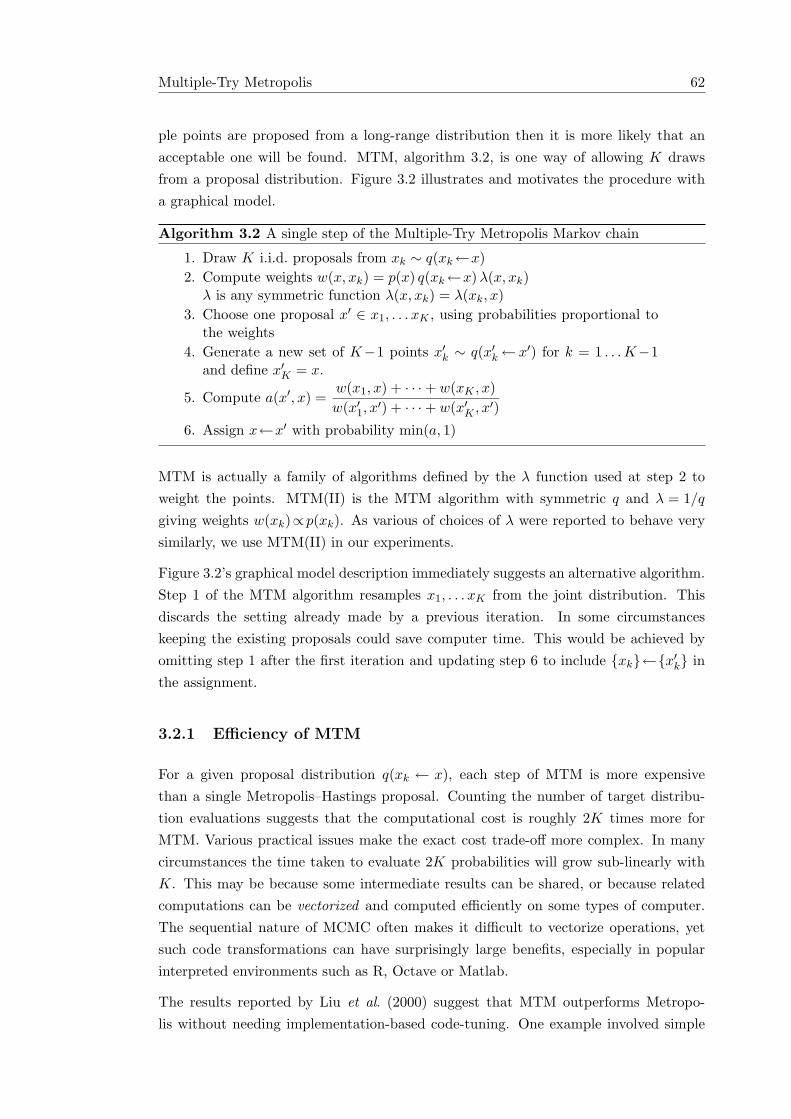
Multiple-Try Metropolis 62
ple points are proposed from a long-range distribution then it is more likely that anacceptable one will be found. MTM, algorithm 3.2, is one way of allowing K drawsfrom a proposal distribution. Figure 3.2 illustrates and motivates the procedure witha graphical model.
Algorithm 3.2 A single step of the Multiple-Try Metropolis Markov chain
1. Draw K i.i.d. proposals from xk ∼ q(xk←x)2. Compute weights w(x, xk) = p(x) q(xk←x) λ(x, xk)
λ is any symmetric function λ(x, xk) = λ(xk, x)3. Choose one proposal x′ ∈ x1, . . . xK , using probabilities proportional to
the weights4. Generate a new set of K−1 points x′k ∼ q(x′k← x′) for k = 1 . . .K−1
and define x′K = x.
5. Compute a(x′, x) =w(x1, x) + · · ·+ w(xK , x)w(x′1, x′) + · · ·+ w(x′K , x′)
6. Assign x←x′ with probability min(a, 1)
MTM is actually a family of algorithms defined by the λ function used at step 2 toweight the points. MTM(II) is the MTM algorithm with symmetric q and λ = 1/q
giving weights w(xk)∝p(xk). As various of choices of λ were reported to behave verysimilarly, we use MTM(II) in our experiments.
Figure 3.2’s graphical model description immediately suggests an alternative algorithm.Step 1 of the MTM algorithm resamples x1, . . . xK from the joint distribution. Thisdiscards the setting already made by a previous iteration. In some circumstanceskeeping the existing proposals could save computer time. This would be achieved byomitting step 1 after the first iteration and updating step 6 to include {xk}←{x′k} inthe assignment.
3.2.1 Efficiency of MTM
For a given proposal distribution q(xk ← x), each step of MTM is more expensivethan a single Metropolis–Hastings proposal. Counting the number of target distribu-tion evaluations suggests that the computational cost is roughly 2K times more forMTM. Various practical issues make the exact cost trade-off more complex. In manycircumstances the time taken to evaluate 2K probabilities will grow sub-linearly withK. This may be because some intermediate results can be shared, or because relatedcomputations can be vectorized and computed efficiently on some types of computer.The sequential nature of MCMC often makes it difficult to vectorize operations, yetsuch code transformations can have surprisingly large benefits, especially in popularinterpreted environments such as R, Octave or Matlab.
The results reported by Liu et al. (2000) suggest that MTM outperforms Metropo-lis without needing implementation-based code-tuning. One example involved simple
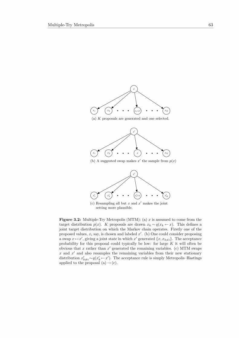
Multiple-Try Metropolis 63
x
x1 x2 xi=x′ xK
(a) K proposals are generated and one selected.
x′
x1 x2 x xK
(b) A suggested swap makes x′ the sample from p(x).
x′
x′
1x
′
2x
′
i=x x
′
K
(c) Resampling all but x and x′ makes the jointsetting more plausible.
Figure 3.2: Multiple-Try Metropolis (MTM): (a) x is assumed to come from thetarget distribution p(x). K proposals are drawn xk ∼ q(xk← x). This defines ajoint target distribution on which the Markov chain operates. Firstly one of theproposed values, xi say, is chosen and labeled x′. (b) One could consider proposinga swap x↔x′, giving a joint state in which x′ generated {x, xk 6=i}. The acceptanceprobability for this proposal could typically be low: for large K it will often beobvious that x rather than x′ generated the remaining variables. (c) MTM swapsx and x′ and also resamples the remaining variables from their new stationarydistribution x′k 6=i∼q(x′k←x′). The acceptance rule is simply Metropolis–Hastingsapplied to the proposal (a)→ (c).
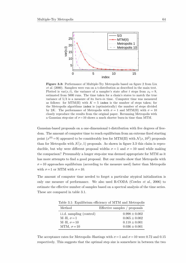
Multiple-Try Metropolis 64
0 5 10 15
5
10
15
20
25
index
var(
x,t)
5/3MTM(II)Metropolis 1Metropolis 10
Figure 3.3: Performance of Multiple-Try Metropolis based on figure 2 from Liuet al. (2000). Samplers were run on a t-distribution as described in the main text.Plotted is var(x, t), the variance of a sampler’s state after t steps from x0 = 9,estimated from 5000 runs. The time taken for a chain’s states to match the truevariance of 5/3 is a measure of its burn-in time. Computer time was measuredas follows: for MTM(II) with K = 5 index is the number of steps taken; forthe Metropolis algorithms index is (optimistically) the number of steps dividedby 2K. The performance of Metropolis with σ = 1 and MTM(II) with σ = 10closely reproduce the results from the original paper. Rerunning Metropolis witha Gaussian step-size of σ=10 shows a much shorter burn-in time than MTM.
Gaussian-based proposals on a one-dimensional t-distribution with five degrees of free-dom. The amount of computer time to reach equilibrium from an extreme fixed startingpoint (x(0) =9) appeared to be considerably less for MTM(II) with N (x, 102) proposalsthan for Metropolis with N (x, 1) proposals. As shown in figure 3.3 this claim is repro-ducible, but why were different proposal widths σ = 1 and σ = 10 used while makingthe comparison? Presumably a longer step-size was deemed appropriate for MTM as ithas more attempts to find a good proposal. But our results show that Metropolis withσ=10 approaches equilibrium (according to the measure used) faster than Metropoliswith σ=1 or MTM with σ=10.
The amount of computer time needed to forget a particular atypical initialization isonly one measure of performance. We also used R-CODA (Cowles et al., 2006) toestimate the effective number of samples based on a spectral analysis of the time series.These are compared in table 3.1.
Table 3.1: Equilibrium efficiency of MTM and Metropolis
Method Effective samples / proposals
i.i.d. sampling (control) 0.998± 0.002M–H, σ=1 0.065± 0.002M–H, σ=10 0.118± 0.001MTM, σ=10 0.036± 0.001
The acceptance rates for Metropolis–Hastings with σ=1 and σ=10 were 0.72 and 0.15respectively. This suggests that the optimal step size is somewhere in between the two
Multiple-Try Metropolis 65
values tried. MTM’s acceptance rate was 0.45, close to ideal for both standard M–Hand — according to Liu et al.’s experience — MTM. Despite this, MTM’s sampling effi-ciency on this very simple example distribution is worse than M–H at both equilibriumsampling and initial burning in.
This is a negative result, but one worth noting. Using multiple parallel proposals is not,in our experience, worthwhile in itself. This makes sense: when proposals are madesequentially a good proposal can be accepted immediately and future proposals movefrom the new location. In contrast, only one point from a set of parallel proposals canbe accepted, if there is more than one good point the rest are wasted.
The motivation for using multiple proposals cannot be to explore larger search regions.Instead we should consider MTM if making multiple proposals together is computation-ally cheaper than making them separately. The orientational bias procedure in Frenkeland Smit (2001, algorithm 22, section 13.1.2) is equivalent to MTM(II). In this contextthe proposals involve moving molecules. A molecule’s probability depends on indepen-dent terms depending on its position and orientation. The orientational bias procedureproposes a single new position with several possible orientations. While the issue isn’tdiscussed in detail, presumably it is sharing the positional energy computation acrossproposals that makes the algorithm worthwhile in molecular dynamics simulations.
A statistical example claiming benefit from multiple proposals is given by Qi and Minka(2002). They drew proposals from local Gaussian approximations based on the Hessianof the log posterior at the current sample location. In high-dimensional problems theseproposals would be expensive to construct1, O(D3) to prepare a matrix factorizationfor a multivariate-Gaussian sampler. Drawing multiple samples is then cheaper, O(D2).Even sequential sampling can take advantage of this, because the proposal will be reuseduntil a move is accepted. One wonders if, given the effort expended to construct thedistribution, drawing more samples than needed for acceptance could be useful. Thereported accuracy for a given CPU time does appear to be slightly better by combiningHessian-based sampling with an MTM variant, multiple-importance try.
3.2.2 Multiple-Importance Try
MTM makes it more likely that the chain moves, but is wasteful of information: multipleevaluations of the probability density are made at each iteration but at most one ofthese points is used. Qi and Minka (2002) suggested a way to use all of the {xk} pointsand called their combined Hessian-based MTM method Adaptive Multiple-ImportanceTry (AMIT). We will refer to the part of the algorithm that concerns including all thepoints in MTM as Multiple-Importance Try (MIT).
1Qi and Minka also discuss cheap approximations to Hessians, but are still keen to get the best usefrom them however constructed.
Multiple-Try Metropolis 66
MIT is the standard multiple-try Metropolis algorithm with a particular choice forpost-processing the samples. If p can be evaluated then the samples are weighted by
wk =p(xk)
q(xk←x). (3.1)
When p(x) is only known up to a constant the wk are computed using the unnormalizedversion p∗(x) and then made to sum to one. This is standard importance sampling usingq(xk←x) as a proposal distribution. The locations x of these importance samplers arechosen using MCMC.
Using local Gaussian approximations can lead to importance sampling estimators withlarge or even infinite variances. This suggests that MIT is likely to give erroneous resultson high-dimensional problems. MIT will work when good global proposal distributionscan be obtained, but we are unsure why MCMC would be an appropriate way toadapt these distributions. These are similar concerns to those discussed in section 3.1regarding “population Monte Carlo”.
3.2.3 Waste-recycled MTM
Waste recycling (subsection 2.2.2) is a method for using proposals that are not acceptedas part of the Markov chain. Here we describe how to recycle the points from theMTM method that are normally unused. Waste recycling does not carry the risks ofhuge variances associated with using importance sampling estimators with Metropolisproposals.
We first take the MTM joint distribution identified in figure 3.2a,
p(x, {xk}Kk=1
)= p(x)
K∏k=1
q(xk←x), (3.2)
and augment it with a new variable x. The marginal distribution of the new variableshould be the target distribution of interest. This could be achieved by copying x orpicking one of the proposals at random and copying it according to the Metropolis–Hastings acceptance rule:
p (x|x, {xk}) =
ak = 1K min
(1, p(xk) q(x←xk)
p(x) q(xk←x)
)x = xk
1−∑
k ak x = x .(3.3)
As in subsection 2.2.2, any quantity can be estimated by averaging over each of the{x, {xk}} settings weighted by their probability under this conditional distribution.
So far we are still discarding the {x′k} variables drawn by the algorithm. If the (x′, {x′k})joint state were accepted we could draw a new auxiliary variable x′∼p (x′|x′, {x′k}) usingthe conditional distribution analogous to equation (3.3). To include both possible joint
Multiple-Try Metropolis 67
settings in an estimator we use a further auxiliary variable ˆx, which is equal to one ofx or x′. We could define the probability of ˆx= x′ according to the min(1, a) acceptanceprobability of the MTM algorithm. However, this would sometimes give zero weight tox. In normal waste-recycling we do not mind ignoring the initial state as it was alreadyused at the previous iteration, but the {xk} were created at this iteration2. Instead weuse
p(ˆx= x′|x, {xk}, x′, {x′k}) =∑
k w(xk, x)∑k w(xk, x) +
∑k w(x′k, x
′), (3.4)
which also gives ˆx the correct stationary distribution. The final estimator averages overall states visited at each iteration based on the following identity for Ep(x)[f(x)]:
Ep(x,{xk},x′,{x′k})
∑x∈{x,{xk}}
x′∈{x′,{x′k}}
p (x|x, {xk}) p(x′|x′, {x′k}
)∑ˆx∈{x,x′}
f(ˆx) p(ˆx|x, {xk}, x′, {x′k})
.
(3.5)The expression looks cumbersome, but when expanded out only costsO(K) to compute.The estimator can be implemented once and used as a “black-box”.
The conditional probabilities of x and x′, equation (3.3), require some backwards pro-posal probabilities not normally needed by MTM or MIT. This would remove thepotential advantage when proposals are expensive, as in Qi and Minka (2002), butwould not be a problem when, as in Frenkel and Smit (2001), the purpose of multipleproposals is shared computation of p(x).
We compared the MTM’s mean square error (MSE) in estimating |x| to that obtainedby the waste-recycled version (WR-MTM) on the same t-distribution example as before.
Table 3.2: Accuracy on t-distribution after 1000 proposals
Method Mean Square Error (MSE)
M–H, σ=1 0.0119± 0.0010M–H σ=10 0.0105± 0.0005MTM, σ=10 0.0267± 0.0014WR-MTM, σ=10 0.0167± 0.0008MIT, σ=10 0.0047± 0.0002
Post-processing the MTM run with waste-recycling reduces the MSE considerably, butstill not to the level of Metropolis–Hastings. Speedups from efficient implementationof parallel proposals would still be required to justify waste-recycled MTM. Treatingthe xk proposals as draws from importance samplers, the MIT estimator, obtains the
2Unless we are applying the alternative algorithm suggested just before subsection 3.2.1.
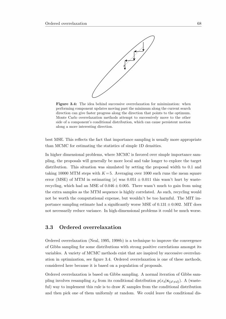
Ordered overrelaxation 68
Figure 3.4: The idea behind successive overrelaxation for minimization: whenperforming component updates moving past the minimum along the current searchdirection can give faster progress along the direction that points to the optimum.Monte Carlo overrelaxation methods attempt to successively move to the otherside of a component’s conditional distribution, which can cause persistent motionalong a more interesting direction.
best MSE. This reflects the fact that importance sampling is usually more appropriatethan MCMC for estimating the statistics of simple 1D densities.
In higher dimensional problems, where MCMC is favored over simple importance sam-pling, the proposals will generally be more local and take longer to explore the targetdistribution. This situation was simulated by setting the proposal width to 0.1 andtaking 10000 MTM steps with K =5. Averaging over 1000 such runs the mean squareerror (MSE) of MTM in estimating |x| was 0.051 ± 0.011 this wasn’t hurt by waste-recycling, which had an MSE of 0.046± 0.005. There wasn’t much to gain from usingthe extra samples as the MTM sequence is highly correlated. As such, recycling wouldnot be worth the computational expense, but wouldn’t be too harmful. The MIT im-portance sampling estimate had a significantly worse MSE of 0.131± 0.002. MIT doesnot necessarily reduce variance. In high-dimensional problems it could be much worse.
3.3 Ordered overrelaxation
Ordered overrelaxation (Neal, 1995, 1998b) is a technique to improve the convergenceof Gibbs sampling for some distributions with strong positive correlations amongst itsvariables. A variety of MCMC methods exist that are inspired by successive overrelax-ation in optimization, see figure 3.4. Ordered overrelaxation is one of these methods,considered here because it is based on a population of proposals.
Ordered overrelaxation is based on Gibbs sampling. A normal iteration of Gibbs sam-pling involves resampling xd from its conditional distribution p(xd|x{d′ 6=d}). A (waste-ful) way to implement this rule is to draw K samples from the conditional distributionand then pick one of them uniformly at random. We could leave the conditional dis-
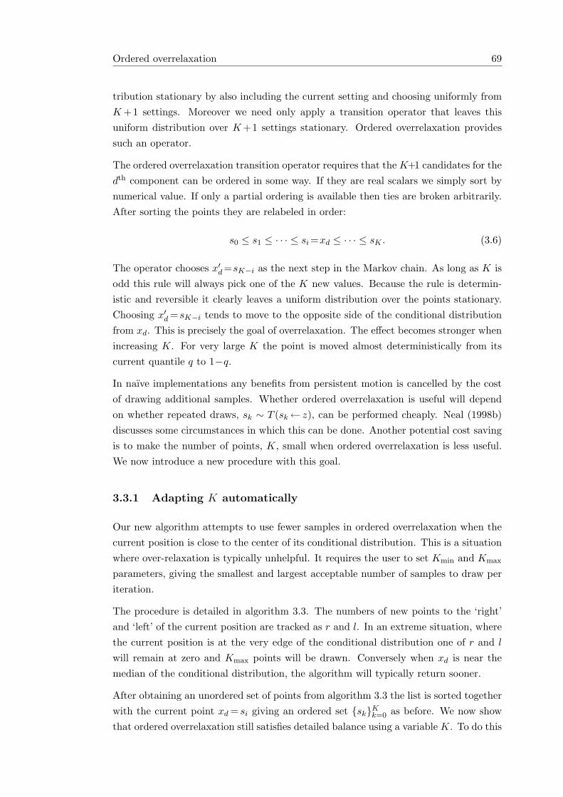
Ordered overrelaxation 69
tribution stationary by also including the current setting and choosing uniformly fromK +1 settings. Moreover we need only apply a transition operator that leaves thisuniform distribution over K +1 settings stationary. Ordered overrelaxation providessuch an operator.
The ordered overrelaxation transition operator requires that the K+1 candidates for thedth component can be ordered in some way. If they are real scalars we simply sort bynumerical value. If only a partial ordering is available then ties are broken arbitrarily.After sorting the points they are relabeled in order:
s0 ≤ s1 ≤ · · · ≤ si =xd ≤ · · · ≤ sK . (3.6)
The operator chooses x′d =sK−i as the next step in the Markov chain. As long as K isodd this rule will always pick one of the K new values. Because the rule is determin-istic and reversible it clearly leaves a uniform distribution over the points stationary.Choosing x′d = sK−i tends to move to the opposite side of the conditional distributionfrom xd. This is precisely the goal of overrelaxation. The effect becomes stronger whenincreasing K. For very large K the point is moved almost deterministically from itscurrent quantile q to 1−q.
In naıve implementations any benefits from persistent motion is cancelled by the costof drawing additional samples. Whether ordered overrelaxation is useful will dependon whether repeated draws, sk ∼ T (sk← z), can be performed cheaply. Neal (1998b)discusses some circumstances in which this can be done. Another potential cost savingis to make the number of points, K, small when ordered overrelaxation is less useful.We now introduce a new procedure with this goal.
3.3.1 Adapting K automatically
Our new algorithm attempts to use fewer samples in ordered overrelaxation when thecurrent position is close to the center of its conditional distribution. This is a situationwhere over-relaxation is typically unhelpful. It requires the user to set Kmin and Kmax
parameters, giving the smallest and largest acceptable number of samples to draw periteration.
The procedure is detailed in algorithm 3.3. The numbers of new points to the ‘right’and ‘left’ of the current position are tracked as r and l. In an extreme situation, wherethe current position is at the very edge of the conditional distribution one of r and l
will remain at zero and Kmax points will be drawn. Conversely when xd is near themedian of the conditional distribution, the algorithm will typically return sooner.
After obtaining an unordered set of points from algorithm 3.3 the list is sorted togetherwith the current point xd = si giving an ordered set {sk}Kk=0 as before. We now showthat ordered overrelaxation still satisfies detailed balance using a variable K. To do this
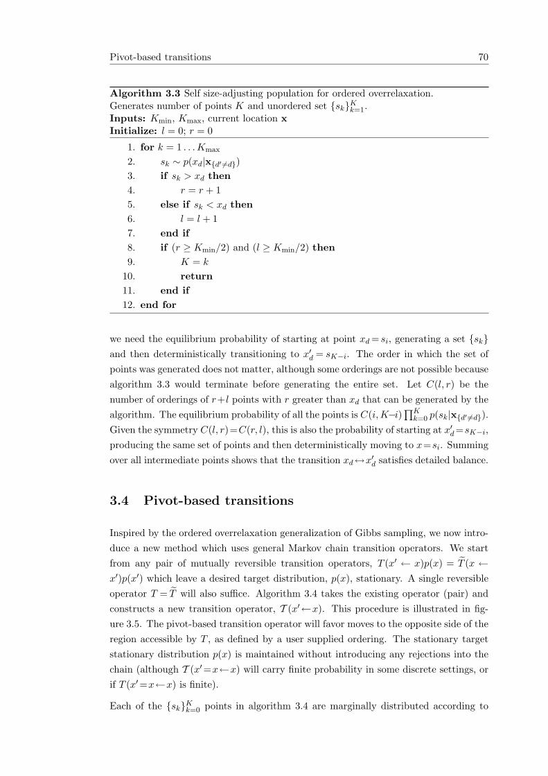
Pivot-based transitions 70
Algorithm 3.3 Self size-adjusting population for ordered overrelaxation.Generates number of points K and unordered set {sk}Kk=1.Inputs: Kmin, Kmax, current location xInitialize: l = 0; r = 0
1. for k = 1 . . .Kmax
2. sk ∼ p(xd|x{d′ 6=d})3. if sk > xd then4. r = r + 15. else if sk < xd then6. l = l + 17. end if8. if (r ≥ Kmin/2) and (l ≥ Kmin/2) then9. K = k
10. return11. end if12. end for
we need the equilibrium probability of starting at point xd = si, generating a set {sk}and then deterministically transitioning to x′d = sK−i. The order in which the set ofpoints was generated does not matter, although some orderings are not possible becausealgorithm 3.3 would terminate before generating the entire set. Let C(l, r) be thenumber of orderings of r+l points with r greater than xd that can be generated by thealgorithm. The equilibrium probability of all the points is C(i,K−i)
∏Kk=0 p(sk|x{d′ 6=d}).
Given the symmetry C(l, r)=C(r, l), this is also the probability of starting at x′d =sK−i,producing the same set of points and then deterministically moving to x=si. Summingover all intermediate points shows that the transition xd↔x′d satisfies detailed balance.
3.4 Pivot-based transitions
Inspired by the ordered overrelaxation generalization of Gibbs sampling, we now intro-duce a new method which uses general Markov chain transition operators. We startfrom any pair of mutually reversible transition operators, T (x′ ← x)p(x) = T (x ←x′)p(x′) which leave a desired target distribution, p(x), stationary. A single reversibleoperator T = T will also suffice. Algorithm 3.4 takes the existing operator (pair) andconstructs a new transition operator, T (x′←x). This procedure is illustrated in fig-ure 3.5. The pivot-based transition operator will favor moves to the opposite side of theregion accessible by T , as defined by a user supplied ordering. The stationary targetstationary distribution p(x) is maintained without introducing any rejections into thechain (although T (x′=x←x) will carry finite probability in some discrete settings, orif T (x′=x←x) is finite).
Each of the {sk}Kk=0 points in algorithm 3.4 are marginally distributed according to
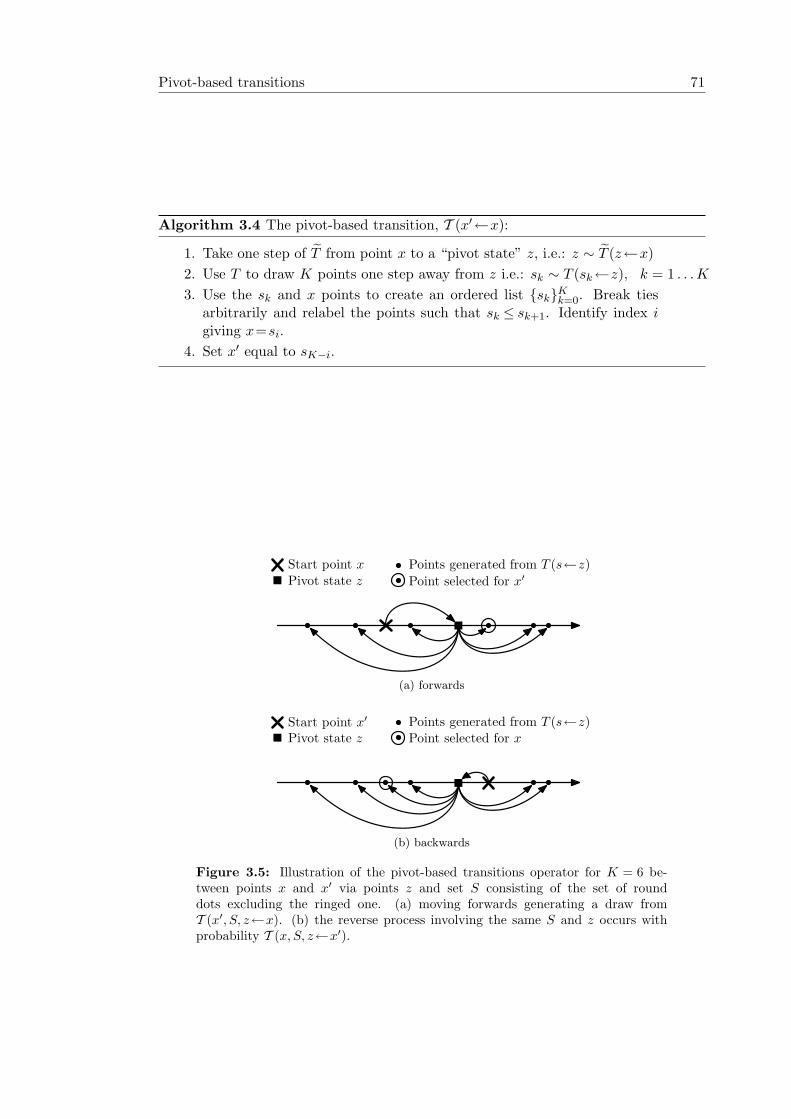
Pivot-based transitions 71
Algorithm 3.4 The pivot-based transition, T (x′←x):
1. Take one step of T from point x to a “pivot state” z, i.e.: z ∼ T (z←x)2. Use T to draw K points one step away from z i.e.: sk ∼ T (sk←z), k = 1 . . .K
3. Use the sk and x points to create an ordered list {sk}Kk=0. Break tiesarbitrarily and relabel the points such that sk ≤ sk+1. Identify index igiving x=si.
4. Set x′ equal to sK−i.
Start point x
Pivot state z
Points generated from T (s←z)
Point selected for x′
(a) forwards
Start point x′
Pivot state z
Points generated from T (s←z)Point selected for x
(b) backwards
Figure 3.5: Illustration of the pivot-based transitions operator for K = 6 be-tween points x and x′ via points z and set S consisting of the set of rounddots excluding the ringed one. (a) moving forwards generating a draw fromT (x′, S, z←x). (b) the reverse process involving the same S and z occurs withprobability T (x, S, z←x′).
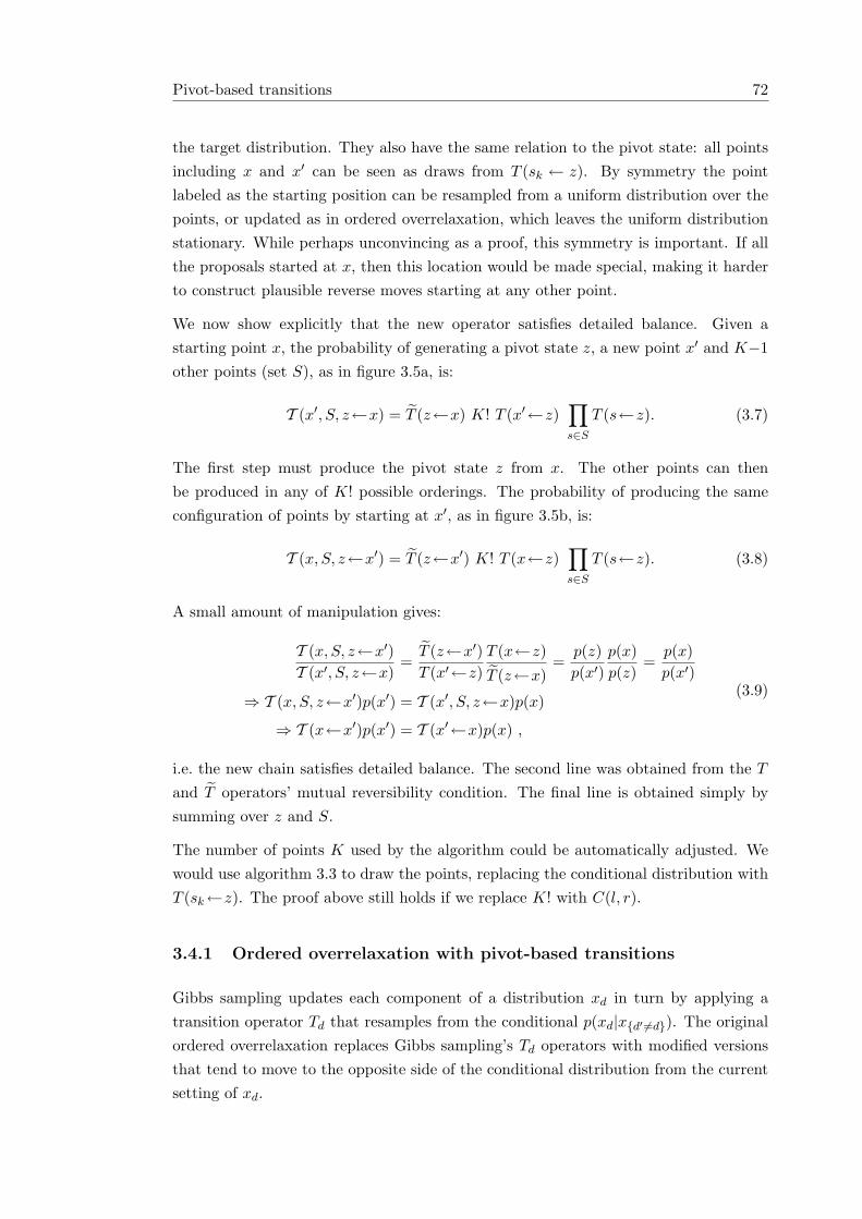
Pivot-based transitions 72
the target distribution. They also have the same relation to the pivot state: all pointsincluding x and x′ can be seen as draws from T (sk ← z). By symmetry the pointlabeled as the starting position can be resampled from a uniform distribution over thepoints, or updated as in ordered overrelaxation, which leaves the uniform distributionstationary. While perhaps unconvincing as a proof, this symmetry is important. If allthe proposals started at x, then this location would be made special, making it harderto construct plausible reverse moves starting at any other point.
We now show explicitly that the new operator satisfies detailed balance. Given astarting point x, the probability of generating a pivot state z, a new point x′ and K−1other points (set S), as in figure 3.5a, is:
T (x′, S, z←x) = T (z←x) K! T (x′←z)∏s∈S
T (s←z). (3.7)
The first step must produce the pivot state z from x. The other points can thenbe produced in any of K! possible orderings. The probability of producing the sameconfiguration of points by starting at x′, as in figure 3.5b, is:
T (x, S, z←x′) = T (z←x′) K! T (x←z)∏s∈S
T (s←z). (3.8)
A small amount of manipulation gives:
T (x, S, z←x′)T (x′, S, z←x)
=T (z←x′)T (x′←z)
T (x←z)
T (z←x)=
p(z)p(x′)
p(x)p(z)
=p(x)p(x′)
⇒ T (x, S, z←x′)p(x′) = T (x′, S, z←x)p(x)
⇒ T (x←x′)p(x′) = T (x′←x)p(x) ,
(3.9)
i.e. the new chain satisfies detailed balance. The second line was obtained from the T
and T operators’ mutual reversibility condition. The final line is obtained simply bysumming over z and S.
The number of points K used by the algorithm could be automatically adjusted. Wewould use algorithm 3.3 to draw the points, replacing the conditional distribution withT (sk←z). The proof above still holds if we replace K! with C(l, r).
3.4.1 Ordered overrelaxation with pivot-based transitions
Gibbs sampling updates each component of a distribution xd in turn by applying atransition operator Td that resamples from the conditional p(xd|x{d′ 6=d}). The originalordered overrelaxation replaces Gibbs sampling’s Td operators with modified versionsthat tend to move to the opposite side of the conditional distribution from the currentsetting of xd.
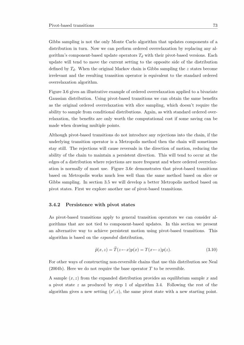
Pivot-based transitions 73
Gibbs sampling is not the only Monte Carlo algorithm that updates components of adistribution in turn. Now we can perform ordered overrelaxation by replacing any al-gorithm’s component-based update operators Td with their pivot-based versions. Eachupdate will tend to move the current setting to the opposite side of the distributiondefined by Td. When the original Markov chain is Gibbs sampling the z states becomeirrelevant and the resulting transition operator is equivalent to the standard orderedoverrelaxation algorithm.
Figure 3.6 gives an illustrative example of ordered overrelaxation applied to a bivariateGaussian distribution. Using pivot-based transitions we can obtain the same benefitsas the original ordered overrelaxation with slice sampling, which doesn’t require theability to sample from conditional distributions. Again, as with standard ordered over-relaxation, the benefits are only worth the computational cost if some saving can bemade when drawing multiple points.
Although pivot-based transitions do not introduce any rejections into the chain, if theunderlying transition operator is a Metropolis method then the chain will sometimesstay still. The rejections will cause reversals in the direction of motion, reducing theability of the chain to maintain a persistent direction. This will tend to occur at theedges of a distribution where rejections are more frequent and where ordered overrelax-ation is normally of most use. Figure 3.6c demonstrates that pivot-based transitionsbased on Metropolis works much less well than the same method based on slice orGibbs sampling. In section 3.5 we will develop a better Metropolis method based onpivot states. First we explore another use of pivot-based transitions.
3.4.2 Persistence with pivot states
As pivot-based transitions apply to general transition operators we can consider al-gorithms that are not tied to component-based updates. In this section we presentan alternative way to achieve persistent motion using pivot-based transitions. Thisalgorithm is based on the expanded distribution,
p(x, z) = T (z←x)p(x) = T (x←z)p(z). (3.10)
For other ways of constructing non-reversible chains that use this distribution see Neal(2004b). Here we do not require the base operator T to be reversible.
A sample (x, z) from the expanded distribution provides an equilibrium sample x anda pivot state z as produced by step 1 of algorithm 3.4. Following the rest of thealgorithm gives a new setting (x′, z), the same pivot state with a new starting point.
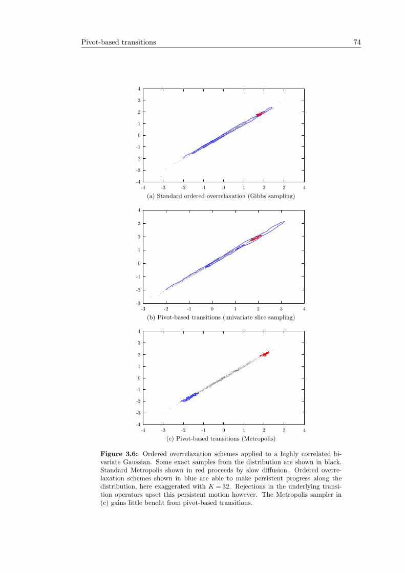
Pivot-based transitions 74
-4
-3
-2
-1
0
1
2
3
4
-4 -3 -2 -1 0 1 2 3 4
(a) Standard ordered overrelaxation (Gibbs sampling)
-3
-2
-1
0
1
2
3
4
-3 -2 -1 0 1 2 3 4
(b) Pivot-based transitions (univariate slice sampling)
-4
-3
-2
-1
0
1
2
3
4
-4 -3 -2 -1 0 1 2 3 4
(c) Pivot-based transitions (Metropolis)
Figure 3.6: Ordered overrelaxation schemes applied to a highly correlated bi-variate Gaussian. Some exact samples from the distribution are shown in black.Standard Metropolis shown in red proceeds by slow diffusion. Ordered overre-laxation schemes shown in blue are able to make persistent progress along thedistribution, here exaggerated with K = 32. Rejections in the underlying transi-tion operators upset this persistent motion however. The Metropolis sampler in(c) gains little benefit from pivot-based transitions.
Pivot-based transitions 75
This procedure leaves the expanded distribution invariant, the proof is similar to before:
T (x′, S; x, z) = K! T (x′←z)∏s∈S
T (s←z)
T (x, S; x′, z) = K! T (x←z)∏s∈S
T (s←z)
T (x, S; x′, z)T (x′, S; x, z)
=T (x←z)T (x′←z)
=T (z←x)p(x)
p(z)p(z)
T (z←x′)p(x′)
=T (z←x)p(x)
T (z←x′)p(x′)
⇒ T (x, S; x′, z) T (z←x′)p(x′) = T (x′, S; x, z) T (z←x)p(x)
⇒ T((x, z)←(x′, z)
)p(x′, z) = T
((x′, z)←(x, z)
)p(x, z) .
(3.11)
The final line was obtained by using equation (3.10) and summing over the intermediatepoints S. We have shown that the appropriate detailed balance relationship holds withrespect to the expanded distribution.
Equation (3.10) suggests that the sample from the expanded distribution can also beinterpreted as an equilibrium sample z and a pivot state x ∼ T (x← z). This pivotstate could be updated by an alternative pivot-based transition operator T based onalgorithm 3.4. As T was used in step 1 we switch to using T to produce the K points instep 2. A version of the above proof shows that this operator also leaves the expandeddistribution invariant.
Given a pair sampled from the expanded distribution (x1, x2) ∼ p(x1, x2) = T (x2 ←x1)p(x1) we alternate between two Markov chain updates. First we update x1 usingx2 as a pivot state with algorithm 3.4 (operator T ). Next we update x2 using x1 as apivot state with the alternate operator T . Figure 3.7 illustrates the effect of alternatelyapplying these two operators. Both operators have a tendency to reverse the orderingof x1 and x2. By continually jumping over each other, the pair move persistently acrossthe space that induces the ordering. By chance, for finite K, the points will sometimesstay in the same order. In subsequent iterations motion will be in the opposite directionallowing the chain to mix across the whole space.
Figure 3.8 shows pivot-based persistent motion when the base transition operator hasa small step size, which would normally lead to slow diffusion. The effect is dramatic:the entire range of the distribution is explored in many fewer iterations. However,the improved dynamics alone are not actually sufficient to justify the increased costof drawing multiple proposals. As with MTM, some further savings, such as parallelcomputation, are required.
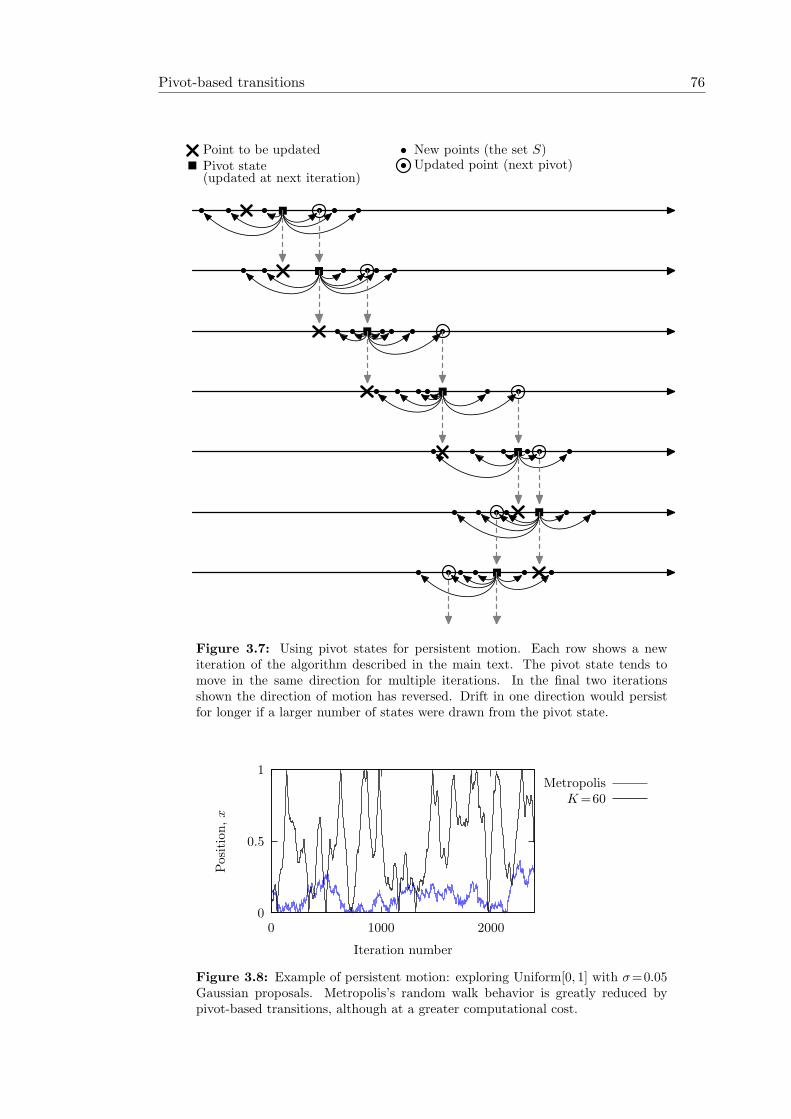
Pivot-based transitions 76
Point to be updatedPivot state(updated at next iteration)
New points (the set S)Updated point (next pivot)
Figure 3.7: Using pivot states for persistent motion. Each row shows a newiteration of the algorithm described in the main text. The pivot state tends tomove in the same direction for multiple iterations. In the final two iterationsshown the direction of motion has reversed. Drift in one direction would persistfor longer if a larger number of states were drawn from the pivot state.
1
0.5
0200010000
Posi
tion,x
Iteration number
Metropolis
K =60
Figure 3.8: Example of persistent motion: exploring Uniform[0, 1] with σ=0.05Gaussian proposals. Metropolis’s random walk behavior is greatly reduced bypivot-based transitions, although at a greater computational cost.
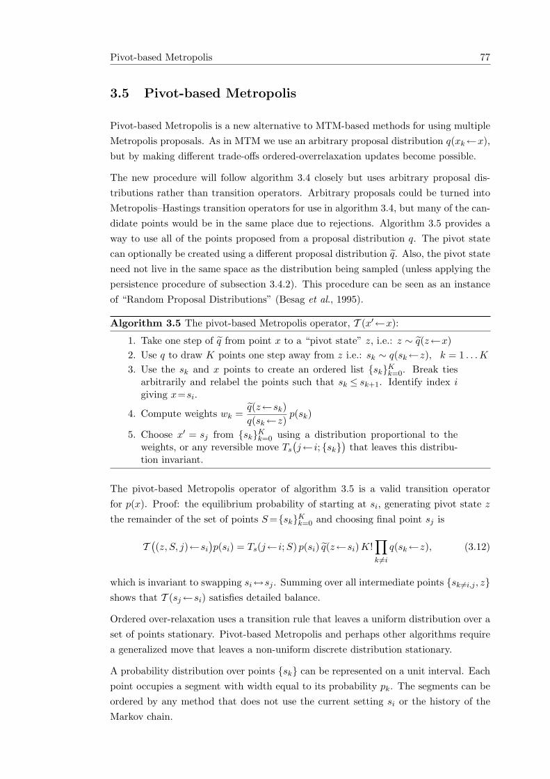
Pivot-based Metropolis 77
3.5 Pivot-based Metropolis
Pivot-based Metropolis is a new alternative to MTM-based methods for using multipleMetropolis proposals. As in MTM we use an arbitrary proposal distribution q(xk←x),but by making different trade-offs ordered-overrelaxation updates become possible.
The new procedure will follow algorithm 3.4 closely but uses arbitrary proposal dis-tributions rather than transition operators. Arbitrary proposals could be turned intoMetropolis–Hastings transition operators for use in algorithm 3.4, but many of the can-didate points would be in the same place due to rejections. Algorithm 3.5 provides away to use all of the points proposed from a proposal distribution q. The pivot statecan optionally be created using a different proposal distribution q. Also, the pivot stateneed not live in the same space as the distribution being sampled (unless applying thepersistence procedure of subsection 3.4.2). This procedure can be seen as an instanceof “Random Proposal Distributions” (Besag et al., 1995).
Algorithm 3.5 The pivot-based Metropolis operator, T (x′←x):
1. Take one step of q from point x to a “pivot state” z, i.e.: z ∼ q(z←x)2. Use q to draw K points one step away from z i.e.: sk ∼ q(sk←z), k = 1 . . .K
3. Use the sk and x points to create an ordered list {sk}Kk=0. Break tiesarbitrarily and relabel the points such that sk ≤ sk+1. Identify index igiving x=si.
4. Compute weights wk =q(z←sk)q(sk←z)
p(sk)
5. Choose x′ = sj from {sk}Kk=0 using a distribution proportional to theweights, or any reversible move Ts
(j← i; {sk}
)that leaves this distribu-
tion invariant.
The pivot-based Metropolis operator of algorithm 3.5 is a valid transition operatorfor p(x). Proof: the equilibrium probability of starting at si, generating pivot state z
the remainder of the set of points S ={sk}Kk=0 and choosing final point sj is
T((z, S, j)←si
)p(si) = Ts(j← i;S) p(si) q(z←si) K!
∏k 6=i
q(sk←z), (3.12)
which is invariant to swapping si↔sj . Summing over all intermediate points {sk 6=i,j , z}shows that T (sj←si) satisfies detailed balance.
Ordered over-relaxation uses a transition rule that leaves a uniform distribution over aset of points stationary. Pivot-based Metropolis and perhaps other algorithms requirea generalized move that leaves a non-uniform discrete distribution stationary.
A probability distribution over points {sk} can be represented on a unit interval. Eachpoint occupies a segment with width equal to its probability pk. The segments can beordered by any method that does not use the current setting si or the history of theMarkov chain.
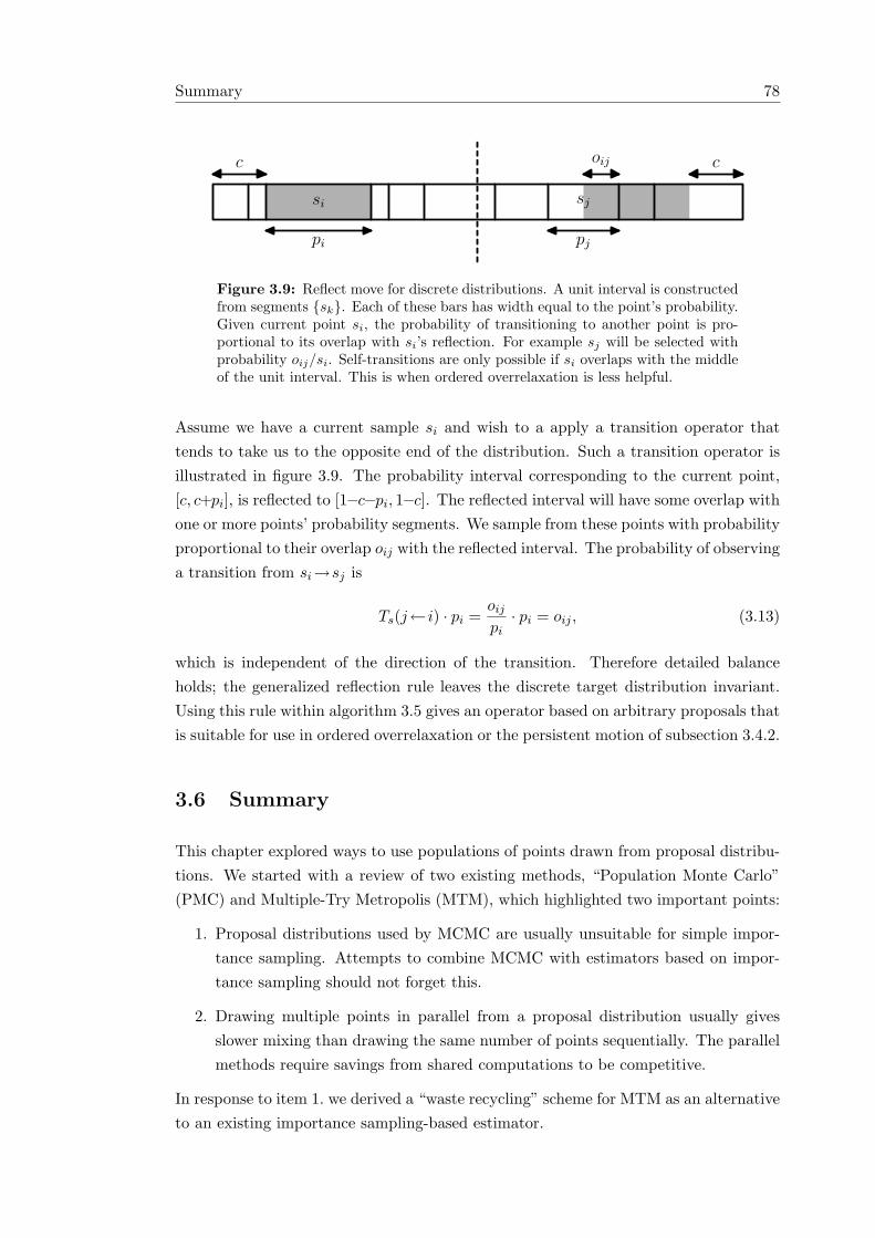
Summary 78
c c
pi pj
oij
si sj
Figure 3.9: Reflect move for discrete distributions. A unit interval is constructedfrom segments {sk}. Each of these bars has width equal to the point’s probability.Given current point si, the probability of transitioning to another point is pro-portional to its overlap with si’s reflection. For example sj will be selected withprobability oij/si. Self-transitions are only possible if si overlaps with the middleof the unit interval. This is when ordered overrelaxation is less helpful.
Assume we have a current sample si and wish to a apply a transition operator thattends to take us to the opposite end of the distribution. Such a transition operator isillustrated in figure 3.9. The probability interval corresponding to the current point,[c, c+pi], is reflected to [1−c−pi, 1−c]. The reflected interval will have some overlap withone or more points’ probability segments. We sample from these points with probabilityproportional to their overlap oij with the reflected interval. The probability of observinga transition from si→sj is
Ts(j← i) · pi =oij
pi· pi = oij , (3.13)
which is independent of the direction of the transition. Therefore detailed balanceholds; the generalized reflection rule leaves the discrete target distribution invariant.Using this rule within algorithm 3.5 gives an operator based on arbitrary proposals thatis suitable for use in ordered overrelaxation or the persistent motion of subsection 3.4.2.
3.6 Summary
This chapter explored ways to use populations of points drawn from proposal distribu-tions. We started with a review of two existing methods, “Population Monte Carlo”(PMC) and Multiple-Try Metropolis (MTM), which highlighted two important points:
1. Proposal distributions used by MCMC are usually unsuitable for simple impor-tance sampling. Attempts to combine MCMC with estimators based on impor-tance sampling should not forget this.
2. Drawing multiple points in parallel from a proposal distribution usually givesslower mixing than drawing the same number of points sequentially. The parallelmethods require savings from shared computations to be competitive.
In response to item 1. we derived a “waste recycling” scheme for MTM as an alternativeto an existing importance sampling-based estimator.
Related and future work 79
We then focussed on methods that use a population of points to move the state ofa Markov chain to the opposite side of a user-defined ordering. Chaining these up-dates together can cause persistent motion through Neal’s ordered overrelaxation orthe method we introduced in subsection 3.4.2. A random walk will explore a distribu-tion with length-scale L in O(L/σ2) steps of size σ. More persistent motion can bringthis down to O(L/σ). Our contributions to this area were:
1. Algorithm 3.3, which automatically reduces the size of a population when orderedoverrelaxation is less likely to be useful, saving computation.
2. Generalizing ordered overrelaxation to transition operators other than Gibbs sam-pling, algorithm 3.4.
3. Using ordered transition operators for persistent motion without usingcomponent-based updates, subsection 3.4.2.
4. Generalizing ordered updates to operate directly on a set of weighted points,section 3.5. These moves are less likely to reject than using Metropolis–Hastingswithin algorithm 3.4, which is important because rejections destroy persistentmotion.
The usefulness of these innovations relies on the assumption that drawing multiple pro-posals is computationally efficient. It remains to be seen if implementations leveragingcaching of intermediate results or parallel computations will make our work effectivein real applications. Similar assumptions are made by related work in the literature,which we now briefly consider along with directions for future research.
3.7 Related and future work
Tjelmeland (2004) and Stormark (2006) investigate an idea similar to pivot-basedMetropolis. They suggest drawing a set of antithetic variables, possibly using quasiMonte Carlo. Recent work also applies these ideas to MTM (Craiu and Lemieux,2007). Pivot-based Metropolis could also be extended in this way. Tjelmeland alsorecommends waste-recycling, which would also apply to pivot-based algorithms. Themain difference in his algorithm is that all the states are drawn as proposals from thecurrent state x, rather than an intermediate state z. Making reversible moves based onthese proposals requires working out the probability of each state reproducing the entireensemble, an O(K2) computation. Our pivot state approach reduces this computationto O(K) and makes an exchange of the current point with one of the proposals seemmore natural.
As an example we showed pivot-based ordered overrelaxation applied to slice sampling.In fact, slice sampling already has its own method for overrelaxation (Neal, 2003), al-though this is susceptible to rejections unless the edges of the slice are found accurately.

Related and future work 80
Ordered overrelaxation may be preferable as it never has rejections while needing onlyenough information to draw K samples. There is a way to eliminate the pivot statewhen slice sampling from unimodal distributions: it is possible to Gibbs sample theslice sampling auxiliary distribution, so standard ordered overrelaxation applies.
Subsection 3.4.2 described a new way to make persistent motion along a direction thatdefines an ordering on the state space. Choosing suitable methods for ordering pointswill be problem-dependent in general. One generic application could be simulated tem-pering (subsection 2.5.1), where energy could be used to define an ordering. Persistentmotion along this ordering should encourage the inverse-temperature to move morerapidly between zero and one.
Radford Neal has suggested (personal communication) considering an alternative topivot-based transitions. This method starts with a random integer f drawn uniformlybetween 0 and K inclusive. The current point x is evolved through a sequence of f
transitions using T . Then starting at x again, a sequence of b = K−f ‘backwards’transitions is simulated using T . Choosing uniformly from the resulting K+1 statesmaintains the stationary distribution. Also reordering the points and choosing thecomplement to x as in ordered overrelaxation is valid. Producing a chain of statesrather than a star of steps starting at a single state is likely to produce larger moves.
A version of Neal’s idea based on the weighted reflect operator of section 3.5 is alsopossible. The chain could use transition operators that leave a cheaper-to-evaluatesurrogate distribution invariant. Proposal weights could be evaluated for a thinnedsubset of the chain and then the reflect operator applied. Yet another possibility is themultipoint Metropolis method (Qin and Liu, 2001), an extension to MTM that uses achain of states.
A disadvantage of using a chain of transitions is that each move must be made se-quentially. The pivot-based algorithms introduced in this chapter could evaluate theirproposals in parallel on suitable computer hardware.
Chapter 4
Normalizing constants and
nested sampling
The computation of normalizing constants plays an important role in inference andstatistical physics. For example, Bayesian model comparison needs the evidence, ormarginal likelihood of a model M given observed data D
Z = p(D|M) =∫
p(D|θ,M)p(θ|M) dθ ≡∫
L(θ)π(θ) dθ, (4.1)
where the model has prior π and likelihood L over parameters θ. In statistical physicsZ(β) =
∫exp(−βE(θ))dθ is the normalizing constant for the distribution over states
with energy E at inverse temperature β. In this context Z is an important quantityknown as the partition function, a function of β from which several fundamental prop-erties of a system can be derived. The marginal likelihood, equation (4.1), is also afunction, in this case of the model M, which will become important in chapter 5. Inthis chapter we focus on estimating the constant for a given model. We also considerestimating the whole Z(β) function from physics which, perhaps surprisingly, is usefulfor solving the marginal likelihood problem.
Statistical physics normally uses the normalization in its log form; − logZ is known asthe free energy of a system. When used in statistical inference logZ has also been foundto be a useful and natural scale for comparing models. Given two modelsM0 andM1
the log-likelihood ratio, log Z1/Z0 =log p(D|M1)−log p(D|M0), can be used in a classicalhypothesis test which rejects M0 in favor of M1 when a threshold is exceeded. Thismeans that absolute differences in logZ0 correspond to shifts in model quality that aremeaningful without reference to an alternative model. Researchers decrypting codesat Bletchley park judged that a difference of roughly a deciban, log10
Z1/Z0 = 1/10, isabout the smallest difference in two models that people can express. Table 4.1 containsqualitative descriptions of the importance of marginal likelihood ratios.
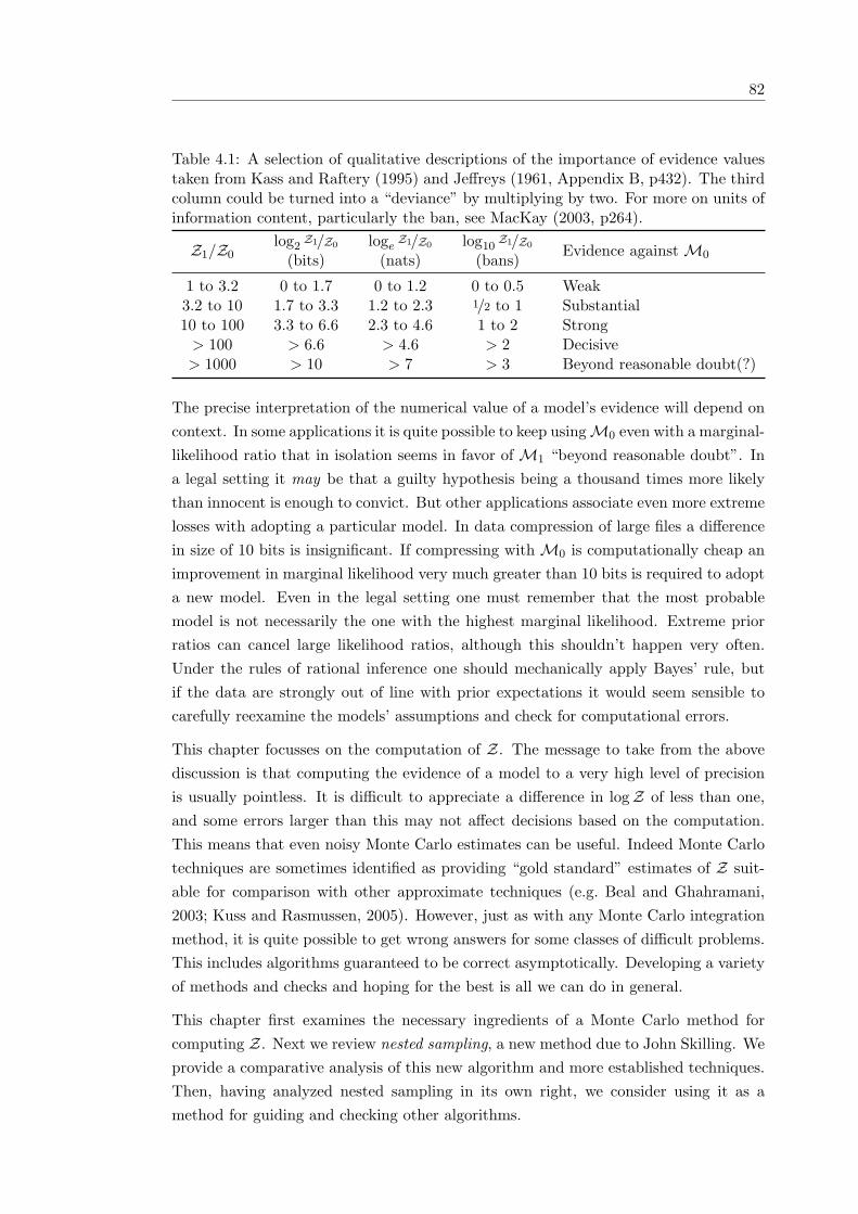
82
Table 4.1: A selection of qualitative descriptions of the importance of evidence valuestaken from Kass and Raftery (1995) and Jeffreys (1961, Appendix B, p432). The thirdcolumn could be turned into a “deviance” by multiplying by two. For more on units ofinformation content, particularly the ban, see MacKay (2003, p264).
Z1/Z0log2
Z1/Z0
(bits)loge
Z1/Z0
(nats)log10
Z1/Z0
(bans)Evidence againstM0
1 to 3.2 0 to 1.7 0 to 1.2 0 to 0.5 Weak3.2 to 10 1.7 to 3.3 1.2 to 2.3 1/2 to 1 Substantial10 to 100 3.3 to 6.6 2.3 to 4.6 1 to 2 Strong
> 100 > 6.6 > 4.6 > 2 Decisive> 1000 > 10 > 7 > 3 Beyond reasonable doubt(?)
The precise interpretation of the numerical value of a model’s evidence will depend oncontext. In some applications it is quite possible to keep usingM0 even with a marginal-likelihood ratio that in isolation seems in favor of M1 “beyond reasonable doubt”. Ina legal setting it may be that a guilty hypothesis being a thousand times more likelythan innocent is enough to convict. But other applications associate even more extremelosses with adopting a particular model. In data compression of large files a differencein size of 10 bits is insignificant. If compressing with M0 is computationally cheap animprovement in marginal likelihood very much greater than 10 bits is required to adopta new model. Even in the legal setting one must remember that the most probablemodel is not necessarily the one with the highest marginal likelihood. Extreme priorratios can cancel large likelihood ratios, although this shouldn’t happen very often.Under the rules of rational inference one should mechanically apply Bayes’ rule, butif the data are strongly out of line with prior expectations it would seem sensible tocarefully reexamine the models’ assumptions and check for computational errors.
This chapter focusses on the computation of Z. The message to take from the abovediscussion is that computing the evidence of a model to a very high level of precisionis usually pointless. It is difficult to appreciate a difference in logZ of less than one,and some errors larger than this may not affect decisions based on the computation.This means that even noisy Monte Carlo estimates can be useful. Indeed Monte Carlotechniques are sometimes identified as providing “gold standard” estimates of Z suit-able for comparison with other approximate techniques (e.g. Beal and Ghahramani,2003; Kuss and Rasmussen, 2005). However, just as with any Monte Carlo integrationmethod, it is quite possible to get wrong answers for some classes of difficult problems.This includes algorithms guaranteed to be correct asymptotically. Developing a varietyof methods and checks and hoping for the best is all we can do in general.
This chapter first examines the necessary ingredients of a Monte Carlo method forcomputing Z. Next we review nested sampling, a new method due to John Skilling. Weprovide a comparative analysis of this new algorithm and more established techniques.Then, having analyzed nested sampling in its own right, we consider using it as amethod for guiding and checking other algorithms.
Starting at the prior 83
4.1 Starting at the prior
By definition the prior π(θ) should spread its probability mass over settings of the pa-rameters deemed reasonable before observing the likelihood L(θ). Therefore, samplesfrom this distribution can sometimes provide a useful representation of the whole pa-rameter space. In particular, as Z is just an average under the prior, a simple MonteCarlo approach could be attempted,
Z =∫
L(θ)π(θ) dθ ≈ 1S
S∑s=1
L(θ(s)), θ(s) ∼ π(θ). (4.2)
The variance of this estimator may be huge. Most of the mass of the integral is as-sociated with parameter settings that are typical under the posterior. The posterioroften occupies a small effective fraction of the prior’s volume, so it can take a long timeto obtain a representative sample. However simple Monte Carlo, equation (4.2), doeswork on small problems and provides a simple-to-implement check of more complexcode. Starting at the prior will also form the basis of more advanced methods.
Why not start at the posterior instead? Posterior samples are concentrated around themass of the integral. Also practitioners already sample from the posterior for makingpredictions. It would be convenient if these samples could also estimate Z. The obviousimportance sampling estimator for Z based on posterior samples is nonsensical as itinvolves knowing Z. A moment of inspiration yields the following harmonic meanestimator noted by Newton and Raftery (1994):
1Z
=1Z
L(θ)L(θ)
∫π(θ) dθ =
∫1
L(θ)p(θ|D,M) dθ
≈ 1S
∑s
1L(θ(s))
, θ(s) ∼ p(θ|D,M).(4.3)
As acknowledged by its creators, this estimator has the unfortunate property that theleast probable points have small L and so carry the largest weights. Thus the effectivesample size tends to be very small; indeed the estimator can easily have infinite variance.
Various attempts have been made to fix the harmonic mean estimator, both withinthe original paper and in more recent research (Raftery et al., 2007). The authorsare keen to avoid sampling from the prior as well as the posterior, however this goalseems misplaced. Firstly, implementing samplers for most priors is relatively simpleand allows several diagnostics to be performed, e.g.: checking prior assumptions lookreasonable, checking against simple importance sampling (equation (4.2)) and Geweke(2004)’s tests for “getting it right”. Secondly, while some specific instances seem towork, there is a generic problem with posterior-only methods as pointed out by Neal inthe discussion of Newton and Raftery (1994). The choice of prior has a strong influenceon the value of Z; taking a broad prior to an improper limit will send Z towards zero.
Starting at the prior 84
However in many inference problems the data are so influential that the statistics ofthe posterior are fairly insensitive to such changes in the prior. This demonstrates thatposterior statistics alone bear little relation to Z in many statistical problems.
Reliable estimates of Z require finding the prior mass associated with the large likeli-hood values found under the posterior. In low-dimensional problems this is a feasibledensity estimation problem, although deterministic approximations to Z based on adirect fit to the posterior may be preferable in those cases. Chib (1995) notes that itis sufficient to know the posterior probability at just a single point. For any point θ∗
Z =L(θ∗) π(θ∗)P (θ∗|D,M)
. (4.4)
Chib provides an estimator for P (θ∗|D,M) based on the probability of a Gibbs sam-pler’s transitioning to θ∗ from each of the points visited by the sampler. Chib’s methodis relatively easy to apply and should work well on unimodal problems.
Posteriors with more complex shapes will lead to subtle difficulties. In general it isunreasonable to expect the sequence of states visited by a sampler to densely cover theposterior in models with many parameters. If this were possible it would be feasible tobuild a kernel density estimate on the basis of a preliminary run and perform importancesampling. Instead practitioners simply hope to get a representative sample of pointsthat are useful for prediction. It is accepted that the sampler may not go near sometypical points. As an analogy consider conducting a survey of the world population.A sample of people might not include anyone from some cities, yet will be adequatefor many statistical purposes. In contrast Chib’s method is likely to fail without fairlydense sampling. If none of the posterior samples can easily reach θ∗ within one Gibbs-sampling iteration (“are in its city”) the estimator will be badly behaved. This won’toccur if θ∗ was chosen from the posterior samples, but this is only hiding the problemat the expense of biasing the estimator.
Jumping directly to the posterior is fraught with problems. The normalizer Z is aglobal quantity that depends on the entire posterior’s relationship to the prior. Ifstandard numerical methods apply, that is good news. But if the posterior is sufficientlycomplicated to justify MCMC the place to start is probably a much simpler distributionlike the prior. On small problems simple Monte Carlo can be more reliable than Chib’smethod Neal (1999). When solving larger problems prior sampling, equation (4.2),doesn’t work either. We need advanced methods that start with a feasible samplingproblem but overcome the variance problems of simple importance sampling.
Bridging to the posterior 85
4.2 Bridging to the posterior
When samples from the prior rarely find regions of high posterior mass a distributioncloser to the posterior is needed for importance sampling to work. Designing or adap-tively finding a tractable approximation to the posterior is one approach, although hardin general. Another solution is a divide-and-conquer approach; rather than finding Zdirectly a series of easier sub-problems are solved.
First consider a family of distributions, specified by an inverse temperature β,
p(θ;β) =1Z(β)
π(θ)L(θ)β =1Z(β)
π(θ) e−βE(θ), E(θ) ≡ − log L(θ). (4.5)
The prior has β =0, while p(θ;β =1) is the posterior. All of the distributions for β >0involve unknown normalizations given by the partition function Z(β). We will try tocompute this function for a range of inverse temperatures β0 =0 < β1 < β2 . . . < βK <
βK+1 =1.
When adjacent distributions p(θ;βk) and p(θ;βk+1) are close they can be comparedwith standard importance sampling. As reviewed in subsection 1.3.2, weights give therelative importance of states evaluated under the two distributions,
w∗k(θ) =π(θ)L(θ)βk+1
π(θ)L(θ)βk= L(θ)βk+1−βk . (4.6)
The expected value of these weights is the ratio of the two distributions’ normalizers:
Z(βk+1)Z(βk)
≈ 1S
S∑s=1
w∗k(θ(s)), θ(s) ∼ p(θ;βk). (4.7)
These estimates can then be combined using
Z =Z(βK+1)Z(β0)
=Z(β1)Z(β0)
Z(β2)Z(β1)
Z(β3)Z(β2)
· · · Z(βK+1)Z(βK)
. (4.8)
Numerical concerns suggest taking logs of a large positive product,
logZ = logZ(βK+1)Z(β0)
=K∑
k=0
logZ(βk+1)Z(βk)
, (4.9)
where each term in the sum can be estimated from samples under p(θ;βk). This formis also convenient for error bars: the variance of an estimator for logZ is the sum ofthe variances of the estimators for the log of each ratio.
Given this basic annealing approach there are several implementation alternatives. Sim-ulated tempering and parallel tempering reviewed back in section 2.5 both offer corre-lated samples from p(θ;β) over a user-set range of β. Annealed importance sampling,
Bridging to the posterior 86
subsection 2.5.3, samples from distributions which are only close to p(θ;β), but a singlerun gives the same estimator as above for S =1:
logZ =K∑
k=0
log w∗k(θ(k)) =
K∑k=0
(βk+1 − βk) log L(θ(k)), (4.10)
where θ(k) is the sample drawn at the kth iteration of AIS, or a single sample fromp(θ;βk).
When S >1 or multiple AIS runs are performed the samples are combined differently.Independent importance samplers provide local gradients or ratio information at eachtemperature. The samples are first combined at each level as in equation (4.7). AISgives up the requirement for valid samples from each p(θ;βk) by running importancesampling on a global distribution (see subsection 2.5.3). Thus AIS dictates forming in-dependent Z estimates from each run and then averaging them. Generally the AIS esti-mator should be used because it does not assume exact samples are available from eachtemperature. In some cases applying equation (4.7) to pseudo-samples from rapidlymixing Markov chains can work better than AIS, but is difficult to justify.
4.2.1 Aside on the ‘prior’ factorization
Some readers may be more familiar with canonical distributions defined by p(θ;β) =exp(−βE(θ))/Z(β). Here the energy E is defined in terms of the negative-log of thewhole unnormalized probability rather than just the likelihood. For finite state spacesthis corresponds to equation (4.5) with a uniform π(θ). In an unbounded state spacep(θ;β =0) is an improper distribution. Introducing a tractable, normalized base mea-sure π(θ) ensures it is always possible to sample from p(θ;β=0).
The base measure π(θ) need not be a prior distribution. Another choice may be com-putationally convenient, or the problem may not be Bayesian and so have no prior. Insubsection 4.7.3 a distribution is factorized in an unconventional way for algorithmicreasons. The term prior is used throughout this chapter to emphasize a common usageof these algorithms, and that π(θ) should usually be a simple, tractable starting point.
4.2.2 Thermodynamic integration
The bridging procedures above have been independently developed by various commu-nities (Gelman and Meng, 1998). These different views can bring a better understandingto the problem. The statistical physics community views Z as a useful function. Apply-ing operators to the partition function often yields interesting, physically meaningful
Bridging to the posterior 87
quantities. In particular for the canonical distribution
p(θ;β) =1Z(β)
π(θ)e−βE(θ), Z(β) =∫
π(θ)e−βE(θ) dθ, (4.11)
the log-normalizer is a moment generating function:
d logZdβ
= − 1Z
∫E(θ) π(θ)e−βE(θ) dθ
= −Ep(θ;β)[E(θ)]
d2 logZdβ2
=1Z
∫E(θ)2 π(θ) e−βE(θ) dθ −
(1Z
∫E(θ) π(θ) e−βE(θ) dθ
)2
= Ep(θ;β)
[E(θ)2
]− Ep(θ;β)[E(θ)]2
= varp(θ;β)[E(θ)]
· · ·
(4.12)
Unlike Z itself these expectations can reasonably be approximated for a given temper-ature using samples recorded under simulations at that temperature. Of course logZis related to its gradients by a trivial identity:
logZ(1) = logZ(0) +∫ 1
0
d logZdβ
∣∣∣∣β
dβ
logZ = logZ(1)Z(0)
= −∫ 1
0Ep(θ;β)[E(θ)] dβ.
(4.13)
The simplest discrete approximation to equation (4.13) uses measurements at a se-quence of temperatures β0 =0, β1, . . . βK in order to estimate the normalizer at inversetemperature βK+1 =1,
logZ = −K∑
k=0
(βk+1 − βk)E(θk), θk ∼ pβk. (4.14)
Comparing to equation (4.10) and remembering that E(θ) = − log L(θ) we see thatsimple thermodynamic integration and a bridging sequence of importance samplers arethe same approximation.
Thermodynamic integration seems deceptively general. The difficulty is in choosing in-termediate distributions. Appropriate temperature-based distributions may be difficultand sometimes impossible to find. This chapter explores how to choose a sequence oftemperatures and alternative methods that don’t use annealing schedules.
Multicanonical sampling 88
4.3 Multicanonical sampling
The multicanonical ensemble was mentioned in section 2.6 as a distribution that mightallow better Markov chain exploration of the state space than the original target dis-tribution. The multicanonical ensemble is available in terms of the target distributionpt(θ)=p∗t (θ)/Zt and a multicanonical weighting function wMC(θ):
pMC(θ) =p∗MC(θ)ZMC
, p∗MC(θ) = p∗t (θ) wMC(θ). (4.15)
The multicanonical heuristic suggests finding a weighting such that a Markov chainexploring pMC(θ) spends equal times at all energies, including those typical of the pos-terior and the prior. A weighting function giving approximately this behavior must befound from preliminary runs.
Samples from pMC can be used as an importance sampling proposal distribution. Asin subsection 1.3.2 weights w∗(θ) = p∗(θ)/p∗MC(θ) give the normalizing constant ratiobetween any distribution p(θ)=p∗(θ)/Zp and the multicanonical distribution pMC:
∆(p) =1S
S∑s=1
w∗(θ(s)) ≈ Zp
ZMC
. (4.16)
The multicanonical normalization ZMC is generally unavailable but can be eliminatedby comparing to the base distribution:
logZt = log ∆(pt)− log ∆(π). (4.17)
Instead of bridging carefully between the prior and posterior, the multicanonical en-semble has the ambitious goal of capturing both at once. One hopes that the broadcoverage of pMC gives estimators with reasonable variance for quantities relating to bothpt and π. This is explored theoretically and experimentally in later sections.
4.4 Nested sampling
Nested sampling is a new Monte Carlo method by Skilling (2004, 2006, 2007) intendedfor “general Bayesian computation”, which bears some relation to earlier work foundin McDonald and Singer (1967). It is designed to be a general and robust alternativeto annealing-based methods. Like annealing it starts at the prior and samples froma sequence of distributions that become more constrained at each iteration. However,nested sampling makes no use of temperature and does not require tuning of intermedi-ate distributions or other large sets of parameters. It also provides a natural means tocompute error bars on all of its results without needing multiple runs of the algorithm.
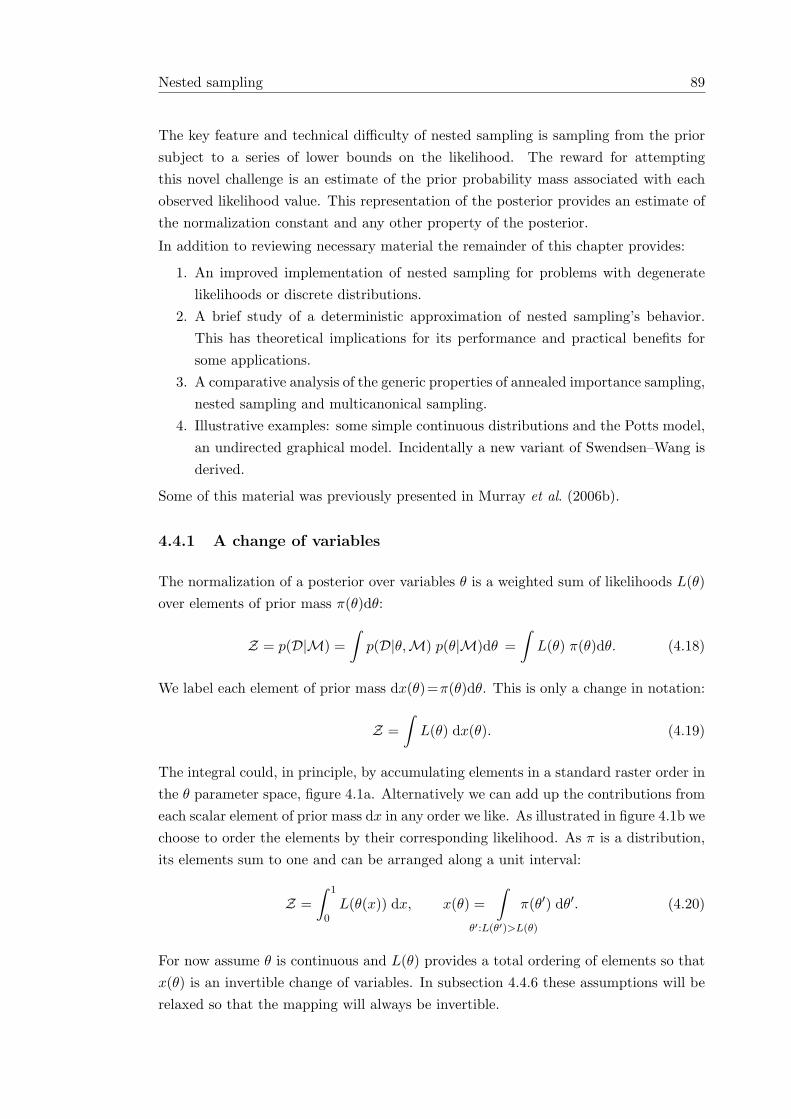
Nested sampling 89
The key feature and technical difficulty of nested sampling is sampling from the priorsubject to a series of lower bounds on the likelihood. The reward for attemptingthis novel challenge is an estimate of the prior probability mass associated with eachobserved likelihood value. This representation of the posterior provides an estimate ofthe normalization constant and any other property of the posterior.
In addition to reviewing necessary material the remainder of this chapter provides:
1. An improved implementation of nested sampling for problems with degeneratelikelihoods or discrete distributions.
2. A brief study of a deterministic approximation of nested sampling’s behavior.This has theoretical implications for its performance and practical benefits forsome applications.
3. A comparative analysis of the generic properties of annealed importance sampling,nested sampling and multicanonical sampling.
4. Illustrative examples: some simple continuous distributions and the Potts model,an undirected graphical model. Incidentally a new variant of Swendsen–Wang isderived.
Some of this material was previously presented in Murray et al. (2006b).
4.4.1 A change of variables
The normalization of a posterior over variables θ is a weighted sum of likelihoods L(θ)over elements of prior mass π(θ)dθ:
Z = p(D|M) =∫
p(D|θ,M) p(θ|M)dθ =∫
L(θ) π(θ)dθ. (4.18)
We label each element of prior mass dx(θ)=π(θ)dθ. This is only a change in notation:
Z =∫
L(θ) dx(θ). (4.19)
The integral could, in principle, by accumulating elements in a standard raster order inthe θ parameter space, figure 4.1a. Alternatively we can add up the contributions fromeach scalar element of prior mass dx in any order we like. As illustrated in figure 4.1b wechoose to order the elements by their corresponding likelihood. As π is a distribution,its elements sum to one and can be arranged along a unit interval:
Z =∫ 1
0L(θ(x)) dx, x(θ) =
∫θ′:L(θ′)>L(θ)
π(θ′) dθ′. (4.20)
For now assume θ is continuous and L(θ) provides a total ordering of elements so thatx(θ) is an invertible change of variables. In subsection 4.4.6 these assumptions will berelaxed so that the mapping will always be invertible.
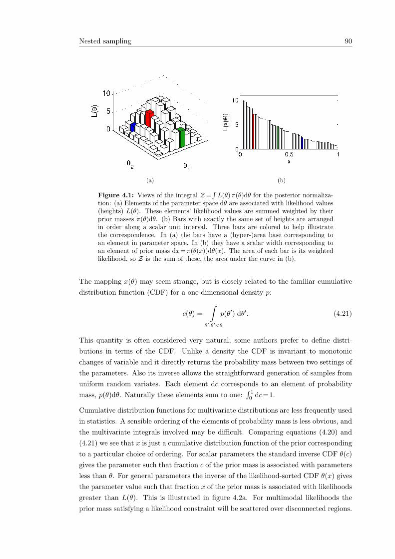
Nested sampling 90
(a) (b)
Figure 4.1: Views of the integral Z=∫
L(θ) π(θ)dθ for the posterior normaliza-tion: (a) Elements of the parameter space dθ are associated with likelihood values(heights) L(θ). These elements’ likelihood values are summed weighted by theirprior masses π(θ)dθ. (b) Bars with exactly the same set of heights are arrangedin order along a scalar unit interval. Three bars are colored to help illustratethe correspondence. In (a) the bars have a (hyper-)area base corresponding toan element in parameter space. In (b) they have a scalar width corresponding toan element of prior mass dx=π(θ(x))dθ(x). The area of each bar is its weightedlikelihood, so Z is the sum of these, the area under the curve in (b).
The mapping x(θ) may seem strange, but is closely related to the familiar cumulativedistribution function (CDF) for a one-dimensional density p:
c(θ) =∫
θ′:θ′<θ
p(θ′) dθ′. (4.21)
This quantity is often considered very natural; some authors prefer to define distri-butions in terms of the CDF. Unlike a density the CDF is invariant to monotonicchanges of variable and it directly returns the probability mass between two settings ofthe parameters. Also its inverse allows the straightforward generation of samples fromuniform random variates. Each element dc corresponds to an element of probabilitymass, p(θ)dθ. Naturally these elements sum to one:
∫ 10 dc=1.
Cumulative distribution functions for multivariate distributions are less frequently usedin statistics. A sensible ordering of the elements of probability mass is less obvious, andthe multivariate integrals involved may be difficult. Comparing equations (4.20) and(4.21) we see that x is just a cumulative distribution function of the prior correspondingto a particular choice of ordering. For scalar parameters the standard inverse CDF θ(c)gives the parameter such that fraction c of the prior mass is associated with parametersless than θ. For general parameters the inverse of the likelihood-sorted CDF θ(x) givesthe parameter value such that fraction x of the prior mass is associated with likelihoodsgreater than L(θ). This is illustrated in figure 4.2a. For multimodal likelihoods theprior mass satisfying a likelihood constraint will be scattered over disconnected regions.
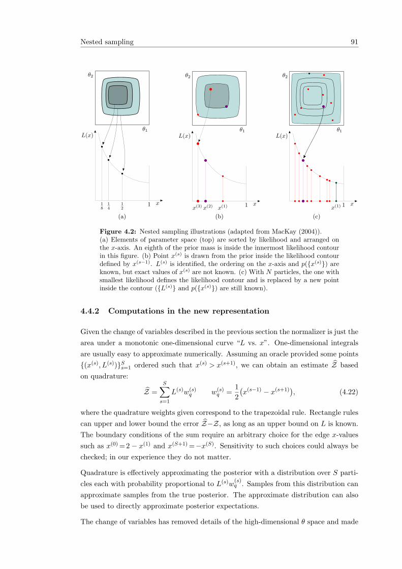
Nested sampling 91
θ1
θ2
x11
2
1
4
1
8
L(x)
(a)
θ1
θ2
x1
L(x)
x(1)
x(2)
x(3)
(b)
θ1
θ2
x1
L(x)
x(1)
(c)
Figure 4.2: Nested sampling illustrations (adapted from MacKay (2004)).(a) Elements of parameter space (top) are sorted by likelihood and arranged onthe x-axis. An eighth of the prior mass is inside the innermost likelihood contourin this figure. (b) Point x(s) is drawn from the prior inside the likelihood contourdefined by x(s−1). L(s) is identified, the ordering on the x-axis and p({x(s)}) areknown, but exact values of x(s) are not known. (c) With N particles, the one withsmallest likelihood defines the likelihood contour and is replaced by a new pointinside the contour ({L(s)} and p({x(s)}) are still known).
4.4.2 Computations in the new representation
Given the change of variables described in the previous section the normalizer is just thearea under a monotonic one-dimensional curve “L vs. x”. One-dimensional integralsare usually easy to approximate numerically. Assuming an oracle provided some points{(x(s), L(s))}Ss=1 ordered such that x(s) > x(s+1), we can obtain an estimate Z basedon quadrature:
Z =S∑
s=1
L(s)w(s)q w(s)
q =12(x(s−1) − x(s+1)
), (4.22)
where the quadrature weights given correspond to the trapezoidal rule. Rectangle rulescan upper and lower bound the error Z−Z, as long as an upper bound on L is known.The boundary conditions of the sum require an arbitrary choice for the edge x-valuessuch as x(0) =2 − x(1) and x(S+1) =−x(S). Sensitivity to such choices could always bechecked; in our experience they do not matter.
Quadrature is effectively approximating the posterior with a distribution over S parti-cles each with probability proportional to L(s)w
(s)q . Samples from this distribution can
approximate samples from the true posterior. The approximate distribution can alsobe used to directly approximate posterior expectations.
The change of variables has removed details of the high-dimensional θ space and made
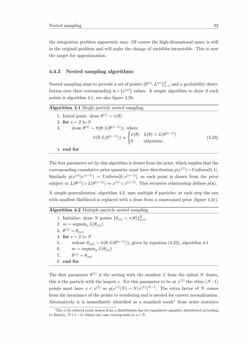
Nested sampling 92
the integration problem apparently easy. Of course the high-dimensional space is stillin the original problem and will make the change of variables intractable. This is nowthe target for approximation.
4.4.3 Nested sampling algorithms
Nested sampling aims to provide a set of points {θ(s), L(s)}Ss=1 and a probability distri-bution over their corresponding x={x(s)} values. A simple algorithm to draw S suchpoints is algorithm 4.1, see also figure 4.2b.
Algorithm 4.1 Single particle nested sampling
1. Initial point: draw θ(1) ∼ π(θ)2. for s = 2 to S
3. draw θ(s) ∼ π(θ;L(θ(s−1))), where
π(θ;L(θ(s−1))) ∝
{π(θ) L(θ) > L(θ(s−1))0 otherwise.
(4.23)
4. end for
The first parameter set by this algorithm is drawn from the prior, which implies that thecorresponding cumulative prior quantity must have distribution p(x(1))=Uniform[0, 1].Similarly p(x(s)|x(s−1)) = Uniform[0, x(s−1)], as each point is drawn from the priorsubject to L(θ(s))>L(θ(s−1))⇒ x(s) <x(s−1). This recursive relationship defines p(x).
A simple generalization, algorithm 4.2, uses multiple θ particles; at each step the onewith smallest likelihood is replaced with a draw from a constrained prior (figure 4.2c).
Algorithm 4.2 Multiple particle nested sampling
1. Initialize: draw N points {θ(n) ∼ π(θ)}Nn=1
2. m = argminn L(θ(n))3. θ(1) = θ(m)
4. for s = 2 to S
5. redraw θ(m) ∼ π(θ;L(θ(s−1))), given by equation (4.23), algorithm 4.16. m = argminn L(θ(n))7. θ(s) = θ(m)
8. end for
The first parameter θ(1) is the setting with the smallest L from the initial N draws,this is the particle with the largest x. For this parameter to be at x(1) the other (N−1)points must have x < x(1) so p(x(1)|N) = N(x(1))N−1. The extra factor of N comesfrom the invariance of the points to reordering and is needed for correct normalization.Alternatively it is immediately identified as a standard result1 from order statistics
1The n-th ordered point drawn from a distribution has its cumulative quantity distributed accordingto Beta(n, N+1−n) where our case corresponds to n=N .
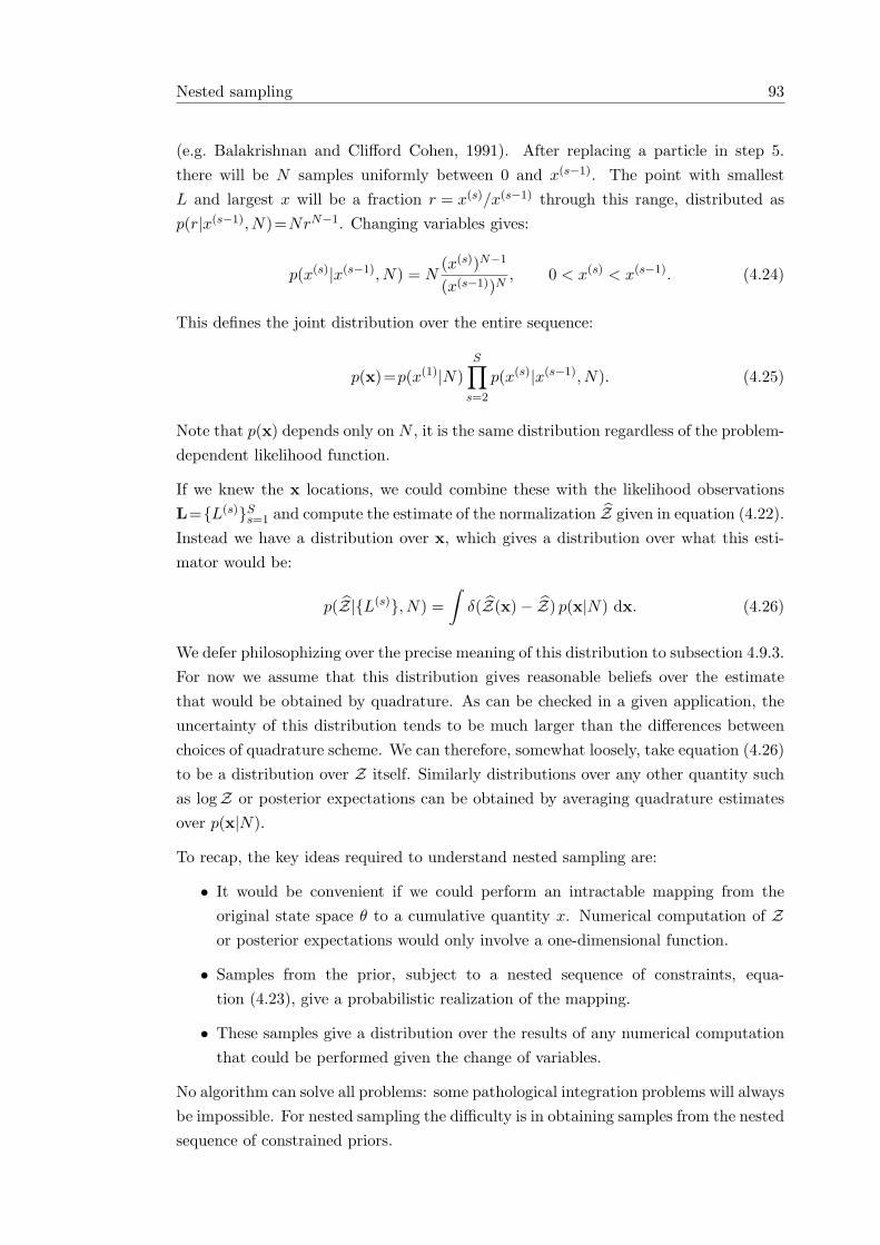
Nested sampling 93
(e.g. Balakrishnan and Clifford Cohen, 1991). After replacing a particle in step 5.there will be N samples uniformly between 0 and x(s−1). The point with smallestL and largest x will be a fraction r = x(s)/x(s−1) through this range, distributed asp(r|x(s−1), N)=NrN−1. Changing variables gives:
p(x(s)|x(s−1), N) = N(x(s))N−1
(x(s−1))N, 0 < x(s) < x(s−1). (4.24)
This defines the joint distribution over the entire sequence:
p(x)=p(x(1)|N)S∏
s=2
p(x(s)|x(s−1), N). (4.25)
Note that p(x) depends only on N , it is the same distribution regardless of the problem-dependent likelihood function.
If we knew the x locations, we could combine these with the likelihood observationsL={L(s)}Ss=1 and compute the estimate of the normalization Z given in equation (4.22).Instead we have a distribution over x, which gives a distribution over what this esti-mator would be:
p(Z|{L(s)}, N) =∫
δ(Z(x)− Z) p(x|N) dx. (4.26)
We defer philosophizing over the precise meaning of this distribution to subsection 4.9.3.For now we assume that this distribution gives reasonable beliefs over the estimatethat would be obtained by quadrature. As can be checked in a given application, theuncertainty of this distribution tends to be much larger than the differences betweenchoices of quadrature scheme. We can therefore, somewhat loosely, take equation (4.26)to be a distribution over Z itself. Similarly distributions over any other quantity suchas logZ or posterior expectations can be obtained by averaging quadrature estimatesover p(x|N).
To recap, the key ideas required to understand nested sampling are:
• It would be convenient if we could perform an intractable mapping from theoriginal state space θ to a cumulative quantity x. Numerical computation of Zor posterior expectations would only involve a one-dimensional function.
• Samples from the prior, subject to a nested sequence of constraints, equa-tion (4.23), give a probabilistic realization of the mapping.
• These samples give a distribution over the results of any numerical computationthat could be performed given the change of variables.
No algorithm can solve all problems: some pathological integration problems will alwaysbe impossible. For nested sampling the difficulty is in obtaining samples from the nestedsequence of constrained priors.
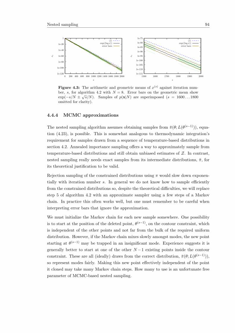
Nested sampling 94
1e-120
1e-100
1e-80
1e-60
1e-40
1e-20
1
0 200 400 600 800 1000 1200 1400 1600 1800 2000
xs
s
〈x〉exp(〈log x〉)
error bars
1e-115
1e-110
1e-105
1e-100
1e-95
1e-90
1e-85
1e-80
1e-75
1500 1600 1700 1800 1900 2000
xs
s
〈x〉exp(〈log x〉)
error bars
Figure 4.3: The arithmetic and geometric means of x(s) against iteration num-ber, s, for algorithm 4.2 with N = 8. Error bars on the geometric mean showexp(−s/N ±
√s/N). Samples of p(x|N) are superimposed (s = 1600 . . . 1800
omitted for clarity).
4.4.4 MCMC approximations
The nested sampling algorithm assumes obtaining samples from π(θ;L(θ(s−1))), equa-tion (4.23), is possible. This is somewhat analogous to thermodynamic integration’srequirement for samples drawn from a sequence of temperature-based distributions insection 4.2. Annealed importance sampling offers a way to approximately sample fromtemperature-based distributions and still obtain unbiased estimates of Z. In contrast,nested sampling really needs exact samples from its intermediate distributions, π, forits theoretical justification to be valid.
Rejection sampling of the constrained distributions using π would slow down exponen-tially with iteration number s. In general we do not know how to sample efficientlyfrom the constrained distributions so, despite the theoretical difficulties, we will replacestep 5 of algorithm 4.2 with an approximate sampler using a few steps of a Markovchain. In practice this often works well, but one must remember to be careful wheninterpreting error bars that ignore the approximation.
We must initialize the Markov chain for each new sample somewhere. One possibilityis to start at the position of the deleted point, θ(s−1), on the contour constraint, whichis independent of the other points and not far from the bulk of the required uniformdistribution. However, if the Markov chain mixes slowly amongst modes, the new pointstarting at θ(s−1) may be trapped in an insignificant mode. Experience suggests it isgenerally better to start at one of the other N−1 existing points inside the contourconstraint. These are all (ideally) draws from the correct distribution, π(θ;L(θ(s−1))),so represent modes fairly. Making this new point effectively independent of the pointit cloned may take many Markov chain steps. How many to use is an unfortunate freeparameter of MCMC-based nested sampling.
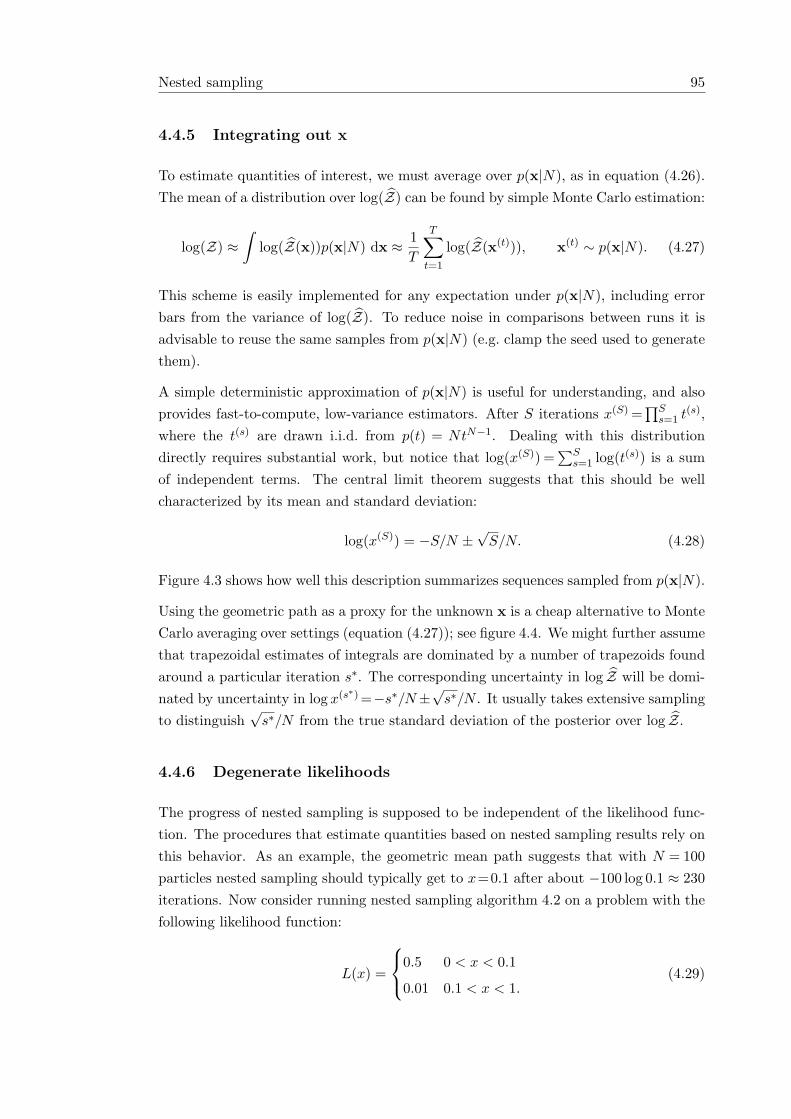
Nested sampling 95
4.4.5 Integrating out x
To estimate quantities of interest, we must average over p(x|N), as in equation (4.26).The mean of a distribution over log(Z) can be found by simple Monte Carlo estimation:
log(Z) ≈∫
log(Z(x))p(x|N) dx ≈ 1T
T∑t=1
log(Z(x(t))), x(t) ∼ p(x|N). (4.27)
This scheme is easily implemented for any expectation under p(x|N), including errorbars from the variance of log(Z). To reduce noise in comparisons between runs it isadvisable to reuse the same samples from p(x|N) (e.g. clamp the seed used to generatethem).
A simple deterministic approximation of p(x|N) is useful for understanding, and alsoprovides fast-to-compute, low-variance estimators. After S iterations x(S) =
∏Ss=1 t(s),
where the t(s) are drawn i.i.d. from p(t) = NtN−1. Dealing with this distributiondirectly requires substantial work, but notice that log(x(S)) =
∑Ss=1 log(t(s)) is a sum
of independent terms. The central limit theorem suggests that this should be wellcharacterized by its mean and standard deviation:
log(x(S)) = −S/N ±√
S/N. (4.28)
Figure 4.3 shows how well this description summarizes sequences sampled from p(x|N).
Using the geometric path as a proxy for the unknown x is a cheap alternative to MonteCarlo averaging over settings (equation (4.27)); see figure 4.4. We might further assumethat trapezoidal estimates of integrals are dominated by a number of trapezoids foundaround a particular iteration s∗. The corresponding uncertainty in log Z will be domi-nated by uncertainty in log x(s∗) =−s∗/N±
√s∗/N . It usually takes extensive sampling
to distinguish√
s∗/N from the true standard deviation of the posterior over log Z.
4.4.6 Degenerate likelihoods
The progress of nested sampling is supposed to be independent of the likelihood func-tion. The procedures that estimate quantities based on nested sampling results rely onthis behavior. As an example, the geometric mean path suggests that with N = 100particles nested sampling should typically get to x=0.1 after about −100 log 0.1 ≈ 230iterations. Now consider running nested sampling algorithm 4.2 on a problem with thefollowing likelihood function:
L(x) =
0.5 0 < x < 0.1
0.01 0.1 < x < 1.(4.29)
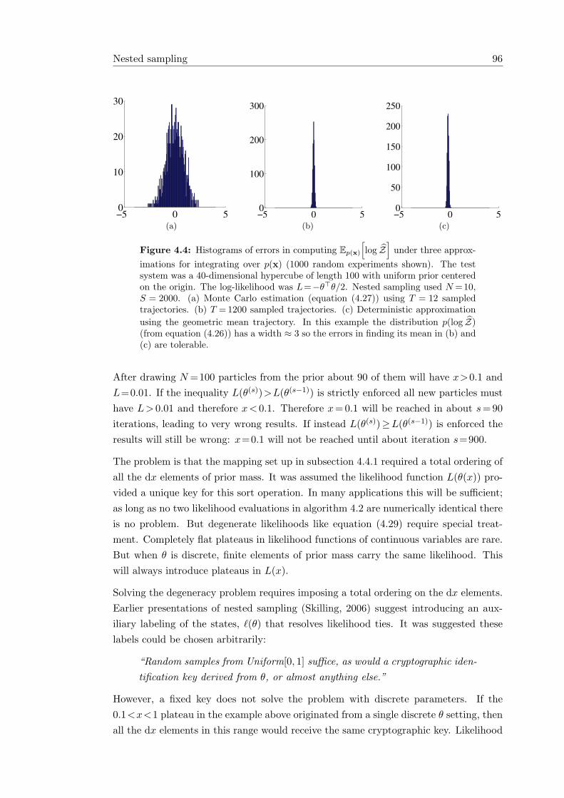
Nested sampling 96
−5 0 50
10
20
30
(a)
−5 0 50
100
200
300
(b)
−5 0 50
50
100
150
200
250
(c)
Figure 4.4: Histograms of errors in computing Ep(x)
[log Z
]under three approx-
imations for integrating over p(x) (1000 random experiments shown). The testsystem was a 40-dimensional hypercube of length 100 with uniform prior centeredon the origin. The log-likelihood was L=−θ>θ/2. Nested sampling used N =10,S = 2000. (a) Monte Carlo estimation (equation (4.27)) using T = 12 sampledtrajectories. (b) T = 1200 sampled trajectories. (c) Deterministic approximationusing the geometric mean trajectory. In this example the distribution p(log Z)(from equation (4.26)) has a width ≈ 3 so the errors in finding its mean in (b) and(c) are tolerable.
After drawing N =100 particles from the prior about 90 of them will have x>0.1 andL=0.01. If the inequality L(θ(s))>L(θ(s−1)) is strictly enforced all new particles musthave L> 0.01 and therefore x< 0.1. Therefore x=0.1 will be reached in about s=90iterations, leading to very wrong results. If instead L(θ(s))≥L(θ(s−1)) is enforced theresults will still be wrong: x=0.1 will not be reached until about iteration s=900.
The problem is that the mapping set up in subsection 4.4.1 required a total ordering ofall the dx elements of prior mass. It was assumed the likelihood function L(θ(x)) pro-vided a unique key for this sort operation. In many applications this will be sufficient;as long as no two likelihood evaluations in algorithm 4.2 are numerically identical thereis no problem. But degenerate likelihoods like equation (4.29) require special treat-ment. Completely flat plateaus in likelihood functions of continuous variables are rare.But when θ is discrete, finite elements of prior mass carry the same likelihood. Thiswill always introduce plateaus in L(x).
Solving the degeneracy problem requires imposing a total ordering on the dx elements.Earlier presentations of nested sampling (Skilling, 2006) suggest introducing an aux-iliary labeling of the states, `(θ) that resolves likelihood ties. It was suggested theselabels could be chosen arbitrarily:
“Random samples from Uniform[0, 1] suffice, as would a cryptographic iden-tification key derived from θ, or almost anything else.”
However, a fixed key does not solve the problem with discrete parameters. If the0.1<x<1 plateau in the example above originated from a single discrete θ setting, thenall the dx elements in this range would receive the same cryptographic key. Likelihood
Nested sampling 97
ties would still be unresolved. If random labels are employed and always regenerated onrepeated observations of the same θ then nested sampling will give the correct results.This is how the code Skilling has made available is implemented2.
Skilling (2007) mentions a better way of thinking about the random ‘labels’. Insteadof an extra piece of information attached to each parameter setting, ` is an extrainput variable for an extended problem with a likelihood that depends on θ and `.The distinction may seem fine: on large problems the same θ location will rarely berevisited. But getting this right is important for obtaining correct answers on small testproblems. The joint distribution view also allows a rejectionless algorithm for the Pottsexample in subsection 4.8.3, which was (tersely) introduced in Murray et al. (2006b).
The auxiliary joint distribution is over the variables of interest θ and an independentvariable ` ∈ [0, 1]:
p(θ, `) = p(θ) · p(`) =1Z
L(θ)π(θ) · 1Z`
L0(`)π0(`)
=1Z
LJ(θ, `)π(θ),(4.30)
where LJ(θ, `)=L(θ)L0(`), L0(`)=1+ ε(`−0.5), π0(`)=1 and Z` =1. Standard nestedsampling is now possible. At each iteration LJ(θ, `) must increase. We can choose ε
such that log(ε) is smaller than the smallest difference in log(L(θ)) allowed by machineprecision. This ensures the auxiliary variable ` will only matter when L(θ)=L(θ(s−1)).The constrained-prior distribution becomes
πJ(θ, `; θ(s−1), `(s−1)) ∝
π(θ) L(θ) > L(θ(s−1))
π(θ) L(θ) = L(θ(s−1)) and ` > `(s−1)
0 otherwise.
(4.31)
MCMC-based implementations of nested sampling require transition operators thatleave πJ stationary. The simplest method is to propose θ with an operator that leavesthe original π constrained prior stationary and then generate `∼Uniform[0, 1], rejectingthe proposal if `<`(s−1).
A rejectionless method would be preferable and is sometimes possible by marginalizingout `
πm(θ; {θ, `}(s−1)) ∝
π(θ) L(θ) > L(θ(s−1))
π(θ)(1− `(s−1)) L(θ) = L(θ(s−1))
0 otherwise.
(4.32)
If the operator used for π was slice sampling (subsection 2.4.2), then πm can alsobe slice sampled directly. Similarly a Gibbs sampler could easily be adapted to usethe conditionals of πm instead of π. If Metropolis–Hastings proposals are used it will
2Available from http://www.inference.phy.cam.ac.uk/bayesys/
Efficiency of the algorithms 98
sometimes be possible to re-weight q(θ′ ← θ) to reduce or eliminate rejections. Anexample of such a transition operator is developed in subsection 4.8.3.
After generating θ(s) the auxiliary variable `(s) can be drawn from its conditional dis-tribution
π(`(s)|θ(s); {θ, `}(s−1)) =
Uniform[0, 1] L(θ(s)) > L(θ(s−1))
Uniform[`(s−1), 1] L(θ(s)) = L(θ(s−1)).(4.33)
As a minor refinement this could be done lazily if and when it is required by the nextiteration.
4.5 Efficiency of the algorithms
This section attempts to compare the computational efficiency of three significant al-gorithms for estimating normalizing constants. General comparisons of Monte Carloalgorithms are hard to make as they are designed for use with problems where groundtruth is unavailable. Also some algorithms are targeted at a particular class of problem,making performance comparisons on other classes unfair.
All three normalizing constant methods considered below are designed to deal withproblems in which the base measure π(θ) is much more diffuse than the compact targetdistribution pt(θ). We look at the scaling of computational cost with the nature of thisdisparity. The behavior of a multivariate Gaussian toy problem is worked out for eachalgorithm. The base distribution π is vaguely distributed with precision τπ,
π(θ) =1Zπ
exp
(−τπ
2
D∑d=1
θ2d
). (4.34)
The target distribution pt has higher precision τt,
pt(θ) =1Zt
exp
(−τt
2
D∑d=1
θ2d
)
=Zπ
Ztπ(θ)L(θ), L(θ) = exp
(−τt − τπ
2
D∑d=1
θ2d
).
(4.35)
We pretend that the normalization constants of the Gaussians are unknown and requireall of the algorithms under study to return an approximation to the (log of the) ratioZt/Zπ =(τt/τπ)(D/2).
Many continuous distributions have locally-Gaussian peaks, so poor performance onthe toy problem would be a general cause for concern. We also make some generalremarks relevant to non-Gaussian modes. Despite this the theoretical comparison pre-sented here is necessarily limited: unreasonable assumptions are made regarding the
Efficiency of the algorithms 99
ability to draw samples from intermediate distributions. Obviously this doesn’t test theability of the algorithms to find and then fairly represent isolated modes. This will beprobed in the empirical comparisons in the sections that follow. For now the analysisis confined to behavior that does not require details of particular Markov chains usedin implementations.
4.5.1 Nested sampling
The scaling behavior of nested sampling can be found without detailed calculation. Thealgorithm is characterized by an exponential shrinkage of the prior mass under consid-eration. If the bulk of the posterior mass is found around x∗, then an N -particle nestedsampling run reaches dominant terms in the integral after s∗ = −N log x∗ iterations.Subsection 4.4.5 explained that the uncertainty in logZ is typically ±
√s∗/N .
Obtaining a unit uncertainty in logZ would require setting the number of particlesto N =
√s∗. For this choice the number of iterations required to reach the target
distribution’s mass from the prior is s∗=(log x∗)2.
Most of a high-dimensional Gaussian’s mass is within a hyper-spherical shell out ata radius of
√D/τ . This means that the bulk of the target distribution is in a shell
enclosing a fraction ∼ (τπ/τt)D of the prior volume. If the prior were uniform thenwe could immediately say that the bulk of the target distribution is found aroundx∗ ≈ (τπ/τt)D. It turns out3 that this is a good enough description for Gaussianstoo: log x∗ ≈−D log τt/τπ. Therefore, the s∗ = (log x∗)2 computational cost of nestedsampling on the toy problem is:
Number of samples for unit error, s∗ ≈ D2 (log τt/τπ)2 . (4.36)
The O(D2) scaling revealed by this analysis is somewhat disappointing. If each sam-ple costs O(D) to produce then the total cost for a unit error is O(D3). If oneknew that each dimension were independent one could estimate the log-normalizerof each Gaussian separately. Making the D estimates have variance 1/D would require≈ D (log τt/τπ)2 samples each. But samples of just one variable only cost O(1) com-putation, which gives a total cost of O(D2) rather than O(D3). The reason to resortto Monte Carlo is that real computations do not decompose this way. But we shallsee that without detailed knowledge of the distribution annealing does only need O(D)iterations. The advantages of nested sampling do come at a cost.
3According to the χ2 cumulative distribution function the log-cumulative prior mass inside a radiusof
pD/τt is log γ(D/2,(Dτπ)/(2τt))
Γ(D/2), which numerically matches the scaling of −D log τt/τπ to within a
small factor over a large range of τπ/τt and D.
Efficiency of the algorithms 100
4.5.2 Multicanonical sampling
As there are many possible algorithms for constructing an approximate multicanonicalensemble a general comparison to ‘the’ method is hard. Instead we generously assumethat we have obtained (by chance) the ideal function that reweights the target distribu-tion such that the distribution over energy is uniform. This avoids having to considerthe details of histogram-building methods or other energy density approximations. Thedanger is that this section’s results may be severely misleading if the dominant com-putational cost is actually obtaining the reweighting. The analysis here should be seenas a lower bound of the costs involved and could be useful for indicating which methodis best for refining initial results, however they were obtained.
By definition the multicanonical ensemble has a uniform marginal distribution over en-ergy. To be defined this distribution must be confined to some finite range, width H say,so pMC(E(θ))=1/H. This ensemble could be used to compute the normalizing constantof a simple target distribution, ps, which also has a uniform energy distribution butover an energy range with smaller width h. The importance weights, equation (4.16),are a constant with probability h/H and zero otherwise. This distribution gives
var[log ∆(ps)] ≈H
Sh(4.37)
after S (effective) samples. Empirically the estimator still exhibits quite heavy tailsafter the S =H/h samples predicted for unit error, but the expression gives good errorbars for larger S. Finding effective widths corresponding to H and h will provide arule-of-thumb estimate of multicanonical’s variance on more complex distributions.
We now derive properties of the multicanonical ensemble for the Gaussian problem.Under the target multivariate Gaussian the energy is
E(θ) = − log L(θ) =τt − τπ
2
D∑d=1
θ2d =
τt − τπ
2R, (4.38)
which is proportional to R =∑D
d=1 θ2d. The square-radius R follows a scaled χ2-
distribution with D degrees of freedom: p(R) ∝ RD/2−1 exp(−τtR/2). Weighting bythe reciprocal of p(R) makes the distribution over R and the energy uniform, givingthe multicanonical ensemble:
p∗MC(θ) ∝ p∗(θ) · wMC(θ)
∝ e−τtR(θ)/2 ·R(θ)1−D/2eτtR(θ)/2
∝ R(θ)1−D/2 0 < R(θ) < R(H).
(4.39)
A maximum energy, H must be imposed for the distribution to be defined. A reasonablechoice for the square radius defining this limit is 4σ larger than the prior mean value:R(H)=(D+4
√2D)/τπ. This cut-off excludes little of the prior mass from the ensemble.
Efficiency of the algorithms 101
The target distribution is softly confined to a narrow range of the energy spectrum withan effective width likely to be related to the standard deviation of a χ2-distribution:R(heff)∼
√2D/τt.
While the exact variance of the estimator does not have a simple analytical form, amore detailed analysis4 shows that the guess H/(Sheff)=R(H)/(SR(heff) is basicallycorrect:
var[logZt
]≈ 1
S
τt
τπ
√D
8π. (4.45)
Astoundingly the number of effective samples required to obtain a unit error scales onlyas O(
√D). This is better than possible by a method that exploited independence and
estimated the normalizer of each of the D Gaussians separately. Perhaps this is a signthat through the weighting function the method has unreasonable a priori knowledgeof the answer.
Despite the ideal weighting function the scaling with precision ratio τt/τπ is not impres-sive. As the target distribution’s precision grows the multicanonical sampler becomesexponentially worse than nested sampling, equation (4.36). This is a clear indicationthat the energy spectrum ratio H/heff can be quite different from the volume ratio thatdetermines nested sampling’s performance. The details of a particular target distribu-tion can make either method dramatically better than the other.
Another concern is the cost of each of the S effective samples. The ensemble pMC isa distribution capturing a large energy range which will usually take many steps ofMCMC exploration to reach equilibrium. In contrast the intermediate distributions ofnested sampling or annealing were designed to be close, so a small number of MCMCsteps may be sufficient to equilibrate states at each iteration. The log-probability of
4
The variance of the two parts (equation (4.16)) of the multicanonical estimator (equation (4.17)) can beapproximated as follows:
var[log ∆(τ)] ≈var[w∗τ ]
S E[w∗τ ]2≈
Eˆw∗τ
2˜
S E[w∗τ ]2(4.40)
The ratio of the target distribution, equation (4.35), and multicanonical distribution, equation (4.39),give importance weights:
w∗τ (θ) = R(θ)D/2−1 exp(−τR(θ)/2). (4.41)
Noting the integralsZ ∞
0w∗τ (R) dR =
2D/2Γ(D/2)
τD/2and
Z ∞
0w∗τ (R)2 dR = τ1−DΓ(D − 1), (4.42)
and that, for suitably large H, these give approximately R(H) times the required expectations we have
var[log ∆(τ)] ≈R(H)τΓ(D − 1)
S2D(Γ(D/2))2≈
R(H)τ
Sp
8π(D − 2)(Stirling’s approx. to both Γ functions). (4.43)
Substituting in R(H), assuming large D and using the approximate independence of the separate log ∆estimators when τt�τπ gives the variance of the final estimator as
varhlogZt
i≈
τt/τπ + 1
S
rD
8π+
2√
π
!. (4.44)
The version in the main text drops further terms for clarity. This footnote is terse because what mattersis the simpler H/heff description in the main text and the following assertion: empirically the expressionabove reasonably matches the observed estimator variance for τt�τπ in a few or more dimensions.
Efficiency of the algorithms 102
pMC has a range of∆EMC = (1−D/2) log τt/τπ (4.46)
between the typical sets of the target and prior distributions. If O(1) iterations ofMCMC are required to change this energy by 1, then it will take at least O(∆E2
MC)iterations to equilibrate the multicanonical ensemble by a random walk. This wouldmake the cost of a obtaining a single effective sample from the multicanonical ensemblethe same order as the total cost of an entire nested sampling run! The potentiallygood performance of the multicanonical method can be wiped out by the use of somestandard Markov chains.
4.5.3 Importance sampling
We now analyze the performance of combining a bridge of K+1 importance samplingestimates as in section 4.2. For the toy Gaussian problem all the intermediate distri-butions are also Gaussian,
pk(θ) =1Zk
π(θ)L(θ)βk
=1Zk
exp
(−τk
2
D∑d=1
θ2d
), τk = (1− β)τπ + βτt.
(4.47)
This allows computation of the variance of the estimator in equation (4.10) under theideal case of direct sampling from each pk.
The log of the importance weights at each level from equation (4.6) become
log w∗k(θ) =τk − τk+1
2
D∑d=1
θ2d. (4.48)
The variance of the log weights under pk is
varpk[log w∗k] =
(τk − τk+1)2
4varpk
[D∑
d=1
θ2d
]=
(τk − τk+1)2
42D
τ2k
=D
2
(1− τk+1
τk
)2
.
(4.49)
The variance of log w∗k only depends on k through the ratio αk = τk+1/τk. The varianceof logZ =
∑Kk=0 log w∗k(θk), is minimized by equalizing all the contributing variances,
αk =α=(τt/τπ)1/(K+1). The resulting estimator has variance
var[log Z
]=
D(K + 1)2
(1−
(τt
τπ
)1/(K+1))2
≈ D
2(K + 1)
(log
τt
τπ
)2
, for large K.
(4.50)
Constructing annealing schedules 103
The approximation becomes accurate very quickly. The amount of computation (∝K+1) required for unit variance scales with dimensionality of the problem as O(D):
Number of samples for unit error, (K+1) ≈ D
2(log τt/τπ)2 . (4.51)
Comparing to equation (4.36) we see that the τ -dependence of the computational costis the same as nested sampling and that the scaling with dimensionality is better. Thisresult is not strongly tied to the tail behavior of a Gaussian. Redoing the calculationsfor distributions p∗ ∝ exp(−τ/2
∑d |θd|p) only changes the number of samples required
slightly to (D/p)(log τt/τπ)2.
Before hastily discarding nested sampling, remember the caveats at the beginning ofthis section. Practical realities of Markov chain based samplers will make performanceworse than predicted here. The Potts model (subsection 1.1.3) will be an example ofa distribution, which while easily sampled by multicanonical and nested sampling, istotally unapproachable with temperature-based annealing methods.
As with multicanonical sampling we were very generous to annealing by assumingthe free parameters defining the annealing schedule were chosen optimally. We wereunlikely to guess
βk+1 =τπ(α− 1)τt − τπ
+ αβk, α =(
τt
τπ
)1/(K+1)
. (4.52)
Indeed the optimal schedule balances variances, which through equation (4.12) areintimately related to Z itself. We cannot know the optimal schedule without alreadyhaving solved the problem.
Some work is required to find a good schedule; default choices may not be sufficient.For example, the linear annealing schedule βk =k/(K + 1) gives5
varβk=k/(K+1)
[logZ
]≈ D
2K
(τt − τπ)2
τtτπ. (4.53)
For large τt this is exponentially worse than the correct schedule and nested sampling.
4.6 Constructing annealing schedules
Various families of annealing schedule have been used in the literature. While demon-strating AIS on some example distributions, Neal (2001) spliced together a linear sched-ule at high temperatures with a geometric schedule at lower temperatures. This is nottoo far from the behavior of equation (4.52), the optimal schedule for some well-behaved
5Found by a large-K integral approximation to the discrete sum over equation (4.49) and alsochecked numerically.
Constructing annealing schedules 104
posteriors. Beal (2003) suggested a family of non-linear annealing schedules
βk =eτk/K
eτ + 1− k/K, (4.54)
where the “linearity parameter” eτ makes the schedule approximately linear for largevalues of eτ but dwells for longer at high temperatures for small positive values. An-other ad hoc non-linear scheme is given by Kuss and Rasmussen (2005), where a linearschedule is raised to the power of four: βk = (k/K)4, k=0 . . .K.
Each of the above schemes were presumably the result of some experimentation. Pre-liminary runs are required to check that a proposed schedule, e.g. “fourth power of alinear schedule”, is adequate and to eliminate others. Also any free parameters mustbe found, such as the number of levels, linearity setting eτ or the change-point betweena linear and geometric schedule. Algorithms for these fitting procedures could be, al-though rarely are, described in detail. Part of the difficulty is deciding how to includeresults from earlier, higher variance runs. Often these are only run informally and sim-ply discarded. Regardless of how an annealing schedule is chosen, the selection shouldideally be performed automatically. Otherwise computer time may become irrelevantcompared to the time required by manual adjustments.
An annealing schedule should control the variance of the log weights,
varβk[log w∗k] = (βk+1 − βk)2 varβk
[log L(θ)] . (4.55)
Rearranging gives a recurrence relationship for the inverse temperatures,
βk+1 = βk +√
v
varβk[log L(θ)]
, (4.56)
which achieves a given target variance v = var[log w∗] on each weight. This updaterule is applied from β0 =0 until an inverse temperature of 1 is reached. The varianceof the logZ estimator, equation (4.10), is (K +1)v. A binary search on the controlparameter v can find a balanced annealing schedule with a user chosen total varianceor computational cost.
Implementing this algorithm for constructing annealing schedules requires the varianceof the log-likelihood or energy at each βk considered. These quantities are not availableexactly, otherwise logZ would be known, so the variances must be approximated fromsome preliminary experiments. Running MCMC at each βk considered would be toocostly. One could try to interpolate results measured at a preliminary range of tem-peratures. Alternatively statistics at any temperature are available from a single runof either multicanonical or nested sampling.
We propose using nested sampling to set a schedule for AIS. The details are given inalgorithm 4.3. Sampling from the multicanonical ensemble would need a large set of
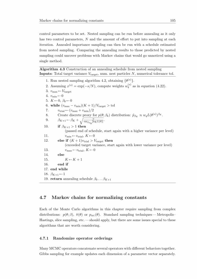
Markov chains for normalizing constants 105
control parameters to be set. Nested sampling can be run before annealing as it onlyhas two control parameters, N and the amount of effort to put into sampling at eachiteration. Annealed importance sampling can then be run with a schedule estimatedfrom nested sampling. Comparing the annealing results to those predicted by nestedsampling could uncover problems with Markov chains that would go unnoticed using asingle method.
Algorithm 4.3 Construction of an annealing schedule from nested samplingInputs: Total target variance Vtarget, num. nest particles N , numerical tolerance tol.
1. Run nested sampling algorithm 4.2, obtaining {θ(s)}.2. Assuming x(s) = exp(−s/N), compute weights w
(s)q as in equation (4.22).
3. vmax←Vtarget
4. vmin←05. K←0, β0←06. while (vmax − vmin)(K + 1)/Vtarget > tol7. vtrial←(vmax + vmin)/28. Create discrete proxy for p(θ;βk) distribution: pβK
∝ wqL(θ(s))βK .9. βK+1←βK +
√v
varpβK[log L(θ)] .
10. if βK+1 > 1 then(passed end of schedule, start again with a higher variance per level)
11. vmin←vtrial, K←012. else if (K + 1)vtrial > Vtarget then
(exceeded target variance, start again with lower variance per level)13. vmax←vtrial, K←014. else15. K←K + 116. end if17. end while18. βK+1←119. return annealing schedule β0 . . . βK+1
4.7 Markov chains for normalizing constants
Each of the Monte Carlo algorithms in this chapter require sampling from complexdistributions: p(θ;β), π(θ) or pMC(θ). Standard sampling techniques — Metropolis–Hastings, slice sampling, etc. — should apply, but there are some issues special to thesealgorithms that are worth considering.
4.7.1 Randomize operator orderings
Many MCMC operators concatenate several operators with different behaviors together.Gibbs sampling for example updates each dimension of a parameter vector separately.
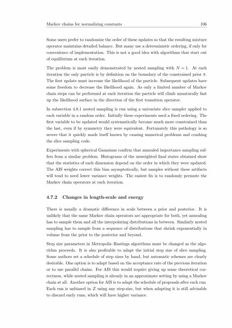
Markov chains for normalizing constants 106
Some users prefer to randomize the order of these updates so that the resulting mixtureoperator maintains detailed balance. But many use a deterministic ordering, if only forconvenience of implementation. This is not a good idea with algorithms that start outof equilibrium at each iteration.
The problem is most easily demonstrated by nested sampling with N = 1. At eachiteration the only particle is by definition on the boundary of the constrained prior π.The first update must increase the likelihood of the particle. Subsequent updates havesome freedom to decrease the likelihood again. As only a limited number of Markovchain steps can be performed at each iteration the particle will climb unnaturally fastup the likelihood surface in the direction of the first transition operator.
In subsection 4.8.1 nested sampling is run using a univariate slice sampler applied toeach variable in a random order. Initially these experiments used a fixed ordering. Thefirst variable to be updated would systematically become much more constrained thanthe last, even if by symmetry they were equivalent. Fortunately this pathology is sosevere that it quickly made itself known by causing numerical problems and crashingthe slice sampling code.
Experiments with spherical Gaussians confirm that annealed importance sampling suf-fers from a similar problem. Histograms of the unweighted final states obtained showthat the statistics of each dimension depend on the order in which they were updated.The AIS weights correct this bias asymptotically, but samples without these artifactswill tend to need lower variance weights. The easiest fix is to randomly permute theMarkov chain operators at each iteration.
4.7.2 Changes in length-scale and energy
There is usually a dramatic difference in scale between a prior and posterior. It isunlikely that the same Markov chain operators are appropriate for both, yet annealinghas to sample them and all the interpolating distributions in between. Similarly nestedsampling has to sample from a sequence of distributions that shrink exponentially involume from the prior to the posterior and beyond.
Step size parameters in Metropolis–Hastings algorithms must be changed as the algo-rithm proceeds. It is also profitable to adapt the initial step size of slice sampling.Some authors set a schedule of step sizes by hand, but automatic schemes are clearlydesirable. One option is to adapt based on the acceptance rate of the previous iterationor to use parallel chains. For AIS this would require giving up some theoretical cor-rectness, while nested sampling is already in an approximate setting by using a Markovchain at all. Another option for AIS is to adapt the schedule of proposals after each run.Each run is unbiased in Z using any step-size, but when adapting it is still advisableto discard early runs, which will have higher variance.
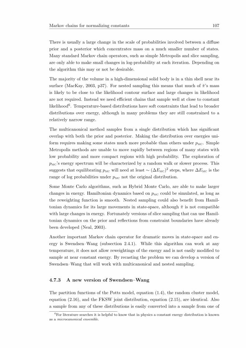
Markov chains for normalizing constants 107
There is usually a large change in the scale of probabilities involved between a diffuseprior and a posterior which concentrates mass on a much smaller number of states.Many standard Markov chain operators, such as simple Metropolis and slice sampling,are only able to make small changes in log-probability at each iteration. Depending onthe algorithm this may or not be desirable.
The majority of the volume in a high-dimensional solid body is in a thin shell near itssurface (MacKay, 2003, p37). For nested sampling this means that much of π’s massis likely to be close to the likelihood contour surface and large changes in likelihoodare not required. Instead we need efficient chains that sample well at close to constantlikelihood6. Temperature-based distributions have soft constraints that lead to broaderdistributions over energy, although in many problems they are still constrained to arelatively narrow range.
The multicanonical method samples from a single distribution which has significantoverlap with both the prior and posterior. Making the distribution over energies uni-form requires making some states much more probable than others under pMC. SimpleMetropolis methods are unable to move rapidly between regions of many states withlow probability and more compact regions with high probability. The exploration ofpMC’s energy spectrum will be characterized by a random walk or slower process. Thissuggests that equilibrating pMC will need at least ∼ (∆EMC)2 steps, where ∆EMC is therange of log probabilities under pMC not the original distribution.
Some Monte Carlo algorithms, such as Hybrid Monte Carlo, are able to make largerchanges in energy. Hamiltonian dynamics based on pMC could be simulated, as long asthe reweighting function is smooth. Nested sampling could also benefit from Hamil-tonian dynamics for its large movements in state-space, although π is not compatiblewith large changes in energy. Fortunately versions of slice sampling that can use Hamil-tonian dynamics on the prior and reflections from constraint boundaries have alreadybeen developed (Neal, 2003).
Another important Markov chain operator for dramatic moves in state-space and en-ergy is Swendsen–Wang (subsection 2.4.1). While this algorithm can work at anytemperature, it does not allow reweightings of the energy and is not easily modified tosample at near constant energy. By recasting the problem we can develop a version ofSwendsen–Wang that will work with multicanonical and nested sampling.
4.7.3 A new version of Swendsen–Wang
The partition functions of the Potts model, equation (1.4), the random cluster model,equation (2.16), and the FKSW joint distribution, equation (2.15), are identical. Alsoa sample from any of these distributions is easily converted into a sample from one of
6For literature searches it is helpful to know that in physics a constant energy distribution is knownas a microcanonical ensemble.
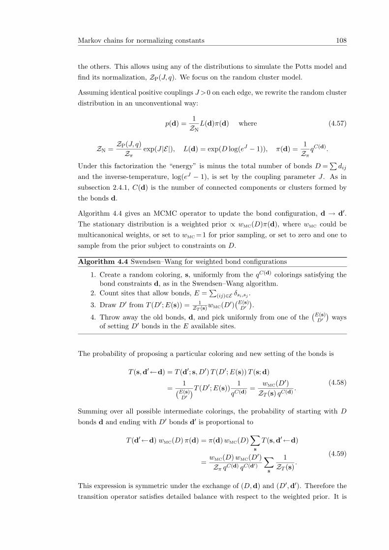
Markov chains for normalizing constants 108
the others. This allows using any of the distributions to simulate the Potts model andfind its normalization, ZP(J, q). We focus on the random cluster model.
Assuming identical positive couplings J >0 on each edge, we rewrite the random clusterdistribution in an unconventional way:
p(d) =1ZN
L(d)π(d) where (4.57)
ZN =ZP(J, q)Zπ
exp(J |E|), L(d) = exp(D log(eJ − 1)), π(d) =1Zπ
qC(d).
Under this factorization the “energy” is minus the total number of bonds D =∑
dij
and the inverse-temperature, log(eJ − 1), is set by the coupling parameter J . As insubsection 2.4.1, C(d) is the number of connected components or clusters formed bythe bonds d.
Algorithm 4.4 gives an MCMC operator to update the bond configuration, d → d′.The stationary distribution is a weighted prior ∝ wMC(D)π(d), where wMC could bemulticanonical weights, or set to wMC =1 for prior sampling, or set to zero and one tosample from the prior subject to constraints on D.
Algorithm 4.4 Swendsen–Wang for weighted bond configurations
1. Create a random coloring, s, uniformly from the qC(d) colorings satisfying thebond constraints d, as in the Swendsen–Wang algorithm.
2. Count sites that allow bonds, E =∑
(ij)∈E δsi,sj .
3. Draw D′ from T (D′;E(s)) = 1ZT (s)wMC(D′)
(E(s)D′
).
4. Throw away the old bonds, d, and pick uniformly from one of the(E(s)
D′
)ways
of setting D′ bonds in the E available sites.
The probability of proposing a particular coloring and new setting of the bonds is
T (s,d′←d) = T (d′; s, D′) T (D′;E(s))T (s;d)
=1(E(s)D′
)T (D′;E(s))1
qC(d)=
wMC(D′)ZT (s) qC(d)
.(4.58)
Summing over all possible intermediate colorings, the probability of starting with D
bonds d and ending with D′ bonds d′ is proportional to
T (d′←d) wMC(D) π(d) = π(d) wMC(D)∑s
T (s,d′←d)
=wMC(D) wMC(D′)Zπ qC(d) qC(d′)
∑s
1ZT (s)
.(4.59)
This expression is symmetric under the exchange of (D,d) and (D′,d′). Therefore thetransition operator satisfies detailed balance with respect to the weighted prior. It is
Experiments 109
also ergodic. Proof: with finite probability all si are given the same color, then any D′
with non-zero weight is possible, in turn all allowable d′ have finite probability.
When performing nested sampling using the weighted prior representation the likeli-hood constraints in π are thresholds on the total number of bonds D. This can berealized by setting wMC =0 for states with fewer bonds. Many states have identical D,which requires careful treatment, as discussed in subsection 4.4.6. The simple imple-mentation that draws a random key for each state will lead to some rejections whenproposing moves to a state with the same D on the constraint surface. Sampling with-out rejections can be achieved by setting the weights such that algorithm 4.4 leaves theauxiliary constrained distribution πm, equation (4.32), invariant.
The number of bonds has previously been identified as a useful energy-like target forreweighting (Janke and Kappler, 1995). In that work the bonds were updated by singlesite Gibbs sampling rather than the block-Gibbs sampling move of step 4. This doesnot allow simulation of the fixed D ensemble, or rapid exploration near fixed D. Singlesite updates are easier to implement however, and would become more attractive onsystems that allow a different Jij on each edge. In this case the implementation ofglobal updates is much more involved.
4.8 Experiments
Detailed comparisons of nested sampling and more established Monte Carlo techniquesare not currently available in the literature. Anecdotally, nested sampling has alreadybeen useful in astronomy. Mukherjee et al. (2006) and Shaw et al. (2007) claim nestedsampling gives speed-ups of 1–2 orders of magnitude over annealing based methods.The annealing approach that was cited in both papers was very carefully implemented(Beltran et al., 2005). These results are somewhat surprising given that both nestedsampling and annealing follow a sequence of increasingly constrained ensembles andtheoretically seem quite similar. If anything nested sampling seems slightly worse,although this should be a small effect for the D = 5 astronomy problems that weretested.
The focus of this section is not applications, but well understood test problems. Hope-fully these will give some better insight into the relative merits of the approaches.
4.8.1 Description of slice sampling experiments
A set of experiments were performed on some continuous distributions that areamenable to slice sampling. This allowed the same MCMC code to be used withineach algorithm. The distributions tested are described first and then details of thealgorithms. The results, which appear in table 4.2, are discussed in the next section.
Experiments 110
Gaussian base and target distributions as considered theoretically in section 4.5 wererun in ten dimensions. These experiments reveal the actual performance when con-founded by interactions with a particular MCMC operator. In version (a) we set thestandard deviation of the base distribution to be 10 times wider than the target, i.e.,τt/τπ =100. In version (b) we made the prior 100 times wider: τt/τπ =10000.
t-distribution: this was included as another simple standard distribution with dif-ferent tail behavior. The target distribution was a ten-dimensional multivariate-t withfive degrees of freedom. The base distribution was Gaussian with τπ =1/100.
Two modes: a mixture of Gaussians as tested in Neal (1998a, 2001).
pt(θ)Zt = exp
[−1
2
6∑d=1
(θd − 1)2
0.12
]+ 128 exp
[−1
2
6∑d=1
(θd + 1)2
0.052
](4.60)
The base distribution was a unit six-dimensional Gaussian, pπ = N (0, I).
Deceptive: this two-dimensional problem bridges from a spherical Gaussian distribu-tion with precision 1/252 to a two-dimensional mixture of 4292 Gaussians taken fromNeal (1994, 1996a).
pt(θ)Zt =+5∑
i=−5
+5∑j=−5
exp(−|θ − µ1,i,j |2
2σ2
)+
+5∑i=−5
+5∑j=−5
exp(−|θ − µ2,i,j |2
2σ2
)(4.61)
++22∑
i=−22
+22∑j=−22
exp(−|θ − µ3,i,j |2
2σ2
)+
+22∑i=−22
+22∑j=−22
exp(−|θ − µ4,i,j |2
2σ2
)where σ = 0.001, and the mixture components are in four groups:
µ1,i,j = (0.0025i + 15, 0.0025j + 15) 121 means in the upper-right quadrant,
µ2,i,j = (0.1500i− 15, 0.1500j + 15) 121 means in the upper-left quadrant,
µ3,i,j = (0.0025i− 15, 0.0025j − 15) 2025 means in the lower-left quadrant,
µ4,i,j = (0.1500i + 15, 0.1500j − 15) 2025 means in the lower-right quadrant.
This target distribution is exceedingly challenging and more pathological than experi-enced in many statistical problems. It is interesting however. The different spacingsof the means make it hard for algorithms to know from a distance where the bulk ofthe probability mass is. This highlights differences between the mass-finding heuristicsimplicitly performed by the algorithms.
In all cases one Markov chain update consisted of a simple univariate slice samplerapplied once to each variable in a new random order at each iteration. A linear steppingout procedure was employed with an initial step-size equal to one or to the range ofsettings currently occupied by particles being simulated in parallel. Some additionalchoices were needed by each method.
Nest: nested sampling runs had two free parameters: the number of particles N andthe number of slice-sampling steps used to update π at each iteration. Unless N =1 each
Experiments 111
new particle was initialized at one of the N−1 particles already satisfying the likelihoodconstraint. As slice samplers always move and there are no plateaus in these problems’likelihood functions the details in subsection 4.4.6 were not required. Rather thansetting a number of iterations, S, we terminated the nested sampler when the estimateof logZ appeared to have converged. In particular, we used a geometric approximationfor x to estimate logZ with equation (4.22) and terminated when the remaining priormass appeared to contribute a fraction of only 10−6 to the sum. The reported resultsused 1000 Monte Carlo samples of x in equation (4.27). These are very similar tothose obtained from the geometric mean approximation but also provide quantiles ofthe predictive posterior over logZ.
AISr,c: annealed importance sampling has two free parameters in addition to its an-nealing schedule. An experiment was repeated r times, each run using c parallel chains.When c>1 the parallel chains are used to set the initial step sizes of the slice sampler.For multimodal distributions this is not strictly justified within the AIS framework butit seems unlikely the results will differ greatly from using preliminary runs instead. AnAIS initialization of “(e, nest N =n. K =k)” estimated an annealing schedule from anested sampling run with the given N and 1 step per iteration. The given value of K
intermediate temperatures was needed for target standard error e. The details of thisprocedure and the linear and fourth power schedules were given in section 4.6.
Multicanonical: ten slice sampling chains initialized from the prior were run in paral-lel on the multicanonical ensemble. Simple error bars were calculated from the varianceof the estimates from each chain. On the Gaussian problem the analytically-derivedweighting function that sets a uniform distribution over energies (equation (4.39)) couldbe used. We also tried setting the multicanonical weights by estimating the distributionover energies from a nested sampling run.
4.8.2 Discussion of slice sampling results
The experiments with a Gaussian highlight differences between the theoretical idealsin section 4.5 and the realities of MCMC. Nested sampling is fastest with N =1, whichwas tried as a preliminary run. The predictions from one or ten slice sampling sweepsper iteration are imprecise as one might expect, but also overconfident: the posteriorover logZ has negligible overlap with the true answer. Increasing the amount of MCMCsampling to 100 slice sampling steps per iteration overcomes the bias, but at a largecomputational cost.
Increasing the number of particles N gives more precise answers, and increases accuracy.There are three reasons: 1) each particle can start at one of the other particles whichare supposed to be drawn from the target π distribution; 2) the more particles thereare the easier it is to forget exactly which one was copied; 3) the π distributions changemore slowly with larger N . The answer from N = 19 with one step of sampling gives
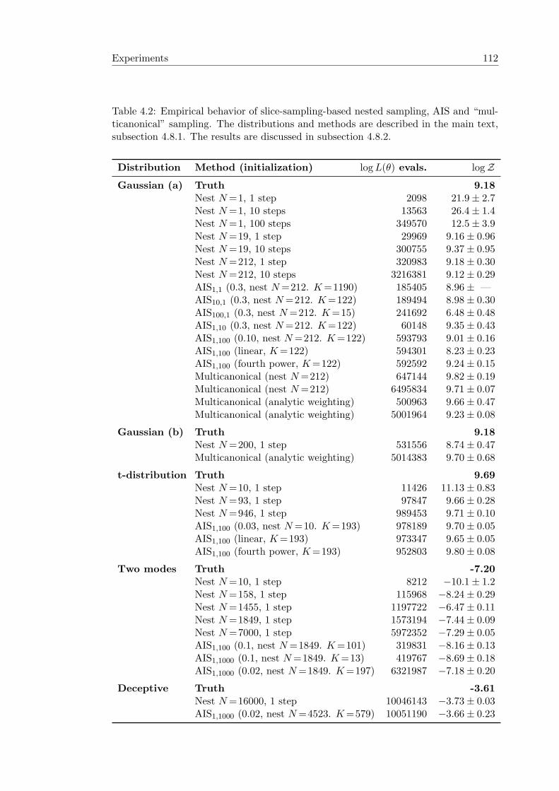
Experiments 112
Table 4.2: Empirical behavior of slice-sampling-based nested sampling, AIS and “mul-ticanonical” sampling. The distributions and methods are described in the main text,subsection 4.8.1. The results are discussed in subsection 4.8.2.
Distribution Method (initialization) log L(θ) evals. logZ
Gaussian (a) Truth 9.18Nest N =1, 1 step 2098 21.9± 2.7Nest N =1, 10 steps 13563 26.4± 1.4Nest N =1, 100 steps 349570 12.5± 3.9Nest N =19, 1 step 29969 9.16± 0.96Nest N =19, 10 steps 300755 9.37± 0.95Nest N =212, 1 step 320983 9.18± 0.30Nest N =212, 10 steps 3216381 9.12± 0.29AIS1,1 (0.3, nest N =212. K =1190) 185405 8.96± —AIS10,1 (0.3, nest N =212. K =122) 189494 8.98± 0.30AIS100,1 (0.3, nest N =212. K =15) 241692 6.48± 0.48AIS1,10 (0.3, nest N =212. K =122) 60148 9.35± 0.43AIS1,100 (0.10, nest N =212. K =122) 593793 9.01± 0.16AIS1,100 (linear, K =122) 594301 8.23± 0.23AIS1,100 (fourth power, K =122) 592592 9.24± 0.15Multicanonical (nest N =212) 647144 9.82± 0.19Multicanonical (nest N =212) 6495834 9.71± 0.07Multicanonical (analytic weighting) 500963 9.66± 0.47Multicanonical (analytic weighting) 5001964 9.23± 0.08
Gaussian (b) Truth 9.18Nest N =200, 1 step 531556 8.74± 0.47Multicanonical (analytic weighting) 5014383 9.70± 0.68
t-distribution Truth 9.69Nest N =10, 1 step 11426 11.13± 0.83Nest N =93, 1 step 97847 9.66± 0.28Nest N =946, 1 step 989453 9.71± 0.10AIS1,100 (0.03, nest N =10. K =193) 978189 9.70± 0.05AIS1,100 (linear, K =193) 973347 9.65± 0.05AIS1,100 (fourth power, K =193) 952803 9.80± 0.08
Two modes Truth -7.20Nest N =10, 1 step 8212 −10.1± 1.2Nest N =158, 1 step 115968 −8.24± 0.29Nest N =1455, 1 step 1197722 −6.47± 0.11Nest N =1849, 1 step 1573194 −7.44± 0.09Nest N =7000, 1 step 5972352 −7.29± 0.05AIS1,100 (0.1, nest N =1849. K =101) 319831 −8.16± 0.13AIS1,1000 (0.1, nest N =1849. K =13) 419767 −8.69± 0.18AIS1,1000 (0.02, nest N =1849. K =197) 6321987 −7.18± 0.20
Deceptive Truth -3.61Nest N =16000, 1 step 10046143 −3.73± 0.03AIS1,1000 (0.02, nest N =4523. K =579) 10051190 −3.66± 0.23
Experiments 113
a much better answer than N = 1 with 100 steps and is also an order of magnitudecheaper. Even with only one sampling step per iteration the estimates and error barswith N =19 and N =212 are indistinguishable from those obtained by exact samplingfrom the constrained priors7.
Three standard annealed importance sampling runs were performed with the sametarget error of 0.3: AIS1,1, AIS10,1 and AIS100,1. Obtaining the target error from onlyone run requires a very long annealing schedule, K = 1190. This gave similar resultsto 10 shorter runs with K = 122, but error bars are much more easily obtained frommultiple runs. Increasing the number of runs to 100 required shortening the annealingschedule further for a similar target error or computational cost. The short K =15 runshad larger errors than predicted and unreliable error bars. This schedule was designedassuming that the algorithm would keep close to the equilibrium distributions definedin the annealing schedule. In this case there were not enough bridging distributions forthis approximation to be accurate.
The result with AIS1,10, K =122, which uses ten parallel chains is similar to the resultfrom separate runs, AIS10,1, but with many fewer likelihood evaluations. In the absenceof a population of points the slice sampling code used an initial step size of one, whichis inappropriately small for this problem at high temperatures. A user not prepared toadapt step-sizes based on a population should find some way to set them appropriately.
The sequence of three AIS1,100 runs with K =122 are deliberately at higher precisionthan necessary so that the error bars are somewhat reliable and reproducible. Some-thing that is sadly not true of the lower precision AIS runs. These confirm that a linearannealing schedule is worse than one that dwells for longer at higher temperatures. Inthis case the fourth power schedule quite closely follows that set by nested samplingand has very similar performance.
The first multicanonical result with weights set by nested sampling seems to give com-parable uncertainty to AIS for the amount of computer effort. However, running thechains for ten times longer reveals problems with this “multicanonical” estimator. Wehad set the weights by estimating the probability mass between each pair of likeli-hood values L(s) and L(s+1) visited by nested sampling. For simplicity we used thedeterministic approximation in equation (4.28). This gives noisy estimates of the idealmulticanonical weights which, it turns out, are not good enough. We could attempt tosmooth the approximate multicanonical weighting function. Instead, for the Gaussiancase, we went directly to the “correct” multicanonical ensemble, equation (4.39). Thisconfirmed that the problem with the estimator was the choice of weighting functionand gives multicanonical a performance somewhere in between nested sampling andAIS on the Gaussian (a) problem. Even with the ideal weighting multicanonical failsto equilibrate and fails to give reasonable error bars on the Gaussian (b) problem. Thisis to be expected given the method’s poor scaling with precision ratio τt/τπ. We did
7We were able to confirm this because π is quite tractable for this toy problem.
Experiments 114
not continue to try multicanonical: adapting the weighting function beyond a nestedsampling initialization seems important and this would complicate the comparison.
Turning to the t-distribution example we see behavior different from the Gaussian case.The annealing schedule estimated from nested sampling is closer to linear than to afourth power. Moreover, the linear schedule and that produced from nested samplingare reproducibly better than the fourth power. Notice the reversal from the Gaussianexperiment. A good annealing schedule was estimated cheaply from nested samplingwith N =10. Obtaining as good answers as AIS with nested sampling alone would bemore expensive. Exactly how much is hard to tell from individual runs because theerror bars can be unreliable.
A more reliable comparison of nested sampling and AIS can be made based on manyrepeated runs. Nested sampling was run 100 times each over a range of N and comparedto AIS with 100 runs of schedules of varying lengths set by nested sampling. Figure 4.5ashows that the actual performance, measured as a mean squared error of the logZestimates, was similar for the two methods. Nested sampling is slightly more accurateat low computational costs, being taken over by AIS at higher precisions. Increasingthe number of AIS runs at the expense of annealing schedule length performs worse forthe same computational cost. This difference goes away at high precisions, but may bea concern when many runs are required on multimodal problems.
The main problem with AIS is that at lower precisions simple estimates and error barsbased on the mean and variance of the importance weights are unreliable. Figure 4.5bshows large biases in estimates for logZ. Figure 4.5c shows that the error bars are toosmall on average. Jackknife estimates (not shown) are sometimes slightly better cali-brated but give very similar results. For a user the error bars are often very important,so in this case the nested sampling estimator is the favorable choice.
The peaks of the “two modes” target distribution are highly separated at low tem-peratures. The fraction of AIS chains ending in the mode in the positive orthant is≈ 0.97, compared to its actual probability mass of a third. Through weighting theseruns AIS converges to the correct answer once enough sufficiently-long chains have beenrun. Further checks show that it also estimated the mass of each mode correctly. Thesame is true for nested sampling, the results from large N obtain nearly the correctrelative masses of the modes and in turn the overall normalization. Detailed analysisstill shows some signs of bias; the posterior overlap with the correct answer is smallerthan apparent from the scalar error bars in the table.
Both methods find “two-modes” difficult because it is not feasible to sample cor-rectly from π at late iterations or from low temperature distributions. AIS relies onreweighting over many runs, nested sampling requires many particles to maintain a fairrepresentation of π.
Even after ≈ 107 likelihood evaluations, both nested sampling and AIS have problems
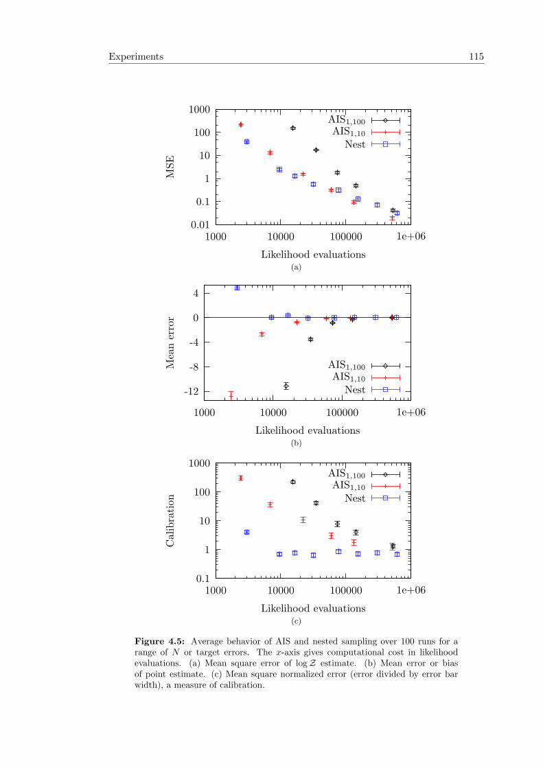
Experiments 115
0.01
0.1
1
10
100
1000
1000 10000 100000 1e+06
MSE
Likelihood evaluations
AIS1,100
AIS1,10
Nest
(a)
4
0
-4
-8
-12
1000 10000 100000 1e+06
Mean
err
or
Likelihood evaluations
AIS1,100
AIS1,10
Nest
(b)
0.1
1
10
100
1000
1000 10000 100000 1e+06
Calibra
tion
Likelihood evaluations
AIS1,100
AIS1,10
Nest
(c)
Figure 4.5: Average behavior of AIS and nested sampling over 100 runs for arange of N or target errors. The x-axis gives computational cost in likelihoodevaluations. (a) Mean square error of logZ estimate. (b) Mean error or biasof point estimate. (c) Mean square normalized error (error divided by error barwidth), a measure of calibration.
Experiments 116
Table 4.3: Estimates of the deceptive distribution
Quadrant True probability Nest estimate AIS estimate
upper-left 0.0282 0.0285± 0.0002 0.0305± 0.0080upper-right 0.0282 0.0214± 0.0002 0.0002± 0.0002lower-left 0.4718 0.4039± 0.0006 0.47± 0.12lower-right 0.4718 0.5482± 0.0005 0.50± 0.12
with the deceptive distribution. Nested sampling has an error bar on logZ that isfar too small. AIS’s estimate is consistent with the correct answer, although as with“two modes” with a higher standard error than targeted due to poor mixing at lowtemperatures. Additional problems are revealed by looking at the probability distri-bution over the four quadrants containing each cluster of modes, table 4.3. Again thenested sampling run is far too confident. In this case AIS’s error bars are generallymuch better, although it is very certain that the upper-right quadrant has much lessprobability mass than it actually does. Runs of nested sampling with smaller N showthat it too can easily lose the upper-right quadrant.
Nested sampling’s answers are wrong, according to its error bars, due to the Markovchain approximation. At late iterations with high likelihood constraints the slice sam-pler is unable to equilibrate π and is relying on a large number of particles to providea good starting point. On this problem the inaccuracy of this approximation does notreduce as fast as the size of the error bars with a large number of points.
Increasing the number of slice sampling steps per iteration does not solve the problembecause it would take an unrealistically large number to move between isolated modes.However, proposals that take all of the particles’ positions into account could help.Shaw et al. (2007) uses an approximate rejection sampler based on uniform sampleswithin ellipsoidal fits to clusters of the existing particles. No problems with biaseswere reported using this method, although clearly problems could still occur when theellipsoids fail to correctly capture π. In general ellipsoids could be used as Metropolisproposals, as part of several and various attempts to equilibrate a particle.
4.8.3 The Potts model
The Potts model was introduced in subsection 1.1.3. It describes a class of undirectedgraphical models over discrete variables s. The variables take on one of q ‘colors’ andthe model has a temperature-like “coupling” parameter J . Gibbs sampling updates of π
are the simplest way to implement (approximate) nested sampling. We also try cluster-based updates, subsection 4.7.3. While physicists tend to be interested in a broaderrange of quantities, we focus here on the normalization constant ZP(J, q), where thediscrete variables s are the θ variables that need to be integrated (i.e. summed) over.
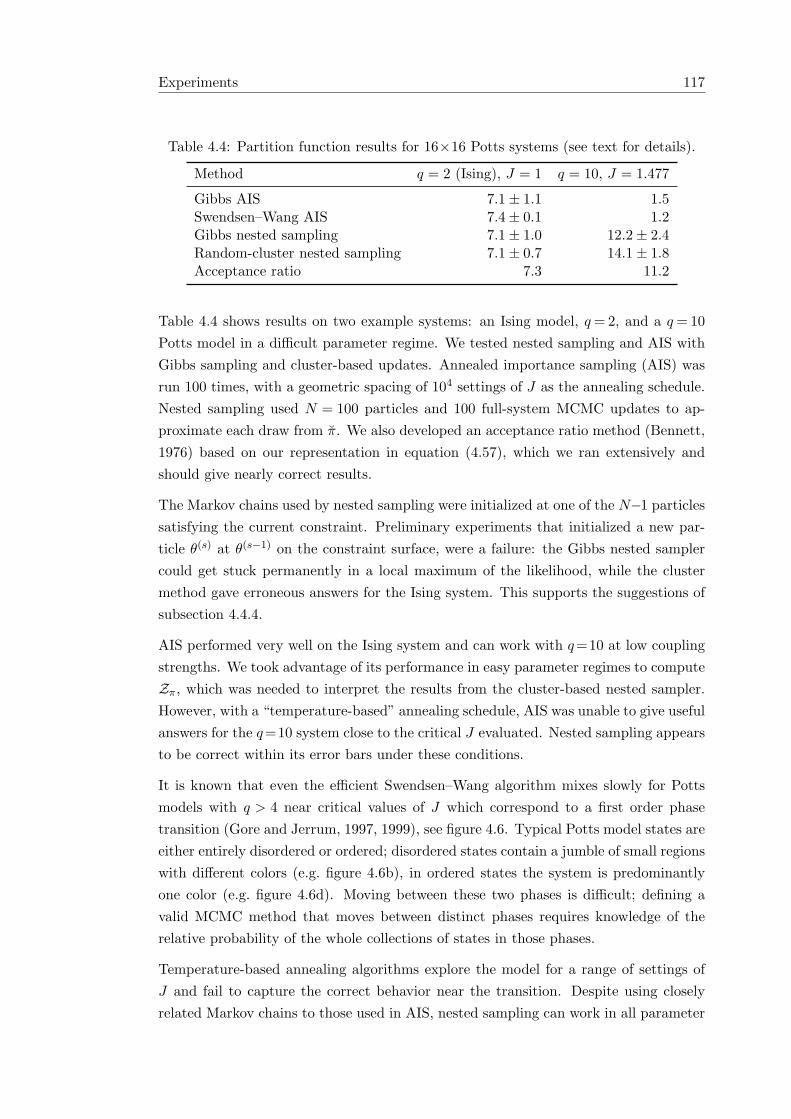
Experiments 117
Table 4.4: Partition function results for 16×16 Potts systems (see text for details).
Method q = 2 (Ising), J = 1 q = 10, J = 1.477
Gibbs AIS 7.1± 1.1 1.5Swendsen–Wang AIS 7.4± 0.1 1.2Gibbs nested sampling 7.1± 1.0 12.2± 2.4Random-cluster nested sampling 7.1± 0.7 14.1± 1.8Acceptance ratio 7.3 11.2
Table 4.4 shows results on two example systems: an Ising model, q = 2, and a q = 10Potts model in a difficult parameter regime. We tested nested sampling and AIS withGibbs sampling and cluster-based updates. Annealed importance sampling (AIS) wasrun 100 times, with a geometric spacing of 104 settings of J as the annealing schedule.Nested sampling used N = 100 particles and 100 full-system MCMC updates to ap-proximate each draw from π. We also developed an acceptance ratio method (Bennett,1976) based on our representation in equation (4.57), which we ran extensively andshould give nearly correct results.
The Markov chains used by nested sampling were initialized at one of the N−1 particlessatisfying the current constraint. Preliminary experiments that initialized a new par-ticle θ(s) at θ(s−1) on the constraint surface, were a failure: the Gibbs nested samplercould get stuck permanently in a local maximum of the likelihood, while the clustermethod gave erroneous answers for the Ising system. This supports the suggestions ofsubsection 4.4.4.
AIS performed very well on the Ising system and can work with q=10 at low couplingstrengths. We took advantage of its performance in easy parameter regimes to computeZπ, which was needed to interpret the results from the cluster-based nested sampler.However, with a “temperature-based” annealing schedule, AIS was unable to give usefulanswers for the q=10 system close to the critical J evaluated. Nested sampling appearsto be correct within its error bars under these conditions.
It is known that even the efficient Swendsen–Wang algorithm mixes slowly for Pottsmodels with q > 4 near critical values of J which correspond to a first order phasetransition (Gore and Jerrum, 1997, 1999), see figure 4.6. Typical Potts model states areeither entirely disordered or ordered; disordered states contain a jumble of small regionswith different colors (e.g. figure 4.6b), in ordered states the system is predominantlyone color (e.g. figure 4.6d). Moving between these two phases is difficult; defining avalid MCMC method that moves between distinct phases requires knowledge of therelative probability of the whole collections of states in those phases.
Temperature-based annealing algorithms explore the model for a range of settings ofJ and fail to capture the correct behavior near the transition. Despite using closelyrelated Markov chains to those used in AIS, nested sampling can work in all parameter
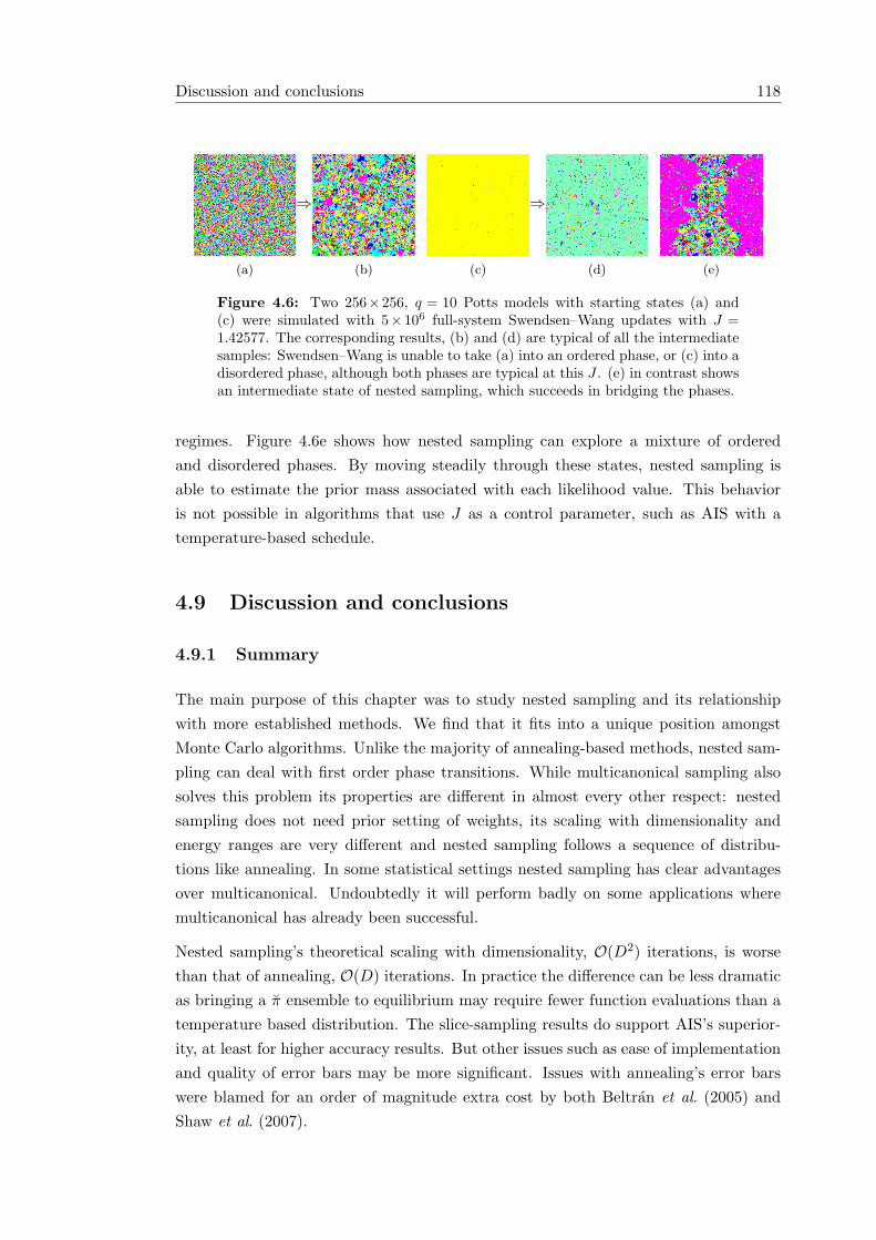
Discussion and conclusions 118
(a)
⇒
(b) (c)
⇒
(d) (e)
Figure 4.6: Two 256×256, q = 10 Potts models with starting states (a) and(c) were simulated with 5×10⁶ full-system Swendsen–Wang updates with J =1.42577. The corresponding results, (b) and (d) are typical of all the intermediatesamples: Swendsen–Wang is unable to take (a) into an ordered phase, or (c) into adisordered phase, although both phases are typical at this J . (e) in contrast showsan intermediate state of nested sampling, which succeeds in bridging the phases.
regimes. Figure 4.6e shows how nested sampling can explore a mixture of orderedand disordered phases. By moving steadily through these states, nested sampling isable to estimate the prior mass associated with each likelihood value. This behavioris not possible in algorithms that use J as a control parameter, such as AIS with atemperature-based schedule.
4.9 Discussion and conclusions
4.9.1 Summary
The main purpose of this chapter was to study nested sampling and its relationshipwith more established methods. We find that it fits into a unique position amongstMonte Carlo algorithms. Unlike the majority of annealing-based methods, nested sam-pling can deal with first order phase transitions. While multicanonical sampling alsosolves this problem its properties are different in almost every other respect: nestedsampling does not need prior setting of weights, its scaling with dimensionality andenergy ranges are very different and nested sampling follows a sequence of distribu-tions like annealing. In some statistical settings nested sampling has clear advantagesover multicanonical. Undoubtedly it will perform badly on some applications wheremulticanonical has already been successful.
Nested sampling’s theoretical scaling with dimensionality, O(D2) iterations, is worsethan that of annealing, O(D) iterations. In practice the difference can be less dramaticas bringing a π ensemble to equilibrium may require fewer function evaluations than atemperature based distribution. The slice-sampling results do support AIS’s superior-ity, at least for higher accuracy results. But other issues such as ease of implementationand quality of error bars may be more significant. Issues with annealing’s error barswere blamed for an order of magnitude extra cost by both Beltran et al. (2005) andShaw et al. (2007).
Discussion and conclusions 119
Despite this the relative under-performance of annealing reported by these astronomersis difficult to account for given the theoretical and practical results of this chapter. Themost likely explanation is a difference in the operators used to update the intermediatedistributions. In this chapter the same or closely related operators where used withAIS and nested sampling. In Shaw et al. (2007) nested sampling was described with itsown special update rule using ellipsoids fitted to the current particles. This algorithmcould easily require fewer function evaluations than a simple slice sampler or Metropolismethod as used within annealing in Beltran et al. (2005). Although the ellipsoid algo-rithm was suggested by the need to sample from nested sampling’s π, there is no reasonnot to use the same basic code to propose moves for an annealing method. Combinedwith an annealing schedule specified by nested sampling AIS might perform as well asor better than nested sampling.
4.9.2 Related work
This chapter only considered a subset of the available methods for computing normal-izing constants. The focus has been on simple methods that compute the normalizingconstant of a generic probability distribution. We avoided assuming detailed knowledgeabout the target distribution and its relationships with other distributions as much aspossible. For users with more time, a richer set of methods are available, some of whichare mentioned here.
The intermediate distributions in annealed importance sampling do not have to betemperature-based distributions. That has been the focus here because of the simplicityand generality of raising the likelihood to a power. Any other way of bringing in thelikelihood gradually can be used: “one data point at a time” may be natural in astatistical setting. A generalization, linked importance sampling (Neal, 2005) may behelpful for such cases where the intermediate levels are fixed and limited in number.
Annealed importance sampling can be seen as a member of a wider family of “SequentialMonte Carlo” (SMC) methods. Some of these algorithms allow transfer of particlesamongst modes, and should definitely be considered by anyone attracted to nestedsampling by this property. A recent example of SMC combined with an interesting setof bridging distributions leveraging the power of graphical models is presented in Hamzeand de Freitas (2006).
Some situations require the computation of more than one normalizing constant. Anoption is to construct a distribution containing each of the models and explore it withMCMC. Reversible jump MCMC (Green, 1995) makes this possible even when themodels have parameter vectors of different dimensionalities. The relative probability ofeach model is available from the amount of time the sampler spent exploring each model,and more advanced estimators based on transition probabilities may be available. This
Discussion and conclusions 120
only provides the normalizing constants up to a constant, although if one of the modelsconsidered is tractable this constant could be found.
The path sampling approach of Gelman and Meng (1998) suggests computing normaliz-ing constants by integrating along a path of model hyperparameters rather than along asingle inverse-temperature parameter. If the normalizer for each setting of the hyperpa-rameters is required this is particularly effective. Contour plots based on independentestimates will usually be very noisy compared to a path sampling approach.
4.9.3 Philosophy
Various authors have noted the irony of using Monte Carlo, a frequentist procedure, forBayesian computation (e.g. O’Hagan, 1987; Neal, 1993; Rasmussen and Ghahramani,2003). Rather than giving beliefs about quantities given the computations performed,Monte Carlo algorithms provide “frequentist” statistical estimators. Skilling claimsthat nested sampling is Bayesian. This section examines the extent to which thisholds.
Our target is a posterior distribution over Z. Philosophically this is slightly tricky,because Z is a constant which we should be able to work out given the prior andlikelihood functions. Thus according to any rational calculus of beliefs as in Cox (1946)or Jaynes (2003) the posterior should concentrate all of its mass at the true value. Theproblem is not lack of available information, but computer time to use it perfectly.
The solution to this conundrum is to be careful about what we claim to know. Assumethat some agent is running nested sampling on our behalf and only reports to usL = {L(s)}. If it reported more information, such as θ(s) locations, we would be inan embarrassing situation. To use this information we would need a probabilisticmodel including θ(s) in which inference would probably be hard. But throwing awayknowledge is hard to deal with rationally, so we pretend it was never available. Thus theinferences for nested sampling, as in Rasmussen and Ghahramani (2003), are rationalfor a fictitious observer with limited information. This observer’s results will be morevague than if {θ(s)} were not ignored but should be sensible, which is not guaranteedby general approximations to Bayesian inference.
We first set up priors based on the knowledge that an agent is running nested sampling,which will provide L(s) quantities with associated x(s) cumulative mass values. Ourknowledge of nested sampling defines a problem-independent prior distribution overx={x(s)}. We should also specify a prior distribution over functions L(x).
After observing L = {L(s)}, we update our beliefs about the underlying cumulativevalues according to Bayes’ rule: P (x|L) = P (L|x) P (x)/P (L). It is this posteriordistribution that should be used when computing posteriors over other quantities such
Discussion and conclusions 121
as Z,
P (Z|L) =∫
P (Z|x,L) P (x|L) dx. (4.62)
Note that specifying a prior over monotonic functions P (L(x)) and computing with itappears difficult in general. Skilling declares that “I can’t, so I don’t”. Instead theprior P (x) is used. This corresponds to a particular assumption: an improper uniformprior over likelihood functions. This cannot be avoided by claiming general ignorance:unlike {θ(s)}, we must be told {L(s)}. Thus to maintain a claim of rationality, we mustbe happy with this particular choice of prior or type of ignorance about the likelihoodfunction.
In addition, and much more seriously, we must assume the agent is actually runningnested sampling as in algorithm 4.2. In fact we really know that some approximationwill be involved. As we have seen this can give us unreasonable beliefs—as with mostprobabilistic modeling where we know a priori that a model’s joint distribution doesnot really capture every detail of a real system.
Similar concerns must surround all such attempts to introduce Bayesian methodologyinto Monte Carlo algorithms for general inference problems. For example Bayesianlearning of the one-dimensional weighting function of the multicanonical method hasbeen attempted (e.g. Smith, 1995). This should be a difficult inference problem asthe output of a sampler has a complicated dependence structure. Only with incorrectassumptions, i.e., approximations, can Bayesian methods be applied. The ultimatejustification for such methods must be their empirical performance, which is sometimesvery good.
Chapter 5
Doubly-intractable distributions
Most of this thesis has been dedicated to sampling from probability distributions wherethe key difficulty has been an intractable normalization. When considering a posteriorover parameters θ given data y,
p(θ|y) =p(y, θ)p(y)
=p(y|θ) p(θ)
p(y), (5.1)
we assumed that the joint probability in the numerator could be easily evaluated forany particular joint setting (y, θ). Chapter 4 described how the important quantityp(y) can be approximated, but it is often infeasible to compute this quantity exactly.
Standard MCMC methods are designed for use with these intractable distributions.Markov chain operators can be constructed by restricting consideration to a manageablesubset of θ’s state space at each step. In Metropolis–Hastings only two settings areconsidered, the current setting θ and a randomly chosen proposal, θ′. Gibbs samplingchanges only one component of θ at a time. Metropolis requires an ability to evaluatep(y, θ) ratios for various θ pairs, and Gibbs sampling requires the ability to samplefrom the conditional distributions p(θi|θ{j 6=i}, y). By considering restricted parts of thestate space, neither method needs to know the global normalizing constant p(y).
But what if p(y, θ), like p(y), contains a summation over a large state space so itcannot feasibly be evaluated point-wise? Then the problem is doubly-intractable and,as we shall see, even performing Markov chain Monte Carlo is potentially exceedinglydifficult.
The next section explains why doubly-intractable distributions arise and the difficultiesinvolved. Section 5.2 explores approximations of standard MCMC algorithms in thecontext of undirected graphical models. Møller et al. (2004, 2006) provided the firstfeasible algorithm for models where sampling from p(y|θ) is possible but its normal-ization is unknown. Their method is reviewed in section 5.4 and generalized by us insection 5.5. Working on these algorithms inspired the new exchange algorithm, sec-
Bayesian learning of undirected models 123
tion 5.3. These innovations were first described in (Murray et al., 2006a). This chapterprovides a slightly more general version of the exchange algorithm with a new derivationwhich is somewhat simpler than the original description. Full mathematical derivationsof detailed balance are provided, which were previously omitted for space reasons. Insection 5.7 we consider further new valid MCMC algorithms for doubly-intractabledistributions, which provide a connection to the Approximate Bayesian Computation(ABC) literature. Section 5.8 provides slice sampling algorithms for doubly-intractabledistributions. Finally new directions for research in this area are considered in sec-tion 5.9.
5.1 Bayesian learning of undirected models
The Potts model discussed in the previous chapter belongs to a very wide class of“energy-based models” where
p(y|θ) =1Z(θ)
exp
−∑j
Ej(ycj , θj)
=
1Z(θ)
∏j
fj(ycj , θj), Z(θ) =∑
y
∏j
fj(ycj , θj).
(5.2)
The sets cj each index a subset of variables that take part in a corresponding poten-tial function fj , parameterized by θj . Each potential expresses mutual compatibilitiesamongst a subset of variables ycj . Sampling from the y variables is possible withMCMC, but computing the normalization can be very difficult.
Section 1.1 reviewed how special structure in a graphical model sometimes allows effi-cient computation of the normalization Z(θ). Most of this chapter concerns methodsthat apply to general distributions, so it is convenient for clarity to collapse the modelto a simpler form:
p(y|θ) = f(y; θ)/Z(θ). (5.3)
We now consider sampling from the posterior over parameters, equation (5.1), whenthe likelihood is of the unnormalized form given in equation (5.3). This posterior,
p(θ|y) =(
f(y; θ)p(θ)Z(θ)
)/p(y), (5.4)
offers a new difficulty. As before p(y) is not needed for MCMC, but the normalizing‘constant’ Z(θ) cannot be ignored as it is a function of the parameters θ, the vari-ables being sampled. Every time new parameter values are considered it appears thatan intractable computation involving Z will be required. As MCMC estimators areapproximations unless an infinite number of iterations are performed, and each itera-
Bayesian learning of undirected models 124
tion is generally infeasible, p(θ|y) in equation (5.4) can be called a doubly-intractabledistribution.
While sampling from parameter posteriors by MCMC is a well established technique, itis largely associated with distributions that could be represented as directed graphicalmodels. However, sampling parameters in anything but the most trivial1 undirectedgraphical model is doubly-intractable. While directed models are a more natural toolfor modeling causal relationships, the soft constraints provided by undirected modelshave proven useful in a variety of problem domains; we briefly mention six applications.
(a) In computer vision Markov random fields (MRFs), a form of undirected model, areused to model the soft constraint a pixel or image feature imposes on nearby pixelsor features (Geman and Geman, 1984); this use of MRFs grew out of a long tradi-tion in spatial statistics (Besag, 1974). (b) In language modeling a common form ofsentence model measures a large number of features of a sentence fj(s), such as thepresence of a word, subject-verb agreement, the output of a parser on the sentence,etc, and assigns each such feature a weight λj . A random field model of this is thenp(s|λ) = (1/Z(λ)) exp{
∑j λjfj(s)} where the weights can be learned via maximum
likelihood iterative scaling methods (Della Pietra et al., 1997). (c) These undirectedmodels can be extended to coreference analysis, which deals with determining, for ex-ample, whether two items (e.g., strings, citations) refer to the same underlying object(McCallum and Wellner, 2003). (d) Undirected models have been used to model pro-tein folding (Winther and Krogh, 2004) and the soft constraints on the configurationof protein side chains (Yanover and Weiss, 2003). (e) Semi-supervised classificationis the problem of classifying a large number of unlabeled points using a small numberof labeled points and some prior knowledge that nearby points have the same label.This problem can be approached by defining an undirected graphical model over bothlabeled and unlabeled data (Zhu and Ghahramani, 2002). (f) Given a set of directedmodels p(y|θj), the products of experts idea is a simple way of defining a more pow-erful (undirected) model by multiplying them: p(y|θ) = (1/Z(θ))
∏j p(y|θj) (Hinton,
2002). The product assigns high probability when there is consensus among componentmodels.
Despite the long history and wide applicability of undirected models, until recentlyBayesian treatments of learning the parameters of large undirected models have beenvirtually non-existent! Indeed there is a related statistical literature on Bayesian in-ference in undirected models, log linear models, and contingency tables (Albert, 1995;Dellaportas and Forster, 1999; Dobra et al., 2006). However, this literature, with thenotable exception of the technique reviewed in section 5.4, assumes that the partitionfunction Z(θ) can be computed exactly. But for many of the machine learning applica-tions of undirected models cited above, this assumption is unreasonable. This chapteraddresses Bayesian learning for models with intractable Z(θ).
1i.e., low tree-width graphs, graphical Gaussian models and small contingency tables.
Bayesian learning of undirected models 125
5.1.1 Do we need Z(θ) for MCMC?
The modeler’s effort was put into specifying f(y; θ); it is tempting to think that Z(θ)should have little relevance and there must be some way to side-step computing it.It was established above that the normalizer Z(θ) is not a constant in the contextof sampling θ. This section explores the role of Z(θ) in more detail, addressing theconsequences for any scheme that avoids computing it.
Algorithm 5.1 gives the straightforward application of standard Metropolis–Hastings(algorithm 2.1) to the doubly-intractable distribution in equation (5.4).
Algorithm 5.1 Standard (but infeasible) Metropolis–Hastings (M–H)Input: initial setting θ, number of iterations S
1. for s = 1 . . . S
2. Propose θ′ ∼ q(θ′←θ; y)3. Compute
a =p(θ′|y)p(θ|y)
q(θ←θ′; y)q(θ′←θ; y)
=f(y; θ′) p(θ′) q(θ←θ′; y)f(y; θ) p(θ) q(θ′←θ; y)
· Z(θ)Z(θ′)
4. Draw r ∼ Uniform[0, 1]5. if (r < a) then set θ←θ′
6. end for
Computing the acceptance ratio requires a ratio of normalizing constants, or at least abound tight enough for step 5. This is difficult in general. There are usually some freechoices while constructing MCMC algorithms. Perhaps some “nuisance” parameterscould be judiciously set to remove Z(θ) through some fortunate cancellations? We arenot free to cancel out Z through a choice of prior p(θ): the prior would have to dependon the number of observed data points and would take on extreme values dominatingany inferences (Murray and Ghahramani, 2004). In theory the proposal distributioncould be defined to remove explicit Z dependence from the acceptance ratio, but inpractice this does not seem to help: e.g. q(θ′←θ; y)=Z(θ)g(θ′) or q(θ′←θ; y)∝1/Z(θ′)would be difficult to construct without knowing Z, and would be terrible proposals.The only distribution we know of that contains Z(θ) gives probabilities in data space,not over parameters.
Section 5.4 reviews and extends a method by Møller et al. (2004, 2006) which intro-duced auxiliary variables taking on values in the data space. This allows proposals thatcancel out the unknown terms, but only if it is possible to draw from the (intractable)distribution p(y|θ). This key insight makes it possible to sample from a limited butsignificant class of distributions for which MCMC was previously impossible. How-ever, the algorithm and its extensions are not a panacea. It is not always possible todraw exact samples from the data distribution. Another problem (or opportunity) is
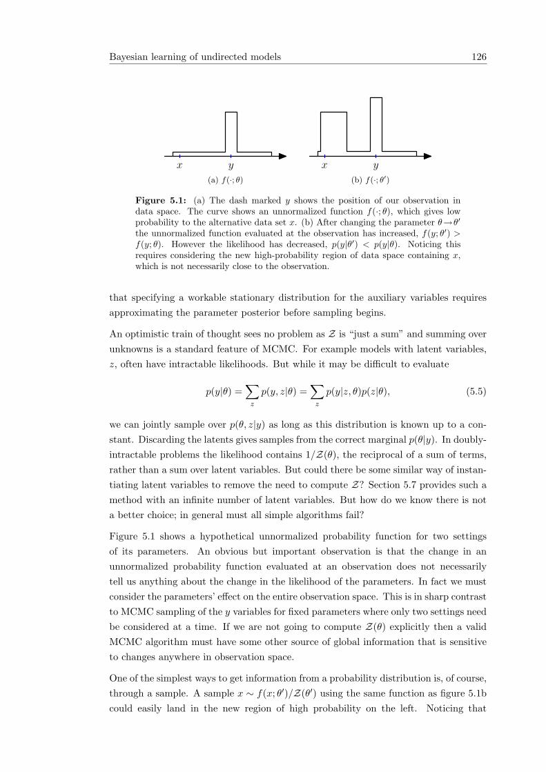
Bayesian learning of undirected models 126
yx
(a) f(·; θ)
yx
(b) f(·; θ′)
Figure 5.1: (a) The dash marked y shows the position of our observation indata space. The curve shows an unnormalized function f(·; θ), which gives lowprobability to the alternative data set x. (b) After changing the parameter θ→θ′
the unnormalized function evaluated at the observation has increased, f(y; θ′) >f(y; θ). However the likelihood has decreased, p(y|θ′) < p(y|θ). Noticing thisrequires considering the new high-probability region of data space containing x,which is not necessarily close to the observation.
that specifying a workable stationary distribution for the auxiliary variables requiresapproximating the parameter posterior before sampling begins.
An optimistic train of thought sees no problem as Z is “just a sum” and summing overunknowns is a standard feature of MCMC. For example models with latent variables,z, often have intractable likelihoods. But while it may be difficult to evaluate
p(y|θ) =∑
z
p(y, z|θ) =∑
z
p(y|z, θ)p(z|θ), (5.5)
we can jointly sample over p(θ, z|y) as long as this distribution is known up to a con-stant. Discarding the latents gives samples from the correct marginal p(θ|y). In doubly-intractable problems the likelihood contains 1/Z(θ), the reciprocal of a sum of terms,rather than a sum over latent variables. But could there be some similar way of instan-tiating latent variables to remove the need to compute Z? Section 5.7 provides such amethod with an infinite number of latent variables. But how do we know there is nota better choice; in general must all simple algorithms fail?
Figure 5.1 shows a hypothetical unnormalized probability function for two settingsof its parameters. An obvious but important observation is that the change in anunnormalized probability function evaluated at an observation does not necessarilytell us anything about the change in the likelihood of the parameters. In fact we mustconsider the parameters’ effect on the entire observation space. This is in sharp contrastto MCMC sampling of the y variables for fixed parameters where only two settings needbe considered at a time. If we are not going to compute Z(θ) explicitly then a validMCMC algorithm must have some other source of global information that is sensitiveto changes anywhere in observation space.
One of the simplest ways to get information from a probability distribution is, of course,through a sample. A sample x ∼ f(x; θ′)/Z(θ′) using the same function as figure 5.1bcould easily land in the new region of high probability on the left. Noticing that
Approximation Schemes 127
f(x; θ)� f(x; θ′) gives some indication that any perceived benefit of f(y; θ′) > f(y; θ)should be penalized. Despite the apparent paucity of such information, surprisinglythese single samples at each parameter setting are sufficient to create valid MCMCalgorithms for p(θ|y) that do not need Z(θ). This is how the approach in Møller et al.(2004) works, which explains why it requires samples from the target distribution usingan exact or perfect sampling method (section 2.7). Approximate samples from a fewMCMC steps cannot guarantee considering the new bubble in data space in figure 5.1b.A Markov chain started at (e.g.) the observation will be heavily biased towards a modenear the starting point and may never consider any other modes.
Are spurious modes in data space a problem in practice? Contrastive divergence learn-ing (Hinton, 2002) uses very brief MCMC sampling starting at the observed data andcan give useful results on complex problems in machine learning. Sometimes we knowthe parameter posterior is simple, it is log-concave for fully-observed exponential-familydistributions. In such cases deterministic approximations to the parameter posteriorperform favorably compared to pseudo-MCMC approaches (Welling and Parise, 2006).However, if we wish to construct a valid MCMC method, we must formally show thatthe entire data space has been properly considered. Exact sampling explicitly tracksbounds that start off considering the entire observation space (section 2.7), a procedurewith this flavor seems an essential part of samplers for doubly-intractable distributions.Thus even though a new latent variable approach introduced in section 5.7 does notuse exact sampling as such, the requirements are, and must be, very similar.
Exact sampling is a formidable requirement; deterministic approaches and MCMCmethods that do not use the correct posterior distribution will always have a place.Some possibilities are studied in the next section. There is also always a place for “goldstandard” methods that given enough time should give correct answers. Those are thefocus of the remainder of the chapter.
5.2 Approximation Schemes
For concreteness this section studies a simple but widespread type of graphical model.The Boltzmann machine (BM) is a Markov random field which defines a probabilitydistribution over a vector of binary variables s = [s1, . . . , sk] where si ∈ {0, 1}:
p(s|W ) =1
Z(W )exp
∑i<j
Wijsisj ,
. (5.6)
The symmetric weight matrix W parameterizes this distribution. In a BM there areusually also linear bias terms
∑i bisi in the exponent, with these the model is equivalent
to a Potts or Ising model with “magnetic field” parameters. We omit these biases tosimplify notation, although the models in the experiments assume them.
Approximation Schemes 128
The usual algorithm for learning BMs is a maximum likelihood version of the EMalgorithm (assuming some of the variables are hidden sH and some observed sO) (Ackleyet al., 1985). The gradient of the log probability is:
∂ log p(sO|W )∂Wij
= Ec[sisj ]− Eu[sisj ] , (5.7)
where Ec[·] denotes expectation under the “clamped” data distribution p(sH |sO,W )and Eu[·] denotes expectation under the “unclamped” distribution p(s|W ). For a dataset S = [s(1) . . . s(n) . . . s(N)] of i.i.d. data the gradient of the log likelihood is simplysummed over n. For Boltzmann machines with large tree-width (see section 1.1) theseexpectations would take exponential time to compute, and the usual approach is toapproximate them using Gibbs sampling or one of many more recent approximateinference algorithms.
5.2.1 Targets for MCMC approximation
Metropolis–Hastings for the parameters of a Boltzmann machine given fully observeddata needs (to bound)
a =p(S|W ′)p(W ′)q(W←W ′;S)p(S|W )p(W )q(W ′←W ;S)
=p(W ′) q(W←W ′;S)p(W ) q(W ′←W ;S)
(Z(W )Z(W ′)
)N
exp
∑n,i<j
(W ′ij −Wij) s
(n)i s
(n)j
.
(5.8)
The first class of approximation we will pursue is to substitute a deterministic approxi-mation Z(W ) ' Z(W ) into the above expression. Clearly this results in an approximatesampler, which does not converge to the true equilibrium distribution over parameters.Moreover, it seems reckless to take an approximate quantity to the N th power. De-spite these caveats we explore empirically whether approaches based on this class ofapproximation are viable.
Note that above we need only compute the ratio of the partition function at pairs ofparameter settings, Z(W )/Z(W ′). This ratio can be approximated directly by impor-tance sampling:
Z(W )Z(W ′)
≡ Ep(s|W ′)
exp
∑i<j
(Wij −W ′ij)sisj
. (5.9)
Thus any method for estimating expectations under p(s|W ′) — sampling-based ordeterministic — can be nested into the Metropolis sampler for W .
For small steps W →W ′ estimating ratios of normalizers and finding gradients withrespect to the parameters are closely related problems. Gradients may be more useful
Approximation Schemes 129
as they provide a direction in which to move, which is useful in algorithms basedon dynamical systems such as Hybrid Monte Carlo (subsection 2.4.3). Hybrid MonteCarlo would also require a Z ratio for its accept/reject step. This effort may not bejustified when the gradients and Z(W ) are only available as approximations. Simplerschemes that use gradient information also exist (Neal, 1993). The simplest of these isthe “uncorrected Langevin method”. Parameters are updated without any rejectionsaccording to the rule:
θ′i = θi +ε2
2∂
∂θilog p(y, θ) + εni, (5.10)
where ni are independent draws from a zero-mean unit variance Gaussian. Intuitivelythis rule performs gradient descent but explores away from the optimum through thenoise term. Strictly this is only an approximation except in the limit of vanishing ε.
Using the above or other dynamical methods, a third target for approximation forsystems with continuous parameters is the gradient of the joint log probability. In thecase of BMs, we have:
∂ log p(S, W )∂Wij
=∑
n
s(n)i s
(n)j −NEp(s|W )[sisj ] +
∂ log p(W )∂Wij
. (5.11)
Assuming an easy to differentiate prior, the main difficulty arises, as in equation (5.7),from computing the middle term: the unclamped expectations over the variables.
Interestingly, although many learning algorithms for undirected models, e.g. the origi-nal Boltzmann machine learning rule, are based on computing gradients such as equa-tion (5.11), and it would be simple to plug these into approximate stochastic dynamicsMCMC methods to do Bayesian inference, this approach does not appear to have beeninvestigated. We explore this approach in our experiments.
This section has considered two existing sampling schemes (Metropolis and Langevin)and identified three targets for approximation to make these schemes tractable: Z(W ),Z(W )/Z(W ′) and Ep(s|W )[sisj ]. While the explicit derivations above focused on Boltz-mann machines, these same expressions generalize in a straightforward way to Bayesianparameter inference in a general undirected model as in equation (5.2). In particular,many undirected models of interest can be parameterized to have potentials in the ex-ponential family, −Ej(ycj , θj) = uj(ycj )
>θj . For such models, the key ingredients toan approximation are the expected sufficient statistics, Ep(y|θ)
[uj(ycj )
].
5.2.2 Approximation algorithms
In this section approximations for each of the three target quantities in equa-tions (5.8), (5.9) and (5.11) are identified. These are used to propose a variety ofapproximate sampling methods for doubly-intractable distributions, first outlined inMurray and Ghahramani (2004).
Approximation Schemes 130
Variational lower bounds were developed in statistical physics, but are also widelyused in machine learning. They use Jensen’s inequality to lower bound the log partitionfunction in the following way:
logZ(θ) = log∑
x
f(x; θ) = log∑
x
q(x)f(x; θ)q(x)
≥∑
x
q(x) logf(x; θ)q(x)
logZ(θ) ≥∑
x
q(x) log f(x; θ) +H(q) ≡ F(θ, q).
(5.12)
The relationship holds for any distribution q(x), provided it is not zero where p(x; θ)has support. The second term in the bound is called the entropy of the distributionH(q)≡−
∑x q(x) log q(x). The over-all bound F is often called the free energy. See
Winn and Bishop (2005) for more details and a framework for automatic constructionand optimization of variational bounds for a large class of graphical models.
The naıve mean field method is a variational method with q constrained to belong to theset of fully factorized distributions Qmf = {q : q(x) =
∏i qi(xi)}. For the Boltzmann
machine a local maximum of this lower bound logZmf(θ) = maxq∈QmfF(θ, q) can be
found with an iterative and tractable fixed-point algorithm, see for example MacKay(2003, chapter 33). Let the mean-field Metropolis algorithm be defined by usingZmf(θ) in place of Z(θ) in the acceptance probability computation, equation (5.8). Theexpectations from the naıve mean field algorithm could also be used to compute directapproximations to the gradients in equation (5.11) for use in a stochastic dynamicsmethod.
Jensen’s inequality can be used to obtain much tighter bounds than those given bythe naıve mean-field method. For example, when constraining q to be in the set of alltree-structured distributions Qtree optimizing the lower bound on the partition functionis still tractable (Wiegerinck, 2000), obtaining Ztree(θ) ≤ Z(θ). The tree Metropolis
algorithm is defined through the use of this approximation in equation (5.8). Alterna-tively, expectations under the tree could be used to form the gradient estimate for astochastic dynamics method, equation (5.11).
Bethe approximation. A recent justification for applying belief propagation tographs with cycles is the relationship between this algorithm’s messages and the fixedpoints of the Bethe free energy (Yedidia et al., 2005). This breakthrough gave a newapproximation for the partition function. In the loopy Metropolis algorithm beliefpropagation is run on each proposed system, and the Bethe free energy is used to ap-proximate the acceptance probability, equation (5.8). Traditionally belief propagationis used to compute marginals; pairwise marginals can be used to compute the expec-tations used in gradient methods, e.g. equation (5.11), or in finding partition functionratios, equation (5.9). These approaches lead to different algorithms, although their
Approximation Schemes 131
approximations are clearly closely related.
Langevin using brief sampling. The pairwise marginals required in equations (5.10)and (5.11) can be approximated by MCMC sampling. The Gibbs sampler used insubsection 5.2.4 is a popular choice, whereas in subsection 5.2.5 a more sophisti-cated Swendsen-Wang sampler is employed. Unfortunately— as in maximum likeli-hood learning, equation (5.7)— the parameter-dependent variance of these estimatescan hinder convergence and introduce biases. The brief Langevin algorithm, inspiredby work on contrastive divergence (Hinton, 2002), uses very brief sampling startingfrom the data, X, which gives biased but low variance estimates of the required expec-tations. As the approximations in this section are run as an inner loop to the mainsampler, the cheapness of brief sampling makes it an attractive option.
Langevin using exact sampling. Unbiased expectations can be obtained in somesystems using an exact sampling algorithm (section 2.7). Although the gradients fromthis method are guaranteed to be unbiased, parameter-dependent variance could leadto worse performance than the proposed brief Langevin method. Variance could bereduced by reusing pseudo random numbers. However, we shall see later that there aremuch more elegant ways to use an exact sampler if one is available.
Pseudo-Likelihood. Replacing the likelihood of the parameters with a tractable prod-uct of conditional probabilities is a common approximation in Markov random fields forimage modeling. One of the earliest Bayesian approaches to learning in large systemsof which we are aware was in this context (Wang et al., 2000; Yu and Cheng, 2003).The models used in the experiments of subsection 5.2.4 were not well approximated bythe pseudo-likelihood, so it is not explored further here.
5.2.3 Extension to hidden variables
So far we have only considered models of the form p(y|θ) where all variables, y, areobserved. Often models need to cope with missing data, or have variables that arealways hidden. These are often the models that would most benefit from a Bayesianapproach to learning the parameters. In fully observed models in the exponential familythe parameter posteriors are often relatively simple as they are log concave if the priorused is also log concave (as seen later in figure 5.2). The parameter posterior withhidden variables will be a linear combination of log concave functions, which need notbe log concave and can be multi-modal.
In theory the extension to hidden variables is simple. First consider a model p(y, h|θ),where h are unobserved variables. The parameter posterior is still proportional to
Approximation Schemes 132
p(y|θ)p(θ), and we observe
p(y|θ) =∑
h
p(y, h|θ) =1Z(θ)
∑h
∏j
fj((y, h)cj , θj)
log p(y|θ) = − logZ(θ) + log∑
h
∏j
fj((y, h)cj , θj)
= − logZ(θ) + logZy(θ).
(5.13)
That is, the sum in the second term is a partition function, Zy, for an undirectedgraph of the variables h. To see this compare to equation (5.2) and consider the fixedobservations y as parameters of the potential functions. In a system with multiplei.i.d. observations Zy must be computed for each setting of y. Note however thatthese additional partition function evaluations are for systems smaller than the original.Therefore, any method that approximates Z(θ) or related quantities directly from theparameters can still be used for parameter learning in systems with hidden variables.
The brief sampling and pseudo-likelihood approximations rely on settings of every vari-able provided by the data. For systems with hidden variables these methods could usesettings from samples conditioned on the observed data. In some systems this samplingcan be performed easily (Hinton, 2002). In subsection 5.2.5 several steps of MCMCsampling over the hidden variables are performed in order to apply the brief Langevinmethod.
5.2.4 Experiments involving fully observed models
The approximate samplers described in subsection 5.2.2 were tested on three systems.The first, taken from Edwards and Havranek (1985), lists six binary properties detail-ing risk factors for coronary heart disease in 1841 men. Modeling these variables asoutputs of a fully-connected Boltzmann machine, we attempted to draw samples fromthe distribution over the unknown weights. We can compute Z(θ) exactly in this sys-tem, which allows us to compare methods against a Metropolis sampler with an exactinner loop. A previous Bayesian treatment of these data also exists (Dellaportas andForster, 1999).
While predictions wouldn’t need as many samples, we performed sampling for 100,000iterations to obtain reasonable histograms for each of the weights (figure 5.2). Themean-field, tree and loopy Metropolis methods each proposed changes to one parameterat a time using a zero-mean Gaussian with variance 0.01. The brief Langevin methodused a step-size ε = 0.01. Qualitatively the results are the same as those reported byDellaportas and Forster (1999), parameters deemed important by them have very littleoverlap with zero.
The mean-field Metropolis algorithm failed to converge, producing noisy and widehistograms over an ever increasing range of weights (figure 5.2). The sampler with the
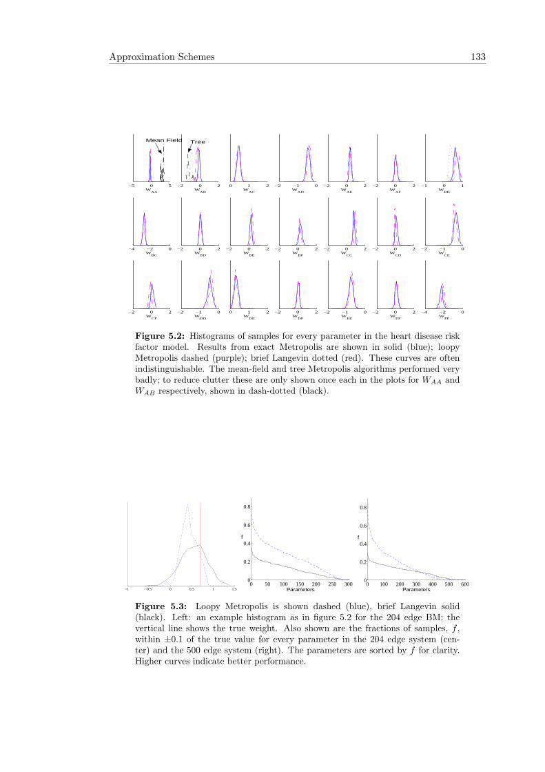
Approximation Schemes 133
−4 −2 0W
FF
−2 0 2W
EF
−2 −1 0W
EE
−2 0 2W
DF
0 1 2W
DE
−2 −1 0W
DD
−2 0 2W
CF
−2 −1 0W
CE
−2 0 2W
CD
−2 0 2W
CC
−2 0 2W
BF
−2 0 2W
BE
−2 0 2W
BD
−4 −2 0W
BC
−1 0 1W
BB
−2 0 2W
AF
−2 0 2W
AE
−2 −1 0W
AD
0 1 2W
AC
−2 0 2W
AB
−5 0 5W
AA
Mean Field Tree
Figure 5.2: Histograms of samples for every parameter in the heart disease riskfactor model. Results from exact Metropolis are shown in solid (blue); loopyMetropolis dashed (purple); brief Langevin dotted (red). These curves are oftenindistinguishable. The mean-field and tree Metropolis algorithms performed verybadly; to reduce clutter these are only shown once each in the plots for WAA andWAB respectively, shown in dash-dotted (black).
−1 −0.5 0 0.5 1 1.50 50 100 150 200 250 300
0
0.2
0.4
0.6
0.8
Parameters
f
0 100 200 300 400 500 6000
0.2
0.4
0.6
0.8
Parameters
f
Figure 5.3: Loopy Metropolis is shown dashed (blue), brief Langevin solid(black). Left: an example histogram as in figure 5.2 for the 204 edge BM; thevertical line shows the true weight. Also shown are the fractions of samples, f ,within ±0.1 of the true value for every parameter in the 204 edge system (cen-ter) and the 500 edge system (right). The parameters are sorted by f for clarity.Higher curves indicate better performance.
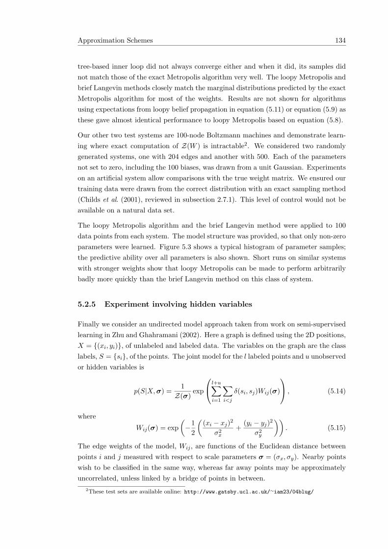
Approximation Schemes 134
tree-based inner loop did not always converge either and when it did, its samples didnot match those of the exact Metropolis algorithm very well. The loopy Metropolis andbrief Langevin methods closely match the marginal distributions predicted by the exactMetropolis algorithm for most of the weights. Results are not shown for algorithmsusing expectations from loopy belief propagation in equation (5.11) or equation (5.9) asthese gave almost identical performance to loopy Metropolis based on equation (5.8).
Our other two test systems are 100-node Boltzmann machines and demonstrate learn-ing where exact computation of Z(W ) is intractable2. We considered two randomlygenerated systems, one with 204 edges and another with 500. Each of the parametersnot set to zero, including the 100 biases, was drawn from a unit Gaussian. Experimentson an artificial system allow comparisons with the true weight matrix. We ensured ourtraining data were drawn from the correct distribution with an exact sampling method(Childs et al. (2001), reviewed in subsection 2.7.1). This level of control would not beavailable on a natural data set.
The loopy Metropolis algorithm and the brief Langevin method were applied to 100data points from each system. The model structure was provided, so that only non-zeroparameters were learned. Figure 5.3 shows a typical histogram of parameter samples;the predictive ability over all parameters is also shown. Short runs on similar systemswith stronger weights show that loopy Metropolis can be made to perform arbitrarilybadly more quickly than the brief Langevin method on this class of system.
5.2.5 Experiment involving hidden variables
Finally we consider an undirected model approach taken from work on semi-supervisedlearning in Zhu and Ghahramani (2002). Here a graph is defined using the 2D positions,X = {(xi, yi)}, of unlabeled and labeled data. The variables on the graph are the classlabels, S = {si}, of the points. The joint model for the l labeled points and u unobservedor hidden variables is
p(S|X, σ) =1Z(σ)
exp
l+u∑i=1
∑i<j
δ(si, sj)Wij(σ)
, (5.14)
where
Wij(σ) = exp(−1
2
((xi − xj)2
σ2x
+(yi − yj)2
σ2y
)). (5.15)
The edge weights of the model, Wij , are functions of the Euclidean distance betweenpoints i and j measured with respect to scale parameters σ = (σx, σy). Nearby pointswish to be classified in the same way, whereas far away points may be approximatelyuncorrelated, unless linked by a bridge of points in between.
2These test sets are available online: http://www.gatsby.ucl.ac.uk/∼iam23/04blug/
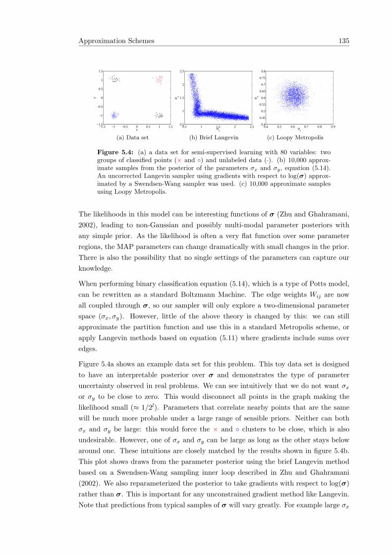
Approximation Schemes 135
−1.5 −1 −0.5 0 0.5 1 1.5−1.5
−1
−0.5
0
0.5
1
1.5
x
y
(a) Data set
0.5 1 1.5 2 2.50.5
1
1.5
2
2.5
σx
σ y
(b) Brief Langevin
0.4 0.5 0.6 0.7 0.8 0.90.4
0.45
0.5
0.55
0.6
0.65
0.7
0.75
0.8
σx
σ y
(c) Loopy Metropolis
Figure 5.4: (a) a data set for semi-supervised learning with 80 variables: twogroups of classified points (× and ◦) and unlabeled data (·). (b) 10,000 approx-imate samples from the posterior of the parameters σx and σy, equation (5.14).An uncorrected Langevin sampler using gradients with respect to log(σ) approx-imated by a Swendsen-Wang sampler was used. (c) 10,000 approximate samplesusing Loopy Metropolis.
The likelihoods in this model can be interesting functions of σ (Zhu and Ghahramani,2002), leading to non-Gaussian and possibly multi-modal parameter posteriors withany simple prior. As the likelihood is often a very flat function over some parameterregions, the MAP parameters can change dramatically with small changes in the prior.There is also the possibility that no single settings of the parameters can capture ourknowledge.
When performing binary classification equation (5.14), which is a type of Potts model,can be rewritten as a standard Boltzmann Machine. The edge weights Wij are nowall coupled through σ, so our sampler will only explore a two-dimensional parameterspace (σx, σy). However, little of the above theory is changed by this: we can stillapproximate the partition function and use this in a standard Metropolis scheme, orapply Langevin methods based on equation (5.11) where gradients include sums overedges.
Figure 5.4a shows an example data set for this problem. This toy data set is designedto have an interpretable posterior over σ and demonstrates the type of parameteruncertainty observed in real problems. We can see intuitively that we do not want σx
or σy to be close to zero. This would disconnect all points in the graph making thelikelihood small (≈ 1/2l). Parameters that correlate nearby points that are the samewill be much more probable under a large range of sensible priors. Neither can bothσx and σy be large: this would force the × and ◦ clusters to be close, which is alsoundesirable. However, one of σx and σy can be large as long as the other stays belowaround one. These intuitions are closely matched by the results shown in figure 5.4b.This plot shows draws from the parameter posterior using the brief Langevin methodbased on a Swendsen-Wang sampling inner loop described in Zhu and Ghahramani(2002). We also reparameterized the posterior to take gradients with respect to log(σ)rather than σ. This is important for any unconstrained gradient method like Langevin.Note that predictions from typical samples of σ will vary greatly. For example large σx
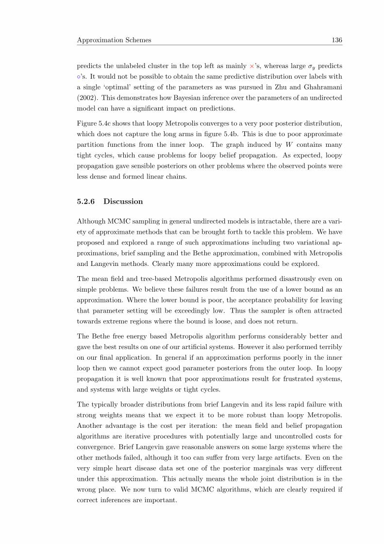
Approximation Schemes 136
predicts the unlabeled cluster in the top left as mainly ×’s, whereas large σy predicts◦’s. It would not be possible to obtain the same predictive distribution over labels witha single ‘optimal’ setting of the parameters as was pursued in Zhu and Ghahramani(2002). This demonstrates how Bayesian inference over the parameters of an undirectedmodel can have a significant impact on predictions.
Figure 5.4c shows that loopy Metropolis converges to a very poor posterior distribution,which does not capture the long arms in figure 5.4b. This is due to poor approximatepartition functions from the inner loop. The graph induced by W contains manytight cycles, which cause problems for loopy belief propagation. As expected, loopypropagation gave sensible posteriors on other problems where the observed points wereless dense and formed linear chains.
5.2.6 Discussion
Although MCMC sampling in general undirected models is intractable, there are a vari-ety of approximate methods that can be brought forth to tackle this problem. We haveproposed and explored a range of such approximations including two variational ap-proximations, brief sampling and the Bethe approximation, combined with Metropolisand Langevin methods. Clearly many more approximations could be explored.
The mean field and tree-based Metropolis algorithms performed disastrously even onsimple problems. We believe these failures result from the use of a lower bound as anapproximation. Where the lower bound is poor, the acceptance probability for leavingthat parameter setting will be exceedingly low. Thus the sampler is often attractedtowards extreme regions where the bound is loose, and does not return.
The Bethe free energy based Metropolis algorithm performs considerably better andgave the best results on one of our artificial systems. However it also performed terriblyon our final application. In general if an approximation performs poorly in the innerloop then we cannot expect good parameter posteriors from the outer loop. In loopypropagation it is well known that poor approximations result for frustrated systems,and systems with large weights or tight cycles.
The typically broader distributions from brief Langevin and its less rapid failure withstrong weights means that we expect it to be more robust than loopy Metropolis.Another advantage is the cost per iteration: the mean field and belief propagationalgorithms are iterative procedures with potentially large and uncontrolled costs forconvergence. Brief Langevin gave reasonable answers on some large systems where theother methods failed, although it too can suffer from very large artifacts. Even on thevery simple heart disease data set one of the posterior marginals was very differentunder this approximation. This actually means the whole joint distribution is in thewrong place. We now turn to valid MCMC algorithms, which are clearly required ifcorrect inferences are important.
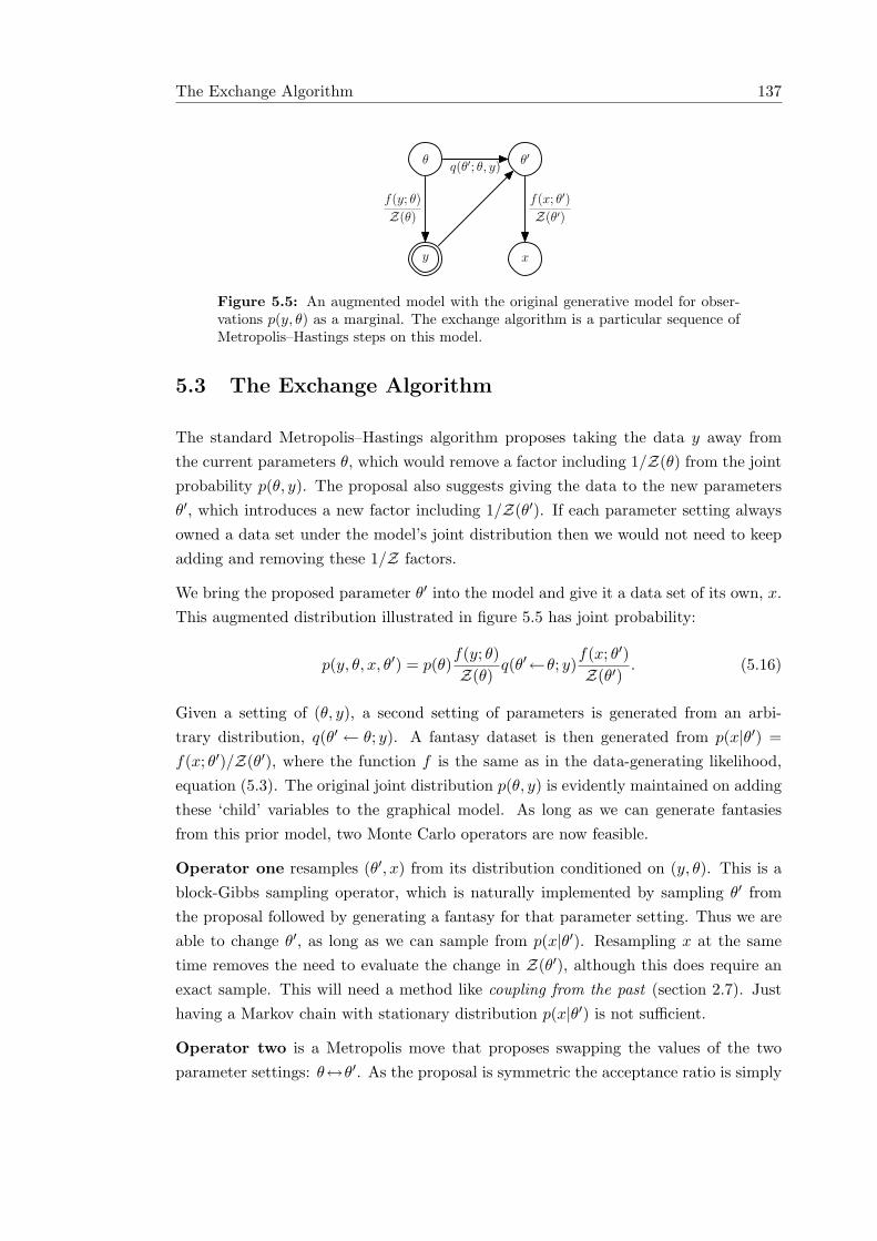
The Exchange Algorithm 137
θ θ′
y x
q(θ′; θ, y)
f(y; θ)
Z(θ)
f(x; θ′)
Z(θ′)
Figure 5.5: An augmented model with the original generative model for obser-vations p(y, θ) as a marginal. The exchange algorithm is a particular sequence ofMetropolis–Hastings steps on this model.
5.3 The Exchange Algorithm
The standard Metropolis–Hastings algorithm proposes taking the data y away fromthe current parameters θ, which would remove a factor including 1/Z(θ) from the jointprobability p(θ, y). The proposal also suggests giving the data to the new parametersθ′, which introduces a new factor including 1/Z(θ′). If each parameter setting alwaysowned a data set under the model’s joint distribution then we would not need to keepadding and removing these 1/Z factors.
We bring the proposed parameter θ′ into the model and give it a data set of its own, x.This augmented distribution illustrated in figure 5.5 has joint probability:
p(y, θ, x, θ′) = p(θ)f(y; θ)Z(θ)
q(θ′←θ; y)f(x; θ′)Z(θ′)
. (5.16)
Given a setting of (θ, y), a second setting of parameters is generated from an arbi-trary distribution, q(θ′ ← θ; y). A fantasy dataset is then generated from p(x|θ′) =f(x; θ′)/Z(θ′), where the function f is the same as in the data-generating likelihood,equation (5.3). The original joint distribution p(θ, y) is evidently maintained on addingthese ‘child’ variables to the graphical model. As long as we can generate fantasiesfrom this prior model, two Monte Carlo operators are now feasible.
Operator one resamples (θ′, x) from its distribution conditioned on (y, θ). This is ablock-Gibbs sampling operator, which is naturally implemented by sampling θ′ fromthe proposal followed by generating a fantasy for that parameter setting. Thus we areable to change θ′, as long as we can sample from p(x|θ′). Resampling x at the sametime removes the need to evaluate the change in Z(θ′), although this does require anexact sample. This will need a method like coupling from the past (section 2.7). Justhaving a Markov chain with stationary distribution p(x|θ′) is not sufficient.
Operator two is a Metropolis move that proposes swapping the values of the twoparameter settings: θ↔θ′. As the proposal is symmetric the acceptance ratio is simply
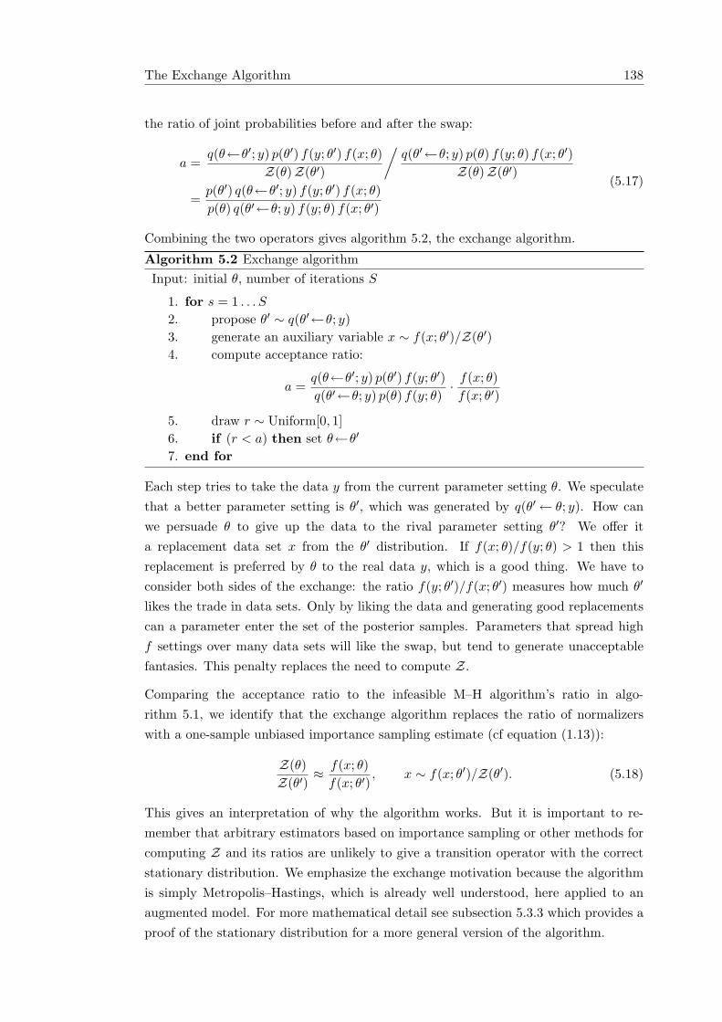
The Exchange Algorithm 138
the ratio of joint probabilities before and after the swap:
a =q(θ←θ′; y) p(θ′) f(y; θ′) f(x; θ)
Z(θ)Z(θ′)
/q(θ′←θ; y) p(θ) f(y; θ) f(x; θ′)
Z(θ)Z(θ′)
=p(θ′) q(θ←θ′; y) f(y; θ′) f(x; θ)p(θ) q(θ′←θ; y) f(y; θ) f(x; θ′)
(5.17)
Combining the two operators gives algorithm 5.2, the exchange algorithm.
Algorithm 5.2 Exchange algorithmInput: initial θ, number of iterations S
1. for s = 1 . . . S
2. propose θ′ ∼ q(θ′←θ; y)3. generate an auxiliary variable x ∼ f(x; θ′)/Z(θ′)4. compute acceptance ratio:
a =q(θ←θ′; y) p(θ′) f(y; θ′)q(θ′←θ; y) p(θ) f(y; θ)
· f(x; θ)f(x; θ′)
5. draw r ∼ Uniform[0, 1]6. if (r < a) then set θ←θ′
7. end for
Each step tries to take the data y from the current parameter setting θ. We speculatethat a better parameter setting is θ′, which was generated by q(θ′← θ; y). How canwe persuade θ to give up the data to the rival parameter setting θ′? We offer ita replacement data set x from the θ′ distribution. If f(x; θ)/f(y; θ) > 1 then thisreplacement is preferred by θ to the real data y, which is a good thing. We have toconsider both sides of the exchange: the ratio f(y; θ′)/f(x; θ′) measures how much θ′
likes the trade in data sets. Only by liking the data and generating good replacementscan a parameter enter the set of the posterior samples. Parameters that spread highf settings over many data sets will like the swap, but tend to generate unacceptablefantasies. This penalty replaces the need to compute Z.
Comparing the acceptance ratio to the infeasible M–H algorithm’s ratio in algo-rithm 5.1, we identify that the exchange algorithm replaces the ratio of normalizerswith a one-sample unbiased importance sampling estimate (cf equation (1.13)):
Z(θ)Z(θ′)
≈ f(x; θ)f(x; θ′)
, x ∼ f(x; θ′)/Z(θ′). (5.18)
This gives an interpretation of why the algorithm works. But it is important to re-member that arbitrary estimators based on importance sampling or other methods forcomputing Z and its ratios are unlikely to give a transition operator with the correctstationary distribution. We emphasize the exchange motivation because the algorithmis simply Metropolis–Hastings, which is already well understood, here applied to anaugmented model. For more mathematical detail see subsection 5.3.3 which provides aproof of the stationary distribution for a more general version of the algorithm.
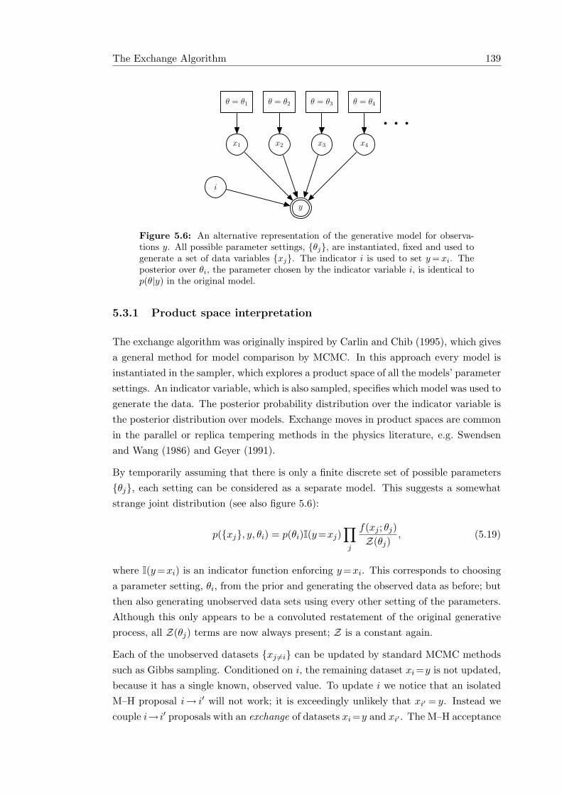
The Exchange Algorithm 139
θ = θ1 θ = θ2 θ = θ3 θ = θ4
x1 x2 x3 x4
y
i
Figure 5.6: An alternative representation of the generative model for observa-tions y. All possible parameter settings, {θj}, are instantiated, fixed and used togenerate a set of data variables {xj}. The indicator i is used to set y = xi. Theposterior over θi, the parameter chosen by the indicator variable i, is identical top(θ|y) in the original model.
5.3.1 Product space interpretation
The exchange algorithm was originally inspired by Carlin and Chib (1995), which givesa general method for model comparison by MCMC. In this approach every model isinstantiated in the sampler, which explores a product space of all the models’ parametersettings. An indicator variable, which is also sampled, specifies which model was used togenerate the data. The posterior probability distribution over the indicator variable isthe posterior distribution over models. Exchange moves in product spaces are commonin the parallel or replica tempering methods in the physics literature, e.g. Swendsenand Wang (1986) and Geyer (1991).
By temporarily assuming that there is only a finite discrete set of possible parameters{θj}, each setting can be considered as a separate model. This suggests a somewhatstrange joint distribution (see also figure 5.6):
p({xj}, y, θi) = p(θi)I(y=xj)∏j
f(xj ; θj)Z(θj)
, (5.19)
where I(y=xi) is an indicator function enforcing y=xi. This corresponds to choosinga parameter setting, θi, from the prior and generating the observed data as before; butthen also generating unobserved data sets using every other setting of the parameters.Although this only appears to be a convoluted restatement of the original generativeprocess, all Z(θj) terms are now always present; Z is a constant again.
Each of the unobserved datasets {xj 6=i} can be updated by standard MCMC methodssuch as Gibbs sampling. Conditioned on i, the remaining dataset xi =y is not updated,because it has a single known, observed value. To update i we notice that an isolatedM–H proposal i→ i′ will not work; it is exceedingly unlikely that xi′ = y. Instead wecouple i→ i′ proposals with an exchange of datasets xi =y and xi′ . The M–H acceptance
The Exchange Algorithm 140
ratio for this proposal is simple; much of the joint distribution in equation (5.19) cancelsleaving:
a =q(i← i′; y) p(θi′) f(y; θi′) f(xi′ ; θi)q(i′← i; y) p(θi) f(y; θi) f(xi′ ; θi′)
. (5.20)
The only remaining problem is that if the number of parameter settings is very large,we require huge amounts of storage and a very long time to reach equilibrium. Inparticular the method seems impractical if θ is continuous.
The solution to these problems recreates the exchange algorithm of the previous section.We declare that at each time step all of the x variables are at equilibrium conditionedon the indicator variable i. But we do not need to store these values; only whena swap of ownership between θ and θ′ is proposed do we need to know the currentsetting of θ′’s data. We can then draw the value from its equilibrium distribution:x ∼ p(x|θ′)=f(x; θ′)/Z(θ′), pretending that this had already been computed. After theexchange has been accepted or rejected the intermediate quantity x can be discarded.We redraw any unobserved data set from its stationary distribution as required. Thisretrospective sampling trick has been used in a variety of other MCMC algorithms forinfinite-dimensional models (Papaspiliopoulos and Roberts, 2005; Beskos et al., 2006).
An infinite-dimensional model and retrospective sampling are not required to describethe exchange algorithm, but provide connections to the literature, which might beuseful for some readers. The product model works without exact sampling for modelswith a small number of parameter settings and is also how the algorithm was originallyconceived. Other readers may prefer the explanation in the previous section: even oncontinuous parameters it uses Metropolis–Hastings on a finite auxiliary system, whichis more established theoretically.
5.3.2 Bridging Exchange Algorithm
The Metropolis–Hastings acceptance rule has the maximum acceptance rate for anyreversible transition operator that may only accept or reject proposals from q (seesubsection 2.1.1). As the exchange algorithm is only approximately the same as thedirect M–H approach, in some sense it rejects moves that it should not. As we havemuch better approximations of normalizing constant ratios than equation (5.18), bettermethods should be possible.
How can good parameter proposals get rejected? It may be that θ′ is a much betterexplanation of the data y than the current parameters θ and would be accepted underM–H. However, the exchange algorithm can reject the swap because x∼f(x; θ′)/Z(θ′)is improbable under θ. This makes movement unnecessarily slow and suggests searchingfor a way to make swaps look more favorable.
The exchange algorithm with bridging draws a fantasy as before, x0∼f(x0; θ′)/Z(θ′),but then applies a series of modifications x0→ x1→ · · ·xK such that xK is typically
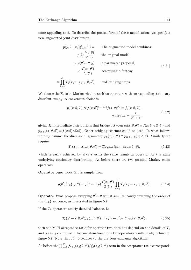
The Exchange Algorithm 141
more appealing to θ. To describe the precise form of these modifications we specify anew augmented joint distribution.
p(y, θ, {xk}Kk=0, θ′) = The augmented model combines:
p(θ)f(y; θ)Z(θ)
the original model,
× q(θ′←θ; y) a parameter proposal,
× f(x0; θ′)Z(θ′)
generating a fantasy
×K∏
k=1
Tk(xk←xk−1; θ, θ′) and bridging steps.
(5.21)
We choose the Tk to be Markov chain transition operators with corresponding stationarydistributions pk. A convenient choice is
pk(x; θ, θ′) ∝ f(x; θ′)(1−βk)f(x; θ)βk ≡ fk(x; θ, θ′),
where βk =k
K + 1,
(5.22)
giving K intermediate distributions that bridge between p0(x; θ, θ′)≡f(x; θ′)/Z(θ′) andpK+1(x; θ, θ′)≡ f(x; θ)/Z(θ). Other bridging schemes could be used. In what followswe only assume the directional symmetry pk(x; θ, θ′)≡ pK+1−k(x; θ′, θ). Similarly werequire
Tk(xk←xk−1; θ, θ′) = TK+1−k(xk←xk−1; θ′, θ), (5.23)
which is easily achieved by always using the same transition operator for the sameunderlying stationary distribution. As before there are two possible Markov chainoperators.
Operator one: block Gibbs sample from
p(θ′, {xk}|y, θ) = q(θ′←θ; y)f(x0; θ′)Z(θ′)
K∏k=1
Tk(xk←xk−1; θ, θ′). (5.24)
Operator two: propose swapping θ′↔θ whilst simultaneously reversing the order ofthe {xk} sequence, as illustrated in figure 5.7.
If the Tk operators satisfy detailed balance, i.e.
Tk(x′←x; θ, θ′)pk(x; θ, θ′) = Tk(x←x′; θ, θ′)pk(x′; θ, θ′), (5.25)
then the M–H acceptance ratio for operator two does not depend on the details of Tk
and is easily computed. The concatenation of the two operators results in algorithm 5.3,figure 5.7. Note that K =0 reduces to the previous exchange algorithm.
As before the∏K
k=0 fk+1(xk; θ, θ′)/fk(xk; θ, θ′) term in the acceptance ratio corresponds
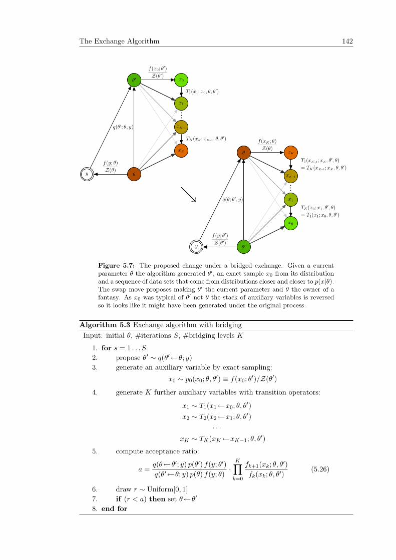
The Exchange Algorithm 142
θ
θ′
y
q(θ′; θ, y)
f(y; θ)
Z(θ)
x0
x1
xK−1
xK
f(x0; θ′)
Z(θ′)
T1(x1; x0, θ, θ′)
TK(xK; xK−1, θ, θ′)
↘
θ′
θ
y
q(θ; θ′, y)
f(y; θ′)
Z(θ′)
x0
x1
xK−1
xK
f(xK ; θ)
Z(θ)
T1(xK−1; xK, θ′, θ)
= TK(xK−1; xK, θ, θ′)
TK(x0; x1, θ′, θ)
= T1(x1; x0, θ, θ′)
Figure 5.7: The proposed change under a bridged exchange. Given a currentparameter θ the algorithm generated θ′, an exact sample x0 from its distributionand a sequence of data sets that come from distributions closer and closer to p(x|θ).The swap move proposes making θ′ the current parameter and θ the owner of afantasy. As x0 was typical of θ′ not θ the stack of auxiliary variables is reversedso it looks like it might have been generated under the original process.
Algorithm 5.3 Exchange algorithm with bridgingInput: initial θ, #iterations S, #bridging levels K
1. for s = 1 . . . S
2. propose θ′ ∼ q(θ′←θ; y)3. generate an auxiliary variable by exact sampling:
x0 ∼ p0(x0; θ, θ′) ≡ f(x0; θ′)/Z(θ′)
4. generate K further auxiliary variables with transition operators:
x1 ∼ T1(x1←x0; θ, θ′)x2 ∼ T2(x2←x1; θ, θ′)
· · ·xK ∼ TK(xK←xK−1; θ, θ′)
5. compute acceptance ratio:
a =q(θ←θ′; y) p(θ′) f(y; θ′)q(θ′←θ; y) p(θ) f(y; θ)
·K∏
k=0
fk+1(xk; θ, θ′)fk(xk; θ, θ′)
(5.26)
6. draw r ∼ Uniform[0, 1]7. if (r < a) then set θ←θ′
8. end for
The Exchange Algorithm 143
to an unbiased estimate of Z(θ)/Z(θ′). Proof: it is an annealed importance sampling(AIS) weight, equation (2.24). This is the natural extension to the simple importanceestimate, equation (5.18), in the original exchange algorithm. Linked importance sam-pling (Neal, 2005) could also be used as a drop-in replacement.
The bridging extension to the exchange algorithm allows us to improve its implicitnormalization constant estimation and improve the acceptance rate, for some additionalcost. Fortunately no further expensive exact sampling, on top of that needed by theoriginal algorithm, is required per iteration. The performance as a function of K isexplored in section 5.6.
5.3.3 Details for proof of correctness
It turns out that the algorithm as stated is also valid when the operators Tk do notsatisfy detailed balance. We give the details of a proof for this more general case.
We define a set of reverse Markov chain operators
Tk(x←x′; θ, θ′) ∝ Tk(x′←x; θ, θ′) pk(x; θ, θ′) =Tk(x′←x; θ, θ′) pk(x; θ, θ′)
pk(x′; θ, θ′). (5.27)
Define the transition operator T by steps 2–7 of algorithm 5.3. Let T be defined bythe same algorithm but using {Tk} rather than {Tk}. We now prove that both T andT leave p(θ|y) stationary:
T (x0, . . ., xK , θ′←θ)p(θ|y) = Probability of transition is
p(θ|y) =p(y|θ)p(θ)
p(y)=
f(y; θ)p(θ)Z(θ)p(y)
probability of being at θ,
× q(θ′←θ; y) proposing a move to θ′,
× f(x0; θ′)Z(θ′)
≡ f0(x0; θ, θ′)Z(θ′)
generating x0,
×K∏
k=1
Tk(xk←xk−1; θ, θ′) generating (x1, . . ., xK)
× min
[1,
q(θ←θ′; y) p(θ′) f(y; θ′)q(θ′←θ; y) p(θ) f(y; θ)
K∏k=0
fk+1(xk; θ, θ′)fk(xk; θ, θ′)
]and finally accepting.
Rearranging and using fK+1(xK ; θ, θ′) ≡ f(xK ; θ):
= min
[p(θ) f(y; θ) q(θ′←θ; y) f(x0; θ′)
p(y)Z(θ)Z(θ′)
K∏k=1
Tk(xk←xk−1; θ, θ′) ,
p(θ′) f(y; θ′) q(θ←θ′; y) f(xK ; θ)p(y)Z(θ′)Z(θ)
K∏k=1
Tk(xk←xk−1; θ, θ′) fk(xk−1; θ, θ′)fk(xk; θ, θ′)
].
The Single Auxiliary Variable Method 144
We substitute equation (5.27) and equation (5.23) into the second product and reorderits terms:
= min
[p(θ) f(y; θ) q(θ′←θ; y) f(x0; θ′)
p(y)Z(θ)Z(θ′)
K∏k=1
Tk(xk←xk−1; θ, θ′) ,
p(θ′) f(y; θ′) q(θ←θ′; y) f(xK ; θ)p(y)Z(θ′)Z(θ)
K∏k=1
Tk(xK−k←xK+1−k; θ′, θ)
].
(5.28)
Now swapping θ and θ′, reversing the order of the auxiliary variables, i.e. mapping(x0, x1, . . . , xK)→ (xK , . . . , x1, x0) and swapping T and T throughout, only swaps thearguments of the min leaving the value of the expression unchanged. Therefore, theprobability of the reverse transition under T , via the same intermediate values, is thesame as in equation (5.28). That is, for any values of {xk}
T ((x0, . . ., xK), θ′←θ) p(θ|y) = T ((xK , . . ., x0), θ←θ′) p(θ′|y) . (5.29)
Summing over all possible intermediate values {xk} gives
T (θ′←θ) p(θ|y) = T (θ←θ′) p(θ′|y) . (5.30)
Further summing over θ or θ′ shows that both T and T leave p(θ|y) stationary. If, aswas originally proposed, T is reversible then T ≡ T and the bridged exchange algorithmalso satisfies detailed balance.
As an aside we mention that the bridging scheme is very similar to that found in themethod of dragging fast variables (Neal, 2004a). Although dragging was presentedusing reversible transition operators, a similar proof to the one above shows that it toocan use non-reversible transition operators.
5.4 The Single Auxiliary Variable Method
The first valid MCMC algorithm for doubly-intractable distributions was discovered byMøller et al. (2004, 2006). For comparison this section reviews their method, which wecall the Single Auxiliary Variable Method (SAVM).
SAVM extends the original model to include a single auxiliary variable, x, which sharesthe same state space as y (figure 5.8):
p(x, y, θ) = p(x|θ, y)f(y; θ)Z(θ)
p(θ). (5.31)
The joint distribution p(y, θ) is unaffected. No known method of defining auxiliaryvariables removes Z(θ) from the joint distribution. However, through careful choice
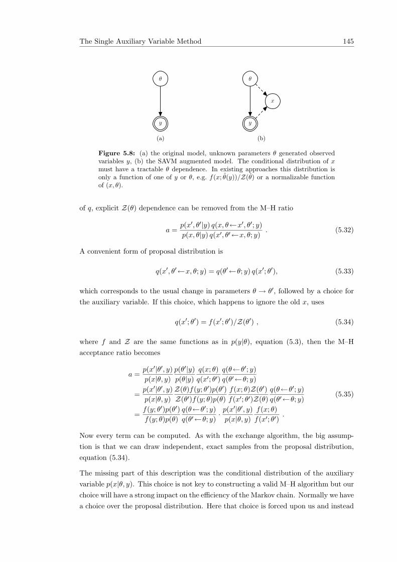
The Single Auxiliary Variable Method 145
θ
y
(a)
y
θ
x
(b)
Figure 5.8: (a) the original model, unknown parameters θ generated observedvariables y, (b) the SAVM augmented model. The conditional distribution of xmust have a tractable θ dependence. In existing approaches this distribution isonly a function of one of y or θ, e.g. f(x; θ(y))/Z(θ) or a normalizable functionof (x, θ).
of q, explicit Z(θ) dependence can be removed from the M–H ratio
a =p(x′, θ′|y) q(x, θ←x′, θ′; y)p(x, θ|y) q(x′, θ′←x, θ; y)
. (5.32)
A convenient form of proposal distribution is
q(x′, θ′←x, θ; y) = q(θ′←θ; y) q(x′; θ′), (5.33)
which corresponds to the usual change in parameters θ → θ′, followed by a choice forthe auxiliary variable. If this choice, which happens to ignore the old x, uses
q(x′; θ′) = f(x′; θ′)/Z(θ′) , (5.34)
where f and Z are the same functions as in p(y|θ), equation (5.3), then the M–Hacceptance ratio becomes
a =p(x′|θ′, y)p(x|θ, y)
p(θ′|y)p(θ|y)
q(x; θ)q(x′; θ′)
q(θ←θ′; y)q(θ′←θ; y)
=p(x′|θ′, y)p(x|θ, y)
Z(θ)f(y; θ′)p(θ′)Z(θ′)f(y; θ)p(θ)
f(x; θ)Z(θ′)f(x′; θ′)Z(θ)
q(θ←θ′; y)q(θ′←θ; y)
=f(y; θ′)p(θ′)f(y; θ)p(θ)
q(θ←θ′; y)q(θ′←θ; y)
· p(x′|θ′, y)p(x|θ, y)
f(x; θ)f(x′; θ′)
.
(5.35)
Now every term can be computed. As with the exchange algorithm, the big assump-tion is that we can draw independent, exact samples from the proposal distribution,equation (5.34).
The missing part of this description was the conditional distribution of the auxiliaryvariable p(x|θ, y). This choice is not key to constructing a valid M–H algorithm but ourchoice will have a strong impact on the efficiency of the Markov chain. Normally we havea choice over the proposal distribution. Here that choice is forced upon us and instead
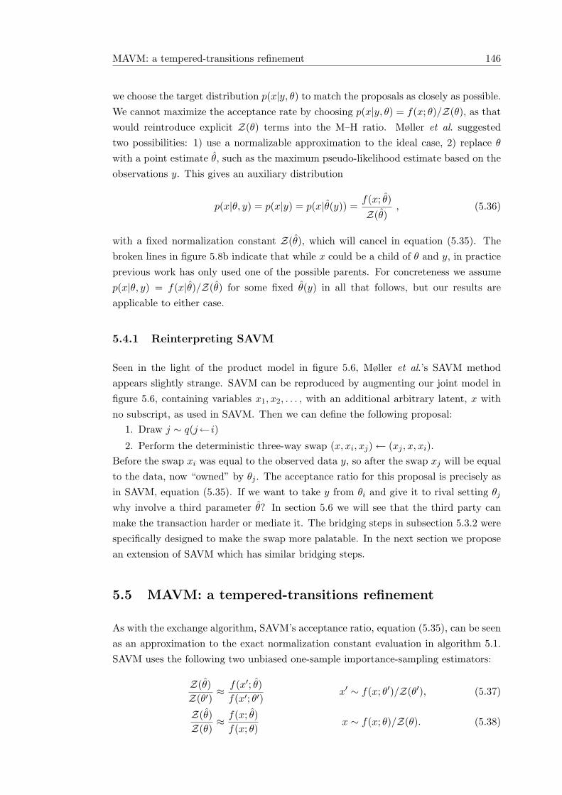
MAVM: a tempered-transitions refinement 146
we choose the target distribution p(x|y, θ) to match the proposals as closely as possible.We cannot maximize the acceptance rate by choosing p(x|y, θ) = f(x; θ)/Z(θ), as thatwould reintroduce explicit Z(θ) terms into the M–H ratio. Møller et al. suggestedtwo possibilities: 1) use a normalizable approximation to the ideal case, 2) replace θ
with a point estimate θ, such as the maximum pseudo-likelihood estimate based on theobservations y. This gives an auxiliary distribution
p(x|θ, y) = p(x|y) = p(x|θ(y)) =f(x; θ)
Z(θ), (5.36)
with a fixed normalization constant Z(θ), which will cancel in equation (5.35). Thebroken lines in figure 5.8b indicate that while x could be a child of θ and y, in practiceprevious work has only used one of the possible parents. For concreteness we assumep(x|θ, y) = f(x|θ)/Z(θ) for some fixed θ(y) in all that follows, but our results areapplicable to either case.
5.4.1 Reinterpreting SAVM
Seen in the light of the product model in figure 5.6, Møller et al.’s SAVM methodappears slightly strange. SAVM can be reproduced by augmenting our joint model infigure 5.6, containing variables x1, x2, . . . , with an additional arbitrary latent, x withno subscript, as used in SAVM. Then we can define the following proposal:
1. Draw j ∼ q(j← i)
2. Perform the deterministic three-way swap (x, xi, xj)← (xj , x, xi).Before the swap xi was equal to the observed data y, so after the swap xj will be equalto the data, now “owned” by θj . The acceptance ratio for this proposal is precisely asin SAVM, equation (5.35). If we want to take y from θi and give it to rival setting θj
why involve a third parameter θ? In section 5.6 we will see that the third party canmake the transaction harder or mediate it. The bridging steps in subsection 5.3.2 werespecifically designed to make the swap more palatable. In the next section we proposean extension of SAVM which has similar bridging steps.
5.5 MAVM: a tempered-transitions refinement
As with the exchange algorithm, SAVM’s acceptance ratio, equation (5.35), can be seenas an approximation to the exact normalization constant evaluation in algorithm 5.1.SAVM uses the following two unbiased one-sample importance-sampling estimators:
Z(θ)Z(θ′)
≈ f(x′; θ)f(x′; θ′)
x′ ∼ f(x; θ′)/Z(θ′), (5.37)
Z(θ)Z(θ)
≈ f(x; θ)f(x; θ)
x ∼ f(x; θ)/Z(θ). (5.38)
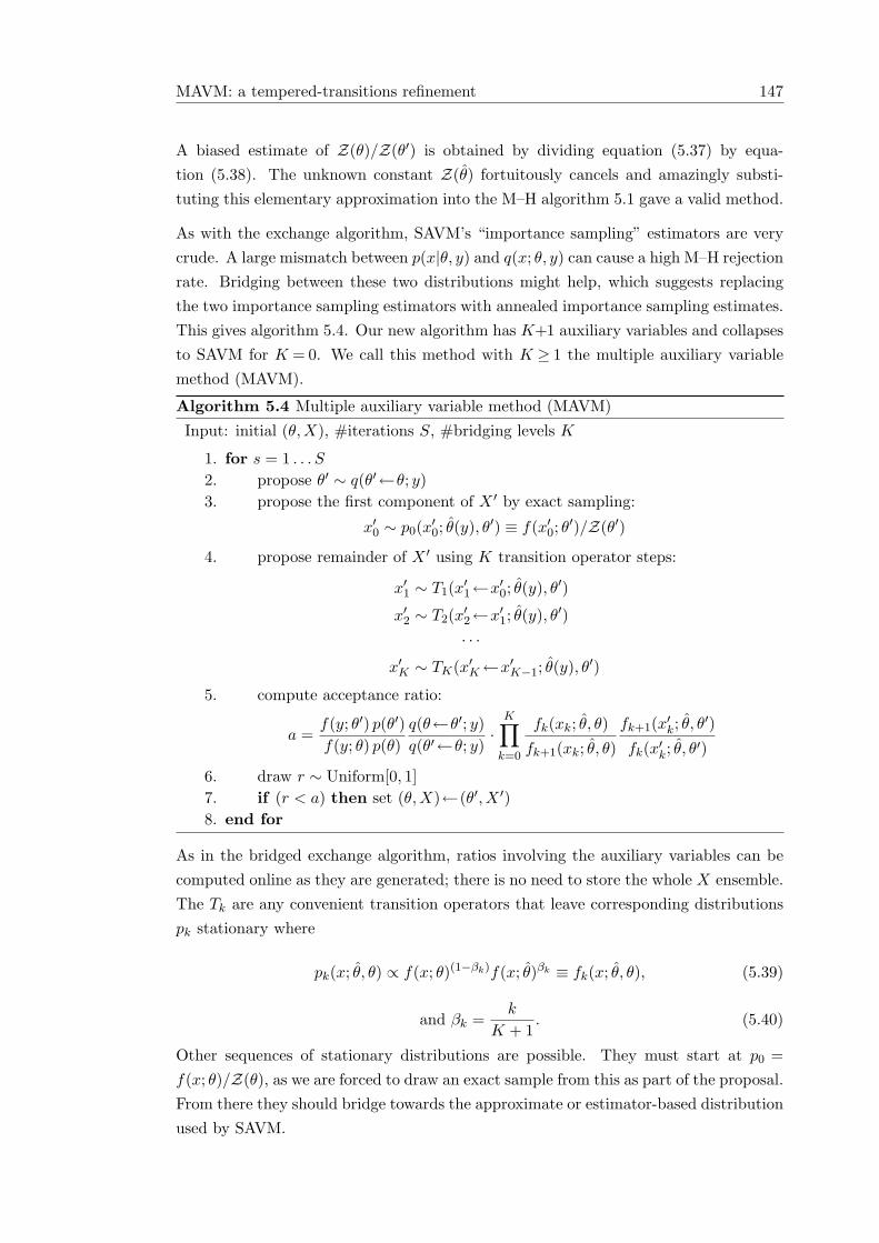
MAVM: a tempered-transitions refinement 147
A biased estimate of Z(θ)/Z(θ′) is obtained by dividing equation (5.37) by equa-tion (5.38). The unknown constant Z(θ) fortuitously cancels and amazingly substi-tuting this elementary approximation into the M–H algorithm 5.1 gave a valid method.
As with the exchange algorithm, SAVM’s “importance sampling” estimators are verycrude. A large mismatch between p(x|θ, y) and q(x; θ, y) can cause a high M–H rejectionrate. Bridging between these two distributions might help, which suggests replacingthe two importance sampling estimators with annealed importance sampling estimates.This gives algorithm 5.4. Our new algorithm has K+1 auxiliary variables and collapsesto SAVM for K = 0. We call this method with K ≥ 1 the multiple auxiliary variablemethod (MAVM).
Algorithm 5.4 Multiple auxiliary variable method (MAVM)Input: initial (θ, X), #iterations S, #bridging levels K
1. for s = 1 . . . S
2. propose θ′ ∼ q(θ′←θ; y)3. propose the first component of X ′ by exact sampling:
x′0 ∼ p0(x′0; θ(y), θ′) ≡ f(x′0; θ′)/Z(θ′)
4. propose remainder of X ′ using K transition operator steps:
x′1 ∼ T1(x′1←x′0; θ(y), θ′)
x′2 ∼ T2(x′2←x′1; θ(y), θ′)· · ·
x′K ∼ TK(x′K←x′K−1; θ(y), θ′)
5. compute acceptance ratio:
a =f(y; θ′) p(θ′)f(y; θ) p(θ)
q(θ←θ′; y)q(θ′←θ; y)
·K∏
k=0
fk(xk; θ, θ)
fk+1(xk; θ, θ)
fk+1(x′k; θ, θ′)
fk(x′k; θ, θ′)
6. draw r ∼ Uniform[0, 1]7. if (r < a) then set (θ, X)←(θ′, X ′)8. end for
As in the bridged exchange algorithm, ratios involving the auxiliary variables can becomputed online as they are generated; there is no need to store the whole X ensemble.The Tk are any convenient transition operators that leave corresponding distributionspk stationary where
pk(x; θ, θ) ∝ f(x; θ)(1−βk)f(x; θ)βk ≡ fk(x; θ, θ), (5.39)
and βk =k
K + 1. (5.40)
Other sequences of stationary distributions are possible. They must start at p0 =f(x; θ)/Z(θ), as we are forced to draw an exact sample from this as part of the proposal.From there they should bridge towards the approximate or estimator-based distributionused by SAVM.
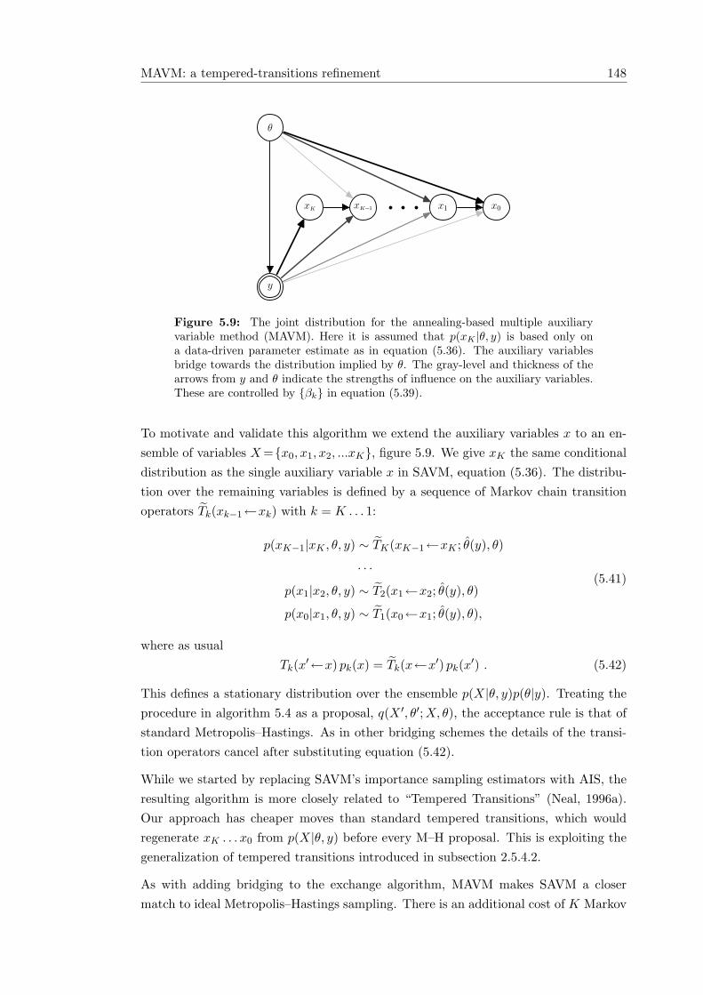
MAVM: a tempered-transitions refinement 148
θ
y
xKxK−1 x1 x0
Figure 5.9: The joint distribution for the annealing-based multiple auxiliaryvariable method (MAVM). Here it is assumed that p(xK |θ, y) is based only ona data-driven parameter estimate as in equation (5.36). The auxiliary variablesbridge towards the distribution implied by θ. The gray-level and thickness of thearrows from y and θ indicate the strengths of influence on the auxiliary variables.These are controlled by {βk} in equation (5.39).
To motivate and validate this algorithm we extend the auxiliary variables x to an en-semble of variables X ={x0, x1, x2, ...xK}, figure 5.9. We give xK the same conditionaldistribution as the single auxiliary variable x in SAVM, equation (5.36). The distribu-tion over the remaining variables is defined by a sequence of Markov chain transitionoperators Tk(xk−1←xk) with k = K . . . 1:
p(xK−1|xK , θ, y) ∼ TK(xK−1←xK ; θ(y), θ)
· · ·
p(x1|x2, θ, y) ∼ T2(x1←x2; θ(y), θ)
p(x0|x1, θ, y) ∼ T1(x0←x1; θ(y), θ),
(5.41)
where as usualTk(x′←x) pk(x) = Tk(x←x′) pk(x′) . (5.42)
This defines a stationary distribution over the ensemble p(X|θ, y)p(θ|y). Treating theprocedure in algorithm 5.4 as a proposal, q(X ′, θ′;X, θ), the acceptance rule is that ofstandard Metropolis–Hastings. As in other bridging schemes the details of the transi-tion operators cancel after substituting equation (5.42).
While we started by replacing SAVM’s importance sampling estimators with AIS, theresulting algorithm is more closely related to “Tempered Transitions” (Neal, 1996a).Our approach has cheaper moves than standard tempered transitions, which wouldregenerate xK . . . x0 from p(X|θ, y) before every M–H proposal. This is exploiting thegeneralization of tempered transitions introduced in subsection 2.5.4.2.
As with adding bridging to the exchange algorithm, MAVM makes SAVM a closermatch to ideal Metropolis–Hastings sampling. There is an additional cost of K Markov
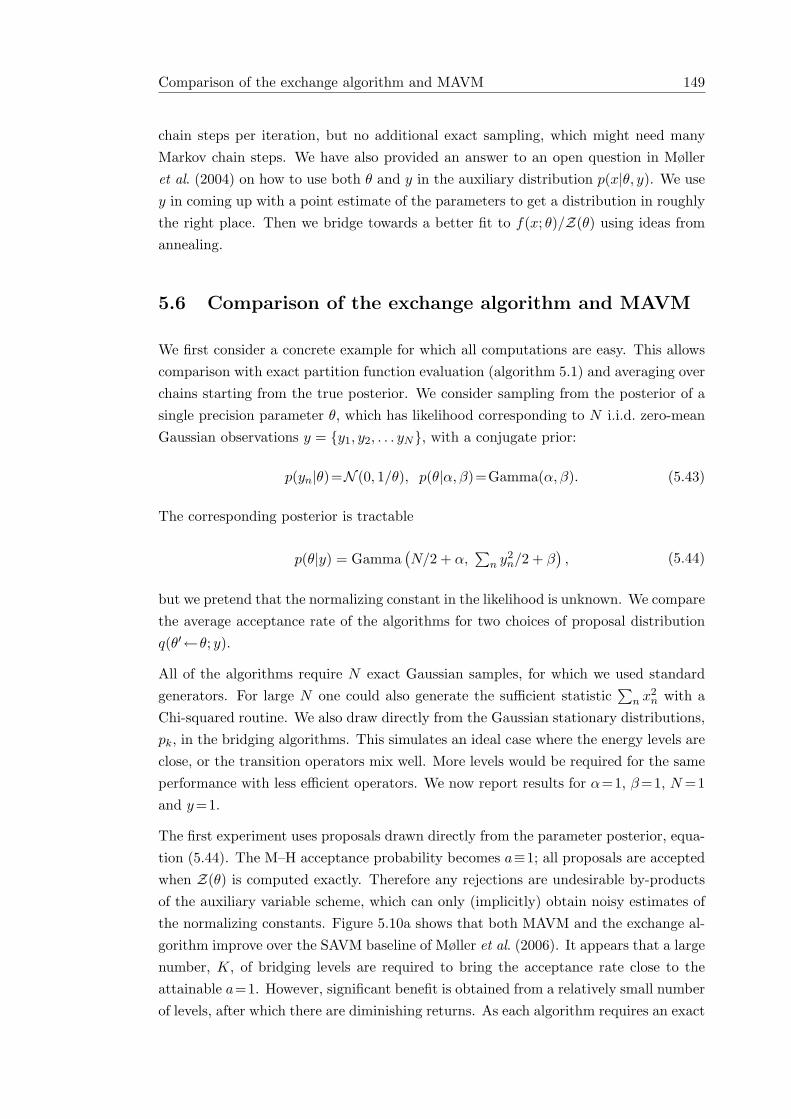
Comparison of the exchange algorithm and MAVM 149
chain steps per iteration, but no additional exact sampling, which might need manyMarkov chain steps. We have also provided an answer to an open question in Mølleret al. (2004) on how to use both θ and y in the auxiliary distribution p(x|θ, y). We usey in coming up with a point estimate of the parameters to get a distribution in roughlythe right place. Then we bridge towards a better fit to f(x; θ)/Z(θ) using ideas fromannealing.
5.6 Comparison of the exchange algorithm and MAVM
We first consider a concrete example for which all computations are easy. This allowscomparison with exact partition function evaluation (algorithm 5.1) and averaging overchains starting from the true posterior. We consider sampling from the posterior of asingle precision parameter θ, which has likelihood corresponding to N i.i.d. zero-meanGaussian observations y = {y1, y2, . . . yN}, with a conjugate prior:
p(yn|θ)=N (0, 1/θ), p(θ|α, β)=Gamma(α, β). (5.43)
The corresponding posterior is tractable
p(θ|y) = Gamma(N/2 + α,
∑n y2
n/2 + β), (5.44)
but we pretend that the normalizing constant in the likelihood is unknown. We comparethe average acceptance rate of the algorithms for two choices of proposal distributionq(θ′←θ; y).
All of the algorithms require N exact Gaussian samples, for which we used standardgenerators. For large N one could also generate the sufficient statistic
∑n x2
n with aChi-squared routine. We also draw directly from the Gaussian stationary distributions,pk, in the bridging algorithms. This simulates an ideal case where the energy levels areclose, or the transition operators mix well. More levels would be required for the sameperformance with less efficient operators. We now report results for α=1, β=1, N =1and y=1.
The first experiment uses proposals drawn directly from the parameter posterior, equa-tion (5.44). The M–H acceptance probability becomes a≡1; all proposals are acceptedwhen Z(θ) is computed exactly. Therefore any rejections are undesirable by-productsof the auxiliary variable scheme, which can only (implicitly) obtain noisy estimates ofthe normalizing constants. Figure 5.10a shows that both MAVM and the exchange al-gorithm improve over the SAVM baseline of Møller et al. (2006). It appears that a largenumber, K, of bridging levels are required to bring the acceptance rate close to theattainable a=1. However, significant benefit is obtained from a relatively small numberof levels, after which there are diminishing returns. As each algorithm requires an exact
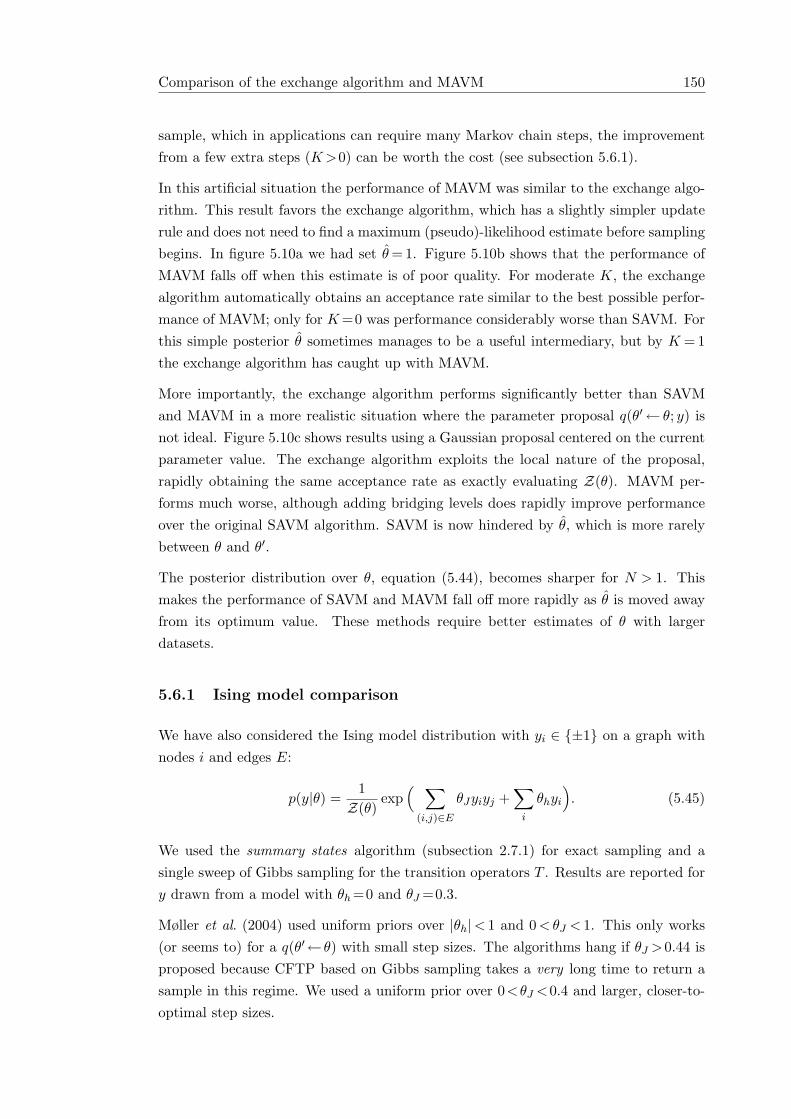
Comparison of the exchange algorithm and MAVM 150
sample, which in applications can require many Markov chain steps, the improvementfrom a few extra steps (K >0) can be worth the cost (see subsection 5.6.1).
In this artificial situation the performance of MAVM was similar to the exchange algo-rithm. This result favors the exchange algorithm, which has a slightly simpler updaterule and does not need to find a maximum (pseudo)-likelihood estimate before samplingbegins. In figure 5.10a we had set θ = 1. Figure 5.10b shows that the performance ofMAVM falls off when this estimate is of poor quality. For moderate K, the exchangealgorithm automatically obtains an acceptance rate similar to the best possible perfor-mance of MAVM; only for K =0 was performance considerably worse than SAVM. Forthis simple posterior θ sometimes manages to be a useful intermediary, but by K = 1the exchange algorithm has caught up with MAVM.
More importantly, the exchange algorithm performs significantly better than SAVMand MAVM in a more realistic situation where the parameter proposal q(θ′← θ; y) isnot ideal. Figure 5.10c shows results using a Gaussian proposal centered on the currentparameter value. The exchange algorithm exploits the local nature of the proposal,rapidly obtaining the same acceptance rate as exactly evaluating Z(θ). MAVM per-forms much worse, although adding bridging levels does rapidly improve performanceover the original SAVM algorithm. SAVM is now hindered by θ, which is more rarelybetween θ and θ′.
The posterior distribution over θ, equation (5.44), becomes sharper for N > 1. Thismakes the performance of SAVM and MAVM fall off more rapidly as θ is moved awayfrom its optimum value. These methods require better estimates of θ with largerdatasets.
5.6.1 Ising model comparison
We have also considered the Ising model distribution with yi ∈ {±1} on a graph withnodes i and edges E:
p(y|θ) =1Z(θ)
exp( ∑
(i,j)∈E
θJyiyj +∑
i
θhyi
). (5.45)
We used the summary states algorithm (subsection 2.7.1) for exact sampling and asingle sweep of Gibbs sampling for the transition operators T . Results are reported fory drawn from a model with θh =0 and θJ =0.3.
Møller et al. (2004) used uniform priors over |θh|< 1 and 0 < θJ < 1. This only works(or seems to) for a q(θ′←θ) with small step sizes. The algorithms hang if θJ >0.44 isproposed because CFTP based on Gibbs sampling takes a very long time to return asample in this regime. We used a uniform prior over 0<θJ <0.4 and larger, closer-to-optimal step sizes.
Comparison of the exchange algorithm and MAVM 151
0.75
0.8
0.85
0.9
0.95
1
0 50 100 150 200 250 300
ave.
acc
epta
nce
pro
bability
K
Exchange
MAVMSAVM
(a)
0.6
0.65
0.7
0.75
0.8
0.85
0.9
0.95
1
0.1 1 10
ave.
acc
epta
nce
pro
bability
θ
MAVM, K=100MAVM, K=10
SAVM
(b)
0.82
0.84
0.86
0.88
0.9
0.92
0.94
0.96
0 50 100 150 200 250 300
ave.
acc
epta
nce
pro
bability
K
Exchange
MAVMSAVM
(c)
Figure 5.10: Comparison of MAVM and the exchange algorithm learning a Gaus-sian precision. (a) Average acceptance rate as a function of K. MAVM with K =0corresponds to SAVM, the method of Møller et al. (2004). Exact normalizing con-stant evaluation in would give an acceptance rate of one. (b) Average acceptancerate as a function of the initial parameter estimate required by SAVM (K =0) andthe extended version, MAVM. Horizontal bars show the results for the exchangealgorithm, which has no θ, for K = 0, 10, 100. (c) As in (a) but with a Gaus-sian proposal distribution of width 0.1 centered on the current parameter setting.The horizontal line shows the maximum average acceptance rate for a reversibletransition operator, this is obtained by exact normalizing constant evaluation.
Comparison of the exchange algorithm and MAVM 152
0
1
2
3
4
5
6
7
8
0 10 20 30 40 50 60 70 80
effici
ency
/10−
4
K
ExchangeMAVMSAVM
(a) σ = 0.04
1
2
3
4
5
6
7
8
0 10 20 30 40 50 60 70 80
effici
ency
/10−
4
K
ExchangeMAVMSAVM
(b) σ = 0.10
Figure 5.11: Performance on a 10×30 toroidal square Ising lattice. The datawere generated from an exact sample with θJ = 0.3 and θh = 0. Proposals wereGaussian perturbations of width σ. The plot shows efficiency: effective number ofsamples, estimated by R-CODA (Cowles et al., 2006), divided by the total numberof Gibbs-sampling sweeps (computer time). All the algorithms are expensive:SAVM requires 104 Gibbs sweeps of the Ising model to obtain one effective sampleof the parameters. This could be improved by using more advanced exact samplingmethods.
Figure 5.11 gives some example results for two different step sizes. For both methods thenumber of effective samples obtained per iteration will tend to the maximum possibleas K→∞. In practice the performance of the two methods does converge. However,these bridging steps come at a cost; the best K is a compromise between the computertime per iteration and the mixing time of the chain. In the examples we tried theexchange algorithm provided better mixing times than SAVM/MAVM for all finite K.Bridging provided good improvements over SAVM, but only gave appreciable benefitsto the exchange algorithm for larger step sizes.
5.6.2 Discussion
MCMC methods typically navigate complicated probability distributions by local diffu-sion — longer range proposals will be rejected unless carefully constructed. It is usuallythe case that as the step-size of proposals are made sufficiently small the acceptancerate of a M–H method tends to one. However, SAVM does not have this property, itintroduces rejections even when θ′=θ. While the exchange algorithm has a→1 for allK as the step-size tends to zero, MAVM will only recover a = 1 as K →∞. This isbecause the third party in the proposed swap (see subsection 5.4.1) is not necessarilyclose to θ. Even in a simple unimodal 1-dimensional posterior distribution, figure 5.10c,this is a significant disadvantage in comparison with the exchange algorithm. We foundthe exchange algorithm performs better than the only other existing MCMC methodfor this problem and is simpler to implement.
Latent History methods 153
5.7 Latent History methods
Both MAVM and the exchange algorithm require exact samples, and use them tocompute similar Metropolis–Hastings acceptance ratios. In this section we propose newalgorithms, which are also valid MCMC methods for doubly-intractable distributionsbut which do not draw exact samples. They do follow a very similar coupling procedure,but the properties of the resulting algorithms are quite different.
We start with an inspiring but impractical rejection sampling algorithm for the param-eters θ, given for example by Marjoram et al. (2003, Algorithm B):
Algorithm 5.5 Simple rejection sampling algorithm for θ ∼ p(θ|y)
1. Generate θ ∼ p(θ)2. Simulate y′ ∼ p(y′|θ)3. Accept θ if y′ = y.
On real problems where the data can take on many values this algorithm will rarelyaccept. Marjoram et al. suggest relaxing the equality in step 3 by accepting datasets that are close in some sense. They also suggest MCMC algorithms, which diffusethe parameters in step 3 rather than drawing from the prior. These algorithms arevalid samplers for the wrong distribution: p(θ|y is near observed value). This sectionwill introduce an alternative approach, which tries to make it more probable that thefantasy data in step 2 is equal to the observed data, while keeping the validity of theoriginal algorithm.
A generative model specifies a likelihood p(y|θ) but not necessarily the details of analgorithm to sample from this distribution. The latent history representation bringsa particular sampling procedure into the description of the model. We declare that astationary ergodic Markov chain T was simulated for an infinite number of time steps,generating an arbitrarily-initialized sequence X ={x−∞, . . ., x−2, x−1, x0} and that weobserved the data y ≡ x0. The marginal probability of any xt, including x0, is thestationary distribution of the Markov chain, which we set to the target model’s p(y|θ).Unraveling a Markov chain and writing it down as a generative model was a trickemployed by Hinton et al. (2006).
Our latent history representation is illustrated in figure 5.12. As in coupling from thepast (section 2.7) we also consider the random variables U = {u−∞, . . ., u−2, u−1, u0}used by the Markov chain transition operator at each time step. Given θ and the ut
variables, which provide T with its source of randomness, each state is a deterministicfunction of the previous: xt = τ(xt−1, ut, θ).
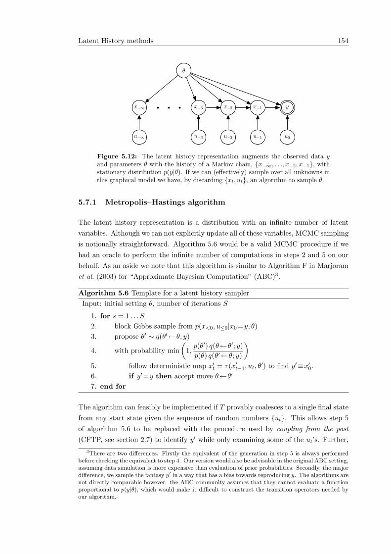
Latent History methods 154
θ
x−∞ x−3 x−2 x−1 y
u−∞ u−3 u−2 u−1 u0
Figure 5.12: The latent history representation augments the observed data yand parameters θ with the history of a Markov chain, {x−∞, . . ., x−2, x−1}, withstationary distribution p(y|θ). If we can (effectively) sample over all unknowns inthis graphical model we have, by discarding {xt, ut}, an algorithm to sample θ.
5.7.1 Metropolis–Hastings algorithm
The latent history representation is a distribution with an infinite number of latentvariables. Although we can not explicitly update all of these variables, MCMC samplingis notionally straightforward. Algorithm 5.6 would be a valid MCMC procedure if wehad an oracle to perform the infinite number of computations in steps 2 and 5 on ourbehalf. As an aside we note that this algorithm is similar to Algorithm F in Marjoramet al. (2003) for “Approximate Bayesian Computation” (ABC)3.
Algorithm 5.6 Template for a latent history samplerInput: initial setting θ, number of iterations S
1. for s = 1 . . . S
2. block Gibbs sample from p(x<0, u≤0|x0 =y, θ)3. propose θ′ ∼ q(θ′←θ; y)
4. with probability min(
1,p(θ′) q(θ←θ′; y)p(θ) q(θ′←θ; y)
)5. follow deterministic map x′t = τ(x′t−1, ut, θ
′) to find y′≡x′0.6. if y′=y then accept move θ←θ′
7. end for
The algorithm can feasibly be implemented if T provably coalesces to a single final statefrom any start state given the sequence of random numbers {ut}. This allows step 5of algorithm 5.6 to be replaced with the procedure used by coupling from the past(CFTP, see section 2.7) to identify y′ while only examining some of the ut’s. Further,
3There are two differences. Firstly the equivalent of the generation in step 5 is always performedbefore checking the equivalent to step 4. Our version would also be advisable in the original ABC setting,assuming data simulation is more expensive than evaluation of prior probabilities. Secondly, the majordifference, we sample the fantasy y′ in a way that has a bias towards reproducing y. The algorithms arenot directly comparable however: the ABC community assumes that they cannot evaluate a functionproportional to p(y|θ), which would make it difficult to construct the transition operators needed byour algorithm.
Latent History methods 155
by combining steps 5 and 6 the coupling from the past can be terminated early if atany point it becomes clear that y′ 6=y.
All we require now is an oracle that can return any ut on request. Creating this servicecan replace the block Gibbs sampling in step 2, as long as we are consistent with itsinfinite computation. Markov properties in the model imply
p(x<0, u≤0|x0, θ) =∏t<0
p(xt−1|xt, θ)∏t<0
p(ut|xt, xt−1). (5.46)
This structure allows resampling of x−1, x−2, . . . in sequence from
p(xt−1|xt, θ) =p(xt|xt−1, θ) p(xt−1|θ)
p(xt|θ)
=T (xt←xt−1; θ) p(xt−1|θ)
p(xt|θ)= T (xt−1←xt; θ),
(5.47)
the reverse transition operator corresponding to T . As long as p(ut|xt, xt−1) is knownfor operator T , any ut value can be sampled after the corresponding xt and xt−1 areavailable. This means that step 2 in algorithm 5.6 can be implemented lazily: “con-struct an object that will provide ut values on request consistent with block Gibbssampling the entire model”. This object will respond to a request for ut by returningthe value from memory if it has previously been sampled, or if necessary by samplingback to xt−1 from the furthest back x value that is known and returning a sample fromp(ut|xt, xt−1). Within each iteration all samples are stored for future use to ensureconsistency.
The practical implementation of a latent history Metropolis–Hastings sampler is sum-marized in algorithm 5.7. This includes an optional refinement, ‘version b’, whichanalytically integrates out u0. This requires computing the transition probability forone step of T , which is usually possible and should increase the acceptance rate. Therefinement also makes the algorithm feasible for Markov chains that do not completelycoalesce, for example on continuous state spaces. A disadvantage of version b) is thatstep 8 may be difficult to implement without always identifying x′−1, whereas step 5 inversion a) will be able to prematurely halt CFTP whenever y 6= x′0, which is often easyto prove.
5.7.2 Performance
A simple special case highlights large differences between latent history samplers andthe previous auxiliary variable algorithms.
We first consider version a) of the sampler applied to a large collection of D independentBernoulli variables sharing a single unknown parameter θ. This is an Ising model inthe limit of zero connection strengths. Assume that the transition operator in use, T ,
Latent History methods 156
Algorithm 5.7 Metropolis–Hastings latent history samplerInput: initial setting θ, number of iterations S and an algorithm CFTP that can
use a finite number of random numbers to prove where an infinitely longMarkov chain ends (see section 2.7).
1. for s = 1 . . . S
2. create lazy ut generator consistent with p(x<0, u≤0|x0 =y, θ)3. Propose θ′ ∼ q(θ′←θ; y)
Either (version a):
4. with probability min(
1,p(θ′) q(θ←θ′; y)p(θ) q(θ′←θ; y)
)5. identify whether y′≡x′0 is y using CFTP and ut generator6. if y′=y then accept move θ←θ′
Or (version b):7. Draw r ∼ Uniform[0, 1]8. identify (enough about) x′−1 for acceptance rule using CFTP and ut’s
9. if r<T (x0 =y←x′−1; θ
′) p(θ′) q(θ←θ′; y)T (x0 =y←x−1; θ) p(θ) q(θ′←θ; y)
then accept move θ←θ′
10. end for
is Gibbs sampling, which for these independent variables draws from the stationarydistribution in one sweep. The sampler is implemented as follows: for each of theobserved spins yd, the corresponding u0,d random variate is uniformly distributed in[0, θ] if the spin is up, and [θ, 1] if the spin is down. Now updates to θ are constrainedto lie within the two closest surrounding u0,d values. This range has a typical scale of1/D. The posterior over parameters has a width that scales as 1/
√D. This suggests
that it will take at least O(D) steps to equilibrate the single scalar parameter θ byrandom walk sampling. Disappointing given the ideal conditions!
Notice that the performance of the algorithm depends on the details of the tran-sition operators. An unreasonably clever transition operator could generate y ifu0 < p(y|θ) and some other data set otherwise. Then the probability of finding y′= y
is min(1, p(y|θ)/p(y|θ′)), giving an overall algorithm similar to the ideal Metropolis–Hastings algorithm (actually the “two stage” rule described in algorithm 2.2). NeitherMAVM nor the exchange algorithm have such dependence on the transition operators— how the exact sample was obtained is irrelevant.
We now turn to version b) of the sampler with the same independent Bernoulli modeland Gibbs sampling operators. Here the transition probabilities in step 9 are equalto the parameters’ likelihoods under the model. The algorithm reduces to standardMetropolis–Hastings for θ, which has the best possible acceptance rate for a givenproposal distribution q. Rapidly mixing operators are rewarded by this version oflatent histories, operators that move very slowly will perform as in version a).
We have implemented both versions of the sampler and applied them to the same Ising
Slice sampling doubly-intractable distributions 157
model problem as in subsection 5.6.1. We used Gibbs sampling for the y variablescombined with the summary states algorithm (subsection 2.7.1) to perform inferencesrequired by the algorithm. The summary states code required some modification sothat its transitions were driven by the latent history sampler’s u-generator rather thana generic random number generator, then the state at time t=0 or t=−1 was identifiedas in subsection 2.7.1. The parameter proposals were Gaussian with width σ = 0.04,which preliminary runs indicated was roughly optimal. In version a) we terminated eachiteration as soon as the summary state algorithm identified the state at time zero or anon-? state at time zero was incompatible with the data. In version b) we always waiteduntil x′−1 had been identified. More elaborate code could terminate earlier based onbounds of the acceptance ratio, but this is also true for the exchange algorithm, MAVMand most standard Metropolis–Hastings algorithms.
As a result of early terminations version a) was roughly five times cheaper per iterationthan our implementation of version b). Even with this advantage the number of effectivesamples per Gibbs-sampling-like sweep through the system was around ten times worsefor version a). The efficiency of version b) was 4×10⁻⁵ effective samples per Gibbs sweep,about half that obtained by SAVM. The latent history efficiency computations includedthe Gibbs-like sweeps needed to compute the u’s, while SAVM was given its randomnumbers for free. This makes the real computation time of the methods comparable.Which method is actually faster will come down to implementation details. However,both the bridged exchange and MAVM algorithms are clearly faster than either variantof latent histories on this Ising problem.
We might hope that latent histories will perform better on other problems. A morerealistic reason to be excited by latent histories is that they might be a much betterroute to approximate methods than any of the previous algorithms in this chapter.We return to this issue in section 5.9. First we turn to the original motivation fordeveloping latent histories: constructing slice samplers.
5.8 Slice sampling doubly-intractable distributions
All of the algorithms for doubly-intractable distributions described so far are basedon Metropolis–Hastings. Such algorithms always require step-size parameters thatneed to be set well. Overly large step-sizes lead to almost all proposals’ being re-jected; overly small step-sizes give lengthy random-walk-like exploration of the poste-rior over θ. It would be nice to be able to use a self-tuning method like slice sampling(subsection 2.4.2), which has less-important or even no step-size parameters.
Slice sampling doubly-intractable distributions 158
5.8.1 Latent histories
The latent history representation naturally allows slice sampling. It also has the prop-erty, like the exchange algorithm, that small steps in θ are always accepted, so moveswill always be possible. The trick is to identify the variables in the joint distribution(figure 5.12) as θ and U , while thinking of the X quantities as just a deterministicfunction of these variables.
Conditioned on the U variables any standard slice sampling algorithm (subsection 2.4.2)can be applied to the parameter θ. The stationary distribution p(θ|U) is simply the priorover the parameters conditioned on x0(θ, U)=y. Any point not satisfying the constraintis off the slice and discarded by the slice sampling procedure. This description gives aslice sampler corresponding to version a) of latent history algorithm 5.7. A slice sam-pling implementation of version b) sets the stationary distribution to T (y←x−1; θ)p(θ).After each iteration U is (effectively) updated in a block-Gibbs update. This involvesresetting a lazy ut generator as in the Metropolis–Hastings algorithm.
5.8.2 MAVM
Standard slice sampling cannot be applied to the θ parameter in the MAVM jointdistribution, because this would involve computing Z(θ). As with Metropolis–Hastingsthe auxiliary variables must be changed simultaneously. It turns out that, with anappropriate definition of a slice, algorithm 5.4 can be converted into a slice sampler.
We first describe the new algorithm. Ostensibly we do just use a standard slice sam-pling procedure (subsection 2.4.2) to update the parameters θ. However, the range ofauxiliary heights 0<h<H is defined in terms of the following quantity:
H(X, θ) = p(θ, y)p(X|θ, y)q(X; θ, y)
Z(θ) = f(y; θ)p(θ)K∏
k=0
fk+1(xk; θ, θ)
fk(xk; θ, θ). (5.48)
After drawing the slice-sampling auxiliary quantity h∼Uniform[0,H(X, θ)] we considernew parameter settings using any of the normal slice sampling procedures. However,whenever a new setting of the parameters θ′ is considered a new setting of auxiliaryX ′ variables is generated in the same way as algorithm 5.4. Then, as usual, slicemembership is assertained by checking H(X ′, θ′)≥h.
We now show that this procedure satisfies detailed balance with respect to the desiredstationary distribution. As in subsection 2.4.2 we use the label S for all rejected pointsand other ancillary points generated while exploring the slice in a stepping-out proce-dure. The probability of starting at a setting (X, θ), generating a particular setting of
Discussion 159
h, generating intermediate quantities S and finally an acceptable new pair (X ′, θ′) is
p(θ|y) p(X|θ, y) · p(h|X, θ, y) · q(S; θ, h) · q(θ′;S, h) q(X ′; θ′, y)
= p(θ|y) p(X|θ, y) · q(X; θ, y)
p(X|θ, y) p(θ, y)Z(θ)· q(S; θ, h) · q(θ′;S, h) q(X ′; θ′, y)
=1
p(y)Z(θ)q(θ′;S, h) q(S; θ, h) q(X; θ, y) q(X ′; θ′, y).
(5.49)
All of the slice-sampling bracketing procedures mentioned in subsection 2.4.2 ensurethat
q(θ′;S, h) q(S; θ, h) = q(θ;S, h) q(S; θ′, h). (5.50)
Therefore equation (5.49) is invariant to exchanging (X, θ) ↔ (X ′, θ′) and the overallprocedure satisfies detailed balance.
This derivation closely follows that of standard slice sampling. This is possible be-cause conditioned on h, the decision to reject intermediate parameters in S is the samewhether generating S forwards from θ or backwards from θ′. In contrast the accept-ability of a proposal in the exchange algorithm cannot be summarized by a scalar sliceheight h. A move depends on giving a new data set to the old parameter, which willhave different probabilities depending on whether the move started at θ or θ′. We don’tcurrently see any way to define a slice sampler for the exchange representation.
As noted in subsection 5.6.2, even very small moves in θ can be rejected when using theMAVM auxiliary system. The usual slice bracketing procedures work on an assump-tion that nearby regions will always be accepted and exponentially shrink towards thecurrent point. Unless a large number of bridging levels are used this behavior couldlead to overly small step sizes. Care would be needed in applying stock slice-samplingcode.
5.9 Discussion
We established in subsection 5.1.1 that global information like that provided by ex-act sampling must be found as part of a strictly valid MCMC algorithm for doubly-intractable distributions. Given this, it seems likely that the exchange algorithm per-forms about as well as is possible. On the problems we have tried the acceptance rateapproaches that of Metropolis–Hastings with moderate K, leaving exact sampling asthe dominant cost. We would generally recommend this algorithm if a valid MCMCprocedure is required. Møller et al. (2004) pointed out that good deterministic approx-imations to p(θ|y) could make SAVM perform very well. Our results firmly support theuse of bridging, and we would recommend always considering MAVM instead.
There is an unresolved issue concerning doubly-intractable distributions when learning
Discussion 160
from N i.i.d. data points:
p(y|θ) =N∏
n=1
p(y(n)|θ) =1
Z(θ)N
N∏n=1
f(y(n); θ
). (5.51)
All of the known valid MCMC algorithms for p(θ|y) require drawing an exact samplefrom p(y|θ). This means drawing a fantasy containing N data sets x={x(n)}Nn=1. Butperhaps there is enough information about Z(θ) in a single exact sample from the datadistribution? Drawing N exact samples may be prohibitively expensive with large datasets. Whether this problem can be avoided is an open question.
Sadly it is not possible to draw exact samples from all distributions; approximaterelaxations must be used for some situations. Section 5.2 observed that a bad choiceof approximations applied to the inner loop of standard Metropolis–Hastings can havesurprising and disastrous consequences on the quality of the approximate samples. Thevalid algorithms discussed in this chapter are an alternative target for approximation.The obvious relaxation of methods requiring exact sampling from the data distributionis to use a brief run of MCMC, possibly starting from the observed data. Møller et al.(2004) report that a fixed length of sampling can be more inefficient than exact samplingfor similar levels of performance. However, this idea would be worth exploring furtherin cases where exact sampling is not possible.
A natural relaxation of the latent history representation is truncating the history tosome finite length of time K. This would require specifying an explicit prior distributionfor x−K , perhaps an approximation to the original model. One could optionally replacethe stationary Markov chain operator T with a sequence of operators Tk bridgingbetween the approximate distribution used for x−K and the target model distribution.This finite model could be simulated using the latent history algorithms with explicitcomputations, or any standard MCMC technique.
We believe that truncated latent history representations are a promising direction forfuture research in approximate inference for doubly-intractable distributions. Runningfinite Markov chains within the exchange algorithm or MAVM is an inner-loop approx-imation, somewhat like those explored in section 5.2. The consequences of approxi-mating MCMC procedures is hard to predict — it is possible that very unreasonableinferences will result. In contrast a truncated latent history representation is a modelon which we can apply standard MCMC algorithms. The model will not describe ex-actly the same beliefs as the original distribution, but all of the inferences performed onit will be self-consistent. Thus if prior draws from the truncated model look reasonableit is likely that the inferences will also be sensible.
This line of reasoning is really suggesting that we throw out the original doubly-intractable model and replace it with a more tractable latent variable model. If themodel was originally introduced as an ad hoc way to introduce dependencies, then us-
Discussion 161
ing an alternative that can be treated consistently may be preferable. In particularwe can look at draws from the prior and see if they actually reflect our beliefs. Heck-erman et al. (2000) follow a related thought process. They discuss circumstances inwhich undirected graphical models may not be a natural representation and provide analternative replacement.
Changing the model doesn’t seem attractive when an undirected model was deriveddirectly from physical considerations. An example of such a model is recent work onlearning protein structure (Podtelezhnikov et al., 2007), which learns the parametersof an energy function using contrastive divergence (Hinton, 2002). A full Bayesiantreatment of these parameters with MCMC seems daunting; exact sampling from theconfigurational-distribution of a protein chain seems infeasibly difficult. However, usingthe wrong model could still be used as an approximation technique and doing so maybe more stable than inner-loop approximations.
This chapter has not addressed computing marginal likelihoods p(y|M) for Bayesianmodel comparison of different undirected graphical models4. Evidently the standardmethods discussed in chapter 4 will apply in theory, although such computations arelikely to be demanding.
4A triply-intractable problem?
Chapter 6
Summary and future work
The Markov chain Monte Carlo method introduced by Metropolis et al. (1953) wasone of the earliest applications of electronic computers. Today it continues to be animportant technique for approximate numerical integration in a growing number ofapplications. Chapter 1 provided an introduction to the challenges involved, whilechapter 2 described some of the current literature along with some minor extensions.
In chapter 3 we explored the promising ideas of using multiple particles and multipleproposals in Markov chain simulations. As with other authors we found that mod-est improvements are possible, largely derived from the basic length-scale informationgiven by a few samples from a distribution. However drawing multiple proposals caneasily cost more to compute than the statistical benefit. It remains to be seen if im-plementations leveraging caching of intermediate results or parallel computations cangain advantage in real applications. Other authors in the literature remain hopeful thatthey can, and our pivot-based approaches seem to bring unique benefits to this area ofthe field.
Chapter 4 investigated methods for computing normalizing constants. One of these, AISis actually an importance sampling method rather than MCMC, and nested samplingoffers a new sampling paradigm in its own right. However, both of these algorithmsuse Markov chains in their practical implementation. We extended existing techniquesfor nested sampling on discrete distributions. We then compared three fundamentallydifferent algorithms based on the same Markov chain. Our theoretical and empiricalresults show that the algorithms perform very differently and that no method is ap-propriate for all distributions. It would seem wise to use more than one algorithm asstandard practice. We proposed one practical approach to realize this: a method fortuning AIS based on preliminary runs of nested sampling.
Chapter 5 serves to highlight the limitations of MCMC. Sampling from doubly-intractable distributions is exceedingly difficult, yet these distributions are found ina large class of ‘undirected’ statistical models and have received a great deal of at-
163
tention in recent years. We have introduced three new algorithms for this problem:MAVM, the exchange algorithm and latent history samplers. These improve the ex-isting state of the art, remove the need for separate deterministic approximations andoffer new directions for approximating this difficult problem. Exploring truncations oflatent histories is a possible area for further work.
This thesis has concentrated on investigating new Markov chains and new algorithmsfor the better use of existing MCMC operators. These have been investigated em-pirically and sometimes theoretically on simple problems designed to demonstrate thealgorithms’ key properties. One limitation of the presentation here has been the focuson stationary distributions — little has been said about the chains’ formal conver-gence rates. This is partly because making meaningful statements about convergencefor general statistical problems seems difficult (section 2.3). Also, wherever possible,we have reduced new algorithms to the Metropolis–Hastings algorithm applied to anauxiliary system. This passes some of the burden of deriving rates of convergence ontoan established literature.
While we have focused on MCMC methodology and proposed a number of novel algo-rithms, ultimately the computational advantages of these methods has to be proven onchallenging real-world applications. This is an area I hope to spend more time on inmy future research.
Bibliography
D. H. Ackley, G. E. Hinton, and T. J. Sejnowski. A learning algorithm for Boltzmannmachines. Cognitive Science, 9(1):147–169, 1985. (page 128)
J. Albert. Bayesian selection of log-linear models. Technical Report Working Paper95-15, Duke University, Institute of Statistics and Decision Sciences, 1995. (page 124)
N. Balakrishnan and A. Clifford Cohen. Order statistics & inference: estimation meth-ods. Academic Press, San Diego, 1991. ISBN 0120769484. (page 93)
T. Bayes. An essay towards solving a problem in the doctrine of chances. Philosoph-ical Transations, 53:370–418, 1763. Communicated by Richard Price, in a letter toJohn Canton. Also available edited by G. A. Barnard in Biometrika 45(3/4):293–315,December 1958. (page 20)
M. J. Beal. Variational algorithms for approximate Bayesian inference. PhD thesis,Gatsby computational neuroscience unit, University College London, 2003. (page 104)
M. J. Beal and Z. Ghahramani. The variational Bayesian EM algorithm for incompletedata: with application to scoring graphical model structures. In J. M. Bernardo, M. J.Bayarri, J. O. Berger, A. P. Dawid, D. Heckerman, A. F. M. Smith, and M. West,editors, Bayesian statistics 7, pages 453–464. Oxford University Press, 2003. (page 82)
M. Beltran, J. Garcıa-Bellido, J. Lesgourgues, A. R. Liddle, and A. Slosar. Bayesianmodel selection and isocurvature perturbations. Physical Review D, 71(6):063532,2005. (pages 109, 118, and 119)
C. H. Bennett. Efficient estimation of free energy differences from Monte Carlo data.Journal of Computational Physics, 22(2):245–268, October 1976. (page 117)
B. A. Berg and T. Neuhaus. Multicanonical ensemble: a new approach to simulatefirst-order phase transitions. Phys. Rev. Lett., 68(1):9–12, January 1992. (page 50)
J. Besag. Spatial interaction and the statistical analysis of lattice systems. Journal ofthe Royal Statistical Society, 36(2):192–236, 1974. (page 124)
J. Besag and P. J. Green. Spatial Statistics and Bayesian Computation. Journal of theRoyal Statistical Society B, 55(1):25–37, 1993. (page 37)
BIBLIOGRAPHY 165
J. Besag, P. Green, D. Higdon, and K. Mengersen. Bayesian computation and stochasticsystems. Statistical Science, 10(1):3–41, 1995. (page 77)
A. Beskos, O. Papaspiliopoulos, G. O. Roberts, and P. Fearnhead. Exact and compu-tationally efficient likelihood-based estimation for discretely observed diffusion pro-cesses (with discussion). Journal of the Royal Statistical Society: Series B (StatisticalMethodology), 68:333–382, 2006. (page 140)
C. Bischof and M. Bucker. Computing derivatives of computer programs. In ModernMethods and Algorithms of Quantum Chemistry, volume 3, pages 315–327, 2000.
(page 41)
C. M. Bishop. Pattern recognition and machine learning. Springer-Verlag, New York,2006. ISBN 0387310738. (page 20)
O. Cappe, A. Guillin, J.-M. Marin, and C. P. Robert. Population Monte Carlo. Journalof Computational & Graphical Statistics, 13(4):907–929, December 2004.
(pages 9, 58, 59, 60, and 61)
B. P. Carlin and S. Chib. Bayesian model choice via Markov chain Monte Carlo meth-ods. Journal of the Royal Statistical Society B (Methodological), 57(3):473–484, 1995.
(page 139)
G. Casella and C. P. Robert. Rao-Blackwellisation of Sampling Schemes. Biometrika,83(1):81–94, 1996. (page 35)
S. Chib. Marginal likelihood from the Gibbs output. Journal of the American StatisticalAssociation, 90(432):1313–1321, December 1995. (page 84)
A. M. Childs, R. B. Patterson, and D. J. C. MacKay. Exact sampling from nonattractivedistributions using summary states. Physical Review E, 63:036113, 2001.
(pages 54 and 134)
A. Christen and C. Fox. MCMC using an approximation. Journal of Computationaland Graphical Statistics, 14(4):795–810, 2005. (page 31)
J. A. Christen and C. Fox. A self-adjusting multi-scale MCMC algorithm, 2006. Posterpresented at Valencia Bayesian meeting, Benidorm 2006. Pre-print available [email protected]; code available from http://www.cimat.mx/∼jac/twalk/. (page 58)
P. Clifford et al. Discussion on the meeting on the Gibbs sampler and other Markovchain Monte Carlo methods. Journal of the Royal Statistical Society. Series B(Methodological), 55(1):53–102, 1993. (page 30)
M. K. Cowles, N. Best, K. Vines, and M. Plummer. R-CODA 0.10-5, 2006. Availablefrom http://www-fis.iarc.fr/coda/. (pages 64 and 152)
BIBLIOGRAPHY 166
R. T. Cox. Probability, frequency and reasonable expectation. American Journal ofPhysics, 14(1):1–13, January 1946. (pages 20 and 120)
R. V. Craiu and C. Lemieux. Acceleration of the multiple-try Metropolis algorithmusing antithetic and stratified sampling. Statistics and Computing, 2007. (page 79)
P. Damien, J. Wakefield, and S. Walker. Gibbs sampling for Bayesian non-conjugateand hierarchical models by using auxiliary variables. Journal of the Royal StatisticalSociety. Series B (Statistical Methodology), 61(2):331–344, 1999. (page 40)
S. Della Pietra, V. J. Della Pietra, and J. D. Lafferty. Inducing features of randomfields. IEEE Transactions on Pattern Analysis and Machine Intelligence, 19(4):380–393, 1997. (page 124)
P. Dellaportas and J. J. Forster. Markov chain Monte Carlo model determinationfor hierarchical and graphical log-linear models. Biometrika, 86(3):615–633, 1999.
(pages 124 and 132)
L. Devroye. Non-uniform random variate generation. Springer-Verlag, New York, 1986.ISBN 0-387-96305-7. Out of print. Available fromhttp://cg.scs.carleton.ca/∼luc/rnbookindex.html. (page 22)
A. Dobra, C. Tebaldi, and M. West. Data augmentation in multi-way contingencytables with fixed marginal totals. Journal of statistical planning and inference, 136(2):355–372, 2006. (page 124)
P. Dostert, Y. Efendiev, T. Y. Hou, and W. Luo. Coarse-gradient Langevin algorithmsfor dynamic data integration and uncertainty quantification. Journal of Computa-tional Physics, 217:123–142, 2006. (page 31)
S. Duane, A. D. Kennedy, B. J. Pendleton, and D. Roweth. Hybrid Monte Carlo.Physics Letters B, 195(2):216–222, September 1987. (page 41)
D. Edwards and T. Havranek. A fast procedure for model search in multidimensionalcontingency tables. Biometrika, 72(2):339–351, August 1985. (page 132)
R. G. Edwards and A. D. Sokal. Generalizations of the Fortuin-Kasteleyn-Swendsen-Wang representation and Monte Carlo algorithm. Physical Review, 38:2009–2012,1988. (pages 37 and 39)
J. Ferkinghoff-Borg. Monte Carlo methods in complex systems. Ph.D. Thesis, GraduateSchool of Biophysics Niels Bohr Institute and Rise National Laboratory Faculty ofScience, University of Copenhagen, May 2002. (page 52)
C. M. Fortuin and P. W. Kasteleyn. On the random-cluster model. I. Introduction andrelation to other models. Physica, 57:536–564, 1972. (page 37)
BIBLIOGRAPHY 167
D. Frenkel. Speed-up of Monte Carlo simulations by sampling of rejected states. Pro-ceedings of the National Academy of Sciences, 101(51):17571–17575, 2004.
(pages 34 and 35)
D. Frenkel and B. Smit. Understanding molecular simulation. Academic Press Inc.,2nd edition, 2001. (pages 65 and 67)
A. E. Gelfand and A. F. M. Smith. Sampling-based approaches to calculating marginaldensities. Journal of the American Statistical Association, 85(410):398–409, 1990.
(page 33)
A. Gelman and X.-L. Meng. Simulating normalizing constants: from importance sam-pling to bridge sampling to path sampling. Statistical Science, 13(2):163–185, 1998.
(pages 86 and 120)
A. Gelman, J. B. Carlin, H. S. Stern, and D. B. Rubin. Bayesian Data Analysis, SecondEdition. Chapman & Hall/CRC, 2003. ISBN 1-58488-388-X. (page 20)
D. Geman and S. Geman. Stochastic relaxation, Gibbs distribution and Bayesianrestoration of images. IEEE Transactions on Pattern Analysis and Machine Intelli-gence, 6:721–741, 1984. (pages 30 and 124)
J. Geweke. Getting it right: joint distribution tests of posterior simulators. Journal ofthe American Statistical Association, 99(467):799–804, 2004. (pages 36 and 83)
C. J. Geyer. Markov chain Monte Carlo maximum likelihood. In Computing Scienceand Statistics: Proceedings of the 23rd Symposium on the Interface, pages 156–163,1991. (page 139)
C. J. Geyer. Practical Markov chain Monte Carlo. Statistical Science, 7(4):473–483,November 1992. (page 32)
W. R. Gilks. Derivative-free adaptive rejection sampling for Gibbs sampling. InJ. Bernardo, J. Berger, A. P. Dawid, and A. F. M. Smith, editors, Bayesian Statistics4. Oxford University Press, 1992. (page 22)
W. R. Gilks and P. Wild. Adaptive rejection sampling for Gibbs sampling. AppliedStatistics, 41(2):337–348, 1992. (page 22)
W. R. Gilks, G. O. Roberts, and E. I. George. Adaptive direction sampling. TheStatistician, 43(1):179–9, 1994. Special Issue: Conference on Practical BayesianStatistics, 1992 (3). (page 57)
V. K. Gore and M. R. Jerrum. The Swendsen-Wang process does not always mixrapidly. In Proceedings of the twenty-ninth annual ACM symposium on Theory ofcomputing, pages 674–681. ACM Press New York, NY, USA, 1997. (page 117)
BIBLIOGRAPHY 168
V. K. Gore and M. R. Jerrum. The Swendsen–Wang process does not always mixrapidly. Journal of Statistical Physics, 97(1):67–86, 1999. (page 117)
P. J. Green. Reversible jump Markov chain Monte Carlo computation and Bayesianmodel determination. Biometrika, 82(4):711–732, December 1995. (pages 55 and 119)
F. Hamze and N. de Freitas. Hot coupling: a particle approach to inference andnormalization on pairwise undirected graphs. In Y. Weiss, B. Scholkopf, and J. Platt,editors, Advances in Neural Information Processing Systems (NIPS*18): Proceedingsof the 2005 Conference. MIT Press, 2006. (page 119)
W. K. Hastings. Monte Carlo sampling methods using Markov chains and their appli-cations. Biometrika, 57(1), April 1970. (pages 27, 49, 50, and 55)
D. Heckerman, D. M. Checkering, C. Meek, R. Rounthwaite, and C. Kadie. Dependencynetworks for inference, collaborative filtering, and data visualization. Journal ofMachine Learning Research (JMLR), 1:49–75, 2000. (page 161)
G. E. Hinton. Training products of experts by minimizing contrastive divergence. NeuralComputation, 14(8):1771–1800, August 2002. (pages 124, 127, 131, 132, and 161)
G. E. Hinton, S. Osindero, and Y.-W. Teh. A fast learning algorithm for deep beliefnets. Neural Computation, 18:1527–1554, 2006. (page 153)
J. D. Hobby. A user’s manual for MetaPost. Technical Report 162, AT&T Bell Labo-ratories, Murray Hill, New Jersey, 1992. (page 4)
K. S. V. Horn. Constructing a logic of plausible inference: a guide to Cox’s theorem.International Journal of Approximate Reasoning, 34(1):3–24, 2003. (page 20)
M. Huber. Exact sampling and approximate counting techniques. In 30th ACM Sym-posium on the Theory of Computing, pages 31–40, 1998. (page 54)
M. Huber. A bounding chain for Swendsen–Wang. Random Structures & Algorithms,22(1):53–59, 2002. (page 55)
Y. Iba. Population Monte Carlo algorithms. Transactions of the Japanese Society forArtificial Intelligence, 16(2):279–286, 2001a. (page 58)
Y. Iba. Extended ensemble Monte Carlo. International Journal of Modern Physics C,12(05):623–656, 2001b. (page 44)
W. Janke and S. Kappler. Multibondic cluster algorithm for Monte Carlo simulations offirst-order phase transitions. Physical Review Letters, 74(2):212–215, 1995. (page 109)
C. Jarzynski. Equilibrium free-energy differences from nonequilibrium measurements:a master-equation approach. Physical Review E, 56(5):5018–5035, November 1997.
(page 46)
BIBLIOGRAPHY 169
E. T. Jaynes. Probability theory: the logic of science: principles and elementary appli-cations vol 1. Cambridge University Press, April 2003. (page 120)
H. Jeffreys. Theory of probability. Oxford University Press, 3rd edition edition, 1961.Republished in Oxford Classic Texts in the Physical Sciences, 1998. (page 82)
M. H. Kalos and P. A. Whitlock. Monte Carlo methods, volume I: basics. John Wiley,1986. ISBN 0-471-89839-2. (page 34)
R. E. Kass and A. E. Raftery. Bayes Factors. Journal of the American StatisticalAssociation, 90(430):773–795, 1995. (page 82)
R. E. Kass, B. P. Carlin, A. Gelman, and R. M. Neal. Markov chain Monte Carlo inpractice: a roundtable discussion. American Statistician, 52(2):93–100, 1998.
(page 36)
S. Kirkpatrick, C. D. Gelatt Jr., and M. P. Vecchi. Optimization by simulated annealing.Science, 220(4598):671–680, 1983. (page 42)
M. Kuss and C. E. Rasmussen. Assessing approximate inference for binary Gaussianprocess classification. Journal of Machine Learning Research, 6:1679–1704, 2005.
(pages 82 and 104)
S. L. Lauritzen and D. J. Spiegelhalter. Local computations with probabilities on graph-ical structures and their application to expert systems (with discussion). Journal ofthe Royal Statistical Society, Series B, 50(2):157–224, 1988. (page 18)
J. S. Liu. Metropolized independent sampling with comparisons to rejection samplingand importance sampling. Statistics and Computing, 6(2):113–119, 1996. (page 49)
J. S. Liu. Monte Carlo strategies in scientific computing. Springer, 2001. ISBN0387952306. (page 31)
J. S. Liu, W. H. Wong, and A. Kong. Covariance structure of the Gibbs sampler withapplications to the comparisons of estimators and augmentation schemes. Biometrika,81(1):27–40, 1994. (page 33)
J. S. Liu, F. Liang, and W. H. Wong. The use of multiple-try method and localoptimization in Metropolis sampling. Journal of American Statistical Association,95(449):121–134, 2000. (pages 60, 62, 64, and 65)
A. P. Lyubartsev, A. A. Martsinovski, S. V. Shevkunov, and P. N. Vorontsov-Velyaminov. New approach to Monte Carlo calculation of the free energy: methodof expanded ensembles. J. Chem. Phys., 96(3):1776–1783, 1992. (page 43)
D. MacKay. Nested sampling explanatory illustrations, 2004. Available fromhttp://www.inference.phy.cam.ac.uk/bayesys/box/nested.pdf. (page 91)
BIBLIOGRAPHY 170
D. J. C. MacKay. Information theory, inference, and learning algorithms. CambridgeUniversity Press, 2003. Available fromhttp://www.inference.phy.cam.ac.uk/mackay/itila/.
(pages 20, 23, 28, 41, 57, 82, 107, and 130)
E. Marinari and G. Parisi. Simulated tempering: a new Monte Carlo scheme. Euro-physics Letters, 19(6):451–458, 1992. (page 43)
P. Marjoram, J. Molitor, V. Plagnol, and S. Tavare. Markov chain Monte Carlo withoutlikelihoods. Proceedings of the National Academy of Sciences, 100(26):15324–15328,2003. (pages 153 and 154)
A. McCallum and B. Wellner. Toward conditional models of identity uncertainty withapplication to proper noun coreference. In IJCAI Workshop on Information Integra-tion on the Web, 2003. (page 124)
I. R. McDonald and K. Singer. Machine calculation of thermodynamic properties of asimple fluid at supercritical temperatures. J. Chem. Phys., 47(11):4766–4772, 1967.
(page 88)
N. Metropolis. The beginning of the Monte Carlo method. Los Alamos Science, 15:125–130, 1987. (page 21)
N. Metropolis, A. W. Rosenbluth, M. N. Rosenbluth, A. H. Teller, and E. Teller.Equation of state calculation by fast computing machines. J. Chem Phys, 21:1087,1953. (pages 3, 28, 55, and 162)
J. Møller, A. N. Pettitt, K. K. Berthelsen, and R. W. Reeves. An efficient Markov chainMonte Carlo method for distributions with intractable normalising constants. Tech-nical Report R-2004-02, Department of Mathematical Sciences, Aalborg University,2004. (pages 122, 125, 127, 144, 149, 150, 151, 159, and 160)
J. Møller, A. N. Pettitt, R. Reeves, and K. K. Berthelsen. An efficient Markovchain Monte Carlo method for distributions with intractable normalising constants.Biometrika, 93(2):451–458, 2006. (pages 122, 125, 144, 146, and 149)
P. Mukherjee, D. Parkinson, and A. R. Liddle. A nested sampling algorithm for cos-mological model selection. The Astrophysical Journal, 638:L51, 2006. (page 109)
I. Murray and Z. Ghahramani. Bayesian learning in undirected graphical models: ap-proximate MCMC algorithms. In M. Chickering and J. Halpern, editors, Proceedingsof the 20th Annual Conference on Uncertainty in Artificial Intelligence, pages 392–399. AUAI Press Arlington, Virginia, United States, 2004. (pages 125 and 129)
BIBLIOGRAPHY 171
I. Murray and E. Snelson. A pragmatic Bayesian approach to predictive uncertainty. InJ. Quinonero-Candela, I. Dagan, B. Magnini, and F. D’Alche-Buc, editors, MachineLearning Challenges. Evaluating Predictive Uncertainty, Visual Object Classification,and Recognising Textual Entailment.: First PASCAL Machine Learning ChallengesWorkshop, Southampton, UK, April 11–13, 2005, Revised Selected Papers., SpringerLecture Notes in Computer Science. 2006. (page 55)
I. Murray, Z. Ghahramani, and D. J. C. MacKay. MCMC for doubly-intractable distri-butions. In R. Dechter and T. S. Richardson, editors, Proceedings of the 22nd AnnualConference on Uncertainty in Artificial Intelligence (UAI-06), pages 359–366. AUAIPress, 2006a. (page 123)
I. Murray, D. MacKay, Z. Ghahramani, and J. Skilling. Nested sampling for Potts mod-els. In Y. Weiss, B. Scholkopf, and J. Platt, editors, Advances in Neural InformationProcessing Systems (NIPS*18): Proceedings of the 2005 Conference, pages 947–954.MIT Press, 2006b. (pages 89 and 97)
R. M. Neal. Bayesian training of backpropagation networks by the hybrid Monte Carlomethod. Technical Report CRG-TR-92-1, Connectionist Research Group, Depart-ment of Computer Science, University of Toronto, April 1992. (page 41)
R. M. Neal. Probabilistic inference using Markov chain Monte Carlo methods. Techni-cal Report CRG-TR-93-1, Department of Computer Science, University of Toronto,September 1993. (pages 41, 120, and 129)
R. M. Neal. Sampling from multimodal distributions using tempered transitions. Tech-nical Report 9421, Department of Statistics, University of Toronto, October 1994.
(pages 46 and 110)
R. M. Neal. Suppressing random walks in Markov chain Monte Carlo using orderedoverrelaxation. Technical Report No. 9508, Department of Statistics, University ofToronto, 1995. (page 68)
R. M. Neal. Sampling from multimodal distributions using tempered transitions. Statis-tics and Computing, 6(4):353–366, 1996a. (pages 46, 47, 48, 110, and 148)
R. M. Neal. Bayesian learning for neural networks. Number 118 in Lecture Notes inStatistics. Springer-Verlag, 1996b. (page 41)
R. M. Neal. Markov chain Monte Carlo methods based on ‘slicing’ the density function.Technical Report 9722, Department of Statistics, University of Toronto, 1997.
(page 39)
R. M. Neal. Annealed importance sampling. Technical Report No. 9805, Departmentof Statistics, University of Toronto, 1998a. (pages 45 and 110)
BIBLIOGRAPHY 172
R. M. Neal. Suppressing random walks in Markov chain Monte Carlo using orderedoverrelaxation. In M. I. Jordan, editor, Learning in graphical models, pages 205–228.Kluwer Academic Publishers, 1998b. (pages 68 and 69)
R. M. Neal. Markov chain sampling methods for Dirichlet process mixture models.Technical Report 9815, Department of Statistics, University of Toronto, September1998c. (page 55)
R. M. Neal. Erroneous results in “Marginal likelihood from the Gibbs output”, 1999.Available from http://www.cs.toronto.edu/∼radford/chib-letter.html.
(page 84)
R. M. Neal. Annealed importance sampling. Statistics and Computing, 11(2):125–139,2001. (pages 45, 49, 103, and 110)
R. M. Neal. Slice sampling. Annals of Statistics, 31(3):705–767, 2003.(pages 39, 40, 59, 79, and 107)
R. M. Neal. Taking bigger Metropolis steps by dragging fast variables. Technical ReportNo. 0411, Department of Statistics, University of Toronto, October 2004a. (page 144)
R. M. Neal. Improving asymptotic variance of MCMC estimators: non-reversible chainsare better. Technical Report 0406, Department of Statistics, University of Toronto,July 2004b. (page 73)
R. M. Neal. Estimating ratios of normalizing constants using linked importance sam-pling. Technical Report No. 0511, Department of Statistics, University of Toronto,2005. (pages 119 and 143)
M. E. J. Newman and R. M. Ziff. Fast Monte Carlo algorithm for site or bond perco-lation. Physical Review E, 64(016706), June 2001. (page 37)
M. A. Newton and A. E. Raftery. Approximate Bayesian inference with the weightedlikelihood bootstrap. Journal of the Royal Statistical Society, Series B (Methodolog-ical), 56(1):3–48, 1994. (page 83)
A. O’Hagan. Monte Carlo is fundamentally unsound. The Statistician, 36(2/3):247–249,1987. In special issue: Practical Bayesian Statistics. (page 120)
O. Papaspiliopoulos and G. O. Roberts. Retrospective MCMC methods for Dirichletprocess hierarchical models, 2005. Submitted manuscript. (page 140)
J. Pearl. Evidential reasoning using stochastic simulation of causal models. ArtificialIntelligence, 32(2):245–257, 1987. (page 34)
P. Peskun. Optimum Monte-Carlo sampling using Markov chains. Biometrika, 60(3):607–612, 1973. (pages 29 and 31)
BIBLIOGRAPHY 173
A. A. Podtelezhnikov, Z. Ghahramani, and D. L. Wild. Learning about protein hydro-gen bonding by minimizing contrastive divergence. Proteins: Structure, Function,and Bioinformatics, 66:588–599, 2007. (page 161)
J. G. Propp and D. B. Wilson. Exact sampling with coupled Markov chains andapplications to statistical mechanics. Random Structures and Algorithms, 9(1&2):223–252, 1996. (pages 52 and 55)
Y. Qi and T. P. Minka. Hessian-based Markov chain Monte-Carlo algorithms. In FirstCape Cod Workshop on Monte Carlo Methods, September 2002. (pages 65 and 67)
Z. S. Qin and J. S. Liu. Multipoint Metropolis method with application to hybridMonte Carlo. Journal of Computational Physics, 172:827–840, 2001. (page 80)
A. E. Raftery, M. A. Newton, J. M. Satagopan, and P. N. Krivitsky. Estimating theintegrated likelihood via posterior simulation using the harmonic mean identity. InJ. M. Bernardo, M. J. Bayarri, J. O. Berger, A. P. Dawid, D. Heckerman, A. F. M.Smith, and M. West, editors, Bayesian Statistics 8, Proceedings of the Valencia /ISBA 8th World Meeting on Bayesian Statistics. Oxford University Press, 2007.
(page 83)
C. E. Rasmussen and Z. Ghahramani. Bayesian Monte Carlo. In S. Becker, S. Thrun,and K. Obermayer, editors, Advances in Neural Information Processing Systems(NIPS*15): Proceedings of the 2002 Conference. MIT Press, 2003. (page 120)
C. Ritter and M. A. Tanner. Facilitating the Gibbs sampler: the Gibbs stopper andthe griddy-Gibbs sampler. Journal of the American Statistical Association, 87(419):861–868, 1992. (page 30)
C. P. Robert and G. Casella. Monte Carlo statistical methods. Springer Texts inStatistics. Springer, 2nd edition, 2004. ISBN 0-387-21239-6. (pages 58, 59, and 61)
M. Seeger. Low rank updates for the Cholesky decomposition. Technical re-port, September 2005. http://www.kyb.tuebingen.mpg.de/bs/people/seeger/
papers/cholupdate.pdf. (page 18)
J. Seward and N. Nethercote. Using valgrind to detect undefined value errors withbit-precision. In Proceedings of the USENIX’05 Annual Technical Conference, April2005. (page 4)
R. Shaw, M. Bridges, and M. P. Hobson. Clustered nested sampling: efficient Bayesianinference for cosmology, 2007. Preprint available fromhttp://arxiv.org/pdf/astro-ph/0701867. (pages 109, 116, 118, and 119)
D. S. Sivia and J. Skilling. Data analysis: a Bayesian tutorial. Oxford Science Publi-cations, 2006. ISBN 0-19-856832-0. (page 20)
BIBLIOGRAPHY 174
J. Skilling. Nested sampling. In R. Fischer, R. Preuss, and U. von Toussaint, editors,Bayesian inference and maximum entropy methods in science and engineering, AIPConference Proceeedings 735, pages 395–405, 2004. (page 88)
J. Skilling. Nested sampling for general Bayesian computation. Bayesian Analysis, 1(4):833–860, 2006. (pages 88 and 96)
J. Skilling. Nested sampling for Bayesian computations. In J. M. Bernardo, M. J.Bayarri, J. O. Berger, A. P. Dawid, D. Heckerman, A. F. M. Smith, and M. West,editors, Bayesian Statistics 8, Proceedings of the Valencia / ISBA 8th World Meetingon Bayesian Statistics. Oxford University Press, 2007. (pages 88 and 97)
J. Skilling and D. J. C. MacKay. Slice sampling — a binary implementation. Annalsof Statistics, 31(3), 2003. In discussion: Slice Sampling, Radford M. Neal. (page 40)
G. R. Smith. The measurement of free energy by Monte Carlo computer simulation.PhD thesis, University of Edinburgh, September 1995. (pages 52 and 121)
A. Sokal. Monte Carlo methods in statistical mechanics: foundations and new algo-rithms, 1996. Lectures at the Cargese Summer School on “Functional Integration:Basics and Applications”. (page 21)
D. J. Spiegelhalter, A. Thomas, N. G. Best, and W. R. Gilks. BUGS examples volumes1 and 2, 1996. Available from http://www.mrc-bsu.cam.ac.uk/bugs/. (page 30)
D. Stern, T. Graepel, and D. J. C. MacKay. Modelling uncertainty in the game ofgo. In L. K. Saul, Y. Weiss, and L. Bottou, editors, Advances in Neural InformationProcessing Systems (NIPS*17): Proceedings of the 2004 Conference. MIT Press,2005. (page 37)
K. Stormark. Multiple proposal strategies for Markov chain Monte Carlo. MSc thesis,Department of Mathematical Sciences, Norwegian University of Science and Tech-nology, 2006. (page 79)
R. H. Swendsen and J.-S. Wang. Replica Monte Carlo simulation of spin-glasses. Phys-ical Review Letters, 57(21):2607–2609, 1986. (page 139)
R. H. Swendsen and J. S. Wang. Nonuniversal critical dynamics in Monte Carlo simu-lations. Physical Review Letters, 58(2):86–88, 1987. (pages 36 and 37)
C. J. F. Ter Braak. A Markov chain Monte Carlo version of the genetic algorithmdifferential evolution: easy Bayesian computing for real parameter spaces. StatisticalComputing, pages 239–249, 2006. (page 58)
L. Tierney. Markov chains for exploring posterior distributions. The Annals of Statis-tics, 22(4):1701–1728, 1994. (page 25)
BIBLIOGRAPHY 175
L. Tierney and A. Mira. Some adaptive Monte Carlo methods for Bayesian inference.Statistics in Medicine, 18(17–18):2507–2515, 1999. (page 59)
H. Tjelmeland. Using all Metropolis–Hastings proposals to estimate mean values. Tech-nical Report 4/2004, Department of Mathematical Sciences, Norwegian Universityof Science and Technology, 2004. (pages 34 and 79)
Z. Tu and S.-C. Zhu. Image segmentation by data-driven Markov chain Monte Carlo.IEEE Transactions on Pattern Analysis and Machine Intelligence, 24(5):657–673,2002. (page 29)
J.-S. Wang and R. H. Swendsen. Low-temperature properties of the ±J Ising spin glassin two dimensions. Physical Review B, pages 4840–4844, September 1988. (page 45)
L. Wang, J. Liu, and S. Z. Li. MRF parameter estimation by MCMC method. Patternrecognition, 33:1919–1925, 2000. (page 131)
G. R. Warnes. The normal kernel coupler: an adaptive MCMC method for efficientlysampling from multi-modal distributions. PhD thesis, Department of Biostatistics,University of Washington, 2000. (page 59)
M. Welling and S. Parise. Bayesian random fields: the Bethe-Laplace approximation. InProceedings of the 22nd Annual Conference on Uncertainty in Artificial Intelligence(UAI-06). AUAI Press, 2006. (page 127)
W. Wiegerinck. Variational approximations between mean field theory and the junctiontree algorithm. In Proceedings of the 16th Conference on Uncertainty in ArtificialIntelligence, pages 626–633. Morgan Kaufmann, 2000. (page 130)
D. B. Wilson. Annotated bibliography of perfectly random sampling with Markovchains. In DIMACS Series in Discrete Mathematics and Theoretical Computer Sci-ence, volume 41. American Mathematical Society, 1998. Updated version availableonline http://dbwilson.com/exact/. (page 52)
J. Winn and C. M. Bishop. Variational message passing. Journal of Machine LearningResearch, 6:661–694, 2005. (page 130)
O. Winther and A. Krogh. Teaching computers to fold proteins. Physical Review E, 70(3):30903, 2004. (page 124)
C. Yanover and Y. Weiss. Approximate inference and protein folding. In S. Becker,S. Thrun, and K. Obermayer, editors, Advances in Neural Information ProcessingSystems (NIPS*15): Proceedings of the 2002 Conference. MIT Press, 2003. (page 124)
J. S. Yedidia, W. T. Freeman, and Y. Weiss. Constructing free-energy approximationsand generalized belief propagation algorithms. IEEE Transactions on InformationTheory, 51(7):2282–2312, July 2005. (page 130)

BIBLIOGRAPHY 176
Y. Yu and Q. Cheng. MRF parameter estimation by an accelerated method. PatternRecognition Letters, 24:1251–1259, 2003. (page 131)
X. Zhu and Z. Ghahramani. Towards semi-supervised classification with Markov ran-dom fields. Technical Report CMU-CALD-02-106, School of Computer Science,Carnegie Mellon University, June 2002. (pages 124, 134, 135, and 136)