Advances in High Frequency Strategies

Marcos López de Prado

Tudor Investment Corp.

Cornell University

March 2012

Notice:

The research contained in this presentation is the result of a continuing collaboration with

Prof. Maureen O’Hara

Prof. David Easley

For more details, please visit: http://ssrn.com/author=434076

ml863@cornell.edu

2

SECTION I The great divide

3

Is speed the real issue?

4

• Faster traders are nothing new:

– Nathan Rothschild is said to have used racing pigeons to trade in advance on the news of Napoleon’s defeat at Waterloo.

– Beginning in 1850s, only a limited number of investors had access to telegraphy.

– The telephone (1875), radio (1915), and more recently screen trading (1986) offered speed advantages to some participants over others.

– Leinweber [2009] relates many instances in which technological breakthroughs have been used to most investors’ disadvantage. So … what is new this time?

A change in paradigm

5

• High Frequency Trading (HFT) is not Low Frequency Trading (LFT) on steroids.

• HFT have been mischaracterized as ‘cheetah-traders’.

• Rather than speed, the true great divide is a “change in the trading paradigm”.

• HFT are strategic traders. In some instances, they:

– act upon the information revealed by LFT’s actions.

– engage in sequential games.

– behave like predators.

• Speed is an advantage, but there is more to it…

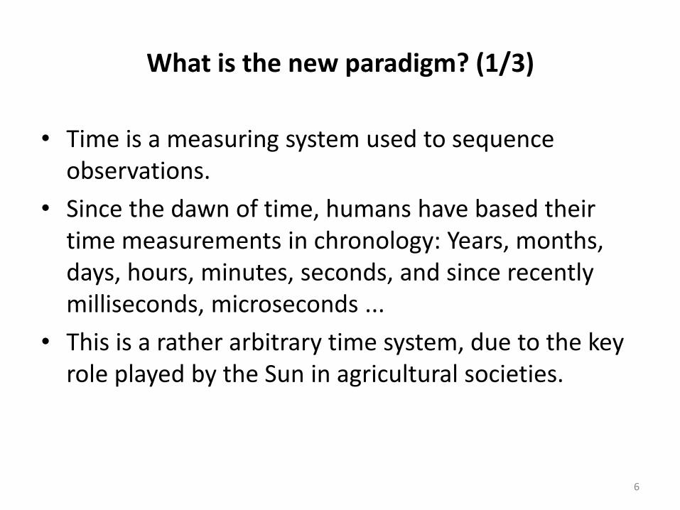
What is the new paradigm? (1/3)

6

• Time is a measuring system used to sequence observations.

• Since the dawn of time, humans have based their time measurements in chronology: Years, months, days, hours, minutes, seconds, and since recently milliseconds, microseconds ...

• This is a rather arbitrary time system, due to the key role played by the Sun in agricultural societies.

What is the new paradigm? (2/3)

7

• Machines operate on an internal clock that is not chrono based, but event based: The cycle.

• A machine will complete a cycle at various chrono rates, depending on the amount of information involved in a particular instruction.

• As it happens, HFT relies on machines, thus measuring time in terms of events.

• Thinking in volume-time is challenging for us humans. But for a ‘silicon trader’, it is the natural way to process information and engage in sequential, strategic trading.

What is the new paradigm? (3/3)

8

• The new paradigm is “event-based time”. The simplest example is dividing the session in equal volume buckets. This transformation removes most intra-session seasonal effects.

• For example, HF market makers may target to turn their portfolio every fixed number of contracts traded (volume bucket), regardless of the chrono time.

• In fact, working in volume time presents significant statistical advantages.

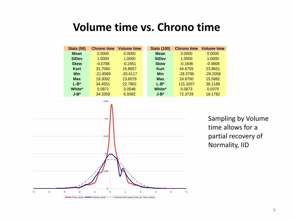
Volume time vs. Chrono time

0

0.05

0.1

0.15

0.2

0.25

-5 -4 -3 -2 -1 0 1 2 3 4 5

Time clock Volume clock Normal Dist (same bins as Time clock)

Sampling by Volume time allows for a partial recovery of Normality, IID

Stats (50) Chrono time Volume time Stats (100) Chrono time Volume time

Mean 0.0000 0.0000 Mean 0.0000 0.0000

StDev 1.0000 1.0000 StDev 1.0000 1.0000

Skew -0.0788 -0.2451 Skew -0.1606 -0.4808

Kurt 31.7060 15.8957 Kurt 44.6755 23.8651

Min -21.8589 -20.6117 Min -28.3796 -29.2058

Max 19.3092 13.8079 Max 24.6700 15.5882

L-B* 34.4551 22.7802 L-B* 115.3207 36.1189

White* 0.0971 0.0548 White* 0.0873 0.0370

J-B* 34.3359 6.9392 J-B* 72.3729 18.1782

9

SECTION II More than speed

10

Example of Sequential Trading model

*[ | ] ( ) ( ) ( )i n i b i g iE S t P t S P t S P t S

( )

( ) [ | ] [ | ]( )

bi i i

b

P tB t E S t E S t S

P t

( )( ) [ | ] [ | ]

( )

g

i i i

g

P tA t E S t S E S t

P t

( ) ( )

( ) [ | ] [ | ]( ) ( )

g bi i i i

g b

P t P tt S E S t E S t S

P t P t

2PIN

11

Easley & O’Hara [1996]

Little known species you should be aware of

12

• Predatory algorithms are a special kind of informed traders. Rather than possessing exogenous information yet to be incorporated in the market price, they know that their endogenous actions are likely to trigger a microstructure mechanism, with foreseeable outcome. Examples include:

– Quote stuffing: Overwhelming an exchange with messages, with the sole intention of slowing down competing algorithms.

– Quote dangling: Sending quotes that force a squeezed trader to chase a price against her interests.

– Pack hunting: Predators hunting independently become aware of each others activities, and form a pack in order to maximize the chances of triggering a cascading effect.

Slow chess may be harder than you think (1/2)

13

• O’Hara [2011] presents evidence of their disruptive activities.

• A quote dangler forcing a desperate trader to chase a price up. As soon as the trader gives up, the dangler quotes back at the original level, and waits for the next victim.

Slow chess may be harder than you think (2/2)

14

• NANEX [2011] shows what appears to be pack hunters forcing a stop loss.

• Speed makes HFTs more effective, but slowing them down won’t change their basic behavior: Strategic sequential trading.

BIG data

15

• Perhaps more critically than speed is that HFT bases its decisions in a large amount of information, known as “big data”: – Level 3 quotes (book depth).

– Estimation of an order’s position in the queue.

– Estimation of other player’s liquidity needs, asymmetric information.

– NLP, etc.

• Regulators have acknowledged that they are not well-equipped for the task at hand (NYT [2010]). It took the SEC+CFTC nearly 5 months to analyze the events of May 6th 2010 (‘flash crash’).

• As a result, regulators have approached the CIFT at LBNL for advise.

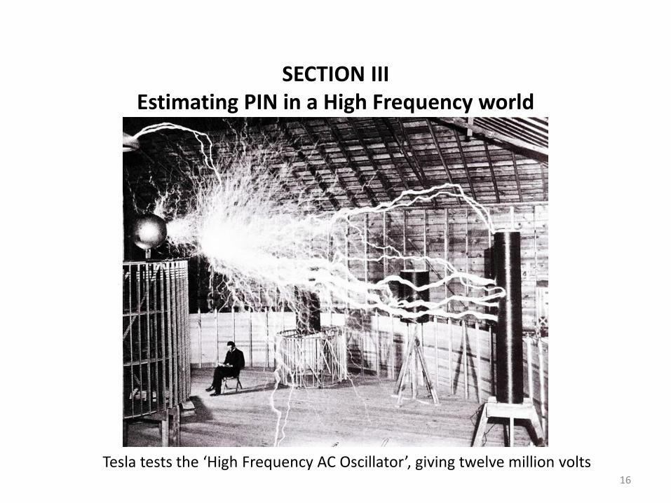
SECTION III Estimating PIN in a High Frequency world

16

Tesla tests the ‘High Frequency AC Oscillator’, giving twelve million volts

How can PIN be estimated – High Frequency (1/2)

17

1. Trades or bars are grouped in equal volume buckets (e.g., 40,000 contracts).

2. For each trade or bar, Z% is classified as buy and (1-Z)% as sell (denoted “bulk classification”). Caution: Not all the volume of a single trade or bar is classified as buy or sell (some researchers are confused by this).

𝑉𝜏𝐵 = 𝑉𝑖 ∙ 𝑍

𝑃𝑖 − 𝑃𝑖−1𝜎∆𝑃

𝑡 𝜏

𝑖=𝑡 𝜏−1 +1

𝑉𝜏𝑆 = 𝑉𝑖 ∙ 1 − 𝑍

𝑃𝑖 − 𝑃𝑖−1𝜎∆𝑃

𝑡 𝜏

𝑖=𝑡 𝜏−1 +1

= 𝑉 − 𝑉𝜏𝐵

where 𝑡 𝜏 is the index of the last time bar included in the τ volume bucket, Z is the CDF of the standard normal distribution and 𝜎∆𝑃 is the estimate of the standard derivation of price changes between time bars.

This procedure leads to better results than the tick rule, etc.

How can PIN be estimated – High Frequency (2/2)

3. We know from Easley, Engle, O’Hara and Wu (2008) that the expected arrival rate of informed trades is E 𝑉𝜏

𝑆 − 𝑉𝜏𝐵 =

𝛼𝜇 2𝛿 − 1 , and E 𝑉𝜏𝑆 − 𝑉𝜏

𝐵 ≈ 𝛼𝜇. The expected arrival rate of total trade is

4. Note that with our convention about volume buckets, VBτ+VS

τ is constant, and is equal to

𝑉

𝑛 for all buckets τ=1,…,n.

5. From the values computed above, we can derive the Volume-Synchronized Probability of Informed Trading (VPIN) as

𝑉𝑃𝐼𝑁 =𝛼𝜇

𝛼𝜇 + 2휀=𝛼𝜇

𝑉≈ 𝑉𝜏

𝑆 − 𝑉𝜏𝐵𝑛

𝜏=1

𝑛𝑉

2111

event no from volumeeventdown from volumeevent up from volume1

VVVn

nSB

SECTION IV Forecasting (and understanding) Volatility

19

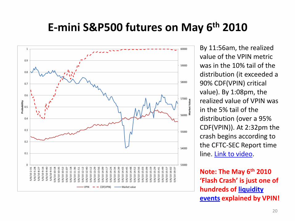
E-mini S&P500 futures on May 6th 2010

By 11:56am, the realized value of the VPIN metric was in the 10% tail of the distribution (it exceeded a 90% CDF(VPIN) critical value). By 1:08pm, the realized value of VPIN was in the 5% tail of the distribution (over a 95% CDF(VPIN)). At 2:32pm the crash begins according to the CFTC-SEC Report time line. Link to video. Note: The May 6th 2010 ‘Flash Crash’ is just one of hundreds of liquidity events explained by VPIN!

53000

54000

55000

56000

57000

58000

59000

60000

0

0.1

0.2

0.3

0.4

0.5

0.6

0.7

0.8

0.9

1

5/6

/10

2:3

1

5/6

/10

5:2

8

5/6

/10

8:2

7

5/6

/10

9:1

6

5/6

/10

9:4

0

5/6

/10

9:5

5

5/6

/10

10

:18

5/6

/10

10

:35

5/6

/10

10

:52

5/6

/10

11

:07

5/6

/10

11

:18

5/6

/10

11

:36

5/6

/10

11

:51

5/6

/10

12

:12

5/6

/10

12

:40

5/6

/10

13

:12

5/6

/10

13

:29

5/6

/10

13

:56

5/6

/10

14

:09

5/6

/10

14

:17

5/6

/10

14

:24

5/6

/10

14

:34

5/6

/10

14

:39

5/6

/10

14

:43

5/6

/10

14

:45

5/6

/10

14

:48

5/6

/10

14

:52

5/6

/10

14

:56

5/6

/10

15

:03

5/6

/10

15

:09

5/6

/10

15

:19

5/6

/10

15

:29

5/6

/10

15

:41

5/6

/10

15

:49

5/6

/10

15

:57

5/6

/10

16

:02

5/6

/10

19

:37

Ma

rke

t V

alu

e

Pro

ba

bil

ity

VPIN CDF(VPIN) Market value

20

VIX on May 6th 2010

VIX had a level of 25.92 at 9:30am, and reached a session high of 40.69 at 15:28pm. VIX didn’t reach historically high levels that day (VIX had a level of 89.53 On 10/24/2008). Rather than predicting the crash, it was impacted by it.

24

26

28

30

32

34

36

38

40

42

5/6

/10 0

:00

5/6

/10 0

:57

5/6

/10 1

:55

5/6

/10 2

:52

5/6

/10 3

:50

5/6

/10 4

:48

5/6

/10 5

:45

5/6

/10 6

:43

5/6

/10 7

:40

5/6

/10 8

:38

5/6

/10 9

:36

5/6

/10 1

0:3

3

5/6

/10 1

1:3

1

5/6

/10 1

2:2

8

5/6

/10 1

3:2

6

5/6

/10 1

4:2

4

5/6

/10 1

5:2

1

5/6

/10 1

6:1

9

5/6

/10 1

7:1

6

5/6

/10 1

8:1

4

5/6

/10 1

9:1

2

5/6

/10 2

0:0

9

5/6

/10 2

1:0

7

5/6

/10 2

2:0

4

5/6

/10 2

3:0

2

5/7

/10 0

:00

Time

Mark

et

Va

lue

0

0.1

0.2

0.3

0.4

0.5

0.6

0.7

0.8

0.9

1

Pro

ba

bil

ity

VIX VPIN CDF(VPIN) CDF(VIX)

21

Toxicity-induced volatility

22

• There is a type of volatility that is not priced by VIX: Toxicity-induced volatility.

• Some characteristics: – Microstructural: This type volatility arises as a result of a failure in the

liquidity provision process. Although Macro news may initiate the flow imbalance, it is MM’s underestimation of VPIN that generates the toxic inventory that ultimately forces them out of the market.

– Endogenous: Unlike macro-volatility, this type of volatility can be predicted, as liquidity providers come under stress gradually. There is a lapse between the rise in VPIN and the liquidity crash, sometimes of hours!

– Short-term: The liquidity failure is typically short-lived. A price jump will attract position takers, which will operate as tactical liquidity providers.

Forecasting Toxicity-induced volatility (1/3)

23

• An event e occurs every time that 𝐶𝐷𝐹 𝑉𝑃𝐼𝑁 𝜏 ≥ 𝐶𝐷𝐹∗ while 𝐶𝐷𝐹 𝑉𝑃𝐼𝑁 𝜏 − 1 < 𝐶𝐷𝐹∗. We can index those events as 𝑒 = 1,… , 𝐸, and record the volume bucket at which 𝐶𝐷𝐹 𝑉𝑃𝐼𝑁 𝜏 crossed the threshold 𝐶𝐷𝐹∗ as 𝜏 𝑒

• For each particular e, Event Horizon h(e) is defined as

ℎ 𝑒 = ℎ0 𝑒 , ℎ1 𝑒 = max0≤ℎ0<ℎ11≤ℎ1≤𝐵𝑝𝐷

𝑃𝜏 𝑒 +ℎ1𝑃𝜏 𝑒 +ℎ0

− 1

• Similarly, Maximum Intermediate Return MIR(e) is defined

𝑀𝐼𝑅 𝑒 =𝑃𝜏 𝑒 +ℎ1 𝑒

𝑃𝜏 𝑒 +ℎ0 𝑒− 1

Forecasting Toxicity-induced volatility (2/3)

24

0

0.05

0.1

0.15

0.2

0.25

0

0.01

0.02

0.03

0.04

0.05

0.06

0.07

-0.15 -0.1 -0.05 0 0.05 0.1 0.15

Dis

trib

uti

on

of

MIR

aft

er

HFP

IN c

ross

ed

th

resh

old

(re

d li

ne

)

Un

con

dit

ion

al d

istr

ibu

tio

n o

f M

IR (

blu

e li

ne

)

Maximum Intermediate Return (MIR)

We have computed two distributions of probability: One for MIRs following an event e (in red), and another one for MIRs at random starts (in blue). Following an event e, most MIR (red) fall within one of the two tails of the unconstrained distribution (blue). High volatility occurred after HFPIN crossed the designated threshold

Forecasting Toxicity-induced volatility (3/3)

25

0

0.1

0.2

0.3

0.4

0.5

0.6

0.7

0.8

0.9

1

0 0.1 0.2 0.3 0.4 0.5 0.6 0.7 0.8 0.9 1

CD

F2[M

IR(e

)],

CD

F[M

IR(e

)]

CDF[MIR(e)]

This qq-plot shows that both distributions are clearly different: HFPIN events are not random and indeed have consequences in terms of non-standard MIR). This is consistent with most (red) 𝑀𝐼𝑅 𝑒 falling at the tails of unconstrained MIR (blue).

SECTION V Optimal Execution Horizon

26

Optimal Execution Strategies

27

• Almgren and Chriss [2000] is one of the most widely used models for execution.

• A key input for execution strategies is the execution horizon. This is typically set as exogenous, however it would be useful coming up with an estimate.

• Our goal: To determine the amount of volume needed to “disguise” a trade so that it leaves a minimum footprint on the trading range.

• This is not an execution strategy in itself, but a comple-ment to Almgren and Chriss [2000] family of models.

Liquidity component

28

• Suppose that we wish to disguise a trade for m contracts within an execution horizon of V contracts. The impact on VPIN will be:

𝑉𝐵 −𝑉𝑆

𝑉≡

𝑉𝐵

𝑉𝑉 − 𝑚 −

𝑉𝑆

𝑉𝑉 − 𝑚 +𝑚

𝑉=

= 2𝑣𝐵 − 1 1 −𝑚

𝑉+𝑚

𝑉

• We call footprint the displacement of the order imbalance generated by our order, from 2𝑣𝐵 − 1 to

𝑂𝐼 = 𝜑 𝑚 2𝑣𝐵 − 1 1 −𝑚

𝑉+𝑚

𝑉

+ 1 − 𝜑 𝑚 2𝑣𝐵 − 1

Timing risk component

29

• At the same time, we cannot wait an unlimited amount of volume V to disguise m.

• For a security price S with St.Dev 𝜎 of price changes over volume buckets of size 𝑉𝜎, the Δ𝑆 over a volume V is

Δ𝑆 = 𝜎 𝑉

𝑉𝜎𝜉

with IID 𝜉~𝑁 0,1 . This is bounded at a significance level 𝜆 by

𝑃 𝑆𝑔𝑛 𝑚 𝛥𝑆 > 𝑍𝜆𝜎 𝑉

𝑉𝜎= 1 − 𝜆

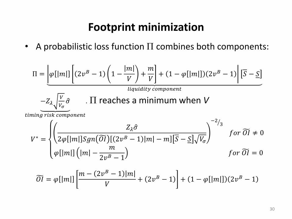
Footprint minimization

30

• A probabilistic loss function Π combines both components:

Π = 𝜑 𝑚 2𝑣𝐵 − 1 1 −𝑚

𝑉+𝑚

𝑉+ 1 − 𝜑 𝑚 2𝑣𝐵 − 1 𝑆 − 𝑆

𝑙𝑖𝑞𝑢𝑖𝑑𝑖𝑡𝑦 𝑐𝑜𝑚𝑝𝑜𝑛𝑒𝑛𝑡

−𝑍𝜆𝑉

𝑉𝜎𝜎

𝑡𝑖𝑚𝑖𝑛𝑔 𝑟𝑖𝑠𝑘 𝑐𝑜𝑚𝑝𝑜𝑛𝑒𝑛𝑡

. Π reaches a minimum when V

𝑉∗ =

𝑍𝜆𝜎

2𝜑 𝑚 𝑆𝑔𝑛 𝑂𝐼 2𝑣𝐵 − 1 𝑚 −𝑚 𝑆 − 𝑆 𝑉𝜎

−23

𝑓𝑜𝑟 𝑂𝐼 ≠ 0

𝜑 𝑚 𝑚 −𝑚

2𝑣𝐵 − 1 𝑓𝑜𝑟 𝑂𝐼 = 0

𝑂𝐼 = 𝜑 𝑚𝑚 − 2𝑣𝐵 − 1 𝑚

𝑉+ 2𝑣𝐵 − 1 + 1 − 𝜑 𝑚 2𝑣𝐵 − 1

Scenario 1: 𝑣𝐵 = 0.4

31

0

2000

4000

6000

8000

10000

12000

0

2,000

4,000

6,000

8,000

10,000

12,000

0 5,000 10,000 15,000 20,000 25,000 30,000 35,000 40,000 45,000 50,000

Liq

uid

ity,

tim

ing

co

mp

on

en

ts

Pro

ba

bil

isti

c lo

ss

Volume horizon

Probabilistic Loss Liquidity component Timing component

𝜎 = 1,000, 𝑉𝜎 = 10,000, 𝑚 = 1,000, 𝑆 − 𝑆 = 10,000, 𝜆 = 0.05 and 𝜑 𝑚 =1.

𝑉∗ = 6,000 We are buying in a selling market, thus our order contributes to narrowing the trading spread. This evidences the fact that order’s side, and not only size, determines the execution horizon.

Scenario 2: 𝑣𝐵 = 0.5

32

𝜎 = 1,000, 𝑉𝜎 = 10,000, 𝑚 = 1,000, 𝑆 − 𝑆 = 10,000, 𝜆 = 0.05 and 𝜑 𝑚 =1.

0

2000

4000

6000

8000

10000

12000

0

2,000

4,000

6,000

8,000

10,000

12,000

0 5,000 10,000 15,000 20,000 25,000 30,000 35,000 40,000 45,000 50,000

Liq

uid

ity,

tim

ing

co

mp

on

en

ts

Pro

ba

bil

isti

c lo

ss

Volume horizon

Probabilistic Loss Liquidity component Timing component

𝑉∗ = 11,392 We are buying in a balanced market. The liquidity component function is now convex decreasing, without an inflexion point, because the market is not leaning against us. The optimal 𝑉∗ must be larger than in Scenario 1, but limited by greater timing risk with increasing V.

Scenario 3: 𝑣𝐵 = 0.6

33

𝜎 = 1,000, 𝑉𝜎 = 10,000, 𝑚 = 1,000, 𝑆 − 𝑆 = 10,000, 𝜆 = 0.05 and 𝜑 𝑚 =1.

𝑉∗ = 9,817 Two forces contribute to this outcome: First, we are leaning with the market, thus we need a larger volume horizon than in Scenario I. Second, the gains from narrowing Σ are offset by the additional timing risk, and Π eventually cannot be improved further.

0

2000

4000

6000

8000

10000

12000

0

2,000

4,000

6,000

8,000

10,000

12,000

0 5,000 10,000 15,000 20,000 25,000 30,000 35,000 40,000 45,000 50,000

Liq

uid

ity,

tim

ing

co

mp

on

en

ts

Pro

ba

bil

isti

c lo

ss

Volume horizon

Probabilistic Loss Liquidity component Timing component

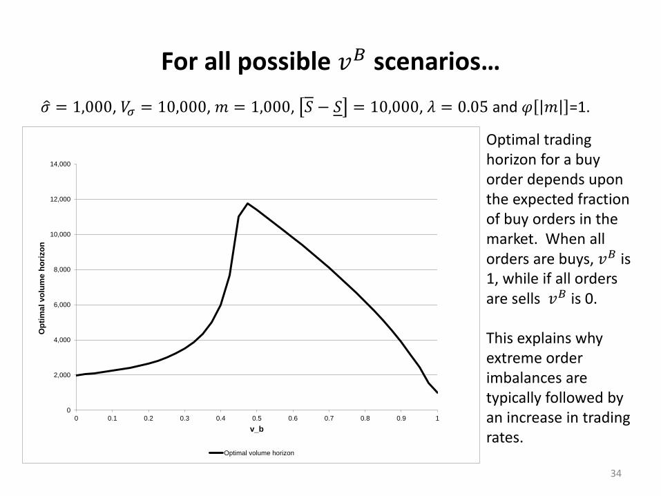
For all possible 𝑣𝐵 scenarios…

34

𝜎 = 1,000, 𝑉𝜎 = 10,000, 𝑚 = 1,000, 𝑆 − 𝑆 = 10,000, 𝜆 = 0.05 and 𝜑 𝑚 =1.

Optimal trading horizon for a buy order depends upon the expected fraction of buy orders in the market. When all orders are buys, 𝑣𝐵 is 1, while if all orders are sells 𝑣𝐵 is 0. This explains why extreme order imbalances are typically followed by an increase in trading rates.

0

2,000

4,000

6,000

8,000

10,000

12,000

14,000

0 0.1 0.2 0.3 0.4 0.5 0.6 0.7 0.8 0.9 1

Op

tim

al vo

lum

e h

ori

zo

n

v_b

Optimal volume horizon

THANKS FOR YOUR ATTENTION!

35

Bibliography (1/2)

• Almgren, R. and N. Chriss (2000): “Optimal Execution of Portfolio Transactions”, Journal of Risk (3), 5-39.

• Easley, D., Kiefer, N., O’Hara, M. and J. Paperman (1996): "Liquidity, Information, and Infrequently Traded Stocks", Journal of Finance, September.

• Easley, D., R. F. Engle, M. O’Hara and L. Wu (2008): “Time-Varying Arrival Rates of Informed and Uninformed Traders”, Journal of Financial Econometrics.

• Easley, D., M. López de Prado and M. O’Hara (2011a): “The Microstructure of the Flash Crash”, The Journal of Portfolio Management, Vol. 37, No. 2, Winter, 118-128. http://ssrn.com/abstract=1695041

• Easley, D., M. López de Prado and M. O’Hara (2011b): “The Exchange of Flow Toxicity”, The Journal of Trading, Vol. 6, No. 2, Spring, 8-13. http://ssrn.com/abstract=1748633

• Easley, D., M. López de Prado and M. O’Hara (2012a): “Flow Toxicity and Liquidity in a High Frequency World”, Review of Financial Studies, forthcoming: http://ssrn.com/abstract=1695596

36

Bibliography (2/2)

• Easley, D., M. López de Prado and M. O’Hara (2012b): “Bulk Volume Classification”, Working paper: http://ssrn.com/abstract=1989555

• Leinweber, D. (2009): “Nerds on Wall Street: Math, Machines and Wired Markets”, Wiley.

• López de Prado, M. (2011): “Advances in High Frequency Strategies”, Ed. Complutense University. http://tinyurl.com/hfpin

• NANEX (2011): “Strange Days June 8'th, 2011 - NatGas Algo”, http://www.nanex.net/StrangeDays/06082011.html

• O’Hara, M. (2011): “What is a quote?”, Journal of Trading, Spring, 10-15.

• The New York Times (2010): “Ex-Physicist Leads Flash Crash Inquiry”, 09/20.

37

Bio

Marcos M. López de Prado is Head of Global Quant Research and High Frequency Futures Trading at Tudor Investment Corp. Formerly, a Partner at PEAK6 Investments, Head of Quantitative Equity Research at UBS Wealth Management, and a Portfolio Manager at Citadel Investment Group. He has been appointed Visiting Scholar at Cornell University, a Postdoctoral Research Fellow of RCC at Harvard University and a Research Affiliate at Lawrence Berkeley National Laboratory (U.S. Department of Energy’s Office of Science). He received a Ph.D. in Financial Economics (2003), Sc.D. in Computational Finance (2011) from Complutense University and the National Graduation Award in Economics by the Government of Spain (National Valedictorian, 1998).

Dr. López de Prado is a member of the editorial board of the Journal of Investment Strategies (Risk Journals), and has co-authored several academic papers with Professors Maureen O’Hara and David Easley (Cornell University), which are listed among the most read in SSRN and have resulted in three international patent applications. His current Erdös number is 3 (with a valence of 2, through Bailey→Pomerance and Foreman→Komjáth), and would be happy to hear from potential co-authors with an Erdös number of 1.

38

Disclaimer

• The views expressed in this document are the authors’ and not necessarily reflect those of Tudor Investment Corporation.

• No investment decision or particular course of action is recommended by this presentation.

• All Rights Reserved.

39