(advances in econometrics)badi h. baltagi-nonstationary panels, panel cointegration, and dynamic...

LIST OF CONTRIBUTORS

Badi H. Baltagi Texas A&M University, Department ofEconomics, College Station, TX 77843-4228,USA. E-mail: [email protected]

M. Douglas Berg Department of Economics and InternationalBusiness, Sam Houston State University,Huntsville, TX 77341, USA

Richard Blundell Institute for Fiscal Studies and UniversityCollege London, UK.E-mail: [email protected]

Stephen Bond Institute for Fiscal Studies and NuffieldCollege, Oxford, UK.E-mail: [email protected]

Jörg Breitung Humboldt University Berlin, Institute ofStatistics and Econometrics, SpandauerStrasse 1, D-10178 Berlin, Germany.Fax: + 49.30.2093.5712;E-mail: [email protected]

Min-Hsien Chiang National Cheng-Kung University, Institute ofInternational Business, Tainan, Taiwan.Fax: 886-6-2766459;E-mail: [email protected]

Alain Hecq University Maastricht, Department ofQuantitative Economics, P.O. Box 616, 6200MD Maastricht, The Netherlands.Fax: + 31-43-388 48 74

Nazrul Islam Department of Economics, Emory University,Atlanta, GA 30322-2240, USA.Fax: 404-727-4639;E-mail: [email protected]

vii

Chihwa Kao Syracuse University, Center for PolicyResearch, Syracuse, NY 13244-1020, USA.Fax: 315-443-1081;E-mail: [email protected]

Heikki Kauppi University of Helsinki, Department ofEconomics, P.O. Box 54 (Unioninkatu 37),FIN-00014 University of Helsinki, Finland.Fax: + 358-9-1917980;E-mail: [email protected]

Qi Li Department of Economics, Texas A&MUniversity, College Station, TX 77843 andDepartment of Economics, University ofGuelph, Guelph, Ontario, N1G 2W1 Canada.E-mail: [email protected]

Chris Murray Department of Economics, University ofHouston, Houston, TX 77204-5882, USA.Fax: (713) 743-3798;E-mail: [email protected]

Franz C. Palm University Maastricht, Department ofQuantitative Economics, P.O. Box 616, 6200MD Maastricht, The Netherlands.Fax: + 31-43-388 48 74

David H. Papell Department of Economics, University ofHouston, Houston, TX 77204-5882, USA.Fax: (713) 743-3798;E-mail: [email protected]

Peter Pedroni Indiana University, Department ofEconomics, Bloomington, IN 47405, USA.E-mail: [email protected]

Aman Ullah Department of Economics, University ofCalifornia, Riverside, CA 92521, USA

viii

Jean-Pierre Urbain University Maastricht, Department ofQuantitative Economics, P.O. Box 616, 6200MD Maastricht, The Netherlands.Fax: + 31-43-388 48 74;E-mail: [email protected]

Frank Windmeijer Institute for Fiscal Studies, 7 RidgmountStreet, London WC1E 7AE, UK.Fax: + 44.(0)20.7323.4780;E-mail: [email protected]

Showen Wu Department of Finance and ManagerialEconomics, State University of New York atBuffalo, Buffalo, NY 14260, USA

Yong Yin Department of Economics, State Universityof New York at Buffalo, Buffalo, NY 14260,USA. Fax: 716-645-2127;E-mail: [email protected]

ix

INTRODUCTION

Badi H. Baltagi, Thomas B. Fomby and R. Carter Hill

Twenty two years ago, the first special issue on panel data econometrics waspublished by the Annales de l’INSEE. This consisted of two volumescontaining a list of ‘who’s who’ in economics and econometrics of panel datathat was edited by Mazodier (1978). Since then, several books on panel datahave been written including the econometric society monograph by Hsiao(1986), a two volume collection of classic papers on the subject by Maddala(1993), a Handbook, which in its second edition contained 33 chapters editedby Matyas & Sevestre (1996) and a textbook by Baltagi (1995a). Severalspecial issues of journals with a panel data theme have also appeared since1978, those include Raj & Baltagi (1992), Matyas (1992), Carraro, et al.(1993), Baltagi (1995b), Sevestre (1999) and Banerjee (1999). There have beennine international conferences on panel data since the first conference atINSEE, the last one was held at the University of Geneva in June, 2000. Paneldata econometrics continues to have an important impact on today’s empiricaleconomics studies. A Journal of Economic Literature search returned 2780citations using the words ‘panel data’ between 1980 and 2000. This volume isdedicated to two recent intensive areas of research in the econometrics of paneldata: nonstationary panels and dynamic panels, see the survey chapter byBaltagi & Kao in this volume. The volume includes eleven refereed chapters onthis subject written by twenty authors. The editors are grateful to the authorsand referees for their cooperation.

The chapter by Baltagi & Kao surveys the nonstationary panels, cointegra-tion in panels and dynamic panels literature. In particular, panel unit root testsare considered first and several important chapters are reviewed including asummary of the finite sample properties of these unit roots tests obtained from

Nonstationary Panels, Panel Cointegration and Dynamic Panels, Volume 15, pages 1–5.Copyright © 2000 by Elsevier Science Inc.All rights of reproduction in any form reserved.ISBN: 0-7623-0688-2

1

extensive simulations. Also, spurious regressions in panel data are consideredfollowed by panel cointegration tests with a summary of the finite sampleproperties of these cointegration tests using Monte Carlo experiments. Next,estimation and inference in panel cointegration models is considered and thechapter concludes with a review of recent developments in dynamic panel datamodels that have occurred over the last five years.

The chapter by Blundell, Bond & Windmeijer reviews recent developmentsin the estimation of dynamic panel data models using generalized method ofmoments (GMM). In particular, this chapter focuses on the system GMMestimator derived by Blundell & Bond (1998) which relies on relatively mildrestrictions on the initial condition process. This system GMM estimatorencompasses the GMM estimator based on the non-linear moment conditionsavailable in the dynamic error components model. Monte Carlo experimentsand asymptotic variance calculations show that this extended GMM estimatorcan offer considerable efficiency gains in situations where the first differencedGMM estimator performs poorly.

The chapter by Pedroni develops methods for estimating and testinghypotheses for cointegrating vectors in dynamic panels. In particular, thischapter proposes methods based on fully modified OLS principles whichaccount for considerable heterogeneity across individual members of the panel.The asymptotic properties of various estimators are compared based on poolingalong the within and between dimensions of the panel. Monte Carlosimulations show that the group mean estimator is well behaved even inrelatively small samples under a variety of scenarios.

The chapter by Hecq, Palm & Urbain extends the concept of serialcorrelation common features analysis to nonstationary panel data models. Thisanalysis is motivated both by the need to study and test for common structuresand comovements in panel data with autocorrelation present and by an increasein efficiency due to pooling. The authors propose sequential testing proceduresand test their performance using a small scale Monte Carlo. Concentratingupon the fixed effects model, they define homogeneous panel common featuremodels and give a series of steps to implement these tests. These tests are usedto investigate the liquidity constraints model for 22 OECD and G7 countries.The presence of a panel common feature vector is rejected at the 5% nominallevel.

The chapter by Breitung studies the local power of panel unit root teststatistics against a sequence of local power alternatives. In particular, thischapter finds that the Levin & Lin (1993) (LL) and Im, Pesaran & Shin (1997)(IPS) tests suffer from severe loss of power if individual specific trends are

2 BADI H. BALTAGI, THOMAS B. FOMBY & R. CARTER HILL

included. Breitung suggests a test statistic that does not employ a biasadjustment whose power is substantially higher than that of LL or the IPS testsusing Monte Carlo experiments. This chapter also finds that the power of theLL and IPS tests is sensitive to the specification of the deterministic terms.

The chapter by Kao & Chiang studies the limiting distributions of ordinaryleast squares (OLS), fully modified OLS (FMOLS) and dynamic OLS (DOLS)estimators in a panel cointegrated regression model. This chapter shows thatthe OLS, FMOLS and DOLS estimators are all asymptotically normallydistributed. However, the asymptotic distribution of the OLS estimator has anon-zero mean. Extensive Monte Carlo experiments are performed which showthat the OLS estimator has a non-negligible bias in finite samples, the FMOLSestimator does not improve on the OLS estimator in general, and the DOLSestimator outperforms both OLS and FMOLS.

The chapter by Murray & Papell proposes a panel unit roots test in thepresence of structural change. In particular, this chapter proposes a unit roottest for non-trending data in the presence of a one-time change in the mean fora heterogeneous panel. The date of the break is endogenously determined. Theresultant test allows for both serial and contemporaneous correlation, both ofwhich are often found to be important in the panel unit roots context. Murray& Papell conduct two power experiments for panels of non-trending, stationaryseries with a one-time change in means and find that conventional panel unitroot tests generally have very low power. Then they conduct the sameexperiment using methods that test for unit roots in the presence of structuralchange and find that the power of the test is much improved.

The chapter by Kauppi develops a new limit theory for panel data that maybe cross sectionally heterogeneous in a fairly general way. This limit theorybuilds upon the concepts of joint convergence in probability and in distributionfor double indexed processes by Phillips & Moon (1999a). This limit theory isapplied to a panel regression model with regressors that are generated by anautoregressive process with a root local to unity. The main results are thefollowing: (i) the usual pooled panel OLS estimator is invalid for inference, (ii)a bias corrected pooled OLS proves to be �NT consistent with an asymptoticnormal distribution centered on the true parameter value irrespective ofwhether the regressors have near or exact unit roots. This positive result holdsonly in the special case where the model does not exhibit any deterministiceffects, such as individual intercepts. (iii) The fully modified panel estimator ofPhillips & Moon (1999a) is also subject to severe bias effects if the regressorsare nearly rather than exactly cointegrated. These theoretical results areconfirmed using Monte Carlo results.

3Introduction

The chapter by Yin & Wu proposes stationarity tests for a heterogeneouspanel data model. The authors consider the case of serially correlated errors inthe level and trend stationary models. The proposed panel tests utilize theKwaitkowski, Phillips, Schmidt & Shin (1992) test and the Leybourne &McCabe (1994) test from the time series literature. Two different ways ofpooling information from the independent tests are used. In particular, thegroup mean and the Fisher type tests are used to develop the panel stationaritytests. Monte Carlo experiments are performed that reveal good small sampleperformance in terms of size and power.

The chapter by Berg, Li & Ullah considers the problem of estimating asemiparametric partially linear dynamic panel data model with disturbancesthat follow a one-way error component structure. Two new semiparametricinstrumental variable (IV) estimators are proposed for the coefficient of theparametric component. These are shown to be more efficient than the onessuggested by Li & Stengos (1996) and Li & Ullah (1998) because they makefull use of the error component structure. This is confirmed using Monte Carloexperiments.

The chapter by Islam conducts a Monte Carlo study to investigate the smallsample properties of dynamic panel data estimators. Although there areextensive Monte Carlo studies on this subject, this study customizes the designto the estimation of the growth convergence equation using the Summers-Heston data. Islam concludes that the OLS estimation of thegrowth-convergence equation is likely to give misleading results. At the sametime, indiscriminate use of panel estimators is risky and one should makejudicious choice of panel estimators.

REFERENCES

Only references that are not cited later in the volume are given here.

Baltagi, B. H. (1995b). Editor’s Introduction: Panel Data. Journal of Econometrics, 68, 1–4.Banerjee, A. (1999). Panel Data Unit Roots and Cointegration: An Overview. Oxford Bulletin of

Economics and Statistics, 61, 607–629.Carraro, C., Peracchi, F., & Weber, G. (Eds.) (1993). The Econometrics of Panels and Pseudo

Panels. Journal of Econometrics, 59, 1–211.Hsiao, C. (1986). Analysis of Panel Data. Cambridge: Cambridge University Press.Maddala, G. S. (Ed.) (1993). The Econometrics of Panel Data. Vols. 1 and 2. Cheltenham: Edward

Elgar.Matyas, L. (Ed.) (1996). Modelling Panel Data. Structural Change and Economic Dynamics, 3,

291–384.

4 BADI H. BALTAGI, THOMAS B. FOMBY & R. CARTER HILL

Matyas, L., & Sevestre, P. (Eds.) (1996). The Econometrics of Panel Data: Handbook of Theoryand Applications. Dordrecht: Kluwer Academic Publishers.

Mazodier P. (Ed.) (1978). The Econometrics of Panel Data. Annales de I’INSEE, 30/31.Raj, B., & Baltagi, B. (1992). Editors’ Introduction and Overview: Panel Data Analysis. Empirical

Economics, 17, 1–8.Sevestre, P. (1999). 1977–1997: Changes and Continuities in Panel Data. Annales D’Economie et

de Statistique, 55–56, 15–25.

5Introduction

NONSTATIONARY PANELS,COINTEGRATION IN PANELS ANDDYNAMIC PANELS: A SURVEY

Badi H. Baltagi and Chihwa Kao

ABSTRACT

This chapter provides an overview of topics in nonstationary panels: panelunit root tests, panel cointegration tests, and estimation of panelcointegration models. In addition it surveys recent developments indynamic panel data models.

I. INTRODUCTION

Two important areas in the econometrics of panel data that have received muchattention recently are dynamic panel data1 and nonstationary panel time seriesmodels.2 This special issue focuses on these two topics. With the growing useof cross-country data over time to study purchasing power parity, growthconvergence and international R&D spillovers, the focus of panel dataeconometrics has shifted towards studying the asymptotics of macro panelswith large N (number of countries) and large T (length of the time series) ratherthan the usual asymptotics of micro panels with large N and small T. In fact, thelimiting distributions of double indexed integrated processes had to bedeveloped, see Phillips & Moon (1999a). The fact that T is allowed to increaseto infinity in macro panel data, generated two strands of ideas. The first rejectedthe homogeneity of the regression parameters implicit in the use of a pooled


7

regression model in favor of heterogeneous regressions, i.e. one for eachcountry, see Pesaran & Smith (1995), Im, Pesaran & Shin (1997), Lee, Pesaran& Smith (1997), Pesaran, Shin & Smith (1999) and Pesaran & Zhao (1999) tomention a few. This literature critically relies on T being large to estimate eachcountry’s regression separately. Another strand of literature applied time seriesprocedures to panels, worrying about non-stationarity, spurious regressions andcointegration. Adding the cross-section dimension to the time-series dimensionoffers an advantage in the testing for nonstationarity and cointegration. Thehope of the econometrics of nonstationary panel data is to combine the best ofboth worlds: the method of dealing with nonstationary data from the time seriesand the increased data and power from the cross-section. The addition of thecross-section dimension, under certain assumptions, can act as repeated drawsfrom the same distribution. Thus as the time and cross-section dimensionincrease panel test statistics and estimators can be derived which converge indistribution to normally distributed random variables.

However, the use of such panel data methods are not without their critics, seeMaddala, Wu & Liu (2000) who argue that panel data unit root tests do notrescue purchasing power parity (PPP). In fact, the results on PPP with panelsare mixed depending on the group of countries studied, the period of study andthe type of unit root test used. More damaging is the argument by Maddala etal. that for PPP, panel data tests are the wrong answer to the low power of unitroot tests in single time series. After all, the null hypothesis of a single unit rootis different from the null hypothesis of a panel unit root for the PPP hypothesis.Using the same line of criticism, Maddala (1999) argued that panel unit roottests did not help settle the question of growth convergence among countries.However, it was useful in spurring much needed research into dynamic paneldata models. Also, Quah (1996) who argued that the basic issues of whetherpoor countries catch up with the rich can never be answered by the use oftraditional panels. Instead, Quah suggested formulating and estimating modelsof income dynamics.

One can find numerous applications of time series methods applied to panelsin recent years. Examples from the purchasing power parity literature includeBernard & Jones (1996), Jorion & Sweeney (1996), MacDonald (1996), Oh(1996), Wu (1996), Coakley & Fuertes (1997), Culver & Papell (1997), Papell(1997), O’Connell (1998), Choi (1999a), Andersson & Lyhagen (1999), andCanzoneri, Cumby & Diba (1999) to mention a few. On health careexpenditures, see McCoskey & Selden (1998), and Gerdtham & Löthgren(1998). On growth and convergence, see Islam (1995), Evans & Karas (1996),Sala-i-Martin (1996), Lee, Pesaran & Smith (1997), and McCoskey & Kao

8 BADI H. BALTAGI & CHIHWA KAO

(1999a). On international R&D spillovers, see Funk (1998) and Kao, Chiang &Chen (1999). On exchange rate models, see Groen & Kleibergen (1999), andGroen (1999). On savings and investment models, see Coakely, Kulasi & Smith(1996) and Moon & Phillips (1998).

The first part of this chapter surveys some of the developments innonstationary panel models that have occurred since the middle of 1990s. Twoother recent surveys on this subject include Phillips & Moon (1999b) on multi-indexed processes and Banerjee (1999) on panel unit roots and cointegrationtests. We will pay attention to the following three topics: (1) panel unit roottests, (2) panel cointegration tests, and (3) estimation and inference in the panelcointegration models. The discussion of each topic will be illustrated byexamples taken from the aforementioned list of references. Section 2 reviewspanel unit root tests, while Section 3 discusses the panel spurious models.Section 4 considers the panel cointegration tests, while Section 5 discussespanel cointegration models. Section 6 reviews some recent developments indynamic panels and Section 7 gives our conclusion.

A word on notation. We write the integral �10 W(s)ds, as � W when there is no

ambiguity over limits. We define �1/2 to be any matrix such that

� = (�1/2)(�1/2), use ⇒ to denote weak convergence, →p to denote convergencein probability, I(0) and I(1) to signify a time series that is integrated of orderzero and one, respectively, and WZ(r) = W(r) � [� WZ�][� ZZ�]Z(r) to denote anL2 projection residual of W(r) on Z(r).

II. PANEL UNIT ROOTS TESTS

Testing for unit roots in time series studies is now common practice amongapplied researchers and has become an integral part of econometric courses.However, testing for unit roots in panels is recent, see Levin & Lin (1992), Im,Pesaran & Shin (1997), Harris & Tzavalis (1999), Maddala & Wu (1999), Choi(1999a), and Hadri (1999). Exceptions are Bharagava et al. (1982), Boumahdi& Thomas (1991), Breitung & Meyer (1994), and Quah (1994). Bharagava etal. proposed a test for random walk residuals in a dynamic model with fixedeffects. They suggested a modified Durbin-Watson (DW) statistic based onfixed effects residuals and two other test statistics based on differenced OLSresiduals. In typical micro panels with N→�, they recommended theirmodified DW statistic. Boumahdi & Thomas (1991) proposed a generalizationof the Dickey-Fuller (DF) test for unit roots in panel data to assess theefficiency of the French capital market using 140 French stock prices over the

9Nonstationary Panels, Cointegration in Panels and Dynamic Panels: A Survey

period January 1973 to February 1986. Breitung & Meyer (1994) appliedvarious modified DF test statistics to test for unit roots in a panel of contractedwages negotiated at the firm and industry level for Western Germany over theperiod 1972–1987. Quah (1994) suggested a test for unit root in a panel datamodel without fixed effects where both N and T go to infinity at the same ratesuch that N/T is constant. Levin & Lin (1992) generalized this model to allowfor fixed effects, individual deterministic trends and heterogeneous seriallycorrelated errors. They assumed that both N and T tend to infinity. However, Tincreases at a faster rate than N with N/T→0. Even though this literature grewfrom time series and panel data, the way in which N, the number of cross-section units, and T, the length of the time series, tend to infinity is crucial fordetermining asymptotic properties of estimators and tests proposed fornonstationary panels, see Phillips & Moon (1999a). Several approaches arepossible including: (i) sequential limits where one index, say N, is fixed and Tis allowed to increase to infinity, giving an intermediate limit. Then by lettingN tend to infinity subsequently, a sequential limit theory is obtained. Phillips &Moon (1999b) argued that these sequential limits are easy to derive and arehelpful in extracting quick asymptotics. However, Phillips and Moon provideda simple example that illustrates how sequential limits can sometimes givemisleading asymptotic results. (ii) A second approach, used by Quah (1994)and Levin & Lin (1992) is to allow the two indexes, N and T to pass to infinityalong a specific diagonal path in the two dimensional array. This path can bedetermined by a monotonically increasing functional relation of the typeT = T(N) which applies as the index N→�. Phillips & Moon (1999b) showedthat the limit theory obtained by this approach is dependent on the specificfunctional relation T = T(N) and the assumed expansion path may not providean appropriate approximation for a given (T, N) situation. (iii) A third approachis a joint limit theory allowing both N and T to pass to infinity simultaneouslywithout placing specific diagonal path restrictions on the divergence. Somecontrol over the relative rate of expansion may have to be exercised in order toget definitive results. Phillips & Moon argued that, in general, joint limit theoryis more robust than either sequential limit or diagonal path limit. However, itis usually more difficult to derive and requires stronger conditions such as theexistence of higher moments that will allow for uniformity in the convergencearguments. The muti-index asymptotic theory in Phillips & Moon (1999a, b) isapplied to joint limits in which T, N→� and (T/N)→�, i.e. to situations wherethe time series sample is large relative to the cross-section sample. However,the general approach given there is also applicable to situations in which (T/N)→0 although different limit results will generally obtain in that case.


A. Levin & Lin (1992) Tests

Consider the model

yit = �iyit�1 + z�it�i + uit, i = 1, . . . , N; t = 1, . . . , T, (1)

where zit is the deterministic component and uit is a stationary process. zit couldbe zero, one, the fixed effects, �i, or fixed effect as well as a time trend, t. TheLevin & Lin (LL) tests assume that uit are iid(0, 2

u) and �i = � for all i. LL areinterested in testing the null hypothesis

H0 : � = 1 (2)

against the alternative hypothesis

Ha : � < 1.

Let � be the OLS estimator of � in (1) and define

zt = (z1t, . . . , zNt)�,

h(t, s) = z�t��T

t=1

ztz�t��1

zs,

uit = uit ��T

s=1

h(t, s)uis,

and

yit = yit ��T

s=1

h(t, s)yis. (3)

Then we have

�NT(� � 1) =

1

�N�N

i=1

1

T�T

t=1

yi, t�1uit

1N�

N

i=1

1T2 �T

t=1

y2i, t�1

and the corresponding t-statistic, under the null hypothesis is given by

t� =

(� � 1)� �N

i=1�T

t=1

y2i, t�1

se

,


where

s2e =

1NT�

N

i=1�T

t=1

u2it.

Assume that there exists a scaling matrix DT and piecewise continuousfunction Z(r) such that

D�1T z[Tr] →Z(r)

uniformly for r�[0, 1]. For a fixed N, we have

1

�N�N

i=1

1T�

T

t=1

yi, t�1uit ⇒1

�N�N

i=1�WiZ dWiZ

and

1N�

N

i=1

1T2 �T

t=1

y2i, t�1 ⇒ 1

N�N

i=1

�W 2iZ,

as T→�. Next we assume that � WiZ dWiZ and � W2iZ, are independent across i

and have finite second moments. Then it follows that

1N�

N

i=1

�W 2iZ →p E�W 2

iZ1

�N�N

i=1

��WiZ dWiZ � E�WiZ dWiZ�⇒ N�0, Var��WiZ dWiZ��as N→� by a law of large numbers and the Lindeberg-Levy central limittheorem. The following moments are taken from Levin & Lin (1992):

zit E[� WiZ dWiZ] Var[� WiZ dWiZ] E[� W2iZ] Var[� WiZ

2 ]

0 012

12

13

1 013

12

? (4)

�i �12

112

16

145

(�i, t) �12

160

115

116300


Using (4), Levin & Lin (1992) obtain the following limiting distributions of�NT(� � 1) and t�:

zit � t�

0 �NT(� � 1) ⇒ N(0, 2) t� ⇒ N(0, 1)

1 �NT(� � 1) ⇒ N(0, 2) t� ⇒ N(0, 1)

�i �NT(� � 1) + 3�N ⇒�0,515 � �1.25t� + �1.875N ⇒ N(0, 1) (5)

(�i, t)��N(T(� � 1) + 7.5) ⇒ N�0,2895112 � �448

277(t� + �3.75N) ⇒ N(0, 1)

Sequential limit theory, i.e. T→� followed by N→�, is used to derive thelimiting distributions in (5). In case uit is stationary, the asymptotic distributionsof � and t� need to be modified due to the presence of serial correlation.

Harris & Tzavalis (1999) also derived unit root tests for (1) withzit = {0}, {�i}, or {(�i, t)�} when the time dimension of the panel, T, is fixed.This is the typical case for micro panel studies. The main results are:

zit �

0 �N(� � 1) ⇒ N�0,2

T(T � 1)��i �N�� 1 +

3T + 1�⇒ N�0,

3(17T2 � 20T + 17)5(T � 1)(T + 1)3 �

(�i, t)� �N�� 1 +15

2(T + 2)�⇒ N�0,15(193T2 � 728T + 1147)

112(T + 2)3(T � 2) �Harris & Tzavalis (1999) also showed that the assumption that T tends toinfinity at a faster rate than N as in LL rather than T fixed as in the case in micropanels, yields tests which are substantially undersized and have low powerespecially when T is small.

Recently, Frankel & Rose (1996), Oh (1996), and Lothian (1996) tested thePPP hypothesis using panel data. All of these articles use LL tests and some ofthem report evidence supporting the PPP hypothesis. O’Connell (1998),


however, showed that the LL tests suffered from significant size distortion inthe presence of correlation among contemporaneous cross-sectional errorterms. O’Connell highlighted the importance of controlling for cross-sectionaldependence when testing for a unit root in panels of real exchange rates. Heshowed that, controlling for cross-sectional dependence, no evidence againstthe null of a random walk can be found in panels of up to 64 real exchangerates.

Virtually all the existing nonstationary panel literature assume cross-sectional independence. It is true that the assumption of independence across iis rather strong, but it is needed in order to satisfy the requirement of theLindeberg-Levy central limit theorem. Moreover, as pointed out by Quah(1994), modeling cross-sectional dependence is involved because individualobservations in a cross-section have no natural ordering. Driscoll & Kraay(1998) presented a simple extension of common nonparametric covariancematrix estimation techniques which yields standard errors that are robust tovery general forms of spatial and temporal dependence as the time dimensionbecomes large. In a recent paper, Conley (1999) presented a spatial model ofdependence among agents using a metric of economic distance that providescross-sectional data with a structure similar to time-series data. Conleyproposed a generalized method of moments (GMM) using such dependent dataand a class of nonparametric covariance matrix estimators that allow for ageneral form of dependence characterized by economic distance.

B. Im, Pesaran & Shin (1997) Tests

The LL test is restrictive in the sense that it requires � to be homogeneousacross i. As Maddala (1999) pointed out, the null may be fine for testingconvergence in growth among countries, but the alternative restricts everycountry to converge at the same rate. Im, Pesaran & Shin (1997) (IPS) allow fora heterogeneous coefficient of yit�1 and proposed an alternative testingprocedure based on averaging individual unit root test statistics. IPS suggestedan average of the augmented DF (ADF) tests when uit is serially correlated withdifferent serial correlation properties across cross-sectional units, i.e. uit =�pi

j=1 ijuit� j + �it. Substituting this uit in (1) we get:

yit = �iyit�1 +�pi

j=1

ij �yit� j + z�it�i + �it. (6)

The null hypothesis is

H0 : �i = 1


for all i and the alternative hypothesis is

Ha : �i < 1

for at least one i. The IPS t-bar statistic is defined as the average of theindividual ADF statistics as

t =1N�

N

i=1

t�i, (7)

where t�iis the individual t-statistic of testing H0 : �i = 1 in (6). It is known that

for a fixed N

t�i⇒� 1

0

WiZ dWiZ

� 1

0

W2iZ1/2

= tiT (8)

as T→�. IPS assume that tiT are iid and have finite mean and variance. Then

�N�1N�

N

i=1

tiT � E[tiT | �i = 1]��Var[tiT | �i = 1]

⇒ N(0, 1) (9)

as N→� by the Lindeberg-Levy central limit theorem. Hence

tIPS =�N(t � E[tiT | �i = ])

�Var[tiT | �i = 1]⇒ N(0, 1) (10)

as T→� followed by N→� sequentially. The values of E[tiT | �i = 1] andVar[tiT | �i = 1] have been computed by IPS via simulations for different valuesof T and p�is.

In this volume, Breitung (2000) studies the local power of LL and IPS testsstatistics against a sequence of local alternatives. Breitung finds that the LL andIPS tests suffer from a dramatic loss of power if individual specific trends areincluded. This is due to the bias correction that also removes the mean underthe sequence of local alternatives. The simulation results indicate that thepower of LL and IPS tests is very sensitive to the specification of thedeterministic terms.

McCoskey & Selden (1998) applied the IPS test for testing unit root for percapita national health care expenditures (HE) and gross domestic product(GDP) for a panel of OECD countries. McCoskey & Selden rejected the null


hypothesis that these two series contain unit roots. Gerdtham & Löthgren(1998) claimed that the stationarity found by McCoskey & Selden are driven bythe omission of time trends in their ADF regression in (6). Using the IPS testwith a time trend, Gerdtham & Löthgren found that both HE and GDP arenonstationary. They concluded that HE and GDP are cointegrated around lineartrends following the results of McCoskey & Kao (1999b).

C. Combining P-Values Tests

Let GiTibe a unit root test statistic for the i-th group in (1) and assume that as

Ti →�, GiTi⇒ Gi. Let pi be the p-value of a unit root test for cross-section i, i.e.

pi = F(GiTi), where F(·) is the distribution function of the random variable Gi.

Maddala & Wu (1999) and Choi (1999a) proposed a Fisher type test

P = � 2�N

i=1

ln pi (11)

which combines the p-values from unit root tests for each cross-section i to testfor unit root in panel data. P is distributed as 2 with 2N degrees of freedom asTi →� for all N. Maddala et al. (1999) argued that the IPS and Fisher tests relaxthe restrictive assumption of the LL test that �i is the same under the alternative.Both the IPS and Fisher tests combine information based on individual unitroot tests. However, the Fisher test has the advantage over the IPS test in thatit does not require a balanced panel. Also, the Fisher test can use different laglengths in the individual ADF regressions and can be applied to any other unitroot tests. The disadvantage is that the p-values have to be derived by MonteCarlo simulations. Choi (1999a) echoes similar advantages of the Fisher test:(1) the cross-sectional dimension, N, can be either finite or infinite, (2) eachgroup can have different types of nonstochastic and stochastic components, (3)the time series dimension, T, can be different for each i, and (4) the alternativehypothesis would allow some groups to have unit roots while others may not.

When N is large, Choi (1999a) proposed a Z test,

Z =

1

�N�N

i=1

( � 2 ln pi � 2)

2(12)

since E[ � 2 ln pi] = 2 and Var[ � 2 ln pi] = 4. Assume that the pi’s are iid anduse the Lindeberg-Levy central limit theorem to get

Z ⇒ N(0, 1)


as Ti →� followed by N→�.3

Choi (1999a) applied the Z test in (12) and the IPS test in (7) to panel dataof real exchange rates and provided evidence in favor of the PPP hypothesis.Choi claimed that this is due to the improved finite sample power of the Fishertest. Maddala & Wu (1999) and Maddala et al. (1999) find that the Fisher testis superior to the IPS test, but they argue that these panel unit root tests still donot rescue the PPP hypothesis. When allowance is made for the deficiency inthe panel data unit root tests and panel estimation methods, support for PPPturns out to be weak.

D. Residual Based LM Test

Hadri (1999) proposed a residual based Lagrange Multiplier (LM) test for thenull that the time series for each i are stationary around a deterministic trendagainst the alternative of a unit root in panel data. Consider the followingmodel

yit = z�it� + rit + �it (13)

where zit is the deterministic component, rit is a random walk

rit = rit�1 + uit

uit ~ iid(0, 2u) and �it is a stationary process. (13) can be written as

yit = z�it� + eit (14)

where

eit =�t

j=1

uij + �it.

Let eit be the residuals from the regression in (14) and 2e be the estimate of the

error variance. Also, let Sit be the partial sum process of the residuals,

Sit =�t

j=1

eij.

Then the LM statistic is

LM =

1N�

N

i=1

1T2 �T

t=1

S2it

2e

.


It can be shown that

LM→p E� W 2iZ

as T→� followed by N→� provided E[� W2iZ] < �. Also,

�N(LM � E[� W2iZ])

�Var[� W2iZ]

⇒ N(0, 1)

as T→� followed by N→�.

E. Finite Sample Properties of Unit Root Tests

Extensive simulations have been conducted to explore the finite sampleperformance of panel unit root tests, e.g. Karlsson & Löthgren (1999), Im et.al. (1997), Maddala & Wu (1999), and Choi (1999a). Choi (1999a) studied thesmall sample properties of IPS t-bar test in (7) and Fisher’s test in (11). Choi’smajor findings are the following:

(1) The empirical size of the IPS and the Fisher test are reasonably close totheir nominal size 0.05 when N is small. But the Fisher test shows mild sizedistortions at N = 100, which is expected from the asymptotic theory.Overall, the IPS t-bar test has the most stable size.

(2) In terms of the size-adjusted power, the Fisher test seems to be superior tothe IPS t-bar test.

(3) When a linear time trend is included in the model, the power of all testsdecrease considerably.

III. SPURIOUS REGRESSION IN PANEL DATA

Entorf (1997) studied spurious fixed effects regressions when the true modelinvolves independent random walks with and without drifts. Entorf found thatfor T→� and N finite, the nonsense regression phenomenon holds for spuriousfixed effects models and inference based on t-values can be highly misleading.Kao (1999) and Phillips & Moon (1999a) derived the asymptotic distributionsof the least squares dummy variable estimator and various conventionalstatistics from the spurious regression in panel data.

Consider a spurious regression model for all i using panel data:

yit = x�it� + z�it� + eit, (15)

where


xit = xit�1 + �it,

and eit is I(1). The OLS estimator of � is

� =�N

i=1�T

t=1

xit xit��1�N

i=1�T

t=1

xityit, (16)

where yit is defined in (3) and

xit = xit ��T

s=1

h(t, s)xis.

It is known that if a time-series regression for a given i is performed in model(15), the OLS estimator of � is spurious. It is easy to see that

1N�

N

i=1

1T2 �T

t=1

xit xit →p E�WiZW�iZ��

and

1N�

N

i=1

1T2 �T

t=1

xityit →p EWiZW�iZ�u�

as by a sequential limit theory, where

zit E[� WiZWiZ�]

012

112

�i

12

Ik

(�i, t)1

15Ik

Then we have

�→p��1

� ��u. (17)

(17) shows that the OLS estimator of �, �, is consistent for its true value,��1

� �u�. This is due to the fact that the noise, eit, is as strong as the signal, xit,


since both eit and xit are I(1). In the panel regression (15) with a large numberof cross-sections, the strong noise of eit is attenuated by pooling the data anda consistent estimate of � can be extracted. The asymptotics of the OLSestimator are very different from those of the spurious regression in pure timeseries. This has an important consequence for residual-based cointegration testsin panel data, because the null distribution of residual-based cointegration testsdepends on the asymptotics of the OLS estimator. This point is explainedfurther in the next section.

IV. PANEL COINTEGRATION TESTS

A. Kao Tests

Kao (1999) presented two types of cointegration tests in panel data, the DF andADF types tests. The DF type tests from Kao can be calculated from theestimated residuals in (15) as:

eit = �eit�1 + vit, (18)

where

eit = yit � x�it�.

In order to test the null hypothesis of no cointegration, the null can be writtenas H0 : � = 1. The OLS estimate of � and the t-statistic are given as:

� =�N

i=1�T

t=2

eiteit�1

�N

i=1�T

t=2

e2it

and

t� =

(� � 1)��N

i=1�T

t=2

e2it�1

se

,

where s2e =

1NT�

N

i=1�T

t=2

(eit � �eit�1)2. Kao proposed the following four DF type

tests by assuming zit = {�i}:

DF� =�NT(� � 1) + 3�N

�10.2,


DFt = �1.25t� + �1.875N,

DF*� =�NT(� � 1) +

3�N2�

20�

�3 +364

�

540�

,

and

DF*t =t� +

�6N�

20�

� 20�

22�

+32

�

1020�

,

where 2� = �u � �u��

�1� and 2

0� = �u � �u��1. While DF� and DFt are based

on the strong exogeneity of the regressors and errors, DF*� and DF*t are for thecointegration with endogenous relationship between regressors and errors. Forthe ADF test, we can run the following regression:

eit = �eit�1 +�j=1

p

�j�eit� j + �itp. (19)

With the null hypothesis of no cointegration, the ADF test statistics can beconstructed as:

ADF =tADF +

�6N�

20�

� 0�2

2�2 +

3�2

100�2

where tADF is the t-statistic of � in (19). The asymptotic distributions of DF�,DFt, DF*�, DF*t, and ADF converge to a standard normal distribution N(0, 1) bythe sequential limit theory.

B. Residual Based LM Test

McCoskey & Kao (1998) derived a residual-based test for the null ofcointegration rather than the null of no cointegration in panels. This test is anextension of the LM test and the locally best invariant (LBI) test for an MA unitroot in the time series literature, see Harris & Inder (1994) and Shin (1994).Under the null, the asymptotics no longer depend on the asymptotic properties


of the estimating spurious regression, rather the asymptotics of the estimationof a cointegrated relationship are needed. For models which allow thecointegrating vector to change across the cross-sectional observations, theasymptotics depend merely on the time series results as each cross-section isestimated independently. For models with common slopes, the estimation isdone jointly and therefore the asymptotic theory is based on the joint estimationof a cointegrated relationship in panel data.

For the residual based test of the null of cointegration, it is necessary to usean efficient estimation technique of cointegrated variables. In the time seriesliterature a variety of methods have been shown to be efficient asymptotically.These include the fully modified (FM) estimator of Phillips & Hansen (1990)and the dynamic least squares (DOLS) estimator as proposed by Saikkonen(1991) and Stock & Watson (1993). For panel data, Kao & Chiang (2000)showed that both the FM and DOLS methods can produce estimators which areasymptotically normally distributed with zero means.

The model presented allows for varying slopes and intercepts:

yit = �i + x�it�i + eit, (20)

xit = xit�1 + �it (21)

eit = �it + uit, (22)

and

�it = �it�1 + �uit,

where uit are i.i.d(0, u2). The null of hypothesis of cointegration is equivalent

to � = 0.The test statistic proposed by McCoskey & Kao (1998) is defined as

follows:

LM =

1N�

i=1

N1T2 �

t=1

T

Sit2

e2 , (23)

where Sit, is partial sum process of the residuals,

Sit =�j=1

t

eij

and e2 is defined in McCoskey and Kao. The asymptotic result for the test is:

�N(LM � ��) ⇒ N(0, �2). (24)


The moments, �� and �2, can be found through Monte Carlo simulation. The

limiting distribution of LM is then free of nuisance parameters and robust toheteroskedasticity.

Urban economists have long sought to explain the relationship betweenurbanization levels and output. McCoskey & Kao (1999a) revisited thisquestion and test the long run stability of a production function includingurbanization using nonstationary panel data techniques. McCoskey and Kaoapplied the IPS test and LM in (23) and showed that a long run relationshipbetween urbanization, output per worker and capital per worker cannot berejected for the sample of thirty developing countries or the sample of twenty-two developed countries over the period 1965–1989. They do find, however,that the sign and magnitude of the impact of urbanization varies considerablyacross the countries. These results offer new insights and potential for dynamicurban models rather than the simple cross-section approach.

C. Pedroni Tests

Pedroni (1997a) also proposed several tests for the null hypothesis of nocointegration in a panel data model that allows for considerable heterogeneity.His tests can be classified into two categories. The first set is similar to the testsdiscussed above, and involve averaging test statistics for cointegration in thetime series across cross-sections. The second set group the statistics such thatinstead of averaging across statistics, the averaging is done in pieces so that thelimiting distributions are based on limits of piecewise numerator anddenominator terms.

The first set of statistics as discussed includes a form of the average of thePhillips & Ouliaris (1990) statistic:

Z� =�i=1

N �t=1

T

(eit�1�eit � �i)

��t=1

T

eit�12 �

, (25)

where eit is estimated from (15), and �i =12

(i2 � si

2), for which i2 and si

2 are

individual long-run and contemporaneous variances respectively of the residualeit. For his second set of statistics, Pedroni defines four panel test statistics. Let�i be a consistent estimate of �i, the long-run variance-covariance matrix.Define Li to be the lower triangular Cholesky composition of �i such that in the


scalar case L22i = � and L11i = u2 �

u�2

�2 is the long-run conditional variance. In

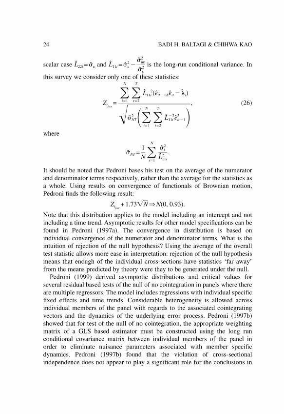
this survey we consider only one of these statistics:

Zt�NT=�i=1

N �t=2

T

L11i�2(eit�1�eit � �i)

�NT2 ��

i=1

N �t=2

T

L11i�2eit�1

2 �, (26)

where

NT =1N�

i=1

Ni

2

L11i2 .

It should be noted that Pedroni bases his test on the average of the numeratorand denominator terms respectively, rather than the average for the statistics asa whole. Using results on convergence of functionals of Brownian motion,Pedroni finds the following result:

Zt�NT+ 1.73�N ⇒ N(0, 0.93).

Note that this distribution applies to the model including an intercept and notincluding a time trend. Asymptotic results for other model specifications can befound in Pedroni (1997a). The convergence in distribution is based onindividual convergence of the numerator and denominator terms. What is theintuition of rejection of the null hypothesis? Using the average of the overalltest statistic allows more ease in interpretation: rejection of the null hypothesismeans that enough of the individual cross-sections have statistics ‘far away’from the means predicted by theory were they to be generated under the null.

Pedroni (1999) derived asymptotic distributions and critical values forseveral residual based tests of the null of no cointegration in panels where thereare multiple regressors. The model includes regressions with individual specificfixed effects and time trends. Considerable heterogeneity is allowed acrossindividual members of the panel with regards to the associated cointegratingvectors and the dynamics of the underlying error process. Pedroni (1997b)showed that for test of the null of no cointegration, the appropriate weightingmatrix of a GLS based estimator must be constructed using the long runconditional covariance matrix between individual members of the panel inorder to eliminate nuisance parameters associated with member specificdynamics. Pedroni (1997b) found that the violation of cross-sectionalindependence does not appear to play a significant role for the conclusions in


favor of weak long run PPP provided that one also includes common timedummies in the regression. Pedroni (2000) also demonstrated how it is possibleto construct a test that can be employed to test whether or not members of apanel with heterogeneous short run dynamics converge to a single commonsteady state.

D. Likelihood-Based Cointegration Test

Larsson, Lyhagen & Löthgren (1998) presented a likelihood-based (LR) paneltest of cointegrating rank in heterogeneous panel models based on the averageof the individual rank trace statistics developed by Johansen (1995). Theproposed LR-bar statistic is very similar to the IPS t-bar statistic in (7) through(10). In Monte Carlo simulation, Larsson et al. investigated the small sampleproperties of the standardized LR-bar statistic. They found that the proposedtest requires a large time series dimension. Even if the panel has a large cross-sectional dimension, the size of the test will be severely distorted.

Groen & Kleibergen (1999) proposed a likelihood-based framework forcointegrating analysis in panels of a fixed number of vector error correctionmodels. Maximum likelihood estimators of the cointegrating vectors areconstructed using iterated generalized method of moments (GMM) estimators.Using these estimators Groen and Kleibergen construct likelihood ratiostatistics, LR(�B|�A), to test for a common cointegration rank across theindividual vector error correction models, both with heterogeneous andhomogeneous cointegrating vectors. Interestingly, the limiting distribution ofLR(�B|�A) is invariant to the covariance matrix of the error terms whichimplies that LR(�B|�A) is robust with respect to the choices of covariancematrix. Let us define the LRs(r|k) as the summation of the N individual tracestatistics

LRs(r | k) =�i=1

N

LRi(r | k) (27)

where LRi(r | k) is the i-th Johansen’s likelihood ratio statistic, so that

LRi(r | k) ⇒ tr�� dBk�r, iB�k�r, i � dBk�r, iB�k�r, i� dBk�r, iB�k�r, i�as T→�. Now for a fixed N, it is clear that


LRs(r | k) =�i=1

N

LRi(r | k)

⇒�i=1

N

tr�� dBk�r, iB�k�r, i � dBk�r, iB�k�r, i� dBk�r, iB�k�r, i�(28)

as T→� by a continuous mapping theorem. It follows that LRs(r | k) isasymptotically equivalent to LR(�B | �A) when N is fixed and T is large. Thismeans that nothing is lost by assuming that the covariance matrix has zero non-diagonal covariances as far as the asymptotics are concerned for the proposedtest statistics in this chapter. More importantly, the tests based on the cross-independence like (27) will perform just as well (asymptotically) as the testsbased on the cross-dependence such as LR(�B | �A). Groen and Kleibergenverified that the likelihood-based cointegration tests proposed by Larsson et al.in (27) are robust with respect to the cross-dependence in panel data. The(asymptotic) equivalence of LRs(r | k) and LR(�B | �A) found in Groen andKleibergen has profound implications to econometricians and applied econo-mists, e.g. there exists tests/estimators based on the cross-independencewhich are equivalent to tests/estimators based on the cross-dependence innonstationary panel time series. Define LR(r | k) to be the average of LRi(r | k):

LR(r | k) =1N

LRs(r | k) =1N�

i=1

N

LRi(r | k).

It can be shown that

LR(r | k) � E[LR(r | k)]

Var[LR(r | k)]⇒ N(0, 1)

as T→� followed by N→� by a continuous mapping theorem and a centrallimit theorem provided E[LR(r | k)] and Var[LR(r | k)] are bounded. Define

LR(�B | �A) =1N

LR(�B | �A). (29)

For a fixed N, it is easy to show that


LR(�B | �A) =1N

LR(�B | �A)

⇒ 1N�

i=1

N

tr�� dBk�r, iB�k�r, i� dBk�r, iB�k�r, i�� dBk�r, iB�k�r, i�

=1N�

i=1

N

Zki

where

Zki = tr�� dBk�r, iB�k�r, i� dBk�r, iB�k�r, i� dBk�r, iB�k�r, i�as T→�. Then

1N�

i=1

N

Zki � E1N�

i=1

N

ZkiVar1

N�i=1

N

Zki ⇒ N(0, 1)

as N→� since Bk�r, i and Bk�r, j are independent for i ≠ j. It implies that

LR(�B | �A) � E[LR(�B | �A)]

Var[LR(�B | �A)]⇒ N(0, 1)

as T→� followed by N→�. The above discussion indicates that LR(r | k) andLR(�B | �A) are also equivalent when T and N are large.

Groen & Kleibergen (1999) applied LR(�B | �A) to a data set of exchangerates and appropriate monetary fundamentals. They found strong evidence forthe validity of the monetary exchange rate model within a panel of vectorcorrection models for three major European countries, whereas the resultsbased on individual vector error correction models for each of these countriesseparately are less supportive.

E. Finite Sample Properties

McCoskey & Kao (1999b) conducted Monte Carlo experiments to compare thesize and power of different residual based tests for cointegration in


heterogeneous panel data: varying slopes and varying intercepts. Two of thetests are constructed under the null hypothesis of no cointegration. These testsare based on the average ADF test and Pedroni’s pooled tests in (25) and (26).The third test is based on the null hypothesis of cointegration which is basedon the McCoskey & Kao LM test in (23). Wu & Yin (1999) performed a similarcomparison for panel tests in which they consider only tests for which the nullhypothesis is that of no cointegration. Wu & Yin compared ADF statistics withmaximum eigenvalue statistics in pooling information on means and p-valuesrespectively. They found that the average ADF performs better with respect topower and their maximum eigenvalue based p-value performs better withregards to size.

The test of the null hypothesis was originally proposed in response to the lowpower of the tests of the null of no cointegration, especially in the time seriescase. Further, in cases where economic theory predicted a long run steady staterelationship, it seemed that a test of the null of cointegration rather than the nullof no cointegration would be appropriate. The results from the Monte Carlostudy showed that the McCoskey & Kao LM test outperforms the other twotests.

Of the two reasons for the introduction of the test of the null hypothesis ofcointegration, low power and attractiveness of the null, the introduction of thecross-section dimension of the panel solves one: all of the tests show decentpower when used with panel data. For those applications where the null ofcointegration is more logical than the null of no cointegration, McCoskey &Kao (1999b), at a minimum, conclude that using the McCoskey & Kao LM testdoes not compromise the ability of the researcher in determining the underlyingnature of the data.

Recently, Hall et al. (1999) proposed a new approach based on principalcomponents analysis to test for the number of common stochastic trendsdriving the nonstationary series in a panel data set. The test is consistent evenif there is a mixture of I(0) and I(1) series in the sample. This makes itunnecessary to pretest the panel for unit root. It also has the advantage ofsolving the problem of dimensionality encountered in large panel data sets.

V. ESTIMATION AND INFERENCE IN PANELCOINTEGRATION MODELS

This section discusses the issues that arise in estimation and inference ofcointegrated panel regression models. The asymptotic properties of theestimators of the regression coefficients and the associated statistical tests aredifferent from those of the time series cointegration regression models. Some


of these differences have become apparent in recent works by Kao & Chiang(2000), Phillips & Moon (1999a) and Pedroni (1996). The panel cointegrationmodels are directed at studying questions that surround long run economicrelationships typically encountered in macroeconomic and financial data. Sucha long run relationship is often predicted by economic theory and it is then ofcentral interest to estimate the regression coefficients and test whether theysatisfy theoretical restrictions. Kao & Chen (1995) showed that the OLS inpanel cointegrated models is asymptotically normal but still asymptoticallybiased. Chen, McCoskey & Kao (1999) investigated the finite sampleproprieties of the OLS estimator, the t-statistic, the bias-corrected OLSestimator, and the bias-corrected t-statistic. They found that the bias-correctedOLS estimator does not improve over the OLS estimator in general. The resultsof Chen et al. suggested that alternatives, such as the fully modified (FM)estimator or dynamic OLS (DOLS) estimator may be more promising incointegrated panel regressions. Phillips & Moon (1999a) and Pedroni (1996)proposed a FM estimator, which can be seen as a generalization of Phillips &Hansen (1990). In this volume, Kao & Chiang (2000) propose an alternativeapproach based on a panel dynamic least squares (DOLS) estimator, whichbuilds upon the work of Saikkonen (1991) and Stock & Watson (1993).

Next, we provide a brief discussion of the OLS estimation methods in apanel cointegrated model. Consider the following panel regression:

yit = x�it� + z�it�i + uit, (30)

where {yit} are 1 � 1, � is a k � 1 vector of the slope parameters, zit is thedeterministic component, and {uit} are the stationary disturbance terms. Weassume that {xit} are k � 1 integrated processes of order one for all i, where

xit = xit�1 + �it.

Under these specifications, (30) describes a system of cointegrated regressions,i.e. yit is cointegrated with xit. The OLS estimator of � is

�OLS =�i=1

N �t=1

T

xit x�it�1�i=1

N �t=1

T

xityit. (31)

It is easy to show that

1N�

i=1

N1T2 �

t=1

T

xit x�it →p limN→�

1N�

i=1

N

E[�2i], (32)

and


1N�

i=1

N1T�

t=1

T

xituit ⇒ limN→�

1N�

i=1

N

E[�1i] (33)

using sequential limit theory, where

zit E[�1i] E[�2i]

0 012

1 0 0

�i �12

��ui + ��ui

16

��i

(�i, t) �12

��ui + ��ui

115

��i

and

�i =�ui

��ui

�u�i

��i

is the long-run covariance matrix of (uit, ��it)�, also �i =�ui

��ui

�u�i

��i is the one-

sided long-run covariance. For example, when zit = {�i}, we get

�NT(�OLS � �) � �N�NT ⇒ N�0, 6��1� � lim

N → �

1N�

N

i=1

�u.��i��1� �,

where �� = limN ⇒ �

1N�

N

i=1

��i and

�NT =1N�

N

i=1

1T2 �T

t=1

(xit � xi)(xit � xi)��1

�1N �

N

i=1

�1/2�i �� Wi dW�i��1/2

�i ��ui + ��ui.

Kao & Chiang (2000) in this volume studied the limiting distributions for theFM, and DOLS estimators in a cointegrated regression and showed they are


asymptotically normal. Phillips & Moon (1999a) and Pedroni (1996) alsoobtained similar results for the FM estimator. The reader is referred to the citedpapers for further details. Kao and Chiang also investigated the finite sampleproperties of the OLS, FM, and DOLS estimators. They found that: (i) the OLSestimator has a non-negligible bias in finite samples, (ii) the FM estimator doesnot improve over the OLS estimator in general, and (iii) the DOLS estimatormay be more promising than OLS or FM estimators in estimating thecointegrated panel regressions.

Choi (1999b) extended Kao & Chiang (2000) to study asymptotic propertiesof OLS, Within and GLS estimators for an error component model. The errorcomponent model involves both stationary and nonstationary regressors. Choi’ssimulation results indicated that the feasible GLS estimator is more efficientthan the Within estimator. Choi (1999c) studied instrumental variableestimation for an error component model with stationary and nearlynonstationary regressors.

Phillips & Moon (1999a) studied various regressions between two panelvectors that may or may not have cointegrating relations, and present afundamental framework for studying sequential and joint limit theories innonstationary panel data. In particular, Phillips and Moon studied regressionlimit theory of nonstationary panels when both N and T go to infinity. Theirlimit theory allows for both sequential limits, where T→� followed by N→�and joint limits, where T, N→� simultaneously. Phillips and Moon require thatN/T→0, so that these results apply for moderate N and large T macro paneldata and not large N and small T micro panel data. The panel modelsconsidered allow for four cases: (i) panel spurious regression, where there is notime series cointegration, (ii) heterogeneous panel cointegration, where eachindividual has its own specific cointegration relation, (iii) homogeneous panelcointegration where individuals have the same cointegration relation, and (iv)near-homogeneous panel cointegration, where individuals have slightlydifferent cointegration relations determined by the value of a localizingparameter. Phillips & Moon (1999a) investigated these four models anddeveloped panel asymptotics for regression coefficients and tests using bothsequential and joint limit arguments. In all cases considered the pooledestimator is consistent and has a normal limiting distribution. In fact, for thespurious panel regression, Phillips & Moon (1999a) showed that under quiteweak regularity conditions, the pooled least squares estimator of the slopecoefficient � is �N consistent for the long-run average relation parameter �and has a limiting normal distribution. Also, Moon & Phillips (1998a) showedthat a limiting cross-section regression with time averaged data is also �Nconsistent for � and has a limiting normal distribution. This is different from


the pure time series spurious regression where the limit of the OLS estimatorof � is a nondegenerate random variate that is a functional of Brownianmotions and is therefore not consistent for �. The idea in Phillips & Moon(1999a) is that independent cross-section data in the panel adds informationand this leads to a stronger overall signal than the pure time series case. Pesaran& Smith (1995) studied limiting cross-section regressions with time averageddata and established consistency with restrictive assumptions on the heteroge-neous panel model. This differs from Phillips & Moon (1999a) in that theformer use an average of the cointegrating coefficients which is different fromthe long run average regression coefficient. This requires the existence ofcointegrating time series relations, whereas the long run average regressioncoefficient � is defined irrespective of the existence of individual cointegratingrelations and relies only on the long run average variance matrix of the panel.Phillips & Moon (1999a) also showed that for the homogeneous and nearhomogeneous cointegration cases, a consistent estimator of the long runregression coefficient can be constructed which they call a pooled FMestimator. They showed that this estimator has faster convergence rate than thesimple cross-section and time series estimators. See also Phillips & Moon(1999b) for a concise review. In fact, the latter paper also shows how to extendthe above ideas to models with individual effects in the data generating process.For the panel spurious regression with individual specific deterministic trends,estimates of the trend coefficients are obtained in the first step and thedetrended data is pooled and used in least squares regression to estimate � inthe second step. Two different detrending procedures are used based on OLSand GLS regressions. OLS detrending leads to an asymptotically more efficientestimator of the long run average coefficient � in pooled regression than GLSdetrending. Phillips & Moon (1999b) explain that ‘‘the residuals after timeseries GLS detrending have more cross section variation than they do after OLSdetrending and this produces great variation in the limit distribution of thepooled regression estimator of the long run average coefficient.”

Moon & Phillips (1999) investigate the asymptotic properties of theGaussian MLE of the localizing parameter in local to unity dynamic panelregression models with deterministic and stochastic trends. Moon and Phillipsfind that for the homogeneous trend model, the Gaussian MLE of the commonlocalizing parameter is �N consistent, while for the heterogeneous trendsmodel, it is inconsistent. The latter inconsistency is due to the presence of aninfinite number of incidental parameters (as N→�) for the individual trends.Unlike the fixed effects dynamic panel data model where this inconsistency dueto the incidental parameter problem disappears as T→�, the inconsistency of


the localizing parameter in the Moon and Phillips model persists even whenboth N and T go to infinity.

Pesaran, Shin & Smith (1999) derived the asymptotics of a pooled meangroup (PMG) estimator. The PMG estimation constrains the long runcoefficients to be identical, but allow the short run and adjustment coefficientsas the error variances to differ across the cross-sectional dimension.

Recently, Binder, Hsiao & Pesaran (2000) considered estimation andinference in panel vector autoregressions (PVARS) with fixed effects when T isfinite and N is large. A maximum likelihood estimator as well as unit root andcointegration tests are proposed based on a transformed likelihood function.This MLE is shown to be consistent and asymptotically normally distributedirrespective of the unit root and cointegrating properties of the PVAR model.The tests proposed are based on standard chi-square and normal distributedstatistics. Binder et al. also show that the conventional GMM estimators basedon standard orthogonality conditions break down if the underlying time seriescontain unit roots. Monte Carlo evidence is provided which favors MLE overGMM in small samples.

In this volume, Kauppi (2000) develops a new joint limit theory where thepanel data may be cross-sectionally heterogeneous in a general way. This limittheory builds upon the concepts of joint convergence in probability and indistribution for double indexed processes by Phillips & Moon (1999a) anddevelops new versions of the law of large numbers and the central limittheorem that apply in panels where the data may be cross-sectionallyheterogeneous in a fairly general way. Kauppi demonstrates how this joint limittheory can be applied to derive asymptotics for a panel regression where theregressors are generated by a local to unit root with heterogeneous localizingcoefficients across cross-sections. Kauppi discusses issues that arise in theestimation and inference of panel cointegrated regressions with near integratedregressors. Kauppi shows that a bias corrected pooled OLS for a commoncointegrating parameter has an asymptotic normal distribution centered on thetrue value irrespective of whether the regressor has near or exact unit root.However, if the regression model contains individual effects and/or determi-nistic trends, then Kauppi’s bias corrected pooled OLS still producesasymptotic bias. Kauppi also shows that the panel FM estimator is subject toasymptotic bias regardless of how individual effects and/or deterministic trendsare contained if the regressors are nearly rather than exacly integrated. Thisindicates that much care should be taken in interpreting empirical resultsachieved by the recent panel cointegration methods that assume exact unit rootswhen near unit roots are equally plausible.


Kao et al. (1999) apply the asymptotic theory of panel cointegrationdeveloped by Kao & Chiang (2000) to the Coe & Helpman (1995) internationalR&D spillover regression. Using a sample of 21 OECD countries and Israel,they re-examine the effects of domestic and foreign R&D capital stocks on totalfactor productivity of these countries. They find that OLS with bias-correction,the fully modified (FM) and the dynamic OLS (DOLS) estimators producedifferent predictions about the impact of foreign R&D on total factorproductivity (TFP). However, all the estimators support the result that domesticR&D is related to TFP. Kao et al.’s empirical results indicate that the estimatedcoefficients in the Coe and Helpman’s regressions are subject to estimationbias. Given the superiority of the DOLS over FM as suggested by Kao &Chiang (2000), Kao et al. leaned towards rejecting the Coe and Helpmanhypothesis that international R&D spillovers are trade related.

Funk (1998) examined the relationship between trade patterns andinternational R&D spillovers among the OECD countries using the panelcointegration methods developed by Kao (1999), Kao & Chiang (2000), andPesaran, Shin & Smith (1999). Using randomly simulated bilateral tradepatterns, Funk found that the choice of weights used in constructing foreignR&D stocks is informative of the avenue of spillover transmission when panelcointegration methods are employed. A re-examination of the relationshipbetween import patterns and R&D spillovers found no evidence to link thepatterns of R&D spillovers to the patterns of imports. Funk found strongevidence indicating that exporters receive substantial R&D spillovers fromtheir customers.

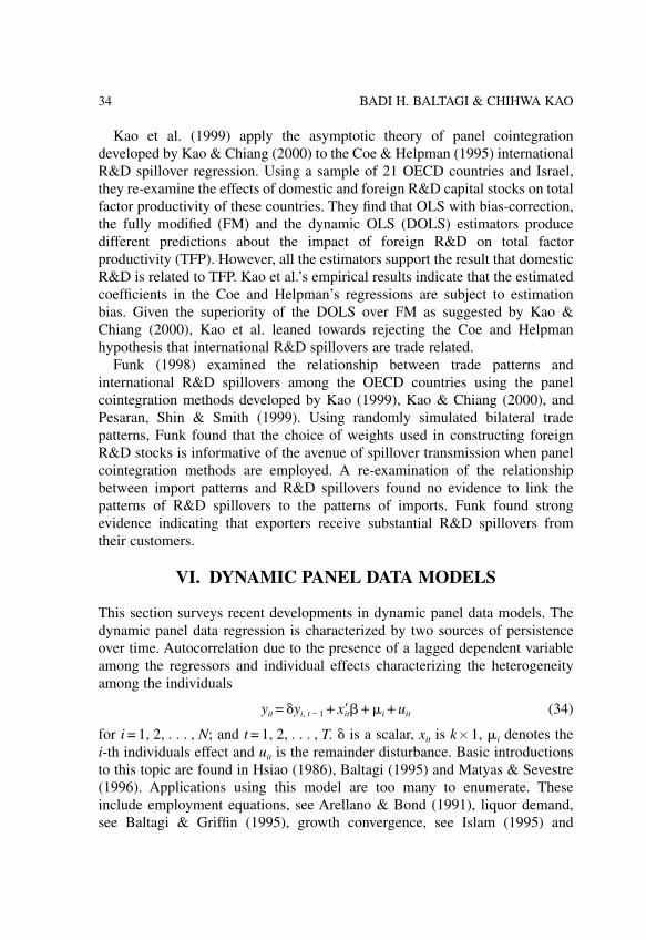
VI. DYNAMIC PANEL DATA MODELS

This section surveys recent developments in dynamic panel data models. Thedynamic panel data regression is characterized by two sources of persistenceover time. Autocorrelation due to the presence of a lagged dependent variableamong the regressors and individual effects characterizing the heterogeneityamong the individuals

yit = �yi, t�1 + x�it� + �i + uit (34)

for i = 1, 2, . . . , N; and t = 1, 2, . . . , T. � is a scalar, xit is k � 1, �i denotes thei-th individuals effect and uit is the remainder disturbance. Basic introductionsto this topic are found in Hsiao (1986), Baltagi (1995) and Matyas & Sevestre(1996). Applications using this model are too many to enumerate. Theseinclude employment equations, see Arellano & Bond (1991), liquor demand,see Baltagi & Griffin (1995), growth convergence, see Islam (1995) and


Nerlove (1999), life cycle labor supply models, see Ziliak (1997), and demandfor gasoline, see Baltagi & Griffin (1997) to mention a few.

It is well known that for typical micro-panels where there are a large numberof firms or individuals (N) observed over a short period of time (T), the fixedeffects (FE) estimator is biased and inconsistent (since T is fixed and N→�),see Nickell (1981) and more recently Kiviet (1995, 1999). Monte Carlo resultshave shown that first order asymptotic properties do not necessarily yieldcorrect inference in finite samples. Therefore, Kiviet (1995) examined higherorder asymptotics which may approximate the actual finite sample propertiesmore closely and lead to better inference. In fact, Kiviet (1995) considered thesimple dynamic linear panel data model with serially uncorrelated disturbancesand strongly exogenous regressors and derived an approximation for the bias ofthe FE estimator. When a consistent estimator of this bias is subtracted from theoriginal FE estimator, a corrected FE estimator results. This corrected FEestimator performed well in simulations when compared with eight otherconsistent instrumental variable or GMM estimators.4

In macro-panels studying for example long run growth, the data covers alarge number of countries N over a moderate size T. In this case, T is not verysmall relative to N. Hence, some researchers may still favor the FE estimatorarguing that its bias may not be large. Judson & Owen (1999) performed someMonte Carlo experiments for N = 20 or 100 and T = 5, 10, 20 and 30 and foundthat the bias in the FE can be sizeable, even when T = 30. The bias of the FEestimator increases with � and decreases with T. But even for T = 30, this biascould be as much as 20% of the true value of the coefficient of interest. Judson& Owen (1999) recommend the corrected FE estimator proposed by Kiviet(1995) as the best choice, GMM being second best and for long panels, thecomputationally simpler Anderson & Hsiao (1982) estimator. This lastestimator first differences the data to get rid of the individual effects and thenuses lagged predetermined variables in levels as instruments.5 Arellano & Bond(1991) proposed GMM procedures that are more efficient than the Anderson &Hsiao (1982) estimator. Ahn & Schmidt (1995) derive additional nonlinearmoment restrictions not exploited by the Arellano & Bond (1991) GMMestimator.6 Ahn & Schmidt (1995, 1997) also give a complete count of the setof orthogonality conditions corresponding to a variety of assumptions imposedon the disturbances and the initial conditions of the dynamic panel data model.While many of the moment conditions are nonlinear in the parameters, Ahn &Schmidt (1997) propose a linearized GMM estimator that is asymptotically asefficient as the nonlinear GMM estimator. They also provide simple momenttests of the validity of these nonlinear restrictions. In addition, they investigatethe circumstances under which the optimal GMM estimator is equivalent to a


linear instrumental variable estimator. They find that these circumstances arequite restrictive and go beyond uncorrelatedness and homoskedasticity of theerrors. Ahn & Schmidt (1995) provide some evidence on the efficiency gainsfrom the nonlinear moment conditions which provide support for their use inpractice. By employing all these conditions, the resulting GMM estimator isasymptotically efficient and has the same asymptotic variance as the MLEunder normality. In fact, Hahn (1997) showed that GMM based on anincreasing set of instruments as N→� would achieve the semiparametricefficiency bound.

Hahn (1997) considers the asymptotic efficient estimation of the dynamicpanel data model with sequential moment restrictions in an environment withi.i.d. observations. Hahn (1997) shows that the GMM estimator with anincreasing set of instruments as the sample size grows attains the semipara-metric efficiency bound of the model. Hahn (1997) explains how Fourier seriesor polynomials may be used as the set of instruments for efficient estimation.In a limited Monte Carlo comparison, Hahn finds that this estimator has similarfinite sample properties as the Keane & Runkle (1992) and/or Schmidt et al.(1992) estimators when the latter estimators are efficient. In cases where thelatter estimators are not efficient, the Hahn efficient estimator outperforms bothestimators in finite samples.

Recently, Wansbeek & Bekker (1996) considered a simple dynamic paneldata model with no exogenous regressors and disturbances uit and randomeffects �i that are independent and normally distributed. They derived anexpression for the optimal instrumental variable estimator, i.e. one withminimal asymptotic variance. A striking result is the difference in efficiencybetween the IV and ML estimators. They find that for regions of theautoregressive parameter � which are likely in practice, ML is superior. Thegap between IV (or GMM) and ML can be narrowed down by adding momentrestrictions of the type considered by Ahn & Schmidt (1995). Hence, Wansbeek& Bekker (1996) find support for adding these nonlinear moment restrictionsand warn against the loss in efficiency as compared with MLE by ignoringthem.

Blundell & Bond (1998) revisit the importance of exploiting the initialcondition in generating efficient estimators of the dynamic panel data modelwhen T is small. They consider a simple autoregressive panel data model withno exogenous regressors

yit = �yi, t�1 + �i + uit (35)

with E(�i) = 0; E(uit) = 0; and E(�iuit) = 0 for i = 1, 2, . . . , N; t = 1, 2, . . . , T.Blundell & Bond (1998) focus on the case where T = 3 and therefore there is


only one orthogonality condition given by E(yi1�ui3) = 0, so that � is just-identified. In this case, the first stage IV regression is obtained by running �yi2

on yi1. Note that this regression can be obtained from (2) evaluated at t = 2 bysubtracting yi1 from both sides of this equation, i.e.

�yi2 = (� � 1)yi, 1 + �i + ui2 (36)

Since we expect E(yi1�i) > 0, (� � 1) will be biased upwards with

plim(� � 1) = (� � 1)c

c + (�2 /u

2)(37)

where c = (1 � �)/(1 + �). The bias term effectively scales the estimatedcoefficient on the instrumental variable yi1 towards zero. They also find that theF-statistic of the first stage IV regression converges to 1

2 with noncentralityparameter

� =(u

2c)2

�2 + u

2c→0 as �→1 (37)

As �→0, the instrumental variable estimator performs poorly. Hence, Blundelland Bond attribute the bias and the poor precision of the first difference GMMestimator due to the problem of weak instruments described in Nelson & Startz(1990) and Staiger & Stock (1997) and characterize this weak IV by itsconcentration parameter �.

Next, Blundell & Bond (1998) show that an additional mild stationarityrestriction on the initial conditions process allows the use of an extendedsystem GMM estimator that uses lagged differences of yit as instruments forequations in levels, in addition to lagged levels of yit as instruments forequations in first differences, see Arellano & Bover (1995). The system GMMestimator is shown to have dramatic efficiency gains over the basic firstdifference GMM as �→1 and (�

2 /u2) increases. In fact, for T = 4 and (�

2 /u

2) = 1, the asymptotic variance ratio of the first difference GMM estimator tothis system GMM estimator is 1.75 for � = 0 and increases to 3.26 for � = 0.5and 55.4 for � = 0.9. This clearly demonstrates that the levels restrictionssuggested by Arellano & Bover (1995) remain informative in cases where firstdifferenced instruments become weak. Things improve for first differenceGMM as T increases. However, with short T and persistent series, the Blundelland Bond findings support the use of the extra moment conditions. Theseresults are reviewed and corroborated in Blundell, Bond & Windmeijer (2000)in this volume, using Monte Carlo experiments as well as an empiricalexample. In fact, simulations that include the weakly exogenous covariates findlarge finite sample bias and very low precision for the standard first differenced


estimator. However, the system GMM estimator not only improves theprecision but also reduces the finite sample bias. The empirical applicationrevisits the estimates of the capital and labor coefficients in a Cobb-Douglasproduction function considered by Griliches & Mairesse (1998). Using data on509 R&D performing US manufacturing companies observed over 8 years(1982–1989), the standard GMM estimator that uses moment conditions on thefirst differenced model finds a low estimate of the capital coefficient and lowprecision for all coefficients estimated. However, the system GMM estimatorgives reasonable and more precise estimates of the capital coefficient andconstant returns to scale is not rejected. Blundell et al. conclude that “a carefulexamination of the original series and consideration of the system GMMestimator can usefully overcome many of the disappointing features of thestandard GMM estimator for dynamic panel models.” Hahn (1999) alsoexamines the role of the initial condition imposed by the Blundell & Bond(1998) estimator. This is done by numerically comparing the semiparametricinformation bounds for the case that incorporates the stationarity of the initialcondition and the case that does not. Hahn (1999) finds that the efficiency gaincan be substantial.

Ziliak (1997) asks the question whether the bias/efficiency trade-off for theGMM estimator considered by Tauchen (1986) for the time series case is stillbinding in panel data where the sample size is normally larger than 500. Fortime series data, Tauchen (1986) shows that even for T = 50 or 75 there is a bias/efficiency trade-off as the number of moment conditions increase. Therefore,Tauchen recommends the use of sub-optimal instruments in small samples.This result was also corroborated by Andersen & Sorensen (1996) who arguethat GMM using too few moment conditions is just as bad as GMM using toomany moment conditions. This problem becomes more pronounced with paneldata since the number of moment conditions increase dramatically as thenumber of strictly exogenous variables and the number of time seriesobservations increase. Even though it is desirable from an asymptotic efficiencypoint of view to include as many moment conditions as possible, it may beinfeasible or impractical to do so in many cases. For example, for T = 10 andfive strictly exogenous regressors, this generates 500 moment conditions forGMM. Ziliak (1997) performs an extensive set of Monte Carlo experiments fora dynamic panel data model and finds that the same trade-off between bias andefficiency exists for GMM as the number of moment conditions increase, andthat one is better off with sub-optimal instruments. In fact, Ziliak finds thatGMM performs well with suboptimal instruments, but is not recommended forpanel data applications when all the moments are exploited for estimation.7

Ziliak estimates a life cycle labor supply model under uncertainty based on 532


men observed over 10 years of data (1978–1987) from the panel study ofincome dynamics. The sample was restricted to continuously married,continuously working prime age men aged 22–51 in 1978. These men werepaid an hourly wage or salaried and could not be piece-rate workers or self-employed. Ziliak finds that the downward bias of GMM is quite severe as thenumber of moment conditions expands, outweighing the gains in efficiency.Ziliak reports estimates of the intertemporal substitution elasticity which is thefocal point of interest in the labor supply literature. This measures theintertemporal changes in hours of work due to an anticipated change in the realwage. For GMM, this estimate changes from 0.519 to 0.093 when the numberof moment conditions used in GMM are increased from 9 to 212. The standarderror of this estimate drops from 0.36 to 0.07. Ziliak attributes this bias to thecorrelation between the sample moments used in estimation and the estimatedweight matrix. Interestingly, Ziliak finds that the forward filter 2SLS estimatorproposed by Keane & Runkle (1992) performs best in terms of the bias/efficiency trade-off and is recommended. Forward filtering eliminates all formsof serial correlation while still maintaining orthogonality with the initialinstrument set. Schmidt, Ahn & Wyhowski (1992) argued that filtering isirrelevant if one exploits all sample moments during estimation. However, inpractice, the number of moment conditions increases with the number of timeperiods T and the number of regressors K and can become computationallyintractable. In fact for T = 15 and K = 10, the number of moment conditions forSchmidt, et al. (1992) is T(T–1)K/2 which is 1040 restrictions, highlighting thecomputational burden of this approach. In addition, Ziliak argues that theoveridentifying restrictions are less likely to be satisfied possibly due to theweak correlation between the instruments and the endogenous regressors.8 Inthis case, the forward filter 2SLS estimator is desirable yielding less bias thanGMM and sizeable gains in efficiency. In fact, for the life cycle labor example,the forward filter 2SLS estimate of the intertemporal substitution elasticity was0.135 for 9 moment conditions compared to 0.296 for 212 moment conditions.The standard error of these estimates dropped from 0.32 to 0.09.

The practical problem of not being able to use more moment conditions aswell as the statistical problem of the trade-off between small sample bias andefficiency prompted Ahn & Schmidt (1999a) to pose the following questions:“Under what conditions can we use a smaller set of moment conditions withoutincurring any loss of asymptotic efficiency? In other words, under whatconditions are some moment conditions redundant in the sense that utilizingthem does not improve efficiency?” These questions were first dealt with by Im,Ahn, Schmidt & Wooldridge (1999) who considered panel data models withstrictly exogenous explanatory variables. They argued that, for example, with


ten strictly exogenous time-varying variables and six time periods, the momentconditions available for the random effects (RE) model is 360 and this reducesto 300 moment conditions for the FE model. GMM utilizing all these momentconditions leads to an efficient estimator. However, these moment conditionsexceed what the simple RE and FE estimators use. Im et al. (1999) provide theassumptions under which this efficient GMM estimator reduces to the simplerFE or RE estimator. In other words, Im et al. (1999) show the redundancy ofthe moment conditions that these simple estimators do not use. Ahn & Schmidt(1999a) provide a more systematic method by which redundant instruments canbe found and generalize this result to models with time-varying individualeffects. However, both papers deal only with strictly exogenous regressors. Ina related paper, Ahn & Schmidt (1999b) consider the cases of strictly andweakly exogenous regressors. They show that the GMM estimator takes theform of an instrumental variables estimator if the assumption of no conditionalheteroskedasticity (NCH) holds. Under this assumption, the efficiency ofstandard estimators can often be established showing that the momentconditions not utilized by these estimators are redundant. However, Ahn &Schmidt (1999b) conclude that the NCH assumption necessarily fails if the fullset of moment conditions for the dynamic panel data model are used. In thiscase, there is clearly a need to find modified versions of GMM, with reducedset of moment conditions that lead to estimates with reasonable finite sampleproperties.

Crepon, Kramarz & Trognon (1997) argue that for the dynamic panel datamodel, when one considers a set of orthogonal conditions, the parameters canbe divided into parameters of interest (like �) and nuisance parameters (like thesecond order terms in the autoregressive error component model). They showthat the elimination of such nuisance parameters using their empiricalcounterparts does not entail an efficiency loss when only the parameters ofinterest are estimated. In fact, Sevestre and Trognon in chapter 6 of Matyas &Sevestre (1996) argue that if one is only interested in �, then one can reducethe number of orthogonality restrictions without loss in efficiency as far as � isconcerned. However, the estimates of the other nuisance parameters are notgenerally as efficient as those obtained from the full set of orthogonalityconditions.

The Alonso-Borrego & Arellano (1999) paper is also motivated by the finitesample bias in panel data instrumental variable estimators when theinstruments are weak. The dynamic panel model generates many over-identifying restrictions even for moderate values of T. Also, the number ofinstruments increases with T, but the quality of these instruments is often poorbecause they tend to be only weakly correlated with first differenced


endogenous variables that appear in the equation. Limited informationmaximum likelihood (LIML) is strongly preferred to 2SLS if the number ofinstruments gets large as the sample size tends to infinity. Hillier (1990)showed that the alternative normalization rules adopted by LIML and 2SLS areat the root of their different sampling behavior. Hillier (1990) also showed thata symmetrically normalized 2SLS estimator has properties similar to those ofLIML. Following Hillier (1990), Alonso-Borrego & Arellano (1999) derive asymmetrically normalized GMM (SNM) and compare it with ordinary GMMand LIML analogues by means of simulations. Monte Carlo and empiricalresults show that GMM can exhibit large biases when the instruments are poor,while LIML and SNM remain unbiased. However, LIML and SNM always hada larger interquartile range than GMM. For T = 4, N = 100, �

2 = 0.2 and �2 = 1,

the bias for � = 0.5 was 6.9% for GMM, 1.7% for SNM and 1.7% for LIML.This bias increases to 17.8% for GMM, 3.7% for SNM and 4.1% for LIML for� = 0.8.

Alvarez & Arellano (1997) studied the asymptotic properties of FE, one-stepGMM and non-robust LIML for a first-order autorgressive model when both Nand T tend to infinity with (N/T)→ c for 0 ≤ c < 2. For T < N, GMM bias isalways smaller than FE and LIML bias is smaller than the other two. In fixedT framework, GMM and LIML are asymptotically equivalent, but as Tincreases, LIML has a smaller asymptotic bias than GMM. These resultsprovide some theoretical support for LIML over GMM.9

Wansbeek & Knaap (1999) consider a simple dynamic panel data modelwith a time trend and heterogeneous coefficients on the lagged dependentvariable and the time trend, i.e.

yit = �iyi, t–1 + �it + �i + uit (39)

This model results from Islam’s (1995) version of Solow’s model on growthconvergence among countries. Wansbeek & Knaap (1999) show that doubledifferencing gets rid of the individual country effects (�i) on the first round ofdifferencing and the heterogeneous coefficient on the time trend (�i) on thesecond round of differencing. Modified OLS, IV and GMM methods areadapted to this model and LIML is suggested as a viable alternative to GMMto guard against the small sample bias of GMM. Macroeconomic data aresubject to measurement error and Wansbeek & Knaap (1999) show how theseestimators can be modified to account for measurement error that is whitenoise. For example, GMM is modified so that it discards the orthogonalityconditions that rely on the absence of measurement error.

Jimenez-Martin (1998) performs Monte Carlo experiments to study theperformance of the Holtz-Eakin (1988) test for the presence of individual


heterogeneity effects in dynamic small T unbalanced panel data models. Thedesign of the experiment includes both endogenous and time-invariantregressors in addition to the lagged dependent variable. The test behavescorrectly for a moderate autoregressive coefficient. However, when thiscoefficient approaches unity, the presence of an additional regressor sharplyaffects the power and the size of the test. The power of this test is higher whenthe variance of the specific effects increases (they are easier to detect), whenthe sample size increases, when the data set is balanced (for a given number ofcross-section units) and when the regressors are strictly exogenous.

A. Heterogeneous Dynamic Panel Data Models

The fundamental assumption underlying pooled homogeneous parametermodels has been called into question. Robertson & Symons (1992) warnedabout the bias from pooled estimators when the estimated model is dynamicand homogeneous when in fact the true model is static and heterogeneous.Pesaran & Smith (1995) argued in favor of dynamic heterogeneous modelswhen N and T are large. In this case, pooled homogeneous estimators areinconsistent whereas an average estimator of heterogeneous parameters canlead to consistent estimates as N and T tend to infinity. Maddala, Srivastava &Li (1994) argued that shrinkage estimators are superior to either heterogeneousor homogeneous parameter estimates especially for prediction purposes. Infact, Maddala, Trost, Li & Joutz (1997) considered the problem of estimatingshort run and long run elasticities of residential demand for electricity andnatural gas for each of 49 states over the period 1970–1990.10 They concludethat individual heterogeneous state estimates were hard to interpret and had thewrong signs. Pooled data regressions were not valid because the hypothesis ofhomogeneity of the coefficients was rejected. They recommend shrinkageestimators if one is interested in obtaining elasticity estimates for each statesince these give more reliable results.

Baltagi & Griffin (1997) compare short run and long run estimates as wellas forecasts for pooled homogeneous, individual heterogeneous and shrinkageestimators of a dynamic demand model for gasoline across 18 OECD countriesover the period 1960–1990. Based on one, five and ten year forecasts andplausibility of the short run and long run elasticity estimates, the results are infavor of pooling. Similar results were obtained for a dynamic model forcigarette demand across 46 states over the period 1963–1992, see Baltagi,Griffin & Xiong (2000).

In chapter 8 of Matyas & Sevestre (1996), Pesaran, Smith & Im investigatedthe small sample properties of various estimators of the long run coefficients


for a dynamic heterogeneous panel data model using Monte Carlo experiments.Their findings indicate that the mean group estimator performs reasonably wellfor large T. However, when T is small, the mean group estimator could beseriously biased, particularly when N is large relative to T. Pesaran & Zhao(1999) examine the effectiveness of alternative bias-correction procedures inreducing the small sample bias of these estimators using Monte Carloexperiments. An interesting finding is that when the coefficient of the laggeddependent variable is greater than or equal to 0.8, none of the bias correctionprocedures seem to work.

Hsiao, Pesaran & Tahmiscioglu (1999) suggest a Bayesian approach forestimating the mean parameters of a dynamic heterogeneous panel data model.The coefficients are assumed to be normally distributed across cross-sectionalunits and the Bayes estimator is implemented using Markov Chain MonteCarlo methods. Hsiao et al. argue that Bayesian methods can be a viablealternative in the estimation of mean coefficients in dynamic panel data modelseven when the initial observations are treated as fixed constants. They establishthe asymptotic equivalence of this Bayes estimator and the mean groupestimator proposed by Pesaran & Smith (1995). The asymptotics are carriedout for both N and T→ ∞ with �N/T→0. Monte Carlo experiments show thatthis Bayes estimator has better sampling properties than other estimators forboth small and moderate size T. Hsiao et al. also caution against the use of themean group estimator unless T is sufficiently large relative to N. The bias in themean coefficient of the lagged dependent variable appears to be serious whenT is small and the true value of this coefficient is larger than 0.6. Hsiao et al.apply their methods to estimate the q-investment model using a panel of 273US firms over the period 1972–1993.

VII. CONCLUSION

This survey gives a brief overview of some of the main results in theeconometrics of nonstationary panels as well as recent developments indynamic panels. There has been an immense amount of research in this arearecently with the demand for empirical studies exceeding the supply ofeconometric theory developed for these models. As this survey indicates,several issues have been resolved but a lot remains to be done.

ACKNOWLEDGMENTS

The authors would like to thank R. Carter Hill, M. H. Pesaran and ananonymous referee for their helpful comments and suggestions. Baltagi was


funded by the Advanced Research Program, Texas Higher Education Board.Kao was supported by a grant from the Chiang Ching-kou Foundation forInternational Scholarly Exchange.

NOTES

1. A collection of dynamic panel data routines can be found in: http://www.cemfi.es/~ arellano/#dpd.

2. Chiang & Kao (2000) have recently put together a fairly comprehensive set ofsubroutines, NPT 1.0, for studying nonstationary panel data. NPT 1.0 can bedownloaded from http://web.syr.edu/ ~ cdkao.

3. Testing for cointegration in panel data by combining p-values tests is astraightforward extension of the testing procedures in this section. For cointegrationtests, the relevant model is equation (15). We let GiTi

be a test for the null of nocointegration and apply the same tests and asymptotic theory in this section.

4. Kiviet (1999) extends this derivation to the case of weakly exogenous variablesand examines to what degree this order of approximation is determined by the initialconditions of the dynamic panel model.

5. Arellano (1989) found that using lagged differences of predetermined variablesas instruments is not recommended since it has a singularity point and very largevariances over a significant range of the parameter values.

6. See also Arellano & Bover (1995), chapter 8 of Baltagi (1995) and chapters 6 and7 of Matyas & Sevestre (1996) for more details.

7. For a Hausman & Taylor (1981) type model, Metcalf (1996) shows that usingless instruments may lead to a more powerful Hausman specification test. Asymptot-ically, more instruments lead to more efficient estimators. However, the asymptotic biasof the less efficient estimator will also be greater as the null hypothesis of no correlationis violated. Metcalf argues that if the bias increases at the same rate as the variance (asthe null is violated) for the less efficient estimator, then the power of the Hausman testwill increase. This is due to the fact that the test statistic is linear in variance butquadratic in bias.

8. See the growing literature on weak instruments by Nelson & Startz (1990),Bekker (1994), Angrist & Kreuger (1995), Bound, Jaeger & Baker (1995) and Staiger& Stock (1997) to mention a few.

9. An alternative one-step method that achieves the same asymptotic efficiency asrobust GMM or LIML estimators is the maximum empirical likelihood estimationmethod, see Imbens (1997). This maximizes a multinomial pseudo-likelihood functionsubject to the orthogonality restrictions. These are invariant to normalization becausethey are maximum likelihood estimators.

10. Maddala et al. (1997) also provide a unified treatment of classical, Bayes andempirical Bayes procedures for estimating this model.

REFERENCES

Ahn, S. C., & Schmidt, P. (1995). Efficient Estimation of Models for Dynamic Panel Data. Journalof Econometrics, 68, 5–27.


Ahn, S. C., & Schmidt, P. (1997). Efficient Estimation of Dynamic Panel Data Models: AlternativeAssumptions and Simplified Estimation. Journal of Econometrics, 76, 309–321.

Ahn, S. C., & Schmidt, P. (1999a). Modified Generalized Instrumental Variables Estimation ofPanel Data Models with Strictly Exogenous Instrumental Variables. In: C. Hsiao, K. Lahiri,L. F. Lee & M. H. Pesaran (Eds.), Analysis of Panel Data and Limited Dependent VariableModels (pp. 171–198). Cambridge: Cambridge University Press.

Ahn, S. C., & P. Schmidt. (1999b). Estimation of Linear Panel Data Models Using GMM. In:Generalized Method of Moments Estimation (pp. 211–247). Cambridge: CambridgeUniversity Press.

Alonso-Borrego, C., & Arellano, M. (1999). Symmetrically Normalized Instrumental VariableEstimation Using Panel Data. Journal of Business and Economic Statistics, 17, 36–49.

Alvarez, J., & Arellano, M. (1997). The Time Series and Cross-section Asymptotics of DynamicPanel Data Estimators. Working paper, CEMFI, Madrid.

Andersen, T. G., & Sørensen, R. E. (1996). GMM Estimation of a Stochastic Volatility Model: AMonte Carlo Study. Journal of Business and Economic Statistics, 14, 328–352.

Anderson, T. W., & Hsiao, C. (1982). Formulation and Estimation of Dynamic Models UsingPanel Data. Journal of Econometrics, 18, 47–82.

Andersson, J., & Lyhagen, J. (1999). A Long Memory Panel Unit Root Test: PPP Revisited.Working paper, Economics and Finance, No. 303, Stockholm School of Economics,Sweden.

Angrist, J. D., & Krueger, A. B. (1995). Split Sample Instrumental Variable Estimates of Returnto Schooling. Journal of Business and Economic Statistics, 13, 225–235.

Arellano, M. (1989). A Note on the Anderson-Hsiao Estimator for Panel Data. Economics Letters,31, 337–341.

Arellano, M., & Bond, S. (1991). Some Tests of Specification for Panel Data: Monte CarloEvidence and An Application to Employment Equations. Review of Economic Studies, 58,277–297.

Arellano, M., & Bover, O. (1995). Another Look at the Instrumental Variables Estimation of Error-Component Models. Journal of Econometrics, 68, 29–51.

Baltagi, B. H. (1995). Econometric Analysis of Panel Data. Chichester: Wiley.Baltagi, B. H., & Griffin, J. M. (1995). A Dynamic Demand Model for Liquor: The Case for

Pooling. Review of Economics and Statistics, 77, 545–553.Baltagi, B. H., & Griffin, J. M. (1997). Pooled Estimators v.s. Their Heterogeneous Counterparts

in the Context of Dynamic Demand for Gasoline. Journal of Econometrics, 77, 303–327.Baltagi, B. H., Griffin, J. M. & Xiong, W. (2000). To Pool or Not to Pool: Homogeneous Versus

Heterogeneous Estimators Applied to Cigarette Demand. Review of Economics andStatistics, 82, 117–126.

Banerjee, A. (1999). Panel Data Unit Roots and Cointegration: An Overview. Oxford Bulletin ofEconomics and Statistics, 61, 607–629.

Bekker, P. A. (1994). Alternative Approximations to the Distributions of Instrumental VariablesEstimators. Econometrica, 62, 657–682.

Bernard, A., & Jones, C. (1996). Productivity Across Industries and Countries: Time Series Theoryand Evidence. Review of Economics and Statistics, 78, 135–146.

Bhargava, A., Franzini, L. & Narendranathan, W. (1982). Serial Correlation and Fixed EffectsModels. Review of Economic Studies, 49, 533–549.

Binder, M., Hsiao, C. & Pesaran, M. H. (2000). Estimation and Inference in Short Panel VectorAutoregressions With Unit Roots and Cointegration. Working paper, Department ofEconomics, University of Maryland.


Blundell, R. W., & Bond, S. (1998). Initial Conditions and Moment Restrictions in Dynamic PanelData Models. Journal of Econometrics, 87, 115–143.

Blundell, R. W., Bond, S., & Windmeijer, F. (2000). Estimation in Dynamic Panel Data Models:Impoving on the Performance of the Standard GMM Estimator. Advances in Econometrics,15, forthcoming.

Boumahdi, R., & Thomas, A. (1991). Testing for Unit Roots Using Panel Data. Economics Letters,37, 77–79.

Bound, J., Jaeger, D. A., & Baker, R. M. (1995). Problems with Instrumental Variables EstimationWhen the Correlation Between the Instruments and the Endogenous Explanatory Variablesis Weak. Journal of the American Statistical Association, 90, 443–450.

Breitung, J. (2000). The Local Power of Some Unit Root Tests for Panel Data. Advances inEconometrics, 15, forthcoming.

Breitung, J., & Meyer, W. (1994). Testing for Unit Roots in Panel Data: Are Wages on DifferentBargaining Levels Cointegrated? Applied Economics, 26, 353–361.

Canzoneri, M. B., Cumby, E. E., & Diba, B. (1999). Relative Labor Productivity and the RealExchange Rate in the Long Run: Evidence for a Panel of OECD Countries. Journal ofInternational Economics, 47, 245–266.

Chen, B., McCoskey, S., & Kao, C. (1999). Estimation and Inference of a Cointegrated Regressionin Panel Data: A Monte Carlo Study. American Journal of Mathematical and ManagementSciences, 19, 75–114.

Chiang, M. H., & Kao, C. (2000). Nonstationary Panel Time Series Using NPT 1.0 – A UserGuide. Manuscript, Center for Policy Research, Syracuse University.

Choi, I. (1999a). Unit Root Tests for Panel Data. Working paper, Department of Economics,Kookmin University, Korea.

Choi, I. (1999b). Asymptotic Analysis of a Nonstationary Error Component Model. Working paper,Department of Economics, Kookmin University, Korea.

Choi, I. (1999c). Instrumental Variables Estimation of a Nearly Nonstationary Error ComponentModel. Working paper, Department of Economics, Kookmin University, Korea.

Coakley, J., & Fuertes, A. M. (1997). New Panel Unit Root Tests of PPP. Economics Letters, 57,17–22.

Coakely, J., Kulasi, F., & Smith, R. (1996). Current Account Solvency and the Feldstein-HoriokaPuzzle. Economic Journal, 106, 620–627.

Coe, D., & Helpman, E. (1995). International R&D Spillovers. European Economic Review, 39,859–887.

Conley, T. G. (1999). GMM Estimation with Cross Sectional Dependence. Journal ofEconometrics, 92, 1–45.

Crepon, B., Kramarz, F., & Trognon, A. (1997). Parameters of Interest, Nuisance Parameters andOrthogonality Conditions: An Application to Autoregressive Error Components Models.Journal of Econometrics, 82, 135–156.

Culver, S. E., & Papell, D. H. (1997). Is There a Unit Root in the Inflation Rate? Evidence fromSequential Break and Panel Data Model. Journal of Applied Econometrics, 35, 155–160.

Driscoll, J. C., & Kraay, A. C. (1998). Consistent Covariance Matrix Estimation with SpatiallyDependent Panel Data. Review of Economics and Statistics, 80, 549–560.

Evans, P., & Karras, G. (1996). Convergence Revisited. Journal of Monetary Economics, 37,249–265.

Entorf, H. (1997). Random Walks with Drifts: Nonsense Regression and Spurious Fixed-EffectEstimation. Journal of Econometrics, 80, 287–296.


Frankel, J. A., & Rose, A. K. (1996). A Panel Project on Purchasing Power Parity: Mean ReversionWithin and Between Countries. Journal of International Economics, 40, 209–224.

Funk, M. (1998). Trade and International R&D Spillovers Among OECD Countries. Workingpaper, Department of Economics, St. Louis University, St. Louis.

Gerdtham, U. G., & Löthgren, M. (1998). On Stationarity and Cointegration of InternationalHealth Expenditure and GDP. Working paper, Economics and Finance, No. 232,Stockholm School of Economics, Sweden.

Griliches, Z., & Mairesse, J. (1998). Production Functions: The Search for Identification. In: S.Strom (Ed.), Essays in Honour of Ragnar Frisch. Econometric Society Monograph Series,Cambridge: Cambridge University Press.

Groen, J. J. J. (1999). The Monetary Exchange Rate Model as A Long-run Phenomenon. Journalof International Economics, forthcoming.

Groen, J. J. J., & Kleibergen, F. (1999). Likelihood-Based Cointegration Analysis in Panels ofVector Error Correction Models. Discussion paper 99–055/4, Tinbergen Institute, TheNetherlands.

Hadri, K. (1999). Testing the Null Hypothesis of Stationarity Against the Alternative of a Unit Rootin Panel Data with Serially Correlated Errors. Manuscript, Department of Economics andAccounting, University of Liverpool, United Kingdom.

Hahn, J. (1997). Efficient Estimation of Panel Data Models With Sequential Moment Restrictions.Journal of Econometrics, 79, 1–21.

Hahn, J. (1999). How Informative is the Initial Condition in the Dynamic Panel Model with FixedEffects? Journal of Econometrics, 93, 309–326.

Hall, S., Lazarova, S., & Urga, G. (1999). A Principal Components Analysis of CommonStochastic Trends in Heterogeneous Panel Data: Some Monte Carlo Evidence. OxfordBulletin of Economics and Statistics, 61, 749–767.

Harris, D., & Inder, B. (1994). A Test of the Null Hypothesis of Cointegration. In: C. P. Hargreaves(Ed.), Nonstationary Time Series Analysis and Cointegration. New York: Oxford UniversityPress.

Harris, R. D. F., & Tzavalis, E. (1999). Inference for Unit Roots in Dynamic Panels Where theTime Dimension is Fixed. Journal of Econometrics, 91, 201–226.

Hausman, J. A., & Taylor, W. E. (1981). Panel Data and Unobservable Individual Effects.Econometrica, 49, 1377–1398.

Hillier, G. H. (1990). On the Normalization of Structural Equations: Properties of DirectionEstimators. Econometrica, 58, 1181–1194.

Holtz-Eakin, D. (1988). Testing for Individual Effects in Autoregressive Models. Journal ofEconometrics, 39, 297–307.

Hsiao, C. (1986). Analysis of Panel Data. Cambridge: Cambridge University Press.Hsiao, C., Pesaran, M. H., & Tahmiscioglu, K. (1999). Bayes Estimation of Short-run Coefficients

in Dynamic Panel Data Models. In: C. Hsiao, K. Lahiri, L. F. Lee & M. H. Pesaran (Eds.),Analysis of Panel Data and Limited Dependent Variable Models (pp. 268–296).Cambridge: Cambridge University Press.

Im, K. S., Ahn, S. C., Schmidt, P., & Wooldridge, J. M. (1999). Efficient Estimation of Panel DataModels with Strictly Exogenous Explanatory Variables. Journal of Econometrics, 93,177–201.

Im, K. S., Pesaran, M. H., & Shin, Y. (1997). Testing for Unit Roots in Heterogeneous Panels.Manuscript, Department of Applied Economics, University of Cambridge, UnitedKingdom.


Imbens, G. (1997). One-Step Estimators for Over-identified Generalized Method of MomentsModels. Review of Economic Studies, 64, 359–383.

Islam, N. (1995). Growth Empirics: A Panel Data Approach. Quarterly Journal of Economics, 110,1127–1170.

Jimenez-Martin, S. (1998). On the Testing of Heterogeneity Effects in Dynamic Unbalanced PanelData Models. Economics Letters, 58, 157–163.

Johansen, S. (1995). Likelihood-Based Inference in Cointegrated Vector Autoregressive Models.Oxford: Oxford University Press.

Jorion, P., & Sweeney, R. (1996). Mean Reversion is Real Exchange Rates: Evidence andImplications for Forecasting. Journal of International Money and Finance, 15, 535–550.

Judson, R. A., & Owen, A. L. (1999). Estimating Dynamic Panel Data Models: A Guide forMacroeconomists. Economics Letters, 65, 9–15.

Kao, C. (1999). Spurious Regression and Residual-Based Tests for Cointegration in Panel Data.Journal of Econometrics, 90, 1–44.

Kao, C., & Chiang, M. H. (2000). On the Estimation and Inference of a Cointegrated Regressionin Panel Data. Advances in Econometrics, 15, forthcoming.

Kao, C., & Chen, B. (1995). On the Estimation and Inference for Cointegration in Panel Datawhen the Cross-Section and Time-Series Dimensions are Comparable. Manuscript, Centerfor Policy Research, Syracuse University.

Kao, C., Chiang, M. H., & Chen, B. (1999). International R&D Spillovers: An Application ofEstimation and Inference in Panel Cointegration. Oxford Bulletin of Economics andStatistics, 61, 691–709.

Karlsson, S., & Löthgren, M. (1999). On the Power and Interpretation of Panel Unit Root Tests.Working paper, Economics and Finance, No. 299, Stockholm School of Economics,Sweden.

Kauppi, H. (2000). Panel Data Limit Theory and Asymptotic Analysis of a Panel Regression withNear Integrated Regressors. Advances in Econometrics, 15, forthcoming.

Keane, M. P., & Runkle, D. E. (1992). On the Estimation of Panel-data Models with SerialCorrelation When Instruments are Not Strictly Exogenous. Journal of Business andEconomics Statistics, 10, 1–9.

Kiviet, J. F. (1995). On Bias, Inconsistency and Efficiency of Some Estimators in Dynamic PanelData Models. Journal of Econometrics, 68, 53–78.

Kiviet, J. F. (1999). Expectations of Expansions for Estimators in a Dynamic Panel Data Model:Some Results for Weakly Exogenous Regressors. In: C. Hsiao, K. Lahiri, L. F. Lee & M.H. Pesaran (Eds.), Analysis of Panel Data and Limited Dependent Variable Models(pp. 199–225). Cambridge: Cambridge University Press.

Larsson, R., Lyhagen, J., & Löthgren, M. (1998). Likelihood-Based Cointegration Tests InHeterogeneous Panels. Working paper, Economics and Finance, No. 250, StockholmSchool of Economics, Sweden.

Lee, K., Pesaran, M. H., & Smith, R. (1997). Growth and Convergence in a Multi-CountryEmpirical Stochastic Solow Model. Journal of Applied Econometrics, 12, 357–392.

Levin, A., & Lin, C. F. (1992). Unit Root Test in Panel Data: Asymptotic and Finite SampleProperties. Discussion paper No. 92–93, University of California at San Diego.

Lothian, J. R. (1996). Multi-Country Evidence on the Behavior of Purchasing Power Parity Underthe Current Float. Journal of International Money and Finance, 16, 19–35.

MacDonald, R. (1996). Panel Unit Root Tests and Real Exchange Rates’’ Economics Letters, 50,7–11.


Maddala, G. S. (1999). On the Use of Panel Data Methods with Cross Country Data. Annalesd’Economie et de Statistique, 55–56, 429–448.

Maddala, G. S., Srivastava, V. K., & Li, H. (1994). Shrinkage Estimators for the Estimation ofShort-run and Long-run Parameters From Panel Data Models. Working paper, Ohio StateUniversity, Ohio.

Maddala, G. S., Trost, R. P., Li, H., & Joutz, F. (1997). Estimation of Short-run and Long-runElasticities of Energy Demand from Panel Data Using Shrinkage Estimators. Journal ofBusiness and Economic Statistics, 15, 90–100.

Maddala, G. S., & Wu, S. (1999). A Comparative Study of Unit Root Tests with Panel Data andA New Simple Test. Oxford Bulletin of Economics and Statistics, 61, 631–652.

Maddala, G. S., Wu, S., & Liu, P. (2000). Do Panel Data Rescue Purchasing Power Parity (PPP)Theory? In: J. Krishnakumar & E. Ronchetti (Eds.), Panel Data Econometrics: FutureDirections (pp. 35–51). Amsterdam: North-Holland.

Mátyás, L., & Sevestre, P. (Eds.) (1996). The Econometrics of Panel Data: A Handbook of Theoryand Applications. Dordrecht: Kluwer Academic Publishers.

McCoskey, S., & Kao, C. (1998). A Residual-Based Test of the Null of Cointegration in PanelData. Econometric Reviews, 17, 57–84.

McCoskey, S., & Kao, C. (1999a). Testing the Stability of a Production Function withUrbanization as a Shift Factor: An Application of Non-Stationary Panel Data Techniques.Oxford Bulletin of Economics and Statistics, 61, 671–690.

McCoskey, S., & Kao, C. (1999b). Comparing Panel Data Cointegration Tests with an Applicationof the Twin Deficits Problems. Working paper, Center for Policy Research, SyracuseUniversity, New York.

McCoskey, S., & Selden, T. (1998). Health Care Expenditures and GDP: Panel Data Unit RootTest Results. Journal of Health Economics, 17, 369–376.

Metcalf, G. E. (1996). Specification Testing in Panel Data with Instrumental Variables. Journal ofEconometrics, 71, 291–307.

Moon, H. R., & Phillips, P. C. B. (1998). A Reinterpretation of the Feldstein-Horioka Regressionsfrom a Nonstationary Panel Viewpoint. Working paper, Department of Economics, YaleUniversity.

Moon, H. R., & Phillips, P. C. B. (1999). Maximum Likelihood Estimation in Panels withIncidental Trends. Oxford Bulletin of Economics and Statistics, 61, 711–747.

Nelson, C., & Startz, R. (1990). The Distribution of the Instrumental Variables Estimator and Itst-ratio When the Instrument Is A Poor One. Journal of Business, 63, S125-S140.

Nerlove, M. (1999). Properties of Alternative Estimators of Dynamic Panel Models: An EmpiricalAnalysis of Cross-country Data for the Study of Economic Growth. In: C. Hsiao, K. Lahiri,L. F. Lee & M.H. Pesaran (Eds.), Analysis of Panel Data and Limited Dependent VariableModels (pp. 136–170). Cambridge: Cambridge University Press.

Nickell, S. (1981). Biases in Dynamic Models with Fixed Effects. Econometrica, 49, 1417–1426.O’Connell, P. G. J. (1998). The Overvaluation of Purchasing Power Parity. Journal of

International Economics, 44, 1–19.Oh, K. Y. (1996). Purchasing Power Parity and Unit Roots Tests Using Panel Data. Journal of

International Money and Finance, 15, 405–418.Papell, D. (1997). Searching for Stationarity: Purchasing Power Parity Under the Current Float.

Journal of International Economics, 43, 313–332.Pedroni, P. (1996). Fully Modified OLS for Heterogeneous Cointegrated Panels and the Case of

Purchasing Power Parity. Working paper, Department of Economics, Indiana University.


Pedroni, P. (1997a). Panel Cointegration: Asymptotic and Finite Sample Properties of Pooled TimeSeries Tests with an Application to the PPP Hypothesis. Working paper, Department ofEconomics, Indiana University.

Pedroni, P. (1997b). Cross Sectional Dependence in Cointegration Tests of Purchasing PowerParity in Panels. Working paper, Department of Economics, Indiana University.

Pedroni, P. (1999). Critical Values for Cointegration Tests in Heterogeneous Panels with MultipleRegressors. Oxford Bulletin of Economics and Statistics, 61, 653–678.

Pedroni, P. (2000). Testing for Convergence to Common Steady States in NonstationaryHeterogeneous Panels. Working paper, Department of Economics, Indiana University.

Pesaran, M. H., & Smith, R. (1995). Estimating Long-run Relationships From DynamicHeterogeneous Panels. Journal of Econometrics, 68, 79–113.

Pesaran, M. H., Shin, Y., & Smith, R. (1999). Pooled Mean Group Estimation of DynamicHeterogeneous Panels. Journal of the American Statistical Association, 94, 621–634.

Pesaran, M. H., & Zhao, Z. (1999). Bias Reduction in Estimating Long-run Relationships FromDynamic Heterogeneous Panels. In: C. Hsiao, K. Lahiri, L. F. Lee & M. H. Persaran (Eds.),Analysis of Panels and Limited Dependent Variable Models (pp. 297–322). Cambridge:Cambridge University Press.

Phillips, P. C. B., & Hansen, B. E. (1990). Statistical Inference in Instrumental VariablesRegression with I (1) Processes. Review of Economic Studies, 57, 99–125.

Phillips, P. C. B., & Moon, H. (1999a). Linear Regression Limit Theory for Nonstationary PanelData. Econometrica, 67, 1057–1111.

Phillips, P. C. B., & Moon, H. (1999b). Nonstationary Panel Data Analysis: An Overview of SomeRecent Developments. Econometric Reviews, forthcoming.

Phillips, P. C. B., & Ouliaris, S. (1990). Asymptotic Properties of Residual Based Tests forCointegration. Econometrica, 58, 165–193.

Quah, D. (1994). Exploiting Cross Section Variation for Unit Root Inference in Dynamic Data.Economics Letters, 44, 9–19.

Quah, D. (1996). Empirics for Economic Growth and Convergence. European Economic Review,40, 1353–1375.

Robertson, D., & Symons, J. (1992). Some Strange Properties of Panel Data Estimators. Journalof Applied Econometrics, 7, 175–189.

Saikkonen, P. (1991). Asymptotically Efficient Estimation of Cointegrating Regressions.Econometric Theory, 58, 1–21.

Sala-i-Martin, X. (1996). The Classical Approach to Convergence Analysis. Economic Journal,106, 1019–1036.

Schmidt, P., Ahn, S. C. & Wyhowski, D. (1992). Comment. Journal of Business and EconomicStatistics, 10, 10–14.

Shin, Y. (1994). A Residual Based Test of the Null of Cointegration Against the Alternative of NoCointegration. Econometric Theory, 10, 91–115.

Staiger, D., & Stock, J. H. (1997). Instrumental Variables Regression With Weak Instruments.Econometrica, 65, 557–586.

Stock, J. (1993). A Simple Estimator of Cointegrating Vectors in Higher Order Integrated Systems.Econometrica, 61, 783–820.

Stock, J., & Watson, M. (1993). A Simple Estimator of Cointegrating Vectors in Higher OrderIntegrated Systems. Econometrica, 61, 783–820.

Tauchen, G. (1986). Statistical Properties of Generalized Method of Moments Estimators ofStructural Parameters Obtained From Financial Market Data. Journal of Business andEconomic Statistics, 4, 397–416.


Wansbeek, T. J., & Bekker, P. (1996). On IV, GMM and ML in a Dynamic Panel Data Model.Economics Letters , 51, 145–152.

Wansbeek, T. J., & Knaap, T. (1999). Estimating a Dynamic Panel Data Model with HeterogenousTrends. Annales d’Economie et de Statistique, 55–56, 331–349.

Wooldridge, J. M. (1997). Multiplicative Panel Data Models Without the Strict ExogeneityAssumption. Econometric Theory, 13, 667–678.

Wu, S., & Yin, Y. (1999). Tests for Cointegration in Heterogeneous Panel: A Monte Carlo Study.Working paper, Department of Economics, State University of New York at Buffalo, NewYork.

Wu, Y. (1996). Are Real Exchange Rates Nonstationary? Evidence from a Panel Data Set. Journalof Money, Credit and Banking, 28, 54–63.

Ziliak, J. P. (1997). Efficient Estimation with Panel Data When Instruments are Predetermined: AnEmpirical Comparison of Moment-condition Estimators. Journal of Business andEconomic Statistics, 15, 419–431.


ESTIMATION IN DYNAMIC PANELDATA MODELS: IMPROVING ON THEPERFORMANCE OF THE STANDARDGMM ESTIMATOR

Richard Blundell, Stephen Bond and Frank Windmeijer

ABSTRACT

This chapter reviews developments to improve on the poor performance ofthe standard GMM estimator for highly autoregressive panel series. Itconsiders the use of the ‘system’ GMM estimator that relies on relativelymild restrictions on the initial condition process. This system GMMestimator encompasses the GMM estimator based on the non-linearmoment conditions available in the dynamic error components model andhas substantial asymptotic efficiency gains. Simulations, that includeweakly exogenous covariates, find large finite sample biases and very lowprecision for the standard first differenced estimator. The use of the systemGMM estimator not only greatly improves the precision but also greatlyreduces the finite sample bias. An application to panel production functiondata for the U.S. is provided and confirms these theoretical andexperimental findings.

1. INTRODUCTION

Much of the recent literature on dynamic panel data estimation has focused onproviding optimal linear Generalised Method of Moments (GMM) estimators


53

under relatively weak auxiliary assumptions about the exogeneity of thecovariate processes and the properties of the heterogeneity and error termprocesses. A standard approach is to first-difference the equation to removepermanent unobserved heterogeneity, and to use lagged levels of the series asinstruments for the predetermined and endogenous variables in first-differences(see Anderson & Hsiao (1981), Holtz-Eakin, Newey & Rosen (1988) andArellano & Bond (1991)). However, in dynamic panel data models where theseries are highly autoregressive and the number of time series observations ismoderately small, this standard GMM estimator has been found to have largefinite sample bias and poor precision in simulation studies (see theexperimental evidence and theoretical discussions in Ahn & Schmidt (1995)and Alonso-Borrego & Arellano (1999), for example).

The poor performance of the standard GMM panel data estimator is alsoreflected in empirical experience with estimation on relatively short panels withhighly persistent data. To quote from the extensive review of productionfunction estimation by Griliches & Mairesse (1998) – one of the originalapplications for panel data estimation – “In empirical practice, the applicationof panel methods to micro-data produced rather unsatisfactory results: low andoften insignificant capital coefficients and unreasonably low estimates ofreturns to scale.” One simple explanation of these findings in the productionfunction context is that lagged levels of the series provide weak instruments forfirst-differenced variables in this case (see Blundell & Bond (2000)).

One response to these findings has been to consider the use of furthermoment conditions that have improved properties for the estimates of theparameters of interest. For example, Ahn & Schmidt (1995) consider the non-linear moment conditions implied by the standard error componentsformulation and show that asymptotic variance ratios can be considerablyimproved. Blundell & Bond (1998) consider alternative estimators that requirefurther restrictions on the initial conditions process, designed to improve theproperties of the standard first-differenced instrumental variables estimator.

This also provides the motivation for the discussion in this chapter. The ideais to consider the performance of a ‘system’ GMM estimator that relies onrelatively mild restrictions on the initial condition process to improve theperformance of the GMM estimator in the dynamic panel data context. Thematerial presented draws extensively from the existing literature. For example,Arellano & Bover (1995) and Blundell & Bond (1998) show that meanstationarity in an AR(1) panel data model is sufficient to justify the use oflagged differences of the dependent variable as instruments for equations inlevels, in addition to lagged levels as instruments for equations in first-differences. This result naturally extends to models with weakly exogenous

54 RICHARD BLUNDELL, STEPHEN BOND & FRANK WINDMEIJER

covariates. The Monte Carlo simulations and asymptotic variance calculationsreported in this paper show that this extended GMM estimator can offerconsiderable efficiency gains in the situations where the standard first-differenced GMM estimator performs poorly. Given this restriction on theinitial conditions, the system GMM estimator is also shown to encompass theGMM estimator based on the non-linear moment conditions available in thedynamic error components model (see Ahn & Schmidt (1995)). The systemGMM estimator has substantial asymptotic efficiency gains relative to this non-linear GMM estimator, and these are reflected in their finite sampleproperties.

The chapter is organised in the following way. The next section reviews thestandard error components structure for a linear dynamic panel data model andlays out the underlying assumptions. Recalling that Within Groups, GLS andOLS on the levels and first-differenced models all suffer from bias even whenthe cross-section dimension is large, this section also briefly considers thebiases that occur for standard panel data estimators in dynamic models. Section3 then presents the linear GMM estimator for this model that uses laggedinformation to instrument current differences in a first-differenced specifica-tion. The following section then outlines the problem of weak instruments inthis case. Following the discussion in Ahn & Schmidt (1995), Section 5considers the use of further non-linear moment conditions that are implied bythe model outlined in Section 2. Section 6 derives a linear moment restrictionfor the levels model using initial condition restrictions and this is thenincorporated into the full system GMM estimator. Asymptotic variancecomparisons among these various GMM estimators are given in Section 8. Thedetailed discussion in these earlier sections uses an AR(1) model and theextension to a multivariate setting is presented in Section 9. Finally, beforemoving to the Monte Carlo results and empirical application, over-identifica-tion tests are reviewed.

The Monte Carlo results presented in Section 11 are the first in the literatureto consider the properties of these GMM estimators in dynamic models withweakly exogenous regressors. As this is perhaps the most common case inempirical applications, these results have important bearing on applied work.The analysis finds both a large bias and very low precision for the standardfirst-differenced estimator when the individual series are highly autoregressive.The use of the system GMM estimator not only greatly improves the precisionbut also greatly reduces the finite sample bias. Exploiting the non-linearmoment conditions also provides significant gains compared to the standardfirst-differenced GMM estimator, but these gains are much less dramatic than

55GMM Estimation in Dynamic Panel Data Models

those provided by the system GMM estimator when the initial conditionsrestriction is valid.

The empirical application returns to the Griliches and Mairesse discussion.The application uses production function data for the U.S. and confirms theGriliches and Mairesse findings for the capital and labor coefficients in a Cobb-Douglas model. Using the standard first-differenced GMM estimator, theestimated coefficient on capital is very low and all coefficient estimates havepoor precision. Constant returns to scale is easily rejected. Moreover, anexamination of the individual series suggests that they are highly autoregressivethus hinting at a weak instruments problem for standard GMM on this data.These production function results are improved by using the system estimator.The capital coefficient is now more precise and takes a reasonable value andconstant returns to scale is not rejected. These Monte Carlo and empiricalresults indicate that a careful examination of the original series and use of thesystem GMM estimator can overcome many of the disappointing features ofthe standard GMM estimator in the context of highly persistent series.

2. DYNAMIC MODELS AND THE BIASES FROMSTANDARD PANEL DATA ESTIMATORS

To analyse the properties of estimators of the parameters in linear dynamicpanel data models we consider an autoregressive panel data model of the form

yit = �yit�1 + ��xit + uit (2.1)

uit = �i + vit (2.2)

for i = 1, . . . , N and t = 2, . . . , T, where �i + vit is the usual ‘error components’decomposition of the error term; N is large, T is fixed and |�| < 1.1 This modelspecification is sufficient to cover most of the standard cases encountered inlinear dynamic panel applications. Allowing the inclusion of xit�1 provides theautoregressive panel data model

yit = �yi, t�1 + ��1xit + ��2xit�1 + �i + vit

which has the corresponding ‘common factor’ restricted (�2 = � ��1) form

yit = ��1xit + fi + �it,

with �it = ��i, t�1 + vit and �i = (1 � �)fi.In our Monte Carlo study and application to panel data production function

equations presented in Sections 11 and 12 we allow for the inclusion of xit

regressors, but for the evaluation of the various estimators we use an AR(1)model with unobserved individual-specific effects


yit = �yi, t�1 + uit (2.3)

uit = �i + vit

for i = 1, . . . , N and t = 2, . . . , T.2 At the outset we will assume that �i and vit

have the familiar error components structure in which

E(�i) = 0, E(vit) = 0, E(vit�i) = 0 for i = 1, . . . , N and t = 2, . . . , T (2.4)

and

E(vitvis) = 0 for i = 1, . . . , N and �t ≠ s. (2.5)

In addition there is the standard assumption concerning the initial conditions yi1

(see Ahn & Schmidt (1995), for example)

E(yi1vit) = 0 for i = 1, . . . , N and t = 2, . . . , T. (2.6)

These ‘standard assumptions’ (2.4), (2.5) and (2.6) imply moment restrictionsthat are sufficient to (identify and) estimate � for T ≥ 3.3

Further restrictions on the initial conditions define a mean stationary processas

yi1 =�i

1 � �+ i1 for i = 1, . . . , N (2.7)

and

E(i1) = E(�ii1) = 0 for i = 1, . . . , N, (2.8)

and a covariance stationary process by further specifying

E(vit2) = v

2 for i = 1, . . . , N and t = 2, . . . , T

E(i12 ) =

v2

1 � �2 for i = 1, . . . , N.

For completeness and to conclude this brief outline of the dynamic errorcomponents model, we consider the biases from the standard panel dataestimators in this model. We consider here the biases found under covariancestationarity (for more details see Baltagi (1995) and Hsiao (1986)).

The asymptotic bias of the simple OLS estimator for � in model (2.3), isgiven by

plim(�OLS � �) = (1 � �)�

2/v2

�2/v

2 + k, with k =

1 � �

1 + �,

where �2 = E(�i

2), and therefore the OLS estimator is biased upwards, with� < plim(�OLS) < 1.


The asymptotic bias of the Within Groups estimator for � has beendocumented by Nickell (1981) and is given by

plim(�WG � �) = �

1 + �

T � 1 �1 �1T

1 � �T

(1 � �)�1 �

2�

(1 � �)(T � 1) �1 �1T

1 � �T

(1 � �)�,

and so, when � > 0, plim(�WG) < �.When the model is transformed into first-differences to eliminate the

unobserved individual heterogeneity component �i,

�yit = ��yit�1 + �uit,

the asymptotic bias of the OLS estimator is given by

plim(�OLSd � �) = �1 + �

2,

and so plim(�OLSd) =� � 1

2< 0.

3. A FIRST-DIFFERENCED GMM ESTIMATOR

3.1. The Standard Moment Conditions

In the absence of any further restrictions on the process generating the initialconditions, the autoregressive error components model (2.3)–(2.6) implies thefollowing md = 0.5(T � 1)(T � 2) orthogonality conditions which are linear inthe � parameter

E(yi, t�s�uit) = 0; for t = 3, . . . , T and 2 ≤ s ≤ t � 1, (3.1)

where �uit = uit � ui, t�1. These depend only on the assumed absence of serialcorrelation in the time varying disturbances vit, together with the restriction(2.6).

The moment restrictions in (3.1) can be expressed more compactly as

E(Z�di�ui) = 0,

where Zdi is the (T � 2) � md matrix given by

yi1 0 0 . . . 0 . . . 0

Zdi =0 yi1 yi2 . . . 0 . . . 0

,. . . . . . . . . . .0 0 0 . . . yi1 . . . yiT�2

and �ui is the (T � 2) vector (�ui3, �ui4, . . . , �uiT)�.


The Generalised Method of Moments (GMM) estimator based on thesemoment conditions minimises the quadratic distance �u�ZdWNZ�d�u for somemetric WN, where Z�d is the md � N(T � 2) matrix (Z�d1, Z�d2, . . . , Z�dN) and �u�is the N(T � 2) vector (�u�1, �u�2, . . . , �u�N). This gives the GMM estimator for� as

�d = (�y��1ZdWNZ�d�y�1)�1�y��1ZdWNZ�d�y,

where �y�i is the (T � 2) vector (�yi3, �yi4, . . . , �yiT), �y�i, �1 is the (T � 2)vector (�yi2, �yi3, . . . , �yi, T�1), and �y and �y�1 are stacked across individ-uals in the same way as �u.

Alternative choices for the weights WN give rise to a set of GMM estimatorsbased on the moment conditions in (3.1), all of which are consistent for largeN and finite T, but which differ in their asymptotic efficiency.4 In general theoptimal weights are given by

WN =�1N �

i=1

N

Z�di�ui�u�iZdi��1

(3.2)

where �ui are residuals from an initial consistent estimator. We refer to this asthe two-step GMM estimator.5 In the absence of any additional knowledgeabout the process for the initial conditions, this estimator is asymptoticallyefficient in the class of estimators based on the linear moment conditions (3.1)(see Hansen (1982) and Chamberlain (1987)).

3.2. Homoskedasticity

Ahn & Schmidt (1995) show that additional linear moment conditions areavailable if the vit disturbances are homoskedastic through time, i.e. if

E(vit2) = i

2 for t = 2, . . . , T. (3.3)

This implies T � 3 orthogonality restrictions of the form

E(yi, t�2�ui, t�1 � yi, t�1�uit) = 0; for t = 4, . . . , T (3.4)

and allows a further T � 3 columns to be added to the instrument matrix Zdi.The additional columns Zhi are

yi2 � yi3 0 . . . 0 0 �

Zhi =0 yi3 � yi4 . . . 0 0

.. . . . . . . .0 0 0 . . . yiT�2 � yiT�1


Calculation of the one-step and two-step GMM estimators then proceedsexactly as described above.

4. WEAK INSTRUMENTS

The instruments used in the standard first-differenced GMM estimator becomeless informative in two important cases. First, as the value of the autoregressiveparameter � increases towards unity; and second, as the variance of theindividual effects �i increases relative to the variance of vit. To examine thisfurther consider the case with T = 3. In this case, the moment conditionscorresponding to the standard GMM estimator reduce to a single orthogonalitycondition. The corresponding method of moments estimator reduces to asimple two stage least squares (2SLS) estimator, with first stage (instrumentalvariable) regression

�yi2 = dyi1 + ri for i = 1, . . . , N.

For sufficiently high autoregressive parameter � or for sufficiently high relativevariance of the individual effects, the least squares estimate of the reduced formcoefficient d can be made arbitrarily close to zero. In this case the instrumentyi1 is only weakly correlated with �yi2. To see this notice that the model (2.3)implies that

�yi2 = (� � 1)yi1 + �i + vi2 for i = 1, . . . , N. (4.1)

The least squares estimator of (� � 1) in (4.1) is generally biased upwards,towards zero, since we expect E(yi1�i) > 0. Assuming covariance stationarityand letting �

2 = var(�i) and v2 = var(vit), the plim of d is given by

plim d = (� � 1)k

�2

v2 + k

; with k =1 � �

1 + �. (4.2)

The bias term effectively scales the estimated coefficient on the instrumentalvariable yi1 toward zero. We find that plim d →0 as �→1 or as (�

2/v2)→�,

which are the cases in which the first stage F-statistic is Op(1). A graph showingboth plim d and � � 1 against � is given in Fig. 1, for �

2 = v2, T = 3.

We are interested in inferences using this first-differenced instrumentalvariable (IV) estimator when d is local to zero, that is where the instrument yi1

is only weakly correlated with �yi2. Following Nelson & Startz (1990a, b) andStaiger & Stock (1997) we characterise this problem of weak instruments usingthe concentration parameter. First note that the F-statistic for the first stageinstrumental variable regression converges to a noncentral chi-squared with one


degree of freedom. The concentration parameter is then the corresponding non-centrality parameter which we label � in this case. The IV estimator performspoorly when � approaches zero. Assuming covariance stationarity, � has thefollowing simple characterisation in terms of the parameters of the AR model

� =(v

2k)2

�2 + v

2k; with k =

1 � �

1 + �.

The performance of the standard GMM differenced estimator in this AR(1)specification can therefore be seen to deteriorate as �→1, as well as fordecreasing values of v

2 and for increasing values of �2. To illustrate this further

Fig. 2 provides a plot of � against � for the case �2 = v

2 = 1, T = 3.Blundell & Bond (2000) note that the finite sample bias of the first-

differenced GMM estimator for the AR(1) model with weak instruments islikely to be in the direction of the Within Groups estimator. This is because the(one-step) first-differenced GMM estimator coincides with a 2SLS estimatorbased on the ‘orthogonal deviations’ transformation of Arellano & Bover(1995), and 2SLS estimators are biased in the direction of OLS in the presenceof weak instruments (see, for example, Bound, Jaeger & Baker (1995)).6 Weexplore the finite sample behaviour of the first-differenced GMM estimatorfurther in Section 11 below.

Fig. 1. plim d and � � 1, 2� = 2

�, T = 3. Source: Blundell & Bond (1998).


5. NON-LINEAR MOMENT CONDITIONS

5.1. Standard Assumptions

The standard assumptions (2.4), (2.5) and (2.6) also imply non-linear momentconditions which are not exploited by the standard linear first-differencedGMM estimator described in Section 3.1. Ahn & Schmidt (1995) show thatthere are a further T � 3 non-linear moment conditions, which can be writtenas

E(uit�ui, t�1) = 0; for t = 4, 5, . . . , T (5.1)

and which could be expected to improve efficiency. These conditions relatedirectly to the absence of serial correlation in vit and do not requirehomoskedasticity. Thus, under the standard assumptions, the complete set ofsecond-order moment conditions available is (3.1) and (5.1). Asymptoticefficiency comparisons reported in Ahn & Schmidt (1995) confirm that thesenon-linear moments are particularly informative in cases where � is close tounity and/or where �

2/v2 is high.

Fig. 2. Concentration Parameter �, 2� = 2

� = 1, T = 3. Source: Blundell & Bond(1998).



Under the homoskedasticity through time restriction (3.3), there is one furthernon-linear moment condition available, in addition to (3.1), (3.4) and (5.1) (seeAhn & Schmidt (1995)). This can be written as

E(ui�ui3) = 0 where ui =1

T � 1�t=2

T

uit. (5.2)

Thus, under the homoskedasticity assumption in addition to the standardassumptions, the complete set of moment conditions available comprises thelinear conditions (3.1) and (3.4), and the non-linear conditions (5.1) and (5.2).

6. INITIAL CONDITIONS AND A LEVELS GMMESTIMATOR

In addition to the standard assumptions set out in Section 2, we now considerthe additional assumption

E(�i�yi2) = 0 for i = 1, . . . , N. (6.1)

Notice that, given (2.3)–(2.6) which specifies yi2 given yi1, assumption (6.1) isa restriction on the initial conditions process generating yi1.

7

If this initial conditions restriction holds in addition to the standardassumptions (2.4), (2.5) and (2.6), the following T � 2 linear momentconditions are valid

E(uit�yi, t�1) = 0; for t = 3, 4, . . . , T. (6.2)

Moreover, given the standard assumptions, these linear moment conditionsimply the T � 3 non-linear moment conditions given in (5.1), and render thesenon-linear conditions redundant for estimation. Thus the complete set ofsecond order moment restrictions implied by (2.3)–(2.6) and (6.1) can beimplemented as a linear GMM estimator.

To consider when the first-differences �yit are uncorrelated with theindividual effects, notice that for the AR(1) model (2.3)

�yit = �t�2�yi2 +�s=0

t�3

�s�ui, t�s

so that �yit will be uncorrelated with �i if and only if �yi2 is uncorrelated with�i. This is precisely the assumption (6.1). To guarantee this, we require theinitial conditions restriction


E��yi1 ��i

1 � ��i�= 0,

which is satisfied under mean stationarity of the yit process, as defined by(2.3)–(2.8).

To show that the moment conditions (6.2) remain informative when �approaches unity or �

2/v2 becomes large, we again consider the case of T = 3.

Here we can use one equation in levels

yi3 = �yi2 + �i + vi3

for which the instrument available is �yi2, and the first stage regression is

yi2 = l�yi2 + ri.

In this case, assuming covariance stationarity, the plim l is given by8

plim l =12

(6.3)

and therefore this moment condition stays informative for high values of �, incontrast to the moment condition available for the first-differenced model.

The 0.5(T + 1)(T � 2) linear moment conditions (3.1) and (6.2) comprise thefull set of second-order moment conditions under mean stationarity inconjunction with the standard assumptions listed in Section 2, and form thebasis for a system GMM estimator which will be discussed in the next section.However, as this system GMM estimator combines the moment conditions forthe model in first-differences with those for the model in levels, we alsoconsider a simpler GMM levels estimator, that is based on theml = 0.5(T � 1)(T � 2) moment conditions

E(uit�yi, t�s) = 0; for t = 3, . . . , T and 1 ≤ s ≤ t � 2, (6.4)

that relate only to the equations in levels. These can be expressed as

E(Z�liui) = 0,

where Zli is the (T � 2) � ml matrix given by

�yi2 0 0 . . . 0 . . . 0

Zli =0 �yi2 �yi3 . . . 0 . . . 0

,. . . . . . . . . . .0 0 0 . . . �yi2 . . . �yiT�1

and ui is the (T � 2) vector (ui3, ui4, . . . , uiT)�. Calculation of the one-step and


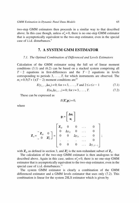
two-step GMM estimators then proceeds in a similar way to that describedabove. In this case though, unless �

2 = 0, there is no one-step GMM estimatorthat is asymptotically equivalent to the two-step estimator, even in the specialcase of i.i.d. disturbances.9

7. A SYSTEM GMM ESTIMATOR

7.1. The Optimal Combination of Differenced and Levels Estimators

Calculation of the GMM estimator using the full set of linear momentconditions (3.1) and (6.2) can be based on a stacked system comprising allT � 2 equations in first-differences and the T � 2 equations in levelscorresponding to periods 3, . . . , T, for which instruments are observed. Thems = 0.5(T + 1)(T � 2) moment conditions are10

E(yi, t�s�uit) = 0; for t = 3, . . . , T and 2 ≤ s ≤ t � 1 (7.1)

E(uit�yi, t�1) = 0; for t = 3, . . . , T. (7.2)

These can be expressed as

E(Z�sipi) = 0,

where

pi =��ui

ui�

Zdi 0 0 . . . 0

Zdi 00 �yi2 0 . . . 0

Zsi = = 0 0 �yi3 . . . 0 ;0 Zli

p

. . . . . . 00 0 0 . . . �yi, T�1

with Zdi as defined in section 3, and Zlip is the non-redundant subset of Zli.

The calculation of the two-step GMM estimator is then analogous to thatdescribed above. Again in this case, unless �

2 = 0, there is no one-step GMMestimator that is asymptotically equivalent to the two-step estimator, even in thespecial case of i.i.d. disturbances.11

The system GMM estimator is clearly a combination of the GMMdifferenced estimator and a GMM levels estimator that uses only (7.2). Thiscombination is linear for the system 2SLS estimator which is given by


�s = (q��1Zs( Z�sZs)�1Z�sq�1)

�1q��1Zs(Z�sZs)�1Z�sq,

where

qi =��yi

yi�.

Becauseq��1Zs(Z�sZs)

�1Z�sq�1 = �y��1Zd(Z�dZd)�1Z�d�y�1 + y��1Zl

p(Zpl �Zl

p)�1Zlp�y�1

the system 2SLS estimator is equivalent to the linear combination�s = ��d + (1 � �) �l

p,where �d and �l

p are the 2SLS first-differenced and levels estimatorsrespectively, with the levels estimator utilising only the T � 2 momentconditions (7.2), and

� =�y��1Zd(Z�dZd)

�1Z�d�y�1

�y��1Zd(Z�dZd)�1Z�d�y�1 + y��1Zl

p(Zpl �Zl

p)�1Zlp�y�1

=��dZ�dZd�d

��dZ�dZd�d + ��lZlp�Zl

p�l

,

where �d and �l are the OLS estimates of the first stage regression coefficientsunderlying these 2SLS estimators. From (4.2) and (6.3) it follows that �→0 if�→1 and/or (�

2/v2)→�, so all the weight for the system estimator will in

these cases be given to the informative levels moment conditions (7.2).


In the case where the initial conditions satisfy restriction (6.1) and the vit satisfyrestriction (3.3), Ahn & Schmidt (1995, equation (12b)) show that the T � 2homoskedasticity restrictions (3.4) and (5.2) can be replaced by a set of T � 2moment conditions

E(yituit � yi, t�1ui, t�1) = 0; for t = 3, . . . , T,which are all linear in the parameter �. The non-linear conditions (5.2) areagain redundant for estimation given (6.1), and the complete set of secondorder moment restrictions implied by (2.3)–(2.6), (3.3) and (6.1) can beimplemented as a linear GMM estimator.

8. ASYMPTOTIC VARIANCE COMPARISONS

To quantify the gains in asymptotic efficiency that result from exploiting thelinear moment conditions (6.2), Table 1 reports the ratio of the asymptoticvariance of the standard first-differenced GMM estimator described in Section3.1 to the asymptotic variance of the system GMM estimator described in


Section 7.1. These asymptotic variance ratios are calculated assuming bothcovariance stationarity and homoskedasticity. They are presented for T = 3 andT = 4, for two fixed values of �

2/v2, and for a range of values of the

autoregressive parameter �. For comparison, we also reproduce from Ahn &Schmidt (1995) the corresponding asymptotic variance ratios comparing first-differenced GMM to the non-linear GMM estimator which uses the quadraticmoment conditions (5.1), but not the extra linear moment conditions (6.2). Inthe T = 3 case there are no quadratic moment restrictions available. Thesecalculations suggest that exploiting conditions (6.2) can result in dramaticefficiency gains when T = 3, particularly at high values of � and high values of�

2/v2. These are indeed the cases where we find the instruments used to obtain

the first-differenced estimator to be weak.In the T = 4 case we still find dramatic efficiency gains at high values of �.

Comparison to the results for the non-linear GMM estimator also shows thatthe gains from exploiting conditions (6.2) can be much larger than the gainsfrom simply exploiting the non-linear restrictions (5.1).

In the Monte Carlo simulations presented in Section 11 we investigatewhether similar improvements are found in finite samples.

9. MULTIVARIATE DYNAMIC PANEL DATA MODELS

In this section the dynamic panel data model with additional regressors isconsidered.12 In particular, we focus on the model

Table 1. Asymptotic Variance Ratios

�2/v

2 = 1.00 �2/v

2 = 0.25

� SYS NON-LINEAR SYS NON-LINEAR

T = 3 0.0 1.33 n/a 1.33 n/a0.3 2.15 1.890.5 4.00 2.910.8 28.00 13.100.9 121.33 47.91

T = 4 0.0 1.75 1.67 1.40 1.290.3 2.31 1.91 1.77 1.330.5 3.26 2.10 2.42 1.350.8 13.97 2.42 8.88 1.410.9 55.40 2.54 30.90 1.45

Source: Blundell & Bond (1998)


yit = �yit�1 + �xit + uit(9.1)

uit = �i + vit

where xit is a scalar. The error components �i and vit again satisfy the conditions(2.4)–(2.6). The xit process is correlated with the individual effects �i and weconsider three possible correlation structures between the xit process and the vit

error process that determine the instruments that can be used to estimate � and�.

First, the xit process is strictly exogenous:

E(xisvit) = 0; for s = 1, . . . , T; t = 2, . . . , T. (9.2)

Secondly, the xit process is weakly exogenous, or predetermined

E(xisvit) = 0; for s = 1, . . . , t; t = 2, . . . , T(9.3)

E(xisvit) ≠ 0; for s = t + 1, . . . , T; t = 2, . . . , T

and thirdly, the xit process is endogenously determined

E(xisvit) = 0; for s = 1, . . . , t � 1; t = 2, . . . , T(9.4)

E(xisvit) ≠ 0; for s = t, . . . , T; t = 2, . . . , T.

We are especially interested in the case when the xit process is endogenouslydetermined, which includes simultaneous processes, but also measurementerror.

For the GMM first-differenced estimator, the 0.5(T � 1)(T � 2) momentconditions (3.1)

E(yi, t�s�uit) = 0; for t = 3, . . . , T and 2 ≤ s ≤ t � 1

remain valid. When the xit process is strictly exogenous, the followingadditional T(T � 2) moment conditions are valid

E(xis�uit) = 0; for t = 3, . . . , T and 1 ≤ s ≤ T. (9.5)

When xit is predetermined there are only the 0.5(T + 1)(T � 2) additionalmoment conditions

E(xi, t�s�uit) = 0; for t = 3, . . . , T and 1 ≤ s ≤ t � 1, (9.6)

whereas when xit is endogenously determined only the following0.5(T � 1)(T � 2) additional moment conditions are valid

E(xi, t�s�uit) = 0; for t = 3, . . . , T and 2 ≤ s ≤ t � 1. (9.7)

For the non-linear GMM estimator, moment conditions (5.1) remain valid,and no further moment conditions result from the presence of xit variables.


For the system GMM estimator, we first consider under what conditions both�yit and �xit are uncorrelated with �i. In order to illustrate this, we specify thefollowing process for the regressor

xit = �xi, t�1 + ��i + eit.

Thus � ≠ 0 allows the level of xit to be correlated with �i, and the covarianceproperties between vit and eis determine whether xit is strictly exogenous,predetermined or endogenously determined. First notice that

�xit = �t�2�xi2 +�s=0

t�3

�s�ei, t�s,

so that �xit will be correlated with �i if and only if �xi2 is correlated with �i.To guarantee E[�xi2�i] = 0 we require the initial conditions restriction

E��xi1 ��i

1 � ��i�= 0 (9.8)

which is satisfied under mean stationarity of the xit process.Given this restriction, writing �yit as

�yit = �t�2�yi2 +�s=0

t�3

�s(��xi, t�s + �ui, t�s) (9.9)

shows that �yit will be correlated with �i if and only if �yi2 is correlated with�i. To guarantee E[�yi2�i] = 0 we then require the similar initial conditionsrestriction

E yi1 �

�� i

1 � ��+ �i

1 � ��i = 0 (9.10)

which would again be satisfied under stationarity. Thus, there are additionalmoment restrictions available for the equations in levels when the yit and xit

processes are both mean stationary.Whilst jointly stationary means is sufficient to ensure that both �yit and �xit

are uncorrelated with �i, this condition is stronger than is necessary. Forexample, if the conditional model (9.1) has generated the yit series forsufficiently long time prior to our sample period for any influence of the trueinitial conditions to be negligible, then an expression analogous to (9.9) showsthat �yit will be uncorrelated with �i provided that �xit is uncorrelated with �i,


even if the mean of xit (and hence yit) is time-varying. Moreover we can notethat it is perfectly possible for �xit to be uncorrelated with �i in cases where �yit

is correlated with �i (for example, when (9.8) holds or � = 0 but (9.10) is notsatisfied). However, given (9.9), it seems very unlikely that �yit will beuncorrelated with �i in contexts where �xit is correlated with �i.

When both �yit and �xit are uncorrelated with �i, the extra momentconditions for the GMM system estimator are, as before, (7.2),

E(uit�yi, t�1) = 0; for t = 3, . . . , T

and

E(uit�xit) = 0; for t = 2, . . . , T (9.11)

in the case where xit is strictly exogenous or predetermined; or

E(uit�xit�1) = 0; for t = 3, . . . , T, (9.12)

when xit is endogenously determined. Therefore, when for example xit isendogenous, the GMM system estimator is based on the moment conditions(7.1), (9.7), (7.2) and (9.12).

10. TESTS OF OVERIDENTIFYING RESTRICTIONS

The standard test for testing the validity of the moment conditions used in theGMM estimation procedure is the Sargan test of overidentifying restrictions(see Sargan (1958) and the development for GMM in Hansen (1982)). For theGMM estimator in the first-differenced model this test statistic is given by

Sard =1N

�u�ZdWNZ�d�u

where WN is the optimal weight matrix as in (3.2) and �u are the two-stepresiduals in the differenced model. In general, under the null that the momentconditions are valid, Sard is asymptotically chi-squared distributed with md � kdegrees of freedom, where md is the number of moment conditions and k is thenumber of estimated parameters.

For the system estimator, the same test is readily defined. Call this test Sars.A test for the validity of the level moment conditions that are utilised by thesystem estimator is then obtained as the difference between Sars and Sard:

Dif-Sar = Sars � Sard (10.1)

and Dif-Sar is asymptotically chi-squared distributed with ms � md degrees offreedom under the null that the level moment conditions are valid.


11. MONTE CARLO RESULTS

This section illustrates the performance of the various estimators, as discussedabove, for a dynamic multivariate panel data model. In particular, the effect ofweak instruments and the potential gains from exploiting initial conditionsrestrictions are investigated.

The model specification is

yit = �yit�1 + �xit + �i + vit (11.1)

xit = �xit�1 + ��i + �vit + eit (11.2)

with

�i ~ N(0, �2); vit ~ N(0, v

2); eit ~ N(0, e2)

and the initial observations are drawn from the covariance stationarydistribution. Although these errors are homoskedastic, we do not consider anyof the additional moment conditions that require homoskedasticity in thesimulated estimators.

We choose the error process parameters in such a way that the xit process ishighly persistent for high values of �. Further, xit is positively correlated with�i and the value of � is negative to mimic the effects of measurement error. Thevalues of the parameters that are kept fixed in the various Monte Carlosimulations presented below are

� = 1, � = 0.25, � = � 0.1,

�2 = 1, v

2 = 1, e2 = 0.16.

The parameters that are varied in the simulations are the autoregressivecoefficients � and �. We consider four designs with � and � both taking thevalues of 0.5 and 0.95. The case when � = 0.5 and � = 0.95 resembles theproduction function data that will be analysed in the next section. The samplesize is N = 500, and the simulation results for the various estimators arepresented in Tables 2 and 3 for T = 4 and in Tables 4 and 5 for T = 8.

Means, standard deviations and root mean squared errors (RMSE) from10,000 simulations are tabulated for the OLS levels estimator (OLS), WithinGroups estimator (WG), the GMM first-differenced estimator (DIF), the non-linear GMM estimator (AS),13 the levels GMM estimator (LEV), and the


Tabl

e2.

Mon

te-C

arlo

res

ults

, T=

4, �

=0.

5, �

=1,

N=

500

OL

SW

GD

IFA

SL

EV

SYS

Mea

nSt

DM

ean

St D

Mea

nSt

DM

ean

St D

Mea

nSt

DM

ean

St D

rmse

rmse

rmse

rmse

rmse

rmse

�0.

762

0.01

7–0

.036

0.03

00.

496

0.09

00.

501

0.07

50.

502

0.05

90.

500

0.05

50.

263

0.53

80.

091

0.07

50.

059

0.05

5

�=

0.5

�0.

820

0.01

10.

010

0.03

10.

469

0.13

10.

516

0.09

50.

512

0.07

00.

512

0.06

00.

320

0.49

10.

135

0.09

60.

070

0.06

1�

0.77

50.

053

0.31

80.

080

0.91

50.

420

1.00

60.

351

1.02

90.

336

1.01

50.

257

0.23

10.

687

0.42

80.

351

0.33

70.

257

�=

0.95

�0.

990

0.00

10.

300

0.03

20.

350

0.48

70.

840

0.24

20.

980

0.02

90.

979

0.03

30.

040

0.65

10.

773

0.26

60.

042

0.04

4�

0.58

30.

053

0.19

40.

075

–0.1

950.

994

0.79

00.

524

1.00

40.

289

1.00

00.

232

0.42

00.

809

1.55

40.

565

0.28

90.

232

Mea

ns a

nd s

tand

ard

deva

tions

of

10,0

00 r

eplic

atio

ns. D

IF, A

S, L

EV

and

SY

S ar

e tw

o-st

ep e

stim

ator

s.


Tabl

e3.

Mon

te-C

arlo

res

ults

, T=

4, �

=0.

95, �

=1,

N=

500

OL

SW

GD

IFA

SL

EV

SYS

Mea

nSt

DM

ean

St D

Mea

nSt

DM

ean

St D

Mea

nSt

DM

ean

St D

rmse

rmse

rmse

rmse

rmse

rmse

�0.

997

0.00

20.

221

0.03

20.

472

0.82

50.

868

0.22

10.

961

0.14

40.

953

0.09

60.

047

0.72

90.

954

0.23

50.

145

0.09

6

�=

0.5

�0.

650

0.01

40.

089

0.03

10.

466

0.10

30.

500

0.06

50.

518

0.05

30.

514

0.04

40.

151

0.41

20.

109

0.06

50.

056

0.04

6�

0.83

00.

034

0.55

10.

090

0.51

71.

438

1.02

10.

461

1.07

80.

160

1.07

50.

153

0.17

40.

458

1.52

20.

461

0.17

80.

170

�=

0.95

�0.

962

0.00

10.

661

0.02

60.

907

0.10

40.

936

0.07

20.

957

0.00

80.

956

0.01

00.

012

0.29

00.

112

0.07

40.

010

0.01

1�

0.90

40.

026

0.46

50.

089

0.23

31.

769

0.86

30.

853

1.02

00.

091

1.02

00.

090

0.10

00.

543

1.92

80.

864

0.09

30.

092

Mea

ns a

nd s

tand

ard

deva

tions

of

10,0

00 r

eplic

atio

ns. D

IF, A

S, L

EV

and

SY

S ar

e tw

o-st

ep e

stim

ator

s.


Tabl

e4.

Mon

te C

arlo

res

ults

, T=

8, �

=0.

5, �

=1,

N=

500

OL

SW

GD

IFA

SL

EV

SYS

Mea

nSt

DM

ean

St D

Mea

nSt

DM

ean

St D

Mea

nSt

DM

ean

St D

rmse

rmse

rmse

rmse

rmse

rmse

�0.

762

0.01

20.

265

0.01

80.

494

0.03

40.

495

0.02

50.

503

0.02

90.

501

0.02

40.

262

0.23

60.

035

0.02

60.

029

0.02

4

�=

0.5

�0.

820

0.00

70.

311

0.01

70.

480

0.04

00.

497

0.02

90.

523

0.03

40.

511

0.02

70.

320

0.19

00.

045

0.02

90.

041

0.02

9�

0.77

50.

034

0.49

00.

045

0.93

00.

136

0.94

40.

134

1.04

10.

157

0.99

70.

124

0.22

80.

512

0.15

30.

145

0.16

20.

124

�=

0.95

�0.

990

0.00

10.

662

0.01

60.

548

0.17

70.

969

0.03

00.

982

0.00

70.

979

0.01

10.

040

0.28

90.

440

0.03

60.

032

0.03

1�

0.58

10.

035

0.38

80.

044

0.22

60.

356

0.97

20.

134

0.97

90.

108

0.98

30.

101

0.42

10.

613

0.85

20.

137

0.11

00.

103

Mea

ns a

nd s

tand

ard

deva

tions

of

10,0

00 r

eplic

atio

ns. D

IF, A

S, L

EV

and

SY

S ar

e tw

o-st

ep e

stim

ator

s.


Tabl

e5.

Mon

te C

arlo

res

ults

, T=

8, �

=0.

95, �

=1,

N=

500

OL

SW

GD

IFA

SL

EV

SYS

Mea

nSt

DM

ean

St D

Mea

nSt

DM

ean

St D

Mea

nSt

DM

ean

St D

rmse

rmse

rmse

rmse

rmse

rmse

�0.

997

0.00

10.

591

0.01

70.

676

0.22

20.

903

0.06

10.

973

0.02

20.

958

0.03

10.

047

0.35

90.

350

0.07

70.

032

0.03

2

�=

0.5

�0.

650

0.00

90.

396

0.01

50.

480

0.03

30.

508

0.02

40.

523

0.02

20.

518

0.02

10.

150

0.10

60.

039

0.02

50.

032

0.02

8�

0.83

00.

022

0.79

60.

040

0.80

00.

290

1.09

90.

125

1.08

40.

058

1.07

50.

059

0.17

10.

208

0.35

20.

159

0.10

10.

095

�=

0.95

�0.

962

0.00

10.

882

0.00

90.

927

0.02

50.

956

0.00

70.

957

0.00

20.

957

0.00

30.

012

0.06

80.

034

0.00

90.

007

0.00

7�

0.90

20.

017

0.74

50.

040

0.61

50.

400

1.01

60.

118

1.01

70.

028

1.01

90.

031

0.10

00.

258

0.55

50.

119

0.03

30.

036

Mea

ns a

nd s

tand

ard

deva

tions

of

10,0

00 r

eplic

atio

ns. D

IF, A

S, L

EV

and

SY

S ar

e tw

o-st

ep e

stim

ator

s.


system GMM estimator (SYS). Thus for the case of estimating the AR(1)model for xit, DIF uses the moment conditions (3.1); AS uses the momentconditions (3.1) and (5.1); LEV uses the moment conditions (6.4); and SYSuses the moment conditions (3.1) and (6.2). The reported results are for thetwo-step GMM estimators.

Tables 2 and 4 present results for � = 0.5. The row labelled ‘�’ presents theresults for the estimates of � in model (11.2), where the various GMMestimators only utilise lagged information on x as instruments, and potentialinformation from the lagged values of y is not used. Our results for the DIF andSYS estimators can therefore be compared to those reported in, for example,Blundell & Bond (1998) and Alonso–Borrego & Arellano (1999). As expected,the OLS estimates are biased upward and the WG estimates are biaseddownwards. In this experiment where xit is not highly persistent and theinstruments available for the equations in first-differences are not weak, all fourGMM estimators are virtually unbiased. The AS, LEV and SYS estimators allprovide an improvement in precision compared to the standard DIF estimator.As we would expect from the asymptotic variance ratios in Table 1, there is agreater gain in precision from using SYS rather than AS at T = 4, although inTable 4 we can observe that this difference becomes very small at T = 8.

The next two rows in Tables 2 and 4 present the estimation results for � and� in model (11.1) when � = 0.5 and � = 0.5. The OLS estimates for � are biasedupwards, whereas those for � are biased downwards. The WG estimates for �and � are both biased downwards. Again, as expected, since both the y and xseries have a low degree of persistence, the four GMM estimators perform quitewell in this experiment. The SYS estimator has the smallest RMSE for bothparameters, but the gains are not dramatic at T = 8.

The final two rows in Tables 2 and 4 are for the model with � = 0.95 and� = 0.5. As this makes the y process highly persistent, the DIF estimator suffersfrom a serious weak instrument bias, as well as being very imprecise. We cannotice that the DIF estimates of � and � are both biased downwards, in thedirection of the Within Groups estimates. The AS estimator is better behaved,as a result of exploiting the non-linear moment conditions (5.1). However theLEV and SYS estimators which exploit the initial conditions restrictionsprovide more dramatic gains in precision, particularly for the estimation of �and particularly in the case with T = 4. With T = 8, the LEV and SYS estimatesof � are biased upwards, in the direction of the OLS estimate, but still dominateon the RMSE criterion.

Tables 3 and 5 present the results for the cases where the xit process is highlypersistent, with � = 0.95. The estimates for � show the familiar pattern: OLS isupward biased, WG is downward biased, and DIF is downward biased towards


WG as a result of weak instruments. The AS estimator provides a substantialimprovement in both bias and precision. However the LEV and SYS estimatorsprovide more dramatic gains, particularly when T = 4.

When � = 0.5, the DIF estimator estimates � quite well, but the DIF estimateof � is very imprecise, biased downwards and on average very similar to theWG estimate of �. The AS, LEV and SYS estimates of � are all close to thetrue value. The AS estimates of � are much less biased than DIF but stillimprecise, particularly at T = 4. The LEV and SYS estimates of � show a littlefinite-sample bias, but again dominate in terms of RMSE. This experiment isintended to capture salient features of the production function data we considerin Section 12, notably a highly persistent explanatory variable that is measuredwith error, and a significant autoregressive parameter that is not close to one.The simulation results confirm that the system GMM estimator has reasonableproperties in this context.

When both � and � are equal to 0.95 the estimators display a similar pattern.One surprise is that the LEV and SYS estimators actually estimate bothparameters better than in the experiments with � = 0.5, and the gain from usingeither of these estimators compared to AS is rather more striking in this case.Also the DIF estimator now estimates � quite well (though not �); this may bebecause by increasing � whilst keeping the variance of �i and vit fixed, we havegreatly increased the variance of the yit series.

To investigate the size properties of the Sargan test of overidentifyingrestrictions, we present in Figures 3–12 p-value plots (see Davidson &MacKinnon, 1996) for the Sargan test statistics for the DIF and SYS GMMestimators. We also present the p-value plots for the Dif-Sar statistic as definedin (10.1), testing the validity of the additional levels moment conditionsexploited by the SYS estimator.

The x-axis of the p-value plots represents the nominal size using theasymptotic critical values of the corresponding chi-squared distributions; the y-axis represents the actual size of the test statistics in the experiments.

Figures 3–6 are the p-value plots for the Sargan tests for the GMMestimators in the univariate model for xit, (11.2). When � = 0.5, the distributionsof the test statistics are all very close to the asymptotic distribution, with aslight over-rejection when T = 8. When the series are persistent, � = 0.95, thetests over-reject, especially for larger T, with the Dif-Sar test having the largestsize distortion when T = 4.

Figures 7–14 present the p-value plots for the Sargan test statistics for themultivariate dynamic panel data model (11.1). These appear to be well behavedin the case with � = 0.5 and � = 0.5. In general, the Dif-Sar test is oversizedwhen either y or x or both are persistent. An interesting case is when � = 0.5,


� = 0.95 and T = 8. The Sars and Dif-Sar tests are considerably oversized in thiscase, whereas the Sard test has the correct size.

Fig. 3. p-value plot, � = 0.5, T = 4.

Fig. 4. p-value plot, � = 0.95, T = 4.


Fig. 5. p-value plot, � = 0.5, T = 8.

Fig. 6. p-value plot, � = 0.95, T = 8.


Fig. 7. � = 0.5, � = 0.5, T = 4.

Fig. 8. � = 0.5, � = 0.95, T = 4.


Fig. 9. � = 0.5, � = 0.5, T = 8.

Fig. 10. � = 0.5, � = 0.95, T = 8.


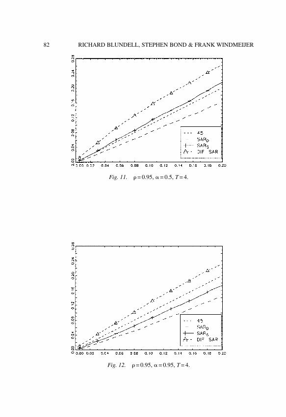
Fig. 11. � = 0.95, � = 0.5, T = 4.

Fig. 12. � = 0.95, � = 0.95, T = 4.


Fig. 13. � = 0.95, � = 0.5, T = 8.

Fig. 14. � = 0.95, � = 0.95, T = 8.


12. AN APPLICATION: THE COBB–DOUGLASPRODUCTION FUNCTION

As Griliches and Mairesse (1998) have argued, the estimation of productionfunctions has highlighted the poor performance of standard GMM estimatorsfor short panels. Here we use the problem of estimating production functionparameters to evaluate the practical significance of the alternative estimatorsreviewed in this chapter. In particular attention is focused on the estimation ofthe Cobb–Douglas production function

yit =�nnit + �kkit + �t + (�i + vit + mit)

vit =�vi, t�1 + eit |�| < 1

eit, mit ~MA(0), (12.1)

where yit is log sales of firm i in year t, nit is log employment, kit is log capitalstock and �t is a year-specific intercept reflecting, for example, a commontechnology shock. Of the error components, �i is an unobserved time-invariantfirm-specific effect, vit is a possibly autoregressive (productivity) shock and mit

reflects serially uncorrelated (measurement) errors. Constant returns to scalewould imply �n + �k = 1, but this is not necessarily imposed.

Interest is in the consistent estimation of the parameters (�n, �k, �) when thenumber of firms (N) is large and the number of years (T) is fixed. We maintainthat both employment (nit) and capital (kit) are potentially correlated with thefirm-specific effects (�i), and with both productivity shocks (eit) andmeasurement errors (mit).

The model has a dynamic (common factor) representation

yit = �nnit � ��nni, t�1 + �kkit � ��kki, t�1 + �yi, t�1

+ (�t � ��t�1) + (�i(1 � �) + eit + mit � �mi, t�1) (12.2)

or

yit = 1nit + 2ni, t�1 + 3kit + 4ki, t�1 + 5yi, t�1 + �*t + (�*

i + wit) (12.3)

subject to two non-linear (common factor) restrictions 2 = � 1 5 and 4 = � 3 5. Given consistent estimates of the unrestricted parameter vector = ( 1, 2, 3, 4, 5) and var( ), these restrictions can be (tested and)imposed using minimum distance to obtain the restricted parameter vector(�n, �k, �). Notice that wit = eit ~ MA(0) if there are no measurement errors(var(mit) = 0), and wit ~ MA(1) otherwise.


12.1. Data and Results

The data used is a balanced panel of 509 R&D-performing U.S. manufacturingcompanies observed for 8 years, 1982–89. These data were kindly madeavailable to us by Bronwyn Hall, and are similar to those used in Mairesse &Hall (1996), although the sample of 509 firms used here is larger than the finalsample of 442 firms used in Mairesse & Hall (1996). Capital stock andemployment are measured at the end of the firm’s accounting year, and sales isused as a proxy for output. Further details of the data construction can be foundin Mairesse & Hall (1996).

Table 6 reports results for the basic production function, not imposingconstant returns to scale, for a range of estimators. We report results for boththe unrestricted model (12.3) and the restricted model (12.1), where thecommon factor restrictions are tested and imposed using minimum distance.14

We report results here for the one-step GMM estimators, for which inferencebased on the asymptotic variance matrix has been found to be more reliablethan for the (asymptotically) more efficient two-step estimator. Simulationssuggest that the loss in precision that results from not using the optimal weightmatrix is unlikely to be large (cf. Blundell & Bond, 1998).

As expected in the presence of firm-specific effects, OLS levels appears togive an upwards-biased estimate of the coefficient on the lagged dependentvariable, whilst Within Groups appears to give a downwards-biased estimate ofthis coefficient. Note that even using OLS, we reject the hypothesis that � = 1,and even using Within Groups we reject the hypothesis that � = 0. Although thepattern of signs on current and lagged regressors in the unrestricted models areconsistent with the AR(1) error-component specification, the common factorrestrictions are rejected for both these estimators. They also reject constantreturns to scale.15

The validity of lagged levels dated t � 2 as instruments in the first-differenced equations is clearly rejected by the Sargan test of overidentifyingrestrictions. This is consistent with the presence of measurement errors.Instruments dated t � 3 (and earlier) are accepted, and the test of commonfactor restrictions is easily passed in these first-differenced GMM results.However the estimated coefficient on the lagged dependent variable is barelyhigher than the Within Groups estimate. Indeed the differenced GMMparameter estimates are all very close to the Within Groups results. Theestimate of �k is low and statistically weak, and the constant returns to scalerestriction is rejected.

The validity of lagged levels dated t � 3 (and earlier) as instruments in thefirst-differenced equations, combined with lagged first-differences dated t � 2


as instruments in the levels equations, appears to be marginal in the systemGMM estimator. However we have seen that these tests do have some tendencyto overreject in samples of this size. Moreover the Dif-Sar statistic that

Table 6. Production Function Estimates

OLS Within DIF DIF SYS SYSLevels Groups t–2 t–3 t–2 t–3

nt 0.479 0.488 0.513 0.499 0.629 0.472(0.029) (0.030) (0.089) (0.101) (0.106) (0.112)

nt–1 –0.423 –0.023 0.073 –0.147 –0.092 –0.278(0.031) (0.034) (0.093) (0.113) (0.108) (0.120)

kt 0.235 0.177 0.132 0.194 0.361 0.398(0.035) (0.034) (0.118) (0.154) (0.129) (0.152)

kt–1 –0.212 –0.131 –0.207 –0.105 –0.326 –0.209(0.035) (0.025) (0.095) (0.110) (0.104) (0.119)

yt–1 0.922 0.404 0.326 0.426 0.462 0.602(0.011) (0.029) (0.052) (0.079) (0.051) (0.098)

m1 –2.60 –8.89 –6.21 –4.84 –8.14 –6.53m2 –2.06 –1.09 –1.36 –0.69 –0.59 –0.35Sar — — 0.001 0.073 0.000 0.032Dif-Sar — — — — 0.001 0.102

�n 0.538 0.488 0.583 0.515 0.773 0.479(0.025) (0.030) (0.085) (0.099) (0.093) (0.098)

�k 0.266 0.199 0.062 0.225 0.231 0.492(0.032) (0.033) (0.079) (0.126) (0.075) (0.074)

� 0.964 0.512 0.377 0.448 0.509 0.565(0.006) (0.022) (0.049) (0.073) (0.048) (0.078)

Comfac 0.000 0.000 0.014 0.711 0.012 0.772CRS 0.000 0.000 0.000 0.006 0.922 0.641

Asymptotic standard errors in parentheses. Year dummies included in all models. m1 and m2 aretests for first- and second-order serial correlation, asymptotically N(0, 1). We test the levelsresiduals for OLS levels, and the first-differenced residuals in all other columns.Comfac is a minimum distance test of the non-linear common factor restrictions imposed in therestricted models. P-values are reported (also for Sar and Dif-Sar). CRS is a Wald test of theconstant resturns to scale hypothesis �n + �k = 1 in the restricted models. P-values are reported.Source: Blundell & Bond (2000).For the one-step GMM estimators, ‘t � s’ indicates that levels of the three series (y, n, k) datedt � s and all observed longer lags are used as instruments for the first-differenced equations. SYSestimators use lagged differences of the three series dated t � s + 1 as instruments for the levelsequations.


specifically tests the additional moment conditions used in the levels equationsaccepts their validity at the 10% level. The system GMM parameter estimatesappear to be reasonable. The estimated coefficient on the lagged dependentvariable is higher than the Within Groups estimate, but well below the OLSlevels estimate. The common factor restrictions are easily accepted, and theestimate of �k is both higher and better determined than the differenced GMMestimate. The constant returns to scale restriction is easily accepted in thesystem GMM results.16

Blundell & Bond (2000) explore this data in more detail and conclude thatthe system GMM estimates in the final column of Table 6 are their preferredresults. In particular they find that the individual series used here are highlypersistent, and that the instruments available for the first-differenced equationsare only weakly correlated with the explanatory variables in first-differences.This is consistent with the similarity between the first-differenced GMM andWithin Groups results. Blundell & Bond (2000) also find that when constantreturns to scale is imposed on the production function – it is not rejected in thepreferred system GMM results – then the results obtained using the first-differenced GMM estimator become more similar to the system GMMestimates.

13. SUMMARY AND CONCLUSIONS

The aim of this chapter has been to review developments in the recent literaturewhich have tried to improve on the poor performance of the standard first-differenced GMM estimator for highly autoregressive panel series by usingadditional moment conditions. In particular, we discuss the use of the ‘system’GMM estimator that relies on relatively mild restrictions on the initialconditions process. This system GMM estimator encompasses the GMMestimator based on the non-linear moment conditions available in the dynamicerror components model and has substantial asymptotic efficiency gainsrelative to this non-linear GMM estimator. The chapter systematically sets outthe assumptions required and moment conditions used by each estimator andprovides a Monte Carlo simulation comparison as well as an application toproduction function estimation.

The simulation results are the first in the literature to consider the propertiesof these GMM estimators in dynamic models with endogenous regressors. Ouranalysis suggests that similar issues arise in this case to those that have beenfound in previous Monte Carlo studies for the AR(1) model. In particular, wefind both a large bias and very low precision for the standard first-differencedestimator when the individual series are highly persistent. By exploiting


instruments available for the equations in levels, the system GMM estimatorcan both greatly improve the precision and greatly reduce the finite sample biaswhen these additional moment conditions are valid. Intermediate results arefound for the non-linear GMM estimator considered, which suggests that thisestimator could also be useful in applications with persistent series where thevalidity of the initial conditions restrictions required for the system GMMestimator are rejected.

The empirical application uses company accounts data for the US to estimatea simple Cobb-Douglas production function. For the standard GMM estimatorthat uses moment conditions only for the first-differenced equations, weconfirm the problems noted by Griliches and Mairesse: the estimatedcoefficient on capital is very low, all coefficient estimates are imprecise, andconstant returns to scale is easily rejected. We notice that the first-differencedGMM results are similar to the Within Groups results, which suggests theremay be a problem of weak instruments. This suggestion is consistent with thepersistence of the underlying sales, employment and capital stock series. Theadditional moment conditions used by the system GMM estimator are notrejected in this context, and lead to a marked improvement in the empiricalresults.

Taken together, these Monte Carlo and empirical results suggest that carefulconsideration of the underlying series and comparisons between different paneldata estimators can be useful in detecting situations where the standard first-differenced GMM estimator is likely to be subject to serious weak instrumentsbiases. Where appropriate, the use of the system GMM estimator offers asimple and powerful alternative, that can overcome many of the disappointingfeatures of the standard first-differenced GMM estimator in the context ofhighly persistent series.

ACKNOWLEDGMENTS

This research is part of the programme of research at the ESRC Centre for theMicro-Economic Analysis of Fiscal Policy at IFS. Financial support from theESRC is gratefully acknowledged.

NOTES

1. All of the estimators discussed and their properties extend in an obvious fashionto higher order autoregressive models.

2. Extensions to dynamic models with additional regressors are considered inSection 9.


3. With T = 3, the absence of serial correlation in vit (2.5) and predetermined initialconditions (2.6) are required to identify � (in the absence of any strictly exogenousinstruments). With T > 3, � can be identified in the presence of suitably low ordermoving average autocorrelation in vit.

4. These estimators are all based on the normalisation (2.3). Alonso-Borrego &Arellano (1999) consider a symmetrically normalised instrumental variable estimatorbased on the normalisation invariance of the standard LIML estimator.

5. As a choice of WN to yield the initial consistent estimator, Arellano & Bond(1991) suggest

WN =�1N�i=1

N

Z�diHdZdi��1

where Hd is the (T � 2) � (T � 2) matrix given by

2 –1 0 . . . 0–1 2 –1 . . . 0

Hd = 0 –1 2 . . . 0. . . . . . . . . . . . .0 0 0 . . . 2

which can be calculated in one step. The use of this Hd matrix accounts for the first-order moving average structure in �uit induced by the first-differencing transformation.Note that when the vit are i.i.d., the one-step and two-step estimators are asymptoticallyequivalent in this model. We follow this suggestion in the Monte Carlo simulations inSection 11.

6. As shown by Arellano & Bover (1995), OLS on the model transformed toorthogonal deviations coincides with the Within Groups estimator.

7. In this section we focus only on moment conditions that are valid underheteroskedasticity. The case with homoskedasticity and assumption (6.1) is consideredin Section 7.2.

8. This corrects the expression for plim l as given in Blundell and Bond (1998,p. 125).

9. As a choice of WN to yield the initial consistent estimator, we use

WN =�1N�i=1

N

Z�liZli��1

in the Monte Carlo simulations reported below.10. The use of moment conditions E(uit�yi, t�s) = 0 for s > 1 can be shown to be

redundant, given (7.1) and (7.2). For balanced panels, the T � 2 equations in levels maybe replaced by a single levels equation for period T, with (7.2) replaced by theequivalent moment conditions E(uiT�yi, T�s) = 0 for s = 1, . . . , T � 2. However thisapproach does not extend easily to the case of unbalanced panels.

11. For an analysis of the potential loss in efficiency due to specific choices of theinitial weight matrix for these system estimators, see Windmeijer (2000). As a choiceof WN to yield the initial consistent estimator, we use


WN =�1N�i=1

N

Z�siHsZsi��1

in our Monte Carlo simulations, where Hs is the matrix

�Hd

00

IT�2�,

IT�2 is the (T � 2) identity matrix and Hd is defined in Section 3.12. Here we only consider moment conditions that do not require any homo-

skedasticity assumptions.13. Define si = [ui3 � ui2, . . . , uiT � uiT�1, ui4(ui3 � ui2), . . . , uiT(uiT�1 � uiT�2)]� and

Znli =�Zdi

00

IT�3�, then the non-linear moment conditions can be written as

E[Z�nlisi] = 0. As an initial weight matrix we use WN =�1N�i=1

N

Z�nliZnli��1

, see Meghir &

Windmeijer (1999).14. The unrestricted results are computed using DPD98 for GAUSS (see Arellano &

Bond, 1998).15. The table reports p-values from minimum distance tests of the common factor

restrictions and Wald tests of the constant returns to scale restrictions.16. One puzzle is that we find little evidence of second-order serial correlation in the

first-differenced residuals (i.e. an MA(1) component in the error term in levels),although the use of instruments dated t � 2 is strongly rejected. It may be that the eit

productivity shocks are also MA(1), in a way that happens to offset the appearance ofserial correlation that would otherwise result from measurement errors.

REFERENCES


Alonso-Borrego, C., & Arellano, M. (1999). Symmetrically Normalised Instrumental-VariableEstimation using Panel Data. Journal of Business and Economic Statistics, 17, 36–49.

Anderson, T. W., & Hsiao, C. (1981). Estimation of Dynamic Models with Error Components.Journal of the American Statistical Association, 76, 598–606.

Arellano, M., & Bond, S. R. (1991). Some Tests of Specification for Panel Data: Monte CarloEvidence and an Application to Employment Equations. Review of Economic Studies, 58,277–297.

Arellano, M., & Bond, S. R. (1998). Dynamic Panel Data Estimation using DPD98 for GAUSS.http://www.ifs.org.uk/staff/steve_b.shtml.

Arellano, M., & Bover, O. (1995). Another Look at the Instrumental-Variable Estimation of Error-Components Models. Journal of Econometrics, 68, 29–52.

Baltagi, B. H. (1995). Econometric Analysis of Panel Data. Chichester: Wiley.


Bhagarva, A., & Sargan, J. D. (1983). Estimating Dynamic Random Effects Models from PanelData Covering Short Time Periods. Econometrica, 51, 1635–1659.

Blundell, R. W., & Bond, S. R. (1998). Initial Conditions and Moment Restrictions in DynamicPanel Data Models. Journal of Econometrics, 87, 115–143.

Blundell, R. W., & Bond, S. (2000). GMM Estimation with Persistent Panel Data: An Applicationto Production Functions. Econometric Reviews, 19(3), 321–340.

Bound, J., Jaeger, D. A., & Baker, R. M. (1995). Problems with Instrumental Variables Estimationwhen the Correlation between the Instruments and the Endogenous Explanatory Variable isWeak. Journal of the American Statistical Association, 90, 443–450.

Chamberlain, G. (1987). Asymptotic Efficiency in Estimation with Conditional MomentRestrictions. Journal of Econometrics, 34, 305–334.

Davidson, R., & MacKinnon, J. G. (1996). Graphical Methods for Investigating the Size andPower of Hypothesis Tests. Manchester School, 66, 1–26.

Griliches, Z., & Mairesse, J. (1998). Production Functions: the Search for Identification. In: S.Strom (Ed.), Essays in Honour of Ragnar Frisch. Econometric Society Monograph Series,Cambridge: Cambridge University Press.

Hansen, L. P. (1982). Large Sample Properties of Generalised Method of Moment Estimators.Econometrica, 50, 1029–1054.

Holtz-Eakin, D., Newey, W., & Rosen, H. S. (1988). Estimating Vector Autoregressions with PanelData. Econometrica, 56, 1371–1396.

Hsiao, C. (1986). Analysis of Panel Data. Cambridge: Cambridge University Press.Mairesse, J., & Hall, B. H. (1996). Estimating the Productivity of Research and Development in

French and US Manufacturing Firms: An Exploration of Simultaneity Issues with GMMMethods. In: K. Wagner & B. Van Ark (Eds), International Productivity Differences and,Their Explanations (pp. 285–315). Elsevier Science.

Meghir, C., & Windmeijer, F. (1999). Moment Conditions for Dynamic Panel Data Models withMultiplicative Individual Effects in the Conditional Variance. Annales d’Économie et deStatistique, 55/56, 317–330.

Nelson, C. R., & Startz, R. (1990a). Some Further Results on the Exact Small Sample Propertiesof the Instrumental Variable Estimator. Econometrica, 58, 967–976.

Nelson, C. R., & Startz, R. (1990b). The Distribution of the Instrumental Variable Estimator andIts t-ratio When the Instrument is A Poor One. Journal of Business and Economic Statistics,63, 5125–5140.

Nickell, S. J. (1981). Biases in Dynamic Models with Fixed Effects. Econometrica, 49,1417–1426.

Sargan, J. D. (1958). The Estimation of Economic Relationships Using Instrumental Variables.Econometrica, 26, 329–338.

Staiger, D., & Stock, J. H. (1997). Instrumental Variables Regression with Weak Instruments.Econometrica, 65, 557–586.

Windmeijer, F. (2000). Efficiency Comparisons for a System GMM Estimator in Dynamic PanelData Models. In: R. D. H. Heijmans, D. S. G. Pollock & A. Satorra (Eds), Innovations inMultivariate Statistical Analysis. A Festschrift for Heinz Neudecker (pp. 175–184). KluwerAcademic Publishers.


FULLY MODIFIED OLS FORHETEROGENEOUS COINTEGRATEDPANELS

Peter Pedroni

ABSTRACT

This chapter uses fully modified OLS principles to develop new methodsfor estimating and testing hypotheses for cointegrating vectors in dynamicpanels in a manner that is consistent with the degree of cross sectionalheterogeneity that has been permitted in recent panel unit root and panelcointegration studies. The asymptotic properties of various estimators arecompared based on pooling along the ‘within’ and ‘between’ dimensionsof the panel. By using Monte Carlo simulations to study the small sampleproperties, the group mean estimator is shown to behave well even inrelatively small samples under a variety of scenarios.

I. INTRODUCTION

In this chapter we develop methods for estimating and testing hypotheses forcointegrating vectors in dynamic time series panels. In particular we proposemethods based on fully modified OLS principles which are able toaccommodate considerable heterogeneity across individual members of thepanel. Indeed, one important advantage to working with a cointegrated panelapproach of this type is that it allows researchers to selectively pool the longrun information contained in the panel while permitting the short run dynamics


93

and fixed effects to be heterogeneous among different members of the panel.An important convenience of the fully modified approach that we propose hereis that in addition to producing asymptotically unbiased estimators, it alsoproduces nuisance parameter free standard normal distributions. In this way,inferences can be made regarding common long run relationships which areasymptotically invariant to the considerable degree of short run heterogeneitythat is prevalent in the dynamics typically associated with panels that arecomposed of aggregate national data.

A. Nonstationary Panels and Heterogeneity

Methods for nonstationary time series panels, including unit root andcointegration tests, have been gaining increased acceptance in a number ofareas of empirical research. Early examples include Canzoneri, Cumby & Diba(1996), Chinn & Johnson (1996), Chinn (1997), Evans & Karras (1996),Neusser & Kugler (1998), Obstfeld & Taylor (1996), Oh (1996), Papell (1997),Pedroni (1996b), Taylor (1996) and Wu (1996), with many more since. Thesestudies have for the most part been limited to applications which simply askwhether or not particular series appear to contain unit roots or are cointegrated.In many applications, however, it is also of interest to ask whether or notcommon cointegrating vectors take on particular values. In this case, it wouldbe helpful to have a technique that allows one to test such hypothesis about thecointegrating vectors in a manner that is consistent with the very general degreeof cross sectional heterogeneity that is permitted in such panel unit root andpanel cointegration tests.

In general, the extension of conventional nonstationary methods such as unitroot and cointegration tests to panels with both cross section and time seriesdimensions holds considerable promise for empirical research considering theabundance of data which is available in this form. In particular, such methodsprovide an opportunity for researchers to exploit some of the attractivetheoretical properties of nonstationary regressions while addressing in a naturaland direct manner the small sample problems that have in the past oftenhindered the practical success of these methods. For example, it is well knownthat superconsistent rates of convergence associated with many of thesemethods can provide empirical researchers with an opportunity to circumventmore traditional exogeneity requirements in time series regressions. Yet the lowpower of many of the associated statistics has often impeded the ability to takefull advantage of these properties in small samples. By allowing data to bepooled in the cross sectional dimension, nonstationary panel methods have thepotential to improve upon these small sample limitations. Conversely, the use

94 PETER PEDRONI

of nonstationary time series asymptotics provides an opportunity to make panelmethods more amenable to pooling aggregate level data by allowingresearchers to selectively pool the long run information contained in the panel,while allowing the short run dynamics to be heterogeneous among differentmembers of the panel.

Initial methodological work on nonstationary panels focused on testing forunit roots in univariate panels. Quah (1994) derived standard normalasymptotic distributions for testing unit roots in homogeneous panels as boththe time series and cross sectional dimensions grow large. Levin & Lin (1993)derived distributions under more general conditions that allow for heteroge-neous fixed effects and time trends. More recently, Im, Pesaran & Shin (1995)study the small sample properties of unit root tests in panels withheterogeneous dynamics and propose alternative tests based on group meanstatistics. In practice however, empirical work often involves relationshipswithin multivariate systems. Toward this end, Pedroni (1993, 1995) studies theproperties of spurious regressions and residual based tests for the null of nocointegration in dynamic heterogeneous panels. This chapter continues this lineof research by proposing a convenient method for estimating and testinghypotheses about common cointegrating vectors in a manner that is consistentwith the degree of heterogeneity permitted in these panel unit root and panelcointegration studies.

In particular, we address here two key sources of cross memberheterogeneity that are particularly important in dealing with dynamiccointegrated panels. One such source of heterogeneity manifests itself in thefamiliar fixed effects form. These reflect differences in mean levels among thevariables of different individual members of the panel and we model these byincluding individual specific intercepts. The second key source of heterogene-ity in such panels comes from differences in the way that individuals respondto short run deviations from equilibrium cointegrating vectors that develop inresponse to stochastic disturbances. In keeping with earlier panel unit root andpanel cointegration papers, we model this form of heterogeneity by allowingthe associated serial correlation properties of the error processes to vary acrossindividual members of the panel.

B. Related Literature

Since the original version of this paper, Pedroni (1996a),1 many more papershave contributed to our understanding of hypothesis testing in cointegratingpanels. For example, Kao & Chiang (1997) extended their original paper on theleast squares dummy variable model in cointegrated panels, Kao & Chen

95Fully Modified OLS for Heterogeneous Cointegrated Panels

(1995), to include a comparison of the small sample properties of a dynamicOLS estimator with other estimators including a FMOLS estimator similar toPedroni (1996a). Specifically, Kao & Chiang (1997) demonstrated that a paneldynamic OLS estimator has the same asymptotic distribution as the type ofpanel FMOLS estimator derived in Pedroni (1996a) and showed that the smallsample size distortions for such an estimator were often smaller than certainforms of the panel FMOLS estimator. The asymptotic theory in these earlierpapers were generally based on sequential limit arguments (allowing thesample sizes T and N to grow large sequentially), whereas Phillips & Moon(1999) subsequently provided a rigorous and more general study of the limittheory in nonstationary panel regressions under joint convergence (allowing Tand N to grow large concurrently). Phillips & Moon (1999) also provided a setof regularity conditions under which convergence in sequential limits impliesconvergence in joint limits, and considered these properties in the context of aFMOLS estimator, although they do not specifically address the small sampleproperties of feasible versions of the estimators. More recently, Mark & Sul(1999) also study a similar form of the panel dynamic OLS estimator firstproposed by Kao & Chiang (1997). They compare the small sample propertiesof a weighted versus unweighted version of the estimator and find that theunweighted version generally exhibits smaller size distortion than the weightedversion.

In this chapter we report new small sample results for the group mean panelFMOLS estimator that was originally proposed in Pedroni (1996a). Anadvantage of the group mean estimator over the other pooled panel FMOLSestimators proposed in the Pedroni (1996a) is that the t-statistic for thisestimator allows for a more flexible alternative hypothesis. This is because thegroup mean estimator is based on the so called ‘between dimension’ of thepanel, while the pooled estimators are based on the ‘within dimension’ of thepanel. Accordingly, the group mean panel FMOLS provides a consistent test ofa common value for the cointegrating vector under the null hypothesis againstvalues of the cointegrating vector that need not be common under thealternative hypothesis, while the pooled within dimension estimators do not.Furthermore, as Pesaran & Smith (1995) argue in the context of OLSregressions, when the true slope coefficients are heterogeneous, group meanestimators provide consistent point estimates of the sample mean of theheterogeneous cointegrating vectors, while pooled within dimension estimatorsdo not. Rather, as Phillips & Moon (1999) demonstrate, when the truecointegrating vectors are heterogeneous, pooled within dimension estimatorsprovide consistent point estimates of the average regression coefficient, not the

96 PETER PEDRONI

sample mean of the cointegrating vectors. Both of these features of the groupmean estimator are often important in practical applications.

Finally, the implementation of the feasible form of the between dimensiongroup mean estimator also has advantages over the other estimators in thepresence of heterogeneity of the residual dynamics around the cointegratingvector. As was demonstrated in Pedroni (1996a), in the presence of suchheterogeneity, the pooled panel FMOLS estimator requires a correction termthat depends on the true cointegrating vector. For a specific null value for acointegrating vector, the t-statistic is well defined, but of course this is of littleuse per se when one would like to estimate the cointegrating vector. Onesolution is to obtain a preliminary estimate of the cointegrating vector usingOLS. However, although the OLS estimator is superconsistent, it still containsa second order bias in the presence of endogeneity, which is not eliminatedasymptotically. Accordingly, this bias leads to size distortion, which is notnecessarily eliminated even when the sample size grows large in the paneldimension. Consequently, this type of approach based on a first stage OLSestimate was not recommended in Pedroni (1996a), and it is not surprising thatMonte Carlo simulations have shown large size distortions for such estimators.Even when the null hypothesis was imposed without using an OLS estimator,the size distortions for this type of estimator were large as reported in Pedroni(1996a). Similarly, Kao & Chiang (1997) also found large size distortions forsuch estimators when OLS estimates were used in the first stage for thecorrection term. By contrast, the feasible version of the between dimensiongroup mean based estimator does not suffer from these difficulties, even in thepresence of heterogeneous dynamics. As we will see, the size distortions forthis estimator are minimal, even in panels of relatively modest dimensions.

The remainder of the chapter is structured as follows. In Section 2, weintroduce the econometric models of interest for heterogeneous cointegratedpanels. We then present a number of theoretical results for estimators designedto be asymptotically unbiased and to provide nuisance parameter freeasymptotic distributions which are standard normal when applied to heteroge-neous cointegrated panels and can be used to test hypotheses regardingcommon cointegrating vectors in such panels. In Section 3 we study the smallsample properties of these estimators and propose feasible FMOLS statisticsthat perform relatively well in realistic panels with heterogeneous dynamics. InSection 4 we enumerate the algorithm used to construct these statistics andbriefly describe a few examples of their uses. Finally, in Section 5 we offerconclusions and discuss a number of related issues in the ongoing research onestimation and inference in cointegrated panels.


II. ASYMPTOTIC RESULTS FOR FULLY MODIFIEDOLS IN HETEROGENEOUS COINTEGRATED PANELS

In this section we study asymptotic properties of cointegrating regressions indynamic panels with common cointegrating vectors and suggest how a fullymodified OLS estimator can be constructed to deal with complicationsintroduced by the presence of parameter heterogeneity in the dynamics andfixed effects across individual members. We begin, however, by discussing thebasic form of a cointegrating regression in such panels and the problemsassociated with unmodified OLS estimators.

A. Cointegrating Regressions in Heterogeneous Panels

Consider the following cointegrated system for a panel of i = 1, . . . , Nmembers,

yit = �i + �xit + �it (1)xit = xit–1 + �it

where the vector error process �it = (�it, �it)� is stationary with asymptoticcovariance matrix �i. Thus, the variables xi, yi are said to cointegrate for eachmember of the panel, with cointegrating vector � if yit is integrated of orderone. The term �i allows the cointegrating relationship to include memberspecific fixed effects. In keeping with the cointegration literature, we do notrequire exogeneity of the regressors. As usual, xi can in general be an mdimensional vector of regressors, which are not cointegrated with each other. Inthis case, we partition �it = (�it, ��it) so that the first element is a scalar series andthe second element is an m dimensional vector of the differences in theregressors �it = xit xit–1 = xit, so that when we construct

�i =��11i

�21i

��21i

�22i� (2)

then �11i is the scalar long run variance of the residual �it, and �22i is the m � mlong run covariance among the �it, and �21i is an m � 1 vector that gives the longrun covariance between the residual �it and each of the �it. However, forsimplicity and convenience of notation, we will refer to xi as univariate in theremainder of this chapter. Each of the results of this study generalize in anobvious and straightforward manner to the vector case, unless otherwiseindicated.2

98 PETER PEDRONI

In order to explore the asymptotic properties of estimators as both the crosssectional dimension, N, and the time series dimension, T, grow large, we willmake assumptions similar in spirit to Pedroni (1995) regarding the degree ofdependency across both these dimensions. In particular, for the time seriesdimension, we will assume that the conditions of the multivariate functionalcentral limit theorems used in Phillips & Durlauf (1986) and Park & Phillips(1988), hold for each member of the panel as the time series dimension growslarge. Thus, we have

Assumption 1.1 (invariance principle): The process �it satisfies a multivariatefunctional central limit theorem such that the convergence as T→� for the

partial sum 1

�T�t=1

[Tr]

�it →Bi(r, �i) holds for any given member, i, of the panel,

where Bi(r, �i) is Brownian motion defined over the real interval r�[0,1], withasymptotic covariance �i.This assumption indicates that the multivariate functional central limit theorem,or invariance principle, holds over time for any given member of the panel. Thisplaces very little restriction on the temporal dependency and heterogeneity ofthe error process, and encompasses for example a broad class of stationaryARMA processes. It also allows the serial correlation structure to be differentfor individual members of the panel. Specifically, the asymptotic covariancematrix, �i varies across individual members, and is given by �i �limT→� E[T –1(�t=1

T �it)(�t=1T �it)], which can also be decomposed as �i =

�io + i + i, where �i

o is the contemporaneous covariance and i is a weightedsum of autocovariances. The off-diagonal terms of these individual �21i

matrices capture the endogenous feedback effect between yit and xit, which isalso permitted to vary across individual members of the panel. For several ofthe estimators that we propose, it will be convenient to work with atriangularization of this asymptotic covariance matrix. Specifically, we willrefer to this lower triangular matrix of �i as Li, whose elements are related asfollows

L11i = (�11i �21i2 /�22i)

1/2, L12i = 0, L21i = �21i /�22i1/2, L22i = �22i

1/2 (3)

Estimation of the asymptotic covariance matrix can be based on any one of anumber of consistent kernel estimators such as the Newey & West (1987)estimator.

Next, for the cross sectional dimension, we will employ the standard paneldata assumption of independence. Hence we have:

Assumption 1.2 (cross sectional independence): The individual processes areassumed to be independent cross sectionally, so that E[�it, �jt] = 0 for all i ≠ j.


More generally, the asymptotic covariance matrix for a panel of dimensionN � T is block diagonal with the ith diagonal block given by the asymptoticcovariance for member i.

This type of assumption is typical of our panel data approach, and we will beusing this condition in the formal derivation of the asymptotic distribution ofour panel cointegration statistics. For panels that exhibit common disturbancesthat are shared across individual members, it will be convenient to capture thisform of cross sectional dependency by the use of a common time dummy,which is a fairly standard panel data technique. For panels with even richercross sectional dependencies, one might think of estimating a full non-diagonalN � N matrix of �ij elements, and then premultiplying the errors by this matrixin order to achieve cross sectional independence. This would require the timeseries dimension to grow much more quickly than the cross sectionaldimension, and in most cases one hopes that a common time dummy willsuffice.

While the derivation of most of the asymptotic results of this chapter arerelegated to the mathematical appendix, it is worth discussing briefly here howwe intend to make use of assumptions 1.1 and 1.2 in providing asymptoticdistributions for the panel statistics that we consider in the next twosubsections. In particular, we will employ here simple and somewhat informalsequential limit arguments by first evaluating the limits as the T dimensiongrows large for each member of the panel in accordance with assumption 1.1and then evaluating the sums of these statistics as the N dimension grows largeunder the independence assumption of 1.2.3 In this manner, as N grows largewe obtain standard distributions as we average the random functionals for eachmember that are obtained in the initial step as a consequence of letting T growlarge. Consequently, we view the restriction that first T→� and then N→� asa relatively strong restriction that ensures these conditions, and it is possiblethat in many circumstances a weaker set of restrictions that allow N and T togrow large concurrently, but with restrictions on the relative rates of growthmight deliver similar results. In general, for heterogeneous error processes,such restrictions on the rate of growth of N relative to T can be expected todepend in part on the rate of convergence of the particular kernel estimatorsused to eliminate the nuisance parameters, and we can expect that our iterativeT→� and then N→� requirements proxy for the fact that in practice ourasymptotic approximations will be more accurate in panels with relatively largeT dimensions as compared to the N dimension. Alternatively, under a morepragmatic interpretation, one can simply think of letting T→� for fixed Nreflect the fact that typically for the panels in which we are interested, it is the

100 PETER PEDRONI

time series dimension which can be expected to grow in actuality rather thanthe cross sectional dimension, which is in practice fixed. Thus, T→� is in asense the true asymptotic feature in which we are interested, and this leads tostatistics which are characterized as sums of i.i.d. Brownian motionfunctionals. For practical purposes, however, we would like to be able tocharacterize these statistics for the general case in which N is large, and in thiscase we take N→� as a convenient benchmark for which to characterize thedistribution, provided that we understand T→� to be the dominant asymptoticfeature of the data.

B. Asymptotic Properties of Panel OLS

Next, we consider the properties of a number of statistics that might be used fora cointegrated panel as described by (1) under assumptions 1.1 and 1.2regarding the time series and cross dimensional dependencies in the data. Thefirst statistic that we examine is a standard panel OLS estimator of thecointegrating relationship. It is well known that the conventional singleequation OLS estimator for the cointegrating vector is asymptotically biasedand that its standardized distribution is dependent on nuisance parametersassociated with the serial correlation structure of the data, and there is noreason to believe that this would be otherwise for the panel OLS estimator. Thefollowing proposition confirms this suspicion.4

Proposition 1.1 (Asymptotic Bias of the Panel OLS Estimator). Consider astandard panel OLS estimator for the coefficient � of panel (1), underassumptions 1.1 and 1.2, given as

�NT =��i=1

N �t=1

T

(xit xi)2–1 �

i=1

N �t=1

T

(xit x i)(yit yi)

where xi and yi refer to the individual specific means. Then,

(a) The estimator is asymptotically biased and its asymptotic distribution willbe dependent on nuisance parameters associated with the dynamics of theunderlying processes.

(b) Only for the special case in which the regressors are strictly exogenous andthe dynamics are homogeneous across members of the panel can validinferences be made from the standardized distribution of �NT or itsassociated t-statistic.

As the proof of proposition 1.1 given in the appendix makes clear, the sourceof the problem stems from the endogeneity of the regressors under the usual


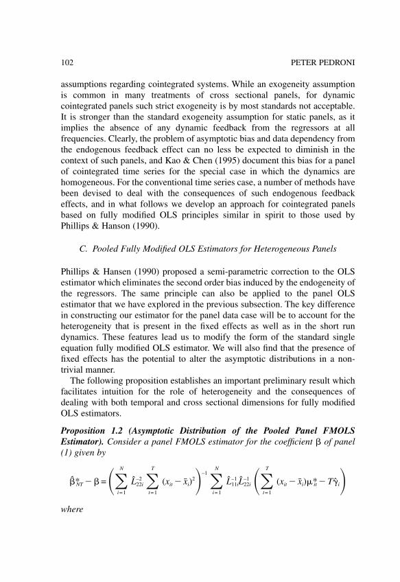
assumptions regarding cointegrated systems. While an exogeneity assumptionis common in many treatments of cross sectional panels, for dynamiccointegrated panels such strict exogeneity is by most standards not acceptable.It is stronger than the standard exogeneity assumption for static panels, as itimplies the absence of any dynamic feedback from the regressors at allfrequencies. Clearly, the problem of asymptotic bias and data dependency fromthe endogenous feedback effect can no less be expected to diminish in thecontext of such panels, and Kao & Chen (1995) document this bias for a panelof cointegrated time series for the special case in which the dynamics arehomogeneous. For the conventional time series case, a number of methods havebeen devised to deal with the consequences of such endogenous feedbackeffects, and in what follows we develop an approach for cointegrated panelsbased on fully modified OLS principles similar in spirit to those used byPhillips & Hanson (1990).

C. Pooled Fully Modified OLS Estimators for Heterogeneous Panels

Phillips & Hansen (1990) proposed a semi-parametric correction to the OLSestimator which eliminates the second order bias induced by the endogeneity ofthe regressors. The same principle can also be applied to the panel OLSestimator that we have explored in the previous subsection. The key differencein constructing our estimator for the panel data case will be to account for theheterogeneity that is present in the fixed effects as well as in the short rundynamics. These features lead us to modify the form of the standard singleequation fully modified OLS estimator. We will also find that the presence offixed effects has the potential to alter the asymptotic distributions in a non-trivial manner.

The following proposition establishes an important preliminary result whichfacilitates intuition for the role of heterogeneity and the consequences ofdealing with both temporal and cross sectional dimensions for fully modifiedOLS estimators.

Proposition 1.2 (Asymptotic Distribution of the Pooled Panel FMOLSEstimator). Consider a panel FMOLS estimator for the coefficient � of panel(1) given by

�*NT � =��i=1

N

L22i–2 �

t=1

T

(xit xi)2–1 �

i=1

N

L11i–1 L22i

–1 ��t=1

T

(xit xi)�*it T�iwhere

102 PETER PEDRONI

�*it = �it L21i

L22i

xit, �i � 21i + �21io

L21i

L22i

( 22i + �22io )

and Li is a lower triangular decomposition of �i as defined in (2) above. Then,under assumptions 1.1 and 1.2, the estimator �*NT converges to the true valueat rate T�N, and is distributed as

T�N(�*NT �)→N(0, v) where v =2 iff xi = yi = 06 else

as T→� and N→�.

As the proposition indicates, when proper modifications are made to theestimator, the corresponding asymptotic distribution will be free of thenuisance parameters associated with any member specific serial correlationpatterns in the data. Notice also that this fully modified panel OLS estimator isasymptotically unbiased for both the standard case without intercepts as well asthe fixed effects model with heterogeneous intercepts. The only difference is inthe size of the variance, which is equal to 2 in the standard case, and 6 in thecase with heterogeneous intercepts, both for xit univariate. More generally,when xit is an m-dimensional vector, the specific values for v will also be afunction of the dimension m. The associated t-statistics, however, will notdepend on the specific values for v, as we shall see.

The fact that this estimator is distributed normally, rather than in terms ofunit root asymptotics as in Phillips & Hansen (1990), derives from the fact thatthese unit root distributions are being averaged over the cross sectionaldimension. Specifically, this averaging process produces normal distributionswhose variance depends only on the moments of the underlying Brownianmotion functionals that describe the properties of the integrated variables. Thisis achieved by constructing the estimator in a way that isolates the idiosyncraticcomponents of the underlying Wiener processes to produce sums of standardand independently distributed Brownian motion whose moments can becomputed algebraically, as the proof of the proposition makes clear. Theestimators L11i and L22i, which correspond to the long run standard errors ofconditional process �it, and the marginal process xit respectively, act to purgethe contribution of these idiosyncratic elements to the endogenous feedback

and serial correlation adjusted statistic �t=1

T

(xit xi)y*it T�i.

The fact that the variance is larger for the fixed effects model in whichheterogeneous intercepts are included stems from the fact that in the presence


of unit roots, the variation from the cross terms of the sample averages xi andyi grows large over time at the same rate T, so that their effect is not eliminatedasymptotically from the distribution of T�N(�*NT �).5 However, since thecontribution to the variance is computable analytically as in the proof ofproposition 1.2, this in itself poses no difficulties for inference. Nevertheless,upon consideration of these expressions, it also becomes apparent that thereshould exist a metric which can directly adjust for this effect in the distributionand consequently render the distribution standard normal. In fact, as thefollowing proposition indicates, it is possible to construct a t-statistic from thisfully modified panel OLS estimator whose distribution will be invariant to thiseffect.

Corollary 1.2 (Asymptotic Distribution of the Pooled Panel FMOLS t-statistic). Consider the following t-statistic for the FMOLS panel estimator of� as defined in proposition 1.2 above. Then under the same assumptions as inproposition 1.2, the statistic is standard normal,

t�*NT= (�*NT �)��

i=1

N

L22i–2 �

t=1

T

(xit xi)21/2

→N(0, 1)

as T→�and N→� for both the standard model without intercepts as well asthe fixed effects model with heterogeneous estimated intercepts.

Again, as the derivation in the appendix makes apparent, because the numeratorof the fully modified estimator �*NT is a sum of mixture normals with zero meanwhose variance depends only on the properties of the Brownian motion

functionals associated with the quadratic �t=1

T

(xit xi)2, the t-statistic con-

structed using this expression will be asymptotically standard normal. This isregardless of the value of v associated with the distribution of T�N(�*NT �)and so will also not depend on the dimensionality of xit in the general vectorcase.

Note, however, that in contrast to the conventional single equation casestudied by Phillips & Hansen (1990), in order to ensure that the distribution ofthis t-statistic is free of nuisance parameters when applied to heterogeneouspanels, the usual asymptotic variance estimator of the denominator is replacedwith the estimator L22i

–2 . By construction, this corresponds to an estimator of theasymptotic variance of the differences for the regressors and can be estimatedaccordingly. This is in contrast to the t-statistic for the conventional singleequation fully modified OLS, which uses an estimator for the conditional

104 PETER PEDRONI

asymptotic variance from the residuals of the cointegrating regression. Thisdistinction may appear puzzling at first, but it stems from the fact that inheterogeneous panels the contribution from the conditional variance of theresiduals is idiosyncratic to the cross sectional member, and must be adjustedfor directly in the construction of the numerator of the �*NT estimator itselfbefore averaging over cross sections. Thus, the conditional variance has alreadybeen implicitly accounted for in the construction of �*NT, and all that is requiredis that the variance from the marginal process xit be purged from the quadratic

�t=1

T

(xit xi)2. Finally, note that proposition 1.2 and its corollary 1.2 have been

specified in terms of a transformation, �*it, of the true residuals. In Section 3 wewill consider various strategies for specifying these statistics in terms ofobservables and consider the small sample properties of the resulting feasiblestatistics.

D. A Group Mean Fully Modified OLS t-Statistic

Before preceding to the small sample properties, we first consider oneadditional asymptotic result that will be of use. Recently Im, Pesaran & Shin(1995) have proposed using a group mean statistic to test for unit roots in paneldata. They note that under certain circumstances, panel unit root tests maysuffer from the fact that the pooled variance estimators need not necessarily beasymptotically independent of the pooled numerator and denominator terms ofthe fixed effects estimator. Notice, however, that the fully modified panel OLSstatistics in proposition 1.2 and corollary 1.2 here have been constructedwithout the use of a pooled variance estimator. Rather, the statistics of thenumerator and denominator have been purged of any influence from thenuisance parameters prior to summing over N. Furthermore, since asymptot-ically the distribution for the numerator is centered around zero, the covariancebetween the summed terms of the numerator and denominator also do not playa role in the asymptotic distribution of T�N(�*NT �) or t�*it

as they wouldotherwise.

Nevertheless, it is also interesting to consider the possibility of a fullymodified OLS group mean statistic in the present context. In particular, thegroup mean t-statistic is useful because it allows one to entertain a somewhatbroader class of hypotheses under the alternative. Specifically, we can think ofthe distinction as follows. The t-statistic for the true panel estimator asdescribed in corollary 1.2 can be used to test the null hypothesis Ho : �i = �o forall i versus the alternative hypothesis Ha : �i = �a ≠ �o for all i where �o is the


hypothesized common value for � under the null, and �a is some alternativevalue for � which is also common to all members of the panel. By contrast, thegroup mean fully modified t-statistic can be used to test the null hypothesisHo : �i = �o for all i versus the alternative hypothesis Ha : �i ≠ �o for all i, so thatthe values for � are not necessarily constrained to be homogeneous acrossdifferent members under the alternative hypothesis.

The following proposition gives the precise form of the panel fully modifiedOLS t-statistic that we propose and gives its asymptotic distributions.

Proposition 1.3 (Asymptotic Distribution of the Panel FMOLS Group Meant-Statistic). Consider the following group mean FMOLS t-statistic for � of thecointegrated panel (1). Then under assumptions 1.1 and 1.2, the statistic isstandard normal, and

t�*NT=

1

�N �i=1

N

L11i–1��

t=1

T

(xit xi)2–1/2 ��

t=1

T

(xit xi)y*it T�i→N(0, 1)

where

y*it = (yit yi) L21i

L22i

xit, �i � 21i + �21io

L21i

L22i

( 22i + �22io )

and Li is a lower triangular decomposition of �i as defined in (2) above, asT→� and N→� for both the standard model without intercepts as well as thefixed effects model with heterogeneous intercepts.

Note that the asymptotic distribution of this group mean statistic is alsoinvariant to whether or not the standard model without intercepts or the fixedeffects model with heterogeneous intercepts has been estimated. Just as withthe previous t-statistic of corollary 1.2, the asymptotic distribution of this panelgroup mean t-statistic will also be independent of the dimensionality of xit forthe more general vector case. Thus, we have presented two different types of t-statistics, a pooled panel OLS based fully modified t-statistic based on the‘within’ dimension of the panel, and a group mean fully modified OLS t-statistic based on the ‘between’ dimension of the panel, both of which areasymptotically unbiased, free of nuisance parameters, and invariant to whetheror not idiosyncratic fixed effects have been estimated. Furthermore, we havecharacterized the asymptotic distribution of the fully modified panel OLSestimator itself, which is also asymptotically unbiased and free of nuisanceparameters, although in this case one should be aware that while thedistribution will be a centered normal, the variance will depend on whetherheterogeneous intercepts have been estimated and on the dimensionality of the

106 PETER PEDRONI

vector of regressors. In the remainder of this chapter we investigate the smallsample properties of feasible statistics associated with these asymptotic resultsand discuss examples of their application.

III. SMALL SAMPLE PROPERTIES OF FEASIBLEPANEL FULLY MODIFIED OLS STATISTICS

In this section we investigate the small sample properties of the pooled andgroup mean panel FMOLS estimators that were developed in the previoussection. We discuss two alternative feasible estimators associated with thepanel FMOLS estimators of proposition 1.2 and its t-statistic, which weredefined only in terms of the true residuals. While these estimators performreasonably well in idealized situations, more generally, size distortions forthese estimators have the potential to be fairly large in small samples, as wasreported in Pedroni (1996a). By contrast, we find that the group mean teststatistics do very well and exhibit relatively little size distortion even inrelatively small panels even in the presence of substantial cross sectionalheterogeniety of the error process associated with the dynamics around thecointegrating vector. Consequently, after discussing some of the basicproperties of the feasible versions of the pooled estimators and the associateddifficulties for small samples, we focus here on reporting the small sampleproperties of the group mean test statistics, which are found to do extremelywell provided that the time series dimension is not smaller than the crosssectional dimension.

A. General Properties of the Feasible Estimators

First, before reporting the results for the between dimension group mean teststatistic, we discuss the general properties of various feasible forms of thewithin dimension pooled panel fully modified OLS statistics and consider theconsequences of these properties in small samples. One obvious candidate fora feasible estimator based on proposition 1.2 would be to simply construct thestatistic in terms of estimated residuals, which can be obtained from the initialN single equation OLS regressions associated with the cointegrating regressionfor (1). Since the single equation OLS estimator is superconsistent, one mighthope that this produces a reasonably well behaved statistic for the panelFMOLS estimator. The potential problem with this reasoning stems from thefact that although the OLS regression is superconsistent it is also asymptot-ically biased in general. While this is a second order effect for the conventional


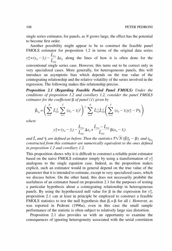
single series estimator, for panels, as N grows large, the effect has the potentialto become first order.

Another possibility might appear to be to construct the feasible panelFMOLS estimator for proposition 1.2 in terms of the original data series


L22i

xit along the lines of how it is often done for the

conventional single series case. However, this turns out to be correct only invery specialized cases. More generally, for heterogeneous panels, this willintroduce an asymptotic bias which depends on the true value of thecointegrating relationship and the relative volatility of the series involved in theregression. The following makes this relationship precise.

Proposition 2.1 (Regarding Feasible Pooled Panel FMOLS) Under theconditions of proposition 1.2 and corollary 1.2, consider the panel FMOLSestimator for the coefficient � of panel (1) given by

�*NT=��

i=1

N

L22i–2 �

t=1

T

(xit xi)2–1 �

i=1

N

L11i–1 L22i

–1��t=1

T

(xit xi)y*it T�iwhere


L22i

xit +L11i L22i

L22i

�(xit xi)

and Li and �i are defined as before. Then the statistics T�N (�*NT �) and t�*NT

constructed from this estimator are numerically equivalent to the ones definedin proposition 1.2 and corollary 1.2.

This proposition shows why it is difficult to construct a reliable point estimatorbased on the naive FMOLS estimator simply by using a transformation of y*itanalogous to the single equation case. Indeed, as the proposition makesexplicit, such an estimator would in general depend on the true value of theparameter that it is intended to estimate, except in very specialized cases, whichwe discuss below. On the other hand, this does not necessarily prohibit theusefulness of an estimator based on proposition 2.1 for the purposes of testinga particular hypothesis about a cointegrating relationship in heterogeneouspanels. By using the hypothesized null value for � in the expression for y*it,proposition 2.1 can at least in principle be employed to construct a feasibleFMOLS statistics to test the null hypothesis that �i = � for all i. However, aswas reported in Pedroni (1996a), even in this case the small sampleperformance of the statistic is often subject to relatively large size distortion.

Proposition 2.1 also provides us with an opportunity to examine theconsequences of ignoring heterogeneity associated with the serial correlation

108 PETER PEDRONI

dynamics for the error process for this type of estimator. In particular, wenotice that the modification involved in this estimator relative to the conventialtime series fully modified OLS estimator differs in two respects. First, itincludes the estimators L11i and L22i that premultiply the numerator anddenominator terms to control for the idiosyncratic serial correlation propertiesof individual cross sectional members prior to summing over N. Secondly, andmore importantly, it includes in the transformation of the dependent variable y*it

an additional term L11i L22i

L22i

�(xit xi). This term is eliminated only in two

special cases: (1) The elements L11i and L22i are identical for all members of thepanel, and do not need to be indexed by i. This corresponds to the case in whichthe serial correlation structure of the data is homogeneous for all members ofthe panel. (2) The elements L11i and L22i are perhaps heterogeneous acrossmembers of the panel, but for each panel L11i = L22i. This corresponds to the casein which asymptotic variances of the dependent and independent variables arethe same. Conversely, the effect of this term increases as (1) the dynamicsbecome more heterogeneous for the panel, and (2) as the relative volatilitybecomes more different between the variables xit and yit for any individualmembers of the panel. For most panels of interest, these are likely to beimportant practical considerations. On the other hand, if the data are known tobe relatively homogeneous or simple in its serial correlation structure, theimprecise estimation of these elements will decrease the attractiveness of thistype of estimator relative to one that implicitly imposes these knownrestrictions.

B. Monte Carlo Simulation Results

We now study small sample properties in a series of Monte Carlo simulations.Given the difficulties associated with the feasible versions of the withindimension pooled panel fully modified OLS estimators discussed in theprevious subsection based on proposition 2.1, it is not surprising that these tendto exhibit relatively large size distortions in certain scenarios, as reported in thePedroni (1996a). Kao & Chiang (1997) subsequently also confirmed the poorsmall sample properties of the within dimension pooled panel fully modifiedestimator based on a version in which a first stage OLS estimate was used forthe adjustment term. Indeed, such results should not be surprising given that thefirst stage OLS estimator introduces a second order bias in the presence ofendogeneity, which is not eliminated asymptotically. Consequently, this biasleads to size distortion for the panel which is not necessarily eliminated evenwhen the sample size grows large. By contrast, the feasible version of the


between dimension group mean estimator does not require such an adjustmentterm even in the presence of heterogeneous serial correlation dynamics, anddoes not suffer from the same size distortion.6 Consequently, we focus here onreporting the small sample Monte Carlo results for the between dimensiongroup mean estimator and refer readers to Pedroni (1996a) for simulationresults for the feasible versions of the within dimension pooled estimators.

To facilitate comparison with the conventional time series literature, we useas a starting point a few Monte Carlo simulations analogous to the ones studiedin Phillips & Loretan (1991) and Phillips & Hansen (1990) based on theiroriginal work on FMOLS estimators for conventional time series. Followingthese studies, we model the errors for the data generating process in terms ofa vector MA(1) process and consider the consequences of varying certain keyparameters. In particular, for the purposes of the Monte Carlo simulations, wemodel our data generating process for the cointegrated panel (1) underassumptions 1.1 and 1.2 as

yit = �i + �xit + �it

xit = xit1 + �it

i = 1, . . . , N, t = 1, . . . , T, for which we model the vector error process�it = (�it, �it) in terms of a vector moving average process given by

�it = �it �i�it1; �it ~ i.i.d. N(0, �i) (3)

where �i is a 2 � 2 coefficient matrix and �i is a 2 � 2 contemporaneouscovariance matrix. In order to accommodate the potentially heterogeneousnature of these dynamics among different members of the panel, we haveindexed these parameters by the subscript i. We will then allow theseparameters to be drawn from uniform distributions according to the particularexperiment. Likewise, for each of the experiments we draw the fixed effects �i

from a uniform distribution, such that �i ~ U(2.0, 4.0).We consider first as a benchmark case an experiment which captures much

of the richness of the error process studied in Phillips & Loretan (1991) and yetalso permits considerable heterogeneity among individual members of thepanel. In their study, Phillips & Loretan (1991), following Phillips & Hansen(1990), fix the following parameters �11i = 0.3, �12i = 0.4, �22i = 0.6,�11i = �22i = 1.0, � = 2.0 and then permit �21i and �21i to vary. The coefficient�21i is particularly interesting since a non-zero value for this parameter reflectsan absence of even weak exogeneity for the regressors in the cointegratingregression associated with (1), and is captured by the term L21i in the panelFMOLS statistics. For our heterogeneous panel, we therefore set�11i = �22i = 1.0, � = 2.0 and draw the remaining parameters from uniform

110 PETER PEDRONI

distributions which are centered around the parameter values set by Phillips &Loretan (1991), but deviate by up to 0.4 in either direction for the elements of�i and by up to 0.85 in either direction for �21i. Thus, in our first experiment,the parameters are drawn as follows: �11i ~ U(–0.1, 0.7), �12i ~ (0.0, 0.8),�21i ~ U(0.0, 0.8), �22i ~ U(0.2, 1.0) and �21i ~ U(–0.85, 0.85). This specificationachieves considerable heterogeneity across individual members and also allowsthe key parameters �21i and �21i to span the set of values considered in Phillipsand Loretan’s study. In this first experiment we restrict the values of �21i to spanonly the positive set of values considered in Phillips and Loretan for thisparameter. In several cases Phillips and Loretan found negative values for �21i

to be particularly problematic in terms of size distortion for many of theconventional test statistics applied to pure time series, and in our subsequentexperiments we also consider the consequences of drawing negative values forthis coefficient. In each case, the asymptotic covariances were estimatedindividually for each member i of the cross section using the Newey-West(1987) estimator. In setting the lag length for the band width, we employ thedata dependent scheme recommended in Newey & West (1994), which is to set

the lag truncation to the nearest integer given by K = 4� T1002/9

, where T is the

number of sample observations over time. Since we consider small sampleresults for panels ranging in dimension from T = 10 to T = 100 by increments of10, this implies that the lag truncation ranges from 2 to 4. For the crosssectional dimension, we consider small sample results for N = 10, N = 20 andN = 30 for each of these values of T.

Results for the first experiment, with �21i ~ U(0.0, 0.8) are reported in TableI of Appendix B. The first column of results reports the bias of the pointestimator and the second column reports the associated standard error of thesampling distribution. Clearly, the biases are small at –0.058 even in extremecases when both the N and T dimensions are as small as N = 10, T = 10 andbecome minuscule as the T dimension grows larger. At N = 10, T = 30 the biasis already down to –0.009, and at T = 100 it goes to –0.001. This should beanticipated, since the estimators are superconsistent and converge at rate T�N,so that even for relatively small dimensions the estimators are extremelyprecise. Furthermore, the Monte Carlo simulations confirm that the bias isreduced more quickly with respect to growth in the T dimension than withrespect to growth in the N dimension. For example, the biases are much smallerfor T = 30, N = 10 than for T = 10, N = 30 for all of the experiments. Thestandard errors in column two confirm that the sampling variance around these


biases are also very small. Similar results continue to hold in subsequentexperiments with negative moving average coefficients, regardless of the datagenerating process for the serial correlation processes. Consequently, the firstthing to note is that these estimators are extremely accurate even in panels withvery heterogeneous serial correlation dynamics, fixed effects and endogenousregressors.

Of course these findings on bias should not come as a surprise given thesuperconsistency results presented in the previous section. Instead, a morecentral concern for the purposes of inference are the small sample properties ofthe associated t-statistic and the possibility for size distortion. For this, weconsider the performance of the small sample sizes of the test under the nullhypothesis for various nominal sizes based on the asymptotic distribution.Specifically, the last two columns report the Monte Carlo small sample resultsfor the nominal 5% and 10% p-values respectively for a two sided test of thenull hypothesis � = 2.0. As a general rule, we find that the size distortions inthese small samples are remarkably small provided that the time seriesdimension, T, is not smaller than the cross sectional dimension, N. The reasonfor this condition stems primarily as a consequence of the estimation of thefixed effects. The number of fixed effects, �i, grows with the N dimension ofthe panel. On the other hand, each of these N fixed effects are estimatedconsistently as T grows large, so that �i �i goes to zero only as T grows large.Accordingly, we require T to grow faster than N in order to eliminate this effectasymptotically for the panel. As a practical consequence, small sample sizedistortion tends to be high when N is large relative to T, and decreases as Tbecomes large relative to N, which can be anticipated in any fixed effectsmodel. As we can see from the results in Table I, in cases when N exceeds T,the size distortions are large, with actual sizes exceeding 30 and 40% whenT = 10 and N grows from 10 to 20 and 30. This represents an unattractivescenario, since in this case, the tests are likely to report rejections of the nullhypothesis when in fact it is not warranted. However, these represent extremecases, as the techniques are designed to deal with the opposite case, where theT dimension is reasonably large relative to the N dimension. In these cases,even when the T dimension is only slightly larger than the N dimension, andeven in cases where it is comparable, we find that the size distortion isremarkably small. For example, in the results reported in Table I we find thatwith N = 20, T = 40 the size of the nominal 5% and 10% tests becomes 4.5%and 9.3% respectively. Similarly, for N = 10, T = 30 the sizes for the MonteCarlo sample become 6.1% and 11% respectively, and for N = 30, T = 60, theybecome 4.7% and 9.6%. As the T dimension grows even larger for a fixed Ndimension, the tests tend to become slightly undersized, with the actual size

112 PETER PEDRONI

becoming slightly smaller than the nominal size. In this case the small sampletests actually become slightly more conservative than one would anticipatebased on the asymptotic critical values.

Next, we consider the case in which the values for �21i span negativenumbers, and for the experiment reported in Table II of Appendix B we drawthis coefficient from �21i ~ U(–0.8, 0.0). Large negative values for movingaverage coefficients are well known to create size distortion for suchestimators, and we anticipate this to be a case in which we have higher smallsample distortion. It is interesting to note that in this case the biases for thepoint estimate become slightly positive, although as mentioned before, theycontinue to be very small. The small sample size distortions follow the samepattern in that they tend to be largest when T is small relative to N and decreaseas T grows larger. In this case, as anticipated, they tend to be higher than for thecase in which �21i spans only positive values. However, the values still fallwithin a fairly reasonable range considering that we are dealing with allnegative values for �21i. For example, with N = 10, T = 100 we have values of6.3% and 12% for the 5% and 10% nominal sizes respectively. For N = 20,T = 100 they become 9% and 15.6% respectively. These are still remarkablysmall compared to the size distortions reported in Phillips & Loretan (1991) forthe conventional time series case.

Finally, we ran a third experiment in which we allowed the values for �21i tospan both positive and negative values so that we draw the values from�21i ~ U(–0.4, 0.4). We consider this to be a fairly realistic case, and thiscorresponds closely to the range of moving average coefficients that wereestimated in the purchasing power parity study contained in Pedroni (1996a).We find the group mean estimator and test statistic to perform very well in thissituation. The Monte Carlo simulation results for this case are reported in TableIII of Appendix B. Whereas the biases for the case with large positive valuesof �21i in Table I were negative, and for the case with large negative values inTable II were positive, here we find the biases to be positive and often evensmaller in absolute value than either of the first two cases. Most importantly,we find the size distortions for the t-statistic to be much smaller here than in thecase where we have exclusively negative values for �21i. For example, withN = 30, and T as small as T = 60, we find the nominal 5% and 10% sizes to be5.4% and 10.5%. Again, generally the small sample sizes for the test are quiteclose to the asymptotic nominal sizes provided that the T dimension is notsmaller than the N dimension. Consequently, it appears to be the case that evenwhen some members of the panel exhibit negative moving average coefficients,as long as other members exhibit positive values, the distortions tend to beaveraged out so that the small sample sizes for the group mean statistic stay


very close to the asymptotic sizes. Thus, we conclude that in general when theT dimension is not smaller than the N dimension, the asymptotic normalityresult appears to provide a very good benchmark for the sampling distributionunder the null hypothesis, even in relatively small samples with heterogeneousserial correlation dynamics.

Finally, although power is generally not a concern for such panel tests, sincethe power is generally quite high, it is worth mentioning the small samplepower properties of the group mean estimator. Specifically, we experimentedby checking the small sample power of the test against the alternativehypothesis by generating the 10,000 draws for the DGP associated with case 3above with � = 1.9. For the test of the null hypothesis that � = 2.0 against thealternative hypothesis that � = 1.9, we found that the power for the 10% p-valuetest reached 100% for N = 10 when T was 40 or more (or 98.2% when T = 30)and reached 100% for N = 20 when T was 30 or more, and for N = 30 the powerreached 100% already when T was 20 or more. Consequently, considering thehigh power and the relatively small size distortion, we find the small sampleproperties of the estimator and associated t-statistic to be extremely wellbehaved in the cases for which it was designed.

IV. ESTIMATION ALGORITHM AND SOME EXAMPLESOF APPLICATIONS7

In this section we describe the algorithm for computing the panel FMOLSestimators and their associated test statistics and then discuss a few examplesof their use. In summary, we can compute any one the desired statistics byperforming the following steps:1. Estimate the panel regression and collect the residuals. Specifically one

should estimate the desired panel cointegration regression, making sure toinclude any desired intercepts, or common time dummies in the regression,and then collect the residuals �i,t for each of the members of the panel. If theslopes are homogeneous, the common time dummy effects can beeliminated more simply by first demeaning the data over the time dimensionprior to estimating the regression. Thus, construct yit yt, xit xt for eachvariable, where yt = N–1 �i=1

N yit, xt = N–1 �i=1N xit prior to estimating the

regression, and prior to the following steps.2. Estimate the long run covariances and autocovariances of the errors. Use

the estimated residuals from part (1) plus the differences of each of theregressors to construct a vector error series �it = (�it, ��it)�. Note that thesecond element is a vector of dimension m, where m corresponds to thenumber of regressors. Now use any long run covariance matrix estimator,

114 PETER PEDRONI

such as the Newey-West (1987) estimator to estimate the elements of thelong run covariance �i and the autocovariances i. This can be done byapplying the estimator to the entire m + 1 vector �it = (�it, ��it)� to produce an(m + 1) � (m + 1) long run covariance matrix and autocovariances matrix.The elements of �i and i then correspond to partitions of the(m + 1) � (m + 1) long run covariance matrix and autocovariance matrixrespectively. Specifically, the far upper right scalar element of the(m + 1) � (m + 1) long run covariance matrix corresponds to �11i. The lowerm � m partition corresponds to �22i, which is an m � m matrix representingthe long run covariance among the regressors, and the remaining m elementsin the column below the far upper right scalar element correspond to �21i.Since the covariance matrix is symmetric, �12i = �21i. The same mappingcorresponds the partitions of the (m + 1) � (m + 1) autocovariance matrix andthe elements of i, except that unlike �i, the autocovariance matrix i is notsymmetric, so 12i ≠ �21i, and these elements must be extracted from thecorresponding column and row partitions separately. Once �i has beenconstructed, apply a Cholesky style triangularization to obtain the elementsof the matrix Li. Finally, we will use an estimate of the standardcontemporaneous covariance matrix, �i

o, for the elements of �it = (�it, ��it)�,similarly partitioned.

3. Construct the estimator. Now we have all of the pieces required to constructthe estimators. Each estimator uses a serial correlation correction term, �i,which can be constructed from the pieces obtained in part (2) above, as

�i � 21i + �21io

L21i

L22i

( 22i + �22io )

Next, using the elements of Li, the expression for y*it = (yit yi) L21i

L22i

xit can be

constructed from the original data. Then the final step is to construct the crossproduct terms between y*it and (xit xi). This is sufficient now to compute eitherthe point estimators or the associated t-statistics for any of the statistics.

It is worth noting two points here. The difference between the panel ‘within’dimension estimators and the group mean ‘between’ dimension estimators is inthe way in which the cross product terms are computed. For the ‘within’dimension statistics, the cross product terms are computed by summing overthe T and N dimensions separately for the numerator and the denominator. Forthe group mean ‘between’ dimension statistics, the cross product terms arecomputed by summing over the T dimension for the numerator anddenominator separately, and then summing over the N dimension for the entireratio. Consequently, the first point to note is that the algorithm as applied to the


group mean estimator describes the same steps that one would take if one wereestimating N different conventional FMOLS estimators and then taking theaverage of these. The same is true for the group mean t-statistic. Thus, if onealready has a routine to estimate the conventional time series FMOLSestimator, then the group mean panel FMOLS estimator is extremely simpleand convenient to estimate. The second point to note is that for the panelFMOLS ‘within’ dimension estimator we have used the estimates of �i, i, �i

o

and �i to compute the weighted panel variances. But it is equally feasible tocompute the unweighted panel variances by first averaging the values �i, i, �i

o

before applying the transformations. Whether or not the two differenttreatments has much consequence for the estimate is likely to depend on howheterogeneous the values of �i are across individual members.

Next, we briefly describe a few examples of the use of these panel FMOLSestimators. One obvious application is to the exchange rate literature, and inparticular the purchasing power parity literature. Long run absolute or strongpurchasing power parity predicts that nominal exchange rates and aggregateprice ratios among countries should be cointegrated with a unit cointegratingvector, so that the real exchange rate is stationary. However, panel unit roottests based on Levin & Lin (1993) have generally found mixed results. See forexample Oh (1996) and Papell (1997) and Wu (1996) among others. On theother hand, panel cointegration tests based on Pedroni (1995, 1997a) havegenerally rejected the null of no cointegration. See for example Canzoneri,Cumby & Diba (1996), Chinn (1997) and Taylor (1996) among others forthese. By contrast, long run relative or weak purchasing power parity simplypredicts that the nominal exchange rate and aggregate price ratios will becointegrated, though not necessarily with a unit cointegrating vector. The panelFMOLS estimators presented in this paper are an obvious way to distinguishbetween these two hypothesis, and Pedroni (1996a, 1999) uses these panelFMOLS estimators to show that only the relative, weak form of purchasingpower parity holds for a panel of post Bretton Woods period floating exchangerates. The latter paper contrasts results for both a parametric group mean DOLSestimator and nonparametric group mean FMOLS estimator for the weakpurchasing power parity test. In a similar spirit, Alexius & Nilson (2000),Canzoneri, Cumby & Diba (1996), Chinn (1997) apply these panel FMOLStests from Pedroni (1996a) to test the Samuelson-Balassa hypothesis that longrun movements of real exchange rates are driven by differences in long runrelative productivities among countries.

Other examples of the use of these panel FMOLS tests have been to thegrowth literature. Neusser & Kugler (1998) use the tests from Pedroni (1996a)to investigate the connection between financial development and growth. Kao,

116 PETER PEDRONI

Chiang & Chen (1999) use a panel FMOLS estimator and compare it to a panelDOLS estimator to investigate the connection between research and develop-ment expenditure and growth. Keller & Pedroni (1999) use the group meanpanel estimator presented in this chapter to study the mechanism by whichimported R&D impacts growth at the industry level and demonstrate theattractiveness of the more flexible form of the group mean estimator. Canning& Pedroni (1999) use the same group mean panel FMOLS test as a first stepestimator to construct a test for the direction of long run causality betweenpublic infrastructure and long run growth. Finally Pedroni & Wen (2000) makeuse of the group mean panel FMOLS estimator as a first step estimator in anoverlapping generations model to identify the position of the U.S., Japaneseand European economies relative to the golden rule, and the extent to whichsocial security transfer programs can move economies closer to this position.

This is just a brief summary of the application of these estimators to twoliteratures, the exchange rate and growth literatures. Needless to say, manypotential applications exist beyond these two literatures.

V. DISCUSSION OF FURTHER RESEARCH ANDCONCLUDING REMARKS

We have explored in this chapter methods for testing and making inferencesabout cointegrating vectors in heterogeneous panels based on fully modifiedOLS principles. When properly constructed to take account of potentialheterogeneity in the idiosyncratic dynamics and fixed effects associated withsuch panels, the asymptotic distributions for these estimators can be made to becentered around the true value and will be free of nuisance parameters.Furthermore, based on Monte Carlos simulations we have shown that inparticular the t-statistic constructed from the between dimension group meanestimator performs very well in that in exhibits relatively little small samplesize distortion. To date, the techniques developed in this study have beenemployed successfully in a number of applications, and it will be interesting tosee if the panel FMOLS methods developed in this paper fare equally well inother scenarios.

The area of research and application of nonstationary panel methods israpidly expanding, and we take this opportunity to remark on a few furtherissues of current and future research as they relate to the subject of this chapter.As we have already discussed, the between dimension group mean estimatorhas an advantage over the within dimension pooled estimators presented in thischapter in that it permits a more flexible alternative hypothesis that allows forheterogeneity of the cointegrating vector. In many cases it is not known a priori


whether heterogeneity of the cointegrating vector can be ruled out, and it wouldbe particularly nice to test the null hypothesis that the cointegrating vectors areheterogeneous in such panels with heterogeneous dynamics. In this context,Pedroni (1998) provides a technique that allows one to test such a nullhypothesis against the alternative hypothesis that they are homogeneous anddemonstrates how the technique can be used to test whether convergence in theSolow growth model occurs to distinct versus common steady states for theSummers and Heston data set.

Another important issue that is often raised for these types of panels pertainsto the assumption of cross sectional independence as per assumption 1.2 in thischapter. The standard approach is to use common time dummies, which inmany cases is sufficient to deal with cross sectional dependence. However, insome cases, common time dummies may not be sufficient, particularly whenthe cross sectional dependence is not limited to contemporaneous effects and isdynamic in nature. Pedroni (1997b) proposes an asymptotic covarianceweighted GLS approach to deal with such dynamic cross sectional dependencefor the case in which the time series dimension is considerably larger than thecross sectional dimension, and applies the panel fully modified form of the testto the purchasing power parity hypothesis using monthly OECD exchange ratedata. It is interesting to note, however, that for this particular application, takingaccount of such cross sectional dependencies does not appear to impact theconclusions and it is possible that in many cases cross sectional dependencedoes not play as large a role as one might anticipate once common timedummies have been included, although this remains an open question.

Another important issue is parameteric versus non-parametric estimation ofnuisance parameters. Clearly, any of the estimators presented here can beimplemented by taking care of the nuisance parameter effects eithernonparameterically using kernel estimators, or parametrically, as for exampleusing dynamic OLS corrections. Generally speaking, non-parametric estima-tion tends to be more robust, since one does not need to assume a specificparametric form. On the other hand, since non-parametric estimation relies onfewer assumptions, it generally requires more data than parametric estimation.Consequently, for conventional time series tests, when data is limited it is oftenworth making specific parameteric assumptions. For panels, on the other hand,the greater abundance of data suggests an opportunity to take advantage of thegreater robustness of nonparametric methods, though ultimately the choicemay simply be a matter of taste. The Monte Carlo simulation results providedhere demonstrate that even in the presence of considerable heterogeneity, non-parametric correction methods do very well for the group mean estimator andthe corresponding t-statistic.

118 PETER PEDRONI

NOTES

1. The results in section 2 and appendix A first appeared in Pedroni (1996a). TheIndiana University working paper series is available at http://www.indiana.edu/ iuecon/workpaps/

2. In fact the computer program which accompanies this paper also allows one toimplement these tests for any arbitrary number of regressors. It is available upon requestfrom the author at [email protected]

3. See Phillips & Moon (1999) for a recent formal study of the regularity conditionsrequired for the use of sequential limit theory in panel data and a set of conditions underwhich sequential limits imply joint limits, including the case in which the long runvariances differ among members of the panel.

4. These results are for the OLS estimator when the variables are cointegrated. Arelated stream of the literature studies the properties of the panel OLS estimator whenthe variables are not cointegrated and the regression is spurious. See for example Entorf(1997), Kao (1999), Phillips & Moon (1999) and Pedroni (1993, 1997a) on spuriousregression in nonstationary panels.

5. A separate issue pertains to differences between the sample averages and the truepopulation means. Since we are treating the asymptotics sequentially, this differencegoes to zero as T grows large prior to averaging over N, and thus does not impact thelimiting distribution. Otherwise, more generally we would require that the ratio N/Tgoes to zero as N and T grow large in order to ensure that these differences do notimpact the limiting distribution. We return to this point in the discussion of the smallsample properties in section 3.2.

6. Of course this is not to say that all within dimension estimators will necessarilysuffer from this particular form of size distortion, and it is likely that some forms of thepooled FMOLS estimator will be better behaved than others. Nevertheless, given theother attractive features of the between dimension group mean estimator, we focus hereon reporting the very attractive small sample properties of this estimator.

7. I am grateful to an anonymous referee for suggesting this section.

ACKNOWLEDGMENTS

I thank especially Bob Cumby, Bruce Hansen, Roger Moon, Peter Phillips,Norman Swanson and Pravin Trivedi and two anonymous referees for helpfulcomments and suggestions on various earlier versions, and Maria Arbatskayafor research assistance. The paper has also benefitted from presentations at theJune 1996 North American Econometric Society Summer Meetings, the April1996 Midwest International Economics Meetings, and workshop seminars atRice University-University of Houston, Southern Methodist University, TheFederal Reserve Bank of Kansas City, U. C. Santa Cruz and WashingtonUniversity. The current version of the paper was completed while I was avisitor at the Department of Economics at Cornell University, and I thank themembers of the Department for their generous hospitality. A computer program


which implements these tests is available upon request from the author [email protected]

REFERENCES

Alexius, A., & Nilson, J. (2000). Real Exchange Rates and Fundamentals: Evidence from 15OECD Countries. Open Economies Review, forthcoming.

Canning, D., & Pedroni, P. (1999). Infrastructure and Long Run Economic Growth. CAE Workingpaper, No. 99–09, Cornell University.

Canzoneri M., Cumby, R., & Diba, B. (1996). Relative Labor Productivity and the Real ExchangeRate in the Long Run: Evidence for a Panel of OECD Countries. NBER Working paper No.5676.

Chinn, M. (1997). Sectoral Productivity, Government Spending and Real Exchange Rates:Empirical Evidence for OECD Countries. NBER Working paper No. 6017.

Chinn, M., & Johnson, L. (1996). Real Exchange Rate Levels, Productivity and Demand Shocks:Evidence from a Panel of 14 Countries. NBER Working paper No. 5709.

Entorf, H. (1997). Random Walks and Drifts: Nonsense Regression and Spurious Fixed-EffectEstimation’. Journal of Econometrics, 80, 287–96.

Evans, P., & Karras, G. (1996). Convergence Revisited. Journal of Monetary Economics, 37,249–265.

Im, K., Pesaran, H., & Shin, Y. (1995). Testing for Unit Roots in Heterogeneous Panels. Workingpaper, Department of Economics, University of Cambridge.

Kao, C. (1999). Spurious Regression and Residual-Based Tests for Cointegration in Panel Data’.Journal of Econometrics, 90, 1–44.

Kao, C., & Chen, B. (1995). On the Estimation and Inference of a Cointegrated Regression inPanel Data When the Cross-section and Time-series Dimensions Are Comparable inMagnitude. Working paper, Department of Economics, Syracuse University.

Kao, C., & Chiang, M. (1997). On the Estimation and Inference of a Cointegrated Regression InPanel Data. Working paper, Department of Economics, Syracuse University.

Kao, C., Chiang, M., & Chen, B. (1999). International R&D Spillovers: An Application ofEstimation and Inference in Panel Cointegration. Oxford Bulletin of Economics andStatistics, 61(4), 691–709.

Keller, W., & Pedroni, P. (1999). Does Trade Affect Growth? Estimating R&D Driven Models ofTrade and Growth at the Industry Level. Working paper, Department of Economics, IndianaUniversity and University of Texas.

Levin, A., & Lin, F. (1993). Unit Root Tests in Panel Data; Asymptotic and Finite-sampleProperties. Working paper, Department of Economic, U. C. San Diego.

Mark, N., & Sul, D. (1999). A Computationally Simple Cointegration Vector Estimator for PanelData. Working paper, Department of Economics, Ohio State University.

Neusser, K., & Kugler, M. (1998). Manufacturing Growth and Financial Development: Evidencefrom OECD Countries. Review of Economics and Statistics, 80, 638–646.

Newey, W., & West, K. (1987). A Simple, Positive Semi-Definite, Heteroskedasticity andAutocorrelation Consistent Coariance Matrix. Econometrica, 55, 703–708.

Newey, W., & West, K. (1994). Autocovariance Lag Selection in Covariance Matrix Estimation’.Review of Economic Studies, 61, 631–653.

120 PETER PEDRONI

Obstfeld M., & Taylor, A. (1996). International Capital-Market Integration over the Long Run:The Great Depression as a Watershed. Working paper, Department of Economics, U. C.Berkeley.

Oh, K. (1996). Purchasing Power Parity and Unit Root Tests Using Panel Data’. Journal ofInternational Money and Finance, 15, 405–418.

Papell, D. (1997). Searching for Stationarity: Purchasing Power Parity Under the Current Float’.Journal of International Economics, 43, 313–32.

Pedroni, P. (1993). Panel Cointegration. Chapter 2 in Panel Cointegration, Endogenous GrowthAnd Business Cycles in Open Economies, Columbia University Dissertation, Ann Arbor,MI: UMI Publishers.

Pedroni, P. (1995). Panel Cointegration; Asymptotic and Finite Sample Properties of Pooled TimeSeries Tests, With an Application to the PPP Hypothesis. Working paper, Department ofEconomics, No. 95–013, Indiana University.

Pedroni, P. (1996a). Fully Modified OLS for Heterogeneous Cointegrated Panels and the Case ofPurchasing Power Parity. Working paper No. 96–020, Department of Economics, IndianaUniversity.

Pedroni, P. (1996b). Human Capital, Endogenous Growth, & Cointegration for Multi-CountryPanels. Working paper, Department of Economics, Indiana University.

Pedroni, P. (1997a). Panel Cointegration; Asymptotic and Finite Sample Properties of Pooled TimeSeries Tests, With an Application to the PPP Hypothesis; New Results. Working paper,Department of Economics, Indiana University.

Pedroni, P. (1997b). On the Role of Cross Sectional Dependency in Dynamic Panel Unit Root andPanel Cointegration Exchange Rate Studies. Working paper, Department of Economics,Indiana University.

Pedroni, P. (1998). Testing for Convergence to Common Steady States in NonstationaryHeterogeneous Panels. Working paper, Department of Economics, Indiana University.

Pedroni, P. (1999). Purchasing Power Parity Tests in Cointegrated Panels. Working paper,Department of Economics, Indiana University.

Pedroni, P., & Wen, Y. (2000). Government and Dynamic Efficiency. Working paper, Departmentof Economics, Cornell University and Indiana University.

Pesaran, H., & Smith, R. (1995). Estimating Long Run Relationships from DynamicHeterogeneous Panels. Journal of Econometrics, 68, 79–114.

Phillips, P., & Durlauf, S. (1986). Multiple Time Series Regressions with Integrated Processes’.Review of Economic Studies, 53, 473–495.

Phillips, P., & Hansen, B. (1990). Statistical Inference in Instrumental Variables Regression withI(1) Processes. Review of Economic Studies, 57, 99–125.

Phillips, P., & Loretan, M. (1991). Estimating Long-run Economic Equilibria. Review of EconomicStudies, 58, 407–436.

Phillips, P., & Moon, H. (1999). Linear Regression Limit Theory for Nonstationary Panel Data’.Econometrica, 67, 1057–1112.

Quah, D. (1994). Exploiting Cross-Section Variation for Unit Root Inference in Dynamic Data’.Economics Letters, 44, 9–19.

Taylor, A. (1996). International Capital Mobility in History: Purchasing Power Parity in the Long-Run. NBER Working paper No. 5742.

Wu, Y. (1996). Are Real Exchange Rates Nonstationary? Evidence from a Panel-Data Test. Journalof Money Credit and Banking, 28, 54–63.


MATHEMATICAL APPENDIX A

Proposition 1.1: We establish notation here which will be used throughout theremainder of the appendix. Let Zit = Zit–1 + �it where �it = (�it, �it)�. Then byvirtue of assumption 1.1 and the functional central limit theorem,

T –1 �t=1

T

Zit��it →�r=0

1

B(r, �i) dB(r, �i)� + i + �io (A1)

T –2 �t=1

T

ZitZ�it →�r=0

1

B(r, �i)B(r, �i)� dr (A2)

for all i, where Zit = Z it Zi refers to the demeaned discrete time process andB(r, �i) is demeaned vector Brownian motion with asymptotic covariance �i. This vector can be decomposed as B(r, �i) = L�i Wi(r) where Li = �i

1/2 is the

lower triangular decomposition of �i and W(r) =�W1(r) �0

1

W1(r) dr,

W2(r) �0

1

W2(r) dr�is a vector of demeaned standard Brownian motion,

with W1i independent of W2i. Under the null hypothesis, the statistic can bewritten in these terms as

T�N(�NT �) =

1

�N�i=1

N �T–1 �t=1

T

Zit��it21

1N�

i=1

N �T–2�t=1

T

ZitZ�it22

(A3)

Based on (A1), as T→�, the bracketed term of the numerator converges to

��r=0

1

B(r, �i) dB(r, �i)�21

+ 21i + �21io (A4)

the first term of which can be decomposed as

��r=0

1

B(r, �i) dB(r, �i)�21

= L11iL22i�� W2i dW1i W 1i(1)� W2i+ L21iL22i�� W2i dW2i W 2i(1)� W2i (A5)

122 PETER PEDRONI

In order for the distribution of the estimator to be unbiased, it will be necessarythat the expected value of the expression in (A4) be zero. But although theexpected value of the first bracketed term in (A5) is zero, the expected value ofthe second bracketed term is given as

E�L21iL22i�� W2i dW2i W2i(1)� W2i�=12

L21iL22i (A6)

Thus, given that the asymptotic covariance matrix, �i, must have positivediagonals, the expected value of the expression (A4) will be zero only ifL21i = 21i = �21i

o = 0, which corresponds to strict exogeneity of regressors for allmembers of the panel. Finally, even if such strict exogeneity does hold, thevariance of the numerator will still be influenced by the parameters L11i, L22i

which reflect the idiosyncratic serial correlation patterns in the individualcross sectional members. Unless these are homogeneous across members of thepanel, they will lead to non-trivial data dependencies in the asymptoticdistribution.

Proposition 1.2: Continuing with the same notation as above, the fully modifiedstatistic can be written under the null hypothesis as

T�N(�*NT �) =

1

�N�i=1

N

L11i–1 L22i

–1�(0,1) �T–1 �t=1

T

Zit��it�1,L21i

L22i�

�i1N �

i=1

N

L22i–2��T–2 �

t=1

T

ZitZ�it22 (A7)

Thus, based on (A1), as T→�, the bracketed term of the numerator convergesto

��r=0

1

B(r, �i) dB(r, �i)�21

L21i

L22i��

r=0

1

B(r, �i) dB(r, �i)�22

+ 21i + �21io

L21i

L22i

( 22i + �22io ) (A8)

which can be decomposed into the elements of Wi such that


��r=0

1

B(r, �i) dB(r, �i)�21

= L11iL22i�� W2i dW1i W1i(1)� W2i+ L21iL22i�� W2i dW2i W2i(1)� W2i (A9)

��r=0

1

B(r, �i) dB(r, �i)�22

= L22i2 �� W2idW2i W2i(1)� W2i (A10)

where the index r has been omitted for notational simplicity. Thus, if aconsistent estimator of �i is employed, so that �i →�i and consequently Li →Li

and �i →�, then

L11i–1 L22i

–1�(0,1)(T –1 �t=1

T

Zit��it)�1, L21i

L22i�

�i→�

0

1

W2i(r) dW1i(r) W1i(1) �0

1

W2i(r) dr (A11)

where the mean and variance of this expression are given by

E�� W2idW1i W1i(1)� W2idr�= 0 (A12)

E�� W2i dW1i2

2W1i(1)� W2idr� W2idW1i + W1i(1)2�� W2idr2�=

12

2 �13+

13

=16

(A13)

respectively. Now that this expression has been rendered void of anyidiosyncratic components associated with the original B(r, �i), then by virtue ofassumption 1.2 and a standard central limit theorem argument,

1

�N�i=1

N ��0

1

W2i(r) dW1i(r) W1i(1)�0

1

W2i(r) dr→N( 0, 1/6) (A14)

124 PETER PEDRONI

as N→�. Next, consider the bracketed term of the denominator of (A3), whichbased on (A1), as T→�, converges to

��r=0

1

B(r, �i)B(r, �i)�22

= L22i2 ��

0

1

W2i(r)2 dr ��0

1

W2i(r) dr 2 (A15)

Thus,

L22i–2�(T –2 �

t=1

T

ZitZ�it)22

→�0

1

W2i(r)2dr ��0

1

W2i(r) dr2

(A16)

which has finite variance, and a mean given by

E��0

1

W2i(r)2dr ��0

1

W2i(r) dr2�=12

13

=16

(A18)

Again, since this expression has been rendered void of any idiosyncraticcomponents associated with the original B(r, �i), then by virtue of assumption1.2 and a standard law of large numbers argument,

1N�

i=1

N ��0

1

W2i(r)2 dr ��0

1

W2i(r) dr2→16

(A18)

as N→�. Thus, by iterated weak convergence and an application of thecontinuous mapping theorem, T�N(�*NT �)→N(0, 6) for this case whereheterogeneous intercepts have been estimated. Next, recognizing that T –1/2yi-

→�0

1

W1i(r) dr and T –1/2xi →�0

1

W2i(r) dr as T→�, and setting

� W1i =� W2i = 0 for the case where yi = xi=0 gives as a special case of (A13)

and (A17) the results for the distribution in the case with no estimated


intercepts. In this case the mean given by (A12) remains zero, but the variancein (A13) become 1

2 and the mean in (A17) also becomes 12. Thus,

T�N(�*NT �)→N(0, 2) for this case.

Corollary 1.2: In terms of earlier notation, the statistic can be rewritten as:

t�*NT=

1

�N�i=1

N

L11i–1 L22i

–1�(0,1) �T–1 �t=1

T


L22i�

�i�1

N�i=1

N

L22i–2��T–2 �

t=1

T

ZitZ�it22

(A19)

where the numerator converges to the same expression as in proposition 1.2,and the root term of the denominator converges to the same value as inproposition 1.2. Since the distribution of the numerator is centered around zero,the asymptotic distribution of t�*NT

will simply be the distribution of thenumerator divided by the square root of this value from the denominator.Since

E�� W2i dW1i2

2W1i(1)� W2i � W2i dW1i + W1i(1)2�� W2i2�= E�� W 2

2i �� W2i2� (A20)

by (A13) and (A17) regardless of whether or not � W1i,� W2i are set to zero,

then t�*NT→N(0, 1) irrespective of whether xi, yi are

estimated or not.

Proposition 1.3: Write the statistic as:

t�*NT=

1

�N�i=1

N

L11i–2�(0, 1)�T –1 �

t=1

T


L22i�

�i��(T –2 �

t=1

T

ZitZ�it)22–1/2

(A21)

Then the first bracketed term converges to

126 PETER PEDRONI

L11iL22i��0

1

W2i(r) dW1i(r) W1i(1)�0

1

W2i(r) dr~ N�0, L11iL22i �

0

1

W2i(r)2 dr ��0

1

W2i(r) dr2 (A22)

by virtue of the independence of W21i(r) and dW1i(r). Since the second bracketedterm converges to

L22i��0

1

W2i(r)2 dr ��0

1

W2i(r) dr2–1/2

(A23)

then, taken together, for Li →Li, (A21) becomes a standardized sum of i.i.d.

standard normals regardless of whether or not � W1i,� W2i are set to zero,

and thus t�*NT→N(0, 1) by a standard central limit theorem argument

irrespective of whether xi, yi are estimated or not.

Proposition 2.1: Insert the expression for y*it into the numerator and useyit yi = �(xit xi) + �it to give

�*NT =�i=1

N

L11i–1 L22i

–1��t=1

T

(xit xi)(�it L21i

L22i

xit) T�i�i=1

N

L22i2 �

t=1

T

(xit xi)2

+�i=1

N

L11i–1 L22i

–1�1 +L11i L22i

L22i��

t=1

T

(xit xi)2

�i=1

N

L22i–2 �

t=1

T

(xit xi)2

(A24)

Since L22i–2 = L11i

–1 L22i–1�1 +

L11i L22i

L22i, the last term in (A24) reduces to �, thereby

giving the desired result.


APPENDIX B

Table I. Small Sample Performance of Group Mean Panel FMOLS withHeterogeneous Dynamics

Case 1: �21i ~ (0.0, 0.8)

N T bias std error 5% size 10% size

10 10 –0.058 0.115 0.282 0.36220 –0.018 0.047 0.084 0.14530 –0.009 0.029 0.061 0.11040 –0.006 0.020 0.035 0.07650 –0.004 0.016 0.027 0.06260 –0.003 0.012 0.020 0.04970 –0.002 0.010 0.016 0.04480 –0.002 0.009 0.014 0.04090 –0.002 0.008 0.014 0.038

100 –0.001 0.007 0.014 0.037

20 10 –0.034 0.079 0.291 0.37820 –0.012 0.033 0.100 0.16630 –0.006 0.020 0.076 0.13240 –0.004 0.014 0.045 0.09350 –0.003 0.011 0.039 0.08160 –0.003 0.009 0.028 0.06670 –0.002 0.007 0.026 0.05980 –0.002 0.006 0.021 0.05590 –0.002 0.006 0.020 0.050

100 –0.001 0.005 0.018 0.052

30 10 –0.049 0.061 0.386 0.47020 –0.017 0.025 0.156 0.23430 –0.009 0.015 0.107 0.17740 –0.006 0.011 0.072 0.13350 –0.004 0.008 0.059 0.11860 –0.003 0.007 0.047 0.09670 –0.003 0.006 0.039 0.08680 –0.002 0.005 0.035 0.07390 –0.002 0.004 0.032 0.077

100 –0.002 0.004 0.030 0.076

Notes: Based on 10,000 independent draws of the cointegrated system (1)–(3), with� = 2.0, �1i ~ U(2.0, 4.0), �11i = �22i = 1.0, �21i ~ U(–0.85, 0.85) and �11i ~ U(–0.1, 0.7),�12i ~ U(0.0, 0.8), �21i ~ U(0.0, 0.8), �22i ~ U(0.2, 1.0).

128 PETER PEDRONI

Table II. Small Sample Performance of Group Mean Panel FMOLS withHeterogeneous Dynamics

Case 2: �21i ~ U(–0.8, 0.0)


10 10 0.082 0.132 0.422 0.49820 0.041 0.058 0.234 0.32430 0.025 0.037 0.187 0.26840 0.016 0.027 0.137 0.21350 0.012 0.021 0.115 0.18560 0.009 0.017 0.091 0.15570 0.007 0.014 0.087 0.15180 0.006 0.012 0.078 0.14090 0.005 0.011 0.072 0.135

100 0.005 0.010 0.063 0.120

20 10 0.093 0.092 0.581 0.64820 0.043 0.042 0.352 0.44730 0.026 0.027 0.265 0.36140 0.017 0.020 0.205 0.29450 0.012 0.015 0.158 0.24260 0.009 0.012 0.130 0.21170 0.007 0.010 0.117 0.19480 0.006 0.009 0.109 0.18190 0.005 0.008 0.103 0.170

100 0.004 0.007 0.090 0.156

30 10 0.070 0.071 0.563 0.63020 0.033 0.032 0.339 0.43330 0.020 0.020 0.259 0.35240 0.013 0.015 0.196 0.28950 0.009 0.011 0.152 0.23660 0.007 0.009 0.131 0.21170 0.006 0.008 0.113 0.19080 0.005 0.007 0.103 0.17590 0.004 0.006 0.096 0.164

100 0.003 0.005 0.087 0.156

Notes: Based on 10,000 independent draws of the cointegrated system (1)–(3), with� = 2.0, �1i ~ U(2.0, 4.0), �11i = �22i = 1.0, �21i ~ U(–0.85, 0.85) and �11i ~ U(–0.1, 0.7),�12i ~ U(–0.8, 0.0), �21i ~ U(–0.8, 0.0), �22i ~ U(0.2, 1.0).


Table III. Small Sample Performance of Group Mean Panel FMOLS withHeterogeneous Dynamics

Case 3: �21i ~ U(–0.4, 0.4)


10 10 0.009 0.129 0.284 0.36720 0.011 0.052 0.113 0.17930 0.008 0.033 0.086 0.15040 0.005 0.023 0.058 0.11350 0.004 0.018 0.048 0.09360 0.003 0.014 0.039 0.08370 0.002 0.012 0.037 0.07780 0.002 0.011 0.031 0.07290 0.002 0.009 0.029 0.068

100 0.001 0.008 0.028 0.062

20 10 0.028 0.090 0.346 0.43020 0.014 0.037 0.145 0.22230 0.009 0.024 0.106 0.17940 0.006 0.017 0.077 0.13850 0.004 0.013 0.060 0.11460 0.003 0.010 0.048 0.09370 0.002 0.009 0.040 0.08580 0.002 0.008 0.037 0.08390 0.001 0.007 0.035 0.079

100 0.001 0.006 0.035 0.078

30 10 0.008 0.069 0.317 0.40220 0.006 0.028 0.122 0.19430 0.004 0.018 0.095 0.15540 0.003 0.013 0.068 0.12250 0.002 0.010 0.054 0.10560 0.001 0.008 0.044 0.08870 0.001 0.007 0.038 0.08280 0.001 0.006 0.036 0.07690 0.001 0.005 0.033 0.073

100 0.001 0.005 0.036 0.074

Notes: Based on 10,000 independent draws of the cointegrated system (1)–(3), with� = 2.0, �1i ~ U(2.0, 4.0), �11i = �22i = 1.0, �21i ~ U(–0.85, 0.85) and �11î ~ U(–0.1, 0.7),�12i ~ U(–0.4, 0.4), �21i ~ U(–0.4, 0.4), �22i ~ U(0.2, 1.0).

130 PETER PEDRONI

TESTING FOR COMMON CYCLICALFEATURES IN NONSTATIONARYPANEL DATA MODELS

Alain Hecq, Franz C. Palm and Jean-Pierre Urbain

ABSTRACT

In this chapter we extend the concept of serial correlation commonfeatures to panel data models. This analysis is motivated both by the needto develop a methodology to systematically study and test for commonstructures and comovements in panel data with autocorrelation presentand by an increase in efficiency coming from pooling procedures. Wepropose sequential testing procedures and study their properties in a smallscale Monte Carlo analysis. Finally, we apply the framework to the wellknown permanent income hypothesis for 22 OECD countries,1950–1992.

I. INTRODUCTION

In economics it is often of interest to test whether a set of time series movestogether, that is whether the series are driven by some common factors. Thevast literature on cointegration has focussed on long-run comovements fornonstationary time series. More recently, some authors have analyzed theexistence of short-run comovements between stationary time series or betweenfirst differenced cointegrated-I(1) series (see Tiao & Tsay, 1989; Engle &Kozicki, 1993; Gouriéroux & Peaucelle, 1993; Vahid & Engle, 1993; Vahid &


131

Engle, 1997; Ahn, 1997). Among these approaches, the concept of serialcorrelation common features (SCCF hereafter) introduced by Engle & Kozicki(1993) appeared to be useful. It means that stationary time series move togetheras there exist linear combinations of these variables that yield white noiseprocesses. These common feature vectors are measures for analyzing short-runrelationships between economic variables suggested by economic theory suchas relative purchasing power parity (Gouriéroux & Peaucelle, 1993), permanentincome hypothesis (Campbell & Mankiw, 1990, Jobert, 1995), cross-countryreal interest rate differentials (Kugler & Neusser, 1993), real business cyclemodels (Issler & Vahid, 1996), convergence of economies (Beine & Hecq,1997, 1998), Okun’s Law (Candelon & Hecq, 2000).

Serial correlation common features imply the existence of a reduced numberof common dynamic factors explaining short-run comovements in economicvariables. A companion form of the common features models is the commonfactor representation which has been used in macroeconomics for somedecades (see e.g. Engle & Watson, 1981; Geweke, 1977; Lumsdaine & Prasad,1997; Singleton, 1980). Beyond economic considerations, through the reduced-rank restrictions, the existence of common features is likely to lead to areduction of the number of parameters to be estimated. In general, imposingcommon cyclical feature restrictions when they are appropriate will induce anincrease in estimation efficiency (Lütkepohl, 1991) and accuracy of forecasts(Vahid & Issler, 1999).

Also as for unit roots and cointegration tests, the power of common cyclicalfeature procedures may be low for small samples (Beine & Hecq, 1999). Thepower of tests might be increased by relying on panel data instead of using onlytime series data. Consequently, in this paper we propose to extend these modelsby testing for serial correlation common features in a panel data framework. Inorder to avoid confusion, it is worth noticing that standard panel data modelswith common parameter structures obviously already imply a common featurestructure, namely the one which allows to pool the behavior of N individuals.Notice that the assumption of poolability often made in panels may be often fartoo strong. An investigator may want to test which poolability restrictions aresupported by the data and which restrictions have to be rejected for the paneldata.

We propose to generalize the SCCF approach and apply it to search forcommon cyclical features in panel data. In particular, we investigate whetherthere exist linear combinations of the variables for individual or entity i whichare white noise for all i, in other words, which weights in the linearcombinations are identical across all entities. Developing a methodology to

132 ALAIN HECQ, FRANZ C. PALM & JEAN-PIERRE URBAIN

analyze and test common cyclical features in panel data is of theoretical andpractical importance since common cyclical feature restrictions are lessrestrictive than the assumption of identical parameters across individualsusually made in panel data modeling.

Some purists might not speak about panel for this type of analysis. Indeed,in situations we are interested with, N will be relatively small compared to itsvalue in usual panel data and T is assumed large (with T→ ∞ asymptotics).Many macroeconomic studies deal with 15 to 50 annual observations for 20 to100 countries, regions, industry levels or big firms. In those cases, the borderbetween pure panel analysis (N→ ∞ ) and pure time series analysis (T→ ∞ ) isfuzzy. Far from impoverishing the panel data analysis, taking into accountmedium or large size time series raises new interesting issues such as testingfor unit roots or cointegration in panel data (see inter alia Levin & Lin, 1993;Pesaran & Smith, 1995; Evans & Karas, 1996a; Kao, 1999; Pedroni, 1997a;Phillips & Moon, 1999b, and Phillips & Moon, 1999a, for the asymptotictheory, and the recent issue of the Oxford Bulletin of Economics and Statistics,1999).

The chapter is organized as follows. Section II provides an example ofcommon features between consumption and income implied by economictheory and likely to be common to data for different countries. In Section III wereview the concept of serial correlation common features. Section IV extendsit to panel data. As we study differences and similarities in macroeconomicseries for different countries, we concentrate our analysis on the fixed effectmodel (see Hsiao, 1986). Section V describes estimation procedures. In SectionVI simulation results are reported. In Section VII we present an empiricalanalysis of the liquidity constraint consumption model for 22 OECD countriesand the G7. Section VIII concludes.

II. AN EXAMPLE OF COMMON FEATURES

To further motivate this chapter, consider the permanent income hypothesis(PIH hereafter) and the heterogeneous consumer model proposed by Campbell& Mankiw (1990, 1991). These authors consider two groups of agents whoreceive a disposable income y1t and y2t in fixed proportions of the total incomerespectively, such that y1t = �yt, y2t = (1 � �)yt and yt = y1t + y2t. Agents in the firstgroup are subject to liquidity constraints. Therefore, they consume their currentincome while agents in the second group consume their permanent income. Weget the following system:

133Testing for Common Cyclical Features

c1t = y1t = �yt

c2t = y2tP = (1 � �)yt

P

y1t = y1tP + y1t

T

y2t = y2tP + y2t

T ,

(1)

where cit is the consumption of agent i and yitP and yit

T are the permanent andtransitory component of income of the agent i which are assumed to be I(1) andI(0), respectively. Aggregating over agents we get ct = y1t

P + y1tT + y2t

P = ytP + y1t

T , andthus:

ct = ytP + �yt

T

yt = ytP + yt

T,(2)

which shows that aggregate consumption and income share a common trend ytP.

Note that because a fraction � of income accrues to individuals who consumetheir current income rather than their permanent income, this model has beenlabelled ‘� model’ by Campbell & Mankiw (1990, 1991). It is also easily seenthat if � = 0 we get the permanent income model. In order to stress the commoncycle component let us take the first difference of aggregate consumptionct = c1t + c2t. By substituting the shares of income in the total income we obtainct = �yt + (1 � �)yt

P which in first differences � can be written as:

�ct = ��yt + (1 � �)�ytP. (3)

Consequently, assuming that the permanent income is a martingale, theconsumption function can be tested by the regression �ct = ��yt + (1 � �)�t.However, �t is a difference martingale which is not orthogonal by constructionto �yt. Therefore this equation cannot be consistently estimated by OLS butinstrumental variables (IV) estimators are appropriate.

With a few exceptions as Vahid & Engle (1993) and Jobert (1995), mostempirical studies do not take the cointegrating vector into account as a validinstrument when testing equation (3) using IV estimates, and therefore may besubject to an omitted variable problem. Vahid & Engle (1993) made theconnection with the common feature hypothesis that �t is a white noise1 with[1 � �] the associate normalized common features vector. Empirical studieshave shown that � is usually significantly different from zero with coefficientsin the range 0.3 to 0.5 for most countries. Therefore in order to test for theexistence of one short-run relationship common to a set of countries and toimprove the power of common feature tests, a pooled common features test inpanel seems appropriate. The use of the cross-section dimension in theestimation could also give rise to substantial efficiency gains.


III. COMMON FEATURES IN TIME SERIES

In the context of time series analysis, serial correlation common features meansthat there exist linear combinations of (stationary) economic time series whichare white noise processes. Consider a cointegrated VAR of order p = 2, withreduced rank autoregressive coefficient matrix, written in its VECM form, forconsumption and income, for t = 1 . . . T:

��ct

�yt�=��1

�2�+��

1�[�21 �22]��ct�1

�yt�1�+��

1�[1 2]�ct�1

yt�1�+��1t

�2t� (4)

where �1 and �2 are constant drift terms, [�1t, �2t] is a bivariate white noiseprocess with non-singular covariance matrix �. (2/1) is the long-run incomeelasticity if one chooses consumption as normalized variable. A distinctioncould be made at this stage between a strong and a weak form reduced rankstructure, as put forward by Hecq, Palm & Urbain (1997, 2000). The StrongForm Reduced Rank Structure (SF) is the original formulation proposed byEngle & Kozicki (1993) in which long-run and short-run matrices share thesame left null space. It corresponds to � = � in system (4). In this case, thereexists a common feature vector = [1 � �] such that premultiplyingexpression (4) by yields a white noise. In the less restrictive model, labelledWeak Form Reduced Rank Structure (WF), � ≠ �, and a linear combination offirst differences in deviation from the long-run equilibrium is a white noise:

��ct

�yt��

1�[1 2�ct�1

yt�1��= ��1t

�2t�. (5)

Formal definitions of the strong and the weak form are given in Hecq, Palm &Urbain (1997, 2000) and consequences in terms of common cycles as well asinference issues are analyzed there as well. Notice that Hecq et al. (1997) alsoconsider the mixed form combining both the strong and the weak form.

Common features relationships give information on short-run comovements.These relationships may come from economic theory (relative purchasingpower parity, PIH) or from stylized facts (convergence, Real Business Cycle(RBC) models) and give the dynamic common factor within the system, i.e.�21�ct�1 + �22�yt�1 in the WF case for instance. The orthogonal complement ofthe , labelled � (� = 0s�2), gives the factor loading of the commondynamics in the equations, that is � = [� 1] in system (4). Note that thesecommon dynamic factors should not be confused with common cycles.


Common cycles are defined in a specific trend-cycle decomposition as thestationary part of the time series left after removing permanent components.Vahid & Engle (1993) show that the existence of s common feature vectors (ofthe SCCF or SF type) leads to n � s common cycles in the multivariateBeveridge-Nelson decomposition. Vahid & Engle (1997) extend this definitionto nonsynchronous cycles. Hecq, Palm & Urbain (2000) propose a Beveridge-Nelson decomposition for the WF that allows for a reduced number of commoncycles. Note that the latter weak form reduced rank structure will in the sequelnot be explicitly considered as we want to focus on the extension of thestandard serial correlation common feature analysis to panel data. We use theterms ‘common dynamic features’, ‘common cyclical features’ and ‘commondynamic factors’ as synonyms to denote reduced rank structures in the short-run dynamics of the first-differenced VAR or the VECM.

In this simple bivariate model (4), the serial correlation common featurehypothesis may also be written in terms of moment conditions such as:

E[(�ct � � � ��yt).Wt] = 0, (6)

where E[.] is the expectation operator and Wt = {1, � ct�1 . . . �ct�k, �yt�1, . . . ,�yt� l, zt�1} is a set of instruments consisting of a constant term, the lags of bothvariables and the deviation from the long-run relationship zt�1 � ct�1 � (2/1)yt�1.

Adopting a two-step approach,2 there are two obvious ways to test for SCCF.The first way is to carry out a canonical correlation analysis betweenconsumption and income on the one hand and the set of instruments on theother hand. The non-significant squared canonical correlations reveal theexistence of linear combinations which yield white noise processes. Alter-natively, one can use generalized method of moments type estimatorsexploiting the moment condition (6). A test of overidentifying restrictionsimplied by (6) is a test of serial correlation common features. The use ofcanonical correlation estimation has the advantage that results do not rely onthe choice of the normalization of the moment conditions. Moreover, it is moreconvenient when we test for the number of common feature vectors. In thispaper we treat the problem in a GMM framework for several reasons. Firstly,we have at most one common feature vector in a bivariate system. Secondly,this framework may be more easily extended to panel data models. Finally,normalization imposed on IV by selecting one variable as having a coefficientequal to one leads to an increase of the power of the test compared with thosebased on canonical correlations.3


IV. EXTENSION TO PANEL DATA MODELS

Frequently, analyses comparing for instance the PIH with ‘� model’,concentrate on one country, very often the USA. In order to motivate thegenerality of the theory, some authors extend their empirical investigation toseveral countries (Campbell & Mankiw, 1991; Evans & Karas, 1996b).However it is difficult to claim that results for different countries areuncorrelated. Since it is not possible to construct a pure time series model withrelatively few observations for a large number of individuals, such as a VARmodel with 2 � N endogenous variables in a bivariate case, alternatives must befound.

One solution would be to analyze the system under separation in commonfeatures (Hecq, Palm & Urbain, 1999), an extension to separation incointegration (Granger & Haldrup, 1997; Konishi & Granger, 1993). Underseparation in common features, the common feature matrix is block-diagonalwith blocks corresponding to one individual i only. Treating the issue in thecomplete system with separation in common features avoids losing efficiencycompared to an analysis of the marginal model for individual i since separationdoes not require block-diagonality of the disturbance covariance matrix. Thissolution is however difficult to implement for more than two or threeindividuals. We illustrate this point via a small Monte Carlo experiment, ofwhich the precise specification will be given in Section VI. Consider a DGPmade out of bivariate systems similar to (4), with � = � (SCCF hypothesis), forrespectively two and five individuals. The only cross-sectional relations are dueto a non-diagonal disturbance covariance matrix. Complete separation incointegration, in common features as well as absence of bidirectional short-runGranger causality are thus maintained. Using a standard canonical correlationframework (see inter alia Hecq, Palm & Urbain, 1997) we perform a serialcorrelation common feature analysis in the marginal model for the firstindividual, ignoring the disturbance cross-correlations. Alternatively, underseparation in common features, we test the number (s = 2 or s = 5) of commonfeature vectors for each individual in the complete system. We then constrainthe common feature space to be block-diagonal (see Hecq, Palm & Urbain,1999) and estimate the vector for the first individual.

In Table 1, we report for 5,000 replications the median and the spread(interquartile range) of the bias, 2 test statistics for the overidentifyingrestrictions implied by the presence of common features as well as a smallsample adjusted version (Hecq, 1999). Although separation in commonfeatures holds at the level of the DGP, some efficiency loss, as measured by thespread, is observed in the marginal model compared to the full system for


T = 25 for N = 2 and for T = 50 for N = 5. However the dispersion is too high forsmaller sample size and test statistics reject too often the presence ofrespectively two and five common feature vectors.

These illustrative Monte Carlo results call for an extension to a (possiblynonstationary) panel common feature analysis.

Let the subscript i = 1, . . . , N indicate the different groups/entities/units,t = 1, . . . , T denote the sample period and j = 1, . . . , n denote the number ofvariables for each group/entity. We assume that the n-dimensional vector ofobserved I(1) variables for entity i, Xi, t, is generated by a pi-th ordercointegrated VAR which can be expressed in error-correction form as follows:

�Xi, t = �i + �t + �ii Xi, t�1 +pi � 1

j=1

�i, j�Xi, t� j + �i, t,

i = 1, . . . N, t = 1, . . . , T, (7)

where �i denotes fixed individual effects, �t denotes a vector of deterministictime effects, �i and i are n � ri matrices of full column rank with ri being thecointegrated rank (ri < n) and �i, t is a disturbance. The vector �t = (�1, t, . . . ,�N, t) is an nN � 1 dimensional homoskedastic Gaussian mean innovationprocess relative to X�1 = {Xi, t� j, i = 1, . . . , N; j < t} with non-singular con-temporaneous covariance matrix �, the (i, j)-th block of which being

Table 1. Monte Carlo Results(Separated vs. Marginal Systems)

Marg· Separ·bias0·5

bias0·75–0·25 2(2) ss2 (2) bias0·5

bias0·75–0·25 2(8) ss2 (8)

N = 2 T = 10 –0.056 0.310 14.64 6.22 –0.040 0.441 70.98 12.8T = 25 –0.026 0.155 7.56 5.20 –0.027 0.138 18.36 7.14T = 50 –0.011 0.104 6.30 5.04 –0.013 0.090 10.16 6.16T = 100 –0.005 0.068 4.86 4.42 –0.007 0.059 6.66 5.14

Marg· Separ·bias0·5

bias0·75–0·25 2(2) ss2 (2) bias0·5

bias0·75–0·25 2(14) ss2 (14)

N = 5 T = 10 –0.061 0.299 14.14 5.86 — — — —T = 25 –0.025 0.152 7.82 5.44 –0.019 0.241 99.76 35.04T = 50 –0.012 0.100 6.30 5.18 –0.011 0.087 62.88 15.26T = 100 –0.006 0.069 5.58 5.04 –0.007 0.052 25.18 9.38


E(�i, t�j, t) = �i, j. Note that one could allow for random individual effects inexpression (7). This would lead to an error-component structure of �i, t similarto that used in the panel-data literature.

For system (7), we define a homogeneous SCCF panel model as follows:

Definition 1. A panel model is called an homogeneous panel common featuremodel if there exists, � i = 1, . . . , N, a (n � si) matrix i = j � i, j = 1, . . . , N,whose columns span the individual co-feature space, such that i� Xi, t = i�i, t

is a si-dimensional white noise process for each individual.

This definition applies to the case where the individual co-feature matrices i,and hence their column ranks si, are the same across all individuals. A typicaldynamic panel data model with fixed effects �i and deterministic time effects�t arises as a special case of (7) when the parameters �i, i, �i, j and �i are thesame across entities i (see e.g. Hoogstrate, 1998). In order to clarify the natureof the hypotheses underlying the panel common feature restrictions, in the nextsubsection, following Groen & Kleibergen (1999) for panel cointegration, weconsider a model resulting from sequentially testing and imposing restrictionson a high dimensional unrestricted VECM.

A. A Panel VECM Representation

We are interested in testing for cointegration and common serial features withrespect to n I(1) time series in vector Xi, t within a dynamic model for Nindividuals i. Without loss of generality, we consider a large VECM with onelag in the first differences, e.g. a VAR with two lags in levels. Thegeneralization to high order dynamics is immediate by substituting �ij by �ij(L)in (8) but it makes the notation heavy. We consider the model without any timedummies for sake of simplicity. For t = 1, . . . , T we may write the nN-dimensional system as:

�11 . . . �1N �11 . . . �1N

�Xt = � ··· � Xt�1 + � ··· � �Xt�1 + ut,�N1 . . . �NN �N1 . . . �NN

(8)

where �Xt = (�X1, t . . . �XN, t), ut = (u1, t . . . uN, t) and Xt�1 = (X1, t�1 . . . XN, t�1)are vectors of dimension nN � 1, or more concisely

�Xt = �urXt�1 + �ur�Xt�1 + ut, (9)

where �ur and �ur are nN � nN matrices and ut = � + �t, � = (�1 , . . . , �N),�t = (�1, t, . . . , �N, t) are nN � 1 vectors with �t ~ N(0, �).


�11 . . . �1N

�nN� nN

= � ··· � .

�N1 . . . �NN

(10)

When �ur = 0, the system (9) is non-cointegrated. The approach presented canbe applied to non-cointegrated systems. Obviously, in such system, the WF andSF reduced rank structures are identical.

Without imposing any zero block restrictions, the large unrestricted model(8) is not estimable in practice. Consequently, restrictions have to beconsidered. We first describe cointegrating restrictions before introducing serialcorrelation common feature restrictions.

1. Cointegrating Restrictions In A Panel VARWe first consider restrictions on the long-run matrix �ur in the unrestrictedVECM. Two types (A and B) of sequences of hypotheses naturally arise inpanel data. The hypotheses involved in a sequence can be tested eithersequentially or jointly.

• A1: Absence of long-run Granger-Causality [see Granger & Lin, 1995]between the individual subgroups, i.e. �ur is block-diagonal with elements�ij = 0 for i ≠ j.

• A2: Cointegration in absence of long-run Granger-causality, i.e. �ii = �ii,with �i and i being n � ri matrices of rank ri, i = 1, . . . , N.

• A3: Homogeneous panel cointegration, i.e. i = 1, i = 1, . . . , N; r = Nr1.• B1: Cointegration, i.e. �ur = �, with � and being nN � r matrices of rank

r.• B2: Complete separation in cointegration (see Granger & Haldrup, 1997), i.e.

� and are block-diagonal with typical blocks �i and i respectively, of rankri, such that a typical block of � is �ii as defined in A2, and r = �i=1

N ri.• B3: Homogeneous panel cointegration, i.e. i = 1 ; i = 1, . . . , N; r = Nr1.

When the first two sets of restrictions in either sequence hold, the followingrestricted structure arises.

�11 0 . . . 0 �11 . . . �1N

�Xt = 0 ··· 0 Xt�1 + � ··· � �Xt�1 + ut.0 0 . . . �NN �N1 . . . �NN

(11)

When it is appropriate to add a restricted trend in the cointegration space, wereplace Xt�1 by X*t�1 = (Xt�1, t). For N fixed, a likelihood ratio statistic fortesting (11) versus (8) can be obtained using the sum of two differentconditional likelihood ratio statistics to test the sets of restrictions {A1, A2} or


{B1, B2}. Next, homogeneity of panel cointegration can be tested using alikelihood ratio test. A decomposition similar to {A1, A2} is proposed byGroen & Kleibergen (1999). The main problem with this approach is that underA1, that is absence of long-run Granger-causality, the usual tests have anunknown asymptotic distribution, as the possible presence of cointegrationinterfers with the block-diagonality of �ur. On the other hand, once thecointegrating rank in the unrestricted VECM has been fixed, a test statistic withseparation as the null hypothesis has an 2-asymptotic distribution. It isworthwhile to mention that although model (11) looks rather specific, it is lessrestrictive than the models used in the dynamic panel literature, where quitefrequently, in addition to separation in cointegration, the same parameterstructure is assumed to hold across individuals (see inter alia the overview inPhillips & Moon, 1999b). Occasionally, complete separation is relaxed torequiring to be block-diagonal leaving � unrestricted (Larsson & Lyhagen,1999).

2. Common Feature RestrictionsImposing serial correlation common feature and short-run Granger-non-causality restrictions, system (11) becomes:

�1�11 0 . . . 0 �1�*1 0 . . . 0�Xt = 0 ··· 0 Xt�1 + 0 ··· 0 �Xt�1 + ut.

0 0 . . . �N�NN 0 0 . . . �N�*N(12)

As for cointegrating restrictions, this model may be obtained by consideringtwo of the next three hypotheses under (11).

• C1: Serial correlation common features: there exists a (nN � s) matrix suchthat �Xt is an s dimensional white noise, with s = �i=1

N si.• C2: Absence of short-run Granger-causality between the individual sub-

groups: �ur is block-diagonal, i.e. �ij = 0 for i ≠ j.• C3: Separation in common features: the matrix is block-diagonal with the

(si � n) matrix i being a typical block on the main diagonal, s = �i=1N si.

• C4: Homogeneity of common features: i = 1; i = 1, . . . , N; s = Ns1.

Actually the hypothesis C2 is implicit when one stacks VECMs. Restriction C3is developed in Hecq, Palm & Urbain (1999) for the SCCF as well as for theweak form structure. Here again a likelihood ratio for testing model (12) versus(11) can be obtained as the sum of two conditional likelihood ratio statistics totest either {C1, C2} or {C2, C3}. This means that we can first test for commoncyclical features under the maintained hypothesis of short-run Granger-non-


causality C2. Alternatively, we can first test for absence of short-run causalityand then test for SCCF since both sequences of restrictions imply separation incommon features. This result is derived from Proposition 3.3. in Hecq, Palm &Urbain (1999) which states that under separation in cointegration and block-diagonality of this long-run matrix, the presence of common features impliesthat the co-feature matrix is block-diagonal.

V. GMM ESTIMATION

To test for common features in a time series context, we have the choicebetween GMM estimators applied to a regression framework and a canonicalcorrelation procedure based on maximum likelihood (ML) estimation. Bothmethods have their advantages and drawbacks. The ML estimation is fullyefficient and likelihood ratio tests are asymptotically most powerful. GMMestimators can be more easily implemented but they are in general not fullyefficient. In this section we present a GMM estimator that will be used in ourempirical analysis of a bivariate system for consumption and income for thecase where at most one serial correlation common feature vector exists.

For each individual, let us split Xi, t = (yi, t, zi, t) and let the bivariate DGP be

�yi, t = �i + *i �zi, t + �i, t (13)

�zi, t = �i(yi � *i zi)t�1 +pi � 1

k=1

�(i)1,k�yi, t�1 +pi � 1

k=1

�(i)2,k�zi, t�1 + �i, t, (14)

where the second equation for �zi, t is just one row of the VECM (11), withnormalized cointegrating vector i = [1, � *i ]. Both the y’s and the z’s areautocorrelated as the disturbances �i, t depend on lagged values of �yi, t, �zi, t

and on the error correction mechanism. Under the null of serial correlationcommon features for individual i, �i, t is a white noise process and thenormalized SCCF vector is given by i = [1, � *i ].

In practice (Vahid & Engle, 1993, 1997), after the cointegration analysis inthe first step, the GMM procedure proceeds as follows. Regress the explanatoryvariables �zt on the whole set of instruments (i.e. lags of �Xt and cointegratingvectors) in order to obtain the best linear prediction �zt. Then regress �yt on aconstant term and �zt. This estimate gives the potential serial correlationcommon feature vector i. Finally, one tests for the validity of theoveridentifying restrictions using Hansen’s (1982) 2 test.


A. Heterogeneous Independent Case

When the observations on individuals are assumed cross-sectionally independ-ent, a joint test for the existence of one individual-specific (heterogeneous)common feature vector can be obtained by computing the 2-statistics for theSCCF restrictions for each individual [�i ~ 2(�i)], with the same number ofvariables for each i but with the possibility of having a different dynamics andthe presence or not of cointegrating vectors. The number of degrees of freedomis then given by �i = n(pi � 1) + ri � (n � 1) since si equals one. Using thestandard central limit theorem for large N, we then have

N

i=1

�i � �

(2�)1/2 ~a N(0, 1) where � =N

k=1

�i (15)

This procedure is however not appropriate in the presence of cross-correlation,a phenomenon pointed out inter alia by O’Connell (1998) in the case of panelunit root tests. The size distortions increase with N and with the cross-correlation. While these distortions are DGP-dependent, we observe empiricalsizes of about 20% (nominal size = 5%) for T = 25 and N = 10 as well as forT = 50 and N = 25 using a Monte Carlo experiment similar to the one presentedin Section 6.4

B. Homogeneous and Heterogeneous Case Dependent

In most cases disturbances across individuals i will be at least contempora-neously correlated i.e. if some �ij ≠ 0 for i ≠ j, and/or for �ii being non-diagonalfor some i. For instance, when testing for PPP in panel data, contemporaneousdisturbance correlation arises because one country must serve as a benchmark.Also, for instance, for a given country consumption and income cannot beassumed independent. One way to deal with this cross-country correlation is toincorporate a common time dummy in the panel. This solution was pursued byPedroni (1997b) in the context of panel cointegration test, but it appears thattime dummies do not capture all the correlation, see O’Connell (1998). Anothersolution we use here is to account for cross-correlation by using GLS or SURtype corrections. These corrections require that T > N and the asymptotics weconsider are mainly based on T→ ∞ while N is fixed or at least grows at alower rate than T.

Assuming that all the variables in levels are I(1), we first test for eachindividual i the existence of a cointegrating relationship using standard time


series-based procedures. In the case the null hypothesis of no-cointegration canbe rejected, the cointegration vector(s) are then considered as known in thesubsequent analyses. An alternative to the time series based cointegrationanalysis is to rely on a test procedure designed for cointegrated panel models,a procedure which could possibly be more powerful. The asymptotic argumentsused in panel cointegration analysis are however mainly based on large N-asymptotics and independence across units while we are here dealing withfixed N cases allowing for dependence across the units. Existing Monte Carlosimulations furthermore reveal (see inter alia McCoskey & Kao, 1998b,Pedroni, 1997b) the occurrence of some problems when cross-correlationexists. Moreover, the properties of common feature test statistics will beaffected by the outcome of the cointegration analysis. Indeed, if oneerroneously imposes an identical homogeneous cointegrating matrix *i for alli, while for some j cointegration does not hold or holds with a cointegratingmatrix different from *i , the likelihood to reject the SCCF restrictions willtend to increase.

Before presenting the GMM-estimator, we present the model under commonfeatures in general terms. Under separation C3, the model (11) can be writtenas

1 0 · · · 0 �X1t 1 0 · · · 0 u1t

0 2 ··· 0 �X2t 0 2 ··· 0 u2t=0 ···

··· 0 � 0 ······ 0 �

0 · · · 0 N �XNt 0 · · · 0 N uNt

s � nN nN � 1 s � nN nN � 1

(16)

with s =i=1

N

si and ut = (u1t, u2t, . . . , uNt) being IIN(0, �).

Under the homogeneity assumption C4, the model (16) specializes tobecome

(IN � 1)�Xt = (IN � 1)ut. (17)

As in (13) and (14), we partition the vector �Xit as [�yit, �zit], where �yit and�zit are si � 1 and (n � si) � 1 subvectors. The matrix i is normalized (withoutloss of generality) as follows i = [Isi

, � *i ]. Under this normalization, thesystem (16) can be expressed as


�y1t *1 0 · · · 0 �z1t

�y2t 0 *2 ··· 0 �z2t= + ut� 0 ···

··· 0 �

�yNt 0 · · · 0 *N �zNt

s � 1 s � (nN � s) (nN � s) � 1

(18)

or more compactly

�yt = B�zt + vt (19)

with �yt = [�y1t, . . . , �yNt], B = diag(*i ), �zt = [�z1t, . . . , �zNt], vt = ut, = diag(i). Transposing (19) and writing the model for a sample of Tobservations, we get

�YT�s

= �ZT� (nN�s)

B(nN�s)�s

+ VT�s

(20)

or in vectorized form

�y*Ts�1

= �Z*Ts� (ns��isi

2)

�(ns��isi

2) � 1

+ v*Ts�1

(21)

with �y* = vec(�Y), v* = vec(V), �Z* = diag(Isi� �Zi) with �Zi = [�zitl], of

dimension T � (n � si), with t = 1, . . . , T, l = 1, . . . , n � si; and � being a vectorwith typical i-th subvector being equal to vec( � *i ). Under the homogeneityassumption C4, *i = *1, i = 1, . . . , N, s = Ns1, the system (21) specializes tobecome

�y* = �Z*r�r + v* (22)

with the [TNs1 � s1(n � s1)] matrix

Is1� �Z1

Is1� �Z2�Z*r =. . .

Is1� �ZN

and the [s1(n � s1) � 1] vector �r = vec( � *1).The vector of parameters � and �r can be estimated by GMM provided we

have a (Ts � k) matrix of instrumental variables W such that EWv* = 0 and k isequal to or larger than the number of unknown parameters in � (or �r).

The GMM estimator solving Wv* = 0 using the weighting matrix S is givenby

�GMM = [�Z*WS�1W�Z*]�1�Z*WS�1W�y*. (23)

The optimal weighting matrix is S = W�W, where � = Ev*v* = IT � �v,�v = �. When � is unknown, it will have to be replaced by a consistent


estimate. The asymptotic covariance matrix of �GMM with optimal weightingmatrix S is given by

Var(�GMM) = [�Z*W(W�W)�1W�Z*]�1. (24)

Under homogeneity C4, �r can be estimated by expression (23) replacing �Z*by �Z*r. When the number of instruments k is strictly larger than the number ofparameters � (or �r) to be estimated, these overidentifying restrictions can betested using the well-known minimum distance criterion

min�

(v*W)(W�W)�1(Wv*), (25)

which has an asymptotic 2-distribution with the number of degrees of freedombeing equal to k minus the number of estimated parameters.

Some remarks on the choice of the instruments have to be made. We candetermine the order pi of the VAR for each country i using for instanceinformation criteria. The lagged first differences of � Xit, i = 1, . . . , pi � 1, andthe lagged long-run relations can be used to yield n(pi � 1) + ri, instruments Wi

for �Zi in (19) and taking W = diag(�Tsi, Wi) where ri is the cointegrating rank of

individual i. As is well-known, the OLS estimator regressing �y* on �Z*,where the �Z* are the projections of �Z* on W, can be obtained as a GMMestimator by selecting S = ITs in (23) and taking W(WW)�1W as instrument.Similarly, the GLS estimator regressing �y* on �Z* = W(W�*�1W)�1

W�*�1�Z*, with �* being the disturbance covariance matrix of the(multivariate) regression of �Z* on W, can be obtained from (23) by takingS = � and using as instruments W(W�*�1W)�1W�*�1 instead of W.

In the empirical analysis in Section VII, we consider a fixed effects modelbecause in the macroeconomic application, we study the population and not asample. Adding fixed effects to the model (21) for the case which we analyze,e.g. for si = 1, i = 1, . . . , N and n = 2, yields

�y = Z�� [ + Z��] + �Z*r �r + v*, (26)

where Z� = �T � IN and Z� = IT � �N, with �T and �N being unit vectors ofdimension T and N respectively. Let JN denote an N � N matrix of ones, soZ�Z� = IT � JN and the projection of JN on Z� is IT � JN with JN = JN/N. Thismatrix averages over individuals. Also define time means by Z�Z� = JT � IN andthe projection of JT on Z� is JT � IN. It is shown in Baltagi (1995, p. 28) that

�r, GMM = (�Z*rQ��1Q�Z*r )�1�Zr*Q��1Q�y, (27)

where Q = INT � JT � IN for model with only individual effects andQ = IT � IN � JT � IN � IT � JN + JT � JN when time dummies are present. Theestimator (27) with �Z*r = W(W�*�1W)�1W�*�1�Z*r will be indicated as the


GLS-LSDV estimator. When the matrix � is replaced by the identity matrix, aless-efficient estimator arises which will be denoted as the LSDV estimator.The asymptotic covariance matrix of �r, GMM with optimal weighting matrix S isthen given by

Var(�r, GMM) = [�Z*r QW(W�W)�1WQ�Z*r ]�1. (28)

A test for the validity the overidentifying restrictions is obtained using (25) andis readily seen to be a test for the null hypothesis of C4, e.g. for the null ofhomogeneity of common features: i = 1; i = 1, . . . , N, with s = Ns1, si = s1 = 1,�i = 1, . . . , N. In this specific case, the number of degrees of freedom for the

overidentifying restrictions test (25) is given by i=1

N

[n(pi � 1) + ri � (n � 1)] +

(n � 1)(N � 1) where n, pi, ri are respectively the number of variables, thenumber of lags and the number of cointegrating relations for each i. Note thatthe factor (n � 1)(N � 1) arises as a consequence of the pooled estimation ofthe common feature vector. Imposing a common co-feature vector actuallydecreases by (n � 1)(N � 1) the number of parameters to be estimated.

More generally, one could naturally extend the analysis (in the case n > 2)and consider similar analyses for s1 = 1, . . . , n � 1. Sequentially testing, fors1 = 1, . . . , n � 1, the validity of the underlying overidentifying restrictionswith (25), provides a direct way to test the number of common co-features ina GMM set-up, provided we first properly normalize the co-feature matrix asabove. A somewhat similar use of GMM for the detection of the dimension ofthe common feature space, albeit in a pure time series context, is discussed inVahid & Engle (1997).

In the next section, we evaluate the merits of this analysis (for si = s1 = 1,�i = 1, . . . , N) in a small Monte Carlo experiment.

VI. MONTE CARLO SIMULATIONS

In this section we present some illustrative Monte Carlo evidence on theusefulness of the common feature test statistic (25) presented above for paneldata. The data are generated as if there exists a huge VECM with both commonfeature and cointegrating restrictions. Under the null of reduced rank structures,the bivariate DGP for each of N individuals assumes the existence of onecointegrating vector and of a single common feature vector. It has the form:


��yi, t

�zi, t�=��1

�2�+�0.25

0.5 �(1 � 1)�y1, t�1

z1, t�1�

+�0.51 �(0.6 0.3)��y1, t�1

�z1, t�1�+��i1, t

�i2, t�,

where the �’s are generated from uniform distributions �1 ~ U(0, 0.3), �2 ~U( � 0.25, 0.15) so that E(�1) = 0.15 and E(�2) = � 0.05. The normalizedcommon feature vector is = (1, � 0.5) and the normalized cointegrationvector is simply = (1, � 1). For each individual i, (�i1, t, �i2, t) is bivariateGaussian with covariance matrix �ii. The cross-contemporaneous correlationmatrices between individual i and j are all equal to �ij so that the panel VECMcovariance matrix is given by (10) with

�ii =�1 0.80.8 1� �ij =�0.7 0.6

0.6 0.75�.

We have added a heterogeneous structure increasing5 with N.Figures 1 and 2 illustrate a realization of the DGP for 10 individuals and two

variables and then they compare processes with (Fig. 2) and without (Fig. 1)

Fig. 1. A Realization of the GDP for 10 Individuals.


this additional heteroscedasticity. From this DGP we see that under theassumption of reduced rank the short run dynamic matrices (for each i) are

simply given by �0.30 0.150.60 0.30�, while under the alternative we chose to

arbitrarily fix one element to zero: �0.30 0.000.60 0.30�.

We consider three sample sizes, i.e. T = 10, 25 and 50, and five cases for thenumber of individuals, i.e. N = 1, 2, 5, 10 and 25. We report the median and thespread (interquartile range) of the bias of the GMM panel estimator. We alsoreport the median of the standard deviation of �r, GMM. We report the empiricalsize (nominal being 5%) as well as the empirical size-adjusted power for over-identifying restrictions test statistics. df denotes the number of degrees offreedom. Due to the huge computational time required for these simulations,5,000 replications were used for N = 1, 2, 5; 2,000 for N = 10 and 1,000 forN = 25.

The results are presented in Table 2. One can directly observe that the biasis small and decreases when both T and/or N increase. The accuracy ofestimates, measured both by the spread and the standard deviation of the

Fig. 2. A Realization of the DGP with Additional Heteroscedasticity.


estimate, also increases with T and/or N. We interpret these illustrative findingsas evidence in favor of the pooling estimator. No substantial size distortions areobserved. Remark that the values of N we have retained in these simulations areclearly too small to assess the validity of a central limit theorem based on largeN asymptotic.

VII. EMPIRICAL ANALYSIS

The data we use are taken from the Penn World Tables Mark 5.6 (see Summers& Heston, 1991).6 Thanks to the homogeneity in their definition, these data areextremely useful and have been extensively used in empirical literature.However the data are certainly not free of measurement errors because the priceto pay for obtaining long series of homogeneous data for more than 150countries is the reliance on a set of hypotheses, approximations andinterpolations. Because of both the quality of the data as well as the underlyingtheoretical motivation, we limit our analysis to 22 OECD countries for thesample period 1950–1992 (up to 1991 for Greece and 1990 for Portugal).7 Thedata extracted are Y = ‘RGDPL: Real GDP per capita (Laspeyres index) in1985 international prices’ and C = ‘C: Real Consumption share of GDP in1985 international prices’ � Y/100. This last operation is necessary to get theconsumption in level and not in percentage of income.8 Figure 3 plots the 44

Table 2. Monte Carlo Results(GMM estimation and test statistic)

biasMedian biasQ75–Q25 �(�r,GMM)Median (df)2 size size-adj. power

N = 1 T = 10 –0.0123 0.2228 0.156 (2) 7.88 9.90T = 25 –0.0101 0.1387 0.098 (2) 5.58 19.78T = 50 –0.0067 0.0944 0.070 (2) 5.54 34.68

N = 2 T = 10 –0.0136 0.1817 0.106 (5) 4.98 8.56T = 25 –0.0069 0.1057 0.079 (5) 6.18 16.58T = 50 –0.0034 0.0726 0.057 (5) 5.72 31.52

N = 5 T = 10 –0.0045 0.1409 0.067 (14) 3.96 7.26T = 25 –0.0044 0.0751 0.060 (14) 5.68 12.52T = 50 –0.0021 0.0460 0.047 (14) 5.74 24.82

N = 10 T = 25 –0.0022 0.0658 0.046 (29) 4.70 11.00T = 50 –0.0020 0.0377 0.038 (29) 4.80 21.55

N = 25 T = 50 0.0002 0.0398 0.029 (74) 5.80 13.80


series, namely consumption and income variables for the OECD countries. Thepicture also pleas in favor of disposing tools in order to modeling thisinformation. Lower case c and y denote natural logarithms of C and Yrespectively.

Table 3 reports time series statistics for each country. The first column ofTable 3 lists in alphabetical order, the names of the countries as well as the dateof joining OECD.9 Column 2 gives the quality ranking of the data as presentedin Summers & Heston (1991). It is seen that for the most part, the quality of thedata is reasonable. Columns 3 and 4 give the value of the Augmented Dickey-Fuller unit root test for respectively consumption and income. All tests arebased on both a constant term and a trend. The number of lags necessary towhiten the residuals is given in parentheses. Columns 5 and 6 give respectivelythe value of the Engle-Granger Augmented Dickey-Fuller cointegrating test foreach country separately and the long-run elasticity of consumption as adependent variable. Column 7 gives the order of the VAR(pi) in level, where pi

is determined using multivariate Hannan-Quinn (HQC) criteria. These lags, aswell as the presence of an error correcting mechanism term, will determine theinstruments to be used in common features test statistics.

In Table 3, a ‘*’ indicates that individual unit root or cointegration teststatistics reject the null at a 5% nominal level. It emerges that, except for

Fig. 3. Consumption and Output Series for the 22 OECD Countries.


Portugal, UK and Turkey, we cannot reject the unit root hypothesis forconsumption and income. Using the Engle-Granger cointegration test, the nullhypothesis of non-cointegration is rejected for nine countries with long-runelasticity *i close10 to 1. Consequently, we will use the cointegrating vectorsas instruments in six different versions: four homogeneous cases and twoheterogeneous ones. We proceed in two steps. In the first step the cointegratingvectors are estimated. They are used as instruments in the second step toestimate the common feature vectors. The results are reported in Table 4.

The homogeneous cases refer to a panel estimation of a commoncointegrating vector, that is parameters are assumed to be the same acrosscountries and the contemporaneous disturbance correlation across countriesand across variables for a given country is ignored. Absence of short-runGranger-causality between countries is assumed throughout steps 1 and 2.

Table 3. Time Series Statistics(Individual countries)

Qual. ADF ct ADF yt EG *i HQC

Australia (1971) A � –1.21(4) –0.93(2) –1.46(1) 0.95 3Austria (1961) A � –0.82(0) –1.25(2) –3.59(0)* 1.00 1Belgium (1961) A –1.43(1) –0.74(1) –2.36(0) 0.94 1Canada (1961) A � –1.50(1) –1.80(1) –3.89(1)* 1.00 1Denmark (1961) A � –0.94(0) –0.94(0) –3.69(0)* 0.82 1Finland (1969) A � –2.48(1) –0.20(2) –1.69(3) 0.98 4France (1961) A –0.11(2) –0.04(1) –1.96(0) 0.98 2Germany (1961) A –2.18(2) –3.10(2) –1.69(2) 1.07 2Greece (1961) A � –0.58(0) 0.01(0) –0.79(0) 0.97 1Iceland (1961) B + –2.64(1) –2.23(1) –4.52(0)* 1.04 1Ireland (1961) A � –2.54(1) –2.82(1) –3.76(2)* 0.81 1Italy (1961) A –0.61(1) –0.77(1) –1.86(1) 1.09 4Japan (1964) A –0.91(0) –0.48(1) –4.75(1)* 0.92 4Luxembourg (1961) A � –1.45(1) –3.32(4) –2.16(4) 1.34 4Netherlands (1961) A –0.71(2) –0.20(2) –3.07(1) 1.08 4New Zealand (1973) A � –2.26(0) –1.52(0) –5.93(0)* 1.02 1Norway (1961) A � –1.29(1) –1.76(1) –1.83(1) 0.80 1Portugal (1961) A � –3.54(3)* –2.95(3) –3.07(3) 0.88 3Spain (1961) A � –1.25(0) –1.34(0) –2.99(0) 0.94 1Sweden (1961) A � –0.70(1) –0.30(1) –3.58(1)* 0.81 2Switzerland (1961) B + 0.03(4) –1.69(2) –3.28(0) 0.92 2Turkey (1961) C –3.26(2) –3.48(0)* –1.73(0) 0.85 1UK (1961) A –3.61(1)* –3.62(1)* –2.13(0) 1.04 3USA (1961) A –1.75(0) –2.05(0) –4.08(0)* 1.15 2


Because most panel cointegration test statistics assume independence acrossindividuals, we cannot, strictly speaking, rely on these panel cointegration teststatistics. However because the estimator of the cointegrating vectors is stillconsistent we use them to get estimates for four different cases.

• As Table 3 shows even when the absence of cointegration is not rejected, theelasticity is close to one. We first analyze a version in which we assume thatthere exists a homogeneous cointegrating relationship for all the countrieswith a coefficient * equal to one (see upper panel of Table 4). Similar resultsare obtained using Johansen’s MLE based procedure.

• A second panel cointegration test uses the group mean estimator (GM) ofPesaran et al. (1997). This means that we average cointegrating vectors overthe 22 individuals.

Table 4. Common Features within 22 OECD Countries

�r,GM NGM �r,GMM �(�r,GMM) Test df p-val

*i = 1, p* = 1 0.770 3.71 0.745 0.050 148.98 65 < 0.001(�i) p* = 2 0.769 6.14 0.660 0.036 173.65 109 < 0.001

p* = 3 0.770 4.43 0.704 0.031 211.27 153 0.001p* = p*i — — 0.718 0.036 156.04 93 < 0.001

*i = *GM = 0.979 p* = 1 0.829 5.36 0.768 0.051 146.67 65 < 0.001(�i) p* = 2 0.804 6.54 0.670 0.036 176.61 109 < 0.001

p* = 3 0.793 4.95 0.710 0.031 214.06 153 < 0.001p* = p*i — — 0.728 0.036 156.92 93 < 0.001

*i = *OLS = 0.939 p* = 1 0.870 5.74 0.814 0.050 131.96 65 < 0.001(�i) p* = 2 0.837 5.12 0.687 0.036 170.16 109 < 0.001

p* = 3 0.822 3.93 0.727 0.031 206.93 153 0.002p* = p*i — — 0.738 0.036 145.01 93 < 0.001

*i = LSDV = 0.968 p* = 1 0.855 6.03 0.782 0.051 142.93 65 < 0.001(�i) p* = 2 0.821 6.25 0.677 0.036 175.97 109 < 0.001

p* = 3 0.804 4.94 0.715 0.031 213.50 153 0.001p* = p*i — — 0.733 0.036 155.12 93 < 0.001

*i = *j p* = 1 0.814 6.89 0.782 0.053 138.45 52 < 0.001(�i,j with p* = 2 0.726 6.16 0.647 0.036 158.74 96 < 0.001cointegration) p* = 3 0.755 4.46 0.696 0.031 210.03 140 < 0.001

p* = p*i — — 0.707 0.037 146.50 80 < 0.001

*i = 1 p* = 1 0.865 1.59 0.810 0.056 115.25 52 < 0.001(�i with p* = 2 0.784 3.89 0.682 0.037 144.00 96 0.001cointegration) p* = 3 0.775 2.72 0.734 0.033 192.33 140 0.002

p* = p*i — — 0.750 0.040 131.56 80 < 0.001


• A third alternative uses the usual OLS estimator.• The last one allows for intercept heterogeneity and is the usual LSDV

estimator.

Note that the pooled FM-OLS estimator proposed by Pedroni (1997a), whichassumes independence across units, gives a point estimate of 0.971 for the 22OECD countries and 1.021 for the G7 countries, the latter being notsignificantly different from one. Both results are very close to those obtainedwith the LSDV and OLS estimators so that the results of the common cyclicalfeature analysis obtained with Pedroni’s FM-OLS estimator are not reported.

For the two heterogeneous cases we impose cointegration for the ninecountries for which the Engle-Granger ADF test is significant. In step 2, wetake as an instrument, cointegrating vectors for countries for which we rejectthe null. Notice that Phillips-Hansen Fully Modified OLS estimation was alsoused to test formally the assumption of unit long-run elasticity. The null of unitlong-run elasticity was formally rejected in all cases of cointegration but forthree (Austria, Canada and New-Zealand). Two different cases are considered:

• For the nine countries we take the estimated value of *i given by the long-run regression.

• We fix these values to 1.

The maximum lag length for a country is four, so that p* = (p–1) = 0, 1, 2 or 3for some countries. The following cases are considered:

• p* is fixed uniformly to respectively 1, 2, 3• p* is fixed to the value determined using the HQ criterion.

Note that over-estimating the lag length will certainly reduce the power of thetest statistics (Beine & Hecq, 1999). The results of the two panel commonfeature statistics are presented. For the heterogeneous cases, the first twocolumns present the group mean estimates (denoted by �r, GM) as well as thevalue of the Normal test statistics (NGM) in (15) which tests for the significanceof one common feature vector. The next columns present the value of commonfeature elasticity for the homogeneous dependent case (denoted by �r, GMM), theassociated standard errors denoted by �(�r, GMM), as well as the value of the testof the overidentifying restrictions implied by the common feature vector(column labelled Test) asymptotically 2(df) under the null, with the column dfindicating the degrees of freedom of these statistics. The final column labelledp-val reports the associated p-values. Note that in the second step, we alwaysassume the occurrence of nonzero contemporaneous disturbances correlation.

It appears that the estimated coefficient �r, GMM and �r, GM are too highcompared with a priori expectations. Moreover we reject the null of a panel


common feature model for both test statistics. Table 5 presents the results forthe G7. The results are similar to those for the panel of 22 countries. Howeverin several situations we cannot reject the null of one homogeneous commonfeatures vector. In these cases, we imposed the unlikely hypotheses of anhomogeneous cointegrating vector with a lag order uniformly fixed to p* = 3.

Finally, we want to notice the implications for empirical modeling thatfollow from a restriction between the number of variables n and the sum ofcointegrated vectors and common features vectors. From Vahid & Engle(1993), Theorem 1, it follows that the common feature space and thecointegration space are linearly independent. This means that the sum of thenumber of common feature vectors (s) and of the number of cointegratingvectors (r) should be less than or equal to the number of variables (n): r + s ≤ n.In a panel context under the absence of long and short-run Granger causality,this has obvious but different implications depending on whether commonfeatures vectors and cointegrating vectors are homogeneous or heterogeneous.

Table 5. Common Features within G7 Countries

�r,GM NGM �r,GMM �(�r,GMM) Test df p-val

*i = 1 = *LSDV p* = 1 0.866 2.47 1.042 0.087 32.83 20 0.035(�i) p* = 2 0.763 2.37 0.856 0.060 53.70 34 0.017

p* = 3 0.755 1.81 0.872 0.052 67.05 48 0.036p* = p*i — — 0.884 0.058 50.84 30 0.010

*i = *GM = 1.035 p* = 1 0.893 1.64 1.021 0.082 31.51 20 0.048(�i) p* = 2 0.777 1.815 0.857 0.060 50.25 34 0.036

p* = 3 0.766 1.49 0.878 0.052 62.75 48 0.075*p* = p*i — — 0.892 0.057 46.22 30 0.029

*i = *OLS = 1.023 p* = 1 0.882 1.75 1.036 0.084 32.06 20 0.043(�i) p* = 2 0.771 1.89 0.856 0.060 51.11 34 0.030

p* = 3 0.762 1.51 0.876 0.052 63.87 48 0.062*p* = p*i — — 0.890 0.057 47.84 30 0.021

*i = *j p* = 1 0.818 6.02 0.894 0.074 49.07 16 < 0.001�i,j with p* = 2 0.710 3.58 0.723 0.053 52.66 30 0.006size cointegration) p* = 3 0.737 2.13 0.787 0.047 64.46 44 0.024

p* = p*i — — 0.800 0.051 46.61 26 0.008

*i = *j = 1 p* = 1 0.875 2.68 1.029 0.089 27.69 16 0.034(�i,j with p* = 2 0.753 2.60 0.859 0.062 47.49 30 0.022size cointegration) p* = 3 0.764 1.66 0.894 0.053 60.14 44 0.053*

p* = p*i — — 0.917 0.061 43.97 26 0.015


A misspecification of the number of homogeneous cointegrating vectors mayfor instance too heavily constrain the dimension of the homogeneous commonfeature space and lead to flawed inference regarding the existence of commonfeatures.

A last remark seems in order. Although we can formally reject the existenceof a common homogeneous co-feature relation in this OECD data set, oneshould be aware that our results do not per se imply the absence of SCCF forsome of the countries taken individually.

VIII. CONCLUSION

In this chapter we extended the serial correlation common feature analysis tononstationary panel data models. Concentrating upon the fixed effect model,we defined homogeneous panel common feature models. We give a series ofsteps allowing to implement these tests. We then apply this framework wheninvestigating the liquidity constraints model for 22 OECD and G7 countries. Ata 5% nominal level, we reject the presence of a panel common feature vector.

From the empirical analysis we can draw several (tentative) conclusions:First, in a country by country analysis for approximately slightly less than

50% of the countries in the sample, there is evidence of cointegration betweenconsumption and income. The cointegrating vector appears to be homogeneousacross these countries with a long-run consumption elasticity close to one.

Second, for the sample of 22 countries, the existence of one homogeneousSF (SCCF) common feature vector is rejected in most instances when using thetest proposed in (15). For the sample of G7 countries, in several instances, theoccurrence of a homogeneous SF common feature vector is not rejected. Noticethat this restriction is obviously less restrictive when it only applies to sevencountries. However the p-values are quite low and the non rejection of the nullhypothesis occurs when the model might be misspecified in particular becausewe have maintained a homogeneous lag length of 3.

Third, the overidentifying restrictions implied by the assumption of ahomogeneous common feature vector are rejected in all instances in the sampleof 22 countries. For the G7 countries, again there is occasionally evidence infavor of the overidentifying restrictions.

Again, it is not surprising to see that the assumption of homogenouscommon features is rejected more frequently than the assumption ofhomogenous cointegration. In the long-run consumption and income areclosely linked to each other, short-run deviations are generally possible and canbe realized through saving or borrowing.


Our model representation is not stricto sensus a dynamic panel because onlya part of the dynamics is common to all individuals. However it does part of thejob. Indeed while no size distortions have been noticed in our Monte Carloresults, we can increase the power of test statistics, by going a step furthertowards dynamic panel data if the null hypothesis of panel common-cyclicalfeature model is not rejected. In the opposite case, it is not worth imposingfurther common restrictions if the null is rejected. This is a clue for consideringless restrictive models like heterogeneous or group homogeneous models. Abootstrap procedure could certainly be undertaken to find the distribution. Thisis also perhaps the place to choose more flexible models like the non-synchronous common cycle model (Vahid & Engle, 1997) or the weak formcommon feature analysis (Hecq, Palm & Urbain, 1997).

ACKNOWLEDGMENT

Support from METEOR through the research project ‘Dynamic and Non-stationary Panels: Theoretical and Empirical Issues’ is gratefullyacknowledged. The authors want to thank two anonymous referees and the co-editor for useful comments of a previous version of this paper. The usualdisclaimer applies. The GAUSS routines and the data that have been used inthis paper are available from http://www.employ.unimaas.nl/j.urbain

NOTES

1. Note that Vahid & Engle (1997) have extended their framework to the case wherea linear combination is a MA(q) process and not a white noise. They labelled this modelnon-synchronous common cycle.

2. The first step checks for the presence of cointegrating relationships and then,given the estimated cointegration relations, the common feature analysis is carried outin a second step. An alternative is to use a joint estimation procedure that exploits boththe cointegration and common features restrictions using a switching algorithm (Hansen& Johansen, 1998; Hecq, 1999).

3. See Anderson and Vahid (1996) for the connection between GMM and canonicalcorrelation estimators.

4. Complete results are available upon request.5. The operation is the following. Consider an N dimensional vector with increment

four g = (1, 5, 9 . . .). We form an nN � nN matrix G = gg � R with R an n � n matrixwith all elements equal to 1. Then the heteroskedasticity disturbance covariance matrix�* is given by �* = G��, with � given in (10) and � the elementwise product orHadamard product.

6. The data may be downloaded via different internet sites such ashttp://www.nber.org/pwt56.html or http://datacentre.epas.utoronto.ca:5620/pwt.

7. Because of computation facility, we have balanced the panel in this study and wedid not consider either Greece and Portugal.


8. We did not consider here a slightly different model in which real governmentexpenditures are substracted from output. Indeed, as raised by Evans & Karas (1996b),the ‘� model’ should be extended to take care of the potential substitutability orcomplementarity between private and public goods. Without a fine distinction of thecomponents of government expenditures, it might be desirable to extend the model totake into account a third variable. It is also possible to consider a simple alternativemodel where all the public goods are substitutable to private one by substracting G fromY.

9. Other countries joined the OECD. This was the case of the Czech Republic in1995, Korea in 1996, Poland 1996 and Mexico 1994. We drop them because the endingyear is 1992 in our data set. Also note that OECD has its origin in the Organization forEuropean Economic Cooperation which grouped European Countries. This organiza-tion was charged with administering United States aid, under the Marshall Plan, toreconstruct Europe after the World War II. Consequently, for countries that did notparticipate at the beginning in this project, homogeneity of cointegration and/orcommon features might be rejected for that reason.

10. As noted in Section 4, the main part of the approach presented in this paper alsoapplies to non-cointegrated systems.

REFERENCES

Ahn, S. K. (1997). Inference of Vector Autoregressive Models with Cointegration and ScalarComponents. Journal of the American Statistical Association, 92, 350–356.

Anderson, H., & Vahid, F. (1996). Testing Multiple Equation Systems for Common NonlinearComponents. Working paper, Department of Economics, Texas A&M University.

Banerjee, A. (Ed.) (1999). Testing for Unit Roots and Cointegration Using Panel Data: Theory andApplications. Oxford Bulletin of Economics and Statistics, 61, 607–629.

Baltagi, B. (1995). Econometric Analysis of Panel Data. New York: John Wiley.Beine, M., & Hecq, A. (1997). Asymmetric Shocks Inside Future EMU. Journal of Economic

Integration, 12, 131–140.Beine, M., & Hecq, A. (1998). Codependence and Convergence, an Application to the EC

Economies. Journal of Policy Modeling, 20, 403–426.Beine, M., & Hecq, A. (1999). Inference in Codependence: Some Monte Carlo Results and

Applications. Annales d’Economies et de Statistique, 54, 69–90.Campbell, J. Y., & Mankiw, N. G. (1990). Permanent Income, Current Income, & Con-

sumption.Journal of Business and Economic Statistics, 8, 265–279.Campbell, J. Y., & Mankiw, N. G. (1991). The Response of Consumption to Income: A Cross-

Country Investigation. European Economic Review, 35, 723–767.Candelon, B., & Hecq, A. (2000). Stability of the Unemployment-Activity Relationship In: A

Codependent System. Applied Economics Letters, forthcoming.Engle, R. F., & Kozicki, S. (1993). Testing for Common Features (with comments). Journal of

Business and Economic Statistics, 11, 369–395.Engle, R. F., & Watson, M. W. (1981). A One-Factor Multivariate Time Series Model of

Metropolitan Wages.Journal of the American Statistical Association, 76, 545–565.Evans, P., & Karras, G. (1996a). Convergence Revisited. Journal of Monetary Economics, 37,

249–265.


Evans, P., & Karras, G. (1996b). Private and Government Consumption With LiquidityConstraints. Journal of International Money and Finance, 2, 255–266.

Geweke, J. (1977). The Dynamic Factor Analysis of Economic Time Series. In: D. J. Aigner & A.S. Goldberger (Eds), Latent Variables in Socio-Economic Models.Amsterdam: North-Holland.

Gouriéroux, C., & Peaucelle, I. (1993). Séries codépendantes: application à l’hypothèse de paritédu pouvoir d’achat. In: Macroéconomie}, Développements Récents. Economica: Paris.

Granger, C. W. J., & Lin, J. L. (1995). Causality in the Long Run. Econometric Theory, 11,530–536.

Granger, C. W. J., & Haldrup, N. (1997). Separation in Cointegrated Systems and P-TDecompositions. Oxford Bulletin of Economics and Statistics, 59, 449–463.

Greene, W. H. (1993). Econometric Analysis. New York: MacMillan.Groen, J. J., & Kleibergen, F. (1999). Likelihood-Based Cointegration Analysis in Panels of Vector

Error Correction Models. Discussion Paper TI 99–055/4, Tinbergen Institute, ErasmusUniversity Rotterdam.

Hamilton, J. D. (1994). Time Series Analysis. Princeton: Princeton University Press.Hansen, L. P. (1982). Large Sample Properties of Generalized Method of Moment Estimators.

Econometrica, 50, 1029–1054.Hansen, P. R., & Johansen, S. (1998). Workbook on Cointegration. Oxford: Oxford University

Press.Hecq, A. (1999). On the Usefulness of Considering Common Serial Features and Cointegrating

Restrictions. Working paper, University of Maastricht RM/99/017.Hecq, A., Palm, F. C., & Urbain, J. P. (1997). Testing for Common Cycles in VAR Models with

Cointegration. Working paper, University of Maastricht RM/97/031 (revised 1998).Hecq, A., Palm, F. C., & Urbain, J. P. (1999). Separation and Weak Exogeneity in Cointegrated

VAR Models with Common Features. mimeo, University of Maastricht.Hecq, A., Palm, F. C., & Urbain, J. P. (2000). Permanent-Transitory Decomposition in VAR

Models with Cointegration and Common Cycles. Oxford Bulletin of Economics andStatistics, forthcoming.

Hoogstrate, A. J. (1998). Dynamic Panel Data Models: Theory and Macroeconomic Applications.Ph. D.Thesis, University of Maastricht.

Hsiao, C. (1986). Analysis of Panel Data. Cambridge: Cambridge University Press.Im, K. S., Pesaran, M. H., & Shin, Y. (1997). Testing for Unit Roots in Heterogeneous Panels.

mimeo, University of Cambridge.Issler, J. V., & Vahid, F. (1996). Common Cycles in Macroeconomic Aggregates. mimeo.Jobert, T. (1995. Tendances et cycles communs à la consommation et au revenu: Implications pour

le modèle de revenu permanent. Economie et Prévision, 121, 19–38.Johansen, S. (1995). Likelihood-Based Inference in Cointegrated Vector Autoregressive Models.

Oxford: Oxford University Press.Kugler, P., & Neusser, K. (1993). International Real Interest Rate Equalization: A Multivariate

Time-Series Approach. Journal of Applied Econometrics, 8, 163–174.Kunst, R., & Neusser, K. (1990). Cointegration in Macroeconomic System. Journal of Applied

Econometrics, 5, 351–365.Kao, C. (1999). Spurious Regression and Residual-Based Tests for Cointegration in Panel Data.

Journal of Econometrics, 40, 1–44.Konishi, T., & Granger, C. W. J. (1993). Separation in Cointegrated Systems. Working paper,

Department of Economics, University of California-San Diego


Levin, A., & Lin, C. F. (1993). Unit Root Tests in Panel Data: Asymptotic and Finite SampleProperties. Working paper, Department of Economics, University of Calfornia-San Diego.

Larsson, R., & Lyhagen, J. (1999). Likelihood-Based Inference in Multivariate Panel Cointegra-tion Models. Working paper 331, Stockholm School of Economics, SSE.

Lumsdaine, R. L., & Prasad, E. (1997). Identifying the Common Components in InternationalEconomic Fluctuations. NBER Working paper 5984.

Lütkepohl, H. (1991). Introduction to Multiple Time Series Models. Berlin: Springer Verlag.McCoskey, S., & C. Kao. (1998a. A Residual-Based Test of the Null of Cointegration in Panel

Data. Econometric Reviews, 17, 57–84.McCoskey, S., & Kao, C. (1998b). A Monte Carlo Comparison of Tests for Cointegration in Panel

Data. mimeo.O’Connell, P. (1998). The Overvaluation of Purchasing Power Parity. Journal of International

Economics, 44, 1–19.Pedroni, P. (1997a). Fully Modified OLS for Heterogeneous Cointegrated Panels and the Case of

Purchasing Power Parity. Working paper, Department of Economics, Indiana University.Pedroni, P. (1997b). Cross Sectional Dependence in Cointegration Tests of Purchasing Power

Parity. Working paper, Department of Economics, Indiana University.Pesaran, M. H., Shin, Y., & Smith, R. P. (1997). Pooled Estimation of Long-Run Relationships in

Dynamic Heterogenous Panels. Working paper, Department of Economics, University ofCambridge.

Pesaran, M. H., & Smith, R. P. (1995). Estimating Long-Run Relationships From DynamicHeterogenous Panels. Journal of Econometrics, 68, 79–113.

Phillips, P. C. B., & Moon, H. (1999a). Linear Regression Limit Theory for Nonstationary PanelData. Econometrica, 67, 1057–1111.

Phillips, P. C. B., & Moon, H. (1999b). Nonstationary Panel Data Analysis: An Overview of SomeRecent Developments. Econometric Reviews, forthcoming.

Singleton, K. (1980). A Latent Time Series Model of the Cyclical Behavior of Interest Rates.International Economic Review, 21, 559–575.

Summers, R., & Heston, A. (1991). The Penn World Table (Mark 5): An Expanded Set ofInternational Comparisons, 1950–1988. Quarterly Journal of Economics, 106, 327–368.

Tiao, G. C., & Tsay, R. S. (1989). Model Specification in Multivariate Time Series. Journal ofRoyal Statistical Society (series B), 51, 157–213.

Vahid, F., & R. F. Engle (1993). Common Trends and Common Cycles. Journal of AppliedEconometrics}, 8, 341–360.

Vahid, F., & R. F. Engle. (1997). Codependent Cycles. Journal of Econometrics, 80, 199–221.Vahid, F., & Issler, J. V. (1999). The Importance of Common-Cyclical Features in VAR Analysis:

A Monte-Carlo Study. Presented at ESEM99 in Madrid, Spain.


THE LOCAL POWER OF SOME UNITROOT TESTS FOR PANEL DATA

Jörg Breitung

ABSTRACT

To test the hypothesis of a difference stationary time series against a trendstationary alternative, Levin & Lin (1993) and Im, Pesaran & Shin (1997)suggest bias adjusted t-statistics. Such corrections are necessary toaccount for the nonzero mean of the t-statistic in the case of an OLSdetrending method. In this chapter the local power of panel unit rootstatistics against a sequence of local alternatives is studied. It is shownthat the local power of the test statistics is affected by two different terms.The first term represents the asymptotic effect on the bias due to thedetrending method and the second term is the usual location parameter ofthe limiting distribution under the sequence of local alternatives. It isargued that both terms can offset each other so that the test has no poweragainst the sequence of local alternatives. These results suggest toconstruct test statistics based on alternative detrending methods. Weconsider a class of t-statistics that do not require a bias correction. Theresults of a Monte Carlo experiment suggest that avoiding the bias canimprove the power of the test substantially.

I. INTRODUCTION

In a panel data set, a variable yit is observed for cross section units i = 1, . . . , Nin t = 1, . . . , T time periods. A well known problem with such data is


161

unobserved heterogeneity (e.g. Hsiao (1986) and Baltagi (1995)). In aunivariate time series context heterogeneity may result in individual specificmean and short run dynamics. For illustration consider an autoregressiveprocess of the form

yit = �i + �iyi, t�1 + �it , (1)

where the error term �it is assumed to be uncorrelated across i and t. In thismodel individual heterogeneity is represented by the individual specificparameters �i, �i and �i

2 = E(�it2). If there are no further assumptions on the

parameters, then the data for each cross section unit can be analyzed separatelyby running N different regressions. In this case, we take no advantage frompooling the data and, thus, inference may be very inefficient. The other extremeis that we ignore a possible heterogeneity altogether and estimate a pooledregression with �1 = · · · = �N, �1 = · · · = �N and �1

2 = · · · = �N2 . Of course,

ignoring heterogeneity in the data may result in biased estimates (e.g. Baltagi(1995) p. 3f).

Traditional panel data analysis adopts a compromise between these twoextremes and assumes that individual heterogeneity can be represented by anindividual specific intercept �i alone. Furthermore, one often encountersadditional assumptions on the individual effect �i, for example, that it israndom and uncorrelated with the regressors. The latter model is known as‘random-effects model’.

It is not surprising that early work on tests for unit roots in panel data startsfrom the Dickey-Fuller type regression with individual specific intercept (e.g.Breitung (1992)). Levin & Lin (henceforth: LL) (1993) and Im, Pesaran & Shin(henceforth: IPS) (1997) consider more general models by allowing forindividual specific short run dynamics and time trends.

It is well known that the usual dummy variable estimator (or ‘within-group’estimator) of dynamic models suffers from the so-called ‘Nickell bias’ (Nickell1981). The same is true if individual specific time trends are estimated by usingthe dummy-variable approach. LL (1993) construct a bias adjusted t-statistic totest the null hypothesis of a unit root process. Unfortunately, bias adjusted teststatistics for the model with a constant or a time trend suffer from a severe lossof power. For example, the power of the LL (1993) test without an intercept(and thus without the need to correct for the Nickell bias) against a stationaryalternative with an autoregressive coefficient of 0.9 is virtually unity for N = 25and T = 25. For the bias adjusted test statistic in the model with individualspecific intercept (trend), the power against the same alternative drops to 0.45(0.25). Furthermore IPS (1997) observe a serious size bias if the bias adjustedLL statistic is augmented with lagged differences.

162 JÖRG BREITUNG

If there is only a constant in the model, the problem is easily resolved bysubtracting the first observation instead of the mean. As argued in Schmidt &Phillips (1992), the first observation is the best estimator of the constant underthe hypothesis of a random walk. Furthermore, subtracting the first observationinstead of the mean avoids the Nickell bias and, therefore, the test does notrequire a bias correction (cf. Breitung & Meyer (1994)). To study theasymptotic properties we compare the local power of the bias adjusted teststatistics. Our analysis demonstrates that the local power of the test depends ontwo different terms. The first term represents the asymptotic effect on the biasdue to the detrending method and the second term is the usual locationparameter of the limiting distribution under the sequence of local alternatives.It is shown that if the long-run variances are estimated consistently, both termscancel out each other so that the test statistic is centered around zero under thelocal alternative. Levin & Lin (1993), suggest to estimate the long-runvariances by using a non-parametric estimator computed from the firstdifferences of the series. An attractive property of this approach is that underthe alternative the non-parametric estimator tends to zero so that the resultingtest statistic has power against the sequence of local alternatives. A class of t-statistics is suggested that do not require a bias correction. These tests are basedon the t-statistic from a simple least-squares regression of transformedvariables and it is shown that the limiting distribution of these tests is standardnormal. The results of our Monte Carlo experiments suggest that avoiding thedetrending bias may improve the power of the test substantially.

The rest of this chapter is organized as follows. In Section II the details ofthe test statistics are given. The local power of the tests is analyzed in SectionIII. In Section IV a class of t-statistics is suggested in order to avoid thedetrending bias. Since the test are based on asymptotic properties, it isinteresting to consider the relative performance of the tests in small samples.This problem is studied in Section V by using Monte Carlo simulations.Furthermore, the actual power against a sequence of local alternatives isinvestigated by means of Monte Carlo simulations. Section VI offers someconclusions and makes suggestions for further research.

Finally, a word on the notational conventions applied in this chapter. Astandard Brownian motion is written as Wi(r). Although there are differentBrownian motions for different cross section units i, we sometimes drop theindex i for convenience. This has no consequences for the final results sincethey depend on the expectation of the stochastic functionals. Furthermore, ifthere is no risk of misunderstanding, we drop the limits and the argument r (ordr). For example, the term �0

1 rWi(r) dr will be economically written as � rW. A

163The Local Power of Some Unit Root Tests

detrended Brownian motion is represented as V(r) � V = W � � W � 12r � rW.As usual in this kind of literature we use [a] to indicate the integer part of a.

The proofs of the lemmas and theorems can be found working paper version(Breitung 1999).

II. THE TEST STATISTICS

Assume that the variable yit can be represented as

yit = �i + �it + xit , t = 1, 2, . . . , T , (2)

where xit is generated by the autoregressive process

xit =�k=1

p+1

�ikxi, t�k + �it (3)

and xis = 0 for s ≤ 0. It is assumed that �it is white noise with E(�it2) = �i

2 andE|�it|

2+� < for all i, t and some � > 0. Furthermore �it is assumed to beindependent of �js for i ≠ j and all t and s.

The null hypothesis is that the process is difference stationary, i.e.

H0: i � �k=1

p+1

�ik � 1 = 0 for all i = 1, . . . , N . (4)

Under the alternative we assume that yit is (trend) stationary, that is, i < 0 forall i.

The assumptions concerning �it ensure that there exists a functional centrallimit theorem such that

T�1/2 �t=1

[rT]

�it ⇒�iWi(r) ,

where Wi(r) is a Brownian motion, �i2 = lim

T→E(T�i

2) and �i = T�1 �t=1

T

�it (e.g.

Phillips & Solo (1992)). The parameter �i2 is sometimes called the ‘long-run

variance’, since it is computed as 2� times the spectral density at frequencyzero.

LL (1993) suggest a test procedure against the alternative 1 = · · · = N < 0.Let eit (vi, t�1) denote the residuals from a regression of �yit (yi, t�1) on1, t, �yi, t�1, . . . , �yi, t�p. Furthermore, let eit = eit /�i and vit = vit /�i, where in

164 JÖRG BREITUNG

practice �i2 is estimated using the residuals eit. The LL test is based on the bias

adjusted t-statistic for = 0 in the regression:

eit = vi, t�1 + it .

LL (1993) show that under the null hypothesis, the ordinary t-statistic tends tominus infinity if a constant or a time trend is included in the model. Therefore,they suggest a bias adjusted test statistic given by

�LL =�i=1

N �t=1

T

[eitvi, t�1 � (�i /�i)aT]

bT��i=1

N �t=1

T

vi, t�12

, (5)

where aT and bT are the small sample analogs of

a = E� V dV (6)

b2 =

var[� VdV]E � V2 (7)

and V � V(r) is a detrended Brownian motion. LL (1993) suggest to use a non-parametric estimator for �i

2 based on the first differences of the data.1

IPS (1997) relax the assumption of a common parameter under thealternative. Accordingly, model (2) is estimated for each cross section unitseparately, yielding an individual specific Dickey-Fuller t-statistic �i. The IPSstatistic is given by:

�IPS = N�1/2 �i=1

N

[�i � mT]/�T ,

where �i is the usual augmented Dickey-Fuller t-statistic for cross section uniti, and mT, �T

2 are small sample analogs of

m = E�� VdV

�� V2 (8)

�2 = var�� VdV

�� V2 . (9)


IPS (1997) provide tables for various values of T and the lag order p. As for theLL test, these tables assume that the panels are balanced, that is, all crosssection units have the same number of time periods T.

III. LOCAL POWER

In this section we study the local power of alternative test procedures. Thesequence of local alternatives given by

yit = �i + �it + xit , (10)

where

xit =1 �c

T�N� xi, t�1 + �it c > 0 . (11)

To analyze the asymptotic behavior of the tests, it is important to specify therelationship between N and T (see Phillips & Moon (1999)). For our analysisit is convenient to apply sequential limits denoted by (T, N→)seq, whereinT→ is followed by N→. Although such an asymptotic framework is morerestrictive than using a joint limit and requires moment conditions that aredifficult to verify (see IPS (1997)), we follow Kao (1999), Moon & Phillips(1999) and others and apply a sequential limit. Whether our results continue tohold for a joint limit theory is an interesting problem for future research.

We will further assume that the initial value yi0 is fixed or stochastic with afinite variance. When the initial conditions are allowed to go into the remotepast, the initial condition plays a role in the limiting distribution of the process(e.g. Phillips & Lee (1996)). In what follows, however, we will neglect suchcomplications in order to keep the analysis reasonably simple.

In the following Lemma we state the important fact that under the localalternative the limiting process of xit is the same as under the null hypothesis.

Lemma 1: Under the local alternative given in (10)–(11) and a sequential limit(T, N→)seq we have

T�1/2xi, [rT] ⇒ �iWi(r) , 0 ≤ c < .

This is an important difference to the asymptotic theory in the usual time seriescontext, where under the local alternative the limiting process is an Ornstein-Uhlenbeck process (cf. Phillips (1987)).

The probability limits of the tests depend on the parameters �i and �i. First,we consider the theoretical value of �i

2 under the local alternative.

166 JÖRG BREITUNG

Lemma 2: Under the local alternative (10)–(11) we have

�i2 = lim

T→E(T�1xiT

2 ) = �i2 .

In what follows we derive the main result by assuming that �i2 is estimated

consistently for all values of c ≥ 0.First, we present the local power in a model without any deterministics. In

this case no bias adjustment is required and the test can be based on the usualt-statistic of the pooled sample (Quah 1994).

Theorem 1: Under the sequence of local alternatives given in (10)–(11) with�i = 0 and �i = 0, the t-statistic for = 0 in the pooled regression �yit =yi, t�1 + �it is asymptotically distributed as �( � c/�2, 1).

In Breitung (1999) it is shown that the same local power is obtained if theindividual mean �i is removed by subtracting the first observation or if inaddition a common time trend �1 = �2 = . . . = �N is assumed.

Next we consider the bias corrected test statistics. Under the local alternativethe bias adjusted (BA) statistic due to LL (1993) converges to the limit

�*BA(c) = limN, T→

�N �EN�1T�1 �

i=1

N �t=1

T

eitvi, t�1�� N�1 �i=1

N

(�i /�i)ab�EN�1T�2 �

i=1

N �t=1

T

vi, t�12 �

.

Note that numerator and denominator are normalized so that both converge toa fixed limit.

Since

eitvi, t�1 = [�i�1 �it � c/(T�N)vi, t�1]vi, t�1

the limit can be written as

�*BA(c) =

limN, T→

�N�N�1 �i=1

N

E(�Ti) � ab�E � V2

�c�E � V2

b

, (12)

where we use �i /�o = 1 under the local alternative and

�Ti = T�1 �t=1

T

�i�1 �itvi, t�1 .

It turns out that the limit of the bias adjusted statistic depends on two differentterms on the right hand side of (12). The first term is due to the detrending


method represented by the statistic �Ti. The second term is proportional to�E � V 2 and is similar to the usual location parameter in the asymptoticdistribution under the null hypothesis. For example, in the simple regressionmodel yt = xt� + ut with stationary variables, the location parameter isproportional to �E(xt

2).It is important to notice that the expectation of �Ti enters the test statistic with

the factor �N and, therefore, for the asymptotic analysis the expectation mustbe determined with an accuracy up to O(N�1/2). The following Lemma providesan approximation of this expectation that is sufficient for our purpose.

Lemma 3: Under the local alternative given in (10)–(11) the asymptoticexpectation of �Ti is given by

limT→

E(�Ti) = (1/15)c/�N � 0.5 + o(N�1/2) .

Since the result of Lemma 3 is crucial for the local power of the bias adjustedtest, the accuracy of the approximation is investigated in a Monte Carloexperiment. First, we generate 10,000 realizations of �Ti by letting T = 200,c = 5 and repeat the experiment with various values for N.2 If Lemma 3 holds,a regression of the sample means of �Ti on c/�N and a constant should yieldan estimate for the intercept close to � 0.5 and a slope of roughly 1/15 = 0.067.Using N�{30, 35, 40, . . . , 500} the following regression function wasobtained for the 71 realizations:

E(�Ti) � � 0.495 + 0.0629c/�N ,

(0.00060) (0.0016)

where standard errors are given in parentheses. The estimated slope coefficientis only slightly smaller than 0.067 and, therefore, the approximation in Lemma3 seems to perform fairly well in finite samples.

Now we present the limiting distribution of the bias adjusted test statistic.

Theorem 2: Consider a sequence of local alternatives given in (10)–(11). If theestimator for �i converges weakly to �i, the bias adjusted test statistic isasymptotically distributed as �(0, 1).

It turns out that the bias adjusted test can fail to have power against thesequence of local alternatives. This finding suggests that the power may beimproved by a modification that avoids the bias correction altogether. Such amodified test procedure is suggested in Section IV.

It is important to notice that the test suggested by LL (1993) employs a non-parametric estimator that converges to zero for a stationary alternative. In theunivariate time series context the unit root tests are inconsistent if the long-run

168 JÖRG BREITUNG

variance is estimated by using the differences of the time series (cf Phillips &Ouliaris (1990), Theorem 5.3). Therefore, Phillips & Perron (1988) estimate �i

2

by using the residuals of the autoregression. In a panel data framework,however, this approach yields a test that has no power against the sequence oflocal alternatives.

Finally the local power of the IPS test is investigated. As in the case of thebias adjusted statistic considered above, the probability limit of the test statisticdepends on two terms. The first term is due to the detrending method anddepends on

�*Ti =�t=1

T

�i�1�itvi, t�1

��t=1

T

vi, t�12

.

Since this statistic is a ratio of correlated random variables, the analyticevaluation of this bias is very complicated. To obtain a suitable approximationwe apply a similar simulation technique that was also used to check thereliability of Lemma 3. Using the same setup as before the followingapproximation is found for the expectation of �*Ti:

E(�*Ti) � � 2.151 + 0.212c/�N

(0.0030) (0.0077) (14)

This approximation can be used to compute the limiting distribution of the IPStest given in

Theorem 3: For a sequence of local alternative given in (10)–(11) the IPS testis asymptotically distributed as �(�c

IPS, 1), where

�cIPS =

c��lim

T→

�E(�*Ti)

�(c/�N) c=0

� E�� V 2Again we find that the local power depends on two terms. Our Monte Carloexperiment suggests that the derivative of E(�*Ti) is positive so that thedetrending bias implies a substantial loss of power.

Using 10,000 Monte Carlo replications, the expression E(�� V 2) isestimated as 0.243. Using the value �100 = �0.597, which is taken from thevalues reported in IPS (1997), we obtain:

�cIPS = c(0.212–0.243)/�0.597 = � 0.0401c .


It turns out that the asymptotic mean function has a relatively small slope ofroughly � 0.04 compared to the slope of � 1/�2 = � 0.707 for the casewithout deterministic trend (see Theorem 1).

III. TEST STATISTICS WITHOUT BIAS ADJUSTMENT

From the local power analysis we found that bias corrections used for the LLand IPS tests may imply a severe loss of power. It is therefore desirable to avoidthe bias term when constructing the t-statistics. For the case that the modelincludes only a constant, such an unbiased statistic is easily obtained bysubtracting the first observation instead of the individual mean. This is theapproach used in Breitung & Meyer (1994). In this section we consider a classof test statistics that do not involve a bias term.3

To facilitate the exposition we will assume that the data are generated by anAR(1) process and, thus, no augmentation with lagged differences is needed.For higher order processes, �yit and yi, t�1 are replaced by the residuals from theregressions of �yit and yi, t�1 on �yi, t�1, . . . , �yi, t�p. Furthermore, to correct forindividual specific variances, the series are adjusted as in the case of the LLstatistic.

The idea is to transform the variables �yit and yi, t�1 such that the usualregression t-statistic can be used to test the unit root hypothesis. For thispurpose we define the T � 1 vectors yi = [�yi1, . . . , �yiT]� and xi =[yi0, . . . , yi, T�1]�. In order to construct the test statistic we use the transformedvectors y*i = Ayi = [y*i1, . . . , y*iT]� and x*i = Bxi = [x*i1, . . . , x*iT]� such that

E(y*it x*it ) = 0 (15)

for all i and t. Imposing further assumptions to rule out degenerate cases it ispossible to show that a t-statistic based on the transformed variables has astandard normal limiting distribution.

Theorem 4: Let �yit be white noise with E(�yit) = �i, E(�yit � �i)2 = �i

2 > 0 andE(�yit � �i)

4 < . Under the assumption (15) and

limT→

E(T�1y*i �y*i ) > 0

limT→

E(T�1x*i �A�Ax*i) > 0

the statistic

170 JÖRG BREITUNG

�UB =�i=1

N

�i�2y*i �x*i

��i=1

N

�i�2x*i �A�Ax*i

has a standard normal limiting distribution as (N, T→)seq.

A simple way to satisfy assumption (15) is to use an upper triangular matrix A,where the elements of each row sum to zero. In other words, only the presentand future observations are used to transform the differences �yit. A wellknown example for such a transformation is the Helmert transformation givenby

y*it = st��yit �1

T � t(�yi, t+1 + · · · + �yiT) , t = 1, 2, . . . , T � 1, (16)

where st2 = (T � t)/(T � t + 1). This transformation is also used in Arellano &

Bover (1995), for example. An important property of this transformation is thatwhenever �yit is a white noise process with constant variance, then the same istrue for y*it. Obviously, if yit is a random walk with (individual specific) timetrend, then y*it has a zero mean and is uncorrelated with yi, t�1.

The matrix B is chosen such that E(x*it) = 0 and E(y*it x*it) = 0. A possibletransformation with the desired properties is:

x*it = yi, t�1 � yi1 �t � 1

TyiT . (17)

Note that T�1yiT = T�1 �t=1

T

�yit is an estimator of �i and, thus, the transformed

variable x*it is adjusted for a time trend. It is easy to verify that in this case y*itand x*it are uncorrelated. Furthermore, since the transformation matrix Acorresponding to the Helmert transformation (16) satisfies A�A = I we concludefrom Theorem 4 that the t-statistic for H0: * = 0 in the pooled regression

y*it = *xit + e*it t = 2, 3, . . . , T � 1 (18)

has a standard normal limiting distribution.To compute the local power function of this test statistic we need an

approximation for

E(�*Ti) = E�T�1 �t=1

T

y*it x*it


that is accurate up to O(N�1/2). As for the LL and IPS statistic, such anapproximation is obtained by fitting a regression function to the simulatedvalues of �*Ti:

E(�*Ti) � � 0.0104 � 0.0407c�N .(19)

(0.0021) (0.0104)

Since the test statistic is constructed to have an expectation of zero under thenull hypothesis, we expect to find a constant close to zero. The estimatedconstant is indeed quite small but nevertheless significant. The slope coefficientis significantly negative so that the test seem to have a local power larger thanthe size. The following theorem presents further details on the local power ofthe UB statistic.

Theorem 5: For a sequence of local alternative given in (10)–(11) the UB testis asymptotically distributed as �(�c

UB, 1), where

�cUB = c�6�lim

T→

�E(�*Ti)

�(c/�N) c=0 .

It is interesting to compare the local power of the IPS and the UB test. Since�6 · 0.0407 > 0.0401, the UB statistic has a location parameter which is morethan twice as large in absolute value compared to the IPS statistic. Again,however, we emphasize that this comparison is inappropriate, because the IPStest is more general than the UB test as it allows for a heterogeneousautoregressive parameter under the alternative.

IV. SMALL SAMPLE PROPERTIES

The asymptotic properties of the tests do not depend on the number of laggeddifferences that are used to account for higher order autoregressive models.However, as noted by IPS (1997) for a small number of time periods T, the nulldistribution may be substantially affected by the augmentation lag. Theytherefore present tables for the mean and the variance of �i that depend on thetype of deterministics (constant/trend), the number of time periods T and theaugmentation lag p.

From the usual Dickey-Fuller test for univariate time series it is known thatthe power of the test deteriorates substantially with an increasing augmentationlag. It is therefore expected that also the power of panel unit root tests areaffected by the choice of the augmentation lag.

To study the robustness of the size and power of the tests considered in theprevious sections we generate time series according to the process

172 JÖRG BREITUNG

xit = �xi, t�1 + �it (20)

and yit = �i + �it + xit. The initial values of the process are set equal to zero. Theerrors are i.i.d. with �it ~ N(0, 1). Since all tests are invariant to the parameters�i and �i, these parameters are set equal to zero. For the bias and variancecorrections of the LL and IPS tests the tabulated values in LL (1993) and IPS(1997) are used. To represent a typical regional panel data set, we let T = 30(years) and N = 20 (countries). All rejection frequencies are computed from1000 realizations with a nominal significance level of 0.05.

Table 1 presents the rejection frequencies for the different tests. For p > 0 theLL test turns out to be quite conservative. This was also observed by IPS (1997)and, therefore, the values for the mean and variance of this test should also betabulated for different augmentation lags. With respect to the power of the testit turns out that for p = 0 the power of the LL and IPS tests are roughly similar.For p > 0 the IPS test is more powerful than the LL test, at least if the criticalvalues of the LL test are not adjusted for different augmentation lags.

The UB statistic suggested in Section IV appears to be substantially morepowerful than the LL and IPS tests. Furthermore the size of the UB test is fairlyrobust with respect to the augmentation lag. Notice that for the UB test notables are required for different values of p and T.

In the next Monte Carlo experiment we consider the validity of thetheoretical results for the actual power of the test. For this purpose we set

Table 1. Empirical size and power for T = 30 and N = 20

LL IPS UB LL IPS UB

� p = 0 p = 1

1.00 0.025 0.046 0.073 0.005 0.053 0.0690.95 0.048 0.076 0.127 0.009 0.077 0.2130.90 0.189 0.198 0.396 0.041 0.152 0.4170.80 0.801 0.723 0.897 0.277 0.544 0.807

� p = 2 p = 3

1.00 0.001 0.045 0.038 0.000 0.040 0.0530.95 0.001 0.072 0.147 0.000 0.056 0.1950.90 0.001 0.118 0.260 0.000 0.107 0.2660.80 0.002 0.365 0.508 0.000 0.257 0.418

Note: Empirical sizes computed from 1000 Monte Carlo replications of model (20).p denotes the number of lagged differences. The nominal size is 0.05.


� = 1–20/(T�N). If the test does not have power against such alternative, weexpect that the power of the test tends to the size as N→ and T→. In ourMonte Carlo comparison we also include a variant of the LL test that estimatesthe long-run variances by using the regression residuals instead of the firstdifference of the process. As shown in Section III such a test has a local powerequal to the size. The critical values for this test are computed by Monte Carlosimulations. The respective test is denoted as LL*.

Table 2 presents the outcome of such a Monte Carlo experiment. Aspredicted by Theorem 2, the power of the LL* test is close the size for all N andT. All other tests appear to converge to a limit larger than the size, where thelimiting power of the UB test is nearly twice as large as the limiting power ofthe IPS test. The original LL test turns out to have power against the localalternative but the power is substantially smaller than the power of the IPS andUB statistics.

The findings of the Monte Carlo experiment can be compared to the resultsof our theoretical analysis. From Theorem 3 it is expected that the IPS test has

Table 2. Power against local alternatives

LL LL* IPS UB

N T N and T→

25 25 0.378 0.064 0.384 0.66850 50 0.269 0.056 0.300 0.66070 70 0.210 0.033 0.296 0.608100 100 0.170 0.050 0.261 0.579

T fixed, N→

50 25 0.235 0.038 0.342 0.57570 25 0.156 0.038 0.313 0.535100 25 0.090 0.028 0.273 0.450

N fixed, T →

25 50 0.415 0.061 0.419 0.72425 70 0.378 0.020 0.421 0.74225 100 0.298 0.028 0.402 0.783

Note: This table reports the rejection rates computed from 1000 replications of model (20) with� = 1 � 20/(T�N). The significance level is 0.05. The statistic LL* is constructed similarly to theLL test but using the residuals from the autoregressions to estimate �i

2. For this test the valuesfor the expectation and variance are computed by additional Monte Carlo simulations.

174 JÖRG BREITUNG

a limiting power of �( � 1.645 + 20 · 0.0401) = 0.199, where �( · ) denotes thec.d.f. of the standard normal distribution. The empirical power for N = 100 andT = 100 is 0.261, which is higher than the predicted power based on Theorem3. This may be due to the simulation error when using (14). An analogouscalculation using the results for the UB statistic yields a limiting power of�( � 1.645 + 20 · 0.0997) = 0.636. Since the empirical power for N = 100 andT = 100 is 0.579, the value derived from Theorem 5 using (19) tends to be toohigh.

Finally it is interesting to note that the power of the tests appears todeteriorate with fixed T and increasing N. For the LL test the local power seemsto tend slowly to the size as T is fixed and T→.

V. CONCLUSION

In this chapter we have considered the local power of some well known testsand a new test for unit roots in panel data. We found that the LL and IPS testssuffer from a severe loss of power if individual specific trends are included.Therefore, a class of test statistic is suggested that does not employ a biasadjustment and it is found that the power of this test is substantially higher thanthe LL and the IPS tests. Furthermore, it turns out that the LL test is verysensitive to the augmentation lag. It is therefore recommended to apply tablesfor the mean and variance that take into account the lag-augmentation of thetest.

The results further indicate that the power of the tests is very sensitive to thespecification of the deterministic terms. If there is only a constant or a jointlinear trend, then subtracting the first observation yields a very powerful test.Including individual specific trends when it is unnecessary leads to a dramaticloss of power. Hence, in practice it is desirable to have a test for a commondeterministic trend against the alternative of individual specific time trends.

As pointed out by a referee, there are other detrending methods that may beused to construct an improved test procedure. A natural candidate is the ‘quasidifference’ detrending suggested by Elliot, Rothenberg & Stock (1996) (seealso Phillips & Xiao (1998)). Unfortunately, it can be shown that a t-statisticcomputed from quasi differenced data also suffers from a (Nickell type) bias sothat again a bias correction is required to obtain a reasonable test procedure.Nevertheless, a test procedure based on quasi differences may perform betterthan test procedures with OLS detrending. In this chapter, our strategy is toavoid the bias term altogether. The comparison of our approach to a testprocedure based on quasi differences is left for future research.


ACKNOWLEDGMENTS

The research for this paper was carried out within the SFB 373 at the HumboldtUniversity Berlin and the METEOR research project ‘Dynamic and Non-stationary Panels: Theoretical and Empirical Issues’. I thank Carsten Trenklerand two referees for their helpful comments and suggestions.

NOTES

1. In LL (1993) the test statistic is divided by �NT which is computed as the overallstandard deviation of eit. However, since eit is already adjusted for its standard deviation,we can drop �NT when computing the test statistic.

2. I repeated the experiment for different values of c and T. The results turn out tobe fairly robust.

3. Another possibility is to use alternative estimation methods like the GeneralizedMethods of Moments (GMM). Breitung (1997) apply second differences and obtains aunit root test without bias adjustment by using an appropriate GMM estimator.

REFERENCES

Arellano M., & Bover, O. (1995). Another Look at the Instrumental-Variable Estimation of Error-Components Models. Journal of Econometrics, 68, 29–51.

Baltagi, B. H. (1995). Econometric Analysis of Panel Data. Chichester: Wiley and Sons.Breitung, J. (1992). Dynamische Modelle für die Paneldatenanalyse (Dynamic Models for the

Analysis of Panel Data). PhD dissertation, Haag + Herchen, Frankfurt.Breitung, J. (1997). Testing for Unit Roots in Panel Data Using a GMM Approach. Statistical

Papers, 38, 253–269.Breitung, J. (1999). The Local Power of Some Unit Root Tests for Panel Data. SFB 373 Discussion

paper, No. 69–1999, Humboldt University Berlin.Breitung, J., & Meyer, W. (1994). Testing for Unit Roots in Panel Data: Are Wages on Different

Bargaining Levels Cointegrated? Applied Economics, 26, 353–361.Cheung, K. S. (1995), Lag Order and Critical Values of the Augmented Dickey-Fuller Test.

Journal of Business and Economic Statistics, 13, 277–280.Dickey, D. A., & Fuller, W. A. (1979). Distribution of the Estimates for Autoregressive Time Series

With a Unit Root. Journal of the American Statistical Association, 74, 427–431.Elliot, G., Rothenberg, T. J., & Stock, J. H. (1996). Efficient Tests for an Autoregressive Unit Root.

Econometrica, 64, 813–836.Hsiao, C. (1986). Analysis of Panel Data. Cambridge: Cambridge University Press.Im, K. S., Pesaran, M. H. & Shin, Y. (1997). Testing for Unit Roots in Heterogenous Panels. DAE

Working paper, No 9526, University of Cambridge, revised version.Kao, C. (1999). Spurious Regression and Residual-based Tests for Cointegration in Panel Data.

Journal of Econometrics, 90, 1–44.Levin, A., & Lin, C. F. (1993). Unit Root Tests in Panel Data: Asymptotic and Finite-Sample

Properties. Working paper, Department of Economics, University of California SanDiego.

176 JÖRG BREITUNG

Moon, H. R., & Phillips, P. C. B. (1999). Estimation of Autoregressive Roots Near Unity UsingPanel Data’.’ mimeo, Yale University.

Nickell, S. (1981). Biases in Dynamic Models with Fixed Effects. Econometrica, 49, 1417–1426.Phillips, P. C. B. (1987). Towards a Unified Asymptotic Theory of Autoregression. Biometrika, 74,

535–48.Phillips, P. C. B., & Lee, C. C. (1996). Efficiency Gains from Quasi-Differencing Under

Nonstationarity. In: P. M. Robinson & M. Rosenblatt (Eds), Essays in Memory of E. J.Hannan (pp. 300–314).

Phillips, P. C. B., & Moon, H. R. (1999). Linear Regression Limit Theory for Nonstationary PanelData. Econometrica, 67, 1057–1111.

Phillips, P. C. B., & Ouliaris, S. (1990). Asymptotic Properties of Residual Based Tests forCointegration. Econometrica, 58, 165–193.

Phillips, P. C. B., & Perron, P. (1988). Testing for a Unit Root in Time Series Regression.Biometrika, 75, 335–346.

Phillips, P. C. B., & Solo, V. (1992). Asymptotics for Linear Processes. Annals of Statistics, 20,971–1001.

Phillips, P. C. B., & Xiao, Z. (1998). A Primer on Unit Root Testing. Journal of Economic Surveys,12, 423–467.

Quah, D, (1994). Exploiting Cross-Section Variation for Unit Root Inference in Dynamic Data.Economics Letters, 44, 9–19.

Schmidt, P., & Phillips, P. C. B. (1992). LM Test for a Unit Root in the Presence of DeterministicTrends. Oxford Bulletin of Economics and Statistics, 54, 257–287.


ON THE ESTIMATION ANDINFERENCE OF A COINTEGRATEDREGRESSION IN PANEL DATA

Chihwa Kao and Min-Hsien Chiang

ABSTRACT

In this chapter, we study the asymptotic distributions for ordinary leastsquares (OLS), fully modified OLS (FMOLS), and dynamic OLS (DOLS)estimators in cointegrated regression models in panel data. We show thatthe OLS, FMOLS, and DOLS estimators are all asymptotically normallydistributed. However, the asymptotic distribution of the OLS estimator isshown to have a non-zero mean. Monte Carlo results illustrate thesampling behavior of the proposed estimators and show that (1) the OLSestimator has a non-negligible bias in finite samples, (2) the FMOLSestimator does not improve over the OLS estimator in general, and (3) theDOLS outperforms both the OLS and FMOLS estimators.

I. INTRODUCTION

Evaluating the statistical properties of data along the time dimension hasproven to be very different from analysis of the cross-section dimension. Aseconomists have gained access to better data with more observations acrosstime, understanding these properties has grown increasingly important. An areaof particular concern in time-series econometrics has been the use of non-stationary data. With the desire to study the behavior of cross-sectional data


179

over time and the increasing use of panel data, e.g. Summers and Heston (1991)data, one new research area is examining the properties of non-stationary time-series data in panel form. It is an intriguing question to ask: how exactly doesthis hybrid style of data combine the statistical elements of traditional cross-sectional analysis and time-series analysis? In particular, what is the correctway to analyze non-stationarity, the spurious regression problem, andcointegration in panel data?

Given the immense interest in testing for unit roots and cointegration in time-series data, not much attention has been paid to testing the unit roots in paneldata. The only theoretical studies we know of in this area are Breitung & Meyer(1994); Quah (1994); Levin & Lin (1993); Im, Pesaran & Shin (1995); andMaddala & Wu (1999). Breitung & Meyer (1994) derived the asymptoticnormality of the Dickey-Fuller test statistic for panel data with a large cross-section dimension and a small time-series dimension. Quah (1994) studied aunit root test for panel data that simultaneously have extensive cross-sectionand time-series variation. He showed that the asymptotic distribution for theproposed test is a mixture of the standard normal and Dickey-Fuller-Phillipsasymptotics. Levin & Lin (1993) derived the asymptotic distributions for unitroots on panel data and showed that the power of these tests increasesdramatically as the cross-section dimension increases. Im et al. (1995) critiquedthe Levin and Lin panel unit root statistics and proposed alternatives. Maddala& Wu (1999) provided a comparison of the tests of Im et al. (1995) and Levin& Lin (1993). They suggested a new test based on the Fisher test.

Recently, some attention has been given to the cointegration tests andestimation with regression models in panel data, e.g. Kao (1999), McCoskey &Kao (1998), Pedroni (1996, 1997) and Phillips & Moon (1999). Kao (1999)studied a spurious regression in panel data, along with asymptotic properties ofthe ordinary least squares (OLS) estimator and other conventional statistics.Kao showed that the OLS estimator is consistent for its true value, but the t-statistic diverges so that inferences about the regression coefficient, �, arewrong with a probability that goes to one. Furthermore, Kao examined theDickey-Fuller (DF) and the augmented Dickey-Fuller (ADF) tests to test thenull hypothesis of no cointegration in panel data. McCoskey & Kao (1998)proposed further tests for the null hypothesis of cointegration in panel data.Pedroni (1997) derived asymptotic distributions for residual-based tests ofcointegration for both homogeneous and heterogeneous panels. Pedroni (1996)proposed a fully modified estimator for heterogeneous panels. Phillips & Moon(1999) developed both sequential limit and joint limit theories for non-stationary panel data. Pesaran & Smith (1995) are not directly concerned withcointegration but do touch on a number of related issues, including the potential

180 CHIHWA KAO & MIN-HSIEN CHIANG

problems of homogeneity misspecification for cointegrated panels. See thesurvey paper by Baltagi & Kao (2000) in this volume.

This chapter makes two main contributions. First, it adds to the literature bysuggesting a computationally simpler dynamic OLS (DOLS) estimator in panelcointegrated regression models. Second, it provides a serious study of the finitesample properties of the OLS, fully modified OLS (FMOLS), and DOLSestimators.

Section 2 introduces the model and assumptions. Section 3 develops theasymptotic theory for the OLS, FMOLS and DOLS estimators. Section 4 givesthe limiting distributions of the FMOLS and DOLS estimators for heteroge-neous panels. Section 5 presents Monte Carlo results to illustrate the finitesample properties of the OLS, FMOLS, and DOLS estimators. Section 6summarizes the findings. The proofs of Theorems 1, 2, and 4 are not presentedsince the proofs can be found in Phillips & Moon (1999) and Pedroni (1997).The appendix contains the proofs of Theorems 3 and 5.

A word on notation. We write the integral �01W(s)ds, as � W, when there is no

ambiguity over limits. We define �1/2 to be any matrix such that � =(�1/2)(�1/2)�. We use || A || to denote {tr(A�A)}1/2, |A| to denote the determinant

of A, ⇒ to denote weak convergence, →p to denote convergence in probability,[x] to denote the largest integer ≤ x, I(0) and I(1) to signify a time-series thatis integrated of order zero and one, respectively, and BM(�) to denoteBrownian motion with the covariance matrix �.

II. THE MODEL AND ASSUMPTIONS

Consider the following fixed effect panel regression:

yit = �i + x�it� + uit, i = 1, . . . , N, t = 1, . . . , T, (1)

where {yit} are 1 � 1, � is a k � 1 vector of the slope parameters, {�i} are theintercepts, and {uit} are the stationary disturbance terms. We assume that {xit}are k � 1 integrated processes of order one for all i, where

xit = xit�1 + �it.

Under these specifications, (1) describes a system of cointegrated regressions,i.e. yit is cointegrated with xit. The initialization of this system is yi0 = xi0 = Op(1)as T→, for all i. The individual constant term �i can be extended into generaldeterministic time trends such as �0i + �1it + , . . . , + �pit

p.

Assumption 1. The asymptotic theory employed in this paper is a sequentiallimit theory established by Phillips & Moon (1999) in which T→ andfollowed by N→.

181Panel Cointegration

Next, we characterize the innovation vector wit = (uit, ��it)�. We assume that wit isa linear process that satisfies the following assumption.

Assumption 2. For each i, we assume:

(a) wit = (L)�it =�j=0

j�it� j,�j=0

ja|| j || < , |(1)| ≠ 0, for some a > 1.

(b) �it is i.i.d. with zero mean, variance matrix ��, and finite fourth ordercumulants.

Assumption 2 implies that (e.g. Phillips & Solo, 1992) the partial sum process

1

�T�t=1

[Tr]

wit satisfies the following multivariate invariance principle:

1

�T�t=1

[Tr]

wit ⇒Bi(r) = BMi(�) as T→ for all i, (2)

where

Bi =�Bui

B�i�.

The long-run covariance matrix of {wit} is given by

� =�j=�

E(wijw�i0)

= (1)��(1)�

= � + + �

=��u

��u

�u�

��,

where

=�j=1

E(wijw�i0) =� u

�u

u�

�� (3)

and


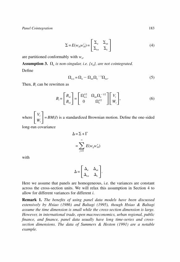
� = E(wi0w�i0) =��u

��u

�u�

�� (4)

are partitioned conformably with wit.

Assumption 3. �� is non-singular, i.e. {xit}, are not cointegrated.

Define

�u.� = �u � �u��1��u. (5)

Then, Bi can be rewritten as

Bi =�Bui

B�i�=��u.�

1/2

0�u��

�1/2

��1/2 ��Vi

Wi�, (6)

where �Vi

Wi�= BM(I) is a standardized Brownian motion. Define the one-sided

long-run covariance

� = � +

=�j=0

E(wijw�i0)

with

� =��u

��u

�u�

��.

Here we assume that panels are homogeneous, i.e. the variances are constantacross the cross-section units. We will relax this assumption in Section 4 toallow for different variances for different i.

Remark 1. The benefits of using panel data models have been discussedextensively by Hsiao (1986) and Baltagi (1995), though Hsiao & Baltagiassume the time dimension is small while the cross-section dimension is large.However, in international trade, open macroeconomics, urban regional, publicfinance, and finance, panel data usually have long time-series and cross-section dimensions. The data of Summers & Heston (1991) are a notableexample.


Remark 2. The advantage of using the sequential limit theory is that it offersa quick and easy way to derive the asymptotics as demonstrated by Phillips &Moon (1999). Phillips & Moon also provide detailed treatments of theconnections between the sequential limit theory and the joint limit theory.

Remark 3. If one wants to obtain a consistent estimate of � in (1) or wants totest some restrictions on �, then an individual time-series regression or amultiple time-series regression is probably enough. So what are the advantagesof using the (N, T) asymptotics, e.g. sequential asymptotics in Assumption 1,instead of T asymptotics? One of the advantages is that we can get a normalapproximation of the limit distributions of the estimators and test statistics withthe convergence rate �NT. More importantly, the biases of the estimators andtest statistics can be reduced when N and T are large. For example, later in thispaper we will show that the biases of the OLS, FMOLS, and DOLS estimatorsin Table 2 were reduced by half when the sample size was changed from(N = 1, T = 20) to (N = 20, T = 20). However, in order to obtain an asymptoticnormality using the (N, T) asymptotics we need to make some strongassumptions; for example, in this paper we assume that the error terms areindependent across i.

Remark 4. The results in this chapter require that regressors are notcointegrated. Assuming that I(1) regressors are not cointegrated with eachother is indeed restrictive. The authors are currently investigating this issue.

III. OLS, FMOLS, AND DOLS ESTIMATORS

Let us first study the limiting distribution of the OLS estimator for equation (1).The OLS estimator of � is

�OLS =��i=1

N �t=1

T

(xit � xi)(xit � xi)��1��i=1

N �t=1

T

(xit � xi)(yit � yi)�. (7)

All the limits in Theorems 1–6 are taken as T→ followed by N→sequentially from Assumption 1. First, we present the following theorem:

Theorem 1. If Assumptions 1–3 hold, then

(a) T(�OLS � �)→p� 3��

�1��u + 6��1��u,

(b) �NT(�OLS � �) � �N�NT ⇒N(0, 6��1�u.�),

where


�NT =�1N�

i=1

N1T 2 �

t=1

T

(xit � xit)(xit � xi)��1

��1N�

i=1

N

��1/2��WidW�i��

�1/2��u + ��u�and Wi = Wi � � Wi.

The normality of the OLS estimator in Theorem 1 comes naturally. Whensumming across i, the non-standard asymptotic distribution due to the unit rootin the time dimension is smoothed out. From Theorem 1 we note that there isan interesting interpretation of the asymptotic covariance matrix, 6��

�1�u.�, i.e.��

�1�u.� can be seen as the long-run noise-to-signal ratio. We also note that�

12��u is due to the endogeneity of the regressor xit, and ��u is due to the serial

correlation. It can be shown easily that

�NT →p� 3��

�1��u + 6��1��u.

If wit = (uit, ��it)� are i.i.d., then

�NT →p 3��1��u,

which was examined by Kao & Chen (1995). Let ��, ��u, ��, and ��u beconsistent estimates of ��, ��u, ��, and ��u respectively. Then from (b) inTheorem 1, we can define a bias-corrected OLS, �OLS

+ ,

�OLS+ = �OLS �

�NT

T

such that

�NT(�OLS+ � �)⇒N(0, 6��

�1�u.�),

where

�NT = � 3��1��u + 6��

�1��u.

Chen, McCoskey & Kao (1999) investigated the finite sample proprieties of theOLS estimator in (7), the t-statistic, the bias-corrected OLS estimator, and thebias-corrected t-statistic. They found that the bias-corrected OLS estimatordoes not improve over the OLS estimator in general. The results of Chen et al.suggest that alternatives, such as the FMOLS estimator or the DOLS estimator(e.g. Saikkonen, 1991; Stock & Watson, 1993) may be more promising in


cointegrated panel regressions. Thus, we begin our study by examining thelimiting distribution of the FMOLS estimator, �FM. The FMOLS estimator isconstructed by making corrections for endogeneity and serial correlation to theOLS estimator �OLS in (7). Define

uit+ = uit � �u��

�1�it, (8)

uit+ = uit � �u��

�1�it, (9)

yit+ = yit � �u��

�1�xit, (10)

and


�1�xit. (11)

Note that

�uit+

�it�=�1

0� �u��

�1

Ik��uit

�it�,

which has the long-run covariance matrix

��u.�

00

��,

where Ik is a k � k identity matrix. The endogeneity correction is achieved bymodifying the variable yit, in (1) with the transformation


�1�xit

= �i + x�it� + uit � �u��1�xit.

The serial correlation correction term has the form

��u+ = (��u ��)� 1

� ��1��u

= ��u � ��

�1��u,

where ��u and �� are kernel estimates of ��u and ��. Therefore, the FMOLSestimator is

�FM =��i=1

N �t=1

T

(xit � xi)(xit � xi)��1

��i=1

N ��t=1

T

(xit � xi)yit+ � T��u

+ �. (12)


Now, we state the limiting distribution of �FM.

Theorem 2. If Assumptions 1–3 hold, then �NT(�FM � �)⇒N(0, 6��1�u.�).

It can be shown easily that the limiting distribution of �FM becomes

�NT(�FM � �)⇒N(0, 2��1�u.�) (13)

by the exclusion of the individual-specific intercept, �i.

Remark 5. Once the estimates of wit, wit, were estimated, we used

� =1

NT �i=1

N �t=1

T

witw�it (14)

to estimate �. � was estimated by

� =1N�

i=1

N 1T�

t=1

T

witw�it +1T�

�=1

l

��l �t=�+1

T

(witw�it�� + wit��w�it)�, (15)

where ��l is a weight function or a kernel. Using Phillips & Durlauf (1986)and sequential limit theory, � and � can be shown to be consistent for � and�.

Remark 6. The distribution results for �FM require �N(� � �) does notdiverge as N grows large. However, � � � may not be small when T is fixed.It follows that �N(� � �) may be non-neglibible in panel data with finitesamples.

Next, we propose a DOLS estimator, �D, which uses the past and future valuesof �xit as additional regressors. We then show that the limiting distribution of�D is the same as the FMOLS estimator, �FM. But first, we need the followingadditional assumption:

Assumption 4. The spectral density matrix fww(�) is bounded away from zeroand full rank for all i, i.e.

fww(�) ≥ �IT, ��[0, �], � > 0.

When Assumptions 2 and 4 hold, the process {uit} can be written as (seeSaikkonen, 1991):

uit =�j=�

cij�it+ j + vit (16)

for all i, where


�j=�

|| cij || < ,

{vit} is stationary with zero mean, and {vit} and {�it} are uncorrelated not onlycontemporaneously but also in all lags and leads. In practice, the leads and lagsmay be truncated while retaining (16) approximately, so that

uit =�j=�q

q

cij�it+ j + vit.

for all i. This is because {cij} are assumed to be absolutely summable, i.e.

�j=�

|| cij || < .

We also need to require that q tends to infinity with T at a suitable rate:

Assumption 5. q→ as T→ such that q3

T→0, and

T1/2 �| j |>q

|| cij || →0 (17)

for all i.

We then substitute (16) into (1) to get

yit = �i + x�it� +�j=�q

q

cij�it+ j + vit,

where

vit = vit +�| j |>q

cij�it+ j. (18)

Therefore, we obtain the DOLS of �, �D, by running the followingregression:

yit = �i + x�it� +�j=�q

q

cij�xit+j + vit. (19)

Next, we show that �D has the same limiting distribution �FM as inTheorem 2.

Theorem 3. If Assumptions 1–5 hold, then �NT(�D � �)⇒N(0, 6��1�u.�).


IV. HETEROGENEOUS PANELS

This chapter so far assumes that the panel data are homogeneous. Thesubstantial heterogeneity exhibited by actual data in the cross-sectionaldimension may restrict the practical applicability of the FMOLS and DOLSestimators. Also, the estimators in Sections 2 and 3 are not easily extended tocases of broader cross-sectional heterogeneity since the variances and biasesare specified in terms of the asymptotic covariance parameters that are assumedto be shared cross-sectionally.

In this section, we propose an alternative representation of the panel FMOLSestimator for heterogeneous panels. Before we discuss the FMOLS estimatorwe need the following assumptions:

Assumption 6. We assume the panels are heterogeneous, i.e. �i, i and �i arevaried for different i. We also assume the invariance principle in (2), (16), and(17) in Assumption 5 still holds.

Let

x*it = �i��1/2xit, (20)

u*it = �iu.��1/2uit

+ ,

uit+ = uit � �iu��i�

�1�it, (21)

yit+ = yit � �iu��i�

�1�xit � �iu.�1/2 (�iu.�

�1/2x�it � (�i��1/2xit)�)�, (22)

and

y*it = �iu.��1/2yit

+ , (23)

where �i� and �iu.� are consistent estimators of �i� and

�iu.� = �iu � �iu��i��1�i�u,

respectively. Similar to Pedroni (1996) the correction term, �iu.�1/2 (�iu.�

�1/2

x�it� � (�i��1/2xit)��), is needed in (22) in the heterogeneous panel. We note that

(22) will be the same as (11) only if �iu.��1/2x�it � (�i�

�1/2xit)� = 0 in theheterogeneous panel. Also (22) requires knowing something about the true �.In practice, � in (22) can be replaced by a preliminary OLS, �OLS. Therefore,let

yit++ = yit � �iu��i�

�1�xit � �iu.�1/2 (�iu.�

�1/2x�it � (�i��1/2xit)�)�OLS,

and

y*it = �iu.��1/2yit

++ .


Assumption 7. �i� is not singular for all i.

Then, we define the FMOLS estimator for heterogeneous panels as

�*FM =��i=1

N �t=1

T

(x*it � x*i )(x*it � x*i )��1��i=1

N ��t=1

T

(x*it � x*i )y*it � T�*i�u�,

(24)

where

�*i�u = �i��1/2�i�u

+ �iu.��1/2

and

�i�u+ = (�i�u �i�)� 1

� �i��1�i�u

= �i�u � �i��i�

�1�i�u.

Theorem 4. If Assumptions 1–2 and 6–7 hold, then �NT(�*FM � �)⇒N(0, 6Ik).

The DOLS estimator for heterogeneous panels, �*D, can be obtained byrunning the following regression:

y*it = �i + x*�it � +�j=�qi

qi

cij�x*it+j + v*it, (25)

where v*it is defined similarly as in (18). Note that in (25) different lagtruncations, qi, may have to be used because the error terms are heterogeneousacross i. Therefore, we need to assume that qi tends to infinity with T at asuitable rate for all i:

Assumption 8. qi → as T→ such that qi

3

T→0, and

T1/2 �| j |>qi

|| cij || →0 (26)

for all i.

In the following theorem we show that �*D also has the same limitingdistribution as �*FM.


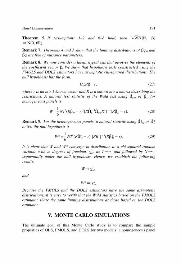
Theorem 5. If Assumptions 1–2 and 6–8 hold, then �NT(�*D � �)⇒N(0, 6Ik).

Remark 7. Theorems 4 and 5 show that the limiting distributions of �*FM and�*D are free of nuisance parameters.

Remark 8. We now consider a linear hypothesis that involves the elements ofthe coefficient vector �. We show that hypothesis tests constructed using theFMOLS and DOLS estimators have asymptotic chi-squared distributions. Thenull hypothesis has the form:

H0:R� = r, (27)

where r is an m � 1 known vector and R is a known m � k matrix describing therestrictions. A natural test statistic of the Wald test using �FM or �D forhomogeneous panels is

W =16

NT2(R�D � r)�[R��1�u.�R�]�1(R�D � r). (28)

Remark 9. For the heterogeneous panels, a natural statistic using �*FM or �*Dto test the null hypothesis is

W* =16

NT2(R�*D � r)�[RR�]�1(R�*D � r). (29)

It is clear that W and W* converge in distribution to a chi-squared randomvariable with m degrees of freedom, �m

2 , as T→ and followed by N→sequentially under the null hypothesis. Hence, we establish the followingresults:

W⇒�m2 ,

and

W*⇒�m2 .

Because the FMOLS and the DOLS estimators have the same asymptoticdistributions, it is easy to verify that the Wald statistics based on the FMOLSestimator share the same limiting distributions as those based on the DOLSestimator.

V. MONTE CARLO SIMULATIONS

The ultimate goal of this Monte Carlo study is to compare the sampleproperties of OLS, FMOLS, and DOLS for two models: a homogeneous panel


and a heterogeneous panel. The simulations were performed by a SunSparcServer 1000 and an Ultra Enterprise 3000. GAUSS 3.2.31 and COINT 2.0were used to perform the simulations. Random numbers for error terms,(u*it, �*it), for Sections 5 A, B and D, were generated by the GAUSS procedureRNDNS. At each replication, we generated an N(T + 1000) length of randomnumbers and then split it into N series so that each series had the same meanand variance. The first 1, 000 observations were discarded for each series. {u*it}and {�*it} were constructed with ui0 = 0 and �i0 = 0.

In order to compare the performance of the OLS, FMOLS, and DOLSestimators, the following data generating process (DGP) was used:

yit = �i + �xit + uit (30)

and

xit = xit�1 + �it

where (uit, �it) follows an ARMA(1, 1) process:

�uit

�it=�0.5 0

0 0.5�uit�1

�it�1+�u*it

�*it+�0.3

�21

� 0.40.6 �u*it�1

�*it�1

with

�u*it�*it ~iid N��0

0�, �1 �21

�21 1�.

The design in (30) nests several important special cases. First, when �0.5 00 0.5

is replaced by �0 00 0 and �21 is constant across i, then the DGP becomes the

homogeneous panel in Section 5A. Second, when �0.5 00 0.5 is replaced by

�0 00 0, and �21 and �21 are random variable different across i, then the DGP

is the heterogeneous panel in Section 5D.

A. Homogeneous Panel

To compare the performance of the OLS, FMOLS, and DOLS estimators forthe homogeneous panel we conducted Monte Carlo experiments based on a


design similar to that of Phillips & Hansen (1990) and Phillips & Loretan(1991).

yit = �i + �xit + uit

and

xit = xit�1 + �it

for i = 1, . . ., N, t = 1, . . . , T, where

�uit

�it=�u*it

�*it+�0.3

�21

� 0.40.6 �u*it�1

�*it�1 (31)

with


0�, � 1�21

�21

1 �.

We generated �i from a uniform distribution, U[0, 10], and set � = 2. FromTheorems 1–3 we know that the asymptotic results depend upon variances andcovariances of the errors uit and �it. The design in (31) is a good one since theendogeneity of the system is controlled by only two parameters, �21 and �21. Weallowed �21 and �21 to vary and considered values of {0.8, 0.4, 0.0, � 0.8} for�21 and {–0.8, –0.4, 0.4} for �21.

The estimate of the long-run covariance matrix in (15) was obtained by usingthe procedure KERNEL in COINT 2.0 with a Bartlett window. The lagtruncation number was set arbitrarily at five. Results with other kernels, such asParzen and quadratic spectral kernels, are not reported, because no essentialdifferences were found for most cases.

Next, we recorded the results from our Monte Carlo experiments thatexamined the finite-sample properties of the OLS estimator, �OLS; the FMOLSestimator, �FM; and the DOLS estimator, �D. The results we report are based on10,000 replications and are summarized in Tables 1–4 and Figures 1–8. TheFMOLS estimator was obtained by using a Bartlett window of lag length fiveas in (15). Four lags and two leads were used for the DOLS estimator.

Table 1 reports the Monte Carlo means and standard deviations (inparentheses) of (�OLS � �), (�FM � �), and (�D � �) for sample sizesT = N = (20, 40, 60). The biases of the OLS estimator, �OLS, decrease at a rate ofT. For example, with �21 = –0.8 and �21 = 0.8, the bias at T = 20 is –0.201 and atT = 40 is –0.104. Also, the biases increase in �21 (with �21 > 0) and decrease in�21.


Tabl

e1.

Mea

ns B

iase

s an

d St

anda

rd D

evia

tions

of

OL

S, F

MO

LS,

and

DO

LS

Est

imat

ors

�21

=–0

.8�

21=

–0.4

�21

=0.

8�

OLS

–��

FM–�

�D–�

�O

LS–�

�F

M–�

�D–�

�O

LS–�

�F

M–�

�D–�

�21

=0.

8T

=20

–0.2

01–0

.176

–0.0

01–0

.097

–0.1

13–0

.002

–0.0

22–0

.069

–0.0

09(0

.049

)(0

.044

)(0

.040

)(0

.032

)(0

.035

)(0

.033

)(0

.011

)(0

.016

)(0

.009

)T

=40

–0.1

04–0

.099

–0.0

00–0

.049

–0.0

62–0

.001

–0.0

11–0

.036

–0.0

04(0

.019

)(0

.017

)(0

.013

)(0

.012

)(0

.013

)(0

.011

)(0

.004

)(0

.006

)(0

.003

)T

=60

–0.0

70–0

.069

–0.0

00–0

.033

–0.0

42–0

.000

–0.0

07–0

.024

–0.0

03(0

.010

)(0

.009

)(0

.007

)(0

.007

)(0

.007

)(0

.006

)(0

.002

)(0

.003

)(0

.002

)�

21=

0.4

T=

20–0

.132

–0.0

64–0

.001

–0.0

82–0

.068

–0.0

02–0

.014

–0.0

73–0

.003

(0.0

38)

(0.0

25)

(0.0

27)

(0.0

30)

(0.0

29)

(0.0

31)

(0.0

13)

(0.0

18)

(0.0

13)

T=

40–0

.066

–0.0

38–0

.001

–0.0

41–0

.038

–0.0

01–0

.007

–0.0

37–0

.001

(0.0

14)

(0.0

09)

(0.0

27)

(0.0

11)

(0.0

11)

(0.0

09)

(0.0

05)

(0.0

06)

(0.0

04)

T=

60–0

.044

–0.0

27–0

.000

–0.0

27–0

.026

–0.0

01–0

.005

–0.0

25–0

.001

(0.0

07)

(0.0

05)

(0.0

05)

(0.0

06)

(0.0

06)

(0.0

05)

(0.0

02)

(0.0

03)

(0.0

02)

�21

=0.

0T

=20

–0.0

79–0

.002

0.00

1–0

.059

–0.0

190.

002

0.00

5–0

.069

0.00

6(0

.027

)(0

.015

)(0

.017

)(0

.026

)(0

.022

)(0

.026

)(0

.016

)(0

.021

)(0

.017

)T

=40

–0.0

39–0

.005

0.00

1–0

.029

–0.0

120.

001

0.00

2–0

.035

0.00

3(0

.009

)(0

.005

)(0

.005

)(0

.009

)(0

.008

)(0

.008

)(0

.006

)(0

.007

)(0

.005

)T

=60

–0.0

26–0

.004

0.00

0–0

.019

–0.0

09–0

.001

0.00

1–0

.023

0.00

2(0

.005

)(0

.003

)(0

.003

)(0

.005

)(0

.004

)(0

.008

)(0

.003

)(0

.004

)(0

.003

)�

21=

–0.8

T=

20–0

.029

0.03

80.

007

–0.0

190.

036

0.00

70.

114

0.01

20.

000

(0.0

16)

(0.0

12)

(0.0

08)

(0.0

17)

(0.0

15)

(0.0

14)

(0.0

34)

(0.0

28)

(0.0

31)

T=

40–0

.015

0.01

80.

003

–0.0

090.

018

0.00

30.

057

0.01

1–0

.000

(0.0

06)

(0.0

04)

(0.0

02)

(0.0

06)

(0.0

05)

(0.0

04)

(0.0

12)

(0.0

09)

(0.0

09)

T=

60–0

.009

0.01

10.

002

–0.0

070.

012

0.00

20.

038

0.01

00.

000

(0.0

03)

(0.0

02)

(0.0

01)

(0.0

03)

(0.0

02)

(0.0

02)

(0.0

07)

(0.0

05)

(0.0

05)

Not

e: (

a) N

=T.

(b)

A l

ag l

engt

h 5

of t

he B

artle

tt w

indo

ws

is u

sed

for

the

FMO

LS

estim

ator

. (c)

4 l

ags

and

2 le

ads

are

used

for

the

DO

LS

esti-

mat

or.


Table 2. Means Biases and Standard Deviations of OLS, FMOLS, and DOLSEstimators for Different N and T

(N,T) �OLS–� �FM(5)–� �FM(2)–� �D(4,2)–� �D(2,1)–�

(1,20) –0.135 –0.104 –0.122 –0.007 0.031(0.184) (0.196) (0.189) (0.297) (0.211)

(1,40) –0.070 –0.059 –0.065 –0.001 0.015(0.093) (0.012) (0.092) (0.106) (0.090)

(1,60) –0.047 –0.041 –0.043 –0.001 0.009(0.063) (0.064) (0.061) (0.064) (0.057)

(1,120) –0.024 –0.023 –0.022 –0.001 0.004(0.032) (0.031) (0.031) (0.029) (0.027)

(20,20) –0.082 –0.068 –0.075 –0.002 0.017(0.030) (0.029) (0.029) (0.031) (0.028)

(20,40) –0.042 –0.039 –0.039 –0.001 0.008(0.016) (0.015) (0.015) (0.015) (0.014)

(20,60) –0.028 –0.027 –0.026 –0.000 0.006(0.010) (0.010) (0.009) (0.009) (0.009)

(20,120) –0.014 –0.014 –0.013 –0.000 0.003(0.005) (0.005) (0.005) (0.005) (0.004)

(40,20) –0.081 –0.066 –0.073 –0.001 0.017(0.022) (0.021) (0.021) (0.022) (0.019)

(40,40) –0.041 –0.038 –0.038 –0.001 0.008(0.011) (0.011) (0.011) (0.009) (0.009)

(40,60) –0.028 –0.026 –0.025 –0.001 0.005(0.007) (0.007) (0.007) (0.007) (0.006)

(40,120) –0.014 –0.014 –0.013 –0.000 0.003(0.004) (0.004) (0.003) (0.003) (0.004)

(60,20) –0.080 –0.067 –0.073 –0.002 0.016(0.017) (0.017) (0.017) (0.018) (0.016)

(60,40) –0.041 –0.038 –0.038 –0.001 0.008(0.009) (0.009) (0.009) (0.008) (0.008)

(60,60) –0.027 –0.026 –0.025 –0.001 0.005(0.006) (0.006) (0.006) (0.005) (0.005)

(60,120) –0.014 –0.014 –0.012 –0.000 0.003(0.003) (0.003) (0.003) (0.003) (0.003)

(120,20) –0.079 –0.066 –0.072 –0.002 0.016(0.012) (0.012) (0.012) (0.012) (0.011)

(120,40) –0.041 –0.037 –0.037 –0.001 0.008(0.006) (0.006) (0.006) (0.006) (0.005)

(120,60) –0.027 –0.026 –0.025 –0.001 0.005(0.004) (0.004) (0.004) (0.004) (0.004)

(120,120) –0.014 –0.014 –0.013 –0.000 0.003(0.002) (0.002) (0.002) (0.002) (0.002)

Note: (a) A lag length 5 and 2 of the Bartlett windows are used for the FMOLS(5) and FMOLS(2)estimators. (b) 4 lags and 2 leads and 2 lags and 1 lead are used for the DOLS(4,2) and DOLS(2,1)estimators. (c) �21 = –0.4 and �21 = 0.4.


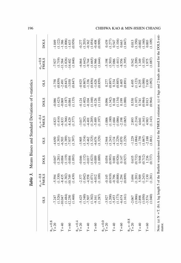
Tabl

e3.

Mea

ns B

iase

s an

d St

anda

rd D

evia

tions

of

t-st

atis

tics

�21

=–0

.8�

21=

–0.4

�21

=0.

8O

LS

FMO

LS

DO

LS

OL

SFM

OL

SD

OL

SO

LS

FMO

LS

DO

LS

�21

=0.

8T

=20

–7.2

47–5

.594

–0.0

47–4

.650

–4.8

23–0

.086

–1.7

58–7

.927

–1.0

49(1

.526

)(1

.330

)(1

.281

)(1

.393

)(1

.414

)(1

.423

)(0

.859

)(1

.719

)(1

.122

)T

=40

–10.

047

–8.4

35–0

.004

–6.5

03–6

.833

–0.0

69–2

.491

–11.

584

–1.3

86(1

.484

)(1

.382

)(1

.119

)(1

.389

)(1

.366

)(1

.187

)(0

.847

)(1

.826

)(1

.006

)T

=60

–12.

250

–10.

749

–0.0

04–7

.937

–8.4

29–0

.084

–3.0

30–1

4.40

2–1

.633

(1.4

68)

(1.4

39)

(1.0

93)

(1.3

97)

(1.3

77)

(1.1

35)

(0.8

47)

(1.8

40)

(0.9

59)

�21

=0.

4T

=20

–5.4

25–2

.377

–0.0

46–3

.905

–3.0

17–0

.124

–0.9

25–6

.864

–0.2

77(1

.340

)(1

.042

)(1

.132

)(1

.334

)(1

.282

)(1

.402

)(0

.867

)(1

.642

)(1

.203

)T

=40

–7.5

07–4

.558

–0.0

17–5

.462

–4.4

01–0

.104

–1.3

36–9

.744

–0.3

62(1

.302

)(1

.071

)(1

.023

)(1

.325

)(1

.205

)(1

.168

)(0

.856

)(1

.665

)(1

.054

)T

=60

–9.1

61–6

.012

–0.0

09–6

.676

–5.4

89–0

.126

–1.6

26–1

1.96

6–0

.408

(1.2

87)

(1.1

09)

(1.0

09)

(1.3

29)

(1.1

97)

(1.1

18)

(0.8

59)

(1.6

44)

(0.9

99)

�21

=0.

0T

=20

–3.9

27–0

.145

0.05

4–2

.944

–1.0

060.

096

0.27

7–5

.198

0.43

9(1

.200

)(0

.919

)(0

.993

)(1

.241

)(1

.180

)(1

.342

)(0

.897

)(1

.503

)(1

.277

)T

=40

–5.4

53–0

.796

0.00

1–4

.134

–1.6

840.

168

0.33

4–7

.086

0.54

7(1

.173

)(0

.888

)(0

.926

)(1

.229

)(1

.086

)(1

.134

)(0

.885

)(1

.441

)(1

.104

)T

=60

–6.6

74–1

.294

0.14

7–5

.070

–2.1

980.

199

0.40

5–8

.556

0.66

3(1

.161

)(0

.899

)(0

.927

)(1

.229

)(1

.065

)(1

.088

)(0

.891

)(1

.395

)(1

.047

)�

21=

–0.8

T=

20–2

.067

3.69

40.

635

–1.2

292.

893

0.53

04.

495

0.54

20.

013

(1.0

66)

(1.2

01)

(0.7

32)

(1.0

84)

(1.2

14)

(1.1

07)

(1.1

23)

(1.2

09)

(1.3

50)

T=

40–2

.898

5.50

90.

948

–1.7

584.

041

0.74

16.

255

1.34

9–0

.002

(1.0

50)

(1.2

43)

(0.7

12)

(1.0

67)

(1.1

61)

(0.9

84)

(1.0

88)

(1.1

03)

(1.1

60)

T=

60–3

.574

7.13

01.

236

–2.1

884.

983

0.91

37.

630

1.97

50.

003

(1.0

40)

(1.2

81)

(0.7

37)

(1.0

61)

(1.1

43)

(0.9

64)

(1.0

92)

(1.0

87)

(1.1

09)

Not

e: (

a) N

=T.

(b)

A l

ag l

engt

h 5

of t

he B

artle

tt w

indo

ws

is u

sed

for

the

FMO

LS

estim

ator

. (c)

4 l

ags

and

2 le

ads

are

used

for

the

DO

LS

esti-

mat

or.


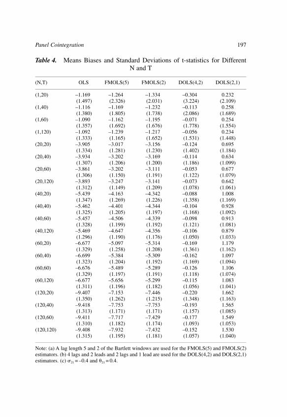
Table 4. Means Biases and Standard Deviations of t-statistics for DifferentN and T

(N,T) OLS FMOLS(5) FMOLS(2) DOLS(4,2) DOLS(2,1)

(1,20) –1.169 –1.264 –1.334 –0.304 0.232(1.497) (2.326) (2.031) (3.224) (2.109)

(1,40) –1.116 –1.169 –1.232 –0.113 0.258(1.380) (1.805) (1.738) (2.086) (1.689)

(1,60) –1.090 –1.162 –1.195 –0.071 0.254(1.357) (1.692) (1.676) (1.778) (1.554)

(1,120) –1.092 –1.239 –1.217 –0.056 0.234(1.333) (1.165) (1.652) (1.531) (1.448)

(20,20) –3.905 –3.017 –3.156 –0.124 0.695(1.334) (1.281) (1.230) (1.402) (1.184)

(20,40) –3.934 –3.202 –3.169 –0.114 0.634(1.307) (1.206) (1.200) (1.186) (1.099)

(20,60) –3.861 –3.202 –3.111 –0.053 0.677(1.306) (1.150) (1.191) (1.122) (1.079)

(20,120) –3.893 –3.247 –3.141 –0.073 0.642(1.312) (1.149) (1.209) (1.078) (1.061)

(40,20) –5.439 –4.163 –4.342 –0.088 1.008(1.347) (1.269) (1.226) (1.358) (1.169)

(40,40) –5.462 –4.401 –4.344 –0.104 0.928(1.325) (1.205) (1.197) (1.168) (1.092)

(40,60) –5.457 –4.506 –4.339 –0.098 0.913(1.328) (1.199) (1.192) (1.121) (1.081)

(40,120) –5.469 –4.647 –4.356 –0.106 0.879(1.296) (1.190) (1.176) (1.050) (1.033)

(60,20) –6.677 –5.097 –5.314 –0.169 1.179(1.329) (1.258) (1.208) (1.361) (1.162)

(60,40) –6.699 –5.384 –5.309 –0.162 1.097(1.323) (1.204) (1.192) (1.169) (1.094)

(60,60) –6.676 –5.489 –5.289 –0.126 1.106(1.329) (1.197) (1.191) (1.118) (1.074)

(60,120) –6.677 –5.656 –5.299 –0.115 1.083(1.311) (1.196) (1.182) (1.056) (1.041)

(120,20) –9.407 –7.153 –7.446 –0.220 1.662(1.350) (1.262) (1.215) (1.348) (1.163)

(120,40) –9.418 –7.753 –7.753 –0.193 1.565(1.313) (1.171) (1.171) (1.157) (1.085)

(120,60) –9.411 –7.717 –7.429 –0.177 1.549(1.310) (1.182) (1.174) (1.093) (1.053)

(120,120) –9.408 –7.932 –7.432 –0.152 1.530(1.315) (1.195) (1.181) (1.057) (1.040)

Note: (a) A lag length 5 and 2 of the Bartlett windows are used for the FMOLS(5) and FMOLS(2)estimators. (b) 4 lags and 2 leads and 2 lags and 1 lead are used for the DOLS(4,2) and DOLS(2,1)estimators. (c) �21 = –0.4 and �21 = 0.4.


Fig

.1.

Dis

trib

utio

n of

bia

ses

of E

stim

ator

s w

ith N

=40

, T=

20.


Fig

.2.

Dis

trib

utio

n of

t-st

atis

tics

with

N=

40, T

=20

.


Fig

.3.

Dis

trib

utio

n of

bia

ses

of E

stim

ator

s w

ith N

=40

, T=

40.


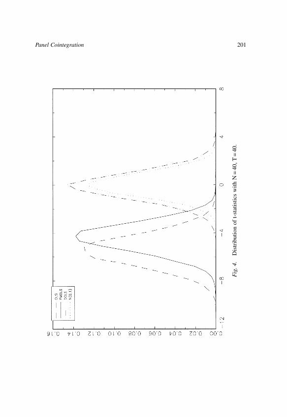
Fig

.4.

Dis

trib

utio

n of

t-st

atis

tics

with

N=

40, T

=40

.


Fig

.5.

Dis

trib

utio

n of

bia

ses

of E

stim

ator

s w

ith N

=40

, T=

60.


Fig

.6.

Dis

trib

utio

n of

t-st

atis

tics

with

N=

40, T

=60

.


Fig

.7.

Dis

trib

utio

n of

bia

ses

of E

stim

ator

s w

ith N

=40

, T=

120.


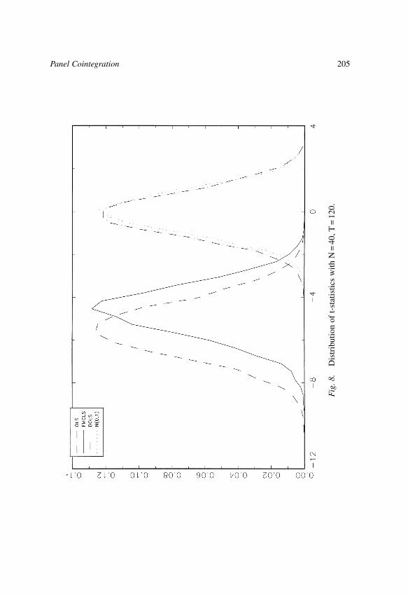
Fig

.8.

Dis

trib

utio

n of

t-st

atis

tics

with

N=

40, T

=12

0.


While we expected the OLS estimator to be biased, we expected the FMOLSestimator to produce much better estimates. However, it is noticeable that theFMOLS estimator has a downward bias when �21 ≥ 0 and an upward bias when�21 < 0. In general, the FMOLS estimator, �FM, presents the same degree ofdifficulty with bias as does the OLS estimator, �OLS. For example, while theFMOLS estimator, �FM, reduces the bias substantially and outperforms �OLS

when �21 > 0 and �21 < 0, the opposite is true when �21 > 0 and �21 > 0. Likewise,when �21 = –0.8, �FM is less biased than �OLS for values of �21 = –0.8. Yet, forvalues of �21 = –0.4, the bias in �OLS is less than the bias in �FM. There seemsto be little to choose between �OLS and �FM when �21 < 0. This is probably dueto the failure of the non-parametric correction procedure in the presence of anegative serial correlation of the errors, i.e. a negative MA value, �21 < 0.Finally, for the cases where �21 = 0.0, �FM outperforms �OLS when �21 < 0. On theother hand, �FM is more biased than �OLS when �21 > 0.

In contrast, the results in Table 1 show that the DOLS, �D, is distinctlysuperior to the OLS and FMOLS estimators for all cases in terms of the meanbiases. It was noticeable that the FMOLS leads to a significant bias. Clearly, theDOLS outperformed both the OLS and FMOLS estimators. The FMOLSestimator is also complicated by the dependence of the correction in (11) and(12) upon the preliminary estimator (here we use OLS), which may be biasedin finite samples. The DOLS differs from the FMOLS estimator in that theDOLS requires no initial estimation and no non-parametric correction.

It is important to know the effects of the variations in panel dimensions onthe results, since the actual panel data have a wide variety of cross-section andtime-series dimensions. Table 2 considers 20 different combinations for N andT, each ranging from 20 to 120 with �21 = –0.4 and �21 = 0.4. First, we noticethat the cross-section dimension has a significant effect on the biases of�OLS, �FM, and �D when N is increased from 1 to 20. However, when N isincreased from 20 to 40 and beyond, there is little effect on the biases of�OLS, �FM, and �D. From this it seems that in practice the T dimension mustexceed the N dimension, especially for the OLS and FMOLS estimators, inorder to get a good approximation of the limiting distributions of theestimators. For example, for each of the estimators in Table 2, the reported biasis substantially less for (T = 120, N = 40) than it is for either (T = 40, N = 40) or(T = 40, N = 120). The results in Table 2 again confirm the superiority of theDOLS. The largest bias in the DOLS with four lags and two leads, DOLS(4, 2),is less than or equal to 0.02 for all cases except at N = 1 and T = 20, which canbe compared with a simulation standard error (in parentheses) that is less than0.007 when N ≥ 20 and, T ≥ 60, confirming the accuracy of the DOLS(4, 2). Thebiases in DOLS with two lags and one lead, DOLS(2, 1) start off slightly biased


at N = 1 and T = 20, and converge to an almost unbiased coefficient estimate atN = 20 and T = 40. The biases of DOLS(2, 1) move in the opposite direction tothose of DOLS(4, 2).

Figures 1, 3, 5 and 7 display estimated pdfs for the estimators for �21 = –0.4and � = 0.4 with N = 40 (T = 20 in Figure 1, T = 40 in Figure 3, T = 60 in Figure5 and T = 120 in Figure 7). In Figure 1, N = 40, T = 20, the DOLS is much bettercentered than the OLS and FMOLS. In Figures 3, 5 and 7, the biases of theOLS and FMOLS were reduced as T increases, the DOLS still dominates theOLS and FMOLS.

Monte Carlo means and standard deviations of the t-statistic, t�=�0, are given

in Table 3. Here, the OLS t-statistic is the conventional t-statistic as printed bystandard statistical packages, and the FMOLS and DOLS t-statistics. With allvalues of �21 and �21, the DOLS(4, 2) t-statistic is well approximated by astandard N(0, 1) suggested from the asymptotic results. The DOLS(4, 2) t-statistic is much closer to the standard normal density than the OLS t-statisticand the FMOLS t-statistic. When �21 > 0 and �21 < 0, the OLS t-statistic is moreheavily biased than the FMOLS t-statistic. Again, when �21 > 0 and �21 > 0, theopposite is true. Even when �21 = 0, the FMOLS t-statistic is not wellapproximated by a standard N(0, 1). The OLS t-statistic performs better thanthe FMOLS t-statistic when �21 = 0.8 and �21 > 0 and when �21 ≤ –0.4 and �21 =–0.8, but not in other cases. The FMOLS t-statistic in general does not performbetter than the OLS t-statistic.

Table 4 shows that both the OLS t-statistic and the FMOLS t-statisticbecome more negatively biased as the dimension of cross-section N increases.The heavily negative biases of the FMOLS t-statistic in Tables 3–4 againindicate the poor performance of the FMOLS estimator. For the DOLS(4, 2),the biases decrease rapidly and the standard errors converge to 1.0 as Tincreases. Similar to Table 2, we observe from Table 4 that for the DOLS t-statistic the T dimension is more important than the N dimension in reducingthe biases of the t-statistics. However, the improvement of the DOLS t-statisticis rather marginal as T increases.

Figures 2, 4, 6 and 8 display estimated pdfs for the t-statistics for �21 = –0.4and � = 0.4 with N = 40 (T = 20 in Figure 2, T = 40 in Figure 4, T = 60 in Figure6 and T = 120 in Figure 8). The figures show clearly that the DOLS t-statisticis well approximated by a standard N(0, 1) especially as T increases. From theresults in Tables 2 and 4 and Figures 1–8 we note that the sequential limittheory approximates the limiting distributions of the DOLS and its t-statisticvery well.

It is known that when the length of time series is short the estimate � in (15)may be sensitive to the length of the bandwidth. In Tables 2 and 4, we first


investigate the sensitivity of the FMOLS estimator with respect to the choice oflength of the bandwidth. We extend the experiments by changing the lag lengthfrom 5 to 2 for a Barlett window. Overall, the results show that changing thelag length from 5 to 2 does not lead to substantial changes in biases for theFMOLS estimator and its t-statistic. However, the biases of the DOLSestimator and its t-statistic are reduced substantially when the lags and leads arechanged from (2, 1) to (4, 2) as predicted from Theorem 3. The results fromTables 2 and 4 show that the DOLS method gives different estimates of � andthe t-statistic depending on the number of lags and leads we choose. This seemsto be a drawback of the DOLS estimator. Further research is needed on how tochoose the lags and leads for the DOLS estimator in the panel setting.

B. ARMA(1, 1) Error Terms

In this section, we look at simulations where, instead of the errors beinggenerated by an MA(1) process, like in (31), the errors are generated by anARMA(1, 1) process, as in (30). One may question that the MA(1)specification in (31) may be unfair to the FMOLS estimator. One of the reasonswhy the performance of the DOLS is much better than that of the FMOLS liesin the simulation design in (31), which assumes that the error terms are MA(1)processes. If (uit , �it)� is an MA(1) process, then uit can be written exactly withthree terms, �it–1, �it, and �it+1 and no lag truncation approximation is requiredfor the DOLS.

Tables 5 and 6 report the performance of OLS, FMOLS, and DOLS and theirt-statistics when the errors are generated by an ARMA(1, 1) process. Tables 5and 6 show that the FMOLS estimator and its t-statistic are less biased than theOLS estimator for most cases and is outperformed by the DOLS. Again, when�21 ≥ 0.0 and �21 = 0.8 the FMOLS estimator and its t-statistic suffer from severebiases. On the other hand, we observe that DOLS shows less improvementcompared with OLS and FMOLS, in contrast to Tables 1 and 3. However, thegood performance of DOLS may disappear for high order ARMA(p, q) errorprocess.

C. Non-normal Errors

In this section, we conduct an experiment where the error terms are non-normal. The DGP is similar to that of Gonzalo (1994):


Tabl

e5.

Mea

ns B

iase

s an

d St

anda

rd D

evia

tions

of

OL

S, F

MO

LS,

and

DO

LS

Est

imat

ors

�21

=–0

.8�

21=

–0.4

�21

=0.

8�

OLS

–��

FM–�

�D–�

�O

LS–�

�F

M–�

�D–�

�O

LS–�

�F

M–�

�D–�

�21

=0.

8T

=20

–0.1

10–0

.101

0.00

3–0

.049

–0.0

620.

000

–0.0

09–0

.036

–0.0

03(0

.042

)(0

.038

)(0

.037

)(0

.029

)(0

.020

)(0

.030

)(0

.011

)(0

.012

)(0

.009

)T

=40

–0.0

52–0

.052

0.00

1–0

.024

–0.0

310.

000

–0.0

04–0

.017

–0.0

01(0

.015

)(0

.014

)(0

.012

)(0

.010

)(0

.011

)(0

.010

)(0

.004

)(0

.004

)(0

.003

)T

=60

–0.0

34–0

.035

0.00

0–0

.015

–0.0

21–0

.000

–0.0

03–0

.012

–0.0

01(0

.008

)(0

.008

)(0

.007

)(0

.006

)(0

.006

)(0

.005

)(0

.002

)(0

.002

)(0

.002

)�

21=

0.4

T=

20–0

.073

–0.0

390.

001

–0.0

45–0

.038

–0.0

00–0

.006

–0.0

37–0

.001

(0.0

32)

(0.0

24)

(0.0

24)

(0.0

28)

(0.0

27)

(0.0

28)

(0.0

13)

(0.0

14)

(0.0

12)

T=

40–0

.034

–0.0

200.

000

–0.0

21–0

.019

–0.0

00–0

.002

–0.0

17–0

.001

(0.0

11)

(0.0

08)

(0.0

08)

(0.0

10)

(0.0

09)

(0.0

09)

(0.0

04)

(0.0

04)

(0.0

04)

T=

60–0

.022

–0.0

130.

000

–0.0

13–0

.012

–0.0

00–0

.002

–0.0

12–0

.000

(0.0

06)

(0.0

04)

(0.0

04)

(0.0

05)

(0.0

05)

(0.0

05)

(0.0

02)

(0.0

02)

(0.0

02)

�21

=0.

0T

=20

–0.0

46–0

.006

0.00

1–0

.035

–0.0

130.

001

–0.0

01–0

.034

0.00

3(0

.025

)(0

.015

)(0

.015

)(0

.025

)(0

.022

)(0

.023

)(0

.016

)(0

.016

)(0

.015

)T

=40

–0.0

21–0

.003

0.00

0–0

.016

–0.0

060.

001

–0.0

01–0

.016

0.00

1(0

.009

)(0

.005

)(0

.005

)(0

.008

)(0

.007

)(0

.008

)(0

.006

)(0

.005

)(0

.005

)T

=60

–0.0

14–0

.002

0.00

1–0

.011

–0.0

040.

001

–0.0

00–0

.010

0.00

2(0

.005

)(0

.003

)(0

.003

)(0

.005

)(0

.004

)(0

.004

)(0

.003

)(0

.003

)(0

.003

)�

21=

–0.8

T=

20–0

.020

0.01

70.

002

–0.0

160.

017

0.00

30.

035

0.01

20.

000

(0.0

16)

(0.0

09)

(0.0

07)

(0.0

17)

(0.0

13)

(0.0

12)

(0.0

24)

(0.0

24)

(0.0

31)

T=

40–0

.008

0.00

80.

002

–0.0

070.

008

0.00

10.

016

0.00

7–0

.000

(0.0

05)

(0.0

03)

(0.0

02)

(0.0

06)

(0.0

04)

(0.0

04)

(0.0

09)

(0.0

09)

(0.0

09)

T=

60–0

.006

0.00

50.

001

–0.0

050.

005

0.00

10.

011

0.00

50.

000

(0.0

03)

(0.0

01)

(0.0

01)

(0.0

03)

(0.0

02)

(0.0

02)

(0.0

05)

(0.0

05)

(0.0

05)

Not

e: (

a) N

=T.

(b)

A l

ag l

engt

h 5

of t

he B

artle

tt w

indo

ws

is u

sed

for

the

FMO

LS

estim

ator

. (c

) 4

lags

and

2 l

eads

are

use

d fo

r th

e D

OL

Ses

timat

or. (

d) T

he e

rror

term

s ar

e ge

nera

ted

by a

n A

RM

A(1

,1)

proc

ess

from

equ

atio

n (3

0).


Tabl

e6.

Mea

ns B

iase

s an

d St

anda

rd D

evia

tions

of

t-st

atis

tics

�21

=–0

.8�

21=

–0.4

�21

=0.

8O

LS

FMO

LS

DO

LS

OL

SFM

OL

SD

OL

SO

LS

FMO

LS

DO

LS

�21

=0.

8T

=20

–5.3

16–3

.569

0.11

9–3

.411

–2.9

120.

006

–1.1

58–4

.589

–0.3

47(1

.929

)(1

.323

)(1

.290

)(1

.924

)(1

.390

)(1

.417

)(1

.426

)(1

.420

)(1

.139

)T

=40

–7.0

13–4

.601

0.09

0–4

.583

–3.5

800.

009

–1.7

23–6

.144

–0.5

05(1

.903

)(1

.219

)(1

.119

)(1

.949

)(1

.216

)(1

.166

)(1

.445

)(1

.343

)(1

.011

)T

=60

–8.4

37–5

.22

0.06

8–5

.523

–4.2

06–0

.006

–2.0

97–7

.428

–0.6

03(1

.899

)(1

.195

)(1

.077

)(1

.969

)(1

.178

)(1

.111

)(1

.435

)(1

.294

)(0

.978

)�

21=

0.4

T=

20–4

.152

–1.8

570.

056

–3.0

64–1

.877

–0.0

25–0

.705

–3.8

58–0

.068

(1.7

62)

(1.1

06)

(1.1

32)

(1.8

67)

(1.3

14)

(1.3

88)

(1.4

54)

(1.3

73)

(1.2

08)

T=

40–5

.424

–2.5

760.

045

–4.0

69–2

.346

–0.0

11–1

.099

–5.0

34–0

.134

(1.7

33)

(1.0

44)

(1.0

27)

(1.8

80)

(1.1

49)

(1.1

52)

(1.4

79)

(1.2

68)

(1.0

53)

T=

60–6

.521

–3.1

790.

034

–4.8

99–2

.779

–0.0

27–1

.343

–6.0

16–0

.144

(1.7

21)

(1.0

36)

(1.0

04)

(1.8

98)

(1.1

14)

(1.0

96)

(1.4

73)

(1.2

11)

(1.0

14)

�21

=0.

0T

=20

–3.1

84–0

.353

0.03

4–2

.538

–0.7

320.

038

–0.0

47–2

.825

0.23

0(1

.644

)(0

.952

)(0

.956

)(1

.769

)(1

.226

)(1

.313

)(1

.498

)(1

.327

)(1

.276

)T

=40

–4.1

20–0

.624

0.04

7–3

.327

–0.9

670.

075

–0.1

94–3

.557

0.21

2(1

.616

)(0

.897

)(0

.909

)(1

.771

)(1

.085

)(1

.116

)(1

.528

)(1

.194

)(1

.095

)T

=60

–4.9

52–0

.827

0.05

8–4

.131

–1.1

410.

206

–0.0

64–4

.005

0.69

3(1

.599

)(0

.904

)(0

.913

)(1

.746

)(1

.021

)(1

.118

)(1

.498

)(1

.096

)(1

.094

)�

21=

–0.8

T=

20–1

.956

1.73

30.

214

–1.4

961.

429

0.22

12.

315

0.56

40.

002

(1.5

29)

(0.9

33)

(0.6

63)

(1.5

89)

(1.0

15)

(1.0

52)

(1.5

77)

(1.1

95)

(1.5

51)

T=

40–2

.471

2.51

10.

317

–1.8

881.

917

0.29

43.

089

0.87

6–0

.005

(1.5

07)

(0.8

71)

(0.6

64)

(1.5

78)

(1.0

10)

(0.9

56)

(1.6

44)

(1.0

88)

(1.2

39)

T=

60–2

.966

3.27

00.

428

–2.2

672.

237

0.36

33.

736

1.13

20.

003

(1.4

84)

(0.8

97)

(0.6

94)

(1.5

71)

(0.9

99)

(0.9

41)

(1.6

76)

(1.0

62)

(1.1

55)

Not

e: (

a) N

=T.

(b)

A l

ag l

engt

h 5

of t

he B

artle

tt w

indo

ws

is u

sed

for

the

FMO

LS

estim

ator

. (c

) 4

lags

and

2 l

eads

are

use

d fo

r th

e D

OL

Ses

timat

or. (

d) T

he e

rror

term

s ar

e ge

nera

ted

by a

n A

RM

A(1

,1)

proc

ess

from

equ

atio

n (3

0).


�uit

�it=�u*it

�*it+�0.3

�21

0.40.6�u*it–1

�*it–1, (32)

u*it =�1�0.5�*it + (1–0.52)1/2u**it ,

and

�*it = ��**it ,

where u**it and �**it are independent exponential random variables with aparameter 1. The results from Tables 7–8 show that while the DOLS estimatorperforms better in terms of the biases, the distribution of the DOLS t-statisticis far from the asymptotic N(0, 1). The standard deviations of the DOLS t-statistic are badly underestimated.

To summarize the results so far, it would appear that the DOLS estimator isthe best estimator overall, though the standard error for the DOLS t-statisticshows significant downward bias when the error terms are generated from non-normal distributions.

D. Heterogeneous Panel

In Sections A–C we compare the small sample properties of the OLS, FMOLS,and DOLS estimators and conclude that the DOLS estimator and its t-statisticgenerally exhibit the least bias. One of the reasons for the poor performance ofthe FMOLS estimator in the homogeneous panel is that the FMOLS estimatorneeds to use a kernel estimator for the asymptotic covariance matrix, while theDOLS does not. By contrast, for the heterogeneous panel both DOLS in (20)and OLS in (33) use kernel estimators. Consequently, one may expect that themuch better performance of the DOLS estimator in Sections 5A-C is limited toonly very specialized cases, e.g. in the homogeneous panel. To test this, we nowcompare the performance of the OLS, FMOLS, and DOLS estimators for aheterogeneous panel using Monte Carlo experiments similar to those in Section5A. The DGP is

yit = �i + �xit + uit

and

xit = xit–1 + �it

for i = 1, . . . , N, t = 1, . . . T, where


Tabl

e7.

Mea

ns B

iase

s an

d St

anda

rd D

evia

tions

of

OL

S, F

MO

LS,

and

DO

LS

Est

imat

ors

�=

0.25

�=

0.5

�=

1�

OLS

–��

FM–�

�D–�

�O

LS–�

�F

M–�

�D–�

�O

LS–�

�F

M–�

�D–�

�21

=0.

8T

=20

–0.0

05–0

.011

–0.0

00–0

.002

–0.0

07–0

.000

–0.0

01–0

.004

–0.0

00(0

.009

)(0

.009

)(0

.002

)(0

.006

)(0

.006

)(0

.003

)(0

.003

)(0

.003

)(0

.002

)T

=40

–0.0

01–0

.003

–0.0

00–0

.001

0.00

2–0

.028

–0.0

00–0

.001

–0.0

00(0

.002

)(0

.002

)(0

.000

)(0

.001

)(0

.001

)(0

.001

)(0

.001

)(0

.001

)(0

.000

)T

=60

–0.0

01–0

.001

–0.0

00–0

.000

–0.0

01–0

.000

–0.0

00–0

.001

–0.0

00(0

.001

)(0

.001

)(0

.000

)(0

.001

)(0

.001

)(0

.000

)(0

.000

)(0

.000

)(0

.000

)�

21=

0.4

T=

20–0

.002

–0.0

08–0

.001

–0.0

02–0

.008

–0.0

00–0

.001

–0.0

05–0

.000

(0.0

09)

(0.0

09)

(0.0

05)

(0.0

09)

(0.0

09)

(0.0

05)

(0.0

04)

(0.0

04)

(0.0

02)

T=

40–0

.002

–0.0

05–0

.000

–0.0

00–0

.002

–0.0

00–0

.000

–0.0

01–0

.000

(0.0

04)

(0.0

04)

(0.0

01)

(0.0

02)

(0.0

02)

(0.0

01)

(0.0

01)

(0.0

01)

(0.0

01)

T=

60–0

.001

–0.0

02–0

.000

–0.0

00–0

.001

–0.0

00–0

.000

–0.0

01–0

.000

(0.0

02)

(0.0

02)

(0.0

01)

(0.0

01)

(0.0

01)

(0.0

01)

(0.0

00)

(0.0

00)

(0.0

00)

�21

=0.

0T

=20

0.01

2–0

.010

0.00

10.

005

–0.0

070.

001

0.00

1–0

.005

0.00

0(0

.058

)(0

.057

)(0

.054

)(0

.017

)(0

.016

)(0

.014

)(0

.005

)(0

.005

)(0

.003

)T

=40

0.00

3–0

.002

0.00

00.

001

–0.0

020.

000

0.00

0–0

.001

0.00

0(0

.014

)(0

.014

)(0

.013

)(0

.004

)(0

.004

)(0

.003

)(0

.001

)(0

.001

)(0

.001

)T

=60

0.00

1–0

.001

0.00

00.

001

–0.0

01–0

.000

0.00

0–0

.001

0.00

0(0

.007

)(0

.007

)(0

.006

)(0

.002

)(0

.002

)(0

.002

)(0

.001

)(0

.001

)(0

.000

)�

21=

–0.8

T=

200.

011

0.02

2–0

.000

0.03

40.

049

0.00

10.

039

0.00

80.

000

(0.0

13)

(0.0

12)

(0.0

02)

(0.0

20)

(0.0

19)

(0.0

13)

(0.0

16)

(0.0

14)

(0.0

13)

T=

400.

003

0.00

60.

000

0.00

90.

014

0.00

00.

012

0.00

3–0

.000

(0.0

03)

(0.0

03)

(0.0

01)

(0.0

05)

(0.0

05)

(0.0

03)

(0.0

04)

(0.0

04)

(0.0

03)

T=

600.

001

0.00

30.

000

0.00

40.

007

0.00

00.

005

0.00

2–0

.000

(0.0

01)

(0.0

01)

(0.0

00)

(0.0

02)

(0.0

02)

(0.0

01)

(0.0

02)

(0.0

02)

(0.0

01)

Not

e: (

a) N

=T.

(b)

A l

ag l

engt

h 5

of t

he B

artle

tt w

indo

ws

is u

sed

for

the

FMO

LS

estim

ator

. (c

) 4

lags

and

2 l

eads

are

use

d fo

r th

e D

OL

Ses

timat

or. (

d) T

he e

rror

term

s ar

e no

n-no

rmal

.


Tabl

e8.

Mea

ns B

iase

s an

d St

anda

rd D

evia

tions

of

t-st

atis

tics

�=

0.25

�=

0.5

�=

1O

LS

FMO

LS

DO

LS

OL

SFM

OL

SD

OL

SO

LS

FMO

LS

DO

LS

T=

20–0

.699

–1.2

48–0

.006

–0.4

72–1

.055

–0.0

39–0

.406

–1.2

65–0

.118

(1.3

11)

(0.9

40)

(0.2

09)

(1.2

45)

(0.9

31)

(0.4

21)

(1.0

40)

(0.9

25)

(0.5

20)

T=

40–0

.717

–0.8

92–0

.002

–0.4

84–0

.752

–0.0

03–0

.424

–0.9

18–0

.096

(1.2

53)

(0.5

99)

(0.1

39)

(1.1

91)

(0.5

97)

(0.2

76)

(0.9

81)

(0.5

88)

(0.3

36)

T=

60–0

.741

–0.7

38–0

.002

–0.5

06–0

.623

–0.0

28–0

.445

–0.7

64–0

.088

(1.2

67)

(0.4

88)

(0.1

13)

(1.1

99)

(0.4

83)

(0.2

27)

(0.9

79)

(0.4

72)

(0.2

76)

�21

=0.

4T

=20

–0.2

59–0

.884

–0.0

71–0

.259

–0.8

84–0

.071

–0.1

99–1

.152

–0.0

19(1

.243

)(0

.932

)(0

.561

)(1

.243

)(0

.932

)(0

.561

)(1

.040

)(0

.927

)(0

.567

)T

=40

–0.5

87–0

.787

–0.0

07–0

.268

–0.6

26–0

.054

–0.2

13–0

.831

–0.0

16(1

.250

)(0

.599

)(0

.230

)(1

.189

)(0

.599

)(0

.363

)(0

.981

)(0

.589

)(0

.368

)T

=60

–0.6

11–0

.651

–0.0

08–0

.289

–0.5

19–0

.052

–0.2

32–0

.692

–0.0

20(1

.264

)(0

.488

)(0

.188

)(1

.197

)(0

.485

)(0

.299

)(0

.978

)(0

.474

)(0

.304

)�

21=

0.0

T=

200.

275

–0.1

640.

014

0.34

0–0

.398

0.03

10.

145

–0.9

610.

066

(1.2

71)

(0.9

41)

(0.8

96)

(1.2

36)

(0.9

41)

(0.7

84)

(1.0

41)

(0.9

31)

(0.6

19)

T=

400.

282

–0.1

060.

013

0.34

7–0

.268

0.02

50.

141

–0.6

850.

053

(1.2

31)

(0.6

16)

(0.5

79)

(1.1

86)

(0.6

11)

(0.5

09)

(0.9

82)

(0.5

94)

(0.4

07)

T=

600.

264

–0.0

930.

002

0.33

2–0

.226

0.01

30.

125

–0.5

700.

039

(1.2

48)

(0.5

05)

(0.4

77)

(1.1

93)

(0.4

97)

(0.4

21)

(0.9

78)

(0.4

78)

(0.3

37)

�21

=–0

.8T

=20

1.10

41.

714

–0.0

002.

286

2.52

80.

035

2.74

90.

539

0.02

6(1

.326

)(0

.951

)(0

.189

)(1

.278

)(0

.976

)(0

.650

)(1

.067

)(0

.984

)(0

.899

)T

=40

1.13

41.

249

0.00

12.

368

1.94

70.

035

2.94

60.

598

0.00

8(1

.262

)(0

.605

)(0

.126

)(1

.208

)(0

.633

)(0

.446

)(0

.992

)(0

.672

)(0

.624

)T

=60

1.16

31.

036

0.00

12.

416

1.63

70.

033

3.01

10.

538

–0.0

02(1

.274

)(0

.492

)(0

.102

)(1

.214

)(0

.513

)(0

.363

)(0

.981

)(0

.554

)(0

.525

)

Not

e: (

a) N

=T.

(b)

A l

ag l

engt

h 5

of t

he B

artle

tt w

indo

ws

is u

sed

for

the

FMO

LS

estim

ator

. (c

) 4

lags

and

2 l

eads

are

use

d fo

r th

e D

OL

Ses

timat

or. (

d) T

he e

rror

term

s ar

e no

n-no

rmal

.


�uit

�it=�u*it

�*it+�0.3

�21

–0.40.6 �u*it–1

�*it–1

with


0�, � 1�21

�21

1 �.

As in Section A, we generated �i from a uniform distribution, U[0, 10], and set� = 2. In this section, we allowed �21 and �21 to be random in order to generatethe heterogeneous panel, i.e. both �21 and �21 are generated from a uniformdistribution, U[–0.8, 0.8]. We hold these values fixed in simulations. Anestimate of �i = �i + i + i�, �i, was obtained by the COINT 2.0 with a Bartlettwindow. The lag truncation number was set at 5.

The three estimators considered are the FMOLS, DOLS, and the OLS, wherethe OLS is defined as

�*OLS =��i=1

N �t=1

T

(x**it � x**i )(x**it � x**i )��–1��i=1

N �t=1

T

(x**it � x**i )(y**it )�(33)

with x**it = wi xit, y**it = wiyit, x**i =1T�

t=1

T

x**it , and wi = [�i–1]11. Two FMOLS

estimators will be considered, one using the lag length of 5 (FMOLS(5)), thesecond using the lag length of 2 (FMOLS(2)). Two DOLS estimators are alsoconsidered: DOLS with four lags and two leads, DOLS(4, 2) and DOLS withtwo lags and one lead, DOLS(2, 1). The relatively good performance of theDOLS estimator in a homogeneous panel can also be observed in Table 9. Thebiases of the OLS and FMOLS estimators are substantial. Again, the DOLSoutperforms the OLS and FMOLS. Note from Table 9 that the FMOLS alwayshas more bias than the OLS for all N and T except when N = 1. The poorperformance of the FMOLS in the heterogenous panels indicates that theFMOLS in Section 4 is not recommended in practice. A possible reason for thepoor performance of the FMOLS in heterogenous panels is that it has to gothrough two non-parametric corrections, as in (22) and (23). Therefore thefailure of the non-parametric correction could be very severe for the FMOLSestimator in heterogenous panels. Pedroni (1996) proposed several alternativeversions of the FMOLS estimator such as an FMOLS estimator based on the


Table 9. Means Biases and Standard Deviations of OLS, FMOLS, and DOLSEstimators for Different N and T in a Heterogeneous Panel

(N,T) �*OLS–� �*FM(5)–� �*FM(2)–� �*D(4,2)–� �*D(2,1)–�

(1,20) –0.102 0.076 –0.008 –0.011 0.004(0.163) (0.319) (0.212) (0.405) (0.264)

(1,40) –0.052 0.006 –0.018 0.001 0.006(0.079) (0.116) (0.084) (0.121) (0.099)

(1,60) –0.035 –0.004 –0.014 0.001 0.005(0.052) (0.066) (0.050) (0.071) (0.061)

(1,120) –0.018 –0.008 –0.009 0.000 0.002(0.026) (0.027) (0.023) (0.030) (0.029)

(20,20) –0.025 –0.069 –0.073 –0.000 0.006(0.032) (0.054) (0.034) (0.054) (0.040)

(20,40) –0.016 –0.041 –0.035 –0.001 0.004(0.014) (0.019) (0.014) (0.020) (0.017)

(20,60) –0.012 –0.028 –0.023 –0.000 0.003(0.009) (0.011) (0.009) (0.012) (0.011)

(20,120) –0.006 –0.014 –0.011 –0.000 0.002(0.004) (0.005) (0.004) (0.005) (0.005)

(40,20) –0.023 –0.089 –0.083 0.000 0.007(0.024) (0.038) (0.024) (0.038) (0.028)

(40,40) –0.015 –0.048 –0.039 –0.001 0.004(0.009) (0.013) (0.009) (0.014) (0.012)

(40,60) –0.013 –0.032 –0.026 0.000 0.003(0.006) (0.008) (0.006) (0.009) (0.008)

(40,120) –0.014 –0.014 –0.012 –0.000 0.002(0.004) (0.004) (0.003) (0.003) (0.004)

(60,20) –0.023 –0.073 –0.074 0.001 0.006(0.019) (0.031) (0.019) (0.031) (0.023)

(60,40) –0.015 –0.042 –0.036 –0.001 0.004(0.008) (0.011) (0.008) (0.011) (0.009)

(60,60) –0.011 –0.029 –0.023 –0.000 0.003(0.005) (0.006) (0.005) (0.007) (0.006)

(60,120) –0.006 –0.014 –0.011 –0.000 0.002(0.002) (0.003) (0.002) (0.003) (0.003)

(120,20) –0.022 –0.075 –0.072 0.001 0.016(0.014) (0.003) (0.022) (0.022) (0.011)

(120,40) –0.015 –0.042 –0.036 –0.001 0.004(0.006) (0.008) (0.006) (0.008) (0.007)

(120,60) –0.011 –0.029 –0.024 –0.000 0.003(0.004) (0.004) (0.004) (0.005) (0.004)

(120,120) –0.006 –0.014 –0.011 –0.000 0.002(0.002) (0.002) (0.002) (0.002) (0.002)

Note: (a) A lag length 5 and 2 of the Bartlett windows are used for the FMOLS(5) and FMOLS(2)estimators. (b) 4 lags and 2 leads and 2 lags and 1 lead are used for the DOLS(4,2) and DOLS(2,1)estimators. (c) �21 ~ U[–0.8,0.8] and �21 ~ U[–0.8,0.8].


transformation of the estimated residuals and a group-mean based FMOLSestimator. It would be interesting to study further the issues of estimation andinference in heterogenous panels. However, it goes beyond the scope of thischapter.

From Table 10, we note that the DOLS t-statistics tend to have heavier tailsthan predicted by the asymptotic distribution theory, though the bias of theDOLS t-statistic is much lower than those of the OLS and FMOLS t-statistics.

It appears that the DOLS still is the best estimator overall in a heterogeneouspanel.

V. CONCLUSION

This chapter discusses limiting distributions for the OLS, FMOLS, and DOLSestimators in a cointegrated regression. We also investigate the finite sampleproprieties of the OLS, FMOLS, and DOLS estimators. The results fromMonte Carlo simulations can be summarized as follows: First, for thehomogeneous panel, when the serial correlation parameter, �21, and theendogeneity parameter, �21, are both negative, the OLS is the most biasedestimator. The OLS is biased in almost all cases for the heterogenous panel.Second, the FMOLS is more biased than the OLS when �21 ≥ 0 and �21 > 0 forthe homogeneous panel. The FMOLS is severely biased for the heterogenouspanel in almost all trials. This indicates the failure of the parametric correctionis very serious, especially in the heterogenous panel. Third, DOLS performsvery well in all cases for both the homogeneous and heterogenous panels.Adding the number of leads and lags reduces the bias of the DOLSsubstantially. This was predicted by the asymptotic theory in Theorem 3.Fourth, the sequential limit theory approximates the limit distributions of theDOLS and its t-statistic very well. All in all, our findings are summarized asfollows:

(i) The OLS estimator has a non-negligible bias in finite samples.(ii) The FMOLS estimator does not improve over the OLS estimator in

general.(iii) The FMOLS estimator is complicated by the dependence of the correction

terms upon the preliminary estimator (here we use OLS), which may bevery biased in finite samples with panel data. More seriously, the failureof the non-parametric correction for the FMOLS in panel data could besevere. This indicates that the DOLS estimator may be more promisingthan the OLS or FMOLS estimators in estimating cointegrated panelregressions.


Table 10. Means Biases and Standard Deviations of t-statistics for DifferentN and T in a Heterogeneous Panel

(N,T) OLS FMOLS(5) FMOLS(2) DOLS(4,2) DOLS(2,1)

(1,20) –0.893 0.588 –0.058 –0.093 0.029(1.390) (2.473) (1.643) (3.303) (2.156)

(1,40) –0.861 0.101 0.280 0.009 0.106(1.265) (1.849) (1.331) (1.980) (1.618)

(1,60) –0.844 –0.095 –0.347 0.016 0.119(1.233) (1.579) (1.207) (1.729) (1.489)

(1,120) –0.845 –0.372 –0.459 0.016 0.101(1.212) (1.336) (1.139) (1.510) (1.405)

(20,20) –1.221 –2.411 –2.530 0.010 0.219(1.578) (1.902) (1.192) (1.983) (1.468)

(20,40) –1.629 –2.899 –2.518 –0.059 0.271(1.344) (1.345) (0.999) (1.485) (1.259)

(20,60) –1.774 –3.031 –2.508 0.004 0.347(1.282) (1.195) (0.952) (1.329) (1.184)

(20,120) –1.957 –3.095 –2.466 0.046 0.393(1.239) (1.047) (0.907) (1.197) (1.121)

(40,20) –1.612 –4.381 –4.079 0.039 0.365(1.640) (1.882) (1.191) (1.987) (1.466)

(40,40) –2.194 –4.807 –3.969 –0.068 0.432(1.392) (1.341) (1.004) (1.472) (1.233)

(40,60) –2.417 –4.905 –3.932 0.007 0.515(1.306) (1.199) (0.960) (1.319) (1.169)

(40,120) –2.832 –4.886 –3.839 0.099 0.608(1.234) (1.059) (0.911) (1.181) (1.099)

(60,20) –1.946 –4.408 –4.474 0.041 0.408(1.697) (1.884) (1.182) (1.932) (1.449)

(60,40) –2.715 –5.171 –4.407 –0.110 0.472(1.389) (1.320) (0.976) (1.452) (1.221)

(60,60) –3.045 –5.361 –4.380 –0.027 0.572(1.328) (1.170) (0.933) (1.307) (1.165)

(60,120) –3.346 –5.420 –4.281 0.105 0.697(1.250) (1.033) (0.889) (1.181) (1.099)

(120,20) –2.675 –6.382 –6.383 0.073 0.580(1.720) (1.878) (1.169) (1.939) (1.439)

(120,40) –3.802 –7.399 –6.272 –0.145 0.683(1.408) (1.314) (0.967) (1.444) (1.215)

(120,60) –4.269 –7.633 –6.209 –0.047 0.803(1.336) (1.162) (0.931) (1.307) (1.165)

(120,120) –4.715 –7.723 –6.084 0.136 0.977(1.250) (1.045) (0.897) (1.178) (1.098)

Note: (a) A lag length 5 and 2 of the Bartlett windows are used for the FMOLS(5) and FMOLS(2)estimators. (b) 4 lags and 2 leads and 2 lags and 1 lead are used for the DOLS(4,2) and DOLS(2,1)estimators. (c) �21 ~ U[–0.8,0.8] and �21 ~ U[–0.8,0.8].


ACKNOWLEDGMENTS

We thank Suzanne McCoskey, Peter Pedroni, Andrew Levin and participants ofthe 1998 North American Winter Meetings of the Econometric Society forhelpful comments and Bangtian Chen for his research assistance on an earlierdraft of this chapter. Thanks also go to Denise Paul for correcting my Englishand carefully checking the manuscript to enhance its readability. A Gaussprogram for this paper can be retrieved from http://web.syr.edu/ ~ cdkao.Address correspondence to: Chihwa Kao, Center for Policy Research,426 Eggers Hall, Syracuse University, Syracuse, NY. 13244–1020; e-mail:[email protected].

REFERENCES

Baltagi, B. (1995). Econometric Analysis of Panel Data. New York: John Wiley and Sons.Baltagi, B., & Kao, C. (2000). Nonstationary Panels, Cointegration in Panels and Dynamic Panels:

A Survey. Advances in Econometrics, 15, 7–51.Breitung, J., & Meyer, W. (1994). Testing for Unit Roots in Panel Data: Are Wages on Different

Bargaining Levels Cointegrated? Applied Economics, 26, 353–361.Chen, B., McCoskey, S., & Kao, C. (1999). Estimation and Inference of a Cointegrated Regression

in Panel Data: A Monte Carlo Study. American Journal of Mathematical and ManagementSciences, 19, 75–114.

Gonzalo, J. (1994). Five Alternative Methods of Estimating Long-Run Equilibrium Relationships.Journal of Econometrics, 60, 203–233.

Hsiao, C. (1986). Analysis of Panel Data. Cambridge: Cambridge University Press.Im, K., Pesaran, H., & Shin, Y. (1995). Testing for Unit Roots in Heterogeneous Panels.

Manuscript, University of Cambridge.Kao, C. (1999). Spurious Regression and Residual-Based Tests for Cointegration in Panel Data.

Journal of Econometrics, 90, 1–44.Kao, C., & Chen, B. (1995). On the Estimation and Inference for Cointegration in Panel Data

When the Cross-Section and Time-Series Dimensions are Comparable. Manuscript, Centerfor Policy Research, Syracuse University.

Levin, A., & Lin, C. F. (1993). Unit Root Tests in Panel Data: New Results. Discussion paper,Department of Economics, UC-San Diego.

Maddala, G. S., & Wu, S. (1999). A Comparative Study of Unit Root Tests with Panel Data anda New Simple Test: Evidence From Simulations and the Bootstrap. Oxford Bulletin ofEconomics and Statistics, 61, 631–652.


Pesaran, H., & Smith, R. (1995). Estimating Long-Run Relationships from Dynamic Heteroge-neous Panels. Journal of Econometrics, 68, 79–113.

Pedroni, P. (1997). Panel Cointegration: Asymptotics and Finite Sample Properties of Pooled TimeSeries Tests with an Application to the PPP Hypothesis. Working paper, Department ofEconomics, No. 95–013, Indiana University.


Pedroni, P. (1996). Fully Modified OLS for Heterogeneous Cointegrated Panels and the Case ofPurchasing Power Parity. Working paper, Department of Economics, No. 96–20, IndianaUniversity.

Phillips, P. C. B., & Durlauf, S. N. (1986). Multiple Time Series Regression with IntegratedProcesses. Review of Economic Studies, 53, 473–495.

Phillips, P. C. B., & Hansen, B. E. (1990). Statistical Inference in Instrumental VariablesRegression with I(1) Processes. Review of Economic Studies, 57, 99–125.

Phillips, P. C. B., & Loretan, M. (1991). Estimating Long-Run Economic Equilibria. Review ofEconomic Studies, 58, 407–436.

Phillips, P. C. B., & Moon, H. (1999). Linear Regression Limit Theory for Non-stationary PanelData. Econometrica, 67, 1057–1111.

Phillips, P. C. B., & Solo, V. (1992). Asymptotics for Linear Processes. Annals of Statistics, 20,971–1001.

Quah, D. (1994). Exploiting Cross Section Variation for Unit Root Inference in Dynamic Data.Economics Letters, 44, 9–19.

Saikkonen, P. (1991). Asymptotically Efficient Estimation of Cointegrating Regressions.Econometric Theory, 58, 1–21.

Summers, R., & Heston, A. (1991). The Penn World Table; An Expanded Set of InternationalComparisons 1950–1988. Quarterly Journal of Economics, 106, 327–368.

Stock, J., & Watson, M. (1993). A Simple Estimator of Cointegrating Vectors in Higher OrderIntegrated Systems. Econometrica, 61, 783–820.

APPENDIX

Proof of Theorem 3

First we write (19) in vector form:

yi = e�i + xi� + ZiqC + vi

= xi� + ZiD + vi (say),

where yi, is a T � 1 vector of yit; e is T � 1 unit vector; Ziq is the T � 2q matrixof observations on the 2 � q regressors �xit�q, · · · , �xit+q; xi is a vector of T � kof xit; C is a (2 � q) � 1 vector of cij; vi is a T � 1 vector of vit; Zi is aT � (2 � q + 1) matrix, Zi = (e, Ziq); and D is a (2 � q + 1) � 1 vector ofparameters. Let Qi = I � Zi(Z�iZi)

�1Z�i. It follows that

(�D � �) =��i=1

N

(x�iQi xi)��1��i=1

N

(x�iQivi)�.

We rescale (�D � �) by �NT to get


�NT(�D � �) =�1N �

i=1

N1T 2 (x�iQi xi)��1��N

1N �

i=1

N1T

(x�iQivi)�=�1

N �i=1

N

�6iT��1��N 1N �

i=1

N

�5iT�= [�6NT]

�1[�N�5NT],

where �5NT =1N �

i=1

N

�5iT, �5iT =1T

(x�iQivi), �6NT =1N �

i=1

N

�6iT, and �6iT =1T 2 (x�iQi xi).

Observe that from Saikkonen (1991)

�6iT =1T 2 (x�iQi xi)

=1T 2 (x�iWT xi) + op(1)

=1T 2 �

t=q+1

T�q

(xit � xi)(xit � xi)� + op(1)

⇒� B�iB��i,

and

�5iT =1T

(x�iQivi)

=1T

(x�iWTvi) + op(1)

=1T �

t=q+1

T�q

(xit � xi)vit + op(1)

⇒� B�dBui+ ,


as T→ ∞ for all i, where B�i = B�i �� B�i and WT = IT �1T

ee�. Then applying

the multivariate Lindeberg-Levy central limit theorem to 1

�N� B�idBui+ and

combining this with the limit of 1N�

i=1

N � B�iB��i as in Theorem 2, we have

�1N �

i=1

N � B�iB��i��1� 1

�N � B�idBui+�⇒N(0, 6��

�1�u.�)

as N→ ∞ . It follows that using the sequential limit theory

�NT(�D � �)⇒N(0, 6��1�u.�)

as required. �

Proof of Theorem 5

The proof is the same as that of Theorem 3. First, similar to Theorem 3, wewrite (25) in vector form:

y*i = e�i + x*i � + Z*iqC + v*i= x*i � + Z*i D + v*i (say),

and define y*i , e, Z*iq, x*i , C, v*i , Z*i , Zi, D, and Q*i as in the proof of Theorem 3.Then we have:

�NT(�*D � �) =�1N �

i=1

N1T 2 (x*�i Q*i x*i )��1��N

1N �

i=1

N1T

(x*�i Q*i v*i )�=�1

N �i=1

N

�8iT��1��N 1N �

i=1

N

�7iT�= [�8NT]

�1[�N�7NT],

where �7NT =1N �

i=1

N

�7iT, �7iT =1T

(x*�i Q*i v*i), �8NT =1N�

i=1

N

�8iT, and

�8iT =1T 2 (x*�i Q*i x*i).


Observe that from Assumption 8, we have

�8iT =1T 2 (x*�i Q*i x*i)

=1T 2 (x*�i W*T x*i ) + op(1)

=1T 2 �

t=qi+1

T�qi

(x*it � x*i )(x*it � x*i )� + op(1)

⇒� WiWi,

and

�7iT =1T

(x*�i Q*i v*i)

=1T

(x*�i WT v*i ) + op(1)

=1T �

t=qi+1

T�qi

(x*it � x*i )v*it + op(1)

⇒� WidVi,

as T→ ∞ for all i. The remainder of the proof follows that of Theorem 3. �


TESTING FOR UNIT ROOTS IN PANELSIN THE PRESENCE OF STRUCTURALCHANGE WITH AN APPLICATION TOOECD UNEMPLOYMENT

Christian J. Murray and David H. Papell

ABSTRACT

There has been extensive research on testing for unit roots in the presenceof structural change and on testing for unit roots in panels. This chaptertakes a small step towards combining the two research agendas. Wepropose a unit root test for non-trending data in the presence of a one-time change in the mean for a heterogeneous panel. The date of the breakis determined endogenously. We perform simulations to investigate thepower of the test, and apply the test to a data set of annual unemploymentrates for 17 OECD countries from 1955 to 1990.

I. INTRODUCTION

The work of Perron (1989) has inspired extensive research on testing for unitroots in the presence of structural change. Banerjee, Lumsdaine & Stock(1992), Zivot & Andrews (1992), and Perron (1997), among many others,develop tests which allow the break to be determined endogenously andLumsdaine & Papell (1997) extend the tests to allow for two breaks. Startingwith Levin & Lin (1992), much work has also been done on testing for unit


223

roots in panels, including papers by Im, Peseran & Shin (1997), Maddala & Wu(1999), and Bowman (1999).

This chapter takes a small step towards combining the two research agendas.We propose a unit root test for non-trending data in the presence of a one-timechange in the mean for a heterogeneous panel. The date of the break, which iscommon across the ‘countries’ of the panel, is determined endogenously and,in the additive outlier framework, is assumed to occur instantaneously. Thespeed of mean reversion is also common across countries. The intercepts,coefficients on the break dummy variable, and serial correlation structure,however, are country specific.

In the context of testing for a unit root in the presence of structural change,our test is most closely related to the work of Perron & Vogelsang (1992). Theydevelop a test for a unit root in non-trending data in the presence of a one-timechange in the mean of a single series, with the date of the change determinedendogenously. In the panel unit root context, the most closely related work isPapell (1997), who utilizes a feasible generalized least squares (SUR) methodwhich allows for both contemporaneous and heterogeneous serial correlation.

Levin & Lin (1992) and Bowman (1999) show that, in the absence ofstructural change, panel unit root tests have good power in moderately sizedsamples of 10 or more countries, even with fairly long persistence. We conducttwo power experiments, both involving panels of non-trending, stationaryseries with a one-time change in the mean. First, using conventional panel unitroot tests, we find very low power to reject the unit root null. Second, usingtests that incorporate structural change, the power is much improved.

We apply the test to a data set of annual unemployment rates for 17 OECDcountries from 1955 to 1990. Using the panel tests in the presence of structuralchange, we find much stronger rejections of unit roots than can be found withunivariate tests that do not incorporate structural change, panel tests that do notincorporate structural change, or univariate tests that do incorporate structuralchange.

II. PANEL UNIT ROOT TESTS IN THE PRESENCE OFSTRUCTURAL CHANGE

In this section, we develop panel unit root tests in the presence of structuralchange. We first discuss conventional Augmented Dickey-Fuller (ADF) unitroot tests, panel unit root tests which do not incorporate structural change, andsingle-equation unit root tests with structural change, and then describe how tocombine elements from the latter two tests to construct a panel unit root test

224 CHRISTIAN J. MURRAY & DAVID H. PAPELL

with structural change. While our tests are for non-trending data, an extensionto trending data would be straightforward.

The most common tests for unit roots are Augmented Dickey-Fuller tests.ADF tests for non-trending data involve running the following regression:

ut = � + �ut�1 +�k

i=1

ci�ut� i + �t, (1)

where ut is the variable of interest. The null hypothesis of a unit root is rejectedif the value of the t-statistic for � (in absolute value) is greater than theappropriate critical value. While the critical values are non-standard, they arereadily available.1

There is substantial evidence that the lag truncation parameter k is bestselected according to data-dependent methods rather than choosing a fixed k apriori. We follow the method suggested by Campbell & Perron (1991), Hall(1994), and Ng & Perron (1995). Start with an upper bound kmax on k. If the t-statistic on the coefficient of the last lag is significant, (using the 10% value ofthe asymptotic distribution of 1.645), then kmax = k. If it is not significant, thenk is lowered by one. This procedure is repeated until the last lag becomessignificant. If no lag is significant, then k is chosen to equal zero.

Panel unit root tests in the ADF framework for non-trending data withheterogeneous intercepts, which are equivalent to including country-specificdummy variables, involve estimating the following regressions:

ujt = �j + �ujt�1 +�kj

i=1

cji�ujt� i + �jt. (2)

The subscript j = 1, . . . , N indexes the elements of the panel which, forconvenience of exposition, we will call ‘countries’. While Levin & Lin (1992)show that imposing homogeneous intercepts results in substantial increases inpower, there is rarely any support for such a restriction in practice.

We estimate equation (2) by feasible generalized least squares (SUR), withthe coefficient � equated across countries and the lag length kj set equal to thevalue chosen by the single equation models described in equation (1).2 Thismethod accounts for contemporaneous and serial correlation, both of which areoften important in practice.3 In Papell (1997), this method is used to investigatepurchasing power parity.

The critical values for panel unit root tests computed by Levin & Lin (1992)do not incorporate serial correlation in the disturbances. While, if the numberof observations is large enough, the panel ADF statistic converges to the

225Testing for Unit Roots in Panels in the Presence of Structural Change

asymptotic distribution of the panel Dickey-Fuller statistic with no serialcorrelation, this is a serious problem in samples of the size normally used,especially when the recursive t-statistic method is used to select the laglength.

Using Monte Carlo methods, we compute finite sample critical values for ourtest statistics which account for both serial correlation and cross correlation inthe residuals. First, we generate unit root series for panels of 5, 10, 15, and 20countries with 50, 100, and 200 observations. We then fit autoregressive (AR)models to the first differences of each series, using the Schwarz criterion tochoose the optimal model, and then treat the optimal estimated AR models asthe true data generating process for the errors of each of the series. For eachpanel, we construct pseudo samples using the optimal AR models with iidN(0, �2) errors where �2 is the estimated innovation variance of the optimal ARmodel.4 We then integrate the AR models to get the data in levels. Our teststatistic is the t-statistic on � in equation (2), with the lag length kj for eachseries chosen by univariate methods as described above. The critical values forthe finite sample distributions, obtained from 10,000 replications, are reportedin Table 1.

We now discuss univariate tests for a unit root in the presence of structuralchange for non-trending data, using the methods of Perron & Vogelsang (1992).Additive Outlier (AO) models, where the structural change occurs instanta-neously, are estimated by the following two equations:5

ut = � + �DUt + t, (3)

and

t =�k

i=0

iDTBt� i + �t�1 +�k

i=1

ci�t� i + �t, (4)

where t is the estimated residual from equation (3).6 TB is the break date,DTBt = 1 if t = TB + 1, 0 otherwise, and DUt = 1 if t > TB, 0 otherwise.7

Equations (3) and (4) are estimated sequentially for each break yearTB = k + 2, . . . , T � 1, where T is the number of observations. The break dateis chosen to minimize the t-statistic for �, and data-dependent methods are usedto select the lag length k. The null hypothesis of a unit root is rejected if the t-statistic on � is sufficiently large (in absolute value). The finite sample criticalvalues of Perron & Vogelsang (1992) can be used to assess the significance ofthe unit root statistic.

We proceed to construct a test for unit roots in panel data in the presence ofstructural change. With heterogeneous intercepts, the panel AO model isestimated by the following two equations:


ujt = �j + �DUjt + jt, (5)

and

jt =�kj

i=0

jtDTBjt� i + �jt�1 +�kj

i=1

cjt�jt� i + �jt, (6)

Table 1. Finite Sample Critical Values for Panel Unit Root Tests withoutStructural Change

1%

T

50 100 200

5 –5.525 –5.272 –5.121N 10 –6.964 –6.604 –6.251

15 –8.327 –7.675 –7.23420 –9.775 –8.683 –8.119

5%

T

50 100 200

5 –4.789 –4.641 –4.512N 10 –6.244 –5.923 –5.640

15 –7.603 –6.964 –6.62920 –8.940 –7.955 –7.512

10%

T

50 100 200

5 –4.452 –4.314 –4.177N 10 –5.857 –5.594 –5.317

15 –7.221 –6.621 –6.30820 –8.528 –7.587 –7.145


where jt are the residuals from (5), DTBjt = 1 if t = TB + 1, 0 otherwise, DUjt = 1if t > TB, 0 otherwise, and j = 1, . . . , N indexes the countries. Using the MonteCarlo methods described above, with 2500 replications, we compute finitesample critical values for our test statistic, the t-statistic on � in equation (6).8

III. POWER OF PANEL UNIT ROOT TESTS

Finite sample critical values for panel unit root tests, which incorporate lagselection, are presented in Table 1. Critical values for panel unit root tests withstructural change are presented in Table 2. As mentioned earlier, we allow forpanels 5, 10, 15, and 20 countries (N), with 50, 100, and 200 observations (T).In selecting the lag length, kmax is set to 4, 8, and 12 for T = 50, 100, and 200respectively. Tables 1 and 2 reveal three properties of panel unit root statistics.An increase in T leads to a decrease in the absolute value of the critical valueof the unit root statistic, whereas an increase in N increases its absolute value.Also, allowing for structural change increases the absolute value of the panelunit root statistic.

We now focus on the power of the t-statistic on � in equations (3) and (4) andequations (5) and (6). The range of � (the sum of the AR coefficients) weconsider is 0.95, 0.90, and 0.80. We consider mean shifts, �, of 0.5 and 1.0. Inthe following empirical application, these values correspond to a one-half andfull percentage point increase in the unemployment rate. We set the break datein the middle of the sample, i.e. TB = T/2.9

Tables 3 and 4 present the finite sample power of panel unit root testswithout and with structural change, respectively. The AR length is again chosenby the Schwarz criterion. The number of repetitions used for Table 3 is 2500,while 1000 repetitions are used for Table 4. The upper bound on the standarderror of rejection frequencies in Table 4 is 0.016.

Table 3 documents the generally poor power of panel unit root tests whichfail to allow for a shift in mean which is indeed present. For the alternativeclosest to the null, � = 0.95 and � = 0.5, power is essentially zero. Holding �constant, power monotonically increases as � is lowered to 0.90 and 0.80, butit is only for the latter case where we begin to see decent power for a reasonableamount of data. Holding � constant, increasing � monotonically reduces power.This is consistent with Perron’s (1989) finding that for a stationary time series,a larger mean shift increases the probability of spuriously finding a unit root.This is problematic in the context of our following empirical example. A valueof � = 1 corresponds to a small (1%), permanent change in the meanunemployment rate. Our results suggest that if � is close to but less than one,


it is probable that panel unit root tests will incorrectly find that unemploymentis integrated, rather than stationary around a one time shift in mean.

Table 4 demonstrates that allowing for a mean shift greatly increases powerrelative to Table 3. For all values of � and � considered, the power is at least50%, and often times 100%, for a panel of at least 10 countries with at least 100observations. Indeed, for T = 100, there are only two instances in which thepower is less that 50%, and those occur for the smallest panel considered,N = 5, and the most persistent value of �, 0.95.

Table 2. Finite Sample Critical Values for Panel Unit Root Tests withStructural Change

1%

T

50 100 200

5 –7.329 –6.941 –6.915N 10 –9.056 –8.658 –8.415

15 –10.940 –9.995 –9.57120 –12.667 –11.103 –10.672

5%

T

50 100 200

5 –6.613 –6.432 –6.334N 10 –8.484 –8.046 –7.852

15 –10.279 –9.461 –9.10520 –12.011 –10.618 –10.225

10%

T

50 100 200

5 –6.344 –6.113 –6.051N 10 –8.203 –7.785 –7.553

15 –10.025 –9.184 –8.81520 –11.705 –10.361 –9.958


IV. EMPIRICAL EXAMPLE: UNIT ROOTS INUNEMPLOYMENT

We use annual series of unemployment for 17 OECD countries from 1955 to1990. The source of the data is Layard, Nickell & Jackman (1991). We do notupdate the data past 1990. Unemployment rates rose sharply, especially inEurope, during the early 1990s. In Papell, Murray & Ghiblawi (2000), thesingle equation methods of Bai & Perron (1998) detect considerable evidence

Table 3. Power of Panel Unit Root Tests without Structural Change

� = 0.95, � = 0.5 � = 0.95, � = 1.0

T T

50 100 200 50 100 200

5 0.0004 0.0008 0.0008 5 0.0000 0.0000 0.0000N 10 0.0008 0.0004 0.0000 N 10 0.0000 0.0000 0.0000

15 0.0000 0.0000 0.0000 15 0.0000 0.0000 0.000020 0.0000 0.0000 0.0000 20 0.0000 0.0000 0.0000

� = 0.90, � = 0.5 � = 0.90, � = 1.0

T T

50 100 200 50 100 200

5 0.0180 0.0560 0.3780 5 0.0000 0.0000 0.0000N 10 0.0116 0.1204 0.8312 N 10 0.0000 0.0000 0.0000

15 0.0120 0.2300 0.9608 15 0.0000 0.0000 0.000020 0.0084 0.3084 0.9924 20 0.0000 0.0000 0.0008

� = 0.80, � = 0.5 � = 0.80, � = 1.0

T T

50 100 200 50 100 200

5 0.3652 0.8400 0.9872 5 0.0036 0.0336 0.2052N 10 0.6848 0.9908 1.0000 N 10 0.0052 0.1784 0.6876

15 0.8216 0.9992 1.0000 15 0.0052 0.4208 0.912420 0.8732 1.0000 1.0000 20 0.0044 0.6432 0.9872


of multiple structural changes with unemployment data extended through 1997.Testing for unit roots in panels with multiple structural changes, however, iswell beyond the scope of this chapter. Our empirical results, therefore, shouldbe interpreted as an illustration of the techniques rather than as an economicanalysis of postwar unemployment.

The first step in our investigation is to test for unit roots using methods thatdo not account for structural change. The objective of this exercise is to providea benchmark for our later results. We run Augmented Dickey-Fuller (ADF)

Table 4. Power of Panel Unit Root Tests with Structural Change

� = 0.95, � = 0.5 � = 0.95, � = 1.0

T T

50 100 200 50 100 200

5 0.0710 0.2320 0.8460 5 0.0220 0.4130 0.9980N 10 0.0840 0.5160 0.9960 N 10 0.0160 0.7570 1.0000

15 0.0810 0.7250 1.0000 15 0.0060 0.8770 1.000020 0.0520 0.8730 1.0000 20 0.0020 0.9570 1.0000

� = 0.90, � = 0.5 � = 0.90, � = 1.0

T T

50 100 200 50 100 200

5 0.2750 0.7790 1.0000 5 0.2920 0.9430 1.0000N 10 0.4730 0.9930 1.0000 N 10 0.5150 1.0000 1.0000

15 0.5730 1.0000 1.0000 15 0.5600 1.0000 1.000020 0.6600 1.0000 1.0000 20 0.5590 1.0000 1.0000

� = 0.80, � = 0.5 � = 0.80, � = 1.0

T T

50 100 200 50 100 200

5 0.8000 1.0000 1.0000 N 5 0.8000 1.0000 1.0000N 10 0.9910 1.0000 1.0000 10 0.8520 1.0000 1.0000

15 0.9990 1.0000 1.0000 15 0.9960 1.0000 1.000020 0.9990 1.0000 1.0000 20 0.9990 1.0000 1.0000


tests, as in equation (1), for each of the 17 countries in the sample. The resultsof the ADF tests are reported in Table 5. We set kmax to 4. Using critical valuesfrom MacKinnon (1991), we find that the null of a unit root cannot be rejectedfor any of the series at the 10% level.

Table 5. Augmented Dickey-Fuller Tests

Country � � k

Australia

Austria

Belgium

Canada

Denmark

Finland

France

Germany

Ireland

Italy

Japan

Netherlands

Norway

Spain

Sweden

U.K.

U.S.A.

0.437(1.60)0.188

(1.26)0.337

(1.48)0.819

(1.61)0.222

(0.82)0.359

(1.42)0.176

(1.38)0.239

(1.19)0.470

(1.36)0.597

(2.04)0.210

(1.91)0.248

(1.21)0.435

(1.01)0.369

(1.85)0.413

(1.82)0.391

(1.38)1.389

(2.14)

0.936(–1.15)

0.915(–1.28)

0.953(–1.40)

0.893(–1.46)

0.993(–0.14)

0.912(–1.26)

0.987(–0.54)

0.929(–1.32)

0.952(–1.28)

0.885(–2.08)

0.883(–2.04)

0.966(–0.96)

0.835(–0.84)

0.945(–2.25 )

0.760(–1.37)

0.947(–1.14)

0.766(–2.16)

0

1

1

0

4

2

1

1

1

3

3

2

2

3

2

2

0

Note: The critical values for the ADF test, calculated from MacKinnon (1991) with 36observations, are –3.62 (1%), –2.94 (5%), and –2.61 (10%). Numbers in parentheses aret-statistics.


One possible reason for the failure of the ADF tests to reject the unit roothypothesis is the relatively short (36 years) time span of the data.10 Weinvestigate this possibility by conducting panel unit root tests, described byequation (2), to exploit cross-section variability among the 17 unemploymentrates. The results of the panel unit root tests are reported in Table 6.11 The nullhypothesis of a unit root cannot be rejected, at even the 10% level, either forthe OECD countries as a whole or for smaller panels consisting of European(13), European Community (EC) (9), European Free Trade Area (EFTA) (4),Non-European (4), or Non-EC (EFTA plus Non-Europe) (8) countries.12

The results for the univariate AO model of equations (3) and (4) are reportedin Table 7. The null hypothesis of a unit root is rejected for Finland, Ireland andSpain at the 1% level, Belgium, France, Italy and Norway at the 5% level, andAustria, Canada, Denmark, and the United Kingdom at the 10% level. Thestructural breaks are all positive, reflecting the general rise in unemploymentamong the OECD countries. The structural break occurs between 1974 and1976 for nine out of eleven countries for which the unit root null can berejected.

The results of the panel unit root tests from equations (5) and (6) that accountfor structural change, along with the associated critical values, are reported in

Table 6. Panel Unit Root Tests

Group N � t�

OECDEUROPEECNON-ECEFTANON-EUROPE

17139844

0.9240.9360.9410.8460.8680.863

–6.40–4.73–3.96–4.82–3.04–3.52

Critical Values

Group 1% 5% 10%

OECDEUROPEECNON-ECEFTANON-EUROPE

–10.16–8.52–7.09–6.83–5.45–5.45

–9.00–7.58–6.28–5.99–4.67–4.67

–8.48–7.16–5.86–5.58–4.27–4.27


Table 8.13 The unit root hypothesis is strongly (at the 1% level) rejected in favorof stationarity with a one-time break in 1975 for the OECD, European, and ECcountries and a break in 1973 for the non-EC and EFTA countries. For the non-

Table 7. The Additive Outlier Model

Country Break Year � � � k

Australia

Austria

Belgium

Canada

Denmark

Finland

France

Germany

Ireland

Italy

Japan

Netherlands

Norway

Spain

Sweden

U.K.

U.S.A.

1973

1979

1975

1976

1975

1974

1975

1972

1976

1976

1969

1976

1986

1974

1964

1974

1974

2.053(6.99)1.704

(13.55)2.771

(8.70)5.145

(17.95)2.557

(8.29)1.915

(8.61)2.052

(6.35)1.417

(3.63)5.627

(10.14)4.650

(16.43)1.653

(12.19)1.945

(4.94)2.094

(16.96)2.400

(2.57)1.470

(10.40)2.715

(6.41)4.840

(19.21)

4.536(10.61)

1.460(6.42)6.908

(13.99)3.754

(8.17)5.696

(11.93)2.885

(8.65)5.914

(11.81)3.317

(6.01)7.287

(8.19)1.907

(4.20)0.423

(2.38)6.662

(10.55)1.781

(4.91)11.463(8.20)0.334

(2.01)5.604

(8.82)2.141

(5.67)

0.609(–3.99)

0.623(–4.33)c

0.404(–4.96)b

0.277(–4.33)c

0.513(–4.34)c

0.227(–6.64)a

0.660(–4.95)b

0.732(–3.63)

0.657(–7.58)a

0.702(–4.75)b

0.783(–3.53)

0.606(–4.06)

0.303(–4.78)b

0.685(–7.61)a

0.536(–3.87)

0.493(–4.60)c

0.251(–4.10)

0

1

4

3

3

1

4

1

3

3

3

2

1

4

1

4

3

Note: The critical values for the AO model, reported in Perron and Vogelsang (1992), are –5.20(1%), –4.67 (5%), and –4.33 (10%). Numbers in parentheses are t-statistics. Superscripts a, b, andc denote rejection of the unit root null at the 1%, 5%, and 10% significance levels respectively.


Europe countries, the unit root null could not be rejected at the 10% level. Thispanel, however, consists of only four countries.

V. CONCLUSIONS

The purpose of this chapter was to develop and implement panel unit root testsin the presence of structural change. To that end, we combine methods fromtwo previously disjoint literatures: testing for a unit root in panels and testing

Table 8. Panel Unit Root Tests with Structural Change

Group N Break Year � t�

OECD

EUROPE

EC

NON-EC

EFTA

NON-EUROPE

17

13

9

8

4

4

1975

1975

1975

1973

1973

1975

0.638

0.651

0.670

0.550

0.557

0.629

–21.91a

–18.92a

–16.15a

–10.36a

–8.45a

–5.61

Critical Values

Group 1% 5% 10%

OECD

EUROPE

EC

NON-EC

EFTA

NON-EUROPE

–12.38

–10.89

–9.13

–8.60

–7.18

–7.18

–11.56

–10.00

–8.35

–8.01

–6.46

–6.46

–11.16

–9.63

–7.97

–7.66

–6.11

–6.11

Note: Superscripts a, b, and c denote rejection of the unit root null at the 1%, 5%, and 10%significance levels respectively.


for a unit root in the presence of structural change. The resultant test allows forboth serial and contemporaneous correlation, both of which are often found tobe important in the panel unit root context.

The motivation for the test comes from the hypothesis that ‘conventional’panel unit root tests, those that do not incorporate structural change, will havelow power if the data are stationary with structural change. While this is wellestablished in the univariate literature, it is only a conjecture in the panelcontext. We investigate this conjecture by conducting power experiments forpanels of non-trending, stationary series with a one-time change in the mean,and find that conventional panel unit root tests generally have very low power.We then conduct the same experiments using methods that test for a unit rootin the presence of structural change, and find that the power of the tests is muchimproved.

We apply our test to a data set of annual unemployment rates for 17 OECDcountries from 1955 to 1990. For these countries, unit root tests that do notincorporate structural change, whether univariate or panel, provide no evidenceagainst the unit root null. While univariate tests that incorporate structuralchange do provide some evidence against unit roots, the short span of the datasuggests that power may be problematic. Using our panel test with a one-timestructural change, we find very strong evidence of regime-wise stationarity.This evidence is both for the full panel and for a number of smaller sub-panels.

Our work could be extended in a number of directions. While the testincorporates a one-time break in non-trending data, extensions to multiplebreaks and/or trending data would be straightforward. Once variety in thenumber of breaks, type of breaks, number of countries, and number ofobservations are allowed for, the number of possibilities increases rapidly. Withthe availability of programs for calculating critical values, we suspect that itwill be more fruitful to develop tests on a case-by-case basis rather than attemptto achieve generality.14

NOTES

1. MacKinnon (1991) shows how to calculate critical values for ADF tests for anysample size.

2. If the coefficient � is not equated across countries, as in Breuer, McNown &Wallace (2000), the gains in power over univariate methods are much smaller. Im,Peseran & Shin (1997) report higher power without equating � across countries, buttheir alternative hypothesis is that one member of the panel, rather than all members, arestationary.


3. If there is no serial correlation (k = 0), or if the k’s and c’s are constrained to beequal across countries, as in O’Connell (1998), the FGLS estimator can be iterated toachieve maximum likelihood. These restrictions, however, rarely (if ever) hold inpractice.

4. For all of the critical value calculations, we generate 50 more observations thanare reported, and then discard the first 50 observations.

5. Innovational outlier models, where the structural change occurs gradually, canalso be estimated.

6. As explained by Perron & Vogelsang (1992), the dummy variables DTBt–i areincluded to ensure that the t-statistic on � in equation (4) has the same asymptoticdistribution as in the IO model and is invariant to the value of k.

7. The dummy variable DTBt is included to allow for a change in the mean under thenull.

8. Abuaf and Jorion (1990) conduct panel unit root tests which allow for structuralchange, but the time of the break is assumed to be known a priori.

9. The results in Tables 3 and 4 are qualitatively unchanged for TB = T/4 or 3T/4.10. Froot & Rogoff (1995) show that, if a variable follows a stationary AR(1) process

with a half life of three years, it would take 72 years of annual data to reject the unitroot null using the 5% Dickey-Fuller critical value.

11. The critical values, also reported in Table 6, are calculated for the exact numberof countries and observations in each of the panels, using the Monte Carlo methodsdescribed above.

12. The members of the EC (included in our data) are Belgium, Denmark, France,Germany, Ireland, Italy, Netherlands, Spain, and the United Kingdom. The EFTAcountries are Austria, Finland, Norway, and Sweden.

13. The critical values are calculated for the exact number of countries andobservations in each of the panels, using the Monte Carlo methods described above.

14. An example is Papell (2000), who develops a panel unit root test in the presenceof three breaks in the slope, but none in the intercept, of the trend function, with furtherrestrictions imposed for consistency with purchasing power parity.

REFERENCES

Abuaf, N., & Jorion, P. (1990). Purchasing Power Parity in the Long Run. Journal of Finance, 45,157–174.

Bai, J., & Perron, P. (1998). Estimating and Testing Linear Models with Multiple StructuralChanges. Econometrica, 66, 47–78.

Banerjee, A., Lumsdaine, R. L., & Stock, J. H. (1992). Recursive and Sequential Tests of the UnitRoot and Trend-Break Hypotheses: Theory and International Evidence. Journal ofBusiness and Economic Statistics, 10, 271–288.

Bowman, D. (1999). Efficient Tests for Autoregressive Unit Roots in Panel Data. IFDP #646,Board of Governors of the Federal Reserve System.

Breuer, J., McNown, R., & Wallace, M. (2000). The Quest for Purchasing Power Parity With ASeries-Specific Test using Panel Data. Working paper, Department of Economics,University of South Carolina.


Campbell, J. Y., & Perron, P. (1991). Pitfalls and Opportunities: What Macroeconomists ShouldKnow About Unit Roots. In: O. J. Blanchard & S. Fischer (Eds), NBER MacroeconomicAnnual (pp. 141–201). Cambridge: MIT Press.

Froot, K. A., & Rogoff, K. (1995). Perspectives on PPP and Long-Run Real Exchange Rates. In:G. Grossman & K. Rogoff (Eds), Handbook of International Economics, Vol. 3 (pp. 1647–1688). North Holland: Amsterdam.

Hall, A. R. (1994). Testing for a Unit Root in Time Series with Pretest Data-Based ModelSelection. Journal of Business and Economic Statistics, 12, 461–470.

Im, S., Pesaran, H., & Shin, Y. (1997). Testing for Unit Roots in Heterogenous Panels. Workingpaper, Department of Economics, University of Cambridge.

Layard, R., Nickell, S., & Jackman, R. (1991). Unemployment: Macroeconomic Performance andThe Labour Market. Oxford: Oxford University Press.

Levin, A., & Lin, C. F. (1992). Unit Root Tests in Panel Data: Asymptotic and Finite-SampleProperties. Discussion paper 92–23, Department of Economics, University of California-San Diego.

Lumsdaine, R. L., & Papell, D. H. (1997). Multiple Trend Breaks and the Unit Root Hypothesis.Review of Economics and Statistics, 79, 212–218.

Maddala, G. S., & Wu, S. (1999). A Comparative Study of Unit Root Tests with Panel Data anda New Simple Test. Oxford Bulletin of Economics and Statistics, 61, 631–652.

MacKinnon, J. G. (1991). Critical Values for Cointegration Tests. In: R. F. Engle & C. W. J.Granger (Eds), Long-Run Economic Relationships: Readings in Cointegration (pp. 267–276). Oxford: Oxford University Press.

Ng, S., & Perron, P. (1995). Unit Root Tests in ARMA Models with Data Dependent Methods forthe Selection of the Truncation Lag. Journal of the American Statistical Association, 90,268–281.

O’Connell, P. G. J. (1998). The Overvaluation of Purchasing Power Parity. Journal ofInternational Economics, 44, 1–20.

Papell, D. H. (1997). Searching for Stationarity: Purchasing Power Parity Under the Current Float.Journal of International Economics, 43, 313–332.

Papell, D. H. (2000). The Great Appreciation, the Great Depreciation, and the Purchasing PowerParity Hypothesis. Working paper, Department of Economics, University of Houston.

Papell, D. H., Murray, C. J., & Ghiblawi, H. (2000). The Structure of Unemployment. Review ofEconomics and Statistics, 82, 309–315.

Perron, P. (1989). The Great Crash, the Oil Price Shock, and the Unit Root Hypothesis. Econometrica, 57, 1361–1401.

Perron, P. (1997). Further Evidence on Breaking Trend Functions in Macroeconomic Variables.Journal of Econometrics, 80, 355–385.

Perron, P., & Vogelsang, T. J. (1992). Non-stationarity and Level Shifts With An Application toPurchasing Power Parity. Journal of Business and Economic Statistics, 10, 301–320.

Zivot, E., & Andrews, D. W. K. (1992). Further Evidence on the Great Crash, the Oil- Price Shock,and The Unit Root Hypothesis. Journal of Business and Economic Statistics, 10,251–270.


PANEL DATA LIMIT THEORY ANDASYMPTOTIC ANALYSIS OF A PANELREGRESSION WITH NEARINTEGRATED REGRESSORS

Heikki Kauppi

ABSTRACT

This chapter develops a new limit theory for panel data with largenumbers of cross section, n, and time series, T, observations. The resultsapply when n and T tend to infinity simultaneously and provide useful toolsfor obtaining convergencies in probability and in distribution in caseswhere the panel data may be cross sectionally heterogenous in a fairlygeneral way. We demonstrate how the new theory can be applied to deriveasymptotics for a panel regression where regressors are generated by alocal to unit root process with heterogenous localizing coefficients acrosscross section.

I. INTRODUCTION

In the last few years much new research has emerged that develops econometricmethods for panel data where both the numbers of cross section and time seriesobservations are large. This research is motivated by the increasing availabilityof important panel data sets that cover large numbers of different countries,sectors, and individuals over long periods of time. Many of these data sets


239

consist of macroeconomic variables that display characteristics resemblingthose generated by integrated processes. Accordingly, standard panel methodscannot be applied for these data and an appropriate method has to take intoaccount the possible strong persistence of the data. Therefore, particulartechniques have been developed for testing for unit roots and cointegration inpanel data and for statistical analysis of panel regressions with integratedregressors. Typical empirical applications of these methods involve estimationand testing for the existence of long-run relationships between internationalfinancial series such as relative prices and spot and future exchange rates.

The purpose of this chapter is to develop a new panel data limit theory thatcan be applied to derive asymptotics for a variety of interesting estimators andtest statistics in the context of models for panel data with large cross sectionaldimension, n, and time series dimension, T. Our new theory assumes that n andT tend to infinity simultaneously and builds upon the concepts of jointconvergence in probability and in distribution for double indexed processesdeveloped by Phillips & Moon (1999a). The contribution of the chapter is todevelop new versions of the law of large numbers and the central limit theoremthat apply in panels where the data may be cross sectionally heterogenous in afairly general way.

We demonstrate the usefulness of the new theory in an application where westudy asymptotic inference in a panel regression in which the regressors aregenerated by an autoregressive process with a root local to unity. In thisframework, both the regression errors and the errors that drive the autore-gressive regressors are specified by a general linear process. The model thendeviates from the previously analyzed panel cointegration regressions only inthat the autoregressive parameters in the regressors are not necessarily exactlyequal to one but rather may be just within a range of near alternatives to unity.This generalization of earlier models is motivated by the fact that in mostempirical questions in macroeconomics and finance where the new panelcointegration methods are applied an assumption about exact unit roots can beconsiderably uncertain. Given that near unit roots are known to result in severeinferential problems for the usual time series cointegration methods it isimportant to examine related problems in the context of panel data analysis.

Our application of the panel asymptotics reveals the following. First, due toerror serial correlation biases the usual pooled panel OLS estimator is invalidfor inference. Second, a corrected version of this estimator proved to be �nT-consistent with an asymptotic normal distribution centered to the trueregression parameter irrespective whether the regressors have near or exact unitroots. Unfortunately, this positive result only holds in the special case wherethe model does not exhibit any deterministic effects, such as individual

240 HEIKKI KAUPPI

intercepts. In the third application, we derive asymptotics for a pooled panelfully modified estimator of Phillips & Moon (1999a) who assumed exact unitroots. The asymptotic results show that this estimator is subject to severe biaseffects, if the regressors are nearly rather than exactly integrated. Ourtheoretical findings are illustrated by small sample simulations. Overall, theanalysis indicates that near unit roots are in general likely to result ininsuperable inferential problems even in the context of panel data analysis.

The organization of the chapter is as follows. The new limit theorems aregiven in Section II. Section III presents the applications of the panelasymptotics, while concluding remarks are given in Section IV. Proofs of thetheorems are in the appendix.

II. THEORY

In panel data limit theory we consider a double indexed process Xn, T, in whichboth n and T tend to infinity. In general, the limit of Xn, T depends on thetreatment of the indices n and T, and the properties that link the two dimensionsof the process. Phillips & Moon (1999a) discuss different approaches. Onepossibility is to allow n and T to pass to infinity along a diagonal pathdetermined by a monotonically increasing functional relation of the typeT = T(n) as the index n→�. This approach simplifies the asymptotic theory byreplacing Xn, T with a single indexed process Xn, T(n). However, a drawback of thisdiagonal path limit theory is that the assumed expansion path (n, T(n))→�may not provide an appropriate approximation for a given (n, T) situation.Furthermore, the limit theory is likely to depend on the specific functionalrelation T = T(n) that is used in the asymptotic development. Following Phillips& Moon (1999a) we therefore focus on an alternative approach where n and Tare allowed to tend to infinity simultaneously without imposing a specificdiagonal path for the divergence of the indices.

Merely as an auxiliary tool, we also consider a special form of multi-indexasymptotics, called the sequential limit theory. Again, this theory is introducedby Phillips & Moon (1999a). The general idea of this approach is to derive limitresults in two steps. The first step is to fix one index, say n, and allow the other,say T, to pass to infinity, giving an intermediate limit. The final limit result isthen obtained by letting n tend to infinity subsequently. While the sequentiallimit theory can offer an easy route to a limit result it may give asymptoticresults that are misleading in cases where both indices tend to infinitysimultaneously (see Phillips & Moon (1999b)). Nevertheless, this theory canoften serve as a helpful tool to obtain conjectures about limit results that holdunder the more general joint limit theory.

241Panel Data Limit Theory and Asymptotic Analysis of a Panel Regression

In this section, we consider a general double indexed process of the form

Xn, T =1kn�i=1

n

Yi, T,

where the Yi, T are independent random vectors across i and kn is either n or �n.A typical Yi, T component is a standardized sum of the time series componentof the panel data. Examples are given in the following section. To this end,

suppose we are interested in the probability limit of Xn, T =1n�

i=1

n

Yi, T. Assume

Yi, T →p Yi as T→� for all i. Then, by the independence of Yi, T across i for all T,

it follows that Xn, T →p Xn as T→� for all n, where Xn =1n�

i=1

n

Yi. Here it should

be noticed that one has to assume that the Yi are defined on the same probability

space for all i so that the sum of the limit random variables 1n�

i=1

n

Yi is well

defined on the same probability space. This can be justified as shown byPhillips & Moon (1999a, Appendix B). By allowing n→� and applying an

appropriate law of large numbers to Xn =1n�

i=1

n

Yi we may then find the

sequential limit of Xn, T. Let �X = limn→�

1n�

i=1

n

E(Yi) exist and be finite. Then,

Xn →p�X so that as T→� followed by n→�,

Xn, T →p�X.

This is a sequential probability limit result in the sense defined by Phillips &Moon (1999a).

In general, the sequential probability limit �X of Xn, T is not the same as theprobability limit of Xn, T under joint convergence of the indices n, T and may noteven exist or requires a different normalization. Examples are given in Phillips& Moon (1999b). Therefore, an interesting question arises: when does thesequential limit coincide with the joint limit? The following theorem is adoptedfrom Phillips & Moon (1999a, Theorem 1) and gives sufficient conditionsunder which the joint probability limit and the sequential probability limit are

242 HEIKKI KAUPPI

identical. Hereafter, we denote by (n, T→�) the joint limit as T→� and n→�simultaneously. Also, note that below ‘⇒ ’ denotes weak convergence of theassociated probability measure, ||A|| is the usual notation for the Euclideannorm �tr(A�A) of a matrix A, 1{.} denotes an indicator function, andlim supn, T xn, T signifies the superior limit of a sequence {xn, T} when jointconvergence is considered.

Theorem 1. Suppose the random (k � 1) vectors Yi, T are independent across ifor all T and integrable. Assume that Yi, T ⇒Yi as T→� for all i. Let thefollowing conditions hold:

(i) lim supn, T

1n �

i=1

n

E||Yi, T|| < �,

(ii) lim supn, T

1n �

i=1

n

||E(Yi, T) � E(Yi)|| = 0,

(iii) lim supn, T

1n �

i=1

n

E||Yi, T||1{||Yi, T|| > n�} = 0 for all � > 0,

(iv) lim supn

1n �

i=1

n

E||Yi||1{||Yi|| > n�} = 0 for all � > 0.

If limn

1

n �i=1

n

E(Yi) = �X exists and Xn =1n �

i=1

n

Yi →p�X as n→�, then

Xn, T =1n �

i=1

n

Yi, T →p�X as (T, n→�).

Theorem 1 gives fairly general conditions under which a joint probability limitcan be established. However, in many cases it may be rather tedious to verifyall the required conditions (i) through (iv) of the theorem. As shown byCorollary 1 of Phillips & Moon (1999a) somewhat easier conditions can beobtained in the special case, where the Yi, T are scaled variates of an iid process.However, there are certainly various interesting situations where the heteroge-neity of the different panel members arises from other sources so that Corollary1 of Phillips & Moon (1999a) cannot be applied. Therefore, for dealing withheterogenous panels of other types we have designed the following theorem.The basic idea of Theorem 2 arises from Markov’s law of large numbers thatapplies in the case of independent variates Zi satisfying ‘Markov’s condition’,E||Zi||

1+� ≤ M < � for some � > 0 and for all i.


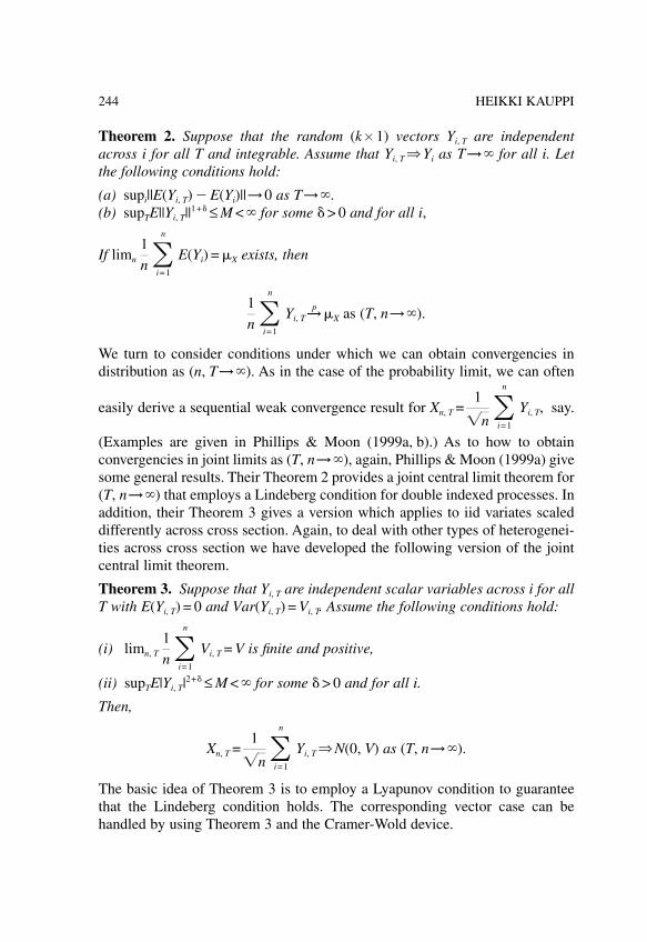
Theorem 2. Suppose that the random (k � 1) vectors Yi, T are independentacross i for all T and integrable. Assume that Yi, T ⇒Yi as T→� for all i. Letthe following conditions hold:

(a) supi||E(Yi, T) � E(Yi)||→0 as T→�.(b) supTE||Yi, T||

1+� ≤ M < � for some � > 0 and for all i,

If limn

1n �

i=1

n

E(Yi) = �X exists, then

1n �

i=1

n

Yi, T →p�X as (T, n→�).

We turn to consider conditions under which we can obtain convergencies indistribution as (n, T→�). As in the case of the probability limit, we can often

easily derive a sequential weak convergence result for Xn, T =1

�n �i=1

n

Yi, T, say.

(Examples are given in Phillips & Moon (1999a, b).) As to how to obtainconvergencies in joint limits as (T, n→�), again, Phillips & Moon (1999a) givesome general results. Their Theorem 2 provides a joint central limit theorem for(T, n→�) that employs a Lindeberg condition for double indexed processes. Inaddition, their Theorem 3 gives a version which applies to iid variates scaleddifferently across cross section. Again, to deal with other types of heterogenei-ties across cross section we have developed the following version of the jointcentral limit theorem.

Theorem 3. Suppose that Yi, T are independent scalar variables across i for allT with E(Yi, T) = 0 and Var(Yi, T) = Vi, T. Assume the following conditions hold:

(i) limn, T

1n �

i=1

n

Vi, T = V is finite and positive,

(ii) supTE|Yi, T|2+� ≤ M < � for some � > 0 and for all i.

Then,

Xn, T =1

�n �i=1

n

Yi, T ⇒N(0, V) as (T, n→�).

The basic idea of Theorem 3 is to employ a Lyapunov condition to guaranteethat the Lindeberg condition holds. The corresponding vector case can behandled by using Theorem 3 and the Cramer-Wold device.

244 HEIKKI KAUPPI

III. AN APPLICATION

Most of the recent applications of the new large n, T panel data limit theory hasinvolved studying and developing estimators and tests for panel cointegratingregressions where the regressors are integrated of order one. In this section weanalyze problems that arise in these models when the regressors are nearlyrather than exactly integrated of order one. We start by introducing the modeland assumptions.

A. The Model

We focus on the simple two variable panel regression

yi, t = xi, t + ui, t, (1)

xi, t = i xi, t�1 + �i, t, i = exp(ci /T) � 1 +ci

T, (2)

(t = 1, . . . , T, i = 1, . . . , n),

where the initial values zi, 0 = (yi, 0, xi, 0)� are iid, E||zi, 0||4 < �, and the errors are

specified below. To this end, notice that if i = 1 (i.e. ci = 0) in (2) for each i, thenthe xi, t are pure or exact unit root processes and the system given by equations(1) and (2) coincides with the homogenous panel cointegration regressionstudied by Phillips & Moon (1999a) and many others (for a survey, see Phillips& Moon (1999b)). In these studies the regression coefficient in (1) is called acointegrating parameter and it represents a stationary relationship that holdsbetween yi, t and xi, t for every i. Such a common long-run relationship is oftenpredicted by economic theory and it is then of central interest to estimate andtest whether it satisfies theoretically sound restrictions. A typical exampleinvolves testing for the existence of a purchasing power parity hypothesis in apanel of suitably similar countries.

In contrast to the recent panel cointegration literature, we do not restrictattention to models, where the regressors are generated by exact unit rootprocesses. Indeed, although most macroeconomic variables analyzed in therecent panel cointegration studies display strong autocorrelation, there areseldom strong prior reasons why the autoregressive parameter should be unity.The problem is aggravated by the fact that unit root tests cannot reliably detectsmall deviations from unity. Given this uncertainty about the unit roots, it is ofinterest to study problems that arise in the statistical inference about theregression parameter in (1) when the autoregressive parameters in (2) are closeto rather than exactly equal to one. From earlier literature we know that such


problematic near alternatives are best modeled by the local to unit root

parametrization i = exp(ci /T) � 1 +ci

Tin (2) (see e.g. Elliott (1998) and Stock

(1997)). By this device it is possible to obtain asymptotic results that providereasonable approximations in cases where the regressors xi, t are stationary butrevert to their means so slowly that the standard fixed i asymptotics fail toattain satisfactory accuracy.

We close this section by imposing the following assumption.

Assumption 1. The errors �i, t = (ui, t, �i, t)� are linear processes satisfying thefollowing conditions:

(a) �i, t = C(L)�i, t =�j=0

�

Cj�i, t� j, where �j=0

�

j3||Cj|| < �,

(b) �i, t = ( i, t, wi, t)�, where i, t and wi, t are mutually independent and iid acrossi and over t with E( i, t) = E(wi, t) = 0, E( i, t

2 ) = E(wi, t2 ) = 1, and E( i, t

4 ) =E(wi, t

4 ) = �4 < � for all i and t.

Under Assumption 1 the error process in the system (1) and (2) satisfy the sameconditions as the error process of the homogenous panel cointegrationregression of Phillips & Moon (1999a, Assumptions 8 and 9).

B. Preliminary Analysis

For preliminary insights, we derive sequential limits for the pooled panel OLSestimator,

=�i=1

n �t=1

T

xi, tyi, t

�i=1

n �t=1

T

x 2i, t

. (3)

Let [Tr] denote the integer part of Tr. From Phillips & Solo (1992), we know

that under Assumption 1, the partial sum process 1

�T�t=1

[Tr]

�i, t converges weakly

to a two dimensional Brownian motion Bi(r) = (Bui(r), B�i

(r))�, (0 ≤ r ≤ 1), with

the long-run covariance matrix � =�j=��

�

E(�i, j��i, 0), which we partition

246 HEIKKI KAUPPI

� = [�kl], (k, l = u, �). Furthermore, by the well know limit theory for nearintegrated processes (e.g. Phillips (1987, 1988)) as T→�,

1T 2 �

t=1

T

xi, t2 ⇒�

0

1

Kci(r)2dr, (4)

1T �

t=1

T

xi, tui, t ⇒�0

1

Kci(r)dBui

(r) + �u�, (5)

where �u� is a non-diagonal element of the one sided long-run covariance

matrix � =�j=0

�

E(�i, j��i, 0) = [�kl], (k, l = u, �), and Kci(r) =�

0

r

e(r�s)cidB�i(s),

(0 ≤ r ≤ 1), is an Ornstein-Uhlenbeck process. Given (4) and (5) we may deducefor fixed n as T→�,

T( � )→�1n �

i=1

n �0

1

Kci(r)2dr��11

n �i=1

n ��0

1

Kci(r)dBui

(r) + �u��. (6)

This result provides the first step for obtaining sequential asymptotics for (3).The second step is to derive the limit of the right hand side of (6) as n→�. For

simplicity assume ci = c for all i. Then, notice that the �0

1

Kci(r)dBui

(r) are iid

with mean zero and variance

E��0

1

Kci(r)dBui

(r)�2

= �uu�� 0

1�0

r

e2(r�s)cdsdr < �, (7)

where the equality follows from well known results for stochastic integrals.Consequently, we may apply the strong law of large numbers to obtain

1n �

i=1

n �0

1

Kci(r)dBui

(r)→as 0, as n→�, (8)

where ‘→as ’ denotes almost sure convergence. Furthermore, the �0

1

Kci(r)2dr are

also iid,

E�0

1

Kci(r)2dr = ��

0

1�0

r

e2(r�s)cdsdr > 0,


and E��0

1

Kci(r)2dr�2

< �. Thus, we may deduce that the denominator on the

right hand side of (6) converges almost surely to �� 0

1�0

r

e2(r�s)cdsdr, as

n→�. In view of these results, we may now conclude that as T→� followedby n→�,

T( � )→p �1/�0

1 �0

r

e2(r�s)cdsdr� �u�

��

. (9)

This result indicates that although is consistent it is subject to a second orderbias effect arising from temporal correlation between the system errors ui, t and�i, t. Note that if i = 1 in (2), the bias term in (9) still exists and actuallybecomes equal to 2�u� /��. In contrast, if �u� = 0, there is no asymptotic bias inthe estimation error of irrespective of the values of the localizing parametersci in (2). In fact, if �u� = 0, we obtain the sequential weak convergence result

�nT( � )→N(0, V), (10)

where

V =�uu

��

1

�0

1 �0

r

e2(r�s)cdsdr

.

The latter limiting result essentially follows from the fact that

1

�n�i=1

n �0

1

Kci(r)dBui

(r)

is asymptotically normally distributed with zero mean and variance given in(7).

C. Serial Correlation Corrected Estimation

In view of the above analysis we may conjecture that the asymptotics in (10)can be attained even when �u� ≠ 0 provided that we have a suitable estimator for

248 HEIKKI KAUPPI

�u�. One alternative is to use the kernel estimation strategy that is used in thepooled fully modified (PFM) estimator of Phillips & Moon (1999a). The PFMestimator will be introduced in the subsequent section and it employes theaveraged kernel estimators � = [�kl] and � = [�kl], (k, l = u, �), of � and �,respectively, defined by

� =1n �

i=1

n

�i, �i = �j=�T+1

T�1

�(j/K)�i(j),

� =1n �

i=1

n

�i, �i =�j=0

T�1

�(j/K)�i(j). (11)

Here �i(j) =1T�

t

�i, t+ j��i, t, where the summation is over 1 ≤ t, t + j ≤ T, while

�(j/K) is a lag kernel for which �(0) = 1, �(x) = �( � x), ��

�

� (x)2dx < �, and

with Parzen’s exponent q�(0, �) such that kq = limx→0

1 � �(x)|x|q

< � . As to

applicable lag kernel functions and the choice of the bandwidth parameter K wefollow Phillips & Moon (1999a) and impose the following assumption.

Assumption 2. The lag kernel �(j/K) in (11) has Parzen exponent q >12, and

the bandwidth parameter K tends to infinity with K/T→0 and K2q/T→� > 0, asT→�.

Remark 1. Under Assumption 2 the normalized estimation errors �n(� � �)and �n(� � �) converge in probability to zero. This result was stated inPhillips & Moon (1999a, Proof of Theorem 9) and holds as (T, n→�) withn/T→0. This result is employed in the proofs of the theorems given below.

Remark 2. Notice that the kernel estimators defined in (11) are not feasible,since they employ the unknown errors �i, t = (ui, t, �i, t)�. A natural approach toestimate ui, t and �i, t is to use the residuals ui, t = yi, t � xi, t, from a preliminarypooled panel OLS regression, and the differences � xi, t , respectively. It is easyto show that the associated estimation errors for ui, t and �i, t are of orders ofmagnitude T �1 and T �1/2, respectively. In view of this and Remark 1 we maythen expect that under the assumptions of this chapter and irrespective whetherthe xi, t in (2) have exact or near unit roots, the use of ui, t and �xi, t in places ofui, t and �i, t, respectively, has no effect on the rate of consistency of the kernel


estimators in (11). However, following Phillips & Moon (1999a), we proceedby working with the true errors �i, t , since we want to avoid any furthertechnical complications that might arise in an asymptotic analysis where thekernel estimators in (11) use the estimates ui, t and �xi, t in places of ui, t and �i, t,respectively.

Now we are ready to define a robust estimator for ,

* =�i=1

n �t=1

T

xi, tyi, t � nT�u�

�i=1

n �t=1

T

xi, t2

, (12)

where �u� is given in (11). The estimator in (12) is called a serial correlationcorrected pooled panel estimator.

We turn to establish the joint asymptotics of the new estimator in (12). Let

Jci(r) =�

0

r

e(r�s)cidWi(s), where Wi(r) is a standard Brownian motion. Hereafter,

we assume that the values of ci are uniformly bounded and such that the

arithmetic mean of the expected values of �0

1

Jci(r)2dr converges to a positive

finite number, i.e.

limn→�

1n �

i=1

n

E��0

1

Jci(r)2 dr�= lim

n→�

1n �

i=1

n �0

1 �0

r

e2(r�s)cidsdr = �xx

exists and is finite by assumption. The latter condition is not restrictive andbasically means that we assume that the appropriately normalized sample

second moment of the pooled regressors xi, t, i.e. 1

nT 2 �i=1

n �i=1

T

xi, t2 , converges in

probability.

Theorem 4. Suppose Assumptions 1 and 2 hold and that data are generated by(1) and (2) with ci such that supi|ci| ≤ c < �. Then under joint limits as(T, n→�) with n/T→0

�nT(* � )→N(0, V*),

where

V* =�uu

��

1�xx

.

250 HEIKKI KAUPPI

As is apparent from Theorem 4 the serial correlation corrected pooled panelOLS estimator has indeed very desirable properties. It is �nT-consistent,asymptotically normal and free of asymptotic biases irrespective whether theregressors xi, t in (2) carry out exact or near unit roots in their generatingmechanisms. This is a remarkable improvement that can be gained, if paneldata are used, since none of the existing time series estimators for cointegratingparameters can achieve these features. Rather, as shown e.g. by Elliott (1998)the time series cointegration regression estimators tend to suffer from secondorder biases unless the regressors are generated by exact unit root processes,and these biases lead to severe size distortions in hypothesis testing. In contrast,we will show below that by the use of the serial correlation corrected pooledpanel OLS estimator we can achieve robust inferences in fairly generalsituations where individual regressors may have roots that vary heteroge-neously within a range of values near one.

Unfortunately, the situation turns out less hopeful, if the panel regression in(1) includes individual intercepts or if the data exhibit linear or higher ordertime trends. While there is a natural way to modify the new serial correlationcorrected pooled OLS estimator to take these effects into account, it turns outthat in these cases near unit roots result in nuisance parameters that producebias effects to the asymptotics of the estimator. To see why this happenssuppose the regression in (1) includes an intercept that may vary acrossindividuals. This suggests the use of demeaned data in the formula of theestimator. Accordingly, modify (12) to the form

* =�i=1

n �t=1

T

xi, tyi, t � nT�u�

�i=1

n �t=1

T

xi, t2

, (13)

where yi, t = yi, t � yi and xi, t = xi, t � xi, with yi =1T �

t=1

T

yi, t and xi =1T �

t=1

T

xi, t,respectively.

The asymptotic properties of the estimator in (13) are easily found byemploying the sequential limit theory. To reveal the most essential part of thisexercise note that we have

1T �

t=1

T

xi, tui, t →�0

1

Kci(r)dBui

(r) + �u�, (14)


where Kci(r) is a demeaned Ornstein-Uhlenbeck process defined by Kci

(r) =

Kci(r) ��

0

1

Kci(s)ds. Now, while the temporal correlation correction in (13) can

still remove the bias effects that arise from the presence of �u� on the right hand

side of (14), the remaining term, i.e. �0

1

Kci(r)dBui

(r), does no longer have a zero

mean in comparison with the case in (5), where we had Kci(r) in place of Kci

(r).In fact,

E�0

1

Kci(r)dBui

(r) = � �u� �0

1�0

r

e(r�s)cidsdr

and we thus obtain

1n �

i=1

n �0

1

Kci(r)dBui

(r)→p� �u��xx, as n→�,

where �xx is given above. In view of this result it is easy to see that theestimator in (13) is subject to an asymptotic bias, which depends on thenuisance parameters ci. Unfortunately, no technique is currently available thatwould provide consistent estimates for the single localizing coefficients ci.Only in the special case where the localizing coefficient are the same across i,we may use the cross sectional dimension of the panel to provide consistentestimates for the common localizing coefficient (see Moon & Phillips (1999)).This fact opens a possibility for correcting the bias effects. However, such acorrection may be rather complicated and is to be restricted in cases where thecommon c is well below zero (cf. Moon & Phillips (1999)). While it is out ofthe scope of this study to consider this matter in more detail, in empiricalapplications the special case of a common c is nevertheless hardly realistic.

D. Fully Modified Estimation

We turn to consider the PFM estimator of Phillips & Moon (1999a). The ideaof the PFM estimator is to modify the pooled OLS estimator in (3) byemploying non-parametric corrections in the same way as in the fully modifiedOLS (FM-OLS) estimator of Phillips & Hansen (1990). The estimator isdefined by

252 HEIKKI KAUPPI

+ =�i=1

n �t=1

T

xi, tyi, t+ � nT�u�

+

�i=1

n �t=1

T

xi, t2

, (15)

where

yi, t+ = yi, t � �u��

�1�xi, t (16)

and

�u�+ = �u� � �u��

�1��, (17)

employ the kernel estimators in (11). The equation (16) gives an endogeneitycorrection and is similar to that in the FM-OLS estimator of Phillips & Hansen(1990). The equation (17) gives the contemporaneous and serial correlationcorrections that are needed to remove all the second order bias effects arisingfrom temporal correlation between ui, t and �i, t.

Under the assumption that the regressors xi, t in (2) have exact unit roots thejoint asymptotics of the PFM estimator are determined by Theorem 9 ofPhillips & Moon (1999a). The following theorem shows how this resultchanges when the regressors xi, t are generated by the more general class of nearunit root processes. Here we make an additional (technical) assumption that thevalues of ci are such that the ci-weighted average of the expected values of

�0

1

Jci(r)2dr converges to a finite number, i.e.

limn→�

1n �

i=1

n

ciE��0

1

Jci(r)2dr�= �xx

c

exists and is finite by assumption.

Theorem 5. Suppose the assumptions of Theorem 4 hold. Then under jointlimits as (T, n→�) with n/T→0

(a) �nT(+ � ) � �nBn, T →N(0, V+ ),

(b) T(+ � )→p B,

where

V+ =

�u · �

��

1�xx

, (18)


with �u · � = �uu � �u�2 ��

�1, and

Bn, T = ��u�

��

�i=1

n

T(eci/T � 1)�t=1

T

xi, t xi, t�1

�i=1

n �t=1

T

xi, t2

, (19)

B = ��u�

��

�xxc

�xx

. (20)

The following corollary holds when the assumption of Phillips & Moon(1999a) about exact unit roots in the regressors xi, t is valid.

Corollary 6. Suppose Assumptions 1 and 2 hold and data are generated by (1)and (2) with ci = 0 for all i. Then under joint limits as (T, n→�) with n/T→0

�nT(+ � )⇒N(0, 2�u · ��1).

It is indeed easy to see that the result of Corollary 6 follows from Theorem 5,

because if ci = 0, then Bn, T = B = 0, and E��0

1

Jci(r)2dr�= E��

0

1

Wi(r)2dr�=12

giving V+ = 2�u · ��1. The result of Corollary 6 coincides precisely with that of

Theorem 9 of Phillips & Moon (1999a) and it is illustrative to compare it toTheorems 4 and 5 above. First, note from Corollary 6 the obvious fact thatwhen the exact unit root assumption holds, then + is �nT-consistent,asymptotically normal and unbiased. In addition, note that in this case + isgenerally more efficient than *, because �u · � = � uu � �u�

2 ��1 ≤ �uu. This is the

price that we have to pay, if the autoregressive parameters in (2) happen to beexactly equal to one and we use the estimator * instead of + .

However, as Theorem 5 indicates the behavior of the estimator + isradically different, if the regressors xi, t are generated by processes with rootsthat are only local to one. First, the estimator + is no more �nT-consistent.Rather, in order to obtain �nT-rate asymptotics, a bias term Bn, T given in (19)has to be subtracted from the estimation error. In fact, in view of the result (b)of Theorem 5, if the xi, t are near, rather than exact, unit root processes, theestimator + is only T-consistent and has an asymptotic bias given by B in (20).If there is no simultaneity in the model, i.e. if �u� = 0, then the biases disappearand the PFM estimator is �nT-consistent and has an asymptotic normaldistribution with the same variance as that of the serial correlation correctedpooled OLS estimator.

To see why the biases arise notice first that when an autoregressive parameteri in (2) is just nearly one with ci non-zero, then �xi, t = �i, t + (eci /T � 1)xi, t�1,

254 HEIKKI KAUPPI

where (eci /T � 1) � ci /T. It is then easy to see that the use of �xi, t in theendogeneity correction term (16) gives raise to Bn, T in (19), which has the limitgiven in (20). It is worth noticing that if the nuisance parameters ci were known,we could employ a quasi-difference in place of the pure difference �xi, t in (16)so that the bias term, Bn, T = 0. However, as we already noted above such asolution is generally infeasible because the localizing coefficient ci areunknown and cannot be consistently estimated from the individual time seriesxi, t.

We close this section by pointing out that the above bias problem also occursin cases where the PFM estimator is modified to account of deterministiceffects like individual intercepts in (1). This fact can be easily verified throughsequential asymptotics (for details see Kauppi (1999, p. 124–125)).

E. Hypothesis Testing

In this section we consider testing a simple hypothesis H0: = 0 againstH1: ≠ 0. First, in view of Theorem 4 we could use the serial correlationcorrected pooled OLS estimator to obtained the t-test statistic

t* = �nT(* � 0)� 1

nT2 �i=1

n �t=1

T

xi, t2

�uu

.

In view of Theorem 4 and the result (36) given in its proof in the appendix itis easy to deduce the following corollary.

Corollary 7. Suppose the assumptions of Theorem 4 hold. Then, under jointlimits as (T, n→�) with n/T→0, t* ⇒N(0, 1).

For comparison we will also consider assuming exact unit roots in xi, t andaccordingly employing the PFM estimator based t-test

t+ = �nT(+ � 0)�12

��

�u · �

,

where �� and �u · � = �uu � �u�2 ��

�1 are obtained from the kernel estimatorsgiven in (11) (cf. Phillips & Moon (1999a, Remark (c), p. 1086)).

Corollary 8. Suppose the assumptions of Theorem 5 hold. Then, under jointlimits as (T, n→�) with n/T→0

(a) t+ diverges, if �u� ≠ 0 and B ≠ 0, where B is given in (20);


(b) t+ ⇒N(0, Vt+), if �u� = 0, where Vt

+ =12

� xx.

Part (a) of Corollary 8 states the obvious consequence of Theorem 5 that the t-test statistic t+ diverges, if the regressors are generated by local to unit rootprocesses and �u� is non-zero. This means that hypothesis tests based on thePFM estimator are generally severely distorted. The result of part (b) ofCorollary 8 shows that even when there is no simultaneity, i.e. �u� = 0, the testdoes not have the desired standard normal distribution. To illustrate this lattereffect suppose that ci = c for all i. Then, if �u� = 0, we have

Vt+ =

2c2

e2c � 2c � 1, (21)

because E�0

1

Jci(r)2dr =�

0

1 �0

r

e2(r�s)cdsdr = (e2c � 2c � 1)/4c2 for all i. It is easy

to see from (21) that for negative values of c, the Vt+ becomes larger than unity.

For example, for c = � 5 and c = � 10, the Vt+ is approximately equal to 5.55

and 10.53, respectively. Notice that if the usual 5% critical value 1.96 is appliedin the t+-test, then the true asymptotic rejection rates that correspond to c = � 5and c = � 10 are approximately equal to 40.3% and 54.6%, respectively.

F. Simulations

In this section, we illustrate the theoretical findings obtained in the previoussection by conducting some simple Monte Carlo experiments. We focus oninvestigating the size behavior of the PFM t-test statistic, t+ , and that of thebias corrected t-test, t*. For the experiments we generate artificial data byemploying equations (1) and (2), where we impose = 1 in (1). The errors�i, t = (ui, t, �i, t)� are generated simply by equation �i, t = chol(C)�i, t, where�i, t ~ nid(0, I2) across i = 1, . . . , n, and over t = 1, . . . , T, and chol(C) is theCholesky decomposition of the matrix C = [Cij] with C11 = C22 = 1,C12 = C21 = �u�. Thus, we have E(ui, t) = E(�i, t) = 0, E(ui, t

2 ) = E(�i, t2 ) = 1 = �uu = ��

and E(ui, t�i, t) = �u�. The initial values yi, 0 and xi, 0 are set to zeros.Table 1 reports percentage rejection rates of the t-tests, t+ and t*,

respectively, when a 5% critical value 1.96 is applied, n = 50, T = 250, and thelocal to unit root coefficients are set equal to a common value c, i.e. we usei = = 1 + c/T for all i. In computing the long-run covariance estimates in t+

and t*, respectively, we employed the Parzen kernel function and thebandwidth parameter value K = 1.[2] The columns under c = 0 report resultswhen an exact unit root assumption holds. In accordance with the analytical

256 HEIKKI KAUPPI

results of the previous section, in this case, the size behavior of the two tests isgood. The columns under c = � 5 and c = � 10 give rejection rates when theroots of the regressors are only nearly one. As predicted by Corollary 8, nowthe t+-test is very sensitive to deviations from exact unit roots and suffers fromsevere size distortions through all values of �u�. Notice that even when �u� = 0the t+-test rejects far in excess to the desired 5% nominal level as waspredicted by the considerations of the previous section. In contrast, as predictedby Corollary 7 the bias corrected t-test, t*, maintains well the desired size levelthrough different values of �u�.

Table 2 reports otherwise similarly computed test results as those of Table 1except that now n and T are set to 25 and 100, respectively. As is apparent theresults do not change much from those of Table 1. This indicates that ourasymptotic results can provide fairly accurate approximations with samplesizes that are typical in empirical applications.

Table 3 examines the performance of the bias corrected t-test when theindividual localizing coefficients in the generating mechanisms of theregressors vary across different panel members. The heterogeneity across panelmembers were obtained by using otherwise similarly generated data as inTables 1 and 2 except that all the individual specific localizing coefficients ci

were drawn from a uniform distribution on the interval [c, 0]. For example, thecolumn denoted by ‘(n = 25, T = 100)’ and ‘c = � 10’ reports simulation results

Table 1. Monte Carlo results with n = 50 and T = 250

c = 0 c = –5 c = –10

�u� t+ t* t+ t* t+ t*

0 5.20 4.70 42.10 5.00 52.30 4.200.2 5.30 4.40 89.80 4.30 99.60 5.400.4 6.60 6.80 100.0 4.90 100.0 4.900.6 4.30 4.50 100.0 4.00 100.0 5.600.8 4.30 4.50 100.0 5.80 100.0 4.50

Notes: The columns under t+ and t* report Monte Carlo rejection rates of the respective t-testscomputed by employing long-run covariance estimates that were achieved by using a Parzenkernel function and a bandwidth parameter value K = 1. A nominal 5% asymptotic level wereapplied. In each replication, the data were obtained by using equations (1) and (2) with = 1 andi = = 1 + c/T in (1) and (2), respectively, initial values zeros, and with the errors �i,t = (ui,t,�i,t)�generated by equation �i,t = chol(C)�i,t, where �i,t ~ nid(0, I2) across i = 1, . . . , n, and overt = 1, . . . , T, and chol(C) is the Cholesky decomposition of the matrix C = [Cij] with C11 = C22 = 1,C12 = C21 = �u�. Results are based on 1000 replications.


based on an experiment, where the autoregressive coefficients i( = 1 + ci/T)across different panel members vary uniformly within the range [0.9, 1]. Acomparison of the results of Table 3 to those of Tables 1 and 2 clearly indicatesthat the bias corrected t-test behaves equally well whether the xi, t havehomogenous or heterogenous localizing coefficients.

In view of the above reported simulation experiments we may conclude thatnear unit roots indeed result in severe size distortions to hypothesis tests basedon the PFM estimator. On the other hand, the results are fairly promising with

Table 2. Monte Carlo results with n = 25 and T = 100

c = 0 c = –5 c = –10

�u� t+ t* t+ t* t+ t*

0 6.80 6.20 37.40 5.50 52.30 5.500.2 6.60 6.10 74.60 4.00 96.50 6.600.4 6.00 5.10 99.20 5.10 100.0 6.200.6 5.40 4.90 100.0 6.20 100.0 5.800.8 5.30 5.80 100.0 5.60 100.0 5.00

Notes: See the notes of Table 1.

Table 3. Monte Carlo results on the bias corrected test when localizingcoefficients are heterogenous

(n = 50, T = 250) (n = 25, T = 100)

�u� c = –5 c = –10 c = –5 c = –10

0 4.82 5.10 5.00} 5.180.2 5.80 5.06 6.20 5.000.4 4.96 4.62 5.12 5.340.6 5.42 5.06 5.98 5.460.8 5.18 5.18 5.44 5.92

Notes: The table reports Monte Carlo rejection rates of the t*-test computed in the same way asin Tables 1 and 2. The data were obtained otherwise similarly as in Tables 1 and 2 except that ineach replication the individual specific localizing coefficient ci (i = 1, . . . , n) were drawn from auniform distribution on the interval [c, 0]. The applied values of c are given in the top of eachcolumn. Results are based on 5000 replications.

258 HEIKKI KAUPPI

regard to the new bias corrected test, which was able to maintain good sizebehavior through all the performed experiments. However, it should be pointedout that our simulation setup here is rather simple and it is likely that someproblems arise in more complicated models. For example, if the datagenerating mechanism obeys a more general short-run dynamics thanexperimented here, then it can be expected that the non-parametric correctionsare subject to somewhat larger (finite sample) estimation errors, which mayweaken the performance of the bias corrected test. Furthermore, an additionalsource of estimation error results in when the non-parametric estimators useestimated values in places of the true values of the errors.

IV. CONCLUDING REMARKS

This chapter developed new panel data limit theory that can be used inobtaining convergencies in probability and in distribution when there isheterogeneity across panel members and the cross sectional and time seriesdimensions of the data tend to infinity simultaneously. The new theory wasapplied to study asymptotics of a panel regression in which the regressors weregenerated by a local to unit root process with cross sectionally heterogenouslocalizing coefficients. The application demonstrated that a serial correlationcorrected pooled panel OLS estimator yields �nT-consistent and asymptot-ically normal estimates that are centered to the true parameter valueirrespective of whether the regressors are nearly or exactly integrated. Whilethis desirable result holds only in the special case without deterministic effects,our asymptotic analysis also indicated that the panel fully modified estimator issubject to asymptotic biases even in this simple case, if the regressors arenearly rather than exactly integrated. Therefore, much care should be taken ininterpreting results achieved by the recent panel cointegration methods thatassume exact unit roots when near unit roots are equally plausible.

NOTES

1. This is proved by Phillips & Moon (1999a, Theorem 8) when ci = 0 for all i.Furthermore, similar result can be proved in the case where the ci are nonzero byfollowing lines given in the proof of Theorem 5 of this chapter.

2. In empirical applications a bandwidth parameter value K = 1 is hardly realistic.However, in the present simulation setup the actual value of K does not play animportant role, because we use iid errors in the simulations. For example, in all of the


reported cases, essentially similar results were obtained by using the bandwidthparameter value K = 4.

ACKNOWLEDGMENTS

I would like to thank the two referees for their useful comments andsuggestions. This paper was completed while the author worked at theResearch Department of the Bank of Finland whose hospitality is gratefullyacknowledged. This paper is a part of the research program of the ResearchUnit on Economic Structures and Growth (RUESG) at the Department ofEconomics at the University of Helsinki. Financial support from the YrjöJahnsson Foundation is appreciated. The usual disclaimer applies.

REFERENCES

Billingsley, P. (1968). Convergence of Probability Measures. New York: John Wiley.Davidson, J. (1994). Stochastic Limit Theory. Oxford University Press.Elliott, G. (1998). On The Robustness of Cointegration Methods When Regressors Almost Have

Unit Roots. Econometrica, 66(1), 149–158.Kauppi, H. (1999). Essays on Econometrics of Cointegration. Research Reports Nro 84,

Dissertationes Oeconomicae, Department of Economics, University of Helsinki.Moon, H., & Phillips, P. C. B. (1999). Estimation of Autoregressive Roots Near Unity Using

Panel Data. Cowles Foundation Discussion Paper No. 1224, Yale University,(http://cowles.econ.yale.edu/).

Phillips, P. C. B. (1987). Towards A Unified Asymptotic Theory for Autoregression. Biometrica,74(3), 535–547.

Phillips, P. C. B. (1988). Regression Theory for Near-integrated Time Series. Econometrica, 56(5),1021–1043.

Phillips, P. C. B., & Hansen, B. E. (1990). Statistical Inference In Instrumental VariablesRegression With I(1) Processes. Review of Economic Studies, 57, 99–125.

Phillips, P. C. B., & Moon, H. (1999a). Linear Regression Limit Theory for Non-stationary PanelData. Econometrica, 67(5), 1057–1111.

Phillips, P. C. B., & Moon, H. (1999b). Non-stationary Panel Data Analysis: An Overview ofSome Recent Developments. Cowles Foundation Discussion Paper No. 1221, YaleUniversity, (http://cowles.econ.yale.edu/).

Phillips, P. C. B., & Solo, V. (1992). Asymptotics for Linear Processes. The Annals of Statistics,20(2), 971–1001.

Stock, J. H. (1997). Cointegration, Long-run Comovements, and Long Horizon Forecasting. In: D.Kreps & K. F. Wallis (Eds), Advances in Econometrics Proceedings of the Seventh WorldCongress of the Econometric Society. Cambridge: Cambridge University Press.

Stout, W. F. (1974). Almost Sure Convergence. New York: Academic Press.White, H. (1984). Asymptotic Theory for Econometricians. Academic Press: San Diego,

California.

260 HEIKKI KAUPPI

APPENDIX

APPENDIX A: PROOF OF THEOREM 2

From the conditions of the theorem we know that Xn, T =1n�

i=1

n

Yi, T ⇒

Xn =1n�

i=1

n

Yi as T→� for all fixed n. Since supTE||Yi, T||1+� ≤ M < � for all i and

because Yi, T ⇒Yi implies ||Yi, T||1+� ⇒ ||Yi||

1+� by the continuous mapping theoremwe also have E||Yi||

1+� ≤ M < � by Theorem 5.3 of Billingsley (1968) (see alsodiscussion on p. 33 of Billingsley (1968)). By arguments given in the proof ofTheorem 1 of Phillips & Moon (1999a) we can justify that the Yi areindependent across i, since the Yi, T are independent across i for all T. Given thisand the fact that E||Yi||

1+� ≤ M < �, we may apply Markov’s law of large

numbers to deduce Xn →p�X as n→� (e.g. White (1984, p. 33)). Furthermore,

if we establish conditions (i) through (iv) of Theorem 1, then Xn, T →p�X as

(T, n→�).First, condition (i) holds, since

1n�

i=1

n

E||Yi, T|| ≤1n�

i=1

n

supT

E||Yi, T|| ≤ M < �,

where the last two inequalities follow from condition (b) of the theorem. Also,condition (ii) holds, since

1n�

i=1

n

||E(Yi, T) � E(Yi)|| ≤ supi

||E(Yi, T) � E(Yi)||→0, as T→�,

by condition (a). For condition (iii) we use the fact that E||Yi, T||1{||Yi, T|| > n�}

≤1

(n�)�sup

TE||Yi, T||

1+� ≤M

(n�)�for all i, where the first inequality follows from

arguments given by Billingsley (1968, p. 32) and the second inequality holdsby condition (b). Now, for any � > 0,

1n�

i=1

n

E||Yi, T||1{||Yi, T|| > n�} ≤M

(n�)�,


and therefore, condition (iii) follows. Condition (iv) holds by the same

argument as we notice that now E||Yi||1{||Yi|| > n�} ≤1

(n�)�E||Yi||

1+� ≤M

(n�)�.

APPENDIX B: PROOF OF THEOREM 3

Let sn, T2 =�

i=1

n

Vi, T and define �i, n, T =Yi, T

sn, T

. Then

�i=1

n

�i, n, T ⇒N(0, 1), as (T, n→�), (22)

by Theorem 2 of Phillips & Moon (1999a), if the Lindeberg condition

limn, T→� �

i=1

n

E[�i, n, T2 1{|�i, n, T| > �}] = 0, � > 0,

holds. Given condition (i), (22) implies 1

�n�i=1

n

Yi, T ⇒N(0, V) as (T, n→�). It

remains to verify the above Lindeberg condition.We have for given � > 0,

�i=1

n

E[�i, n, T2 1{�i, n, T

2 > �}] =�i=1

n

EYi, T2

sn, T2 1Y i, T

2

sn, T2 > ��

=n

sn, T2

1n�

i=1

n

EY i, T2 1Y i, T

2 >�sn, T2

n �n��≤

nsn, T

2

1n�

i=1

n

supT

EY i, T2 1Y i, T

2 >�sn, T2

n �n��. (23)

By condition (ii) we can always find � > 0 such that supT

E|Y i, T2 |(1+�) ≤ N < � for

all i. Given this we obtain

supT

EY i, T2 1Y i, T

2 >�sn, T2

n �n��≤N

n��sn, T2

n ��

, (24)

262 HEIKKI KAUPPI

for all i (cf. Billingsley (1968, p. 32)). In view of (23) and (24) and given that

condition (i) implies limn, T→�

nsn, T

2 = 1/V < � (V > 0) and limn, T→�

sn, T2

n= V < � we may

now conclude that

limn, T→� �

i=1

n

E[�i, n, T2 1{�i, n, T

2 > �}] = 0,

so that the Lindeberg condition follows.

APPENDIX C: PROOF OF THEOREM 4

We start by giving some intermediate results that we will use repeatedly in themain part of the proof given below. First, just as in Phillips & Moon (1999a,Lemma 2), based on Phillips and Solo (1992), we decompose the �i, t as

�i, t = C�i, t + �i, t�1 � �i, t, (25)

where C = C(1) =�k=0

�

Ck and �i, t =�j=0

�

Cj�i, t� j with Cj =�k=j+1

�

Ck. Under

Assumption 1(a), C is finite and �j=0

�

j2||Cj||2 =�

j=0

�

j2 �s=j+1

�

Cs 2

< � (see

Phillips & Moon (1999a, p. 1083)). It follows that

E||�i, t||2 ≤ M < �. (26)

We partition C = [Cab], (a, b = , w), so that the long-run covariance matrix

� = CC� =� C 2 + C w

2

C Cw + C wCww

C Cw + C wCww

Cw 2 + Cww

2 �=��uu

��u

�u�

�� (27)

For subsequent reference note that the components of �i, t = (ui, t, �i, t)� in (25)may be written as

ui, t = C i, t + C wwi, t + ui, t�1 � ui, t, (28)

�i, t = Cw i, t + Cwwwi, t + �i, t�1 � �i, t, (29)

where ui, t and �i, t are the two components in �i, t.Next, by equation (2)

xi, t =�s=1

t

e((t�s)/T)ci�i, s + e(t/T)cixi, 0


and using (29) we can write this as

xi, t = Cw f( )i, t + Cww f(w)i, t + R(x)i, t, (30)

where have used the notation

f(a)i, t =�s=1

t

e((t�s)/T)ciai, s, a = , w, (31)

and

R(x)i, t = e(t�1)/T)ci�i, 0 + (1 � eci /T)�s=1

t�1

e((t�1�s)/T)ci�i, s � �i, t + e(t/T)cixi, 0. (32)

For later analysis it is useful to have the following two moment bounds. First,

supi

sup1≤t≤T

E�f(a)i, t2

T �≤ sup1≤t≤T

1T�

s=1

t

e((t�s)/T)2 supi|ci| ≤ M < �, (33)

since e((t�s)/T)2 supi|ci| ≤ M < � (recall that supi|ci| ≤ c < �). Second, using the

inequality E �i=1

m

Xi|2 ≤ m�

i=1

m

E|Xi|2 (e.g. Davidson (1994, p. 140)) and the fact

�i, t are iid across i we obtain

supi

sup1≤t≤T

E(R(x)i, t2 ) ≤ 4� sup

1≤t≤Te((t�1)/T)2 supi|ci|�E(�i, 0

2 ) + 4 sup1≤t≤T

E(�i, t2 )

+ 4( sup1≤t≤T

e(t/T)2 supi|ci|)E(xi, 02 )

+ 4T 2(1 � esupi|ci| /T)2 sup1≤t≤T

1T 2

��k=1

t�1 �s=1

t�1

e((2t�2�k�s)/T)2 supi|ci|E|�i, s�i, k|

≤ M < �. (34)

To see that (34) holds note that sup1≤t≤T e(t/T)2 supi|ci| ≤ e2 supi|ci|, E(�i, t2 ) ≤ M by (26),

E(xi, 02 ) ≤ M (by the initial value condition), T 2(1 � esupi|ci| /T)2 = O(1), and by the

Cauchy-Schwartz inequality E|�i, k�i, s| ≤ �E(�i, k)2E(�i, s)

2 ≤ M, where the latterinequality follows again from (26).

264 HEIKKI KAUPPI

We turn to give the completing steps of the proof of Theorem 4. Write

�nT(* � ) =

1

�n�i=1

n1

T�t=1

T

(xi, tui, t � �u�) � �n(�u� � �u�)

1n�

i=1

n1T 2 �

t=1

T

xi, t2

,

where �n(�u� � �u�) = op(1), as (n, T→�) with n/T→0 (recall Remark 1). Itsuffices to show that

1

�nT�i=1

n �t=1

T

(xi, tui, t � �u�)⇒N(0, �uu��xx), as (T, n→�) with n/T→0,

(35)

and

1nT 2 �

i=1

n �t=1

T

xi, t2 →p

��xx, as (T, n→�). (36)

To prove (36) use (30) to write

1nT 2 �

i=1

n �t=1

T

xi, t2 = Cw

21n�

i=1

n1T 2 �

t=1

T

f( )i, t2 + Cww

2 1n�

i=1

n1T 2 �

t=1

T

f(w)i, t2

+ 2Cw Cww

1n�

i=1

n1T 2 �

t=1

T

f( )i, t f(w)i, t + 2Cw

1n�

i=1

n1T 2 �

t=1

T

f( )i, tR(x)i, t

+ 2Cww

1n�

i=1

n1T 2 �

t=1

T

f(w)i, tR(x)i, t +1n�

i=1

n1T 2 �

t=1

T

R(x)i, t2

= Cw 2 Ib1 + Cww

2 Ib2 + 2Cw CwwIIb1 + 2Cw IIb2 + 2CwwIIb3 + IIb4, say.

We now show that Cw 2Ib1 + Cww

2 Ib2 →p��xx and IIb1, IIb2, IIb3, IIb4 →p 0 as

(T, n→�) so that (36) follows.Write

Ib1 =1n�

i=1

n

Yi, T, (37)


where Yi, T =1T 2 �

t=1

T

f( )i, t2 . For an application of Theorem 2 observe that Yi, T are

independent across i for all T and as T→�, Yi, T ⇒Yi =�0

1

Jci(r)2dr. We know

E(Yi) =�0

1�0

r

e(r�s)2cidsdr and by assumption limn→�

1n�

i=1

n �0

1 �0

r

e(r�s)2cidsdr = �xx

exists. Therefore, if the conditions (i) and (ii) of Theorem 2 hold,

1n�

i=1

n

Yi, T →p�xx as (T, n→�).

For verifying condition (i) let p = 1 + � and use the definition of Yi, T in (37)to obtain

(E|Yi, T|p)1/p =

1T 2�E �

t=1

T

f( )i, t2 p�1/p

≤1T 2 �

t=1

T �E �s=1

t

e((t�s)/T)ci i, s 2p�1/p

, (38)

where the inequality follows from the Minkowski’s inequality and thedefinition of f( )i, t in (31). Now, the e((t�s)/T)ci i, s, (1 ≤ s ≤ t ≤ T), are independentrandom variables with zero means and E|e((t�s)/T)ci i, s|

2p ≤ (esupi|ci|})2+2�

E| i, s|2+2� ≤ M for some M < � and some � > 0. Therefore, we may apply

Theorem 3.7.8 of Stout (1974, p. 213) to obtain

E �s=1

t

e((t�s)/T)ci i, s 2p

≤ Mt p, (39)

where M is finite and independent of i. By inserting (39) into (38) and risingto the power of p = 1 + � it is easy to see that E|Yi, T|

1+� ≤ M so that condition (i)of Theorem 2 follows. For condition (ii) of Theorem 2 it suffices to note that

the supremum of the absolute difference between E(Yi, T) =1T 2 �

t=1

T �q=1

t

e(t�q/T)2ci

and E(Yi) =�0

1�0

r

e(r�s)2cidsdr tends to zero uniformly in i as T→� (this follows

since supi|ci| ≤ c < �, for details see Kauppi (1999, p. 135–136)).

266 HEIKKI KAUPPI

Obviously the above analysis remains the same if we replace i, t in thedefinition of Yi, T in (37) with wi, t implying that Ib2 has the same limit as Ib1.Noticing from (27) that Cw

2 + Cww2 = �� we therefore see that Cw

2 Ib1 + Cww2 Ib2

converges in probability to ��xx as desired.

We turn to prove that IIb1, IIb2, IIb3, IIb4 →p 0 as (T, n→�) by showing thatE(IIb1)

2, E|IIb2|, E|IIb3|, E|IIb4|→0 as (T, n→�). First, by the inequality

E �i=1

m

Xi|2 ≤ m�

i=1

m

E|Xi|2 (e.g. Davidson, 1994, p. 140) and condition (b) of

Assumption 1 we have E(IIb1)2 =

1n2T�

i=1

n �t=1

T

E(f( )i, t /�T)2E(f(w)i, t /�T)2 =

O�1n�, where the latter equality follows from (33). Second, the use of the

triangular and Cauchy-Schwartz inequalities shows that

E 1n�

i=1

n1T 2 �

t=1

T

f(a)i, tR(x)i, t ≤1

�T

1n�

i=1

n1T�

t=1

T �E f(a)i, t

�T 2

E|R(x)i, t|2 = O� 1

�T�,

where the equality follows from (33) and (34). Hence, E|IIb2|, E|IIb3|→0 as(T, n→�). It is also straightforward to do similar calculations with IIb4 thatshow E|IIb4|→0 as (T, n→�). This completes the proof of (36).

We turn to prove the result in (35). First, use (28) through (30) to write

1

�nT�i=1

n �t=1

T

(xi, tui, t � �u�)

=1

�n�i=1

n 1T�

t=1

T

(Cw f( )i, t + Cww f(w)i, t)(C i, t + C wwi, t) � �u��+

1

�n�i=1

n 1T�

t=1

T

[xi, t(ui, t�1 � ui, t) + R(x)i, t(C i, t + C wwi, t)] + �u� � �u��= Ia + IIa, say. (40)

Note that f(a)i, 1 = ai, 1 and f(a)i, t = eci /Tf(a)i, t�1 + ai, t, (ai, t = i, t, wi, t), t ≥ 2, so that wemay write


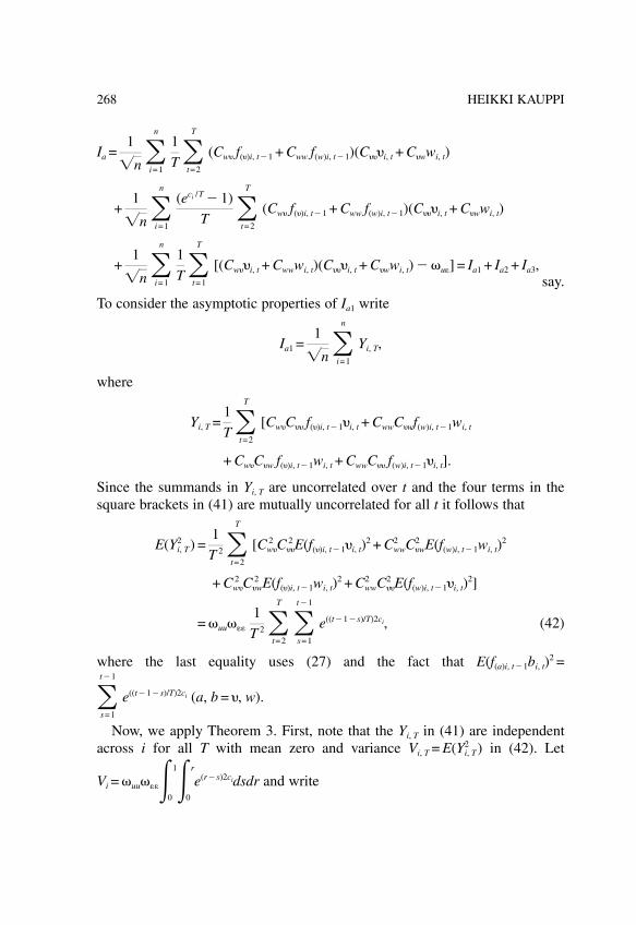
Ia =1

�n�i=1

n1T�

t=2

T

(Cw f( )i, t�1 + Cww f(w)i, t�1)(C i, t + C wwi, t)

+1

�n�i=1

n(eci /T � 1)

T �t=2

T

(Cw f( )i, t�1 + Cww f(w)i, t�1)(C i, t + C wwi, t)

+1

�n�i=1

n1T�

t=1

T

[(Cw i, t + Cwwwi, t)(C i, t + C wwi, t) � �u�] = Ia1 + Ia2 + Ia3,say.

To consider the asymptotic properties of Ia1 write

Ia1 =1

�n�i=1

n

Yi, T,

where

Yi, T =1T�

t=2

T

[Cw C f( )i, t�1 i, t + CwwC wf(w)i, t�1wi, t

+ Cw C w f( )i, t�1wi, t + CwwC f(w)i, t�1 i, t].

Since the summands in Yi, T are uncorrelated over t and the four terms in thesquare brackets in (41) are mutually uncorrelated for all t it follows that

E(Yi, T2 ) =

1T 2 �

t=2

T

[Cw 2 C

2 E(f( )i, t�1 i, t)2 + Cww

2 C w2 E(f(w)i, t�1wi, t)

2

+ Cw 2 C w

2 E(f( )i, t�1wi, t)2 + Cww

2 C 2 E(f(w)i, t�1 i, t)

2]

= �uu��

1T 2 �

t=2

T �s=1

t�1

e((t�1�s)/T)2ci, (42)

where the last equality uses (27) and the fact that E(f(a)i, t�1bi, t)2 =

�s=1

t�1

e((t�1�s)/T)2ci (a, b = , w).

Now, we apply Theorem 3. First, note that the Yi, T in (41) are independentacross i for all T with mean zero and variance Vi, T = E(Yi, T

2 ) in (42). Let

Vi = �uu��0

1�0

r

e(r�s)2cidsdr and write

268 HEIKKI KAUPPI

1n�

i=1

n

Vi, T =1n�

i=1

n

Vi +1n�

i=1

n

(Vi, T � Vi). (43)

Using the fact that supi|ci| ≤ c < � it is straightforward to show that the secondterm on the right hand side of (43) tends to zero as n, T→� (see Kauppi (1999,p. 135–136)). On the other hand, the first term in (43) has the positive and finitelimit �xx. Thus, condition (i) of Theorem 3 holds with V = �uu��xx. Forestablishing condition (ii) of Theorem 3 recall the definition of Yi, T from (41),

let p = 2 + � and apply the inequality E �i=1

m

Xi p

≤ mp�1�i=1

m

E|Xi|p (e.g.

Davidson (1994, p. 140)) to obtain

E|Yi, T|p ≤ M E 1

T�t=2

T

f( )i, t�1 i, t p

+ MwwE 1T�

t=2

T

f(w)i, t�1wi, t p

+ M wE 1T�

t=2

T

f( )i, t�1wi, t p

+ Mw E 1T�

t=2

T

f(w)i, t�1 i, t p

, (44)

where Mab = 4p�1|CwaC b|p ≤ M < �(a, b = , w). Furthermore, by the fact that i, t

are iid we have

E 1

�Tf( )i, t�1 i, t p

= E 1

�T�s=1

t�1

e((t�1�s)/T)ci i, s i, t p

= E| i, t|pE 1

�T�s=1

t�1

e((t�1�s) /T)ci i, s p

≤ M�t � 1T �p/2

≤ M < �, (45)

because |e((t�1�s)/T)ci| ≤ esupi|ci|} ≤ M < �, E| i, t|2+� ≤ M < �, and E �

s=1

t�1

i, s 2+�

≤

M(t � 1)(2+�)/2 for some M < � and for some � > 0, where the result with regard

to E �s=1

t�1

i, s 2+�

follows from Theorem 3.7.8 of Stout (1974, p. 213) (note that


an iid sequence is also a martingale difference sequence). Now, given (45) andthe fact that the f( )i, t�1 i, t, (2 ≤ t ≤ T) are martingale difference sequences for alli, we may apply Theorem 3.7.8 of Stout (1974, p. 213) one more time giving

E 1

�T�t=2

Tf( )i, t�1 i, t

�T p

≤ K�T � 1T �p/2

≤ M < � for all i.

The same arguments show that the other three expectations in (44) are similarlybounded, and therefore, supTE|Yi, T|

p = supTE|Yi, T|2+� ≤ M < � for some � > 0 and

all i. Hence, the conditions of Theorem 3 hold and we have shown that Ia1

converges weakly to the distribution given in (35) as (T, n→�). Furthermore,

since supi|eci /T � 1| = O(T �1), it follows immediately that Ia2 →p 0 as (T, n→�).

For Ia3 recall from (27) that �u� = C Cw + C wCww so that

Ia3 =1

�n�i=1

n1T�

t=1

T

[(Cw i, t + Cwwwi, t)(C i, t + C wwi, t) � (C Cw + C wCww)]

=1

�n�i=1

n1T�

t=1

T

[C Cw ( i, t2 � 1) + CwwC w(wi, t

2 � 1)

+ (Cw C w + CwwC ) i, twi, t]→p 0 as (T, n→�),

where the probability limit follows because the summands in the squarebrackets are iid with zero mean and finite second order moment across both iand t.

The remaining step in the proof of Theorem 4 is to show that IIa in (40) isasymptotically negligible. First, in the same way as in the proof of Lemma 16of Phillips & Moon (1999, p. 1105) we may decompose the one sided long-runcovariance matrix

� = � +�k=1

� �s=k

�

CsC�k ��k=0

� �s=1

�

CkC�s = � +�k=0

�

CkC�k+1 � CC�0 .

Using this in conjunction with the partition Cj = [Cab, j], (a, b = , w); we maywrite

IIa =1

�n�i=1

n 1T�

t=1

T

xi, t(ui, t�1 � ui, t) ��j=0

�

(Cw , j+1C , j + Cww, j+1C w, j)�

270 HEIKKI KAUPPI

+1

�n�i=1

n 1T�

t=1

T

R(x)i, t(C i, t + C wwi, t) + (Cw , 0C + Cww, 0C w)} = IIa1 + IIa2,

say.

For IIa1 note that we can write

1T�

t=1

T

xi, tui, t�1 =1T

xi, 1ui, 0 +1T�

t=2

T

xi, tui, t�1 =1T

xi, 1ui, 0 +1T�

t=1

T�1

xi, t+1ui, t

=1T

xi, 1ui, 0 + eci /T 1T�

t=1

T�1

xi, tui, t +1T�

t=1

T�1

�i, t+1ui, t,

and, thus,

1T�

t=1

T

xi, t(ui, t�1 � ui, t) =1T�

t=1

T�1

�i, t+1ui, t +1T

xi, 1ui, 0 �1T

xi, Tui, T

+ (eci /T � 1)1T�

t=1

T�1

xi, tui, t.

In view of this expression we get

IIa1 =1

�n�i=1

n1T�

t=1

T�1�i, t+1ui, t ��j=0

�

(Cw , j+1C , j + Cww, j+1C w, j)�+

1

�n�i=1

n1T

xi, 1ui, 0 �1

�n�i=1

n1T

xi, Tui, T +1

�n�i=1

n

(eci /T � 1)1T�

t=1

T�1

xi, tui, t

+�nT ��

j=0

�

(Cw , j+1C , j + Cww, j+1C w, j)�= IIa1a + IIa1b + IIa1c + IIa1d + O��n

T �, say.

As a counterpart to the result ‘E 1

�n�i=1

n

R1, i, T 2

= O�1T�’ derived in the

proof of Lemma 16 of Phillips & Moon (1999, p. 1107) we have


E 1

�n�i=1

n1T�

t=1

T�1 ��i, t��t+1 ��k=0

�

CkC�k+1� 2

= O�1T�. (46)

Since IIa1a is the (1, 2) element of the matrix inside the norm on the left hand

side of (46), we have IIa1a →p 0 as (T, n→�). Next, by the triangle and Cauchy-Schwartz inequalities

E 1

�n�i=1

n1T

xi, Tui, T ≤�nT

1n�

i=1

n �E xi, T

�T 2

E|ui, T|2

≤�nT� sup

1≤i≤nE xi, T

�T 2

�E|ui, T|2 = O��n

T�,

where the equality is easily verified by using (26), (30), (33) and (34).

Therefore, IIa1c →p 0 as (T, n→�) with n/T→0. Obviously, also, IIa1b →p 0 as(T, n→�) with n/T→0. Finally, for IIa1d, let rT = T|esup|ci|/T � 1| and note that

E|IIa1d| ≤ rTE1

�n�i=1

n 1T 2 �

t=1

T�1

xi, tui, t ≤ rT�nT

1n�

i=1

n1T�

t=1

T�1

E xi, t

�Tui, t

≤ rT�nT

1n�

i=1

n1T�

t=1

T�1 �E xi, t

�T 2

�E|ui, t|2 = O��n

T�,

by similar arguments to those used for IIa1c and the fact that rT = O(1).

We turn to show that IIa2 →p 0 as (T, n→�) with n/T→0. Using (32) write

IIa2 = �1

�n�i=1

n 1T�

t=1

T

�i, t(C i, t + C wwi, t) � (Cw , 0C + Cww, 0C w)�+

1

�n�i=1

n1T�

t=1

T

(e((t�1)/T)ci�i, 0 + (1 � eci /T)�s=1

t�1

e((t�1�s)/T)ci�i, s + e(t/T)cixi, 0)

� (C i, t + C wwi, t) = IIa2a + IIa2b, say.

Here IIa2a →p 0 as (T, n→�) with n/T→0, because IIa2a is identical with the

term ‘1

�n�i=1

n

R3, i, T’ in the proof of Lemma 16 of Phillips & Moon (1999a,

272 HEIKKI KAUPPI

p. 1105). Finally, the result IIa2b →p 0 as (T, n→�) with n/T→0 follows fromsimilar arguments as those used for IIa1. Details are straightforward and thus areomitted. This completes the proof of the theorem.

APPENDIX D: PROOF OF THEOREM 5

The proof follows from the same arguments as the proof of Theorem 4. To seethe main lines write

�nT(+ � ) � �nBn, T

=

1

�n�i=1

n1

T�t=1

T

[xi, t(ui, t � �u��1�xi, t � �u�

+ ) + T(eci /T � 1)�u��1xi, txi, t�1]

1

n�i=1

n1T 2 �

t=1

T

xi, t2

,

where the denominator has the limit given in (36). Next let �u�+ = �u� �

�u��1�� and note that the nominator in the above estimation error can be

written as

1

�n�i=1

n1T�

t=1

T

[xi, t(ui, t � �u��1�i, t) � �u�

+ ]

� �n(�u��1 � �u��

�1)1n�

i=1

n1T�

t=1

T

(xi, t�xi, t � ��)

� �n(�u� � �u�) + �u��1�n(�� ),

where the �n-normalized estimation errors of the kernel estimators are op(1)as (n, T→�) with n/T→0 (recall Remark 1). Furthermore, using the fact that�xi, t = (eci /T � 1)xi, t�1 + �i, t we can write

1n�

i=1

n1T�

t=1

T

(xi, t�xi, t � ��) =1n�

i=1

n(eci /T � 1)

T �t=1

T

xi, txi, t�1

+1n�

i=1

n1T�

t=1

T

(xi, t�i, t � ��) = Op(1),

where the last equality holds as (n, T→�) and can be proved by applying thearguments given in the proof of Theorem 4. Thus, for the result in part (a) ofTheorem 5, it suffices that


1

�n�i=1

n1T�

t=1

T

[xi, t(ui, t � �u��1�i, t) � �u�

+ ]⇒N(0, �u · ��xx),

as (T, n→�) with n/T→0. The details of the proof of this latter result aresimilar to those of the proof of (35) and are thus omitted. Finally, note that thelimiting result in part (b) of the theorem follows from lines used in the proofof (36) and the fact that the arithmetic average of the quantities ciE(�0

1 Jci(r)2dr)

converges to a finite number �xxc .

274 HEIKKI KAUPPI

STATIONARITY TESTS INHETEROGENEOUS PANELS

Yong Yin and Shaowen Wu

ABSTRACT

Several stationarity tests in heterogeneous panel data models areproposed in this chapter. By allowing maximum degree of heterogeneity inthe panel, two different ways of pooling information from independenttests, the group mean and the Fisher tests, are used to develop the panelstationarity tests. We consider the case of serially correlated errors in thelevel and trend stationary models. The small sample performances of thetests are investigated via Monte Carlo simulations. The simulationexperiments reveal good small sample performances. In the presence ofserial correlation, either the group mean or the Fisher tests based onindividual KPSS tests with l2 and LMC tests with p = 1 are recommendedfor use in empirical work due to their good small sample performances.

I. INTRODUCTION

Dynamic panel data analysis has attracted more and more attention. This ispartly due to the recent availability of large panel data sets. These data setsusually cover different countries, industries, or regions over relatively long timespans. They offer new opportunities as well as challenges to the analysis ofdynamic panel data models, especially the heterogeneous panel data models asresearchers usually would anticipate great differences among the cross-sectionunits in the data.


275

Along with the development of univariate non-stationary time seriesanalysis, researchers also show more interests in analyzing non-stationarypanel data. So far, people have proposed various methods to test for unit rootsand cointegration along with methods of estimating cointegrating system in thecontext of panel data, see Baltagi & Kao (2000) for an up to date survey in thisvolume. The biggest advantage of using the panel data approach is theincreased effective sample size, therefore it can effectively increase the powersof statistical tests and the efficiencies of estimation methods compared withtheir univariate counterparts. However, extending univariate methods ofhandling non-stationary data to the context of panel data raises the question ofheterogeneity as well.

The early development of dynamic panel data analysis mainly deals with thehomogeneous models. But the availability of panel data sets such as the PennWorld Table raises the issue of plausibility of the homogeneous assumption.The parameters as well as dynamic structures of different cross-section unitsmight be different. Hence, it is necessary to develop methods investigating thenon-stationary properties in the heterogeneous panel data models. Heteroge-neous panel data model is referred to the situation that both the error termstructures as well as the slopes can be different across the units. This is quitedifferent from the usual fixed-effects (random-effects) models.

There have been some papers dealing with tests for unit root andcointegration in the heterogeneous panel in the literature, see, for example, Im,Pesaran & Shin (1997), Maddala & Wu (1999) for panel unit root tests, andPedroni (1995, 1997), Kao (1999), McCoskey & Kao (1997, 1998), and Wu &Yin (1999) for panel cointegration tests. Baltagi & Kao (2000) recently give acomplete survey on this subject as well. As in the univariate case, it would beinteresting to test for unit roots by using stationarity as the null. Not only doesit provide a complement to the conventional unit root tests using non-stationarity as the null, but it also incorporates the moving average structurethat seems to be a common empirical feature, especially for macroeconomicdata.1 Thus, it is quite natural to develop stationarity tests for the heterogeneouspanel.

However, panel stationarity tests have not yet received serious attention inthe literature. Stationarity tests have been developed for residuals to be used asthe residual-based tests for the null of cointegration in panel data models inMcCoskey & Kao (1998). Hadri (1998) addresses panel stationarity testdirectly. However, he only considers models with i.i.d. errors and onlyconsiders homogeneous deterministic trends under the null hypothesis.

In this chapter, we shall develop some stationarity tests in heterogeneouspanel data models. The models we consider will allow both heterogeneous

276 YONG YIN & SHAOWEN WU

deterministic trends under the null and different error structures. The testsshould be able to handle serially correlated errors in the models. In theunivariate case, based on a Lagrange Multiplier (LM) test in case of i.i.d.errors, there are two different extensions to handle the existence of serialcorrelation. Kwiatkowski, Phillips, Schmidt & Shin (1992) (KPSS hereafter)propose to use nonparametric estimation to handle the situation whileLeybourne & McCabe (1994) (LMC hereafter) propose to use augmentedautoregressive components to take care of it. We shall propose panelstationarity tests utilizing both tests. One type of the tests we propose would bebased on the group mean of the individual test statistics, which can be shownto have a normal distribution asymptotically after some adjustments are madeto the group mean. The second test is in line with Maddala & Wu (1999). Theidea of the test could be traced back to Fisher (1932), which pools the p-valuesfrom individual tests. We will also design some Monte Carlo experiments toinvestigate the small sample performances of the proposed tests.

The rest of the chapter is organized as follows. In Section II we will set upthe models for heterogeneous panel and discuss panel stationary tests. MonteCarlo simulation designs and results aiming at investigating small sampleperformances of proposed tests can be found in Section III, and Section IVconcludes.

II. TESTS FOR STATIONARITY IN THEHETEROGENEOUS PANELS

The basic model for testing for trend stationarity in the univariate time seriesis as follows:

yt = rt + �t + �t (1)

where rt is a random walk:

rt = rt�1 + �t

It is assumed that �t ~ iid(0, �2�), �t ~ iid(0, �2

�), and �t and �t are independent.The initial value r0 is treated as fixed and serves as the role of an intercept. Thenull of stationarity is simply �2

� = 0. Under the null, yt is trend stationarybecause �t is assumed to be stationary. Define q = �2

�/�2�. q is the so-called

signal-to-noise ratio in structural time series models. The null can be specifiedas H0 : q = 0 as well. If � = 0, the model will be reduced to

yt = rt + �t (2)

and under the null yt is level stationary instead of trend stationary.

277Panel Stationarity Tests

The statistic considered in the literature is both the one-sided LM teststatistic and the local best invariant (LBI) test statistic under the strongerassumption that the �t’s are normal.2 Let et be the residuals from the regression

of yt on a linear time trend. Define �2� as �2

� =�T

t=1

e2t /T and the partial sum

process of the residuals St =�t

i=1

ei . Then the LM test statistic is LM =�T

t=1

S2t /�

2� .

In order to construct the LM test statistic to test the null hypothesis of levelstationary instead of trend stationary, we should define et as the residuals fromthe regression of yt on an intercept only.

It has been shown that for the trend stationary model, T –2LM→d �1

0

V2(r)2 dr

under the null hypothesis, where V2(r) is the second-level Brownian bridge

given by V2(r) = W(r) + (2r � 3r2)W(1) + (–6r + 6r2)�1

0

W(s) ds, with W(r)

being a Wiener process. For the level stationary model, under the null,

T –2LM→d �1

0

V(r)2 dr, where V(r) is a standard Brownian bridge:

V(r) = W(r) � rW(1).There are two ways to incorporate serial correlation into the basic univariate

models. One way is due to KPSS and the other one is due to LMC. In KPSS,the models are still (1) and (2) with modification that �t can be seriallycorrelated in any form. The usual specification is that �t satisfies the strongmixing regularity conditions of Phillips & Perron (1988). Under suchconditions, the normalized numerators of the LM test statistics will converge tothe corresponding Brownian bridges associated with the long-run variance �2

of �t. So the effort is concentrated on how to get a consistent estimatorof �2. KPSS consider the Newey & West (1987) consistent estimator s2(l),

which is based on nonparametric estimation of s2(l) = T –1 �T

t=1

e2t + 2T –1

�l

s=1

w(s, l) �T

t=s+1

etet�s . This estimator depends on the choice of a spectral

window w(s, l) along with the truncation parameter l.KPSS use the Bartlett window and recommend choosing l = o(T 1/2). The

resulting test statistics are labeled as �� for level stationary models and �� for


tend stationary models with ��(�) = T –2 �T

l=1

S2t /s

2(l), where both S2t and s2(l)

depend on et, which is the residual from the regression of yt on an intercept onlyfor the level stationary models and on a linear trend for the trend stationary

models. It has also been proved that �� →d �1

0

V(r)2 dr, �� →d �1

0

V2(r)2 dr and

both tests are consistent. See KPSS for more details of derivation and proofalong with some simulation results.

The KPSS tests handle the serial correlation in a way similar to those ofPhillips-Perron tests for unit roots. LMC, on the other hand, propose to use theaugmented autoregression to handle serial correlation, which is similar in a wayto those of the Augmented Dickey-Fuller tests for unit roots. Since anystationary structure can be represented by autoregressive structures, LMC workwith transformed models of (1) and (2). That is, (L)yt = rt + �t + �t for trendstationary models, and (L)yt = rt + �t for level stationary models, where (L)is a polynomial in lag operator L.

To construct the test statistics, one should estimate ARIMA(p, 1, 1) modelsin order to remove the serial correlation first, and proceed with the ‘whitened’series to get the LM test statistic as if there is no serial correlation. LMC labelthe test statistic s for the level stationary models and s� for the trend stationarymodels. Please see their paper for detailed descriptions and discussions of the

tests. They also show that under the null s →d �1

0

V(r)2 dr and s� →d �1

0

V2(r)2 dr.

LMC argue that their tests are superior to the KPSS tests due to the fact that theaugmented autoregression is used to control for serial correlation. Theoret-ically, the LMC tests are more powerful than the KPSS tests because the LMCtest statistics are Op(T) under the alternative while the KPSS test statistics areOp(T/l). This superiority is also shown through Monte Carlo simulation.3

The univariate model for testing for stationarity can be readily extended tothe panel data models. Let yit, i = 1, . . . , N, t = 1, . . . , T, be the observed Ncross section units of time span of T for which we want to test for stationarity.Let us consider the following models.

Level stationarity: yit = rit + �it (3)

Trend stationarity: yit = rit + �it + �it (4)

Where rit = rit�1 + �it, with ri0’s being fixed constants such that ri0 is notnecessarily equal to rj0 if i ≠ j.4


Assumption

(i) E(�it) = 0, and E(�it�js) =��2�i

0if i = j and t = sotherwise

(ii) For each cross-section unit i, �it either satisfies the strong mixingconditions for functional central limit theorem to be hold with long-runvariance of �2

�i, or it can be expressed in a p-th order AR model.

(iii) E(�it�js) = 0 �i, j, t, s

Note that assumption (i) adds heterogeneity to the error structure of � byallowing heteroskedasticity. Assumption (ii) also allows heteroskedasticity in �while assumption (iii) rules out contemporaneous correlation and states that �and � are uncorrelated within units as well.

Define qi = �2�i/�2

�i, that is, qi’s are the signal-to-noise ratios in each cross-

section units. The null hypothesis can be expressed as H0 : qi = 0 for all i. Forlevel stationary models, under H0, each cross-section unit is stationary arounda level ri0, which is not necessarily the same across the units. While for trendstationary models, under H0, each cross-section unit is stationary around alinear trend ri0 + �it, which is also not necessarily the same across the units. Thedifferent levels and linear trends truly reflect the possibility of heterogeneityacross sections. The alternative hypothesis is that H1 : qi > 0 for all i. Here, weintroduce heterogeneity by allowing different signal-to-noise ratios acrosssections. That is, the signal-to-noise ratios are only required to be greater than0 but not necessarily to be the same under the alternative.

Let �� and �� be the individual KPSS test statistic for the i-th unit. Define

�1 =�1

0

V(r)2 dr and �2 =�1

0

V2(r)2 dr. We can construct the standardized group

mean tests as

�� =

�N�1N �

N

i=1

��i� E(�1)�

�Var(�1)for level stationary models

and

�� =

�N�1N �

N

i=1

��i� E(�2)�

�Var(�2)for trend stationary models.

Similarly, let siand s�i

be the individual LMC test statistic for the i-th unit.Define the standardized group mean tests as


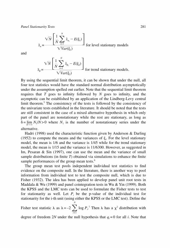
s =

�N �1N �

N

i=1

si� E(�1)�

�Var(�1)for level stationary models

and

s� =

�N �1N �

N

i=1

s�i� E(�2)�

�Var(�2)for trend stationary models.

By using the sequential limit theorem, it can be shown that under the null, allfour test statistics would have the standard normal distribution asymptoticallyunder the assumption spelled out earlier. Note that the sequential limit theoremrequires that T goes to infinity followed by N goes to infinity, and theasymptotic can be established by an application of the Lindberg-Levy centrallimit theorem.5 The consistency of the tests is followed by the consistency ofthe univariate tests established in the literature. It should be noted that the testsare still consistent in the case of a mixed alternative hypothesis in which onlypart of the panel are nonstationary while the rest are stationary, as long as = lim

N→�N1/N > 0 where N1 is the number of nonstationary series under the

alternative.Hadri (1998) used the characteristic function given by Anderson & Darling

(1952) to compute the means and the variances of �i. For the level stationarymodel, the mean is 1/6 and the variance is 1/45 while for the trend stationarymodel, the mean is 1/15 and the variance is 11/6300. However, as suggested inIm, Pesaran & Sin (1997), one can use the mean and the variance of smallsample distributions (in finite T) obtained via simulations to enhance the finitesample performances of the group mean tests.6

The group mean test pools independent individual test statistics to findevidence on the composite null. In the literature, there is another way to poolinformation from individual test to test the composite null, which is due toFisher (1932). The idea has been applied to develop panel unit root tests inMaddala & Wu (1999) and panel cointegration tests in Wu & Yin (1999). Boththe KPSS and the LMC tests can be used to formulate the Fisher tests to testfor stationarity as well. Let Pi be the p-value of the individual test forstationarity for the i-th unit (using either the KPSS or the LMC test). Define the

Fisher test statistic � as � = –2�N

i=1

log Pi.7 Then � has a �2 distribution with

degree of freedom 2N under the null hypothesis that qi = 0 for all i. Note that


the validity of the �2 distribution depends on the accuracy of the distributionsfrom which Pi’s are derived, and thus it does not rely on the asymptotic of Nwhere the group mean test does. On the other hand, the small sampledistribution is usually unknown, so it is necessary to get the small sampledistributions via simulations to enhance the small sample performance of theFisher tests.8

III. MONTE CARLO SIMULATION RESULTS

In this section, we will design some Monte Carlo simulation experiments toinvestigate the small sample properties of the panel stationarity tests weproposed in the previous section. The object of the simulations is to shed lightson the relative small sample performances of various tests. As we have seen, wecan use either the KPSS or the LMC tests to handle the serial correlation. Foreach univariate stationarity test, we can use either the group mean test or theFisher test to formulate the panel version. As illustrated in Maddala & Wu(1999) and Wu & Yin (1999), in many cases they considered, the performancesof the group mean and Fisher tests are very similar to each other. However westill need to investigate it for stationarity tests. As for the univariate KPSS andLMC tests, LMC established small sample supremacy of their tests. Butwhether this supremacy can be carried over to the panel tests based on theindividual LMC test remains a question, and it can be answered by simulationexperiments.

The basic models for simulations are models (3) and (4) with rit = rit�1 + �it

where �it ~ iidN(0, qi�2i ). The models for �it are �it = �i�it�1 + uit where

uit ~ iidN(0, (1 � �2i )�

2i ). Hence when �i = 0, �it’s are i.i.d. within each unit, while

�it’s are serially correlated within each unit when �i ≠ 0.These two models are extensions of the standard univariate models for

stationarity to the panel data. The introduction of different �i �2i ri0 and �i is to

allow the largest degree of heterogeneity. For this purpose, we set theparameters as follows:

�i ~ U[0, 1], �2i ~ U[0.5, 1.5], ri0 ~ U[0, 5]

�i = 0 for i.i.d. case

and

�i ~ U[0.1, 0.3] for the case of serial correlation

where U denotes the uniform distribution.The null hypothesis is specified as qi = 0 for all i. For the alternative

hypothesis, we only consider the case where all qi’s are positive following the


tradition in the literature. It should be noted that all our tests are consistent evenwhen there are only parts of the series are non-stationary under the alternativeas long as the portion of nonstationary units is non-vanishing asymptotically.Furthermore, we only consider the alternative H1 : qi = q = 0.001 for simplicity.9

We consider time dimensions of 25, 50, and 100 and cross sectionaldimensions of 15, 25, 50, and 100. The normal variates are generated byRNDN function in the matrix programming language GAUSS. We apply thegroup mean and Fisher tests based on the LM, KPSS, and LMC tests to eachpanel. For each case, the number of iterations is 5,000. For the group mean test,the mean and the variance of small sample distributions are derived from100,000 simulations for the corresponding time span and test procedures. Forthe Fisher test, the small sample distributions are simulated using 100,000replications as well.

In order to carry out our experiments, we still need to select two parameters.One is the truncation parameter l in the individual KPSS tests and the other oneis the order of autoregression p in the individual LMC tests. Followingearlier simulation results regarding the univariate KPSS tests in the litera-

ture, we experiment with l1 = int�4� T1001/4�, l2 = int�8� T

1001/4�, and

l3 = int�12� T1001/4�, where int[ ] returns the integer part of the argument.

Also, following earlier simulation results in the literature, we choose the Parzenwindow instead of the Bartlett window used by KPSS as the former performsbetter than the later. For the LMC test, we experiment with p = 1, 2, and 3following Monte Carlo experiments by LMC.

Let us first look at the white noise case. In this case �i = 0 and the tests basedon the individual LM tests are the appropriate ones to be used. Table 1 presentsthe sizes of the group mean and the Fisher tests based on the LM, KPSS, andLMC tests for the level stationary model. Note that by choosing l = 0 in theKPSS test or p = 0 in the LMC test, the resulting test statistic is nothing but thatof the LM test. That is why the results for the tests based on the LM test arelisted in the column with the heading of p(l) = 0. We also listed the results forN = 1 as a benchmark, where the results simply replicate those for the univariatecase. As we can see from the table, the size performances of the panelstationarity tests are quite satisfactory in this case. In addition the performancesare relatively better as T gets larger. In most cases, the Fisher tests have bettersize performances than the group mean tests, especially for larger T and smallerN. This is not surprising as the Fisher test is an exact test while the group mean


Table 1. Sizes of Panel Stationarity Tests: Level Stationary Model, WhiteNoise

KPSS LMCT N p(l) = 0 l1 l2 l3 p = 1 p = 2 p = 3

1 0.047 0.049 0.053 0.055 0.047 0.049 0.051

Group Mean Test15 0.061 0.057 0.061 0.059 0.063 0.059 0.06325 0.053 0.057 0.053 0.053 0.057 0.058 0.06350 0.054 0.055 0.055 0.055 0.054 0.054 0.059

25 100 0.046 0.047 0.050 0.053 0.046 0.050 0.051

Fisher Test15 0.050 0.047 0.051 0.056 0.046 0.045 0.05225 0.045 0.048 0.048 0.051 0.048 0.044 0.05350 0.047 0.050 0.052 0.053 0.046 0.047 0.052

100 0.043 0.043 0.047 0.052 0.041 0.046 0.047

1 0.047 0.046 0.047 0.051 0.047 0.050 0.050

Group Mean Test15 0.066 0.059 0.058 0.064 0.051 0.065 0.05825 0.066 0.062 0.060 0.058 0.067 0.070 0.06750 0.056 0.053 0.050 0.054 0.059 0.065 0.057

50 100 0.057 0.054 0.057 0.061 0.056 0.061 0.055

Fisher Test15 0.052 0.050 0.050 0.054 0.049 0.050 0.04625 0.054 0.052 0.053 0.053 0.054 0.055 0.05350 0.049 0.045 0.043 0.048 0.049 0.055 0.049

100 0.051 0.050 0.054 0.057 0.048 0.054 0.051

1 0.051 0.050 0.049 0.049 0.048 0.045 0.049

Group Mean Test15 0.056 0.058 0.057 0.059 0.060 0.063 0.06925 0.057 0.057 0.058 0.061 0.061 0.062 0.06350 0.056 0.057 0.058 0.054 0.062 0.054 0.064

100 100 0.056 0.058 0.056 0.055 0.059 0.056 0.059

Fisher Test15 0.047 0.046 0.047 0.046 0.045 0.049 0.04825 0.047 0.049 0.051 0.051 0.050 0.049 0.04950 0.049 0.051 0.051 0.049 0.051 0.047 0.053

100 0.053 0.053 0.053 0.051 0.053 0.052 0.051

Note:1. The data generating process is yit = ri0 + �it, and �it ~ i.i.d.N(0, �2

i ).2. Please see text for choices of parameters3. li is the truncation parameter used in individual KPSS test and p is the order of autoregression

in ARIMA(p,1,1) used in individual LMC test. p(l) = 0 indicates individual LM test is used.


test is an asymptotic test (in N). As for the tests based on the KPSS tests withdifferent lag truncation parameters and the LMC tests with differentautoregression orders, the sizes are also quite close to the nominal size of 5%.In general, we also observe that the size performances are better for larger Tand the Fisher tests have better size performances in this case.

Table 2 presents the powers of the panel stationarity tests for the levelstationary models. To make things comparable, all the powers are adjustedaccording to their true sizes. The powers of the LM based tests clearly state thesuperiority of the panel stationary tests over their univariate counterparts. WhenT = 25, the power of the univariate LM test is only 0.117, while the powerjumps to 0.392 when 15 cross-section units are used, and it is close to 1 (0.954for the group mean test and 0.952 for the Fisher test) when N = 100. As a matterof fact, all the powers for T = 100 are 1 and they are close to 1 when T = 50.The powers of the group mean and the Fisher tests in most cases are almost thesame.

It is documented in the literature that increasing the lag truncation parameterl in the KPSS tests and the autoregression order p in the LMC tests can reducethe powers. This is replicated in Table 2 as those entries for N = 1. However,due to the powerfulness of the panel stationarity tests, the reduction in thepowers by overestimating is not an issue in some cases, especially for larger Tand N, as in those cases the powers are 1 or close to 1. This is a unique featureof panel stationarity tests. The reduction in power is smaller for the LMC testsas p increases than for the KPSS tests as l increases.

The size and power performances of panel stationarity tests in the case ofwhite noise for the trend stationary models are reported in Tables 3 and 4. Wehave similar observations in these two tables. One thing we need to point outis that in this case the powers are smaller than those of level stationary models,especially for the case of T = 25 where the powers are much smaller. Thepowers are only 0.280 for the group mean test and 0.279 for the Fisher test evenwhen N = 100, though these represent an increase of nearly four-folds from theunivariate case.

Next, let us look at the results for the case of serial correlation. Table 5 givesus the sizes of panel stationarity tests in this case. Note that size distortions areexpected for the tests based on the LM tests. This can be seen in the table forthe case of N = 1. But the size distortions become much worse as N increases.As a matter of fact, the actual sizes are close to 1 when N = 100. This is due tothe fact that the size distortions are amplified through pooling the cross-sectional units, as pointed out in Wu & Yin (1999) for the panel cointegrationtests as well. The size distortions are still quite severe when l1 is used in theKPSS tests and they become moderate when l2 and l3 are used for T = 50 and


Table 2. Size Adjusted Powers of Panel Stationarity Tests: Level StationaryModel, White Noise


1 0.117 0.110 0.089 0.074 0.105 0.094 0.086

Group Mean Test15 0.392 0.365 0.272 0.183 0.305 0.263 0.23325 0.546 0.491 0.383 0.262 0.414 0.341 0.30650 0.775 0.712 0.576 0.377 0.630 0.527 0.473

25 100 0.954 0.936 0.834 0.612 0.874 0.779 0.727

Fisher Test15 0.384 0.362 0.271 0.156 0.302 0.264 0.23525 0.542 0.492 0.381 0.236 0.408 0.346 0.30850 0.771 0.719 0.576 0.359 0.635 0.526 0.477

100 0.952 0.936 0.835 0.584 0.873 0.780 0.729

1 0.302 0.284 0.268 0.224 0.277 0.251 0.218

Group Mean Test15 0.961 0.939 0.903 0.815 0.931 0.884 0.83525 0.995 0.990 0.977 0.944 0.986 0.969 0.94150 1.000 1.000 1.000 0.998 1.000 0.999 0.999

50 100 1.000 1.000 1.000 1.000 1.000 1.000 1.000

Fisher Test15 0.960 0.938 0.908 0.828 0.932 0.891 0.83625 0.995 0.991 0.978 0.946 0.986 0.972 0.94450 1.000 1.000 1.000 0.998 1.000 0.999 0.999

100 1.000 1.000 1.000 1.000 1.000 1.000 1.000

1 0.583 0.536 0.495 0.455 0.566 0.547 0.512

Group Mean Test15 1.000 1.000 1.000 1.000 1.000 1.000 1.00025 1.000 1.000 1.000 1.000 1.000 1.000 1.00050 1.000 1.000 1.000 1.000 1.000 1.000 1.000

100 100 1.000 1.000 1.000 1.000 1.000 1.000 1.000

Fisher Test15 1.000 1.000 1.000 1.000 1.000 1.000 1.00025 1.000 1.000 1.000 1.000 1.000 1.000 1.00050 1.000 1.000 1.000 1.000 1.000 1.000 1.000

100 1.000 1.000 1.000 1.000 1.000 1.000 1.000

Note:1. The data generating process is yit = rit + �it, rit = ri,t�1 + �it, �it ~ i.i.d.N(0, q�2

i ), and�it ~ i.i.d.N(0, �2

i ).2. See Note 2 in Table 1.3. See Note 3 in Table 1.


Table 3. Sizes of Panel Stationarity Test Based on Group Mean: TrendStationary Model, White Noise


1 0.052 0.052 0.060 0.054 0.051 0.050 0.054

Group Mean Test15 0.065 0.064 0.058 0.057 0.071 0.061 0.06525 0.064 0.058 0.059 0.062 0.073 0.067 0.06750 0.066 0.063 0.060 0.062 0.064 0.065 0.063

25 100 0.062 0.060 0.058 0.060 0.060 0.060 0.063

Fisher Test15 0.057 0.055 0.052 0.050 0.055 0.051 0.05825 0.054 0.051 0.052 0.051 0.057 0.053 0.05950 0.059 0.057 0.055 0.054 0.055 0.056 0.057

100 0.054 0.053 0.056 0.056 0.053 0.053 0.057

1 0.046 0.047 0.045 0.049 0.046 0.047 0.050

Group Mean Test15 0.050 0.055 0.056 0.065 0.064 0.073 0.06825 0.060 0.053 0.053 0.060 0.062 0.073 0.06950 0.057 0.055 0.053 0.056 0.068 0.075 0.068

50 100 0.058 0.054 0.050 0.059 0.064 0.072 0.074

Fisher Test15 0.049 0.047 0.050 0.056 0.049 0.053 0.05125 0.051 0.048 0.049 0.055 0.048 0.056 0.05350 0.052 0.049 0.049 0.052 0.055 0.061 0.054

100 0.054 0.052 0.049 0.056 0.056 0.066 0.064

1 0.046 0.042 0.041 0.042 0.043 0.050 0.048

Group Mean Test15 0.061 0.062 0.060 0.058 0.064 0.070 0.07425 0.057 0.057 0.057 0.055 0.063 0.065 0.06850 0.059 0.059 0.060 0.056 0.062 0.068 0.066

100 100 0.054 0.053 0.056 0.055 0.062 0.060 0.059

Fisher Test15 0.052 0.051 0.051 0.052 0.052 0.053 0.06025 0.049 0.050 0.050 0.049 0.053 0.055 0.05750 0.052 0.051 0.051 0.051 0.053 0.060 0.057

100 0.048 0.049 0.050 0.048 0.054 0.054 0.053

Note:1. The data generating process is yit = ri0 + �it + �it, and �it ~ i.i.d.N(0, �2



Table 4. Size Adjusted Powers of Panel Stationarity Test:Trend StationaryModel, White Noise


1 0.068 0.060 0.047 0.045 0.061 0.061 0.058

Group Mean Test15 0.108 0.106 0.069 0.040 0.091 0.090 0.08025 0.144 0.128 0.074 0.034 0.090 0.092 0.08350 0.172 0.159 0.085 0.031 0.118 0.109 0.102

25 100 0.280 0.245 0.116 0.027 0.185 0.164 0.132

Fisher Test15 0.109 0.103 0.067 0.040 0.089 0.086 0.07925 0.144 0.138 0.070 0.030 0.090 0.092 0.08350 0.163 0.157 0.084 0.027 0.127 0.109 0.098

100 0.279 0.257 0.108 0.024 0.187 0.169 0.140

1 0.133 0.124 0.106 0.079 0.120 0.106 0.095

Group Mean Test15 0.485 0.426 0.327 0.159 0.374 0.287 0.25225 0.629 0.576 0.450 0.212 0.509 0.374 0.31750 0.867 0.806 0.677 0.320 0.723 0.564 0.488

50 100 0.986 0.971 0.901 0.508 0.937 0.817 0.718

Fisher Test15 0.490 0.427 0.325 0.153 0.385 0.293 0.25225 0.631 0.574 0.445 0.205 0.518 0.400 0.33650 0.864 0.805 0.673 0.311 0.740 0.581 0.509

100 0.985 0.968 0.898 0.488 0.939 0.833 0.730

1 0.341 0.317 0.275 0.231 0.321 0.272 0.239

Group Mean Test15 0.991 0.975 0.938 0.874 0.978 0.946 0.87325 1.000 1.000 0.993 0.972 0.999 0.994 0.97450 1.000 1.000 1.000 0.999 1.000 1.000 1.000

100 100 1.000 1.000 1.000 1.000 1.000 1.000 1.000

Fisher Test15 0.990 0.972 0.937 0.868 0.979 0.950 0.88825 1.000 1.000 0.992 0.972 0.999 0.995 0.98250 1.000 1.000 1.000 1.000 1.000 1.000 1.000

100 1.000 1.000 1.000 1.000 1.000 1.000 1.000

Note:1. The data generating process is yit = rit + �it + �it, rit = ri,t�1 + �it, �it ~ i.i.d.N(0, q�2

i ), and�it ~ i.i.d.N(0, �2



Table 5. Sizes of Panel Stationarity Tests: Level Stationary Model, SerialCorrelation


1 0.079 0.059 0.050 0.047 0.051 0.054 0.058

Group Mean Test15 0.532 0.232 0.074 0.032 0.130 0.150 0.15225 0.694 0.302 0.076 0.025 0.144 0.182 0.17250 0.904 0.433 0.079 0.017 0.181 0.230 0.221

25 100 0.993 0.657 0.087 0.012 0.212 0.314 0.328

Fisher Test15 0.490 0.205 0.066 0.028 0.104 0.129 0.12925 0.669 0.270 0.067 0.024 0.123 0.160 0.15050 0.897 0.401 0.072 0.016 0.156 0.210 0.206

100 0.993 0.641 0.089 0.012 0.212 0.314 0.328

1 0.080 0.057 0.050 0.046 0.055 0.060 0.059

Group Mean Test15 0.551 0.162 0.081 0.058 0.099 0.126 0.13825 0.747 0.208 0.090 0.052 0.102 0.144 0.16150 0.945 0.300 0.103 0.049 0.117 0.182 0.209

50 100 0.999 0.472 0.132 0.048 0.145 0.250 0.286

Fisher Test15 0.517 0.140 0.070 0.050 0.077 0.096 0.10925 0.729 0.190 0.077 0.050 0.082 0.113 0.13750 0.944 0.279 0.095 0.047 0.091 0.155 0.178

100 0.999 0.456 0.128 0.047 0.116 0.213 0.264

1 0.094 0.062 0.053 0.052 0.052 0.058 0.057

Group Mean Test15 0.563 0.130 0.080 0.065 0.077 0.086 0.09925 0.783 0.169 0.083 0.063 0.082 0.094 0.11450 0.944 0.210 0.091 0.065 0.081 0.096 0.124

100 100 0.998 0.307 0.104 0.066 0.087 0.106 0.145

Fisher Test15 0.532 0.109 0.062 0.052 0.057 0.066 0.07425 0.773 0.148 0.071 0.056 0.064 0.075 0.08350 0.943 0.193 0.083 0.059 0.066 0.072 0.092

100 0.998 0.293 0.098 0.062 0.070 0.083 0.112

Note:1. The data generating process is yit = ri0 + �it, �it = �i�i,t�1 + uit, and uit ~ i.i.d.N(0, (1 � �2

i )�2i ).

2. See Note 2 in Table 1.3. See Note 3 in Table 1.


100. For the LMC test, the size distortion is still considerably large when thetrue order of autoregression (p = 1) is used when T = 25. The size distortionsbecome smaller and moderate when T increases to 50 and 100. Interestingly,overestimating in this case increases the size distortions. We can also observethat the Fisher tests in general have better size performances than the groupmean tests.

Table 6 reports the power performances of the panel stationarity tests in thepresence of serial correlation. The first thing we can notice is that the powersare lower than those in the white noise case for some combinations of N andT. The powers are around 60% even when N = 100 and T = 25 for the KPSS testswith l2 and the LMC tests with p = 1, which have relatively moderate sizedistortions. The powers are close to 1 when N is larger than 50 and T = 50 forthese two tests (the group mean and Fisher tests). When T = 100, however, allthe powers are still 1 or very close to 1. In such a case, smaller size distortionwould be the primary criterion to decide which test to be used in practice. Thepowers of the KPSS tests with l2 and the LMC test with p = 1 are almost thesame for most cases though the results for N = 1 actually indicate that the laterhas an advantage in the univariate case, which agrees with the findings in LMC.There are almost no differences in the power performances of the group meanand the Fisher tests.

The size distortions of the panel stationarity tests for the trend stationarymodels with serial correlation are presented in Table 7 with size adjustedpowers presented in Table 8. For the size distortions, we have the sameobservations as those for the level stationary models. Quite interestingly, theKPSS tests with l2 has slightly edge over the LMC tests with p = 1 when T = 50while the situation is reversed when T = 100. But we observe severe negativesize distortions for the KPSS tests with l2 when T = 25. Except for this case, thesize distortions for these two tests are smaller than the corresponding ones inthe level stationary models. The Fisher tests have relatively better sizeperformances than the group mean tests, especially when the individual LMCtests are used. As for the adjusted powers, we only need to report the lowerpowers compared to the level stationary models since things are relatively thesame as those for the level stationary models. For the KPSS tests with l2 and theLMC tests with p = 1, the powers are about 70% even when N = 100 for T = 50,compared with powers of 1 in the same situation for the level stationarymodels. The powers are close to 1 when T = 100 and there are more than 25cross-section units in the panel.

In summary, through Monte Carlo simulations, we found the tests weproposed have quite satisfactory small sample performances in most cases weconsidered. In the absence of serial correlation, the tests based on the LM tests


Table 6. Size Adjusted Powers of Panel Stationarity Tests:Level StationaryModel, Serial Correlation


1 0.153 0.109 0.095 0.079 0.100 0.095 0.089

Group Mean Test15 0.249 0.234 0.211 0.161 0.207 0.174 0.15725 0.338 0.319 0.264 0.210 0.250 0.207 0.20450 0.489 0.478 0.400 0.306 0.394 0.329 0.302

25 100 0.754 0.724 0.619 0.474 0.588 0.532 0.479

Fisher Test15 0.247 0.228 0.205 0.163 0.212 0.171 0.16125 0.337 0.316 0.269 0.209 0.248 0.207 0.20050 0.484 0.488 0.412 0.301 0.394 0.331 0.304

100 0.750 0.729 0.620 0.466 0.584 0.534 0.490

1 0.316 0.242 0.219 0.197 0.235 0.198 0.183

Group Mean Test15 0.886 0.831 0.761 0.656 0.775 0.712 0.64325 0.862 0.939 0.904 0.841 0.912 0.854 0.81350 0.998 0.996 0.992 0.980 0.993 0.981 0.967

50 100 1.000 1.000 1.000 0.999 1.000 1.000 0.999

Fisher Test15 0.885 0.833 0.772 0.673 0.774 0.723 0.65125 0.962 0.941 0.910 0.844 0.917 0.858 0.81250 1.000 1.000 1.000 1.000 1.000 1.000 1.000

100 1.000 1.000 1.000 1.000 1.000 1.000 1.000

1 0.530 0.500 0.468 0.429 0.524 0.490 0.471

Group Mean Test15 1.000 0.999 0.999 0.996 1.000 0.999 0.99825 1.000 1.000 1.000 1.000 1.000 1.000 1.00050 1.000 1.000 1.000 1.000 1.000 1.000 1.000

100 100 1.000 1.000 1.000 1.000 1.000 1.000 1.000

Fisher Test15 1.000 0.999 0.999 0.996 1.000 0.999 0.99925 1.000 1.000 1.000 1.000 1.000 1.000 1.00050 1.000 1.000 1.000 1.000 1.000 1.000 1.000

100 1.000 1.000 1.000 1.000 1.000 1.000 1.000

Note:1. The data generating process is yit = ri0 + �it, rit = ri,t�1 + �it, �it ~ i.i.d.N(0, q�2

i ), �it = �i�i,t�1 + uit,and uit ~ i.i.d.N(0, (1 � �2

i )�2i ).



Table 7. Sizes of Panel Stationarity Tests:Trend Stationary Model, SerialCorrelation


1 0.091 0.067 0.044 0.003 0.056 0.057 0.066

Group Mean Test15 0.657 0.252 0.016 0.007 0.144 0.156 0.14225 0.808 0.314 0.001 0.004 0.151 0.181 0.17450 0.975 0.495 0.005 0.000 0.183 0.267 0.245

25 100 0.999 0.723 0.001 0.000 0.223 0.377 0.338

Fisher Test15 0.610 0.226 0.014 0.003 0.108 0.134 0.12725 0.775 0.292 0.012 0.002 0.121 0.158 0.15750 0.966 0.459 0.005 0.000 0.149 0.239 0.231

100 0.999 0.700 0.001 0.000 0.185 0.362 0.333

1 0.094 0.060 0.051 0.040 0.057 0.062 0.061

Group Mean Test15 0.758 0.177 0.058 0.019 0.079 0.134 0.16025 0.931 0.252 0.053 0.011 0.091 0.160 0.19450 0.991 0.332 0.048 0.006 0.092 0.189 0.237

50 100 1.000 0.524 0.048 0.001 0.091 0.251 0.341

Fisher Test15 0.717 0.155 0.049 0.017 0.060 0.096 0.12025 0.913 0.224 0.050 0.010 0.066 0.118 0.15950 0.988 0.305 0.050 0.007 0.072 0.138 0.198

100 1.000 0.500 0.056 0.002 0.067 0.189 0.297

1 0.092 0.053 0.044 0.041 0.049 0.048 0.054

Group Mean Test15 0.789 0.138 0.059 0.042 0.062 0.076 0.09825 0.928 0.171 0.061 0.039 0.056 0.076 0.10150 0.998 0.259 0.069 0.032 0.053 0.075 0.115

100 100 1.000 0.377 0.066 0.026 0.051 0.074 0.133

Fisher Test15 0.752 0.114 0.052 0.039 0.046 0.052 0.06425 0.911 0.148 0.054 0.036 0.043 0.057 0.07750 0.997 0.236 0.062 0.031 0.046 0.055 0.081

100 1.000 0.354 0.063 0.027 0.046 0.051 0.091

Note:1. The data generating process is yit = rit + �it + �it, �it = �i�i,t�1 + uit, and uit ~ i.i.d.N(0, (1 � �2

i )�2i ).



Table 8. Size Adjusted Powers of Panel Stationarity Tests:Trend StationaryModel, Serial Correlation


1 0.065 0.060 0.051 0.044 0.064 0.065 0.054

Group Mean Test15 0.055 0.068 0.076 0.054 0.059 0.066 0.06425 0.088 0.089 0.076 0.044 0.072 0.078 0.07150 0.130 0.122 0.088 0.037 0.086 0.100 0.090

25 100 0.203 0.185 0.106 0.036 0.120 0.122 0.090

Fisher Test15 0.052 0.067 0.072 0.053 0.056 0.061 0.06625 0.088 0.085 0.078 0.042 0.072 0.077 0.07650 0.132 0.119 0.087 0.037 0.091 0.098 0.090

100 0.203 0.178 0.106 0.032 0.119 0.121 0.089

1 0.123 0.109 0.097 0.087 0.100 0.090 0.086

Group Mean Test15 0.389 0.311 0.240 0.139 0.240 0.207 0.18625 0.381 0.381 0.324 0.213 0.302 0.238 0.19050 0.693 0.603 0.489 0.274 0.437 0.367 0.324

50 100 0.905 0.827 0.699 0.391 0.674 0.548 0.478

Fisher Test15 0.389 0.312 0.252 0.140 0.234 0.203 0.18925 0.377 0.384 0.330 0.216 0.312 0.247 0.19950 0.696 0.608 0.481 0.270 0.444 0.374 0.333

100 0.903 0.829 0.694 0.403 0.680 0.554 0.502

1 0.302 0.264 0.235 0.208 0.273 0.236 0.200

Group Mean Test15 0.935 0.908 0.853 0.767 0.881 0.816 0.70725 0.993 0.984 0.958 0.909 0.976 0.930 0.85550 1.000 1.000 0.998 0.993 1.000 0.995 0.981

100 100 1.000 1.000 1.000 1.000 1.000 1.000 1.000

Fisher Test15 0.934 0.902 0.849 0.754 0.886 0.823 0.73525 0.993 0.984 0.955 0.882 0.974 0.939 0.86950 1.000 1.000 0.998 0.990 1.000 0.997 0.985

100 1.000 1.000 1.000 1.000 1.000 1.000 1.000

Note:1. The data generating process is yit = rit + �it + �it, rit = ri,t�1 + �it, �it ~ i.i.d.N(0, q�2

i ), �it =�i�i,t�1 + uit, and uit ~ i.i.d.N(0, (1 � �2

i )�2i )



have sizes close to the nominal size and powers much higher than the univariateLM tests. Using the KPSS and LMC tests in this case would not result in muchsize distortions, but would result in power losses for some combinations of Nand T, while the powers are already 1 or close to 1 for other combinations ofN and T. In the presence of serial correlation, we found that the tests based onthe KPSS tests with l2 and the LMC tests with p = 1 have relatively good sizeperformances though there are still moderate to severe size distortions when thetime span is short (T = 25), especially for the trend stationary models. And thepowers of all tests are lower than their counterparts in the white noise case.Overall, the Fisher tests have better size performances than the group meantests while their power performances are almost the same.

IV. CONCLUSION

In this chapter, we developed several tests for stationarity in the heterogeneouspanel. We analyzed both level stationary and trend stationary models. Byallowing maximum degree of heterogeneity in the panel, we considered twodifferent ways to pool information regarding the null hypothesis from eachcross-section units by using the group mean test and the Fisher test. The groupmean test pools the information of the univariate test statistics while the Fishertest summarizes the p-values of the individual tests. For the univariatestationary tests, we consider the KPSS and LMC tests in the case of serialcorrelation. The group mean tests based on the KPSS, and LMC tests areasymptotically normal while the Fisher test statistics follow �2 distributions.

The small sample performances of the tests were investigated via MonteCarlo simulation experiments. The results of simulations showed that the testswe proposed have quite satisfactory size and power performances. In general,the Fisher type tests have better size performances than the group mean typetests while they have similar power performances. The tests based on the KPSStests with l2 and the LMC tests with p = 1 perform very similarly in terms ofsize and power in most cases when there is serial correlation, except for theshort time span (T = 25). The size performances of these two tests are quitegood in the presence of serial correlation when T = 50 and 100. However, thereare still moderate to severe size distortions when T = 25 in the presence of serialcorrelation. In such a case, bootstrapping method might be an effective way toobtain better size performances. This would be an interesting topic for futureresearch. According to our simulation results, we would recommend to useeither the group mean tests or the Fisher tests which are based on both theKPSS tests with l2 and the LMC tests with p = 1 to test for stationarity in theheterogeneous panel data models in empirical work.


ACKNOWLEDGMENTS

We would like to thank Badi Baltagi and three anonymous referees for theirhelpful comments. Of course, all remaining errors are ours.

NOTES

1. See, for example, Schwert (1987).2. See KPSS for all relevant references and derivations of the tests.3. Please see LMC for the details of this argument. Of course, this supremacy

depends on the correct specification of the LMC model, as pointed out by oneanonymous referee.

4. This means that the intercepts in different cross-section units can be different, oneaspect of the heterogeneous panel.

5. The moment restriction in applying the Lindberg-Levy CLT should not be aproblem here because all tests are variants of the LM tests, which are bounded.

6. The small sample distributions of these tests can be derived by simulating seriesof given T under the null and apply the given test to the simulated series over a pre-specified number of iterations.

7. In a recent paper, Choi (2000) proposes to standardize the Fisher test statistics aswell. But this is unnecessary unless N is large enough.

8. Please see Maddala & Wu (1999) for a detailed comparison between the groupmean and the Fisher tests.

9. By construction of the tests, the qi’s can be different across the units.

REFERENCES

Anderson, T. W., & Darling, D. A. (1952). Asymptotic Theory of Certain ‘Goodness of Fit’Criteria Based on Stochastic Processes. Annals of Mathematical Statistics 23: 193–212.

Baltagi, B., & Kao, C. (2000). Nonstationary Panels, Cointegration in Panels and Dynamic Panels:A Survey. Advances in Econometrics, 15, 7–51.

Choi, I, (1999). Unit Root Tests for Panel Data’. Manuscript, Kookmin University.Fisher, R. A, (1932). Statistical Methods for Research Workers (4th ed.). Edinburgh: Oliver and

Boyd.Hadri, K, (1998). Testing for Stationarity in Heterogeneous Panel Data. Working paper, School of

Business and Economics, Exeter University.Im, K. S., Pesaran, M. H. & Shin, Y. (1997). Testing for Unit Roots in Heterogeneous Panels.

Discussion paper, University of Cambridge.Kao, C, (1999). Spurious Regression and Residual-Based Tests for Cointegration in Panel Data.

Journal of Econometrics, 90, 1–44.Kwiatkowski, D., Phillips, P. C. B., Schmidt, P., & Shin, Y. (1992). Testing the Null Hypothesis

of Stationarity Against the Alternative of a Unit Root. Journal of Econometrics, 54,91–115.

Leybourne, S. J., & McCabe, B. P. M. (1994). A Consistent Test for a Unit Root. Journal ofBusiness and Economic Statistics, 12, 157–166.


Maddala, G. S., & Wu, S. (1999). A Comparative Study of Unit Root Tests with Panel Data anda New Simple Test. Oxford Bulletin of Economics and Statistics, forthcoming.


McCoskey, S., & Kao, C. (1997). A Monte Carlo Comparison of Tests for Cointegration in PanelData. Working paper, Center for Policy Research and Department of Economics, SyracuseUniversity.

Newey, W. K., & West,K. D. (1987). A Simple Positive Semi-Definite Heteroskedasticity andAutocorrelation Consistent Covariance Matrix. Econometrica, 55, 703–708.

Pedroni, P, (1995). Panel Cointegration: Asymptotic and Finite Sample Properties of Pooled TimeSeries Tests With an Application to the PPP Hypothesis. Working paper, Department ofEconomics, Indiana University.

Pedroni, P, (1997). Panel Cointegration: Asymptotic and Finite Sample Properties of Pooled TimeSeries Tests With an Application to the PPP Hypothesis, New Results. Working paper,Department of Economics, Indiana University.

Phillips, P. C. B., & Perron, P. (1988). Testing For a Unit Root in Time Series Regression.Biometrika, 75, 335–346.

Wu, S., & Yin, Y. (1999). Tests for Cointegration in Heterogeneous Panel: A Monte CarloComparison. Working paper, Department of Economics, State University of New York atBuffalo.


INSTRUMENTAL VARIABLEESTIMATION OF SEMIPARAMETRICDYNAMIC PANEL DATA MODELS:MONTE CARLO RESULTS ONSEVERAL NEW AND EXISTINGESTIMATORS

M. Douglas Berg, Qi Li and Aman Ullah

ABSTRACT

We consider the problem of instrumental variable estimation of semipara-metric dynamic panel data models. We propose several newsemiparametric instrumental variable estimators for estimating a dynamicpanel data model. Monte Carlo experiments show that the new estimatorsperform much better than the estimators suggested by Li & Stengos (1996)and Li & Ullah (1998).

I. INTRODUCTION

Economic research has been enriched by the availability of panel data thatmeasure individual cross-sectional behavior over time. For reviews on theliterature of estimation and inference in parametric panel data models, seeBaltagi (1995), Chamberlain (1984), Hsiao (1986) and Matyas & Sevestre

Nonstationary Panels, Panel Cointegration and Dynamic Panels, Volume 15, pages 297–315.2000 by Elsevier Science Inc.ISBN: 0-7623-0688-2

297

(1996)). Recently, semiparametric modeling and estimation has attracted muchattention among statisticians and econometricians. One popular semiparametricmodel is the partially linear model. In this chapter we consider the problem ofestimating a semiparametric dynamic panel data model which includes thefollowing model as a special case:

yit = �yit�1 + �(zit) + uit, (1.1)

where the functional form of �( · ) is unspecified. Therefore (1.1) is asemiparametric dynamic panel data model. When �( · ) has a known form, say�(zit) = z�it�, we obtain a parametric dynamic panel data model:

yit = �yit�1 + z�it� + uit. (1.2)

When the error uit has a one-way error component structure, i.e. uit = �i + �it,then yit�1 and uit are correlated and instrumental variable methods are neededto obtain consistent estimation for �.

There is a rich literature on how to obtain consistent and efficient estimationresults for parametric dynamic models, see Ahn & Schmidt (1995), Anderson& Hsiao (1981), Arellano & Bover (1995), Baltagi & Griffin (1998), Pesaran& Smith (1995) and Kiviet (1995), among others. The consistent and efficientestimation results for the parametric dynamic panel data model (1.2) dependcrucially on the correct specification of the model. If �(zit) ≠ z�it�, parametricestimation methods based on a misspecified model (1.2) will in general lead toinconsistent estimation of �.

Semiparametric partially linear models have the advantage of not specifyingthe functional form of �( · ). Hence a consistent semiparametric estimator of �based on (1.1) is robust to functional form specification of �( · ). There is a richliterature on estimating a partially linear model with independent data usingvarious non-parametric techniques, e.g. Engle et al. (1986), Robinson (1988),Stock (1989), Donald & Newey (1994), Li (1996). Also, see Ullah & Roy(1998), Ullah & Mundra (1998), and Khanna et al. (1999) for the estimationand applications of static partially linear panel data models. However, littleattention has been paid to dynamic partially linear panel data models. AlthoughLi & Stengos (1996) and Li & Ullah (1998) discussed how to estimate model(1.1) by semiparametric instrumental variable methods, no simulations arereported in those works and hence the finite sample performance of theestimators proposed in Li & Stengos (1996) and Li & Ullah (1998) areunknown.1

Li & Stengos (1996) proposed a semiparametric OLS type IV (OLS–IV)estimator for estimating �. When the error follows an one-way errorcomponents structure. The OLS type estimator is not efficient because it

298 M. DOUGLAS BERG, QI LI & AMAN ULLAH

ignores this error structure. Li & Ullah (1996) therefore proposed asemiparametric GLS-type IV (GLS–IV) estimator. However, the GLS–IVestimator in Li & Ullah (1998) did not make full use of the one-way errorcomponent structure. In fact when the model is just identified, theirsemiparametric IV–GLS estimator reduces to a semiparametric IV–OLSestimator and hence it is inefficient in the sense that the one-way errorcomponent structure is not utilized in constructing the estimator. In this chapterwe propose a new semiparametric IV–GLS estimator and a new semipara-metric IV–Within estimator that are more efficient than the ones considered inLi & Stengos (1996), and Li & Ullah (1998). We then use Monte Carloexperiments to examine the finite sample performances of the new semipara-metric estimators and some existing estimators (e.g. Li & Ullah (1998) and Li& Stengos (1998)). Our simulation results show that the new estimatorsperform substantially better than the existing ones.

The chapter is organized as follows. Section 2 first reviews the semipara-metric estimators of Li & Stengos (1996), and Li & Ullah (1998). We thenpropose some new estimators. Section 3 reports Monte Carlo simulations tocompare the relative performances of various estimators. Finally section 4concludes the paper.

II. THE MODEL

We consider a slightly more general semiparametric dynamic panel data modelthan (1.1) considered in the introduction section.

yit = x�it + �(zit) + uit, (i = 1, . . . , N; t = 1, . . . , T), (2.1)

where xit is of dimension p 1, is a p 1 unknown parameter, zit is ofdimension d, �(·) is an unknown smooth function. We assume that the firstelement of xit is yit�1 so that model (2.1) is a semiparametric dynamic panel datamodel. We are mainly interested in obtaining accurate estimation for .

We consider the case that the error uit follows an one-way error componentsspecification,

uit = �i + �it, (2.2)

where �i is i.i.d. (0, �2�), �it is i.i.d. (0, �2

�), �i and �jt are uncorrelated for all iand jt.

In this chapter we propose a new semiparametric IV–GLS estimator thatfully uses the one-way error component structure. We also propose asemiparametric IV-within-transformation estimator which has the advantage ofcomputationally simplicity. Because it does not require one to estimate the

299Semiparametric Dynamic Panel Data Model

variance components. We then employ Monte Carlo simulations to investigatethe finite sample performance of our proposed semiparametric IV estimatorsand compare them with some existing estimators.

GLS type estimators require knowledge of error variance structure. In vectornotation, the one-way error component model of (2.2) has the following form,

u = (IN � eT)� + �, (2.3)

where eT is a column of ones of dimension T, � = (�1, �2, . . . , �N)� is ofdimension N 1, u and � are both of dimension NT 1 with u = (u11, . . . ,u1T, . . . , uN1, . . . , uNT)� and � is similarly defined.

� = E(uu�) = ��2 IN � JT + ��

2 INT, (2.4)

= IN � [�12JT + ��

2ET] � IN � , (2.5)

where JT = eT e�T is a T T matrix with all elements equal to one, JT = JT /T,ET = IT � JT and �1

2 = T��2 + ��

2. By noting the facts that JTET = 0, JT + ET = IT, andboth JT and ET are idempotent matrices, it is easy to check that the inverse of� is given by2

��1 = IN � [(1/�12)JT + (1/��

2 )ET] � IN � �1, (2.6)

and

��1/2 = IN � [(1/�1)JT + (1/��)ET] � IN � �1/2, (2.7)

The above expression of ��1 and ��1/2 will be used in GLS estimationprocedure discussed below.

A. Some Infeasible Estimators

Equation (2.1) contains an unknown function �( · ), following Robinson (1988),we first eliminate �( · ). Taking conditional expectation of (2.1) conditional onzit and then subtracting it from (2.1) leads to

yit � E(yit|zit) = (xit � E(xit|zit))� + uit

� v�it + uit, (2.8)

where vit =def xit � E(xit|zit). In vector-matrix notation we have

y � E(y|z) = v + u, (2.9)

where y, E(y|z) and u are all NT 1 vectors with typical elements given by yit,E(yit|zit) and uit, respectively, and v is of dimension NT p with typical rowgiven by vit = xit � E(xit|zit).


Equation (2.9) no longer contains the unknown function �( · ). Note that vit

and uit are correlated because vit contains yit�1 and uit contains the randomindividual effects �i. Suppose there exists a q 1(q ≥ p) instrumental variable �it

that is correlated with xit and uncorrelated with uit, then we can use

wit =def�it � E(�it|zit) as IV for vit. For example, consider a simple case where both

xit and zit are scalars with xit = yit�1 and zit is strictly exogenous, then one canchoose �it = zit�1 as instrument for yit�1.

In vector-matrix notation, an (infeasible) IV–OLS estimator of based on(2.9) is (see White (1984, 1987) for a discussion on IV estimation)

IVO = (v�ww�v)�1v�ww�(y � E(y|z)) = + (v�ww�v)�1v�ww�u. (2.10)

When the model is just identified, i.e. p = q, and if we assume that w�v isinvertible, then IVO becomes

IVO = (w�v)�1(v�w)�1v�ww�(y � E(y|z)) = (w�v)�1w�(y � E(y|z)). (2.11)

The above IV–OLS estimator is not efficient because it ignores the errorcomponent variance structure. Li and Ullah (1998) suggested estimating by

= (v�w(w��1w)�1w�v)�1 v�w(w��1w)�1w�(y � E(y|z)). (2.12)

However, when q = p and if we assume that the square matrices v�w andw��1w are both invertible, then we have from (2.12)

= (w�v)�1(w��1w)(v�w)�1v�w(w��1w)�1w�(y � E(y|z))

= (w�v)�1w�(y � E(y|z)) = IVO,

that is, reduces to the IV–OLS estimator of (2.11) when the model is justidentified. Therefore, the IV estimator also ignores the variance componentstructure when the model is just identified.

A new IV–GLS estimator that fully uses the one-way error componentstructure is given by

IVG = (v��1w(w��1w)�1w��1v)�1v��1w(w��1w)�1w��1(y � E(y|z))

= + (v��1w(w��1w)�1w��1v)�1v��1w(w��1w)�1w��1u, (2.13)

IVG of (2.13) is an optimal IV estimator as discussed in White (1984, 1987).When the model is just identified, i.e. p = q, and if we assume that both

w��1v and w��1w are invertible, then IVG of (2.13) becomes

IVG = (w��1v)�1(w��1w)(v��1w)�1v��1w(w��1w)�1w��1(y � E(y|z))

= (w��1v)�1w��1(y � E(y|z)), (2.14)

which is different from IVO of (2.11). Note that one can transform the modelby premultiplying y, v and w by ��1/2. Denote y* = ��1/2y, v* = ��1/2v andw* = ��1/2w, then the IV–GLS estimator of (2.13) is simply


IVG = (w*�v*)�1(w*�w*)(v*�w*)�1v*�w*(w*�w*)�1w*�(y* � E(y*|z)), (2.15)

which is easier to compute since it does not require one to invert a NT NTmatrix.

Let n = NT, then under the conditions of (i) w�u/n→p 0 (w is a legitimate IV),

(ii) v��1w/n→p A, and (iii) w��1w/n→p B, a positive definite matrix, one canshow that

�n(IVG � )→p N(0, AB�1A). (2.16)

The proof of (2.16) is similar to the proof of lemma 3 of Li and Ullah andis therefore omitted here.

Next we propose a simple IV estimator based on the within transformation.Within type estimator has the advantage of computationally simple, it onlyrequires the least squares regression of the within transformed variables. Define�it = E(yit|zit) and define the within transformed variables: yit = yit � yi · ,�it = �it � �i · , vit = vit � vi · and wit = wit � wi · , where yi · = �T

s=1 yis /T, �i · , vi · and wi ·

are similarly defined. The IV–Within estimator is given by

IVW = (v�ww�v)�1v�ww�(y � �). (2.17)

When the model is just identified, we have

IVW = (w�v)�1(v�w)�1v�ww�(y � �).

= (w�v)�1w�(y � �). (2.18)

The within type estimator has the advantage of being computationally simplebecause it does not require one to estimate the error variance �.

B. Feasible Estimators

The estimators IVO, IVG and IVW discussed above are not feasible, because theconditional mean functions E(y|z), E(x|z) and E(w|z) as well as �, are unknown.The feasible estimators can be obtained by replacing the unknown conditionalmean functions by their non-parametric estimators, such as the non-parametrickernel estimators, and replacing �2

1 and �2� by consistent estimators of them.

Following Robinson (1988), we use a kernel estimation method to estimatethe unknown conditional expectations. Specifically we denote the kernelestimators of f(zit), E(yit|zit), E(xit|zit), E(wit|zit) by fit, yit, xit and wit, respectively,where

fit =1

NThd �j�

s

Kit, js, (2.19)


yit =1

NThd �j�

s

yjsKit, js / fit, (2.20)

xit =1

NThd �j�

s

xjsKit, js / fit, (2.21)

and

wit =1

NThd �j�

s

wjsKit, js / fit, (2.22)

where Kit, js = K((zit � zjs)/h), K( · ) is the kernel function and h is the smoothingparameter.

Note that when xit = yit�1, we have

xit = E(yit�1|zit) = (NThd)�1 �j�

s

yjs�1 Kit, js / fit, (2.23)

which is different from yit�1 = E(yit�1|zit�1) = (NThd)�1 �j�

s

yjs�1 Kit�1, js�1 /fit�1.

We estimate vit � xit � E(xit|zit) by xit � xit and we estimate wit � �it � E(�it|zit)by �it � �it, where

�it = (NThd)�1 �j�

s

�js Kit, js / fit, (2.24)

is the kernel estimator of E(�it|zit).In vector-matrix notation, the feasible IV–OLS estimator of is obtained

from (2.10) by replacing E(yit|zit), vit = xit � E(xit|zit) and wit = �it � E(�it|zit) bytheir kernel estimators yit, xit � xit and �it � �it, respectively,

IVO = [(x � x)�(� � �)(� � �)�(x � x)]�1(x � x)�(� � �)(� � �)�(y � y). (2.25)

Similarly, we have

IVG = {(x � x)��1(� � �) [(� � �)��1(� � �)]�1(� � �)��1(x � x)}�1

(x � x)��1(� � �)[(� � ��)��1(� � �)]�1(� � �)��1(y � y), (2.26)

where ��1 is a consistent estimator of ��1 given by

��1 = IN � �1, (2.27)


with

�1 = (1/�2�)ET + (1/�2

1)JT, (2.28)

�2� = u�(IN � ET)u/[N(T � 1)] (2.29)

�21 = T��

2 + ��2, (2.30)

�2� = u�(IN � JT)u/N, (2.31)

and u is of dimension n 1 with a typical element given by

uit = yit � yit � (xit � xit)�IVO. (2.32)

For the feasible semiparametric IV within estimator, we will use the sametilde notation to denote the feasible quantity to avoid introducing too many newnotations. For example we use vit to denote kernel estimator of vit � vi · . Recallthat vit = xit � E(xit|zit). Hence we have

vit = (xit � xit) �1T �

s=1

T

(xis � xis). (2.33)

Similarly, recall that wit = �it � E(�it|zit) and �it = E(yit|zit), we have

wit = (�it � �it) �1T�

s=1

T

(�is � �is), (2.34)

and

�it = �it �1T �

s=1

T

�is. (2.35)

yit remains the same as yit = yit � yi · . With the notations given in (2.33) to (2.35),we obtain the feasible semiparametric IV–Within estimator,

IVW = (v�ww�v)�1v�ww�(y � �). (2.36)

In the next section we compare the finite sample performances of the newestimators proposed in this paper with those suggested by Li & Stengos (1996)and Li & Ullah (1998) via Monte Carlo simulations.

III. MONTE CARLO RESULTS

We use the following data generating process (DGP):

yit = yit�1 + zit + �zit2 + �i + �it

= yit�1 + �(zit) + �i + �it, (2.37)


where zit is independent and uniformly distributed in the interval of[ � �3,�3], �it is i.i.d. N(0,1). We choose = 0.5, � = 0, 0.5, 1. We fix totalvariance of �2

� + �2� = 10 and vary � = �2

�/(�2� + �2

�) to be 0.2, 0.5, 0.8. Wechoose �it = zit�1 as IV for yit�1.

For comparison we also compute the following non-IV semiparametricestimators:

(I) A semiparametric OLS estimator given by

OLS = [(x � x)�(x � x)]�1(x � x)�(y � y). (2.38)

(II) A semiparametric GLS estimator defined by

GLS = [(x � x)��1(x � x)]�1(x � x)��1(y � y). (2.39)

(III) A semiparametric within estimator

W = [v�v]�1v�y, (2.40)

where vit = xit � xit � (1/T)�s=1

T

(xis � xis) is the same as defined in (2.33) and

yit = yit � (1/T)�s=1

T

yis.

(I)–(III) do not use instrumental variables and hence these estimators areexpected to have large bias because they ignore the fact that yit and uit arecorrelated. However, they are also expected to have smaller variancescompared with the IV estimators. Therefore, for small and moderate samples,their mean square error (MSE) are not necessarily larger than the semipara-metric IV estimators. Of course when the sample size is sufficiently large, weexpect the semiparametric IV estimators to have smaller MSE because after all,they are consistent estimators, while the non-IV estimators are inconsistent.The bias of non-IV estimators will not die out as the sample size increases.

We report estimated bias, standard deviation (Std) and root mean squareerrors (Rmse) for all the estimators. These are computed via

Bias() = M�1 �j=1

M

(j � ), Std() =�M�1�j=1

M

(j � Mean())2�1/2

and

Rmse() = {M�1 �j=1

M

(j � )2}1/2, where M is the number of replication and j

is the estimated value of at the jth replication. We use M = 2000 in all thesimulations. We choose T = 6 and N = 50, 100, 200, 500.


The simulation results are given in Tables 1 and 2. The smallest Rmse foreach case (for a given N and �) is shown as boldface number(s). Thesimulations results are qualitatively similar for � = 0, � = 0.5 and � = 1.Therefore, we only report the cases of � = 0 and � = 1 to save space.

Table 1 reports the result for � = 0. From Table 1 we see that the non-IVestimators: OLS, GLS and W have large bias because these estimators ignorethe fact that yit�1 is correlated with uit. However, these non-IV estimators allhave smaller standard deviations (or variances) than the semiparametric IVestimators.

When N is small (N ≤ 100) and with small to moderate values of �(� ≤ 0.5),GLS has the smallest Rmse among all the estimators.

For N ≤ 100 with � = 0.8, GLS is no longer the best because of the large biasdue to the strong individual effects. In this case IVG and IVW have the smallestRmse.

For N = 200 and N = 500 and for small � = 0.2, IVO has the smallest Rmse.But larger values of �(� = 0.5, 0.8), IVG and IVW become the best in terms ofthe Rmse criterion.

For N ≤ 100 and � ≤ 0.5 GLS has the smallest Rmse. However, for � = 0.8, thebias in GLS is very large and hence its Rmse is much larger than the IVestimators. IVG and IVW have the smallest Rmse for � = 0.8.

As N increases, the bias in OLS, GLS and W remain the same order asexpected. The variances of the IV estimators decrease as N increases, and as aresult, the IV estimators dominate the non-IV estimators when N ≥ 200. For� = 0.2, IV–OLS estimator has the smallest Rmse. For � = 0.5 and � = 0.8, IV–GLS and IV–Within estimators have much smaller Rmse compared with theIV–OLS estimator. The IV–OLS estimator ignores the one-way errorcomponent structure. Hence when the individual effects are large, IV–OLS’sperformance is expected to be worse than that of the IV–GLS estimator.

We observe, as expected, the bias of non-IV estimators increase as �increases.

We also observe that the Rmse for IV–OLS estimator remain the same fordifferent values of �, while for IV–GLS and IV–Within estimators, the Rmsedecrease as � increases.

Next, we observe that the results of Table 2 is very similar to that of Table1. That is, the result is not sensitive to the different functional form of �(zit).This is as expected because all the estimators are semiparametric and hencethey are robust to functional form specifications of �( · ).

The DGP given in (2.37) is a just identified model. We have also conductedsome simulations for over identified model. In particular, we consider thefollowing model


Table 1. The case of � = 0.

N = 50� = 0.2 � = 0.5 � = 0.8

Bias Std Rmse Bias Std Rmse Bias Std Rmse

OLS 0.193 0.045 0.198 0.352 0.030 0.353 0.442 0.016 0.442GLS –0.103 0.056 0.117 0.099 0.059 0.115 0.310 0.040 0.313W –0.241 0.058 0.248 –0.213 0.057 0.220 –0.136 0.061 0.149IVO –0.019 0.290 0.291 –0.042 0.329 0.331 –0.128 2.39 2.39IVG –0.006 0.215 0.215 –0.008 0.171 0.171 –0.012 0.111 0.112IVW –0.005 0.225 0.225 –0.009 0.174 0.174 –0.013 0.111 0.112

N = 100� = 0.2 � = 0.5 � = 0.8



N = 200� = 0.2 � = 0.5 � = 0.8



N = 500� = 0.2 � = 0.5 � = 0.8




Table 2. The case of � = 1.

N = 50� = 0.2 � = 0.5 � = 0.8



N = 100� = 0.2} � = 0.5 � = 0.8



N = 200� = 0.2 � = 0.5 � = 0.8



N = 500� = 0.2 � = 0.5 � = 0.8




yit = yi,t�1 + z1,it + �1z1,it + z2,it + �2z2,it + �i + �it

= yi,t�1 + �(z1,it,z2,it) + �i + �it. (2.41)

The simulation results for the above over identified model lead to the sameconclusion as the just identified model. Therefore, we do not report the resultsfor the over identified case to save space. However, the results are availablefrom the authors upon request.

IV. CONCLUDING REMARKS

In this chapter we consider the problem of estimating a semiparametricpartially linear panel data model with errors that has a one-way errorcomponents structure. We propose two new semiparametric IV estimator forthe coefficient of the parametric component, and we argue that the newsemiparametric estimators are more efficient than the ones suggested by Li &Stengos (1996) and Li & Ullah (1998) because the new estimators make fulluse of the one-way error components structure. The Monte Carlo simulationresults confirm our theoretical analysis.

Throughout the chapter we assume the existence of random individualeffects. In practice one may want to test the existence of random individualeffects. For this purpose one can use the test statistic suggested by Li & Hsiao(1998) for testing the null of no random individual effects in a partially lineardynamic panel data model.

Also in this chapter we only consider the case that �i is a random effect. Wenow briefly discuss the case of fixed effects semiparametric partially linearmodels. The model is the same as given in (2.1) and (2.2) except that now weassume the individual effect �i is a fixed effect rather than a random effect. Thesemiparametric IV–OLS and IV–GLS estimators that either ignore the fixedeffects or treat the fixed effects as random effects will not lead to consistentestimation results by the same reason as in the parametric regression modelcase. However, the semiparametric within estimator, which wipes out theindividual effects whether it is fixed or random, remains a consistent estimatorin the case of a fixed effect model.

Our Monte Carlo results of Section 3 show that the within semiparametricestimator IVW performs quite well relative to other estimators. Therefore, werecommend its use in practice.

ACKNOWLEDGMENTS

We would like to thank a referee and Badi Baltagi for very useful commentsthat greatly improve the paper. Q. Li’s research is supported by Natural


Sciences and Engineering Research Council of Canada, the Social Sciencesand Humanities Research Council of Canada, Ontario Premier’s ResearchExcellence Awards, and Bush program in economics on public policy. A. Ullahthanks the Academic Senate of UCR for the research support.

NOTES

1. Li & Ullah (1998) reported some Monte Carlo results on a static semiparametricpanel data model. They also proposed two semiparametric instrumental variableestimators for a semiparametric dynamic panel data model, but they did not conduct anyMonte Carlo simulations on the dynamic model.

2. Using the simple spectral decomposition method to derive the inverse of � wasproposed by Wansbeek & Kapteyn (1982, 1983).

REFERENCES


Anderson, T. W., & Hsiao, C. (1981). Estimation of Dynamic Models With Error Components.Journal of American Statistical Association, 76, 598–606.

Arellano, M., & Bover, O. (1995). Another Look at The Instrumental Variable Estimation of ErrorComponents Models. Journal of Econometrics, 68, 28–51.

Baltagi, B. H. (1995). Econometric Analysis of Panel Data. New York: Wiley.Baltagi, B. H., & Griffin, J. M. (1997). Pooled Estimators vs. Their Heterogeneous Counterparts

in The Context of Dynamic Demand for Gasoline. Journal of Econometrics, 77, 303–327.Chamberlain, G. (1984). Panel Data. In: Z. Griliches & M. Intriligator (Eds), Handbook of

Econometrics (pp. 1247–1318 ), Vol. II. Amsterdam: North Holland.Donald, S. G., & Newey, W. K. (1994). Series Estimation of Semilinear Regression. Journal of

Multivariate Analysis, 50, 30–40.Engle, R. F., Granger, C. W. J., Rice, J., & Weiss, A. (1986). Semiparametric Estimates of The

Relationship Between Weather and Electricity Sales. Journal of the American StatisticalAssociation, 81, 310–320.

Hsiao, C. (1986). Analysis of Panel Data. Econometric Society monograph No. 11. New York:Cambridge: Cambridge University Press.

Khanna, M., Mundra, K., & Ullah, A. (1999). Parametric and Semiparametric Estimation of TheEffect of Firm Attributes on Efficiency: The Electricity Generating Sector in India. Journalof International Trade and Economic Development, forthcoming.

Kiviet, J. F. (1995). On Bias, Inconsistency and Efficiency of Some Estimators in Dynamic PanelData Models. Journal of Econometrics, 68, 53–78.

Li, Q. (1996). On The Root-n-consistent Semiparametric Estimation of Partially Linear Models.Economics Letters, 51, 277–285.

Li, Q., & Hsiao, C. (1998). Testing Serial Correlation in Semiparametric Panel Data Models.Journal of Econometrics, 87, 207–237.

Li, Q., & Stengos, T. (1996). Semiparametric Estimation of Partially Linear Panel Data Models.Journal of Econometrics, 71, 389–397.


Li, Q., & Ullah, A. (1998). Estimating partially linear models with one-way error components.Econometric Reviews, 17, 145–166.

Matyas, L., & Sevestre, P. (1992). The Econometrics of Panel Data. Dordrecht: Kluwer, 2ndedition.

Pesaran, M. H., & Smith, R. (1995). Estimation of Long-run Relationship From DynamicHeterogeneous Panels. Journal of Econometrics, 68, 79–114.

Robinson, P. M. (1988). Root-N-consistent Semiparametric Regression. Econometrica, 56,931–954.

Stock, J. H. (1989). Nonparametric Policy Analysis. Journal of the American StatisticalAssociation, 84, 567–575.

Ullah, A., & Roy, N. (1998). Nonparametric and Semiparametric Econometrics of Panel Data. In:A. Ullah and D. E. A. Giles (Eds), Handbook on Applied Economic Statistics (pp. 579–604), Ch. 17. Marcel Dekker.

Ullah, A., & Mundra, K. (1999). Semiparametric Panel Data Estimation: An Application toImmigrates Homelink Effect on U.S. Producer Trade Flows. Working paper 15, Departmentof Economics, University of California at Riverside.

Wansbeek, T. J., & Kapteyn, A. (1982). A Simple Way to Obtain the Spectral Decomposition ofVariance Components Models for Balanced Data. Communications in Statistics, A11,2105–2112.

Wansbeek, T. J., & Kapteyn, A. (1983). A Note on Spectral Decomposition and MaximumLikelihood Estimation of ANOVA Models With Balanced Data. Statistics and ProbabilityLetters, 1, 213–215.

White, H. (1984). Asymptotic Theory for Econometricians. New York: Academic Press.White, H. (1986. Instrumental Variables Analogs of Generalized Least Squares Estimator. R. S.

Mariano (Ed.), Advances in Statistical Analysis and Statistical Computing (pp.173–277),Vol.1. New York: JAI Press.

APPENDIX

/** This is a gauss program using Monte Carlo simulation to examine the finitesample performanes of some semiparametric instrumental variable estimatorsin a semiparametric dynamic panel data model, written by M. Douglas Berg **/

output file = c:\gauss\doug\work1.out reset;format /rd 8,3;n = 100; T = 6;T00 = 30; T0 = T + T00 + 1; NT = N*T;nr = 500; @ number of replication @lamt = 0.5; b1 = 1; b2 = 0; sig2 = 10;rho = 0.8;sigmu2 = rho*sig2;signu2 = (1-rho)*sig2; sigmu = sqrt(sigmu2);signu = sqrt(signu2); s1_5 = sqrt(t*sigmu2 + signu2);sv_5 = signu; @ true parameter values @

ycz = zeros(nt,1); y1cz = ycz; z1cz = ycz; fz = ycz;


kel = zeros(nt,1); lam1 = zeros(nr,1);lam3 = lam1; lam1n = lam1; lam3n = lam1; lam4n = lam1;lam6n = lam1; y0 = zeros(n,t0);

rndseed 7893450;i1 = 1; do while i1 < = nr; @ Monte Carlo simulation loop @

z0 = 2*sqrt(3)*rndu(n,t0) – sqrt(3);u0 = rndn(n,t0); mu = rndn(n,1);

i2 = 2; do while i2 < = t0;y0[.,i2] = lamt*y0[.,i2–1] + b1*z0[.,i2]+ b2*z0[.,i2]2 + signu*u0[.,i2] + sigmu*mu; @ Generate y @

i2 = i2 + 1;endo;

y = y0[.,T00 + 1:T00 + T];y1 = y0[.,T00:T00 + T–1];z = z0[.,T00 + 1:T00 + T];z1 = z0[.,T00:T00 + T–1];yv = reshape( y, nt, 1 );y1v = reshape( y1, nt, 1 );zv = reshape( z, nt, 1 );z1v = reshape( z1, nt, 1 );

hz = stdc(zv)*(nt(–1/5));hz1 = stdc(z1v)*(nt(–1/5));zvh = zv/hz; z1vh = z1v/hz1;

i3 = 1; do while i3 < = nt; @ Nonparametric Estimation Loop @zd = zvh[i3,.] – zvh;z1d = z1vh[i3,.] – z1vh;kelz = prodc( (exp(–0.5*zd2))’ )/sqrt(2*pi);kelz1 = prodc( (exp(–0.5*z1d2))’ )/sqrt(2*pi);

ycz[i3,.] = yv’*kelz/(nt*hz);y1cz[i3,.] = y1v’*kelz/(nt*hz);z1cz[i3,.] = z1v’*kelz/(nt*hz);fz[i3,.] = sumc( kelz )/(nt*hz);

i3 = i3 + 1;endo;

w1v = z1v – z1cz./fz; @ Li-Ullah, Li-Stengos IV @xxv = y1v – y1cz./fz;yyv = yv – ycz./fz;


lam1[i1,.] = inv(w1v’*xxv)*w1v’*yyv; @ IV-OLS estimator @lam3[i1,.] = inv(xxv’*xxv)*xxv’*yyv; @ Semi-OLS estimator @u01 = yyv – xxv*lam1[i1,.];u03 = yyv – xxv*lam3[i1,.];

Jbt = ones(t,t)/t;Et = eye(t) – Jbt;

u11 = Et*( (reshape( u01,n,t))’ );u11 = reshape( u11’,nt,1 );sv2 = u11’*u11/(n*(t–1));u22 = Jbt*( (reshape(u01,n,t))’ );u22 = reshape( u22’,nt,1 );smu2 = u22’*u22/n;s12 = sv2 + t*smu2;sv_1 = sqrt( sv2 );s1_1 = sqrt( s12 );

u11 = Et*( (reshape( u03,n,t))’ );u11 = reshape( u11’,nt,1 );sv2 = u11’*u11/(n*(t–1));u22 = Jbt*( (reshape(u03,n,t))’ );u22 = reshape( u22’,nt,1 );smu2 = u22’*u22/n;s12 = sv2 + t*smu2;sv_3 = sqrt( sv2 );s1_3 = sqrt( s12 );

At_1 = Jbt/s1_1 + Et/sv_1;At_3 = Jbt/s1_3 + Et/sv_3;At_5 = Jbt/s1_5 + Et/sv_5;At_w = Et;yyn_1 = At_1*( (reshape(yyv,n,t))’ );yyn_3 = At_3*( (reshape(yyv,n,t))’ );yyn_6 = At_w*( (reshape(yyv,n,t))’ );xxn_1 = At_1*( (reshape(xxv,n,t))’ );xxn_3 = At_3*( (reshape(xxv,n,t))’ );xxn_6 = At_w*( (reshape(xxv,n,t))’ );w1n_w = At_w*( (reshape(w1v,n,t))’ );w1n = At_1*( (reshape(w1v,n,t))’ );yyv_1 = reshape(yyn_1’,nt,1);yyv_3 = reshape(yyn_3’,nt,1);


yyv_6 = reshape(yyn_6’,nt,1);xxv_1 = reshape(xxn_1’,nt,1);xxv_3 = reshape(xxn_3’,nt,1);w1v_w = reshape(w1n_w’,nt,1);xxv_6 = reshape(xxn_6’,nt,1);w1v = reshape(w1n’,nt,1);

lam1n[i1,.] = inv(w1v’*xxv_1)*w1v’*yyv_1; @ IV-GLS estimato@ lam3n[i1,.] = inv(xxv_3’*xxv_3)*xxv_3’*yyv_3;@ Semi-GLS estimator @ lam4n[i1,.] = inv(w1v_w’*xxv_6)*w1v_w’*yyv_6;@ IV-Within estimator @ lam6n[i1,.] = inv(xxv_6’*xxv_6)*xxv_6’*yyv_6;@ Semi-Within est. @ i1 = i1 + 1;endo;

Bias1 = meanc( lam1 – lamt ); @ Bias @Bias3 = meanc( lam3 – lamt );rmse1 = sqrt( meanc( (lam1-lamt)2 ) ); @ Root-MSE @rmse3 = sqrt( meanc( (lam3-lamt)2 ) );std1 = stdc(lam1); @ Standard Dev. @std3 = stdc(lam3);

Bias1n = meanc( lam1n – lamt );Bias3n = meanc( lam3n – lamt );Bias4n = meanc( lam4n – lamt );Bias6n = meanc( lam6n – lamt );

rmse1n = sqrt( meanc( (lam1n-lamt)2 ) );rmse3n = sqrt( meanc( (lam3n-lamt)2 ) );rmse4n = sqrt( meanc( (lam4n-lamt)2 ) );rmse6n = sqrt( meanc( (lam6n-lamt)2 ) );

std1n = stdc(lam1n);std3n = stdc(lam3n);std4n = stdc(lam4n);std6n = stdc(lam6n);

print "********************************************************";print "IVO1, bias1, std1, rmse1 = " bias1 std1 rmse1;print "OLS, bias3, std3, rmse3 = " bias3 std3 rmse3;print "********************************************************";print "IVG1, bias1n, std1n, rmse1n = " bias1n std1n rmse1n;print "GLS, bias3n, std3n, rmse3n = " bias3n std3n rmse3n;print "********************************************************";print "With1, bias4n, std4n, rmse4n = " bias4n std4n rmse4n;


print "With, bias6n, std6n, rmse6n = " bias6n std6n rmse6n;print "********************************************************";

end;


SMALL SAMPLE PERFORMANCE OFDYNAMIC PANEL DATA ESTIMATORSIN ESTIMATING THEGROWTH-CONVERGENCE EQUATION:A MONTE CARLO STUDY

Nazrul Islam

ABSTRACT

This chapter conducts a Monte Carlo investigation into small sampleproperties of some of the dynamic panel data estimators that have beenapplied to estimate the growth-convergence equation using Summers-Heston data set. The results show that the OLS estimation of this equationis likely to yield seriously upward biased estimates. However, indiscrimi-nate use of panel estimators is also risky, because some of them displaylarge bias and mean square error. Yet, there are panel estimators that havemuch smaller bias and mean square error. Through a judicious choice ofpanel estimators it is therefore possible to obtain better estimates of theparameters of the growth-convergence equation. The growth researchersmay make use of this potential.

I. INTRODUCTION

One of the issues around which the recent growth literature has evolved is thatof convergence. This refers to the idea that, because of diminishing returns to


317

capital, poorer economies should grow faster and catch up with the richer ones.Statistically, convergence is therefore interpreted as a negative correlationbetween the initial level of income and the subsequent growth rate.Accordingly, a popular method for testing the convergence hypothesis has beento run growth-initial level regressions or growth-convergence regressions,where subsequent growth rates are regressed on initial levels of income.

For a long time, growth-convergence regressions were estimated using cross-section data. However, recently researchers have drawn attention to the fact thatthe growth-convergence equation actually represents a dynamic panel datamodel, and by ignoring the individual effects, cross-section estimation courtsomitted variable bias (OVB). Thus, Islam (1993, 1995) argues for using panelprocedures to overcome this bias and in particular implements Chamberlain’s(1982, 1983) Minimum Distance (MD) procedure to estimate the equation.Knight et al. (1993) make similar arguments and also use the MinimumDistance procedure to produce similar results. Islam, in addition, presentsresults from the Least Squares with Dummy Variables (LSDV) procedure.

Since these initial works, panel estimation of the growth-convergenceequation has spread considerably. For example, Lee, Pesaran & Smith (1997,1998) consider maximum likelihood estimation of the growth-convergenceequation using panel data. Caselli et al. (1996) emphasize the problem ofendogeneity in this equation and use the Arellano-Bond GMM panel procedureto overcome the problem. Barro (1997) and Barro & Sala-i-Martin (1995) usepooled estimation on panel data sets. Lee et al. (1998) also present evidence onpanel estimation of the growth convergence equation.

The panel estimates presented in these papers generally differ fromcorresponding cross-section estimates. However, they also differ amongthemselves. Nerlove (1999) highlights this by using a variety of panelestimators to estimate the growth-convergence equation and compiling theresults. Similar findings were presented earlier in Islam (1993). This creates aproblem of choosing among various panel estimators. Unfortunately, theoret-ical properties of dynamic panel data estimators are generally asymptotic andoften equivalent. This creates the necessity of Monte Carlo studies to ascertainthe small sample properties of these estimators. However, Monte Carlo studiesare more useful when they are customized to the specification and the data setthat are used in actual estimation. Although many researchers have recentlypresented Monte Carlo evidence on small sample properties of dynamic panelestimators, studies focusing on the growth-convergence equation and using theSummers-Heston (1988, 1991) data set are rare.

This chapter tries to help overcome this lacking. The study focuses on thoseestimators that have been used so far to estimate the growth-convergence

318 NAZRUL ISLAM

equation. Accordingly, the estimators included are: least squares with dummyvariables (LSDV); the two instrumental variable estimators of Anderson &Hsiao (1981, 1982), namely AH(l), based on ‘level’ instruments, and AH(d),based on ‘difference’ instruments; the minimum distance (MD) estimator,suggested by Chamberlain (1982, 1983); and the one-step (ABGMM1) andtwo-step (ABGMM2) generalized method of moments estimators proposed byArellano & Bond (1991). In addition, the exercise includes simultaneousequations (SE) estimators such as the two stage least squares estimator (2SLS),the three stage least squares estimator (3SLS), and the generalized three stageleast squares estimator (G3SLS). To complete the picture, the study alsoincludes the (pooled) ordinary least squares (OLS) estimator, which ignores theindividual effects.

The two main parameters of the model are the dynamic adjustmentparameter � (attached to the lagged dependent variable) and �, the parameterof the exogenous variable. The Monte Carlo results show that the OLSestimates of � are, as expected, positively biased, and the magnitude of this biasaverages to about seventeen percent of the true parameter value. For most of thepanel estimators, the direction of bias is negative, with only the AH(d)estimator providing some exceptions. The bias is small for the AH(d), theLSDV, and the MD estimators, ranging between five and six percent. The biasof the 2SLS, 3SLS, and 3SGLS estimates of � ranges between eight to tenpercent. The largest bias is observed for the ABGMM estimators, averaging totwenty two percent. The AH(l) estimator perform so poorly that we refrainfrom reporting its results.

The results regarding root mean square error (RMSE) demonstrate a similarpattern. The average RMSE as percentage of the true value of � proves to beseventeen percent for the OLS estimator. For the LSDV and the MD estimators,this percentage ranges between six and seven. For the AH(d), 2SLS, 3SLS, and3GSLS estimators, it ranges between ten and twenty. This percentage is thehighest for the ABGMM estimators, ranging between forty to forty-sixpercent.

With regard to �, the bias of the OLS estimates is again positive, but nowaverages much higher to forty-eight percent of the parameter value. Thedirection of bias of the panel estimates of � is quite mixed. However, panelestimates of � are on average quite close to the true parameter value. Themagnitude of the algebraic average of the bias for the 2SLS, 3SLS, LSDV andthe MD estimator remain under one percent. For AH(d) and G3SLS it rangesbetween one and two percent. For the ABGMM estimates, this percentage ishigher but still within five to seven percent.

319Monte Carlo Study of Panel Estimators for Growth-Convergence Equation

The RMSE results for � display a similar ranking of performance.However, the smallness of bias in estimation of � is nullified greatly by largevariance of the estimates. As a result, the RMSE values for � are in generalmuch higher than for �. For a good number of panel estimators, whichinclude AH(d), 2SLS, and 3SLS, the RMSE remain under thirty-five percent oftrue value of �. For the LSDV and the MD, this percentage is undertwenty-five. However, for 3GSLS, this percentage is fifty-six. For theABGMM it is around two hundred percent. For the OLS the ratio is fifty-sixpercent.

The results indicate that the OLS estimation of the growth-convergenceequation is very likely to give considerably biased results. However,indiscriminate use of panel estimators is risky too. Yet, there are panelestimators that have much smaller bias and RMSE than the OLS. Hence, ajudicious choice of panel estimator has the potential to yield much betterestimates of the parameters of the growth convergence equation. Growthresearchers may make use of this potential.

In addition to the above, several general points emerge from this study. First,the performances of the two AH estimators contrast sharply. The source of thiscontrast lies in different degree of correlation of the instruments with theinstrumented variables. This highlights the importance of research intoestimation with ‘weak’ instruments. Second, a comparison of the ABGMM1results with that of ABGMM2 and of 2SLS results with that of either 3SLS or3GSLS shows that simpler estimators not requiring estimated weightingmatrices may perform better than sophisticated estimators that do require suchmatrices. Use of estimated weighting matrices creates avenue for unwarrantednoise to enter into estimation. Third, increasing the number of instruments maynot necessarily improve estimation results. This is revealed by the poorperformance of the ABGMM estimators compared to that of AH(d). Fourth,theoretically inconsistent estimators can display good small sample perform-ance. The performance of the LSDV estimator, which is inconsistent in thedirection of N, illustrates this. Finally, the results of this chapter are in generalagreement with other recent Monte Carlo studies, which have also reportedlarge bias of the ABGMM estimators and better performance of the LSDVestimator.

The discussion of the chapter is organized as follows. Section 2 reviewsprevious Monte Carlo studies of dynamic panel estimators and specifies theobjectives of the current study. Section 3 presents the model and discusses thedata generation processes. Section 4 presents the results. Section 5 containssome concluding remarks.

320 NAZRUL ISLAM

II. PREVIOUS MONTE CARLO STUDIES

Much of the recent empirical research on growth has revolved aroundestimation of the growth-convergence equation. A close inspection of thisequation shows that it is actually a dynamic panel data model.1A cross-sectionestimation of the equation therefore suffers from omitted variable bias. This hasled to panel estimation. Different panel estimators have however produceddifferent results. Theoretical properties of many of these estimators areasymptotic and equivalent. Hence, Monte Carlo evidence is necessary to gaugewhich of these estimates are more acceptable.

The issue of small sample properties of dynamic panel estimators is not new.Earlier, the gas demand study by Balestra & Nerlove (1966) also raised thisissue. This led Nerlove to conduct several Monte Carlo studies. Nerlove (1967)considers a simple auto-regressive model with no exogenous variable andcompares the performance of the OLS, LSDV, MLE, and several variants of theGLS estimator in estimating the model. In Nerlove (1971), the dynamic panelmodel is extended to include an exogenous variable. This allows considerationof instrumental variable (IV) estimator with lagged values of the exogenousvariable as instrument. It also allows having another variant of the two-stageGLS. Overall, Nerlove’s Monte Carlo results favor the GLS estimators overother estimators.

Since Nerlove’s work, there have been significant developments in the fieldof dynamic panel data estimators.2 Among these is introduction of theAnderson & Hsiao (1981, 1982) instrumental variable estimators that usefurther lagged values of the dependent variable as instruments. Arellano &Bond (1991) carry this idea further and propose using all lagged variables(provided they qualify) as instruments within a GMM framework. Ahn &Schimdt (1995, 1997, 1999), Arellano & Bover (1995), Blundell & Bond(1998), Hahn (1999), Wansbeek & Knaap (1998), and Ziliak (1997) suggestvarious extensions and modifications of the Arellano-Bond GMM estimator(ABGMM). On the other hand, Kiviet (1995) and Wansbeek & Knaap (1998)propose modifications of the LSDV and LIML estimators, respectively.

Many of the recent works offer Monte Carlo evidence too. Thus Arellano &Bond (1991) perform a Monte Carlo study to compare primarily the smallsample properties of their GMM estimators with corresponding properties ofthe Anderson-Hsiao estimators. According to their results, the GMM estimatorsperform better than the Anderson-Hsiao IV estimators, though not so much interms of bias as in terms of dispersion. However, simulation studies of Alonso-Borrengo & Arellano (1999), Kiviet (1995), Harris & Matyas (1996), Judson &Owen (1997), Wansbeek & Knaap (1998), and Ziliak (1997) report significant


bias of the ABGMM estimators. Kiviet (1995) reports good performance of hisbias-corrected LSDV estimator. On the other hand, Wansbeek & Knaap (1998)report better performance of a covariance-corrected instrumental variableestimator and their LIML estimator. Baltagi & Kao (2000) in this volume givean extensive survey of recent developments in dynamic panel data models.

These studies have illuminated the small sample properties of variousdynamic panel estimators. However, most of these studies do not focus on anyparticular model or data set. Ziliak (1997)’s study is probably an exception, andit focuses on a labor supply model and uses the PSID data. However, it isknown that Monte Carlo results are more useful when the exercise iscustomized to the model whose estimation is in question and when thesimulations are conducted on the basis of the data set that is actually used forestimation of the model. From this point of view there exists a void regardingthe growth-convergence equation. Monte Carlo evidence on small sampleperformance of panel data estimators in estimating this equation is rare.

This chapter tries to overcome this lacking to some extent. It focusesexclusively on the growth-convergence equation and bases the simulations onthe Summers-Heston data set that has been widely used in estimating thisequation. This focus also guides the choice of estimators to be included in thestudy. The main feature of the growth-convergence equation is that theexogenous variable of the model is correlated with the individual, countryeffects. This implies that panel estimators that rely on uncorrelated random-effects assumption are not suitable for estimation of this equation. On the otherhand, estimators that highlight this correlation, such as the Minimum Distanceestimator of Chamberlain, may play an important role in estimating it. Thestudy also considers several different generation mechanism of the randomerror term, and it considers estimation of the equation in several differentsamples that have widely figured in the recent growth literature. Because of itscustomized nature, the results of this study should be directly useful for theempirical growth researchers.

III. MODEL, PARAMETER VALUES, AND DATAGENERATION

A. The Model

The dynamic panel data model that arises in the convergence literature is asfollows:

yit = �yi,t�1 + �xi,t�1 + �i + �t + vit. (1)

322 NAZRUL ISLAM

Here yit represents log of per capita GDP of country i at time t, yi,t�1 is the samelagged by one period, and xi,t�1 is the difference in log of investment andpopulation growth rate variables of country i at time t � 1. Finally, �i and �t areindividual and time effect terms, and vit is the transitory error which variesacross both individual and time. In this set up, (t–1) and t denote ‘initial’ and‘subsequent’ periods of time, respectively. The derivation of this equationproceeds from the Cobb-Douglas aggregate production function, Yt =K�

t (AtLt)1��, where Y, K, and L are output, capital, and labor respectively, and A

is the labor-augmenting technology which grows exponentially at theexogenous rate g. The derivation yields the following correspondence betweenthe coefficients of equation (1) and the structural parameters of the productionfunction:

� = e�� (2)

� = (1 � e��) �

1 � �(3)

�i = (1 � e��) ln A0i (4)

�t = g(t2 � e��t1). (5)

Here is the length of time between t2 and t1, where t2 and t1 correspond to tand (t–1) of equation (1), respectively. The parameter � is known as the rate ofconvergence and is given by � = (1 � �)(n + g + ), where n is the exponentialgrowth rate of L, and is the rate of depreciation of capital.

An important issue regarding this model is specification of the individualeffect term �i. The equation (4) shows that �i basically stands for A0i. Mankiw,Romer & Weil (1992, p. 6) define A0i as follows: ‘The A0i term reflects not justtechnology but resource endowments, climate, institutions, and so on; it maytherefore differ across countries’. From this definition, it is obvious that A0i iscorrelated with xi,t�1, which represents savings and fertility behavior in aneconomy. Thus equation (1) represents a dynamic panel data model withcorrelated effects. This shows why random-effects estimators are notappropriate for the growth-convergence equation.

However, there are different ways to specify the correlation between �i andxi,t�1. Mundlak (1971) proposes a simple specification whereby �i is a functionof xi, the time mean of xi,t�1. This is however restrictive and renders the randomeffects model equivalent to the fixed effects model, provided the transitoryerror term is serially uncorrelated. Hence, a more general specification ispreferable. Following Chamberlain, we adopt the following specification of�i:

�i = �0 + �1xi0 + �2xi1 + · · · + �TxT�1 + �i, (6)


where �i distributed as N(0, �2�). Viewed as a linear predictor, this does not

involve any restriction. Viewed as a conditional expectation function, the onlyrestriction is linearity.

Almost all researchers have used the Summers-Heston data set to estimatethe growth-convergence equation. This data set has yearly data. However, it isgenerally believed that yearly data are not suitable for studying growth,because influence of business fluctuations are likely to have more role in suchdata. Most of the panel studies have used five-year averages/panels forestimation of the model. Accordingly, the value of in this study is set tofive.3

B. Parameter Values

Considered in full, the model presented in equation (1) and (6) has three setsof parameters. The first consists of the auto-regressive parameter � and theslope parameter �. These are the main parameters of interest. The second setconsists of �0, �1, . . . . , �T, which arise from specification of the individualeffect term �i. In addition, this set includes the time effect terms, �t’s. The thirdset consists of parameters which govern the error terms vit and �i.

An important issue in data generation is specification of the transitory errorterm vit. A value of five implies that vits are five years apart. However, somepossibility of serial correlation in vit still remains. Accordingly we allow for thefollowing three possibilities:

1. UC (serially Uncorrelated) process: vit ~ N(0, �2v).

2. MA (1) process: vit = it + � i,t�1, with ~ N(0, �2 ).

3. AR (1) process: vit = �vi,t�1 + �, with ~ N(0, �2 ).

There are two reasons for limiting the order of MA and AR processes to one.First, given that vit’s are five calendar years apart, orders greater than one arenot very plausible theoretically. Second, even if such higher orders cannot beruled out theoretically, the limited value of T does not make them very feasible.The data used in this chapter range from 1960 to 1985. With equal to five, thisimplies five cross-sections in the panel, i.e. T equals five.

With regard to parameter values for which to conduct the simulations, weagain follow the principle of customization. We let the data determine the setof parameter values for which to conduct the simulations. The following three-step procedure is employed for this purpose. In the first step, we obtainconsistent estimates of � and �. This is done by an instrumental variable (IV)regression based on the first-differenced model and using lagged xit’s asinstruments. These consistent estimates of � and � are used to compute

324 NAZRUL ISLAM

composite residuals (�t + �i + vit). In the second step, these residuals areregressed on xit’s and year dummies to get estimates of �’s and �t’s. Theresiduals from this second step regression give estimates of (�i + vit)’s. We candenote these as uit’s. The third step consists of estimating the parameters of theMA(1) and AR(1) models from the estimated values of uit’s. We useChamberlain’s Minimum Distance estimation procedure to do this and getestimated values of �, �, and the corresponding values of � and ��.

4

In growth-convergence studies, three different samples have been frequentlyused. Following Mankiw et al. (1992), these samples are often referred to as theNONOIL, INTER, and OECD. Of these, the OECD is the smallest and consistsof 22 OECD countries. The NONOIL is the largest and consists of most of thesizable countries of the world for which oil extraction is not the dominanteconomic activity. This sample consists of 96 countries. Finally, the INTER isan intermediate sample comprised of all those countries included in theNONOIL sample except those for which data quality is not satisfactory. Thissample consists of 74 countries.

Table 1 gives the values of the parameters that belong to the first and secondset. These are also the parameters that remain the same under differentgeneration mechanisms of vit.

Certain aspects of these parameter values are worth noting. First, there seemsto be some agreement across samples regarding direction in which xit’s ofdifferent years relate to the individual effect term �i. This is reflected in similarsigns of �t’s across samples. However, this agreement is not complete. Second,the way different time periods affect the growth process differs across samples.

Table 1. Common Parameter Values

Parameter NONOIL INTER OECD

� 0.7886 0.7925 0.6294� 0.1641 0.1732 0.0954�0 1.3334 1.3588 2.8986�1 –0.0028 0.1927 0.5863�2 0.1200 –0.1098 –0.6354�3 –0.1243 –0.1644 –0.0702�4 0.0267 0.1286 0.6355�5 0.2277 0.1715 –0.3484�70 0.0171 0.0093 0.0680�75 –0.0156 –0.0015 0.0827�80 –0.0067 0.0218 0.1295�85 –0.0669 –0.0523 0.1238


This is revealed by the signs of �t’s in different samples. There are somedifferences in this regard between the NONOIL and the INTER samples.However, the difference between these two samples on the one hand, and theOECD, on the other, proves to be more significant.

Next we turn to the parameter values that differ with the three differentgeneration mechanisms of vit. The estimated values of these parameters arecompiled in Table 2.

Several things may be noted from this Table. First, the largest estimatedvalues of � and � are about 0.2 and 0.3, respectively. This indicates that anyserial dependence that vit may have in the actual data is of fairly low order.5

This in turn suggests that the relative performance of different estimators maynot vary widely across different ways of modeling of vit. Second, variance ofthe individual country effect term remains quite stable under alternativegenerating schemes of vit in all different samples. Third, the estimate of thevariance of vit also remains very similar across the samples. Fourth, the relativevalues of �� and �v suggest that variation in the individual effect term �i

account for a significant part of the overall variation in the data.

C. Data Generation

Once the parameter values are available, data generation can begin. It proceedsthrough the following steps. First of all, values of xit’s are constructed from the

Table 2. Parameter Values for Different Generating Mechanisms of vit

Parameter NONOIL INTER OECD

Uncorrelated vit

�v 0.1054 0.0872 0.0300�� 0.1281 0.0139 0.0762

MA(1) vit

� 0.2037 0.1250 0.1125�v 0.1179 0.0990 0.0302�� 0.1225 0.1010 0.0742� 0.1153 0.0980 0.0300

AR(1) vit

� 0.2994 0.1787 0.1394�v 0.1227 0.0943 0.0319�� 0.1183 0.0995 0.0742� 0.1171 0.0927 0.0316

326 NAZRUL ISLAM

Summers-Heston data set in the way described above.6 This data set alsoprovides the initial values, y0i. We assume that all disturbance terms havenormal distribution.7 The second step differs for different models of vit. For theuncorrelated model, random values of vit and �i are generated usingdistributions N(0, �2

v) and N(0, �2�), respectively. These values of vit and �i are

then combined with the given values of yi,t�1 and xi,t�1, and the parametervalues in Table 1 to produce yit. For the first period, y0i’s serve as the yi,t�1’s. Forthe subsequent periods, the value of yit serves as the lagged value of y forgenerating yi,t+1. The process continues till the last (T-th) period is reached. Forthe MA(1) model, �i is again generated using distribution N(0, �2

�). However,generation of vit now requires generation of it from the distribution N(0, �2

).These values of it are then combined with the values of � to produce the vit’s.Generation of vit’s for the AR(1) proceeds in analogous manner.

Once the data are generated, estimation can proceed. We now turn to theestimation results.

IV. SIMULATION RESULTS

Given a certain number of cross-sections available (i.e. given T), different paneldata estimators can make use of different numbers of these cross-sections at thefinal stage of estimation. In simulation, therefore, it is possible to adopt twodifferent approaches. One is to keep the actual number of cross-sections usedby the estimators the same by generating varying number of cross-sections fordifferent estimators. The other is to keep the number of cross-sectionsgenerated the same and let the number of actual cross-sections used in the finalstage of estimation by different estimators to vary. It is the second situation thata researcher faces in actual practice. In order to conform to this real situation,we adopt the second approach. In our particular case, there are five cross-sections available, namely for 1965, 1970, 1975, 1980, and 1985, and T is five.We let the actual number of cross-sections used by individual estimators tovary.8

As is known, not all panel estimators are geared to estimation of all theparameters of the model. Because of this and also in order not to clutter thepresentation with too many numerical results, we focus here only on resultsregarding � and �. The simulation results presented in this chapter are on thebasis of one thousand replications. In most cases, Monte Carlo distributionsstabilized with only one hundred replications. Hence increasing the number ofreplications by any further was not necessary.

The two criteria that are usually used in judging performance of an estimatorare bias and mean square error (MSE). In order to make assessment easy, we


present tables showing bias and root mean square error (RMSE) in relativeform, i.e. as percentage of the true parameter value.9 Tables 3 and 4 provide therelative magnitudes of bias, and Tables 5 and 6 show the relative magnitudes ofroot mean square error for the estimates of � and �, respectively.

These Tables indicate that the relative performance of the estimators variesacross samples and vit generation mechanisms (DGM). To convey an overallpicture, we therefore compute the (algebraic) average of the bias and RMSE foreach estimator. These are row-averages and are presented in the last column ofthe Tables. We will first describe the results in terms of these averages and thenconsider the inter-sample and inter-DGM variations.

Beginning with �, we may first consider results regarding bias. Table 3shows that the OLS estimates of � are, as expected, positively biased, and thisbias averages to seventeen percent. The panel estimates of �, on the other handand as expected, are negatively biased. The only exception in this regard is theAH(d) estimator, which displays small positive bias when vit is generated underthe uncorrelated (UC) scheme. However, the average bias is negative for thisestimator too. We refrain from reporting results for the AH(l) estimator becauseof its very poor performance. (We will come to this issue shortly.) Among thepanel estimators, the bias is smaller for the AH(d), the LSDV, and the MDestimators, ranging between five and six percent. These are followed by the SEestimators, for which this bias ranges between eight to ten percent. The largestbias, about twenty-two percent, is associated with the ABGMM estimators.

Table 5 shows that the RMSE in estimating � has a similar pattern. Theaverage RMSE for the OLS estimator stands at seventeen percent. For theLSDV and the MD estimator, this ratio lies between six and seven percent. Forthe AH(d) estimator the ratio averages to eleven percent. For the SE estimators,this ratio lies between thirteen to twenty percent. For the ABGMM estimators,this ratio equals to or exceeds forty percent.

Looking at the bias results for � (Table 4), we see that the OLS estimates areagain severely biased upwards, with the bias now averaging to forty-eightpercent. The direction of bias of the panel estimators is mixed. But the panelprocedures yield estimates that are on average quite close to the true parametervalues. The absolute value of this bias for the panel estimators ranges fromunder one to seven percent. Within this range, however, the LSDV, the MD, the2SLS, and the 3SLS estimators perform better, with average bias being lessthan one percent. Next comes the AH(d) and the G3SLS estimator, having abias ranging between one and two percent. The largest biases, ranging betweenfive and seven percent, are recorded for the ABGMM estimators.

The smallness of the average biases of the panel estimates of � is howeverswamped by large variances of the Monte Carlo distributions. This finds

328 NAZRUL ISLAM

Tabl

e3.

Bia

s as

Per

cent

age

of T

rue

Para

met

er V

alue

For

�in

the

mod

el: y

it=

�y i

,t�

1+

�x i

,t�

1+

�i+

�t+

v it

Est

imat

orN

ON

OIL

NO

NO

ILN

ON

OIL

INT

ER

INT

ER

INT

ER

OE

CD

OE

CD

OE

CD

Row

UC

MA

(1)

AR

(1)

UC

MA

(1)

AR

(1)

UC

MA

(1)

AR

(1)

Ave

rage

OL

S14

.814

.614

.815

.215

.215

.421

.520

.921

.217

.1L

SDV

–8.0

–8.2

–7.9

–8.4

–9.3

–8.0

–1.6

–1.7

–1.4

–6.1

AH

(l)

n ·r ·

n ·r ·

n ·r ·

n ·r ·

n ·r ·

n ·r ·

n ·r ·

n ·r ·

n ·r ·

n ·r ·

AH

(d)

0.4

–14.

5–1

5.9

0.2

–9.5

–10.

00.

6–1

.2–1

.6–5

.7A

GM

M1

–10.

7–1

0.4

–10.

6–4

4.4

–49.

5–4

3.4

–9.5

–8.6

–8.3

–21.

7A

GM

M2

–9.7

–10.

1–1

0.2

–47.

3–4

9.5

–44.

4–8

.6–8

.2–8

.5–2

1.8

2SL

S–9

.3–9

.3–8

.6–3

.1–3

.1–2

.8–1

8.8

–15.

8–1

7.1

–9.8

3SL

S–4

.5–3

.3–6

.5–5

.8–7

.9–5

.3–1

2.7

–12.

2–1

2.2

–7.8

G3S

LS

–6.0

–5.4

–5.2

–8.3

–10.

1–8

.8–1

9.9

–16.

5–1

3.4

–10.

4M

D–6

.7–6

.9–6

.4–6

.9–7

.9–6

.7–1

.3–1

.1–1

.2–5

.0

Not

es:

1.T

he tr

ue v

alue

s of

�ar

e di

ffer

ent f

or d

iffe

rent

sam

ple

and

are

prov

ided

in T

able

1.

2.‘R

ow A

vera

ge’

is th

e al

gebr

aic

aver

age

of th

e nu

mbe

rs in

the

row

.3.

The

NO

NO

IL,

INT

ER

, an

d O

EC

D a

re d

iffe

rent

sam

ples

, an

d U

C,

MA

, an

d A

R r

efer

to

Unc

orre

late

d, M

ovin

g A

vera

ge,

and

Aut

oreg

ress

ive

gene

ratio

n m

echa

nism

of

the

tran

sito

ry e

rror

vit.

4.‘n

.r’.

sta

nds

for

‘Not

Rep

orte

d’, b

ecau

se th

ese

num

bers

gen

eral

ly p

rove

to b

e to

o la

rge.


Tabl

e4.

Bia

s as

Per

cent

age

of T

rue

Para

met

er V

alue

For

�in

the

mod

el: y

it=

�y i

,t�

1+

�x i

,t�

1+

�i+

�t+

v it

Est

imat

orN

ON

OIL

NO

NO

ILN

ON

OIL

INT

ER

INT

ER

INT

ER

OE

CD

OE

CD

OE

CD

Row

UC

MA

(1)

AR

(1)

UC

MA

(1)

AR

(1)

UC

MA

(1)

AR

(1)

Ave

rage

OL

S31

.432

.131

.611

.811

.711

.110

0.0

99.9

100.

547

.8L

SDV

1.0

–0.7

–0.3

0.5

1.4

1.1

–1.5

–0.7

–2.1

–0.1

AH

(l)

n ·r ·

n ·r ·

n ·r ·

n ·r ·

n ·r ·

n ·r ·

n ·r ·

n ·r ·

n ·r ·

n ·r ·

AH

(d)

0.4

–2.2

–4.0

–0.6

–1.1

–1.0

–1.7

–2.5

–0.4

–1.5

AG

MM

113

.714

.414

.5–7

.516

.326

.4–7

.3–5

.4–2

.66.

9A

GM

M2

3.9

5.2

14.7

3.1

22.1

34.5

–17.

3–1

9.9

1.5

5.3

2SL

S–2

.3–2

.7–1

.92.

72.

02.

5–0

.8–3

.9–3

.9–0

.93S

LS

–0.2

–0.2

–2.0

–2.0

–2.3

9.3

–5.1

4.5

–8.9

–0.8

G3S

LS

–1.3

–2.4

–1.7

2.0

2.2

8.7

–14.

2–8

.12.

0–1

.4M

D0.

2–0

.7–0

.81.

00.

50.

0–0

.6–0

.61.

30.

03

Not

es:

1.T

he tr

ue v

alue

s of

�ar

e di

ffer

ent f

or d

iffe

rent

sam

ple

and

are

prov

ided

in T

able

1.

2.‘R

ow A

vera

ge’

is th

e al

gebr

aic

aver

age

of th

e nu

mbe

rs in

the

row

.3.

The

NO

NO

IL,

INT

ER

, an

d O

EC

D a

re d

iffe

rent

sam

ples

, an

d U

C,

MA

, an

d A

R r

efer

to

Unc

orre

late

d, M

ovin

g A

vera

ge,

and

Aut

oreg

ress

ive

gene

ratio

n m

echa

nism

of

the

tran

sito

ry e

rror

vit.

4.‘n

.r’.

sta

nds

for

‘Not

Rep

orte

d’, b

ecau

se th

ese

num

bers

gen

eral

ly p

rove

to b

e to

o la

rge.

330 NAZRUL ISLAM

Tabl

e5.

Roo

t MSE

as

Perc

enta

ge o

f T

rue

Para

met

er V

alue

For

�in

the

mod

el: y

it=

�y i

,t�

1+

�x i

,t�

1+

�i+

�t+

v it

Est

imat

orN

ON

OIL

NO

NO

ILN

ON

OIL

INT

ER

INT

ER

INT

ER

OE

CD

OE

CD

OE

CD

Row

UC

MA

(1)

AR

(1)

UC

MA

(1)

AR

(1)

UC

MA

(1)

AR

(1)

Ave

rage

OL

S15

.014

.814

.915

.315

.315

.322

.321

.722

.017

.4L

SDV

8.5

8.7

8.5

8.9

9.9

8.7

3.5

3.6

3.6

7.1

AH

(l)

n ·r ·

n ·r ·

n ·r ·

n ·r ·

n ·r ·

n ·r ·

n ·r ·

n ·r ·

n ·r ·

n ·r ·

AH

(d)

8.3

16.6

17.6

5.4

13.9

13.3

7.3

7.2

7.5

10.8

AG

MM

127

.727

.526

.764

.870

.465

.924

.321

.923

.739

.2A

GM

M2

29.6

29.3

28.9

79.7

84.9

77.1

32.9

29.1

31.0

46.9

2SL

S12

.112

.612

.05.

15.

45.

024

.321

.323

.013

.43S

LS

8.5

14.7

10.4

9.6

11.1

8.9

28.4

28.4

23.6

16.0

G3S

LS

10.0

18.1

8.7

11.9

13.8

12.6

40.9

37.6

29.3

20.3

MD

7.4

7.8

7.4

7.6

8.7

7.6

3.0

3.1

3.2

6.2

Not

es:

1.T

he tr

ue v

alue

s of

�ar

e di

ffer

ent f

or d

iffe

rent

sam

ple

and

are

prov

ided

in T

able

1.

2.‘R

ow A

vera

ge’

is th

e al

gebr

aic

aver

age

of th

e nu

mbe

rs in

the

row

.3.

The

NO

NO

IL,

INT

ER

, an

d O

EC

D a

re d

iffe

rent

sam

ples

, an

d U

C,

MA

, an

d A

R r

efer

to

Unc

orre

late

d, M

ovin

g A

vera

ge,

and

Aut

oreg

ress

ive

gene

ratio

n m

echa

nism

of

the

tran

sito

ry e

rror

vit.

4.‘n

.r’.

sta

nds

for

‘Not

Rep

orte

d’, b

ecau

se th

ese

num

bers

gen

eral

ly p

rove

to b

e to

o la

rge.


Tabl

e6.

Roo

t MSE

as

Perc

enta

ge o

f T

rue

Para

met

er V

alue

For

�in

the

mod

el: y

it=

�y i

,t�

1+

�x i

,t�

1+

�i+

�t+

v it

Est

imat

orN

ON

OIL

NO

NO

ILN

ON

OIL

INT

ER

INT

ER

INT

ER

OE

CD

OE

CD

OE

CD

Row

UC

MA

(1)

AR

(1)

UC

MA

(1)

AR

(1)

UC

MA

(1)

AR

(1)

Ave

rage

OL

S34

.635

.234

.718

.818

.117

.711

7.4

116.

611

6.0

56.6

LSD

V12

.815

.315

.412

.414

.514

.340

.144

.943

.823

.7A

H(l

)n ·

r ·n ·

r ·n ·

r ·n ·

r ·n ·

r ·n ·

r ·n ·

r ·n ·

r ·n ·

r ·n ·

r ·A

H(d

)19

.920

.119

.120

.321

.218

.164

.960

.262

.134

.0A

GM

M1

147.

015

1.9

145.

314

8.0

153.

814

3.6

243.

523

7.9

226.

517

7.5

AG

MM

216

9.6

169.

716

5.1

187.

720

5.2

181.

930

6.8

284.

628

4.1

217.

22S

LS

17.1

18.4

17.5

19.5

20.8

19.3

58.3

54.7

57.9

31.5

3SL

S13

.721

.916

.116

.515

.617

.867

.264

.982

.535

.1G

3SL

S17

.528

.215

.417

.818

.523

.511

9.4

111.

114

9.6

55.7

MD

13.3

15.4

15.8

12.6

15.1

14.4

40.5

44.6

45.6

24.1

Not

es:

1.T

he tr

ue v

alue

s of

�ar

e di

ffer

ent f

or d

iffe

rent

sam

ple

and

are

prov

ided

in T

able

12)

‘Row

Ave

rage

’ is

the

alge

brai

cav

erag

e of

the

num

bers

in th

e ro

w.

3.T

he N

ON

OIL

, IN

TE

R,

and

OE

CD

are

dif

fere

nt s

ampl

es,

and

UC

, M

A,

and

AR

ref

er t

o U

ncor

rela

ted,

Mov

ing

Ave

rage

, an

d A

utor

egre

ssiv

ege

nera

tion

mec

hani

sm o

f th

e tr

ansi

tory

err

or v

it.4.

‘n.r

’. s

tand

s fo

r ‘N

ot R

epor

ted’

, bec

ause

thes

e nu

mbe

rs g

ener

ally

pro

ve to

be

too

larg

e.

332 NAZRUL ISLAM

reflection in the large relative RMSE values reported in Table 6. The ratio ofRMSE to true value of � for the OLS estimator stands at fifty-seven percent.For most of the panel estimators this ratio is much lower. For the LSDV and theMD estimators, this ratio is close to twenty-four percent. For the AH(d), the2SLS, and 3SLS estimators, the ratio lies between thirty-two and thirty-fivepercent. The G3SLS estimator displays a higher ratio, fifty-six percent, whichis close to that observed for the OLS estimator. For the ABGMM estimators,however, this ratio ranges from 178 to 217 percent, which is much higher thanthat for the OLS.

These results show that the OLS estimation of the growth-convergenceequation is very likely to produce significantly biased estimates. Theperformance of the panel estimators, on the other hand, varies. The LSDV andthe MD estimators perform well. The SE estimators come next in performance.The AH estimators display very contrasting performance. The AH(l) estimatorperform so poorly that we refrain from presenting its results. On the other hand,the AH(d) estimator performs sometimes better than the SE estimators. TheABGMM estimators are found to display large bias and RMSE.

These results agree with recent Monte Carlo evidence produced by otherresearchers in other contexts. For example several studies have reported bias ofthe ABGMM estimators. Other studies have reported good small sampleperformance of the LSDV estimator. These results imply that the OLSestimation of the growth-convergence equation should be avoided. Indiscrimi-nate use of panel estimator is also fraught with danger. However, a judiciouschoice of panel estimator can yield better estimates of the parameters of thegrowth convergence equation. Empirical growth researchers can make use ofthis possibility.

Beyond these results of immediate concern, the study brings out severalgeneral points. The first of these concerns the contrasting performance of theAH estimators. Both these estimators rely on the assumption of orthogonalityof lagged yi to vit. This assumption holds only when vit is serially uncorrelated.Therefore, one would expect both these estimators to perform well when vit isserially uncorrelated, and both of them to perform poorly when vit followseither the AR(1) or the MA(1) pattern. However, as the numbers in the Tablesshow, the AH(d) performs relatively well under all different generationmechanisms of vit and for all samples, while the performance of AH(l) is foundto be unsatisfactory under all different generation mechanisms of vit and for allsamples, particularly for the NONOIL and the INTER samples. Theexplanation, as it turns out, lies in the difference in the degree of correlation ofthe instruments with the instrumented variables. It is found that (yi,t�2 � yi,t�3),the instrument used by the AH(d), is strongly correlated with the explanatory


variable (yi,t�1 � yi,t�2), while yi,t�2, the instrument used by the AH(l), is verypoorly correlated with (yi,t�1 � yi,t�2). This poor correlation finds reflection inastronomically large values of standard error for the AH(l) estimates. Theseresults reconfirm the necessity of instruments to be sufficiently correlated withthe instrumented variable (in addition to being uncorrelated with the error), andhighlight the importance of the research on estimation with ‘weak’ instru-ments.10

A second point concerns the performance of the ABGMM estimators as wellas the AH(d) estimator. The performance of these estimators does not vary thatmuch over the three generation mechanisms of vit. This is particularly true withregard to estimation of �. This is somewhat surprising because these estimatorsdepend rather heavily for their validity on orthogonality of lagged values of yit

to vit, and this orthogonality is violated when vit follows either an AR or a MAscheme. It is true that the order of serial correlation is low. However, one wouldexpect some effect of the serial correlation given that it nullifies validity of somany instruments. Actually, the AH(d) estimator does show some sensitivitywith respect to the generation scheme of vit. Why the ABGMM estimators donot display similar sensitivity is an intriguing question.

The third point relates to the variation of performance of the estimatorsacross samples. The overall picture portrayed above is on the basis of averageover samples and DGMs. Looking at inter-sample variation, however, it isdifficult to establish a pattern. For example, going by the results on bias ofestimated �, the performance of the OLS estimator deteriorates for the OECDwhen compared with that for either the NONOIL or the INTER samples.However, in case of the LSDV and the MD estimators, the opposite is true. TheABGMM and the SE estimators show a yet different kind of contrast. Theperformance of the ABGMM estimators deteriorates for the INTER sample incomparison with that for either the NONOIL or the OECD samples. In case ofthe SE estimators, the opposite is true. The contrasting performance of theABGMM and the SE estimators may not be entirely surprising in view of thefact that while the former depends on lagged yit’s as instruments, the SEestimators rely entirely on the xit’s.

The fourth point concerns relative performance of simple and sophisticatedversions of generically similar estimators. The averaged RMSE valuespresented in Tables 5 and 6 show that the simpler 2SLS estimators outperformsthe 3SLS and the G3SLS. Similarly, in terms of these averaged values, theABGMM1 outperforms the ABGMM2.11 This highlights the fact thatsophisticated estimators requiring estimated weighting matrices may notnecessarily perform better than their simpler counterpart estimators that do notrequire such matrices. Estimation of these weighting matrices creates

334 NAZRUL ISLAM

additional scope for noise to enter the estimation process, and that may nullifythe potential gain.

The final point concerns the performance of the LSDV estimator. As isknown, for a dynamic panel data model, the LSDV is inconsistent in thedirection of N. True that the LSDV estimator is consistent in the direction of T.However T in this study is too small to make one a-priori hopeful of the benefitof T-asymptotics. The results of this chapter regarding LSDV estimates showthat even theoretically inconsistent estimators can have good small sampleproperties. This reinforces the importance of Monte Carlos studies.

V. CONCLUDING REMARKS

The issue of small sample properties of dynamic panel estimators is important.Both substantive and methodological conclusions often depend on attentiongiven to this issue. For example, Caselli et al. (1996) reject the Solow modelbased on their results from estimation of the growth-convergence equationusing a variant of the ABGMM estimator. The small sample bias of thisestimator reported in this and other studies may raise the question whether sucha rejection was too quick. Also, the estimation results prompt the authors toabandon the strictly model-based specification in favor of an extended versionthat includes a variety of variables based on heuristic reasoning. From amethodological point of view, this is a throwback to the earlier stage of cross-country growth research when specifications used to be informal, and thecoefficient of the regressions did not have exact correspondence with thestructural parameters of the production function. One of the great merits ofMankiw, Romer & Weil (1992) and Barro & Sala-i-Martin (1992) was to putan end to this stage. Methodologically, therefore, a return to informalspecifications may not be the ideal thing to do. A more satisfactory solution isperhaps to adopt a two-stage analysis, with the first stage adhering to theformal, model-based specification and yielding unbiased estimates of parame-ters and productivity. The second stage may focus on the role of the ‘heuristic’variables in explaining productivity differences. However, this requiresattention to the issue of small sample performance of the estimator used in thefirst stage.

NOTES

1. For a derivation of the growth-convergence equation, see Barro & Sala-i-Martin(1992, 1995), Mankiw, Romer & Weil (1992), and Mankiw (1995). For conversion ofthe growth-convergence equation into a dynamic panel data model, see Islam (1993,1995).


2. For discussions of many of these new estimators, see Baltagi (1995) and Hsiao(1986).

3. This is value of that has been used in Islam (1993, 1995), Knight et al. (1993),Caselli et al. (1996) and in several other papers.

4. For example, for the MA(1) model, this starts by noticing that E(uiu�i ) has thefollowing structure:

�2 + (1 + �2)�2 �2

� + ��2 �2

� �2� �2

�

�2� + ��2

�2� + (1 + �2)�2

�2� + ��2

�2� �2

�

E(uiu�i) = �2� �2

� + ��2 �2

� + (1 + �2)�2 �2

� + ��2 �2

�

�2� �2

� �2� + ��2

�2� + (1 + �2)�2

�2� + ��2

�2� �2

� �2� �2

� + ��2 �2

� + (1 + �2)�2

where ui = (ui1, ui2, . . . , uiT)�, and T = 5. As expected, E(uiu�i) has three parameters,namely �, � , and ��. The sample analog of this covariance matrix is obtained from

1N�i

uiui, where ui = (ui1, . . . , uiT), and uit’s are obtained from the second step. There

are T(T + 1)/2 = 15 distinct elements in this sample covariance matrix, which are (non-linear) functions of the three underlying parameters �, � , and ��. Estimates of �, � ,and �� can be obtained from these 15 elements using the MD estimation framework.See for details Chamberlain (1982, 1983). An analogous procedure is followed for theAR(1) model to obtain the estimates of �, � , and ��. Estimation of �v and �� for theUC case is easier.

5. Perhaps also of interest is that the value of both � and � are the largest in theNONOIL sample and the smallest in the OECD sample, with the values for the INTERsample being in between.

6. For further details on construction of the xit’s, see Islam (1995).7. In this study we have limited ourselves to parametric distributions of the

disturbance term. In principle it is possible to do away with parametric assumptions. Weleave this as a future task.

8. To save space, we do not provide detailed description of the estimators. Many ofthese are well known. For the rest, the interested reader can see the cited references. Anappendix containing the description of the estimators is also available from the authorupon request.

9. In this chapter we report only the summary results. The detailed results are in a setof Appendix Tables, which are available upon request.

10. See for example Nelson & Startz (1990), Staiger & Stock (1997), and Wang &Zivot (1998).

11. To be sure, this ranking does not hold for every sample and every DGM. Forexample in the NONOIL sample, regardless of the DGM, results from the 3SLS and theG3SLS estimators seem to be better than that from the 2SLS. For the INTER sample,however, the 2SLS seems to perform better than either the 3SLS or the G3SLS. In caseof the OECD sample, the situation is less clear cut. In terms of the mean of the MonteCarlo distribution, the 3SLS and the G3SLS fare better than the 2SLS, though not interms of dispersion. On the other hand, in the OECD sample, the Monte Carlodistributions for the 2SLS estimator have very large standard deviation. One reason for

336 NAZRUL ISLAM

deterioration of performance of the 3SLS and the G3SLS estimators in the INTER andthe OECD samples, when compared to that in the NONOIL sample, may lie in sample-size. The sizes of the former samples are smaller that that of the latter. Since thesuperiority of the 3SLS and the G3SLS over the 2SLS estimator is an asymptotic result,a larger sample size may help this result to surface.

ACKNOWLEDGMENTS

I would like to thank Professor Chamberlain, Professor Jorgenson, andProfessor Guido Imbens for their guidance to my work on this paper. Initialversions of this chapter were presented in seminars at Harvard University andEmory University. Comments of the participants of these seminars are greatlyappreciated. I would like to extend my sincere thanks to the three referees andthe editor, Professor Badi Baltagi, for their comments and suggestions that ledto significant improvement of this chapter. All remaining errors are mine.

REFERENCES


Ahn, S. C., & Schmidt, P. (1997). Efficient Estimation of Dynamic Panel Models: AlternativeAssumptions and Simplified Estimation. Journal of Econometrics, 76, 309–321.

Ahn, S. C., & Schmidt, P. (1999). Estimation of Linear Panel Data Models Using GMM. In:Matyas (Eds), Generalized Method of Moments Estimation. Cambridge: CambridgeUniversity Press.

Alonso-Borrengo, C., & Arellano, M. (1999). Symmetrically Nomalized Instrumental-VariableEstimation Using Panel Data. Journal of Business and Economic Statistics, 17, 36–49.

Anderson, T. W., & Hsiao, C. (1981). Estimation of Dynamic Models with Error Components.Journal of American Statistical Association, 76, 598–606.

Anderson, T. W., & Hsiao, C. (1982). Formulation and Estimation of Dynamic Models UsingPanel Data. Journal of Econometrics, 18, 47–82.

Arellano, M., & Bond, S. (1991). Some Tests of Specification for Panel Data: Monte CarloEvidence and an Application to Employment Equations. The Review of Economic Studies,58, 277–297.

Arellano, M., & Bover, O. (1995). Another Look at the Instrumental Variable Estimation of ErrorComponents Models. Journal of Econometrics, 68, 29–52.

Balestra, P., & Nerlove, M. (1966). Pooling Cross-section and Time Series Data in the Estimationof a Dynamic Model: The Demand of Natural Gas. Econometrica, 34, 585–612.

Baltagi, B. H. (1995). Econometric Analysis of Panel Data. New York: John Wiley and Sons.Baltagi, B. H., & Kao, C. (2000). Non-stationary Panels, Cointegration in Panels, & Dynamic

Panels: A Survey. Advances in Econometrics, 15 (this volume).Barro, R. (1997). Determinants of Economic Growth: A Cross-country Empirical Study.

Cambridge: MIT Press.Barro, R., & Sala-i-Martin, X. (1992). Convergence. Journal of Political Economy, 100(2),

223–251.


Barro, R., & Sala-i-Martin, X. (1995). Economic Growth. Boston: McGraw Hill.Bekker, P. A. (1994). Alternative Approximations to the Distributions of Instrumental Variable

Estimators. Econometrica, 62, 657–681.Blundell, R., & Bond, S. (1998). Initial Conditions and Moment Restrictions in Dynamic Panel

Data Models. Journal of Econometrics, 87, 115–143.Caselli, F., Esquivel, G., & Lefort, F. (1996). Reopening the Convergence Debate: A New Look

at Cross-country Growth Empirics. Journal of Economic Growth, 1(3), 363–390.Chamberlain, G. (1982). Multivariate Regression Models for Panel Data. Journal of Econometrics,

18, 5–46.Chamberlain, G. (1983). Panel Data. In: Z. Griliches, Z. & M. Intrilligator (Eds), Handbook of

Econometrics (pp. 1247–1318), Vol. II. North-Holland.Hahn, J. (1999). How Informative is the Initial Condition in the Dynamic Panel Model with Fixed

Effects? Journal of Econometrics, 93, 309–326.Harris, M. N., & Matyas, L. A. (1996). Comparative Analysis of Different Estimators for Dynamic

Panel Data Models. Working paper: 04/96, Department of Econometrics and BusinessStatistics, Monash University.

Harris, M., Longmire, R., & Maytas, L. (1996). Robustness of Estimators for Dynamic Panel DataModels to Misspecification. Working paper No. 14/96, Department of Econometrics andBusiness Statistics, Monash University.

Hsiao, C. (1986). Analysis of Panel Data. Cambridge: Cambridge University Press.Islam, N. (1993). Estimation of Dynamic Models from Panel Data. Unpublished Ph.D.

Dissertation, Department of Economics, Harvard University.Islam, N. (1995). Growth Empirics: A Panel Data Approach. Quarterly Journal of Economics, CX,

1127–1170.Judson, R. A., & Owen, A. L. (1997). Estimating Dynamic Panel Data Models: Practical Guide

for Macroeconomists. Board of Governors of the Federal Reserve System, Finance andEconomics Discussion Paper Series 1997/03.

Kiviet, J. (1995). On Bias, Inconsistency, & Efficiency of Various Estimators in Dynamic PanelData Models. Journal of Econometrics, 68, 53–78.

Knight, M., Loyaza, N., & Villanueva, D. (1993). Testing for Neoclassical Theory of Growth. IMFStaff Papers, 40(3), 512–541.

Lee, K., Pesaran, H., & Smith, R. (1997). Growth and Convergence in a Multi-Country EmpiricalStochastic Growth Model. Journal of Applied Econometrics, 12, 357–392.

Lee, K., Pesaran, H., & Smith, R. (1998). Growth Empirics: A Panel Data Approach – AComment. Quarterly Journal of Economics, CXIII, 319–323.

Lee, M., Longmire, R., Matyas, L., & Harris, M. (1998). Growth Convergence: Some PanelEvidence. Applied Economics, 30, 907–912.

Mankiw, N. G. (1995). The Growth of Nations. Brookings Papers on Economic Activity, 1,275–310.

Mankiw, N. G., Romer, D., & Weil, D. (1992). A Contribution to the Empirics of Growth.Quarterly Journal of Economics, CVII, 407–437.

Maytas, L. (Ed.) (1999). Generalized Method of Moments Estimation. Cambridge: CambridgeUniversity Press.

Mundlak, Y. (1971). On the Pooling of Time Series and Cross-section Data. Econometrica, XXXVI,69–85.

Nelson, C. R., & Startz, R. (1990). Some Further Results on the Exact Small Sample Propertiesof the Instrumental Variables Estimator. Econometrica, 58, 967–976.

338 NAZRUL ISLAM

Nerlove, M. (1967). Experimental Evidence on the Estimation of Dynamic Economic Relationsfrom a Time Series of Cross-sections. Economic Studies Quarterly, 18, 42–74.

Nerlove, M. (1971). Further Evidence on the Estimation of Dynamic Economic Relations from aTime Series of Cross-sections. Econometrica, 39, 383–396.

Nerlove, M. (1999). Properties of Alternative Estimators of Dynamic Panel Models: An EmpiricalAnalysis of Cross-country Data for the Study of Economic Growth. In: C. Hsiao, K. Lahiri,L. Lee & M. Pesaran (Eds), Analysis of Panel and Limited Dependent Variable Models.Cambridge: Cambridge University Press.

Nickel, S. (1979). Biases in Dynamic Models with Fixed Effects. Econometrica, 49, 1399–1416.Staiger, D., & Stock, J. H. (1997). Instrumental Variable Regressions with Weak Instruments.

Econometrica, 65, 557–586.Summers, R., & Heston, A. (1988). A New Set of International Comparisons of Real Product and

Price Levels Estimates for 130 Countries, 1950–85. Review of Income and Wealth, XXXIV,1–26.

Summers, R., & Heston, A. (1991). The Penn World Table (Mark 5): An Expanded Set ofInternational Comparisons, 1950–1988. Quarterly Journal of Economics, 106, 327–368.

Wang, J., & Zivot, E. (1998). Inference on Structural Parameters in Instrumental VariablesRegression with Weak Instruments. Econometrica, 66(6), 1389–1404.

Wansbeek, T. J., & Knaap, T. (1998). Estimating a Dynamic Panel Data Model with HeterogenousTrends. Working paper, Department of Economics, University of Groningen.

Ziliak, J. P. (1997). Efficient Estimation with Panel Data When Instruments are Predetermined: AnEmpirical Comparison of Moment-Condition Estimators. Journal of Business andEconomic Statistics, 15, 419–431.


(advances in econometrics)badi h. baltagi-nonstationary panels, panel cointegration, and dynamic...

Documents

university ofhouston

emory university

university ofguelph

university ofcalifornia

murray department of

ullah department of

li department of economics

papell department of