Advanced Undergraduate Acoustics Experiment

Michael Anderson, Jesse Berezovsky

Department of Physics, Case Western Reserve University, Cleveland, OH

Abstract

Acoustics represents a body of science that is rich in theory and new concepts and has many

applications in everyday life. Unfortunately, many undergraduates are not afforded the opportunity to

explore acoustics past a brief introduction. The purpose of this project, then, is to implement an

acoustics experiment in the undergraduate advanced laboratory course in the CWRU Physics

Department. The experiment will closely follow suggestions made by Robertson and Parker in their

2012 paper Acoustic impulse response method as a source of undergraduate research projects

and advanced laboratory experiments.[3] Students will learn skills in signal processing and data

analysis as they probe the acoustic impulse responses of PVC waveguides with a condenser

microphone and wide-range monitor.

Introduction

Acoustics represents a body of science that is rich in theory and new concepts and has many

direct applications in everyday life. Since acoustics is the study of sound, any noise in the world can

provide meaningful insight in some way, from an orchestra concert to radio static and the silence of an

anechoic chamber to the sonic boom of a passing jet. Sound is a wave, so concepts like interference,

refraction and so on show up almost everywhere. Furthermore, following wave mechanics in general,

many acoustic phenomena have optical analogues. For example, single-slit diffraction, double-slit

interference and Lloyd’s mirror experiment. Students can complete an acoustics experiment and learn

some of the same concepts that they would learn completing an optics experiment, which may be more

expensive and delicate.

Laboratory experiments and courses in acoustics have already been implemented at other

universities. Kettering University in Flint, MI runs a complete laboratory course in acoustics.[1] The

course is designed to impart a select few concepts in acoustics while coupling with the university’s

cooperative program to teach real-world engineering skills. The U.S. Naval Academy in Annapolis,

MD utilizes ultrasound transducers in one demonstration to teach about multiple source interference and

its application to beamforming.[2] Middle Tennessee State University in Murfreesboro, TN suggests an

impulse response experiment that uses polyvinyl chloride (PVC) pipes as waveguides.[3] These last two

examples are particularly useful because the experimental equipment is simple, robust, and is of good

enough quality to provide useful results. Following one of these experiments in an undergraduate

laboratory course would be a simple investment to get started in acoustics.

The purpose of this project, then, is to implement an acoustics experiment in the undergraduate

advanced laboratory course in the Case Western Reserve University (CWRU) Physics Department. In

their paper “Acoustic impulse response method as a source of undergraduate research projects and

advanced laboratory experiments”, Robertson and Parker describe an acoustics experiment for an

advanced undergraduate laboratory course. Using a simple setup consisting of a speaker, microphone,

computer and data acquisition module, they measure the acoustic impulse response of various PVC

waveguides. The experiment in this project will follow their design very closely to produce a useful

learning opportunity for physics students at CWRU. The experiment will expose students to interesting

acoustics concepts such as propagation in waveguides, filter response characteristics, and signal

processing. Introducing this experiment to the laboratory course will provide new horizons for students

to explore.

Theory

LTI Systems

The theoretical basis of this project is derived from linear time-invariant (LTI) systems theory.

Any signals and systems text (see, for example, Ref. [4]) is sufficient for explaining the level of theory

presented in this paper. This project assumes that all of the systems explored by the experiment

described here are LTI systems. Assuming linearity and time-invariance makes the math and analysis

required to complete the experiment much more tractable for undergraduates.

The first major assumption about LTI systems is that they are linear. That is to say, the output of

the system is linearly related to the input. For a larger input, the system yields a proportionally larger

output. An important result of linearity is linear wave superposition, which is a familiar concept to a

majority students in the advanced undergraduate physics laboratory class at CWRU, who will have

completed the introductory physics courses that first present this concept. Linear wave superposition

states that when two signals are present in a medium, the resultant signal at any point in the medium is

equal to the sum of the two original signals at that same point, independent of the value of any of the

signals anywhere else. When applied to systems, linearity yields equation (1) below, which illustrates

linearity and wave superposition mathematically. In equation (1), x1(t) and x2(t) are inputs to the system,

multiplied by constant gains of a1 and a2, respectively. The arrow represents the inputs x1(t) and x2(t)

passing through the system and yielding outputs y1(t) and y2(t), respectively.

x (t) a x (t) y (t) a y (t) a1 1 + 2 2 → a1 1 + 2 2 (1)

The second assumption about LTI systems is that they are time-independent. That is to say, the

output of the system is temporally related to the input. For a delayed input, the system yields a similarly

delayed output. For a given input, whether it is input to the system in the morning at 0500 or late at night

at 2200, an LTI system will always give the same output, delayed relative to the input the same amount

each time. Equation (2) below illustrates time-invariance, where x(t-T) is an input, x(t), delayed in time

by T, and y(t-T) is the output corresponding to input x(t), delayed in time by T.

(t ) (t ) x − T → y − T (2)

An interesting result comes from these two assumptions of linearity and time-invariance: an LTI

system can be completely described by its impulse response. A system’s impulse response is exactly

what it sounds like: it is the response, or output, of the system for an input impulse. With a system’s

impulse response, h(t), and the convolution operation, ∗, equation (3) shows how the system’s output,

y(t), can be calculated for any arbitrary input, x(t). Equation (4) shows how the convolution operation is

carried out.

(t) x(t) (t) y = * h (3)

(t) (τ)h(t )dτy = ∫∞

∞−

x − τ (4)

An LTI system can also be completely described by its frequency response, H(f). Unlike the

impulse response, which describes a system in time, the frequency response describes a system based

on its response to sine waves at different frequencies. For an input sine wave, an LTI system outputs a

sine wave of the same frequency but shifted in phase and magnitude. This magnitude and phase shift of

the sine wave at a frequency, f, is then the frequency response, H(f), of the system evaluated at that

frequency. A special property of LTI systems is that the impulse response, h(t), and frequency

response, H(f), form a Fourier transform pair. Using properties of the Fourier transform, equation (3) in

the time domain can then be rewritten as equation (5) in the frequency domain.

(f ) X(f )H(f ) Y = (5)

The form of equation (5) is much easier to deal with than equation (3) because the operation is

simplified from a convolution in the time domain to a multiplication in the frequency domain. Equation (5)

can now easily be rearranged to solve for the frequency response of the system, H(f), given the input,

X(f), and output, Y(f), as shown in equation (6).

(f ) Y (f ) X(f ) H = / (6)

Equation (6) represents one of the main points to be explored in the experiment: the frequency

response of an LTI system as calculated from the input and output signals. Students will compute the

theoretical impulse and frequency response of a system and then measure the same in the lab. Some

sample systems that students might investigate for the experiment are shown in figure (1). These include

cross-section modulation, side-loaded stubs and an acoustic version of a Mach-Zehnder interferometer.

Computing the impulse response of the first two systems is relatively simple as there are only two

discontinuities to deal with. The impulse responses of the other systems, while not impossible to

compute, are more difficult to obtain. Students will be able to make and test these systems as well as

many other arbitrary systems out of PVC pipe.

FIGURE 1: Sample systems to test for the experiment include (a) cross-section modulation, (b)

side-loaded stub, (c) acoustic Mach-Zehnder interferometer, (d) periodic cross-section modulation, and

(e) periodically side-loaded stubs.

Acoustic Impulse Response

The acoustic impulse response of any of these PVC waveguide systems is created through

reflections and transmissions occurring inside the system. Whenever a pressure wave travelling through a

waveguide encounters a change in impedance, some of the wave is transmitted across and some

reflected back from the point where the impedance change occurs. For a cylindrical air-filled

waveguide, change in impedance can be related to change in cross-sectional area. This relation, along

with some other properties of pressure waves travelling inside waveguides, can be used to calculate the

impulse response of any of the systems shown in figure (1). The fundamental acoustic principles used

here to calculate the impulse response of a system can be found in most texts on acoustics (see, for

example, Ref. [5]).

FIGURE 2: Reflection from a single discontinuity. The waveguide is cylindrical and infinite in length in

both directions. The discontinuity in cross-sectional area occurs at x=0 along the length of the

waveguide.

Figure (2) illustrates reflection and transmission at a single discontinuity in a cylindrical

waveguide. In this example, the waveguide is semi-infinite to the left with cross-sectional area S0, and it

is semi-infinite to the right with cross-sectional area S1. The incident right-travelling pressure wave, p0+,

of frequency ω reaches the discontinuity at x=0 and generates the right-travelling transmitted pressure

wave, p1+, and left-travelling reflected pressure wave, p0

-. Equations (7) and (8) arise from requiring that

both pressure, p, and volume velocity, U, of the air be continuous at x=0.

p p p0+ + 0

− = 1+ (7)

U U U 0+ + 0

− = 1+ (8)

Acoustic impedance, Z, at a surface is defined as the pressure divided by the volume velocity at

that surface. Equation (9) illustrates this definition.

Z = p

U (9)

Dividing equation (7) by equation (8) and utilizing equation (9) to rearrange terms yields

equations (10) and (11), which relate the transmission ratio, t0,1, and reflection ratio, r0,1, to the

impedances of the different waveguide sections. The subscript “0,1” indicates that these ratios are

calculated for an incident pressure wave travelling from section 0 toward section 1 of the waveguide.

t0,1 = p0

+

p1+

= 2Z1

Z + Z1 0(10)

r0,1 = p0

+

p0−

= Z + Z1 0

Z Z1 − 0 (11)

The acoustic impedance in an air-filled cylinder is Z=ρc/S, and it only depends on three things:

air density, ρ, speed of sound, c, and cross-sectional area of the cylinder, S. This expression of the

acoustic impedance allows equations (10) and (11) to be rewritten in terms of the cross-sectional areas

S0 and S1, as shown in equations (12) and (13).

t0,1 = 2S0

S + S0 1(12)

r0,1 = S + S0 1

S S0 − 1 (13)

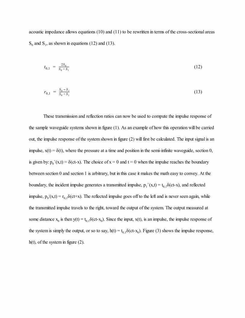
These transmission and reflection ratios can now be used to compute the impulse response of

the sample waveguide systems shown in figure (1). As an example of how this operation will be carried

out, the impulse response of the system shown in figure (2) will first be calculated. The input signal is an

impulse, x(t) = δ(t), where the pressure at a time and position in the semi-infinite waveguide, section 0,

is given by: p0+(x,t) = δ(ct-x). The choice of x = 0 and t = 0 when the impulse reaches the boundary

between section 0 and section 1 is arbitrary, but in this case it makes the math easy to convey. At the

boundary, the incident impulse generates a transmitted impulse, p1+(x,t) = t0,1δ(ct-x), and reflected

impulse, p0-(x,t) = r0,1δ(ct+x). The reflected impulse goes off to the left and is never seen again, while

the transmitted impulse travels to the right, toward the output of the system. The output measured at

some distance x0 is then y(t) = t0,1δ(ct-x0). Since the input, x(t), is an impulse, the impulse response of

the system is simply the output, or so to say, h(t) = t0,1δ(ct-x0). Figure (3) shows the impulse response,

h(t), of the system in figure (2).

FIGURE 3: Input impulse and impulse response of system shown in figure (2). The cross-sectional

areas S0 and S1 are 0.196 in2 and 0.785 in2, respectively (diameters 0.5 in and 1 in, respectively). The

input impulse is “measured” at x=0m, while the output is “measured” at 1000m. The speed of the

pressure wave is c=340m/s. These are not actual measurements, but rather they are theoretical

calculations.

Applying this method of calculating the impulse transmission and reflection at each discontinuity

in a waveguide system can yield the impulse responses of the sample waveguide systems shown in figure

(1). With this plan, it is important to note that the impulse response of a system may be infinite in

duration as reflections bounce back and forth indefinitely between two discontinuities. Some impulse

responses, therefore, cannot be calculated accurately on a computer. From the impulse response, the

frequency response can be calculated by taking the Fourier transform of the impulse response. Students

completing the experiment can then compare their theoretical predictions and actual measurements of

the impulse and frequency responses for various PVC waveguide systems.

Figures (4) and (5) show the calculated impulse and frequency responses of systems (a)

cross-section modulation and (b) side-loaded stub, shown in figure (1). The systems are calculated here

with the diameter of the small pipe as ½ in and the diameter of the large pipe as 1 in. The length of each

section of pipe is 8 in. That is, the length of the wide section of pipe in (a) is 8 in, the length of the stub in

(b) is 8 in, and the trailing ends to the left and to the right of each are all 8 in. These lengths are the same

used for the real systems tested in this project, for which data are shown in the results section of this

paper.

FIGURE 4: Impulse and frequency response of system (a) cross-section modulation, shown in figure

(1). Dimensions of the system: 1 in diameter on wide section, ½ in diameter on trailing ends, and each

section is 8 in long.

FIGURE 5: Impulse and frequency response of system (b) side-loaded stub, shown in figure (1).

Dimensions of the system: ½ in diameter for all sections, and each section is 8 in long.

Calculating Dispersion from Phase

Once the frequency response magnitude and phase have been calculated, many possible

analyses that can be performed. One of these analyses is calculating the dispersion relation of phase

velocity versus frequency for the system. Robertson explains this calculation in depth in several of his

papers (see Refs. [3], [6] and [7]), so this paper will only briefly review the procedure.

Phase velocity in the system, vp, versus frequency, f, can be represented as the speed of sound,

c, modified by a dimensionless factor, n, as in equation (14).

(f ) c n(f ) vp = / (14)

With equation (14), the phase difference, Δφ, between the frequency responses of the system

under test and a straight-pipe system of the same length can be calculated as in equation (15).

φ (n(f ) 1)L Δ = − c

2πf(15)

Here, L is the length of the system. Equation (15) can be rearranged to solve for the

dimensionless factor n, shown in equation (16). This dimensionless factor can then be used in equation

(14) to calculate the dispersion relation of phase velocity versus frequency for the system.

(f ) 1n = cΔφ

2πfL+ (16)

Setup

The object of the experiment presented in this paper is to measure the frequency response, H(f),

of a system and to compare that measurement with the expected frequency response obtained from

theoretical calculations. According to equation (6), this can easily be accomplished by dividing the

fourier transform of an output signal, y(t), by the fourier transform of its corresponding input signal, x(t).

This method to obtain H(f) only requires that the input and output signals be known. Thus, the setup for

the experiment must be able to acquire both the input and output signals. Figure (6) shows the setup

used to obtain the data presented in the results section.

FIGURE 6: Setup of the experiment.

The experimental setup is much the same as that used by Robertson and Parker.[3] The entire

experiment is controlled by a computer. The computer sound card sends the input signal to the speaker.

The speaker plays the acoustic signal into the PVC waveguide, which guides the signal to the system

under test. After passing through the system under test, the modified acoustic signal passes through a

second waveguide to a microphone. The microphone picks up the signal, which is then passed through a

digital preamplifier back to the computer.

One thing to note in figure (6) is the trigger signal being sent from the computer sound card

directly to the digital preamplifier. Both the computer sound card and digital preamplifier have two

channels so that the input signal and trigger signal do not interfere with one another. This trigger signal

allows the computer to detect the exact time at which the input signal was sent to the speaker. Such

timing is important to analyzing delays and phase shifts that the acoustic signal undergoes while inside the

waveguide system.

The equipment for this experiment is relatively inexpensive, totalling under $600 without the

computer. Price is a consideration in this project because the experiment will be put in an undergraduate

lab for learning purposes. Students may not initially know how to use the equipment properly and may

inadvertently break something. Needing to replace equipment is a real possibility, and therefore cost

should be low so as not to prohibit a student’s learning opportunity.

Any computer with MATLAB installed and a sound card is sufficient to control the experiment.

Programming languages other than MATLAB will work, but this paper provides scripts written solely in

MATLAB. The bare minimum sound card capability is 44.1 kHz sampling, which covers the entire

band of frequencies that the Nady CM 100 microphone (discussed later) can pick up. However, sound

cards capable of higher fidelity are desirable, as well as easily obtainable, for re-creating arbitrary

signals. The junior physics lab at CWRU is already equipped with computers that have MATLAB

installed, and all of them have working sound cards. So, the choice of computer for the experiment is

really just a choice of where in the junior lab the experiment will be set up.

The speaker is an Avantone Active MixCube. It is capable of reproducing frequencies in the

range 90-17,000 Hz, and it has a built-in amplifier with a 90-50,000 +/- 0 dB response and 113 dB

signal-to-noise ratio (SNR). The condenser microphone is a Nady CM 100, and it has a useful

response over the range 15-20,000 Hz. The response of the Nady CM 100 is shown in figure (7). The

digital preamplifier is a Steinberg UR22 Audio Interface. The interface is capable of 24 bit/192 kHz

analog-to-digital conversion, which puts quantization noise floor well below any other sources of noise

in the experiment. These numbers mean that almost any arbitrary signal in the range of human hearing

can be recreated on the speaker and measured on the microphone. Students will not be limited in the

signals they can use for the experiment, and they can explore how choice of signal affects the results

they get.

FIGURE 7: Frequency response of the Nady CM 100 condenser microphone. This figure is from the

CM 100 user guide, available on the Nady Audio website.

Method

For students completing the experiment in the junior physics lab at CWRU, the method will

detail how to measure the frequency response of a system. In simplest terms, this entails measuring an

input and output signal as briefly described in the setup section above and applying equation (6) to

obtain the frequency response of the system under test. The method for this paper, however, details the

method and initial setup needed to attain a desired signal quality. Students will naturally try to improve

signal quality as they complete the experiment, but the initial setup provides a base for them to work

from. Students ought to be able to explore and learn about the experiment, free from the frustrations of

obtaining data of bare minimum quality.

Noise Reduction

The bare minimum signal quality goal is 30 dB SNR with 0.1 seconds of otherwise

interference-free data. With 30 dB SNR, plotted data will have noise that is only barely visibly

perceptible. And with 0.1 seconds of data, the Fourier transform of the data will have a useful resolution

of 10 Hz, a high enough resolution to calculate characteristic lengths to 1% accuracy near 8 inches, the

approximate length scale for features in the PVC waveguides.

The first part of improving SNR is signal strength. The goal here is to find a signal that has

enough energy to overcome the noise in the experiment, and then that signal will be used to measure the

frequency response of the systems under test. In an ideal world, the signal is an impulse of infinite

pressure and infinitesimal width in time. However, the equipment in the experiment is not capable of

reproducing such a signal. The signal for the experiment must then be limited to a bandwidth and

magnitude that the equipment can handle, but the signal must still have enough energy to overcome

noise. An indicator of energy is the signal’s time-bandwidth product, or the signal’s duration in time

multiplied by its bandwidth. Students will have the opportunity, if they wish, to explore whatever signals

they choose, but the signal chosen for acquiring data for this paper is a linear frequency modulated

(LFM) chirp. The LFM chirp can be readily reproduced on the Avantone MixCube, and its

time-bandwidth product is higher than that of other time-limited signals such as a truncated gaussian or a

single sine burst.

The second part of improving SNR is coherent averaging, or averaging the output over many

iterations to reduce incoherent noise. The waveguide is a time-invariant system, so the output is exactly

the same each and every iteration for the same input signal. Incoherent noise changes with time and

therefore is different for each iteration. Averaging many iterations allows the signal to constructively

interfere while the incoherent noise, on average, destructively interferes. This method yields a higher

SNR, which reduces uncertainty in the measurement. To make sure that all the iterations are averaged

coherently (i.e. the outputs from each iteration are lined up in time), a triggered measurement is

performed. A trigger signal is sent from one channel of the sound card stereo output directly to channel

2 of the digital preamplifier. The exact time of the signal can then be retrieved by the computer from

channel 2 of the digital preamplifier, and the output can be retrieved with correct time displacement from

channel 1. Performing many iterations using this coherent averaging method yields a cleaner signal and

better end results. Figure (8) compares a single iteration of a pulse signal to 300 iterations coherently

averaged together.

FIGURE 8: Single shot versus multiple shot data. The pulse used here is a single wavelength of a sine

wave at 1600 Hz. After 300 iterations, the incoherent noise has been attenuated enough to allow the

reflections of the signal to be visible in the data plot.

The third part of improving SNR is physical sound damping. Not all noise is incoherent, and so

some noise still ends up in the signal after the coherent averaging operation. Most of the correlated noise

in the experiment comes from reverberations in the room and apparatus. Each time the speaker plays

the acoustic signal, sound waves bounce back and forth around the room and apparatus. Coherent

averaging cannot remove this noise because it is the same for each iteration. Figure (9a) shows a power

spectral density (PSD) plot of a measured signal with significant reverberation noise. Reverberation is

reduced in the experiment simply by placing sound-absorbing materials in the room and around the

setup to attenuate noise as much as possible. Egg-carton packing foam is placed around the mic. The

speaker is boxed in with foam sheets and surrounded by shredded paper. These materials are not

explicitly intended for sound absorption applications, but they absorb more sound than open air and are

readily available in the junior physics lab at CWRU. Students may wish to explore other options for

sound-damping materials to use in the lab. Figure (9b) shows a PSD plot of a measured signal with the

reverberation noise reduced by sound-damping materials.

(a)

(b)

FIGURE 9: (a) PSD plot of a measured signal with significant reverberation noise. A linear frequency

modulated (LFM) chirp, sweeping from 7,500 Hz to 50 Hz in 0.02 s, is used as the input signal. (b)

PSD plot of a measured signal with reverberation signal reduced. All parameters are the same as for the

data shown in figure 9a except that physical sound-damping materials have been applied around the

microphone and speaker.

Reflections of the signal can be seen in both figures (8) and (9b). These reflections arise because

of the impedance discontinuity at the termination of the waveguide. Reflections from the end of the

waveguide cannot be eradicated because there is a speaker at one end and a microphone at the other.

The impedance of the speaker and microphone cannot easily be matched to the impedance of the

waveguide, so other means must be used to deal with the nuisance of reflections. In an ideal world, the

waveguide would be infinite in length so that the signal never reflects back toward the system. So, the

experiment must imitate this behavior and have pseudo-infinite waveguides. In other words, the

waveguides need to be sufficiently long so that reflections do not interfere with the signal.

Figures (8) and (9b) both show data taken with 30 ft waveguides before and after the system.

With about 60 feet of total waveguide to go through, the signal arrives at the microphone 0.055 seconds

after it leaves the speaker. The signal then reflects off the end of the waveguide back to the system, and

then it reflects off the system-waveguide coupling back to the microphone. The first reflection reaches

the microphone 0.055 seconds after the original signal. This leaves 0.11 seconds of reflection-free data,

attaining the goal of over 0.1 seconds of useable data.

The waveguides should not be made much longer than a total of 60 feet, though. As it

propagates through the waveguide, the signal is attenuated. Figure (10) shows SNR values for an LFM

chirp, the same as used for the data in figures (9a) and (9b), propagating through different lengths of

waveguide and averaged over 300 iterations. At very short distances, the signal is not attenuated very

much and is much stronger than the noise. At distances over 60 feet, however, the signal is attenuated

so much that the SNR begins to fall below 30 dB. The waveguide length should therefore not exceed a

total of about 80 feet unless further measures are taken to reduce noise and boost signal strength.

FIGURE 10: Measured SNR values for an LFM chirp propagating through a ½ in waveguide and

averaged over 300 iterations. Propagating through a waveguide of 60 ft, the LFM chirp has an SNR

that nears 30 dB, the goal for bare minimum signal quality.

Data Acquisition

As stated before, a computer running MATLAB controls the experiment. Playing the acoustic

signal on the speaker, recording from the microphone, detecting the trigger signal, and averaging

iterations together is all accomplished in a MATLAB script (see appendix (A)). The most important part

of the script is detecting the trigger signal to align data runs together properly. The impulse response of a

matched filter, matched to the trigger signal, is convolved with the trigger signal to detect the point in

time where the trigger signal occurs. That time index is then used to select the start point of the signal in

the raw microphone data, and the signal is extracted from the raw microphone data starting at the time

index. Each data iteration is thus temporally aligned with all the other iterations, and all iterations are

averaged together to obtain the final measured output of the system. Implementing a matched filter is a

signal processing skill that students will need to learn in order to successfully complete the lab.

Sample Results

The measured frequency response for the first sample system, (a) cross-section modulation, is

shown in figure (11). Comparing the magnitude of the measured frequency response reveals that the

behavior follows that given by theory (see figure (5)). The response starts close to unity at 0 Hz, dips

down and then rises close to unity again around 820 Hz. The calculated phase velocity is equal to the

speed of sound for all frequencies.

Sample data for all the other systems from figure (1) are in appendix (B).

FIGURE 11: Measured frequency response and calculated dispersion for (a) cross-section modulation.

Dimensions are the same as the system described for figure (5).

Conclusion

The experiment presented here is ready to be implemented in the junior physics lab at CWRU.

Students completing the experiment will be able to learn about topics in signal processing and acoustic

phenomena. The main three points for students to learn when completing the experiment are: (1)

calculate the theoretical impulse response of simple acoustic waveguide systems, (2) implement

triggered data acquisition and coherent averaging and (3) compute the frequency response of a system

from measured data. The first point is discussed in the theory section of this paper, and students can

reasonably be expected to calculate the two frequency responses shown in figures (4) and (5). The

second and third points are discussed in the method section and will take up the bulk of students’ time in

the lab.

References

[1] D.A. Russell, D.O. Ludwigsen, “Acoustic testing and modeling: An advanced undergraduate

laboratory,” J. Acoust. Soc. Am. 131(3) 2515-2524 (2012)

[2] E.J. Tucholski, “Tabletop demonstration of multiple source interference using ultrasonic

transducers,” Am. J. Physics 77(10) 938-942 (2009)

[3] W.M. Robertson, J.M. Parker, “Acoustic impulse response method as a source of undergraduate

research projects and advanced laboratory experiments,” J. Acoust. Soc. Am. 131(3)

2488-2494 (2012)

[4] Schetzen, Martin, Linear Time-Invariant Systems, Wiley-IEEE Press; 1 edition (November 21,

2002)

[5] Kinsler, Frey, Coppens and Sanders, Fundamentals of Acoustics, Wiley; 4th edition (December

30, 1999)

[6] Robertson and Rudy III, “Measurement of acoustic stop bands in two-dimensional periodic

scattering arrays,” J. Acoust. Soc. Am. 104, 694–699 (1998).

[7] Ash and Robertson, “Acoustic band gap measurements in wave-guides with periodic resonant

structures,” Z. Kristallogr. 220, 824–828 (2005).

Appendix A: MATLAB script for data acquisition

% Parameters

tPlay = 0.3; % Play time for pulse

tPulse = 0.018; % Length of pulse to be played

Fsplay = 96000; % Playback sample rate

Fsrecord = Fsplay; % Record sample rate

t = linspace(0,tPlay,Fsplay*tPlay);

y = zeros(size(t));

Fstart = 7500;

Fend = 50;

phi = 2*pi*(Fstart + 0.5*t(1:round(tPulse*Fsplay))*...

(Fend-Fstart)/tPulse).*t(1:round(tPulse*Fsplay));

y(1:round(tPulse*Fsplay)) = sin(phi);

% Taper with 10% Tukey window

y(1:round(tPulse*Fsplay)) = y(1:round(tPulse*Fsplay)).*...

tukeywin(round(tPulse*Fsplay),0.1)';

b = conj(y(end:-1:1)); % Matched filter impulse response

% Create system objects

hap = dsp.AudioPlayer('SampleRate',Fsplay);

hap.QueueDuration = tPlay;

har = dsp.AudioRecorder(Fsrecord);

har.QueueDuration = 2.1*tPlay;

% Create temporary arrays

temp = zeros(2*length(y),2); % Temporary for input

data = zeros(size(y)); % Final data

numInc = 0; % Number of incomplete recordings

% Iterate

for i = 1:100

step(hap,y'); % Play sound

% Record sound

ind = 1;

while ind < length(temp)

temp(ind:ind+har.SamplesPerFrame-1,:) = step(har);

ind = ind + har.SamplesPerFrame;

end

release(hap); release(har); % Release resources

% Pull data from temp array and average with other runs

[~,index] = max(conv(b,temp(:,2)));

if ((index-length(y)) > 0) && (index <= length(temp))

data = data.*(i-1)./i +...

temp(index-length(y)+1:index,1)'./i;

else

numInc = numInc + 1;

end

end

% Plot results

figure; plot(t,data);

xlabel('time (s)', 'fontsize',14);

ylabel('Output from preamp', 'fontsize',14);

s = sprintf('Raw data for %s %gs pulse - %d iterations',

waveform,tPulse,i);

title(s, 'fontsize',14);

set(gca, 'fontsize',14);

% Display number incomplete recordings

fprintf('\n%d of %d recordings contained incomplete...

data and were not used.\n\n',numInc,i);

Appendix B: Frequency responses and dispersion relations for sample systems

In the phase data of each frequency response there are jumps between π and -π. The data does

not actually discontinuously change phase by 360 degrees at these points. The phase is sometimes

outside the range -π to π, but MATLAB interprets these phases as being shifted into the range -π to π.