advanced topic in astrophysics lecture...

1

Advanced Topic in AstrophysicsLecture 4

“Radio Astronomy - Antennas & Imaging”

Lecture 4

2

p.2

Resources/Acknowledgments

ATNF Synthesis Imaging workshops 2003, 2006 http://www.atnf.csiro.au/whats_on/workshops/synthesis2006/prog.html

Material from Ravi Subrahmanyan, Dave McConnell, Ron Ekers

Tools of Radio Astronomy Rohfl & Wilson

An introduction to Radio Astronomy Burke & Graham-Smith

Interferometry & Synthesis in Radio Astronomy

Thompson, Moran, Swenson

-------------------------------------

Radio Astronomy Kraus

Lecture 4

3

p.3

Outline

Following on from Lecture 1-3 (Single dishes & HI)We will cover: Multiple Dish Radio Astronomy Direct & Indirect imaging

Synthesis Arrays

Van Cittert-Zernike equations

Advantages and Disadvantages of Both Examples using the observations of Cygnus A

Problems with Arrays; be EW or have a w-term

A Case study Methanol Masers: Basics of masers

Example of Methanol Maser VLBI; outcomes

Example of Methanol Maser Single Dish; outcomes

Lecture 4

4

p.4

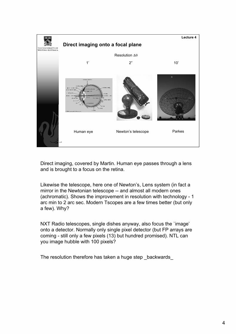
Direct imaging onto a focal plane

2” 10’1’

Resolution Δθ

Human eye Newton’s telescope Parkes

Lecture 4

Direct imaging, covered by Martin. Human eye passes through a lensand is brought to a focus on the retina.

Likewise the telescope, here one of Newton’s, Lens system (in fact amirror in the Newtonian telescope -- and almost all modern ones(achromatic). Shows the improvement in resolution with technology - 1arc min to 2 arc sec. Modern Tscopes are a few times better (but onlya few). Why?

NXT Radio telescopes, single dishes anyway, also focus the `image’onto a detector. Normally only single pixel detector (but FP arrays arecoming - still only a few pixels (13) but hundred promised). NTL canyou image hubble with 100 pixels?

The resolution therefore has taken a huge step _backwards_

5

p.5

Diffraction limits

DλΔθ=1”

50 km20 cmRadio

125 mm500 nmOptical

Δθ=1.22 λ/D

Lecture 4

This is the reason why. Resolution is a function of wavelength.Basically sharpness.

Radio wavelengths are 100 of mm, opticals are 100s of nm: differenceof a bit less than 10^6.To get a resolution of 1”We can not build a radio telescope a million times bigger than a opticaltelescope100m rather than 1m (optical can be bigger, but the resolution is rarelydiffraction limited-- this is usually ~ 20cm)

6

p.6

Indirect imaging

Indirect imaging is used where we cannot form adirect map of the object on the focal plane. We cannotbuild a 50km single dish telescope.

We infer the properties of the object from certaincharacteristics of the received electromagnetic field.

I.e. the image is formed `indirectly’

Lecture 4

7

p.7

Examples of Indirect Imaging

Interferometry Radio, optical, IR

Aperture Synthesis Earth rotation, X-ray crystallography

Axial Tomography NMR, ultrasound, PET

Seismology

Fourier Filtering, Pattern Recognition

Adaptive Optics, Speckle

Lecture 4

8

p.8

Indirect Imaging - synthesis radio telescopes

Australia Telescope CompactArray (ATCA)

Very Large Array (VLA) US Westerbork SRT (Netherlands)

Lecture 4

Here are some images of radio telescopes. ATCA, Westerbork, VLA.

All of these have a `few’ dishes 6 in CA, 10 in Westerbork, 27 in VLA

9

p.9

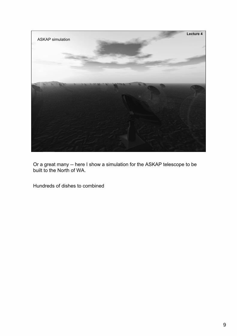
ASKAP simulationLecture 4

Or a great many -- here I show a simulation for the ASKAP telescope to bebuilt to the North of WA.

Hundreds of dishes to combined

10

p.10

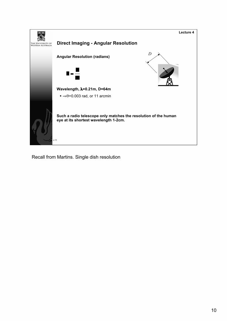
Direct Imaging - Angular Resolution

Angular Resolution (radians)

Wavelength, λ=0.21m, D=64m

⇒θ=0.003 rad, or 11 arcmin

Such a radio telescope only matches the resolution of the humaneye at its shortest wavelength 1-2cm.

D

Lecture 4

Recall from Martins. Single dish resolution

11

p.11

Indirect imaging (interferometer) - angular resolution

The angular resolution of a connected array of radio telescopes is:

B can be several thousand km in the case of Very Long BaselineInterferometry

λ=7mm, B=8000km (VLBA) ⇒θ=9.10-10 rad or 0.2 milliarcsec

B

Lecture 4

Here we combine antennae to make an effective size of B, not D

12

p.12

A 21cm HI single-dishimage of the LMC withthe Parkes telescope(Staveley-Smith et al.2003)

Telescope alternatelyscanned in RA and Dec.

Angular resolution 15’

A 21cm HI CompactArray observation of theLMC (Kim et al. 2003)

1344 separate pointingcentres mosaicedtogether.

Angular resolution 1’

Lecture 4

Here is a beautiful examples. 15’ with Parkes, done by our own Lister. But 1’with ATCA. But note 1344 pointings need to be merged.

13

p.13

Direct Imaging: Single dish radio telescope

Lecture 4

Imaging a dish, pointing in one direction and or the other

14

p.14

Equivalent to…

Σ

Lecture 4

Σ

Imaging rather than a continuous dish it was made of subsections(RATAN-600)

Furthermore one could focus the signal in each section, and then carrythe voltage to the `big dish focus’, where it could be summed.

Or even it could be done any where,

15

p.15

Phased array

Delay

Indirect Imaging - phased array

Lecture 4

I.e. the image is formed `indirectly’ . Even more distant from theoriginal situation, we could put the sub-collectors on the ground.Then we have to add in the extra delays.

This summed mode of operation is called a phased array.

As the dishes of the smaller the `steering’ can be done differently.The beamsize is bigger, so one can steer within the beam by changingthe delays. The different colours

16

p.16

Delay

Indirect imaging - synthesis array

CorrelatorFourier Transform

Lecture 4

But a better approach is to, rather than sum, is to multiply the voltagesand then one can form or synthesis the image via a fourier transform.

One can form a baseline between each pair of antenna. I.e. thenumber of baselines is N(N-1)/2.ATCA: 6 antennae, 15 baselines; VLA 27 antennae, 351 baselines;LBA 5 antennae, 10 baselines

How many baselines do you need? This 1D array has resolution in 1Donly. Need range of separations in a range of directions to solve forcomplexity

Synthesis -> image is synthesized (FT) out of the data collected

17

p.17

Delay

Indirect imaging - synthesis arrayLecture 4

Baseline bλ (in wavelengths)

τg

SS

Delay is the dot product of the two vectors: bλ. . S

Different baselines give you different delays: extra informationWhich can be `synthesised’ to produce the imageFurthermore the baseline changes with time: Even more information. This technique is called Earth Rotation Synthesis.

How many baselines do you need? Changing direction of the sourcegives a range of projected separations and orientations.

Demonstrate ERS

18

p.18

Indirect imaging - synthesis array

`Voltage multiplied ‘: Easily said, not so easily done

Dickey Switch: <V1+V2>2-<V1-V2>2

= 4<V1V2>

Now with non-linear devices, or software: V1*V2 where V are the instanenous Voltages

V1 = <V1> cos(2π vt)V2 = <V2> cos(2π v(t - τ )) (Where τ = bλ. . S)

Cross correlation is the correlation of two signals in time: Γ = <x(t) y(t- τ)> therefore

Γ = < V1 V2 >= A(s) S cos (2π τ)

Lecture 4

Page 53 intro RA V = Antenna response Source flux

19

p.19

The Dickey Switch

Σ±

±

<>

20

p.20

τ = bλ. . S

Here is the the Michelson Morley interferometer:

The Interferometer

Lecture 4

Here is the MM interferometer. I hope you all recognise it. It is an optical I. butthe basic set up is the same.Light from two extremes are brought together, with equal path length, lightfrom a slightly different direction would have a different path length.

A source not directly above has a path length difference, and this is the dotproduct of the b baseline and s direction.

This is the response as the source passes overhead: there is a maximum asthen `fringes’ minima and maxima on each side.

The Max/Min come about as there is a geometrical fringe (from the change indelay between the two sides, and an envelope of the response function fromthe system.

But the crucial thing is that the source fringe only goes to null if the sourcedoes not resolve.If it does then it does not have such extreme maxima andminima.

21

p.21

Relationship between I(ϴ) and V(u)

V(t)

Voltage sampled in time Voltage sampled in frequency

Voltage sampled in space Intensity sampled over sky

FourierTransfer

FourierTransfer

V(v)

I(Θ)V(u)

Total power

Spatial power

Auto correlations

Cross correlations

Lecture 4

Intro 57Increase samples at ubar -> better constraints on theta

22

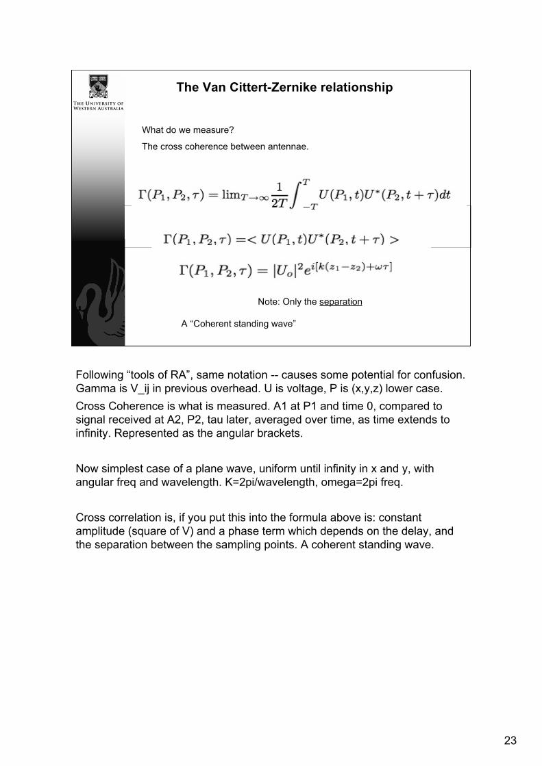
The Van Cittert-Zernike relationship

Let us formalise this:

Full derivation of this is more than I want to attempt.But is not too complicated. Possible Problem Sheet?

Let us build up what we need:

The sources move on the sky, therefore we must track them.This defines the axes of the co-ordinate system.

X and Y on the plane of the sky. l and m are the direction cosinesU and V are co-ordinates of the antenna separation. Not those on the ground

V, the visibility a function of direction vector S, and the antenna separation uand v is the integral of the Antenna response function in the directions l andm, the sky brightness in these directions, and the exponential of i2pi (u.s),integrated over the sky.

First we will define the tracking centre, and the coordinate system.

23


What do we measure?

The cross coherence between antennae.

Note: Only the separation

A “Coherent standing wave”

Following “tools of RA”, same notation -- causes some potential for confusion.Gamma is V_ij in previous overhead. U is voltage, P is (x,y,z) lower case.Cross Coherence is what is measured. A1 at P1 and time 0, compared tosignal received at A2, P2, tau later, averaged over time, as time extends toinfinity. Represented as the angular brackets.

Now simplest case of a plane wave, uniform until infinity in x and y, withangular freq and wavelength. K=2pi/wavelength, omega=2pi freq.

Cross correlation is, if you put this into the formula above is: constantamplitude (square of V) and a phase term which depends on the delay, andthe separation between the sampling points. A coherent standing wave.

24


A more complex case: The cross coherence for a complex source:

Case for two point sources, can be extended to multiple, and thus to any combination

Lets us start with the simplest of more complex cases. Two point sources,with signals propagating along two directional vectors, sa and sb.

Here is the image of what is happening. The source has an angular extentover the sky, the contributions from across this source are collected - in asum as they are voltages - by the antennae. We are thinking only about twodirections at this moment, but the extension is obvious.

The CC is the CC of the contributions, I.e. the CC of sum of the receivedvoltages. Now we ASSUME that the CC of signals from different parts of thesky are uncorrelated. Indeed how could they not be? One atom can not knowwhat random processes another atom is undergoing, when that atom is manylight years away. Yes? Well not quite, there are some cases in which thiscould be different. For example grav lenses; light from one place takes twodifferent paths through the sky, bent by an intervening galaxy. But the pathsare very different lengths, so the two signals are received outside thecoherence time. Pulsars emit via coherent processes, so the emission fromdifferent parts of the beam are in fact coherent. But no one has the resolutionto resolve these beams as yet -- so it has not been a problem.

Therefore the CC becomes the sum of the CC of the individual components. Iour simple case that is the CC of two different point sources. But it can beextended to infinite components - and therefore any arbitrary sky brightness.

25


A more complex case: The cross coherence for a complex source:

Following the fashion of time and frequency, u is calledSPATIAL FREQUENCY and I is the brightness distribution.

Each baseline measures a different spatial frequency

To stick for the point source case for a moment, if we assume that they havethe same brightness Ub=Ua=UoThen, by substituting Sa=1/2(Sa+Sb)+(Sa-Sb) and Sb similarly, we can findthe CC for these sources. It is similar to that of the single source. The phaseterm is of the average direction vector. However the amplitude is not aconstant anymore. There is a slowly varying cosine in amp, which is afunction of the source separation. Note the amplitude goes negative -- but wewould interpreter this as a switch in phase sign. Note also has the separationgets smaller (sa-sb) we require a large u (antennae separation - or baseline)to be able to detect the changing amplitude. If the baseline is too small wewould not detect the change - not resolve.

So to finish up. As I said, the sky brightness, the image one wishes to make,is the intergral across the angular extent of the sky.

And one can form the CC, if the sky is incoherent in different directions, asthe integral across that sky brightness. And when the delays are zero -- which just means that the path lengths areequalised -- or that the array is calibrated -- there is a Fourier relationshipbetween CC and the sky brightness,

advanced topic in astrophysics lecture...

Documents