advanced time series and forecasting lecture 5 structural ...bhansen/crete/crete5.pdf · advanced...
TRANSCRIPT

Advanced Time Series and ForecastingLecture 5
Structural Breaks
Bruce E. Hansen
Summer School in Economics and EconometricsUniversity of CreteJuly 23-27, 2012
Bruce Hansen (University of Wisconsin) Structural Breaks July 23-27, 2012 1 / 99
Organization
Detection of Breaks
Estimating Breaks
Forecasting after Breaks
Bruce Hansen (University of Wisconsin) Structural Breaks July 23-27, 2012 1 / 99

Types of Breaks
Breaks in Mean
Breaks in Variance
Breaks in Relationships
Single Breaks
Multiple Breaks
Continuous Breaks
Bruce Hansen (University of Wisconsin) Structural Breaks July 23-27, 2012 2 / 99

ExampleSimple AR(1) with mean and variance breaks
yt = ρyt−1 + µt + etet ∼ N(0, σ2t )
Eyt =µt1− ρ
var(yt ) =σ2t
1− ρ2
µt and/or σ2t may be constant or may have a break at some point inthe sampleSample size nQuestions: Can you guess:
I Is there a structural break?I If so, when?I Is the shift in the mean or variance? How large do you guess?
Bruce Hansen (University of Wisconsin) Structural Breaks July 23-27, 2012 3 / 99

Bruce Hansen (University of Wisconsin) Structural Breaks July 23-27, 2012 4 / 99
Bruce Hansen (University of Wisconsin) Structural Breaks July 23-27, 2012 5 / 99

Bruce Hansen (University of Wisconsin) Structural Breaks July 23-27, 2012 6 / 99

Terminology
Sample Period: t = 1, ..., n
Breakdate: T1I Date of change
Breakdate fraction: τ1 = T1/nPre-Break Sample: t = 1, ...,T1
I T1 observations
Post-Break Sample: t = T1 + 1, ..., nI n− T1 observations
Bruce Hansen (University of Wisconsin) Structural Breaks July 23-27, 2012 7 / 99

Structural Break Model
Full structural break
yt = β′1xt + et , t ≤ T1yt = β′2xt + et , t > T1
oryt = β′1xt1 (t ≤ T1) + β′2xt1 (t > T1) + et
Partial structural break
yt = β′0zt + β′1xt1 (t ≤ T1) + β′2xt1 (t > T1) + et
Bruce Hansen (University of Wisconsin) Structural Breaks July 23-27, 2012 8 / 99
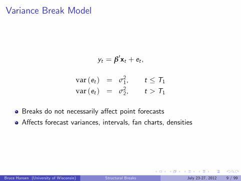
Variance Break Model
yt = β′xt + et ,
var (et ) = σ21, t ≤ T1var (et ) = σ22, t > T1
Breaks do not necessarily affect point forecasts
Affects forecast variances, intervals, fan charts, densities
Bruce Hansen (University of Wisconsin) Structural Breaks July 23-27, 2012 9 / 99

Detection of Breaks
Bruce Hansen (University of Wisconsin) Structural Breaks July 23-27, 2012 10 / 99

Testing for a Break
Classic Test (Chow)
Assume T1 is known
Test H0 : β1 = β2Use classic linear hypothesis test (F, Wald, LM, LR)
Least-Squares
yt = β′0zt + β
′1xt1 (t ≤ T1) + β
′2xt1 (t > T1) + et
Bruce Hansen (University of Wisconsin) Structural Breaks July 23-27, 2012 11 / 99

Full Break Model
Y1 = X1β1 + e1Y2 = X1β2 + e2
β1 = (X ′1X1)−1(X ′1Y1)
β2 = (X ′2X2)−1(X ′2Y2)
e1 = Y1 − X1 β1
e2 = Y2 − X2 β2
SSE (T1) = e ′1 e1 + e′2 e2
σ2(T1) =1
n−m(e ′1 e1 + e
′2 e2)
Bruce Hansen (University of Wisconsin) Structural Breaks July 23-27, 2012 12 / 99

F Test Statistic
F test
F (T1) =(SSE − SSE (T1)) /kSSE (T1)(n−m)
where k = dim(β1), m =all parameters,
SSE = e ′e
σ2 =1
n− k(e ′e)
e = Y − X β
(full sample estimate)I F test assumes homoskedasticity, better to use Wald test
Bruce Hansen (University of Wisconsin) Structural Breaks July 23-27, 2012 13 / 99

Wald Test Statistic
W (T1) = n(
β1 − β2
)′ (V1nT1+ V2
nn− T1
)−1 (β1 − β2
)where V1 and V2 are standard asymptotic variance estimators for β1 andβ2 (on the split samples:
V1 = Q−11 Ω1Q−11V2 = Q−12 Ω2Q−12
Q1 =1T1X ′1X1
Q2 =1
n− T1X ′2X2
Bruce Hansen (University of Wisconsin) Structural Breaks July 23-27, 2012 14 / 99

HAC variance optionsFor iid et
Ω1 = σ2Q1Ω2 = σ2Q2
For homoskedastic (within regiome
σ21 =1
T1 − k(e ′1 e1
)σ22 =
1n− T1 − k
(e ′2 e2
)For serially uncorrelated but possibly heteroskedastic
Ω1 =1
T1 − kT1
∑t=1xtx′t e
2t
Ω2 =1
n− T1 − kn
∑t=T1+1
xtx′t e2t
Bruce Hansen (University of Wisconsin) Structural Breaks July 23-27, 2012 15 / 99
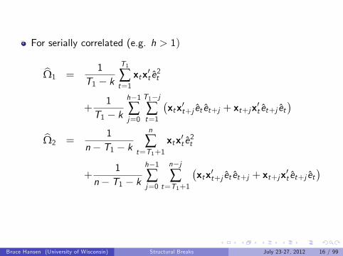
For serially correlated (e.g. h > 1)
Ω1 =1
T1 − kT1
∑t=1xtx′t e
2t
+1
T1 − kh−1∑j=0
T1−j∑t=1
(xtx′t+j et et+j + xt+jx
′t et+j et
)Ω2 =
1n− T1 − k
n
∑t=T1+1
xtx′t e2t
+1
n− T1 − kh−1∑j=0
n−j∑
t=T1+1
(xtx′t+j et et+j + xt+jx
′t et+j et
)
Bruce Hansen (University of Wisconsin) Structural Breaks July 23-27, 2012 16 / 99

Classic Theory
Under H0, if the number of observations pre- and post-break arelarge, then
F (T1)→dχ2kk
under homoskedasticity, and in general
W (T1)→d χ2k
We can reject H0 in favor of H1 if the test exceeds the critical valueI Thus “find a break” if the test rejects
Bruce Hansen (University of Wisconsin) Structural Breaks July 23-27, 2012 17 / 99

Modern Approach
Break dates are unknown
Sup tests (Andrews, 1993)
SupF = supT1F (T1)
SupW = supT1W (T1)
The sup is taken over all break dates T1 in the region [t1, t2] wheret1 >> 1 and t2 << n
I The region [t1, t2 ] are candidate breakdates. If the proposed break istoo near the beginning or end of sample, the estimates and tests will bemisleading
I Recommended rule t1 = [.15n], t2 = [.85n]
Numerically, calculate SupW using a loop
Bruce Hansen (University of Wisconsin) Structural Breaks July 23-27, 2012 18 / 99

Example
US GDP example presented yesterday
Quarterly data 1960:2011
k = 7
Bruce Hansen (University of Wisconsin) Structural Breaks July 23-27, 2012 19 / 99

Bruce Hansen (University of Wisconsin) Structural Breaks July 23-27, 2012 20 / 99

Evidence for Structural Break?
SupW=27
Is this significant?
Bruce Hansen (University of Wisconsin) Structural Breaks July 23-27, 2012 21 / 99

Theorem (Andrews)
Under H0, if the regressors xt are strictly stationary, thenI SupF, SupW, etc, converge to non-standard asymptotic distributionswhich depend on
F k (the number of parameters tested for constancyF π1 = t1/nF π2 = t2/nF Only depend on π1 and π2 through λ = π2(1− π1)/(π1(1− π2))
Critical values in Andrews (2003, Econometrica, pp 395-397)
p-value approximation function in Hansen (1997 JBES, pp 60-67)
Critical values much larger than chi-square
Bruce Hansen (University of Wisconsin) Structural Breaks July 23-27, 2012 22 / 99

Evidence for Structural Break?
SupW=27
k = 7
1% asymptotic critical value = 26.72
Asymptotic p-value=0.008
Bruce Hansen (University of Wisconsin) Structural Breaks July 23-27, 2012 23 / 99

Non-Constancy in Marginal or Conditional?
The model is
yt = β′0zt + β′1xt1 (t ≤ T1) + β′2xt1 (t > T1) + et
The goal is to check for non-constancy in the conditional relationship(in the coeffi cients β) while being agnostic about the marginal (thedistribution of the regressors xt)Andrews assume that xt are strictly stationary, which excludesstructural change in the regressors
In Hansen (2000, JoE) I show that this assumption is bindingI If xt has a structural break in its mean or variance, the asymptoticdistribution of the SupW test changes
I This can distort inference (a large test may be due to instability in xt ,not regression instability)
There is a simple solution: Fixed Regressor BootstrapI Requires h = 1 (no serial correlation)
Bruce Hansen (University of Wisconsin) Structural Breaks July 23-27, 2012 24 / 99

Fixed Regressor Bootstrap
Similar to a bootstrap, a method to simulate the asymptotic nulldistribution
Fix (zt , xt , et ), t = 1, ..., nLet y ∗t be iid N(0, e
2t ), t = 1, ..., n
Estimate the regression
y ∗t = β∗′0 zt + β
∗′1 xt1 (t ≤ T1) + β
∗′2 xt1 (t > T1) + e
∗t
Form the Wald, SupW statistics on this simulated data
W ∗(T1) = n(
β∗1(T1)− β
∗2(T1)
)′ (V ∗1 (T1)
nT1+ V ∗2 (T1)
nn− T1
)−1(
β∗1(T1)− β
∗2(T1)
)SupW∗ = sup
T1W ∗(T1)
Bruce Hansen (University of Wisconsin) Structural Breaks July 23-27, 2012 25 / 99

Repeat this B ≥ 1000 times.Let SupW∗b denote the b’th value
Fixed Regressor bootstrap p-value
p =1B
N
∑b=1
1 (SupW∗b ≥ SupW∗)
Fixed Regressor bootstrap critical values are quantiles of empiricaldistribution of SupW∗bImportant restriction: Requires serially uncorrelated errors (h = 1)
Bruce Hansen (University of Wisconsin) Structural Breaks July 23-27, 2012 26 / 99

Bruce Hansen (University of Wisconsin) Structural Breaks July 23-27, 2012 27 / 99

Evidence for Structural Break?
SupW=27
Asymptotic p-value=0.008
Fixed regressor bootstrap p-value=0.106
Bootstrap eliminates significance!
Bruce Hansen (University of Wisconsin) Structural Breaks July 23-27, 2012 28 / 99

Recommendation
In small samples, the SupW test highly over-rejects
The Fixed Regressor Bootstrap (h = 1) greatly reduces this problem
Furthermore, it makes the test robust to structural change in themarginal distribution
For h > 1, tests not well investigated
Bruce Hansen (University of Wisconsin) Structural Breaks July 23-27, 2012 29 / 99

Testing for Breaks in the Variance
yt = β′xt + et ,
var (et ) = σ21, t ≤ T1var (et ) = σ22, t > T1
Since var (et ) = Ee2t , this is the same as a test for a break in aregression of e2t on a constant
Estimate constant-parameter model
yt = β′xt + et
Obtain squared residuals e2tApply Andrews SupW test to a regression of e2t on a constant
k = 1 critical values
Bruce Hansen (University of Wisconsin) Structural Breaks July 23-27, 2012 30 / 99
GDP Example: Break in Variance?
Apply test to squared OLS residuals
Bruce Hansen (University of Wisconsin) Structural Breaks July 23-27, 2012 31 / 99

Bruce Hansen (University of Wisconsin) Structural Breaks July 23-27, 2012 32 / 99

Break in Variance?
SupW=15.96
k = 1
1% asymptotic critical value =12.16
Asymptotic p-value=0.002
Fixed regressor bootstrap p-value=0.000
Strong rejection of constancy in varianceI Great moderation
Bruce Hansen (University of Wisconsin) Structural Breaks July 23-27, 2012 33 / 99

End-of-Sample Breaks
Bruce Hansen (University of Wisconsin) Structural Breaks July 23-27, 2012 34 / 99

End-of-Sample Breaks
The SupW tests are powerful against structural changes which occurin the interior of the sample
T1 ∈ [.15n, .85n]Have low power against breaks at the end of the sample
Yet for forecasting, this is a critical period
Classic Chow test allows for breaks at end of sampleI But requires finite sample normality
New end-of-sample instability test by Andrews (Econometrica, 2003)
Bruce Hansen (University of Wisconsin) Structural Breaks July 23-27, 2012 35 / 99

End-of-Sample Test
Write model as
Y1 = X1β1 + e1Y2 = X1β2t + e2
where Y1 is n× 1, Y2 is m× 1 and X has k regressors
m is known but small
Test is for non-constancy in β2t
Let β be full sample (n+m) LS estimate, e = Y − X β full-sampleresiduals
Partition e = (e1, e2)
Test depends on Σ = E (e2e ′2)First take case Σ = Imσ2
Bruce Hansen (University of Wisconsin) Structural Breaks July 23-27, 2012 36 / 99

Ifm ≥ dS = e ′2X2
(X ′2X2
)−1 X ′2 e2If m < d
P = e ′2X2X′2 e2
If m is large we could use a chi-square approximation
But when m is small we cannot
Bruce Hansen (University of Wisconsin) Structural Breaks July 23-27, 2012 37 / 99
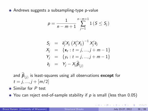
Andrews suggests a subsampling-type p-value
p =1
n−m+ 1n−m+1
∑j=1
1 (S ≤ Sj )
Sj = e ′jXj(X ′j Xj
)−1 X ′j ejXj = xt : t = j , ..., j +m− 1Yj = yt : t = j , ..., j +m− 1ej = Yj − Xj β(j)
and β(j) is least-squares using all observations except fort = j , ..., j + [m/2]Similar for P test
You can reject end-of-sample stability if p is small (less than 0.05)
Bruce Hansen (University of Wisconsin) Structural Breaks July 23-27, 2012 38 / 99

Weighted Tests
Andrews suggested improved power by exploiting correlation in e2
S = e ′2Σ−1X2
(X ′2Σ
−1X2)−1
X ′2Σ−1 e2
where
Σ =1
n+ 1
n+1
∑j=1
(Yj − Xj β
) (Yj − Xj β
)′The subsample calculations are the same as before except that
Sj = e ′j Σ−1Xj
(X ′j Σ
−1Xj)−1
X ′j Σ−1 ej
Bruce Hansen (University of Wisconsin) Structural Breaks July 23-27, 2012 39 / 99

Example: End-of-Sample Instability in GDP Forecasting?
m = 12 (last 3 years)
S statistics (p-values)
Unweighted Weightedh = 1 .20 .21h = 2 .08 .36h = 3 .02 .29h = 4 .18 .27h = 5 .95 .94h = 6 .91 .83h = 7 .86 .70h = 8 .78 .86
Evidence does not suggest end-of-sample instability
Bruce Hansen (University of Wisconsin) Structural Breaks July 23-27, 2012 40 / 99

Breakdate Estimation
Bruce Hansen (University of Wisconsin) Structural Breaks July 23-27, 2012 41 / 99

Breakdate Estimation
The model is a regression
yt = β′0zt + β′1xt1 (t ≤ T1) + β′2xt1 (t > T1) + et
Thus a natural estimator is least squares
The SSE function is
S(β,T1) =1n
n
∑t=1
(yt − β′0zt − β′1xt1 (t ≤ T1)− β′2xt1 (t > T1)
)2(β, T1) = argmin S(β,T1)
The function is quadratic in β, nonlinear in T1I Convenient solution is concentration
Bruce Hansen (University of Wisconsin) Structural Breaks July 23-27, 2012 42 / 99

Least-Squares Algorithm
(β, T1) = argminβ,T1
S(β,T1)
= argminT1
minβS(β,T1)
= argminT1
S(T1)
where
S(T1) = minβS(β,T1)
=1n
n
∑t=1et (T1)2
and et (T1) are the OLS residuals from
yt = β′0zt + β
′1xt1 (t ≤ T1) + β
′2xt1 (t > T1) + et (T1)
with T1 fixed.Bruce Hansen (University of Wisconsin) Structural Breaks July 23-27, 2012 43 / 99

Least-Squares Estimator
T1 = argminT1
S(T1)
For each T1 ∈ [t1, t2], estimate structural break regression, calculateresiduals and SSE S(T1)
Find T1 which minimizes S(T1)
Even if n is large, this is typically a quick calculation.
Plots of S(T1) against T1 are useful
The sharper the “peak”, then better T1 is identified
Bruce Hansen (University of Wisconsin) Structural Breaks July 23-27, 2012 44 / 99

Example: Breakdate Estimation in GDP
Plot SSE as function of breakdate
Break Date Estimate is lowest point of graph
Bruce Hansen (University of Wisconsin) Structural Breaks July 23-27, 2012 45 / 99

Bruce Hansen (University of Wisconsin) Structural Breaks July 23-27, 2012 46 / 99

Break Date Estimate
T1 (minimum of SSE (T1) = 1980:4 (82nd observation)
Minimum not well defined
Consistent with weak break or no break
Bruce Hansen (University of Wisconsin) Structural Breaks July 23-27, 2012 47 / 99

Example: Breakdate Estimation for GDP Variance
Plot SSE as function of breakdate
Bruce Hansen (University of Wisconsin) Structural Breaks July 23-27, 2012 48 / 99

Bruce Hansen (University of Wisconsin) Structural Breaks July 23-27, 2012 49 / 99

Break Date Estimate for Variacne
T1 (minimum of SSE (T1) = 1983:4 (93rd observation)
Well defined minimum
Sharp V shape
Consistent with strong single break
Bruce Hansen (University of Wisconsin) Structural Breaks July 23-27, 2012 50 / 99
Distribution Theory and Confidence Intervals
Bruce Hansen (University of Wisconsin) Structural Breaks July 23-27, 2012 51 / 99

Distribution of Break-Date Estimator
Bai (Review of Economics and Statistics, 1997)
DefineI Q = E (xtx′t )I Ω = E
(xtx′te2t
)I δ = β2 − β1
Bruce Hansen (University of Wisconsin) Structural Breaks July 23-27, 2012 52 / 99

Theorem
[If δ→ 0, and the distribution of (xt , et ) does not change at T1, then](δ′Qδ
)2δ′Ωδ
(T1 − T1
)→d ζ = argmax
s
[W (s)− |s |
2
]where W (s) is a double-sided Brownian motion. The distribution of ζ forx ≥ 0 is
G (x) = 1+
√x2π
exp(−x8
)− x + 5
2Φ(−√x2
)+3ex
2Φ(−3√x2
)and G (x) = 1− G (−x).If the errors are iid, then Ω1 = Q1σ21 and
δ′Q1δσ21
(T1 − T1
)→d ζ
Bruce Hansen (University of Wisconsin) Structural Breaks July 23-27, 2012 53 / 99
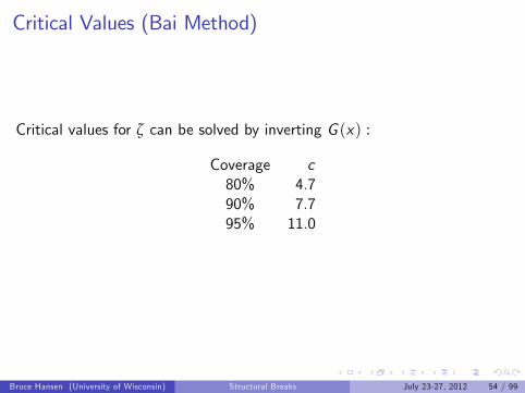
Critical Values (Bai Method)
Critical values for ζ can be solved by inverting G (x) :
Coverage c80% 4.790% 7.795% 11.0
Bruce Hansen (University of Wisconsin) Structural Breaks July 23-27, 2012 54 / 99

Confidence Intervals for Break Date (Bai Method)Point Estimate T1
Theorem: T1 ∼ T1 +δ′Ωδ(δ′Qδ
)2 ζ
Confidence interval is then
T1 ±δ′Ωδ(
δ′Q δ)2 c
where
δ = β2 − β1
Q =1n
n
∑t=1xtx′t
Ω =1
n− kn
∑t=1xtx′t e
2t +
1n− k
h−1∑j=0
T1−j∑t=1
(xtx′t+j et et+j + xt+jx
′t et+j et
)Bruce Hansen (University of Wisconsin) Structural Breaks July 23-27, 2012 55 / 99

Confidence Intervals under Homoskedasticity
T1 ±nσ2(
β2 − β1
)′(X ′X )
(β2 − β1
)c
Bruce Hansen (University of Wisconsin) Structural Breaks July 23-27, 2012 56 / 99

Example
Break for GDP ForecastI Point Estimate: 1980:4I Bai 90% Interval: 1979:2 - 1982:2
Break for GDP VarianceI Point Estimate: 1983:3I Bai 90% Interval: 1983:2 - 1983:4I Very tight
Bruce Hansen (University of Wisconsin) Structural Breaks July 23-27, 2012 57 / 99

Confidence Intervals (Elliott-Mueller)
Elliott-Mueller (JoE, 2007) argue that Bai’s confidence intervalssystematically undercover when breaks are small to moderate
They recommend an alternative simple procedure
For each breakdate T1 for which the regression can be estimatedI Calculate the regression
yt = β′0zt + β
′1xt1 (t ≤ T1) + β
′2xt1 (t > T1) + et
Bruce Hansen (University of Wisconsin) Structural Breaks July 23-27, 2012 58 / 99

yt = β′0zt + β
′1xt1 (t ≤ T1) + β
′2xt1 (t > T1) + et
Ω1 =1
T1 − k
(T1
∑t=1xtx′t e
2t +
h−1∑j=0
T1−j∑t=1
(xtx′t+j et et+j + xt+jx
′t et+j et
))
Ω2 =1
n− T1 − k
(n
∑t=T1+1
xtx′t e2t +
h−1∑j=0
n−j∑
t=T1+1
(xtx′t+j et et+j + xt+jx
′t et+j et
))
Sj =j
∑t=1xt et
U(T1) =1T 21
T1
∑j=1S ′j Ω
−11 Sj +
1
(n− T1)2n
∑j=T1+1
S ′j Ω−12 Sj
Bruce Hansen (University of Wisconsin) Structural Breaks July 23-27, 2012 59 / 99

Theorem (Elliott-Muller)
U(T1)→d∫ 10 B(s)
′B(s)ds where B(s) is a 2k × 1 Brownian bridge,k = dim(xt )This is the Cramer-vonMises distribution
To form a confidence set for T1, find the set of T1 for which U(T1)are less than the critical value
The Elliott-Muller intervals can be much larger than Bai’sI Unclear if they are perhaps too large
Bruce Hansen (University of Wisconsin) Structural Breaks July 23-27, 2012 60 / 99

Critical Values for Confidence Intervals(Elliott-MullerMethod)
Coverage
99% 97.5% 95% 92.5% 90% 80%k = 1 1.07 0.90 0.75 0.67 0.61 0.47k = 2 1.60 1.39 1.24 1.14 1.07 0.88k = 3 2.12 1.89 1.68 1.58 1.49 1.28k = 4 2.59 2.33 2.11 1.99 1.89 1.66k = 5 3.05 2.76 2.54 2.40 2.29 2.03k = 6 3.51 3.18 2.96 2.81 2.69 2.41k = 7 3.90 3.60 3.34 3.19 3.08 2.77k = 8 4.30 4.01 3.75 3.58 3.46 3.14k = 9 4.73 4.40 4.14 3.96 3.83 3.50k = 10 5.13 4.79 4.52 4.36 4.22 3.86
Bruce Hansen (University of Wisconsin) Structural Breaks July 23-27, 2012 61 / 99
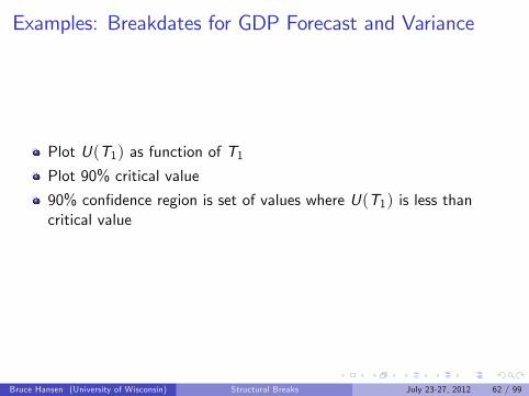
Examples: Breakdates for GDP Forecast and Variance
Plot U(T1) as function of T1Plot 90% critical value
90% confidence region is set of values where U(T1) is less thancritical value
Bruce Hansen (University of Wisconsin) Structural Breaks July 23-27, 2012 62 / 99

Bruce Hansen (University of Wisconsin) Structural Breaks July 23-27, 2012 63 / 99

Bruce Hansen (University of Wisconsin) Structural Breaks July 23-27, 2012 64 / 99

Example
Break for GDP ForecastI Point Estimate: 1980:4I Bai 90% Interval: 1979:2 - 1982:2I Elliott-Muller: 1981:2 - 2011:2
Break for GDP VarianceI Point Estimate: 1983:3I Bai 90% Interval: 1983:2 - 1983:4I Elliott-Muller: 1980:4 - 1993:4
Elliott-Muller intervals are much wider
Bruce Hansen (University of Wisconsin) Structural Breaks July 23-27, 2012 65 / 99

Slope Estimators
Estimate slopes from regression with estmate T1
yt = β′0zt + β
′1xt1 (t ≤ T1) + β
′2xt1 (t > T1) + et (T1)
In the case of full structural change, this is the same as estimation oneach sub-sample.
Asymptotic Theory:I The sub-sample slope estimates are consistent for the true slopesI If there is a structural break, their asymptotic distributions are“conventional”
F You can treat the structural break as if known
I Compute standard erros using conventional HAC formula
Bruce Hansen (University of Wisconsin) Structural Breaks July 23-27, 2012 66 / 99

Example: Variance Estimates
Pre 1983: σ21 = 14.8 (2.3)
Post 193: σ22 = 4.9 (1.0)
Bruce Hansen (University of Wisconsin) Structural Breaks July 23-27, 2012 67 / 99

Multiple Breaks
Bruce Hansen (University of Wisconsin) Structural Breaks July 23-27, 2012 68 / 99

Multiple Structural Breaks
Breaks T1 < T2
yt = β′0zt + β′1xt1 (t ≤ T1) + β′2xt1 (T1 < t ≤ T2)+β′3xt1 (t > T2) + et
Testing/estimation: Two approachesI Joint testing/estimationI Sequential
Major contributors: Jushan Bai, Pierre Perron
Bruce Hansen (University of Wisconsin) Structural Breaks July 23-27, 2012 69 / 99

Joint Methods
TestingI Test the null of constant parameters against the alternative of two(unknown) breaks
I Given T1,T2, construct Wald test for non-constancyI Take the largest test over T1 < T2I Asymptotic distribution a generalization of Andrews
EstimationI The sum-of-squared errors is a function of (T1,T2)I The LS estimates (T1, T2) jointly minimize the SSE
Bruce Hansen (University of Wisconsin) Structural Breaks July 23-27, 2012 70 / 99

Joint Methods - Computation
For 2 breaks, these tests/estimates require O(n2) regressionsI cumbersome but quite feasible
For 3 breaks, naive estimation requires O(n3) regressions,I not feasible
Bai-Perron developed effi cient computer code which solves theproblem of order O(n2) for arbitrary number of breaks
Bruce Hansen (University of Wisconsin) Structural Breaks July 23-27, 2012 71 / 99

Sequential Method
If the truth is two breaks, but you estimate a one-break model, theSSE will (asymptotically) have local minima at both breakdates
Thus the LS breakdate estimator will consistently estimate one of thetwo breaks, e.g. T1 for T1Given an estimated break, you can split the sample and test forbreaks in each subsample
I You can then find T2 for T2
Refinement estimator:I Split the entire sample at T2I Now re-estimate the first break T1I The refined estimators are asymptotically effi cient
Bruce Hansen (University of Wisconsin) Structural Breaks July 23-27, 2012 72 / 99

Forecasting Focuses on Final Breakdate
If you only want to find the last break
First test for structural change on the full sample
If it rejects, split the sample
Test for structural change on the second half
If it rejects, split again...
Bruce Hansen (University of Wisconsin) Structural Breaks July 23-27, 2012 73 / 99

Forecasting After Breaks
Bruce Hansen (University of Wisconsin) Structural Breaks July 23-27, 2012 74 / 99

Forecasting After Breaks
There is no good theory about how to forecast in the presence ofbreaks
There is a multitude of comflicting recommendations
One important contribution:I Pesaran and Timmermann (JoE, 2007)
They show that in a regression with a single break, the optimalwindow for estimation includes all of the observations after the break,and some of the observations before the breakBy including more observations you decrease variance at the cost ofsome bias
They provide empirical rules for selecting sample sizes
Bruce Hansen (University of Wisconsin) Structural Breaks July 23-27, 2012 75 / 99

Recommentation
The simulations in Persaran-Timmermann suggest that there littlegain for the complicated procedures
The simple rule —Split the sample at the estimated break — seems towork as well as anything else
My recommendationI Test for structural breaks using the Andrews or Bai/Perron testsI If there is evidence of a break, estimate its date using Bai’sleast-squares estimator
I Calculate a confidence interval to assess accuracy (calculate both Baiand Elliott-Muller for robustness)
I Split the sample at the break, use the post-break period for estimationI Use economic judgment to enhance statistical findings
Bruce Hansen (University of Wisconsin) Structural Breaks July 23-27, 2012 76 / 99
Examples Revisited
Bruce Hansen (University of Wisconsin) Structural Breaks July 23-27, 2012 77 / 99

Examples from Beginning of Class
Simple AR(1) with mean and variance breaks
yt = ρyt−1 + µt (1− ρ) + etet ∼ N(0, σ2t (1− ρ2))
µt and/or σ2t may be constant or may have a break at some point inthe sample
Sample size n
Questions: Can you guess the timing and type of structural break?
Bruce Hansen (University of Wisconsin) Structural Breaks July 23-27, 2012 78 / 99

Model A
Bruce Hansen (University of Wisconsin) Structural Breaks July 23-27, 2012 79 / 99

Bruce Hansen (University of Wisconsin) Structural Breaks July 23-27, 2012 80 / 99

Results - Regression
SupW = 0.01 (fixed regressor bootstrap p-value)
Breakdate Estimate = 62I Bai Interval = [55, 69]
Estimates
yt = 0.03(.60)
+ 0.69(.67)
yt−1 + et , t ≤ 62
yt = 0.69(.99)
+ 0.59(.53)
yt−1 + et , t > 62
Bruce Hansen (University of Wisconsin) Structural Breaks July 23-27, 2012 81 / 99
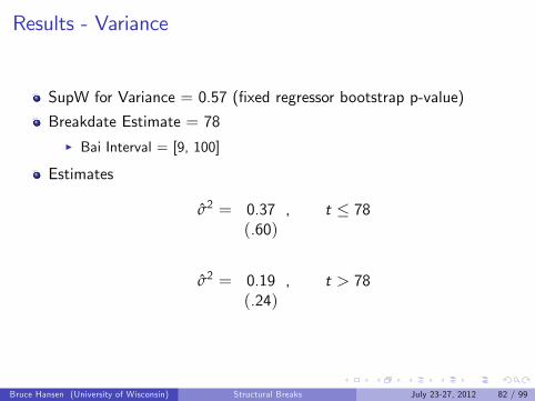
Results - Variance
SupW for Variance = 0.57 (fixed regressor bootstrap p-value)
Breakdate Estimate = 78I Bai Interval = [9, 100]
Estimates
σ2 = 0.37(.60)
, t ≤ 78
σ2 = 0.19(.24)
, t > 78
Bruce Hansen (University of Wisconsin) Structural Breaks July 23-27, 2012 82 / 99

Bruce Hansen (University of Wisconsin) Structural Breaks July 23-27, 2012 83 / 99

Bruce Hansen (University of Wisconsin) Structural Breaks July 23-27, 2012 84 / 99

DGP (Model A)
T1 = 60
µ1 = 0.2
µ2 = 0.4
σ21 = σ22 = 0.36
ρ = 0.8
Bruce Hansen (University of Wisconsin) Structural Breaks July 23-27, 2012 85 / 99

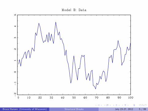
Model B
Bruce Hansen (University of Wisconsin) Structural Breaks July 23-27, 2012 86 / 99

Bruce Hansen (University of Wisconsin) Structural Breaks July 23-27, 2012 87 / 99

Results - Regression
SupW = 0.07 (fixed regressor bootstrap p-value)
Breakdate Estimate = 37I Bai Interval = [20, 54]
Estimates
yt = 0.53(1.12)
+ 0.82(.40)
yt−1 + et , t ≤ 37
yt = 0.10(.70)
+ 0.85(.40)
yt−1 + et , t > 37
Bruce Hansen (University of Wisconsin) Structural Breaks July 23-27, 2012 88 / 99

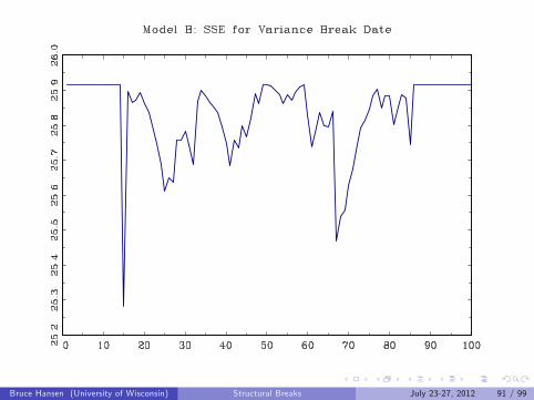
Results - Variance
SupW for Variance = 0.06 (fixed regressor bootstrap p-value)
Breakdate Estimate = 15I Bai Interval = [0, 69]
Estimates
σ2 = 0.17(.17)
, t ≤ 15
σ2 = 0.40(.55)
, t > 15
Bruce Hansen (University of Wisconsin) Structural Breaks July 23-27, 2012 89 / 99

Bruce Hansen (University of Wisconsin) Structural Breaks July 23-27, 2012 90 / 99
Bruce Hansen (University of Wisconsin) Structural Breaks July 23-27, 2012 91 / 99

DGP (Model B)
T1 = 40
µ1 = 0.5
µ2 = 0.2
σ21 = σ22 = 0.36
ρ = 0.8
Bruce Hansen (University of Wisconsin) Structural Breaks July 23-27, 2012 92 / 99
Model C
Bruce Hansen (University of Wisconsin) Structural Breaks July 23-27, 2012 93 / 99

Bruce Hansen (University of Wisconsin) Structural Breaks July 23-27, 2012 94 / 99

Results
SupW = 0.11 (fixed regressor bootstrap p-value)
Regression Breakdate Estimate = 84I Bai Interval = [78, 90]
Estimates
yt = 0.27(1.02)
+ 0.73(.70)
yt−1 + et , t ≤ 37
yt = 1.53(2.44)
+ −0.11(1.47)
yt−1 + et , t > 37
Bruce Hansen (University of Wisconsin) Structural Breaks July 23-27, 2012 95 / 99

Results - VarianceSupW for Variance = 0.13 (fixed regressor bootstrap p-value)Breakdate Estimate = 69
I Bai Interval = [65, 73]
Estimates
σ2 = 0.43(.51)
, t ≤ 69
σ2 = 1.77(3.06)
, t > 69
Bruce Hansen (University of Wisconsin) Structural Breaks July 23-27, 2012 96 / 99

Bruce Hansen (University of Wisconsin) Structural Breaks July 23-27, 2012 97 / 99

DGP (Model C)
T1 = 70
µ1 = µ2 = 0.2
σ21 = 0.36
σ22 = 1.44
ρ = 0.8
Bruce Hansen (University of Wisconsin) Structural Breaks July 23-27, 2012 98 / 99

Assignment
Take your favorite model
Estimate the model allowing for one-time structure change in themean
Test the model for one-time structural change in the mean
If appropriate, revise your forecasts
Bruce Hansen (University of Wisconsin) Structural Breaks July 23-27, 2012 99 / 99