advanced statistics using r - psychstat.org · 2019-05-29 · using r series advanced statistics...
TRANSCRIPT

Using R Series
Advanced StatisticsUsing R
Zhiyong ZhangLijuan Wang
ISDSA Press · Granger, IN

Zhiyong Zhang, Ph.D.Department of PsychologyUniversity of Notre DameNotre Dame, IN 46556, USA
Lijuan Wang, Ph.D.Department of PsychologyUniversity of Notre DameNotre Dame, IN 46556, USA
Copyright c© 2017 International Society for Data Science and Analytic
PUBLISHED BY ISDSA PRESS GRANGER, INWWW.ISDSA.ORG
ISBN (HTML): 978-1-946728-01-2ISBN (PDF): 978-1-946728-05-0
This work is subject to copyright. All rights are reserved by the ISDSA Press and the authors,whether the whole or part of the material is concerned, specifically the rights of translation,reprinting, reuse of illustrations, recitation, broadcasting, reproduction on microfilms or in anyother physical way, and transmission or information storage and retrieval, electronic adaptation,computer software, or by similar or dissimilar methodology now known or hereafter developed.Exempted from this legal reservation are brief excerpts in connection with reviews or scholarlyanalysis or material supplied specifically for the purpose of being entered and executed on acomputer system, for exclusive use by the purchaser of the work. Duplication of this publicationor parts thereof is permitted only under the provisions of the Copyright Law of the Publisher’slocation, in its current version, and permission for use must always be obtained from ISDSA Press.Violations are liable to prosecution under the respective Copyright Law.
Trademarked names, logos, and images may appear in this book. Rather than use a trademarksymbol with every occurrence of a trademarked name, logo, or image we use the names, logos, andimages only in an editorial fashion and to the benefit of the trademark owner, with no intention ofinfringement of the trademark. The use in this publication of trade names, trademarks, servicemarks, and similar terms, even if they are not identified as such, is not to be taken as an expressionof opinion as to whether or not they are subject to proprietary rights.
While the advice and information in this book are believed to be true and accurate at the date ofpublication, neither the authors nor the editors nor the publisher can accept any legal responsibilityfor any errors or omissions that may be made. The publisher makes no warranty, express orimplied, with respect to the material contained herein.
2017

Preface
The book was developed from the teaching materials used for the Advanced Statistics taughtby Drs. Zhiyong Zhang and Lijuan Wang at the University of Notre Dame started in Fall 2010.Advanced Statistics is a second course in statistics, which is intended to help students have abroader and deeper understanding of some widely used statistical methods in psychologicalresearch, beyond what has been covered in the Introduction to Statistics class taught atNotre Dame. Topics include a review of basic statistical concepts, an introduction to R,statistical inference, multiple regression, repeated measures ANOVA, mediation, moderation,factor analysis, logistic regression analysis, and longitudinal data analysis. The emphasis ison developing skills for implementing statistical methods for psychological research.
The book was initially offered as an online book on our webiste https://advstats.psychstat.org/supported by digital learning initiatives at the University of Notre Dame to provide affordabletextbooks for students. With more and more demending, we decided to publish it as anE-book as you are reading.
We would like to thank all the students who took the class and motivated the developmentof the book.
About the authors
Zhiyong Zhang
Dr. Zhiyong Zhang is an Associate Professor in quantitative psychology in the Departmentof Psychology at the University of Notre Dame. He is interested in developing and applyingstatistical methods and software in the areas of psychology, education and health research.He has taught Advanced Statistics from 2010 to 2013 and from 2016 to 2019 at the Universityof Notre Dame.
Lijuan Wang
Dr. Lijuan Wang is an Associate Professor in quantitative psychology in the Departmentof Psychology at the University of Notre Dame. Her research interests are in the areas oflongitudinal data analysis (e.g., methods and models for studying intra-individual change,
i

ii
variability, and relations, and inter-individual differences in them), multilevel modeling (e.g.,dyadic data analysis), structural equation modeling (e.g., mediation analysis), and studydesign issues (e.g., sample size determination). She has taught Advanced Statistics in 2014and 2015 at the University of Notre Dame.
Cite the book
To cite the book, please use the following:
Zhang, Z. & Wang, L. (2017). Advanced statistics using R. [https://advstats.psychstat.org].Granger, IN: ISDSA Press. ISBN: 978-1-946728-01-2.

Contents
Preface iAbout the authors . . . . . . . . . . . . . . . . . . . . . . . . . . . . . . . . . . . i
Zhiyong Zhang . . . . . . . . . . . . . . . . . . . . . . . . . . . . . . . . . . iLijuan Wang . . . . . . . . . . . . . . . . . . . . . . . . . . . . . . . . . . . . i
Cite the book . . . . . . . . . . . . . . . . . . . . . . . . . . . . . . . . . . . . . . ii
1 R Basics 11.1 Introduction to R . . . . . . . . . . . . . . . . . . . . . . . . . . . . . . . . . 1
1.1.1 What is R? . . . . . . . . . . . . . . . . . . . . . . . . . . . . . . . . 11.1.2 Why R? . . . . . . . . . . . . . . . . . . . . . . . . . . . . . . . . . . 11.1.3 How to install R? . . . . . . . . . . . . . . . . . . . . . . . . . . . . . 2
1.2 Basic operations in R . . . . . . . . . . . . . . . . . . . . . . . . . . . . . . . 31.3 Vector . . . . . . . . . . . . . . . . . . . . . . . . . . . . . . . . . . . . . . . 4
1.3.1 Create a vector . . . . . . . . . . . . . . . . . . . . . . . . . . . . . . 41.3.2 Operating a vector . . . . . . . . . . . . . . . . . . . . . . . . . . . . 5
1.4 Array and Matrix . . . . . . . . . . . . . . . . . . . . . . . . . . . . . . . . . 61.4.1 Create an array / matrix . . . . . . . . . . . . . . . . . . . . . . . . . 61.4.2 Operating an array or matrix . . . . . . . . . . . . . . . . . . . . . . 7
1.5 List . . . . . . . . . . . . . . . . . . . . . . . . . . . . . . . . . . . . . . . . . 81.5.1 Create a list . . . . . . . . . . . . . . . . . . . . . . . . . . . . . . . . 81.5.2 Access the object of a list . . . . . . . . . . . . . . . . . . . . . . . . 9
1.6 Data Frame . . . . . . . . . . . . . . . . . . . . . . . . . . . . . . . . . . . . 101.6.1 Create a data frame . . . . . . . . . . . . . . . . . . . . . . . . . . . 101.6.2 Access the components of a data frame . . . . . . . . . . . . . . . . . 10
2 Data in R 112.1 Reading Data from Files . . . . . . . . . . . . . . . . . . . . . . . . . . . . . 11
2.1.1 Read Data from a Free Format Text File . . . . . . . . . . . . . . . . 112.1.2 Access data . . . . . . . . . . . . . . . . . . . . . . . . . . . . . . . . 122.1.3 CSV (comma separated value) Data . . . . . . . . . . . . . . . . . . . 132.1.4 Read Data from a .csv File . . . . . . . . . . . . . . . . . . . . . . . . 142.1.5 Save other types of data to csv format . . . . . . . . . . . . . . . . . 14
2.2 Excel, SPSS, SAS, and Stata Data . . . . . . . . . . . . . . . . . . . . . . . 152.2.1 Excel data . . . . . . . . . . . . . . . . . . . . . . . . . . . . . . . . . 15
iii

iv CONTENTS
2.2.2 SPSS, SAS, and Stata data . . . . . . . . . . . . . . . . . . . . . . . 15
3 Statistical Graphs in R 173.1 Pie Chart . . . . . . . . . . . . . . . . . . . . . . . . . . . . . . . . . . . . . 173.2 Bar Graph . . . . . . . . . . . . . . . . . . . . . . . . . . . . . . . . . . . . . 19
3.2.1 A simple bar plot . . . . . . . . . . . . . . . . . . . . . . . . . . . . . 193.2.2 Clustered (side by side or stacked) bar plot . . . . . . . . . . . . . . . 203.2.3 Compare a Pie chart to a Bar graph . . . . . . . . . . . . . . . . . . 22
3.3 Boxplot . . . . . . . . . . . . . . . . . . . . . . . . . . . . . . . . . . . . . . 233.3.1 A simple boxplot . . . . . . . . . . . . . . . . . . . . . . . . . . . . . 243.3.2 Compare multiple groups . . . . . . . . . . . . . . . . . . . . . . . . . 25
3.4 Histogram . . . . . . . . . . . . . . . . . . . . . . . . . . . . . . . . . . . . . 273.4.1 Examples . . . . . . . . . . . . . . . . . . . . . . . . . . . . . . . . . 283.4.2 Probability density vs. frequency . . . . . . . . . . . . . . . . . . . . 303.4.3 Add an estimated density curve and a normal curve . . . . . . . . . . 31
3.5 Scatter plot . . . . . . . . . . . . . . . . . . . . . . . . . . . . . . . . . . . . 323.5.1 Examples . . . . . . . . . . . . . . . . . . . . . . . . . . . . . . . . . 353.5.2 Add regression line and a smoothing curve . . . . . . . . . . . . . . . 35
3.6 Line plot . . . . . . . . . . . . . . . . . . . . . . . . . . . . . . . . . . . . . . 363.6.1 A single line plot . . . . . . . . . . . . . . . . . . . . . . . . . . . . . 373.6.2 Compare the change trajectory of two participants . . . . . . . . . . 373.6.3 Plot more lines (use of for loop) . . . . . . . . . . . . . . . . . . . . . 38
4 Hypothesis testing 414.1 Null hypothesis testing . . . . . . . . . . . . . . . . . . . . . . . . . . . . . . 41
4.1.1 Step 1. State the research question . . . . . . . . . . . . . . . . . . . 414.1.2 Step 2. State the null and alternative hypotheses . . . . . . . . . . . 424.1.3 Step 3. Set the significance level α . . . . . . . . . . . . . . . . . . . 424.1.4 Step 4. Collect or locate data . . . . . . . . . . . . . . . . . . . . . . 424.1.5 Step 5. Calculate the test statistic and the p value . . . . . . . . . . . 434.1.6 Step 6. Make a decision . . . . . . . . . . . . . . . . . . . . . . . . . 454.1.7 Step 7. Answer the research question . . . . . . . . . . . . . . . . . . 454.1.8 Remarks on hypothesis testing . . . . . . . . . . . . . . . . . . . . . . 45
4.2 Effect size . . . . . . . . . . . . . . . . . . . . . . . . . . . . . . . . . . . . . 464.3 Criticisms of Null Hypothesis Testing and p-value . . . . . . . . . . . . . . . 47
4.3.1 The focus of null hypothesis . . . . . . . . . . . . . . . . . . . . . . . 474.3.2 The test is done given that the null is true . . . . . . . . . . . . . . . 484.3.3 The logic of NHST is flawed . . . . . . . . . . . . . . . . . . . . . . . 484.3.4 NHST tells nothing about the probability of neither null hypothesis
nor alternative hypothesis . . . . . . . . . . . . . . . . . . . . . . . . 484.3.5 NHST does not tell whether a result can be replicated . . . . 494.3.6 p-value, effect size and sample size . . . . . . . . . . . . . . . . . . . 494.3.7 The choice of significance level at 0.05 . . . . . . . . . . . . . . . . . 50
4.4 Bayes’ Theorem . . . . . . . . . . . . . . . . . . . . . . . . . . . . . . . . . . 504.4.1 An example . . . . . . . . . . . . . . . . . . . . . . . . . . . . . . . . 51
CONTENTS v
5 Confidence Interval 535.1 Formal definition . . . . . . . . . . . . . . . . . . . . . . . . . . . . . . . . . 53
5.1.1 Remarks . . . . . . . . . . . . . . . . . . . . . . . . . . . . . . . . . . 535.2 How to obtain a confidence interval . . . . . . . . . . . . . . . . . . . . . . . 54
5.2.1 An example . . . . . . . . . . . . . . . . . . . . . . . . . . . . . . . . 545.3 An experiment for CI interpretation . . . . . . . . . . . . . . . . . . . . . . . 565.4 Confidence interval and hypothesis testing . . . . . . . . . . . . . . . . . . . 585.5 Bootstrap . . . . . . . . . . . . . . . . . . . . . . . . . . . . . . . . . . . . . 59
5.5.1 Basic idea . . . . . . . . . . . . . . . . . . . . . . . . . . . . . . . . . 605.5.2 Bootstrap standard error and confidence intervals . . . . . . . . . . . 625.5.3 Example for correlation coefficient . . . . . . . . . . . . . . . . . . . . 62
6 t-test 656.1 One-sample t-test . . . . . . . . . . . . . . . . . . . . . . . . . . . . . . . . . 65
6.1.1 Test statistic . . . . . . . . . . . . . . . . . . . . . . . . . . . . . . . 666.1.2 Effect size . . . . . . . . . . . . . . . . . . . . . . . . . . . . . . . . . 68
6.2 t-test for paired samples . . . . . . . . . . . . . . . . . . . . . . . . . . . . . 696.3 Independent two-sample t-test . . . . . . . . . . . . . . . . . . . . . . . . . . 70
6.3.1 Welch’s t test (unpooled two independent sample t test) . . . . . . . 706.3.2 Pooled two independent sample t test . . . . . . . . . . . . . . . . . . 716.3.3 Effect size . . . . . . . . . . . . . . . . . . . . . . . . . . . . . . . . . 72
7 Analysis of variance 757.1 One-way ANOVA . . . . . . . . . . . . . . . . . . . . . . . . . . . . . . . . . 75
7.1.1 Post-hoc multiple comparison . . . . . . . . . . . . . . . . . . . . . . 777.1.2 Barplot with standard error or confidence interval . . . . . . . . . . . 78
7.2 Two-way ANOVA . . . . . . . . . . . . . . . . . . . . . . . . . . . . . . . . . 817.2.1 Type of effects and hypotheses . . . . . . . . . . . . . . . . . . . . . . 817.2.2 Two-way ANOVA F tests . . . . . . . . . . . . . . . . . . . . . . . . 817.2.3 Example: Effects of training and gender on the memory test performance 837.2.4 Plot data . . . . . . . . . . . . . . . . . . . . . . . . . . . . . . . . . 84
7.3 Repeated-measures ANOVA . . . . . . . . . . . . . . . . . . . . . . . . . . . 857.3.1 An example . . . . . . . . . . . . . . . . . . . . . . . . . . . . . . . . 857.3.2 Long format of data . . . . . . . . . . . . . . . . . . . . . . . . . . . 867.3.3 One within-subject factor . . . . . . . . . . . . . . . . . . . . . . . . 877.3.4 One within-subject factor and one between-subject factor . . . . . . . 87
8 Simple Linear Regression 898.1 Simple regression model . . . . . . . . . . . . . . . . . . . . . . . . . . . . . 908.2 Parameter estimation . . . . . . . . . . . . . . . . . . . . . . . . . . . . . . . 91
8.2.1 Least squares estimation . . . . . . . . . . . . . . . . . . . . . . . . . 918.2.2 Hypothesis testing . . . . . . . . . . . . . . . . . . . . . . . . . . . . 928.2.3 Regression in R . . . . . . . . . . . . . . . . . . . . . . . . . . . . . . 92
8.3 An example . . . . . . . . . . . . . . . . . . . . . . . . . . . . . . . . . . . . 928.4 Coefficient of Determination (Multiple R-squared) . . . . . . . . . . . . . . . 94
vi CONTENTS
8.4.1 Calculation and interpretation of R2 . . . . . . . . . . . . . . . . . . 94
9 Multiple Linear Regression 979.1 Multiple Regression Analysis . . . . . . . . . . . . . . . . . . . . . . . . . . . 97
9.1.1 Multiple regression model . . . . . . . . . . . . . . . . . . . . . . . . 979.1.2 Parameter estimation . . . . . . . . . . . . . . . . . . . . . . . . . . . 989.1.3 R2 . . . . . . . . . . . . . . . . . . . . . . . . . . . . . . . . . . . . . 989.1.4 Hypothesis testing of regression coefficient(s) . . . . . . . . . . . . . . 999.1.5 An example . . . . . . . . . . . . . . . . . . . . . . . . . . . . . . . . 101
9.2 Centering and Standardization . . . . . . . . . . . . . . . . . . . . . . . . . . 1069.2.1 Centering . . . . . . . . . . . . . . . . . . . . . . . . . . . . . . . . . 1079.2.2 Standardization . . . . . . . . . . . . . . . . . . . . . . . . . . . . . . 108
9.3 Relative Importance of Predictors . . . . . . . . . . . . . . . . . . . . . . . . 1099.3.1 Basic idea of lmg . . . . . . . . . . . . . . . . . . . . . . . . . . . . . 1109.3.2 R package relaimpo . . . . . . . . . . . . . . . . . . . . . . . . . . . . 1109.3.3 An example . . . . . . . . . . . . . . . . . . . . . . . . . . . . . . . . 1109.3.4 Bootstrap relative importance . . . . . . . . . . . . . . . . . . . . . . 112
9.4 Variable Selection . . . . . . . . . . . . . . . . . . . . . . . . . . . . . . . . . 1149.4.1 Statistics/criteria for variable selection . . . . . . . . . . . . . . . . . 1159.4.2 An example . . . . . . . . . . . . . . . . . . . . . . . . . . . . . . . . 1169.4.3 All possible (best) subsets . . . . . . . . . . . . . . . . . . . . . . . . 1179.4.4 Backward elimination . . . . . . . . . . . . . . . . . . . . . . . . . . . 1209.4.5 Forward selection . . . . . . . . . . . . . . . . . . . . . . . . . . . . . 1219.4.6 Stepwise regression . . . . . . . . . . . . . . . . . . . . . . . . . . . . 1239.4.7 Remarks . . . . . . . . . . . . . . . . . . . . . . . . . . . . . . . . . . 125
9.5 Regression with Categorical Predictors . . . . . . . . . . . . . . . . . . . . . 1269.5.1 An example . . . . . . . . . . . . . . . . . . . . . . . . . . . . . . . . 1279.5.2 A naive analysis . . . . . . . . . . . . . . . . . . . . . . . . . . . . . . 1279.5.3 Regression with categorical predictors . . . . . . . . . . . . . . . . . . 1289.5.4 lm() for data analysis . . . . . . . . . . . . . . . . . . . . . . . . . . . 129
10 Logistic Regression 13910.1 An example . . . . . . . . . . . . . . . . . . . . . . . . . . . . . . . . . . . . 13910.2 Basic ideas . . . . . . . . . . . . . . . . . . . . . . . . . . . . . . . . . . . . . 140
10.2.1 Why is this? . . . . . . . . . . . . . . . . . . . . . . . . . . . . . . . . 14110.3 Fitting a logistic regression model in R . . . . . . . . . . . . . . . . . . . . . 14110.4 Interpret the results . . . . . . . . . . . . . . . . . . . . . . . . . . . . . . . . 14210.5 Statistical inference for logistic regression . . . . . . . . . . . . . . . . . . . . 144
10.5.1 Test a single coefficient (z-test and confidence interval) . . . . . . . . 14410.5.2 Test the overall model . . . . . . . . . . . . . . . . . . . . . . . . . . 14510.5.3 Test a subset of predictors . . . . . . . . . . . . . . . . . . . . . . . . 146
11 Moderation Analysis 14711.1 What is a moderator? . . . . . . . . . . . . . . . . . . . . . . . . . . . . . . 14711.2 How to conduct moderation analysis? . . . . . . . . . . . . . . . . . . . . . . 148
CONTENTS vii
11.2.1 Steps for moderation analysis . . . . . . . . . . . . . . . . . . . . . . 14911.2.2 An example . . . . . . . . . . . . . . . . . . . . . . . . . . . . . . . . 14911.2.3 Another example - continuous moderator . . . . . . . . . . . . . . . . 151
12 Mediation Analysis 15512.1 Path diagrams . . . . . . . . . . . . . . . . . . . . . . . . . . . . . . . . . . . 155
12.1.1 Rules to draw a path diagram . . . . . . . . . . . . . . . . . . . . . . 15512.1.2 How to draw path diagrams? . . . . . . . . . . . . . . . . . . . . . . 156
12.2 What is mediation or what is a mediator? . . . . . . . . . . . . . . . . . . . 15612.3 Mediation effects . . . . . . . . . . . . . . . . . . . . . . . . . . . . . . . . . 15712.4 Testing mediation effects . . . . . . . . . . . . . . . . . . . . . . . . . . . . . 157
12.4.1 An example . . . . . . . . . . . . . . . . . . . . . . . . . . . . . . . . 15712.4.2 Baron and Kenny (1986) method . . . . . . . . . . . . . . . . . . . . 15812.4.3 Sobel test . . . . . . . . . . . . . . . . . . . . . . . . . . . . . . . . . 16112.4.4 Bootstrapping for mediation analysis . . . . . . . . . . . . . . . . . . 162
13 Path Analysis 16513.1 Path diagrams . . . . . . . . . . . . . . . . . . . . . . . . . . . . . . . . . . . 16513.2 Example 1. Mediation analysis – Test the direct and indirect effects . . . . . 16713.3 Example 2. Testing a theory of no direct effect . . . . . . . . . . . . . . . . . 16913.4 Example 3: A more complex path model . . . . . . . . . . . . . . . . . . . . 171
14 Factor Analysis 17514.1 Measurement Error and Factor Analysis . . . . . . . . . . . . . . . . . . . . 175
14.1.1 Measurement error . . . . . . . . . . . . . . . . . . . . . . . . . . . . 17514.1.2 Influences of measurement error . . . . . . . . . . . . . . . . . . . . . 17614.1.3 How to deal with measurement error? . . . . . . . . . . . . . . . . . . 17714.1.4 Factor analysis . . . . . . . . . . . . . . . . . . . . . . . . . . . . . . 177
14.2 Exploratory Factor Analysis . . . . . . . . . . . . . . . . . . . . . . . . . . . 17814.2.1 An example . . . . . . . . . . . . . . . . . . . . . . . . . . . . . . . . 17914.2.2 Exploratory factor analysis . . . . . . . . . . . . . . . . . . . . . . . . 181
14.3 Confirmatory Factor Analysis . . . . . . . . . . . . . . . . . . . . . . . . . . 18914.3.1 An example . . . . . . . . . . . . . . . . . . . . . . . . . . . . . . . . 18914.3.2 Confirmatory factor analysis . . . . . . . . . . . . . . . . . . . . . . . 189
15 Structural Equation Models 19915.1 Example 1. Autoregressive model . . . . . . . . . . . . . . . . . . . . . . . . 20115.2 Example 2. Mediation analysis with latent variables . . . . . . . . . . . . . . 204
16 Multilevel Regression 20916.1 Multilevel data . . . . . . . . . . . . . . . . . . . . . . . . . . . . . . . . . . 209
16.1.1 Lee and Bryk school achievement data . . . . . . . . . . . . . . . . . 20916.2 Source of variances . . . . . . . . . . . . . . . . . . . . . . . . . . . . . . . . 210
16.2.1 Use of R package lme4 . . . . . . . . . . . . . . . . . . . . . . . . . . 21116.2.2 Intraclass correlation coefficient (ICC) . . . . . . . . . . . . . . . . . 213

viii CONTENTS
16.2.3 Explain/model the difference . . . . . . . . . . . . . . . . . . . . . . . 21316.3 Multilevel regression . . . . . . . . . . . . . . . . . . . . . . . . . . . . . . . 215
17 Longitudinal Data Analysis 22117.1 Growth curve model . . . . . . . . . . . . . . . . . . . . . . . . . . . . . . . 22217.2 GCM as a mulitlevel/mixed-effect model . . . . . . . . . . . . . . . . . . . . 223
17.2.1 Unconditional model (model without second level predictors) . . . . . 22417.2.2 Conditional model (model with second level predictors) . . . . . . . . 228
17.3 GCM as a SEM . . . . . . . . . . . . . . . . . . . . . . . . . . . . . . . . . . 228
18 Statistical Power Analysis 23518.1 What is statistical power? . . . . . . . . . . . . . . . . . . . . . . . . . . . . 235
18.1.1 Factors influencing statistical power . . . . . . . . . . . . . . . . . . . 23618.1.2 Calculate power and sample size . . . . . . . . . . . . . . . . . . . . . 237
18.2 Practical power analysis using R . . . . . . . . . . . . . . . . . . . . . . . . . 23918.2.1 Correlation coefficient . . . . . . . . . . . . . . . . . . . . . . . . . . 23918.2.2 Two-sample mean (t-test) . . . . . . . . . . . . . . . . . . . . . . . . 24118.2.3 One-Way ANOVA . . . . . . . . . . . . . . . . . . . . . . . . . . . . 24318.2.4 Linear regression . . . . . . . . . . . . . . . . . . . . . . . . . . . . . 244
References 245
Chapter 1
R Basics
1.1 Introduction to R
1.1.1 What is R?
R is a statistical language and software for data analysis and graphing. It is an open-sourceimplementation of the S language which was developed at Bell Laboratories (formerly AT&T,now Lucent Technologies) by John Chambers and colleagues. Therefore, much code writtenfor S runs directly under R.
R is built through packages, including the base package and thousands of extended packagesor extensions.The base package contains the basic functions which let R function as a language:arithmetic, input/output, basic programming support, etc. It also allows the creation ofextension packages based on it. With the base package and the extensions, many statisticaldata analysis can be conducted and high quality statistical graphs can be produced.
R is available as Free Software under the terms of the Free Software Foundation’s GNUGeneral Public License in source code form. It compiles and runs on a wide variety of UNIXplatforms and similar systems (including FreeBSD and Linux), Windows and Mac OS.
1.1.2 Why R?
R is now widely used by both statisticians and applied researchers for good reasons.
• R is free and open-source and can be used on Windows, Mac OS, Linux and even online.• R is an integrated environment suitable for data manipulation, data analysis and
graphical display.• R is designed around a true computer language, and it allows users to write their own
functions and packages for even the newestly developed statistical methods.• R is supported by thousands of users around the world. Try out this link: https:
//www.r-project.org/help.html.
1

2 CHAPTER 1. R BASICS
1.1.3 How to install R?
• R can be installed on different operating systems.
• For Windows PC
1. Download the latest version of R from this url: https://cran.r-project.org/bin/windows/base/
2. Double click the downloaded file for a Windows style installer. Select defaultoptions to proceed the installation.
• For Mac
1. Download R from this url: https://cran.r-project.org/bin/macosx/2. Double click the downloaded file for installation.3. For Mac OS X 10.4 or earlier, please use this link http://cran.stat.ucla.edu/bin/
macosx/old/R-2.9.2.dmg
• For Linux: See the instruction for Ubuntu, Redhat, SUSE and Debian at https://cran.r-project.org/bin/linux/
• Rstudio (the desktop version) is a free and open source integrated development environ-ment (IDE) you may find useful. ### Start R R is most easily used in an interactivemanner. You ask R a question and it gives you an answer. Questions are asked andanswered on the command line. To start R, the following procedure can be used.
• On an operating system with Windows interface such as Windows and Mac OS X,
double click the R icon will open the R console. For example, the console onWindows looks like

1.2. BASIC OPERATIONS IN R 3
• On machines without Windows interface such as Ubuntu server, one can start R bytyping R and return in the terminal.
1.2 Basic operations in R
R can be first used as an advanced calculator. The code below shows the use of addition (+),subtraction (-), multiplication (*), division (/), logarithm (ln), exponential (exp).2+3## [1] 54-1## [1] 32*3## [1] 6(2+3)/4## [1] 1.25log(10)## [1] 2.302585exp(2)## [1] 7.3890565^3## [1] 125

4 CHAPTER 1. R BASICS
Each value used in R can be given a name and the value can be referred using its name. Forexample, if we let a = 2, then a can be used anywhere to replace the value 2. Some examplecode is given below.a = 2b <- 34 -> d
a*b## [1] 6(a+b)/d## [1] 1.25d^2## [1] 16
1.3 Vector
R is called a “vector language” because it can work on vectors directly. Vector is the mostbasic data structure in R. A vector is a collection of elements of the same data type. Thedata types can be logical, integer, double, character, complex or raw.
1.3.1 Create a vector
A vector can be created using the c() function, which combines its arguments or input toform a vector. Several examples are given below. As for the simple operations, names can beused for vectors. By typing its name, the content of a vector will be printed.outcome <- c(1, 0, 0, 1, 0, 1)gender <- c('F', 'F', 'M', 'F', 'M')income <- c(100, 500, 900, 400, 700, 650, 320)
outcome## [1] 1 0 0 1 0 1gender## [1] "F" "F" "M" "F" "M"income## [1] 100 500 900 400 700 650 320
1.3. VECTOR 5
1.3.2 Operating a vector
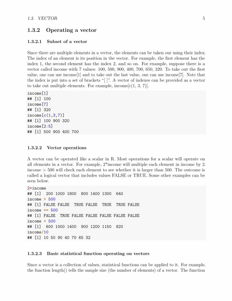
1.3.2.1 Subset of a vector
Since there are multiple elements in a vector, the elements can be taken our using their index.The index of an element is its position in the vector. For example, the first element has theindex 1, the second element has the index 2, and so on. For example, suppose there is avector called income with 7 values: 100, 500, 900, 400, 700, 650, 320. To take out the firstvalue, one can use income[1] and to take out the last value, one can use income[7]. Note thatthe index is put into a set of brackets “[ ]”. A vector of indexes can be provided as a vectorto take out multiple elements. For example, income[c(1, 3, 7)].income[1]## [1] 100income[7]## [1] 320income[c(1,3,7)]## [1] 100 900 320income[2:5]## [1] 500 900 400 700
1.3.2.2 Vector operations
A vector can be operated like a scalar in R. Most operations for a scalar will operate onall elements in a vector. For example, 2*income will multiple each element in income by 2.income > 500 will check each element to see whether it is larger than 500. The outcome iscalled a logical vector that includes values FALSE or TRUE. Some other examples can beseen below.2*income## [1] 200 1000 1800 800 1400 1300 640income > 500## [1] FALSE FALSE TRUE FALSE TRUE TRUE FALSEincome == 500## [1] FALSE TRUE FALSE FALSE FALSE FALSE FALSEincome + 500## [1] 600 1000 1400 900 1200 1150 820income/10## [1] 10 50 90 40 70 65 32
1.3.2.3 Basic statistical function operating on vectors
Since a vector is a collection of values, statistical functions can be applied to it. For example,the function length() tells the sample size (the number of elements) of a vector. The function

6 CHAPTER 1. R BASICS
sum() adds all the values in the vector together. Other functions include min(), max(),median(), sd(), var(), and many others.length(income)## [1] 7summary(income)## Min. 1st Qu. Median Mean 3rd Qu. Max.## 100 360 500 510 675 900min(income)## [1] 100max(income)## [1] 900median(income)## [1] 500sd(income)## [1] 265.8947var(income)## [1] 70700
1.4 Array and Matrix
R saves a table of data in an array or a matrix. We usually deal with two-dimensional matrixbut higher-dimensional matrix can also be used in R.
1.4.1 Create an array / matrix
Two functions can be used to create a matrix, array() or matrix(). We show how to create a3 by 4 matrix.
The code below creates a matrix using the function array(). Note that 1:12 generates asequence of values, 1, 2, . . . , 12. The sequence of valus are used to create the matrix.dim=c(3,4) tells there are 3 rows and 4 columns in the matrix. The function takes the 12values and fills each column sequentially. For example, it first fills in the first column using 1,2, and 3. Then it fills the second column using 4, 5, and 6.
To change the positions of the values in the matrix, one has to change the input values. Seethe difference in the creation of matrix y.x <- array(1:12, dim=c(3,4))x## [,1] [,2] [,3] [,4]## [1,] 1 4 7 10## [2,] 2 5 8 11## [3,] 3 6 9 12

1.4. ARRAY AND MATRIX 7
y <- array(c(1,5,9,2,6,10,3,7,11,4,8,12), dim=c(3,4))y## [,1] [,2] [,3] [,4]## [1,] 1 2 3 4## [2,] 5 6 7 8## [3,] 9 10 11 12
The function matrix() can control how to fill the values in a matrix. For example, settingbyrow=TRUE, the values will be filled by rows instead of by columns. Note that to use thefunction, one needs to tell either the number of rows using nrow or the number of columnsusing ncol.x <- matrix(1:12, nrow=3)x## [,1] [,2] [,3] [,4]## [1,] 1 4 7 10## [2,] 2 5 8 11## [3,] 3 6 9 12
y <- matrix(1:12, nrow=3, byrow=TRUE)y## [,1] [,2] [,3] [,4]## [1,] 1 2 3 4## [2,] 5 6 7 8## [3,] 9 10 11 12
1.4.2 Operating an array or matrix
We are often interested in taking out a subset of values in a matrix. x[i,j] takes out valuesaccording to the index i for the rows and j for the columns. Both i and j can be a single valueor a vector. When i is replaced by blank, the whole column(s) is taken out and when j isreplaced by blank, the whole row(s) is taken out. Some examples are given below.
Note that when a vector of values are taken out, by default, the sub-matrix will be convertedto a vector and lose the matrix property. To keep the matrix property, add the optiondrop=FALSE.x <- array(1:12, dim=c(3,4))x## [,1] [,2] [,3] [,4]## [1,] 1 4 7 10## [2,] 2 5 8 11## [3,] 3 6 9 12
8 CHAPTER 1. R BASICS
x[2,3]## [1] 8x[1:2, 1:2]## [,1] [,2]## [1,] 1 4## [2,] 2 5x[2, ]## [1] 2 5 8 11x[2, , drop=FALSE]## [,1] [,2] [,3] [,4]## [1,] 2 5 8 11
x[, 3]## [1] 7 8 9x[, 3, drop=FALSE]## [,1]## [1,] 7## [2,] 8## [3,] 9
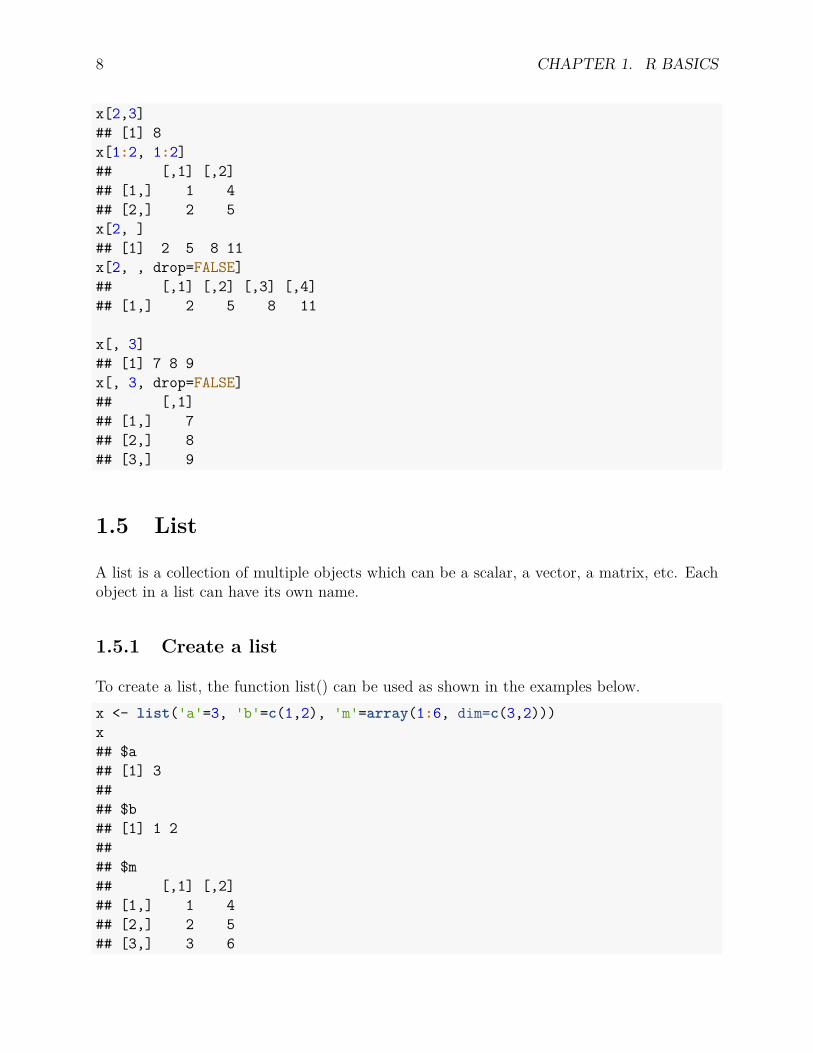
1.5 List
A list is a collection of multiple objects which can be a scalar, a vector, a matrix, etc. Eachobject in a list can have its own name.
1.5.1 Create a list
To create a list, the function list() can be used as shown in the examples below.x <- list('a'=3, 'b'=c(1,2), 'm'=array(1:6, dim=c(3,2)))x## $a## [1] 3#### $b## [1] 1 2#### $m## [,1] [,2]## [1,] 1 4## [2,] 2 5## [3,] 3 6
1.5. LIST 9
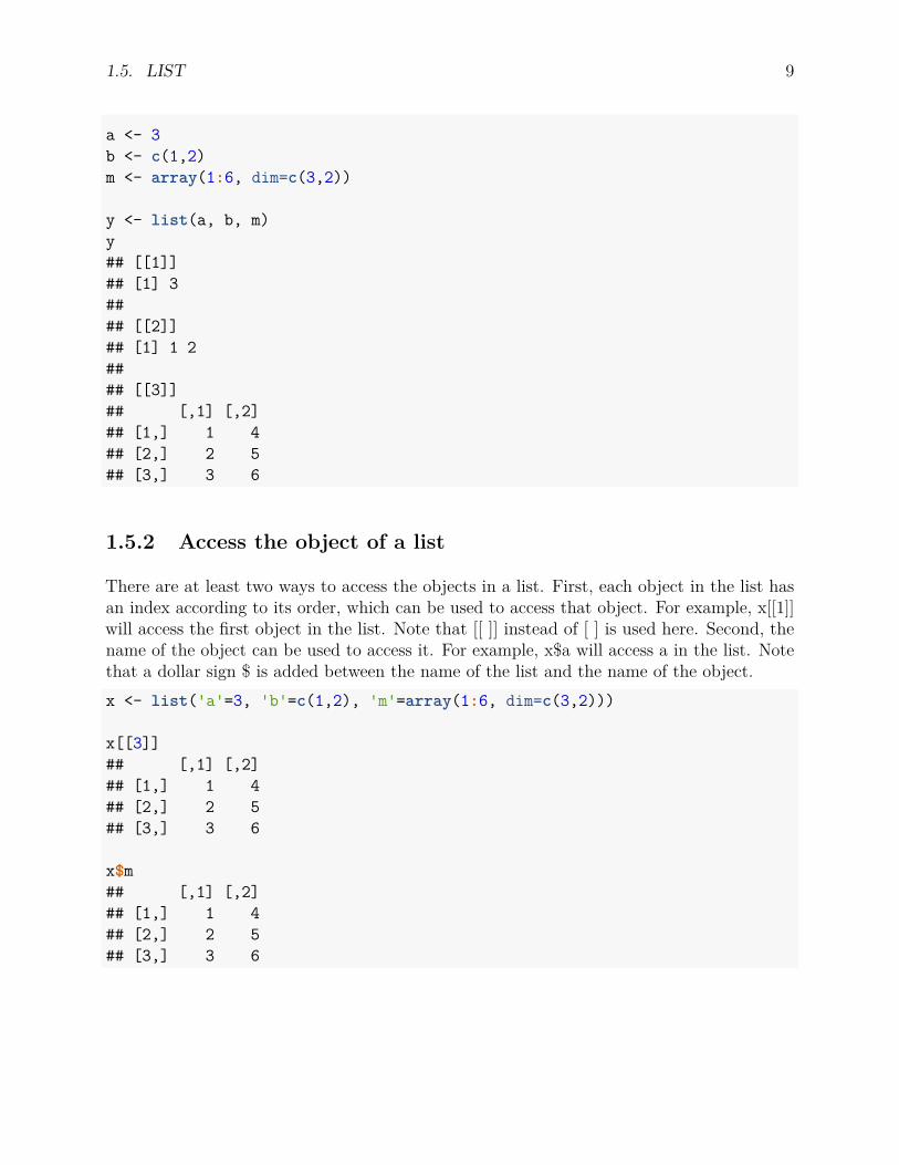
a <- 3b <- c(1,2)m <- array(1:6, dim=c(3,2))
y <- list(a, b, m)y## [[1]]## [1] 3#### [[2]]## [1] 1 2#### [[3]]## [,1] [,2]## [1,] 1 4## [2,] 2 5## [3,] 3 6
1.5.2 Access the object of a list
There are at least two ways to access the objects in a list. First, each object in the list hasan index according to its order, which can be used to access that object. For example, x[[1]]will access the first object in the list. Note that [[ ]] instead of [ ] is used here. Second, thename of the object can be used to access it. For example, x$a will access a in the list. Notethat a dollar sign $ is added between the name of the list and the name of the object.x <- list('a'=3, 'b'=c(1,2), 'm'=array(1:6, dim=c(3,2)))
x[[3]]## [,1] [,2]## [1,] 1 4## [2,] 2 5## [3,] 3 6
x$m## [,1] [,2]## [1,] 1 4## [2,] 2 5## [3,] 3 6

10 CHAPTER 1. R BASICS
1.6 Data Frame
A data frame is a special list in which every object has the same size.
1.6.1 Create a data frame
To create a data frame, the function data.frame() can be used as shown in the examplesbelow. The data read from a file into R are often saved into a data frame.a <- 1:3b <- 4:6d <- 7:9y <- data.frame(a,b,d)y## a b d## 1 1 4 7## 2 2 5 8## 3 3 6 9
1.6.2 Access the components of a data frame
The same methods for access the objects in a list can be used for a data frame. For example,y$a will access a in the data frame. The R function attach() can conveniently copy all objectsin a data frame into R workspace so that they can be accessed using their names directly. Toremove those objects, the function detach() can be used. Some examples are given below.y <- data.frame(a=1:4,b=5:8,d=9:12)y## a b d## 1 1 5 9## 2 2 6 10## 3 3 7 11## 4 4 8 12
y$a## [1] 1 2 3 4
attach(y)b## [1] 4 5 6
detach(y)

Chapter 2
Data in R
2.1 Reading Data from Files
In practical data analysis, data are often stored in a data file. R can read different types ofdata files such as the free format text files, comma separated value files, Excel files, SPSSfiles, SAS files, and Stata files.
2.1.1 Read Data from a Free Format Text File
The most common way to get data into R is to save data as free format in a text file andthen use read.table() function to read the data. For example, let’s read the data in a filecalled gpa.txt which is available on the website. The content of the data file is shown below.
## GPA data## 999 represents missing dataid gender college gpa weight1 f yes 3.6 1102 m yes 3.5 1703 m no 99.0 1654 m no 999.0 1905 f no 999.0 956 m yes 3.7 2007 m yes 3.6 1508 f yes 3.8 1009 f yes 3.0 130
10 f no 999.0 120
Note that the first two lines of the data file start with “#”, which are clearly notes orcomments about the data. The third line appears to be variable names. After that, there are10 lines of data.
11
12 CHAPTER 2. DATA IN R
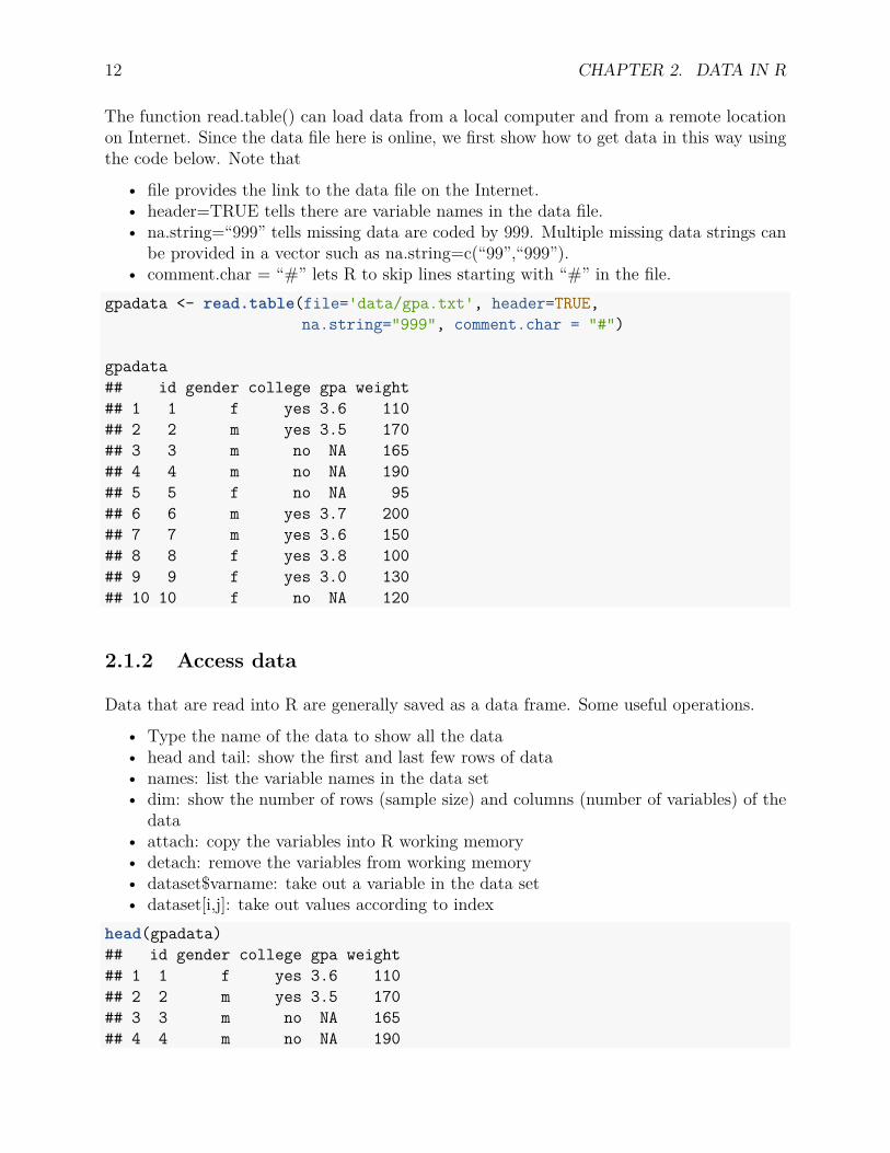
The function read.table() can load data from a local computer and from a remote locationon Internet. Since the data file here is online, we first show how to get data in this way usingthe code below. Note that
• file provides the link to the data file on the Internet.• header=TRUE tells there are variable names in the data file.• na.string=“999” tells missing data are coded by 999. Multiple missing data strings can
be provided in a vector such as na.string=c(“99”,“999”).• comment.char = “#” lets R to skip lines starting with “#” in the file.
gpadata <- read.table(file='data/gpa.txt', header=TRUE,na.string="999", comment.char = "#")
gpadata## id gender college gpa weight## 1 1 f yes 3.6 110## 2 2 m yes 3.5 170## 3 3 m no NA 165## 4 4 m no NA 190## 5 5 f no NA 95## 6 6 m yes 3.7 200## 7 7 m yes 3.6 150## 8 8 f yes 3.8 100## 9 9 f yes 3.0 130## 10 10 f no NA 120
2.1.2 Access data
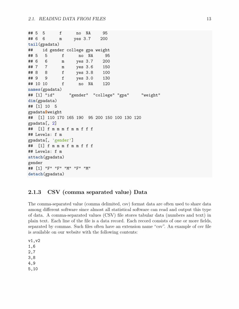
Data that are read into R are generally saved as a data frame. Some useful operations.
• Type the name of the data to show all the data• head and tail: show the first and last few rows of data• names: list the variable names in the data set• dim: show the number of rows (sample size) and columns (number of variables) of the
data• attach: copy the variables into R working memory• detach: remove the variables from working memory• dataset$varname: take out a variable in the data set• dataset[i,j]: take out values according to index
head(gpadata)## id gender college gpa weight## 1 1 f yes 3.6 110## 2 2 m yes 3.5 170## 3 3 m no NA 165## 4 4 m no NA 190
2.1. READING DATA FROM FILES 13
## 5 5 f no NA 95## 6 6 m yes 3.7 200tail(gpadata)## id gender college gpa weight## 5 5 f no NA 95## 6 6 m yes 3.7 200## 7 7 m yes 3.6 150## 8 8 f yes 3.8 100## 9 9 f yes 3.0 130## 10 10 f no NA 120names(gpadata)## [1] "id" "gender" "college" "gpa" "weight"dim(gpadata)## [1] 10 5gpadata$weight## [1] 110 170 165 190 95 200 150 100 130 120gpadata[, 2]## [1] f m m m f m m f f f## Levels: f mgpadata[, 'gender']## [1] f m m m f m m f f f## Levels: f mattach(gpadata)gender## [1] "F" "F" "M" "F" "M"detach(gpadata)
2.1.3 CSV (comma separated value) Data
The comma-separated value (comma delimited, csv) format data are often used to share dataamong different software since almost all statistical software can read and output this typeof data. A comma-separated values (CSV) file stores tabular data (numbers and text) inplain text. Each line of the file is a data record. Each record consists of one or more fields,separated by commas. Such files often have an extension name “csv”. An example of csv fileis available on our website with the following contents:
v1,v21,62,73,84,95,10
14 CHAPTER 2. DATA IN R
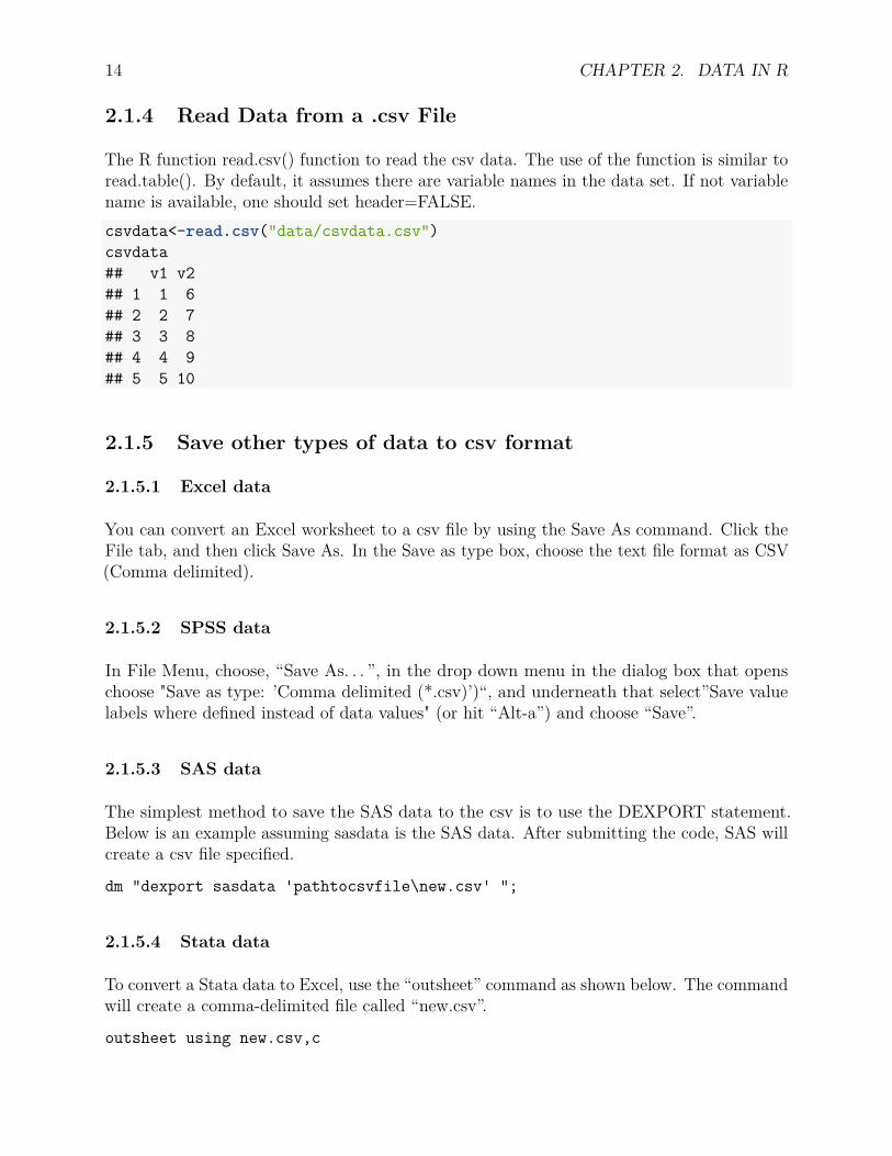
2.1.4 Read Data from a .csv File
The R function read.csv() function to read the csv data. The use of the function is similar toread.table(). By default, it assumes there are variable names in the data set. If not variablename is available, one should set header=FALSE.csvdata<-read.csv("data/csvdata.csv")csvdata## v1 v2## 1 1 6## 2 2 7## 3 3 8## 4 4 9## 5 5 10
2.1.5 Save other types of data to csv format
2.1.5.1 Excel data
You can convert an Excel worksheet to a csv file by using the Save As command. Click theFile tab, and then click Save As. In the Save as type box, choose the text file format as CSV(Comma delimited).
2.1.5.2 SPSS data
In File Menu, choose, “Save As. . . ”, in the drop down menu in the dialog box that openschoose "Save as type: ’Comma delimited (*.csv)’)“, and underneath that select”Save valuelabels where defined instead of data values" (or hit “Alt-a”) and choose “Save”.
2.1.5.3 SAS data
The simplest method to save the SAS data to the csv is to use the DEXPORT statement.Below is an example assuming sasdata is the SAS data. After submitting the code, SAS willcreate a csv file specified.
dm "dexport sasdata 'pathtocsvfile\new.csv' ";
2.1.5.4 Stata data
To convert a Stata data to Excel, use the “outsheet” command as shown below. The commandwill create a comma-delimited file called “new.csv”.
outsheet using new.csv,c

2.2. EXCEL, SPSS, SAS, AND STATA DATA 15
2.2 Excel, SPSS, SAS, and Stata Data
Although there are packages and functions to read Excel, SPSS, SAS, and Stata data into R,the best way to use such kinds of data is to first convert them to csv data and then use theread.csv() function to read the csv data.
2.2.1 Excel data
Several R packages are available to read Excel data. Here we will use XLConnect. Thepackage has to be installed first if not done yet. To install a package, use the functioninstall.packages(). To load the package, use the function library(). An example is shownbelow. The sheet argument specifies which sheet you exactly want to import into R. Notethat the function does not support reading remote data files. Therefore, an error is resulted.library('XLConnect')exceldata <- readWorksheetFromFile("data/csvdata.xlsx", sheet=1)exceldata## v1 v2## 1 1 6## 2 2 7## 3 3 8## 4 4 9## 5 5 10
2.2.2 SPSS, SAS, and Stata data
To read SPSS, SAS, and Stata data, we will use the R package haven. The package has thefunctions read_spss, read_sas, and read_dta. Some examples are given below.library(haven)spssdata <- read_spss("data/spssdata.sav")spssdata## # A tibble: 6 x 2## var1 var2## <dbl> <dbl>## 1 1 7## 2 2 8## 3 3 9## 4 4 10## 5 5 11## 6 6 12

16 CHAPTER 2. DATA IN R

Chapter 3
Statistical Graphs in R
A good graph can convey information more than words. The Napoleon’s march to Moscowgraph by Charles Minard is widely believed to be the most famous statistical graph.
Tufte (1983, p.40) described the graph as follows.
Beginning at the left on the Polish Russian border near the Nieman River, the thick band shows the size of the army (422,000 men) as it invaded Russia in June 1812. The width of the band indicates the size of the army at each place on the map. In September the army reached Moscow, which was by then stacked and deserted, with 100,000 men. The path of Napoleon€s retreat from Moscow is depicted by the darker, lower band, which is linked to a temperature scale and dates at the bottom of the chart. It was a bitterly cold winter, and many froze on the march out of Russia. As the graphic shows, the crossing of the Berezina River was a disaster, and the army finally struggled back to Poland with only 10,000 remaining. Also shown are the movements of auxiliary troops, as they sought to protect the rear and flank of the advancing army. Minard€s graphic tells a rich, coherent story with its multivariate data, far more enlightening than just a single number bouncing along over time. Six variables are plotted: the size of the army, its location on a two-dimensional surface, direction of the army€s movement, and temperature on various dates during the retreat from Moscow.
3.1 Pie Chart
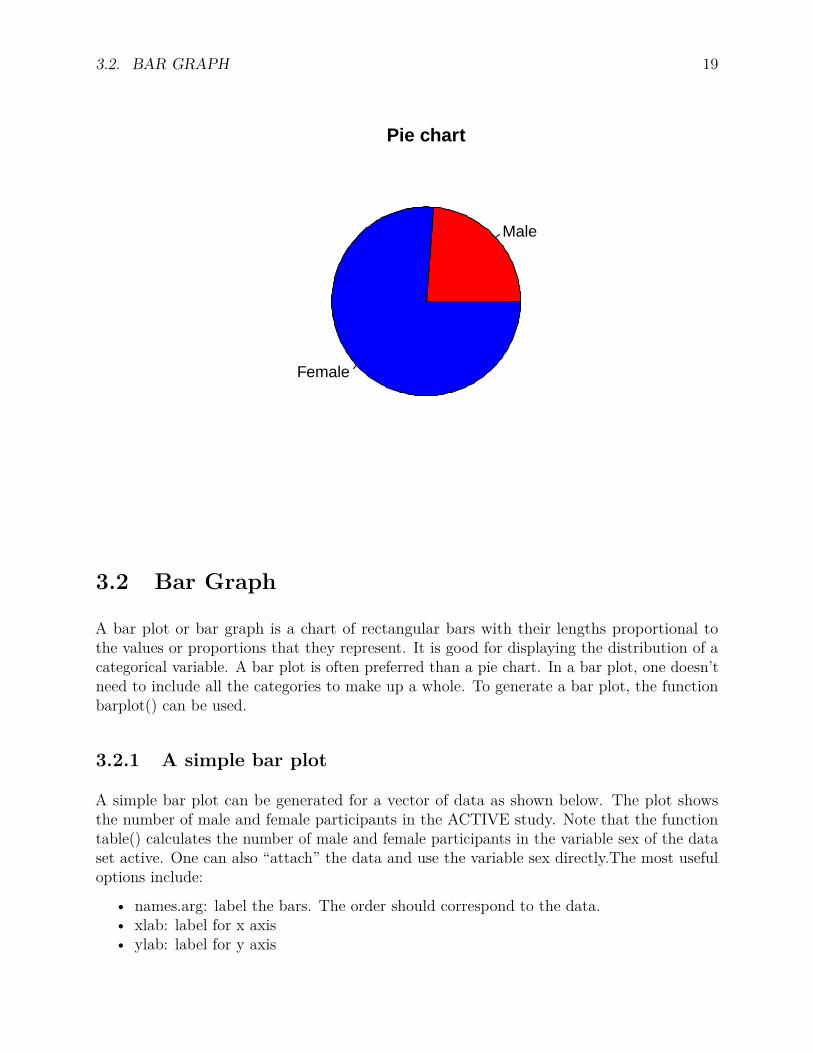
A pie chart (or a circle graph) is a circular chart divided into sectors, illustrating proportion.In a pie chart, the arc length of each sector (and consequently its central angle and area), isproportional to the quantity it represents. It is useful in comparing a slice with the whole piebut not effective to compare slices because our eyes are good at judging linear measures andbad at judging relative areas.
17

18 CHAPTER 3. STATISTICAL GRAPHS IN R
To generate a pie chart, the function pie() can be used. The function takes a vector of data.The most useful options include:
• labels: label the slices• col: colors of the slices• main: title of the plot
As an example, we compare the proportions of male and female participants in the ACTIVEstudy. The plot clearly showed there were more female participants than male participantsin the sample. Note that the function table() calculates the number of male and femaleparticipants in the variable sex of the data set active. One can also “attach” the data anduse the variable sex directly.active <- read.csv("data/active.csv")head(active)## site age edu group booster sex reason ufov hvltt hvltt2 hvltt3 hvltt4 mmse id## 1 1 76 12 1 1 1 28 16 28 28 17 22 27 1## 2 1 67 10 1 1 2 13 20 24 22 20 27 25 2## 3 6 67 13 3 1 2 24 16 24 24 28 27 27 3## 4 5 72 16 1 1 2 33 16 35 34 32 34 30 4## 5 4 69 12 4 0 2 30 16 35 29 34 34 28 5## 6 1 70 13 1 1 1 35 23 29 27 26 29 23 6pie(table(active$sex), labels=c('Male','Female'),
col=c('red','blue'), main='Pie chart')
3.2. BAR GRAPH 19
Male
Female
Pie chart
3.2 Bar Graph
A bar plot or bar graph is a chart of rectangular bars with their lengths proportional tothe values or proportions that they represent. It is good for displaying the distribution of acategorical variable. A bar plot is often preferred than a pie chart. In a bar plot, one doesn’tneed to include all the categories to make up a whole. To generate a bar plot, the functionbarplot() can be used.
3.2.1 A simple bar plot
A simple bar plot can be generated for a vector of data as shown below. The plot showsthe number of male and female participants in the ACTIVE study. Note that the functiontable() calculates the number of male and female participants in the variable sex of the dataset active. One can also “attach” the data and use the variable sex directly.The most usefuloptions include:
• names.arg: label the bars. The order should correspond to the data.• xlab: label for x axis• ylab: label for y axis
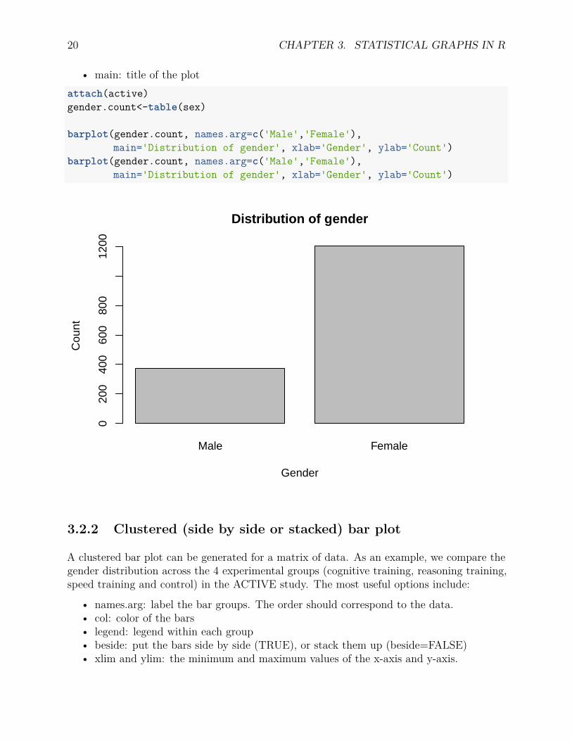
20 CHAPTER 3. STATISTICAL GRAPHS IN R
• main: title of the plotattach(active)gender.count<-table(sex)
barplot(gender.count, names.arg=c('Male','Female'),main='Distribution of gender', xlab='Gender', ylab='Count')
barplot(gender.count, names.arg=c('Male','Female'),main='Distribution of gender', xlab='Gender', ylab='Count')
Male Female
Distribution of gender
Gender
Cou
nt
020
040
060
080
012
00
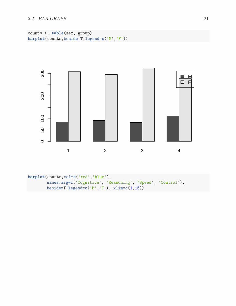
3.2.2 Clustered (side by side or stacked) bar plot
A clustered bar plot can be generated for a matrix of data. As an example, we compare thegender distribution across the 4 experimental groups (cognitive training, reasoning training,speed training and control) in the ACTIVE study. The most useful options include:
• names.arg: label the bar groups. The order should correspond to the data.• col: color of the bars• legend: legend within each group• beside: put the bars side by side (TRUE), or stack them up (beside=FALSE)• xlim and ylim: the minimum and maximum values of the x-axis and y-axis.
3.2. BAR GRAPH 21
counts <- table(sex, group)barplot(counts,beside=T,legend=c('M','F'))
1 2 3 4
MF
050
100
200
300
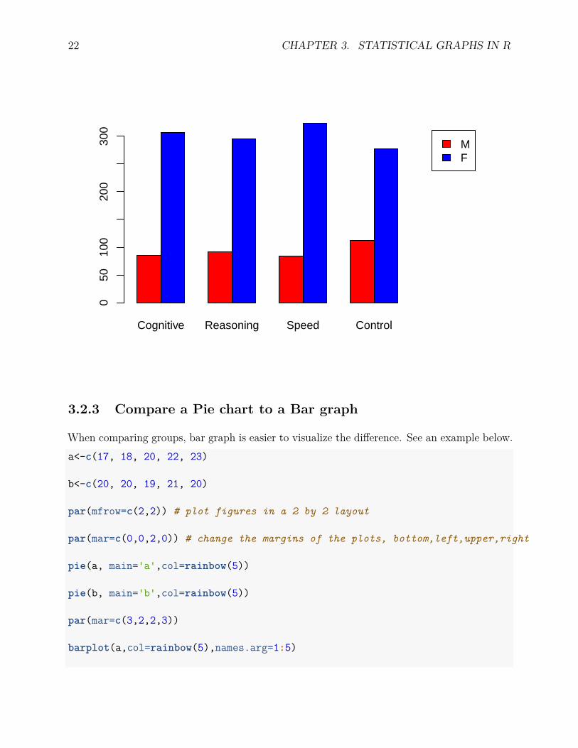
barplot(counts,col=c('red','blue'),names.arg=c('Cognitive', 'Reasoning', 'Speed', 'Control'),beside=T,legend=c('M','F'), xlim=c(1,15))
22 CHAPTER 3. STATISTICAL GRAPHS IN R
Cognitive Reasoning Speed Control
MF
050
100
200
300
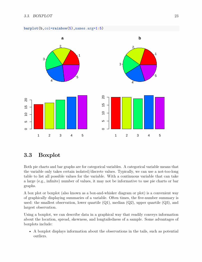
3.2.3 Compare a Pie chart to a Bar graph
When comparing groups, bar graph is easier to visualize the difference. See an example below.a<-c(17, 18, 20, 22, 23)
b<-c(20, 20, 19, 21, 20)
par(mfrow=c(2,2)) # plot figures in a 2 by 2 layout
par(mar=c(0,0,2,0)) # change the margins of the plots, bottom,left,upper,right
pie(a, main='a',col=rainbow(5))
pie(b, main='b',col=rainbow(5))
par(mar=c(3,2,2,3))
barplot(a,col=rainbow(5),names.arg=1:5)
3.3. BOXPLOT 23
barplot(b,col=rainbow(5),names.arg=1:5)
1
2
3
45
a
1
2
3
4
5
b
1 2 3 4 5
05
1015
20
1 2 3 4 5
05
1015
20
3.3 Boxplot
Both pie charts and bar graphs are for categorical variables. A categorical variable means thatthe variable only takes certain isolated/discrete values. Typically, we can use a not-too-longtable to list all possible values for the variable. With a continuous variable that can takea large (e.g., infinite) number of values, it may not be informative to use pie charts or bargraphs.
A box plot or boxplot (also known as a box-and-whisker diagram or plot) is a convenient wayof graphically displaying summaries of a variable. Often times, the five-number summary isused: the smallest observation, lower quartile (Q1), median (Q2), upper quartile (Q3), andlargest observation.
Using a boxplot, we can describe data in a graphical way that readily conveys informationabout the location, spread, skewness, and longtailedness of a sample. Some advantages ofboxplots include:
• A boxplot displays information about the observations in the tails, such as potentialoutliers.
24 CHAPTER 3. STATISTICAL GRAPHS IN R
• Boxplots can be displayed side-by-side to compare the distribution of several variables.• A boxplot is easy to construct.• A boxplot is easily understood by users of statistics.
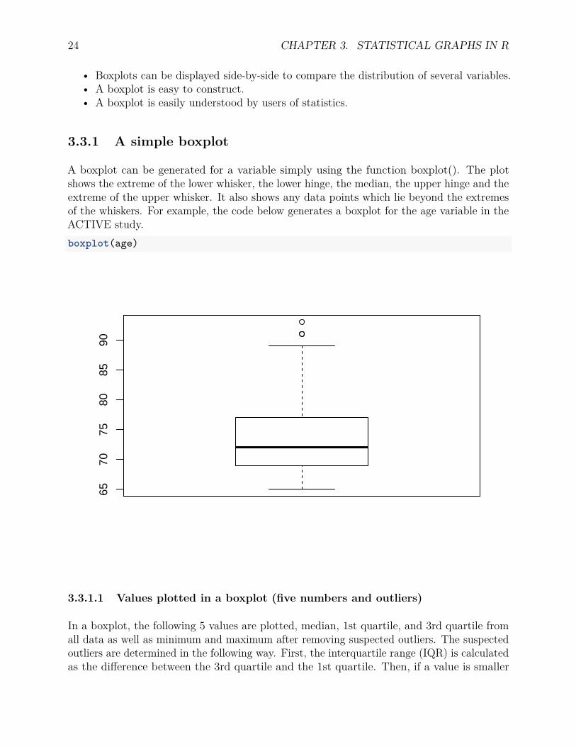
3.3.1 A simple boxplot
A boxplot can be generated for a variable simply using the function boxplot(). The plotshows the extreme of the lower whisker, the lower hinge, the median, the upper hinge and theextreme of the upper whisker. It also shows any data points which lie beyond the extremesof the whiskers. For example, the code below generates a boxplot for the age variable in theACTIVE study.boxplot(age)
6570
7580
8590
3.3.1.1 Values plotted in a boxplot (five numbers and outliers)
In a boxplot, the following 5 values are plotted, median, 1st quartile, and 3rd quartile fromall data as well as minimum and maximum after removing suspected outliers. The suspectedoutliers are determined in the following way. First, the interquartile range (IQR) is calculatedas the difference between the 3rd quartile and the 1st quartile. Then, if a value is smaller
3.3. BOXPLOT 25
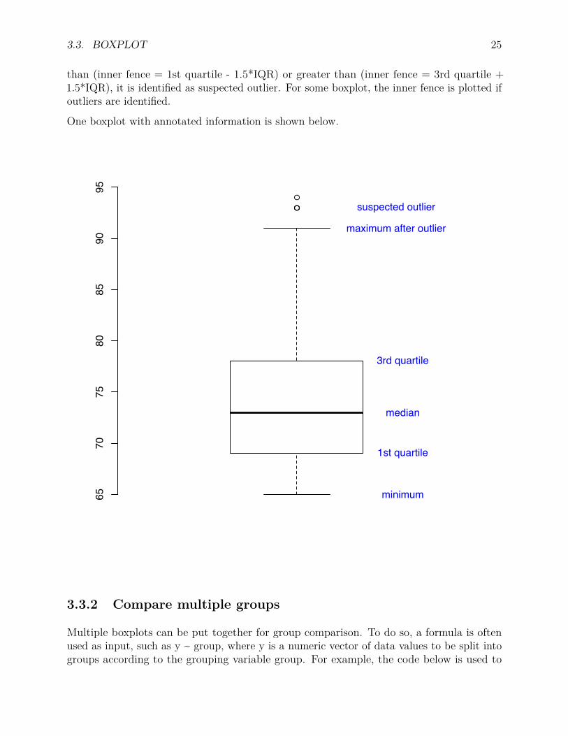
than (inner fence = 1st quartile - 1.5*IQR) or greater than (inner fence = 3rd quartile +1.5*IQR), it is identified as suspected outlier. For some boxplot, the inner fence is plotted ifoutliers are identified.
One boxplot with annotated information is shown below.
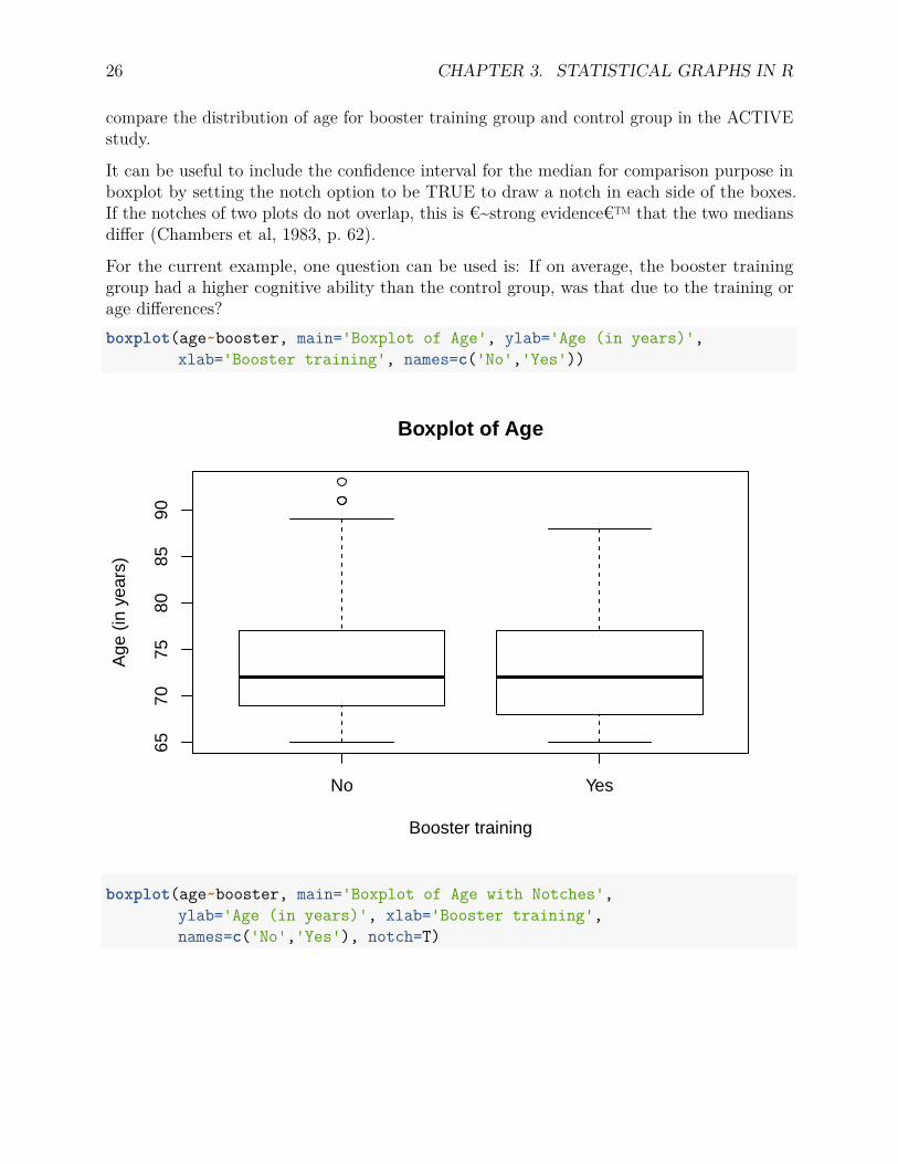
3.3.2 Compare multiple groups
Multiple boxplots can be put together for group comparison. To do so, a formula is oftenused as input, such as y ~ group, where y is a numeric vector of data values to be split intogroups according to the grouping variable group. For example, the code below is used to
26 CHAPTER 3. STATISTICAL GRAPHS IN R
compare the distribution of age for booster training group and control group in the ACTIVEstudy.
It can be useful to include the confidence interval for the median for comparison purpose inboxplot by setting the notch option to be TRUE to draw a notch in each side of the boxes.If the notches of two plots do not overlap, this is €~strong evidence€™ that the two mediansdiffer (Chambers et al, 1983, p. 62).
For the current example, one question can be used is: If on average, the booster traininggroup had a higher cognitive ability than the control group, was that due to the training orage differences?boxplot(age~booster, main='Boxplot of Age', ylab='Age (in years)',
xlab='Booster training', names=c('No','Yes'))
No Yes
6570
7580
8590
Boxplot of Age
Booster training
Age
(in
yea
rs)
boxplot(age~booster, main='Boxplot of Age with Notches',ylab='Age (in years)', xlab='Booster training',names=c('No','Yes'), notch=T)

3.4. HISTOGRAM 27
No Yes
6570
7580
8590
Boxplot of Age with Notches
Booster training
Age
(in
yea
rs)
3.4 Histogram
A histogram is a graphical display of frequencies over a set of continuous intervals for acontinuous variable. The range of a variable is divided into a list of equal intervals. Withineach interval, the number of participants, frequency, is counted. Then, the frequencies can beplotted with attached bars. Heights of the bars stand for frequencies or relative frequencies.
The purpose of a histogram is often to graphically summarize the distribution of a variablesuch as
• center (i.e., the location) of the data• spread (i.e., the scale) of the data• skewness of the data• presence of outliers• presence of multiple modes in the data.
Some examples of histogram are given below.

28 CHAPTER 3. STATISTICAL GRAPHS IN R
3.4.1 Examples
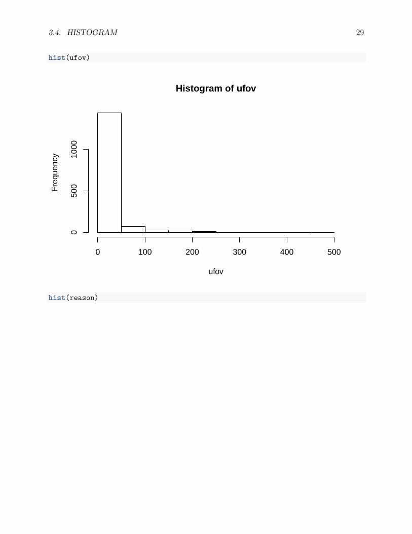
To generate a histogram, the function hist() can be used. In the following, we have histogramfor the ufov (useful field of view) variable and the reason (reasoning ability) variable of theACTIVE study. Clearly, the distribution of ufov is highly skewed while the distribution ofreason is more normal.
3.4. HISTOGRAM 29
hist(ufov)
Histogram of ufov
ufov
Fre
quen
cy
0 100 200 300 400 500
050
010
00
hist(reason)
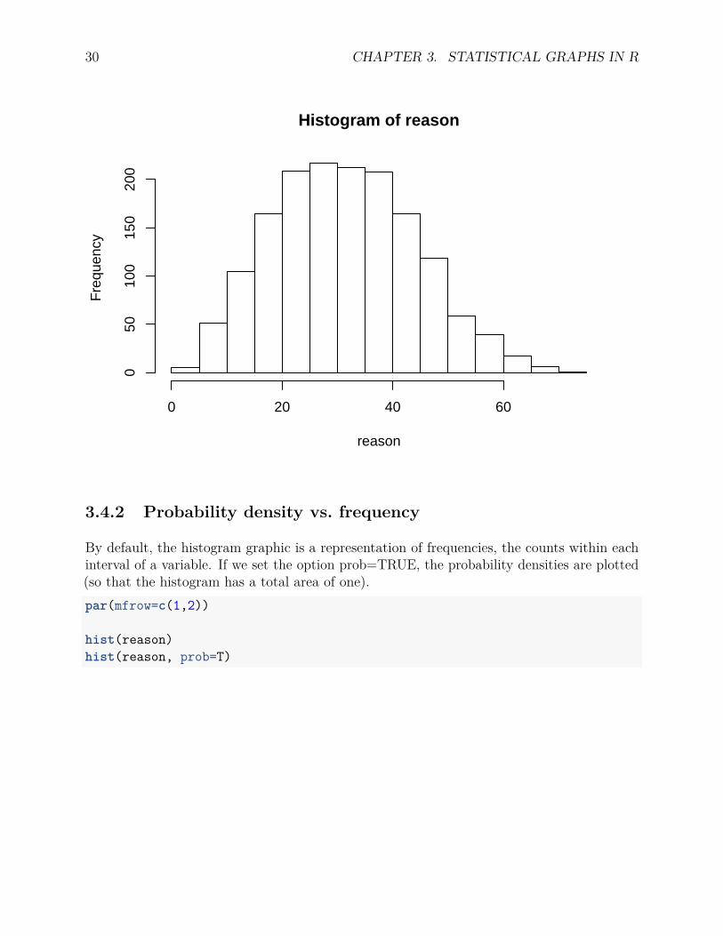
30 CHAPTER 3. STATISTICAL GRAPHS IN R
Histogram of reason
reason
Fre
quen
cy
0 20 40 60
050
100
150
200
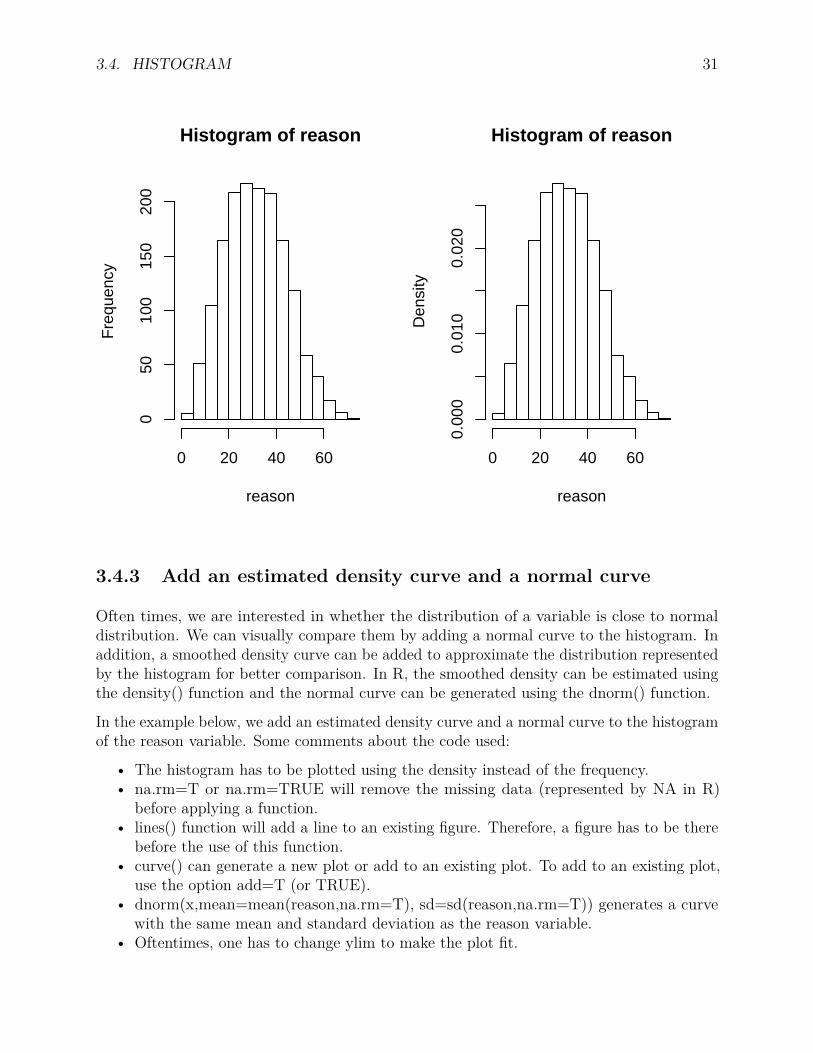
3.4.2 Probability density vs. frequency
By default, the histogram graphic is a representation of frequencies, the counts within eachinterval of a variable. If we set the option prob=TRUE, the probability densities are plotted(so that the histogram has a total area of one).par(mfrow=c(1,2))
hist(reason)hist(reason, prob=T)
3.4. HISTOGRAM 31
Histogram of reason
reason
Fre
quen
cy
0 20 40 60
050
100
150
200
Histogram of reason
reason
Den
sity
0 20 40 600.
000
0.01
00.
020
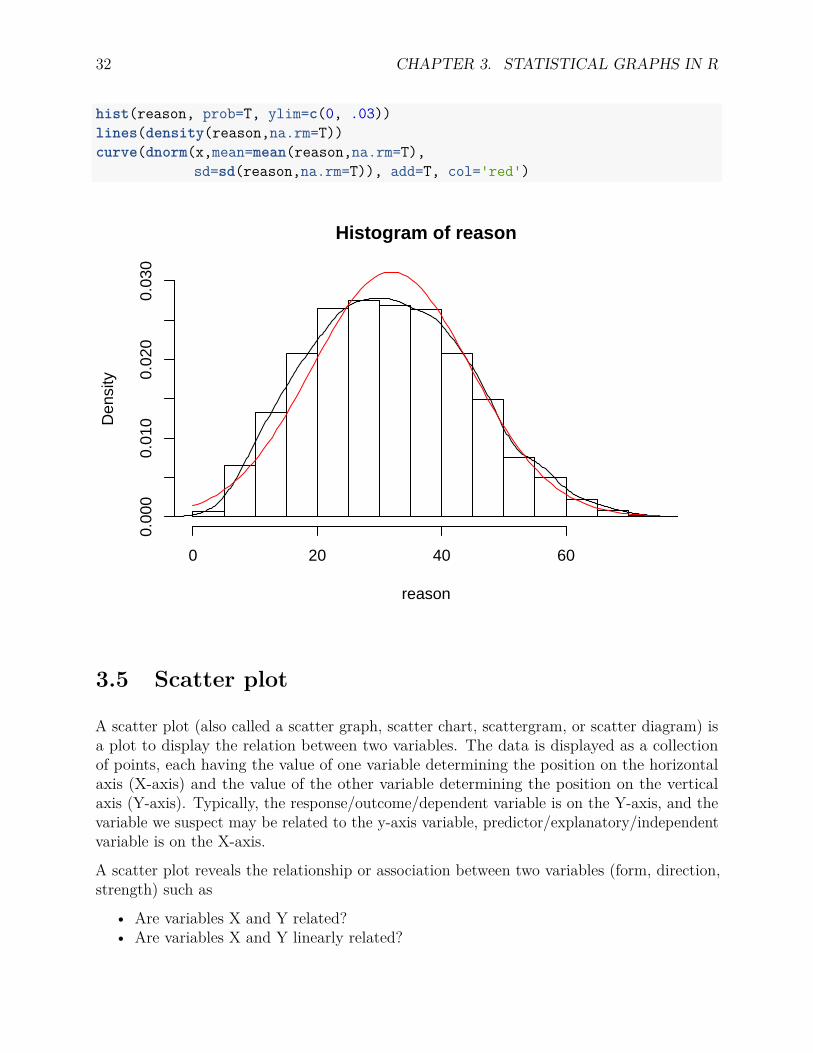
3.4.3 Add an estimated density curve and a normal curve
Often times, we are interested in whether the distribution of a variable is close to normaldistribution. We can visually compare them by adding a normal curve to the histogram. Inaddition, a smoothed density curve can be added to approximate the distribution representedby the histogram for better comparison. In R, the smoothed density can be estimated usingthe density() function and the normal curve can be generated using the dnorm() function.
In the example below, we add an estimated density curve and a normal curve to the histogramof the reason variable. Some comments about the code used:
• The histogram has to be plotted using the density instead of the frequency.• na.rm=T or na.rm=TRUE will remove the missing data (represented by NA in R)
before applying a function.• lines() function will add a line to an existing figure. Therefore, a figure has to be there
before the use of this function.• curve() can generate a new plot or add to an existing plot. To add to an existing plot,
use the option add=T (or TRUE).• dnorm(x,mean=mean(reason,na.rm=T), sd=sd(reason,na.rm=T)) generates a curve
with the same mean and standard deviation as the reason variable.• Oftentimes, one has to change ylim to make the plot fit.
32 CHAPTER 3. STATISTICAL GRAPHS IN R
hist(reason, prob=T, ylim=c(0, .03))lines(density(reason,na.rm=T))curve(dnorm(x,mean=mean(reason,na.rm=T),
sd=sd(reason,na.rm=T)), add=T, col='red')
Histogram of reason
reason
Den
sity
0 20 40 60
0.00
00.
010
0.02
00.
030
3.5 Scatter plot
A scatter plot (also called a scatter graph, scatter chart, scattergram, or scatter diagram) isa plot to display the relation between two variables. The data is displayed as a collectionof points, each having the value of one variable determining the position on the horizontalaxis (X-axis) and the value of the other variable determining the position on the verticalaxis (Y-axis). Typically, the response/outcome/dependent variable is on the Y-axis, and thevariable we suspect may be related to the y-axis variable, predictor/explanatory/independentvariable is on the X-axis.
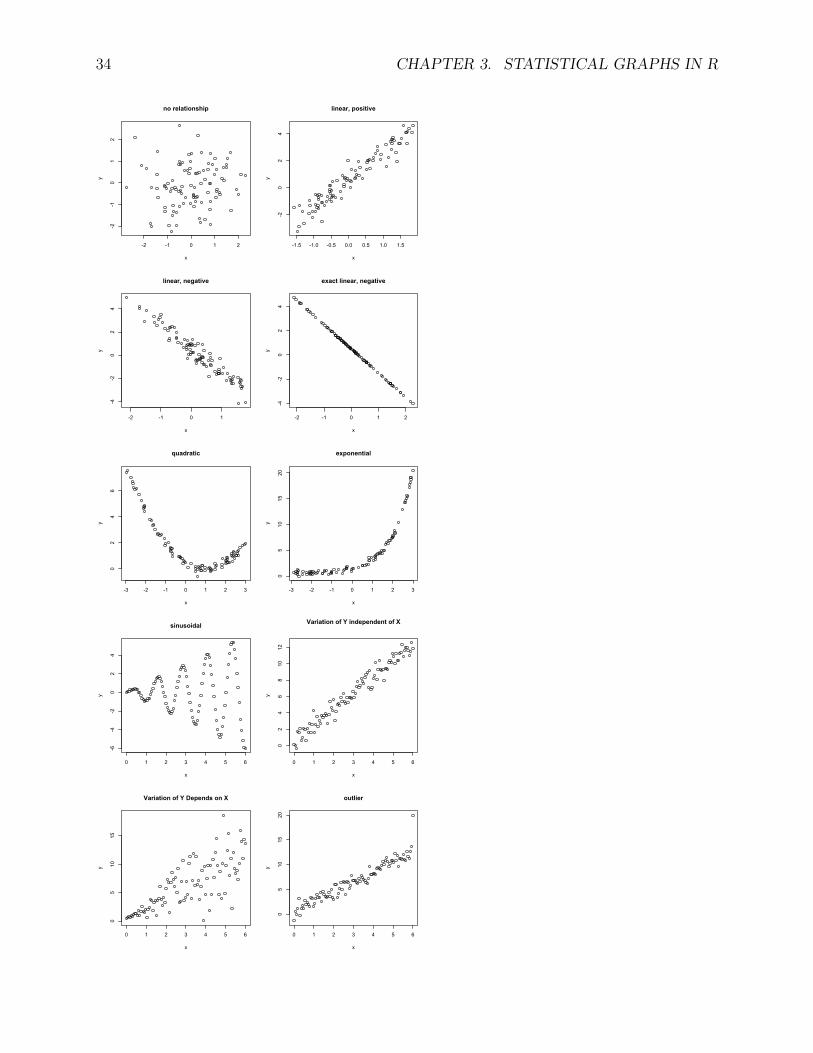
A scatter plot reveals the relationship or association between two variables (form, direction,strength) such as
• Are variables X and Y related?• Are variables X and Y linearly related?

3.5. SCATTER PLOT 33
• Are variables X and Y non-linearly related?• Are changes in Y related to changes in X?• Are there any outliers?
Some examples of scatter plots are given below.
34 CHAPTER 3. STATISTICAL GRAPHS IN R
3.5. SCATTER PLOT 35
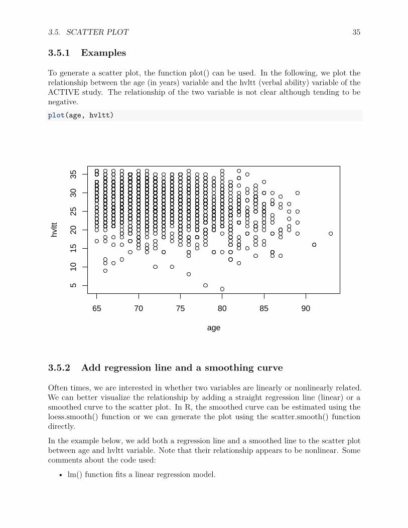
3.5.1 Examples
To generate a scatter plot, the function plot() can be used. In the following, we plot therelationship between the age (in years) variable and the hvltt (verbal ability) variable of theACTIVE study. The relationship of the two variable is not clear although tending to benegative.plot(age, hvltt)
65 70 75 80 85 90
510
1520
2530
35
age
hvltt
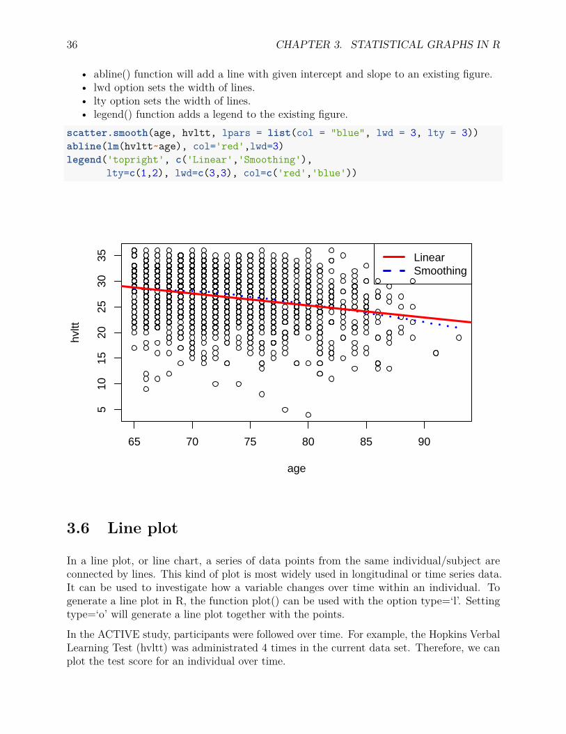
3.5.2 Add regression line and a smoothing curve
Often times, we are interested in whether two variables are linearly or nonlinearly related.We can better visualize the relationship by adding a straight regression line (linear) or asmoothed curve to the scatter plot. In R, the smoothed curve can be estimated using theloess.smooth() function or we can generate the plot using the scatter.smooth() functiondirectly.
In the example below, we add both a regression line and a smoothed line to the scatter plotbetween age and hvltt variable. Note that their relationship appears to be nonlinear. Somecomments about the code used:
• lm() function fits a linear regression model.
36 CHAPTER 3. STATISTICAL GRAPHS IN R
• abline() function will add a line with given intercept and slope to an existing figure.• lwd option sets the width of lines.• lty option sets the width of lines.• legend() function adds a legend to the existing figure.
scatter.smooth(age, hvltt, lpars = list(col = "blue", lwd = 3, lty = 3))abline(lm(hvltt~age), col='red',lwd=3)legend('topright', c('Linear','Smoothing'),
lty=c(1,2), lwd=c(3,3), col=c('red','blue'))
65 70 75 80 85 90
510
1520
2530
35
age
hvltt
LinearSmoothing
3.6 Line plot
In a line plot, or line chart, a series of data points from the same individual/subject areconnected by lines. This kind of plot is most widely used in longitudinal or time series data.It can be used to investigate how a variable changes over time within an individual. Togenerate a line plot in R, the function plot() can be used with the option type=‘l’. Settingtype=‘o’ will generate a line plot together with the points.
In the ACTIVE study, participants were followed over time. For example, the Hopkins VerbalLearning Test (hvltt) was administrated 4 times in the current data set. Therefore, we canplot the test score for an individual over time.

3.6. LINE PLOT 37
3.6.1 A single line plot
In the example below, we plot the Hopkins Verbal Learning Test for the first participant inthe data set.plot(1:4, active[1,9:12], type='o',
xlab='time', ylab='HVLTT',ylim=c(0,36))
1.0 1.5 2.0 2.5 3.0 3.5 4.0
05
1015
2025
3035
time
HV
LTT
3.6.2 Compare the change trajectory of two participants
Two lines can be plotted together to compare changes for two subjects. Note that the secondline can be added using the lines() function.plot(1:4, active[1,9:12], type='o',
xlab='time', ylab='HVLTT',ylim=c(0,36))lines(1:4, active[2,9:12], type='o',
pch=22, lty=2, col='red')legend('bottomleft', c('first', 'second'),
lty=c(1,2), col=c('black', 'red'))
38 CHAPTER 3. STATISTICAL GRAPHS IN R
1.0 1.5 2.0 2.5 3.0 3.5 4.0
05
1015
2025
3035
time
HV
LTT
firstsecond
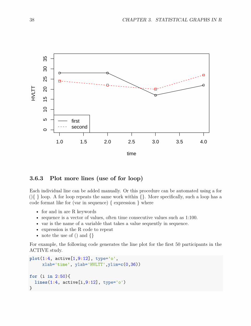
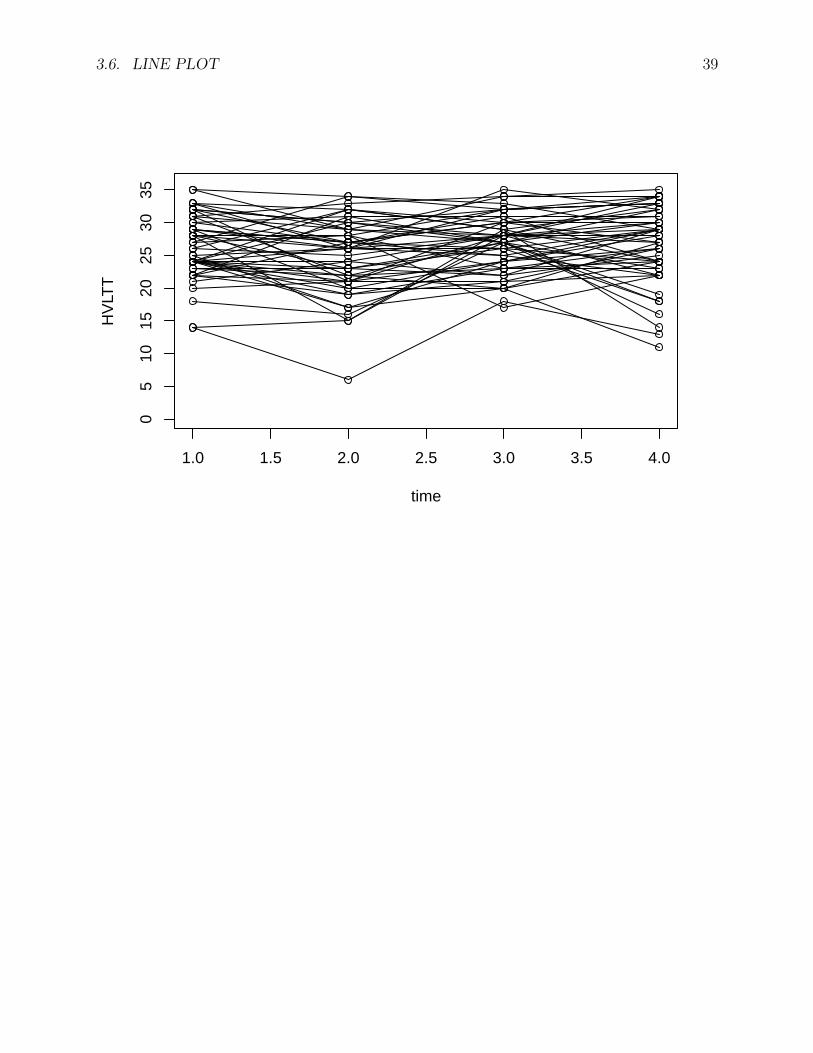
3.6.3 Plot more lines (use of for loop)
Each individual line can be added manually. Or this procedure can be automated using a for(){ } loop. A for loop repeats the same work within {}. More specifically, such a loop has acode format like for (var in sequence) { expression } where
• for and in are R keywords• sequence is a vector of values, often time consecutive values such as 1:100.• var is the name of a variable that takes a value sequently in sequence.• expression is the R code to repeat• note the use of () and {}
For example, the following code generates the line plot for the first 50 participants in theACTIVE study.plot(1:4, active[1,9:12], type='o',
xlab='time', ylab='HVLTT',ylim=c(0,36))
for (i in 2:50){lines(1:4, active[i,9:12], type='o')
}
3.6. LINE PLOT 39
1.0 1.5 2.0 2.5 3.0 3.5 4.0
05
1015
2025
3035
time
HV
LTT

40 CHAPTER 3. STATISTICAL GRAPHS IN R

Chapter 4
Hypothesis testing
4.1 Null hypothesis testing
Null hypothesis testing is a procedure to evaluate the strength of evidence against a nullhypothesis. Given/assuming the null hypothesis is true, we evaluate the likelihood ofobtaining the observed evidence or more extreme, when the study is on a randomly-selectedrepresentative sample. The null hypothesis assumes no difference/relationship/effect in thepopulation from which the sample is selected. The likelihood is measured by a p value. Ifthe p value is small enough, we reject the null. In the significance testing approach of RonaldFisher, a null hypothesis is rejected on the basis of data that are significantly unlikely if thenull is true. However, the null hypothesis is never accepted or proved. This is analogous to acriminal trial: The defendant is assumed to be innocent (null is not rejected) until provenguilty (null is rejected) beyond a reasonable doubt (to a statistically significant degree).
To conduct a typical null hypothesis test, the following 7 steps can be followed:
1. State the research question2. State the null and alternative hypotheses based on the research question3. Select a value for significance level α4. Collect or locate data5. Calculate the test statistic and the p value6. Make a decision on rejecting or failing to reject the hypothesis7. Answer the research question
4.1.1 Step 1. State the research question
A hypothesis testing is used to answer a question. Therefore, the first step is to state aresearch question. For example, a research question could be “Does memory training improveparticipants’ performance on a memory test?” in the ACTIVE study.
41
42 CHAPTER 4. HYPOTHESIS TESTING
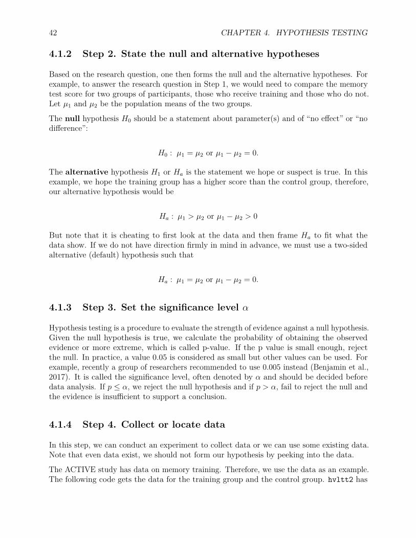
4.1.2 Step 2. State the null and alternative hypotheses
Based on the research question, one then forms the null and the alternative hypotheses. Forexample, to answer the research question in Step 1, we would need to compare the memorytest score for two groups of participants, those who receive training and those who do not.Let µ1 and µ2 be the population means of the two groups.
The null hypothesis H0 should be a statement about parameter(s) and of “no effect” or “nodifference”:
H0 : µ1 = µ2 or µ1 − µ2 = 0.
The alternative hypothesis H1 or Ha is the statement we hope or suspect is true. In thisexample, we hope the training group has a higher score than the control group, therefore,our alternative hypothesis would be
Ha : µ1 > µ2 or µ1 − µ2 > 0
But note that it is cheating to first look at the data and then frame Ha to fit what thedata show. If we do not have direction firmly in mind in advance, we must use a two-sidedalternative (default) hypothesis such that
Ha : µ1 = µ2 or µ1 − µ2 = 0.
4.1.3 Step 3. Set the significance level α
Hypothesis testing is a procedure to evaluate the strength of evidence against a null hypothesis.Given the null hypothesis is true, we calculate the probability of obtaining the observedevidence or more extreme, which is called p-value. If the p value is small enough, rejectthe null. In practice, a value 0.05 is considered as small but other values can be used. Forexample, recently a group of researchers recommended to use 0.005 instead (Benjamin et al.,2017). It is called the significance level, often denoted by α and should be decided beforedata analysis. If p ≤ α, we reject the null hypothesis and if p > α, fail to reject the null andthe evidence is insufficient to support a conclusion.
4.1.4 Step 4. Collect or locate data
In this step, we can conduct an experiment to collect data or we can use some existing data.Note that even data exist, we should not form our hypothesis by peeking into the data.
The ACTIVE study has data on memory training. Therefore, we use the data as an example.The following code gets the data for the training group and the control group. hvltt2 has
4.1. NULL HYPOTHESIS TESTING 43
information on all 4 training groups (memory=1, reasoning=2, speed=3, control=4). Notethat we use hvltt2[group==1] to select a subset of data from hvltt2. This means we wantto get the data from hvltt2 when the group value is equal to 1. Similarly, we select the datafor the control group.
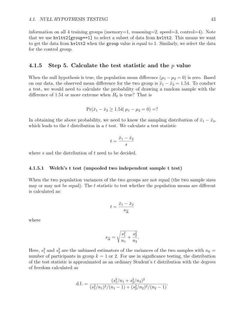
4.1.5 Step 5. Calculate the test statistic and the p value
When the null hypothesis is true, the population mean difference (µ1−µ2 = 0) is zero. Basedon our data, the observed mean difference for the two group is x1 − x2 = 1.54. To conducta test, we would need to calculate the probability of drawing a random sample with thedifference of 1.54 or more extreme when H0 is true? That is
Pr(x1 − x2 ≥ 1.54| µ1 − µ2 = 0) =?
In obtaining the above probability, we need to know the sampling distribution of x1 − x2,which leads to the t distribution in a t test. We calculate a test statistic
t = x1 − x2
s
where s and the distribution of t need to be decided.
4.1.5.1 Welch’s t test (unpooled two independent sample t test)
When the two population variances of the two groups are not equal (the two sample sizesmay or may not be equal). The t statistic to test whether the population means are differentis calculated as:
t = x1 − x2
s∆
where
s∆ =√s2
1n1
+ s22n2.
Here, s21 and s2
2 are the unbiased estimators of the variances of the two samples with nk =number of participants in group k = 1 or 2. For use in significance testing, the distributionof the test statistic is approximated as an ordinary Student’s t distribution with the degreesof freedom calculated as
d.f. = (s21/n1 + s2
2/n2)2
(s21/n1)2/(n1 − 1) + (s2
2/n2)2/(n2 − 1) .
44 CHAPTER 4. HYPOTHESIS TESTING
This is known as the Welch-Satterthwaite equation. The true distribution of the test statisticactually depends (slightly) on the two unknown population variances.
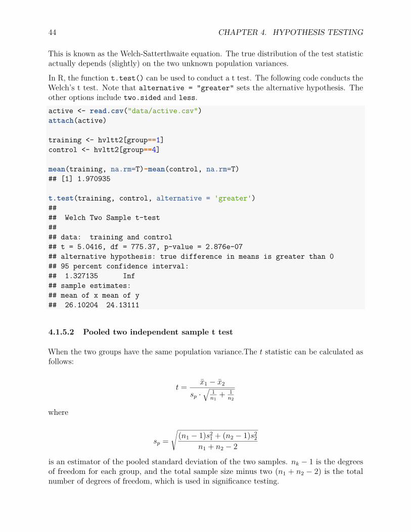
In R, the function t.test() can be used to conduct a t test. The following code conducts theWelch’s t test. Note that alternative = "greater" sets the alternative hypothesis. Theother options include two.sided and less.active <- read.csv("data/active.csv")attach(active)
training <- hvltt2[group==1]control <- hvltt2[group==4]
mean(training, na.rm=T)-mean(control, na.rm=T)## [1] 1.970935
t.test(training, control, alternative = 'greater')#### Welch Two Sample t-test#### data: training and control## t = 5.0416, df = 775.37, p-value = 2.876e-07## alternative hypothesis: true difference in means is greater than 0## 95 percent confidence interval:## 1.327135 Inf## sample estimates:## mean of x mean of y## 26.10204 24.13111
4.1.5.2 Pooled two independent sample t test
When the two groups have the same population variance.The t statistic can be calculated asfollows:
t = x1 − x2
sp ·√
1n1
+ 1n2
where
sp =√
(n1 − 1)s21 + (n2 − 1)s2
2n1 + n2 − 2
is an estimator of the pooled standard deviation of the two samples. nk − 1 is the degreesof freedom for each group, and the total sample size minus two (n1 + n2 − 2) is the totalnumber of degrees of freedom, which is used in significance testing.
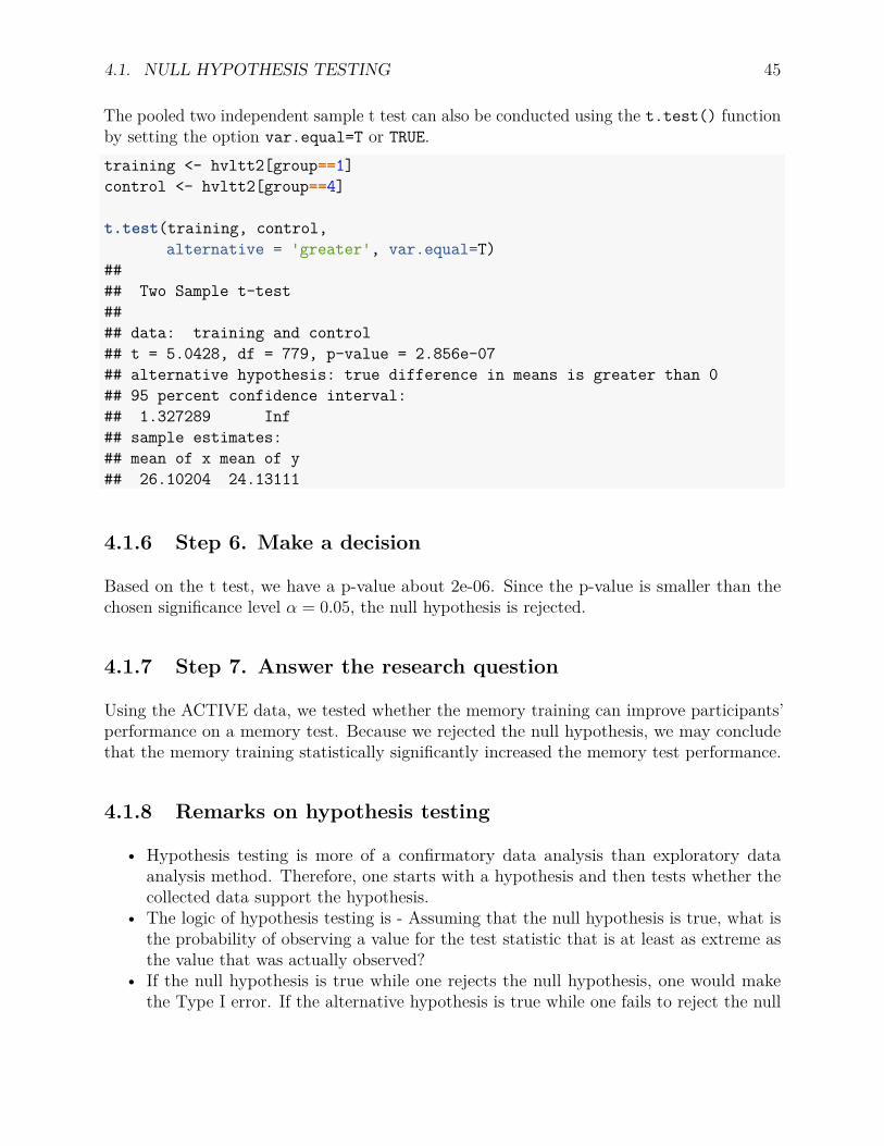
4.1. NULL HYPOTHESIS TESTING 45
The pooled two independent sample t test can also be conducted using the t.test() functionby setting the option var.equal=T or TRUE.training <- hvltt2[group==1]control <- hvltt2[group==4]
t.test(training, control,alternative = 'greater', var.equal=T)
#### Two Sample t-test#### data: training and control## t = 5.0428, df = 779, p-value = 2.856e-07## alternative hypothesis: true difference in means is greater than 0## 95 percent confidence interval:## 1.327289 Inf## sample estimates:## mean of x mean of y## 26.10204 24.13111
4.1.6 Step 6. Make a decision
Based on the t test, we have a p-value about 2e-06. Since the p-value is smaller than thechosen significance level α = 0.05, the null hypothesis is rejected.
4.1.7 Step 7. Answer the research question
Using the ACTIVE data, we tested whether the memory training can improve participants’performance on a memory test. Because we rejected the null hypothesis, we may concludethat the memory training statistically significantly increased the memory test performance.
4.1.8 Remarks on hypothesis testing
• Hypothesis testing is more of a confirmatory data analysis than exploratory dataanalysis method. Therefore, one starts with a hypothesis and then tests whether thecollected data support the hypothesis.
• The logic of hypothesis testing is - Assuming that the null hypothesis is true, what isthe probability of observing a value for the test statistic that is at least as extreme asthe value that was actually observed?
• If the null hypothesis is true while one rejects the null hypothesis, one would makethe Type I error. If the alternative hypothesis is true while one fails to reject the null
46 CHAPTER 4. HYPOTHESIS TESTING
hypothesis, one would make the Type II error. Statistical power is when one wouldreject the null hypothesis when the alternative hypothesis is true.
Fail to reject H0
Reject H0
Null hypothesis H0 is true
Correct decision
Type I error
Alternative hypothesis H1 is true
Type II error
Power
• Statistical significance means that the results are unlikely to have occurred by chance,given that the null is true.
• Statistical significance does not imply practical importance. For example, in comparingtwo groups, the difference can still be statistically significant even if the difference istiny.
4.2 Effect size
To measure the practical importance, effect size is often recommended to use. For example,for mean difference, the commonly used effect size measure is Cohen’s “d” (Cohen, 1988).Cohen’s d is defined as the difference between two means divided by a standard deviation.
d = x1 − x2
sp
Cohen defined sp, the pooled standard deviation, as
sp =√
(n1 − 1)s2x1 + (n2 − 1)s2
x2
n1 + n2 − 2
A Cohen’s d with the value around 0.2 is considered small, .5, median, and ≥.8, large.
For example, the Cohen’s d for the memory training example is 0.25, representing a smalleffect even though the p-value is small and indicates a statistical significance.mean1=mean(training,na.rm=T)mean2=mean(control,na.rm=T)meandiff=mean1-mean2

4.3. CRITICISMS OF NULL HYPOTHESIS TESTING AND P-VALUE 47
n1=length(training)-sum(is.na(training))n2=length(control)-sum(is.na(control))
v1=var(training,na.rm=T)v2=var(control,na.rm=T)s=sqrt(((n1-1)*v1+(n2-1)*v2)/(n1+n2-2))s## [1] 5.461292
cohend=meandiffcohend## [1] 1.970935
4.3 Criticisms of Null Hypothesis Testing and p-value
Let H0 and Ha (or H1) denote the null and alternative hypotheses, respectively. Let D denotethe data observed. The hypothesis testing is based on the calculation of the probability thatsuch a data set D and more extreme data can be observed given the hypothesis is true:
Pr(D|H0) = p,
which is often called p-value. In Fisher’s formulation, a low p -value means either that thenull hypothesis is true and a highly improbable event has occurred, or that the null hypothesisis false. If the probability p is smaller than, typically, 0.05, one would argue that there is avery small chance that the data set D (or more extreme data) can be observed. Thus, thenull hypothesis should be rejected. Otherwise, one fails to reject the null hypothesis.
There have been criticisms since the use of the null hypothesis testing (NHT). We summarizethe main criticisms below.
4.3.1 The focus of null hypothesis
In NHT, the null hypothesis is a statement of no effect, no difference, or no relation. However,researchers often believe the null hypothesis is false and are interested in finding certain effect.If the null hypothesis is always false, then what’s the point to reject it? As Cohen put it:
The null hypothesis, taken literally (and that’s the only way you can take it in formal hypothesistesting), is always false in the real world. It can only be true in the bowels of a computerprocessor running a Monte Carlo study (and even then a stray electron may make it false). Ifit is false, even to a tiny degree, it must be the case that a large enough sample will produce asignificant result and lead to its rejection. So if the null is always false, what€™s the big dealabout rejecting it? (Cohen, 1990, p. 1308).

48 CHAPTER 4. HYPOTHESIS TESTING
Similarly, Meehl (1990) stated that everything is related to everything else. He argued thatthe “pairwise correlations of even arbitrarily chosen variables in most soft domains tend torun large enough to yield frequent pseudoconfirmations of unrelated substantive theories,given conventional levels of the statistical power function based on pilot studies” (p. 237).Tukey (1991) wrote that "It is foolish to ask ‘Are the effects of A and B different?’ They arealways different - for some decimal place." (p. 100).
4.3.2 The test is done given that the null is true
In general, researchers choose to conduct a study because they believe there exists a significanteffect. Therefore, they firmly believe that the null hypothesis is not true but the alternativehypothesis is true. However, the null hypothesis testing is conducted based on the nullhypothesis. The whole rationale is “Assuming that the null hypothesis is true, what is theprobability of observing a value for the test statistic that is at least as extreme as the valuethat was actually observed?”
4.3.3 The logic of NHST is flawed
In logic, contraposition means that a conditional statement is logically equivalent to itscontrapositive. For example, given the statement that “if A is true, then B is true”, itsequivalence is “if B is not true, then A is not true.”
In using NHST, one tends to reason in the following way. If the null hypothesis is correct,then the data can not be observed. However, since we have observed the current data, thenull hypothesis is false. This is the contraposition and therefore logically correct.
However, the logic of NHST is not like this. Its logic is as follows. If the null hypothesis iscorrect, then the data are highly unlikely to observe. Now, these data have been observed.Therefore, the null hypothesis is highly unlikely to be correct. If this sounds right to you,consider the following example (Cohen, 1994):
If a person is an American, then he is probably not a member of Congress. This person is amember of Congress. Therefore, he is probably not an American.
Clearly, the conclusion of the example cannot be more wrong. Therefore, the logic of NHSTis flawed.
4.3.4 NHST tells nothing about the probability of neither nullhypothesis nor alternative hypothesis
Ultimately, a research is interested in Pr(H1|D) or at least Pr(H0|D). However, NHSTonly provides Pr(D|H0). Generally speaking, Pr(H0|D) 6= Pr(D|H0), meaning that rejectingthe null hypothesis says nothing or very little about the likelihood that the null is true.Furthermore, Pr(H1|D) 6= Pr(D|H0) or even Pr(H0|D) 6= 1− Pr(D|H0). Therefore, rejecting
4.3. CRITICISMS OF NULL HYPOTHESIS TESTING AND P-VALUE 49
the null hypothesis in no means suggests the support of the alternative hypothesis. However,too many times, people incorrectly believe Pr(H0|D) = Pr(D|H0) or even Pr(H0|D) =1− Pr(D|H0). Doing so can be extremely dangerous.
Consider the following example. Suppose a crime has been committed and blood is found atthe crime scene that is directly related to the crime in a city of 800,000 residents. Statisticsshows that the type of blood is present in 1% of the population. Given a person is found tohave this type of blood, one wants to infer whether the person is innocent (H0) or not(H1).Using the idea of NHST, we can get
Pr(blood|H0) = 0.01
Given it’s smaller than 0.05, one may reject the null that the person is innocent. However,it does not suggest the person is actually innocent or guilt at all. Note that with 800,000residents, there are 8,000 residents with this type of blood. If we assume everyone has theequal chance to commit the crime, a person only has a 1/8,000 probability to be guilt, closeto 100% to be innocent.
4.3.5 NHST does not tell whether a result can be replicated
Too many times, researchers would wrongly believe that a significant result indicates therejection of the null hypothesis in a replication study. The probability to replicate a study isrelated to power π = Pr(reject H0|H1). However, a p-value does not indicate much, if thereis any, about replication. For example, for a one-tail one-sample t-test, its power is
π = 1− Φ(−δ√n+ c1−α)
where
• Φ is the normal distribution function,• δ is the effect size,• n is the sample size,• and c is the critical value for a standard normal distribution with probability 1− α.
Suppose in a study, we observe a p-value 0.01 which is used as α in the above formular. Thenif the effect size is 0.036, the power for a sample with size 100 is only about 0.1. This meansthat among 10 replication studies, there will be only one study to show significant results.Therefore, it never means there is a 99% (1-0.01) probability to have significant results.
4.3.6 p-value, effect size and sample size
p-value in NHST is at least related to effect size and sample size. A small p-value does notnecessarily indicate large effect size. Therefore, a smaller p-value certainly does not meanmore important findings. With a large enough sample size, one would always reject the null

50 CHAPTER 4. HYPOTHESIS TESTING
hypothesis no matter how small the observed difference is practically. Consider a two-samplet-test, the test statistic is
t = x1 − x2
s.e.(x1 − x2) = x1 − x2√s2
1n1
+ s22n2
.
If we have x1 − x2 = 0.01, s21 = 1, s2
2 = 1, n1 = n2 = 80, 000, then we have t = 2 andp− value = 0.0455. Clearly, even though the two-sample difference is only 0.01, we wouldstill reject the null hypothesis based on NHST using 0.05 as the significance level.
4.3.7 The choice of significance level at 0.05
The choice of significant level at 0.05 or other values has no foundation and is almostcompletely subjective.
To summarize, in using NHST, one should be very cautious in interpreting the p-value. Bearin mind that:
• The p-value is not the probability that the null hypothesis is true (not Pr(H0|D)), noris it the probability that the alternative hypothesis is false (not 1− Pr(H1|D)) €“ it isnot connected to either of these. In fact, frequentist statistics does not, and cannot,attach probabilities to hypotheses.
• The p-value is not the probability of falsely rejecting the null hypothesis. This error isa version of the so-called prosecutor’s fallacy.
• The p-value is not the probability that a replicating experiment would not yield thesame conclusion. Quantifying the replicability of an experiment was attempted throughthe concept of p-rep.
• The significance level of the test, such as 0.05, is not determined by the p-value.• The p-value does not indicate the size or importance of the observed effect.
For a compilation of some commentaries on hypothesis testing, see http://www.indiana.edu/~stigtsts/.
4.4 Bayes’ Theorem
We have shown the potential problems of NHST. One solution to the problems is to use theBayesian method that is built on Bayes’ theorem. The Bayes’ theorem is stated mathematicallyas:
Pr(A | B) = Pr(B | A) Pr(A)Pr(B) ,
where A and B are events and Pr(B) 6= 0. For example, A can be a hypothesis and B can bedata. In the formula,

4.4. BAYES’ THEOREM 51
• Pr(A) and Pr(B) are the probabilities of observing A and B without regard to eachother.
• Pr(A|B) , a conditional probability, is the probability of observing event A given thatB is true.
• Pr(B|A) is the probability of observing event B given that A is true.
In terms of hypothesis testing, we are interested in Pr(H0|D) and Pr(H1|D), the probabilityof each hypothesis given data. Suppose there are only one null hypothesis and one alternativehypothesis. Then the probability that the null hypothesis is true given the observed data is
Pr(H0|D) = Pr(D|H0) Pr(H0)Pr(D|H1) Pr(H1) + Pr(D|H0) Pr(H0) ,
and the probability that the alternative hypothesis is true given the observed data
Pr(H1|D) = Pr(D|H1) Pr(H1)Pr(D|H1) Pr(H1) + Pr(D|H0) Pr(H0) .
Note that Pr(D) = Pr(D|H1) Pr(H1)+Pr(D|H0) Pr(H0) based on the law of total probability.
Clearly, Bayes’ theorem provides a way to directly tangle the probability of the hypotheses,which is often the focus of a study. The Bayesian interpretation of the formula is asfollows. Pr(H0) is called prior that presents one’s belief about the probability that thehypothesis H0 is true before collection of data and/or conducting a study. With the collecteddata D, one can update the probability about the same hypothesis to get the posteriorPr(H0|D).
4.4.1 An example
Suppose a crime has been committed and blood is found at the crime scene that is directlyrelated to the crime. Statistics shows that the type of blood is present in 1% of the population.
The prosecutor may state: “There is a 1% chance that the defendant would have the crimeblood type if he were innocent. Thus, there is a 99% chance that he is guilty.”
However, the defender may argue: “The city of crime scene has 800,000 people. The bloodtype would be found in about 8,000 people. The defendant only has a chance of 1 in 8,000 tobe guilty. Thus, the defendant is innocent.”
There are problems in both of the statements. The first statement is known as the prosecutor’sfallacy and the second one is known as the defender’s fallacy.
In this example, the null hypothesis is that the defendant is innocent (I) and the alternativehypothesis is that the defendant is guilty (G). Now we want to know the probability that thedefendant is guilty or innocent given the evidence of the found blood (E). From the statistics,we know that p(E|I) = 1/100. The prosecutor seems to believe p(G|E) = 1 − p(I|E) =
52 CHAPTER 4. HYPOTHESIS TESTING
1− p(E|I) = 99/100, which is not true. But note this is a typical mistake when employingNHST.
If there is no any evidence (or information) about who is the criminal, then everyone in thecity has the equal probability to be guilty so that
p(I) = 799, 999800, 000 and p(G) = 1− p(I) = 1
800, 000 .
Those probabilities are prior probability in Bayesian terms. Now we need to find thatconditional probability of I given the evidence E - p(I|E). Based on the statistics, we knowp(E|G) = 1 and p(E|I) = 1/100. This is because if the defendant committed the crime,the probability that his/her blood type would be found is 100%. However, even he/she isinnocent, there is still a 1% chance that her/his blood type would be found.
Using Bayes’ theorem, we know that
p(I|E) = p(E|I)p(I)p(E) = p(E|I)p(I)
p(E|I)p(I) + p(E|G)p(G) = .999875.
Thus, the defendant is very likely to be innocent based on the current limited information.This is equivalent to the argument of the defender.
To investigate the two kinds of fallacies, we can also get
p(G|E) = p(E|G)p(G)p(E|G)p(G) + p(E|I)p(I) .
Then we havep(G|E)p(I|E) = p(E|G)
p(E|I)p(G)p(I) = 100× p(G)
p(I) .
Clearly, the odds of guilty to innocent conditionally on the evidence found falls back to theodds of prior probability - the probability without considering the current evident at all. Theprosecutor believes that the defendant has equal chance (50%) to commit the crime. Thus,the prior odds is 1 and the posterior odds is 100. Then the prosecutor can conclude that thedefendant has 99% chance to be guilty.
The defender assumes that the p(G)/p(I) = 1/799, 999. Thus, the posterior odds is
100/799, 999 ≈ 1/8, 000.
However, if the defender is arrested, there must be more evidence than the blood type only.Then, the prior odds could be much larger. As shown above, even the prior odds is 1, thereis a 99% probablity for the defendant to be guilty.
Chapter 5
Confidence Interval
Psychological Science is a prestigious journal for psychological research. Its submissionguidelines consist of specific guideline on the use of NHST:
Effective January 2014, Psychological Science recommends the use of the “new statistics”- effect sizes, confidence intervals, and meta-analysis - to avoid problems associated withnull-hypothesis significance testing (NHST).
Confidence interval provides an alternative method to NHST, which some have arguedprovides more information on the NHST. A confidence interval (CI) is a type of intervalestimate, instead of a point estimate, of a population parameter.
5.1 Formal definition
Let θ denote a population parameter (unknowns) and X denote a random variable (e.g.,GPA) from which the data can be observed. Assume the observed outcome for X is x. Wecan calculate an interval [l(x), u(x)] based on the observed data. More generally, we candefine
Pr(l(X) ≤ θ ≤ u(X)) = 1− α = C
Then [l(X), u(X)] is a confidence interval with confidence level 1− α = C, or 100(1− α)%.l(X) and u(X) are called confidence limits (bounds), lower limit and upper limit, respectively.
5.1.1 Remarks
• A CI is an observed interval calculated based on a set of observed data. In general, itis different from sample to sample. Therefore, for two studies on the same topic, theCIs can be very different even following exactly the same study design.
53
54 CHAPTER 5. CONFIDENCE INTERVAL
• Different from the point estimate, a CI consists of a range of potential values as goodestimates of the unknown population parameter.
• For a given CI, it either includes or does not include the population parameter value.Therefore, a CI does not necessarily cover the true parameter values at all.
• If we conduct many separate data analyses of repeated experiment and each timewe calculate a CI, the proportion of such intervals that contain the true value of theparameter matches the confidence level C (1− α), This is called confidence level.
• When we say, “we are 99% confident that the true value of the parameter is in ourconfidence interval”, we express that 99% of the observed confidence intervals willcontain the true value of the parameter.
• The desired level of confidence is set by the researchers, not determined by data. If acorresponding hypothesis test is performed, the confidence level is the complement ofrespective level of significance, i.e. a 95% confidence interval reflects a significance levelof 0.05.
5.2 How to obtain a confidence interval
The basic idea to get a CI is straightforward in theory but can be very difficult in practice.It involves three steps:
1. Obtain a point estimate θ for θ. Note that θ is a function of x or your data.2. Find out the sampling distribution of θ.3. An equal-tail confidence interval with 95% confidence level can be constructed using
the 2.5th and 97.5th percentiles of the sampling distribution.
5.2.1 An example
Suppose we want to estimate and obtain the confidence interval estimate of the average GPA(µ) of all undergraduate students at University of Notre Dame. GPA typically follows anormal distribution X ∼ N(µ, σ). Instead of going out to collect data from students, wewill simulate (generate) some data for our example. To simulate data, we need to know thepopulation mean and standard deviation of GPA. Here we assume the mean is µ = 3.5 andthe standard deviation σ = .2. Furthermore, we would like to generate a sample of data withthe sample size 100.
In R, to generate random number from a normal distribution, the function rnorm() can beused. Specifically for this example, the code x<-rnorm(100,3.5,0.2) generates 100 valuesfrom a normal distribution with mean 3.5 and standard deviation 0.2. Therefore, in thefunction, the first number is the number of the values to generate, the second is the meanand the third is the standard deviation. The code below generates the values, prints themin the output, and displays the histogram of the generated data. Note that the histogramshows a bell shape.

5.2. HOW TO OBTAIN A CONFIDENCE INTERVAL 55
x<-rnorm(100,3.5,0.2)x ## show x## [1] 3.666912 3.505393 3.513702 3.350762 3.871895 3.283462 3.596087 3.684136## [9] 3.484478 3.449249 3.731040 3.517792 3.487425 3.502360 3.592607 3.698745## [17] 3.330702 3.247605 3.722761 3.576887 3.237014 3.394764 3.628747 3.516893## [25] 3.377679 3.655581 3.452306 3.532775 3.598987 3.498750 3.500586 3.364941## [33] 3.300062 3.354139 3.543074 3.774578 3.151708 3.556460 3.603588 3.751199## [41] 3.313614 3.553871 3.685358 3.522354 3.228461 3.628803 3.728081 3.574248## [49] 2.774994 3.741848 3.358530 3.381607 3.680215 3.451822 3.610234 3.559326## [57] 3.202037 3.540493 3.797942 3.442803 3.515349 3.493575 3.692337 3.690732## [65] 3.364037 3.584569 3.623174 3.490238 3.787200 3.587465 3.548139 3.440446## [73] 3.428566 4.060038 3.669719 3.533509 3.580912 3.644130 3.374645 3.584907## [81] 3.524748 3.330325 3.099236 3.543366 3.117910 3.542406 3.549324 3.676061## [89] 3.669131 3.411652 3.248079 3.628749 3.380642 3.304864 3.613016 3.760375## [97] 3.504437 3.424153 3.227398 3.429180hist(x) ## histogram
Histogram of x
x
Fre
quen
cy
3.0 3.2 3.4 3.6 3.8 4.0
05
1015
20
With the simulated data for 100 students, an estimate of the average GPA (θ) is
x = 1100
100∑i=1
xi.

56 CHAPTER 5. CONFIDENCE INTERVAL
Based on the central limit theorem, if the population variance σ is known, regardless of theshape of the population distribution, x is at least approximately normally distributed withmean (µ) and standard deviation (standard error of the mean)
s.e.(x) =√
1nσ2 = .1σ.
Now we the point estimate is θ = x and its sampling distribution is a normal distribution.Then a 95% equal-tail confidence interval can be constructed using the 2.5% and 97.5%percentile of the normal distribution as [Φ−1(0.025),Φ−1(0.975)] where Φ is the normaldistribution function. The whole procedure to calculate a CI for a set of simulated data isshown below.x <- rnorm(100,3.5,0.2)xbar <- mean(x)s.e. <- 0.2/10qnorm(c(.025, .975), xbar, s.e.)## [1] 3.445282 3.523681
Now, try run the code above one more time. Do you get the same confidence interval?
5.3 An experiment for CI interpretation
A CI changes each time with a study. If we repeat the same study again and again, 100(1−α)%of the time the obtained confidence intervals would cover the true population parameter value.This can be shown through a simulation study or experiment. Using the GPA example, wecan conduct an experiment using the following steps:
1. Generate a set of GPA data with 100 students from the population2. Calculate the observed sample mean of GPA and the standard error of x bar3. Calculate the confidence interval4. Check whether the confidence interval covers the population parameter value5. Repeat (1)-(4) 1000 times and count the total number of times that the confidence
intervals cover the population value.6. For a 95% CI, one would expect about 950 times the CIs cover the population value.
The R code below carries out the experiment. The output shows that the among the 1000 setsof CIs calculated based on the 1000 sets of simulated data, 949 of them cover the populationvalue 3.5.count<-0
for (i in 1:1000){x<-rnorm(100, 3.5, .2)xbar<-mean(x)s.e.<-.2/10
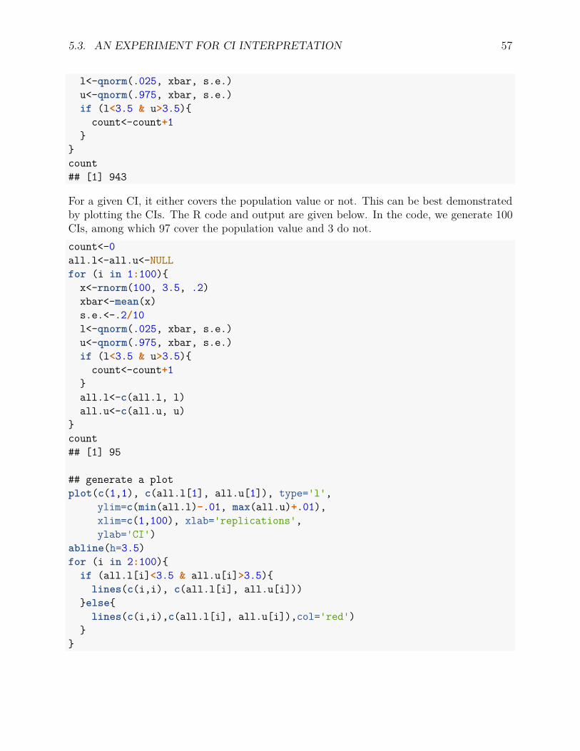
5.3. AN EXPERIMENT FOR CI INTERPRETATION 57
l<-qnorm(.025, xbar, s.e.)u<-qnorm(.975, xbar, s.e.)if (l<3.5 & u>3.5){
count<-count+1}
}count## [1] 943
For a given CI, it either covers the population value or not. This can be best demonstratedby plotting the CIs. The R code and output are given below. In the code, we generate 100CIs, among which 97 cover the population value and 3 do not.count<-0all.l<-all.u<-NULLfor (i in 1:100){
x<-rnorm(100, 3.5, .2)xbar<-mean(x)s.e.<-.2/10l<-qnorm(.025, xbar, s.e.)u<-qnorm(.975, xbar, s.e.)if (l<3.5 & u>3.5){
count<-count+1}all.l<-c(all.l, l)all.u<-c(all.u, u)
}count## [1] 95
## generate a plotplot(c(1,1), c(all.l[1], all.u[1]), type='l',
ylim=c(min(all.l)-.01, max(all.u)+.01),xlim=c(1,100), xlab='replications',ylab='CI')
abline(h=3.5)for (i in 2:100){
if (all.l[i]<3.5 & all.u[i]>3.5){lines(c(i,i), c(all.l[i], all.u[i]))
}else{lines(c(i,i),c(all.l[i], all.u[i]),col='red')
}}

58 CHAPTER 5. CONFIDENCE INTERVAL
0 20 40 60 80 100
3.40
3.45
3.50
3.55
3.60
replications
CI
5.4 Confidence interval and hypothesis testing
Confidence intervals do not require a-priori hypotheses, nor do they test trivial hypotheses.A confidence interval provides information on both the effect and its precision. A smallerinterval usually suggests the estimate is more precise. For example, [3.3, 3.7] is more precisethan [3,4].
A confidence interval can be used for hypothesis testing. For example, given the null hypothesis
θ = θ0
for any value of θ0. If a confidence interval with confidence level C = 1− α contains θ0, wefail to reject the corresponding null hypothesis at the significance level α. Otherwise, wereject the null hypothesis at the significance level α.
For example, suppose we are interested in testing whether a training intervention methodis effective or not. Based on a pre- and post-test design, we find the confidence interval forthe change after training is [0.7, 1.5] with the confidence level 0.95. Since this CI does notinclude 0, we would reject the null hypothesis that the change is 0 at the alpha level 0.05.
Using CI for hypothesis testing does not provide the exact p-value. However, a CI can beused to test multiple hypotheses. For example, for any null hypothesis that the change score
5.5. BOOTSTRAP 59
is less than 0.7, one would reject it.
CI kinds of focuses on the alternative hypothesis, the effect of interest. It provides a range ofplausible values to estimate the effect of interest.
Reichardt and Gollob (1997) discussed conditions that NHST and CI can be useful. NHSTis shown generally to be more informative than confidence intervals when assessing (1) theprobability that a parameter equals a pre-specified value; (2) the direction of a parameterrelative to a pre-specified value (e.g., 0); and (3) the probability that a parameter lies withina pre-specified range.
On the other hand, confidence intervals are shown generally to be more informative thanNHST when assessing the size of a parameter (1) without reference to a pre-specified valueor range of values; (2) with reference to many pre-specified values or ranges of values.Hagen (1997) pointed out: “We cannot escape the logic of NHST [null hypothesis statisticaltesting] by turning to point estimates and confidence intervals” (p. 22). In addition, Schmidtand Hunter (1997) suggested: “The assumption underlying this objection is that becauseconfidence intervals can be interpreted as significance tests, they must be so interpreted. Butthis is a false assumption” (p. 50).
5.5 Bootstrap
Obtaining a CI is not an easy, most times an extremely difficult, task. For example, evenfor the most widely used correlation coefficient, it is already difficult to get the confidenceinterval. For bivariate normal data, one can get the exact distribution of the sample correlationcoefficient r as
f(r) = (n− 2) Γ(n− 1)(1− ρ2)n−12 (1− r2)n−4
2√
2πΓ(n− 1
2
)(1− ρr)n− 3
22F1
(12 ,
12; 2n− 1
2 ; ρr + 12
).
With the sampling distribution, theoretically, one can get an exact CI for the correlationcoefficient ρ. However, because the computational difficulty, many ways have been proposedto approximate it instead (see https://arxiv.org/pdf/1410.8165.pdf). The most widely usedmethod is based on Fisher’s z-transformation. For a sample correlation r, its Fisher’stransformation is
Z = 12 ln 1 + r
1− r .
After transformation, Z approximately follows a normal distribution with mean
12 ln 1 + φ
1− φ
and variance φ = 1/(φ− 3).
60 CHAPTER 5. CONFIDENCE INTERVAL
To get the CI for ρ, we first construct a CI for
12 ln 1 + ρ
1− ρas [
12 ln 1 + r
1− r −z1−α/2√n− 3
,12 ln 1 + r
1− r + z1−α/2√n− 3
]With Zα denoting the 100α% percentile of the standard normal distribution. Then, we cansolve this for the the CI of ρ.
Bootstrap provides a useful procedure that can be used to construct a CI. Bootstrap methodis computationally intensive but can be used to get the distribution of a quantity of interestespecially when the theoretical distribution of a statistic is complicated or unknown and / orthe sample size is insufficient for straightforward statistical inference.
5.5.1 Basic idea
The basic idea of the bootstrap method is to circumvent the difficulty to get the samplingdistribution of a statistic. Sometimes, one can get the theoretical distribution of such astatistic through derivation. But the underlying idea can be understood through a simpleexample.
Suppose we are interested in estimating a parameter called θ, such as average GPA of studentsat University of Notre Dame. To do so, we can get a sample with sample size 100 and then usethe average GPA as an estimate of θ, denoted as θ. To make inference, we would need to getthe sampling distribution of θ, which is the distribution of the statistic for all possible samplesfrom the same population (students at Notre Dame) of a given size (100). Although generallyit is not feasible to get all possible samples, we assume we can repeatedly get R samples eachwith sample size 100. For each sample, we can get the average GPA as θi, i = 1, . . . , R. Then,the R average GPA will form a distribution, which can be viewed as an approximation of thesampling distribution. If R is equal to the number of all possible samples, then it would bethe exact sampling distribution. This procedure is illustrated in the figure below.
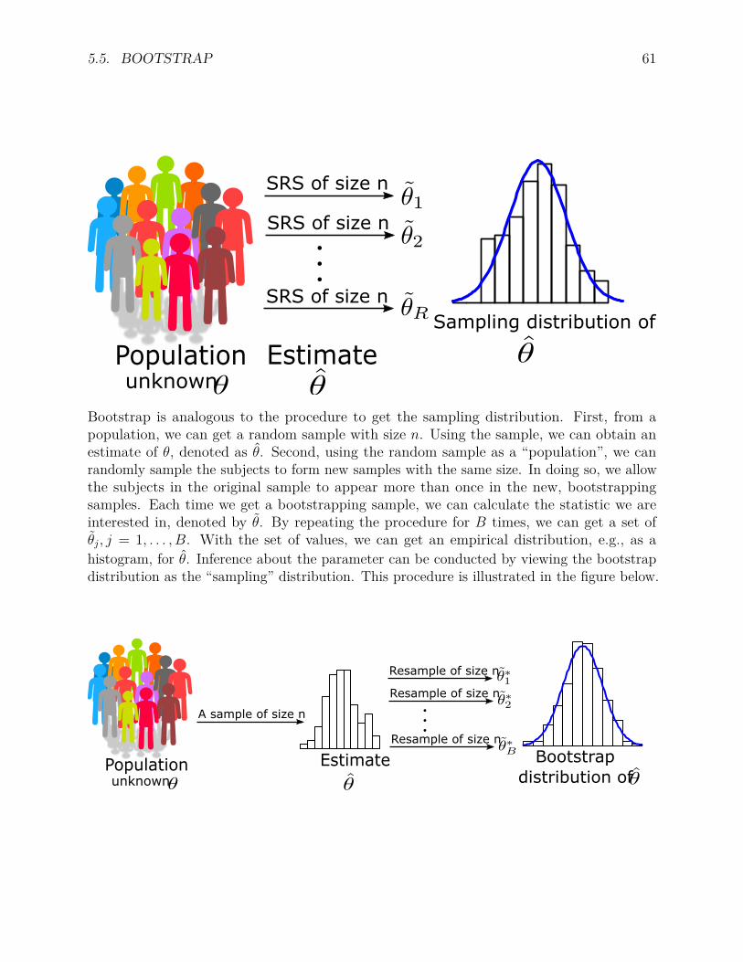
5.5. BOOTSTRAP 61
Population
SRS of size n
unknown
SRS of size n
SRS of size n
Sampling distribution of
Estimate
Bootstrap is analogous to the procedure to get the sampling distribution. First, from apopulation, we can get a random sample with size n. Using the sample, we can obtain anestimate of θ, denoted as θ. Second, using the random sample as a “population”, we canrandomly sample the subjects to form new samples with the same size. In doing so, we allowthe subjects in the original sample to appear more than once in the new, bootstrappingsamples. Each time we get a bootstrapping sample, we can calculate the statistic we areinterested in, denoted by θ. By repeating the procedure for B times, we can get a set ofθj, j = 1, . . . , B. With the set of values, we can get an empirical distribution, e.g., as ahistogram, for θ. Inference about the parameter can be conducted by viewing the bootstrapdistribution as the “sampling” distribution. This procedure is illustrated in the figure below.
Population
Resample of size n
unknown
Bootstrap distribution of
A sample of size n
Resample of size n
Resample of size n
Estimate
62 CHAPTER 5. CONFIDENCE INTERVAL
5.5.2 Bootstrap standard error and confidence intervals
The bootstrap method is often used to obtain bootstrap standard error or confidence intervalsfor statistics of interest. The bootstrap standard error of the parameter estimate θ can becalculated as
s.e.(θp) =
√√√√√ B∑j=1
(θj − ¯θj)2/(B − 1)
with¯θ =
B∑j=1
θj/B.
One way to construct a confidence interval is based on the standard error by assuming anormal distribution. Specially, a normal based 1− 2α CI can be constructed as
[θ − z1−αs.e.(θ), θp + z1−αs.e.(θ)].
A widely used CI is called the percentile bootstrap CI that is constructed by
[θ(α), θ(1− α)]
with θ(α) denoting the 100αth percentile of the B bootstrap estimates. Practically, this isconstructed by ordering all the bootstrap estimates θ and then select the pair of values thatare at the 100αth percentile and the 100(1− α)th percentile.
5.5.3 Example for correlation coefficient
As an example, we obtain the bootstrap standard error and confidence interval for thecorrelation between the verbal test scores at time 1 and time 2. The complete R code is givenbelow.active <- read.csv("data/active.csv")attach(active)
## calculate correlation for the sample
orig.cor <- cor(hvltt, hvltt2)orig.cor## [1] 0.6793641
## calculate the sample sizen<-length(hvltt)
## Bootstrap for 1000 times

5.5. BOOTSTRAP 63
B<-1000boot.cor.all<-NULL
for (i in 1:B){index<-sample(1:n, replace=T)boot.hvltt2<-hvltt2[index]boot.hvltt<-hvltt[index]boot.cor<-cor(boot.hvltt2, boot.hvltt)boot.cor.all<-c(boot.cor.all, boot.cor)
}
## plot the bootstrap distributionhist(boot.cor.all,prob=T)lines(density(boot.cor.all))
Histogram of boot.cor.all
boot.cor.all
Den
sity
0.62 0.64 0.66 0.68 0.70 0.72
05
1015
2025
## Bootstrap standard errorsd(boot.cor.all)## [1] 0.01527072
## percentile bootstrap CIquantile(boot.cor.all, prob=c(0.025, 0.975))

64 CHAPTER 5. CONFIDENCE INTERVAL
## 2.5% 97.5%## 0.6497606 0.7081108
We now explain the code line by line.
• usedata('active') is used to set the data set “active.csv” to be used in this example.We use attach(active) to attach the dataframe so that the variables in the data canbe accessed directly.
• The correlation for the two variables hvltt and hvltt2 is calculated using orig.cor <-cor(hvltt, hvltt2), where cor() is the R function to calculate a correlation.
• To use bootstrap, the data have to be sampled with replacement. Thus, the samedatum can appear more than once in the bootstrap sample. sample() is a functionto sample data randomly from an input vector. To sample with replacement, theoption replace=T should be supplied. 1:n, where n is the sample size, is a vectorthat represents the index of each subject in the data. Therefore, index<-sample(1:n,replace=T) will generate a set of values with the length n.
• hvltt[index] and hvltt2[index] will obtain the values in the two variables usingthe index from above. Therefore, each time, a new set of values for hvltt and hvltt2 areobtained and saved into boot.hvltt and boot.hvltt2, respectively.
• The correlation based on the newly sampled data is calculated and called boot.cor.• for () is a control function for loop. Using this function, the same statements, for
example, the procedure for resampling and correlation calculation, can be repeated.The statements to be repeated are put into a pair of braces. (i in 1:B) tell R that iis the index for the repetition.
• At each time, we can get a bootstrapping correlation. We can combine all the correlationstogether using the R function c(). After running the for loop, the correlations aresaved as boot.cor.all. Note that we define boot.cor.all as NULL, meaning thereis no value inside initially. Since B<-1000, there will be 1000 values in boot.cor.allafter the analysis.
• With the bootstrapping information in boot.cor.all, we can plot the histogram,calculate bootstrap standard error and percentile CI (using quantile() function).
Chapter 6
t-test
A t-test is a family of statistical hypothesis tests in which the test statistic follows a Student’st-distribution under the null hypothesis. The most widely used t-tests include the one-samplet-test, t-test for paired samples and independent two-sample t-test.
6.1 One-sample t-test
The one-sample t-test is used to test the null hypothesis the population mean µ is equal to aspecified value µ0, which is often 0. Therefore, the null hypothesis is
H0 : µ = µ0.
Depending on the alternative hypothesis, we can carry out either a one-tailed or two-tailedtest. If the sign for the difference between µ and µ0 is not known, a two-tailed test should beused and the alternative hypothesis is
H1 : µ 6= µ0
Otherwise, a one-tailed test is used and the alternative hypothesis is
Ha : µ > µ0
if it is expected the population mean is greater than µ0, or
Ha : µ < µ0
if it is expected the population mean is less than µ0.
65

66 CHAPTER 6. T-TEST
6.1.1 Test statistic
For one-sample t-test, the statistic
t = x− µ0
s/√n
where x is the sample mean, s is the sample standard deviation of the sample and n is thesample size. This is also called the t-statistics, which follows a t−distribution with the degreesof freedom nˆ′1, under the assumption that the data follow a normal distribution. With thet−distribution, the calculation of a p-value is illustrated in the figure below.

6.1. ONE-SAMPLE T-TEST 67
68 CHAPTER 6. T-TEST
Using the ACTIVE data, we want to test whether the education level of people older than 65years is above high school (years of education is greater than 13). From the t-test output, wehave t-value 2.465. Comparing that with a t-distribution with degrees of freedom 2801, weget the p-value = 0.007. We therefore reject the null hypothesis.active <- read.csv("data/active.csv")attach(active)
t.test(edu, mu=12, alternative = "greater" )#### One Sample t-test#### data: edu## t = 3.7234, df = 1574, p-value = 0.0001017## alternative hypothesis: true mean is greater than 12## 95 percent confidence interval:## 13.30691 Inf## sample estimates:## mean of x## 14.34222
6.1.2 Effect size
For the one-sample t-test, the effect size is defined as
δ = µ− µ0
δ,
where δ is the population standard deviation. The sample effect size
d = x− µ0
s.
Whether an effect size should be interpreted small, medium, or large depends on its substantivecontext and its operational definition. Some guidelines were provided in the literature asshown in the table below. However, they should be used with extraordinary caution.
Effect size
d
Very small
0.01
Small
0.20
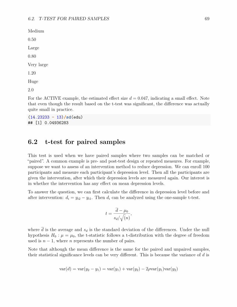
6.2. T-TEST FOR PAIRED SAMPLES 69
Medium
0.50
Large
0.80
Very large
1.20
Huge
2.0
For the ACTIVE example, the estimated effect size d = 0.047, indicating a small effect. Notethat even though the result based on the t-test was significant, the difference was actuallyquite small in practice.(14.23233 - 13)/sd(edu)## [1] 0.04936283
6.2 t-test for paired samples
This test is used when we have paired samples where two samples can be matched or“paired”. A common example is pre- and post-test design or repeated measures. For example,suppose we want to assess of an intervention method to reduce depression. We can enroll 100participants and measure each participant’s depression level. Then all the participants aregiven the intervention, after which their depression levels are measured again. Our interest isin whether the intervention has any effect on mean depression levels.
To answer the question, we can first calculate the difference in depression level before andafter intervention: di = yi2 − yi1. Then di can be analyzed using the one-sample t-test.
t = d− µ0
sd/√
(n),
where d is the average and sd is the standard deviation of the differences. Under the nullhypothesis H0 : µ = µ0, the t-statistic follows a t-distribution with the degree of freedomused is n− 1, where n represents the number of pairs.
Note that although the mean difference is the same for the paired and unpaired samples,their statistical significance levels can be very different. This is because the variance of d is
var(d) = var(y2 − y1) = var(y1) + var(y2)− 2ρvar(y1)var(y2)
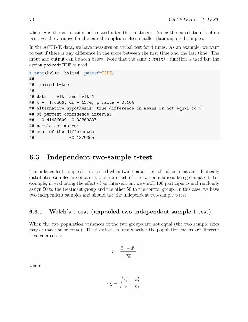
70 CHAPTER 6. T-TEST
where ρ is the correlation before and after the treatment. Since the correlation is oftenpositive, the variance for the paired samples is often smaller than unpaired samples.
In the ACTIVE data, we have measures on verbal test for 4 times. As an example, we wantto test if there is any difference in the score between the first time and the last time. Theinput and output can be seen below. Note that the same t.test() function is used but theoption paired=TRUE is used.t.test(hvltt, hvltt4, paired=TRUE)#### Paired t-test#### data: hvltt and hvltt4## t = -1.6266, df = 1574, p-value = 0.104## alternative hypothesis: true difference in means is not equal to 0## 95 percent confidence interval:## -0.41456609 0.03869307## sample estimates:## mean of the differences## -0.1879365
6.3 Independent two-sample t-test
The independent samples t-test is used when two separate sets of independent and identicallydistributed samples are obtained, one from each of the two populations being compared. Forexample, in evaluating the effect of an intervention, we enroll 100 participants and randomlyassign 50 to the treatment group and the other 50 to the control group. In this case, we havetwo independent samples and should use the independent two-sample t-test.
6.3.1 Welch’s t test (unpooled two independent sample t test)
When the two population variances of the two groups are not equal (the two sample sizesmay or may not be equal). The t statistic to test whether the population means are differentis calculated as:
t = x1 − x2
s∆
where
s∆ =√s2
1n1
+ s22n2.

6.3. INDEPENDENT TWO-SAMPLE T-TEST 71
Here, s21 and s2
2 are the unbiased estimators of the variances of the two samples with nk =number of participants in group k = 1 or 2. For use in significance testing, the distributionof the test statistic is approximated as an ordinary Student’s t distribution with the degreesof freedom calculated as
d.f. = (s21/n1 + s2
2/n2)2
(s21/n1)2/(n1 − 1) + (s2
2/n2)2/(n2 − 1)
This is known as the Welch-Satterthwaite equation. The true distribution of the test statisticactually depends (slightly) on the two unknown population variances.
In R, the function t.test() can be used to conduct a t test. The following code conducts theWelch’s t test. Note that alternative = "greater" sets the alternative hypothesis. Theother options include two.sided and less.training<-hvltt2[group==1]control<-hvltt2[group==4]
mean(training, na.rm=T)-mean(control, na.rm=T)## [1] 1.970935
t.test(training, control, alternative = 'greater')#### Welch Two Sample t-test#### data: training and control## t = 5.0416, df = 775.37, p-value = 2.876e-07## alternative hypothesis: true difference in means is greater than 0## 95 percent confidence interval:## 1.327135 Inf## sample estimates:## mean of x mean of y## 26.10204 24.13111
6.3.2 Pooled two independent sample t test
When the two samples have the same population variance.The t statistic can be calculatedas follows:
t = x1 − x2
sp ·√
1n1
+ 1n2
where
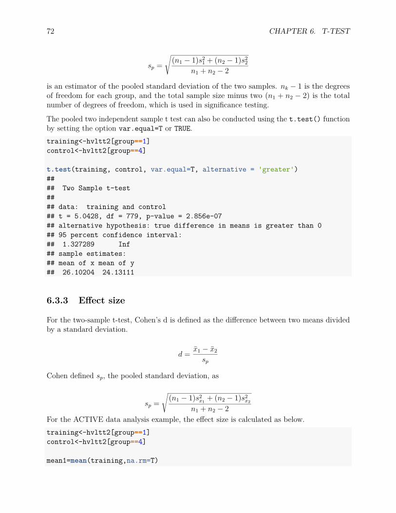
72 CHAPTER 6. T-TEST
sp =√
(n1 − 1)s21 + (n2 − 1)s2
2n1 + n2 − 2
is an estimator of the pooled standard deviation of the two samples. nk − 1 is the degreesof freedom for each group, and the total sample size minus two (n1 + n2 − 2) is the totalnumber of degrees of freedom, which is used in significance testing.
The pooled two independent sample t test can also be conducted using the t.test() functionby setting the option var.equal=T or TRUE.training<-hvltt2[group==1]control<-hvltt2[group==4]
t.test(training, control, var.equal=T, alternative = 'greater')#### Two Sample t-test#### data: training and control## t = 5.0428, df = 779, p-value = 2.856e-07## alternative hypothesis: true difference in means is greater than 0## 95 percent confidence interval:## 1.327289 Inf## sample estimates:## mean of x mean of y## 26.10204 24.13111
6.3.3 Effect size
For the two-sample t-test, Cohen’s d is defined as the difference between two means dividedby a standard deviation.
d = x1 − x2
sp
Cohen defined sp, the pooled standard deviation, as
sp =√
(n1 − 1)s2x1 + (n2 − 1)s2
x2
n1 + n2 − 2For the ACTIVE data analysis example, the effect size is calculated as below.training<-hvltt2[group==1]control<-hvltt2[group==4]
mean1=mean(training,na.rm=T)

6.3. INDEPENDENT TWO-SAMPLE T-TEST 73
mean2=mean(control,na.rm=T)meandiff=mean1-mean2
n1=length(training)-sum(is.na(training))n2=length(control)-sum(is.na(control))
v1=var(training,na.rm=T)v2=var(control,na.rm=T)s=sqrt(((n1-1)*v1+(n2-1)*v2)/(n1+n2-2))s## [1] 5.461292
cohend=meandiffcohend## [1] 1.970935

74 CHAPTER 6. T-TEST

Chapter 7
Analysis of variance
Analysis of variance (ANOVA) is a collection of statistical models used to analyze thedifferences between group means, developed by R.A. Fisher (Fisher, 1925). In ANOVA,the observed variance in a particular variable, usually an outcome variable, is partitionedinto components attributable to different sources of variation: typically the between-groupvariation and the within-group variation. Simply speaking, ANOVA provides a statisticaltest of whether or not the means of several groups are equal, and therefore generalizes thet-test to more than two groups.
7.1 One-way ANOVA
One-way ANOVA typically evaluates whether there is difference in means of three or moregroups, although it also works for two-group analysis. In other words, it investigates theeffect a grouping variable on the outcome variable.
In the ACTIVE data, we have 4 groups: one control group and three training groups -memory, reasoning, and speed training groups. As an example, we test whether there isany difference in the four groups in terms of memory performance measured by the HopkinsVerbal Learning Test, denoted by the hvltt2 variable in the data set. Then, one-way ANOVAcan be used.
Specifically for this example, the null and alternative hypotheses
H0 : µ1 = µ2 = µ3 = µ4
Ha : H0 is not true or at least two groups have different means.
For the hypothesis testing, an F-test is used. The basic idea is to decompose the totalvariation of the outcome variance into the variation because of the difference between groups
75

76 CHAPTER 7. ANALYSIS OF VARIANCE
and the variation within groups. The variation is measured by the sum of squares. Forone-way ANOVA, we have
SST = SSB + SSW
• SST is the total sum of squares.• SSB is the between-group sum of squares.• SSW is the within-group sum of squares.
Then the F-statistic isF = SSB/dfB
SSW/dfW= MSB
MSW
• dfB is the between-group degrees of freedom, which is equal to the number of groups -1. For the ACTIVE example, it is 4− 1 = 3.
• dfW is the within-group degrees of freedom, which is equal to the total sample size -the number of groups. Since the sample size is 1575, dfW = 1575− 4 = 1571.
If the null hypothesis is true, the F-statistic should follow an F distribution with degreesof freedom dfB and dfW under certain condition. The R code below conducts the one-wayANOVA for the ACTIVE data.
• ANOVA in R is based on the linear regression. Therefore, the model is fitted using thefunction lm(). Then the function anova() is used to construct the ANOVA source ofvariation table. In the table, the sum of squares (Sum Sq), mean sum of squares (MeanSq), degrees of freedom (Df), F value and p-value (Pr(>F)) are included.
• In the data set, the group variable is coded using numeric values. To conduct ANOVA,one needs to first change it to a grouping variable, which is done using the functionfactor().
• Specifically for this example, we have F=10.051. Comparing it to an F distributionwith degrees of freedom (3, 1571), we obtain the p-value = 1.466e-06. Therefore, onewould reject the null hypothesis. The memory performance significantly differed acrossthe 4 groups.
active <- read.csv("data/active.csv")attach(active)
model<-lm(hvltt~factor(group))anova(model)## Analysis of Variance Table#### Response: hvltt## Df Sum Sq Mean Sq F value Pr(>F)## factor(group) 3 130 43.251 1.7464 0.1556## Residuals 1571 38907 24.766
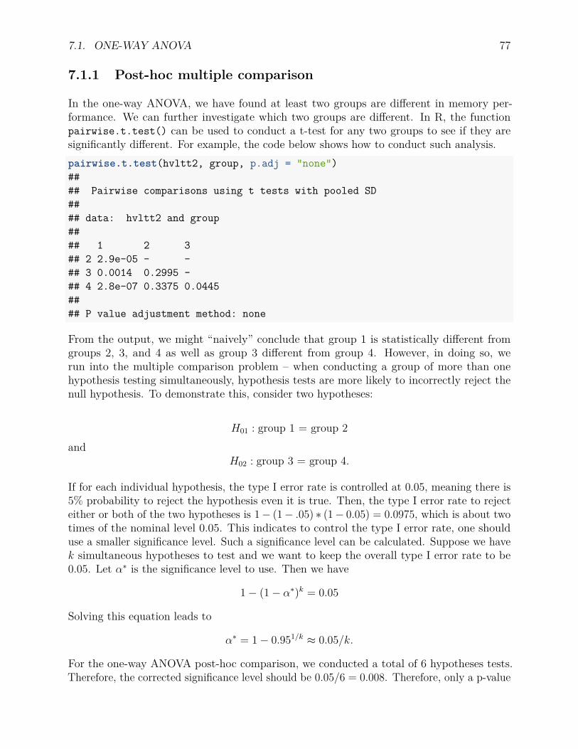
7.1. ONE-WAY ANOVA 77
7.1.1 Post-hoc multiple comparison
In the one-way ANOVA, we have found at least two groups are different in memory per-formance. We can further investigate which two groups are different. In R, the functionpairwise.t.test() can be used to conduct a t-test for any two groups to see if they aresignificantly different. For example, the code below shows how to conduct such analysis.pairwise.t.test(hvltt2, group, p.adj = "none")#### Pairwise comparisons using t tests with pooled SD#### data: hvltt2 and group#### 1 2 3## 2 2.9e-05 - -## 3 0.0014 0.2995 -## 4 2.8e-07 0.3375 0.0445#### P value adjustment method: none
From the output, we might “naively” conclude that group 1 is statistically different fromgroups 2, 3, and 4 as well as group 3 different from group 4. However, in doing so, werun into the multiple comparison problem – when conducting a group of more than onehypothesis testing simultaneously, hypothesis tests are more likely to incorrectly reject thenull hypothesis. To demonstrate this, consider two hypotheses:
H01 : group 1 = group 2and
H02 : group 3 = group 4.
If for each individual hypothesis, the type I error rate is controlled at 0.05, meaning there is5% probability to reject the hypothesis even it is true. Then, the type I error rate to rejecteither or both of the two hypotheses is 1− (1− .05) ∗ (1− 0.05) = 0.0975, which is about twotimes of the nominal level 0.05. This indicates to control the type I error rate, one shoulduse a smaller significance level. Such a significance level can be calculated. Suppose we havek simultaneous hypotheses to test and we want to keep the overall type I error rate to be0.05. Let α∗ is the significance level to use. Then we have
1− (1− α∗)k = 0.05
Solving this equation leads to
α∗ = 1− 0.951/k ≈ 0.05/k.
For the one-way ANOVA post-hoc comparison, we conducted a total of 6 hypotheses tests.Therefore, the corrected significance level should be 0.05/6 = 0.008. Therefore, only a p-value
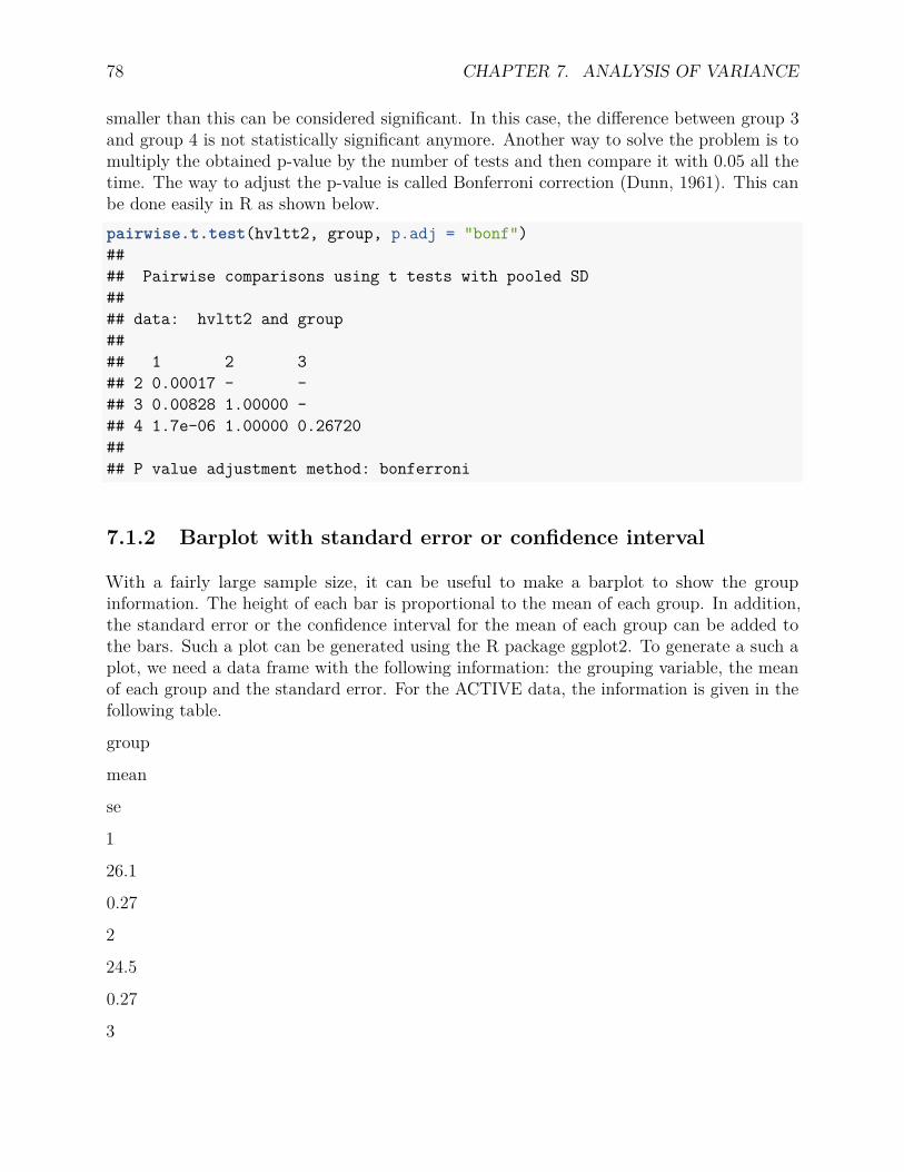
78 CHAPTER 7. ANALYSIS OF VARIANCE
smaller than this can be considered significant. In this case, the difference between group 3and group 4 is not statistically significant anymore. Another way to solve the problem is tomultiply the obtained p-value by the number of tests and then compare it with 0.05 all thetime. The way to adjust the p-value is called Bonferroni correction (Dunn, 1961). This canbe done easily in R as shown below.pairwise.t.test(hvltt2, group, p.adj = "bonf")#### Pairwise comparisons using t tests with pooled SD#### data: hvltt2 and group#### 1 2 3## 2 0.00017 - -## 3 0.00828 1.00000 -## 4 1.7e-06 1.00000 0.26720#### P value adjustment method: bonferroni
7.1.2 Barplot with standard error or confidence interval
With a fairly large sample size, it can be useful to make a barplot to show the groupinformation. The height of each bar is proportional to the mean of each group. In addition,the standard error or the confidence interval for the mean of each group can be added tothe bars. Such a plot can be generated using the R package ggplot2. To generate a such aplot, we need a data frame with the following information: the grouping variable, the meanof each group and the standard error. For the ACTIVE data, the information is given in thefollowing table.
group
mean
se
1
26.1
0.27
2
24.5
0.27
3

7.1. ONE-WAY ANOVA 79
24.9
0.25
4
24.1
0.29
The R code below calculates the information in the table and generates a bar plot as shownin the output. We now explain each line of the R code.library(Rmisc)library(ggplot2)
stats <- summarySE(active, measurevar="hvltt2", groupvars=c("group"))stats## group N hvltt2 sd se ci## 1 1 392 26.10204 5.293416 0.2673579 0.5256389## 2 2 387 24.49871 5.307817 0.2698115 0.5304842## 3 3 407 24.89189 5.116197 0.2536005 0.4985340## 4 4 389 24.13111 5.625401 0.2852192 0.5607685
ggplot(stats, aes(x=factor(group), y=hvltt2)) +geom_bar(stat="identity", fill="blue", width=0.8) +geom_errorbar(aes(ymin=hvltt2-se, ymax=hvltt2+se),
width=.2, colour='red') +xlab("Groups") +ylab("Memory test score") +scale_x_discrete(breaks=c("1", "2", "3", "4"),
labels=c("Memory", "Reasoning", "Speed", "Control"))
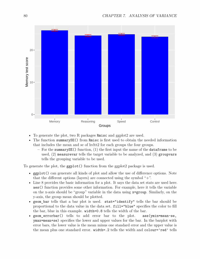
80 CHAPTER 7. ANALYSIS OF VARIANCE
0
10
20
Memory Reasoning Speed Control
Groups
Mem
ory
test
sco
re
• To generate the plot, two R packages Rmisc and ggplot2 are used.• The function summarySE() from Rmisc is first used to obtain the needed information
that includes the mean and se of hvltt2 for each groups the four groups.– For the summarySE() function, (1) the first input the name of the dataframe to be
used, (2) measurevar tells the target variable to be analyzed, and (3) groupvarstells the grouping variable to be used.
To generate the plot, the ggplot() function from the ggplot2 package is used.
• ggplot() can generate all kinds of plot and allow the use of difference options. Notethat the different options (layers) are connected using the symbol “+”.
• Line 8 provides the basic information for a plot. It says the data set stats are used here.aes() function provides some other information. For example, here it tells the variableon the x-axis should be “group” variable in the data using x=group. Similarly, on they-axis, the group mean should be plotted.
• geom_bar tells that a bar plot is used. stat="identify" tells the bar should beproportional to the data value in the data set. fill="blue" specifies the color to fillthe bar, blue in this example. width=0.8 tells the width of the bar.
• geom_errorbar() tells to add error bar to the plot. aes(ymin=mean-se,ymax=mean+se) specifies the lower and upper values for the bar. In the barplot witherror bars, the lower value is the mean minus one standard error and the upper value isthe mean plus one standard error. width=.2 tells the width and colour='red' tells
7.2. TWO-WAY ANOVA 81
the color of the error bars.• xlab and ylab add the labels for the x-axis and y-axis.• scale_x_discrete can be used to customize the labels for each group. In the original
data, the 4 groups are represented by 1, 2, 3, and 4. breaks tells the position of theoriginal data and labels provides the new labels for each group.
7.2 Two-way ANOVA
Two-way analysis of variance (two-way ANOVA) is an extension of the one-way ANOVA toexamine the influence of two different categorical independent variables on one continuousdependent variable. The two-way ANOVA can evaluate not only the main effect of eachindependent variable but also the potential interaction between them. For example, for theACTIVE data, we can test whether the four training groups and gender are related to thememory test performance.
7.2.1 Type of effects and hypotheses
In two-way ANOVA with two factors (independent variables) A and B, we can test two maineffects and one interaction effect:
• Main effect of A: whether the population means are the same for different levels (groups)of A?– The null hypothesis: the population means are the same for different levels of A.
• Main effect of A: whether the population means are the same for different levels (groups)of A?– The null hypothesis: the population means are the same for different levels of A.
• The interaction effect of A and B: whether the difference in the population means fordifference level of A depends on the level of B or vice visa?– The null hypothesis: the effect of A or B on the outcome does not depend on B or
A.
7.2.2 Two-way ANOVA F tests
Like in one-way ANOVA, F test is used in hypothesis testing. The test is constructed basedon the decomposition of the sum of squares of the outcome variables. Specifically, we have
SST = SSA + SSB + SSA×B + SSW
• SST or SStotal is the sum of squares for the outcome variable.• SSA is the sum of squares attributes to the factor A.• SSB is the sum of squares attributes to the factor B.• SSA×B is the sum of squares attributes to the joint effect of A and B.

82 CHAPTER 7. ANALYSIS OF VARIANCE
• SSW or SSwithin is the residual sum of squares that cannot be explain by A, B or theirinteraction.
Let N be the sample size, J is the number of levels in factor A, and K is the number of levelsin factor B. With the information, we can construct a source of variance table below:
Source
Sum of squares
Degree of freedom
Mean square
F statistic
Factor A
SSA
J − 1
MSA = SSA
J−1
FA = MSA
MSW
Factor B
SSB
K − 1
MSB = SSB
K−1
FB = MSB
MSW
Interaction A*B
SSA×B
(J − 1) ∗ (K − 1)
MSA×B = SSA×B
(J−1)×(K−1)
FA×B = MSA×B
MSW
Within
SSW
N − (J ×K)
MSW = SSW
N−(J×K)
Total
SST
7.2. TWO-WAY ANOVA 83
N − 1
It is easy to see that SST = SSA+SSB+SSA×B+SSW . For testing the effect of Factor A, wecompare the statistic FA to an F distribution with degrees of freedom J − 1 and N − (J ×K).For testing the effect of Factor B, we compare the statistic FB to an F distribution withdegrees of freedom K − 1 and N − (J × K). To test the interaction effect of Factor Aand Factor B, we compare the statistic FA×B to an F distribution with degrees of freedom(J − 1) ∗ (K − 1) and N − (J ×K).
7.2.3 Example: Effects of training and gender on the memory testperformance
As an example, we test the effect of training and gender on the memory test performanceusing the ACTIVE data. We want to answer the following questions:
1. At the population level, are there any difference in memory test performance for the 4training groups?
2. At the population level, are there any difference in memory test performance for maleand female participants?
3. Do the effects of training on the memory test performance differ across the two gendergroups?
The R code below carries out the two-way ANOVA to answer the above questions.model<-lm(hvltt2~factor(group)*factor(sex), data=active)anova(model)## Analysis of Variance Table#### Response: hvltt2## Df Sum Sq Mean Sq F value Pr(>F)## factor(group) 3 859 286.20 10.2434 1.114e-06 ***## factor(sex) 1 919 919.28 32.9013 1.161e-08 ***## factor(group):factor(sex) 3 34 11.46 0.4102 0.7457## Residuals 1567 43783 27.94## ---## Signif. codes: 0 '***' 0.001 '**' 0.01 '*' 0.05 '.' 0.1 ' ' 1
7.2.3.1 Main effect of training group
From the output, the F-statistic for testing the main effect of training group is 10.2434.Based on the F distribution with degrees of freedom 3 and 1567, the corresponding p-value is1.114e-06, which indicates a significant main effect for training group. Therefore, one mayconclude there is significant difference in memory performance among the four groups.

84 CHAPTER 7. ANALYSIS OF VARIANCE
7.2.3.2 Main effect of sex
From the output, the F-statistic for testing the main effect of sex is 32.9013. Based on theF distribution with degrees of freedom 1 and 1567, the corresponding p-value is 1.161e-08,which indicates a significant main effect sex. Therefore, one may conclude there is significantdifference in memory performance between the male and female participants.
7.2.3.3 Interaction effect between training group and sex
From the output, the F-statistic for testing the interaction effect [factor(group):factor(sex)]is 0.41. Based on the F distribution with degrees of freedom 3 and 1567, the correspondingp-value is 0.7457, which indicates an insignificant interaction effect. Therefore, one mayconclude the difference in memory performance among the four training group does notdepend on sex.
7.2.4 Plot data
As in one-way ANOVA, we can also plot data with two factors with error bars. The codebelow can be used.stats <- summarySE(active, measurevar="hvltt2", groupvars=c("group","sex"))stats## group sex N hvltt2 sd se ci## 1 1 1 85 24.52941 5.412922 0.5871138 1.1675401## 2 1 2 307 26.53746 5.184920 0.2959190 0.5822937## 3 2 1 92 23.34783 5.453973 0.5686160 1.1294858## 4 2 2 295 24.85763 5.219019 0.3038631 0.5980225## 5 3 1 84 23.78571 5.477383 0.5976314 1.1886649## 6 3 2 323 25.17957 4.986810 0.2774735 0.5458900## 7 4 1 112 22.54464 5.950075 0.5622293 1.1140948## 8 4 2 277 24.77256 5.367870 0.3225240 0.6349197
ggplot(stats,aes(x = factor(group), y = hvltt2, fill = factor(sex),
ymax=hvltt2+se, ymin=hvltt2-se)) +geom_bar(stat="identity", position = "dodge", width = 0.7) +geom_bar(stat="identity", position = "dodge",
colour = "black", width = 0.7) +geom_errorbar(position=position_dodge(width=0.7),
width=0.2, size=0.5, color="black") +labs(x = "Group",
y = "Memory performance") +
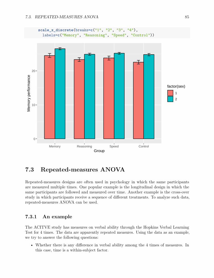
7.3. REPEATED-MEASURES ANOVA 85
scale_x_discrete(breaks=c("1", "2", "3", "4"),labels=c("Memory", "Reasoning", "Speed", "Control"))
0
10
20
Memory Reasoning Speed Control
Group
Mem
ory
perf
orm
ance
factor(sex)
1
2
7.3 Repeated-measures ANOVA
Repeated-measures designs are often used in psychology in which the same participantsare measured multiple times. One popular example is the longitudinal design in which thesame participants are followed and measured over time. Another example is the cross-overstudy in which participants receive a sequence of different treatments. To analyze such data,repeated-measures ANOVA can be used.
7.3.1 An example
The ACITVE study has measures on verbal ability through the Hopkins Verbal LearningTest for 4 times. The data are apparently repeated measures. Using the data as an example,we try to answer the following questions:
• Whether there is any difference in verbal ability among the 4 times of measures. Inthis case, time is a within-subject factor.
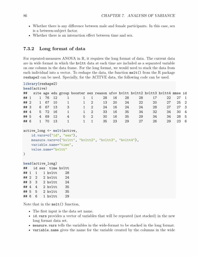
86 CHAPTER 7. ANALYSIS OF VARIANCE
• Whether there is any difference between male and female participants. In this case, sexis a between-subject factor.
• Whether there is an interaction effect between time and sex.
7.3.2 Long format of data
For repeated-measures ANOVA in R, it requires the long format of data. The current dataare in wide format in which the hvltt data at each time are included as a separated variableon one column in the data frame. For the long format, we would need to stack the data fromeach individual into a vector. To reshape the data, the function melt() from the R packagereshape2 can be used. Specially, for the ACITVE data, the following code can be used.library(reshape2)head(active)## site age edu group booster sex reason ufov hvltt hvltt2 hvltt3 hvltt4 mmse id## 1 1 76 12 1 1 1 28 16 28 28 17 22 27 1## 2 1 67 10 1 1 2 13 20 24 22 20 27 25 2## 3 6 67 13 3 1 2 24 16 24 24 28 27 27 3## 4 5 72 16 1 1 2 33 16 35 34 32 34 30 4## 5 4 69 12 4 0 2 30 16 35 29 34 34 28 5## 6 1 70 13 1 1 1 35 23 29 27 26 29 23 6
active_long <- melt(active,id.vars=c("id", "sex"),measure.vars=c("hvltt", "hvltt2", "hvltt3", "hvltt4"),variable.name="time",value.name="hvltt"
)
head(active_long)## id sex time hvltt## 1 1 1 hvltt 28## 2 2 2 hvltt 24## 3 3 2 hvltt 24## 4 4 2 hvltt 35## 5 5 2 hvltt 35## 6 6 1 hvltt 29
Note that in the melt() function,
• The first input is the data set name.• id.vars provides a vector of variables that will be repeated (not stacked) in the new
long format data set.• measure.vars tells the variables in the wide-format to be stacked in the long format.• variable.name gives the name for the variable created by the columns in the wide

7.3. REPEATED-MEASURES ANOVA 87
format.• value.name gives the name for the variable created by the data in the long format. In
this example, that is hvltt data.
7.3.3 One within-subject factor
We first consider just one within-subject factor, time, to evaluate whether there is anydifference in verbal ability across the 4 times of data. To answer the question, the followinganalysis can be conducted.ex1<-aov(hvltt~time+Error(id/time), data=active_long)summary(ex1)#### Error: id## Df Sum Sq Mean Sq F value Pr(>F)## Residuals 1 0.3716 0.3716#### Error: id:time## Df Sum Sq Mean Sq## time 3 3800 1267#### Error: Within## Df Sum Sq Mean Sq F value Pr(>F)## time 3 1112 370.7 13.12 1.54e-08 ***## Residuals 6292 177742 28.2## ---## Signif. codes: 0 '***' 0.001 '**' 0.01 '*' 0.05 '.' 0.1 ' ' 1
To look at the effect of “time”, we check the output in the “Error: Within” section. For theF value 13.12 with the degrees of freedom 3 and 6292, we have p-value 1.54e-08. Therefore,there is a significant difference among the 4 times of data.
Note that to conduct the repeated-measures ANOVA, the R function aov() is used. Thefunction uses the regular expression to represent the model. In this case, the outcome ishvltt and the predictor is time. Error(id/time) is used to divide the error variance into 4different clusters, which therefore takes into account of the repeated measures.
7.3.4 One within-subject factor and one between-subject factor
As an example, we consider an additional between-subject factor, sex. With the two factors,we can also test the interaction effect between time and sex. The code below can be used toconduct the analysis. Based on the output, we have significant time and sex effects but nointeraction effect.

88 CHAPTER 7. ANALYSIS OF VARIANCE
ex2<-aov(hvltt~time*sex+Error(id/(time*sex)), data=active_long)summary(ex2)#### Error: id## Df Sum Sq Mean Sq## sex 1 0.3716 0.3716#### Error: id:time## Df Sum Sq Mean Sq## time 3 3800 1267#### Error: id:sex## Df Sum Sq Mean Sq## sex 1 5020 5020#### Error: id:time:sex## Df Sum Sq Mean Sq## time 3 204.9 68.29#### Error: Within## Df Sum Sq Mean Sq F value Pr(>F)## time 3 1091 363.8 13.383 1.05e-08 ***## sex 1 1592 1592.1 58.564 2.26e-14 ***## time:sex 3 116 38.6 1.419 0.235## Residuals 6284 170830 27.2## ---## Signif. codes: 0 '***' 0.001 '**' 0.01 '*' 0.05 '.' 0.1 ' ' 1

Chapter 8
Simple Linear Regression
In the ACTIVE study, we have data on verbal ability at two times (hvltt and hvltt2). Toinvestigate the relationship between them, we can generate a scatterplot using hvltt andhvltt2 as shown below. From the plot, it is easy to observe that those with a higher score onhvltt tend to have a higher score on hvltt2. Certainly, it is not difficult to find two peoplewhere the one with higher score on hvltt has a lower score on hvltt2. But in general hvlttand hvltt2 tend to go up and down together.
Furthermore, the association between hvltt and hvltt2 seems to be able to be described by astraight line. The red line in the figure is one that run across the points in the scatter plot.The straight line can be expressed using
hvltt2 = 5.19 + 0.73 ∗ hvltt
It says multiplying one’s test score (hvltt) at the first occasion by 0.73 and adding 5.19predict his/her test score (hvltt2) at the second occasion.active <- read.csv("data/active.csv")attach(active)
plot(hvltt, hvltt2)abline(5.19, 0.73, col='red')
89
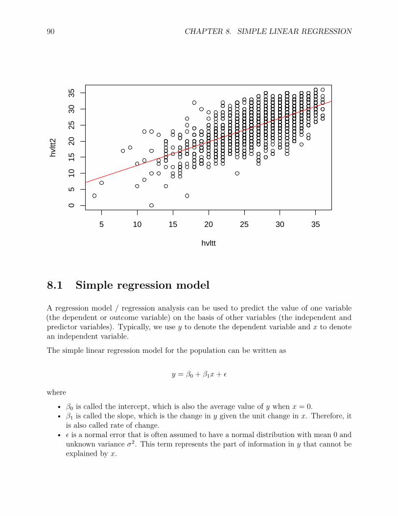
90 CHAPTER 8. SIMPLE LINEAR REGRESSION
5 10 15 20 25 30 35
05
1015
2025
3035
hvltt
hvltt
2
8.1 Simple regression model
A regression model / regression analysis can be used to predict the value of one variable(the dependent or outcome variable) on the basis of other variables (the independent andpredictor variables). Typically, we use y to denote the dependent variable and x to denotean independent variable.
The simple linear regression model for the population can be written as
y = β0 + β1x+ ε
where
• β0 is called the intercept, which is also the average value of y when x = 0.• β1 is called the slope, which is the change in y given the unit change in x. Therefore, it
is also called rate of change.• ε is a normal error that is often assumed to have a normal distribution with mean 0 and
unknown variance σ2. This term represents the part of information in y that cannot beexplained by x.

8.2. PARAMETER ESTIMATION 91
8.2 Parameter estimation
In practice, the population parameters β0 and β1 are unknown. However, with a set of sampledata, they can be estimated. One often used estimation method for regression analysis iscalled least squares estimation method. We explain the method here.
Let the model below represent the estimated regression model:
y = b0 + b1x+ e
where
• b0 is an estimate of the population intercept β0• b1 is an estimate of the population slope β1• e is the residual, which estimate ε.
Assume we already get the estimates b0 and b1, then we can make a prediction of the valueof y based on the value of x. For example, for the ith participant, if his/her score onthe independent variable is xi, then the corresponding predicted outcome yi based on theregression model is
yi = b0 + b1xi.
The difference between the predicted value and the observed data for this participant, alsocalled the prediction error, is
ei = yi − yi.
The parameter b0 and b1 potentially can take any values. A good choice could be those thatmake the errors smallest, which leads to the least squares estimation.
8.2.1 Least squares estimation
The least squares estimation obtains b0 and b1 by minimizing the sum of the squared predictionerrors. Therefore, such a set of parameters makes yi closest to yi on average. Specifically, oneminimizes SSE as
SSE = ∑ni=1 e
2i = ∑n
i=1(yi − yi)2 = ∑ni=1(yi − b0 − b1xi)2.
The values of b0 and b1 that minimize SSE can be calculated by
b1 = SxyS2x
=∑ni=1(xi − x)(yi − y)∑n
i=1(xi − x)2
and
92 CHAPTER 8. SIMPLE LINEAR REGRESSION
b0 = y − b1x
where x = ∑ni=1 xi/n and y = ∑n
i=1 yi/n.
8.2.2 Hypothesis testing
If no linear relationship exists between the two variables, we would expect the regressionline to be horizontal, that is, to have a slope of zero. Therefore, we can test whether thehypothesis that the population regression slope is 0. More specifically, we have the nullhypothesis
H0 : β1 = 0.
And the alternative hypothesis is
H1 : β1 6= 0.
To conduct the hypothesis testing, we calculate a t test statistic
t = b1 − β1
sb1
where sb1 is the standard error of b1.
If β1 = 0 in the population, then the statistic t follows a t-distribution with degrees of freedomn− 2.
8.2.3 Regression in R
Both the parameter estimates and the t test can be conducted using an R function lm().
8.3 An example
To show how to conduct a simple linear regression, we analyze the relationship between hvlttand hvltt2 from the ACTIVE study. The R input and output for the regression analysis isgiven below.
• Within the function lm(), the first required input is a “formula” to specify the model.A model is usually formed by the “~” operator. For a regression, we use y ~ x, whichis interpreted as the outcome variable y is modelled by a linear predictor x. Therefore,for the regression analysis in this specific example, we use hvltt2 ~ hvltt.
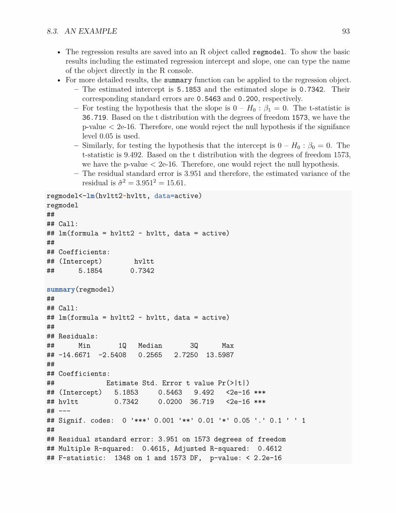
8.3. AN EXAMPLE 93
• The regression results are saved into an R object called regmodel. To show the basicresults including the estimated regression intercept and slope, one can type the nameof the object directly in the R console.
• For more detailed results, the summary function can be applied to the regression object.– The estimated intercept is 5.1853 and the estimated slope is 0.7342. Their
corresponding standard errors are 0.5463 and 0.200, respectively.– For testing the hypothesis that the slope is 0 – H0 : β1 = 0. The t-statistic is
36.719. Based on the t distribution with the degrees of freedom 1573, we have thep-value < 2e-16. Therefore, one would reject the null hypothesis if the signifancelevel 0.05 is used.
– Similarly, for testing the hypothesis that the intercept is 0 – H0 : β0 = 0. Thet-statistic is 9.492. Based on the t distribution with the degrees of freedom 1573,we have the p-value < 2e-16. Therefore, one would reject the null hypothesis.
– The residual standard error is 3.951 and therefore, the estimated variance of theresidual is σ2 = 3.9512 = 15.61.
regmodel<-lm(hvltt2~hvltt, data=active)regmodel#### Call:## lm(formula = hvltt2 ~ hvltt, data = active)#### Coefficients:## (Intercept) hvltt## 5.1854 0.7342
summary(regmodel)#### Call:## lm(formula = hvltt2 ~ hvltt, data = active)#### Residuals:## Min 1Q Median 3Q Max## -14.6671 -2.5408 0.2565 2.7250 13.5987#### Coefficients:## Estimate Std. Error t value Pr(>|t|)## (Intercept) 5.1853 0.5463 9.492 <2e-16 ***## hvltt 0.7342 0.0200 36.719 <2e-16 ***## ---## Signif. codes: 0 '***' 0.001 '**' 0.01 '*' 0.05 '.' 0.1 ' ' 1#### Residual standard error: 3.951 on 1573 degrees of freedom## Multiple R-squared: 0.4615, Adjusted R-squared: 0.4612## F-statistic: 1348 on 1 and 1573 DF, p-value: < 2.2e-16
94 CHAPTER 8. SIMPLE LINEAR REGRESSION
8.4 Coefficient of Determination (Multiple R-squared)
Significant tests show if a linear relationship exists but not the strength of the relation-ship. The coefficient of determination, R2, is a descriptive measure of the strength of theregression relationship, a measure on how well the regression line fits the data. In general thehigher the value of R2, the better the model fits the data.
• R2 = 1: Perfect match between the line and the data points.• R2 = 0: There are no linear relationship between x and y.
R2 is an effect size measure. Cohen (1988) defined some standards for interpreting R2.
• R2 = .01: Small effect• R2 = .06: Medium effect• R2 = .15: Large effect.
For the regression example, the R2 = 0.4615, representing a large effect.
8.4.1 Calculation and interpretation of R2
Simply speaking, the R2 tells the percentage of variance in y that can be explained by theregression model or by x.
The variance of y is
V ar(y) =n∑i=1
(yi − y)2
With some simple re-arrangement, we have
V ar(y) =n∑i=1
(yi − y)2
=n∑i=1
(yi − yi + yi − y)2
=n∑i=1
(yi − yi)2 +n∑i=1
(yi − y)2
= Residual variance + Variance explained by regression.
And the R2 is
R2 =∑ni=1(yi − y)2
V ar(y) = 1−∑ni=1(yi − yi)2
V ar(y) .
This can be illustrated using the figure below.

8.4. COEFFICIENT OF DETERMINATION (MULTIPLE R-SQUARED) 95

96 CHAPTER 8. SIMPLE LINEAR REGRESSION

Chapter 9
Multiple Linear Regression
9.1 Multiple Regression Analysis
The general purpose of multiple regression (the term was first used by Pearson, 1908), as ageneralization of simple linear regression, is to learn about how several independent variablesor predictors (IVs) together predict a dependent variable (DV). Multiple regression analysisoften focuses on understanding (1) how much variance in a DV a set of IVs explain and (2)the relative predictive importance of IVs in predicting a DV.
In the social and natural sciences, multiple regression analysis is very widely used in research.Multiple regression allows a researcher to ask (and hopefully answer) the general question“what is the best predictor of . . . ”. For example, educational researchers might want to learnwhat the best predictors of success in college are. Psychologists may want to determine whichpersonality dimensions best predicts social adjustment.
9.1.1 Multiple regression model
A general multiple linear regression model at the population level can be written as
yi = β0 + β1x1i + β2x2i + . . .+ βkxki + εi
• yi: the observed score of individual i on the DV.• x1, x2, . . . , xk : a set of predictors.• x1i: the observed score of individual i on IV 1; xki: observed score of individual i on IVk.
• β0: the intercept at the population level, representing the predicted y score when allthe independent variables have their values at 0.
• β1, . . . , βk: regression coefficients at the population level; β1: representing the amountpredicted y changes when x1 changes in 1 unit while holding the other IVs constant; βk:
97
98 CHAPTER 9. MULTIPLE LINEAR REGRESSION
representing the amount predicted y changes when xk changes in 1 unit while holdingthe other IVs constant.
• ε: unobserved errors with mean 0 and variance σ2.
9.1.2 Parameter estimation
The least squares method used for the simple linear regression analysis can also be usedto estimate the parameters in a multiple regression model. The basic idea is to minimizethe sum of squared residuals or errors. Let b0, b1, . . . , bk represent the estimated regressioncoefficients.The individual i’s residual ei is the difference between the observed yi and thepredicted yi
ei = yi − yi = yi − b0 − b1x1i − . . .− bkxki.
The sum of squared residuals is
SSE =n∑i=1
e2i =
n∑i=1
(yi − yi)2.
By minimizing SSE, the regression coefficient estimates can be obtained as
b = (X ′X)−1X ′y = (∑
xix′i)−1(
∑xiyi).
9.1.3 R2
How well the multiple regression model fits the data can be assessed using the R2. Itscalculation is the same as for the simple regression
R2 = 1−∑e2i∑n
i=1(yi − y)2
= Variation explained by IVsTotal variation
.
In multiple regression, R2 is the total proportion of variation in y explained by the multiplepredictors.
The R2 increases or at least is the same with the inclusion of more predictors. However, withmore predators, the model becomes more complex and potentially more difficult to interpret.In order to take into consideration of the model complexity, the adjusted R2 has been defined,which is calculated as
aR2 = 1− (1−R2) n− 1n− k − 1 .
9.1. MULTIPLE REGRESSION ANALYSIS 99
9.1.4 Hypothesis testing of regression coefficient(s)
With the estimates of regression coefficients and their standard errors estimates, we canconduct hypothesis testing for one, a subset, or all regression coefficients.
9.1.4.1 Testing a single regression coefficient
At first, we can test the significance of the coefficient for a single predictor. In this situation,the null and alternative hypotheses are
H0 : βj = 0 vs H1 : βj 6= 0
with βj denoting the regression coefficient of xj at the population level.
As in the simple regression, we use a test statistic
tj = bj − βjs.e.(bj)
where bj is the estimated regression coefficient of xj using data from a sample. If the nullhypothesis is true and βj = 0, the test statistic follows a t-distribution with degrees of freedomn− k − 1 where k is the number of predictors.
One can also test the significance of βj by constructing a confidence interval for it. Based ona t distribution, the 100(1− α)% confidence interval is
[bj + tn−k−1(α/2) ∗ s.e.(bj), bj + tn−k−1(1− α/2) ∗ s.e.(bj)]
where tn−k−1(α/2) is the α/2 percentile of the t distribution. As previously discussed, if theconfidence interval includes 0, the regression coefficient is not statistically significant at thesignificance level α.
9.1.4.2 Testing all the regression coefficients together (overall model fit)
Given the multiple predictors, we can also test whether all of the regression coefficients are 0at the same time. This is equivalent to test whether all predictors combined can explaineda significant portion of the variance of the outcome variable. Since R2 is a measure of thevariance explained, this test is naturally related to it.
For this hypothesis testing, the null and alternative hypothesis are
H0 : β1 = β2 = . . . = βk = 0
vs.
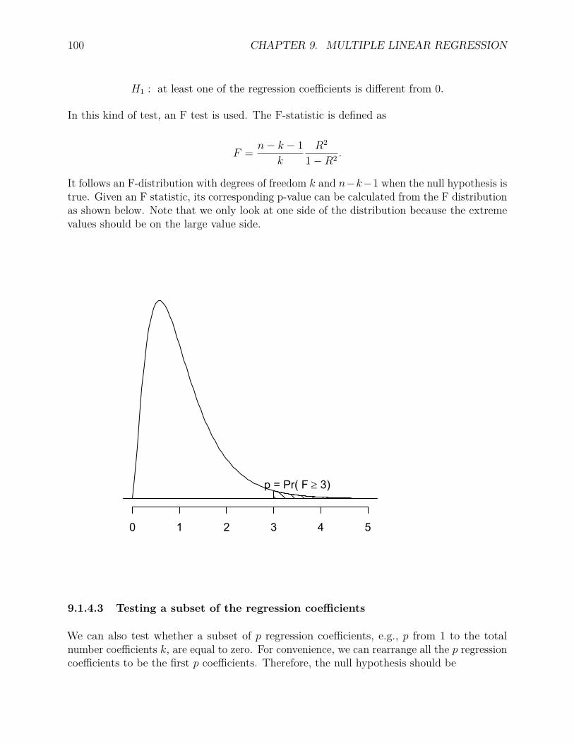
100 CHAPTER 9. MULTIPLE LINEAR REGRESSION
H1 : at least one of the regression coefficients is different from 0.
In this kind of test, an F test is used. The F-statistic is defined as
F = n− k − 1k
R2
1−R2 .
It follows an F-distribution with degrees of freedom k and n−k−1 when the null hypothesis istrue. Given an F statistic, its corresponding p-value can be calculated from the F distributionas shown below. Note that we only look at one side of the distribution because the extremevalues should be on the large value side.
9.1.4.3 Testing a subset of the regression coefficients
We can also test whether a subset of p regression coefficients, e.g., p from 1 to the totalnumber coefficients k, are equal to zero. For convenience, we can rearrange all the p regressioncoefficients to be the first p coefficients. Therefore, the null hypothesis should be
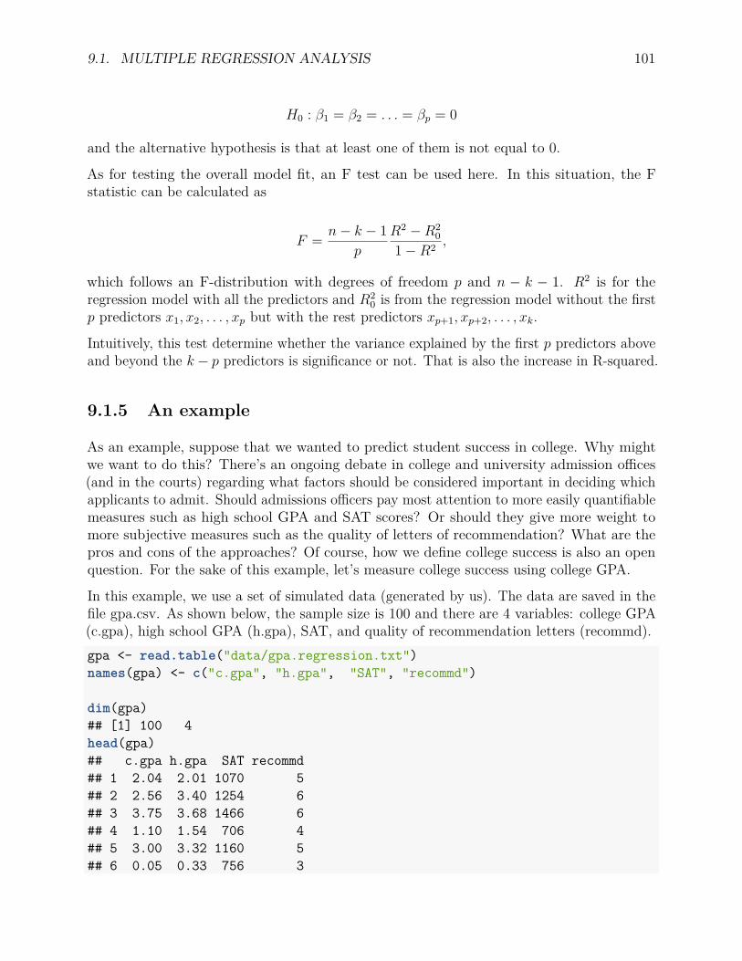
9.1. MULTIPLE REGRESSION ANALYSIS 101
H0 : β1 = β2 = . . . = βp = 0
and the alternative hypothesis is that at least one of them is not equal to 0.
As for testing the overall model fit, an F test can be used here. In this situation, the Fstatistic can be calculated as
F = n− k − 1p
R2 −R20
1−R2 ,
which follows an F-distribution with degrees of freedom p and n − k − 1. R2 is for theregression model with all the predictors and R2
0 is from the regression model without the firstp predictors x1, x2, . . . , xp but with the rest predictors xp+1, xp+2, . . . , xk.
Intuitively, this test determine whether the variance explained by the first p predictors aboveand beyond the k − p predictors is significance or not. That is also the increase in R-squared.
9.1.5 An example
As an example, suppose that we wanted to predict student success in college. Why mightwe want to do this? There’s an ongoing debate in college and university admission offices(and in the courts) regarding what factors should be considered important in deciding whichapplicants to admit. Should admissions officers pay most attention to more easily quantifiablemeasures such as high school GPA and SAT scores? Or should they give more weight tomore subjective measures such as the quality of letters of recommendation? What are thepros and cons of the approaches? Of course, how we define college success is also an openquestion. For the sake of this example, let’s measure college success using college GPA.
In this example, we use a set of simulated data (generated by us). The data are saved in thefile gpa.csv. As shown below, the sample size is 100 and there are 4 variables: college GPA(c.gpa), high school GPA (h.gpa), SAT, and quality of recommendation letters (recommd).gpa <- read.table("data/gpa.regression.txt")names(gpa) <- c("c.gpa", "h.gpa", "SAT", "recommd")
dim(gpa)## [1] 100 4head(gpa)## c.gpa h.gpa SAT recommd## 1 2.04 2.01 1070 5## 2 2.56 3.40 1254 6## 3 3.75 3.68 1466 6## 4 1.10 1.54 706 4## 5 3.00 3.32 1160 5## 6 0.05 0.33 756 3

102 CHAPTER 9. MULTIPLE LINEAR REGRESSION
9.1.5.1 Graph the data
Before fitting a regression model, we should check the relationship between college GPA andeach predictor through a scatterplot. A scatterplot can tell us the form of relationship, e.g.,linear, nonlinear, or no relationship, the direction of relationship, e.g., positive or negative,and the strength of relationship, e.g., strong, moderate, or weak. It can also identify potentialoutliers.
The scatterplots between college GPA and the three potential predictors are given below.From the plots, we can roughly see all three predictors are positively related to the collegeGPA. The relationship is close to linear and the relationship seems to be stronger for highschool GPA and SAT than for the quality of recommendation letters.attach(gpa)
par(mfrow=c(2,2))plot(h.gpa, c.gpa)plot(SAT, c.gpa)plot(recommd, c.gpa)
1 2 3 4
02
4
h.gpa
c.gp
a
400 600 800 1200
02
4
SAT
c.gp
a
2 4 6 8 10
02
4
recommd
c.gp
a
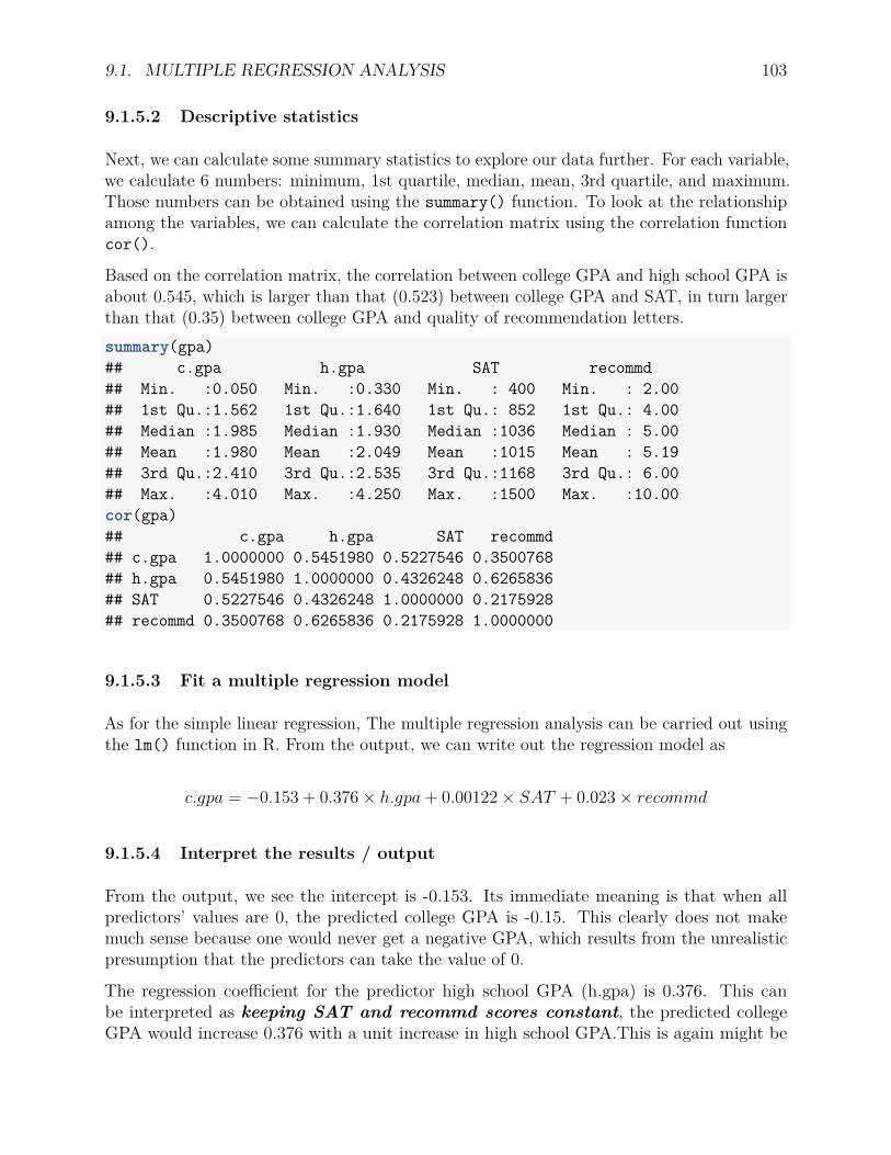
9.1. MULTIPLE REGRESSION ANALYSIS 103
9.1.5.2 Descriptive statistics
Next, we can calculate some summary statistics to explore our data further. For each variable,we calculate 6 numbers: minimum, 1st quartile, median, mean, 3rd quartile, and maximum.Those numbers can be obtained using the summary() function. To look at the relationshipamong the variables, we can calculate the correlation matrix using the correlation functioncor().
Based on the correlation matrix, the correlation between college GPA and high school GPA isabout 0.545, which is larger than that (0.523) between college GPA and SAT, in turn largerthan that (0.35) between college GPA and quality of recommendation letters.summary(gpa)## c.gpa h.gpa SAT recommd## Min. :0.050 Min. :0.330 Min. : 400 Min. : 2.00## 1st Qu.:1.562 1st Qu.:1.640 1st Qu.: 852 1st Qu.: 4.00## Median :1.985 Median :1.930 Median :1036 Median : 5.00## Mean :1.980 Mean :2.049 Mean :1015 Mean : 5.19## 3rd Qu.:2.410 3rd Qu.:2.535 3rd Qu.:1168 3rd Qu.: 6.00## Max. :4.010 Max. :4.250 Max. :1500 Max. :10.00cor(gpa)## c.gpa h.gpa SAT recommd## c.gpa 1.0000000 0.5451980 0.5227546 0.3500768## h.gpa 0.5451980 1.0000000 0.4326248 0.6265836## SAT 0.5227546 0.4326248 1.0000000 0.2175928## recommd 0.3500768 0.6265836 0.2175928 1.0000000
9.1.5.3 Fit a multiple regression model
As for the simple linear regression, The multiple regression analysis can be carried out usingthe lm() function in R. From the output, we can write out the regression model as
c.gpa = −0.153 + 0.376× h.gpa+ 0.00122× SAT + 0.023× recommd
9.1.5.4 Interpret the results / output
From the output, we see the intercept is -0.153. Its immediate meaning is that when allpredictors’ values are 0, the predicted college GPA is -0.15. This clearly does not makemuch sense because one would never get a negative GPA, which results from the unrealisticpresumption that the predictors can take the value of 0.
The regression coefficient for the predictor high school GPA (h.gpa) is 0.376. This canbe interpreted as keeping SAT and recommd scores constant, the predicted collegeGPA would increase 0.376 with a unit increase in high school GPA.This is again might be

104 CHAPTER 9. MULTIPLE LINEAR REGRESSION
problematic because it might be impossible to increase high school GPA while keeping theother two predictors unchanged. The other two regression coefficients can be interpreted inthe same way.
From the output, we can also see that the multiple R-squared (R2) is 0.3997. Therefore, about40% of the variation in college GPA can be explained by the multiple linear regression withh.GPA, SAT, and recommd as the predictors. The adjusted R2 is slightly smaller because ofthe consideration of the number of predictors. In fact,
aR2 = 1− (1−R2) n− 1n− k − 1
= 1− (1− .3997) 100− 1100− 3− 1
= .3809
9.1.5.5 Hypothesis testing
9.1.5.5.1 Testing Individual Regression Coefficient
For any regression coefficients for the three predictors (also the intercept), a t test can beconducted. For example, for high school GPA, the estimated coefficient is 0.376 with thestandard error 0.114. Therefore, the corresponding t statistic is t = 0.376/0.114 = 3.294. Sincethe statistic follows a t distribution with the degrees of freedom df = n−k−1 = 100−3−1 = 96,we can obtain the p-value as p = 2 ∗ (1− pt(3.294, 96)) = 0.0013. Since the p-value is lessthan 0.05, we conclude the coefficient is statistically significant. Note the t value and p-valueare directly provided in the output.t <- 0.376/0.114t## [1] 3.2982462*(1-pt(t, 96))## [1] 0.001365401
9.1.5.5.2 Overall model fit (testing all coefficients together)
To test all coefficients together or the overall model fit, we use the F test. Given the R2, theF statistic is
F = n− k − 1k
R2
1−R2
=(100− 3− 1
3
)×( 0.3997
1− .3997
)= 21.307
which follows the F distribution with degrees of freedom df1 = k = 3 and df2 = n−k−1 = 96.The corresponding p-value is 1.160e-10. Note that this information is directly shown in the

9.1. MULTIPLE REGRESSION ANALYSIS 105
output as “F-statistic: 21.31 on 3 and 96 DF, p-value: 1.160e-10”.
Therefore, at least one of the regression coefficients is statistically significantly different from0. Overall, the three predictors explained a significant portion of the variance in college GPA.The regression model with the 3 predictors is significantly better than the regression modelwith intercept only (i.e., predict c.gpa by the mean of c.gpa).F <- (100 - 3 -1)/3*0.3997/(1-0.3997)F## [1] 21.306681 - pf(F, 3, 96)## [1] 1.162797e-10
9.1.5.5.3 Testing a subset of regression coefficients
Suppose we are interested in testing whether the regression coefficients of high school GPAand SAT together are significant or not. Alternative, we want to see above and beyondthe quality of recommendation letters, whether the two predictors can explain a significantportion of variance in college GPA. To conduct the test, we need to fit two models:
• A full model: which consists of all the predictors to predict c.gpa by intercept, h.gpa,SAT, and recommd.
• A reduced model: obtained by removing the predictors to be tested in the full model.
From the full model, we can get the R2 = 0.3997 with all three predictors and from thereduced model, we can get the R2
0 = 0.1226 with only quality of recommendation letters.Then the F statistic is constructed as
F = n− k − 1p
R2 −R20
1−R2 =(100− 3− 1
2
)× .3997− .1226
1− .3997 = 22.157.
Using the F distribution with the degrees of freedom p = 2 (the number of coefficients to betested) and n− k − 1 = 96, we can get the p-value close to 0 (p = 1.22e− 08).model.reduce <- lm(c.gpa~recommd, data=gpa)summary(model.reduce)#### Call:## lm(formula = c.gpa ~ recommd, data = gpa)#### Residuals:## Min 1Q Median 3Q Max## -1.90257 -0.33372 0.01973 0.43457 1.71204#### Coefficients:## Estimate Std. Error t value Pr(>|t|)## (Intercept) 1.07020 0.25596 4.181 6.31e-05 ***
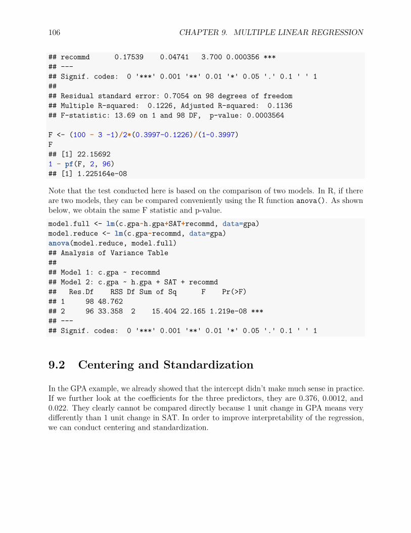
106 CHAPTER 9. MULTIPLE LINEAR REGRESSION
## recommd 0.17539 0.04741 3.700 0.000356 ***## ---## Signif. codes: 0 '***' 0.001 '**' 0.01 '*' 0.05 '.' 0.1 ' ' 1#### Residual standard error: 0.7054 on 98 degrees of freedom## Multiple R-squared: 0.1226, Adjusted R-squared: 0.1136## F-statistic: 13.69 on 1 and 98 DF, p-value: 0.0003564
F <- (100 - 3 -1)/2*(0.3997-0.1226)/(1-0.3997)F## [1] 22.156921 - pf(F, 2, 96)## [1] 1.225164e-08
Note that the test conducted here is based on the comparison of two models. In R, if thereare two models, they can be compared conveniently using the R function anova(). As shownbelow, we obtain the same F statistic and p-value.model.full <- lm(c.gpa~h.gpa+SAT+recommd, data=gpa)model.reduce <- lm(c.gpa~recommd, data=gpa)anova(model.reduce, model.full)## Analysis of Variance Table#### Model 1: c.gpa ~ recommd## Model 2: c.gpa ~ h.gpa + SAT + recommd## Res.Df RSS Df Sum of Sq F Pr(>F)## 1 98 48.762## 2 96 33.358 2 15.404 22.165 1.219e-08 ***## ---## Signif. codes: 0 '***' 0.001 '**' 0.01 '*' 0.05 '.' 0.1 ' ' 1
9.2 Centering and Standardization
In the GPA example, we already showed that the intercept didn’t make much sense in practice.If we further look at the coefficients for the three predictors, they are 0.376, 0.0012, and0.022. They clearly cannot be compared directly because 1 unit change in GPA means verydifferently than 1 unit change in SAT. In order to improve interpretability of the regression,we can conduct centering and standardization.
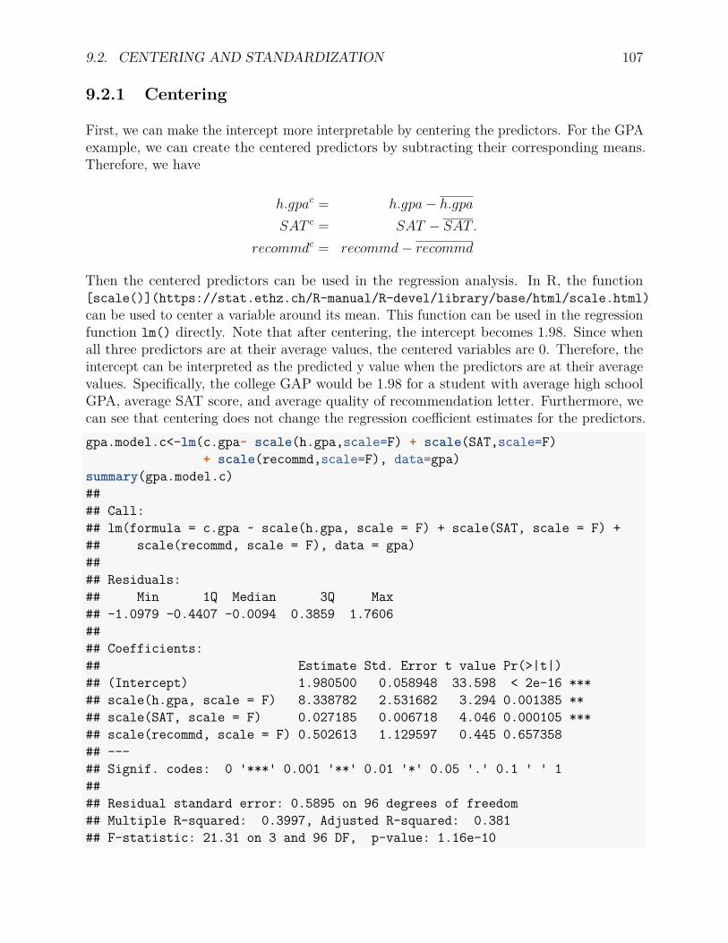
9.2. CENTERING AND STANDARDIZATION 107
9.2.1 Centering
First, we can make the intercept more interpretable by centering the predictors. For the GPAexample, we can create the centered predictors by subtracting their corresponding means.Therefore, we have
h.gpac = h.gpa− h.gpaSAT c = SAT − SAT
recommdc = recommd− recommd.
Then the centered predictors can be used in the regression analysis. In R, the function[scale()](https://stat.ethz.ch/R-manual/R-devel/library/base/html/scale.html)can be used to center a variable around its mean. This function can be used in the regressionfunction lm() directly. Note that after centering, the intercept becomes 1.98. Since whenall three predictors are at their average values, the centered variables are 0. Therefore, theintercept can be interpreted as the predicted y value when the predictors are at their averagevalues. Specifically, the college GAP would be 1.98 for a student with average high schoolGPA, average SAT score, and average quality of recommendation letter. Furthermore, wecan see that centering does not change the regression coefficient estimates for the predictors.gpa.model.c<-lm(c.gpa~ scale(h.gpa,scale=F) + scale(SAT,scale=F)
+ scale(recommd,scale=F), data=gpa)summary(gpa.model.c)#### Call:## lm(formula = c.gpa ~ scale(h.gpa, scale = F) + scale(SAT, scale = F) +## scale(recommd, scale = F), data = gpa)#### Residuals:## Min 1Q Median 3Q Max## -1.0979 -0.4407 -0.0094 0.3859 1.7606#### Coefficients:## Estimate Std. Error t value Pr(>|t|)## (Intercept) 1.980500 0.058948 33.598 < 2e-16 ***## scale(h.gpa, scale = F) 8.338782 2.531682 3.294 0.001385 **## scale(SAT, scale = F) 0.027185 0.006718 4.046 0.000105 ***## scale(recommd, scale = F) 0.502613 1.129597 0.445 0.657358## ---## Signif. codes: 0 '***' 0.001 '**' 0.01 '*' 0.05 '.' 0.1 ' ' 1#### Residual standard error: 0.5895 on 96 degrees of freedom## Multiple R-squared: 0.3997, Adjusted R-squared: 0.381## F-statistic: 21.31 on 3 and 96 DF, p-value: 1.16e-10
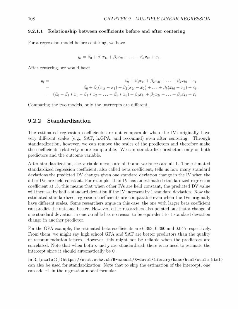
108 CHAPTER 9. MULTIPLE LINEAR REGRESSION
9.2.1.1 Relationship between coefficients before and after centering
For a regression model before centering, we have
yi = β0 + β1x1i + β2x2i + . . .+ βkxki + εi.
After centering, we would have
yi = β0 + β1x1i + β2x2i + . . .+ βkxki + εi
= β0 + β1(x1i − x1) + β2(x2i − x2) + . . .+ βk(xki − xk) + εi
= (β0 − β1 ∗ x1 − β2 ∗ x2 − . . .− βk ∗ xk) + β1x1i + β2x2i + . . .+ βkxki + εi
.
Comparing the two models, only the intercepts are different.
9.2.2 Standardization
The estimated regression coefficients are not comparable when the IVs originally havevery different scales (e.g., SAT, h.GPA, and recommd) even after centering. Throughstandardization, however, we can remove the scales of the predictors and therefore makethe coefficients relatively more comparable. We can standardize predictors only or bothpredictors and the outcome variable.
After standardization, the variable means are all 0 and variances are all 1. The estimatedstandardized regression coefficient, also called beta coefficient, tells us how many standarddeviations the predicted DV changes given one standard deviation change in the IV when theother IVs are held constant. For example, If an IV has an estimated standardized regressioncoefficient at .5, this means that when other IVs are held constant, the predicted DV valuewill increase by half a standard deviation if the IV increases by 1 standard deviation. Now theestimated standardized regression coefficients are comparable even when the IVs originallyhave different scales. Some researchers argue in this case, the one with larger beta coefficientcan predict the outcome better. However, other researchers also pointed out that a change ofone standard deviation in one variable has no reason to be equivalent to 1 standard deviationchange in another predictor.
For the GPA example, the estimated beta coefficients are 0.363, 0.360 and 0.045 respectively.From them, we might say high school GPA and SAT are better predictors than the qualityof recommendation letters. However, this might not be reliable when the predictors arecorrelated. Note that when both x and y are standardized, there is no need to estimate theintercept since it should automatically be 0.
In R, [scale()](https://stat.ethz.ch/R-manual/R-devel/library/base/html/scale.html)can also be used for standardization. Note that to skip the estimation of the intercept, onecan add -1 in the regression model formular.
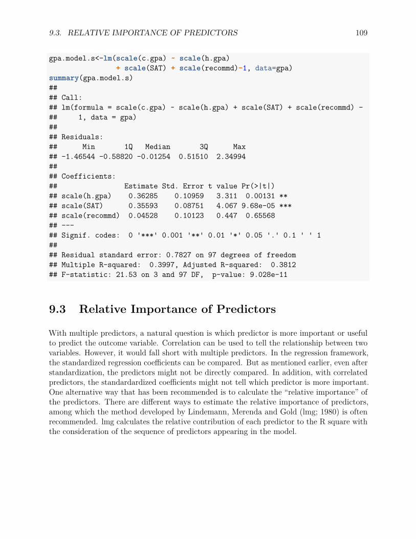
9.3. RELATIVE IMPORTANCE OF PREDICTORS 109
gpa.model.s<-lm(scale(c.gpa) ~ scale(h.gpa)+ scale(SAT) + scale(recommd)-1, data=gpa)
summary(gpa.model.s)#### Call:## lm(formula = scale(c.gpa) ~ scale(h.gpa) + scale(SAT) + scale(recommd) -## 1, data = gpa)#### Residuals:## Min 1Q Median 3Q Max## -1.46544 -0.58820 -0.01254 0.51510 2.34994#### Coefficients:## Estimate Std. Error t value Pr(>|t|)## scale(h.gpa) 0.36285 0.10959 3.311 0.00131 **## scale(SAT) 0.35593 0.08751 4.067 9.68e-05 ***## scale(recommd) 0.04528 0.10123 0.447 0.65568## ---## Signif. codes: 0 '***' 0.001 '**' 0.01 '*' 0.05 '.' 0.1 ' ' 1#### Residual standard error: 0.7827 on 97 degrees of freedom## Multiple R-squared: 0.3997, Adjusted R-squared: 0.3812## F-statistic: 21.53 on 3 and 97 DF, p-value: 9.028e-11
9.3 Relative Importance of Predictors
With multiple predictors, a natural question is which predictor is more important or usefulto predict the outcome variable. Correlation can be used to tell the relationship between twovariables. However, it would fall short with multiple predictors. In the regression framework,the standardized regression coefficients can be compared. But as mentioned earlier, even afterstandardization, the predictors might not be directly compared. In addition, with correlatedpredictors, the standardardized coefficients might not tell which predictor is more important.One alternative way that has been recommended is to calculate the “relative importance” ofthe predictors. There are different ways to estimate the relative importance of predictors,among which the method developed by Lindemann, Merenda and Gold (lmg; 1980) is oftenrecommended. lmg calculates the relative contribution of each predictor to the R square withthe consideration of the sequence of predictors appearing in the model.
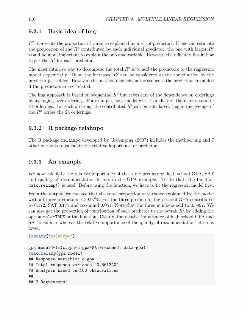
110 CHAPTER 9. MULTIPLE LINEAR REGRESSION
9.3.1 Basic idea of lmg
R2 represents the proportion of variance explained by a set of predictors. If one can estimatethe proportion of the R2 contributed by each individual predictor, the one with larger R2
would be more important to explain the outcome variable. However, the difficulty lies in howto get the R2 for each predictor.
The most intuitive way to decompose the total R2 is to add the predictors to the regressionmodel sequentially. Then, the increased R2 can be considered as the contribution by thepredictor just added. However, this method depends on the sequence the predictors are addedif the predictors are correlated.
The lmg approach is based on sequential R2 but takes care of the dependence on orderingsby averaging over orderings. For example, for a model with 4 predictors, there are a total of24 orderings. For each ordering, the contributed R2 can be calculated. lmg is the average ofthe R2 across the 24 orderings.
9.3.2 R package relaimpo
The R package relaimpo developed by Groemping (2007) includes the method lmg and 7other methods to calculate the relative importance of predictors.
9.3.3 An example
We now calculate the relative importance of the three predictors: high school GPA, SATand quality of recommendation letters in the GPA example. To do that, the functioncalc.relimp() is used. Before using the function, we have to fit the regression model first.
From the output, we can see that the total proportion of variance explained by the modelwith all three predictors is 39.97%. For the three predictors, high school GPA contributedto 0.172, SAT 0.177 and recommd 0.051. Note that the three numbers add to 0.3997. Wecan also get the proportion of contribution of each predictor to the overall R2 by adding theoption rela=TRUE in the function. Clearly, the relative importance of high school GPA andSAT is similar whereas the relative importance of the quality of recommendation letters islower.library('relaimpo')
gpa.model<-lm(c.gpa~h.gpa+SAT+recommd, data=gpa)calc.relimp(gpa.model)## Response variable: c.gpa## Total response variance: 0.5613402## Analysis based on 100 observations#### 3 Regressors:

9.3. RELATIVE IMPORTANCE OF PREDICTORS 111
## h.gpa SAT recommd## Proportion of variance explained by model: 39.97%## Metrics are not normalized (rela=FALSE).#### Relative importance metrics:#### lmg## h.gpa 0.17169723## SAT 0.17698341## recommd 0.05105477#### Average coefficients for different model sizes:#### 1X 2Xs 3Xs## h.gpa 0.56549057 0.481773394 0.37635109## SAT 0.00180201 0.001416298 0.00122693## recommd 0.17539410 0.065635789 0.02268425calc.relimp(gpa.model, rela=TRUE)## Response variable: c.gpa## Total response variance: 0.5613402## Analysis based on 100 observations#### 3 Regressors:## h.gpa SAT recommd## Proportion of variance explained by model: 39.97%## Metrics are normalized to sum to 100% (rela=TRUE).#### Relative importance metrics:#### lmg## h.gpa 0.4295272## SAT 0.4427514## recommd 0.1277214#### Average coefficients for different model sizes:#### 1X 2Xs 3Xs## h.gpa 0.56549057 0.481773394 0.37635109## SAT 0.00180201 0.001416298 0.00122693## recommd 0.17539410 0.065635789 0.02268425
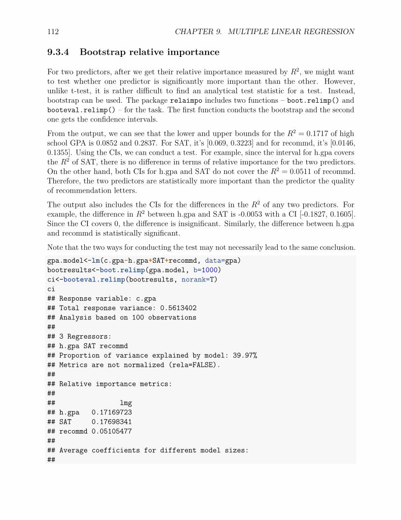
112 CHAPTER 9. MULTIPLE LINEAR REGRESSION
9.3.4 Bootstrap relative importance
For two predictors, after we get their relative importance measured by R2, we might wantto test whether one predictor is significantly more important than the other. However,unlike t-test, it is rather difficult to find an analytical test statistic for a test. Instead,bootstrap can be used. The package relaimpo includes two functions – boot.relimp() andbooteval.relimp() – for the task. The first function conducts the bootstrap and the secondone gets the confidence intervals.
From the output, we can see that the lower and upper bounds for the R2 = 0.1717 of highschool GPA is 0.0852 and 0.2837. For SAT, it’s [0.069, 0.3223] and for recommd, it’s [0.0146,0.1355]. Using the CIs, we can conduct a test. For example, since the interval for h.gpa coversthe R2 of SAT, there is no difference in terms of relative importance for the two predictors.On the other hand, both CIs for h.gpa and SAT do not cover the R2 = 0.0511 of recommd.Therefore, the two predictors are statistically more important than the predictor the qualityof recommendation letters.
The output also includes the CIs for the differences in the R2 of any two predictors. Forexample, the difference in R2 between h.gpa and SAT is -0.0053 with a CI [-0.1827, 0.1605].Since the CI covers 0, the difference is insignificant. Similarly, the difference between h.gpaand recommd is statistically significant.
Note that the two ways for conducting the test may not necessarily lead to the same conclusion.gpa.model<-lm(c.gpa~h.gpa+SAT+recommd, data=gpa)bootresults<-boot.relimp(gpa.model, b=1000)ci<-booteval.relimp(bootresults, norank=T)ci## Response variable: c.gpa## Total response variance: 0.5613402## Analysis based on 100 observations#### 3 Regressors:## h.gpa SAT recommd## Proportion of variance explained by model: 39.97%## Metrics are not normalized (rela=FALSE).#### Relative importance metrics:#### lmg## h.gpa 0.17169723## SAT 0.17698341## recommd 0.05105477#### Average coefficients for different model sizes:##
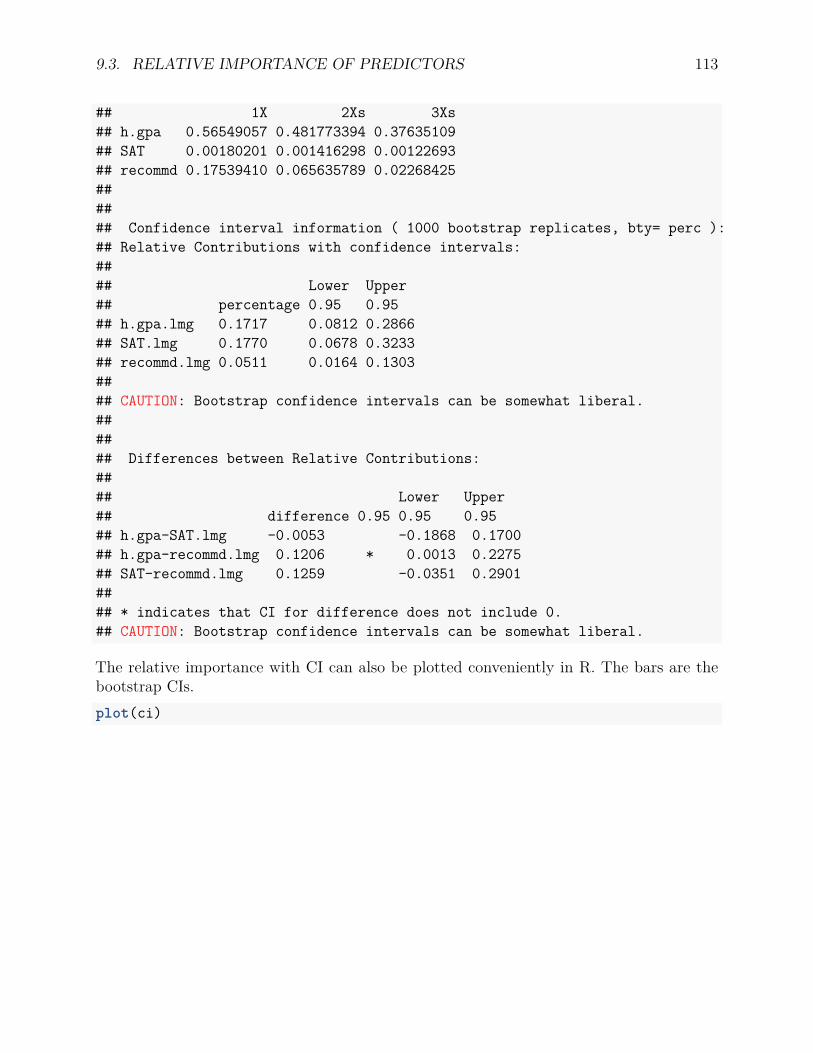
9.3. RELATIVE IMPORTANCE OF PREDICTORS 113
## 1X 2Xs 3Xs## h.gpa 0.56549057 0.481773394 0.37635109## SAT 0.00180201 0.001416298 0.00122693## recommd 0.17539410 0.065635789 0.02268425###### Confidence interval information ( 1000 bootstrap replicates, bty= perc ):## Relative Contributions with confidence intervals:#### Lower Upper## percentage 0.95 0.95## h.gpa.lmg 0.1717 0.0812 0.2866## SAT.lmg 0.1770 0.0678 0.3233## recommd.lmg 0.0511 0.0164 0.1303#### CAUTION: Bootstrap confidence intervals can be somewhat liberal.###### Differences between Relative Contributions:#### Lower Upper## difference 0.95 0.95 0.95## h.gpa-SAT.lmg -0.0053 -0.1868 0.1700## h.gpa-recommd.lmg 0.1206 * 0.0013 0.2275## SAT-recommd.lmg 0.1259 -0.0351 0.2901#### * indicates that CI for difference does not include 0.## CAUTION: Bootstrap confidence intervals can be somewhat liberal.
The relative importance with CI can also be plotted conveniently in R. The bars are thebootstrap CIs.plot(ci)
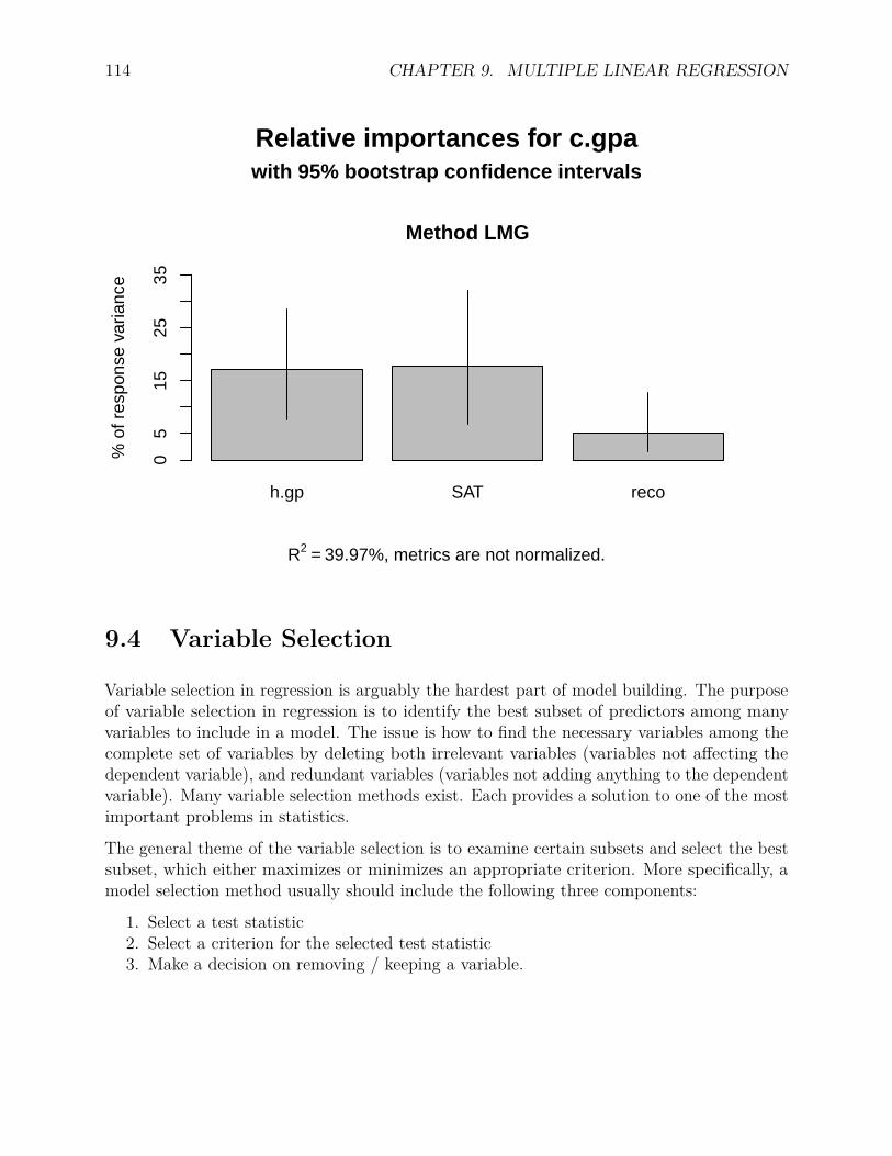
114 CHAPTER 9. MULTIPLE LINEAR REGRESSION
h.gp SAT reco
Method LMG
% o
f res
pons
e va
rianc
e
05
1525
35Relative importances for c.gpawith 95% bootstrap confidence intervals
R2 = 39.97%, metrics are not normalized.
9.4 Variable Selection
Variable selection in regression is arguably the hardest part of model building. The purposeof variable selection in regression is to identify the best subset of predictors among manyvariables to include in a model. The issue is how to find the necessary variables among thecomplete set of variables by deleting both irrelevant variables (variables not affecting thedependent variable), and redundant variables (variables not adding anything to the dependentvariable). Many variable selection methods exist. Each provides a solution to one of the mostimportant problems in statistics.
The general theme of the variable selection is to examine certain subsets and select the bestsubset, which either maximizes or minimizes an appropriate criterion. More specifically, amodel selection method usually should include the following three components:
1. Select a test statistic2. Select a criterion for the selected test statistic3. Make a decision on removing / keeping a variable.
9.4. VARIABLE SELECTION 115
9.4.1 Statistics/criteria for variable selection
In the literature, many statistics have been used for the variable selection purpose. Before wediscuss them, bear in mind that different statistics/criteria may lead to very different choicesof variables.
9.4.1.1 t-test for a single predictor at a time
We have learned how to use t-test for significance test of a single predictor. It is often usedas a way to select predictors. The general rule is that if a predictor is significant, it can beincluded in a regression model.
9.4.1.2 F-test for the whole model or for comparing two nested models
As for the F-test, it can be used to test the significance of one or more than one predictors.Therefore, it can also be used for variable selection. For example, for a subset of predictorsin a model, if its overall F-test is not significant, then one might simply remove them fromthe regression model.
9.4.1.3 R2 and Adjusted R2
R2 can be used to measure the practical importance of a predictor. If a predictor cancontribute significantly to the overall R2 or adjusted R2, it should be considered to beincluded in the model.
9.4.1.4 Mallows’ Cp
Mallows’ Cp is widely used in variable selection. It compares a model with p predictors vs. allk predictors (k > p) using a Cp statistic:
Cp = SSEpMSEk
−N + 2(p+ 1)
where SSEp is the sum of squared errors for the model with p predictors and MSEk is themean squared residuals for the model with all k predictors. The expectation of Cp is p+ 1.Intuitively, if the model with p predictors fits as well as the model with k predictors – thesimple model fits as well as a more complex model, the mean squared error should be thesame. Therefore, we would expect SSEp/MSEk = N − p − 1. Therefore, Cp = p + 1. Invariable selection, we therefore should look for a subset of variables with Cp around p + 1(Cp ≈ p+ 1) or smaller (Cp < p+ 1) than p+ 1. On the other hand, a model with bad fitwould have a Cp much bigger than p+1.

116 CHAPTER 9. MULTIPLE LINEAR REGRESSION
9.4.1.5 Information criteria
Information criteria such as AIC (Akaike information criterion) and BIC (Bayesian informationcriterion) are often used in variable selection. AIC and BIC are define as
AIC = n ln(SSE/n) + 2pBIC = n ln(SSE/n) + p ln(n)
.
Note that AIC and BIC are trade-off between goodness of model fit and model complexity.With more predictors in a regression model, SSE typically would become smaller or at leastthe same and therefore the first part of AIC and BIC becomes smaller. However, with modelpredictors, the model would become more complex and therefore the second part of AIC andBIC becomes bigger. An information criterion tries to identify the model with the smallestAIC and BIC that balance the model fit and model complexity.
9.4.2 An example
Through an example, we introduce different variable selection methods and illustrate theiruse. The data here were collected from 189 infants and mothers at the Baystate MedicalCenter, Springfield, Mass in 1986 on the following variables.
• low: indicator of birth weight less than 2.5 kg.• age: mother’s age in years.• lwt: mother’s weight in pounds at last menstrual period.• race: mother’s race (1 = white, 2 = black, 3 = other).• smoke: smoking status during pregnancy.• ptl: number of previous premature labors.• ht: history of hypertension.• ui: presence of uterine irritability.• ftv: number of physician visits during the first trimester.• bwt: birth weight in grams.
A subset of the data is shown below. Note that the data are included with the R packageMASS. Therefore, once the package is loaded, one can access the data using data(birthwt).library(MASS)data(birthwt)head(birthwt)## low age lwt race smoke ptl ht ui ftv bwt## 85 0 19 182 2 0 0 0 1 0 2523## 86 0 33 155 3 0 0 0 0 3 2551## 87 0 20 105 1 1 0 0 0 1 2557## 88 0 21 108 1 1 0 0 1 2 2594## 89 0 18 107 1 1 0 0 1 0 2600## 91 0 21 124 3 0 0 0 0 0 2622

9.4. VARIABLE SELECTION 117
The purpose of the study is to identify possible risk factors associated with low infant birthweight. Using the study and the data, we introduce four methods for variable selection: (1)all possible subsets (best subsets) analysis, (2) backward elimination, (3) forward selection,and (4) Stepwise selection/regression.
9.4.3 All possible (best) subsets
The basic idea of the all possible subsets approach is to run every possible combination ofthe predictors to find the best subset to meet some pre-defined objective criteria such as Cpand adjusted R2. It is hoped that that one ends up with a reasonable and useful regressionmodel. Manually, we can fit each possible model one by one using lm() and compare themodel fits. To automatically run the procedure, we can use the regsubsets() function inthe R package leaps.
Using the birth weight data, we can run the analysis as shown below. In the functionregsubsets(),
• The regular formula can be used to specify the model with all the predictors to bestudied. In this example, it is bwt~lwt+race+smoke+ptl+ht+ui+ftv. One can alsoprovides the outcome variable as a vector and the predictors in a matrix.
• data tells the data set to be used.• nbest is the number of the best subsets of each size to save. If nbest=1, only the best
model will be saved for each number of predictors. If nbest=2, the best two modelswith be saved given the number of predictors.
• nvmax is the maximum size of subsets of predictors to examine. It specifies the maximumnumber of predictors you want to include in the final regression model. For example, ifyou have 7 predictors but set nvmax=5, then the most complex model to be evaluatedwill have only 5 predictors. Using this option will largely reduce computing time if alarge number of predictors are evaluated.
library(leaps)all<-regsubsets(bwt~lwt+race+smoke+ptl+ht+ui+ftv,
data=birthwt,nbest=1, nvmax=7)
all## Subset selection object## Call: regsubsets.formula(bwt ~ lwt + race + smoke + ptl + ht + ui +## ftv, data = birthwt, nbest = 1, nvmax = 7)## 7 Variables (and intercept)## Forced in Forced out## lwt FALSE FALSE## race FALSE FALSE## smoke FALSE FALSE## ptl FALSE FALSE## ht FALSE FALSE
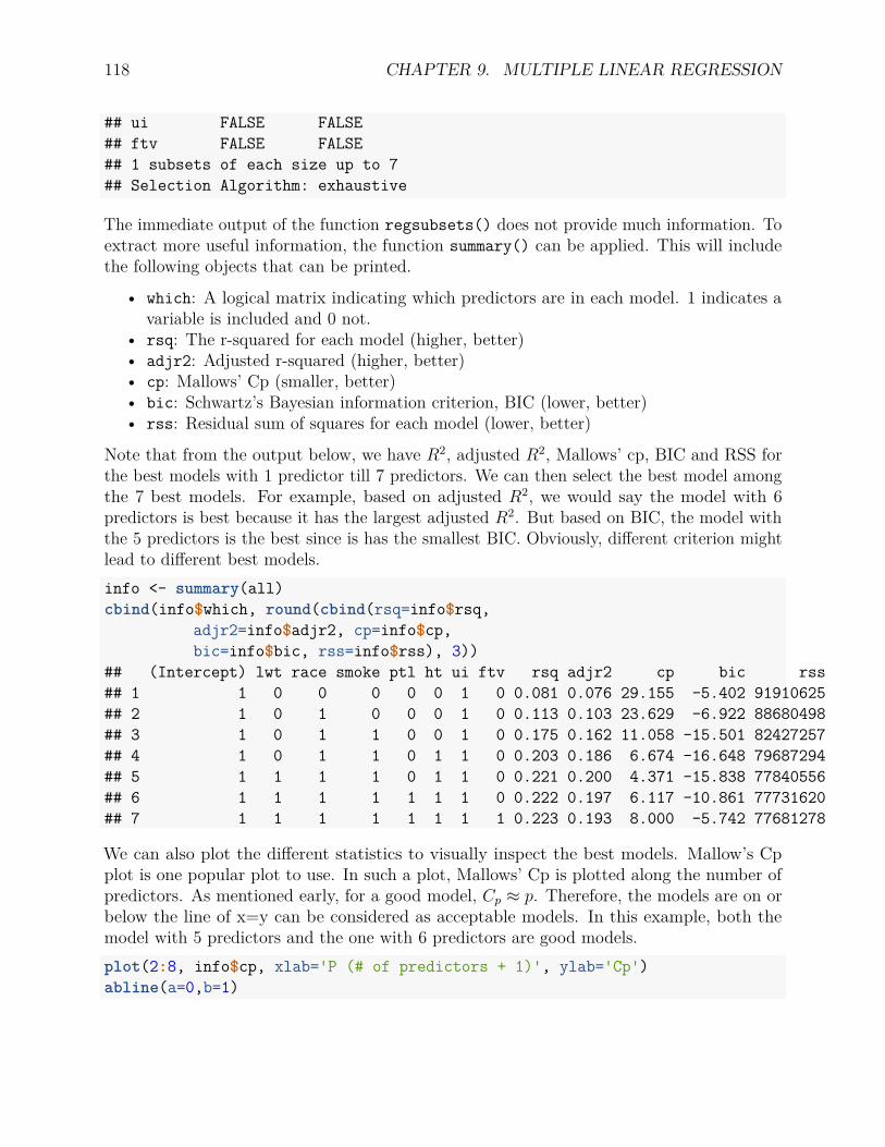
118 CHAPTER 9. MULTIPLE LINEAR REGRESSION
## ui FALSE FALSE## ftv FALSE FALSE## 1 subsets of each size up to 7## Selection Algorithm: exhaustive
The immediate output of the function regsubsets() does not provide much information. Toextract more useful information, the function summary() can be applied. This will includethe following objects that can be printed.
• which: A logical matrix indicating which predictors are in each model. 1 indicates avariable is included and 0 not.
• rsq: The r-squared for each model (higher, better)• adjr2: Adjusted r-squared (higher, better)• cp: Mallows’ Cp (smaller, better)• bic: Schwartz’s Bayesian information criterion, BIC (lower, better)• rss: Residual sum of squares for each model (lower, better)
Note that from the output below, we have R2, adjusted R2, Mallows’ cp, BIC and RSS forthe best models with 1 predictor till 7 predictors. We can then select the best model amongthe 7 best models. For example, based on adjusted R2, we would say the model with 6predictors is best because it has the largest adjusted R2. But based on BIC, the model withthe 5 predictors is the best since is has the smallest BIC. Obviously, different criterion mightlead to different best models.info <- summary(all)cbind(info$which, round(cbind(rsq=info$rsq,
adjr2=info$adjr2, cp=info$cp,bic=info$bic, rss=info$rss), 3))
## (Intercept) lwt race smoke ptl ht ui ftv rsq adjr2 cp bic rss## 1 1 0 0 0 0 0 1 0 0.081 0.076 29.155 -5.402 91910625## 2 1 0 1 0 0 0 1 0 0.113 0.103 23.629 -6.922 88680498## 3 1 0 1 1 0 0 1 0 0.175 0.162 11.058 -15.501 82427257## 4 1 0 1 1 0 1 1 0 0.203 0.186 6.674 -16.648 79687294## 5 1 1 1 1 0 1 1 0 0.221 0.200 4.371 -15.838 77840556## 6 1 1 1 1 1 1 1 0 0.222 0.197 6.117 -10.861 77731620## 7 1 1 1 1 1 1 1 1 0.223 0.193 8.000 -5.742 77681278
We can also plot the different statistics to visually inspect the best models. Mallow’s Cpplot is one popular plot to use. In such a plot, Mallows’ Cp is plotted along the number ofpredictors. As mentioned early, for a good model, Cp ≈ p. Therefore, the models are on orbelow the line of x=y can be considered as acceptable models. In this example, both themodel with 5 predictors and the one with 6 predictors are good models.plot(2:8, info$cp, xlab='P (# of predictors + 1)', ylab='Cp')abline(a=0,b=1)

9.4. VARIABLE SELECTION 119
2 3 4 5 6 7 8
510
1520
2530
P (# of predictors + 1)
Cp
9.4.3.1 Remarks
Using the all possible subsets method, one would select a model with a larger adjustedR-square, smaller Cp, smaller rsq, and smaller BIC. The different criteria quantify differentaspects of the regression model, and therefore often yield different choices for the best set ofpredictors. That’s okay €” as long as we don’t misuse best subsets regression by claimingthat it yields the best model. Rather, we should use best subsets regression as a screeningtool €” that is, as a way to reduce the large number of possible regression models to just ahandful of models that we can evaluate further before arriving at one final model. If there aretwo competing models, one can select the one with fewer predictors or the one with practicalor theoretical sense.
With many predictors, for example, more than 40 predictors, the number of possible subsetscan be huge. Often, there are several good models, although some are unstable. The bestsubset may be no better than a subset of some randomly selected variables, if the sample sizeis relatively small to the number of predictors. The regression fit statistics and regressioncoefficient estimates can also be biased. In addition, all-possible-subsets selection can yieldmodels that are too small. Generally speaking, one should not blindly trust the results. Thedata analyst knows more than the computer and failure to use human knowledge producesinadequate data analysis.
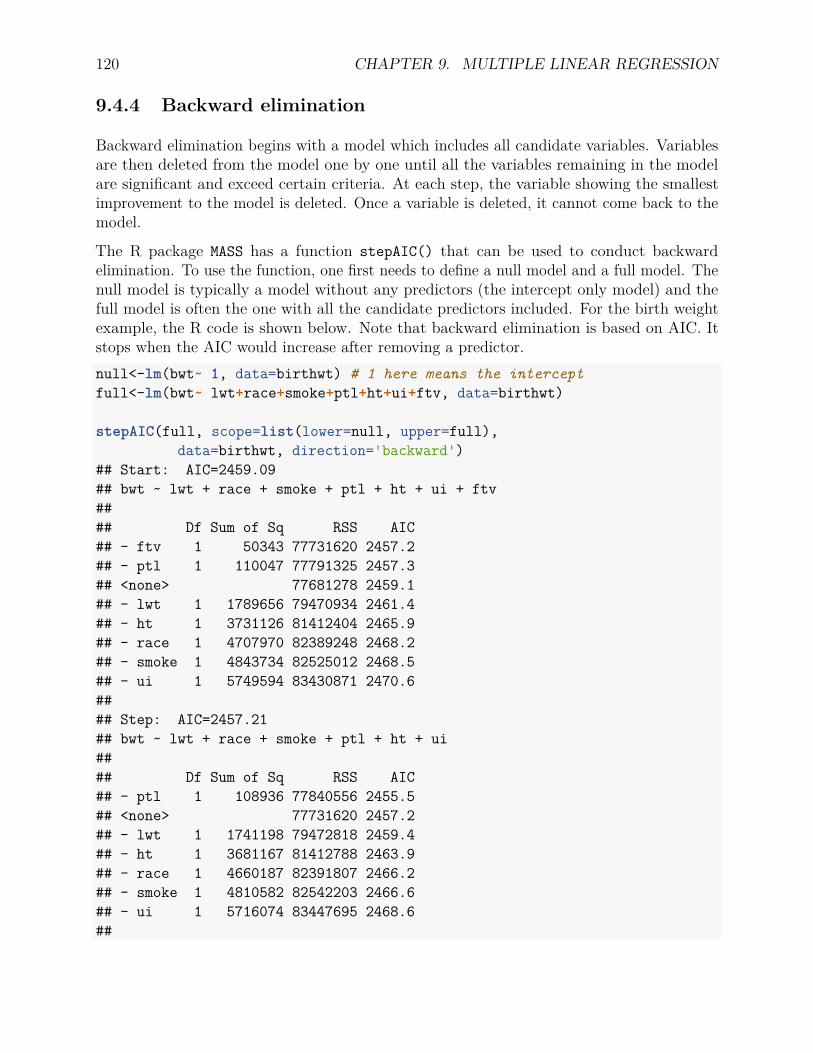
120 CHAPTER 9. MULTIPLE LINEAR REGRESSION
9.4.4 Backward elimination
Backward elimination begins with a model which includes all candidate variables. Variablesare then deleted from the model one by one until all the variables remaining in the modelare significant and exceed certain criteria. At each step, the variable showing the smallestimprovement to the model is deleted. Once a variable is deleted, it cannot come back to themodel.
The R package MASS has a function stepAIC() that can be used to conduct backwardelimination. To use the function, one first needs to define a null model and a full model. Thenull model is typically a model without any predictors (the intercept only model) and thefull model is often the one with all the candidate predictors included. For the birth weightexample, the R code is shown below. Note that backward elimination is based on AIC. Itstops when the AIC would increase after removing a predictor.null<-lm(bwt~ 1, data=birthwt) # 1 here means the interceptfull<-lm(bwt~ lwt+race+smoke+ptl+ht+ui+ftv, data=birthwt)
stepAIC(full, scope=list(lower=null, upper=full),data=birthwt, direction='backward')
## Start: AIC=2459.09## bwt ~ lwt + race + smoke + ptl + ht + ui + ftv#### Df Sum of Sq RSS AIC## - ftv 1 50343 77731620 2457.2## - ptl 1 110047 77791325 2457.3## <none> 77681278 2459.1## - lwt 1 1789656 79470934 2461.4## - ht 1 3731126 81412404 2465.9## - race 1 4707970 82389248 2468.2## - smoke 1 4843734 82525012 2468.5## - ui 1 5749594 83430871 2470.6#### Step: AIC=2457.21## bwt ~ lwt + race + smoke + ptl + ht + ui#### Df Sum of Sq RSS AIC## - ptl 1 108936 77840556 2455.5## <none> 77731620 2457.2## - lwt 1 1741198 79472818 2459.4## - ht 1 3681167 81412788 2463.9## - race 1 4660187 82391807 2466.2## - smoke 1 4810582 82542203 2466.6## - ui 1 5716074 83447695 2468.6##

9.4. VARIABLE SELECTION 121
## Step: AIC=2455.47## bwt ~ lwt + race + smoke + ht + ui#### Df Sum of Sq RSS AIC## <none> 77840556 2455.5## - lwt 1 1846738 79687294 2457.9## - ht 1 3718531 81559088 2462.3## - race 1 4727071 82567628 2464.6## - smoke 1 5237430 83077987 2465.8## - ui 1 6302771 84143327 2468.2#### Call:## lm(formula = bwt ~ lwt + race + smoke + ht + ui, data = birthwt)#### Coefficients:## (Intercept) lwt race smoke ht ui## 3104.438 3.434 -187.849 -366.135 -595.820 -523.419
9.4.5 Forward selection
Forward selection begins with a model which includes no predictors (the intercept only model).Variables are then added to the model one by one until no remaining variables improve themodel by a certain criterion. At each step, the variable showing the biggest improvement tothe model is added. Once a variable is in the model, it remains there.
The function stepAIC() can also be used to conduct forward selection. For the birth weightexample, the R code is shown below. Note that forward selection stops when the AIC woulddecrease after adding a predictor.stepAIC(null, scope=list(lower=null, upper=full),
data=birthwt, direction='forward')## Start: AIC=2492.76## bwt ~ 1#### Df Sum of Sq RSS AIC## + ui 1 8059031 91910625 2478.9## + race 1 3790184 96179472 2487.5## + smoke 1 3625946 96343710 2487.8## + lwt 1 3448639 96521017 2488.1## + ptl 1 2391041 97578614 2490.2## + ht 1 2130425 97839231 2490.7## <none> 99969656 2492.8## + ftv 1 339993 99629663 2494.1##

122 CHAPTER 9. MULTIPLE LINEAR REGRESSION
## Step: AIC=2478.88## bwt ~ ui#### Df Sum of Sq RSS AIC## + race 1 3230127 88680498 2474.1## + ht 1 3162595 88748030 2474.3## + smoke 1 2996636 88913988 2474.6## + lwt 1 2074421 89836203 2476.6## <none> 91910625 2478.9## + ptl 1 854664 91055961 2479.1## + ftv 1 172098 91738526 2480.5#### Step: AIC=2474.11## bwt ~ ui + race#### Df Sum of Sq RSS AIC## + smoke 1 6253241 82427257 2462.3## + ht 1 3000965 85679533 2469.6## + lwt 1 1367676 87312822 2473.2## <none> 88680498 2474.1## + ptl 1 869259 87811239 2474.2## + ftv 1 59737 88620761 2476.0#### Step: AIC=2462.29## bwt ~ ui + race + smoke#### Df Sum of Sq RSS AIC## + ht 1 2739963 79687294 2457.9## + lwt 1 868170 81559088 2462.3## <none> 82427257 2462.3## + ptl 1 220563 82206694 2463.8## + ftv 1 8390 82418867 2464.3#### Step: AIC=2457.9## bwt ~ ui + race + smoke + ht#### Df Sum of Sq RSS AIC## + lwt 1 1846738 77840556 2455.5## <none> 79687294 2457.9## + ptl 1 214476 79472818 2459.4## + ftv 1 1134 79686160 2459.9#### Step: AIC=2455.47## bwt ~ ui + race + smoke + ht + lwt
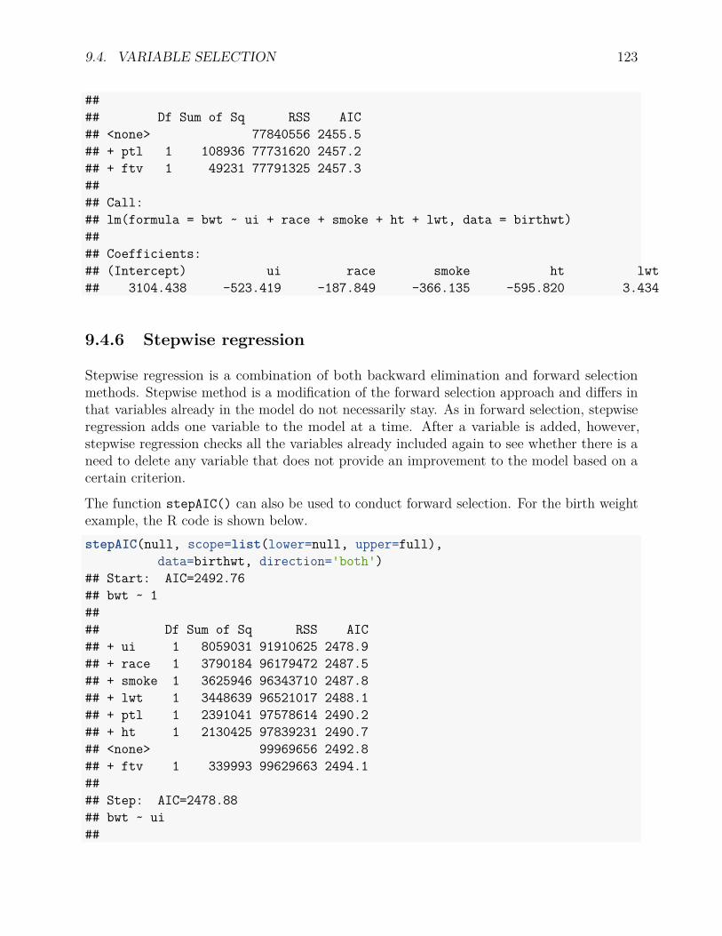
9.4. VARIABLE SELECTION 123
#### Df Sum of Sq RSS AIC## <none> 77840556 2455.5## + ptl 1 108936 77731620 2457.2## + ftv 1 49231 77791325 2457.3#### Call:## lm(formula = bwt ~ ui + race + smoke + ht + lwt, data = birthwt)#### Coefficients:## (Intercept) ui race smoke ht lwt## 3104.438 -523.419 -187.849 -366.135 -595.820 3.434
9.4.6 Stepwise regression
Stepwise regression is a combination of both backward elimination and forward selectionmethods. Stepwise method is a modification of the forward selection approach and differs inthat variables already in the model do not necessarily stay. As in forward selection, stepwiseregression adds one variable to the model at a time. After a variable is added, however,stepwise regression checks all the variables already included again to see whether there is aneed to delete any variable that does not provide an improvement to the model based on acertain criterion.
The function stepAIC() can also be used to conduct forward selection. For the birth weightexample, the R code is shown below.stepAIC(null, scope=list(lower=null, upper=full),
data=birthwt, direction='both')## Start: AIC=2492.76## bwt ~ 1#### Df Sum of Sq RSS AIC## + ui 1 8059031 91910625 2478.9## + race 1 3790184 96179472 2487.5## + smoke 1 3625946 96343710 2487.8## + lwt 1 3448639 96521017 2488.1## + ptl 1 2391041 97578614 2490.2## + ht 1 2130425 97839231 2490.7## <none> 99969656 2492.8## + ftv 1 339993 99629663 2494.1#### Step: AIC=2478.88## bwt ~ ui##

124 CHAPTER 9. MULTIPLE LINEAR REGRESSION
## Df Sum of Sq RSS AIC## + race 1 3230127 88680498 2474.1## + ht 1 3162595 88748030 2474.3## + smoke 1 2996636 88913988 2474.6## + lwt 1 2074421 89836203 2476.6## <none> 91910625 2478.9## + ptl 1 854664 91055961 2479.1## + ftv 1 172098 91738526 2480.5## - ui 1 8059031 99969656 2492.8#### Step: AIC=2474.11## bwt ~ ui + race#### Df Sum of Sq RSS AIC## + smoke 1 6253241 82427257 2462.3## + ht 1 3000965 85679533 2469.6## + lwt 1 1367676 87312822 2473.2## <none> 88680498 2474.1## + ptl 1 869259 87811239 2474.2## + ftv 1 59737 88620761 2476.0## - race 1 3230127 91910625 2478.9## - ui 1 7498974 96179472 2487.5#### Step: AIC=2462.29## bwt ~ ui + race + smoke#### Df Sum of Sq RSS AIC## + ht 1 2739963 79687294 2457.9## + lwt 1 868170 81559088 2462.3## <none> 82427257 2462.3## + ptl 1 220563 82206694 2463.8## + ftv 1 8390 82418867 2464.3## - smoke 1 6253241 88680498 2474.1## - ui 1 6323012 88750270 2474.3## - race 1 6486731 88913988 2474.6#### Step: AIC=2457.9## bwt ~ ui + race + smoke + ht#### Df Sum of Sq RSS AIC## + lwt 1 1846738 77840556 2455.5## <none> 79687294 2457.9## + ptl 1 214476 79472818 2459.4## + ftv 1 1134 79686160 2459.9
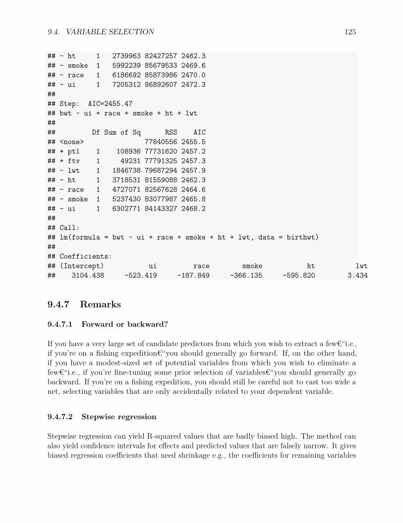
9.4. VARIABLE SELECTION 125
## - ht 1 2739963 82427257 2462.3## - smoke 1 5992239 85679533 2469.6## - race 1 6186692 85873986 2470.0## - ui 1 7205312 86892607 2472.3#### Step: AIC=2455.47## bwt ~ ui + race + smoke + ht + lwt#### Df Sum of Sq RSS AIC## <none> 77840556 2455.5## + ptl 1 108936 77731620 2457.2## + ftv 1 49231 77791325 2457.3## - lwt 1 1846738 79687294 2457.9## - ht 1 3718531 81559088 2462.3## - race 1 4727071 82567628 2464.6## - smoke 1 5237430 83077987 2465.8## - ui 1 6302771 84143327 2468.2#### Call:## lm(formula = bwt ~ ui + race + smoke + ht + lwt, data = birthwt)#### Coefficients:## (Intercept) ui race smoke ht lwt## 3104.438 -523.419 -187.849 -366.135 -595.820 3.434
9.4.7 Remarks
9.4.7.1 Forward or backward?
If you have a very large set of candidate predictors from which you wish to extract a few€“i.e.,if you’re on a fishing expedition€“you should generally go forward. If, on the other hand,if you have a modest-sized set of potential variables from which you wish to eliminate afew€“i.e., if you’re fine-tuning some prior selection of variables€“you should generally gobackward. If you’re on a fishing expedition, you should still be careful not to cast too wide anet, selecting variables that are only accidentally related to your dependent variable.
9.4.7.2 Stepwise regression
Stepwise regression can yield R-squared values that are badly biased high. The method canalso yield confidence intervals for effects and predicted values that are falsely narrow. It givesbiased regression coefficients that need shrinkage e.g., the coefficients for remaining variables
126 CHAPTER 9. MULTIPLE LINEAR REGRESSION
are too large. It also has severe problems in the presence of collinearity and increasing thesample size doesn’t help very much.
9.4.7.3 Stepwise or all-possible-subsets?
Stepwise regression often works reasonably well as an automatic variable selection method,but this is not guaranteed. If the number of candidate predictors is large compared to thenumber of observations in your data set (say, more than 1 variable for every 10 observations),or if there is excessive multicollinearity (predictors are highly correlated), then the stepwisealgorithms may go crazy and end up throwing nearly all the variables into the model, especiallyif you used a low threshold on a criterion like F statistic.
All-possible-subsets goes beyond stepwise regression and literally tests all possible subsets ofthe set of potential independent variables. But it carries all the caveats of stepwise regression.
9.4.7.4 Use your knowledge
A model selected by automatic methods can only find the “best” combination from amongthe set of variables you start with: if you omit some important variables, no amount ofsearching will compensate! Remember that the computer is not necessarily right in its choiceof a model during the automatic phase of the search. Don’t accept a model just because thecomputer gave it its blessing. Use your own judgment and intuition about your data to tryto fine-tune whatever the computer comes up with.
9.5 Regression with Categorical Predictors
In the variable selection example, we have a predictor – race, which has three categories: 1 =white, 2 = black, 3 = other. In the previous example, we blindly treated it as continuous bytaking the numbers literally. This can cause problems. For example, when we interpret theregression slope, we say how much change in the outcome for one unit change the predictor.Although numerically it is fine to say the change from 1 to 2 is the same as the change from2 to 3, it does not make sense at all to compare the change in the actual race categories.Therefore, although the categories are coded using numerical values, they should be treated asdiscrete values. This kind variables is called nominal variables. A typical example is ANOVAwhere the different levels of a factor should be treated as discrete values. In regression, suchvariables need special treatment for valid statistical inference. We show how to conduct suchregression analysis through an example.

9.5. REGRESSION WITH CATEGORICAL PREDICTORS 127
9.5.1 An example
In this example, we study the mid-career median salary of college graduates. The data setcollege.csv includes the information on salary and college backgrounds. Specifically, thereare 6 variables in the data set: id, name of the college, mid-career median salary of graduates,cost of study, whether the college is public (1) or private (0), and the location of the college:1, Southern colleges; 2, Midwestern; 3, Northeastern; and 4, Western. A subset of the dataas well as some summary information are given below. In total, there are 85 colleges in thedata and 50 of them are private colleges. Clearly, the variables public and location in thedata set should be treated as categorical variables. Using this example, we study the factorsrelated to median salary.college <- read.csv("data/college.csv")
head(college)## id name salary cost public location## 1 1 Massachusetts Institute of Technology (MIT) 119000 189300 0 3## 2 2 Harvard University 121000 189600 0 3## 3 3 Dartmouth College 123000 188400 0 3## 4 4 Princeton University 123000 188700 0 3## 5 5 Yale University 110000 194200 0 3## 6 6 University of Notre Dame 112000 181900 0 2attach(college)table(public)## public## 0 1## 50 35table(location)## location## 1 2 3 4## 20 19 25 21
9.5.2 A naive analysis
Suppose we simply treat the variables public and location and fit a multiple regression modelto directly. Then, we would get the results as shown below. Then the regression model is
salary = 105.48− 11.679 ∗ public− 1.869 ∗ location.
Using the typical way to interpret the regression coefficients, we would say (1) when public=0and location=0, the average salary is 105.48; (2) when public changes from 0 to 1, the salarywould reduce 11.679; and (3) when location increases 1, the salary decreases 1.869. Clearly,(1) and (3) do not make sense at all even though (2) seems to be ok.

128 CHAPTER 9. MULTIPLE LINEAR REGRESSION
By fitting the above regression model, we assume that each predictor has equal interval intheir values. For example, for the location variable, the change from Southern to Midwesternis the same as the change from Midwestern to Northeastern. This assumption is certainlyquestionable for variables with distinct, non-numerical categories. The location variable hereis a categorical variable, not a continuous one. The use of numerical values in the data filefor categorical variables is for convenience of data input and storage and should be viewed asdiscrete instead of continuous values. For example, for the “public” variable, 0 should read asprivate and 1 should read as public. Similarly, for the “location” variable, 1 means Southern, 2means Midwestern, etc. To deal with such variables, we need recode the categorical variables.
9.5.3 Regression with categorical predictors
9.5.3.1 Code categorical numerical values to avoid confusion
To avoid mistakenly treating the categorical data as continuous, we can code the numericalvalues as discrete values, or better yet, more descriptive strings. In R, this can be doneeasily using the function factor(). For example, the following R code changes the value 0to Private and 1 to Public and for location variable, the values 1 to 4 are recoded as S, MW,NE, and W, respectively. Note that each category of a variable is called a level. So, for thepublic variable, there are two levels and for the location variables, there are 4 levels.public<-factor(public, c(0,1), labels=c('Private', 'Public'))public## [1] Private Private Private Private Private Private Private Private Private## [10] Private Private Private Private Private Private Private Private Public## [19] Private Private Public Private Private Private Public Private Private## [28] Private Private Private Private Public Private Private Public Public## [37] Private Private Public Private Public Private Private Private Public## [46] Public Public Private Private Private Public Private Private Public## [55] Public Public Public Private Public Public Public Private Public## [64] Private Public Private Public Public Public Public Private Public## [73] Private Public Public Public Public Public Private Public Public## [82] Public Private Public Private## Levels: Private Public
location<-factor(location, c(1,2,3,4), labels=c('S', 'MW','NE', 'W'))location## [1] NE NE NE NE NE MW NE S NE NE NE NE NE NE S NE S W NE NE S NE MW NE S## [26] NE MW S NE S NE S S MW MW MW MW MW S MW S S W S NE S MW MW S S## [51] MW S MW S S NE MW S MW W NE W W MW NE W W MW NE W W MW W W W## [76] W W W W MW W W W W W## Levels: S MW NE W
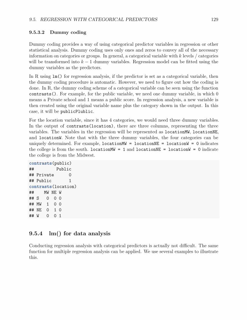
9.5. REGRESSION WITH CATEGORICAL PREDICTORS 129
9.5.3.2 Dummy coding
Dummy coding provides a way of using categorical predictor variables in regression or otherstatistical analysis. Dummy coding uses only ones and zeros to convey all of the necessaryinformation on categories or groups. In general, a categorical variable with k levels / categorieswill be transformed into k − 1 dummy variables. Regression model can be fitted using thedummy variables as the predictors.
In R using lm() for regression analysis, if the predictor is set as a categorical variable, thenthe dummy coding procedure is automatic. However, we need to figure out how the coding isdone. In R, the dummy coding scheme of a categorical variable can be seen using the functioncontrasts(). For example, for the public variable, we need one dummy variable, in which 0means a Private school and 1 means a public score. In regression analysis, a new variable isthen created using the original variable name plus the category shown in the output. In thiscase, it will be publicPlublic.
For the location variable, since it has 4 categories, we would need three dummy variables.In the output of contrasts(location), there are three columns, representing the threevariables. The variables in the regression will be represented as locationMW, locationNE,and locationW. Note that with the three dummy variables, the four categories can beuniquely determined. For example, locationMW = locationNE = locationW = 0 indicatesthe college is from the south. locationMW = 1 and locationNE = locationW = 0 indicatethe college is from the Midwest.contrasts(public)## Public## Private 0## Public 1contrasts(location)## MW NE W## S 0 0 0## MW 1 0 0## NE 0 1 0## W 0 0 1
9.5.4 lm() for data analysis
Conducting regression analysis with categorical predictors is actually not difficult. The samefunction for multiple regression analysis can be applied. We use several examples to illustratethis.

130 CHAPTER 9. MULTIPLE LINEAR REGRESSION
9.5.4.1 Example 1. A predictor with two categories (one-way ANOVA)
Suppose we want to see if there is a difference in salary for private and public colleges. Then,we use the public variable as a predictor, which has two categories. The input and outputfor the analysis are given below.salary <- salary / 1000
summary(lm(salary ~ public))#### Call:## lm(formula = salary ~ public)#### Residuals:## Min 1Q Median 3Q Max## -25.944 -7.134 0.156 5.156 24.166#### Coefficients:## Estimate Std. Error t value Pr(>|t|)## (Intercept) 100.844 1.473 68.478 < 2e-16 ***## publicPublic -12.010 2.295 -5.233 1.23e-06 ***## ---## Signif. codes: 0 '***' 0.001 '**' 0.01 '*' 0.05 '.' 0.1 ' ' 1#### Residual standard error: 10.41 on 83 degrees of freedom## Multiple R-squared: 0.2481, Adjusted R-squared: 0.239## F-statistic: 27.39 on 1 and 83 DF, p-value: 1.231e-06
First, note that the same formula as for the regular regression analysis is used. However, nowthe public variable is a categorical variable. Second, in the output, there is a variable calledpublicPublic, which was created by the R function automatically. It has two values, 0 and1. From the output of contrasts(public), we know that for a private college, it takes thevalue 0 and for a public college, it takes the value 1.
9.5.4.1.1 Write out the model
When using a categorical variable, it’s best to write out the model for all the differentcategories.
salary = b0 + b1 ∗ publicPublic= 100.8− 12publicPublic
=
100.8 For private colleges(publicPublic = 0)88.8 For public colleges(publicPublic = 1)

9.5. REGRESSION WITH CATEGORICAL PREDICTORS 131
9.5.4.1.2 Interpretation
First, note that the difference in the average salaries between the private colleges and the publiccolleges is equal to 12k, which is also the estimated regression coefficient for publicPublic.To test whether the difference is significantly different from 0, it is equivalent to testing thesignificance of the regression coefficient. In this case, it is significant given t = −5.233 andp < .0011. Note that this is just another way of doing the pooled two-independent sample ttest!
9.5.4.2 Example 2. A predictor with four categories
Suppose we are interested in whether the location of college is related to the salary. For thelocation variable, there are four categories. As expected, three dummy variables are neededto conduct the regression analysis as shown below. The three dummy variable predictors arelocationMW, locationNE, locationW.summary(lm(salary ~ location))#### Call:## lm(formula = salary ~ location)#### Residuals:## Min 1Q Median 3Q Max## -22.988 -4.010 -0.888 3.605 28.890#### Coefficients:## Estimate Std. Error t value Pr(>|t|)## (Intercept) 96.635 1.913 50.514 < 2e-16 ***## locationMW -2.940 2.741 -1.073 0.286556## locationNE 10.253 2.567 3.995 0.000142 ***## locationW -12.525 2.673 -4.686 1.11e-05 ***## ---## Signif. codes: 0 '***' 0.001 '**' 0.01 '*' 0.05 '.' 0.1 ' ' 1#### Residual standard error: 8.555 on 81 degrees of freedom## Multiple R-squared: 0.5047, Adjusted R-squared: 0.4863## F-statistic: 27.51 on 3 and 81 DF, p-value: 2.287e-12
Based on the output, we can write out the model for the predicted salaries as below.

132 CHAPTER 9. MULTIPLE LINEAR REGRESSION
Based on the analysis, we can get the following information:
• The average salary of each area. The South area is the reference area, called referencegroup since the other groups can be directly compared with it.
• -2.94 is the difference in the average salaries between South and Midwest. Whetherthis difference is significantly different from 0 can be tested, therefore, through testingthe regression coefficient of locationMW. Since t = -1.073, p = 0.287, the differenceis not signifcant at the 0.05 level.
• 10.25 is the difference in the average salaries between South and Northeast. Since t =3.995, p = .0001 for the parameter in the regression, the difference is significantlydifferent from 0.
• -12.53 is the difference in the average salaries between South and West. Since t =-4.686, p = 1.11e-05 for the parameter in the regression, the difference is significantlydifferent from 0.
9.5.4.2.1 Testing the significance of the predictor
To test the significance of a categorical predictor, one can check the overall model fit ofthe regression analysis based on the F-test. This is equivalent to test the significanceof all the dummy variables together. For this specific example, we have F=27.51 andp-value=2.287e-12. Therefore, the predictor is statistically significant.
9.5.4.3 Example 3. Two categorical predictors (two-way ANOVA)
Now let’s consider the use of both predictors: public and location. With two categoricalvariables, we can dummy code each of them separately. Then, we should combine the dummycoded variables together to identify features based on the predictors for all possible subjectsin the data. For example, for the current analysis, we have the following 4 dummy codedvariables.
Sector
Location
MW
NE
W

9.5. REGRESSION WITH CATEGORICAL PREDICTORS 133
Public
Public
South
0
0
0
1
Public
Midwest
1
0
0
1
Public
Northeast
0
1
0
1
Public
West
0
0
1
1
Private
South
0
0
0

134 CHAPTER 9. MULTIPLE LINEAR REGRESSION
0
Private
Midwest
1
0
0
0
Private
Northeast
0
1
0
0
Private
West
0
0
1
0
In fitting the model, we would expect the three dummy variables locationMW, locationNE,locationW for the categorical variable location and publicPublic for the categoricalvariable public. Note that when locationMW=0, locationNE=0, locationW=0 andpublicPublic=1, the college is a public college in the south. For the other colleges, they canbe identified in the same way using the 4 dummy coded variables.
The R input and output for the analysis are given below.summary(lm(salary~public+location))#### Call:## lm(formula = salary ~ public + location)#### Residuals:## Min 1Q Median 3Q Max## -17.147 -4.754 -0.348 2.847 31.672##
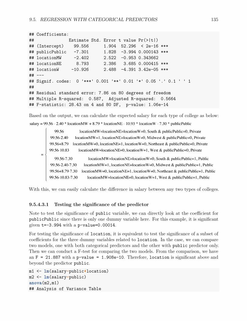
9.5. REGRESSION WITH CATEGORICAL PREDICTORS 135
## Coefficients:## Estimate Std. Error t value Pr(>|t|)## (Intercept) 99.556 1.904 52.296 < 2e-16 ***## publicPublic -7.301 1.828 -3.994 0.000143 ***## locationMW -2.402 2.522 -0.953 0.343662## locationNE 8.793 2.386 3.685 0.000415 ***## locationW -10.926 2.488 -4.391 3.42e-05 ***## ---## Signif. codes: 0 '***' 0.001 '**' 0.01 '*' 0.05 '.' 0.1 ' ' 1#### Residual standard error: 7.86 on 80 degrees of freedom## Multiple R-squared: 0.587, Adjusted R-squared: 0.5664## F-statistic: 28.43 on 4 and 80 DF, p-value: 1.06e-14
Based on the output, we can calculate the expected salary for each type of college as below:
With this, we can easily calculate the difference in salary between any two types of colleges.
9.5.4.3.1 Testing the significance of the predictor
Note to test the significance of public variable, we can directly look at the coefficient forpublicPublic since there is only one dummy variable here. For this example, it is significantgiven t=-3.994 with a p-value=0.00014.
For testing the significance of location, it is equivalent to test the significance of a subset ofcoefficients for the three dummy variables related to location. In the case, we can comparetwo models, one with both categorical predictors and the other with public predictor only.Then we can conduct a F-test for comparing the two models. From the comparison, we havean F = 21.887 with a p-value = 1.908e-10. Therefore, location is significant above andbeyond the predictor public.m1 <- lm(salary~public+location)m2 <- lm(salary~public)anova(m2,m1)## Analysis of Variance Table

136 CHAPTER 9. MULTIPLE LINEAR REGRESSION
#### Model 1: salary ~ public## Model 2: salary ~ public + location## Res.Df RSS Df Sum of Sq F Pr(>F)## 1 83 9000.1## 2 80 4943.0 3 4057.1 21.887 1.908e-10 ***## ---## Signif. codes: 0 '***' 0.001 '**' 0.01 '*' 0.05 '.' 0.1 ' ' 1
9.5.4.4 Example 4. Two categorical predictors with interaction
We can also look the interaction effects between two categorical predictors. In doing theanalysis, we simply include the product of the two predictors. R automatically includes theinteraction terms among the dummy coded variables. To investigate the significance of theinteraction, we similarly can compare the models with and without the interaction term. Forthis particular example, we have an F = 8.4569 with a p-value = 6.316e-05. Therefore,the interaction is significant.m1 <- lm(salary~public+location)m2 <- lm(salary~public*location)anova(m1,m2)## Analysis of Variance Table#### Model 1: salary ~ public + location## Model 2: salary ~ public * location## Res.Df RSS Df Sum of Sq F Pr(>F)## 1 80 4943## 2 77 3718 3 1225 8.4569 6.316e-05 ***## ---## Signif. codes: 0 '***' 0.001 '**' 0.01 '*' 0.05 '.' 0.1 ' ' 1
Note that one can directly apply anova() function in the regression analysis as in ANOVA.
9.5.4.5 Example 4. Regression with one categorical and one continuous predic-tors (ANCOVA)
One might argue that the salary is related to the cost of education. Therefore, when lookingat the salary difference across locations, one should first control the effect of the cost ofeduction. Such analysis can be carried out conveniently as below. And from the output, westill observe significant location effect after controlling the cost of eduction.cost <- cost/1000summary(res<-lm(salary~cost + location))##
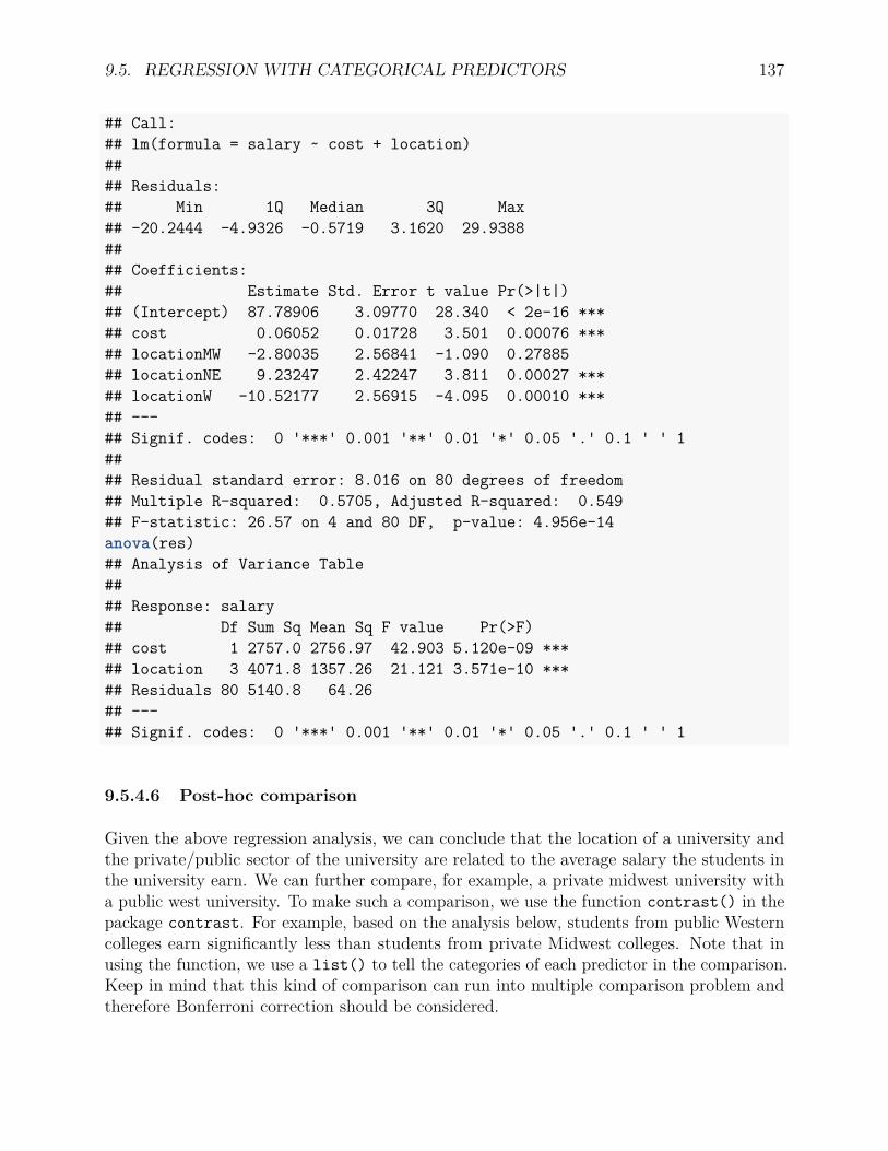
9.5. REGRESSION WITH CATEGORICAL PREDICTORS 137
## Call:## lm(formula = salary ~ cost + location)#### Residuals:## Min 1Q Median 3Q Max## -20.2444 -4.9326 -0.5719 3.1620 29.9388#### Coefficients:## Estimate Std. Error t value Pr(>|t|)## (Intercept) 87.78906 3.09770 28.340 < 2e-16 ***## cost 0.06052 0.01728 3.501 0.00076 ***## locationMW -2.80035 2.56841 -1.090 0.27885## locationNE 9.23247 2.42247 3.811 0.00027 ***## locationW -10.52177 2.56915 -4.095 0.00010 ***## ---## Signif. codes: 0 '***' 0.001 '**' 0.01 '*' 0.05 '.' 0.1 ' ' 1#### Residual standard error: 8.016 on 80 degrees of freedom## Multiple R-squared: 0.5705, Adjusted R-squared: 0.549## F-statistic: 26.57 on 4 and 80 DF, p-value: 4.956e-14anova(res)## Analysis of Variance Table#### Response: salary## Df Sum Sq Mean Sq F value Pr(>F)## cost 1 2757.0 2756.97 42.903 5.120e-09 ***## location 3 4071.8 1357.26 21.121 3.571e-10 ***## Residuals 80 5140.8 64.26## ---## Signif. codes: 0 '***' 0.001 '**' 0.01 '*' 0.05 '.' 0.1 ' ' 1
9.5.4.6 Post-hoc comparison
Given the above regression analysis, we can conclude that the location of a university andthe private/public sector of the university are related to the average salary the students inthe university earn. We can further compare, for example, a private midwest university witha public west university. To make such a comparison, we use the function contrast() in thepackage contrast. For example, based on the analysis below, students from public Westerncolleges earn significantly less than students from private Midwest colleges. Note that inusing the function, we use a list() to tell the categories of each predictor in the comparison.Keep in mind that this kind of comparison can run into multiple comparison problem andtherefore Bonferroni correction should be considered.

138 CHAPTER 9. MULTIPLE LINEAR REGRESSION
m1 <- lm(salary~public+location)
library(contrast)contrast(m1, list(location='W', public='Public'),
list(location='MW', public='Private'))## lm model parameter contrast#### Contrast S.E. Lower Upper t df Pr(>|t|)## 1 -15.82522 2.93855 -21.67312 -9.97732 -5.39 80 0
Chapter 10
Logistic Regression
Logistic regression is widely used in social and behavioral research in analyzing the binary(dichotomous) outcome data. In logistic regression, the outcome can only take two values 0and 1. Some examples that can utilize the logistic regression are given in the following.
• The election of Democratic or Republican president can depend on the factors such asthe economic status, the amount of money spent on the campaign, as well as genderand income of the voters.
• Whether an assistant professor can be tenured may be predicted from the number ofpublications and teaching performance in the first three years.
• Whether or not someone has a heart attack may be related to age, gender and livinghabits.
• Whether a student is admitted may be predicted by her/his high school GPA, SATscore, and quality of recommendation letters.
We use an example to illustrate how to conduct logistic regression in R.
10.1 An example
In this example, the aim is to predict whether a woman is in compliance with mammographyscreening recommendations from four predictors, one reflecting medical input and threereflecting a woman’s psychological status with regarding to screening.
• Outcome y: whether a woman is in compliance with mammography screening recom-mendations (1: in compliance; 0: not in compliance)
• Predictors:– x1: whether she has received a recommendation for screening from a physician;– x2: her knowledge about breast cancer and mammography screening;– x3: her perception of benefit of such a screening;– x4: her perception of the barriers to being screened.
139

140 CHAPTER 10. LOGISTIC REGRESSION
mamm <- read.table("data/mamm.txt", header=TRUE)head(mamm)## y x1 x2 x3 x4## 1 1 1 0.22 4 3## 2 0 0 0.56 1 1## 3 1 0 0.44 4 3## 4 0 0 0.33 3 0## 5 1 1 0.44 5 0## 6 0 1 0.56 5 0
10.2 Basic ideas
With a binary outcome, the linear regression does not work any more. Simply speaking, thepredictors can take any value but the outcome cannot. Therefore, using a linear regressioncannot predict the outcome well. In order to deal with the problem, we model the probabilityto observe an outcome 1 instead, that is p = Pr(y = 1). Using the mammography example,that’ll be the probability for a woman to be in compliance with the screening recommendation.
Even directly modeling the probability would work better than predicting the 1/0 outcome,intuitively. A potential problem is that the probability is bound between 0 and 1 butthe predicted values are generally not. To further deal with the problem, we conduct atransformation using
η = log p
1− p.
After transformation, η can take any value from −∞ when p = 0 to ∞ when p = 1. Such atransformation is called logit transformation, denoted by logit(p). Note that pi/(1− pi) iscalled odds, which is simply the ratio of the probability for the two possible outcomes. Forexample, if for one woman, the probability that she is in compliance is 0.8, then the odds is0.8/(1-0.2)=4. Clearly, for equal probability of the outcome, the odds=1. If odds>1, there isa probability higher than 0.5 to observe the outcome 1. With the transformation, the η canbe directly modeled.
Therefore, the logistic regression is
logit(pi) = log( pi1− pi
) = ηi = β0 + β1x1i + . . .+ βkxki
where pi = Pr(yi = 1). Different from the regular linear regression, no residual is used in themodel.

10.3. FITTING A LOGISTIC REGRESSION MODEL IN R 141
10.2.1 Why is this?
For a variable y with two and only two outcome values, it is often assumed it follows aBernoulli or binomial distribution with the probability p for the outcome 1 and probability1− p for 0. The density function is
py(1− p)1−y.
Note that when y = 1, py(1− p)1−y = p exactly.
Furthermore, we assume there is a continuous variable y∗ underlying the observed binaryvariable. If the continuous variable takes a value larger than certain threshold, we wouldobserve 1, otherwise 0. For logistic regression, we assume the continuous variable has alogistic distribution with the density function:
e−y∗
1 + e−y∗ .
The probability for observing 1 is therefore can be directly calculated using the logisticdistribution as:
p = 11 + e−y∗ ,
which transforms to
log p
1− p = y∗.
For y∗, since it is a continuous variable, it can be predicted as in a regular regression model.
10.3 Fitting a logistic regression model in R
In R, the model can be estimated using the glm() function. Logistic regression is one exampleof the generalized linear model (glm). Below gives the analysis of the mammography data.
• glm uses the model formula same as the linear regression model.• family = tells the distribution of the outcome variable. For binary data, the binomial
distribution is used.• link = tell the transformation method. Here, the logit transformation is used.• The output includes the regression coefficients and their z-statistics and p-values.• The dispersion parameter is related to the variance of the response variable.
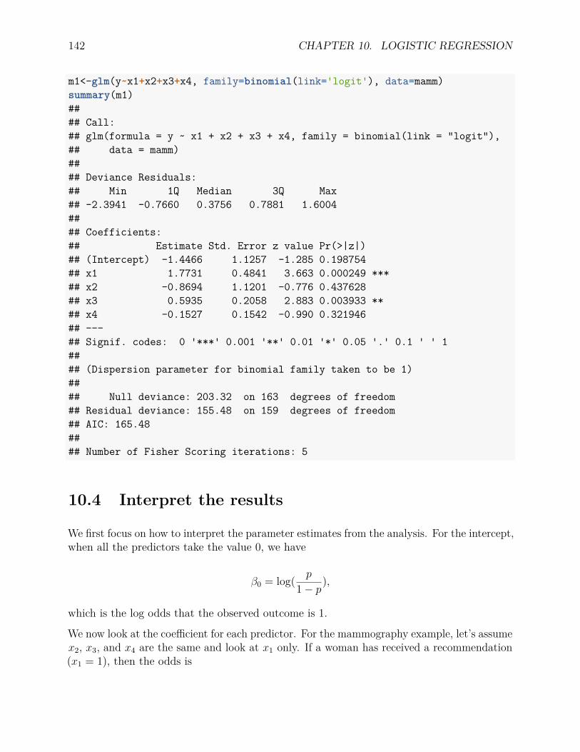
142 CHAPTER 10. LOGISTIC REGRESSION
m1<-glm(y~x1+x2+x3+x4, family=binomial(link='logit'), data=mamm)summary(m1)#### Call:## glm(formula = y ~ x1 + x2 + x3 + x4, family = binomial(link = "logit"),## data = mamm)#### Deviance Residuals:## Min 1Q Median 3Q Max## -2.3941 -0.7660 0.3756 0.7881 1.6004#### Coefficients:## Estimate Std. Error z value Pr(>|z|)## (Intercept) -1.4466 1.1257 -1.285 0.198754## x1 1.7731 0.4841 3.663 0.000249 ***## x2 -0.8694 1.1201 -0.776 0.437628## x3 0.5935 0.2058 2.883 0.003933 **## x4 -0.1527 0.1542 -0.990 0.321946## ---## Signif. codes: 0 '***' 0.001 '**' 0.01 '*' 0.05 '.' 0.1 ' ' 1#### (Dispersion parameter for binomial family taken to be 1)#### Null deviance: 203.32 on 163 degrees of freedom## Residual deviance: 155.48 on 159 degrees of freedom## AIC: 165.48#### Number of Fisher Scoring iterations: 5
10.4 Interpret the results
We first focus on how to interpret the parameter estimates from the analysis. For the intercept,when all the predictors take the value 0, we have
β0 = log( p
1− p),
which is the log odds that the observed outcome is 1.
We now look at the coefficient for each predictor. For the mammography example, let’s assumex2, x3, and x4 are the same and look at x1 only. If a woman has received a recommendation(x1 = 1), then the odds is
10.4. INTERPRET THE RESULTS 143
log( p
1− p)|(x1 = 1) = β0 + β1 + β2x2 + β3x3 + β4x4.
If a woman has not received a recommendation (x1 = 0), then the odds is
log( p
1− p)|(x1 = 0) = β0 + β2x2 + β3x3 + β4x4.
The difference is
log( p
1− p)|(x1 = 1)− log( p
1− p)|(x1 = 0) = β1.
Therefore, the logistic regression coefficient for a predictor is the difference in the log oddswhen the predictor changes 1 unit given other predictors unchanged.
This above equation is equivalent to
log p(x1=1)
1−p(x1=1)p(x1=0)
1−p(x1=0)
= β1.
More descriptively, we have
log(
ODDS(received recommendation)ODDS(not received recommendation)
)= β1.
Therefore, the regression coefficients is the log odds ratio. By a simple transformation, wehave
ODDS(received recommendation)ODDS(not received recommendation) = exp(β1)
or
ODDS(received recommendation) = exp(β1) ∗ODDS(not received recommendation).
Therefore, the exponential of a regression coefficient is the odds ratio. For the example,exp(β1)=exp(1.7731)=5.9. Thus, the odds in compliance to screening for those who receivedrecommendation is about 5.9 times of those who did not receive recommendation.
For continuous predictors, the regression coefficients can also be interpreted the same way.For example, we may say that if high school GPA increase one unit, the odds a student to beadmitted can be increased to 6 times given other variables the same.
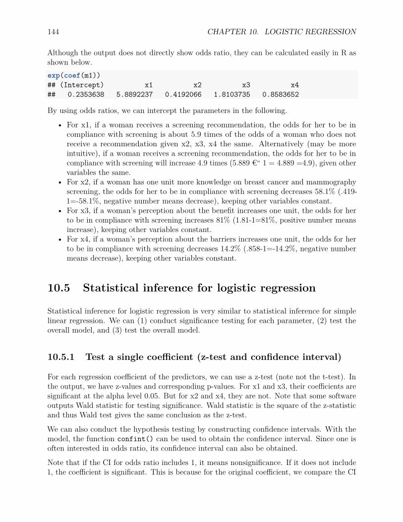
144 CHAPTER 10. LOGISTIC REGRESSION
Although the output does not directly show odds ratio, they can be calculated easily in R asshown below.exp(coef(m1))## (Intercept) x1 x2 x3 x4## 0.2353638 5.8892237 0.4192066 1.8103735 0.8583652
By using odds ratios, we can intercept the parameters in the following.
• For x1, if a woman receives a screening recommendation, the odds for her to be incompliance with screening is about 5.9 times of the odds of a woman who does notreceive a recommendation given x2, x3, x4 the same. Alternatively (may be moreintuitive), if a woman receives a screening recommendation, the odds for her to be incompliance with screening will increase 4.9 times (5.889 €“ 1 = 4.889 =4.9), given othervariables the same.
• For x2, if a woman has one unit more knowledge on breast cancer and mammographyscreening, the odds for her to be in compliance with screening decreases 58.1% (.419-1=-58.1%, negative number means decrease), keeping other variables constant.
• For x3, if a woman’s perception about the benefit increases one unit, the odds for herto be in compliance with screening increases 81% (1.81-1=81%, positive number meansincrease), keeping other variables constant.
• For x4, if a woman’s perception about the barriers increases one unit, the odds for herto be in compliance with screening decreases 14.2% (.858-1=-14.2%, negative numbermeans decrease), keeping other variables constant.
10.5 Statistical inference for logistic regression
Statistical inference for logistic regression is very similar to statistical inference for simplelinear regression. We can (1) conduct significance testing for each parameter, (2) test theoverall model, and (3) test the overall model.
10.5.1 Test a single coefficient (z-test and confidence interval)
For each regression coefficient of the predictors, we can use a z-test (note not the t-test). Inthe output, we have z-values and corresponding p-values. For x1 and x3, their coefficients aresignificant at the alpha level 0.05. But for x2 and x4, they are not. Note that some softwareoutputs Wald statistic for testing significance. Wald statistic is the square of the z-statisticand thus Wald test gives the same conclusion as the z-test.
We can also conduct the hypothesis testing by constructing confidence intervals. With themodel, the function confint() can be used to obtain the confidence interval. Since one isoften interested in odds ratio, its confidence interval can also be obtained.
Note that if the CI for odds ratio includes 1, it means nonsignificance. If it does not include1, the coefficient is significant. This is because for the original coefficient, we compare the CI
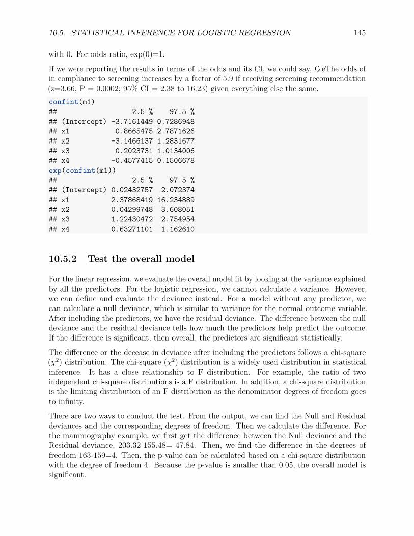
10.5. STATISTICAL INFERENCE FOR LOGISTIC REGRESSION 145
with 0. For odds ratio, exp(0)=1.
If we were reporting the results in terms of the odds and its CI, we could say, €œThe odds ofin compliance to screening increases by a factor of 5.9 if receiving screening recommendation(z=3.66, P = 0.0002; 95% CI = 2.38 to 16.23) given everything else the same.confint(m1)## 2.5 % 97.5 %## (Intercept) -3.7161449 0.7286948## x1 0.8665475 2.7871626## x2 -3.1466137 1.2831677## x3 0.2023731 1.0134006## x4 -0.4577415 0.1506678exp(confint(m1))## 2.5 % 97.5 %## (Intercept) 0.02432757 2.072374## x1 2.37868419 16.234889## x2 0.04299748 3.608051## x3 1.22430472 2.754954## x4 0.63271101 1.162610
10.5.2 Test the overall model
For the linear regression, we evaluate the overall model fit by looking at the variance explainedby all the predictors. For the logistic regression, we cannot calculate a variance. However,we can define and evaluate the deviance instead. For a model without any predictor, wecan calculate a null deviance, which is similar to variance for the normal outcome variable.After including the predictors, we have the residual deviance. The difference between the nulldeviance and the residual deviance tells how much the predictors help predict the outcome.If the difference is significant, then overall, the predictors are significant statistically.
The difference or the decease in deviance after including the predictors follows a chi-square(χ2) distribution. The chi-square (χ2) distribution is a widely used distribution in statisticalinference. It has a close relationship to F distribution. For example, the ratio of twoindependent chi-square distributions is a F distribution. In addition, a chi-square distributionis the limiting distribution of an F distribution as the denominator degrees of freedom goesto infinity.
There are two ways to conduct the test. From the output, we can find the Null and Residualdeviances and the corresponding degrees of freedom. Then we calculate the difference. Forthe mammography example, we first get the difference between the Null deviance and theResidual deviance, 203.32-155.48= 47.84. Then, we find the difference in the degrees offreedom 163-159=4. Then, the p-value can be calculated based on a chi-square distributionwith the degree of freedom 4. Because the p-value is smaller than 0.05, the overall model issignificant.

146 CHAPTER 10. LOGISTIC REGRESSION
The test can be conducted simply in another way. We first fit a model without any predictorand another model with all the predictors. Then, we can use anova() to get the difference indeviance and the chi-square test result.## method 1d_chi <- 203.32 - 155.48d_df <- 163 - 159
1 - pchisq(d_chi, d_df)## [1] 1.019117e-09
## method 2m0 <- glm(y~1, family=binomial(link='logit'), data=mamm)anova(m0,m1)## Analysis of Deviance Table#### Model 1: y ~ 1## Model 2: y ~ x1 + x2 + x3 + x4## Resid. Df Resid. Dev Df Deviance## 1 163 203.32## 2 159 155.48 4 47.837
10.5.3 Test a subset of predictors
We can also test the significance of a subset of predictors. For example, whether x3 andx4 are significant above and beyond x1 and x2. This can also be done using the chi-squaretest based on the difference. In this case, we can compare a model with all predictors and amodel without x3 and x4 to see if the change in the deviance is significant. In this example,the p-value is 0.002, indicating the change is signficant. Therefore, x3 and x4 are statisticallysignificant above and beyond x1 and x2.m1<-glm(y~x1+x2+x3+x4, family=binomial(link='logit'), data=mamm)m2 <- glm(y~x1+x2, family=binomial(link='logit'), data=mamm)
anova(m2, m1)## Analysis of Deviance Table#### Model 1: y ~ x1 + x2## Model 2: y ~ x1 + x2 + x3 + x4## Resid. Df Resid. Dev Df Deviance## 1 161 168.23## 2 159 155.48 2 12.749
1 - pchisq(12.749, 2)## [1] 0.001704472

Chapter 11
Moderation Analysis
11.1 What is a moderator?
To explain what is a moderator, we start with a bivariate relationship between an inputvariable X and an outcome variable Y . For example, X could be the number of trainingsessions (training intensity) and Y could be math test score. We can hypothesize that thereis a relationship between them such that the number of training sessions predicts math testperformance. Using a diagram, we can portray the relationship below.
The above path diagram can be expressed using a regression model as
Y = β0 + β1 ∗X + ε
where β0 is the intercept and β1 is the slope.
A moderator variable Z is a variable that alters the strength of the relationship between Xand Y . In other words, the effect of X on Y depends on the levels of the moderator Z. Forinstance, if male students (Z = 0) benefit more (or less) from training than female students(Z = 1), then gender can be considered as a moderator. Using the diagram, if the coefficienta is different b, there is a moderation effect.
147

148 CHAPTER 11. MODERATION ANALYSIS
To summarize, a moderator Z is a variable that alters the direction and/or strength of therelation between a predictor X and an outcome Y .
Questions involving moderators address when or for whom a variable most strongly predictsor causes an outcome variable. Using a path diagram, we can express the moderation effectas:
11.2 How to conduct moderation analysis?
Moderation analysis can be conducted by adding one or multiple interaction terms in aregression analysis. For example, if Z is a moderator for the relation between X and Y , wecan fit a regression model
Y = β0 + β1 ∗X + β2 ∗ Z + β3 ∗X ∗ Z + ε
= β0 + β2 ∗ Z + (β1 + β3 ∗ Z) ∗X + ε.
Thus, if β3 is not equal to 0, the relationship between X and Y depends on the value of Z,which indicates a moderation effect. In fact, from the regression model, we can get:
• If z = 0, the effect of X on Y is β1 + β3 ∗ 0 = β1.• If z = 2, the effect of X on Y is β1 + β3 ∗ 2.• If z = 4, the effect of X on Y is β1 + β3 ∗ 4.
If Z is a dichotomous/binary variable, for example, gender, the above equation can be writtenas
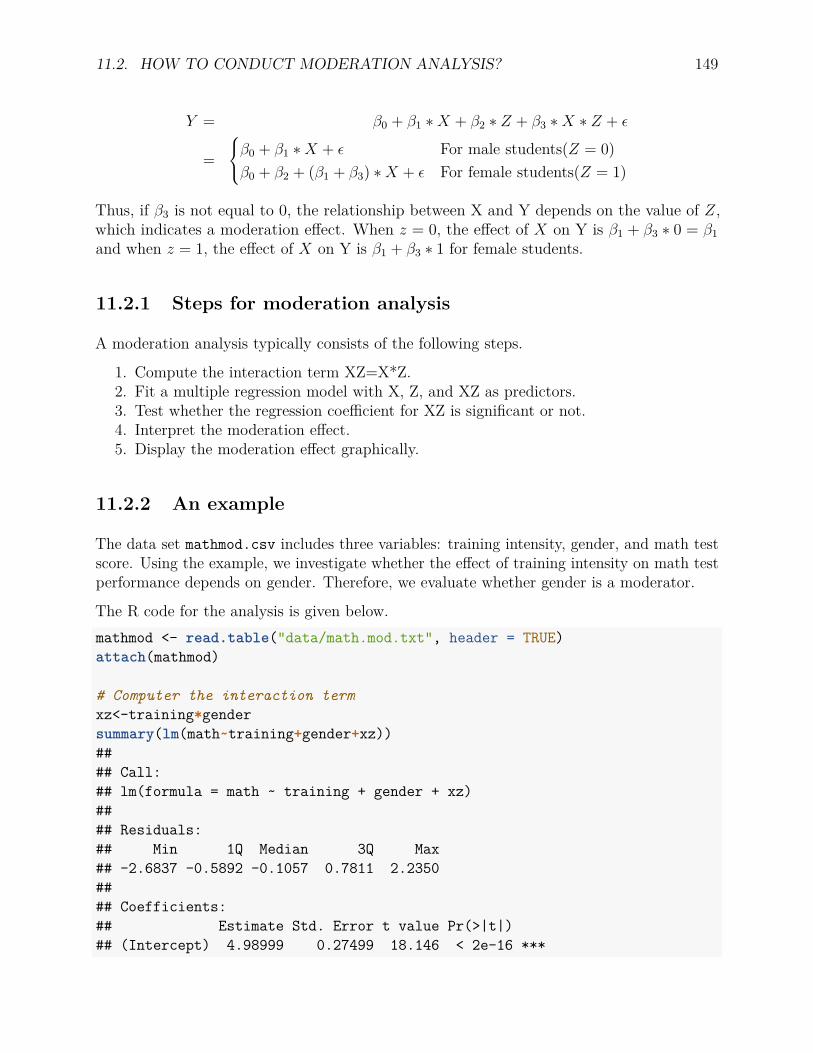
11.2. HOW TO CONDUCT MODERATION ANALYSIS? 149
Y = β0 + β1 ∗X + β2 ∗ Z + β3 ∗X ∗ Z + ε
=
β0 + β1 ∗X + ε For male students(Z = 0)β0 + β2 + (β1 + β3) ∗X + ε For female students(Z = 1)
Thus, if β3 is not equal to 0, the relationship between X and Y depends on the value of Z,which indicates a moderation effect. When z = 0, the effect of X on Y is β1 + β3 ∗ 0 = β1and when z = 1, the effect of X on Y is β1 + β3 ∗ 1 for female students.
11.2.1 Steps for moderation analysis
A moderation analysis typically consists of the following steps.
1. Compute the interaction term XZ=X*Z.2. Fit a multiple regression model with X, Z, and XZ as predictors.3. Test whether the regression coefficient for XZ is significant or not.4. Interpret the moderation effect.5. Display the moderation effect graphically.
11.2.2 An example
The data set mathmod.csv includes three variables: training intensity, gender, and math testscore. Using the example, we investigate whether the effect of training intensity on math testperformance depends on gender. Therefore, we evaluate whether gender is a moderator.
The R code for the analysis is given below.mathmod <- read.table("data/math.mod.txt", header = TRUE)attach(mathmod)
# Computer the interaction termxz<-training*gendersummary(lm(math~training+gender+xz))#### Call:## lm(formula = math ~ training + gender + xz)#### Residuals:## Min 1Q Median 3Q Max## -2.6837 -0.5892 -0.1057 0.7811 2.2350#### Coefficients:## Estimate Std. Error t value Pr(>|t|)## (Intercept) 4.98999 0.27499 18.146 < 2e-16 ***

150 CHAPTER 11. MODERATION ANALYSIS
## training -0.33943 0.05387 -6.301 8.70e-09 ***## gender -2.75688 0.37912 -7.272 9.14e-11 ***## xz 0.50427 0.06845 7.367 5.80e-11 ***## ---## Signif. codes: 0 '***' 0.001 '**' 0.01 '*' 0.05 '.' 0.1 ' ' 1#### Residual standard error: 0.9532 on 97 degrees of freedom## Multiple R-squared: 0.3799, Adjusted R-squared: 0.3607## F-statistic: 19.81 on 3 and 97 DF, p-value: 4.256e-10
Since the regression coefficient (0.504) for the interaction term XZ is significant at the alphalevel 0.05 with a p-value=5.8e-11, there exists a significant moderation effect. In otherwords, the effect of training intensity on math performance significantly depends on gender.
When Z=0 (male students), the estimated effect of training intensity on math performanceis β1 = −.34. When Z=1 (female students), the estimated effect of training intensity onmath performance is β1 + β3 = −.34 + .50 = .16. The moderation analysis tells us that theeffects of training intensity on math performance for males (-.34) and females (.16) aresignificantly different for this example.
11.2.2.1 Interaction plot
A moderation effect indicates the regression slopes are different for different groups. Therefore,if we plot the regression line for each group, they should interact at certain point. Such aplot is called an interaction plot. To get the plot, we first calculate the intercept and slopefor each level of the moderator. For this example, we have
Y = β0 + β1 ∗X + β2 ∗ Z + β3 ∗X ∗ Z (11.1)
=
β0 + β1 ∗X For male students(Z = 0)β0 + β2 + (β1 + β3) ∗X For female students(Z = 1)
. (11.2)
=
5− 0.34 ∗X For male students(Z = 0)2.23 + 0.16 ∗X For female students(Z = 1)
(11.3)
With the information, we can generate a plot using the R code below. Note that the optiontype='n' generates a figure without actually plotting the data. In the function abline(),the first value is the intercept and the second is the slope. Note that the values for each levelcan also be added to the plot.plot(training, math, type='n') ## create an empty frameabline(5, -.34) ## for maleabline(2.23, .16, lty=2, col='red') ## for femalelegend('topright', c('Male', 'Female'), lty=c(1,2),
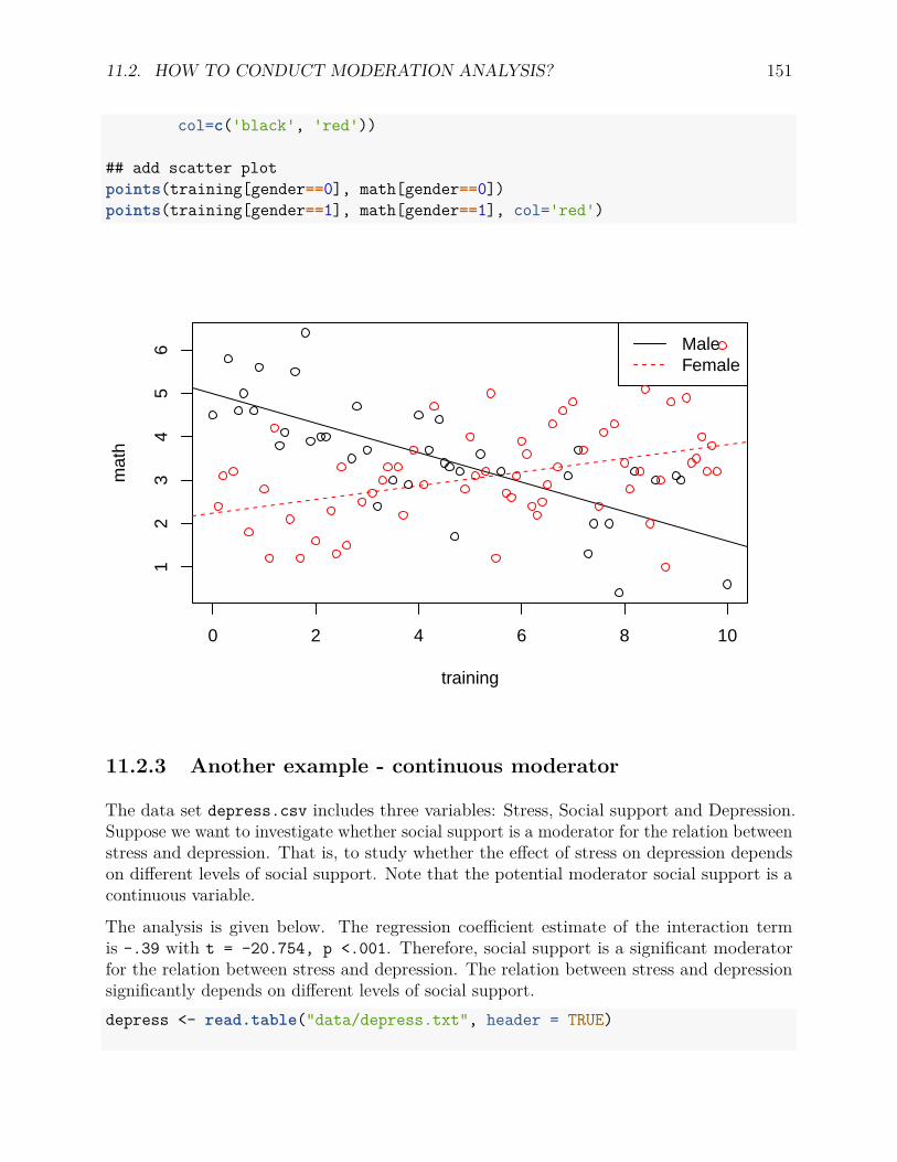
11.2. HOW TO CONDUCT MODERATION ANALYSIS? 151
col=c('black', 'red'))
## add scatter plotpoints(training[gender==0], math[gender==0])points(training[gender==1], math[gender==1], col='red')
0 2 4 6 8 10
12
34
56
training
mat
h
MaleFemale
11.2.3 Another example - continuous moderator
The data set depress.csv includes three variables: Stress, Social support and Depression.Suppose we want to investigate whether social support is a moderator for the relation betweenstress and depression. That is, to study whether the effect of stress on depression dependson different levels of social support. Note that the potential moderator social support is acontinuous variable.
The analysis is given below. The regression coefficient estimate of the interaction termis -.39 with t = -20.754, p <.001. Therefore, social support is a significant moderatorfor the relation between stress and depression. The relation between stress and depressionsignificantly depends on different levels of social support.depress <- read.table("data/depress.txt", header = TRUE)

152 CHAPTER 11. MODERATION ANALYSIS
# the interaction termdepress$inter<-depress$stress*depress$supportsummary(lm(depress~stress+support+inter, data=depress))#### Call:## lm(formula = depress ~ stress + support + inter, data = depress)#### Residuals:## Min 1Q Median 3Q Max## -3.7322 -0.9035 -0.1127 0.8542 3.6089#### Coefficients:## Estimate Std. Error t value Pr(>|t|)## (Intercept) 29.2583 0.6909 42.351 <2e-16 ***## stress 1.9956 0.1161 17.185 <2e-16 ***## support -0.2356 0.1109 -2.125 0.0362 *## inter -0.3902 0.0188 -20.754 <2e-16 ***## ---## Signif. codes: 0 '***' 0.001 '**' 0.01 '*' 0.05 '.' 0.1 ' ' 1#### Residual standard error: 1.39 on 96 degrees of freedom## Multiple R-squared: 0.9638, Adjusted R-squared: 0.9627## F-statistic: 853 on 3 and 96 DF, p-value: < 2.2e-16
Since social support is a continuous variable, there is no immediate levels to look at therelationship between stress and depression. However, we can choose several difference levels.One way is to use these three levels of a moderator: mean, one standard deviation below themean and one standard deviation above the mean. For this example, the three values forsocial support are 5.37, 2.56 and 8.18. The fitted regression lines for the three values are
ˆdepress = 29.26 + 2.00 ∗ stress− .24 ∗ support− .39 ∗ stress ∗ support (11.4)
=
28.65 + 1 ∗ stress support = 2.5627.97− .09 ∗ stress support = 5.37.27.30− 1.19 ∗ stress support = 8.18
(11.5)
From it, we can clearly see that with more social support, the relationship between depressionand stress becomes negative from positive. This can also be seen from the interaction plotbelow.## create an empty frameplot(depress$stress, depress$depress, type='n',
xlab='Stress', ylab='Depression')
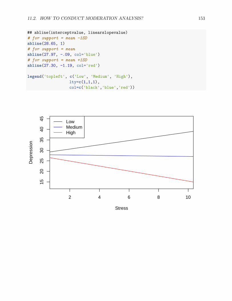
11.2. HOW TO CONDUCT MODERATION ANALYSIS? 153
## abline(interceptvalue, linearslopevalue)# for support = mean -1SDabline(28.65, 1)# for support = meanabline(27.97, -.09, col='blue')# for support = mean +1SDabline(27.30, -1.19, col='red')
legend('topleft', c('Low', 'Medium', 'High'),lty=c(1,1,1),col=c('black','blue','red'))
2 4 6 8 10
1520
2530
3540
45
Stress
Dep
ress
ion
LowMediumHigh

154 CHAPTER 11. MODERATION ANALYSIS

Chapter 12
Mediation Analysis
12.1 Path diagrams
Consider a bivariate relationship between X and Y. If X is a predictor and Y is the outcome,we can fit a regression model
Y = iY 0 + cX + eY 0
where c is the effect of X on Y , also called as the total effect of X on Y . The model can beexpressed as a path diagram as shown below.
12.1.1 Rules to draw a path diagram
In a path diagram, there are three types of shapes: a rectangle, a circle, and a triangle, as wellas two types of arrows: one-headed (single-headed) arrow and two-headed (double-headed)arrows.
A rectangle represents an observed variable, which is a variable in the dataset with knowninformation from the subjects. A circle or elliptical represents an unobserved variable, which
155
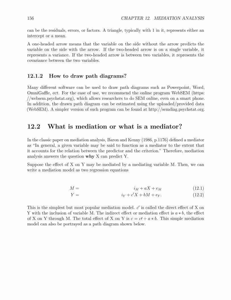
156 CHAPTER 12. MEDIATION ANALYSIS
can be the residuals, errors, or factors. A triangle, typically with 1 in it, represents either anintercept or a mean.
A one-headed arrow means that the variable on the side without the arrow predicts thevariable on the side with the arrow. If the two-headed arrow is on a single variable, itrepresents a variance. If the two-headed arrow is between two variables, it represents thecovariance between the two variables.
12.1.2 How to draw path diagrams?
Many different software can be used to draw path diagrams such as Powerpoint, Word,OmniGaffle, ect. For the ease of use, we recommend the online program WebSEM (https://websem.psychstat.org), which allows researchers to do SEM online, even on a smart phone.In addition, the drawn path diagram can be estimated using the uploaded/provided data(WebSEM). A simpler version of such program can be found at http://semdiag.psychstat.org.
12.2 What is mediation or what is a mediator?
In the classic paper on mediation analysis, Baron and Kenny (1986, p.1176) defined a mediatoras “In general, a given variable may be said to function as a mediator to the extent thatit accounts for the relation between the predictor and the criterion.” Therefore, mediationanalysis answers the question why X can predict Y.
Suppose the effect of X on Y may be mediated by a mediating variable M. Then, we canwrite a mediation model as two regression equations
M = iM + aX + eM (12.1)Y = iY + c′X + bM + eY . (12.2)
This is the simplest but most popular mediation model. c′ is called the direct effect of X onY with the inclusion of variable M. The indirect effect or mediation effect is a ∗ b, the effectof X on Y through M. The total effect of X on Y is c = c′ + a ∗ b. This simple mediationmodel can also be portrayed as a path diagram shown below.
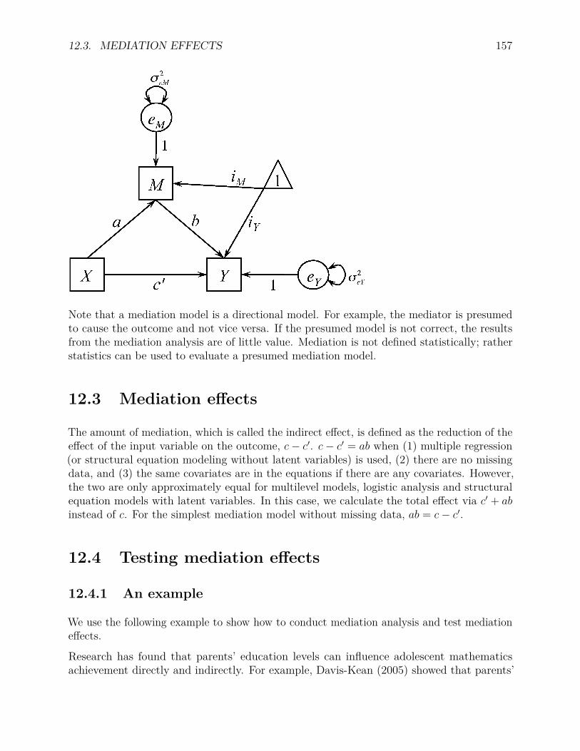
12.3. MEDIATION EFFECTS 157
Note that a mediation model is a directional model. For example, the mediator is presumedto cause the outcome and not vice versa. If the presumed model is not correct, the resultsfrom the mediation analysis are of little value. Mediation is not defined statistically; ratherstatistics can be used to evaluate a presumed mediation model.
12.3 Mediation effects
The amount of mediation, which is called the indirect effect, is defined as the reduction of theeffect of the input variable on the outcome, c− c′. c− c′ = ab when (1) multiple regression(or structural equation modeling without latent variables) is used, (2) there are no missingdata, and (3) the same covariates are in the equations if there are any covariates. However,the two are only approximately equal for multilevel models, logistic analysis and structuralequation models with latent variables. In this case, we calculate the total effect via c′ + abinstead of c. For the simplest mediation model without missing data, ab = c− c′.
12.4 Testing mediation effects
12.4.1 An example
We use the following example to show how to conduct mediation analysis and test mediationeffects.
Research has found that parents’ education levels can influence adolescent mathematicsachievement directly and indirectly. For example, Davis-Kean (2005) showed that parents’
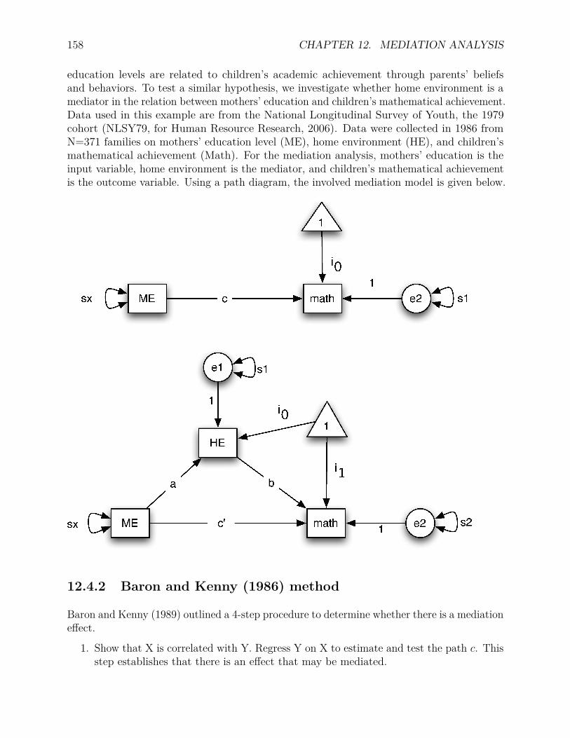
158 CHAPTER 12. MEDIATION ANALYSIS
education levels are related to children’s academic achievement through parents’ beliefsand behaviors. To test a similar hypothesis, we investigate whether home environment is amediator in the relation between mothers’ education and children’s mathematical achievement.Data used in this example are from the National Longitudinal Survey of Youth, the 1979cohort (NLSY79, for Human Resource Research, 2006). Data were collected in 1986 fromN=371 families on mothers’ education level (ME), home environment (HE), and children’smathematical achievement (Math). For the mediation analysis, mothers’ education is theinput variable, home environment is the mediator, and children’s mathematical achievementis the outcome variable. Using a path diagram, the involved mediation model is given below.
12.4.2 Baron and Kenny (1986) method
Baron and Kenny (1989) outlined a 4-step procedure to determine whether there is a mediationeffect.
1. Show that X is correlated with Y. Regress Y on X to estimate and test the path c. Thisstep establishes that there is an effect that may be mediated.
12.4. TESTING MEDIATION EFFECTS 159
2. Show that X is correlated with M. Regress M on X to estimate and test path a. Thisstep essentially involves treating the mediator as if it were an outcome variable.
3. Show that M affects Y. Regress Y on both X and M to estimate and test path b. Notethat it is not sufficient just to correlate the mediator with the outcome; the mediatorand the outcome may be correlated because they are both caused by the input variableX. Thus, the input variable X must be controlled in establishing the effect of themediator on the outcome.
4. To establish that M completely mediates the X-Y relationship, the effect of X on Ycontrolling for M (path c′) should be zero. The effects in both Steps 3 and 4 areestimated in the same equation.
If all four of these steps are met, then the data are consistent with the hypothesis thatvariable M completely mediates the X-Y relationship, and if the first three steps are met butthe Step 4 is not, then partial mediation is indicated.
The R code for the 4-step method for the example data is shown below.nlsy <- read.table("data/nlsy.med.comp.txt", header=TRUE)attach(nlsy)
# Step 1summary(lm(math~ME))#### Call:## lm(formula = math ~ ME)#### Residuals:## Min 1Q Median 3Q Max## -14.6224 -2.9299 -0.4574 2.4876 29.4876#### Coefficients:## Estimate Std. Error t value Pr(>|t|)## (Intercept) 6.1824 1.3709 4.510 8.73e-06 ***## ME 0.5275 0.1199 4.398 1.43e-05 ***## ---## Signif. codes: 0 '***' 0.001 '**' 0.01 '*' 0.05 '.' 0.1 ' ' 1#### Residual standard error: 4.618 on 369 degrees of freedom## Multiple R-squared: 0.04981, Adjusted R-squared: 0.04723## F-statistic: 19.34 on 1 and 369 DF, p-value: 1.432e-05
# Step 2summary(lm(HE~ME))#### Call:## lm(formula = HE ~ ME)

160 CHAPTER 12. MEDIATION ANALYSIS
#### Residuals:## Min 1Q Median 3Q Max## -5.5020 -0.7805 0.2195 1.2195 3.3587#### Coefficients:## Estimate Std. Error t value Pr(>|t|)## (Intercept) 4.10944 0.49127 8.365 1.25e-15 ***## ME 0.13926 0.04298 3.240 0.0013 **## ---## Signif. codes: 0 '***' 0.001 '**' 0.01 '*' 0.05 '.' 0.1 ' ' 1#### Residual standard error: 1.655 on 369 degrees of freedom## Multiple R-squared: 0.02766, Adjusted R-squared: 0.02502## F-statistic: 10.5 on 1 and 369 DF, p-value: 0.001305
# Step 3 & 4summary(lm(math~ME+HE))#### Call:## lm(formula = math ~ ME + HE)#### Residuals:## Min 1Q Median 3Q Max## -14.9302 -3.0045 -0.2226 2.2386 29.3856#### Coefficients:## Estimate Std. Error t value Pr(>|t|)## (Intercept) 4.2736 1.4764 2.895 0.004022 **## ME 0.4628 0.1201 3.853 0.000137 ***## HE 0.4645 0.1434 3.238 0.001311 **## ---## Signif. codes: 0 '***' 0.001 '**' 0.01 '*' 0.05 '.' 0.1 ' ' 1#### Residual standard error: 4.559 on 368 degrees of freedom## Multiple R-squared: 0.07613, Adjusted R-squared: 0.07111## F-statistic: 15.16 on 2 and 368 DF, p-value: 4.7e-07
In Step 1, we fit a regression model using ME as the predictor and math as the outcomevariable. Based on this analysis, we have c =.5275 (t = 4.298, p <.001) and thus ME issignificantly related to math. Therefore, Step 1 is met: the input variable is correlated withthe outcome.
In Step 2, we fit a regression model using ME as the predictor and HE as the outcomevariable. From this analysis, we have a = .139 (t = 3.24, p = .0013) and thus ME is
12.4. TESTING MEDIATION EFFECTS 161
significantly related to HE. Therefore, Step 2 is met: the input variable is correlated with themediator.
In Step 3, we fit a multiple regression model with ME and HE as predictors and math as theoutcome variable. For the analysis, we have b=.4645 (t = 3.238, p =.0013). Becauseboth a and b are significant, we can say HE significantly mediates the relationship betweenME and math. The mediation effect estimate is ab = .139∗.4645 = 0.065.
Step 4, from the results in Step 3, we know that the direct effect c’ (c′=.4628, t = 3.853,p = .00013) is also significant. Thus, there exists a partial mediation.
12.4.3 Sobel test
Many researchers believe that the essential steps in establishing mediation are Steps 2 and3. Step 4 does not have to be met unless the expectation is for complete mediation. Inthe opinion of most researchers, though not all, Step 1 is not required. However, note thata path from the input variable to the outcome is implied if Steps 2 and 3 are met. If c′were in the opposite sign to that of ab, then it could be the case that Step 1 would not bemet, but there is still mediation. In this case the mediator acts like a suppressor variable.MacKinnon, Fairchild, and Fritz (2007) called it inconsistent mediation. For example, considerthe relationship between stress and mood as mediated by coping. Presumably, the directeffect is negative: more stress, the worse the mood. However, likely the effect of stress oncoping is positive (more stress, more coping) and the effect of coping on mood is positive(more coping, better mood), making the indirect effect positive. The total effect of stresson mood then is likely to be very small because the direct and indirect effects will tend tocancel each other out. Note that with inconsistent mediation, the direct effect is typicallylarger than the total effect.
It is therefore much more common and highly recommended to perform a single test of ab,than the two seperate tests of a and b. The test was first proposed by Sobel (1982) andthus is also called the Sobel test. The standard error estimate of a is denoted as sa and thestandard error estimate of b is denoted as sb. The Sobel test used the following standarderror estimate of ab
√b2s2
a + a2s2b.
The test of the indirect effect is given by dividing ab by the above standard error estimateand treating the ratio as a Z test:
z − score = ab√b2s2
a + a2s2b
.
If a z-score is larger than 1.96 in absolute value, the mediation effect is significant at the .05level.
162 CHAPTER 12. MEDIATION ANALYSIS
From the example in the 4-step method, the mediation effect is ab=0.065 and its standarderror is
√b2s2
a + a2s2b
=√.46452 ∗ .0432 + .1392 ∗ .14342 = .028.
Thus,
z − score = .065.028 = 2.32.
Because the z-score is greater than 1.96, the mediation effect is significant at the alpha level0.05. Actually, the p-value is 0.02.
The Sobel test is easy to conduct but has many disadvantages. The derivation of the Sobelstandard error estimate presumes that a and b are independent, something that may not betrue. Furthermore, the Sobel test assumes ab is normally distributed and might not workwell for small sample sizes. The Sobel test has also been shown to be very conservative andthus the power of the test is low. One solution is to use the bootstrap method.
12.4.4 Bootstrapping for mediation analysis
The bootstrap method was first employed in the mediation analysis by Bollen and Stine(1990). This method has no distribution assumption on the indirect effect ab. Instead, itapproximates the distribution of ab using its bootstrap distribution. The bootstrap methodwas shown to be more appropriate for studies with sample sizes 20-80 than single samplemethods. Currently, the bootstrap method of mediation is generally following the procedureused in Bollen and Stine (1990).
The method works in the following way. Using the original data set (Sample size = n) as thepopulation, draw a bootstrap sample of n individuals with paired (Y, X, M) scores randomlyfrom the data set with replacement. From the bootstrap sample, estimate ab through somemethod such as OLS based on a set of regression models. Repeat the two steps for a totalof B times. B is called the number of bootstraps. The empirical distribution based on thisbootstrap procedure can be viewed as the distribution of ab. The (1− α) ∗ 100% confidenceinterval of ab can be constructed using the α/2 and 1 − α/2 percentiles of the empiricaldistribution.
In R, mediation analysis based on both Sobel test and bootstrapping can be conducted usingthe R bmem() package. For example, the R code for Sobel test is given below.library(bmem)
m1 <- "math = b*HE + cp*MEHE = a*ME"

12.4. TESTING MEDIATION EFFECTS 163
nlsy.model<-specifyEquations(text=m1, exog.variances=T)
effects<-c('a*b', 'cp+a*b')nlsy.res<-bmem.sobel(nlsy, nlsy.model,effects)## Estimate S.E. z-score p.value## b 0.46450283 0.14304860 3.247168 1.165596e-03## cp 0.46281480 0.11977862 3.863918 1.115825e-04## a 0.13925694 0.04292438 3.244239 1.177650e-03## V[HE] 2.73092635 0.20078170 13.601471 0.000000e+00## V[math] 20.67659134 1.52017323 13.601471 0.000000e+00## V[ME] 4.00590078 0.29451968 13.601471 0.000000e+00## a*b 0.06468524 0.02818457 2.295059 2.172977e-02## cp+a*b 0.52750005 0.11978162 4.403848 1.063474e-05
Note that to use the package, we need to specify the mediation model first. The mediationmodel can be provided using equations. For the simple mediation model, there need tworegression equation: math = b*HE + cp*ME and HE = a*ME. Clearly, the outcome variable ison the left of the “=” sign. In addition, we should include the parameter labels in the model.For example, a, b, and cp represent the parameters in the model. The function to specify themodel is specifyEquations(), which is a function of the R package bmem(), which bmem()was developed based on. In this function, we also use the option exog.variances=T, whichis used to specify the variance parameters automatically.
In addition to the model, we also need to provide the indirect effects or any other effects ofinterest. Multiple effects can be provided using a vector. Each effect is a combination ofmultiple model parameters. For example, a*b is the mediation effect and a*b + cp is thetotal effect.
Finally, the function bmem.sobel() is used to conduct the Sobel test. The function requiresat least three options: a data set, a model, and the effects of interest, in the order presented.
The output includes the parameter estimate, standard error, z-score and p-value for eachparameter and effect under investigation. Note that the mediation effect is again 0.065 andis significant at the alpha level 0.05.
Conducting a bootstrap is similar to Sobel test. In this case, the function bmem() is used. Inaddition to provide a data set, a model, and the effects of interest, we can also specify howmany bootstrap samples are used (the option boot=). The default is 1,000. In this example,we used 500.
The output includes the 95% bootstrap CIs. Using a CI, we can conduct a test. Based onthe fact that the CI for ab [.0258, .1377] does not include 0, there is a significant mediationeffect. In addition, because the CI for c′ does not contain 0, c′ is significantly different from0. Thus, we have a partial mediation effect.m2 <- "math = b*HE + cp*MEHE = a*ME"
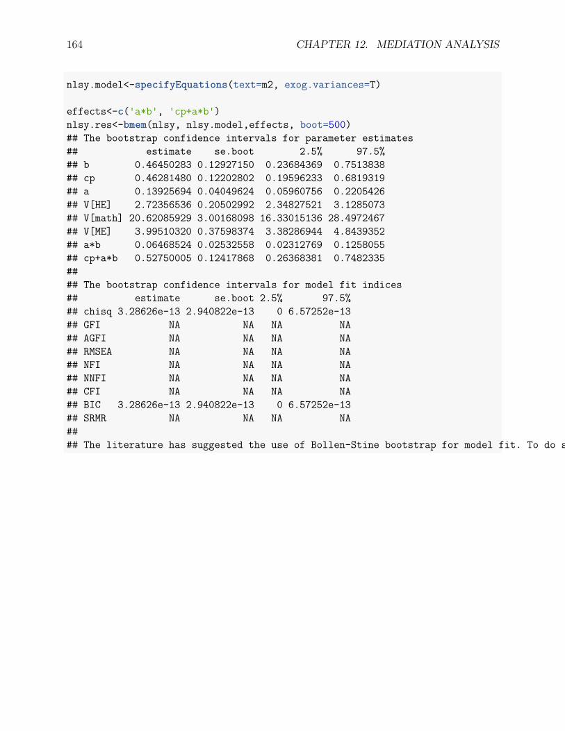
164 CHAPTER 12. MEDIATION ANALYSIS
nlsy.model<-specifyEquations(text=m2, exog.variances=T)
effects<-c('a*b', 'cp+a*b')nlsy.res<-bmem(nlsy, nlsy.model,effects, boot=500)## The bootstrap confidence intervals for parameter estimates## estimate se.boot 2.5% 97.5%## b 0.46450283 0.12927150 0.23684369 0.7513838## cp 0.46281480 0.12202802 0.19596233 0.6819319## a 0.13925694 0.04049624 0.05960756 0.2205426## V[HE] 2.72356536 0.20502992 2.34827521 3.1285073## V[math] 20.62085929 3.00168098 16.33015136 28.4972467## V[ME] 3.99510320 0.37598374 3.38286944 4.8439352## a*b 0.06468524 0.02532558 0.02312769 0.1258055## cp+a*b 0.52750005 0.12417868 0.26368381 0.7482335#### The bootstrap confidence intervals for model fit indices## estimate se.boot 2.5% 97.5%## chisq 3.28626e-13 2.940822e-13 0 6.57252e-13## GFI NA NA NA NA## AGFI NA NA NA NA## RMSEA NA NA NA NA## NFI NA NA NA NA## NNFI NA NA NA NA## CFI NA NA NA NA## BIC 3.28626e-13 2.940822e-13 0 6.57252e-13## SRMR NA NA NA NA#### The literature has suggested the use of Bollen-Stine bootstrap for model fit. To do so, use the function bmem.bs().

Chapter 13
Path Analysis
Path analysis is a type of statistical method to investigate the direct and indirect relationshipamong a set of exogenous (independent, predictor, input) and endogenous (dependent, output)variables. Path analysis can be viewed as generalization of regression and mediation analysiswhere multiple input, mediators, and output can be used. The purpose of path analysis isto study relationships among a set of observed variables, e.g., estimate and test direct andindirect effects in a system of regression equations and estimate and test theories about theabsence of relationships
13.1 Path diagrams
Path analysis is often conducted based on path diagrams. Path diagram represents a modelusing shapes and paths. For example, the diagram below portrays the multiple regressionmodel Y = β0 + βXX + βWW + βZZ + e.
165

166 CHAPTER 13. PATH ANALYSIS
In a path diagram, different shapes and paths have different meanings:
• Squares or rectangular boxes: observed or manifest variables• Circles or ovals: errors, factors, latent variables• Single-headed arrows: linear relationship between two variables. Starts from an inde-
pendent variable and ends on a dependent variable.• Double-headed arrows: variance of a variable or covariance between two variables• Triangle: a constant variable, usually a vector of ones
A simplified path diagram is often used in practice in which the intercept term is removedand the residual variances are directly put on the outcome variables. For example, for theregression example, the path diagram is shown below.
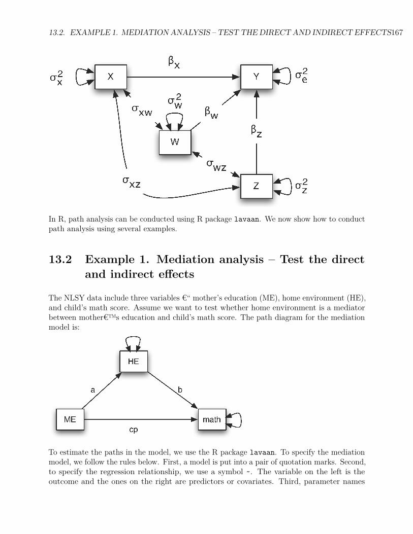
13.2. EXAMPLE 1. MEDIATION ANALYSIS – TEST THE DIRECT AND INDIRECT EFFECTS167
In R, path analysis can be conducted using R package lavaan. We now show how to conductpath analysis using several examples.
13.2 Example 1. Mediation analysis – Test the directand indirect effects
The NLSY data include three variables €“ mother’s education (ME), home environment (HE),and child’s math score. Assume we want to test whether home environment is a mediatorbetween mother€™s education and child’s math score. The path diagram for the mediationmodel is:
To estimate the paths in the model, we use the R package lavaan. To specify the mediationmodel, we follow the rules below. First, a model is put into a pair of quotation marks. Second,to specify the regression relationship, we use a symbol ~. The variable on the left is theoutcome and the ones on the right are predictors or covariates. Third, parameter names
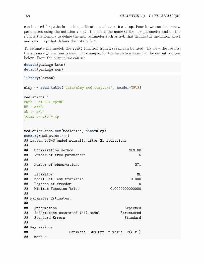
168 CHAPTER 13. PATH ANALYSIS
can be used for paths in model specification such as a, b and cp. Fourth, we can define newparameters using the notation :=. On the left is the name of the new parameter and on theright is the formula to define the new parameter such as a*b that defines the mediation effectand a*b + cp that defines the total effect.
To estimate the model, the sem() function from lavaan can be used. To view the results,the summary() function is used. For example, for the mediation example, the output is givenbelow. From the output, we can seedetach(package:bmem)detach(package:sem)
library(lavaan)
nlsy <- read.table("data/nlsy.med.comp.txt", header=TRUE)
mediation<-'math ~ b*HE + cp*MEHE ~ a*MEab := a*btotal := a*b + cp'
mediation.res<-sem(mediation, data=nlsy)summary(mediation.res)## lavaan 0.6-3 ended normally after 21 iterations#### Optimization method NLMINB## Number of free parameters 5#### Number of observations 371#### Estimator ML## Model Fit Test Statistic 0.000## Degrees of freedom 0## Minimum Function Value 0.0000000000000#### Parameter Estimates:#### Information Expected## Information saturated (h1) model Structured## Standard Errors Standard#### Regressions:## Estimate Std.Err z-value P(>|z|)## math ~
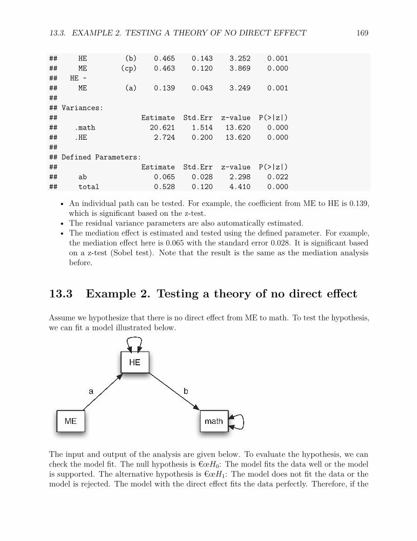
13.3. EXAMPLE 2. TESTING A THEORY OF NO DIRECT EFFECT 169
## HE (b) 0.465 0.143 3.252 0.001## ME (cp) 0.463 0.120 3.869 0.000## HE ~## ME (a) 0.139 0.043 3.249 0.001#### Variances:## Estimate Std.Err z-value P(>|z|)## .math 20.621 1.514 13.620 0.000## .HE 2.724 0.200 13.620 0.000#### Defined Parameters:## Estimate Std.Err z-value P(>|z|)## ab 0.065 0.028 2.298 0.022## total 0.528 0.120 4.410 0.000
• An individual path can be tested. For example, the coefficient from ME to HE is 0.139,which is significant based on the z-test.
• The residual variance parameters are also automatically estimated.• The mediation effect is estimated and tested using the defined parameter. For example,
the mediation effect here is 0.065 with the standard error 0.028. It is significant basedon a z-test (Sobel test). Note that the result is the same as the mediation analysisbefore.
13.3 Example 2. Testing a theory of no direct effect
Assume we hypothesize that there is no direct effect from ME to math. To test the hypothesis,we can fit a model illustrated below.
The input and output of the analysis are given below. To evaluate the hypothesis, we cancheck the model fit. The null hypothesis is €œH0: The model fits the data well or the modelis supported. The alternative hypothesis is €œH1: The model does not fit the data or themodel is rejected. The model with the direct effect fits the data perfectly. Therefore, if the

170 CHAPTER 13. PATH ANALYSIS
current model also fits the data well, we fail to reject the null hypothesis. Otherwise, wereject it. The test of the model can be conducted based on a chi-squared test. From theoutput, the Chi-square is 14.676 with 1 degree of freedom. The p-value is about 0. Therefore,the null hypothesis is rejected. This indicates that the model without direct effect is not agood model.model2<-'math ~ b*HEHE ~ a*ME'
model2.res<-sem(model2, data=nlsy)summary(model2.res)## lavaan 0.6-3 ended normally after 17 iterations#### Optimization method NLMINB## Number of free parameters 4#### Number of observations 371#### Estimator ML## Model Fit Test Statistic 14.676## Degrees of freedom 1## P-value (Chi-square) 0.000#### Parameter Estimates:#### Information Expected## Information saturated (h1) model Structured## Standard Errors Standard#### Regressions:## Estimate Std.Err z-value P(>|z|)## math ~## HE (b) 0.556 0.144 3.873 0.000## HE ~## ME (a) 0.139 0.043 3.249 0.001#### Variances:## Estimate Std.Err z-value P(>|z|)## .math 21.453 1.575 13.620 0.000## .HE 2.724 0.200 13.620 0.000

13.4. EXAMPLE 3: A MORE COMPLEX PATH MODEL 171
13.4 Example 3: A more complex path model
Path analysis can be used to test more complex theories. In this example, we look at howage and education influence EPT using the ACTIVE data. Both age and education mayinfluence EPT directly or through memory and reasoning ability. Therefore, we can fit amodel shown below.
Suppose we want to test the total effect of age on EPT and its indirect effect. The di-rect effect is the path from age to ept1 directly, denoted by p1. One indirect path goesthrough hvltt1, that is p2*p7. The second indirect effect through ws1 is p3*p8. The thirdindirect effect through ls1 is p4*p9. The last indirect effect through lt1 is p5*p10. Thetotal indirect effect is p2*p7+p3*p8+p4*p9+p5*p10. The total effect is the sum of themp1+p2*p7+p3*p8+p4*p9+p5*p10.
The output from such a model is given below. From it, we can see that the indirect effectind1=p2*p7 is significant. The total indirect (indirect) from age to EPT is also significant.Finally, the total effect (total) from age to EPT is significant.
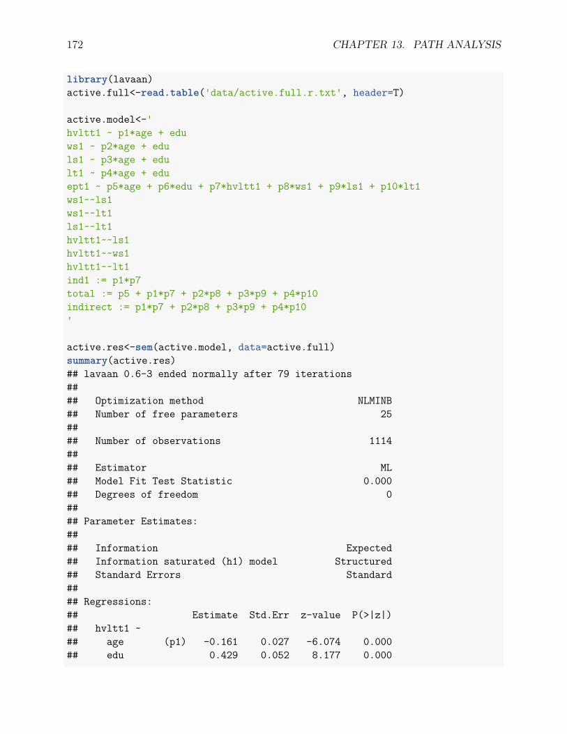
172 CHAPTER 13. PATH ANALYSIS
library(lavaan)active.full<-read.table('data/active.full.r.txt', header=T)
active.model<-'hvltt1 ~ p1*age + eduws1 ~ p2*age + eduls1 ~ p3*age + edult1 ~ p4*age + eduept1 ~ p5*age + p6*edu + p7*hvltt1 + p8*ws1 + p9*ls1 + p10*lt1ws1~~ls1ws1~~lt1ls1~~lt1hvltt1~~ls1hvltt1~~ws1hvltt1~~lt1ind1 := p1*p7total := p5 + p1*p7 + p2*p8 + p3*p9 + p4*p10indirect := p1*p7 + p2*p8 + p3*p9 + p4*p10'
active.res<-sem(active.model, data=active.full)summary(active.res)## lavaan 0.6-3 ended normally after 79 iterations#### Optimization method NLMINB## Number of free parameters 25#### Number of observations 1114#### Estimator ML## Model Fit Test Statistic 0.000## Degrees of freedom 0#### Parameter Estimates:#### Information Expected## Information saturated (h1) model Structured## Standard Errors Standard#### Regressions:## Estimate Std.Err z-value P(>|z|)## hvltt1 ~## age (p1) -0.161 0.027 -6.074 0.000## edu 0.429 0.052 8.177 0.000
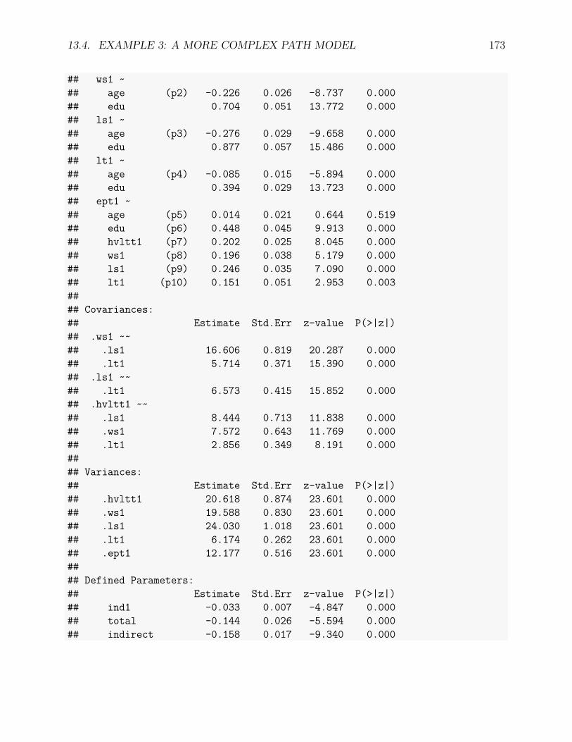
13.4. EXAMPLE 3: A MORE COMPLEX PATH MODEL 173
## ws1 ~## age (p2) -0.226 0.026 -8.737 0.000## edu 0.704 0.051 13.772 0.000## ls1 ~## age (p3) -0.276 0.029 -9.658 0.000## edu 0.877 0.057 15.486 0.000## lt1 ~## age (p4) -0.085 0.015 -5.894 0.000## edu 0.394 0.029 13.723 0.000## ept1 ~## age (p5) 0.014 0.021 0.644 0.519## edu (p6) 0.448 0.045 9.913 0.000## hvltt1 (p7) 0.202 0.025 8.045 0.000## ws1 (p8) 0.196 0.038 5.179 0.000## ls1 (p9) 0.246 0.035 7.090 0.000## lt1 (p10) 0.151 0.051 2.953 0.003#### Covariances:## Estimate Std.Err z-value P(>|z|)## .ws1 ~~## .ls1 16.606 0.819 20.287 0.000## .lt1 5.714 0.371 15.390 0.000## .ls1 ~~## .lt1 6.573 0.415 15.852 0.000## .hvltt1 ~~## .ls1 8.444 0.713 11.838 0.000## .ws1 7.572 0.643 11.769 0.000## .lt1 2.856 0.349 8.191 0.000#### Variances:## Estimate Std.Err z-value P(>|z|)## .hvltt1 20.618 0.874 23.601 0.000## .ws1 19.588 0.830 23.601 0.000## .ls1 24.030 1.018 23.601 0.000## .lt1 6.174 0.262 23.601 0.000## .ept1 12.177 0.516 23.601 0.000#### Defined Parameters:## Estimate Std.Err z-value P(>|z|)## ind1 -0.033 0.007 -4.847 0.000## total -0.144 0.026 -5.594 0.000## indirect -0.158 0.017 -9.340 0.000

174 CHAPTER 13. PATH ANALYSIS

Chapter 14
Factor Analysis
14.1 Measurement Error and Factor Analysis
14.1.1 Measurement error
Suppose we want to measure reasoning ability. For participant i, the true reasoning abilityscore is Ti and the observed score is yi. If there is no measurement error, we would expectthat
yi = Ti.
However, often times, we can not perfectly measure something like reasoning ability becauseof measurement error. With measurement error, the above equation becomes
yi = Ti + ei.
where ei is the difference between the observed value and its true score in reasoning abilityfor participant i. Measurement error is almost always present in a measurement. It is causedby unpredictable fluctuations in the the data collection. It can show up as different resultsfor the same repeated measurement.
It is often assumed that the mean of ei is equal to 0. We need to estimate the variance of ei.Note that we ignore the systematic errors here. The measurement error discussed here ispurely random error.
We can express the measurement error using a path diagram shown below. Both the truescore and the measurement error are unobserved. The only quantity that is available is theobserved score y. From the relationship, we can easily see that
V ar(y) = V ar(T ) + V ar(e).
175

176 CHAPTER 14. FACTOR ANALYSIS
That is the observed variance is equal to the sum of the true score variance and the measure-ment error variance. Note that reliability is define as
reliability = V ar(T )V ar(T ) + V ar(e) .
Measurement error can be estimated by comparing multiple measurements, and reduced byaveraging multiple measurements.
14.1.2 Influences of measurement error
The most well known influence of measurement error is the attenuation of a relationship. Forexample, it can lead to reduced correlation between two variables if the two variables areobserved with measurement error. In terms of regression analysis, it results in attenuatedregression slope estimates, which is also known as regression dilution.
We can illustrate this through an example on correlation. The path diagram for the exampleis given below.
Note that from the diagram, we have
X = ξ + δ1 and Y = η + δ2.
The variances for the true score ξ and η are σ2ξ and σ2
η, respectively. The variances for themeasurement error δ1 and δ2 are σ2
1 and σ22, respectively. The covariance between ξ and η is
σξη
The correlation between the true scores is
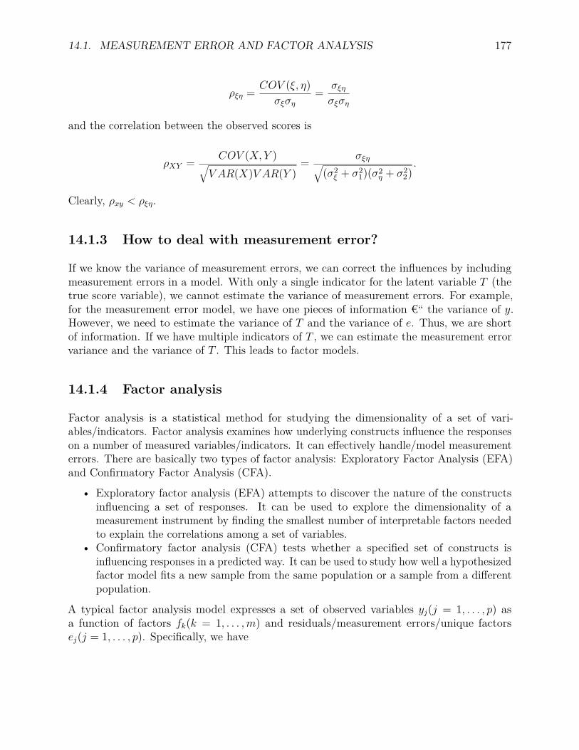
14.1. MEASUREMENT ERROR AND FACTOR ANALYSIS 177
ρξη = COV (ξ, η)σξση
= σξησξση
and the correlation between the observed scores is
ρXY = COV (X, Y )√V AR(X)V AR(Y )
= σξη√(σ2
ξ + σ21)(σ2
η + σ22).
Clearly, ρxy < ρξη.
14.1.3 How to deal with measurement error?
If we know the variance of measurement errors, we can correct the influences by includingmeasurement errors in a model. With only a single indicator for the latent variable T (thetrue score variable), we cannot estimate the variance of measurement errors. For example,for the measurement error model, we have one pieces of information €“ the variance of y.However, we need to estimate the variance of T and the variance of e. Thus, we are shortof information. If we have multiple indicators of T , we can estimate the measurement errorvariance and the variance of T . This leads to factor models.
14.1.4 Factor analysis
Factor analysis is a statistical method for studying the dimensionality of a set of vari-ables/indicators. Factor analysis examines how underlying constructs influence the responseson a number of measured variables/indicators. It can effectively handle/model measurementerrors. There are basically two types of factor analysis: Exploratory Factor Analysis (EFA)and Confirmatory Factor Analysis (CFA).
• Exploratory factor analysis (EFA) attempts to discover the nature of the constructsinfluencing a set of responses. It can be used to explore the dimensionality of ameasurement instrument by finding the smallest number of interpretable factors neededto explain the correlations among a set of variables.
• Confirmatory factor analysis (CFA) tests whether a specified set of constructs isinfluencing responses in a predicted way. It can be used to study how well a hypothesizedfactor model fits a new sample from the same population or a sample from a differentpopulation.
A typical factor analysis model expresses a set of observed variables yj(j = 1, . . . , p) asa function of factors fk(k = 1, . . . ,m) and residuals/measurement errors/unique factorsej(j = 1, . . . , p). Specifically, we have
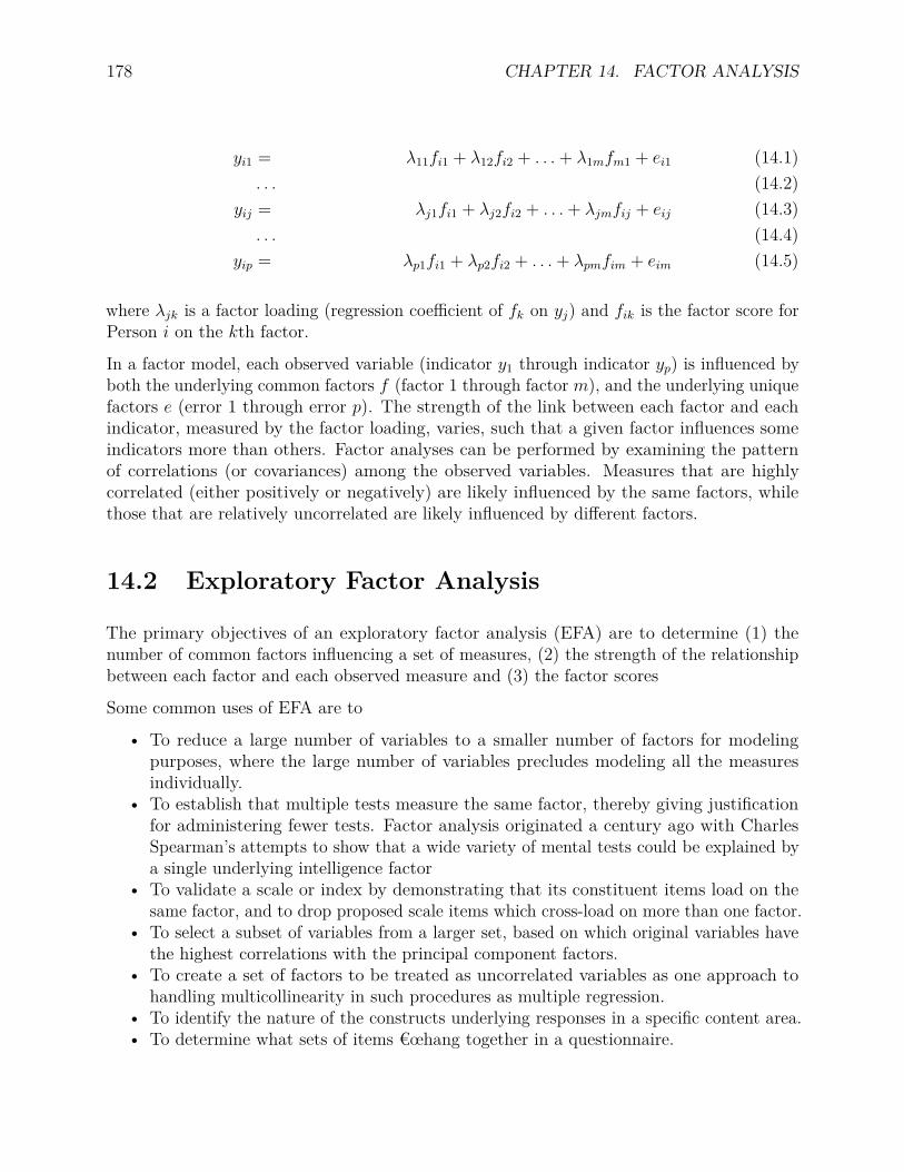
178 CHAPTER 14. FACTOR ANALYSIS
yi1 = λ11fi1 + λ12fi2 + . . .+ λ1mfm1 + ei1 (14.1). . . (14.2)
yij = λj1fi1 + λj2fi2 + . . .+ λjmfij + eij (14.3). . . (14.4)
yip = λp1fi1 + λp2fi2 + . . .+ λpmfim + eim (14.5)
where λjk is a factor loading (regression coefficient of fk on yj) and fik is the factor score forPerson i on the kth factor.
In a factor model, each observed variable (indicator y1 through indicator yp) is influenced byboth the underlying common factors f (factor 1 through factor m), and the underlying uniquefactors e (error 1 through error p). The strength of the link between each factor and eachindicator, measured by the factor loading, varies, such that a given factor influences someindicators more than others. Factor analyses can be performed by examining the patternof correlations (or covariances) among the observed variables. Measures that are highlycorrelated (either positively or negatively) are likely influenced by the same factors, whilethose that are relatively uncorrelated are likely influenced by different factors.
14.2 Exploratory Factor Analysis
The primary objectives of an exploratory factor analysis (EFA) are to determine (1) thenumber of common factors influencing a set of measures, (2) the strength of the relationshipbetween each factor and each observed measure and (3) the factor scores
Some common uses of EFA are to
• To reduce a large number of variables to a smaller number of factors for modelingpurposes, where the large number of variables precludes modeling all the measuresindividually.
• To establish that multiple tests measure the same factor, thereby giving justificationfor administering fewer tests. Factor analysis originated a century ago with CharlesSpearman’s attempts to show that a wide variety of mental tests could be explained bya single underlying intelligence factor
• To validate a scale or index by demonstrating that its constituent items load on thesame factor, and to drop proposed scale items which cross-load on more than one factor.
• To select a subset of variables from a larger set, based on which original variables havethe highest correlations with the principal component factors.
• To create a set of factors to be treated as uncorrelated variables as one approach tohandling multicollinearity in such procedures as multiple regression.
• To identify the nature of the constructs underlying responses in a specific content area.• To determine what sets of items €œhang together in a questionnaire.
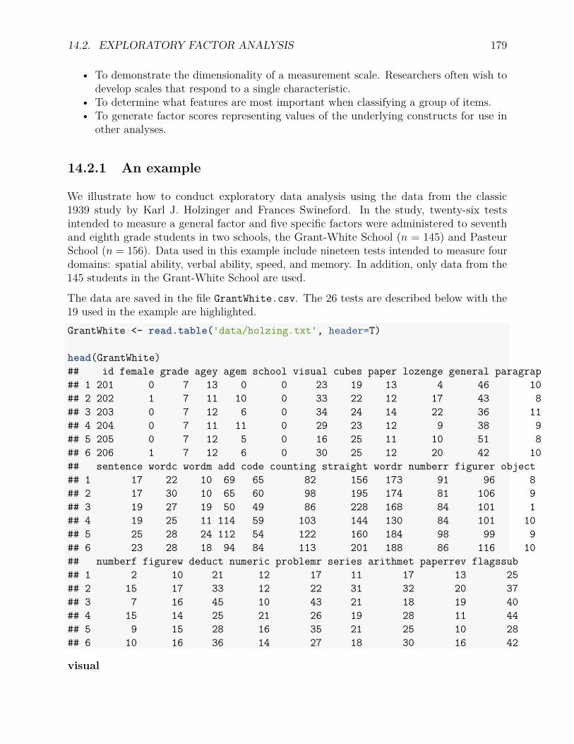
14.2. EXPLORATORY FACTOR ANALYSIS 179
• To demonstrate the dimensionality of a measurement scale. Researchers often wish todevelop scales that respond to a single characteristic.
• To determine what features are most important when classifying a group of items.• To generate factor scores representing values of the underlying constructs for use in
other analyses.
14.2.1 An example
We illustrate how to conduct exploratory data analysis using the data from the classic1939 study by Karl J. Holzinger and Frances Swineford. In the study, twenty-six testsintended to measure a general factor and five specific factors were administered to seventhand eighth grade students in two schools, the Grant-White School (n = 145) and PasteurSchool (n = 156). Data used in this example include nineteen tests intended to measure fourdomains: spatial ability, verbal ability, speed, and memory. In addition, only data from the145 students in the Grant-White School are used.
The data are saved in the file GrantWhite.csv. The 26 tests are described below with the19 used in the example are highlighted.GrantWhite <- read.table('data/holzing.txt', header=T)
head(GrantWhite)## id female grade agey agem school visual cubes paper lozenge general paragrap## 1 201 0 7 13 0 0 23 19 13 4 46 10## 2 202 1 7 11 10 0 33 22 12 17 43 8## 3 203 0 7 12 6 0 34 24 14 22 36 11## 4 204 0 7 11 11 0 29 23 12 9 38 9## 5 205 0 7 12 5 0 16 25 11 10 51 8## 6 206 1 7 12 6 0 30 25 12 20 42 10## sentence wordc wordm add code counting straight wordr numberr figurer object## 1 17 22 10 69 65 82 156 173 91 96 8## 2 17 30 10 65 60 98 195 174 81 106 9## 3 19 27 19 50 49 86 228 168 84 101 1## 4 19 25 11 114 59 103 144 130 84 101 10## 5 25 28 24 112 54 122 160 184 98 99 9## 6 23 28 18 94 84 113 201 188 86 116 10## numberf figurew deduct numeric problemr series arithmet paperrev flagssub## 1 2 10 21 12 17 11 17 13 25## 2 15 17 33 12 22 31 32 20 37## 3 7 16 45 10 43 21 18 19 40## 4 15 14 25 21 26 19 28 11 44## 5 9 15 28 16 35 21 25 10 28## 6 10 16 36 14 27 18 30 16 42
visual

180 CHAPTER 14. FACTOR ANALYSIS
scores on visual perception test, test 1
cubes
scores on cubes test, test 2
paper
scores on paper form board test, test 3
lozenge
scores on lozenges test, test 4
general
scores on general information test, test 5
paragrap
scores on paragraph comprehension test, test 6
sentence
scores on sentence completion test, test 7
wordc
scores on word classification test, test 8
wordm
scores on word meaning test, test 9
add
scores on add test, test 10
code
scores on code test, test 11
counting
scores on counting groups of dots test, test 12
straight
scores on straight and curved capitals test, test 13
wordr
scores on word recognition test, test 14
numberr
scores on number recognition test, test 15
figurer

14.2. EXPLORATORY FACTOR ANALYSIS 181
scores on figure recognition test, test 16
object
scores on object-number test, test 17
numberf
scores on number-figure test, test 18
figurew
scores on figure-word test, test 19
deduct
scores on deduction test, test 20
numeric
scores on numerical puzzles test, test 21
problemr
scores on problem reasoning test, test 22
series
scores on series completion test, test 23
arithmet
scores on Woody-McCall mixed fundamentals, form I test, test 24
paperrev
scores on additional paper form board test, test 25
flagssub
scores on flags test, test 26
14.2.2 Exploratory factor analysis
The usual exploratory factor analysis involves (1) Preparing data, (2) Determining the numberof factors, (3) Estimation of the model, (4) Factor rotation, (5) Factor score estimation and(6) Interpretation of the analysis.
14.2.2.1 Preparing data
In EFA, a correlation matrix is analyzed. The following R code calculates the correlationmatrix.
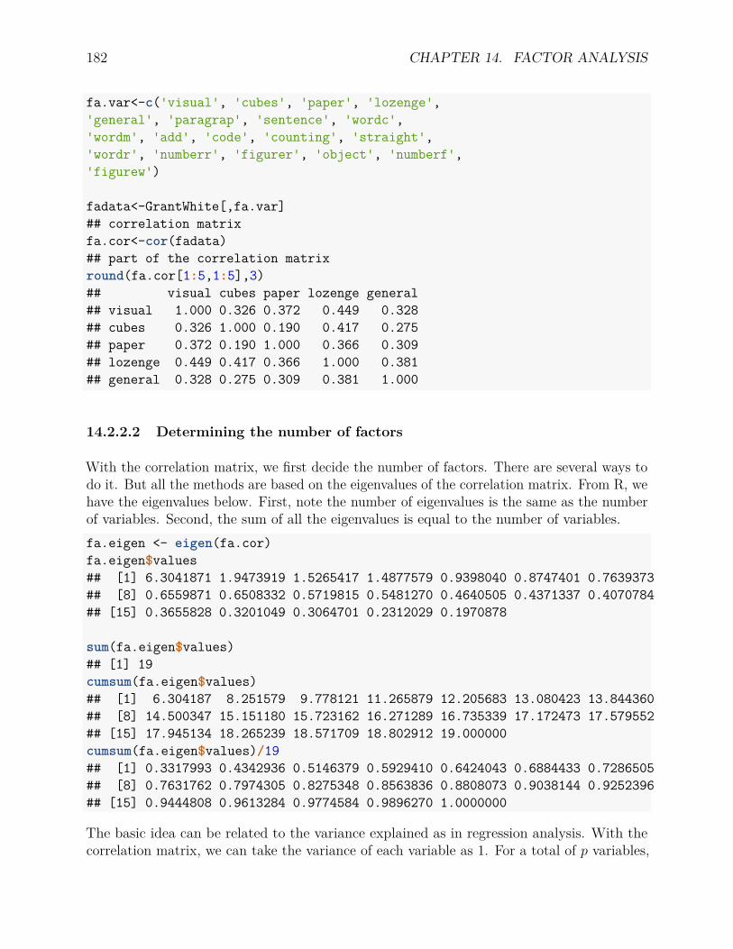
182 CHAPTER 14. FACTOR ANALYSIS
fa.var<-c('visual', 'cubes', 'paper', 'lozenge','general', 'paragrap', 'sentence', 'wordc','wordm', 'add', 'code', 'counting', 'straight','wordr', 'numberr', 'figurer', 'object', 'numberf','figurew')
fadata<-GrantWhite[,fa.var]## correlation matrixfa.cor<-cor(fadata)## part of the correlation matrixround(fa.cor[1:5,1:5],3)## visual cubes paper lozenge general## visual 1.000 0.326 0.372 0.449 0.328## cubes 0.326 1.000 0.190 0.417 0.275## paper 0.372 0.190 1.000 0.366 0.309## lozenge 0.449 0.417 0.366 1.000 0.381## general 0.328 0.275 0.309 0.381 1.000
14.2.2.2 Determining the number of factors
With the correlation matrix, we first decide the number of factors. There are several ways todo it. But all the methods are based on the eigenvalues of the correlation matrix. From R, wehave the eigenvalues below. First, note the number of eigenvalues is the same as the numberof variables. Second, the sum of all the eigenvalues is equal to the number of variables.fa.eigen <- eigen(fa.cor)fa.eigen$values## [1] 6.3041871 1.9473919 1.5265417 1.4877579 0.9398040 0.8747401 0.7639373## [8] 0.6559871 0.6508332 0.5719815 0.5481270 0.4640505 0.4371337 0.4070784## [15] 0.3655828 0.3201049 0.3064701 0.2312029 0.1970878
sum(fa.eigen$values)## [1] 19cumsum(fa.eigen$values)## [1] 6.304187 8.251579 9.778121 11.265879 12.205683 13.080423 13.844360## [8] 14.500347 15.151180 15.723162 16.271289 16.735339 17.172473 17.579552## [15] 17.945134 18.265239 18.571709 18.802912 19.000000cumsum(fa.eigen$values)/19## [1] 0.3317993 0.4342936 0.5146379 0.5929410 0.6424043 0.6884433 0.7286505## [8] 0.7631762 0.7974305 0.8275348 0.8563836 0.8808073 0.9038144 0.9252396## [15] 0.9444808 0.9613284 0.9774584 0.9896270 1.0000000
The basic idea can be related to the variance explained as in regression analysis. With thecorrelation matrix, we can take the variance of each variable as 1. For a total of p variables,
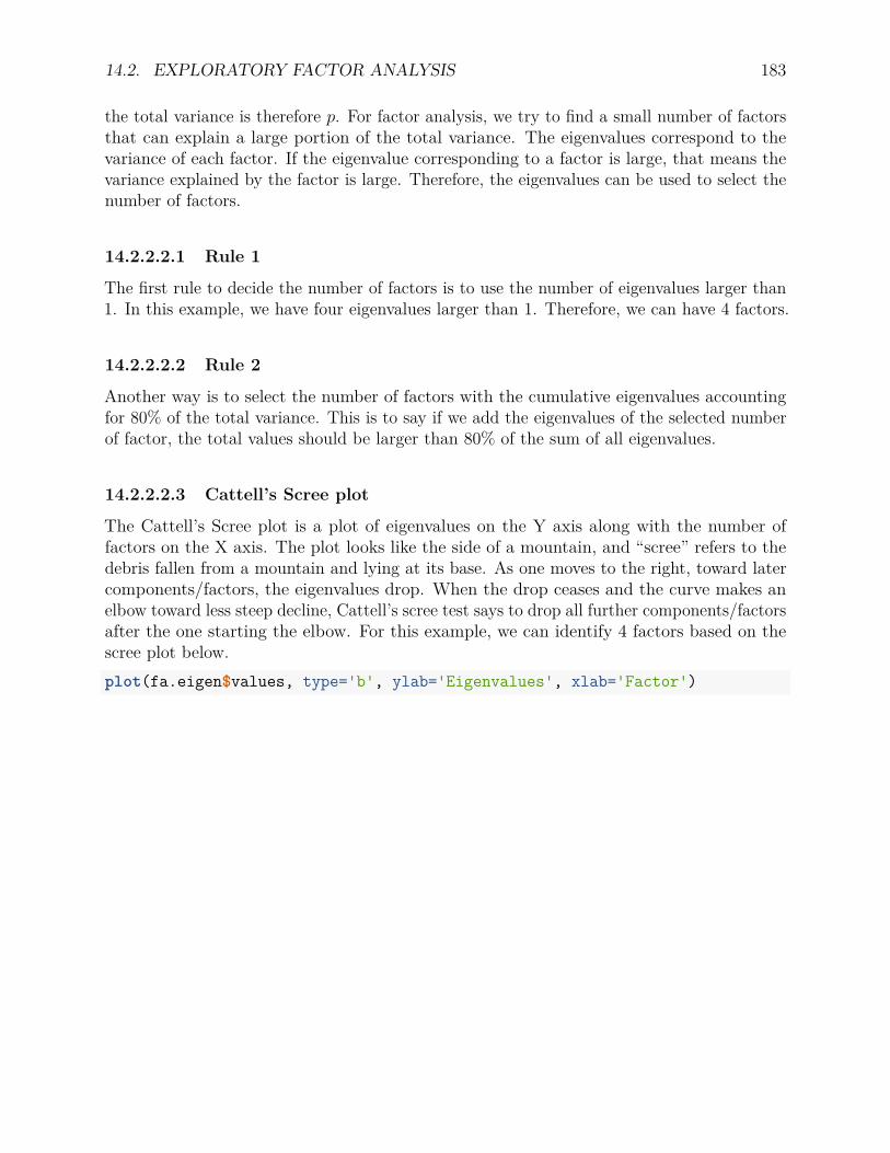
14.2. EXPLORATORY FACTOR ANALYSIS 183
the total variance is therefore p. For factor analysis, we try to find a small number of factorsthat can explain a large portion of the total variance. The eigenvalues correspond to thevariance of each factor. If the eigenvalue corresponding to a factor is large, that means thevariance explained by the factor is large. Therefore, the eigenvalues can be used to select thenumber of factors.
14.2.2.2.1 Rule 1
The first rule to decide the number of factors is to use the number of eigenvalues larger than1. In this example, we have four eigenvalues larger than 1. Therefore, we can have 4 factors.
14.2.2.2.2 Rule 2
Another way is to select the number of factors with the cumulative eigenvalues accountingfor 80% of the total variance. This is to say if we add the eigenvalues of the selected numberof factor, the total values should be larger than 80% of the sum of all eigenvalues.
14.2.2.2.3 Cattell’s Scree plot
The Cattell’s Scree plot is a plot of eigenvalues on the Y axis along with the number offactors on the X axis. The plot looks like the side of a mountain, and “scree” refers to thedebris fallen from a mountain and lying at its base. As one moves to the right, toward latercomponents/factors, the eigenvalues drop. When the drop ceases and the curve makes anelbow toward less steep decline, Cattell’s scree test says to drop all further components/factorsafter the one starting the elbow. For this example, we can identify 4 factors based on thescree plot below.plot(fa.eigen$values, type='b', ylab='Eigenvalues', xlab='Factor')
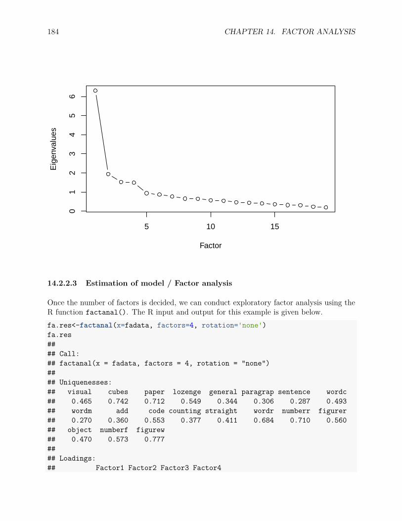
184 CHAPTER 14. FACTOR ANALYSIS
5 10 15
01
23
45
6
Factor
Eig
enva
lues
14.2.2.3 Estimation of model / Factor analysis
Once the number of factors is decided, we can conduct exploratory factor analysis using theR function factanal(). The R input and output for this example is given below.fa.res<-factanal(x=fadata, factors=4, rotation='none')fa.res#### Call:## factanal(x = fadata, factors = 4, rotation = "none")#### Uniquenesses:## visual cubes paper lozenge general paragrap sentence wordc## 0.465 0.742 0.712 0.549 0.344 0.306 0.287 0.493## wordm add code counting straight wordr numberr figurer## 0.270 0.360 0.553 0.377 0.411 0.684 0.710 0.560## object numberf figurew## 0.470 0.573 0.777#### Loadings:## Factor1 Factor2 Factor3 Factor4
14.2. EXPLORATORY FACTOR ANALYSIS 185
## visual 0.536 0.176 0.392 -0.249## cubes 0.330 0.302 -0.228## paper 0.440 0.110 0.247 -0.147## lozenge 0.505 0.358 -0.253## general 0.762 -0.238 -0.113## paragrap 0.759 -0.338## sentence 0.762 -0.322 -0.166## wordc 0.701## wordm 0.762 -0.381## add 0.455 0.475 -0.451## code 0.545 0.367 0.103## counting 0.434 0.593 -0.238 -0.162## straight 0.592 0.393 -0.289## wordr 0.394 0.149 0.362## numberr 0.352 0.139 0.219 0.315## figurer 0.435 0.183 0.425 0.192## object 0.445 0.241 0.522## numberf 0.454 0.383 0.221 0.157## figurew 0.389 0.115 0.133 0.202#### Factor1 Factor2 Factor3 Factor4## SS loadings 5.722 1.625 1.065 0.945## Proportion Var 0.301 0.086 0.056 0.050## Cumulative Var 0.301 0.387 0.443 0.492#### Test of the hypothesis that 4 factors are sufficient.## The chi square statistic is 102.06 on 101 degrees of freedom.## The p-value is 0.452
In EFA, each observed data consists of two part, the common factor part and the uniquenesspart. The common factor part is based on the four factors, which are also called the commonfactors. The uniqueness part is also called uniqueness factor, which is specific to each observedvariable.
Using the variable visual as an example, we have
visual = 0.536× Factor1 + 0.176× Factor2 + 0.392× Factor3− 0.249× Factor4 + uvisual
Note the factor loadings are from the Loadings section of the output. The loadings are theregression coefficients of the latent factors on the manifest indicators or observed variables.The variance of the uniqueness is in the Uniquenesses section. For uvisual, the variance is0.465. For the other variables, it’s the same.
The other section is related to the variance explained by the factors. SS loadings is thesum squared loadings related to each factor. It is the overall variance explained in all the 19
186 CHAPTER 14. FACTOR ANALYSIS
variables by each factor. Therefore, the first factor explains the total of 5.722 variance, that’sabout 30.1%=5.722/19. Proportion Var is the variances in the observed variables/indicatorsexplained by each factor. Cumulative Var is the cumulative proportion of variance explainedby all factors.
A test is conducted to test whether the factor model is sufficient to explain the observeddata. The null hypothesis that a 4-factor model is sufficient. For this model, the chi-squarestatistic is 102.06 withdegrees of freedom 101. The p-value for the chi-square test is 0.452 which is larger than .05.Therefore,we fail to reject the null hypothesis that the factor model have a good fit to thedata.
14.2.2.4 Factor rotation
Although we have identified 4 factors and found the 4-factor model is a good model. Wecannot find a clear pattern in the factor loadings to have a deep understanding of thefactors. Through factor rotation, we can make the output more understandable and is usuallynecessary to facilitate the interpretation of factors. The aim is to find a simple solutionthat each factor has a small number of large loadings and a large number of zero (or small)loadings. There are many different rotation methods such as the varimax rotation, quadtimaxrotation, equimax rotation, oblique rotation, etc. The PROMAX rotation is one kind ofoblique rotation and is widely used. After PROMAX rotation, the factor will be correlated.
The output of PROMAX rotation is shown below. In the output, we use print(fa.res,cut=0.2) to show factor loadings that are greater than 0.2. Note that after rotation, manyloading are actually smaller than 0.2. The pattern of the factor loadings are much clear now.For example, the variable visual has a large loading 0.747 on Factor 2 but small than 0.2loadings on all the other three factors. In this case, we might say that the variable visual ismainly influenced by Factor 2.
Different from the variable visual, the variable straight has large loadings on both Factor2 and Factor 4. Alternatively, straight measures both factors than just a single factor.
We can also see that the primary indicators for Factor 1 are general, paragrap, sentence,wordc, and wordm. And for Factor 4, the indictors include add, code, counting, andstraight.
The correlation among the factors are given in the section of Factor Correlation. Forexample, the correlation between Factor 1 and Factor 2 is 0.368. Note that after rotation,the test of the model is the same as without rotation.fa.res<-factanal(x=fadata, factors=4, rotation='promax')print(fa.res, cut=0.2)#### Call:## factanal(x = fadata, factors = 4, rotation = "promax")##
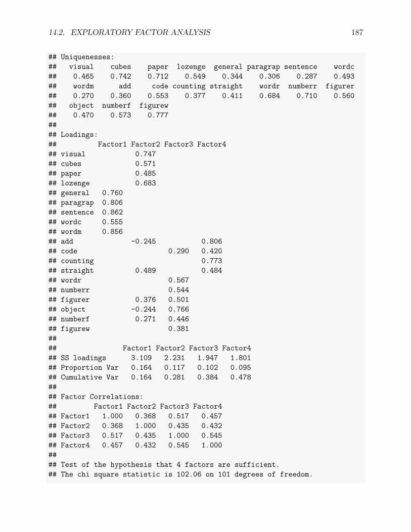
14.2. EXPLORATORY FACTOR ANALYSIS 187
## Uniquenesses:## visual cubes paper lozenge general paragrap sentence wordc## 0.465 0.742 0.712 0.549 0.344 0.306 0.287 0.493## wordm add code counting straight wordr numberr figurer## 0.270 0.360 0.553 0.377 0.411 0.684 0.710 0.560## object numberf figurew## 0.470 0.573 0.777#### Loadings:## Factor1 Factor2 Factor3 Factor4## visual 0.747## cubes 0.571## paper 0.485## lozenge 0.683## general 0.760## paragrap 0.806## sentence 0.862## wordc 0.555## wordm 0.856## add -0.245 0.806## code 0.290 0.420## counting 0.773## straight 0.489 0.484## wordr 0.567## numberr 0.544## figurer 0.376 0.501## object -0.244 0.766## numberf 0.271 0.446## figurew 0.381#### Factor1 Factor2 Factor3 Factor4## SS loadings 3.109 2.231 1.947 1.801## Proportion Var 0.164 0.117 0.102 0.095## Cumulative Var 0.164 0.281 0.384 0.478#### Factor Correlations:## Factor1 Factor2 Factor3 Factor4## Factor1 1.000 0.368 0.517 0.457## Factor2 0.368 1.000 0.435 0.432## Factor3 0.517 0.435 1.000 0.545## Factor4 0.457 0.432 0.545 1.000#### Test of the hypothesis that 4 factors are sufficient.## The chi square statistic is 102.06 on 101 degrees of freedom.
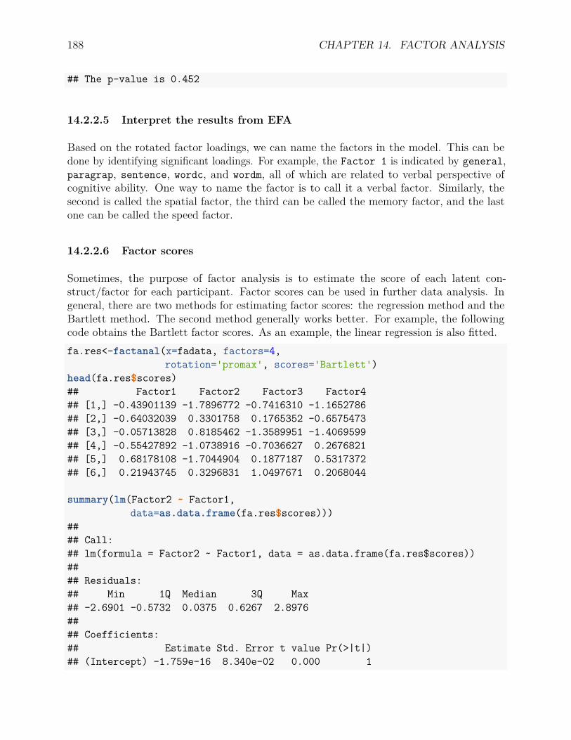
188 CHAPTER 14. FACTOR ANALYSIS
## The p-value is 0.452
14.2.2.5 Interpret the results from EFA
Based on the rotated factor loadings, we can name the factors in the model. This can bedone by identifying significant loadings. For example, the Factor 1 is indicated by general,paragrap, sentence, wordc, and wordm, all of which are related to verbal perspective ofcognitive ability. One way to name the factor is to call it a verbal factor. Similarly, thesecond is called the spatial factor, the third can be called the memory factor, and the lastone can be called the speed factor.
14.2.2.6 Factor scores
Sometimes, the purpose of factor analysis is to estimate the score of each latent con-struct/factor for each participant. Factor scores can be used in further data analysis. Ingeneral, there are two methods for estimating factor scores: the regression method and theBartlett method. The second method generally works better. For example, the followingcode obtains the Bartlett factor scores. As an example, the linear regression is also fitted.fa.res<-factanal(x=fadata, factors=4,
rotation='promax', scores='Bartlett')head(fa.res$scores)## Factor1 Factor2 Factor3 Factor4## [1,] -0.43901139 -1.7896772 -0.7416310 -1.1652786## [2,] -0.64032039 0.3301758 0.1765352 -0.6575473## [3,] -0.05713828 0.8185462 -1.3589951 -1.4069599## [4,] -0.55427892 -1.0738916 -0.7036627 0.2676821## [5,] 0.68178108 -1.7044904 0.1877187 0.5317372## [6,] 0.21943745 0.3296831 1.0497671 0.2068044
summary(lm(Factor2 ~ Factor1,data=as.data.frame(fa.res$scores)))
#### Call:## lm(formula = Factor2 ~ Factor1, data = as.data.frame(fa.res$scores))#### Residuals:## Min 1Q Median 3Q Max## -2.6901 -0.5732 0.0375 0.6267 2.8976#### Coefficients:## Estimate Std. Error t value Pr(>|t|)## (Intercept) -1.759e-16 8.340e-02 0.000 1
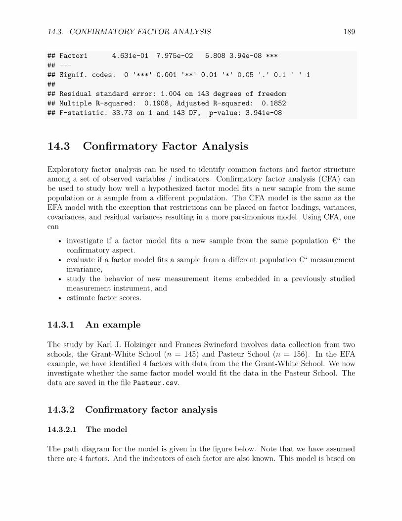
14.3. CONFIRMATORY FACTOR ANALYSIS 189
## Factor1 4.631e-01 7.975e-02 5.808 3.94e-08 ***## ---## Signif. codes: 0 '***' 0.001 '**' 0.01 '*' 0.05 '.' 0.1 ' ' 1#### Residual standard error: 1.004 on 143 degrees of freedom## Multiple R-squared: 0.1908, Adjusted R-squared: 0.1852## F-statistic: 33.73 on 1 and 143 DF, p-value: 3.941e-08
14.3 Confirmatory Factor Analysis
Exploratory factor analysis can be used to identify common factors and factor structureamong a set of observed variables / indicators. Confirmatory factor analysis (CFA) canbe used to study how well a hypothesized factor model fits a new sample from the samepopulation or a sample from a different population. The CFA model is the same as theEFA model with the exception that restrictions can be placed on factor loadings, variances,covariances, and residual variances resulting in a more parsimonious model. Using CFA, onecan
• investigate if a factor model fits a new sample from the same population €“ theconfirmatory aspect.
• evaluate if a factor model fits a sample from a different population €“ measurementinvariance,
• study the behavior of new measurement items embedded in a previously studiedmeasurement instrument, and
• estimate factor scores.
14.3.1 An example
The study by Karl J. Holzinger and Frances Swineford involves data collection from twoschools, the Grant-White School (n = 145) and Pasteur School (n = 156). In the EFAexample, we have identified 4 factors with data from the the Grant-White School. We nowinvestigate whether the same factor model would fit the data in the Pasteur School. Thedata are saved in the file Pasteur.csv.
14.3.2 Confirmatory factor analysis
14.3.2.1 The model
The path diagram for the model is given in the figure below. Note that we have assumedthere are 4 factors. And the indicators of each factor are also known. This model is based on
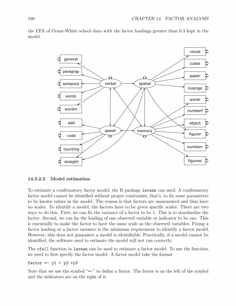
190 CHAPTER 14. FACTOR ANALYSIS
the EFA of Grant-White school data with the factor loadings greater than 0.3 kept in themodel.
visual
cubes
paper
lozenge
general
paragrap
sentence
wordc
wordm
add
code
counting
straight
wordr
numberr
figurer
object
numberf
figurew
verbal
speed memory
spatial
14.3.2.2 Model estimation
To estimate a confirmatory factor model, the R package lavaan can used. A confirmatoryfactor model cannot be identified without proper constraints, that’s, to fix some parametersto be known values in the model. The reason is that factors are unmeasured and thus haveno scales. To identify a model, the factors have to be given specific scales. There are twoways to do this. First, we can fix the variance of a factor to be 1. This is to standardize thefactor. Second, we can fix the loading of one observed variable or indicator to be one. Thisis essentially to make the factor to have the same scale as the observed variables. Fixing afactor loading or a factor variance is the minimum requirement to identify a factor model.However, this does not guarantee a model is identifiable. Practically, if a model cannot beidentified, the software used to estimate the model will not run correctly.
The cfa() function in lavaan can be used to estimate a factor model. To use the function,we need to first specify the factor model. A factor model take the format
factor =~ y1 + y2 +y3
Note that we use the symbol “=~” to define a factor. The factor is on the left of the symboland the indicators are on the right of it.

14.3. CONFIRMATORY FACTOR ANALYSIS 191
The R code for the example is given below.library(lavaan)Pasteur <- read.csv('data/Pasteur.csv')
cfa.model<-'spatial =~ visual+cubes+paper+lozenge+straight+figurerverbal =~ general+paragrap+sentence+wordc+wordmspeed =~ add+code+counting+straightmemory =~ wordr+numberr+figurer+object+numberf+figurew'
cfa.est<-cfa(cfa.model, data=Pasteur)summary(cfa.est, fit=TRUE)## lavaan 0.6-3 ended normally after 251 iterations#### Optimization method NLMINB## Number of free parameters 46#### Number of observations 156#### Estimator ML## Model Fit Test Statistic 238.751## Degrees of freedom 144## P-value (Chi-square) 0.000#### Model test baseline model:#### Minimum Function Test Statistic 1149.278## Degrees of freedom 171## P-value 0.000#### User model versus baseline model:#### Comparative Fit Index (CFI) 0.903## Tucker-Lewis Index (TLI) 0.885#### Loglikelihood and Information Criteria:#### Loglikelihood user model (H0) -9899.892## Loglikelihood unrestricted model (H1) -9780.517#### Number of free parameters 46## Akaike (AIC) 19891.785## Bayesian (BIC) 20032.078
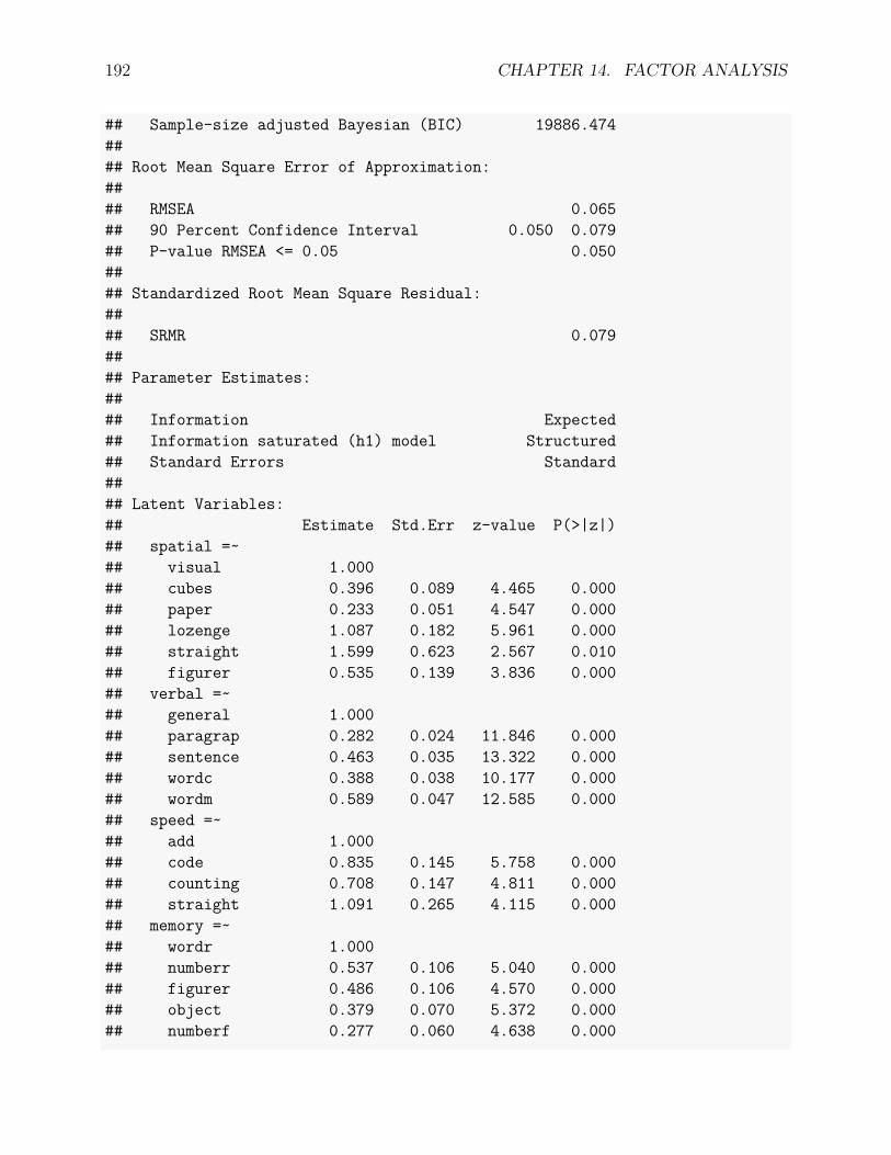
192 CHAPTER 14. FACTOR ANALYSIS
## Sample-size adjusted Bayesian (BIC) 19886.474#### Root Mean Square Error of Approximation:#### RMSEA 0.065## 90 Percent Confidence Interval 0.050 0.079## P-value RMSEA <= 0.05 0.050#### Standardized Root Mean Square Residual:#### SRMR 0.079#### Parameter Estimates:#### Information Expected## Information saturated (h1) model Structured## Standard Errors Standard#### Latent Variables:## Estimate Std.Err z-value P(>|z|)## spatial =~## visual 1.000## cubes 0.396 0.089 4.465 0.000## paper 0.233 0.051 4.547 0.000## lozenge 1.087 0.182 5.961 0.000## straight 1.599 0.623 2.567 0.010## figurer 0.535 0.139 3.836 0.000## verbal =~## general 1.000## paragrap 0.282 0.024 11.846 0.000## sentence 0.463 0.035 13.322 0.000## wordc 0.388 0.038 10.177 0.000## wordm 0.589 0.047 12.585 0.000## speed =~## add 1.000## code 0.835 0.145 5.758 0.000## counting 0.708 0.147 4.811 0.000## straight 1.091 0.265 4.115 0.000## memory =~## wordr 1.000## numberr 0.537 0.106 5.040 0.000## figurer 0.486 0.106 4.570 0.000## object 0.379 0.070 5.372 0.000## numberf 0.277 0.060 4.638 0.000
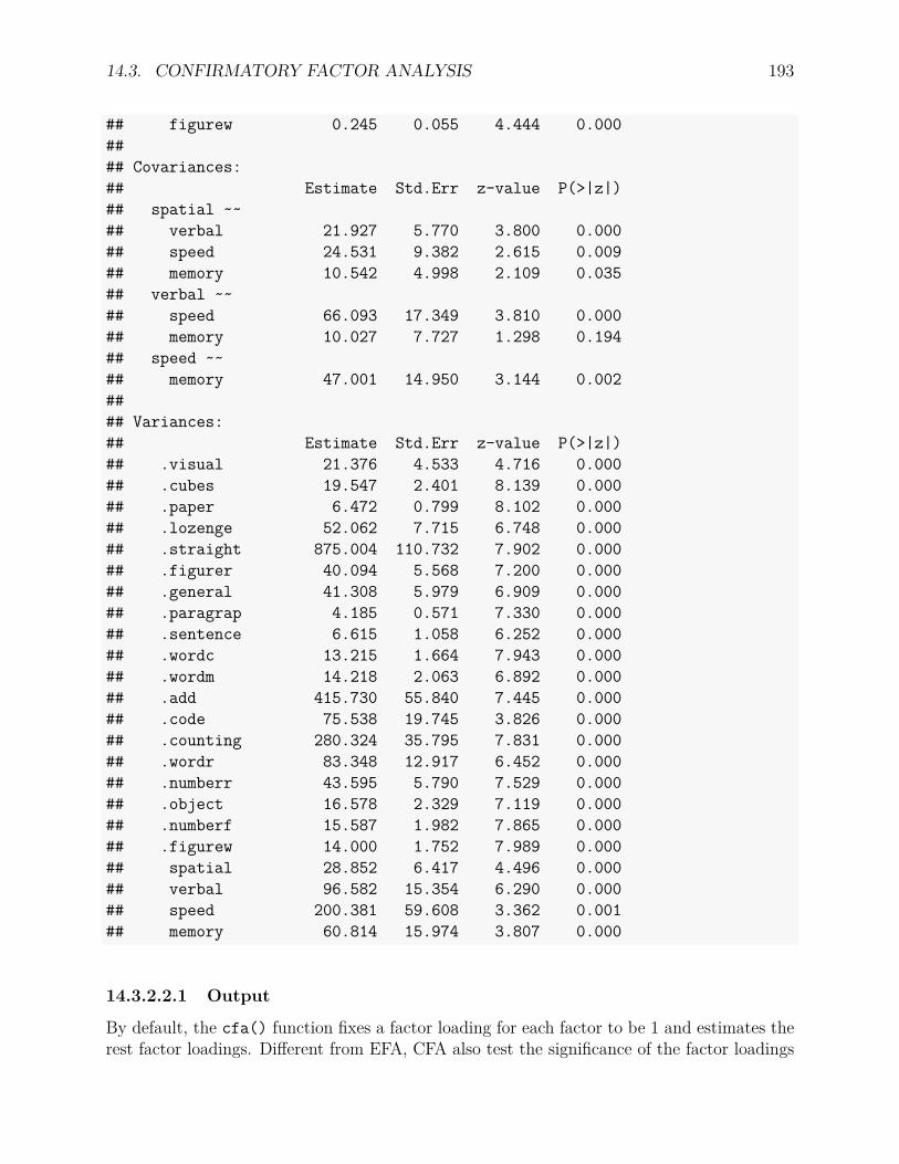
14.3. CONFIRMATORY FACTOR ANALYSIS 193
## figurew 0.245 0.055 4.444 0.000#### Covariances:## Estimate Std.Err z-value P(>|z|)## spatial ~~## verbal 21.927 5.770 3.800 0.000## speed 24.531 9.382 2.615 0.009## memory 10.542 4.998 2.109 0.035## verbal ~~## speed 66.093 17.349 3.810 0.000## memory 10.027 7.727 1.298 0.194## speed ~~## memory 47.001 14.950 3.144 0.002#### Variances:## Estimate Std.Err z-value P(>|z|)## .visual 21.376 4.533 4.716 0.000## .cubes 19.547 2.401 8.139 0.000## .paper 6.472 0.799 8.102 0.000## .lozenge 52.062 7.715 6.748 0.000## .straight 875.004 110.732 7.902 0.000## .figurer 40.094 5.568 7.200 0.000## .general 41.308 5.979 6.909 0.000## .paragrap 4.185 0.571 7.330 0.000## .sentence 6.615 1.058 6.252 0.000## .wordc 13.215 1.664 7.943 0.000## .wordm 14.218 2.063 6.892 0.000## .add 415.730 55.840 7.445 0.000## .code 75.538 19.745 3.826 0.000## .counting 280.324 35.795 7.831 0.000## .wordr 83.348 12.917 6.452 0.000## .numberr 43.595 5.790 7.529 0.000## .object 16.578 2.329 7.119 0.000## .numberf 15.587 1.982 7.865 0.000## .figurew 14.000 1.752 7.989 0.000## spatial 28.852 6.417 4.496 0.000## verbal 96.582 15.354 6.290 0.000## speed 200.381 59.608 3.362 0.001## memory 60.814 15.974 3.807 0.000
14.3.2.2.1 Output
By default, the cfa() function fixes a factor loading for each factor to be 1 and estimates therest factor loadings. Different from EFA, CFA also test the significance of the factor loadings
194 CHAPTER 14. FACTOR ANALYSIS
based on a z-test. For example, the factor loading for cubes on factor 1 is 0.396 with thestandard error 0.089. The corresponding z-value is 4.465 with a p-value almost 0. Therefore,this factor loading is statistically significant from 0. In addition, it also estimates the factorvariances and covariances as well as the uniqueness factor variances.
14.3.2.3 Model fit evaluation
CFA provides a lot more information to evaluate whether a model fits a sample. First, achi-square test can be used. For this test, the null hypothesis is that the model fits the datawell. Therefore, one would hope to get a small chi-square statistic and a corresponding largep-value. Typically, when p-value is larger than 0.5, one fails to reject the model.
There are many other fit statistics and indices that can be used to evaluate model fit. Themost widely used ones include CFI, RMSEA, and SRMR.
• Comparative fit index (CFI) compares the model under evaluation with a baselinemodel. One form of the baseline model is the independent model where it assumes theindependence among the observed variables. In general, such a baseline model wouldnot fit the data well. Therefore, CFI measures the relative improvement of the currentmodel. It is generally accepted that a CFI greater than 0.96 (or 0.95) indicates a goodfit model.
• Root mean square error of approximation (RMSEA) is a measure of chi-square attributedto each participate after controlling the model complexity. Therefore, a smaller valueindicates better fit. In the literature,– a RMSEA ≤ 0.05 indicates a model fits the data closely.– a 0.05 < RMSEA ≤ 0.08 indicates a model fits the data reasonably well.– a RMSEA > 0.1 indicates a model is a bad model.
• Standardized root mean square residual (SRMR) measures the difference between theobserved covariance matrix from the data and the predicted covariance matrix basedon the model. A value SRMR=0 indicates a perfect of the model. In general, a valueless than 0.08 is considered a good fit of the model under evaluation.
Using these criteria, we can evaluate whether the confirmatory factor model identified usingthe data from Grant-White school fits the data from the Pasteur school well.
• The chi-square statistic (Minimum Function Test Statistic in the output) is 238.75with the degrees of freedom 144 and a p-value close to 0. Therefore, one would rejectthe hypothesis that the model fits the data simply based on it.
• Comparative Fit Index (CFI) is 0.903, which is smaller than the cut-off value 0.95. Italso suggests a bad fit.
• The RMSEA = 0.065, which lies the range of a reasonable fit model.• The SRMR = 0.079, which is smaller than but close to the cut-off value 0.08.
Overall, the chi-square test and the other criteria suggest the model barely fits the data.Therefore, we cannot replicate the factor structure identified in EFA for the Grant-Whiteschool data in the Pasteur school.

14.3. CONFIRMATORY FACTOR ANALYSIS 195
14.3.2.4 Estimate the model with standardized factors
Instead of fitting a factor loading to be 1, we can also fix the factor variances to be 1. The Rcode below does the analysis. Note that the model fit is exactly the same as before. However,we can now directly estimate the factor correlation matrix.cfa.est<-cfa(cfa.model, data=Pasteur, std.lv=TRUE)summary(cfa.est, fit=TRUE)## lavaan 0.6-3 ended normally after 30 iterations#### Optimization method NLMINB## Number of free parameters 46#### Number of observations 156#### Estimator ML## Model Fit Test Statistic 238.751## Degrees of freedom 144## P-value (Chi-square) 0.000#### Model test baseline model:#### Minimum Function Test Statistic 1149.278## Degrees of freedom 171## P-value 0.000#### User model versus baseline model:#### Comparative Fit Index (CFI) 0.903## Tucker-Lewis Index (TLI) 0.885#### Loglikelihood and Information Criteria:#### Loglikelihood user model (H0) -9899.892## Loglikelihood unrestricted model (H1) -9780.517#### Number of free parameters 46## Akaike (AIC) 19891.785## Bayesian (BIC) 20032.078## Sample-size adjusted Bayesian (BIC) 19886.474#### Root Mean Square Error of Approximation:#### RMSEA 0.065## 90 Percent Confidence Interval 0.050 0.079
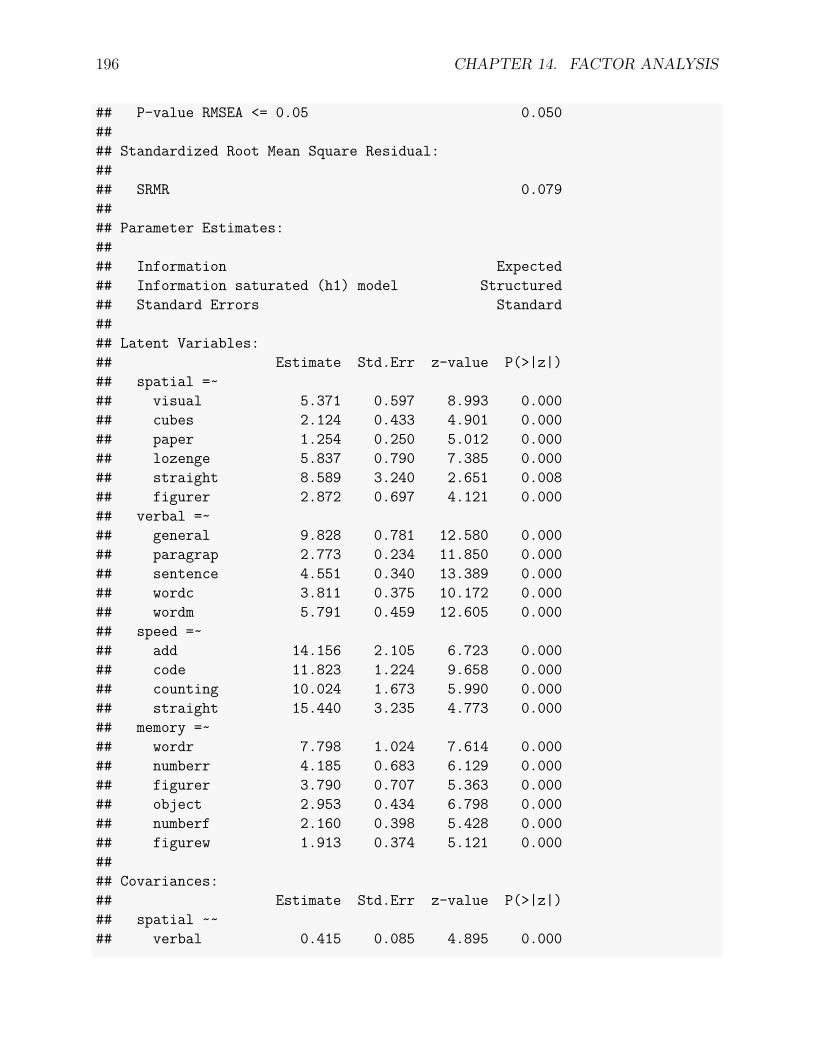
196 CHAPTER 14. FACTOR ANALYSIS
## P-value RMSEA <= 0.05 0.050#### Standardized Root Mean Square Residual:#### SRMR 0.079#### Parameter Estimates:#### Information Expected## Information saturated (h1) model Structured## Standard Errors Standard#### Latent Variables:## Estimate Std.Err z-value P(>|z|)## spatial =~## visual 5.371 0.597 8.993 0.000## cubes 2.124 0.433 4.901 0.000## paper 1.254 0.250 5.012 0.000## lozenge 5.837 0.790 7.385 0.000## straight 8.589 3.240 2.651 0.008## figurer 2.872 0.697 4.121 0.000## verbal =~## general 9.828 0.781 12.580 0.000## paragrap 2.773 0.234 11.850 0.000## sentence 4.551 0.340 13.389 0.000## wordc 3.811 0.375 10.172 0.000## wordm 5.791 0.459 12.605 0.000## speed =~## add 14.156 2.105 6.723 0.000## code 11.823 1.224 9.658 0.000## counting 10.024 1.673 5.990 0.000## straight 15.440 3.235 4.773 0.000## memory =~## wordr 7.798 1.024 7.614 0.000## numberr 4.185 0.683 6.129 0.000## figurer 3.790 0.707 5.363 0.000## object 2.953 0.434 6.798 0.000## numberf 2.160 0.398 5.428 0.000## figurew 1.913 0.374 5.121 0.000#### Covariances:## Estimate Std.Err z-value P(>|z|)## spatial ~~## verbal 0.415 0.085 4.895 0.000
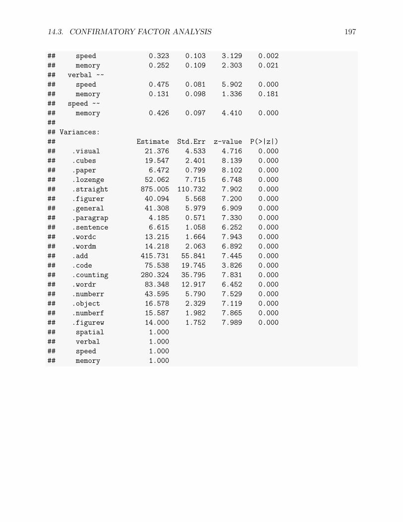
14.3. CONFIRMATORY FACTOR ANALYSIS 197
## speed 0.323 0.103 3.129 0.002## memory 0.252 0.109 2.303 0.021## verbal ~~## speed 0.475 0.081 5.902 0.000## memory 0.131 0.098 1.336 0.181## speed ~~## memory 0.426 0.097 4.410 0.000#### Variances:## Estimate Std.Err z-value P(>|z|)## .visual 21.376 4.533 4.716 0.000## .cubes 19.547 2.401 8.139 0.000## .paper 6.472 0.799 8.102 0.000## .lozenge 52.062 7.715 6.748 0.000## .straight 875.005 110.732 7.902 0.000## .figurer 40.094 5.568 7.200 0.000## .general 41.308 5.979 6.909 0.000## .paragrap 4.185 0.571 7.330 0.000## .sentence 6.615 1.058 6.252 0.000## .wordc 13.215 1.664 7.943 0.000## .wordm 14.218 2.063 6.892 0.000## .add 415.731 55.841 7.445 0.000## .code 75.538 19.745 3.826 0.000## .counting 280.324 35.795 7.831 0.000## .wordr 83.348 12.917 6.452 0.000## .numberr 43.595 5.790 7.529 0.000## .object 16.578 2.329 7.119 0.000## .numberf 15.587 1.982 7.865 0.000## .figurew 14.000 1.752 7.989 0.000## spatial 1.000## verbal 1.000## speed 1.000## memory 1.000

198 CHAPTER 14. FACTOR ANALYSIS

Chapter 15
Structural Equation Models
Simply speaking, a structural equation model (SEM) is a combination of confirmatory factoranalysis and path analysis. Structural equation modeling includes two sets of models €“ themeasurement model and the structural model. The measurement model can be expressedas a factor model. Figure 1 is a model to measure cognitive ability using three variables €“verbal ability, math ability, and speed ability (note each of them can be viewed as factorsmeasured by lower level observed variables).
Figure 2 gives another example of measurement model €“ a model to measure health.
199

200 CHAPTER 15. STRUCTURAL EQUATION MODELS
If one believes that health influences cognitive ability, then one can fit a path model usingthe factors €“ cognitive ability and health. Therefore, a structural model is actually a pathmodel. Putting them together, we have a model in Figure 3. This model is called SEMmodel.
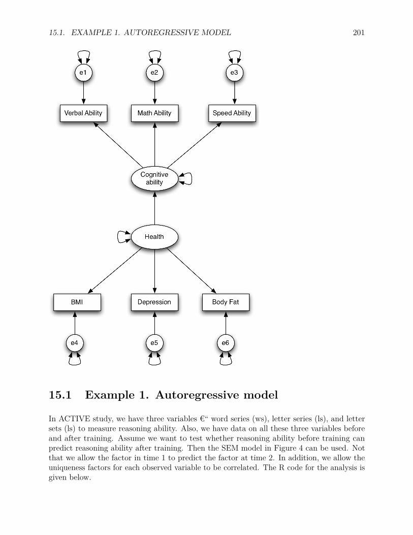
15.1. EXAMPLE 1. AUTOREGRESSIVE MODEL 201
15.1 Example 1. Autoregressive model
In ACTIVE study, we have three variables €“ word series (ws), letter series (ls), and lettersets (ls) to measure reasoning ability. Also, we have data on all these three variables beforeand after training. Assume we want to test whether reasoning ability before training canpredict reasoning ability after training. Then the SEM model in Figure 4 can be used. Notthat we allow the factor in time 1 to predict the factor at time 2. In addition, we allow theuniqueness factors for each observed variable to be correlated. The R code for the analysis isgiven below.

202 CHAPTER 15. STRUCTURAL EQUATION MODELS
reasoning1
ws1 ls1 lt1
reasoning2
ws2 ls2 lt2
First look at model fit. The chi-square value is 27 with 5 degrees of freedom. The p-value forchi-square test is almost 0. Thus, based on chi-square test, this is not a good model. However,CFI and TFI are both close to 1. The RMSEA is about 0.063 and SRMR is about 0.011.Considering the sample size here is large €“ N=1114, overall, we may accept this model is afairly good model. Then we can answer our question. Because the regression coefficient fromreasoning1 to reasoning2 is significant, reasoning ability before training seems to predictreasoning ability after training. In other words, those with higher reasoning ability beforetraining tend to have higher reasoning ability after training.library(lavaan)active.full <- read.csv('data/active.full.csv')automodel <- 'reasoning1 =~ ws1 + ls1 + lt1reasoning2 =~ ws2 + ls2 + lt2reasoning2 ~ reasoning1ws1 ~~ ws2ls1 ~~ ls2lt1 ~~ lt2'
auto.res <- sem(automodel, data=active.full)summary(auto.res, fit=TRUE)## lavaan 0.6-3 ended normally after 66 iterations#### Optimization method NLMINB## Number of free parameters 16#### Number of observations 1114#### Estimator ML## Model Fit Test Statistic 27.213## Degrees of freedom 5## P-value (Chi-square) 0.000#### Model test baseline model:

15.1. EXAMPLE 1. AUTOREGRESSIVE MODEL 203
#### Minimum Function Test Statistic 5827.630## Degrees of freedom 15## P-value 0.000#### User model versus baseline model:#### Comparative Fit Index (CFI) 0.996## Tucker-Lewis Index (TLI) 0.989#### Loglikelihood and Information Criteria:#### Loglikelihood user model (H0) -16447.377## Loglikelihood unrestricted model (H1) -16433.771#### Number of free parameters 16## Akaike (AIC) 32926.755## Bayesian (BIC) 33007.006## Sample-size adjusted Bayesian (BIC) 32956.186#### Root Mean Square Error of Approximation:#### RMSEA 0.063## 90 Percent Confidence Interval 0.041 0.087## P-value RMSEA <= 0.05 0.151#### Standardized Root Mean Square Residual:#### SRMR 0.013#### Parameter Estimates:#### Information Expected## Information saturated (h1) model Structured## Standard Errors Standard#### Latent Variables:## Estimate Std.Err z-value P(>|z|)## reasoning1 =~## ws1 1.000## ls1 1.192 0.030 40.091 0.000## lt1 0.422 0.016 26.301 0.000## reasoning2 =~## ws2 1.000
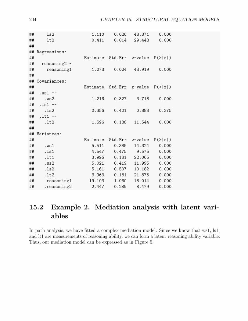
204 CHAPTER 15. STRUCTURAL EQUATION MODELS
## ls2 1.110 0.026 43.371 0.000## lt2 0.411 0.014 29.443 0.000#### Regressions:## Estimate Std.Err z-value P(>|z|)## reasoning2 ~## reasoning1 1.073 0.024 43.919 0.000#### Covariances:## Estimate Std.Err z-value P(>|z|)## .ws1 ~~## .ws2 1.216 0.327 3.718 0.000## .ls1 ~~## .ls2 0.356 0.401 0.888 0.375## .lt1 ~~## .lt2 1.596 0.138 11.544 0.000#### Variances:## Estimate Std.Err z-value P(>|z|)## .ws1 5.511 0.385 14.324 0.000## .ls1 4.547 0.475 9.575 0.000## .lt1 3.996 0.181 22.065 0.000## .ws2 5.021 0.419 11.995 0.000## .ls2 5.161 0.507 10.182 0.000## .lt2 3.963 0.181 21.875 0.000## reasoning1 19.103 1.060 18.014 0.000## .reasoning2 2.447 0.289 8.479 0.000
15.2 Example 2. Mediation analysis with latent vari-ables
In path analysis, we have fitted a complex mediation model. Since we know that ws1, ls1,and lt1 are measurements of reasoning ability, we can form a latent reasoning ability variable.Thus, our mediation model can be expressed as in Figure 5.

15.2. EXAMPLE 2. MEDIATION ANALYSIS WITH LATENT VARIABLES 205
age
edu
hvltt1
reasoning
ept1
ws1 ls1 lt1
Given CFI = 0.997, RMSEA = 0.034 and SRMR = 0.015, we accept the model as a goodmodel even though the chi-square test is significant. Based on the Sobel test, the totalindirect effect from age to ept1 through hvltt1 and reasoning is significant.med.model <- 'reasoning =~ ws1 + ls1 + lt1reasoning ~ p4*age + p8*eduhvltt1 ~ p2*age + p7*eduhvltt1 ~~ reasoningept1 ~ p1*age + p6*edu + p3*hvltt1 + p5*reasoningindirect := p2*p3 + p4*p5total := p1 + p2*p3 + p7*p3'
med.res <- sem(med.model, data=active.full)summary(med.res, fit=TRUE)## lavaan 0.6-3 ended normally after 51 iterations#### Optimization method NLMINB## Number of free parameters 17#### Number of observations 1114#### Estimator ML## Model Fit Test Statistic 18.363## Degrees of freedom 8## P-value (Chi-square) 0.019#### Model test baseline model:##

206 CHAPTER 15. STRUCTURAL EQUATION MODELS
## Minimum Function Test Statistic 3344.605## Degrees of freedom 20## P-value 0.000#### User model versus baseline model:#### Comparative Fit Index (CFI) 0.997## Tucker-Lewis Index (TLI) 0.992#### Loglikelihood and Information Criteria:#### Loglikelihood user model (H0) -14628.420## Loglikelihood unrestricted model (H1) -14619.238#### Number of free parameters 17## Akaike (AIC) 29290.840## Bayesian (BIC) 29376.107## Sample-size adjusted Bayesian (BIC) 29322.110#### Root Mean Square Error of Approximation:#### RMSEA 0.034## 90 Percent Confidence Interval 0.013 0.055## P-value RMSEA <= 0.05 0.889#### Standardized Root Mean Square Residual:#### SRMR 0.015#### Parameter Estimates:#### Information Expected## Information saturated (h1) model Structured## Standard Errors Standard#### Latent Variables:## Estimate Std.Err z-value P(>|z|)## reasoning =~## ws1 1.000## ls1 1.181 0.029 41.262 0.000## lt1 0.430 0.016 26.758 0.000#### Regressions:## Estimate Std.Err z-value P(>|z|)
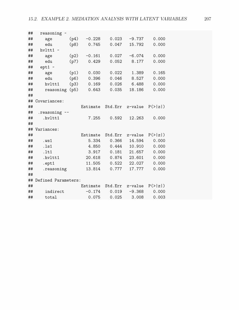
15.2. EXAMPLE 2. MEDIATION ANALYSIS WITH LATENT VARIABLES 207
## reasoning ~## age (p4) -0.228 0.023 -9.737 0.000## edu (p8) 0.745 0.047 15.792 0.000## hvltt1 ~## age (p2) -0.161 0.027 -6.074 0.000## edu (p7) 0.429 0.052 8.177 0.000## ept1 ~## age (p1) 0.030 0.022 1.389 0.165## edu (p6) 0.396 0.046 8.527 0.000## hvltt1 (p3) 0.169 0.026 6.488 0.000## reasoning (p5) 0.643 0.035 18.186 0.000#### Covariances:## Estimate Std.Err z-value P(>|z|)## .reasoning ~~## .hvltt1 7.255 0.592 12.263 0.000#### Variances:## Estimate Std.Err z-value P(>|z|)## .ws1 5.334 0.366 14.594 0.000## .ls1 4.850 0.444 10.910 0.000## .lt1 3.917 0.181 21.657 0.000## .hvltt1 20.618 0.874 23.601 0.000## .ept1 11.505 0.522 22.027 0.000## .reasoning 13.814 0.777 17.777 0.000#### Defined Parameters:## Estimate Std.Err z-value P(>|z|)## indirect -0.174 0.019 -9.368 0.000## total 0.075 0.025 3.008 0.003

208 CHAPTER 15. STRUCTURAL EQUATION MODELS

Chapter 16
Multilevel Regression
16.1 Multilevel data
Lee and Bryk (1989) analyzed a set of data in illustrating the use of multilevel modeling. Thedata set includes mathematics scores for senior-year high school students from 160 schools.For each student, information on her/his social and economic status (SES) is also available.For each school, data are available on the sector (private or public) of the schools. In addition,a school level variable called average SES (MSES) was created from the students’ SES tomeasure the SES of each school.
There is a clear two-level structure in the data. At the first level, the student level, we haveinformation on individual students. At the second level, the school level, we have informationon schools. The students are nested within schools. This kind of data are called multileveldata.
16.1.1 Lee and Bryk school achievement data
As an example, we use a subset of data from the Lee and Bryk (1989) study. In total, thereare n = 7, 185 students at the first level. At the second level, there are J = 160 schools.The data are saved in the file LeeBryk.csv. A subset of data are shown below. sector=0indicates a public school and sector=1 indicates a private Catholic high school.LeeBryk <- read.csv('data/LeeBryk.csv')head(LeeBryk)## schoolid math ses mses sector## 1 1 5.88 -1.53 -0.43 0## 2 1 19.71 -0.59 -0.43 0## 3 1 20.35 -0.53 -0.43 0## 4 1 8.78 -0.67 -0.43 0## 5 1 17.90 -0.16 -0.43 0
209
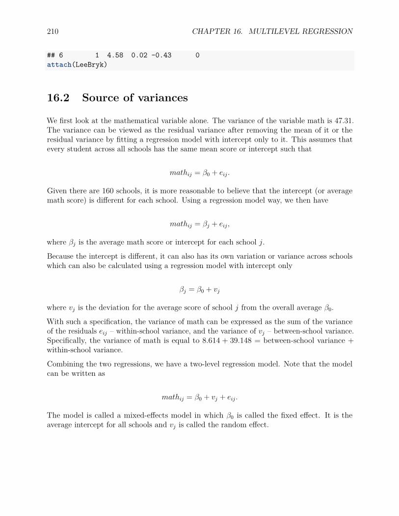
210 CHAPTER 16. MULTILEVEL REGRESSION
## 6 1 4.58 0.02 -0.43 0attach(LeeBryk)
16.2 Source of variances
We first look at the mathematical variable alone. The variance of the variable math is 47.31.The variance can be viewed as the residual variance after removing the mean of it or theresidual variance by fitting a regression model with intercept only to it. This assumes thatevery student across all schools has the same mean score or intercept such that
mathij = β0 + eij.
Given there are 160 schools, it is more reasonable to believe that the intercept (or averagemath score) is different for each school. Using a regression model way, we then have
mathij = βj + eij,
where βj is the average math score or intercept for each school j.
Because the intercept is different, it can also has its own variation or variance across schoolswhich can also be calculated using a regression model with intercept only
βj = β0 + vj
where vj is the deviation for the average score of school j from the overall average β0.
With such a specification, the variance of math can be expressed as the sum of the varianceof the residuals eij – within-school variance, and the variance of vj – between-school variance.Specifically, the variance of math is equal to 8.614 + 39.148 = between-school variance +within-school variance.
Combining the two regressions, we have a two-level regression model. Note that the modelcan be written as
mathij = β0 + vj + eij.
The model is called a mixed-effects model in which β0 is called the fixed effect. It is theaverage intercept for all schools and vj is called the random effect.

16.2. SOURCE OF VARIANCES 211
16.2.1 Use of R package lme4
A multilevel model or a mixed-effects model can be estimated using the R package lme4.Particularly, the function lmer() should be used. The function not only estimates thefixed-effects β0 but also the random-effects vj. The function use the format lmer(math~1 +(1|schoolid), data=school). In the function, the first “1” tells to estimate a fixed-effectsas the overall intercept. (1|schoolid) tells there is a random component in the intercept.
The output includes the Fixed effects, for which a t-test is also conducted for its significance.The Random effects part includes the variance of the residuals (eij) and the variance of therandom intercept (vj).library(lme4)
m2<-lmer(math ~ 1 + (1|schoolid), data=LeeBryk)summary(m2)## Linear mixed model fit by REML ['lmerMod']## Formula: math ~ 1 + (1 | schoolid)## Data: LeeBryk#### REML criterion at convergence: 47116.7#### Scaled residuals:## Min 1Q Median 3Q Max## -3.06294 -0.75337 0.02658 0.76060 2.74221#### Random effects:## Groups Name Variance Std.Dev.## schoolid (Intercept) 8.614 2.935## Residual 39.148 6.257## Number of obs: 7185, groups: schoolid, 160#### Fixed effects:## Estimate Std. Error t value## (Intercept) 12.6374 0.2444 51.71
The random-effects vj can be obtained using the function ranef(). With them, the interceptor average math score for each school can be calculated and also plotted as shown below.m2<-lmer(math ~ 1 + (1|schoolid), data=LeeBryk)bi<-ranef(m2)
school.intercept <- bi$schoolid + 12.6374plot(school.intercept[,1],type='h',
xlab='School ID', ylab='Intercept')abline(h=12.6374)
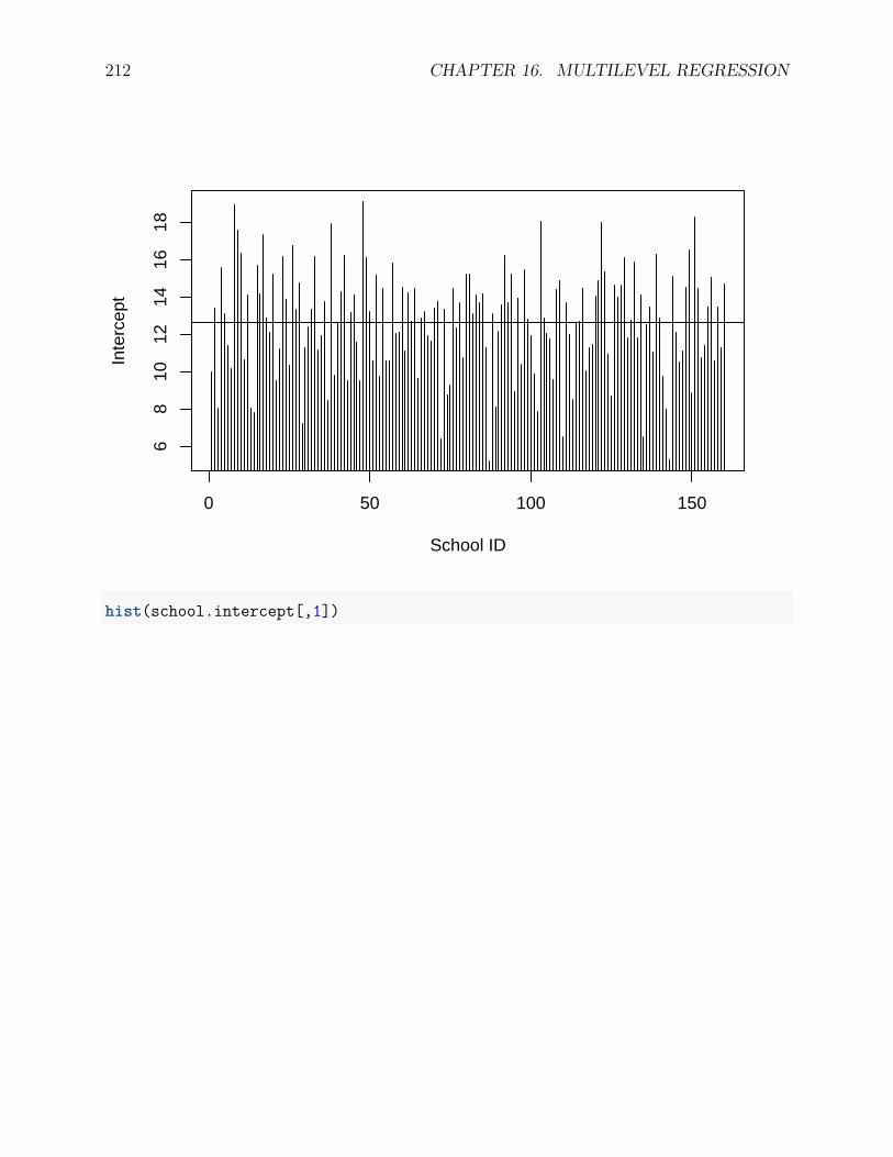
212 CHAPTER 16. MULTILEVEL REGRESSION
0 50 100 150
68
1012
1416
18
School ID
Inte
rcep
t
hist(school.intercept[,1])
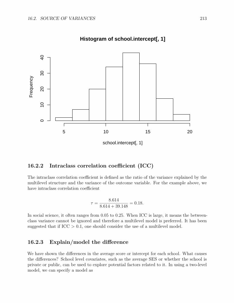
16.2. SOURCE OF VARIANCES 213
Histogram of school.intercept[, 1]
school.intercept[, 1]
Fre
quen
cy
5 10 15 20
010
2030
40
16.2.2 Intraclass correlation coefficient (ICC)
The intraclass correlation coefficient is defined as the ratio of the variance explained by themultilevel structure and the variance of the outcome variable. For the example above, wehave intraclass correlation coefficient
τ = 8.6148.614 + 39.148 = 0.18.
In social science, it often ranges from 0.05 to 0.25. When ICC is large, it means the between-class variance cannot be ignored and therefore a multilevel model is preferred. It has beensuggested that if ICC > 0.1, one should consider the use of a multilevel model.
16.2.3 Explain/model the difference
We have shown the differences in the average score or intercept for each school. What causesthe differences? School level covariates, such as the average SES or whether the school isprivate or public, can be used to explore potential factors related to it. In using a two-levelmodel, we can specify a model as
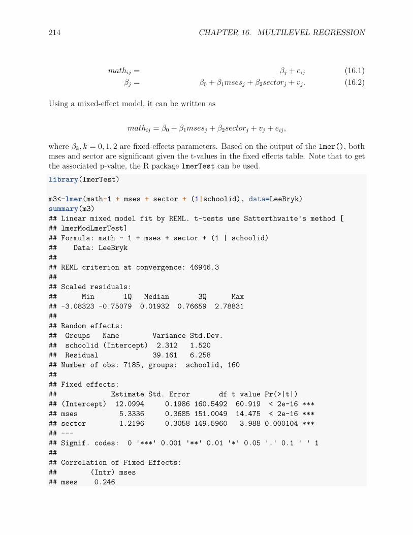
214 CHAPTER 16. MULTILEVEL REGRESSION
mathij = βj + eij (16.1)βj = β0 + β1msesj + β2sectorj + vj. (16.2)
Using a mixed-effect model, it can be written as
mathij = β0 + β1msesj + β2sectorj + vj + eij,
where βk, k = 0, 1, 2 are fixed-effects parameters. Based on the output of the lmer(), bothmses and sector are significant given the t-values in the fixed effects table. Note that to getthe associated p-value, the R package lmerTest can be used.library(lmerTest)
m3<-lmer(math~1 + mses + sector + (1|schoolid), data=LeeBryk)summary(m3)## Linear mixed model fit by REML. t-tests use Satterthwaite's method [## lmerModLmerTest]## Formula: math ~ 1 + mses + sector + (1 | schoolid)## Data: LeeBryk#### REML criterion at convergence: 46946.3#### Scaled residuals:## Min 1Q Median 3Q Max## -3.08323 -0.75079 0.01932 0.76659 2.78831#### Random effects:## Groups Name Variance Std.Dev.## schoolid (Intercept) 2.312 1.520## Residual 39.161 6.258## Number of obs: 7185, groups: schoolid, 160#### Fixed effects:## Estimate Std. Error df t value Pr(>|t|)## (Intercept) 12.0994 0.1986 160.5492 60.919 < 2e-16 ***## mses 5.3336 0.3685 151.0049 14.475 < 2e-16 ***## sector 1.2196 0.3058 149.5960 3.988 0.000104 ***## ---## Signif. codes: 0 '***' 0.001 '**' 0.01 '*' 0.05 '.' 0.1 ' ' 1#### Correlation of Fixed Effects:## (Intr) mses## mses 0.246
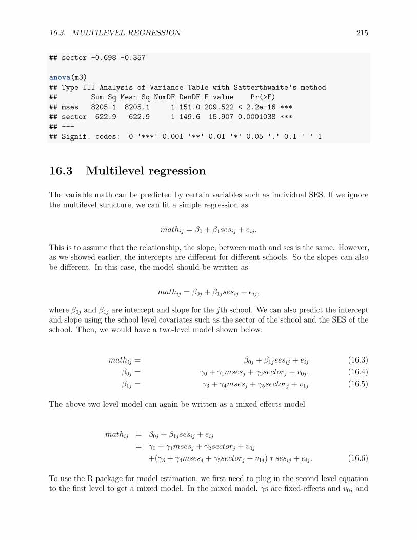
16.3. MULTILEVEL REGRESSION 215
## sector -0.698 -0.357
anova(m3)## Type III Analysis of Variance Table with Satterthwaite's method## Sum Sq Mean Sq NumDF DenDF F value Pr(>F)## mses 8205.1 8205.1 1 151.0 209.522 < 2.2e-16 ***## sector 622.9 622.9 1 149.6 15.907 0.0001038 ***## ---## Signif. codes: 0 '***' 0.001 '**' 0.01 '*' 0.05 '.' 0.1 ' ' 1
16.3 Multilevel regression
The variable math can be predicted by certain variables such as individual SES. If we ignorethe multilevel structure, we can fit a simple regression as
mathij = β0 + β1sesij + eij.
This is to assume that the relationship, the slope, between math and ses is the same. However,as we showed earlier, the intercepts are different for different schools. So the slopes can alsobe different. In this case, the model should be written as
mathij = β0j + β1jsesij + eij,
where β0j and β1j are intercept and slope for the jth school. We can also predict the interceptand slope using the school level covariates such as the sector of the school and the SES of theschool. Then, we would have a two-level model shown below:
mathij = β0j + β1jsesij + eij (16.3)β0j = γ0 + γ1msesj + γ2sectorj + v0j. (16.4)β1j = γ3 + γ4msesj + γ5sectorj + v1j (16.5)
The above two-level model can again be written as a mixed-effects model
mathij = β0j + β1jsesij + eij
= γ0 + γ1msesj + γ2sectorj + v0j
+(γ3 + γ4msesj + γ5sectorj + v1j) ∗ sesij + eij. (16.6)
To use the R package for model estimation, we first need to plug in the second level equationto the first level to get a mixed model. In the mixed model, γs are fixed-effects and v0j and

216 CHAPTER 16. MULTILEVEL REGRESSION
v1j are random effects. The variances of v0j and v1j and their correlation can also be obtained.We can also get the variance of eij. Those variance parameters are called random-effectsparameters while γs are called fixed-effects parameters. In R, each term in the mixed-effectsmodel needs to be specified except for eij . The random effects are specified using the notation| where before it are the random-effects terms and after it is the grouping variable or classvariable.
For the math example, the R input and output shown below.m4<-lmer(math~1 + mses + sector
+ ses + ses*mses + ses*sector+ (1 + ses|schoolid), data=LeeBryk)
summary(m4)## Linear mixed model fit by REML. t-tests use Satterthwaite's method [## lmerModLmerTest]## Formula: math ~ 1 + mses + sector + ses + ses * mses + ses * sector +## (1 + ses | schoolid)## Data: LeeBryk#### REML criterion at convergence: 46505.1#### Scaled residuals:## Min 1Q Median 3Q Max## -3.14226 -0.72478 0.01375 0.75508 2.98328#### Random effects:## Groups Name Variance Std.Dev. Corr## schoolid (Intercept) 2.40635 1.5512## ses 0.01441 0.1201 1.00## Residual 36.75783 6.0628## Number of obs: 7185, groups: schoolid, 160#### Fixed effects:## Estimate Std. Error df t value Pr(>|t|)## (Intercept) 12.1026 0.2028 166.5178 59.684 < 2e-16 ***## mses 3.3224 0.3884 178.5459 8.554 5.28e-15 ***## sector 1.1882 0.3080 148.3337 3.857 0.00017 ***## ses 2.9057 0.1483 4350.7595 19.595 < 2e-16 ***## mses:ses 0.8475 0.2717 3545.4952 3.119 0.00183 **## sector:ses -1.5793 0.2246 4345.3418 -7.033 2.34e-12 ***## ---## Signif. codes: 0 '***' 0.001 '**' 0.01 '*' 0.05 '.' 0.1 ' ' 1#### Correlation of Fixed Effects:## (Intr) mses sector ses mss:ss
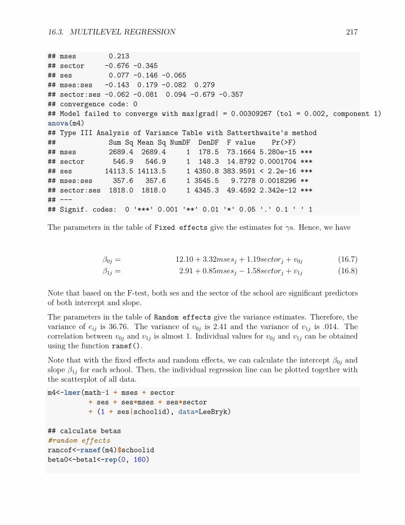
16.3. MULTILEVEL REGRESSION 217
## mses 0.213## sector -0.676 -0.345## ses 0.077 -0.146 -0.065## mses:ses -0.143 0.179 -0.082 0.279## sector:ses -0.062 -0.081 0.094 -0.679 -0.357## convergence code: 0## Model failed to converge with max|grad| = 0.00309267 (tol = 0.002, component 1)anova(m4)## Type III Analysis of Variance Table with Satterthwaite's method## Sum Sq Mean Sq NumDF DenDF F value Pr(>F)## mses 2689.4 2689.4 1 178.5 73.1664 5.280e-15 ***## sector 546.9 546.9 1 148.3 14.8792 0.0001704 ***## ses 14113.5 14113.5 1 4350.8 383.9591 < 2.2e-16 ***## mses:ses 357.6 357.6 1 3545.5 9.7278 0.0018296 **## sector:ses 1818.0 1818.0 1 4345.3 49.4592 2.342e-12 ***## ---## Signif. codes: 0 '***' 0.001 '**' 0.01 '*' 0.05 '.' 0.1 ' ' 1
The parameters in the table of Fixed effects give the estimates for γs. Hence, we have
β0j = 12.10 + 3.32msesj + 1.19sectorj + v0j (16.7)β1j = 2.91 + 0.85msesj − 1.58sectorj + v1j (16.8)
Note that based on the F-test, both ses and the sector of the school are significant predictorsof both intercept and slope.
The parameters in the table of Random effects give the variance estimates. Therefore, thevariance of eij is 36.76. The variance of v0j is 2.41 and the variance of v1j is .014. Thecorrelation between v0j and v1j is almost 1. Individual values for v0j and v1j can be obtainedusing the function ranef().
Note that with the fixed effects and random effects, we can calculate the intercept β0j andslope β1j for each school. Then, the individual regression line can be plotted together withthe scatterplot of all data.m4<-lmer(math~1 + mses + sector
+ ses + ses*mses + ses*sector+ (1 + ses|schoolid), data=LeeBryk)
## calculate betas#random effectsrancof<-ranef(m4)$schoolidbeta0<-beta1<-rep(0, 160)
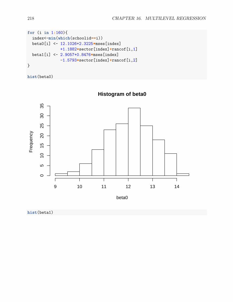
218 CHAPTER 16. MULTILEVEL REGRESSION
for (i in 1:160){index<-min(which(schoolid==i))beta0[i] <- 12.1026+2.3225*mses[index]
+1.1882*sector[index]+rancof[i,1]beta1[i] <- 2.9057+0.8476*mses[index]
-1.5793*sector[index]+rancof[i,2]}
hist(beta0)
Histogram of beta0
beta0
Fre
quen
cy
9 10 11 12 13 14
05
1015
2025
3035
hist(beta1)
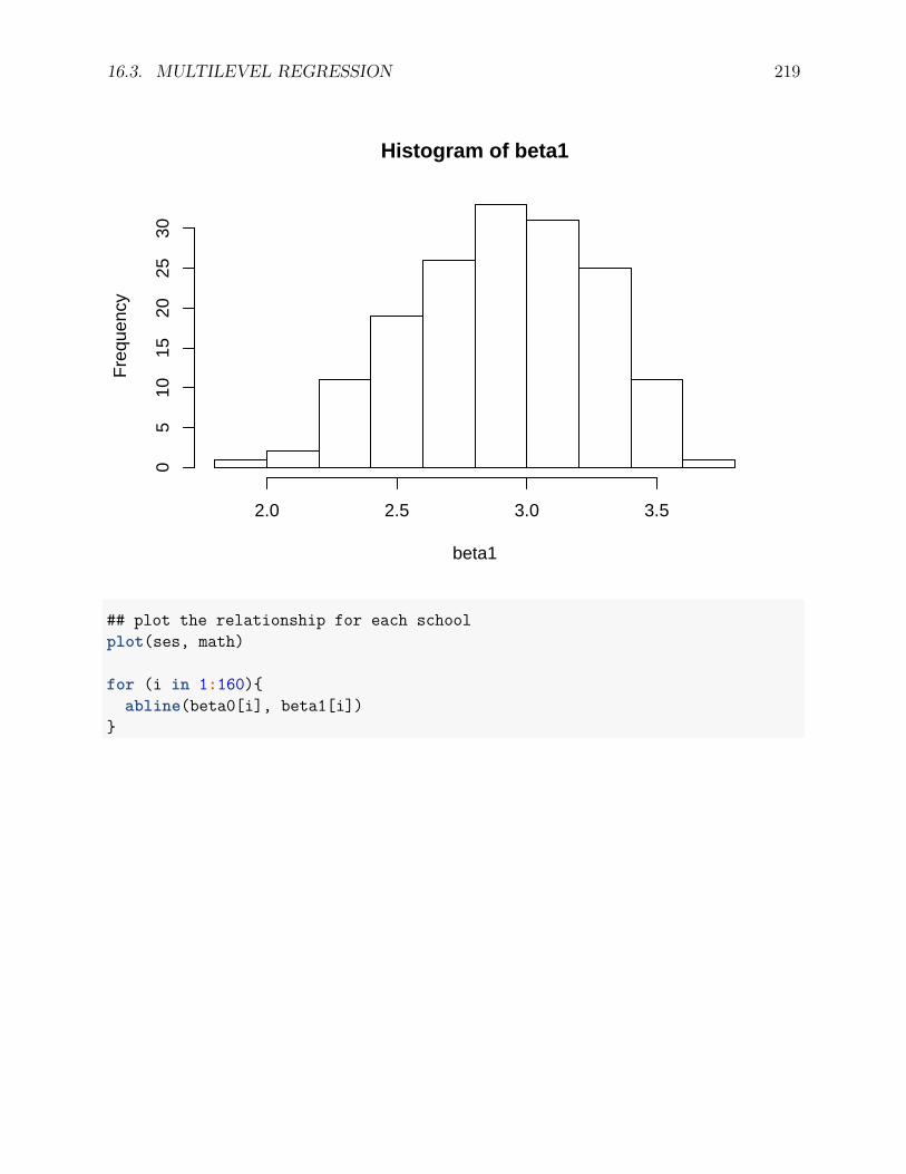
16.3. MULTILEVEL REGRESSION 219
Histogram of beta1
beta1
Fre
quen
cy
2.0 2.5 3.0 3.5
05
1015
2025
30
## plot the relationship for each schoolplot(ses, math)
for (i in 1:160){abline(beta0[i], beta1[i])
}
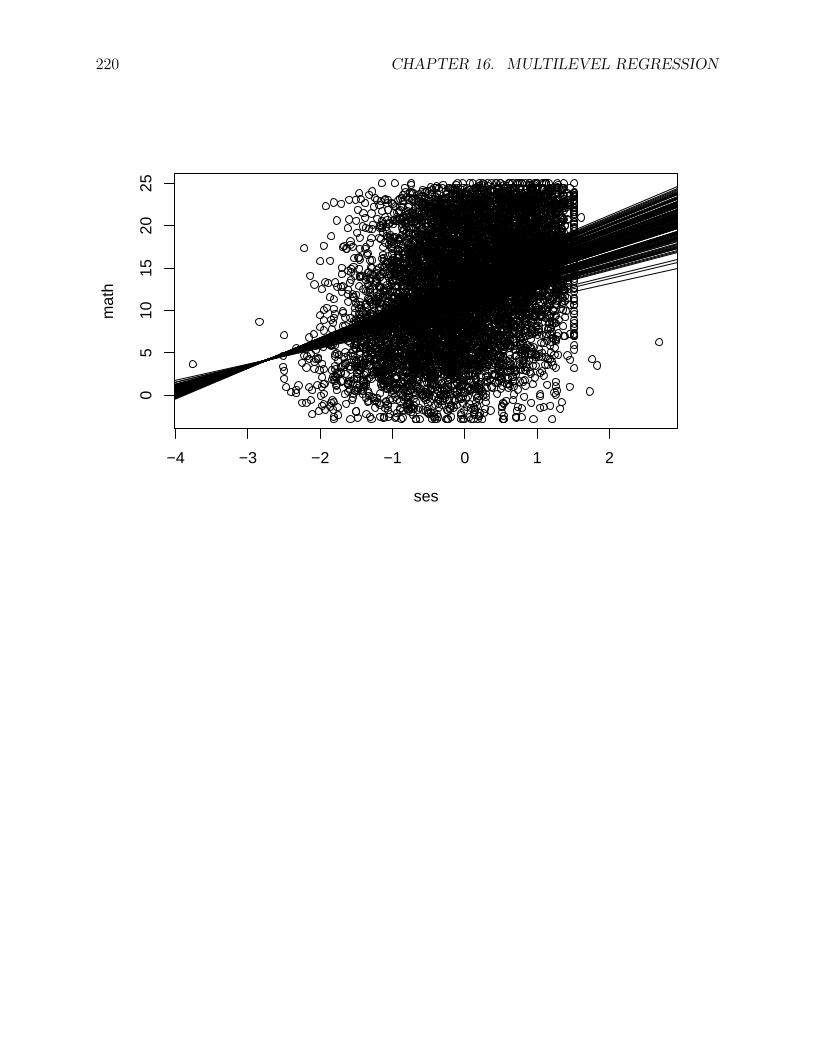
220 CHAPTER 16. MULTILEVEL REGRESSION
−4 −3 −2 −1 0 1 2
05
1015
2025
ses
mat
h
Chapter 17
Longitudinal Data Analysis
Longitudinal data can be viewed as a special case of the multilevel data where time is nestedwithin individual participants. All longitudinal data share at least three features: (1) the sameentities are repeatedly observed over time; (2) the same measurements (including paralleltests) are used; and (3) the timing for each measurement is known (Baltes & Nesselroade,1979). To study phenomena in their time-related patterns of constancy and change is aprimary reason for collecting longitudinal data. Figure 1 show the plot of 50 participantsfrom the ACTIVE study on the variable EPT for 6 times. Clearly, each line represents aparticipant. From it, we can see how an individual changes over time.
221
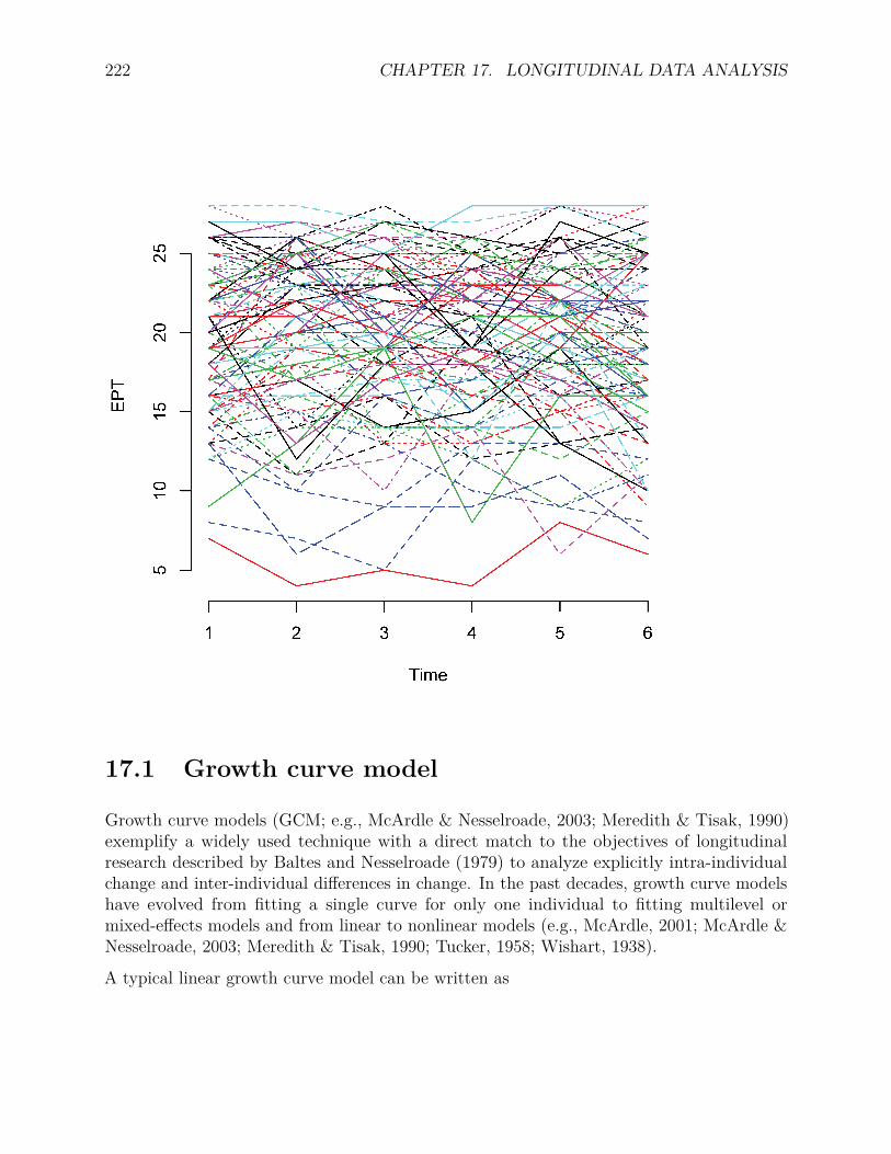
222 CHAPTER 17. LONGITUDINAL DATA ANALYSIS
17.1 Growth curve model
Growth curve models (GCM; e.g., McArdle & Nesselroade, 2003; Meredith & Tisak, 1990)exemplify a widely used technique with a direct match to the objectives of longitudinalresearch described by Baltes and Nesselroade (1979) to analyze explicitly intra-individualchange and inter-individual differences in change. In the past decades, growth curve modelshave evolved from fitting a single curve for only one individual to fitting multilevel ormixed-effects models and from linear to nonlinear models (e.g., McArdle, 2001; McArdle &Nesselroade, 2003; Meredith & Tisak, 1990; Tucker, 1958; Wishart, 1938).
A typical linear growth curve model can be written as
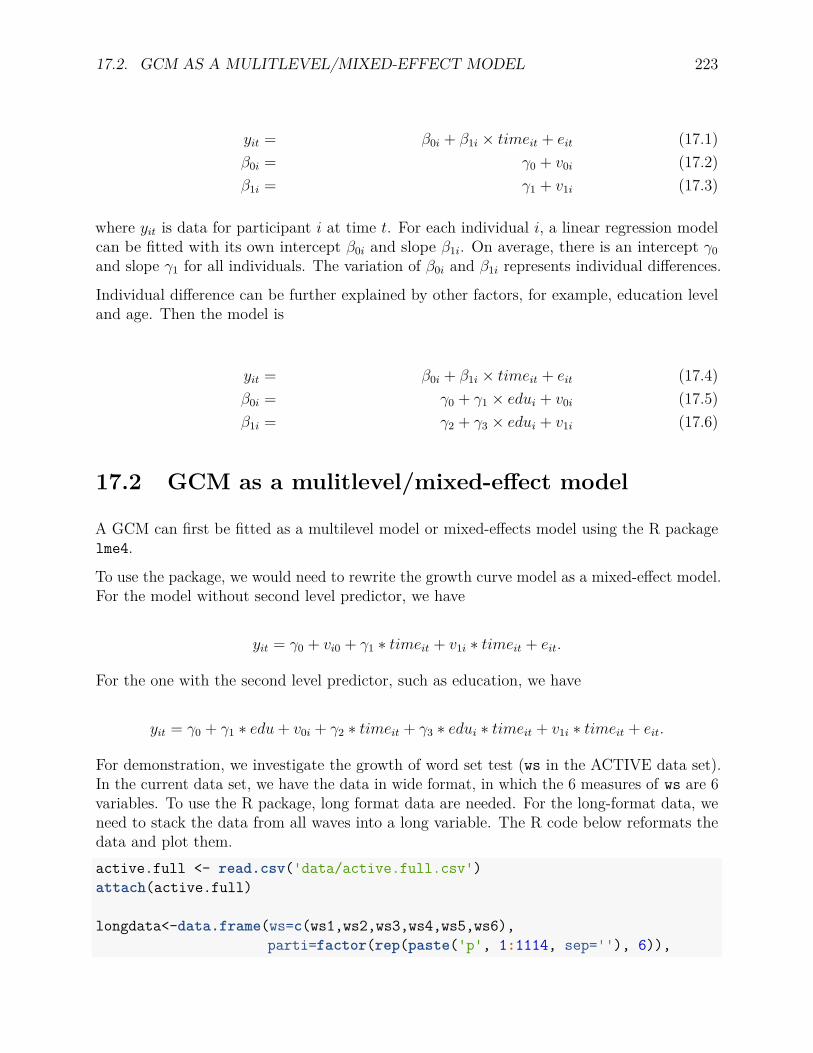
17.2. GCM AS A MULITLEVEL/MIXED-EFFECT MODEL 223
yit = β0i + β1i × timeit + eit (17.1)β0i = γ0 + v0i (17.2)β1i = γ1 + v1i (17.3)
where yit is data for participant i at time t. For each individual i, a linear regression modelcan be fitted with its own intercept β0i and slope β1i. On average, there is an intercept γ0and slope γ1 for all individuals. The variation of β0i and β1i represents individual differences.
Individual difference can be further explained by other factors, for example, education leveland age. Then the model is
yit = β0i + β1i × timeit + eit (17.4)β0i = γ0 + γ1 × edui + v0i (17.5)β1i = γ2 + γ3 × edui + v1i (17.6)
17.2 GCM as a mulitlevel/mixed-effect model
A GCM can first be fitted as a multilevel model or mixed-effects model using the R packagelme4.
To use the package, we would need to rewrite the growth curve model as a mixed-effect model.For the model without second level predictor, we have
yit = γ0 + vi0 + γ1 ∗ timeit + v1i ∗ timeit + eit.
For the one with the second level predictor, such as education, we have
yit = γ0 + γ1 ∗ edu+ v0i + γ2 ∗ timeit + γ3 ∗ edui ∗ timeit + v1i ∗ timeit + eit.
For demonstration, we investigate the growth of word set test (ws in the ACTIVE data set).In the current data set, we have the data in wide format, in which the 6 measures of ws are 6variables. To use the R package, long format data are needed. For the long-format data, weneed to stack the data from all waves into a long variable. The R code below reformats thedata and plot them.active.full <- read.csv('data/active.full.csv')attach(active.full)
longdata<-data.frame(ws=c(ws1,ws2,ws3,ws4,ws5,ws6),parti=factor(rep(paste('p', 1:1114, sep=''), 6)),

224 CHAPTER 17. LONGITUDINAL DATA ANALYSIS
time=rep(1:6, each=1114),edu=rep(edu, 6))
plot(1:6, longdata$ws[longdata$parti=="p1"], type='l',xlab='Time', ylab="ws", ylim=c(0, max(longdata$ws)))
for (i in 2:50){lines(1:6, longdata$ws[longdata$parti==paste("p", i, sep="")])
}
1 2 3 4 5 6
05
1015
2025
30
Time
ws
17.2.1 Unconditional model (model without second level predic-tors)
Fitting the model is actually straightforward using the lmer() function. The input andoutput are given below. Based on the output, the fixed effects for time (.214, t-value=11.59)is significant, therefore, there is a linear growth trend. The average intercept is 11.93 and isalso significant.library(lme4)library(lmerTest)
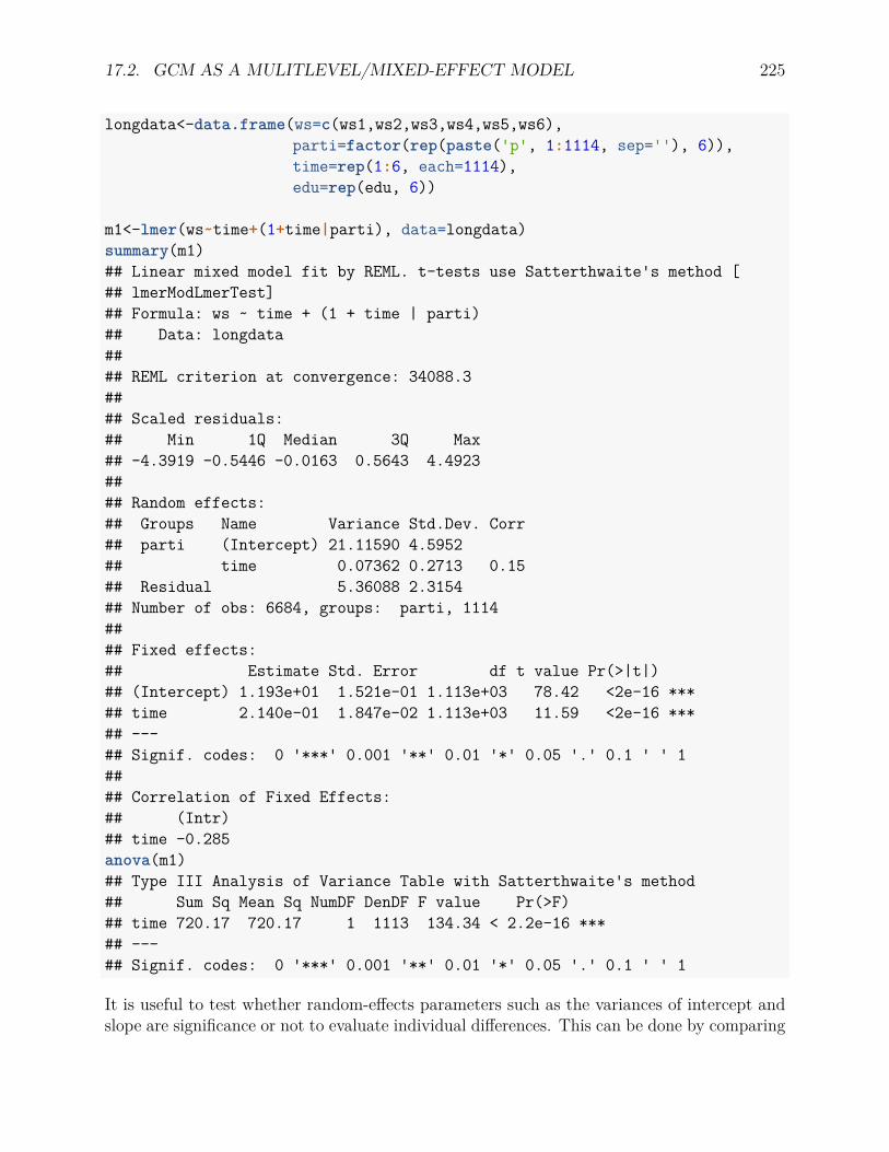
17.2. GCM AS A MULITLEVEL/MIXED-EFFECT MODEL 225
longdata<-data.frame(ws=c(ws1,ws2,ws3,ws4,ws5,ws6),parti=factor(rep(paste('p', 1:1114, sep=''), 6)),time=rep(1:6, each=1114),edu=rep(edu, 6))
m1<-lmer(ws~time+(1+time|parti), data=longdata)summary(m1)## Linear mixed model fit by REML. t-tests use Satterthwaite's method [## lmerModLmerTest]## Formula: ws ~ time + (1 + time | parti)## Data: longdata#### REML criterion at convergence: 34088.3#### Scaled residuals:## Min 1Q Median 3Q Max## -4.3919 -0.5446 -0.0163 0.5643 4.4923#### Random effects:## Groups Name Variance Std.Dev. Corr## parti (Intercept) 21.11590 4.5952## time 0.07362 0.2713 0.15## Residual 5.36088 2.3154## Number of obs: 6684, groups: parti, 1114#### Fixed effects:## Estimate Std. Error df t value Pr(>|t|)## (Intercept) 1.193e+01 1.521e-01 1.113e+03 78.42 <2e-16 ***## time 2.140e-01 1.847e-02 1.113e+03 11.59 <2e-16 ***## ---## Signif. codes: 0 '***' 0.001 '**' 0.01 '*' 0.05 '.' 0.1 ' ' 1#### Correlation of Fixed Effects:## (Intr)## time -0.285anova(m1)## Type III Analysis of Variance Table with Satterthwaite's method## Sum Sq Mean Sq NumDF DenDF F value Pr(>F)## time 720.17 720.17 1 1113 134.34 < 2.2e-16 ***## ---## Signif. codes: 0 '***' 0.001 '**' 0.01 '*' 0.05 '.' 0.1 ' ' 1
It is useful to test whether random-effects parameters such as the variances of intercept andslope are significance or not to evaluate individual differences. This can be done by comparing
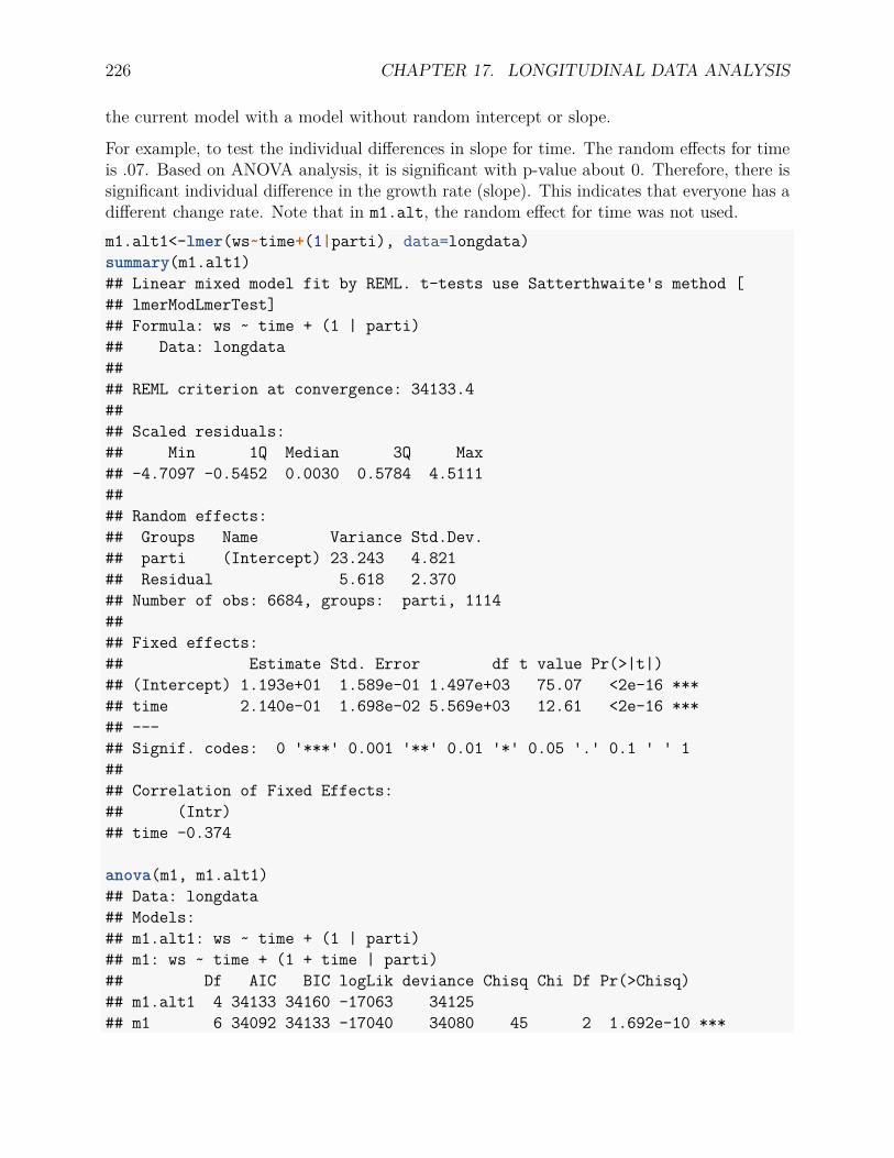
226 CHAPTER 17. LONGITUDINAL DATA ANALYSIS
the current model with a model without random intercept or slope.
For example, to test the individual differences in slope for time. The random effects for timeis .07. Based on ANOVA analysis, it is significant with p-value about 0. Therefore, there issignificant individual difference in the growth rate (slope). This indicates that everyone has adifferent change rate. Note that in m1.alt, the random effect for time was not used.m1.alt1<-lmer(ws~time+(1|parti), data=longdata)summary(m1.alt1)## Linear mixed model fit by REML. t-tests use Satterthwaite's method [## lmerModLmerTest]## Formula: ws ~ time + (1 | parti)## Data: longdata#### REML criterion at convergence: 34133.4#### Scaled residuals:## Min 1Q Median 3Q Max## -4.7097 -0.5452 0.0030 0.5784 4.5111#### Random effects:## Groups Name Variance Std.Dev.## parti (Intercept) 23.243 4.821## Residual 5.618 2.370## Number of obs: 6684, groups: parti, 1114#### Fixed effects:## Estimate Std. Error df t value Pr(>|t|)## (Intercept) 1.193e+01 1.589e-01 1.497e+03 75.07 <2e-16 ***## time 2.140e-01 1.698e-02 5.569e+03 12.61 <2e-16 ***## ---## Signif. codes: 0 '***' 0.001 '**' 0.01 '*' 0.05 '.' 0.1 ' ' 1#### Correlation of Fixed Effects:## (Intr)## time -0.374
anova(m1, m1.alt1)## Data: longdata## Models:## m1.alt1: ws ~ time + (1 | parti)## m1: ws ~ time + (1 + time | parti)## Df AIC BIC logLik deviance Chisq Chi Df Pr(>Chisq)## m1.alt1 4 34133 34160 -17063 34125## m1 6 34092 34133 -17040 34080 45 2 1.692e-10 ***
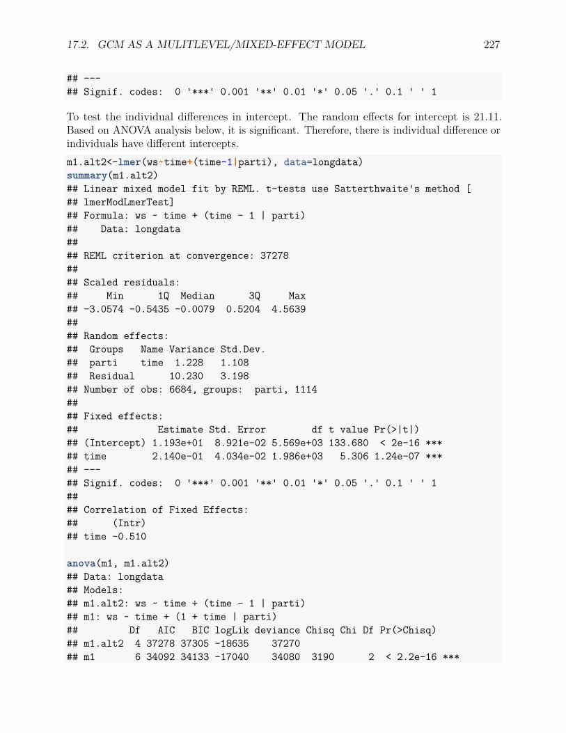
17.2. GCM AS A MULITLEVEL/MIXED-EFFECT MODEL 227
## ---## Signif. codes: 0 '***' 0.001 '**' 0.01 '*' 0.05 '.' 0.1 ' ' 1
To test the individual differences in intercept. The random effects for intercept is 21.11.Based on ANOVA analysis below, it is significant. Therefore, there is individual difference orindividuals have different intercepts.m1.alt2<-lmer(ws~time+(time-1|parti), data=longdata)summary(m1.alt2)## Linear mixed model fit by REML. t-tests use Satterthwaite's method [## lmerModLmerTest]## Formula: ws ~ time + (time - 1 | parti)## Data: longdata#### REML criterion at convergence: 37278#### Scaled residuals:## Min 1Q Median 3Q Max## -3.0574 -0.5435 -0.0079 0.5204 4.5639#### Random effects:## Groups Name Variance Std.Dev.## parti time 1.228 1.108## Residual 10.230 3.198## Number of obs: 6684, groups: parti, 1114#### Fixed effects:## Estimate Std. Error df t value Pr(>|t|)## (Intercept) 1.193e+01 8.921e-02 5.569e+03 133.680 < 2e-16 ***## time 2.140e-01 4.034e-02 1.986e+03 5.306 1.24e-07 ***## ---## Signif. codes: 0 '***' 0.001 '**' 0.01 '*' 0.05 '.' 0.1 ' ' 1#### Correlation of Fixed Effects:## (Intr)## time -0.510
anova(m1, m1.alt2)## Data: longdata## Models:## m1.alt2: ws ~ time + (time - 1 | parti)## m1: ws ~ time + (1 + time | parti)## Df AIC BIC logLik deviance Chisq Chi Df Pr(>Chisq)## m1.alt2 4 37278 37305 -18635 37270## m1 6 34092 34133 -17040 34080 3190 2 < 2.2e-16 ***
228 CHAPTER 17. LONGITUDINAL DATA ANALYSIS
## ---## Signif. codes: 0 '***' 0.001 '**' 0.01 '*' 0.05 '.' 0.1 ' ' 1
17.2.2 Conditional model (model with second level predictors)
Using the same set of data, we now investigate whether education is a predictor of randomintercept and slope. Given there is individual differences in intercept and slope, we want toexplain why. So, we use Edu as a explanatory variable. From the output, we can see that theparameter γ1 = .78 is significant. Higher education relates to bigger intercept. In addition,the parameter γ3 = −.022 is significant. Higher education relates to lower growth rate of ws.
17.3 GCM as a SEM
In addition to estimating a GCM as a multilevel or mixed-effects model, we can also estimateit as a SEM. To illustrate this, we consider a linear growth curve model. If a group ofparticipants all have linear change trend, for each individual, we can fit a regression modelsuch as
yit = βi0 + βi1t+ eit
where βi0 and βi1 are intercept and slope, respectively. Note that here we let timeit = t. Ifeach individual has different time of data collection, it can still be done in the SEM frameworkbut would be more complex. By writing the time out, we would have
yi1yi2...yiT
=
1 11 21 ...1 T
(βi0βi1
)+
ei1ei2...eiT
Note that the above equation resembles a factor model with two factors - b0 and b1 and afactor loading matrix with known factor loading matrix. The individual intercept and slopecan be viewed as factor scores to be estimated. Furthermore, we are interested in model withmean structure because the means of β0 and β1 have their meaning as average intercept andslope (rate of change). The variances of the factors can be estimated - they indicate thevariations of intercept and slope. Using path diagram, the model is shown in the figure below.
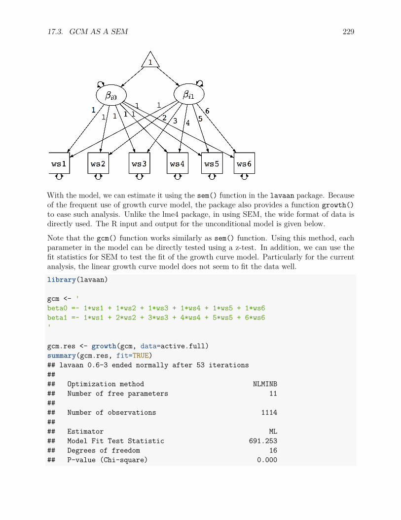
17.3. GCM AS A SEM 229
With the model, we can estimate it using the sem() function in the lavaan package. Becauseof the frequent use of growth curve model, the package also provides a function growth()to ease such analysis. Unlike the lme4 package, in using SEM, the wide format of data isdirectly used. The R input and output for the unconditional model is given below.
Note that the gcm() function works similarly as sem() function. Using this method, eachparameter in the model can be directly tested using a z-test. In addition, we can use thefit statistics for SEM to test the fit of the growth curve model. Particularly for the currentanalysis, the linear growth curve model does not seem to fit the data well.library(lavaan)
gcm <- 'beta0 =~ 1*ws1 + 1*ws2 + 1*ws3 + 1*ws4 + 1*ws5 + 1*ws6beta1 =~ 1*ws1 + 2*ws2 + 3*ws3 + 4*ws4 + 5*ws5 + 6*ws6'
gcm.res <- growth(gcm, data=active.full)summary(gcm.res, fit=TRUE)## lavaan 0.6-3 ended normally after 53 iterations#### Optimization method NLMINB## Number of free parameters 11#### Number of observations 1114#### Estimator ML## Model Fit Test Statistic 691.253## Degrees of freedom 16## P-value (Chi-square) 0.000
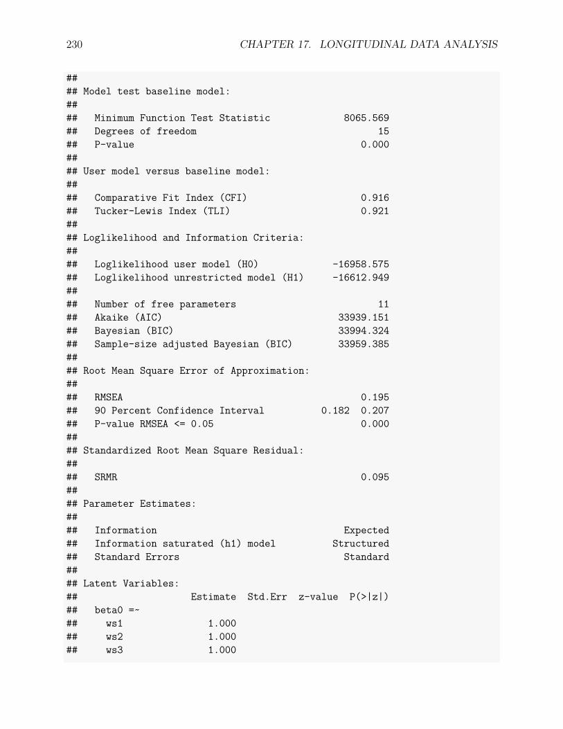
230 CHAPTER 17. LONGITUDINAL DATA ANALYSIS
#### Model test baseline model:#### Minimum Function Test Statistic 8065.569## Degrees of freedom 15## P-value 0.000#### User model versus baseline model:#### Comparative Fit Index (CFI) 0.916## Tucker-Lewis Index (TLI) 0.921#### Loglikelihood and Information Criteria:#### Loglikelihood user model (H0) -16958.575## Loglikelihood unrestricted model (H1) -16612.949#### Number of free parameters 11## Akaike (AIC) 33939.151## Bayesian (BIC) 33994.324## Sample-size adjusted Bayesian (BIC) 33959.385#### Root Mean Square Error of Approximation:#### RMSEA 0.195## 90 Percent Confidence Interval 0.182 0.207## P-value RMSEA <= 0.05 0.000#### Standardized Root Mean Square Residual:#### SRMR 0.095#### Parameter Estimates:#### Information Expected## Information saturated (h1) model Structured## Standard Errors Standard#### Latent Variables:## Estimate Std.Err z-value P(>|z|)## beta0 =~## ws1 1.000## ws2 1.000## ws3 1.000

17.3. GCM AS A SEM 231
## ws4 1.000## ws5 1.000## ws6 1.000## beta1 =~## ws1 1.000## ws2 2.000## ws3 3.000## ws4 4.000## ws5 5.000## ws6 6.000#### Covariances:## Estimate Std.Err z-value P(>|z|)## beta0 ~~## beta1 0.406 0.106 3.817 0.000#### Intercepts:## Estimate Std.Err z-value P(>|z|)## .ws1 0.000## .ws2 0.000## .ws3 0.000## .ws4 0.000## .ws5 0.000## .ws6 0.000## beta0 12.263 0.155 79.217 0.000## beta1 0.161 0.018 8.770 0.000#### Variances:## Estimate Std.Err z-value P(>|z|)## .ws1 8.999 0.443 20.293 0.000## .ws2 5.614 0.284 19.751 0.000## .ws3 3.867 0.209 18.539 0.000## .ws4 4.091 0.219 18.639 0.000## .ws5 4.712 0.249 18.915 0.000## .ws6 6.420 0.343 18.723 0.000## beta0 20.854 1.143 18.246 0.000## beta1 -0.004 0.019 -0.186 0.853
Fitting a conditional model is similar but one would need to use the predictor for the factors.gcm2 <- 'beta0 =~ 1*ws1 + 1*ws2 + 1*ws3 + 1*ws4 + 1*ws5 + 1*ws6beta1 =~ 1*ws1 + 2*ws2 + 3*ws3 + 4*ws4 + 5*ws5 + 6*ws6beta0 ~ edubeta1 ~ edu

232 CHAPTER 17. LONGITUDINAL DATA ANALYSIS
'
gcm2.res <- growth(gcm2, data=active.full)summary(gcm2.res, fit=TRUE)## lavaan 0.6-3 ended normally after 54 iterations#### Optimization method NLMINB## Number of free parameters 13#### Number of observations 1114#### Estimator ML## Model Fit Test Statistic 697.223## Degrees of freedom 20## P-value (Chi-square) 0.000#### Model test baseline model:#### Minimum Function Test Statistic 8259.498## Degrees of freedom 21## P-value 0.000#### User model versus baseline model:#### Comparative Fit Index (CFI) 0.918## Tucker-Lewis Index (TLI) 0.914#### Loglikelihood and Information Criteria:#### Loglikelihood user model (H0) -16864.596## Loglikelihood unrestricted model (H1) -16515.985#### Number of free parameters 13## Akaike (AIC) 33755.192## Bayesian (BIC) 33820.397## Sample-size adjusted Bayesian (BIC) 33779.105#### Root Mean Square Error of Approximation:#### RMSEA 0.174## 90 Percent Confidence Interval 0.163 0.186## P-value RMSEA <= 0.05 0.000#### Standardized Root Mean Square Residual:
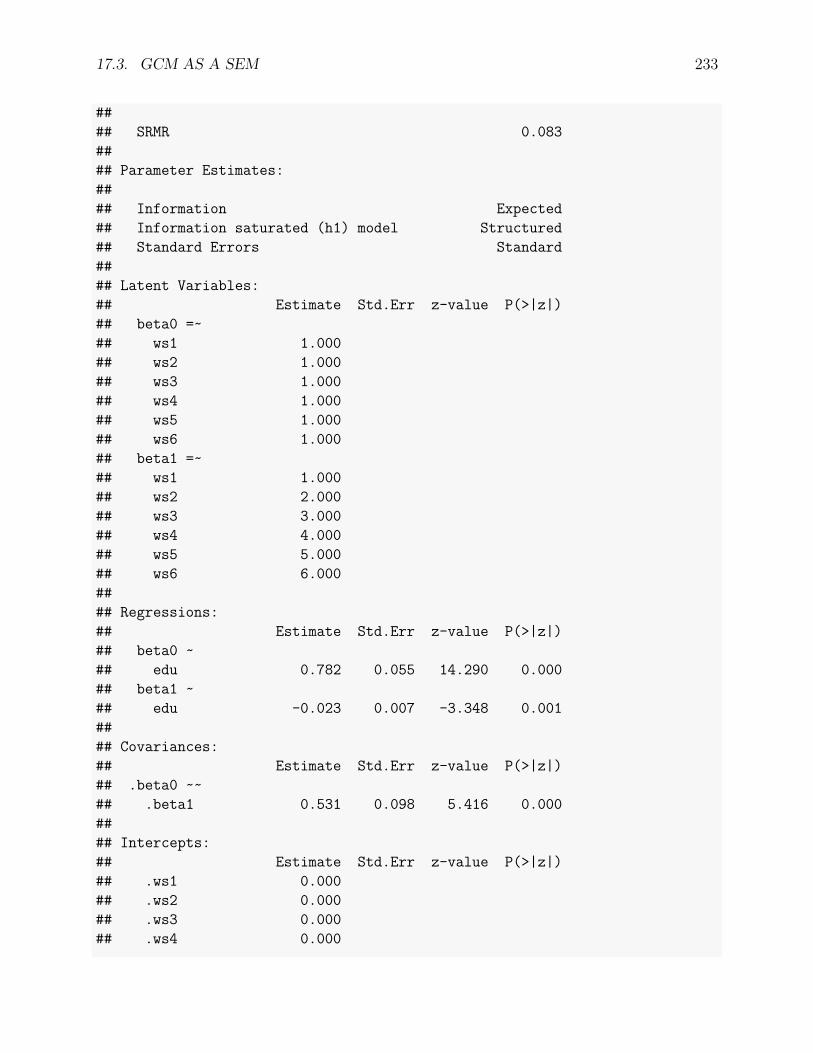
17.3. GCM AS A SEM 233
#### SRMR 0.083#### Parameter Estimates:#### Information Expected## Information saturated (h1) model Structured## Standard Errors Standard#### Latent Variables:## Estimate Std.Err z-value P(>|z|)## beta0 =~## ws1 1.000## ws2 1.000## ws3 1.000## ws4 1.000## ws5 1.000## ws6 1.000## beta1 =~## ws1 1.000## ws2 2.000## ws3 3.000## ws4 4.000## ws5 5.000## ws6 6.000#### Regressions:## Estimate Std.Err z-value P(>|z|)## beta0 ~## edu 0.782 0.055 14.290 0.000## beta1 ~## edu -0.023 0.007 -3.348 0.001#### Covariances:## Estimate Std.Err z-value P(>|z|)## .beta0 ~~## .beta1 0.531 0.098 5.416 0.000#### Intercepts:## Estimate Std.Err z-value P(>|z|)## .ws1 0.000## .ws2 0.000## .ws3 0.000## .ws4 0.000

234 CHAPTER 17. LONGITUDINAL DATA ANALYSIS
## .ws5 0.000## .ws6 0.000## .beta0 1.510 0.765 1.974 0.048## .beta1 0.486 0.098 4.959 0.000#### Variances:## Estimate Std.Err z-value P(>|z|)## .ws1 8.860 0.434 20.406 0.000## .ws2 5.641 0.283 19.939 0.000## .ws3 3.903 0.209 18.686 0.000## .ws4 4.090 0.219 18.637 0.000## .ws5 4.717 0.249 18.921 0.000## .ws6 6.428 0.342 18.772 0.000## .beta0 16.695 0.968 17.246 0.000## .beta1 -0.006 0.019 -0.340 0.734

Chapter 18
Statistical Power Analysis
Performing statistical power analysis and sample size estimation is an important aspect ofexperimental design. Without power analysis, sample size may be too large or too small. Ifsample size is too small, the experiment will lack the precision to provide reliable answersto the questions it is investigating. If sample size is too large, time and resources will bewasted, often for minimal gain. Statistical power analysis and sample size estimation allowus to decide how large a sample is needed to enable statistical judgments that are accurateand reliable and how likely your statistical test will be to detect effects of a given size in aparticular situation.
18.1 What is statistical power?
The power of a statistical test is the probability that the test will reject a false null hypothesis(i.e. that it will not make a Type II error). Given the null hypothesis H0 and an alternativehypothesis H1, we can define power in the following way. The type I error is the probabilityto incorrect reject the null hypothesis. Therefore
Type I error = Pr(Reject H0|H0 is true).
The type II error is the probability of failing to reject the null hypothesis while the alternativehypothesis is correct. That is
Type II error = Pr(Fail to reject H0|H1 is true).
Statistical power is the probability of correctly rejecting the null hypothesis while thealternative hypothesis is correct. That is = 1 - Type II error.
Power = Pr(Fail to reject H0|H1 is true) = 1 - Type II error.
We can summarize these in the table below.
Fail to reject H0
235
236 CHAPTER 18. STATISTICAL POWER ANALYSIS
Reject H0
Null Hypothesis H0 is true
Good
Type I error
Alternative Hypothesis H1 is true
Type II error
Power
18.1.1 Factors influencing statistical power
Statistical power depends on a number of factors. But in general, power nearly alwaysdepends on the following three factors: the statistical significance criterion (alpha level), theeffect size and the sample size. In general, power increases with larger sample size, largereffect size, and larger alpha level.
18.1.1.1 alpha level
A significance criterion is a statement of how unlikely a result must be, if the null hypothesisis true, to be considered significant. The most commonly used criteria are probabilities of0.05 (5%, 1 in 20), 0.01 (1%, 1 in 100), and 0.001 (0.1%, 1 in 1000). If the criterion is0.05, the probability of obtaining the observed effect when the null hypothesis is true mustbe less than 0.05, and so on. One easy way to increase the power of a test is to carry outa less conservative test by using a larger significance criterion. This increases the chanceof obtaining a statistically significant result (rejecting the null hypothesis) when the nullhypothesis is false, that is, reduces the risk of a Type II error. But it also increases the risk ofobtaining a statistically significant result when the null hypothesis is true; that is, it increasesthe risk of a Type I error.
18.1.1.2 Effect size
The magnitude of the effect of interest in the population can be quantified in terms of aneffect size, where there is greater power to detect larger effects. An effect size can be a directestimate of the quantity of interest, or it can be a standardized measure that also accounts forthe variability in the population. For example, in an analysis comparing outcomes in a treatedand control population, the difference of outcome means µ1 − µ2 would be a direct measureof the effect size, whereas (µ1 − µ2)/σ, where σ is the common standard deviation of theoutcomes in the treated and control groups, would be a standardized effect size. If constructedappropriately, a standardized effect size, along with the sample size, will completely determine

18.1. WHAT IS STATISTICAL POWER? 237
the power. An unstandardized (direct) effect size will rarely be sufficient to determine thepower, as it does not contain information about the variability in the measurements.
18.1.1.3 Sample size
The sample size determines the amount of sampling error inherent in a test result. Otherthings being equal, effects are harder to detect in smaller samples. Increasing sample size isoften the easiest way to boost the statistical power of a test. However, a large sample sizewould require more resources to achieve, which might not be possible in practice.
18.1.1.4 Other factors
Many other factors can influence statistical power. First, increasing the reliability of datacan increase power. The precision with which the data are measured influences statisticalpower. Consequently, power can often be improved by reducing the measurement error inthe data. A related concept is to improve the “reliability” of the measure being assessed (asin psychometric reliability).
Second, the design of an experiment or observational study often influences the power. Forexample, in a two-sample testing situation with a given total sample size n, it is optimalto have equal numbers of observations from the two populations being compared (as longas the variances in the two populations are the same). In regression analysis and Analysisof Variance, there is an extensive theory, and practical strategies, for improving the powerbased on optimally setting the values of the independent variables in the model.
Third, for longitudinal studies, power increases with the number of measurement occasions.Power may also be related to the measurement intervals.
Fourth, missing data reduce sample size and thus power. Furthermore, different missing datapattern can have difference power.
18.1.2 Calculate power and sample size
To ensure a statistical test will have adequate power, we usually must perform special analysesprior to running the experiment, to calculate how large an n is required. Although there areno formal standards for power, most researchers assess the power using 0.80 as a standard foradequacy. This convention implies a four-to-one trade off between Type II error and Type Ierror.
We now use a simple example to illustrate how to calculate power and sample size. Morecomplex power analysis can be conducted in the similar way.
Suppose a researcher is interested in whether training can improve mathematical ability. S/hecan conduct a study to get the math test scores from a group of students before and after
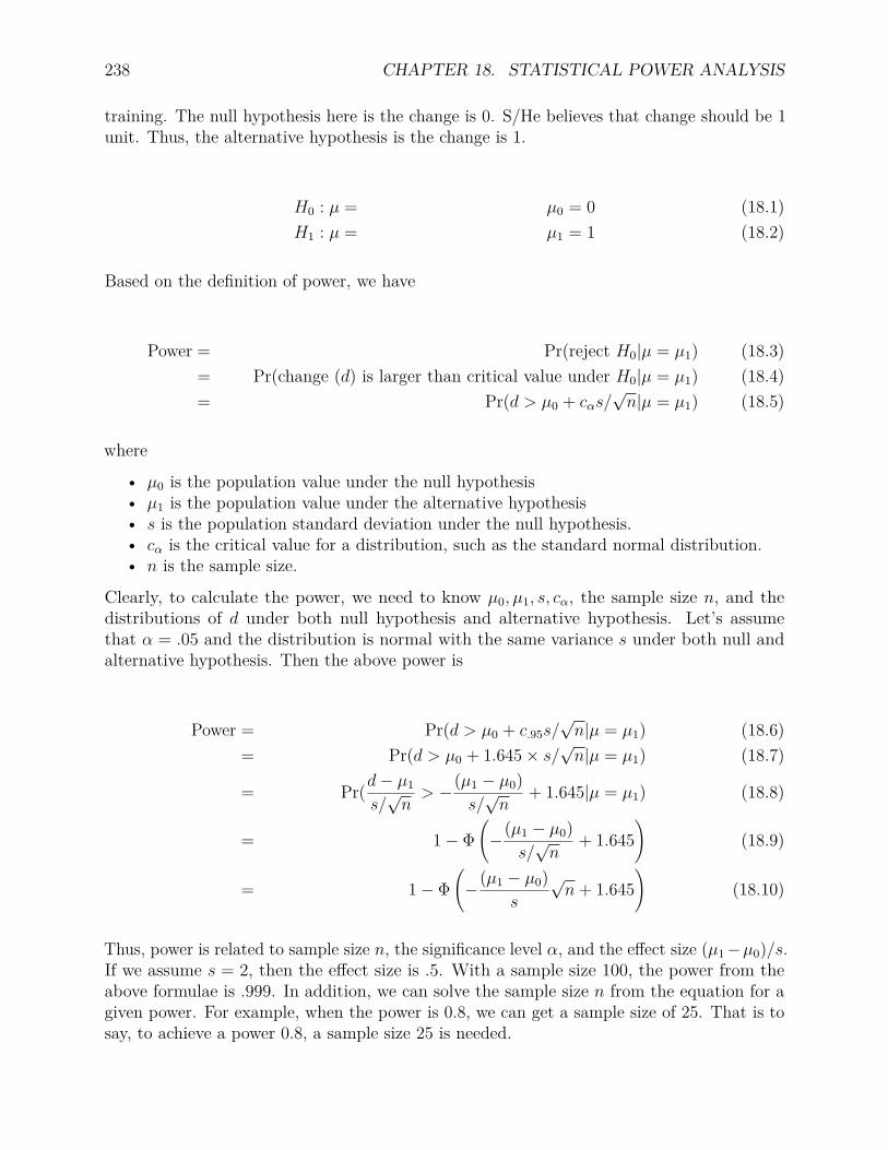
238 CHAPTER 18. STATISTICAL POWER ANALYSIS
training. The null hypothesis here is the change is 0. S/He believes that change should be 1unit. Thus, the alternative hypothesis is the change is 1.
H0 : µ = µ0 = 0 (18.1)H1 : µ = µ1 = 1 (18.2)
Based on the definition of power, we have
Power = Pr(reject H0|µ = µ1) (18.3)= Pr(change (d) is larger than critical value under H0|µ = µ1) (18.4)= Pr(d > µ0 + cαs/
√n|µ = µ1) (18.5)
where
• µ0 is the population value under the null hypothesis• µ1 is the population value under the alternative hypothesis• s is the population standard deviation under the null hypothesis.• cα is the critical value for a distribution, such as the standard normal distribution.• n is the sample size.
Clearly, to calculate the power, we need to know µ0, µ1, s, cα, the sample size n, and thedistributions of d under both null hypothesis and alternative hypothesis. Let’s assumethat α = .05 and the distribution is normal with the same variance s under both null andalternative hypothesis. Then the above power is
Power = Pr(d > µ0 + c.95s/√n|µ = µ1) (18.6)
= Pr(d > µ0 + 1.645× s/√n|µ = µ1) (18.7)
= Pr(d− µ1
s/√n> −(µ1 − µ0)
s/√n
+ 1.645|µ = µ1) (18.8)
= 1− Φ(−(µ1 − µ0)
s/√n
+ 1.645)
(18.9)
= 1− Φ(−(µ1 − µ0)
s
√n+ 1.645
)(18.10)
Thus, power is related to sample size n, the significance level α, and the effect size (µ1−µ0)/s.If we assume s = 2, then the effect size is .5. With a sample size 100, the power from theabove formulae is .999. In addition, we can solve the sample size n from the equation for agiven power. For example, when the power is 0.8, we can get a sample size of 25. That is tosay, to achieve a power 0.8, a sample size 25 is needed.
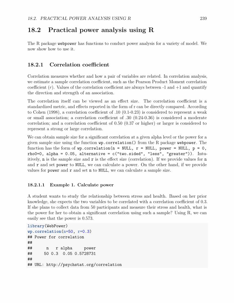
18.2. PRACTICAL POWER ANALYSIS USING R 239
18.2 Practical power analysis using R
The R package webpower has functions to conduct power analysis for a variety of model. Wenow show how to use it.
18.2.1 Correlation coefficient
Correlation measures whether and how a pair of variables are related. In correlation analysis,we estimate a sample correlation coefficient, such as the Pearson Product Moment correlationcoefficient (r). Values of the correlation coefficient are always between -1 and +1 and quantifythe direction and strength of an association.
The correlation itself can be viewed as an effect size. The correlation coefficient is astandardized metric, and effects reported in the form of r can be directly compared. Accordingto Cohen (1998), a correlation coefficient of .10 (0.1-0.23) is considered to represent a weakor small association; a correlation coefficient of .30 (0.24-0.36) is considered a moderatecorrelation; and a correlation coefficient of 0.50 (0.37 or higher) or larger is considered torepresent a strong or large correlation.
We can obtain sample size for a significant correlation at a given alpha level or the power for agiven sample size using the function wp.correlation() from the R package webpower. Thefunction has the form of wp.correlation(n = NULL, r = NULL, power = NULL, p = 0,rho0=0, alpha = 0.05, alternative = c("two.sided", "less", "greater")). Intu-itively, n is the sample size and r is the effect size (correlation). If we provide values for nand r and set power to NULL, we can calculate a power. On the other hand, if we providevalues for power and r and set n to NULL, we can calculate a sample size.
18.2.1.1 Example 1. Calculate power
A student wants to study the relationship between stress and health. Based on her priorknowledge, she expects the two variables to be correlated with a correlation coefficient of 0.3.If she plans to collect data from 50 participants and measure their stress and health, what isthe power for her to obtain a significant correlation using such a sample? Using R, we caneasily see that the power is 0.573.library(WebPower)wp.correlation(n=50, r=0.3)## Power for correlation#### n r alpha power## 50 0.3 0.05 0.5728731#### URL: http://psychstat.org/correlation
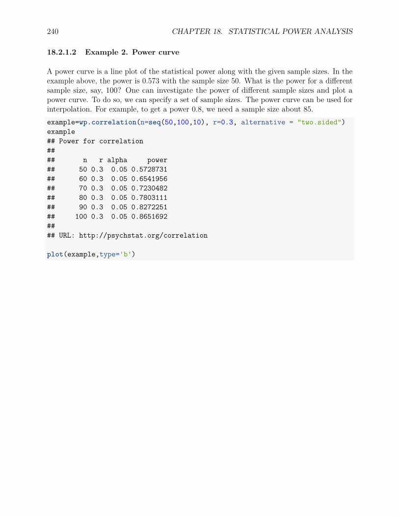
240 CHAPTER 18. STATISTICAL POWER ANALYSIS
18.2.1.2 Example 2. Power curve
A power curve is a line plot of the statistical power along with the given sample sizes. In theexample above, the power is 0.573 with the sample size 50. What is the power for a differentsample size, say, 100? One can investigate the power of different sample sizes and plot apower curve. To do so, we can specify a set of sample sizes. The power curve can be used forinterpolation. For example, to get a power 0.8, we need a sample size about 85.example=wp.correlation(n=seq(50,100,10), r=0.3, alternative = "two.sided")example## Power for correlation#### n r alpha power## 50 0.3 0.05 0.5728731## 60 0.3 0.05 0.6541956## 70 0.3 0.05 0.7230482## 80 0.3 0.05 0.7803111## 90 0.3 0.05 0.8272251## 100 0.3 0.05 0.8651692#### URL: http://psychstat.org/correlation
plot(example,type='b')
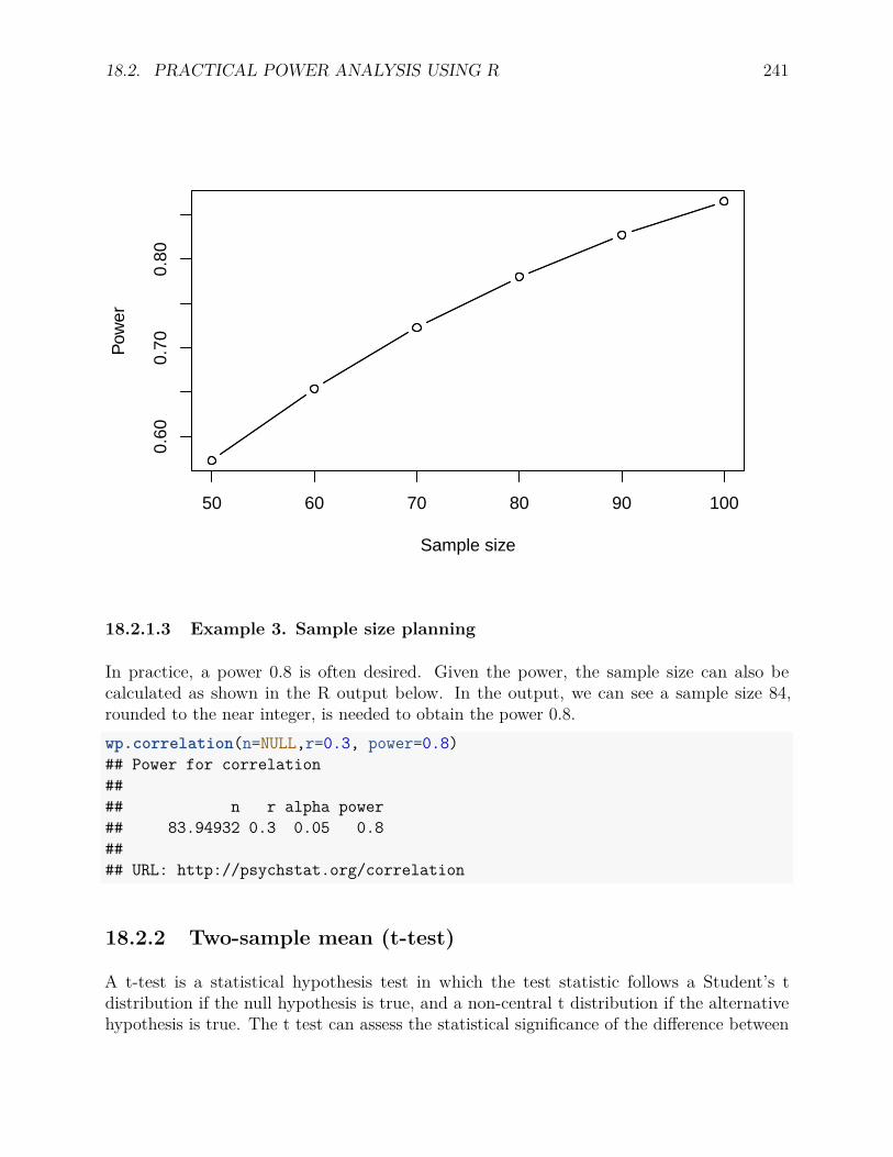
18.2. PRACTICAL POWER ANALYSIS USING R 241
50 60 70 80 90 100
0.60
0.70
0.80
Sample size
Pow
er
18.2.1.3 Example 3. Sample size planning
In practice, a power 0.8 is often desired. Given the power, the sample size can also becalculated as shown in the R output below. In the output, we can see a sample size 84,rounded to the near integer, is needed to obtain the power 0.8.wp.correlation(n=NULL,r=0.3, power=0.8)## Power for correlation#### n r alpha power## 83.94932 0.3 0.05 0.8#### URL: http://psychstat.org/correlation
18.2.2 Two-sample mean (t-test)
A t-test is a statistical hypothesis test in which the test statistic follows a Student’s tdistribution if the null hypothesis is true, and a non-central t distribution if the alternativehypothesis is true. The t test can assess the statistical significance of the difference between
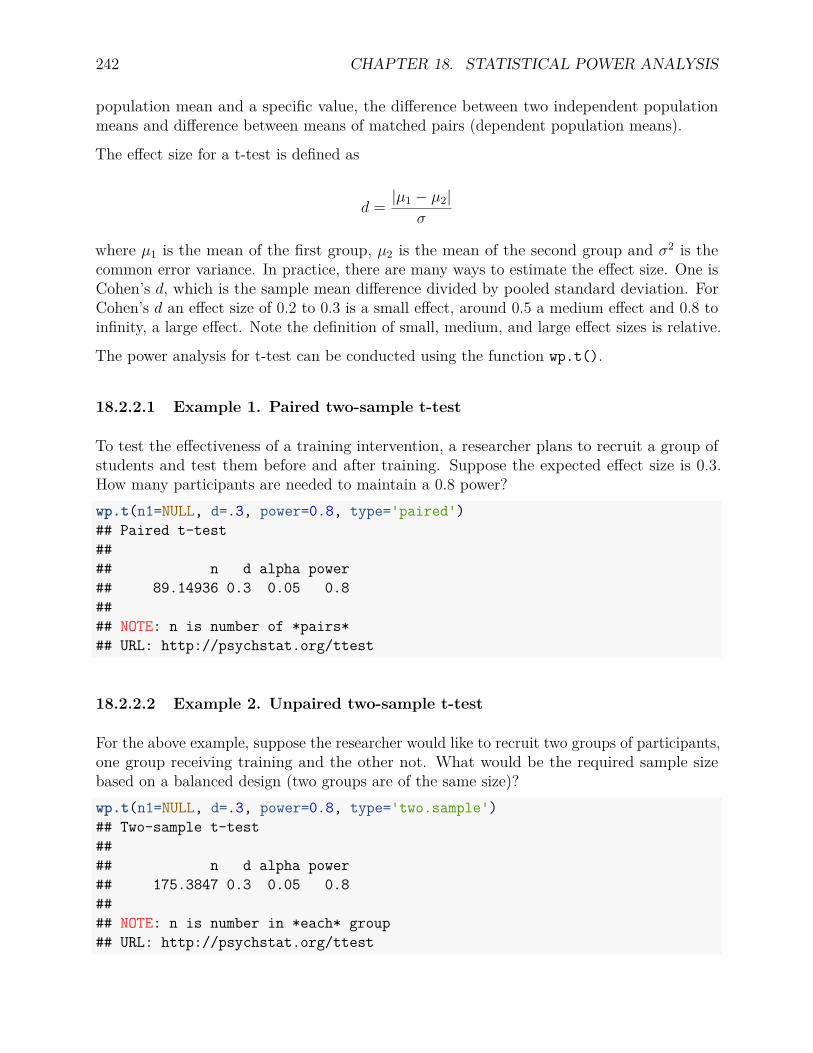
242 CHAPTER 18. STATISTICAL POWER ANALYSIS
population mean and a specific value, the difference between two independent populationmeans and difference between means of matched pairs (dependent population means).
The effect size for a t-test is defined as
d = |µ1 − µ2|σ
where µ1 is the mean of the first group, µ2 is the mean of the second group and σ2 is thecommon error variance. In practice, there are many ways to estimate the effect size. One isCohen’s d, which is the sample mean difference divided by pooled standard deviation. ForCohen’s d an effect size of 0.2 to 0.3 is a small effect, around 0.5 a medium effect and 0.8 toinfinity, a large effect. Note the definition of small, medium, and large effect sizes is relative.
The power analysis for t-test can be conducted using the function wp.t().
18.2.2.1 Example 1. Paired two-sample t-test
To test the effectiveness of a training intervention, a researcher plans to recruit a group ofstudents and test them before and after training. Suppose the expected effect size is 0.3.How many participants are needed to maintain a 0.8 power?wp.t(n1=NULL, d=.3, power=0.8, type='paired')## Paired t-test#### n d alpha power## 89.14936 0.3 0.05 0.8#### NOTE: n is number of *pairs*## URL: http://psychstat.org/ttest
18.2.2.2 Example 2. Unpaired two-sample t-test
For the above example, suppose the researcher would like to recruit two groups of participants,one group receiving training and the other not. What would be the required sample sizebased on a balanced design (two groups are of the same size)?wp.t(n1=NULL, d=.3, power=0.8, type='two.sample')## Two-sample t-test#### n d alpha power## 175.3847 0.3 0.05 0.8#### NOTE: n is number in *each* group## URL: http://psychstat.org/ttest
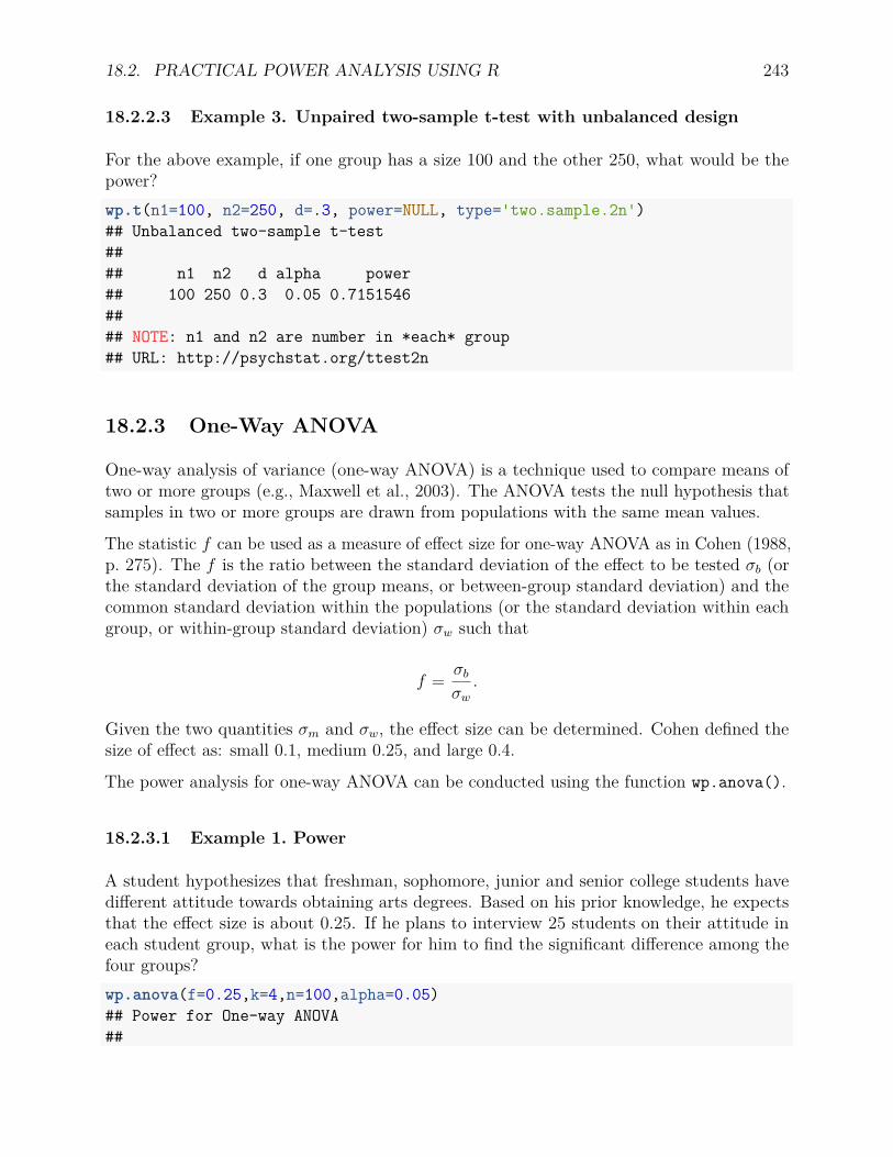
18.2. PRACTICAL POWER ANALYSIS USING R 243
18.2.2.3 Example 3. Unpaired two-sample t-test with unbalanced design
For the above example, if one group has a size 100 and the other 250, what would be thepower?wp.t(n1=100, n2=250, d=.3, power=NULL, type='two.sample.2n')## Unbalanced two-sample t-test#### n1 n2 d alpha power## 100 250 0.3 0.05 0.7151546#### NOTE: n1 and n2 are number in *each* group## URL: http://psychstat.org/ttest2n
18.2.3 One-Way ANOVA
One-way analysis of variance (one-way ANOVA) is a technique used to compare means oftwo or more groups (e.g., Maxwell et al., 2003). The ANOVA tests the null hypothesis thatsamples in two or more groups are drawn from populations with the same mean values.
The statistic f can be used as a measure of effect size for one-way ANOVA as in Cohen (1988,p. 275). The f is the ratio between the standard deviation of the effect to be tested σb (orthe standard deviation of the group means, or between-group standard deviation) and thecommon standard deviation within the populations (or the standard deviation within eachgroup, or within-group standard deviation) σw such that
f = σbσw.
Given the two quantities σm and σw, the effect size can be determined. Cohen defined thesize of effect as: small 0.1, medium 0.25, and large 0.4.
The power analysis for one-way ANOVA can be conducted using the function wp.anova().
18.2.3.1 Example 1. Power
A student hypothesizes that freshman, sophomore, junior and senior college students havedifferent attitude towards obtaining arts degrees. Based on his prior knowledge, he expectsthat the effect size is about 0.25. If he plans to interview 25 students on their attitude ineach student group, what is the power for him to find the significant difference among thefour groups?wp.anova(f=0.25,k=4,n=100,alpha=0.05)## Power for One-way ANOVA##

244 CHAPTER 18. STATISTICAL POWER ANALYSIS
## k n f alpha power## 4 100 0.25 0.05 0.5181755#### NOTE: n is the total sample size (overall)## URL: http://psychstat.org/anova
18.2.3.2 Example 2. Minimum detectable effect
One can also calculate the minimum detectable effect to achieve certain power given a samplesize. For the above example, we can see that to get a power 0.8 with the sample size 100, thepopulation effect size has to be at least 0.337.wp.anova(f=NULL,k=4,n=100,power=0.8, alpha=0.05)## Power for One-way ANOVA#### k n f alpha power## 4 100 0.3369881 0.05 0.8#### NOTE: n is the total sample size (overall)## URL: http://psychstat.org/anova
18.2.4 Linear regression
Linear regression is a statistical technique for examining the relationship between one ormore independent variables and one dependent variable. The independent variables areoften called predictors or covariates, while the dependent variable are also called outcomevariable or criterion. Although regression is commonly used to test linear relationship betweencontinuous predictors and an outcome, it may also test interaction between predictors andinvolve categorical predictors by utilizing dummy or contrast coding.
We use the effect size measure f 2 proposed by Cohen (1988, p.410) as the measure of theregression effect size. Cohen discussed the effect size in three different cases, which actuallycan be generalized using the idea of a full model and a reduced model by Maxwell et al.(2003). The f 2 is defined as
f 2 = R2Full −R2
Reduced
1−R2Full
,
where R2Full and R2
Reduced are R-squared for the full and reduced models respectively. Sup-pose we are evaluating the impact of one set of predictors (B) above and beyond a second setof predictors (A). Then R2
Full is variance accounted for by variable set A and variable set Btogether and R2
Reduced is variance accounted for by variable set A only.
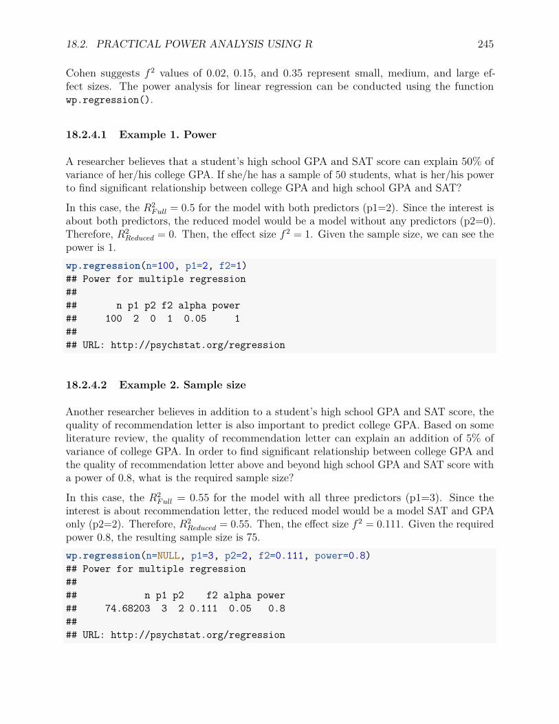
18.2. PRACTICAL POWER ANALYSIS USING R 245
Cohen suggests f 2 values of 0.02, 0.15, and 0.35 represent small, medium, and large ef-fect sizes. The power analysis for linear regression can be conducted using the functionwp.regression().
18.2.4.1 Example 1. Power
A researcher believes that a student’s high school GPA and SAT score can explain 50% ofvariance of her/his college GPA. If she/he has a sample of 50 students, what is her/his powerto find significant relationship between college GPA and high school GPA and SAT?
In this case, the R2Full = 0.5 for the model with both predictors (p1=2). Since the interest is
about both predictors, the reduced model would be a model without any predictors (p2=0).Therefore, R2
Reduced = 0. Then, the effect size f 2 = 1. Given the sample size, we can see thepower is 1.wp.regression(n=100, p1=2, f2=1)## Power for multiple regression#### n p1 p2 f2 alpha power## 100 2 0 1 0.05 1#### URL: http://psychstat.org/regression
18.2.4.2 Example 2. Sample size
Another researcher believes in addition to a student’s high school GPA and SAT score, thequality of recommendation letter is also important to predict college GPA. Based on someliterature review, the quality of recommendation letter can explain an addition of 5% ofvariance of college GPA. In order to find significant relationship between college GPA andthe quality of recommendation letter above and beyond high school GPA and SAT score witha power of 0.8, what is the required sample size?
In this case, the R2Full = 0.55 for the model with all three predictors (p1=3). Since the
interest is about recommendation letter, the reduced model would be a model SAT and GPAonly (p2=2). Therefore, R2
Reduced = 0.55. Then, the effect size f 2 = 0.111. Given the requiredpower 0.8, the resulting sample size is 75.wp.regression(n=NULL, p1=3, p2=2, f2=0.111, power=0.8)## Power for multiple regression#### n p1 p2 f2 alpha power## 74.68203 3 2 0.111 0.05 0.8#### URL: http://psychstat.org/regression

246 CHAPTER 18. STATISTICAL POWER ANALYSIS
References
[Bates et al., 2015] Bates, D., Mächler, M., Bolker, B., & Walker, S. (2015). Fitting linearmixed-effects models using lme4. Journal of Statistical Software, 67(1), 1–48.
[Benjamin et al., 2018] Benjamin, D. J., Berger, J. O., Johannesson, M., Nosek, B. A.,Wagenmakers, E.-J., Berk, R., Bollen, K. A., Brembs, B., Brown, L., Camerer, C., et al.(2018). Redefine statistical significance. Nature Human Behaviour, 2(1), 6.
[Cohen, 1988] Cohen, J. (1988). Statistical power analysis for the behavioral sciences. Hillsdale,NJ: Lawrence Ehrlbaum Associates, 2nd edition.
[Cohen, 1990] Cohen, J. (1990). Things I have learned (so far). American Psychologist,45(12), 1304–1312.
[Cohen et al., 2003] Cohen, J., Cohen, P., West, S. G., & Aiken, L. S. (2003). Applied MultipleRegression/Correlation Analysis for the Behavioral Sciences. Hillsdale NJ: LawrenceErlbaum Associates, 3rd edition.
[Fisher, 1955] Fisher, R. (1955). Statistical methods and scientific induction. Journal of theRoyal Statistical Society: Series B (Methodological), 17(1), 69–78.
[Fisher, 2006] Fisher, R. A. (2006). Statistical methods for research workers. Genesis Pub-lishing Pvt Ltd.
[Fox, 2006] Fox, J. (2006). Structural equation modeling with the sem package in r. StructuralEquation Modeling, 13, 465–486.
[Hagen, 1997] Hagen, R. L. (1997). In praise of the null hypothesis statistical test.
[Hope, 2013] Hope, R. M. (2013). Rmisc: Rmisc: Ryan Miscellaneous. R package version1.5.
[Kuznetsova et al., 2017] Kuznetsova, A., Brockhoff, P. B., & Christensen, R. H. B. (2017).lmerTest package: Tests in linear mixed effects models. Journal of Statistical Software,82(13), 1–26.
[Meehl, 1990] Meehl, P. E. (1990). Why summaries of research on psychological theories areoften uninterpretable. Psychological reports, 66(1), 195–244.
[Mirai Solutions GmbH, 2018] Mirai Solutions GmbH (2018). XLConnect: Excel Connectorfor R. R package version 0.2-15.
247
248 REFERENCES
[R Core Team, 2018] R Core Team (2018). R: A Language and Environment for StatisticalComputing. R Foundation for Statistical Computing, Vienna, Austria.
[Reichardt & Gollob, 1997] Reichardt, C. S. & Gollob, H. F. (1997). When confidenceintervals should be used instead of statistical tests, and vice versa. What if there were nosignificance tests, (pp. 259–284).
[Rosseel, 2012] Rosseel, Y. (2012). lavaan: An R package for structural equation modeling.Journal of Statistical Software, 48, 1–36.
[Schmidt & Hunter, 1997] Schmidt, F. L. & Hunter, J. E. (1997). Eight common but falseobjections to the discontinuation of significance testing in the analysis of research data.What if there were no significance tests, (pp. 37–64).
[Thomas, 1974] Thomas, D. A. H. (1974). Error rates in multiple comparisons among means-results of a stimulation exercise. Applied Statistics, 23(3), 284–294.
[Tufte, 1983] Tufte, E. R. (1983). The Visual Display of Quantitative Information. Cheshire,CT: Graphics Press.
[Tukey, 1991] Tukey, J. W. (1991). The philosophy of multiple comparisons. Statisticalscience, (pp. 100–116).
[Venables & Ripley, 2002] Venables, W. N. & Ripley, B. D. (2002). Modern Applied Statisticswith S. New York: Springer, fourth edition. ISBN 0-387-95457-0.
[Wickham, 2007] Wickham, H. (2007). Reshaping data with the reshape package. Journalof Statistical Software, 21(12), 1–20.
[Wickham, 2016] Wickham, H. (2016). ggplot2: Elegant Graphics for Data Analysis. Springer-Verlag New York.
[Wickham & Miller, 2019] Wickham, H. & Miller, E. (2019). haven: Import and Export’SPSS’, ’Stata’ and ’SAS’ Files. R package version 2.1.0.
[Zhang et al., 2015] Zhang, Z., Hamagami, F., Grimm, K. J., & McArdle, J. J. (2015). Usingr package rampath for tracing sem path diagrams and conducting complex longitudinaldata analysis. Structural Equation Modeling: A Multidisciplinary Journal, 22(1), 132–147.
[Zhang et al., 2007] Zhang, Z., Hamagami, F., Wang, L., Grimm, K. J., & Nesselroade, J. R.(2007). Bayesian analysis of longitudinal data using growth curve models. InternationalJournal of Behavioral Development, 31(4), 374–383.
[Zhang & Mai, 2018] Zhang, Z. & Mai, Y. (2018). WebPower: Basic and Advanced StatisticalPower Analysis. R package version 0.5.2.
[Zhang & Wang, 2009] Zhang, Z. & Wang, L. (2009). Statistical power analysis for growthcurve models using sas. Behavior Research Methods, 41, 1083–1094.
[Zhang & Wang, 2013a] Zhang, Z. & Wang, L. (2013a). bmem: Mediation analysis withmissing data using bootstrap. R package version 1.5.

REFERENCES 249
[Zhang & Wang, 2013b] Zhang, Z. & Wang, L. (2013b). Methods for mediation analysis withmissing data. Psychometrika, 78, 154–184.
[Zhang & Yuan, 2018] Zhang, Z. & Yuan, K.-H. (2018). Practical Statistical Power AnalysisUsing Webpower and R. ISDSA Press.