Advanced Spatial Analysis

Spatial Regression Modeling

GISPopSci

Day 5

Paul R. Vossand

Katherine J. Curtis

GISPopSci

Review of yesterday

• Dealing with heterogeneity in relationships across space

• Discrete & continuous spatial heterogeneity in relationships

• GWR- concept & motivation- how to do it- what it all means

GISPopSci

Questions?

GISPopSci

Plan for today• Shift away from spatial econometrics

– away from the classical, frequentist perspective– away from the MLE world

• Spatial data analysis from a Bayesian perspective– example using count data & Poisson likelihood– meaning of Bayes’ rule– MCMC

• Afternoon lab– brief demonstration of spatial modeling in WinBUGS & R– your analyses; your data; your issues

GISPopSci

Bayesian orientation…

GISPopSci

Back in my day…OLS linear regression modelscontinuous dependent variablesindependent & normally distributed errors(Legendre 1805; Gauss 1809; Galton

1875)

Adiren-Marie Legendre(1752-1853)

Carl Friedrich Gauss(1777-1855)

Francis Galton(1822-1911)

Situate this in a statistical framework (1)

GISPopSci

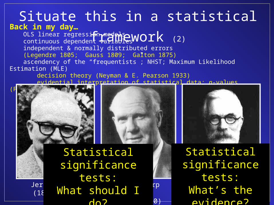
Situate this in a statistical framework (2)Back in my day…

OLS linear regression modelscontinuous dependent variablesindependent & normally distributed errors(Legendre 1805; Gauss 1809; Galton 1875)ascendency of the “frequentists”; NHST; Maximum Likelihood Estimation (MLE)

decision theory (Neyman & E. Pearson 1933)evidential interpretation of statistical data; p-values (Fisher 1922 – 1960s)

Jerzy Neyman(1894-1981)

Egon Sharp Pearson(1895-1980)

Ronald Aylmer Fisher(1890-1962)

Statistical significance tests:What should I do?

Statistical significance tests:

What’s the evidence?

GISPopSci

Back in my day…OLS linear regression modelscontinuous dependent variablesindependent & normally distributed errorsascendency of the “frequentists”;

Generalized Linear Models…fixed effects regressionaccommodate many kinds of outcomes:

Gaussian, Poisson, binomialmaximum likelihood estimationindependent observations(Nelder & Wedderburn 1972; McCullagh & Nelder

1989)

John Ashworth Nelder(1924 – 8/7/10)

R. W. M. Wedderburn(1947 – 1975)

Peter McCullochUniversity of Chicago

Situate this in a statistical framework (3)

GISPopSci

Back in my day…OLS linear regression modelscontinuous dependent variablesindependent & normally distributed errorsascendency of the “frequentists”

Generalized Linear Models…fixed effects regressionaccommodate many kinds of outcomes:

Gaussian, Poisson, binomialmaximum likelihood estimation(Nelder & Wedderburn 1972; McCullagh & Nelder

1989)

Generalized Linear Mixed Models…linear predictor contains random effectsMLE (difficult integrals over the random effects)Iterative approximations of the likelihood:

Laplace, PQL, MQL, numerical quadrature(Breslow & Clayton 1993)

Norman E. BreslowUniv. of Washington

David G. ClaytonCambridge Univ.

Situate this in a statistical framework (4)

GISPopSci

Back in my day…OLS linear regression modelscontinuous dependent variablesindependent & normally distributed errors(Legendre 1805; Gauss 1809; Galton

1875)Generalized Linear Models…

fixed effects regressionaccommodate many kinds of outcomes:

Gaussian, Poisson, binomialmaximum likelihood estimation(Nelder & Wedderburn 1972; McCullagh & Nelder

1989)

Generalized Linear Mixed Models…linear predictor contains random effectsMLE (difficult integrals over the random effects)Iterative approximations of the likelihood:

Laplace, PQL, MQL, numerical quadrature(Breslow & Clayton 1993)

MCMC…simulations on Bayesian posterior

distributionssamplers:

Gibbs, M-H, others(enormous literature)

Situate this in a statistical framework (5)

1950s onward

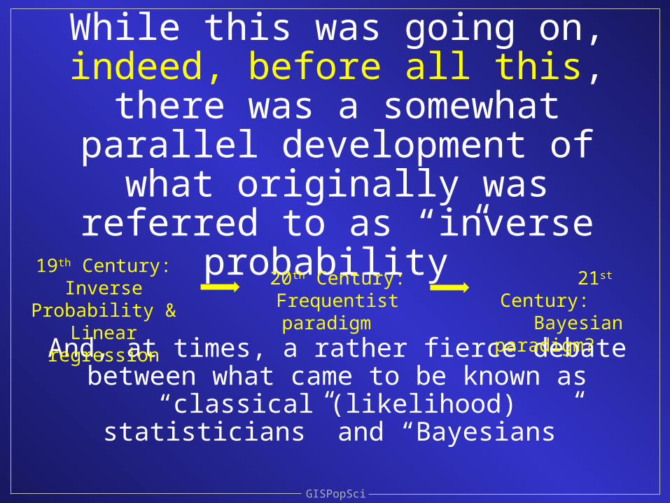
While this was going on, indeed, before all this, there was a

somewhat parallel development of what originally was referred to as

“inverse probability”

GISPopSci

And, at times, a rather fierce debate between what came to be known as “classical (likelihood)

statisticians” and “Bayesians”

19th Century:Inverse Probability &

Linear regression

20th Century: Frequentist paradigm

21st Century: Bayesian paradigm?

GISPopSci

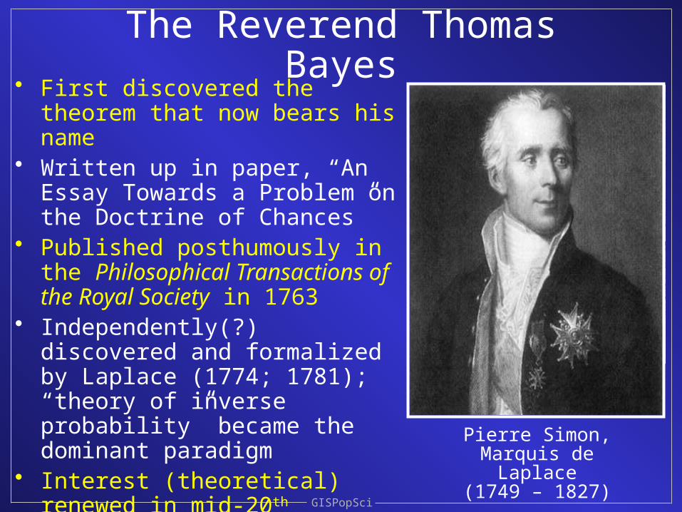
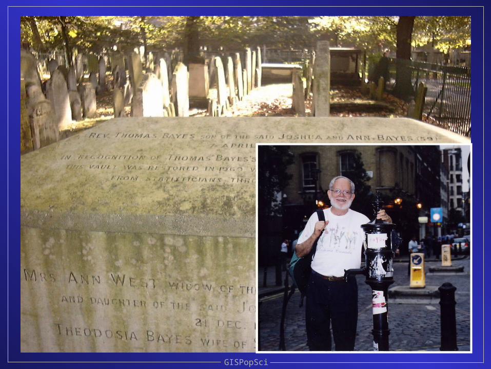
The Reverend Thomas Bayes• First discovered the theorem that

now bears his name• Written up in paper, “An Essay

Towards a Problem on the Doctrine of Chances”

• Published posthumously in the Philosophical Transactions of the Royal Society in 1763

• Independently(?) discovered and formalized by Laplace (1774; 1781); “theory of inverse probability” became the dominant paradigm

• Interest (theoretical) renewed in mid-20th century; interest (applied) exploded around 1985-90

Thomas Bayes(1702 – 1761)

Pierre Simon,Marquis de Laplace

(1749 – 1827)

GISPopSci

GISPopSci

Bayesian methods are often turned to when likelihood estimation becomes difficult or

unrealistic (especially in the world of spatial data analysis)

• Advantages of a Bayesian perspective- more natural interpretation of parameter intervals & probability

intervals- clear & overt assumptions regarding prior assumptions- ease with which the true parameter density is obtained- ability to update as new data become available- likelihood maximization not required (for probit & logit models,

maximization of the simulated likelihood function can be difficult)- desirable estimation properties (consistency & efficiency)

• Disadvantages of a Bayesian perspective- steep learning curve; for those of us trained in a classical

perspective, things don’t come easy- determining a reasonable prior

From early understanding of the laws of probability…

GISPopSci

P(AB) = P(A|B)P(B) = P(B|A)P(A)

from which we obtain “Bayes’ formula”:

P(B|A) = P(A|B)P(B) P(A)

This statement is true whether you take a Bayesian perspective or not. It’s only in a certain understanding of this formula that

you become a Bayesian

So… Bayes’ formula

GISPopSci

P(B|A) = P(A|B)P(B) P(A)

P(B|A) P(A|B)P(B)“Prior” probability“Likelihood”“Posterior” probability

Now, from the “Law of Total Probability”, we have for mass probabilities:

B

dBBPBAPAP )()|()(

)()|()()|()( cc BPBAPBPBAPAP

or, for density probabilities:

Usually the focus is on using the Bayes formulation to estimate model parameters

(rather than expressing relationships among event probabilities

GISPopSci

P(B|A) P(A|B)P(B)

“Prior” probability“Data Likelihood”“Posterior” probability

P(parameters|data) P(data|parameters)P(parameters)

The goal generally is to achieve “optimal” parameter estimates where attention is focused

on precision (std. errors of the parameters)

The “Bayesian mantra”

GISPopSci

From this we have the “Bayesian mantra”

POSTERIOR LIKELIHOOD x PRIOR

P[θ|D] P[D|θ] P[θ]

In full Bayesian modeling the prior distribution is formulated before

consulting the data

In so-called empirical Bayesian modeling the prior distribution is

derived from the data

Approaches to Model Buildingi.e., approaches to making good “guesses” about

the values of the parameters in the model and inferences about them

• Classical statistics• Bayesian statistics• Regardless of approach, the process of

statistics involves:– formulating a research question– collecting data– developing a probability model for the data– estimating the model– assessing the quality of the “fit” & modifying the model as necessary– summarizing the results in order to answer the research question

(“statistical inference”)

GISPopSci

Classical approach (1)

• Three basic steps:– specify the model– estimate & evaluate the model (MLE)– inference

• Fundamental idea:– a good choice for the estimate of a parameter (viewed as

fixed) is that value of the parameter that makes the observed data most likely to have occurred

GISPopSci

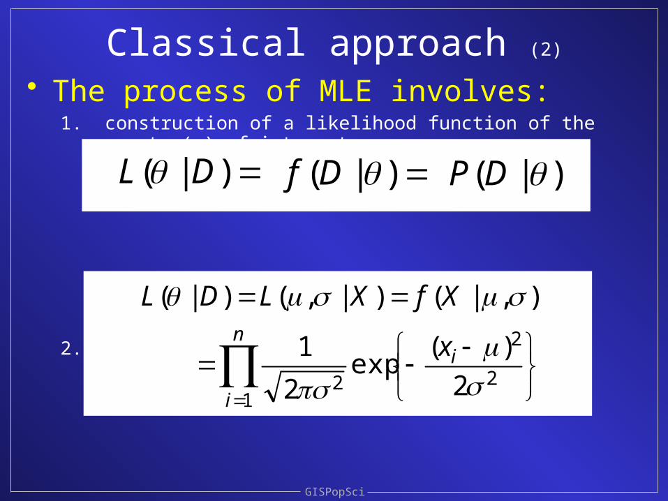
• The process of MLE involves:1. construction of a likelihood function of the parameter(s) of interest

2. for example, normal likelihood:

– Note: observations {xi, x2,…,xn) are assumed (conditionally) independent

Classical approach (2)

GISPopSci

)|( DP)|( Df)|( DL

2

2

12 2

)(exp

2

1

),|()|,()|(

in

i

x

XfXLDL

• The process of MLE involves:(3) Simplify the likelihood function:– for example, for the normal likelihood:

(4) Take logarithm of likelihood function:

Classical approach (3)

GISPopSci

n

iixXL

n

1

22

)(2

1exp)22()|,( 2

n

iixnX

1

22

)(2

1)ln()|,(

• The process of MLE involves:(5) Take partial derivative of the log-likelihood function with respect to

each parameter (for example, for the normal log likelihood):

(6) Set the partial derivatives to zero and solve for the parameters:

These should look familiar

Classical approach (4)

GISPopSci

n

iix

nxn

1

232

)(1)(

and

n

x

x

n

ii

1

2

2

)(

ˆˆ

and

• The process of MLE involves:(7) Take partial second derivatives to obtain estimates of the variability

in the estimates for the mean & standard deviation (Hessian matrix):

Classical approach (5)

GISPopSci

6

1

2

44

42

4

2

2

2

2

2

2

2

2

)(

2

)(

)(

n

i i

T

xnxn

xnn

Bayesian approach• Three basic steps (same as classical approach),

with a rather different notion about the parameters• Fundamental idea:

– a good choice for the estimate of the parameters (not fixed) are those values of the parameter estimated from a probability distribution involving both the observed data and our subjective notion of the value of the parameter

– Bayesian approach tells you how to alter your beliefs

• The modern Bayesian approach involves:– specification of a “likelihood function” (“sampling density”) for the data,

conditional on the parameters– specification of a “prior distribution” for the model parameters– derivation of the “posterior distribution” for the model parameters,

given the likelihood function and the prior distribution– obtain a sample (Monte Carlo simulation) from the posterior

distribution of the parameters– Summarize the parameter samples and draw inferences

GISPopSci

I’m going to use as a running example an application in spatial

epidemiology

GISPopSci

South Carolina congenital abnormality deaths 1990

Data set developed & much used byAndrew Lawson,

Spatial epidemiologist,Biostatistics, Bioinformatics, and

Epidemiology programMedical University of South Carolina

0

7

1

5

11

5

16

0

17

4

00

1

1

71

3

0

0

8

2

13

7

0

8

0

3

2

41

110

1

2

3

3

8

6

143

11

6

0

1

5

South Carolina congenital abnormality deaths 1990

GISPopSci

Some considerations:• Data are a complete realization, not a sample• Need to know something about the underlying population

to understand elevated counts; understand the relative risk

• Spatial structure is relevant; it’s not just a list of numbers• Areal units are arbitrary; have nothing to do with health

outcomes• Areal units are irregular in shape and size

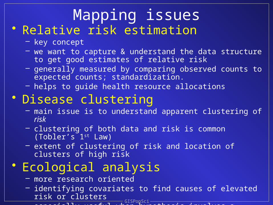
Mapping issues• Relative risk estimation

– key concept– we want to capture & understand the data structure to get good

estimates of relative risk– generally measured by comparing observed counts to expected

counts; standardization.– helps to guide health resource allocations

• Disease clustering– main issue is to understand apparent clustering of risk– clustering of both data and risk is common (Tobler’s 1st Law)– extent of clustering of risk and location of clusters of high risk

• Ecological analysis– more research oriented– identifying covariates to find causes of elevated risk or clusters– especially useful when hypothesis involves a putative source of

pollution

GISPopSci

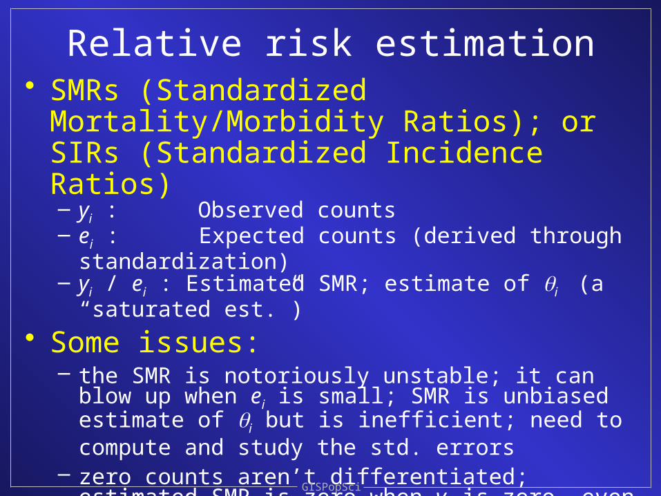
Relative risk estimation• SMRs (Standardized Mortality/Morbidity

Ratios); or SIRs (Standardized Incidence Ratios)– yi : Observed counts– ei : Expected counts (derived through standardization)– yi / ei : Estimated SMR; estimate of i (a “saturated est.”)

• Some issues:– the SMR is notoriously unstable; it can blow up when ei is

small; SMR is unbiased estimate of i but is inefficient; need to compute and study the std. errors

– zero counts aren’t differentiated; estimated SMR is zero when yi is zero, even when ei may vary considerably

– confusing notation: ei has different meanings

GISPopSci

If we assume the underlying process is a Poisson process…

GISPopSci

• Individuals within the study population behave independently wrt disease propensity, after allowance is made for observed or unobserved confounding variables; “conditional independence”

• The underlying “at risk” background intensity (RR) has a continuous & constant (i.e., i = ) spatial distribution within the study area

• Events are unique (occur as spatially separate events)

• When these (Poisson process) assumptions are met, the data can be modeled via a likelihood approach with an intensity function representing the “at risk” background

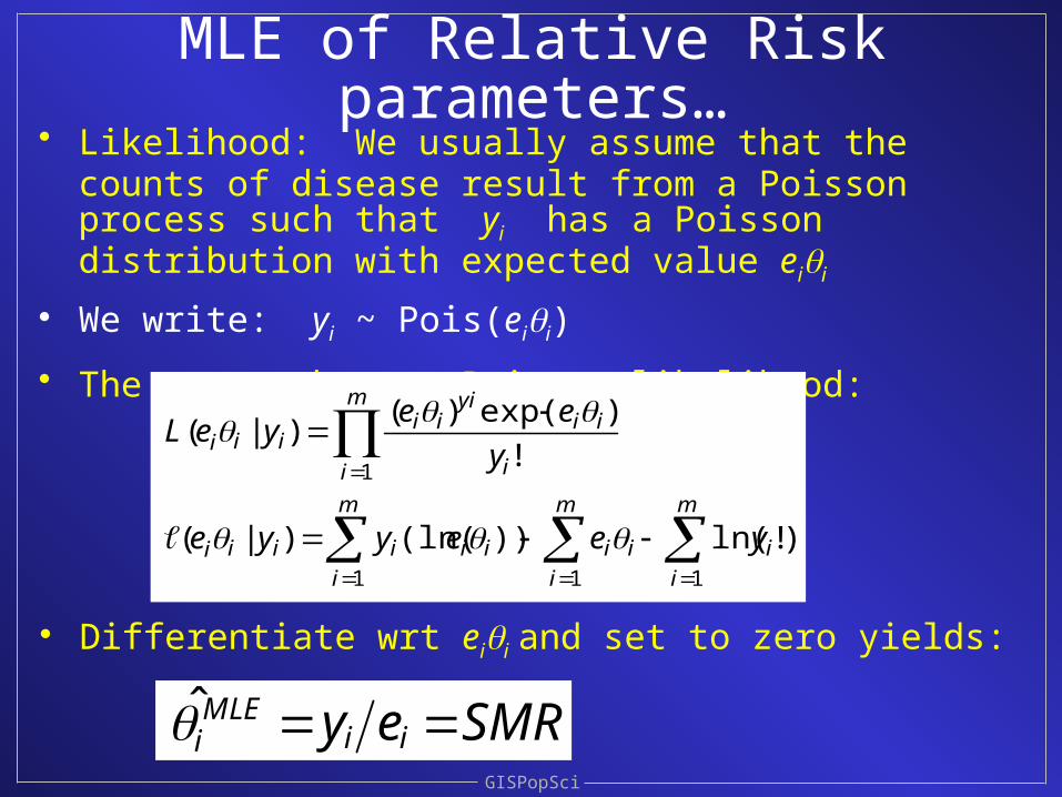
MLE of Relative Risk parameters…• Likelihood: We usually assume that the counts of disease

result from a Poisson process such that yi has a Poisson distribution with expected value eii

• We write: yi ~ Pois(eii)

• The counts have a Poisson likelihood:

GISPopSci

m

i

m

i

m

i

iiiiiiiii

m

i i

iiyi

iiiii

yeeyye

y

eeyeL

1 1 1

1

)!ln())(ln()|(

!

)exp()()|(

• Differentiate wrt eii and set to zero yields:

SMRey iiMLE

i ̂

So, with MLE…• The counts have a joint probability of arising

based on the likelihood, L(eii |yi)

• L(eii |yi) is the product of Poisson probabilities for each of the areas (again, why can we say this?)

• It tells us how likely the parameter estimates of i are given the data, yi , under a set of Poisson process assumptions

• This is a common approach for obtaining estimates of parameters

GISPopSci

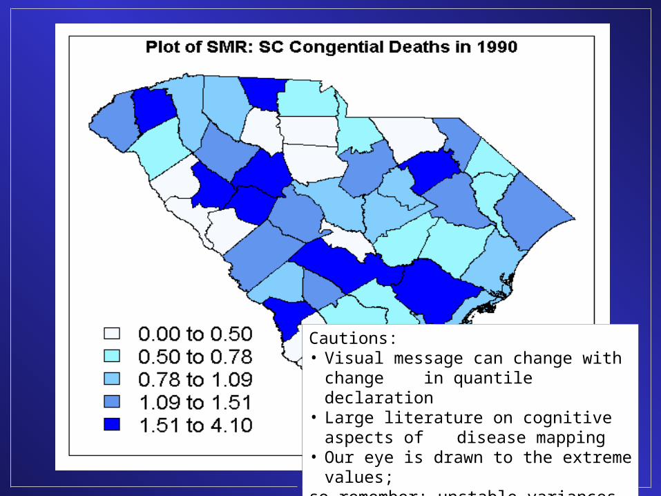
GISPopSci

Mean = 0.9703Std. dev. = 0.8024

Cautions:• Visual message can change with change

in quantile declaration

• Large literature on cognitive aspects of disease mapping

• Our eye is drawn to the extreme values;so remember: unstable variances

So… what have we got here?

GISPopSci

• Choropleth map of SMRs of infant mortality from congenital abnormalities, SC counties, 1990

• SMRi = yi/ei, where yi is the observed count & ei is the expected count (note: we permit ei to be fractional)

• In this example, the ei are simple expectations generated using “indirect standardization”; i.e., by applying the crude rate (per 1,000 births) for SC, aggregated over the years 1990-98, to county births in 1990:

46

1

981990

46

1

981990

19901990*

ii

ii

iie

(births)

deaths)yabnormalitl(congenita

Births

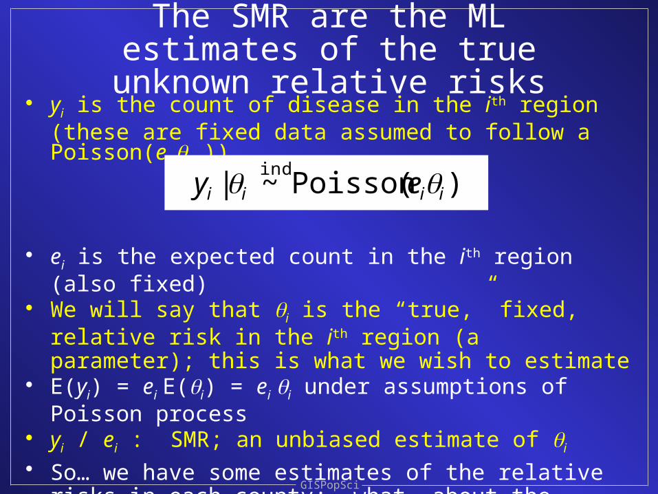
The SMR are the ML estimates of the true unknown relative risks

• yi is the count of disease in the ith region (these are fixed data assumed to follow a Poisson(ei i ))

• ei is the expected count in the ith region (also fixed)• We will say that i is the “true,” fixed, relative risk in the ith

region (a parameter); this is what we wish to estimate• E(yi) = ei E(i) = ei i under assumptions of Poisson process• yi / ei : SMR; an unbiased estimate of i

• So… we have some estimates of the relative risks in each county; what about the variance of these estimates?

• It turns out that there are different opinions about this

GISPopSci

)(~| iiii ey Poissonind

We now move beyond MLE…

GISPopSci

In particular, we drop the classical notion that i

is a vector of fixed parameters; we assume that the i are random variables (having a

distribution) and we will make some parametric assumptions concerning these parameters

Which as Bayesians we will call “priors”

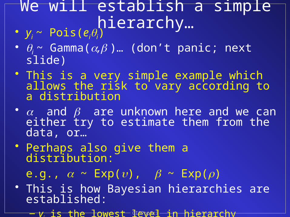
We will establish a simple hierarchy…• yi ~ Pois(eii)• i ~ Gamma(, )… (don’t panic; next slide)• This is a very simple example which allows the

risk to vary according to a distribution• and are unknown here and we can either try

to estimate them from the data, or…• Perhaps also give them a distribution:

e.g., ~ Exp(), ~ Exp()• This is how Bayesian hierarchies are established:

– yi is the lowest level in hierarchy

– i is the next level

– & affect i ; i affects yi ; & affect &

GISPopSci

Why assume a gamma prior?• That is, why i ~ Gamma(, ) ?• It makes conceptual sense; as estimates of

relative risk, we want a distribution for i that requires the i are non-zero, and have a mean probably not too far from unity while allowing for some observations well above unity– Gamma is one such distribution, although in its

simplicity has some shortcomings

– Log-normal distribution shares these distributional attributes (and opens up opportunities not permitted by the Gamma distribution

• Important: Gamma prior is the “conjugate” prior for the Poisson likelihood

• And what’s & ?GISPopSci

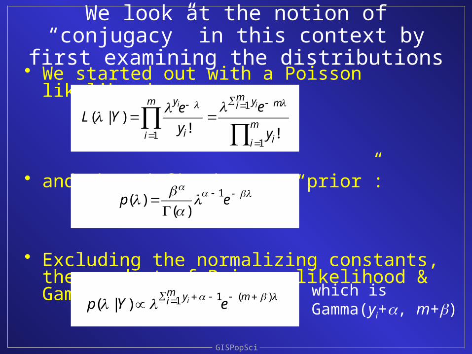
We look at the notion of “conjugacy” in this context by first examining the distributions

• We started out with a Poisson likelihood:

• and then defined Gamma “prior”:

• Excluding the normalizing constants, the product of Poisson likelihood & Gamma prior is:

GISPopSci

m

i i

mmi ym

i i

y

y

e

y

eYL

ii

1

1

1 !!)|(

ep

1

)()(

)(11)|( mm

i yeYp i

which isGamma(yi+, m+)

Now…define “conjugacy”:• When the prior & likelihood are of such a form that

the posterior distribution follows the same form as the prior, the prior and likelihood are said to be “conjugate”

• By way of illustration, the previous slide reveals that a Poisson likelihood and a Gamma prior yield a Gamma posterior

• Very important matter prior to modern MCMC estimation

GISPopSci

A basic hierarchy

GISPopSci

Data ParameterHyperparameter

Hyperparameter

Data 1st level 2nd level

LikelihoodDistribution

PriorDistribution

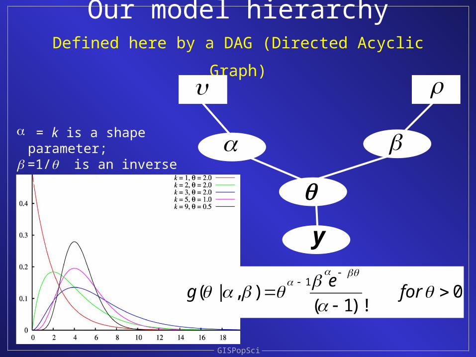
Our model hierarchyDefined here by a DAG (Directed Acyclic Graph)

GISPopSci

y

0)!1(

),|(1

fore

g

a = k is a shape parameter; =1/ is an inverse scale parameter

What do we do when conjugacy analysis fails us?

GISPopSci

• In general, a posterior distribution will be so complex that we must use simulation to obtain samples

• So… (cue the music!) Modern Posterior Inference (MCMC) to the rescue!

Modern Posterior Inference• Unlike the ML parameters (estimates of risk), Bayesian

model parameters are described by a distribution; consequently a range of values of risk will arise (some more likely than others); not just the single most likely value

• Posterior distributions are sampled to give a range of these values (posterior sample). This sample will contain a large amount of information about the parameter of interest

• Again, a Bayesian model consists of a likelihood and prior distribution(s)

• The product of the likelihood and the prior distribution(s) yields the posterior distribution

• In Bayesian modeling, all the inference about parameters is made from the posterior distribution

GISPopSci

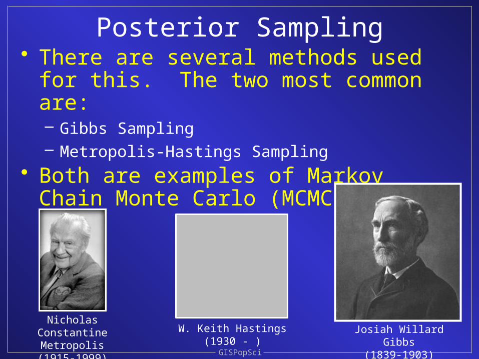
Posterior Sampling• There are several methods used for this.

The two most common are:– Gibbs Sampling– Metropolis-Hastings Sampling

• Both are examples of Markov Chain Monte Carlo (MCMC) methods

GISPopSci

Josiah Willard Gibbs(1839-1903)

Nicholas Constantine Metropolis

(1915-1999)

W. Keith Hastings(1930 - )

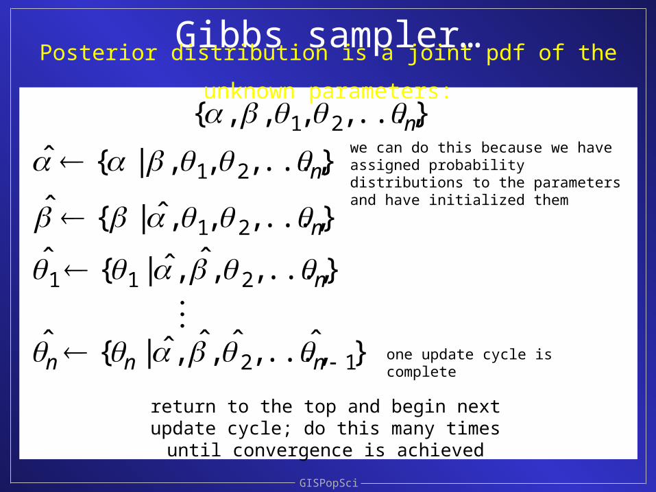
Gibbs Sampler• Fast algorithm; it yields a new sample value at

each iteration• Requires knowledge of the conditional

distributions of the parameters given the other parameters

• For parameter set [{i }, , ]:– Fix the i ‘s and to estimate – Then, fix the new and , say, to estimate 1

– etc. etc. etc.

• BUGS (later WinBUGS) was developed for this method (Bayesian inference Using Gibbs Sampling)

GISPopSci

Gibbs sampler…

GISPopSci

}...,,,,,{ 21 nPosterior distribution is a joint pdf of the unknown parameters:

}...,,,,|{ˆ 21 n

}...,,,,ˆ|{ˆ21 n

}...,,,ˆ,ˆ|{ˆ211 n

}ˆ...,,ˆ,ˆ,ˆ|{ˆ12 nnn

we can do this because we have assigned probability distributions to the parameters and have initialized them

one update cycle is complete

return to the top and begin next update cycle; do this many times until convergence is achieved

Metropolis-Hastings (MH) sampler

• This is a simple algorithm (more simple than Gibbs sampling) for updating parameters and sampling posterior distributions

• It does not require knowledge of the conditional distributions, but it does not guarantee a useful new sample at each iteration

• Simple to implement• WinBUGS now includes MH updating

GISPopSci

GISPopSci

Metropolis-Hastings (MH) samplerWorks off a very simple rule: accept an updated

parameter value if it moves the simulation toward the Posterior limiting distribution:

Let (, ’) be the acceptance probability of moving from current parameter estimate to proposed update ’:

}...,,,...,,,|{

}...,,,...,,,|'{,1min)',(

1121

1121

nkkk

nkkkkk p

p

Update is accepted if the proposal function is > 1

Brief history• Thomas Bayes (1702 – 1761); Oh… him• Gibbs sampler: Geman & Geman (1984)• MCMC: Gelfand & Smith (JASA, 1990)• BUGS: Biostatistics Unit, Medical Research

Council, Cambridge University; 1989• WinBUGS: Imperial College School of Medicine

at St Mary's, London; 2000• Continued development:

– OpenBUGS– DoodleBUGS– GeoBUGS– BRUGS– R2WinBUGS

GISPopSci

Using WinBUGS• WinBUGS is a windows version of the

BUGS package. BUGS stands for Bayesian inference using Gibbs Sampling

• The software must be programmed to sample form Bayesian models

• For simple models there is an interactive Doodle editor; more complex models must be written out fully.

GISPopSci

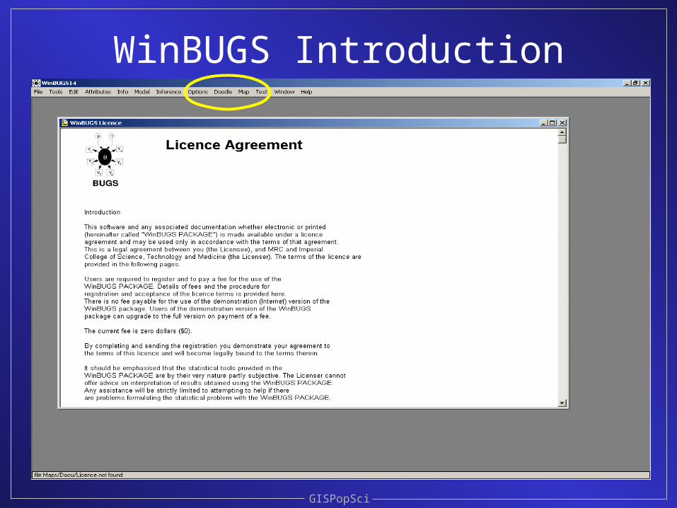
WinBUGS Introduction

GISPopSci

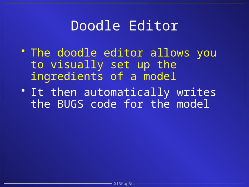
Doodle Editor

• The doodle editor allows you to visually set up the ingredients of a model

• It then automatically writes the BUGS code for the model

GISPopSci

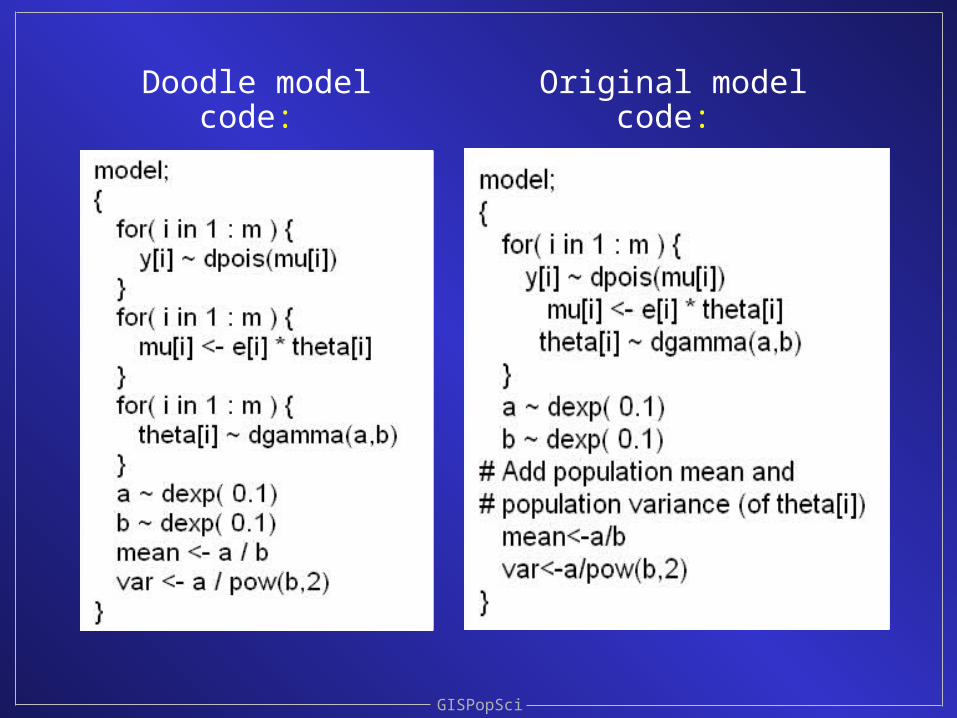
BUGS code and Doodle stagesfor simple Poisson-Gamma model

GISPopSci

GISPopSci

BUGS code and Doodle stagesfor simple Poisson-Gamma model

GISPopSci

Original model code: Doodle model code:

GISPopSci

Sometimes we may choose to just set the hyperparameters

Or let the data determine the values (so-called “Empirical Bayes”)

GISPopSci

For example, we might set the Gamma hyperparameters to, say, 0.1 & 0.1

These are somewhat “uninformative” or “diffuse” priors

GISPopSci

Even a very non-informative prior has the effect of slightly pulling the likelihood estimates

(the SMRs) toward the mean of the prior“Bayesian smoothing”

0

7

1

5

11

5

16

0

17

4

00

1

1

71

3

0

0

8

2

13

7

0

8

0

3

2

41

110

1

2

3

3

8

6

143

11

6

0

1

5

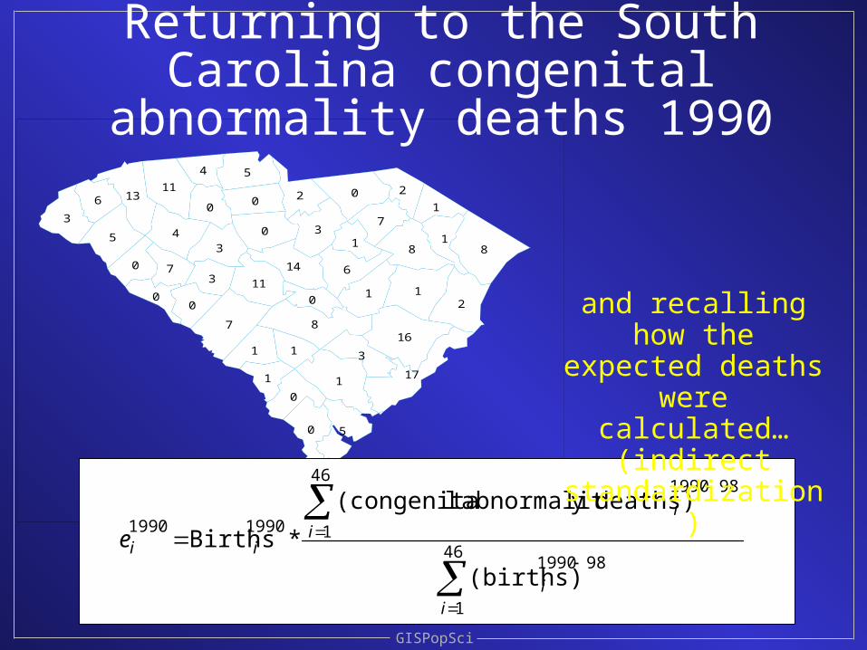
Returning to the South Carolina congenital abnormality deaths 1990

GISPopSci

46

1

981990

46

1

981990

19901990*

ii

ii

iie

(births)

deaths)yabnormalitl(congenita

Births

and recalling how the expected deaths were calculated…

(indirect standardization)

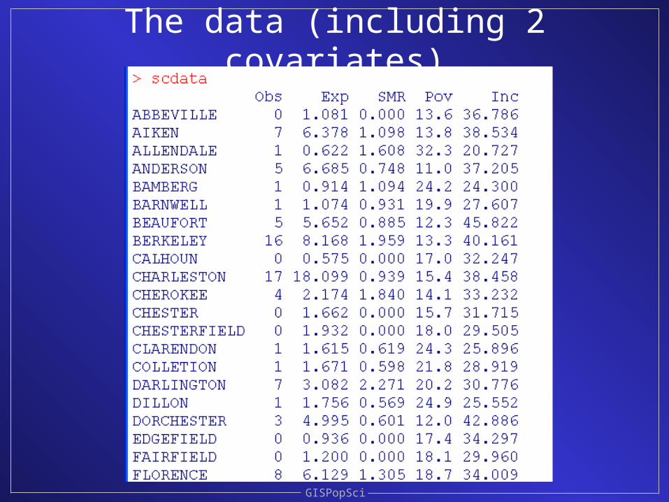
The data (including 2 covariates)

GISPopSci

GISPopSci

Berkeley County, SC1990 Deaths: 16; Expected: 8.54SMR: 1.87 (1.07 – 3.04)2000 pop: 143,00068% whitePoverty rate: 11.8%Density: 129 pers/mi2

Part of the Charleston-North Charleston-Sommerville-Metropolitan Statistical Area

Principal employer: U.S. Naval Weapons Station (18,450)

GISPopSci

1990 Deaths: 3; Expected: 0.77 SMR: 3.92 (0.81 – 11.46)

2000 pop: 18,000 66% white

Poverty rate: 15.6% Density: 41 pers/mi2

Saluda County, SC

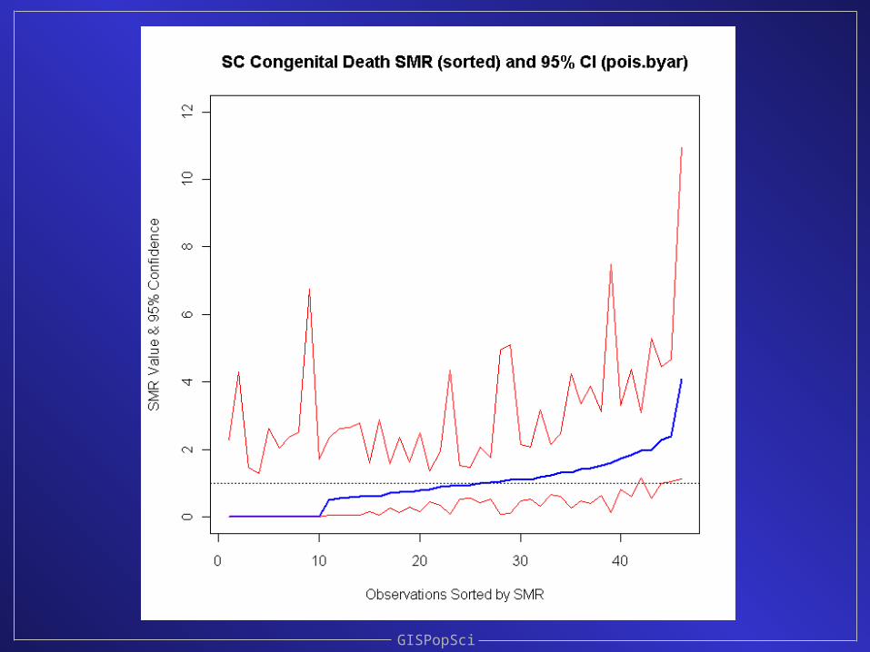
Confidence intervals for the SMRs

GISPopSci

It turns out that there are many options

We’ll examine some of this in lab this afternoon

GISPopSci

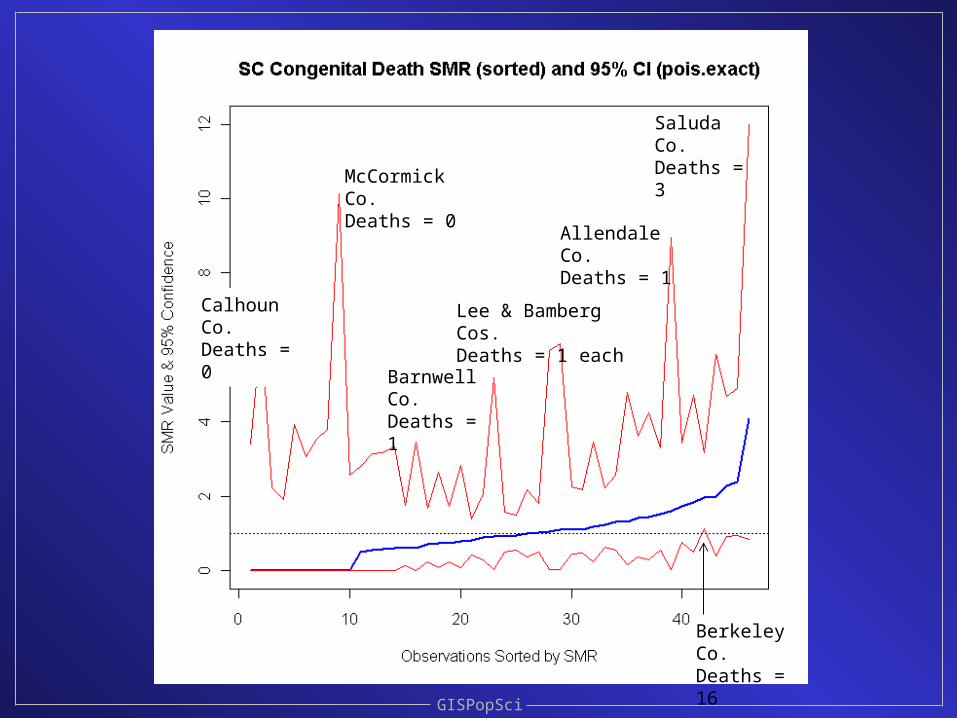
GISPopSci

Barnwell Co.Deaths = 1

Lee & Bamberg Cos.Deaths = 1 each

Allendale Co.Deaths = 1

Saluda Co.Deaths = 3

McCormick Co.Deaths = 0

Calhoun Co.Deaths = 0

Berkeley Co.Deaths = 16

GISPopSci

GISPopSci

GISPopSci

GISPopSci

GISPopSci

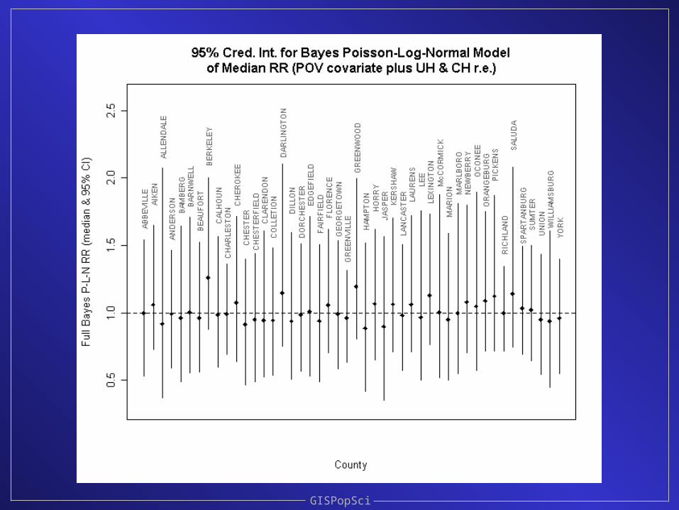
This afternoon we will see what happens when various Bayesian models are fit to

these data to estimate relative risk• Simple Poisson-Gamma• Poisson-Log-Normal with pov. covariate• Poisson-Log-Normal with inc. covariate• Poisson-Log-Normal with both pov. & inc.• Poisson-Log-Normal with pov. & UH• Poisson-Log-Normal with pov., UH & CH• Preview: Bayesian smoothing tells us there’s

probably nothing interesting in these data regarding the incidence of infant congenital deaths in 1990

GISPopSci

GISPopSci

Mean = 0.9703Std. dev. = 0.8024

GISPopSci

Mean = 1.0373Std. dev. = 0.0814

GISPopSci

Mean = 0.9703Std. dev. = 0.8024

Original SMR MLE saturated estimates of relative risk

Mean = 1.0373Std. dev. = 0.0814

Full Bayes mean posterior estimates of

relative risk (model: PLNPovUHCH)

GISPopSci

GISPopSci

GISPopSci

GISPopSci

GISPopSci

GISPopSci

GISPopSci

GISPopSci

Things I’ve learned• This stuff is not easy

– the price of entry is high, despite the free software

• Learning to efficiently code in R takes practice– my R script is not particularly elegant

• Look at carefully at the WinBUGS log file– the model doesn’t always converge (see next slide)– may have to try it 3-4 times

• Because full Bayes modeling is based on a simulation, the results vary from one run to another– This takes some time getting used to

GISPopSci

Good

Not good

GISPopSci

Readings for today• Besag, Julian, Jeremy York, & Annie Mollié.

1991. “Bayesian Image Restoration with Two Applications in Spatial Statistics.” Annals of the Institute of Statistical Mathematics 43(1):1-20. [In the beginning…]

• Package ‘R2WinBUGS: Running WinBUGS and OpenBUGS from R / S-PLUS. Version 2.1-18. March 22, 2011. [Useful acces to R functionality in a Bayesian framework]

GISPopSci

Afternoon Lab

Bayesian Modeling in WinBUGS & R

Presentations & discussion

Areas of needed research:• Spatial panel models; space-time

interactions• Latent continuous variables; binary

dependent variable; counts; etc.• Flow models• Endogenous weighting matrices• More users of the Bayesian perspective in

the social sciences

GISPopSci

Thanks for your participation!!Special thanks Stephen Matthews, Don

Janelle, & the terrific PSU support!

GISPopSci

See you this afternoon