advanced servo control for hard disk drives in … · advanced servo control for hard disk drives...
TRANSCRIPT
Founded 1905
ADVANCED SERVO CONTROL FOR
HARD DISK DRIVES IN MOBILE
APPLICATIONS
BY
JINGLIANG ZHANG
(BEng, MEng)
A THESIS SUBMITTED
FOR THE DEGREE OF DOCTOR OF PHILOSOPHY
DEPARTMENT OF ELECTRICAL & COMPUTER ENGINEERING
NATIONAL UNIVERSITY OF SINGAPORE
2011

I dedicate this dissertation to my lovely children: Jerry, Jenny and Jessie.

Acknowledgements
I would especially like to thank Professor Shuzhi Sam Ge, my supervisor, for his
many suggestions, constant support and guidance throughout this research. I would
also like to express my gratitude to Professor Frank Lewis for his kind help.
I express my sincere gratitude to the Data Storage Institute of Singapore for its
support of my part-time Ph.D. program.
Of course, I am grateful to my family for their patience and love. Without them
this work would never have come into existence literally.
Finally, I wish to thank the following colleagues: Linlin Thi (for her patience
and hardworking in developing hardware and firmware for the experiment setup
together with me), Dr. Chunling Du and Dr. Fan Hong (for the endless chatter
about control theory and controller design), Dr. Qingwei Jia (for his friendship
and kind support).
Jingliang Zhang
December 27, 2010
i
Contents
Contents
Acknowledgements i
List of Figures vi
List of Tables x
Abstract 1
1 Introduction 2
1.1 Background of HDD and Magnetic Recording . . . . . . . . . . . . 2
1.2 Servo Control Issues in HDD . . . . . . . . . . . . . . . . . . . . . . 4
1.3 Outline of Chapters . . . . . . . . . . . . . . . . . . . . . . . . . . . 8
2 HDD Servo Mechanism and Modeling 10
2.1 The Servo Loop in HDD . . . . . . . . . . . . . . . . . . . . . . . . 11
2.2 Mechanical Structural Resonances . . . . . . . . . . . . . . . . . . 13
2.2.1 Spindle Motor . . . . . . . . . . . . . . . . . . . . . . . . . . 13
2.2.2 Disks Platter . . . . . . . . . . . . . . . . . . . . . . . . . . 15
ii
Contents
2.2.3 Suspension and Arm . . . . . . . . . . . . . . . . . . . . . . 16
2.3 Modeling of Servo System . . . . . . . . . . . . . . . . . . . . . . . 17
2.3.1 Modeling of VCM Actuator . . . . . . . . . . . . . . . . . . 17
2.3.2 Modeling of Micro-actuator . . . . . . . . . . . . . . . . . . 18
2.3.3 Modeling of Disturbances . . . . . . . . . . . . . . . . . . . 22
3 Design Pseudo-sine Current Profile for Smooth Seeking 28
3.1 Problem Formulation for Track-seeking . . . . . . . . . . . . . . . . 30
3.1.1 Minimum Jerk Seeking . . . . . . . . . . . . . . . . . . . . . 30
3.2 2DOF with Model Referenced Position and Current Feedforward
Control . . . . . . . . . . . . . . . . . . . . . . . . . . . . . . . . . 31
3.3 The Strategy to Design Pseudo-sine Current Profile . . . . . . . . . 33
3.3.1 Pseudo-sine Current Profile Generation . . . . . . . . . . . . 35
3.3.2 Minimizing Residual Vibrations . . . . . . . . . . . . . . . . 37
3.4 Simulation and Comparison with PTOS . . . . . . . . . . . . . . . 38
3.5 Conclusions . . . . . . . . . . . . . . . . . . . . . . . . . . . . . . . 43
4 IES Settling Controller for Dual-stage Servo System 44
4.1 Settling Problem in Dual-stage Servo Systems . . . . . . . . . . . . 45
4.2 IES for Dual-Stage Systems . . . . . . . . . . . . . . . . . . . . . . 47
4.2.1 IES for Initial Position . . . . . . . . . . . . . . . . . . . . . 48
4.2.2 IES for Initial Velocity . . . . . . . . . . . . . . . . . . . . . 49
iii
Contents
4.3 More Considerations in Designing F (z) . . . . . . . . . . . . . . . . 50
4.4 Design Example . . . . . . . . . . . . . . . . . . . . . . . . . . . . . 51
4.5 Implementation Method . . . . . . . . . . . . . . . . . . . . . . . . 57
4.6 Switching Conditions . . . . . . . . . . . . . . . . . . . . . . . . . . 58
4.7 Experimental Setup and Results . . . . . . . . . . . . . . . . . . . . 59
4.8 Conclusions . . . . . . . . . . . . . . . . . . . . . . . . . . . . . . . 60
5 Design Feedback Controller Using Advanced Loop Shaping 63
5.1 Control Design Using Generalized KYP Lemma . . . . . . . . . . . 65
5.1.1 Problem Description . . . . . . . . . . . . . . . . . . . . . . 65
5.1.2 Generalized KYP Lemma . . . . . . . . . . . . . . . . . . . 65
5.1.3 YOULA Parametrization . . . . . . . . . . . . . . . . . . . . 67
5.1.4 Design Procedures Using KYP Lemma . . . . . . . . . . . . 69
5.2 H2 Optimal Control . . . . . . . . . . . . . . . . . . . . . . . . . . 70
5.2.1 H2 Norm . . . . . . . . . . . . . . . . . . . . . . . . . . . . 71
5.2.2 Continuous-time H2 Optimal Control . . . . . . . . . . . . . 73
5.2.3 Discrete-time H2 Optimal Control . . . . . . . . . . . . . . . 75
5.3 Combine H2 and KYP Lemma . . . . . . . . . . . . . . . . . . . . . 78
5.3.1 Problem Formulation . . . . . . . . . . . . . . . . . . . . . . 78
5.3.2 Design Controller for Specific Disturbance Rejection and Over-
all Error Minimization . . . . . . . . . . . . . . . . . . . . . 79
iv
Contents
5.3.3 Q Parametrization to Meet Specifications for Disturbance
Rejection . . . . . . . . . . . . . . . . . . . . . . . . . . . . 80
5.3.4 Q Parametrization to Minimize H2 Performance . . . . . . . 82
5.3.5 Design Procedure . . . . . . . . . . . . . . . . . . . . . . . . 84
5.4 Experimental Setup and Results . . . . . . . . . . . . . . . . . . . . 85
5.4.1 Servo Writing Technologies . . . . . . . . . . . . . . . . . . . 85
5.4.2 STW Experimental Platform with Hybrid Dual-stage Servo . 86
5.4.3 System Functions of STW Platform . . . . . . . . . . . . . . 87
5.4.4 Servo Mechanism of STW Platform . . . . . . . . . . . . . . 88
5.4.5 Measurement and Modeling of Vibrations and Noises . . . . 90
5.4.6 Experimental Verification of the Controller Performance for
PZT Loop . . . . . . . . . . . . . . . . . . . . . . . . . . . . 94
6 Conclusions and Future Work 102
6.1 Summary of Results . . . . . . . . . . . . . . . . . . . . . . . . . . 102
6.2 Future Work . . . . . . . . . . . . . . . . . . . . . . . . . . . . . . . 104
Author’s Publications 105
Bibliography 107
v

List of Figures
List of Figures
1.1 Data storage density for disk drives versus time [1]. . . . . . . . . . 3
2.1 The mechanism inside a conventional HDD. . . . . . . . . . . . . . 10
2.2 A typical servo loop in HDD. . . . . . . . . . . . . . . . . . . . . . 12
2.3 The bode plot of a typical sensitivity function. . . . . . . . . . . . . 13
2.4 The structure of ball bearing and fluid dynamic bearing. . . . . . . 14
2.5 The spindle resonant modes: pitch and radial. . . . . . . . . . . . . 15
2.6 The typical eigenmodes of disk. . . . . . . . . . . . . . . . . . . . . 15
2.7 The eigenmodes of suspension. . . . . . . . . . . . . . . . . . . . . . 16
2.8 The typical arm mode shapes: (a) lateral QR mode and (b) lateral
bending mode. . . . . . . . . . . . . . . . . . . . . . . . . . . . . . . 16
2.9 The block diagram of VCM model. . . . . . . . . . . . . . . . . . . 17
2.10 Bode plots of frequency response for VCM. (solid line: measured;
dotted: identified; dash-dotted: double integrator) . . . . . . . . . . 18
2.11 The technology evolution for micro-actuator. . . . . . . . . . . . . . 19
2.12 The dual-stage actuator inside Seagate Cheetah 10K7 HDD. . . . . 20
vi

List of Figures
2.13 A PZT actuated suspension. . . . . . . . . . . . . . . . . . . . . . . 20
2.14 Equivalent spring mass system of PZT microactuator. . . . . . . . . 21
2.15 A typical frequency response of PZT microactuator. . . . . . . . . . 22
2.16 Block diagram of closed-loop with disturbances . . . . . . . . . . . 24
2.17 The NRRO spectrum measured in a commercial HDD. . . . . . . . 25
2.18 The bode plot of sensitivity function for a commercial HDD. . . . . 25
2.19 Control system with augmented disturbance and noise models. . . . 27
3.1 The current profile for conventional seeking controller. . . . . . . . . 29
3.2 The optimal current profile for minimum jerk. . . . . . . . . . . . . 32
3.3 Block diagram of the model referenced feedforward control. . . . . . 32
3.4 Pseudo sinusoidal current profile. . . . . . . . . . . . . . . . . . . . 34
3.5 The process to generate current profile. . . . . . . . . . . . . . . . . 36
3.6 The block diagram of PTOS. . . . . . . . . . . . . . . . . . . . . . . 39
3.7 The block diagram of 2DOF with MRF. . . . . . . . . . . . . . . . 39
3.8 Position output for one track seeking. . . . . . . . . . . . . . . . . . 40
3.9 Velocity and current profile for one track seeking. . . . . . . . . . . 40
3.10 Position output for 50 tracks seeking. . . . . . . . . . . . . . . . . . 41
3.11 Velocity and current profile for 50 tracks seeking. . . . . . . . . . . 42
3.12 Input current while seeking with different T1. . . . . . . . . . . . . . 42
3.13 Input current while seeking with different Th. . . . . . . . . . . . . 43
vii

List of Figures
4.1 Parallel-type dual-stage servo system. . . . . . . . . . . . . . . . . . 45
4.2 Equivalent closed-loop control system with IES for initial position
and velocity. . . . . . . . . . . . . . . . . . . . . . . . . . . . . . . . 47
4.3 Frequency response of VCM actuator. . . . . . . . . . . . . . . . . . 52
4.4 Frequency response of PZT micro-actuator. . . . . . . . . . . . . . . 52
4.5 Step response of the dual-stage servo system. . . . . . . . . . . . . . 53
4.6 Poles/zeros map of the closed-loop system. . . . . . . . . . . . . . . 54
4.7 Settling transient due to initial position y0 = 1 track (A: no compen-
sation; B: with compensation and without considering acoustic and
slow modes; C: with compensation considering acoustic and slow
modes). . . . . . . . . . . . . . . . . . . . . . . . . . . . . . . . . . 55
4.8 VCM controller output with initial position compensation (B: acous-
tic oscillation observed; C: no acoustic problem). . . . . . . . . . . . 56
4.9 Settling transient due to initial velocity. . . . . . . . . . . . . . . . . 57
4.10 PZT output under different initial conditions with IES. . . . . . . . 59
4.11 Experiment setup for dual-stage servo. . . . . . . . . . . . . . . . . 60
4.12 Seeking profile with FIR seeking controller. . . . . . . . . . . . . . . 61
4.13 Experimental results with IES (A: no compensation; B: with com-
pensation). . . . . . . . . . . . . . . . . . . . . . . . . . . . . . . . . 61
5.1 Equivalent system for KYP analysis. . . . . . . . . . . . . . . . . . 66
5.2 Configuration of standard optimal control. . . . . . . . . . . . . . . 74
5.3 H2 control scheme with Q parametrization for controller design. . . 78
viii
List of Figures
5.4 Dual stage STW experimental platform. . . . . . . . . . . . . . . . 86
5.5 Functional block diagram of the HSSTW platform. . . . . . . . . . 87
5.6 Hybrid dual-stage servo system. . . . . . . . . . . . . . . . . . . . . 88
5.7 Equivalent PZT servo loop. . . . . . . . . . . . . . . . . . . . . . . 90
5.8 Spectrum of PES NRRO without the second loop. . . . . . . . . . . 91
5.9 The format of servo bursts and typical servo pattern readback signal. 91
5.10 Spectrum of PES demodulation noise. . . . . . . . . . . . . . . . . . 92
5.11 Frequency response for piezo chip. . . . . . . . . . . . . . . . . . . . 93
5.12 Sensitivity function simulated. (solid: KYP; dashed: PLPF). . . . . 97
5.13 Open loop frequency response. (solid: KYP; dashed: PLPF). . . . . 97
5.14 Spectra of PES NRRO with the secondary loop (solid: KYP; dashed:
PLPF). . . . . . . . . . . . . . . . . . . . . . . . . . . . . . . . . . 98
5.15 Frequency response of open-loop transfer functions. (solid: KYP+H2;
dashed: KYP). . . . . . . . . . . . . . . . . . . . . . . . . . . . . . 100
5.16 Simulations of sensitivity function. (solid: KYP+H2; dashed: KYP). 100
5.17 Sensitivity functions measured. (solid: KYP+H2; dashed: KYP). . 101
5.18 Spectra of PES NRRO with the secondary loop (solid: KYP+H2;
dashed: KYP). . . . . . . . . . . . . . . . . . . . . . . . . . . . . . 101
ix

List of Tables
List of Tables
3.1 Parameters for resonant modes . . . . . . . . . . . . . . . . . . . . 38
4.1 Characteristic of poles/zeros in tracking. . . . . . . . . . . . . . . . 54
4.2 PZT output at different initial conditions. . . . . . . . . . . . . . . 58
5.1 Tracking accuracy for different servo bandwidth. . . . . . . . . . . . 94
5.2 Performance with different controllers for PZT loop. . . . . . . . . . 99
6.1 Performance of servo controllers using different design method. . . . 103
x
List of Tables
Abstract
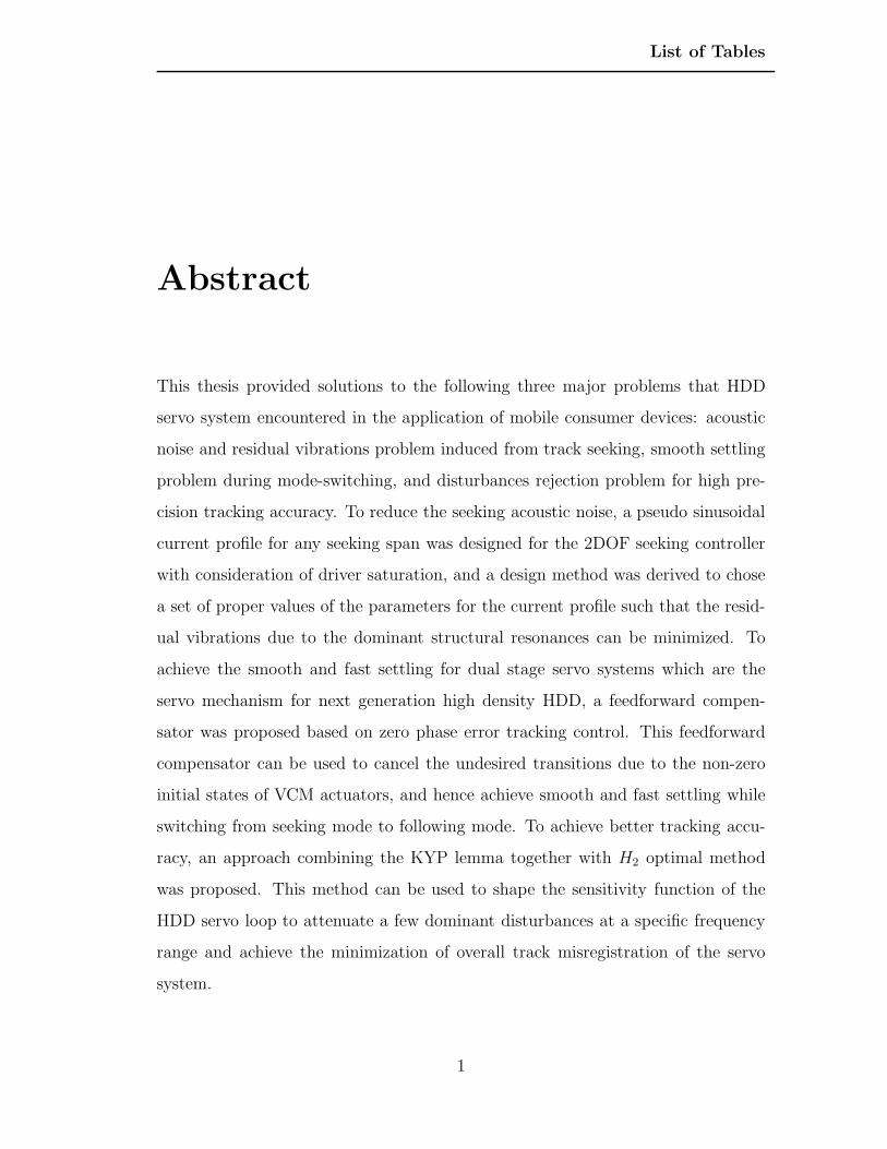
This thesis provided solutions to the following three major problems that HDD
servo system encountered in the application of mobile consumer devices: acoustic
noise and residual vibrations problem induced from track seeking, smooth settling
problem during mode-switching, and disturbances rejection problem for high pre-
cision tracking accuracy. To reduce the seeking acoustic noise, a pseudo sinusoidal
current profile for any seeking span was designed for the 2DOF seeking controller
with consideration of driver saturation, and a design method was derived to chose
a set of proper values of the parameters for the current profile such that the resid-
ual vibrations due to the dominant structural resonances can be minimized. To
achieve the smooth and fast settling for dual stage servo systems which are the
servo mechanism for next generation high density HDD, a feedforward compen-
sator was proposed based on zero phase error tracking control. This feedforward
compensator can be used to cancel the undesired transitions due to the non-zero
initial states of VCM actuators, and hence achieve smooth and fast settling while
switching from seeking mode to following mode. To achieve better tracking accu-
racy, an approach combining the KYP lemma together with H2 optimal method
was proposed. This method can be used to shape the sensitivity function of the
HDD servo loop to attenuate a few dominant disturbances at a specific frequency
range and achieve the minimization of overall track misregistration of the servo
system.
1
Chapter 1
Introduction
1.1 Background of HDD and Magnetic Recording
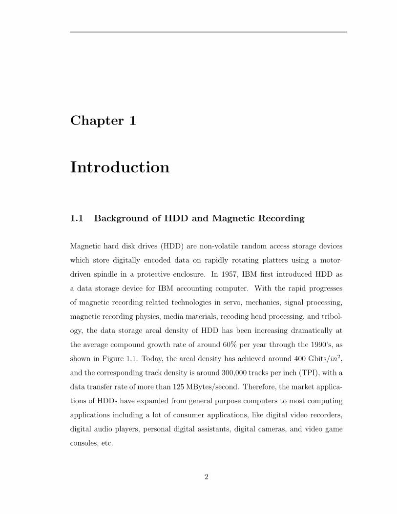
Magnetic hard disk drives (HDD) are non-volatile random access storage devices
which store digitally encoded data on rapidly rotating platters using a motor-
driven spindle in a protective enclosure. In 1957, IBM first introduced HDD as
a data storage device for IBM accounting computer. With the rapid progresses
of magnetic recording related technologies in servo, mechanics, signal processing,
magnetic recording physics, media materials, recoding head processing, and tribol-
ogy, the data storage areal density of HDD has been increasing dramatically at
the average compound growth rate of around 60% per year through the 1990’s, as
shown in Figure 1.1. Today, the areal density has achieved around 400 Gbits/in2,
and the corresponding track density is around 300,000 tracks per inch (TPI), with a
data transfer rate of more than 125 MBytes/second. Therefore, the market applica-
tions of HDDs have expanded from general purpose computers to most computing
applications including a lot of consumer applications, like digital video recorders,
digital audio players, personal digital assistants, digital cameras, and video game
consoles, etc.
2
1.1 Background of HDD and Magnetic Recording
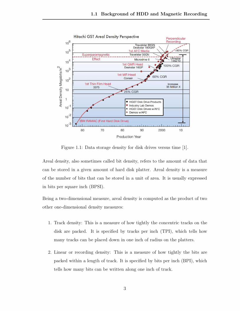
Figure 1.1: Data storage density for disk drives versus time [1].
Areal density, also sometimes called bit density, refers to the amount of data that
can be stored in a given amount of hard disk platter. Areal density is a measure
of the number of bits that can be stored in a unit of area. It is usually expressed
in bits per square inch (BPSI).
Being a two-dimensional measure, areal density is computed as the product of two
other one-dimensional density measures:
1. Track density: This is a measure of how tightly the concentric tracks on the
disk are packed. It is specified by tracks per inch (TPI), which tells how
many tracks can be placed down in one inch of radius on the platters.
2. Linear or recording density: This is a measure of how tightly the bits are
packed within a length of track. It is specified by bits per inch (BPI), which
tells how many bits can be written along one inch of track.
3
1.2 Servo Control Issues in HDD
There are two ways to increase areal density: increase the linear density by packing
the bits on each track closer together so that each track holds more data; or increase
the track density so that each platter holds more tracks. Typically new generation
drives improve both measures. It’s important to realize that increasing areal density
leads to drives that are not just bigger, but also faster. The reason is that the areal
density of the disk impacts both of the key hard disk performance factors: the
track to track positioning speed and data transfer rate.
Increasing the areal density of disks is a difficult task that requires many technolog-
ical advances and changes to various components of the hard disk [2]. As the data
is packed closer and closer together, problems result with interference between bits.
This is often dealt with by reducing the strength of the magnetic signals stored
on the disk, but then this creates other problems such as ensuring that the signals
are stable on the disk and that the read/write (R/W) heads are sensitive and close
enough to the surface to pick them up. Changes to the media layer on the platters,
actuators, control electronics and other components are made to continually im-
prove areal density. Every few years a R/W head technology breakthrough enables
a significant jump in density, which is why hard disks have been doubling in size
so frequently, as shown in Figure 1.1 .
1.2 Servo Control Issues in HDD
The HDD servo systems play a vital role in the demand of increasingly high track
density and high performance HDDs. In HDDs, the servo system provides two
major functions: track seeking and track following. The track seeking servo moves
R/W head from one track to another in minimal time, which is seeking time. The
less the seeking time is, the faster the data can transfer. The track following servo
maintains the R/W head position over the center of a target track. The measured
deviation of R/W head from the center of the track is called position error signal
4
1.2 Servo Control Issues in HDD
(PES). It is the performance of track following servo that limits the achievable
track density. The tracking accuracy of HDD servo is often measured by a 3σ
number of PES, assuming a Gaussian distribution. This performance measure is
also called as track misregistration (TMR). Typical TMR is 12% of the track width,
which matches with the off-track-reading-capability (OTRC) of the coding channel.
OTRC is a measure of the R/W system’s ability to read previously-written data
as a function of servo tracking-error, and proximity of an adjacent data-track. If
TMR is larger than 12%, the data reading channel will have unrecoverable error.
In general, the HDDs have top performance if TMR is less than 5% of track 99.7%
of the time.
The track-following control in HDDs is an inherently difficult problem, as the plant
is marginally stable and it becomes unstable in the presence of delays due to sam-
pling and computation. Besides this, the HDD servo system is non-collocated, as
sensors are placed at the read head while control is applied at the voice-coil-motor
(VCM) [3] [4]. Furthermore, the servo system in HDD is non-minimum phase
system, which imposes limits on tracking performance [5]. The servo robustness
and tracking accuracy are limited by the following factors: (1) resonance and gain
variations between heads, at different radius, ages, and temperatures; (2) excessive
three-dimensional vibrations; (3) mechanical constraints (e.g. form factor) limit
the dynamic properties of the plant, which in turn place limitations on the con-
troller performance; (4) uncertainties, and nonlinearities, such as friction due to
near contact recording and pivot, and backlash/hysteresis of micro-actuator/milli-
actuator.
Traditionally, HDD servos are designed using linear control theory. Current disk
drive utilizes typical linear feedback digital control systems based on error signal,
PES. The PES is demodulated from the position information that is encoded onto
the disks during the manufacturing process. PID controllers were used initially,
and they are subsequently augmented with notch filters to suppress the mechanical
5
1.2 Servo Control Issues in HDD
resonant modes, thereby increasing the bandwidth. The performances of these
methods are limited by the effects of Bode Integral Theorem [6]. As a consequence
of this theory, servo loop will amplify vibrations at other frequencies [7], if the
servo sensitivity transfer function is designed to reject more vibrations in some
frequencies. This is also known as waterbed effect.
Another formidable challenge for track-following controller is to achieve precise
tracking accuracy so as to satisfy the requirement for ultra-high track density higher
than 500k TPI, despite the presence of uncertainties in the dynamic model. PES
demodulation noise in HDD is scaled with signal to noise ratio (SNR) of head and
media, and used to be the major TMR sources. However, for high density HDD
in mobile applications, disturbances are no longer limited to PES noise, but also
disk motion, air flow, and external vibration, etc. Although external sensors, such
as accelerometers, can be used in the suppression of external vibrations in order
to maintain the tracking accuracy [8] [9] [10] [11], the relationship between XY
acceleration and PES may be highly nonlinear, which results in further difficulties
in the design of feed forward controllers. In addition, some nonlinearities currently
being neglected or simplified in control system design must be taken into account
for a system with such a high accuracy requirement. The nonlinearities preventing
the system accuracy of a hard disk drive from further improvement include ribbon
flexibility and nonlinear friction of the actuator pivot of a HDD [12] [13] [14].
Furthermore, inconsistencies of system parameters between units are prevalent as
HDDs are mass-produced products. These parameters vary with age and thermal
effects, although the time scales are usually sufficiently large such that they can be
considered to be slowly-varying or even time-invariant.
Therefore, the track-following servo controller are designed with two kinds of funda-
mental trade off, performance trade-off due to bode integration, and performance
trade-off with system robustness due to uncertainties of plant dynamic and dis-
turbances. The performance versus robustness trade-off is an important aspect
6
1.2 Servo Control Issues in HDD
of the development of H∞ control theory [15] [16]. Many papers are published
on the loop-shaping design methods to look for the reasonable trade-off between
robustness and performance [17] [18] [19].
A few researchers have investigated the feasibility of applying adaptive or learning
algorithms like neural network and fuzzy control. In [20] [21] [22] [23], an adaptive
neural network controller is designed to compensate for the pivot nonlinearity. In
[24], a model-based adaptive controller is added to a linear time invariant (LTI) sta-
bilizing controller to minimize the tracking error of the read/write head. In [25], an
adaptive robust controller was developed, which is applicable to both track-seeking
and track-following. In [26] [27] [28] [29], an adaptive notch filter was designed to
compensate for the resonant modes with uncertain frequencies. However, most of
the adaptive algorithms are not feasible in HDD servo due to either robustness,
or degraded performance with existence of noise and disturbances, or the slow
convergence of adaptation.
In a traditional HDD servo system, nonlinear controllers such as proximate time-
optimal servo (PTOS) [30] [31] [32] are widely used for track-seeking. Other efforts
include designing a unified control structure for both track-seeking and following,
such as two-degree-of freedom (2DOF) servo mechanism with adaptive robust con-
trol and zero phase error tracking techniques [33] [34] [35]. Most of these works
focus on reducing seeking and settling time. But for the HDDs application in
consumer electronics where the quietness is essential, such as home entertainment
system, car navigation and digital video recorder, HDD acoustic noise is one of the
key performance indices most concerned. Another challenge for the seeking/settling
controller is the residual vibrations induced in the transition switching from seek-
ing to track-following [36] [37] [38]. The residual vibrations are not only one of the
significant TMR sources, but may also induce acoustic noise.
7
1.3 Outline of Chapters
1.3 Outline of Chapters
The contributions presented in this dissertation include the following: (1) Pro-
posed an advanced systematic loop shaping method using Kalman-Yakubovic-
Popov (KYP) Lemma to optimize the track-following controller with considera-
tions of the spectrum models of input disturbances, output disturbances and sens-
ing noise. The method was experimentally validated in our servo writing platform;
(2) Proposed a method to design an optimal seek current profile for the seeking
controller to reduce acoustic noise and residual vibrations; (3) Proposed and ex-
perimentally validated a novel settling controller for dual-stage servo system to
achieve fast and smoothly settling on target track.
The dissertation is organized as follows. In Chapter 2, the mechanical components
used in current HDDs are described. It details the possible sources of TMR during
normal operation and when the HDD is subjected to external shock and vibrations.
It also provides the modeling of the typical VCM actuator, piezoelectric (PZT)
micro-actuator, disturbances and noises.
In Chapter 3, the seeking process in HDDs is detailed. We propose a direct ap-
proach to design the pseudo-sinusoidal seek current profile, which is able to reduce
both the acoustic noise and residual vibrations. With consideration of both cur-
rent saturation limit and maximum seeking velocity limit, the saturation period,
frequency of sinusoidal wave, and coasting time can be optimally designed for ar-
bitrary seeking span to reduce residual vibrations.
In Chapter 4, the dual-stage servo system in HDD is first introduced. We formulate
the problem due to the initial values of states in the transition from track-seeking
to track-following. After a brief discussion of the conventional initial value compen-
sation (IVC) method, we describe the new proposed method initial error shaping
(IES) basing on the zero-phase error tracking (ZPET), followed by the experimental
results.
8
1.3 Outline of Chapters
In Chapter 5, a general KYP-method is introduced to shape the sensitivity function
and suppress the disturbances at certain frequencies. With the spectrum model of
disturbances and noises, an H2 optimal method is introduced to design an optimal
feedback control to achieve overall an optimal tracking performance. A systematic
procedure is then presented to design an optimal track-following controller com-
bining KYP-lemma with H2 optimal control. We introduce the servo loops in the
servo writing experimental platform and present experimental results to verify the
performances of controller designed with different approaches.
In the final chapter, Chapter 6, the major results and achievements of this research
are summarized. Further, a recommendation for future work is also outlined.
9

Chapter 2
HDD Servo Mechanism andModeling
VCM Arm
Suspension Disk StackRecording Head
Pivot Bearing
Flexi-Cable Base Casting
Spindleu-actuator
Tracks
Figure 2.1: The mechanism inside a conventional HDD.
Figure 2.1 shows an overview of the mechanism inside a HDD. The major compo-
nents in a modern HDD include: 1) device enclosure, which usually consists of a
base plate and a cover to provide supports to the spindle, actuator, and electronics
card; 2) disk stack assembly, where several disks are stacked on the spindle motor
shaft and rotate at up to 15,000 rotations per minute (RPM) in high end 3.5-inch
drives and 5,400 - 7,200 RPM in 2.5-inch drives. On the surface of a disk, sev-
eral hundred thousand data tracks are magnetically recorded, and the latest track
10
2.1 The Servo Loop in HDD
pitch is about 80 nm; 3) head stack assembly which contains of a voice coil motor
(VCM), actuator arm, suspension and gimbal assembly. A slider is supported by
a suspension and a carriage, and is suspended at less than ten nanometers above
the disk surface. The VCM actuates the carriage and moves the slider on a de-
sired track. To increase the servo bandwidth to improve positioning accuracy for
higher track density drives, dual-stage servo using a suspension-driven PZT micro-
actuator has been commercially applied to HDD; 4) electronics circuit board which
involves drivers for spindle motor and VCM, read/write (R/W) electronics, servo
channel demodulator, a micro processor/digital signal processor (DSP) for servo
control and the interface to host computer. The position signals are recorded mag-
netically on each disk using a servo track writer (STW). The position signals are
recorded in a certain time interval on each track. Consequently, the PES between
the head and the reference track center can be detected directly by reading the
position signal.
2.1 The Servo Loop in HDD
The head-positioning servomechanism in HDD is a control system that moves the
R/W head from current track near to another target track (track-seeking), and
re-positions the R/W head over a desired track center with minimum statistical
deviation from the track center (track-following). A settling controller is used in
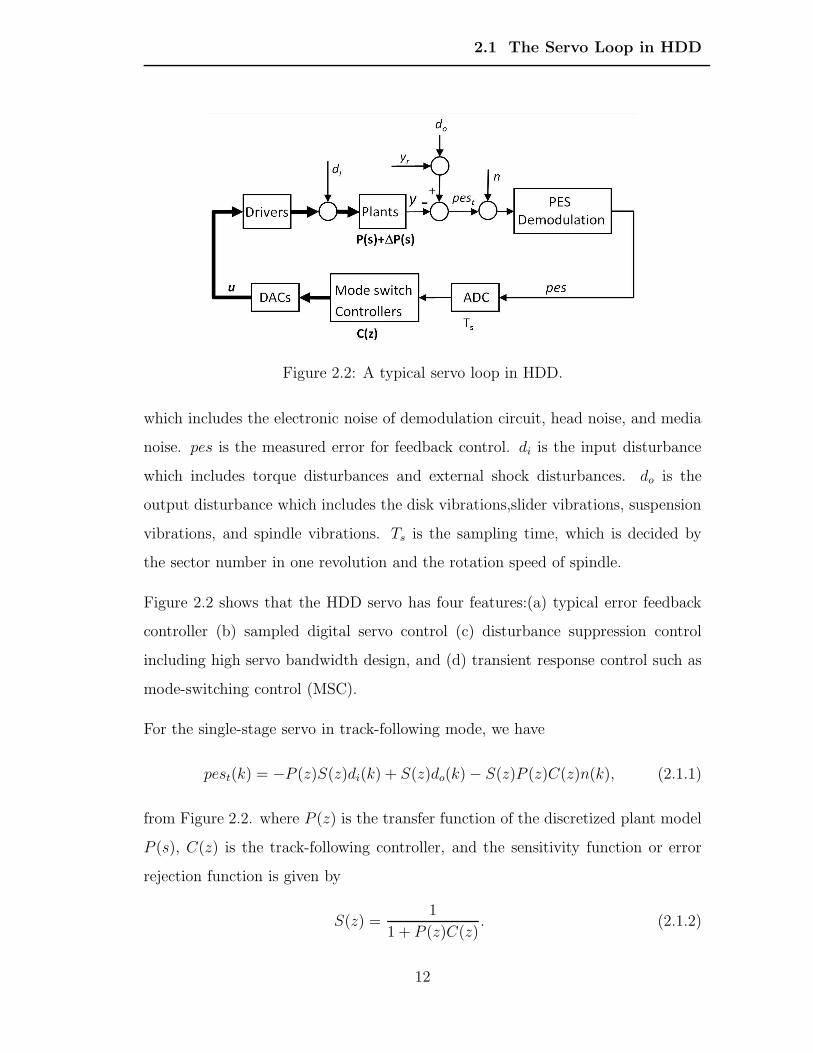
between the above seeking and following modes. Figure 2.2 shows the typical
functional block diagram where plants involve VCM and PZT actuators for the
dual-stage servo system in HDD. The plant dynamics (P (s) + ∆P (s)) include the
dynamic of arm, suspension, and driver, and y is the position of R/W head (it is
the sum of VCM and PZT output for dual-stage HDD). yr is the reference input
of the desired track center. pest is the true PES signal which tells exactly how
well the R/W head follows the reference track center. n is measurement noise
11
2.1 The Servo Loop in HDD
Figure 2.2: A typical servo loop in HDD.
which includes the electronic noise of demodulation circuit, head noise, and media
noise. pes is the measured error for feedback control. di is the input disturbance
which includes torque disturbances and external shock disturbances. do is the
output disturbance which includes the disk vibrations,slider vibrations, suspension
vibrations, and spindle vibrations. Ts is the sampling time, which is decided by
the sector number in one revolution and the rotation speed of spindle.
Figure 2.2 shows that the HDD servo has four features:(a) typical error feedback
controller (b) sampled digital servo control (c) disturbance suppression control
including high servo bandwidth design, and (d) transient response control such as
mode-switching control (MSC).
For the single-stage servo in track-following mode, we have
pest(k) = −P (z)S(z)di(k) + S(z)do(k)− S(z)P (z)C(z)n(k), (2.1.1)
from Figure 2.2. where P (z) is the transfer function of the discretized plant model
P (s), C(z) is the track-following controller, and the sensitivity function or error
rejection function is given by
S(z) =1
1 + P (z)C(z). (2.1.2)
12
2.2 Mechanical Structural Resonances
which is shown as in Figure 2.3.
(2.1.1) tells that the servo tracking accuracy (3σ(pest)) is limited by the disturbance
rejection capability of sensitivity function and the distribution of disturbances in
frequency domain. An improved mechanical design is expected to have less internal
structural vibrations and provides the actuator with better dynamic performance.
On the other hand, a good closed-loop servo system is expected to be able to reject
more disturbances. This typically demands a high servo bandwidth, which requires
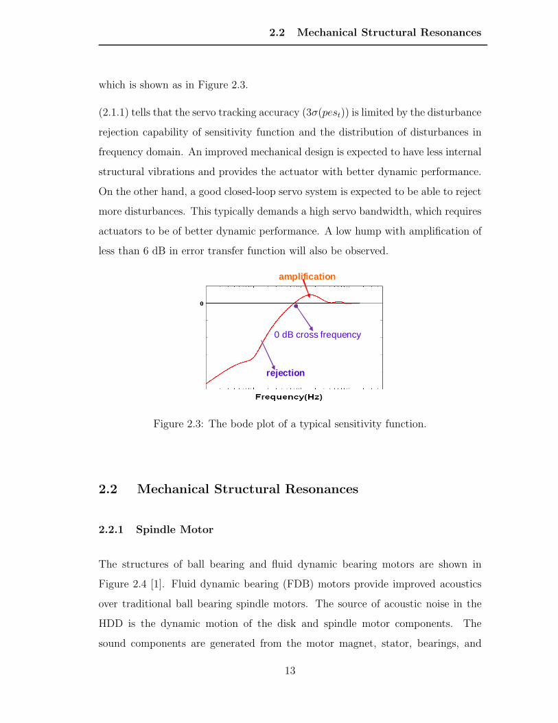
actuators to be of better dynamic performance. A low hump with amplification of
less than 6 dB in error transfer function will also be observed.
rejection
amplification
0 dB cross frequency
Figure 2.3: The bode plot of a typical sensitivity function.
2.2 Mechanical Structural Resonances
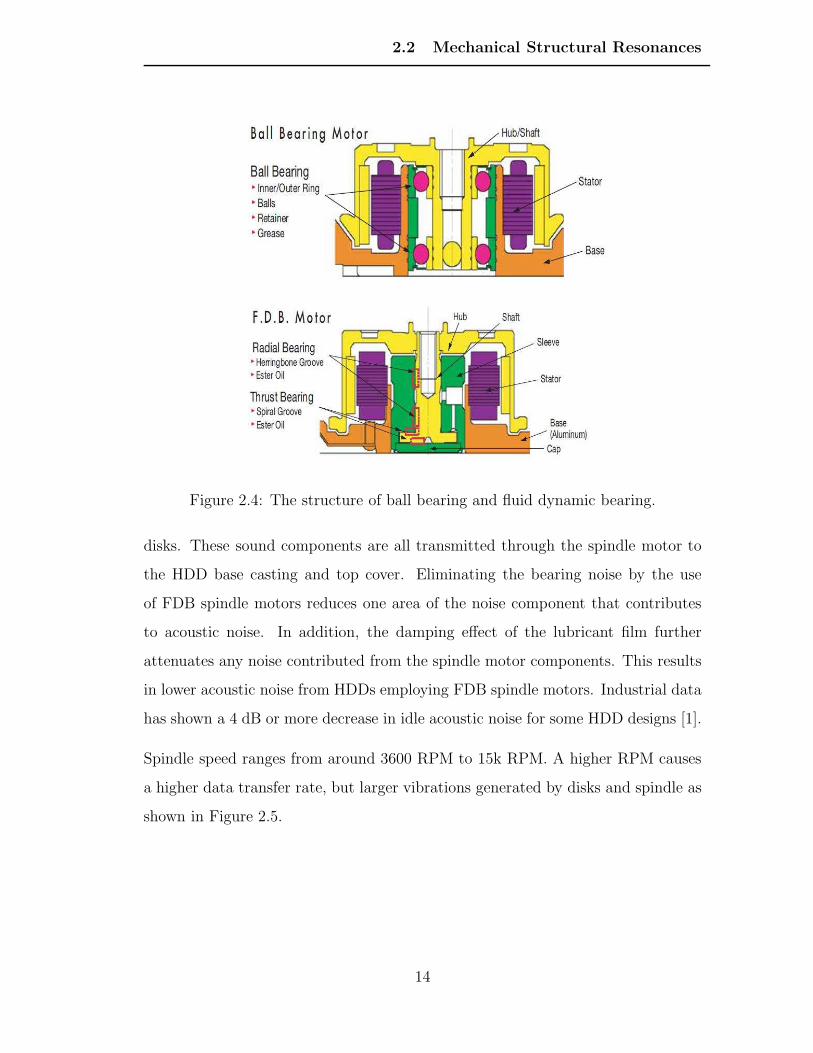
2.2.1 Spindle Motor
The structures of ball bearing and fluid dynamic bearing motors are shown in
Figure 2.4 [1]. Fluid dynamic bearing (FDB) motors provide improved acoustics
over traditional ball bearing spindle motors. The source of acoustic noise in the
HDD is the dynamic motion of the disk and spindle motor components. The
sound components are generated from the motor magnet, stator, bearings, and
13
2.2 Mechanical Structural Resonances
Figure 2.4: The structure of ball bearing and fluid dynamic bearing.
disks. These sound components are all transmitted through the spindle motor to
the HDD base casting and top cover. Eliminating the bearing noise by the use
of FDB spindle motors reduces one area of the noise component that contributes
to acoustic noise. In addition, the damping effect of the lubricant film further
attenuates any noise contributed from the spindle motor components. This results
in lower acoustic noise from HDDs employing FDB spindle motors. Industrial data
has shown a 4 dB or more decrease in idle acoustic noise for some HDD designs [1].
Spindle speed ranges from around 3600 RPM to 15k RPM. A higher RPM causes
a higher data transfer rate, but larger vibrations generated by disks and spindle as
shown in Figure 2.5.
14
2.2 Mechanical Structural Resonances
Figure 2.5: The spindle resonant modes: pitch and radial.
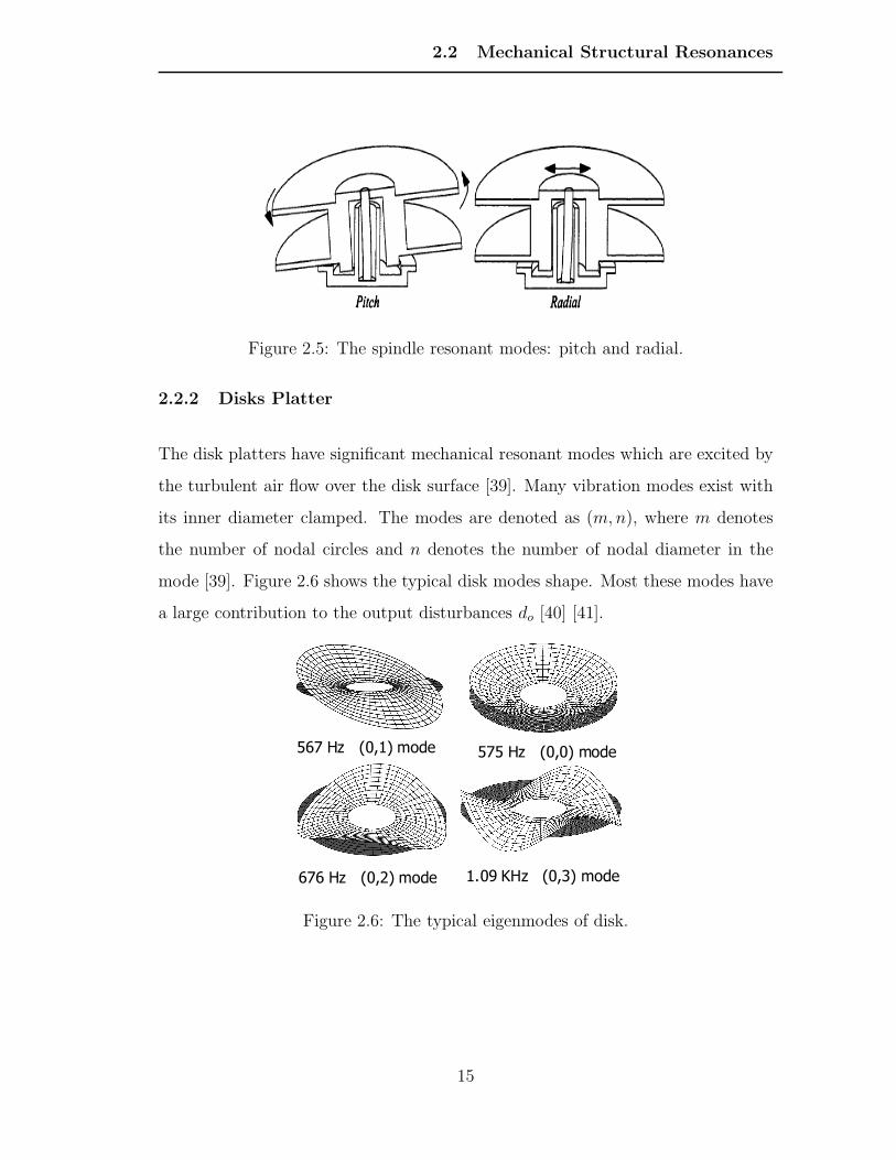
2.2.2 Disks Platter
The disk platters have significant mechanical resonant modes which are excited by
the turbulent air flow over the disk surface [39]. Many vibration modes exist with
its inner diameter clamped. The modes are denoted as (m,n), where m denotes
the number of nodal circles and n denotes the number of nodal diameter in the
mode [39]. Figure 2.6 shows the typical disk modes shape. Most these modes have
a large contribution to the output disturbances do [40] [41].
575 Hz (0,0) mode567 Hz (0,1) mode
676 Hz (0,2) mode 1.09 KHz (0,3) mode
Figure 2.6: The typical eigenmodes of disk.
15
2.2 Mechanical Structural Resonances
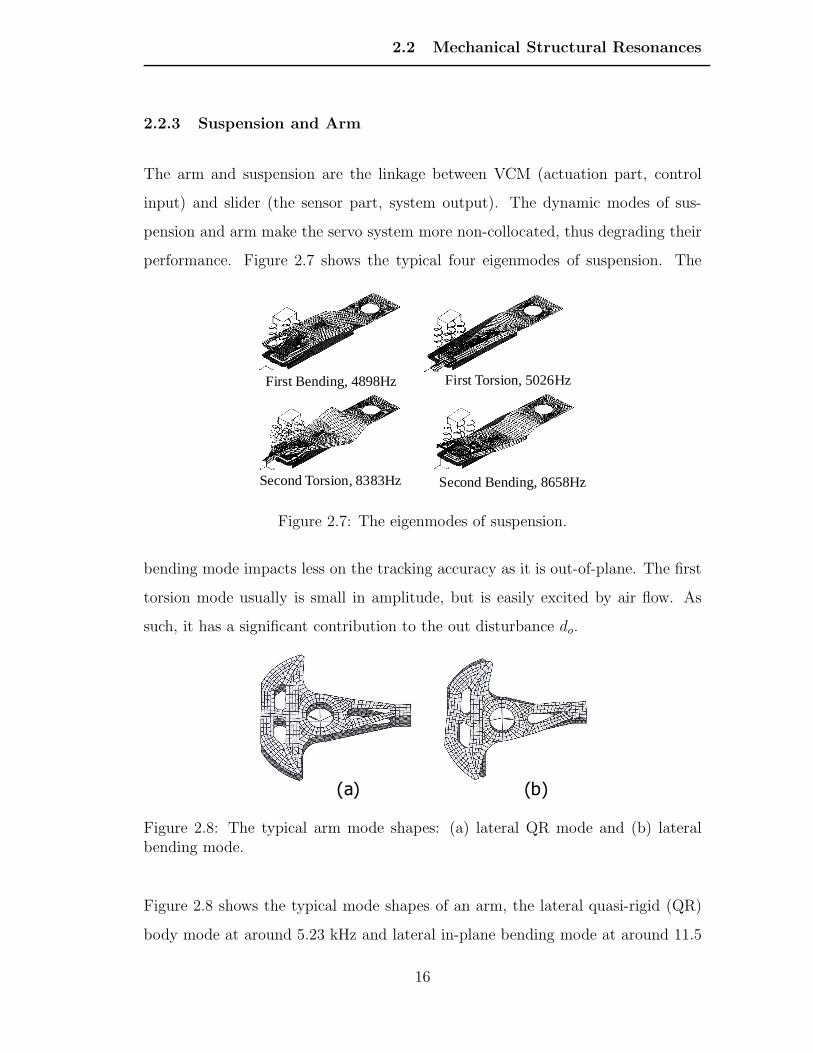
2.2.3 Suspension and Arm
The arm and suspension are the linkage between VCM (actuation part, control
input) and slider (the sensor part, system output). The dynamic modes of sus-
pension and arm make the servo system more non-collocated, thus degrading their
performance. Figure 2.7 shows the typical four eigenmodes of suspension. The
First Bending, 4898Hz First Torsion, 5026Hz
Second Torsion, 8383Hz Second Bending, 8658Hz
Figure 2.7: The eigenmodes of suspension.
bending mode impacts less on the tracking accuracy as it is out-of-plane. The first
torsion mode usually is small in amplitude, but is easily excited by air flow. As
such, it has a significant contribution to the out disturbance do.
( a ) ( b ) (a) (b)
Figure 2.8: The typical arm mode shapes: (a) lateral QR mode and (b) lateralbending mode.
Figure 2.8 shows the typical mode shapes of an arm, the lateral quasi-rigid (QR)
body mode at around 5.23 kHz and lateral in-plane bending mode at around 11.5
16
2.3 Modeling of Servo System
kHz. QR mode is typically the first mode which limits the servo bandwidth, and it
is usually compensated with phase-stable design, notch filters, or active damping
[3].
2.3 Modeling of Servo System
2.3.1 Modeling of VCM Actuator
vk
syk
s( )dH s
yu v
Rigid body
Figure 2.9: The block diagram of VCM model.
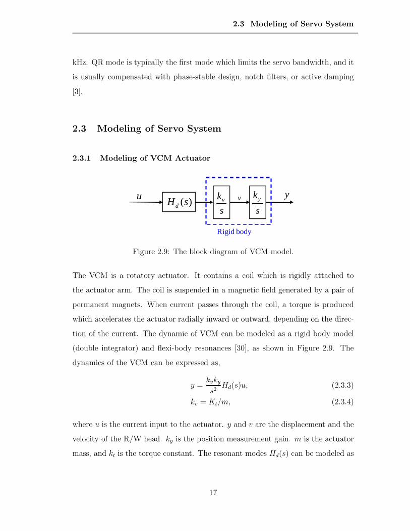
The VCM is a rotatory actuator. It contains a coil which is rigidly attached to
the actuator arm. The coil is suspended in a magnetic field generated by a pair of
permanent magnets. When current passes through the coil, a torque is produced
which accelerates the actuator radially inward or outward, depending on the direc-
tion of the current. The dynamic of VCM can be modeled as a rigid body model
(double integrator) and flexi-body resonances [30], as shown in Figure 2.9. The
dynamics of the VCM can be expressed as,
y =kvkys2
Hd(s)u, (2.3.3)
kv = Kt/m, (2.3.4)
where u is the current input to the actuator. y and v are the displacement and the
velocity of the R/W head. ky is the position measurement gain. m is the actuator
mass, and kt is the torque constant. The resonant modes Hd(s) can be modeled as
17
2.3 Modeling of Servo System
Figure 2.10: Bode plots of frequency response for VCM. (solid line: measured;dotted: identified; dash-dotted: double integrator)
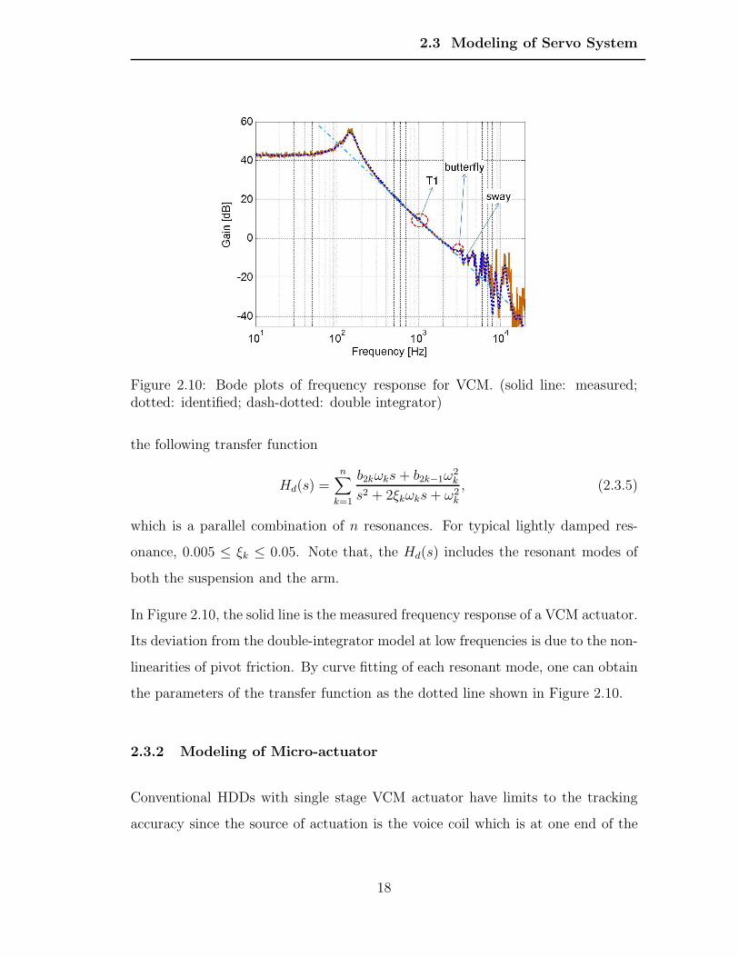
the following transfer function
Hd(s) =n∑
k=1
b2kωks+ b2k−1ω2k
s2 + 2ξkωks+ ω2k
, (2.3.5)
which is a parallel combination of n resonances. For typical lightly damped res-
onance, 0.005 ≤ ξk ≤ 0.05. Note that, the Hd(s) includes the resonant modes of
both the suspension and the arm.
In Figure 2.10, the solid line is the measured frequency response of a VCM actuator.
Its deviation from the double-integrator model at low frequencies is due to the non-
linearities of pivot friction. By curve fitting of each resonant mode, one can obtain
the parameters of the transfer function as the dotted line shown in Figure 2.10.
2.3.2 Modeling of Micro-actuator
Conventional HDDs with single stage VCM actuator have limits to the tracking
accuracy since the source of actuation is the voice coil which is at one end of the
18
2.3 Modeling of Servo System
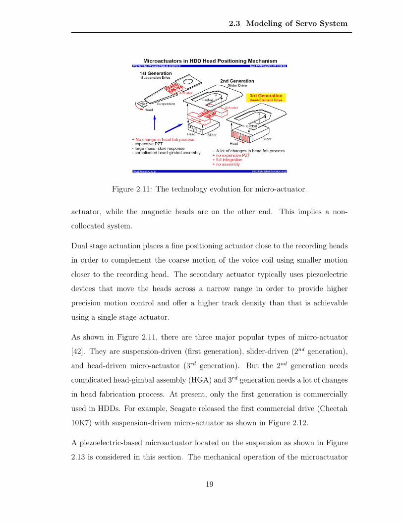
Figure 2.11: The technology evolution for micro-actuator.
actuator, while the magnetic heads are on the other end. This implies a non-
collocated system.
Dual stage actuation places a fine positioning actuator close to the recording heads
in order to complement the coarse motion of the voice coil using smaller motion
closer to the recording head. The secondary actuator typically uses piezoelectric
devices that move the heads across a narrow range in order to provide higher
precision motion control and offer a higher track density than that is achievable
using a single stage actuator.
As shown in Figure 2.11, there are three major popular types of micro-actuator
[42]. They are suspension-driven (first generation), slider-driven (2nd generation),
and head-driven micro-actuator (3rd generation). But the 2nd generation needs
complicated head-gimbal assembly (HGA) and 3rd generation needs a lot of changes
in head fabrication process. At present, only the first generation is commercially
used in HDDs. For example, Seagate released the first commercial drive (Cheetah
10K7) with suspension-driven micro-actuator as shown in Figure 2.12.
A piezoelectric-based microactuator located on the suspension as shown in Figure
2.13 is considered in this section. The mechanical operation of the microactuator
19

2.3 Modeling of Servo System
Figure 2.12: The dual-stage actuator inside Seagate Cheetah 10K7 HDD.
Figure 2.13: A PZT actuated suspension.
20
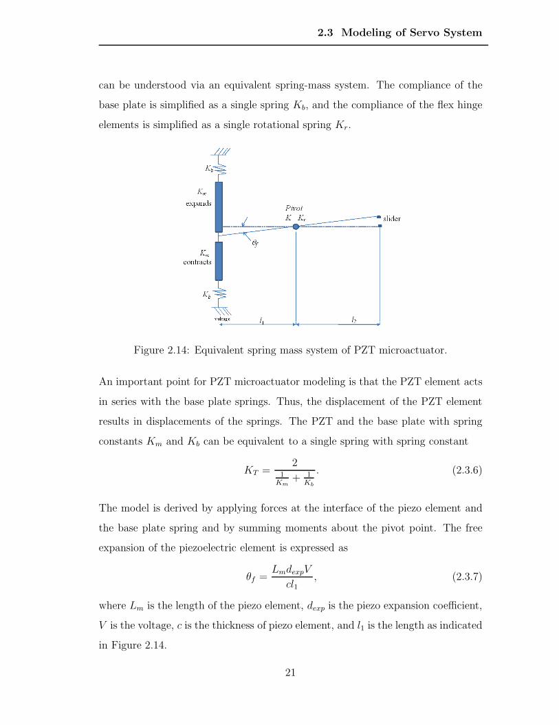
2.3 Modeling of Servo System
can be understood via an equivalent spring-mass system. The compliance of the
base plate is simplified as a single spring Kb, and the compliance of the flex hinge
elements is simplified as a single rotational spring Kr.
Figure 2.14: Equivalent spring mass system of PZT microactuator.
An important point for PZT microactuator modeling is that the PZT element acts
in series with the base plate springs. Thus, the displacement of the PZT element
results in displacements of the springs. The PZT and the base plate with spring
constants Km and Kb can be equivalent to a single spring with spring constant
KT =2
1Km
+ 1Kb
. (2.3.6)
The model is derived by applying forces at the interface of the piezo element and
the base plate spring and by summing moments about the pivot point. The free
expansion of the piezoelectric element is expressed as
θf =LmdexpV
cl1, (2.3.7)
where Lm is the length of the piezo element, dexp is the piezo expansion coefficient,
V is the voltage, c is the thickness of piezo element, and l1 is the length as indicated
in Figure 2.14.
21
2.3 Modeling of Servo System
101
102
103
104
−30
−20
−10
0
Mag
nitu
de(d
B)
101
102
103
104
−200
−160
−120
−80
−40
0
Pha
se(d
eg)
Frequency(Hz)
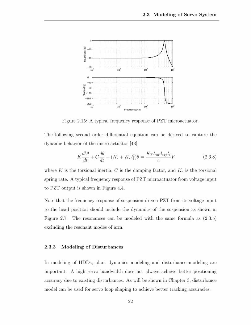
Figure 2.15: A typical frequency response of PZT microactuator.
The following second order differential equation can be derived to capture the
dynamic behavior of the micro-actuator [43]
Kd2θ
dt+ C
dθ
dt+ (Kr +KT l
21)θ =
KTLmdexpl1c
V, (2.3.8)
where K is the torsional inertia, C is the damping factor, and Kr is the torsional
spring rate. A typical frequency response of PZT microactuator from voltage input
to PZT output is shown in Figure 4.4.
Note that the frequency response of suspension-driven PZT from its voltage input
to the head position should include the dynamics of the suspension as shown in
Figure 2.7. The resonances can be modeled with the same formula as (2.3.5)
excluding the resonant modes of arm.
2.3.3 Modeling of Disturbances
In modeling of HDDs, plant dynamics modeling and disturbance modeling are
important. A high servo bandwidth does not always achieve better positioning
accuracy due to existing disturbances. As will be shown in Chapter 3, disturbance
model can be used for servo loop shaping to achieve better tracking accuracies.
22
2.3 Modeling of Servo System
Vibrations in disk drives cause the deviation of the R/W head positioning from the
desired track center. It is the combination of the repeatable runout (RRO) and the
non-repeatable runout (NRRO). Runout that is the same for every revolution of
the disk is called RRO. Hence RRO has identical magnitude at each servo wedge
of a track. Since RRO is synchronized with the frequency of rotation of spindle,
its spectrum is distributed only at the fundamental frequency of spindle rotation
and its harmonics. Disk slip is one of the major causes of RRO. Another major
source of RRO occurs during servo-writing. Servo-writing is the process of writing
servo patterns onto the magnetic disk. Any tracking errors during servo-writing are
permanently written onto each servo pattern and become RRO during the normal
operation of HDD. Other sources of RRO arise from imperfections in the spindle
bearing and magnetic imbalance in the spindle motor. NRRO has many periodic
components as well, but they are not synchronous to the spindle rotation. The
major sources of NRRO are PES demodulation noise, disk vibrations, actuator arm
vibrations, disk enclosure vibrations, and windage [4]. As the repeatable runout is
compensated by iterative adaptive feedforward [44] [45] [46], we focus on the model
of NRRO.
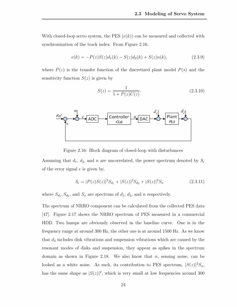
Figure 2.16 shows a simplified block-diagram of disk drive servo loop. y is the
position of the R/W head and e is the position error signal. The signal d1 represents
all the torque disturbances to the system. Such disturbances include any torque
due to air-turbulence force on the actuator, the suspension, and the slider. The
effects of the torque disturbances are dominant at frequencies that are relatively low
as compared to the servo bandwidth. The signal d2 represents output disturbances
that are due to non-repeatable motions of the disk and motor, which are directly
added to the relative position of the R/W head and the reference track. The sensing
noises n includes media noise, head noise, electric noise, and A/D quantization noise
in the PES demodulation circuit. Therefore it is reasonable to model the sensing
noise signal n as a broad-band white noise.
23
2.3 Modeling of Servo System
With closed-loop servo system, the PES (e(k)) can be measured and collected with
synchronization of the track index. From Figure 2.16,
e(k) = −P (z)S(z)d1(k)− S(z)d2(k) + S(z)n(k), (2.3.9)
where P (z) is the transfer function of the discretized plant model P (s) and the
sensitivity function S(z) is given by
S(z) =1
1 + P (z)C(z). (2.3.10)
Figure 2.16: Block diagram of closed-loop with disturbances
Assuming that d1, d2, and n are uncorrelated, the power spectrum denoted by Se
of the error signal e is given by,
Se = |P (z)S(z)|2Sd1 + |S(z)|2Sd2 + |S(z)|2Sn (2.3.11)
where Sd1 , Sd2 , and Sn are spectrum of d1, d2, and n respectively.
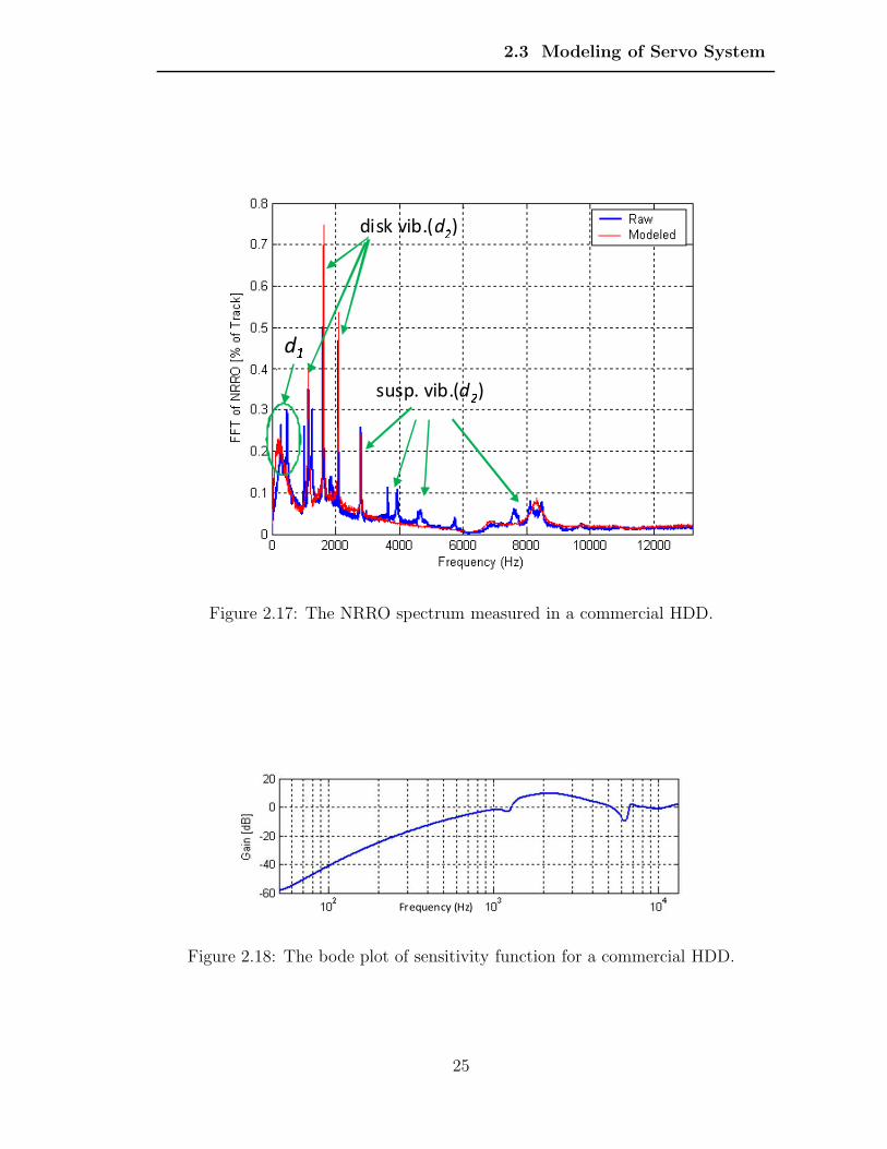
The spectrum of NRRO component can be calculated from the collected PES data
[47]. Figure 2.17 shows the NRRO spectrum of PES measured in a commercial
HDD. Two humps are obviously observed in the baseline curve. One is in the
frequency range at around 300 Hz, the other one is at around 1500 Hz. As we know
that d2 includes disk vibrations and suspension vibrations which are caused by the
resonant modes of disks and suspension, they appear as spikes in the spectrum
domain as shown in Figure 2.18. We also know that n, sensing noise, can be
looked as a white noise. As such, its contribution to PES spectrum, |S(z)|2Sn,
has the same shape as |S(z)|2, which is very small at low frequencies around 300
24
2.3 Modeling of Servo System
disk vib.(d)susp. vib.(d)d
Figure 2.17: The NRRO spectrum measured in a commercial HDD.
Frequency (Hz)
Figure 2.18: The bode plot of sensitivity function for a commercial HDD.
25
2.3 Modeling of Servo System
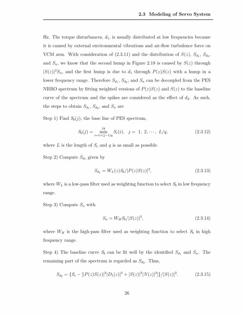
Hz. The torque disturbances, d1, is usually distributed at low frequencies because
it is caused by external environmental vibrations and air-flow turbulence force on
VCM arm. With consideration of (2.3.11) and the distribution of S(z), Sd1 , Sd2 ,
and Sn, we know that the second hump in Figure 2.18 is caused by S(z) through
|S(z)|2Sn, and the first hump is due to d1 through P (z)S(z) with a hump in a
lower frequency range. Therefore Sd1 , Sd2 , and Sn can be decoupled from the PES
NRRO spectrum by fitting weighted versions of P (z)S(z) and S(z) to the baseline
curve of the spectrum and the spikes are considered as the effect of d2. As such,
the steps to obtain Sd1 , Sd2 , and Sn are
Step 1) Find Sb(j), the base line of PES spectrum,
Sb(j) =jq
mini=1+(j−1)q
Se(i), j = 1, 2, · · · , L/q, (2.3.12)
where L is the length of Se and q is as small as possible.
Step 2) Compute Sd1 given by
Sd1 = WL(z)Sb/|P (z)S(z)|2, (2.3.13)
whereWL is a low-pass filter used as weighting function to select Sb in low frequency
range.
Step 3) Compute Sn with
Sn = WHSb/|S(z)|2, (2.3.14)
where WH is the high-pass filter used as weighting function to select Sb in high
frequency range.
Step 4) The baseline curve Sb can be fit well by the identified Sd1 and Sn. The
remaining part of the spectrum is regarded as Sd2 . Thus,
Sd2 = Se − [|P (z)S(z)|2|D1(z)|2 + |S(z)|2|N(z)|2]/|S(z)|2. (2.3.15)
26
2.3 Modeling of Servo System
Step 5) Find stable D1(z), D2(z), and N(z) such that
|D1(z)|2 = Sd1 , (2.3.16)
|D2(z)|2 = Sd2 , (2.3.17)
|N(z)|2 = Sn. (2.3.18)
Step 6) Calculate the models D1(s), D2(s), and N(s) from D1(z), D2(z), and N(z)
using the bilinear approximation method [48].
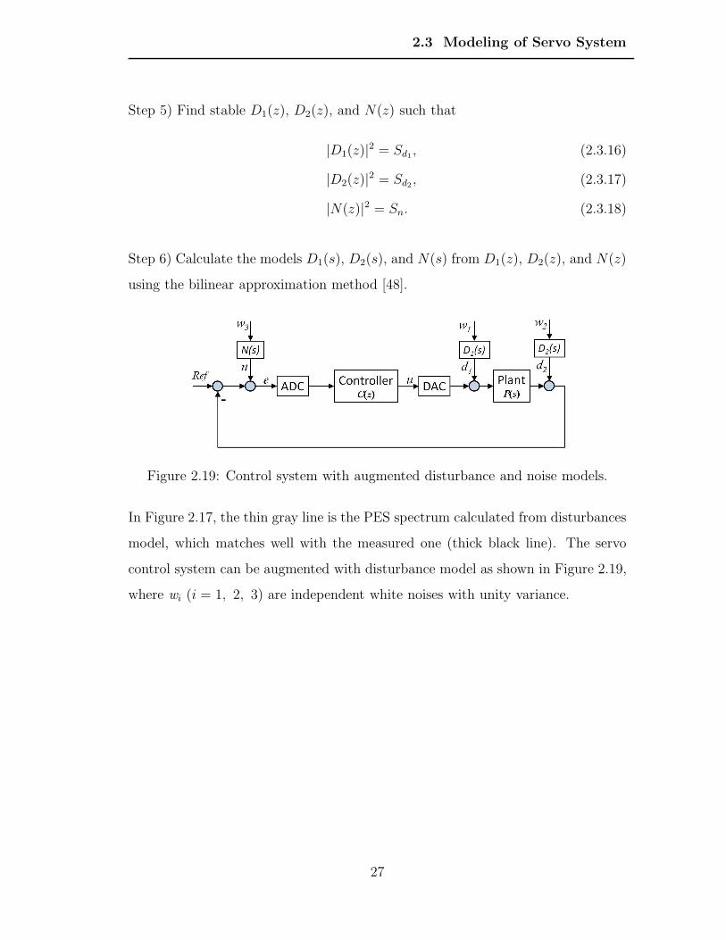
Figure 2.19: Control system with augmented disturbance and noise models.
In Figure 2.17, the thin gray line is the PES spectrum calculated from disturbances
model, which matches well with the measured one (thick black line). The servo
control system can be augmented with disturbance model as shown in Figure 2.19,
where wi (i = 1, 2, 3) are independent white noises with unity variance.
27
Chapter 3
Design Pseudo-sine CurrentProfile for Smooth Seeking
Hard disk drive is widely used in consumer electronics where acoustic noise is
becoming a more important performance index. Quiet seeking is required since
seeking noise is one of the major source of acoustic noise. Residual vibrations
are a significant factor not only to the acoustic problem, but also to the tracking
performance of HDD.
In HDDs, the servo system moves R/W head from one track to another target track
during track seeking. Conventionally, nonlinear controllers such as proximate time-
optimal servo (PTOS) mechanism [30] [31] [32] are widely used for track-seeking.
Other efforts include designing a unified control structure for both track-seeking and
following, such as two-degree-of freedom (2DOF) servo mechanism with adaptive
robust control or zero phase error tracking techniques [33] [34] [35][49]. For most of
these works, the current profile as shown in Figure 3.1 is designed to compromise
between the seek time and smooth switching from seeking to tracking. In Figure
3.1, the actuator is accelerated at maximum positive control effort until it reaches
the maximum velocity. It is kept moving at constant velocity for a certain period,
then it is decelerated at maximum negative control effort until it reaches close
28
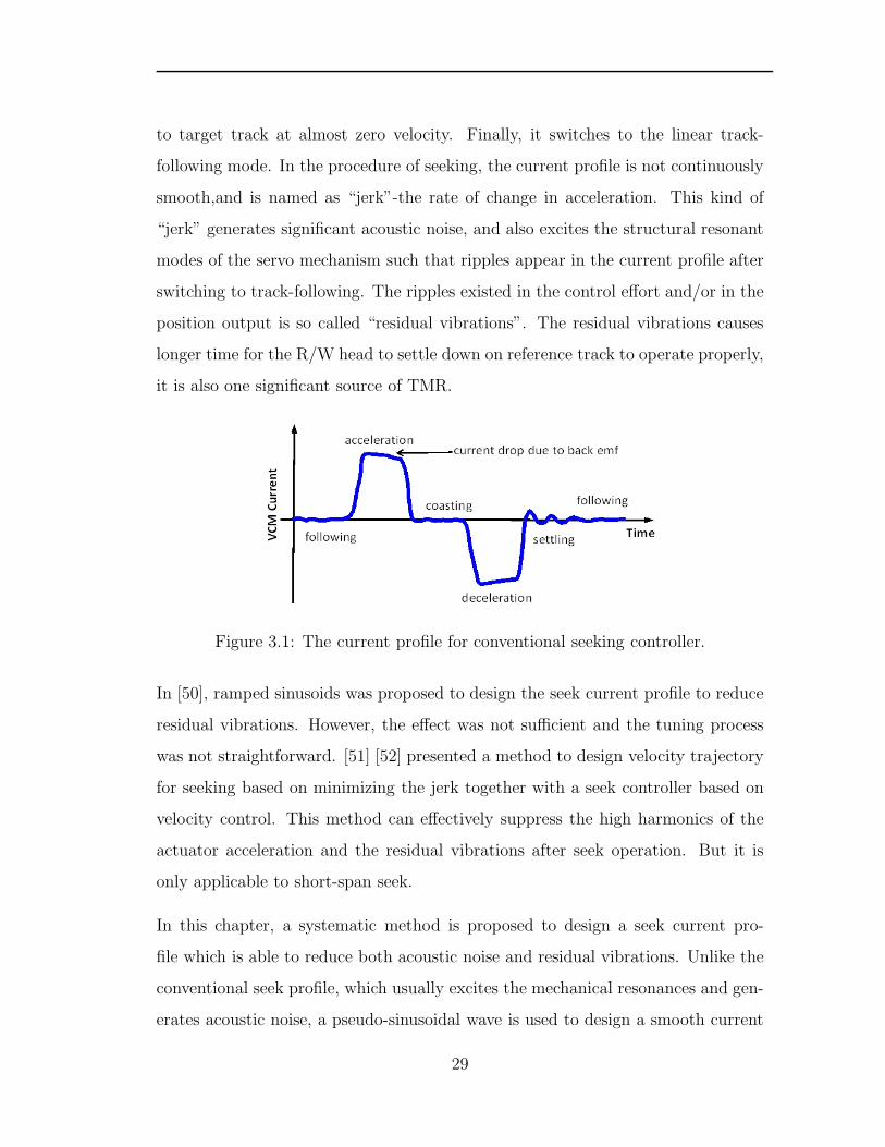
to target track at almost zero velocity. Finally, it switches to the linear track-
following mode. In the procedure of seeking, the current profile is not continuously
smooth,and is named as “jerk”-the rate of change in acceleration. This kind of
“jerk” generates significant acoustic noise, and also excites the structural resonant
modes of the servo mechanism such that ripples appear in the current profile after
switching to track-following. The ripples existed in the control effort and/or in the
position output is so called “residual vibrations”. The residual vibrations causes
longer time for the R/W head to settle down on reference track to operate properly,
it is also one significant source of TMR.
Figure 3.1: The current profile for conventional seeking controller.
In [50], ramped sinusoids was proposed to design the seek current profile to reduce
residual vibrations. However, the effect was not sufficient and the tuning process
was not straightforward. [51] [52] presented a method to design velocity trajectory
for seeking based on minimizing the jerk together with a seek controller based on
velocity control. This method can effectively suppress the high harmonics of the
actuator acceleration and the residual vibrations after seek operation. But it is
only applicable to short-span seek.
In this chapter, a systematic method is proposed to design a seek current pro-
file which is able to reduce both acoustic noise and residual vibrations. Unlike the
conventional seek profile, which usually excites the mechanical resonances and gen-
erates acoustic noise, a pseudo-sinusoidal wave is used to design a smooth current
29
3.1 Problem Formulation for Track-seeking
profile without “jerk”. The current saturation limit and maximum velocity limit
are also considered in the design of current profile to achieve arbitrary seek-length.
A systematic method with a set of design parameters is proposed to minimize the
residual vibrations caused by the most significant resonant mode.
3.1 Problem Formulation for Track-seeking
The rigid model VCM plant in Figure 2.9 can be expressed in state space as,
X = ApX +Bpu
y = CpX (3.1.1)
where
Ap =
0 ky
0 0
, Bp =
0
kv
, Cp =
[
1 0
]
, X =[
y v
]T
The objective of seeking controller is to move actuator from initial state [0 0]T
to target state [y0 0]T . The time optimal controller [30] problem is to minimize
the cost function in (3.1.2) to achieve the fastest seeking, which results maximum
acceleration and deceleration in the velocity profile.
J =∫ tf0 1dt, when |u| ≤ um. (3.1.2)
The time optimal controller will cause chattering at switching point in existence of
noise. PTOS [30] introduces a linear region for switching to overcome chattering
problem.
3.1.1 Minimum Jerk Seeking
For consideration with acoustic noise, one more state x3 = u is introduced, which
is the rate of change in acceleration. For a typical seeking process, the initial states
30
3.2 2DOF with Model Referenced Position and Current FeedforwardControl
and terminating conditions are
x1(0)
x2(0)
x3(0)
=
x01
0
0
, and
x1(tf)
x2(tf)
x3(tf)
=
0
0
0
,
respectively.
Note that tf is fixed, and no constraint is placed for u(t) for simplifying the problem.
The control objective is to find an optimal u∗(t), t ∈ [0, tf ] which minimizes the
cost function J
J =∫ tf0 x2
3(t)dt. (3.1.3)
The optimal control for the minimum jerk seeking is [51],
u∗(t) = −120x0
1
t5ft3 +
180x01
t4ft2 −
60x01
t3ft. (3.1.4)
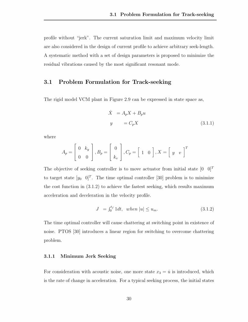
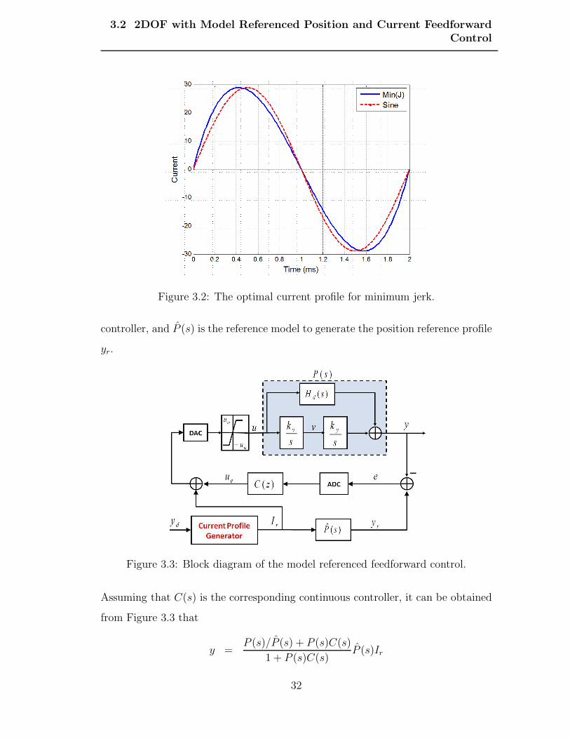
In Figure 3.2, the solid line shows the optimal current profile when x01 = −20, tf =
2, and it is very similar to the dashed line which is a sinusoidal curve.
The optimal current profile in (3.1.4) is derived when the current and velocity
are not limited. It is only applicable for short-span seeking in practice. However,
it infers that smooth sinusoidal current profile causes less jerk and generates less
acoustic noise.
3.2 2DOF with Model Referenced Position and Current
Feedforward Control
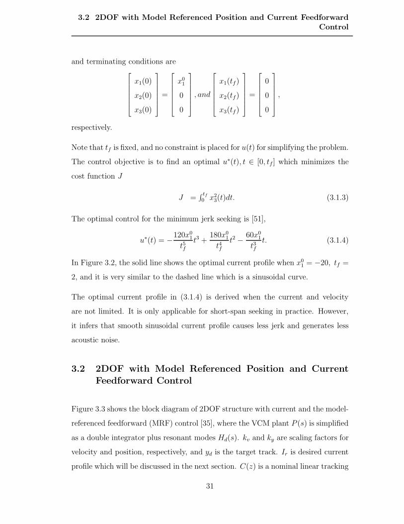
Figure 3.3 shows the block diagram of 2DOF structure with current and the model-
referenced feedforward (MRF) control [35], where the VCM plant P (s) is simplified
as a double integrator plus resonant modes Hd(s). kv and ky are scaling factors for
velocity and position, respectively, and yd is the target track. Ir is desired current
profile which will be discussed in the next section. C(z) is a nominal linear tracking
31
3.2 2DOF with Model Referenced Position and Current FeedforwardControl
Figure 3.2: The optimal current profile for minimum jerk.
controller, and P (s) is the reference model to generate the position reference profile
yr.
Figure 3.3: Block diagram of the model referenced feedforward control.
Assuming that C(s) is the corresponding continuous controller, it can be obtained
from Figure 3.3 that
y =P (s)/P (s) + P (s)C(s)
1 + P (s)C(s)P (s)Ir
32

3.3 The Strategy to Design Pseudo-sine Current Profile
=P (s)/P (s) + P (s)C(s)
1 + P (s)C(s)yr, (3.2.5)
and
e = yr − y =1− P (s)/P (s)
1 + P (s)C(s)yr (3.2.6)
(3.2.5) and (3.2.6) show that the output y will follow the reference track profile yr
exactly if the reference model P (s) is the same as the plant P (s). The advantage
of using the MRF lies in the fact that the VCM actuator can be driven directly
by the feedforward current signal, whose profile can be customized by designers.
Furthermore, the feedforward current loop is not limited by inherent sampling
frequency of HDD servo system, which is determined by the number of servo sectors
and spindle rotational speed. As such, a novel current profile can be designed to
minimize the residual vibrations which is discussed in Section 3.3.
3.3 The Strategy to Design Pseudo-sine Current Profile
In HDD servo channel, the current driver can only provide limited value of current
as shown in Figure 3.3. In addition, the maximum seeking velocity is also limited to
keep the read/write head flying properly and to ensure reading back the full servo
patterns in servo wedges. A proper current profile Ir(t), as shown in Fig. 3.4, has
acceleration (0 to t1), coasting (t1 to t2), and deceleration (t2 to t5) stages. I1(t)
is a current profile with no saturation and coasting for short-span seeking. The
velocity of VCM increases until the maximum value reaches during the acceleration
stage. During the coasting stage, the acceleration is zero and the velocity keeps
at its maximum value. During the deceleration stage, the velocity of VCM is
reduced from its maximum to zero before settling down on a target track. Both
the acceleration and deceleration stages are divided into three segments: rising
transition (S1, S4), saturation (maximum acceleration/deceleration), and falling
transition (S2, S3).
33
3.3 The Strategy to Design Pseudo-sine Current Profile
0 10 20 30 40 50 60 70 80−1.25
−1
−0.75
−0.5
−0.25
0
0.25
0.5
0.75
1
1.25Current Profile
Normalized Time (Samples)
Nor
mal
ized
Am
plitu
de
Ir(t)
cosI1(t)
S2
S1
Settling
t1
cosinoidal wave
t2
t5
S4S
3
T1
Th
Tc
t3
t4
Figure 3.4: Pseudo sinusoidal current profile.
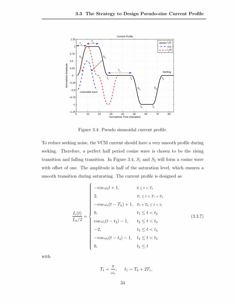
To reduce seeking noise, the VCM current should have a very smooth profile during
seeking. Therefore, a perfect half period cosine wave is chosen to be the rising
transition and falling transition. In Figure 3.4, S1 and S2 will form a cosine wave
with offset of one. The amplitude is half of the saturation level, which ensures a
smooth transition during saturating. The current profile is designed as
Ir(t)
Im/2=
−cosωit+ 1, 0 ≤ t < T1
2, T1 ≤ t < T1 + Th
−cosωi(t− Th) + 1, T1 + Th ≤ t < t1
0, t1 ≤ t < t2
cosωi(t− t2)− 1, t2 ≤ t < t3
−2, t3 ≤ t < t4
−cosωi(t− t4)− 1, t4 ≤ t < t5
0, t5 ≤ t
(3.3.7)
with
T1 =π
ωi
, t1 = Th + 2T1,
34

3.3 The Strategy to Design Pseudo-sine Current Profile
t2 = t1 + Tc, t3 = t2 + T1,
t4 = t3 + Th, t5 = t4 + T1,
where ωi is the frequency of cosine wave, Th is saturation time, and Tc is coasting
time. With the current profile and the reference model, we can derive the trajectory
of the velocity and position. A rigid VCM plant model, a double integrator with
velocity and position scaling factor kv and ky as shown in Fig. 3.3, is used as
reference model in this chapter. The velocity and position reference trajectory
can be derived from the current profile directly. In practical implementation, the
position reference trajectory can be generated from reference model directly.
3.3.1 Pseudo-sine Current Profile Generation
Before deriving a proper current profile for seeking the target track yd, the following
parameters need to be specified:
1. The frequency of the sinusoidal wave (ωi) with consideration of reducing
acoustic noise:
It determines the acceleration of current which will affect the amplitude of
acoustic noise and seek time. The acoustic noise is mainly caused by the
jerk in acceleration. As such, a low frequency will result in low acoustic
noise but relatively long seek time. As the relationship in between seeking
acoustic noise and frequency is not clearly known yet, the determination of
the frequency is based on trial and error.
2. The maximum current (Im):
It is specified by current driver.
3. The maximum velocity (Vmax):
It is set to ensure read/write head to fly properly [53] and to read back a full
servo pattern properly.
35
3.3 The Strategy to Design Pseudo-sine Current Profile
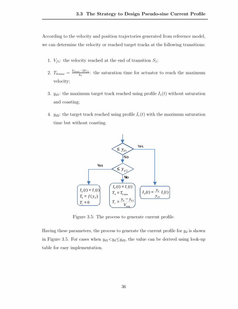
According to the velocity and position trajectories generated from reference model,
we can determine the velocity or reached target tracks at the following transitions:
1. Vf1: the velocity reached at the end of transition S1;
2. Thmax =Vmax−2Vf1
kv: the saturation time for actuator to reach the maximum
velocity;
3. yd1: the maximum target track reached using profile I1(t) without saturation
and coasting;
4. yd2: the target track reached using profile Ir(t) with the maximum saturation
time but without coasting.
1dy≤
2dy≤
)()( 1
1
tIy
ytI
d
dd =
0
)(
)()(
==
=
c
dh
rd
T
yfT
tItI
max
2
max
)()(
V
yyT
TT
tItI
ddc
hh
rd
−=
==
Figure 3.5: The process to generate current profile.
Having these parameters, the process to generate the current profile for yd is shown
in Figure 3.5. For cases when yd1<yd≤yd2, the value can be derived using look-up
table for easy implementation.
36
3.3 The Strategy to Design Pseudo-sine Current Profile
3.3.2 Minimizing Residual Vibrations
The seeking residual vibrations are caused by the lightly-damped structural reso-
nant modes of the actuator. The residual vibrations are actually the response of
the resonant dynamics Hd(s) (in Fig. 3.3) to the transients, such as S1, S2, S3, and
S4 in the current profile.
According to the current profile shown in Fig. 3.4, we have,
S2(t)=−S1(t−T1−Th), (3.3.8)
S4(t)=−S3(t−T1−Th). (3.3.9)
Define Vri(t) as the response of Hd(s) to Si(t) for i=1, 2, 3, 4. Note that
Vr2=−Vr1(t−T1−Th), (3.3.10)
Vr4=−Vr3(t−T1−Th). (3.3.11)
The total residual vibrations due to S1 and S2 denoted by V12(t), and that due to
S3 and S4 denoted by V34(t) can be calculated
V12(t) = Vr1(t)− Vr1(t− T1 − Th), (3.3.12)
V34(t) = Vr3(t)− Vr3(t− T1 − Th), (3.3.13)
respectively.
Since there is usually one dominant resonant mode in Hd(s) whose frequency is
ωr, both Vr1 and Vr2 are slowly decayed periodical signals with period Tr=2πωr. If
T1+Th=N×Tr with N being an integer, V12 is minimized by using the response to
S2 to cancel the response to S1. The same scenario is applied to V34.
On the other hand for short-span seek where Th is zero, T1 needs to be multiples
of Tr to minimize residual vibrations. In addition, as V34 can be regarded as −V12
delayed by (2T1+Th+Tc), we can choose T1, Th, and Tc to be multiples of Tr to
achieve minimum residual vibration for all cases.
37
3.4 Simulation and Comparison with PTOS
Note that Tc and Th are not arbitrary selected but calculated from yd. When
the calculated values are not multiples of Tr, the following strategy can be applied.
First, set the value to the closest multiples of Tr by increasing the calculated values.
As such, the reached target track will be different from yd, e.g. yd. We can then
scale the amplitude of current profile by the factor ydyd.
3.4 Simulation and Comparison with PTOS
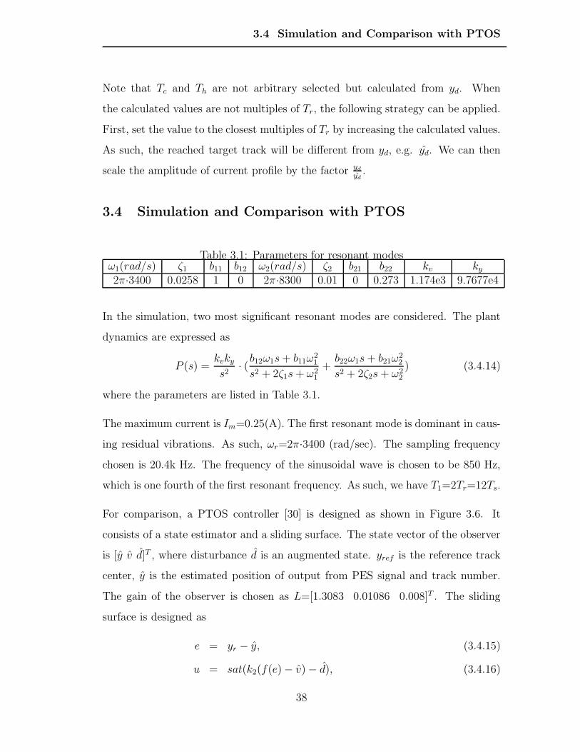
Table 3.1: Parameters for resonant modesω1(rad/s) ζ1 b11 b12 ω2(rad/s) ζ2 b21 b22 kv ky2π·3400 0.0258 1 0 2π·8300 0.01 0 0.273 1.174e3 9.7677e4
In the simulation, two most significant resonant modes are considered. The plant
dynamics are expressed as
P (s) =kvkys2
· (b12ω1s+ b11ω
21
s2 + 2ζ1s+ ω21
+b22ω1s+ b21ω
22
s2 + 2ζ2s+ ω22
) (3.4.14)
where the parameters are listed in Table 3.1.
The maximum current is Im=0.25(A). The first resonant mode is dominant in caus-
ing residual vibrations. As such, ωr=2π·3400 (rad/sec). The sampling frequency
chosen is 20.4k Hz. The frequency of the sinusoidal wave is chosen to be 850 Hz,
which is one fourth of the first resonant frequency. As such, we have T1=2Tr=12Ts.
For comparison, a PTOS controller [30] is designed as shown in Figure 3.6. It
consists of a state estimator and a sliding surface. The state vector of the observer
is [y v d]T , where disturbance d is an augmented state. yref is the reference track
center, y is the estimated position of output from PES signal and track number.
The gain of the observer is chosen as L=[1.3083 0.01086 0.008]T . The sliding
surface is designed as
e = yr − y, (3.4.15)
u = sat(k2(f(e)− v)− d), (3.4.16)
38
3.4 Simulation and Comparison with PTOS
f(e) =
k1k2(e), for |e| ≤ yl
sgn(e)[√
2αImkv|e| −Imk2], for |e| > yl
(3.4.17)
where yl=Imk1, k1 and k2 are chosen to be 0.032 and 2.7581, respectively.
)(sP
vk
syk
s
( )dH smaxu
maxu− driver
du
y
State Estimator
ADC
ˆdu
vy( )f ⋅
2k
+
cv −
−
+
+
−
++
my
++
+
−
Plant:
u
PTOS
e
refydy
Figure 3.6: The block diagram of PTOS.
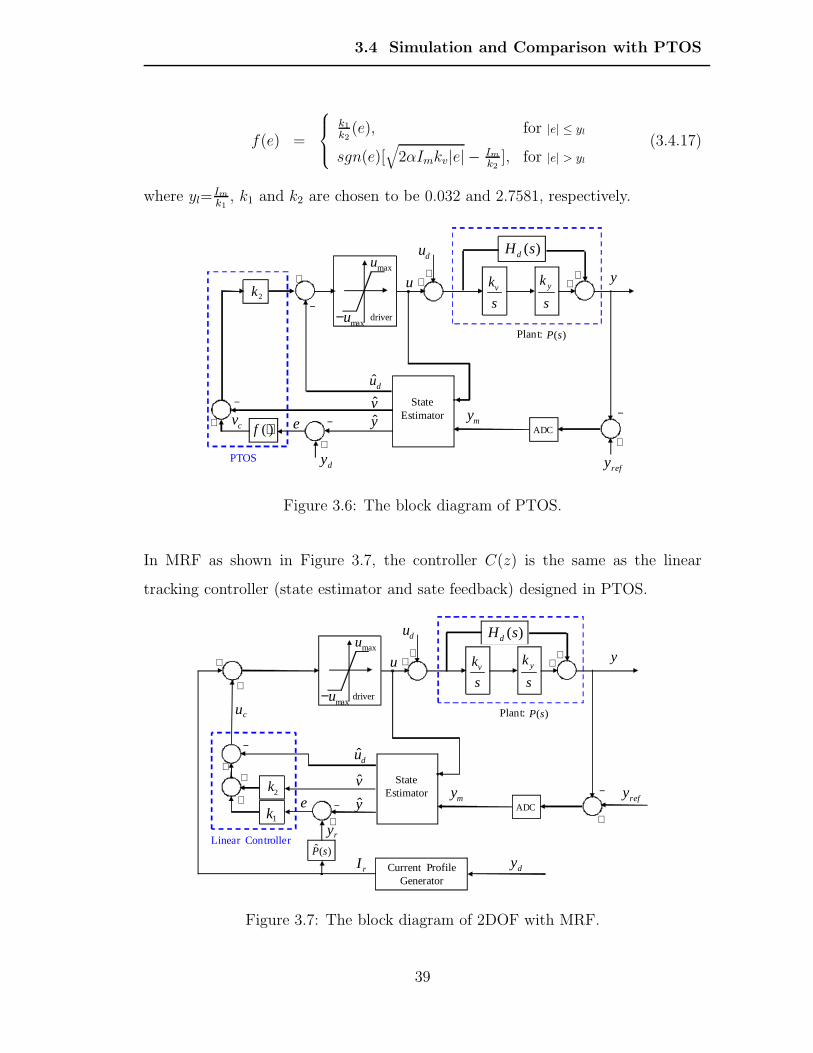
In MRF as shown in Figure 3.7, the controller C(z) is the same as the linear
tracking controller (state estimator and sate feedback) designed in PTOS.
vk
syk
s
( )dH smaxu
maxu− driver
du
y
State Estimator
ADC
ˆdu
v
y2k
+−
+
−
++
my
++
+
−
Plant:
u
e refy
ry1k
+
+
Linear Controller
Current Profile Generator
dy
)(sP
rI
+
+
cu
)(ˆ sP
Figure 3.7: The block diagram of 2DOF with MRF.
39
3.4 Simulation and Comparison with PTOS
0 1 2 3 4 5 6
x 10−3
−0.2
0
0.2
0.4
0.6
0.8
1
Time (second)
Pos
ition
(T
rack
s)
One track seek
PTOS−yMRF−yPTOS−y zoomedMRF−y zoomed
Zoomed
MRF
Figure 3.8: Position output for one track seeking.
0 1 2 3 4 5 6
x 10−3
−0.01
0
0.01
0.02
0.03
Time (second)
Cur
rent
(A
mp)
, Vel
ocity
(0.
5m/s
)
One track seek
PTOS−CurrentMRF−CurrentPTOS−VelocityMRF−VelocityMRF
Figure 3.9: Velocity and current profile for one track seeking.
40
3.4 Simulation and Comparison with PTOS
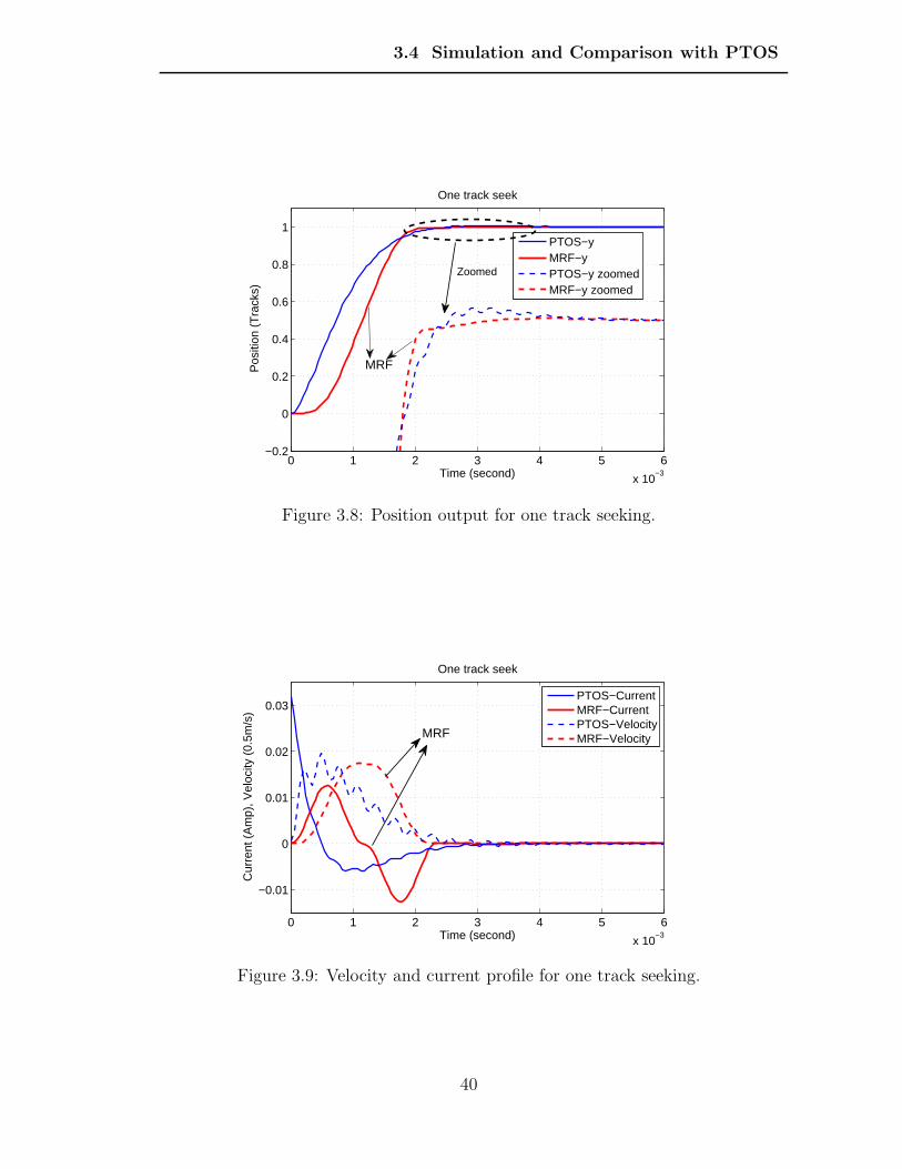
Figures. 3.8 and 3.9 show the position output, velocity, and current profiles for
one track seeking, where thin lines are for PTOS and thick lines are for MRF. As
the full-scaled current profile I1(t) shown in Figure 3.4 can reach 19.839 tracks, the
feedforward current can be derived as [I1(t)/19.839]. From the position curves, it
can be seen that the residual vibration is significantly reduced in MRF, which is
also confirmed in velocity trajectory. The seek time for MRF is even less than that
for PTOS. Although the starting current and ending current in MRF are smaller
than those in PTOS, the intermediate acceleration and deceleration in MRF are
larger, which enable that the MRF scheme can provide rather smooth signal for
starting and ending currents as well as faster seeking.
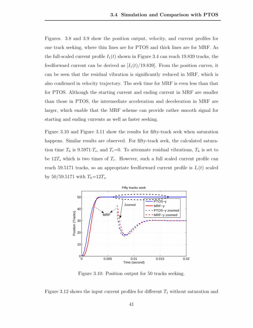
Figure 3.10 and Figure 3.11 show the results for fifty-track seek when saturation
happens. Similar results are observed. For fifty-track seek, the calculated satura-
tion time Th is 9.5971·Ts, and Tc=0. To attenuate residual vibrations, Th is set to
be 12Ts which is two times of Tr. However, such a full scaled current profile can
reach 59.5171 tracks, so an appropriate feedforward current profile is Ir(t) scaled
by 50/59.5171 with Th=12Ts.
0 0.005 0.01 0.015 0.020
10
20
30
40
50
Time (second)
Pos
ition
(T
rack
s)
Fifty tracks seek
PTOS−yMRF−yPTOS−y zoomedMRF−y zoomed
Zoomed
MRF
Figure 3.10: Position output for 50 tracks seeking.
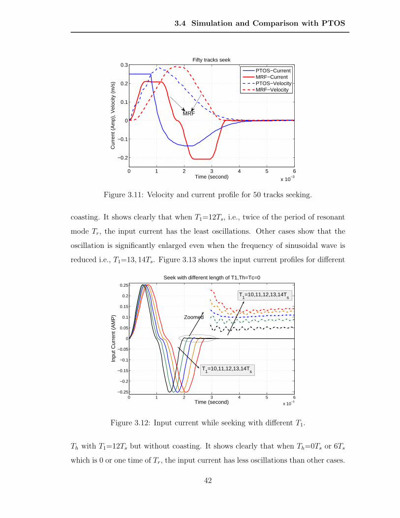
Figure 3.12 shows the input current profiles for different T1 without saturation and
41
3.4 Simulation and Comparison with PTOS
0 1 2 3 4 5 6
x 10−3
−0.2
−0.1
0
0.1
0.2
0.3
Time (second)
Cur
rent
(A
mp)
, Vel
ocity
(m
/s)
Fifty tracks seek
PTOS−CurrentMRF−CurrentPTOS−VelocityMRF−Velocity
MRF
Figure 3.11: Velocity and current profile for 50 tracks seeking.
coasting. It shows clearly that when T1=12Ts, i.e., twice of the period of resonant
mode Tr, the input current has the least oscillations. Other cases show that the
oscillation is significantly enlarged even when the frequency of sinusoidal wave is
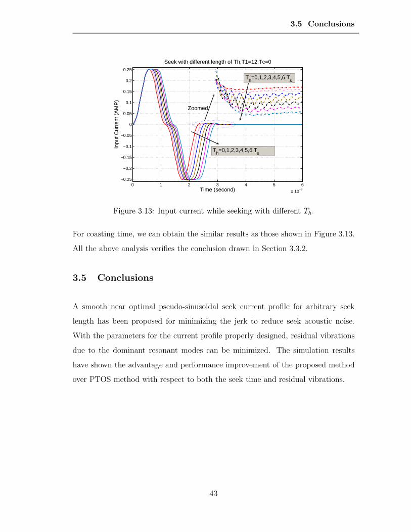
reduced i.e., T1=13, 14Ts. Figure 3.13 shows the input current profiles for different
0 1 2 3 4 5 6
x 10−3
−0.25
−0.2
−0.15
−0.1
−0.05
0
0.05
0.1
0.15
0.2
0.25
Time (second)
Inpu
t Cur
rent
(A
MP
)
Seek with different length of T1,Th=Tc=0
Zoomed
T1=10,11,12,13,14T
s
T1=10,11,12,13,14T
s
Figure 3.12: Input current while seeking with different T1.
Th with T1=12Ts but without coasting. It shows clearly that when Th=0Ts or 6Ts
which is 0 or one time of Tr, the input current has less oscillations than other cases.
42
3.5 Conclusions
0 1 2 3 4 5 6
x 10−3
−0.25
−0.2
−0.15
−0.1
−0.05
0
0.05
0.1
0.15
0.2
0.25
Time (second)
Inpu
t Cur
rent
(A
MP
)
Seek with different length of Th,T1=12,Tc=0
Th=0,1,2,3,4,5,6 T
s
Th=0,1,2,3,4,5,6 T
s
Zoomed
Figure 3.13: Input current while seeking with different Th.
For coasting time, we can obtain the similar results as those shown in Figure 3.13.
All the above analysis verifies the conclusion drawn in Section 3.3.2.
3.5 Conclusions
A smooth near optimal pseudo-sinusoidal seek current profile for arbitrary seek
length has been proposed for minimizing the jerk to reduce seek acoustic noise.
With the parameters for the current profile properly designed, residual vibrations
due to the dominant resonant modes can be minimized. The simulation results
have shown the advantage and performance improvement of the proposed method
over PTOS method with respect to both the seek time and residual vibrations.
43
Chapter 4
IES Settling Controller forDual-stage Servo System
Dual-stage servo system is one of the most obvious technologies to achieve the
high servo performance [54] [55] [56] [40] [57] [58]. The design of tracking/seeking
controller proposed in Chapter 3 and 4 can be applied to dual-stage servo systems
for the requirements of HDD in consumer applications. In this chapter, a settling
controller is proposed for dual-stage servo systems. There are a few algorithms
developed to achieve fast and smooth settling in current literature. The most
famous is initial value compensation (IVC) method [59] [60]. This method is quite
effective for the single stage servo loop with voice coil motor (VCM). However, it
will encounter problem if the servo system has double roots, which lead to a singular
matrix whose inverse does not exist. Another method is command shaping [61] [62]
method, which only considers initial value of displacement. In the method proposed
in this chapter, the transient response of the position error due to the VCM nonzero
initial states is taken into account, and a compensation signal is generated and
injected at the controller input to shape the position error signal and thus cancel the
undesired transitions due to the initial states. This is the called initial error shaping
(IES) method. The IES method can be used to deal with transient problems caused
by both initial position and initial velocity. With this method, only one feedforward
controller is needed, and the implementation is straightforward using look up table
44
4.1 Settling Problem in Dual-stage Servo Systems
(LUT) without requirement of much computation resources.
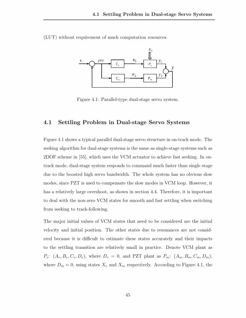
Figure 4.1: Parallel-type dual-stage servo system.
4.1 Settling Problem in Dual-stage Servo Systems
Figure 4.1 shows a typical parallel dual-stage servo structure in on-track mode. The
seeking algorithm for dual-stage systems is the same as single-stage systems such as
2DOF scheme in [55], which uses the VCM actuator to achieve fast seeking. In on-
track mode, dual-stage system responds to command much faster than single stage
due to the boosted high servo bandwidth. The whole system has no obvious slow
modes, since PZT is used to compensate the slow modes in VCM loop. However, it
has a relatively large overshoot, as shown in section 4.4. Therefore, it is important
to deal with the non-zero VCM states for smooth and fast settling when switching
from seeking to track-following.
The major initial values of VCM states that need to be considered are the initial
velocity and initial position. The other states due to resonances are not consid-
ered because it is difficult to estimate these states accurately and their impacts
to the settling transition are relatively small in practice. Denote VCM plant as
Pv: (Av, Bv, Cv, Dv), where Dv = 0, and PZT plant as Pm: (Am, Bm, Cm, Dm),
where Dm = 0, using states Xv and Xm respectively. According to Figure 4.1, the
45
4.1 Settling Problem in Dual-stage Servo Systems
dual-stage plant P (s) = [Pv(s), Pm(s)] is described as,
Xp =
Xv
Xm
, u =
u1
u2
,
Xp(k + 1)−
X0
0
= ApXp(k) +Bpu(k)
y(k) = y1(k) + y2(k) = CpXp(k)
,
(4.1.1)
where
Ap =
Av 0
0 Xm
, Bp =
Bv 0
0 Bm
, Cp =
[
Cv Cm
]
. (4.1.2)
The controller C(z)T = [Cv(z) Cm(z)] is written in state space as,
Xc(k + 1) = AcXc(k) +Bc(yr(k)− y(k)),
u(k) = CcXc(k) +Dc(yr(k)− y(k)).(4.1.3)
The output of the closed-loop system is obtained as
y = [C · adj(zI − A)B
|zI −A|+D]yr +
C · adj(zI − A)z
|zI −A|
X0
0
, (4.1.4)
where
A =
Ap − BpDcCp BpCc
−BcCp Ac
, B =
Bp
Cc
, C =[
Cp 0
]
, D = 0. (4.1.5)
X0 is the plant initial states including initial position y0 and initial velocity v0 of
VCM actuator. yr is the command reference signal. Given yr being zero during
tracking, we could deduce the transient response to the non-zero VCM actuator ini-
tial states y0 and v0 from (4.1.4) after mode-switching [63]. This transient response
to non-zero initial states of VCM can lead to a longer settling time.
46
4.2 IES for Dual-Stage Systems
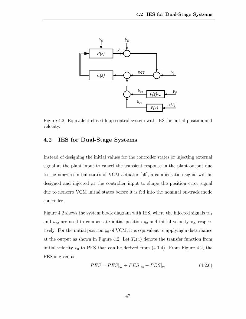
Figure 4.2: Equivalent closed-loop control system with IES for initial position andvelocity.
4.2 IES for Dual-Stage Systems
Instead of designing the initial values for the controller states or injecting external
signal at the plant input to cancel the transient response in the plant output due
to the nonzero initial states of VCM actuator [59], a compensation signal will be
designed and injected at the controller input to shape the position error signal
due to nonzero VCM initial states before it is fed into the nominal on-track mode
controller.
Figure 4.2 shows the system block diagram with IES, where the injected signals uc1
and uc2 are used to compensate initial position y0 and initial velocity v0, respec-
tively. For the initial position y0 of VCM, it is equivalent to applying a disturbance
at the output as shown in Figure 4.2. Let Tv(z) denote the transfer function from
initial velocity v0 to PES that can be derived from (4.1.4). From Figure 4.2, the
PES is given as,
PES = PES|yr + PES|y0 + PES|v0 (4.2.6)
47
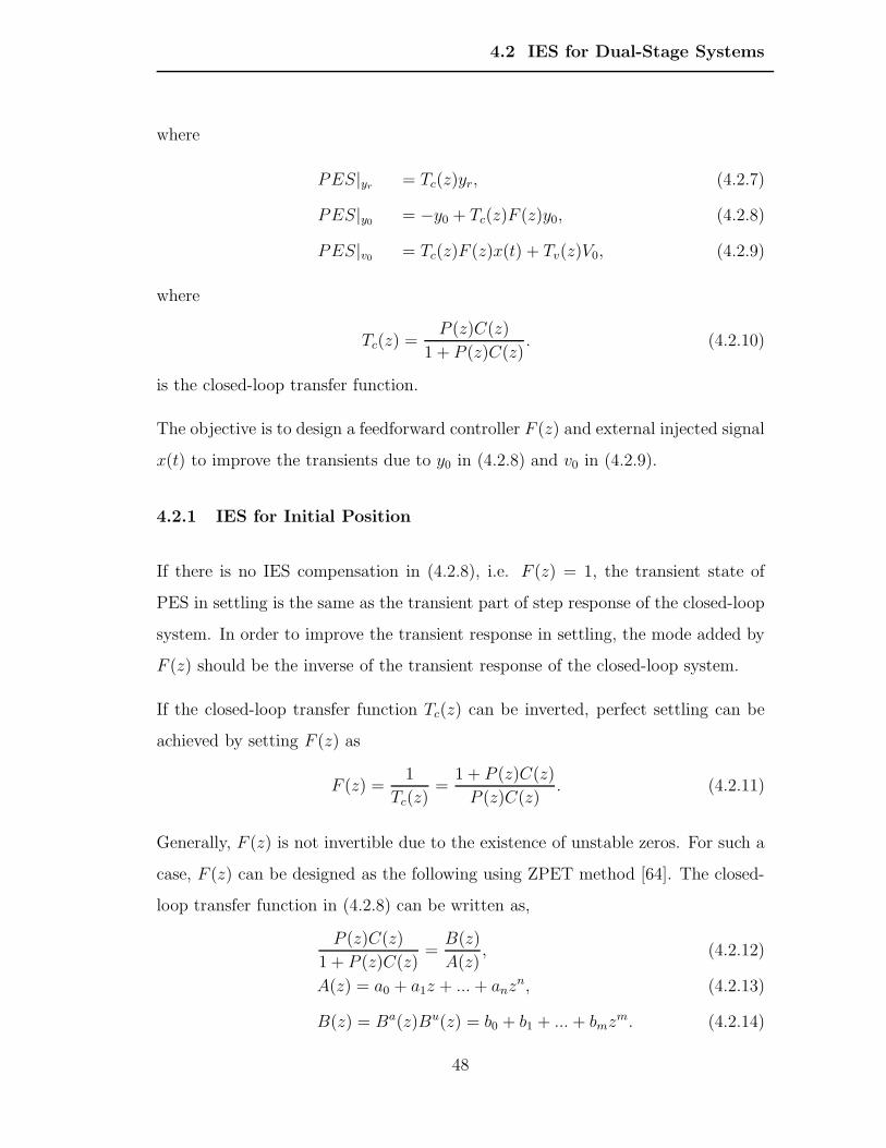
4.2 IES for Dual-Stage Systems
where
PES|yr = Tc(z)yr, (4.2.7)
PES|y0 = −y0 + Tc(z)F (z)y0, (4.2.8)
PES|v0 = Tc(z)F (z)x(t) + Tv(z)V0, (4.2.9)
where
Tc(z) =P (z)C(z)
1 + P (z)C(z). (4.2.10)
is the closed-loop transfer function.
The objective is to design a feedforward controller F (z) and external injected signal
x(t) to improve the transients due to y0 in (4.2.8) and v0 in (4.2.9).
4.2.1 IES for Initial Position
If there is no IES compensation in (4.2.8), i.e. F (z) = 1, the transient state of
PES in settling is the same as the transient part of step response of the closed-loop
system. In order to improve the transient response in settling, the mode added by
F (z) should be the inverse of the transient response of the closed-loop system.
If the closed-loop transfer function Tc(z) can be inverted, perfect settling can be
achieved by setting F (z) as
F (z) =1
Tc(z)=
1 + P (z)C(z)
P (z)C(z). (4.2.11)
Generally, F (z) is not invertible due to the existence of unstable zeros. For such a
case, F (z) can be designed as the following using ZPET method [64]. The closed-
loop transfer function in (4.2.8) can be written as,
P (z)C(z)
1 + P (z)C(z)=
B(z)
A(z), (4.2.12)
A(z) = a0 + a1z + ... + anzn, (4.2.13)
B(z) = Ba(z)Bu(z) = b0 + b1 + ... + bmzm. (4.2.14)
48
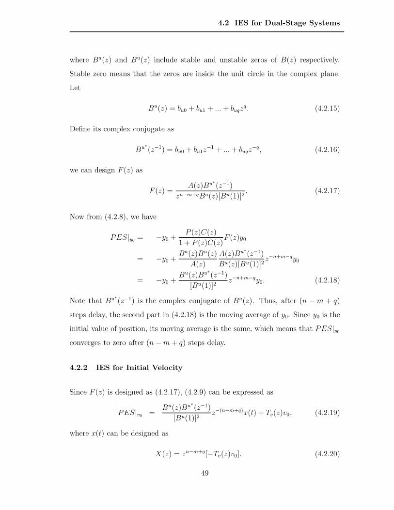
4.2 IES for Dual-Stage Systems
where Ba(z) and Bu(z) include stable and unstable zeros of B(z) respectively.
Stable zero means that the zeros are inside the unit circle in the complex plane.
Let
Bu(z) = bu0 + bu1 + ... + buqzq. (4.2.15)
Define its complex conjugate as
Bu∗
(z−1) = bu0 + bu1z−1 + ...+ buqz
−q, (4.2.16)
we can design F (z) as
F (z) =A(z)Bu∗
(z−1)
zn−m+qBa(z)[Bu(1)]2. (4.2.17)
Now from (4.2.8), we have
PES|y0 = −y0 +P (z)C(z)
1 + P (z)C(z)F (z)y0
= −y0 +Ba(z)Bu(z)
A(z)
A(z)Bu∗
(z−1)
Ba(z)[Bu(1)]2z−n+m−qy0
= −y0 +Bu(z)Bu∗
(z−1)
[Bu(1)]2z−n+m−qy0. (4.2.18)
Note that Bu∗
(z−1) is the complex conjugate of Bu(z). Thus, after (n − m + q)
steps delay, the second part in (4.2.18) is the moving average of y0. Since y0 is the
initial value of position, its moving average is the same, which means that PES|y0
converges to zero after (n−m+ q) steps delay.
4.2.2 IES for Initial Velocity
Since F (z) is designed as (4.2.17), (4.2.9) can be expressed as
PES|v0 =Bu(z)Bu∗
(z−1)
[Bu(1)]2z−(n−m+q)x(t) + Tv(z)v0, (4.2.19)
where x(t) can be designed as
X(z) = zn−m+q[−Tv(z)v0]. (4.2.20)
49

4.3 More Considerations in Designing F (z)
We have,
PES|v0 =Bu(z)Bu∗
(z−1)
[Bu(1)]2z−(n−m+q)zn−m+q[−Tv(z)v0] + Tv(z)v0
=Bu(z)Bu∗
(z−1)
[Bu(1)]2[−Tv(z)v0] + Tv(z)v0. (4.2.21)
Notice again that Bu∗
(z−1) is the complex conjugate of Bu(z), thus the first part
of the above equation is the moving average of −Tv(z)v0, which is very close to
−Tv(z)v0 due to the fact that −Tv(z)v0 is the smooth transient response to slow
decaying of energy stored in VCM. Thus, it cancels the Tv(z)v0 due to the initial
velocity.
4.3 More Considerations in Designing F (z)
In the previous section, all the stable zeros of Tc(z) are treated as acceptable and
are cancelled by the corresponding poles of F (z). If the zero is close to the unit
circle, and is not exactly cancelled by pole in the F (z) due to model estimation
error, oscillations will occur in the output and input current which is so-called as
“acoustic” problem, as shown in section 4.4.
To avoid the acoustic problem, an acceptable circle inside unit circle will be de-
fined with radius less than one. Generally, it is chosen as 0.96 (typical structural
resonances with damping ratio of less than 0.1 are located outside this circle). The
acceptable zeros located inside the acceptable circle will be cancelled by corre-
sponding poles in F (z), and others are cancelled by the corresponding conjugate
zeros in F (z).
Usually, the closed-loop transfer Tc(z) for dual stage servo system is a high-order
system. Some of its zeros are already cancelled by the poles nearby, and these
poles and zeros can be neglected during designing F (z) to reduce the order of
F (z). However, if the zero is located around the positive real axis near unit circle,
it is a slow mode. For a slow mode zero, it should be included in the design of F (z)
50

4.4 Design Example
even it has a corresponding pole around canceling it.
In conclusion, we can design the F (z) according to the ZPET rule as the following
steps:
1. Analyze the poles and zeros of the closed-loop transfer function. Ignore those
poles and zeros that are matched well except the slow mode zeros;
2. Identify the acceptable and unacceptable zeros;
3. Cancel all the unmatched poles by placing the corresponding zeros into F (z);
4. Cancel all the acceptable zeros by placing the corresponding poles into F (z);
5. Cancel all the unacceptable zeros by placing the their complex conjugate
zeros into F (z). For example, if a+ bi is one unacceptable zero, then place a
zero a−bia2+b2
into F (z);
6. Place proper number of poles at 0 into F (z) to balance the order between
the denominator and numerator of F (z);
7. Scale F (z) such that it has unit gain.
Step 6 will increase order and delay. However, the delay induced is cancelled by
designing X(z) = zn−m+q[−Tv(z)v0] which includes corresponding steps advanced.
The injected compensation signals −F (z)X(z) and y0(1− F (z)) are precalculated
in practical implementation using look-up table, thus the increased order will not
increase the complexity of computation.
4.4 Design Example
The frequency responses of the VCM and PZT actuator are shown in Figure 4.3
and Figure 4.4, where the dotted line is the measured response while the solid line
51
4.4 Design Example
10 10 -50 3 4
-40
-30
-20
-10
0
10
20
Frequency (Hz)
Mag
nitu
de (
dB)
measured
estimated model
Figure 4.3: Frequency response of VCM actuator.
10 3 10 4 -50
-40
-30
-20
-10
0
10
Frequency (Hz)
Mag
nitu
de (d
B)
measured
estimated model
Figure 4.4: Frequency response of PZT micro-actuator.
52
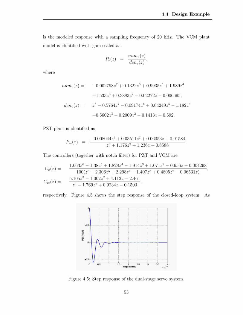
4.4 Design Example
is the modeled response with a sampling frequency of 20 kHz. The VCM plant
model is identified with gain scaled as
Pv(z) =numv(z)
denv(z),
where
numv(z) = −0.002798z7 + 0.1322z6 + 0.9935z5 + 1.989z4
+1.533z3 + 0.3883z2 − 0.02272z − 0.006695,
denv(z) = z8 − 0.5764z7 − 0.09174z6 + 0.04249z5 − 1.182z4
+0.5602z3 − 0.2009z2 − 0.1413z + 0.592.
PZT plant is identified as
Pm(z) =−0.008044z3 + 0.03511z2 + 0.06053z + 0.01584
z3 + 1.176z2 + 1.236z + 0.8588.
The controllers (together with notch filter) for PZT and VCM are
Cv(z) =1.063z6 − 1.38z5 + 1.828z4 − 1.914z3 + 1.071z2 − 0.656z + 0.004298
100(z6 − 2.306z5 + 2.298z4 − 1.407z3 + 0.4805z2 − 0.06531z),
Cm(z) =5.105z3 − 1.002z2 + 4.112z − 2.461
z3 − 1.769z2 + 0.9234z − 0.1503,
respectively. Figure 4.5 shows the step response of the closed-loop system. As
Figure 4.5: Step response of the dual-stage servo system.
53
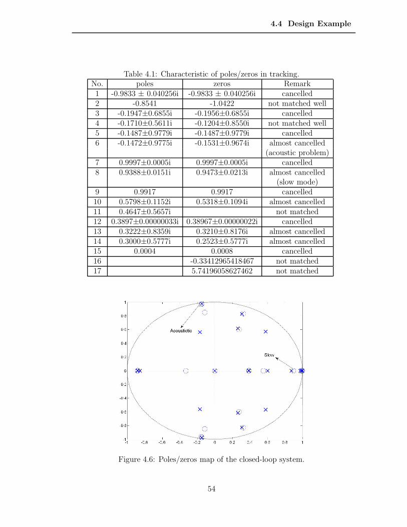
4.4 Design Example
Table 4.1: Characteristic of poles/zeros in tracking.No. poles zeros Remark1 -0.9833 ± 0.040256i -0.9833 ± 0.040256i cancelled2 -0.8541 -1.0422 not matched well3 -0.1947±0.6855i -0.1956±0.6855i cancelled4 -0.1710±0.5611i -0.1204±0.8550i not matched well5 -0.1487±0.9779i -0.1487±0.9779i cancelled6 -0.1472±0.9775i -0.1531±0.9674i almost cancelled
(acoustic problem)7 0.9997±0.0005i 0.9997±0.0005i cancelled8 0.9388±0.0151i 0.9473±0.0213i almost cancelled
(slow mode)9 0.9917 0.9917 cancelled10 0.5798±0.1152i 0.5318±0.1094i almost cancelled11 0.4647±0.5657i not matched12 0.3897±0.00000033i 0.38967±0.00000022i cancelled13 0.3222±0.8359i 0.3210±0.8176i almost cancelled14 0.3000±0.5777i 0.2523±0.5777i almost cancelled15 0.0004 0.0008 cancelled16 -0.33412965418467 not matched17 5.74196058627462 not matched
Figure 4.6: Poles/zeros map of the closed-loop system.
54
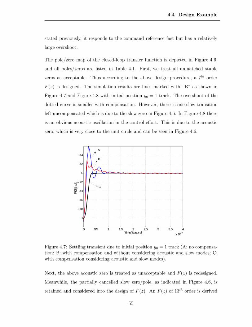
4.4 Design Example
stated previously, it responds to the command reference fast but has a relatively
large overshoot.
The pole/zero map of the closed-loop transfer function is depicted in Figure 4.6,
and all poles/zeros are listed in Table 4.1. First, we treat all unmatched stable
zeros as acceptable. Thus according to the above design procedure, a 7th order
F (z) is designed. The simulation results are lines marked with “B” as shown in
Figure 4.7 and Figure 4.8 with initial position y0 = 1 track. The overshoot of the
dotted curve is smaller with compensation. However, there is one slow transition
left uncompensated which is due to the slow zero in Figure 4.6. In Figure 4.8 there
is an obvious acoustic oscillation in the control effort. This is due to the acoustic
zero, which is very close to the unit circle and can be seen in Figure 4.6.
0 0.5 1 1.5 2 2.5 3 3.5 4
x 10-3
-1
-0.8
-0.6
-0.4
-0.2
0
0.2
0.4
Time[Second]
PES
[trac
k]
A
B
C
Figure 4.7: Settling transient due to initial position y0 = 1 track (A: no compensa-tion; B: with compensation and without considering acoustic and slow modes; C:with compensation considering acoustic and slow modes).
Next, the above acoustic zero is treated as unacceptable and F (z) is redesigned.
Meanwhile, the partially cancelled slow zero/pole, as indicated in Figure 4.6, is
retained and considered into the design of F (z). An F (z) of 13th order is derived
55
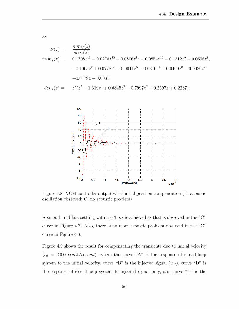
4.4 Design Example
as
F (z) =numf(z)
denf (z),
numf(z) = 0.1308z13 − 0.0278z12 + 0.0806z11 − 0.0854z10 − 0.1512z9 + 0.0696z8,
−0.1065z7 + 0.0778z6 − 0.0011z5 − 0.0310z4 + 0.0460z3 − 0.0080z2
+0.0179z − 0.0031
denf(z) = z8(z5 − 1.319z4 + 0.6345z3 − 0.7997z2 + 0.2697z + 0.2237).
Figure 4.8: VCM controller output with initial position compensation (B: acousticoscillation observed; C: no acoustic problem).
A smooth and fast settling within 0.3 ms is achieved as that is observed in the “C”
curve in Figure 4.7. Also, there is no more acoustic problem observed in the “C”
curve in Figure 4.8.
Figure 4.9 shows the result for compensating the transients due to initial velocity
(v0 = 2000 track/second), where the curve “A” is the response of closed-loop
system to the initial velocity, curve “B” is the injected signal (uc2), curve “D” is
the response of closed-loop system to injected signal only, and curve ”C” is the
56
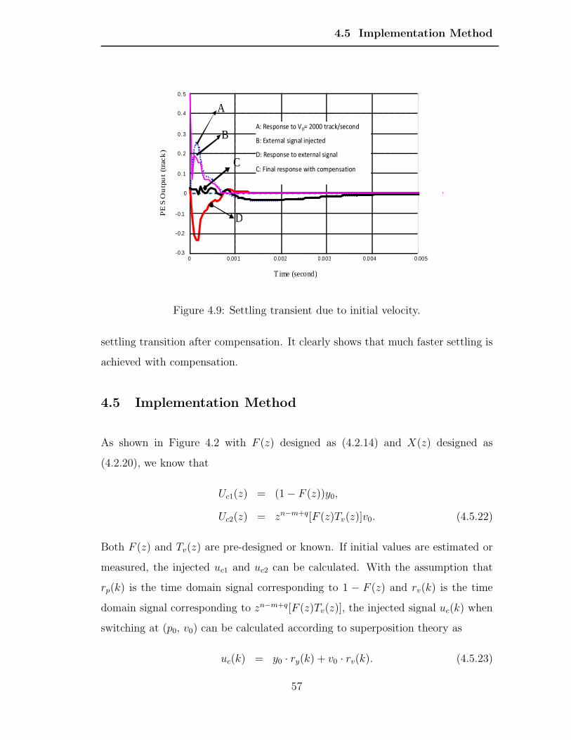
4.5 Implementation Method
0 0.001 0.002 0.003 0.004 0.005 -0.3
-0.2
-0.1
0
0. 1
0. 2
0. 3
0. 4
0. 5
T ime (second)
PE
S O
utp
ut
(tra
ck
)
A
D
B
C
A: Response to V0= 2000 track/secondB: External signal injectedD: Response to external signal C: Final response with compensation
Figure 4.9: Settling transient due to initial velocity.
settling transition after compensation. It clearly shows that much faster settling is
achieved with compensation.
4.5 Implementation Method
As shown in Figure 4.2 with F (z) designed as (4.2.14) and X(z) designed as
(4.2.20), we know that
Uc1(z) = (1− F (z))y0,
Uc2(z) = zn−m+q[F (z)Tv(z)]v0. (4.5.22)
Both F (z) and Tv(z) are pre-designed or known. If initial values are estimated or
measured, the injected uc1 and uc2 can be calculated. With the assumption that
rp(k) is the time domain signal corresponding to 1 − F (z) and rv(k) is the time
domain signal corresponding to zn−m+q[F (z)Tv(z)], the injected signal uc(k) when
switching at (p0, v0) can be calculated according to superposition theory as
uc(k) = y0 · ry(k) + v0 · rv(k). (4.5.23)
57
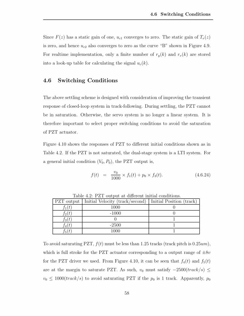
4.6 Switching Conditions
Since F (z) has a static gain of one, uc1 converges to zero. The static gain of Tv(z)
is zero, and hence uc2 also converges to zero as the curve “B” shown in Figure 4.9.
For realtime implementation, only a finite number of ry(k) and rv(k) are stored
into a look-up table for calculating the signal uc(k).
4.6 Switching Conditions
The above settling scheme is designed with consideration of improving the transient
response of closed-loop system in track-following. During settling, the PZT cannot
be in saturation. Otherwise, the servo system is no longer a linear system. It is
therefore important to select proper switching conditions to avoid the saturation
of PZT actuator.
Figure 4.10 shows the responses of PZT to different initial conditions shown as in
Table 4.2. If the PZT is not saturated, the dual-stage system is a LTI system. For
a general initial condition (V0, P0), the PZT output is,
f(t) =v0
1000× f1(t) + p0 × f3(t). (4.6.24)
Table 4.2: PZT output at different initial conditions.PZT output Initial Velocity (track/second) Initial Position (track)
f1(t) 1000 0f2(t) -1000 0f3(t) 0 1f4(t) -2500 1f5(t) 1000 1
To avoid saturating PZT, f(t) must be less than 1.25 tracks (track pitch is 0.25um),
which is full stroke for the PZT actuator corresponding to a output range of ±8v
for the PZT driver we used. From Figure 4.10, it can be seen that f4(t) and f5(t)
are at the margin to saturate PZT. As such, v0 must satisfy −2500(track/s) ≤
v0 ≤ 1000(track/s) to avoid saturating PZT if the p0 is 1 track. Apparently, p0
58
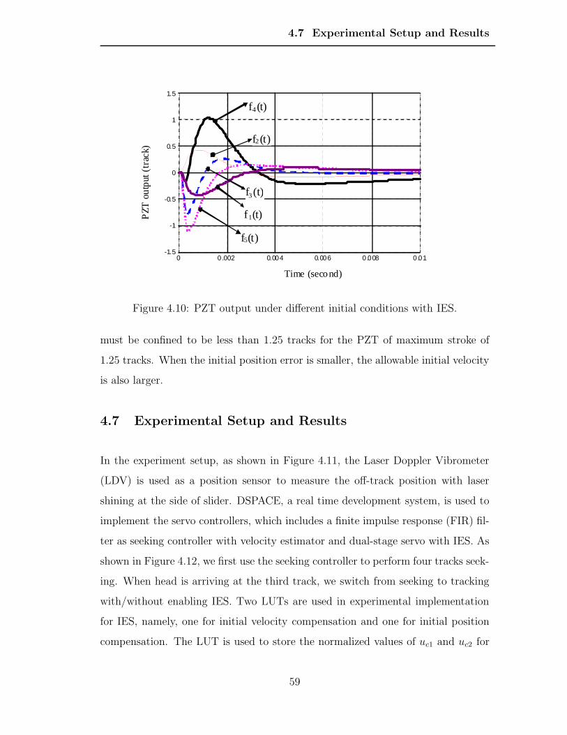
4.7 Experimental Setup and Results
0 0.002 0.004 0.006 0.008 0.01 -1.5
-1
-0.5
0
0.5
1
1.5
Time (second)
PZT
ou
tput
(tra
ck)
f4(t)
f2(t)
f3(t)
f 1(t)
f5(t)
Figure 4.10: PZT output under different initial conditions with IES.
must be confined to be less than 1.25 tracks for the PZT of maximum stroke of
1.25 tracks. When the initial position error is smaller, the allowable initial velocity
is also larger.
4.7 Experimental Setup and Results
In the experiment setup, as shown in Figure 4.11, the Laser Doppler Vibrometer
(LDV) is used as a position sensor to measure the off-track position with laser
shining at the side of slider. DSPACE, a real time development system, is used to
implement the servo controllers, which includes a finite impulse response (FIR) fil-
ter as seeking controller with velocity estimator and dual-stage servo with IES. As
shown in Figure 4.12, we first use the seeking controller to perform four tracks seek-
ing. When head is arriving at the third track, we switch from seeking to tracking
with/without enabling IES. Two LUTs are used in experimental implementation
for IES, namely, one for initial velocity compensation and one for initial position
compensation. The LUT is used to store the normalized values of uc1 and uc2 for
59
4.8 Conclusions
LDV
dSpace Real Time System (Seeking, Settling and Tracking Controller)
PZT Driver
VCM Driver
Position Feedback
PZT Control Effort
VCM Control Effort
Figure 4.11: Experiment setup for dual-stage servo.
a short settling period. To implement online compensation, the values in LUT are
scaled by the corresponding initial values of velocity/postion and injected into the
nominal controller.
The experimental results are shown in Figure 4.13, where y0 is 1 track, and v0 is
an estimated value around 1345 tracks/second at the switching point from seeking
to settling. It can be seen that the settling transient with IES (persistent curve B)
is significantly improved, and a settling time of less than 0.35ms is achieved.
4.8 Conclusions
In this chapter, an effective and easily implemented settling scheme has been pre-
sented to achieve fast and smooth track settling for a dual-stage servo system. In
this scheme, a feedforward compensator can be used to cancel the error caused by
the initial position and velocity of VCM during mode-switching.
Based on ZPET, a systematic pole/zero cancelation scheme is used in the design
of the IES feedforward compensator.
60
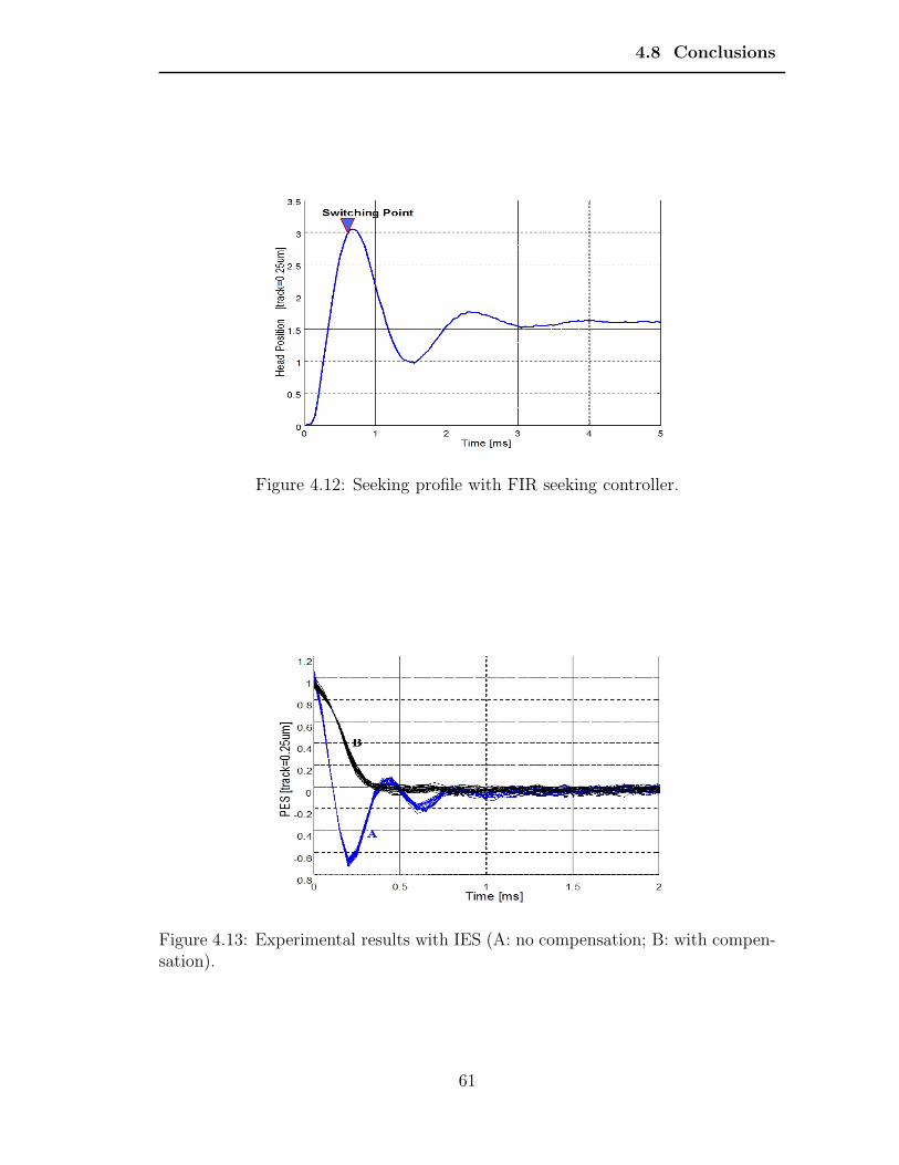
4.8 Conclusions
Figure 4.12: Seeking profile with FIR seeking controller.
Figure 4.13: Experimental results with IES (A: no compensation; B: with compen-sation).
61

4.8 Conclusions
Both simulation and experiment results show that this method can improve settling
performance significantly. In future, it is valuable to study the optimal switching
conditions.
62
Chapter 5
Design Feedback Controller UsingAdvanced Loop Shaping
To shape the frequency responses of closed-loop transfer functions such as sensitiv-
ity/complementary sensitivity functions, H∞ optimization together with frequency
weighting is a commonly used method. However, the frequency weighting func-
tions increase the system and controller complexities since the weighting functions
usually are of high orders in order to formulate the desired specifications accu-
rately. The process of choosing appropriate weighting function is also tedious and
time-consuming.
The KYP lemma [65] establishes the equivalence between a frequency domain in-
equality (FDI) for a transfer function and a linear matrix inequality associated with
its state space realization. It provides a solution to characterize various properties
of dynamic systems in the frequency domain in terms of linear matrix inequalities.
The standard KYP Lemma is only applicable for the infinite frequency range, while
the generalized KYP Lemma [66] establishes the equivalence between a frequency
domain property and a linear matrix inequality over a finite frequency range, which
allows designers to impose expected performance requirements over selected finite
or infinite frequency ranges. Therefore, the generalized KYP is very suitable for
63
analysis and synthesis problems in practical applications where different specifica-
tions over different frequency ranges are required.
The KYP Lemma-based loop shaping method does not count for overall positioning
error minimization which can be translated into the H2 optimal control problem
by taking into consideration the disturbance and noise models. On the other hand,
the H2 control design which incorporates all disturbance and noise models can
result in an average performance across the entire frequency range and a high
order controller. Thus, it usually does not have the flexibility to specifically reject
disturbances in certain frequency ranges, which however may be the dominant
factors that influence the overall performance. Therefore, there is a need to suppress
disturbances of specific frequencies when minimizing the positioning error, which is
the motivation to incorporate the KYP lemma-based method with the H2 control
method. With the selected specific disturbances handled by the KYP Lemma-
based design, the H2 control is formulated with a lower order disturbance model,
excluding the disturbances covered in the above design. This will not only reduce
the computation time in the H2 control design, but also result in a lower order
controller.
In this chapter, the generalized KYP lemma is applied to design a feedback control
such that the sensitivity function can attenuate the disturbances at some specific
frequency ranges. Unlike the standard KYP lemma, the matrix inequality in the
generalized KYP lemma involves a matrix variable which is not necessarily posi-
tive definite, and thus the Schur complement cannot be applied to convexify the
controller design. To overcome this difficulty, the Youla parametrization approach
is used to parameterize the closed-loop transfer function. The search for the coeffi-
cients of the parameter Q(z) is then converted to a linear matrix inequality problem
within the generalized KYP lemma framework. Next, considering the system with
an augmented disturbance model, the generalized KYP lemma is combined the H2
64
5.1 Control Design Using Generalized KYP Lemma
method to design a controller for minimization of tracking error as well as attenu-
ation of dominant disturbances at certain frequencies. Lastly, the two methods are
applied to design track-following controller for our STW experiment platform.
5.1 Control Design Using Generalized KYP Lemma
5.1.1 Problem Description
It is known that the power spectrum of PES in Figure 2.16 is given by
Se = |P (z)S(z)|2Sd1 + |S(z)|2Sd2 + |S(z)|2Sn, (5.1.1)
where the sensitivity function S(z) shows the disturbance rejection capability of
the servo loop. It becomes rather significant to design a controller such that the
sensitivity function reject dominant disturbances with known frequencies.
The problem can be stated as: To design a dynamic feedback controller C(z) forplant P (z) such that the closed-loop system is stable and for some prescribed positivescalars ri and frequency ranges (fi1, fi2), i = 1, ..., N , such that
|S(f)| < ri, when fi1 ≤ f ≤ fi2. (5.1.2)
A smaller ri means the less contribution of the disturbance in frequency range
(fi1, fi2) to the error.
5.1.2 Generalized KYP Lemma
Figure 5.1 shows a equivalent system where the transfer function from w to z is
the same as the sensitivity function, S(z), in Figure 2.16. The state-space model
of the plant under consideration is denoted as (Ap, Bp, Cp, Dp). The state-space
representation of the system in Figure 5.1 is given by
x(k + 1) = Apx(k) +Bpu(k), (5.1.3)
z(k) = −Cpx(k) + w(k)−Dpu(k), (5.1.4)
65
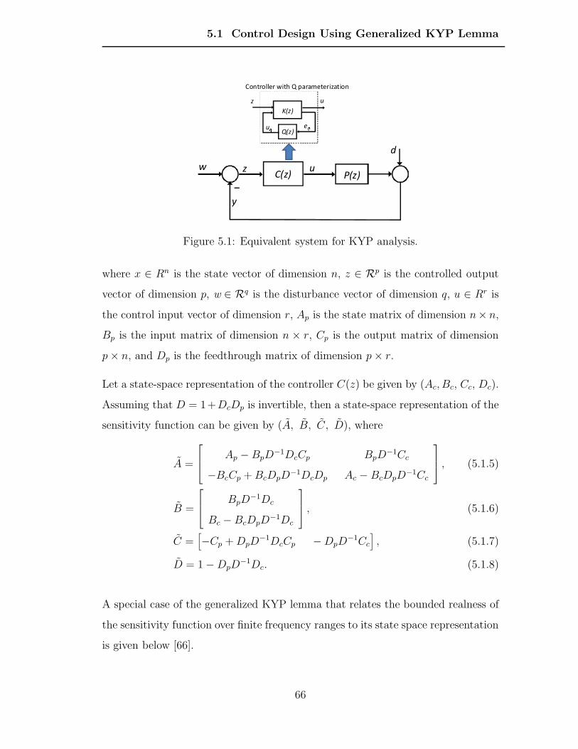
5.1 Control Design Using Generalized KYP Lemma
d
P(z)C(z)w z
y
u
Q(z)
K(z)eu uz
Controller with Q parameterization
Figure 5.1: Equivalent system for KYP analysis.
where x ∈ Rn is the state vector of dimension n, z ∈ Rp is the controlled output
vector of dimension p, w ∈ Rq is the disturbance vector of dimension q, u ∈ Rr is
the control input vector of dimension r, Ap is the state matrix of dimension n× n,
Bp is the input matrix of dimension n × r, Cp is the output matrix of dimension
p× n, and Dp is the feedthrough matrix of dimension p× r.
Let a state-space representation of the controller C(z) be given by (Ac, Bc, Cc, Dc).
Assuming that D = 1+DcDp is invertible, then a state-space representation of the
sensitivity function can be given by (A, B, C, D), where
A =
Ap − BpD−1DcCp BpD
−1Cc
−BcCp +BcDpD−1DcDp Ac − BcDpD
−1Cc
, (5.1.5)
B =
BpD−1Dc
Bc − BcDpD−1Dc
, (5.1.6)
C =[
−Cp +DpD−1DcCp −DpD
−1Cc
]
, (5.1.7)
D = 1−DpD−1Dc. (5.1.8)
A special case of the generalized KYP lemma that relates the bounded realness of
the sensitivity function over finite frequency ranges to its state space representation
is given below [66].
66
5.1 Control Design Using Generalized KYP Lemma
Lemma 5.1.1 Consider the sensitivity function S(z) = C(zI − A)−1B + D withA being stable. Then, for a given scalar r > 0, |S(ejθ)| ≤ r over a finite frequencyrange if and only if there exist Hermitian matrices U and V ≥ 0 such that
[
A BI 0
]
∗
Σ
[
A BI 0
]
+
[
0 00 −r2
]
[
C D]
∗
[
C D]
−I
≤ 0, (5.1.9)
where
(i) for low frequency range |θ| ≤ θl,
Σ =
[
−U VV U − (2cosθl)V
]
; (5.1.10)
(ii) for middle frequency range θ1 ≤ θ ≤ θ2,
Σ =
[
−U ejθcVe−jθcV U − (2cosθd)V
]
,
θc = (θ1 + θ2)/2, θd = (θ2 − θ1)/2; (5.1.11)
(iii) for high frequency range |θ| ≥ θh,
Σ =
[
−U −V−V U + (2cosθh)V
]
. (5.1.12)
For a given controller C(z), the above gives a necessary and sufficient condition to
evaluate whether |S(z)| ≤ r over some given frequency range in terms of an LMI.
However, (5.1.9) is no longer an LMI when the controller C(z) = (Ac, Bc, Cc, Dc)
is to be designed, since A and B involve the unknown parameters Ac, Bc, Cc and
Dc. Further, it is not possible to convert to an LMI via Schur complement as the
matrix Σ is not definite.
5.1.3 YOULA Parametrization
Let K(z) be a state feedback controller with a state estimator, i.e.,
x(k + 1) = Apx(k) +Bpu(k) + L(z(k) + Cpx(k)), (5.1.13)
u(k) = −Mx(k). (5.1.14)
67
5.1 Control Design Using Generalized KYP Lemma
where L is the estimator gain, and M is state feedback gain. A set of sensitivity
functions can be parameterized as [67]
S(z) = T11(z) + T12(z)Q(z)T21(z), (5.1.15)
where Q(z) is a stable transfer function to be designed and
T11(z) T12(z)
T21(z) 0
= CT (zI − AT )−1BT +DT ,
AT BT
CT DT
=
Ap −BpM 0 Bp
−LCp Ap − BpM + LCp L Bp
−Cp DpM 1 −Dp
−Cp Cp 1 0
. (5.1.16)
If Q(z) has the state-space realization (Aq, Bq, Cq, Dq), the designed controller C(z)
is given by
Ac =
Ap −BpM + LCp +BpDqCp BpCq
BqCp Aq
, (5.1.17)
Bc =
L+BpDq
Bq
, (5.1.18)
Cc =[
−M +DqCp Cq
]
, (5.1.19)
Dc = Dq. (5.1.20)
The controller C(z) is now of the structure as shown in Figure 5.1.
Denote the state-space representations of T11(z) and T12(z)T21(z) by (At11, Bt11,
Ct11, Dt11) and (At, Bt, Ct, Dt), respectively, a state space model of S(z) can be
written as from (5.1.15)
A =
At11 0 0
0 At 0
0 BqCt Aq
, (5.1.21)
68
5.1 Control Design Using Generalized KYP Lemma
B =
Bt11
Bt
BqDt
, (5.1.22)
C =[
Ct11 DqCt Cq
]
, (5.1.23)
D = Dt11 +DqDt. (5.1.24)
Let Q(z) be an FIR filter, such that
Q(z) = q0 + q1z−1 + q2z
−2 + ...+ qτz−τ , (5.1.25)
q = [q0 q1 q2, ... , qτ ], (5.1.26)
which is to be designed so that the required bounded realness of the sensitivity
function is satisfied. It is known that a state-space realization for Q(z) can be
given by
Aq =
0 Iτ−1
0 0
, Bq =
0(τ−1)×1
1
,
Cq = [qτ qτ−1 · · · q1] , Dq = q0,
where Iτ−1 is the identity matrix of dimension (τ − 1) × (τ − 1) and 0(τ−1)×1 is
the zero matrix of dimension (τ − 1) × 1. Note that the filter parameter q to be
designed only appears in Cq and Dq. From (5.1.21)-(5.1.24), we know that q exists
in C and D only. In this case, (5.1.9) defines an LMI in terms of the variables
U , V , and q. As such, U , V , and the design parameter q can be computed via a
convex optimization.
5.1.4 Design Procedures Using KYP Lemma
The KYP lemma-based control design can be carried out according following steps:
Step 1. Compute M and L using Matlab commands
M = dlqr(Ap, Bp, CTp Cp, R),
L = Ap · dlqe(Ap, Bp,−Cp,Wd,Wv),
69
5.2 H2 Optimal Control
where R is the weighting for the control input in the cost function
J =∑
(xTCTp Cpx+ uTRu)
for linear quadratic regulator design, and Wd and Wv are the variance matrices of
process noise and measurement noise for the Kalman estimator design. In the KYP
lemma-based control design, R, Wd, and Wv can be chosen as identity matrices.
Step 2. Compute T11(z), T12(z), and T21(z) from (5.1.16).
Step 3. Obtain the state-space model (A, B, C, D) in (5.1.21)-(5.1.24).
Step 4. Based on disturbance spectrum, specify the positive scalars ri and frequency
points fi(i = 1, ..., N) for the sensitivity function
|S(fi)| < ri, fi1 ≤ fi ≤ fi2, (5.1.27)
where fi1 and fi2 define the frequency range. For each specification on the resultant
sensitivity function in the frequency range, construct the LMI (5.1.9) in terms of
the variables U , V , and q, with r = ri.
Step 5. Obtain q, U , and V by solving these LMIs using Matlab LMI toolbox. If
the LMIs are not solvable, the specifications given in Step 4 are to be adjusted.
Step 6. Obtain the controller parameters from (5.1.17)-(5.1.20).
5.2 H2 Optimal Control
KYP lemma can be used to shape the loop transfer function to attenuate specific
disturbances. However, it can not achieve overall minimization of tracking error
which can be achieved by H2 optimal control.
70

5.2 H2 Optimal Control
5.2.1 H2 Norm
The H2 norm of a matrix transfer function G(s) analytic in Re(s) > 0 (open
right-half plane) is defined as
‖G‖2 :=
√
supσ>0
1
2π
∫ +∞
−∞
Trace[G∗(σ + jω)G(σ + jω)]dω, (5.2.28)
or equivalently [68]
‖G‖2 =
√
1
2π
∫ +∞
−∞
Trace[G∗(jω)G(jω)]dω. (5.2.29)
Although ‖G‖2 can be computed from its definition, there are some simple alter-
natives taking advantage of a state-space representation of G(s).
Lemma 5.2.1 Consider a system G(s) with a state-space representation (A,B,C,D).If A is stable and D = 0, we have [69]
‖G‖22 = Trace(BTY2B) = Trace(CX2CT ), (5.2.30)
where X2 and Y2 are the controllability and observability Gramians that can beobtained from the following Lyapunov equations
AX2 +X2AT +BBT = 0, (5.2.31)
ATY2 + Y2A+ CTC = 0. (5.2.32)
We also consider a discrete-time linear time-invariant system G(z) with the follow-
ing state-space representation
x(k + 1) = Ax(k) +Bw(k), (5.2.33)
z(k) = Cx(k) +Dw(k), (5.2.34)
where x ∈ Rn is the state vector of dimension n , z ∈ Rp is the controlled output
vector of dimension p , w ∈ Rq is the disturbance vector of dimension q. Let Tzw
71
5.2 H2 Optimal Control
denote the transfer function from the input w to the output z. Then the H2 norm
is defined as
‖Tzw‖2 =
√
1
2πTrace[
∫ π
−πT ∗
zw(ejω)Tzw(ejω)dω]. (5.2.35)
By Parseval’s Theorem, ‖Tzw‖2 can equivalently be defined as
‖Tzw‖2 =
√
√
√
√Trace[∞∑
k=0
g(k)gT (k)], (5.2.36)
where g(k) is the impulse response of Tzw.
Let the input w to the system be a wide-band stationary stochastic process. The
H2 norm of Tzw can also be interpreted as the RMS value of the output z(k) when
the system is subject to a white noise having zero mean and unit variance. That is
‖Tzw‖2 =√
E[zTz]. (5.2.37)
The H2 norm for the discrete-time system Tzw can be computed as
‖Tzw‖2 =√
Trace(DTD +BTY2B) =√
Trace(DDT + CX2CT ), (5.2.38)
where Y2 and X2 are the reachability and observability Gramians that can be
obtained from the following Lyapunov equations
AY2AT − Y2 +BBT = 0, (5.2.39)
ATX2A−X2 + CTC = 0. (5.2.40)
The following theorem presents an alternative LMI approach for bounding the H2
norm of the discrete-time system Tzw.
Lemma 5.2.2 Consider a discrete-time transfer function Tzw of realization (A,B,C,D).Given a scalar µ > 0, ‖Tzw‖
22 < µ if and only if there exist X2 = XT
2 and Y2 = Y T2
72
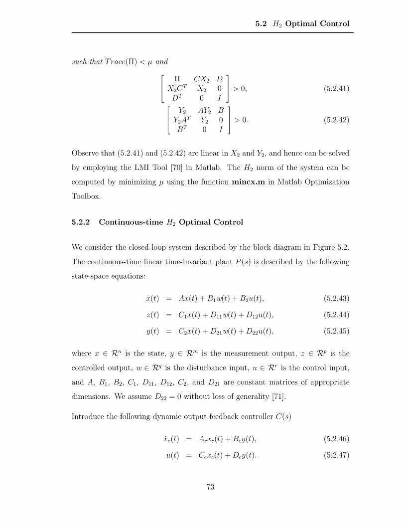
5.2 H2 Optimal Control
such that Trace(Π) < µ and
Π CX2 DX2C
T X2 0DT 0 I
> 0, (5.2.41)
Y2 AY2 BY2A
T Y2 0BT 0 I
> 0. (5.2.42)
Observe that (5.2.41) and (5.2.42) are linear in X2 and Y2, and hence can be solved
by employing the LMI Tool [70] in Matlab. The H2 norm of the system can be
computed by minimizing µ using the function mincx.m in Matlab Optimization
Toolbox.
5.2.2 Continuous-time H2 Optimal Control
We consider the closed-loop system described by the block diagram in Figure 5.2.
The continuous-time linear time-invariant plant P (s) is described by the following
state-space equations:
x(t) = Ax(t) +B1w(t) +B2u(t), (5.2.43)
z(t) = C1x(t) +D11w(t) +D12u(t), (5.2.44)
y(t) = C2x(t) +D21w(t) +D22u(t), (5.2.45)
where x ∈ Rn is the state, y ∈ Rm is the measurement output, z ∈ Rp is the
controlled output, w ∈ Rq is the disturbance input, u ∈ Rr is the control input,
and A, B1, B2, C1, D11, D12, C2, and D21 are constant matrices of appropriate
dimensions. We assume D22 = 0 without loss of generality [71].
Introduce the following dynamic output feedback controller C(s)
xc(t) = Acxc(t) +Bcy(t), (5.2.46)
u(t) = Ccxc(t) +Dcy(t). (5.2.47)
73
5.2 H2 Optimal Control
Denote ξ = [xT xTc ]
T . From (5.2.43)-(5.2.45) and (5.2.46)-(5.2.47), the closed-loop
system is given by
ξ(t) = Aξ(t) + Bw(t), (5.2.48)
z(t) = Cξ(t) + Dw(t), (5.2.49)
where
A =
A +B2DcC2 B2Cc
BcC2 Ac
, B =
B2DcD21 +B1
BcD21
, (5.2.50)
C = [C1 +D12DcC2 D12Cc] , D = D12DcD21 +D11. (5.2.51)
The continuous-time H2 control problem is to find a proper and real rational con-
troller C(s) that stabilizes P internally and minimizes the H2 norm of the closed-
loop transfer function matrix Tzw from w to z in (5.2.48)-(5.2.49).
Figure 5.2: Configuration of standard optimal control.
Assume that the system (5.2.43)-(5.2.45) satisfies the following condition
Assumption 3.1
(1). D12 is of full column rank;
(2). The subsystem (A,B2, C1, D12) has no invariant zeros on the imaginary axis;
(3). D21 is of full row rank;
74
5.2 H2 Optimal Control
(4). The subsystem (A, B1, C2, D21) has no invariant zeros on the imaginary axis.
Let X2 ≥ 0 and Y2 ≥ 0 be the solutions of the following Riccati equations
ATX2 +X2A− (X2B2 + CT1 D12)(D
T12D12)
−1(X2B2 + CT1 D12)
T
+CT1 C1 = 0, (5.2.52)
Y2AT + AY2 − (Y2C
T2 +B1D
T21)(D21D
T21)
−1(Y2CT2 +B1D
T21)
T
+B1BT1 = 0. (5.2.53)
According to the H2 optimal control theory, an H2 optimal controller can be ob-
tained as [72]
Ac = A+B2F +KC2, Bc = −K, Cc = F, Dc = 0, (5.2.54)
where
F = −(DT12D12)
−1(DT12C1 +BT
2 X2),
K = −(Y2CT2 +B1D
T21)(D21D
T21)
−1. (5.2.55)
The minimal H2 norm of the transfer function Tzw is given by
‖Tzw‖2 =√
Trace(BT1 X2B1) + Trace[(ATX2 +X2A + CT
1 C1)Y2]. (5.2.56)
If any condition among (1)-(4) in Assumption 3.1 is not satisfied, the so-called per-
turbation method is applied [72] so that the above design method is still applicable
to find an appropriate controller.
5.2.3 Discrete-time H2 Optimal Control
Consider the discrete-time linear time-invariant system P (z) with the following
state-space representation
x(k + 1) = Ax(k) +B1w(k) +B2u(k), (5.2.57)
75
5.2 H2 Optimal Control
z(k) = C1x(k) +D11w(k) +D12u(k), (5.2.58)
y(k) = C2x(k) +D21w(k) +D22u(k), (5.2.59)
where x ∈ Rn is the state, y ∈ Rm is the measurement output, z ∈ Rp is the
controlled output, w ∈ Rq is the disturbance input, u ∈ Rr is the control input,
and A, B1, B2, C1, D11, D12, C2, and D21 are constant matrices of appropriate
dimensions. D22 = 0 is also assumed for brevity but without loss of generality.
Introduce the following dynamic output feedback controller C(z),
xc(k + 1) = Acxc(k) +Bcy(k), (5.2.60)
u(k) = Ccxc(k) +Dcy(k). (5.2.61)
Denote ξ = [xT xTc ]
T . From (5.2.57)-(5.2.59) and (5.2.60)-(5.2.61), the closed-loop
system is given by
ξ(k + 1) = Aξ(k) + Bw(k), (5.2.62)
z(k) = Cξ(k) + Dw(k), (5.2.63)
where
A =
A +B2DcC2 B2Cc
BcC2 Ac
, B =
B2DcD21 +B1
BcD21
, (5.2.64)
C = [C1 +D12DcC2 D12Cc] , D = D12DcD21 +D11. (5.2.65)
The discrete-time H2 control problem is to find a proper and real rational controller
C(z) that stabilizes P (z) internally and minimizes the H2 norm of the transfer
function matrix Tzw(z) from w to z of the closed-loop system (5.2.62)-(5.2.63).
The counterpart of the Riccati equations (5.2.52)-(5.2.53) for discrete-time systems
is as follows.
ATX2A− (ATX2B2 + CT1 D12)(D
T12D12 +BT
2 X2B2)−1(ATX2B2 + CT
1 D12)T
76
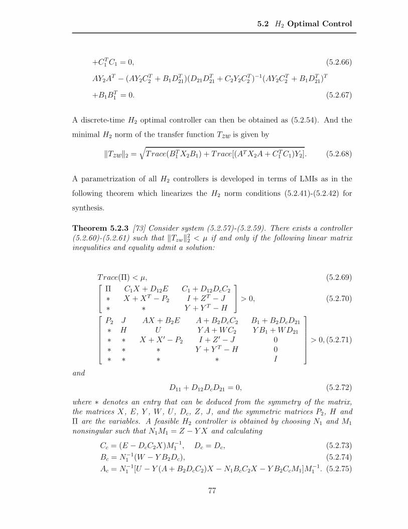
5.2 H2 Optimal Control
+CT1 C1 = 0, (5.2.66)
AY2AT − (AY2C
T2 +B1D
T21)(D21D
T21 + C2Y2C
T2 )
−1(AY2CT2 +B1D
T21)
T
+B1BT1 = 0. (5.2.67)
A discrete-time H2 optimal controller can then be obtained as (5.2.54). And the
minimal H2 norm of the transfer function Tzw is given by
‖Tzw‖2 =√
Trace(BT1 X2B1) + Trace[(ATX2A+ CT
1 C1)Y2]. (5.2.68)
A parametrization of all H2 controllers is developed in terms of LMIs as in the
following theorem which linearizes the H2 norm conditions (5.2.41)-(5.2.42) for
synthesis.
Theorem 5.2.3 [73] Consider system (5.2.57)-(5.2.59). There exists a controller(5.2.60)-(5.2.61) such that ‖Tzw‖
22 < µ if and only if the following linear matrix
inequalities and equality admit a solution:
Trace(Π) < µ, (5.2.69)
Π C1X +D12E C1 +D12DcC2
∗ X +XT − P2 I + ZT − J∗ ∗ Y + Y T −H
> 0, (5.2.70)
P2 J AX +B2E A+B2DcC2 B1 +B2DcD21
∗ H U Y A+WC2 Y B1 +WD21
∗ ∗ X +X ′ − P2 I + Z ′ − J 0∗ ∗ ∗ Y + Y T −H 0∗ ∗ ∗ ∗ I
> 0, (5.2.71)
and
D11 +D12DcD21 = 0, (5.2.72)
where ∗ denotes an entry that can be deduced from the symmetry of the matrix,the matrices X, E, Y , W , U , Dc, Z, J , and the symmetric matrices P2, H andΠ are the variables. A feasible H2 controller is obtained by choosing N1 and M1
nonsingular such that N1M1 = Z − Y X and calculating
Cc = (E −DcC2X)M−11 , Dc = Dc, (5.2.73)
Bc = N−11 (W − Y B2Dc), (5.2.74)
Ac = N−11 [U − Y (A+B2DcC2)X −N1BcC2X − Y B2CcM1]M
−11 . (5.2.75)
77
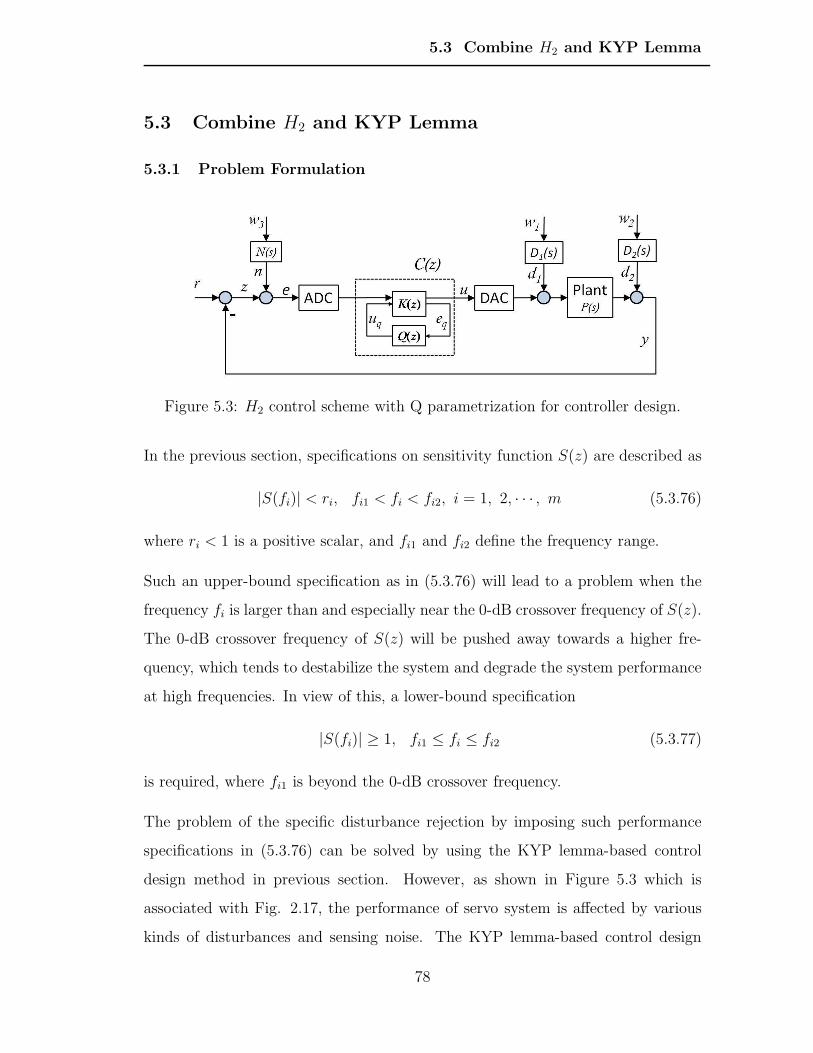
5.3 Combine H2 and KYP Lemma
5.3 Combine H2 and KYP Lemma
5.3.1 Problem Formulation
Figure 5.3: H2 control scheme with Q parametrization for controller design.
In the previous section, specifications on sensitivity function S(z) are described as
|S(fi)| < ri, fi1 < fi < fi2, i = 1, 2, · · · , m (5.3.76)
where ri < 1 is a positive scalar, and fi1 and fi2 define the frequency range.
Such an upper-bound specification as in (5.3.76) will lead to a problem when the
frequency fi is larger than and especially near the 0-dB crossover frequency of S(z).
The 0-dB crossover frequency of S(z) will be pushed away towards a higher fre-
quency, which tends to destabilize the system and degrade the system performance
at high frequencies. In view of this, a lower-bound specification
|S(fi)| ≥ 1, fi1 ≤ fi ≤ fi2 (5.3.77)
is required, where fi1 is beyond the 0-dB crossover frequency.
The problem of the specific disturbance rejection by imposing such performance
specifications in (5.3.76) can be solved by using the KYP lemma-based control
design method in previous section. However, as shown in Figure 5.3 which is
associated with Fig. 2.17, the performance of servo system is affected by various
kinds of disturbances and sensing noise. The KYP lemma-based control design
78
5.3 Combine H2 and KYP Lemma
cannot include all disturbances and noises which contribute to the position error.
In view of this, we also need to take into account the overall performance of the
servo control system, which is represented as the so-called TMR in HDD servo.
The TMR is contributed by by w =[
w1 w2 w3
]T
through D1(s), D2(s), and
N(s). It is expressed by the standard deviation σz of z, and
σz = ‖Tzw‖2 , (5.3.78)
where w is white noise with zero mean and identity covariance matrix, and Tzw is
the transfer function from w to z.
The problem can be stated as: To design a dynamic feedback controller C(z) for
plant P (z) such that the closed-loop system is stable and satisfy the specifications
in (5.3.76) and (5.3.77), and minimizing σz in (5.3.78) simultaneously.
5.3.2 Design Controller for Specific Disturbance Rejection and OverallError Minimization
Let (Ap, Bp, Cp, Dp) and (Ac, Bc, Cc, Dc) be the state-space model of plant P (z)
and controller C(z) respectively. In order to convexify matrix inequalities, the
Youla parametrization approach with the Q(z) in a FIR filter form is applied and
the controller structure is shown in Figure 5.3. K(z) is an observer based controller
that can be designed using the LQG method as in (5.1.13)-(5.1.14).
For the presentation of the KYP lemma, we denote
σ(S,Π) :=
S
I
∗
Π
S
I
(5.3.79)
where S(z) = S(ejθ), I stands for an identity matrix, and Π a Hermitian matrix of
the form
Π =
Π11 Π12
Π∗
12 Π22
, (5.3.80)
which specifies the frequency domain property to be investigated.
79
5.3 Combine H2 and KYP Lemma
5.3.3 Q Parametrization to Meet Specifications for Disturbance Rejec-tion
A. Specification (5.3.76)
Recall from (5.1.15)-(5.1.16) that a set of sensitivity functions S(z): (A, B, C, D)
can be Q-parameterized. According to the denotation (5.3.79)-(5.3.80), the speci-
fication |S(z)| ≤ r is written as σ(S, Π) ≤ 0 with
Π =
Π11 Π12
Π∗
12 Π22
=
1 0
0 − r2
. (5.3.81)
Thus based on the KYP lemma,∣
∣
∣S(
ejθ)∣
∣
∣ ≤ r for the frequency range θ1 ≤ θ ≤ θ2
can be achieved by solving the following matrix inequality
A B
I 0
∗
Σ
A B
I 0
+
C D
0 I
∗
Π
C D
0 I
≤ 0, (5.3.82)
which is equivalent to
A B
I 0
∗
Σ
A B
I 0
+
0 0
0 −r2
[
C D
]
∗
Π11
Π11
[
C D
]
−Π11
≤ 0, (5.3.83)
where
Σ =
−U ejθcV
e−jθcV U − (2 cos θd)V
, (5.3.84)
θc = (θ1 + θ2)/2, θd = (θ2 − θ1)/2, (5.3.85)
since Π11 > 0. U and V are Hermitian matrices and V ≥ 0.
To convexify the matrix inequality (5.3.83), we shall give a state-space realization of
S(z) = T11 (z)+T12 (z)Q (z) T21 (z). Denote the state-space representation of T11(z)
and T12(z)T21(z) by (At11, Bt11, Ct11, Dt11) and (At, Bt, Ct, Dt), respectively. A
state-space model of S(z) can be written as (5.1.21)-(5.1.24).
80

5.3 Combine H2 and KYP Lemma
B. Specification (5.3.77)
Similarly, according to the denotation (5.3.79)-(5.3.80), the specification |S(z)| ≥ r
is equivalent to σ(S,Π) ≤ 0 with
Π =
Π11 Π12
Π∗
12 Π22
=
−1 0
0 r2
. (5.3.86)
However, because Π11 < 0, (5.3.82) can not be converted equivalently to (5.3.83),
which means (5.3.82) is not possibly convexified according to the method in Section
5.3.3. Hence, we resort to the following specification
σ (S,Π) = aR (S) + bI (S) + c, Π :=
0 a+ jb
a− jb 2c
(5.3.87)
where R and I denote the real and the imaginary parts of S(ejθ). When a, b, and
c are properly selected, |S(z)| ≥ r can be achieved. A simple selection is a = 0,
b = −1, and c = r, and
σ (S,Π) = −I (S) + r. (5.3.88)
Thus σ(S,Π) ≤ 0 means I (S) ≥ r, and subsequently |S(z)| ≥ r. In this situation,
Π =
Π11 Π12
Π∗
12 Π22
=
0 −j
j 2r
, (5.3.89)
where Π11 = 0 and (5.3.82) is equivalent to
A B
I 0
∗
Σ
A B
I 0
+
0 C∗Π12
Π∗
12C D∗Π12 +Π∗
12D +Π22
≤ 0,(5.3.90)
which is a linear matrix inequality with unknown variables in C and D only. This
can be solved using the same method as in Section 5.3.3 A.
81

5.3 Combine H2 and KYP Lemma
It should be mentioned that R (S) ≥ r can also be used to achieve |S(z)| ≥ r, if it
is suitable for a specific application. In this case,
Π =
Π11 Π12
Π∗
12 Π22
=
0 −1
−1 2r
, (5.3.91)
and the linear matrix inequality (5.3.90) remains applicable.
5.3.4 Q Parametrization to Minimize H2 Performance
Next we focus on the design of Q(z) to minimize the H2 norm ‖Tzw‖2. From Figure
5.3 we have
−z = N (z)w3 + S (z) [P (z)D1 (z)w1 +D2 (z)w2 −N (z)w3] . (5.3.92)
Denote a state-space realization of P (z)D1(z), D2(z) and N(z) by (A1, B1, C1, D1),
(A2, B2, C2, D2), and (A3, B3, C3, D3), respectively. It follows from (5.1.15) and
(5.1.21)-(5.1.24) that
x (k + 1) = Ax (k) + Bw(k), (5.3.93)
−z (k) = Cx (k) + Dw(k), (5.3.94)
where,
A =
A1 0 0 0
0 A2 0 0
0 0 A3 0
BC1 BC2 −BC3 A
, B =
B1 0 0
0 B2 0
0 0 B3
BD1 BD2 −BD3
, (5.3.95)
C =[
DC1 DC2 −DC3 + C3 C
]
, D =[
DD1 DD2 −DD3 +D3
]
.
The H2 norm ‖Tzw‖2 can be minimized as
min(Ξ=ΞT>0, Ω=ΩT>0)
Trace (Ω) , (5.3.96)
82
5.3 Combine H2 and KYP Lemma
subject to
ATΞA− Ξ + CT C < 0, (5.3.97)
BTΞB + DT D < Ω, (5.3.98)
or equivalently,
ATΞA− Ξ CT
C −I
< 0, (5.3.99)
−Ω + BTΞB DT
D −I
< 0, (5.3.100)
where
A =
A1 0 0 0 0 0
0 A2 0 0 0 0
0 0 A3 0 0 0
Bt11C1 Bt11C2 −Bt11C3 At11 0 0
BtC1 BtC2 −BtC3 0 At 0
BqDtC1 BqDtC −BqDtC3 0 BqCt Aq
,
B =
B1 0 0
0 B2 0
0 0 B3
Bt11D1 B
t11D2 −B
t11D3
BtD1 BtD2 −BtD3
BqDtD1 BqDtD2 −BqDtD3
,
C =[
(Dt11 +DqDt)C1 (Dt11 +DqDt)C2
(Dt11 +DqDt)C3 Ct11 DqCt Cq
]
,
D =[
(Dt11 +DqDt)D1 (Dt11 +DqDt)D2
− (Dt11 +DqDt)D3 +D3] . (5.3.101)
83
5.3 Combine H2 and KYP Lemma
Note that the Q(z) coefficients qi(i = 0, 1, . . . , τ) only appear in Cq and Dq. There-
fore from (5.1.21)-(5.1.24) and (5.3.101), we know that qi exists only in C, D, C,
and D. In this case, (5.3.83), (5.3.90), and (5.3.99)-(5.3.100) define the LMIs in
terms of the variables U , V , Ξ, Ω, and qi. Hence, the Q(z) coefficients qi can be
computed via convex optimization.
With the solved Q(z), the controller C(z) in terms (Aq, Bq, Cq, Dq) is then given
by
Ac =
Ap −BpM + LCp +BpDqCp BpCq
BqCp Aq
,
Bc =
L+BpDq
Bq
,
Cc =[
−M +DqCp Cq
]
,
Dc = Dq.
(5.3.102)
5.3.5 Design Procedure
The design procedure for controller C(z) in previous section can be summarized as
follows.
Step 1. Design K(z) from (5.1.13)-(5.1.14).
Step 2. Compute T11(z), T12(z) and T21(z) from (5.1.16), and obtain the state
space model (A, B, C, D) in (5.1.21)-(5.1.24).
Step 3. Based on disturbance spectrum and bandwidth requirement, specify the
positive scalars ri and rj , the frequency points fi (i = 1, . . . , m), and fj (j = 1,
. . . , n) for the sensitivity function S(z) such that
|S (fi)| < ri, fi1 ≤ fi ≤ fi2, (5.3.103)
and
|S (fj)| > rj, fj1 ≤ fj ≤ fj2. (5.3.104)
84
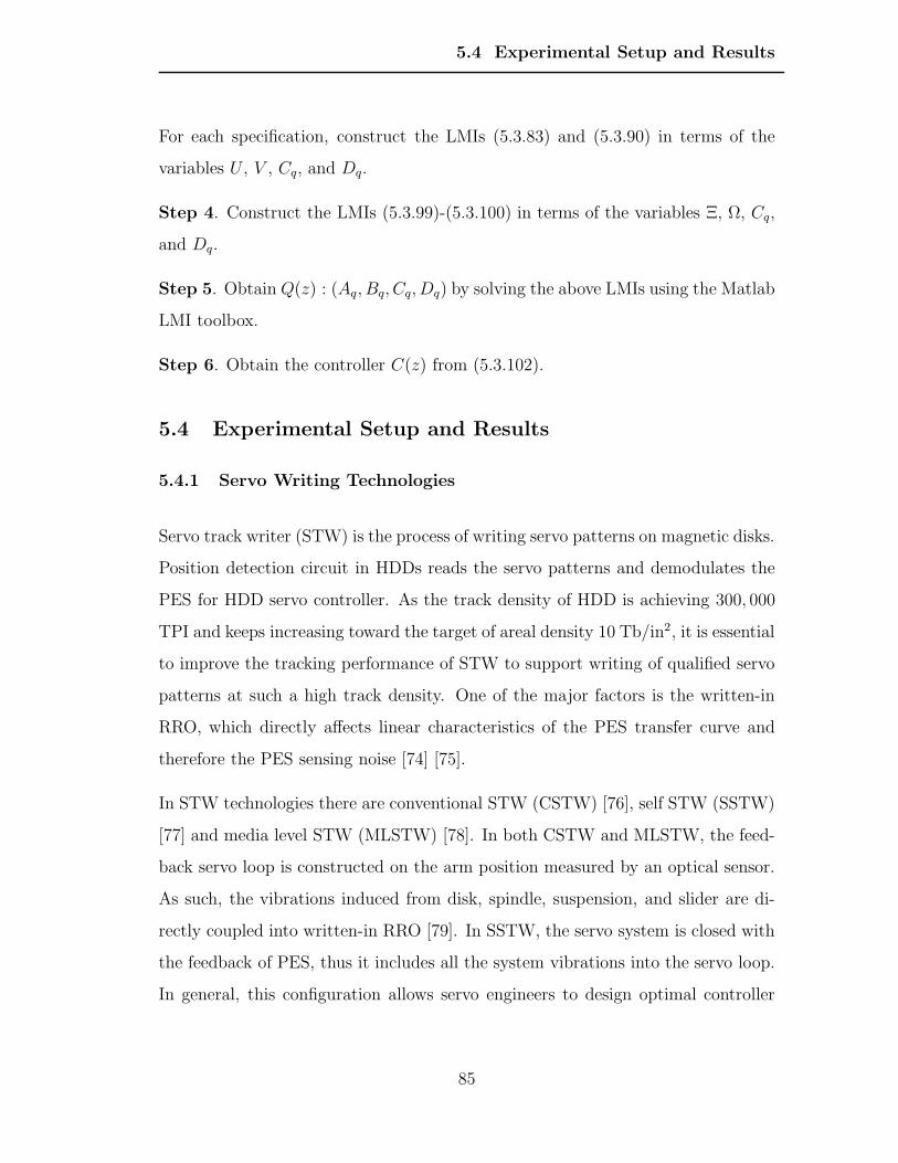
5.4 Experimental Setup and Results
For each specification, construct the LMIs (5.3.83) and (5.3.90) in terms of the
variables U , V , Cq, and Dq.
Step 4. Construct the LMIs (5.3.99)-(5.3.100) in terms of the variables Ξ, Ω, Cq,
and Dq.
Step 5. Obtain Q(z) : (Aq, Bq, Cq, Dq) by solving the above LMIs using the Matlab
LMI toolbox.
Step 6. Obtain the controller C(z) from (5.3.102).
5.4 Experimental Setup and Results
5.4.1 Servo Writing Technologies
Servo track writer (STW) is the process of writing servo patterns on magnetic disks.
Position detection circuit in HDDs reads the servo patterns and demodulates the
PES for HDD servo controller. As the track density of HDD is achieving 300, 000
TPI and keeps increasing toward the target of areal density 10 Tb/in2, it is essential
to improve the tracking performance of STW to support writing of qualified servo
patterns at such a high track density. One of the major factors is the written-in
RRO, which directly affects linear characteristics of the PES transfer curve and
therefore the PES sensing noise [74] [75].
In STW technologies there are conventional STW (CSTW) [76], self STW (SSTW)
[77] and media level STW (MLSTW) [78]. In both CSTW and MLSTW, the feed-
back servo loop is constructed on the arm position measured by an optical sensor.
As such, the vibrations induced from disk, spindle, suspension, and slider are di-
rectly coupled into written-in RRO [79]. In SSTW, the servo system is closed with
the feedback of PES, thus it includes all the system vibrations into the servo loop.
In general, this configuration allows servo engineers to design optimal controller
85
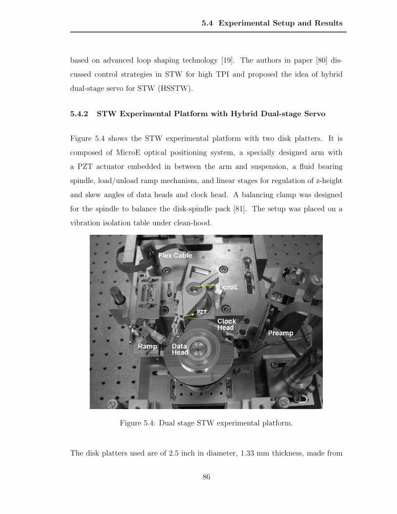
5.4 Experimental Setup and Results
based on advanced loop shaping technology [19]. The authors in paper [80] dis-
cussed control strategies in STW for high TPI and proposed the idea of hybrid
dual-stage servo for STW (HSSTW).
5.4.2 STW Experimental Platform with Hybrid Dual-stage Servo
Figure 5.4 shows the STW experimental platform with two disk platters. It is
composed of MicroE optical positioning system, a specially designed arm with
a PZT actuator embedded in between the arm and suspension, a fluid bearing
spindle, load/unload ramp mechanism, and linear stages for regulation of z-height
and skew angles of data heads and clock head. A balancing clamp was designed
for the spindle to balance the disk-spindle pack [81]. The setup was placed on a
vibration isolation table under clean-hood.
Figure 5.4: Dual stage STW experimental platform.
The disk platters used are of 2.5 inch in diameter, 1.33 mm thickness, made from
86
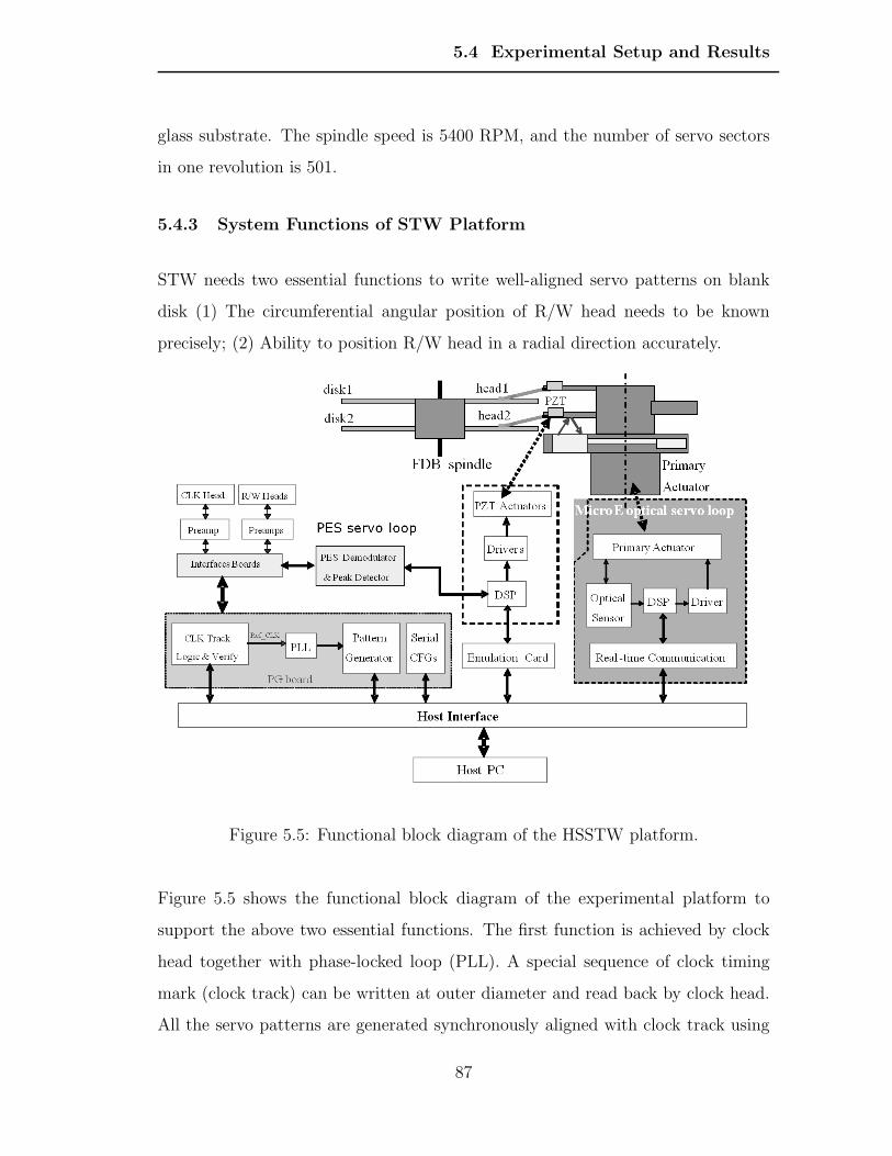
5.4 Experimental Setup and Results
glass substrate. The spindle speed is 5400 RPM, and the number of servo sectors
in one revolution is 501.
5.4.3 System Functions of STW Platform
STW needs two essential functions to write well-aligned servo patterns on blank
disk (1) The circumferential angular position of R/W head needs to be known
precisely; (2) Ability to position R/W head in a radial direction accurately.
Figure 5.5: Functional block diagram of the HSSTW platform.
Figure 5.5 shows the functional block diagram of the experimental platform to
support the above two essential functions. The first function is achieved by clock
head together with phase-locked loop (PLL). A special sequence of clock timing
mark (clock track) can be written at outer diameter and read back by clock head.
All the servo patterns are generated synchronously aligned with clock track using
87
5.4 Experimental Setup and Results
PLL. The clock tracks work as reference to tell the circumferential angular position,
and the PLL is used to track the variations of spindle rotational speed.
In Figure 5.5, there are two servo loops to control the radial position of data head.
MicroE optical positioning servo system controls the radial position of arm, while
the PES servo loop with PZT actuator is used to control the position of data head
more accurately. This will be discussed in details in the next section.
y1
v1
pes
P1(s) C1(s)
uc1
C2(s) y2 r2 P2(s)
no
r1
y1m
u1
u2 h
pest v2
tn-1 nd
tn
2nd PZT Loop v
Optical sensor
dt
1st MicroE Loop
Figure 5.6: Hybrid dual-stage servo system.
5.4.4 Servo Mechanism of STW Platform
Figure 5.6 shows the block diagram of the hybrid dual-stage servo system (“hybrid”
means the mixture of optical positioning and PES servo loop). In Figure 5.6,
P1(s), C1(s), P2(s), and C2(s) are plants and controllers for MicroE actuator and
PZT micro-actuator, respectively. y1 is the position of the actuator arm, y2 is the
displacement of PZT, r1 and r2 are references for optical positioning, and PES
servo loop, respectively. h is the position of R/W head, v1 includes vibrations of
suspension, slider, and head, v2 includes vibrations of spindle and disk, and dt is
88
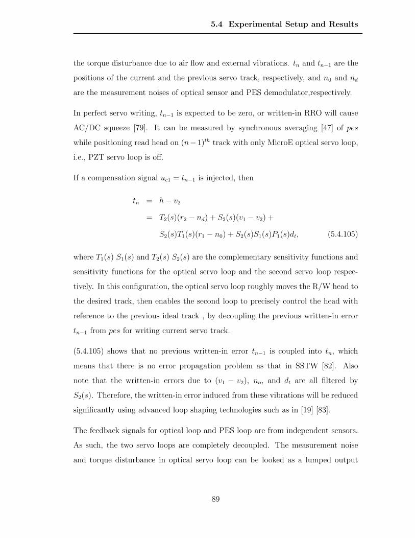
5.4 Experimental Setup and Results
the torque disturbance due to air flow and external vibrations. tn and tn−1 are the
positions of the current and the previous servo track, respectively, and n0 and nd
are the measurement noises of optical sensor and PES demodulator,respectively.
In perfect servo writing, tn−1 is expected to be zero, or written-in RRO will cause
AC/DC squeeze [79]. It can be measured by synchronous averaging [47] of pes
while positioning read head on (n−1)th track with only MicroE optical servo loop,
i.e., PZT servo loop is off.
If a compensation signal uc1 = tn−1 is injected, then
tn = h− v2
= T2(s)(r2 − nd) + S2(s)(v1 − v2) +
S2(s)T1(s)(r1 − n0) + S2(s)S1(s)P1(s)dt, (5.4.105)
where T1(s) S1(s) and T2(s) S2(s) are the complementary sensitivity functions and
sensitivity functions for the optical servo loop and the second servo loop respec-
tively. In this configuration, the optical servo loop roughly moves the R/W head to
the desired track, then enables the second loop to precisely control the head with
reference to the previous ideal track , by decoupling the previous written-in error
tn−1 from pes for writing current servo track.
(5.4.105) shows that no previous written-in error tn−1 is coupled into tn, which
means that there is no error propagation problem as that in SSTW [82]. Also
note that the written-in errors due to (v1 − v2), no, and dt are all filtered by
S2(s). Therefore, the written-in error induced from these vibrations will be reduced
significantly using advanced loop shaping technologies such as in [19] [83].
The feedback signals for optical loop and PES loop are from independent sensors.
As such, the two servo loops are completely decoupled. The measurement noise
and torque disturbance in optical servo loop can be looked as a lumped output
89
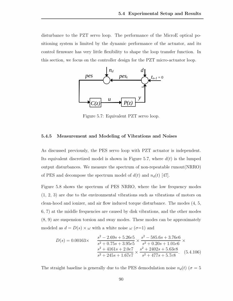
5.4 Experimental Setup and Results
disturbance to the PZT servo loop. The performance of the MicroE optical po-
sitioning system is limited by the dynamic performance of the actuator, and its
control firmware has very little flexibility to shape the loop transfer function. In
this section, we focus on the controller design for the PZT micro-actuator loop.
y
tn-1 = 0 pest d
pes
P(z) C(z)
nd
u
Figure 5.7: Equivalent PZT servo loop.
5.4.5 Measurement and Modeling of Vibrations and Noises
As discussed previously, the PES servo loop with PZT actuator is independent.
Its equivalent discretized model is shown in Figure 5.7, where d(t) is the lumped
output disturbances. We measure the spectrum of non-repeatable runout(NRRO)
of PES and decompose the spectrum model of d(t) and nd(t) [47].
Figure 5.8 shows the spectrum of PES NRRO, where the low frequency modes
(1, 2, 3) are due to the environmental vibrations such as vibrations of motors on
clean-hood and ionizer, and air flow induced torque disturbance. The modes (4, 5,
6, 7) at the middle frequencies are caused by disk vibrations, and the other modes
(8, 9) are suspension torsion and sway modes. These modes can be approximately
modeled as d = D(s)× ω with a white noise ω (σ=1) and
D(s) = 0.00163×s2 − 2.69s+ 5.26e5
s2 + 0.75s+ 3.95e5×
s2 − 585.6s+ 3.76e6
s2 + 0.20s+ 1.01e6×
s2 + 4161s+ 2.0e7
s2 + 245s+ 1.67e7×
s2 + 2402s+ 5.63e8
s2 + 477s+ 5.7e8. (5.4.106)
The straight baseline is generally due to the PES demodulation noise nd(t) (σ = 5
90
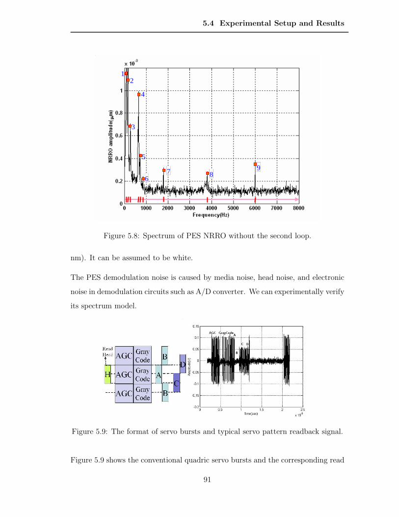
5.4 Experimental Setup and Results
1 2
3
4
5
6 7 8
9
Figure 5.8: Spectrum of PES NRRO without the second loop.
nm). It can be assumed to be white.
The PES demodulation noise is caused by media noise, head noise, and electronic
noise in demodulation circuits such as A/D converter. We can experimentally verify
its spectrum model.
Figure 5.9: The format of servo bursts and typical servo pattern readback signal.
Figure 5.9 shows the conventional quadric servo bursts and the corresponding read
91
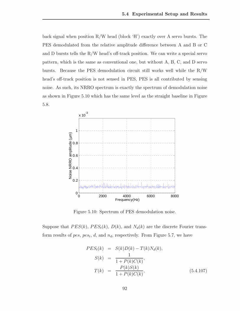
5.4 Experimental Setup and Results
back signal when position R/W head (block ‘H’) exactly over A servo bursts. The
PES demodulated from the relative amplitude difference between A and B or C
and D bursts tells the R/W head’s off-track position. We can write a special servo
pattern, which is the same as conventional one, but without A, B, C, and D servo
bursts. Because the PES demodulation circuit still works well while the R/W
head’s off-track position is not sensed in PES, PES is all contributed by sensing
noise. As such, its NRRO spectrum is exactly the spectrum of demodulation noise
as shown in Figure 5.10 which has the same level as the straight baseline in Figure
5.8.
0 2000 4000 6000 80000
0.2
0.4
0.6
0.8
1
x 10-3
Frequency(Hz)
Noi
se N
RR
O a
mpl
itude
( µm
)
Figure 5.10: Spectrum of PES demodulation noise.
Suppose that PES(k), PESt(k), D(k), and Nd(k) are the discrete Fourier trans-
form results of pes, pest, d, and nd, respectively. From Figure 5.7, we have
PESt(k) = S(k)D(k)− T (k)Nd(k),
S(k) =1
1 + P (k)C(k),
T (k) =P (k)S(k)
1 + P (k)C(k), (5.4.107)
92
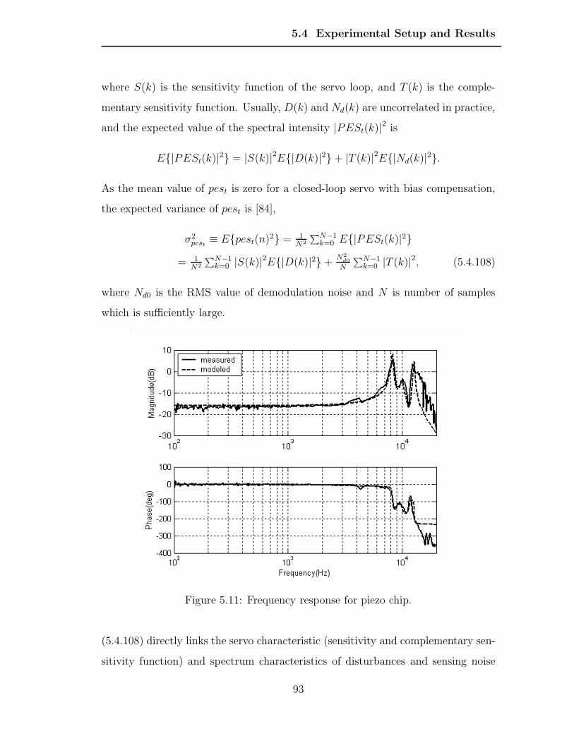
5.4 Experimental Setup and Results
where S(k) is the sensitivity function of the servo loop, and T (k) is the comple-
mentary sensitivity function. Usually, D(k) and Nd(k) are uncorrelated in practice,
and the expected value of the spectral intensity |PESt(k)|2 is
E|PESt(k)|2 = |S(k)|2E|D(k)|2+ |T (k)|2E|Nd(k)|
2.
As the mean value of pest is zero for a closed-loop servo with bias compensation,
the expected variance of pest is [84],
σ2pest
≡ Epest(n)2 = 1
N2
∑N−1k=0 E|PESt(k)|
2
= 1N2
∑N−1k=0 |S(k)|2E|D(k)|2+
N2
d0
N
∑N−1k=0 |T (k)|2, (5.4.108)
where Nd0 is the RMS value of demodulation noise and N is number of samples
which is sufficiently large.
Figure 5.11: Frequency response for piezo chip.
(5.4.108) directly links the servo characteristic (sensitivity and complementary sen-
sitivity function) and spectrum characteristics of disturbances and sensing noise
93
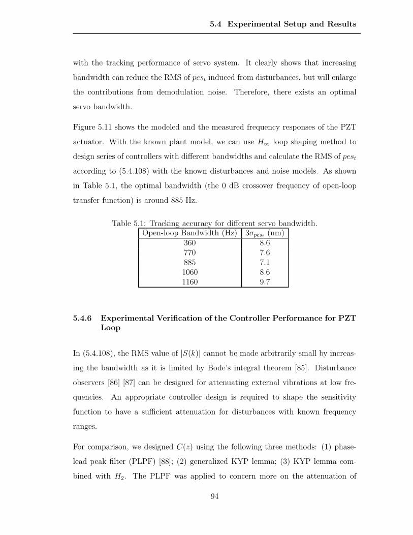
5.4 Experimental Setup and Results
with the tracking performance of servo system. It clearly shows that increasing
bandwidth can reduce the RMS of pest induced from disturbances, but will enlarge
the contributions from demodulation noise. Therefore, there exists an optimal
servo bandwidth.
Figure 5.11 shows the modeled and the measured frequency responses of the PZT
actuator. With the known plant model, we can use H∞ loop shaping method to
design series of controllers with different bandwidths and calculate the RMS of pest
according to (5.4.108) with the known disturbances and noise models. As shown
in Table 5.1, the optimal bandwidth (the 0 dB crossover frequency of open-loop
transfer function) is around 885 Hz.
Table 5.1: Tracking accuracy for different servo bandwidth.Open-loop Bandwidth (Hz) 3σpest (nm)
360 8.6770 7.6885 7.11060 8.61160 9.7
5.4.6 Experimental Verification of the Controller Performance for PZTLoop
In (5.4.108), the RMS value of |S(k)| cannot be made arbitrarily small by increas-
ing the bandwidth as it is limited by Bode’s integral theorem [85]. Disturbance
observers [86] [87] can be designed for attenuating external vibrations at low fre-
quencies. An appropriate controller design is required to shape the sensitivity
function to have a sufficient attenuation for disturbances with known frequency
ranges.
For comparison, we designed C(z) using the following three methods: (1) phase-
lead peak filter (PLPF) [88]; (2) generalized KYP lemma; (3) KYP lemma com-
bined with H2. The PLPF was applied to concern more on the attenuation of
94
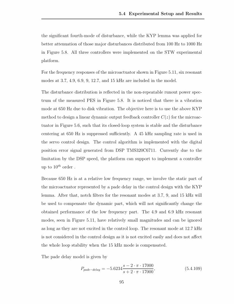
5.4 Experimental Setup and Results
the significant fourth-mode of disturbance, while the KYP lemma was applied for
better attenuation of those major disturbances distributed from 100 Hz to 1000 Hz
in Figure 5.8. All three controllers were implemented on the STW experimental
platform.
For the frequency responses of the microactuator shown in Figure 5.11, six resonant
modes at 3.7, 4.9, 6.9, 9, 12.7, and 15 kHz are included in the model.
The disturbance distribution is reflected in the non-repeatable runout power spec-
trum of the measured PES in Figure 5.8. It is noticed that there is a vibration
mode at 650 Hz due to disk vibration. The objective here is to use the above KYP
method to design a linear dynamic output feedback controller C(z) for the microac-
tuator in Figure 5.6, such that its closed-loop system is stable and the disturbance
centering at 650 Hz is suppressed sufficiently. A 45 kHz sampling rate is used in
the servo control design. The control algorithm is implemented with the digital
position error signal generated from DSP TMS320C6711. Currently due to the
limitation by the DSP speed, the platform can support to implement a controller
up to 10th order .
Because 650 Hz is at a relative low frequency range, we involve the static part of
the microactuator represented by a pade delay in the control design with the KYP
lemma. After that, notch filters for the resonant modes at 3.7, 9, and 15 kHz will
be used to compensate the dynamic part, which will not significantly change the
obtained performance of the low frequency part. The 4.9 and 6.9 kHz resonant
modes, seen in Figure 5.11, have relatively small magnitudes and can be ignored
as long as they are not excited in the control loop. The resonant mode at 12.7 kHz
is not considered in the control design as it is not excited easily and does not affect
the whole loop stability when the 15 kHz mode is compensated.
The pade delay model is given by
Ppade−delay = −5.6234s− 2 · π · 17000
s+ 2 · π · 17000, (5.4.109)
95
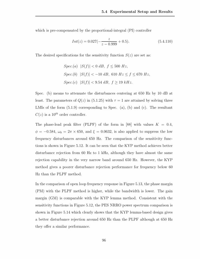
5.4 Experimental Setup and Results
which is pre-compensated by the proportional-integral (PI) controller
Int(z) = 0.027(−z
z − 0.999+ 0.5). (5.4.110)
The desired specifications for the sensitivity function S(z) are set as:
Spec.(a) |S(f)| < 0 dB, f ≤ 500 Hz,
Spec.(b) |S(f)| < −10 dB, 610 Hz ≤ f ≤ 670 Hz,
Spec.(c) |S(f)| < 9.54 dB, f ≥ 19 kHz.
Spec. (b) means to attenuate the disturbances centering at 650 Hz by 10 dB at
least. The parameters of Q(z) in (5.1.25) with τ = 1 are attained by solving three
LMIs of the form (5.1.9) corresponding to Spec. (a), (b) and (c). The resultant
C(z) is a 10th order controller.
The phase-lead peak filter (PLPF) of the form in [88] with values K = 0.4,
φ = −0.584, ω0 = 2π × 650, and ξ = 0.0632, is also applied to suppress the low
frequency disturbances around 650 Hz. The comparison of the sensitivity func-
tions is shown in Figure 5.12. It can be seen that the KYP method achieves better
disturbance rejection from 60 Hz to 1 kHz, although they have almost the same
rejection capability in the very narrow band around 650 Hz. However, the KYP
method gives a poorer disturbance rejection performance for frequency below 60
Hz than the PLPF method.
In the comparison of open loop frequency response in Figure 5.13, the phase margin
(PM) with the PLPF method is higher, while the bandwidth is lower. The gain
margin (GM) is comparable with the KYP lemma method. Consistent with the
sensitivity functions in Figure 5.12, the PES NRRO power spectrum comparison is
shown in Figure 5.14 which clearly shows that the KYP lemma-based design gives
a better disturbance rejection around 650 Hz than the PLPF although at 650 Hz
they offer a similar performance.
96
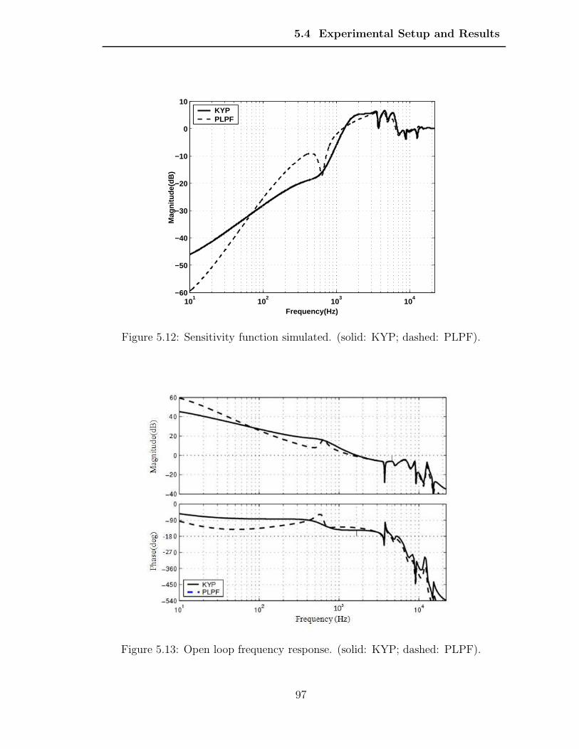
5.4 Experimental Setup and Results
101
102
103
104
−60
−50
−40
−30
−20
−10
0
10
Mag
nitu
de(d
B)
Frequency(Hz)
KYPPLPF
Figure 5.12: Sensitivity function simulated. (solid: KYP; dashed: PLPF).
Figure 5.13: Open loop frequency response. (solid: KYP; dashed: PLPF).
97
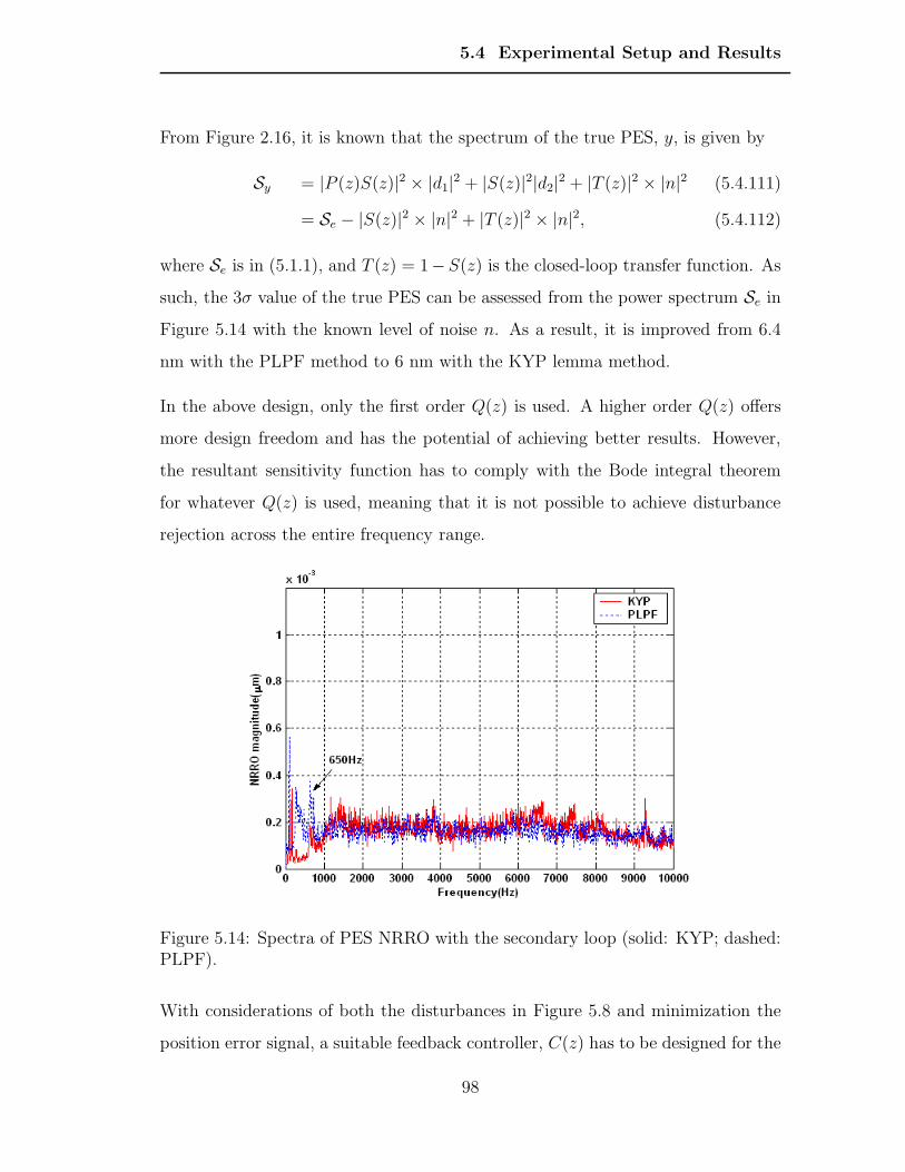
5.4 Experimental Setup and Results
From Figure 2.16, it is known that the spectrum of the true PES, y, is given by
Sy = |P (z)S(z)|2 × |d1|2 + |S(z)|2|d2|
2 + |T (z)|2 × |n|2 (5.4.111)
= Se − |S(z)|2 × |n|2 + |T (z)|2 × |n|2, (5.4.112)
where Se is in (5.1.1), and T (z) = 1−S(z) is the closed-loop transfer function. As
such, the 3σ value of the true PES can be assessed from the power spectrum Se in
Figure 5.14 with the known level of noise n. As a result, it is improved from 6.4
nm with the PLPF method to 6 nm with the KYP lemma method.
In the above design, only the first order Q(z) is used. A higher order Q(z) offers
more design freedom and has the potential of achieving better results. However,
the resultant sensitivity function has to comply with the Bode integral theorem
for whatever Q(z) is used, meaning that it is not possible to achieve disturbance
rejection across the entire frequency range.
Figure 5.14: Spectra of PES NRRO with the secondary loop (solid: KYP; dashed:PLPF).
With considerations of both the disturbances in Figure 5.8 and minimization the
position error signal, a suitable feedback controller, C(z) has to be designed for the
98
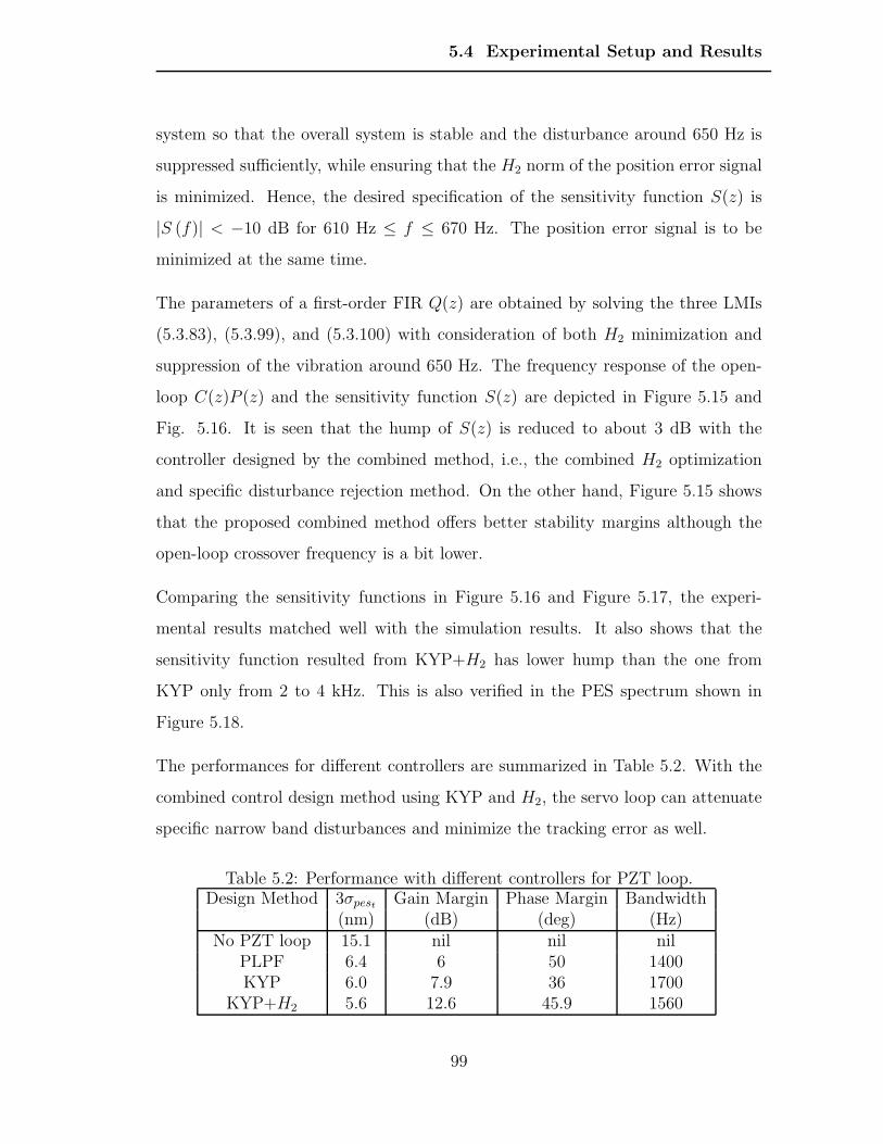
5.4 Experimental Setup and Results
system so that the overall system is stable and the disturbance around 650 Hz is
suppressed sufficiently, while ensuring that the H2 norm of the position error signal
is minimized. Hence, the desired specification of the sensitivity function S(z) is
|S (f)| < −10 dB for 610 Hz ≤ f ≤ 670 Hz. The position error signal is to be
minimized at the same time.
The parameters of a first-order FIR Q(z) are obtained by solving the three LMIs
(5.3.83), (5.3.99), and (5.3.100) with consideration of both H2 minimization and
suppression of the vibration around 650 Hz. The frequency response of the open-
loop C(z)P (z) and the sensitivity function S(z) are depicted in Figure 5.15 and
Fig. 5.16. It is seen that the hump of S(z) is reduced to about 3 dB with the
controller designed by the combined method, i.e., the combined H2 optimization
and specific disturbance rejection method. On the other hand, Figure 5.15 shows
that the proposed combined method offers better stability margins although the
open-loop crossover frequency is a bit lower.
Comparing the sensitivity functions in Figure 5.16 and Figure 5.17, the experi-
mental results matched well with the simulation results. It also shows that the
sensitivity function resulted from KYP+H2 has lower hump than the one from
KYP only from 2 to 4 kHz. This is also verified in the PES spectrum shown in
Figure 5.18.
The performances for different controllers are summarized in Table 5.2. With the
combined control design method using KYP and H2, the servo loop can attenuate
specific narrow band disturbances and minimize the tracking error as well.
Table 5.2: Performance with different controllers for PZT loop.Design Method 3σpest Gain Margin Phase Margin Bandwidth
(nm) (dB) (deg) (Hz)No PZT loop 15.1 nil nil nil
PLPF 6.4 6 50 1400KYP 6.0 7.9 36 1700
KYP+H2 5.6 12.6 45.9 1560
99
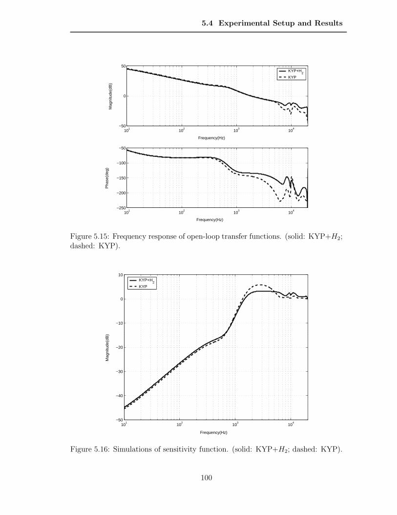
5.4 Experimental Setup and Results
101
102
103
104
−50
0
50
Mag
nitu
de(d
B)
101
102
103
104
−250
−200
−150
−100
−50
Pha
se(d
eg)
Frequency(Hz)
KYP+H2
KYP
Frequency(Hz)
Figure 5.15: Frequency response of open-loop transfer functions. (solid: KYP+H2;dashed: KYP).
101
102
103
104
−50
−40
−30
−20
−10
0
10
Mag
nitu
de(d
B)
Frequency(Hz)
KYP+H2
KYP
Figure 5.16: Simulations of sensitivity function. (solid: KYP+H2; dashed: KYP).
100
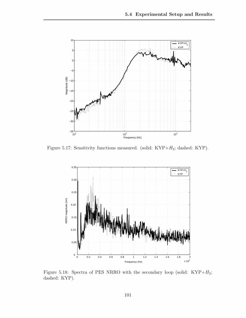
5.4 Experimental Setup and Results
102
103
104
−35
−30
−25
−20
−15
−10
−5
0
5
10
Frequency (Hz)
Mag
nitu
de (
dB)
KYP+H2
KYP
Figure 5.17: Sensitivity functions measured. (solid: KYP+H2; dashed: KYP).
0 0.2 0.4 0.6 0.8 1 1.2 1.4 1.6 1.8 2
x 104
0
0.05
0.10
0.15
0.20
0.25
0.30
0.35
Frequency (Hz)
NR
RO
mag
nitu
de (
nm)
KYP+H2
KYP
Figure 5.18: Spectra of PES NRRO with the secondary loop (solid: KYP+H2;dashed: KYP).
101
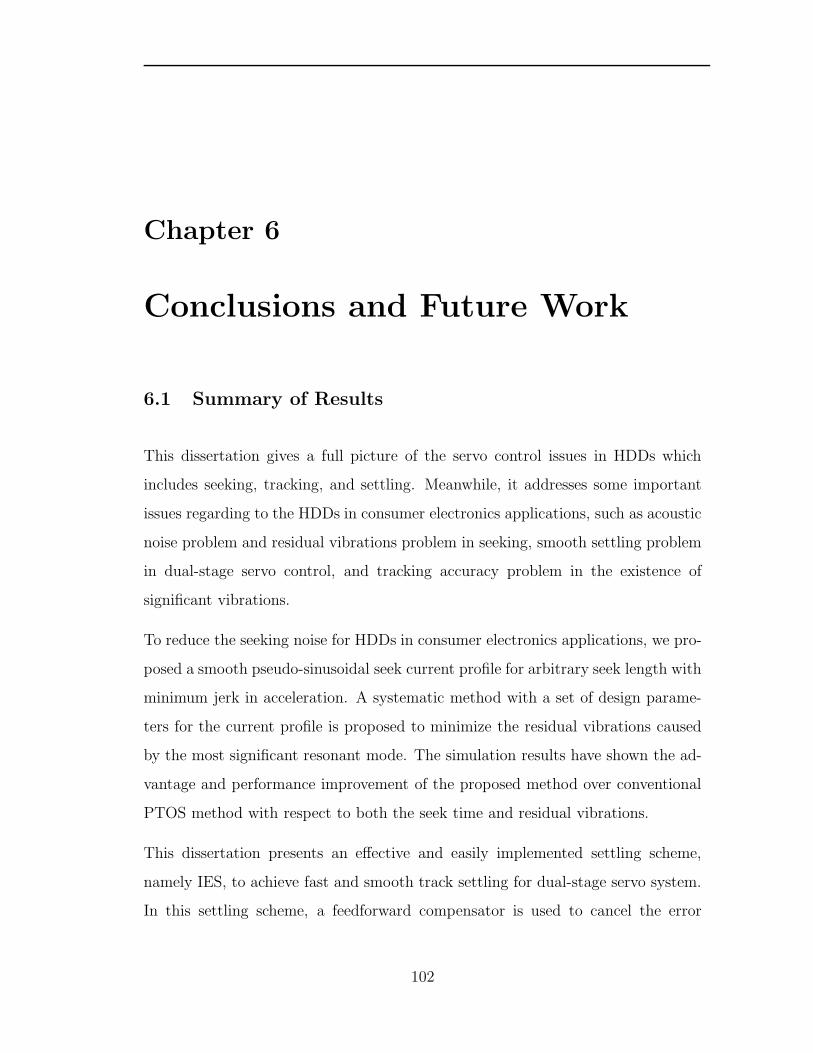
Chapter 6
Conclusions and Future Work
6.1 Summary of Results
This dissertation gives a full picture of the servo control issues in HDDs which
includes seeking, tracking, and settling. Meanwhile, it addresses some important
issues regarding to the HDDs in consumer electronics applications, such as acoustic
noise problem and residual vibrations problem in seeking, smooth settling problem
in dual-stage servo control, and tracking accuracy problem in the existence of
significant vibrations.
To reduce the seeking noise for HDDs in consumer electronics applications, we pro-
posed a smooth pseudo-sinusoidal seek current profile for arbitrary seek length with
minimum jerk in acceleration. A systematic method with a set of design parame-
ters for the current profile is proposed to minimize the residual vibrations caused
by the most significant resonant mode. The simulation results have shown the ad-
vantage and performance improvement of the proposed method over conventional
PTOS method with respect to both the seek time and residual vibrations.
This dissertation presents an effective and easily implemented settling scheme,
namely IES, to achieve fast and smooth track settling for dual-stage servo system.
In this settling scheme, a feedforward compensator is used to cancel the error
102
6.1 Summary of Results
caused by the initial position and velocity of VCM actuator during mode-switching.
Based on ZPET, a detailed pole/zero cancelation scheme is used in the design of
the feedforward compensator. The experiment results show that settling time can
be significantly reduced from 0.7 ms to 0.3 ms.
The dissertation also presents an advanced systematic loop shaping method using
KYP Lemma to optimize the track-following controller with considerations of the
spectrum models of torque disturbances, output disturbances and sensing noise.
The Youla parametrization approach is first used to parameterize the closed-loop
transfer function. The search for the coefficients of the parameter Q(z) is then con-
verted to a linear matrix inequality problem within the generalized KYP lemma
framework. Next, considering the system with an augmented disturbance model,
the generalized KYP lemma is combined the H2 method to design a controller
for minimization of tracking error as well as attenuation of dominant disturbances
at certain frequencies. We applied this method to design a track-following con-
troller and implemented it on our STW experiment platform. The performances
for controllers using different design method are summarized in Table 6.1. With
the combined control design method using KYP and H2, the servo loop can achieve
better tracking accuracy and provide better robustness with more gain margin and
phase margin than the other methods. As such, we achieved servo-writing track
density of 420, 000 TPI on the STW experiment platform.
Table 6.1: Performance of servo controllers using different design method.Design Method 3σpest Gain Margin Phase Margin Bandwidth
(nm) (dB) (deg) (Hz)PLPF 6.4 6 50 1400KYP 6.0 7.9 36 1700
KYP+H2 5.6 12.6 45.9 1560
103
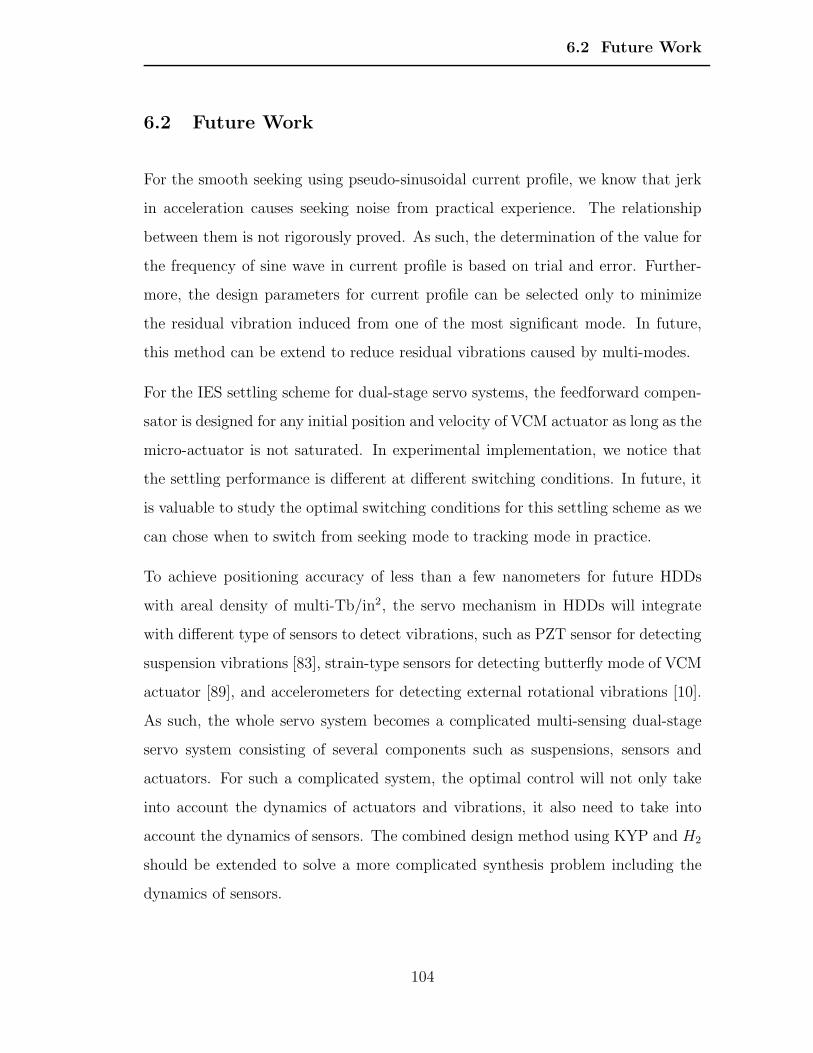
6.2 Future Work
6.2 Future Work
For the smooth seeking using pseudo-sinusoidal current profile, we know that jerk
in acceleration causes seeking noise from practical experience. The relationship
between them is not rigorously proved. As such, the determination of the value for
the frequency of sine wave in current profile is based on trial and error. Further-
more, the design parameters for current profile can be selected only to minimize
the residual vibration induced from one of the most significant mode. In future,
this method can be extend to reduce residual vibrations caused by multi-modes.
For the IES settling scheme for dual-stage servo systems, the feedforward compen-
sator is designed for any initial position and velocity of VCM actuator as long as the
micro-actuator is not saturated. In experimental implementation, we notice that
the settling performance is different at different switching conditions. In future, it
is valuable to study the optimal switching conditions for this settling scheme as we
can chose when to switch from seeking mode to tracking mode in practice.
To achieve positioning accuracy of less than a few nanometers for future HDDs
with areal density of multi-Tb/in2, the servo mechanism in HDDs will integrate
with different type of sensors to detect vibrations, such as PZT sensor for detecting
suspension vibrations [83], strain-type sensors for detecting butterfly mode of VCM
actuator [89], and accelerometers for detecting external rotational vibrations [10].
As such, the whole servo system becomes a complicated multi-sensing dual-stage
servo system consisting of several components such as suspensions, sensors and
actuators. For such a complicated system, the optimal control will not only take
into account the dynamics of actuators and vibrations, it also need to take into
account the dynamics of sensors. The combined design method using KYP and H2
should be extended to solve a more complicated synthesis problem including the
dynamics of sensors.
104
Author’s Publications
Author’s Publications
1. J. L. Zhang, F. Hong, S. S. Ge, “The strategy of designing seek current
profile to reduce acoustic noise and residual vibrations,” IEEE Transactions
on Magnetics, vol. 46, no. 6, pp. 1319-1323, 2010.
2. J. L. Zhang, C. L. Du, S. J. Jiang, “Measurement and modeling of distur-
bances in a servo track writer and advanced loop shaping to achieve higher
track density ,” Transactions of the Institute of Measurement and Control,
vol. 32, no. 2, pp. 221-224, April, 2010.
3. J. L. Zhang, B. Hredzak, C. L. Du, G. Guo, “High density servo track writing
using two-stage configuration,” in Proceedings of IEEE International Confer-
ence on Control Applications, Singapore, pp. 124-129, 2007.
4. J. L. Zhang, F. Hong, S. S. Ge, “A novel settling controller for Dual-Stage
servo systems ,” IEEE Transactions on Magnetics, vol. 44, no. 11, pp. 3757-
3760 , 2008.
5. B. Hredzak, F. Hong, S. S. Ge, J. L. Zhang and Z. M. He, “Modeling and
compensation of pivot nonlinearity in hard disk drives,” in Proceedings of
IEEE International Conference on Control Applications, Singapore, pp. 108-
113, 2007.
6. C. L. Du, L. H. Xie, J. L. Zhang, G. Guo, “Disturbance rejection for a data
storage system via sensitivity loop shaping and adaptive nonlinear compen-
sation,” IEEE/ASME Transactions on Mechatronics, vol. 13, pp. 493-501,
105
Author’s Publications
2008.
7. C. L. Du, L. H. Xie, G. Guo, J. L. Zhang, Q. Li, “A generalized KYP lemma
based control design and application for 425 kTPI servo track writing,” in
Proceedings of the American Control Conference, Minneapolis, Minnesota,
pp. 1303-1308, 2006.
8. C. L. Du, L. H. Xie, J. L. Zhang, “Compensation of VCM actuator pivot fric-
tion based on an operator modeling method,” IEEE Transactions on Control
Systems Technology, vol. 18, pp. 918-926, 2010.
106
Bibliography
Bibliography
[1] W. C. Blount, “Fluid dynamic bearing spindle motors: Their future in hard
disk drives,” http://www.hitachigst.com, 2007.
[2] R. W. Wood, J. Miles, and T. Olson, “Recording technologies for Terabit per
square inch systems,” IEEE Transactions on Magnetics, vol. 38, no. 4, pp.
1711–1718, 2002.
[3] T. Yamaguchi and T. Atsumi, “HDD servo control technologies- what we have
done and where we should go,” in Proceedings of the 17th World Congress, The
International Federation of Automatic Control, Coex, Korea, 2008, pp. 821–
826.
[4] W. Messner and R. Ehrlich, “A tutorial on controls for disk drives,” in Proceed-
ings of the American Control Conference, Arlington, VA, 2001, pp. 408–420.
[5] J. Hoagg and D. Bernstein, “Nonminimum-phase zeros: Much to do about
nothing,” IEEE Transactions on Control Systems, vol. 27, pp. 45–57, 2007.
[6] C. Mohtadi and M. DPhil, “Bode’s integral theorem for discrete-time sys-
tems,” IEE Proceedings, Control Theory and Applications, vol. 137, no. 2, pp.
57–66, 1990.
[7] D. Abramovitch, T. Hurst, and D. Henze, “The PES pareto method: uncov-
ering the strata of position error signals in disk drives,” in Proceedings of the
American Control Conference, Albuquerque, NM, June 1997, pp. 2888–2895.
107
Bibliography
[8] S. Baek and S. Lee, “Vibration rejection control for disk drives by acceleration
feedforward control,” in Proceedings of the IEEE Conference on Decision and
Control, Phoenix, AZ, 1999, pp. 5259–5262.
[9] J. Ishikawa and M. Tomizuka, “Pivot friction compensation using an ac-
celerometer and a disturbance observer for hard disk drives,” IEEE/ASME
Transactions on Mechatronics, vol. 3, no. 3, pp. 194–201, 1998.
[10] A. Jinzenji, T. Sasamoto, K. Aikawa, S. Yoshida, and K. Aruga, “Acceleration
feedforward control against rotational disturbance in hard disk drives,” IEEE
Transactions on Magnetics, vol. 37, no. 2, pp. 888–893, 2001.
[11] M. Kobayashi, T. Yamaguchi, T. Yoshida, and H. Hirai, “Multi-sensing servo
with carriage-acceleration feedback for magnetic disk drives,” in Proceedings
of the IEEE Conference Decision and Control, Philadelphia, PA, 1998, pp.
3038–3042.
[12] H. S. Chang, S. E. Baek, J. H. Park, and Y. K. Byun, “Modeling of pivot
friction using relay function and estimation of its frictional parameters,” in
Proceedings of the American Control Conference, San Diego, CA, 1999, pp.
3784–3789.
[13] M. K. Ciliz and M. Tomizuka, “Modeling and compensation of frictional uncer-
tainties in motion control: a neural network based approach,” in Proceedings
of the American Control Conference, Seattle, WA, 1995, pp. 3269–3273.
[14] S. S. Ge, T. H. Lee, and S. X. Ren, “Adaptive friction compensation of servo
mechanisms,” International Journal of Systems Science, vol. 32, no. 4, pp.
523–532, 2001.
[15] G. Zames, “Feedback and optimal sensitivity: Model reference tranformations,
multiplicative seminorms, and spproximate inverses,” IEEE Transactions Au-
tomatic Control, vol. 26, no. 2, pp. 301–320, 1981.
108
Bibliography
[16] B. Francies, A Course in H∞ Control Theory. Springer-Verlag, Berlin: Lec-
ture Notes in Control and Information Science 88, 1987.
[17] B. M. Chen, Z. L. Lin, and K. X. Liu, “Robust and perfect tracking of discrete
time systems,” in Proceedings of the American Control Conference, Arlington,
VA, 2001, pp. 2594–2599.
[18] G. Cheng, K. Peng, B. M. Chen, and T. H. Lee, “A microdrive track follow-
ing controller design using robust and perfect tracking control with nonlinear
compensation,” Mechatronics, vol. 15, no. 8, pp. 933–948, 2005.
[19] C. Du, L. Xie, J. N. Teoh, and G. Guo, “H2 control for head positioning in
axial and radial dimensions for self-servo track writing,” IEEE Transactions
on Control Systems Technology, vol. 16, no. 1, pp. 177–181, 2008.
[20] G. Herrmann, S. S. Ge, and G. Guo, “Practical implementation of a neu-
ral network controller in a hard disk drive,” IEEE Transactions on Control
Systems Technology, vol. 32, no. 4, pp. 146–154, 2005.
[21] G. Herrmann, S. Ge, and G. Guo, “A neural network controller augmented
to a high performance linear controller and its application to a HDD-track
following servo system,” in Proceedings of the 16th IFAC World Congress,
Prague, Czech Republic, 2005.
[22] Y.-C. Chang, “Adaptive fuzzy-based tracking control for nonlinear SISO sys-
tems via VSS and H∞ approaches,” IEEE Transactions on Fuzzy Systems,
vol. 9, no. 2, pp. 278–292, 2001.
[23] B.-S. Chen, C.-H. Lee, and Y.-C. Chang, “H∞ tracking design of uncertain
nonlinear SISO systems: adaptive fuzzy approach,” IEEE Transactions on
Fuzzy Systems, vol. 4, no. 1, pp. 32–43, 1996.
109
Bibliography
[24] N. Aramcibia, T. Tsao, and S. Gibson, “Adaptive tuning and control of a
hard disk drive,” in Proceedings of the American Control Conference, New
York, USA, 2007, pp. 1526–1530.
[25] H. Taghirad and E. Jamei, “Robust performance verification of adaptive robust
controller for hard disk drives,” IEEE Transactions on Industrial Electronics,
vol. 55, no. 1, pp. 448–456, 2008.
[26] D. Wu, G. Guo, and T.-C. Chong, “Adaptive compensation of microactuator
resonance in hard disk drives,” IEEE Transactions on Magnetics, vol. 36, no. 5,
pp. 2247–2250, 2000.
[27] K. Ohno and T. Hara, “Adaptive resonance mode compensation for hard disk
drives,” IEEE Transactions on Industrial Electronics, vol. 53, no. 2, pp. 624–
630, 2006.
[28] C. I. Kang and C. H. Kim, “An adaptive notch filter for suppressing mechanical
resonance in high track density disk drives,” Microsystem Technologies, vol. 11,
pp. 638–652, 2005.
[29] K. P. Tee, S. S. Ge, and E. H. Tay, “Adaptive resonance compensation for
hard disk drive servo systems,” in Proceedings of the 46th IEEE Conference
Decision and Control, New Orleans, LA, 2007, pp. 3567–3572.
[30] G. Franklin, J. Powell, and M. Workman, Digital control of dynamic systems.
Reading, Mass.: Addsion-Wesley Publishing Company, 1990.
[31] H. Ho, “Fast servo bang-bang seek control,” IEEE Transactions on Magnetics,
vol. 33, no. 6, pp. 4522–4527, Nov. 1997.
[32] G. X. Guo, T. Huang, K. Tay, S. Weerasooriya, and A. Al-Mamun, “A DSP
based hard disk drive servo test stand,” IEEE Transactions on Magnetics,
vol. 34, no. 2, pp. 480–482, March 1998.
110
Bibliography
[33] S. Hara, T. Hara, L. Yi, and M. Tomizuka, “Novel reference signal genera-
tion for two-degree-of-freedom controllers for hard disk drives,” IEEE/ASME
Transactions on Mechatronics, vol. 5, no. 1, pp. 73–78, March 2000.
[34] L. Yi and M. Tomizuka, “Two-degree-of-freedom control with robust feedback
control for hard disk servo systems,” IEEE/ASME Transactions on Mecha-
tronics, vol. 4, no. 1, pp. 17–24, March 1999.
[35] S. Nakagawa, T. Yamaguchi, I. Fujimoto, Y. Hori, Y. Ito, and Y. Hata, “Multi-
rate two-degree-of-freedom control for fast and vibration-less seeking of hard
disk drives,” in Proceedings of the American Control Conference, Arlington,
VA, June 2001, pp. 2797–2802.
[36] A. Al-Mamun, T. Suthasun, and T. H. Lee, “Simplified multi-rate control
for reduced residual vibration - frequency domain analysis,” in Proceedings
International Conference on Measurement and Control, Pittsburgh, USA, May
2001.
[37] S. Zeng, R. Lin, and L. Xu, “Novel method for minimizing track seeking
residual vibrations of hard disk drives,” IEEE Transactions on Magnetics,
vol. 37, no. 3, pp. 1146–1156, May 2001.
[38] D. Oh, S. Lee, and S. Baek, “Adaptive feedforward rejection of microactuator
resonance in disk drive dual-stage actuator servo,” in Asia-Pacific Magnetic
Recording Conference, Singapore, 2000, pp. TP11, 1–2.
[39] N.-C. P. Dong-Woohn Kim, Jin Koo Lee and Y. P. Park, “Vibration analysis
of HDD actuator with equivalent finite element model of vcm coil,” Journal
of Mechanical Science and Technology, vol. 17, no. 5, pp. 679–690, 2003.
[40] L. Guo and Y. Chen, “Disk flutter and its impact on HDD servo performance,”
IEEE Transactions on Magnetics, vol. 37, no. 2, pp. 866–870, 2001.
111
Bibliography
[41] G. Guo and J. Zhang, “Feedforward control for reducing disk-flutter-induced
track misregistration,” IEEE Transactions on Magnetics, vol. 39, no. 4, pp.
2103–2108, 2003.
[42] Trendfocus, “Annual trendfocus report,” http://www.trendfocus.com, 2008.
[43] R. Evans, J. Griesbach, and W. Messner, “Piezoelectric microactuator for
dual-stage control,” IEEE Transactions on Magnetics, vol. 35, no. 2, pp. 977–
982, 1999.
[44] Y. Chen, K. Moore, J. Yu, and T. Zhang, “Iterative learning control and
repetitive control in hard disk drive industry - a tutorial,” in Proceedings of
the 2006 IEEE International Conference on Decision and Control, San Diego,
USA, 2006, pp. 1–15.
[45] J. L. Zhang, S. Weerasooriya, T. Huang, and T. S. Low, “Modified AFC runout
cancellation and its influence on track following,” in Proceedings of the Inter-
national Conference on Industrial Electronics, Control and Instrumentation,
Japan, 1997, pp. 35–40.
[46] A. Sacks, M. Bodson, and W. Messner, “Advanced methods for repeatable
runout compensation,” IEEE Transactions on Magnetics, vol. 31, no. 2, pp.
1031–1036, 1995.
[47] R. Ehrlich and D. Curran, “Major HDD TMR sources and projected scaling
with TPI,” IEEE Transactions on Magnetics, vol. 35, no. 2, pp. 885–891, 1999.
[48] G. F. Franklin, J. D. Powell, and A. Emami-Naeini, Feedback Control of Dy-
namic Systems, 4th ed. Upper Saddle River, NJ: Prentice Hall, 2002.
[49] V. Venkataramanan, B. Chen, T. Lee, and G. Guo, “A new approach to the
design of mode switching control in hard disk drive servo systems,” Control
Engineering Practice, vol. 10, no. 9, pp. 925–939, 2002.
112
Bibliography
[50] P. Meckel and K. Kudo, “Input shaping technique of reduce vibration for
disk-drive heads,” ASME, Advances in Information Storage Systems, vol. 5,
pp. 45–58, 1993.
[51] Y. Mizoshita, S. Hasegawa, and K. Takaishi, “Vibration minimized access
control for disk drives,” IEEE Transactions on Magnetics, vol. 32, no. 3, pp.
1793–1798, 1996.
[52] D. K. Miu and S. P. Bhat, “Minimum power and minimum jerk position
control and its applications in computer disk drives,” IEEE Transactions on
Magnetics, vol. 27, no. 6, pp. 4471–4475, 1991.
[53] B. Schardt and E. Schreck, “Flying height measurement while seeking in hard
disk drives,” IEEE Transactions on Magnetics, vol. 34, pp. 1765–1767, 1998.
[54] L. Guo, J. Chang, and X. Hu, “Track-following and seek/settle control
schemes for high density disk drives with dual-stage actuators,” in Proceed-
ings IEEE/ASME International Conference Advanced Intelligent Mechatron-
ics, Como, Italy, 2001, pp. 1136–1141.
[55] M. Kobayashi and R. Horowitz, “Track seek control for hard disk dual-stage
servo systems,” IEEE Transactions on Magnetics, vol. 37, no. 2, pp. 949–954,
2001.
[56] G. X. Guo, Q. Hao, and T. S. Low, “A dual-stage control design for high track
per inch hard disk drives,” IEEE Transactions on Magnetics, vol. 37, no. 2,
pp. 860–865, 2001.
[57] M. Kobayashi, S. Nakagawa, and S. Nakamura, “A phase-stabilized servo con-
troller for dual-stage actuators in hard disk drives,” IEEE Transactions on
Magnetics, vol. 39, no. 2, pp. 844–850, 2003.
113
Bibliography
[58] Z. M. Li, K. X. Liu, B. M. Chen, and T. H. Lee, “Robust and perfect tracking
control design of a hard disk drive with a dual-stage actuator,” in Proceedings
of the American Control Conference, Arlington, VA, 2001, pp. 3849–3854.
[59] T. Yamaguchi, Y. Soyama, H. Hosokawa, K. Tsuneta, and H. Hirai, “Improve-
ment of settling response of disk drive head positioning servo using mode
switching control with initial value compensation,” IEEE Transactions on
Magnetics, vol. 32, no. 3, pp. 1767–1772, 1996.
[60] T. Yamaguchi, K. Shishida, S. Tohyama, and H. Hirai, “Mode switching con-
trol design with initial value compensation and its application to head po-
sitioning control on magnetic disk drives,” IEEE Transactions on Industrial
Electronics, vol. 43, no. 1, pp. 65–73, 1996.
[61] W. Singhose, W. Seering, and N. Singer, “Residual vibration reduction us-
ing vector diagrams to generate shaped inputs,” ASME Journal of Mechnical
Design, vol. 116, pp. 654–659, 1994.
[62] T. Singh and W. Singhose, “Tutorial on input shaping/time delay control
of maneuvering flexible structures,” in Proceedings of the American Control
Conference, Alaska, USA, 2002, pp. 1717–1731.
[63] T. Yamaguchi, “A mode-switching controller with initial value compensation
for hard disk drive servo control,” Control Engineering Practice, vol. 5, no. 11,
pp. 1525–1532, 1997.
[64] M. Tomizuka, “Zero phase error tracking algorithm for digital control,” ASME
Journal of Dynamic Systems, Measurement, and Control, vol. 109, pp. 65–68,
1987.
[65] A. Rantzer, “On the Kalman-Yakubovic-Popov lemma,” Systems and Control
Letter, vol. 28, no. 1, pp. 7–10, 1996.
114
Bibliography
[66] T. Iwasaki, G. Meinsma, and M. Fu, “Generalized S-procedure and finite fre-
quency KYP lemma,” Mathematical Problems in Engineering, vol. 6, pp. 305–
320, 2000.
[67] S. Boyd and C. H. Barratt, Linear Controller Design: Limits of Performance.
Eaglewood Cliffs: Prentice Hall, 1991.
[68] B. A. Francis and J. C. Doyle, “Linear control theory with an H∞ optimality
criteron,” SIAM Journal on Control and Optimization, vol. 25, pp. 815–844,
1987.
[69] K. Zhou and J. C. Doyle, Essentials of Robust Control. Prentice Hall Inc.,
1989.
[70] T. Coleman, M. Branch, and A. Grace, Optimization Toolbox For Use with
Matlab. The MathWorks Inc. Natick, Mass, 1999.
[71] K. Glover, D. J. N. Limebeer, J. C. Doyle, and E. M. Kasenally, “A charac-
terization of all solutions to the four block general distance problem,” SIAM
Journal on Control and Optimization, vol. 27, pp. 283–324, 1991.
[72] A. Saberi, P. Sannuti, and B. Chen, H2 Optimal Control. Prentice-Hall,
Englewood Cliffs, NJ, 1995.
[73] M. C. de Oliviera, J. Geromel, and J. Bernussou, “An LMI optimization ap-
proach to multiobjective controller design for discrete-time systems,” in Pro-
ceedings of the 38th IEEE Conference Decision and Control, Phoenix, AZ,
1999, pp. 3611–3616.
[74] H. Ho and T. Doan, “Distortion effects on servo position error transfer func-
tion,” IEEE Transactions on Magnetics, vol. 33, no. 4, pp. 2569–2572, 1997.
115
Bibliography
[75] M.-T. Ho, A. Datta, and S. P. Bhattacharyya, “Control system design us-
ing low order controllers: constant gain, PI and PID,” in Proceedings of the
American Control Conference, Albuquerque, New Mexico, 1997, pp. 571–578.
[76] Y. Uematsu, M. Fukushi, and K. Taniguchi, “Development of the pushpin free
STW,” IEEE Transactions on Magnetics, vol. 37, no. 2, pp. 964–968, 2001.
[77] M. Schultz, “A self-servowrite clocking process,” IEEE Transactions on Mag-
netics, vol. 37, no. 2, pp. 1878–1880, 2001.
[78] K. Takaishi and Y. Uematsu, “Hard disk drive servo technology for media-
level servo track writing,” IEEE Transactions on Magnetics, vol. 39, no. 2,
pp. 851–856, 2003.
[79] J. L. Zhang, B. Hredzak, and C. L. Du, “High density servo track writing using
two-stage configuration,” in Proceedings of the IEEE International Conference
on Control Applications, Singapore, 2007, pp. 124–129.
[80] G. Guo and J. Zhang, “Control strategies for writing servo tracks narrower
than 5 micro inches,” in Proceedings of the of 2003 JSME-IIP/ASME-ISPS
Joint Conference on Micromechatronics for Information and Precision Equip-
ment, Singapore, 2003, pp. 1–5.
[81] B. Hredzak, G. Guo, and J. Zhang, “Investigation of the effect of hard disk
drive unbalance on repeatable and non-repeatable runout,” in Proceedings of
2003 IEEE International Conference on Power Electronics and Drive Sys-
temsl, Singapore, 2003, pp. 1359–1363.
[82] H. Ye, V. Sng, C. Du, J. Zhang, and G. Guo, “Radial error propagation
issues in self servo track writing technology,” IEEE Transactions on Magnetics,
vol. 38, no. 5, pp. 2180–2182, 2002.
116
Bibliography
[83] Y. Li, R. Horowitz, and R. Evans, “Vibration control of a PZT actuated
suspension dual-stage servo system using a PZT sensor,” IEEE Transactions
on Magnetics, pp. 932–937, 2003.
[84] R. Ehrlich, J. Adler, and H. Hindi, “Rejecting oscillatory, non-synchronous
mechanical disturbance in hard disk drives,” IEEE Transactions on Magnetics,
vol. 37, no. 2, pp. 646–650, 2001.
[85] D. Abramovitch, T. Hurst, and D. Henze, “An overview of PES Pareto method
for decomposing daseline noise sources in hard disk position error signals,”
IEEE Transactionsctions on Magnetics, vol. 34, no. 1, pp. 17–23, 1998.
[86] G. Herrmann, S. S. Ge, and G. Guo, “Practical implementation of neural
network controller in a hard disk drive,” IEEE Transactions Control Systems
Technology, vol. 13, no. 1, pp. 146–154, 2005.
[87] S. S. Ge, B. Ren, and T. H. Lee, “Hard disk drive control in mobile applica-
tions,” System Science and Complexity, vol. 20, pp. 215–225, 2007.
[88] J. Zheng, C. Du, G. Guo, Y. Wang, J. Zhang, Q. Li, and B. Hredzak, “Phase
lead peak filter method to high TPI servo track writer with microactuators,”
in Proceedings of the American Control Conference, Minneapolis, MN, 2006,
pp. 1309–1314.
[89] F. Huang, T. Semba, W. Imaino, and F. Lee, “Active damping in HDD actu-
ator,” IEEE Transactions on Magnetics, vol. 37, no. 2, pp. 847–849, 2001.
117