advanced quantum mechanics - vumulders/aqm2010.pdf · advanced quantum mechanics ... week 36...

Advanced Quantum Mechanics

P.J. Mulders

Department of Physics and Astronomy, Faculty of Sciences,Vrije Universiteit Amsterdam

De Boelelaan 1081, 1081 HV Amsterdam, the Netherlands

email: [email protected]

September 2010 (vs 2.13)

Lectures given in the academic year 2010-2011

1

Introduction 2

Voorwoord

The lectures Advanced Quantum Mechanics in the fall semester 2010 will be taught by Prof. Piet Mulders,assisted by Drs Wilco den Dunnen for the tutorial sessions.

We will be using various books, depending on the choice of topics. For the basis we will use the bookIntroduction to Quantum Mechanics, second edition van D.J. Griffiths (Pearson) or these lecture notes.

The course is for 6 credits and is given fully in period 1. This means that during this period you willneed to work on this course 50% of your time.

Piet MuldersSeptember 2010

Schedule (indicative, to be completed later)

Books Notes Exercises

Week 36 Griffiths 1 - 3, 5.3.2 1 1, 2, 3Griffiths 4.1 - 4.3 2, 3

Week 37 Griffiths 4.4 4, 5 4, 5, 6CT X, p. 999-1058 4, 5 7, 8, 9, 10, 11, 12

Week 38 Griffiths 5.1, 5.2 6, 7 13, 14, 15Griffiths 6 8, 9 16, 17, 18, 19, 20

Week 39 Griffiths 7 10 21, 22Griffiths 9 11, 12 23

Week 40 Griffiths 10 13 24

Week 41

Week 42

Literature

1. D.J. Griffiths, Introduction to Quantum Mechanics, Pearson 2005

2. B. Bransden and C. Joachain, Quantum Mechanics, Prentice hall 2000

3. F. Mandl, Quantum Mechanics, Wiley 1992

4. C. Cohen-Tannoudji, B. Diu and F. Laloe, Quantum Mechanics I and II, Wiley 1977

5. J.J. Sakurai, Modern Quantum Mechanics, Addison-Wesley 1991

6. E. Merzbacher, Quantum Mechanics, Wiley 1998

Introduction 3

Contents

1 Basics in quantum mechanics 11.1 Introduction . . . . . . . . . . . . . . . . . . . . . . . . . . . . . . . . . . . . . . . . . . . . 11.2 Translation symmetry . . . . . . . . . . . . . . . . . . . . . . . . . . . . . . . . . . . . . . 11.3 Time evolution . . . . . . . . . . . . . . . . . . . . . . . . . . . . . . . . . . . . . . . . . . 41.4 Rotational symmetry . . . . . . . . . . . . . . . . . . . . . . . . . . . . . . . . . . . . . . . 41.5 Gallilean invariance . . . . . . . . . . . . . . . . . . . . . . . . . . . . . . . . . . . . . . . . 61.6 Discrete symmetries . . . . . . . . . . . . . . . . . . . . . . . . . . . . . . . . . . . . . . . 71.7 Time reversal . . . . . . . . . . . . . . . . . . . . . . . . . . . . . . . . . . . . . . . . . . . 9

2 Angular momentum and spherical harmonics 102.1 Spherical harmonics . . . . . . . . . . . . . . . . . . . . . . . . . . . . . . . . . . . . . . . 102.2 The radial Schrodinger equation . . . . . . . . . . . . . . . . . . . . . . . . . . . . . . . . 122.3 The free wave solution . . . . . . . . . . . . . . . . . . . . . . . . . . . . . . . . . . . . . . 14

3 The hydrogen atom 153.1 Transformation to the center of mass . . . . . . . . . . . . . . . . . . . . . . . . . . . . . . 153.2 Solving the eigenvalue equation . . . . . . . . . . . . . . . . . . . . . . . . . . . . . . . . . 153.3 Appendix: Generalized Laguerre polynomials . . . . . . . . . . . . . . . . . . . . . . . . . 173.4 A note on Bohr quantization . . . . . . . . . . . . . . . . . . . . . . . . . . . . . . . . . . 18

4 Spin 204.1 Definition . . . . . . . . . . . . . . . . . . . . . . . . . . . . . . . . . . . . . . . . . . . . . 204.2 Rotation invariance . . . . . . . . . . . . . . . . . . . . . . . . . . . . . . . . . . . . . . . . 204.3 Spin states . . . . . . . . . . . . . . . . . . . . . . . . . . . . . . . . . . . . . . . . . . . . 214.4 Why is ℓ integer . . . . . . . . . . . . . . . . . . . . . . . . . . . . . . . . . . . . . . . . . 224.5 Matrix representations of spin operators . . . . . . . . . . . . . . . . . . . . . . . . . . . . 234.6 Rotated spin states . . . . . . . . . . . . . . . . . . . . . . . . . . . . . . . . . . . . . . . . 23

5 Combination of angular momenta 265.1 Quantum number analysis . . . . . . . . . . . . . . . . . . . . . . . . . . . . . . . . . . . . 265.2 Clebsch-Gordon coefficients . . . . . . . . . . . . . . . . . . . . . . . . . . . . . . . . . . . 275.3 The Wigner-Eckart theorem . . . . . . . . . . . . . . . . . . . . . . . . . . . . . . . . . . . 29

6 Identical particles 316.1 Permutation symmetry . . . . . . . . . . . . . . . . . . . . . . . . . . . . . . . . . . . . . . 316.2 Applications . . . . . . . . . . . . . . . . . . . . . . . . . . . . . . . . . . . . . . . . . . . . 32

7 Spin in Atomic Physics 357.1 The Helium atom . . . . . . . . . . . . . . . . . . . . . . . . . . . . . . . . . . . . . . . . . 357.2 Atomic multiplets . . . . . . . . . . . . . . . . . . . . . . . . . . . . . . . . . . . . . . . . 367.3 Selection rules . . . . . . . . . . . . . . . . . . . . . . . . . . . . . . . . . . . . . . . . . . . 37

8 Bound state perturbation theory 398.1 Basic treatment . . . . . . . . . . . . . . . . . . . . . . . . . . . . . . . . . . . . . . . . . . 398.2 Perturbation theory for degenerate states . . . . . . . . . . . . . . . . . . . . . . . . . . . 408.3 Applications . . . . . . . . . . . . . . . . . . . . . . . . . . . . . . . . . . . . . . . . . . . 40

Introduction 4

9 Magnetic effects in atoms and the electron spin 449.1 The Zeeman effect . . . . . . . . . . . . . . . . . . . . . . . . . . . . . . . . . . . . . . . . 449.2 Spin-orbit interaction and magnetic fields . . . . . . . . . . . . . . . . . . . . . . . . . . . 45

10 Variational approach 4710.1 Basic treatment . . . . . . . . . . . . . . . . . . . . . . . . . . . . . . . . . . . . . . . . . . 4710.2 Application: ground state of Helium atom . . . . . . . . . . . . . . . . . . . . . . . . . . . 4710.3 Application: ionization energies and electron affinities . . . . . . . . . . . . . . . . . . . . 48

11 Time-dependent perturbation theory 4911.1 Explicit time-dependence . . . . . . . . . . . . . . . . . . . . . . . . . . . . . . . . . . . . 4911.2 Example: two-level system . . . . . . . . . . . . . . . . . . . . . . . . . . . . . . . . . . . . 5011.3 Fermi’s golden rule . . . . . . . . . . . . . . . . . . . . . . . . . . . . . . . . . . . . . . . . 52

12 Emission and absorption of radiation and lifetimes 5412.1 Application: emission and absorption of radiation by atoms . . . . . . . . . . . . . . . . . 5412.2 Application: unstable states . . . . . . . . . . . . . . . . . . . . . . . . . . . . . . . . . . . 56

13 Adiabatic processes 5713.1 Sudden and adiabatic approximation . . . . . . . . . . . . . . . . . . . . . . . . . . . . . . 5713.2 An example: Berry’s phase for an electron in a precessing field . . . . . . . . . . . . . . . 5813.3 The geometric nature of Berry’s phase . . . . . . . . . . . . . . . . . . . . . . . . . . . . . 59

14 Scattering theory 6114.1 Differential cross sections . . . . . . . . . . . . . . . . . . . . . . . . . . . . . . . . . . . . 6114.2 Cross section in Born approximation . . . . . . . . . . . . . . . . . . . . . . . . . . . . . . 6114.3 Applications to various potentials . . . . . . . . . . . . . . . . . . . . . . . . . . . . . . . . 63

15 Scattering off a composite system 6615.1 Form factors . . . . . . . . . . . . . . . . . . . . . . . . . . . . . . . . . . . . . . . . . . . 6615.2 Examples of form factors . . . . . . . . . . . . . . . . . . . . . . . . . . . . . . . . . . . . . 67

16 Time-independent scattering solutions 6916.1 Asymptotic behavior and relation to cross section . . . . . . . . . . . . . . . . . . . . . . . 6916.2 The integral equation for the scattering amplitude . . . . . . . . . . . . . . . . . . . . . . 7116.3 The Born approximation and beyond . . . . . . . . . . . . . . . . . . . . . . . . . . . . . . 7216.4 Identical particles . . . . . . . . . . . . . . . . . . . . . . . . . . . . . . . . . . . . . . . . . 73

17 Partial wave expansion 7517.1 Phase shifts . . . . . . . . . . . . . . . . . . . . . . . . . . . . . . . . . . . . . . . . . . . . 7517.2 Cross sections and partial waves . . . . . . . . . . . . . . . . . . . . . . . . . . . . . . . . 7617.3 Application: the phase shift from the potential . . . . . . . . . . . . . . . . . . . . . . . . 76

Basics in quantum mechanics 1

1 Basics in quantum mechanics

1.1 Introduction

At this point, you should be familiar with the basic aspects of quantum mechanics. That means youshould be familiar with working with operators, in particular position and momentum operators that donot commute, but satisfy the basic commutation relation

[ri, pj ] = i~ δij. (1)

The most common way of working with these operators is in an explicit Hilbert space of square integrable(complex) wave functions ψ(r, t) in which operators just produce new functions (ψ → ψ′ = Oψ). Theposition operator produces a new function by just multiplication with the position itself. The momentumoperator acts as a derivative, p = −i~ ∇, with the appropriate factors such that the basic commutationrelation is satisfied. We want to stress at this point the non-observability of the wave function. It arethe operators and their eigenvalues as outcome of measurements that are relevant. As far as the Hilbertspace is concerned, one can work with any appropriate basis, for instance the eigenstates of any specificoperator, given as a set of functions or more formal in the Dirac representation as quantum states |r〉or |p〉, etc. Here the kets contain a set of ’good’ quantum numbers, i.e. a number of eigenvalues ofcompatible (commuting) operators.———————–Question: Why is it essential that the quantum numbers within one ket correspond to eigenvalues ofcompatible operators?———————–The coordinate state wave function then is nothing else as an overlap of states given by the inner productin Hilbert space, φ(r) = 〈r|φ〉, of which the square gives the probability to find a state |φ〉 in the state|r〉. Similarly one has the momentum state wave function, φ(p) = 〈p|φ〉.

Some operators can be constructed from the basic operators such as angular momentum operatorsℓi = ǫijk rjpk. The most important operator in quantum mechanics is the Hamiltonian. It determinesthe time evolution to be discussed below. The Hamiltonian H(r,p, s) may also contain other operatorscorresponding to specific properties, such as the spin operators, satisfying the commutation relations

[si, sj ] = i~ ǫijk sk. (2)

The spin properties of systems are ’independent’ from spatial properties, which at the operator levelmeans that spin operators commute with the position and momentum operators. As a reminder, thisimplies that momenta and spins can be specified simultaneously (compatibility of the operators). Thespin states are usually represented as spinors (column vectors) in spin-space (a linear space over thecomplex numbers).

1.2 Translation symmetry

Symmetry considerations are at the heart of our understanding of nature. We have to understand howthey are implemented in a quantum world. Let’s start with translations as an example. Translations canbe considered in space-time or in the Hilbert space of wave functions, it will affect operators, etc.

Let us start with translations in one dimension,

x −→ x′ = x+ a. (3)

This is an example of a continuous transformation. There are many translations, in fact infinitely manydetermined by the continuous parameter a. Continuous transformations are contrasted with discretetransformations, such as x → x′ = −x (space inversion, which is discussed elsewhere). One of the


issues with transformations is the investigation of the consequences when it constitutes a symmetrytransformation, i.e. when the ’world’ is invariant under the transformation.

To see how we investigate the consequences referred to above, we first look at ways to ’translatea function’ or ’translate an operator’. We first investigate what happens with a wave function. Forcontinuous transformations, it turns out to be extremely useful to study first the infinitesimal problem(in general true for so-called Lie transformations). We get for small a a ’shifted’ function

φ′(x) = φ(x+ a) = φ(x) + adφ

dx+ . . . =

(

1 +i

~a px + . . .

)

︸︷︷︸

U(a)

φ(x), (4)

which defines the shift operator U(a) of which the momentum operator px = −i~ (d/dx) is the generator.One can extend the above to higher orders,

φ′(x) = φ(x + a) = φ(x) + ad

dxφ+

1

2!a2 d

dx2φ+ . . . ,

Using the (for operators new!) definition

eA ≡ 1 +A+1

2!A2 + . . . ,

one finds

U(a) = exp

(

+i

~a px

)

. (5)

In general, if A is a hermitean operator (A† = A), then eiA is a unitary operator (U−1 = U †). Thus theshift operator produces new wavefunctions, preserving orthonormality.

How does a translation affect an operator? That is simple. Since we know that Oφ is a function, wehave

(Oφ)′(x) = Oφ(x + a) = U(a)Oφ(x) = U(a)OU−1(a)︸︷︷︸

O′

U(a)φ︸︷︷︸

φ′

(x), (6)

thus for operatorsO −→ O′ = U(a)OU−1(a). (7)

For continuous symmetries this implies for infinitesimal translations

O′ =

(

1 +i

~a px + . . .

)

O

(

1 − i

~a px + . . .

)

= O +i

~a [px, O] + . . . . (8)

This can be generalized to obtain a set of shifted operators O(a) given by

O(a) = ei apx/~ O(0) e−i apx/~, (9)

for which one has

−i~ dOda

= ei apx/~[px, O

]e−i apx/~ and − i~

dO

da

∣∣∣∣a=0

=[px, O

]. (10)

———————–Exercise: Show that the above transformation properties for operators (for infinitesimal as well as forfinite translations) imply for the position operators x → x′ = x + a, thus exactly the same behavior asfor the ’coordinate’ x. Show that the operator px → p′x = px.———————–Exercise: Show that for the ket state one has U(a)|x〉 = |x − a〉. An active translation of a localizedstate with respect to a fixed frame, thus is given by |x+ a〉 = U−1(a)|x〉 = U †(a)|x〉 = e−i apx/~|x〉 .———————–


Invariance under translations

Assume now that we have a Hamiltonian H , that is invariant under translations. This implies thatH(x) = H(x + a). What does this imply? Just compare the Taylor expansion of the operator in a withthe infinitesimal expansion discussed previously,

H(x+ a) = H(x) + a

(dH

dx

)

+ . . . = H(x) +i

~a [px, H ] + . . . ,

and we conclude that translation invariance implies

H(x+ a) = H(x) ⇐⇒ [px, H ] = 0. (11)

———————–Exercise: show directly (by acting on a wave function) that indeed −i~(dH/dx) = [px, H ] ,

[px, H

]φ(x) = −i~

(dH

dx

)

φ(x).

———————–Translation invariance can easily be generalized to three coordinates of one particle and to more particlesby considering

ri −→ r′i = ri + a. (12)

The global shift operator is

U(a) = exp

(

+a ·∑

i

∇i

)

= exp

(

+i

~a ·∑

i

pi

)

= exp

(

+i

~a · P

)

, (13)

where pi = −i~∇i are the one-particle operators and P =∑

i pi is the total momentum operator.

Translation invariance of the whole world implies that for U(a) in Eq. 13

U(a)H U−1(a) = H ⇐⇒ [P , H ] = 0. (14)

Thus a translation-invariant Hamiltonian usually does not commute with the momenta of individual par-ticles or with relative momenta, but only with the total momentum operator (center of mass momentum),of which the expectation value thus is conserved.

Bloch theorem

The Bloch theorem is a very nice application of translation symmetry in solid state physics. We will proofthe Bloch theorem in one dimension. Consider a periodic potential (in one dimension), V (x+ d) = V (x).One has a periodic Hamiltonian that commutes with the (unitary) shift operator U(d) = exp(+i d px/~),

[H,U(d)] = 0 (15)

(prove this!). Thus these operators have a common set of eigenstates φE,k, satisfying H φE,k(x) =E φE,k(x) and U(d)φE,k(x) = ei kd φE,k(x) in which kd runs (for instance) between −π ≤ kd ≤ π. Usingthat U(d) is the translation operator, one finds that

φE,k(x+ d) = ei kd φE,k(x) (16)

Equivalently by writing φ as the Bloch wave

φE,k(x) ≡ eikx uE,k(x) (17)


one finds that uE,k(x) is periodic, satisfying uE,k(x+ d) = uE,k(x).To appreciate this result, realize that for a constant potential (translation invariance or invariance

for any value of d or effectively d → 0)) the Bloch wave is constant and the wave function is a plainwave (with no restrictions on k, −∞ < k < ∞). The energy becomes E(k) = ~

2 k2/2m. For periodicpotentials the k-values are limited (Brillouin zone) and the dispersion E(k) exhibits typically a bandstructure, which can e.g. be easily demonstrated by working out the solutions for a grid of δ-functions orfor a block-potential (Kronig-Penney model).

1.3 Time evolution

In analogy to space translation, we have an (active) operator describing time evolution,

ψ′(t) = ψ(t+ τ) = ψ(t) + τdψ

dt+ . . . =

(

1 − i

~aH + . . .

)

︸︷︷︸

U(τ)

ψ(t). (18)

Time evolution is generated by the Hamiltonian H = i~ d/dt and given by the (unitary) operator

U(τ) = exp

(

− i

~τ H

)

. (19)

Since time evolution is usually our aim in solving problems, it is necessary to know the Hamiltonian,usually in terms of the positions, momenta and spins of the particles involved.

1.4 Rotational symmetry

Rotations are characterized by a rotation axis (n) and an angle (0 ≤ α ≤ 2π),

r −→ r′ = R(n, α) r or ϕ −→ ϕ′ = ϕ+ α, (20)

where the latter refers to the polar angle around the n-direction, e.g. for a rotation around the z-axis onehas explicitly

xyz

−→

x′

y′

z′

=

cosα − sinα 0sinα cosα 0

0 0 1

xyz

. (21)

Note that here the components of the vector r change. It would correspond to a rotation R(z,−α) forthe axes. Such a rotation also gives rise to transformations in the Hilbert space of wave functions. Usingpolar coordinates and a rotation around the z-axis, we find

φ(r, θ, ϕ + α) = φ(r, θ, ϕ) + α∂

∂ϕφ+ . . . =

(

1 +i

~α ℓz + . . .

)

φ, (22)

from which one concludes that ℓz = −i~(∂/∂ϕ) is the generator of rotations around the z-axis, and therotation operator in the Hilbert space is

U(z, α) = exp

(

+i

~α ℓz

)

= 1 +i

~α ℓz + . . . . (23)

As for the translations, an operator (e.g. the Hamiltonian) behaves as

H(r, θ, ϕ+ α) = H +i

~α [ℓz, H ] + . . . = U(z, α)H U−1(z, α). (24)

= H(r, θ, ϕ) + α

(∂H

∂ϕ

)

+ . . . (25)


Rotational invariance (around z-axis) implies that

U(z, α)H U−1(z, α) = H ⇐⇒ [ℓz, H ] = 0. (26)

For more particles, invariance under rotations of the world implies

H invariant ⇐⇒ [L, H ] = 0, (27)

where L =∑

i ℓi. This is a fundamental symmetry of nature for particles without spin!

Although the situation looks quite similar to the translations, there is an important difference. For twoconsecutive rotations the order is important (rotations do not commute). This is true in coordinate spaceas well as Hilbert space, R(x, α)R(y, β) 6= R(y, β)R(x, α) and U(x, α)U(y, β) 6= U(y, β)U(x, α). Forthe rotations in the Hilbert space, it is evident from the infinitesimal rotations. The generators (angularmomentum operators) do not commute,

[ℓi, ℓj ] = i~ ǫijk ℓz.

———————–Exercise: If you like a bit of puzzling, there is the Baker-Campbell-Hausdorff relation of which the firstterms are

eA eB = eC with C = A+B +1

2[A,B] +

1

12[A, [A,B]] +

1

12[B, [A,B]] + . . . ,

which shows that (only) for commuting operators one can ’add’ the operators in the exponent, as isknown to work for numbers.———————–

Positions and momenta are not invariant under rotations. Quantummechanically this translates into thenon-commutativity of the generators of rotations ℓ and these operators. The commutation relations

[ℓi, rj ] = i~ ǫijk rk, (28)

[ℓi, pj ] = i~ ǫijk pk, (29)

just imply for operators r → r′ = R(n, α)r and p → p′ = R(n, α)p, i.e. the same behavior as thecoordinate r and the same as classical positions and momenta.

x

x’

x’’ x’’’

y

y’=y’’

y’’’

z=z’

z’’=z’’’

θ

χφ

χθφ

Euler Rotations

A standard way to rotate any object to a given orienta-tion are the Euler rotations. Here one rotates the axesas given in the figure. This corresponds (in our conven-tion) to

RE(ϕ, θ, χ) = R(z′′,−χ)R(y′,−θ)R(z,−ϕ)

= R(z,−ϕ)R(y,−θ)R(z,−χ)

Correspondingly one has the rotation operator inHilbert space

UE(ϕ, θ, χ) = e−iϕ ℓz/~ e−iθ ℓy/~ e−iχ ℓz/~. (30)


Using the rotation UE(ϕ, θ, χ) to orient an axi-symmetric object (around z-axis) in the direction n withpolar angles θ and ϕ, the angle χ doesn’t play a role. In order to get nicer symmetry properties, oneuses in that case UE(ϕ, θ,−ϕ). For a non-symmetric system (with three different moments of inertia)one needs all angles.

1.5 Gallilean invariance

From classical mechanics we know that there are a number of basic symmetries governing the physicalworld, known as the (ten) Gallilean transformations. These are

t → t′ = t+ τ, one time translation, (31)

r → r′ = r + a three translations, (32)

r → r′ = R(n, α)r three rotations, (33)

r → r′ = r − ut three boosts. (34)

Classically one can show that invariance under these transformations implies conserved quantities, fortime translations the total energy E, for space translations the total momentum P , for rotations the totalangular momentum L. Also boost invariance implies a conserved quantity, namely K = MR−tP . Boostinvariance will become much more important when we later consider the transformations in a relativistictheory (Lorentz invariance instead of Gallilean invariance).

In quantum mechanics, the conserved quantities correspond to operators of which the expectationvalue is time independent. These are precisely the generators of the corresponding symmetries. Fromthe known relation

i~d〈O〉dt

= [H,O] + 〈∂O∂t

〉. (35)

one sees that this is true if [H,Pi] = [H,Li] = 0 and [H,Ki] = −i~Pi. These specific commutators arepart of the full set of commutation relations between the 10 generators of the Gallilei group (known asthe Lie algebra),

[Pi, Pj ] = [Pi, H ] = [Ji, H ] = 0,

[Ji, Jj ] = i~ ǫijkJk, [Ji, Pj ] = i~ ǫijkPk, [Ji,Kj] = i~ ǫijkKk,

[Ki, H ] = i~Pi, [Ki,Kj] = 0, [Ki, Pj ] = 0. (36)

For the generators of the rotations we have used here J instead of L, because, as we shall shortly see,the full rotation matrix can and even has to be more than just the orbital angular momentum, includingan intrinsic angular momentum (spin). The second line in this equation simply gives the characteristicbehavior of vectors under rotations.

It is easy to check that for a single (free) particle the quantum mechanical set of operators

H =p2

2M, (37)

P = p, (38)

J = ℓ + s = r × p + s (39)

K = mr − tp. (40)

satisfy the above commutation relations (do this!), starting with the canonical relations [ri, pj] = i~ δijand for spin operators [si, sj ] = i~ ǫijk sk and [ri, sj ] = [pi, sj ] = 0. The latter two commutators implythat spin decouples from the spatial part of the wave function.

Adding a potential V (r) to the Hamiltonian, the commutation relations would no longer indicateGallilei invariance. A potential (e.g. centered around an origin) breaks translation invariance, the specific


r-dependence might break rotational invariance, etc. On the other hand, for two particles one finds thatin terms of CM and relative coordinates using total and reduced masses M = m1+m2 and µ = m1m2/Mthe generators

H = H1 +H2 =P 2

2M+Hint,

P = P 1 + P 2 = P ,

J = ℓ1 + s1 + ℓ2 + s2 = R × P + S,

K = K1 + K2 = M R − tP , (41)

satisfy the commutation relations for the Gallilei group, where

P = p1 + p2 and p =m2

Mp1 −

m1

Mp2,

R =m1

Mr1 +

m2

Mr2 and r = r1 − r2,

S = r × p + s1 + s2,

Hint =p2

2µ+ V (r,p, s1, s2).

All commutation relations start simply from the canonical commutation relation for each of the particles.The CM system behaves as a free (composite) system with constant energy and momentum and a spindetermined by the ’relative’ orbital angular momentum and the spins of the constituents. The examplealso shows that even without spins of the constituents (s1 = s2 = 0) a composite system has an intrinsicangular momentum showing up as its spin.

Finally we note that in classical mechanics the Lie algebra structure of the symmetry group is evidentin the Poisson bracket structure of particular quantities A and B, which in that case are functions ofpositions and momenta,

[A(x, p), B(x, p)]P ≡ dA

dx

dB

dp− dA

dp

dB

dx.

———————–Exercise: In analogy to Eq. 10 one has for the generators of boost transformations,

−i~ dO

dux

∣∣∣∣ux=0

=[Kx, O

], etc.

Use this relation to derive [Ki, rj ] and [Ki, pj ] from the requirement that the classical behavior r → r′ =r − ut and p → p′ = p −mu remains valid for the operators. Check that these commutation relationsare satisfied for K = mr − tp.———————–Exercise: Check that the canonical commutation relations for r1 and p1 and those for r2 and p2 implythe canonical commutation relations for R and P as well as for r and p.———————–Exercise: Check that

ℓ1 + ℓ2 = r1 × p1 + r2 × p2 = R × P + r × p.

———————–

1.6 Discrete symmetries

Three important discrete symmetries that we will be discuss are space inversion, time reversal and(complex) conjugation.


Space inversion and Parity

Starting with space inversion operation, we consider its implication for coordinates,

r −→ −r and t −→ t, (42)

implying for instance that classically for p = mr and ℓ = r × p one has

p −→ −p and ℓ −→ ℓ. (43)

The same is true for the quantummechanical operators, e.g. p = −i~ ∇.In quantum mechanics the states |ψ〉 correspond (in coordinate representation) with functions ψ(r, t).

In the configuration space we know the result of inversion, r → −r and t → t, in the case of moreparticles generalized to ri → −ri and t → t. What is happening in the Hilbert space of wave functions.We can just define the action on functions, ψ → ψ′ ≡ Pψ in such a way that

Pφ(r) ≡ φ(−r). (44)

The function Pφ is a new wave function obtained by the action of the parity operator P . It is a hermitianoperator (convince yourself). The eigenvalues and eigenfunctions of the parity operator,

Pφπ(r) = π φπ(r), (45)

are π = ±1, both eigenvalues infinitely degenerate. The eigenfunctions corresponding to π = +1 are theeven functions, those corresponding to π = −1 are the odd functions.

———————–Exercise: Although this looks evident, think carefully about the proof, which requires comparing P 2φusing Eqs 44 and 45.———————–

The action of parity on the operators is as for any operator in the Hilbert space given by

Aφ −→ PAφ = PAP−1︸︷︷︸

A′

Pφ︸︷︷︸

φ′

, thus A −→ PAP−1. (46)

(Note that for the parity operator actually P−1 = P = P †). Examples are

r −→ PrP−1 = −r, (47)

p −→ PpP−1 = −p, (48)

ℓ −→ PℓP−1 = +ℓ, (49)

H(r,p) −→ PH(r,p)P−1 = H(−r,−p). (50)

If H is invariant under inversion, one has

PHP−1 = H ⇐⇒ [P,H ] = 0. (51)

This implies that eigenfunctions of H are also eigenfunctions of P , i.e. they are even or odd. Although Pdoes not commute with r or p (classical quantities are not invariant), the specific behavior POP−1 = −Ooften also is very useful, e.g. in discussing selection rules. The operators are referred to as P -odd operators.

———————–Exercise: Show that for a P -even operator (satisfying POP−1 = +O or [P,O] = PO − OP = 0) thetransition probability

Probα→β = |〈β|O|α〉|2


for parity eigenstates is only nonzero if πα = πβ .What is the selection rule for a P -odd operator (satisfying POP−1 = −O or P,O = PO +OP = 0).———————–

1.7 Time reversal

In classical mechanics with second order differential equations, one has for time-independent forces auto-matically time reversal invariance, i.e. invariance under t→ −t and r → r. There seems an inconsistencywith quantum mechanics for the momentum p and energy E. Classically it equals mr which changessign, while ∇ → ∇. Similarly one has classically E → E, while H = i~(∂/∂t) appears to change sign.The problem can be solved by requiring time reversal to be accompagnied by a complex conjugation, inwhich case one consistently has p = −i~∇ → i~∇ = −p and H → H . Furthermore a stationary stateψ(t) ∼ exp(−iEt) now nicely remains invariant, ψ∗(−t) = ψ(t).

Such a consistent description of the time reversal operator in Hilbert space is straightforward. Forunitary operators one has (mathematically) also the anti-linear option, where an anti-linear operatorsatisfies T (c1|φ1〉 + c2|φ2〉) = c∗1 T |φ1〉 + c∗2 T |φ2〉. It is easily implemented as

T |φ〉 = 〈Tφ|, (52)

which for matrix elements implies

〈φ|ψ〉 = 〈φ|T †T |ψ〉 = 〈Tψ|Tφ〉 = 〈Tφ|Tψ〉∗ (53)

〈φ|A|ψ〉 = 〈φ|T †T AT †T |ψ〉 = 〈Tφ|A|Tψ〉∗. (54)

Operators satisfying TT † = T †T = 1, but swapping bra and ket space (being anti-linear) are known asanti-unitary operators.

Together with conjugation C, which for spinless systems is just complex conjugation, one can lookat CPT -invariance by combining the here discussed discrete symmetries. For all known interactions inthe world the combined CPT transformation appears to be a good symmetry. The separate discretesymmetries are violated, however, e.g. space inversion is broken by the weak force that causes decays ofelementary particles with clear left-right asymmetries. Also T and CP have been found to be broken.

Angular momentum and spherical harmonics 10

2 Angular momentum and spherical harmonics

In this section we repeat the basic results for the (three) angular momentum operators ℓ = r × p =−i~ r × ∇, looking for eigenvalues and eigenstates. The angular momentum operators are best studiedin polar coordinates,

x = r sin θ cosϕ, (55)

y = r sin θ sinϕ, (56)

z = r cos θ, (57)

from which one gets

∂∂r

∂∂θ

∂∂ϕ

=

x/r y/r z/r

x cot θ y cot θ −r sin θ

−y x 0

∂∂x

∂∂y

∂∂z

.

The ℓ operators are given by

ℓx = −i~(

y∂

∂z− z

∂

∂y

)

= i~

(

sinϕ∂

∂θ+ cot θ cosϕ

∂

∂ϕ

)

, (58)

ℓy = −i~(

z∂

∂x− x

∂

∂z

)

= i~

(

− cosϕ∂

∂θ+ cot θ sinϕ

∂

∂ϕ

)

, (59)

ℓz = −i~(

x∂

∂y− y

∂

∂x

)

= −i~ ∂

∂ϕ, (60)

and the square ℓ2 becomes

ℓ2 = ℓ2x + ℓ2y + ℓ2z = −~2

[1

sin θ

∂

∂θ

(

sin θ∂

∂θ

)

+1

sin2 θ

∂2

∂ϕ2

]

. (61)

From the expressions in polar coordinates, one immediately sees that the operators only acts on theangular dependence. One has ℓi f(r) = 0 for i = x, y, z and thus also ℓ2 f(r) = 0. Being a simple

differential operator (with respect to azimuthal angle about one of the axes) one has ℓi(fg) = f (ℓig) +

(ℓif) g.

2.1 Spherical harmonics

We first study the action of the angular momentum operator on the Cartesian combinations x/r, y/rand z/r (only angular dependence). One finds

ℓz

(x

r

)

= i~(y

r

)

, ℓz

(y

r

)

= −i~(x

r

)

, ℓz

(z

r

)

= 0,

which shows that the ℓ operators acting on polynomials of the form

(x

r

)n1(y

r

)n2(z

r

)n3

do not change the total degree n1 + n2 + n3 ≡ ℓ. They only change the degrees of the coordinates in theexpressions. For a particular degree ℓ, there are 2ℓ+ 1 functions. This is easy to see for ℓ = 0 and ℓ = 1.For ℓ = 2 one must take some care and realize that (x2 + y2 + z2)/r2 = 1, i.e. there is one function less


than the six that one might have expected at first hand. The symmetry of ℓ2 in x, y and z immediatelyimplies that polynomials of a particular total degree ℓ are eigenfunctions of ℓ2 with the same eigenvalue~

2 λ.Using polar coordinates one easily sees that for the eigenfunctions of ℓz only the ϕ dependence matters.

The eigenfunctions are of the form fm(ϕ) ∝ ei mϕ, where the actual eigenvalue is m~ and in order thatthe eigenfunction is univalued m must be integer. For fixed degree ℓ of the polynomials m can at mostbe equal to ℓ, in which case the θ-dependence is sinℓ θ. It is easy to calculate the ℓ2 eigenvalue for thisfunction, for which one finds ~

2ℓ(ℓ + 1). The rest is a matter of normalisation and convention and canbe found in many books. In particular, the eigenfunctions of ℓ2 and ℓz, referred to as the sphericalharmonics, are given by

ℓ2 Y mℓ (θ, ϕ) = ℓ(ℓ+ 1)~2 Y m

ℓ (θ, ϕ), (62)

ℓz Ymℓ (θ, ϕ) = m~Y m

ℓ (θ, ϕ), (63)

with the value ℓ = 0, 1, 2, . . . and for given ℓ (called orbital angular momentum) 2ℓ+1 possibilities for thevalue of m (the magnetic quantum number), m = −ℓ,−ℓ+ 1, . . . , ℓ. Given one of the operators, ℓ2 or ℓz,there are degenerate eigenfunctions, but with the eigenvalues of both operators one has a unique labeling(we will come back to this). Note that these functions are not eigenfunctions of ℓx and ℓy. Using kets todenote the states one uses |ℓ,m〉 rather than |Y ℓ

m〉. From the polynomial structure, one immediately seesthat the behavior of the spherical harmonics under space inversion (r → −r) is determined by ℓ. Thisbehavior under space inversion, known as the parity, of the Y m

ℓ ’s is (−)ℓ.The explicit result for ℓ = 0 is

Y 00 (θ, ϕ) =

1√4π. (64)

Explicit results for ℓ = 1 are

Y 11 (θ, ϕ) = −

√

3

8π

x+ iy

r= −

√

3

8πsin θ eiϕ, (65)

Y 01 (θ, ϕ) =

√

3

4π

z

r=

√

3

4πcos θ, (66)

Y −11 (θ, ϕ) =

√

3

8π

x− iy

r=

√

3

8πsin θ e−iϕ. (67)

-0.2

0.0

0.2

-0.2

0.0

0.2

-0.5

0.0

0.5

The ℓ = 2 spherical harmonics are the (five!) quadratic polynomials of degreetwo,

Y ±22 (θ, ϕ) =

√

15

32π

(x2 − y2) ± 2i xy

r2=

√

15

32πsin2 θ e±2iϕ, (68)

Y ±12 (θ, ϕ) = ∓

√

15

8π

z(x± iy)

r2= ∓

√

15

8πsin θ cos θ e±iϕ. (69)

Y 02 (θ, ϕ) =

√

5

16π

3 z2 − r2

r2=

√

5

16π

(3 cos2 θ − 1

), (70)

where the picture of |Y 02 | is produced using Mathematica,

SphericalPlot3D[Abs[SphericalHarmonicY[2,0,theta,phi]],

theta,0,Pi,phi,0,2*Pi].

The spherical harmonics form a complete set of functions on the sphere, satisfying the orthonormality


relations ∫

dΩ Y m∗ℓ (θ, ϕ)Y m′

ℓ′ (θ, ϕ) = δℓℓ′ δmm′ . (71)

Any function f(θ, ϕ) can be expanded in these functions,

f(θ, ϕ) =∑

ℓ,m

cℓm Y mℓ (θ, ϕ),

with cℓm =∫dΩY m∗

ℓ (θ, ϕ) f(θ, ϕ). Useful relations are the following,

Y mℓ (θ, ϕ) = (−)(m+|m|)/2

√

2ℓ+ 1

4π

(ℓ− |m|)!(ℓ+ |m|)! P

|m|ℓ (cos θ) eimϕ, (72)

where ℓ = 0, 1, 2, . . . and m = ℓ, ℓ− 1, . . . ,−ℓ, and the associated Legendre polynomials are given by

P|m|ℓ (x) =

1

2ℓ ℓ!(1 − x2)|m|/2 dℓ+|m|

dxℓ+|m|

[(x2 − 1)ℓ

]. (73)

The m = 0 states are related to the (orthogonal) Legendre polynomials, Pℓ = P 0ℓ , given by

Pℓ(cos θ) =

√

4π

2ℓ+ 1Y 0

ℓ (θ). (74)

They are defined on the [−1, 1] interval. They can be used to expand functions that only depend on θ(see chapter on scattering theory).

The lowest order Legendre polynomials Pn(x)(LegendreP[n,x]) are

P0(x) = 1,

P1(x) = x,

P2(x) =1

2(3x2 − 1)

(given in the figure to the right).

-1.0 -0.5 0.5 1.0

-1.0

-0.5

0.5

1.0

Some of the associated Legendre polynomialsPm

n (x) (LegendreP[n,m,x]) are

P 11 (x) = −

√

1 − x2,

P 12 (x) = −3x

√

1 − x2,

P 22 (x) = 3 (1 − x2)

(shown in the figure Pm2 (x) for m = 0, 1 en

2).

-1.0 -0.5 0.5 1.0

-1

1

2

3

2.2 The radial Schrodinger equation

In three dimensions the eigenstates of the Hamiltonian for a particle in a potential are found from

H ψ(r) =

[

− ~2

2m∇

2 + V (r)

]

ψ(r) = E ψ(r). (75)


In particular in the case of a central potential, V (r) = V (r) it is convenient to use spherical coordinates.Introducing polar coordinates one has

∇2 =

1

r2∂

∂r

(

r2∂

∂r

)

+1

r2 sin θ

∂

∂θ

(

sin θ∂

∂θ

)

+1

r2 sin2 θ

∂2

∂ϕ2(76)

=1

r2∂

∂r

(

r2∂

∂r

)

− ℓ2

~2 r2. (77)

where ℓ are the three angular momentum operators. If the potential has no angular dependence, theeigenfunctions can be written as

ψnℓm(r) = Rnℓm(r)Y mℓ (θ, ϕ). (78)

Inserting this in the eigenvalue equation one obtains

[

− ~2

2mr2∂

∂r

(

r2∂

∂r

)

+

(~

2 ℓ(ℓ+ 1)

2mr2+ V (r)

)]

Rnℓ(r) = EnℓRnℓ(r), (79)

in which the radial function R and energy E turn out to be independent of the magnetic quantum numberm.

In order to investigate the behavior of the wave function for r → 0, let us assume that near zero onehas R(r) ∼ C rs. Substituting this in the equation one finds for a decent potential (limr→0 r

2 V (r) = 0)immediately that s(s+1) = ℓ(ℓ+1), which allows two types of solutions, namely s = ℓ (regular solutions)or s = −(ℓ + 1) (irregular solutions). The irregular solutions cannot be properly normalized and arerejected1.

For the regular solutions, it is convenient to write

ψ(r) = R(r)Y mℓ (θ, ϕ) =

u(r)

rY m

ℓ (θ, ϕ). (80)

Inserting this in the eigenvalue equation for R one obtains the radial Schrodinger equation

[

− ~2

2m

d2

dr2+

~2 ℓ(ℓ+ 1)

2mr2+ V (r)

︸︷︷︸

Veff (r)

−Enℓ

]

unℓ(r) = 0, (81)

with boundary condition unℓ(0) = 0, since u(r) ∼ C rℓ+1 for r → 0. This is simply a one-dimensionalSchrodinger equation on the positive axis with a boundary condition at zero and an effective potentialconsisting of the central potential and an angular momentum barrier.

———————–Exercise: Show that for an angle-independent operator O

∫

d3r ψ∗1(r)Oψ2(r) =

∫ ∞

0

r2 dr

∫

dΩ ψ∗1(r)Oψ2(r) =

∫ ∞

0

dr u∗1(r)O u2(r).

———————–

1Actually, in the case ℓ = 0, the irregular solution R(r) ∼ 1/r is special. One might say that it could be normalized, butwe note that it is not a solution of ∇

2R(r) = 0, rather one has ∇2 1

r= δ3(r) as may be known from courses on electricity

and magnetism.


2.3 The free wave solution

The solutions of the Schrodinger equation in the absence of a potential are well-known, namely the planewaves, φk(r) = exp(ik · r), characterized by a wave vector k and energy E = ~

2k2/2m. But this alsorepresents a spherically symmetric situation, so another systematic way of obtaining the solutions of thehomogeneous where the radial wave function u(r) satisfies the homogeneous equation

(d2

dr2− ℓ(ℓ+ 1)

r2+ k2

)

uℓ(r) = 0, (82)

depending on ℓ. There are two type of solutions of this equation

• Regular solutions: spherical Bessel functions of the first kind: uℓ(r) = kr jℓ(kr).Properties:

j0(z) =sin z

z,

jℓ(z) = zℓ

(

−1

z

d

dz

)ℓsin z

z

z→0−→ zℓ,

z→∞−→ sin(z − ℓπ/2)

z.

• Irregular solutions: spherical Bessel functions of the second kind: uℓ(r) = kr nℓ(kr).Properties:

n0(z) = −cos z

z,

nℓ(z) = −zℓ

(

−1

z

d

dz

)ℓcos z

z

z→0−→ z−(ℓ+1),

z→∞−→ −cos(z − ℓπ/2)

z.

Equivalently one can use linear combinations, known as Hankel functions,

kr h(1)ℓ (kr) = kr (jℓ(kr) + i nℓ(kr))

z→∞−→ (−i)ℓ+1 ei kr ,

kr h(2)ℓ (kr) = kr (jℓ(kr) − i nℓ(kr))

z→∞−→ (i)ℓ+1 e−i kr.

Having two equivalent ways of solving the free Schrodinger equation, it must be possible to express theplane wave as an expansion into these spherical solutions. This expansion is

exp(ik · r) = ei kz = ei kr cos θ =

∞∑

ℓ=0

(2ℓ+ 1) iℓ jℓ(kr)Pℓ(cos θ), (83)

where the Legendre polynomials Pℓ as discussed before is related to Y 0ℓ . Indeed, because of the azimuthal

dependence only m = 0 spherical harmonics contribute in this expansion.

———————–ExerciseCompare the (order and pattern of) energies (including degeneracies) of bound states in a cube withthose in a sphere.For this one needs the zeros of the spherical Bessel functions; the first few using jℓ(xnℓ) = 0 are xn0 = nπ,x11 = 4.493, x21 = 7.725, x12 = 5.763, x22 = 9.095, x13 = 6.988, x14 = 8.183, x15 = 9.356.———————–

The hydrogen atom 15

3 The hydrogen atom

3.1 Transformation to the center of mass

For a hydrogen-like atom, one starts with the hamiltonian for the nucleus with charge +Ze (mass mN )and the electron with charge −e (mass me),

H = − ~2

2mN∇

2p −

~2

2me∇

2e −

Ze2

4πǫ0 |re − rp|. (84)

This can using total mass M = me +mN and reduced mass m = memN/M be rewritten in terms of thecenter of mass and relative coordinates,

MR = mNrN +mere and r = re − rN , (85)

and similar momenta

P = pe + pN = −i~∇R, andp

m=

pe

me− pN

mN= − i~

m∇r. (86)

One obtains

H = − ~2

2M∇

2R

︸︷︷︸

Hcm

− ~2

2m∇

2r −

Ze2

4πǫ0 r︸︷︷︸

Hrel

. (87)

The hamiltonian is separable, the eigenfunction ψE(R, r) is the product of the solutions ψEcm(R) of Hcm

and ψErel(r) of Hrel, while the eigenvalue is the sum of the eigenvalues. In particular one knows that

ψEcm(R) = exp (iP · R) with Ecm = P 2/2M , leaving a one-particle problem in the relative coordinater for a particle with reduced mass m.

3.2 Solving the eigenvalue equation

The (one-dimensional) radial Schrodinger equation for the relative wave function in the Hydrogen atomreads [

− ~2

2m

d2

dr2+

~2 ℓ(ℓ+ 1)

2mr2+ Vc(r)

︸︷︷︸

Veff (r)

−E]

unℓ(r) = 0, (88)

with boundary condition unℓ(0) = 0. First of all it is useful to make this into a dimensionless differentialequation for which we then can use our knowledge of mathematics. Define ρ = r/a0 with for the timebeing a0 still unspecified. Multiplying the radial Schrodinger equation with 2ma2

0/~2 we get

[

− d2

dρ2+ℓ(ℓ+ 1)

ρ2− e2

4πǫ0

2ma0

~2

Z

ρ− 2ma2

0E

~2

]

uEℓ(ρ) = 0. (89)

From this dimensionless equation we find that the coefficient multiplying 1/ρ is a number. Since wehaven’t yet specified a0, this is a good place to do so and one defines the Bohr radius

a0 ≡ 4πǫ0 ~2

me2. (90)

The stuff in the last term in the equation multiplying E must be of the form 1/energy. One defines theRydberg energy

R∞ =~

2

2ma20

=1

2

e2

4πǫ0 a0=

me4

32π2ǫ20 ~2. (91)


One then obtains the dimensionless equation[

− d2

dρ2+ℓ(ℓ+ 1)

ρ2− 2Z

ρ− ǫ

]

uǫℓ(ρ) = 0 (92)

with ρ = r/a0 and ǫ = E/R∞.Before solving this equation let us look at the magnitude of the numbers with which the energies and

distances in the problem are compared. Using the dimensionless fine structure constant one can expressthe distances and energies in the electron Compton wavelength,

α =e2

4π ǫ0 ~c≈ 1/137, (93)

a0 ≡ 4πǫ0 ~2

me2=

4πǫ0 ~c

e2~c

mc2=

1

α

~c

mc2≈ 0.53 × 10−10 m, (94)

R∞ =~

2

2ma20

=1

2α

(~c

a0

)

=1

2α2mc2 ≈ 13.6 eV. (95)

One thing to be noticed is that the defining expressions for a0 and R∞ involve the electromagneticcharge e/

√ǫ0 and Planck’s constant ~, but it does not involve c. The hydrogen atom invokes quantum

mechanics, but not relativity! The nonrelativistic nature of the hydrogen atom is confirmed in thecharacteristic energy scale being R∞. We see that it is of the order α2 ∼ 10−4 − 10−5 of the restenergyof the electron, i.e. very tiny!

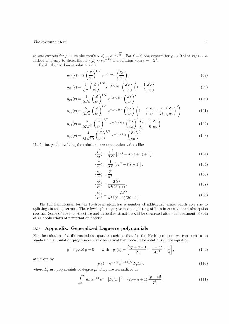
To find the solutions in general, we can turn to an algebraic manipulation program or a mathematicalhandbook to look for the solutions of the dimensionless differential equation (see subsection on Laguerrepolynomials). We see from this treatment that (using p → n − ℓ − 1, a → 2ℓ + 1 and x → 2Zρ/n) thesolutions for hydrogen are

unℓ(ρ) =

(2Z

na0

)1/2√

(n− ℓ− 1)!

2n (n+ ℓ)!e−Zρ/n

(2Zρ

n

)ℓ+1

L2ℓ+1n−ℓ−1

(2Zρ

n

)

(96)

with eigenvalues (energies)

Enℓ = −Z2

n2R∞, (97)

labeled by a principal quantum number number n, choosen such that the energy only depends on n. Fora given ℓ one has n ≥ ℓ+ 1. Actually nr = n− ℓ− 1 is the number of nodes in the wave function.

-1

-1/9-1/4

l = 0

3s 3d3p2p2s

1s

l = 1 l = 2

(2x)

(2x)(2x)

(6x)(6x) (10x)

E [Rydberg]The spectrum of the hydrogen atom.For a given n one has degenerate ℓ-levelswith ℓ = 0, 1, . . . , n−1. The degeneracy,including the electron spin, adds up to2n2. The hamiltonian is invariant underinversion, hence its eigenstates are alsoparity eigenstates. The parity of ψnlm

is given by Π = (−)ℓ.

Some aspects of the solution can be easily understood. For instance, looking at equation 92 one sees thatthe asymptotic behavior of the wave function is found from

u′′(ρ) + ǫ u(ρ) = 0,


so one expects for ρ → ∞ the result u(ρ) ∼ e−ρ√

|ǫ|. For ℓ = 0 one expects for ρ → 0 that u(ρ) ∼ ρ.Indeed it is easy to check that u10(ρ) ∼ ρ e−Zρ is a solution with ǫ = −Z2.

Explicitly, the lowest solutions are:

u10(r) = 2

(Z

a0

)1/2

e−Zr/a0

(Zr

a0

)

, (98)

u20(r) =1√2

(Z

a0

)1/2

e−Zr/2a0

(Zr

a0

)(

1 − 1

2

Zr

a0

)

(99)

u21(r) =1

2√

6

(Z

a0

)1/2

e−Zr/2a0

(Zr

a0

)2

(100)

u30(r) =2

3√

3

(Z

a0

)1/2

e−Zr/3a0

(Zr

a0

)(

1 − 2

3

Zr

a0+

2

27

(Zr

a0

)2)

(101)

u31(r) =8

27√

6

(Z

a0

)1/2

e−Zr/3a0

(Zr

a0

)2(

1 − 1

6

Zr

a0

)

(102)

u32(r) =4

81√

30

(Z

a0

)1/2

e−Zr/3a0

(Zr

a0

)3

(103)

Useful integrals involving the solutions are expectation values like

〈 r2

a20

〉 =n2

2Z2

[5n2 − 3 ℓ(ℓ+ 1) + 1

], (104)

〈 ra0

〉 =1

2Z

[3n2 − ℓ(ℓ+ 1)

], (105)

〈a0

r〉 =

Z

n2, (106)

〈a20

r2〉 =

2Z2

n3(2ℓ+ 1), (107)

〈a30

r3〉 =

2Z3

n3 ℓ(ℓ+ 1)(2ℓ+ 1). (108)

The full hamiltonian for the Hydrogen atom has a number of additional terms, which give rise tosplittings in the spectrum. These level splittings give rise to splitting of lines in emission and absorptionspectra. Some of the fine structure and hyperfine structure will be discussed after the treatment of spinor as applications of perturbation theory.

3.3 Appendix: Generalized Laguerre polynomials

For the solution of a dimensionless equation such as that for the Hydrogen atom we can turn to analgebraic manipulation program or a mathematical handbook. The solutions of the equation

y′′ + g0(x) y = 0 with g0(x) =

[2p+ a+ 1

2x+

1 − a2

4x2− 1

4

]

, (109)

are given byy(x) = e−x/2 x(a+1)/2 La

p(x). (110)

where Lap are polynomials of degree p. They are normalized as

∫ ∞

0

dx xa+1 e−x[La

p(x)]2

= (2p+ a+ 1)(p+ a)!

p!, (111)


and also satisfy the differential equation

[

xd2

dx2+ (a+ 1 − x)

d

dx+ p

]

Lap(x) = 0. (112)

Note that depending on books, different conventions are around, differing in the indices of the polynomials,the normalization, etc. Some useful properties are

Lp(x) ≡ L0p(x) =

ex

p!

dp

dxp

[xp e−x

]=

1

p!

(d

dx− 1

)p

xp, (113)

Lap(x) = (−)a da

dxa[Lp+a(x)] . (114)

Some general expressions areLa

0(x) = 1, La1(x) = 1 + a− x.

Some recursion relations are

(p+ 1)Lap+1(x) = (2p+ a+ 1 − x)La

p(x) − (p+ a)Lap−1(x), (115)

xLa+1p (x) = (x− p)La

p(x) + (p+ a)Lap−1(x), (116)

Lap(x) = La−1

p (x) + Lap−1(x). (117)

Some explicit polynomials are

L0(x) = 1,

L1(x) = 1 − x,

L2(x) = 1 − 2x+1

2x2,

L3(x) = 1 − 3x+3

2x2 − 1

6x3,

L10(x) = 1,

L11 = 2

(

1 − 1

2x

)

,

L12(x) = 3

(

1 − x+1

6x2

)

.

1 2 3 4

-3

-2

-1

1

2

The Lp(x) or LaguerreL[p,x] functions for p= 0, 1, 2, and 3.

1 2 3 4

-2

-1

1

2

3

The Lap(x) or LaguerreL[p,a,x] functions for a

= 1 and p = 0, 1, and 2.

3.4 A note on Bohr quantization

The model of Bohr of the atom imposes quantization in an ad hoc way by requiring ℓ = n ~ with n beinginteger. For the electron in the atom one uses the condition that the central force to bind the electron isprovided by the Coulomb attraction,

mv2

r=

Z e2

4πǫ0 r2, (118)


We can solve this for classical (circular) orbits and find

E(r) =1

2mv2 − Z e2

4πǫ0 r= −1

2

Z e2

4πǫ0 r,

ℓ2(r) = m2v2r2 = Z rme2

4πǫ0

Using the quantization condition on ℓ to eliminate v one finds

rn =n2

Z

4πǫ0 ~2

me2, (119)

En =Z2

n2

me4

32πǫ20~2, (120)

which turns out to give the correct (quantized) energy levels and also a good estimate of the radii. Atthe classical level the Sommerfeld model of the atom even includes quantization conditions for treatingelliptical orbits.

It is interesting to observe that the Bohr quantization condition not only gives the right characteristicsize (a0) and energy (R∞) and the right power dependence on quantities like Z, but what is moresurprising also the right power behavior of the quantum numbers (n, ℓ). Note e.g. that the Bohr modelgives r ∝ n2 and (indeed) all the expectation values involving rp have a polynomial behavior in (n, ℓ) oforder 2p.

Spin 20

4 Spin

4.1 Definition

In quantum mechanics spin is introduced as an observable defined via the vector operator s, which is apart of the rotation operator. These (three) hermitean operators satisfy commutation relations

[si, sj ] = i~ǫijk sk, (121)

similar to the commutation relations for the angular momentum operator ℓ = r × p. The spin operatorss commute with the operators r and p and thus also with ℓ. That’s it. All the rest follows from thesecommutation relations.

4.2 Rotation invariance

For the orbital angular momentum, we have seen the link to rotations, ℓz = −i~ ∂/∂ϕ. That means thatscalars (e.g. numbers) are not affected. Also operators that do not have azimuthal dependence are notaffected, which means for operators that they commute with ℓz. The various components of a vector dodepend on the azimuthal angle and ’vector operators’ such as r or p do not commute with ℓz. In factscalar operators S and vector operators V satisfy

[ℓi, S] = 0[ℓi, Vj ] = i~ ǫijk Vk

for a single particle without spin, (122)

e.g. scalars S = r2, p2, r · p or ℓ2 and vectors V = r, p or ℓ.Including spin vectors s, this seems no longer true, e.g. [ℓi, sj ] = 0 and [ℓi, ℓ · s] = −i~ (ℓ × s)i. But

with the ’correct’ rotation operatorj ≡ ℓ + s, (123)

we do get[ji, S] = 0[ji, Vj ] = i~ ǫijk Vk,

for a single particle (124)

not only for the above examples, but now also for the vectors s and j and including scalars like s2 andℓ · s.

For a system of many particles the operators r, p and s for different particles commute. It is easy tosee that the operators

L =

N∑

n=1

ℓn, S =

N∑

n=1

sn, J =

N∑

n=1

jn = L + S, (125)

satisfy commutation relations [Li, Lj] = i~ ǫijk Lk, [Si, Sj ] = i~ ǫijk Sk, and [Ji, Jj ] = i~ ǫijk Jk, whileonly the operator J satisfies

[Ji, S] = 0[Ji, Vj ] = i~ ǫijk Vk

for an isolated system (126)

for any scalar operator S or vector operator V .

———————–Exercise: Show that the inner product a · b of two vector operators satisfying the commutation relationin Eq. 126 indeed behaves as a scalar operator, satifying the required scalar commutation relation.———————–

Spin 21

An important property is that rotational invariance is one of the basic symmetries of our world, whichreflects itself in quantum mechanics as

Rotation invariance of a system of particles requires

[J , H ] = 0, (127)

where J = L+S =∑

i(ℓi +si). This is the (generalized, cf. Eq. 27) fundamental symmetry of naturefor particles with spin!

Besides the behavior under rotations, also the behavior under parity is considered to classify operators.Vector operators behave as P V P−1 = −V , axial vectors as P AP−1 = +A, a scalar operator Sbehaves as P S P−1 = +S, and a pseudoscalar operator S′ behaves as P S′ P−1 = −S′. Examples ofspecific operators are

vector axial vector scalar pseudoscalarr ℓ r2 s · rp s p2 s · p

j ℓ2

ℓ · s

The hamiltonian is a scalar operator. Therefore, if we have parity invariance, combinations as s ·r cannotappear but a tensor operator of the form (s1 · r)(s2 · r) is allowed. Note, however, that such an operatordoes not commute with ℓ.

4.3 Spin states

As mentioned above, the commutation relations are all that defines spin. As an operator that commuteswith all three spin operators (a socalled Casimir operator) we have s2 = s2x + s2y + s2z,

[si, sj ] = i~ ǫijk sk, (128)

[s2, si] = 0. (129)

Only one of the three spin operators can be used to label states, for which we without loss of generality

can take sz. In addition we can use s2, which commutes with sz. We write states χ(s)m = |s,m〉 satisfying

s2|s,m〉 = ~2 s(s+ 1)|s,m〉, (130)

sz|s,m〉 = m~ |s,m〉. (131)

It is of course a bit premature to take ~2 s(s + 1) as eigenvalue. We need to prove that the eigenvalue

of s2 is positive, but this is straightforward as it is the sum of three squared operators. Since the spinoperators are hermitean each term is not just a square but also the product of the operator and itshermitean conjugate. In the next step, we recombine the operators sx and sy into

s± ≡ sx ± i sy. (132)

The commutation relations for these operators are,

[s2, s±] = 0, (133)

[sz , s±] = ±~ s±, (134)

[s+, s−] = 2~ sz, (135)

Spin 22

The first two can be used to show that

s2 s±|s,m〉 = s±s2|s,m〉 = ~2 s(s+ 1) s±|s,m〉,

sz s±|s,m〉 = (s±sz ± ~ s±) |s,m〉 = (m± 1)~ s±|s,m〉,

hence the name step-operators (raising and lowering operator) which achieve

s±|s,m〉 = c±|s,m± 1〉.

Furthermore we have s†± = s∓ and s2 = s2z + (s+s− + s−s+)/2, from which one finds that

|c±|2 = 〈s,m|s†±s±|s,m〉 = 〈s,m|s2 − s2z − [s±, s∓]/2|s,m〉= 〈s,m|s2 − s2z ∓ ~ sz|s,m〉 = s(s+ 1) −m(m± 1).

It is convention to define

s+|s,m〉 = ~

√

s(s+ 1) −m(m+ 1) |s,m+ 1〉= = ~

√

(s−m)(s+m+ 1) |s,m+ 1〉 (136)

s−|s,m〉 = ~

√

s(s+ 1) −m(m− 1) |s,m− 1〉= ~

√

(s+m)(s−m+ 1) |s,m− 1〉. (137)

This shows that given a state |s,m〉, we have a whole series of states

. . . |s,m− 1〉, |s,m〉, |s,m+ 1〉, . . .

But, we can also easily see that since s2 − s2z = s2x + s2y must be an operator with positive definite

eigenstates that s(s + 1) − m2 ≥ 0, i.e. |m| ≤√

s(s+ 1) or strictly |m| < s + 1. From the secondexpressions in Eqs 136 and 137 one sees that this inequality requires mmax = s as one necessary stateto achieve a cutoff of the series of states on the upper side, while mmin = −s is required as a necessarystate to achieve a cutoff of the series of states on the lower side. Moreover to have both cutoffs the stepoperators require that the difference mmax −mmin = 2 s must be an integer, i.e. the only allowed valuesof spin quantum numbers are

s = 0, 1/2, 1, 3/2, . . . ,

m = s, s− 1, . . . ,−s.

Thus for spin states with a given quantum number s, there exist 2s+ 1 states.

4.4 Why is ℓ integer

Purely on the basis of the commutation relations, the allowed values for the quantum numbers s and mhave been derived. Since the angular momentum operators ℓ = r×p satisfy the same commutation rela-tions, one has the same restrictions on ℓ and mℓ, the eigenvalues connected with ℓ2 and ℓz. However, wehave only found integer values for the quantum numbers in our earlier treatment. This is the consequenceof restrictions imposed because for ℓ we know more than just the commutation relations. The operatorshave been introduced explicitly working in the space of functions, depending on the angles in R3. Oneway of seeing where the constraint is coming from is realizing that we want uni-valued functions. Theeigenfunctions of ℓz = −i~ d/dφ, were found to be

Y mℓ (θ, φ) ∝ ei mφ.

Spin 23

In order to have the same value for φ and φ+2π we need exp(2π im) = 1, hence m (and thus also ℓ) canonly be integer.

For spin, there are only the commutation relations, thus the spin quantum numbers s can also takehalf-integer values. Particles with integer spin values are called bosons (e.g. pions, photons), particleswith half-integer spin values are called fermions (e.g. electrons, protons, neutrinos, quarks). For theangular momenta which are obtained as the sum of other operators, e.g. j = ℓ+s, etc. one can easily seewhat is allowed. Because the z-components are additive, one sees that for any orbital angular momentumthe quantum numbers are integer, while for spin and total angular momentum integer and half-integerare possible.

4.5 Matrix representations of spin operators

In the space of spin states with a given quantum number s, we can write the spin operators as (2s+ 1)×(2s+ 1) matrices. Let us illustrate this first for spin s = 1/2. Define the states

|1/2,+1/2〉 ≡ χ(1/2)+1/2 ≡ χ+ ≡

10

and |1/2,−1/2〉 ≡ χ(1/2)−1/2 ≡ χ− ≡

01

.

Using the definition of the quantum numbers in Eq. 131 one finds that

sz = ~

1/2 00 −1/2

, s+ = ~

0 01 0

, s− = ~

0 10 0

,

For spin 1/2 we then find the familiar spin matrices, s = ~σ/2,

σx =

0 11 0

, σy =

0 −ii 0

, σz =

1 00 −1

.

For spin 1 we define the basis states |1,+1〉, |1, 0〉 and |1,−1〉 or

χ(1)+1 ≡

100

, χ

(1)0 ≡

010

, χ

(1)−1 ≡

001

.

The spin matrices are then easily found,

sz = ~

1 0 00 0 00 0 −1

, s+ = ~

0√

2 0

0 0√

20 0 0

, s− = ~

0 0 0√2 0 0

0√

2 0

,

from which also sx and sy can be constructed.

———————–Exercise: Convince yourself that you can do this construction, e.g. by doing it for spin 3/2.———————–

4.6 Rotated spin states

Instead of the spin states defined as eigenstates of sz, one might be interested in eigenstates of s · n, e.g.because one wants to measure it with a Stern-Gerlach apparatus with an inhomogeneous B-field in the

n direction. We choose an appropriate notation like |n,±〉 or two component spinors χ(s)ms(n), shorthand

χ(1/2)+1/2(n) = χ+(n) and χ

(1/2)−1/2(n) = χ−(n)

Spin 24

Suppose that we want to write them down in terms of the eigenstates of sz, given above, χ+/−(z) =χ↑/↓. To do this we work in the matrix representation discussed in the previous section. Taking n =(sin θ, 0, cos θ), we can easily write down

s · n =1

2~ σ · n =

~

2

cos θ sin θsin θ − cos θ

. (138)

We find the following two eigenstates and eigenvalues

χ+(n) =

cos(θ/2)sin(θ/2)

with eigenvalue + ~/2,

χ−(n) =

− sin(θ/2)cos(θ/2)

with eigenvalue − ~/2.

The probability that given a state χ+ with spin along the z-direction, a measurement of the spin alongthe +n-direction yields the value +~/2 is thus given by

∣∣∣∣χ†

+(n)χ↑

∣∣∣∣

2

= cos2(θ/2).

Instead of explicitly solving the eigenstates, we of course also can use the rotation operators in quantummechanics,

U(θ, n) = exp (i θ n · J) , (139)

where J is the total angular momentum operator referred to before in chapter one and in the section onrotation invariance. The total angular momentum operator is the generator of rotations.

A simple example is the rotation of a spin 1/2 spinor. The rotation matrix that brings a spin up statealong the z-axis into a spin up state along a rotated direction with polar angle in the x− z plane is2 is

U(θ) = e−i θσy/2 = cos(θ/2) I − i sin(θ/2)σy.

where I is the 2 × 2 unit matrix.

———————–Exercise: Check that U(θ)|1/2, 1/2〉 gives the rotated spin state above, while S · n = U(θ)Sz U

−1(θ).———————–

To find the expansion of any rotated spinor in the original spin states one considers in general theEuler rotations of the form

U(ϕ, θ,−ϕ) = e−i ϕ Jz e−i θ Jy ei ϕ Jz

Its matrix elements are referred to as the D-functions,

〈j,m′|U(ϕ, θ,−ϕ)|j,m〉 = D(j)m′m(ϕ, θ,−ϕ) = ei(m−m′)ϕ d

(j)m′m(θ). (140)

In general the rotated eigenstates are written as

χ(s)m (n) =

d(s)sm(θ)

...

d(s)m′m(θ)

...

d(s)−sm(θ)

. (141)

2Use the relation exp (iθ n · σ/2) = cos(θ/2) I + i σ · n sin(θ/2).

Spin 25

where dm′m(θ) are the d-functions. These are in fact just matrix elements of the spin rotation matrixexp(−i θ Jy) between states quantized along the z-direction. Extended to include azimuthal dependenceit is necessary to use the rotation matrix e−i ϕ Jz e−i θ Jy e−i χ Jz and the relevant functions are calledDm′m(ϕ, θ, χ). For integer ℓ one has

D(ℓ)m0(ϕ, θ, 0) =

√

4π

2ℓ+ 1Y m∗

ℓ (θ, ϕ), (142)

D(ℓ)m0(0, θ, ϕ) = (−)m

√

4π

2ℓ+ 1Y m∗

ℓ (θ, ϕ). (143)

Combination of angular momenta 26

5 Combination of angular momenta

5.1 Quantum number analysis

We consider situations in which two sets of angular momentum operators play a role, e.g.

• An electron with spin in an atomic (nℓ)-orbit (spin s and orbital angular momentum ℓ combinedinto a total angular momentum j = ℓ + s). Here one combines the R

3 and the spin-space.

• Two electrons with spin (spin operators s1 and s2, combined into S = s1 + s2). Here we have theproduct of spin-space for particle 1 and particle 2.

• Two electrons in atomic orbits (orbital angular momenta ℓ1 and ℓ2 combined into total orbitalangular momentum L = ℓ1 + ℓ2). Here we have the direct product spaces R

3 ⊗ R3 for particles 1

and 2.

• Combining the total orbital angular momentum of electrons in an atom (L) and the total spin (S)into the total angular momentum J = L + S.

Let us discuss as the generic exampleJ = j1 + j2. (144)

We have states characterized by the direct product of two states,

|j1,m1〉 ⊗ |j2,m2〉, (145)

which we can write down since not only [j21, j1z] = [j2

2, j2z] = 0, but also [j1m, j2n] = 0. The sum-operator J obviously is not independent, but since the J-operators again satisfy the well-known angularmomentum commutation relations we can look for states characterized by the commuting operators J2

and Jz, | . . . ; J,M〉. It is easy to verify that of the four operators characterizing the states in Eq. 145,[J2, j1z ] 6= 0 and [J2, j2z] 6= 0 (Note that J2 contains the operator combination 2j1 · j2, which containsoperators like j1x, which do not commute with j1z). It is easy to verify that one does have

[J2, j21] = [J2, j2

2] = 0,

[Jz , j21] = [Jz, j

22] = 0,

and thus we can relabel the (2j1 +1)(2j2+1) states in Eq. 145 into states characterized with the quantumnumbers

|j1, j2; J,M〉. (146)

The basic observation in the relabeling is that Jz = j1z + j2z and hence M = m1 +m2. This leads to thefollowing scheme, in which in the left part the possible m1 and m2-values are given and the upper rightpart the possible sum-values for M including their degeneracy.

j2

j1j1

j2

j1 j2

j1 j2+=

+

+

xm

M

m1

2

-

-

-


1. Since |m1| ≤ j1 and |m2| ≤ j2, the maximum value for M is j1 + j2. This state is unique.

2. Since J+ = j1+ + j2+ acting on this state is zero, it corresponds to a state with J = j1 + j2. Then,there must exist other states (in total 2J + 1), which can be constructed via J− = j1− + j2− (inthe scheme indicated as the first set of states in the right part below the equal sign).

3. In general the state with M = j1 + j2−1 is twofold degenerate. One combination must be the stateobtained with J− from the state with M = j1 + j2, the other must be orthogonal to this state andagain represents a ’maximum M ’-value corresponding to J = j1 + j2 − 1.

4. This procedure goes on till we have reached M = |j1 − j2|, after which the degeneracy is equal tothe min2j1 + 1, 2j2 + 1, and stays constant till the M -value reaches the corresponding negativevalue.

Thus

Combining two angular momenta j1 and j2 we find resulting angular momenta J with values

J = j1 + j2, j1 + j2 − 1, . . . , |j1 − j2|, (147)

going down in steps of one.

Note that the total number of states is (as expected)

j1+j2∑

J=|j1−j2|

(2J + 1) = (2j1 + 1)(2j2 + 1). (148)

Furthermore we have in combining angular momenta:

half-integer with half-integer −→ integerinteger with half-integer −→ half-integerinteger with integer −→ integer

5.2 Clebsch-Gordon coefficients

The actual construction of states just follows the steps outlined above. Let us illustrate it for the case ofcombining two spin 1/2 states. We have four states according to labeling in Eq. 145,

|s1,m1〉 ⊗ |s2,m2〉 : |1/2,+1/2〉 ⊗ |1/2,+1/2〉 ≡ | ↑↑〉,|1/2,+1/2〉 ⊗ |1/2,−1/2〉 ≡ | ↑↓〉,|1/2,−1/2〉 ⊗ |1/2,+1/2〉 ≡ | ↓↑〉,|1/2,−1/2〉 ⊗ |1/2,−1/2〉 ≡ | ↓↓〉.

1. The highest state has M = 1 and must be the first of the four states above. Thus for the labeling|s1, s2;S,M〉

|1/2, 1/2; 1,+1〉 = | ↑↑〉. (149)

2. Using S− = s1− + s2− we can construct the other S + 1 states.

S−|1/2, 1/2; 1,+1〉 = ~√

2 |1/2, 1/2; 1, 0〉,(s1− + s2−)| ↑↑〉 = ~(| ↑↓〉 + | ↓↑〉),


and thus

|1/2, 1/2; 1, 0〉 =1√2

(

| ↑↓〉 + | ↓↑〉)

. (150)

Continuing with S− (or in this case using the fact that we have the lowest nondegenerate M -state)we find

|1/2, 1/2; 1,−1〉 = | ↓↓〉. (151)

3. The state with M = 0 is twofold degenerate. One combination is already found in the aboveprocedure. The other is made up of the same two states appearing on the right hand side inEq. 150. Up to a phase, it is found by requiring it to be orthogonal to the state |1/2, 1/2; 1, 0〉 orby requiring that S+ = s1+ + s2+ gives zero. The result is

|1/2, 1/2; 0, 0〉 =1√2

(

| ↑↓〉 − | ↓↑〉)

. (152)

The convention for the phase is that the higher m1-value appears with a positive sign.

It is easy to summarize the results in a table, where one puts the states |j1,m1〉 ⊗ |j2,m2〉 in thedifferent rows and the states |j1, j2; J,M〉 in the different columns, i.e.

j1 × j2... J

...... M

.... . . . . .m1 m2

. . . . . .

For the above case we have

1/2 × 1/2 1 1 0 11 0 0 -1

+1/2 +1/2 1

+1/2 −1/2√

12

√12

−1/2 +1/2√

12 −

√12

−1/2 −1/2 1

Note that the recoupling matrix is block-diagonal because of the constraintM = m1+m2. The coefficientsappearing in the matrix are the socalled Clebsch-Gordan coefficients. We thus have

|j1, j2; J,M〉 =∑

m1,m2

C(j1,m1, j2,m2; J,M) |j1,m1〉 ⊗ |j2,m2〉. (153)

Represented as a matrix as done above, it is unitary (because both sets of states are normalized). Sincethe Clebsch-Gordan coefficients are choosen real, the inverse is just the transposed matrix, or

|j1,m2〉 ⊗ |j2,m2〉 =∑

J,M

C(j1,m1, j2,m2; J,M) |j1, j2; J,M〉. (154)

In some cases (like combining two spin 1/2 states) one can make use of symmetry arguments. If aparticular state has a well-defined symmetry under permutation of states 1 and 2, then all M -statesbelonging to a particular J-value have the same symmetry (because j1±+j2± does not alter the symmetry.This could have been used for the 1/2 × 1/2 case, as the highest total M is symmetric, all S = 1 statesare symmetric. This is in this case sufficient to get the state in Eq. 150.


We will give two other examples. The first is

1 × 1/2 3/2 3/2 1/2 3/2 1/2 3/2+3/2 +1/2 +1/2 −1/2 −1/2 −3/2

+1 +1/2 1

+1 −1/2√

13

√23

0 +1/2√

23 −

√13

0 −1/2√

23

√13

−1 +1/2√

13 −

√23

−1 −1/2 1

for instance needed to obtain the explicit states for an electron with spin in an (2p)-orbitcoupled to a total angular momentum j = 3/2 (indicated as 2p3/2) with m = 1/2 is

φ(r, t) =u2p(r)

r

(√

1

3Y 1

1 (θ, ϕ)χ↓ +

√

2

3Y 0

1 (θ, ϕ)χ↑

)

.

The second is

1 × 1 2 2 1 2 1 0 2 1 2+2 +1 +1 0 0 0 −1 −1 −2

+1 +1 1

+1 0√

12

√12

0 +1√

12 −

√12

+1 −1√

16

√12

√13

0 0√

23 0 −

√13

+1 −1√

16 −

√12

√13

0 −1√

12

√12

−1 0√

12 −

√12

−1 −1 1

This example, useful in the combination of two spin 1 particles or two electrons in p-waves,illustrates the symmetry of the resulting wave functions.

5.3 The Wigner-Eckart theorem

Specific matrix elements of the form 〈β|O|α〉 describe for instance transitions between states α and β.For instance the absorption or emission of a photon in a state α produces the state O|α〉. The probabilitythat this state is observed as a state |β〉 is

Probα→β = |〈β|O|α〉|2 .

For particular operators O we can make statements on the transition being allowed for specific angularmomentum quantum numbers of the states (similar as illustrated for parity).

We first note that for any operator S commuting with the angular momentum operators ([J , S] = 0),the quantum numbers are not changed, thus

〈J ′M ′|S|J,M〉 ∼ δJJ′ δMM ′ . (155)


Thus one has ∆J = ∆M = 0.A second interesting case are vector operators, for which we also know the commutation relations. It

is easy to rewrite these using J± = Jx ± i Jy and V± = Vx ± i Vy. One has

[Jx, V±] = ∓~Vz, [Jy, V±] = −i~Vz, [Jz, V±] = ±~V±, (156)

or using J±,[J+, V+] = [J−, V−] = 0, [J±, V∓] = ±2~Vz. (157)

These can just as in the analysis of angular momentum quantum numbers be used to show that

J2 V |J,M〉 = ~2J(J + 1)V |J,M〉, (158)

Jz V±|J,M〉 = (M ± 1) ~V±|J,M〉, (159)

Thus we have the selection rules stating that one can have nonzero transition probabilities only underspecific changes of quantum numbers,

for Vz : ∆M = M −M ′ = 0,

for V+ : ∆M = M −M ′ = +1,

for V− : ∆M = M −M ′ = −1.

Because of the commutation relations with the J operators one refers to this as the ’spherical basis’V m

ℓ = V m1 ,

V ±11 = ∓Vx ± i Vy√

2, V 0

1 = Vz. (160)

These are chosen such that

[Jz , Omℓ ] = m ~Om

ℓ and [J±, Omℓ ] = ~

√

ℓ(ℓ+ 1) −m(m± 1)Om±1ℓ , (161)

for which one in general can write

〈J ′M ′|Omℓ |J,M〉 = C(ℓ,m; J,M ; J ′,M ′)

〈J ′||Oℓ||J〉√2J ′ + 1

. (162)

The quantity |J ′||Oℓ||J〉 is referred to as reduced matrix element. The most well-known applicationsof the Wigner-Eckart theorem are its application to the multipole operators describing the interactionsof photons with matter, as well as selection rules in interactions between atomic nuclei and elementaryparticles with different spin states. It reduces (2J + 1)(2ℓ+ 1)(2J ′ + 1) matrix elements to one reducedmatrix element and the use of (tabulated) Clebsch-Gordan coefficients.

Identical particles 31

6 Identical particles

6.1 Permutation symmetry

The hamiltonian for Z electrons in an atom,

H(r1, . . . , rZ ; p1, . . . ,pZ) =Z∑

i=1

(

− ~2

2m∇

2i −

Ze2

4πǫ0 ri

)

+Z∑

i>j

e2

4πǫ0 |ri − rj |(163)

is invariant under permutations of the particle labels, i↔ j, written symbolically as

H(1 . . . i . . . j . . . Z) = H(1 . . . j . . . i . . . Z). (164)

Consider first two identical particles and assume an eigenstate φ(12),

H(12)φ(12) = Eφ(12),

Because H(12) = H(21) one has also

H(21)φ(12) = Eφ(12).

Since the labeling is arbitrary one can rewrite the latter to

H(12)φ(21) = Eφ(21).

Thus there are two degenerate solutions φ(1, 2) and φ(2, 1). In particular we can choose symmetric andantisymmetric combinations

φS/A = φ(12) ± φ(21), (165)

which are also eigenstates with the same energy. These are eigenfunctions of the permutation operatorPij , which interchanges two labels, i.e. Pijφ(1 . . . i . . . j . . .) = φ(1 . . . j . . . i . . .) with eigenvalues + and -respectively. This operator commutes with H and the symmetry is not changed in time.

For three particles one has six degenerate solutions, φ(123), φ(213), φ(231), φ(321), φ(312) and φ(132).There is one totally symmetric combination,

φS = φ(123) + φ(213) + φ(231) + φ(321) + φ(312) + φ(132), (166)

(any permutation operator gives back the wave function), one totally antisymmetric combination

φA = φ(123) − φ(213) + φ(231) − φ(321) + φ(312) − φ(132), (167)

(any permutation operator gives back minus the wave function) and there are four combinations withmixed symmetry. Nature is kind and only allows the symmetric or antisymmetric function according tothe socalled

spin-statistics theorem: for a system of identical particles one has either symmetric wave functions(Bose-Einstein statistics) or antisymmetric wave function (Fermi-Dirac statistics). For identical par-ticles obeying Bose-Einstein statistics the wave function does not change under interchange of anytwo particles. Such particles are called bosons. For particles obeying Fermi-Dirac statistics the wavefunction changes sign under a permutation of any two particles. Such particles are called fermions.This feature is coupled to the spin of the particles (known as the spin-statistics connection): particleswith integer spin are bosons, particles with half-integer spin are fermions.


For instance electrons which have spin 1/2 (two possible spin states) are fermions. The total wavefunction must be antisymmetric. This has profound consequences. It underlies the periodic table ofelements. Consider again for simplicity a two-particle system which neglecting mutual interactions has aseparable hamiltonian of the form

H = H0(1) +H0(2).

Suppose the solutions of the single-particle hamiltonian are known,

H0(1)φa(1) = Eaφa(1), H0(1)φb(1) = Ebφb(1),

etc. Considering the lowest two single-particle states available, there are three symmetric states and oneanti-symmetric state,

symmetric:

φa(1)φa(2)φa(1)φb(2) + φb(1)φa(2)φb(1)φb(2)

antisymmetric: φa(1)φb(2) − φb(1)φa(2)

In particular bosons can reside in the same state, while any two fermions cannot be in the same state,known as the Pauli exclusion principle.

A way to obtain the completely antisymmetric wave function is by constructing the antisym-metric wave function as a Slater determinant, for instance for three particles the antisymmet-ric wave function constructed from three available states φa, φb and φc is

φA(123) =1√3!

∣∣∣∣∣∣

φa(1) φa(2) φa(3)φb(1) φb(2) φb(3)φc(1) φc(2) φc(3)

∣∣∣∣∣∣

.

6.2 Applications

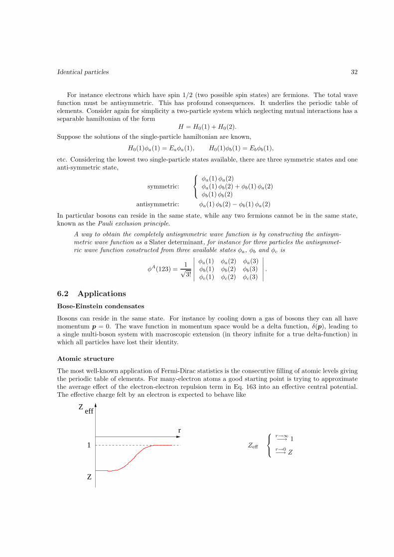
Bose-Einstein condensates

Bosons can reside in the same state. For instance by cooling down a gas of bosons they can all havemomentum p = 0. The wave function in momentum space would be a delta function, δ(p), leading toa single multi-boson system with macroscopic extension (in theory infinite for a true delta-function) inwhich all particles have lost their identity.

Atomic structure

The most well-known application of Fermi-Dirac statistics is the consecutive filling of atomic levels givingthe periodic table of elements. For many-electron atoms a good starting point is trying to approximatethe average effect of the electron-electron repulsion term in Eq. 163 into an effective central potential.The effective charge felt by an electron is expected to behave like

r

1

Z eff

Z

Zeff

r→∞−→ 1

r→0−→ Z


The behavior of Zeff(r) can e.g. be obtained from the electron densities in a self-consistent matter. Thus,one can approximate the many-electron hamiltonian by

H(r1, . . . , rZ ; p1, . . . ,pZ) ≈Z∑

i=1

(

− ~2

2m∇

2i −

Zeff(r) e2

4πǫ0 ri

)

+ . . . (168)

The advantage of this procedure is that part of the repulsion is taken into account retaining a centralinteraction and a separable hamiltonian. This will modify the spectrum, lifting the degeneracy betweendifferent ℓ-values for given n. In general the higher ℓ values will because of the angular momentumcontribution ~

2 ℓ(ℓ+1)/2mr2 in the effective radial potential will feel a smaller charge and hence becomeless bound.

l = 0

3d

1s

l = 1 l = 2

(2x)

(10x)(6x)

(6x)(2x)

(2x)

2s

3s

2p

3p

EThe (schematic) spectrum for many-electronatoms. A possible parametrization of the levelstaking into account the screening effect is

Enℓ = − R∞

(n− δℓ)2,

where δℓ is referred to as quantum defect, andone expects δℓ → 0 for large ℓ-values. This willwork particularly well for atoms with one electronoutside a closed shell.

In the central field approximation, the hamiltonian is separable for the different electrons and the solutionis an antisymmetrized product of single electron states (Slater determinant), where one needs to keepin mind the spin degeneracy (2 for each level). Operators compatible with the hamiltonian are ℓi (andsimilarly spin operators), just as is the parity operator. Hence one has many good quantum numbers. Atthis level of approximation one can label the states by giving the various (nℓ) levels and their multiplicities,e.g. for the ground state of helium (1s)2, for Carbon (1s)2(2s)2(2p)2, etc. Combining the angular momentaand spins into specific multiplets will be discussed as an application of spin but is not yet relevant, sinceall states are at this stage degenerate. This remains true if one refines the picture by using an effectivecentral charge Zeff(r). The only effect of the latter is the splitting of different ℓ-values corresponding tothe same principal quantum number n.

The structure of the periodic table is summarized in the table given below with the levels given inorder of increasing energy. In this table the noble gases correspond to situations in which there are largeenergy gaps between the filled shell and the next available one. Characteristics of these noble gases area high ionization energy and a small affinity to other elements, e.g. Eionization = 24.6 eV (He), 21.6 eV(Ne) and 15.8 eV (Ar). The level scheme in the table can also be used to establish the excited states.


n summed #1 2 3 4 5 6 7 of levels remarks

(1s)2 2 (He)

(2s)2 4(2p)6 10 (Ne)

(3s)2 12(3p)6 18 (Ar)

(4s)2 20(3d)10 30 Fe-group

(4p)2 36 (Kr)

(5s)2 38(4d)10 48 Pd-group

(5p)6 54 (Xe)

(6s)2 56(4f)14 70 Lanthanides

(5d)10 80 Pt-group(6p)6 86 (Rn)

(7s)2 88(5f)14 102 Actinides

(6d)10 112 Pt-group(7p)6 118 (?)

Spin in Atomic Physics 35

7 Spin in Atomic Physics

7.1 The Helium atom

As a first-order description of the helium atom, one can consider the independent-electron approxima-tion, starting with a hamiltonian in which the electron-electron interaction is neglected, as well as anyinteractions involving the spin of the electrons. In that case one has a separable hamiltonian and foreach of the electrons the solutions are given by hydrogen-like states (Z = 2), characterized by (nℓ). Letus investigate the possible ground-state configurations, (1s)2 and the first excited levels (1s)(2p) and(1s)(2s).

• The ground state configurations (1s)2.Knowing the two angular momenta involved is sufficient to know the parity of these states, Π =(−)ℓ1(−)ℓ2 = +. The angular momentum recoupling works in the following way.

– Combining ℓ1 = 0 and ℓ2 = 0, the only possibility is L = 0. The orbital wave function then issymmetric under the interchange of the two electrons 1 and 2.

– Combining the spins s1 = 1/2 and s2 = 1/2 gives two possibilities, S = 0 or S = 1. The firstpossibility is antisymmetric under the interchange of the electrons, the second is symmetric.

– The total wave function (product of orbital and spin parts) must be antisymmetric for fermionsaccording to the Pauli principle, hence L = 0 can only be combined with S = 0. This leavesonly one possibility for the total angular momentum, J = 0. The notation for the only allowedground state configuration is

(n1 ℓ1)(n2 ℓ2)2S+1LJΠ = (1s)2 1S0+ .

• The configurations (1s)(2p) with parity Π = −.

– We have L = 1, but appearing twice. We can construct the symmetric and antisymmetriccombinations,

φs/aLML

=1√2

[u1s(r1)

r1Y 0

0 (Ω1)u2p(r2)

r2Y ML

1 (Ω2) ±u2p(r1)

r1Y ML

1 (Ω1)u1s(r2)

r2Y 0

0 (Ω2)

]

for the spatial part.

– The combination of the spins gives again an antisymmetric S = 0 and a symmetric S = 1wave function.

– The allowed configurations are thus obtained by the appropriate antisymmetric combinationsof orbital and spin parts,

[(1s)(2p)]s 1P1− and [(1s)(2p)]a 3P0−,1−,2− .

• The configurations (1s)(2s) with parity Π = +.

– We have L = 0, but now also appearing twice in a symmetric and antisymmetric combination.

– As above, antisymmetric S = 0 and symmetric S = 1.

– This gives the allowed configurations

[(1s)(2s)]s 1S0+ and [(1s)(2s)]a 3S1+ .


Summarizing in tabular formConfigurations in Helium

configuration E(0)/R∞ L S Parity Symmetry J-configurations # states(1s)2 −8 0 0 + A 1S0+ 1

1 + S not allowed 3(1s)(2p) & (2p)(1s) −5 1 0 − S/A 1P1− 3

1 − S/A 3P0−,1−,2− 9(1s)(2s) & (2s)(1s) −5 0 0 + S/A 1S0+ 1

1 + S/A 3S1+ 3

Important to note is that although additional terms may be present in the full hamiltonian, the solutionsfound in this way do form a complete set of states for the atom. Other interaction terms give rise toshifts in the zeroth order energies and they may mix the states. To calculate such shifts we need to useperturbation theory.

7.2 Atomic multiplets

In a more realistic atom the ee-interaction term (or what remains after taken into account an effectivecharge) must also be considered. It breaks rotational invariance in the hamiltonian for the electroncoordinate ri, thus ℓi is no longer compatible with the hamiltonian. We note that L is still compatiblewith the hamiltonian. Since there is no spin-dependence, spin operators si and also S are compatiblewith the hamiltonian and corresponding quantum numbers still can be used.

To illustrate how one easily finds the allowed L and S values given an electron configuration, weconsider the ground state configuration of Carbon, (1s)2(2s)2(2p)2. The allowed states in a shell can berepresented as a number of boxes, e.g. an s-shell as two boxes, a p-shell as six boxes,

ms ↓ mℓ 0

+1/2−1/2

ms ↓ mℓ −1 0 +1

+1/2−1/2

etc. Putting N electrons in these boxes with at most one electron per box (Pauli principle) one has6!/N !(6 − N)! possibilities, e.g. for a filled only one possibility. Obviously then all magnetic quantumnumbers combine to zero, ML = MS = 0 and one also has for the total L and S quantum numbersL = S = 0. Hence filled shells can be disregarded for finding total (L, S) values.

As a consequence the specta of atoms with one electron outside a closed shell (Li, Na, K, Rb, Cs,Fr) resemble the spectrum of hydrogen, e.g. the configurations for sodium (Na) are (nℓ) with n ≥ 3.The groundstate for Na is (3s)2S1/2, the first excited states are the (3p)2P1/2 and (3p)2P3/2 levels. Theelectric dipole transition 2P →2 S is the well-known yellow Na-line in the visible spectrum, which bythe fine-structure (see below) is split into two lines corresponding to the transitions 2P3/2 →2 S1/2 and2P1/2 →2 S1/2. For atoms with two electrons outside a closed shell (Be, Mg, Ca, Sr, Ba, Ra) the multipletstructure resembles that of helium.

For a particular number of electrons it is easy to look at the number of possibilities to constructparticular ML and MS values. This is denoted in a Slater diagram

MS ↓ ML −2 −1 0 +1 +2

+1 0 1 1 1 00 1 2 3 2 1−1 0 1 1 1 0

It is easy to disentangle this into


0 0 0 0 01 1 1 1 10 0 0 0 0

(L, S) = (2, 0)

+

0 1 1 1 00 1 1 1 00 1 1 1 0

(L, S) = (1, 1)

+

0 0 0 0 00 0 1 0 00 0 0 0 0

(L, S) = (0, 0)

Thus for the Carbon one finds in the groundstate configurations the multiplets

1D 3P 1S

Also for configurations involving more shells that are not completely filled, it is straightforward to findthe states in an MS −ML diagram. At this point we have completed the quantum number analysis ofthe spectrum. In order to find the energies one needs to use perturbation theory as well as variationalmethods to be discussed next. The results of these methods have shown that for the ordering in thespectrum a number of phenomenological rules can be formulated, the Hund rules. In particular for thegroundstate configuration one has that the terms with highest S-values (highest multiplicity) and thenhighest L-values have the lowest energy, i.e. in the example for Carbon

E(3P ) < E(1D) < E(1S).

7.3 Selection rules

For emission and absorption of light (photons) the relevant operator is the electric dipole operator, whichin essence is the position operator. The calculation of transition probabilities are given by the matrixelements between the appropriate states. Since the dipole operator does not involve spin operators, thespin wave function doesn’t change in a dipole transition, giving rise to a spin selection rule: ms 1 = ms 2,i.e.

∆s = ∆ms = 0. (169)

In fact the photon polarization determines which of the components of the position operator is the relevantoperator. The photon polarizations for linearly polarized light (directed in z-direction) are

linear : ǫx = x and ǫy = y,

orcircular : ǫ+ = −(x+ i y)/

√2 and ǫ− = (x− i y)/

√2

For polarized light we thus precisely get the (spherical) representation of the position vector in terms ofthe two spherical harmonics with ℓ = 1,

r · ǫmγ=

√

4π

3rY

mγ

1 .

We now just can do the explicit calculation

〈1|r · ǫ|2〉 =

√

4π

3

∫

d3r ψ∗n1ℓ1m1

(r) r Ymγ

1 (θ, ϕ)ψn2ℓ2m2(r),

which factorizes into

〈1|r · ǫ|2〉 =

√

4π

3

∫

dr r un1ℓ1(r)un2ℓ2(r)

∫

dΩ Y m1 ∗ℓ1

(θ, ϕ)Ymγ

1 (θ, ϕ)Y m2

ℓ2(θ, ϕ).

From the ϕ-dependence of the spherical harmonics one sees that the matrix element is proportional to∫

dϕ e−i m1ϕ ei mγϕ ei m2ϕ = 2π δ(m2 +mγ −m1),


giving rise to the selection rule∆mℓ = ±1, (170)

each of these corresponding to a specific photon polarization. The integral for the ϕ-dependent part issimple, but more general one can use the properties of the Y m

ℓ -functions to see what happens with thefull angular integration. One only gets a nonzero result if the addition of angular momenta |ℓ2,m2〉 and|1,mγ〉 can yield the final state |ℓ1,m1〉 via the well-known angular momentum addition rules. The resultis simply proportional to the Clebsch-Gordan coefficient in this recoupling,

〈1|r · ǫ|2〉 =

√

4π

3

∫

dr r un1ℓ1(r)un2ℓ2(r)C(1,mγ , ℓ2,m2; ℓ1,m1).

which is an explicit example of the Wigner-Eckart theorem. This leads besides the m-selection rule to|∆ℓ| ≤ 1 Knowing the parity of the spherical harmonics one immediately gets a parity selection rule,namely Π1Π2 = −1 or with Π = (−)ℓ, one is left with

∆ℓ = ±1. (171)

Rotational invariance further requires that the sum of the total angular momentum in initial and finalstate is conserved. This becomes relevant if the orbital angular momentum and spin of electrons and/oratomic nuclei are coupled to a specific total angular momentum. In many cases the orbital angularmomentum then is no longer a good quantum number. Still, even when ℓ and s are coupled to j, or formany particles L and S are coupled to J , the transition operator involves a simple Y

mγ

1 , implying

∆J = 0, ±1 (172)

(with J = 0 → J = 0 forbidden!).The interactions (absorption or emission) of photons in atoms can also proceed via different operators.

The one treated here is known as electric dipole radiation (E1). In order of strength one has also themagnetic dipole radiation (M1), electric quadrupole radiation (E2), etc. For instance electric quadrupoleradiation is governed by operators of the type xi xj , i.e. in a spherical representation the ℓ = 2 sphericalharmonics. This leads to transition selection rules in which parity is not changed and since the operatorsare proportional to r2 Y

mγ

2 one has ∆ℓ = 2.

Bound state perturbation theory 39

8 Bound state perturbation theory

8.1 Basic treatment

Perturbation theory is used to obtain in a systematic way a solution for a hamiltonian H = H0 + λVin the form of an expansion in the (small) parameter λ, assuming the solutions of H0 are known, (H0 −E

(0)n ) |φn〉 = 0. One inserts expansions for the energy and the solution of the form

En = E(0)n + λE(1)

n + λ2 E(2)n + . . . , (173)

|ψn〉 = |φn〉 + λ |ψ(1)n 〉, (174)

into the Schrodinger equation (H − En)|ψn〉 = 0,(H0 + λV

)(|φn〉 + λ |ψ(1)

n 〉 + . . .)

=(E(0)

n + λE(1)n + . . .

)(|φn〉 + λ |ψ(1)

n 〉 + . . .). (175)

After ordering the terms according to the power of λ, one finds at zeroth order the unperturbed Schrodingerequation for |φn〉 and at first order

λV |φn〉 + λH0|ψ(1)n 〉 = λE(1)

n |φn〉 + λE(0)n |ψ(1)

n 〉. (176)

Realizing that the unperturbed solutions form a complete set we take the scalar product with 〈φn| andwith 〈φm| for m 6= n, yielding

λE(1)n = 〈φn|λV |φn〉, (177)

λ(E(0)

n − E(0)m

)〈φm|ψ(1)

n 〉 = 〈φm|λV |φn〉 (for m 6= n). (178)

To obtain the first equation we have assumed that ψ(1)n 〉 can be choosen orthogonal to |φn〉 (thus

〈φn|〉ψ(1)n 〉 = 0). This can be done without loss of generality. It may be necessary to renormalize

the final result, because we have more or less arbitrary set the coefficient of |φn〉 equalt to one. The first

equation gives the first order shift in the energy ∆E = E − En = λE(1)n , the second gives the correction

in the wave function. Summarizing,

E(1)n = 〈φn|V |φn = Vnn, (179)

|ψ(1)n 〉 =

∑

m 6=n

|φm〉〈φm|V |φn〉E

(0)n − E

(0)m

=∑

m 6=n

|φm〉 Vmn

E(0)n − E

(0)m

. (180)

The latter result can be written down only for the case that the unperturbed state |φn〉 is nondegenerate.The second order results involve the λ2 terms of Eq. 175, giving

H0|ψ(2)n 〉 + V |ψ(1)

n 〉 = E(0)n |ψ(2)

n 〉 + E(1)n |ψ(1)

n 〉 + E(2)n |φn〉. (181)

Taking the scalar product with 〈φn| gives the result

E(2)n = 〈φn|V |ψ(1)

n 〉 =∑

m 6=n

Vnm Vmn

E(0)n − E

(0)m

. (182)

Perturbation theory is very useful if the first-order shift in the energies is small, to be more precise if

|〈φm|λV |φn〉| ≪ |E(0)n − E

(0)m | for all m 6= n. In principle the expressions have been written down for

discrete spectra, but for bound states we can generalize

∑

m 6=n

⇒∑

m 6=n

+

∫ ∞

0

dE ρ(E), (183)

where the integral covers the continuum spectrum in which ρ(E) dE is the number of states in an energyinterval dE around E.


8.2 Perturbation theory for degenerate states

In many applications we will encounter the situation that the energy levels in the unperturbed hamiltonianwill be degenrate, in which case the step from Eq. 178 to 180 cannot be made. Eq. 178, however, alsotells us how to proceed. Make sure that the states |φn1〉, . . . , |φns〉 which are degenerate with respect toH0 are choosen to be eigenstates of the perturbation λV . In that case we can choose the wave functioncorrections orthogonal to all |φnr〉 and we have 〈φni|λV |φnj〉 = 0. The result is that we get instead ofEq. 180 the result

|ψ(1)n 〉 =

∑

E(0)m 6=E

(0)n

|φm〉〈φm|V |φn〉E

(0)n − E

(0)m

. (184)

In practice we often look for a suitable set of states for which both the unperturbed hamiltonian and theperturbation potential are diagonal by looking for a relevant set of compatible operators. In worst caseone can ressort to a brute force diagonalisation of the perturbation potential.

8.3 Applications

Fine structure in hydrogen: the mass correction

In the hydrogen atom there are a number of additional terms in the hamiltonian that can be attributedto relativistic corrections,

H = H0 +Hmass +HFoldy +Hso (185)

The first term is a correction coming from the difference of the relativistic and nonrelativistic kineticenergies,

Hmass =√

p2c2 +m2c4 −mc2 − p2

2m≈ − p4

8m3c2. (186)

Including this correction, the operators ℓ2 and ℓz still remain compatible with the hamiltonian, butthe radial dependence now will be modified. However in first order perturbation theory one obtains anaccurate estimate of the energy shifts by calculating the expectation value of the correction. We herejust state the result (treated in many quantum mechanics books),

∆Emass(nℓ) = 〈nℓm . . . | − p4

8m3c2|nℓm . . .〉 = −α2 R∞

n3

(1

ℓ+ 12

− 3

4n

)

. (187)

Fine structure in hydrogen: the spin-orbit interaction

Another interaction term arises because of the interaction of the spin with the induced magnetic field bythe orbital motion. It can be up to a factor 2 be derived with classical arguments, but a proper derivationrequires the use of the relativistic Dirac equation for the electron. The result for a particle in a centralpotential is

Hso =1

2m2c21

r

dVc

drℓ · s. (188)

When applying perturbation theory for this term one must be careful. One cannot simply calculate theexpectation value between hydrogen states |nℓsmℓms〉. Since the level is 2(2ℓ + 1)-fold degenerate theperturbation mixes these degenerate states. Application of perturbation theory requires a reordering ofthese states, such that they are compatible with the perturbation. Instead of the brute force way ofdiagonalizing the matrix 〈nℓsm′

ℓm′s|Hso|nℓsmℓms〉, there is a smarter way. By rewriting

ℓ · s =1

2

[j2 − ℓ2 − s2

],


one sees that the operators ℓ2, s2, j2 and jz (which from the theory of addition of angular momentaare known to be compatible with each other) are also compatible with the hamiltonian. This is not truefor the set ℓ2, s2, ℓz and sz. Hence if we use states |nℓsjm〉, the correction term has no off-diagonalelements, hence does (for given ℓ and s not mix the unperturbed degenerate states and the splitting forthe correct combinations of states is directly found as

∆Eso(nℓsjm) =1

2m2c2〈nℓsjm|1

r

dVc

drℓ · s|nℓsjm〉

=e2 ~

2

32πǫ0m2c2〈nℓ| 1

r3|nℓ〉 [j(j + 1) − ℓ(ℓ+ 1) − s(s+ 1)]

=e2 ~

2

32πǫ0m2c2j(j + 1) − ℓ(ℓ+ 1) − s(s+ 1)

a30 n

3 ℓ(ℓ+ 1)(ℓ+ 12 )

(189)

We thus must couple ℓ and s to j-eigenstates. For one electron with a given ℓ 6= 0 there are two possibilitiesfor j, namely j = ℓ± 1

2 giving for ℓ 6= 0

∆Eso(nℓj) = α2 R∞

n3

(1

ℓ+ 12

− 1

j + 12

)

(190)

and for the combined result

∆Emass + so = −α2 R∞

n3

(1

j + 12

− 3

4n

)

(191)

In the Hydrogen atom one also has the Foldy term, which is a relativistic correction proportional toδ3(r) and thus only affects s-waves. It makes the above equation valid also for s-waves. Schematically(not on scale) one has the following fine structure in the hydrogen spectrum

2S1/2

2S1/2

2P3/2

2P3/2

2P1/2

2S1/2

2S1/2

2P1/25.7 x 10−5 eV

4 x 10 eV−6

E = − 3.4 eV

E = −13.6 eV

2

1 1s

2s2p

H0 spin−orbitspin−orbitmassFoldy

F = 1

F = 0

Lamb−shift

hyperfine structure

5.9 x 10 eV−6

The various terms cause shifts in the order of 10−4 eV, giving within a orbit characterized by the principalquantum number n states with well-defined j-values. We denote such a level with a term symbol, forhydrogen

(nℓ) (2S+1)LJ

where (nℓ) indicates the spatial part of the electron wave function, 2S+1 is the total spin multiplicity andL is the total orbital angular momentum of the electrons (using notation S, P,D, . . . for L = 0, 1, 2, . . .).In this specific case of hydrogen with just one electron S = 1/2 and the multiplicity is always 2 whileL = ℓ. The splitting of the 2S1/2 and 2P1/2 is about 4 × 10−6 eV produces a splitting of the Lyman αline. Also transitions between both levels are possible via an E1 transition with frequency of about 1GHz.


Fine structure in hydrogen: the hyperfine splitting

The hyperfine structure in hydrogen is due to the interaction of the magnetic moments of electron andnucleus. Also the proton has a magnetic moment, which induces a magnetic dipole field felt by theelectron and vice versa. It produces an interaction term, which for s-waves is of the form

Vss =1

6πǫ0 c2µe · µp ∇

2 1

r. (192)

We know that µe = ge (e/me)S and µp = gp (e/Mp) I (where we use the in atomic physics conventionalnotation I for the nuclear spin). The splitting thus is proportional to

∆Ess ∝ ge gp 〈|S · I|〉 =1

2ge gp ~

2 [F (+F1) − S(S + 1) − I(I + 1)] . (193)

The proper eigenstates are labeled by eigenstates for the angular momentum operators F 2 and Fz, whereF = S + I. For normal hydrogen in the ground state (I = 1/2), it produces two states with F = 0(para-) and F = 1 (ortho-hydrogen). The splitting is much smaller than the fine structure. For the(1s) 2S1/2 level in hydrogen the splitting is 5.9 × 10−6 eV (see figure in previous section), correspondingto a transition frequency νhf = 1.42 GHz or a wavelength of 21 cm. Although the radiative transitionis heavily suppressed (it is certainly not an electric dipole transition!) it plays a very important role inradio astronomy. It traces the abundant occurence of hydrogen in the universe not in the least since the21 cm wavelength is not strongly attenuated by interstellar dust.

The fine structure of atoms

When combining angular momenta, we discussed the multiplets forming the fine structure in atoms. Fornot too heavy atoms, the splitting of energies within the multiplets turn out to be described well by aspin-orbit interaction of the form

Hso = A(L, S)L · S, (194)

with a strenght A depending on the multiplet, coming among others from the radial dependence ofthe basic interaction. The spin-orbit interaction splits states with different J-values, leading to 2S+1LJ

multiplets and a magnitude for the splitting being given by

∆E(LSJM) =1

2A~

2 [J(J + 1) − L(L+ 1) − S(S + 1)] . (195)

An example of the splitting of the three terms for an (np)2 configuration is given below.

(np) 2 (np) 2

2S+1L J

01

2

2

0

D

P

S1

1

3

( j , j )J

(3/2,3/2)

(1/2,1/2)

0

2

2

1

0

(3/2,1/2)


Note that the average (beware of degeneracy) of a multiplet gives the energy of the multiplet without thespin-orbit interaction. The pattern of levels can in principle be obtained from atomic spectra. The use ofmagnetic fields is helpful to determine the degeneracy of the levels. But already the spin-orbit splittingscontains interesting patterns, such as

r =E(2S+1LJ) − E(2S+1LJ−1)

E(2S+1LJ−1) − E(2S+1LJ−2)=

J

J − 1, (196)

e.g. for the ratio (E(3P2) − E(3P1))/(E(3P1) − E(3P0)) one expects r = 2 if LS-coupling describes thefine structure. For Carbon the actual ratio is 1.65, for Silicium (Si) it is 1.89, but for a heavy atom aslead (Pb) the result is just 0.36, indicating a different type of fine structure. A different scheme is thejj-scheme in which first the orbital angular momenta and spins of the electrons are coupled, which inturn are combined into J-values, illustrated in the figure for the (np)2 configuration. Note that couplingtwo identical j-values of the electrons, one needs to account for the symmetry of the wave function. Thewave function for the maximal J = 2 j is symmetric, for the next lower J it is antisymmetric, thenagain symmetric, etc. This explains the J-values in the jj-coupling scheme. In the final result the sameJ-values must appear, but note that the actual wave functions are different.

Magnetic effects in atoms and the electron spin 44

9 Magnetic effects in atoms and the electron spin

9.1 The Zeeman effect

Interaction of orbital angular momentum with magnetic field

In a magnetic field an additional interaction is added to the hamiltonian,

H = − ~2

2m∇

2 − Ze2

4πǫ0 r︸︷︷︸

H0

+Vmag, (197)

where Vmag = −µ ·B. Neglecting spin, the magnetic moment of a particle in orbit is given by

µℓ = −gℓe

2mℓ (198)

with gℓ = 1. What are the eigenfunctions and eigenvalues (energies) of this new hamiltonian. For thisit is useful to find as many as possible commuting operators. Commuting operators are H , ℓ2, ℓz (and,although overcomplete, the parity operator). However, the term

Vmag =e

2mℓ · B,

implies that one only can have ℓz as an operator compatible with H if the z-axis is chosen along B, i.e.B = B z. In that case it is easy to convince oneself that the eigenfunctions are still the hydrogen wavefunctions, while the energies are shifted over an amount

∆Enℓmℓ= 〈nℓmℓ|

eB

2mℓz|nℓmℓ〉 = mℓ µBB, (199)

where

µB =e~

2m=

1

2e c

~

mc≈ 5.8 × 10−5 eV/T (200)

is the Bohr magneton.

Interaction of electron spin with magnetic field

For a proper description of an electron, one needs to specify in addition to ψ(r, t) a spin wave function.For electrons with spin 1/2 one can resort to a description with two-component wave functions, where thespin operators are given by matrices, s = 1

2 ~ σ where σ are the three Pauli matrices. Just as the orbitalangular momentum, the spin gives in a magnetic field rise to an interaction term in the hamiltonian.

Vmag = −µs · B, (201)

with

µs = −gse

2ms = −gs

e~

mσ. (202)

The g-factor for the spin of the electron is gs ≈ 2. Actually the deviation from 2 is due to subtle butcalculable effects in quantum electrodynamics, ge − 2 = α/π + . . . ≈ 0.00232. If the interaction of thespin with the magnetic field is the only interaction (e.g. for s-waves), the result of the interaction term isa simple shift in the energies for the states, that now include also spin quantum numbers.


The Zeeman effect in many-electron atoms

In general a 2S+1L level in a magnetic field is split by an interaction term

Vmag = −µ · B, (203)

where µ = −µB(gL L + gS S), resulting in a number of levels with the splitting given by

∆E(LSMLMS) = −µBB(ML + 2MS). (204)

In normal magnetic fields (say smaller or of the order of 1 T), the splittings are only fractions of an eVand there are other effects causing different splitting patterns, such as the L · S spin-orbit interaction.But for very large magnetic fields one does see the above normal Zeeman splitting pattern.

-+ -+

M10

0

2M

0

0

111

1

-1

-1-1

1

-1

L S

νσπ

ν

P

S

2

2

Zeeman splitting of levels in a magneticfield (no spin-orbit). Also indicated arethe transitions, separated into ∆ML =0 (π-transitions) and ∆ML = ±1 (σ-transitions).

Finally we note that the magnetic effects discussed here are those in an external magnetic field. Thisdefines a preferential direction in space and leads to dependence on eigenvalues of the (z-)component ofthe angular momentum operators. This is also found back in the names magnetic quantum numbers formℓ, ms, etc.

9.2 Spin-orbit interaction and magnetic fields

Inclusion of the spin-orbit interaction is important to describe the fine structure of the multiplets inatomic spectra. This fine structure in general turns out to be considerably larger than the magneticallyinduced splittings. In that case one cannot simply use the results for the normal Zeeman effect whenspin plays a role. So consider the situation that one has an interaction term in the atom of the form

Hint = AL · S − µ · B, (205)

with µ = µB(gLL + gSS)/~ = µB (L + 2 S)/~. We have already seen what happens in the situationsA = 0 and B = |B| = 0. One has

A = 0 : eigenstates |(. . .)LSMLMS〉,∆E(LSMLMS) = µBB(ML + 2MS),

B = 0 : eigenstates |(. . .)LSJM〉,

∆E(LSJM) =1

2A~

2 [J(J + 1) − L(L+ 1) − S(S + 1)] .


The splitting pattern for A = 0 has already been given, for B = 0 it splits the 2S+1L multiplet into thedifferent 2S+1LJ multiplets, for the 2P →2 S transition indicated as the first splitting in the figure below.

3/23/23/23/2

J

1/21/2

1/21/2

M+3/2+1/2-1/2+3/2+1/2-1/2

+1/2-1/2

1/2

3/2

1/2

P2

S2

P2

P2

S2

The spin-orbit splitting lead-ing to the 2S+1LJ multipletsfor the 2P and 2S levels andthe consecutive splitting in amagnetic field for the case ofa small magnetic field.

When one switches on the magnetic field, one deals with an interaction term for which neither |LSMLMS〉,nor |LSJM〉 are proper states (check compatibility of the relevant operators!). If the magnetic field issmall the states will be in first order given by |LSJM〉 and one can calculate the energy shift via

∆Emag = µBB 〈(. . .)LSJM |Lz + 2Sz|(. . .)LSJM〉 = µBB 〈(. . .)LSJM |Jz + Sz|(. . .)LSJM〉. (206)

The part with which we need to be careful is the expectation value of Sz, Evaluating it between stateswith different M -values belonging to the same J gives zero, because if two M values involve the sameMS , the ML’s must be different (remember that in the coupling M = ML +MS). Thus we just need

〈LSJM |Sz|LSJM〉 = MJ(J + 1) + S(S + 1) − L(L+ 1)

2J(J + 1)(207)

which follows from a subtle relation involving S and J operators3, J2Sz +SzJ2 = 2 Jz (J ·S) leading to

∆Emag =

[

1 +J(J + 1) + S(S + 1) − L(L+ 1)

2J(J + 1)

]

︸︷︷︸

gJ

M µBB, (208)

where gJ is called the Lande factor. This splitting is also indicated in the figure. Note that the procedureonly works for small B-values. For large B-values (Paschen-Back limit) the assumption of states beingapproximately given by |LSJM〉 is not valid and one gets the previously discussed normal Zeemansplitting.

3From [Ji, Aj ] = i~ǫijkAk one obtains the relations [J2, Ai] = −i~ǫikl(JkAl + AlJk), which yields [J2, [J2, Ai]] =2~2(J2Ai +AiJ

2)−4~2(A ·J)Ji. For the proof one also needs to realize that between J2 eigenstates the expectation value

〈JM |[J2, O]|JM〉 = 0 for any operator.

Variational approach 47

10 Variational approach

10.1 Basic treatment

The variational method is used to obtain an estimate for the ground state energy and the ground statewave function for a given hamiltonian. This is done by taking a trial wave function |ψ[α1,α2,...]〉 dependingon a number of parameters αi and calculating the expectation value for the (given) hamiltonian,

E[α1,α2,...] =〈ψ[α1,α2,...]|H |ψ[α1,α2,...]〉〈ψ[α1,α2,...]|ψ[α1,α2,...]〉

. (209)

It is a simple exercise to show that if the true solutions and energies of H are given by (H−En) |φn〉 = 0,that

E[α1,α2,...] ≥ E0, (210)

with the equal sign being true if |ψ[α1,α2,...]〉 = φ0. By minimizing the expectation value of the hamiltonianby varying the parameters,

∂E[α1,α2,...]

∂αi= 0, (211)

one hopes to get close to the true ground state. The succes of the method not only depends on thenumber of parameters used and the calculational power of computers, but also on smart choices for thetrial wave function such as choosing the correct symmetry, the correct number of nodes and the correctasymptotic (large and small r) behavior of the wave function.

If one wants to apply variational methods to find other (higher-lying) states, one must ensure that thetrial function is chosen to be orthogonal to any lower state. This may be achieved by looking for stateswith a particular symmetry, which of course (why?) only works if the Hamiltonian one is working with,has this symmetry. In this way one can look for the lowest p-wave in radially symmetric Hamiltonian byusing an ansatz of the form ψ ∝ z f(r). One might also constrain oneself to wave functions which alwayshave a node, keeping in mind the node theorem for bound states.

10.2 Application: ground state of Helium atom

As a trial function for the He ground a good ansatz could be a simple product of wave functions,

ψT (r1, r2) =α3

π a30

e−α r1/a0 e−α r2/a0 . (212)

By allowing the coefficient α in the exponent to vary, we try to incorporate the screening. We can usethe variational approach to see how well we can do. With the results from the sections on the hydrogenatom and those of the previous section we find

〈ψT | −~

2

2m

(∇

21 + ∇

22

)|ψT 〉 =

~2

ma20

α2 = 2α2R∞, (213)

〈ψT |−Ze24πǫ0

(1

r1+

1

r2

)

|ψT 〉 = − 2Ze2

4πǫ0 a0α = −4ZαR∞, (214)

〈ψT |e2

4πǫ0 r12|ψT 〉 =

5

4αR∞, (215)

and thus

E[α] = 2

[

α2 −(

2Z − 5

8

)

α

]

R∞, (216)

Variational approach 48

which is minimized for

α = Zeff = Z − 5

16(217)

with

E[αmin] = −2

(

Z − 5

16

)2

R∞. (218)

For He this gives Egs = −5.7R∞, wich is within a few percent of the experimental value of −5.81R∞ =79.0 eV and much better than the perturbative value discussed in section 8.3 (which of course is just theresult obtained for α = 2). As expected the value Zeff = 27/16 is less than 2.

10.3 Application: ionization energies and electron affinities

Some results that we have encountered in previous sections are

H+ + e− = H + 13.6 eV,

He++ + e− = He+ + 54.4 eV,

Adding another electron in the latter case yields

He+ + e− = He + 24.6 eV, (219)

showing that adding electrons one gains less energy if there are already other electrons. The energy onegains in adding the last electron is the ionization energy. In many cases one can still add additionalelectrons and gain some energy, which is called the electron affinity E.g. for Chlorine

Cl+ + e− = Cl + 13.0 eV,

Cl + e− = Cl− + 3.6 eV.

The binding energy of Chlorine is 13.0 eV, the electron affinity is 3.6 eV. Electron affinities play a rolein molecular binding.

An interesting example is actually the hydrogen atom, which also has a positive electron affinity,

H + e− = H− + 0.76 eV.

The H atom, however, also illustrates that adding a second electron completely changes the structure ofthe wave functions. Adding one electron to H+ or He++ one has simple hydrogen-like wave functions.But adding the second electron one has to account for the presence of the other electron as illustratedfor He using the variational approach. In that case a product wave function still worked fine. If one triesfor a second electron in H− such a product wave function one does not find a positive electron affinity.In order to find a positive electron affinity for the H-atom (for which an equivalent statement is that theH−-ion has a binding energy of 0.056R∞ = 0.76 eV) one can use e.g. a trial function of the form

ψT = C[

e−(α1r1+α2r2)/a0 + e−(α1r2+α2r1)/a0

]

. (220)

The form is suggestive for two different orbits with fall-off parameters α1 and α2, but as electrons areindistinguishable one must (anti)-symmetrize (depending on spin) the two terms. With a plus sign onehas wave functions without nodes giving the lowest energy.

Time-dependent perturbation theory 49

11 Time-dependent perturbation theory

11.1 Explicit time-dependence

Repeating the case of a hamiltonian without explicit time-dependence, i.e. H0 = H0(r,p, . . .). Oneemploys the time-independent solutions of the eigenvalue equation H(r,p, . . .)φn = En φn. Using thecompleteness of the states φn one can write

ψ(t) =∑

n

cn(t)φn, (221)

insert this in the Schrodinger equation,

i~∂ψ

∂t= Hψ(t) (222)

leading toi~cn(t) = En cn(t) =⇒ cn(t) = cn e

−i Ent/~, (223)

with constant coefficients cn = cn(0). There are two possibilities:

1. One starts (e.g. after a measurement) with ψ(0) = φi, where φi is one of the eigenstates of H0 witheigenvalue/energy Ei. In that case

ψ(t) = φi e−iEit/~, (224)

known as a stationary state. All expectation values of operators (that do not explicitly depend ontime) are time-independent.

2. One starts in a mixed state, say ψ(0) = c1 φ1 + c2 φ2. In that case one has

ψ(t) = c1 φ1 e−iE1t/~ + c2 φ2 e

−iE2t/~, (225)

which leads to oscillations in expectation values with frequency ω12 = (E1 − E2)/~.

In the situation that the hamiltonian of a system contains explicit time dependence, i.e. H = H(r,p, . . . , t)one no longer has simple stationary state solutions of the form φn e

−iEnt/~. We consider the case thatthe time-dependence is contained in a part of the Hamiltonian.

H = H0 + V (t). (226)

The part H0 does not have explicit t-dependence, while the second part has a (possible) time-dependence.Assume the problem H0 to be known with eigenstates φn and eigen-energies En. When doing time-independent perturbation theory (i.e. the case that V is time-independent) one tries to express the trueeigenfunctions of H in the complete set φn. In the present treatment one makes the observation that ifthe system at some time is in a state φi, it will at a later time have a nonzero probability to be in anotherstate. The calculation of the rate of change is what is done in time-dependent perturbation theory. Thiscan actually be used for both time-independent and time-dependent perturbations.

Starting with the known (time-independent) part H0, we use completeness of the states φn to write

ψ(t) =∑

n

cn(t)φn e−iEnt/~. (227)

Note that one could have absorbed the exponential time-dependence in cn(t), but not doing so is moreappropriate because the time-dependence of cn is then solely a consequence of V .

By substituting the expression for ψ(t) in the Schrodinger equation,

i~∂

∂tψ(t) = (H0 + V (t))ψ(t), (228)


one simply finds

i~ cp(t) =∑

n

Vpn(t) cn(t) e+i ωpnt, (229)

where Vpn = 〈φp|V (t)|φn〉 is the expectation value of the potential V between the (time-independent)eigenstates of H0, and ωpn = (Ep − En)/~. As expected if V = 0, the righthand-side is zero and thecoefficients are time-independent.

In the next section we solve the above equations for a simple two-state system. Often, however, onewill encounter a perturbative approach treated after that example.

11.2 Example: two-level system

Consider a two-state system, with φa and φb being solutions of the unperturbed Hamiltonian with eigen-values Ea and Eb, H0 φa = Ea φa and H0 φb = Eb φb. Using a matrix notation and the basis

φa ≡

10

and φb =

01

(230)

the Hamiltonian H0 and the perturbation V are taken to be

H0 =

Ea 00 Eb

and V =

Vaa(t) Vab(t)Vba(t) Vbb(t)

=

0 Vab(t)

V ∗ab(t) 0

. (231)

We have restrict ourselves to the simpler situation that there is only a time-dependent off-diagonalelement. Most applications can be cast in this form anyway. The solution can be written as

ψ(t) = ca(t)

10

e−iEat/~ + cb(t)

01

e−iEbt/~ =

ca(t) e−iEat/~

cb(t) e−iEbt/~

, (232)

and the coefficients ca(t) and cb(t) obey a simple coupled set of equations of the form

i~

ca(t)cb(t)

=

0 Vab(t) e

+iωabt

V ∗ab(t) e

−iωabt 0

ca(t)cb(t)

≡ ~

0 v(t)

v∗(t) 0

ca(t)cb(t)

, (233)

representing simple coupled equations,

i ca(t) = v(t) cb(t), (234)

i cb(t) = v∗(t) ca(t), (235)

Two-level system with harmonic perturbation

Let us assume a harmonic time dependence for Vab(t). An example would be the following hamiltonianfor a two-state system,

H = −µ · B(t) = −γ s · B(t), (236)

describing the interaction of a spinning particle (with magnetic moment µ proportional to its spin) ina magnetic field. For instance for an elementary electron µ = −(e/m) s where s = (~/2)σ. For other(composite particles) the factor may be different. However, for any spin 1/2 particle the spin operatorscan be represented by the Pauli matrices. Starting with a constant magnetic field in (say) the z-direction,B0 = (0, 0, B0), and using the matrix representation for a spin 1/2 particle one has

H0 = −γB0

2~σz = −γB0

2~

1 00 −1

. (237)


The solutions are easily obtained,

φa =

10

with Ea = −γB0

2~, (238)

φb =

01

with Eb =γB0

2~, (239)

If the system is in a spin-state along the z-direction, it will stay in this state. If it is in another direction,it will start to oscillate with a frequency ωab = (Ea − Eb)/~ = −γ B0, known as the Larmor frequency.

Next consider the system in a circulating magnetic field in the x-y plane, superimposed on B0, B(t)= B0 + B1(t), where B1(t) = (B1 cosωt,B1 sinωt, 0). In that case

H = −γB0

2~σz − γB1

2~(σx cosωt+ σy sinωt)

= −γB0

2~

1 00 −1

− γB1

2~

0 e−iωt

e+iωt 0

. (240)

We thus have a harmonic perturbation of the form

Vab(t) = −γB1

2e−iωt and v(t) =

Vab(t)

~e+iωabt = v1 e

−i(ω−ωab)t. (241)

with v1 = −γB1/2.The coupled equations in Eq. 233 can now simply be rewritten into a second order differential equation

for ca,ca + i(ω − ωab) ca + v2

1 ca = 0. (242)

This equation has two independent solutions of the form ei pt with

p = −1

2(ω − ωab) ± ωr (243)

with the Rabi flopping frequency ωr = 12

√

(ω − ωab)2 + 4v21 . The general solution can then be written as

ca(t) = e−12 i(ω−ωab)t (A sin(ωr t) +B cos(ωr t)) ,

cb(t) =i

v(t)ca(t). (244)

Starting off with ca(0) = 0 and |cb(0)| = 1, it is straightforward to check that

ca(t) = Ae−12 i (ω−ωab)t sin(ωr t), (245)

|A|2 =v21

ω2r

=γ2B2

1

(ω − ωab)2 + γ2B21

, (246)

|ca(t)|2 + |cb(t)|2 = 1. (247)

Thus, given an initial spin aligned parallel or antiparallel to the B0 field, the probability for transition tothe other spin state shows oscillations with a frequency ωr, while the magnitude depends on the frequencyof the rotating perpendicular B1 field, showing a resonance at ω = ωab. In that case the spin completelyflips from parallel to antiparallel and back with frequency ωr (at resonance we have ωr = |v1|).


11.3 Fermi’s golden rule

In many case we are not able to exactly solve the time-dependent problem and we treat the problemperturbatively. Writing, H = H0 + λV (t), including a multiplicative factor λ to keep track of orders. Inthe case of perturbation theory, we realize that in writing a solution of the form

cp(t) = c(0)p (t) + λ c(1)p (t) + . . . , (248)

the time-dependence of a specific order is determined by the next lower order,

i~ c(m+1)p =

∑

n

Vpn(t) c(m)n (t) e+i ωpnt. (249)

Starting with cp(0) = δpi, one immediately sees that the first two orders are given by

c(0)p (τ) = δpi, (250)

c(1)p (τ) =1

i~

∫ τ

0

dt Vpi(t) e+i ωpit. (251)

This can straightforwardly been extended and leads to the socalled ‘time-ordered’ exponential, which wewill not discuss here.

The quantity |cp(τ)|2 is the probability to find the system in the state φp, which means the probability

for a transition i→ p. The first order result is valid if |c(0)p (τ) + c(1)p (τ)|2 ≈ 1.

Even for a time-independent interaction V , transitions occur, if the initial state is not an eigenstate ofthe full Hamiltonian, but only of H0. For a time-independent interactions V , and slightly more generalfor an interaction with a harmonic time dependence proportional to e−i ωt, we can easily obtain the

coefficient c(1)p . If V is sufficiently weak, we find the result in first order perturbation theory,

c(1)p (τ) =|Vpi|i~

∫ τ

0

dt e−i(ω−ωpi)t =|Vpi|

~(ω − ωpi)e−i(ω−ωpi)t

∣∣∣∣

τ

0

=|Vpi|

~(ω − ωpi)

(

1 − e−i(ω−ωpi)τ)

=2 |Vpi|

~(ω − ωpi)sin((ω − ωpi)τ/2) e−i (ω−ωpi)τ/2, (252)

and thus for p 6= i,

P(1)i→p(τ) =

4 |Vpi|2~2

sin2((ω − ωpi)τ/2)

(ω − ωpi)2. (253)

The function

f(ω) =sin2(ωτ/2)

ω2

is for increasing times τ ever more strongly peaked around ω = 0. The value at zero is f(0) = τ2/4, thefirst zeros are at |ω| = 2π/τ . Since

∫

dωsin2(ωτ/2)

ω2=π τ

2, (254)

we approximatesin2(ωτ/2)

ω2=π τ

2δ(ω). (255)

Then we find4

P(1)i→p(τ) = τ

2π

~|Vpi|2 δ(Ep − Ei −Q) (256)

4 δ(ax) = 1

|a|δ(x)


where Q = ~ω, or for the transition probability per unit time,

Wi→p ≈ P(1)i→p =

2π

~|Vpi|2 δ(Ep − Ei −Q) Fermi’s Golden Rule. (257)

Including a harmonic perturbation, Fermi’s golden rule implies Ef = Ei + Q, where Q is the energytransferred to the system in the interaction. Although the allowed final state is selected via the energydelta function, it is often possible that the system can go to many final states, because we are dealingwith a continuum. In that case one needs the density of states ρf (E), where ρf (E) dE is the number ofstates in an energy interval dE around E. The transition probability per unit time is then given by

Wi→f ≈∫

dEp ρf (Ep)2π

~|Vfi|2 δ(Ep − Ei −Q) =

2π

~|Vfi|2 ρf (Ei +Q) (258)

(Fermi’s Golden Rule No. 2).

Emission and absorption of radiation and lifetimes 54

12 Emission and absorption of radiation and lifetimes

12.1 Application: emission and absorption of radiation by atoms

We take a plane wave for the scalar and vector potential,

φ = φ(k, ω) exp[i(k · r − ωt)], (259)

A = A(k, ω) exp[i(k · r − ωt)], (260)

with ω = |k|c, corresponding with the energy and momentum relation, E = |p|c, for a massless photon.Although the physical fields are real, we can work with the plane waves by always taking also the complexconjugate solution into account. The corresponding behavior for the electric and magnetic fields can beobtained from the potentials5

E = E(k, ω) exp[i(k · r − ωt)], (261)

B = B(k, ω) exp[i(k · r − ωt)]. (262)

The interaction of matter with an electromagnetic field is given by

Hint =

∫

d3r [ρ(r)φ(r) − j(r) · A(r)] , (263)

where ρ and j are the charge and current distribution. The dipole approximation is valid when the wavelength λ = 2π/|k| is much larger than the typical size of the system, e.g. for light (λ ≈ 6000 A) andatoms (size ≈ 1 − 10 A). In that case one can restrict oneself to the first nontrivial term in

exp[i(k · r − ωt)] = e−i ωt (1 + ik · r + . . .). (264)

One obtains

Hint = e−iωt

∫

d3r[

(1 + ik · r) ρ(r) φ(k, ω) − (1 + ik · r) j(r) · A(k, ω)]

(265)

= e−iωt[

Q φ(k, ω) − D · E(k, ω) − µ · B(k, ω) + . . .]

, (266)

where we have used that ik φ = −E + (ω/c) A and ik × A = B. The charge and current distributionsgive rise to charge, electric and magnetic dipole moments,

Q =

∫

d3r ρ(r) =⇒∑

i

qi, (267)

D =

∫

d3r r ρ(r) =⇒∑

i

qi ri, (268)

µ =

∫

d3r r × j(r) =⇒∑

i

qimi

ℓi, (269)

The results after the arrow in the above equations indicate the results for a number of charges qi atposition ri, i.e. ρ(r) =

∑

i qi δ3(r − ri). For a neutral system the first interaction term disappears and

the next important one is the interaction with the electric dipole moment (D).

5Recall that

E = −∇Φ −1

c

∂A

∂t,

B = ∇× A


The radiation fields can be obtained from the vector potential

A = ǫ(k, ω)c E0(k, ω)

i ωexp[i(k · r − ωt)] (270)

and φ = 0. The vector ǫ is called the polarization. One has

E = ǫ E0 exp[i(k · r − ωt)], (271)

B =k × ǫ

|k| E0 exp[i(k · r − ωt)]. (272)

In the dipole approximation the interaction with matter is given by

V (t) = −D · E(t) = −D · ǫ E0 e−i ωt. (273)

Although we have a time-dependent interaction, we can proceed as in the derivation of Fermi’s goldenrule. We obtain now

c(1)p (τ) =〈φp|D · ǫ|φi〉E0

i~

ei (ωpi−ω)τ − 1

i (ωpi − ω), (274)

which gives as before rise to a delta function δ(ω−ωpi). With ω being the positive photon frequency, thiscan only describe absorption of a photon, ~ω = Ep − Ei > 0. For the real electromagnetic fields also thecomplex conjugate solution must be considered, which gives the same result with ω → −ω. This givesrise to a delta function δ(ω + ωpi) and describes the emission of a photon, ~ω = −~ωpi = Ei − Ep > 0.The transition probability can be summarized by

P(1)i→p(τ) =

E20(ω)

~2|〈φp|D · ǫ|φi〉|2

π τ

2δ(ω − |ωpi|). (275)

If one is not working with monochromatic light one has an integral over different frequencies ω. In-stead of the intensity of the field E0 = E0(ω) one can use the number of incident photons N(ω)(number/(area×time)). This number is determined by equating the energy densities in a frequencyinterval dω,

1

2ǫ0E

20(ω) dω =

N(ω) ~ω

cdω. (276)

Integrating over the photon frequencies, one sees that the atom absorps or emits photons of the rightfrequency leading to a transition rate

P(1)i→p =

π

ǫ0 ~c|ωpi|N(|ωpi|) |〈φp|D · ǫ|φi〉|2. (277)

For electrons D = −∑i e ri = −eR. For unpolarized light ǫ is arbitrary and averaging gives a factor1/3. In terms of the fine structure constant α = e2/4π ǫ0 ~c the averaged transition rate is

Wi→p = P(1)i→p =

4

3π2 α |ωpi|N(|ωpi|) |〈φp|R|φi〉|2. (278)

Note that by treating also the electromagnetic field quantummechanically one finds in addition to thestimulated absorption or emission rate a spontaneous emission rate

Wspont.i→p =

4

3αω3

ip

c2|〈φp|R|φi〉|2, (279)

governed by the same transition matrix element and thus obeying the same selection rules.


12.2 Application: unstable states

In many circumstances one encounters unstable states, i.e. the probability P to find a system in aparticular state decreases in time,

P (t+ dt) = P (t) (1 − γ dt) =⇒ dP

dt= −γ P (t),

where γ is the decay rate or decay probability per unit time. The solution is

P (t) = P (0) e−γ t = P (0) e−t/T , (280)

with T = 1/γ ≡ ~/Γ the lifetime. The quantity Γ is referred to as the width of a state. For a decayingstate we thus write

|ψn(t)〉 ∝ e−i Ent/~−γnt/2. (281)

We can expand a decaying state in eigenmodes according to

e−i Ent/~−γnt/2 θ(t) =

∫ ∞

−∞

dω

2πc(ω) e−i ωt, (282)

(including the Heavyside step function θ) with

c(ω) =

∫ ∞

0

dt e+i (ω−ωn+iγn/2)t

=−i

ω − ωn + iγn/2e+i (ω−ωn+iγn/2)t

∣∣∣∣

∞

0

=i

ω − ωn + iγn/2. (283)

For unstable states the transition amplitude for emission or absorption of a photon is then proportionalto

T (ω) =

∫dω′

1

2π

dω′2

2πc∗2(ω

′2) c1(ω

′1) 2π δ(ω − ω′

1 + ω′2)

=

∫dω′

2πc∗2(ω

′) c1(ω′ + ω)

=

∫dω′

2π

∫ ∞

0

dt1

∫ ∞

0

dt2 e−i (ω′−ω2−iγ2/2)t2 e+i (ω′+ω−ω1+iγ1/2)t1

=

∫ ∞

0

dt1

∫ ∞

0

dt2 e+i (ω2+iγ2/2)t2 e+i (ω−ω1+iγ1/2)t1 δ(t1 − t2)

=

∫ ∞

0

dt e+i (ω−ω12+iγ12/2)t =i

ω − ω12 + iγ12/2, (284)

where ω12 = ω1 − ω2 and γ12 = γ1 + γ2. Thus the line-intensity becomes instead of a delta-functionδ(ω − |ωpi|) proportional to

I(ω) ∝ |T (ω)|2 ∝ 1

(ω − ω12)2 + γ212/4

,

or normalizing to the peak intensity

I(ω) = I0Γ2

12/4

~2 (ω − ω12)2 + Γ212/4

, (285)

showing the reason for the name width. The quantity Γ12 is precisely the width of the peak at half-maximum intensity, when plotting I as a function of the photon energy ~ω. The function is known as aLorentzian distribution or a Breit-Wigner distribution.

Adiabatic processes 57

13 Adiabatic processes

13.1 Sudden and adiabatic approximation

The sudden approximation, where an instantaneous jump between (time-independent) Hamiltonians H−

and H+ at time t = 0 is considered, in essence involves reexpressing the instantaneous wave function ψ(0)in terms of the new eigenstates of H2, which determines the time evolution for t > 0. Its validity canbe investigated and requires the timescale of the change to be much faster than the typical timescalesrelated to the initial motion.

The opposite is an adiabatic approximation, where the change in the Hamiltonian is slow. Althoughthe treatment is similar on some parts, the difference with time-dependent perturbation theory is thatthe whole system (full spectrum) changes, usually due to the environment, expressed as H(t) = H(R(t)).One might think here of moving the center of mass of a complex system through an environment thatdetermines (part of) the Hamiltonian, but also of changing gradually some other external parameters,such as slowly increasing the strength of a confining harmonic oscillator well or of slowly varying electricor magnetic fields.

We simply start with writing down instantaneous sets of (normalized) eigenfunctions,

H(t)φn(t) = En(t)φn(t), (286)

and solve for

i~∂

∂tψ = H(t)ψ(t). (287)

For the solution we use the ansatz

ψ(t) =∑

n

cn(t)φn(t) eiθn(t), (288)

with

iθn(t) =1

i~

∫ t

0

dt′ En(t′), (289)

satisfying iθn(t) = En(t)/i~ = −i ωn(t). Singling out this phase is just convenient, generalizing the time-independent treatment. For a time-independent Hamiltonian with time-independent eigenfunctions andeigenvalues we actually get iθn(t) = −iωnt.

We find from the Schrodinger equation that

cp = −∑

n

〈φp|φn〉 cn ei(θn−θp). (290)

Note all quantities in this expression are time-dependent. The matrix element can be related to thematrix element of H , starting from Eq. 286, Hφn = −Hφn + Enφn + Enφn, giving

〈φp|H|φn〉 = (En − Ep) 〈φp|φn〉. (291)

This gives the result

cp = −〈φp|φp〉 cp −∑

n6=p

〈φp|H |φn〉En − Ep

cn ei(θn−θp). (292)

In the adiabatic limit the change of the Hamiltonian is assumed to be small compared to the intrinsictime-dependence, which is of the order of ~/∆E, where ∆E are typical energies or energy differences inthe spectrum. Therefore, omitting the second term, and starting with ψ(0) = φn(0) in the nth eigenstate,one gets in the adiabatic limit

ψ(t) = eiθn(t) eiγn(t) φn(t), (293)


where the phase γn, defined as

γn(t) ≡ i

∫ t

0

dt′ 〈φn|φn〉, (294)

incorparates the effect of the (first) term on the righthandside in Eq. 292. As defined, the phase γn isreal, because it’s imaginary part (the real part of 〈φn|φn〉) is zero for normalized wave functions. Thephase γn is known as Berry’s phase.

13.2 An example: Berry’s phase for an electron in a precessing field

For an electron in a precessing magnetic field one has (using ω0 = −γ B),

H(t) = −γ S · B =~ω0

2(cosασz + sinα cos(ωt)σx + sinα sin(ωt)σy)

=~ω0

2

cosα e−iωt sinα

e+iωt sinα − cosα

.

The energies are E± = ±~ω0/2 and the normalized eigenspinors are

χ+(t) =

cos(α/2) e−iωt/2

sin(α/2) e+iωt/2

, χ−(t) =

− sin(α/2) e−iωt/2

cos(α/2) e+iωt/2

.

In this case the exact solution is actually known (see Eq. 245). With the appropriate starting point andrealizing that in this case the Rabi frequency is

ωr = 12

√

(ω − ω0 cosα)2 + ω20 sin2 α = 1

2

√

ω2 + ω20 − 2ωω0 cosα,

one has

χ(t) =

cos(α/2) e−iωt/2(

cos(ωrt) − i (ω0−ω)2 ωr

sin(ωrt))

sin(α/2) e+iωt/2(

cos(ωrt) − i (ω0+ω)2 ωr

sin(ωrt))

. (295)

The overlap with χ−(t) is (exactly)

|〈χ−(t)|χ(t)〉|2 =ω2

ω2r

sin2 α sin2(ωrt).

In the adiabatic limit (ω small) the Rabi frequency becomes

ωr ≈ 1

2(ω0 − ω cosα) ,

and one has ω ≪ ω0 ∼ ωr. The overlap with χ−(t) disappears and the remaining part is

χ(t) ≈ e−i ω0t/2 ei(ω cos α)t/2 χ+(t). (296)

Using

i χ+(t) = 12ω

cos(α/2) e−iωt/2

− sin(α/2) e+iωt/2

,

Berry’s phase is indeed also found from Eq. 294

γ+(t) = i

∫ t

0

dt′ 〈χ+|χ+〉 = 12 (ω cosα)t.


13.3 The geometric nature of Berry’s phase

Berry’s phase is an example of a phase that depends on the nature of solutions and their dependence onparameters, such as shape of potential, position in external fields. Such positions or shapes can returnto their original position but still the phase may persist. The phase, however, does not depend on thetime it takes to get back to the original situation, but on the path in the parameter space. Such a phaseis called a geometric phase. To see the geometric nature of Berry’s phase, one realizes that the timedependence in φn comes from the ’environment’, summarized as the motion R(t) in parameter space.The change in φn(t) = φn(R(t) becomes

φn = ∇R φn (R(t)) · dRdt,

and the phase is given by

γn(t) = i

∫ t

0

dt′dR

dt′· 〈φn|∇R φn〉 = i

∫ Rf

Ri

dR · 〈φn|∇R φn〉. (297)

For a closed contour C in R-space, enclosing a surface S, this phase can also be written as a surfaceintegral

γn(t) = i

∮

C

dR · 〈φn|∇R φn〉 = i

∫

S

dA · ∇R × 〈φn|∇R φn〉. (298)

Example 1: Electron in rotating magnetic field

The example worked out in the previous section, can for the phase after a full cycle, also be done for thespinor corresponding to spin pointing in the direction (θ, ϕ).

χ+ =

cos(θ/2)

eiϕ sin(θ/2)

.

(Note that this choice is well-defined at θ = 0). Performing the calculation (use polar coordinates) onefinds

〈χ+|∇χ+〉 = isin2(θ/2)

r sin θϕ. and ∇ × 〈χ+|∇χ+〉 =

i

2 r2r.

In one cycle of the magnetic field, the phase is

γ+(cycle) = −1

2

∫r · dar2

= −1

2

∫

dΩ = −1

2Ω, (299)

where Ω is the solid angle swept out by the magnetic field, which is in the example of the electron in arotating magnetic field was Ω = π(1 − cosα).

Example 2: the Bohm-Aharonov effect

Another famous example of a Berry type of phase is the phase acquired by an electron moving around amagnetic field enclosed in an infinitely long solenoid. In such a solenoid (radius R and taken along the z-axis) the B-field is uniform inside the solenoid, it is zero outside and it is described by an electromagneticvector potential

r < a : A =Br

2ϕ =

(−By2

,Bx

2, 0

)

,

r > a : A =BR2

2 rϕ =

(−BR2 y

2 r2,BR2 x

2 r2, 0

)

.


In quantum mechanics the field A is very relevant. In fact the Hamiltonian for a charge in an electro-magnetic field is described by

H =1

2m(−i~∇ − qA)

2+ q φ. (300)

Taking the electric field zero, one sees that the solution is found by looking for eigenstates

(−i~∇ − qA)φk(r) = ~k φk(r). (301)

Outside of the solenoid, where ∇ × A = 0, the exact solutions involve a line integral

φk(r; A) = exp

(

iq

~

∫ r

O

ds ·A(s)

)

exp (ik · r) . (302)

This result is in fact nothing else than Berry’s phase modifying the plane wave solution. Eq. 300 imme-diately gives us the gradient of φk(r), which can be used in Eq. 297 to get the phase.

Scattering theory 61

14 Scattering theory

14.1 Differential cross sections

The quantummechanical treatment of a scattering problem is that of a particle (with massm and incomingmomentum p) scattering in a given potential V (r). We assume that the particle is scattered into a finalstate with momentum p′. The latter is the result of a measurement with a detector with opening angledΩ, located under an angle (θ, φ) with respect to the incoming momentum.

dΩ

p

V(r)p

The number of scattered particles per unit time per solid angle, n(θ, φ), is proportional to the incomingflux jin, the number of particles per area per unit time,

n(θ, φ) dΩ = |jin| dσ(θ, φ). (303)

This is the definition of the differential cross section dσ, from which it should be immediately clear thatthe unit of cross section indeed is that of an area.

Typically cross sections have something to do with the area of the target as seen by the in-coming particle, e.g. for proton-proton scattering a characteristic cross section is 40 mb, where1 barn = 1 b ≡ 10−28 m2. The number 40 mb, indeed, is roughly equal to the area of a proton(with a radius of about 1 fm = 10−15 m). Besides the area of the target the cross sectionsalso depends on the strength of the interaction. For instance electromagnetic interactions aretypically a factor 100 or (100)2 smaller, e.g. σγp ≈ 100 µb and σep ≈ 1µb, corresponding tothe presence of the fine structure constant α or α2 respectively, where α = e2/4πǫ0~c = 1/137.Weak interactions, e.g. neutrino-proton scattering, again have much smaller cross section inthe order of 10−2 pb, indicative for the weakness of the ”weak” interactions.

14.2 Cross section in Born approximation

We use the result of time-dependent perturbation theory to obtain an expression for the cross section,namely the unperturbed situation is the free case, with as possible solutions, the incoming particle in aplane wave, φi(r) =

√ρ exp (ip · r/~), with energy E = p2/2m and the detected final state, φf (r) =√

ρ exp (ip′ · r/~), with energy E′ = p′2/2m. Note that we allow processes in which the energy of thescattered particle changes. writing Q ≡ E′−E one has Q = 0 for an elastic scattering process, an energyrelease, Q > 0, for an exothermic process and energy absorption, Q < 0, for an endothermic process.The potential V is a perturbation that can cause transitions between these states. Using Fermi’s goldenrule, we have for the number of particles with momentum p′ (of which the direction with respect to p isgiven by the angles θ, φ),

n(θ, φ) dΩ =2π

~

[

|〈φf |V |φi〉|2 ρ(E′)]

E′=E+Q. (304)

In order to get dσ we need to get the flux I in the initial state and the density of states ρ(E′) in thefinal state.


• Initial state flux.The initial state flux is obtained from the wave function in the initial state via the expression forthe current,

j(r, t) =~

2im(ψ∗

∇ψ − (∇ψ)∗ψ) = ρp

m= ρv. (305)

The incoming flux is along p and, as expected, given by I = ρ v = ρ p/m (we use p = |p|).

• Final state density of states. The final states are plane waves and the density of plane waves is inmomentum space given by

ρ(p) d3p =1

ρ

d3p

(2π~)3. (306)

This can be seen by looking at the expansion of the unit operators in coordinate and momentumspace consistent with the choice of the normalization of the plane waves,

1 =

∫

d3r |r〉〈r| =1

ρ

∫d3p

(2π~)3|p〉〈p|. (307)

Another way is to use box normalization, in which case one finds that for one particle in a box withsides L, i.e. 0 ≤ x ≤ L, 0 ≤ y ≤ L and 0 ≤ z ≤ L (i.e. density ρ = 1/L3), the wave function isfound after imposing periodic boundary conditions,

φp(r) =1

L3/2exp(ip · r/~), (308)

with p = (2π~/L) (nx, ny, nz), showing a density of states in p-space given by (L/2π~)3. Rewritingthe final state density ρ(p′) in terms of E′ and Ω′ we find

ρ(p′)d3p′ =1

ρ

p′2

(2π~)3dp′ dΩ′ =

1

ρ

mp′

(2π~)3dE′ dΩ′ = ρ(E′) dE′ dΩ′. (309)

With the flux and density of final states, we get immediately

dσ(θ, φ) = dΩ′( m

2π~2

)2 p′

p

∣∣∣∣

∫

d3r exp

(i

~(p − p′) · r

)

V (r)

∣∣∣∣

2

E′=E+Q

, (310)

or introducing the Fourier transform

V (k) =

∫

d3r V (r) exp(ik · r), (311)

one obtains the following expression for the differential cross section in the socalled Born approximation,

dσ

dΩ′=( m

2π~2

)2 p′

p

∣∣∣V (q)

∣∣∣

2

, (312)

where q = (p − p′)/~ is the momentum transfer in the process. Often the differential cross sectionis azimuthally symmetric and one uses dΩ = d cos θ dφ = 2π d cos θ to obtain dσ/dθ. Integrating thedifferential cross section over all angles one obtains the total cross section,

σ(E) =

∫

dΩdσ

dΩ(E,Ω). (313)


Note that in the case of elastic scattering one has p′ = p in which case the momentum transfer squaredis given by

~2q2 = |p − p′|2 = p2 + p′2 + 2 pp′ cos(θ)

= 2 p2(1 − cos θ) = 4 p2 sin2(θ/2). (314)

A dependence of the differential cross section (dσ/dΩ)(E, θ) on this combination is a test for the validity ofthe Born approximation. This dependence is in particular applicable for central potentials, V (r) = V (r),in which case the Fourier transform

V (q) =

∫

d3r V (r) exp(i q · r)

= 2π

∫ ∞

0

dr

∫ 1

−1

d cosα r2V (r) ei qr cos α

=4π

q

∫ ∞

0

dr rV (r) sin(qr), (315)

only depends on q = |q|.

14.3 Applications to various potentials

The square well potential

As a first application consider the square well potential, V (r) = V0 for r ≤ a and zero elsewhere forsufficiently weak potentials at low energies and small angles (qa ≪ 1). We will come back to theapplicability of the Born approximation in a later section. The Fourier transform is given by

V (q) =4π V0

q

∫ a

0

dr r sin(qr)

=4π V0

q3

∫ qa

0

dx x sin(x)

=4π V0

q3[sin qa− qa cos qa]

qa≪1−→ 4π V0

q3

[

qa− 1

3!(qa)3 − qa+

1

2!(qa)3 + . . .

]

=4π

3V0a

3, (316)

leading for E → 0 to

dσ

dΩ≈ 1

9

(2mV0 a

2

~2

)2

a2 (317)

The Coulomb potential

The integral

V (q) = − Ze2

4πǫ0

4π

q

∫ ∞

0

dr sin(qr) (318)


diverges and we need to consider for instance the screened Coulomb potential, multiplied with exp(−µr).In that case one obtains

V (q) = − Ze2

4πǫ0

4π

q

∫ ∞

0

dr sin(qr) e−µr

= − Ze2

4πǫ0

4π

q

∫ ∞

0

dr1

2i

(

ei(q+iµ)r − ei(q−iµ)r)

= −Ze2

ǫ0

1

q2 + µ2, (319)

allowing even the limit µ→ 0 to be taken. Thus

dσ

dΩ(E, θ) =

( m

2π ~2

)2(Ze2

ǫ0

)21

q4=

(Ze2

8π ǫ0 pv

)21

sin4(θ/2). (320)

This result is known as the Rutherford cross section.

Processes near threshold

If the volume integral over the potential exists, one knows that V (0) is finite and one sees that for smallvalues of the momentum transfer one can write

σ(E) ∝ p′

p=

√

E′

E. (321)

Thus for an endothermic process (energy absorption or Q < 0) one has a threshold value for the incomingenergy, Ethr = |Q| and one has for E ≈ Ethr

σ(E) ∝√

E − Ethr. (322)

For an exothermic process (with energy release Q > 0) one can scatter for any (positive) energy E andone has near E ≈ 0

σ(E) ∝ 1√E. (323)

Application to two-particle collisions

In most applications, the target is not an ”external” potential, but rather two particles that collide(collider experiments) or one particle that is shot onto another one (fixed target experiments). This canin general lead to several possibilities corresponding to several scattering channels,

a+ b −→ a+ b (elastic scattering)

−→ c1 + c2−→ d1 + d2 + d3

(inelastic scattering) (324)

Nevertheless, one can deal with these processes, at least the two → two ones, by considering the problemin the center of mass (CM) system. Considering two particles with momenta p1 and p2 and massesm1 and m2, for which the only translationally invariant interaction that is allowed must be of the formV (r1 − r2) = V (r) with r = r1 − r2 the relative coordinate. Since the flux factor is just given by

I = ρ |v1 − v2| = ρ

∣∣∣∣

p1

m1− p2

m2

∣∣∣∣= ρ

∣∣∣∣

p

µ

∣∣∣∣, (325)

where p is the relative momentum and µ the reduced mass one sees that the collision of two particlesindeed can be described by considering the scattering of one particle with reduced mass µ having therelative momentum p, scattering of the potential V (r).


p

p

1

2

2

1

p

pp

V(r) p

Notes:

• Note that in the scattering of one particle in an ”external” potential, there is no translation in-variance, hence no momentum conservation, while for two particles with a potential depending onthe relative coordinate there is translation invariance. The latter requires conservation of the totalmomentum P = p1 + p2, but not of the relative momentum.

• In the limit that one of the masses becomes very large, the light particle’s momentum and mass,indeed, coincide with relative momentum and reduced mass, so one finds (consistently) that theheavy particle can be considered as scattering center.

Scattering off a composite system 66

15 Scattering off a composite system

15.1 Form factors

Consider the scattering of an electron off an extended object, e.g. an atomic nucleus consisting of Zprotons with charge +e each (and N neutral neutrons) or an atom with a nucleus with charge +Ze andZ electrons with charge −e each. The hamiltonian is given by

H = Hsystem +He + V, (326)

where Hsystem is the hamiltonian for the nucleus or the atom, He is the free electron hamiltonian and Vdescribes the interaction between the scattering electron and the system. Let us start with the simplestsituation in which the system is described by a wave function Ψ(r′), remaining the same during thecollision. The wave functions of the scattering electron in initial and final states are as before planewaves characterized by the momenta p = ~k and p′ = ~k′, respectively. The full initial state and finalstate wave functions are then Ψi(r) = exp(ik ·r)Φ(r′) and Ψf(r) = exp(ik′ ·r)Φ(r′), respectively. TheFourier transform of the potential needed in the cross section now becomes

V (q) =

∫

d3r

∫

d3r′ exp(−ik′ · r)Φ∗B(r′)

−e24π ǫ0 |r − r′| ΦA(r′) exp(ik · r)

= − e2

4π ǫ0

∫

d3r exp(i q · r)

∫

d3r′ρ(r′)

|r − r′| , (327)

which shows how the potential is modified by the fact that the system has a finite extension. To evaluatethis, we exchange the integrations and introduce r′′ = r − r′ as integration variable to obtain

V (q) = − e2

4π ǫ0

∫

d3r′ exp(i q · r′)

∫

d3r′′ exp(i q · r′′)ρ(r′)

r′′

= − e2

4π ǫ0

4π

q2F (q), (328)

where we have introduced the form factor

F (q) =

∫

d3r exp(i q · r) ρ(r) (329)

which is the Fourier transform of the density. The result for the cross section is

dσ

dΩ=

(me2

2π ǫ0 ~2 q2

)2p′

p|F (q)|2 . (330)

and shows the possibility to determine the charge distribution of the system.In realistic cases the charge density often corresponds to a many-particle system, e.g. an atomic

nucleus. In that case one has a charge density for each of the Z positively charged protons, leading to

ρBA(r) =

Z∑

j=1

∫ Z∏

k=1

d3rk δ3(r − rj)Φ∗

B(r1, . . . , rZ)ΦA(r1, . . . , rZ)

= Z

∫ Z∏

k=2

Φ∗B(r, r2, . . . , rZ)ΦA(r, r2, . . . , rZ) = Z ρBA(r). (331)

The second line of this equation could be written down because the wave functions ΦA and ΦB are fullyantisymmetric under interchange of particles (Pauli principle). The quantity ρBA(r) is called the one-nucleon (transition) density and its Fourier transform is the (transition) form factor FBA(q). The effectin the cross section is a factor Z2 |FBA(q)|2.


One can in turn also include the intrinsic density of the protons, which in the cross section will appearas a multiplicative factor |Fp(q)|2, where Fp(q) is related to the charge distribution within the proton.Then one should also include the charge densities of the neutrons.

In the case of scattering off an atom one obtains contributions from the atomic nucleus and theelectrons. These contributions are additive in the form factor, leading to a contribution in the crosssection of the form Z2|δab − Fba|2.

15.2 Examples of form factors

Form factors as encountered in the previous section are defined as the Fourier transform of a density,

F (q) =

∫

d3r exp(i q · r) ρ(r). (332)

As before in discussing the potential in momentum space, one has for a spherically symmetric density,

F (q) =4π

q

∫

dr r ρ(r) sin(qr). (333)

For a spherical distributions it is trivial to find by expanding the exponential exp(i q · r) = 1 + i q · r -12 (q · r)2 + . . ., that

F (q) = Q− 1

6q2 〈r2〉 + . . . , (334)

where

Q =

∫

d3r ρ(r), (335)

〈r2〉 =

∫

d3r r2 ρ(r). (336)

This is the reason that the small-q behavior of a form factor can be used to determine the charge radiusof an atom or similarly of elementary particles, like pions or nucleons.

Some examples of form factors corresponding to specific densities are:

• A uniform densityρ(r) = ρ0 for x ≤ R (337)

(and zero elsewhere). If ρ0 = 3/4π a3, i.e. the integrated density is one, the Fourier transform isgiven in terms of the Bessel function j1,

F (q) =3 j1(qR)

qR, (338)

where

j1(x) =sinx

x2− cosx

x. (339)

Note that3 j1(x)

x≈ 1 − 1

10x2 + . . . , (340)

and, indeed, the charge radius of a uniform distribution is 〈r2〉 = 35 R

2.


• A (normalized) Yukawa distribution

ρ(r) =µ2

4π

e−µr

r, (341)

has as form factor

F (q) =µ2

q2 + µ2=

1

1 + q2/µ2, (342)

which is called a monopole form factor. We have encountered this example already in a previoussection where we derived the momentum space screened Coulomb potential.

• The form factor of the exponential distribution

ρ(r) =µ3

8πe−µr, (343)

is simply found by differentiation of the Yukawa form factor with respect to µ,

e−µr = − d

dµ

(e−µr

r

)

.

This gives

F (q) =1

(1 + q2/µ2)2 , (344)

which is called a dipole form factor.

• Finally a normalized Gaussian distribution

ρ(r) = ρ0 e− 1

2 r2/R2

(345)

has also a Gaussian form factorF (q) = e−

12 q2 R2

. (346)

Time-independent scattering solutions 69

16 Time-independent scattering solutions

In this section we will attack the scattering of a potential in a different way, namely by solving theSchrodinger equation. The time-independent Schrodinger equation can be rewritten as

(∇

2 + k2)φ(r) =

2m

~2V (r)φ(r), (347)

where E = ~2k2/2m. This is a linear equation of which the righthandside is referred to as source term.

There is a whole family of solutions of such an equation. Given a solution of the above inhomogeneousequation, one can obtain all solutions by adding any of the possible solutions of the homogeneous equation,

(∇

2 + k2)φhom(r) = 0. (348)

The solutions of the homogeneous equation are well-known, namely the plane waves,

φk(r) = exp(ik · r),

characterized by a wave vector k. This plane wave can be expanded in terms of spherical harmonicsmultiplying spherical Bessel functions, which will be used to treat scattering problems using a PartialWave Expansion.

16.1 Asymptotic behavior and relation to cross section

In order to construct solutions of the Schrodinger equation that describe a scattering process, one wantsthe appropriate asymptotic behavior, which includes a plane wave part, describing the incoming part andoutgoing spherical waves, describing the scattering part, pictorially represented below

p

V(r)

We thus require the following asymptotic form,

φ(r)r→∞−→ exp(ik · r) +

ei kr

rf(k; θ, φ). (349)

We have seen in the previous chapter that for r → ∞, this is a solution of the homogeneous equation.

It can also simply be checked that the above represents a solution if r → ∞, by inserting itinto the homogeneous equation. In order to select the leading part for large r one needs to usethat ∇f(k; θ, φ) ∝ 1/r and ∇

2f(k; θ, φ) ∝ 1/r2.

For the asymptotic solution the current corresponding to the first part is given by

jin =~k

m, (350)


while the second part up to O(1/r) corresponds with a radially outward directed flux of magnitude

jr = − i~

2m

[

φ∗d

drφ−

(d

drφ∗)

φ

]

=~k

m

|f(k; θ, φ)|2r2

. (351)

From it, one derives the cross section using that

|jin| dσ(θ, φ) = n(θ, φ) dΩ = jr r2 dΩ, (352)

i.e.dσ

dΩ= |f(k; θ, φ)|2. (353)

The above considerations require a careful analysis of the forward direction (θ = 0), where also theinterference term becomes important. For an acceptable asymptotic scattering solution one must havethat

∫dΩ jr|r=R = 0 for large R, i.e. that there is no loss of probability. This leads to the optical theorem

or Bohr-Peierls-Placzek relation,

Imfel(θ = 0) =k

4πσT , (354)

where σT is the total cross section and fel is the scattering amplitude for elastic scattering.

In order to derive this result, one can just consider the current corresponding to the full wavefunction in Eq. 349. Keeping only the dominant contributions when r → ∞, this is given by

jr =~k

m

cos θ +|f |2r2

+ Re

[

(1 + cos θ)eikr(1−cos θ)

rf

]

Integrating over the polar angle (writing cos θ ≡ X) gives for the interference term:

Re

∫ 1

−1

dX (1 +X)ei kr(1−X)

rf

= Re

∫ 1

−1

d(

ei kr(1−X)) (1 +X)f

−i kr2

= Re

(2 f(k; θ = 0)

−i kr2)

− 2Re

∫ 1

−1

dXei kr(1−X)

−i kr2d

dX[(1 +X)f ]

= −2 Imf(k; θ = 0)

kr2+ O

(1

r3

)

.

The interference term thus actually only contributes at forward angles if r → ∞. Neglectingany contribution disappearing faster than 1/r2 the integral over the angles gives

∫

dΩ jr

∣∣∣∣r=R

=1

R2

[∫

dΩ |f |2 − 4π

kImf(k; θ = 0)

]

,

yielding the optical theorem. In fact the result is only derived if the total cross section is givenby the integration over |f |2, but it should be clear that flux conservation needs only to holdif we integrate over elastic and inelastic channels, while the interference only occurs for theelastic channel. We will encounter the result again in the section on partial wave expansions.


16.2 The integral equation for the scattering amplitude

In order to solve the inhomogeneous equation with which we started, we solve the Green’s functionequation

(∇

2 + k2)G(r, r′) = −δ3(r − r′). (355)

With the help of the Green’s function an inhomogeneous solution for

(∇

2 + k2)φ(r) = ρ(r),

can be written down, namely

φ(r) = φhom(r) −∫

d3r′ G(r, r′) ρ(r′).

By choosing an ’appropriate’ Green’s function one can built in boundary conditions. Note thatthe difference between any two Green’s function is a solution of the homogeneous equation.

It is possible to check that two particular Green’s functions in our case are

G(±)(r − r′) = −exp (±i k|r − r′|)4π |r − r′| . (356)

Note that the difference between these two is a solution of the homogeneous equation. In particularG(+) has the correct asymptotic behavior as discussed in the previous section. As an exact, but implicit,solution valid for all r, we can write

φ(r) = exp(ik · r) − m

2π ~2

∫

d3r′exp (+i k|r − r′|)

|r − r′| V (r′)φ(r′). (357)

This result is the desired integral representation of the inhomogenous Schrodinger equation, which hasthe advantages that the boundary conditions for interpretation as a scattering solution have been builtin. It is therefore a good starting point for approximations

The result for f(k; θ, φ) is obtained by taking the limit for r → ∞ in the integral equation, in particular

|r − r′| = r

√

1 − 2r · r′

r2+r′2

r2≈ r

[

1 − r · r′

r2+ . . .

]

,

exp (+i k|r − r′|)|r − r′| ≈ ei kr

rexp

(ik′ · r′

)+ . . . ,

where k′ ≡ kr. This gives

φ(+)sc (r)

r→∞−→ exp(ik · r) − ei kr

r

m

2π ~2

∫

d3r′ exp(−ik′ · r′

)V (r′)φ(+)

sc (r′). (358)

and thus the exact expression is

f(k; θ, φ) = − m

2π ~2

∫

d3r′ exp(−ik′ · r′

)V (r′)φ(+)

sc (r′). (359)


16.3 The Born approximation and beyond

The Born approximation is obtained by using perturbation methods, namely to approximate in the aboveexpression φ(r′) = exp (ik · r′), yielding the result

f(k; θ, φ) = − m

2π ~2

∫

d3r′ exp (i q · r′) V (r′), (360)

where q = k− k′. This gives for the cross section the same result as we found using Fermi’s golden rule.

We can go beyond the first order result by introducing the scattering amplitude T . It is definedby

V φ(+)sc ≡ Tφ,

where φ(+)sc is the scattering solution and φ the incoming plane wave part of it. One then finds

that the integral equation, V φ(+)sc = V φ + V G V φ

(+)sc turns into Tφ = V φ + V G Tφ, i.e. an

equation for T ,T = V + V G T, (361)

the socalled Lippmann-Schwinger equation. Here G is the Green’s function with factor −2m/~2

absorbed, which is the inverse of E −H0. The exact expression for the scattering amplitudef is thus given by

f(k; θ, φ) = − m

2π ~2〈p′|T |p〉. (362)

The lowest order (Born approximation) result is the first term in the expansion obtained fromEq. 361,

T = V + V G V + V G V G V + . . . .

To judge the validity of the Born approximation one requires that the scattering term in the wave functionis small, i.e.

m

2π ~2

∣∣∣∣

∫

d3r′exp (i k|r − r′|)

|r − r′| V (r′)φ(+)sc (r′)

∣∣∣∣≪ 1. (363)

The disturbance of the plane wave is near r ≈ 0, while for selfconsistency φ(+)sc (r) should be dominantly

plane wave, thus

∣∣∣∣

∫

d3r′exp (i kr′ + ik · r′)

r′V (r′)

∣∣∣∣≪ 2π ~

2

m∣∣∣∣2π

∫ 1

−1

dX

∫

dr′ r′ ei kr′(1+X) V (r′)

∣∣∣∣≪ 2π ~

2

m,

∣∣∣∣

∫

dr′(

e2i kr′ − 1)

V (r′)

∣∣∣∣≪ ~

2k

m= ~v.

We see two limits in which the Born approximation is applicable

• Weak potentials with a finite range.Starting with the second of the above estimates, we see for a potential with average depth V0 andrange a one has after bringing the absolute value under the integral V0 a

2 ≪ ~2/m, i.e.

V0 ≪ ~2

ma2, (364)

a condition where an approximately equal sign usually is already ok.


• High energies (but nonrelativistic!).In the last of the three expressions the exponential is fast-varying for high momenta k and can beneglected, so V0 a≪ ~

2 k/m, i.e.

ka≫ mV0 a2

~2or E ≫ mV 2

0 a2

~2. (365)

16.4 Identical particles

We already discussed how to treat the scattering of two particles in the center of mass frame. In the casethat one has two identical particles the scattering in the following two situations both leads to the samefinal state,

p

p

p

p

p

pp

p

θθ

π−θ

1 2 2 1

Thus if ψ12 is the wave function in which particle 1 is coming from the left and is scattered over an angleθ and ψ21 is the wave function in which particle 1 is coming from the right and is scattered over an angleπ − θ,

φ12(r) = ei kz + f(k; θ, φ)ei kr

r, (366)

φ21(r) = e−i kz + f(k;π − θ, φ+ π)ei kr

r, (367)

one has the same final state. One should use the appropriately symmetrized or antisymmetrized wavefunctions, leading to (omitting φ-dependence)

n(θ, φ) dΩ =~k

µ|f(k; θ) ± f(k;π − θ)|2 dΩ

In the cross section,

dσ

dΩ= |f(k; θ) ± f(k;π − θ)|2

= |f(k; θ)|2 + |f(k;π − θ)|2 ± 2 Re [f∗(k; θ) f(k;π − θ)] , (368)

the (third) interference term gives rise to oscillations. Note that in order to determine the total crosssection one has to integrate over the range 0 ≤ θ ≤ π/2 in order to avoid double counting. Note that thecross sections at angles θ and π − θ are identical. For destructive interference (a minus sign) the crosssection is zero at θ = 90 degrees.

For example in the (hypothetical) scattering process of two pions the amplitudes interfere construc-tively as pions are bosons (spin 0 particles) and the wave function must be symmetric. When scatteringtwo electrons (spin 1/2 particles) off each other the total wave function is antisymmetric, but the sym-metry of the scattering solution depends on the spin state. In the spin 0 state (singlet) the spin wavefunction is antisymmetric, while in the spin 1 state (triplet) the spin wave function is symmetric. Hence

dσs

dΩ= |fs(θ) + fs(π − θ)|2, (369)

dσt

dΩ= |ft(θ) − ft(π − θ)|2, (370)


If one scatters unpolarized electrons, the initial state has a probability 1/4 to be in the singlet state, 3/4to be in the triplet state, thus for a spin-independent potential

dσ

dΩ=

1

4

dσs

dΩ+

3

4

dσt

dΩ= |f(k; θ)|2 + |f(k;π − θ)|2 − Re [f(k; θ) f∗(k;π − θ)] . (371)

Partial wave expansion 75

17 Partial wave expansion

17.1 Phase shifts

At low energies a particle scattering off a target with impact parameter b has an angular momentum~√

ℓ(ℓ+ 1) = p b,

b arangep

If the potential has a finite range a the angular momenta that are important correspond to b ≤ a. Fromthis we obtain ~ℓ ≤ pa = ~ka or ℓ ≤ ka. Therefore it is especially at low energies convenient to expandinto different partial waves, eigenstates of angular momentum, because the lower partial waves dominate.Also for central potentials, which satisfy [L, V (r)] = 0, it is useful to expand in partial waves, since eachangular momentum state in that case is a proper scattering solution.

Starting off with the plane wave, we have

eikz =∑

ℓ

(2ℓ+ 1) iℓ jℓ(kr)Pℓ(cos θ). (372)

The expansion only contains the φ-independent spherical harmonics, Y 0ℓ (θ) =

√

(2ℓ+ 1)/4πPℓ(cos θ).Assuming azimuthal symmetry the scattering amplitude only depends on θ and also can be expanded inLegendre polynomials,

f(k; θ) =∑

ℓ

(2ℓ+ 1) fℓ(k)Pℓ(cos θ). (373)

Thus one obtains

φsc(r)r→∞−→

∑

ℓ

(2ℓ+ 1)Pℓ(cos θ) iℓ[

jℓ(kr) + (−i)ℓ ei kr

rfℓ(k)

]

︸︷︷︸

φ(ℓ)sc (r)

. (374)

Rewriting the scattering wave in the following way,

φ(ℓ)sc (r)

r→∞−→ sin(kr − ℓπ/2)

kr+ (−i)ℓ e

i kr

rfℓ(k)

=1

2i k

[

−e−i(kr−ℓπ/2)

r+ei(kr−ℓπ/2)

r(1 + 2i kfℓ(k))

]

, (375)

Conservation of flux tells us that the incoming and outgoing fluxes should be equal in magnitude, i.e.

1 + 2i kfℓ(k) ≡ e2i δℓ(k), (376)

where δℓ(k) is called the phase shift. Going back and expressing fℓ(k) in the phase shift it is easy to seethat

fℓ(k) =e2i δℓ(k) − 1

2i k=ei δℓ(k) sin δℓ(k)

k, (377)

and

φ(ℓ)sc (r)

r→∞−→ ei δℓ(k) sin(kr − ℓπ/2 + δℓ(k))

kr. (378)


17.2 Cross sections and partial waves

At this point it is useful to slightly generalize the result of the previous section. If also inelastic scatteringis possible a particular ℓ-wave amplitude is parametrized

1 + 2i kfℓ(k) ≡ ηℓ e2i δℓ(k), (379)

where ηℓ is called the elasticity. One then has for the elastic cross section

dσel

dΩ= |f(k; θ)|2 = 4π

∑

ℓ,ℓ′

√

(2ℓ+ 1)(2ℓ′ + 1) fℓ(k) fℓ′(k)Y0∗ℓ (θ)Y 0

ℓ′ (θ). (380)

Integrating over angles the orthonormality of the Y mℓ ’s can be used to get

σel =4π

k2

∑

ℓ

(2ℓ+ 1) sin2 δℓ(k) (381)

Via the optical theorem, which relates the forward scattering amplitude to the total cross section onefinds

σT =2π

k2

∑

ℓ

(2ℓ+ 1) (1 − ηℓ cos 2δℓ), (382)

which indeed is identical for purely elastic scattering (ηℓ = 1). The difference is the inelastic cross section,

σinel =π

k2

∑

ℓ

(2ℓ+ 1) (1 − η2ℓ ). (383)

17.3 Application: the phase shift from the potential

The easiest illustration of the calculation of the phase shift is the calculation for a square well, V (r) = V0

for r ≤ a and zero elsewhere. We immediately know that for r ≥ a the solution must be the asymptoticsolution. Inside the square well we use the radial Schrodinger equation to get the radial wave functionu(r). Thus for

φℓm(r) =uℓ(r)

rY m

ℓ (θ, φ), (384)

we have [

− ~2

2m

d2

dr2+ℓ(ℓ+ 1)

r2+ V (r)

]

uℓ(r) = E uℓ(r). (385)

Knowing that uℓ(0) = 0 we obtain for s-waves (ℓ = 0)

r ≤ a u(r) = A sinKr with K =

√

2m

~2(E − V0),

r ≥ a u(r) = B sin(kr + δ0) with k =

√

2m

~2E,

Matching the logarithmic derivative (du/dr)/u(r) at r = a gives

tan(ka+ δ0) =k

KtanKa (386)


or

tan δ0(k) =kK tanKa− tanka

1 + kK tanKa tan ka

(387)

ka≪1−→ ka[tan Ka

Ka − 1]

1 + (ka)2 tan KaKa

, (388)

Ka≪1−→ ka

[tanKa

Ka− 1

]

≈ K2 a3

3k (389)

For low energies, where s-waves are the dominant contribution, the above result and its limits can be usedto understand many qualitative features in the cross section, e.g. the disappearance of the cross sectionat specific energies, because of a zero in 1− tanKa/Ka (the Ramsauer-Townsend effect) or the behaviorof the cross section near threshold for weak potentials. The first two coefficients of the phase shift in anexpansion in the momentum,

δ0(k) = a0 k +1

2re k

2 + . . . , (390)

have specific names, namely scattering length and effective range, respectively.

advanced quantum mechanics - vumulders/aqm2010.pdf · advanced quantum mechanics ... week 36...

Documents