advanced quantum mechanics - department of …mulders/aqm2013.pdf · the lectures advanced quantum...
TRANSCRIPT

Advanced Quantum Mechanics
P.J. Mulders
Department of Physics and Astronomy, Faculty of Sciences,Vrije Universiteit Amsterdam
De Boelelaan 1081, 1081 HV Amsterdam, the Netherlands
email: [email protected]
September 2013 (vs 5.0)
Lecture notes for the academic year 2013-2014
1

Introduction 2
Preface
The lectures Advanced Quantum Mechanics in the fall semester 2012 will be taught by Piet Mulders.We will be using a few books, depending on the choice of topics. For the basis we will use these lecturenotes and the books Introduction to Quantum Mechanics, second edition by D.J. Griffiths (Pearson) andQuantum Mechanics; second edition by B.H. Bransden and C.J. Joachain (Prentice Hall). The course isfor 6 credits and is given fully in period 1. This means that during this period you will need to work onthis course 50% of your study time. The lectures will be given on Tuesday and Thursday mornings from10.00 a.m. to 12.45 with the problem sessions and discussions integrated.
Piet MuldersSeptember 2013
Schedule (indicative, to be completed later)
Notes Books Remarks
Week 36 1, 2, 3 G 1 - 34, 5 G 5.3, 4.1 - 4.3
Week 37 6 G 4.47 G CT X, p. 999-1058
Week 38 8 G 59 G 5
Week 39 10, 11 G 612 G 7
Week 40 13, 14 G 915, 16 G 10
Week 41 17, 18 G 1119, 20 G 11, BJ 15
Week 42 21, 22 BJ 15
Literature: Useful books are
1. (G) D.J. Griffiths, Introduction to Quantum Mechanics, Pearson 2005
2. (BJ) B.H. Bransden and C.J. Joachain, Quantum Mechanics, Prentice hall 2000
3. (M) F. Mandl, Quantum Mechanics, Wiley 1992
4. (CT) C. Cohen-Tannoudji, B. Diu and F. Laloe, Quantum Mechanics I and II, Wiley 1977
5. (S) J.J. Sakurai, Modern Quantum Mechanics, Addison-Wesley 1991
6. (M) E. Merzbacher, Quantum Mechanics, Wiley 1998

Introduction 3
Contents
1 Basics in quantum mechanics 1
2 Concepts of quantum mechanics 22.1 The Hilbert space . . . . . . . . . . . . . . . . . . . . . . . . . . . . . . . . . . . . . . . . . 22.2 Operators in Hilbert space: observables and measurements . . . . . . . . . . . . . . . . . . 32.3 Stationary states . . . . . . . . . . . . . . . . . . . . . . . . . . . . . . . . . . . . . . . . . 72.4 Compatibility of operators and commutators . . . . . . . . . . . . . . . . . . . . . . . . . 7
3 Concepts in classical mechanics 103.1 Euler-Lagrange equations . . . . . . . . . . . . . . . . . . . . . . . . . . . . . . . . . . . . 103.2 Hamilton equations . . . . . . . . . . . . . . . . . . . . . . . . . . . . . . . . . . . . . . . . 113.3 Conserved quantities (Noether’s theorem) . . . . . . . . . . . . . . . . . . . . . . . . . . . 123.4 Poisson brackets . . . . . . . . . . . . . . . . . . . . . . . . . . . . . . . . . . . . . . . . . 13
4 Symmetries 154.1 Space translations . . . . . . . . . . . . . . . . . . . . . . . . . . . . . . . . . . . . . . . . 154.2 Time evolution . . . . . . . . . . . . . . . . . . . . . . . . . . . . . . . . . . . . . . . . . . 174.3 Rotational symmetry . . . . . . . . . . . . . . . . . . . . . . . . . . . . . . . . . . . . . . . 184.4 Boost invariance . . . . . . . . . . . . . . . . . . . . . . . . . . . . . . . . . . . . . . . . . 204.5 The two-particle system . . . . . . . . . . . . . . . . . . . . . . . . . . . . . . . . . . . . . 214.6 Discrete symmetries . . . . . . . . . . . . . . . . . . . . . . . . . . . . . . . . . . . . . . . 224.7 A relativistic extension∗ . . . . . . . . . . . . . . . . . . . . . . . . . . . . . . . . . . . . . 24
5 Employing symmetries 265.1 Translation symmetry . . . . . . . . . . . . . . . . . . . . . . . . . . . . . . . . . . . . . . 265.2 Rotational symmetry . . . . . . . . . . . . . . . . . . . . . . . . . . . . . . . . . . . . . . . 285.3 The radial Schrodinger equation . . . . . . . . . . . . . . . . . . . . . . . . . . . . . . . . 325.4 The spherical solutions for plane waves . . . . . . . . . . . . . . . . . . . . . . . . . . . . . 345.5 The hydrogen atom (repetition) . . . . . . . . . . . . . . . . . . . . . . . . . . . . . . . . . 35
6 Spin 396.1 Rotational invariance (extended to spinning particles) . . . . . . . . . . . . . . . . . . . . 396.2 Spin states . . . . . . . . . . . . . . . . . . . . . . . . . . . . . . . . . . . . . . . . . . . . 406.3 Why is ℓ integer . . . . . . . . . . . . . . . . . . . . . . . . . . . . . . . . . . . . . . . . . 416.4 Matrix representations of spin operators . . . . . . . . . . . . . . . . . . . . . . . . . . . . 426.5 Rotated spin states . . . . . . . . . . . . . . . . . . . . . . . . . . . . . . . . . . . . . . . . 42
7 Combination of angular momenta 457.1 Quantum number analysis . . . . . . . . . . . . . . . . . . . . . . . . . . . . . . . . . . . . 457.2 Clebsch-Gordon coefficients . . . . . . . . . . . . . . . . . . . . . . . . . . . . . . . . . . . 467.3 Recoupling of angular momenta . . . . . . . . . . . . . . . . . . . . . . . . . . . . . . . . . 497.4 The Wigner-Eckart theorem . . . . . . . . . . . . . . . . . . . . . . . . . . . . . . . . . . . 50
8 Identical particles 538.1 Permutation symmetry . . . . . . . . . . . . . . . . . . . . . . . . . . . . . . . . . . . . . . 538.2 Atomic structure . . . . . . . . . . . . . . . . . . . . . . . . . . . . . . . . . . . . . . . . . 548.3 Quantum statistics . . . . . . . . . . . . . . . . . . . . . . . . . . . . . . . . . . . . . . . . 56

Introduction 4
9 Spin and permutation symmetry in Atomic Physics 609.1 The Helium atom . . . . . . . . . . . . . . . . . . . . . . . . . . . . . . . . . . . . . . . . . 609.2 Atomic multiplets . . . . . . . . . . . . . . . . . . . . . . . . . . . . . . . . . . . . . . . . 62
10 Bound state perturbation theory 6410.1 Basic treatment . . . . . . . . . . . . . . . . . . . . . . . . . . . . . . . . . . . . . . . . . . 6410.2 Perturbation theory for degenerate states . . . . . . . . . . . . . . . . . . . . . . . . . . . 6510.3 Applications in Hydrogen . . . . . . . . . . . . . . . . . . . . . . . . . . . . . . . . . . . . 6510.4 The fine structure of atoms . . . . . . . . . . . . . . . . . . . . . . . . . . . . . . . . . . . 67
11 Magnetic effects in atoms and the electron spin 6911.1 The Zeeman effect . . . . . . . . . . . . . . . . . . . . . . . . . . . . . . . . . . . . . . . . 6911.2 Spin-orbit interaction and magnetic fields . . . . . . . . . . . . . . . . . . . . . . . . . . . 70
12 Variational approach 7312.1 Basic treatment . . . . . . . . . . . . . . . . . . . . . . . . . . . . . . . . . . . . . . . . . . 7312.2 Example: electron-electron repulsion . . . . . . . . . . . . . . . . . . . . . . . . . . . . . . 7412.3 The Hartree-Fock model . . . . . . . . . . . . . . . . . . . . . . . . . . . . . . . . . . . . . 75
13 Time-dependent perturbation theory 7613.1 Explicit time-dependence . . . . . . . . . . . . . . . . . . . . . . . . . . . . . . . . . . . . 7613.2 Example: two-level system . . . . . . . . . . . . . . . . . . . . . . . . . . . . . . . . . . . . 7713.3 Fermi’s golden rule . . . . . . . . . . . . . . . . . . . . . . . . . . . . . . . . . . . . . . . . 79
14 Emission and absorption of radiation and lifetimes 8114.1 Application: emission and absorption of radiation by atoms . . . . . . . . . . . . . . . . . 8114.2 Application: unstable states . . . . . . . . . . . . . . . . . . . . . . . . . . . . . . . . . . . 83
15 Adiabatic processes 8415.1 Sudden and adiabatic approximation . . . . . . . . . . . . . . . . . . . . . . . . . . . . . . 8415.2 An example: Berry’s phase for an electron in a precessing field . . . . . . . . . . . . . . . 8515.3 The geometric nature of Berry’s phase . . . . . . . . . . . . . . . . . . . . . . . . . . . . . 86
16 Scattering theory 8816.1 Differential cross sections . . . . . . . . . . . . . . . . . . . . . . . . . . . . . . . . . . . . 8816.2 Cross section in Born approximation . . . . . . . . . . . . . . . . . . . . . . . . . . . . . . 8816.3 Applications to various potentials . . . . . . . . . . . . . . . . . . . . . . . . . . . . . . . . 90
17 Scattering off a composite system 9317.1 Form factors . . . . . . . . . . . . . . . . . . . . . . . . . . . . . . . . . . . . . . . . . . . 9317.2 Examples of form factors . . . . . . . . . . . . . . . . . . . . . . . . . . . . . . . . . . . . . 94
18 Time-independent scattering solutions 9618.1 Asymptotic behavior and relation to cross section . . . . . . . . . . . . . . . . . . . . . . . 9618.2 The integral equation for the scattering amplitude . . . . . . . . . . . . . . . . . . . . . . 9818.3 The Born approximation and beyond . . . . . . . . . . . . . . . . . . . . . . . . . . . . . . 9918.4 Identical particles . . . . . . . . . . . . . . . . . . . . . . . . . . . . . . . . . . . . . . . . . 100

Introduction 5
19 Partial wave expansion 10219.1 Phase shifts . . . . . . . . . . . . . . . . . . . . . . . . . . . . . . . . . . . . . . . . . . . . 10219.2 Cross sections and partial waves . . . . . . . . . . . . . . . . . . . . . . . . . . . . . . . . 10319.3 Application: the phase shift from the potential . . . . . . . . . . . . . . . . . . . . . . . . 104
20 Relativity and Quantum Mechanics 10520.1 Lorentz transformations . . . . . . . . . . . . . . . . . . . . . . . . . . . . . . . . . . . . . 10520.2 Symmetry generators in Relativistic Quantum Mechanics . . . . . . . . . . . . . . . . . . 10620.3 Relativistic equations . . . . . . . . . . . . . . . . . . . . . . . . . . . . . . . . . . . . . . . 107
21 The Klein-Gordon equation 10821.1 Solutions of the Klein-Gordon equation . . . . . . . . . . . . . . . . . . . . . . . . . . . . 10821.2 Charged particle in an electromagnetic field . . . . . . . . . . . . . . . . . . . . . . . . . . 108
22 The Dirac equation 110
A Generalized Laguerre polynomials 114
B Three-vectors, four-vectors and tensors 116
C Exam questions 2013 1
D Exam questions 2013 (including answers) 1

Introduction 6
Basics in quantum mechanics 1
1 Basics in quantum mechanics
At this point, you should be familiar with the basic aspects of quantum mechanics. That means youshould be familiar with working with operators, in particular position and momentum operators that donot commute, but satisfy the basic commutation relation
[ri, pj ] = i~ δij. (1)
The most common way of working with these operators is in an explicit Hilbert space of square integrable(complex) wave functions ψ(r, t) in which operators just produce new functions (ψ → ψ′ = Oψ). Theposition operator produces a new function by just multiplication with the position (argument) itself. Themomentum operator acts as a derivative, p = −i~∇, with the appropriate factors such that the operatoris hermitean and the basic commutation relation is satisfied. We want to stress at this point the non-observability of the wave function. It are the operators and their eigenvalues as outcome of measurementsthat are relevant. As far as the Hilbert space is concerned, one can work with any appropriate basis. Thiscan be a finite basis, for example the two spin states along a specified direction for a spin 1/2 particleor an infinite dimensional basis, for example the position or momentum eigenstates. In general a basisis a set of eigenstates of one or more operators, denoted by a bra in Dirac representation containing the(relevant) eigenvalues to label the quantum states. Here the kets must contain a set of ’good’ quantumnumbers, i.e. a number of eigenvalues of compatible (commuting) operators.
==========================================================
Question: Why is it essential that the quantum numbers within one ket correspond to eigenvalues ofcommuting operators?
==========================================================
The connection with wave functions uses the (formal) eigenstates of position or momentum operators, |r〉or |p〉. The coordinate state wave function then is just the overlap of states given by the inner productin Hilbert space, φ(r) = 〈r|φ〉, of which the square gives the probability to find a state |φ〉 in the state|r〉. Similarly one has the momentum state wave function, φ(p) = 〈p|φ〉.
Some operators can be constructed from the basic operators such as the angular momentum operatorℓ = r × p with components ℓi = ǫijk rjpk. The most important operator in quantum mechanics is theHamiltonian. It determines the time evolution to be discussed below. The Hamiltonian H(r,p, s, . . .)may also contain operators other than those related to space (r and p). These correspond to specificproperties, such as the spin operators, satisfying the commutation relations
[si, sj ] = i~ ǫijk sk. (2)
In non-relativistic quantum mechanics all spin properties of systems are ’independent’ from spatial prop-erties, which at the operator level means that spin operators commute with the position and momentumoperators. As a reminder, this implies that momenta and spins can be specified simultaneously (com-patibility of the operators). The spin states are usually represented as spinors (column vectors) in anabstract spin-space, which forms a linear space over the complex numbers.
The most stunning feature of quantum mechanics is the possibility of superposition of quantum states.This property is of course the basic requisite for having a description in terms of a linear space over thecomplex numbers C.
Concepts of quantum mechanics (repetition) 2
2 Concepts of quantum mechanics
2.1 The Hilbert space
In quantum mechanics the degrees of freedom of classical mechanics become operators acting in a Hilbertspace H , which is a linear space of quantum states, denoted as kets |u〉. These form a linear vectorspace over the complex numbers (C), thus a combination |u〉 = c1|u1〉 + c2|u2〉 also satisfies |u〉 ∈ H .Having a linear space we can work with a complete basis of linearly independent kets, |u1〉, . . . , |u1〉 foran N -dimensional Hilbert-space, although N in many quantum mechanical applications certainly can beinfinite! An operator A acts as a mapping in the Hilbert-space H , i.e. |v〉 = A|u〉 = |Au〉 ∈ H . Mostrelevant operators are linear, if |u〉 = c1|u1〉+ c2|u2〉 then A|u〉 = c1A|u1〉+ c2A|u2〉.
It is important to realize that operators in general do not commute. One defines the commutator oftwo operators as [A,B] ≡ AB − BA. We already mentioned the commutator of position and momentu-moperators, satisfying
[xi, xj ] = [pi, pj] = 0 and [xi, pj] = i~ δij , (3)
The commutator is a bilinear product and satisfies
• [A,B] = −[B,A]
• [A,BC] = [A,B]C +B[A,C] (Leibniz identity)
• [A, [B,C]] + [B, [C,A]] + [C, [A,B]] = 0 (Jacobi identity),
• [f(A), A] = 0.
The last property follows assuming that a function of operators is defined via a Taylor expansion in termsof powers of A, f(A) = c0 1 + c1A+ c2A
2 + . . . and the fact that [An, A] = AnA−AAn = 0.
==========================================================
Exercise: Use the above relations to show some or all examples below of commutators
[ℓi, ℓj ] = i~ ǫijk ℓk and [ℓ2, ℓi] = 0,
[ℓi, rj ] = i~ ǫijk rk and [ℓi, pj] = i~ ǫijk pk,
[ℓi, r2] = 0, [ℓi,p
2] = 0 and [ℓi,p · r] = 0,
[pi, r2] = −2 i~ ri, [ri,p
2] = 2 i~ pi, and [pi, V (r)] = −i~∇iV.
==========================================================
Quantum states
Within the Hilbert space, one constructs the inner product of two states. For elements |u〉, |v〉 ∈H theinner product is defined as the complex number 〈u|v〉 ∈ C, for which
• 〈u|v〉∗ = 〈v|u〉,
• If |u〉 = c1|u1〉+ c2|u2〉 then 〈v|u〉 = c1〈v|u1〉+ c2〈v|u2〉,
• 〈u|u〉 ≥ 0.
The second property implies 〈u|v〉 = 〈v|u〉∗ = c∗1〈v|u1〉∗ + c∗2〈v|u2〉∗ = c∗1〈u1|v〉 + c∗2〈u2|v〉. Beside theket-space we can also introduce the dual bra-space, H ∗ = 〈u|, which is anti-linear meaning that
|u〉 = c1|u1〉+ c2|u2〉 ←→ 〈u| = c∗1〈u1|+ c∗2〈u2|.

Concepts of quantum mechanics (repetition) 3
The scalar product is constructed from a bra-vector and a ket-vector (”bra(c)ket”).With the help of the inner product, we can define normalized states, 〈u|u〉 = 1 and orthogonal states
satisfying 〈u|v〉 = 0. In a linear vector space an orthonormal basis |u1〉, |u2〉, . . . with 〈um|un〉 = δmn
can be constructed. Every state can be expanded in the basis. Using the orthonormal basis, we can easilyfind the expansion coefficients
|u〉 =∑
n
cn|un〉 with cn = 〈un|u〉 (4)
and we can write
|u〉 =∑
n
|un〉 〈un|u〉︸ ︷︷ ︸
cn
≡
c1c2...
. (5)
Note that 〈u|u〉 = 1 implies∑
n |cn|2 = 1, hence the name probability amplitude for cn and probability forthe squared amplitude |cn|2.
2.2 Operators in Hilbert space: observables and measurements
One of the pecularities of quantum mechanics is the role of measurements. Which quantities are measur-able? In quantum mechanics it turns out that a measurement performed on a system characterized by aparticular state in general does not give a unique answer. But immediately repeating the measurementit does give the same result. Performing another type of measurement in general again gives more pos-sibilities for the outcome. The way it works in quantum mechanics where observables correspond withoperators requires considering the eigenvalues and eigenstates of the operator A, defined as
A|an〉 = an|an〉. (6)
Here the |an〉 is referred to as the eigenstate belonging to the eigenvalue an. In general a system is ina state |u〉, which is not necessarily an eigenstate of A, but it can be expanded in eigenstates |an〉 as|u〉 =∑n cn|an〉. Performing a measurement of an observable A then gives one of the eigenvalues an witha probability |cn|2 and leaves the system in the corresponding eigenstate |an〉, schematically representedas
state before→ measurement → outcome and probability→ state after.
|u〉 → A →
→...
→ an Prob = |cn|2 → |an〉→
...
After the measurement (yielding e.g. a1 the system is in the eigenstate |a1〉 belonging to that eigenvalue(or a linear combination of states if there is degeneracy, i.e. if there are more states with the sameeigenvalue). This postulate has wide implications.
There are a few points to keep in mind about the operators. We mostly have operators with realeigenvalues, which implies hermitean operators (see below). The collection of eigenvalues an is referredto as the spectrum of an operator. It can be discrete or continuous. For example for the momentumoperator px the eigenstates |φk〉 are the functions φk(x) = exp(i kx) with eigenvalues ~k taking any real
value. For the angular momentum operator ℓz the eigenfunctions are φm(ϕ) = exp(imϕ) with eigenvaluesm~ with m ∈ Z. The full set of eigenstates of an hermitean operator actually forms a basis of the Hilbertspace, so one can expand any state.

Concepts of quantum mechanics (repetition) 4
Expectation values and matrix mechanics
To formalize some of the results it is useful to consider in general the matrix elements of (usually linear)operators 〈u|A|v〉. which is referred to as the matrix element of A between states |u〉 and |v〉. It is theinner product of the states A|v〉 and |u〉. If |u〉 = |v〉 we call this the expectation value of A, if |u〉 6= |v〉we refer to it as transition matrix element. Using any orthonormal basis of states, one can write theoperators as matrices, If |u〉 =∑n cn|un〉 =
∑
n |un〉〈un|u〉 then we can write for A|u〉
A|u〉 =∑
n
A|un〉〈un|u〉
=∑
m,n
|um〉 〈um|A|un〉︸ ︷︷ ︸
Amn
〈un|u〉︸ ︷︷ ︸
cn
=∑
m
|um〉(∑
n
Amncn
)
=
A11 A12 . . .A21 A22 . . ....
...
c1c2...
. (7)
With |v〉 =∑n dn|un〉, matrix element of A is given by
〈v|A|u〉 =∑
m,n
〈v|um〉︸ ︷︷ ︸
d∗
m
〈um|A|un〉︸ ︷︷ ︸
Amn
〈un|u〉︸ ︷︷ ︸
cn
= (d∗1 d∗2 . . .)
A11 A12 . . .A21 A22 . . ....
...
c1c2...
(8)
The matrix elements between basis states thus are precisely the entries in the matrix, of which eachcolumn gives the image of a basis state.
The unit operator acts as I|u〉 = |u〉 and can with the help of a complete orthornormal basis |un〉be written as
I =∑
n
|un〉〈un|, (9)
directly following from Eq. 5 and known as completeness relation
Hermitean operators
The Hamiltonian and many other operators (like position and momentum operators) used in quantummechanics are hermitean operators. Besides real eigenvalues, the eigenstates form a complete set ofeigenstates. To formalize some of the aspects of hermitean operators, first look at the adjoint operatorA†, which is defined by giving its matrix elements in terms of those of the operator A,
〈u|A†|v〉 ≡ 〈v|A|u〉∗ = 〈v|Au〉∗ = 〈Au|v〉. (10)
Thus note that de bra-state 〈Au| = 〈u|A†. In matrix language one thus has that A† = AT∗. An operatorA is hermitean when expectation values are real, thus
〈u|Au〉 = 〈u|Au〉∗ = 〈Au|u〉. (11)
By applying this to a state c1|u〉 + c2|v〉 with arbitrary coefficients one sees that for a linear operatorthis definition is equivalent with 〈u|Av〉 = 〈Au|v〉 which can be also written as 〈u|A|v〉 = 〈u|A†|v〉, thusA = A†, i.e. A is self-adjoint.
Now consider the eigenstates |an〉 of a hermitean operator A, i.e. A|an〉 = an|an〉. For the eigenvalues(an) and eigenstates (|an〉), of a hermitean operator we have some important properties,

Concepts of quantum mechanics (repetition) 5
• Normalizing the eigenstates, one sees that 〈an|A|an〉 = an are the (real) eigenvalues.
• Eigenstates corresponding with nondegenerate eigenvalues are orthogonal,
If A|an〉 = an|an〉 and A|am〉 = am|am〉 and am 6= an then 〈am|an〉 = 0.
If eigenvalues are degenerate, we can construct orthogonal eigenstates within the subspace of de-generate eigenstates using straightforward orthogonalization known from linear algebra.
• Thus, eigenstates can be choosen as an orthonormal basis, 〈am|an〉 = δmn. Using this basis A isdiagonal,
A =∑
n
|an〉an〈an| =
a1 0 . . .0 a2 . . ....
.... . .
. (12)
We can now express the expectation value of a hermitean operator as
〈u|A|u〉 =∑
n
〈u|an〉︸ ︷︷ ︸
c∗n
an 〈an|u〉︸ ︷︷ ︸
cn
=∑
n
an |cn|2. (13)
This shows that the expectation value of an operator in a state |u〉 is the average outcome of measuringthe observable A. The quantity |cn|2 is the probability to find the state |an〉 and obtain the result an ina measurement as in the scheme above.
==========================================================
In many applications we will encounter the Pauli matrices being (hermitean) operators in the 2-dimensionalspace of complex spinors,
σx =
(0 11 0
)
; σy =
(0 −ii 0
)
; σz =
(1 00 −1
)
.
Find the eigenvalues and eigenvectors of these operators.
==========================================================
Unitary operators
Useful operators in quantum mechanics are also the unitary operators. An operator U is unitary whenU−1 = U †, or UU † = U †U = I. It is easy to prove that a unitary operator conserves the scalar products,
〈Uv|Uw〉 = 〈v|w〉 (14)
With a unitary matrix we can transform an orthonormal basis |ui〉 in another such basis U |ui〉. As amatrix the states U |ui〉 are the columns of a matrix, which are normalized and orthogonal to each other.Since also U−1 = U † is unitary, also the rows are normalized and orthogonal to each other. In general,we can diagonalize a hermitean matrix with unitary matrices,
〈ui|A|uj〉 =∑
n
〈ui|an〉an〈an|uj〉 or A = S AdiagS†. (15)
where S is the matrix that has the eigenstates |an〉 as columns and Adiag is the matrix with eigenvalueson the diagonal (Eq. 12).

Concepts of quantum mechanics (repetition) 6
Coordinate and momentum representation
Coordinate and momentum operators can also be treated along the lines above, which provides the linkbetween wave quantum mechanics (Schrodinger) and matrix quantum mechanics (Heisenberg). With theDirac notation at hand, we can formalize some issues on wave mechanics. We have used |ψ〉 and ψ(r)more or less interchangeable. Using position eigenstates |r〉 satisfying r|r〉 = r|r〉 one writes operators
I =
∫
d 3r |r〉〈r| and r =
∫
d 3r |r〉r〈r|. (16)
and expands any state as
|ψ〉 =∫
d 3r |r〉〈r|ψ〉 ≡∫
d 3r |r〉ψ(r) (17)
in which ψ(r) ∈ C is the coordinate space wave function. The form of the unit operator also fixes thenormalization,
〈r|r′〉 = δ3(r − r′), (18)
which is also the coordinate space wave function for |r′〉.==========================================================
Exercise: Check that rψ(r) = r ψ(r) with the above definition of ψ(r).
==========================================================
Exercise: Similarly use the unit operator to express the scalar products 〈ψ|ψ〉 and 〈φ|ψ〉 as integralsover ψ(r) and φ(r).
==========================================================
In the coordinate representation the momentum operator is given by
p =
∫
d 3r |r〉 (−i~∇) 〈r|, (19)
which is identical to p = −i~∇ in the space of wave functions, obeying [ri, pj] = i~ δij. Knowing thefunction φp(r) translates for the momentum eigenstate |p〉 into
〈r|p〉 = √ρ exp (ip · r/~) . (20)
This defines ρ, e.g. in a box ρ = 1/L3, which is in principle arbitrary. Quite common choices for thenormalization of plane waves are ρ = 1 or ρ = (2π~)−3 (non-relativistic) or ρ = 2E (relativistic). Thequantity ρ also appears in the normalization of the momentum eigenstates,
〈p|p′〉 = ρ (2π~)3 δ3(p− p′). (21)
Using for momentum eigenstates p|p〉 = p|p〉 one has with the above normalization,
I =
∫d 3p
(2π~)3 ρ|p〉〈p| and p =
∫d 3p
(2π~)3 ρ|p〉p〈p|. (22)
The expansion of a state
|ψ〉 =∫
d 3p
(2π~)3 ρ|p〉 〈p|ψ〉 ≡
∫d 3p
(2π~)3 ρ|p〉 ψ(p) (23)
defines the momentum space wave function, which is the Fourier transform of the coordinate space wavefunction.

Concepts of quantum mechanics (repetition) 7
2.3 Stationary states
A special role is played by the eigenvalues and eigenstates of the Hamiltonian, which is built from otheroperators, but also describes time evolution. When the Hamiltonian is independent of time itself and hasa set of (time-independent) eigenfunctions,
Hφn = Enφn. (24)
the eigenvalues define the energy spectrum of the system. The eigenstates are referred to as stationarystates, Since the Hamiltonian also describes the time evolution,H = i~ ∂/∂twe obtain the time-dependentsolution,
ψn(t) = φn e−i Ent/~, (25)
Depending on the starting point at time t = 0 a non-disturbed system evolves as a stationary state or asuperposition of stationary states. If ψ(0) = φn then ψ(t) is given by Eq. 25, but
if ψ(0) =∑
n
cn φn then ψ(t) =∑
n
cn(t)φn =∑
n
cn φn e−iEnt/~. (26)
In general the resulting state |an〉 after a measurement of A as discussed above is not an eigenstate ofH , and one must re-expand it in energy eigenstates to find its further time evolution. Doing anothermeasurement at a later time then again requires expansion of the time-evolved state in eigenstates of A.
2.4 Compatibility of operators and commutators
Two operators A and B are compatible if they have a common (complete) orthonormal set of eigenfunc-tions. For compatible operators we know after a measurement of A followed by a measurement of B botheigenvalues and we can confirm this by performing again a measurement of A. Suppose we have a com-plete common set ψabr, labeled by the eigenvalues of A, B and possibly an index r in case of degeneracy.Thus Aψabr = aψabr and B ψabr = b ψabr. Suppose we have an arbitrary state ψ =
∑
abr cabr ψabr, thenwe see that measurements of A and B or those in reverse order yield similar results,
ψ → A → a→∑
b,k
cabk ψabk → B → b→∑
k
cabk ψabk,
ψ → B → b→∑
a,k
cabk ψabk → A → a→∑
k
cabk ψabk.
Compatible operators can be readily identified using the following theorem:
A and B are compatible ⇐⇒ [A,B] = 0. (27)
Proof (⇒): There exists a complete common set ψn of eigenfunctions for which one thus has[A,B]ψn = (AB −BA)ψn = (anbn − bnan)ψn = 0.Proof (⇐): Suppose ψa eigenfunction of A. Then A(Bψa) = ABψa = BAψa = B aψa =aBψa. Thus Bψa is also an eigenfunction of A. Then one can distinguish(i) If a is nondegenerate, then Bψa ∝ ψa, say Bψa = bψa which implies that ψa is also aneigenfunction of B.(ii) If a is degenerate (degeneracy s), consider that part of the Hilbert space that is spannedby the functions ψar (r = 1, . . . , s). For a given ψap (eigenfunction of A) Bψap also can bewritten in terms of the ψar. Thus we have an hermitean operator B in the subspace of thefunctions ψar. In this subspace B can be diagonalized, and we can use the eigenvalues b1, . . . bsas second label, which leads to a common set of eigenfunctions.
We have seen the case of degeneracy for the spherical harmonics. The operators ℓ2 and ℓz commute andthe spherical harmonics Y ℓ
m(θ, ϕ) are the common set of eigenfunctions.

Concepts of quantum mechanics (repetition) 8
The uncertainty relations
For measurements of observables A and B (operators) we have
[A,B] = 0 ⇒ A and B have common set of eigenstates.For these common eigenstates one has ∆A = ∆B = 0 and hence ∆A∆B = 0.
[A,B] 6= 0 ⇒ A and B are not simultaneously measurable.The product of the standard deviations is bounded, depending on the commutator.
The precise bound on the product is given by
∆A∆B ≥ 1
2|〈 [A,B] 〉|, (28)
known as the uncertainty relation.
The proof of the uncertainty relation is in essence a triangle relation for inner products.Define for two hermitean operators A and B, the (also hermitean) operators α = A − 〈A〉and β = B − 〈B〉. We have [α, β] = [A,B]. Using positivity for any state, in particular|(α+ iλ β)ψ〉 with λ arbitrary, one has
0 ≤ 〈(α + iλ β)ψ|(α + iλ β)ψ〉 = 〈ψ|(α − iλ β)(α+ iλ β)|ψ〉 = 〈α2〉+ λ2 〈β2〉+ λ 〈 i[α, β] 〉︸ ︷︷ ︸
〈γ〉
.
Since i [α, β] is a hermitean operator (why), 〈γ〉 is real. Positivity of the quadratic equation〈α2〉+ λ2 〈β2〉+λ 〈γ〉 ≥ 0 for all λ gives 4 〈α2〉 〈β2〉 ≥ 〈γ〉2. Taking the square root then givesthe desired result.
The most well-known example of the uncertainty relation is the one originating from the noncompatibilityof positionn and momentum operator, specifically from [x, px] = i~ one gets
∆x∆px ≥1
2~. (29)
Constants of motion
The time-dependence of an expectation value and the correspondence with classical mechanics is oftenused to find the candidate momentum operator in quantum mechanics. We now take a more general lookat this and write
d〈A〉dt
=d
dt
∫
d3r ψ∗(r, t)Aψ(r, t) =
∫
d3r
[∂ψ∗
∂tAψ + ψ∗A
∂ψ
∂t+ ψ∗
∂A
∂tψ
]
=1
i~〈 [A,H ] 〉+ 〈 ∂
∂tA〉. (30)
Examples of this relation are the Ehrenfest relations
d
dt〈r〉 = 1
i~〈[r, H ]〉 = 1
i~
1
2m〈[r,p2]〉 = 〈p〉
m, (31)
d
dt〈p〉 = 1
i~〈[p, H ]〉 = 1
i~〈[p, V (r)]〉 = 〈−∇V (r)〉. (32)
An hermitean operator A that is compatible with the Hamiltonian, i.e. [A,H ] = 0 and that does not haveexplicit time dependence, i.e. ∂A
∂t = 0 is referred to as a constant of motion. From Eq. 30 it is clear thatits expectation value is time-independent.

Concepts of quantum mechanics (repetition) 9
==========================================================
Exercise: Check the following examples of constants of motion, compatible with the Hamiltonian andthus providing eigenvalues that can be used to label eigenfunctions of the Hamiltonian.
(a) The hamiltonian for a free particle
H =p2
2MCompatible set: H,p
The plane waves φk(r) = exp(ik · r) form a common set of eigenfunctions.
(b) The hamiltonian with a central potential:
H =p2
2M+ V (|r|) Compatible set: H, ℓ2, ℓz
This allows writing the eigenfunctions of this hamiltonian as φnℓm(r) = (u(r)/r)Y ℓm(θ, ϕ).
==========================================================

Concepts in classical mechanics (repetition) 10
3 Concepts in classical mechanics
3.1 Euler-Lagrange equations
Starting with positions and velocities, Newton’s equations in the form of a force that gives a change ofmomentum, F = dp/dt = d(mr)/dt can be used to solve many problems. Here momentum including themass m shows up. One can extend it to several masses or mass distributions in which m =
∫d3x ρ(r),
where density and mass might itself be time-dependent. In several cases the problem is made easier byintroducing other coordinates, such as center of mass and relative coordinates, or using polar coordinates.Furthermore many forces are conservative, in which case they can be expressed as F = −∇V .
In a system with several degrees of freedom ri, the forces in F i−mri may contain internal constrainingforces that satisfy
∑
i Finti · δri = 0 (no work). This leads to D’alembert’s principle,
∑
i
(F ext
i −mri)· δri = 0. (33)
This requires the sum, because the variations δri are not necessarily independent. Identifying the trulyindependent variables,
ri = ri(qα, t), (34)
with i being any of 3N coordinates of N particles and α running up to 3N − k where k is the number ofconstraints. The true path can be written as a variational principle,
∫ t2
t1
dt∑
i
(F ext
i −mri
)· δri = 0, (35)
or in terms of the independent variables as a variation of the action between fixed initial and final times,
δS(t1, t2) = δ
∫ t2
t1
dt L(qα, qα, t) = 0. (36)
The solution for variations in qα and qα between endpoints is
δS =
∫ t2
t1
dt∑
α
(∂L
∂qαδqα +
∂L
∂qαδqα
)
=
∫ t2
t1
dt∑
α
(∂L
∂qα− d
dt
∂L
∂qα
)
δqα +∑
α
∂L
∂qαδqα
∣∣∣∣∣
t2
t1
(37)
which because of the independene of the δqα’s gives the Euler-Lagrange equations
d
dt
∂L
∂qα=
∂L
∂qα. (38)
For a simple unconstrained system of particles in an external potential, one has
L(ri, ri, t) =∑
i
12 mir
2i − V (ri, t), (39)
giving Newton’s equations.The Euler-Lagrange equations lead usually to second order differential equations. With the introduc-
tion of the canonical momentum for each degree of freedom,
pα ≡∂L
∂qα, (40)

Concepts in classical mechanics (repetition) 11
one can rewrite the Euler-Lagrange equations as
pα =∂L
∂qα, (41)
which is a first order differential equation for pα.
3.2 Hamilton equations
The action principle also allows for the identification of quantities that are conserved in time, two examplesof which where already mentioned in our first chapter. Consider the effect of changes of coordinates andtime. Since the coordinates are themselves functions of time, we write
t −→ t′ = t+ δt, (42)
qα(t) −→ q′α(t) = qα(t) + δqα, (43)
and the full variationqα(t) −→ q′α(t
′) = qα(t) + δqα + qα(t) δt︸ ︷︷ ︸
∆qα(t)
. (44)
The Euler-Lagrange equations remain valid (obtained by considering any variation), but considering theeffect on the surface term, we get in terms of ∆qα and δt the surface term
δS = . . .+
(∑
α
pα ∆qα −H δt
)∣∣∣∣
t2
t1
, (45)
where the quantity H is known as the Hamiltonian
H(qα, pα, t) =∑
α
pαqα − L(qα, qα, t). (46)
The full variation of this quantity is
δH =∑
α
qαδpα − pαδqα −∂L
∂tδt,
which shows that it is conserved if L does not explicitly depend on time, while one furthermore can workwith q and p as the independent variables (the dependence on δq drops out). One thus finds the Hamiltonequations,
qα =∂H
∂pαand pα = − ∂H
∂qαwith
dH
dt=∂H
∂t= −∂L
∂t. (47)
The (q, p) space defines the phase space for the classical problem.For the unconstrained system, we find pi = m ri and
H(pi, ri, t) =∑
i
p2i
2mi+ V (ri, t), (48)
and
ri =pi
miand pi = −
∂V
∂riwith
dH
dt=∂V
∂t. (49)

Concepts in classical mechanics (repetition) 12
3.3 Conserved quantities (Noether’s theorem)
Next we generalize the transformations to any continuous transformation. In general, one needs to realizethat a transformation may also imply a change of the Lagrangian,
L(qα, qα, t)→ L(qα, qα, t) +dΛ(qα, qα, t)
dt, (50)
that doesn’t affect the Euler-Lagrange equations, because it changes the action with a boundary term,
S(t1, t2)→ S(t1, t2) + Λ(qα, qα, t)∣∣∣
t2
t1. (51)
Let λ be the continuous parameter (e.g. time shift τ , translation ax, rotation angle φ, . . . ), then ∆qα =(dq′α/dλ)λ=0 δλ, δt = (dt′/dλ)λ=0 δλ, and ∆Λ = (dΛ/dλ)λ=0 δλ. This gives rise to a surface term of theform (Q(t2)−Q(t1))δλ, or a conserved quantity
Q(qα, pα, t) =∑
α
pα
(dq′αdλ
)
λ=0
+H
(dt′
dλ
)
λ=0
−(dΛ
dλ
)
λ=0
. (52)
==========================================================
Exercise: Get the conserved quantities for time translation (t′ = t + τ and r′ = r) for a one-particlesystem with V (r, t) = V (r).
==========================================================
Exercise: Get the conserved quantity for space translations (t′ = t and r′ = r + a) for a system of twoparticles with a potential of the form V (r1, r2, t) = V (r1 − r2).
==========================================================
Exercise: Show for a one-particle system with potential V (r, t) = V (|r|) that for rotations around thez-axis (coordinates that change are x′ = cos(α)x − sin(α) y and y′ = sin(α)x + cos(α) y) the conservedquantity is ℓz = xpy − ypz.
==========================================================
Exercise: Consider the special Galilean transformation or boosts in one dimension. The change ofcoordinates corresponds to looking at the system from a moving frame with velocity u. Thus t′ = t andx′ = x− ut. Get the conserved quantity for a one-particle system with V (x, t) = 0.
==========================================================
Exercise: Show that in the situation that the Lagrangian is not invariant but changes according to
L′ = L+dΛ
dt+∆LSB
(that means a change that is ’more’ than just a full time derivative, referred to as the symmetry breakingpart ∆LSB), one does not have a conserved quantity. One finds
dQ
dt=
(d∆LSB
dλ
)
λ=0
.
Apply this to the previous exercises by relaxing the conditions on the potential.
==========================================================

Concepts in classical mechanics (repetition) 13
3.4 Poisson brackets
If we have an quantity A(qi, pi, t) depending on (generalized) coordinates q and the canonical momentapi and possible explicit time-dependence, we can write
dA
dt=
∑
i
(∂A
∂qiqi +
∂A
∂pipi
)
+∂A
∂t
=∑
i
(∂A
∂qi
∂H
∂pi− ∂A
∂pi
∂H
∂qi
)
+∂A
∂t= A,HP +
∂A
∂t. (53)
The quantity
A,BP ≡∑
i
(∂A
∂qi
∂B
∂pi− ∂A
∂pi
∂B
∂qi
)
(54)
is the Poisson bracket of the quantities A and B. It is a bilinear product which has the following properties(omitting subscript P),
(1) A,A = 0 or A,B = −B,A,(2) A,BC = A,BC +BA,C (Leibniz identity),
(3) A, B,C+ B, C,A+ C, A,G (Jacobi identity).
You may remember these properties for commutators of two operators [A,B] in linear algebra or quantummechanics. One has the basic brackets,
qi, qjP = pi, pjP = 0 and qi, pjP = δij . (55)
Many of our previous relations may now be written with the help of Poisson brackets, such as
qi = qi, HP and pi = pi, HP . (56)
Furthermore making a canonical transformation in phase space, going from (q, p) → (q, p) such thatq(q, p), p(q, p) = 1, one finds that for A(p, q) = A(p, q) the Poisson brackets A(p, q), B(p, q)qp =
A(p, q), B(p, q)qp, i.e. they remain the same taken with respect to (q, p) or (q, p).A particular set of canonical transformations, among them very important space-time transformations
such as translations and rotations, are those of the type
q′i = qi + δqi = qi +∂G
∂piδλ, (57)
p′i = pi + δpi = pi −∂G
∂qiδλ. (58)
This implies that
δA(pi, qi) =∑
i
(∂A
∂qiδqi +
∂A
∂piδpi
)
=∑
i
(∂A
∂qi
∂G
∂pi+∂A
∂pi
∂G
∂qi
)
δλ = A,GPδλ (59)
Quantities G of this type are called generators of symmetries. For the Hamiltonian (omitting explicit timedependence) one has δH(pi, qi) = H,GPδλ. Looking at the constants of motion Q in Eq. 52 one seesthat those that do not have explicit time dependence leave the Hamiltonian invariant and have vanishingPoisson brackets H,QP = 0. These constants of motion thus generate the symmetry transformationsof the Hamiltonian.

Concepts in classical mechanics (repetition) 14
==========================================================
Exercise: Study the infinitesimal transformations for time and space translations, rotations and boosts.Show that they are generated by the conserved quantities that you have found in the previous exercises(that means, check the Poisson brackets of the quantities with coordinates and momenta).
==========================================================
Exercise: Show that the Poisson bracket of the components of the angular momentum vector ℓ = r× p
satisfyℓx, ℓyP = ℓz.
==========================================================

Symmetries 15
4 Symmetries
In this chapter, we want to complete the picture by discussing symmetries in all of their glory, in par-ticular the space-time symmetries, translations, rotations and boosts. They are important, because theychange time, coordinates and momenta, but in such a way that they leave basic quantities invariant (likeLagrangian and/or Hamiltonian) or at least they leave them in essence invariant (up to an irrelevantchange that can be expressed as a total time derivative). Furthermore, they modify coordinates andmomenta in such a way that these retain their significance as canonical variables. We first consider thefull set of (non-relativistic) space-time transformations known as the Galilean group. These include tentransformations, each of them governed by a (real) parameter. They are one time translation, threespace translations (one for each direction in space), three rotations (one for each plane in space) andthree boosts (one for each direction in space). They change the coordinates
t → t′ = t+ τ, one time translation, (60)
r → r′ = r + a three translations, (61)
r → r′ = R(n, α)r three rotations, (62)
r → r′ = r − ut three boosts. (63)
with parameters being (τ , a, αn, u). The Lagrangian and Hamiltonian that respect this symmetry arethe ones for a free particle or in the case of a many particle system, those for the center of mass system,
L =1
2mr2 and H =
p2
2m.
with p = mr.
4.1 Space translations
Let’s look at the translations T (a) in space. It is clear what is happening with positions and momenta,
r → r′ = r + a and p→ p′ = p. (64)
and infinitesimally,δr = δa and δp = 0. (65)
This is through Noether’s theorem consistent with ’conserved quantities’ Q·δa = p·δa, thus the momentap, which also generate the translations (see Eq. 59),
δxi = xi,pP ·δa = δai and δpi = −pi,pP ·δa = 0. (66)
Translations in Hilbert space
Let’s start with the Hilbert space of functions and look at ways to ’translate a function’ and then at waysto ’translate an operator’. Let us work in one dimension. For continuous transformations, it turns out tobe extremely useful to look at the infinitesimal problem (in general true for so-called Lie transformations).We get for small a a ’shifted’ function
φ′(x) = φ(x+ a) = φ(x) + adφ
dx+ . . . =
(
1 +i
~a px + . . .
)
︸ ︷︷ ︸
U(a)
φ(x), (67)

Symmetries 16
which defines the shift operator U(a) of which the momentum operator px = −i~ (d/dx) is referred to asthe generator. One can extend the above to higher orders,
φ′(x) = φ(x + a) = φ(x) + ad
dxφ+
1
2!a2
d
dx2φ+ . . . ,
Using the (operator) definition
eA ≡ 1 +A+1
2!A2 + . . . ,
one finds φ′ = U(a)φ with
U(a) = exp
(
+i
~a px
)
= I +i
~a px + . . . . (68)
In general, if G is a hermitean operator (G† = G), then eiλG is a unitary operator (U−1 = U †). Thusthe shift operator produces new wavefunctions, preserving orthonormality.
To see how a translation affects an operator, we look at Oφ, which is a function changing as
(Oφ)′(x) = Oφ(x + a) = U Oφ(x) = U OU−1︸ ︷︷ ︸
O′
Uφ︸︷︷︸
φ′
(x), (69)
thus for operators in Hilbert space
O −→ O′ = U OU−1 = eiλGO e−iλG. (70)
which expanded gives O′ = (1 + iλG+ . . .)O(1 − iλG+ . . .) = O + iλ[G,O] + . . ., thus
δO = −i[O,G]δλ. (71)
One has for the translation operator
O′ = ei apx/~O(0) e−i apx/~ and δO = −(i/~) [O, px] δa, (72)
which for position and momentum operator gives
δx = − i~[x, px] δa = δa and δpx = − i
~[px, px] δa = 0. (73)
Note that to show the full transformations for x and px one can use the exact relations
idO′
dλ= ei λG
[O,G
]e−i λG and i
dO′
dλ
∣∣∣∣λ=0
=[O,G
]. (74)
==========================================================
Exercise: Show that for the ket state one has U(a)|x〉 = |x − a〉. An active translation of a localizedstate with respect to a fixed frame, thus is given by |x+ a〉 = U−1(a)|x〉 = U †(a)|x〉 = e−i apx/~|x〉 .
==========================================================

Symmetries 17
4.2 Time evolution
Time plays a special role, both in classical mechanics and quantum mechanics. We have seen the centralrole of the Hamiltonian in classical mechanics (conserved energy) and the dual role as time evolution andenergy operator in quantum mechanics. Actively describing time evolution,
ψ(t+ τ) = ψ(t) + τdψ
dt+ . . . =
(
1− i
~τ H + . . .
)
︸ ︷︷ ︸
U(τ)
ψ(t), (75)
we see that evolution is generated by the Hamiltonian H = i~ d/dt and given by the (unitary) operator
U(τ) = exp (−i τ H/~) . (76)
Since time evolution is usually our aim in solving problems, it is necessary to know the Hamiltonian,usually in terms of the positions, momenta (and spins) of the particles involved. If this Hamiltonian istime-independent, we can solve for its eigenfunctions, Hφn(x) = En φn(x) and use completeness to getthe general time-dependence (see Eq. 26).
Schrodinger and Heisenberg picture
The time evolution from t0 → t of a quantum mechanical system thus is generated by the Hamiltonian,
U(t, t0) = exp (−i(t− t0)H/~) , satisfying i~∂
∂tU(t, t0) = H U(t, t0). (77)
Two situations can be distinguished:
(i) Schrodinger picture, in which the operators are time-independent, AS(t) = AS and the states aretime dependent, |ψS(t)〉 = U(t, t0)|ψS(t0)〉,
i~∂
∂t|ψS〉 = H |ψS〉, (78)
i~∂
∂tAS ≡ 0. (79)
(ii) Heisenberg picture, in which the states are time-independent, |ψH(t)〉 = |ψH〉, and the operatorsare time-dependent, AH(t) = U−1(t, t0)AH(t0)U(t, t0),
i~∂
∂t|ψH〉 ≡ 0, (80)
i~∂
∂tAH = [AH , H ]. (81)
We note that in the Heisenberg picture one has the equivalence with classical mechanics, because thetime-dependent classical quantities are considered as time-dependent operators. In particular we have
i~d
dtr(t) = [r, H ] and i~
d
dtp(t) = [p, H ], (82)
to be compared with the classical Hamilton equations.
==========================================================
Exercise: Show that the time dependence of expectation values is the same in the two pictures, i.e.
〈ψ′S(t)|AS |ψS(t)〉 = 〈ψ′H |AH(t)|ψH〉.This is important to get the Ehrenfest relations in Eqs 31 and 32 from the Eqs 82.
==========================================================

Symmetries 18
4.3 Rotational symmetry
Rotations are characterized by a rotation axis (n) and an angle (0 ≤ α ≤ 2π),
r −→ r′ = R(n, α) r or ϕ −→ ϕ′ = ϕ+ α, (83)
where the latter refers to the polar angle around the n-direction. The rotation R(z, α) around the z-axisis given by
xyz
−→
x′
y′
z′
=
cosα − sinα 0sinα cosα 00 0 1
xyz
. (84)
==========================================================
Exercise: Check that for polar coordinates (defined with respect to the z-axis),
x = r sin θ cosϕ, y = r sin θ sinϕ, z = r cos θ,
the rotations around the z-axis only change the azimuthal angle, ϕ′ = ϕ+ α.
==========================================================
Conserved quantities and generators in classical mechanics
Using Noether’s theorem, we construct the conserved quantity for a rotation around the z-axis. One hasthe infinitesimal changes δx = −y δα and δy = x δα, thus Qzδα = pxδx+ pyδy + pzδz = (xpy − ypx)δα,thus Qz = ℓz and in general for all rotations all components of the angular momentum ℓ are conserved,at least if H, ℓP = 0. The angular momenta indeed generate the symmetry, leading to
δx = x, ℓzP δα = −yδα and δy = y, ℓzPδα = xδα, (85)
δpx = px, ℓzPδα = −pyδα and δpy = py, ℓzPδα = pxδα. (86)
with as general expressions for the Poisson brackets
ℓi, xjP = ǫijk xk and ℓi, pjP = ǫijk pk. (87)
The result found for the ℓi, ℓjP = ǫijk ℓk bracket indicates that angular momenta also change likevectors under rotations.
Rotation operators in Hilbert space
Rotations also gives rise to transformations in the Hilbert space of wave functions. Using polar coordinatesand a rotation around the z-axis, we find
φ(r, θ, ϕ + α) = φ(r, θ, ϕ) + α∂
∂ϕφ+ . . . =
(
1 +i
~α ℓz + . . .
)
︸ ︷︷ ︸
U(z,α)
φ, (88)
from which one concludes that ℓz = −i~(∂/∂ϕ) is the generator of rotations around the z-axis in Hilbertspace. As we have seen, in Cartesian coordinates this operator is ℓz = −i~(x∂/∂y−y ∂/∂x) = xpy−ypx,the z-component of the (orbital) angular momentum operator ℓ = r × p.
The full rotation operator in the Hilbert space is
U(z, α) = exp
(
+i
~α ℓz
)
= 1 +i
~α ℓz + . . . . (89)

Symmetries 19
The behavior of the various quantum operators under rotations is given by
O′ = eiαℓz/~O e−iαℓz/~ or δO = − i~[O, ℓz] δα. (90)
Using the various commutators calculated for quantum operators in Hilbert space (starting from the basic[xi, pj ] = i~ δij commutator,
[ℓi, rj ] = i~ ǫijk rk, [ℓi, pj ] = i~ ǫijk pk, and [ℓi, ℓj ] = i~ ǫijk ℓk, (91)
(note again their full equivalence with Poisson brackets) one sees that the behavior under rotations of thequantum operators r, p and ℓ is identical to that of the classical quantities. This is true infinitesimally,but also for finite rotations one has for operators r → r′ = R(n, α)r and p→ p′ = R(n, α)p. Finally therotational invariance of the Hamiltonian corresponds to [H, ℓ] = 0 and in that case it also implies timeindependence of the Heisenberg operator or the the expectation values 〈ℓ〉.
Generators of rotations in Euclidean space
A characteristic difference between rotations and translations is the importance of the order. The orderin which two consecutive translations are performed does not matter T (a)T (b) = T (b)T (a). This is alsotrue for the Hilbert space operators U(a)U(b) = U(b)U(a). The order does matter for rotations. Thisis so in coordinate space as well as Hilbert space, R(x, α)R(y, β) 6= R(y, β)R(x, α) and U(x, α)U(y, β) 6=U(y, β)U(x, α).
Going back to Euclidean space and looking at the infinitesimal form of rotations around the z-axis,
R(z, δα) = 1− i δα Jz (92)
one also can identify here the generator
Jz =1
−i∂R(α, z)
∂ϕ
∣∣∣∣α=0
=
0 −i 0i 0 00 0 0
. (93)
In the same way we can consider rotations around the x- and y-axes that are generated by
Jx =
0 0 00 0 −i0 i 0
, Jy =
0 0 i0 0 0−i 0 0
, (94)
The generators in Euclidean space do not commute. Rather they satisfy
[Ji, Jj ] = i ǫijk Jk. (95)
The same non-commutativity of generators is exhibited in Hilbert space by the commutator of the cor-responding quantum operators ℓ/~ and by the Poisson brackets for the conserved quantities in classicalmechanics. But realize an important point. Although identical, the commutation relations for the quan-tum operators are in Hilbert space, found starting from the basic (canonical) commutation relationsbetween r and p operators! The consistence of commutation relations in Hilbert space with the require-ments of symmetries is a prerequisite for achieving a consistent quantization of theories.
==========================================================

Symmetries 20
Exercise: For rotation operations, we have seen that the commutation relations for differential operatorsℓ/~ and for Euclidean rotation matrices J are identical. It is also possible to get a representation ina matrix space for the translations. Embedding the three-dimensional space in a 4-dimensional one,(x, y, z)→ (x, y, z, 1), the rotations and translations can be described by
Rz(α) =
cosα − sinα 0 0sinα cosα 0 00 0 1 00 0 0 1
, T (a) =
1 0 0 ax0 1 0 ay0 0 1 az0 0 0 1
.
Check this and find the generators Jz, Px, Py and Pz . The latter are found as T (δa) = 1 + i δa·P .Calculate the commutation relations between the generators in this (extended) Euclidean space. You willfind
[Ji, Pj ] = i ǫijkPk (96)
(at least for i = 3 using Jz). Compare these relations with those for the (quantum mechanical) differentialoperators and the classical Poisson brackets.
==========================================================
4.4 Boost invariance
For the free particle lagrangian, we consider the boost transformation (going to a frame moving withvelocity u), governed by real parameters u,
t′ = t and r′ = r − u t, and p′ = p−mu. (97)
while also the Lagrangian and Hamiltonian change but with a total derivative,
L′ = L+d
dt
(m r · u+ 1
2 mu2 t)
︸ ︷︷ ︸
Λ
. (98)
The (classical) conserved quantities from Noether’s theorem become
K = tp−m r. (99)
which is conserved because one has
K, HP = p and∂K
∂t= p, thus
dK
dt= 0. (100)
The nature of K is seen inKi,KjP = 0, ℓi,KjP = ǫijkKk. (101)
The way it changes the coordinates, momenta is consistent with
Ki, rjP = −t δij , Ki, pjP = mδij . (102)
In the Hilbert space of quantum operators the basic commutator [ri, pj ] = i~ δij is sufficient to reproduceall the above Poisson brackets as commutators in Hilbert space, where the boost operator is given by
U(u) = exp iu ·K/~. (103)

Symmetries 21
Explicitly we have for the quantum operators
]K, H ] = i~p and∂K
∂t= p, thus
d〈K〉dt
= 0, (104)
[Ki,Kj ] = 0, [ℓi,Kj] = i~ǫijkKk. (105)
[Ki, rj ] = −i~ t δij, [Ki, pj ] = i~mδij. (106)
Finally if one implements the transformations in space-time, e.g. writing them as matrices as done forrotations and translations, one gets a set of ten generators of the Gallilei transformations, which aredenoted as H (time translation generator), P (three generators of translations), J (three generators ofrotations) and K (three generators for boosts). They satisfy
[Pi, Pj ] = [Pi, H ] = [Ji, H ] = 0,
[Ji, Jj ] = i ǫijkJk, [Ji, Pj ] = i ǫijkPk, [Ji,Kj ] = i ǫijkKk,
[Ki, H ] = i Pi, [Ki,Kj] = 0, [Ki, Pj ] = im δij. (107)
This structure is indeed realized in the description of the quantum world. The commutator structure ofthe symmetry group (Lie algebra of generators) is the same as the commutator structure in the Hilbertspace or the Poisson bracket structure in the phase space of classical mechanics. To be precise
iu, vP ⇐⇒[u, v]
~. (108)
are homomorphic to the commutation relations of the generators in the symmetry group, while thecorrespondence between Poisson brackets and quantum commutation relations is further extended tocoordinates and momenta.
4.5 The two-particle system
We ended the previous section with the commutation relations that should be valid for a free-movingsystem to which the invariance under Gallilei transformations applies. It is easy to check that for a single(free) particle the classically conserved quantities and the quantum mechanical set of operators
H = mc2 +p2
2m, (109)
P = p, (110)
J = ℓ+ s = r × p+ s (111)
K = mr − tp. (112)
satisfy the required Poisson brackets in classical phase space and the required commutation relationsin Hilbert space, in the latter case starting with the canonical commutation relations [ri, pj ] = i~ δij .This is true even if we allow for a set of spin operators [si, sj ] = i~ ǫijk sk as long as these satisfy[ri, sj ] = [pi, sj] = 0. The latter two commutators imply that spin decouples from the spatial partof the wave function. In classical language one would phrase this as that the spins do not depend onposition or velocity/momentum. A constant contribution to the energy doesn’t matter either. Uponadding a potential V (r) to the Hamiltonian, the symmetry requirements would fail and we do not haveGallilei invariance. A potential (e.g. centered around an origin) breaks translation invariance, the specificr-dependence might break rotational invariance, etc.
As we have seen, for two particles it is convenient to change to CM and relative coordinates R andr with dorresponding conjugate momenta P and p. and introduce the sum mass M and the reducedmass m. The center of mass system should reflect again a free particle. On the other hand, the behavior

Symmetries 22
under Gallilei transformations, implies applying the transformation to both coordinates. The sum of thegenerators is given by
H = H1 +H2 =P 2
2M+Hint,
P = p1 + p2,
J = J1 + J2 = ℓ1 + s1 + ℓ2 + s2 = R× P + S,
K = K1 +K2 =M R− tP , (113)
with
S = r × p+ s1 + s2, (114)
Hint =Mc2 +p2
2m+ V (r,p, s1, s2), (115)
only involving relative coordinates or spins (commuting with CM operators). These center of massgenerators then satisfy the classical Poisson brackets or quantum commutation relations for the Gallileigroup, starting simply from the canonical relations for each of the particles. The CM system behaves asa free (composite) system with constant energy and momentum and a spin determined by the ’relative’orbital angular momentum and the spins of the constituents. The example also shows that even withoutspins of the constituents (s1 = s2 = 0) a composite system has an intrinsic angular momentum showingup as its spin.
==========================================================
Exercise: Check that the canonical Poisson brackets or commutation relations for r1 and p1 and thosefor r2 and p2 imply the canonical commutation relations for R and P as well as for r and p.
==========================================================
4.6 Discrete symmetries
Three important discrete symmetries that we will be discuss are space inversion, time reversal and(complex) conjugation.
Space inversion and Parity
Starting with space inversion operation, we consider its implication for coordinates,
r −→ −r and t −→ t, (116)
implying for instance that classically for p = mr and ℓ = r × p one has
p −→ −p and ℓ −→ ℓ. (117)
The same is true for the explicit quantummechanical operators, e.g. p = −i~∇.In quantum mechanics the states |ψ〉 correspond (in coordinate representation) with functions ψ(r, t).
In the configuration space we know the result of inversion, r → −r and t → t, in the case of moreparticles generalized to ri → −ri and t→ t. What is happening in the Hilbert space of wave functions.We can just define the action on functions, ψ → ψ′ ≡ Pψ in such a way that
Pφ(r) ≡ φ(−r). (118)

Symmetries 23
The function Pφ is a new wave function obtained by the action of the parity operator P . It is a hermitianoperator (convince yourself). The eigenvalues and eigenfunctions of the parity operator,
Pφπ(r) = π φπ(r), (119)
are π = ±1, both eigenvalues infinitely degenerate. The eigenfunctions corresponding to π = +1 are theeven functions, those corresponding to π = −1 are the odd functions.
==========================================================
Exercise: Proof that the eigenvalues of P are π = ±1. Although this looks evident, think carefullyabout the proof, which requires comparing P 2φ using Eqs 118 and 119.
==========================================================
The action of parity on the operators is as for any operator in the Hilbert space given by
Aφ −→ PAφ = PAP−1︸ ︷︷ ︸
A′
Pφ︸︷︷︸
φ′
, thus A −→ PAP−1. (120)
(Note that for the parity operator actually P−1 = P = P †). Examples are
r −→ PrP−1 = −r, (121)
p −→ PpP−1 = −p, (122)
ℓ −→ PℓP−1 = +ℓ, (123)
H(r,p) −→ PH(r,p)P−1 = H(−r,−p). (124)
If H is invariant under inversion, one has
PHP−1 = H ⇐⇒ [P,H ] = 0. (125)
This implies that eigenfunctions of H are also eigenfunctions of P , i.e. they are even or odd. Although Pdoes not commute with r or p (classical quantities are not invariant), the specific behavior POP−1 = −Ooften also is very useful, e.g. in discussing selection rules. The operators are referred to as P -odd operators.
==========================================================
Exercise: Show that the parity operation leaves ℓ invariant and show that the parity operator commuteswith ℓ2 and ℓz. The eigenfunctions of the latter operators (spherical harmonics) indeed are eigenfunctionsof P . What is the parity of the Y m
ℓ ’s.
==========================================================
Exercise: Show that for a P -even operator (satisfying POP−1 = +O or [P,O] = PO − OP = 0) thetransition probability
Probα→β = |〈β|O|α〉|2
for parity eigenstates is only nonzero if πα = πβ .What is the selection rule for a P -odd operator (satisfying POP−1 = −O or P,O = PO +OP = 0).
==========================================================

Symmetries 24
Time reversal
In classical mechanics with second order differential equations, one has for time-independent forces auto-matically time reversal invariance, i.e. invariance under t→ −t and r → r. There seems an inconsistencywith quantum mechanics for the momentum p and energy E. Classically it equals mr which changessign, while ∇ → ∇. Similarly one has classically E → E, while H = i~(∂/∂t) appears to change sign.The problem can be solved by requiring time reversal to be accompagnied by a complex conjugation, inwhich case one consistently has p = −i~∇ → i~∇ = −p and H → H . Furthermore a stationary stateψ(t) ∼ exp(−iEt) now nicely remains invariant, ψ∗(−t) = ψ(t).
Such a consistent description of the time reversal operator in Hilbert space is straightforward. Forunitary operators one has (mathematically) also the anti-linear option, where an anti-linear operatorsatisfies T (c1|φ1〉+ c2|φ2〉) = c∗1 T |φ1〉+ c∗2 T |φ2〉. It is easily implemented as
T |φ〉 = 〈Tφ|, (126)
which for matrix elements implies
〈φ|ψ〉 = 〈φ|T †T |ψ〉 = 〈Tψ|Tφ〉 = 〈Tφ|Tψ〉∗ (127)
〈φ|A|ψ〉 = 〈φ|T †T AT †T |ψ〉 = 〈Tφ|T AT †|Tψ〉∗. (128)
Operators satisfying TT † = T †T = 1, but swapping bra and ket space (being anti-linear) are known asanti-unitary operators.
Together with conjugation C, which for spinless systems is just complex conjugation, one can lookat CPT -invariance by combining the here discussed discrete symmetries. For all known interactions inthe world the combined CPT transformation appears to be a good symmetry. The separate discretesymmetries are violated, however, e.g. space inversion is broken by the weak force that causes decays ofelementary particles with clear left-right asymmetries. Also T and CP have been found to be broken.
4.7 A relativistic extension∗
The symmetry group for relativistic systems is the Poincare group, with as essential difference that boosts(with parameter u still representing a moving frame, are (for a boost in the x-direction given by
ct′ = γ ct− βγ x (129)
x′ = x− βγ ct, (130)
while y′ = y and z′ = z. The quantities β and γ are given by
β =u
cand γ =
1√
1− β2=
1√
1− u2/c2. (131)
These transformations guarantee that the velocity of light is constant in any frame, satisfying
c2t2 − r2 = c2t′ 2 − u′ 2 = c2τ2, (132)
where τ is referred to as eigentime (time in rest-frame of system). Mathematically one can look at thisstructure as we did for rotations and find the commutation relations of the Poincare group
[P i, P j ] = [P i, H ] = [J i, H ] = 0,
[J i, Jj ] = i ǫijkJk, [J i, P j ] = i ǫijkP k, [J i,Kj] = i ǫijkKk,
[Ki, H ] = i P i, [Ki,Kj ] = −i ǫijkJk/c2, [Ki, P j ] = i δijH/c2. (133)

Symmetries 25
The action of a relativistic free particle is actually extremely simple,
S = mc2∫
dτ = mc2∫
dt√
1− v2/c2. (134)
One can find the Lagrangian and Hamiltonian,
L = mc2√
1− v2/c2 and H =√
m2c4 + p2c2, (135)
where we have p = mv γ. Note that for E = mc2 dt/dτ and p = mcdr/dτ , so (E/c,p) transform amongthemselves exactly as (ct, r).
For a single free particle or for the CM coordinates, the classically conserved quantities or generatorsof the Poincare group can be found using Noether’s theorem. They are
H =√
p2 c2 +m2 c4,
P = p,
J = r × p+ s,
K =1
2c2(rH +Hr)− tp+
p× s
H +mc2. (136)
A consistent relativistic quantum mechanical treatment in terms of relative coordinates, however, requiresgreat care [See e.g. L.L. Foldy, Phys. Rev. 122 (1961) 275 and H. Osborn, Phys. Rev. 176 (1968) 1514]and is possible in an expansion in 1/c. Interaction terms, however, enter not only in the Hamiltonian,but also in the boost operators.

Employing symmetries 26
5 Employing symmetries
5.1 Translation symmetry
Translations are generated by the momentum operator. We have seen how the translation operators acton wave functions, states or operators. We have seen there the use of the commutator in the infinitesimaltransformation of operators. The emergence of the commutator can also be seen directly in function space.Look at a Hamiltonian H , that is invariant under translations. This implies that H(x) = H(x+a). Whatdoes this imply? Just compare the Taylor expansion of the operator in a with the infinitesimal expansiondiscussed previously,
H(x+ a) = H(x) + a
(dH
dx
)
+ . . . = H(x) +i
~a [px, H ] + . . . ,
and we conclude that translation invariance implies
H(x+ a) = H(x) ⇐⇒ [px, H ] = 0. (137)
==========================================================
Exercise: show directly (by acting on a wave function) that indeed −i~(dH/dx) = [px, H ] , i.e. showthat
[px, H
]φ(x) = −i~
(dH
dx
)
φ(x).
==========================================================
Translation invariance can easily be generalized to translations T (a) in three dimensions including alsomore particles by considering
ri −→ r′i = ri + a. (138)
The index i refers to the particular particle. The global quantum mechanical shift operator is
U(a) = exp
(
+a ·∑
i
∇i
)
= exp
(
+i
~a ·∑
i
pi
)
= exp
(
+i
~a ·P
)
, (139)
where pi = −i~∇i are the one-particle operators and P =∑
i pi is the total momentum operator.
Translation invariance of the whole world implies that for U(a) in Eq. 139
U(a)H U−1(a) = H ⇐⇒ [P , H ] = 0. (140)
Thus a translation-invariant Hamiltonian usually does not commute with the momenta of individual par-ticles or with relative momenta, but only with the total momentum operator (center of mass momentum),of which the expectation value thus is conserved.
The eigenfunctions of translation operators
We already have seen these in various forms, formal as momentum states |p〉, and in function space asφp(x) = exp(ik·r) where p = ~k. Since the three translation operators commute among themselves,they can be looked at independently and indeed the eigenfunctions in three dimensions is the product ofeigenfunctions in one dimension. In the section on coordinate and momentum representation the implica-tions of the normalization for the ’counting’ of states (integration in p-space) have been discussed. Using

Employing symmetries 27
either coordinate or momentum representation (using the wave number k rather than the momentum p
to avoids ~’s and using ρ = 1) we have
ψ(r) = 〈r|ψ〉 =
∫d 3k
(2π)3〈r|k〉〈k|ψ〉 =
∫d 3k
(2π)3exp (ik · r) ψ(k), (141)
ψ(k) = 〈k|ψ〉 =
∫
d 3r 〈k|r〉〈r|ψ〉 =∫
d 3r exp (−ik · r)ψ(r), (142)
mathematically corresponding to Fourier transforming. Actually, Eq. 141 is just the expansion of anywave function in momentum eigenstates using the proper counting (Eq. 22), while Eq. 142 is just thecalculation of the coefficients in this expansion.
In a box, plane waves can actually be normalized, but in that case one also has to impose boundaryconditions. Physically, one usually considers the box as the limit of a potential well with infinite walls.Mathematically, the necessity of boundary conditions also follows from the necessity to have a hermiteanoperator. The boundary condition must guarantee that −i~ d/dx works to left and right with the sameresult. Without boundary conditions one also would have an overcomplete set of functions in the box.
Bloch theorem
The Bloch theorem is a very nice application of translation symmetry in solid state physics. We will proofthe Bloch theorem in one dimension. Consider a periodic potential (in one dimension), V (x+ d) = V (x).One has a periodic Hamiltonian that commutes with the (unitary) shift operator U(d) = exp(+i d px/~),
[H,U(d)] = 0 (143)
==========================================================
Exercise: Prove that the Hamiltonian commutes with the translation operator U(d), [H,U(d)] = 0 fora periodic potential.
==========================================================
Thus these operators have a common set of eigenstates φE,k, satisfying H φE,k(x) = E φE,k(x) andU(d)φE,k(x) = ei kd φE,k(x). The latter eigenvalue is written in exponential form. Since a unitaryoperator doesn’t change the normalization, kd is then real and periodic modulo 2π, limited to (forinstance) −π ≤ kd ≤ π. Using that U(d) is the translation operator, one has
φE,k(x+ d) = ei kd φE,k(x) (144)
Equivalently one can write φ as a Bloch wave
φE,k(x) ≡ eikx uE,k(x), (145)
in which the ’momentum’ k is limited to one cell and one finds that uE,k(x) is periodic, satisfyinguE,k(x+ d) = uE,k(x).
To appreciate this result, realize that for a constant potential (translation invariance or invariancefor any value of d or effectively d → 0)) the Bloch wave is constant and the wave function is a plainwave (with no restrictions on k, −∞ < k <∞ and it now truly is the momentum). The energy becomesE(k) = ~2 k2/2m. For periodic potentials the k-values are limited (Brillouin zone) and the dispersionE(k) exhibits typically a band structure, which can e.g. be easily demonstrated by working out thesolutions for a grid of δ-functions or for a block-potential (Kronig-Penney model).
==========================================================

Employing symmetries 28
Exercise: We consider the periodic version of a delta function potential, i.e. V (x + n d) = V (x) forinteger n (d can be considered as the lattice spacing starting with
V (x) = − ~2
maδ(x)
near zero. One has the condition
limx↓0
φ′(x)− limx↑0
φ′(x) = −2φ(0)
a,
and the same condition around any point n d (n ∈ Z). We have found in this section that the solutionssatisfy φn k(x+ d) = ei kd φn k(x) (Bloch condition).
(a) Without loss of generality we can choose φ..k(0) = 1 and φ..k(d) = ei kd. Determine the most generalsolution in 0 ≤ x ≤ d writing
φE,k(x) = Aei qx +B e−i qx with E =~2 q2
2m
or
φE,k(x) = Aeκx +B e−κx with E = −~2 κ2
2m
(note: κ = i q).
(b) Calculate the derivatives φ′(ǫ) and φ′(−ǫ (note the domain for which the expressions in (a) can beused!) and take the limit ǫ→ 0.
(c) Use this to derive the condition on q (or κ) and k,
qa =sin(qd)
cos(qd)− cos(kd)or κa =
sinh(κd)
cosh(κd)− cos(kd).
(d) Shown at the right is the dispersion E(k) found under (c) oractually q2d2 plotted as function of kd for the case a = d. Themodel is suitable to study the band structure in solids (Do youunderstand why?). Study the band structure for some othervalues of a (look at a < d and a > d (What corresponds totight binding or weak binding?). What do you notice (look atband gaps, compare with free dispersion relation and boundstate energy).
-3 -2 -1 1 2 3k
10
20
30
40
50
q2
==========================================================
5.2 Rotational symmetry
Eigenfunctions of angular momentum operators
For rotations in a plane, there is only one generator, e.g. the operator Lz = −i~∂/∂ϕ for rotations in thex-y plane. Its eigenfunctions are eimϕ with eigenvalues m~ for integer m.

Employing symmetries 29
To study the (three) angular momentum operators ℓ = r × p = −i~ r ×∇, it is useful to use theircommutation relations, [ℓi, ℓj] = i~ ǫijk ℓk and the fact that the operator ℓ2 commutes with all of them,[ℓ2, ℓi] = 0. To find the explicit form of the functions, it is useful to know the expressions in polar
coordinates, where the ℓ operators are given by
ℓx = −i~(
y∂
∂z− z ∂
∂y
)
= i~
(
sinϕ∂
∂θ+ cot θ cosϕ
∂
∂ϕ
)
, (146)
ℓy = −i~(
z∂
∂x− x ∂
∂z
)
= i~
(
− cosϕ∂
∂θ+ cot θ sinϕ
∂
∂ϕ
)
, (147)
ℓz = −i~(
x∂
∂y− y ∂
∂x
)
= −i~ ∂
∂ϕ, (148)
and the square ℓ2 becomes
ℓ2 = ℓ2x + ℓ2y + ℓ2z = −~2[
1
sin θ
∂
∂θ
(
sin θ∂
∂θ
)
+1
sin2 θ
∂2
∂ϕ2
]
. (149)
From the expressions in polar coordinates, one immediately sees that the operators only acts on theangular dependence. One has ℓi f(r) = 0 for i = x, y, z and thus also ℓ2 f(r) = 0. Being a simple
differential operator (with respect to azimuthal angle about one of the axes) one has ℓi(fg) = f (ℓig) +
(ℓif) g.
Spherical harmonics
We first study the action of the angular momentum operator on the Cartesian combinations x/r, y/rand z/r (only angular dependence). One finds
ℓz
(x
r
)
= i~(y
r
)
, ℓz
(y
r
)
= −i~(x
r
)
, ℓz
(z
r
)
= 0,
which shows that the ℓ operators acting on polynomials of the form
(x
r
)n1(y
r
)n2(z
r
)n3
do not change the total degree n1 + n2 + n3 ≡ ℓ. They only change the degrees of the coordinates in theexpressions. For a particular degree ℓ, there are 2ℓ+ 1 functions. This is easy to see for ℓ = 0 and ℓ = 1.For ℓ = 2 one must take some care and realize that (x2 + y2 + z2)/r2 = 1, i.e. there is one function less
than the six that one might have expected at first hand. The symmetry of ℓ2 in x, y and z immediatelyimplies that polynomials of a particular total degree ℓ are eigenfunctions of ℓ2 with the same eigenvalue~2 λ.
Using polar coordinates one easily sees that for the eigenfunctions of ℓz only the ϕ dependence matters.The eigenfunctions are of the form fm(ϕ) ∝ eimϕ, where the actual eigenvalue is m~ and in order thatthe eigenfunction is univalued m must be integer. For fixed degree ℓ of the polynomials m can at mostbe equal to ℓ, in which case the θ-dependence is sinℓ θ. It is easy to calculate the ℓ2 eigenvalue for thisfunction, for which one finds ~
2ℓ(ℓ + 1). The rest is a matter of normalisation and convention and canbe found in many books. In particular, the (simultaneous) eigenfunctions of ℓ2 and ℓz, referred to as thespherical harmonics, are given by
ℓ2 Y mℓ (θ, ϕ) = ℓ(ℓ+ 1)~2 Y m
ℓ (θ, ϕ), (150)
ℓz Ymℓ (θ, ϕ) = m~Y m
ℓ (θ, ϕ), (151)

Employing symmetries 30
with the value ℓ = 0, 1, 2, . . . and for given ℓ (called orbital angular momentum) 2ℓ+1 possibilities for thevalue of m (the magnetic quantum number), m = −ℓ,−ℓ+1, . . . , ℓ. Given one of the operators, ℓ2 or ℓz,there are degenerate eigenfunctions, but with the eigenvalues of both operators one has a unique labeling(we will come back to this). Note that these functions are not eigenfunctions of ℓx and ℓy. Using kets todenote the states one uses |ℓ,m〉 rather than |Y ℓ
m〉. From the polynomial structure, one immediately seesthat the behavior of the spherical harmonics under space inversion (r → −r) is determined by ℓ. Thisbehavior under space inversion, known as the parity, of the Y m
ℓ ’s is (−)ℓ.The explicit result for ℓ = 0 is
Y 00 (θ, ϕ) =
1√4π. (152)
Explicit results for ℓ = 1 are
Y 11 (θ, ϕ) = −
√
3
8π
x+ iy
r= −
√
3
8πsin θ eiϕ, (153)
Y 01 (θ, ϕ) =
√
3
4π
z
r=
√
3
4πcos θ, (154)
Y −11 (θ, ϕ) =
√
3
8π
x− iyr
=
√
3
8πsin θ e−iϕ. (155)
-0.2
0.0
0.2
-0.2
0.0
0.2
-0.5
0.0
0.5
The ℓ = 2 spherical harmonics are the (five!) quadratic polynomials of degreetwo,
Y ±22 (θ, ϕ) =
√
15
32π
(x2 − y2)± 2i xy
r2=
√
15
32πsin2 θ e±2iϕ, (156)
Y ±12 (θ, ϕ) = ∓√
15
8π
z(x± iy)r2
= ∓√
15
8πsin θ cos θ e±iϕ. (157)
Y 02 (θ, ϕ) =
√
5
16π
3 z2 − r2r2
=
√
5
16π
(3 cos2 θ − 1
), (158)
where the picture of |Y 02 | is produced using Mathematica,
SphericalPlot3D[Abs[SphericalHarmonicY[2,0,theta,phi]],
theta,0,Pi,phi,0,2*Pi].
The spherical harmonics form a complete set of functions on the sphere, satisfying the orthonormalityrelations ∫
dΩ Y m∗ℓ (θ, ϕ)Y m′
ℓ′ (θ, ϕ) = δℓℓ′ δmm′ . (159)
Any function f(θ, ϕ) can be expanded in these functions,
f(θ, ϕ) =∑
ℓ,m
cℓm Y mℓ (θ, ϕ),
with cℓm =∫dΩY m∗
ℓ (θ, ϕ) f(θ, ϕ). Useful relations are the following,
Y mℓ (θ, ϕ) = (−)(m+|m|)/2
√
2ℓ+ 1
4π
(ℓ− |m|)!(ℓ+ |m|)! P
|m|ℓ (cos θ) eimϕ, (160)

Employing symmetries 31
where ℓ = 0, 1, 2, . . . and m = ℓ, ℓ− 1, . . . ,−ℓ, and the associated Legendre polynomials are given by
P|m|ℓ (x) =
1
2ℓ ℓ!(1− x2)|m|/2 dℓ+|m|
dxℓ+|m|[(x2 − 1)ℓ
]. (161)
The m = 0 states are related to the (orthogonal) Legendre polynomials, Pℓ = P 0ℓ , given by
Pℓ(cos θ) =
√
4π
2ℓ+ 1Y 0ℓ (θ). (162)
They are defined on the [−1, 1] interval. They can be used to expand functions that only depend on θ(see chapter on scattering theory).
The lowest order Legendre polynomials Pn(x)(LegendreP[n,x]) are
P0(x) = 1,
P1(x) = x,
P2(x) =1
2(3x2 − 1),
given in the figure to the right.
-1.0 -0.5 0.5 1.0
-1.0
-0.5
0.5
1.0
Some of the associated Legendre polynomialsPmn (x) (LegendreP[n,m,x]) are
P 11 (x) = −
√
1− x2,P 12 (x) = −3x
√
1− x2,P 22 (x) = 3 (1− x2),
shown in the figure Pm2 (x) for m = 0, 1 en 2.
-1.0 -0.5 0.5 1.0
-1
1
2
3
BCH Relations, etc.
The commutation relations between exponentiated operators is generalized using the linear operations
(adA)B = [A,B], (163)
(AdA)B = ABA−1. (164)
with (adA)2B = [A, [A,B]], etc. These operations are related through
Ad eA = eadA or eABe−A = B + [A,B] +1
2![A, [A,B]] + . . . , (165)
which is proven by introducing F (τ) = eτAB e−τA and showing that dF/dτ = (adA)F , yielding theresult F (τ) = eτ adAB.
==========================================================
Exercise: If you like a bit of puzzling, look at the Baker-Campbell-Hausdorff relation
eA eB = eC with C = A+B +1
2[A,B] +
1
12[A, [A,B]] +
1
12[B, [A,B]] + . . . ,
which shows that (only) for commuting operators one can ’add’ operators in the exponent just as numbers.

Employing symmetries 32
==========================================================
x
x’
x’’ x’’’
y
y’=y’’
y’’’
z=z’
z’’=z’’’
θ
χφ
χθφ
Euler Rotations
A standard way to rotate any object to a given orienta-tion are the Euler rotations. Here one rotates the axesas given in the figure. This corresponds (in our conven-tion) to
RE(ϕ, θ, χ) = R(z′′,−χ)R(y′,−θ)R(z,−ϕ)= R(z,−ϕ)R(y,−θ)R(z,−χ)
Correspondingly one has the rotation operator inHilbert space
UE(ϕ, θ, χ) = e−iϕ ℓz/~ e−iθ ℓy/~ e−iχ ℓz/~. (166)
Using the rotation UE(ϕ, θ, χ) to orient an axi-symmetric object (around z-axis) in the direction n withpolar angles θ and ϕ, the angle χ doesn’t play a role. In order to get nicer symmetry properties, oneuses in that case UE(ϕ, θ,−ϕ). For a non-symmetric system (with three different moments of inertia)one needs all angles.
5.3 The radial Schrodinger equation
A very important application of rotational symmetry is its use to reduce a three-dimensional problemto a (simpler) one-dimensional problem. In three dimensions the eigenstates of the Hamiltonian for aparticle in a potential are found from
H ψ(r) =
[
− ~2
2m∇
2 + V (r)
]
ψ(r) = E ψ(r). (167)
In particular in the case of a central potential, V (r) = V (r) it is convenient to use spherical coordinates.Introducing polar coordinates one has
∇2 =
1
r2∂
∂r
(
r2∂
∂r
)
+1
r2 sin θ
∂
∂θ
(
sin θ∂
∂θ
)
+1
r2 sin2 θ
∂2
∂ϕ2(168)
=1
r2∂
∂r
(
r2∂
∂r
)
− ℓ2
~2 r2. (169)
where ℓ are the three angular momentum operators. If the potential has no angular dependence, oneknows that [H,L] = 0 and the eigenfunctions can be written as
ψnℓm(r) = Rnℓm(r)Y mℓ (θ, ϕ). (170)
Inserting this in the eigenvalue equation one obtains
[
− ~2
2mr2∂
∂r
(
r2∂
∂r
)
+
(~2 ℓ(ℓ+ 1)
2mr2+ V (r)
)]
Rnℓ(r) = EnℓRnℓ(r), (171)
in which the radial function R and energy E turn out to be independent of the magnetic quantum numberm.

Employing symmetries 33
In order to investigate the behavior of the wave function for r → 0, let us assume that near zero onehas R(r) ∼ C rs. Substituting this in the equation one finds for a decent potential (limr→0 r
2 V (r) = 0)immediately that s(s+1) = ℓ(ℓ+1), which allows two types of solutions, namely s = ℓ (regular solutions)or s = −(ℓ + 1) (irregular solutions). The irregular solutions cannot be properly normalized and arerejected1.
For the regular solutions, it is convenient to write
ψ(r) = R(r)Y mℓ (θ, ϕ) =
u(r)
rY mℓ (θ, ϕ). (172)
Inserting this in the eigenvalue equation for R one obtains the radial Schrodinger equation[
− ~2
2m
d2
dr2+
~2 ℓ(ℓ+ 1)
2mr2+ V (r)
︸ ︷︷ ︸
Veff (r)
−Enℓ
]
unℓ(r) = 0, (173)
with boundary condition unℓ(0) = 0, since u(r) ∼ C rℓ+1 for r → 0. This is simply a one-dimensionalSchrodinger equation on the positive axis with a boundary condition at zero and an effective potentialconsisting of the central potential and an angular momentum barrier.
==========================================================
Exercise: Show that for an angle-independent operator O∫
d3r ψ∗1(r)Oψ2(r) =
∫ ∞
0
r2 dr
∫
dΩ ψ∗n′ℓ′m′(r)Oψnℓm(r) = δℓ′ℓ δm′m
∫ ∞
0
dr u∗n′ℓ(r)O unℓ(r).
==========================================================
Exercise: Derive the Schrodinger equation in cylindrical coordinates (ρ, φ, z), following the steps forspherical coordinates, starting with
x = ρ cosϕ, y = ρ sinϕ, z = z.
==========================================================
Exercise: In the previous exercise you have found that the Hamiltonian can be expressed in termsof pz and ℓz, where pz = −i~ ∂/∂z and ℓz = −i~ ∂/∂ϕ. Give the most general solution for a cylin-drically symmetric potential only depending on ρ, using eigenfunctions of these operators and givethe Schrodinger equation that determines the ρ-dependence. Try to simplify this into a truely ’one-dimensional’ Schrodinger equation as was done by choosing R(r) = u(r)/r in case of spherical symmetry.
==========================================================
Properties of one-dimensional Schrodinger equations
Using symmetries and defining appropriate degrees of freedom (CM and relative coordinates) one canoften reduce a problem to a simpler one, in particular a two-body system can often be reduced to a one-body problem in the CM system and using rotational invariance a one dimensional Schrodinger equationremains.
We recall the nice properties of one dimensional problems:
1Actually, in the case ℓ = 0, the irregular solution R(r) ∼ 1/r is special. One might say that it could be normalized, butwe note that it is not a solution of ∇2R(r) = 0, rather one has ∇
2 1
r= δ3(r) as may be known from courses on electricity
and magnetism.

Employing symmetries 34
• In one dimension any attractive potential has always at least one bound state. This property is onlytrue if one has a one-dimensional domain −∞ < x <∞, so it is not true for the radial Schrodingerequation on the domain 0 ≤ r <∞.
• For consecutive (in energy) solutions one has the node theorem, which states that the states can beordered according to the number of nodes (zeros) in the wave function. The lowest energy solutionhas no node, the next has one node, etc. Depending on your counting, the radial Schrodingerequation starts with a node because u(0) = 0
• Bound state solutions of the one-dimensional Schrodinger equation are nondegenerate. Let’s proofthis one. Suppose that φ1 and φ2 are two solutions with the same energy. Construct
W (φ1, φ2) = φ1(x)dφ2dx− φ2(x)
dφ1dx
, (174)
known as the Wronskian. It is easy to see that
d
dxW (φ1, φ2) = 0.
Hence one has W (φ1, φ2) = constant, where the constant because of the asymptotic vanishing ofthe wave functions must be zero. Thus
(dφ1/dx)
φ1=
(dφ2/dx)
φ2⇒ d
dxlnφ1 =
d
dxlnφ2
⇒ d
dxln
(φ1φ2
)
= 0 ⇒ ln
(φ1φ2
)
= constant ⇒ φ1 ∝ φ2,
and hence (when normalized) the functions are identical.
Besides these elementary properties one can often study asymptotic limits, implying oscillatory behavior(sin kr and cos kr or complex exponentials e±ikr) for positive energies E = ~2k2/2m or exponentialbehavior (e±κr) for negative energiesE = −~2κ2/2m. Furthermore one has for a potential that is not moresingular at the origin than the angular momentum barrier, the short-distance behavior u(r) ∝ C rℓ+1.
5.4 The spherical solutions for plane waves
The solutions of the Schrodinger equation in the absence of a potential are well-known, namely the planewaves, φk(r) = exp(ik · r), characterized by a wave vector k and energy E = ~2k2/2m. But this alsorepresents a spherically symmetric situation, so another systematic way of obtaining the solutions isstarting with the radial Schrodinger equation in Eq. 173,
(d2
dr2− ℓ(ℓ+ 1)
r2+ k2
)
uℓ(r) = 0, (175)
depending on ℓ. There are two type of solutions of this equation
• Regular solutions: spherical Bessel functions of the first kind: uℓ(r) = kr jℓ(kr).Properties:
j0(z) =sin z
z,
jℓ(z) = zℓ(
−1
z
d
dz
)ℓsin z
z
z→0−→ zℓ,
z→∞−→ sin(z − ℓπ/2)z
.

Employing symmetries 35
• Irregular solutions: spherical Bessel functions of the second kind: uℓ(r) = kr nℓ(kr).Properties:
n0(z) = −cos z
z,
nℓ(z) = −zℓ(
−1
z
d
dz
)ℓcos z
z
z→0−→ z−(ℓ+1),
z→∞−→ −cos(z − ℓπ/2)z
.
Equivalently one can use linear combinations, known as Hankel functions,
kr h(1)ℓ (kr) = kr (jℓ(kr) + i nℓ(kr))
z→∞−→ (−i)ℓ+1 ei kr ,
kr h(2)ℓ (kr) = kr (jℓ(kr) − i nℓ(kr))
z→∞−→ (i)ℓ+1 e−i kr.
Comparing this with the other well-known solution of the free Schrodinger equation in terms of planewaves, it must be possible to express the plane wave as an expansion into these spherical solutions. Thisexpansion is
exp(ik · r) = ei kz = ei kr cos θ =
∞∑
ℓ=0
(2ℓ+ 1) iℓ jℓ(kr)Pℓ(cos θ), (176)
where the Legendre polynomials Pℓ as discussed before are related to Y 0ℓ . Indeed, because of the azimuthal
dependence only m = 0 spherical harmonics contribute in this expansion.
==========================================================
Exercise: Compare the (order and pattern of) energies (including degeneracies) of bound states in acube with those in a sphere.For this one needs the zeros of the spherical Bessel functions; the first few using jℓ(xnℓ) = 0 are xn0 = nπ,x11 = 4.493, x21 = 7.725, x12 = 5.763, x22 = 9.095, x13 = 6.988, x14 = 8.183, x15 = 9.356.
==========================================================
5.5 The hydrogen atom (repetition)
The (one-dimensional) radial Schrodinger equation for the relative wave function in the Hydrogen atomreads [
− ~2
2m
d2
dr2+
~2 ℓ(ℓ+ 1)
2mr2+ Vc(r)
︸ ︷︷ ︸
Veff (r)
−E]
unℓ(r) = 0, (177)
with boundary condition unℓ(0) = 0. First of all it is useful to make this into a dimensionless differentialequation for which we then can use our knowledge of mathematics. Define ρ = r/a0 with for the timebeing a0 still unspecified. Multiplying the radial Schrodinger equation with 2ma20/~
2 we get[
− d2
dξ2+ℓ(ℓ+ 1)
ξ2− e2
4πǫ0
2ma0~2
Z
ξ− 2ma20E
~2
]
uEℓ(ξ) = 0. (178)
From this dimensionless equation we find that the coefficient multiplying 1/ξ is a number. Since wehaven’t yet specified a0, this is a good place to do so and one defines the Bohr radius
a0 ≡4πǫ0 ~
2
me2. (179)

Employing symmetries 36
The stuff in the last term in the equation multiplying E must be of the form 1/energy. One defines theRydberg energy
R∞ =~2
2ma20=
1
2
e2
4πǫ0 a0=
me4
32π2ǫ20 ~2. (180)
One then obtains the dimensionless equation
[
− d2
dξ2+ℓ(ℓ+ 1)
ξ2− 2Z
ξ− ǫ]
uǫℓ(ξ) = 0 (181)
with ξ = r/a0 and ǫ = E/R∞.Before solving this equation let us look at the magnitude of the numbers with which the energies and
distances in the problem are compared. Using the dimensionless fine structure constant one can expressthe distances and energies in the electron Compton wavelength,
α =e2
4π ǫ0 ~c≈ 1/137, (182)
a0 ≡4πǫ0 ~
2
me2=
4πǫ0 ~c
e2~c
mc2=
1
α
~c
mc2≈ 0.53× 10⁻¹⁰ m, (183)
R∞ =~2
2ma20=
1
2α
(~c
a0
)
=1
2α2mc2 ≈ 13.6 eV. (184)
One thing to be noticed is that the defining expressions for a0 and R∞ involve the electromagneticcharge e/
√ǫ0 and Planck’s constant ~, but it does not involve c. The hydrogen atom invokes quantum
mechanics, but not relativity! The nonrelativistic nature of the hydrogen atom is confirmed in thecharacteristic energy scale being R∞. We see that it is of the order α2 ∼ 10−4 − 10−5 of the restenergyof the electron, i.e. very tiny! The scaled expressions can also be used to first solve for Z = 1 (Hydrogen)and afterwards look at the Hydrogenic case (one electron and nuclear charge Ze). We simply have torealize that one needs the replacements
e2 → Z e2 or α → Z α, a0 → a0/Z, R∞ → Z2R∞. (185)
Some aspects of the solution can be easily understood. For instance, looking at equation 181 one seesthat the asymptotic behavior of the wave function is found from
u′′(ξ) + ǫ u(ξ) = 0,
so one expects for ξ → ∞ the result u(ξ) ∼ e−ξ√|ǫ| = e−ρ, with ρ = ξ
√
|ǫ|. In terms of E = −~2κ2/2mone has ρ = κ r, showing the expected asymptotic fall-off of the wave function. For ℓ = 0 one expects forρ→ 0 that u(ρ) ∼ ρ. Thus it is easy to check that u10(ρ) ∼ ρ e−ρ is a solution with ǫ = −1.
To find the solutions in general (using Z = 1), we can turn to an algebraic manipulation program or amathematical handbook to look for the solutions of the dimensionless differential equation (see appendixon Laguerre polynomials). It is actually easier to rewrite the equation in terms of ρ (even if it doesdepend on the specific solution). One gets
[
− d2
dρ2+ℓ(ℓ+ 1)
ρ2− 2/
√
|ǫ|ρ
− 1
]
uǫℓ(ρ) = 0 (186)
and can compare this with a general mathematical treatment of Laguerre polynomials that satisfy thistype of differential equation, identifying 2p+ a + 1 = 2/
√
|ǫ|, 1 − a2 = 4ℓ(ℓ + 1) and x = 2ρ. We then

Employing symmetries 37
find that a→ 2ℓ+ 1 and with p→ n− ℓ− 1 one has 1/√
|ǫ| = n, The solutions for hydrogen found thisway are
unℓ(ξ) =
(2
n a0
)1/2√
(n− ℓ− 1)!
2n (n+ ℓ)!e−ξ/n
(2ξ
n
)ℓ+1
L2ℓ+1n−ℓ−1
(2ξ
n
)
(187)
with eigenvalues (energies)
Enℓ = −1
n2R∞, (188)
labeled by a principal quantum number number n, choosen such that the energy only depends on n. Fora given ℓ one has n ≥ ℓ+1. Actually p = n− ℓ− 1 is precisely the number of nodes in the wave function.
-1
-1/9-1/4
l = 0
3s 3d3p2p2s
1s
l = 1 l = 2
(2x)
(2x)(2x)
(6x)(6x) (10x)
E [Rydberg]The spectrum of the hydrogen atom.For a given n one has degenerate ℓ-levelswith ℓ = 0, 1, . . . , n−1. The degeneracy,including the electron spin, adds up to2n2. The hamiltonian is invariant underinversion, hence its eigenstates are alsoparity eigenstates. The parity of ψnlm
is given by Π = (−)ℓ.
Explicitly, the lowest solutions are:
u10(r) = 2
(1
a0
)1/2
e−r/a0
(r
a0
)
, (189)
u20(r) =1√2
(1
a0
)1/2
e−r/2a0
(r
a0
)(
1− 1
2
r
a0
)
(190)
u21(r) =1
2√6
(1
a0
)1/2
e−r/2a0
(r
a0
)2
(191)
u30(r) =2
3√3
(1
a0
)1/2
e−r/3a0
(r
a0
)(
1− 2
3
r
a0+
2
27
(r
a0
)2)
(192)
u31(r) =8
27√6
(1
a0
)1/2
e−r/3a0
(r
a0
)2(
1− 1
6
r
a0
)
(193)
u32(r) =4
81√30
(1
a0
)1/2
e−r/3a0
(r
a0
)3
(194)

Employing symmetries 38
Useful integrals involving the solutions are expectation values like
〈 r2
a20〉 = n2
2
[5n2 − 3 ℓ(ℓ+ 1) + 1
], (195)
〈 ra0〉 = 1
2
[3n2 − ℓ(ℓ+ 1)
], (196)
〈a0r〉 = 1
n2, (197)
〈a20
r2〉 = 2
n3(2ℓ+ 1), (198)
〈a30
r3〉 = 2
n3 ℓ(ℓ+ 1)(2ℓ+ 1). (199)
The full hamiltonian for the Hydrogen atom has a number of additional terms, which give rise to splittingsin the spectrum. These level splittings give rise to splitting of lines in emission and absorption spectra.Some of the fine structure and hyperfine structure will be discussed after the treatment of spin or asapplications of perturbation theory.

Spin 39
6 Spin
6.1 Rotational invariance (extended to spinning particles)
As discussed earlier in addition to orbital angular momentum a system, elementary or composite canhave a spin, which may include internal orbital angular momentum. Hence spin is a vector operator s,which is a part of the rotation operator. These (three) hermitean operators satisfy commutation relations
[si, sj ] = i~ǫijk sk, (200)
similar to the commutation relations for the angular momentum operator ℓ = r× p. The spin operatorss commute with the operators r and p and thus also with ℓ. That’s it. All the rest follows from thesecommutation relations.
For the orbital angular momentum, we have seen the explicit link to spatial rotations, ℓz = −i~ ∂/∂ϕ.That means that scalars (e.g. numbers) are not affected. Also operators that do not have azimuthaldependence are not affected, which means for operators that they commute with ℓz. The various compo-nents of a vector do depend on the azimuthal angle and ’vector operators’ such as r or p do not commutewith ℓz. In fact scalar operators S and vector operators V satisfy
[ℓi, S] = 0[ℓi, Vj ] = i~ ǫijk Vk
for a single particle without spin, (201)
e.g. scalars S = r2, p2, r · p or ℓ2 and vectors V = r, p or ℓ. Including spin vectors s, this behaviorseems to be no longer true, e.g. [ℓi, sj ] = 0 and [ℓi, ℓ · s] = −i~ (ℓ× s)i. But with the ’correct’ rotationoperator
j ≡ ℓ+ s, (202)
we do get[ji, S] = 0[ji, Vj ] = i~ ǫijk Vk,
for a single particle (203)
not only for the above examples, but now also for the vectors s and j and scalars like s2 and ℓ · s.For a system of many particles the operators r, p and s for different particles commute. Their sums
L =
N∑
n=1
ℓn, S =
N∑
n=1
sn, J =
N∑
n=1
jn = L+ S, (204)
also satisfy angular momentum commutation relations [Li, Lj] = i~ ǫijk Lk, [Si, Sj ] = i~ ǫijk Sk, and[Ji, Jj ] = i~ ǫijk Jk, while only the operator J satisfies
[Ji, S] = 0[Ji, Vj ] = i~ ǫijk Vk
for an isolated system (205)
for any scalar operator S or vector operator V .
==========================================================
Exercise: Show that from [Ji, Aj ] = i~ ǫijk Ak and [Ji, Bj ] = i~ ǫijk Bk (satisfying Eq. 205) one finds
[Ji,A ·B] = 0,
i.e. if A and B are vector operators, A·B is a scalar operator. Prove this for Jx without loss of generality.
==========================================================

Spin 40
An important property is that rotational invariance is one of the basic symmetries of our world, whichreflects itself in quantum mechanics as
Rotation invariance of a system of particles requires
[J , H ] = 0, (206)
where J = L+S =∑
i(ℓi+si). This is the (generalized, cf. Eq. 89) fundamental rotational symmetryof nature for a system of many particles including spin!
Besides the behavior under rotations, also the behavior under parity is considered to classify operators.Vector operators behave as P V P−1 = −V , axial vectors as P AP−1 = +A, a scalar operator Sbehaves as P S P−1 = +S, and a pseudoscalar operator S′ behaves as P S′ P−1 = −S′. Examples ofspecific operators are
vector axial vector scalar pseudoscalarr ℓ r2 s · rp s p2 s · p
j ℓ2
ℓ · s
The hamiltonian is a scalar operator. Therefore, if we have parity invariance, combinations as s ·r cannotappear but a tensor operator of the form (s1 · r)(s2 · r) is allowed. Note, however, that such an operatordoes not commute with ℓ.
6.2 Spin states
As mentioned above, the commutation relations are all that defines spin. As an operator that commuteswith all three spin operators (a socalled Casimir operator) we have s2 = s2x + s2y + s2z,
[si, sj ] = i~ ǫijk sk, (207)
[s2, si] = 0. (208)
Only one of the three spin operators can be used to label states, for which we without loss of generality
can take sz. In addition we can use s2, which commutes with sz. We write states χ(s)m = |s,m〉 satisfying
s2|s,m〉 = ~2 s(s+ 1)|s,m〉, (209)
sz|s,m〉 = m~ |s,m〉. (210)
It is of course a bit premature to take ~2 s(s + 1) as eigenvalue. We need to prove that the eigenvalue
of s2 is positive, but this is straightforward as it is the sum of three squared operators. Since the spinoperators are hermitean each term is not just a square but also the product of the operator and itshermitean conjugate. In the next step, we recombine the operators sx and sy into
s± ≡ sx ± i sy. (211)
The commutation relations for these operators are,
[s2, s±] = 0, (212)
[sz , s±] = ±~ s±, (213)
[s+, s−] = 2~ sz, (214)

Spin 41
The first two can be used to show that
s2 s±|s,m〉 = s±s2|s,m〉 = ~
2 s(s+ 1) s±|s,m〉,sz s±|s,m〉 = (s±sz ± ~ s±) |s,m〉 = (m± 1)~ s±|s,m〉,
hence the name step-operators (raising and lowering operator) which achieve
s±|s,m〉 = c±|s,m± 1〉.
Furthermore we have s†± = s∓ and s2 = s2z + (s+s− + s−s+)/2, from which one finds that
|c±|2 = 〈s,m|s†±s±|s,m〉 = 〈s,m|s2 − s2z − [s±, s∓]/2|s,m〉= 〈s,m|s2 − s2z ∓ ~ sz|s,m〉 = s(s+ 1)−m(m± 1).
It is convention to define
s+|s,m〉 = ~√
s(s+ 1)−m(m+ 1) |s,m+ 1〉= = ~
√
(s−m)(s+m+ 1) |s,m+ 1〉 (215)
s−|s,m〉 = ~√
s(s+ 1)−m(m− 1) |s,m− 1〉= ~
√
(s+m)(s−m+ 1) |s,m− 1〉. (216)
This shows that given a state |s,m〉, we have a whole series of states
. . . |s,m− 1〉, |s,m〉, |s,m+ 1〉, . . .
But, we can also easily see that since s2 − s2z = s2x + s2y must be an operator with positive definite
eigenstates that s(s + 1) − m2 ≥ 0, i.e. |m| ≤√
s(s+ 1) or strictly |m| < s + 1. From the secondexpressions in Eqs 215 and 216 one sees that this inequality requires mmax = s as one necessary stateto achieve a cutoff of the series of states on the upper side, while mmin = −s is required as a necessarystate to achieve a cutoff of the series of states on the lower side. Moreover to have both cutoffs the stepoperators require that the difference mmax −mmin = 2 s must be an integer, i.e. the only allowed valuesof spin quantum numbers are
s = 0, 1/2, 1, 3/2, . . . ,
m = s, s− 1, . . . ,−s.
Thus for spin states with a given quantum number s, there exist 2s+ 1 states.
6.3 Why is ℓ integer
Purely on the basis of the commutation relations, the allowed values for the quantum numbers s and mhave been derived. Since the angular momentum operators ℓ = r×p satisfy the same commutation rela-tions, one has the same restrictions on ℓ and mℓ, the eigenvalues connected with ℓ2 and ℓz. However, wehave only found integer values for the quantum numbers in our earlier treatment. This is the consequenceof restrictions imposed because for ℓ we know more than just the commutation relations. The operatorshave been introduced explicitly working in the space of functions, depending on the angles in R3. Oneway of seeing where the constraint is coming from is realizing that we want uni-valued functions. Theeigenfunctions of ℓz = −i~ d/dφ, were found to be
Y mℓ (θ, φ) ∝ eimφ.

Spin 42
In order to have the same value for φ and φ+2π we need exp(2π im) = 1, hence m (and thus also ℓ) canonly be integer.
For spin, there are only the commutation relations, thus the spin quantum numbers s can also takehalf-integer values. Particles with integer spin values are called bosons (e.g. pions, photons), particleswith half-integer spin values are called fermions (e.g. electrons, protons, neutrinos, quarks). For theangular momenta which are obtained as the sum of other operators, e.g. j = ℓ+s, etc. one can easily seewhat is allowed. Because the z-components are additive, one sees that for any orbital angular momentumthe quantum numbers are integer, while for spin and total angular momentum integer and half-integerare possible.
6.4 Matrix representations of spin operators
In the space of spin states with a given quantum number s, we can write the spin operators as (2s+1)×(2s+ 1) matrices. Let us illustrate this first for spin s = 1/2. Define the states
|1/2,+1/2〉 ≡ χ(1/2)+1/2 ≡ χ+ ≡
10
and |1/2,−1/2〉 ≡ χ(1/2)−1/2 ≡ χ− ≡
01
.
Using the definition of the quantum numbers in Eq. 210 one finds that
sz = ~
1/2 00 −1/2
, s+ = ~
0 10 0
, s− = ~
0 01 0
,
For spin 1/2 we then find the familiar spin matrices, s = ~σ/2,
σx =
0 11 0
, σy =
0 −ii 0
, σz =
1 00 −1
.
For spin 1 we define the basis states |1,+1〉, |1, 0〉 and |1,−1〉 or
χ(1)+1 ≡
100
, χ
(1)0 ≡
010
, χ
(1)−1 ≡
001
.
The spin matrices are then easily found,
sz = ~
1 0 00 0 00 0 −1
, s+ = ~
0√2 0
0 0√2
0 0 0
, s− = ~
0 0 0√2 0 0
0√2 0
,
from which also sx and sy can be constructed.
==========================================================
Exercise: Convince yourself that you can do this construction, e.g. by doing it for spin 3/2.
==========================================================
6.5 Rotated spin states
Instead of the spin states defined as eigenstates of sz, one might be interested in eigenstates of s · n, e.g.because one wants to measure it with a Stern-Gerlach apparatus with an inhomogeneous B-field in the
n direction. We choose an appropriate notation like |n,±〉 or two component spinors χ(s)ms(n), shorthand
χ(1/2)+1/2(n) = χ+(n) and χ
(1/2)−1/2(n) = χ−(n)

Spin 43
Suppose that we want to write them down in terms of the eigenstates of sz, given above, χ+/−(z) =χ↑/↓. To do this we work in the matrix representation discussed in the previous section. Taking n =(sin θ, 0, cos θ), we can easily write down
s · n =1
2~σ · n =
~
2
cos θ sin θsin θ − cos θ
. (217)
We find the following two eigenstates and eigenvalues
χ+(n) =
cos(θ/2)sin(θ/2)
with eigenvalue + ~/2,
χ−(n) =
− sin(θ/2)cos(θ/2)
with eigenvalue − ~/2.
The probability that given a state χ+ with spin along the z-direction, a measurement of the spin alongthe +n-direction yields the value +~/2 is thus given by
∣∣∣∣χ†+(n)χ↑
∣∣∣∣
2
= cos2(θ/2).
Instead of explicitly solving the eigenstates, we of course also can use the rotation operators in quantummechanics,
U(θ, n) = exp (i θ n · J) , (218)
where J is the total angular momentum operator referred to before in chapter one and in the section onrotation invariance. The total angular momentum operator is the generator of rotations.
A simple example is the rotation of a spin 1/2 spinor. The rotation matrix that brings a spin up statealong the z-axis into a spin up state along a rotated direction with polar angle in the x− z plane is2 is
U(θ) = e−i θσy/2 = cos(θ/2) I − i sin(θ/2)σy.where I is the 2× 2 unit matrix.
==========================================================
Exercise: Check that U(θ)|1/2, 1/2〉 gives the rotated spin state above, while S · n = U(θ)Sz U−1(θ).
==========================================================
To find the expansion of any rotated spinor in the original spin states one considers in general theEuler rotations of the form
U(ϕ, θ,−ϕ) = e−i ϕ Jz e−i θ Jy ei ϕ Jz
Its matrix elements are referred to as the D-functions,
〈j,m′|U(ϕ, θ,−ϕ)|j,m〉 = D(j)m′m(ϕ, θ,−ϕ) = ei(m−m
′)ϕ d(j)m′m(θ). (219)
In general the rotated eigenstates are written as
χ(s)m (n) =
d(s)sm(θ)...
d(s)m′m(θ)
...
d(s)−sm(θ)
. (220)
2Use the relation exp (iθ n · σ/2) = cos(θ/2) I + iσ · n sin(θ/2). Properties of the Pauli matrices can be found in manybooks.

Spin 44
where dm′m(θ) are the d-functions. These are in fact just matrix elements of the spin rotation matrixexp(−i θ Jy) between states quantized along the z-direction. Extended to include azimuthal dependenceit is necessary to use the rotation matrix e−i ϕ Jz e−i θ Jy e−i χ Jz and the relevant functions are calledDm′m(ϕ, θ, χ). For integer ℓ one has
D(ℓ)m0(ϕ, θ, 0) =
√
4π
2ℓ+ 1Y m∗ℓ (θ, ϕ), (221)
D(ℓ)m0(0, θ, ϕ) = (−)m
√
4π
2ℓ+ 1Y m∗ℓ (θ, ϕ). (222)
==========================================================
Exercise: Give the explicit matrix U(ϕ, θ,−ϕ) for j = 1/2.
==========================================================

Combination of angular momenta 45
7 Combination of angular momenta
7.1 Quantum number analysis
We consider situations in which two sets of angular momentum operators play a role, e.g.
• An electron with spin in an atomic (nℓ)-orbit (spin s and orbital angular momentum ℓ combinedinto a total angular momentum j = ℓ+ s). Here one combines the R3 and the spin-space.
• Two electrons with spin (spin operators s1 and s2, combined into S = s1 + s2). Here we have theproduct of spin-space for particle 1 and particle 2.
• Two electrons in atomic orbits (orbital angular momenta ℓ1 and ℓ2 combined into total orbitalangular momentum L = ℓ1 + ℓ2). Here we have the direct product spaces R3 ⊗ R3 for particles 1and 2.
• Combining the total orbital angular momentum of electrons in an atom (L) and the total spin (S)into the total angular momentum J = L+ S.
Let us discuss as the generic exampleJ = j1 + j2. (223)
We have states characterized by the direct product of two states,
|j1,m1〉 ⊗ |j2,m2〉, (224)
which we can write down since not only [j21, j1z] = [j22, j2z] = 0, but also [j1m, j2n] = 0. The sum-operator J obviously is not independent, but since the J-operators again satisfy the well-known angularmomentum commutation relations we can look for states characterized by the commuting operators J2
and Jz, | . . . ; J,M〉. It is easy to verify that of the four operators characterizing the states in Eq. 224,[J2, j1z ] 6= 0 and [J2, j2z] 6= 0 (Note that J2 contains the operator combination 2j1 · j2, which containsoperators like j1x, which do not commute with j1z). It is easy to verify that one does have
[J2, j21] = [J2, j22] = 0,
[Jz , j21] = [Jz, j
22] = 0,
and thus we can relabel the (2j1+1)(2j2+1) states in Eq. 224 into states characterized with the quantumnumbers
|j1, j2; J,M〉. (225)
The basic observation in the relabeling is that Jz = j1z + j2z and hence M = m1 +m2. This leads to thefollowing scheme, in which in the left part the possible m1 and m2-values are given and the upper rightpart the possible sum-values for M including their degeneracy.
j2
j1j1
j2
j1 j2
j1 j2+=
+
+
xm
M
m1
2
-
-
-

Combination of angular momenta 46
1. Since |m1| ≤ j1 and |m2| ≤ j2, the maximum value for M is j1 + j2. This state is unique.
2. Since J+ = j1+ + j2+ acting on this state is zero, it corresponds to a state with J = j1 + j2. Then,there must exist other states (in total 2J + 1), which can be constructed via J− = j1− + j2− (inthe scheme indicated as the first set of states in the right part below the equal sign).
3. In general the state with M = j1+ j2−1 is twofold degenerate. One combination must be the stateobtained with J− from the state with M = j1 + j2, the other must be orthogonal to this state andagain represents a ’maximum M ’-value corresponding to J = j1 + j2 − 1.
4. This procedure goes on till we have reached M = |j1 − j2|, after which the degeneracy is equal tothe min2j1 + 1, 2j2 + 1, and stays constant till the M -value reaches the corresponding negativevalue.
Thus
Combining two angular momenta j1 and j2 we find resulting angular momenta J with values
J = j1 + j2, j1 + j2 − 1, . . . , |j1 − j2|, (226)
going down in steps of one.
Note that the total number of states is (as expected)
j1+j2∑
J=|j1−j2|
(2J + 1) = (2j1 + 1)(2j2 + 1). (227)
Furthermore we have in combining angular momenta:
half-integer with half-integer −→ integerinteger with half-integer −→ half-integerinteger with integer −→ integer
7.2 Clebsch-Gordon coefficients
The actual construction of states just follows the steps outlined above. Let us illustrate it for the case ofcombining two spin 1/2 states. We have four states according to labeling in Eq. 224,
|s1,m1〉 ⊗ |s2,m2〉 : |1/2,+1/2〉 ⊗ |1/2,+1/2〉 ≡ | ↑↑〉,|1/2,+1/2〉 ⊗ |1/2,−1/2〉 ≡ | ↑↓〉,|1/2,−1/2〉 ⊗ |1/2,+1/2〉 ≡ | ↓↑〉,|1/2,−1/2〉 ⊗ |1/2,−1/2〉 ≡ | ↓↓〉.
1. The highest state has M = 1 and must be the first of the four states above. Thus for the labeling|s1, s2;S,M〉
|1/2, 1/2; 1,+1〉= | ↑↑〉. (228)
2. Using S− = s1− + s2− we can construct the other S + 1 states.
S−|1/2, 1/2; 1,+1〉= ~√2 |1/2, 1/2; 1, 0〉,
(s1− + s2−)| ↑↑〉 = ~(| ↑↓〉+ | ↓↑〉),

Combination of angular momenta 47
and thus
|1/2, 1/2; 1, 0〉= 1√2
(
| ↑↓〉+ | ↓↑〉)
. (229)
Continuing with S− (or in this case using the fact that we have the lowest nondegenerate M -state)we find
|1/2, 1/2; 1,−1〉= | ↓↓〉. (230)
3. The state with M = 0 is twofold degenerate. One combination is already found in the aboveprocedure. The other is made up of the same two states appearing on the right hand side inEq. 229. Up to a phase, it is found by requiring it to be orthogonal to the state |1/2, 1/2; 1, 0〉 orby requiring that S+ = s1+ + s2+ gives zero. The result is
|1/2, 1/2; 0, 0〉= 1√2
(
| ↑↓〉 − | ↓↑〉)
. (231)
The convention for the phase is that the higher m1-value appears with a positive sign.
It is easy to summarize the results in a table, where one puts the states |j1,m1〉 ⊗ |j2,m2〉 in thedifferent rows and the states |j1, j2; J,M〉 in the different columns, i.e.
j1 × j2... J
...... M
.... . . . . .m1 m2
. . . . . .
For the above case we have
1/2 × 1/2 1 1 0 11 0 0 -1
+1/2 +1/2 1
+1/2 −1/2√
12
√12
−1/2 +1/2√
12 −
√12
−1/2 −1/2 1
Note that the recoupling matrix is block-diagonal because of the constraintM = m1+m2. The coefficientsappearing in the matrix are the socalled Clebsch-Gordan (CG) coefficients. We thus have
|j1, j2; J,M〉 =∑
m1,m2
C(j1,m1, j2,m2; J,M) |j1,m1〉 ⊗ |j2,m2〉. (232)
Represented as a matrix as done above, it is unitary (because both sets of states are normalized). Sincethe Clebsch-Gordan coefficients are choosen real, the inverse is just the transposed matrix, or
|j1,m1〉 ⊗ |j2,m2〉 =∑
J,M
C(j1,m1, j2,m2; J,M) |j1, j2; J,M〉. (233)
In some cases (like combining two spin 1/2 states) one can make use of symmetry arguments. If aparticular state has a well-defined symmetry under permutation of states 1 and 2, then all M -statesbelonging to a particular J-value have the same symmetry (because j1±+j2± does not alter the symmetry.This could have been used for the 1/2× 1/2 case, as the highest total M is symmetric, all S = 1 statesare symmetric. This is in this case sufficient to get the state in Eq. 229.
We will give two other examples. The first is

Combination of angular momenta 48
1× 1/2 3/2 3/2 1/2 3/2 1/2 3/2+3/2 +1/2 +1/2 −1/2 −1/2 −3/2
+1 +1/2 1
+1 −1/2√
13
√23
0 +1/2√
23 −
√13
0 −1/2√
23
√13
−1 +1/2√
13 −
√23
−1 −1/2 1
for instance needed to obtain the explicit states for an electron with spin in an (2p)-orbit coupled to atotal angular momentum j = 3/2 (indicated as 2p3/2) with m = 1/2 is
φ(r, t) =u2p(r)
r
(√
1
3Y 11 (θ, ϕ)χ↓ +
√
2
3Y 01 (θ, ϕ)χ↑
)
.
The second example is
1× 1 2 2 1 2 1 0 2 1 2+2 +1 +1 0 0 0 −1 −1 −2
+1 +1 1
+1 0√
12
√12
0 +1√
12 −
√12
+1 −1√
16
√12
√13
0 0√
23 0 −
√13
+1 −1√
16 −
√12
√13
0 −1√
12
√12
−1 0√
12 −
√12
−1 −1 1
This example, useful in the combination of two spin 1 particles or two electrons in p-waves, also illustratesthe symmetry of the resulting wave functions.
==========================================================
Exercise: Repeat the steps outlined for 1/2 ⊗ 1/2 = 0 ⊕ 1 for one of the cases above and calculate theCG coefficients.
==========================================================
Exercise: You can find CG coefficients using ClebschGordan[j1,m1,j2,m2,J,M] in Mathe-matica. Check some examples from previous Tables and construct the wavefunction for the stateJ = 3/2,M = 1/2 in terms of the eigenstates of j21 , j1z, j
22 en j2z with j1 = 1 and j2 = 3/2.
==========================================================
Exercise: The table (given below) contains Clebsch-Gordan coefficients for some general cases. Verifyat least one of the entries in the first Table. Check the |l1, l2; l,m〉 = |1, 1; 0, 0〉 state explicitly using our1× 1 calculation above and the Table.
==========================================================

Combination of angular momenta 49
Table 1: Clebsch-Gordan coefficients 〈j1, 12 ;m1,m2|jm〉
j m2 = 12 m2 = − 1
2
j1 +12
(j1+m+ 1
2
2j1+1
) 12
(j1−m+ 1
2
2j1+1
) 12
j1 − 12 −
(j1−m+ 1
2
2j1+1
) 12
(j1+m+ 1
2
2j1+1
) 12
Table 2: Clebsch-Gordan coefficients 〈j1, 1;m1,m2|jm〉
j m2 = 1 m2 = 0 m2 = −1
j1 + 1[(j1+m)(j1+m+1)(2j1+1)(2j1+2)
] 12
[(j1−m+1)(j1+m+1)
(2j1+1)(j1+1)
] 12
[(j1−m)(j1−m+1)(2j1+1)(2j1+2)
] 12
j1 −[(j1+m)(j1−m+1)
2j1(j1+1)
] 12 m
[j1(j1+1)]12
[(j1−m)(j1+m+1)
2j1(j1+1)
] 12
j1 − 1[(j1−m)(j1−m+1)
2j1(2j1+1)
] 12
-[(j1−m)(j1+m)
j1(2j1+1)
] 12
[(j1+m)(j1+m+1)
2j1(2j1+1)
] 12
7.3 Recoupling of angular momenta
The possibility of finding in the coupling j1 ⊗ j2 the angular momentum j3 actually also implies thatj3⊗ j2 contains j1, or that j1⊗ j2⊗ j3 couples to zero. For that purpose one has introduced the 3j-symbol
(j1 j2 j3m1 m2 m3
)
,
which is just a notation (no matrix or so!). It has nice symmetry properties and is related to variousCG coefficients as C(j1,m1, j2,m2; j3,m3) or C(j1,m1, j3,m3; j2,m2), etc. The proportionality constantsturn out to be independent of the magnetic quantum numbers mi, but do contain typically some factors√2j + 1 and sign factors (−)j .Similarly one finds that the recoupling of three momenta to a total momentum J , can be done in
different ways with as intermediate steps j1 ⊗ j2 → J12 or j1 ⊗ j3 → J13. The recoupling between suchdifferent basis states is independent of magnetic quantum numbers with overlap matrix elements beingproportional to the Wigner 6j-symbol, denoted
j2 j1 J12j3 J J13
.
Again the precise form with several factors√2j + 1 is constructed to exhibit many nice symmetries under
the interchange of the angular momenta involved.The recouplings of four momenta by first recoupling particular pairs are related through 9j-symbols,
denoted
j1 j2 J12j3 j4 J34J13 J24 J
.
Properties and definitions of these Wigner symbols can be found in e.g. Messiah.

Combination of angular momenta 50
7.4 The Wigner-Eckart theorem
Specific matrix elements of the form 〈β|O|α〉 describe for instance transitions between states α and β.For instance the absorption or emission of a photon in a state α produces the state O|α〉. The probabilitythat this state is observed as a state |β〉 is
Probα→β = |〈β|O|α〉|2 .
For particular operators O we can make statements on the transition being allowed for specific angularmomentum quantum numbers of the states (similar as illustrated for parity).
We first note that for any operator S commuting with the angular momentum operators ([J , S] = 0),the quantum numbers are not changed, thus
〈J ′M ′|S|J,M〉 ∼ δJJ′ δMM ′ . (234)
Thus one has ∆J = ∆M = 0.A second interesting case are vector operators, for which we also know the commutation relations. It
is easy to rewrite these using J± = Jx ± i Jy and V± = Vx ± i Vy. One has
[Jx, V±] = ∓~Vz, [Jy, V±] = −i~Vz, [Jz, V±] = ±~V±, (235)
or using J±,[J+, V+] = [J−, V−] = 0, [J±, V∓] = ±2~Vz. (236)
These can just as in the analysis of angular momentum quantum numbers be used to show that
J2 V |J,M〉 = ~2J(J + 1)V |J,M〉, (237)
Jz V±|J,M〉 = (M ± 1) ~V±|J,M〉, (238)
Thus we have the selection rules stating that one can have nonzero transition probabilities only underspecific changes of quantum numbers,
for Vz : ∆M =M −M ′ = 0,
for V+ : ∆M =M −M ′ = +1,
for V− : ∆M =M −M ′ = −1.
Because of the commutation relations with the J operators one refers to this as the ’spherical basis’V mℓ = V m
1 ,
V ±11 = ∓Vx ± i Vy√2
, V 01 = Vz. (239)
These are chosen such that
[Jz , Omℓ ] = m ~Om
ℓ and [J±, Omℓ ] = ~
√
ℓ(ℓ+ 1)−m(m± 1)Om±1ℓ , (240)
for which one in general can write
〈J ′M ′|Omℓ |J,M〉 = C(ℓ,m; J,M ; J ′,M ′)
〈J ′||Oℓ||J〉√2J ′ + 1
. (241)
The quantity 〈J ′||Oℓ||J〉 is referred to as reduced matrix element. The most well-known applicationsof the Wigner-Eckart theorem are its application to the multipole operators describing the interactionsof photons with matter, as well as selection rules in interactions between atomic nuclei and elementaryparticles with different spin states. It reduces (2J + 1)(2ℓ+ 1)(2J ′ + 1) matrix elements to one reducedmatrix element and the use of (tabulated) Clebsch-Gordan coefficients.

Combination of angular momenta 51
Emission and absorption of light
For emission and absorption of light (photons) the relevant operator is the electric dipole operator, whichin essence is the position operator, or more precisely the position operator weighted by the charges,D =
∑
i ei ri. The calculation of transition probabilities are given by the matrix elements between theappropriate states. Since the dipole operator does not involve spin operators, we have [Di, Sj ] = 0 and thespin wave function doesn’t change in a dipole transition, giving rise to a spin selection rule: ms 1 = ms 2,i.e.
∆s = ∆ms = 0. (242)
In fact the photon polarization determines which of the components of the position operator is the relevantoperator. The photon polarizations for linearly polarized light (directed in z-direction) are
linear : ǫx = x and ǫy = y,
orcircular : ǫ+ = −(x+ i y)/
√2 and ǫ− = (x− i y)/
√2
For polarized light we thus precisely get the (spherical) representation of the position vector in terms ofthe two spherical harmonics with ℓ = 1,
r · ǫmγ=
√
4π
3rY
mγ
1 . (243)
We now just can do the explicit calculation
〈1|r · ǫ|2〉 =√
4π
3
∫
d3r ψ∗n1ℓ1m1(r) r Y
mγ
1 (θ, ϕ)ψn2ℓ2m2(r),
which factorizes into
〈1|r · ǫ|2〉 =√
4π
3
∫
dr r un1ℓ1(r)un2ℓ2(r)
∫
dΩ Y m1 ∗ℓ1
(θ, ϕ)Ymγ
1 (θ, ϕ)Y m2
ℓ2(θ, ϕ).
From the ϕ-dependence of the spherical harmonics one sees that the matrix element is proportional to∫
dϕ e−im1ϕ eimγϕ eim2ϕ = 2π δ(m2 +mγ −m1),
giving rise to the selection rule∆mℓ = ±1, (244)
each of these corresponding to a specific photon polarization. The integral for the ϕ-dependent part issimple, but more general one can use the properties of the Y m
ℓ -functions to see what happens with thefull angular integration. One only gets a nonzero result if the addition of angular momenta |ℓ2,m2〉 and|1,mγ〉 can yield the final state |ℓ1,m1〉 via the well-known angular momentum addition rules. The resultis simply proportional to the Clebsch-Gordan coefficient in this recoupling,
〈1|r · ǫ|2〉 =√
4π
3
∫
dr r un1ℓ1(r)un2ℓ2(r)C(1,mγ , ℓ2,m2; ℓ1,m1).
which is an explicit example of the Wigner-Eckart theorem, and of course precisely follows the generalframework pointed out above.
This leads besides the m-selection rule to |∆ℓ| ≤ 1 Knowing the parity of the spherical harmonics oneimmediately gets a parity selection rule, namely Π1Π2 = −1 or with Π = (−)ℓ, one is left with
∆ℓ = ±1. (245)

Combination of angular momenta 52
Rotational invariance further requires that the sum of the total angular momentum in initial and finalstate is conserved. This becomes relevant if the orbital angular momentum and spin of electrons and/oratomic nuclei are coupled to a specific total angular momentum. In many cases the orbital angularmomentum then is no longer a good quantum number. Still, even when ℓ and s are coupled to j, or formany particles L and S are coupled to J , the transition operator involves a simple Y
mγ
1 , implying
∆J = 0, ±1 (246)
(with J = 0 → J = 0 forbidden!).The interactions (absorption or emission) of photons in atoms can also proceed via different operators.
The one treated here is known as electric dipole radiation (E1). In order of strength one has also themagnetic dipole radiation (M1), electric quadrupole radiation (E2), etc. For instance electric quadrupoleradiation is governed by operators of the type xi xj , i.e. in a spherical representation the ℓ = 2 sphericalharmonics. This leads to transition selection rules in which parity is not changed and since the operatorsare proportional to r2 Y
mγ
2 one has ∆ℓ = 2.
Identical particles 53
8 Identical particles
8.1 Permutation symmetry
In many cases, most well-known the case of many electrons in an atom, the Hamiltonian is invariantunder permutations of the particle labels, i↔ j, written symbolically as
H(1 . . . i . . . j . . . Z) = H(1 . . . j . . . i . . . Z). (247)
Consider first two identical particles and assume an eigenstate φ(12),
H(12)φ(12) = Eφ(12),
Because H(12) = H(21) one has also
H(21)φ(12) = Eφ(12).
Since the labeling is arbitrary one can rewrite the latter to
H(12)φ(21) = Eφ(21).
Thus there are two degenerate solutions φ(1, 2) and φ(2, 1). In particular we can choose symmetric andantisymmetric combinations
φS/A = φ(12)± φ(21), (248)
which are also eigenstates with the same energy. These are eigenfunctions of the permutation operatorPij , which interchanges two labels, i.e. Pijφ(1 . . . i . . . j . . .) = φ(1 . . . j . . . i . . .) with eigenvalues + and -respectively. This operator commutes with H and the symmetry is not changed in time.
For three particles one has six degenerate solutions, φ(123), φ(213), φ(231), φ(321), φ(312) and φ(132).There is one totally symmetric combination,
φS = φ(123) + φ(213) + φ(231) + φ(321) + φ(312) + φ(132), (249)
(any permutation operator gives back the wave function), one totally antisymmetric combination
φA = φ(123)− φ(213) + φ(231)− φ(321) + φ(312)− φ(132), (250)
(any permutation operator gives back minus the wave function) and there are four combinations withmixed symmetry. Nature is kind and only allows the symmetric or antisymmetric function according tothe socalled
spin-statistics theorem: for a system of identical particles one has either symmetric wave functions(Bose-Einstein statistics) or antisymmetric wave function (Fermi-Dirac statistics). For identical par-ticles obeying Bose-Einstein statistics the wave function does not change under interchange of anytwo particles. Such particles are called bosons. For particles obeying Fermi-Dirac statistics the wavefunction changes sign under a permutation of any two particles. Such particles are called fermions.This feature is coupled to the spin of the particles (known as the spin-statistics connection): particleswith integer spin are bosons, particles with half-integer spin are fermions.
For instance electrons which have spin 1/2 (two possible spin states) are fermions. The total wavefunction must be antisymmetric. This has profound consequences. It underlies the periodic table ofelements. Consider again for simplicity a two-particle system which neglecting mutual interactions has aseparable hamiltonian of the form
H = H0(1) +H0(2).

Identical particles 54
Suppose the solutions of the single-particle hamiltonian are known,
H0(1)φa(1) = Eaφa(1), H0(1)φb(1) = Ebφb(1),
etc. Considering the lowest two single-particle states available, there are three symmetric states and oneanti-symmetric state,
symmetric:
φa(1)φa(2)φa(1)φb(2) + φb(1)φa(2)φb(1)φb(2)
antisymmetric: φa(1)φb(2)− φb(1)φa(2)
In particular bosons can reside in the same state, while any two fermions cannot be in the same state,known as the Pauli exclusion principle.
A way to obtain the completely antisymmetric wave function is by constructing the antisymmetricwave function as a Slater determinant, for instance for three particles the antisymmetric wave functionconstructed from three available states φa, φb and φc is
φA(123) ∝ 1√3!
∣∣∣∣∣∣
φa(1) φa(2) φa(3)φb(1) φb(2) φb(3)φc(1) φc(2) φc(3)
∣∣∣∣∣∣
.
Note that only when the states a, b and c are orthonormal, the normalization is 1/√3!.
==========================================================
Exercise: Two (one-dimensional) particles can be in orthonormal states a or b.
(a) If the two particles are distinguishable and particle 1 is in state a, while particle 2 is in state b, thewave function can be denoted
φ(x1, x2) = φa(x1)φb(x2) or |φ〉 = |ab〉 = |a〉 ⊗ |b〉.
Determine the (normalized) two-body wave function φ(x1, x2) if (i) the particles are indistinguish-able bosons; (ii) the particles are indistinguishable fermions.
(b) Show that for distinguishable particles the expectation value of the distance squared is given by
〈φ|x21 + x22 − 2x1x2|φ〉 = (〈x〉a − 〈x〉b)2 + (∆x)2a + (∆x)2b
Express in the same way this expectation value in terms of matrix elements for the states φa andφb for cases (i) and (ii) under (a)
(c) Explain from the answer in (b) that identical bosons tend to attract each other, while identicalfermions tend to repel each other.
==========================================================
8.2 Atomic structure
The most well-known application of Fermi-Dirac statistics is the consecutive filling of atomic levels givingthe periodic table of elements. For many-electron atoms a good starting point is trying to approximatethe average effect of the electron-electron repulsion term in the many-electron Hamiltonian
H(r1, . . . , rZ ;p1, . . . ,pZ) =
Z∑
i=1
(
− ~2
2m∇
2i −
Ze2
4πǫ0 ri
)
+
Z∑
i>j
e2
4πǫ0 |ri − rj |(251)

Identical particles 55
by an effective central potential. The effective charge felt by an electron is expected to behave like
r
1
Z eff
Z
Zeff
r→∞−→ 1
r→0−→ Z
The behavior of Zeff(r) can e.g. be obtained from the electron densities in a self-consistent matter. Thus,one can approximate the many-electron hamiltonian by
H(r1, . . . , rZ ;p1, . . . ,pZ) ≈Z∑
i=1
(
− ~2
2m∇
2i −
Zeff(r) e2
4πǫ0 ri
)
+ . . . (252)
The advantage of this procedure is that part of the repulsion is taken into account retaining a centralinteraction and a separable hamiltonian. This will modify the spectrum, lifting the degeneracy betweendifferent ℓ-values for given n. In general the higher ℓ values will, because of the angular momentumcontribution ~2 ℓ(ℓ + 1)/2mr2 in the effective radial potential, feel a smaller charge and hence becomeless bound.
l = 0
3d
1s
l = 1 l = 2
(2x)
(10x)(6x)
(6x)(2x)
(2x)
2s
3s
2p
3p
EThe (schematic) spectrum for many-electronatoms. A possible parametrization of the levelstaking into account the screening effect is
Enℓ = −R∞
(n− δℓ)2,
where δℓ is referred to as quantum defect, andone expects δℓ → 0 for large ℓ-values. This willwork particularly well for atoms with one electronoutside a closed shell.
In the central field approximation, the hamiltonian is separable for the different electrons and the solutionis an antisymmetrized product of single electron states (Slater determinant), where one needs to keepin mind the spin degeneracy (2 for each level). Operators compatible with the hamiltonian are ℓi (andsimilarly spin operators), just as is the parity operator. Hence one has many good quantum numbers. Atthis level of approximation one can label the states by giving the various (nℓ) levels and their multiplicities,e.g. for the ground state of helium (1s)2, for Carbon (1s)2(2s)2(2p)2, etc. Combining the angular momentaand spins into specific multiplets will be discussed as an application of spin but is not yet relevant, sinceall states are at this stage degenerate. This remains true if one refines the picture by using an effectivecentral charge Zeff(r). The only effect of the latter is the splitting of different ℓ-values corresponding tothe same principal quantum number n.
The structure of the periodic table is summarized in the table given below with the levels given inorder of increasing energy. In this table the noble gases correspond to situations in which there are large

Identical particles 56
energy gaps between the filled shell and the next available one. Characteristics of these noble gases area high ionization energy and a small affinity to other elements, e.g. Eionization = 24.6 eV (He), 21.6 eV(Ne) and 15.8 eV (Ar). The level scheme in the table can also be used to establish the excited states.
n summed #1 2 3 4 5 6 7 of levels remarks
(1s)2 2 (He)
(2s)2 4(2p)6 10 (Ne)
(3s)2 12(3p)6 18 (Ar)
(4s)2 20(3d)10 30 Fe-group
(4p)2 36 (Kr)
(5s)2 38(4d)10 48 Pd-group
(5p)6 54 (Xe)
(6s)2 56(4f)14 70 Lanthanides
(5d)10 80 Pt-group(6p)6 86 (Rn)
(7s)2 88(5f)14 102 Actinides
(6d)10 112 Pt-group(7p)6 118 (?)
8.3 Quantum statistics
When we have a large number of particles (gases, liquids) they in principle occupy available levels. Theguiding principle is the equipartition theorem, which is the assumption that all states with the same totalenergy have equal probability. Extreme states, e.g. all particles in the ground state and a single oneoccupying a very high level to achieve a particular configuration with high energy is then one out of analmost infinite set, while the groundstate with all particles in the lowest state is one out of one possibility.To deal with this one introduces temperature, which is nothing else than the average energy per degreeof freedom (modulo a constant, the Boltzmann constant, which is just defining the temperature scale).
E1
N
N
N1
E
E2
3 3
2
(d x)1
2(d x)
(d x)3
Consider a situation in which a particular level with energy En,which has a degeneracy dn, is occupied by Nn particles. Thetotal number of particles is N =
∑
nNn, the total energy isE =
∑
nNnEn. The challenge of quantum statistics is to do theproper counting for distinguishable particles (a) or for identicalparticles in the case of fermions (b) or bosons (c). In all of thesecases one needs the number Q(N1, N2, . . .), which is the numberof different ways to obtain one particular configuration such asshown in the figure left.

Identical particles 57
This is worked out for example in Griffith’s and we have
Q(N1, N2, . . .) = N !∏
n
dNnn
Nn!(distinguishable particles), (253)
Q(N1, N2, . . .) =∏
n
(dnNn
)
=∏
n
dn!
Nn!(dn −Nn)!(indistinguishable fermions), (254)
Q(N1, N2, . . .) =∏
n
(Nn + dn − 1
Nn
)
=∏
n
(Nn + dn − 1)!
Nn!(dn − 1)!(indistinguishable bosons),(255)
To put in constraints of a given total energy and/or a given total number of particles, one adds Lagrangemultipliers and minimizes with respect to the parameters, which are identified with temperature andchemical potential, respectively. That is, one looks for the stationary point by varying
G ≡ lnQ(N1, N2, . . .) + α
[
N −∑
n
Nn
]
+ β
[
E −∑
n
NnEn
]
, (256)
with respect to the Nn’s and
β ≡ 1
kB Tand α ≡ −µ(T )
kB T. (257)
The result, assuming that dn ≫ Nn and using Stirling’s formula ln z! ≈ z ln z−z, gives the most probableconfiguration for the three cases,
Nn =dn
e(α+β En)(distinguishable particles), (258)
Nn =dn
e(α+β En) + 1(indistinguishable fermions), (259)
Nn =dn − 1
e(α+β En) − 1(indistinguishable bosons). (260)
The introduction of temperature (parameter β) is the most important one. The Boltzmann constantkB = 1.38×10⁻²³ J/K = 8.6×10⁻⁵ eV/K, just sets the temperature scale. In cases in which the numberof particles is not conserved (e.g. photons), one omits the introduction of α, and the result is the samewith α = 0.
Quantum gases
The most well-known application are the levels in a volume V for free particles. The quantum states areplane waves of which the density of states in momentum space is given by
dk = d(k) d3k =1
ρ
d3k
(2π)3. (261)
This can be seen by looking at the expansion of the unit operators in coordinate and momentum spaceconsistent with the choice of the normalization of the plane waves,
1 =
∫
d3r |r〉 〈r| = 1
ρ
∫d3k
(2π)3|k〉 〈k|.
Another way is to use box normalization, in which case one finds that for one particle in a box with sidesL, i.e. 0 ≤ x ≤ L, 0 ≤ y ≤ L and 0 ≤ z ≤ L (i.e. density ρ = 1/L3), the wave function is found afterimposing periodic boundary conditions,
φk(r) =1
L3/2exp(ik · r),

Identical particles 58
with k = (2π/L) (nx, ny, nz), showing a density of states in k-space given by (L/2π)3. Rewriting thedensity of states d(k) in terms of k and Ωk or E and Ωk we find for the degeneracy
dk = d(k)d3k =1
ρ
k2
(2π)3dk dΩ. (262)
Integrating over the spherically symmetric k-space and putting in the volume, ρ = 1/V , one gets,
dk =V
2π2k2 dk = d(k) dk or dE =
V
4π2
(2m
~2
)3/2 √E dE (263)
Thus for a gas one gets (take α = 0) the energy
E =V
4π2
(2m
~2
)3/2 ∫
dE E3/2 exp(−β E) = V3
2
(m
2π β ~2
)3/2
(264)
(using∫dx xn−1 e−x = Γ(n) satisfying Γ(n + 1) = nΓ(n) = n! and Γ(1/2) =
√π, thus Γ(3/2) =
√π/2
and Γ(5/2) = 3√π/4). Including the constraint for N one gets
N = V e−α(
2m
2π β ~2
)3/2
, (265)
E = V3
2e−α
(m
2π β ~2
)3/2
, (266)
satisfying (with β = 1/kBT ) the well-known relation
E =3
2N kBT, (267)
and for which we have for the chemical potential
e−α = exp(µ(T )/kBT ) =N
V
(2π β ~2
m
)3/2
. (268)
The occupancies thus are
n(E) =NE
dE=
1
e(E−µ)/kBT + c. (269)
with c = 0 for a gas of distinguishable particles (Maxwell-Boltzmann distribution), c = +1 for a gas ofindistinguishable fermions (Fermi-Dirac distribution) and c = −1 for a gas of indistinguishable bosons(Bose-Einstein distribution).
==========================================================
Exercise: Show that for a Fermi-Dirac distribution one has at T = 0 that n(E < EF ) = 1 andn(E > EF ) = 0, where EF = µ(0).
==========================================================
Exercise: Derive the Planck distribution of photons at a given temperature, using the energy andmomentum relation for photons, E = ~ω and k = ω/c and show that the energy density is
E(ω, T ) = ~ω3
π2 c31
e~ω/kBT − 1.

Identical particles 59
==========================================================
Exercise: Calculate the density of photons in the universe from the temperature of the cosmic microwavebackground, T = 2.725 K.
==========================================================
Exercise: Study the relativistic version of Eq. 262 - 268.
==========================================================

Spin and permutation symmetry in Atomic Physics 60
9 Spin and permutation symmetry in Atomic Physics
9.1 The Helium atom
As a first-order description of the helium atom, one can consider the independent-electron approxima-tion, starting with a hamiltonian in which the electron-electron interaction is neglected, as well as anyinteractions involving the spin of the electrons. In that case one has a separable hamiltonian and foreach of the electrons the solutions are given by hydrogen-like states (Z = 2), characterized by (nℓ). Letus investigate the possible ground-state configurations, (1s)2 and the first excited levels (1s)(2p) and(1s)(2s).
• The ground state configurations (1s)2.Knowing the two angular momenta involved is sufficient to know the parity of these states, Π =(−)ℓ1(−)ℓ2 = +. The angular momentum recoupling works in the following way.
– Combining ℓ1 = 0 and ℓ2 = 0, the only possibility is L = 0. The orbital wave function then issymmetric under the interchange of the two electrons 1 and 2.
– Combining the spins s1 = 1/2 and s2 = 1/2 gives two possibilities, S = 0 or S = 1. The firstpossibility is antisymmetric under the interchange of the electrons, the second is symmetric.
– The total wave function (product of orbital and spin parts) must be antisymmetric for fermionsaccording to the Pauli principle, hence L = 0 can only be combined with S = 0. This leavesonly one possibility for the total angular momentum, J = 0. The notation for the only allowedground state configuration is
(n1 ℓ1)(n2 ℓ2)2S+1LJΠ = (1s)2 1S0+ .
• The configurations (1s)(2p) with parity Π = −.
– We have L = 1, but appearing twice. We can construct the symmetric and antisymmetriccombinations,
φs/aLML
=1√2
[u1s(r1)
r1Y 00 (Ω1)
u2p(r2)
r2YML
1 (Ω2)±u2p(r1)
r1YML
1 (Ω1)u1s(r2)
r2Y 00 (Ω2)
]
for the spatial part.
– The combination of the spins gives again an antisymmetric S = 0 and a symmetric S = 1wave function.
– The allowed configurations are thus obtained by the appropriate antisymmetric combinationsof orbital and spin parts,
[(1s)(2p)]s 1P1− and [(1s)(2p)]a 3P0−,1−,2− .
• The configurations (1s)(2s) with parity Π = +.
– We have L = 0, but now also appearing twice in a symmetric and antisymmetric combination.
– As above, antisymmetric S = 0 and symmetric S = 1.
– This gives the allowed configurations
[(1s)(2s)]s 1S0+ and [(1s)(2s)]a 3S1+ .
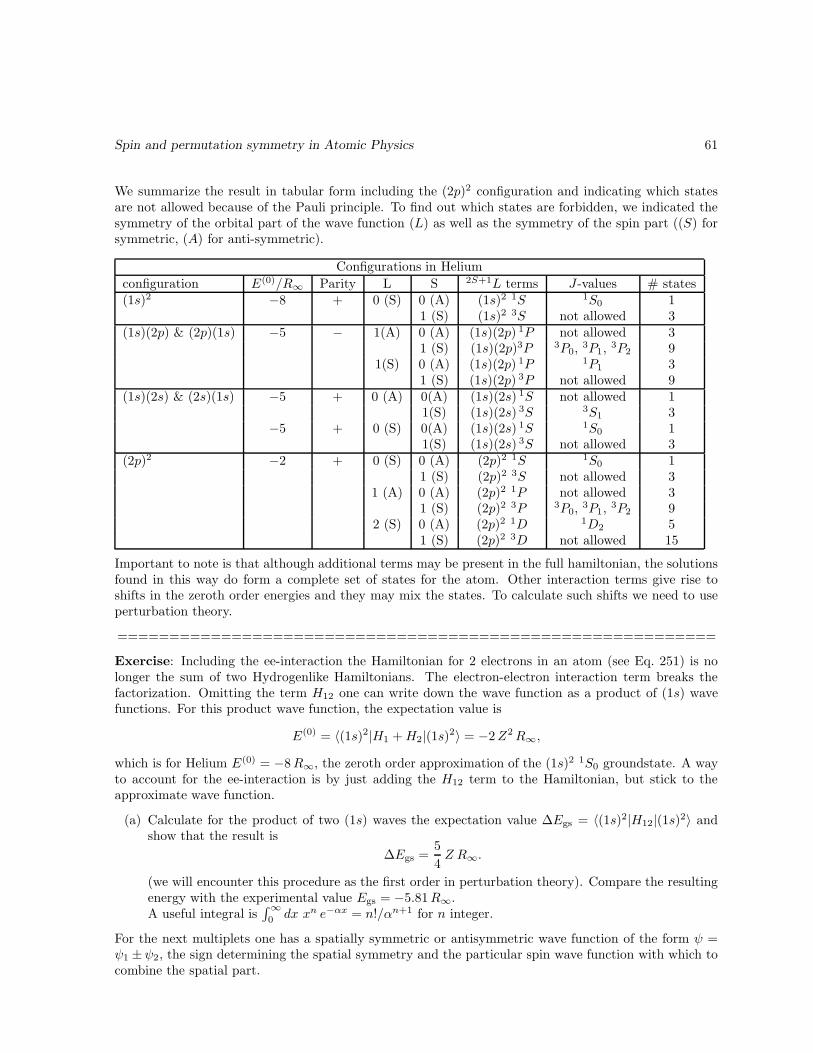
Spin and permutation symmetry in Atomic Physics 61
We summarize the result in tabular form including the (2p)2 configuration and indicating which statesare not allowed because of the Pauli principle. To find out which states are forbidden, we indicated thesymmetry of the orbital part of the wave function (L) as well as the symmetry of the spin part ((S) forsymmetric, (A) for anti-symmetric).
Configurations in Helium
configuration E(0)/R∞ Parity L S 2S+1L terms J-values # states(1s)2 −8 + 0 (S) 0 (A) (1s)2 1S 1S0 1
1 (S) (1s)2 3S not allowed 3(1s)(2p) & (2p)(1s) −5 − 1(A) 0 (A) (1s)(2p) 1P not allowed 3
1 (S) (1s)(2p)3P 3P0,3P1,
3P2 91(S) 0 (A) (1s)(2p) 1P 1P1 3
1 (S) (1s)(2p) 3P not allowed 9(1s)(2s) & (2s)(1s) −5 + 0 (A) 0(A) (1s)(2s) 1S not allowed 1
1(S) (1s)(2s) 3S 3S1 3−5 + 0 (S) 0(A) (1s)(2s) 1S 1S0 1
1(S) (1s)(2s) 3S not allowed 3(2p)2 −2 + 0 (S) 0 (A) (2p)2 1S 1S0 1
1 (S) (2p)2 3S not allowed 31 (A) 0 (A) (2p)2 1P not allowed 3
1 (S) (2p)2 3P 3P0,3P1,
3P2 92 (S) 0 (A) (2p)2 1D 1D2 5
1 (S) (2p)2 3D not allowed 15
Important to note is that although additional terms may be present in the full hamiltonian, the solutionsfound in this way do form a complete set of states for the atom. Other interaction terms give rise toshifts in the zeroth order energies and they may mix the states. To calculate such shifts we need to useperturbation theory.
==========================================================
Exercise: Including the ee-interaction the Hamiltonian for 2 electrons in an atom (see Eq. 251) is nolonger the sum of two Hydrogenlike Hamiltonians. The electron-electron interaction term breaks thefactorization. Omitting the term H12 one can write down the wave function as a product of (1s) wavefunctions. For this product wave function, the expectation value is
E(0) = 〈(1s)2|H1 +H2|(1s)2〉 = −2Z2R∞,
which is for Helium E(0) = −8R∞, the zeroth order approximation of the (1s)2 1S0 groundstate. A wayto account for the ee-interaction is by just adding the H12 term to the Hamiltonian, but stick to theapproximate wave function.
(a) Calculate for the product of two (1s) waves the expectation value ∆Egs = 〈(1s)2|H12|(1s)2〉 andshow that the result is
∆Egs =5
4Z R∞.
(we will encounter this procedure as the first order in perturbation theory). Compare the resultingenergy with the experimental value Egs = −5.81R∞.A useful integral is
∫∞
0 dx xn e−αx = n!/αn+1 for n integer.
For the next multiplets one has a spatially symmetric or antisymmetric wave function of the form ψ =ψ1 ±ψ2, the sign determining the spatial symmetry and the particular spin wave function with which tocombine the spatial part.

Spin and permutation symmetry in Atomic Physics 62
(b) Express the expectation energy of the Hamiltonian for the (normalized) symmetric and antisym-metric wave functions in terms of the following integrals
〈ψ1|ψ1〉 = 〈ψ2|ψ2〉 = 1 ψ1and ψ2 (assumed normalized),
〈ψ1|Hi|ψ1〉 = E(0)i (i = 1,2),
〈ψ1|ψ2〉 = 〈ψ2|ψ1〉 = S (overlap integral),
〈ψ1|H12|ψ1〉 = 〈ψ2|H12|ψ2〉 = C (Coulomb integral),
〈ψ1|H12|ψ2〉 = 〈ψ2|H12|ψ1〉 = K (exchange integral).
(c) Looking at the (1s)(2p) and (1s)(2s) configurations the Coulomb integral is smallest for (1s)(2s)(could you think of a reason), while the exchange integral is positive. Sketch the spectrum ofHelium including the lowest para-Helium and ortho-Helium states and indicate some of the allowedradiative dipole transitions.
==========================================================
9.2 Atomic multiplets
In a more realistic atom the ee-interaction term (or what remains after taken into account an effectivecharge) must also be considered. It breaks rotational invariance in the hamiltonian for the electroncoordinate ri, thus ℓi is no longer compatible with the hamiltonian. We note that L is still compatiblewith the hamiltonian. Since there is no spin-dependence, spin operators si and also S are compatiblewith the hamiltonian and corresponding quantum numbers still can be used.
To illustrate how one easily finds the allowed L and S values given an electron configuration, weconsider the ground state configuration of Carbon, (1s)2(2s)2(2p)2. The allowed states in a shell can berepresented as a number of boxes, e.g. an s-shell as two boxes, a p-shell as six boxes,
ms ↓ mℓ 0
+1/2−1/2
ms ↓ mℓ −1 0 +1
+1/2−1/2
etc. Putting N electrons in these boxes with at most one electron per box (Pauli principle) one has6!/N !(6 − N)! possibilities, e.g. for a filled only one possibility. Obviously then all magnetic quantumnumbers combine to zero, ML = MS = 0 and one also has for the total L and S quantum numbersL = S = 0. Hence filled shells can be disregarded for finding total (L, S) values.
As a consequence the specta of atoms with one electron outside a closed shell (Li, Na, K, Rb, Cs,Fr) resemble the spectrum of hydrogen, e.g. the configurations for sodium (Na) are (nℓ) with n ≥ 3.The groundstate for Na is (3s)2S1/2, the first excited states are the (3p)2P1/2 and (3p)2P3/2 levels. Theelectric dipole transition 2P →2 S is the well-known yellow Na-line in the visible spectrum, which bythe fine-structure (see below) is split into two lines corresponding to the transitions 2P3/2 →2 S1/2 and2P1/2 →2 S1/2. For atoms with two electrons outside a closed shell (Be, Mg, Ca, Sr, Ba, Ra) the multipletstructure resembles that of helium.
For a particular number of electrons it is easy to look at the number of possibilities to constructparticular ML and MS values. This is denoted in a Slater diagram
MS ↓ ML −2 −1 0 +1 +2
+1 0 1 1 1 00 1 2 3 2 1−1 0 1 1 1 0

Spin and permutation symmetry in Atomic Physics 63
It is easy to disentangle this into
0 0 0 0 01 1 1 1 10 0 0 0 0
(L, S) = (2, 0)
+
0 1 1 1 00 1 1 1 00 1 1 1 0
(L, S) = (1, 1)
+
0 0 0 0 00 0 1 0 00 0 0 0 0
(L, S) = (0, 0)
Thus for the Carbon one finds in the groundstate configurations the multiplets
1D 3P 1S
Also for configurations involving more shells that are not completely filled, it is straightforward to findthe states in an MS −ML diagram. At this point we have completed the quantum number analysis ofthe spectrum. In order to find the energies one needs to use perturbation theory as well as variationalmethods to be discussed next. The results of these methods have shown that for the ordering in thespectrum a number of phenomenological rules can be formulated, the Hund rules. In particular for thegroundstate configuration one has that the terms with highest S-values (highest multiplicity) and thenhighest L-values have the lowest energy, i.e. in the example for Carbon
E(3P ) < E(1D) < E(1S).
==========================================================
Exercise:
(a) Construct the possible multiplets (spectroscopic terms) of a Barium atom in a (6p)(5d) state. Givethe degeneracy of each of the terms and check that there are (as expected) 60 states. Use the Hundrules to order the states.
(b) Construct the multiplets for all possible (np)N configurations of electrons in an atom and give theirordering in energy.
==========================================================
Exercise: Another system is that consisting of two nucleons, proton-proton, proton-neutron or neutron-neutron. Nucleons have spin 1/2, hence are fermions. They interact with each other through a potentialof the form
V = V1(r) + V2(r) s1 · s2 + V3(r)
[3(s1 · r)(s2 · r)
r2− s1 · s2
]
,
where r is the relative coordinate.
• Omitting V3, what are the good quantum numbers? Give the various (2S+1)ℓJ quantum numbersfor pp, pn and nn. Include parity.
• Which of these quantum numbers remain good quantum numbers including the V3 term?
==========================================================
Exercise: Because of the similarity of the interaction for protons and neutrons, they are often consideredas a nucleon with two possible isospin states |p〉 and |n〉 in analogy to spin states (thus isospin 1/2).Construct the isospin 0 and isospin 1 states. What is their symmetry. Show that one can use permutationsymmetry including isospin as a degree of freedom and get the same allowed quantum numbers for thetwo-nucleon system.
==========================================================

Bound state perturbation theory 64
10 Bound state perturbation theory
10.1 Basic treatment
Perturbation theory is used to obtain in a systematic way a solution for a hamiltonian H = H0 + λVin the form of an expansion in the (small) parameter λ, assuming the solutions of H0 are known, (H0 −E
(0)n ) |φn〉 = 0. One inserts expansions for the energy and the solution of the form
En = E(0)n + λE(1)
n + λ2 E(2)n + . . . , (270)
|ψn〉 = |φn〉+ λ |ψ(1)n 〉, (271)
into the Schrodinger equation (H − En)|ψn〉 = 0,(H0 + λV
)(|φn〉+ λ |ψ(1)
n 〉+ . . .)=(E(0)
n + λE(1)n + . . .
)(|φn〉+ λ |ψ(1)
n 〉+ . . .). (272)
After ordering the terms according to the power of λ, one finds at zeroth order the unperturbed Schrodingerequation for |φn〉 and at first order
λV |φn〉+ λH0|ψ(1)n 〉 = λE(1)
n |φn〉+ λE(0)n |ψ(1)
n 〉. (273)
Realizing that the unperturbed solutions form a complete set we take the scalar product with 〈φn| andwith 〈φm| for m 6= n, yielding
λE(1)n = 〈φn|λV |φn〉, (274)
λ(E(0)
n − E(0)m
)〈φm|ψ(1)
n 〉 = 〈φm|λV |φn〉 (for m 6= n). (275)
To obtain the first equation we have assumed that ψ(1)n 〉 can be choosen orthogonal to |φn〉 (thus
〈φn|〉ψ(1)n 〉 = 0). This can be done without loss of generality. It may be necessary to renormalize
the final result, because we have more or less arbitrary set the coefficient of |φn〉 equalt to one. The first
equation gives the first order shift in the energy ∆E = E − En = λE(1)n , the second gives the correction
in the wave function. Summarizing,
E(1)n = 〈φn|V |φn = Vnn, (276)
|ψ(1)n 〉 =
∑
m 6=n
|φm〉〈φm|V |φn〉E
(0)n − E(0)
m
=∑
m 6=n
|φm〉Vmn
E(0)n − E(0)
m
. (277)
The latter result can be written down only for the case that the unperturbed state |φn〉 is nondegenerate.The second order results involve the λ2 terms of Eq. 272, giving
H0|ψ(2)n 〉+ V |ψ(1)
n 〉 = E(0)n |ψ(2)
n 〉+ E(1)n |ψ(1)
n 〉+ E(2)n |φn〉. (278)
Taking the scalar product with 〈φn| gives the result
E(2)n = 〈φn|V |ψ(1)
n 〉 =∑
m 6=n
Vnm Vmn
E(0)n − E(0)
m
. (279)
Perturbation theory is very useful if the first-order shift in the energies is small, to be more precise if
|〈φm|λV |φn〉| ≪ |E(0)n − E(0)
m | for all m 6= n. In principle the expressions have been written down fordiscrete spectra, but for bound states we can generalize
∑
m 6=n
⇒∑
m 6=n
+
∫ ∞
0
dE ρ(E), (280)
where the integral covers the continuum spectrum in which ρ(E) dE is the number of states in an energyinterval dE around E.

Bound state perturbation theory 65
10.2 Perturbation theory for degenerate states
In many applications we will encounter the situation that the energy levels in the unperturbed hamiltonianwill be degenrate, in which case the step from Eq. 275 to 277 cannot be made. Eq. 275, however, alsotells us how to proceed. Make sure that each subset of states |φn1〉, . . . , |φns〉 which are degenerate withrespect to H0 are choosen to be eigenstates of the perturbation λV . In that case we can choose the wavefunction corrections orthogonal to all |φnr〉 and we have 〈φni|λV |φnj〉 = 0. The result is that we getinstead of Eq. 277 the result
|ψ(1)n 〉 =
∑
E(0)m 6=E
(0)n
|φm〉〈φm|V |φn〉E
(0)n − E(0)
m
. (281)
In practice we often look for a suitable set of states for which both the unperturbed hamiltonian and theperturbation potential are diagonal by looking for a relevant set of compatible operators. In worst caseone can ressort to a brute force diagonalisation of the perturbation potential. One needs to diagonalizethe degenerate subspace. This assures that within that subspace the off-diagonal matrix elements are
zero and the steps towards obtaining |ψ(1)n 〉 can be made.
10.3 Applications in Hydrogen
In the hydrogen atom there are a number of additional terms in the hamiltonian that can be attributedto relativistic corrections,
H = H0 +Hmass +HFoldy +Hso (282)
The first term is a correction coming from the difference of the relativistic and nonrelativistic kineticenergies, the mass term,
Hmass =√
p2c2 +m2c4 −mc2 − p2
2m≈ − p4
8m3c2. (283)
Including this correction, the operators ℓ2 and ℓz still remain compatible with the hamiltonian, butthe radial dependence now will be modified. However in first order perturbation theory one obtains anaccurate estimate of the energy shifts by calculating the expectation value of the correction. We herejust state the result3,
∆Emass(nℓ) = 〈nℓm . . . | − p4
8m3c2|nℓm . . .〉 = −α2 R∞
n3
(1
ℓ+ 12
− 3
4n
)
. (284)
Another interaction term arises because of the interaction of the spin with the induced magnetic fieldby the orbital motion, the spin-orbit interaction. It can be up to a factor 2 be derived with classicalarguments, but a proper derivation requires the use of the relativistic Dy spectrumirac equation for theelectron. The result for a particle in a central potential is
Hso =1
2m2c21
r
dVcdr
ℓ · s. (285)
When applying perturbation theory for this term one must be careful. One cannot simply calculate theexpectation value between hydrogen states |nℓsmℓms〉. Since the level is 2(2ℓ + 1)-fold degenerate theperturbation mixes these degenerate states. Application of perturbation theory requires a reordering ofthese states, such that they are compatible with the perturbation. Instead of the brute force way ofdiagonalizing the matrix 〈nℓsm′ℓm′s|Hso|nℓsmℓms〉, there is a smarter way. By rewriting
ℓ · s =1
2
[j2 − ℓ2 − s2
],
3The calculation is treated in many quantum mechanics books, usually done by rewriting (p2)2 = 4m2(H − V (r))2.This symmetric treatment avoids problems with non-hermiticity of p4 because of boundary terms at r = 0

Bound state perturbation theory 66
one sees that the operators ℓ2, s2, j2 and jz (which from the theory of addition of angular momentaare known to be compatible with each other) are also compatible with the hamiltonian. This is not truefor the set ℓ2, s2, ℓz and sz. Hence if we use states |nℓsjm〉, the correction term has no off-diagonalelements, hence does (for given ℓ and s not mix the unperturbed degenerate states and the splitting forthe correct combinations of states is directly found as
∆Eso(nℓsjm) =1
2m2c2〈nℓsjm|1
r
dVcdr
ℓ · s|nℓsjm〉
=e2 ~2
32πǫ0m2c2〈nℓ| 1
r3|nℓ〉 [j(j + 1)− ℓ(ℓ+ 1)− s(s+ 1)]
=e2 ~2
32πǫ0m2c2j(j + 1)− ℓ(ℓ+ 1)− s(s+ 1)
a30 n3 ℓ(ℓ+ 1)(ℓ+ 1
2 )(286)
We thus must couple ℓ and s to j-eigenstates. For one electron with a given ℓ 6= 0 there are two possibilitiesfor j, namely j = ℓ± 1
2 giving for ℓ 6= 0
∆Eso(nℓj) = α2 R∞n3
(1
ℓ+ 12
− 1
j + 12
)
(287)
and for the combined result
∆Emass + so = −α2 R∞n3
(1
j + 12
− 3
4n
)
(288)
In the Hydrogen atom one also has the Foldy term, which also is a relativistic correction. It isproportional to δ3(r) and thus only affects s-waves. It makes the above equation valid also for s-waves.We return to this later. Schematically (not on scale) one has the following fine structure in the hydrogenspectrum
2S1/2
2S1/2
2P3/2
2P3/2
2P1/2
2S1/2
2S1/2
2P1/25.7 x 10−5 eV
4 x 10 eV−6
E = − 3.4 eV
E = −13.6 eV
2
1 1s
2s2p
H0 spin−orbitspin−orbitmassFoldy
F = 1
F = 0
Lamb−shift
hyperfine structure
5.9 x 10 eV−6
The various terms cause shifts in the order of 10−4 eV, giving within a orbit characterized by the principalquantum number n states with well-defined j-values. We denote such a level with a term symbol, forhydrogen
(nℓ) (2S+1)LJ
where (nℓ) indicates the spatial part of the electron wave function, 2S+1 is the total spin multiplicity andL is the total orbital angular momentum of the electrons (using notation S, P,D, . . . for L = 0, 1, 2, . . .).In this specific case of hydrogen with just one electron S = 1/2 and the multiplicity is always 2 whileL = ℓ. The splitting of the 2S1/2 and 2P1/2 is about 4 × 10⁻⁶ eV produces a splitting of the Lyman αline. Also transitions between both levels are possible via an E1 transition with frequency of about 1GHz.

Bound state perturbation theory 67
Fine structure in hydrogen: the hyperfine splitting
The hyperfine structure in hydrogen is due to the interaction of the magnetic moments of electron andnucleus. Also the proton has a magnetic moment, which induces a magnetic dipole field felt by theelectron and vice versa. It produces an interaction term, which for s-waves is of the form
Vss =1
6πǫ0 c2µe · µp ∇
2 1
r. (289)
We know that µe = ge (e/me)S and µp = gp (e/Mp) I (where we use the in atomic physics conventionalnotation I for the nuclear spin). The splitting thus is proportional to
∆Ess ∝ ge gp 〈|S · I|〉 =1
2ge gp ~
2 [F (+F1)− S(S + 1)− I(I + 1)] . (290)
The proper eigenstates are labeled by eigenstates for the angular momentum operators F 2 and Fz, whereF = S + I. For normal hydrogen in the ground state (I = 1/2), it produces two states with F = 0(para-) and F = 1 (ortho-hydrogen). The splitting is much smaller than the fine structure. For the(1s) 2S1/2 level in hydrogen the splitting is 5.9× 10⁻⁶ eV (see figure in previous section), correspondingto a transition frequency νhf = 1.42 GHz or a wavelength of 21 cm. Although the radiative transitionis heavily suppressed (it is certainly not an electric dipole transition!) it plays a very important role inradio astronomy. It traces the abundant occurence of hydrogen in the universe not in the least since the21 cm wavelength is not strongly attenuated by interstellar dust.
10.4 The fine structure of atoms
When combining angular momenta, we discussed the multiplets forming the fine structure in atoms. Fornot too heavy atoms, the splitting of energies within the multiplets turn out to be described well by aspin-orbit interaction of the form
Hso = A(L, S)L · S, (291)
with a strenght A depending on the multiplet, coming among others from the radial dependence ofthe basic interaction. The spin-orbit interaction splits states with different J-values, leading to 2S+1LJ
multiplets and a magnitude for the splitting being given by
∆E(LSJM) =1
2A~2 [J(J + 1)− L(L+ 1)− S(S + 1)] . (292)
An example of the splitting of the three terms for an (np)2 configuration is given below.
(np) 2 (np) 2
2S+1L J
01
2
2
0
D
P
S1
1
3
( j , j )J
(3/2,3/2)
(1/2,1/2)
0
2
2
1
0
(3/2,1/2)

Bound state perturbation theory 68
Note that the average (beware of degeneracy) of a multiplet gives the energy of the multiplet without thespin-orbit interaction. The pattern of levels can in principle be obtained from atomic spectra. The use ofmagnetic fields is helpful to determine the degeneracy of the levels. But already the spin-orbit splittingscontains interesting patterns, such as
r =E(2S+1LJ)− E(2S+1LJ−1)
E(2S+1LJ−1)− E(2S+1LJ−2)=
J
J − 1, (293)
e.g. for the ratio (E(3P2) − E(3P1))/(E(3P1) − E(3P0)) one expects r = 2 if LS-coupling describes thefine structure. For Carbon the actual ratio is 1.65, for Silicium (Si) it is 1.89, but for a heavy atom aslead (Pb) the result is just 0.36, indicating a different type of fine structure.
A different scheme, that works in some cases better for heavy atoms, is the jj-scheme in which firstthe orbital angular momenta and spins of the electrons are coupled, which in turn are combined intoJ-values, illustrated in the figure for the (np)2 configuration, in which case the interaction is
Hjj = A(j1, j2) j1 · j2, (294)
and the splitting is given by
∆E(j1j2JM) =1
2A~2 [J(J + 1)− j1(j1 + 1)− j2(j2 + 1)] . (295)
Note that coupling two identical j-values of the electrons, one needs to account for the symmetry ofthe wave function. The wave function for the maximal J = 2 j is symmetric, for the next lower J it isantisymmetric, then again symmetric, etc. This explains the J-values in the jj-coupling scheme. Afterhaving done all recouplings and accounting for permutation symmetry, the same J-values must appearin both schemes.

Magnetic effects in atoms and the electron spin 69
11 Magnetic effects in atoms and the electron spin
11.1 The Zeeman effect
Interaction of orbital angular momentum with magnetic field
In a magnetic field an additional interaction is added to the hamiltonian,
H = − ~2
2m∇
2 − Ze2
4πǫ0 r︸ ︷︷ ︸
H0
+Vmag, (296)
where Vmag = −µ ·B. Neglecting spin, the magnetic moment of a particle in orbit is given by
µℓ = −gℓe
2mℓ (297)
with gℓ = 1. What are the eigenfunctions and eigenvalues (energies) of this new hamiltonian. For thisit is useful to find as many as possible commuting operators. Commuting operators are H , ℓ2, ℓz (and,although overcomplete, the parity operator). However, the term
Vmag =e
2mℓ ·B,
implies that one only can have ℓz as an operator compatible with H if the z-axis is chosen along B, i.e.B = B z. In that case it is easy to convince oneself that the eigenfunctions are still the hydrogen wavefunctions, while the energies are shifted over an amount
∆Enℓmℓ= 〈nℓmℓ|
eB
2mℓz|nℓmℓ〉 = mℓ µBB, (298)
where
µB =e~
2m=
1
2e c
~
mc≈ 5.8× 10⁻⁵ eV/T (299)
is the Bohr magneton.
Interaction of electron spin with magnetic field
For a proper description of an electron, one needs to specify in addition to ψ(r, t) a spin wave function.For electrons with spin 1/2 one can resort to a description with two-component wave functions, where thespin operators are given by matrices, s = 1
2 ~σ where σ are the three Pauli matrices. Just as the orbitalangular momentum, the spin gives in a magnetic field rise to an interaction term in the hamiltonian.
Vmag = −µs ·B, (300)
with
µs = −gse
2ms = −gs
e~
mσ. (301)
The g-factor for the spin of the electron is gs ≈ 2. Actually the deviation from 2 is due to subtle butcalculable effects in quantum electrodynamics, ge − 2 = α/π + . . . ≈ 0.00232. If the interaction of thespin with the magnetic field is the only interaction (e.g. for s-waves), the result of the interaction term isa simple shift in the energies for the states, that now include also spin quantum numbers.

Magnetic effects in atoms and the electron spin 70
The Zeeman effect in many-electron atoms
In general a 2S+1L level in a magnetic field is split by an interaction term
Vmag = −µ ·B, (302)
where µ = −µB(gL L+ gS S), resulting in a number of levels with the splitting given by
∆E(LSMLMS) = −µBB(ML + 2MS). (303)
In normal magnetic fields (say smaller or of the order of 1 T), the splittings are only fractions of an eVand there are other effects causing different splitting patterns, such as the L · S spin-orbit interaction.But for very large magnetic fields one does see the above normal Zeeman splitting pattern.
-+ -+
M10
0
2M
0
0
111
1
-1
-1-1
1
-1
L S
νσπ
ν
P
S
2
2
Zeeman splitting of levels in a magneticfield (no spin-orbit). Also indicated arethe transitions, separated into ∆ML =0 (π-transitions) and ∆ML = ±1 (σ-transitions).
Finally we note that the magnetic effects discussed here are those in an external magnetic field. Thisdefines a preferential direction in space and leads to dependence on eigenvalues of the (z-)component ofthe angular momentum operators. This is also found back in the names magnetic quantum numbers formℓ, ms, etc.
11.2 Spin-orbit interaction and magnetic fields
Inclusion of the spin-orbit interaction is important to describe the fine structure of the multiplets inatomic spectra. This fine structure in general turns out to be considerably larger than the magneticallyinduced splittings. In that case one cannot simply use the results for the normal Zeeman effect whenspin plays a role. So consider the situation that one has an interaction term in the atom of the form
Hint = AL · S − µ ·B, (304)
with µ = µB(gLL + gSS)/~ = µB (L + 2S)/~. We have already seen what happens in the situationsA = 0 and B = |B| = 0. One has
A = 0 : eigenstates |(. . .)LSMLMS〉,∆E(LSMLMS) = µBB(ML + 2MS),
B = 0 : eigenstates |(. . .)LSJM〉,
∆E(LSJM) =1
2A~2 [J(J + 1)− L(L+ 1)− S(S + 1)] .

Magnetic effects in atoms and the electron spin 71
The splitting pattern for A = 0 has already been given, for B = 0 it splits the 2S+1L multiplet into thedifferent 2S+1LJ multiplets, for the 2P →2 S transition indicated as the first splitting in the figure below.
3/23/23/23/2
J
1/21/2
1/21/2
M+3/2+1/2-1/2+3/2+1/2-1/2
+1/2-1/2
1/2
3/2
1/2
P2
S2
P2
P2
S2
The spin-orbit splitting lead-ing to the 2S+1LJ multipletsfor the 2P and 2S levels andthe consecutive splitting in amagnetic field for the case ofa small magnetic field.
When one switches on the magnetic field, one deals with an interaction term for which neither |LSMLMS〉,nor |LSJM〉 are proper states (check compatibility of the relevant operators!). If the magnetic field issmall the states will be in first order given by |LSJM〉 and one can calculate the energy shift via
∆Emag = µBB 〈(. . .)LSJM |Lz + 2Sz|(. . .)LSJM〉 = µBB 〈(. . .)LSJM |Jz + Sz|(. . .)LSJM〉. (305)
The part with which we need to be careful is the expectation value of Sz, Evaluating it between stateswith different M -values belonging to the same J gives zero, because if two M values involve the sameMS , the ML’s must be different (remember that in the coupling M =ML +MS). Thus we just need
〈LSJM |Sz|LSJM〉 =MJ(J + 1) + S(S + 1)− L(L+ 1)
2J(J + 1)(306)
which follows from a subtle relation involving S and J operators4, J2Sz +SzJ2 = 2 Jz (J ·S) leading to
∆Emag =
[
1 +J(J + 1) + S(S + 1)− L(L+ 1)
2J(J + 1)
]
︸ ︷︷ ︸
gJ
M µBB, (307)
where gJ is called the Lande factor. This splitting is also indicated in the figure. Note that the procedureonly works for small B-values. For large B-values (Paschen-Back limit) the assumption of states beingapproximately given by |LSJM〉 is not valid and one gets the previously discussed normal Zeemansplitting.
==========================================================
Exercise:
(a) Use for the 2P states the basis states |L, S;ML,MS〉 and write down the spin-orbit hamiltonianHso = AL · S as a matrix. Use for this the explicit expression
Hso =A
2(2LzSz + L+S− + L−S+) .
Determine the eigenvalues and eigenstates. The latter are of course precisely the |L, S; J,M〉 states.4From [Ji, Aj ] = i~ ǫijkAk one obtains the relations [J2, Ai] = −i~ ǫikl(JkAl + AlJk), which yields [J2, [J2, Ai]] =
2~2(J2Ai +AiJ2)−4~2(A ·J)Ji. For the proof one also needs to realize that between J2 eigenstates the expectation value
〈JM |[J2, O]|JM〉 = 0 for any operator.

Magnetic effects in atoms and the electron spin 72
(b) On the same basis, write down the hamiltonian in an external magnetic field, Hint = AL ·S−µ ·B,using the explicit form
Hint =A
2(2LzSz + L+S− + L−S+)− µB B0 (Lz + 2Sz) .
Find all eigenvalues and check that they coincide with the approximations made for small and largeB-fields.
==========================================================

Variational approach 73
12 Variational approach
12.1 Basic treatment
The variational method is used to obtain an estimate for the ground state energy and the ground statewave function for a given hamiltonian. This is done by taking a trial wave function |ψ[α1,α2,...]〉 dependingon a number of parameters αi and calculating the expectation value for the (given) hamiltonian,
E[α1,α2,...] =〈ψ[α1,α2,...]|H |ψ[α1,α2,...]〉〈ψ[α1,α2,...]|ψ[α1,α2,...]〉
. (308)
If the true solutions and energies of H are given by (H − En) |φn〉 = 0, it is simple to show that
E[α1,α2,...] ≥ E0, (309)
with the equal sign being true if |ψ[α1,α2,...]〉 = φ0. By minimizing the expectation value of the hamiltonianby varying the parameters,
∂E[α1,α2,...]
∂αi= 0, (310)
one hopes to get close to the true ground state. The succes of the method not only depends on thenumber of parameters used and the calculational power of computers, but also on smart choices for thetrial wave function such as choosing the correct symmetry, the correct number of nodes and the correctasymptotic (large and small r) behavior of the wave function.
If one wants to apply variational methods to find other (higher-lying) states, one must ensure that thetrial function is chosen to be orthogonal to any lower state. This may be achieved by looking for stateswith a particular symmetry, which of course (why?) only works if the Hamiltonian one is working with,has this symmetry. In this way one can look for the lowest p-wave in radially symmetric Hamiltonian byusing an ansatz of the form ψ ∝ z f(r). One might also constrain oneself to wave functions which alwayshave a node, keeping in mind the node theorem for bound states.
==========================================================
Exercise:
(a) Estimate the ground state energy in a linear potential, V (r) = T0 r. Some useful integrals might be∫ ∞
0
dr rα exp(−Ar) = Γ(α+ 1)
Aα+1,
∫ ∞
0
dr r32α exp
(
−Ar3/2)
=2
3
Γ(α+ 2
3
)
Aα+ 23
,
∫ ∞
0
dr r2α exp(−Ar2
)=
1
2
Γ(α+ 1
2
)
Aα+ 12
,
valid for α ≥ 0. Note that Γ(z + 1) = z!, satisfying Γ(z + 1) = zΓ(z). Some specific values areΓ(1) = 0! = 1, Γ(1/2) =
√π, and Γ(2/3) = 1.35412.
(b) To appreciate the accuracy of your result, note that the exact solution is an Airy function Ai(z),solution of Ai′′(z)− z Ai(z) = 0. Argue that the function
u(r) ∼ Ai(r
r0− ǫ)
.
with r0 = (~2/2mT0)1/3 is a solution of the three-dimensional linear potential if Ai(−ǫ) = 0. Show
that it represents a solution with boundary condition u(0) = 0 and energy E = −ǫ E0, whereE0 = (~2T 2
0 /2m)1/3. The first (negative) zero of the Airy function is at ǫ = 2.3381.
==========================================================
Variational approach 74
12.2 Example: electron-electron repulsion
Ground state of Helium atom
As a trial function for the He ground a good ansatz could be a simple product of wave functions,
ψT (r1, r2) =α3
π a30e−αr1/a0 e−αr2/a0 . (311)
By allowing the coefficient α in the exponent to vary, we try to incorporate the screening. We can usethe variational approach to see how well we can do. With the results from the sections on the hydrogenatom and those of the previous section we find
〈ψT | −~2
2m
(∇
21 +∇
22
)|ψT 〉 =
~2
ma20α2 = 2α2R∞, (312)
〈ψT |−Ze24πǫ0
(1
r1+
1
r2
)
|ψT 〉 = −2Ze2
4πǫ0 a0α = −4ZαR∞, (313)
〈ψT |e2
4πǫ0 r12|ψT 〉 =
5
4αR∞, (314)
and thus
E[α] = 2
[
α2 −(
2Z − 5
8
)
α
]
R∞, (315)
which is minimized for
α = Zeff = Z − 5
16(316)
with
E[αmin] = −2(
Z − 5
16
)2
R∞. (317)
For He this gives Egs = −5.7R∞, wich is within a few percent of the experimental value of −5.81R∞= 79.0 eV and much better than the value using perturbation theory (which of course is just the resultobtained for α = 2). As expected the value Zeff = 27/16 is less than 2.
The H−-ion
An interesting second example is actually the hydrogen atom, which also has a positive electron affinity,H + e− → H− + 0.76 eV. Here, adding a second electron actually is harder to deal with in a variationalapproach. If one tries for the two electrons in H− a simple product wave function does not produce apositive electron affinity (check this). In order to find a positive electron affinity for the H-atom (forwhich an equivalent statement is that the H−-ion has a binding energy of 0.056R∞ = 0.76 eV) one canuse e.g. a trial function of the form
ψT = C[
e−(α1r1+α2r2)/a0 + e−(α1r2+α2r1)/a0
]
. (318)
The form is suggestive for two different orbits with fall-off parameters α1 and α2, but as electrons areindistinguishable one must (anti)-symmetrize (depending on spin) the two terms.
==========================================================
Exercise: Apply the variational principle to find a suitable wave function for H−. Try the product wavefunction that has been used for He. What do you find for the electron affinity of H in that case. Then try

Variational approach 75
the two-orbit form proposed in this chapter and show that it at least leads to a positive electron affinity.A useful integral is
∫
d3r1 d3r2
e−2α1 r1−2α2 r2
|r1 − r2|=
(π
α31
)(π
α32
)α1α2
(α21 + α2
2 + 3α1α2
)
(α1 + α2)3
α1=α2=5
8α( π
α3
)2
.
==========================================================
12.3 The Hartree-Fock model
The Hartree-Fock model is a self-consistent model for determining the effective potential for electronsthat we discussed earlier in the context of the periodic table. It starts from the Hamiltonian like inEq. 251 including all electron-electron interactions, The variational approach is actually done through aself-consistent solution of
δ〈ψ|H − E|ψ〉 = 0, (319)
under varying the solution ψ, restricting oneself to solutions in the form of an antisymmetrized product(Slater determinant) of (normalized) single electron wave functions,
ψ(r1, . . . , rZ) = Aφ1(r1) . . . φZ(rZ), (320)
which satisfy
[
~2
2m∇
2i −
Z e2
4πǫ0 ri+∑
j 6=i
∫
d3rj |φj(rj)|2e2
4πǫ0 |ri − rj |︸ ︷︷ ︸
Wi(ri)
−Ei
]
φi(ri) = 0 (321)
The solution can be obtained iteratively by starting with an ansatz for the potential Wi(ri), solve forthe single particle solutions, reconstruct the new Wi(ri), continuing till convergence is reached for theeffective potential W .
==========================================================
Exercise: Start for Helium with Wi(ri) = 0 and construct the potential Wi(ri) after one step and lookif you can find Zeff(r) as in Eq. 252.
==========================================================

Time-dependent perturbation theory 76
13 Time-dependent perturbation theory
13.1 Explicit time-dependence
Repeating the case of a hamiltonian without explicit time-dependence, i.e. H0 = H0(r,p, . . .). Oneemploys the time-independent solutions of the eigenvalue equation H(r,p, . . .)φn = En φn. Using thecompleteness of the states φn one can write
ψ(t) =∑
n
cn(t)φn, (322)
insert this in the Schrodinger equation,
i~∂ψ
∂t= Hψ(t) (323)
leading toi~cn(t) = En cn(t) =⇒ cn(t) = cn e
−i Ent/~, (324)
with constant coefficients cn = cn(0). There are two possibilities:
1. One starts (e.g. after a measurement) with ψ(0) = φi, where φi is one of the eigenstates of H0 witheigenvalue/energy Ei. In that case
ψ(t) = φi e−iEit/~, (325)
known as a stationary state. All expectation values of operators (that do not explicitly depend ontime) are time-independent.
2. One starts in a mixed state, say ψ(0) = c1 φ1 + c2 φ2. In that case one has
ψ(t) = c1 φ1 e−iE1t/~ + c2 φ2 e
−iE2t/~, (326)
which leads to oscillations in expectation values with frequency ω12 = (E1 − E2)/~.
In the situation that the hamiltonian of a system contains explicit time dependence, i.e. H = H(r,p, . . . , t)one no longer has simple stationary state solutions of the form φn e
−iEnt/~. We consider the case thatthe time-dependence is contained in a part of the Hamiltonian.
H = H0 + V (t). (327)
The part H0 does not have explicit t-dependence, while the second part has a (possible) time-dependence.Assume the problem H0 to be known with eigenstates φn and eigen-energies En. When doing time-independent perturbation theory (i.e. the case that V is time-independent) one tries to express the trueeigenfunctions of H in the complete set φn. In the present treatment one makes the observation that ifthe system at some time is in a state φi, it will at a later time have a nonzero probability to be in anotherstate. The calculation of the rate of change is what is done in time-dependent perturbation theory. Thiscan actually be used for both time-independent and time-dependent perturbations.
Starting with the known (time-independent) part H0, we use completeness of the states φn to write
ψ(t) =∑
n
cn(t)φn e−iEnt/~. (328)
Note that one could have absorbed the exponential time-dependence in cn(t), but not doing so is moreappropriate because the time-dependence of cn is then solely a consequence of V .
By substituting the expression for ψ(t) in the Schrodinger equation,
i~∂
∂tψ(t) = (H0 + V (t))ψ(t), (329)

Time-dependent perturbation theory 77
one simply finds
i~ cp(t) =∑
n
Vpn(t) cn(t) e+i ωpnt, (330)
where Vpn = 〈φp|V (t)|φn〉 is the expectation value of the potential V between the (time-independent)eigenstates of H0, and ωpn = (Ep − En)/~. As expected if V = 0, the righthand-side is zero and thecoefficients are time-independent.
In the next section we solve the above equations for a simple two-state system. Often, however, onewill encounter a perturbative approach treated after that example.
13.2 Example: two-level system
Consider a two-state system, with φa and φb being solutions of the unperturbed Hamiltonian with eigen-values Ea and Eb, H0 φa = Ea φa and H0 φb = Eb φb. Using a matrix notation and the basis
φa ≡
10
and φb =
01
(331)
the Hamiltonian H0 and the perturbation V are taken to be
H0 =
Ea 00 Eb
and V =
Vaa(t) Vab(t)Vba(t) Vbb(t)
=
0 Vab(t)
V ∗ab(t) 0
. (332)
We have restricted ourselves to the simpler situation that there is only a time-dependent off-diagonalelement. Most applications can be cast in this form anyway. The solution can be written as
ψ(t) = ca(t)
10
e−iEat/~ + cb(t)
01
e−iEbt/~ =
ca(t) e
−iEat/~
cb(t) e−iEbt/~
, (333)
and the coefficients ca(t) and cb(t) obey a simple coupled set of equations of the form
i~
ca(t)cb(t)
=
0 Vab(t) e
+iωabt
V ∗ab(t) e−iωabt 0
ca(t)cb(t)
≡ ~
0 v(t)
v∗(t) 0
ca(t)cb(t)
, (334)
representing simple coupled equations,
i ca(t) = v(t) cb(t), (335)
i cb(t) = v∗(t) ca(t), (336)
==========================================================
Exercise: Show that in the presence of Vaa(t) ≡ ~va(t) and Vbb(t) ≡ ~vb(t) in the two-channel case onecan get again a ’simple’ coupling problem if we start with the ansatz
ψ(t) =
ca(t) e
−iEat/~ e−i∫
t
0dt′ va(t
′)
cb(t) e−iEbt/~ e−i
∫t
0dt′ vb(t
′)
,
==========================================================

Time-dependent perturbation theory 78
Two-level system with harmonic perturbation
Let us assume a harmonic time dependence for Vab(t). An example would be the following hamiltonianfor a two-state system,
H = −µ ·B(t) = −γ s ·B(t), (337)
describing the interaction of a spinning particle (with magnetic moment µ proportional to its spin) ina magnetic field. For instance for an elementary electron µ = −(e/m) s where s = (~/2)σ. For other(composite particles) the factor may be different. However, for any spin 1/2 particle the spin operatorscan be represented by the Pauli matrices. Starting with a constant magnetic field in (say) the z-direction,B0 = (0, 0, B0), and using the matrix representation for a spin 1/2 particle one has
H0 = −γB0
2~σz = −γB0
2~
1 00 −1
. (338)
The solutions are easily obtained,
φa =
10
with Ea = −γB0
2~, (339)
φb =
01
with Eb =γB0
2~, (340)
If the system is in a spin-state along the z-direction, it will stay in this state. If it is in another direction,it will start to oscillate with a frequency ωab = (Ea − Eb)/~ = −γ B0, known as the Larmor frequency.
Next consider the system in a circulating magnetic field in the x-y plane, superimposed on B0, B(t)= B0 +B1(t), where B1(t) = (B1 cosωt,B1 sinωt, 0). In that case
H = −γB0
2~σz −
γB1
2~(σx cosωt+ σy sinωt)
= −γB0
2~
1 00 −1
− γB1
2~
0 e−iωt
e+iωt 0
. (341)
We thus have a harmonic perturbation of the form
Vab(t) = −γB1
2e−iωt and v(t) =
Vab(t)
~e+iωabt = v1 e
−i(ω−ωab)t. (342)
with v1 = −γB1/2.The coupled equations in Eq. 334 can now simply be rewritten into a second order differential equation
for ca,ca + i(ω − ωab) ca + v21 ca = 0. (343)
This equation has two independent solutions of the form ei pt with
p = −1
2(ω − ωab)± ωr (344)
with the Rabi flopping frequency ωr = 12
√
(ω − ωab)2 + 4v21 . The general solution can then be written as
ca(t) = e−12 i(ω−ωab)t (A sin(ωr t) +B cos(ωr t)) ,
cb(t) =i
v(t)ca(t). (345)

Time-dependent perturbation theory 79
Starting off with ca(0) = 0 and |cb(0)| = 1, it is straightforward to check that
ca(t) = Ae−12 i (ω−ωab)t sin(ωr t), (346)
|A|2 =v21ω2r
=γ2B2
1
(ω − ωab)2 + γ2B21
, (347)
|ca(t)|2 + |cb(t)|2 = 1. (348)
Thus, given an initial spin aligned parallel or antiparallel to the B0 field, the probability for transition tothe other spin state shows oscillations with a frequency ωr, while the magnitude depends on the frequencyof the rotating perpendicular B1 field, showing a resonance at ω = ωab. In that case the spin completelyflips from parallel to antiparallel and back with frequency ωr (at resonance we have ωr = |v1|).
13.3 Fermi’s golden rule
In many case we are not able to exactly solve the time-dependent problem and we treat the problemperturbatively. Writing, H = H0 + λV (t), including a multiplicative factor λ to keep track of orders. Inthe case of perturbation theory, we realize that in writing a solution of the form
cp(t) = c(0)p (t) + λ c(1)p (t) + . . . , (349)
the time-dependence of a specific order is determined by the next lower order,
i~ c(m+1)p =
∑
n
Vpn(t) c(m)n (t) e+i ωpnt. (350)
Starting with cp(0) = δpi, one immediately sees that the first two orders are given by
c(0)p (τ) = δpi, (351)
c(1)p (τ) =1
i~
∫ τ
0
dt Vpi(t) e+i ωpit. (352)
This can straightforwardly been extended and leads to the socalled ‘time-ordered’ exponential, which wewill not discuss here.
The quantity |cp(τ)|2 is the probability to find the system in the state φp, which means the probability
for a transition i→ p. The first order result is valid if |c(0)p (τ) + c(1)p (τ)|2 ≈ 1.
Even for a time-independent interaction V , transitions occur, if the initial state is not an eigenstate ofthe full Hamiltonian, but only of H0. For a time-independent interactions V , and slightly more generalfor an interaction with a harmonic time dependence proportional to e−i ωt, we can easily obtain the
coefficient c(1)p . If V is sufficiently weak, we find the result in first order perturbation theory,
c(1)p (τ) =|Vpi|i~
∫ τ
0
dt e−i(ω−ωpi)t =|Vpi|
~(ω − ωpi)e−i(ω−ωpi)t
∣∣∣∣
τ
0
=|Vpi|
~(ω − ωpi)
(
1− e−i(ω−ωpi)τ)
=2 |Vpi|
~(ω − ωpi)sin((ω − ωpi)τ/2) e
−i (ω−ωpi)τ/2, (353)
and thus for p 6= i,
P(1)i→p(τ) =
4 |Vpi|2~2
sin2((ω − ωpi)τ/2)
(ω − ωpi)2. (354)
The function
f(ω) =sin2(ωτ/2)
ω2

Time-dependent perturbation theory 80
is for increasing times τ ever more strongly peaked around ω = 0. The value at zero is f(0) = τ2/4, thefirst zeros are at |ω| = 2π/τ . Since
∫
dωsin2(ωτ/2)
ω2=π τ
2, (355)
we approximatesin2(ωτ/2)
ω2=π τ
2δ(ω). (356)
Then we find5
P(1)i→p(τ) = τ
2π
~|Vpi|2 δ(Ep − Ei −Q) (357)
where Q = ~ω, or for the transition probability per unit time,
Wi→p ≈ P (1)i→p =
2π
~|Vpi|2 δ(Ep − Ei −Q) Fermi’s Golden Rule. (358)
Including a harmonic perturbation, Fermi’s golden rule implies Ef = Ei + Q, where Q is the energytransferred to the system in the interaction. Although the allowed final state is selected via the energydelta function, it is often possible that the system can go to many final states, because we are dealingwith a continuum. In that case one needs the density of states ρf (E), where ρf (E) dE is the number ofstates in an energy interval dE around E. The transition probability per unit time is then given by
Wi→f ≈∫
dEp ρf (Ep)2π
~|Vfi|2 δ(Ep − Ei −Q) =
2π
~|Vfi|2 ρf (Ei +Q) (359)
(Fermi’s Golden Rule No. 2).
==========================================================
Exercise: The cross section dσ in scattering theory is defined as the ratio between number of particlesscattered under a particular angle divided by the flux of incoming particles
n(θ, ϕ) dΩ = |ji| dσ(θ, ϕ),
The left hand side is given byWi→f =Wp→p′ , which is the transition probability per unit time of a planewave φi = φp into a plane wave φf = φp′ , for which we use Fermi’s Golden Rule.
(a) Calculate for a plane wave φi(r) = φp(r) =√ρ exp(ip · r) the flux |ji|.
(b) Calculate the density of states in the final state,
ρf (E′) dE′ dΩ =
1
ρ
d3p′
(2π~)3.
(c) Show that the matrix element Vfi is proportional to the Fourier transform of V (r),
Vfi = ρ
∫
d3r V (r) exp(i q · r) = ρ V (q).
Express q in p and p′.
(d) Combine all results to find dσ/dΩ.
==========================================================
5 δ(ax) = 1
|a|δ(x)

Emission and absorption of radiation and lifetimes 81
14 Emission and absorption of radiation and lifetimes
14.1 Application: emission and absorption of radiation by atoms
We take a plane wave for the scalar and vector potential,
φ = φ(k, ω) exp[i(k · r − ωt)], (360)
A = A(k, ω) exp[i(k · r − ωt)], (361)
with ω = |k|c, corresponding with the energy and momentum relation, E = |p|c, for a massless photon.Although the physical fields are real, we can work with the plane waves by always taking also the complexconjugate solution into account. The corresponding behavior for the electric and magnetic fields can beobtained from the potentials6
E = E(k, ω) exp[i(k · r − ωt)], (362)
B = B(k, ω) exp[i(k · r − ωt)]. (363)
The interaction of matter with an electromagnetic field is given by
Hint =
∫
d3r [ρ(r)φ(r)− j(r) ·A(r)] , (364)
where ρ and j are the charge and current distribution. The dipole approximation is valid when the wavelength λ = 2π/|k| is much larger than the typical size of the system, e.g. for light (λ ≈ 6000 A) andatoms (size ≈ 1− 10 A). In that case one can restrict oneself to the first nontrivial term in
exp[i(k · r − ωt)] = e−i ωt (1 + ik · r + . . .). (365)
One obtains
Hint = e−iωt
∫
d3r[
(1 + ik · r) ρ(r) φ(k, ω)− (1 + ik · r) j(r) · A(k, ω)]
(366)
= e−iωt[
Q φ(k, ω)−D · E(k, ω)− µ · B(k, ω) + . . .]
, (367)
where we have used that ik φ = −E + (ω/c) A and ik × A = B. The charge and current distributionsgive rise to charge, electric and magnetic dipole moments,
Q =
∫
d3r ρ(r) =⇒∑
i
qi, (368)
D =
∫
d3r r ρ(r) =⇒∑
i
qi ri, (369)
µ =
∫
d3r r × j(r) =⇒∑
i
qimi
ℓi, (370)
The results after the arrow in the above equations indicate the results for a number of charges qi atposition ri, i.e. ρ(r) =
∑
i qi δ3(r − ri). For a neutral system the first interaction term disappears and
the next important one is the interaction with the electric dipole moment (D).
6Recall that
E = −∇Φ−1
c
∂A
∂t,
B = ∇×A

Emission and absorption of radiation and lifetimes 82
The radiation fields can be obtained from the vector potential
A = ǫ(k, ω)c E0(k, ω)
i ωexp[i(k · r − ωt)] (371)
and φ = 0. The vector ǫ is called the polarization. One has
E = ǫ E0 exp[i(k · r − ωt)], (372)
B =k × ǫ
|k| E0 exp[i(k · r − ωt)]. (373)
In the dipole approximation the interaction with matter is given by
V (t) = −D ·E(t) = −D · ǫ E0 e−i ωt. (374)
We already calculated for such a time-dependent interaction, the transition amplitude,
c(1)p (τ) =〈φp|D · ǫ|φi〉E0
i~
ei (ωpi−ω)τ − 1
i (ωpi − ω), (375)
which gives as before rise to a delta function δ(ω−ωpi). With ω being the positive photon frequency, thiscan only describe absorption of a photon, ~ω = Ep − Ei > 0. For the real electromagnetic fields also thecomplex conjugate solution must be considered, which gives the same result with ω → −ω. This givesrise to a delta function δ(ω + ωpi) and describes the emission of a photon, ~ω = −~ωpi = Ei − Ep > 0.The transition probability can be summarized by
P(1)i→p(τ) =
E20(ω)
~2|〈φp|D · ǫ|φi〉|2
π τ
2δ(ω − |ωpi|). (376)
If one is not working with monochromatic light one has an integral over different frequencies ω. In-stead of the intensity of the field E0 = E0(ω) one can use the number of incident photons N(ω)(number/(area×time)). This number is determined by equating the energy densities in a frequencyinterval dω,
1
2ǫ0E
20(ω) dω =
N(ω) ~ω
cdω. (377)
Integrating over the photon frequencies, one sees that the atom absorps or emits photons of the rightfrequency leading to a transition rate
P(1)i→p =
π
ǫ0 ~c|ωpi|N(|ωpi|) |〈φp|D · ǫ|φi〉|2. (378)
For electrons D = −∑
i e ri = −eR. For unpolarized light ǫ is arbitrary and averaging gives a factor1/3. In terms of the fine structure constant α = e2/4π ǫ0 ~c the averaged transition rate is
Wi→p = P(1)i→p =
4
3π2 α |ωpi|N(|ωpi|) |〈φp|R|φi〉|2. (379)
Note that by treating also the electromagnetic field quantummechanically one finds in addition to thestimulated absorption or emission rate a spontaneous emission rate
Wspont.i→p =
4
3αω3ip
c2|〈φp|R|φi〉|2, (380)
governed by the same transition matrix element and thus obeying the same selection rules.

Emission and absorption of radiation and lifetimes 83
14.2 Application: unstable states
In many circumstances one encounters unstable states, i.e. the probability P to find a system in aparticular state decreases in time,
P (t+ dt) = P (t) (1− γ dt) =⇒ dP
dt= −γ P (t),
where γ is the decay rate or decay probability per unit time. The solution is
P (t) = P (0) e−γ t = P (0) e−t/T , (381)
with T = 1/γ ≡ ~/Γ the lifetime. The quantity Γ is referred to as the width of a state. For a decayingstate we thus write
|ψn(t)〉 ∝ e−iEnt/~−γnt/2. (382)
We can expand a decaying state in eigenmodes according to
e−i Ent/~−γnt/2 θ(t) =
∫ ∞
−∞
dω
2πc(ω) e−i ωt, (383)
(including the Heavyside step function θ) with
c(ω) =
∫ ∞
0
dt e+i (ω−ωn+iγn/2)t
=−i
ω − ωn + iγn/2e+i (ω−ωn+iγn/2)t
∣∣∣∣
∞
0
=i
ω − ωn + iγn/2. (384)
For unstable states the transition amplitude for emission or absorption of a photon is then proportionalto
T (ω) =
∫dω′12π
dω′22π
c∗2(ω′2) c1(ω
′1) 2π δ(ω − ω′1 + ω′2)
=
∫dω′
2πc∗2(ω
′) c1(ω′ + ω)
=
∫dω′
2π
∫ ∞
0
dt1
∫ ∞
0
dt2 e−i (ω′−ω2−iγ2/2)t2 e+i (ω′+ω−ω1+iγ1/2)t1
=
∫ ∞
0
dt1
∫ ∞
0
dt2 e+i (ω2+iγ2/2)t2 e+i (ω−ω1+iγ1/2)t1 δ(t1 − t2)
=
∫ ∞
0
dt e+i (ω−ω12+iγ12/2)t =i
ω − ω12 + iγ12/2, (385)
where ω12 = ω1 − ω2 and γ12 = γ1 + γ2. Thus the line-intensity becomes instead of a delta-functionδ(ω − |ωpi|) proportional to
I(ω) ∝ |T (ω)|2 ∝ 1
(ω − ω12)2 + γ212/4,
or normalizing to the peak intensity
I(ω) = I0Γ212/4
~2 (ω − ω12)2 + Γ212/4
, (386)
showing the reason for the name width. The quantity Γ12 is precisely the width of the peak at half-maximum intensity, when plotting I as a function of the photon energy ~ω. The function is known as aLorentzian distribution or a Breit-Wigner distribution.

Adiabatic processes 84
15 Adiabatic processes
15.1 Sudden and adiabatic approximation
The sudden approximation, where an instantaneous jump between (time-independent) Hamiltonians H−and H+ at time t = 0 is considered, in essence involves reexpressing the instantaneous wave function ψ(0)in terms of the new eigenstates of H+, which determines the time evolution for t > 0. Its validity canbe investigated and requires the timescale of the change to be much faster than the typical timescalesrelated to the initial motion.
The opposite is an adiabatic approximation, where the change in the Hamiltonian is slow. Althoughthe treatment is similar on some parts, the difference with time-dependent perturbation theory is thatthe whole system (full spectrum) changes, usually due to the environment, expressed as H(t) = H(R(t)).One might think here of moving the center of mass of a complex system through an environment thatdetermines (part of) the Hamiltonian, but also of changing gradually some other external parameters,such as slowly increasing the strength of a confining harmonic oscillator well or of slowly varying electricor magnetic fields.
We simply start with writing down instantaneous sets of (normalized) eigenfunctions,
H(t)φn(t) = En(t)φn(t), (387)
and solve for
i~∂
∂tψ = H(t)ψ(t). (388)
For the solution we use the ansatz
ψ(t) =∑
n
cn(t)φn(t) eiθn(t), (389)
with
iθn(t) =1
i~
∫ t
0
dt′ En(t′), (390)
satisfying iθn(t) = En(t)/i~ = −i ωn(t). Singling out this phase is just convenient, generalizing the time-independent treatment. For a time-independent Hamiltonian with time-independent eigenfunctions andeigenvalues we actually get iθn(t) = −iωnt.
We find from the Schrodinger equation that
cp = −∑
n
〈φp|φn〉 cn ei(θn−θp). (391)
Note all quantities in this expression are time-dependent. The matrix element can be related to thematrix element of H , starting from Eq. 387, Hφn = −Hφn + Enφn + Enφn, giving
〈φp|H|φn〉 = (En − Ep) 〈φp|φn〉. (392)
This gives the result
cp = −〈φp|φp〉 cp −∑
n6=p
〈φp|H |φn〉En − Ep
cn ei(θn−θp). (393)
In the adiabatic limit the change of the Hamiltonian is assumed to be small compared to the intrinsictime-dependence, which is of the order of ~/∆E, where ∆E are typical energies or energy differences inthe spectrum. Therefore, omitting the second term, and starting with ψ(0) = φn(0) in the nth eigenstate,one gets in the adiabatic limit
ψ(t) = eiθn(t) eiγn(t) φn(t), (394)

Adiabatic processes 85
where the phase γn, defined as
γn(t) ≡ i∫ t
0
dt′ 〈φn|φn〉, (395)
incorparates the effect of the (first) term on the righthandside in Eq. 393. As defined, the phase γn isreal, because it’s imaginary part (the real part of 〈φn|φn〉) is zero for normalized wave functions. Thephase γn is known as Berry’s phase.
15.2 An example: Berry’s phase for an electron in a precessing field
For an electron in a precessing magnetic field one has (using ω0 = −γ B),
H(t) = −γ S ·B =~ω0
2(cosασz + sinα cos(ωt)σx + sinα sin(ωt)σy)
=~ω0
2
cosα e−iωt sinα
e+iωt sinα − cosα
.
The energies are E± = ±~ω0/2 and the normalized eigenspinors are
χ+(t) =
cos(α/2) e−iωt/2
sin(α/2) e+iωt/2
, χ−(t) =
− sin(α/2) e−iωt/2
cos(α/2) e+iωt/2
.
In this case the exact solution is actually known (see Eq. 346). With the appropriate starting point andrealizing that in this case the Rabi frequency is
ωr = 12
√
(ω − ω0 cosα)2 + ω20 sin2 α = 1
2
√
ω2 + ω20 − 2ωω0 cosα,
one has
χ(t) =
cos(α/2) e−iωt/2(
cos(ωrt)− i (ω0−ω)2ωr
sin(ωrt))
sin(α/2) e+iωt/2(
cos(ωrt)− i (ω0+ω)2ωr
sin(ωrt))
. (396)
The overlap with χ−(t) is (exactly)
|〈χ−(t)|χ(t)〉|2 =ω2
ω2r
sin2 α sin2(ωrt).
In the adiabatic limit (ω small) the Rabi frequency becomes
ωr ≈1
2(ω0 − ω cosα) ,
and one has ω ≪ ω0 ∼ ωr. The overlap with χ−(t) disappears and the remaining part is
χ(t) ≈ e−i ω0t/2 ei(ω cosα)t/2 χ+(t). (397)
Using
i χ+(t) =12ω
cos(α/2) e−iωt/2
− sin(α/2) e+iωt/2
,
Berry’s phase is indeed also found from Eq. 395
γ+(t) = i
∫ t
0
dt′ 〈χ+|χ+〉 = 12 (ω cosα)t.

Adiabatic processes 86
15.3 The geometric nature of Berry’s phase
Berry’s phase is an example of a phase that depends on the nature of solutions and their dependence onparameters, such as shape of potential, position in external fields. Such positions or shapes can returnto their original position but still the phase may persist. The phase, however, does not depend on thetime it takes to get back to the original situation, but on the path in the parameter space. Such a phaseis called a geometric phase. To see the geometric nature of Berry’s phase, one realizes that the timedependence in φn comes from the ’environment’, summarized as the motion R(t) in parameter space.The change in φn(t) = φn(R(t) becomes
φn = ∇R φn (R(t)) · dRdt,
and the phase is given by
γn(t) = i
∫ t
0
dt′dR
dt′· 〈φn|∇R φn〉 = i
∫ Rf
Ri
dR · 〈φn|∇R φn〉. (398)
For a closed contour C in R-space, enclosing a surface S, this phase can also be written as a surfaceintegral
γn(t) = i
∮
C
dR · 〈φn|∇R φn〉 = i
∫
S
dA ·∇R × 〈φn|∇R φn〉. (399)
Example 1: Electron in rotating magnetic field
The example worked out in the previous section, can for the phase after a full cycle, also be done for thespinor corresponding to spin pointing in the direction (θ, ϕ).
χ+ =
cos(θ/2)
eiϕ sin(θ/2)
.
(Note that this choice is well-defined at θ = 0). Performing the calculation (use polar coordinates) onefinds
〈χ+|∇χ+〉 = isin2(θ/2)
r sin θϕ. and ∇× 〈χ+|∇χ+〉 =
i
2 r2r.
In one cycle of the magnetic field, the phase is
γ+(cycle) = −1
2
∫r · dar2
= −1
2
∫
dΩ = −1
2Ω, (400)
where Ω is the solid angle swept out by the magnetic field, which is in the example of the electron in arotating magnetic field was Ω = π(1− cosα).
Example 2: the Bohm-Aharonov effect
Another famous example of a Berry type of phase is the phase acquired by an electron moving around amagnetic field enclosed in an infinitely long solenoid. In such a solenoid (radius R and taken along the z-axis) the B-field is uniform inside the solenoid, it is zero outside and it is described by an electromagneticvector potential
r < a : A =Br
2ϕ =
(−By2
,Bx
2, 0
)
,
r > a : A =BR2
2 rϕ =
(−BR2 y
2 r2,BR2 x
2 r2, 0
)
.

Adiabatic processes 87
In quantum mechanics the field A is very relevant. In fact the Hamiltonian for a charge in an electro-magnetic field is described by
H =1
2m(−i~∇− qA)
2+ q φ. (401)
Taking the electric field zero, one sees that the solution is found by looking for eigenstates
(−i~∇− qA)φk(r) = ~k φk(r). (402)
Outside of the solenoid, where ∇×A = 0, the exact solutions involve a line integral
φk(r;A) = exp
(
iq
~
∫ r
O
ds ·A(s))
exp (ik · r) . (403)
This result is in fact nothing else than Berry’s phase modifying the plane wave solution. Eq. 401 imme-diately gives us the gradient of φk(r), which can be used in Eq. 398 to get the phase.

Scattering theory 88
16 Scattering theory
16.1 Differential cross sections
The quantummechanical treatment of a scattering problem is that of a particle (with massm and incomingmomentum p) scattering in a given potential V (r). We assume that the particle is scattered into a finalstate with momentum p′. The latter is the result of a measurement with a detector with opening angledΩ, located under an angle (θ, φ) with respect to the incoming momentum.
dΩ
p
V(r)p
The number of scattered particles per unit time per solid angle, n(θ, φ), is proportional to the incomingflux jin, the number of particles per area per unit time,
n(θ, φ) dΩ = |jin| dσ(θ, φ). (404)
This is the definition of the differential cross section dσ, from which it should be immediately clear thatthe unit of cross section indeed is that of an area.
Typically cross sections have something to do with the area of the target as seen by the in-coming particle, e.g. for proton-proton scattering a characteristic cross section is 40 mb, where1 barn = 1 b ≡ 10−28 m2. The number 40 mb, indeed, is roughly equal to the area of a proton(with a radius of about 1 fm = 10−15 m). Besides the area of the target the cross sectionsalso depends on the strength of the interaction. For instance electromagnetic interactions aretypically a factor 100 or (100)2 smaller, e.g. σγp ≈ 100 µb and σep ≈ 1µb, corresponding tothe presence of the fine structure constant α or α2 respectively, where α = e2/4πǫ0~c = 1/137.Weak interactions, e.g. neutrino-proton scattering, again have much smaller cross section inthe order of 10−2 pb, indicative for the weakness of the ”weak” interactions.
16.2 Cross section in Born approximation
We use the result of time-dependent perturbation theory to obtain an expression for the cross section,namely the unperturbed situation is the free case, with as possible solutions, the incoming particle in aplane wave, φi(r) =
√ρ exp (ip · r/~), with energy E = p2/2m and the detected final state, φf (r) =√
ρ exp (ip′ · r/~), with energy E′ = p′2/2m. Note that we allow processes in which the energy of thescattered particle changes. writing Q ≡ E′−E one has Q = 0 for an elastic scattering process, an energyrelease, Q > 0, for an exothermic process and energy absorption, Q < 0, for an endothermic process.The potential V is a perturbation that can cause transitions between these states. Using Fermi’s goldenrule, we have for the number of particles with momentum p′ (of which the direction with respect to p isgiven by the angles θ, φ),
n(θ, φ) dΩ =2π
~
[
|〈φf |V |φi〉|2 ρ(E′)]
E′=E+Q. (405)
In order to get dσ we need to get the flux I in the initial state and the density of states ρ(E′) in thefinal state.

Scattering theory 89
• Initial state flux.The initial state flux is obtained from the wave function in the initial state via the expression forthe current,
j(r, t) =~
2im(ψ∗∇ψ − (∇ψ)∗ψ) = ρ
p
m= ρv. (406)
The incoming flux is along p and, as expected, given by I = ρ v = ρ p/m (we use p = |p|).
• Final state density of states. The final states are plane waves and the density of plane waves is inmomentum space given by
ρ(p) d3p =1
ρ
d3p
(2π~)3. (407)
This can be seen by looking at the expansion of the unit operators in coordinate and momentumspace consistent with the choice of the normalization of the plane waves,
1 =
∫
d3r |r〉 〈r| = 1
ρ
∫d3p
(2π~)3|p〉 〈p|. (408)
Another way is to use box normalization, in which case one finds that for one particle in a box withsides L, i.e. 0 ≤ x ≤ L, 0 ≤ y ≤ L and 0 ≤ z ≤ L (i.e. density ρ = 1/L3), the wave function isfound after imposing periodic boundary conditions,
φp(r) =1
L3/2exp(ip · r/~), (409)
with p = (2π~/L) (nx, ny, nz), showing a density of states in p-space given by (L/2π~)3. Rewritingthe final state density ρ(p′) in terms of E′ and Ω′ we find
ρ(p′)d3p′ =1
ρ
p′2
(2π~)3dp′ dΩ′ =
1
ρ
mp′
(2π~)3dE′ dΩ′ = ρ(E′) dE′ dΩ′. (410)
With the flux and density of final states, we get immediately
dσ(θ, φ) = dΩ′( m
2π~2
)2 p′
p
∣∣∣∣
∫
d3r exp
(i
~(p− p′) · r
)
V (r)
∣∣∣∣
2
E′=E+Q
, (411)
or introducing the Fourier transform
V (k) =
∫
d3r V (r) exp(ik · r), (412)
one obtains the following expression for the differential cross section in the socalled Born approximation,
dσ
dΩ′=( m
2π~2
)2 p′
p
∣∣∣V (q)
∣∣∣
2
, (413)
where q = (p − p′)/~ is the momentum transfer in the process. Often the differential cross sectionis azimuthally symmetric and one uses dΩ = d cos θ dφ = 2π d cos θ to obtain dσ/dθ. Integrating thedifferential cross section over all angles one obtains the total cross section,
σ(E) =
∫
dΩdσ
dΩ(E,Ω). (414)

Scattering theory 90
Note that in the case of elastic scattering one has p′ = p in which case the momentum transfer squaredis given by
~2q2 = |p− p′|2 = p2 + p′2 + 2 pp′ cos(θ)
= 2 p2(1 − cos θ) = 4 p2 sin2(θ/2). (415)
A dependence of the differential cross section (dσ/dΩ)(E, θ) on this combination is a test for the validity ofthe Born approximation. This dependence is in particular applicable for central potentials, V (r) = V (r),in which case the Fourier transform
V (q) =
∫
d3r V (r) exp(i q · r)
= 2π
∫ ∞
0
dr
∫ 1
−1
d cosα r2V (r) ei qr cosα
=4π
q
∫ ∞
0
dr rV (r) sin(qr), (416)
only depends on q = |q|.
==========================================================
Exercise: Derive for elastic scattering the relativistic expression for dσ/dΩ(E, θ). The differences withthe nonrelativistic case are the use of a relativistic density (ρ = E/mc2) and the use of the relativistic
expression for the energy (E =√
m2c4 + p2c2) and the velocity (v = pc2/E) which will modify the formof the density of states ρ(E).
==========================================================
16.3 Applications to various potentials
The square well potential
As a first application consider the square well potential, V (r) = V0 for r ≤ a and zero elsewhere forsufficiently weak potentials at low energies and small angles (qa ≪ 1). We will come back to theapplicability of the Born approximation in a later section. The Fourier transform is given by
V (q) =4π V0q
∫ a
0
dr r sin(qr)
=4π V0q3
∫ qa
0
dx x sin(x)
=4π V0q3
[sin qa− qa cos qa]
qa≪1−→ 4π V0q3
[
qa− 1
3!(qa)3 − qa+ 1
2!(qa)3 + . . .
]
=4π
3V0a
3, (417)
leading for E → 0 to
dσ
dΩ≈ 1
9
(2mV0 a
2
~2
)2
a2 (418)

Scattering theory 91
The Coulomb potential
The integral
V (q) = − Ze2
4πǫ0
4π
q
∫ ∞
0
dr sin(qr) (419)
diverges and we need to consider for instance the screened Coulomb potential, multiplied with exp(−µr).In that case one obtains
V (q) = − Ze2
4πǫ0
4π
q
∫ ∞
0
dr sin(qr) e−µr
= − Ze2
4πǫ0
4π
q
∫ ∞
0
dr1
2i
(
ei(q+iµ)r − ei(q−iµ)r)
= −Ze2
ǫ0
1
q2 + µ2, (420)
allowing even the limit µ→ 0 to be taken. Thus
dσ
dΩ(E, θ) =
( m
2π ~2
)2(Ze2
ǫ0
)21
q4=
(Ze2
8π ǫ0 pv
)21
sin4(θ/2). (421)
This result is known as the Rutherford cross section.
==========================================================
Exercise: Derive the relativistic expression for the elastic Coulomb scattering cross section using theresult of the exercise in the previous section.
==========================================================
Processes near threshold
If the volume integral over the potential exists, one knows that V (0) is finite and one sees that for smallvalues of the momentum transfer one can write
σ(E) ∝ p′
p=
√
E′
E. (422)
Thus for an endothermic process (energy absorption or Q < 0) one has a threshold value for the incomingenergy, Ethr = |Q| and one has for E ≈ Ethr
σ(E) ∝√
E − Ethr. (423)
For an exothermic process (with energy release Q > 0) one can scatter for any (positive) energy E andone has near E ≈ 0
σ(E) ∝ 1√E. (424)
Application to two-particle collisions
In most applications, the target is not an ”external” potential, but rather two particles that collide(collider experiments) or one particle that is shot onto another one (fixed target experiments). This canin general lead to several possibilities corresponding to several scattering channels,
a+ b −→ a+ b (elastic scattering)
−→ c1 + c2−→ d1 + d2 + d3
(inelastic scattering) (425)

Scattering theory 92
Nevertheless, one can deal with these processes, at least the two→ two ones, by considering the problemin the center of mass (CM) system. Considering two particles with momenta p1 and p2 and massesm1 and m2, for which the only translationally invariant interaction that is allowed must be of the formV (r1 − r2) = V (r) with r = r1 − r2 the relative coordinate. Since the flux factor is just given by
I = ρ |v1 − v2| = ρ
∣∣∣∣
p1
m1− p2
m2
∣∣∣∣= ρ
∣∣∣∣
p
µ
∣∣∣∣, (426)
where p is the relative momentum and µ the reduced mass one sees that the collision of two particlesindeed can be described by considering the scattering of one particle with reduced mass µ having therelative momentum p, scattering of the potential V (r).
p
p
1
2
2
1
p
pp
V(r) p
Notes:
• Note that in the scattering of one particle in an ”external” potential, there is no translation in-variance, hence no momentum conservation, while for two particles with a potential depending onthe relative coordinate there is translation invariance. The latter requires conservation of the totalmomentum P = p1 + p2, but not of the relative momentum.
• In the limit that one of the masses becomes very large, the light particle’s momentum and mass,indeed, coincide with relative momentum and reduced mass, so one finds (consistently) that theheavy particle can be considered as scattering center.

Scattering off a composite system 93
17 Scattering off a composite system
17.1 Form factors
Consider the scattering of an electron off an extended object, e.g. an atomic nucleus consisting of Zprotons with charge +e each (and N neutral neutrons) or an atom with a nucleus with charge +Ze andZ electrons with charge −e each. The hamiltonian is given by
H = Hsystem +He + V, (427)
where Hsystem is the hamiltonian for the nucleus or the atom, He is the free electron hamiltonian and Vdescribes the interaction between the scattering electron and the system. Let us start with the simplestsituation in which the system is described by a wave function Ψ(r′), remaining the same during thecollision. The wave functions of the scattering electron in initial and final states are as before planewaves characterized by the momenta p = ~k and p′ = ~k′, respectively. The full initial state and finalstate wave functions are then Ψi(r) = exp(ik ·r)Φ(r′) and Ψf(r) = exp(ik′ ·r)Φ(r′), respectively. TheFourier transform of the potential needed in the cross section now becomes
V (q) =
∫
d3r
∫
d3r′ exp(−ik′ · r)Φ∗B(r′)−e2
4π ǫ0 |r − r′| ΦA(r′) exp(ik · r)
= − e2
4π ǫ0
∫
d3r exp(i q · r)∫
d3r′ρ(r′)
|r − r′| , (428)
which shows how the potential is modified by the fact that the system has a finite extension. To evaluatethis, we exchange the integrations and introduce r′′ = r − r′ as integration variable to obtain
V (q) = − e2
4π ǫ0
∫
d3r′ exp(i q · r′)∫
d3r′′ exp(i q · r′′) ρ(r′)
r′′
= − e2
4π ǫ0
4π
q2F (q), (429)
where we have introduced the form factor
F (q) =
∫
d3r exp(i q · r) ρ(r) (430)
which is the Fourier transform of the density. The result for the cross section is
dσ
dΩ=
(me2
2π ǫ0 ~2 q2
)2p′
p|F (q)|2 . (431)
and shows the possibility to determine the charge distribution of the system.In realistic cases the charge density often corresponds to a many-particle system, e.g. an atomic
nucleus. In that case one has a charge density for each of the Z positively charged protons, leading to
ρBA(r) =
Z∑
j=1
∫ Z∏
k=1
d3rk δ3(r − rj)Φ∗B(r1, . . . , rZ)ΦA(r1, . . . , rZ)
= Z
∫ Z∏
k=2
Φ∗B(r, r2, . . . , rZ)ΦA(r, r2, . . . , rZ) = Z ρBA(r). (432)
The second line of this equation could be written down because the wave functions ΦA and ΦB are fullyantisymmetric under interchange of particles (Pauli principle). The quantity ρBA(r) is called the one-nucleon (transition) density and its Fourier transform is the (transition) form factor FBA(q). The effectin the cross section is a factor Z2 |FBA(q)|2.

Scattering off a composite system 94
One can in turn also include the intrinsic density of the protons, which in the cross section will appearas a multiplicative factor |Fp(q)|2, where Fp(q) is related to the charge distribution within the proton.Then one should also include the charge densities of the neutrons.
In the case of scattering off an atom one obtains contributions from the atomic nucleus and theelectrons. These contributions are additive in the form factor, leading to a contribution in the crosssection of the form Z2|δab − Fba|2.
17.2 Examples of form factors
Form factors as encountered in the previous section are defined as the Fourier transform of a density,
F (q) =
∫
d3r exp(i q · r) ρ(r). (433)
As before in discussing the potential in momentum space, one has for a spherically symmetric density,
F (q) =4π
q
∫
dr r ρ(r) sin(qr). (434)
For a spherical distributions it is trivial to find by expanding the exponential exp(i q · r) = 1 + i q · r -12 (q · r)2 + . . ., that
F (q) = Q− 1
6q2 〈r2〉+ . . . , (435)
where
Q =
∫
d3r ρ(r), (436)
〈r2〉 =∫
d3r r2 ρ(r). (437)
This is the reason that the small-q behavior of a form factor can be used to determine the charge radiusof an atom or similarly of elementary particles, like pions or nucleons.
Some examples of form factors corresponding to specific densities are:
• A uniform densityρ(r) = ρ0 for x ≤ R (438)
(and zero elsewhere). If ρ0 = 3/4π a3, i.e. the integrated density is one, the Fourier transform isgiven in terms of the Bessel function j1,
F (q) =3 j1(qR)
qR, (439)
where
j1(x) =sinx
x2− cosx
x. (440)
Note that3 j1(x)
x≈ 1− 1
10x2 + . . . , (441)
and, indeed, the charge radius of a uniform distribution is 〈r2〉 = 35 R
2.

Scattering off a composite system 95
• A (normalized) Yukawa distribution
ρ(r) =µ2
4π
e−µr
r, (442)
has as form factor
F (q) =µ2
q2 + µ2=
1
1 + q2/µ2, (443)
which is called a monopole form factor. We have encountered this example already in a previoussection where we derived the momentum space screened Coulomb potential.
• The form factor of the exponential distribution
ρ(r) =µ3
8πe−µr, (444)
is simply found by differentiation of the Yukawa form factor with respect to µ,
e−µr = − d
dµ
(e−µr
r
)
.
This gives
F (q) =1
(1 + q2/µ2)2 , (445)
which is called a dipole form factor.
• Finally a normalized Gaussian distribution
ρ(r) = ρ0 e− 1
2 r2/R2
(446)
has also a Gaussian form factorF (q) = e−
12 q2 R2
. (447)
==========================================================
Exercise: Give the differential cross section for elastic scattering of an electron off a proton with chargedistribution
ρ(r) =e−r/R
8πR3.
with R = 0.8× 10⁻¹⁵ m. Show that the typical value of q at which one notices the composite nature ofthe proton, implies that the electrons should be ultra-relativistic (−λe = ~/mec ≈ 4× 10⁻¹³ m).
==========================================================

Time-independent scattering solutions 96
18 Time-independent scattering solutions
18.1 Asymptotic behavior and relation to cross section
In this section we will attack the scattering of a potential in a different way, namely by solving theSchrodinger equation. The time-independent Schrodinger equation can be rewritten as
(∇
2 + k2)φ(r) =
2m
~2V (r)φ(r), (448)
where E = ~2k2/2m. This is a linear equation of which the righthandside is referred to as source term.There is a whole family of solutions of such an equation. Given a solution of the above inhomogeneousequation, one can obtain all solutions by adding any of the possible solutions of the homogeneous equation,
(∇
2 + k2)φhom(r) = 0. (449)
The solutions of the homogeneous equation are well-known, namely the plane waves,
φk(r) = exp(ik · r),
characterized by a wave vector k. This plane wave can be expanded in terms of spherical harmonicsmultiplying spherical Bessel functions, which will be used to treat scattering problems using a PartialWave Expansion.
In order to construct solutions of the Schrodinger equation that describe a scattering process, onewants the appropriate asymptotic behavior, which includes a plane wave part, describing the incomingpart and outgoing spherical waves, describing the scattering part, pictorially represented below
p
V(r)
We thus require the following asymptotic form,
φ(r)r→∞−→ exp(ik · r) + ei kr
rf(k; θ, φ). (450)
We have seen in the previous chapter that for r →∞, this is a solution of the homogeneous equation.
==========================================================
Exercise: For the second part in the above ansatz one has to be aware that one makes the ansatzfor r → ∞. One can simply check that the above represents a solution in this limit by inserting itinto the homogeneous equation. In order to select the leading part for large r one needs to use that∇f(k; θ, φ) ∝ 1/r and ∇
2f(k; θ, φ) ∝ 1/r2.
==========================================================

Time-independent scattering solutions 97
For the asymptotic solution the current corresponding to the first part is given by
jin =~k
m, (451)
while the second part up to O(1/r) corresponds with a radially outward directed flux of magnitude
jr = − i~
2m
[
φ∗d
drφ−
(d
drφ∗)
φ
]
=~k
m
|f(k; θ, φ)|2r2
. (452)
From it, one derives the cross section using that
|jin| dσ(θ, φ) = n(θ, φ) dΩ = jr r2 dΩ, (453)
i.e.dσ
dΩ= |f(k; θ, φ)|2. (454)
The above considerations require a careful analysis of the forward direction (θ = 0), where also theinterference term becomes important. For an acceptable asymptotic scattering solution one must havethat
∫dΩ jr|r=R = 0 for large R, i.e. that there is no loss of probability. This leads to the optical theorem
or Bohr-Peierls-Placzek relation,
Imfel(θ = 0) =k
4πσT , (455)
where σT is the total cross section and fel is the scattering amplitude for elastic scattering.
In order to derive this result, one can just consider the current corresponding to the full wavefunction in Eq. 450. Keeping only the dominant contributions when r→∞, this is given by
jr =~k
m
cos θ +|f |2r2
+ Re
[
(1 + cos θ)eikr(1−cos θ)
rf
]
Integrating over the polar angle (writing cos θ ≡ X) gives for the interference term:
Re
∫ 1
−1
dX (1 +X)ei kr(1−X)
rf
= Re
∫ 1
−1
d(
ei kr(1−X)) (1 +X)f
−i kr2
= Re
(2 f(k; θ = 0)
−i kr2)
− 2Re
∫ 1
−1
dXei kr(1−X)
−i kr2d
dX[(1 +X)f ]
= −2Imf(k; θ = 0)
kr2+ O
(1
r3
)
.
The interference term thus actually only contributes at forward angles if r → ∞. Neglectingany contribution disappearing faster than 1/r2 the integral over the angles gives
∫
dΩ jr
∣∣∣∣r=R
=1
R2
[∫
dΩ |f |2 − 4π
kImf(k; θ = 0)
]
,
yielding the optical theorem. In fact the result is only derived if the total cross section is givenby the integration over |f |2, but it should be clear that flux conservation needs only to holdif we integrate over elastic and inelastic channels, while the interference only occurs for theelastic channel. We will encounter the result again in the section on partial wave expansions.

Time-independent scattering solutions 98
18.2 The integral equation for the scattering amplitude
In order to solve the inhomogeneous equation with which we started, we solve the Green’s functionequation
(∇
2 + k2)G(r, r′) = −δ3(r − r′). (456)
With the help of the Green’s function an inhomogeneous solution for
(∇
2 + k2)φ(r) = ρ(r),
can be written down, namely
φ(r) = φhom(r)−∫
d3r′ G(r, r′) ρ(r′).
By choosing an ’appropriate’ Green’s function one can built in boundary conditions. Note thatthe difference between any two Green’s function is a solution of the homogeneous equation.
It is possible to check that two particular Green’s functions in our case are
G(±)(r − r′) = −exp (±i k|r − r′|)4π |r − r′| . (457)
Note that the difference between these two is a solution of the homogeneous equation.
==========================================================
Exercise: In this exercise we look at the ingredients needed to find the Green function for the 3-dimensional Schrodinger equation.
(a) Show that
∇2
(1
r
)
= 0 if r 6= 0 and
∫
d3r ∇2
(1
r
)
= −4π,
which implies that
∇2
(1
r
)
= −4π δ3(r).
(b) Argue that G(r, r′) in the inhomogeneous equation which on the righthandside has δ3(r− r′) onlydepends on r − r′, thus we have to solve
(∇
2 + k2)G(r) = −δ3(r).
(c) Show that G(r) = e±ikr/4π r are solutions of the equation under (b).
==========================================================
In particular G(+) has the correct asymptotic behavior as discussed in the previous section. As an exact,but implicit, solution valid for all r, we can the write the scattering solution
φ(r) = exp(ik · r)− m
2π ~2
∫
d3r′exp (+i k|r − r′|)
|r − r′| V (r′)φ(r′). (458)
This result is the desired integral representation of the inhomogenous Schrodinger equation, which hasthe advantages that the boundary conditions for interpretation as a scattering solution have been builtin. It is therefore a good starting point for approximations

Time-independent scattering solutions 99
The result for f(k; θ, φ) is obtained by taking the limit for r →∞ in the integral equation, in particular
|r − r′| = r
√
1− 2r · r′r2
+r′2
r2≈ r
[
1− r · r′r2
+ . . .
]
,
exp (+i k|r − r′|)|r − r′| ≈ ei kr
rexp
(ik′ · r′
)+ . . . ,
where k′ ≡ kr. This gives
φ(+)sc (r)
r→∞−→ exp(ik · r)− ei kr
r
m
2π ~2
∫
d3r′ exp(−ik′ · r′
)V (r′)φ(+)
sc (r′). (459)
and thus the exact expression is
f(k; θ, φ) = − m
2π ~2
∫
d3r′ exp(−ik′ · r′
)V (r′)φ(+)
sc (r′). (460)
18.3 The Born approximation and beyond
The Born approximation is obtained by using perturbation methods, namely to approximate in the aboveexpression φ(r′) = exp (ik · r′), yielding the result
f(k; θ, φ) = − m
2π ~2
∫
d3r′ exp (i q · r′) V (r′), (461)
where q = k− k′. This gives for the cross section the same result as we found using Fermi’s golden rule.
We can go beyond the first order result by introducing the scattering amplitude T . It is definedby
V φ(+)sc ≡ Tφ,
where φ(+)sc is the scattering solution and φ the incoming plane wave part of it. One then finds
that the integral equation, V φ(+)sc = V φ + V G V φ
(+)sc turns into Tφ = V φ + V G Tφ, i.e. an
equation for T ,T = V + V G T, (462)
the socalled Lippmann-Schwinger equation. Here G is the Green’s function with factor −2m/~2absorbed, which is the inverse of E −H0. The exact expression for the scattering amplitudef is thus given by
f(k; θ, φ) = − m
2π ~2〈p′|T |p〉. (463)
The lowest order (Born approximation) result is the first term in the expansion obtained fromEq. 462,
T = V + V G V + V G V G V + . . . .
To judge the validity of the Born approximation one requires that the scattering term in the wave functionis small, i.e.
m
2π ~2
∣∣∣∣
∫
d3r′exp (i k|r − r′|)|r − r′| V (r′)φ(+)
sc (r′)
∣∣∣∣≪ 1. (464)

Time-independent scattering solutions 100
The disturbance of the plane wave is near r ≈ 0, while for selfconsistency φ(+)sc (r) should be dominantly
plane wave, thus∣∣∣∣
∫
d3r′exp (i kr′ + ik · r′)
r′V (r′)
∣∣∣∣≪ 2π ~2
m∣∣∣∣2π
∫ 1
−1
dX
∫
dr′ r′ ei kr′(1+X) V (r′)
∣∣∣∣≪ 2π ~2
m,
∣∣∣∣
∫
dr′(
e2i kr′ − 1
)
V (r′)
∣∣∣∣≪ ~
2k
m= ~v.
We see two limits in which the Born approximation is applicable
• Weak potentials with a finite range.Starting with the second of the above estimates, we see for a potential with average depth V0 andrange a one has after bringing the absolute value under the integral V0 a
2 ≪ ~2/m, i.e.
V0 ≪~2
ma2, (465)
a condition where an approximately equal sign usually is already ok.
• High energies (but nonrelativistic!).In the last of the three expressions the exponential is fast-varying for high momenta k and can beneglected, so V0 a≪ ~2 k/m, i.e.
ka≫ mV0 a2
~2or E ≫ mV 2
0 a2
~2. (466)
18.4 Identical particles
We already discussed how to treat the scattering of two particles in the center of mass frame. In the casethat one has two identical particles the scattering in the following two situations both leads to the samefinal state,
p
p
p
p
p
pp
p
θθ
π−θ
1 2 2 1
Thus if ψ12 is the wave function in which particle 1 is coming from the left and is scattered over an angleθ and ψ21 is the wave function in which particle 1 is coming from the right and is scattered over an angleπ − θ,
φ12(r) = ei kz + f(k; θ, φ)ei kr
r, (467)
φ21(r) = e−i kz + f(k;π − θ, φ+ π)ei kr
r, (468)
one has the same final state. One should use the appropriately symmetrized or antisymmetrized wavefunctions, leading to (omitting φ-dependence)
n(θ, φ) dΩ =~k
µ|f(k; θ)± f(k;π − θ)|2 dΩ

Time-independent scattering solutions 101
In the cross section,
dσ
dΩ= |f(k; θ)± f(k;π − θ)|2
= |f(k; θ)|2 + |f(k;π − θ)|2 ± 2Re [f∗(k; θ) f(k;π − θ)] , (469)
the (third) interference term gives rise to oscillations. Note that in order to determine the total crosssection one has to integrate over the range 0 ≤ θ ≤ π/2 in order to avoid double counting. Note that thecross sections at angles θ and π − θ are identical. For destructive interference (a minus sign) the crosssection is zero at θ = 90 degrees.
For example in the (hypothetical) scattering process of two pions the amplitudes interfere construc-tively as pions are bosons (spin 0 particles) and the wave function must be symmetric. When scatteringtwo electrons (spin 1/2 particles) off each other the total wave function is antisymmetric, but the sym-metry of the scattering solution depends on the spin state. In the spin 0 state (singlet) the spin wavefunction is antisymmetric, while in the spin 1 state (triplet) the spin wave function is symmetric. Hence
dσsdΩ
= |fs(θ) + fs(π − θ)|2, (470)
dσtdΩ
= |ft(θ)− ft(π − θ)|2, (471)
If one scatters unpolarized electrons, the initial state has a probability 1/4 to be in the singlet state, 3/4to be in the triplet state, thus for a spin-independent potential
dσ
dΩ=
1
4
dσsdΩ
+3
4
dσtdΩ
= |f(k; θ)|2 + |f(k;π − θ)|2 −Re [f(k; θ) f∗(k;π − θ)] . (472)

Partial wave expansion 102
19 Partial wave expansion
19.1 Phase shifts
At low energies a particle scattering off a target with impact parameter b has an angular momentum~√
ℓ(ℓ+ 1) = p b,
b arangep
If the potential has a finite range a the angular momenta that are important correspond to b ≤ a. Fromthis we obtain ~ℓ ≤ pa = ~ka or ℓ ≤ ka. Therefore it is especially at low energies convenient to expandinto different partial waves, eigenstates of angular momentum, because the lower partial waves dominate.Also for central potentials, which satisfy [L, V (r)] = 0, it is useful to expand in partial waves, since eachangular momentum state in that case is a proper scattering solution.
Starting off with the plane wave, we have
eikz =∑
ℓ
(2ℓ+ 1) iℓ jℓ(kr)Pℓ(cos θ). (473)
The expansion only contains the φ-independent spherical harmonics, Y 0ℓ (θ) =
√
(2ℓ+ 1)/4πPℓ(cos θ).Assuming azimuthal symmetry the scattering amplitude only depends on θ and also can be expanded inLegendre polynomials,
f(k; θ) =∑
ℓ
(2ℓ+ 1) fℓ(k)Pℓ(cos θ). (474)
Thus one obtains
φsc(r)r→∞−→
∑
ℓ
(2ℓ+ 1)Pℓ(cos θ) iℓ
[
jℓ(kr) + (−i)ℓ ei kr
rfℓ(k)
]
︸ ︷︷ ︸
φ(ℓ)sc (r)
. (475)
Rewriting the scattering wave in the following way,
φ(ℓ)sc (r)r→∞−→ sin(kr − ℓπ/2)
kr+ (−i)ℓ e
i kr
rfℓ(k)
=1
2i k
[
−e−i(kr−ℓπ/2)
r+ei(kr−ℓπ/2)
r(1 + 2i kfℓ(k))
]
, (476)
Conservation of flux tells us that the incoming and outgoing fluxes should be equal in magnitude, i.e.
1 + 2i kfℓ(k) ≡ e2i δℓ(k), (477)
where δℓ(k) is called the phase shift. Going back and expressing fℓ(k) in the phase shift it is easy to seethat
fℓ(k) =e2i δℓ(k) − 1
2i k=ei δℓ(k) sin δℓ(k)
k, (478)
and
φ(ℓ)sc (r)r→∞−→ ei δℓ(k)
sin(kr − ℓπ/2 + δℓ(k))
kr. (479)

Partial wave expansion 103
==========================================================
Exercise: In fact a phase shift is a characteristic feature of a one-dimensional problem if one only hasreflection. You may remember the following problem, in which one investigates the wave function in thecase of the potential step
V (x) =
V00
x ≤ 0x > 0
.
a. Give the possible solutions of the Schrodinger equation for negative and positive x for energies0 ≤ E ≤ V0.
b. Write the wave function for x ≥ 0 as
φ(x) = e−ikx +ARe+ikx,
calculate AR and show that |AR| = 1.
c. The phase shift δ of the reflected wave compared with the incoming wave is defined as
AR ≡ −e2iδ.
Rewrite the wave function as a sine with the phase shift in the argument. Calculate for a givenenergy E the phase shift δ(E) and sketch as a function of E/V0.
d. Wat are AR and the complete wave function in the limit V0 →∞ and explain the result.
==========================================================
19.2 Cross sections and partial waves
At this point it is useful to slightly generalize the result of the previous section. If also inelastic scatteringis possible a particular ℓ-wave amplitude is parametrized
1 + 2i kfℓ(k) ≡ ηℓ e2i δℓ(k), (480)
where ηℓ is called the elasticity. One then has for the elastic cross section
dσeldΩ
= |f(k; θ)|2 = 4π∑
ℓ,ℓ′
√
(2ℓ+ 1)(2ℓ′ + 1) fℓ(k) fℓ′(k)Y0∗ℓ (θ)Y 0
ℓ′ (θ). (481)
Integrating over angles the orthonormality of the Y mℓ ’s can be used to get
σel =4π
k2
∑
ℓ
(2ℓ+ 1) sin2 δℓ(k) (482)
Via the optical theorem, which relates the forward scattering amplitude to the total cross section onefinds
σT =2π
k2
∑
ℓ
(2ℓ+ 1) (1− ηℓ cos 2δℓ), (483)
which indeed is identical for purely elastic scattering (ηℓ = 1). The difference is the inelastic cross section,
σinel =π
k2
∑
ℓ
(2ℓ+ 1) (1− η2ℓ ). (484)

Relativity and Quantum Mechanics 104
19.3 Application: the phase shift from the potential
The easiest illustration of the calculation of the phase shift is the calculation for a square well, V (r) = V0for r ≤ a and zero elsewhere. We immediately know that for r ≥ a the solution must be the asymptoticsolution. Inside the square well we use the radial Schrodinger equation to get the radial wave functionu(r). Thus for
φℓm(r) =uℓ(r)
rY mℓ (θ, φ), (485)
we have [
− ~2
2m
d2
dr2+ℓ(ℓ+ 1)
r2+ V (r)
]
uℓ(r) = E uℓ(r). (486)
Knowing that uℓ(0) = 0 we obtain for s-waves (ℓ = 0)
r ≤ a u(r) = A sinKr with K =
√
2m
~2(E − V0),
r ≥ a u(r) = B sin(kr + δ0) with k =
√
2m
~2E,
Matching the logarithmic derivative (du/dr)/u(r) at r = a gives
tan(ka+ δ0) =k
KtanKa (487)
or
tan δ0(k) =kK tanKa− tanka
1 + kK tanKa tan ka
(488)
ka≪1−→ ka[tanKaKa − 1
]
1 + (ka)2 tanKaKa
, (489)
Ka≪1−→ ka
[tanKa
Ka− 1
]
≈ K2 a3
3k (490)
For low energies, where s-waves are the dominant contribution, the above result and its limits can be usedto understand many qualitative features in the cross section, e.g. the disappearance of the cross sectionat specific energies, because of a zero in 1− tanKa/Ka (the Ramsauer-Townsend effect) or the behaviorof the cross section near threshold for weak potentials. The first two coefficients of the phase shift in anexpansion in the momentum,
δ0(k) = a0 k +1
2re k
2 + . . . , (491)
have specific names, namely scattering length and effective range, respectively.
==========================================================
Determine the s-wave phase shift for a hard core potential of the form V (r) =∞ for r ≤ b and V (r) = 0else.
==========================================================
Exercise: We now look at a potential of the form V (r) = V0 a δ(r − a), which represents a ’sharp’ wallat r = a. Determine the s-wave phase shift for this potential and the s-wave contribution to the crosssection (consider what happens in the limit that V0 becomes very strong or very weak).
==========================================================

Relativity and Quantum Mechanics 105
20 Relativity and Quantum Mechanics
20.1 Lorentz transformations
In section 4.4 we have seen the Gallilei transformations. The 10 generators of the Gallilei transformationshave specific commutation relations which are similar as operators in space-time and as operators inHilbert space. For the operators in Hilbert space the expectation value is time-independent.
For a relativistic theory the relevant transformations are the Poincare transformations, consisting offour (space and time) translations, three rotations and three boosts, the latter six transformations arealso referred to as Lorentz transformations. The difference with the Gallilei transformations is in theboosts, which in the relativistic situation mix space and time, explicitly for a boost in the z-direction, wehave
Special Gallilean transformation
ct′ = ct
x′ = x
y′ = y
z′ = z − β ct
Lorentz boost
ct′ = γ ct− βγ z,x′ = x,
y′ = y,
z′ = γ z − βγ ct,where we work with ct (multiplied with the velocity of light c) such that all coordinates have the samedimensions. The quantity β = uz/c corresponds to the boost velocity (divided by c). Hence, there are
three boosts. The quantity γ = 1/√
1− β2. It is easy to see that c2 t2 − x2 is invariant, telling us thatthe velocity of light
c = 299 792 458 m s−1, (492)
is the same in any reference frame), if x = ct then also x′ = ct′. The quantity
x2 = x · x = c2t2 − x2 = c2t2 − x2 − y2 − z2, (493)
is called the invariant length of the four-vector (xµ) = (x0,x) = (ct, x, y, z), which lives in Minkowskispace (see Appendix B). Its invariance is actually the definition of Lorentz transformations. Lorentztransformations thus include the three boosts and three rotations, where the latter are a subgroup thatdoes not affect time and leaves x2 = x2 + y2 + z2 invariant. While rotations mix two coordinates in aplane, the boosts mix time with any of the spatial coordinates. Because of the minus sign in the definitionof the invariant length, one sees that while the rotations can be parametrized using the cosine and sine ofan angle α, the boost can be naturally written as cosine and sine hyperbolic of an real number η, knownas rapidity. Considering rotations around z-axis and boosts in z-direction,
Rotations
ct′ = ct
x′ = cos(α)x− sin(α) y
y′ = sin(α)x+ cos(α) y
z′ = z
Boosts
ct′ = cosh(η) ct− sinh(η) z,
x′ = x,
y′ = y,
z′ = − sinh(η) ct+ cosh(η) z,
thus γ = cosh(η) and βγ = sinh(η). From the explicit matrices in Minkowski space, one can also findthe generators and their commutation relations. We have for rotations around the z-axis ΛR(α, z) =

Relativity and Quantum Mechanics 106
exp(i ϕ J3), infinitesimally given by ΛR(α, z) ≈ I − i α J3. Thus
ΛR(α, z) =
1 0 0 00 cosα − sinα 00 sinα cosα 00 0 0 1
−→ J3 =
0 0 0 00 0 −i 00 i 0 00 0 0 0
. (494)
For boosts along the z-direction we have ΛB(η, z) = exp(+i η cK3), infinitesimally given by ΛB(η, z) ≈I + i η cK3. Explicitly we have
ΛB(η, z) =
cosh η 0 0 − sinh η0 1 0 00 0 1 0
− sinh η 0 0 cosh η
−→ cK3 =
0 0 0 i0 0 0 00 0 0 0i 0 0 0
. (495)
In this way one finds all generators for the Lorentz transformations and one can determine their commu-tation relations,
[J i, Jj ] = i ǫijk Jk,
[J i,Kj] = i ǫijkKk,
[Ki,Kj ] = −i ǫijk Jk/c2.
==========================================================
Exercise: Include translations and denoting their generators as P = (Pµ) = (H/c,P ), one can lookat the generators of the Poincare transformations. Convince yourself that they satisfy the commutationrelations
[P i, P j ] = [P i, H ] = [J i, H ] = 0,
[J i, Jj ] = i ǫijkJk, [J i, P j ] = i ǫijkP k, [J i,Kj] = i ǫijkKk,
[Ki, H ] = i P i, [Ki,Kj ] = −i ǫijkJk/c2, [Ki, P j ] = i δijH/c2. (496)
==========================================================
20.2 Symmetry generators in Relativistic Quantum Mechanics
In non-relativistic quantum mechanics, the symmetry operators in Hilbert space satisfied the appropriatecommutation relations after introducing momentum operators (pµ) = (i~ ∂µ) = (H/c,p) and imposingcanonical commutation operators. A quantum theory starting with positions r as relevant degrees offreedom, with (nonzero) commutation relations [ri, pj] = i~ δij and [si, sj] = i~ ǫijksk, and with H =p2/2m is consistent with the requirements of Galilean invariance.
This can be extended to a relativistic theory for a free particle, in which case the generators of thePoincare group are given by
H =√
p2 c2 +m2 c4,
P = p,
J = r × p+ s,
K =1
2c2(rH +Hr)− tp+
p× s
H +mc2. (497)
As soon as one wants to extend this to a theory for more degrees of freedom with interactions, one runsinto problems, such as the fact that interactions are needed not only in the Hamiltonian, but also in theboost operator. These do not matter in the non-relativistic limit (c → ∞), that’s why many-particlenon-relativistic quantum mechanics is ’easy’.

Relativity and Quantum Mechanics 107
==========================================================
Exercise: Check the commutation relations for [J1,K2] and for [K1,K2] starting from the canonicalcommutators.
==========================================================
Note that in a function space of functions f(x) = f(t,x) the generators of boosts and translations are
Mµν = i~(xµ∂ν − xν∂µ),
for boosts and rotations. One has J3 =M12 and cK3 =M30. It illustrates that, in Minkowski space, thetensor nature of the rotations and boosts is that of an antisymmetrix second rank tensor. In Euclideanspace the J i = 1
2ǫijkM jk and cKi =M i0 are three-vectors.
==========================================================
20.3 Relativistic equations
It is not that hard to get relativistic equations. We will discuss the examples of the Klein-Gordon equationand the Dirac equation, starting with an covariant equation (valid in any reference frame). Consider, forexample, the relation
E = mc2 +p2
2m.
It makes sense in classical mechanics. It involves scalar quantities such as the energy E and a vectorquantity p. In the equation both sides are scalars. But it doesn’t make sense in a relativistic theory.In a relativistic theory one has scalars, such as mass m, four-vectors such as x = (xµ) = (ct,x) orp = (pµ) = (E/c,p). The above equation then relates a zero component of a four-vector to somethingelse.
==========================================================
If you really want to see that the equation is not invariant, just apply a Lorentz boost on the four-momentum p = (mc,0) which gives p = (mcγ,mcβγ) and see that the equation is not covariant.
==========================================================
A covariant wave equation for a wave function can be obtained by making the covariant equation pµpµ =m2 into an operator acting on the wave function under the replacement
pµ −→ i~ ∂µ,
which implies p0 = E/c→ i~ ∂0 = i~ ∂/∂t and pi → i~ ∂i = −i~ ∂i or p→ −i~∇. The result acting ona wave function is
(~2∂µ∂µ +m2c2
)ψ(x) =
(~2+m2c2
)ψ(x) =
(~2
c2∂2
∂t2− ~
2∇
2 +m2c2)
ψ(x) = 0,
which is known as the Klein-Gordon equation.It will turn out that in a consistent relativistic theory, the functions ψ(x) in these relativistic equations
need a completely different interpretation. They in turn will become operators containing creation andannihilation operators. The x-dependence, however, found by solving the equations, will remain useful,describing the space-time dependence of the modes that can be created. We will look at this space-timedependence and indicate some of the problems that need to be addressed in a full relativistic treatmentin the next sections (Chapter 15 of Bransden & Joachain).

The Klein-Gordon equation 108
21 The Klein-Gordon equation
21.1 Solutions of the Klein-Gordon equation
We have seen how the Klein-Gordon (KG) equation,
(~2c2∂µ∂µ +m2c4
)ψ(x) =
(~2c2+m2c4
)ψ(x) =
(
~2 ∂
2
∂t2− ~
2c2∇2 +m2c4)
ψ(x) = 0, (498)
has been constructed as a covariant equation. Indeed, its solutions are easily found to be
ψk(x) = exp(−ik · x), (499)
or making explicit time and space dependence,
ψk(x, t) = exp(−iωt+ ik · x), (500)
where p = ~k is the momentum (eigenvalue of pµ = i ∂µ), a four-vector that is constraint to be p2 = m2c2.This implies
E = ±√
p2c2 +m2c4,
This infinite number of negative energy states clearly constitutes a problem.But this is not the only problem with the KG equation. To interpret the function, we want to identify
things like density and current, to be precise the components of the four-current (jµ) = (j0, j) = (cρ, j),that satisfy the (covariant) continuity equation,
∂µjµ = 0 or
∂
∂tρ = −∇ · j. (501)
==========================================================
Exercise Show that
jµ =i~
2m(ψ∗ ∂µψ − (∂µψ∗)ψ) , (502)
satisfies the continuity equation if ψ and ψ∗ satisfy the Klein-Gordon equation.
==========================================================
In particular, one has
ρ =i~
2mc2
(
ψ∗∂
∂tψ − ψ ∂
∂tψ∗)
. (503)
Since ψ is a second order differential equation one can find solutions for any given value for ψ and ψat a given time, thus one not only has negative energies, but also negative densities. These problemsare solved by considering the negative energy modes as positive energy anti-particle modes. The positiveenergy solutions of the Klein-Gordon equation can be used to describe the wave functions of spin-less(spin zero) particles.
21.2 Charged particle in an electromagnetic field
By minimal substitution,i∂µ −→ i∂µ − q Aµ, (504)

The Klein-Gordon equation 109
where (Aµ) = (φ/c,A) is the field known from covariant electrodynamics one obtains the KG equationfor a particle with charge q in an electromagnetic field,
1
c2
(
i~∂
∂t− qφ
)2
ψ =((−i~∇− qA)2 +m2c2
)ψ. (505)
It simply follows that introducing
ψ(x, t) = e−imc2 t/~ ψNR(x, t), (506)
one gets in the limit that |qφ| ≪ mc2 the nonrelativistic Schrodinger equation,
i~∂
∂tψNR =
((−i~∇− qA)2
2m+ q φ
)
ψNR. (507)
==========================================================
Exercise: Show that in the case where the remaining time dependence of ψNR in Eq. 506 is slow enoughone gets ρ = |ψNR|2.
==========================================================
One can actually exactly solve Eq. 505 for stationary solutions with energy E in a central electric field,which are of the form
ψ(r, t) =u(r)
rY mℓ (θ, ϕ) e−iEt/~,
satisfying(
E +Zα~c
r
)2
u(r) =
(
~2c2(
− d2
dr2+ℓ(ℓ+ 1)
r2
)
+m2c4)
u(r), (508)
or (
~2c2(
− d2
dr2+ℓ(ℓ+ 1)− Z2α2
r2
)
− 2E Zα~c
r− (E2 −m2c4)
)
u(r) = 0. (509)
==========================================================
Exercise: By mapping this into a ’generalized Laguerre polynomial’ form show that one finds solutionswith energies
Enℓ =mc2
√
1− Z2α2
(n−δℓ)2
, (510)
where δℓ = ℓ+ 1/2−√
(ℓ+ 1/2)2 − Z2α2.
==========================================================

The Dirac equation 110
22 The Dirac equation
To solve the problem with positive and negative energies and get a positive definite density, an attemptto construct a first order differential equation for the time evolution would be to write,
i~
c
∂
∂tψ(r, t) = (−i~α ·∇+mcβ)ψ(r, t), (511)
where ψ is a wave function and the nature of α and β (numbers, matrices, ...) is left open for the moment.
==========================================================
Exercise: Show that relativistic invariance, i.e. making sure that each component of ψ satisfies theKlein-Gordon equation (in terms of differential operators ∂µ∂
µ +m2 = 0) requires the anticommutationrelation7
αi, αj = 2 δij I, αi, β = 0, and β2 = I.
==========================================================
From this one concludes that α and β must be matrix-valued and ψ must be a multi-component wavefunction. Next one might try to see if the positive definite quantity ψ†ψ (generalization of ψ∗ψ to morecomponents) is suitable to represent a density.
==========================================================
Exercise: Show that one has current conservation for the current
j0 = ψ†ψ and j = ψ†αψ.
==========================================================
Thus, the answer is ’yes’, there is a candidate (positive definite) density.Next problem is covariance. We see that H = α · pc+mc2β. To assure covariance we need that β is
a zeroth component of a four-vector (of Dirac matrices), β = γ0. Multiplying Eq. 511 with β and usingthe requirement (see Exercise above) that β2 = I, we rewrite that equation into
(i~γµ∂µ −mc)ψ(x) = 0, (512)
the Dirac equation where γ = βα and the Dirac matrices satisfy
γµ, γν = 2 gµν . (513)
We have found a covariant equation, linear in p. The covariant form of the four-current is
j = (jµ) = (ψ†ψ, ψ†γ0γψ)
which is usually written asjµ = ψγµψ, (514)
with ψ ≡ ψ†γ0. There is no unique set of γ matrices, since one can make arbitrary unitary transformationsin Dirac space. We will use the following set (known as the standard representation), which is particularlyuseful to take the non-relativistic limit,
γ0 =
1 00 −1
= ρ3 ⊗ 1, γk =
0 σk
−σk 0
= iρ2 ⊗ σk. (515)
We have used here a (direct) product notation where the 4 × 4 Dirac matrices are written as directproducts ρ⊗ σ (with ⊗ usually suppressed) of 2 × 2 Pauli matrices.
7We denote the commutator as [A,B] = AB − BA and the anticommutator as A,B = AB + BA.

The Dirac equation 111
==========================================================
Using properties of the (three) Pauli matrices (with Euclidean indices), such as
σi σj = δij + i ǫijk σk,
[σi, σj ] = 2i ǫijk σk,
one can easily verify the (anti)-commutation relations of the γ-matrices.
==========================================================
Lorentz invariance
We have introduced a four-vector of matrices with components γµ. This implies that Lorentz trans-formations should change this vector in the required way. The resulting operations in Dirac space,γµ → LγµL−1 must be such that they have the effect of a boost, thus LγµL−1 = Λµ
ν γν . We will just
give the answer for the generators in Dirac space, they are J3 = i4~[γ
1, γ2], etc. and cK3 = i4~[γ
3, γ0],etc., or explicitly
J =~
2
σ 00 σ
=~
2Σ and cK =
~
2
0 −iσ−iσ 0
(516)
The contribution to rotations from the internal part is known as spin. The full rotation operator in Diracspace thus is
J = r × p+ s = −i~ r ×∇+~
2Σ. (517)
The explicit form of the Hamiltonian is
H = α · pc+mc2 β =
mc2 σ · pcσ · pc −mc2
(518)
We note that H doesn’t commute with L or S,
[H, ℓ] = −i~c (α× p), (519)
[H, s] = −i~c (α× p), (520)
but [H,J ] = 0 as required by Lorentz invariance for a single particle (without having potentials).
Free particle solutions of Dirac equation
==========================================================
Show, by acting on the Dirac equation with (iγν∂ν +mc2), using the symmetry of ∂µ∂ν = ∂ν∂µ and thecommutation relations of the γ matrices that a solution of the Dirac equation,
(i~γµ∂µ −mc)ψ(x) = 0,
also is a solution of the Klein-Gordon equation
(~2∂µ∂µ +m2c2
)ψ(x) = 0.
==========================================================

The Dirac equation 112
Since the Dirac equation also obeys the Klein-Gordon equation, it also has positive and negative energysolutions. Starting with a plane wave for the space-time dependence, we have solutions
ψ(x) = u(p, s) eip·x/~ and ψ(x) = v(p, s) e−ip·x/~ (521)
with positive and negative energies, respectively. Inserting the solutions into the Dirac equation, one gets
(γµpµ +mc)u(p, s) = 0 and (γµpµ −mc)v(p, s) = 0. (522)
Indicating with χs and χs, respectively the two possible two-component spin eigenstates (of σz) for thesesolutions, the explicit solutions are
u(p, s) = N
χs
σ·pEp+mc2 c χs
with E = +Ep = +
√
p2c2 +m2c4, (523)
and
v(p, s) = N
σ·pEp+mc2 c χs
χs
with E = −Ep = −
√
p2c2 +m2c4. (524)
(with usually the normalization taken as N =√Ep +mc2). For a particle in its restframe (three-
momentum is zero) one has two positive energy solutions with only upper components and two negativeenergy solutions with only lower components (interpreted already by Dirac as antiparticle solutions).At any finite momentum, however, the relativistic description will mix upper and lower components,although the mixing of components is suppressed as long as |p|c≪ mc2.
==========================================================
Check that u(p, s) is a solution of (H − Ep)u(p, s) = 0.
==========================================================
Dirac equation in an electromagnetic field
Looking for stationary solutions with positive energy, ψ(x) = ψ(r, t) = ψ(r) e−iEt/~, we can write theDirac equation or (H −E)ψ(x) = 0 in an electromagnetic field using minimal substitution, E → E − qΦand p = −i~∇→ −i~∇− qA, as
−Enr + qΦ ~cσ · (−i∇− qA)
~cσ · (−i∇− qA) −2mc2 − Enr + qΦ
ψu(r)
ψl(r)
=
0
0
, (525)
where Enr = E −mc2. We can write down coupled equations for upper and lower components and useone of them to eliminate (for instance) the lower component, which gives us the Pauli equation,
Enr ψu(r) = ~2c2 σ · (−i∇− qA)
1
2mc2 + Enr − qΦσ · (−i∇− qA)ψu(r) + qΦψu(r). (526)
We did put explicitly the 1/(2mc2 + Enr − qΦ) in the middle as it is an operator, of which the inversecan be written in a series,
1
2mc2 + Enr − qΦ=
1
2mc2
(
1− Enr − qΦ2mc2
+ . . .
)
.
We will consider two cases in more detail.

The Dirac equation 113
Spin 1/2 particle in an electromagnetic field
Taking the leading term, we get the non-relativistic limit of the Pauli equation,
Enr ψu(r) =~2
2mσ · (−i∇− qA)σ · (−i∇− qA)ψu(r) + qΦψu(r). (527)
Using σiσj = δij + iǫijkσk, and being careful with the interchange of gradients and A,
i ǫijk∂iAjψu = i ǫijk(∂iAj)ψu + i ǫijkAj(∂iψu) = i Bkψu + i ǫijkAj(∂iψu),
the result is
Enr ψu(r) =~2(−i∇− qA)2
2mψu(r)−
q~
2mσ ·B ψu(r) + qΦψu(r). (528)
This shows that the interaction of a spin 1/2 particle for which the spin operator is given by s = ~σ/2in a magnetic field involves a g-factor, to be precise
Hmagnetic = −gsq
2ms ·B, (529)
with gs = 2.
Higher order corrections in Hydrogen atom
Again we start from the Pauli equation (Eq. 526) considering only the potential V (r) = qΦ(r), assumingit to be a central potential. We have
Enr ψu(r) = −~2
2m(σ ·∇)
(
1− Enr − V (r)
2mc2+ . . .
)
(σ ·∇)ψu(r) + V (r)ψu(r). (530)
The first thing to investigate here is the operator combination, where we get contributions because∇V (r) = r dV/dr. Furthermore, to assure hermiticity of the Hamiltonian one averages actions of the
derivative to right and left, ∇ ≡↔
∇=→
∇ −←
∇,
(σ·↔
∇)V (r)(σ·↔
∇) =1
2
(←
∇2 V (r) + V (r)
→
∇2
)
− (σ · r) 12r
dV
dr(σ·
→
∇)− (σ·←
∇)1
2r
dV
dr(σ · r)
=1
2
(←
∇2 V (r) + V (r)
→
∇2
)
− i
σ · (r ×∇),1
2r
dV
dr
−
1
2r
dV
dr, r∂
∂r
=1
2
(←
∇2 V (r) + V (r)
→
∇2
)
+1
r
dV
dr
ℓ · σ~− 1
2∇
2V.
(note derivatives without arrows act to the right or to the left with a opposite sign). It gives precisely allcorrection terms discussed for Hydrogen,
H = −p2op
2m+ V (r) − 1
4mc2
p2op
2m,p2op
2m
+1
2m2c21
r
dV
drℓ · s+
~2
8m2c2∇
2V (r). (531)
This Hamiltonian shows the relativistic corrections, such as the p4 term for the kinetic energy, thespin-orbit interactions and the Darwin term. This last term is for the Coulomb interaction given by
HDarwin =π ~3
2m2cZα δ3(r). (532)

Appendices 114
A Generalized Laguerre polynomials
For the solution of a dimensionless equation such as that for the Hydrogen atom we can turn to analgebraic manipulation program or a mathematical handbook. The solutions of the equation
y′′ + g0(x) y = 0 with g0(x) =
[2p+ a+ 1
2x+
1− a24x2
− 1
4
]
, (533)
are given byy(x) = e−x/2 x(a+1)/2 La
p(x). (534)
where Lap are polynomials of degree p. They are normalized as
∫ ∞
0
dx xa+1 e−x[Lap(x)
]2= (2p+ a+ 1)
(p+ a)!
p!, (535)
and also satisfy the differential equation
[
xd2
dx2+ (a+ 1− x) d
dx+ p
]
Lap(x) = 0. (536)
Note that depending on books, different conventions are around, differing in the indices of the polynomials,the normalization, etc. Some useful properties are
Lp(x) ≡ L0p(x) =
ex
p!
dp
dxp[xp e−x
]=
1
p!
(d
dx− 1
)p
xp, (537)
Lap(x) = (−)a da
dxa[Lp+a(x)] . (538)
Some general expressions areLa0(x) = 1, La
1(x) = 1 + a− x.Some recursion relations are
(p+ 1)Lap+1(x) = (2p+ a+ 1− x)La
p(x) − (p+ a)Lap−1(x), (539)
xLa+1p (x) = (x− p)La
p(x) + (p+ a)Lap−1(x), (540)
Lap(x) = La−1
p (x) + Lap−1(x). (541)
Some explicit polynomials are
L0(x) = 1,
L1(x) = 1− x,
L2(x) = 1− 2x+1
2x2,
L3(x) = 1− 3x+3
2x2 − 1
6x3,
L10(x) = 1,
L11 = 2
(
1− 1
2x
)
,
L12(x) = 3
(
1− x+1
6x2)
.

Appendices 115
1 2 3 4
-3
-2
-1
1
2
The Lp(x) or LaguerreL[p,x] functions for p= 0, 1, 2, and 3.
1 2 3 4
-2
-1
1
2
3
The Lap(x) or LaguerreL[p,a,x] functions for a
= 1 and p = 0, 1, and 2.

Appendices 116
B Three-vectors, four-vectors and tensors
We start with vectors in Euclidean 3-space E(3). A vector x can be expanded with respect to a basis ei(i = 1, 2, 3 or i = x, y, z),
x =3∑
i=1
xi ei = xi ei, (542)
to get the three components of a vector, xi. When a repeated index appears, such as on the right handside of this equation, summation over this index is assumed (Einstein summation convention). Choosingan orthonormal basis, the metric in E(3) is given by ei · ej = δij , where the Kronecker delta is given by
δij =
1 if i = j0 if i 6= j,
. (543)
The inner product of two vectors is given by
x · y = xi yi ei · ej = xi yj δij = xiyi. (544)
The inner product of a vector with itself gives its length squared. A vector can be rotated, x′ = Rxor x′i = Rijxj leading to a new vector with different components. Actually, rotations are those real,linear transformations that do not change the length of a vector. Tensors of rank n are objects with ncomponents that transform according to T ′i1...in = Ri1j1 . . . Rinjn Tj1...jn . A vector is a tensor of rank 1.The inner product of two vectors is a rank 0 tensor or scalar. The Kronecker delta is a constant rank-2tensor. It is an invariant tensor that does not change under rotations. The only other invariant constanttensor in E(3) is the Levi-Civita tensor
ǫijk =
1 if ijk is an even permutation of 123−1 if ijk is an odd permutation of 1230 otherwise.
(545)
that can be used in the cross product of two vectors z = x × y, in which case zi = ǫijk xjyk. Usefulrelations are
ǫijk ǫℓmn =
∣∣∣∣∣∣
δiℓ δim δinδjℓ δjm δjnδkℓ δkm δkn
∣∣∣∣∣∣
, (546)
ǫijk ǫimn = δjm δkn − δjn δkm, (547)
ǫijk ǫijl = 2 δkl. (548)
We note that for Euclidean spaces (with a positive definite metric) vectors and tensors there is only onetype of indices. No difference is made between upper or lower. So we could have used all upper indicesin the above equations. When 3-dimensional space is considered as part of Minkowski space, however,we will use upper indices for the three-vectors.
In special relativity we start with a four-dimensional real vector space E(1,3) with basis nµ (µ =0,1,2,3). Vectors are denoted x = xµnµ. The length (squared) of a vector is obtained from the scalarproduct,
x2 = x · x = xµxν nµ · nν = xµxνgµν . (549)
The quantity gµν ≡ nµ · nν is the metric tensor, given by g00 = −g11 = −g22 = −g33 = 1 (the othercomponents are zero). For four-vectors in Minkowski space we will use the notation with upper indicesand write x = (ct,x) = (x0, x1, x2, x3), where the coordinate t = x0 is referred to as the time component,xi are the three space components. Because of the different signs occurring in gµν , it is convenient to

Appendices 117
distinguish lower indices from upper indices. The lower indices are constructed in the following way,xµ = gµνx
ν , and are given by (x0, x1, x2, x3) = (ct,−x). One has
x2 = xµxµ = c2t2 − x2. (550)
The scalar product of two different vectors x and y is denoted
x · y = xµyνgµν = xµyµ = xµyµ = x0y0 − x · y. (551)
Within Minkowski space the real, linear transformations that do not change the length of a four-vectorare called the Lorentz transformations. These transformations do change the components of a vector,denoted as V ′µ = Λµ
ν Vν , The (invariant) lengths often have special names, such as eigentime τ for the
position vector c2τ2 ≡ x2 = c2t2 − x2. The invariant distance between two points x and y in Minkowskispace is determined from the length dsµ = (x − y)µ. The real, linear transformations that leave thelength of a vector invariant are called (homogeneous) Lorentz transformations. The transformations thatleave invariant the distance ds2 = c2dt2− (dx2+dy2+dz2) between two points are called inhomogeneousLorentz transformations or Poincare transformations. The Poincare transformations include Lorentztransformations and translations.
Unlike in Euclidean space, the invariant length or distance (squared) is not positive definite. One candistinguish:
• ds2 > 0 (timelike intervals); in this case an inertial system exists in which the two points are at thesame space point and in that frame ds2 just represents the time difference ds2 = c2dt2;
• ds2 < 0 (spacelike intervals); in this case an inertial system exists in which the two points are atthe same time and ds2 just represents minus the spatial distance squred ds2 = −dx2;
• ds2 = 0 (lightlike or null intervals); the points lie on the lightcone and they can be connected by alight signal.
Many other four vectors and tensors transforming like T ′µ1...µn = Λµ1ν1 . . .Λ
µnνn T
ν1...νn can be con-structed. In Minkowski space, one must distinguish tensors with upper or lower indices and one canhave mixed tensors. Relations relating tensor expressions, independent of a coordinate system, are calledcovariant. Examples are the scalar products above but also relations like pµ = mdxµ/dτ for the momen-tum four vector. Note that in this equation one has on left- and righthandside a four vector because τis a scalar quantity! The equation with t = x0/c instead of τ simply would not make sense! The mo-mentum four vector, explicitly written as (p0,p) = (E/c,p), is timelike with invariant length (squared)p2 = p · p = pµpµ = E2/c2 − p2 = m2c2, where m is called the mass of the system.
The derivative ∂µ is defined ∂µ = ∂/∂xµ and we have a four vector ∂ with components
(∂0, ∂1, ∂2, ∂3) =
(1
c
∂
∂t,∂
∂x,∂
∂y,∂
∂z
)
=
(1
c
∂
∂t,∇
)
. (552)
It is easy to convince oneself of the nature of the indices in the above equation, because one has
∂µ xν = gνµ. (553)
Note that gνµ with one upper and lower index, constructed via the metric tensor itself, gνµ = gµρgρν and
is in essence a ’Kronecker delta’, g00 = g11 = g22 = g33 = 1. The length squared of ∂ is the d’Alembertianoperator, defined by
= ∂µ∂µ =1
c2∂2
∂t2−∇
2. (554)

Appendices 118
The value of the antisymmetric tensor ǫµνρσ is determined in the same way as for ǫijk, starting from
ǫ0123 = 1. (555)
(Note that there are different conventions around and sometimes the opposite sign is used). It is aninvariant tensor, not affected by Lorentz transformations. The product of two epsilon tensors is given by
ǫµνρσǫµ′ν′ρ′σ′
= −
∣∣∣∣∣∣∣∣
gµµ′
gµν′
gµρ′
gµσ′
gνµ′
gνν′
gνρ′
gνσ′
gρµ′
gρν′
gρρ′
gρσ′
gσµ′
gσν′
gσρ′
gσσ′
∣∣∣∣∣∣∣∣
, (556)
ǫµνρσǫ ν′ρ′σ′
µ = −
∣∣∣∣∣∣
gνν′
gνρ′
gνσ′
gρν′
gρρ′
gρσ′
gσν′
gσρ′
gσσ′
∣∣∣∣∣∣
, (557)
ǫµνρσǫ ρ′σ′
µν = −2(
gρρ′
gσσ′ − gρσ′
gσρ′
)
, (558)
ǫµνρσǫ σ′
µνρ = −6gσσ′
, (559)
ǫµνρσǫµνρσ = −24. (560)
The first identity, for instance, is easily proven for ǫ0123 ǫ0123 from which the general case can be obtainedby making permutations of indices on the lefthandside and permutations of rows or columns on therighthandside. Each of these permutations leads to a minus sign, but more important has the same effecton lefthandside and righthandside. For the contraction of a vector with the antisymmetric tensor oneoften uses the shorthand notation
ǫABCD = ǫµνρσAµBνCρDσ. (561)

Exam questions 2013 1
C Exam questions 2013
Hand in at T224 (secretariat), T238 (my room at VU) at latest on Tuesday October 22,2013
Exam exercise 1
(a) Useeiapx/~ x e−iapx/~ = x+ a
to show that exp(−iapx/~)|x〉 is an eigenstate of x and determine its eigenvalue.
(b) Classically a boost changes both r and p. What is the conserved quantity if a system is invariantunder boosts characterized by a velocity u. You can take, for instance, a free particle system.
(c) Show that this quantity K in the quantum Hilbert space plays the role of generator for the boosts,i.e. study
O′ = exp(−iu·K) O exp(iu·K).
for r and p.
Exam exercise 2
Consider the three-nucleon atomic nuclei 3H (one proton, two neutrons) and 3He (two protons, oneneutron). In the groundstate the spatial part of the wave functions of protons and neutrons can (in firstapproximation) be taken as symmetric s-waves (in the relative coordinates). Note that this assumptionhas implications for the permutation symmetry of the remaining (spin) part of the wave function.
(a) Construct the (spin part of the) wave function of these nuclei in terms of proton and neutron spinstates, |p ↑〉, |p ↓〉, |n ↑〉 and |n ↓〉. You can best start with writing down the spin wave functionfor the two protons or two neutrons and then add the third nucleon.
(b) The magnetic moment of the nucleons is given by
µp = gpe
2Msp and µn = gn
e
2Msn,
where M is the nucleon mass, sp and sn are the individual nucleon spin operators and gp ≈ 5.6and gn ≈ −3.8. The magnetic moment operator of the nucleus is found as the sum of the nucleonmagnetic moments,
µA =∑
i
gie
2Msi.
and its expectation value for a nucleua can be written in terms of the expectation value of the totalspin S (why? This is actually not a trivial question!),
〈µA〉 = ge
2M〈S〉.
Calculate g for 3H and 3He.
Exam questions 2013 2
Exam exercise 3
We now go one level down and consider the three-quark description for protons p (two up quarks, onedown quark) and n (two down quarks, one up quark). Again for the groundstate the orbital part of thewave functions of the quarks can be assumed to be s-waves. An important difference is that there is anadditional degree of freedom, namely the color of the quarks. This color part of the wave function is asinglet wave function for three colors which is the completely antisymmetric combination,
|color〉 = 1√6(|rgb〉 − |grb〉+ |gbr〉 − |rbg〉+ |brg〉 − |bgr〉) .
Note that the permutation symmetry of orbital and color parts has implications for the permutationsymmetry of the remaining (spin) part of the wave function of the three-quark system.
(a) Construct the (spin part of the) wave function of the nucleons, that have spin 1/2, in terms ofquark spin states, |u ↑〉, |u ↓〉, |d ↑〉 and |d ↓〉. You can best start with writing down the spin wavefunctions for the two up quarks or two down quarks, respectively and then add the third quark(using appropriate Clebsch- Gordan coefficients).
(b) The sum of the magnetic moment operators of the quarks (being elementary fermions with g-factorsbeing 2) are given by
µN =∑
q
geq2mq
sq =∑
q
eqmq
sq,
where mq is a quark (constituent) mass, which we as a first guess take to be mu = md =M/3. Thecharges are eu = +2/3 e and ed = −1/3 e. What do you find for the nucleon magnetic moments,i.e. calculate gp and gn in
〈µN 〉 = gNe
2M〈sN 〉.
(c) Show that it is possible to construct other three-quark spin states if all quarks remain in the(symmetric) lowest orbital wave function? What is the spin of this/these state(s) and give theirwave function for the state(s) that has/have two up quarks and one down quark.
Exam exercise 4
Look at the exact solution of a two-level problem where the unperturbed (time-independent) Hamiltonian
H0 has eigenvalues E(0)1 and E
(0)2 and the (time-independent) perturbation is of the form
V =
V11 V12V21 V22
.
(a) Show in the limit that the matrix elements of V are much smaller than the difference of theunperturbed energies that the results for first and second order perturbation theory arise afterexpanding the exact results up to the appropriate order.
(b) Show that the diagonalization process also gives the new eigenstate and check that its expansionagrees with the result in perturbation theory (first order).
(c) What goes wrong if V1 = V2 (degenerate case)?

Exam questions 2013 3
Exam exercise 5
(a) Determine the s-wave phase shift for a hard core potential of the form V (r) = ∞ for r ≤ b andV (r) = 0 else.
(b) We now look at a potential of the form V (r) = V0 a δ(r − a), which represents a ’sharp’ wall atr = a. Determine the s-wave phase shift for this potential and the s-wave contribution to the crosssection (consider what happens in the limit that V0 becomes very strong or very weak).
Exam exercise 6
One can exactly solve the Klein-Gordon equation for stationary solutions with energy E in a centralelectric field. The solutions sre of the form
ψ(r, t) =u(r)
rY mℓ (θ, ϕ) e−iEt/~,
Show that they satisfy
(
E +Zα~c
r
)2
u(r) =
(
~2c2(
− d2
dr2+ℓ(ℓ+ 1)
r2
)
+m2c4)
u(r). (562)
By mapping this equation into a ’generalized Laguerre polynomial’ form show that one finds solutionswith energies
Enℓ =mc2
√
1 + Z2α2
(n−δℓ)2
, (563)
where δℓ = ℓ+ 1/2−√
(ℓ+ 1/2)2 − Z2α2.