advanced optical technologies for phytoplankton
TRANSCRIPT

Universitat Politecnica de Catalunya
Doctoral Thesis
Advanced optical technologies forphytoplankton discrimination: Application in
adaptive ocean sampling networks
Author:
Ismael Fernandez Aymerich
Supervisors:
Dr. Jaume Piera
Dr. Albert Miquel
A thesis submitted in fulfilment of the requirements
for the degree of Doctor of Philosophy in Telecommunications Engineering
in the
Universitat Politecnica de Catalunya (UPC)
Department of Signal Theory and Communications
Barcelona, November 2015


“Cree a aquellos que buscan la verdad. Duda de los que la encuentran.”
”Croyez ceux qui cherchent la verite, doutez de ceux qui la trouvent.”
Andre Gide


Abstract
There is a lack on ocean dynamics understanding, and that lead oceanographers to the need of
acquiring more reliable data to study ocean characteristics. Oceanographic measurements are diffi-
cult and expensive but essential for effective study oceanic and atmospheric systems. Despite rapid
advances in ocean sampling capabilities, the number of disciplinary variables that are necessary to
solve oceanographic problems is large. In addition, the time scales of important processes span over
ten orders of magnitude, and due to technology limitations, there are important spectral gaps in
the sampling methods obtained in the last decades. Thus, the main limitation to understand these
dynamics is an inaccurate measurement of the process due to undersampling. But fortunately,
recent advances in ocean platforms and in situ autonomous sampling systems and satellite sen-
sors are enabling unprecedented rates of data acquisition as well as the expansion of temporal and
spatial coverage. Many advances in technologies involving different areas such as computing, nan-
otechnology, robotics, molecular biology, etc. are being developed. There exist the effort that these
advantages could be applied to ocean sciences and will prove to extremely beneficial for oceanog-
raphers in the next few decades. Autonomous underwater vehicles, in situ automatic sampling
devices, high spectral resolution optical and chemical sensors are some of the new advances that
are being utilized by a limited number of oceanographers, and in a few years are expected to be
widely used. Thanks to new technologies and, for instance, utilization of data assimilation models
coupled with autonomous sampling platforms can increase temporal and spatial sampling capabil-
ities. For instance, studies of phytoplankton dynamics in the water column, or the transportation
and aggregation of organisms need a high rate of sampling because of their rapid evolution, that
is why new strategies and technologies to increase sampling rate and coverage would be really
useful. However, other challenges come up when increasing the variety and quantity of ocean mea-
surements. For instance, number of measurements are limited by costs of instruments and their
deployment, as well as data processing and production of useful data products and visualizations.
In some studies, there exists the necessity to discriminate and detect different phytoplankton species
present in sea water, and even track their evolution. The use of their optical properties is one of
the approximations used by some of them. Acquiring optical properties is a non-invasive and non-
destructive method to study phytoplankton communities. Phytoplankton species are then organized
thanks to presenting similar optical characteristics. Fluorescence spectroscopy has been used and

found as a really potential technique for this goal, although passive optical techniques such as the
study of the absorption can be also useful, or even their combination can be studied. Specifically
speaking about fluorescence, the majority of the studies have centered their effort in discriminating
phytoplankton groups using their excitation spectra because the emission spectra contains less
information. The inconvenient of using this kind of information, is that the acquisition is not
instantaneous and it is necessary to spend some time (over a second) exciting the sample at different
wavelengths sequentially. In contrast, the whole emission spectra can be acquired instantaneously.
Therefore, the aim of this thesis is to explore new and powerful signal processing techniques able
to discriminate between different phytoplankton groups from their emission fluorescence spectra.
This document presents important results that demonstrate the capabilities of these methods.

Resum
Existeix una falta de coneixement sobre les dinamiques dels oceans, i aixo porta als oceanografs
a la necessitat d’adquirir dades mes fiables per tal d’estudiar les caracterıstiques dels oceans. Les
mesures oceanografiques son difıcils i costoses d’adquirir, pero son essencials per estudiar de manera
efectiva els sistemes oceanics i atmosferics. A causa dels rapids avencos a l’hora de mostrejar aquest
medi tan hostil, es necessari que diverses disciplines treballin juntes per tal de solucionar el gran
nombre de problematiques que es poden trobar. A mes, els processos que s’han d’estudiar poden
perdurar fins i tot deu ordres de magnitud, i per culpa de les limitacions tecnologiques, existeixen
importants manques en els metodes de mostrejar que es porten utilitzant en les ultimes decades.
Per tant, la principal limitacio per entendre aquestes dinamiques es la impossibilitat de mesurar els
processos correctament com a consequencia d’una baixa frequencia de mostreig. Per sort, avencos
recents en plataformes oceaniques i sistemes de mostratge autonoms, junt amb dades de satel·lit
estan millorant molt aquestes frequencies d’adquisicio, i per tant augmentant la cobertura temporal
i espacial d’aquests processos.
Actualment hi ha disciplines com computacio, nanotecnologia, robotica, biologia molecular, etc.
que estan protagonitzant uns avencos tecnologics sense precedents. La intencio es aprofitar tot
aquest esforc i aplicar-ho en oceanografia. Vehicles autonoms sota l’aigua, sistemes automatics de
mostreig, sensors optics o quımics d’alta resolucio son algunes de les tecnologies que es comencen
a utilitzar, pero que per culpa del seu cost encara no estan esteses i s’espera que ho puguin estar
en els proxims anys.
Gracies a algunes d’aquestes tecnologies, com per exemple la utilitzacio de models d’assimilacio de
dates conjuntament amb plataformes autonomes de mostreig, es pot incrementar la capacitat de
mostreig, tant temporal com espacial. Un exemple clar d’aplicacio es l’estudi de les dinamiques del
fitoplancton, aixı com el transport i agregacio d’organismes dins la columna d’aigua. No obstant
aixo, no tot son aspectes positius, altres reptes sorgeixen en augmentar la varietat i quantitat de
mesures oceanografiques. El nombre de mesures queda doncs limitat pels costos dels instruments
i les campanyes, i a mes s’han d’estudiar nous sistemes per processar i extreure informacio util
d’aquestes dades, ja que els metodes coneguts fins ara potser no son els mes adients.

La deteccio i discriminacio de diferents especies de fitoplancton al mar es molt important en certs
estudis cientıfics. Alguns d’aquests estudis es basen en extreure informacio de les seves propietats
optiques, per que es un metode no invasiu ni destructiu. Espectroscopia a partir de la resposta
de fluorescencia del fitoplancton s’ha fet servir en molts experiments i s’ha demostrat que es una
tecnica amb gran potencial, tot i que l’estudi dels espectres d’absorcio o d’altres tecniques basades
en metodes passius tambe es poden fer servir, inclus combinar-les. Centrant-se en la fluorescencia,
la majoria dels estudis s’han centrat en discriminar grups de fitoplancton a partir dels espectres
d’excitacio per que els espectres d’emissio contenen menys informacio. El desavantatge es que
el temps necessari per adquirir una mostra pot estar entorn al segon, per que es necessita es-
timular la mostra a diferents longituds d’ona sequencialment. En el cas dels espectres d’emissio,
amb els avencos actuals en sensors optics, les respostes espectrals poden ser adquirides gairebe
instantaniament. Per aquest motiu, l’objectiu principal d’aquesta tesi es explorar noves tecniques
de processat capaces de discriminar diferents grups de fitoplancton a partir dels seus espectres
d’emissio de fluorescencia. Aquest document presenta doncs importants resultats que demostren la
capacitat de discriminacio d’aquest tipus d’informacio en combinacio amb tecniques de processat
adients.

Acknowledgements
Tots aquells que han arribat a aquest moment de presentar una tesi doctoral saben que es un camı
llarg i dur, on el treball basicament es individual. Pero durant aquest temps hi ha persones que
t’ajuden i et donen suport. A totes aquestes persones els hi dono les gracies per que sense la seva
aportacio, per petita que sembli, no hagues estat possible terminar aquesta tesi. Sense menysprear
el suport de ningu, voldria destacar en aquestes lınies a algunes persones, sabent que aixo sempre
pot comportar que m’oblidi d’algu, i que demano perdo d’avantma.
Evidentment, el meu primer agraıment es pel meu director de tesi, en Jaume Piera, que juntament
amb l’Albert Miquel, codirector, m’han ajudat a tirar endavant aquest projecte i poder acabar la
tesi. Tanmateix, voldria tambe agrair a en Sergi Pons i l’Elena Torrecilla el suport mutu que ens
hem donat durant aquesta etapa. Ara queden molt lluny aquelles llargues jornades, compartint
dubtes i treballant fins a les tantes de la nit. Encara recordo aquelles converses que tenıem, Sergi,
quan ens quedavem sols al despatx i gairebe a tot l’edifici, que ens servien per desconnectar encara
que fos una estona. A les persones de l’ICM i la UTM amb qui he compartit el dia a dia, en especial
a en Ruben, la Nuria i en Marc, amb qui he compartit dinars, converses, discussions, molts bons
moments i d’altres no tan bons, pero sempre animant i aportant en positiu.
About my internships in the TU Berlin and the IST Lisboa, I would also like to thank Prof.
Obermayer and Prof. Bioucas for letting me work in their research group. It was an enormous
pleasure to work with them and their colleagues. Their knowledge and expertise were really valuable
and priceless for this thesis.
Tambe mereixen un agraıment aquelles persones que m’ha donat suport fora de l’ambit academic.
Gracies a tots els meus amics, especialment als meus amics Raul, David, Javi, Oscar, Luıs, Jaume,
Carlos, que sempre m’han ajudat a tenir moments de desconnexio de la tesi, totalment necessaris
per afrontar la feina amb nous anims i forces per seguir treballant. Ara, per fi, tenen un document
que poden llegir per tal de saber a que li dedicava tant de temps, i entendre en que consistia la
meva feina.
Tambe hi han hagut persones i fets que han contribuıt a que aquest camı hagi estat mes dur i llarg,
pero que inclus tambe mereixen aquest reconeixement, per que sense elles no estaria tampoc ara
aquı, ni seria la persona que soc ara.
viii

Pero en especial, i no per estar en ultim lloc es menys important, sino tot el contrari, vull agrair a
la meva famılia el suport i comprensio que han tingut tots aquests anys amb mi. Comencant pels
meus pares, Manuel i Eugenia, que ho han donat tot per mi. El meu germa i la meva cunyada,
Jose i Adela, i acabant amb els meus nebots, Joel i Carla. Ells han viscut amb mi els moments
bons i dolents que he tingut en tots aquests anys. Entre tots ho hem superat i mirem endavant.
Us estimo a tots.

Contents
Abstract iv
Resum vi
Acknowledgements viii
Contents x
List of Figures xiv
List of Tables xvi
Abbreviations xviii
1 Introduction 1
1.1 Objectives . . . . . . . . . . . . . . . . . . . . . . . . . . . . . . . . . . . . . . . . . . 7
2 Optical Discriminant Methods for Phytoplankton Discrimination based on theirFluorescence Spectra 9
2.1 Introduction . . . . . . . . . . . . . . . . . . . . . . . . . . . . . . . . . . . . . . . . . 10
2.2 Data Analysis . . . . . . . . . . . . . . . . . . . . . . . . . . . . . . . . . . . . . . . . 11
2.2.1 Transformations . . . . . . . . . . . . . . . . . . . . . . . . . . . . . . . . . . 12
2.2.1.1 Derivative Analysis . . . . . . . . . . . . . . . . . . . . . . . . . . . 12
2.2.1.2 Denoising . . . . . . . . . . . . . . . . . . . . . . . . . . . . . . . . . 13
2.2.2 Clustering and classification techniques . . . . . . . . . . . . . . . . . . . . . 15
2.2.2.1 Neural Networks. Self-Organizing Maps . . . . . . . . . . . . . . . . 15
2.2.2.2 Kernel Methods applied on Potential-Support Vector Machines . . . 18
2.2.3 Performance and Evaluation . . . . . . . . . . . . . . . . . . . . . . . . . . . 22
2.3 Results and Discussion . . . . . . . . . . . . . . . . . . . . . . . . . . . . . . . . . . . 24
2.3.1 Data Acquisition . . . . . . . . . . . . . . . . . . . . . . . . . . . . . . . . . . 24
2.3.2 Discrimination using Self-Organizing Maps . . . . . . . . . . . . . . . . . . . 26
2.3.2.1 Classification using Excitation Spectra . . . . . . . . . . . . . . . . 27
2.3.2.2 Classification using Emission Spectra . . . . . . . . . . . . . . . . . 30
2.3.2.3 Classification applying derivative analysis to Emission Spectra . . . 33
x

Contents xi
2.3.3 Potential-Support Vector Machines for Phytoplankton Discrimination: Com-parison with Self-Organizing Maps . . . . . . . . . . . . . . . . . . . . . . . . 35
2.3.3.1 Classification using Excitation Spectra . . . . . . . . . . . . . . . . 36
2.3.3.2 Classification using Emission Spectra . . . . . . . . . . . . . . . . . 38
2.3.3.3 Classification applying derivative analysis . . . . . . . . . . . . . . . 39
2.4 Conclusions . . . . . . . . . . . . . . . . . . . . . . . . . . . . . . . . . . . . . . . . . 39
3 Chlorophyll a Fluorescence Peak Analysis 43
3.1 Introduction . . . . . . . . . . . . . . . . . . . . . . . . . . . . . . . . . . . . . . . . . 44
3.2 Processing Techniques . . . . . . . . . . . . . . . . . . . . . . . . . . . . . . . . . . . 46
3.2.1 Denoising . . . . . . . . . . . . . . . . . . . . . . . . . . . . . . . . . . . . . . 47
3.2.1.1 The Weighted Moving Average Method . . . . . . . . . . . . . . . . 48
3.2.1.2 The Savitzky Golay Method . . . . . . . . . . . . . . . . . . . . . . 48
3.2.1.3 The Wavelet Method . . . . . . . . . . . . . . . . . . . . . . . . . . 48
3.2.2 Normalization . . . . . . . . . . . . . . . . . . . . . . . . . . . . . . . . . . . . 50
3.2.2.1 The Min-Max Method . . . . . . . . . . . . . . . . . . . . . . . . . . 50
3.2.2.2 The Growing Spectra Modeling Method . . . . . . . . . . . . . . . . 50
3.2.2.3 The Standard Normal Variate Method . . . . . . . . . . . . . . . . . 51
3.2.2.4 The Modified Scale Based Normalization Mehod . . . . . . . . . . . 51
3.2.3 Transformation and Dimensionality Reduction . . . . . . . . . . . . . . . . . 52
3.2.3.1 The Derivative Method . . . . . . . . . . . . . . . . . . . . . . . . . 52
3.2.3.2 The Genetic Algorithm Method . . . . . . . . . . . . . . . . . . . . 53
3.2.3.3 The Principal Component Analysis Method . . . . . . . . . . . . . . 54
3.2.4 Classification . . . . . . . . . . . . . . . . . . . . . . . . . . . . . . . . . . . . 54
3.2.4.1 The K-Neighbors Method . . . . . . . . . . . . . . . . . . . . . . . . 55
3.2.4.2 The SOM Method . . . . . . . . . . . . . . . . . . . . . . . . . . . . 55
3.2.4.3 The Growing Cell Structures Method . . . . . . . . . . . . . . . . . 55
3.3 Results and Discussion . . . . . . . . . . . . . . . . . . . . . . . . . . . . . . . . . . . 56
3.3.1 Denoising . . . . . . . . . . . . . . . . . . . . . . . . . . . . . . . . . . . . . . 56
3.3.2 Normalization . . . . . . . . . . . . . . . . . . . . . . . . . . . . . . . . . . . . 58
3.3.3 Transformation and Dimensionality Reduction . . . . . . . . . . . . . . . . . 60
3.3.3.1 The Derivative Method . . . . . . . . . . . . . . . . . . . . . . . . . 60
3.3.3.2 The Genetic Algorithm Method . . . . . . . . . . . . . . . . . . . . 60
3.3.3.3 The PCA Method . . . . . . . . . . . . . . . . . . . . . . . . . . . . 61
3.3.4 Classification . . . . . . . . . . . . . . . . . . . . . . . . . . . . . . . . . . . . 61
3.3.5 Effect of noise in the Classification . . . . . . . . . . . . . . . . . . . . . . . . 64
3.4 Conclusions . . . . . . . . . . . . . . . . . . . . . . . . . . . . . . . . . . . . . . . . . 67
4 Detecting the presence of different phytoplankton species mixed in a sample 71
4.1 Introduction . . . . . . . . . . . . . . . . . . . . . . . . . . . . . . . . . . . . . . . . . 71
4.2 Linear Mixing Model (LMM) . . . . . . . . . . . . . . . . . . . . . . . . . . . . . . . 75
4.2.0.1 Linear Spectral Mixing Model . . . . . . . . . . . . . . . . . . . . . 76
4.3 Results and Discussion . . . . . . . . . . . . . . . . . . . . . . . . . . . . . . . . . . . 79
4.3.1 CASE I: Unmixing phytoplankton fluorescence mixtures from laboratory sam-ples . . . . . . . . . . . . . . . . . . . . . . . . . . . . . . . . . . . . . . . . . 79

Contents xii
4.3.2 CASE II: Unmixing the water column from simulated data . . . . . . . . . . 85
4.3.2.1 a) Study of hyperspectral Irradiance Reflectance (R) or DiffuseAttenuation Coefficient (Kd) . . . . . . . . . . . . . . . . . . . . . . 87
4.3.2.2 b) Diffuse Attenuation Coefficient (Kd) simulations . . . . . . . . . 92
4.4 Conclusions . . . . . . . . . . . . . . . . . . . . . . . . . . . . . . . . . . . . . . . . . 94
5 Summary and Conclusions 101
5.1 Summary and Conclusions . . . . . . . . . . . . . . . . . . . . . . . . . . . . . . . . . 101
5.2 Future Work . . . . . . . . . . . . . . . . . . . . . . . . . . . . . . . . . . . . . . . . 103
Bibliography 107


List of Figures
1.1 Time and horizontal scales of ocean processes. . . . . . . . . . . . . . . . . . . . . . . 2
1.2 Example of sampling strategies . . . . . . . . . . . . . . . . . . . . . . . . . . . . . . 5
1.3 Example of adaptative sampling platform . . . . . . . . . . . . . . . . . . . . . . . . 8
2.1 Schematic of the processing chain proposed . . . . . . . . . . . . . . . . . . . . . . . 11
2.2 Wavelet denoising schematic diagram . . . . . . . . . . . . . . . . . . . . . . . . . . . 14
2.3 Self-Organizing Maps schema and an example of weight vectors . . . . . . . . . . . . 17
2.4 Complete Self-Organizing Maps classification diagram . . . . . . . . . . . . . . . . . 19
2.5 Example of Fuzzy hit-matrices . . . . . . . . . . . . . . . . . . . . . . . . . . . . . . 19
2.6 Support Vector Machines margin maximization . . . . . . . . . . . . . . . . . . . . . 21
2.7 Schematic computation of the index Kappa . . . . . . . . . . . . . . . . . . . . . . . 24
2.8 Selection of the best excitation wavelength . . . . . . . . . . . . . . . . . . . . . . . . 26
2.9 Example of excitation fluorescence spectra training data set . . . . . . . . . . . . . . 28
2.10 Label representation once the network has been trained using excitation spectra . . 28
2.11 Alexandrium minutum’s growth curve . . . . . . . . . . . . . . . . . . . . . . . . . . 30
2.12 Example of emission fluorescence spectra training data set . . . . . . . . . . . . . . . 31
2.13 Label representation once the network has been trained using emission spectra . . . 32
2.14 Example of derivative emission fluorescence spectra training data set . . . . . . . . . 34
2.15 Example of excitation and emission fluorescence spectra used with P-SVM . . . . . . 37
3.1 Four-step processing chain proposed . . . . . . . . . . . . . . . . . . . . . . . . . . . 47
3.2 Growing Spectra Modeling (GSM) example . . . . . . . . . . . . . . . . . . . . . . . 49
3.3 Linearity between µ and σ respect the fluorescence maximum for MSBN . . . . . . . 53
3.4 Block diagram of the genetic algorithm performance . . . . . . . . . . . . . . . . . . 54
3.5 Gaussian windows used with the WMA method . . . . . . . . . . . . . . . . . . . . . 57
3.6 Example using Savitzky-Golay for denoising . . . . . . . . . . . . . . . . . . . . . . . 58
3.7 Examples of different normalizations . . . . . . . . . . . . . . . . . . . . . . . . . . . 59
3.8 Examples of different derivative band separations . . . . . . . . . . . . . . . . . . . . 60
3.9 Example of PCA Analysis . . . . . . . . . . . . . . . . . . . . . . . . . . . . . . . . . 61
3.10 Example of signal degradation . . . . . . . . . . . . . . . . . . . . . . . . . . . . . . . 65
3.11 Resulted optimal four-step processing chain . . . . . . . . . . . . . . . . . . . . . . . 67
4.1 Schematic Linear Mixing example . . . . . . . . . . . . . . . . . . . . . . . . . . . . . 73
4.2 Schematic Non-Linear Mixing example . . . . . . . . . . . . . . . . . . . . . . . . . . 74
4.3 Example of phytoplankton endmembers . . . . . . . . . . . . . . . . . . . . . . . . . 80
4.4 Example of phytoplankton mixture and the constituent endmembers . . . . . . . . . 80
xiv

List of Figures xv
4.5 Hierarchical Clustering of phytoplankton culture spectra. . . . . . . . . . . . . . . . 84
4.6 Hydrolight-Ecolight Radiative Transfer schema . . . . . . . . . . . . . . . . . . . . . 87
4.7 Triangular concentration profile used for simulacions. . . . . . . . . . . . . . . . . . . 89
4.8 Example of variations of R and Kd with depth. . . . . . . . . . . . . . . . . . . . . . 91
4.9 Example of variations of R and Kd with concentration and depth . . . . . . . . . . . 91
4.10 Kd phytoplankton endmembers at different depths . . . . . . . . . . . . . . . . . . . 94
4.11 Resulted abundances using LSMM of mixtures 1, 2 and 3 . . . . . . . . . . . . . . . 95
4.12 Resulted abundances using LSMM of mixtures 4, 5 and 6. . . . . . . . . . . . . . . . 96
4.13 Resulted abundances using LSMM of mixtures 7, 8 and 9. . . . . . . . . . . . . . . . 97
4.14 Performance error retrieving abundances using Kd . . . . . . . . . . . . . . . . . . . 98

List of Tables
2.1 Simple example of a binary confusion matrix. . . . . . . . . . . . . . . . . . . . . . . 22
2.2 Phytoplankton species used in this chapter and number of samples acquired in eachexperiment. . . . . . . . . . . . . . . . . . . . . . . . . . . . . . . . . . . . . . . . . . 26
2.3 Example of a confusion matrix. Classification of excitation spectra from a randomselection of training and test samples. . . . . . . . . . . . . . . . . . . . . . . . . . . 29
2.4 Confusion matrix. Classification behavior using excitation spectra. Samples fromthe stable growth stage used for training, and samples from the exponential growthstage used for testing. . . . . . . . . . . . . . . . . . . . . . . . . . . . . . . . . . . . 30
2.5 Example of a confusion matrix. Classification of emission spectra from a randomselection of training and test samples. . . . . . . . . . . . . . . . . . . . . . . . . . . 32
2.6 Confusion matrix. Classification behavior using emission spectra. Samples from thestable growth stage used for training, and samples from the exponential growth stageused for testing. . . . . . . . . . . . . . . . . . . . . . . . . . . . . . . . . . . . . . . . 33
2.7 Example of a confusion matrix. Classification of first-derivative emission spectrafrom a random selection of training and test samples. . . . . . . . . . . . . . . . . . . 34
2.8 Confusion matrix. Classification behavior using first-derivative emission spectra.Samples from the stable growth stage used for training, and samples from the expo-nential growth stage used for testing. . . . . . . . . . . . . . . . . . . . . . . . . . . . 35
2.9 Example of confusion matrix obtained from excitation spectra: (a) P-SVM, (b) SOM 37
2.10 Example of confusion matrix obtained from emission spectra: (a) P-SVM, (b) SOM 38
2.11 Example of confusion matrix obtained from derivative excitation spectra: (a) P-SVM, (b) SOM . . . . . . . . . . . . . . . . . . . . . . . . . . . . . . . . . . . . . . . 39
2.12 Example of confusion matrix obtained from derivative excitation spectra: (a) P-SVM, (b) SOM . . . . . . . . . . . . . . . . . . . . . . . . . . . . . . . . . . . . . . . 40
3.1 Algorithms of the four-step signal-processing chain. . . . . . . . . . . . . . . . . . . . 47
3.2 Taxonomic groups of the five cultures. . . . . . . . . . . . . . . . . . . . . . . . . . . 54
3.3 RMSE between the covariance of the original data and the covariance of the smootheddata at 684 nm. . . . . . . . . . . . . . . . . . . . . . . . . . . . . . . . . . . . . . . . 58
3.4 Kappa indices obtained with the three classification techniques and the four nor-malization methods when denoising with the WMA method (Gaussian window withα2). . . . . . . . . . . . . . . . . . . . . . . . . . . . . . . . . . . . . . . . . . . . . . 62
3.5 Kappa indices obtained with the three classification techniques and the four normal-ization methods when denoising with the Savitzky-Golay method and n=13. . . . . . 62
3.6 Kappa indices obtained with the three classification techniques and the four normal-ization methods when denoising with the wavelet method (the letter denotes the useeither soft or hard threshold). . . . . . . . . . . . . . . . . . . . . . . . . . . . . . . . 62
xvi

List of Tables xvii
3.7 Kappa indices obtained with the three classification techniques and the three trans-formation methods, considering the WMA (Gaussian window with α2) as a denoisingmethod and the modified SBN as a normalization method. . . . . . . . . . . . . . . . 63
3.8 Computational cost expressed in terms of execution time (in seconds), consideringthe WMA (Gaussian window with α2) as a denoising method and the modified SBNas a normalization method. . . . . . . . . . . . . . . . . . . . . . . . . . . . . . . . . 63
3.9 Averaged confusion matrix obtained with the SOM classification method when usingthe Savitzky-Golay and the Min-Max methods to denoise and normalize. Results ofthe confusion matrix have been averaged due to the five-fold cross-validation. . . . . 64
3.10 Averaged confusion matrix obtained with the SOM algorithm when using the wavelet(soft threshold) and the Min-Max methods to denoise and normalize. Results of theconfusion matrix have been averaged due to the five-fold cross-validation. . . . . . . 64
3.11 Kappa indices obtained with the three classification techniques and the four nor-malization methods when denoising with the WMA method (Gaussian window withα2). . . . . . . . . . . . . . . . . . . . . . . . . . . . . . . . . . . . . . . . . . . . . . 65
3.12 Kappa indices obtained with the WMA method to denoise, the SNV method tonormalize, the PCA method for a dimensional reduction and the k-neighbors toclassify, by using the degraded samples with four different variances (σ) of the noiseGaussian distribution. . . . . . . . . . . . . . . . . . . . . . . . . . . . . . . . . . . . 66
4.1 Phytoplankton species merged for mixtures. The abbreviation is neccesary to followthe discussion and to understand table 4.2. . . . . . . . . . . . . . . . . . . . . . . . 81
4.2 Summary of mixtures acquired in the laboratory. It is indicated for each mixturethe phytoplankton species mixed and the abundance in volume percentage of eachone. . . . . . . . . . . . . . . . . . . . . . . . . . . . . . . . . . . . . . . . . . . . . . 82
4.3 List of species used in this chapter experiment grouped by Class. . . . . . . . . . . 83
4.4 List of species grouped by major algal functional groups following the proposal statedby Beutler in [1]. . . . . . . . . . . . . . . . . . . . . . . . . . . . . . . . . . . . . . . 83
4.5 List of species grouped by spectral similarity using Hierarchical Clustering Analysis(HCA). . . . . . . . . . . . . . . . . . . . . . . . . . . . . . . . . . . . . . . . . . . . 84
4.6 Phytoplankton groups under study working with hyperspectral Irradiance Reflectance(R) and Diffuse Attenuation Coefficient (Kd) simulations. . . . . . . . . . . . . . . . 88
4.7 Performance results of similarity for different mixed profiles. Combinations of con-centrations between the first and second peak (bold for Kd). . . . . . . . . . . . . . . 92
4.8 Performance results of similarity for different mixed profiles after derivative analysis.Combinations of concentrations between the first and second peak (bold for Kd). . . 92
4.9 Phytoplankton groups using Diffuse Attenuation Coefficient (Kd) for unmixing usingLinear Spectral Mixing Model (LSMM) . . . . . . . . . . . . . . . . . . . . . . . . . 93
4.10 Summary of mixtures simulated in Hydrolight-Ecolight to be unmixed. It is listedthe abundance of each constituent. . . . . . . . . . . . . . . . . . . . . . . . . . . . . 93

Abbreviations
ANN Artificial Neural Networks
AOP Apparent Optical Property
AUV Autonomous Underwater Vehicle
BMU Best Matching Unit
CCA Convex Cone Analysis
DWT Discrete Wavelet Transform
EMR ElectroMagnetic Radiation
FCLS Full Constrained Least Squares
FN False Negative
FP False Positive
FPR False Positive Rate
FWT Fast Wavelet Transform
GCS Growing Cell Structures
GSM Growing Spectra Modeling
HCA Hierarchical Clustering Analysis
HE HydroLight-Eco-Light
ICA Independent Component Analysis
IDWT Inverse Discrete Wavelet Transform
IFA Independent Factor Analysis
IOP Inherent Optical Property
LMM Linear Mixing Model
LSE Least Squares Error
LSMM Linear Spectral Mixing Model
MLE Maximum Likelihood Estimator
xviii

Abbreviations xix
MWV Max-Wins Voting
NCLS Nonegatively Constrained Least Squares
NLMM Non-Linear Mixing Model
PCA Principal Component Analysis
P-SVM Potential-Support Vector Machines
RMSE Root Mean Square Error
SBN Scale-Based Normalization
SMA Spectral Mixture Analysis
SNR Signal to Noise Ratio
SNV Standard Normal Variate
SOM Self-Organizing Maps
SVD Singular Value Decomposition
SVM Support Vector Machines
TN True Negative
TP True Positive
TPR True Positive Rate
VCA Vertex Component Analysis
WMA Weighted Moving Average

Dedicada a la meva familia per estar sempre al meu costat.
xx


Chapter 1
Introduction
Oceans flow over nearly three quarters of the Earth, and holds almost the 97% of the planet’s
water. Oceans are also responsible of more than a half of the oxygen produced and released to the
atmosphere, as well as the absorption of the most carbon dioxide from it. Oceanic processes like El
Nino change weather patterns. About half of the world’s population lives within the coastal zones,
and their economy are direct or indirectly related with ocean-based businesses, contributing to the
world’s economy. Oceans are in so many ways really crucials for us, and it is not surprising the
importance of studying and understanding them [2].
Oceanography is an example of interdisciplinary science. Diverse scientific disciplines are required
to successfully solve the wide variety of oceanographic problems. There is a lack on ocean dynamics
understanding, and that lead oceanographers to the need of acquiring more reliable data to study
ocean characteristics. Oceanographic measurements are difficult and expensive but essential for
effective study of the oceanic and atmospheric systems. Ocean’s complexity and variability at spatial
and temporal scales are spanning over ten orders of magnitude (Figure 1.1) and environmental
adversity makes it one of the most challenging environments of science. Further, episodic events
such as tsunamis, hurricanes, typhoons, submarine volcanic eruptions, earthquakes, harmful algal
blooms (HABs), oil leakages, etc., which are difficult to include in time-space diagrams such as
Figure 1.1, present especially great sampling challenges.
Oceanographers study such a richly diverse spectrum of interesting problems that it is difficult to
focus on a single example. However, from several relevant studies, as Dickey and Bidigare pointed
1

Chapter 1. Introduction 2
Figure 1.1: Example of different ocean processes and how they span in time and horizontal space(Figure adapted from [3]).
out in [3], four interdisciplinary problems can be extracted as the most important and challenging,
and this thesis is focused in one of them.
• Biogeochemical variability and global climate change: Understanding of biogeochemical vari-
ability, ocean circulation and processes, and global change will require an effort to obtain
more accurate measurements using a higher temporal and spatial resolution. The influence
of changing oceanic conditions on climatic time scale phenomena and vice versa should be
studied, and it is especially challenging.
• Impacts of hurricanes and typhoons on the ocean: Their impacts on the open and coastal
ocean have remained largely documented, but there is not much knowledge about the ocean
key processes. Especially regarding how they affect the distributions of physical, biological,
chemical, and geological variables. Recent studies have provided new insights into oceanic
effects on currents, mixing, biological productivity, gas exchange, and sediment resuspension

Chapter 1. Introduction 3
[4, 5]. However, hurricane or typhoon responses over broad regions have not been observed
because satellites can just infer surface processes.
• Oceans and human health: It is also important to mention that the application of biotechnol-
ogy to the marine biosphere can provide for example new drugs and processes that serve a
broad array of sectors, including human health or environmental advances. The biodiversity
of the subtropical ocean, for instance, is really high, and mostly unknown. Recent studies
have shown that certain microorganisms possess novel compounds with anti-bacterial and
anti-fungal activities as well as anti-tumor activity [3]. Tropical coastal waters remain also
uncharacterized with regard to conditions, which are responsible for higher transmission of
diseases in the use of these waters. It is then necessary to continue exploring this field in
order to make great advances in human health.
• Harmful algal blooms (HABs): The fourth topic highlighted by Dickey in his review is the
impact of harmful algal blooms, or commonly called red tides [6], on human health, ocean
ecosystems and economic consequences for coastal communities. The technologies required to
understand and model HABs and some other processes are quite diverse. The identification
of HABs and other species is necessary in many studies. Since HABs generally have their
greatest impacts in coastal environments, the complexity of the coastal ocean comes into play.
In particular, HAB processes can span from hours to decades, for this reason it is important
to adequately set the sampling rate. Spatial coverage is also another important parameter
since these processes can also cover a wide distance range.
Although there are still lots of unsolved oceanographic problems limited by technological barriers (as
summarized in Table 2 of [3]) and their complex and unfavorable environment, powerful techniques
applied to other sectors of science and engineering can be applied. Interdisciplinary work is really
profitable, and in the case of oceanography needed. It is important to take advantage of this
collaboration that is accelerating the understanding of the ocean environment.
One of the main concerns due to the temporal and spatial variability of the ocean processes is the
adequate sampling strategy. Sampling the ocean is complicated and expensive, for this reason it
continues undersampled. Over the last years, technological advances have accelerated this progress.
Advances in sensors and systems for measuring chemical, bio-optical or bio-acoustical variables, as
well as technological achievements have led oceanographers to be able to improve their studies,

Chapter 1. Introduction 4
and their knowledge about ocean. 4-dimensional measurements open a field of study, where new
integrated optical, chemical, and physical observation systems can be deployed from stationary
and mobile platforms, and even obtain real-time or near real-time data. 4D observations involve
sampling a vast ocean extension (3-dimensions) for a long period (4th-dimension is time). Several
platforms such as airbone or satellite based sensors, or mooring based measurements systems are
used to provide important information about oceans [7]. These two examples are really important
because they complement each other. Airbone or satellite measurements [8] can obtain data of
large portions of the ocean’s surface or at most a few centimeters of the very near surface layer.
However, as mentioned, information from greater depths is limited. On the other hand, mooring
based platforms, acquire mainly local data, but they have not this depth constraint, being able
to sample the complete water column. However, there exist other underwater platforms able to
cover large areas, such as AUV’s (Autonomous Underwater Vehicles), but their coverage is not
comparable to airbone or satellite systems. For this reason, there is the need to work collaboratively
with different platforms to cover a wide surface range, sampling the water column during long time
periods. These platforms then facilitate simultaneous and rapid measurements that can capture the
variability of important ocean processes. Figure 1.2 exemplifies how different sampling platforms
can work together towards the same objective of characterizing an ocean region. The image shows
an example of a long-term ecosystem observatory, with different sampling platforms (image taken
from Rutgers Center of Ocean Observing Leadership (COOL)). Deal with this complex sampling
scenario is also challenging and there exist several works where they study how these platforms can
interact and work collaboratively [9, 10].
This thesis is facing the fourth topic presented above (HABs). Phytoplankton is one of the basic
organic compounds of natural waters and its diagnosis is really important for evaluating the eco-
logical status of coastal seawater areas. The existence of phytoplankton is of fundamental interest
as they form the base of the aquatic food web, providing an essential ecological function for all
aquatic life. Phytoplankton are also responsible for most of the transfer of carbon dioxide from the
atmosphere to the ocean. CO2 is consumed during photosynthesis, and the carbon is incorporated
in the phytoplankton. Some of this carbon is carried to the deep ocean when phytoplankton die,
or transferred to other ocean layers as phytoplankton are eaten by other creatures. This process
plays an important role on the carbon cycle and, in consequence, may affect atmospheric carbon
dioxide concentrations, having a positive influence on the climate.

Chapter 1. Introduction 5
Figure 1.2: Example of different sampling platforms working together characterizing a specificregion. This long-term ecosystem observatory is presented by Rutgers Center of Ocean Observing
Leadership (COOL).
Frequently, phytoplankton studies are relegated to a single unique product, the chlorophyll a (Chl
a) concentration [11–13]. However, in addition to Chl a, phytoplankton have other compounds that
can be studied and can provide useful information to carry out new important research projects.
Bearing this in mind, researchers are currently studying several rapid analysis techniques for mea-
suring seawater properties directly and providing qualitative and quantitative information about
phytoplankton. Among these techniques, the analysis of spectral fluorescence [14] is widely ap-
plied for characterizing the phytoplankton community in the marine environment. Measuring algae
bio-optical properties is an efficient tool in high-frequency sensing of the algal community. The fluo-
rescence method has been widely used, for example, to study the vertical distribution of chlorophyll
a concentration with high spatial resolution [15]. Moreover, this method is easy to perform and
provides highly sensitive on-line information on the distribution of algae. It is also worth noting
that changes in the phytoplankton community often take place with a high frequency and that this
technique is fast enough to provide important information about them. Furthermore, the technique
is nondestructive and requires little or no sample preparation.
Several studies have been carried out since Yentsch and Phinney [14] proposed an ataxonomic

Chapter 1. Introduction 6
technique that utilized the spectral fluorescence signatures of major ocean phytoplankton to study
their population structure in 1985. Kolbowski and Schreiber [16] showed in 1995 that with four
excitation wavelengths using light emitting diodes (LEDs) they were able to discriminate between
three groups of algae. Beutler [1] presented a free-falling depth profiler using five different excitation
wavelengths and acquiring the fluorescence response at 680 nm (chl a emission). In this case, four
phytoplankton groups can be distinguished (blue algae/cyanobacteria, green algae, brown algae,
and cryptophyceae). The system is adaptable to new algae classes added to the measuring system,
but diatoms and dinoflagellates cannot be distinguished from each other because they have similar
fluorescence spectra. This is important because of their easiness in bloom-forming algae. Zhang et
al. [17] analyzed the discrimination between different phytoplankton classes using the information
extracted from excitation–emission matrices (EEMs). They used processing methods such as sin-
gular value decomposition and Bayesian linear discriminant analysis to distinguish different algae
from excitation fluorescence spectra, and they even achieved discrimination between diatoms and
dinoflagellates. Using EEMs of this kind, Moore et al. [18] also presented an under-test prototype
for in situ measurements and analysis. However, the use of these methods involves some limitations.
They offer good performance in terms of high taxonomic accuracy, but they all require nearly a
second to acquire each sample, or even more in the case of the techniques using EEMs. The problem
is that they need to stimulate at different excitation wavelengths. This time requirement means a
limitation in the number of samples acquired and, in consequence, a low vertical resolution. Al-
though low resolution is not a handicap for some studies, Cowles et al. [19, 20] pointed out that
some physiological and trophic processes may be constrained by physical processes operating over
spatial scales of a few centimeters and temporal scales of seconds to minutes.
The importance of detecting these processes, or what are called ‘thin layers’, emphasizes the need
to develop new techniques aimed at increasing the number of samples and the vertical resolution.
Several studies and efforts have focused on this goal [21]. Another important aspect pointed out
by Margalef [22] is that there is some evidence that pigment composition changes during the life
of phytoplankton. This statement introduces another variable that makes the classification even
more challenging.

Chapter 1. Introduction 7
1.1 Objectives
The aim of the work presented in this thesis is to find optimal methodologies able to discriminate
between different phytoplankton species/groups (depending on the detection accuracy), not only
biomass based on chlorophyll a, as it has been done during the last decades. To this end, several
signal processing algorithms have been developed and tested to compare their performance when
applied on high dimensional (hyperspectral) data. Furthermore, the methods presented are planned
to be used in mobile adaptive platforms and free-falling profilers, thus, they have to be compu-
tationally fast, and suitable to be implemented in embedded systems. Trying to take advantage
of the new sampling strategies and platforms explained above, there exist an effort to provide the
sampling platforms with decision capabilities. Instruments are then thought to be more intelligent.
A clear example towards this objective is presented in [23]. In this work, AUV’s use information
from satellites to identify interesting sampling spots, and using prediction models they follow the
evolution of a specific event taking samples 1.3. Furthermore, the AUV’s can compare the infor-
mation detected by their sensors and make corrections to their planned survey. For this goal, the
sensors have to acquire the signal relatively fast, and the instrument have to process, take decisions
and react also immediately.
Ocean research is always a challenge and even more for the technology used. Sensors and other
technological tools necessary for ocean studies are usually expensive. Thinking about a scenario
such as the one shown in Figure 1.2, the investment in instrumentation for such an observatory
is enormous. Is is interesting how some cheaper alternatives are appearing nowadays, and it is
important to check the performance of these technologies and sensors compared with high-precision
and expensive ones. In this framework, one of the chapters of this thesis is dedicated to evaluate
some processing methods applied to low-cost optical sensors.
This thesis is then focused on signal processing techniques able to be used in intelligent sampling
instruments and it is organized as follows:
Chapter 2: This chapter tries to answer the question: Is phytoplankton emission fluorescence
signal discriminative enough to differentiate among phytoplankton species?. Different processing
techniques are analyzed in order to discriminate phytoplankton species based on their fluorescence
spectra. The optical discriminant methods used are tested acquiring fluorescence spectra from

Chapter 1. Introduction 8
Figure 1.3: Example of how AUV’s take decisions and adapt their planned survey in order tofollow an ocean process.
phytoplankton cultures, considering it as an algal bloom situation. The results of this work have
been published in [24, 25].
Chapter 3: Due to the difficulties in studying the ocean, technology and sensors needed for sampling
in this adverse environment are usually expensive. Thanks to recent advances, there exist new
cheaper sensors able to acquired sensible data but not with the same resolution, sensitivity or
precision as more expensive ones. In this regard, this chapter analyzes several techniques applied to
low Signal-to-noise ratio (SNR) data, simulating a low-cost optical sensor. The question addressed
is then: Is it possible to discriminate among phytoplankton species from their emission fluorescence
spectra when working with low-cost optical sensors?. The results of this work have been published
in [26, 27].
Chapter 4: Are we able to determine the phytoplankton species that contribute to a mixed sample?
and the abundance of each contribution?. This is the question discussed in chapter 4. In natural
waters, it is not common to find situations of bloom, and usually several compounds and phyto-
plankton species are present together during the sampling process. In this context, the objective
is the identification of dominant species/groups in phytoplankton assemblages under non-bloom
conditions. The results of this work have been publish in [28].
Chapter 5: This chapter summarizes the work presented in this document and exposes the main
conclusions extracted from the results obtained from the different experiments carried out during
this thesis.

Chapter 2
Optical Discriminant Methods for
Phytoplankton Discrimination based
on their Fluorescence Spectra
The main objective of the work presented in this chapter is to evaluate the performance of different
discriminating methods to classify phytoplankton species based on their fluorescence spectra. As
it has been mentioned above, fluorescence spectra have been mainly studied from its excitation
spectra, but the aim of this chapter is to answer two main questions: “Is it possible to achieve
automatic phytoplankton discrimination from its emission fluorescence spectra?” and “Is it possible
to use fluorescence spectra as a rapid and discriminative acquisition system?”. In order to answer
these two questions comparative results from both different approaches (excitation and emission
fluorescence spectra) are shown. The chapter is organized as follows. First of all, the problematic
and how the intrinsic constrains have been addressed are introduced. Once the aim of the chapter
has been stated, the characteristics and singularities of the data are briefly described, as well as
the main data analysis techniques used in this work, the pre-processing methods used to adapt our
data and the main two classification techniques tested for the discrimination step. Later, the results
achieved are presented, and finally some important conclusions are extracted from the results.
The main results shown in this chapter have already been published in Rapid Technique for Classi-
fying Phytoplankton Fluorescence Spectra Based on Self-Organizing Maps [24] and Potential support
vector machines and Self-Organizing Maps for phytoplankton discrimination [25].
9

Chapter 2. Phytoplankton Fluorescence Spectra Discrimination 10
2.1 Introduction
High dimensional data is being widely used for many studies since computation machines became
more powerful and also due to the arrival of new sensors providing a huge amount of information.
In the case tackled in this thesis, hyperspectral optical sensors provide hundreds of characteristics
for each measurement, increasing the dimensionality of the data to be analyzed. Specific processing
techniques are needed to deal with such quantity of information. Traditional processing methods
were designed to be used with data that usually lays in a low-dimensional space. However, there
are many applications where data is of considerably higher dimensionality, and these methods have
important limitations when dealing with this data and need to be modified or simply replaced by
other methods specifically developed for this goal. That is the case, for instance, of the two main
classifications methods used in this chapter, neural networks or machine learning, techniques that
have their potential application dealing with high dimensional data.
Hyperspectral optical sensors provide hundreds of bands or characteristics of the measured signal.
Next section will introduce the type of data used to discriminate phytoplankton, its characteristics,
and how it is acquired. As mentioned, data acquired with a hyperspectral optical sensor lays in
a high dimensional space, which makes it very difficult to analyze and visualize, except for some
techniques like Self-Organizing Maps (SOM). Self-Organizing Maps, which is a method helpful to
discover low-dimensional manifolds in such dimensional data, is a type of artificial neural network
(ANN) that has been successfully applied for extracting interpretable patterns from large and
complex data sets, for example, in satellite remote sensing [29]. It has not been widely applied to
oceanographic data, but in recent years several studies have shown its good performance in pattern
recognition and classification [30–32]. In our case, SOM is part of a solution to the problem that
involve other steps and techniques. As it is shown later, the first approximation uses this cluster
analysis method to determine possible classes and it is a preliminary step to achieve discrimination
results. It is also shown, how with an appropriate treatment of the data, using some pre-processing
techniques, it is possible to improve the final results.
However, SOM is not always the best technique. In some cases it cannot find a low-dimensional
manifold (probably because it does not exist) and cannot converge. In those cases there is still the
possibility of using other techniques, such as Support Vector Machines (SVM), which searches for
a separation plane, not in a low-dimensional space, but in a much higher space than the analyzed

Chapter 2. Phytoplankton Fluorescence Spectra Discrimination 11
data dimension. Although it can seem more computationally expensive, it is not. The properties
of SVMs make them well-suited to tackle the problem of hyperspectral classification since it can:
a) handle large input spaces efficiently; b) deal with noisy samples in a robust way; and c) produce
sparse solutions. Thus, this chapter shows the results with SOM and a comparison between SOM
and a variant of SVM called Potential-Support Vector Machines (P-SVM).
About the chapter organization, next section will briefly introduce several processing techniques
used in the data analysis chain followed for this study, focusing the attention on those more impor-
tant such as Self-Organizing Maps or Potential-Support Vector Machines. First of all, a couple of
transformations that have been proven really powerful in several studies will be introduced: deriva-
tive analysis and wavelet denoising. Next, the clustering and classification techniques explored in
this chapter are explained, as well as a performance an evaluation index called kappa. This index
helps to evaluate the performance of the classification analyzing the confusion matrices generated.
And once the theoretical background has been set, the results of this study are presented, together
with some conclusions.
2.2 Data Analysis
Figure 2.1 shows a block diagram of the processing steps followed in this chapter. Once data have
been obtained, two actuations can be done: either attempt directly the classification or adapt the
data to extract as much information as possible in order to increase the classification performance.
For this reason, in this work the results with and without this pre-processing step have been
compared, which in the block diagram appears in two separated blocks: denoising and derivative
analysis.
Figure 2.1: Schematic of the proposed processing chain.
On the other hand, the classification step includes the study of phytoplankton discrimination using
the two techniques mentioned above: SOM and P-SVM, and finally the performance evaluation.

Chapter 2. Phytoplankton Fluorescence Spectra Discrimination 12
2.2.1 Transformations
Several transformations useful to adapt the measured data are described in this chapter. Transfor-
mations are used to better extract as much information as possible from the available data, and
make its classification easier.
2.2.1.1 Derivative Analysis
Until relatively recently, studies using optical information have centered their attention in mul-
tispectral data. However, thanks to new technology such as the above mentioned hyperspectral
sensors, with higher resolution, signals can be thought as spectrally continuous. Typical multispec-
tral analysis methods treat each spectral band as an independent variable, a reasonable assumption
for multispectral data but it might not be really appropriate for hyperspectral data. Till nowadays,
few researchers have tried to manipulate data as truly spectrally continuous data [33–35].
Derivative spectroscopy, for instance, is a promising technique to be used with hyperspectral data,
including fluorescence. In remote sensing, some researchers have already addressed applications
using spectral derivatives [35–37]. One concern about the derivative analysis is the derivative or-
der. While some of these studies have used high order derivatives, others such as [38, 39] use first
and second order derivatives. For example, [40] describes the application and utility of derivative
analysis of absorption spectra in conjunction with spectral similarity analysis to discriminate the
presence and dominance of G. breve in natural phytoplankton assemblages. In this experiment,
derivatives are estimated using a finite divided difference scheme. The advantage is that the deriva-
tives can be computed according to different finite band resolutions (band separations) to extract
special spectral features of interest at different spectral scales. The first derivative can be estimated
as follows 2.1:
ds
dλ|i '
s(λi)− s(λj)∆λ
(2.1)
where s is the original spectrum and ∆λ is the band separation.

Chapter 2. Phytoplankton Fluorescence Spectra Discrimination 13
2.2.1.2 Denoising
Spectra are increasingly analyzed using methods such as derivative analysis. These techniques
require smooth spectra because they are extremely sensitive to noise. There is then the need
of smoothing algorithms that fulfill the requirement of preserving local spectral features while
simultaneously removing noise. Minimizing random noise is often the first pre-processing step after
acquisition. Although the signal can be affected by different noise sources, in this specific case,
data are basically affected by instrumental noise.
In this chapter, wavelet denoising has been applied and it is briefly introduced in the next section.
However, there exist several denoising techniques that can be used, and actually, in the next chapter
some other techniques are explained and tested.
Wavelet Denoising
The wavelet denoising [41] is a more refined method that separates the frequency content of the
original signals into different data structures. The low-frequency components (approximation coef-
ficients) keep the global features of the signal, while the high-frequency components (detail coeffi-
cients) retain the local features. For discrete data, it can be computed as:
x(λ, k) =
∞∑ρ=−∞
x(ρ)1√2λ
Ψ
(ρ− k2λ
2λ
)(2.2)
being Ψ the mother wavelet function, x the discrete wavelet transform (DWT), and k a location
parameter. A fast algorithm to compute the discrete wavelet transform is presented in [41]. Soft
and hard threshold techniques [42, 43] can be used to reduce the noise, and the threshold level is
selected as described in [42], following equation 2.3:
thr = ξ√
2log(n) (2.3)
where n is the number of samples and ξ is a rescaling factor estimated from the noise level present in
the signal. The estimation of the noise level can be based on the first level of the detail coefficients
(D1) as [44]:

Chapter 2. Phytoplankton Fluorescence Spectra Discrimination 14
ξ =median(|D1|)
0.6745(2.4)
Finally, by applying the inverse wavelet transform, a smoothed version of the original signal is
recovered. The advantage of this method relies on a denoising procedure that does not affect the
sharp structures of the original data, which can contain important information.
Figure 2.2 shows an example of a three-level wavelet decomposition. First, the original signal x
yields one series of approximation coefficients A3 and a set of three distinct detail coefficient signals
D1,2,3. Then, either a soft or a hard threshold methodology is applied on the detail coefficients. In a
soft threshold (Figure 2.2a), coefficients smaller than the threshold thr are suppressed while the rest
of the coefficients are shrunk an equivalent of the threshold value [41]. In a hard threshold (Figure
2.2b), coefficients smaller than the threshold thr are set to 0 while the rest of the coefficients remain
intact. The denoised profile x′ is finally recovered from the transformed coefficients by applying
the inverse discrete wavelet transform (IDWT).
Figure 2.2: Schematic diagram of the three steps of the wavelet method: multilevel decomposi-tion, thresholding, and multilevel reconstruction. Thresholding is obtained via (a) soft threshold
techniques or (b) hard threshold techniques.

Chapter 2. Phytoplankton Fluorescence Spectra Discrimination 15
2.2.2 Clustering and classification techniques
Nowadays there exist a wide range of classifiers that are employed in numerous applications, from
face recognition to speech processing. The results of these studies are really successful, however,
there does not exist a classifier that can reliably outperform all the others on a given data set
[45]. Thus, choosing a classifier is still a process of trial and error. The accuracy of a particular
classifier on a given data set will clearly depend on the relationship between the classifier and the
data. Classification algorithms can be grouped into parametric and non-parametric techniques. For
parametric classifiers, such as the Maximum Likelihood Classifier, the data is assumed to follow
a statistical distribution. For this reason, the major drawback of parametric classifiers is their
high dependence on assumptions related to statistical distribution of the data. Furthermore, these
algorithms are more likely to suffer from the problem of the curse of dimensionality or Hughes
phenomenon [46] in hyperspectral classification.
Non-parametric classifiers, such as those based on neural networks and decision trees, are then
often used to classify hyperspectral data. Although neural networks have the advantage of a good
performance with complex data sets, they are slow in the training phase. On the other hand,
Support Vector Machines, based on machine learning algorithms, have been proposed that can
overcome some of the limitations of other non-parametric classifiers, such as neural networks [47].
Therefore, two non-parametric approaches have been tested: an artificial neural network (Self-
Organizing Maps) and a machine learning method (Potential-Support Vector Machines). The main
characteristics of these two techniques are briefly presented below.
2.2.2.1 Neural Networks. Self-Organizing Maps
Artificial neural networks are a processing technology that has been widely studied over the last
few decades. Inspired by neuroscience, they are trained to behave like biological neural networks,
emulating how they process the data. One of their advantages is that they are more robust in
handling noisy and missing data than traditional methods. How neural networks work depends on
the interconnectivity between the neurons. As it is mentioned in [48], there are three categories of
neural networks, each one based on a different philosophy. In feedforward networks sets of input
signals are transformed into sets of output signals, and this transformation is determined by exter-
nally adjusting several parameters. In feedback networks, the parameters are changed iteratively

Chapter 2. Phytoplankton Fluorescence Spectra Discrimination 16
from an initial state until the desired outcome is obtained. Finally, in competitive, unsupervised,
or self-organizing networks, neighboring cells in a neural network compete and interact to correctly
match (represent) the input space.
SOMs are commonly used for clustering high dimensional data, but also for pattern recognition and
visualization of complex data sets in a variety of environmental science applications. It is a useful
tool for multivariate data analysis because it is both a projection method, mapping high-dimensional
data to a low-dimensional space, and a clustering method, mapping similar data patterns onto
neighbouring SOM output nodes [49]. SOMs have been used in a wide range of studies, from
meteoroloical and climatology applications [50–54] and to oceanographic studies. In this sense,
it has been increasingly used since Richardson showed in [29] the use of the SOMs to the wider
oceanographic community [55, 56]. SOMs have also been used for sea surface temperature studies
[29, 57] and ocean colour and chlorophyll studies [58, 59], among others [60, 61].
Self-Organizing Maps (SOM)
The Kohonen self-organizing maps [48] are a type of artificial neural network based on unsupervised
learning, which means that the network learns only based on the input training data. In contrast,
supervised learning needs the pairs of input/output training patterns in order to approximate the
input data. The SOM projects high-dimensional input data, usually onto a two-dimensional map,
a feature that is useful for the visualization and classification of high-dimensional data. Also, the
algorithm is topology-preserving, which means that similar input data will be mapped to spatially
close areas on the map, and elements which are spatially close on the map should have similar input
data.
A SOM output map consists of neurons organized on a regular low-dimensional grid, each one
holding a weight vector (Wij) (figure 2.3). This weight vector has exactly the same length as the
dimension of the input data, and the lattice of the nodes can be either hexagonal or rectangular.
Once the weight vectors are initialized, the SOM training algorithm adapts them so that the
neurons span across the data cloud. At the end of the training phase the map is organized such
that neighboring neurons in the grid have similar weight vectors. Two auxiliary matrices are
generated to help in the visualization of the resulting clusters, the U-matrix and the hit-matrix.
The training algorithm can be summarized in two steps:

Chapter 2. Phytoplankton Fluorescence Spectra Discrimination 17
Figure 2.3: (a) Example of weight vectors, codebook, once the neural network has been trained.Neighbor neurons have a similar weight vector. and schematic neural adaptation. (b) Visualrepresentation of the adaptive step, in which the BMU and its neighborhood learn and change theirweight vectors. The data point of the training set driving the adaptation of neurons is representedas an X. The BMU moves into this position in the feature space. Due to the neighboring function
definition, neighboring neurons are moved in the same direction.
• Finding the Best Matching Unit: During each training step, one input sample x is randomly
chosen from the training set. The distances between this input sample and the weight vectors
of all neurons are then computed (typically Euclidean distance). The neuron that has the
minimum Euclidean distance between the input vector and its weight vector is the winning
neuron and is called the best-matching unit (BMU).
• Adapting the Weight Vector: Once the BMU has been chosen and the input vector has been
assigned to the winning neuron, it is time to learn. The BMU and its neighboring neurons
update their weight vectors to make them similar to the input vector as follows (Eq. 2.5).
Wij(t+ 1) = Wij(t) + α(t)× hc(t)× [x(t)−Wij(t)] (2.5)
where x(t) is the input data vector, hc(t) is the learning neighborhood function (typically a
Gaussian bell-shaped one), and α(t) is the learning rate. The neighboring function (hc(t))

Chapter 2. Phytoplankton Fluorescence Spectra Discrimination 18
defines the region of influence that the input sample has on the SOM, and both α and hc
decrease with time, performing a fine tuning at the end of the training. At each learning step,
all the neurons within the neighborhood (Nc) are updated, whereas cells outside (Nc) are left
intact. The neighborhood function is often taken to be Gaussian (Eq. 2.6):
h(t) = exp
[−ρ
2(t)
2σ2
](2.6)
where σ2 is the variance parameter specifying the spread of the Gaussian function, and ρ(t)
is the radius of the neighboring function centered at the BMU. The learning rate denotes the
regularization parameter of the adapting procedure (Fig. 2).
Once the SOM training has finished, the U-matrix is constructed, representing the distances between
the neurons of the output map, for example, as gray values. For a network of P ×Q neurons, the U-
matrix has (2P−1)×(2Q−1) distances between neurons or values [62]. It is used in order to obtain
an initial idea of the cluster distribution [63]. Clusters are characterized in this representation as a
homogeneous area of dark gray values separated by edge-wise elongated areas of light gray values (as
an example, figure 2.4 shows the resulted U-matrix clustering 5 different species of phytoplankton).
Once the output map has been trained, the data set is applied once again in order to obtain the
winning neuron for each sample. This information is accumulated, and the most-frequent winning
values can be considered as the most representative ones. The result, presented in a two-dimensional
histogram, is the so called hit-matrix, used in the classification step (figure 2.5). In this study, the
somtoolbox [64] for Matlab was used for the presented result computation.
2.2.2.2 Kernel Methods applied on Potential-Support Vector Machines
The basic idea of kernel methods is that they apply two consecutive mappings to data. The first
one maps the points of the input space (the input data) into an intermediate space called feature
space. This step transforms the original nonlinear problem into a linear one. If a problem in the
original representation can only be solved by nonlinear approaches, its transformed version in the
feature space can be solved using linear methods. The theoretical background of applying nonlinear
mapping to transform a nonlinear problem into a linear one comes from the Cover’s theorem on
the separability of patterns [65]. Cover’s theorem states that a multidimensional space may be
transformed into a new feature space where the patterns are linearly separable with high probability

Chapter 2. Phytoplankton Fluorescence Spectra Discrimination 19
Figure 2.4: Complete classification schema using Self-Organizing Maps. Diagram of the stepsfollowed by the SOM classification method used in this thesis. Excitation spectra are used in this
example, acquiring the different emission fluorescence spectra at 680nm.
Figure 2.5: Example of two fuzzy hit-matrices from different cultures; (a) Thalassiosira weissflogii(Thwi) and (b) Alexandrium minutum (Amin), extracted from excitation spectra analysis. This
information is used in the classification step.

Chapter 2. Phytoplankton Fluorescence Spectra Discrimination 20
if two conditions are satisfied: a) the transformation is nonlinear, and b) the dimensionality of the
feature space is high enough. Based on this theorem it can be stated that it is more likely to
represent a classification problem in a linearly separable way in a high-dimensional space than in a
low-dimensional one.
Kernel machines solve the dimensionality-problem by applying what is called kernel trick. Although,
they apply nonlinear mapping from input space into feature space, they do not look for the solution
in the feature space, instead the solution is obtained in the kernel space, which is defined easily. The
significance of using the kernel trick is that the complexity of the solution is greatly reduced: the
dimension of the kernel space is upper bounded by the number of training samples independently
of the dimension of the feature space. Or, in other words, they operate in the feature space without
ever computing the coordinates of the data in that space, but rather by simply computing the inner
products between all pairs of data in the feature space. This operation is often computationally
cheaper than the explicit computation of the coordinates.
Support Vector Machines (SVM)
Support Vector Machines [66–69] is a non-parametric classification method for a supervised classifi-
cation that is particularly suited for hyperspectral data. SVMs is a machine learning algorithm that
utilizes optimization tools, which seek to identify an optimal separating hyperplane to discriminate
between two classes of interest. SVMs can perform better classification of hyperspectral data than
other competing algorithms with the same number of training data samples [70], so it seems a priori
to have a great potential in our case of study.
The goal of SVMs is to maximize the margin between two classes of interest and find a linear
separating hyperplane between them (figure 2.6). For this reason, this technique can obtain a
better classification performance and have more generalization capacity than other classifiers that
try to minimize the training error rate alone such as neural network classifiers. Vapnik [68, 69]
showed that the bounds on the generalization error rate can be minimized by explicitly maximizing
the margin of separation. Consequently, a better classification performance on unseen data can be
expected. Therefore, it obtains high generalization. Moreover, since the margin of separation is not
dependent on the dimensionality of the data, a good classification performance on high dimensional
data is possible.

Chapter 2. Phytoplankton Fluorescence Spectra Discrimination 21
Figure 2.6: Visual explanation about the maximization of the margin and support vectors selec-tion done by SVM.
SVMs can adapt themselves to become a nonlinear classifier by simply mapping data into a higher
dimensional feature space that spreads the data out. SVMs are, then, applied to the dataset in a
higher dimensional feature space. This is equivalent to a nonlinear classifier in the original input
space. One of the main problems working with high dimensional data is the Hughes Phenomenon,
and SVMs have the potential to minimize this problematic because they can adequately classify
data in a higher dimensional feature space with a limited number of training data sets.
In this study, a variant of SVM called Potential-Support Vector Machine (P-SVM) is tested. P-
SVM [71] is a supervised learning method used for classification and regression. As well as standard
Support Vector Machines, it is based on kernels. The P-SVM is a large margin method that uses
an objective function, which minimizes a scale-invariant capacity measure, and several constraints,
which enforce a low empirical error. In contrast to standard support vector machines approaches,
the P-SVM can also handle negative definite and non-square kernel matrices.
Standard SVMs have a couple of disadvantages [71]. For example, the solution of a SVM is scale
sensitive, and this problem is solved in P-SVM because its cost function has been modified. Another
disadvantage is that the number of support vectors can be larger than necessary. In that case, P-
SVM leads to an expansion of the predictor into a sparse set of what is called descriptive row
objects rather than training data points as in standard SVM approaches. It can therefore be used
as a wrapper method for feature selection applications [72, 73], as it has been also tested in this
thesis.
Finally, it is important to mention, that as well as SVM, P-SVM performs binary classifications,

Chapter 2. Phytoplankton Fluorescence Spectra Discrimination 22
and its implementation addressing multiclass classification problems can be approached in two ways
[74, 75]:
• The first consists of defining an architecture made up of an ensemble of binary classifiers.
The decision is then taken by combining the partial decisions of the single members of the
ensemble.
• The second is represented by SVMs formulated directly as a multiclass optimization problem.
However, because of the number of classes that are to be discriminated simultaneously, the
number of parameters to be estimated increases considerably in a multiclass optimization
formulation. This renders the method less stable and, accordingly, affects the classification
performances in terms of accuracy. For this reason, multiclass optimization is not as successful
as the approach based on the two-class optimization [76].
Thus, the first approach is followed in this thesis. The multiclass approach is then implemented
using one-against-one method, following the max-wins voting strategy (MWV).
2.2.3 Performance and Evaluation
The techniques tested in this chapter are evaluated in this section. A commonly used tool to assess
the performance of a classifier, not necessary binary, is the confusion matrix, which is a matrix
where each row represents the instances in a predicted class, while each column represents the
instances in an actual class. In the case of binary classification, the 2x2 confusion matrix stores the
number of elements of class 0 classified as 0, denoted TP, and the number of elements of class 0
classified as 1, denoted FN. TN and FP are defined analogously (Table 2.1). In this thesis, in order
to evaluate the classification performance the percentage of true positives (true positive rate: TPR,
or sensitivity) and the percentage of false positives (false positive rate: FPR) were calculated. FPR
is computed from the specificity (True Negative Rate, TNR), and they are defined as follows:
Table 2.1: Simple example of a binary confusion matrix.
Predicted Class1 0
Actual Class 1 TP FN0 FP TN

Chapter 2. Phytoplankton Fluorescence Spectra Discrimination 23
• TPR = TPTP+FN
• TNR = TNTN+FP
• FPR = 1− TNR = 1− TNTN+FP
Note that, since a classifier assigns data items to classes, the TPR represents the percentage of
items pairs correctly assigned to different classes, while the FPR is the percentage of item pairs
incorrectly assigned to different classes.
In a multiclass classification, these indexes are computed as follows:
• TPR= (# test samples classified as class 1 actually corresponding to class 1)/(total of test
samples actually corresponding to class 1)
• FPR= (# test samples classified as class 1 actually corresponding to other classes different
from class 1)/(total of test samples actually corresponding to other classes different from class
1)
So as to complete this evaluation the Kappa index (Eq. 2.7) is the main reference index. This index
is commonly used in remote sensing. It is a measure of confidence that considers all the elements
in the confusion matrix, the diagonal elements as well as the errors of commission (classifying a
sample as a class A belonging to any other class) and the errors of omission (classifying a sample
of class A into any other class). Therefore, the Kappa value can be computed by applying the
following expression:
K =n∑r
k=1Xkk −∑r
k=1Xk+X+k
n2 −∑r
k=1Xk+X+k(2.7)
where n is the total number of samples and Xkk is the correctly classified samples in class k. If
the confusion matrix is considered line by line for class k, then Xk+ is the user’s accuracy, whereas
a column-by-column analysis specifies the producer’s accuracy as X+k. Figure 2.7 serves as an
example to interpret the indices contained in the Kappa’s expression and how to compute it. In
table 2.4 there is also an exemplary description on how to compute this index.

Chapter 2. Phytoplankton Fluorescence Spectra Discrimination 24
Figure 2.7: Intuitive diagram to interpret the expression of the index Kappa, where ρ, µ and σare the different classes to classify.
2.3 Results and Discussion
Once the techniques used to process the data have been described, the data used in this work to
achieve phytoplankton discrimination is introduced, as well as the classification results obtained
with the techniques above mentioned. Finally, some conclusions from these results are extracted.
As mentioned above, the experiments and the results presented herein have been published in
[24] and [25]. In order to follow the same procedure and be coherent with the results, they are
presented chronologically. First, the work presented in [24] is shown. In this work, seven different
phytoplankton cultures are discriminated using Self-Organizing Maps. Later, corresponding with
the work published in [25], a comparison of performance between P-SVM and SOM is shown,
increasing the number of observation or samples, but decreasing the number of phytoplankton
species (five in this case) due to difficulties to replicate the same species. Both experiments compare
the results using excitation and emission fluorescence data (difference explained in the next section).
2.3.1 Data Acquisition
In both aforementioned works, two different approaches have been followed: the first one taking
into account excitation fluorescence spectra, while the second one is using emission fluorescence
spectra. The results of both approximations are addressed in this chapter. Seven different strains
from different taxonomic groups of phytoplankton were used in the present work. Table 2.2 shows
the data available for each experiment. The second part of the chapter, when working with P-
SVM, only five phytoplanton species were used. Synechococcus sp. and Ostreococcus sp. were not
available to replicate the experiment in the lab.
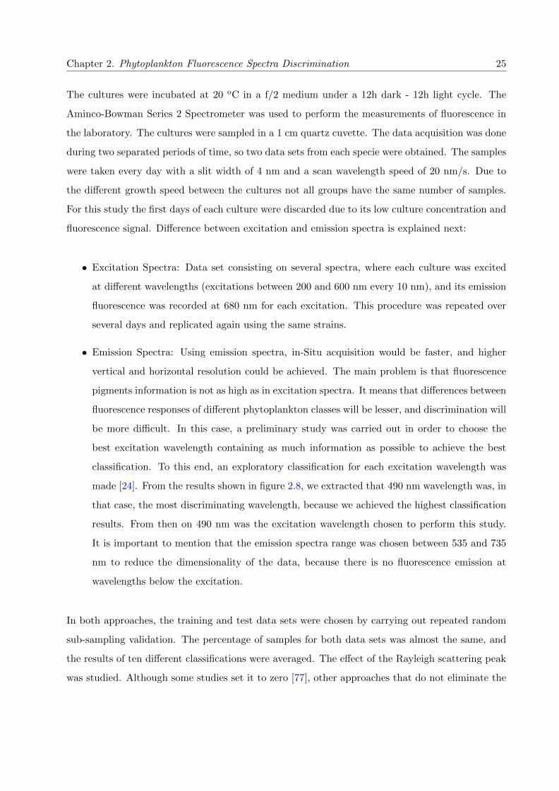
Chapter 2. Phytoplankton Fluorescence Spectra Discrimination 25
The cultures were incubated at 20 oC in a f/2 medium under a 12h dark - 12h light cycle. The
Aminco-Bowman Series 2 Spectrometer was used to perform the measurements of fluorescence in
the laboratory. The cultures were sampled in a 1 cm quartz cuvette. The data acquisition was done
during two separated periods of time, so two data sets from each specie were obtained. The samples
were taken every day with a slit width of 4 nm and a scan wavelength speed of 20 nm/s. Due to
the different growth speed between the cultures not all groups have the same number of samples.
For this study the first days of each culture were discarded due to its low culture concentration and
fluorescence signal. Difference between excitation and emission spectra is explained next:
• Excitation Spectra: Data set consisting on several spectra, where each culture was excited
at different wavelengths (excitations between 200 and 600 nm every 10 nm), and its emission
fluorescence was recorded at 680 nm for each excitation. This procedure was repeated over
several days and replicated again using the same strains.
• Emission Spectra: Using emission spectra, in-Situ acquisition would be faster, and higher
vertical and horizontal resolution could be achieved. The main problem is that fluorescence
pigments information is not as high as in excitation spectra. It means that differences between
fluorescence responses of different phytoplankton classes will be lesser, and discrimination will
be more difficult. In this case, a preliminary study was carried out in order to choose the
best excitation wavelength containing as much information as possible to achieve the best
classification. To this end, an exploratory classification for each excitation wavelength was
made [24]. From the results shown in figure 2.8, we extracted that 490 nm wavelength was, in
that case, the most discriminating wavelength, because we achieved the highest classification
results. From then on 490 nm was the excitation wavelength chosen to perform this study.
It is important to mention that the emission spectra range was chosen between 535 and 735
nm to reduce the dimensionality of the data, because there is no fluorescence emission at
wavelengths below the excitation.
In both approaches, the training and test data sets were chosen by carrying out repeated random
sub-sampling validation. The percentage of samples for both data sets was almost the same, and
the results of ten different classifications were averaged. The effect of the Rayleigh scattering peak
was studied. Although some studies set it to zero [77], other approaches that do not eliminate the

Chapter 2. Phytoplankton Fluorescence Spectra Discrimination 26
peak were evaluated. However,in this thesis an interpolation of the two neighboring samples to
avoid this effect is used because it obtains better results in combination with SOM.
Table 2.2: Phytoplankton species used in this chapter and number of samples acquired in eachexperiment.
Species Class AbbreviationNumber samplesExperiment n. 1
Number samplesExperiment n. 2
Alexandrium minutum Dinophyceae Am 22 41Thalassiosira weissflogii Bacillariophyceae Thwi 18 38Dunaliella Chlorophyceae Duna 20 40Isochrysis galbana Prymnesiophyceae Iso 10 30Pleurocrysis elongata Prymnesiophyceae Pl 21 42Synechococcus sp. Cyanophyceae Syn 15 -Ostreococcus sp. Prasinophyceae Ost 15 -
Figure 2.8: Classification performance curve at different excitation wavelengths to select the bestexcitation wavelength to work with.
2.3.2 Discrimination using Self-Organizing Maps
In this section, the first results obtained using SOM and published in [24] are shown. The classifi-
cation using SOM can be explained in three steps. First, the network is trained using the training
data set. The network adapts its properties to the input data and then the distances between
neurons are calculated. The result of this process is the U-matrix (figure 2.4), which shows the
distances between neighboring neurons. The light gray is the edge of the clusters, where these

Chapter 2. Phytoplankton Fluorescence Spectra Discrimination 27
distances are higher. Afterwards, as explained above, a variant of the hit-matrix called the fuzzy
hit-matrix [62] is computed. This matrix is obtained for each culture. Figure 2.5 shows an example
of these matrices. The gray value of the matrices represents a particular neuron’s membership of
the culture class. The matrices are then labeled. Lastly, we wish to assign a label to each sample
to classify, so the best-matching unit of each sample is found. Then, the different membership
values, which are extracted from the fuzzy hit-matrices, are compared. The winning class, whose
label is then taken to classify the sample into one culture or another, is that with the largest BMU
membership value.
As explained above, two different approaches have been followed. First of all, the results using
excitation spectra are shown, while those obtained with emission fluorescence spectra will be pre-
sented later. Finally, derivative analysis has been applied to emissions spectra in order to increase
classification performance. The data used in this section is the one obtained in the experiment n.
1 (table 2.2).
2.3.2.1 Classification using Excitation Spectra
Discrimination results among seven different phytoplankton cultures using SOM are now presented.
In this step only the responses at 680 nm emission wavelength with a range of 200–600 nm exci-
tations were used. In this case, randomly selected training and test data sets were constructed to
evaluate the method. An example of a training data set is shown in figure 2.9. Once the neural net-
work has been defined with 8x15 neurons, it is trained, and a label can be assigned to each neuron
in the SOM by first computing the hit-matrix over the whole training set. The label of each neuron
corresponds to the label of the class with a maximal number of hits in each neuron. In this label
representation, the discrimination of the method can be appreciated (figure 2.10). The neurons
have changed their properties to better characterize the input data. The different cultures should
appear classified, grouping all the samples of the same culture, but there are some mixed samples.
The samples that have a similar spectrum appear closer. For instance, Alexandrium minutum and
Synechococcus sp. have similar excitation spectra because they appear close one from each other,
whereas Thalassiosira weissflogii differs because it is in a separated region of the network.
Once the neural network has been trained, the labeled output map can be used to classify the
test data set, using the membership matrices. Based on this classification, the confusion matrix is

Chapter 2. Phytoplankton Fluorescence Spectra Discrimination 28
Figure 2.9: An example of a training data set working with excitation spectra. Fluorescenceexcitation spectra acquired at 680 nm. 60 samples randomly selected representing the seven cultures.
The excitation range is 200–600 nm, every 10 nm.
Figure 2.10: An example of the results obtained from randomly chosen training and test samplesusing excitation spectra.

Chapter 2. Phytoplankton Fluorescence Spectra Discrimination 29
computed in order to evaluate the performance of the classification methodology. The confusion
matrix summarizes in a table how well the classifier is working. It shows the number of samples
correctly classified and how many have been mistakenly classified. The Kappa, the TPR, and the
FPR indexes are calculated. Ten different validation runs, in which the training and test data sets
had been randomly constructed iteratively, were undertaken. Thence the results were averaged in
order to make the performance evaluation as independent as possible from the selected training set.
An example of a confusion matrix is presented in table 2.3.
Table 2.3: Example of a confusion matrix. Classification of excitation spectra from a randomselection of training and test samples.
Predicted Class
Ost Syn Thwii Duna Pl Am Iso Sum TPR FPR
Tru
eC
lass
Ost 4 0 0 2 0 0 2 8 0.5 0Syn 0 4 0 0 2 2 0 8 0.5 0
Thwii 0 0 8 1 0 1 10 0.8 0.88 0.018Duna 0 0 0 8 1 0 1 10 0.8 0.057
Pl 0 0 0 0 5 6 0 11 0.45 0.058Am 0 0 0 0 0 11 0 11 1 0.157Iso 0 0 1 0 0 0 4 5 0.8 0.052
Even though the discrimination does not seem to be good enough, the average TPR and the average
FPR over cultures and validation runs were 0.7344 and 0.0508, respectively. Also, the Kappa index
value was quite good, 0.6839, with 1 denoting a perfect classification without any mistake, and
0 denoting the result of a random classification. The greatest problems arose with Pleurochrysis
elongata, which is not properly classified. This means that the spectra from this culture are very
similar, in this case, to those of Alexandrium minutum.
Some studies carried out by Margalef [22] pointed out that pigment composition changes during
the life of phytoplankton. This statement introduces another variable that makes the classification
even more challenging. For this reason, another configuration of training and test data has been
proven. In this case, the system has been trained with the samples from the stable growth stage of
the culture, while the test samples have been taken from the exponential growth stage (figure 2.11),
the performance of the method using the stable samples as training data is then evaluated. The
resulting U-matrix is shown in Figure 2.4. Pigment composition variations play here an important
role in the classification. Testing samples from the exponential growth stage were classified to form
the confusion matrix (table 2.4). The Kappa index obtained was 0.4974 (TPR = 0.5787, FPR =

Chapter 2. Phytoplankton Fluorescence Spectra Discrimination 30
0.0981). Again, the greatest classification problems arose with Pleurochrysis. Although initially the
U-matrix seems to be better, the Kappa value was below 0.5. This result could be a consequence
of the pigment changes that phytoplankton cultures suffer during their growth stage.
Figure 2.11: As an example, Alexandrium minutum’s growth curve is shown. It has been madecomputing the fluorescence emission at 680 nm every day with 490 nm excitation wavelength.
Table 2.4: Confusion matrix. Classification behavior using excitation spectra. Samples fromthe stable growth stage used for training, and samples from the exponential growth stage used for
testing.
Predicted Class
Ost Syn Thwii Duna Pl Am Iso Sum TPR FPR
Tru
eC
lass
Ost 4 0 0 2 0 0 4 10 0.4 0.013Syn 0 3 0 0 0 7 0 10 0.2 0
Thwii 1 0 9 2 1 0 0 13 0.692 0Duna 0 0 0 11 1 3 0 15 0.666 0.028
Pl 0 0 0 1 2 13 0 16 0.187 0.086Am 0 0 0 0 0 17 0 17 1 0.348Iso 0 0 0 1 0 0 4 5 0.8 0.049
Using this table, the Kappa index is computed as follows:n∑r
k=1Xkk = 86× (4 + 3 + 9 + 11 + 2 + 17 + 4) = 86× 50 = 4300∑rk=1Xk+X+k = (10× 5) + (10× 3) + (13× 9) + (15× 17) + (16× 4) + (17× 40) + (5× 8) = 1236
K = (n∑r
k=1Xkk −∑r
k=1Xk+X+k)/(n2−∑r
k=1Xk+X+k) = (4300− 1236)/(862− 1236) = 0.4974
2.3.2.2 Classification using Emission Spectra
The idea of working with emission spectra comes up from the need of a rapid acquisition method.
There are some physiological and trophic processes that may be constrained by physical processes
operating over spatial scales of a few centimeters and temporal scales of seconds to minutes [15].

Chapter 2. Phytoplankton Fluorescence Spectra Discrimination 31
The importance of detecting these processes emphasizes the need to develop new techniques aimed
at increasing the number of samples and improving then horizontal and vertical resolution. Ac-
quiring excitation spectra takes almost a second, and the speed of a free falling vertical profiler is
near 10cm/s. In contrast, acquiring emission fluorescence spectra is almost instantaneous and the
number of samples could be increased. Using the emission spectra, in situ acquisition would be
faster and a higher vertical and horizontal resolution could be achieved. The main problem is that
fluorescence information is not as high in emission spectra as in excitation spectra. This means
that there are less differences between fluorescence responses of different phytoplankton classes,
and their discrimination is more difficult. Having established the good performance of the SOM
with excitation spectra, its performance using only emission spectra was evaluated. The results are
described in the following paragraphs.
Figure 2.12: An example of a training data set working with emission spectra. Fluorescenceemission spectra excited at 490 nm. 60 samples randomly selected representing the seven cultures.
The emission range is 535–735 nm, every 1 nm.
The EEMs acquired were used again, but now using the training and test data sets as described
above: emission spectra (520–735 nm) with 1 nm resolution (216 features) excited at 490 nm and
randomly sub-sampled. An example of training samples for this case is presented in figure 2.12.
The discrimination can be observed in figure 2.13, and table 2.5 represents the confusion matrix
obtained. The averaged TPR index over ten validation runs is 0.7046, the average FPR is 0.0588,
and the Kappa index is 0.6343. Although a good classification performance is obtained, there are
again some classes that appear mixed. For example, Synechococcus sp. is clearly distinguishable,

Chapter 2. Phytoplankton Fluorescence Spectra Discrimination 32
Figure 2.13: An example of the results obtained from randomly chosen training and test samplesusing emission spectra.
Table 2.5: Example of a confusion matrix. Classification of emission spectra from a randomselection of training and test samples.
Predicted Class
Ost Syn Thwii Duna Pl Am Iso Sum TPR FPR
Tru
eC
lass
Ost 6 0 0 0 0 0 2 8 0.75 0Syn 0 8 0 0 0 0 0 8 1 0
Thwii 0 0 9 0 0 0 0 9 1 0.037Duna 0 0 1 5 4 0 0 10 0.5 0.038
Pl 0 0 1 0 7 3 0 11 0.63 0.176Am 0 0 0 0 5 6 0 11 0.54 0.035Iso 0 0 0 2 0 0 3 5 0.6 0.035
while the other classes appear closer and mixed. The reason is that these classes have very similar
spectra and they are more difficult to discriminate from emission fluorescence.
Repeating the same procedure as in the previous section, we now focus our attention on the eval-
uation of the performance using the stable samples for training and then classifying samples from
the growth stage. Surprisingly, using emission spectra, the results (table 2.6) are better than using
excitation spectra stable samples; the Kappa index is equal to 0.5985. From this result and that
obtained with excitation spectra, it seems that the pigment changes have a greater effect on the
excitation spectra (K=0.4974) than on the emission spectra (K=0.5985), making emission spectra

Chapter 2. Phytoplankton Fluorescence Spectra Discrimination 33
more robust to these changes. Several studies use derivative techniques to enhance minute differ-
ences between similar signals [35, 38]. These techniques have proven to be a powerful tool that
is commonly used, for example, in the analysis of hyperspectral data. However, the derivative
spectroscopy used to explore these minute features in spectral data is notoriously sensitive to noise
[78]. To remove this noise from the hyperspectral data, smoothing techniques are commonly used
[79]. It is worth noting that there must be a trade-off between noise removal and the ability to re-
solve fine spectral details [80]. The following section is devoted to the analysis of the SOM method
classification, using as input data the derivative of the spectra.
Table 2.6: Confusion matrix. Classification behavior using emission spectra. Samples from thestable growth stage used for training, and samples from the exponential growth stage used for
testing.
Predicted Class
Ost Syn Thwii Duna Pl Am Iso Sum TPR FPR
Tru
eC
lass
Ost 5 0 1 0 0 0 4 10 0.5 0Syn 0 10 0 0 0 0 0 10 1 0
Thwii 0 0 10 2 1 0 0 13 0.77 0.041Duna 0 0 1 9 0 5 0 15 0.6 0.028
Pl 0 0 0 0 2 14 0 16 0.125 0.014Am 0 0 0 0 0 17 0 17 1 0.275Iso 0 0 1 0 0 0 4 5 0.8 0.049
2.3.2.3 Classification applying derivative analysis to Emission Spectra
In typical multispectral analysis, each spectral band is considered as an independent variable, a
reasonable assumption for multispectral data, but this is not suitable for hyperspectral data. Due
to the huge number of bands of the hyperspectral data, it can be treated as spectrally continuous
data, and some methods particularly developed for this type of data can be applied. Among
these methods, derivative analysis is particularly promising dealing with hyperspectral signals.
Derivative techniques enhance minute fluctuations in spectra and separate closely related features.
But derivatives are notoriously sensitive to noise. Thus, smoothing or otherwise minimizing random
noise is a major issue.
In an attempt to increase the performance of the classification using emission fluorescence spectra,
derivative analysis was applied to the emission spectra in order to enhance the differences between
the fluorescence spectra of each algae. The noise of the signals was reduced using a wavelet denoising

Chapter 2. Phytoplankton Fluorescence Spectra Discrimination 34
Figure 2.14: An example of a training data set working with derivative emission spectra. Deriva-tive fluorescence emission spectra excited at 490 nm. 60 samples randomly selected representing
the seven cultures. The emission range is 535–735 nm, every 1 nm.
applied to both data sets before using derivative analysis. Once obtained the first-order derivative
spectra, SOM has been applied in order to evaluate the performance using the derivative pre-
processing step to enhance their subtle differences.
First of all, the samples were also randomly sub-sampled in order to evaluate the classification
indexes for different training and test data sets. An example of the results obtained using the
derivative training data is presented in figure 2.14. The discrimination this time was higher. The
neurons of the network were properly distributed and the indices obtained (table 2.5) were slightly
better than those obtained using excitation spectra: TPR = 0.7574, FPR = 0.0481, and Kappa =
0.7109.
Table 2.7: Example of a confusion matrix. Classification of first-derivative emission spectra froma random selection of training and test samples.
Predicted Class
Ost Syn Thwii Duna Pl Am Iso Sum TPR FPR
Tru
eC
lass
Ost 8 0 0 0 0 0 0 8 1 0Syn 0 8 0 0 0 0 0 8 1 0
Thwii 0 0 6 2 1 0 0 9 0.66 0.019Duna 0 0 0 9 1 0 0 10 0.9 0.057
Pl 0 0 1 1 6 3 0 11 0.54 0.059Am 0 0 0 0 1 10 0 11 0.9 0.059Iso 0 0 0 0 0 0 5 5 1 0
In the case of using stable samples for training, the results obtained were TPR = 0.7638, FPR
= 0.0611, and Kappa = 0.6803 (table 2.8). As can be clearly seen in the confusion matrices, the

Chapter 2. Phytoplankton Fluorescence Spectra Discrimination 35
greatest problems arose with Pleurochrysis elongata (Pl). The fluorescence properties of Alexan-
drium minutum and Pl are very similar for this method. Both species like coastal areas where
they can form blooms [81–84]. It has also been noticed that coastal species in coccolithophores
share pigments unexpected by their phylogeny [85], and if these two cultures are joined into one
group, the performance increases considerably. For example, for the confusion matrices found in
the last two approximations studied above (using derivative emission fluorescence spectra), if these
two species are grouped the Kappa indices are 0.8105 and 0.8439, respectively.
Table 2.8: Confusion matrix. Classification behavior using first-derivative emission spectra. Sam-ples from the stable growth stage used for training, and samples from the exponential growth stage
used for testing.
Predicted Class
Ost Syn Thwii Duna Pl Am Iso Sum TPR FPR
Tru
eC
lass
Ost 10 0 0 0 0 0 0 10 1 0Syn 0 10 0 0 0 0 0 10 1 0
Thwii 0 0 9 0 4 0 0 13 0.692 0Duna 0 0 0 10 0 5 0 15 0.666 0.014
Pl 0 0 0 0 3 13 0 16 0.187 0.057Am 0 0 0 0 0 17 0 17 1 0.26Iso 0 0 0 1 0 0 4 5 0.8 0
2.3.3 Potential-Support Vector Machines for Phytoplankton Discrimination:
Comparison with Self-Organizing Maps
In this section Potential-Support Vector Machines is tested for phytoplankton fluorescence spectra
discrimination. The results of P-SVM are presented and compared with SOM. This technique
has already been introduced above, but just comment that, in this work, it has been used with
C-Support Vector classification and a radial basis function kernel. The optimal cost parameters, C,
and gamma parameters, g, are determined by performing 8-fold cross validation. Although SVMs
were originally developed to perform binary classifications, multiclass classification (more than two
classes), is frequently applied, for example, in remote sensing applications. A number of methods
to generate multiclass SVMs from the binary SVMs have been proposed. More information on
multiclass classification with their advantages and disadvantages can be found in [75]. In this
thesis, SVMs binary classifiers are created for all the possible pairs of classes. Thus, the multiclass
approach to the problem has been implemented using one-against-one approximation, following
the max-wins voting strategy (MWV). In that approach, one binary classifier is constructed for

Chapter 2. Phytoplankton Fluorescence Spectra Discrimination 36
every pair of different classes, resulting in M(M − 1)/2 classifications for each sample (where M
is the number of classes, in this case 5 species). The output from each classifier is obtained in the
form of a class label. The class label that occurs the most is assigned to that sample. For one
sample x to be classified, if the classifier says x is in class A, then the vote for class A is added by
one. Otherwise, the vote for class B is increased by one. After each of the M(M − 1)/2 binary
classifiers makes its vote, MWV strategy assigns x to the class with the largest number of votes.
A tie-breaking strategy may be adopted in case of a tie. A common tie-breaking strategy is to
randomly select one of the class labels that are tied. Using then the winner class, the classification
results of each sample are presented as a confusion matrix. From these matrices, the Kappa, the
TPR, and the FPR indexes are calculated. Following the same procedure as above, ten different
validation runs, in which the training and test data sets had been randomly constructed iteratively,
were undertaken. Then the results were averaged in order to make the performance evaluation as
independent as possible from the selected training set.
2.3.3.1 Classification using Excitation Spectra
Following the same schema presented above, the first part of the experiment was carried out using
excitation fluorescence spectra acquired at 680 nm, ranged 300-600 nm with a resolution of 10 nm.
As it has been previously mentioned, the total number of samples/specie is shown in table 2.2,
containing 31 features each sample (figure 2.15). The samples of both experiments are used in this
case, but only taking into account the five species present in both experiments. Training and test
data sets were chosen using leave one out cross-validation, and the confusion matrix was computed
from the results. Rayleigh scattering was suppressed interpolating the two neighbouring samples.
Table 2.9 shows the resulted confusion matrix.
SOM performs better than P-SVM using excitation spectra. The Kappa indices from both tech-
niques are 0.66015 and 0.42497, respectively. The difference in performance is clear, but the major
errors from both techniques came from different misclassified cultures. Using SOM cultures Pl and
Am had more problems to be correctly classified, while P-SVM found more difficulties classifying
Thwii, Duna and Iso. It is also remarkable the results obtained with P-SVM in the case Pl and
Am, where the classification is significantly better than using SOM.

Chapter 2. Phytoplankton Fluorescence Spectra Discrimination 37
Figure 2.15: Fluorescence spectra used for P-SVM classification: (a) Example of training dataset from excitation fluorescence spectra, (b) example of training data set from emission fluorescence
spectra.
Table 2.9: Example of confusion matrix obtained from excitation spectra: (a) P-SVM, (b) SOM
Predicted Class
(a) Thwii Duna Pl Am Iso Sum TPR FPR
Tru
eC
lass
Thwii 12 0 22 0 4 38 0,316 0,034Duna 1 27 11 0 0 39 0,692 0,115
Pl 0 4 23 12 2 41 0,561 0,308Am 0 0 7 33 0 40 0,825 0,082Iso 4 13 5 0 7 29 0,241 0,038
(b) Thwii Duna Pl Am Iso Sum TPR FPR
Tru
eC
lass
Thwii 37 0 0 0 1 38 0,974 0,201Duna 2 36 0 0 1 39 0,923 0,000
Pl 19 0 9 4 9 41 0,220 0,041Am 7 0 6 27 0 40 0,675 0,027Iso 2 0 0 0 27 29 0,931 0,070

Chapter 2. Phytoplankton Fluorescence Spectra Discrimination 38
2.3.3.2 Classification using Emission Spectra
Following the same procedure, the data used for this experiment consists on emission fluorescence
spectra exited at 490 nm and ranged 520-735 nm with 1 nm resolution (216 features). Leave one
out cross-validation was used and the results are collected in the confusion matrices shown in table
2.10. The performances of both techniques calculated from these matrices are Kpsvm=0.54252
and Ksom=0.6426. It is worth noting that while SOM obtained a similar kappa index as using
excitation spectra, P-SVM improve its performance using emission fluorescence spectra, but it still
did not obtain comparable results to SOM. Even though the results of Am and Iso are significantly
better than using SOM, the main problem in this case for P-SVM is the misclassified samples of
Thwii and Pl.
Table 2.10: Example of confusion matrix obtained from emission spectra: (a) P-SVM, (b) SOM
Predicted Class
(a) Thwii Duna Pl Am Iso Sum TPR FPR
Tru
eC
lass
Thwii 15 1 21 1 0 38 0,395 0,059Duna 6 29 4 1 0 40 0,725 0,100
Pl 3 7 18 13 0 41 0,439 0,201Am 0 0 3 38 0 41 0,927 0,101Iso 0 7 2 0 21 30 0,700 0,000
(b) Thwii Duna Pl Am Iso Sum TPR FPR
Tru
eC
lass
Thwii 36 0 2 0 0 38 0,947 0,086Duna 1 34 4 1 0 40 0,850 0,120
Pl 9 6 16 9 1 41 0,390 0,081Am 2 0 6 33 0 41 0,805 0,067Iso 1 12 0 0 17 30 0,567 0,006
Analyzing the matrices, P-SVM shows better results dealing with Iso, while maintains the problems
with species Thwii and Pl. Regarding SOM, it continues having problems with Pl, but with emission
spectra it has more difficulties to classify Iso than Am. A possible explanation for this could be
that the information contained in excitation fluorescence spectra, although consistent, can differ
from that contained in the emission fluorescence spectra.

Chapter 2. Phytoplankton Fluorescence Spectra Discrimination 39
2.3.3.3 Classification applying derivative analysis
Derivative spectra have been also used in this comparison. The confusion matrix resulted from
the classification of the derivatives of excitation spectra is shown in table 2.11. The computed
index Kappa is Kpsvm=0.68435. This result is slightly below the value obtained with SOM,
Ksom=0.73869. In that case, the major misclassified samples are from classes Thwii and Pl, while
surprisingly class Iso seems to present fewer problems. The reason for this is that the derivative
analysis has enhanced minute singularities that were not detectable by the classifier. Applying
derivative analysis to emission fluorescence spectra, P-SVM obtains Kpsvm=0,68091, while Ksom
is 0,65617 (table 2.12). It can be noticed that comparing with the results without derivative, the
performance of all species has increased, except Iso, which classification results using P-SVM have
notably decreased.
Table 2.11: Example of confusion matrix obtained from derivative excitation spectra: (a) P-SVM,(b) SOM
Predicted Class
(a) Thwii Duna Pl Am Iso Sum TPR FPR
Tru
eC
lass
Thwii 25 0 11 2 0 38 0,658 0,054Duna 0 34 2 3 0 39 0,872 0,000
Pl 7 0 21 13 0 41 0,512 0,144Am 1 0 6 33 0 40 0,825 0,122Iso 0 0 2 0 27 29 0,931 0,000
(b) Thwii Duna Pl Am Iso Sum TPR FPR
Tru
eC
lass
Thwii 36 0 0 2 0 38 0,947 0,107Duna 0 37 2 0 0 39 0,949 0,020
Pl 13 2 20 5 1 41 0,488 0,082Am 2 0 10 28 0 40 0,700 0,048Iso 1 1 0 0 27 29 0,931 0,006
2.4 Conclusions
The study presented in this chapter, shows self-organizing maps (SOM) and Potential-Support
Vector Machines (P-SVM) as feasible methods for processing fluorescence data in order to clas-
sify phytoplankton cultures. For this purpose different cultures were cultivated and their excita-
tion–emission fluorescence responses were acquired.

Chapter 2. Phytoplankton Fluorescence Spectra Discrimination 40
Table 2.12: Example of confusion matrix obtained from derivative excitation spectra: (a) P-SVM,(b) SOM
Predicted Class
(a) Thwii Duna Pl Am Iso Sum TPR FPRT
rue
Cla
ss
Thwii 28 1 8 1 0 38 0,737 0,007Duna 0 31 9 0 0 40 0,775 0,140
Pl 0 3 33 5 0 41 0,805 0,134Am 1 0 2 38 0 41 0,927 0,040Iso 0 17 1 0 12 30 0,400 0,000
(b) Thwii Duna Pl Am Iso Sum TPR FPR
Tru
eC
lass
Thwii 37 1 0 0 0 38 0,974 0,112Duna 0 35 5 0 0 40 0,875 0,127
Pl 3 8 25 5 0 41 0,610 0,074Am 13 0 6 22 0 41 0,537 0,034Iso 1 10 0 0 19 30 0,633 0,000
Both questions proposed at the beginning of the chapter have been addressed. Emission fluorescence
spectra has been shown as a feasible and fast method to discriminate among phytoplankton species,
and with adequate processing methods, can achieve really promising results.
The results presented showed that the fluorescence signals of the different cultures are very similar
and are difficult to discriminate. Based on the results, classification using excitation fluorescence
spectra is better than classification using only emission fluorescence spectra. However, it is worth
mentioning that the use of adequate pre-processing techniques such as derivative analysis can help
to improve the results of the latter, and even obtain performances higher than using excitation
fluorescence spectra.
From the results of the first part, where SOM was used to discriminate among seven different
cultures, it can be concluded that it shows good performance using both, excitation and emission
spectra. Furthermore, the performance of the method improves when emission spectra are combined
with derivative analysis to enhance spectra singularities. This combination is a powerful method
for obtaining a good discrimination among different cultures. Moreover, Thalassiosira weissflogii
can be distinguished from Alexandrium minutum using only one excitation, an important result for
distinguishing diatoms from dinoflagellates. However, Pleurochrysis elongata cannot be differenti-
ated from Alexandrium minutum at all, which means that their fluorescence properties are very
similar. One possibility would be grouping them for consideration together.

Chapter 2. Phytoplankton Fluorescence Spectra Discrimination 41
Regarding the classification using P-SVM, it has been implemented doing repeated binary classi-
fications, following the max-wins voting strategy. It can be extracted that there exist differences
between excitation and emission fluorescence data, because the results differ one from each other.
For example, in case of excitation spectra, P-SVM has difficulties discriminating among classes
Thwii, Pl and Iso, while taking into account emission fluorescence spectra Iso has more successful
classification. It is worth noting that the performance increase using emission fluorescence spectra,
but it is also important to mention that using derivative analysis the results (Kpsvm=0.68091) are
comparable with the best results obtained with both techniques (Ksom=0.73869 from derivative
excitation spectra), but in this case from emission fluorescence spectra.
From the results obtained in these works can be concluded that although SOM performed better
than P-SVM, the kernel method is faster in terms of computation (training + classification of
samples). This feature is the key in applications where near real time processing must be used.
Another characteristic of P-SVM is the possibility to efficiently deal with a very large number of
features due to the exploitation of kernel functions, which makes it an attractive technique. A
particular advantage of P-SVM is “sparseness of the solution”. This means that a P-SVM classifier
depends only on the support vectors, and the classifier function is not influenced by the whole data
set, as it is the case for SOM.
The preliminary results are then encouraging. Working with emission spectra obviates the need
to use different excitation sources, and thus reduces the acquisition time. However, further work
is necessary in order to better adjust the parameters of the methods, and different pre-processing
techniques could even be tested in future work. One of these could be using an average of the input
data (i.e., an average of normal and derivative spectra) for training, which would perhaps provide
better discrimination between the strains.


Chapter 3
Chlorophyll a Fluorescence Peak
Analysis
The need for covering large areas in oceanographic measurement campaigns and the general interest
in reducing the observational costs open the necessity to develop new strategies towards this objec-
tive, fundamental to deal with current and future research projects. In this respect, the development
of low-cost instruments becomes a key factor, but optimal signal-processing techniques must be used
to balance their measurements with those obtained from accurate but expensive instruments. In
this chapter, in addition to the study presented in Chapter 2, a complete signal-processing chain
to process the fluorescence spectra of marine organisms for taxonomic discrimination is also pro-
posed. This time, the pre-processing methods presented have been designed to deal with noisy,
narrow-band and low-resolution data obtained from low-cost sensors or instruments and to opti-
mize its computational cost. It consists of four separated blocks that denoise, normalize, transform
and classify the samples. For each block, several techniques are tested and compared to find the
best combination that optimizes the classification of the samples. The main difference with the
previous chapter is that the signal processing has been focused only on the Chlorophyll a (Chl a)
fluorescence peak, since it presents the highest emission levels and it can be measured with sensors
presenting poor sensitivity and signal-to-noise ratios. The whole methodology has been successfully
validated by means of the fluorescence spectra emitted by five different cultures. The chapter has
been organized similar to the previous chapter, and some of the techniques are shared, for this
reason, or because are well-known techniques, some of them are just briefly introduced. First of all,
43

Chapter 3. Chlorophyll a Fluorescence Peak Analysis 44
the chapter contains a short introduction explaining the importance of low-cost instrumentation
and why the study has been centered in the Chlorophyll a peak. Following, a section introducing
the methodologies used for this work is presented. The results are presented next, and finally the
main conclusions extracted from the results are exposed.
The results obtained in this chapter have been already published in ”Analysis of Discrimination
Techniques for Low-Cost Narrow-Band Spectrofluorometers” [26] and ”Optimal processing algo-
rithms for taxonomic discrimination with low-cost narrow-band spectrofluorometers” [27].
3.1 Introduction
Chlorophyll (Chl) fluorescence techniques have been widely used to assess the taxonomic composi-
tion of microscopic photosynthetic organisms (phytoplankton) in order to avoid the time constraints
imposed by the microscopic analysis of water samples [15]. The basis of fluorometric taxonomic
discrimination, as explained above, relies in the specific features of the excitation and emission
spectra of each phytoplankton taxonomic group [15, 86], and multiple approaches have been used
to determine such differences. For instance, the spectral deconvolution analysis, used by Chekalyuk
[87] to discriminate between two different organisms, or the self-organizing maps (SOM) technique
presented in the previous chapter [24] to classify seven strains from different taxonomic groups of
phytoplankton, among others. Nevertheless, these techniques have mostly been tested with accu-
rate and precise data obtained with expensive instruments. This involves an important limitation,
since the observational costs spent in infrastructure and instruments in order to obtain high vol-
umes of accurate data in shallow or open water is extremely high, and consumes most part of the
money budget available in a research project. In this regard, the concept of ”citizen science” has
arisen as an effective methodology to mitigate the expenses while covering large areas with high
temporal and spatial resolution measurements [88], but this concept only makes sense through the
development of extreme low-cost sensors, as those presented in [89–95]. Reportedly, their accu-
racy (sensibility, resolution and signal-to-noise ratio (SNR)) is not comparable to the most precise
(and consequently, expensive) alternatives, but they present a considerable potential if a correct
pre-processing step is performed. Therefore, there is an increasing need for the development of
signal-processing strategies able to suitably process the noisy and low-accurate data obtained from
instruments based on low-cost sensors.

Chapter 3. Chlorophyll a Fluorescence Peak Analysis 45
In this chapter, the analysis of the discrimination skills of a potential low-cost hyperspectral flu-
orescence instrument presenting a lower performance in terms of sensibility, SNR and processing
capabilities is presented. To this end, three different techniques based on pattern recognition are
tested, evaluated and compared to find which one presents the optimal performance considering two
main constraints. First, a successful taxonomic discrimination must be obtained even when using
as primary information only the highest fluorescence emission levels (if the SNR of the sensor is
extremely low, only those levels would be reliable), which correspond to the Chl fluorescence peak
(around the 680 nm). This consideration differs from [24, 87] and the previous chapter, where the
whole optical spectra bandwidth is analyzed, and it is actually feasible assuming that the fluores-
cence signal in this wavelength range is not only due to the Chl a emission peak, but also the Chl
b, c and d emission peaks along with additional complement pigments (such as the phycocyanin,
whose fluorescence emission is located in the 630-to-660 nm band). Besides, this consideration re-
laxes the needed sensor’s spectra bandwidth performance. Second, the computational cost needed
to develop the algorithms must be optimally reduced in order to decrease the electronic hardware
requirements needed to implement the instrument (which will directly influence on its economic
cost). In order to deal with these two requirements and considering high levels of noise in the
measurement samples, three signal-processing blocks previous to the classification one have been
established, accounting for denoising, normalization and transformation of the measured data.
The denoising block reduces the noise introduced by the sensor; the normalization block equals
the emission contribution measured at different growth states, which improves the discrimination
outcomes; and the transformation block transforms and reduces the data dimension, improving
the computational-cost efficiency. Thereby, the most convenient technique in each of these three
blocks, which, in combination with the best classification algorithm, provides an optimal taxonomic
discrimination even when dealing with the two measurement constraints described above, is sought.
In order to test the performance of different algorithms in the presented signal-processing chain,
the fluorescence spectra of five isolated cultures have been measured at different growth stages.
Hyperspectral low-cost fluorescence instruments for in-situ or in-vivo measurements of phytoplank-
ton responses have not been developed yet. Fluorescence sensors or instruments based on low-cost
technology are presented in [89, 93–95], but their measurements do not exhibit a hyperspectral
performance. Therefore, measurements have been firstly obtained with an accurate fluorescence
instrument and degraded afterwards in terms of resolution and SNR to emulate the potential low-
cost sensor performance. Those measurements are then processed in each block, where well-known

Chapter 3. Chlorophyll a Fluorescence Peak Analysis 46
methods such as moving average, wavelet or principal components, are put into practice along with
other algorithms developed in this study specifically designed for this work. This new approach,
mainly based on a reliable signal-processing chain, considerably reduces the sensor’s requirements
(spectra bandwidth and computational cost) needed to perform a suitable classification. Besides,
its conclusive results constitute an important stimulus to develop new and optimal low-cost flu-
orometers enhancing their discrimination capabilities and encouraging marine research groups to
continue studying this field by considerably reducing the instrumentation costs.
This chapter is then structured as follows. A brief introduction to the algorithms used in this study
is presented in the next Section 3.2. In Section 3.3, measurements from five phytoplankton cultures
from different taxonomic groups are used to perform a comparison of the different algorithms.
The results presented in this section were processed first with the original data, and later with a
degraded version of the measurements in order to simulate the performance of a low-cost sensor.
Section 3.4 outlines the conclusions derived from this work.
3.2 Processing Techniques
Figure 3.1 shows the block diagram of the four-step signal-processing chain. Three steps before ad-
dressing a classification method, where the taxonomic discrimination is performed, are proposed in
order to optimize the processing efficiency. Any electro-optical sensor is a noisy source mainly due
to the shot and thermal noise, and this is emphasized in low-cost sensors, which usually present a
lower performance. Denoising techniques are firstly applied to mitigate the noise effect, considering
that a careful attention must be paid in order to avoid the loss of information due to an excessive
smoothing. The fluorescence intensity depends upon the cell concentration, the biological growth
state, the temperature conditions and the incident light, among other factors, and measurements
of the same culture may present significant range variations. Since the classification techniques
are usually based on the Euclidean distance between the sample under test and a reference, their
objective functions will not appropriately discriminate the samples if such variations are presented
within the same culture. Therefore, all measurements must be normalized in a second step in order
to make the contribution of their particular features equivalent. Finally, the transformation tech-
niques that adapt the data to increase the discrimination capacity of the classification algorithms,
and the reduction of dimension methods that increase the efficiency of the learning algorithms, are

Chapter 3. Chlorophyll a Fluorescence Peak Analysis 47
included in the third step. In the latter, if the classification techniques have to deal only with those
wavelengths that are more representative of the features that characterize the culture (obviating
redundant information), the computational cost is considerably reduced.
Figure 3.1: The four-step signal-processing chain proposed.
The whole set of techniques used in each step are presented in Table 3.1, and described in the
following subsections. Widely known methods such as moving average, principal components or
k-neighbors are used along with other techniques developed and adapted to improve the taxonomic
analysis proposed in this study. Moreover, the complete signal-processing chain has been centered
in the Chl a fluorescence peak (around 680 nm), which largely simplifies the computational cost
that the analysis of the whole hyperspectral data would need.
Table 3.1: Algorithms of the four-step signal-processing chain.
Denoising Normalization Transformation Classification
WMA Min-Max Derivative k-neighborsSavitzky-Golay GSM Genetic-Algorithm* SOM
Wavelet* SNV PCA GCSModified SBN
3.2.1 Denoising
In this chapter, a more exhaustive study of noise robustness is done. Optical detectors are sub-
jected to several influences such as optical shot noise (which follows a Poisson distribution), thermal
noise (Poisson distribution), read noise (approximately Gaussian), background light from blackbody
radiation (Plank distribution), flicker noise (pink power distribution) and technical noise due to
various imperfections (which do not follow a specific distribution). The noise-floor level in a mea-
surement is determined by the thermal and the read noises, while the shot noise dominates at high
signal values. In a low-performance sensor, it is expected to have significant levels of noise and, in
consequence, a poor SNR. Therefore, a denoising block is needed as a first step for the proposed

Chapter 3. Chlorophyll a Fluorescence Peak Analysis 48
processing chain. Three different techniques have been considered to smooth the measurements
acquired for this study (see the first column of Table 3.1). These techniques are briefly described
below.
3.2.1.1 The Weighted Moving Average Method
The weighted moving average (WMA) [96] is the most widely used technique for denoising. In it,
the output averaged data vector (y) can be computed as the weighted mean of the nearest 2 · P
wavelengths (P wavelengths for each side) for each value of the noisy raw data (x), and can be
expressed as:
y(λ) =1∑P
ρ=−P w(ρ)
P∑ρ=−P
w(ρ)x(λ− ρ) (3.1)
being w the weighting factor vector and λ the wavelength. The particular case where all weighting
factors are equal to one is usually known as the standard moving average.
3.2.1.2 The Savitzky Golay Method
The Savitzky-Golay technique [96] computes a local polynomial regression to approximate the
nearest noisy samples using the least squares method, as:
y(λ) =
P∑ρ=−P
b0(ρ)x(λ− ρ) (3.2)
being b0 the steady-state Savitzky-Golay filter which coefficients are determined using the least-
squares fit. The main advantage of this approach is that it tends to preserve distribution features
such as relative maxima, minima and width, usually flattened with the WMA technique at the
expense of not removing as much noise as the WMA.
3.2.1.3 The Wavelet Method
As mentioned in the previous chapter, the method for noise reduction proposed here is derived
from a wavelet-thresholding algorithm based on Mallat’s scheme [42, 97]. A fast wavelet algorithm

Chapter 3. Chlorophyll a Fluorescence Peak Analysis 49
(FWT) that computes the DWT very efficiently was presented in [41]. The technique implemented
in this thesis has been done following the steps explained in [44] and shown above in figure 2.2.
The original signal is first decomposed into low and high-frequency components by convolution-
subsampling operations using low and high-pass filters directly on the discrete domain. The low-
frequency components (approximation coefficients) keep the global features of the signal, while
the high-frequency components (detail coefficients) retain the local features. The decomposition
process can be iterated recursively on the approximation coefficients. And, at the last iteration,
both approximation and detail coefficients are kept to be used in the reconstruction step. Some of
the resulting wavelet coefficients correspond to details in the data set. If the details are small, they
might be omitted without substantially affecting the main features of the data set. The idea of
thresholding, then, is to set to zero all coefficients that are less than a particular threshold because
they are basically caused by noise. These coefficients are used in an inverse wavelet transformation
to reconstruct the data set. The signal is transformed, thresholded and inverse-transformed. The
technique is a significant step forward in handling noisy data because the denoising is carried
out without smoothing out the sharp structures. The result is cleaned-up signal that still shows
important details.
Another important advantage of this method is that it not only optimizes the mean-square error
but also ensures, with high probability, that the denoised signal is at least as smooth as the original
[42]. This property is important because other techniques that optimize mean square error, in some
cases, introduce artifacts that can affect signal characteristics.
Figure 3.2: Growing Spectra Modeling (GSM) example: (a) Fluorescence measurements of aparticular culture at different growth states; (b) Fluorescence at 660 nm and 680 nm related to
each fluorescence maximum, and linear regression for the two cases.

Chapter 3. Chlorophyll a Fluorescence Peak Analysis 50
3.2.2 Normalization
Once the measurements have been denoised, the next step is the normalization. The second column
of table 3.1 shows the normalization methods considered in this chapter and described below
3.2.2.1 The Min-Max Method
The Min-Max is a simple method of fitting the fluorescence curve into a fixed range. Minimum
and maximum values (a and b, respectively) become equal for all the samples, and the normalized
curve is obtained with:
y(λ) = a+(x(λ)−min(x))(b− a)
max(x)−min(x)(3.3)
3.2.2.2 The Growing Spectra Modeling Method
The growing spectra modeling (GSM) is a new method that exploits the simplicity of the Min-Max
normalization but uses the information of all the values at each wavelength simultaneously in order
to increase its robustness. In it, each wavelength fluorescence value of a particular culture and
at a specific growth state is compared with its fluorescence maximum. Measurements on different
cultures have shown that this relationship is linear at all wavelengths, which allows obtaining an
accurate approximation using their linear regression coefficients, as:
Flλ(m) = aλm+ bλ (3.4)
being aλ and bλ the linear regression coefficients of the wavelength λ , and Flλ its fluorescence
evaluated at m. Figure 3.2a shows an example of the smoothed fluorescence measurements of
a particular culture at different growth states. As can be observed, the fluorescence maximum
presents an important level variability according to different growth states. When all the measure-
ments on a single wavelength are plotted against its fluorescence maximum, a linear relationship,
as shown in Figure 3.2b for two particular wavelengths (660 nm and 680 nm), is obtained. The
linear regression has also been plotted for these two cases, showing a decrement on the slope when
moving away from the maximum. In general, a unitary slope is obtained around 680 nm, and a

Chapter 3. Chlorophyll a Fluorescence Peak Analysis 51
close-to-zero slope around the fluorescence minimum. The model finally uses the linear regression
coefficients to compute the normalization factor for each measurement and wavelength. This is done
by evaluating Equation 3.4 at two point values, the maximum fluorescence in that measurement
(obtaining Flλ1) and the desired (or normalized) maximum fluorescence (obtaining Flλ2). The
coefficient obtained from the relationship Flλ1/F lλ2 is the normalization factor used to normalize
the initial data value.
3.2.2.3 The Standard Normal Variate Method
The standard normal variate (SNV) [98, 99] is a robust method against noisy data. It is based on
the mean and variance (µ and σ2, respectively) matching of all the measured samples, as:
y(λ) =(x(λ)− µ+ µtot)
√σ2tot√
σ2(3.5)
being µtot and σ2tot the averaged mean and variance of the whole set of samples. A typical approx-
imation is done considering µtot = 0 and σ2tot = 1.
3.2.2.4 The Modified Scale Based Normalization Mehod
The three previous methods significantly distort those signals that are more different from the
general pattern, leading, in some cases, to a significant deformation of the small details that char-
acterize the nature of the sample. A more general and flexible version of the SNV method is the
scale-based normalization (SBN) introduced in [98]. When applying the wavelet decomposition
to a signal, its variance is also faithfully decomposed, allowing a more precise scaling. Variance
normalization to 1 (σ2tot = 1) and mean to 0 (µtot = 0) is performed using only those wavelets that
do not contain the high-frequency noise, as:
y(λ) =Di(λ) + ...+Dj(λ)√
σ2i + ...+ σ2j
(3.6)
being Di(λ)+ ...+Dj(λ) the j− i noise-free detail functions of the wavelet decomposition (obtained
with Equation 2.2), and σ2i + ... + σ2j their variances. The SNV method constitutes a special case

Chapter 3. Chlorophyll a Fluorescence Peak Analysis 52
of Equation 3.6 by using i = 1 and j = log2n (being n the number of discrete points of the original
signal).
In this chapter, this method has been extended and the normalization of the mean and variance
in the approximation coefficients case, and only the variance in the detail coefficients case (since
their mean is zero), is done using normalization coefficients different from 0 and 1, respectively.
Thereby, the information useful for further classification contained in the relationship between the
different levels is conserved. In order to select suitable normalization coefficients, the relationship
between the mean and the standard deviation of the approximation and detail coefficients and their
fluorescence maximum is firstly obtained. Several measurements on different cultures have shown
that this relationship is linear, as seen in the example of Figure 3.3. In the standard deviation
case (Figure 3.3b), the relationship is extremely linear with a decreasing slope as the detail level
decreases. A higher dispersion is obtained in the mean case (Figure 3.3a), even though a linear
relationship can still be considered. Then, the linear regressions for all plots are obtained as it
was done with Equation 3.4 (also shown in Figure 3.3), and they are evaluated at the desired
(or normalized) maximum fluorescence (µD and σD). Finally, each wavelet level is independently
normalized using 3.5 with σ2tot = 1 and µtot = 0, and adjusted as:
A/DiSMB(λ) = A/DiSNV (λ) · σDi + µDi (3.7)
being A/Di the ith approximation/detail coefficient.
3.2.3 Transformation and Dimensionality Reduction
Before addressing the classification problem, the transformation and dimensionality reduction step
is presented. The third column of the Table 3.1 shows the different approaches proposed in this
study. A brief description of these techniques is presented below.
3.2.3.1 The Derivative Method
The derivative method [78] is a transformation method that computes the derivative of the signal
for discrimination purposes. A suitable analysis of this derivative is able to highlight subtle features
from the original spectra.

Chapter 3. Chlorophyll a Fluorescence Peak Analysis 53
Figure 3.3: Linearity between µ and σ respect the fluorescence maximum for MSBN: (a) Mean(µ) plotted against fluorescence maximum for the approximation coefficients at level 6, and (b)standard deviation (σ) plotted against fluorescence maximum for the approximation coefficients atlevel 6 and detail coefficients at levels 36, all obtained from fluorescence measurements on an actual
phytoplankton culture. The linear regression is also shown for all cases.
3.2.3.2 The Genetic Algorithm Method
The genetic algorithm [100] is a heuristic-search method used to estimate those wavelengths that are
more representative of the significant features that characterize a culture in order to reduce the data
dimension. It is based on the process of natural selection and exploits the principles of evolution
to find the optimal results. Its performance can be summarized as follows. First, a vector of
solutions (each solution contains a reduced number of wavelengths) is randomly generated. Then,
the complete vector is evaluated by the fitness function. This is done by using the fluorescence
information contained only in those wavelengths given by each solution in a classification technique
and verifying if a suitable discrimination is obtained. Better results give a better score to that
solution.
After the evaluation, the algorithm may stop if either a maximum number of generations (each
generation is a new vector of solutions) or a satisfactory fitness level has been reached. If the
convergence condition is not fulfilled, the best solutions are selected and separated. Part of these
elite is then recombined (crossover) and randomly mutated to provide genetic diversity and broaden
the search space. The new set of solutions is reevaluated and inserted again into the solutions vector,
which completes the cycle. After convergence is achieved, the algorithm presents the best solution
it has been able to find. Figure 3.4 summarizes the working diagram of the genetic algorithm.

Chapter 3. Chlorophyll a Fluorescence Peak Analysis 54
Figure 3.4: Block diagram of the genetic algorithm performance.
3.2.3.3 The Principal Component Analysis Method
The principal component analysis (PCA) method [101] is an unsupervised method that uses an
orthogonal transformation to convert the covariance matrix of the measured data into a set of
linearly uncorrelated variables called principal components. This method highlights the similarities
and differences between measurements and allows to clearly discriminating the least significant
components, which can be discarded reducing thus the number of dimensions without much loss of
information.
3.2.4 Classification
Classification algorithms can be grouped into parametric and non-parametric techniques. For para-
metric classifiers the data are assumed to follow a statistical distribution, which may be a major
drawback if the data do not meet this condition. Furthermore, these algorithms are more likely to
suffer from the problem of the curse of dimensionality or Hughes phenomenon [46] in hyperspectral
classification. Therefore, only non-parametric methods for taxonomic discrimination are shown in
the fourth column of Table 3.2. They are described below.
Table 3.2: Taxonomic groups of the five cultures.
Species Division Abbreviation No. Samples No. Samples(1st Sampling) (2nd Sampling)
Thalassiosira weissflogii Bacillariophyceae Thwi 16 22Dunaliella primolecta Chlorophyceae Duna 18 22Pleurochrysis elongata Primnesiophyceae Pl 16 22Alexandrium minutum Dinophyceae Amin 10 16
Isochrysis galbana Primnesiophyceae Iso 8 22

Chapter 3. Chlorophyll a Fluorescence Peak Analysis 55
3.2.4.1 The K-Neighbors Method
The k-neighbors method [102] is a nonparametric technique that computes the distance between
the sample that needs to be classified and a known set of k samples. The sample is simply assigned
to the class of the nearest neighbors.
3.2.4.2 The SOM Method
The SOM method [103] consists of an artificial neural network based on unsupervised learning, i.e.,
the network learns only based on the training data. Each neuron has a weighting vector with the
same dimension as the input data. The SOM projects the high-dimensional input samples onto a
two-dimensional map, a feature useful for their visualization and classification, and modifies the
weighting vector of those neurons closer to the sample. This is done as:
Wij(λ+ 1) = Wij(λ) + α(λ)× hc(λ)× (x(λ)−Wij(λ)) (3.8)
where x(λ) is the input data vector, hc(λ) is the learning neighborhood function (typically a Gaus-
sian bell-shaped function), and α(λ) is the learning rate. At the end of the training phase the map
is organized such that neighboring neurons in the grid have similar weighting vectors.
3.2.4.3 The Growing Cell Structures Method
The growing cell structures (GCS) method [104] is a self-organizing network which important
feature is its ability to automatically find an optimal network structure and size suitable to deal
with a specific problem. The algorithm starts with a very simple network and inserts new neurons
near those positions that match better with the input data. This controlled growing process is an
important advantage over other static neural networks such as SOM, which initiates the training
process using a regular network with a fixed number of neurons, and may not be able to suitably
adapt their initial structure to the problem under analysis.
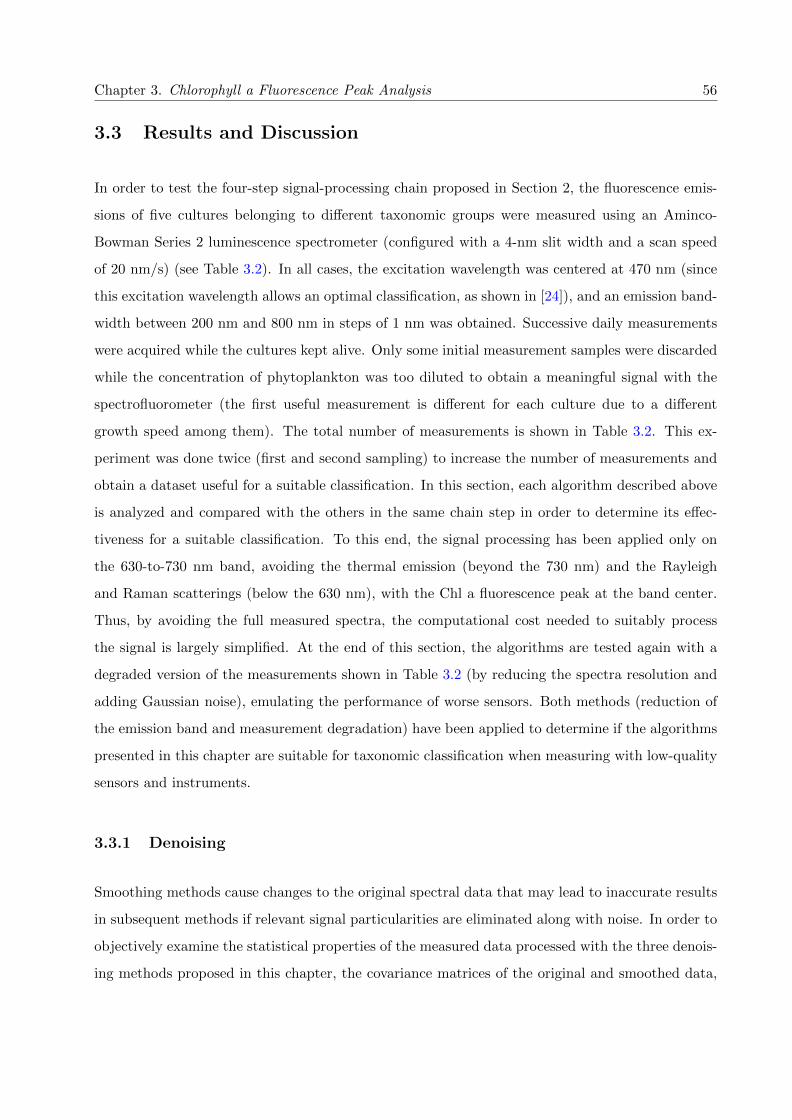
Chapter 3. Chlorophyll a Fluorescence Peak Analysis 56
3.3 Results and Discussion
In order to test the four-step signal-processing chain proposed in Section 2, the fluorescence emis-
sions of five cultures belonging to different taxonomic groups were measured using an Aminco-
Bowman Series 2 luminescence spectrometer (configured with a 4-nm slit width and a scan speed
of 20 nm/s) (see Table 3.2). In all cases, the excitation wavelength was centered at 470 nm (since
this excitation wavelength allows an optimal classification, as shown in [24]), and an emission band-
width between 200 nm and 800 nm in steps of 1 nm was obtained. Successive daily measurements
were acquired while the cultures kept alive. Only some initial measurement samples were discarded
while the concentration of phytoplankton was too diluted to obtain a meaningful signal with the
spectrofluorometer (the first useful measurement is different for each culture due to a different
growth speed among them). The total number of measurements is shown in Table 3.2. This ex-
periment was done twice (first and second sampling) to increase the number of measurements and
obtain a dataset useful for a suitable classification. In this section, each algorithm described above
is analyzed and compared with the others in the same chain step in order to determine its effec-
tiveness for a suitable classification. To this end, the signal processing has been applied only on
the 630-to-730 nm band, avoiding the thermal emission (beyond the 730 nm) and the Rayleigh
and Raman scatterings (below the 630 nm), with the Chl a fluorescence peak at the band center.
Thus, by avoiding the full measured spectra, the computational cost needed to suitably process
the signal is largely simplified. At the end of this section, the algorithms are tested again with a
degraded version of the measurements shown in Table 3.2 (by reducing the spectra resolution and
adding Gaussian noise), emulating the performance of worse sensors. Both methods (reduction of
the emission band and measurement degradation) have been applied to determine if the algorithms
presented in this chapter are suitable for taxonomic classification when measuring with low-quality
sensors and instruments.
3.3.1 Denoising
Smoothing methods cause changes to the original spectral data that may lead to inaccurate results
in subsequent methods if relevant signal particularities are eliminated along with noise. In order to
objectively examine the statistical properties of the measured data processed with the three denois-
ing methods proposed in this chapter, the covariance matrices of the original and smoothed data,

Chapter 3. Chlorophyll a Fluorescence Peak Analysis 57
which show the variance relationship between different wavelength distributions, are compared.
The more similar the matrices are the least distortion is being introduced by the denoising method.
Table 3.3 resumes the results obtained from fluorescence measurements in the Duna culture case,
using different conditions for each denoising method. The similarity between the covariance ma-
trices of the original and smoothed data is evaluated using the root mean square error (RMSE).
As can be seen, the WMA method has been applied along with square windows of 3, 7 and 11
samples and with three Gaussian windows, each one with a different standard deviation (σ1, σ2
and σ3, respectively), as shown in Table 3.3 and Figure 3.5; the Savitzky-Golay method has been
applied along with windows of 13, 17 and 23 samples; and a 6th-level wavelet method (using the
Daubechies wavelet family with nine vanishing moments as in [44] and suitable for signals with
zero-mean Gaussian white noise) has been applied considering two different filtering thresholds.
While the first method (thr1) uses a soft threshold on the whole detail level set, the second method
(thr2) applies a hard threshold on the same set (Figure 2.2a and 2.2b, respectively). In both cases,
the adaptive threshold selection technique described above is used to estimate the suitable threshold
level. It must be noted that the optimal mother wavelet mainly depends on the noise properties
and the signal characteristics, and therefore, once the low-cost sensor is implemented, an analysis
of its characteristics should be performed for a suitable selection.
Figure 3.5: Gaussian windows used with the WMA method.
In general, for small or intermediate values of the smoothing parameters, the covariance curves
present a high overlapping. As the smoothing factor increases, both curves diverge, increasing the
RMSE between them. As observed, the covariance matrix comparison shows that the statistical
properties in the WMA case diverges for square or Gaussian windows wider than a few samples,
while the Savitzky-Golay method keeps a small distance length even for windows up to 17 samples.

Chapter 3. Chlorophyll a Fluorescence Peak Analysis 58
Table 3.3: RMSE between the covariance of the original data and the covariance of the smootheddata at 684 nm.
Algorithm Parameters RMSE
WMA (Square window)
n=3 0.012n=7 0.047n=11 0.102
WMA (Gaussian window)
σ1=1.04 0.016σ2=1.56 0.030σ3=3.12 0.090
Savitzki-Golay
n=13 0.015n=17 0.028n=23 0.062
Waveletthr1 0.032thr2 0.012
Finally, the wavelet method shows a smaller distance in the hard threshold case than in the soft one.
Similar results have also been obtained using different cultures. Table 3.3 gives an idea about the
smoothing rate introduced by each algorithm, but it is not decisive when selecting the most suitable
one. Further results are shown in Subsection 3.3.4 when using them to classify the samples. Figure
3.6 shows the original and smoothed spectra for the Pl measurements using the Savitzky-Golay
method and n=17 as an example.
Figure 3.6: Example using Savitzky-Golay for denoising: (a) Original and (b) smoothed spectraof all the Pl measurements obtained with the Savitzky-Golay method and n=17.
3.3.2 Normalization
Figure 3.7 shows the four normalization methods proposed in this chapter applied on the Thwi
measurements after denoising using the wavelet method and soft threshold.

Chapter 3. Chlorophyll a Fluorescence Peak Analysis 59
Figure 3.7: Different normalizations applied on the denoised Thwi measurements (with waveletmethod and soft threshold) using: (a) the min-max method; (b) the GSM method; (c) the SNV
method; (d) the modified SBN method.
As can be observed, the four spectra plots are quite similar, but slight differences can be appreciat-
ed. The spectra obtained with the min-max method, Figure 3.7a, presents flat shapes around the
640 nm and 680 nm with minimum and maximum values, respectively, not seen in any other plot,
due to the scaling method. Such distortion may affect the statistical properties present at those
wavelengths. As expected, the GSM method improves the spectral shape, as shown in Figure 3.7b,
and presents the best normalization below 660 nm. However, all the curves tend to concentrate
around a single point in its maximum since it is taken as the reference and it can affect the
classification step. The SVN and the modified SBN methods, Figure 3.7c and 3.7d, respectively,
present similar curves and do not suffer from any distortion on their fluorescence values. The four
algorithms are objectively compared in Subsection 3.3.4 against the denoising and classification
methods to determine the most suitable one.

Chapter 3. Chlorophyll a Fluorescence Peak Analysis 60
3.3.3 Transformation and Dimensionality Reduction
3.3.3.1 The Derivative Method
The derivative of the denoised and normalized samples (using the wavelet and SBN methods, respec-
tively) of the Thwi culture was obtained using different band separations, as shown in Figure 3.8.
As the band separation increases, a smoother curve is obtained. In order to know if the derivatives
of the original fluorescence signals contain hidden properties that may facilitate the discrimination
process, they are used in Subsection 3.3.4, along with the three classification methods, to compare
its taxonomic discrimination results with the ones obtained using the original measurements.
Figure 3.8: Derivative of the Thwi samples for different band separation: (a) 5 sampling intervals;(b) 10 sampling intervals; (c) 20 sampling intervals.
3.3.3.2 The Genetic Algorithm Method
The first step before using the genetic algorithm is to find the minimum data dimension that keeps a
suitable classification efficiency. The maximum likelihood estimator (MLE) technique [105], which
uses the principle of maximum likelihood on the distances between close neighbors to group them,
was applied on the fluorescence data of the five cultures denoised and normalized with the wavelet
(hard threshold) and SBN methods, respectively, obtaining a minimum dimension of 5 bands. Then,
the genetic algorithm was used in combination with the k-neighbors classification method (with
k=1) to find the value of these five wavelengths. Among the classification methods, the k-neighbors
was selected since it does not need a training and thereby it is the fastest one. The results obtained
after 20 generations over an initial vector of 100 solutions are 637 nm, 677 nm, 694 nm, 710 nm and
720 nm. Since these results are spaced along the whole bandwidth, it can be concluded that the
particular features of each culture are not concentrated in a narrow band but widely distributed.

Chapter 3. Chlorophyll a Fluorescence Peak Analysis 61
3.3.3.3 The PCA Method
Figure 3.9 shows the results obtained with the PCA method applied on all the samples. As can be
seen, a significant reduction of the data dimension can be applied since the first three components
concentrate the 99% of the data variability. The other ones will not significantly contribute to obtain
a better classification of the culture. In the next subsection, the first three components obtained
with this algorithm are used in combination with the three classification methods to compare its
results with previous methods.
Figure 3.9: Example of PCA Analysis: Representation of (a) the first 20 eigenvectors, and (b)their percentage of variance.
3.3.4 Classification
The comparison between the classification methods (and the different denoising and normalization
techniques) has been performed using the confusion matrix and the Kappa index (K), introduced
in the previous chapter [24]. As explained, the confusion matrix displays both the number of
samples that were correctly and incorrectly classified, and, in the latter case, provides insight into
which was the wrong chosen culture. The Kappa index is a measure of the global classification
error whose calculation is made from elements of the confusion matrix. In order to maximize the
performance of k-neighbors, a previous optimization of the variable k was done finding the value
that presents the best classification results, obtaining k = 1. The training for the SOM and GCS
classification algorithms, with 32 nodes each, was done using both sampling columns of Table 3.2
in a 5-fold cross-validation technique. Tables 3.4 to 3.6 resume the classification performance of
the three classification methods, in combination with the three denoising methods and the four
normalization techniques, through the Kappa index. As can be observed, all combinations present

Chapter 3. Chlorophyll a Fluorescence Peak Analysis 62
accurate classifications achieving in some cases a perfect result. In general, the net growing concept
seems to present a better performance than the static net of SOM. However, the three tables coincide
in pointing out the k-neighbors as the best classification method. Besides, among the denoising
techniques, the WMA denoising algorithm (Table 3.4) gives the higher Kappa indices, as the SNV
does among the normalization ones. Therefore, an optimal solution for the signal-processing chain
is obtained when using these two algorithms (WMA and SNV) in combination with the k-neighbors
method.
Table 3.4: Kappa indices obtained with the three classification techniques and the four normal-ization methods when denoising with the WMA method (Gaussian window with α2).
Min-Max GSM SNV SBN
k-neighbors 0.994 1 1 1SOM 0.925 0.987 0.994 0.994GCS 0.974 0.991 1 0.974
Table 3.5: Kappa indices obtained with the three classification techniques and the four normal-ization methods when denoising with the Savitzky-Golay method and n=13.
Min-Max GSM SNV SBN
k-neighbors 0.994 1 1 1SOM 0.918 0.987 0.975 0.994GCS 0.965 0.991 1 0.982
Table 3.6: Kappa indices obtained with the three classification techniques and the four normal-ization methods when denoising with the wavelet method (the letter denotes the use either soft or
hard threshold).
Min-Max GSM SNV SBN
k-neighbors 0.984s/0.994h 0.994s/0.994h 1s/1h 1s/1hSOM 0.919s/0.931h 1s/0.975h 0.981s/0.987h 0.994s/0.994hGCS 0.965s/0.965h 1s/1h 0.991s/1h 0.982s/0.965h
Table 3.7 shows the Kappa index obtained with the three classification methods and the three
transformation methods when considering the WMA (Gaussian window with α2) as a denoising
method and the modified SBN to normalize. The optimal performance is obtained again with the
k-neighbors method using only the five bands given by the genetic algorithm (as expected since the
genetic algorithm uses the k-neighbors method to find the suitable wavelengths) or in combination
with the first three components given by the PCA method. SOM gives its best result using the five
bands of the genetic algorithm and, in contrast, GCS gives its one in combination with the PCA.

Chapter 3. Chlorophyll a Fluorescence Peak Analysis 63
Table 3.7: Kappa indices obtained with the three classification techniques and the three trans-formation methods, considering the WMA (Gaussian window with α2) as a denoising method and
the modified SBN as a normalization method.
Derivative GeneticPCA
(First Order) Algorithm
k-neighbors 0.994 1 1SOM 0.962 0.994 0.987GCS 0.974 0.982 0.991
All these results reinforce the idea that an important reduction of the data dimension can be applied
without much loss of performance, which involves a reduction of the needed computational cost. In
order to evaluate the degree of optimization, Table 3.8 shows the time employed on the execution
of the previous example with and without a reduction of the data dimension using an Intel Pentium
4 at 3 GHz, with a 1 GB RAM and running a Windows 7. As can be seen, the time needed to
complete the signal processing is reduced between 30%-33% in the SOM case, 8%-9% in the GCS
case, and 20%-24% in the k-neighbors case. Even without the further computational-cost reduction,
the k-neighbors algorithm is already much optimal than SOM and GCS algorithms, since training
is not necessary, and therefore preferred from this point of view. On the other hand, the derivative
of the original spectra does not seem to improve in a significant way the classification techniques,
and its performance worsens proportionally to an increasing derivative order.
Table 3.8: Computational cost expressed in terms of execution time (in seconds), considering theWMA (Gaussian window with α2) as a denoising method and the modified SBN as a normalization
method.
StandardGenetic
PCAAlgorithm
k-neighbors 1.13 s 0.90 s 0.86 sSOM 19.91 s 14.10 s 13.40 sGCS 106.06 s 98.10 s 96.87 s
Tables 3.9 and 3.10 show the averaged confusion matrices (due to the five-fold cross-validation)
for the worst solutions obtained in Tables reftab:KappaResultsdenWMA to 3.8, that is, the one
obtained with the SOM classification method when using the Savitzky-Golay and the Min-Max
methods to denoise and normalize (Table 3.9), and the one obtained with the SOM algorithm when
using the wavelet method with a soft threshold and the Min-Max method to denoise and normalize
(Table 3.10). Thus, those samples that are more difficult to be suitable classified can be identified.
In the Savitzky-Golay case (Table 3.9), some Pl samples are classified as Duna, but the major
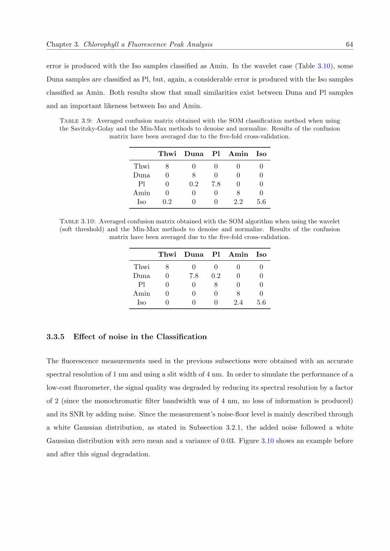
Chapter 3. Chlorophyll a Fluorescence Peak Analysis 64
error is produced with the Iso samples classified as Amin. In the wavelet case (Table 3.10), some
Duna samples are classified as Pl, but, again, a considerable error is produced with the Iso samples
classified as Amin. Both results show that small similarities exist between Duna and Pl samples
and an important likeness between Iso and Amin.
Table 3.9: Averaged confusion matrix obtained with the SOM classification method when usingthe Savitzky-Golay and the Min-Max methods to denoise and normalize. Results of the confusion
matrix have been averaged due to the five-fold cross-validation.
Thwi Duna Pl Amin Iso
Thwi 8 0 0 0 0Duna 0 8 0 0 0
Pl 0 0.2 7.8 0 0Amin 0 0 0 8 0
Iso 0.2 0 0 2.2 5.6
Table 3.10: Averaged confusion matrix obtained with the SOM algorithm when using the wavelet(soft threshold) and the Min-Max methods to denoise and normalize. Results of the confusion
matrix have been averaged due to the five-fold cross-validation.
Thwi Duna Pl Amin Iso
Thwi 8 0 0 0 0Duna 0 7.8 0.2 0 0
Pl 0 0 8 0 0Amin 0 0 0 8 0
Iso 0 0 0 2.4 5.6
3.3.5 Effect of noise in the Classification
The fluorescence measurements used in the previous subsections were obtained with an accurate
spectral resolution of 1 nm and using a slit width of 4 nm. In order to simulate the performance of a
low-cost fluorometer, the signal quality was degraded by reducing its spectral resolution by a factor
of 2 (since the monochromatic filter bandwidth was of 4 nm, no loss of information is produced)
and its SNR by adding noise. Since the measurement’s noise-floor level is mainly described through
a white Gaussian distribution, as stated in Subsection 3.2.1, the added noise followed a white
Gaussian distribution with zero mean and a variance of 0.03. Figure 3.10 shows an example before
and after this signal degradation.

Chapter 3. Chlorophyll a Fluorescence Peak Analysis 65
Figure 3.10: Example of signal degradation:(a) Measured Thwi fluorescence, and (b) Thwi flu-orescence after reducing the spectral resolution and adding noise, which follows a white Gaussiandistribution with zero mean and a variance of 0.03, to emulate the measurements obtained with
low-cost sensors.
The algorithms of the signal-processing chain described in this chapter were applied on the degraded
samplings to determine if a suitable classification performance could be obtained under such con-
straints. The WMA denoising method with a Gaussian window (and using α2) showed to be the
most successful one, as seen in Tables 3.4 to 3.6. Therefore, this method was selected to compare
the three classification methods against the four normalization techniques, as seen in Table 3.11.
Again, the best result is obtained when using the SNV normalization method and the k-neighbors
classification one, achieving almost a perfect classification.
Table 3.11: Kappa indices obtained with the three classification techniques and the four normal-ization methods when denoising with the WMA method (Gaussian window with α2).
Min-Max GSM SNV SBN
k-neighbors 0.750 0.625 0.994 0.794SOM 0.575 0.575 0.943 0.681GCS 0.279 0.310 0.680 0.517
In order to determine if this new set of samples can be dimensionally reduced to decrease the
computational cost but still obtaining accurate results, the genetic algorithm was applied again
to obtain the five frequencies that mostly characterize them. By firstly using only these five fre-
quencies along with the k-neighbors classification method, and secondly the PCA along with the
k-neighbors classification method, the Kappa index obtained were of 0.890 and 0.981, respectively.
This classification result shows that the best combination of algorithms, in the k-neighbors method
case, include the PCA method as the optimal one to reduce the computational cost (the successful
classification percentage only drops a 2% and thus an accurate classification result is still obtained,

Chapter 3. Chlorophyll a Fluorescence Peak Analysis 66
whereas the execution time is reduced by a 28%). Additionally, in the PCA case, a study of the
classification performance for different levels of noise was performed by modifying the variance of
the Gaussian distribution, obtaining the results shown in Table 3.12. As expected, the Kappa index
decreases as the variance increases. At a variance beyond 0.2 the classification cannot be considered
successful (Kappa index drops far below 0.8).
Table 3.12: Kappa indices obtained with the WMA method to denoise, the SNV method tonormalize, the PCA method for a dimensional reduction and the k-neighbors to classify, by using
the degraded samples with four different variances (σ) of the noise Gaussian distribution.
σ=0.03 σ=0.06 σ=0.1 σ=0.2
Kappa index 0.981 0.937 0.850 0.787
The results presented above show that the best combination of algorithms in the signal-processing
chain that showed an optimal classification with the accurate fluorescence measurements, is also the
best combination when handling with low-accurate data (degraded in terms of resolution and SNR).
As stated in Table reftab:KappadenoisingWMA, this combination includes the WMA method to
denoise, the SNV method to normalize, the PCA method for a dimensional reduction and the k-
neighbors to classify the measurements (see Figure 3.11), reaching a discrimination performance
with a Kappa index of 0.981 (when σ = 0.03). This is also the best solution in terms of compu-
tational cost, since the k-neighbors algorithm presents the lowest execution time (5% of the total
SOM execution time and 1% of the whole GCS execution time), and, after adding the dimensional
reduction block, the execution time is further reduced by a 24% (as seen in Table 3.8). Taking
into account the results presented above, it has been proven the initial hypothesis of a feasible
taxonomic classification using only the narrow 630-to-730 nm band of fluorescence emissions, which
corresponds to the Chl a peak, since other cellular contents (which differs depending on the strain)
also modify its spectral shape. With this, the two constraints given by the measurements obtained
with low-performance sensors, i.e., high noise levels in a narrow bandwidth and an optimal com-
putational cost, have been dealt. To conclude, despite the fact that a limited number of samples
obtained from only five different cultures constituted the whole dataset, the results presented in
this section are significantly accurate, and constitute an optimistic beginning to continue working
in this direction, either designing more accurate algorithms or improving the current ones. Besides,
they stimulate the investment in the development of a new hyperspectral low-cost sensor with dis-
crimination capabilities cen-tred in the Chl a peak spectral range. It should be noted that, if a new
low-cost sensor was actually developed, its measurement uncertainty (regarding to spectrometric

Chapter 3. Chlorophyll a Fluorescence Peak Analysis 67
and radiometric errors) should be perfectly characterized and evaluated to see if the performance
of the signal processing presented in this chapter is severely degraded.
Figure 3.11: Resulted optimal four-step processing chain: Optimal algorithms for the four-stepsignal-processing chain designed to deal with low-accurate narrowband fluorescence measurements.
3.4 Conclusions
Current constraints in money budget for research projects have motivated the development of new
low-cost technologies. That, in consequence, requires an effort to extract as much information as
possible from instruments exhibiting a low performance. In this chapter, an optimal-computational-
cost signal-processing chain designed to deal with fluorescence measurements featuring poor signal-
to-noise ratios, low resolution, narrow bandwidth and, therefore, suitable for low-cost sensors and
instruments, has been presented. The main objective of this research was focused in finding that
combination of algorithms that optimizes the instrument performance when discriminating between
different taxonomic cultures of phytoplankton species present in marine environments considering
two constraints. The first one was given by the potential low-performance of the sensor, which limits
the measurable spectra (the lowest fluorescence emissions may be found under the noise floor level
of the sensor). Thereby, only the highest values of fluorescence emissions, that is, those close to the
Chlorophyll a peak placed around the 680 nm, were considered. The second constraint was given
by the processing limits of a low-cost hardware. To minimize the signal-processing requirements,
algorithms should exhibit an optimal performance in terms of computational cost. In order to fulfill
with these two requirements, the signal-processing chain was established in four separated blocks,
each one with a different processing function, which include the denoising, the normalization, the
transformation and the classification of the input data. The denoising techniques were used to
smooth the noisy data, the normalization methods to make the hyperspectral signature of cultures
measured at different growth stages equivalent, the transformation block to modify and reduce the

Chapter 3. Chlorophyll a Fluorescence Peak Analysis 68
data dimension in order to decrease the computational cost while trying to enhance its feature
information, and finally the classification algorithms to discern the nature of the samples.
The algorithms of the whole signal-processing chain selected in this research work were experimen-
tally tested and compared using the actual fluorescence measurements obtained from five different
species of phytoplankton. In order to deal with the objective of this study, the data measured with
a laboratory spectrofluorometer was synthetically degraded in terms of bandwidth, resolution and
signal-to-noise ratio to simulate the performance of a potential low-performance low-cost sensor.
Accurate classification results were achieved in most of the combinations when using the original
data and, although a decrement in the classification performance was observed; still very good
results were obtained in a few combinations when using the degraded quality signal. The optimal
chain implementation was obtained by means of the weighted moving average technique as a de-
noising method, the standard normal variate method for normalization, the principal component
analysis to reduce the data dimension and the k-neighbors to classify the cultures. The k-neighbors
does not only provide the best classification results when dealing with fluorescence measurements,
but it is also the fastest method, since it does not require a preliminary training, in contrast to
the self-organizing maps technique or the growing cell structures method. This combination, ad-
ditionally, is optimal in terms of the computational cost, and an accurate classification can be
achieved with the minimum hardware requirements. These results have also confirmed that a suit-
able discrimination of different taxonomic cultures can be achieved examining only the emission
fluorescence data placed around 680 nm and excited at 470 nm, where the fluorescence peak of
the Chlorophyll a is allocated. While other research works use the whole visible spectra to clas-
sify the samples obtained with accurate but expensive instruments, this work has shown that the
630-to-730-nm band presents enough information to determine the sample origin after smoothing,
normalizing and reducing its dimension. This is due to a different proportion of the Chlorophyll
a among different cultures, but also to the presence of different pigment and Chlorophyll b, c and
d ratios, which slightly modify the spectral shape of the culture. These results, obtained from
fluorescence measurements performed on pure cultures, are a preliminary but necessary validation
in order to proceed with the more complex unmixing techniques for taxonomic discrimination in
mixed scenarios. The methodology to obtain fluorescence measurements suggests that it is neces-
sary to address this problem using a non-linear unmixing approach (since the photons emitted by
one particle can be absorbed or scattered by other particles). This issue opens the way for the
development of a wide range of new methodologies and techniques to be implemented in a low-cost

Chapter 3. Chlorophyll a Fluorescence Peak Analysis 69
instrument, which is of great importance to improve the current lengthy methods of taxonomic
identification while reducing the expenses in oceanographic research.


Chapter 4
Detecting the presence of different
phytoplankton species mixed in a
sample
4.1 Introduction
The analysis of phytoplankton species and their abundance is a routine task in marine environ-
ment monitoring. In recent years, frequently occurring red tides have led researchers to develop
rapid analysis technology that measures seawater directly and yields qualitative information about
phytoplankton.
Previous chapters showed the viability of using classification techniques in order to use phyto-
plankton fluorescence spectra to achieve discrimination among different species. In those chapters
phytoplankton fluorescence spectra acquired from pure cultures were used. In a real environment,
such as natural waters, phytoplankton species are not isolated, but mixed with other phytoplankton
species, minerals or other suspended materials. However, in the case of bloom, almost all the con-
tribution to the fluorescence signal is only due to the dominant phytoplankton specie. Thus, once
it has been shown that fluorescence signal from phytoplankton is able to achieve discrimination
from pure cultures, this chapter is focused on the determination of phytoplankton contributions in
a mixed sample, or non-bloom conditions.
71

Chapter 4. Detecting phytoplankton species in a mixed sample 72
Given a set of mixed spectral vectors, Spectral Mixture Analysis (SMA), or spectral unmixing,
aims at estimating the number of reference materials, also called endmembers, and their fractional
abundances. Spectral unmixing analysis has been applied in a variety of studies, for instance,
in satellite images in order to determine the water quality over the Amazon floodplain [106], for
mapping the snow cover in forests [107], or desert shrub rangeland [108]. Spectral imaging sensors
record scenes in which numerous materials contribute to the spectrum measured from a single pixel.
That is so when the spatial resolution of this sensor is high enough such that adjacent materials can
jointly occupy a single pixel, then the resulting spectral measurement will be a composite of the
individual endmembers. Thus, in a pixel spectra there are mixed several spectral responses from
different compounds. Given such mixed pixel, the goal is to identify the individual constituent
materials present in the mixture, as well as the proportions in which they appear. The problem
is then very similar to the one we are facing in this chapter, in which different phytoplankton
species contribute to the spectrum acquired. Spectral unmixing is then the procedure by which the
measured spectrum of a mixed sample is decomposed into a collection of constituent spectra, or
endmembers, and a set of corresponding fractions, or abundances, that indicate the proportion of
each endmember present in the sample.
There exist several techniques to unmix hyperspectral signals. [109] is a good and exhaustive survey
of spectral unmixing algorithms applied to remote sensing hyperspectral images. In this survey, the
complete end-to-end unmixing problem is decomposed to a sequence of three consecutive stages:
dimension reduction, endmember determination and inversion.
• Dimension reduction: this step is thought to be used to reduce the computational load of
the processing algorithms, although it can be also used to increase their performance as it
has been shown in previous chapters. While this first step is optional, but it has been proven
useful in our study case, the next one, endmember determination, is indispensable in any
case.
• Endmember determination: In remote sensing imaging, endmembers normally correspond to
familiar macroscopic objects present in the scene, such as water, soil, metal, or any natural or
man-made material. In this context, there exist basically two approaches in order to determine
the endmembers. In the first one, scientists can acquire the reflection of the different materials
that can appear in an image by simply taking the signal in the lab or in a controlled field
acquisition, and they can build a library of materials with their response to be used as

Chapter 4. Detecting phytoplankton species in a mixed sample 73
endmembers. The second approach is the more commonly used, and it consists in using
certain algorithms to select the endmembers directly from the satellite image. It assumes
that there exist pixels in the image that are fully occupied by a material, and the response
from this pixel is generated just due to this material. With this approach they ensure that the
endmembers spectra are affected by the atmosphere or other disturbing effects that affect also
the image they are working with. There exist several methods to select endmembers from
a satellite image such as Vertex Component Analysis (VCA) [110], Convex Cone Analysis
(CCA) [111] among others [112]. In our case, the endmembers can not be collected from
an image, so they should be acquired separately. The endmembers are then acquired in
laboratory or using radiative transfer models, as it will be explained below. The next sections
will discuss in more detail this problem and how it has been tackled in each case of study.
• Inversion: Finally, the last step is the inversion. Depending on the interaction of the light with
the materials present in the scene or mixtures, the response signal acquired by the sensor can
be linear or non-linear [113–115], and the inversion model used depends on this characteristic.
Linear mixing model (LMM) holds when the detected photons interact mainly with a single
component on the scene before they reach the sensor [116, 117](Figure 4.1), while the non-
linear mixing model (NLMM) appears when the light suffers multiple scattering involving
different materials [118](Figure 4.2).
Figure 4.1: Schematic representation of a Linear Mixing example (Image extracted from [113]).
In a linear mixing scenario, the acquired spectral vectors are a linear combination of the endmembers
signatures present in the sample weighted by the respective fractional abundances. On the other

Chapter 4. Detecting phytoplankton species in a mixed sample 74
Figure 4.2: Schematic representation of a Non-Linear Mixing example (Image extracted from[113]).
hand, in a non-linear mixing scenario, the model for the scattered light is much more complex and
typically application dependent. There exist particular situations in which a non-linear model can
be approximated with a linear one. Although the application case faced in this chapter is probably
a non-linear scenario, and there are some studies dealing with non-linear problems [119, 120], it is
much more complicated to solve and it would imply a complete thesis research. Thus, before facing
this scenario, it is always suggested to prove if the problem can be approximately solved by a linear
mixing model.
To accomplish this goal, two different approaches are presented in this chapter:
• Use of laboratory mixed samples: In this case, optical responses of phytoplankton cultures
are acquired in the laboratory, as well as fluorescence responses of mixtures obtained merging
these phytoplankton cultures.
• Use of a radiative transfer model: For this study, a radiative transfer model implemented in a
commercial software (Hydrolight [121]) is used to simulate several scenarios of bloom (single
algae simulation) and mixture (two phytoplankton species mixed). Simulation outputs are
used for testing unmixing techniques
This chapter is then organized as follows: Next section introduces the processing techniques used
for this study. Linear Mixing Model (LMM) is introduced to better understand how it works and

Chapter 4. Detecting phytoplankton species in a mixed sample 75
it is applied. After that, both approaches are presented. Generated data for each approach is
explained and some conclusions are extracted from the results. Some of the results presented in
this chapter were presented in [28].
4.2 Linear Mixing Model (LMM)
As it has been already shown during this thesis, each phytoplankton specie produces a different
fluorescence spectra, since they are composed of different pigments that provide them their char-
acteristic colors and different spectral responses, depending on the source that illuminates them
(intensity and wavelength). This property allows to distinguish and classify the different species
present in the water [24].
In marine environments more than one specie is present in the water, so the measurement equipment
will not acquire just a pure fluorescent compound but the contribution of all the species present
in the specific environment, as well as other fluorescent particles. The aim of this chapter is then
to determine if it is possible to distinguish the proportion of each specie in a measurement using a
linear unmixing method.
As mentioned during the thesis, several techniques use phytoplankton fluorescence spectroscopy to
discriminate between different phytoplankton groups [1, 17]. Some of these techniques can achieve
a high taxonomic discrimination but they are based on measurements that require excitation at
different wavelengths. During this thesis, and the results presented in [24, 26], the possibility to use
the information contained in emission fluorescence spectra to discriminate between several phyto-
plankton species has been evaluated. Self-Organizing Maps (SOM), as well as other classification
techniques such as P-SVM, k-neighbors, Growing Cell Structures, etc. were used and their perfor-
mance were presented as feasible techniques to use in those studies, in which time acquisition is
an important constraint, e.g. mobile platforms for high spatial resolution measurements. In this
chapter, we go one step further. The fluorescence of different mixtures has been acquired and a
first approach using the Linear Mixture Model (LMM) [114] is analyzed in order to evaluate how
this model can be applied to this kind of data. LMM is herein briefly described and finally, the
results of the unmixing using this linear approach are presented and discussed.
There exist other techniques such as Independent component analysis (ICA) [122] or independent
factor analysis (IFA) [123] which have been used by many authors to unmix hyperspectral data.

Chapter 4. Detecting phytoplankton species in a mixed sample 76
However, they are based in the assumption of source statistical independence and this is not satisfied
in spectral applications [113], since the source are fractions and, thus, non-negative and sum one.
That is why methods based in ICA or IFA have important limitations in this field. In [124] the
impact of this source statistical dependence is addressed. In this study, evidence that the unmixing
matrix minimizing the mutual information might be far from the true one is given. In this chapter,
and bearing this in mind, linear spectral mixing model is used, and it is explained in the next
section.
4.2.0.1 Linear Spectral Mixing Model
The basic premise of mixture modeling is that within a given scene, the medium, in a general
case, is dominated by a small number of distinct materials that have relatively constant spectral
properties. Theses distinct substances are called endmembers and the fractions in which they appear
in a mixture are called fractional abundances. In this sense, there should exist a linear relationship
between the fractional abundance of the substances present in the medium being monitored and
the fluorescence spectra measured by the sensor. This relation in a linear process is called Linear
Spectral Mixing Model (LSMM), and it can be written as:
x =M∑i=1
aiSi + w = Sa+ w (4.1)
where x is the measured spectrum vector (L × 1 vector, being L the number of features), S is
a L × M matrix whose columns are the endmember signatures (L × 1 vectors belonging to M
endmembers), a is the M × 1 fractional abundance vector whose entries are ai (being i = 1, ...,M)
and w is the L× 1 additive observation noise vector.
Inversion algorithms consist on the estimation of the fractional abundances of the constituents
present in a mixed sample, taking into account the spectrum acquired and the endmembers spectra.
Minimizing the squared-error is one of the most widely used inversion algorithms. Least squares
inversion methods are usually used as a first approach. They start from a simple approach and
increase in complexity as further assumptions are imposed on the problem. Usually two assumptions
or constraints are imposed: the sum of the abundances must be 1 (∑M
i=1 ai = 1), and the abundances
must be a positive value below 1 (0 6 ai 6 1, i = 1, ...,M). The results shown below present the

Chapter 4. Detecting phytoplankton species in a mixed sample 77
performance of the methodology with and without constraints. The approach from non-constraint
least squares solutions to full-constraint followed in ths thesis is presented in [125].
Considering a Linear Spectral Mixing Model (LSMM) problem, described above (eq. 4.1), the as-
sumption of no additional noise, and no constraints, the least squares estimation for the abundances
(aLS) is:
aLS = (STS)−1STx = S#x (4.2)
where S# is the pseudo inverse matrix of S.
In order to solve these equations, Singular Value Decomposition (SVD) can be used [126]. The
SVD is a well-known eigenanalysis mathematical method of decomposing a matrix A into matrices
U , S and V , such that A = USV T , where UTU = V TV = I, I is the identity matrix, and S is a
diagonal matrix whose diagonal elements are the singular values [127, 128].
The previous approach imposed no constraints on the abundance solution. A partial constraint
approach can be reach if the constraint of sum to one is applied (∑M
i=1 ai = 1). In this case, the
obtention of the abundances aSCLS can be obtained following equation 4.3:
aSCLS = PMaLS + (STS)−11[1T (MTM)−1 (4.3)
where aLS is given by 4.1 and
PM = I − (MTM)−11[1T (MTM)−11]−11Ta = (STS)−1STx = S#x (4.4)
with 1 = (1, 1, ..., 1)T .
About the nonnegatively constrained least squares (NCLS) is based on the following optimization
problem:
Minimize LSE = (Sa− x)T (Sa− x) subject to ai > 0 where i = 1, ...,M (4.5)

Chapter 4. Detecting phytoplankton species in a mixed sample 78
where LSE is the least squares error used as the criterion for optimality and ai > 0, i = 1, ...,M
represents the nonnegativity constraint. The problem is now a set of inequalities that following
the equation development shown in [129] the constraint optimization problem results in the next
iterative equations given by:
aNCLS = (MTM)−1MTx− (MTM)−1λ = aLS − (MTM)−1λ (4.6)
λ = MT (x−MaNCLS) (4.7)
These two equations 4.6 and 4.7 can be used to solve the optimal solution aNCLS and the Lagrange
multiplier vector λ = (λ1, λ2, ..., λ3)T .
Finally, following the method considered in [130, 131], a full-constraint optimal solution (FCLS) can
be obtained by making use of the previous NCLS algorithm, introducing the sum-to-one constraint.
This constraint can be included modifying the signature matrix M by a new one denoted by N ,
defined by:
N =
δM1T
(4.8)
with 1 = (1, 1, ..., 1)T , and a new vector x, denoted by s:
s =
δx1
(4.9)
The use of δ in 4.8 and 4.9 controls the impact of the sum-to-one constraint, and can be used as
a tunable parameter. The full-constraint algorithm is obtained replacing M and x used in NCLS
with N and s.

Chapter 4. Detecting phytoplankton species in a mixed sample 79
4.3 Results and Discussion
In this study, two different approximations can be clearly distinguished. First (case I), a study done
with samples mixed in the laboratory using several phytoplankton cultures. The second approach
(case II) is using a radiative transfer model to simulate different mixed scenarios. Each subsection
will introduce the specific data generated for each approach and will show the results obtained.
4.3.1 CASE I: Unmixing phytoplankton fluorescence mixtures from laboratory
samples
This experiment shows the performance obtained unmixing emission fluorescence phytoplankton
spectra acquired in the laboratory. First, the data acquired for this work is explained and after
that, the results obtained are shown.
Data preparation
In order to create a data set with mixtures of different phytoplankton species, the fluorescence
emission of approx. 80 mixtures were acquired. The measurements were done with the same
spectrometer used during this thesis, an Aminco-Bowman Series 2 luminiscence spectrometer (con-
figured with a 4 nm slit width and a scan speed of 20 nm/s). 59 mixtures of two components and
24 of three were acquired over several days, merging eight different phytoplankton species (Table
4.1), representing the major algae divisions. In this work, and having as a reference the goal of a
fast discrimination method, emission fluorescence spectra excited at 490nm were acquired. These
fluorescence spectra ranged between 520 - 735 nm, were used as an input data to work with. In
order to select the best possible endmembers, they have been chosen as the emission fluorescence
of the isolated cultures acquired the same day as the mixture. Figure 4.3 shows an example of
the spectra acquired for each phytoplankton specie. These spectra are then used as endmembers
in the unmixing process. As it can be seen, the spectra are very similar, unless Cryptomonas and
Rhinomonas, both belonging to Cryptophyceae class, which present a tiny peak at 590 nm. From
this image, the difficulty of the unmixing step can be appreciated, but it is even more obvious in
the next figure. Figure 4.4 shows an example of a mixture spectra and the signature spectra of both
phytoplankton species used in this mixture. Table 4.2 summarizes the available mixtures acquired
for this study, and the abundances of each constituent.

Chapter 4. Detecting phytoplankton species in a mixed sample 80
Figure 4.3: This figure shows an example of endmember for each phytoplankton specie.
Figure 4.4: This figure shows an example of a phytoplankton mixture and the constituent end-members used. Iso and Amin were mixed in a 50%− 50% proportion.

Chapter 4. Detecting phytoplankton species in a mixed sample 81
Table 4.1: Phytoplankton species merged for mixtures. The abbreviation is neccesary to followthe discussion and to understand table 4.2.
Species Division Abbreviation
Pleurochrysis elongata Prymnesiophyceae Pl (1)Isochrysis galbana Prymnesiophyceae Iso (2)Cryptomonas sp. Cryptophyceae Crypt (3)
Rhinomonas reticulata Cryptophyceae Rhin (4)Dunaliella primolecta Chlorophyceae Duna (5)
Nannochloropsis oculata Eustigmatophyceae Nano (6)Alexandrium minutum Dinophyceae Amin (7)
Thalassiosira weissflogii Bacillariophyceae Thwi (8)
Results
After the effort of the laboratory work, the study presented in this section was the first approach
to unmix phytoplankton mixtures. In this case, an intensive search of different combinations of
two and three components is done. For instance, taking a two component mixture, all the possible
combinations of two species from the list of eight (Table 4.1) are found (C82 = 8!
2!(8−2)! = 28 possible
combinations). Then, LSMM with NCLS approximation was applied for each combination of two
endmembers. From these abundances, the estimated mixtured is computed for each combination
and the error between the original mixture and the reconstructed from the estimated abundances
is computed as the norm of the difference vector. The combination of two endmembers with less
error is the winner, and taken as the best fit combination for this specific mixture under study.
The same procedure is followed for the rest of two and three mixtures left. In the case of mixtures
containing three components, the number of possible combinations is 56.
The performance is then computed as (eq. 4.10):
performance =n correct predictions
n total mixtures∗ 100 (4.10)
Taking into account all the two and three component mixtures measured for this study (Table 4.2)
the performance of this approach methodology is about 65%. In order to improve the results, taking
as a reference the results presented in the previous chapters, denoising and derivative analysis were
perform. This time the results were not the expected, since applying wavelet denoising to the
spectra the performance decrease to 61.44%. Derivative analysis does not make it better obtaining
just a 60.24%.

Chapter 4. Detecting phytoplankton species in a mixed sample 82
Table 4.2: Summary of mixtures acquired in the laboratory. It is indicated for each mixture thephytoplankton species mixed and the abundance in volume percentage of each one.
Day Mixed Species Abundance (%) Day Mixed Species Abundance (%)
1-2 50%-50%, 75%-25% 1-7 50%-50%, 75%-25%3-4 50%-50%, 75%-25% 2-8 50%-50%, 75%-25%
Day 1 5-6 50%-50%, 75%-25% Day 6 3-5 50%-50%, 75%-25%7-8 50%-50%, 75%-25% 4-6 50%-50%, 75%-25%
1-2-3 33%-33%-33% 1-4-7 33%-33%-33%
1-3 50%-50%, 75%-25% 1-8 50%-50%, 75%-25%2-4 50%-50%, 75%-25% 2-7 50%-50%, 75%-25%
Day 2 5-7 50%-50%, 75%-25% Day 7 3-6 50%-50%, 75%-25%6-7 50%-50%, 75%-25% 4-5 50%-50%, 75%-25%
4-5-6 50%-25%-25% 6-8-3 25%-50%-25%
3-4-7 33%-33%-33%1-4 50%-50%, 75%-25% 3-5-8 25%-25%-50%2-3 50%-50%, 75%-25% 2-6-8 50%-25%-25%
Day 3 5-8 50%-50%, 75%-25% Day 8 1-5-7 25%-25%-50%6-7 50%-50%, 75%-25% 4-7-8 33%-33%-33%
7-8-1 50%-25%-25% 2-6-7 50%-25%-25%5-7-8 33%-33%-33%3-4-2 25%-25%-50%
5-7-8 50%-25%-25%1-5 50%-50% 3-5-7 33%-33%-33%2-6 50%-50% 1-2-7 50%-25%-25%
Day 4 3-8 50%-50% Day 9 2-5-8 25%-50%-25%4-7 50%-50% 4-6-7 33%-33%-33%
2-4-8 33%-33%-33% 3-6-8 50%-25%-25%3-4-6 25%-25%-50%1-2-6 25%-50%-25%
1-2 50%-50%1-6 50%-50%, 75%-25% 3-4 50%-50%2-5 50%-50%, 75%-25% 5-6 50%-50%
Day 5 3-7 50%-50%, 75%-25% Day 10 7-8 50%-50%4-8 50%-50%, 75%-25% 2-4-7 33%-33%-33%
3-5-7 50%-25%-25% 2-4 50%-50%5-7 50%-50%3-7 50%-50%

Chapter 4. Detecting phytoplankton species in a mixed sample 83
At this point, there seems to exist a good behavior in terms of linearity, but the performance is still
poor. For this reason, the next step was grouping the species and see if there exists a meaningful
grouping criteria that helps increasing the performance and still offering enough useful information.
In this direction, three grouping scenarios were studied:
• Grouping species by class.
The groups are shown in Table 4.3, where the species are just ordered by their taxonomic
class. The results as expected increased the performance reaching the 71.08% (68.67% after
denoising the spectra and 66.26% using derivative analysis).
Table 4.3: List of species used in this chapter experiment grouped by Class.
Class Species
Bacillariophyceae ThwiEustigmatophyceae Nano
Chlorophyceae DunaDinophyceae Amin
Cryptophyceae Crypt, RhinPrymnesiophyceae Iso, Pl
• Grouping species by functional algal grups (following Beutler’s proposal [1]).
In [1] Beutler groups the phytoplankton species into major funtional algal groups (Table 4.4,
which are mainly named by their color. The results as expected increased the performance
reaching the 74.70% (72.29% after denoising the spectra and 74.70% using derivative analysis).
Table 4.4: List of species grouped by major algal functional groups following the proposal statedby Beutler in [1].
Class Species
Green (Chlorophyceae) DunaBlue (Cyanobacteria) X
Brown (Dinophyceae, Prymnesiophyceae,Amin, Iso, Pl, Nano, ThwiEustigmatophyceae,Bacillariophyceae)
Mixed group (Cryptophyceae) Crypt, Rhin
• Grouping species doing a study of distances among spectra.
This time, instead of fixing the groups in advance following certain criteria like it was done in
both previous approaches, the relation among the species spectra was studied. A clustering
algorithm based on spectral similarity was applied. Hierarchical clustering Analysis (HCA)

Chapter 4. Detecting phytoplankton species in a mixed sample 84
[132] is a well-known method that clusters data based on their spectral distance (in this case,
euclidean distance) and a selected threshold. Figure 4.5 shows the result of the hierarchical
clustering and the threshold was fixed to 4, resulting in 5 different groups (Table 4.5). The
performance rises following these functional groups based on their spectral similarity, reaching
the 85.54% (83.13% after denoising the spectra and 73.49% using derivative analysis).
Figure 4.5: Hierarchical Clustering of phytoplankton culture spectra.
Table 4.5: List of species grouped by spectral similarity using Hierarchical Clustering Analysis(HCA).
Group Species
Group 1 Thwi, NanoGroup 2 Duna, PlGroup 3 Crypt, RhinGroup 4 AminGroup 5 Iso
From this preliminary experiment, it can be said that even obtaining an 85% of performance when
grouping phytoplankton by their spectral similarity, the results are not conclusive. The mixing
scenario seems not to be linear but the results show some evidences that maybe need to studied
carefully and carry out some other experiments. But these experiments in laboratory working with
living samples of phytoplankton are time consuming and statistically not very significant, as it has
been seen in this section. Besides, the percentage of each mixed sample is not accurately known. In
order to know these abundances accurately each mixture have to be analyzed counting cells or with

Chapter 4. Detecting phytoplankton species in a mixed sample 85
advanced systems to exactly determine the exact number of cells of each component present in the
mixture. Nowadays there exist some techniques able to approximately estimate these quantities,
but they are really sophisticated and difficult to set up, calibrate and must be used by qualified
personal. For this reason, it was decided that this job wasn’t part of this thesis, as well as cell
counting. The solution found was then to evaluate unmixing techniques but not requiring such
an amount of time, resources and qualified personal. The decision was using one of the radiative
transfer models available to simulate underwater light conditions. Using radiative transfer model
both drawbacks are solved, since all the quantities used in a simulation are exactly known, and it
can be used to perform as many mixings as desired. Both advantages facilitate the determination of
the limits of applicability of the unmixing techniques in this particular problem. Radiative transfer
models have been studied for a long time and they are widely used in lots of theoretical underwater
studies. Lots of data can be obtained simulating underwater light behaviors without investing
long periods in laboratory, need sophisticate technology or specific personal. Next section focus its
attention in this kind of data.
4.3.2 CASE II: Unmixing the water column from simulated data
Optical properties have been widely used for the characterization of the water column. Natural
light intensity exponentially decreases with depth, unless the sample is not illuminated with an
external excitation. The severity of attenuation differs with the wavelength of the electromagnetic
radiation (EMR). For instance, in the region of visible light, the red part of the spectrum attenuates
more rapidly than the shorter-wavelength, blue part, but other parts of the spectra can be affected
depending on the constituents present in the water. As depth increases, the separability of habitat
spectra declines. The spectral properties recorded by an optical sensor are therefore dependent
both on the constituents and on depth.
There already exists, for instance, a hyperspectral vertical profiler prototype [87] and the commercial
Hyperpro from Satlantic [133], that are able to acquire optical properties from the water column
with hyperspectral sensors. This Hyperpro platform measures the apparent optical properties
(AOP’s) of the ocean, which depend on the inherent optical properties (IOP’s) and also on the
light field in which they are measured. That is, IOP’s depend only upon the medium and are
therefore independent of the ambient light field, while apparent optical properties (AOP’s) depend
on both the medium and the geometric structure of the ambient light field [134]. The Radiative

Chapter 4. Detecting phytoplankton species in a mixed sample 86
transfer theory provides a connection between inherent and apparent optical properties (IOP’s and
AOP’s). The water column’s hyperspectral profile can be then used to detect and classify different
water layers applying analog methodologies used for classifying pixels in terrestrial hyperspectral
images.
There exists several Radiative Transfer Models to be used in simulations, but there is still a lack on
accuracy in how they simulate inelastic processes such as fluorescence. For this reason, although
fluorescence has been used during all this thesis, in this study it will not be used. Instead, the main
goal is to evaluate the use of two specific AOP’s as a potential references (i. e. endmembers) in
hyperspectral characterization of the water column. The AOP’s selection is based on their intrinsic
properties, and the selected ones are:
• the spectral irradiance reflectance factor, R(z, λ), (hereafter referred to as reflectance) defined
as the ratio of spectral upwelling, Eu(z, λ), to downwelling, Ed(z, λ), irradiance.
R(z, λ) =Eu(z, λ)
Ed(z, λ)(4.11)
• the irradiance attenuation coefficient, also known as diffuse attenuation coefficient Kd, that is
essentially the attenuation experienced by sunlight, measuring the variation of Ed in function
of depth.
Kd(z, λ) = −d lnEd(z, λ)
dz= − 1
Ed(z, λ)
dEd(z, λ)
dz[m−1] (4.12)
The validation of R and Kd as useful parameters to discriminate between different optical compo-
nents present in the water column, was based on numerical modelization. The radiative transfer
model simulator HydroLight-EcoLight (HE) [121] has been used to generate the scenarios used for
this goal. The HydroLight-Ecolight radiative transfer numerical model computes radiance distri-
butions and related quantities (irradiances, reflectances, diffuse attenuation functions, etc.) in any
water body. Water absorption and scattering properties, sky conditions, or the bottom boundary
conditions are some of the parameters specified as the inputs of the simulation. All these parame-
ters are used in the scalar radiative transfer equation to compute the in-water radiance and other
AOP’s (e. g. R or Kd, used in this chapter) as a function of depth, direction, and wavelength
(Figure 4.6). Therefore, HE can act as a controlled environment to predict what the light field

Chapter 4. Detecting phytoplankton species in a mixed sample 87
received by a sensor would be under a wide range of conditions. Such control of the environment
cannot be obtained in the field, which is best used for final testing and evaluation of sensors.
Figure 4.6: Radiative Transfer schema used by Hydrolight-Ecolight (HE).
Two different simulations have been carried out for this study using Hydrolight-Ecolight and will
be exposed next:
• a) Study of hyperspectral Irradiance Reflectance (R) and Diffuse Attenuation Coefficient
(Kd). This experiment studies both parameters to demonstrate if they are suitable for phy-
toplankton discrimination, and which one obtains better results.
• b) Diffuse Attenuation Coefficient (Kd) simulations. Here, simulations using HE are used to
obtain Kd. In this case, LSMM is applied to Kd data of several mixed scenarios trying to
unmix the complete water column.
4.3.2.1 a) Study of hyperspectral Irradiance Reflectance (R) or Diffuse Attenuation
Coefficient (Kd)
In this experiment, a preliminary study about these two magnitudes is shown. Are they useful
to discriminate phytoplankton species?. Simulations using Hidrolight-Ecolight are performed and
their variance with depth and concentration studied.
Data preparation

Chapter 4. Detecting phytoplankton species in a mixed sample 88
In this work, five different algal groups are considered (Table 4.6). The HE simulations were
designed as simple as possible, without taking into account inelastic scattering, for example, and
based on the following criteria:
• Simulate profiles containing only one type of algae with homogeneous concentration at all
depths, and at different concentration ratios to evaluate if these two target properties (R and
Kd) are subjected to relevant changes with depth or concentration.
• Simulate a scenario where two different types/populations of algae are present in the water
column to evaluate which of the AOP’s studied (R or Kd) is more suitable for the detection
and identification of the phytoplankton groups.
For each algal group, three different levels of concentration have been simulated (6, 12 and
18 mg·Chl/m3) to generate the homogeneous profiles (using total water depth of 15 m and a
wavelength range 376-725 nm).
In the case of the mixed profile, the algae concentrations follow a triangular shape distribution
with depth (Figure 4.7). In this study, only two groups have been mixed in the simulation,
Bacillariophyceae and Prasinophyceae. As it can be seen in the figure (Figure 4.7), this
distribution shows different parts:
– Parts with no algal presence.
– Parts with only one algae present.
– Parts with both species are mixed with different levels of abundance.
Table 4.6: Phytoplankton groups under study working with hyperspectral Irradiance Reflectance(R) and Diffuse Attenuation Coefficient (Kd) simulations.
Group Abbreviation
Bacillariophyceae ThwiChlorophyceae DunaDinophyceae Amin
Cryptophyceae CryptPrasinophyceae Prasi
In this study, computation of distances among spectra have been used as a metric of similarity.
Minimum distance means that the specie is more likely to be present in the sample. In addition to
the correlation among spectra, two different similarity indexes were also used:

Chapter 4. Detecting phytoplankton species in a mixed sample 89
Figure 4.7: Mixed profile used for simulations. Both phytoplankton groups follow a triangulardistribution at different depths for simulation. Each peak represents one specie, but the position
varies during the experiment.
• Euclidean distance is the geometric distance between two vectors:
d(~p, ~q) =
n∑i=1
(pi − qi)2 (4.13)
• Cosine distance is a measure of similarity between two vectors of n dimensions by finding the
cosine angle between them:
d(~p, ~q) = cos(ϑ) =~p · ~q‖~p‖ ‖~q‖
(4.14)
The performance was evaluated following equation 4.15, where n correct detections is the number
of correct detections of the most abundant algae in the mixed sample profile, while n total samples
is the total number of samples in depth:
performance =n correct detections
n total samples(4.15)

Chapter 4. Detecting phytoplankton species in a mixed sample 90
Results
This section is divided in two parts. The first one is devoted to show how both parameters (Irradi-
ance Reflectance (R) and Diffuse Attenuation Coefficient (Kd)) change with depth or concentration,
in order to check if they can be used as endmembers for phytoplankton detection in the whole water
column. The second part presents the results using these parameters to detect the most abundant
algae present in the mixed profile.
Study of invariance of R and Kd
In order to use Kd or R to discriminate phytoplankton species in the water column, it is necessary
to use reference spectra, or endmembers, representing the spectral signature of each specie. Fur-
thermore, these spectra have to be depth invariant, or one spectrum per depth would be needed,
and also invariant to algae concentration. Figure 4.8 shows how these two parameters change their
spectral response with depth. All five phytoplankton groups and 300 depth samples for each one are
represented. It can be observed that both parameters present an expected slight attenuation with
depth, while their shapes are fairly constant. It can be also seen that they present differentiable
shapes, an important characteristic in order to discriminate them.
Figure 4.9 shows an example of the spectra from just one group for three different concentration
levels simulated with HE. It can be seen that R is less sensitive to changes in concentration than
Kd. However, although Kd changes in value, it seems to maintain its shape, which makes it suitable
also to shape analysis techniques.
Most abundant algae detection
As mentioned previously, in this section a simulation of a triangular phytoplankton distribution in
the water column (figure 4.7) is used. This simulation presents parts with only one algae present
and another where they are mixed. In this case, similarity indices were used to detect the most
abundant phytoplankton specie. The reference spectra were taken from pure culture simulations.
Specifically, reference spectra were picked at 7.5m depth and 12 mg·Chl/m3. Similarity indices
between reference spectra and mixed samples are computed, and the phytoplankton specie with
higher similarity index is selected as the most abundant at a specific depth. Table 4.7 summarizes
the results where performance values are between 0 and 1. It shows the percentatge of correct
matching of the correct solution in the water column for different combinations of concentration
levels between both species.

Chapter 4. Detecting phytoplankton species in a mixed sample 91
Figure 4.8: Example of variations of R andKd with depth. Resulting R andKd from homogeneoussimulations (concentration 6 mg·Chl/m3). All 300 samples of each group are represented.
Figure 4.9: Example of variations of R and Kd with concentration and depth. Resulting Rand Kd from homogeneous simulations (concentration 6, 12 and 18 mg·Chl/m3). All 300 samples
represented.
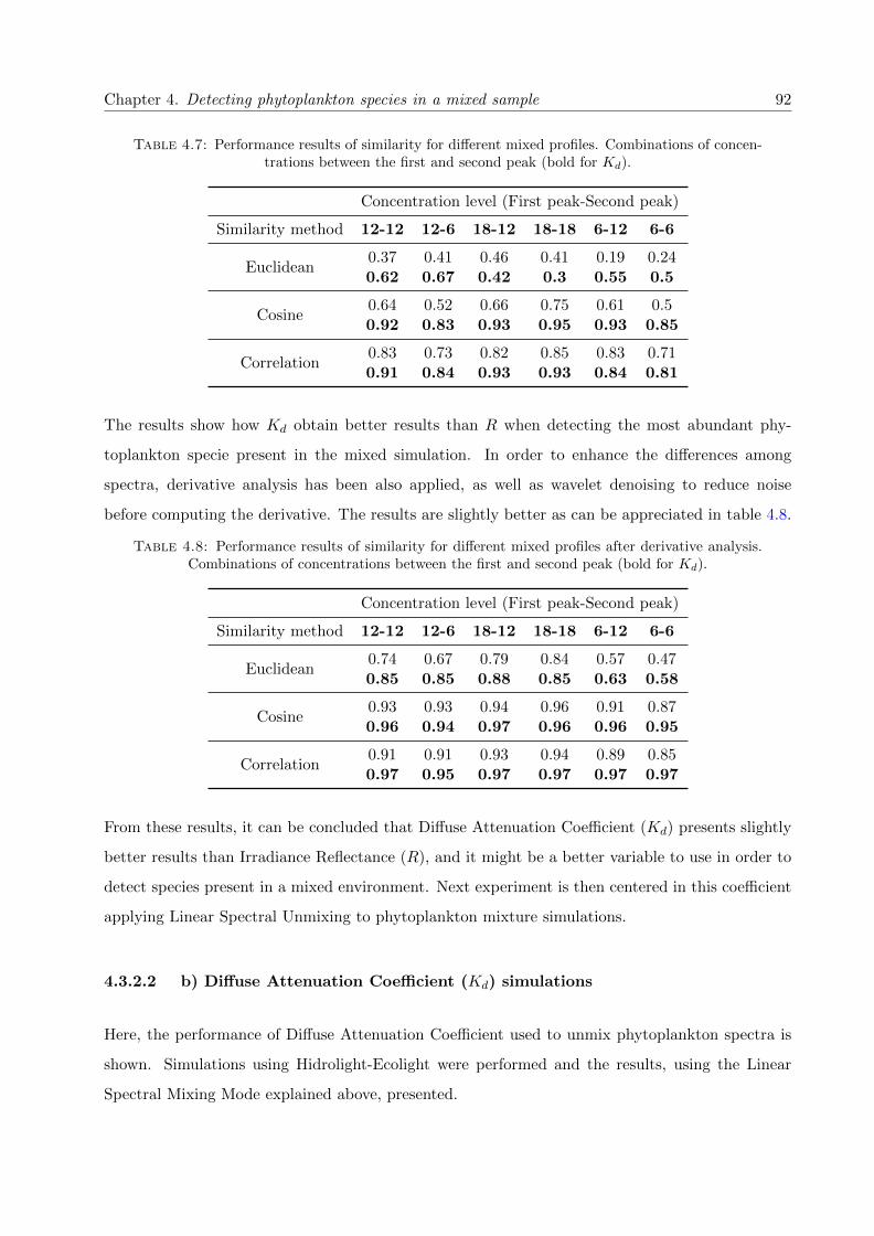
Chapter 4. Detecting phytoplankton species in a mixed sample 92
Table 4.7: Performance results of similarity for different mixed profiles. Combinations of concen-trations between the first and second peak (bold for Kd).
Concentration level (First peak-Second peak)
Similarity method 12-12 12-6 18-12 18-18 6-12 6-6
Euclidean0.37 0.41 0.46 0.41 0.19 0.240.62 0.67 0.42 0.3 0.55 0.5
Cosine0.64 0.52 0.66 0.75 0.61 0.50.92 0.83 0.93 0.95 0.93 0.85
Correlation0.83 0.73 0.82 0.85 0.83 0.710.91 0.84 0.93 0.93 0.84 0.81
The results show how Kd obtain better results than R when detecting the most abundant phy-
toplankton specie present in the mixed simulation. In order to enhance the differences among
spectra, derivative analysis has been also applied, as well as wavelet denoising to reduce noise
before computing the derivative. The results are slightly better as can be appreciated in table 4.8.
Table 4.8: Performance results of similarity for different mixed profiles after derivative analysis.Combinations of concentrations between the first and second peak (bold for Kd).
Concentration level (First peak-Second peak)
Similarity method 12-12 12-6 18-12 18-18 6-12 6-6
Euclidean0.74 0.67 0.79 0.84 0.57 0.470.85 0.85 0.88 0.85 0.63 0.58
Cosine0.93 0.93 0.94 0.96 0.91 0.870.96 0.94 0.97 0.96 0.96 0.95
Correlation0.91 0.91 0.93 0.94 0.89 0.850.97 0.95 0.97 0.97 0.97 0.97
From these results, it can be concluded that Diffuse Attenuation Coefficient (Kd) presents slightly
better results than Irradiance Reflectance (R), and it might be a better variable to use in order to
detect species present in a mixed environment. Next experiment is then centered in this coefficient
applying Linear Spectral Unmixing to phytoplankton mixture simulations.
4.3.2.2 b) Diffuse Attenuation Coefficient (Kd) simulations
Here, the performance of Diffuse Attenuation Coefficient used to unmix phytoplankton spectra is
shown. Simulations using Hidrolight-Ecolight were performed and the results, using the Linear
Spectral Mixing Mode explained above, presented.

Chapter 4. Detecting phytoplankton species in a mixed sample 93
Data preparation
This time the attention has been centered at Diffuse Attenuation Coefficient (Kd). In these simu-
lations, again using Hydrolight-Ecolight software for its Radiative Transfer Model, three different
phytoplankton species belonging to three different phytoplankton groups (Table 4.9) are used to
obtain nine simulations of mixture vertical profiles (Table 4.10) with distinct abundances. The sim-
ulations are 10 m deep, taking a sample each meter, with a wavelength resolution ranged between
352-748 nm every 4 nm (total 100 bands). The concentration this time was set to 10 mg·Chl/m3.
Following the same procedure used in the above simulations, optical properties obtained from sim-
ulations of the water column using just one compound were used as endmembers.
Table 4.9: Phytoplankton groups using Diffuse Attenuation Coefficient (Kd) for unmixing usingLinear Spectral Mixing Model (LSMM)
Group
BacillariophyceaeDinophyceae
Prymnesiophyceae
Table 4.10: Summary of mixtures simulated in Hydrolight-Ecolight to be unmixed. It is listedthe abundance of each constituent.
%spA Bacillariophyceae %spB Dinophyceae %spC Prymnesiophyceae
Mixture 1 50% 50% 0%Mixture 2 50% 0% 50%Mixture 3 0% 50% 50%Mixture 4 25% 25% 50%Mixture 5 50% 25% 25%Mixture 6 25% 50% 25%Mixture 7 30% 30% 40%Mixture 8 40% 30% 30%Mixture 9 30% 40% 30%
Results
In this case, as explained in the data preparation section, a part from phytoplankton water column
simulations with pure cultures and a constant profile concentration (used to extract endmembers
spectra), there have been also simulated water column mixtures. In contrast with the previous
study, the profile concentration of the mixtures was constant as well, following table 4.10. Fig-
ure 4.10 shows the spectral signatures, or endmembers, for each phytoplankton group, and their
variations with depth.

Chapter 4. Detecting phytoplankton species in a mixed sample 94
Figure 4.10: Kd phytoplankton endmembers at different depths: SpA) Bacillariophyceae, spB)Dinophyceae, and spC) Prymnesiophyceae.
The results of the Linear Spectral Mixing Model (LSMM) are presented in figures 4.11, 4.12 and
4.13. In these figures the abundances and species predicted are shown. As it can be seen, the
prediction is particularly good at the surface and the near surface meters. It almost have a perfect
prediction the first 2 and 3 meters, but it is getting worse while depth is increasing. In order to
illustrate this, two different error indices are computed. Figure 4.14a presents the error between
the real abundance vector and the predicted at each depth. Cosine distance is used for this result,
and it can be visually appreciated, in a logarithmic representation, how the error increases with
depth. On the other hand, figure 4.14b represents the error between the real mixture under study
and the reconstructed mixture from the predicted abundances. In this case, from the abundances
predicted with the LSMM, the predicted mixture is reconstructed and the cosine distance between
both is computed and represented in this figure. The result corroborate the conclusion that the
linear prediction decreases its performance with depth.
4.4 Conclusions
This chapter was an exploratory work towards the detection of phytoplankton species present in
mixed samples. As explained, in natural water, phytoplankton will not appear isolated. There exist
other particles able to contribute in the spectral response, as well as other phytoplankton species.
When light interacts with these particles before reaching the sensor, it can affected by different
processes and the acquired signal is a combination of all of them. As explained in this chapter,
basically two different scenarios can be pictured. Depending on the interaction of the light with the
materials present in the scene or sample, the response signal acquired by the sensor can be linear o

Chapter 4. Detecting phytoplankton species in a mixed sample 95
Figure 4.11: Resulted abundances using LSMM: a) Mixtures 1, b) Mixture 2, and c) Mixture 3.On the left, the mixture spectra for each depth on the water column. The figure on the right shows
the abundances of each constituent at each depth.

Chapter 4. Detecting phytoplankton species in a mixed sample 96
Figure 4.12: Resulted abundances using LSMM: a) Mixtures 4, b) Mixture 5, and c) Mixture 6.On the left, the mixture spectra for each depth on the water column. The figure on the right shows
the abundances of each constituent at each depth.

Chapter 4. Detecting phytoplankton species in a mixed sample 97
Figure 4.13: Resulted abundances using LSMM: a) Mixtures 7, b) Mixture 8, and c) Mixture 9.On the left, the mixture spectra for each depth on the water column. The figure on the right shows
the abundances of each constituent at each depth.

Chapter 4. Detecting phytoplankton species in a mixed sample 98
Figure 4.14: Performance error from retrieved abundances: a) Similarity between abundancesvectors and predicted abundances, and b) Similarity between predicted mixture and real mixture
under study.
non-linear, and the study of these data depends on this characteristic. In our case, light interacts
with different particles before being acquired, and it is presumably a non-linear scenario. However,
since non-linear solutions are usually more complex and time consuming, it is always preferably to
explore if there exists any possibility where the problem can be solved with linear solutions. This
is the case studied in this chapter.
Two different scenarios were studied depending on the data origin. In the first one, an intensive
laboratory work was done in order to acquire phytoplankton fluorescence responses of cultures
and mixtures. The results using Linear Spectral Mixing Model were not conclusive, although
they presented a good performance detecting the presence of a major phytoplankton group. This
might be interesting when the target is included in one of these groups. However, due to the
important laboratory work necessary to carry out more experiments and better characterize the
data acquired, it was decided to continue the research using Radiative Transfer Models, which
simulates the interaction of light with particles present in the water column. The use of numerical
modeling of the ocean optical properties can help to understand how they react to changes in
the water column composition. For this reason, Hydrolight-Ecolight (HE), a well-known software
used in the whole community, was used in order to simulate different scenarios to study how two
Apparent Optical Properties (AOPs) such as Irradiance Reflectance (R) and Diffuse Attenuation
Coefficient (Kd) could be used to detect the presence of an specific group in the water column.

Chapter 4. Detecting phytoplankton species in a mixed sample 99
R and Kd were shown fairly invariant with depth and constant in shape when several concentrations
were simulated. A simple preliminary approach using similarity indices was used to evaluate if these
parameters could be used as reference spectra for unmixing problems in the water column. The
results showed that there is a good correlation between the reference spectra and the simulated
mixed profile when the most abundant algae is the target. Kd seemed to get better results, and
for this reason this parameter was used in the last part of this chapter applying LSMM to unmix
simulated data. The results of the last experiment showed how linear mixing models obtained good
unmixing performance in the first couple of meters, while the error increased with depth.
Although the results are still preliminary, it is a very promising starting point for studying phy-
toplankton mixes in the ocean because of the difficulty to have references to detect the different
components present in natural waters. The big variability of environmental conditions (light atten-
uation with depth, physiological state of the cell, changing meteorological conditions, etc...) makes
the task of obtaining automated methods for discrimination of phytoplankton in situ a very difficult
one.


Chapter 5
Summary and Conclusions
5.1 Summary and Conclusions
Phytoplankton discrimination or detection of special phytoplankton species is a key application
in marine biology studies. Marine ecology, studies of phytoplankton migration, water quality,
turbulence and physical processes occurring in the water column, etc., are several examples of
research studies interested in this topic. But not only the scientific community is interested in
fast discrimination methodologies. For instance, mussel and oyster farms have high interest in
detecting in advance the proliferation of specific toxic algae. Nowadays, these toxic blooms can
cause an important economic impact in this industry, specially for the people, families and business
owners of the affected farm. The problem is an important health issue, because the seafood exposed
to these phytoplankton can even intoxicate animals or human being that eats it.
This thesis was centered in the discrimination and detection of phytoplankton species or algal
groups. This problem could be tackled in different ways, but it was decided to work with optical
information. The major part of this thesis has been centered in the study of phytoplankton fluo-
rescence response acquired with hyperspectral sensors. Although some studies use the excitation
fluorescence spectra for this goal, this method requires sequentially excitation of the sample, spend-
ing a certain time in the acquisition. In some applications where the acquisition time is a concern,
such as a free-falling profiler, it might be necessary to speed up the process, and the use of emission
fluorescence spectra instead of excitation was tested.
101

Chapter 5. Summary and Conclusions 102
The study presented in this document aimed answering a key question: Are we able to discriminate
phytoplankton species from their emission fluorescence spectra? The work was consciously presented
in chronological order, trying to address several specific questions on each chapter in order to gently
get a global overview towards an answer.
Chapter 2 faces the first question: Is phytoplankton emission fluorescence signal discriminative
enough to differentiate among phytoplankton species?. To answer this question several phytoplank-
ton species were grown and their fluorescence spectra acquired individually. Two main classifica-
tion methods were used in order to prove emission fluorescence to be useful: Self-Organizing Maps
(SOM) and Potential-Support Vector Machines (P-SVM). The results were published in [24, 25],
and show that in combination with suitable pre-processing techniques applied to the emission flu-
orescence spectra, and with a properly tuned classification method, phytoplankton species can be
differentiated one from each other. However, some troubles were found with phytoplankton species
having similar spectral response. Discrimination performance depends then on the target phyto-
plankton species willing to detect. Grouping phytoplankton species by major algal groups increased
the performance. These results were encouraging to keep working on this thesis and led to the next
chapter.
Chapter 3 contemplates a specific scenario where the techniques presented in chapter 2 can be
applied in research studies, in which cost is a constraint and are limited in budget. The development
of low-cost instruments becomes a key factor, and nowadays can be found sensors and instruments
suitable for these objectives. However, they might lack in some characteristics compared with other
more expensive instruments. For instance, low-cost hyperspectral sensors can have lower resolution,
sensitivity, or Signal-to-noise ratio (SNR). Thus, in this chapter the question addressed was: Is
it possible to discriminate among phytoplankton species from their emission fluorescence spectra
when working with low-cost optical sensors? This objective was addressed focusing the attention
to the chlorophyll a peak, reducing the operating bandwidth and decreasing the resolution, to
simulate the behavior of a low-cost optical sensor. The SNR was also reduced adding noise to
the acquired signal. The results were published in [26], and it shows a good performance when
discriminating phytoplankton species using classification techniques such as SOM, K-Neighbors or
Growing Cell Structures (GCS). It was also studied the effect of different normalization methods in
order to increase the performance, obtaining a surprising increase of the performance once a specific
normalization was applied. It is concluded then that in some cases an adequate processing chain

Chapter 5. Summary and Conclusions 103
can improve the information extracted from certain low-cost optical sensors. These results open a
wide field of possibilities for those research projects in which the high cost of the instrumentation
needed is a big constraint.
Chapters 2 and 3 centered the work on phytoplankton cultures discrimination. This study was
crucial. It was the needed step to demonstrate that phytoplankton emission fluorescence spectra
have enough information to discriminate between isolated phytoplankton cultures. Phytoplank-
ton species were grown and their spectral responses were acquired individually. Then, different
processing techniques were studied in order to elucidate whether they could be discriminated or
not. But in natural waters it is impossible to find them isolated (only when a high concentration
bloom is detected, where a highly dominant phytoplankton specie is present, it might be treat as
isolated). For this reason, Chapter 4 studied the situation in which several phytoplankton species
contribute to the acquired signal. The question addressed in this chapter was: Are we able to
determine the phytoplankton species that contribute to a mixed sample? and the abundance of each
contribution? The work in this chapter wanted to be a preliminary study towards this objective
and it was tackled as a spectral mixing problem. Depending on the interaction of the light with
the particles present in the sample the problem can be approached using linear or non-linear tech-
niques. Since non-linear solutions are often more complex and time consuming, it was decided that
this thesis would study if this problem could be approached with linear solutions. Bearing this in
mind, different tests were conducted. Data from phytoplankton mixtures mixed and acquired in
the laboratory and simulated data using a contrasted Radiative Transfer Model were tested in this
chapter. From the results obtained (partly published in [28]) it can be deduced that the problem
follows a non-linear interaction, and in consequence it might be better solved using non-linear un-
mixing techniques. However, the results showed that in the upper part of the water column, where
the interaction among particles and the light extinction is still low, the linear mixing model is able
to fairly estimate the phytoplankton species present in the mixture and their abundances.
5.2 Future Work
The results presented in this thesis show phytoplankton emission fluorescence spectra as a feasible
measurable magnitude for phytoplankton discrimination, avoiding sequentially illumination usually

Chapter 5. Summary and Conclusions 104
used in studies working with excitation spectra. However, some issues and possible studies to be
addressed in the future have appeared in the thesis.
The techniques presented in this work were tested obtaining good results. In this concern, there
exist other techniques that could improve the results. It might be interesting to test them, and see
if the performance is improved.
Related with the techniques used, there were some studies, which could result interesting for the
thesis, but they were not performed because of time restrictions. For instance, it could have been
interesting to study the computational performance of these techniques. Since the goal of this thesis
was to find a suitable measure to discriminate phytoplankton species in almost real time, mounted
in a free-falling profiler for instance, it would have been important to measure the computational
requirements of each technique. Although Chapter 3 shows a preliminary study of some processing
techniques in terms of time consumption, it is necessary to test them in order to extract conclusions
about hardware needs.
Besides the computational requirements, hyperspectral sensors provide a huge amount of data.
Traditional processing techniques were not ideally designed to deal with such a high dimensional
data. This is another key question to bear in mind when working with hyperspectral sensors.
Although Chapter 3 explores the use of Genetic Algorithm and PCA to reduce the dimension of
the data, it can be interesting to study other dimensionality reduction methods, and check their
impact on the performance of each technique.
As it has been mentioned, the study of mixtures is still in a preliminary stage. Lots of possibilities
are open to work on this direction. First of all, working with numerical models allows having more
data and control over the scenarios where to test the processing techniques, but it is important to
still work on the radiative transfer models. Nowadays they are not enough developed for this type
of studies, and, for instance, the inelastic processes are not well implemented. Thus, simulations
are not accurate to real scenarios. The best alternative is always work with real natural samples,
but it has its own problems. It is necessary an exhaustive work to characterize the sample, an
expert is needed for this work, and in the sample can be present other materials that affect the
measure. Using natural samples you do not have a controlled environment, and the acquisition of
samples is usually statistically less significative, because of the difficulty of sampling the ocean. On
the contrary, one concern has always been whether laboratory cultivated strains differ significantly
from those of natural populations. These two issues are really important, and there is always a

Chapter 5. Summary and Conclusions 105
compromise when studying real world environments. Although it is the final objective, some work
must be done before working with natural samples. A hard work should be done testing if the
techniques presented in this document can be applied to real natural water samples, and this work
can go forward in both ways.
Finally, it would be important to develop a low-cost emission fluorescence hyperspectral sensor to
test the techniques proposed in this thesis. It would be really interesting to repeat experiments
in both sensors (lab spectrofluorometer and custom low-cost sensor) to compare the results using
isolated phytoplankton cultures, and also with mixed samples.


Bibliography
[1] Beutler, M.; Wiltshire, K.H.; Meyer, B.; Moldaenke, C.; Luring, C.; Meyerhofer, M.;
Hansen, U.P.; Dau, H. A fluorometric method for the differentiation of algal populations
in vivo and in situ. Photosynthesis Research 2002, 72, 39–53.
[2] Council, N.; Studies, D.; Board, O.; Plan, C. A Review of the Ocean Research Priorities
Plan and Implementation Strategy; National Academies Press, 2007.
[3] Dickey, T.D.; Bidigare, R.R. Interdisciplinary oceanographic observations: the wave of the
future. Scientia Marina 2005, 69, 23–42.
[4] Dickey, T.D. The role of new technology in advancing ocean biogeochemical research.
OCEANOGRAPHY-WASHINGTON DC-OCEANOGRAPHY SOCIETY- 2001, 14, 108–
120.
[5] Dickey, T.D.; Chang, G.C. Recent advances and future visions: temporal variability of
optical and bio-optical properties of the ocean. OCEANOGRAPHY-WASHINGTON DC-
OCEANOGRAPHY SOCIETY- 2002, 14, 15–29.
[6] Chang, G.; Mahoney, K.; Briggs-Whitmire, A.; Kohler, D.; Mobley, C.; Lewis, M.; Moline,
M.; Boss, E.; Kim, M.; Philpot, W.; others. The new age of hyperspectral oceanography
2004.
[7] Dickey, T.D. Emerging ocean observations for interdisciplinary data assimilation systems.
Journal of Marine Systems 2003, 40, 5–48.
[8] McClain, C.R. A decade of satellite ocean color observations*. Annual Review of Marine
Science 2009, 1, 19–42.
107

Bibliography 108
[9] Fallon, M.F.; Papadopoulos, G.; Leonard, J.J.; Patrikalakis, N.M. Cooperative AUV nav-
igation using a single maneuvering surface craft. The International Journal of Robotics
Research 2010, p. 0278364910380760.
[10] Fiorelli, E.; Leonard, N.E.; Bhatta, P.; Paley, D.; Bachmayer, R.; Fratantoni, D.M.; others.
Multi-AUV control and adaptive sampling in Monterey Bay. Oceanic Engineering, IEEE
Journal of 2006, 31, 935–948.
[11] Gong, G.C.; Wen, Y.H.; Wang, B.W.; Liu, G.J. Seasonal variation of chlorophyll a concen-
tration, primary production and environmental conditions in the subtropical East China
Sea. Deep Sea Research Part II: Topical Studies in Oceanography 2003, 50, 1219–1236.
[12] Desortova, B. Relationship between Chlorophyll-α Concentration and Phytoplankton
Biomass in Several Reservoirs in Czechoslovakia. Internationale Revue der gesamten Hy-
drobiologie und Hydrographie 1981, 66, 153–169.
[13] Gitelson, A.A.; Gurlin, D.; Moses, W.J.; Barrow, T. A bio-optical algorithm for the remote
estimation of the chlorophyll-a concentration in case 2 waters. Environmental Research
Letters 2009, 4, 045003.
[14] Yentsch, C.; Phinney, D. Spectral fluorescence: an ataxonomic tool for studying the struc-
ture of phytoplankton populations. Journal of Plankton Research 1985, 7, 617–632.
[15] Cowles, T.; Desiderio, R.; Neuer, S. In situ characterization of phytoplankton from vertical
profiles of fluorescence emission spectra. Marine Biology 1993, 115, 217–222.
[16] Kolbowski, J.; Schreiber, U. Computer-controlled phytoplankton analyzer based on 4-
wavelengths PAM chlorophyll fluorometer. Photosynthesis: from light to biosphere 1995,
5, 825–828.
[17] Zhang, Q.Q.; Lei, S.H.; Wang, X.L.; Wang, L.; Zhu, C.J. Discrimination of phytoplankton
classes using characteristic spectra of 3D fluorescence spectra. Spectrochimica Acta Part A:
Molecular and Biomolecular Spectroscopy 2006, 63, 361–369.
[18] Moore, C.; Da Cuhna, J.; Rhoades, B.; Twardowski, M.; Zaneveld, J.; Dombroski, J. A
new in-situ measurement and analysis system for excitation-emission fluorescence in natural
waters. Ocean Optics XVII, Freemantle, Australia 2004.

Bibliography 109
[19] Cowles, T.; Desiderio, R. Resolution of biological microstructure through in situ fluorescence
emission spectra. Oceanography 1993, 6, 105–111.
[20] Cowles, T.; Desiderio, R.; Carr, M.E. Small-scale planktonic structure: persistence
and trophic consequences. OCEANOGRAPHY-WASHINGTON DC-OCEANOGRAPHY
SOCIETY- 1998, 11, 4–9.
[21] George, R.A.; Gee, L.A.; Hill, A.W.; Thomson, J.A.; Jeanjean, P.; others. High-resolution
AUV surveys of the eastern Sigsbee Escarpment. Offshore Technology Conference. Offshore
Technology Conference, 2002.
[22] Margalef, R. Perspectives in ecological theory. University of Chicago Press 1968.
[23] Das, J.; Rajan, K.; Frolov, S.; Pyy, F.; Ryan, J.; Caron, D.; Sukhatme, G.S.; others.
Towards marine bloom trajectory prediction for AUV mission planning. Robotics and
Automation (ICRA), 2010 IEEE International Conference on. IEEE, 2010, pp. 4784–4790.
[24] Aymerich, I.F.; Piera, J.; Soria-Frisch, A.; Cros, L. A rapid technique for classifying
phytoplankton fluorescence spectra based on self-organizing maps. Applied spectroscopy
2009, 63, 716–726.
[25] Aymerich, I.F.; Piera, J.; Soria-Frisch, A. Potential support vector machines and Self-
Organizing Maps for phytoplankton discrimination. Neural Networks (IJCNN), The 2010
International Joint Conference on. IEEE, 2010, pp. 1–5.
[26] Aymerich, I.F.; Sanchez, A.M.; Perez, S.; Piera, J. Analysis of Discrimination Techniques
for Low-Cost Narrow-Band Spectrofluorometers. Sensors 2014, 15, 611–634.
[27] Shez, A.M.; Aymerich, I.F.; Prez, S.; Piera, J. Optimal processing algorithms for taxonomic
discrimination with low-cost narrow-band spectrofluorometers. 2015.
[28] Aymerich, I.F.; Pons, S.; Piera, J.; Torrecilla, E.; Ross, O.N. Comparing the use of hyper-
spectral Irradiance Reflectance and Diffuse Attenuation Coeficient as indicators for algal
presence in the water column. Hyperspectral Image and Signal Processing: Evolution in
Remote Sensing (WHISPERS), 2010 2nd Workshop on. IEEE, 2010, pp. 1–4.
[29] Richardson, A.; Risien, C.; Shillington, F. Using self-organizing maps to identify patterns
in satellite imagery. Progress in Oceanography 2003, 59, 223–239.

Bibliography 110
[30] Ainsworth, E.J.; Jones, I.S. Radiance spectra classification from the ocean color and tem-
perature scanner on ADEOS. Geoscience and Remote Sensing, IEEE Transactions on 1999,
37, 1645–1656.
[31] Richardson, A.; Pfaff, M.; Field, J.; Silulwane, N.; Shillington, F. Identifying characteristic
chlorophyll a profiles in the coastal domain using an artificial neural network. Journal of
Plankton Research 2002, 24, 1289–1303.
[32] Silulwane, N.; Richardson, A.; Shillington, F.; Mitchell-Innes, B. Identification and clas-
sification of vertical chlorophyll patterns in the Benguela upwelling system and Angola-
Benguela Front using an artificial neural network. South African Journal of Marine Science
2001, 23, 37–51.
[33] Talsky, G. Derivative spectrophotometry; Wiley-VCH Verlag GmbH, 1994.
[34] Curran, P.J.; Dungan, J.L.; Macler, B.A.; Plummer, S.E.; Peterson, D.L. Reflectance
spectroscopy of fresh whole leaves for the estimation of chemical concentration. Remote
Sensing of Environment 1992, 39, 153–166.
[35] Demetriades-Shah, T.H.; Steven, M.D.; Clark, J.A. High resolution derivative spectra in
remote sensing. Remote Sensing of Environment 1990, 33, 55–64.
[36] Penuelas, J.; Gamon, J.; Fredeen, A.; Merino, J.; Field, C. Reflectance indices associated
with physiological changes in nitrogen-and water-limited sunflower leaves. Remote Sensing
of Environment 1994, 48, 135–146.
[37] Philpot, W.D. The derivative ratio algorithm: avoiding atmospheric effects in remote
sensing. Geoscience and Remote Sensing, IEEE Transactions on 1991, 29, 350–357.
[38] BUTLER, W.t.; Hopkins, D. Higher derivative analysis of complex absorption spectra.
Photochemistry and Photobiology 1970, 12, 439–450.
[39] Fell, A.; Smith, G. Higher derivative methods in ultraviolet-visible and infrared spectropho-
tometry. Analytical Proceedings, 1982, Vol. 54, pp. 28–32.
[40] Millie, D.; Schofield, O.; Kirkpatrick, G.; Johnsen, G.; Tester, P.; Vinyard, B. Phytoplank-
ton pigments and absorption spectra as potential biomarkers for harmful algal blooms: A
case study of the Florida red-tide dinoflagellate, Gymnodinium breve. Limnol. Oceanogr
1997, 42, 1240–1251.

Bibliography 111
[41] Mallat, S.G. A theory for multiresolution signal decomposition: the wavelet representation.
Pattern Analysis and Machine Intelligence, IEEE Transactions on 1989, 11, 674–693.
[42] Donoho, D.L. De-noising by soft-thresholding. Information Theory, IEEE Transactions on
1995, 41, 613–627.
[43] Donoho, D.L.; Johnstone, I.M. Adapting to unknown smoothness via wavelet shrinkage.
Journal of the american statistical association 1995, 90, 1200–1224.
[44] Piera, J.; Roget, E.; Catalan, J. Turbulent patch identification in microstructure pro-
files: A method based on wavelet denoising and Thorpe displacement analysis. Journal of
Atmospheric and Oceanic Technology 2002, 19, 1390–1402.
[45] Michie, D.; Spiegelhalter, D.J.; Taylor, C.C. Machine learning, neural and statistical clas-
sification 1994.
[46] Hughes, G. On the mean accuracy of statistical pattern recognizers. Information Theory,
IEEE Transactions on 1968, 14, 55–63.
[47] Watanachaturaporn, P.; Varshney, P.K.; Arora, M.K. Evaluation of factors affecting sup-
port vector machines for hyperspectral classification. the American Society for Photogram-
metry & Remote Sensing (ASPRS) 2004 Annual Conference, Denver, CO, 2004.
[48] Kohonen, T. Self-organizing maps; Vol. 30, Springer Science & Business Media, 2001.
[49] Liu, Y.; Weisberg, R.H. A review of self-organizing map applications in meteorology and
oceanography; INTECH Open Access Publisher, 2011.
[50] Cavazos, T. Using self-organizing maps to investigate extreme climate events: An applica-
tion to wintertime precipitation in the Balkans. Journal of climate 2000, 13, 1718–1732.
[51] Raju, K.S.; Kumar, D.N. Classification of Indian meteorological stations using cluster and
fuzzy cluster analysis, and Kohonen artificial neural networks. Nordic Hydrology 2007,
38, 303–314.
[52] Tadross, M.; Hewitson, B.; Usman, M. The interannual variability of the onset of the maize
growing season over South Africa and Zimbabwe. Journal of climate 2005, 18, 3356–3372.
[53] Gutierrez, J.; Cano, R.; Cofino, A.; Sordo, C. Analysis and downscaling multi-model
seasonal forecasts in Peru using self-organizing maps. Tellus A 2005, 57, 435–447.

Bibliography 112
[54] Chang, F.J.; Chang, L.C.; Kao, H.S.; Wu, G.R. Assessing the effort of meteorological
variables for evaporation estimation by self-organizing map neural network. Journal of
Hydrology 2010, 384, 118–129.
[55] Risien, C.M.; Reason, C.; Shillington, F.; Chelton, D.B. Variability in satellite winds over
the Benguela upwelling system during 1999–2000. Journal of Geophysical Research: Oceans
(1978–2012) 2004, 109.
[56] Liu, Y.; Weisberg, R.H. Ocean currents and sea surface heights estimated across the West
Florida Shelf. Journal of Physical Oceanography 2007, 37, 1697–1713.
[57] Iskandar, I. Variability of satellite-observed sea surface height in the tropical Indian Ocean:
comparison of EOF and SOM Analysis. MAKARA SAINS 2009, 13, 173–179.
[58] Yacoub, M.; Badran, F.; Thiria, S. A topological hierarchical clustering: Application to
ocean color classification. In Artificial Neural NetworksICANN 2001; Springer, 2001; pp.
492–499.
[59] Telszewski, M.; Padın, X.; Rıos, A.F.; others. Estimating the monthly pCO2 distribution
in the North Atlantic using a self-organizing neural network. Biogeosciences 2009, 6, 1405–
1421.
[60] Liu, Y.; Weisberg, R.H. Patterns of ocean current variability on the West Florida Shelf
using the self-organizing map. Journal of Geophysical Research: Oceans (1978–2012) 2005,
110.
[61] Jin, B.; Wang, G.; Liu, Y.; Zhang, R. Interaction between the East China Sea Kuroshio
and the Ryukyu Current as revealed by the self-organizing map. Journal of Geophysical
Research: Oceans (1978–2012) 2010, 115.
[62] Soria-Frisch, A. Unsupervised construction of fuzzy measures through self-organizing fea-
ture maps and its application in color image segmentation. International journal of approx-
imate reasoning 2006, 41, 23–42.
[63] Vesanto, J.; Alhoniemi, E. Clustering of the self-organizing map. Neural Networks, IEEE
Transactions on 2000, 11, 586–600.
[64] Vesanto, J.; Himberg, J.; Alhoniemi, E.; Parhankangas, J. SOM toolbox for Matlab 5;
Citeseer, 2000.

Bibliography 113
[65] Cover, T.M. Geometrical and statistical properties of systems of linear inequalities with
applications in pattern recognition. Electronic Computers, IEEE Transactions on 1965,
pp. 326–334.
[66] Boser, B.E.; Guyon, I.M.; Vapnik, V.N. A training algorithm for optimal margin classifiers.
Proceedings of the fifth annual workshop on Computational learning theory. ACM, 1992,
pp. 144–152.
[67] Cortes, C.; Vapnik, V. Support-vector networks. Machine learning 1995, 20, 273–297.
[68] Vapnik, V.N.; Vapnik, V. Statistical learning theory; Vol. 1, Wiley New York, 1998.
[69] Vapnik, V. The nature of statistical learning theory; Springer Science & Business Media,
2000.
[70] Shah, C.; Watanachaturaporn, P.; Varshney, P.; Arora, M. Some recent results on hy-
perspectral image classification. Advances in Techniques for Analysis of Remotely Sensed
Data, 2003 IEEE Workshop on. IEEE, 2003, pp. 346–353.
[71] Hochreiter, S.; Obermayer, K. Support vector machines for dyadic data. Neural Computa-
tion 2006, 18, 1472–1510.
[72] Hochreiter, S.; Obermayer, K. Classification, regression, and feature selection on matrix
data; Citeseer, 2004.
[73] Hochreiter, S.; Obermayer, K. Nonlinear feature selection with the potential support vector
machine. In Feature Extraction; Springer, 2006; pp. 419–438.
[74] Duan, K.B.; Keerthi, S.S. Which is the best multiclass SVM method? An empirical study.
In Multiple Classifier Systems; Springer, 2005; pp. 278–285.
[75] Hsu, C.W.; Lin, C.J. A comparison of methods for multiclass support vector machines.
Neural Networks, IEEE Transactions on 2002, 13, 415–425.
[76] Melgani, F.; Bruzzone, L. Classification of hyperspectral remote sensing images with
support vector machines. Geoscience and Remote Sensing, IEEE Transactions on 2004,
42, 1778–1790.

Bibliography 114
[77] Zhang, K.L.; Liu, C.M.; Huang, F.Q.; Zheng, C.; Wang, W.D. Study of the electronic
structure and photocatalytic activity of the BiOCl photocatalyst. Applied Catalysis B:
Environmental 2006, 68, 125–129.
[78] Tsai, F.; Philpot, W. Derivative analysis of hyperspectral data. Remote Sensing of Envi-
ronment 1998, 66, 41–51.
[79] Vaiphasa, C. Consideration of smoothing techniques for hyperspectral remote sensing.
ISPRS journal of photogrammetry and remote sensing 2006, 60, 91–99.
[80] Torrecilla, E.; Aymerich, I.F.; Pons, S.; Piera, J. Effect of spectral resolution in hyperspec-
tral data analysis. Geoscience and Remote Sensing Symposium, 2007. IGARSS 2007. IEEE
International. IEEE, 2007, pp. 910–913.
[81] Saez, A.G.; Probert, I.; Young, J.R.; Edvardsen, B.; Eikrem, W.; Medlin, L.K. A review of
the phylogeny of the Haptophyta. In Coccolithophores; Springer, 2004; pp. 251–269.
[82] Saez, A.G.; Zaldivar-Riveron, A.; Medlin, L.K. Molecular systematics of the Pleurochrysi-
daceae, a family of coastal coccolithophores (Haptophyta). Journal of plankton research
2008, 30, 559–566.
[83] Balech, E. Redescription of Alexandrium minutum Halim (Dinophyceae) type species of
the genus Alexandrium. Phycologia 1989, 28, 206–211.
[84] Delgado, M.; Estrada, M.; Camp, J.; Fernandez, J.V.; Santmartı, M.; Lletı, C.; others.
Development of a toxic Alexandrium minutum Halim (Dinophyceae) bloom in the harbour
of Sant Carles de la Rapita (Ebro Delta, northwestern Mediterranean). Scientia marina
1990, 54, 1–7.
[85] Van Lenning, K.; Probert, I.; Latasa, M.; Estrada, M.; Young, J.R. Pigment diversity of
coccolithophores in relation to taxonomy, phylogeny and ecological preferences. In Coccol-
ithophores; Springer, 2004; pp. 51–73.
[86] MacIntyre, H.L.; Lawrenz, E.; Richardson, T.L. Taxonomic discrimination of phytoplank-
ton by spectral fluorescence. In Chlorophyll a fluorescence in aquatic sciences: methods and
applications; Springer, 2010; pp. 129–169.
[87] Chekalyuk, A.; Hafez, M. Advanced laser fluorometry of natural aquatic environments.
Limnology and Oceanography: Methods 2008, 6, 591–609.

Bibliography 115
[88] Cohn, J.P. Citizen science: Can volunteers do real research? BioScience 2008, 58, 192–197.
[89] Leeuw, T.; Boss, E.S.; Wright, D.L. In situ measurements of phytoplankton fluorescence
using low cost electronics. Sensors 2013, 13, 7872–7883.
[90] Bardajı, R.; Zafra, E.; Simon, C.; Piera, J. Comparing water transparency measurements
obtained with low-cost citizens science instruments and high-quality oceanographic instru-
ments. OCEANS 2014-TAIPEI. IEEE, 2014, pp. 1–4.
[91] Kantzas, E.P.; McGonigle, A.J.; Bryant, R.G. Comparison of low cost miniature spectrom-
eters for volcanic SO2 emission measurements. Sensors 2009, 9, 3256–3268.
[92] Yeh, T.S.; Tseng, S.S. A low cost LED based spectrometer. Journal of the Chinese Chemical
Society 2006, 53, 1067–1072.
[93] Attivissimo, F.; Guarnieri Calo Carducci, C.; Lanzolla, A.M.L.; Massaro, A.; Vadrucci,
M.R. A portable optical sensor for sea quality monitoring. Sensors Journal, IEEE 2015.
[94] Kissinger, J.; Wilson, D. Portable fluorescence lifetime detection for chlorophyll analysis in
marine environments. Sensors Journal, IEEE 2011, 11, 288–295.
[95] Blockstein, L.; Yadid-Pecht, O. Lensless miniature portable fluorometer for measurement
of chlorophyll and CDOM in water using fluorescence contact imaging. Photonics Journal,
IEEE 2014, 6, 1–16.
[96] Orfanidis, S. Introduction to Signal Procesing; Beijing: Tsinghua University Publishing
House, 1998.
[97] Donoho, D.L.; Johnstone, J.M. Ideal spatial adaptation by wavelet shrinkage. Biometrika
1994, 81, 425–455.
[98] Barnes, R.; Dhanoa, M.; Lister, S.J. Standard normal variate transformation and de-
trending of near-infrared diffuse reflectance spectra. Applied spectroscopy 1989, 43, 772–
777.
[99] Randolph, T.W. Scale-based normalization of spectral data. Cancer Biomarkers 2006,
2, 135–144.

Bibliography 116
[100] Vaiphasa, C.; Skidmore, A.K.; de Boer, W.F.; Vaiphasa, T. A hyperspectral band selector
for plant species discrimination. ISPRS Journal of Photogrammetry and Remote Sensing
2007, 62, 225–235.
[101] Alpaydin, E. Introduction to machine learning; MIT press, 2014.
[102] Collins, G.; Krzanowski, W. Nonparametric discriminant analysis of phytoplankton species
using data from analytical flow cytometry. Cytometry 2002, 48, 26–33.
[103] Aymerich, I.F.; Piera, J.; Mohr, J.; Soria-Frisch, A.; Obermayer, K. Fast phytoplankton
classification from fluorescence spectra: comparison between PSVM and SOM. OCEANS
2009-EUROPE. IEEE, 2009, pp. 1–4.
[104] Fritzke, B. Kohonen feature maps and growing cell structures-a performance comparison.
Advances in neural information processing systems 5. Citeseer, 1993.
[105] Levina, E.; Bickel, P.J. Maximum likelihood estimation of intrinsic dimension. Advances
in neural information processing systems, 2004, pp. 777–784.
[106] Rudorff, C.d.M.; Leao de Moraes Novo, E.M.; Galvao, L.S. Spectral mixture analysis
for water quality assessment over the Amazon floodplain using Hyperion/EO-1 images.
Ambiente & Agua-An Interdisciplinary Journal of Applied Science 2007, 1, 65–79.
[107] Vikhamar, D.; Solberg, R. Snow-cover mapping in forests by constrained linear spectral
unmixing of MODIS data. Remote Sensing of Environment 2003, 88, 309–323.
[108] Sohn, Y.; McCoy, R.M. Mapping desert shrub rangeland using spectral unmixing and mod-
eling spectral mixtures with TM data. Photogrammetric Engineering and Remote Sensing
1997, 63, 707–716.
[109] Keshava, N. A survey of spectral unmixing algorithms. Lincoln Laboratory Journal 2003,
14, 55–78.
[110] Nascimento, J.M.; Dias, J.M.B. Vertex component analysis: A fast algorithm to unmix
hyperspectral data. Geoscience and Remote Sensing, IEEE Transactions on 2005, 43, 898–
910.
[111] Ifarraguerri, A.; Chang, C.I. Multispectral and hyperspectral image analysis with convex
cones. Geoscience and Remote Sensing, IEEE Transactions on 1999, 37, 756–770.

Bibliography 117
[112] Veganzones, M.A.; Grana, M. Endmember extraction methods: A short review. Knowledge-
Based Intelligent Information and Engineering Systems. Springer, 2008, pp. 400–407.
[113] Bioucas-Dias, J.M.; Plaza, A.; Dobigeon, N.; Parente, M.; Du, Q.; Gader, P.; Chanussot,
J. Hyperspectral unmixing overview: Geometrical, statistical, and sparse regression-based
approaches. Selected Topics in Applied Earth Observations and Remote Sensing, IEEE
Journal of 2012, 5, 354–379.
[114] Keshava, N.; Mustard, J.F. Spectral unmixing. Signal Processing Magazine, IEEE 2002,
19, 44–57.
[115] Liangrocapart, S.; Petrou, M. Mixed pixels classification. Remote Sensing. International
Society for Optics and Photonics, 1998, pp. 72–83.
[116] Hapke, B. Bidirectional reflectance spectroscopy: 1. Theory. Journal of Geophysical Re-
search: Solid Earth (1978–2012) 1981, 86, 3039–3054.
[117] Clark, R.N.; Roush, T.L. Reflectance spectroscopy: Quantitative analysis techniques for
remote sensing applications. Journal of Geophysical Research: Solid Earth (1978–2012)
1984, 89, 6329–6340.
[118] Borel, C.C.; Gerstl, S.A. Nonlinear spectral mixing models for vegetative and soil surfaces.
Remote sensing of environment 1994, 47, 403–416.
[119] Broadwater, J.; Chellappa, R.; Banerjee, A.; Burlina, P. Kernel fully constrained least
squares abundance estimates. Geoscience and Remote Sensing Symposium, 2007. IGARSS
2007. IEEE International. IEEE, 2007, pp. 4041–4044.
[120] Altmann, Y.; Halimi, A.; Dobigeon, N.; Tourneret, J.Y. Supervised nonlinear spectral
unmixing using a postnonlinear mixing model for hyperspectral imagery. Image Processing,
IEEE Transactions on 2012, 21, 3017–3025.
[121] Mobley, C.; Sundman, L. Hydrolight 5 Ecolight 5 technical documentation. Sequoia Scien-
tific, Incorporated, Bellevue, WA 2008, 98005, 95.
[122] Comon, P. Independent component analysis, a new concept? Signal processing 1994,
36, 287–314.
[123] Attias, H. Independent factor analysis. Neural computation 1999, 11, 803–851.

Bibliography 118
[124] Nascimento, J.M.P. Unsupervised hyperspectral unmixing. PhD thesis, Universidade
Tecnica de Lisboa, 2006.
[125] Heinz, D.C.; Chang, C.I. Fully constrained least squares linear spectral mixture analy-
sis method for material quantification in hyperspectral imagery. Geoscience and Remote
Sensing, IEEE Transactions on 2001, 39, 529–545.
[126] Ball, J.E.; Kari, S.; Younan, N.H. Hyperspectral pixel unmixing using singular value
decomposition. International Geoscience and Remote Sensing Symposium, 2004.
[127] Fotinea, S.E.; Dologlou, I.; Hatzigeorgiu, N.; Carayannis, G. Spectral estimation based
on the eigenanalysis of companion-like matrices. Acoustics, Speech, and Signal Processing,
2000. ICASSP’00. Proceedings. 2000 IEEE International Conference on. IEEE, 2000, Vol. 1,
pp. 257–260.
[128] Younan, N.; Taylor, C. On using the SVD-Prony Method to Extract Poles of an EM System
from its Transient Response. Electromagnetics 1991, 11, 223–233.
[129] Chang, C.I.; Heinz, D.C. Constrained subpixel target detection for remotely sensed imagery.
Geoscience and Remote Sensing, IEEE Transactions on 2000, 38, 1144–1159.
[130] Lawson, C.L.; Hanson, R.J. Solving Least Squares Problems; Vol. 15, SIAM, 1995.
[131] Haskell, K.H.; Hanson, R.J. An algorithm for linear least squares problems with equality
and nonnegativity constraints. Mathematical Programming 1981, 21, 98–118.
[132] Kriegel, H.P.; Kroger, P.; Zimek, A. Clustering high-dimensional data: A survey on sub-
space clustering, pattern-based clustering, and correlation clustering. ACM Transactions
on Knowledge Discovery from Data (TKDD) 2009, 3, 1.
[133] Satlantic. Profiler II: Free-Falling Optical Profiler. Technical report, Satlantic, 2014.
[134] Mobley, C.D. Light and water: Radiative transfer in natural waters; Academic press, 1994.
