advanced modeling and system parameter identification

AFRL-RW-EG-TP-2014-004

Advanced Modeling and System Parameter Identification through Minimal Dynamic Stimulation and Digital Signal Processing

Anthony J. Hébert Paul R. Mackin Air Force Research Laboratory, Munitions Directorate Division Name (AFRL/RWWG) Eglin AFB FL 32542-5910 August 2014 TECHNICAL PAPER

DISTRIBUTION A. Approved for public release: distribution unlimited

DESTRUCTION NOTICE: For unclassified, limited documents destroy by any method that will prevent disclosure of contents or reconstruction of the document.

AIR FORCE RESEARCH LABORATORY MUNITIONS DIRECTORATE

EGLIN AFB FL

NOTICE AND SIGNATURE PAGE Using Government drawings, specifications, or other data included in this document for any purpose other than Government procurement does not in any way obligate the U.S. Government. The fact that the Government formulated or supplied the drawings, specifications, or other data does not license the holder or any other person or corporation; or convey any rights or permission to manufacture, use, or sell any patented invention that may relate to them. Qualified requestors may obtain copies of this report from the Defense Technical Information Center (DTIC) <http://www.dtic.mil/dtic/index.html>. AFRL-RW-EG-TP-2014-004 HAS BEEN REVIEWED AND IS APPROVED FOR PUBLICATION IN ACCORDANCE WITH ASSIGNED DISTRIBUTION STATEMENT. FOR THE DIRECTOR: ___________________________ ____________________________ CRAIG M. EWING, PhD, DR-IV Munition System Effects Sciences CTC Lead

PAUL R. MACKIN AFRL/RWWG – Program Manager

This report is published in the interest of scientific and technical information exchange, and its publication does not constitute the Government’s approval or disapproval of its ideas or findings.

DISTRIBUTION A. Approved for public release, distribution unlimited. (96ABW-2013-0227)

ii

REPORT DOCUMENTATION PAGE Form Approved

OMB No. 0704-0188 Public reporting burden for this collection of information is estimated to average 1 hour per response, including the time for reviewing instructions, searching existing data sources, gathering and maintaining the data needed, and completing and reviewing this collection of information. Send comments regarding this burden estimate or any other aspect of this collection of information, including suggestions for reducing this burden to Department of Defense, Washington Headquarters Services, Directorate for Information Operations and Reports (0704-0188), 1215 Jefferson Davis Highway, Suite 1204, Arlington, VA 22202-4302. Respondents should be aware that notwithstanding any other provision of law, no person shall be subject to any penalty for failing to comply with a collection of information if it does not display a currently valid OMB control number. PLEASE DO NOT RETURN YOUR FORM TO THE ABOVE ADDRESS.

1. REPORT DATE 13-08-2014

2. REPORT TYPE Interim

3. DATES COVERED (From - To) 5 Jan 2013-30 Jul 2013

4. TITLE AND SUBTITLE

Advanced Modeling and System Parameter Identification through Minimal Dynamic Stimulation and Digital Signal Processing

5a. CONTRACT NUMBER 5b. GRANT NUMBER 5c. PROGRAM ELEMENT NUMBER

6. AUTHOR(S) Anthony J. Hébert Paul R. Mackin

5d. PROJECT NUMBER 20688500 5e. TASK NUMBER 5f. WORK UNIT NUMBER W02N

7. PERFORMING ORGANIZATION NAME(S) AND ADDRESS(ES)

Air Force Research Laboratory, Munitions Directorate Division Name (AFRL/RWWG) Eglin AFB FL 32542-5910

8. PERFORMING ORGANIZATION REPORT NUMBER AFRL-RW-EG-TP-2014-004

9. SPONSORING / MONITORING AGENCY NAME(S) AND ADDRESS(ES)

Air Force Research Laboratory Munitions Directorate Eglin AFB FL 32542-5910

10. SPONSOR/MONITOR’S ACRONYM(S)

AFRL-RW-EG

11. SPONSOR/MONITOR’S REPORT NUMBER(S)

12. DISTRIBUTION / AVAILABILITY STATEMENT DISTRIBUTION A. Approved for public release: distribution unlimited. 96ABW-2013-0227 13. SUPPLEMENTARY NOTES DISTRIBUTION STATEMENT INDICATING AUTHORIZED ACCESS IS ON THE COVER PAGE AND BLOCK 12 OF THIS FORM. DATA RIGHTS RESTRICTIONS AND AVAILABILITY OF THIS REPORT ARE SHOWN ON THE NOTICE AND SIGNATURE PAGE. 14. Abstract This paper describes the Hébert-Mackin Parameter Identification Method (HMPIM). This methodology is applicable to testing both hardware and software and enables identification of system or algorithm performance modeling parameters through minimal dynamic stimulation of the hardware or software. Exposing hardware to extensive operation and testing to determine salient system or component level modeling parameters is both costly, time consuming, and potentially risky. Classical test waveforms such as steps, ramps, or sinusoids expose the asset being tested to continuous probing and shaking and each test by itself does not drive out the entire set of essential modeling parameters. The HMPIM, utilizing persistent spectral excitation and data processing, allows the analyst or modeler to determine all the essential system performance and modeling parameters with a single 5 or 10 second excitation of the hardware or software algorithm. 15. SUBJECT TERMS Dynamic Modeling, frequency response, system parameters, spectral excitation

16. SECURITY CLASSIFICATION OF:

17. LIMITATION OF ABSTRACT

18. NUMBER OF PAGES

19a. NAME OF RESPONSIBLE PERSON Paul R. Mackin

a. REPORT UNCLASSIFIED

b. ABSTRACT UNCLASSIFIED

c. THIS PAGE UNCLASSIFIED

SAR

23

19b. TELEPHONE NUMBER 850-883-1917


iii

Advanced Modeling and System Parameter Identification

through Minimal Dynamic Stimulation and Digital Signal Processing

Anthony J. Hébert 1 Engility Corporation, Shalimar, Florida 32579

Paul R. Mackin 2 AFRL/RWWG, Eglin AFB, FL 32542

This paper describes the Hébert-Mackin Parameter Identification Method (HMPIM). This methodology is applicable to testing both hardware and software and enables identification of system or algorithm performance modeling parameters through minimal dynamic stimulation of the hardware or software. Exposing hardware to extensive operation and testing to determine salient system or component level modeling parameters is both costly, time consuming, and potentially risky. Classical test waveforms such as steps, ramps, or sinusoids expose the asset being tested to continuous probing and shaking and each test by itself does not drive out the entire set of essential modeling parameters. The HMPIM, utilizing persistent spectral excitation and data processing, allows the analyst or modeler to determine all the essential system performance and modeling parameters with a single 5 or 10 second excitation of the hardware or software algorithm.

I. Introduction This paper describes the Hébert-Mackin Parameter Identification Method (HMPIM)1. This methodology,

applicable to testing both hardware and software, allows identification of system or algorithm performance modeling parameters through minimal dynamic stimulation of the hardware or software. Exposing hardware to extensive operation and testing to determine salient system or component level modeling parameters is both costly, time consuming, and potentially risky. Classical testing techniques such as steps, ramps, or sinusoids expose the asset being tested to continuous probing and shaking and each test by itself does not drive out the entire set of essential modeling parameters. Figure 1 is an example of a model of a sensor including its hardware and software. Effects such as processing delay, data holds, measurement dynamics, measurement noise, measurement bias and accuracy, and sensor saturation are all represented.

1 Senior Systems Analyst, Engility Corporation, 51 Third Street, Building 9. 2 Senior Engineer, Integration Guidance Simulation Branch, 101 W Eglin Blvd STE 234.

American Institute of Aeronautics and Astronautics


1

Figure 1. Sensor model example

The HMPIM, utilizing persistent spectral excitation and data processing, allows the analyst or modeler to determine salient system performance and modeling parameters with a single 5 or 10 second excitation of the hardware or software algorithm. An example is shown in Fig. 2.

Figure 2. Example of input stimulus, measured output, and resultant frequency response

Digital Signal Processing (DSP) of both the stimulus and output data efficiently calculates salient modeling parameters. The development and evaluation of this methodology was accomplished by integrating flight test hardware onto and stimulating it with the Advanced Guided Weapon Testbed (AGWT) facility’s flight motion simulator (FMS) and visible scene projector located at the Air Force Research Laboratory, Munitions Directorate (AFRL/RW), Eglin Air Force Base, Florida. The AGWT is a research facility used to investigate advanced weapon system concepts and system components through hardware-in-the-loop simulation, distributed simulation, and war gaming. This paper describes the development of the HMPIM stimulus and constraints imposed by the test hardware. Figure 3 depicts the development of the stimulus for using position, velocity, or acceleration or any combination of the three for excitation of the asset to be tested. The stimulus development process includes provisions for limiting the angular position, velocity, and acceleration in order to protect hardware that may be sensitive to vibration at relevant excitation frequencies. The amplitude of the excitation is extinguished at higher frequencies through the use of an extinction factor in order to hold the angular velocities and accelerations to the constraints of the hardware being evaluated. The trade in the development of the stimulus is to minimize the excitation while still sufficiently stimulating the hardware being evaluated over its full spectrum of intended operation.



2

Figure 3. Example of input stimulus with constraints

The HMPIM parameter identification process, which makes use of discrete Fourier transforms, autocorrelation, cross-correlation, and covariance data processing techniques, is discussed at length in the sections to follow. Test data and performance results of the methodology are presented. The paper uses the HMPIM to determine model parameters for postulated dynamic systems and algorithms, as well as the AGWT facility’s five axis flight motion simulator.

II. Advanced Guided Weapon Test Bed Tools The Advanced Guided Weapon Testbed (AGWT)2 in AFRL/RW has all the tools necessary to characterize, test,

and model sensors or other hardware carried on weaponry. Among the tools are flight motion simulators (FMS), visible and infrared scene projectors, computers with real-time operating systems, multiple precision timing sources, and a suite of software tools including MATLAB®.

The FMS is a 5-axis hydraulic table built by Carco in 2001 and is driven by an Ideal Aerosmith Aero 4000 controller installed in 2011. The controller has a 10 MHz internal clock that is phase-locked to GPS. The inner three axes carry the unit under test (UUT) and are used to provide true inertial rotations to the UUT. The outer two axes known as the target axes carry the target simulator and are used to provide stimuli to the UUT at true line-of-sight (LOS) angles. All axes have position accuracy and repeatability of less than 0.003 degrees. FMS dynamic specifications are shown in Fig. 4.

Figure 4. 5-axis flight motion simulator

Roll Yaw Pitch Azimuth Elevation Position, deg +/-120 +/-55 +/-120 +/-45 +/-45 Angular Rate, deg/s 800 400 200 180 180

Angular Acceleration, deg/s2

33,000 16,000 14,000 1,000 900

Bandwidth, Hz 43 25 20 9.5 7



3

The scene projector is a high-definition visible projector mounted on an optics bench carried by the FMS target azimuth gimbal. The images are collimated and focused at infinity. Dynamic scenes are generated in real time on a Linux-based PC running the Fast Line-of-sight Imagery for Target and Exhaust Signatures (FLITES)3 scene generation program. FLITES is capable of producing scenes ranging from simple point sources to complex jet aircraft with exhaust plumes flying low over a city.

The scene projector, FMS, and data collection are driven from a Concurrent iHawk computer. The iHawk computes the forcing functions for the FMS and scene projector and collects and time-stamps the data from the FMS and the hardware under test. The iHawk software is synchronized to a hardware interrupt that is phase-locked to the same GPS signal as the FMS.

III. Stimulus Waveform Development Historically, testing conducted on system or subsystems to be modeled have consisted of steps, ramps, and

sinusoids. A battery of these tests was required to extract the entire set of salient modeling elements of a system or subsystem. The goal to develop a waveform that stimulates the system so that all of the performance parameters can be determined within a single test can be realized only if frequency domain properties are analyzed. Ideally, the waveform should provide persistent excitation over all frequencies. The realization of such a waveform is overkill and unobtainable. Persistent excitation over ~DC to the Nyquist Frequency4 of the collection system is desirable, but excitation over a reasonable frequency range that the system is expected to operate within is sufficient.

Although a single step of ramp response can glean many salient parameters for a potential model, the data collected will not provide the ability to develop a frequency response of the system, nor the scale factor and bias of a potential measuring device. A single sinusoid allows the tester to place a single point on a potential frequency response plot. In order to develop a reasonable plot of frequency response, many sinusoid tests need to be performed. A sum of sinusoids coupled with Fourier analyses of measured response and the stimulus will yield a frequency response only valid at the discrete sinusoids that were summed. In order to capture the frequency response within a single test, a frequency sweep or chirp throughout the test is required. Figure 5 depicts the differing types of stimuli along with their Fourier transforms. Notice how the chirp is the only test that provides a persistent spectral excitation across a frequency band.

Figure 5. Frequency domain characteristics of waveforms

Taking into account hardware fragility and testing asset performance limitations, a modified chirp or HMPIM waveform was developed to utilize the Fourier qualities of the chirp while protecting potential assets through extinction of the signal where large velocity and accelerations would be required.

The following section develops the HMPIM waveform from a computational perspective.



4

fi = waveform frequency (Hz) at time = 0 ff = waveform frequency (Hz) at time = T

T = Total Time of the Chirp (sec)

Where the following constants are defined:

𝑎 =2𝜋�𝑓𝑓 − 𝑓𝑖 �

𝑇, 𝑏 = 2𝜋𝑓𝑖 .

In order to simplify the following equations let 𝜎1 = 𝑎𝑡

2

2+ 𝑏𝑡 and 𝜎2 = 𝑏 + 𝑎

2.

A potential excitation waveform could be a chirp over a period of T seconds that sweeps from frequency fi to frequency ff as depicted in Figure 5 and developed using Eq. (1). The 1st and 2nd derivatives of the signal are given in equations (2) and (3) as well. These three signals would allow stimulus of position, rate, and acceleration in combination if a system accepts these types of input commands in conjunction.

𝑋𝑆(Chirp) = sin(𝜎1)𝜎2

(1)

�̇�𝑆(Chirp) = (𝑏+𝑎𝑡)∗cos(𝜎1)𝜎2

(2)

�̈�𝑆(Chirp) = a∗cos(𝜎1)𝜎2

− (𝑏+𝑎𝑡)2∗sin(𝜎1)𝜎2

(3)

For the HMPIM waveform, 𝜎2 needs to be modified to include both a gain (G) and an extinction factor (n). The gain is used to limit the position amplitude, and the extinction factor is used to bound both the rate and acceleration amplitudes. These tuning parameters allow the waveform to be tuned to protect hardware being tested from damage due to high rates or accelerations and limit any commanded accelerations, velocities, and positions to within the testing hardware’s capabilities.

modify 𝜎2𝐸𝑥𝑡 ∶= 𝑏 + 𝑎𝑡𝑛

2 (4)

where 𝑛 = extinction factor for the Chirp, (Where n = 0.0 provides no extinction of the signal) Although the math is a little more involved to derive the derivatives, the following equations are still readily

realizable through either real-time computation within a testing system or through prior evaluation:

𝐻𝑀𝑃𝐼𝑀𝑤𝑎𝑣𝑒𝑓𝑜𝑟𝑚 = 𝑋𝑆(Chirp𝐸𝑥𝑡) = 𝐺 sin(𝜎1)𝜎2𝐸𝑥𝑡

(5)

�̇�𝑆(Chirp𝐸𝑥𝑡) = G �(𝑏+𝑎𝑡)∗cos(𝜎1)𝜎2𝐸𝑥𝑡

− 𝑎∗𝑛∗𝑡𝑛−1 ∗sin(𝜎1)

2�𝜎2𝐸𝑥𝑡�2 � (6)

�̈�𝑆(Chirp𝐸𝑥𝑡) = G

⎣⎢⎢⎢⎡

a∗cos(𝜎1)𝜎2𝐸𝑥𝑡

− (𝑏+𝑎𝑡)2∗sin(𝜎1)𝜎2𝐸𝑥𝑡

− 𝑎2∗𝑛2∗𝑡2𝑛−2 ∗sin(𝜎1)

2𝜎2𝐸𝑥𝑡3

− (𝑛−1)∗𝑎∗𝑛∗𝑡𝑛−2 ∗sin(𝜎1)2𝜎2𝐸𝑥𝑡

2 − (𝑏+𝑎𝑡)∗𝑎∗𝑛∗𝑡𝑛−1 ∗cos(𝜎1)𝜎2𝐸𝑥𝑡

2 ⎦⎥⎥⎥⎤ (7)

IV. Model Parameter Identification through Digital Signal Processing The following sections will describe the analysis techniques used on the data collected through stimulus of the

test asset with the HMPIM waveform. These techniques will allow the tester to resolve the salient parameters for a potential model of the asset. Figure 6 depicts an example of the data flow for testing of a potential subsystem and the model parameters to be determined from the test.



5

Figure 6. Angle measurement sensor model excitation with HMPIM

Figure 7 below is an example of data collected from a HMPIM stimulus.

Figure 7. Example excitation with HMPIM and measured output

A. Processing Delay/System Lag When the dynamic stimulus (HMPIM waveform) for angle motion is presented to the test asset as shown in the

example in Fig. 7, the processing delay can be determined by a cross-correlation4 of the true angle ε and the measured angle 𝜀̃ shown in Eq. (8).

𝑅ε𝜀�(𝑘) = ε ε�(𝑛 − 𝑘)�� = 1𝑁

∑ ε(𝑛) ε�(𝑛 − 𝑘)𝑁−1𝑛=0 (8)

The processing delay is the time of the peak of the cross correlation plot as shown in Fig. 8 below. In this instance the delay is determined to be ~150 msec.



6

Figure 8. Cross-correlation of HMPIM and measure output

B. Scale factor and bias The test asset’s measurement bias (K𝐶) is computed by calculating the autocorrelation4 of the time corrected

measurement error as defined by Eq. (9).

𝜀meas(𝑛) = ε(𝑛) − 𝜀̃�𝑛 − 𝛿𝑝𝑟𝑜𝑐𝑒𝑠𝑠𝑖𝑛𝑔� , (9)

where 𝛿𝑝𝑟𝑜𝑐𝑒𝑠𝑠𝑖𝑛𝑔 is computed using the cross correlation method discussed in the previous section. An example autocorrelation of measurement error is shown in Eq. (10) and depicted graphically in Fig. 9,

𝑅𝜀𝑚𝑒𝑎𝑠𝜀𝑚𝑒𝑎𝑠(𝑘) = 𝜀𝑚𝑒𝑎𝑠(𝑛) 𝜀𝑚𝑒𝑎𝑠(𝑛 − 𝑘)�� = 1𝑁

∑ 𝜀𝑚𝑒𝑎𝑠(𝑛) 𝜀𝑚𝑒𝑎𝑠(𝑛 − 𝑘)𝑁−1𝑛=0 , (10)

and the measurement bias is

K𝐶 = 𝑀𝑒𝑎𝑠𝑢𝑟𝑒𝑚𝑒𝑛𝑡 𝑏𝑖𝑎𝑠 = �𝑅𝜀𝑚𝑒𝑎𝑠𝜀𝑚𝑒𝑎𝑠(0) . (11)

Figure 9. Example of autocorrelation of measurement error



7

Utilizing the near DC components of the HMPIM, the measurement scale factor can be determined by analyzing the initial period of the excitation and measurement. Figure 10 depicts the initial period of the time corrected measurement vs. the excitation. The zero crossings of the time corrected comparison of the HMPIM and the measurements depict the measurement bias (K𝐶). The scale factor (𝐾𝜀) can be determined by utilizing the data at the non-zero points of excitation using Eqs. (12) and (13).

ε�(𝑛) = ε(𝑛) ∗ 𝐾𝜀 + K𝐶 (12)

𝐾𝜀 = ε��𝑛− 𝛿𝑝𝑟𝑜𝑐𝑒𝑠𝑠𝑖𝑛𝑔�−K𝐶

ε(𝑛) (13)

Figure 10. Scale factor computation example

C. Process/Measurement Noise The measurement noise can be determined by the difference of the mean-square value and the square of the

mean using autocorrelation as shown in Eq. (14) 4 and Fig.11.

𝜎2 = 𝑅𝜀𝑚𝑒𝑎𝑠𝜀𝑚𝑒𝑎𝑠(0) − 𝑅𝜀𝑚𝑒𝑎𝑠𝜀𝑚𝑒𝑎𝑠(∞) . (14)



8

Figure 11. Autocorrelation of tracker measurement error (noise)

D. Dynamic Response5 In order to determine the dynamic response of the test item, frequency domain analyses are required. Utilizing

the Fourier transform of the HMPIM stimulus as well as the Fourier transform of the measured output, frequency domain properties of the system under test can be extracted. In order to maximize the data to be extracted and not develop extraneous results, certain properties and limitations of the Fast Fourier Transform (FFT) and Discrete Fourier Transform (DFT) need to be understood.

The primary goal of any spectral analysis utilizing the FFT or DFT is to approximate the Fourier Transform of a continuous time signal. In general three phenomena that result in errors between the computed and desired transform have to be addressed. 1. Aliasing

The phenomenon of aliasing is caused by not sampling the time signals at a high enough rate. If the transform of a time signal is assumed to be band limited to 0 ≤ f ≤ 𝑓ℎ, and the rate at which you plan to sample the signal is less than 2𝑓ℎ, there will be spectral overlap in the computation of the DFT. The only solution to the problem of aliasing is to assure that the sample rate is sufficiently high to avoid spectral overlap. 2. Leakage

This problem arises because of the real world requirement to view signals in finite intervals or limited observations. The HMPIM is a finite signal used to stimulate the test item. The data collected for the response is finite as well. If one could run the signal without turning it off, this issue would not arise. Truncating a signal at some finite interval is equivalent to multiplying the signal by a rectangular window in the time domain and convolution of the desired spectrum with the spectrum of a rectangular window in the frequency domain. While a rectangular window may be acceptable in some applications, using a window that tapers the edges of the signal will alleviate the leakage issue. The lower left Bode plot in Fig. 12 shows the effect of leakage in the 8 to 10 Hz range of the plot. The lower right plot shows how the windowing of the signal reduces the leakage, but also reduces the gain at both the lower and upper regions of the spectrum of interest. Choosing an appropriate window and tuning the HMPIM to a wide enough spectral stimuli will minimize leakage errors in the analyses. 3. Picket Fence Effect

The picket fence effect is produced by the inability of the DFT to resolve the spectrum as a continuous function. Computation of the spectrum is limited to integer multiples of the fundamental frequency. One method of reducing picket fence effect is to vary the number of points of the DFT by padding the signal with zeroes at end of the time signal. When using this method and windowing the data to reduce leakage, one should only window across the true signal and not the padded zeros. This padding and approach does not distort the windowing of the data.



9

Figure 12 is an example of a HMPIM waveform created to stimulate a test article from 0.1 to 10 Hz, with maximum amplitude of 10 degrees, a maximum velocity of 1000 deg/s, and a maximum acceleration of 40000 deg/s2. The waveform is constructed with a sample rate of 500 Hz. Notice how with the constraints stated previously no extinction of the signal is required. The lower Bode plots show how windowing (Gaussian window with α = 1.5, see Eq. (15)) of the waveform prior to the DFT reduces leakage and still provides adequate signal (50 dB of gain) for analysis at 10 Hz.

Figure 12. DFT of HMPIM and windowing effects

Figure 13 is an example of a HMPIM waveform created to stimulate a test article from 0.1 to 40 Hz, with

maximum amplitude of 10 deg, a maximum velocity of 500 deg/s, and a maximum acceleration of 40000 deg/s2. The waveform is constructed with a sample rate of 500 Hz. Notice how, with the constraints stated previously, an extinction factor of 0.81 is required and the amplitude of the signal is reduced to ~ 1 degree at the higher frequencies in the waveform. The lower Bode plots show how windowing (Gaussian window with α = 1.5, see Eq. (15)) of the waveform prior to the DFT reduces leakage and still provides adequate signal (20 dB of gain) for analysis at 40 Hz.



10

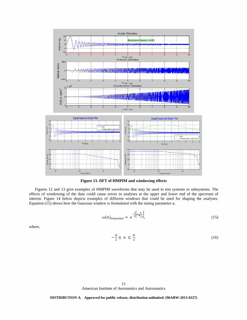
Figure 13. DFT of HMPIM and windowing effects

Figures 12 and 13 give examples of HMPIM waveforms that may be used to test systems or subsystems. The effects of windowing of the data could cause errors in analyses at the upper and lower end of the spectrum of interest. Figure 14 below depicts examples of different windows that could be used for shaping the analyses. Equation (15) shows how the Gaussian window is formulated with the tuning parameter α.

ω(𝑛)𝐺𝑎𝑢𝑠𝑠𝑖𝑎𝑛 = e−12�𝛼

𝑛𝑁 2�

�, (15)

where,

−N2≤ 𝑛 ≤ N

2. (16)



11

Figure 14. Time and frequency domain windowing examples

The Fast Fourier Transform (FFT) or Discrete Fourier Transform (DFT)4 will produce a spectral analysis of both the stimulus and response, and is used to determine the dynamic response of the item under test. The ratio of response to stimulus produces the frequency response of the test item,

𝑋(𝑘) = ∑ 𝑥(𝑗)𝜔𝑁(𝑗−1)(𝑘−1)𝑁

𝑗=1 , (17)

where 𝜔𝑁 = 𝑒(−2𝜋𝑖) 𝑁⁄ .

𝑇𝑟𝑎𝑛𝑠𝑓𝑒𝑟 𝐹𝑢𝑛𝑐𝑡𝑖𝑜𝑛 = 𝐹𝐹𝑇(𝑟𝑒𝑠𝑝𝑜𝑛𝑠𝑒)𝐹𝐹𝑇(𝑠𝑡𝑖𝑚𝑢𝑙𝑢𝑠)

= 𝑌(𝑗𝜔)𝑋(𝑗𝜔)

= 𝐺(𝑗𝜔) (18)

The transfer function is described in the frequency domain by the relation:

𝐺(𝑗𝜔) = 𝑅(𝑗𝜔) + 𝑗𝐼(𝑗𝜔), (19)

where

𝑅(𝑗𝜔) = 𝑅𝑒𝑎𝑙(𝐺(𝑗𝜔)), (20)

and

𝐼(𝑗𝜔) = 𝐼𝑚𝑎𝑔(𝐺(𝑗𝜔)) . (21)

Alternately, the transfer function can be represented by a magnitude |𝐺(𝑗𝜔)|and phase 𝜑(𝑗𝜔) as:

𝐺(𝑗𝜔) = |𝐺(𝑗𝜔)|𝑒𝑗𝜑(𝑗𝜔) = |𝐺(𝑗𝜔)|/𝜑(𝜔), (22)

where

𝜑(𝜔) = tan−1( 𝐼(𝑗𝜔)/ 𝑅(𝑗𝜔)), (23)

and

|𝐺(𝑗𝜔)|2 = (𝑅(𝑗𝜔))2 + (𝐼(𝑗𝜔))2. (24)



12

Figure 15 shows the frequency response (magnitude and phase) of an example seeker model and tracker when stimulated by a HMPIM waveform representing a true line of sight rate and measuring the resultant platform rate command. In the plots below, the frequency response exhibits a phase lag of 90 degrees at approximately 1.8 Hz. This is the basic measure of merit used to determine the effective system bandwidth.

Figure 15. Example seeker model frequency response

Figure 16 depicts how the frequency response5,6 of the system can be used to determine where the system dynamics natural frequency lies. In order to determine the natural frequency of the system dynamics, the phase lag from any pure delays in the measurement must be removed. Based on the processing delay (𝛿𝑝𝑟𝑜𝑐𝑒𝑠𝑠𝑖𝑛𝑔) calculated from the cross correlation analysis discussed in section IV.A, the phase lag due to the processing delay (𝜑(𝜔)𝑝𝑟𝑜𝑐𝑒𝑠𝑠𝑖𝑛𝑔) can be readily calculated as stated in Eq. (25).

𝜑(𝜔)𝑝𝑟𝑜𝑐𝑒𝑠𝑠𝑖𝑛𝑔 = −ω𝛿𝑝𝑟𝑜𝑐𝑒𝑠𝑠𝑖𝑛𝑔, (25)

Figure 16. HMPIM analyses of Bode plot

Given that each 1st order lag will add 45 degrees of phase lag at the natural frequency, if a quadratic lag is assumed for the system postulated above, then once the system phase lag is equal to 90 degrees below the phase lag



13

attributed to the processing delay, the system dynamic’s natural frequency can be determined. Once the natural frequency is determined, the damping ratio is determined by the hump in the magnitude plot as shown in Fig. 16.

Figure 17 shows the results of a HMPIM analysis on a sample model of a system with system dynamics consisting of a quadratic lag with a natural frequency of 10 Hz and a damping ratio of 0.4, measurement noise of 0.1 degrees (1σ), measurement bias of 0.6 degrees, and a pure delay of 150 msec. Then data were collected at 200 Hz and the HMPIM waveform used was a frequency sweep for 0.1 to 20 Hz with an n = 1.0 extinction of the signal. A Gaussian window with α = 1.5 was used in the frequency analyses.

As you can see from the analysis results the noise and bias were predicted within 3% of truth. The pure delay was predicted perfectly. (Note: the cross correlation’s capability to determine time delay is accurate only to one over the sample frequency, or in this case to +/- 5 ms.) The system dynamics were assumed to be a second order response and based on the total phase lag and the processing delay lag, the natural frequency of the system was predicted to be 9.83 Hz (modeled as 10 Hz). Based on the total system phase lag, the system exhibits a phase response (-90 degrees), or an effective bandwidth of 1.78 Hz. Notice the hump (~ 3 dB above DC) in the magnitude plot which is indicative of an under damped system (. i.e. a damping ratio < 0.7, and in this case 0.4).

Figure 17. Sample model parameter ID using HMPIM analyses

V. Data Collection and Analyses of AGWT 5-Axis Flight Motion Simulator

A. Data Collection A study was conducted using HMPIM techniques to characterize the AGWT 5-axis FMS under multiple

conditions of interest. Each axis was driven with: 1) position commands only; 2) position and velocity commands; and 3) position, velocity, and acceleration commands. In addition each set of tests was run at command frequencies of 500 and 1000 Hz, both of which are typical update rates for systems tested in the AGWT. The HMPIM waveforms used for testing were designed to incorporate enough spectral content to determine the bandwidth of the axis in test as well as stimulate the axis near its velocity and acceleration limits. The azimuth and elevation axes’ velocity and acceleration limits were lowered even further to protect the scene generator carried on these gimbals which is used to simulate vehicle to target geometry.



14

B. Data Analyses and Model Development Figure 18 depicts the HMPIM waveforms used to stimulate both the azimuth and elevation axes of the FMS and

their respective Bode plots with windowing. The stimuli in both cases sweep frequency from 0.1 to 20 Hz and have severe extinction of the signal at the higher frequencies to protect the image generator hardware. The expected performance bandwidths of these axes are 9.5 and 7 Hz respectively as stated back in Fig. 4. The goal is to stimulate the axes with sufficient signal across the spectrum of interest, in this case up to 10 Hz. As shown in Fig. 18, the signal level is above 30 dB at frequencies up to 10 Hz. And using a sample rate of 1000 Hz adds an additional 6 dB of signal. These should be sufficient to allow Fourier analyses over the spectrum of interest.

Figure 18. HMPIM stimuli and Bode plots for Az/El axes at 500 Hz and 1000 Hz

Figures 19 and 20 are the HMPIM analyses for azimuth and elevation axes respectively. Notice how there is little to no difference in bandwidth determination between the 500 and 1000 Hz update rates for these axes. Also notice how the performance of these axes differs from the stated bandwidths in Fig. 4. This is expected because the acceptance tests were done with a different mass and inertia than that of the scene generator presently housed on these gimbals. Bandwidth is proportional to the torque to inertia ratio of the gimbal and the HMPIM analyses here highlight an important feature of this parameter identification. Depending on the loads carried by the gimbals, the table will have differing performance. Also, the plant dynamics will have differing processing requirements in differing real time simulations. Within less than a minute of HMPIM testing and analyses, the performance characteristic of all axes of the FMS can be determined based on the loads carried and the update rate of the plant dynamics. These modeled characteristics of the FMS can now be used in a system level analysis with both hardware and plant dynamic models to determine whether the FMS performance adversely affects the real time simulation.



15

Figure 19. Azimuth axis 500 Hz and 1000 Hz HMPIM analyses

Figure 20. Elevation axis 500 Hz and 1000 Hz HMPIM analyses

Figure 21 shows the HMPIM analyses for pitch and yaw axes of the FMS. Their bandwidths differ from that stated in Fig. 4 because a different hardware mounting bracket was carried than that of the acceptance test mass.



16

Figure 21. Pitch and yaw axes 500 Hz HMPIM analyses

Figure 22 shows how the HMPIM analyses can be used to understand the linear performance range of a system or subsystem. Stimulating the pitch channel with HMPIM waveforms that drive maximum accelerations to differing levels will stimulate the nonlinear components of the system. The 8600 deg/sec2 stimuli start to excite the coulomb and viscous friction aspects of the gimbal during the last ½ second of the test (30 Hz region of the HMPIM). These nonlinear effects start to reduce the effective bandwidth of the system and our ability to use strictly linear analysis techniques.

Figure 22. HMPIM analyses nonlinear example



17

Figure 23 is an example of the picket fence effect stated previously in section IV.D.3. Using a higher sample rate for the analyses allows better HMPIM waveform generation at the higher frequencies as well as resolution in the Fourier analyses.

Figure 23. HMPIM analyses picket fence example

Finally, Figures 24 and 25 show the HMPIM analyses results when all axes of the FMS were stimulated with HMPIM waveforms simultaneously. Note: that with 10 seconds of data collection, all modeling parameters for the FMS were determined for all axes! Further inspection of the roll axis data and analysis shows that through cross coupling, the maximum acceleration limits where either exceeded or close to being exceeded. This caused the HMPIM automated software to calculate a lower effective bandwidth (~22 Hz) because of noise in the phase computation of the analysis. Closer inspection of the phase plot allows the user to determine a better estimate of bandwidth to be ~ 33 Hz.



18

Figure 24. HMPIM all axes simultaneous analyses (pitch, yaw, and roll)

Figure 25. HMPIM all axes simultaneous analyses (azimuth and elevation)



19

VI. Conclusions The HMPIM methodology and analyses developed by AFRL/RW utilizing the AGWT FMS enable the

characterization and model development of differing hardware and software methodologies as well general system performances. This parameter identification testing methodology coupled with digital signal processing allows the tester to test and determine salient modeling parameters in less than a minute of testing and analyses. Any hardware or software algorithm can be analyzed using suitable HMPIM stimuli and the analysis techniques described above with minimal asset risk and testing time.

References 1 Hébert, A., Mackin, P., "Dynamic model development utilizing the Advanced Guided Weapon Testbed facility’s flight

motion simulator at the Air Force Research Laboratory Munitions Directorate", AIAA Missile Sciences Conference, Monterey, Ca, 2012.

2 Ewing, C., “The Advanced Guided Weapon Testbed (AGWT) at the Air Force Research Laboratory Munitions Directorate”, AIAA Modeling and Simulation Technologies Conference, Chicago, IL 2009.

3 Crow, D., Coker, C. and Keen, W., "Fast line-of-sight imagery for target and exhaust-plume signatures (FLITES) scene generation program", SPIE Defense and Security Symposium, SPIE, Orlando, FL, 2006.

4 Stanley, W.D., Dougherty, G.R., and Dougherty, R., Digital Signal Processing, 2nd ed., Reston Publishing Company, Inc, Reston, Virginia 1984, Chaps. 2, 3, 4, and 5.

5 Dorf, R.C., Modern Control Systems, 3rd ed., Addison-Wesley Publishing Company, Reading, Massachusetts 1980, Chaps. 2, 3, 4, and 7.

6 Ogata, K., Modern Control Engineering, Prentice-Hall, Englewood Cliffs, N.J. 1970, Chaps. 2, 4, 6, 9, and 13.



20

advanced modeling and system parameter identification

Documents