advanced microeconomics...
TRANSCRIPT

Advanced Microeconomics Theory
Chapter 8: Imperfect Competition
Outline
• Basic Game Theory • Bertrand Model of Price Competition • Cournot Model of Quantity Competition • Product Differentiation • Dynamic Competition • Capacity Constraints • Endogenous Entry • Repeated Interaction
Advanced Microeconomic Theory 2

Introduction
• Monopoly: a single firm • Oligopoly: a limited number of firms
– When allowing for 𝑁𝑁 firms, the equilibrium predictions embody the results in perfectly competitive and monopoly markets as special cases.
Advanced Microeconomic Theory 3

Basic Game Theory
Advanced Microeconomic Theory 4

Basic Game Theory
• Consider a setting with 𝐽𝐽 firms, each with a strategy 𝑠𝑠𝑗𝑗 – Example: an output level, a price, or an advertising
expenditure. • Let (𝑠𝑠𝑗𝑗 , 𝑠𝑠−𝑗𝑗) denote a strategy profile where 𝑠𝑠−𝑗𝑗
represents the strategies selected by all firms 𝑘𝑘 ≠ 𝑗𝑗, i.e., 𝑠𝑠−𝑗𝑗 = (𝑠𝑠1, … , 𝑠𝑠𝑗𝑗−1, 𝑠𝑠𝑗𝑗+1, … , 𝑠𝑠𝐽𝐽).
• Strategy 𝑠𝑠𝑗𝑗∗ strictly dominates another strategy 𝑠𝑠𝑗𝑗
′ ≠ 𝑠𝑠𝑗𝑗∗
for firm 𝑗𝑗 if 𝜋𝜋𝑗𝑗(𝑠𝑠𝑗𝑗
∗, 𝑠𝑠−𝑗𝑗) > 𝜋𝜋𝑗𝑗(𝑠𝑠𝑗𝑗′, 𝑠𝑠−𝑗𝑗) for all 𝑠𝑠−𝑗𝑗
– That is, 𝑠𝑠𝑗𝑗∗ yields a higher profit than 𝑠𝑠𝑗𝑗
′ does, regardless of the strategy 𝑠𝑠−𝑗𝑗 selected by all of firm 𝑗𝑗’s rivals.
Advanced Microeconomic Theory 5

Firm B Low prices High prices
Firm A Low prices 5, 5 9, 1 High prices 1, 9 7, 7
Basic Game Theory • Payoff matrix (Normal Form Game)
Advanced Microeconomic Theory 6
• “Low prices” yields a higher payoff than “high prices” both when a firm’s rival chooses “low prices” and when it selects “high prices.” – “Low prices” is a strictly dominant strategy for both firms
(i.e., 𝑠𝑠𝑗𝑗∗).
– “High prices” is referred to as a strictly dominated strategy (i.e., 𝑠𝑠𝑗𝑗
′).

Basic Game Theory
• A strictly dominated strategy can be deleted from the set of strategies a rational player would use.
• This helps to reduce the number of strategies to consider as optimal for each player.
• In the above payoff matrix, both firms will select “low prices” in the unique equilibrium of the game.
• However, games do not always have a strictly dominated strategy.
Advanced Microeconomic Theory 7

Basic Game Theory
• 𝑈𝑈 is better than 𝐷𝐷 for firm 𝐴𝐴 if its opponent selects 𝐿𝐿, but becomes worse otherwise.
• Similarly, 𝐿𝐿 is better than 𝑅𝑅 for firm 𝐵𝐵 if its opponent chooses 𝑈𝑈, but becomes worse otherwise.
• Hence, no strictly dominated strategies for either player. Advanced Microeconomic Theory 8
Firm B L R
Firm A U 3, 1 0, 0 D 0, 0 1, 3

Basic Game Theory
• What is the equilibrium of the game then? – The Nash equilibrium solution concept
• A strategy profile (𝑠𝑠𝑗𝑗∗, 𝑠𝑠−𝑗𝑗
∗ ) is a Nash equilibrium (NE) if, for every player 𝑗𝑗,
𝜋𝜋𝑗𝑗 𝑠𝑠𝑗𝑗∗, 𝑠𝑠−𝑗𝑗
∗ ≥ 𝜋𝜋𝑗𝑗 𝑠𝑠𝑗𝑗 , 𝑠𝑠−𝑗𝑗∗ for every 𝑠𝑠𝑗𝑗 ≠ 𝑠𝑠𝑗𝑗
∗
– That is, 𝑠𝑠𝑗𝑗∗ is player 𝑗𝑗’s best response to his opponents
choosing 𝑠𝑠−𝑗𝑗∗ as 𝑠𝑠𝑗𝑗
∗ yields a better payoff than any of his available strategies 𝑠𝑠𝑗𝑗 ≠ 𝑠𝑠𝑗𝑗
∗.
Advanced Microeconomic Theory 9

Basic Game Theory
• In the above game: – Firm 𝐴𝐴’s best response to firm 𝐵𝐵’s playing 𝐿𝐿 is
𝐵𝐵𝑅𝑅𝐴𝐴 𝐿𝐿 = 𝑈𝑈, while to firm 𝐵𝐵 playing 𝑅𝑅 is 𝐵𝐵𝑅𝑅𝐴𝐴 𝑅𝑅 = 𝐷𝐷.
– Similarly, firm 𝐵𝐵’s best response to firm 𝐴𝐴 choosing 𝑈𝑈 is 𝐵𝐵𝑅𝑅𝐵𝐵 𝑈𝑈 = 𝐿𝐿, whereas to firm 𝐴𝐴 selecting 𝐷𝐷 is 𝐵𝐵𝑅𝑅𝐵𝐵 𝐷𝐷 = 𝑅𝑅.
– Hence, strategy profiles (𝑈𝑈, 𝐿𝐿) and (𝐷𝐷, 𝑅𝑅) are mutual best responses (i.e., the two Nash equilibria).
Advanced Microeconomic Theory 10

Bertrand Model of Price Competition
Advanced Microeconomic Theory 11

Bertrand Model of Price Competition
• Consider: – An industry with two firms, 1 and 2, selling a
homogeneous product – Firms face market demand 𝑥𝑥(𝑝𝑝), where 𝑥𝑥(𝑝𝑝) is
continuous and strictly decreasing in 𝑝𝑝 – There exists a high enough price (choke
price) �̅�𝑝 < ∞ such that 𝑥𝑥(𝑝𝑝) = 0 for all 𝑝𝑝 > �̅�𝑝 – Both firms are symmetric in their constant
marginal cost 𝑐𝑐 > 0, where 𝑥𝑥 𝑐𝑐 ∈ (0, ∞) – Every firm 𝑗𝑗 simultaneously sets a price 𝑝𝑝𝑗𝑗
Advanced Microeconomic Theory 12

Bertrand Model of Price Competition
• Firm 𝑗𝑗’s demand is
𝑥𝑥𝑗𝑗(𝑝𝑝𝑗𝑗 , 𝑝𝑝𝑘𝑘) =
𝑥𝑥(𝑝𝑝𝑗𝑗) if 𝑝𝑝𝑗𝑗 < 𝑝𝑝𝑘𝑘12
𝑥𝑥(𝑝𝑝𝑗𝑗) if 𝑝𝑝𝑗𝑗 = 𝑝𝑝𝑘𝑘
0 if 𝑝𝑝𝑗𝑗 > 𝑝𝑝𝑘𝑘
• Intuition: Firm 𝑗𝑗 captures – all market if its price is the lowest, 𝑝𝑝𝑗𝑗 < 𝑝𝑝𝑘𝑘 – no market if its price is the highest, 𝑝𝑝𝑗𝑗 > 𝑝𝑝𝑘𝑘 – shares the market with firm 𝑘𝑘 if the price of both
firms coincide, 𝑝𝑝𝑗𝑗 = 𝑝𝑝𝑘𝑘 Advanced Microeconomic Theory 13

Bertrand Model of Price Competition
• Given prices 𝑝𝑝𝑗𝑗 and 𝑝𝑝𝑘𝑘, firm 𝑗𝑗’s profits are therefore
(𝑝𝑝𝑗𝑗 − 𝑐𝑐) ∙ 𝑥𝑥𝑗𝑗 (𝑝𝑝𝑗𝑗 , 𝑝𝑝𝑘𝑘)
• We are now ready to find equilibrium prices in the Bertrand duopoly model. – There is a unique NE (𝑝𝑝𝑗𝑗
∗, 𝑝𝑝𝑘𝑘∗) in the Bertrand
duopoly model. In this equilibrium, both firms set prices equal to marginal cost, 𝑝𝑝𝑗𝑗
∗ = 𝑝𝑝𝑘𝑘∗ = 𝑐𝑐.
Advanced Microeconomic Theory 14

Bertrand Model of Price Competition
• Let’s us describe the best response function of firm 𝑗𝑗. • If 𝑝𝑝𝑘𝑘 < 𝑐𝑐, firm 𝑗𝑗 sets its price at 𝑝𝑝𝑗𝑗 = 𝑐𝑐.
– Firm 𝑗𝑗 does not undercut firm 𝑘𝑘 since that would entail negative profits.
• If 𝑐𝑐 < 𝑝𝑝𝑘𝑘 < 𝑝𝑝𝑗𝑗, firm 𝑗𝑗 slightly undercuts firm 𝑘𝑘, i.e., 𝑝𝑝𝑗𝑗 = 𝑝𝑝𝑘𝑘 − 𝜀𝜀. – This allows firm 𝑗𝑗 to capture all sales and still make a
positive margin on each unit. • If 𝑝𝑝𝑘𝑘 > 𝑝𝑝𝑚𝑚, where 𝑝𝑝𝑚𝑚 is a monopoly price, firm 𝑗𝑗 does
not need to charge more than 𝑝𝑝𝑚𝑚, i.e., 𝑝𝑝𝑗𝑗 = 𝑝𝑝𝑚𝑚. – 𝑝𝑝𝑚𝑚 allows firm 𝑗𝑗 to capture all sales and maximize profits
as the only firm selling a positive output.
Advanced Microeconomic Theory 15

pj
pk
pm
pm
c
c
pj (pk)
45°-line (pj = pk)
Bertrand Model of Price Competition
• Firm 𝑗𝑗’s best response has: – a flat segment for all
𝑝𝑝𝑘𝑘 < 𝑐𝑐, where 𝑝𝑝𝑗𝑗(𝑝𝑝𝑘𝑘) = 𝑐𝑐
– a positive slope for all 𝑐𝑐 < 𝑝𝑝𝑘𝑘 < 𝑝𝑝𝑗𝑗, where firm 𝑗𝑗 charges a price slightly below firm 𝑘𝑘
– a flat segment for all 𝑝𝑝𝑘𝑘 > 𝑝𝑝𝑚𝑚, where 𝑝𝑝𝑗𝑗(𝑝𝑝𝑘𝑘) = 𝑝𝑝𝑚𝑚
Advanced Microeconomic Theory 16

pj
pk
c
c
pj (pk)
pk (pj)
pm
pm
45°-line (pj = pk)
Bertrand Model of Price Competition
• A symmetric argument applies to the construction of the best response function of firm 𝑘𝑘.
• A mutual best response for both firms is
(𝑝𝑝1∗, 𝑝𝑝2
∗) = (𝑐𝑐, 𝑐𝑐) where the two best response functions cross each other.
• This is the NE of the Bertrand model – Firms make no economic
profits.
Advanced Microeconomic Theory 17

Bertrand Model of Price Competition
• With only two firms competing in prices we obtain the perfectly competitive outcome, where firms set prices equal to marginal cost.
• Price competition makes each firm 𝑗𝑗 face an infinitely elastic demand curve at its rival’s price, 𝑝𝑝𝑘𝑘. – Any increase (decrease) from 𝑝𝑝𝑘𝑘 infinitely reduces
(increases, respectively) firm 𝑗𝑗’s demand.
Advanced Microeconomic Theory 18

Bertrand Model of Price Competition
• How much does Bertrand equilibrium hinge into our assumptions? – Quite a lot
• The competitive pressure in the Bertrand model with homogenous products is ameliorated if we instead consider: – Price competition (but allowing for heterogeneous
products) – Quantity competition (still with homogenous
products) – Capacity constraints
Advanced Microeconomic Theory 19

Bertrand Model of Price Competition
• Remark: – How our results would be affected if firms face
different production costs, i.e., 0 < 𝑐𝑐1 < 𝑐𝑐2? – The most efficient firm sets a price equal to the
marginal cost of the least efficient firm, 𝑝𝑝1 = 𝑐𝑐2. – Other firms will set a random price in the uniform
interval [𝑐𝑐1, 𝑐𝑐1 + 𝜂𝜂]
where 𝜂𝜂 > 0 is some small random increment with probability distribution 𝑓𝑓 𝑝𝑝, 𝜂𝜂 > 0 for all 𝑝𝑝.
Advanced Microeconomic Theory 20

Cournot Model of Quantity Competition
Advanced Microeconomic Theory 21
Cournot Model of Quantity Competition
• Let us now consider that firms compete in quantities.
• Assume that: – Firms bring their output 𝑞𝑞1 and 𝑞𝑞2 to a market, the
market clears, and the price is determined from the inverse demand function 𝑝𝑝(𝑞𝑞), where 𝑞𝑞 = 𝑞𝑞1 + 𝑞𝑞2.
– 𝑝𝑝(𝑞𝑞) satisfies 𝑝𝑝𝑝(𝑞𝑞) < 0 at all output levels 𝑞𝑞 ≥ 0, – Both firms face a common marginal cost 𝑐𝑐 > 0 – 𝑝𝑝(0) > 𝑐𝑐 in order to guarantee that the inverse
demand curve crosses the constant marginal cost curve at an interior point.
Advanced Microeconomic Theory 22

Cournot Model of Quantity Competition
• Let us first identify every firm’s best response function
• Firm 1’s PMP, for a given output level of its rival, 𝑞𝑞�2,
max 𝑞𝑞1≥0
𝑝𝑝 𝑞𝑞1 + 𝑞𝑞�2Price
𝑞𝑞1 − 𝑐𝑐𝑞𝑞1
• When solving this PMP, firm 1 treats firm 2’s production, 𝑞𝑞�2, as a parameter, since firm 1 cannot vary its level.
Advanced Microeconomic Theory 23

Cournot Model of Quantity Competition
• FOCs: 𝑝𝑝′(𝑞𝑞1 + 𝑞𝑞�2)𝑞𝑞1 + 𝑝𝑝(𝑞𝑞1 + 𝑞𝑞�2) − 𝑐𝑐 ≤ 0
with equality if 𝑞𝑞1 > 0 • Solving this expression for 𝑞𝑞1, we obtain firm 1’s
best response function (BRF), 𝑞𝑞1(𝑞𝑞�2). • A similar argument applies to firm 2’s PMP and its
best response function 𝑞𝑞2(𝑞𝑞�1). • Therefore, a pair of output levels (𝑞𝑞1
∗, 𝑞𝑞2∗) is NE of
the Cournot model if and only if 𝑞𝑞1
∗ ∈ 𝑞𝑞1(𝑞𝑞�2) for firm 1’s output 𝑞𝑞2
∗ ∈ 𝑞𝑞2(𝑞𝑞�1) for firm 2’s output Advanced Microeconomic Theory 24

Cournot Model of Quantity Competition
• To show that 𝑞𝑞1∗, 𝑞𝑞2
∗ > 0, let us work by contradiction, assuming 𝑞𝑞1
∗ = 0. – Firm 2 becomes a monopolist since it is the only firm
producing a positive output. • Using the FOC for firm 1, we obtain
𝑝𝑝′(0 + 𝑞𝑞2∗)0 + 𝑝𝑝(0 + 𝑞𝑞2
∗) ≤ 𝑐𝑐 or 𝑝𝑝(𝑞𝑞2
∗) ≤ 𝑐𝑐 • And using the FOC for firm 2, we have
𝑝𝑝′(𝑞𝑞2∗ + 0)𝑞𝑞2
∗ + 𝑝𝑝(𝑞𝑞2∗ + 0) ≤ 𝑐𝑐
or 𝑝𝑝′(𝑞𝑞2∗)𝑞𝑞2
∗ + 𝑝𝑝(𝑞𝑞2∗) ≤ 𝑐𝑐
• This implies firm 2’s MR under monopoly is lower than its MC. Thus, 𝑞𝑞2
∗ = 0. Advanced Microeconomic Theory 25

Cournot Model of Quantity Competition
• Hence, if 𝑞𝑞1∗ = 0, firm 2’s output would also be
zero, 𝑞𝑞2∗ = 0.
• But this implies that 𝑝𝑝(0) < 𝑐𝑐 since no firm produces a positive output, thus violating our initial assumption 𝑝𝑝(0) > 𝑐𝑐. – Contradiction!
• As a result, we must have that both 𝑞𝑞1∗ > 0 and
𝑞𝑞2∗ > 0.
• Note: This result does not necessarily hold when both firms are asymmetric in their production cost.
Advanced Microeconomic Theory 26

Cournot Model of Quantity Competition
• Example (symmetric costs): – Consider an inverse demand curve 𝑝𝑝(𝑞𝑞) = 𝑎𝑎 −
𝑏𝑏𝑞𝑞, and two firms competing à la Cournot both facing a marginal cost 𝑐𝑐 > 0.
– Firm 1’s PMP is 𝑎𝑎 − 𝑏𝑏(𝑞𝑞1 + 𝑞𝑞�2) 𝑞𝑞1 − 𝑐𝑐𝑞𝑞1
– FOC wrt 𝑞𝑞1: 𝑎𝑎 − 2𝑏𝑏𝑞𝑞1 − 𝑏𝑏𝑞𝑞�2 − 𝑐𝑐 ≤ 0
with equality if 𝑞𝑞1 > 0 Advanced Microeconomic Theory 27

Cournot Model of Quantity Competition
• Example (continue): – Solving for 𝑞𝑞1, we obtain firm 1’s BRF
𝑞𝑞1(𝑞𝑞�2) = 𝑎𝑎−𝑐𝑐2𝑏𝑏
− 𝑞𝑞�22
– Analogously, firm 2’s BRF
𝑞𝑞2(𝑞𝑞�1) = 𝑎𝑎−𝑐𝑐2𝑏𝑏
− 𝑞𝑞�12
Advanced Microeconomic Theory 28

Cournot Model of Quantity Competition
Advanced Microeconomic Theory 29
• Firm 1’s BRF: – When 𝑞𝑞2 = 0, then
𝑞𝑞1 = 𝑎𝑎−𝑐𝑐2𝑏𝑏
, which coincides with its output under monopoly.
– As 𝑞𝑞2 increases, 𝑞𝑞1 decreases (i.e., firm 1’s and 2’s output are strategic substitutes)
– When 𝑞𝑞2 = 𝑎𝑎−𝑐𝑐𝑏𝑏
, then 𝑞𝑞1 = 0.

Cournot Model of Quantity Competition
Advanced Microeconomic Theory 30
• A similar argument applies for firm 2’s BRF.
• Superimposing both firms’ BRFs, we obtain the Cournot equilibrium output pair (𝑞𝑞1
∗, 𝑞𝑞2∗).

Cournot Model of Quantity Competition
Advanced Microeconomic Theory 31
q1
q2
a – c
q1(q2)
2bq2(q1)
a – cb
a – cb
a – c2b
a – c3b
a – c3b
(q1,q2 ) * *
45°-line (q1 = q2)q1 + q2 = qc = a – cb
q1 + q2 = qm = a – c2b
Perfect competition
Monopoly
45°

Cournot Model of Quantity Competition
• Cournot equilibrium output pair (𝑞𝑞1∗, 𝑞𝑞2
∗) occurs at the intersection of the two BRFs, i.e.,
(𝑞𝑞1∗, 𝑞𝑞2
∗) = 𝑎𝑎−𝑐𝑐3𝑏𝑏
, 𝑎𝑎−𝑐𝑐3𝑏𝑏
• Aggregate output becomes
𝑞𝑞∗ = 𝑞𝑞1∗ + 𝑞𝑞2
∗ = 𝑎𝑎−𝑐𝑐3𝑏𝑏
+ 𝑎𝑎−𝑐𝑐3𝑏𝑏
= 2(𝑎𝑎−𝑐𝑐)3𝑏𝑏
which is larger than under monopoly, 𝑞𝑞𝑚𝑚 = 𝑎𝑎−𝑐𝑐2𝑏𝑏
, but smaller than under perfect competition, 𝑞𝑞𝑐𝑐 = 𝑎𝑎−𝑐𝑐
𝑏𝑏.
Advanced Microeconomic Theory 32

Cournot Model of Quantity Competition
• The equilibrium price becomes
𝑝𝑝 𝑞𝑞∗ = 𝑎𝑎 − 𝑏𝑏𝑞𝑞∗ = 𝑎𝑎 − 𝑏𝑏 2 𝑎𝑎−𝑐𝑐3𝑏𝑏
= 𝑎𝑎+2𝑐𝑐3
which is lower than under monopoly, 𝑝𝑝𝑚𝑚 = 𝑎𝑎+𝑐𝑐2
, but higher than under perfect competition, 𝑝𝑝𝑐𝑐 = 𝑐𝑐.
• Finally, the equilibrium profits of every firm 𝑗𝑗
𝜋𝜋𝑗𝑗∗ = 𝑝𝑝 𝑞𝑞∗ 𝑞𝑞𝑗𝑗
∗ − 𝑐𝑐𝑞𝑞𝑗𝑗∗ = 𝑎𝑎+2𝑐𝑐
3𝑎𝑎−𝑐𝑐3𝑏𝑏
− 𝑐𝑐 𝑎𝑎−𝑐𝑐3𝑏𝑏
= 𝑎𝑎−𝑐𝑐 2
9𝑏𝑏
which are lower than under monopoly, 𝜋𝜋𝑚𝑚 = 𝑎𝑎−𝑐𝑐 2
4𝑏𝑏,
but higher than under perfect competition, 𝜋𝜋𝑐𝑐 = 0.
Advanced Microeconomic Theory 33

Cournot Model of Quantity Competition
• Quantity competition (Cournot model) yields less competitive outcomes than price competition (Bertrand model), whereby firms’ behavior mimics that in perfectly competitive markets – That’s because, the demand that every firm faces in
the Cournot game is not infinitely elastic. – A reduction in output does not produce an infinite
increase in market price, but instead an increase of − 𝑝𝑝′(𝑞𝑞1 + 𝑞𝑞2).
– Hence, if firms produce the same output as under marginal cost pricing, i.e., half of 𝑎𝑎−𝑐𝑐
2, each firm would
have incentives to deviate from such a high output level by marginally reducing its output.
Advanced Microeconomic Theory 34

Cournot Model of Quantity Competition
• Equilibrium output under Cournot does not coincide with the monopoly output either. – That’s because, every firm 𝑖𝑖, individually increasing its
output level 𝑞𝑞𝑖𝑖, takes into account how the reduction in market price affects its own profits, but ignores the profit loss (i.e., a negative external effect) that its rival suffers from such a lower price.
– Since every firm does not take into account this external effect, aggregate output is too large, relative to the output that would maximize firms’ joint profits.
Advanced Microeconomic Theory 35
Cournot Model of Quantity Competition
• Example (Cournot vs. Cartel): – Let us demonstrate that firms’ Cournot output is
larger than that under the cartel. – PMP of the cartel is
max𝑞𝑞1,𝑞𝑞2
(𝑎𝑎 − 𝑏𝑏(𝑞𝑞1+𝑞𝑞2))𝑞𝑞1 − 𝑐𝑐𝑞𝑞1
+ (𝑎𝑎 − 𝑏𝑏(𝑞𝑞1+𝑞𝑞2))𝑞𝑞2 − 𝑐𝑐𝑞𝑞2 – Since 𝑄𝑄 = 𝑞𝑞1 + 𝑞𝑞2, the PMP can be written as
max𝑞𝑞1,𝑞𝑞2
𝑎𝑎 − 𝑏𝑏(𝑞𝑞1+𝑞𝑞2) (𝑞𝑞1+𝑞𝑞2) − 𝑐𝑐(𝑞𝑞1+𝑞𝑞2)
= max𝑄𝑄
𝑎𝑎 − 𝑏𝑏𝑄𝑄 𝑄𝑄 − 𝑐𝑐𝑄𝑄 = 𝑎𝑎𝑄𝑄 − 𝑏𝑏𝑄𝑄2 − 𝑐𝑐𝑄𝑄
Advanced Microeconomic Theory 36

Cournot Model of Quantity Competition
• Example (continued): – FOC with respect to 𝑄𝑄
𝑎𝑎 − 2𝑏𝑏𝑄𝑄 − 𝑐𝑐 ≤ 0 – Solving for 𝑄𝑄, we obtain the aggregate output
𝑄𝑄∗ = 𝑎𝑎−𝑐𝑐2𝑏𝑏
which is positive since 𝑎𝑎 > 𝑐𝑐, i.e., 𝑝𝑝(0) = 𝑎𝑎 > 𝑐𝑐. – Since firms are symmetric in costs, each produces
𝑞𝑞𝑖𝑖 = 𝑄𝑄2
= 𝑎𝑎−𝑐𝑐4𝑏𝑏
Advanced Microeconomic Theory 37

Cournot Model of Quantity Competition
• Example (continued): – The equilibrium price is
𝑝𝑝 = 𝑎𝑎 − 𝑏𝑏𝑄𝑄 = 𝑎𝑎 − 𝑏𝑏 𝑎𝑎−𝑐𝑐2𝑏𝑏
= 𝑎𝑎+𝑐𝑐2
– Finally, the equilibrium profits are 𝜋𝜋𝑖𝑖 = 𝑝𝑝 ⋅ 𝑞𝑞𝑖𝑖 − 𝑐𝑐𝑞𝑞𝑖𝑖
= 𝑎𝑎+𝑐𝑐2
⋅ 𝑎𝑎−𝑐𝑐4𝑏𝑏
− 𝑐𝑐 𝑎𝑎−𝑐𝑐4𝑏𝑏
= 𝑎𝑎−𝑐𝑐 2
8𝑏𝑏
which is larger than firms would obtain under
Cournot competition, 𝑎𝑎−𝑐𝑐 2
9𝑏𝑏.
Advanced Microeconomic Theory 38

Cournot Model of Quantity Competition: Cournot Pricing Rule
• Firms’ market power can be expressed using a variation of the Lerner index. – Consider firm 𝑗𝑗’s profit maximization problem
𝜋𝜋𝑗𝑗 = 𝑝𝑝(𝑞𝑞)𝑞𝑞𝑗𝑗 − 𝑐𝑐𝑗𝑗(𝑞𝑞𝑗𝑗) – FOC for every firm 𝑗𝑗
𝑝𝑝′ 𝑞𝑞 𝑞𝑞𝑗𝑗 + 𝑝𝑝 𝑞𝑞 − 𝑐𝑐𝑗𝑗 = 0 or 𝑝𝑝(𝑞𝑞) − 𝑐𝑐𝑗𝑗 = −𝑝𝑝′ 𝑞𝑞 𝑞𝑞𝑗𝑗
– Multiplying both sides by 𝑞𝑞 and dividing them by 𝑝𝑝(𝑞𝑞) yield
𝑞𝑞𝑝𝑝 𝑞𝑞 − 𝑐𝑐𝑗𝑗
𝑝𝑝(𝑞𝑞)=
−𝑝𝑝′ 𝑞𝑞 𝑞𝑞𝑗𝑗
𝑝𝑝(𝑞𝑞)𝑞𝑞
Advanced Microeconomic Theory 39

Cournot Model of Quantity Competition: Cournot Pricing Rule
– Recalling 1𝜀𝜀
= −𝑝𝑝′ 𝑞𝑞 ⋅ 𝑞𝑞𝑝𝑝 𝑞𝑞
, we have
𝑞𝑞 𝑝𝑝 𝑞𝑞 −𝑐𝑐𝑗𝑗
𝑝𝑝(𝑞𝑞)= 1
𝜀𝜀𝑞𝑞𝑗𝑗
or 𝑝𝑝 𝑞𝑞 −𝑐𝑐𝑗𝑗
𝑝𝑝(𝑞𝑞)= 1
𝜀𝜀𝑞𝑞𝑗𝑗
𝑞𝑞
– Defining 𝛼𝛼𝑗𝑗 ≡ 𝑞𝑞𝑗𝑗
𝑞𝑞 as firm 𝑗𝑗’s market share, we obtain
𝑝𝑝 𝑞𝑞 − 𝑐𝑐𝑗𝑗
𝑝𝑝(𝑞𝑞)=
𝛼𝛼𝑗𝑗
𝜀𝜀
which is referred to as the Cournot pricing rule. Advanced Microeconomic Theory 40

Cournot Model of Quantity Competition: Cournot Pricing Rule
– Note: When 𝛼𝛼𝑗𝑗 = 1, implying that firm 𝑗𝑗 is a monopoly, the
IEPR becomes a special case of the Cournot price rule. The larger the market share 𝛼𝛼𝑗𝑗 of a given firm, the
larger the price markup of firm 𝑗𝑗. The more inelastic demand 𝜀𝜀 is, the larger the price
markup of firm 𝑗𝑗.
Advanced Microeconomic Theory 41
Cournot Model of Quantity Competition: Cournot Pricing Rule
• Example (Merger effects on Cournot Prices): – Consider an industry with 𝑛𝑛 firms and a constant-
elasticity demand function 𝑞𝑞(𝑝𝑝) = 𝑎𝑎𝑝𝑝−1, where 𝑎𝑎 > 0 and 𝜀𝜀 = 1.
– Before merger, we have 𝑝𝑝𝐵𝐵 − 𝑐𝑐
𝑝𝑝𝐵𝐵 =1𝑛𝑛
⟹ 𝑝𝑝𝐵𝐵 =𝑛𝑛𝑐𝑐
𝑛𝑛 − 1
– After the merger of 𝑘𝑘 < 𝑛𝑛 firms 𝑛𝑛 − 𝑘𝑘 + 1 firms remain in the industry, and thus
𝑝𝑝𝐴𝐴 − 𝑐𝑐𝑝𝑝𝐴𝐴 =
1𝑛𝑛 − 𝑘𝑘 + 1
⟹ 𝑝𝑝𝐴𝐴 =𝑛𝑛 − 𝑘𝑘 + 1 𝑐𝑐
𝑛𝑛 − 𝑘𝑘
Advanced Microeconomic Theory 42

Cournot Model of Quantity Competition: Cournot Pricing Rule
• Example (continued): – The percentage change in prices is
%Δ𝑝𝑝 =𝑝𝑝𝐴𝐴 − 𝑝𝑝𝐵𝐵
𝑝𝑝𝐵𝐵 =𝑛𝑛 − 𝑘𝑘 + 1 𝑐𝑐
𝑛𝑛 − 𝑘𝑘 − 𝑛𝑛𝑐𝑐𝑛𝑛 − 1
𝑛𝑛𝑐𝑐𝑛𝑛 − 1
=𝑘𝑘 − 1
𝑛𝑛(𝑛𝑛 − 𝑘𝑘)> 0
– Hence, prices increase after the merger. – Also, %Δ𝑝𝑝 increases as the number of merging firms
𝑘𝑘 increases 𝜕𝜕𝜕Δ𝑝𝑝
𝜕𝜕𝑘𝑘=
𝑛𝑛 − 1𝑛𝑛 𝑛𝑛 − 𝑘𝑘 2 > 0
Advanced Microeconomic Theory 43

%Δp
k20 40 60 80 100
0.10
0.20 %Δp(k)
Cournot Model of Quantity Competition: Cournot Pricing Rule
• Example (continued): – The percentage
increase in price after the merger, %Δ𝑝𝑝, as a function of the number of merging firms, 𝑘𝑘.
– For simplicity, 𝑛𝑛 =100.
Advanced Microeconomic Theory 44

Cournot Model of Quantity Competition: SOC
• Let us check if the first order (necessary) conditions are also sufficient.
• Recall that FOCs are 𝑝𝑝′ 𝑞𝑞 𝑞𝑞𝑗𝑗 + 𝑝𝑝 𝑞𝑞 − 𝑐𝑐𝑗𝑗
′(𝑞𝑞𝑗𝑗) ≤ 0 • Differentiating FOCs wrt 𝑞𝑞𝑗𝑗 yields
𝑝𝑝′′ 𝑞𝑞 𝑞𝑞𝑗𝑗 + 𝑝𝑝′ 𝑞𝑞 + 𝑝𝑝′ 𝑞𝑞 − 𝑐𝑐𝑗𝑗′′(𝑞𝑞𝑗𝑗) ≤ 0
– 𝑝𝑝′ 𝑞𝑞 < 0: by definition (negatively sloped inverse demand curve)
– 𝑐𝑐𝑗𝑗′′(𝑞𝑞𝑗𝑗) ≥ 0: by assumption (constant or increasing
marginal costs) – 𝑝𝑝′′ 𝑞𝑞 𝑞𝑞𝑗𝑗 ≤ 0: as long as the demand curve decreases at a
constant or decreasing rate Advanced Microeconomic Theory 45

Cournot Model of Quantity Competition: SOC
• Example (linear demand): – The linear inverse demand curve is 𝑝𝑝(𝑞𝑞) = 𝑎𝑎 − 𝑏𝑏𝑞𝑞
and constant marginal cost is 𝑐𝑐 > 0. – Since 𝑝𝑝′ 𝑞𝑞 = −𝑏𝑏 < 0, 𝑝𝑝′′ 𝑞𝑞 = 0, 𝑐𝑐′ 𝑞𝑞 = 𝑐𝑐 and
𝑐𝑐′′(𝑞𝑞) = 0, the SOC reduces to
0 − 2𝑏𝑏 − 0 = −2𝑏𝑏 < 0
where 𝑏𝑏 > 0 by definition. – Hence the equilibrium output is indeed profit
maximizing. Advanced Microeconomic Theory 46

Cournot Model of Quantity Competition: SOC
• Note that SOCs coincides with the cross-derivative
𝜕𝜕2𝜋𝜋𝑗𝑗
𝜕𝜕𝑞𝑞𝑗𝑗𝜕𝜕𝑞𝑞𝑘𝑘=
𝜕𝜕𝜕𝜕𝑞𝑞𝑘𝑘
𝑝𝑝′ 𝑞𝑞 𝑞𝑞𝑗𝑗 + 𝑝𝑝 𝑞𝑞 − 𝑐𝑐′(𝑞𝑞𝑗𝑗)
= 𝑝𝑝′′ 𝑞𝑞 𝑞𝑞𝑗𝑗 − 𝑝𝑝′ 𝑞𝑞 for all 𝑘𝑘 ≠ 𝑗𝑗. • Hence, the firm 𝑗𝑗’s BRF decreases in 𝑞𝑞𝑘𝑘 as long as
𝑝𝑝′′ 𝑞𝑞 𝑞𝑞𝑗𝑗 − 𝑝𝑝′ 𝑞𝑞 < 0 – That is, firm 𝑗𝑗’s BRF is negatively sloped.
Advanced Microeconomic Theory 47
Cournot Model of Quantity Competition: Asymmetric Costs
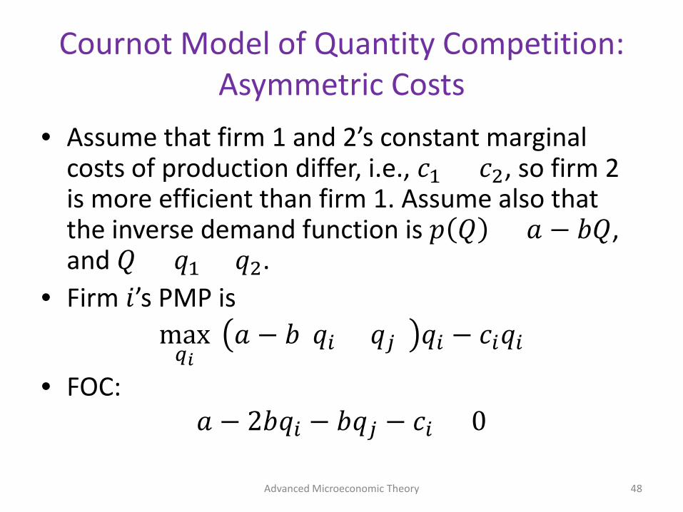
• Assume that firm 1 and 2’s constant marginal costs of production differ, i.e., 𝑐𝑐1 > 𝑐𝑐2, so firm 2 is more efficient than firm 1. Assume also that the inverse demand function is 𝑝𝑝 𝑄𝑄 = 𝑎𝑎 − 𝑏𝑏𝑄𝑄, and 𝑄𝑄 = 𝑞𝑞1 + 𝑞𝑞2.
• Firm 𝑖𝑖’s PMP is max
𝑞𝑞𝑖𝑖 𝑎𝑎 − 𝑏𝑏(𝑞𝑞𝑖𝑖 + 𝑞𝑞𝑗𝑗) 𝑞𝑞𝑖𝑖 − 𝑐𝑐𝑖𝑖𝑞𝑞𝑖𝑖
• FOC: 𝑎𝑎 − 2𝑏𝑏𝑞𝑞𝑖𝑖 − 𝑏𝑏𝑞𝑞𝑗𝑗 − 𝑐𝑐𝑖𝑖 = 0
Advanced Microeconomic Theory 48

Cournot Model of Quantity Competition: Asymmetric Costs
• Solving for 𝑞𝑞𝑖𝑖 (assuming an interior solution) yields firm 𝑖𝑖’s BRF
𝑞𝑞𝑖𝑖(𝑞𝑞𝑗𝑗) =𝑎𝑎 − 𝑐𝑐𝑖𝑖
2𝑏𝑏−
𝑞𝑞𝑗𝑗
2
• Firm 1’s optimal output level can be found by plugging firm 2’s BRF into firm 1’s
𝑞𝑞1∗ =
𝑎𝑎 − 𝑐𝑐1
2𝑏𝑏−
12
𝑎𝑎 − 𝑐𝑐2
2𝑏𝑏−
𝑞𝑞1∗
2⟺ 𝑞𝑞1
∗ =𝑎𝑎 − 2𝑐𝑐1 + 𝑐𝑐2
3𝑏𝑏
• Similarly, firm 2’s optimal output level is
𝑞𝑞2∗ =
𝑎𝑎 − 𝑐𝑐2
2𝑏𝑏−
𝑞𝑞1∗
2=
𝑎𝑎 + 𝑐𝑐1 − 2𝑐𝑐2
3𝑏𝑏
Advanced Microeconomic Theory 49

Cournot Model of Quantity Competition: Asymmetric Costs
• If firm 𝑖𝑖’s costs are sufficiently high it will not produce at all. – Firm 1: 𝑞𝑞1
∗ ≤ 0 if 𝑎𝑎+𝑐𝑐22
≤ 𝑐𝑐1
– Firm 2: 𝑞𝑞2∗ ≤ 0 if 𝑎𝑎+𝑐𝑐1
2≤ 𝑐𝑐2
• Thus, we can identify three different cases: – If 𝑐𝑐𝑖𝑖 ≥
𝑎𝑎+𝑐𝑐𝑗𝑗
2 for all firms 𝑖𝑖 = {1,2}, no firm produces a
positive output – If 𝑐𝑐𝑖𝑖 ≥
𝑎𝑎+𝑐𝑐𝑗𝑗
2 but 𝑐𝑐𝑗𝑗 < 𝑎𝑎+𝑐𝑐𝑖𝑖
2, then only firm 𝑗𝑗 produces
positive output – If 𝑐𝑐𝑖𝑖 <
𝑎𝑎+𝑐𝑐𝑗𝑗
2 for all firms 𝑖𝑖 = {1,2}, both firms produce
positive output Advanced Microeconomic Theory 50

c2
c1
a
a
45° (c1 = c2)a + c2
2c1 =
a + c12c2 =
a2
a2
No firmsproduce
Both firmsproduce
Only firm 1produces
Only firm 2produces
Cournot Model of Quantity Competition: Asymmetric Costs
Advanced Microeconomic Theory 51

Cournot Model of Quantity Competition: Asymmetric Costs
• The output levels (𝑞𝑞1∗, 𝑞𝑞2
∗) also vary when (𝑐𝑐1, 𝑐𝑐2) changes
𝜕𝜕𝑞𝑞1∗
𝜕𝜕𝑐𝑐1= −
23𝑏𝑏
< 0 and 𝜕𝜕𝑞𝑞1
∗
𝜕𝜕𝑐𝑐2=
13𝑏𝑏
> 0
𝜕𝜕𝑞𝑞2∗
𝜕𝜕𝑐𝑐1=
13𝑏𝑏
> 0 and 𝜕𝜕𝑞𝑞2
∗
𝜕𝜕𝑐𝑐2= −
23𝑏𝑏
< 0
• Intuition: Each firm’s output decreases in its own costs, but increases in its rival’s costs.
Advanced Microeconomic Theory 52

q1
q2a – c2 2b
a – c1 2b
a – c1 b
a – c2 b
(q1,q2 ) * *
q1(q2)
q2(q1)
Cournot Model of Quantity Competition: Asymmetric Costs
• BRFs for firms 1 and 2 when 𝑐𝑐1 > 𝑎𝑎+𝑐𝑐2
2 (i.e.,
only firm 2 produces).
• BRFs cross at the vertical axis where 𝑞𝑞1
∗ = 0 and 𝑞𝑞2
∗ > 0 (i.e., a corner solution)
Advanced Microeconomic Theory 53

Cournot Model of Quantity Competition: 𝐽𝐽 > 2 firms
• Consider 𝐽𝐽 > 2 firms, all facing the same constant marginal cost 𝑐𝑐 > 0. The linear inverse demand curve is 𝑝𝑝 𝑄𝑄 = 𝑎𝑎 − 𝑏𝑏𝑄𝑄, where 𝑄𝑄 = ∑ 𝑞𝑞𝑘𝑘𝐽𝐽 .
• Firm 𝑖𝑖’s PMP is
max𝑞𝑞𝑖𝑖
𝑎𝑎 − 𝑏𝑏 𝑞𝑞𝑖𝑖 + � 𝑞𝑞𝑘𝑘𝑘𝑘≠𝑖𝑖
𝑞𝑞𝑖𝑖 − 𝑐𝑐𝑞𝑞𝑖𝑖
• FOC:
𝑎𝑎 − 2𝑏𝑏𝑞𝑞𝑖𝑖∗ − 𝑏𝑏 � 𝑞𝑞𝑘𝑘
∗
𝑘𝑘≠𝑖𝑖
− 𝑐𝑐 ≤ 0
Advanced Microeconomic Theory 54

Cournot Model of Quantity Competition: 𝐽𝐽 > 2 firms
• Solving for 𝑞𝑞𝑖𝑖∗, we obtain firm 𝑖𝑖’s BRF
𝑞𝑞𝑖𝑖∗ =
𝑎𝑎 − 𝑐𝑐2𝑏𝑏
−12 � 𝑞𝑞𝑘𝑘
∗
𝑘𝑘≠𝑖𝑖
• Since all firms are symmetric, their BRFs are also symmetric, implying 𝑞𝑞1
∗ = 𝑞𝑞2∗ = ⋯ = 𝑞𝑞𝐽𝐽
∗. This implies ∑ 𝑞𝑞𝑘𝑘
∗𝑘𝑘≠𝑖𝑖 = 𝐽𝐽𝑞𝑞𝑖𝑖
∗ − 𝑞𝑞𝑖𝑖∗ = 𝐽𝐽 − 1 𝑞𝑞𝑖𝑖
∗. • Hence, the BRF becomes
𝑞𝑞𝑖𝑖∗ =
𝑎𝑎 − 𝑐𝑐2𝑏𝑏
−12
𝐽𝐽 − 1 𝑞𝑞𝑖𝑖∗
Advanced Microeconomic Theory 55

Cournot Model of Quantity Competition: 𝐽𝐽 > 2 firms
• Solving for 𝑞𝑞𝑖𝑖∗
𝑞𝑞𝑖𝑖∗ =
𝑎𝑎 − 𝑐𝑐𝐽𝐽 + 1 𝑏𝑏
which is also the equilibrium output for other 𝐽𝐽 − 1 firms.
• Therefore, aggregate output is
𝑄𝑄∗ = 𝐽𝐽𝑞𝑞𝑖𝑖∗ =
𝐽𝐽𝐽𝐽 + 1
𝑎𝑎 − 𝑐𝑐𝑏𝑏
and the corresponding equilibrium price is
𝑝𝑝∗ = 𝑎𝑎 − 𝑏𝑏𝑄𝑄∗ =𝑎𝑎 + 𝐽𝐽𝑐𝑐𝐽𝐽 + 1
Advanced Microeconomic Theory 56

Cournot Model of Quantity Competition: 𝐽𝐽 > 2 firms
• Firm 𝑖𝑖’s equilibrium profits are 𝜋𝜋𝑖𝑖
∗ = 𝑎𝑎 − 𝑏𝑏𝑄𝑄∗ 𝑞𝑞𝑖𝑖∗ − 𝑐𝑐𝑞𝑞𝑖𝑖
∗
= 𝑎𝑎 − 𝑏𝑏𝐽𝐽
𝐽𝐽 + 1𝑎𝑎 − 𝑐𝑐
𝑏𝑏𝑎𝑎 − 𝑐𝑐
𝐽𝐽 + 1 𝑏𝑏
− 𝑐𝑐𝑎𝑎 − 𝑐𝑐
𝐽𝐽 + 1 𝑏𝑏=
𝑎𝑎 − 𝑐𝑐𝐽𝐽 + 1 𝑏𝑏
2= 𝑞𝑞𝑖𝑖
∗ 2
Advanced Microeconomic Theory 57

Cournot Model of Quantity Competition: 𝐽𝐽 > 2 firms
• We can show that
lim𝐽𝐽→2
𝑞𝑞𝑖𝑖∗ =
𝑎𝑎 − 𝑐𝑐2 + 1 𝑏𝑏
=𝑎𝑎 − 𝑐𝑐
3𝑏𝑏
lim𝐽𝐽→2
𝑄𝑄∗ =2(𝑎𝑎 − 𝑐𝑐)2 + 1 𝑏𝑏
=2(𝑎𝑎 − 𝑐𝑐)
3𝑏𝑏
lim𝐽𝐽→2
𝑝𝑝∗ =𝑎𝑎 + 2𝑐𝑐2 + 1
=𝑎𝑎 + 2𝑐𝑐
3
which exactly coincide with our results in the Cournot duopoly model.
Advanced Microeconomic Theory 58

Cournot Model of Quantity Competition: 𝐽𝐽 > 2 firms
• We can show that
lim𝐽𝐽→1
𝑞𝑞𝑖𝑖∗ =
𝑎𝑎 − 𝑐𝑐1 + 1 𝑏𝑏
=𝑎𝑎 − 𝑐𝑐
2𝑏𝑏
lim𝐽𝐽→1
𝑄𝑄∗ =1(𝑎𝑎 − 𝑐𝑐)1 + 1 𝑏𝑏
=𝑎𝑎 − 𝑐𝑐
2𝑏𝑏
lim𝐽𝐽→1
𝑝𝑝∗ =𝑎𝑎 + 1𝑐𝑐1 + 1
=𝑎𝑎 + 𝑐𝑐
2
which exactly coincide with our findings in the monopoly.
Advanced Microeconomic Theory 59
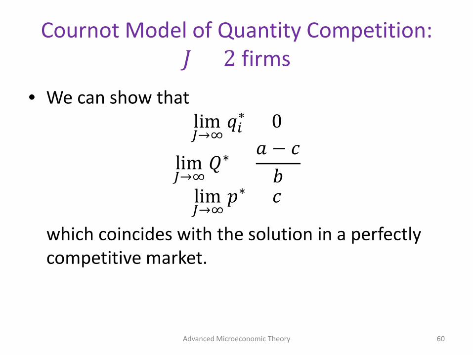
Cournot Model of Quantity Competition: 𝐽𝐽 > 2 firms
• We can show that lim𝐽𝐽→∞
𝑞𝑞𝑖𝑖∗ = 0
lim𝐽𝐽→∞
𝑄𝑄∗ =𝑎𝑎 − 𝑐𝑐
𝑏𝑏
lim𝐽𝐽→∞
𝑝𝑝∗ = 𝑐𝑐
which coincides with the solution in a perfectly competitive market.
Advanced Microeconomic Theory 60

Product Differentiation
Advanced Microeconomic Theory 61

Product Differentiation
• So far we assumed that firms sell homogenous (undifferentiated) products.
• What if the goods firms sell are differentiated? – For simplicity, we will assume that product
attributes are exogenous (not chosen by the firm)
Advanced Microeconomic Theory 62

Product Differentiation: Bertrand Model
• Consider the case where every firm 𝑖𝑖, for 𝑖𝑖 = {1,2}, faces demand curve
𝑞𝑞𝑖𝑖(𝑝𝑝𝑖𝑖 , 𝑝𝑝𝑗𝑗) = 𝑎𝑎 − 𝑏𝑏𝑝𝑝𝑖𝑖 + 𝑐𝑐𝑝𝑝𝑗𝑗 where 𝑎𝑎, 𝑏𝑏, 𝑐𝑐 > 0 and 𝑗𝑗 ≠ 𝑖𝑖.
• Hence, an increase in 𝑝𝑝𝑗𝑗 increases firm 𝑖𝑖’s sales. • Firm 𝑖𝑖’s PMP:
max𝑝𝑝𝑖𝑖≥0
(𝑎𝑎 − 𝑏𝑏𝑝𝑝𝑖𝑖 + 𝑐𝑐𝑝𝑝𝑗𝑗)𝑝𝑝𝑖𝑖
• FOC: 𝑎𝑎 − 2𝑏𝑏𝑝𝑝𝑖𝑖 + 𝑐𝑐𝑝𝑝𝑗𝑗 = 0
Advanced Microeconomic Theory 63

Product Differentiation: Bertrand Model
• Solving for 𝑝𝑝𝑖𝑖, we find firm 𝑖𝑖’s BRF
𝑝𝑝𝑖𝑖(𝑝𝑝𝑗𝑗) =𝑎𝑎 + 𝑐𝑐𝑝𝑝𝑗𝑗
2𝑏𝑏
• Firm 𝑗𝑗 also has a symmetric BRF. • Note:
– BRFs are now positively sloped – An increase in firm 𝑗𝑗’s price leads firm 𝑖𝑖 to
increase his, and vice versa – In this case, firms’ choices (i.e., prices) are
strategic complements
Advanced Microeconomic Theory 64

Product Differentiation: Bertrand Model
Advanced Microeconomic Theory 65
p1
p2
a 2b
p2 *
p1(p2)
p2(p1)
p1 *
a 2b

Product Differentiation: Bertrand Model
• Simultaneously solving the two BRS yields 𝑝𝑝𝑖𝑖
∗ =𝑎𝑎
2𝑏𝑏 − 𝑐𝑐
with corresponding equilibrium sales of
𝑞𝑞𝑖𝑖∗(𝑝𝑝𝑖𝑖
∗, 𝑝𝑝𝑗𝑗∗) = 𝑎𝑎 − 𝑏𝑏𝑝𝑝𝑖𝑖
∗ + 𝑐𝑐𝑝𝑝𝑗𝑗∗ =
𝑎𝑎𝑏𝑏2𝑏𝑏 − 𝑐𝑐
and equilibrium profits of
𝜋𝜋𝑖𝑖∗ = 𝑝𝑝𝑖𝑖
∗ ∙ 𝑞𝑞𝑖𝑖∗ 𝑝𝑝𝑖𝑖
∗, 𝑝𝑝𝑗𝑗∗ =
𝑎𝑎2𝑏𝑏 − 𝑐𝑐
𝑎𝑎𝑏𝑏2𝑏𝑏 − 𝑐𝑐
=𝑎𝑎2𝑏𝑏
2𝑏𝑏 − 𝑐𝑐 2 Advanced Microeconomic Theory 66
Product Differentiation: Cournot Model
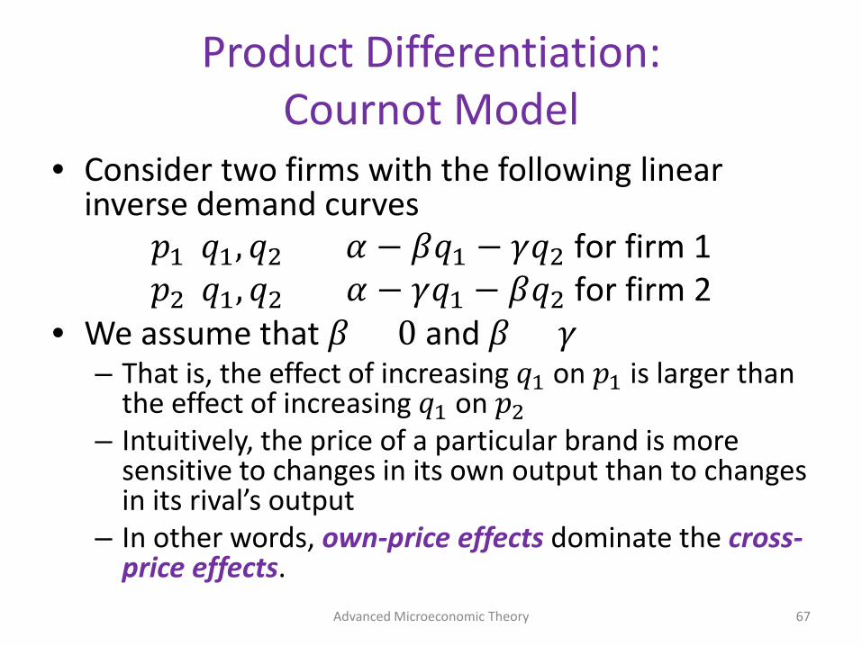
• Consider two firms with the following linear inverse demand curves
𝑝𝑝1(𝑞𝑞1, 𝑞𝑞2) = 𝛼𝛼 − 𝛽𝛽𝑞𝑞1 − 𝛾𝛾𝑞𝑞2 for firm 1 𝑝𝑝2(𝑞𝑞1, 𝑞𝑞2) = 𝛼𝛼 − 𝛾𝛾𝑞𝑞1 − 𝛽𝛽𝑞𝑞2 for firm 2
• We assume that 𝛽𝛽 > 0 and 𝛽𝛽 > 𝛾𝛾 – That is, the effect of increasing 𝑞𝑞1 on 𝑝𝑝1 is larger than
the effect of increasing 𝑞𝑞1 on 𝑝𝑝2 – Intuitively, the price of a particular brand is more
sensitive to changes in its own output than to changes in its rival’s output
– In other words, own-price effects dominate the cross-price effects. Advanced Microeconomic Theory 67

Product Differentiation: Cournot Model
• Firm 𝑖𝑖’s PMP is (assuming no costs) max𝑞𝑞𝑖𝑖≥0
(𝛼𝛼 − 𝛽𝛽𝑞𝑞𝑖𝑖 − 𝛾𝛾𝑞𝑞𝑗𝑗)𝑞𝑞𝑖𝑖
• FOC: 𝛼𝛼 − 2𝛽𝛽𝑞𝑞𝑖𝑖 − 𝛾𝛾𝑞𝑞𝑗𝑗 = 0
• Solving for 𝑞𝑞𝑖𝑖 we find firm 𝑖𝑖’s BRF
𝑞𝑞𝑖𝑖(𝑞𝑞𝑗𝑗) =𝛼𝛼
2𝛽𝛽−
𝛾𝛾2𝛽𝛽
𝑞𝑞𝑗𝑗
• Firm 𝑗𝑗 also has a symmetric BRF
Advanced Microeconomic Theory 68

Product Differentiation: Cournot Model
Advanced Microeconomic Theory 69
q1
q2
(q1,q2 ) * *
q1(q2)
q2(q1)α2β
αγ
α2β
αγ

Product Differentiation: Cournot Model
• Comparative statics of firm 𝑖𝑖’s BRF – As 𝛽𝛽 → 𝛾𝛾 (products become more homogeneous),
BRF becomes steeper. That is, the profit-maximizing choice of 𝑞𝑞𝑖𝑖 is more sensitive to changes in 𝑞𝑞𝑗𝑗 (tougher competition)
– As 𝛾𝛾 → 0 (products become very differentiated), firm 𝑖𝑖’s BRF no longer depends on 𝑞𝑞𝑗𝑗 and becomes flat (milder competition)
Advanced Microeconomic Theory 70

Product Differentiation: Cournot Model
• Simultaneously solving the two BRF yields
𝑞𝑞𝑖𝑖∗ =
𝛼𝛼2𝛽𝛽 + 𝛾𝛾
for all 𝑖𝑖 = {1,2}
with a corresponding equilibrium price of
𝑝𝑝𝑖𝑖∗ = 𝛼𝛼 − 𝛽𝛽𝑞𝑞𝑖𝑖
∗ − 𝛾𝛾𝑞𝑞𝑗𝑗∗ =
𝛼𝛼𝛽𝛽2𝛽𝛽 + 𝛾𝛾
and equilibrium profits of
𝜋𝜋𝑖𝑖∗ = 𝑝𝑝𝑖𝑖
∗𝑞𝑞𝑖𝑖∗ =
𝛼𝛼𝛽𝛽2𝛽𝛽 + 𝛾𝛾
𝛼𝛼2𝛽𝛽 + 𝛾𝛾
=𝛼𝛼2𝛽𝛽
2𝛽𝛽 + 𝛾𝛾 2
Advanced Microeconomic Theory 71

Product Differentiation: Cournot Model
• Note: – As 𝛾𝛾 increases (products become more
homogeneous), individual and aggregate output decrease, and individual profits decrease as well.
– If 𝛾𝛾 → 𝛽𝛽 (indicating undifferentiated products), then 𝑞𝑞𝑖𝑖
∗ = 𝛼𝛼2𝛽𝛽+𝛽𝛽
= 𝛼𝛼3𝛽𝛽
as in standard Cournot models of
homogeneous products. – If 𝛾𝛾 → 0 (extremely differentiated products), then
𝑞𝑞𝑖𝑖∗ = 𝛼𝛼
2𝛽𝛽+0= 𝛼𝛼
2𝛽𝛽 as in monopoly.
Advanced Microeconomic Theory 72

Dynamic Competition
Advanced Microeconomic Theory 73

Dynamic Competition: Sequential Bertrand Model with Homogeneous Products
• Assume that firm 1 chooses its price 𝑝𝑝1 first, whereas firm 2 observes that price and responds with its own price 𝑝𝑝2.
• Since the game is a sequential-move game (rather than a simultaneous-move game), we should use backward induction.
Advanced Microeconomic Theory 74

Dynamic Competition: Sequential Bertrand Model with Homogeneous Products
• Firm 2 (the follower) has a BRF given by
𝑝𝑝2(𝑝𝑝1) = �𝑝𝑝1 − 𝜀𝜀 if 𝑝𝑝1 > 𝑐𝑐𝑐𝑐 if 𝑝𝑝1 ≤ 𝑐𝑐
while firm 1’s (the leader’s) BRF is 𝑝𝑝1 = 𝑐𝑐
• Intuition: the follower undercuts the leader’s price 𝑝𝑝1 by a small 𝜀𝜀 > 0 if 𝑝𝑝1 > 𝑐𝑐, or keeps it at 𝑝𝑝2 = 𝑐𝑐 if the leader sets 𝑝𝑝1 = 𝑐𝑐.
Advanced Microeconomic Theory 75

Dynamic Competition: Sequential Bertrand Model with Homogeneous Products
• The leader expects that its price will be: – undercut by the follower when 𝑝𝑝1 > 𝑐𝑐 (thus yielding
no sales) – mimicked by the follower when 𝑝𝑝1 = 𝑐𝑐 (thus entailing
half of the market share)
• Hence, the leader has (weak) incentives to set a price 𝑝𝑝1 = 𝑐𝑐.
• As a consequence, the equilibrium price pair remains at (𝑝𝑝1
∗, 𝑝𝑝2∗) = (𝑐𝑐, 𝑐𝑐), as in the
simultaneous-move version of the Bertrand model.
Advanced Microeconomic Theory 76

Dynamic Competition: Sequential Bertrand Model with Heterogeneous Products
• Assume that firms sell differentiated products, where firm 𝑗𝑗’s demand is
𝑞𝑞𝑗𝑗 = 𝐷𝐷𝑗𝑗(𝑝𝑝𝑗𝑗 , 𝑝𝑝𝑘𝑘) – Example: 𝑞𝑞𝑗𝑗(𝑝𝑝𝑗𝑗, 𝑝𝑝𝑘𝑘) = 𝑎𝑎 − 𝑏𝑏𝑝𝑝𝑗𝑗 + 𝑐𝑐𝑝𝑝𝑘𝑘, where
𝑎𝑎, 𝑏𝑏, 𝑐𝑐 > 0 and 𝑏𝑏 > 𝑐𝑐
• In the second stage, firm 2 (the follower) solves following PMP
max𝑝𝑝2≥0
𝜋𝜋2 = 𝑝𝑝2𝑞𝑞2 − 𝑇𝑇𝑇𝑇(𝑞𝑞2)
= 𝑝𝑝2𝐷𝐷2(𝑝𝑝2, 𝑝𝑝1) − 𝑇𝑇𝑇𝑇(𝐷𝐷2(𝑝𝑝2, 𝑝𝑝1)𝑞𝑞2
)
Advanced Microeconomic Theory 77

Dynamic Competition: Sequential Bertrand Model with Heterogeneous Products
• FOCs wrt 𝑝𝑝2 yield
𝐷𝐷2(𝑝𝑝2, 𝑝𝑝1) + 𝑝𝑝2𝜕𝜕𝐷𝐷2(𝑝𝑝2, 𝑝𝑝1)
𝜕𝜕𝑝𝑝2
−𝜕𝜕𝑇𝑇𝑇𝑇 𝐷𝐷2(𝑝𝑝2, 𝑝𝑝1)
𝜕𝜕𝐷𝐷2(𝑝𝑝2, 𝑝𝑝1) 𝜕𝜕𝐷𝐷2(𝑝𝑝2, 𝑝𝑝1)
𝜕𝜕𝑝𝑝2Using the chain rule
= 0
• Solving for 𝑝𝑝2 produces the follower’s BRF for every price set by the leader, 𝑝𝑝1, i.e., 𝑝𝑝2(𝑝𝑝1).
Advanced Microeconomic Theory 78

Dynamic Competition: Sequential Bertrand Model with Heterogeneous Products
• In the first stage, firm 1 (leader) anticipates that the follower will use BRF 𝑝𝑝2(𝑝𝑝1) to respond to each possible price 𝑝𝑝1, hence solves following PMP
max𝑝𝑝1≥0
𝜋𝜋1 = 𝑝𝑝1𝑞𝑞1 − 𝑇𝑇𝑇𝑇 𝑞𝑞1
= 𝑝𝑝1𝐷𝐷1 𝑝𝑝1, 𝑝𝑝2 𝑝𝑝1𝐵𝐵𝐵𝐵𝐹𝐹2
− 𝑇𝑇𝑇𝑇 𝐷𝐷1 𝑝𝑝1, 𝑝𝑝2(𝑝𝑝1)𝑞𝑞1
Advanced Microeconomic Theory 79

Dynamic Competition: Sequential Bertrand Model with Heterogeneous Products
• FOCs wrt 𝑝𝑝1 yield 𝐷𝐷1(𝑝𝑝1, 𝑝𝑝2) + 𝑝𝑝1
𝜕𝜕𝐷𝐷1(𝑝𝑝1, 𝑝𝑝2)𝜕𝜕𝑝𝑝1
+𝜕𝜕𝐷𝐷1(𝑝𝑝1, 𝑝𝑝2)
𝜕𝜕𝑝𝑝2(𝑝𝑝1)𝜕𝜕𝑝𝑝2(𝑝𝑝1)
𝜕𝜕𝑝𝑝1New Strategic Effect
−𝜕𝜕𝑇𝑇𝑇𝑇 𝐷𝐷1(𝑝𝑝1, 𝑝𝑝2)
𝜕𝜕𝐷𝐷1(𝑝𝑝1, 𝑝𝑝2)𝜕𝜕𝐷𝐷1(𝑝𝑝1, 𝑝𝑝2)
𝜕𝜕𝑝𝑝1+
𝜕𝜕𝐷𝐷1(𝑝𝑝1, 𝑝𝑝2)𝜕𝜕𝑝𝑝2(𝑝𝑝1)
𝜕𝜕𝑝𝑝2(𝑝𝑝1)𝜕𝜕𝑝𝑝1
New Strategic Effect
= 0
• Or more compactly as
𝐷𝐷1(𝑝𝑝1, 𝑝𝑝2) + 𝑝𝑝1 −𝜕𝜕𝑇𝑇𝑇𝑇 𝐷𝐷1(𝑝𝑝1, 𝑝𝑝2)
𝜕𝜕𝐷𝐷1(𝑝𝑝1, 𝑝𝑝2)𝜕𝜕𝐷𝐷1(𝑝𝑝1, 𝑝𝑝2)
𝜕𝜕𝑝𝑝11 +
𝜕𝜕𝑝𝑝2(𝑝𝑝1)𝜕𝜕𝑝𝑝1𝑁𝑁𝑁𝑁𝑁𝑁
= 0
Advanced Microeconomic Theory 80

Dynamic Competition: Sequential Bertrand Model with Heterogeneous Products
• In contrast to the Bertrand model with simultaneous price competition, an increase in firm 1’s price now produces an increase in firm 2’s price in the second stage.
• Hence, the leader has more incentives to raise its price, ultimately softening the price competition.
• While a softened competition benefits both the leader and the follower, the real beneficiary is the follower, as its profits increase more than the leader’s.
Advanced Microeconomic Theory 81

Dynamic Competition: Sequential Bertrand Model with Heterogeneous Products
• Example: – Consider a linear demand 𝑞𝑞𝑖𝑖 = 1 − 2𝑝𝑝𝑖𝑖 + 𝑝𝑝𝑗𝑗, with no
marginal costs, i.e., 𝑐𝑐 = 0. – Simultaneous Bertrand model: the PMP is
max𝑝𝑝𝑗𝑗≥0
𝜋𝜋𝑗𝑗 = 𝑝𝑝𝑗𝑗 ∙ (1 − 2𝑝𝑝𝑗𝑗 + 𝑝𝑝𝑘𝑘) for any 𝑘𝑘 ≠ 𝑗𝑗
where FOC wrt 𝑝𝑝𝑗𝑗 produces firm 𝑗𝑗’s BRF
𝑝𝑝𝑗𝑗(𝑝𝑝𝑘𝑘) =14
+14
𝑝𝑝𝑘𝑘
– Simultaneously solving the two BRFs yields 𝑝𝑝𝑗𝑗∗ = 1
3≃
0.33, entailing equilibrium profits of 𝜋𝜋𝑗𝑗∗ = 2
9≃ 0.222.
Advanced Microeconomic Theory 82

Dynamic Competition: Sequential Bertrand Model with Heterogeneous Products
• Example (continued): – Sequential Bertrand model: in the second stage, firm
2’s (the follower’s) PMP is max𝑝𝑝2≥0
𝜋𝜋2 = 𝑝𝑝2 ∙ 1 − 2𝑝𝑝2 + 𝑝𝑝1
where FOC wrt 𝑝𝑝2 produces firm 2’s BRF
𝑝𝑝2(𝑝𝑝1) =14
+14
𝑝𝑝1
– In the first stage, firm 1’s (the leader’s) PMP is
max𝑝𝑝1≥0
𝜋𝜋1 = 𝑝𝑝1 ∙ 1 − 2𝑝𝑝1 +14 +
14 𝑝𝑝1
𝐵𝐵𝐵𝐵𝐹𝐹2
= 𝑝𝑝1 ∙14 (5 − 7𝑝𝑝1)
Advanced Microeconomic Theory 83

Dynamic Competition: Sequential Bertrand Model with Heterogeneous Products
• Example (continued): – FOC wrt 𝑝𝑝1, and solving for 𝑝𝑝1, produces firm 1’s
equilibrium price 𝑝𝑝1∗ = 5
14= 0.36.
– Substituting 𝑝𝑝1∗ into the BRF of firm 2 yields
𝑝𝑝2∗ 0.36 = 1
4+ 1
40.36 = 0.34.
– Equilibrium profits are hence
𝜋𝜋1∗ = 0.36
14
5 − 7 0.36 = 0.223 for firm 1
𝜋𝜋2∗ = 0.34 1 − 2 0.34 + 0.36 = 0.230 for firm 2
Advanced Microeconomic Theory 84

p1
p2
p1(p2)
p2(p1)
⅓
¼
¼
Prices with sequential price competition
0.36
0.34⅓
Prices with simultaneous price competition
Dynamic Competition: Sequential Bertrand Model with Heterogeneous Products
• Example (continued): – Both firms’ prices and
profits are higher in the sequential than in the simultaneous game.
– However, the follower earns more than the leader in the sequential game! (second mover’s advantage)
Advanced Microeconomic Theory 85

Dynamic Competition: Sequential Cournot Model with Homogenous Products
• Stackelberg model: firm 1 (the leader) chooses output level 𝑞𝑞1, and firm 2 (the follower) observing the output decision of the leader, responds with its own output 𝑞𝑞2(𝑞𝑞1).
• By backward induction, the follower’s BRF is 𝑞𝑞2(𝑞𝑞1) for any 𝑞𝑞1.
• Since the leader anticipates 𝑞𝑞2(𝑞𝑞1) from the follower, the leader’s PMP is
max𝑞𝑞1≥0
𝑝𝑝 𝑞𝑞1 + 𝑞𝑞2(𝑞𝑞1)𝐵𝐵𝐵𝐵𝐹𝐹2
𝑞𝑞1 − 𝑇𝑇𝑇𝑇1(𝑞𝑞1)
Advanced Microeconomic Theory 86

Dynamic Competition: Sequential Cournot Model with Homogenous Products
• FOCs wrt 𝑞𝑞1 yields
𝑝𝑝 𝑞𝑞1 + 𝑞𝑞2(𝑞𝑞1) + 𝑝𝑝′ 𝑞𝑞1 + 𝑞𝑞2(𝑞𝑞1) 𝑞𝑞1 +𝜕𝜕𝑞𝑞2(𝑞𝑞1)
𝜕𝜕𝑞𝑞1𝑞𝑞1
−𝜕𝜕𝑇𝑇𝑇𝑇1(𝑞𝑞1)
𝜕𝜕𝑞𝑞1= 0
or more compactly
𝑝𝑝 𝑄𝑄 + 𝑝𝑝′ 𝑄𝑄 𝑞𝑞1 + 𝑝𝑝′ 𝑄𝑄𝜕𝜕𝑞𝑞2(𝑞𝑞1)
𝜕𝜕𝑞𝑞1𝑞𝑞1
Strategic Effect
−𝜕𝜕𝑇𝑇𝑇𝑇1 𝑞𝑞1
𝜕𝜕𝑞𝑞1= 0
• This FOC coincides with that for standard Cournot model with simultaneous output decisions, except for the strategic effect.
Advanced Microeconomic Theory 87
Dynamic Competition: Sequential Cournot Model with Homogenous Products
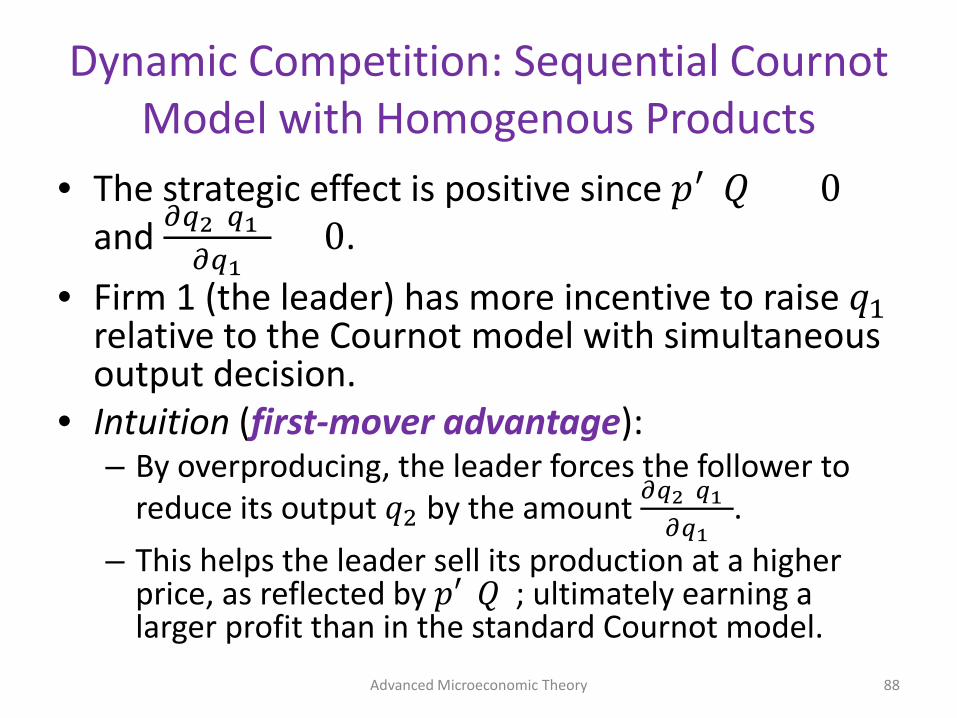
• The strategic effect is positive since 𝑝𝑝′(𝑄𝑄) < 0 and 𝜕𝜕𝑞𝑞2(𝑞𝑞1)
𝜕𝜕𝑞𝑞1< 0.
• Firm 1 (the leader) has more incentive to raise 𝑞𝑞1 relative to the Cournot model with simultaneous output decision.
• Intuition (first-mover advantage): – By overproducing, the leader forces the follower to
reduce its output 𝑞𝑞2 by the amount 𝜕𝜕𝑞𝑞2(𝑞𝑞1)𝜕𝜕𝑞𝑞1
. – This helps the leader sell its production at a higher
price, as reflected by 𝑝𝑝′(𝑄𝑄); ultimately earning a larger profit than in the standard Cournot model.
Advanced Microeconomic Theory 88

Dynamic Competition: Sequential Cournot Model with Homogenous Products
• Example: – Consider linear inverse demand 𝑝𝑝 = 𝑎𝑎 − 𝑄𝑄, where
𝑄𝑄 = 𝑞𝑞1 + 𝑞𝑞2, and a constant marginal cost of 𝑐𝑐. – Firm 2’s (the follower’s) PMP is
max𝑞𝑞2
(𝑎𝑎 − 𝑞𝑞1 − 𝑞𝑞2)𝑞𝑞2 − 𝑐𝑐𝑞𝑞2
– FOC: 𝑎𝑎 − 𝑞𝑞1 − 2𝑞𝑞2 − 𝑐𝑐 = 0
– Solving for 𝑞𝑞2 yields the follower’s BRF 𝑞𝑞2 𝑞𝑞1 = 𝑎𝑎−𝑞𝑞1−𝑐𝑐
2
Advanced Microeconomic Theory 89
Dynamic Competition: Sequential Cournot Model with Homogenous Products
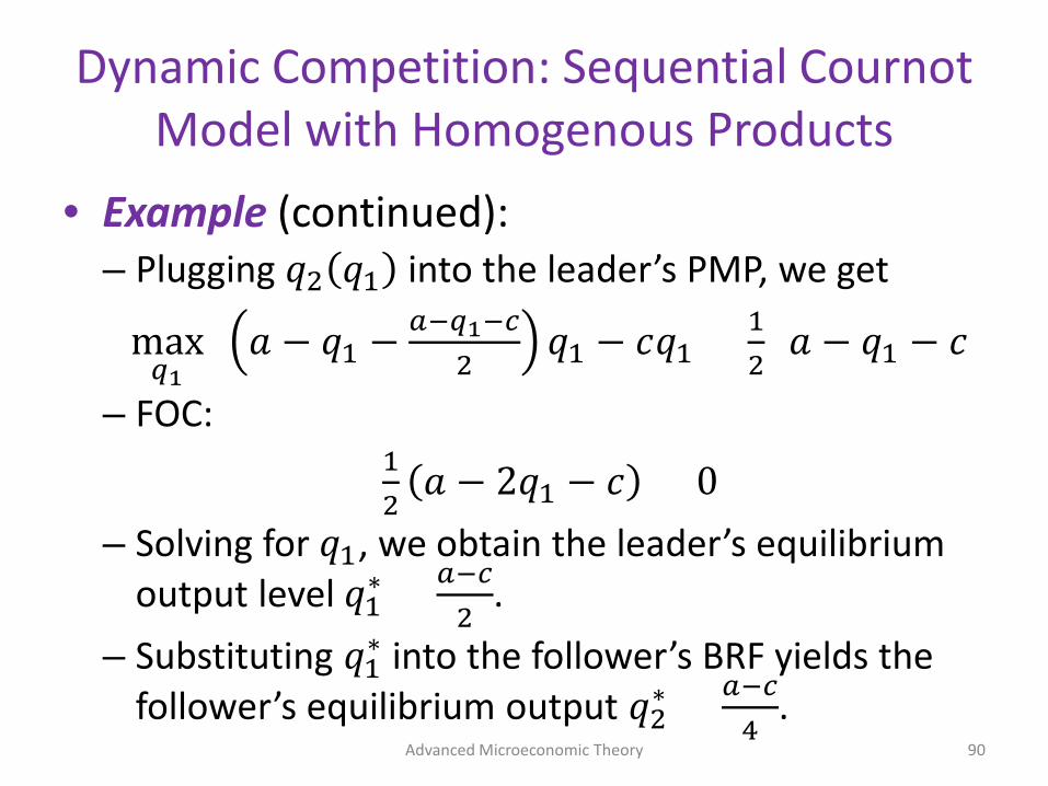
• Example (continued): – Plugging 𝑞𝑞2 𝑞𝑞1 into the leader’s PMP, we get
max𝑞𝑞1
𝑎𝑎 − 𝑞𝑞1 − 𝑎𝑎−𝑞𝑞1−𝑐𝑐2
𝑞𝑞1 − 𝑐𝑐𝑞𝑞1 = 12
(𝑎𝑎 − 𝑞𝑞1 − 𝑐𝑐)
– FOC: 12
𝑎𝑎 − 2𝑞𝑞1 − 𝑐𝑐 = 0 – Solving for 𝑞𝑞1, we obtain the leader’s equilibrium
output level 𝑞𝑞1∗ = 𝑎𝑎−𝑐𝑐
2.
– Substituting 𝑞𝑞1∗ into the follower’s BRF yields the
follower’s equilibrium output 𝑞𝑞2∗ = 𝑎𝑎−𝑐𝑐
4.
Advanced Microeconomic Theory 90

Dynamic Competition: Sequential Cournot Model with Homogenous Products
Advanced Microeconomic Theory 91
q1
q2
a – c
q1(q2)
2
q2(q1)
a – c2
Cournot Quantities
Stackelberg Quantities

Dynamic Competition: Sequential Cournot Model with Homogenous Products
• Example (continued): – The equilibrium price is
𝑝𝑝 = 𝑎𝑎 − 𝑞𝑞1∗ − 𝑞𝑞2
∗ =𝑎𝑎 + 3𝑐𝑐
4
– And the resulting equilibrium profits are
𝜋𝜋1∗ = 𝑎𝑎+3𝑐𝑐
4𝑎𝑎−𝑐𝑐
2− 𝑐𝑐 𝑎𝑎−𝑐𝑐
2= 𝑎𝑎−𝑐𝑐 2
8
𝜋𝜋2∗ = 𝑎𝑎+3𝑐𝑐
4𝑎𝑎−𝑐𝑐
4− 𝑐𝑐 𝑎𝑎−𝑐𝑐
4= 𝑎𝑎−𝑐𝑐 2
16
Advanced Microeconomic Theory 92

Price
a
a + c2
a – c2b
Monopoly
Units
a + 2c3
a + 3c4
2(a – c)3b
3(a – c)4b
a – cb
ab
pm =
pCournot =
pStackelberg =
pP.C. =pBertrand = c
Cournot
Stackelberg
Bertrand and Perfect Competition
Dynamic Competition: Sequential Cournot Model with Homogenous Products
• Linear inverse demand 𝑝𝑝 𝑄𝑄 = 𝑎𝑎 − 𝑄𝑄
• Symmetric marginal costs 𝑐𝑐 > 0
Advanced Microeconomic Theory 93

Dynamic Competition: Sequential Cournot Model with Heterogeneous Products
• Assume that firms sell differentiated products, with inverse demand curves for firms 1 and 2
𝑝𝑝1(𝑞𝑞1, 𝑞𝑞2) = 𝛼𝛼 − 𝛽𝛽𝑞𝑞1 − 𝛾𝛾𝑞𝑞2 for firm 1 𝑝𝑝2(𝑞𝑞1, 𝑞𝑞2) = 𝛼𝛼 − 𝛾𝛾𝑞𝑞1 − 𝛽𝛽𝑞𝑞2 for firm 2
• Firm 2’s (the follower’s) PMP is max
𝑞𝑞2 (𝛼𝛼 − 𝛾𝛾𝑞𝑞1 − 𝛽𝛽𝑞𝑞2) ∙ 𝑞𝑞2
where, for simplicity, we assume no marginal costs. • FOC:
𝛼𝛼 − 𝛾𝛾𝑞𝑞1 − 2𝛽𝛽𝑞𝑞2 = 0 Advanced Microeconomic Theory 94

Dynamic Competition: Sequential Cournot Model with Heterogeneous Products
• Solving for 𝑞𝑞2 yields firm 2’s BRF 𝑞𝑞2(𝑞𝑞1) = 𝛼𝛼−𝛾𝛾𝑞𝑞1
2𝛽𝛽
• Plugging 𝑞𝑞2 𝑞𝑞1 into the leader’s firm 1’s (the leader’s) PMP, we get
max𝑞𝑞1
𝛼𝛼 − 𝛽𝛽𝑞𝑞1 − 𝛾𝛾 𝛼𝛼−𝛾𝛾𝑞𝑞12𝛽𝛽
𝑞𝑞1 =
max𝑞𝑞1
𝛼𝛼 2𝛽𝛽−𝛾𝛾2𝛽𝛽
− 2𝛽𝛽2−𝛾𝛾2
2𝛽𝛽𝑞𝑞1 𝑞𝑞1
• FOC:
𝛼𝛼 2𝛽𝛽−𝛾𝛾2𝛽𝛽
− 2𝛽𝛽2−𝛾𝛾2
𝛽𝛽𝑞𝑞1 = 0
Advanced Microeconomic Theory 95

Dynamic Competition: Sequential Cournot Model with Heterogeneous Products
• Solving for 𝑞𝑞1, we obtain the leader’s equilibrium output level 𝑞𝑞1
∗ = 𝛼𝛼(2𝛽𝛽−𝛾𝛾)2(2𝛽𝛽2−𝛾𝛾2)
• Substituting 𝑞𝑞1
∗ into the follower’s BRF yields the follower’s equilibrium output
𝑞𝑞2∗ = 𝛼𝛼−𝛾𝛾𝑞𝑞1
∗
2𝛽𝛽= 𝛼𝛼(4𝛽𝛽2−2𝛽𝛽𝛾𝛾−𝛾𝛾2)
4𝛽𝛽(2𝛽𝛽2−𝛾𝛾2)
• Note: – 𝑞𝑞1
∗ > 𝑞𝑞2∗
– If 𝛾𝛾 → 𝛽𝛽 (i.e., the products become more homogeneous), (𝑞𝑞1
∗, 𝑞𝑞2∗) convege to the standard Stackelberg values.
– If 𝛾𝛾 → 0 (i.e., the products become very differentiated), (𝑞𝑞1
∗, 𝑞𝑞2∗) converge to the monopoly output 𝑞𝑞𝑚𝑚 = 𝛼𝛼
2𝛽𝛽.
Advanced Microeconomic Theory 96

Capacity Constraints
Advanced Microeconomic Theory 97

Capacity Constraints
• How come are equilibrium outcomes in the standard Bertrand and Cournot models so different?
• Do firms really compete in prices without facing capacity constraints? – Bertrand model assumes a firm can supply infinitely
large amount if its price is lower than its rivals. • Extension of the Bertrand model:
– First stage: firms set capacities, 𝑞𝑞�1 and 𝑞𝑞�2, with a cost of capacity 𝑐𝑐 > 0
– Second stage: firms observe each other’s capacities and compete in prices, simultaneously setting 𝑝𝑝1 and 𝑝𝑝2
Advanced Microeconomic Theory 98

Capacity Constraints
• What is the role of capacity constraint? – When a firm’s price is lower than its capacity, not all
consumers can be served. – Hence, sales must be rationed through efficient
rationing: the customers with the highest willingness to pay get the product first.
• Intuitively, if 𝑝𝑝1 < 𝑝𝑝2 and the quantity demanded at 𝑝𝑝1 is so large that 𝑄𝑄(𝑝𝑝1) > 𝑞𝑞�1, then the first 𝑞𝑞�1 units are served to the customers with the highest willingness to pay (i.e., the upper segment of the demand curve), while some customers are left in the form of residual demand to firm 2.
Advanced Microeconomic Theory 99
p
q
p2
p1
Q(p2) Q(p1)
Q(p)
q1, firm 1's capacity
q1 Unserved customers by firm 1
These units become residual demand for firm 2.
Q2(p2) – q1
1st
2nd
3rd
4th
5th
6th
Capacity Constraints
Advanced Microeconomic Theory 100
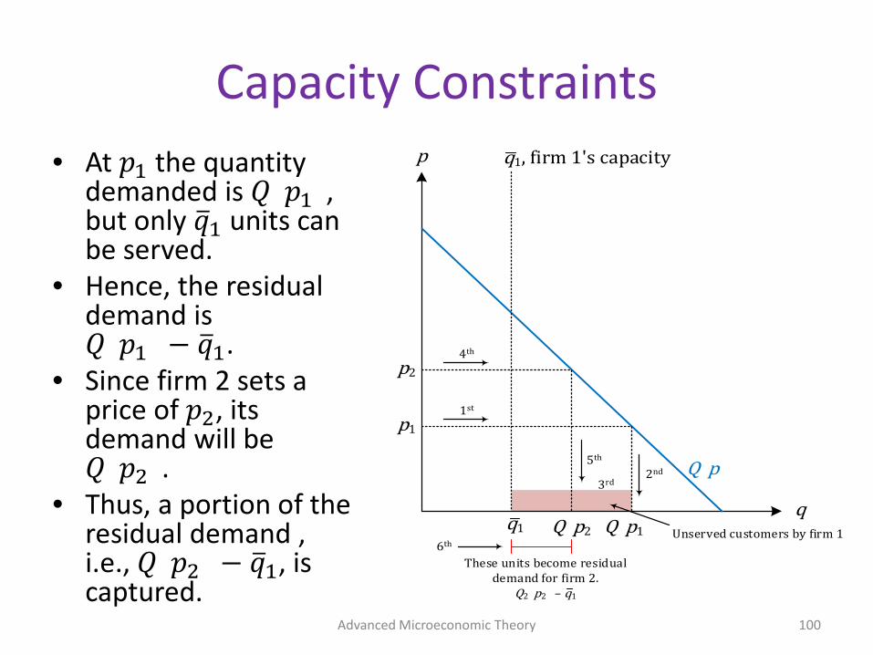
• At 𝑝𝑝1 the quantity demanded is 𝑄𝑄(𝑝𝑝1), but only 𝑞𝑞�1 units can be served.
• Hence, the residual demand is 𝑄𝑄(𝑝𝑝1) − 𝑞𝑞�1.
• Since firm 2 sets a price of 𝑝𝑝2, its demand will be 𝑄𝑄(𝑝𝑝2).
• Thus, a portion of the residual demand , i.e., 𝑄𝑄(𝑝𝑝2) − 𝑞𝑞�1, is captured.
Capacity Constraints
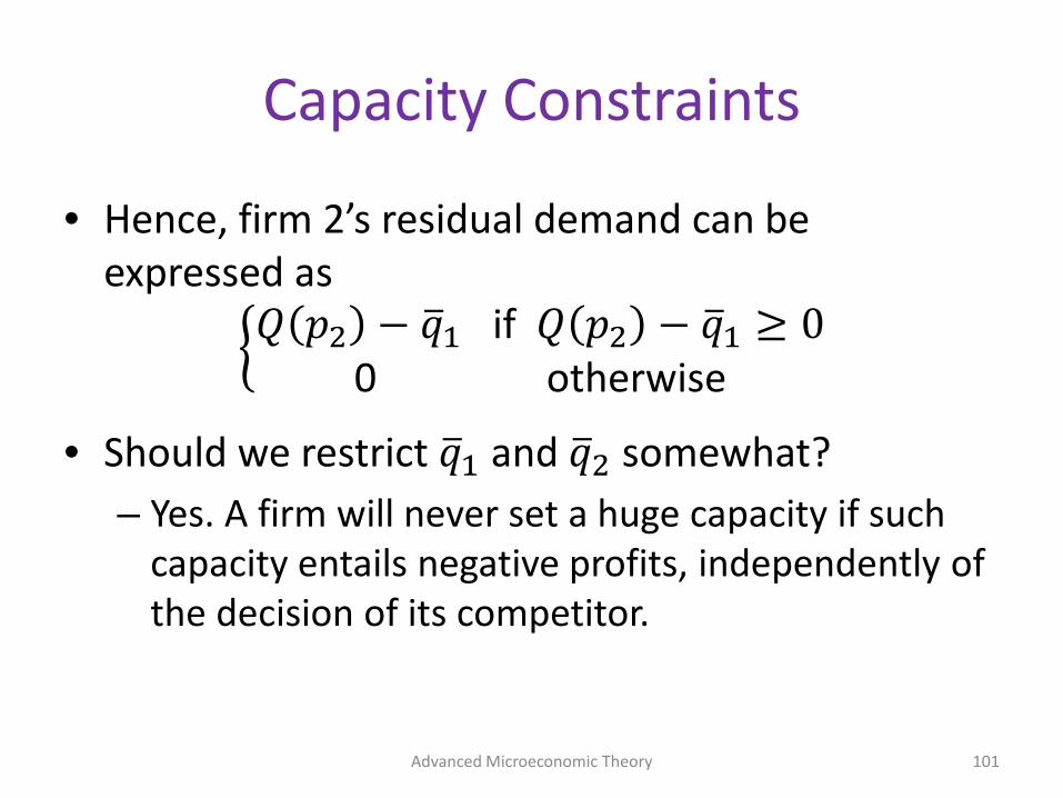
• Hence, firm 2’s residual demand can be expressed as
�𝑄𝑄 𝑝𝑝2 − 𝑞𝑞�1 if 𝑄𝑄 𝑝𝑝2 − 𝑞𝑞�1 ≥ 00 otherwise
• Should we restrict 𝑞𝑞�1 and 𝑞𝑞�2 somewhat? – Yes. A firm will never set a huge capacity if such
capacity entails negative profits, independently of the decision of its competitor.
Advanced Microeconomic Theory 101
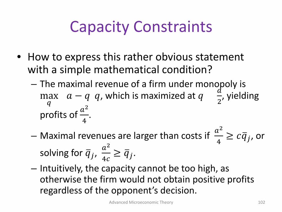
Capacity Constraints
• How to express this rather obvious statement with a simple mathematical condition? – The maximal revenue of a firm under monopoly is
max𝑞𝑞
(𝑎𝑎 − 𝑞𝑞)𝑞𝑞, which is maximized at 𝑞𝑞 = 𝑎𝑎2, yielding
profits of 𝑎𝑎2
4.
– Maximal revenues are larger than costs if 𝑎𝑎2
4≥ 𝑐𝑐𝑞𝑞�𝑗𝑗, or
solving for 𝑞𝑞�𝑗𝑗, 𝑎𝑎2
4𝑐𝑐≥ 𝑞𝑞�𝑗𝑗.
– Intuitively, the capacity cannot be too high, as otherwise the firm would not obtain positive profits regardless of the opponent’s decision.
Advanced Microeconomic Theory 102

Capacity Constraints: Second Stage
• By backward induction, we start with the second stage (pricing game), where firms simultaneously choose prices 𝑝𝑝1 and 𝑝𝑝2 as a function of the capacity choices 𝑞𝑞�1 and 𝑞𝑞�2.
• We want to show that in this second stage, both firms set a common price
𝑝𝑝1 = 𝑝𝑝2 = 𝑝𝑝∗ = 𝑎𝑎 − 𝑞𝑞�1 − 𝑞𝑞�2
where demand equals supply, i.e., total capacity, 𝑝𝑝∗ = 𝑎𝑎 − 𝑄𝑄�, where 𝑄𝑄� ≡ 𝑞𝑞�1 + 𝑞𝑞�2
Advanced Microeconomic Theory 103

Capacity Constraints: Second Stage
• In order to prove this result, we start by assuming that firm 1 sets 𝑝𝑝1 = 𝑝𝑝∗. We now need to show that firm 2 also sets 𝑝𝑝2 = 𝑝𝑝∗, i.e., it does not have incentives to deviate from 𝑝𝑝∗.
• If firm 2 does not deviate, 𝑝𝑝1 = 𝑝𝑝2 = 𝑝𝑝∗, then it sells up to its capacity 𝑞𝑞�2.
• If firm 2 reduces its price below 𝑝𝑝∗, demand would exceed its capacity 𝑞𝑞�2. As a result, firm 2 would sell the same units as before, 𝑞𝑞�2, but at a lower price.
Advanced Microeconomic Theory 104

Capacity Constraints: Second Stage
• If, instead, firm 2 charges a price above 𝑝𝑝∗, then 𝑝𝑝1 = 𝑝𝑝∗ < 𝑝𝑝2 and its revenues become
𝑝𝑝2𝑄𝑄�(𝑝𝑝2) = �𝑝𝑝2(𝑎𝑎 − 𝑝𝑝2 − 𝑞𝑞�1) if 𝑎𝑎 − 𝑝𝑝2 − 𝑞𝑞�1 ≥ 00 otherwise
• Note: – This is fundamentally different from the standard
Bertrand model without capacity constraints, where an increase in price by a firm reduces its sales to zero.
– When capacity constraints are present, the firm can still capture a residual demand, ultimately raising its revenues after increasing its price.
Advanced Microeconomic Theory 105

Capacity Constraints: Second Stage
• We now find the maximum of this revenue function. FOC wrt 𝑝𝑝2 yields:
𝑎𝑎 − 2𝑝𝑝2 − 𝑞𝑞�1 = 0 ⟺ 𝑝𝑝2 =𝑎𝑎 − 𝑞𝑞�1
2
• The non-deviating price 𝑝𝑝∗ = 𝑎𝑎 − 𝑞𝑞�1 − 𝑞𝑞�2 lies above the maximum-revenue price 𝑝𝑝2 = 𝑎𝑎−𝑞𝑞�1
2 when
𝑎𝑎 − 𝑞𝑞�1 − 𝑞𝑞�2 >𝑎𝑎 − 𝑞𝑞�1
2 ⟺ 𝑎𝑎 > 𝑞𝑞�1 + 2𝑞𝑞�2
• Since 𝑎𝑎2
4𝑐𝑐≥ 𝑞𝑞�𝑗𝑗 (capacity constraint), we can obtain
𝑎𝑎2
4𝑐𝑐+ 2
𝑎𝑎2
4𝑐𝑐> 𝑞𝑞�1 + 2𝑞𝑞�2 ⇔
3𝑎𝑎2
4𝑐𝑐> 𝑞𝑞�1 + 2𝑞𝑞�2
Advanced Microeconomic Theory 106

Capacity Constraints: Second Stage
• Therefore, 𝑎𝑎 > 𝑞𝑞�1 + 2𝑞𝑞�2 holds if 𝑎𝑎 > 3𝑎𝑎2
4𝑐𝑐 which,
solving for 𝑎𝑎, is equivalent to 4𝑐𝑐3
> 𝑎𝑎.
Advanced Microeconomic Theory 107

Capacity Constraints: Second Stage
• When 4𝑐𝑐3
> 𝑎𝑎 holds, capacity constraint 𝑎𝑎2
4𝑐𝑐≥ 𝑞𝑞�𝑗𝑗 transforms into
3𝑎𝑎2
4𝑐𝑐> 𝑞𝑞�1 + 2𝑞𝑞�2, implying
𝑝𝑝∗ > 𝑝𝑝2 = 𝑎𝑎 − 𝑞𝑞�12
.
• Thus, firm 2 does not have incentives to increase its price 𝑝𝑝2 from 𝑝𝑝∗, since that would lower its revenues.
Advanced Microeconomic Theory 108

Capacity Constraints: Second Stage
• In short, firm 2 does not have incentives to deviate from the common price
𝑝𝑝∗ = 𝑎𝑎 − 𝑞𝑞�1 − 𝑞𝑞�2 • A similar argument applies to firm 1 (by
symmetry). • Hence, we have found an equilibrium in the
pricing stage.
Advanced Microeconomic Theory 109

Capacity Constraints: First Stage
• In the first stage (capacity setting), firms simultaneously select their capacities 𝑞𝑞�1 and 𝑞𝑞�2.
• Inserting stage 2 equilibrium prices, i.e., 𝑝𝑝1 = 𝑝𝑝2 = 𝑝𝑝∗ = 𝑎𝑎 − 𝑞𝑞�1 − 𝑞𝑞�2,
into firm 𝑗𝑗’s profit function yields 𝜋𝜋𝑗𝑗(𝑞𝑞�1, 𝑞𝑞�2) = (𝑎𝑎 − 𝑞𝑞�1 − 𝑞𝑞�2)
𝑝𝑝∗𝑞𝑞�𝑗𝑗 − 𝑐𝑐𝑞𝑞�𝑗𝑗
• FOC wrt capacity 𝑞𝑞�𝑗𝑗 yields firm 𝑗𝑗’s BRF
𝑞𝑞�𝑗𝑗(𝑞𝑞�𝑘𝑘) =𝑎𝑎 − 𝑐𝑐
2−
12
𝑞𝑞�𝑘𝑘 Advanced Microeconomic Theory 110

Capacity Constraints: First Stage
• Solving the two BRFs simultaneously, we obtain a symmetric solution
𝑞𝑞�𝑗𝑗 = 𝑞𝑞�𝑘𝑘 =𝑎𝑎 − 𝑐𝑐
3
• These are the same equilibrium predictions as those in the standard Cournot model.
• Hence, capacities in this two-stage game coincide with output decisions in the standard Cournot model, while prices are set equal to total capacity.
Advanced Microeconomic Theory 111

Endogenous Entry
Advanced Microeconomic Theory 112

Endogenous Entry
• So far the number of firms was exogenous • What if the number of firms operating in a
market is endogenously determined? • That is, how many firms would enter an
industry where – They know that competition will be a la Cournot – They must incur a fixed entry cost 𝐹𝐹 > 0.
Advanced Microeconomic Theory 113

Endogenous Entry
• Consider inverse demand function 𝑝𝑝(𝑞𝑞), where 𝑞𝑞 denotes aggregate output
• Every firm 𝑗𝑗 faces the same total cost function, 𝑐𝑐(𝑞𝑞𝑗𝑗), of producing 𝑞𝑞𝑗𝑗 units
• Hence, the Cournot equilibrium must be symmetric – Every firm produces the same output level 𝑞𝑞(𝑛𝑛), which is a
function of the number of entrants. • Entry profits for firm 𝑗𝑗 are
𝜋𝜋𝑗𝑗 𝑛𝑛 = 𝑝𝑝 𝑛𝑛 ∙ 𝑞𝑞 𝑛𝑛𝑄𝑄
𝑝𝑝(𝑄𝑄)
𝑞𝑞 𝑛𝑛 − 𝑐𝑐 𝑞𝑞 𝑛𝑛Production Costs
− 𝐹𝐹⏟Fixed Entry Cost
Advanced Microeconomic Theory 114

Endogenous Entry
• Three assumptions (valid under most demand and cost functions): – individual equilibrium output 𝑞𝑞(𝑛𝑛) is decreasing in
𝑛𝑛; – aggregate output 𝑞𝑞 ≡ 𝑛𝑛 ∙ 𝑞𝑞(𝑛𝑛) increases in 𝑛𝑛; – equilibrium price 𝑝𝑝(𝑛𝑛 ∙ 𝑞𝑞(𝑛𝑛)) remains above
marginal costs regardless of the number of entrants 𝑛𝑛.
Advanced Microeconomic Theory 115

Endogenous Entry
• Equilibrium number of firms: – The equilibrium occurs when no more firms have
incentives to enter or exit the market, i.e., 𝜋𝜋𝑗𝑗(𝑛𝑛𝑁𝑁) = 0.
– Note that individual profits decrease in 𝑛𝑛, i.e.,
𝜋𝜋′ 𝑛𝑛 = 𝑝𝑝 𝑛𝑛𝑞𝑞 𝑛𝑛 − 𝑐𝑐′ 𝑞𝑞 𝑛𝑛+
𝜕𝜕𝑞𝑞(𝑛𝑛)𝜕𝜕𝑛𝑛
−
+ 𝑞𝑞 𝑛𝑛 𝑝𝑝′ 𝑛𝑛𝑞𝑞 𝑛𝑛−
𝜕𝜕[𝑛𝑛𝑞𝑞 𝑛𝑛 ]𝜕𝜕𝑛𝑛+
< 0
Advanced Microeconomic Theory 116

Endogenous Entry
• Social optimum: – The social planner chooses the number of entrants
𝑛𝑛𝑜𝑜 that maximizes social welfare
max𝑛𝑛
𝑊𝑊 𝑛𝑛 ≡ � 𝑝𝑝 𝑠𝑠 𝑑𝑑𝑠𝑠 − 𝑛𝑛 ∙ 𝑐𝑐 𝑞𝑞 𝑛𝑛 − 𝑛𝑛 ∙ 𝐹𝐹𝑛𝑛𝑞𝑞(𝑛𝑛)
0
Advanced Microeconomic Theory 117

p
Q
p(n ∙q(n))
p(Q)
n ∙c (q(n))
n ∙c (q)A
B
C
D
n ∙q(n)
Endogenous Entry
• ∫ 𝑝𝑝 𝑠𝑠 𝑑𝑑𝑠𝑠𝑛𝑛𝑞𝑞(𝑛𝑛)0 =
𝐴𝐴 + 𝐵𝐵 + 𝑇𝑇 + 𝐷𝐷
• 𝑛𝑛 ∙ 𝑐𝑐 𝑞𝑞 𝑛𝑛 =𝑇𝑇 + 𝐷𝐷
• Social welfare is thus 𝐴𝐴 + 𝐵𝐵 minus total entry costs 𝑛𝑛 ∙ 𝐹𝐹
Advanced Microeconomic Theory 118
Endogenous Entry
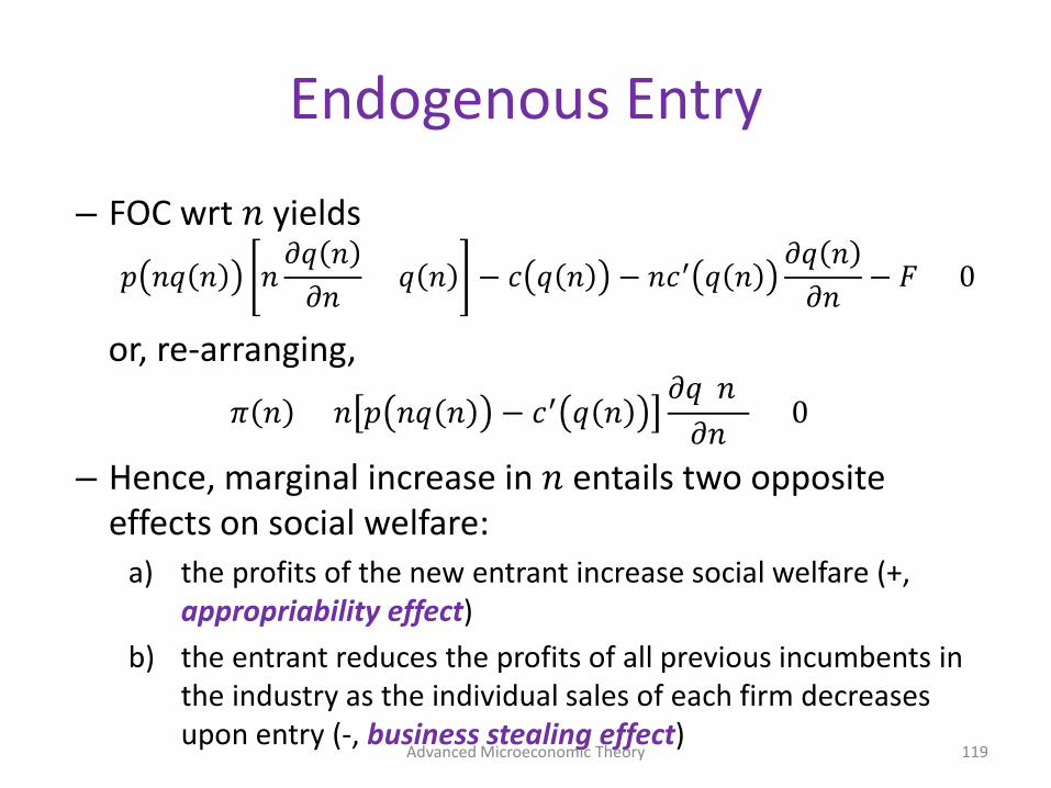
– FOC wrt 𝑛𝑛 yields
𝑝𝑝 𝑛𝑛𝑞𝑞 𝑛𝑛 𝑛𝑛𝜕𝜕𝑞𝑞 𝑛𝑛
𝜕𝜕𝑛𝑛+ 𝑞𝑞 𝑛𝑛 − 𝑐𝑐 𝑞𝑞 𝑛𝑛 − 𝑛𝑛𝑐𝑐′ 𝑞𝑞 𝑛𝑛
𝜕𝜕𝑞𝑞 𝑛𝑛𝜕𝜕𝑛𝑛
− 𝐹𝐹 = 0
or, re-arranging,
𝜋𝜋 𝑛𝑛 + 𝑛𝑛 𝑝𝑝 𝑛𝑛𝑞𝑞 𝑛𝑛 − 𝑐𝑐′ 𝑞𝑞 𝑛𝑛𝜕𝜕𝑞𝑞(𝑛𝑛)
𝜕𝜕𝑛𝑛 = 0
– Hence, marginal increase in 𝑛𝑛 entails two opposite effects on social welfare:
a) the profits of the new entrant increase social welfare (+, appropriability effect)
b) the entrant reduces the profits of all previous incumbents in the industry as the individual sales of each firm decreases upon entry (-, business stealing effect)
Advanced Microeconomic Theory 119

Endogenous Entry
• The “business stealing” effect is represented by:
𝑛𝑛 𝑝𝑝 𝑛𝑛𝑞𝑞 𝑛𝑛 − 𝑐𝑐′ 𝑞𝑞 𝑛𝑛𝜕𝜕𝑞𝑞(𝑛𝑛)
𝜕𝜕𝑛𝑛< 0
which is negative since 𝜕𝜕𝑞𝑞(𝑛𝑛)𝜕𝜕𝑛𝑛
< 0 and 𝑛𝑛 𝑝𝑝 𝑛𝑛𝑞𝑞 𝑛𝑛 − 𝑐𝑐′ 𝑞𝑞 𝑛𝑛 > 0 by definition.
• Therefore, an additional entry induces a
reduction in aggregate output by 𝑛𝑛 𝜕𝜕𝑞𝑞(𝑛𝑛)𝜕𝜕𝑛𝑛
, which in turn produces a negative effect on social welfare.
Advanced Microeconomic Theory 120

Endogenous Entry
• Given the negative sign of the business stealing effect, we can conclude that
𝑊𝑊′ 𝑛𝑛 = 𝜋𝜋 𝑛𝑛 + 𝑛𝑛 𝑝𝑝 𝑛𝑛𝑞𝑞 𝑛𝑛 − 𝑐𝑐′ 𝑞𝑞 𝑛𝑛𝜕𝜕𝑞𝑞 𝑛𝑛
𝜕𝜕𝑛𝑛−
< 𝜋𝜋(𝑛𝑛)
and therefore more firms enter in equilibrium than in the social optimum, i.e., 𝑛𝑛𝑁𝑁 > 𝑛𝑛𝑜𝑜.
Advanced Microeconomic Theory 121

Endogenous Entry
Advanced Microeconomic Theory 122

Endogenous Entry
• Example: – Consider a linear inverse demand 𝑝𝑝 𝑄𝑄 = 1 − 𝑄𝑄
and no marginal costs. – The equilibrium quantity in a market with 𝑛𝑛 firms
that compete a la Cournot is
𝑞𝑞 𝑛𝑛 = 1𝑛𝑛+1
– Let’s check if the three assumptions from above hold.
Advanced Microeconomic Theory 123

Endogenous Entry
• Example (continued): – First, individual output decreases with entry
𝜕𝜕𝑞𝑞 𝑛𝑛𝜕𝜕𝑛𝑛
= − 1𝑛𝑛+1 2 < 0
– Second, aggregate output 𝑛𝑛𝑞𝑞(𝑛𝑛) increases with entry
𝜕𝜕 𝑛𝑛𝑞𝑞 𝑛𝑛𝜕𝜕𝑛𝑛
= 1𝑛𝑛+1 2 > 0
– Third, price lies above marginal cost for any number of firms
𝑝𝑝 𝑛𝑛 − 𝑐𝑐 = 1 − 𝑛𝑛 ∙ 1𝑛𝑛+1
= 1𝑛𝑛+1
> 0 for all 𝑛𝑛
Advanced Microeconomic Theory 124

Endogenous Entry
• Example (continued): – Every firm earns equilibrium profits of
𝜋𝜋 𝑛𝑛 =1
𝑛𝑛 + 1𝑝𝑝(𝑛𝑛)
1𝑛𝑛 + 1
𝑞𝑞(𝑛𝑛)
− 𝐹𝐹 =1
𝑛𝑛 + 1 2 − 𝐹𝐹
– Since equilibrium profits after entry, 1𝑛𝑛+1 2, is
smaller than 1 even if only one firm enters the industry, 𝑛𝑛 = 1, we assume that entry costs are lower than 1, i.e., 𝐹𝐹 < 1.
Advanced Microeconomic Theory 125
Endogenous Entry
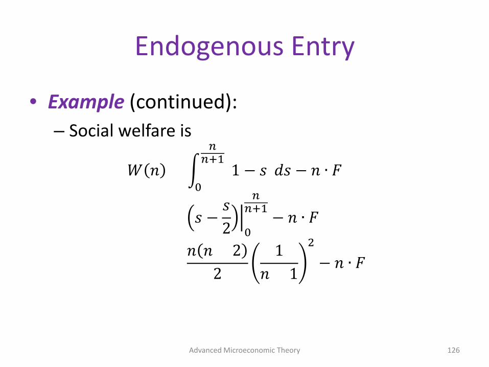
• Example (continued): – Social welfare is
𝑊𝑊 𝑛𝑛 = � (1 − 𝑠𝑠)𝑑𝑑𝑠𝑠 − 𝑛𝑛 ∙ 𝐹𝐹𝑛𝑛
𝑛𝑛+1
0
= 𝑠𝑠 −𝑠𝑠2
�0
𝑛𝑛𝑛𝑛+1 − 𝑛𝑛 ∙ 𝐹𝐹
=𝑛𝑛 𝑛𝑛 + 2
21
𝑛𝑛 + 1
2
− 𝑛𝑛 ∙ 𝐹𝐹
Advanced Microeconomic Theory 126

Endogenous Entry
• Example (continued): – The number of firms entering the market in
equilibrium, 𝑛𝑛𝑁𝑁, is that solving 𝜋𝜋 𝑛𝑛𝑁𝑁 = 0, 1
𝑛𝑛𝑁𝑁 + 1 2 − 𝐹𝐹 = 0 ⟺ 𝑛𝑛𝑁𝑁 =1𝐹𝐹
− 1
whereas the number of firms maximizing social welfare, i.e., 𝑛𝑛𝑜𝑜 solving 𝑊𝑊′ 𝑛𝑛𝑜𝑜 = 0,
𝑊𝑊′ 𝑛𝑛𝑜𝑜 =1
𝑛𝑛𝑜𝑜 + 1 3 = 0 ⟺ 𝑛𝑛𝑜𝑜 =1𝐹𝐹3 − 1
where 𝑛𝑛𝑁𝑁 < 𝑛𝑛𝑜𝑜 for all admissible values of 𝐹𝐹, i.e., 𝐹𝐹 ∈ 0,1 .
Advanced Microeconomic Theory 127

Entry costs, F
ne = – 1 (Equilibrium)1F ½
no = – 1 (Soc. Optimal)1F ⅓
Number of firms
0
Endogenous Entry
• Example (continued):
Advanced Microeconomic Theory 128

Repeated Interaction
Advanced Microeconomic Theory 129

Repeated Interaction • In all previous models, we considered firms interacting
during one period (i.e., one-shot game). • However, firms compete during several periods and, in
some cases, during many generations. • In these cases, a firm’s actions during one period might
affect its rival’s behavior in future periods. • More importantly, we can show that under certain
conditions, the strong competitive results in the Bertrand (and, to some extent, in the Cournot) model can be avoided when firms interact repeatedly along time.
• That is, collusion can be supported in the repeated game even if it could not in the one-shot game.
Advanced Microeconomic Theory 130

Repeated Interaction: Bertrand Model
• Consider two firms selling homogeneous products. • Let 𝑝𝑝𝑗𝑗
𝑡𝑡 denote firm 𝑗𝑗’s pricing strategy at period 𝑡𝑡, which is a function of the history of all price choices by the two firms, 𝐻𝐻𝑡𝑡−1 = 𝑝𝑝1
𝑡𝑡 , 𝑝𝑝2𝑡𝑡
𝑡𝑡=1𝑡𝑡−1.
• Conditioning 𝑝𝑝𝑗𝑗𝑡𝑡 on the full history of play allows for a
wide range of pricing strategies: – setting the same price regardless of previous history – retaliation if the rival lowers its price below a “threshold
level” – increasing cooperation if the rival was cooperative in
previous periods (until reaching the monopoly price 𝑝𝑝𝑚𝑚) Advanced Microeconomic Theory 131

Repeated Interaction: Bertrand Model
• Finitely repeated game: – Can we support cooperation if the Bertrand game
is repeated for a finite number of 𝑇𝑇 rounds? No!
– To see why, consider the last period of the repeated game (period 𝑇𝑇): Regardless of previous pricing strategies, every firms’
optimal pricing strategy in this stage is to set 𝑝𝑝𝑖𝑖,𝑇𝑇∗ = 𝑐𝑐,
as in the one-shot Bertrand game.
Advanced Microeconomic Theory 132

Repeated Interaction: Bertrand Model
– Now, move to the previous to the last period (𝑇𝑇 − 1): Both firms anticipate that, regardless of what they choose at
𝑇𝑇 − 1, they will both select 𝑝𝑝𝑖𝑖,𝑇𝑇∗ = 𝑐𝑐 in period 𝑇𝑇. Hence, it is
optimal for both to select 𝑝𝑝𝑖𝑖,𝑇𝑇−1∗ = 𝑐𝑐 in period 𝑇𝑇 − 1 as well.
– Now, move to period (𝑇𝑇 −2): Both firms anticipate that, regardless of what they choose at
𝑇𝑇 − 2, they will both select 𝑝𝑝𝑖𝑖,𝑇𝑇∗ = 𝑐𝑐 in period 𝑇𝑇 and 𝑝𝑝𝑖𝑖,𝑇𝑇−1
∗ = 𝑐𝑐 in period 𝑇𝑇 − 1. Thus, it is optimal for both to select 𝑝𝑝𝑖𝑖,𝑇𝑇−2
∗ = 𝑐𝑐 in period 𝑇𝑇 − 2 as well.
– The same argument extends to all previous periods, including the first round of play 𝑡𝑡 = 1.
– Hence, both firms behave as in one-shot Bertrand game.
Advanced Microeconomic Theory 133

Repeated Interaction: Bertrand Model
• Infinitely repeated game: – Can we support cooperation if the Bertrand game is
repeated for an infinite periods? Yes! Cooperation (i.e., selecting prices above marginal cost)
can indeed be sustained using different pricing strategies.
– For simplicity, consider the following pricing strategy 𝑝𝑝𝑗𝑗𝑡𝑡 𝐻𝐻𝑡𝑡−1 = �𝑝𝑝𝑚𝑚 if all elements in 𝐻𝐻𝑡𝑡−1 are 𝑝𝑝𝑚𝑚, 𝑝𝑝𝑚𝑚 or 𝑡𝑡 = 1
𝑐𝑐 otherwise
In words, every firm 𝑗𝑗 sets the monopoly price 𝑝𝑝𝑚𝑚 in period 1. Then, in each subsequent period 𝑡𝑡 > 1, firm 𝑗𝑗 sets 𝑝𝑝𝑚𝑚 if both firms charged 𝑝𝑝𝑚𝑚 in all previous periods. Otherwise, firm 𝑗𝑗 charges a price equal to marginal cost.
Advanced Microeconomic Theory 134

Repeated Interaction: Bertrand Model
– This type of strategy is usually referred to as Nash reversion strategy (NRS): firms cooperate until one of them deviates, in which case
firms thereafter revert to the Nash equilibrium of the unrepeated game (i.e., set prices equal to marginal cost)
– Let us show that NRS can be sustained in the equilibrium of the infinitely repeated game.
– We need to demonstrate that firms do not have incentives to deviate from it, during any period 𝑡𝑡 > 1 and regardless of their previous history of play.
Advanced Microeconomic Theory 135

Repeated Interaction: Bertrand Model
– Consider any period 𝑡𝑡 > 1, and a history of play for which all firms have been cooperative until 𝑡𝑡 − 1.
– By cooperating, firm 𝑗𝑗’s profits would be 𝑝𝑝𝑚𝑚 − 𝑐𝑐 1
2 𝑥𝑥(𝑝𝑝𝑚𝑚), i.e., half of monopoly profits 𝜋𝜋
𝑚𝑚
2,
in all subsequent periods 𝜋𝜋𝑚𝑚
2+ 𝛿𝛿
𝜋𝜋𝑚𝑚
2+ 𝛿𝛿2 𝜋𝜋𝑚𝑚
2+ ⋯
= 1 + 𝛿𝛿 + 𝛿𝛿2 + ⋯𝜋𝜋𝑚𝑚
2=
11 − 𝛿𝛿
𝜋𝜋𝑚𝑚
2
where 𝛿𝛿 ∈ (0,1) denotes firms’ discount factor Advanced Microeconomic Theory 136
Repeated Interaction: Bertrand Model
– If, in contrast, firm 𝑗𝑗 deviates in period 𝑡𝑡, the optimal deviation is 𝑝𝑝𝑗𝑗,𝑡𝑡 = 𝑝𝑝𝑚𝑚 − 𝜀𝜀, where 𝜀𝜀 > 0, given its rival still sets a price 𝑝𝑝𝑘𝑘,𝑡𝑡 = 𝑝𝑝𝑚𝑚.
– This allows firm 𝑗𝑗 to capture all market, and obtain monopoly profits 𝜋𝜋𝑚𝑚 during the deviating period.
– A deviation is detected in period 𝑡𝑡 + 1, triggering a NRS from firm 𝑘𝑘 (i.e., setting a price equal to marginal cost) thereafter, and entailing a zero profit for both firms.
– The discounted stream of profits for firm 𝑗𝑗 is then 𝜋𝜋𝑚𝑚 + 𝛿𝛿𝛿 + 𝛿𝛿20 + ⋯ = 𝜋𝜋𝑚𝑚
Advanced Microeconomic Theory 137

Repeated Interaction: Bertrand Model
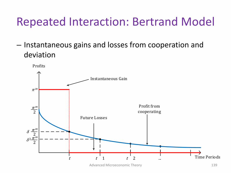
– Hence, firm 𝑗𝑗 prefers to stick to the NRS at period 𝑡𝑡 if 1
1 − 𝛿𝛿𝜋𝜋𝑚𝑚
2> 𝜋𝜋𝑚𝑚 ⟺ 𝛿𝛿 >
12
– That is, cooperation can be sustained as long as firms assign a sufficiently high value to future profits.
Advanced Microeconomic Theory 138
Profits
Time Periodst t + 1 t + 2 ...
Instantaneous Gain
Profit from cooperating
π m
2
π m
Future Losses
π m
2π m
2
δ
δ 2
Repeated Interaction: Bertrand Model
– Instantaneous gains and losses from cooperation and deviation
Advanced Microeconomic Theory 139

Repeated Interaction: Bertrand Model
• What about firm 𝑗𝑗’s incentives to use NRS after a history of play in which some firms deviated? – NRS calls for firm 𝑗𝑗 to revert to the equilibrium of
the unrepeated Bertrand model. – That is, to implement the punishment embodied
in NRS after detecting a deviation from any player.
• By sticking to the NRS, firm 𝑗𝑗’s discounted stream of payoffs is
0 + 𝛿𝛿𝛿 + ⋯ = 0 Advanced Microeconomic Theory 140

Repeated Interaction: Bertrand Model
• By deviating from NRS (i.e., setting a price 𝑝𝑝𝑗𝑗 = 𝑝𝑝𝑚𝑚 while its opponent sets a punishing price 𝑝𝑝𝑘𝑘 = 𝑐𝑐), profits are also zero in all periods.
• Hence, firm 𝑗𝑗 has incentives to carry out the threat – That is, setting a punishing price of 𝑝𝑝𝑗𝑗 = 𝑐𝑐, upon
observing a deviation in any previous period. • As a result, the NRS can be sustained in
equilibrium, since both firms have incentives to use it, at any time period 𝑡𝑡 > 1 and irrespective of the previous history of play.
Advanced Microeconomic Theory 141
Repeated Interaction: Bertrand Model
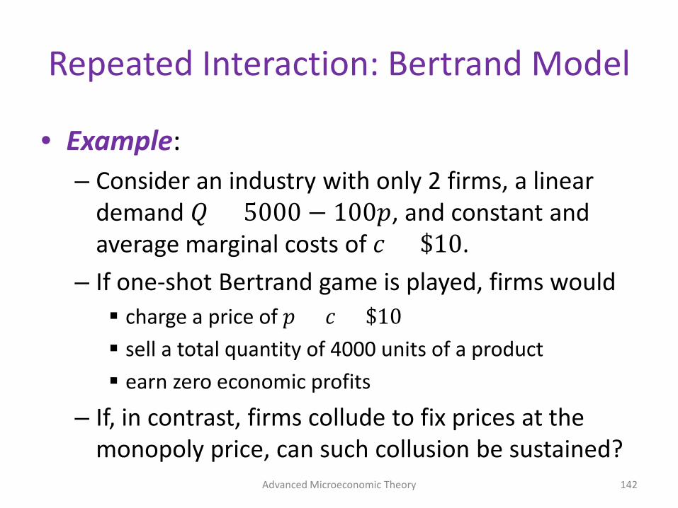
• Example: – Consider an industry with only 2 firms, a linear
demand 𝑄𝑄 = 5000 − 1𝛿𝛿𝑝𝑝, and constant and average marginal costs of 𝑐𝑐 = $10.
– If one-shot Bertrand game is played, firms would charge a price of 𝑝𝑝 = 𝑐𝑐 = $10 sell a total quantity of 4000 units of a product earn zero economic profits
– If, in contrast, firms collude to fix prices at the monopoly price, can such collusion be sustained?
Advanced Microeconomic Theory 142

Repeated Interaction: Bertrand Model
• Example (continued): – Monopoly price is determined by solving the
firms’ joint PMP max
𝑝𝑝 𝑝𝑝 − 10 ⋅ 𝑄𝑄 = 𝑝𝑝(5000
− 1𝛿𝛿𝑝𝑝) − 10(5000 − 1𝛿𝛿𝑝𝑝) – FOC:
5000 − 2𝛿𝛿𝑝𝑝 + 1000 = 0 – Solving for 𝑝𝑝 yields the monopoly price 𝑝𝑝𝑚𝑚 = 30. – The aggregate output is 𝑄𝑄 = 2000 (i.e., 1000
units per firm) and the corresponding profits are 𝜋𝜋𝑚𝑚 = $40,000 ($20,000 per firm).
Advanced Microeconomic Theory 143
Repeated Interaction: Bertrand Model
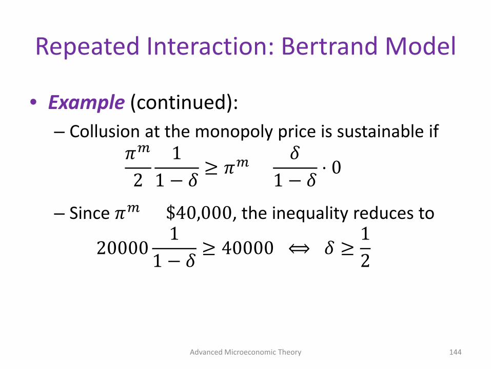
• Example (continued): – Collusion at the monopoly price is sustainable if
𝜋𝜋𝑚𝑚
21
1 − 𝛿𝛿≥ 𝜋𝜋𝑚𝑚 +
𝛿𝛿1 − 𝛿𝛿
⋅ 0
– Since 𝜋𝜋𝑚𝑚 = $40,000, the inequality reduces to
200001
1 − 𝛿𝛿≥ 40000 ⟺ 𝛿𝛿 ≥
12
Advanced Microeconomic Theory 144

Repeated Interaction: Bertrand Model
• Example (continued): – What would happen if there were 𝑛𝑛 firms? – Each firm’s share of the monopoly profit stream
under collusion would be 𝜋𝜋𝑚𝑚
𝑛𝑛= 40000
𝑛𝑛.
– Collusion at the monopoly price is sustainable if 40000
𝑛𝑛1
1−𝛿𝛿≥ 40000 ⟺ 𝛿𝛿 ≥ 1 − 1
𝑛𝑛≡ 𝛿𝛿̅
– Hence, as the number of firms in the industry increases, it becomes more difficult to sustain cooperation.
Advanced Microeconomic Theory 145

Repeated Interaction: Bertrand Model
• Example (continued): minimal discount factor sustaining collusion
Advanced Microeconomic Theory 146

Repeated Interaction: Cournot Model
• We can extend a similar analysis to the Cournot model of quantity competition with two firms selling homogeneous products.
• For simplicity, consider the following NRS for every firm 𝑗𝑗
𝑞𝑞𝑗𝑗𝑡𝑡 𝐻𝐻𝑡𝑡−1 = �𝑞𝑞𝑚𝑚
2if all elements in 𝐻𝐻𝑡𝑡−1 equal
𝑞𝑞𝑚𝑚
2 ,
𝑞𝑞𝑚𝑚
2 or 𝑡𝑡 = 1
𝑞𝑞𝑗𝑗𝐶𝐶𝑜𝑜𝐶𝐶𝐶𝐶𝑛𝑛𝑜𝑜𝑡𝑡 otherwise
In words, firm 𝑗𝑗’s strategy is to produce half of the monopoly output 𝑞𝑞
𝑚𝑚
2 in period 𝑡𝑡 = 1. Then, in each
subsequent period 𝑡𝑡 > 1, firm 𝑗𝑗 continues producing 𝑞𝑞𝑚𝑚
2 if
both firms produced 𝑞𝑞𝑚𝑚
2 in all previous periods. Otherwise,
firm 𝑗𝑗 reverts to the Cournot equilibrium output. Advanced Microeconomic Theory 147

Repeated Interaction: Cournot Model
• Let us show that NRS can be sustained in the equilibrium of the infinitely repeated game.
• If firm 𝑗𝑗 uses the NRS in period 𝑡𝑡, it obtains half of monopoly profits, 𝜋𝜋
𝑚𝑚
2, thereafter, with a
discounted stream of profits of 𝜋𝜋𝑚𝑚
21
1−𝛿𝛿.
• But, what if firm 𝑗𝑗 deviates from this strategy? What is its optimal deviation? – Since firm 𝑘𝑘 sticks to the NRS, and thus produces 𝑞𝑞
𝑚𝑚
2
units, we can evaluate firm 𝑗𝑗’s BRF 𝑞𝑞𝑗𝑗(𝑞𝑞𝑘𝑘) at 𝑞𝑞𝑘𝑘 = 𝑞𝑞𝑚𝑚
2,
or 𝑞𝑞𝑗𝑗𝑞𝑞𝑚𝑚
2.
Advanced Microeconomic Theory 148

Repeated Interaction: Cournot Model
• For compactness, let 𝑞𝑞𝑗𝑗𝑑𝑑𝑁𝑁𝑑𝑑 ≡ 𝑞𝑞𝑗𝑗
𝑞𝑞𝑚𝑚
2 denote firm
𝑗𝑗’s optimal deviation. • This yields profits of
𝜋𝜋𝑗𝑗𝑑𝑑𝑁𝑁𝑑𝑑 ≡ 𝑝𝑝 𝑞𝑞𝑗𝑗
𝑑𝑑𝑁𝑁𝑑𝑑 ,𝑞𝑞𝑚𝑚
2× 𝑞𝑞𝑗𝑗
𝑑𝑑𝑁𝑁𝑑𝑑 − 𝑐𝑐𝑗𝑗 × 𝑞𝑞𝑗𝑗𝑑𝑑𝑁𝑁𝑑𝑑
• By deviating firm 𝑗𝑗 obtains following stream of profits
𝜋𝜋𝑗𝑗𝑑𝑑𝑁𝑁𝑑𝑑 + 𝛿𝛿𝜋𝜋𝑗𝑗
𝐶𝐶𝑜𝑜𝐶𝐶𝐶𝐶𝑛𝑛𝑜𝑜𝑡𝑡 + 𝛿𝛿2𝜋𝜋𝑗𝑗𝐶𝐶𝑜𝑜𝐶𝐶𝐶𝐶𝑛𝑛𝑜𝑜𝑡𝑡 + ⋯
= 𝜋𝜋𝑗𝑗𝑑𝑑𝑁𝑁𝑑𝑑 +
𝛿𝛿1 − 𝛿𝛿
𝜋𝜋𝑗𝑗𝐶𝐶𝑜𝑜𝐶𝐶𝐶𝐶𝑛𝑛𝑜𝑜𝑡𝑡
Advanced Microeconomic Theory 149

Repeated Interaction: Cournot Model
• Hence, firm 𝑗𝑗 sticks to the NRS as long as 1
1 − 𝛿𝛿𝜋𝜋𝑚𝑚
2> 𝜋𝜋𝑗𝑗
𝑑𝑑𝑁𝑁𝑑𝑑 +𝛿𝛿
1 − 𝛿𝛿𝜋𝜋𝑗𝑗
𝐶𝐶𝑜𝑜𝐶𝐶𝐶𝐶𝑛𝑛𝑜𝑜𝑡𝑡
• Multiplying both sides by (1 − 𝛿𝛿) and solving for 𝛿𝛿 we obtain
𝛿𝛿 >𝜋𝜋𝑗𝑗
𝑑𝑑𝑁𝑁𝑑𝑑 − 𝜋𝜋𝑚𝑚
2𝜋𝜋𝑗𝑗
𝑑𝑑𝑁𝑁𝑑𝑑 − 𝜋𝜋𝑗𝑗𝐶𝐶𝑜𝑜𝐶𝐶𝐶𝐶𝑛𝑛𝑜𝑜𝑡𝑡 ≡ 𝛿𝛿̅
• Intuitively, every firm 𝑗𝑗 sticks to the NRS as long as it assigns a sufficient weight to future profits.
Advanced Microeconomic Theory 150

Repeated Interaction: Cournot Model
• Instantaneous gains and losses from deviation
Advanced Microeconomic Theory 151

Repeated Interaction: Cournot Model
• What about firm 𝑗𝑗’s incentives to use NRS after a history of play in which some firms deviated? – NRS calls for firm 𝑗𝑗 to revert to the equilibrium of the
unrepeated Cournot model. – That is, to implement the punishment embodied in NRS
after detecting a deviation from any player.
• By sticking to the NRS, firm 𝑗𝑗’s discounted stream of payoffs is 1
1−𝛿𝛿𝜋𝜋𝑚𝑚
2.
• By deviating from 𝑞𝑞𝑗𝑗𝐶𝐶𝑜𝑜𝐶𝐶𝐶𝐶𝑛𝑛𝑜𝑜𝑡𝑡, while firm 𝑘𝑘 produces
𝑞𝑞𝑘𝑘𝐶𝐶𝑜𝑜𝐶𝐶𝐶𝐶𝑛𝑛𝑜𝑜𝑡𝑡, firm 𝑗𝑗’s profits, 𝜋𝜋�, are lower than 𝜋𝜋𝑗𝑗
𝐶𝐶𝑜𝑜𝐶𝐶𝐶𝐶𝑛𝑛𝑜𝑜𝑡𝑡 since firm 𝑗𝑗’s best response to its rival producing 𝑞𝑞𝑘𝑘
𝐶𝐶𝑜𝑜𝐶𝐶𝐶𝐶𝑛𝑛𝑜𝑜𝑡𝑡 is 𝑞𝑞𝑗𝑗𝐶𝐶𝑜𝑜𝐶𝐶𝐶𝐶𝑛𝑛𝑜𝑜𝑡𝑡.
Advanced Microeconomic Theory 152

Repeated Interaction: Cournot Model
• Firm 𝑗𝑗 sticks to the NRS after a history of deviations since
𝜋𝜋𝐶𝐶𝑜𝑜𝐶𝐶𝐶𝐶𝑛𝑛𝑜𝑜𝑡𝑡 + 𝛿𝛿𝜋𝜋𝐶𝐶𝑜𝑜𝐶𝐶𝐶𝐶𝑛𝑛𝑜𝑜𝑡𝑡 + ⋯ > 𝜋𝜋� + 𝛿𝛿𝜋𝜋𝐶𝐶𝑜𝑜𝐶𝐶𝐶𝐶𝑛𝑛𝑜𝑜𝑡𝑡 + ⋯
which holds given that 𝜋𝜋𝐶𝐶𝑜𝑜𝐶𝐶𝐶𝐶𝑛𝑛𝑜𝑜𝑡𝑡 > 𝜋𝜋�.
• Hence, no need to impose any further conditions on the minimal discount factor sustaining cooperation, 𝛿𝛿̅.
Advanced Microeconomic Theory 153

Repeated Interaction: Cournot Model
• Example: – Consider an industry with 2 firms, a linear inverse
demand 𝑝𝑝(𝑞𝑞1, 𝑞𝑞2) = 𝑎𝑎 − 𝑏𝑏(𝑞𝑞1 + 𝑞𝑞2), and constant and average marginal costs of 𝑐𝑐 > 0.
– Firm 𝑖𝑖’s PMP is max
𝑞𝑞𝑖𝑖 𝑎𝑎 − 𝑏𝑏(𝑞𝑞𝑖𝑖 + 𝑞𝑞𝑗𝑗) 𝑞𝑞𝑖𝑖 − 𝑐𝑐𝑞𝑞𝑖𝑖
– FOCs: 𝑎𝑎 − 2𝑏𝑏𝑞𝑞𝑖𝑖 − 𝑏𝑏𝑞𝑞𝑗𝑗 − 𝑐𝑐 = 0 – Solving for 𝑞𝑞𝑖𝑖 yields firm 𝑖𝑖’s BRF
𝑞𝑞𝑖𝑖(𝑞𝑞𝑗𝑗) = 𝑎𝑎−𝑐𝑐2𝑏𝑏
− 𝑞𝑞𝑗𝑗
2
Advanced Microeconomic Theory 154

Repeated Interaction: Cournot Model
• Example (continued): – Solving the two BRFs simultaneously yields
𝑞𝑞𝑖𝑖𝐶𝐶𝑜𝑜𝐶𝐶𝐶𝐶𝑛𝑛𝑜𝑜𝑡𝑡 = 𝑎𝑎−𝑐𝑐
3𝑏𝑏
with corresponding price of
𝑝𝑝 = 𝑎𝑎 − 𝑏𝑏 𝑎𝑎−𝑐𝑐3𝑏𝑏
+ 𝑎𝑎−𝑐𝑐3𝑏𝑏
= 𝑎𝑎+2𝑐𝑐3
and equilibrium profits of
𝜋𝜋𝑖𝑖𝐶𝐶𝑜𝑜𝐶𝐶𝐶𝐶𝑛𝑛𝑜𝑜𝑡𝑡 = 𝑎𝑎+2𝑐𝑐
3𝑎𝑎−𝑐𝑐3𝑏𝑏
− 𝑐𝑐 𝑎𝑎−𝑐𝑐3𝑏𝑏
= 𝑎𝑎−𝑐𝑐 2
9𝑏𝑏
Advanced Microeconomic Theory 155

Repeated Interaction: Cournot Model
• Example (continued): – If, instead, each firm produced half of monopoly
output, 𝑞𝑞𝑖𝑖𝑚𝑚 = 𝑞𝑞𝑚𝑚
2= 𝑎𝑎−𝑐𝑐
4𝑏𝑏, they would face a
corresponding price of 𝑝𝑝𝑚𝑚 = 𝑎𝑎+𝑐𝑐2
and receive half
of the monopoly profits 𝜋𝜋𝑖𝑖𝑚𝑚 = 𝜋𝜋𝑚𝑚
2= 𝑎𝑎−𝑐𝑐 2
8𝑏𝑏.
– In this setting, the optimal deviation of firm 𝑖𝑖 is found by plugging 𝑞𝑞𝑖𝑖
𝑚𝑚 into its BRF
𝑞𝑞𝑖𝑖𝐷𝐷𝑁𝑁𝑑𝑑 = 𝑞𝑞𝑖𝑖(𝑞𝑞𝑗𝑗
𝑚𝑚) = 𝑎𝑎−𝑐𝑐2𝑏𝑏
− 12
𝑎𝑎−𝑐𝑐4𝑏𝑏
= 3 𝑎𝑎−𝑐𝑐8𝑏𝑏
Advanced Microeconomic Theory 156
Repeated Interaction: Cournot Model
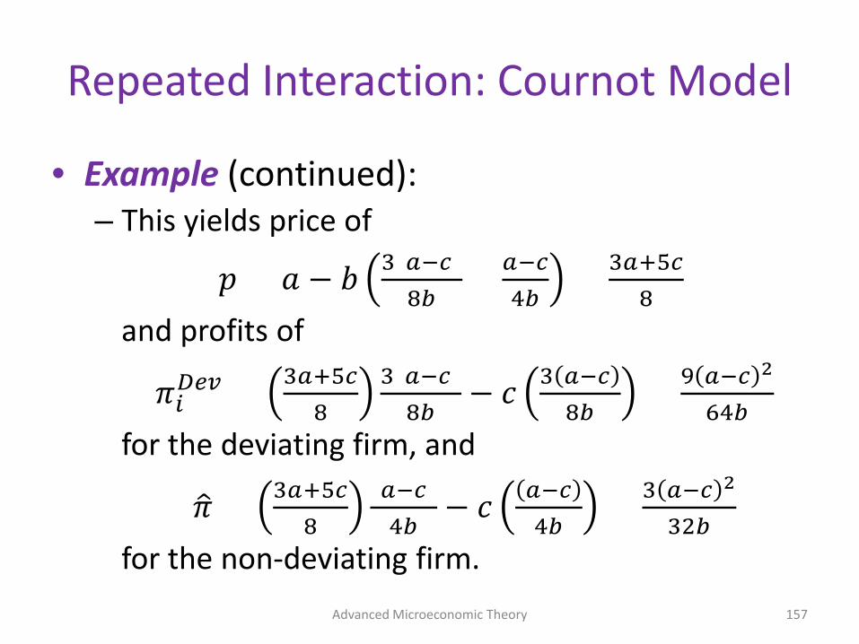
• Example (continued): – This yields price of
𝑝𝑝 = 𝑎𝑎 − 𝑏𝑏 3(𝑎𝑎−𝑐𝑐)8𝑏𝑏
+ 𝑎𝑎−𝑐𝑐4𝑏𝑏
= 3𝑎𝑎+5𝑐𝑐8
and profits of
𝜋𝜋𝑖𝑖𝐷𝐷𝑁𝑁𝑑𝑑 = 3𝑎𝑎+5𝑐𝑐
83(𝑎𝑎−𝑐𝑐)
8𝑏𝑏− 𝑐𝑐 3 𝑎𝑎−𝑐𝑐
8𝑏𝑏= 9 𝑎𝑎−𝑐𝑐 2
64𝑏𝑏
for the deviating firm, and
𝜋𝜋� = 3𝑎𝑎+5𝑐𝑐8
(𝑎𝑎−𝑐𝑐)4𝑏𝑏
− 𝑐𝑐 𝑎𝑎−𝑐𝑐4𝑏𝑏
= 3 𝑎𝑎−𝑐𝑐 2
32𝑏𝑏
for the non-deviating firm. Advanced Microeconomic Theory 157

Repeated Interaction: Cournot Model
• Example (continued): – Cooperation is sustainable if
11−𝛿𝛿
𝜋𝜋𝑚𝑚
2> 𝜋𝜋𝑗𝑗
𝑑𝑑𝑁𝑁𝑑𝑑 + 𝛿𝛿1−𝛿𝛿
𝜋𝜋𝑗𝑗𝐶𝐶𝑜𝑜𝐶𝐶𝐶𝐶𝑛𝑛𝑜𝑜𝑡𝑡
or, in our case, 1
1−𝛿𝛿𝑎𝑎−𝑐𝑐 2
8𝑏𝑏> 9 𝑎𝑎−𝑐𝑐 2
64𝑏𝑏+ 𝛿𝛿
1−𝛿𝛿𝑎𝑎−𝑐𝑐 2
9𝑏𝑏 ⟺ 𝛿𝛿 > 9
17
– For the non-deviating firm, we have 𝜋𝜋𝑖𝑖𝐶𝐶𝑜𝑜𝐶𝐶𝐶𝐶𝑛𝑛𝑜𝑜𝑡𝑡 > 𝜋𝜋�
That is, if the rival firm defects, the non-defecting firm will obtain a larger profit by reverting to the Cournot output level.
Advanced Microeconomic Theory 158

Repeated Interaction: Cournot Model
• Extensions: – Temporary reversions to the equilibrium of the
unrepeated game – (Temporary) punishments that yield even lower
payoffs – Less “pure” forms of cooperations – Imperfect monitoring
Advanced Microeconomic Theory 159