advanced excel for emis coordinators - omeresa.net excel advanced 1 per page.pdf · “hide” and...
TRANSCRIPT

11/9/2018
1
© 2015 Metropolitan Educational Technology Association
Advanced Excel for EMIS Coordinators
Helen Mills

11/9/2018
2
Outline
• Macros• Conditional Formatting• Text to Columns• Pivot Tables• V-Lookup

11/9/2018
3
Macros
• What is a macro?• How to use• How to remove

11/9/2018
4
What is a Macro?If you have tasks in Excel that you do repeatedly, you can record a macro to automate those tasks. When you create a macro you are recording your mouse clicks and keystrokes.
We are going to create a macro in this example to auto-magically prepare all reports.
In one click Excel will:
• Freeze top row
• Wrap Header Text
• Justify Columns
• Apply Filters
• Create it once and use it over and over again!
• Start by opening your FTE Detail report from the data collector.

11/9/2018
5
Begin Creating a Macro
From the View tab, select the down arrow under Macros and select
“Record Macro.”
Select the down arrow
This begins the recording
11/9/2018
6
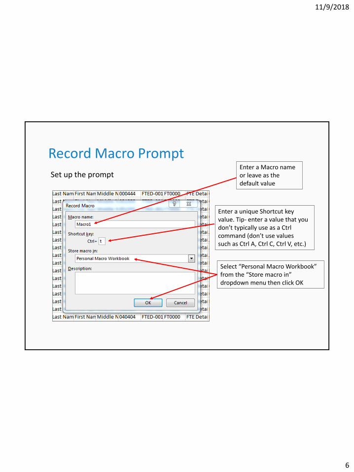
Record Macro Prompt
Set up the promptEnter a Macro name or leave as the default value
Enter a unique Shortcut key value. Tip- enter a value that you don’t typically use as a Ctrl command (don’t use values such as Ctrl A, Ctrl C, Ctrl V, etc.)
Select “Personal Macro Workbook” from the “Store macro in” dropdown menu then click OK

11/9/2018
7
Recording the Macro
• Macro is now recording
• Ready status and a small square icon show at bottom left
Hovering over the icon will generate the message-“A macro is currently recording. Click to stop recording.”

11/9/2018
8
Recording the Macro cont’d
Start by selecting the top row
Click on the “1” to select the first row

11/9/2018
9
Recording the Macro cont’d
From the View tab, select “Freeze Panes” and “Freeze Top Row”

11/9/2018
10
Recording the Macro cont’d
From the Home tab, select “Wrap Text”

11/9/2018
11
Recording the Macro cont’d
Click on the triangle between Column A and Row 1 to select theentire spreadsheet
Place cursor between any two column headers and double click

11/9/2018
12
Recording the Macro cont’d
From the Home tab, select “Sort & Filter” and then “Filter”

11/9/2018
13
Stop the Recording
Click on the small square icon at the bottom left to stop the recording
The appearance of the icon will change and a hover message will appear. “No macros are currently recording. Click to begin recording a new macro.”

11/9/2018
14
Make the Macro a Quick Link
Select the Quick Link dropdown arrow, then “More Commands”
In the “Choose commands from” dropdown, select “Macros”

11/9/2018
15
Make the Macro a Quick Link
Highlight your macro from the list and click “Add”
The macro will move to the list on the right. While it is highlighted, select “Modify” and choose an icon that you like. Click Ok and Ok.

11/9/2018
16
Quick Link
New Quick Link now appears
To remove the Quick Link, right click on the icon and select “Remove from Quick Access Toolbar”

11/9/2018
17
Save the Macro
• You can choose to save or not save your spreadsheet
• A second prompt will ask you if you want to save the changes you
made to your Personal Macro Workbook
Select Save so that the macro will be available to use on future spreadsheets

11/9/2018
18
Delete a Macro
Once a Macro is created, a few extra steps are needed to delete if desired.
From a new or existing spreadsheet select “Unhide” from the View tab
In the Unhide prompt with PERSONAL.XLSB selected, click OK
11/9/2018
19
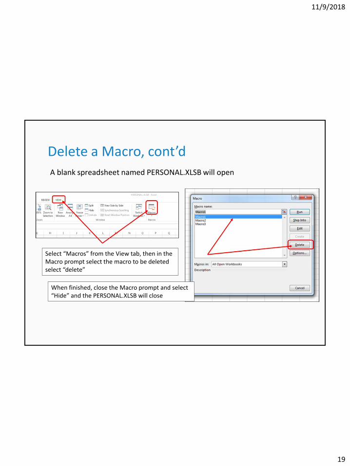
Delete a Macro, cont’d
A blank spreadsheet named PERSONAL.XLSB will open
Select “Macros” from the View tab, then in the Macro prompt select the macro to be deleted select “delete”
When finished, close the Macro prompt and select “Hide” and the PERSONAL.XLSB will close

11/9/2018
20
Conditional Formatting
• What is conditional formatting?• How to use• How to remove

11/9/2018
21
What is Conditional Formatting?
Conditional formatting is a way to format cells that meet a criteria you
specify. In this example, we are going to apply formatting to FTE detail
rows where the adjusted FTE is different than the original FTE.
• Start by opening your FTE detail report
• Run your macro

11/9/2018
22
Apply Conditional Formatting
Select columns P & Q. On the Home tab select conditional formatting, and
then highlight cells rules, and then more rules.

11/9/2018
23
Apply Conditional Formatting
Click format to specify how you want the cells to look.
Use the fill tab to choose a fill color
Choose OK once formatted to your liking.
Type the following equation: =$P1<>$Q1
Choose OK to apply conditional formatting

11/9/2018
24
Conditional Formatting
You can now view your formatting. For adjusted FTE lower than original
FTE, use the FTE Adjustments report to troubleshoot or verify.

11/9/2018
25
Removing Conditional Formatting
To remove conditional formatting, on the home tab choose Conditional
Formatting, then clear rules, then clear rules from entire sheet.

11/9/2018
26
Text to Columns
• How to use

11/9/2018
27
Text to ColumnsText to columns is a feature within excel that can split a column the way you would like to see it. For example, let’s say we are performing an upload and the birth month, date, and year must all be in separate columns. We have an export with the students’ birthdate on it. We need to have 3 blank columns to the right of the birthdate in order to perform text to columns. Select the column with the birthdate in it and choose Text to Columns from the data tab.

11/9/2018
28
Text to Columns cont’dThe text to columns wizard will pop up. The first prompt we see asks if we are
splitting the text delimited (using a character) or fixed width (a certain position
within the column). For the example we are using delimited. Click “Next.”

11/9/2018
29
Text to Columns cont’d
Choose the delimiter. The backslash is not an option in the list, so we will
check the “other” box and type a backslash in the box. Then click “Next.”

11/9/2018
30
Text to Columns cont’d
The last prompt is a preview and it asks how you would like the output to
be formatted. The default setting is “General,” but we want to select
“Text”. Next Click “Finish.”

11/9/2018
31
Text to Columns
We now have the components of the birth dates in separate columns! You
can name the columns “Birth Month” “Birth date” and “Birth Year”.

11/9/2018
32
Pivot TablesGenerate Reports Quickly
• What is a Pivot Table?• How to use• How to remove• EMIS Examples

11/9/2018
33
Pivot Tables
Pivot tables are a powerful and helpful Excel tool. These tables take very
large amounts of data and summarize it in the way we specify.
There are many ways we can use Pivot tables in EMIS. Here are a few
examples of when we would use a pivot table:
• Quickly summarize special education students (Example)
• Easily verify calendars
• Summarize FTE report
• Start by opening your FTE detail report

11/9/2018
34
Summarize SPED Students
Select the entire sheet. On the Insert tab, choose Pivot Table

11/9/2018
35
Summarize SPED Students
Choose OK to begin building the pivot table on a new sheet.
11/9/2018
36
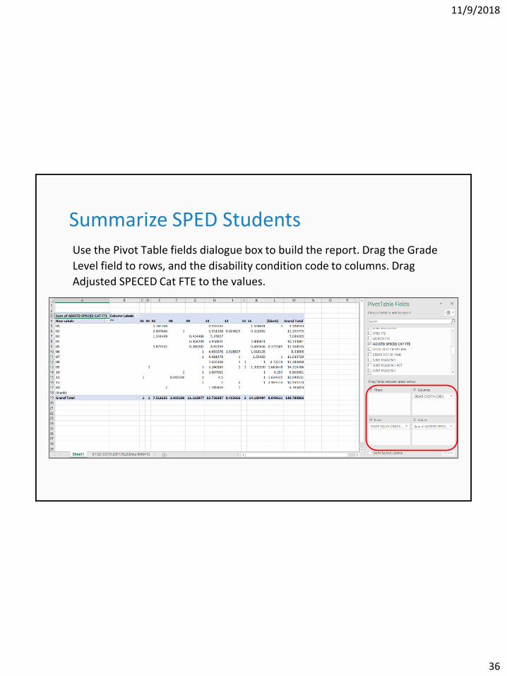
Summarize SPED Students
Use the Pivot Table fields dialogue box to build the report. Drag the Grade
Level field to rows, and the disability condition code to columns. Drag
Adjusted SPECED Cat FTE to the values.

11/9/2018
37
Summarize SPED Students
In the values square, make sure you are seeing the SUM of the FTE. Click
the arrow to the right and choose “Value Field Settings” to change this.
Once you have the desired value, choose OK.

11/9/2018
38
Summarize SPED Students
Now you can see the FTE you are generating for each disability category in
each grade level.

11/9/2018
39
Summarize SPED Students
You can take it one step further by adding a filter. You could filter by
district of residence, or even FTE Fund Pattern code. In this example we
will filter using district of residence. Choose the districts you’d like to see.

11/9/2018
40
Summarize SPED Students
You can now view your report the way you set it up. You can make any
updates to this using the pivot table options. Right click on the pivot table
and choose refresh to refresh the pivot table data if needed. Since the
Pivot table is on it’s own sheet, simply delete if no longer needed.

11/9/2018
41
V-Lookup
• What is V-Lookup?• How to use• EMIS Examples

11/9/2018
42
What is V-Lookup?
The V-Lookup function in Excel will lookup and retrieve data from a
specific column in a table. Lookup values must appear in the first column
of the table, with lookup columns to the right.
In this example, we are going to:
• Use V-Lookup to insert the district name using the IRN number
• Use V-Lookup to verify staff years of experience
• Start by opening your FTE-Detail report from the data collector and
apply your macro to format it.

11/9/2018
43
Using V-Lookup to add District Names
When generating reports, it can be helpful to include the names that are
associated with the district IRN. In this example, we will add the district of
residence name to the FTE detail report.
• Generate a list of IRNs and district names from OEDS.
Choose OEDS Data from the menu

11/9/2018
44
Generate a list of IRNs
Under District, check “Public District” and choose “Generate Report”
Open the report in Excel

11/9/2018
45
Prepare FTE Report for V-Lookup
Add a column to the right of the District of Residence IRN column, Column
S. Do this by right-clicking Column T, and choosing Insert. Name this
column as desired

11/9/2018
46
Use the Wizard to Write the Formula
With your cursor in cell T2, use the Insert Function button to open the
function arguments dialogue box. Choose V-Lookup from the list and
choose OK.

11/9/2018
47
Use the Wizard to Write the Formula cont’d
State the function arguments. In the Lookup_Value, choose the District of
Residence IRN from your FTE detail spreadsheet (Cell S2). Click into the
table_array box and go to the OEDS export. Use your cursor to select all
IRN numbers and names.

11/9/2018
48
Use the Wizard to Write the Formula cont’d
In the column index number, we specify which column of data in our
selection we want returned to us. Since we want the district names, we
will put a 2 because this is in the second column of our table array.

11/9/2018
49
Use the Wizard to Write the Formula cont’d
The range lookup is false.
Verify the preview makes sense
Click OK

11/9/2018
50
View District Names
You can now see the names populated in cell T2. Double click on the green
square in the bottom right hand corner to populate the names in the
whole column.

11/9/2018
51
Copy & Paste Values
When you use V-Lookup, the values you are seeing are actually a part of a
formula. To keep this data there, no matter how we may re-arrange our
spreadsheets, we need to copy and paste values. Copy Column T and paste
it back in column T, using “Paste Values”.

11/9/2018
52
V-Lookup for Staff
We are going to use V-Lookup to verify teacher years of experience. Open
the CI and CK from the data collector.

11/9/2018
53
V-Lookup for Staff
On the CK, in Column AH, add the header “Years of Experience.”

11/9/2018
54
V-Lookup for Staff
With your cursor in cell AH2, use the Insert Function button to open the
function arguments dialogue box. Choose V-Lookup from the list and
choose OK.

11/9/2018
55
V-Lookup for Staff
The lookup value is cell
F2, where the staff ID is.
The table array is everything from the CI record. Starting with the staff ID in column J and ending with years of experience in column Q. Use your cursor to make this selection.
The authorized years of experience is the 8th column in our selection. Range lookup is false.

11/9/2018
56
V-Lookup for Staff
Once your formula looks right, click OK. Double click this green square to fill the formula all the way down

11/9/2018
57
V-Lookup for Staff
Copy & Pasta values. You could then go on to filter or sort by position
code. This gives you a nice report to have verified.

11/9/2018
58
Questions?