advanced architectures and control concepts for more ... · 1 a european project supported by the...
TRANSCRIPT

1
A European Project Supported by the European Commission
within the Sixth Framework Programme for RTD
Advanced Architectures and Control Concepts for More Microgrids
Contract No: SES6-019864
WORK PACKAGE G
DG3. Report on the technical, social, economic, and environmental benefits provided by Microgrids on
power system operation
Annex 2 – Node-to-Link Load Flow and Its Application to OPF Problems
November 30th 2009
Final Version
Coordination: C. Schwaegerl [email protected]
Authors: L. Tao [email protected]
C. Schwaegerl [email protected]
PUBLIC

2
Executive summary Since modelling of DER units are based on sequential Monte Carlo method in this report, load flow calculation has to be performed for each considered point of time in the examined period (namely 8760 hourly average values) — this poses an extremely high requirement on computational time of the load flow algorithm. In order to reduce the amount of time needed for stochastic examination, a load flow estimation algorithm (LFEA) based on forward / backward sweep approach is introduced in chapter 2 of this report. The LFEA method aims to exploit the pan-radial feature of distribution grids by replacing large matrix calculations with sequential iterations, which proves to be a very effective strategy in terms of time-saving. Computational accuracy of the LFEA method is also examined and found to be acceptable considering initial data availability and measurement error of distribution grids.

3
Chapter 1 Load Flow Estimation Algorithm for Evaluation of DER Impact ..........5 2.1 Load Flow Estimation Algorithm for Radial Feeders ..........................................5
2.1.1 Description of Basic Formulas for LF Estimation .........................................6 2.1.2 Calculation Steps of LFEA in a Radial Feeder.............................................9
2.2 Load Flow Estimation Algorithm for Meshed Feeders......................................14 2.2.1 Equivalent Meshing Powers (EMP) Estimation Approaches .....................15 2.2.2 Calculation Steps of LFEA in a Meshed Feeder ........................................22
2.3 Load Flow Estimation Algorithm for Test Network............................................23 2.3.1 Power-Based Transformer Voltage Estimation (PBTVE)...........................26 2.3.2 Modeling of Branched Feeders in LFEA....................................................28 2.3.3 Calculation Steps of LFEA for Test Network..............................................31 2.3.4 Error Analysis for Estimation Results under Rated Condition....................33 2.3.5 Load Curve Extension of LFEA for Test Network ......................................35 2.3.6 Error Analysis for Load Curve Estimation Results .....................................38
2.4 Algorithm Extension to General Distribution Grids ...........................................41 2.4.1 Topology Definition: Grid-wise and Feeder-wise .......................................41 2.4.2 General Applicability and Feeder Data Structure.......................................43 2.4.3 Extended Power and Voltage Estimation Approaches ..............................45
2.5 Summary ..........................................................................................................47 Chapter 2 A Load Flow Algorithm Based on Node-to-Link Deduction ...............49
Executive Summary................................................................................................49 Review of Existing Load Flow Methods..................................................................51 Terminal-to-Difference Equations for Serial Components ......................................52
Reintroduction of Equivalent π Model.................................................................52 Formulation of Voltage Magnitude and Angle Differences..................................54 Formulation of Active and Reactive Power Differences......................................58 Formula Consistency Check for Line-to-Line System.........................................60 Summary of All Terminal-to-Difference Formulas...............................................62
Modeling of Network Topology Information ............................................................63 Modeling of Link-to-Node Correlation Matrix ......................................................63 Modeling of Meshing Equilibrium Equations .......................................................66 Nodal Voltage Deduction Process ......................................................................69
Modeling Extension to More General Conditions ...................................................72 Modeling of Multiple Slacks ................................................................................72 Modeling of PV Nodes ........................................................................................73 Construction of Extended Evolution Matrix .........................................................75 Consideration of Current-Constant and Impedance-Constant Loads .................76
Load Flow Calculation via Power-Voltage Iteration ................................................77 Layout of the Iterative Procedure........................................................................77 Accuracy and Convergence Evaluation of the NtL Algorithm .............................79 NtL Execution Efficiency Compared to Newton-Raphson Method......................84
Simplified Optimal Power Flow Using NtL Formulation ..........................................87 Linear / Quadratic Formulation of Network State Variables................................87 Optimal Power Flow Using NtL and Quadratic Programming Methods ..............88
Open Topics and Potential Extensions...................................................................92 References................................................................................................................93 References................................................................................................................96
Content

4
Abbreviations NtL Method Node-to-Link Load Flow Method NR Method Newton-Raphson Load Flow Method CI Method Current Iteration Load Flow Method AM Method Admittance Matrix Load Flow Method l - n Line to Neutral l - l Line to Line PQ Constant Active Power and Reactive Power Type PV Constant Active Power and Voltage Magnitude Type P Active Power Q Reactive Power U Voltage Magnitude α Voltage Angle d- Link Variable Difference (Outgoing Minus Incoming) -i Incoming Link Variable -o Outgoing Link Variable T Link-to-Node Correlation / Deduction Matrix TD Decoupled Link-to-Node Correlation / Deduction Matrix M Evolution Matrix J Jacobian Matrix L Loop Index Matrix VD Node-to-Difference Voltage Deduction Matrix xL Combined Link Power Vector xN Combined Node Power Vector Nnd Number of Nodes in a Grid Nlk Number of Links in a Grid (Both Real and Artificial Ones) Nmh Number of Loops in a Grid Nsl Number of Additional Slacks (Total Minus One) in a Grid Npv Number of PV Nodes in a Grid Nuv Number of Unknown Variables in a NtL Load Flow Formulation OPF Optimal Power Flow QP Quadratic Programming LP Linear Programming

5
Chapter 1 Load Flow Estimation Algorithm for Evaluation of DER Impact
In order to determine benefits of Microgrid operation, in a first step optimum size and location of DG units has to be determined; it was necessary to develop a load flow estimation algorithm (LFEA) for fast evaluation of DG impact. Existing network simulation programs turned out to be not suitable for this first evalulation due to high calculation times and big database sizes caused by the stochastic simulation approach. With a number of approximations assumed for calculating certain network parameters, an iterative load flow algorithm was developed to ensure relatively reasonable estimation outputs as well as minimum calculation efforts required.
2.1 Load Flow Estimation Algorithm for Radial Feeders A radial test network is given in Figure 1-1 to illustrate the basic working mechanism of LFEA. The network primarily resembles a simplified 20-kV distribution feeder supplied from an 110kV grid, and the radial feeder consists of four major customers of different types (household, industrial, business, agricultural, etc.). In the mean time, potential Photovoltaic (PV) and Wind Turbine (WT) connections are considered at each customer’s location.
Figure 1-1 Radial Test Network In order to describe the feeder in a relatively compact manner, the 20kV network can be seen as the serial connection of four LNL (Line-Node-Load) elements. An LNL element can be defined as the combination of a distribution line, a connection node, and a synthetic load (consisting of a customer load and one or more potential DG units connected at the same node). It is explained in Figure 1-2:
Figure 1-2 Illustration of an LNL Element
PA ( i ) QA ( i ) SA ( i ) IA ( i )
Line ( i )
Po ( i ) Qo ( i ) So ( i ) Io ( i )
dP ( i ) dQ ( i ) dS ( i )
dU ( i ) du ( i ) dα ( i )
Irat ( i ) Srat ( i )
Pi ( i ) Qi ( i ) Si ( i ) Ii ( i )
Node ( i )Node ( i -1 )
Load ( i )
PL ( i ) QL ( i ) SL ( i )
Uo ( i ) uo ( i ) αo ( i )
Ui ( i ) ui ( i ) αi ( i )

6
2.1.1 Description of Basic Formulas for LF Estimation The network variables of an LNL element can be categorized into terminal variables (input and output pairs) and differential ones (those related to the behavior of the distribution line). They can be respectively described by following equations: 1. Description of Terminal Variables:
⎩⎨⎧
++=++=
⎪⎩
⎪⎨
⎧
−=−=−=
⎪⎩
⎪⎨
⎧
⋅=
+=
⎪⎩
⎪⎨
⎧
⋅=
+=
)()1()()()1()(
)1()()1()()1()(
)(3)(
)(
)()()(
)(3)(
)(
)()()( 2222
iQiQiQiPiPiP
iuiuiiiUiU
iUiS
iI
iQiPiS
iUiS
iI
iQiPiS
Lio
Lio
oi
oi
oi
o
oo
ooo
i
ii
iii
αα
Equation 1-1
2. Description of Differential Variables
( )( )
( )
[ ]
[ ]⎪⎪⎩
⎪⎪⎨
⎧
⋅⋅=
=
⎪⎩
⎪⎨
⎧
−=−=−=
⎪⎪
⎩
⎪⎪
⎨
⎧
+=
+=
+=+=
⎪⎪
⎩
⎪⎪
⎨
⎧
−=
+=
−=−=
)(3)(),(
)(
)()(),(
)(
)()()()()()()()()(
2/)()()()()()(
2/)()()(2/)()()(
)()()()()()(
)()()()()()(
2222
iIUiSiSMax
iSrat
iIiIiIMax
iIrat
iuiuiduiiidiUiUidU
iIiIiIiQiPiS
iQiQiQiPiPiP
iIiIidIidQidPidS
iQiQidQiPiPidP
NN
oi
N
oi
oi
oi
oi
oiA
AAA
oiA
oiA
oi
oi
oi
ααα
Equation 1-2
It should be noted that the equations above have not included network parameters of distribution lines that are necessary for load flow estimation. As an addition, the typical model of a 20kV distribution line is given in Figure 1-3 [44]:
Figure 1-3 Equivalent Circuit of a Distribution Line
7
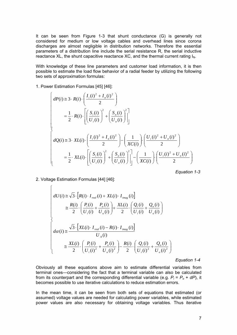
It can be seen from Figure 1-3 that shunt conductance (G) is generally not considered for medium or low voltage cables and overhead lines since corona discharges are almost negligible in distribution networks. Therefore the essential parameters of a distribution line include the serial resistance R, the serial inductive reactance XL, the shunt capacitive reactance XC, and the thermal current rating IN. With knowledge of these line parameters and customer load information, it is then possible to estimate the load flow behavior of a radial feeder by utilizing the following two sets of approximation formulas: 1. Power Estimation Formulas [45] [46]:
⎪⎪⎪⎪⎪⎪⎪
⎩
⎪⎪⎪⎪⎪⎪⎪
⎨
⎧
⎟⎟⎠
⎞⎜⎜⎝
⎛ +⋅⎟⎟
⎠
⎞⎜⎜⎝
⎛−
⎥⎥⎦
⎤
⎢⎢⎣
⎡⎟⎟⎠
⎞⎜⎜⎝
⎛+⎟⎟
⎠
⎞⎜⎜⎝
⎛⋅⋅=
⎟⎟⎠
⎞⎜⎜⎝
⎛ +⋅⎟⎟
⎠
⎞⎜⎜⎝
⎛−⎟⎟
⎠
⎞⎜⎜⎝
⎛ +⋅⋅≅
⎥⎥⎦
⎤
⎢⎢⎣
⎡⎟⎟⎠
⎞⎜⎜⎝
⎛+⎟⎟
⎠
⎞⎜⎜⎝
⎛⋅⋅=
⎟⎟⎠
⎞⎜⎜⎝
⎛ +⋅⋅≅
2)()(
)(1
)()(
)()(
)(21
2)()(
)(1
2)()(
)(3)(
)()(
)()(
)(21
2)()(
)(3)(
2222
2222
22
22
iUiUiXCiU
iSiUiS
iXL
iUiUiXC
iIiIiXLidQ
iUiS
iUiS
iR
iIiIiRidP
oi
o
o
i
i
oioi
o
o
i
i
oi
Equation 1-3
2. Voltage Estimation Formulas [44] [46]:
[ ]
[ ]
⎪⎪⎪⎪⎪⎪
⎩
⎪⎪⎪⎪⎪⎪
⎨
⎧
⎟⎟⎠
⎞⎜⎜⎝
⎛+⋅−⎟⎟
⎠
⎞⎜⎜⎝
⎛+⋅≅
⋅−⋅⋅≅
⎟⎟⎠
⎞⎜⎜⎝
⎛+⋅+⎟⎟
⎠
⎞⎜⎜⎝
⎛+⋅≅
⋅+⋅⋅≅
2222 )()(
)()(
2)(
)()(
)()(
2)(
)()()()()(3
)(
)()(
)()(
2)(
)()(
)()(
2)(
)()()()(3)(
iUiQ
iUiQiR
iUiP
iUiPiXL
iUiIiRiIiXL
id
iUiQ
iUiQiXL
iUiP
iUiPiR
iIiXLiIiRidU
o
o
i
i
o
o
i
i
A
imagreal
o
o
i
i
o
o
i
i
imagreal
α
Equation 1-4
Obviously all these equations above aim to estimate differential variables from terminal ones—considering the fact that a terminal variable can also be calculated from its counterpart and the corresponding differential variable (e.g. Pi = Po + dP), it becomes possible to use iterative calculations to reduce estimation errors. In the mean time, it can be seen from both sets of equations that estimated (or assumed) voltage values are needed for calculating power variables, while estimated power values are also necessary for obtaining voltage variables. Thus iterative

8
calculations can also be applied between voltage and power variables to reduce estimation errors of both. These two types of iterations, together with the approximation formulas introduced beforehand, are the basic foundations of the load flow estimation algorithm (LFEA). They are frequently utilized not only for the radial case, but also for meshed and even more complicated situations. Figure 1-4 gives a rough picture of the basic working mechanism of them:
Figure 1-4 Two Types of Iterations Used in LFEA For any approximation approach, it is always important to know the general accuracy of estimation. In order to evaluate the validity of Equation 1-3 and Equation 1-4, the following Table 1-1 is given showing the difference between calculated (using PSS SINCAL) and estimated (using Equation 1-3 and Equation 1-4) dP, dQ, dU, and dα of radial test network under a WT-penetrated scenario (simulated under rated condition with a 5 MW wind turbine connected at node T1). In order to minimize disturbance, zero error is assumed for all the input variables of approximation equations, which means Table 1-1 shows the ideal output of estimation algorithm. dP in MW U in kV LNL1 LNL2 dQ in MVar α in º calculated estimated calculated estimated cal_dP est_dP 1,2686E-04 1,2737E-04 3,6775E-03 3,6775E-03 cal_dQ est_dQ -6,5976E-02 -6,5976E-02 -3,8317E-03 -3,8317E-03 cal_dU cal_dU 5,4973E-03 5,4973E-03 1,4682E-02 1,4682E-02 cal_dα cal_dα 5,9086E-03 5,9086E-03 5,9669E-03 5,9669E-03 abs_error rel_error % abs_error rel_error % abs_dP rel_dP 5,0304E-07 3,9652E-01 3,4480E-10 9,3759E-06 abs_dQ rel_dQ 3,4661E-07 -5,2535E-04 1,6971E-10 -4,4290E-06 abs_dU rel_dU -2,8933E-08 -5,2631E-04 -1,2722E-09 -8,6655E-06 abs_dα rel_dα 2,1362E-10 3,6153E-06 1,6050E-09 2,6898E-05 dP in MW U in kV LNL3 LNL4 dQ in MVar α in º calculated estimated calculated estimated cal_dP est_dP 3,1582E-03 3,1582E-03 9,3208E-03 9,3207E-03 cal_dQ est_dQ -7,9213E-03 -7,9213E-03 1,0109E-02 1,0108E-02 cal_dU cal_dU 1,8780E-02 1,8780E-02 7,3253E-02 7,3252E-02 cal_dα cal_dα 1,6820E-03 1,6820E-03 1,3462E-01 1,3462E-01 abs_error rel_error % abs_error rel_error % abs_dP rel_dP 3,8138E-09 1,2076E-04 -5,7866E-09 -6,2083E-05 abs_dQ rel_dQ 1,3895E-09 -1,7542E-05 -1,3217E-06 -1,3074E-02 abs_dU rel_dU -3,8583E-09 -2,0544E-05 -1,2523E-07 -1,7095E-04 abs_dα rel_dα 7,4624E-10 4,4368E-05 7,8936E-07 5,8635E-04 Table 1-1 Estimation Accuracy Examined by Test Radial Network
Terminal Variables
Differential Variables
Power Variables
Voltage Variables
9
Table 1-1 shows that estimation accuracy varies from line to line, but it generally deteriorates when the length of a cable or overhead line becomes too large (as in case of LNL1 and LNL 4). Table 1-1 also indicates that absolute error turns out to be a more consistent criterion than relative error—especially for evaluating power data. Thus by using absolute error as evaluation criterion, the approximation formulas should be able to achieve the following levels of accuracy (worst case scenario): dP—error in Ws dQ—error in VARs dU—error in mVs dα—error in 10-6 º However, it should be noted that the accuracy levels estimated above are calculated against Equation 1-3 and Equation 1-4 only while ignoring all external disturbances. In practice, all the input variables for these two approximation equations are estimated values themselves, and estimation error might rise with increasing system scale and complexity. Therefore, a final error range of up to more than 10 times the above mentioned levels should be expected for the test distribution system.
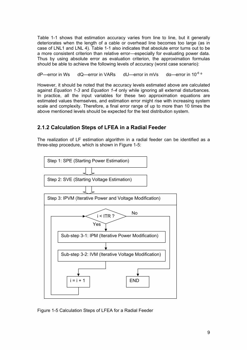
2.1.2 Calculation Steps of LFEA in a Radial Feeder The realization of LF estimation algorithm in a radial feeder can be identified as a three-step procedure, which is shown in Figure 1-5:
Figure 1-5 Calculation Steps of LFEA for a Radial Feeder
Yes
No
Step 1: SPE (Starting Power Estimation)
Step 2: SVE (Starting Voltage Estimation)
i < ITR ?
Step 3: IPVM (Iterative Power and Voltage Modification)
Sub-step 3-1: IPM (Iterative Power Modification)
Sub-step 3-2: IVM (Iterative Voltage Modification)
i = i + 1 END

10
It can be seen from Figure 1-5 that the given three steps (SPE, SVE, and IPVM) literally comprise the power-voltage iteration cycles revealed in Figure 1-4. The first two steps (SPE and SVE) are separated from IPVM sub-steps in order to initialize system power and voltage data, which serve as the basis of iterative calculations. In addition, for most applications, a cycling order of ITR = 3 is sufficient for achieving a moderate accuracy. When compared to the sub-steps of IPVM, the algorithm of SVE is almost identical to that of IVM in terms of logical structure, while SPE proves to be simpler than IPM since the former neither considers the variation of node voltages nor utilizes both ends of terminal data to calculate differential power. In order to explain how these steps and sub-steps work, following three flow charts (Figure 1-6, Figure 1-7, Figure 1-8) are given to show the algorithms of SPE, SVE / IVM, and IPM.
Figure 1-6 Algorithm of SPE (Starting Power Estimation)
No
Yes
Initialization: AcP = 0, AcQ = 0, j = EL
j > 0 ?
AcP = AcP + PL( j ) AcQ = AcQ + QL( j )
Po( j ) = AcP Qo( j ) = AcQ
dP( j ) = R( j ) * [ So( j ) / UN ]2 dQ( j ) = XL( j ) * [ So( j ) / UN ]2 – UN
2 / XC( j )
AcP = AcP + dP( j ) AcQ = AcQ + dQ( j )
Pi( j ) = AcP Qi( j ) = AcQ
j = j – 1 END
So( j ) = ( AcP2 + AcQ2)0.5

11
Figure 1-7 Algorithm of SVE (Starting Voltage Estimation) and IVM (Iterative Voltage Modification)
Yes
Yes
No
No
Initialization: Uo(0) = Uo, j = 1
Ui( j ) = Uo( j – 1 ) αi( j ) = αo( j – 1 )
j < = EL ?
dU( j ) = [ R( j ) * Pi( j ) + XL( j ) * Qi( j ) ] / Ui( j ) Uo( j ) = Ui( j ) – dU( j )
k < N ?
dU( j ) = R( j ) * [ Pi( j ) / Ui( j ) + Po( j ) / Uo( j )] / 2 + XL( j ) * [ Qi( j ) / Ui( j ) + Qo( j ) / Uo( j ) ] / 2
Uo( j ) = Ui( j ) – dU( j )
k = k + 1
dα( j ) = XL( j ) * [ Pi( j ) / Ui( j ) + Po( j ) / Uo( j )] / 2 – R( j ) * [ Qi( j ) / Ui( j ) + Qo( j ) / Uo( j ) ] / 2
αo( j ) = αi( j ) – dα( j )
j = j + 1 END

12
Figure 1-8 Algorithm of IPM (Iterative Power Modification)
No
Yes
Initialization: AcP = 0, AcQ = 0, j = EL
j > 0 ?
AcP = AcP + PL( j ) AcQ = AcQ + QL( j )
Po( j ) = AcP Qo( j ) = AcQ So( j ) = ( AcP2 + AcQ2)0.5
dP( j ) = R( j ) * [ So( j ) / Uo( j )]2 dQ( j ) = XL( j ) * [ So( j ) / Uo( j )]2 – Uo( j ) 2 / XC( j )
Pi( j ) = AcP + dP( j ) Qi( j ) = AcQ + dQ( j )
j = j – 1
END
No
Yes
k < N ?
dP( j ) = R( j ) * [ So( j ) / Uo( j ) ]2 / 2 + R( j ) * [ Si( j ) / Ui( j ) ]2 / 2 dQ( j ) = XL( j ) * [ So( j ) / Uo( j ) ]2 / 2 – Uo( j )2 / XC( j ) / 2 + XL( j ) * [ Si( j ) / Ui( j ) ]2 / 2 – Ui( j )2 / XC( j ) / 2
Pi( j ) = Po( j ) + dP( j ) Qi( j ) = Qo( j ) + dQ( j )
k = k + 1
AcP = Pi( j ) AcQ = Pi( j )
13
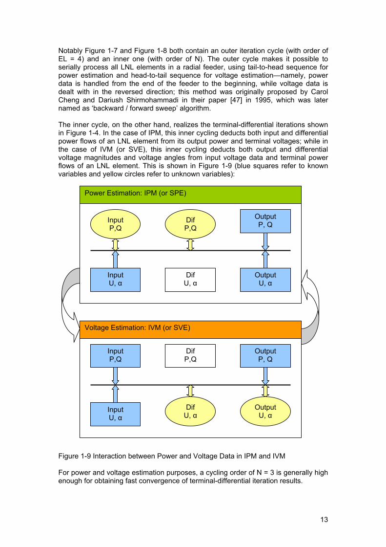
Notably Figure 1-7 and Figure 1-8 both contain an outer iteration cycle (with order of EL = 4) and an inner one (with order of N). The outer cycle makes it possible to serially process all LNL elements in a radial feeder, using tail-to-head sequence for power estimation and head-to-tail sequence for voltage estimation—namely, power data is handled from the end of the feeder to the beginning, while voltage data is dealt with in the reversed direction; this method was originally proposed by Carol Cheng and Dariush Shirmohammadi in their paper [47] in 1995, which was later named as ‘backward / forward sweep’ algorithm. The inner cycle, on the other hand, realizes the terminal-differential iterations shown in Figure 1-4. In the case of IPM, this inner cycling deducts both input and differential power flows of an LNL element from its output power and terminal voltages; while in the case of IVM (or SVE), this inner cycling deducts both output and differential voltage magnitudes and voltage angles from input voltage data and terminal power flows of an LNL element. This is shown in Figure 1-9 (blue squares refer to known variables and yellow circles refer to unknown variables):
Figure 1-9 Interaction between Power and Voltage Data in IPM and IVM For power and voltage estimation purposes, a cycling order of N = 3 is generally high enough for obtaining fast convergence of terminal-differential iteration results.
Input U, α
Input P,Q
Dif U, α
Dif P,Q
Output U, α
Output P, Q
Input P,Q
Dif P,Q
Output P, Q
Input U, α
Dif U, α
Output U, α
Power Estimation: IPM (or SPE)
Voltage Estimation: IVM (or SVE)
14
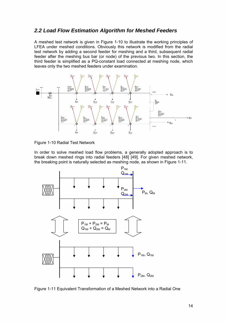
2.2 Load Flow Estimation Algorithm for Meshed Feeders A meshed test network is given in Figure 1-10 to illustrate the working principles of LFEA under meshed conditions. Obviously this network is modified from the radial test network by adding a second feeder for meshing and a third, subsequent radial feeder after the meshing bus bar (or node) of the previous two. In this section, the third feeder is simplified as a PQ-constant load connected at meshing node, which leaves only the two meshed feeders under examination.
Figure 1-10 Radial Test Network In order to solve meshed load flow problems, a generally adopted approach is to break down meshed rings into radial feeders [48] [49]. For given meshed network, the breaking point is naturally selected as meshing node, as shown in Figure 1-11.
Figure 1-11 Equivalent Transformation of a Meshed Network into a Radial One
P2M, Q2M
P1M, Q1M
P1M + P2M = PM Q1M + Q2M = QM
P1M Q1M
PM, QM P2M Q2M

15
As explained in Figure 1-11, network transformation is achieved by splitting the meshed ring into two radial feeders, which in effect divides the equivalent total meshing load (PM + jQM) into two separate loads (P1M + jQ1M and P2M + jQ2M). The active and reactive power flows of these two equivalent loads respectively equal the output power flows in the ending line of each feeder in the original meshed network, namely:
⎩⎨⎧
=
=
⎩⎨⎧
=
=
)5()5(
)5()5(
22
22
11
11
oM
oM
oM
oM
QQPP
QQPP
Equation 1-5
Obviously, if no further feeders are connected after the meshing node—i.e., PM = 0 and QM = 0, then P1M = -P2M, Q1M = -Q2M. In this case, the two equivalent meshing loads with opposite power flow directions from each other can be seen as splitted from a zero-power imaginary load that is connected to the meshing node. By using this equivalent transformation method, LFEA for meshed feeders can be easily developed from its radial version (detailed in 2.1) if the active and reactive equivalent meshing powers (EMP) can be estimated from given network parameters and variables. Thus the following section will be focused on introducing a number of EMP estimation approaches that aim to tackle this issue under different situations.
2.2.1 Equivalent Meshing Powers (EMP) Estimation Approaches The basic idea behind EMP estimation is to build and solve power equations through voltage relationships—namely, the ending nodes of two equivalent radial feeders are splitted from one original meshing node and thus should have the same voltage magnitudes and voltage angles. Considering the fact that both feeders also originate from the same 20-kV bus bar, the total voltage magnitude drops and voltage angle drops along these two feeders should be consequently the same, which can be expressed by the Equation 1-6:
⎪⎪⎩
⎪⎪⎨
⎧
=
=
⇒
⎩⎨⎧
====
⎪⎪⎩
⎪⎪⎨
⎧
−=
−=
⎪⎪⎩
⎪⎪⎨
⎧
−=
−=
∑∑
∑∑
∑
∑
∑
∑
==
==
=
=
=
=
5
12
5
11
5
12
5
11
2121
2121
5
1222
5
1222
5
1111
5
1111
)()(
)()(
)1()1(),1()1()5()5(),5()5(
)()1()5(
)()1()5(
)()1()5(
)()1()5(
jj
jj
iiii
oooo
jio
jio
jio
jio
jdjd
jdUjdU
UUUU
Since
jd
jdUUU
jd
jdUUU
αα
αααα
αααααα
Equation 1-6
By applying Equation 1-4 into Equation 1-6, Equation 1-7 can be obtained as:
16
⎪⎪⎪⎪⎪⎪⎪
⎩
⎪⎪⎪⎪⎪⎪⎪
⎨
⎧
⎭⎬⎫
⎩⎨⎧
⎟⎟⎠
⎞⎜⎜⎝
⎛+⋅−⎟⎟
⎠
⎞⎜⎜⎝
⎛+⋅=
⎭⎬⎫
⎩⎨⎧
⎟⎟⎠
⎞⎜⎜⎝
⎛+⋅−⎟⎟
⎠
⎞⎜⎜⎝
⎛+⋅
⎭⎬⎫
⎩⎨⎧
⎟⎟⎠
⎞⎜⎜⎝
⎛+⋅+⎟⎟
⎠
⎞⎜⎜⎝
⎛+⋅=
⎭⎬⎫
⎩⎨⎧
⎟⎟⎠
⎞⎜⎜⎝
⎛+⋅+⎟⎟
⎠
⎞⎜⎜⎝
⎛+⋅
∑
∑
∑
∑
=
=
=
=
5
12
2
22
2
222
2
22
2
22
5
12
1
12
1
112
1
12
1
11
5
1 2
2
2
22
2
2
2
22
5
1 1
1
1
11
1
1
1
11
)()(
)()(
2)(
)()(
)()(
2)(
)()(
)()(
2)(
)()(
)()(
2)(
)()(
)()(
2)(
)()(
)()(
2)(
)()(
)()(
2)(
)()(
)()(
2)(
j o
o
i
i
o
o
i
i
j o
o
i
i
o
o
i
i
j o
o
i
i
o
o
i
i
j o
o
i
i
o
o
i
i
jUjQ
jUjQjR
jUjP
jUjPjXL
jUjQ
jUjQjR
jUjP
jUjPjXL
jUjQ
jUjQjXL
jUjP
jUjPiR
jUjQ
jUjQjXL
jUjP
jUjPjR
Equation 1-7
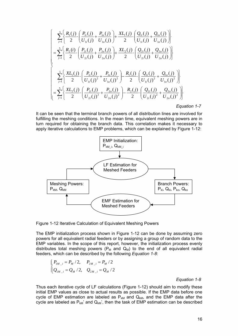
It can be seen that the terminal branch powers of all distribution lines are involved for fulfilling the meshing conditions. In the mean time, equivalent meshing powers are in turn required for obtaining the branch data. This correlation makes it necessary to apply iterative calculations to EMP problems, which can be explained by Figure 1-12:
Figure 1-12 Iterative Calculation of Equivalent Meshing Powers The EMP initialization process shown in Figure 1-12 can be done by assuming zero powers for all equivalent radial feeders or by assigning a group of random data to the EMP variables. In the scope of this report, however, the initialization process evenly distributes total meshing powers (PM and QM) to the end of all equivalent radial feeders, which can be described by the following Equation 1-8:
⎪⎩
⎪⎨⎧
==
==
2/,2/
2/,2/
_2_1
_2_1
MiMMiM
MiMMiM
QQQQ
PPPP
Equation 1-8
Thus each iterative cycle of LF calculations (Figure 1-12) should aim to modify these initial EMP values as close to actual results as possible. If the EMP data before one cycle of EMP estimation are labeled as PkM and QkM, and the EMP data after the cycle are labeled as PkM’ and QkM’, then the task of EMP estimation can be described
EMP Initialization: PkM_i, QkM_i
LF Estimation for Meshed Feeders
Branch Powers: Pki, Qki, Pko, Qko
EMF Estimation for Meshed Feeders
Meshing Powers: PkM, QkM

17
as finding the differences ΔPkM = PkM’ - PkM and ΔQkM = QkM’ - QkM such that estimation errors of PkM’ and QkM’ should be minimum. In most distribution networks, transmitted power values can be assumed to be far larger than resistive and inductive power losses in the lines—i.e., Pi>>Ploss, Po>>Ploss, Qi>>QLloss, Qo>>QLloss (however, it should be noted that the reactive power losses here only consist of inductive losses caused by XL since the magnitude of negative capacitive losses of power cables can be close to or even larger than transmitted reactive powers). Therefore, the following simplifications in Equation 1-9 can be made for faster calculations of ΔPkM and ΔQkM:
[ ] [ ]
⎩⎨⎧
Δ+=Δ+=Δ+=Δ+=
⎩⎨⎧
Δ+=Δ+=
∈∀∈∀
kMkokokMkoko
kMkikikMkiki
kMkMkM
kMkMkM
QjQjQPjPjPQjQjQPjPjP
ThenQQQ
PPPkjthatAssume
)()(',)()(')()(',)()('
''
2,1,5,1:
Equation 1-9
By applying Equation 1-9 into Equation 1-7, Equation 1-10 can be obtained as:
⎪⎪⎪⎪⎪⎪⎪⎪⎪
⎩
⎪⎪⎪⎪⎪⎪⎪⎪⎪
⎨
⎧
=Δ+Δ=Δ+Δ
+⎪⎭
⎪⎬⎫
⎪⎩
⎪⎨⎧
⎟⎟⎠
⎞⎜⎜⎝
⎛ Δ+
Δ⋅−⎟⎟
⎠
⎞⎜⎜⎝
⎛ Δ+
Δ⋅=
+⎪⎭
⎪⎬⎫
⎪⎩
⎪⎨⎧
⎟⎟⎠
⎞⎜⎜⎝
⎛ Δ+
Δ⋅−⎟⎟
⎠
⎞⎜⎜⎝
⎛ Δ+
Δ⋅
+⎭⎬⎫
⎩⎨⎧
⎟⎟⎠
⎞⎜⎜⎝
⎛ Δ+
Δ⋅+⎟⎟
⎠
⎞⎜⎜⎝
⎛ Δ+
Δ⋅=
+⎭⎬⎫
⎩⎨⎧
⎟⎟⎠
⎞⎜⎜⎝
⎛ Δ+
Δ⋅+⎟⎟
⎠
⎞⎜⎜⎝
⎛ Δ+
Δ⋅
⇓
⎪⎪⎩
⎪⎪⎨
⎧
=
=
∑∑
∑∑
∑∑
∑∑
∑∑
∑∑
==
==
==
==
==
==
00
)()()(2
)()()(2
)(
)()()(2
)()()(2
)(
)()()(2
)()()(2
)(
)()()(2
)()()(2
)(
)(')('
)(')('
21
21
5
12
5
12
2
22
2
222
2
22
2
22
5
11
5
12
1
12
1
112
1
12
1
11
5
12
5
1 1
2
2
22
2
2
2
22
5
11
5
1 1
1
1
11
1
1
1
11
5
12
5
11
5
12
5
11
MM
MM
jj o
M
i
M
o
M
i
M
jj o
M
i
M
o
M
i
M
jj o
M
i
M
o
M
i
M
jj o
M
i
M
o
M
i
M
jj
jj
QQPP
jdjU
QjU
QjRjU
PjU
PjXL
jdjU
QjU
QjRjU
PjU
PjXL
jdUjU
QjU
QjXLjU
PjU
PjR
jdUjU
QjU
QjXLjU
PjU
PjR
jdjd
jdUjdU
α
α
αα
Equation 1-10
Four decoupled linear equations above are now obtained for solving four unknown variables (P1M, Q1M, P2M, and Q2M). Thus simple matrix calculations will suffice for estimating EMP values. In the following two sections, two different solutions are provided to suit different situations.
18
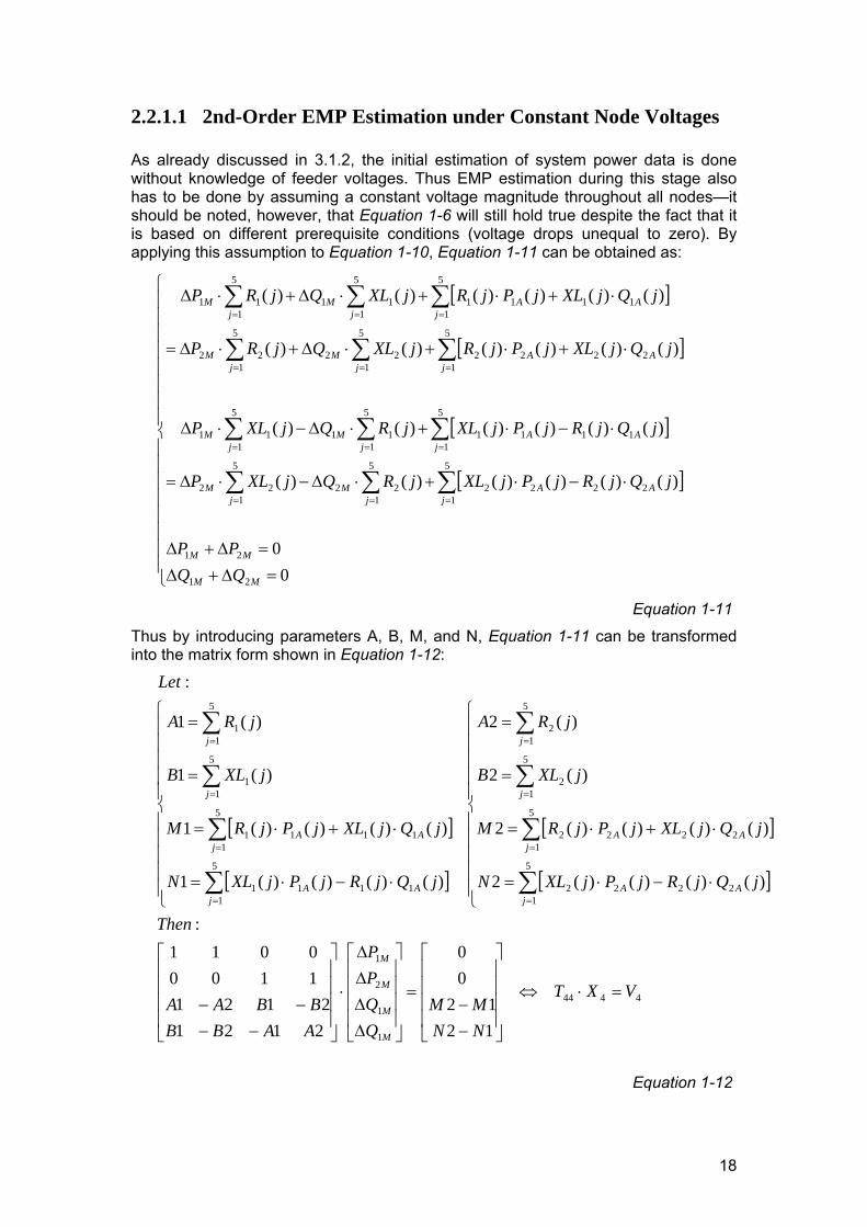
2.2.1.1 2nd-Order EMP Estimation under Constant Node Voltages As already discussed in 3.1.2, the initial estimation of system power data is done without knowledge of feeder voltages. Thus EMP estimation during this stage also has to be done by assuming a constant voltage magnitude throughout all nodes—it should be noted, however, that Equation 1-6 will still hold true despite the fact that it is based on different prerequisite conditions (voltage drops unequal to zero). By applying this assumption to Equation 1-10, Equation 1-11 can be obtained as:
[ ]
[ ]
[ ]
[ ]
⎪⎪⎪⎪⎪⎪⎪⎪
⎩
⎪⎪⎪⎪⎪⎪⎪⎪
⎨
⎧
=Δ+Δ=Δ+Δ
⋅−⋅+⋅Δ−⋅Δ=
⋅−⋅+⋅Δ−⋅Δ
⋅+⋅+⋅Δ+⋅Δ=
⋅+⋅+⋅Δ+⋅Δ
∑∑∑
∑∑∑
∑∑∑
∑∑∑
===
===
===
===
00
)()()()()()(
)()()()()()(
)()()()()()(
)()()()()()(
21
21
5
12222
5
122
5
122
5
11111
5
111
5
111
5
12222
5
122
5
122
5
11111
5
111
5
111
MM
MM
jAA
jM
jM
jAA
jM
jM
jAA
jM
jM
jAA
jM
jM
QQPP
jQjRjPjXLjRQjXLP
jQjRjPjXLjRQjXLP
jQjXLjPjRjXLQjRP
jQjXLjPjRjXLQjRP
Equation 1-11
Thus by introducing parameters A, B, M, and N, Equation 1-11 can be transformed into the matrix form shown in Equation 1-12:
[ ]
[ ]
[ ]
[ ]
4444
1
1
2
1
5
12222
5
12222
5
12
5
12
5
11111
5
11111
5
11
5
11
1212
00
21212121
11000011
:
)()()()(2
)()()()(2
)(2
)(2
)()()()(1
)()()()(1
)(1
)(1
:
VXT
NNMM
QQPP
AABBBBAA
Then
jQjRjPjXLN
jQjXLjPjRM
jXLB
jRA
jQjRjPjXLN
jQjXLjPjRM
jXLB
jRA
Let
M
M
M
M
jAA
jAA
j
j
jAA
jAA
j
j
=⋅⇔
⎥⎥⎥⎥
⎦
⎤
⎢⎢⎢⎢
⎣
⎡
−−
=
⎥⎥⎥⎥
⎦
⎤
⎢⎢⎢⎢
⎣
⎡
ΔΔΔΔ
⋅
⎥⎥⎥⎥
⎦
⎤
⎢⎢⎢⎢
⎣
⎡
−−−−
⎪⎪⎪⎪⎪
⎩
⎪⎪⎪⎪⎪
⎨
⎧
⋅−⋅=
⋅+⋅=
=
=
⎪⎪⎪⎪⎪
⎩
⎪⎪⎪⎪⎪
⎨
⎧
⋅−⋅=
⋅+⋅=
=
=
∑
∑
∑
∑
∑
∑
∑
∑
=
=
=
=
=
=
=
=
Equation 1-12

19
Therefore, the EMP variable vector X4 can obtained through the product of T44-1 and
V4, as shown in Equation 1-13:
⎥⎥⎥⎥
⎦
⎤
⎢⎢⎢⎢
⎣
⎡
−−
⋅
⎥⎥⎥⎥
⎦
⎤
⎢⎢⎢⎢
⎣
⎡
−−−−
=
⎥⎥⎥⎥
⎦
⎤
⎢⎢⎢⎢
⎣
⎡
ΔΔΔΔ
⇔⋅=
−
−
1212
00
21212121
11000011 1
1
1
2
1
41
444
NNMM
AABBBBAA
QQPP
VTX
M
M
M
M
Equation 1-13
Obviously, this type of EMP estimation method under constant node voltages (CNV) should be applied to SVE (Starting Voltage Estimation) stage of calculation, as it is not accurate enough for further iterative calculations. This is why section 2.2.1.2 is provided below, in which a more accurate estimation approach is suggested.
2.2.1.2 2nd-Order EMP Estimation under Varying Node Voltages When LF estimation comes to the stage of iterative calculations, all system node voltages will become available, therefore the assumption made in section 2.2.1.1 is no longer necessary or valid. In this case, Equation 1-10 can be solved directly for EMP variables. Thus by introducing parameters A, B, C, D, M, and N, Equation 1-14 can be obtained as:
4444
1
1
2
1
5
12
5
12
5
12
22
2
2
5
12
22
2
2
5
1 22
2
5
1 22
2
5
11
5
11
5
12
12
1
1
5
12
12
1
1
5
1 11
1
5
1 11
1
1212
00
21212121
11000011
:
)(2
)(2
)(1
)(1
2)(
2
)(1
)(1
2)(
2
)(1
)(1
2)(
2
)(1
)(1
2)(
2
)(1
)(1
)(1
)(1
2)(
1
)(1
)(1
2)(
1
)(1
)(1
2)(
1
)(1
)(1
2)(
1
:
VXT
NNMM
QQPP
CCDDBBAA
Then
jdN
jdUM
jUjUjXL
D
jUjUjR
C
jUjUjXL
B
jUjUjR
A
jdN
jdUM
jUjUjXL
D
jUjUjR
C
jUjUjXL
B
jUjUjR
A
Let
M
M
M
M
j
j
j oi
j oi
j oi
j oi
j
j
j oi
j oi
j oi
j oi
=⋅⇔
⎥⎥⎥⎥
⎦
⎤
⎢⎢⎢⎢
⎣
⎡
−−
=
⎥⎥⎥⎥
⎦
⎤
⎢⎢⎢⎢
⎣
⎡
ΔΔΔΔ
⋅
⎥⎥⎥⎥
⎦
⎤
⎢⎢⎢⎢
⎣
⎡
−−−−
⎪⎪⎪⎪⎪⎪⎪⎪⎪
⎩
⎪⎪⎪⎪⎪⎪⎪⎪⎪
⎨
⎧
=
=
⎥⎦
⎤⎢⎣
⎡+⋅=
⎥⎦
⎤⎢⎣
⎡+⋅=
⎥⎦
⎤⎢⎣
⎡+⋅=
⎥⎦
⎤⎢⎣
⎡+⋅=
⎪⎪⎪⎪⎪⎪⎪⎪⎪
⎩
⎪⎪⎪⎪⎪⎪⎪⎪⎪
⎨
⎧
=
=
⎥⎦
⎤⎢⎣
⎡+⋅=
⎥⎦
⎤⎢⎣
⎡+⋅=
⎥⎦
⎤⎢⎣
⎡+⋅=
⎥⎦
⎤⎢⎣
⎡+⋅=
∑
∑
∑
∑
∑
∑
∑
∑
∑
∑
∑
∑
=
=
=
=
=
=
=
=
=
=
=
=
αα
Equation 1-14
20
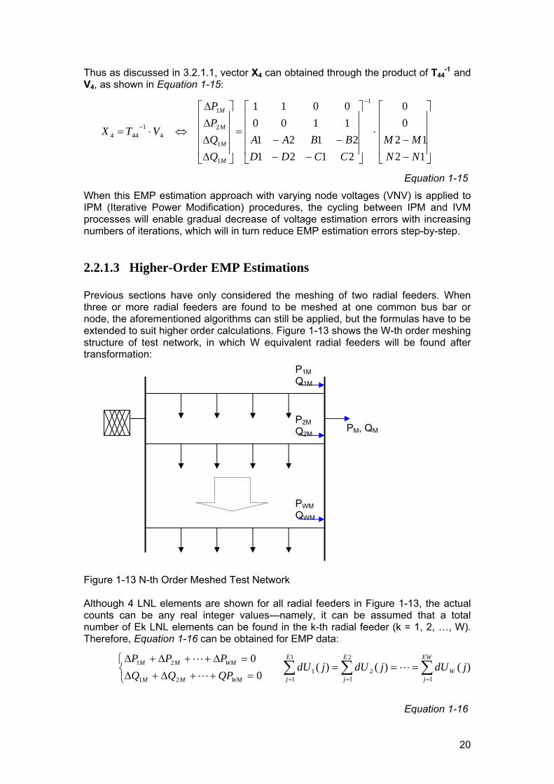
Thus as discussed in 3.2.1.1, vector X4 can obtained through the product of T44-1 and
V4, as shown in Equation 1-15:
⎥⎥⎥⎥
⎦
⎤
⎢⎢⎢⎢
⎣
⎡
−−
⋅
⎥⎥⎥⎥
⎦
⎤
⎢⎢⎢⎢
⎣
⎡
−−−−
=
⎥⎥⎥⎥
⎦
⎤
⎢⎢⎢⎢
⎣
⎡
ΔΔΔΔ
⇔⋅=
−
−
1212
00
21212121
11000011 1
1
1
2
1
41
444
NNMM
CCDDBBAA
QQPP
VTX
M
M
M
M
Equation 1-15
When this EMP estimation approach with varying node voltages (VNV) is applied to IPM (Iterative Power Modification) procedures, the cycling between IPM and IVM processes will enable gradual decrease of voltage estimation errors with increasing numbers of iterations, which will in turn reduce EMP estimation errors step-by-step.
2.2.1.3 Higher-Order EMP Estimations Previous sections have only considered the meshing of two radial feeders. When three or more radial feeders are found to be meshed at one common bus bar or node, the aforementioned algorithms can still be applied, but the formulas have to be extended to suit higher order calculations. Figure 1-13 shows the W-th order meshing structure of test network, in which W equivalent radial feeders will be found after transformation:
Figure 1-13 N-th Order Meshed Test Network Although 4 LNL elements are shown for all radial feeders in Figure 1-13, the actual counts can be any real integer values—namely, it can be assumed that a total number of Ek LNL elements can be found in the k-th radial feeder (k = 1, 2, …, W). Therefore, Equation 1-16 can be obtained for EMP data:
∑ ∑∑= ==
===⎩⎨⎧
=++Δ+Δ=Δ++Δ+Δ 2
1 12
1
11
21
21 )()()(0
0 E
j
EW
jW
E
jWMMM
WMMM jdUjdUjdUQPQQPPP
LL
L
Equation 1-16
PWM QWM
P1M Q1M
PM, QM P2M Q2M
21
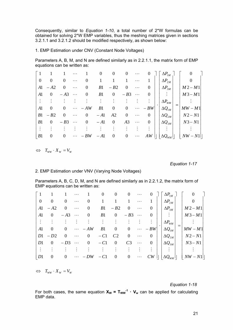
Consequently, similar to Equation 1-10, a total number of 2*W formulas can be obtained for solving 2*W EMP variables, thus the meshing matrices given in sections 3.2.1.1 and 3.2.1.2 should be modified respectively, as shown below: 1. EMP Estimation under CNV (Constant Node Voltages) Parameters A, B, M, and N are defined similarly as in 2.2.1.1, the matrix form of EMP equations can be written as:
WWWW
WM
M
M
M
WM
M
M
M
VXT
NNW
NNNNMMW
MMMM
Q
QQQP
PPP
AWABWB
AABBAABB
BWBAWA
BBAABBAA
=⋅⇔
⎥⎥⎥⎥⎥⎥⎥⎥⎥⎥⎥⎥⎥⎥
⎦
⎤
⎢⎢⎢⎢⎢⎢⎢⎢⎢⎢⎢⎢⎢⎢
⎣
⎡
−
−−−
−−
=
⎥⎥⎥⎥⎥⎥⎥⎥⎥⎥⎥⎥⎥⎥
⎦
⎤
⎢⎢⎢⎢⎢⎢⎢⎢⎢⎢⎢⎢⎢⎢
⎣
⎡
Δ
ΔΔΔΔ
ΔΔΔ
⋅
⎥⎥⎥⎥⎥⎥⎥⎥⎥⎥⎥⎥⎥⎥
⎦
⎤
⎢⎢⎢⎢⎢⎢⎢⎢⎢⎢⎢⎢⎢⎢
⎣
⎡
−−
−−−−
−−
−−−−
1
13121
1312
00
001001
0301030100210021
001001
03010301002100211111000000001111
3
2
1
3
2
1
M
M
M
M
LL
MMMMMMMMMM
LL
LL
LL
MMMMMMMMMM
LL
LL
LL
LL
Equation 1-17
2. EMP Estimation under VNV (Varying Node Voltages) Parameters A, B, C, D, M, and N are defined similarly as in 2.2.1.2, the matrix form of EMP equations can be written as:
WWWW
WM
M
M
M
WM
M
M
M
VXT
NNW
NNNNMMW
MMMM
Q
QQQP
PPP
CWCDWD
CCDDCCDD
BWBAWA
BBAABBAA
=⋅⇔
⎥⎥⎥⎥⎥⎥⎥⎥⎥⎥⎥⎥⎥⎥
⎦
⎤
⎢⎢⎢⎢⎢⎢⎢⎢⎢⎢⎢⎢⎢⎢
⎣
⎡
−
−−−
−−
=
⎥⎥⎥⎥⎥⎥⎥⎥⎥⎥⎥⎥⎥⎥
⎦
⎤
⎢⎢⎢⎢⎢⎢⎢⎢⎢⎢⎢⎢⎢⎢
⎣
⎡
Δ
ΔΔΔΔ
ΔΔΔ
⋅
⎥⎥⎥⎥⎥⎥⎥⎥⎥⎥⎥⎥⎥⎥
⎦
⎤
⎢⎢⎢⎢⎢⎢⎢⎢⎢⎢⎢⎢⎢⎢
⎣
⎡
−−
−−−−
−−
−−−−
1
13121
1312
00
001001
0301030100210021
001001
03010301002100211111000000001111
3
2
1
3
2
1
M
M
M
M
LL
MMMMMMMMMM
LL
LL
LL
MMMMMMMMMM
LL
LL
LL
LL
Equation 1-18
For both cases, the same equation XW = TWW-1 Vw can be applied for calculating
EMP data.

22
2.2.2 Calculation Steps of LFEA in a Meshed Feeder The LF estimation procedure for meshed feeders can be seen as modified from its radial version (Figure 1-5) by applying EMP estimation process shown in Figure 1-12 into SPE and IPM algorithms, which can be seen from Figure 1-14:
Figure 1-14 Calculation Steps of LFEA for a Meshed Feeder
Yes
No
Sub-step 1-2: Rough LF Estimation for MF’s
Sub-step 1-3: EMP Estimation for MF’s, under CNV
i < ITR ?
Step 3: IPVM for MF’s (Meshed Feeders)
Sub-step 3-1: IPM for MF’s (Meshed Feeders)
Sub-step 3-2: IVM for MF’s (Meshed Feeders)
i = i + 1 END
Sub-step 1-1: EMP Initialization
Sub-step 1-4: Modified LF Estimation for MF
Step 2: SVE for MF’s (Meshed Feeders)
Step 1: SPE for MF’s (Meshed Feeders)
Sub-step 3-1-2: Rough LF Estimation for MF’s
Sub-step 3-1-3: EMP Estimation for MF’s, under VNV
Sub-step 3-1-1: EMP Re-initialization
Sub-step 3-1-4: Modified LF Estimation for MF’s

23
It should be noted that voltage estimation algorithms (SVE and IVM) for meshed feeders are exactly the same as their radial counterparts, while the LF estimation processes (sub-steps 2 and 4) for meshed SPE and IPM can be seen as equivalent to simultaneously applying radial power estimation algorithms (SPE or IPM) to all equivalent radial feeders of a meshed set. In a meshed SPE or IPM process, power flows in all meshed feeders are calculated both before and after EMP estimation in order to minimize errors when calculating voltage drops from power data.
2.3 Load Flow Estimation Algorithm for Test Network In scope of this report, major network calculations are carried out for a real-life 20kV German distribution grid. The general structure of this grid is shown in Figure 1-15.
Figure 1-15 General Structure of Test Network

24
It can be seen that test network consists of 16 separate feeders, which can be categorized into 2 sub-networks that are both fed from the 2nd side of transformer. Detailed network plot is shown in Figure 1-16.
Figure 1-16 Detailed Structure of Test Network
25
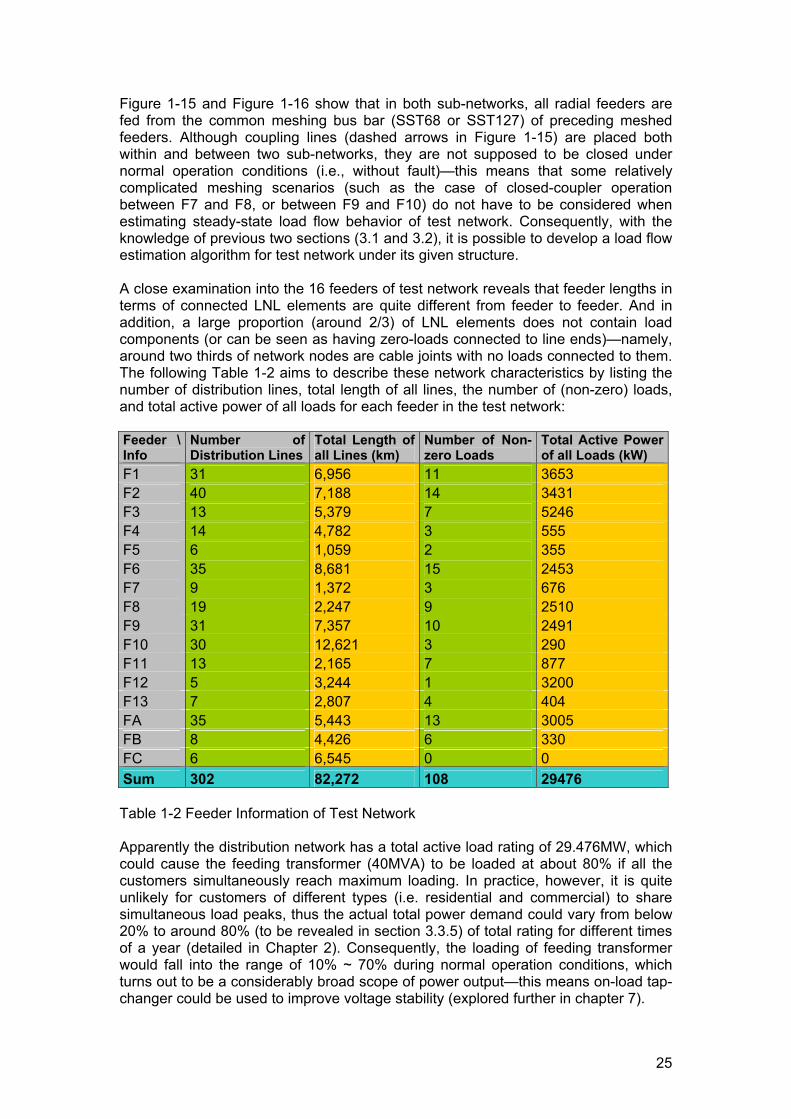
Figure 1-15 and Figure 1-16 show that in both sub-networks, all radial feeders are fed from the common meshing bus bar (SST68 or SST127) of preceding meshed feeders. Although coupling lines (dashed arrows in Figure 1-15) are placed both within and between two sub-networks, they are not supposed to be closed under normal operation conditions (i.e., without fault)—this means that some relatively complicated meshing scenarios (such as the case of closed-coupler operation between F7 and F8, or between F9 and F10) do not have to be considered when estimating steady-state load flow behavior of test network. Consequently, with the knowledge of previous two sections (3.1 and 3.2), it is possible to develop a load flow estimation algorithm for test network under its given structure. A close examination into the 16 feeders of test network reveals that feeder lengths in terms of connected LNL elements are quite different from feeder to feeder. And in addition, a large proportion (around 2/3) of LNL elements does not contain load components (or can be seen as having zero-loads connected to line ends)—namely, around two thirds of network nodes are cable joints with no loads connected to them. The following Table 1-2 aims to describe these network characteristics by listing the number of distribution lines, total length of all lines, the number of (non-zero) loads, and total active power of all loads for each feeder in the test network: Feeder \ Info
Number of Distribution Lines
Total Length of all Lines (km)
Number of Non-zero Loads
Total Active Power of all Loads (kW)
F1 31 6,956 11 3653 F2 40 7,188 14 3431 F3 13 5,379 7 5246 F4 14 4,782 3 555 F5 6 1,059 2 355 F6 35 8,681 15 2453 F7 9 1,372 3 676 F8 19 2,247 9 2510 F9 31 7,357 10 2491 F10 30 12,621 3 290 F11 13 2,165 7 877 F12 5 3,244 1 3200 F13 7 2,807 4 404 FA 35 5,443 13 3005 FB 8 4,426 6 330 FC 6 6,545 0 0 Sum 302 82,272 108 29476 Table 1-2 Feeder Information of Test Network Apparently the distribution network has a total active load rating of 29.476MW, which could cause the feeding transformer (40MVA) to be loaded at about 80% if all the customers simultaneously reach maximum loading. In practice, however, it is quite unlikely for customers of different types (i.e. residential and commercial) to share simultaneous load peaks, thus the actual total power demand could vary from below 20% to around 80% (to be revealed in section 3.3.5) of total rating for different times of a year (detailed in Chapter 2). Consequently, the loading of feeding transformer would fall into the range of 10% ~ 70% during normal operation conditions, which turns out to be a considerably broad scope of power output—this means on-load tap-changer could be used to improve voltage stability (explored further in chapter 7).
26
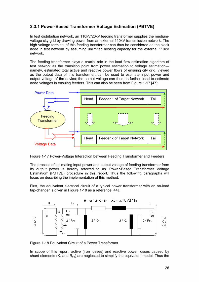
2.3.1 Power-Based Transformer Voltage Estimation (PBTVE) In test distribution network, an 110kV/20kV feeding transformer supplies the medium-voltage city grid by drawing power from an external 110kV transmission network. The high-voltage terminal of this feeding transformer can thus be considered as the slack node in test network by assuming unlimited hosting capacity for the external 110kV network. The feeding transformer plays a crucial role in the load flow estimation algorithm of test network as the transition point from power estimation to voltage estimation—namely, estimated total active and reactive power flows of ensuing city grid, viewed as the output data of this transformer, can be used to estimate input power and output voltage of the device; the output voltage can thus be further used to estimate node voltages in ensuing feeders. This can also be seen from Figure 1-17 [47]:
Figure 1-17 Power-Voltage Interaction between Feeding Transformer and Feeders The process of estimating input power and output voltage of feeding transformer from its output power is hereby referred to as ‘Power-Based Transformer Voltage Estimation’ (PBTVE) procedure in this report. Thus the following paragraphs will focus on describing the implementation of this method. First, the equivalent electrical circuit of a typical power transformer with an on-load tap-changer is given in Figure 1-18 as a reference [44].
Figure 1-18 Equivalent Circuit of a Power Transformer In scope of this report, active (iron losses) and reactive power losses caused by shunt elements (Xh and RFe) are neglected to simplify the equivalent model. Thus the
Feeding Transformer
Feeder 1 of Target Network Head Tail
Feeder x of Target Network Head Tail
Power Data
Voltage Data
27
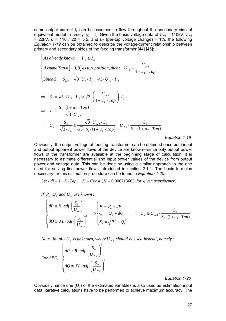
same output current Io can be assumed to flow throughout the secondary side of equivalent model—namely, Ii2 = Io. Given the basic voltage data of UN1 = 110kV, UN2 = 20kV, ü = 110 / 20 = 5.5, and uT (per-tap voltage change) = 1%, the following Equation 1-19 can be obtained to describe the voltage-current relationship between primary and secondary sides of the feeding transformer [44] [45]:
[ ]
( )
( ) ( )TapuSS
UTapuS
SUI
SU
UTapuS
I
ITapu
UIUS
IUIUSSSince
TapuU
UthenpositiontapasTapAssume
IIknownalreadyAs
Ti
oN
Ti
oN
o
oo
N
Tio
oT
Niii
iiiiii
T
Ni
oi
⋅+⋅⋅=
⋅+⋅⋅
⋅⋅≅
⋅=⇒
⋅
⋅+⋅≅⇒
⋅⎟⎟⎠
⎞⎜⎜⎝
⎛⋅+
⋅≅⋅⋅=⇒
⎪⎪
⎩
⎪⎪
⎨
⎧
⋅⋅=⋅⋅=
⋅+=−∈
≅
1133
3
31
133
33,
1:,9,9
:
22
2
222
222
22
2
Equation 1-19
Obviously, the output voltage of feeding transformer can be obtained once both input and output apparent power flows of the device are known—since only output power flows of the transformer are available at the beginning stage of calculation, it is necessary to estimate differential and input power values of the device from output power and voltage data. This can be done by using a similar approach to the one used for solving line power flows introduced in section 2.1.1. The basic formulas necessary for this estimation procedure can be found in Equation 1-20:
⎪⎪
⎩
⎪⎪
⎨
⎧
⎟⎟⎠
⎞⎜⎜⎝
⎛⋅⋅≅
⎟⎟⎠
⎞⎜⎜⎝
⎛⋅⋅≅
⋅+⋅⋅≅⇒
⎪⎪⎩
⎪⎪⎨
⎧
+=
+=+=
⇒
⎪⎪
⎩
⎪⎪
⎨
⎧
⎟⎟⎠
⎞⎜⎜⎝
⎛⋅⋅≅
⎟⎟⎠
⎞⎜⎜⎝
⎛⋅⋅≅
⇒
==⋅+=
2
2
2
2
2
2
22
2
2
,
:,,:
)1(
:,
)006713662.0(,1
N
o
N
o
No
Ti
oNo
iii
oi
oi
o
o
o
o
ooo
US
adjXLdQ
US
adjRdPSPEFor
namelyinsteadusedbeshouldUwhereunknownisUInitallyNote
TapuSS
UU
QPS
dQQQdPPP
US
adjXLdQ
US
adjRdP
knownareUandQPIf
rtransformegivenforKConstKTapKadjLet
Equation 1-20
Obviously, since one (Uo) of the estimated variables is also used as estimation input data, iterative calculations have to be performed to achieve maximum accuracy. The

28
iteration cycles can be expressed by Figure 1-19 (squared variables are already known before estimation, while circled variables are originally unknown):
Figure 1-19 Basic Iteration Cycle of Power-Based Transformer Voltage Estimation Study into test distribution grid shows that 10 iteration cycles are generally sufficient for fast convergence of estimated power and voltage data, since further cycles of iteration would modify estimated data on scales much smaller than expected estimation accuracy level (referred to 2.1.1) and are thus unnecessary.
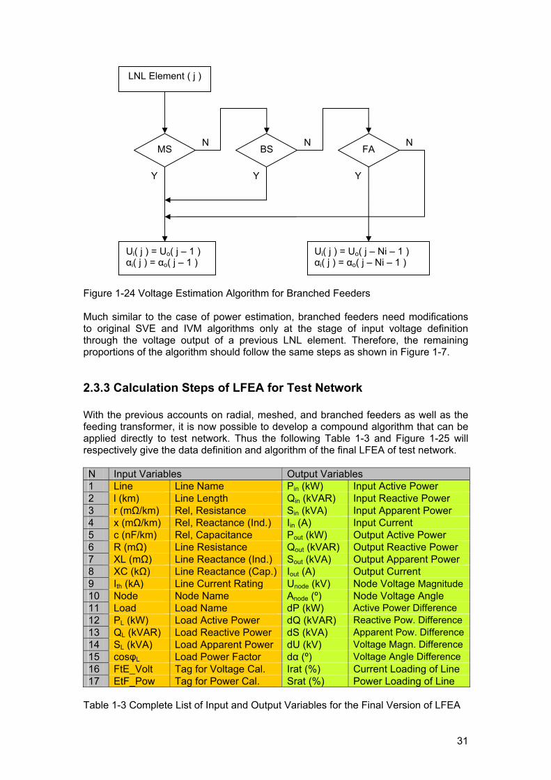
2.3.2 Modeling of Branched Feeders in LFEA In test network, a large proportion of feeders share a common topological feature—they have one or more branches. The existence of branches in a feeder invariably complicates the algorithm of load flow estimation [48], as the previous linear accumulation of power data and monotonous stepping down of node voltages can no longer be applied to the whole feeder range. In orders to tackle this issue, tag variables need to be defined to mark different sections of a branched feeder. In this section, only one degree of freedom is considered for branching of all feeders—namely, only one branch can be connected to a given node and no sub-branches should exist. In Figure 1-20, a typical branched feeder of this type is given.
F(BEi+2)F(BBi-2) F(BEi+1)F(BBi-1)
F(BBi) = Bi(1)
F(1)
F(BBi+1) = Bi(2)
F(BEi) = Bi(Ni)
F(x)
LNL Element
F(M)
Figure 1-20 Naming Convention and Topological Structure of a Branched Feeder
Initialization
OutputP, Q
OutputU
Dif P, Q
InputP, Q
RatedUN2
29
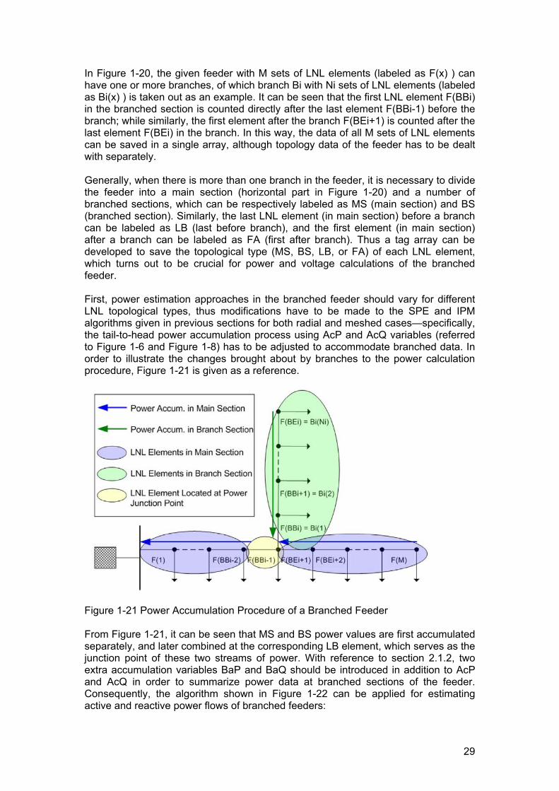
In Figure 1-20, the given feeder with M sets of LNL elements (labeled as F(x) ) can have one or more branches, of which branch Bi with Ni sets of LNL elements (labeled as Bi(x) ) is taken out as an example. It can be seen that the first LNL element F(BBi) in the branched section is counted directly after the last element F(BBi-1) before the branch; while similarly, the first element after the branch F(BEi+1) is counted after the last element F(BEi) in the branch. In this way, the data of all M sets of LNL elements can be saved in a single array, although topology data of the feeder has to be dealt with separately. Generally, when there is more than one branch in the feeder, it is necessary to divide the feeder into a main section (horizontal part in Figure 1-20) and a number of branched sections, which can be respectively labeled as MS (main section) and BS (branched section). Similarly, the last LNL element (in main section) before a branch can be labeled as LB (last before branch), and the first element (in main section) after a branch can be labeled as FA (first after branch). Thus a tag array can be developed to save the topological type (MS, BS, LB, or FA) of each LNL element, which turns out to be crucial for power and voltage calculations of the branched feeder. First, power estimation approaches in the branched feeder should vary for different LNL topological types, thus modifications have to be made to the SPE and IPM algorithms given in previous sections for both radial and meshed cases—specifically, the tail-to-head power accumulation process using AcP and AcQ variables (referred to Figure 1-6 and Figure 1-8) has to be adjusted to accommodate branched data. In order to illustrate the changes brought about by branches to the power calculation procedure, Figure 1-21 is given as a reference.
Figure 1-21 Power Accumulation Procedure of a Branched Feeder From Figure 1-21, it can be seen that MS and BS power values are first accumulated separately, and later combined at the corresponding LB element, which serves as the junction point of these two streams of power. With reference to section 2.1.2, two extra accumulation variables BaP and BaQ should be introduced in addition to AcP and AcQ in order to summarize power data at branched sections of the feeder. Consequently, the algorithm shown in Figure 1-22 can be applied for estimating active and reactive power flows of branched feeders:

30
Figure 1-22 Power Estimation Algorithm for Branched Feeders It should be noted, however, that branching information only affects the load-power accumulation fraction of SPE and IPM processes, thus the remaining proportions of power estimation procedures should follow the same steps as shown in section 2.1.2. Voltage estimation algorithm, on the other hand, will be affected by feeder branching in a relatively different manner from the case of power estimation discussed so far. Considering the fact that SVE and IVM processes originally rely on a head-to-tail sequence to calculate voltage data in a feeder, FA elements—instead of LB ones—will take on the most crucial role in the voltage estimation processes of branched feeders. This is also shown in Figure 1-23:
Figure 1-23 Voltage Degradation Procedure of a Branched Feeder It can be seen from Figure 1-23 that linear degradation of node voltages can be assumed for both the main section before a branch and the branch itself, while the FA element retraces the node voltage to that of the corresponding LB element and apply the voltage drop of FA line directly to it. This can be explained by Figure 1-24.
N N N
YYY
MS BS LB
LNL Element ( j )
AcP = AcP + PL( j ) AcQ = AcQ + QL( j )
BaP = BaP + PL( j ) BaQ = BaQ + QL( j )
AcP = AcP + BaP + PL( j ) AcQ = AcQ + BaQ + QL( j )
31
Figure 1-24 Voltage Estimation Algorithm for Branched Feeders Much similar to the case of power estimation, branched feeders need modifications to original SVE and IVM algorithms only at the stage of input voltage definition through the voltage output of a previous LNL element. Therefore, the remaining proportions of the algorithm should follow the same steps as shown in Figure 1-7.
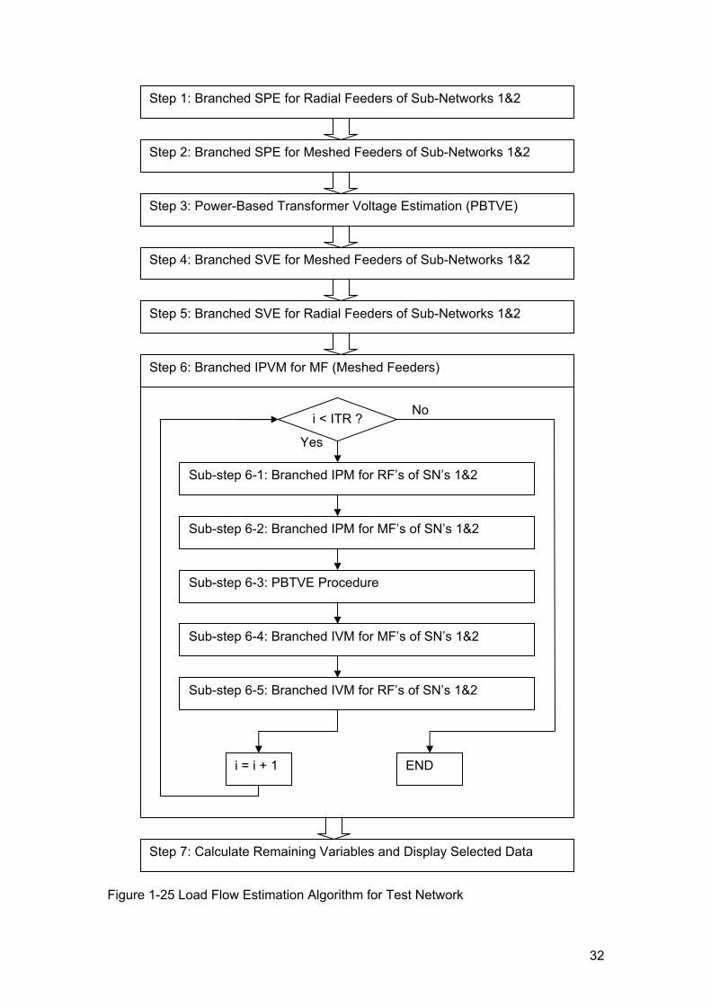
2.3.3 Calculation Steps of LFEA for Test Network With the previous accounts on radial, meshed, and branched feeders as well as the feeding transformer, it is now possible to develop a compound algorithm that can be applied directly to test network. Thus the following Table 1-3 and Figure 1-25 will respectively give the data definition and algorithm of the final LFEA of test network. N Input Variables Output Variables 1 Line Line Name Pin (kW) Input Active Power 2 l (km) Line Length Qin (kVAR) Input Reactive Power 3 r (mΩ/km) Rel, Resistance Sin (kVA) Input Apparent Power 4 x (mΩ/km) Rel, Reactance (Ind.) Iin (A) Input Current 5 c (nF/km) Rel, Capacitance Pout (kW) Output Active Power 6 R (mΩ) Line Resistance Qout (kVAR) Output Reactive Power 7 XL (mΩ) Line Reactance (Ind.) Sout (kVA) Output Apparent Power 8 XC (kΩ) Line Reactance (Cap.) Iout (A) Output Current 9 Ith (kA) Line Current Rating Unode (kV) Node Voltage Magnitude 10 Node Node Name Αnode (º) Node Voltage Angle 11 Load Load Name dP (kW) Active Power Difference 12 PL (kW) Load Active Power dQ (kVAR) Reactive Pow. Difference 13 QL (kVAR) Load Reactive Power dS (kVA) Apparent Pow. Difference 14 SL (kVA) Load Apparent Power dU (kV) Voltage Magn. Difference 15 cosφL Load Power Factor dα (º) Voltage Angle Difference 16 FtE_Volt Tag for Voltage Cal. Irat (%) Current Loading of Line 17 EtF_Pow Tag for Power Cal. Srat (%) Power Loading of Line
Table 1-3 Complete List of Input and Output Variables for the Final Version of LFEA
N N N
YYY
MS BS FA
LNL Element ( j )
Ui( j ) = Uo( j – 1 ) αi( j ) = αo( j – 1 )
Ui( j ) = Uo( j – Ni – 1 ) αi( j ) = αo( j – Ni – 1 )
32
Figure 1-25 Load Flow Estimation Algorithm for Test Network
Yes
No i < ITR ?
Step 6: Branched IPVM for MF (Meshed Feeders)
Sub-step 6-1: Branched IPM for RF’s of SN’s 1&2
Sub-step 6-5: Branched IVM for RF’s of SN’s 1&2
i = i + 1 END
Step 4: Branched SVE for Meshed Feeders of Sub-Networks 1&2
Step 1: Branched SPE for Radial Feeders of Sub-Networks 1&2
Step 2: Branched SPE for Meshed Feeders of Sub-Networks 1&2
Step 3: Power-Based Transformer Voltage Estimation (PBTVE)
Step 5: Branched SVE for Radial Feeders of Sub-Networks 1&2
Sub-step 6-2: Branched IPM for MF’s of SN’s 1&2
Sub-step 6-3: PBTVE Procedure
Sub-step 6-4: Branched IVM for MF’s of SN’s 1&2
Step 7: Calculate Remaining Variables and Display Selected Data
33
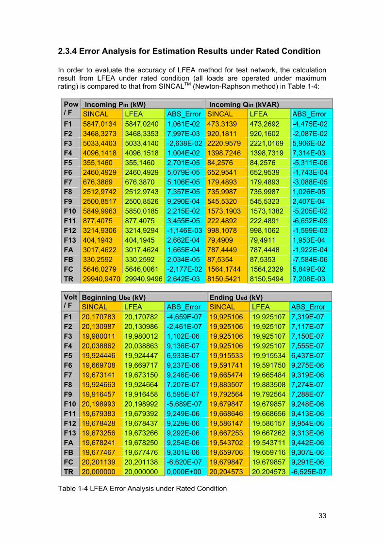
2.3.4 Error Analysis for Estimation Results under Rated Condition In order to evaluate the accuracy of LFEA method for test network, the calculation result from LFEA under rated condition (all loads are operated under maximum rating) is compared to that from SINCALTM (Newton-Raphson method) in Table 1-4:
Incoming Pin (kW) Incoming Qin (kVAR) Pow / F SINCAL LFEA ABS_Error SINCAL LFEA ABS_Error F1 5847,0134 5847,0240 1,061E-02 473,3139 473,2692 -4,475E-02 F2 3468,3273 3468,3353 7,997E-03 920,1811 920,1602 -2,087E-02 F3 5033,4403 5033,4140 -2,638E-02 2220,9579 2221,0169 5,906E-02 F4 4096,1418 4096,1518 1,004E-02 1398,7246 1398,7319 7,314E-03 F5 355,1460 355,1460 2,701E-05 84,2576 84,2576 -5,311E-06 F6 2460,4929 2460,4929 5,079E-05 652,9541 652,9539 -1,743E-04 F7 676,3869 676,3870 5,106E-05 179,4893 179,4893 -3,088E-05 F8 2512,9742 2512,9743 7,357E-05 735,9987 735,9987 1,026E-05 F9 2500,8517 2500,8526 9,290E-04 545,5320 545,5323 2,407E-04 F10 5849,9963 5850,0185 2,215E-02 1573,1903 1573,1382 -5,205E-02 F11 877,4075 877,4075 3,455E-05 222,4892 222,4891 -6,652E-05 F12 3214,9306 3214,9294 -1,146E-03 998,1078 998,1062 -1,599E-03 F13 404,1943 404,1945 2,662E-04 79,4909 79,4911 1,953E-04 FA 3017,4622 3017,4624 1,665E-04 787,4449 787,4448 -1,922E-04 FB 330,2592 330,2592 2,034E-05 87,5354 87,5353 -7,584E-06 FC 5646,0279 5646,0061 -2,177E-02 1564,1744 1564,2329 5,849E-02 TR 29940,9470 29940,9496 2,642E-03 8150,5421 8150,5494 7,208E-03
Beginning Ube (kV) Ending Ued (kV) Volt
/ F SINCAL LFEA ABS_Error SINCAL LFEA ABS_Error F1 20,170783 20,170782 -4,659E-07 19,925106 19,925107 7,319E-07 F2 20,130987 20,130986 -2,461E-07 19,925106 19,925107 7,117E-07 F3 19,980011 19,980012 1,102E-06 19,925106 19,925107 7,150E-07 F4 20,038862 20,038863 9,136E-07 19,925106 19,925107 7,555E-07 F5 19,924446 19,924447 6,933E-07 19,915533 19,915534 6,437E-07 F6 19,669708 19,669717 9,237E-06 19,591741 19,591750 9,275E-06 F7 19,673141 19,673150 9,246E-06 19,665474 19,665484 9,319E-06 F8 19,924663 19,924664 7,207E-07 19,883507 19,883508 7,274E-07 F9 19,916457 19,916458 6,595E-07 19,792564 19,792564 7,288E-07 F10 20,198993 20,198992 -5,689E-07 19,679847 19,679857 9,248E-06 F11 19,679383 19,679392 9,249E-06 19,668646 19,668656 9,413E-06 F12 19,678428 19,678437 9,229E-06 19,586147 19,586157 9,954E-06 F13 19,673256 19,673266 9,292E-06 19,667253 19,667262 9,313E-06 FA 19,678241 19,678250 9,254E-06 19,543702 19,543711 9,442E-06 FB 19,677467 19,677476 9,301E-06 19,659706 19,659716 9,307E-06 FC 20,201139 20,201138 -6,620E-07 19,679847 19,679857 9,291E-06 TR 20,000000 20,000000 0,000E+00 20,204573 20,204573 -6,525E-07
Table 1-4 LFEA Error Analysis under Rated Condition
34
The active and reactive power data shown in Table 1-4 are taken at the incoming end of all feeders in test network, thus each power value can be seen as representing maximum error in its feeder due to the tail-to-head power calculation nature of LFEA. In the mean while, the voltage data in Table 1-4 are taken respectively from nodes of the first (Ube) and the last (Ued) LNL element in each feeder, which makes its possible to examine the general variation of voltage estimation error along each feeder. Table 1-4 reveals that the estimation error of power and voltage data summarized at the feeding transformer (last line ‘TR’ in Table 1-4) approximately fall into the size ranges calculated in 3.1.1 (respectively in kW’s, kVAR’s, and mV’s); while the estimation error of a specific feeder or a LNL element could be more than 10 times larger than the calculated values. This can also be seen through the following Table 1-5, in which the second column shows the maximum errors from all feeders and the third column shows the maximum errors obtained from the output data of the feeding transformer: Feeder Transf. Feeder / Transf. Abs_Err_P (W) 26.3833 2.642 9,986109 Abs_Err_Q (VAR) 59.0586 7.208 8,193479 Abs_Err_U (mV) 9.9543 0.6525 15,25563
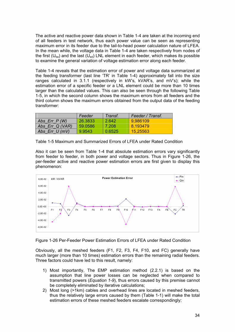
Table 1-5 Maximum and Summarized Errors of LFEA under Rated Condition Also it can be seen from Table 1-4 that absolute estimation errors vary significantly from feeder to feeder, in both power and voltage sectors. Thus in Figure 1-26, the per-feeder active and reactive power estimation errors are first given to display this phenomenon:
Power Estimation Error
-6,0E-02
-4,0E-02
-2,0E-02
0,0E+00
2,0E-02
4,0E-02
6,0E-02
8,0E-02
F1 F2 F3 F4 F5 F6 F7 F8 F9 F10 F11 F12 F13 FA FB FC TR
kW / kVARPinQin
Figure 1-26 Per-Feeder Power Estimation Errors of LFEA under Rated Condition Obviously, all the meshed feeders (F1, F2, F3, F4, F10, and FC) generally have much larger (more than 10 times) estimation errors than the remaining radial feeders. Three factors could have led to this result, namely:
1) Most importantly, The EMP estimation method (2.2.1) is based on the assumption that line power losses can be neglected when compared to transmitted powers (Equation 1-9), thus errors caused by this premise cannot be completely eliminated by iterative calculations;
2) Most long (>1km) cables and overhead lines are located in meshed feeders, thus the relatively large errors caused by them (Table 1-1) will make the total estimation errors of these meshed feeders escalate correspondingly;
35
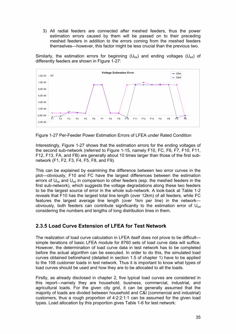
3) All radial feeders are connected after meshed feeders, thus the power estimation errors caused by them will be passed on to their preceding meshed feeders in addition to the errors coming from the meshed feeders themselves—however, this factor might be less crucial than the previous two.
Similarly, the estimation errors for beginning (Ube) and ending voltages (Ued) of differently feeders are shown in Figure 1-27:
Voltage Estimation Error
-2,0E-06
0,0E+00
2,0E-06
4,0E-06
6,0E-06
8,0E-06
1,0E-05
1,2E-05
F1 F2 F3 F4 F5 F6 F7 F8 F9 F10 F11 F12 F13 FA FB FC TR
kVUbeUed
Figure 1-27 Per-Feeder Power Estimation Errors of LFEA under Rated Condition Interestingly, Figure 1-27 shows that the estimation errors for the ending voltages of the second sub-network (referred to Figure 1-15, namely F10, FC, F6, F7, F10, F11, F12, F13, FA, and FB) are generally about 10 times larger than those of the first sub-network (F1, F2, F3, F4, F5, F8, and F9). This can be explained by examining the difference between two error curves in the plot—obviously, F10 and FC have the largest differences between the estimation errors of Ube and Ued in comparison to other feeders (esp. the meshed feeders in the first sub-network), which suggests the voltage degradations along these two feeders to be the largest source of error in the whole sub-network. A look-back at Table 1-2 reveals that F10 has the largest total line length (over 12km) of all feeders, while FC features the largest average line length (over 1km per line) in the network—obviously, both feeders can contribute significantly to the estimation error of Ued considering the numbers and lengths of long distribution lines in them.
2.3.5 Load Curve Extension of LFEA for Test Network The realization of load curve calculation in LFEA itself does not prove to be difficult—simple iterations of basic LFEA module for 8760 sets of load curve data will suffice. However, the determination of load curve data in test network has to be completed before the actual algorithm can be executed. In order to do this, the simulated load curves obtained beforehand (detailed in section 1.5 of chapter 1) have to be applied to the 108 customer loads in test network. Thus it is important to know what types of load curves should be used and how they are to be allocated to all the loads. Firstly, as already disclosed in chapter 2, five typical load curves are considered in this report—namely they are household, business, commercial, industrial, and agricultural loads. For the given city grid, it can be generally assumed that the majority of loads are divided between household and C&I (commercial and industrial) customers, thus a rough proportion of 4:2:2:1:1 can be assumed for the given load types. Load allocation by this proportion gives Table 1-6 for test network:

36
A_Household ΣP(kW) No. B_Business ΣP(kW) No. sumB1 2189 4 sumA1 1349 8 sumB2 1956 4 sumA2 1388 8 sumB3 1758 4 sumA3 1373 9 sum_B 5903 12 sumA4 1310 10 Percent_B % 20,02646 11,11111 sumA5 1264 9 sumA6 1294 10 C_Commercial ΣP(kW) No. sumA7 1309 8 sumC1 1963 5 sumA8 1382 9 sumC2 2090 4 sumA9 1319 10 sumC3 1832 4 sum_A 11988 81 sum_C 5885 13 Percent_A % 40,67038 75 Percent_C % 19,9654 12,03704 D_Industrial ΣP(kW) No. E_Agricultural ΣP(kW) No. sum_D 2500 1 sum_E 3200 1 Percent_D % 8,481476 0,925926 Percent_E % 10,85629 0,925926
ΣP(kW) No. ΣP — Total Rated Active Power of Loads sum_total 29476 108
No.— Load Count of the Same Type
Table 1-6 Allocation of Load Types for Test Network In the bold lines of Table 3-6, the summarized allocation results for each type of load can be seen through the total amount of active power (ΣP) and the number of loads included (No.). The total power ratio after allocation turns out to be rather close to the original 4:2:2.1:1 setting, which can be seen through Figure 1-28:
20%
20%
8%
11%
41%HouseholdBusinessCommercialIndustiralAgricultural
Figure 1-28 Total Power Ratio of All Load Types in Test Network In addition, Table 1-6 also suggests that for each type of load, several equivalent load curves that share the same stochastic property (RCV—referred to section 2.5) should be generated and distributed evenly (for both power and number of loads). It can be seen from the table that the actual numbers of load curves taken for the given load types are 9, 3, 3, 1, 1, thus if a general RCV 0 of 5% is assumed throughout the whole network, then the RCV for these five types of load curves can be calculated as 15%, 8.7%, 8.7%, 5%, 5% (2.5.3). This is also shown in Figure 1-29:

37
Figure 1-29 Detailed Load Allocation Scheme in Test Network

38
With the obtained annual load data, it is then possible to extend the existing load flow estimation algorithm to suit the purpose of load curve calculations. In later chapters, the generation curves of wind turbines and PV arrays are also included in the estimation algorithm, which implements the stochastic DG evaluation function in the LFEA module as well. It should be noted, however, that during the annual load curve calculation process, the tap-changer of feeding transformer is currently fixed at a selected position for all data points. This measure is taken to simplify DG evaluation procedures in ensuing chapters, while on-load tap changing possibility will be later considered for implementation of active network control.
2.3.6 Error Analysis for Load Curve Estimation Results In order to check into the performance of LFEA under different loading scenarios during load curve calculation processes, a weekly set (168) of load curve data is tested both with LFEA and SINCAL. In following paragraphs, the calculated total load power demand (summarized from power demands of all loads in network), total power losses, and the voltage magnitudes of the starting bus bar UA31 from both sources are first compared with each other, and then the absolute errors of LFEA are subsequently obtained for each of them. Firstly, the following three figures (Figure 1-30, Figure 1-31, and Figure 1-32) show respectively the weekly curves of total active load power (Pload), total reactive load power (Qload), and the absolute estimation errors of the previous two variables:
Pload
0
5
10
15
20
25
1 9 17 25 33 41 49 57 65 73 81 89 97 105 113 121 129 137 145 153 161 169
sincalestimat
Qload
0
1
2
3
4
5
6
7
8
9
1 9 17 25 33 41 49 57 65 73 81 89 97 105 113 121 129 137 145 153 161 169
sincalestimat
Figure 1-30 Weekly Active Load Power Figure 1-31 Weekly Reactive Load Power
Absolute Error_Load Power
-6,00E-09
-4,00E-09
-2,00E-09
0,00E+00
2,00E-09
4,00E-09
6,00E-09
1 6 11 16 21 26 31 36 41 46 51 56 61 66 71 76 81 86 91 96 101 106 111 116 121 126 131 136 141 146 151 156 161 166
MW/MVAR PloadQload
Figure 1-32 Weekly Load Power Estimation Errors

39
It can be seen that estimation errors for total load power demand generally fall into the range of several mW’s or mVAR’s, which can be regarded as negligible when compared to the MW- and MVAR- scales of Pload and Qload. The totally random nature of estimation errors (shown in Figure 1-32) suggests the cause of the error to be the difference in the accuracy levels (e.g., the number of decimal digits taken for a double variable) of two programs under examination. Similar to the plots before, the following three figures (Figure 1-33, Figure 1-34, and Figure 1-35) respectively show the weekly curves of total active power loss (dPtot), total reactive power loss (dQtot), and the absolute estimation errors of both variables:
Ploss
0
0,05
0,1
0,15
0,2
0,25
0,3
0,35
0,4
0,45
1 9 17 25 33 41 49 57 65 73 81 89 97 105 113 121 129 137 145 153 161 169
sincalestimat
Qloss
-2,5
-2
-1,5
-1
-0,5
0
0,5
1
1,5
1 9 17 25 33 41 49 57 65 73 81 89 97 105 113 121 129 137 145 153 161 169
sincalestimat
Figure 1-33 Weekly Active Power Loss Figure 1-34 Weekly Reactive Power Loss
Absolute Error_Power Losses
0,00E+00
1,00E-06
2,00E-06
3,00E-06
4,00E-06
5,00E-06
6,00E-06
7,00E-06
8,00E-06
9,00E-06
1,00E-05
1 7 13 19 25 31 37 43 49 55 61 67 73 79 85 91 97 103 109 115 121 127 133 139 145 151 157 163
MW/MVAR PlossQloss
Figure 1-35 Weekly Power Loss Estimation Errors Obviously, the estimation errors of dP and dQ shown in Figure 1-35 vary within the range of several kW’s or kVAR’s, which can be seen as consistent with the outcome of LFEA under rated operating condition (3.3.4). Figure 1-35 also suggests that the error curves of dP and dQ respectively follow some roughly daily cycles, which indicates the influence of input load curves on the estimation accuracy of LFEA. Another noticeable fact concerning Figure 1-35 is that dP and dQ generally have opposing trends of error curve development—namely, the error of dQ will most likely decrease when the error of dP increases, and vice versa. Thus simultaneous error reduction for both variables does not appear to be achievable for current algorithm. With given descriptions on total load power demands and total power losses, it is now possible to obtain the estimation errors of system slack power summarized at the incoming end of feeding transformer through Equation 1-21.

40
⎪⎩
⎪⎨⎧
+=
+=
∑∑∑∑
dQQQ
dPPP
loadslack
loadslack
Equation 1-21
Obviously, since slack power flows can be seen as the sum of total power demands and power losses, estimation errors of them should follow the same relationship. As it is already known that estimation errors of total power demands (mW, mVAR) are around 1000 times smaller than those of power losses (W, VAR), estimation errors of slack power flows can be seen as approximately equal to those of the power losses. Finally, voltage estimation accuracy of LFEA is examined in Figure 1-36 and Figure 1-37, which show respectively the weekly curves of the voltage magnitude at starting bus bar UA31 and the absolute estimation errors of the estimated results:
Voltage
19,4
19,6
19,8
20
20,2
20,4
20,6
1 6 11 16 21 26 31 36 41 46 51 56 61 66 71 76 81 86 91 96 101 106 111 116 121 126 131 136 141 146 151 156 161 166
kV sincalestimat
Figure 1-36 Weekly UA31 Voltage Magnitudes
Absolute Error_Voltage Magnitude
-8,00E-07
-7,00E-07
-6,00E-07
-5,00E-07
-4,00E-07
-3,00E-07
-2,00E-07
-1,00E-07
0,00E+001 6 11 16 21 26 31 36 41 46 51 56 61 66 71 76 81 86 91 96 101 106 111 116 121 126 131 136 141 146 151 156 161 166
kVVoltage
Figure 1-37 Weekly UA31 Voltage Magnitude Estimation Errors When compared to Figure 1-35, the estimation error curve of UA31 voltage in Figure 1-37 shows similar behaviors as the curves of power losses. In order to compare the error ranges of slack power and starting voltage data, Table 1-7 is given: Tran_Low Tran_Upp F/T Fed_Low Fed_Upp U/L Abs_Err_P (W) 2.5 5.5 10 25 55 2.2 Abs_Err_Q (VAR) 5.5 9.5 10 55 95 1.7 Abs_Err_U (mV) 0.4 0.8 15 6 12 2
Table 1-7 Transformer and Feeder Error Ranges of LFEA Load Curve Calculation

41
The second and the third columns in Table 1-7 respectively give the lower and upper boundaries of summarized power and voltage estimation errors, which are taken directly from Figure 1-35 and Figure 1-37. With the Max/Sum ratios estimated from Table 1-5, expected maximum estimation errors for single network elements are listed in the fifth and sixth columns in Table 1-7. Comparison of summarized and maximum error data between Table 1-5 and Table 1-7 shows relatively good consistency of LFEA under various loading conditions, which, in addition to the fact that upper-to-lower boundary ratios (U/L) of both power and voltage data approximate 2, proves the fact that LFEA exhibit a reasonably good applicability to load curve calculations.
2.4 Algorithm Extension to General Distribution Grids Up to section 2.3, a load flow estimation algorithm (LFEA) has been introduced to provide approximated LF solutions for various network structures. However, the algorithms presented in these sections are ad-hoc solutions in essence and can only be applied to specific networks. In order to avoid repetitive modifications of LFEA code to accommodate different distribution grids, standardized modules are implemented to LFEA in this section.
2.4.1 Topology Definition: Grid-wise and Feeder-wise The topology of a typical distribution grid can be viewed in a two-step manner—first, a grid-wise viewpoint can be taken to describe the whole grid in terms of feeders and transformers; and then a feeder-wise perspective will present each feeder in the grid with LNL elements. In Figure 1-38, a sample network is presented grid-wise.
Figure 1-38 Definition of Grid-wise Topology for a Sample Distribution Network

42
As can be seen from Figure 1-38, LFEA sub-divides a distribution grid into different layers so as to facilitate serial calculation of power and voltage. For each layer (>1), a number of power inflow nodes (e.g. P2 for Layer 2) and a number of power outflow nodes (e.g. P3, P4, and P5 for Layer 2) act as intermediates between neighboring layers. Due to the generally radial characteristics of distribution grids, LFEA assumes that the number of inflow nodes should be equal or less than outflow nodes for each grid-wise layer. In the mean time, it can be seen from Figure 1-38 that between any pair of inflow and outflow nodes three potential network segments could be found:
1. One transformer (e.g. T2) 2. One feeder (e.g. F3) 3. A number of parallel meshed feeders (e.g. F1 and F2)
Consequently, in any given grid layer an inflow node could be connected to one or more network segments belonging to any one of the three types described above, while an outflow node could only be connected to one network segment under the assumptions made for current LFEA. Such a pan-radial structure in grid-wise sense makes it possible to apply backward/forward sweep principle to calculate power and voltage data. Now that overall network topology is expressed in a grid-wise plot, feeder-wise detailed definitions of LNL elements can be seen from Figure 1-39. Obviously, for each feeder a main section (MS) and a certain amount of sub-sections (SS) can be identified, while the sub-sections can be again sorted into different feeder layers. In order to tackle with multiple layers of sub-sections, branched LF solution given in section 3.3.2 has to be adapted significantly, which will be done in ensuing sections.
Figure 1-39 Definition of Feeder-wise Topology for a Sample Distribution Feeder
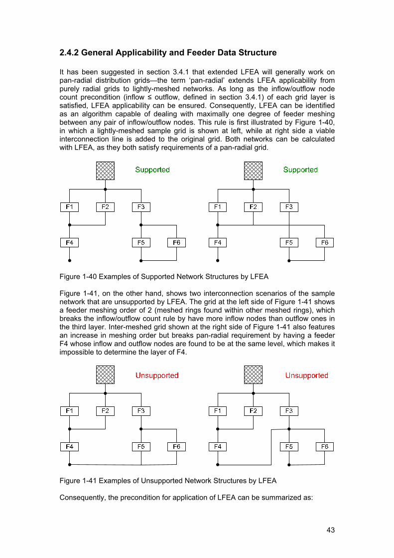
43
2.4.2 General Applicability and Feeder Data Structure It has been suggested in section 3.4.1 that extended LFEA will generally work on pan-radial distribution grids—the term ‘pan-radial’ extends LFEA applicability from purely radial grids to lightly-meshed networks. As long as the inflow/outflow node count precondition (inflow ≤ outflow, defined in section 3.4.1) of each grid layer is satisfied, LFEA applicability can be ensured. Consequently, LFEA can be identified as an algorithm capable of dealing with maximally one degree of feeder meshing between any pair of inflow/outflow nodes. This rule is first illustrated by Figure 1-40, in which a lightly-meshed sample grid is shown at left, while at right side a viable interconnection line is added to the original grid. Both networks can be calculated with LFEA, as they both satisfy requirements of a pan-radial grid.
Figure 1-40 Examples of Supported Network Structures by LFEA Figure 1-41, on the other hand, shows two interconnection scenarios of the sample network that are unsupported by LFEA. The grid at the left side of Figure 1-41 shows a feeder meshing order of 2 (meshed rings found within other meshed rings), which breaks the inflow/outflow count rule by have more inflow nodes than outflow ones in the third layer. Inter-meshed grid shown at the right side of Figure 1-41 also features an increase in meshing order but breaks pan-radial requirement by having a feeder F4 whose inflow and outflow nodes are found to be at the same level, which makes it impossible to determine the layer of F4.
Figure 1-41 Examples of Unsupported Network Structures by LFEA Consequently, the precondition for application of LFEA can be summarized as:

44
1. Between any two nodes in grid-wise topology, only singe or parallel feeders or transformers are connected (i.e. no further nodes found in between);
2. For any grid layer, the number of inflow nodes must be smaller or equal to the number of outflow nodes;
3. The two terminal nodes of any network segment (defined in section 2.4.1) can not belong to the same level (i.e. both at inflow or outflow side of a layer).
It should be noted, however, that meshing is only allowed on a grid-wise level; while on a feeder-wise level only purely radial structures are allowed (as shown by Figure 1-39). Since LFEA is essentially based on linear accumulation of LNL estimation results, feeders with complicated branching conditions should have a linear data storage structure to facilitate calculations. In Figure 1-42, an example is given to illustrate this linearization process.
Figure 1-42 Feeder Data Storage Structure for LFEA With the storage sequence suggested by Figure 1-42, line and load information could be saved in different categories as defined in Table 1-3. However, in order to extend LFEA to accommodate varied feeder structures, additional topology information are needed for calculation, which can be seen from Table 1-8 (Index as the index of LNL element in main section or a sub-section; Layer as feeder-layer of sub-section; Ref as an arbitrary reference name given to each sub-section; SpNd refers to Splitting Node in the preceding layer). Index 1 1 1 1 2 2 3 2 3 4 Layer 0 1 2 3 2 1 1 0 0 0 Ref 0 1 1-1 1-1-1 1-1 1 1 0 0 0 SpNd 0 1 1 1 1 1 1 0 0 0 Table 1-8 Linearized Topology Information of a Feeder

45
With current LFEA extension, only Index, Layer and Ref information are crucial for specifying branch structure in the process of power or voltage calculation, as they can serve as the guideline of how unknown network variables are obtained from input data with a linear algorithm.
2.4.3 Extended Power and Voltage Estimation Approaches Similar to the methodologies introduced in section 2.3.2, both power estimation and voltage estimation processes could be modified to include branching information by classification of nodes (main / branch section, power junction / voltage retracing point etc.). However, the branching algorithms introduced in section 2.3.2 are not capable of dealing with either multiple branch layers or branches with a common splitting node. Consequently, more complicated approaches are needed to extend existing method to more general structures of a radial feeder. In order to achieve this goal, more than one dimension of node categorization will be necessary, namely:
1) Firstly, all nodes should be differentiated by whether or not it is the common point of two or even more (branched) sections, if it is shared by multiple sections (criterion A1), then the node will be defined as Power Junction Point in backward sweep and Voltage Splitting Point in forward sweep;
2) Secondly, all nodes should be categorized according to its position in the section it belongs to: if it is the first node in a branched section after a Power Junction / Voltage Splitting Point in the previous layer (criterion B1), then it will be defined as Power Summary Point in backward sweep and Voltage Following Point in forward sweep; if it is the first node in the same layer as a Power Junction / Voltage Splitting Point after one or more branched section(s) (criterion B2), it will be defined as Voltage Retracing Point in forward sweep;
3) If none of the conditions described above is satisfied, the examined node is just a normal node for which standard LFEA procedure should be applied.
Notably, a feeder node could hold properties from both category 1) and category 2) listed above, or none of them as described in category 3). Consequently, although only three criteria (A1, B1, B2) are given for identifying peculiar nodes, actual node types could be more as combinations from these two listed categories are formed. In order to contain such probabilities, node type could be described by a two-digit tag for both power and voltage estimation procedures, which is shown in Figure 2-43
A1 Layer(i) = Layer(i+1) - 1
B1 Index(i) = 1 & Layer(i) ≠ 0
B2 Layer(i) = Layer(i-1) - 1
N None
Criterion \ Condition
B1
Power Tag
A1 N
N
11
10
1
0
B1
Voltage Tag
A1 N
B2
11
12
1
2
N 10 0
Figure 1-43 Power and Voltage Tags under Different Scenarios

46
In order to better illustrate how power tags and voltage tags are defined in an actual network, Figure 1-44 and Figure 1-45 are provided to exhibit naming conventions with a sample branched feeder. Physical meanings for different tag values are also listed for reference.
Figure 1-44 Nodal Power Tags of a Sample Feeder during Backward Sweep
Figure 1-45 Nodal Voltage Tags of a Sample Feeder during Forward Sweep Obviously, since real-life distribution feeders could have multiple layers of branches (such as the feeder shown in Figure 1-44 and Figure 1-45), a single dimension of power accumulation or voltage degradation is not sufficient for calculation. Therefore temporary variables such as active power accumulator AcP used in power or voltage estimation procedures should be extended in dimension according to the deepest layer of branch in a given feeder. The extended power and voltage estimation procedures are described in Figure 1-46

47
( ) ( ) ( )( ) ( ) ( )( )( )
( ) ( )( ) ( )
ifendkQkLayerAcQkLayerAcQkPkLayerAcPkLayerAcP
elsekLayerJnQkLayerJnP
kLayerJnQkQkLayerAcQkLayerAcQkLayerJnPkPkLayerAcPkLayerAcP
thenPowTagIf
)()()()()()(
0)(0)(
)()()()()()()()(
10
+=+=
==
++=++=
≥
( ) ( ) ( )( ) ( ) ( )( )( )
ifendkLayerAcQkLayerAcP
kLayerAcQkLayerJnQkLayerJnQkLayerAcPkLayerJnPkLayerJnP
thenPowTagorPowTagIf
0)(0)(
)()()()()()(
111
==
+=+=
==
( ) ( )( ) ( )
( ) ( )( ) ( )
( ) ( )( ) ( )
ifendkLayerBrAkAkLayerBrUkU
thenVolTagorVolTagifelsekLayerBrAkAkLayerBrUkU
thenVolTagorVolTagifelsekAkAkUkU
thenVolTagIf
i
i
i
i
oi
oi
)()(
1221)(1)(111
11
0
==
==−=−===
−=−=
=
( ) ( )( ) ( )
ifendkAkLayerBrAkUkLayerBrU
thenVolTagIf
o
o
==
≥
)()(
10
Figure 1-46 Extended Power and Voltage Estimation Steps Including Tag Information
2.5 Summary In this chapter, a load flow estimation algorithm (LFEA) modified from the backward / forward sweep method [47] is introduced in full detail. Step-by-step explanation of the algorithm is given from the simplest radial topology to the test distribution network taken from real life, while basic principles as well as realization details of each step are both covered with full strength. By the end of the chapter, error analyses are performed for both the standard calculation procedure and the load curve extension

48
of LFEA, after which further explanation of how LFEA can be adapted from an ad-hoc solution to a more generally applicable approach is covered in various aspects. The advantages of LFEA, in retrospect, appear in two main aspects: firstly, linear (except for EMP estimation) real-number calculations can be used in stead of large matrix computations with complex numbers (as in the case of the mostly used Newton-Raphson load flow calculation practices), which can make a big difference for extremely time-consuming load curve calculations; secondly, the per-LNL-element processing order of LFEA makes it relatively easy to evaluate the impact of DG or active network control units under the given framework, thus some basic estimation formulas of LFEA will also serve directly or indirectly as the theoretical basis of ensuing topics on DER allocation. But on the other hand, there are also disadvantages of LFEA: firstly, LFEA is, after all, essentially an estimation approach, thus no matter how many error-reducing measures it takes, there is no way to eliminate the presence of errors; secondly, LFEA is designed to suit the relatively simple topologies (featured by radial, meshed, branched, and simple hybrid feeders) of distribution grids, thus comparatively complicated inter-meshing scenarios (such as some coupling possibilities shown in Figure 1-15 or the sample grid structures from Figure 1-41) will inevitably prove too complicated to be realized by LFEA; finally, only symmetrical network conditions are considered in current LFEA, unbalanced load or generation among 3 phases are not dealt with in the given algorithm (however, possibilities of extending the current module to include this aspect should exist [50]). Therefore, it is important to evaluate the specific applicability of LFEA before applying it to a certain network for a given purpose; and presumably, further improvements on the algorithm could be expected that would help to yield better estimation accuracies or accommodate more complicated network topologies. Within the scope of this report, however, the currently used LFEA module already suffices the purpose of DG evaluation and thus will be used for this purpose in ensuing chapters.

49
Chapter 2 A Load Flow Algorithm Based on Node-to-Link Deduction
Executive Summary
A novel load flow calculation algorithm has been proposed in this chapter with the following features: • Iterative power-voltage correction with good efficiency and convergence
behavior.
• Real-number matrix operations based on standard sparse techniques.
• Capable of producing good estimation results after 1 or 2 iterations.
• Calculation accuracy level equals or even excels Newton-Raphson method.
• Linear/quadratic formulation of network states from nodal power injection/extraction.
• Easy extension to optimal power flow and probabilistic power flow problems.
Currently the following functionalities are proven to be applicable in this chapter but not implemented yet on programming level:
• Currently all loads are implemented as power-constant, while current-constant or impedance-constant loads should be easily adaptable without further complexity.
• Currently only PQ generator models are programmed, while PV operation mode can be modeled with a slightly higher computational complexity.
• Implemented algorithm currently assumes one slack node, while multiple slacks can be realized at the cost of a slightly higher computational complexity.
• Active control (OLTC or switchable capacitor banks) measures have not been modeled so far, but should be potentially implementable.
• The algorithm has been implemented for balanced three-phase power systems, while computational complexity will increase greatly under unbalanced conditions.
The algorithm is found to be inherently restricted in the following aspects:
• Computational complexity increases with the number of network connections (i.e. degree of meshing) and the number of slack and PV nodes.
• Convergence rate is found to be close to backward/forward sweep method, which means much more iterations are needed under extreme voltage conditions.
In comparison with existing main-stream approaches (Newton-Raphson, current iteration etc.), the new load flow algorithm provides a simpler, more robust, and potentially faster solution that could provide explicit insights into

50
network characteristics. It is extremely suitable for sensitivity analysis, optimal / probabilistic power flow problems, and simulation of complex distribution networks with a high amount of dispersed generators.

51
Review of Existing Load Flow Methods Currently, the majority of commercial and educational power system software utilizes the Newton-Raphson method [1] [2] [3] for solving load flow problems. The popularity of this approach is mainly based on its high execution efficiency and good applicability to varied network structures and different component models. Although ranking among the earliest approaches [2] developed for solving load flow, the Newton-Raphson method has been consistently improved over the years, thus up to today it still holds significant advantages over other known approaches as the most mature load flow algorithm. In comparison with other classical load flow solutions such as Gauss-Seidel and Fast Decoupled Power Flow, Newton-Raphson method stands out with faster convergence speed (compared to Gauss-Seidel) and/or better applicability and accuracy (compared to Fast Decoupled Power Flow) [54]. The main restrictions of Newton-Raphson method, however, lie in its poor handling of ill-conditioned networks [61] and heavy reliance on a good guess of initial system condition [62] (which can be partially mitigated by using a number of Gauss-Seidel iterations for voltage initiation [54]). In addition, under specific conditions the Newton-Raphson method might be disfavored due to performance or speed concerns—for example, for contingency calculations of large transmission networks with low R/X ratio, the Fast Decoupled Power Flow converges much faster than Newton-Raphson method, while accuracy differences can be largely ignored. In recent decades, a large number of novel alternatives for solving the load flow problem have been proposed by different authors—such as direct (non-iterative) solutions in [55] and [56], pattern recognition method in [57], genetic algorithm approach in [58], fuzzy logic variant in [59], and conic quadratic formulation in [60]. In general these proposals all serve as refreshing ideas on an academic level, but almost all of them suffer from one or more of the following two problems: (1) general applicability, especially to large networks with complicated topology and multiple active components; (2) execution efficiency, specifically in comparison with Newton-Raphson or other commercial-level packages. Consequently, most of these new ideas are still at Lab-testing stage of application. Aside from the heavily-theoretical non-Newton approaches described above, there is also another important line of practice-oriented load flow solution techniques developed specifically for distribution networks [61] [62] [63] [47] [49]. This category of load flow algorithm is generally named as backward / forward sweep method, which utilizes the radial or weakly-meshed topological feature of distribution networks to reduce dimension of calculations. First proposed in [61], this method was adapted from current-iteration to power-iteration in [62], revised with better loop handling in [63], and added with more active component models in [47] and [49]. The major drawback with backward / forward method, however, comes from the adoption of loop breakpoints—this operation limits the algorithm to ad hoc category and makes it only applicable to simple topologies. The load flow algorithm proposed in this chapter shares similar power-voltage correction concepts as the backward-forward sweep method, yet it surpasses the later in terms of general applicability to highly-meshed networks with multiple active components.

52
Terminal-to-Difference Equations for Serial Components
Reintroduction of Equivalent π Model A central part of load flow analysis is the modeling of network components, especially serial components that will largely determine the node admittance matrix used as basis of most calculation algorithms. In Figure 2-1 and Figure 2-2, the π-models of a typical transmission line and a typical power transformer are respectively plotted. It can be seen that the transmission line can be modeled as a pure π element, while the transformer model includes an extra voltage turns ratio between primary and secondary sides.
Figure 2-1 π-Model for Transmission Lines
Figure 2-2 π-Model for Power Transformers
By considering only the π element part of transformer model in Figure 2-2, both lines and transformers (partial) can be described by a same π model shown by Figure 2-3. Obviously, the same serial resistance and reactance models apply to both cases. However, lines are found with zero shunt conductance (Gq) and capacitive shunt susceptance (Bq < 0); while transformers has positive values for both Gq and Bq.
Figure 2-3 Equivalent π-Model for Serial Components
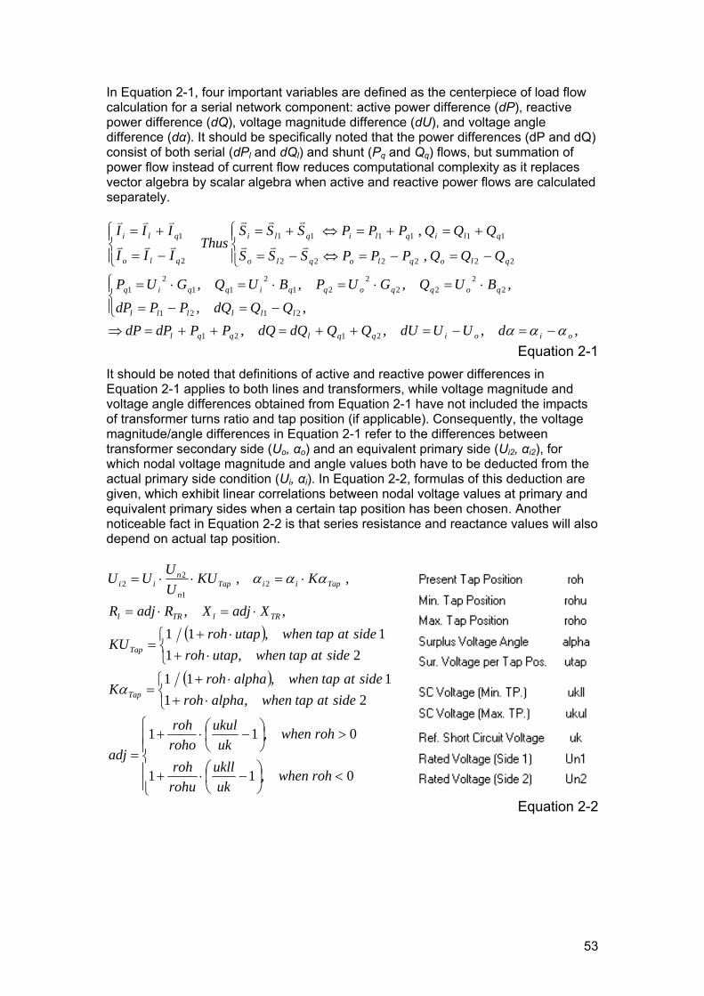
53
In Equation 2-1, four important variables are defined as the centerpiece of load flow calculation for a serial network component: active power difference (dP), reactive power difference (dQ), voltage magnitude difference (dU), and voltage angle difference (dα). It should be specifically noted that the power differences (dP and dQ) consist of both serial (dPl and dQl) and shunt (Pq and Qq) flows, but summation of power flow instead of current flow reduces computational complexity as it replaces vector algebra by scalar algebra when active and reactive power flows are calculated separately.
,,,,,,
,,,,
,
,
2121
2121
22
222
212
112
1
222222
111111
2
1
oioiqqlqql
llllll
qoqqoqqiqqiq
qloqloqlo
qliqliqli
qlo
qli
dUUdUQQdQdQPPdPdPQQdQPPdP
BUQGUPBUQGUP
QQQPPPSSS
QQQPPPSSSThus
III
III
ααα −=−=++=++=⇒
⎪⎩
⎪⎨⎧
−=−=
⋅=⋅=⋅=⋅=
⎪⎩
⎪⎨⎧
−=−=⇔−=
+=+=⇔+=
⎪⎩
⎪⎨⎧
−=
+=vvv
vvv
vvv
vvv
Equation 2-1 It should be noted that definitions of active and reactive power differences in Equation 2-1 applies to both lines and transformers, while voltage magnitude and voltage angle differences obtained from Equation 2-1 have not included the impacts of transformer turns ratio and tap position (if applicable). Consequently, the voltage magnitude/angle differences in Equation 2-1 refer to the differences between transformer secondary side (Uo, αo) and an equivalent primary side (Ui2, αi2), for which nodal voltage magnitude and angle values both have to be deducted from the actual primary side condition (Ui, αi). In Equation 2-2, formulas of this deduction are given, which exhibit linear correlations between nodal voltage values at primary and equivalent primary sides when a certain tap position has been chosen. Another noticeable fact in Equation 2-2 is that series resistance and reactance values will also depend on actual tap position.
( )
( )
⎪⎪⎩
⎪⎪⎨
⎧
<⎟⎠⎞
⎜⎝⎛ −⋅+
>⎟⎠⎞
⎜⎝⎛ −⋅+
=
⎩⎨⎧
⋅+⋅+
=
⎩⎨⎧
⋅+⋅+
=
⋅=⋅=
⋅=⋅⋅=
0,11
0,11
2,11,11
2,11,11
,,
,, 21
22
rohwhenukukll
rohuroh
rohwhenuk
ukulrohoroh
adj
sideattapwhenalpharohsideattapwhenalpharoh
K
sideattapwhenutaprohsideattapwhenutaproh
KU
XadjXRadjR
KKUUUUU
Tap
Tap
TRlTRl
TapiiTapn
nii
α
ααα
Equation 2-2

54
Formulation of Voltage Magnitude and Angle Differences
Two popular estimation formulas have been used by many power system engineers as an intuitive approximation of line/transformer voltage drop and phase angle difference. In Equation 2-3 these two formulas are shown in their standard format [44].
2,U
QRPXdU
QXPRdU ⋅−⋅≅
⋅+⋅≅ α
Equation 2-3 In this section, however, the approximated formulas in Equation 2-3 will be redefined under the equivalent π-model shown by Figure 2-2 and thereby extended to eliminate their inherent errors. Eventually this makes it possible to calculate differences in both voltage magnitude and voltage angle across a line or transformer through knowledge of terminal power (both active and reactive) and voltage states. Apparently, such a possibility serves as the first step to iterative power-voltage modification method for solving the load flow problem.
In Figure 2-4, a vector diagram is taken from [66] (page 117) to illustrate inter-dependencies between input and output voltage magnitudes and angles. Apparently in Figure 2-4, the output voltage (Uo) has been taken as the reference vector, against which voltage difference has been mirrored in parallel or perpendicular directions.
Figure 2-4 Vector Diagram for Input and Output Voltages of an Equivalent π-Model
By exploring geometric features of the right-angled triangular in Figure 2-4, Equation 2-4 (referred also to [66]) can be obtained when the vector correlations are examined with output voltage as reference vector (αo).
( ) ( )
⎟⎟⎠
⎞⎜⎜⎝
⎛ ⋅−⋅⋅+⎟⎟
⎠
⎞⎜⎜⎝
⎛ ⋅+⋅+=
−⋅+++=⋅+=
+=∠=−
====
o
llll
o
llllo
o
llllolloi
oooo
ll
o
lloi
UQRPXj
UQXPRU
UjQPjXRjUIZUUThus
jUUUU
jQPUSIThenLet
2222
22
22*
*2
0
00,,0,
vvvv
vv
vv
αηα
Equation 2-4 Up to now, Figure 2-4 and Equation 2-4 do not show any difference from [66]. However, a simple change of reference frame from Uo to Ui will lead to a completely new diagram and a new set of equations, as shown by Figure 2-5 and Equation 2-5.
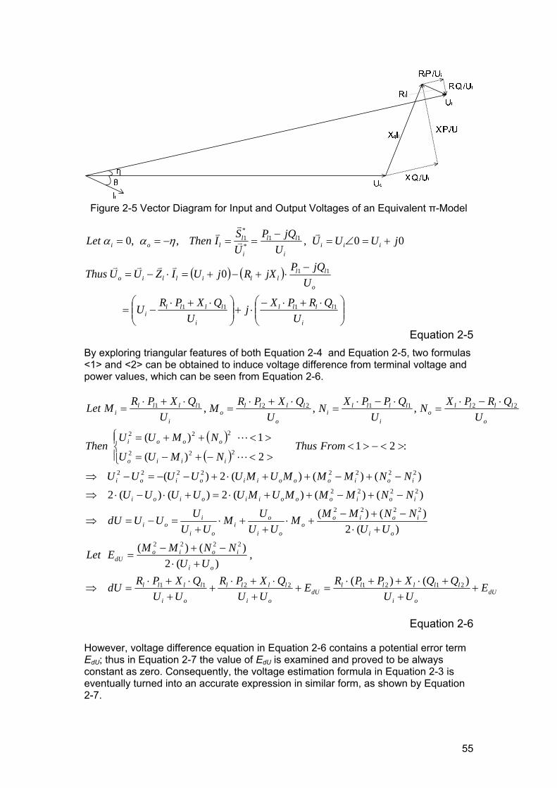
55
Figure 2-5 Vector Diagram for Input and Output Voltages of an Equivalent π-Model
( ) ( )
⎟⎟⎠
⎞⎜⎜⎝
⎛ ⋅+⋅−⋅+⎟⎟
⎠
⎞⎜⎜⎝
⎛ ⋅+⋅−=
−⋅+−+=⋅−=
+=∠=−
==−==
i
llll
i
lllli
o
llllillio
iiii
ll
i
lloi
UQRPXj
UQXPRU
UjQPjXRjUIZUUThus
jUUUU
jQPUSIThenLet
1111
11
11*
*1
0
00,,,0
vvvv
vv
vv
ηαα
Equation 2-5 By exploring triangular features of both Equation 2-4 and Equation 2-5, two formulas <1> and <2> can be obtained to induce voltage difference from terminal voltage and power values, which can be seen from Equation 2-6.
( )( )
dUoi
lllllldU
oi
llll
oi
llll
oi
ioiodU
oi
ioioo
oi
oi
oi
ioi
ioioooiioioi
ioioooiioioi
iiio
oooi
o
llllo
i
lllli
o
llllo
i
lllli
EUU
QQXPPREUU
QXPRUU
QXPRdU
UUNNMMELet
UUNNMMM
UUUM
UUUUUdU
NNMMMUMUUUUU
NNMMMUMUUUUU
FromThusNMUU
NMUUThen
UQRPXN
UQPPXN
UQXPRM
UQXPRMLet
++
+⋅++⋅=+
+⋅+⋅
++
⋅+⋅=⇒
+⋅−+−
=
+⋅−+−
+⋅+
+⋅+
=−=⇒
−+−++⋅=+⋅−⋅⇒
−+−++⋅+−−=−⇒
><−><⎪⎩
⎪⎨⎧
><−+−=
><++=
⋅−⋅=
⋅−⋅=
⋅+⋅=
⋅+⋅=
)()(
,)(2
)()(
)(2)()(
)()()(2)()(2
)()()(2)(
:212)(
1)(
,,,
21212211
2222
2222
2222
22222222
222
222
22112211
L
L
Equation 2-6
However, voltage difference equation in Equation 2-6 contains a potential error term EdU; thus in Equation 2-7 the value of EdU is examined and proved to be always constant as zero. Consequently, the voltage estimation formula in Equation 2-3 is eventually turned into an accurate expression in similar form, as shown by Equation 2-7.

56
[ ]
( ) ( ) ( ) ( )
( ) ( ) ( ) ( )
[ ]
oi
lllllldU
oi
llllll
lloi
ll
i
l
o
l
oi
ll
i
llll
o
llll
oi
i
llllllll
o
llllllll
oi
iioooioi
ioiodU
UUQQXPPRE
UUQQXPPRdU
Thus
IIUU
XRUS
US
UUXR
UQPXR
UQPXR
UU
UQRPXQXPR
UQRPXQXPR
UU
NMNMUUUU
NNMME
++⋅++⋅
=++
+⋅++⋅=
=−⋅+⋅
+=⎥
⎦
⎤⎢⎣
⎡−⋅
+⋅+
=
⎥⎦
⎤⎢⎣
⎡ +⋅+−
+⋅+⋅
+⋅=
⎥⎦
⎤⎢⎣
⎡ −++−
−++⋅
+⋅=
+−+⋅+⋅
=+⋅
−+−=
)()()()(:
0)(2
)()(2
)(
)(21
)(21
)()()(2
1)(2
)()(
21212121
2222
2
21
2
22
22
2
21
21
22
2
22
22
22
2
211
211
2
222
222
22222222
Equation 2-7
Now that the voltage (magnitude) difference estimation formula in Equation 2-3 has been extended to an accurate version, a similar procedure can be performed for estimation formula of voltage angle variation. In Equation 2-8, voltage angle difference is deduced from right-angle triangular features of both Figure 2-4 and Figure 2-5, and then eventually transformed into an accurate version with similar form as Equation 2-3.
oi
llllll
oi
llllll
oi
llllll
oi
iioo
o
i
i
o
o
i
i
o
UUQQRPPX
UUQQRPPXdsmallisdWhen
UUQQRPPX
UUUNUN
UN
UNd
UN
UNdAs
⋅⋅+⋅−+⋅
≅⎟⎟⎠
⎞⎜⎜⎝
⎛⋅⋅
+⋅−+⋅=
⋅⋅+⋅−+⋅
=⋅⋅
⋅+⋅=⎟⎟
⎠
⎞⎜⎜⎝
⎛+=⇒
==
−
2)()(
2)()(sin,
2)()(
22/)sin(
)sin(
212121211
2121
αα
α
α
Equation 2-8
One noticeable fact concerning Equation 2-7 and Equation 2-8 is that all power terms are intermediate values (Pl1 Pl2 Ql1 Ql2) instead of terminal values (Pi Po Qi Qo). In Equation 2-9, transformation of these intermediate values into terminal ones has been performed. Obviously, the difference comes from shunt conductance and susceptance.
( )( )⎪⎩
⎪⎨⎧
⋅−⋅++=++−=+
⋅−⋅++=++−=+
⋅=⋅=⋅=⋅=
12
22
2121
12
22
2121
22
222
212
112
1
)()()(
)()()(
,,,,
qiqooiqoqill
qiqooiqoqill
qoqqoqqiqqiq
BUBUQQQQQQQQ
GUGUPPPPPPPPAs
BUQGUPBUQGUP
Equation 2-9 By applying Equation 2-9 to Equation 2-7, calculation formula for voltage magnitude difference can be expressed in terms of terminal power and terminal voltage values, which is illustrated by Equation 2-10.

57
( ) ( )
[ ]qlqloi
oiloil
oiqlqloi
oiloil
ioi
qlql
ooi
qlql
oi
oiloil
oi
llllll
BXGRUU
QQXPPRdU
Thus
UUBXGRUU
QQXPPRUUU
BXGRUUU
BXGRUU
QQXPPR
UUQQXPPRdU
⋅+⋅+⎥⎦
⎤⎢⎣
⎡+
+⋅++⋅=
−⋅⋅+⋅−+
+⋅++⋅=
⎥⎦
⎤⎢⎣
⎡+
⋅+⋅−
+
⋅+⋅+
++⋅++⋅
=
++⋅++⋅
=
1)()(
)()(/)(/)(
)()(
)()(
211
222
2121
Equation 2-10 Similarly, Equation 2-9 can be applied to Equation 2-7 to deduce calculation formula for voltage angle difference expressed in terms of terminal power and terminal voltage values, which is illustrated by Equation 2-11.
( ) ( )
( )
( )⎥⎥⎦
⎤
⎢⎢⎣
⎡⋅−⋅⋅⎟⎟
⎠
⎞⎜⎜⎝
⎛−⋅+
⋅⋅+⋅−+⋅
=
⋅−⋅⋅⎟⎟⎠
⎞⎜⎜⎝
⎛−⋅+
⋅⋅+⋅−+⋅
=
⎥⎦
⎤⎢⎣
⎡⋅−⋅⋅
⋅−⋅−⋅⋅
⋅+
⋅⋅+⋅−+⋅
=
⋅⋅+⋅−+⋅
=
−qlql
o
i
i
o
oi
oiloil
qlqlo
i
i
o
oi
oiloil
qlqlo
iqlql
i
o
oi
oiloil
oi
llllll
BRGXUU
UU
UUQQRPPXd
BRGXUU
UU
UUQQRPPX
BRGXU
UBRGXU
UUU
QQRPPX
UUQQRPPXd
21
2)()(sin
21
2)()(
222)()(
2)()()sin(
1
1122
2121
α
α
Equation 2-11
One noticeable feature of Equation 2-10 is that right-hand data—specifically, input and output voltages (Ui, Uo)—simultaneously decide the voltage difference and are decided by the voltage difference. This discovery introduces the possibility of an iterative solution to the load flow problem. However, it is obvious that iterative deduction of terminal-to-difference voltages only provides one aspect of this potential solution, as both active and reactive power flows have to be determined to ensure an accurate yield from Equation 2-10. In the following section Chapter 0, this issue will be addressed in consequence. Examination of Equation 2-11 suggests that no inter-dependencies exist between left-hand and right-hand side values. Thus theoretically Equation 2-11 is not a prerequisite for iterative load flow solution. However, later in this chapter Equation 2-11 will be needed for arriving at an accurate solution for meshed systems.
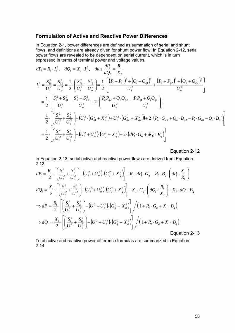
58
Formulation of Active and Reactive Power Differences In Equation 2-1, power differences are defined as summation of serial and shunt flows, and definitions are already given for shunt power flow. In Equation 2-12, serial power flows are revealed to be dependent on serial current, which is in turn expressed in terms of terminal power and voltage values.
( ) ( ) ( ) ( )
( ) ( )( ) ( )
( ) ( ) ( )⎥⎥⎦
⎤
⎢⎢⎣
⎡⋅+⋅⋅−+⋅+−⎟⎟
⎠
⎞⎜⎜⎝
⎛+⋅=
⎥⎥⎦
⎤
⎢⎢⎣
⎡⋅−⋅−⋅+⋅⋅++⋅++⋅+⎟⎟
⎠
⎞⎜⎜⎝
⎛+⋅=
⎥⎥⎦
⎤
⎢⎢⎣
⎡⎟⎟⎠
⎞⎜⎜⎝
⎛ +−
+⋅+
++
+⋅=
⎥⎥⎦
⎤
⎢⎢⎣
⎡ ++++
−+−⋅=⎟⎟
⎠
⎞⎜⎜⎝
⎛+⋅===
=⋅=⋅=
qlqlqqoio
o
i
i
qiqiqoqoqqoqqio
o
i
i
i
qiqi
o
qoqo
o
qo
i
qi
o
qoqo
i
qiqi
o
l
i
l
o
l
i
ll
l
l
l
lllllll
BdQGdPXGUUUS
US
BQGPBQGPXGUXGUUS
US
UQQPP
UQQPP
USS
USS
UQQPP
UQQPP
US
US
US
USI
XR
dQdPthusIXdQIRdP
221
221
221
21
21
,,
22222
2
2
2
112222
22
221
21
22
2
2
2
211
222
2
22
2
2
21
2
2
22
22
2
21
21
2
22
2
21
2
22
2
212
22
Equation 2-12
In Equation 2-13, serial active and reactive power flows are derived from Equation 2-12.
( ) ( )
( ) ( )
( ) ( ) ( )
( ) ( ) ( )qlqlqqoio
o
i
ill
qlqlqqoio
o
i
ill
qlll
llqlqqoi
o
o
i
ill
l
llqlqllqqoi
o
o
i
ill
BXGRXGUUUS
USXdQ
BXGRXGUUUS
USRdP
BdQXXRdQGXXGUU
US
USXdQ
RXdPBRGdPRXGUU
US
USRdP
⋅+⋅+⎥⎦
⎤⎢⎣
⎡+⋅+−⎟⎟
⎠
⎞⎜⎜⎝
⎛+⋅=⇒
⋅+⋅+⎥⎦
⎤⎢⎣
⎡+⋅+−⎟⎟
⎠
⎞⎜⎜⎝
⎛+⋅=⇒
⋅⋅−⎟⎟⎠
⎞⎜⎜⎝
⎛⋅⋅⋅−⎥
⎦
⎤⎢⎣
⎡+⋅+−⎟⎟
⎠
⎞⎜⎜⎝
⎛+⋅=
⎟⎟⎠
⎞⎜⎜⎝
⎛⋅⋅⋅−⋅⋅−⎥
⎦
⎤⎢⎣
⎡+⋅+−⎟⎟
⎠
⎞⎜⎜⎝
⎛+⋅=
12
12
2
2
22222
2
2
2
22222
2
2
2
22222
2
2
2
22222
2
2
2
Equation 2-13 Total active and reactive power difference formulas are summarized in Equation 2-14.

59
( )
( ) ( ) ( ) ( )
( )
( ) ( ) ( ) ( )qlqlqqoio
o
i
iloiq
oiqqlqql
qlqlqqoio
o
i
iloiq
oiqqlqql
BXGRXGUUUS
USXUUB
UUBdQQdQQQdQdQ
BXGRXGUUUS
USRUUG
UUGdPPdPPPdPdP
⋅+⋅+⎥⎦
⎤⎢⎣
⎡+⋅+−⎟⎟
⎠
⎞⎜⎜⎝
⎛+⋅++⋅=
+⋅+=+=++=
⋅+⋅+⎥⎦
⎤⎢⎣
⎡+⋅+−⎟⎟
⎠
⎞⎜⎜⎝
⎛+⋅++⋅=
+⋅+=+=++=
12
12
22222
2
2
222
2221
22222
2
2
222
2221
Equation 2-14

60
Formula Consistency Check for Line-to-Line System It should be noted that all formulations in this chapter so far are based on line-to-neutral system values, thus it is a question whether the voltage magnitude/angle formulas in Equation 2-10 / Equation 2-11 and active/reactive power formulas in Equation 2-14 will need modification when applied to the line-to-line system. Since in balanced three-phase networks line-to-line values are de facto used for load flow calculation, consistency check is performed in this section for all obtained conclusions.
In Equation 2-15, the calculation of voltage magnitude difference is extended to line-to-line system based on Equation 2-10. It can be seen that exactly the same formula can be applied to line-to-line system without any need of modification.
[ ]
[ ]
[ ]qlqlllo
lli
llo
llil
llo
llil
qlqlll
oll
i
llo
llil
llo
llil
qlqlnlo
nli
nlo
nlil
nlo
nlilnlll
BXGRUU
QQXPPR
BXGRUU
QQXPPR
BXGRUU
QQXPPRdUdU
neutraltolineasnllinetolineasll
⋅+⋅+⎥⎦
⎤⎢⎣
⎡
++⋅++⋅
=
⋅+⋅+
⎥⎥⎥⎥
⎦
⎤
⎢⎢⎢⎢
⎣
⎡
⋅+⋅
⋅+⋅⋅+⋅+⋅⋅⋅=
⋅+⋅+⎥⎦
⎤⎢⎣
⎡
++⋅++⋅
⋅=⋅=
−−
−−
−−−−
−−
−−−−
−−
−−−−−−
1)()(
1
31
31
)31
31()
31
31(
3
1)()(33
,
Equation 2-15
In Equation 2-16, the line-to-neutral formula from Equation 2-11 is extended to the line-to-line system, again the same formulation holds true for both cases.
( )
( )
( )qlqlllo
lli
lli
llo
llo
lli
llo
llil
llo
llil
qlqlll
o
lli
lli
llo
llo
lli
llo
llil
llo
llil
qlqlnlo
nli
nli
nlo
nlo
nli
nlo
nlil
nlo
nlilnlll
BRGXUU
UU
UUQQRPPX
BRGXU
U
U
U
UU
QQRPPX
BRGXUU
UU
UUQQRPPXdd
neutraltolineasnllinetolineasll
⋅−⋅⋅⎟⎟⎠
⎞⎜⎜⎝
⎛−⋅+
⋅⋅+⋅−+⋅
=
⋅−⋅⋅
⎟⎟⎟⎟
⎠
⎞
⎜⎜⎜⎜
⎝
⎛
⋅
⋅−
⋅
⋅⋅+
⋅⋅⋅⋅
⋅+⋅⋅−⋅+⋅⋅=
⋅−⋅⋅⎟⎟⎠
⎞⎜⎜⎝
⎛−⋅+
⋅⋅+⋅−+⋅
==
−−
−
−
−
−
−−
−−−−
−
−
−
−
−−
−−−−
−
−
−
−
−−
−−−−−−
21
2)()(
313
1
313
1
21
31
312
)31
31()
31
31(
21
2)()()sin()sin(
,
αα
Equation 2-16
Finally, in Equation 2-17 and Equation 2-18, active power difference and reactive power difference equations are respectively extended to line-to-line case based on Equation 2-14. As can be expected, the same formulas apply nonetheless.
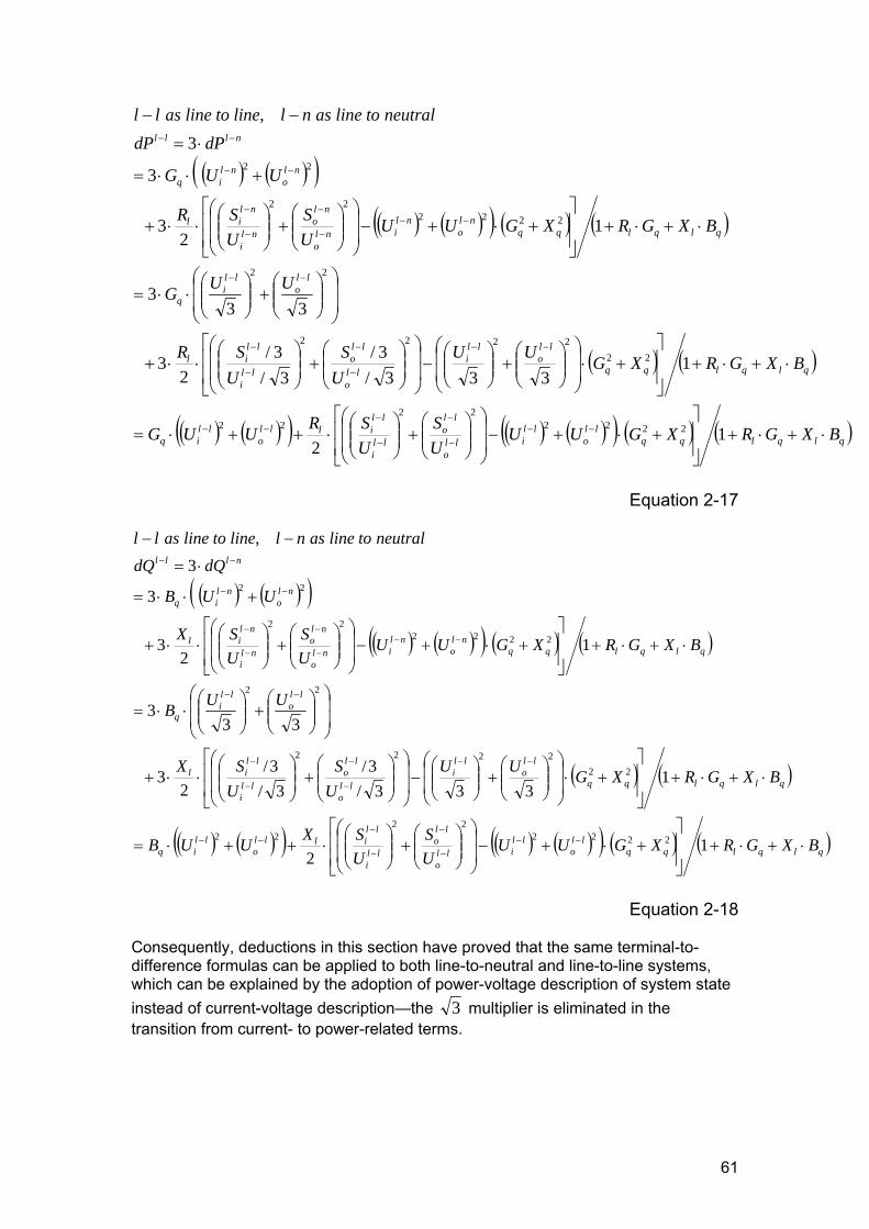
61
( ) ( )( )( ) ( )( ) ( ) ( )
( ) ( )
( ) ( )( ) ( ) ( )( ) ( ) ( )qlqlqqll
oll
illo
llo
lli
llilll
oll
iq
qlqlqq
llo
lli
llo
llo
lli
llil
llo
lli
q
qlqlqqnl
onl
inlo
nlo
nli
nlil
nlo
nliq
nlll
BXGRXGUUUS
USRUUG
BXGRXGUUU
SU
SR
UUG
BXGRXGUUUS
USR
UUG
dPdPneutraltolineasnllinetolineasll
⋅+⋅+⎥⎥
⎦
⎤
⎢⎢
⎣
⎡+⋅+−⎟
⎟
⎠
⎞
⎜⎜
⎝
⎛⎟⎟⎠
⎞⎜⎜⎝
⎛+⎟⎟
⎠
⎞⎜⎜⎝
⎛⋅++⋅=
⋅+⋅+⎥⎥
⎦
⎤
⎢⎢
⎣
⎡+⋅
⎟⎟
⎠
⎞
⎜⎜
⎝
⎛⎟⎟⎠
⎞⎜⎜⎝
⎛+⎟⎟
⎠
⎞⎜⎜⎝
⎛−⎟
⎟
⎠
⎞
⎜⎜
⎝
⎛⎟⎟⎠
⎞⎜⎜⎝
⎛+⎟⎟
⎠
⎞⎜⎜⎝
⎛⋅⋅+
⎟⎟
⎠
⎞
⎜⎜
⎝
⎛⎟⎟⎠
⎞⎜⎜⎝
⎛+⎟⎟
⎠
⎞⎜⎜⎝
⎛⋅⋅=
⋅+⋅+⎥⎥
⎦
⎤
⎢⎢
⎣
⎡+⋅+−⎟
⎟
⎠
⎞
⎜⎜
⎝
⎛⎟⎟⎠
⎞⎜⎜⎝
⎛+⎟⎟
⎠
⎞⎜⎜⎝
⎛⋅⋅+
+⋅⋅=
⋅=
−−
−−−
−
−
−−−
−−
−
−
−
−
−−
−−−
−
−
−
−−
−−
12
1333/
3/3/
3/2
3
333
12
3
3
3,
222222
22
222222
22
222222
22
Equation 2-17
( ) ( )( )( ) ( )( ) ( ) ( )
( ) ( )
( ) ( )( ) ( ) ( )( ) ( ) ( )qlqlqqll
oll
illo
llo
lli
llilll
oll
iq
qlqlqq
llo
lli
llo
llo
lli
llil
llo
lli
q
qlqlqqnl
onl
inlo
nlo
nli
nlil
nlo
nliq
nlll
BXGRXGUUUS
USXUUB
BXGRXGUUU
SU
SX
UUB
BXGRXGUUUS
USX
UUB
dQdQneutraltolineasnllinetolineasll
⋅+⋅+⎥⎥
⎦
⎤
⎢⎢
⎣
⎡+⋅+−⎟
⎟
⎠
⎞
⎜⎜
⎝
⎛⎟⎟⎠
⎞⎜⎜⎝
⎛+⎟⎟
⎠
⎞⎜⎜⎝
⎛⋅++⋅=
⋅+⋅+⎥⎥
⎦
⎤
⎢⎢
⎣
⎡+⋅
⎟⎟
⎠
⎞
⎜⎜
⎝
⎛⎟⎟⎠
⎞⎜⎜⎝
⎛+⎟⎟
⎠
⎞⎜⎜⎝
⎛−⎟
⎟
⎠
⎞
⎜⎜
⎝
⎛⎟⎟⎠
⎞⎜⎜⎝
⎛+⎟⎟
⎠
⎞⎜⎜⎝
⎛⋅⋅+
⎟⎟
⎠
⎞
⎜⎜
⎝
⎛⎟⎟⎠
⎞⎜⎜⎝
⎛+⎟⎟
⎠
⎞⎜⎜⎝
⎛⋅⋅=
⋅+⋅+⎥⎥
⎦
⎤
⎢⎢
⎣
⎡+⋅+−⎟
⎟
⎠
⎞
⎜⎜
⎝
⎛⎟⎟⎠
⎞⎜⎜⎝
⎛+⎟⎟
⎠
⎞⎜⎜⎝
⎛⋅⋅+
+⋅⋅=
⋅=
−−
−−−
−
−
−−−
−−
−
−
−
−
−−
−−−
−
−
−
−−
−−
12
1333/
3/3/
3/2
3
333
12
3
3
3,
222222
22
222222
22
222222
22
Equation 2-18
Consequently, deductions in this section have proved that the same terminal-to-difference formulas can be applied to both line-to-neutral and line-to-line systems, which can be explained by the adoption of power-voltage description of system state instead of current-voltage description—the 3 multiplier is eliminated in the transition from current- to power-related terms.

62
Summary of All Terminal-to-Difference Formulas Now that four terminal-to-difference formulas have been respectively obtained for dU, dα, dP and dQ and examined in section Chapter 0 for their applicability to line-to-line system, they are confirmed to be readily usable for an iterative solution of the load flow problem. In Equation 2-19, these four formulas are summarized and expressed in a simple vector form indicating input (terminal) and output (difference) variables.
[ ]
( )
( ) ( ) ( ) ( )
( ) ( ) ( ) ( )
[ ] [ ],,,:
,,,,,,,,
12
12
21
2)()(
sin
1)()(
22222
22
2
2222
22222
22
2
2222
1
dQQQdPPPdUUUAndQQPPUUfdQdPddU
BXGRXGUUU
QPU
QPXUUBdQ
BXGRXGUUU
QPU
QPRUUGdP
BRGXUU
UU
UUQQRPPX
d
BXGRUU
QQXPPRdU
ioioio
oioioi
qlqlqqoio
oo
i
iiloiq
qlqlqqoio
oo
i
iiloiq
qlqlo
i
i
o
oi
oiloil
qlqloi
oiloil
−=−=−==⇒
⋅+⋅+⎥⎥⎦
⎤
⎢⎢⎣
⎡+⋅+−⎟⎟
⎠
⎞⎜⎜⎝
⎛ ++
+⋅++⋅=
⋅+⋅+⎥⎥⎦
⎤
⎢⎢⎣
⎡+⋅+−⎟⎟
⎠
⎞⎜⎜⎝
⎛ ++
+⋅++⋅=
⎥⎦
⎤⎢⎣
⎡⋅−⋅⋅⎟⎟
⎠
⎞⎜⎜⎝
⎛−⋅+
⋅⋅+⋅−+⋅
=
⋅+⋅+⎥⎦
⎤⎢⎣
⎡+
+⋅++⋅=
−
rα
α
Equation 2-19 The vector formula in Equation 2-19 clearly indicates that terminal voltage and terminal active and reactive power values can be used to deduce differences in voltage and active/reactive power across a line or transformer. And conversely, when variables at incoming side of the line/transformer are known, the out-going variables can be updated with the knowledge of difference values. Thus these two procedures can be combined into a loop to solve the load flow problem with single line / transformer configuration (2-node problem). However, in a more complicated network Equation 2-19 has to be used in combination with topology information, which will be detailed in section Chapter 0.
In the simple case of zero shunt power flow, terminal-to-difference formulas in Equation 2-19 can be simplified, as shown by Equation 2-20. It should be noted that Equation 2-20 can also be applied to series capacitors or inductors.
⎟⎟⎠
⎞⎜⎜⎝
⎛ ++
+⋅=⎟⎟
⎠
⎞⎜⎜⎝
⎛ ++
+⋅=
⎥⎦
⎤⎢⎣
⎡⋅⋅
+⋅−+⋅=
++⋅++⋅
=
==
−
2
22
2
22
2
22
2
22
1
2,
2
2)()(sin,)()(
:0,0
o
oo
i
iil
o
oo
i
iil
oi
oiloil
oi
oiloil
UQP
UQPXdQ
UQP
UQPRdP
UUQQRPPXd
UUQQXPPRdU
BGWhen
α
Equation 2-20
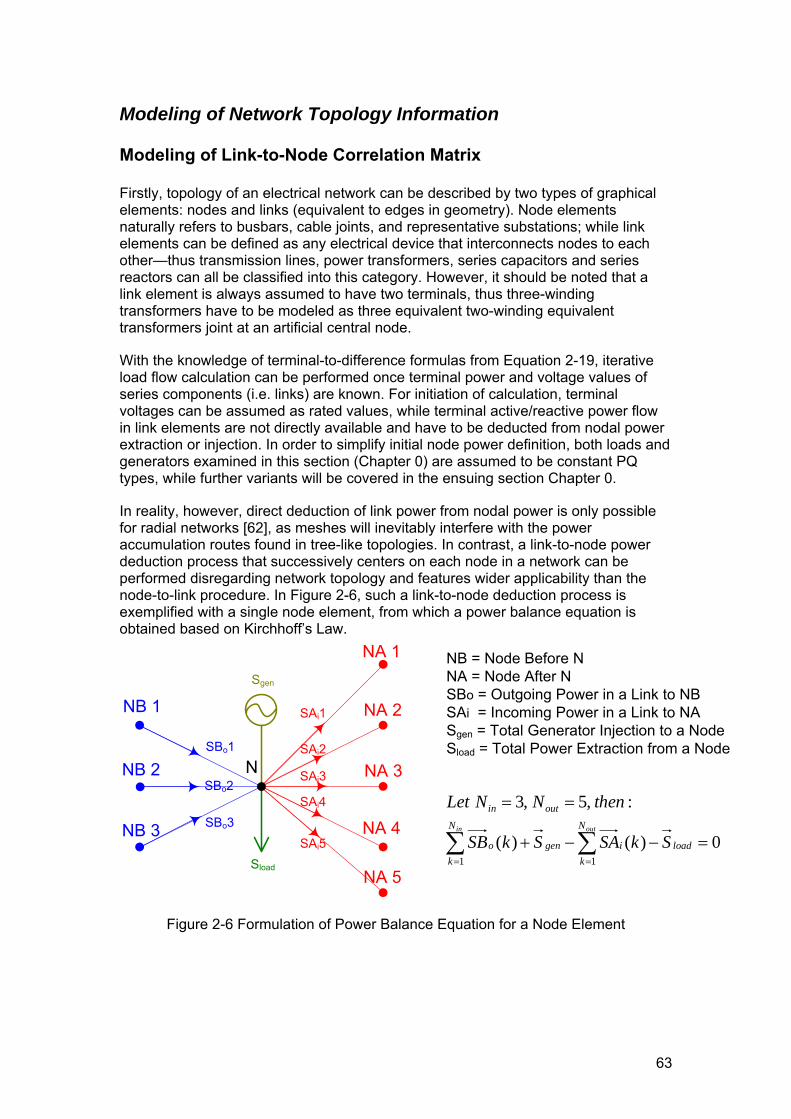
63
Modeling of Network Topology Information
Modeling of Link-to-Node Correlation Matrix
Firstly, topology of an electrical network can be described by two types of graphical elements: nodes and links (equivalent to edges in geometry). Node elements naturally refers to busbars, cable joints, and representative substations; while link elements can be defined as any electrical device that interconnects nodes to each other—thus transmission lines, power transformers, series capacitors and series reactors can all be classified into this category. However, it should be noted that a link element is always assumed to have two terminals, thus three-winding transformers have to be modeled as three equivalent two-winding equivalent transformers joint at an artificial central node.
With the knowledge of terminal-to-difference formulas from Equation 2-19, iterative load flow calculation can be performed once terminal power and voltage values of series components (i.e. links) are known. For initiation of calculation, terminal voltages can be assumed as rated values, while terminal active/reactive power flow in link elements are not directly available and have to be deducted from nodal power extraction or injection. In order to simplify initial node power definition, both loads and generators examined in this section (Chapter 0) are assumed to be constant PQ types, while further variants will be covered in the ensuing section Chapter 0.
In reality, however, direct deduction of link power from nodal power is only possible for radial networks [62], as meshes will inevitably interfere with the power accumulation routes found in tree-like topologies. In contrast, a link-to-node power deduction process that successively centers on each node in a network can be performed disregarding network topology and features wider applicability than the node-to-link procedure. In Figure 2-6, such a link-to-node deduction process is exemplified with a single node element, from which a power balance equation is obtained based on Kirchhoff’s Law.
NB = Node Before NNA = Node After NSBo = Outgoing Power in a Link to NBSAi = Incoming Power in a Link to NASgen = Total Generator Injection to a NodeSload = Total Power Extraction from a Node
0)()(
:,5,3
11=−−+
==
∑∑==
load
N
kigen
N
ko
outin
SkSASkSB
thenNNLetoutin
N
NB 1
NB 2
NB 3
NA 1
NA 2
NA 3
NA 4
NA 5
SBo1
SBo2
SBo3
SAi1
SAi2
SAi3
SAi4
SAi5
Sgen
Sload
Figure 2-6 Formulation of Power Balance Equation for a Node Element

64
Observation of the power balance equation in Figure 2-6 reveals that output power flows are taken from incoming links, while input power flows are used for outgoing links. When a number of nodes are considered as a whole, usage of both input and output power flows in one link will cause unnecessary confusion and non-uniform definition of ‘link power’. Therefore, in Equation 2-21 the nodal power balance equation is modified to contain only input power flow or only output power flow for a specific link. In practice both formulations will lead to the same calculation result, thus the input power flow denotation will be used hereafter to specifically represent ‘link’ power flow.
[ ][ ] ⎪
⎪⎩
⎪⎪⎨
⎧
−+=−
−+=−⇒
⎪⎪⎩
⎪⎪⎨
⎧
=−+−+
=−−+−
⇒=−−+
∑∑∑
∑∑∑
∑∑
∑∑
∑∑
===
===
==
==
==
genload
N
k
N
ko
N
ko
genload
N
k
N
ki
N
ki
load
N
kogen
N
ko
load
N
kigen
N
ki
load
N
kigen
N
ko
SSkdSAkSAkSB
SSkdSBkSAkSB
SkdSAkSASkSB
SkSASkdSBkSB
SkSASkSB
outoutin
outoutin
inin
outin
outin
111
111
11
11
11
)()()(
)()()(
0)()()(
0)()()(
0)()(
Equation 2-21
Now Equation 2-21 has provided a basic template for link-to-node deduction: on the left side of balance equation incoming link powers are multiplied by +1 while outgoing link powers are multiplier by -1, and on the right side of the equation net nodal power extraction (load minus generation) is added on top of power losses in incoming links (using input power flow denotation). In order to explore applications of these rules to more general conditions, a radial test network is given in Figure 2-7 as an example.
Figure 2-7 Sample Radial Network with Node-Link Labeling When compared to Figure 2-6, Figure 2-7 has obviously omitted all nodal elements such as loads and generators to simplify layout. However, power flow direction as a crucial graphical property is also missing in Figure 2-7. By assuming slack to be the only power source, link directions can be easily obtained for the radial grid, as shown by Figure 2-8.
Figure 2-8 Sample Radial Network with Flow Direction Labeling A simple count of node elements and link elements in Figure 2-8 points both numbers to 8. Apparent this contradicts with the graphical property of radial grids—node number should always be equal to one plus link number. However, further examination of link L1 reveals it to be an artificial line that only has an ending node (N1), which explains why node count is equal to link count. This extra line is

65
purposefully added so as to obtain slack injection together with other link power results. Obviously, this artificial line is assumed to be ideal and thus incurs no power losses at all. By applying the link-to-node deduction process from Figure 2-6 to all graphical elements in Figure 2-8, a summarized link-to-node correlation matrix (T) can be defined as shown by Equation 2-22. Apparently for radial grids, introduction of artificial slack link brings node count and link count equal, thus the link-to-node correlation matrix (T) becomes a non-singular square matrix. Consequently, the link power vector SL can be obtained from the product of inversed T and the node power vector SN—it should be noted, however, that the equation can also be solved without inverting T, as standard linear solver (e.g. LU decomposition) can be directly applied with a higher computational efficiency. The advantage of obtaining explicit inverse of T, however, lies in the fact that the inversion process only need to be executed once in iterative load flow solution process, as no elements in T will be updated throughout the iterations.
NNNN
NlkNlkNndNnd
i
i
i
i
i
i
i
i
genload
genload
genload
genload
genload
genload
genload
genload
SNTSLNNlkNndWhen
SLTSNThenNlkNndLet
dS
SLSLSLSLSLSLSLSL
SSdSSSdSSSdSSSdSSSdSSSdSSSdS
SS
SNSNSNSNSNSNSNSN
⋅=⇒==
⋅===
=
⎥⎥⎥⎥⎥⎥⎥⎥⎥⎥⎥
⎦
⎤
⎢⎢⎢⎢⎢⎢⎢⎢⎢⎢⎢
⎣
⎡
⋅
⎥⎥⎥⎥⎥⎥⎥⎥⎥⎥⎥
⎦
⎤
⎢⎢⎢⎢⎢⎢⎢⎢⎢⎢⎢
⎣
⎡
−−
−−
−−−
=
⎥⎥⎥⎥⎥⎥⎥⎥⎥⎥⎥
⎦
⎤
⎢⎢⎢⎢⎢⎢⎢⎢⎢⎢⎢
⎣
⎡
−+−+−+−+−+−+−+−+
=
⎥⎥⎥⎥⎥⎥⎥⎥⎥⎥⎥
⎦
⎤
⎢⎢⎢⎢⎢⎢⎢⎢⎢⎢⎢
⎣
⎡
×−
×
1
1*
8
7
6
5
4
3
2
1
888
777
666
555
444
333
222
11*
8
7
6
5
4
3
2
1
:
:8,8
0
100000000100000010100000
01010000001010000001010000001110000000110
Equation 2-22
One noticeable feature of link-to-node correlation matrix (T) is that it can be applied to both complex apparent powers as a whole and real-number active / reactive powers separately. In Equation 2-23, this property is utilized to create combined power vectors on node (xN) and link (xL) levels, while an evolution matrix M is defined in the process. For radial networks, using M instead of T is not meaningful due to a doubled matrix dimension—however, for meshed grids the introduction of M will become indispensible.
NNNN
NlkNlkNndNnd
Nlk
Nlk
NlkNndNlkNnd
NlkNndNlkNnd
Nnd
Nnd
xNMxLNNlkNndWhen
xLMxNQLPL
TT
QNPN
2221
2
2222
:
00
⋅===
⋅=⇔⎥⎥⎦
⎤
⎢⎢⎣
⎡⋅
⎥⎥⎦
⎤
⎢⎢⎣
⎡=
⎥⎥⎦
⎤
⎢⎢⎣
⎡
×−
×
××
××
Equation 2-23
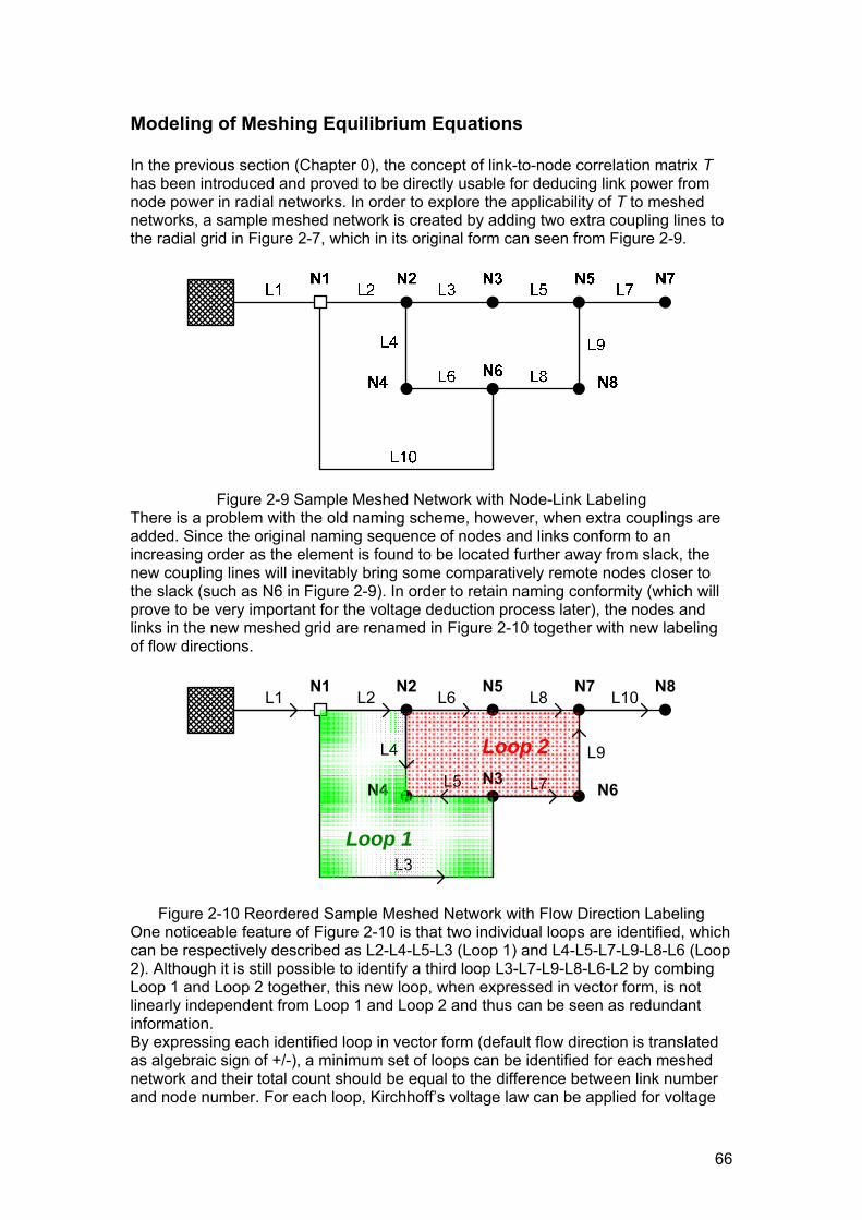
66
Modeling of Meshing Equilibrium Equations
In the previous section (Chapter 0), the concept of link-to-node correlation matrix T has been introduced and proved to be directly usable for deducing link power from node power in radial networks. In order to explore the applicability of T to meshed networks, a sample meshed network is created by adding two extra coupling lines to the radial grid in Figure 2-7, which in its original form can seen from Figure 2-9.
Figure 2-9 Sample Meshed Network with Node-Link Labeling There is a problem with the old naming scheme, however, when extra couplings are added. Since the original naming sequence of nodes and links conform to an increasing order as the element is found to be located further away from slack, the new coupling lines will inevitably bring some comparatively remote nodes closer to the slack (such as N6 in Figure 2-9). In order to retain naming conformity (which will prove to be very important for the voltage deduction process later), the nodes and links in the new meshed grid are renamed in Figure 2-10 together with new labeling of flow directions.
L1 L2 L6 L8 L10
L5 L7
N1 N2
N4
N5
N3
L4
N6
N7 N8
L9
L3Loop 1
Loop 2
Figure 2-10 Reordered Sample Meshed Network with Flow Direction Labeling One noticeable feature of Figure 2-10 is that two individual loops are identified, which can be respectively described as L2-L4-L5-L3 (Loop 1) and L4-L5-L7-L9-L8-L6 (Loop 2). Although it is still possible to identify a third loop L3-L7-L9-L8-L6-L2 by combing Loop 1 and Loop 2 together, this new loop, when expressed in vector form, is not linearly independent from Loop 1 and Loop 2 and thus can be seen as redundant information. By expressing each identified loop in vector form (default flow direction is translated as algebraic sign of +/-), a minimum set of loops can be identified for each meshed network and their total count should be equal to the difference between link number and node number. For each loop, Kirchhoff’s voltage law can be applied for voltage

67
magnitude and voltage angle, which is described by Equation 2-24. A loop index matrix (L) is defined in this process, which is the summary of all eigenvectors from the minimum loop set.
[ ][ ]
[ ]NmhNlkNlkNmhNmhNlkNlkNmh
T
T
dLdULasWrite
ddU
thenddddddddddd
dUdUdUdUdUdUdUdUdUdUdUNote
dddddddUdUdUdUdUdU
dddddUdUdUdU
NndNlkNmhcountloopdefineNlkNndDenote
0,0:
0000
01111110000000011110
:,,,,,,,,,,
,,,,,,,,,
00
00
2,10,8
10987654321
10987654321
689754
689754
4253
4253
=⋅=⋅
⎥⎦
⎤⎢⎣
⎡=⋅⎥
⎦
⎤⎢⎣
⎡−−−
−−⇒
⎪⎩
⎪⎨⎧
=
=
⎩⎨⎧
=−−++−=−−++−
⎩⎨⎧
=−−+=−−+
=−===
×× α
α
ααααααααααα
αααααααααα
Equation 2-24 By applying the conclusions of Equation 2-19 to Equation 2-24, a total of 2·Nmh (Nmh as number of loops) meshing equilibrium equations can be obtained in Equation 2-25. It can be seen that linearization of voltage angle difference (dα) equation will inevitably induce error from the inversed sine function, which, however, can be iteratively mitigated by approximating the error item (Edα) from previously calculated dα results.
( ) ( ) ( )
[ ][ ] [ ] [ ]
( )
( ) ( )[ ][ ]
[ ] [ ] [ ][ ] [ ] [ ]
equationsmequilibriumeshingasxLLSLKWrite
xLCLCL
xLCULCUL
CxLCL
CUxLCUL
CxLCddCxLCECxLCd
theniterationpreviousfromresultdcalculatedasdAssume
CxLCdCUxLCUdUThen
CCCCUCUCUQPxLWrite
CQCPC
UUdQRdPX
UU
UUQ
UURP
UUXd
CUQCUPCUUU
dQXdPRQUU
XPUU
RdU
BRGXBXGRWrite
NlkNlkNmhNmh
NlkNlkNmhSNmhkM
NlkNlkNmhSNmhK
KMS
KS
KMSprvprvKSdKS
prv
KSKS
T
QPSQPS
T
ii
KiQiP
oi
ll
o
i
i
oi
oi
li
oi
l
KiQiP
Uoi
lli
Uoi
li
Uoi
l
qlqlqlqlU
2222
22
22
1
1
1
0
0
sin
:,
sin,:
,,:
sin
221sin
22,1
⋅=⇒
⎪⎩
⎪⎨⎧
⋅⋅=⋅
⋅⋅=⋅⇒
⎪⎩
⎪⎨⎧
=−⋅⋅
=−⋅⋅⇒
−⋅=−+−⋅≅+−⋅=
−⋅=−⋅=
===
−⋅+⋅=
⎥⎥⎦
⎤
⎢⎢⎣
⎡⎟⎟⎠
⎞⎜⎜⎝
⎛
⋅⋅⋅−⋅
−⋅⎟⎟⎠
⎞⎜⎜⎝
⎛−⋅+⋅
⋅−⋅
⋅=
−⋅+⋅=⋅+⋅+⋅
−⋅⋅+
⋅+⋅
⋅+⋅
=
⋅−⋅=⋅+⋅+=
×
×
×
−
−
−
αααα
ααααααααα
αα
ααα
ααα
ααα
μα
μμμ
μμ
α
α
α
Equation 2-25

68
In the mean time, the addition of two extra coupling lines in Figure 2-10 changes the original balance between link count and node count suggested by Equation 2-22. In Equation 2-26, the link-to-node correlation matrix T is redefined for the meshed network and it can be obviously seen that T is no longer a square matrix and cannot be directly used for deducing link power from node power. In order to transfer the complex expression of apparent power into separate real terms of active and reactive power, a decoupled correlation matrix TD is derived from T in Equation 2-26.
NlkNlkNndNnd
Nlk
NlkNlk
Nnd
NndNnd
NlkNndNlkNnd
NlkNndNlkNndNlkNnd
NlkNlkNndNnd
i
i
i
i
i
i
i
i
i
i
xLTDxNThen
QLPLxL
QNPNxN
TTTDLet
SLTSNThenNlkNndLet
SLSLSLSLSLSLSLSLSLSL
SNSNSNSNSNSNSNSN
2222
2222
10
9
8
7
6
5
4
3
2
1
8
7
6
5
4
3
2
1
:
,,,0
0
:10,8
10000000001110000000
010100000000101000000000011000000101010000001010100000000111
⋅=
⎥⎥⎦
⎤
⎢⎢⎣
⎡=
⎥⎥⎦
⎤
⎢⎢⎣
⎡=
⎥⎥⎦
⎤
⎢⎢⎣
⎡=
⋅===
⎥⎥⎥⎥⎥⎥⎥⎥⎥⎥⎥⎥⎥⎥
⎦
⎤
⎢⎢⎢⎢⎢⎢⎢⎢⎢⎢⎢⎢⎢⎢
⎣
⎡
⋅
⎥⎥⎥⎥⎥⎥⎥⎥⎥⎥⎥
⎦
⎤
⎢⎢⎢⎢⎢⎢⎢⎢⎢⎢⎢
⎣
⎡
−−
−
−−−−
−−
=
⎥⎥⎥⎥⎥⎥⎥⎥⎥⎥⎥
⎦
⎤
⎢⎢⎢⎢⎢⎢⎢⎢⎢⎢⎢
⎣
⎡
×
××
×××
×
Equation 2-26
Now that Equation 2-25 and Equation 2-26 respectively represents 2·Nmh and 2·Nnd equilibrium conditions, a total of 2·Nlk (as total link count equals total node count plus total loop count) linear equations can be obtained for corresponding 2·Nlk unknown variables (considering both active and reactive powers separately). Consequently the link power flows are again solvable as a standard real-number linear space problem, as can be seen from Equation 2-27. Obviously, the evolution matrix M is redefined with additional meshing information in comparison with Equation 2-27.
[ ]
NlkNlkNlkNlkNlkNlkNlkNlk
Nlk
NlkNlkNlkNmh
NlkNnd
NlkNmh
Nnd
NlkNlkNmhNmh
NlkNlkNndNnd
yLMxLThenxLMyLWrite
xLLSTD
LKxN
xLLSLK
xLTDxNSince
NmhNndNlkthatknownisIt
2221
22222
2
2222
22
22
2
2222
2222
:
:
⋅=⇒⋅=
⋅⎥⎥⎦
⎤
⎢⎢⎣
⎡=
⎥⎥⎦
⎤
⎢⎢⎣
⎡⇒
⎪⎩
⎪⎨⎧
⋅=
⋅=
+=
×−
×
××
×
×
×
Equation 2-27
Additionally, it should be noted that parallel lines and transformers can be either combined into one equivalent element or modeled as small loops each consisting of two elements only.
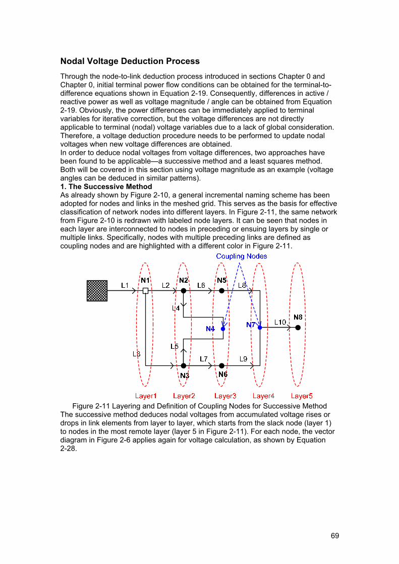
69
Nodal Voltage Deduction Process Through the node-to-link deduction process introduced in sections Chapter 0 and Chapter 0, initial terminal power flow conditions can be obtained for the terminal-to-difference equations shown in Equation 2-19. Consequently, differences in active / reactive power as well as voltage magnitude / angle can be obtained from Equation 2-19. Obviously, the power differences can be immediately applied to terminal variables for iterative correction, but the voltage differences are not directly applicable to terminal (nodal) voltage variables due to a lack of global consideration. Therefore, a voltage deduction procedure needs to be performed to update nodal voltages when new voltage differences are obtained. In order to deduce nodal voltages from voltage differences, two approaches have been found to be applicable—a successive method and a least squares method. Both will be covered in this section using voltage magnitude as an example (voltage angles can be deduced in similar patterns). 1. The Successive Method As already shown by Figure 2-10, a general incremental naming scheme has been adopted for nodes and links in the meshed grid. This serves as the basis for effective classification of network nodes into different layers. In Figure 2-11, the same network from Figure 2-10 is redrawn with labeled node layers. It can be seen that nodes in each layer are interconnected to nodes in preceding or ensuing layers by single or multiple links. Specifically, nodes with multiple preceding links are defined as coupling nodes and are highlighted with a different color in Figure 2-11.
Figure 2-11 Layering and Definition of Coupling Nodes for Successive Method
The successive method deduces nodal voltages from accumulated voltage rises or drops in link elements from layer to layer, which starts from the slack node (layer 1) to nodes in the most remote layer (layer 5 in Figure 2-11). For each node, the vector diagram in Figure 2-6 applies again for voltage calculation, as shown by Equation 2-28.

70
[ ]
.)()(*
)()()(,1)()(
,,,
*1
linkprecedingonehasjNAnodewhenonlyapplicabledirectlyisjUcalculatedThe
jdUjUjUNjAndN
idUiUU
afternodeasNAbeforenodeasNBcountlinkensuingasNcountlinkprecedingasN
NA
NANNAoutin
N
iNBNB
N
outin
in
−==∀−
=∑= L
Equation 2-28
Special care is required for coupling nodes, for which nodal voltage is taken as the average of deduced end-terminal voltages from multiple preceding links. The majority of nodes, however, only has one preceding link in Figure 2-11, thus their voltages can be arbitrarily determined from such single sources. 2. The Least Squares Method In comparison with the idea of deducing nodal voltages from link voltage differences, an operation in the reversed direction is much easier to implement: in Equation 2-29, a node-to-difference voltage deduction matrix VD is defined for the meshed grid shown by Figure 2-10 and Figure 2-11. Voltage terms of slack node and artificial slack link are taken out from the equations, which leaves VD size to be Nlk-1 by Nnd-1.
[ ] [ ])1()1()1()1()1(
2)1(2)1(
11
1
1
)1(
8
7
6
5
4
3
2
1
10
9
8
7
6
5
4
3
2
1
,
:0,,10,8
0000000
11000000011000000101000000100100000100100000110000001010000001010000001100000000
−−−×−−
−−
−
+⋅=⇒
==
≡===
⎥⎥⎥⎥⎥⎥⎥⎥⎥⎥⎥⎥
⎦
⎤
⎢⎢⎢⎢⎢⎢⎢⎢⎢⎢⎢⎢
⎣
⎡
=⇒
⎥⎥⎥⎥⎥⎥⎥⎥⎥⎥⎥
⎦
⎤
⎢⎢⎢⎢⎢⎢⎢⎢⎢⎢⎢
⎣
⎡
⋅
⎥⎥⎥⎥⎥⎥⎥⎥⎥⎥⎥⎥⎥⎥
⎦
⎤
⎢⎢⎢⎢⎢⎢⎢⎢⎢⎢⎢⎢⎢⎢
⎣
⎡
−−−
−−
−−
−−
=
⎥⎥⎥⎥⎥⎥⎥⎥⎥⎥⎥⎥⎥⎥
⎦
⎤
⎢⎢⎢⎢⎢⎢⎢⎢⎢⎢⎢⎢⎢⎢
⎣
⎡
NlkNndNndNlkNlk
TNndNnd
TNlkNlk
Nlk
KUUNVDdU
UNUNUNdUdUdUWrite
dUConstUNSinceNlkNndLet
UNUN
KUDefine
UNUNUNUNUNUNUNUN
dUdUdUdUdUdUdUdUdUdU
LL
Equation 2-29 For radial grids, VD is a non-singular square matrix that can be directly inversed to obtain nodal voltages from link voltage difference values. For meshed grids, however, the matrix contains redundant information so that no unique solution exists for the linear system. Use of least squares method, however, could theoretically lead to minimum deduction error in general, as shown by Equation 2-30.
[ ][ ] [ ])1()1()1()1(
1)1()1()1()1()1(
)1()1()1()1(1
)1(
−−−×−
−
−×−−×−−
−−−×−−
−
−⋅⋅⋅=⇒>
−⋅=⇒=
NlkNlkNlkNndT
NndNlkNlkNndT
Nnd
NlkNlkNlkNndNnd
KUdUVDVDVDUNNndNlkWhen
KUdUVDUNNndNlkWhen
Equation 2-30

71
Now that working principles of both successive and least squares methods are given, a general performance comparison can be drawn between them using the meshed grid in Figure 2-11 as an example. Firstly, by summarizing individual nodal analysis steps from the successive method into one collective difference-to-link voltage deduction matrix, Equation 2-31 can be obtained to describe the eventual correlation between nodal voltages and voltage differences. Obviously, all elements in the matrix are negative, which means the flow directions depicted by arrows in Figure 2-11 are always kept under the successive method. In addition, nodes that are neither coupling nodes nor nodes located after coupling nodes can always be expressed by simple summation of voltage differences in preceding links (row elements to be either -1 or 0), while the other nodes feature more diverse values for corresponding row elements (such as -0.5).
⎟⎟⎟⎟⎟⎟⎟⎟⎟⎟⎟⎟⎟
⎠
⎞
⎜⎜⎜⎜⎜⎜⎜⎜⎜⎜⎜⎜⎜
⎝
⎛
⎥⎥⎥⎥⎥⎥⎥⎥⎥⎥⎥⎥
⎦
⎤
⎢⎢⎢⎢⎢⎢⎢⎢⎢⎢⎢⎢
⎣
⎡
−
⎥⎥⎥⎥⎥⎥⎥⎥⎥⎥⎥⎥
⎦
⎤
⎢⎢⎢⎢⎢⎢⎢⎢⎢⎢⎢⎢
⎣
⎡
⋅
⎥⎥⎥⎥⎥⎥⎥⎥⎥
⎦
⎤
⎢⎢⎢⎢⎢⎢⎢⎢⎢
⎣
⎡
−−−−−−−−−−−−−
−−−−
−−−−−
−
=
⎥⎥⎥⎥⎥⎥⎥⎥⎥
⎦
⎤
⎢⎢⎢⎢⎢⎢⎢⎢⎢
⎣
⎡
0000000
15.05.05.05.0005.05.005.05.05.05.0005.05.0000100010000010001000005.05.05.05.0000000010000000001 1
1
10
9
8
7
6
5
4
3
2
8
7
6
5
4
3
2 UNUN
dUdUdUdUdUdUdUdUdU
UNUNUNUNUNUNUN
Equation 2-31
A similar matrix is obtained in Equation 2-32 for the least squares method by simply applying VD definition from Equation 2-29 to Equation 2-30. Comparison of this new matrix to the one obtained in Equation 2-31 shows that not all elements in the new matrix are negative (which means reversed flows are considered), and more non-zero row elements are defined for nodes that are neither coupling nodes nor nodes located after coupling nodes. Although potentially capable of accelerating convergence speed, the least squares method is undoubtedly more computationally demanding than the successive method considering the additional efforts needed for matrix inversion.
⎟⎟⎟⎟⎟⎟⎟⎟⎟⎟⎟⎟⎟
⎠
⎞
⎜⎜⎜⎜⎜⎜⎜⎜⎜⎜⎜⎜⎜
⎝
⎛
⎥⎥⎥⎥⎥⎥⎥⎥⎥⎥⎥⎥
⎦
⎤
⎢⎢⎢⎢⎢⎢⎢⎢⎢⎢⎢⎢
⎣
⎡
−
⎥⎥⎥⎥⎥⎥⎥⎥⎥⎥⎥⎥
⎦
⎤
⎢⎢⎢⎢⎢⎢⎢⎢⎢⎢⎢⎢
⎣
⎡
⋅
⎥⎥⎥⎥⎥⎥⎥⎥⎥
⎦
⎤
⎢⎢⎢⎢⎢⎢⎢⎢⎢
⎣
⎡
−−−−−−−−−−−−−
−−−−−−−−−−−−
−−−−−−−−−
−−−−−
=
⎥⎥⎥⎥⎥⎥⎥⎥⎥
⎦
⎤
⎢⎢⎢⎢⎢⎢⎢⎢⎢
⎣
⎡
0000000
15.05.05.05.0005.05.005.05.05.05.0005.05.003.03.07.03.01.01.06.04.003.03.03.07.01.01.04.06.0000005.05.05.05.001.01.01.01.02.02.07.03.001.01.01.01.02.02.03.07.0 1
1
10
9
8
7
6
5
4
3
2
8
7
6
5
4
3
2 UNUN
dUdUdUdUdUdUdUdUdU
UNUNUNUNUNUNUN
Equation 2-32
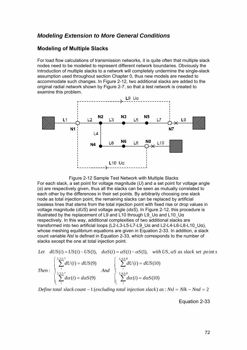
72
Modeling Extension to More General Conditions
Modeling of Multiple Slacks
For load flow calculations of transmission networks, it is quite often that multiple slack nodes need to be modeled to represent different network boundaries. Obviously the introduction of multiple slacks to a network will completely undermine the single-slack assumption used throughout section Chapter 0, thus new models are needed to accommodate such changes. In Figure 2-12, two additional slacks are added to the original radial network shown by Figure 2-7, so that a test network is created to examine this problem.
Figure 2-12 Sample Test Network with Multiple Slacks For each slack, a set point for voltage magnitude (U) and a set point for voltage angle (α) are respectively given, thus all the slacks can be seen as mutually correlated to each other by the differences in their set points. By arbitrarily choosing one slack node as total injection point, the remaining slacks can be replaced by artificial lossless lines that stems from the total injection point with fixed rise or drop values in voltage magnitude (dUS) and voltage angle (dαS). In Figure 2-12, this procedure is illustrated by the replacement of L9 and L10 through L9_Uα and L10_Uα respectively. In this way, additional complexities of two additional slacks are transformed into two artificial loops (L2-L3-L5-L7-L9_Uα and L2-L4-L6-L8-L10_Uα), whose meshing equilibrium equations are given in Equation 2-33. In addition, a slack count variable Nsl is defined in Equation 2-33, which corresponds to the number of slacks except the one at total injection point.
2:)(1
)10()(
)10()(
)9()(
)9()(:
int,),1()()(),1()()(
8,6,4,2
8,6,4,2
7,5,3,2
7,5,3,2
=−=−
⎪⎪⎩
⎪⎪⎨
⎧
=
=
⎪⎪⎩
⎪⎪⎨
⎧
=
=
−=−=
∑
∑
∑
∑
NndNlkNslasslackinjectiontotalexcludingcountslacktotalDefine
Sdid
dUSidUAnd
Sdid
dUSidUThen
sposetslackasSUSwithSiSiSdUSiUSidUSLet
i
i
i
i
αααα
αααα
Equation 2-33

73
Since the voltage equilibrium equations in Equation 2-33 are similar to the ones used for normal loops in Equation 2-25 except for the adoption of dUS and dαS instead of zero on right-hand side, the separate formulas in Equation 2-33 can be consequently re-ordered and expressed in standard form, as shown by Equation 2-34.
[ ][ ]
[ ] [ ] [ ][ ] [ ] [ ]
equationsmequilibriuslackasxLSSSKWrite
xLCLSdCL
xLCULdUSCUL
SdCxLCL
dUSCUxLCUL
SdSd
SddUSdUS
dUSLLet
NlkNlkNslNsl
NlkNlkNslSNslkM
NlkNlkNslSNslK
NslNlkKMSNlkNsl
NslNlkKSNlkNsl
NslNslNlkNsl
2222
22
22
)10()9(
,)10()9(
,00101010100001010110
:
⋅=⇒
⎪⎩
⎪⎨⎧
⋅⋅=+⋅
⋅⋅=+⋅⇒
⎪⎩
⎪⎨⎧
=−⋅⋅
=−⋅⋅⇒
⎥⎦
⎤⎢⎣
⎡=⎥
⎦
⎤⎢⎣
⎡=⎥
⎦
⎤⎢⎣
⎡=
×
×
×
×
×
×
αααααα
αα
α
Equation 2-34
Equation 2-34 suggests that a total of 2·Nsl slack equilibrium equations can be obtained after the addition of Nsl extra slacks—i.e., the increase of 2·Nsl unknown active and reactive artificial link power flows in the solution space is accompanied by the same number of additional linear equations, thus the multi-slack system remains solvable and still has only one unique solution. Calculated power flows in the artificial links correspond directly to power extractions from the additional slacks, but actual output from the slack at total injection point should be calculated as the difference between total slack injection and the sum of remaining slack outputs.
Modeling of PV Nodes Power system generators are known to be operated under two basic modes: PQ and PV. Models so far are only applicable to the PQ case, thus in this section PV generator models are examined using Figure 2-13 as an example.
Figure 2-13 Sample Test Network with PQ Nodes
A PV generator is characterized by an active power set point and a voltage magnitude set point, thus it can be seen as a mixture of slack and (negative) load. Due to the absence of reactive power set point, a PV generator cannot be modeled as a normal (PQ) node element; while the missing voltage angle set point also makes

74
it impossible to replace a PV generator completely by an artificial link. Consequently, in Figure 2-13 the PV generators are plotted as half-node, half-link elements—the node part represents constant P injection with zero Q output, while the link part contains only reactive power flow and physical constraint from the voltage magnitude set point. When observed under the linear system model, half-node part of a PV generator does no impose any further computational complexities, while the half-link part increases the amount of unknown reactive link power values by the total number of PV generators—which is exactly half of the dimension increase brought about by the same number of additional slacks (as explained in section Chapter 0). Consequently, the total number of link variables for active power will be smaller than the number of variables for reactive power when PV generators are connected to a grid. The impact of this difference on the dimension of link-to-node correlation matrix is illustrated by Equation 2-35.
)2()2(22)()()(
10
9
8
7
6
5
4
3
2
1
8
7
6
5
4
3
2
1
)()(
8
7
6
5
4
3
2
1
8
7
6
5
4
3
2
1
00
00100000000001000000001010000000010100001000101000010001010000000011101100000011
100000000100000010100000
0101000000101000000101000000111000000011
:,2:
NpvNlkNpvNlkNndNnd
Nlk
NpvNlk
NlkNndNlkNnd
NpvNlkNndNpvNlkNnd
Nnd
Nnd
NlkNlkNndNnd
i
i
i
i
i
i
i
i
i
i
NpvNlkNpvNlkNndNnd
i
i
i
i
i
i
i
i
xLTDxNQL
PLTQ
TPQNPN
QLTQQN
QLQLQLQLQLQLQLQLQLQL
QNQNQNQNQNQNQNQN
PLTPPN
PLPLPLPLPLPLPLPL
PNPNPNPNPNPNPNPN
thenNndNlkNpvasgeneratorsPVofcounttotalDefine
−−×−
××
−×−×
×
−−×
⋅=⇔⎥⎥⎦
⎤
⎢⎢⎣
⎡⋅
⎥⎥⎦
⎤
⎢⎢⎣
⎡=
⎥⎥⎦
⎤
⎢⎢⎣
⎡
⋅=⇔
⎥⎥⎥⎥⎥⎥⎥⎥⎥⎥⎥⎥⎥⎥
⎦
⎤
⎢⎢⎢⎢⎢⎢⎢⎢⎢⎢⎢⎢⎢⎢
⎣
⎡
⋅
⎥⎥⎥⎥⎥⎥⎥⎥⎥⎥⎥
⎦
⎤
⎢⎢⎢⎢⎢⎢⎢⎢⎢⎢⎢
⎣
⎡
−−
−−
−−−−−
=
⎥⎥⎥⎥⎥⎥⎥⎥⎥⎥⎥
⎦
⎤
⎢⎢⎢⎢⎢⎢⎢⎢⎢⎢⎢
⎣
⎡
⋅=⇔
⎥⎥⎥⎥⎥⎥⎥⎥⎥⎥⎥
⎦
⎤
⎢⎢⎢⎢⎢⎢⎢⎢⎢⎢⎢
⎣
⎡
⋅
⎥⎥⎥⎥⎥⎥⎥⎥⎥⎥⎥
⎦
⎤
⎢⎢⎢⎢⎢⎢⎢⎢⎢⎢⎢
⎣
⎡
−−
−−
−−−
=
⎥⎥⎥⎥⎥⎥⎥⎥⎥⎥⎥
⎦
⎤
⎢⎢⎢⎢⎢⎢⎢⎢⎢⎢⎢
⎣
⎡
=−=
Equation 2-35
From Equation 2-35, it can be seen that the link-to-node correlation matrix for active power is scaled down and therefore different from the one used for reactive power. Thus both decoupled correlation matrix TD and link power vector xL are re-dimensioned as a consequence. In Equation 2-36, the virtual loops created by addition of half-links for PV generators are utilized to obtain PV equilibrium equations (total number equals PV generator count) that can be used for solving the linear

75
system problem. Similar to the multi-slack case, subtractions are needed to obtain reactive power output from the slack.
[ ]
[ ][ ] [ ] [ ]
equationsmequilibriuPVasxLVSVKWrite
xLCULdUSCUL
dUSCUxLCUL
CUxLCUdUThen
CUCUCUQL
PLxL
dUSdUS
dUSLDefine
dUSidUAnddUSidUThen
posetvoltagesgeneratorPVasUSwithUSiUSidUSLet
NpvNlkNpvNlkNpvNpv
NpvNlkNpvNlkNpvSNpvK
NpvNlkKSNlkNpv
NlkKNpvNlkNpvNlkNlkSNlk
NlkNlkQNpvNlkNlkPNpvNlkNlkSNlk
NpvNlkNpvNlk
NpvNlkNpv
ii
)2()2(
)2()2(
,)2()2(,
,)(,)2(,)(
)2(
4,23,2
:
,,
)10()9(
,00000010100000000110
:
)10()()9()(:
int'),1()()(
−−×
−−×
×
−−×
×−×−×
−−
×
⋅=⇒
⋅⋅=+⋅⇒
=−⋅⋅⇒
−⋅=
=⎥⎥⎦
⎤
⎢⎢⎣
⎡=
⎥⎦
⎤⎢⎣
⎡=⎥
⎦
⎤⎢⎣
⎡=
==
−=
∑∑
Equation 2-36
Construction of Extended Evolution Matrix
Figure 2-14 Sample Test Network with Meshes, Multi-Slacks and PV Generators
Now that the impacts of additional slacks and PV generators are explored in sections Chapter 0 and Chapter 0, the definition of evolution matrix provided in Equation 2-27 can be extended to accommodate corresponding updates. By adding the additional slacks from Figure 2-12 and extra PV generators from Figure 2-13 to the meshed test grid shown in Figure 2-10, a combined test network with all complexities considered

76
so far can be obtained, as shown by Figure 2-14. In order to solve the load flow of such a complex system, all equilibrium equations obtained from Equation 2-27, Equation 2-34, and Equation 2-36 have to be combined to produce an evolution matrix M that is square and non-singular. In Equation 2-37, this procedure is illustrated in detail.
[ ]
NuvNuvNuvNuvNuvNuvNuvNuv
Nuv
NuvNuvNpvNlkNpv
NpvNlkNsl
NpvNlkNmh
NpvNlkNnd
NuvNpv
Nsl
Nmh
Nnd
NpvNlkNpvNlkNpvNpv
NpvNlkNpvNlkNslNsl
NpvNlkNpvNlkNmhNmh
NpvNlkNpvNlkNndNnd
yLMxLThenxLMyLWrite
xL
VSSSLSTD
VKSKLKxN
xLVSVK
xLSSSK
xLLSLK
xLTDxN
theniablesunknownofnumberasNpvNlkNuvWriteNlkNpvNslNmhNndWith
NpvNslNmhNndNlkthatknownisIt
221
)2(
)2(2
)2(2
)2(2
2
2
2
)2()2(
)2()2(22
)2()2(22
)2()2(22
:
:,var262:,14,2,2,2,8:
:
⋅=⇒⋅=
⋅
⎥⎥⎥⎥⎥
⎦
⎤
⎢⎢⎢⎢⎢
⎣
⎡
=
⎥⎥⎥⎥⎥
⎦
⎤
⎢⎢⎢⎢⎢
⎣
⎡
⇒
⎪⎪
⎩
⎪⎪
⎨
⎧
⋅=
⋅=
⋅=
⋅=
=−⋅======
+++=
×−
×
×−×
−×
−×
−×
−−×
−−×
−−×
−−×
Equation 2-37
It should be noted that the link count variable Nlk in Equation 2-37 relates to the total number of both real links representing lines and transformers and artificial links that are manually created for modeling of additional slacks or PV generators. A noticeable feature of M resides in the fact that the TD part of it remains constant over all iterations while the LS, SS, and VS parts need to be updated each time when new power and voltage values are obtained. Proper utilization of this feature could potentially improve algorithm efficiency to a considerable extent (especially for grids with simple topologies).
Consideration of Current-Constant and Impedance-Constant Loads
In Figure 1-15, power demand variations of power-constant, current-constant, and impedance-constant loads are plotted against varying nodal voltage conditions. Obviously, the later two load types will have higher power initiation errors when grid voltage conditions are bad. Although eventually the errors can be eliminated via iterations, convergence speed will suffer and first-guess results are far less accurate than those of power-constant (PQ type) loads.
Power-Voltage Curves of Power-Constant, Current-Constant, and Impedance-Constant Loads
0%
50%
100%
150%
200%
250%
50% 75% 100% 125% 150%
U_actual / U_rating
S_ac
tual
/ S_
ratin
g
S_ConstI_ConstZ_Const
Figure 2-15 Load Type Comparison
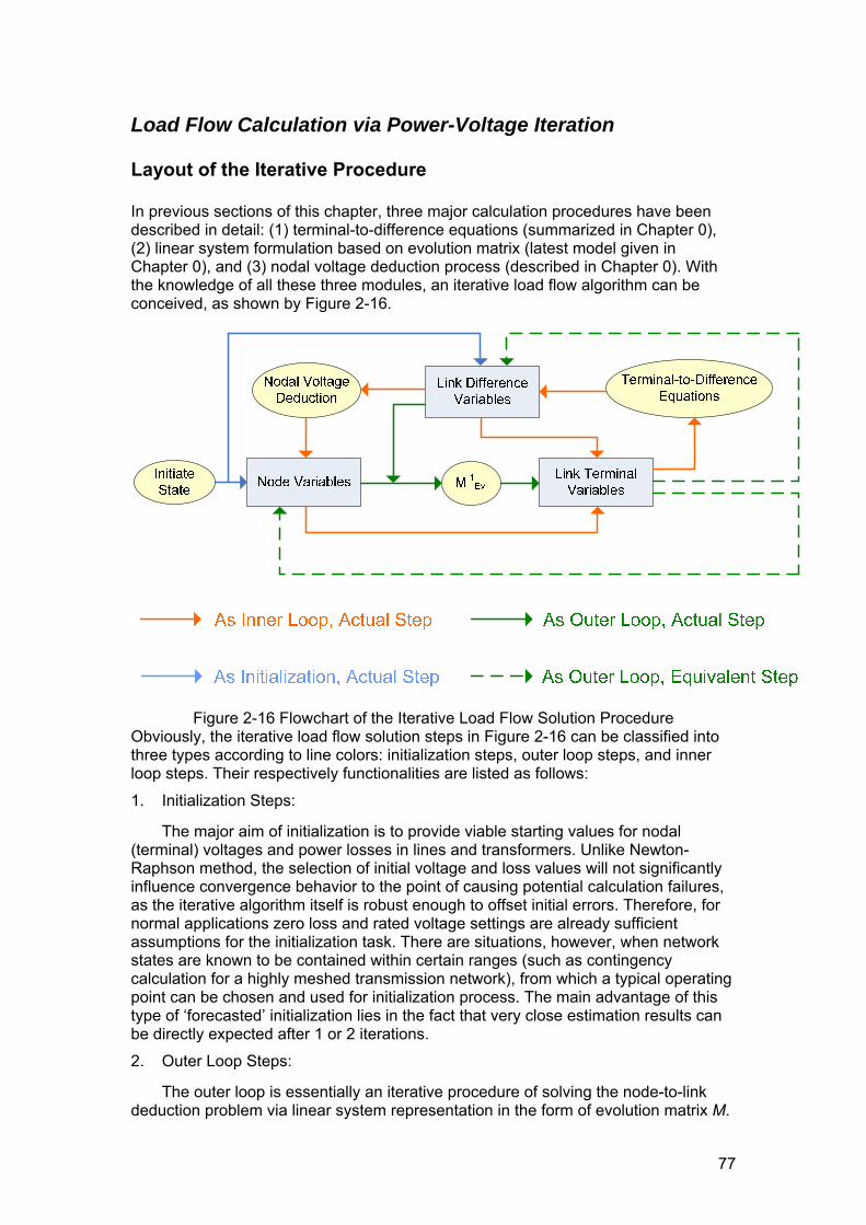
77
Load Flow Calculation via Power-Voltage Iteration
Layout of the Iterative Procedure
In previous sections of this chapter, three major calculation procedures have been described in detail: (1) terminal-to-difference equations (summarized in Chapter 0), (2) linear system formulation based on evolution matrix (latest model given in Chapter 0), and (3) nodal voltage deduction process (described in Chapter 0). With the knowledge of all these three modules, an iterative load flow algorithm can be conceived, as shown by Figure 2-16.
Figure 2-16 Flowchart of the Iterative Load Flow Solution Procedure Obviously, the iterative load flow solution steps in Figure 2-16 can be classified into three types according to line colors: initialization steps, outer loop steps, and inner loop steps. Their respectively functionalities are listed as follows:
1. Initialization Steps:
The major aim of initialization is to provide viable starting values for nodal (terminal) voltages and power losses in lines and transformers. Unlike Newton-Raphson method, the selection of initial voltage and loss values will not significantly influence convergence behavior to the point of causing potential calculation failures, as the iterative algorithm itself is robust enough to offset initial errors. Therefore, for normal applications zero loss and rated voltage settings are already sufficient assumptions for the initialization task. There are situations, however, when network states are known to be contained within certain ranges (such as contingency calculation for a highly meshed transmission network), from which a typical operating point can be chosen and used for initialization process. The main advantage of this type of ‘forecasted’ initialization lies in the fact that very close estimation results can be directly expected after 1 or 2 iterations.
2. Outer Loop Steps:
The outer loop is essentially an iterative procedure of solving the node-to-link deduction problem via linear system representation in the form of evolution matrix M.
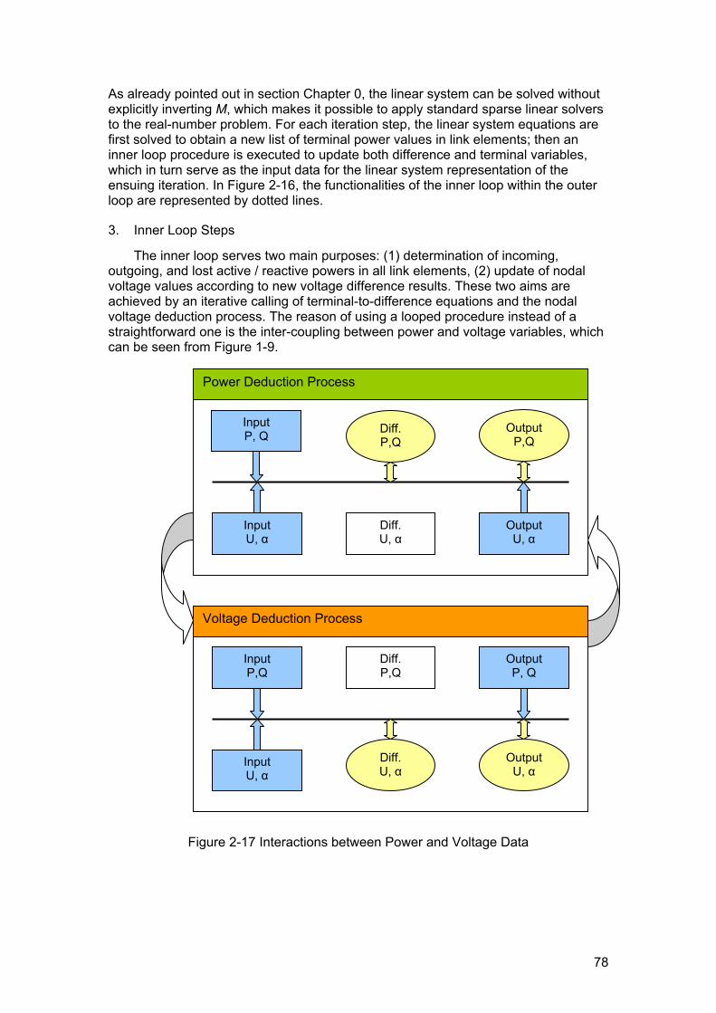
78
As already pointed out in section Chapter 0, the linear system can be solved without explicitly inverting M, which makes it possible to apply standard sparse linear solvers to the real-number problem. For each iteration step, the linear system equations are first solved to obtain a new list of terminal power values in link elements; then an inner loop procedure is executed to update both difference and terminal variables, which in turn serve as the input data for the linear system representation of the ensuing iteration. In Figure 2-16, the functionalities of the inner loop within the outer loop are represented by dotted lines.
3. Inner Loop Steps
The inner loop serves two main purposes: (1) determination of incoming, outgoing, and lost active / reactive powers in all link elements, (2) update of nodal voltage values according to new voltage difference results. These two aims are achieved by an iterative calling of terminal-to-difference equations and the nodal voltage deduction process. The reason of using a looped procedure instead of a straightforward one is the inter-coupling between power and voltage variables, which can be seen from Figure 1-9.
Figure 2-17 Interactions between Power and Voltage Data
Input U, α
Output P,Q
Diff. U, α
Diff. P,Q
Output U, α
Input P, Q
Input P,Q
Diff. P,Q
Output P, Q
Input U, α
Diff. U, α
Output U, α
Power Deduction Process
Voltage Deduction Process
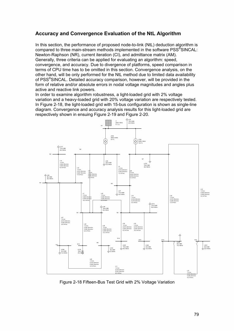
79
Accuracy and Convergence Evaluation of the NtL Algorithm
In this section, the performance of proposed node-to-link (NtL) deduction algorithm is compared to three main-stream methods implemented in the software PSS®SINCAL: Newton-Raphson (NR), current iteration (CI), and admittance matrix (AM). Generally, three criteria can be applied for evaluating an algorithm: speed, convergence, and accuracy. Due to divergence of platforms, speed comparison in terms of CPU time has to be omitted in this section. Convergence analysis, on the other hand, will be only performed for the NtL method due to limited data availability of PSS®SINCAL. Detailed accuracy comparison, however, will be provided in the form of relative and/or absolute errors in nodal voltage magnitudes and angles plus active and reactive link powers. In order to examine algorithm robustness, a light-loaded grid with 2% voltage variation and a heavy-loaded grid with 20% voltage variation are respectively tested. In Figure 2-18, the light-loaded grid with 15-bus configuration is shown as single-line diagram. Convergence and accuracy analysis results for this light-loaded grid are respectively shown in ensuing Figure 2-19 and Figure 2-20.
2T382000,0 MVA10,0 %
2T362000,0 MVA8,0 %
L351,0 km0,015 Ohm/km0,030 Ohm/km8,0 nF/km
L341,0 km0,015 Ohm/km0,035 Ohm/km10,0 nF/km
L331,0 km0,020 Ohm/km0,040 Ohm/km9,0 nF/kmL32
1,0 km0,015 Ohm/km0,028 Ohm/km7,0 nF/km
L311,0 km0,012 Ohm/km0,020 Ohm/km4,0 nF/km
L301,0 km0,020 Ohm/km0,040 Ohm/km6,0 nF/km
L291,0 km0,028 Ohm/km0,048 Ohm/km12,0 nF/km
L281,0 km0,010 Ohm/km0,020 Ohm/km3,0 nF/km
L271,0 km0,014 Ohm/km0,026 Ohm/km4,8 nF/km
L261,0 km0,032 Ohm/km0,036 Ohm/km7,5 nF/km
L251,0 km0,026 Ohm/km0,040 Ohm/km8,2 nF/km
LO2440,0 MW15,0 MVAr
LO23170,0 MW45,0 MVAr
LO2265,0 MW15,0 MVAr LO21
80,0 MW20,0 MVArLO20
50,0 MW10,0 MVAr
LO19180,0 MW35,0 MVAr
LO1835,0 MW8,0 MVAr
LO17110,0 MW20,0 MVAr
LO16150,0 MW25,0 MVAr
L151,0 km0,018 Ohm/km0,018 Ohm/km4,0 nF/km
L141,0 km0,024 Ohm/km0,033 Ohm/km6,0 nF/km
LO13210,0 MW60,0 MVAr
L121,0 km0,030 Ohm/km0,040 Ohm/km5,0 nF/km
L111,0 km0,018 Ohm/km0,022 Ohm/km8,0 nF/km
L101,0 km0,010 Ohm/km0,025 Ohm/km7,0 nF/km
LO9120,0 MW40,0 MVAr
LO885,0 MW20,0 MVAr
LO7110,0 MW35,0 MVAr
LO6220,0 MW70,0 MVAr
LO5150,0 MW45,0 MVAr
L41,0 km0,015 Ohm/km0,020 Ohm/km7,0 nF/km
L31,0 km0,020 Ohm/km0,030 Ohm/km15,0 nF/km
I12000,0 MVA0,1 p.u.
N15N14
N13 N12
N11 N10N9
N8
N7
N6N5
N4 N3
N2
N1
Figure 2-18 Fifteen-Bus Test Grid with 2% Voltage Variation

80
Voltage Magnitude Error Development, 15-Bus Grid
1,E-15
1,E-14
1,E-13
1,E-12
1,E-11
1,E-10
1,E-09
1,E-08
1,E-07
1,E-06
1,E-05
1,E-04
1,E-03
1,E-02
1,E-01
1,E+001 2 3 4 5 6 7 8
Iterations
kV
N2N7N3N4N5N13N12N6N8N11N9N10N15N14
Voltage Angle Error Development, 15-Bus Grid
1,E-15
1,E-14
1,E-13
1,E-12
1,E-11
1,E-10
1,E-09
1,E-08
1,E-07
1,E-06
1,E-05
1,E-04
1,E-03
1,E-02
1,E-01
1,E+001 2 3 4 5 6 7 8
Iterations
Degree
N2N7N3N4N5N13N12N6N8N11N9N10N15N14
Active Link Power Error Development, 15-Bus Grid
1,E-14
1,E-13
1,E-12
1,E-11
1,E-10
1,E-09
1,E-08
1,E-07
1,E-06
1,E-05
1,E-04
1,E-03
1,E-02
1,E-01
1,E+00
1,E+01
1 2 3 4 5 6 7 8
Iterations
MWL3L4L10L11L12L14L15L25L26L27L28L29L30L32L33L34L352T362T38
Reactive Link Power Error Development, 15-Bus Grid
1,E-141,E-131,E-121,E-111,E-10
1,E-091,E-081,E-071,E-061,E-051,E-041,E-031,E-02
1,E-011,E+001,E+011,E+02
1 2 3 4 5 6 7 8
Iterations
MVAR L3L4L10L11L12L14L15L25L26L27L28L29L30L32L33L34L352T362T38
Figure 2-19 NtL Convergence Behavior under 15-Bus Test Grid Voltage Magnitude Error Comparison for 15-Bus Grid
1,E-11
1,E-10
1,E-09
1,E-08
1,E-07
1,E-06
1,E-05
1,E-04
1,E-03
N7 N12 N13 N2 N3 N4 N11 N9 N8 N5 N6 N14 N15 N10
Node
kV
NtL_NRNtL_CINtL_AM
Voltage Angle Error Comparison for 15-Bus Grid
1,E-11
1,E-10
1,E-09
1,E-08
1,E-07
1,E-06
1,E-05
1,E-04
1,E-03
N7 N12 N2 N13 N3 N4 N11 N9 N5 N8 N6 N14 N15 N10
Node
Degree
NtL_NRNtL_CINtL_AM
Active Link Power Error Comparison for 15-Bus Grid
1,E-11
1,E-10
1,E-09
1,E-08
1,E-07
1,E-06
1,E-05
1,E-04
1,E-03
1,E-02
2T36
2T38 L15
L26
L32
L10
L12 L4 L30
L35 L3 L14
L27
L33
L25
L28
L34
L29
L11 Link
MW
NtL_NRNtL_CINtL_AM
Reactive Link Power Error Comparison for 15-Bus Grid
1,E-11
1,E-10
1,E-09
1,E-08
1,E-07
1,E-06
1,E-05
1,E-04
1,E-03
1,E-02
2T36
2T38 L15
L26
L32
L10
L12 L4 L30
L35 L3 L14
L27
L33
L25
L28
L34
L29
L11
Link
MVAR
NtL_NRNtL_CINtL_AM
Figure 2-20 NtL Relative Errors Compared to Existing Methods under 15-Bus Test
Grid

81
In Figure 2-19, the convergence rate of NtL method is represented by the development of iterative calculation errors of voltage magnitude, voltage angle, active link power, and reactive link power. The errors are defined as the absolute values of differences between concurrent and finalized (converged) results. Despite individual differences among nodes and links, Figure 2-19 exhibit a linear trend of error reduction (inferior to the quadratic trend of NR, as illustrated by [67]) under logarithmic scale, which means calculation errors of NtL method decrease exponentially over iterations. For the light-loaded grid, a total of 8 iterations are already sufficient for bringing all examined error terms 10-10 times smaller, which means error reduction capability of each iteration can be seen as more than 10 times in general. Figure 2-20, on the other hand, lists the relative errors of NtL method when compared to existing algorithms. The error terms are defined as absolute values of the differences between calculation results from NtL and a designated algorithm (i.e. NR, CI, or AM). It can be clearly seen that for the light-loaded grid, NtL result is found to be closest to NR result with relative errors between them falling below 10-10 in general. Since Newton-Raphson has been generally acknowledged to be the best-performing algorithm for networks in good condition, the NtL method can be seen as capable of offering a close accuracy level to NR for networks under good voltage conditions. Now that evaluation of NtL method for the light-loaded 15-bus test grid is done, a more critical test network is presented in Figure 2-21. In order to ensure convergence of all examine algorithms within finite steps, the meshed grid in Figure 2-21 is designed to have the simplest 3-bus topology. Loading levels on bus N2 and N3, however, are increased to extreme conditions so that expected voltage levels of these two nodes will be around 80% of the rated value.
2T382000,0 MVA10,0 %
2T362000,0 MVA8,0 %
LO74400,0 MW1400,0 MVAr
LO68800,0 MW2800,0 MVAr
LO5150,0 MW45,0 MVAr
L41,0 km0,015 Ohm/km0,020 Ohm/km7,0 nF/km
I12000,0 MVA0,1 p.u.
N3N2
N1
Figure 2-21 Three-Bus Test Grid with 20% Voltage Variation
Similar to the 15-bus case, in Figure 2-22 and Figure 2-23 NtL convergence behavior and relative error data are respectively plotted.

82
Voltage Manitude Error Development, 3-Bus Grid
1,E-151,E-141,E-131,E-121,E-111,E-101,E-091,E-081,E-071,E-061,E-051,E-041,E-031,E-021,E-011,E+00
0 10 20 30 40 50 60Iterations
kV
N2N3
Voltage Angle Error Development, 3-Bus Grid
1,E-15
1,E-14
1,E-13
1,E-12
1,E-11
1,E-10
1,E-09
1,E-08
1,E-07
1,E-06
1,E-05
1,E-04
1,E-03
1,E-02
1,E-01
1,E+000 10 20 30 40 50 60
Iterations
Degree
N2N3
Active Link Power Error Development, 3-Bus Grid
1,E-101,E-091,E-081,E-071,E-061,E-051,E-041,E-031,E-021,E-011,E+001,E+011,E+021,E+031,E+041,E+051,E+06
0 10 20 30 40 50 60Iterations
MW
L42T362T38
Reactive Link Power Error Development, 3-Bus Grid
1,E-101,E-091,E-081,E-071,E-061,E-051,E-041,E-031,E-021,E-011,E+001,E+011,E+021,E+031,E+041,E+051,E+06
0 10 20 30 40 50 60Iterations
MVAR
L42T362T38
Figure 2-22 NtL Convergence Behavior under 3-Bus Test Grid
Voltage Magnitude Error Comparison for 3-Bus Grid
1,E-06
1,E-05
1,E-04
1,E-03
1,E-02
N3 N2Node
kV
NtL_NRNtL_CINtL_AM
Voltage Angle Error Comparison for 3-Bus Grid
1,E-06
1,E-05
1,E-04
1,E-03
1,E-02
N3 N2 Node
Degree
NtL_NRNtL_CINtL_AM
Active Link Power Error Comparison for 3-Bus Grid
1,E-06
1,E-05
1,E-04
1,E-03
1,E-02
1,E-01
1,E+00
1,E+01
2T36 2T38 L4 Link
MW
NtL_NRNtL_CINtL_AM
Reactive L-Power Error Comparison for 3-Bus Grid
1,E-06
1,E-05
1,E-04
1,E-03
1,E-02
1,E-01
1,E+00
1,E+01
2T36 2T38 L4Link
MVAR
NtL_NRNtL_CINtL_AM
Figure 2-23 NtL Relative Errors Compared to Existing Methods under 3-Bus Test
Grid
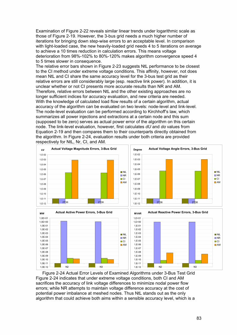
83
Examination of Figure 2-22 reveals similar linear trends under logarithmic scale as those of Figure 2-19. However, the 3-bus grid needs a much higher number of iterations for bringing down step-wise errors to an acceptable level. In comparison with light-loaded case, the new heavily-loaded grid needs 4 to 5 iterations on average to achieve a 10 times reduction in calculation errors. This means voltage deterioration from 98%-102% to 80%-120% makes algorithm convergence speed 4 to 5 times slower in consequence. The relative error bars shown in Figure 2-23 suggests NtL performance to be closest to the CI method under extreme voltage conditions. This affinity, however, not does mean NtL and CI share the same accuracy level for the 3-bus test grid as their relative errors are still considerably large (esp. reactive link power). In addition, it is unclear whether or not CI presents more accurate results than NR and AM. Therefore, relative errors between NtL and the other existing approaches are no longer sufficient indices for accuracy evaluation, and new criteria are needed. With the knowledge of calculated load flow results of a certain algorithm, actual accuracy of the algorithm can be evaluated on two levels: node-level and link-level. The node-level evaluation can be performed according to Kirchhoff’s law, which summarizes all power injections and extractions at a certain node and this sum (supposed to be zero) serves as actual power error of the algorithm on this certain node. The link-level evaluation, however, first calculates dU and dα values from Equation 2-19 and then compares them to their counterparts directly obtained from the algorithm. In Figure 2-24, evaluation results under both criteria are provided respectively for NtL, Nr, CI, and AM.
Actual Voltage Magnitude Errors, 3-Bus Grid
1,E-12
1,E-11
1,E-10
1,E-09
1,E-08
1,E-07
1,E-06
1,E-05
1,E-04
1,E-03
1,E-02
2T36 2T38
kV
NtLNRCIAM
Actual Voltage Angle Errors, 3-Bus Grid
1,E-12
1,E-11
1,E-10
1,E-09
1,E-08
1,E-07
1,E-06
1,E-05
1,E-04
1,E-03
1,E-02
2T36 2T38
Degree
NtLNRCIAM
Actual Active Power Errors, 3-Bus Grid
1,0E-121,0E-11
1,0E-101,0E-09
1,0E-081,0E-07
1,0E-061,0E-05
1,0E-041,0E-03
1,0E-021,0E-01
1,0E+001,0E+01
N2 N3
MW
NtLNRCIAM
Actual Reactive Power Errors, 3-Bus Grid
1,E-121,E-11
1,E-101,E-09
1,E-081,E-07
1,E-061,E-05
1,E-041,E-03
1,E-021,E-01
1,E+001,E+01
N2 N3
MVAR
NtLNRCIAM
Figure 2-24 Actual Error Levels of Examined Algorithms under 3-Bus Test Grid
Figure 2-24 indicates that under extreme voltage conditions, both CI and AM sacrifices the accuracy of link voltage differences to minimize nodal power flow errors; while NR attempts to maintain voltage difference accuracy at the cost of potential power imbalance at meshed nodes. Thus NtL stands out as the only algorithm that could achieve both aims within a sensible accuracy level, which is a

84
proof of its superiority over existing commercial packages in terms of accurate handling of ill-conditioned grids.
NtL Execution Efficiency Compared to Newton-Raphson Method
As already stated at the beginning of section Chapter 0, CPU time of the NtL method has not been compared to Newton-Raphson or other existing approaches due to differences in utilized software platforms. A general evaluation of NtL computational complexity, however, is possible via direct comparison to the layout of Newton-Raphson method. Specifically, dimensions of evolution (M) and Jacobian (J) matrices can be both expressed in terms of network element counts, as shown by Equation 2-38.
222)1(20,
000,222
:,,
−−⋅−⋅=+−−−⋅=⎩⎨⎧
===≠≠≠+⋅+⋅+⋅
=
××
NpvNslNndNpvNpvNslNndNNpvNslNmhwhenNnd
NpvorNslorNmhwhenNpvNslNmhNndN
thenJmatrixJacobianofsizeasNMmatrixevolutionofsizeasNAssume
J
M
NNJNNM JJMM
Equation 2-38
Since both M and J are real, square, and non-singular, Equation 2-38 clearly indicates the potential sizes of linear systems to be solved under NtL and NR methods. For radial grids with one slack and purely PQ loads, the NtL method can directly utilize link-to-node correlation matrix to solve decoupled active and reactive power flows and thus provides a much simpler formulation than NR method. For more complicated grids with loops, extra slacks, and/or PV generators, the size of M will become undoubtedly larger than J—each loop or PV node will increase their dimensional difference by 2 (equivalent to an additional PQ node in NR), while each extra slack will increase the difference by 4.
The larger size of M (comparison with J) apparently places NtL at an unfavorable position when dealing with meshed grids with multiple active components. However, there are two features of M that could potentially offset its size disadvantage, namely: (1) the sparsity of M is generally greater than J, (2) each matrix M consists of a constant part (TD) that stays unchanged over iterations and a variable part (LS, SS, and VS) that needs to be iteratively updated. Proper utilization of these two features could greatly reduce computational efforts needed for solving the linear system equations presented by Equation 2-37. In order to illustrate the basic working principles behind this idea, a partitioned LU decomposition procedure can be introduced to tackle the M formulation.
Now consider a standard LU decomposition procedure without pivoting table operation on M, which should convert M into a lower triangular matrix L and an upper triangular matrix U such that M = L × U. In order to facilitate illustration, a four-node grid in Figure 2-25 with one loop, one slack, and one PV node is taken as an example.
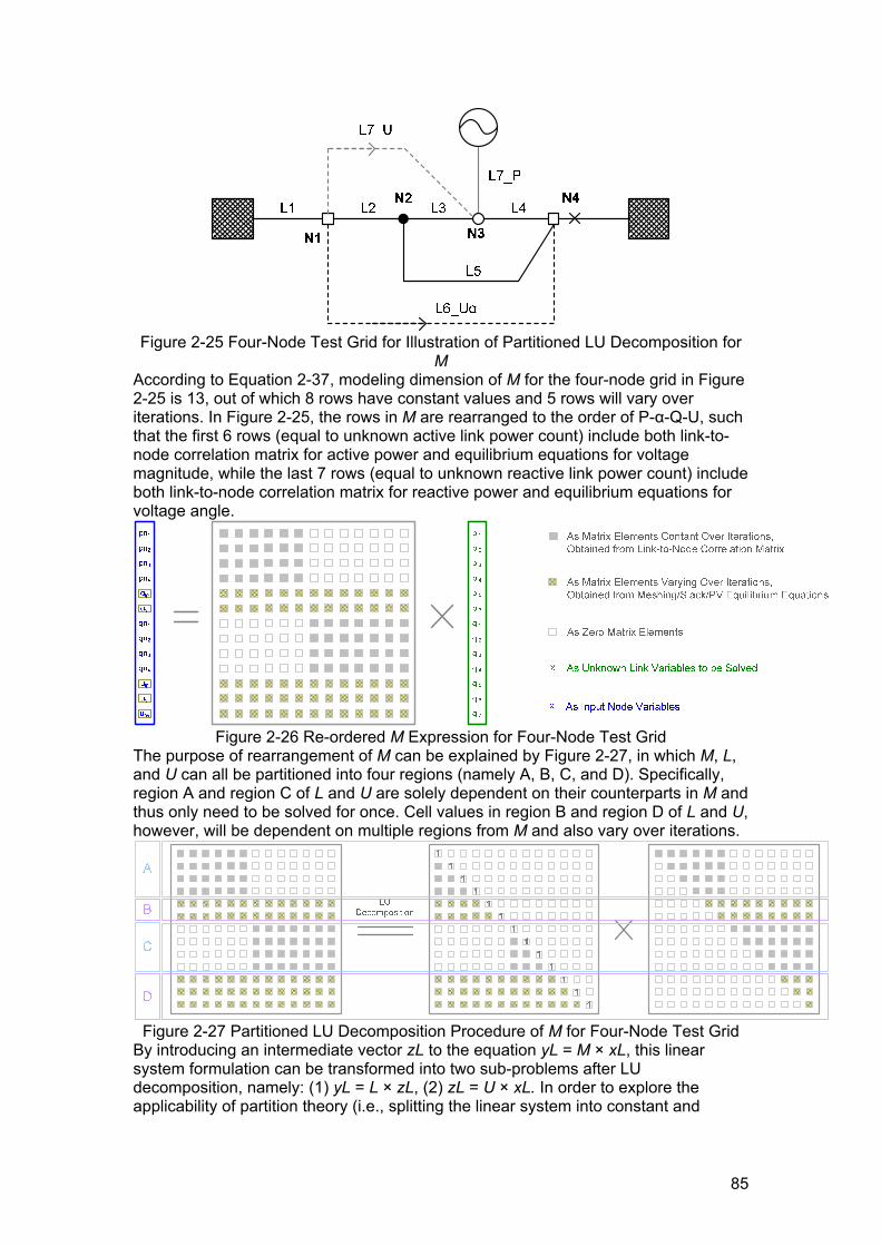
85
Figure 2-25 Four-Node Test Grid for Illustration of Partitioned LU Decomposition for
M According to Equation 2-37, modeling dimension of M for the four-node grid in Figure 2-25 is 13, out of which 8 rows have constant values and 5 rows will vary over iterations. In Figure 2-25, the rows in M are rearranged to the order of P-α-Q-U, such that the first 6 rows (equal to unknown active link power count) include both link-to-node correlation matrix for active power and equilibrium equations for voltage magnitude, while the last 7 rows (equal to unknown reactive link power count) include both link-to-node correlation matrix for reactive power and equilibrium equations for voltage angle.
Figure 2-26 Re-ordered M Expression for Four-Node Test Grid
The purpose of rearrangement of M can be explained by Figure 2-27, in which M, L, and U can all be partitioned into four regions (namely A, B, C, and D). Specifically, region A and region C of L and U are solely dependent on their counterparts in M and thus only need to be solved for once. Cell values in region B and region D of L and U, however, will be dependent on multiple regions from M and also vary over iterations.
Figure 2-27 Partitioned LU Decomposition Procedure of M for Four-Node Test Grid
By introducing an intermediate vector zL to the equation yL = M × xL, this linear system formulation can be transformed into two sub-problems after LU decomposition, namely: (1) yL = L × zL, (2) zL = U × xL. In order to explore the applicability of partition theory (i.e., splitting the linear system into constant and
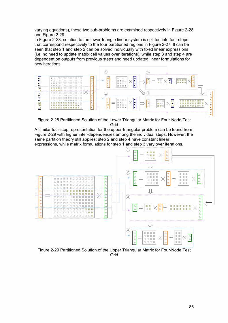
86
varying equations), these two sub-problems are examined respectively in Figure 2-28 and Figure 2-29. In Figure 2-28, solution to the lower-triangle linear system is splitted into four steps that correspond respectively to the four partitioned regions in Figure 2-27. It can be seen that step 1 and step 2 can be solved individually with fixed linear expressions (i.e. no need to update matrix cell values over iterations), while step 3 and step 4 are dependent on outputs from previous steps and need updated linear formulations for new iterations.
Figure 2-28 Partitioned Solution of the Lower Triangular Matrix for Four-Node Test
Grid A similar four-step representation for the upper-triangular problem can be found from Figure 2-29 with higher inter-dependencies among the individual steps. However, the same partition theory still applies: step 2 and step 4 have constant linear expressions, while matrix formulations for step 1 and step 3 vary over iterations.
pt1
pt2
pt3
pt4
pt5
pt6
qt1
qt2
qt3
qt4
qt5
qt6
qt7
pl1
pl2
pl3
pl4
pl5
pl6
ql1
ql2
ql3
ql4
ql5
ql6
ql7
ql5
ql6
ql7
qt5
qt6
qt7
ql1
ql2
ql3
ql4
qt1
qt2
qt3
qt4
ql5
ql6
ql7
pl5
pl6
pt5
pt6
ql1
ql2
ql3
ql4
ql5
ql6
ql7
pl1
pl2
pl3
pl4
pt1
pt2
pt3
pt4
pl5
pl6
1
2
3
4
Figure 2-29 Partitioned Solution of the Upper Triangular Matrix for Four-Node Test
Grid

87
Simplified Optimal Power Flow Using NtL Formulation
Linear / Quadratic Formulation of Network State Variables
With the introduction of linear system formulation of node-to-link deduction problem via evolution matrix M, it is possible to explicitly inverse M to express active and reactive link power flows in terms of nodal power injection / extraction vector xL, which can be seen from Equation 2-39. It should be noted that this operation can be performed in every iteration step of a load flow procedure with increasing coefficient accuracy over time, although only the results obtained from the initial condition can be seen as a direct linear formulation of the node-to-link deduction problem.
⎪⎩
⎪⎨⎧
+⋅=
+⋅=⇒⋅=
−⋅=+++=
×
××
−
NlkNndNndNlkNlk
NlkNndNndNlkNlk
NuvNuvNuvNuv
cqxNbqQL
cpxNbpPLyLMxL
thenNpvNlkNuvNpvNslNmhNndNlkWith
22
2222
1
:,2,:
Equation 2-39 The linearized formulation of Equation 2-39 provides an opportunity of expressing varied network state variables in terms of individual load sizes and/or generator output levels, which can be extremely useful for contingency calculation, sensitivity analysis, and optimal / probabilistic load flow applications. In scope of this section, three types of network variables are mainly examined: total system active power loss, nodal voltage magnitudes, and link (line / transformer) element loading levels. Firstly, in Equation 2-40 the quadratic formulation of total active power loss is given in terms of node powers.
( ) ( ) ( ) ( )
( )
clxNblxNalxN
kclxNkblxNkalxNdP
kclxNkblxNkalxNkdP
thenkcqxNkbqQkcpxNkbpkPLet
kckQkbqkPkbpkQkPka
kcU
QPU
QPka
BXGRXGUUU
QPU
QPRUUGkdP
NdT
NdNdNdNdT
Nnd
Nlk
kNd
Nlk
k
T
NdNd
Nlk
kNdNd
TNnd
NdT
NdNdNdNd
TNnd
NndT
NndiNndT
Nndi
iiii
o
oo
i
ii
qlqlqqoio
oo
i
iiloiq
+⋅+⋅⋅=
+⋅⎟⎠
⎞⎜⎝
⎛+⋅⎟
⎠
⎞⎜⎝
⎛⋅=∑⇒
+⋅+⋅⋅=⇒
+⋅=+⋅=
+⋅+⋅++⋅=
+⎥⎦
⎤⎢⎣
⎡ ++
+⋅=
⋅+⋅+⎥⎦
⎤⎢⎣
⎡+⋅+−⎟⎟
⎠
⎞⎜⎜⎝
⎛ ++
+⋅++⋅=
×
===×
×
∑∑∑
222222
12
122
1222
222222
2222
22
2
22
2
22
22222
22
2
2222
)()()(
)()()()(
:),()(),()()(
)()()()()()()()(
)(0)(0
12
)(
Equation 2-40
Similarly, in Equation 2-41 the nodal voltages are expressed as linearly dependent on node power injections/extractions.
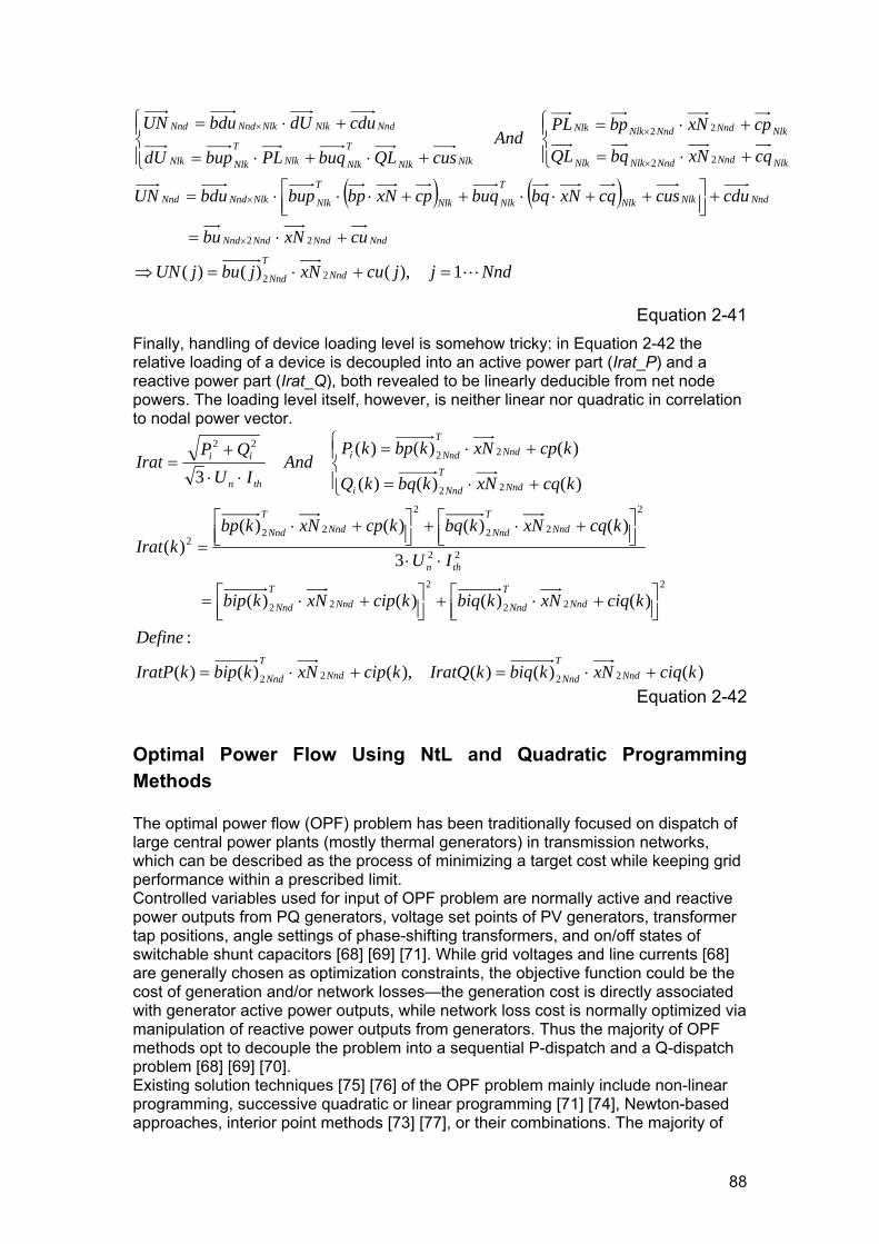
88
( ) ( )
NndjjcuxNjbujUN
cuxNbu
cducuscqxNbqbuqcpxNbpbupbduUN
cqxNbqQL
cpxNbpPLAnd
cusQLbuqPLbupdU
cdudUbduUN
NndT
Nnd
NndNndNndNnd
NndNlkNlk
T
NlkNlk
T
NlkNlkNndNnd
NlkNndNndNlkNlk
NlkNndNndNlkNlk
NlkNlk
T
NlkNlkT
NlkNlk
NndNlkNlkNndNnd
L1),()()( 22
22
22
22
=+⋅=⇒
+⋅=
+⎥⎦⎤
⎢⎣⎡ ++⋅⋅++⋅⋅⋅=
⎪⎩
⎪⎨⎧
+⋅=
+⋅=
⎪⎩
⎪⎨⎧
+⋅+⋅=
+⋅=
×
×
×
××
Equation 2-41
Finally, handling of device loading level is somehow tricky: in Equation 2-42 the relative loading of a device is decoupled into an active power part (Irat_P) and a reactive power part (Irat_Q), both revealed to be linearly deducible from net node powers. The loading level itself, however, is neither linear nor quadratic in correlation to nodal power vector.
)()()(),()()(
:
)()()()(
3
)()()()()(
)()()(
)()()(3
2222
2
22
2
22
22
2
22
2
222
22
2222
kciqxNkbiqkIratQkcipxNkbipkIratP
Define
kciqxNkbiqkcipxNkbip
IU
kcqxNkbqkcpxNkbpkIrat
kcqxNkbqkQ
kcpxNkbpkPAnd
IUQP
Irat
NndT
NndNndT
Nnd
NndT
NndNndT
Nnd
thn
NndT
NndNndT
Nnd
NndT
Nndi
NndT
Nndi
thn
ii
+⋅=+⋅=
⎥⎦⎤
⎢⎣⎡ +⋅+⎥⎦
⎤⎢⎣⎡ +⋅=
⋅⋅⎥⎦⎤
⎢⎣⎡ +⋅+⎥⎦
⎤⎢⎣⎡ +⋅
=
⎪⎩
⎪⎨⎧
+⋅=
+⋅=
⋅⋅
+=
Equation 2-42
Optimal Power Flow Using NtL and Quadratic Programming Methods
The optimal power flow (OPF) problem has been traditionally focused on dispatch of large central power plants (mostly thermal generators) in transmission networks, which can be described as the process of minimizing a target cost while keeping grid performance within a prescribed limit. Controlled variables used for input of OPF problem are normally active and reactive power outputs from PQ generators, voltage set points of PV generators, transformer tap positions, angle settings of phase-shifting transformers, and on/off states of switchable shunt capacitors [68] [69] [71]. While grid voltages and line currents [68] are generally chosen as optimization constraints, the objective function could be the cost of generation and/or network losses—the generation cost is directly associated with generator active power outputs, while network loss cost is normally optimized via manipulation of reactive power outputs from generators. Thus the majority of OPF methods opt to decouple the problem into a sequential P-dispatch and a Q-dispatch problem [68] [69] [70]. Existing solution techniques [75] [76] of the OPF problem mainly include non-linear programming, successive quadratic or linear programming [71] [74], Newton-based approaches, interior point methods [73] [77], or their combinations. The majority of
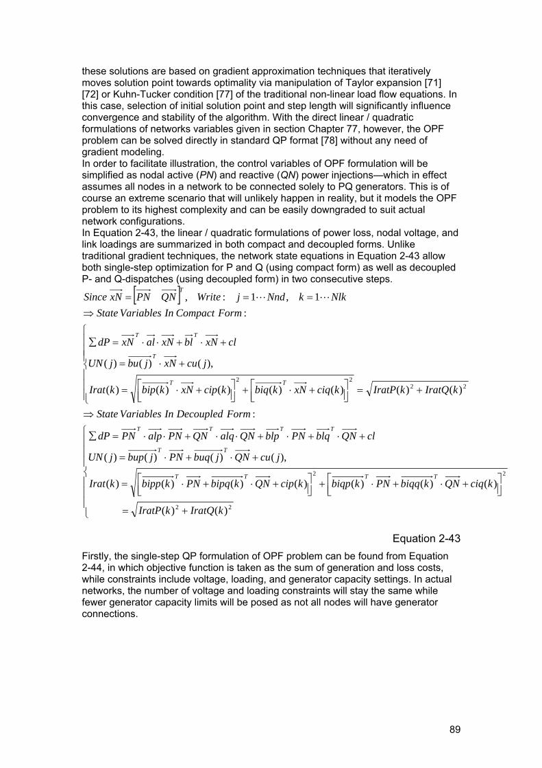
89
these solutions are based on gradient approximation techniques that iteratively moves solution point towards optimality via manipulation of Taylor expansion [71] [72] or Kuhn-Tucker condition [77] of the traditional non-linear load flow equations. In this case, selection of initial solution point and step length will significantly influence convergence and stability of the algorithm. With the direct linear / quadratic formulations of networks variables given in section Chapter 77, however, the OPF problem can be solved directly in standard QP format [78] without any need of gradient modeling. In order to facilitate illustration, the control variables of OPF formulation will be simplified as nodal active (PN) and reactive (QN) power injections—which in effect assumes all nodes in a network to be connected solely to PQ generators. This is of course an extreme scenario that will unlikely happen in reality, but it models the OPF problem to its highest complexity and can be easily downgraded to suit actual network configurations. In Equation 2-43, the linear / quadratic formulations of power loss, nodal voltage, and link loadings are summarized in both compact and decoupled forms. Unlike traditional gradient techniques, the network state equations in Equation 2-43 allow both single-step optimization for P and Q (using compact form) as well as decoupled P- and Q-dispatches (using decoupled form) in two consecutive steps.
[ ]
⎪⎪⎪
⎩
⎪⎪⎪
⎨
⎧
+=
⎥⎦⎤
⎢⎣⎡ +⋅+⋅+⎥⎦
⎤⎢⎣⎡ +⋅+⋅=
+⋅+⋅=
+⋅+⋅+⋅⋅+⋅⋅=∑
⇒
⎪⎪⎪
⎩
⎪⎪⎪
⎨
⎧
+=⎥⎦⎤
⎢⎣⎡ +⋅+⎥⎦
⎤⎢⎣⎡ +⋅=
+⋅=
+⋅+⋅⋅=∑
⇒===
22
22
2222
)()(
)()()()()()()(
),()()()(
:
)()()()()()()(
),()()(
:1,1:,
kIratQkIratP
kciqQNkbiqqPNkbiqpkcipQNkbipqPNkbippkIrat
jcuQNjbuqPNjbupjUN
clQNblqPNblpQNalqQNPNalpPNdP
FormDecoupledInVariablesState
kIratQkIratPkciqxNkbiqkcipxNkbipkIrat
jcuxNjbujUN
clxNblxNalxNdP
FormCompactInVariablesStateNlkkNndjWriteQNPNxNSince
TTTT
TT
TTTT
TT
T
TT
TLL
Equation 2-43
Firstly, the single-step QP formulation of OPF problem can be found from Equation 2-44, in which objective function is taken as the sum of generation and loss costs, while constraints include voltage, loading, and generator capacity settings. In actual networks, the number of voltage and loading constraints will stay the same while fewer generator capacity limits will be posed as not all nodes will have generator connections.

90
⎪⎪
⎩
⎪⎪
⎨
⎧
≤⎥⎦⎤
⎢⎣⎡ +⋅+⎥⎦
⎤⎢⎣⎡ +⋅=
⎪⎩
⎪⎨⎧
≤≤≤≤≤+⋅≤=
⇒
⋅+⋅⋅=−−+=⇒
⎪⎩
⎪⎨⎧
+⋅+⋅⋅=
+⋅+⋅⋅=
222
maxminmaxmin
maxmin
)()()()()(:1
)()()(),()()()()()()(:1
:..
:min
:cos
cos
kIkciqxNkbiqkcipxNkbipNlktokfor
jQNjQNjQNjPNjPNjPNjUjcuxNjbujUNndtojfor
ts
xNbkxNakxNclcgKKf
asclxNblxNalxNKtlossnetwork
cgPNbgPNagPNKtgenerationwithnformulatioOPF
th
TT
T
TT
LGP
TT
L
TT
G
Equation 2-44
Noticeably, in Equation 2-44 the thermal loading constraints are not linear expressions and thus do not fit into standard QP definition. Consequently, they have to be converted into linear equivalents using multiple inequality formulations illustrated by Equation 2-29. Obviously, usage of more inequations will lead to higher accuracy but lower efficiency.
maxmax22 2sin2cos:1 SQ
nkP
nkntokForSQP ≤⋅⎟
⎠⎞
⎜⎝⎛ ⋅+⋅⎟
⎠⎞
⎜⎝⎛ ⋅=⇒≤+
ππ
Q
P
Q
P
Q
P
n = 4 n = 6 n = 8
⎟⎠⎞
⎜⎝⎛⋅≤⋅⎟
⎠⎞
⎜⎝⎛ ⋅++⋅⎟
⎠⎞
⎜⎝⎛ ⋅+=⇒≤+
nSQ
nk
nP
nk
nntokForSQP πππππ cos2sin2cos:1 maxmax
22
Figure 2-30 Linearization of Thermal Loading Constraints
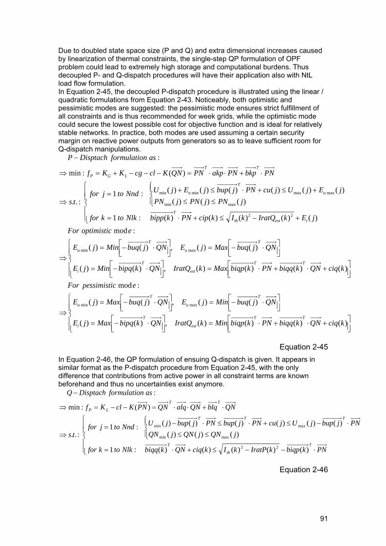
91
Due to doubled state space size (P and Q) and extra dimensional increases caused by linearization of thermal constraints, the single-step QP formulation of OPF problem could lead to extremely high storage and computational burdens. Thus decoupled P- and Q-dispatch procedures will have their application also with NtL load flow formulation. In Equation 2-45, the decoupled P-dispatch procedure is illustrated using the linear / quadratic formulations from Equation 2-43. Noticeably, both optimistic and pessimistic modes are suggested: the pessimistic mode ensures strict fulfillment of all constraints and is thus recommended for week grids, while the optimistic mode could secure the lowest possible cost for objective function and is ideal for relatively stable networks. In practice, both modes are used assuming a certain security margin on reactive power outputs from generators so as to leave sufficient room for Q-dispatch manipulations.
⎪⎪⎩
⎪⎪⎨
⎧
⎥⎦⎤
⎢⎣⎡ +⋅+⋅=⎥⎦
⎤⎢⎣⎡ ⋅−=
⎥⎦⎤
⎢⎣⎡ ⋅−=⎥⎦
⎤⎢⎣⎡ ⋅−=
⇒
⎪⎪⎩
⎪⎪⎨
⎧
⎥⎦⎤
⎢⎣⎡ +⋅+⋅=⎥⎦
⎤⎢⎣⎡ ⋅−=
⎥⎦⎤
⎢⎣⎡ ⋅−=⎥⎦
⎤⎢⎣⎡ ⋅−=
⇒
⎪⎪⎩
⎪⎪⎨
⎧
+−≤+⋅=
⎪⎩
⎪⎨⎧
≤≤+≤+⋅≤+=
⇒
⋅+⋅⋅=−−−+=⇒
−
)()()()(,)()(
)()(,)()(
:mod
)()()()(,)()(
)()(,)()(
:mod
)()()()()(:1
)()()()()()()()()(:1
:..
)(:min
:
maxmin
maxmin
22
maxmin
maxmaxminmin
kciqQNkbiqqPNkbiqpMinkIratQQNkbipqMaxjE
QNjbuqMinjEQNjbuqMaxjE
ecpessimistiFor
kciqQNkbiqqPNkbiqpMaxkIratQQNkbipqMinjE
QNjbuqMaxjEQNjbuqMinjE
eoptimisticFor
jEkIratQkIkcipPNkbippNlktokfor
jPNjPNjPNjEjUjcuPNjbupjEjUNndtojfor
ts
PNbkpPNakpPNQNKclcgKKf
asnformulatioDisptachP
TT
est
T
i
T
u
T
u
TT
est
T
i
T
u
T
u
iestth
T
u
T
u
TT
LGP
Equation 2-45
In Equation 2-46, the QP formulation of ensuing Q-dispatch is given. It appears in similar format as the P-dispatch procedure from Equation 2-45, with the only difference that contributions from active power in all constraint terms are known beforehand and thus no uncertainties exist anymore.
⎪⎪⎩
⎪⎪⎨
⎧
⋅−−≤+⋅=
⎪⎩
⎪⎨⎧
≤≤⋅−≤+⋅≤⋅−=
⇒
⋅+⋅⋅=−−=⇒
−
PNkbiqpkIratPkIkciqQNkbiqqNlktokfor
jQNjQNjQNPNjbupjUjcuPNjbupPNjbupjUNndtojfor
ts
QNblqQNalqQNPNKclKf
asnformulatioDisptachQ
T
th
T
TTT
TT
LP
)()()()()(:1
)()()()()()()()()(:1
:..
)(:min
:
22
maxmin
maxmin
Equation 2-46

92
Open Topics and Potential Extensions
The following list of topics is currently open and need to be reckoned upon: 1. In comparison with NR, The NtL method uses a larger but sparser (and can be
partitioned) evolution matrix instead of Jacobian matrix, but the factorization process is much simpler using NtL. Whether this change leads to higher or lower efficiency is unknown unless actual computation times are compared.
2. Convergence behavior of NtL method shows linear trend under logarithmic scale, which is similar to Gauss, backward/forward sweep and fast decoupled methods but obviously inferior to the quadratic convergence rate of Newton-Raphson [67], thus any modification that can speed up NtL convergence will be a critical improvement.
3. Modeling of active control measures such as OLTC and switchable capacitor banks are currently missing, but implementation should be possible via remedial (iterative modification) or precognitive (set control aim beforehand) techniques. Node-based control variables should be generally easier to implement than link-based ones.
4. As the terminal-to-difference equations have been proven to be applicable to both line-to-neutral and line-to-line systems, the NtL algorithm is potentially extensible to unbalanced load flow problems. However, it is arguable if M dimension should be enlarged by 3 times to accommodate individual phases or the same size of M can be used for each phase with decoupled line-to-neutral link power solutions.

93
References [1] Thomas Ackermann, Gören Andersson, Lennart Söder, Distributed Generation:
a Definition, Electric Power Systems Research 57 (2001) 154-204 [2] Gaudenz Keoppel, Distributed Generation—Literature Review and Outline of the
Swiss Situation, EEH ETH Internal Report, November 2003 [3] W. Dürrschmidt, G. Zimmermann, Renewable Energies—Innovation for the
Future, (German) Federal Ministry for the Environment, Nature Reservation and Nuclear Safety (BMU) Brochure, April 2006
[4] Robert Priddle, Distributed Generation in Liberalised Electricity Market,
Organisation for Economic Co-operation and Development (OECD) / International Energy Agency (IEA) 2002 ISBN 92-64-19802-4
[5] Ward Jewell, Evaluation of Distributed Energy Storage and Generation, Power
Systems Engineering Research Centre (PSERC), Final Project Report, July 2004
[6] A. Fernández, I. Cobelo, Library of Models, EU-DEEP Internal Report, WP2,
Sub-task 2.2.1.0.2, June 2005 [7] Gary L. Johnson, Wind Energy Systems, December 2001 [8] European Commision, Energy for the Future: Renewable Sources of Energy,
White Paper for a Community Strategy and Action Plan, November 1997 [9] Karl M. Maribu, Modeling the Economics and Market Adoption of Distributed
Power Generation, Department of Electrical Power Engineering, Norwegian University of Science and Technology, Doctoral Thesis, June 2006
[10] Jürgen Garche, Elektrochemische Energiespeicher: Stand, Probleme,
Perspektiven, Energiewirtschaftliche Tagesfragen, 10-2006, pp. 61—66. [11] B. Blažic, U. Kerin, I.Papic, Techniques for DER Integration and Active Networks
Management Phase I, SOLID-DER Work Package II, Deliverable number D 2.1, Task 2.2, October 2006
[12] Sébastien Grenard, Danny Pudjianto, Coran Strbac, Benifits of Active
Management of Distribution Network in UK, CIRED 18th International Conference on Electricity Distribution, Turin 6-9 June 2005
[13] G. Celli, E. Ghiani, S. Mocci, F. Pilo, Distributed Generation and Intentional
Islanding: Effects on Reliability in Active Networks, CIRED 18th International Conference on Electricity Distribution, Turin 6-9 June 2005
[14] Constantin, Surdu, Leaonardo-Geo Manescu, et al, On the Interest of the Virtual
Power Plant Concept in the Distribution Networks, CIGRE 2006

94
[15] Christine Schwaegerl, Alex Baitch, Demand Side Management and Response with Distributed Energy Resources—Chances and First Experience, CIGRE 2006
[16] BORKOWSKA, B., Probabilistic Load Flow, IEEE Trans., 1974, PAS-93, (3). pp.
752-759 [17] Chun-Lien Su, Distribution Probabilistic Load Flow Solution Considering Network
Reconfiguration and Voltage Control Devices, 15th PSCC, Liege, 22-26 August 2005, Session 10, Paper 3, Page 1
[18] G.Papaefthymiou, P.H.Schavemaker, L. van der Sluis et al, Integration of
Stochastic Generation in Power Systems, 15th PSCC, Liege, 22-26 August 2005, Session 42, Paper 1, Page 1
[19] N.D. Hatziargyriou, T.S. Karakatsanis, M. Papadopoulos, Probabilistic Load
Flow in Distribution Systems Containing Dispersed Wind Power Generation, IEEE Transactions on Power Systems, Vol. 8, No. 1, February 1993
[20] Zechun Hu, Xifan Wang, A Probabilistic Load Flow Method Considering Branch
Outages, IEEE Transactions on Power Systems, Vol. 21, No. 2, May 2006, pp. 507-514
[21] Leite da Silva. A.M., Arienti, V.L., Allan, R.N., Probabilistic Load Flow
Considering Dependence Between Input Nodal Powers, IEEE Trans., 1984, PAS-103, (6), pp. 1524-1530
[22] Micheal C. Caramanis, Richard D. Tabors et al, The Introduction of Non-
Dispatchable Technologies as Decision Variables in Long-term Generation Expansion Models, IEEE Transactions on Power Apparatus and System, Vol. PAS-101, No.8, August 1982, pp. 2658-2667
[23] Jeremy A. Bloom, Probabilistic Production Costing with Dependent Generating
Sources, IEEE Transactions on Power Apparatus and System, Vol. PAS-104, No.8, August 1985, pp. 2064-2071
[24] Pei Zhang, Stephen T. Lee, Probabilistic Load Flow Computation Using the
Method of Combined Cumulants and Gram-Charlier Expansion, IEEE Transactions on Power Systems, Vol. 19, No. 1, February 2004, pp. 676-682
[25] Charles M. Grinstead and J. Laurie Snell, Introduction to Probability, American
Mathematical Society, Swarthmore College and Dartmouth College; [26] Arvid C. Johnson and Nick T. Thomopoulos, Characteristics and Tables of the
Left-Truncated Normal Distribution, Dominican University and Illinois Institute of Technology;
[27] Brian A'Hearn and John Komlos, Improvements in Maximum Likelihood
Estimators of Truncated Normal Samples with Prior Knowledge of σ, Ludwig-Maximilians-Universität München, July 2003
[28] André Berchtold and Adrian Raftery, The Mixture Transition Distribution (MTD)
Model for Higher-Order Markov Chains and Non-Gaussian Time Series, University of Washington, August 1999;

95
[29] Jukka V. Paatero and Peter D. Lund, A Model for Generating Household Electricity Load Profiles, International Journal of Energy Research Vol. 30:5;
[30] Anssi Seppälä, Load Research and Load Estimation in Electricity Distribution,
Doctoral Dissertation, VTT Energy Nov 1996 [31] Suleiman Abu-Sharkh, Microgrids: Distributed On-site Generation, Tyndall
Centre for Climate Change Research, March 2005 [32] John Geweke, Efficient Simulation from the Multivariate Normal and Student-t
Distributions Subject to Linear Constraints and the Evaluation of Constraint Probabilities, Computing Science and Statistics: the Twenty-Third Symposium on the Interface, Seattle, April 22-24, 1991
[33] George Marsaglia, Wai Wan Tsang, A Simple Method for Generating Gamma
Variables, ACM Transactions on Mathematical Software, Vol. 26, No. 3, September 2000, Pages 363-372
[34] S.A. Herman, Probabilistic Cost Model for Analysis of Offshore Wind Energy
Costs and Potential, ECN May 2002 [35] Sami Repo, Hannu Laaksonen and Pertti Järventausta, New Methods and
Requirements for Planning of Medium Voltage Network Due to Distributed Generation, Tampere University of Technology, Finland
[36] H. NFAOUI, H. ESSIARAB and A. SAYIGH, A Stochastic Markov Chain Model
for Simulating Wind Speed Time Series at Tangiers, Morocco, FIER 2002; [37] Elizabeth Stoltzfus, Stochastic Approaches to Modeling Alternative Energy
Systems, University of California, Berkeley [38] Francesco GROPPI, Grid-Connected Photovoltaic Power Systems: Power Value
and Capacity Value of PV Systems, 2000 [39] P. Denholm and R. Margolis, Very Large-Scale Deployment of Grid-Connected
Solar Photovoltaics in the United States: Challenges and Opportunities, Solar 2006 Denver, Colorado July 2006
[40] Charlotte Sprndergren, Hans F. Raxn, A Method to Perform Probabilistic
Production Simulation Involving Combined Heat and Power Units, IEEE Transactions on Power Systems, Vol. 11, No. 2, May 1996
[41] Giancarlo Ferrari-Trecate, Eduardo Gallestey et al, Modeling and Control of Co-
generation Power Plants: A Hybrid System Approach, ETH - Eidgenössische Technische Hochschule Zürich, Jan 2002
[42] Erik Dotzauer, Algorithms for Short-Term Production-Planning of Cogeneration
Plants, Linköping Studies in Science and Technology, Thesis No. 644, 1997 [43] C. Randy Hudson, ORNL CHP Capacity Optimizer User’s Manual, Oak Ridge
National Laboratory 2005 [44] Univ.-Prof. Dr.-Ing. Hans Jürgen Haubrich: Elektrische Energieversorgungs-
systeme. Aachen: Institut für Elektrische Anlagen und Energiewirtschaft – Forschungsgesellschaft Energie an der RWTH Aachen 2001

96
[45] SINCALTM Help File on Load Flow 2006 [46] N.D.Hatziargyriou, T.S. Karakatsanis, Distribution System Voltage and Reactive
Power Control Based on Probabilistic Load Flow Analysis, IEEE Proc.—Gener. Transm. Distrib. Vol. 144, No. 4, July 1997
[47] Carol Cheng and Dariush Shirmohammadi, A three-phase power flow method
for real-time distribution system analysis, IEEE Transactions on Power Systems, Vol. 10, No. 2, pp. 671-679, May 1995
[48] Antonino Augugliaro, Luigi Dusonchet, A New Model of PV Nodes in Distribution
Networks Backward/Forward Analysis, Dipartimento di Ingegneria Elettrica Università di Palermo, Italy
[49] Chen G.J., Li K.K., Chung T.S., Tang G.Q., An Efficient Two-stage Load Flow
Method for Meshed Distribution Networks, IEEE International Conference on Advances in Power System Control, Operation and Management (APSCOM), 2000.
[50] Ray D. Zimmerman, Hsiao-Dong Chiang, Fast Decoupled Power Flow for
Unbalanced Radial Distribution Systems, School of Electrical Engineering, Cornell University, USA
References [51] Univ.-Prof. Dr.-Ing. Hans Jürgen Haubrich: Elektrische Energieversorgungs-
systeme. Aachen: Institut für Elektrische Anlagen und Energiewirtschaft – Forschungsgesellschaft Energie an der RWTH Aachen 2001
[52] J. Duncan Glover, Mulukutla. S. Sarma, Power System Analysis and Design,
EISBN 0-534-95367-0, Thomson Learning 2002 [53] Andersson Göran, Modelling and Analysis of Electric Power Systems: Power
Flow Analysis, Fault Analysis, Power System Dynamics and Stability, Lecture 227-0526-00, ITET ETH Zürich, September 2008
[54] Keyhani A., Abur A., Hao S., Evaluation of power flow techniques for personal
computers, IEEE Transactions on Power Systems, Vol. 4, No. 2, pp. 817-826, May 1989
[55] Xu W., Liu Y., Salmon J.C., Le T., Chang G.W.K., Series load flow: a novel
noniterative load flow method, IEE Proceedings on Generation, Transmission, and Distribution, Vol. 145, No. 3, pp 251-256, May 1998
[56] Jen-Hao Teng, A direct approach for distribution system load flow solutions,
IEEE Transactions on Power Delivery, Vol. 18, No. 3, pp. 882-887, July 2003
97
[57] Li Wei Dong, Tang Li Yan, Song Jia Hua, Liu Zhuo, A novel strategy to
determine power system load flow, International Conference on Power System Technology (POWERCON '98.), Proceedings Vol. 1, pp 745-749, Aug 1998
[58] Wong K.P., Li A, Law T.M.Y., Advanced constrained genetic algorithm load flow
method, IEE Proceedings on Generation, Transmission, and Distribution, Vol. 146, pp 609-616, Nov 1999
[59] Shishir Dixit, Laxmi Srivastava, Ganga Agnihotri, Power flow analysis using
fuzzy logic, Power India Conference, 2006 IEEE, ISBN: 0-7803-9525-5 [60] Rabih A. Jabr, Optimal Power Flow Using an Extended Conic Quadratic
Formulation, IEEE Transactions on Power Systems, Vol. 23, No. 3, august 2008. [61] D. Shirmohammadi, H.W. Hong, A. Semlyen, G.X. Luo, A Compensation-Based
Power Flow Method for Weakly Meshed Distribution and Transmission Networks, IEEE Transactions on Power Systems, Vol. 3, No. 2, pp. 753-762, May 1988
[62] G.X. Luo, A. Semlyen, Efficient Load Flow for Large Weakly Meshed Networks,
IEEE Transactions on Power Systems, Vol. 5, No. 4, pp. 1309-1316, May 1990 [63] Dragoslav R., Risto A., Rubin T., Voltage Correction Power Flow, IEEE
Transactions on Power Systems, Vol. 9, No. 2, pp. 1056-1062, April 1994 [64] Carol Cheng and Dariush Shirmohammadi, A three-phase power flow method
for real-time distribution system analysis, IEEE Transactions on Power Systems, Vol. 10, No. 2, pp. 671-679, May 1995
[65] Chen G.J., Li K.K., Chung T.S., Tang G.Q., An Efficient Two-stage Load Flow
Method for Meshed Distribution Networks, IEEE International Conference on Advances in Power System Control, Operation and Management (APSCOM), 2000.
[66] Andersson Göran, Electric Power Systems: Electric Power Transmission and
Distribution, EEH – Power Systems Laboratory, ETH Zürich [67] Zimmerman, R.D., Hsiao-Dong Chiang, Fast decoupled power flow for
unbalanced radial distribution systems, IEEE Transactions on Power Systems, Vol. 10, No. 4, pp. 2045-2052, Nov. 1995
[68] P. A. Charmorel, A. J. Germond, An Efficient Constrained Power Flow
Technique Based on Active-Reactive Decoupling and the Use of Linear Programming, IEEE Transactions on Power Apparatus and Systems, Vol. PAS-101, No. 1, January 1982, pp.158-167
[69] Raymond R. Shoults, D. T. Sun, Optimal Power Flow Based Upon P-Q
Decomposition, IEEE Transactions on Power Apparatus and Systems, Vol. PAS-101, No. 2, February 1982, pp.397-405
[70] R. C. Burchett, H. H. Happ et al, D. R. Vierath, K. A. Wirgau, Developments in
Optimal Power Flow, IEEE Transactions on Power Apparatus and Systems, Vol. PAS-101, No. 2 February 1982, pp.406-414

98
[71] V. H. Quintana, M. Santos-Nieto, Reactive-Power Dispatch by Successive Quadratic Programming, IEEE Transactions on Energy Conversion, Vol. 4, No. 3, September 1989, pp.425-435
[72] M. Huneault, F. D. Galiana, An Investigation of The Solution to The Optimal
Power Flow Problem Incorporation Continuation Methods, IEEE Transactions on Power System, Vol. 5, No. 1, February 1990, pp. 103-110
[73] H. Wei, H. Sasaki, R. Yokoyama, An Application of Interior Point Quadratic
Programming Algorithm to Power System Optimization Problems, IEEE Transactions on Power Systems, Vol. 11, No. 1, February 1996, pp.260-266
[74] N. Grudinin, Reactive Power Optimization Using Successive Quadratic
Programming Method, IEEE Transactions on Power Systems, Vol. 13, No. 4, November 1998, pp.1219-1225
[75] James A. Momoh, M. E. El-Hawary, Ramababu Adapa, A Review of Selected
Optimal Power Flow Literature to 1993 Part I: NonLinear and Quadratic Programming Approaches, IEEE Transactions on Power Systems, Vol. 14, No. 1, February 1999, pp96-104
[76] James A. Momoh, M. E. El-Hawary, Ramababu Adapa, A Review of Selected
Optimal Power Flow Literature to 1993 Part II: Newton, Linear Programming and Interior Point Methods, IEEE Transactions on Power Systems, Vol. 14, No. 1, February 1999, pp. 105-111
[77] Imad M. Nejdawi, Kevin A. Clements, Paul W. Davis, An Efficient Interior Point
Method For Sequential Quadratic Programming Based Optimal Power Flow, IEEE Transactions on Power Systems, Vol. 15, No. 4, November 2000, pp. 1179-1183
[78] D. Goldfarb, A. Idnani, A Numerically Stable Dual Method for Solving Strictly
Convex Quadratic Programs, Mathematical Programming 27 (1983) pp. 1-33.