advanced aircraft designdl.booktolearn.com/ebooks2/...aircraft_design_b577.pdf · 1 design of the...
TRANSCRIPT

ADVANCED AIRCRAFTDESIGN
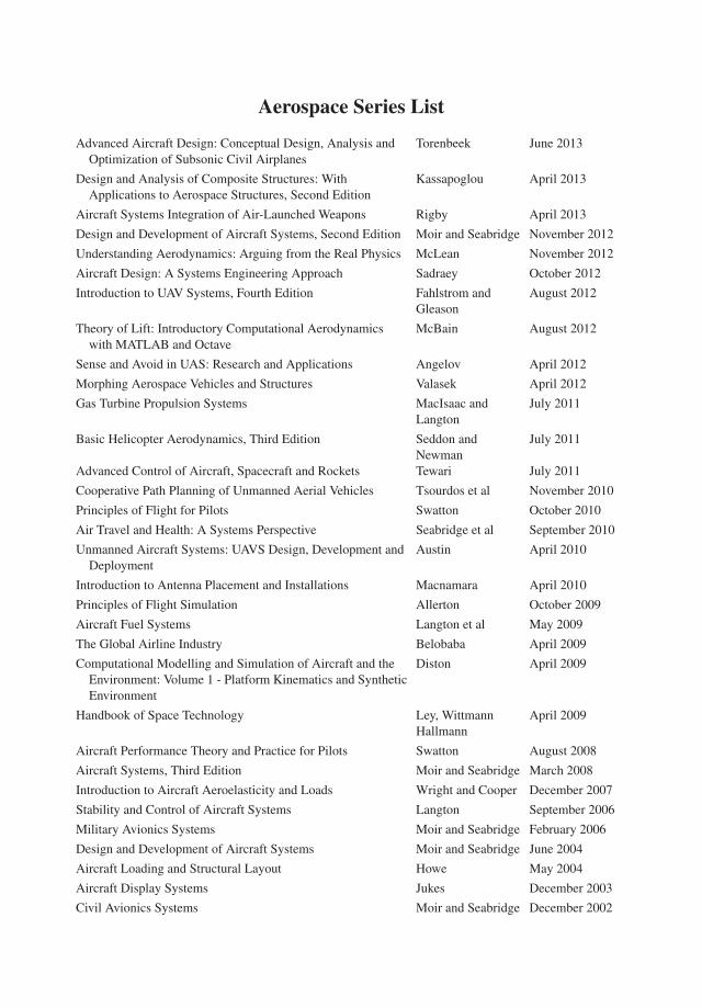
Aerospace Series List
Advanced Aircraft Design: Conceptual Design, Analysis andOptimization of Subsonic Civil Airplanes
Torenbeek June 2013
Design and Analysis of Composite Structures: WithApplications to Aerospace Structures, Second Edition
Kassapoglou April 2013
Aircraft Systems Integration of Air-Launched Weapons Rigby April 2013
Design and Development of Aircraft Systems, Second Edition Moir and Seabridge November 2012
Understanding Aerodynamics: Arguing from the Real Physics McLean November 2012
Aircraft Design: A Systems Engineering Approach Sadraey October 2012
Introduction to UAV Systems, Fourth Edition Fahlstrom andGleason
August 2012
Theory of Lift: Introductory Computational Aerodynamicswith MATLAB and Octave
McBain August 2012
Sense and Avoid in UAS: Research and Applications Angelov April 2012
Morphing Aerospace Vehicles and Structures Valasek April 2012
Gas Turbine Propulsion Systems MacIsaac andLangton
July 2011
Basic Helicopter Aerodynamics, Third Edition Seddon andNewman
July 2011
Advanced Control of Aircraft, Spacecraft and Rockets Tewari July 2011
Cooperative Path Planning of Unmanned Aerial Vehicles Tsourdos et al November 2010
Principles of Flight for Pilots Swatton October 2010
Air Travel and Health: A Systems Perspective Seabridge et al September 2010
Unmanned Aircraft Systems: UAVS Design, Development andDeployment
Austin April 2010
Introduction to Antenna Placement and Installations Macnamara April 2010
Principles of Flight Simulation Allerton October 2009
Aircraft Fuel Systems Langton et al May 2009
The Global Airline Industry Belobaba April 2009
Computational Modelling and Simulation of Aircraft and theEnvironment: Volume 1 - Platform Kinematics and SyntheticEnvironment
Diston April 2009
Handbook of Space Technology Ley, WittmannHallmann
April 2009
Aircraft Performance Theory and Practice for Pilots Swatton August 2008
Aircraft Systems, Third Edition Moir and Seabridge March 2008
Introduction to Aircraft Aeroelasticity and Loads Wright and Cooper December 2007
Stability and Control of Aircraft Systems Langton September 2006
Military Avionics Systems Moir and Seabridge February 2006
Design and Development of Aircraft Systems Moir and Seabridge June 2004
Aircraft Loading and Structural Layout Howe May 2004
Aircraft Display Systems Jukes December 2003
Civil Avionics Systems Moir and Seabridge December 2002

ADVANCED AIRCRAFTDESIGNCONCEPTUAL DESIGN, ANALYSISAND OPTIMIZATION OF SUBSONICCIVIL AIRPLANES
Egbert TorenbeekDelft University of Technology, The Netherlands
A John Wiley & Sons, Ltd., Publication

C© 2013 Egbert TorenbeekAll rights reserved 2013 John Wiley and Sons, Ltd.
Registered officeJohn Wiley & Sons Ltd, The Atrium, Southern Gate, Chichester, West Sussex, PO19 8SQ, United Kingdom
For details of our global editorial offices, for customer services and for information about how to apply forpermission to reuse the copyright material in this book please see our website at www.wiley.com.
The right of the author to be identified as the author of this work has been asserted in accordance with the Copyright,Designs and Patents Act 1988.
All rights reserved. No part of this publication may be reproduced, stored in a retrieval system, or transmitted, in anyform or by any means, electronic, mechanical, photocopying, recording or otherwise, except as permitted by the UKCopyright, Designs and Patents Act 1988, without the prior permission of the publisher.
Wiley also publishes its books in a variety of electronic formats. Some content that appears in print may not beavailable in electronic books.
Designations used by companies to distinguish their products are often claimed as trademarks. All brand names andproduct names used in this book are trade names, service marks, trademarks or registered trademarks of theirrespective owners. The publisher is not associated with any product or vendor mentioned in this book.
Limit of Liability/Disclaimer of Warranty: While the publisher and author have used their best efforts in preparingthis book, they make no representations or warranties with respect to the accuracy or completeness of the contents ofthis book and specifically disclaim any implied warranties of merchantability or fitness for a particular purpose. It issold on the understanding that the publisher is not engaged in rendering professional services and neither thepublisher nor the author shall be liable for damages arising herefrom. If professional advice or other expertassistance is required, the services of a competent professional should be sought.
MATLAB R© is a trademark of The MathWorks, Inc. and is used with permission. The MathWorks does not warrantthe accuracy of the text or exercises in this book. This book’s use or discussion of MATLAB R© software or relatedproducts does not constitute endorsement or sponsorship by The MathWorks of a particular pedagogical approach orparticular use of the MATLAB R© software.
Library of Congress Cataloging-in-Publication Data
Torenbeek, Egbert.Advanced aircraft design : conceptual design, analysis, and optimization of subsonic civil airplanes / Egbert
Torenbeek.pages cm
Includes bibliographical references and index.ISBN 978-1-118-56811-8 (cloth)
1. Transport planes–Design and construction. 2. Jet planes–Design and construction.3. Airplanes–Performance. I. Title.
TL671.2.T668 2013629.133’34–dc23
2013005449
A catalogue record for this book is available from the British Library.
ISBN: 9781119969303
Typeset in 10/12pt Times by Aptara Inc., New Delhi, India
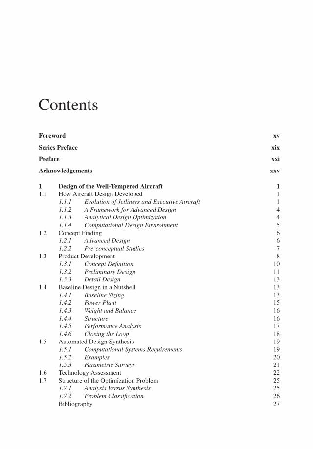
Contents
Foreword xv
Series Preface xix
Preface xxi
Acknowledgements xxv
1 Design of the Well-Tempered Aircraft 11.1 How Aircraft Design Developed 1
1.1.1 Evolution of Jetliners and Executive Aircraft 11.1.2 A Framework for Advanced Design 41.1.3 Analytical Design Optimization 41.1.4 Computational Design Environment 5
1.2 Concept Finding 61.2.1 Advanced Design 61.2.2 Pre-conceptual Studies 7
1.3 Product Development 81.3.1 Concept Definition 101.3.2 Preliminary Design 111.3.3 Detail Design 13
1.4 Baseline Design in a Nutshell 131.4.1 Baseline Sizing 131.4.2 Power Plant 151.4.3 Weight and Balance 161.4.4 Structure 161.4.5 Performance Analysis 171.4.6 Closing the Loop 18
1.5 Automated Design Synthesis 191.5.1 Computational Systems Requirements 191.5.2 Examples 201.5.3 Parametric Surveys 21
1.6 Technology Assessment 221.7 Structure of the Optimization Problem 25
1.7.1 Analysis Versus Synthesis 251.7.2 Problem Classification 26Bibliography 27

vi Contents
2 Early Conceptual Design 312.1 Scenario and Requirements 31
2.1.1 What Drives a Design? 312.1.2 Civil Airplane Categories 332.1.3 Top Level Requirements 35
2.2 Weight Terminology and Prediction 362.2.1 Method Classification 362.2.2 Basic Weight Components 372.2.3 Weight Limits 392.2.4 Transport Capability 39
2.3 The Unity Equation 412.3.1 Mission Fuel 432.3.2 Empty Weight 442.3.3 Design Weights 45
2.4 Range Parameter 462.4.1 Aerodynamic Efficiency 472.4.2 Specific Fuel Consumption and Overall Efficiency 482.4.3 Best Cruise Speed 49
2.5 Environmental Issues 512.5.1 Energy and Payload Fuel Efficiency 512.5.2 ‘Greener by Design’ 54Bibliography 56
3 Propulsion and Engine Technology 593.1 Propulsion Leading the Way 593.2 Basic Concepts of Jet Propulsion 60
3.2.1 Turbojet Thrust 603.2.2 Turbofan Thrust 613.2.3 Specific Fuel Consumption 623.2.4 Overall Efficiency 633.2.5 Thermal and Propulsive Efficiency 633.2.6 Generalized Performance 653.2.7 Mach Number and Altitude Effects 66
3.3 Turboprop Engines 673.3.1 Power and Specific Fuel Consumption 673.3.2 Generalized Performance 683.3.3 High Speed Propellers 69
3.4 Turbofan Engine Layout 703.4.1 Bypass Ratio Trends 703.4.2 Rise and Fall of the Propfan 723.4.3 Rebirth of the Open Rotor? 74
3.5 Power Plant Selection 743.5.1 Power Plant Location 753.5.2 Alternative Fuels 763.5.3 Aircraft Noise 77Bibliography 78

Contents vii
4 Aerodynamic Drag and Its Reduction 814.1 Basic Concepts 81
4.1.1 Lift, Drag and Aerodynamic Efficiency 824.1.2 Drag Breakdown and Definitions 83
4.2 Decomposition Schemes and Terminology 844.2.1 Pressure and Friction Drag 844.2.2 Viscous Drag 854.2.3 Vortex Drag 854.2.4 Wave Drag 86
4.3 Subsonic Parasite and Induced Drag 874.3.1 Parasite Drag 874.3.2 Monoplane Induced Drag 904.3.3 Biplane Induced Drag 914.3.4 Multiplane and Boxplane Induced Drag 94
4.4 Drag Polar Representations 954.4.1 Two-term Approximation 954.4.2 Three-term Approximation 964.4.3 Reynolds Number Effects 974.4.4 Compressibility Correction 98
4.5 Drag Prediction 994.5.1 Interference Drag 1004.5.2 Roughness and Excrescences 1014.5.3 Corrections Dependent on Operation 1024.5.4 Estimation of Maximum Subsonic L/D 1024.5.5 Low-Speed Configuration 104
4.6 Viscous Drag Reduction 1064.6.1 Wetted Area 1074.6.2 Turbulent Friction Drag 1084.6.3 Natural Laminar Flow 1084.6.4 Laminar Flow Control 1104.6.5 Hybrid Laminar Flow Control 1114.6.6 Gains, Challenges and Barriers of LFC 112
4.7 Induced Drag Reduction 1144.7.1 Wing Span 1144.7.2 Spanwise Camber 1154.7.3 Non-planar Wing Systems 115Bibliography 115
5 From Tube and Wing to Flying Wing 1215.1 The Case for Flying Wings 121
5.1.1 Northrop’s All-Wing Aircraft 1215.1.2 Flying Wing Controversy 1235.1.3 Whither All-Wing Airliners? 1245.1.4 Fundamental Issues 126
5.2 Allocation of Useful Volume 1275.2.1 Integration of the Useful Load 1285.2.2 Study Ground Rules 128

viii Contents
5.2.3 Volume Ratio 1295.2.4 Zero-Lift Drag 1305.2.5 Generalized Aerodynamic Efficiency 1315.2.6 Partial Optima 132
5.3 Survey of Aerodynamic Efficiency 1345.3.1 Altitude Variation 1345.3.2 Aspect Ratio and Span 1355.3.3 Engine-Airframe Matching 136
5.4 Survey of the Parameter ML/D 1385.4.1 Optimum Flight Conditions 1385.4.2 The Drag Parameter 139
5.5 Integrated Configurations Compared 1405.5.1 Conventional Baseline 1415.5.2 Is a Wing Alone Sufficient? 1435.5.3 Blended Wing Body 1445.5.4 Hybrid Flying Wing 1465.5.5 Span Loader 147
5.6 Flying Wing Design 1495.6.1 Hang-Ups or Showstopper? 1495.6.2 Structural Design and Weight 1505.6.3 The Flying Wing: Will It Fly? 151Bibliography 152
6 Clean Sheet Design 1576.1 Dominant and Radical Configurations 157
6.1.1 Established Configurations 1576.1.2 New Paradigms 159
6.2 Morphology of Shapes 1596.2.1 Classification 1606.2.2 Lifting Systems 1606.2.3 Plan View Classification 1626.2.4 Strut-Braced Wings 1636.2.5 Propulsion and Concept Integration 164
6.3 Wing and Tail Configurations 1656.3.1 Aerodynamic Limits 1656.3.2 The Balanced Design 1676.3.3 Evaluation 1686.3.4 Relaxed Inherent Stability 169
6.4 Aircraft Featuring a Foreplane 1696.4.1 Canard Configuration 1706.4.2 Three-Surface Aircraft 172
6.5 Non-Planar Lifting Systems 1736.5.1 Transonic Boxplane 1736.5.2 C-Wing 175
6.6 Joined Wing Aircraft 1776.6.1 Structural Principles and Weight 1786.6.2 Aerodynamic Aspects 179

Contents ix
6.6.3 Stability and Control 1806.6.4 Design Integration 181
6.7 Twin-Fuselage Aircraft 1826.7.1 Design Integration 185
6.8 Hydrogen-Fuelled Commercial Transports 1866.8.1 Properties of LH2 1876.8.2 Fuel System 1886.8.3 Handling Safety, Economics and Logistics 189
6.9 Promising Concepts 189Bibliography 190
7 Aircraft Design Optimization 1977.1 The Perfect Design: An Illusion? 1977.2 Elements of Optimization 198
7.2.1 Design Parameters 1987.2.2 Optimal Control and Discrete-Variable Optimization 1997.2.3 Basic Terminology 2007.2.4 Single-Objective Optimization 2017.2.5 Unconstrained Optimizer 2027.2.6 Constrained Optimizer 204
7.3 Analytical or Numerical Optimization? 2067.3.1 Analytical Approach 2067.3.2 Multivariate Optimization 2077.3.3 Unconstrained Optimization 2097.3.4 Constrained Optimization 2107.3.5 Response Surface Approximation 2117.3.6 Global Models 212
7.4 Large Optimization Problems 2137.4.1 Concept Sizing and Evaluation 2137.4.2 Multidisciplinary Optimization 2147.4.3 System Decomposition 2157.4.4 Multilevel Optimization 2177.4.5 Multi-Objective Optimization 218
7.5 Practical Optimization in Conceptual Design 2197.5.1 Arguments of the Sceptic 2197.5.2 Problem Structure 2207.5.3 Selecting Selection Variables 2207.5.4 Design Sensitivity 2227.5.5 The Objective Function 222Bibliography 223
8 Theory of Optimum Weight 2298.1 Weight Engineering: Core of Aircraft Design 229
8.1.1 Prediction Methods 2308.1.2 Use of Statistics 231

x Contents
8.2 Design Sensitivity 2328.2.1 Problem Structure 2328.2.2 Selection Variables 233
8.3 Jet Transport Empty Weight 2348.3.1 Weight Breakdown 2348.3.2 Wing Structure (Item 10) 2358.3.3 Fuselage Structure (Item 11) 2368.3.4 Empennage Structure (Items 12 and 13) 2378.3.5 Landing Gear Structure (Item 14) 2388.3.6 Power Plant and Engine Pylons (Items 2 and 15) 2388.3.7 Systems, Furnishings and Operational Items (Items 3, 4 and 5) 2388.3.8 Operating Empty Weight: Example 239
8.4 Design Sensitivity of Airframe Drag 2398.4.1 Drag Decomposition 2408.4.2 Aerodynamic Efficiency 242
8.5 Thrust, Power Plant and Fuel Weight 2438.5.1 Installed Thrust and Power Plant Weight 2438.5.2 Mission Fuel 2458.5.3 Propulsion Weight Penalty 2458.5.4 Wing and Propulsion Weight Fraction 2488.5.5 Optimum Weight Fractions Compared 249
8.6 Take-Off Weight, Thrust and Fuel Efficiency 2498.6.1 Maximum Take-Off Weight 2498.6.2 Installed Thrust and Fuel Energy Efficiency 2518.6.3 Unconstrained Optima Compared 2528.6.4 Range for Given MTOW 2538.6.5 Extended Range Version 254
8.7 Summary and Reflection 2548.7.1 Which Figure of Merit? 2548.7.2 Conclusion 2568.7.3 Accuracy 257Bibliography 257
9 Matching Engines and Airframe 2619.1 Requirements and Constraints 2619.2 Cruise-Sized Engines 262
9.2.1 Installed Take-Off Thrust 2629.2.2 The Thumbprint 263
9.3 Low Speed Requirements 2659.3.1 Stalling Speed 2659.3.2 Take-Off Climb 2669.3.3 Approach and Landing Climb 2669.3.4 Second Segment Climb Gradient 267
9.4 Schematic Take-Off Analysis 2679.4.1 Definitions of Take-Off Field Length 2689.4.2 Take-Off Run 269

Contents xi
9.4.3 Airborne Distance 2709.4.4 Take-Off Distance 2709.4.5 Generalized Thrust and Span Loading Constraint 2719.4.6 Minimum Thrust for Given TOFL 273
9.5 Approach and Landing 2739.5.1 Landing Distance Analysis 2739.5.2 Approach Speed and Wing Loading 274
9.6 Engine Selection and Installation 2759.6.1 Identifying the Best Match 2759.6.2 Initial Engine Assessment 2769.6.3 Engine Selection 277Bibliography 278
10 Elements of Aerodynamic Wing Design 28110.1 Introduction 281
10.1.1 Problem Structure 28210.1.2 Relation to Engine Selection 283
10.2 Planform Geometry 28310.2.1 Wing Area and Design Lift Coefficient 28510.2.2 Span and Aspect Ratio 286
10.3 Design Sensitivity Information 28610.3.1 Aerodynamic Efficiency 28710.3.2 Propulsion Weight Contribution 28810.3.3 Wing and Tail Structure Weight 28910.3.4 Wing Penalty Function and MTOW 290
10.4 Subsonic Aircraft Wing 29110.4.1 Problem Structure 29110.4.2 Unconstrained Optima 29210.4.3 Minimum Propulsion Weight Penalty 29410.4.4 Accuracy 294
10.5 Constrained Optima 29510.5.1 Take-Off Field Length 29610.5.2 Tank Volume 29610.5.3 Wing and Tail Weight Fraction 29710.5.4 Selection of the Design 297
10.6 Transonic Aircraft Wing 29810.6.1 Geometry 29810.6.2 Wing Drag in the Design Condition 29910.6.3 Modified Wing Penalty Function 30010.6.4 Thickness Ratio Limit 30110.6.5 WPF Affected by Sweep Angle and Thickness Ratio 303
10.7 Lift Coefficient and Aspect Ratio 30410.7.1 Partial Optima 30410.7.2 Constraints 30610.7.3 Refining the Optimization 307

xii Contents
10.8 Detailed Design 30910.8.1 Taper and Lift Distribution 30910.8.2 Camber and Twist Distribution 31010.8.3 Forward Swept Wing (FSW) 31110.8.4 Wing-Tip Devices 312
10.9 High Lift Devices 31310.9.1 Aerodynamic Effects 31310.9.2 Design Aspects 314Bibliography 315
11 The Wing Structure and Its Weight 31911.1 Introduction 319
11.1.1 Statistics can be Useful 31911.1.2 Quasi-Analytical Weight Prediction 320
11.2 Methodology 32111.2.1 Weight Breakdown and Structural Concept 32111.2.2 Basic Approach 32311.2.3 Load Factors 324
11.3 Basic Wing Box 32611.3.1 Bending due to Lift 32611.3.2 Bending Material 33111.3.3 Shear Material 33311.3.4 In-Plane Loads and Torsion 33411.3.5 Ribs 334
11.4 Inertia Relief and Design Loads 33511.4.1 Relief due to Fixed Masses 33611.4.2 Weight-Critical UL and Design Weights 337
11.5 Non-Ideal Weight 33811.5.1 Non-Taper, Joints and Fasteners 33911.5.2 Fail Safety and Damage Tolerance 34011.5.3 Manholes and Access Hatches 34011.5.4 Reinforcements, Attachments and Support Structure 34111.5.5 Dynamic Over Swing 34211.5.6 Torsional Stiffness 342
11.6 Secondary Structures and Miscellaneous Items 34411.6.1 Fixed Leading Edge 34511.6.2 Leading Edge High-Lift Devices 34511.6.3 Fixed Trailing Edge 34611.6.4 Trailing Edge Flaps 34611.6.5 Flight Control Devices 34811.6.6 Tip Structures 34811.6.7 Miscellaneous Items 349
11.7 Stress Levels in Aluminium Alloys 34911.7.1 Lower Panels 35011.7.2 Upper Panels 35011.7.3 Shear Stress in Spar Webs 352

Contents xiii
11.8 Refinements 35211.8.1 Tip Extensions 35211.8.2 Centre Section 35311.8.3 Compound Taper 35411.8.4 Exposed Wing Lift 35511.8.5 Advanced Materials 355
11.9 Application 35711.9.1 Basic Ideal Structure Weight 35711.9.2 Refined Ideal Structure Weight 35811.9.3 Wing Structure Weight 35911.9.4 Accuracy 35911.9.5 Conclusion 360Bibliography 361
12 Unified Cruise Performance 36312.1 Introduction 363
12.1.1 Classical Solutions 36312.1.2 Unified Cruise Performance 36412.1.3 Specific Range and the Range Parameter 365
12.2 Maximum Aerodynamic Efficiency 36612.2.1 Logarithmic Drag Derivatives 36812.2.2 Interpretation of Log-Derivatives 36912.2.3 Altitude Constraint 370
12.3 The Parameter ML/D 37112.3.1 Subsonic Flight Mach Number 37112.3.2 Transonic Flight Mach Number 372
12.4 The Range Parameter 37412.4.1 Unconstrained Optima 37412.4.2 Constrained Optima 37612.4.3 Interpretation of ηM 37612.4.4 Optimum Cruise Condition 378
12.5 Range in Cruising Flight 37912.5.1 Breguet Range Equation 37912.5.2 Continuous Cruise/Climb 38012.5.3 Horizontal Cruise, Constant Speed 38112.5.4 Horizontal Cruise, Constant Lift Coefficient 381
12.6 Cruise Procedures and Mission Fuel 38212.6.1 Subsonic Flight 38212.6.2 Transonic Flight 38312.6.3 Cruise Fuel 38412.6.4 Mission Fuel 38512.6.5 Reserve Fuel 387
12.7 Reflection 38812.7.1 Summary of Results 38812.7.2 The Design Connection 389Bibliography 390

xiv Contents
A Volumes, Surface and Wetted Areas 393A.1 Wing 393A.2 Fuselage 394A.3 Tail Surfaces 395A.4 Engine Nacelles and Pylons 395A.5 Airframe Wetted Area 395
Bibliography 396
B International Standard Atmosphere 397
C Abbreviations 399
Index 403

Foreword
Aircraft design is a very fascinating and motivating topic for pupils, students and youngresearchers. They are interested in the engineering subject, knowing that this is a complexsubject with the aerodynamics to make the aircraft fly, with the structural layout to accom-modate some sort of payload and keep the integrity of the vehicle, and with the aspects offlight mechanics to stabilize and control the aircraft, just to mention the basic aspects. Inthe scientific world, the faculties of aerospace engineering follow this principle and considerthe basic disciplines such as aerodynamics, lightweight structures, flight mechanics and spacetechnologies as the fundamentals to provide the envelope for aeronautics and space for theengineering students. Aircraft design is normally not considered a specific discipline worthyof inaugurating a specific chair. Some exceptions, however, do exist. The Delft University ofTechnology was one of the first Technical Universities in Europe to inaugurate a specific chairfor aircraft design, and with the nomination of Egbert Torenbeek in 1980 they found a verystrong personality who has further developed the scientific approach and methodology forpreliminary aircraft design. The Technical University of Munchen (TUM) in 1995 establisheda new chair for aeronautical engineering with the specific focus on aircraft design and I wasnominated for this chair. This shows that the focus of integrated aircraft design has only slowlyfound its role in the scientific world.
A similar view can also be seen in industry. During my time at Airbus, the Technicalmanagement was not fully convinced that the aircraft design had the same importance androle as the big engineering departments like aerodynamics, structures, systems, propulsionand cabin. On the other hand, Airbus suddenly discovered about some ten years ago withsome urgency that they did not have enough engineers with sufficient global knowledge tounderstand the total aircraft as a complex system. A huge push was then started to developwithin the company ‘aircraft architects’ and ‘aircraft integrators’, also highlighting, that thediscipline ‘aircraft design’ with its specific knowledge and experience is of prime importance.
There is, however, a huge discrepancy between industry and research centres or universitieswith regard to integrated aircraft design. Industry claims and wishes that universities as wellas research centres should not look too closely at aircraft integration; this is seen as the uniquerole of industry. Industry claims to be the only partner, who knows the market demand andwho has to consider the right design approach with respect to time, cost, quality and riskbefore deciding on a new product and its introduction onto the market. Industry thereforewould like to keep the universities out of the domain of aircraft design, and do not want togive too many details to the scientific community, on how to prepare an innovative aircraftdesign. On the other hand, students and young engineers have to be trained and have to learn

xvi Foreword
and understand the basic features of aircraft design at university during their studies. Studentsare primarily not so much fascinated by details of low speed aerodynamics or the detaileddesign of a fuselage frame compared to designing an aircraft. They are motivated to developaircraft models, sailplanes and want to know how to design this sort of flying vehicles andwhat is the approach to defining the size of the wing, tailplane and engines. The scientificapproach to aircraft design is therefore a major topic for the universities and has to be part ofthe aeronautical engineering curriculum.
There are several good books on the market, one of the best in my view written by EgbertTorenbeek. But these books were written mainly in the years 1980 to 1990 and have establisheda lot of design data, collected from aircraft designs of the 1960s to the 1980s. Also at that timethe focus was on the preliminary aircraft design, starting from the weight breakdown, definingwing and tailplane areas and checking stability and controllability.
Over the past twenty years, computer capabilities have improved considerably and a lot ofaircraft design software programs are distributed on the market with some quite good successand good results as long as the aircraft design follows the classical design features. The newdimension which has been added to the aircraft design process is called multidisciplinaryoptimization (MDO) methodologies. The continuous increase in computer speed and capacityhas first allowed FEM methods for all sort of structural layout and CFD methods for theaerodynamic design of aircraft components and the total aircraft to be developed. The next stepswere then multidisciplinary tools, first, to integrate the different design boundaries such as high-speed and low-speed aerodynamics, and in a next step, today the multidisciplinary methodspermit an aircraft to be designed by using the integration of aerodynamic, structural and flightmechanics design constraints and by using multidisciplinary optimization methodologies.MDO is the new design methodology for all aircraft design features and nearly all papers inaircraft design are now using some sort of multidisciplinary optimization approach.
I remember that some five years ago – sitting on the Wolga beach in Samara (Russia) duringa seminar for aircraft design professors – we had some lively discussions on some aircraftoptimization problems. We also learned that Egbert Torenbeek was working on a new bookabout advanced aircraft design. However, he had some doubts whether there were still enoughpeople interested in learning about the complex aspects of advanced aircraft design, while allinstitutions are just working with big and complex software tools. He was not sure whetherthe aircraft community would like to see such a book. We encouraged him very much tocontinue. Egbert Torenbeek has a very high reputation among the aircraft design professorsand I am very happy to see that he finally managed to finish his book. Having read severalchapters, I really believe that his way of addressing a quasi-analytical approach to aircraftdesign is very valuable and an excellent complementary way to the common normal approachof computerized analysis.
In the next decades, the aeronautical industry will be faced with considerable new environ-mental challenges. The past success of air transport will be confronted with new questionslike ‘Which optimal flight altitude will have minimum impact on the atmosphere?’ or ‘Howcan new aircraft concepts with new engine options like Open Rotors improve fuel efficiencyand also the environmental footprint for a given mission?’ I am convinced that new aircraftconcepts for the future will be required to cope better with the increasing environmentalrestrictions which air transport will have to face. This book will be of great help and interestfor these sorts of questions where the impact of new boundary conditions will have to beanalyzed and investigated and where the large industrial computer software is not yet properly

Foreword xvii
validated and verified. The physics-based approach of this book will help to better qualify thedominant parameters for different new and unconventional aircraft concepts and also help thereader to understand the assessment of benefits and risks of these concepts.
I wish this book a lot of success and hope that my colleagues from industry and the scientificcommunity and especially the young scientists will appreciate this book as well.
Prof.h.c. Dr.-Ing. Dr.h.c. Dieter SchmittAeronautical consultant. Former Head of Future Projects at Airbus SASFormer Professor at TU Munchen, Institute of Aeronautical Engineering
Blagnac, 25th November 2012

Series Preface
The Aerospace Series covers a wide range of aerospace vehicles and their systems, compre-hensively covering aspects of structural and system design in theoretical and practical terms.This book complements the others in the Series by looking at the concept phase of design ofthe aircraft.
Aircraft Design is an early stage of activity in the evolution of an aircraft project starting atthe concept and enduring until the preliminary design. It is time for broad thinkers, for peopleprepared to take risks and to understand the big picture. At this stage of an aircraft project theimportant issues are the shape of the aircraft, its fuel and load carrying capability and its massleading to an assessment of its suitability to perform a mission. From ideas generated duringthis process will gradually emerge a solution that can be committed to design and manufacture.
The author introduces the topic with an overview of the advanced design process, consideringdesign requirements and methodologies, considerations driving a design, followed by anexample of early design mass prediction. The next stage deals with the selection of theaircraft general arrangement, an essential but complex issue which concerns new technologyapplications and operational properties. Decisions made at this stage involve and affect manydisciplines in a project – many of those dealt with in other books in the Series. This isthe challenging stage of integration and the role of the Chief Designer. Then an approach toexplicit optimization by means of quasi-analytic relations is developed and the book concludeswith analytical examples that are essential to advanced design in general and optimization inparticular.
This is performed in a clear and concise manner to make the book a comprehensive treatiseon the subject of advanced design of subsonic civil aircraft from initial sizing through to finaldrag calculations. There are lessons to be learned here also for military aircraft designers. Itwill be of great use to undergraduate and postgraduate students as well as to practitioners inthe field of aircraft design and scientists in aerospace research and development. The authorhas given his work authority by basing it on many years of research at the Delft University ofTechnology where this subject is taught under the auspices of a Chair in the subject.
Peter Belobaba, Jonathan Cooper and Allan Seabridge

Preface
I don’t know why people are frightened by new ideas.It’s the old ones that frighten me.
—John Cage, American composer
Advanced Design (AD) is the name for the activity of a team of engineers and analysts duringthe early stages of an aircraft design and development process. The point of departure is a setof top level requirements specifying payload/range capabilities, cabin accommodation, flightperformance, operational, and environmental characteristics. The first design activity generatesa conceptual baseline configuration defined by (electronic) drawings of its layout, a databasespecifying the physical characteristics and the essential technological assumptions, and anassessment of the feasibility of complying with the requirements. Designers may proposeone or several concepts which are subsequently refined and compared during the secondadvanced design stage called the preliminary design. Conceptual design and preliminarydesign are crucial phases in the development process during which creativity and ingenuityare of paramount importance to support the far-reaching decisions that can make or break theprogramme as a whole.
Since the 1970s, aircraft design has become the subject of academic education and researchat an increasing number of academic institutions which have an aerospace curriculum. Manytopics typical of aircraft design projects are nowadays covered in academic courses, and edu-cational handbooks, and an abundance of software tools have become available to supportstudents in their design exercises. Although many academic courses pay modest attentionto aircraft design, a design-oriented approach to the traditional aeronautical disciplines cancontribute to an improved understanding of aeronautical science as a whole. However, designhandbooks are essentially based on existing or even obsolete technology and may produceunrealistic results when applied to future advanced aircraft design projects. And design tech-nologies are becoming more complicated due to the introduction of integrated product designtechnology and multidisciplinary design optimization, subjects not covered in most handbooks.
In writing this book it has been the author’s aim to contribute to the advancement of aircraftdesign (teaching) by emphasizing clear design thinking rather than sophisticated computationor using a huge collection of statistical information. Another orientation came from industrialdesign staff and academic teachers who indicated that they would be particularly interested inassessments of unusual aircraft concepts and examples of practical optimization in the earlydesign stage. It was decided to focus on subsonic transports and executive (business) aircraft.The present text combines the author’s academic teaching approach with numerous results

xxii Preface
from in-depth investigations on advanced technologies and innovative aircraft configurationsreported since the 1970s. Particular attention is paid to research by staff of the aircraft designchair at Delft University of Technology between 1980 and 2000. Although some informationabout design methodologies and statistical data of recent airplane models are included, theresult is not intended to be used as a handbook in the first place. Most of the materialpresented is readily understood by those who have previous experience with airplane design.The niche market for this book is formed by MSc and PhD students doing design-orientedresearch, academic staff teaching design, advanced airplane designers and applied scientistsat aeronautical research laboratories.
The contents of this book can be subdivided into the following groups of chapters.
1. Chapters 1 and 2 offer an overview of the advanced design process, design requirementsand methodologies, considerations driving a design, and an example of early design weightprediction by applying the unity equation. Chapter 3 is a summary of modern gas turbineengine technology and configurations, defining characteristics such as overall efficiencyand thrust lapse rates to be used in subsequent chapters. Chapter 4 introduces the readerto different methods of decomposing and predicting aerodynamic drag and to technologiesfor drag reduction. Many of these topics are familiar to experienced designers; some ofthem may be eye-openers to students or researchers.
2. Chapters 5 and 6 focus on the choice of the aircraft’s general arrangement. This is anessential but complex issue since numerous decisions with respect to (new) technologyapplications and operational properties are involved and many of these decisions have ahighly interdisciplinary sphere of influence. Chapter 5 deals with the basic question of howto allocate the useful load inside a generic combination of a wing and a fuselage body. Inthe past, this question gave rise to a discussion between analysts, some in favour of andsome against the flying wing. However, the optimum configuration is not necessarily anall-wing aircraft or a traditional tube and wing (TAW). For instance, the blended wing bodycould become a viable alternative. Chapter 6 deals with clean-sheet design of aircraft whichdo not have a payload inside the wing. A qualitative assessment is made of several unusualconcepts such as canard and three-surface configurations, highly non-linear lifting systems,the joined wing, twin-fuselage and hydrogen-propelled aircraft. An unusual configurationmay be the best solution in the case of a dominant performance requirement or geometricconstraint.
3. Chapters 7 to 10 are intended to develop an approach to explicit optimization by means ofquasi-analytic relations between figures of merit – such as the maximum take-off weightor energy efficiency – and primary selection variables. Chapter 7 offers an overview of thegeneral optimization problem, terminology and strategies to identify a feasible solution.Chapter 8 is primarily devoted to weight engineering, an essential discipline of aircraftdesign. Design-sensitive expressions are derived for the gross weight and its components.These are intended to show how a baseline design may be modified to improve differentfigures of merit, disregarding design constraints. Chapter 9 deals with matching the enginesto the airframe by incorporating constraints on the installed engine power or thrust derivedfrom high- and low-speed performance requirements. Chapter 10 derives analytical criteriafor optimum wing planform area, aspect ratio, sweep angle and thickness ratio. Results areillustrated for a subsonic freighter and a transonic jetliner, both with a classical generalarrangement.

Preface xxiii
4. The last chapters deal with subjects with a predominantly analytical character that areessential to advanced design in general and optimization in particular. Chapter 11 presentsthe derivation of a wing structure weight prediction methodology which satisfies mostof the requirements for application to conceptual optimization. Chapter 12 explains whytraditional criteria for optimum cruising flight cannot be applied to high-speed airplanes.The theory is unified for (optimum) cruise performance analysis of propeller- as well asjet-powered aircraft and includes a simplified estimation of mission and reserve fuel.
The quasi-analytical character of the present approach to conceptual design optimizationcannot replace rigorous numerical methods. Intended primarily to support advanced designersand researchers and help them to understand the complex relationships between the effects onairplane characteristics of varying design parameters, the results may also be useful to validatecomplex design sizing and optimization programs. Moreover, the simplicity of the analyticalcriteria is useful to quickly estimate the effects of introducing alternative technologies forpropulsion and airframe design. If used judiciously, quasi-analytical relationships can besufficiently accurate to successfully answer ‘what-if’ questions and make trade-off studiessuch as weight growth problems, specification changes and considering derivative aircraft.From this perspective, the present book can be seen as a tribute to prominent scientists anddesigners from the past – such as I.H. Ashkenas, R.T. Jones, D. Kuchemann, and G.H. Lee –who pioneered this approach during the era when computer-based aircraft design technologydid not yet exist. The author hopes that this effort will contribute to the way of thinking ofthose who consider conceptual design as an art rather than a science: the art of conceiving andbuilding well-tempered aircraft.

Acknowledgements
I am indebted to chair holders Michel van Tooren and Theo van Holten who offered me thehospitality of their disciplinary group SEAD and to Michiel Haanschoten for his professionalassistance with ICT problems. I am grateful to the staff of DAR – in particular, ArvindGangoli Rao, Gianfranco la Rocca, Dries Visser, Roelof Vos and Mark Voskuijl – for frequentinteresting communications on propulsion and aircraft design and for giving valuable feedbackafter reading draft versions of chapters. Thanks are also due to Evert Jesse of ADSE who hasbeen my prime consultant on the subject of weight prediction.
This book would never have been realized without the support of my wife. Dear NellieVolker, considering my weakness to find a proper balance between the dedication you deserveand my insatiable fascination for aeronautical engineering, I am eternally grateful that youtolerated my periods of distraction and continued to respect me during the more than 10 yearsof writing this book.
E. TorenbeekDelft University of Technology, The Netherlands, April 2013

1Design of the Well-TemperedAircraft
Let no new improvement in flying and flying equipment pass us by.—Bill Boeing (1928)
As our industry has matured . . . we have become increasingly enslaved to our data bases ofpast successful achievements. Increased competitive pressures and emphasis on control of rapidlyescalating costs have combined to preclude the level of bold risks taking in exploring possible newconfiguration options that might offer some further increase in performance, etc., but for whichno adequate data exist to aid development.
—J.H. McMasters [57] (2005)
1.1 How Aircraft Design Developed
1.1.1 Evolution of Jetliners and Executive Aircraft
The second half of the twentieth century has been truly revolutionary. In particular, the period1945–1960 produced some highly innovative projects which demonstrated that propulsionof transport aircraft by means of jet engines had become feasible. In combination with theappearance of the sweptback wing, this resulted in a jump in maximum cruising speedsfrom about 550 to more than 850 km/h (Figure 2.1). Having pioneered the B-47 swept-wingbomber, Boeing introduced its basic jet concept to the 367-80 tanker transport and later tothe 707 passenger transport; see Figure 1.1(a). This concept proved successful and has beenadopted for jetliners almost universally since the 1960s. When one realizes that in the early1950s designers did not yet avail themselves of the advantage of electronic computers, it willbe appreciated that this revolution in design technology was a monumental achievement.Modern jetliners are mostly low-wing designs with two or four engines installed in nacelles
mounted underneath and to the fore of the wing leading edge. It should not be concluded, how-ever, that since the Boeing 707 little progress has been made in configuration design. An earlyexample of an unusual mutation was the Sud-Est Caravelle, see Figure 1.1(b), the airliner that
Advanced Aircraft Design: Conceptual Design, Analysis and Optimization of Subsonic Civil Airplanes, First Edition. Egbert Torenbeek.
© 2013 by Egbert Torenbeek. Published 2013 by John Wiley & Sons, Ltd.

2 Advanced Aircraft Design
Figure 1.1 Prime examples of early post-WW II passenger aircraft. (a) Boeing 707 (1954): the first jet-powered airliner of US design. (b) Sud-Est Caravelle (1959): the first airliner with rear fuselage-mountedjet engines. (c) Fokker F 27 (1955): turboprop designed as a regional aircraft; still operational in 2012.(d) Gates Learjet 24B (1963): business jet designed in the early 1960s
pioneered jet engines attached to the rear fuselage. Even though this was a patented concept,several short-haul designs soon emerged with a similar layout and some of these were verysuccessful. The introduction of bypass engines (∼1960) and large turbofans (∼1970) furtherimproved the productivity and economy of jetliners. In combination with the strong worldwideeconomic expansion, this resulted in an unprecedented growth of air traffic and the almostcomplete extinction of competing modes of transportation over long distances, including thelong-haul piston-powered and even the brand-new turboprop-powered propeller airliners.Short-range jets initially suffered from poor low speed performances and high fuel expen-
diture. This market niche was filled by the four-engine Vickers Viscount and other turbopropsdesigned in the 1950s. The twin-engine Fokker Friendship – see Figure 1.1(c) – had its Rolls-Royce Dart turboprop engines mounted to the high-set wing. This configuration was difficult toimprove on and became the standard for similar propeller aircraft appearing later. Short-rangeturboprops have survived the twentieth century thanks to their excellent fuel economy and lowoperating costs. The idea of producing economy-size jets for large companies and wealthyindividuals came around 1960. A prime example of a successful business jet was the Learjetdepicted in Figure 1.1(d). Seating six in a slim fuselage (‘no-one walks about in a Cadillac’),it outperformed jetliners of its time in maximum speed. Learjet’s general arrangement, a low-wing design with engines attached to the rear fuselage and a high-set horizontal tail, has beenadopted on most executive jets.

Design of the Well-Tempered Aircraft 3
Since the introduction of the first jetliners, subsonic civil airplane technology developmenthas advanced in an evolutionary way. During the time span between 1950 and 2000, consider-able improvement has been accomplished in all technical areas, but none could be regarded asrevolutionary. The basic properties of traditional designs – such as lift, drag, weight and flightperformances – have become well understood. Computational methods supporting advanceddesign (AD) have steadily developed over a long period of time and a wealth of empiricalevidence confirms their accuracy. Consequently, aircraft with a conventional layout can bedeveloped with a high degree of confidence in the analysis. Though designing an innovativeconfiguration will always be challenging from an engineering viewpoint, its application in anindustrial project entails many challenges. This may lead to the situation that, after severalyears of costly configuration development, the project has to be terminated by a show stopper.It is also observed that airline management tends to avoid the uncertainties of an unusualgeneral arrangement and prefers the purchase of a traditional configuration.The conformity between modern airliners is not caused by the lack of conceptual creativity
of designers; arguments supporting this statement can be found in publications such as [12]and [14]. In fact, several innovative designs proposed during the last decennia of the twentiethcentury have not been developed into a for-sale aircraft because airlines were reluctant to orderthem for non-technical reasons. The following projects serve as examples.
• The Boeing 7J7 project of the 1980s – Figure 1.2 (a) – was a 150-seat airliner in whichnew technologies were integrated: a fly-by-wire control system, unducted fan (UDF) enginetechnology, advanced system and flight deck technologies, and advanced aluminium alloys.The 7J7 did not find favour with the airlines mainly because the anticipated spike in fuelprices did not occur.
• Boeing’s Sonic Cruiser – Figure 1.2 (b) – was designed to connect typical long-range citypairs atMach 0.95 or above. In a business class layout for 100 seats it would attract passengerswhowould bewilling to pay a fare premium to save several hours on long distance flightswithincreased comfort. The 300-seat version would be used for continental flights circumventingthe large hubs. The Sonic Cruiser became the victim of the aftermath of the events followingSeptember 2001, when airlines began to re-evaluate their business models resulting in a
(a) (b)
Figure 1.2 Boeing design projects which were not put into production. (a) 7J7 open rotor-powerednarrow body airliner of the 1980s. (b) Sonic Cruiser long-range wide bodyMach 0.95 airliner 1999–2002

4 Advanced Aircraft Design
preference for a more economical (slower) design which became the 787 [41]. The SonicCruiser was not developed into a for-sale product because potential customers would rathersee its advanced technology developed for integration into an airplane optimized for lowerMach numbers.
1.1.2 A Framework for Advanced Design
The non-recurring costs of a commercial aircraft development programme are so enormousthat even a relatively minor technical hiccup may be magnified into an unacceptable com-mercial risk. Consequently, a certain amount of conservatism is inherent in the developmentof civil aircraft design. In spite of this, conservatism in design is risky because it can lead tomissed opportunities when maturing aerodynamic, structural and propulsive technologies arebecoming available which find their best application in concepts different from the currentdominant configuration.In civil aircraft development programmes, far-reaching decisions concerning top level spec-
ifications, general arrangement, propulsion and enabling technologies are made before andduring the concept finding and the conceptual design phases. The preliminary design phaseis then entered during which the aircraft’s characteristics are defined in more detail, initialassumptions are verified and the feasibility and risk level of the project are investigated. A yearor more may elapse before management will decide to give the green light or withdraw fromfurther development. The next phase consists of design verification (testing) and detail designduring which major modifications of the basic configuration can be very labour-intensive andcostly. Clearly, ESDU’s trademark phrase, ‘get it right the first time’ is highly relevant for theinitial aircraft system design process.The observation has frequently been made that no more than a few percent of the pre-
production costs are attributed by a few designers committing to a large fraction of totalaircraft programme cost. In some cases this observation was made in favour of strengtheningthe advanced design capability of the aeronautical industry and/or the effort in academia tooffer excellent aircraft design teaching. Although these arguments are fully justified, it isnot always acknowledged that a large portion of aircraft programme costs is committed bymerely specifying the need for the particular vehicle rather than by defining its technical andoperational characteristics. If a new airplane has been developed for which no market exists,the project will be doomed to fail. The project design team cannot be blamed for a wronggo-ahead/exit decision and devoting more manpower to advanced design is not necessarily apanacea for avoiding misjudgement of the market. Although concept finding is not, in general,considered a part of the design project, it is at least as crucial to the success of a programmeas the actual concept development phase.
1.1.3 Analytical Design Optimization
Since advanced design is highly relevant to the company’s viability, one would expect that thediscipline of design optimization has traditionally received a great deal of attention from theaeronautical community – in fact, this is not the case. Until the time of large-scale computerapplications, only a few systematic efforts were made to develop a fundamental frameworkfor non-intuitive decision-making. Most of these were small-scale programs initiated by indi-viduals in research institutes and academia and their impact on the actual practice in design

Design of the Well-Tempered Aircraft 5
offices has not become entirely clear. Nevertheless, from the educational point of view, severalapproaches and trends from the past still deserve to be mentioned even though not all of themhave received widespread recognition.Early parametric surveys were made on a limited scale in the industry by experienced
designers. Until the 1960s, efforts to include optimization in conceptual design were basedon relatively simple methods with minimum take-off gross weight (TOGW) considered as thecriterion for the figure of merit. The analytical approach to sizing and improving a designin the conceptual stage was discussed in 1948 by Cherry and Croshere Jr [19]. Thoughtheir methodology was based on experience with propeller airplanes, its systematic characterappeared useful for jet aircraft as well. In 1958, G. Backhaus proposed a comprehensive(quasi-)analytical optimization of jet transports [20]. His article did not get the recognitionit deserved, probably because it was published in German. Another pioneer of the analyticalapproach to concept optimizationwasD. Kuchemann. During the 1960s, he and his co-workersat the Royal Aircraft Establishment in the UK developed analytical design methods of aircraftintended to fly over widely different ranges at different (subsonic, supersonic and hypersonic)speeds [21]. Part of this work was based on research in connection with the conception ofConcorde and was compiled in a unique book [1]. The elegance and lucidity of Kuchemann’sanalysis inspired the present author to initiate a systematic study of fundamental designconsiderations [27]; some of its results are included in the present book in a modified form.After the advent of computational design analysis and optimization technology in the 1970s,the (quasi-)analytical approach has appealed to only a few researchers; see, for example, W.H.Mason and B. Malone in [34, 35].
1.1.4 Computational Design Environment
During the first decennia after WWII, aircraft design was performed manually with the useof hand calculators and drawing boards. Despite the commercial success of several excellentairliners and business airplanes developed during this period, the ‘paper method’ is nowa-days considered too labor-intensive and ineffective. Since the 1970s, the advancement ofdesign technology changed fundamentally due to the availability of powerful computers andinteractive graphics devices. Simultaneously, significant progress was made in the fields ofcomputational engineering methods and numerical optimization, a trend set by early appli-cations in astronautics and chemical engineering. The aeronautical community initially paidmost attention to developing complex computer-based design synthesis programs such as thosereported in [62] and [68]. Although automated design optimization has attracted much atten-tion from research institutes such as NASA, reputed designers initially viewed these effortswith apprehension for reasons to be discussed in Chapter 2.The penetration of ICT into all fields of aeronautics since 1980 has drastically changed
the aircraft development scene. Whereas designs were traditionally almost exclusively pro-duced by the aircraft company’s design offices, reports presented at scientific conferencesindicate that research institutions and universities have become new actors in the aircraftconfiguration design field. The remarkable expansion of multidisciplinary design optimiza-tion (MDO) and concurrent engineering methodologies have brought about a design cli-mate change in aeronautics as well as in other engineering disciplines. Since the 1990s, theEU Framework Programs have stimulated the industry, research institutions and academia

6 Advanced Aircraft Design
to cooperate in order to improve aircraft design technology. These efforts have resulted inimproved possibilities for designers to gain insight into the impact of new technologies andconcepts on the design quality in pre-competitive phases before excessive resources have to becommitted.With the intention of offering a fresh and practical approach, the present book emphasizes
the fundamentals of aircraft conceptual design sizing and optimization. The treatment ofadvanced computational systems and the presentation of design data collections is consideredto be outside its scope. Fortunately, those involved in design teaching, students and practisingdesigners can avail themselves of an abundance of detailed guidelines for drawing up aconceptual aircraft design in excellent books quoted in the bibliography of this chapter. Severalof these and other publications have been used to compile this overview. The author is alsoindebted to J. van Toor for his permission to quote freely from personal correspondence [43].
1.2 Concept FindingHow an engineer generates good design concepts remains a mystery that researchers from engi-neering, computer and cognitive sciences are working together to unravel.
—P. Raj [95]
1.2.1 Advanced Design
The essential transportation properties of a new aircraft type, its overall system concept,design data and detailed geometry are defined by the company’s advanced design (AD) officewhich is responsible for the generation of aircraft concept proposals including the technical,technological, competitive and commercial aspects. Focussing on new product development,the AD team is active in the overall concept development and in defining its technical andoperational properties. AD is a vital and essential part of product development and has asubstantial influence on the company’s competitiveness and effectiveness. Dependent on theinternal organization, most of the AD tasks can be categorized into the following activities.
• Future projects. The prime task of a future projects team is carrying out pre-conceptualstudies, conceptual design and proof of concept for a new (‘clean sheet’) design and makingproposals for novel configurations. This complex activity has a highly multidisciplinarycharacter which requires that individuals from functional groups such as flight physics,structures/materials and systems integration are involved in the AD process. The team mustaccomplish the projected task subject to boundary conditions such as top level require-ments, certification rules, technical capabilities and economic environment of the company,customer operational aspects and other considerations.
• Tool development. Software tools for aircraft sizing, performance analysis, weight and costprediction and optimization techniques are of vital importance for a successful design effort.Reflecting the expertise of the company, these tools are in general not available on thecommercial market. The capability to investigate a wide variety of vehicles and alternativeconcepts requires the design tools to be continuously improved bymaking themmore reliableand versatile and by incorporating and expanding design databases. Advanced designers will
Design of the Well-Tempered Aircraft 7
also be active in merging new results from the (applied) research field with available methodsand procedures. Chapter 11 illustrates how a design tool can be developed.
• Enabling technologies. Most of the company’s R & D activities aim at applications withone of its (future) production programmes. AD identifies the required key technologies inaccordancewith the company’s technology objectives and gives guidance in the developmentof new technologies enabling competitive products. Included activities are assessment ofoperational research and market analysis, and available manufacturing capabilities.
• Competition evaluation. The technical, technological and economical situation of the com-pany’s products is judged versus competing products and developments. This requires year-round exploration and modelling of competing airplanes under consideration by the samepotential customers and creation of a well organized competition database.
In addition to these focussed activities, AD is responsible for highly constrained temporarytasks. These may entail, for instance, interaction with the company’s sales department and with(potential) customers, external suppliers and partners. The engine selection process requiresthat regular contacts are made with engine manufacturers. During the validation and detaileddesign phases of an ongoing project, AD specifies and coordinates the peripheral activitiescarried out externally such as wind tunnel, structural and system testing. Another activity isdeveloping proposals for upgrade programmes and future derivatives or modifications of thecompany’s existing product line.
1.2.2 Pre-conceptual Studies
The starting point for any project development is an understanding of market requirementsand answering the question why – rather than how – a new product will be developed. Theunderlying reason for any commercial aircraft programme is its ability to provide a profit tothe company that designs and builds it as well as the customer that uses it. Reliable forecastsabout the demand for new aircraft are obtained from continuously monitoring and assessingthe advancements in aeronautical research and technology. The pre-conceptual study phase isintended to identify a product line within the company’s capabilities that fits a potential market.This entails a complex processwhich ideally includes a dialogue between design,management,marketing and customer support. The pre-conceptual phase includes aircraft configurationtrade studies identifying techniques and technology requirements suitable for integration intothe new product. This is accomplished by initial aircraft sizing, engine matching, weightestimation and evolution of a family of aircraft with a given set of payload versus rangecombinations. At the end of the process, a management decision is expected for a selectedconfiguration to be visualized in a provisional three view drawing.Different terms exist for the pre-conceptual phase: companies may call it the pre-feasibility,
concept finding or architectural phase. In fact, the notion of architecture refers to a trans-portation system – this could be an airline, a number of airlines or some other transportationservice of which the future plane will be a constituent part – rather than to the characteristicsof the aircraft itself. Pre-conceptual studies produce an agreed and binding set of definitionsthat will drive the design, generally known as top level requirements (TLRs). Together withairworthiness certification rules, these will form the principal framework of objectives andconstraints for the following design phases, eventually leading to a new product development.

8 Advanced Aircraft Design
researchmarket/operations analysiscustomer requirements
DETAIL DESIGN
GROWTH VERSIONS
SALESEFFORTS
configurationdevelopment
detail design
product support
SPECIFICATION
CONCEPTUAL DESIGN
PRELIMINARY DESIGN
FLIGHT TEST
OPERATIONS
Figure 1.3 Schedule of the civil airplane development process [40]. Courtesy of J.H. McMasters
TLRs also include the criteria for a go-ahead or exit decision at the end of the product designphase. Although the concept finding phase may eventually lead to a new product, it is notusually considered as part of a design project; hence, concept finding entails a more continu-ous activity than project development.Top level requirements identify characteristics that should not be subject to significant
variations during project design since this could entail a violation of the transportation systemarchitecture that has been identified as desirable for the new product. An illustration is theselection of the design cruise speed or Mach number. This parameter has a major impact on theaircraft geometry, propulsion, weight, operating costs, as well as on the way airline operationsare carried out. Compared to a high cruise Mach number, a reduced speed is likely to result ina lighter aircraft structure, reduced installed engine power and less fuel consumption. But thelow block speed may be detrimental to efficient and flexible operation, as well as commercialproductivity.1 Similar arguments apply to available field lengths for take-off and landing.Since these basic performance requirements are selected at the transportation system level,they should be considered as design constraints during conceptual sizing.
1.3 Product Development
The potential customer of a new airliner thinks that the life of a design begins with drawingup its requirements. However, advanced designers consider the conceptual design phase asthe starting point of product development. The schedule of the development phases of acommercial or business airplane depicted in Figure 1.3 is helpful for understanding the design
1This rather complex selection problem must not be confused with mission performance analysis and optimizationfor an aircraft with given physical properties, a favoured, but not always properly treated topic of flight mechanicsresearch (see Chapter 12).
Design of the Well-Tempered Aircraft 9
1989 1990 1991 1992 1993 1994 1995
authorizationto offer go ahead
25%productdefinitionrelease
startmajorassembly rollout
firstflight certification
1st delivery90% productdefinitionrelease
enginecertification
firmconfiguration
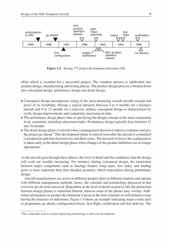
Figure 1.4 Boeing 777 project development milestones [36]
effort which is essential for a successful project. The complete process is subdivided intoproduct design, manufacturing and testing phases. The product design process is broken downinto conceptual design, preliminary design and detail design.
• Conceptual design encompasses sizing of the most promising overall aircraft concept andproof of its feasibility. Having a typical duration between 4 to 6 months for a businessaircraft and 9 to 12 months for a mid-size airliner, conceptual design is characterized bycyclic design improvements and complexity increasing in time.
• The preliminary design phase aims at specifying the design concept at the main componentlevel, sometimes including subsystem trades. Preliminary design typically lasts between 12and 16 months.
• The detail design phase is entered when a management decision is taken to continue and givethe project go-ahead.2 This development phase is entered soon after the aircraft is committedto production and lasts between two and three years. The decision to freeze the configurationis taken early in the detail design phase when changes in the product definition are no longerappropriate.
As the aircraft goes through these phases, the level of detail and the confidence that the designwill work are steadily increasing. For instance, during conceptual design, the interactionbetween major components such as fuselage frames, wing spars, fuel tanks, and landinggears is more important than their detailed geometry which materializes during preliminarydesign.Aircraft manufacturers are active in different product lines in different markets and operate
with different management methods; hence, the schedule and terminology discussed in thisoverview are far from universal. Dependent on the level of detail exerted in AD, the distinctionbetween design phases is somewhat blurred, whereas some of the phases may overlap. Addi-tional information on product development is given in the time schedule of well-defined eventshaving the character of milestones. Figure 1.4 shows an example indicating major events suchas programme go-ahead, configuration freeze, first flight, certification and first delivery. The
2The comparable term in system engineering terminology is full-scale development.

10 Advanced Aircraft Design
development time span between the first concept studies and certification is typically betweenthree years for a light business aircraft and six years for a clean sheet wide body airliner.This illustrates why an aircraft must be conceived at least a decade ahead of the anticipatedutilization period. Therefore, flexibility and extended duration have a strong impact on manyapplication alternatives and the growth potential which a good design must have from itsinception.
1.3.1 Concept Definition
The concept definition phase can be characterized as the highly creative and imaginativeidea stage during which the component geometry, placement and connectivity of a futureaircraft designed to fulfil the needs of a specific market are defined. Conceptual design alsoentails the development of a novel aircraft concept at an overall system level in competitionwith a more traditional layout. The objective is to explore a preferred configuration3 todetermine a layout which is technically superior and economically viable. This involvespreliminary performance predictions and provision of three-dimensional electronic drawingswith several cross-sections, an inboard profile showing the approximate placement and sizeof the major vehicle components. A weight and balance diagram provides another essentialproof of concept.There is an intimate relationship between the design objectives of an aircraft and the
configuration concept capable of fulfilling these objectives. The overall concept describes ahighly complex system which has to reach a compromise between contradicting requirements.Application of new technologies affecting all sub-systems is indispensable for economicsuccess of the new product. The conceptual design phase is intended to generate a credibleproposal of a feasible baseline design in order to convince management that it is worth thesubstantial resources required to develop and improve the design in further detail. Design toolsare semi-empirical and low to medium fidelity methods used in trade-off studies and basicoptimizations – most of the geometry is provisional. Validated design tools developed by theAD office are calibrated with statistical data bases, handbooks and historical trends, takinginto account improvements expected from new technologies. The amount of data generatedfor a baseline design will be moderate and prediction errors are around 5%, typically.4
In an environment where designs are developed which fit into an existing product line,designers may investigate different fuselage cross-sections, wing positions and planforms,number and/or location of engines, empennage and undercarriage concepts. A few promisingconcepts are analyzed and selected for further study. Conceptual studies may also be carriedout to investigate potential gains expected from new aerodynamic devices, structural concepts,materials and/or system technologies and/or an advanced engine concept. All of these featureshave a far-reaching effect when integrated into the design. Designers who are supposed to
3In the context of this chapter, the term configuration refers to the airplane’s general arrangement, not to be confusedwith the same term used in flight mechanics defining operational parameters of a particular aircraft such as enginerating, flap and slat deflection angles, tailplane incidence, undercarriage position, etc.4An error in the concept stage is defined as the difference between a predicted value and the established value ofa parameter after completion and testing of the first aircraft. Since the certified aircraft will make its inaugurationseveral years after concept definition, the detailed design has gone through many modifications. Hence, predictionerrors are inaccuracies rather than mistakes.

Design of the Well-Tempered Aircraft 11
explore a radical concept may consider an integrated configuration such as a blended wingbody (BWB) or an all-wing aircraft (AWA) (Chapter 5). Less radical alternatives are a canardor three-surface aircraft, a twin-fuselage aircraft concept, a strut-braced or a nonplanar wing(Chapter 6). A detailed assessment of advantages and disadvantages must then be made bycomparison with more conventional solutions. During all the stages of concept definition, thetechnical risks and costs of possible failure must be closely examined.5
Typical of concept design is its iterative character: primary components – wing, fuselage,nacelles, tailplane, landing gear, propulsion and other systems – are sized provisionally toresult in a baseline design. Dependent on where improvements are desirable, the processmay recycle to an earlier definition level at each point in time. A baseline design is notnecessarily an optimized airplane and, for a traditional layout, the combined application ofactive constraints will normally give an adequate approximation to the best feasible design.If a novel solution is tried, the estimation of the aircraft effectiveness will be based in someareas on slender evidence and simple mathematical models. The best available model maythen change rapidly with time and will probably be too crude to warrant rigorous treatment.In any case a comprehensive design optimization at the conceptual stage is of little value [66].
1.3.2 Preliminary Design
After selection of a baseline airplane concept, the design and analysis process will enter thepreliminary design phase. As opposed to conceptual design which deals with the whole aircraftsystem, preliminary design aims at defining subsystems, making component trade-offs andoptimization. Specialists from different functional groups contribute to this process of refiningthe initial vehicle concept –AD remains responsible for coordination. This teamwill (re)designthe delivered baseline vehicle in sufficient detail to carry out supporting analysis and specifyperipheral testing programmes but not with enough detail to specify each sub-assembly.Information to establish the programme feasibility is generated by means of sophisticatedcomputational aerodynamical, mechanical and structural analysis, prediction of the economicsand expected market penetration. Preliminary design can be characterized as setting goals forthe extensive efforts to be made in the downstream detail design phase. Typical subjects arecategorized as follows:
• Design definition. The baseline design team is committed to elaborate detailed analysis andsensitivity studies, with the aim of developing the best feasible configuration. This includesfinding a balance between required volumes, main dimensions, weight distribution andengine performances. Details of the aircraft geometry, aerodynamic properties, structuralloads and deformations and flying qualities have to be settled.
• Design validation. The predicted characteristics of the preferred configuration are verifiedby high-fidelity supporting analysis, simulations and test data. This becomes the final stepof the preliminary design cycles.
5It is often said that ‘In aircraft design one never gets a free lunch.’ This statement applies in particular to conceptualdesign where it may be interpreted as follows: ‘The greater the promise, the higher the risk of show stopper.’

12 Advanced Aircraft Design
A detailed analysis is usually made to determine the sensitivity of the configuration to tech-nology inputs, performance objectives and design constraints. This makes sense since duringpreliminary design there still exists considerable freedom for refinements and improvementsthrough optimization of variables such as detailed wing design, engine thrust, location of thepower plant and empennage design. These trade studies have a widespread effect on mostareas of the design and must therefore be carried out with scrutiny using high-fidelity analysis.Particular attention will be paid to the following issues:
• Detailed volumetric sizing and mass breakdown, centre of gravity (CG) location and loadingrestrictions, and moments of inertia, resulting in a considerable expansion of the designdatabase.
• Definition of the aerodynamic shape of lifting surfaces, including high-lift devices, usingcomputational fluid dynamics (CFD) methods and wind tunnel testing.
• Layout and sizing of main mechanical and structural concepts, aero-elastic analysis bymeans of finite element methods (FEM), and structural testing.
• Layout of the basic flight control system and control surfaces and devices, including predic-tion of flying qualities.
• Drawing up the specifications for buy-out components to be subcontracted to suppliers. Thisconcerns the power plant (engines, propellers, nacelles) and other major aircraft systemssuch as the auxiliary power plant, environmental control, fuel system, hydraulic system,electrical system and avionics.
• Economic analysis in terms of operating costs. Commercial prospects are then predicted bymeans of economic analysis and a market penetration model.
• Analysis of environmental issues such as internal/external noise and engine emissions.
All activities are based on standards of the selected airworthiness codes and regulations as theprimary measure for acceptance of design solutions. The scope and depth of the physics-basedanalysis and the fidelity of the computational models are increased to such a level that theimpact on aircraft performance and cost of proposals to modify the baseline configurationcan be quantified. Although CFD and FEM codes provide high-fidelity results, computersimulations cannot always be relied on for an accurate prediction of operational properties.Design validation will therefore require extensive wind tunnel testing6 and testing of structuralmodels to ensure that achieved performances will be no more than a few percent off therequirements.Whereas the engineers involved in conceptual design generally belong to AD, specialists
from various functional disciplines become involved when the preliminary design stage isentered. From then on the approach to be taken relies heavily on system engineering tech-niques. This phase may span a year or more with a team of dozens up to hundreds of engineersworking in a multidisciplinary environment. The amount of detailed data generated is sub-stantial, prediction errors should amount to no more than few percent. The end product isan optimized and verified airplane configuration resulting in the technical description of pro-totypes to be tested and the type specification of the aircraft. When the design project is
6A future addition to the presently available (high-cost) wind tunnel testing technology could be the use of free flyingsub-scale models referred to as robot vehicle flight testing [56].

Design of the Well-Tempered Aircraft 13
sufficiently mature, it may get an authorization to be offered for sale with written (contrac-tually binding) guarantees on cost and performance. When market prospects appear to bepromising, management authorizes the project go-ahead. In view of the high costs incurredby major configuration changes during the following design stage, this decision brings theiterative design cycle to an end by freezing the configuration.
1.3.3 Detail Design
The pieces of hardware that will actually be built and installed in the airframe are conceivedduring the detail design phase which is entered after the aircraft is committed to production.The objective of detail design is to specify the geometry of all components and plan their man-ufacturing processes. This encompasses drawing up instructions for the production departmentand the development of a careful plan for assembling the aircraft. Throughout this activity,drawings are progressively released for production. Results are complete production descrip-tions and specifications of all structures, systems and subsystems. Compared to preliminarydesign, detail design is much more labour-intensive and far more staff are involved. The par-ticipation of AD is restricted to coordinating measures to be taken when detail design appearsto have an effect on the technical specifications. A typical example is when a significant emptyweight growth has to be addressed by a weight reduction programme. After completion of thedetail design phase, the manufacturing of components begins, followed by the final assemblyof one or more flight-test vehicles, roll-out, first flight, flight testing, and certification. In thecase of an all-new civil airplane development, the completion of the airworthiness certificationprocess and first delivery to the customer will occur some five to eight years after the initialdesign efforts (Figure 1.4).
1.4 Baseline Design in a Nutshell
This book focusses on the conceptual and preliminary design definition rather than on thedesign validation and detail design. Although the described sizing procedure for conceiving abaseline design of a civil jet airplane is by no means a standard process, it contains a set ofessential activity clusters. Conceptual design is a continuous iterative process that begins withan initialization of a few major characteristics to be discussed in Chapter 2. The followingbird’s eye view of a baseline design sizing process describes the logical order of activitiesvisualized in Figure 1.5 leading to a converged design in as few iterations as possible. Theresult is a non-optimized but feasible jetliner design which complies with TLRs – the sizingprocess of a turboprop airplane is similar although sizing relationships are different. Thediagram indicates an inner loop for satisfying payload/range and high speed performancerequirements and an outer loop for making sure that low-speed properties comply with TLRsand other constraints. This approach is in the interests of an efficient iteration process but doesnot necessarily lead to the best feasible design. The next steps are optimization and trade-offstudies as discussed in later sections.
1.4.1 Baseline Sizing
A baseline design is materialized in the form of a fairly comprehensive definition of itsbasic geometry, using a computer assisted design (CAD) system. Defining the geometry by

14 Advanced Aircraft Design
PRE-CONCEPT STUDY
Top level requirements- design payload / range- cruise speed / altitude- field length limitations- approach speed- environmental standards- ............
Technology standards- propulsion- aerodynamics- flight mechanics- systems- structural materials- production- ..........
- useful load disposition- lifting & stabilizing surfaces
disposition- engines, number & location- landing gear configuration- ..........
DESIGN LAYOUT
CONCEPT SIZING
WEIGHT & BALANCE
FIELD PERFORMANCES
mission fuel balanced?
requirements met?
Fuselage- cabin cross-section- cabin & flight deck layout- freight holds, exits, doors,- external shapeWing- area & span- planform shape- sections- spar locations- high lift & control devicesEmpennage- horizontal tail planform- vertical tail planformPower plant- engine type & thrust- nacelle geometry- fuel tank size & location- .............
- group weight breakdown- load & balance diagram- wing & tail location- landing gears location
yes
no
change design weights
- take-off- engine-out climb- landing- community noise
yes
MISSION ANALYSIS
- lift, drag & thrust variation- flight envelope- mission fuel & time vs. range- ..........
no
OPTIMIZATION
change engine thrustMARKET RESEARCH ANDTECHNOLOGY EVALUATION
Figure 1.5 Schematic outline of a jetliner baseline design process
a parametric description helps the designer to predict the variation of mass distribution andaerodynamic properties due to variation of independent design variables such as wing areaand aspect ratio, engine power or thrust, and empennage size. Figure 1.5 illustrates that initial‘guesstimates’ are made of several important design characteristics.
• Design weights. Payload, fuel weight and take-off and landing gross weights correspondingto the design mission are estimated together with initial values of the empty weight and thezero fuel weight; see Chapter 2.
• Total take-off thrust and number of engines to be installed.• Wing loading; that is, the maximum TOGW per unit of wing area.
These characteristics are revised as soon as more detailed design information becomes avail-able. For designs with a conventional general arrangement, they are probably based on statis-tics, using input from the TLRs and data from similar existing or projected aircraft. For moreinnovative concepts, relevant publications on applied research should have been studied beforestarting the actual sizing.For passenger aircraft and freighters with a traditional layout, the first geometric element
to be conceived is typically a pressure cabin cross-section and floor planform, based on thespecified transport function and comfort standards. Passenger cabin layout is based on selectionof items such as number of passenger decks, number of seats abreast in a basic cross-section,seat pitch and number of seat rows for several accommodation standards, width and height ofaisles and overhead bins, and allocation of restrooms and galleys. Pressure cabin dimensions

Design of the Well-Tempered Aircraft 15
are obtained by combining typical seating arrangements with (a) location and size of passengerand servicing entrance/exit doors and emergency exits; (b) flight deck geometry, entrance doorand escape hatches; and (c) luggage/cargo hold geometry and loading/unloading hatches.Addition of a cabin wall with realistic thickness, fuselage nose and tail shapes results in athree-dimensional definition of the basic external fuselage shape. For airliners this is normallya streamlined hull with a cylindrical mid-section enclosing the contents arranged with goodaccessability inside the smallest possible skin. Cabin volume, floor area, and fuselage skinarea are basic input for aerodynamic and weight prediction. In order to obtain an arrangementthat is flexible enough to suit an airliner family concept, it may be necessary to repeat thefuselage sizing process for a future derivative or a freighter version.The wing is the second main component to be sized. Wing geometry has to be matched
to the performance requirements and is defined in terms of several parameters used in flightperformance analysis. Prominent parameters of a lifting surface are the gross planform area,the span or the aspect ratio, the taper ratio, the thickness/chord ratio at the root and the tip,and the angle of sweep of the quarter-chord line. It is also desirable to specify a standardfor aerodynamic wing design, such as supercritical or laminar flow technology. However,variation along the section shape and incidence along the span are the subject of downstreamaerodynamic wing design (Chapter 10).
1.4.2 Power Plant
Figure 1.5 relates to the case that candidate engine types are under development. Each of thefollowing options will lead to design processes that are different in the details.
• One option could be that a new aircraft design or a variant of an existing type is considered inresponse to the availability of a new engine type. In this case, installed engine performancesand geometry are specified in detail by the engine manufacturer. In the interest of minimumproject development costs, the basic properties of the existing aircraft are retained as muchas possible, leading to a modest airframe modification. In this situation there is little or noopportunity for optimization.
• In order to match the engine to an existing airframe, its thrust is scaled up or down by meansof a procedure known as engine rubberizing. A baseline engine is then characterized byits installed take-off thrust. Variations of engine performances with altitude and speed aredescribed by generalized characteristics such as thrust as a fraction of take-off thrust – thethrust lapse rate – and specific fuel consumption (SFC) or overall efficiency of the engine.Scaling relationships for engine size and weight are derived from the engine manufacturer’sinformation. Rubberizing includes the effects on the engine’s installation characteristicswhich means that nacelles are scaled up or down so that performance losses due to nacelledrag and power off-takes are properly taken into account.
• A far more complicated situation occurs when different engine cycles are studied, forexample, for investigating the effects of turbofan bypass ratio variation. This requires athermodynamic cycle analysis for computing engine performances as well as prediction ofengine plus nacelle geometry and weight, all of these in relation to the bypass ratio and thetake-off thrust. It goes without saying that the various scaling rules should be drawn up incooperation with the engine manufacturer’s project design office.

16 Advanced Aircraft Design
The decision of where and how engines are attached to the airframe constitutes one of themost essential choices of layout design (Chapter 3).
1.4.3 Weight and Balance
The allowable variation of the useful load and its location determines the aircraft’s loadingflexibility. This is restricted by the allowable centre of gravity (CG) travel which in turn relatesto the amount of (inherent or artificial) stability required for the configuration. The horizontaltail size is obtained from longitudinal stability and control requirements in combination withload and balance computations. For a givenwing position relative to the fuselage and horizontaltail size/location, the following results are derived:
• Empty weights of major assemblies and their CG location, airplane CG location andmoments of inertia about the three body axes. Some of these are be based on analysis,others are obtained from statistical information, using initial design weight estimates anddesign geometry.
• Envelopes of loaded aircraft fore and aft CG locations versus GW corresponding to likelycombinations of payload and fuel.
• Allowable fore and aft CG locations for several important flight conditions derived fromstability and control requirements, known as aerodynamic limits.
The required and allowable CG envelopes versus GW form the load and balance envelopewhich gives a tool for making sure that the operationally required CG range always fitswithin the aerodynamic limits. If that is not the case, measures have to be taken to obtain abalanced aircraft: (a) by relocating the wing relative to the fuselage; (b) by changing the wingsweep angle; (c) by relocating system components or operating items; or (d) by increasingthe horizontal tail size. If these measures do not help, loading restrictions may be necessary –an undesirable situation. Vertical tail size follows from required directional stability, lateralcontrol after engine failure and coping with cross-wind during the landing. When the airplaneappears to be safely flyable in all practical conditions, the main landing gear elements aresized and arranged relative to the CG range so that the aircraft can be manoeuvred safely onthe ground. Having located the landing gears, the designer may have to make another iterationof the CG envelope and/or horizontal tail sizing. The balancing process is thus highly iterative.
1.4.4 Structure
Part and parcel of the geometric development are the conception of a provisional structuralconfiguration and distribution of the following system elements:
• Topology and major components of the cabin structure such as major fuselage frames wherethe wing, tail surfaces and engine pylons are attached, longerons, with pressure bulkheads,doors and hatches and pylons of fuselage-mounted engines.
• Principal structural elements of the wing: skin/stringer panels, spars and ribs, fixed leadingand trailing edge structures, high lift devices, flight controls and their supports. Also specifiedare pylons of wing-mounted engines, landing gears and their attachments, and wheel wells.
• Basic structure of the empennage and its attachment to the fuselage body, taking into accountprovisions for flight controls and stabilizer incidence adjustment.

Design of the Well-Tempered Aircraft 17
Size and location of major systems hardware such as the auxiliary power unit (APU) and theenvironmental control unit (ECU) are indicated to make sure that they can be fitted inside theavailable structure.
1.4.5 Performance Analysis
Aerodynamic and engine characteristics can be predicted as soon as the baseline design geom-etry is defined. First, lift and drag coefficients in the en-route configuration are computed as afunction of the angle of attack and Mach number. Second, engine thrust and fuel consumptionas a function of the altitude and Mach number are determined for several climb and cruiseratings. Before analyzing a flight profile, it is useful to check that the available thrust matchesthe drag at the desired cruise conditions. If that is not the case, the engines are scaled upor down in thrust and dimensions and part of the sizing loop is repeated, as indicated inFigure 1.5.The objective of mission analysis is to compute the amount of fuel burned, distance travelled
and time elapsed during each flight segment and during the complete flight from the airfieldof departure to the destination. The flight profile of a civil aircraft (Figure 1.6) is composedof the segments take-off, climb and acceleration, cruise, descent, approach, aborted landingand diversion to an alternate airfield. The intention is to make sure that, when taking off, therequired mission fuel is available to fly the design payload over the required distance, afterwhich there remains sufficient reserve fuel to make a holding flight and divert to an alternatefield. If a mission analysis is carried out after computation of the MTOW, it is mostly foundthat the range is not exactly equal to the design range specified in the TLRs. The next sizingiteration is then started as indicated in Figure 1.5. In principle, all design weights, many emptyweight components and the amount of fuel have to be revised and the mission analysis isrepeated until the weight distribution is balanced with the required range.Aircraft handling and performances while taxying, taking off from and landing on the
airfield, and in low-speed flight are primarily affected by take-off and landing weights, thenumber of engines and their forward and reverse thrust, wing area and planform shape,aerodynamic properties of high-lift and drag modulation devices, and landing gear brakingcapacity. The distance that a civil aircraft requires to make a safe continued or aborted take-offafter failure of an engine during the take-off run is referred to as the balanced field length(BFL). This distance must not be longer than the available runway length. Moreover, it has tobe verified that minimum climb-out performances can be attained in case the flight is continued
Figure 1.6 Typical flight profile
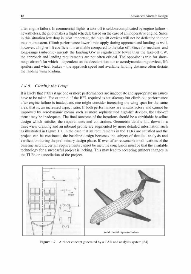
18 Advanced Aircraft Design
after engine failure. In commercial flights, a take-off is seldom complicated by engine failure –nevertheless, the pilot makes a flight schedule based on the case of an inoperative engine. Sincein this situation low drag is most important, the high lift devices will not be deflected to theirmaximum extent. Climb performance lower limits apply during approach and landing as well,however, a higher lift coefficient is available compared to the take-off. Since for medium- andlong-range (subsonic) aircraft the landing GW is significantly lower than the take-off GW,the approach and landing requirements are not often critical. The opposite is true for short-range aircraft for which – dependent on the deceleration due to aerodynamic drag devices, liftspoilers and wheel brakes – the approach speed and available landing distance often dictatethe landing wing loading.
1.4.6 Closing the Loop
It is likely that at this stage one or more performances are inadequate and appropriate measureshave to be taken. For example, if the BFL required is satisfactory but climb-out performanceafter engine failure is inadequate, one might consider increasing the wing span for the samearea, that is, an increased aspect ratio. If both performances are unsatisfactory and cannot beimproved by aerodynamic means such as more sophisticated high-lift devices, the take-offthrust may be inadequate. The final outcome of the iterations should be a certifiable baselinedesign which satisfies the requirements and constraints. Geometric details laid down in athree-view drawing and an inboard profile are augmented by more detailed information suchas illustrated in Figure 1.7. In the case that all requirements in the TLRs are satisfied and theproject can be continued, the baseline design becomes the subject of detailed analysis andverification during the preliminary design phase. If, even after reasonable modifications of thebaseline aircraft, certain requirements cannot be met, the conclusion must be that the availabletechnology for a successful project is lacking. This may lead to accepting (minor) changes inthe TLRs or cancellation of the project.
solid model representation
Figure 1.7 Airliner concept generated by a CAD and analysis system [84]
Design of the Well-Tempered Aircraft 19
1.5 Automated Design Synthesis
Conceptual design tools used by aircraft manufacturers are not available on the softwaremarket since they contain sensitive information reflecting the expertise of the company. How-ever, automated design synthesis (ADS) systems have been developed by consultancy firms,research institutes and academia. Automated design systems emphasize optimization ratherthan sizing. Although synthesis programs are used primarily for sizing a baseline design, theycan be useful for other tasks as well. For example, figures of merit (FOMs) for evaluating theimportance of design variables are operational/commercial performance and cost. Comparingthe characteristics of aircraft optimized for different FOMs is a complex but revealing activitythat can be carried out only with a ADS system. Investigations of unconventional concepts,technology trade-off studies between alternate designs and weight-related studies are almostinvariably made by applications of ADS programs. And, last but not least, synthesis programsare useful for validating and improving drag and weight prediction tools.
1.5.1 Computational Systems Requirements
The aim of a high-fidelity design analysis is to obtain more credible predictions in the interestof reducing development risk. However, a comprehensive synthesis program is used in variousstages of the design process and should therefore have the capability to provide computationswith different levels of prediction accuracy. Low fidelity methods are used in the early concep-tual phase to derive simple but statistically validated predictions based on only a small numberof essential inputs. As the vehicle definition becomes more detailed, the fidelity of designtools increases. Accordingly, aerodynamic analysis ranges from (semi-)empirical handbookmethods through several levels of computational complexity to interpretations of wind tunneldata. Other technical disciplines have similar levels. High fidelity analysis requires a detailedinput which is not available until the preliminary design phase is entered. Internal and externalgeometry – in particular, the volumetric disposition andwetted areas – are essential inputs to theADS program, and shape optimization requires that the geometry can be parameterized. Thisrequires simplification by ignoring details such as small fairings between major components,wing leading and trailing edge extensions and kinks. The internal geometry is schematizedby considering large structures to be built from generic components, such as the primary andsecondary wing structure, the fuselage shell, floors, bulkheads and secondary structures.ADS systems must be flexible enough to allow the design problem structure to be defined
according to the designer’s needs. They are usually highly modular so that the functions tobe performed are clearly separated and can be assembled to perform various sequences ofcomputations, depending on the problem. Each individual module provides the intermediatedata from a particular technical discipline, thus forming the input of other modules as well asthe geometric definitions needed for vehicle (component) definition. These modules shouldbe verified prior to integration with other modules. Modularity leads to obtaining a moretransparent design procedure since it simplifies data transfer and identification of errors duringprogram development. A control program is used to exercise the individual modules and tocoordinate data transfer to other modules. This set-up is required in order to ensure that ineach stage of an iteration the definition of the vehicle as a system remains unambiguous andconsistent. A correct problem structure is at least as important as the accuracy of the analysismethods used. Accordingly, a great deal of thinking and arranging of equations are required

20 Advanced Aircraft Design
before the computations can be made. In contrast to many publications which emphasizethe mathematical treatment of optimization, the designer’s activity is a blend of interactivegraphics manipulation and visualization, computation and organization of data flow. In anefficient integrated program the selection of the appropriate levels of computational fidelityand the preferred search strategy remain under the designer’s control.
1.5.2 Examples
Synthesis programs contain simplified vehicle descriptions and merely mimic the process byhumans to accomplish the design and analysis solutions provided by statistics and calculator-basedmethods from handbooks. The primary objective of the synthesis process is to carry out atrade-off between basic design parameters and characteristics that will warrant a more detailedstudy. In particular, wing size and engine power or thrust are primary candidates for trade-off.Computerized synthesis is a complex activity which integrates the contributions of variousdisciplines involved illustrated in Figure 7.8. A practical engineering approach requires a largecomputer program connecting the inputs and outputs of each discipline. The final result is acombined answer indicating the overall feasibility of the project.Figure 1.8 shows schematically the principal lines of data flow of an early – but still repre-
sentative – ADS program structure [62]. Analysis programs are modularized by discipline, thesequence of calculations is controlled by a separatemodule. Via the performance and economicevaluations block, design objectives are initially introduced as input into the program flow.Part of the concepts introduced into the modules is technology state-of-the-art information.
Figure 1.8 Schematic sizing and optimization data flow of a design synthesis program [62]

Design of the Well-Tempered Aircraft 21
In aerodynamics this could be the sophistication of airfoil and high lift technology. Structuralconcepts’ state of the art includes the degree of composite materials application in primarystructures. Propulsion technology defines the gas generator compressor pressure and temper-ature levels and the bypass ratio. And in flight controls the degree of artificial stability is atypical concept for reducing tailplane size, drag and weight. Note that in Figure 1.8 the outputfrom the disciplinary modules as well as the configuration design eventually goes to the perfor-mance and evaluation block. Some of the paths are direct, others are indirect via weights andconfiguration design. Flight systems, structures, aerodynamics and propulsion all feed weightsas well as configuration design. However, since drag, thrust and aircraft weight are the onlyforce vectors necessary for performance evaluation, the aerodynamics, propulsion and weightblocks are sufficient to deliver the data input. The design converges after several iterations andthe outcome of the process is an evaluation of the design by the performance module. Theuser will then decide to accept the outcome or to continue the process through variations inthe design. For this purpose, modern synthesis programs have a separate optimization drivercontaining a suite of algorithms to choose from.Major design organizations are developing their own ADS programs. Commercially avail-
able programs developed by consulting companies are mostly based on handbooks [102]whereas several programs exist in the public domain using a similar approach as shown inFigure 1.8. Systems developed by NASA institutes are available in the public domain [75,91, 96], systems developed in academia are reported in [80, 83, 89, 98]. Automated systemshave proved effective for designing airplanes within the prescribed domain – some of themhave been continuously improved and have become highly trusted. New approaches based onobject-oriented and knowledge based engineering (KBE) may be particularly promising fordeveloping sizing tools to study unusual air vehicle concepts [94, 100, 103].
1.5.3 Parametric Surveys
The traditional approach to conceptual sizing and optimization is to carry out parametric sur-veys by solving the system of equations for a few – typically, not more than five – selectionvariables defining the design space (Chapter 7). The most relevant properties of the evaluateddesigns are presented for inspection in tables and/or carpet plots [39] such as Figure 1.9.It should be noted that every combination of wing area and engine thrust represents a pro-visional but complete aircraft design for which the weight breakdown has been computedor interpolated. Since many of these designs do not comply with all TLRs, constraints areadded to indicate the feasible region of the design space. The baseline design complies withall requirements, although a lower MTOW is obtained by selecting a larger wing area and aslightly smaller engine. Quasi-analytical methods for obtaining parametric surveys are derivedand illustrated in Chapters 8 to 10.Parametric surveys are rooted in the industrial approach, where they are considered valuable
since the designer can make maximum use of experience and keeps complete control overdecisions. These surveys accept relatively simple programming techniques such as spreadsheetmethods adaptable to the situation [86]. This approach has the advantages that an a priorichoice of a single FOM is not required and sensitivity to less-than-optimum design conditionsremains visible; hence, maximum use is made of calculated results. The number of designvariations and modifications can be selected in accordance with the time budget available.

22 Advanced Aircraft Design
Figure 1.9 Carpet plot depicting results of a parametric survey. Wing loading and engine thrust aredesign variables, MTOW is the figure of merit
If the overall concept is within the designer’s experience, parametric investigations may behelpful in optimization work although this pragmatic approach may not be entirely satisfactoryfor the following reasons.
• Due to the restricted number of selection variables, there is no guarantee that the solutionrepresents the ‘real optimum’.
• The method is practical for a small number of selection variables. The designer may resistincreasing the design space since the addition of more variables will increase the amount ofcomputation by an order of magnitude.
• The majority of the analyzed configurations are used for the purpose of the parametric studyonly and are discarded afterwards whereas small changes in the TLRsmaymake all previousresults obsolete.
1.6 Technology Assessment
The challenge for conceptual designers active in an AD office is to strike a balance betweenthe pros and cons of enabling technologies that are considered mature for application. Theyhave to make an assessment of economic benefits, effects on safety, cabin comfort, reliability,maintainability, and environmental compatibility. The aim is to identify and select the mostcost-effective breakthrough technical innovations and to find outwhether they can be developedin time, and whether their integration into the aircraft system requires a departure from theconventional aircraft configuration. A long list of potential innovations can be made – themore radical of these tend to be achievable only with considerable development effort, costsand risk. However, using advanced technologies may drive up operating cost and degradeoperational flexibility, maintainability or even passenger appeal. Assessment of emergingtechnologies must take into account possible program development risks. The enormous costsof developing jetliners are justified only when potential customers can be convinced that thenew product will outperform existing types in its category both technically and economically.

Design of the Well-Tempered Aircraft 23
AIRPLANE CONCEPT
multi fuselage conceptinnovative fuselage cross-sectioncanard / three lifting surfaces
noise shielding conceptsnon-planarwing
flying wing
AERODYNAMICTECHNOLOGY
natural laminar flowhybrid laminar flowturbulence managementshock / boundary layer interactionwing tip devices / special wing tipsadvanced high-lift system devicesnoise reduction at high liftwake vortex control
STRUCTURAL CONCEPTS
aero-elastictailoringadaptive / morphing structuressandwich panelsand shellsintegrated lightning protectionsmart structures
MATERIALS/ MANUFACTURING
fibre-reinforced plasticsthermoplasticsfibre metal laminatesmanufacturing of advanced materialsaluminium-lithium and titaniumwelding of compositesdiffusion bonding of titanium
AIRBORNE SYSTEMS
full fly-by-wire / fibreopticselectro-hydrostatic actuatorsmore-/all-electric aircraftbleedless environmental controlautomatic anti-ice control
PROPULSIONTECHNOLOGY
very / ultra-high bypass ratiogeared turbofanopen rotor technologymulti-bladed propeller/ propfan
FLIGHTAND LOAD CONTROL
flight control computeractive controlsstability augmentationenvelopeprotectionmanoeuvre / gust load alleviationdirectliftcontrolthrust vectoring
Figure 1.10 Overview of disciplines and enabling technologies
In general, this requires the introduction of an advanced but sufficiently mature technologystandard in several design disciplines. Accordingly, conceptual design studies are frequentlyinitiated to assess how the application of new technology will affect future designs rather thanto develop a new aircraft development project. Disregarding the appearance of a new enginegeneration, the largest impact on operating economics is due to the accumulative effect ofseveral relatively small advancements. Improvements in new airplane designs have thereforetraditionally been evolutionary rather than revolutionary.Conceptual design studies are based on choices from the most promising advancements in
the state of the art; see Figure 1.10. For a particular project more alternatives can be added,other topics may already have been eliminated beforehand. Chapters 3 and 4 are dedicated toidentifying improvements of aerodynamic and propulsive efficiencies. Specific technologieswith a large impact on the overall airplane layout are treated extensively in Chapters 5 and 6.Factors driving the design of airliners are relevant to some extent for business aircraft designas well:
• Propulsion. Turbofans of the next generation of civil aircraft are expected to have an ultra-high bypass ratio and geared turbofans. A more radical concept is open rotor engine technol-ogy in the form of contra-rotating propfans or unducted fans. Integration into the airframe ofthese new engine concepts may require an innovative overall airplane concept. Turbopropsfor high speeds will drive multi-bladed crescent-shaped propellers.
24 Advanced Aircraft Design
• Airplane configurations. Evolutionary development of airliners may result in different con-cepts emphasizing low-cost transportation, improved cabin comfort, reduced atmosphericcontamination and external noise. Radical concepts such as integrated configurations, non-planar wings, all-wing aircraft and propulsion by hydrogen fueleld engines require majorinvestments in research and development.
• High-speed aerodynamics. Small airliners and business aircraft with a small wing leadingedge sweep may achieve areas of natural laminar flow (NLF). Laminar flow control (LFC)by suction of the boundary layer through a porous skin is a potentially powerful fuel saver.Winglets and sheared tips reduce induced drag by up to 15%.
• Low-speed aerodynamics. Airplanes with stringent airfield performances require advancedhigh-lift devices. Options are variable camber, full-span flaps and powered lift by meansof externally blown flaps or engines blowing over the wing. Reduction of aerodynamicflap/slat noise and manipulation of trailing vortices can have a favourable effect on air trafficmanagement (ATM) and environmental compatibility.
• Flight control systems. Flight envelope protection and stability augmentation are accommo-dated by a flight control computer and active controls. Manoeuvre and gust load alleviationare considered additional provisions for saving structural weight and improving comfort.Direct lift control and/or thrust vectoring can be considered for unusual configurations toimprove their controllability.
• Airborne systems. Except for very light aircraft, fly-by-wire has become the standard forairliners and business jets – fibre optics may be considered in the future. More-electricaircraft enable environmental and automatic icing control without making use of enginebleed air and simplify the auxiliary power unit.
• Materials andmanufacturing. Composites are becoming increasingly dominant with applica-tions of fibre-reinforced plastics in primary and secondary structures. Fibre metal laminatesare applied in fatigue-sensitive areas and secondary structures. Aluminium-lithium alloysreplace the traditional 5000 series, leading to about 10% weight reduction.
• Structural concepts. Affordable composite fuselages are becoming an option for many airlin-ers and business jets. Lightning protection is required for all exposed composite structures.Aero-elastic tailoring is applied to avoid divergence or flutter and may be considered toenable a forward swept or very high aspect ratio wing. A morphing wing structure adaptsthe shape of high-lift devices off-design flight conditions.
Conceptual designers base their judgement concerning new technologies on experience andon how much credibility they attach to innovations, taking into account that airlines are oftenmore conservative than airframe manufacturers. Neither of them do want to be involved in ahigh-risk technology leading to unexpected development, certification and maintenance costs.In this respect a (seemingly radical) technology such as active LFC is considered suspecteven though its aerodynamic and operational feasibility has been demonstrated in R & Tprograms in the US and in Europe. Conceptual design technological standards are specified inrelation to the operational profile and the time of introduction into service of the new type. Forexample, long-range airliners are usually large and cruise at high speeds – they require moreadvanced technology than regional aircraft spending more time at low altitudes and speeds.The preference for a particular technology will also be affected by the company’s capabilitiesto incorporate them into their manufacturing processes. Although innovations generated bytechnological research are continuously reported worldwide, application in actual design
Design of the Well-Tempered Aircraft 25
practice can only be justified after a study of all aspects associated with their integration intothe aircraft and its production process.
1.7 Structure of the Optimization Problem
The structure of an optimization problem is essential to make its results credible. This sectionis intended to stimulate the (inexperienced) advanced designer to avoid unrealistic results ofa complex aircraft system optimization. Reference is made to Chapter 7 for the terminologyused and more background information.
1.7.1 Analysis Versus Synthesis
It is useful to make a clear distinction between design analysis and synthesis. This is illustratedby showing the differences between performance analysis of a specified design and sizing adesign for specified performance.
• Flight performance analysis applies to an aircraft (design) that is fully defined in terms ofgeometry,weight distribution, aerodynamic characteristics and propulsion systemproperties.The underlying physics – mainly flight mechanics and dynamics – is mono-disciplinary andthe solution is fully determined. Validated programs based on substantial experience areavailable to assist the analyst. For instance, cruise performance analysis is a matter ofroutine although Chapter 12 demonstrates that for cruising at a transonic Mach number, thiscan be more complicated than is usually thought.
• Synthesizing an aircraft design that has to comply ‘in an optimum fashion’ with a specifiedset of TLRs. The designers’ task is to find a satisfactory compromise between conflictingrequirements which may lead to an indeterminate problem. The underlying physics origi-nate from many interacting – but to a large extent fundamentally unrelated – aeronauticaldisciplines and the set of equations does not always have a unique solution. Although atfirst sight the freedom to select the independent design variables may seem overwhelming,constraints reduce the dimensionality of the design space. Guidelines based on statisticscan be useful when choosing selection variables if a suitable objective function cannot bequantified, although these ‘rules of a thumb’ may be reliable only for configurations that arenot too different from existing ones.
A practical example is selecting the preferable cruise altitude. The best initial cruise conditionof an operational aircraft with given gross weight is readily obtained from performanceanalysis – it is usually defined as the altitude where the fuel consumption per distance travelledis minimal. For an aircraft taking off with its MTOW, this optimum is probably constrainedby the available cruise thrust. On the other hand, the sizing problem is to find the definition ofa design that yields the most economical performance by computing the effects on the cruisealtitude of varying wing geometry and installed thrust. In the latter case, the designer has tocope with the following challenges:
• The sensitivity of dependent design variables (lift, drag, gross weight, initial cruise altitude)to variation in independent design variables (wing geometry and installed thrust) must beestablished.

26 Advanced Aircraft Design
• A criterion must be found defining ‘the best aircraft’ within the set of design constraints.• A choice has to be made of representative conditions – in particular, payload and range –for which operational and economics characteristics are evaluated. This is often referred toas the design condition.
In principle, this problem definition determines the solution of the aircraft system optimization.However, even the basic task of defining the best cruise altitude must not be underestimated,whereas the problem of determining an optimum cruise Mach number is a challenging task.For both examples, the case of a given (operational) aircraft is fairly easy if not trivial,but computing the best design cruise Mach number of a clean-sheet design is extremelycomplicated, if not impossible. In both examples, the conceptual designer may decide that amaximum payload or a long-range condition is most important and that an all-out optimizationdoes not have a high priority. Using the quasi-analytical approach discussed in Chapters 8 to10 may then be preferable.
1.7.2 Problem Classification
In accordance with the structure of the aircraft system optimization problem and the previousconsiderations, the ground rules and the computational approach discussed in this book areclarified according to one of the following options.
1. Optimizing flight conditions for a given airframe-cum-engine combination. The problemis to derive a mission profile resulting in minimum fuel burn, flight duration or directoperating costs (DOC). This is basically an optimal control problem occurring in designstudies as well as mission analysis of existing aircraft. Depending on the design phase(conceptual or preliminary), the solution may be simplified by accepting approximations,resulting in a closed-form equation for the mission fuel required to fly a given range orthe range obtainable with a given mission fuel. Treated in Chapter 12, these subjects formessential elements of the aircraft sizing process.
2. Determining the optimum airframe properties for specified engines. This is a typical con-ceptual design exercise of matching the airframe to engines selected a priori in an optimumfashion.Wing geometry is then the primary candidate for a highly constrained optimization.A similar situation occurs if a new engine technology becomes available for installationin an existing aircraft (family). The aircraft’s commercial value may then be enhanced byincreasing the payload versus range capabilities, preferably with minor modifications ofthe airframe.
3. Finding the best combination of the airframe and a given number of engines. Selectionof the engines and their position relative to the airframe has far-reaching consequences.In order to find the best match during the conceptual stage, basic airframe properties arevaried and engine properties are scaled by rubberizing the engines. The final selection islikely to be made during preliminary or detailed design. Chapter 9 deals with the subjectof engine and airframe matching and derives a FOM for initial engine selection.
This book focusses on how conclusions can be obtained and interpretedwith regard to optimumconditions by means of a quasi-analytical approach. To this end, the problem is simplified to

Design of the Well-Tempered Aircraft 27
such an extent that the objective function is differentiable so that (closed form) analyticalsolutions are obtained. The emphasis is initially on unconstrained optima which are easilyobtained by means of classical theory of local optima. These optima are interesting becausethey identify the ultimate design quality achievable for a given generic task –moving a payloadover a given distance. Although practical considerations associated with technological limitsmay degrade this ‘well-tempered aircraft design’ into an unfeasible solution, the penalty to bepaid for the best feasible solution becomes explicit by comparing it with the unconstrainedoptimum. The analytical approach may also give useful information on the sensitivity of adesign to small changes in the TLRs and technological parameters.
Bibliography
[1] Kuchemann, D., The Aerodynamic Design of Aircraft, Pergamon Press, Oxford, 1978.[2] Torenbeek, E., Synthesis of Subsonic Airplane Design, Springer Verlag, Heidelberg, 1981.[3] Roskam, J., Airplane Design, Roskam Aviation and Engineering Corporation, Kansas, 1985.[4] Niu, M.C-Y., Airframe Structural Design: Practical Design Information and Data on Aircraft Structures,
Conmilit Press Ltd., Hong Kong, and Technical Book Company, Los Angeles, CA, 1988.[5] Niu, M.C-Y., Composite Airframe Structures: Practical Design Information and Data, Conmilit Press Ltd.,
Hong Kong, and Technical Book Company, Los Angeles, CA, 1992.[6] Wilkinson, R., Aircraft Structures and Systems, Addison Wesley Longman Ltd., Harlow, 1996.[7] Brandt, S.A., R.J. Stiles, J.J. Bertin, and R. Whitford, Introduction to Aeronautics: A Design Perspective,
AIAA Education Series, AIAA, Inc., Washington, DC, 1997.[8] Jenkinson, L.R., P. Simpkin, and D. Rhodes, Civil Jet Aircraft Design, Arnold, London, 1999.[9] Schaufele, R., The Elements of Aircraft Preliminary Design, Aries Publications, Santa Anna, CA, 2000.[10] Howe, D., Aircraft Conceptual Design Synthesis, Professional Engineering Publishing, London, 2000.[11] Jenkinson, L.R., and J. Marchman, Aircraft Design Projects, Butterworth Heinemann, Oxford, 2003.[12] Torenbeek, E., and H. Deconinck (eds), Innovative Configurations and Advanced Concepts for Future Civil
Aircraft, von Karman Institute for Fluid Dynamics, Lecture Series 2005-06, June 2005.[13] Raymer, D.P., Aircraft Design: A Conceptual Approach, Fourth Edition, AIAA Education Series, AIAA, Inc.,
Reston, Virginia, 2006.[14] Whitford, R., Evolution of the Airliner, The Crowood Press, Ramsbury, 2007.[15] Gunston, B., Airbus: The Complete Story, Haynes Publishing, Sparkford, 2009.[16] Obert, E., Aerodynamic Design of Transport Aircraft, IOS Press, Amsterdam, 2009.[17] Kundu, A.K., Aircraft Design, Cambridge University Press, New York, 2010.[18] Sadraey, M.H., Aircraft Design: A Systems Engineering Approach, John Wiley & Sons, Chichester, UK, 2013.
Design Development and Methodology
[19] Cherry, H.H., and A.B. Croshere Jr., “An Approach to the Analytical Design of Aircraft”, SAE QuarterlyTransactions, Vol. 2, No. 1, pp. 12–18, January 1948.
[20] Backhaus, G., “Grundbeziehungen fur den Entwurf optimaler Verkehsflugzeuge”, Jahrbuch der WGL,pp. 201–213, 1958.
[21] Kuchemann, D., and J. Weber, “An Analysis of Some Performance Aspects of Various Types of AircraftDesigned to Fly over Different Ranges at Different Speeds,” Progress in Aeronautical Sciences, Vol. 9,pp. 324–456, 1968.
[22] Ladner, F.K., and A.J. Roch, “A Summary of the Design Synthesis Process”, SAWE Paper No. 907, May 1972.[23] Lange, R.H., “Parametric Analysis of ATT Configurations”, AIAA Paper No. 72-757, 1972.[24] Black, R.E., and J.A. Stern, “Creative Advanced Design: a Key to Reduced Life-Cycle Costs”, AGARD
CP-147-Vol.1, Paper No. 4, 1973.[25] Fulton, R.E., “Overview of Integrated Programs for Aerospace-Vehicle Design”, NASATM-81874, September
1980.

28 Advanced Aircraft Design
[26] Harris, D.H.W., “Applying Computer Aided Design (CAD) to the 767”, Astronautics and Aeronautics, pp.44–49, September 1980.
[27] Torenbeek, E., “Fundamentals of Conceptual Design Optimization of Subsonic Transport Aircraft”, TU Delft,Department of Aerospace Engineering, Report LR-292, August 1980.
[28] Steiner, J.E., “How Decisions are Made: Major Considerations for Aircraft Programs”, AIAA 45th WrightBrothers Lecture, the Boeing Company, Seattle, August 24, 1982.
[29] Koen, B.V., “Definition of the Engineering Method”, ASEE, Washington, DC, USA, 1985.[30] Fetterman, D.E. Jr., “Preliminary Sizing and Performance of Aircraft”, NASA TM 86357, 1985.[31] Loftin, L.K., Jr., “Quest for Performance – the Evolution of Modern Aircraft”, NASA SP-468, 1985.[32] Daues, J.J., “Project Management Issues & Lessons Learned from Computer-Aided Design Applications”,
AIAA Paper No. 87-2912, September 1987.[33] Michaut, C., D. Cavalli, H.T. Huynh, and H. Lethuy, “Preliminary Design of Aircraft”, AIAA Paper No. 89-
2152, July–August 1989.[34] Mason, W.H., “Analytic Models for Technology Integration in Aircraft Design”, AIAA Paper No. 90-3262,
September 1990.[35] Malone, B., and W.H. Mason, “Multidisciplinary Optimization in Aircraft Design Using Analytic Technology
Methods”, AIAA Paper No. 91-3187, September 1991.[36] Petersen, T.J., and P.L. Sutcliffe, “Systems Engineering as Applied to the Boeing 777”, AIAA Paper No.
92-1010, February 1992.[37] Bushnell, D.M., “Far Term Visions in Aeronautics”, Transportation Beyond 2000: Technologies Needed for
Engineering Design, Part 1, NASA TP 10184, pp. 261–298, 1996.[38] Mavris, D.N., and D.N. DeLaurentis, “A Probabilistic Approach for Examining Aircraft Concept Feasibility
and Viability”, Aircraft Design, Vol. 3, No. 2, pp. 79–101, 2000.[39] ESDU, “Examples of Construction of Carpet Plots from Experimental Data”, Data Item No. 04012, 2004.[40] McMasters, J.H., and R.M. Cummings, “Rethinking the Airplane Design Process: An Early 21st Century
Perspective”, AIAA Paper No. 2004-0693, 2004.[41] Friend, M.G., and C.P. Nelson, “From Concept to Market Reality: A Case Study of the Sonic Cruiser”,
Innovative Configurations and Advanced Concepts for Future Civil Aircraft, von Karman Institute for FluidDynamics, Lecture Series 2005-06, June 2005.
[42] Kehayas, N., “Aeronautical Technology for Future Subsonic Civil Transport Aircraft”, Aircraft Engineeringand Aerospace Technology, Vol. 79, No. 6, pp. 600–610, 2007.
[43] Toor, J. van, and T. Ahn, “The Role of Advanced Design in Aircraft Development and Product Definition”,private communication, 2010.
Transport Aircraft Technology
[44] Schneider, W., and M. Wittmann, “Cost Efficiency Considerations Concerning the Application of AdvancedTechnologies for Civil Transport Aircraft”, SAWE Paper No. 1214, May 1978.
[45] Shevell, R.S., “Technological Development of Transport Aircraft – Past and Future”, Journal of Aircraft, Vol.17, No. 2, pp. 67–80, February 1980.
[46] Swihart, J.M., “The Next Generation of Commercial Aircraft: The Technology Imperative”, ICAS Paper No.80-0.2, October 1980.
[47] Maglieri, D.J., and S.M. Dollyhigh, “We Have Just Begun to Create Efficient Transport Aircraft”, Astronauticsand Aeronautics, Vol. 20, No. 1, pp. 26–38, February 1982.
[48] Williams, L.J., “Advanced Technology for Future Regional Transport Aircraft”, SAE Paper No. 820731, 1982.[49] Wright, H.T., “NASA Technology Program for Future Civil Transports”, AIAA Paper No. 83-1603, 1983.[50] Kayten, G.G., C. Driver, and D.J. Maglieri, “The Revolutionary Impact of Evolving Aeronautical Technolo-
gies”, AIAA Paper No. 84-2445, 1984.[51] Swihart, J.M., “The Progress of Aeronautics”, AGARD Report No. R-782, Paper 1, June 1990.[52] Flosdorff, H., J. Roeder, and J. Szodruch, “Technological Requirements Concerning Subsonic Transport
Aircraft”, paper presented at German Aerospace Congress, Bremen, 29 September-2 October 1992.[53] Szodruch, J., and R. Hilbig, “Building the Future Aircraft Design for the Next Century”, AIAA Paper 98-135,
1998.
Design of the Well-Tempered Aircraft 29
[54] McMasters, J.H., and R.M. Cummings, “Airplane Design: Past, Present and Future”, Journal of Aircraft,Vol. 39, No. 1, pp. 10–17, January–February 2002; also AIAA Paper No. 2001-0535.
[55] Jarry, P., “Market Drivers and Innovation Behind Airbus Products”, ICAS Paper No. 02-0.5, September 2002.[56] McMasters, J.H., and R.M. Cummings, “From Farther, Faster, Higher to Leaner, Meaner, Greener: Further
Directions in Airplane Design”, Journal of Aircraft, Vol. 41, No. 1, pp. 51–61, January–February 2004; alsoAIAA Paper No. 2003-0553.
[57] McMasters, J.H., “A U.S. Perspective on Future Commercial Airliner Design”, Innovative Configurationsand Advanced Concepts for Future Civil Aircraft, von Karman Institute for Fluid Dynamics, Lecture Series2005-06, June 2005.
[58] Frota, J., and Y. Vigneron, “Airbus Future Projects Approach to New Aircraft Concepts and Research andTechnology”, Innovative Configurations and Advanced Concepts for Future Civil Aircraft, Von KarmanInstitute for Fluid Dynamics, Lecture Series 2005-06, June 2005.
[59] Kehayas, N., “Aeronautical Technology for Future Subsonic Civil Transport Aircraft”, Aircraft Engineeringand Aerospace Technology, Vol. 79, No. 6, pp. 600–610, 2007.
Computer-Assisted Synthesis and Design Integration
[60] Lee, V.A., H.G. Ball, E.A. Wadsworth, W.J. Moran, and J.D. McLeod, “Computerized Aircraft Synthesis”,Journal of Aircraft, Vol. 4, No. 5, September–October, pp. 402–408, 1967.
[61] Boyles, R.Q., “Aircraft Design Augmented by a Man–Computer Graphic System”, Journal of Aircraft, Vol. 5,No. 5, 1968.
[62] Wallace, R.E., “Parametric and Optimisation Techniques for Airplane Design Synthesis”, AGARD LS-56,April 1972.
[63] Wallace, R.E., “A Computerized System for the Preliminary Design of Commercial Airplanes”, AIAA PaperNo. 72-793, August 1972.
[64] Ardema, M.D., and L.J. Williams, “Automated Synthesis of Transonic Transports”, AIAA Paper No. 72-794,August 1972.
[65] Fulton, R.E., Sobieszczanski, J., and Landrum, E.J., “An Integrated Computer System for Preliminary Designof Advanced Aircraft”, AIAA Paper No. 72-796, August 1972.
[66] Bishop, A.W., and A.N. Page, “An Approach to Design Integration”, AGARD CP-147, Vol. 1, Paper No. 5,October 1973.
[67] Gregory, T.J., “Computerized Preliminary Design at the Early Stages of Vehicle Design”, AGARD CP-147,Vol. 1, Paper No. 6, October 1973.
[68] Heldenfels, R.R., “Integrated Computer-Aided Design of Aircraft”, AGARD CP-147, Vol. 1, Paper No. 16,October 1973; also AIAA Paper No. 73-410, March 1973.
[69] Galloway, T.L., and M.H. Waters, “Computer-Aided Parametric Analysis of General Aviation Aircraft”, SAEPaper No. 730332, April 1973.
[70] English, C.H., “Interactive Computer Aided Technology: Evolution of the Design Manufacturing Process”,McDonnell Aircraft Co., AIAA Meeting Paper, MC-AIR75-009, August 1975.
[71] Hitch, H.P.Y., “Computer Aided Aircraft Project Design”, Aeronautical Journal, Vol. 81, No. 469, pp. 51–62,February 1977.
[72] Oman, B.H., “Vehicle Design Evaluation Program”, NASA CR-145700, January 1977.[73] Gregory, T.J., and L. Roberts, “An Acceptable Role for Computers in the Aircraft Design Process”, AGARD
CP-280, Paper No. 3, September 1979.[74] Howe, D., “The Application of Computer Aided Techniques to Project Design”, Aeronautical Journal, Vol.
83. No. 492, pp. 16–21, January 1979.[75] Sliwa, S.M., and P.D. Arbuckle, “OPDOT: A Computer Program for the Optimum Preliminary Design of a
Transport Airplane”, NASA TM-81857, 1980.[76] Smyth, S.J., “CADAMData Handling from Conceptual Design through Product Support”, Journal of Aircraft,
Vol. 17, No. 10, pp. 753–760, October 1980.[77] Fulton, R.E., “CAD/CAM Approach to Improving Industry Productivity Gathers Momentum”, Astronautics
and Aeronautics, pp. 64–70, February 1982.[78] Stack, S.H., “A Computer-Aided Design System Geared Toward Conceptual Design in a Research Environ-
ment”, AIAA Paper No. 81-0372, January 1981.

30 Advanced Aircraft Design
[79] Eckels, W.E., “Civil Transport Aircraft Design Technology”, AIAA Paper No. 83-2463, October 1983.[80] Haberland, C., J. Thorbeck and W. Fenske, “A Computer Augmented Procedure for Commercial Aircraft
Preliminary Design and Optimization”, ICAS Paper 84-4-8-1, 1984.[81] Victor, K., and T. Weir, “Application of Computers to the Aircraft Design Process”, AIAA, pp. 390–397. Paper
No. 85-3044, October 1985.[82] Haberland, C., and W. Fenske, “A Computer Augmented Procedure for Commercial Aircraft Configuration
Development and Optimization”, Journal of Aircraft, Vol. 23, No. 5, pp. 390–397, May 1986.[83] Bil, C., “Applications of Computer-Aided Engineering to Subsonic Aircraft Design in a University Environ-
ment”, ICAS Paper 86-3.1.1., 1986.[84] Bil, C., Development and Application of a Computer-Based System for Conceptual Aircraft Design, Doctoral
Dissertation, TU Delft, 1988.[85] Michaut, C., C. Cavalli, H.T. Huynh, and H. Lethuy, “Preliminary Design of Civil Transport Aircraft” AIAA
Paper No. 89-2152, August 1989.[86] Hays, A.P., “Spreadsheet Methods for Aircraft Design”, AIAA Paper No. 89-2059, August 1989.[87] Michaut, C., D. Cavalli and H.T. Huynh, “Conceptual Design of Civil Transport Aircraft”, ICAS
Paper 90-2.1.2., 1990. September 1990.[88] Denisov, V.E., “Application of Methods and Tools for Computer-Aided Design in Investigation of Prospects
for Civil Aircraft Progress”, ICAS Paper No. 90-2.1.4, September 1990.[89] Haberland, C., W. Fenske, O. Kranz, and R. Stoer, “Computer-Aided Conceptual Aircraft Configuration
Development by an Integrated Optimization Approach”, ICAS Paper No. 90-2.6R, September 1990.[90] Kroo, I.H., “An Interactive System for Aircraft Design and Optimization”, AIAA Paper No. 92-1190, February
1992.[91] ACSYNT Institute, “ACSYNT (Aircraft SYNThesis) V2.0”, January 1993.[92] Myklebust, A., and P. Gelhausen, “Putting the ACSYNT on Airplane Design”, Aerospace America, Vol. 32,
No. 9, pp. 26–30, September 1994.[93] Bloor, J.M., “Efficient Parametrization of Generic Aircraft Geometry”, Journal of Aircraft, Vol. 32, No. 6,
pp. 1269-1275, 1995.[94] Schneegans, A., O. Kranz, and Ch. Haberland, “Flying Objects: An Object-Oriented Toolbox for Multidisci-
plinary Design and Evaluation of Aircraft”, ICAS Paper No. 98-6.4.4, September 1998.[95] Raj, P., “Aircraft Design in the 21st Century: Implications for Design Methods insert paper presented at, 29th
AIAA Fluid Dynamics Conference, Albuquerque, AIAA, 1998.[96] McCullers, L.A., “FLOPS: FLightOPtimization System,Release 5.94User’sGuide”, NASALangleyResearch
Center, December 1998.[97] Xiaobin Xie, “A New Numerical Design Tool for Concept Evaluation of Propeller Aircraft”, Aircraft Design,
Vol. 2, No. 3, pp. 147–165, 1999.[98] Osterheld, C., W. Heinze, and P. Horst, “Preliminary Design of a Blended Wing Body Configuration Using
the Design Tool PrADO”, in CEAS Conference on Multidisciplinary Aircraft Design and Optimization, Mater-nushaus, Koln, pp. 119–128, June 2001.
[99] Pouchet, C., E. Forbes, D. DeLaurentis, and D. Mavris, “An Exploration of a Novel Approach to AircraftVolumetric Sizing”, AIAA Paper No. 2003-6710, 2003.
[100] Zhijie Lu, E-S Yang, D.A. DeLaurentis, and D.N. Mavris, “Formulation and Test of an Object-OrientedApproach to Aircraft Sizing”, AIAA Paper No. 2004-4302, 2004.
[101] Rentema, D.W.E., “AIDA: Articifial Intelligence Supported Conceptual Design of Aircraft”, Doctoral Disser-tation, TU Delft, November 2004.
[102] Anemaat, W.A.J.,“Conceptual Airplane Design Systems”, in Encyclopaedia of Aerospace Engineering,R. Blockly, and W. Shyy (eds), John Wiley & Sons, Chichester, October 2010.
[103] la Rocca, G., “Knowledge Based Engineering Techniques to Support Aircraft Design and Optimization ”,Doctoral Dissertation, TU Delft, March 2011.

2Early Conceptual Design
In today’s world of high-speed computer programs, sophisticated analysis, and computer-aideddesign, the need still remains for quick, cursory methods of estimating weight, especially for earlyconceptual studies. One might say that there is still a need to take a quick look at the forest beforeexamining a few of the trees.
—D.P. Marsh [13] (1982)
2.1 Scenario and Requirements
2.1.1 What Drives a Design?
Before starting the design of a clean-sheet aircraft, the first step is to gain an understanding ofthe dominant needs and conditions that will have a major effect on the design characteristics.Typically, this activity includes: (a) an assessment of the enabling technologies required tocomply with the design and certification requirements; (b) comparative studies to evaluatethe implications of choosing different conceptual general arrangements of the design; and(c) identification of the selection variables to be optimized in order to obtain an economicallysuperior aircraft. Table 2.1 summarizes some of the dominant drivers for designing a transportaircraft. Many of these issues are incorporated in the design synthesis process, others have tobe dealt with by specialists during the detail design phase. Most requirements are specified inthe top level requirements (TLRs) in the form of performance limits, others are selected bythe advanced design team. Finding a balance between all the relevant issues is a challenge thatcan best be countered by expertise and common sense rather than by a formalized (numerical)optimization process.It is widely acknowledged that, for a given payload and mission performance, reduction of
fuel weight and maximum take-off gross weight (MTOW) has a favourable effect on flightperformance and on operating expenses. It is therefore not surprising that – during manydecennia of commercial airplane development – designers have focussed on minimizing theMTOW. However, the sharp rise in oil prices since 2000, the forecasts regarding the depletionof fossil fuels and the worldwide concerns about CO2 emissions have shifted the emphasis
Advanced Aircraft Design: Conceptual Design, Analysis and Optimization of Subsonic Civil Airplanes, First Edition. Egbert Torenbeek.
© 2013 by Egbert Torenbeek. Published 2013 by John Wiley & Sons, Ltd.

32 Advanced Aircraft Design
Table 2.1 Primary design drivers of commercial transport aircraft
Design driver Relevant issues
Transport function Payload/range, design speedPassenger cabin Accessibility, comfort, evacuation, aestheticsPropulsion Engine technology, power/thrust, fuel consumptionStructure Strength, stiffness, fatigue life, manufacturingSystems technology Flight control system, avionicsFlight envelope Dynamic pressure and altitude limitsLow-speed performance Stalling and reference speeds, field lengthAirfield Runway conditions, aircraft handlingFlight safety Flying qualities, engine-out performanceEnvironment Community noise, emissions, wake vortex clearanceEconomy Productivity, direct operating costsOperations Load and balance, reliability, maintainability
to reducing fuel burn-off and using alternative fuels. Although the aims of reducing grossweight and fuel consumption are not necessarily conflicting, the second objective emphasizesaerodynamic and propulsive efficiency more than the first. In the interest of minimizingenvironmental damage, airplane manufacturers presently emphasize energy efficiency as animportant element of merit (Section 2.5). A spin-off is the emergence of investigations oninnovative or unusual airplane design concepts.Designers have limited freedom to reduce empty weight by the appropriate selection
of the airplane’s layout and geometry – such as volumetric efficiency, surface areas andwing span – and through the use of advanced structural materials. Key items determiningengine efficiency and installed thrust are take-off field length, climb-out performance andthe (initial) cruise conditions. Design freedom is, however, constrained by safety and air-worthiness requirements, operating costs and environmental issues. Even if the project isto deliver a clean sheet design, its initial concept will inevitably be influenced by com-pany traditions and information on competing or announced designs.1 The next step is thento consider improvements by introducing technological advances – or even embracing anunusual general arrangement – leading to adjustments of the initially estimated weight anddrag components.This chapter demonstrates that TLRs and statistical information on existing aircraft are
sufficient in the early conceptual design phase to make a realistic estimation of empty weight,fuel weight at take-off and design weights. Key factors are data on the overall efficiencyof the engines and the aerodynamic efficiency in cruising flight. The proposed elementaryweight prediction method should be refined as soon as more information becomes availablefrom sizing computations. Weight sensitivity information is essential input for optimizationof independent design variables (Chapter 8).
1The use of statistical information on similar aircraft is useful to obtain a realistic initial baseline design. However,the use of statistics is not an asset to the creative design process and designers of a traditional configuration shouldnot be surprised when their creation appears not to be superior to existing aircraft.

Early Conceptual Design 33
1920 1940 1960 1980 2000
1,000
800
600
400
200
1,200
Vanguard
B757/767 A 340B777
MD-11B747-400
DC-10B747-100B707/727
DC8 L-1011
Comet1
Electra
DC-7
DC-4DC-3
B247
Fokker F.IIFord 5AT
L-749
sonics peed at 11 km altitude
propelleraircraft
jeta ircraft
DC-6
Convair240
BritanniaSAAB 2000
B307 Stratoliner
0
Do328
year of introduction
A380
Figure 2.1 Historical development of maximum cruise speeds
2.1.2 Civil Airplane Categories
Essential parameters characterizing the general properties of a new design are the maximumcruise speed and the type of propulsion. The historical development of airlinermaximum cruisespeeds (Figure 2.1) shows that, between 1920 and 1960, propeller aircraft speed increasedprogressively from 150 to 650 km/h and levelled off thereafter. Modern turboprops do notexceed 700 km/h; further development of high-speed propellers may increase their cruisespeed to 750 km/h. The introduction of jet engines during the 1950s expedited a jump inmaximum speed to 900 km/h where it stayed during the rest of the twentieth century; somelong-range business jets attain 950 km/h. Boeing’s Sonic Cruiser project (Figure 1.2(b)) aimedat cruise speeds up toMach 0.97 (1030 km/h) to be realized bymeans of a revolutionary generalarrangement. Future long-range airliners optimized for environmentally friendly operationmaycruise at no more than Mach 0.75 (800 km/h).The required transport function of an airplane has a large impact on the best arrangement
and location of its main components. The majority of presently operational airliners can beclassified into one of the following categories:
• Regional propeller aircraft seating between 20 and 90 passengers in a single-aisle cabin.• Regional jet aircraft seating between 50 and 110 passengers in a single-aisle cabin. Thehorizontal stabilizer is attached to the rear fuselage or to the fin.
• Narrow body jet aircraft seating between 110 and 220 passengers on a single-aisle singledeck.
• Wide body jet aircraft seating at least 220 passengers on one or two twin-aisle passengerdecks.
Propeller planes are powered by two turboprop engines in front of the low or high-set straightwing and the horizontal stabilizer is attached to the rear fuselage or the fin. Most jet transports

34 Advanced Aircraft Design
Table 2.2 Classification of business jets based on the manufacturer-defined role. Range applies totypical seating, NBAA reserves. Entry-level single-engine jets are excluded
MTOW, Number of Cabin Maximum Range,Category ton seats height, cm cruise speed 1 000 km
Very light < 5 2 + (3–4) 130–150 340–380 kt 2.0–2.5Light 5–9 2 + (4–7) 135–170 400–460 kt 2.5–4.5Mid–size 9–18 2 + (6–14) 140–185 430–465 kt 3.5–5.5Large 18–38 (2–3) + (8–19) 165–190 Mach 0.80–0.86 5.0–8.5Long distance 38–50 (3–4) + (8–19) 185–195 Mach 0.86–0.92 8.5–13
Figure 2.2 Productivity analysis of business aircraft [22]
are powered by two or four turbofan engines suspended below the leading edge of the low-setwing; they feature a horizontal tail attached to the rear fuselage. Several regional jets havetwo engines attached to the fuselage section behind the cabin in combination with a high-sethorizontal stabilizer2 – a T-tail. Most freighters are derived from passenger aircraft; dedicatedfreighters have a high-set wing.Due to the availability of surplus aircraft, piston-powered propeller aircraft dedicated to
the corporate and air taxi scene appeared soon after the Second World War. Nowadays, thehigh reliability of gas turbines for general aviation has enabled turboprop singles to makecommercial flights during day- and nighttime. Turboprop twins have the added features ofimproved safety after engine failure and a higher cruise speed. High-end business aviation isassociated with corporate jets.Table 2.2 shows a proposed size classification of business jets which had their first flight
between 1990 and 2010. Dedicated business jets have a multi-functional cabin, low-set wing,turbofans attached to the rear fuselage and a high-set horizontal tail. Market surveys show thatthe most significant parameters are cabin volume, speed, range and field length. Figure 2.2
2Jet transports with three engines were developed during the 1960s and 1970s: Hawker Siddeley Trident, Boeing 727,Lockheed 1011, Douglas DC-10 (modified into the MD-11), and the Tupolev 134 and 154.

Early Conceptual Design 35
demonstrates that the capability of satisfying the customers’ need for productivity must be paidfor by a proportional price increase, although design ingenuity will be useful in maintainingcompetitiveness.
2.1.3 Top Level Requirements
It is not difficult to visualize a saving of hundreds of millions of dollars on the C-5A program iffreedom had existed to increase the empty weight in the specification by, say, five percent (about16,000 pounds).
—F.A. Cleveland [9]
Apart from specifying the airworthiness rules [6] according to which the aircraft type hasto be certified, TLRs define objectives and constraints in a degree of detail complying withthe purpose of advanced design. The following is a typical set of requirements and technicalobjectives for jet transports:
• Payload, regional or continental (US domestic) flights: seating capacity in single- or two-class configurations.Payload, long-range (international) flights: seating capacity in three-class configuration withincreased cabin baggage.Passenger accommodation: seat width and pitch, aisle width and height, cabin amenities,pressurization level, boarding/deboarding facilities.Baggage/freight holds: minimum volume for passenger baggage. Large airliners load under-floor baggage in standard containers.
• Range: the maximum distance over which the payload can be transported, for example, UScontinental 5 600 km (3 000 nm) or transpacific 14 000 km (7 600 nm). Policies concerningflight execution and fuel reserves are stated explicitly and a distinction can be made betweeneconomical and high-speed cruising conditions corresponding to different ranges. Regionalairliners are mostly designed for multi-stage operations for which a number of flights arespecified to be flown without intermediate refuelling.
• Cruise speed/altitude capability: minimum cruise speed or Mach number, often in com-bination with a minimum initial altitude. Requirements may pertain to standard and/ornon-standard ambient conditions. The one-engine-inoperative (OEI) ceiling is importantwhen flying over mountainous terrain or oceans.
• Low speed performance: constraints to the required take-off/field length (TOFL), engine-outclimb gradients, approach speed and/or landing field length (LFL), in combination with aspecified mission. Different limits may pertain to take-off and landing in standard sea leveland non-standard ambient conditions. In particular, an airfield may be specified with a higherthan standard temperature located at an elevated level (‘hot and high’).
• Airport compatibility: airfield classification, defining limitations to wing span and length,landing gear track and runway pavement loading.
• Environmental issues: maximum noise emission levels defined relative to certificationrequirements in FAR Chapter 36 and similar standards in ICAO Annex 16. For exam-ple, cumulative limit of 30 dB below FAA Stage 4. Engine exhaust emission targets during

36 Advanced Aircraft Design
take-off and landing are defined relative to internationally agreed criteria; in particular,CAEP/6 NOx restrictions.
• Reliability and durability: intense airliner utilization emphasizes the need to achieve aspecified lifetime in terms of a number of flight hours and/or flight cycles.
Many airliners are conceived in the framework of family planning rather than a single mission.Several versions with increased or decreased range and/or payload are generated during the lifecycle of the project. This requires evaluation during the conceptual design of several derivativedesigns having their cabin cross-section in common with the basic version.
2.2 Weight Terminology and Prediction
Weight engineering is a principal discipline involved in aircraft design. The concepts ofweight evaluation in the conceptual phase involve an extensive database which is transformedby regression techniques into statistical weight prediction methods for particular classes ofaircraft. In the pre-conceptual phase, the only well-defined data are derived from the TLRs,previous project studies and statistical information. More design parameters become availableas the design progresses and weight predictions become based more on analysis rather thanstatistics, leading to more accurate results.
2.2.1 Method Classification
Weight predictions of various types and levels of detail comply with the need for sizinginformation throughout the project development phases. The following classification is typicalbut should not be considered as standard:
• Class I – Pre-conceptual studies. Class 1 weight estimation uses a low-fidelity approachto get an impression of the complete vehicle weight without using design geometry. It isbased on the TLRs and a database of existing aircraft. Input consists typically of the aircraftcertification category, technology levels and one or more combinations of payload and range.A Class I weight estimation preferably uses this basic input in combination with carefullyinterpreted statistical information on weight fractions of similar aircraft.
• Class II – Conceptual design. At the stage when the airplane’s configuration is selectedand the basic geometry, performance and other general characteristics are determined, amore detailed weight prediction is made by adding weight components computed by meansof medium-fidelity methods. Design weights obtained from a Class I weight estimation, aprovisional three-view drawing and installed engine thrust or power are used as input. Theweight components are collected in a group weight statement resulting in new values ofthe design weights. Prediction of structural weight components is based on quasi-analyticaland analytical methods using geometric information augmented and calibrated by statistics.Systems and equipment weight components are based on statistics. Results are visible atgroup weight statement level, as well as the centre of gravity (CG) location of each group –both are required for the aircraft balancing process. There may also be a requirement forweight sensitivity to variation of wing geometry and installed power or thrust.
Early Conceptual Design 37
• Class III – Preliminary design. Further development and increasing information about designfeatures make the weight prediction more complex and detailed. Computations are carriedout in cooperation between AD engineers, weight engineers and specialists from functionalgroups. A Class III weight prediction involves a breakdown of structures, systems andequipment into elements at subsystem levels with information on weight augmented by CGlocations and moments of inertia. Since refinement of the baseline design is the objective,weight analysis methods must accurately predict the effects of variations in relevant designvariables. Information on design sensitivity is obtained from high-fidelity analysis methods,in particular computational fluid dynamics (CFD) and finite element methods (FEM) forlift and drag, loads analysis and sizing of structural components. A digital geometry database is used as a frequently consulted source of input. Even at this AD stage, statisticalcalibrations cannot be completely avoided. Results are used for performance and flightdynamics analysis, design of flight control systems and as input for the detail design phase.
• Class IV – Detail design. Thousands of (electronic) drawings of hardware details are usedby weight engineers to maintain an inventory of accurate masses and moments of inertiaof all items designed in-house as well as bought-in products and subsystems. The weightengineering group monitors all recorded masses and makes comparisons with the airplanetype specification. Results are visible at detail weight statement and assembly level. A smalldiscrepancy between specification and actual weights is usually acceptable – however, aweight reduction programme is imposed on the organization in the case of a considerableexcess weight.
This chapter demonstrates that a Class I weight estimation of a jetliner can be obtained withlittle engineering work – it is no great effort to derive a similar approach for a business jet or apropeller plane. The use of Class II methods to the initial sizing process and some optimizationexamples are discussed in Chapters 8 and 10. Derivation of a quasi-analytical method for wingstructure weight prediction is the subject of Chapter 11. It is worth noting that – since theweight of an object varies slightly with its location on earth – weight engineers prefer to calltheir discipline mass engineering. In subsonic airplane design, this aspect is somewhat futileand it is assumed here that weight components are always based on the standard value of thegravitational acceleration: g 0 = 9.80665 m/s2.
2.2.2 Basic Weight Components
The gross weight (GW) – that is, the all-up weight (AUW) of an operating aircraft – is subjectto variations. The GW at take-off is the take-off weight (TOW), composed of the nominallyconstant3 operating empty weight (OEW) and the useful load (UL),
WTO = WOE + Wul (2.1)
TheOEWconsists of the emptyweight of the aircraft delivered by themanufacturer, removableequipment and operator’s items (OI). Due to different cabin layout standards, there can be
3The empty weight increases during the lifetime of an aircraft due to in-service modifications, structural repairs andcontamination at airfields. Airlines pay due attention to operational weight growth since flight performance is sensitiveto GW, especially in case of an engine failure during take-off.

38 Advanced Aircraft Design
Table 2.3 Airliner payload and cargo densities
Payload component Mass, kg
Passenger, including carry-on baggage 75Passenger luggage – domestic 20Passenger luggage – international 25Cubic metre of bulk cargo 160Full cargo container (LD-3) 1 590
significant differences between the OEWs of aircraft of the same type. OIs are provisions forevery flight: flight deck and cabin personnel, cabin amenities, safety equipment, system fluids,and unusable fuel. UL denotes the combination of payload (index pay) and fuel load (index f)in the take-off condition,
Wul = Wpay + Wf (2.2)
Airliner payload consists of the weight of passengers, including their luggage, and additionalcargo – see Table 2.3.The payload of a business aircraft depends on the category of operation, such as executive
or company shuttle flying, and may or may not include the pilot(s). The payload of freighteraircraft is the total weight of cargo plus additional passengers, if any.Figure 1.6 illustrates that fuel at take-off consists of mission fuel (index misf) – also known
as block fuel or trip fuel – required to fly to the destination, and reserve fuel (index resf) formanoeuvring, holding, aborting the landing and making a diversion flight,
Wf = Wmisf + Wresf (2.3)
The GW decreases during the flight due to fuel burn-off. The zero fuel weight (ZFW) is theweight of the aircraft with payload on board and empty fuel tanks,
WZF = WOE + Wpay (2.4)
Equation (2.1) shows that the TOW is
WTO = WZF + Wf = WOE + Wpay + Wf (2.5)
Landing weight (LW) is the GW when touching down after the flight,
WL = WTO − Wmisf = WZF + Wresf (2.6)
Fuel used during taxying after landing is counted as reserve fuel.

Early Conceptual Design 39
2.2.3 Weight Limits
Flight performance and loads on the aircraft structure are sensitive to variations in the GWand the distribution of weight components in the aircraft. In the interest of operational safety,well-defined weight limits are imposed which have to be adhered to in aircraft operation. Theirdefinitions are found in relevant airworthiness requirements [5]. These weight limits determinethe highest loads on the aircraft structure and, hence, they are also known as design weights.Although many loading restrictions have to be considered in the preliminary design, the
most pertinent of them are relevant to an early conceptual weight estimation.
• The maximum zero fuel weight (MZFW) is the maximum value of the aircraft GW withempty tanks. The MZFW is mostly based on the maximum loads which can be withstoodby the wing structure and by the fuselage structure which absorbs stress at the introductionof the wing load.
• The structural payload (SPL) is the maximum payload that can be transported withoutexceeding the MZFW. Hence, SPL =MZFW– OEW.
• The total fuel loaded on the apron equals the pre-flight fuel for starting up the engines andtaxying to the runway, mission fuel and reserve fuel. The maximum fuel load is determinedby the fuel tank capacity.
• An aircraft may not take off at a gross weight in excess of the maximum take-off weight(MTOW). The MTOW is mostly determined by the capability of the structure to withstandloads exerted during taking off and by the maximum en-route GW. The MTOW limits theuseful load to UL≤MTOW– OEW.
• The maximum landing weight (MLW) must not be exceeded during the landing after anormal flight as well as in certain emergency conditions. The MLW depends on the strengthof the landing gears and on the impact loads on the structure to which it is attached.
In order to increase their loading flexibility for short and medium-range flights, airlinerscan accommodate a payload which is (considerably) above the value for multi-class seating.The space limited or volumetric payload (VPL) is the maximum payload available in acabin arrangement for single-class seating and/or volumetric limitations in cargo and baggagecompartments. The VPL may not exceed the MPL nor the maximum seating capacity forwhich the aircraft is certificated. The maximum seating capacity corresponds to, for example,the number of emergency exits in the cabin. An aircraft with a large margin between structuraland volumetric payload limits may suffer from either an empty weight penalty or inefficientuse of available cabin space. The discrepancy between the MPL and the VPL can be one of thereasons for developing different versions of the basic aircraft. The volumetric payload capacityof a cargo aircraft is determined by the maximum number of containers, pallets and/or amountof bulk cargo that can be loaded in the freight hold.
2.2.4 Transport Capability
Commercial transport aircraft are conceived in such a way that maximum fuel cannot be loadedwhen the MPL is boarded. This is ascribed to three limitations on the UL which depend onthe distance to be flown as depicted in Figure 2.3 (a). (1) The available PL on short flights is

40 Advanced Aircraft Design
volumetric limit
fuel weight
ΔR
(a) limitations on payload and fuel (b) payload versus range diagram
RH
ΔWpay
H
D
RD RM RU
MPL
range
M
DPL
structural limit
Figure 2.3 Relationship between design limits, payload and mission range
either the SPL or the VPL. (2) The UL for long flights is limited by the MTOW. Consequently,when the mission fuel is increased to fly a longer distance, the payload has to be reduced bythe same amount. (3) An aircraft can fly its maximum distance when the fuel tanks are filledto their capacity. These limitations are translated into the payload versus range diagram inFigure 2.3 (b) which summarizes the transport capability. The following characteristic rangesare defined:
• The harmonic range RH is the maximum range attainable when taking off with the MTOWand the MPL, corresponding to the MZFW and partly filled fuel tanks (point H). The MPLcorresponds to a single-class economy seating arrangement.
• The design range RD is the distance achievable when taking off with the MTOW and adesign payload (DPL) less than the MPL and fuel (point D). The DPL mostly correspondsto a multi-class cabin of a medium or long range airliner.
• The maximum range RM is attained when departing with the MFL and the MTOW (pointM). The payload is (considerably) less than the MPL.
• The ultimate range RU is attained when departing for a ferry flight with the MFL and zeropayload.
A range increment�R = RD − RH requires a payload reduction�Wpay equal to the requiredfuel weight increment �Wf . The range increment is determined by �Wpay and the specificrange �R/�Wf . Section 2.4 explains how the specific range is derived from the local slopeof a payload vs. range diagram.For an aircraft to be conceived, the TLRs generally specify either RH or RD. If two com-
binations of payload and range are specified, the sizing process results in two values of theMTOW. Both requirements are satisfied for the highest of the two take-off weights. A com-plication threatening the designer is hidden behind this simple statement since a completesizing process is needed for both MTOW values, virtually resulting in two design cycles. Theproposed prediction method can be of some assistance to find out as early as possible whichpayload/range combination is dominating.

Early Conceptual Design 41
2.3 The Unity Equation
An early Class I weight estimation can be based on little more than a specified mission andstatistical information regarding weight fractions of existing or projected aircraft. Relevantweight fractions are the ratios of empty weight, payload and fuel weight to TOGW as obtainedfrom Equation (2.5), resulting in the weight balance or unity equation,
WOE
WTO+ Wpay
WTO+ Wf
WTO= 1 (2.7)
Although this equation applies to any aircraft loading condition and gross weight, it is usedmostly for the aircraft when loaded to its MTOW. Weight fractions are seemingly simple butthey are often misinterpreted. In order to apply Equation (2.7) correctly, the definitions ofweight components and the associated fractions and the corresponding mission range must beunambiguous and in accordance with TLRs.Figure 2.4 is a visualization of the unity equation showing the weight fraction breakdown
for regional, standard body and wide body jetliners. The payload corresponds to the harmonicrange, the fuel weight equals the MTOW minus the MZFW and the fuel tanks are partiallyfilled. The left part of the figure applies to short/medium-range aircraft, with fuel fractionsless than 0.2 and empty weight fractions between 0.55 and 0.65. Airliners with a fuel fractionaround 0.10 are mostly short-range versions for which the unity equation prescribes a highempty weight fraction. Extended-range versions of a basic aircraft have a considerably higherMTOW to allow for more fuel whereas their (absolute) OEW shows amuch smaller increment.
fuelweight fraction 1 - MZFW/MT O W
1.0
0.9
0.8
0.7
0.6
0.5
0.4
0.30.50.40.30.20.10
MZFWMTOW
MPLMTOW
MLW
MTOW
regional
standard body
wide body, single deck
OEWMTOW
wide body, twin deck
Figure 2.4 The unity equation based on data of commercial jet aircraft with EIS between 1980 and2012. Members of an aircraft family are connected by dotted lines
42 Advanced Aircraft Design
Consequently, the line connecting different airliner versions has a downward slope. Standardbody airliners have an OEW between 65 and 70% of the MZFW. Similar trends apply to widebody aircraft with fuel fractions generally between 0.25 and 0.40 and empty weight fractionsbetween 0.45 and 0.55. Their OEW is mostly between 70 and 75% of the MZFW whereas thetwin-deck A 380 forms a special category. Similar observations are made in [13] for businessaircraft and freighters.In spite of the large data collection in Figure 2.4, most OEW fractions show a fairly small
deviation from the overall trend. Surprisingly, the same trend applies to the older generationof jetliners, which have been omitted for clarity. It seems that continuous attempts to reduceempty weights are hardly reflected in these statistics. For instance, the OEW of the B 787 witha predominantly composite structure is only a few percent below the average in Figure 2.4.The conclusion is justified that most improvements of hardware-oriented technology havebeen negated by measures to increase operational lifetime, reliability, economy and passengercomfort, leading to more durable but not necessarily lighter structures and systems. Anotherexplanation could be that the increasing passenger capacities through the years, leading towide body aircraft in particular, have had the consequence that attempts to defeat the squarecube law [9] have not been completely successful. These considerations suggest that the OEWfraction of a new design is more closely related to the fuel weight fraction – hence, to rangeperformance – than to any other characteristic. If an aircraft has a relatively low OEW fraction,this is not necessarily due to a very light structure. Instead, a combination of an extreme rangerequirement, relatively high aerodynamic drag and/or engine fuel consumption results in alarge fuel load and a high MTOW; hence, the empty weight fraction will be low. On the otherhand, when similar aircraft are compared for the same fuel weight fraction, the lighter emptyaircraft is not necessarily a better design than the heavier. If structural heaviness is due to amodest wing loading (large wing) in combination with simple high-lift devices, the aircraftmay have better aerodynamic and range performance and more growth potential than a highlywing-loaded design.According to Equation (2.7), the required MTOW for a given payload/range capability is
found from
WTO = Wpay
1− (WOE/WTO + Wf/WTO)(2.8)
This equation can be refined by decomposing the gross weight into (a) fixed weight (index fix)with values assigned or based on mission requirements, such as payload, crew, cabin furnitureand equipment; and (b) variable weight (index var) components such as fuel, wing and landinggear structure and power plant which are estimated as a fraction of the MTOW. The unityequation is thus generalized as
WTO = �ni=1Wfixi
1− �mj=1Wvar j /WTO
(2.9)
This first step of the weight estimation depends to a large extent on the availability of infor-mation about the category to which the airplane belongs. The unity equation is a useful pointof departure for initial weight prediction based on the design mission fuel fraction as themost influential parameter. The following approach applies to airliners introduced into service
Early Conceptual Design 43
between 1980 and 2010. A more accurate answer can be obtained by focussing on the specificcategory to which the airplane belongs, by using low-speed performance requirements asadditional input and by calibration of the method for aircraft with similar state of the art andcruise Mach number. An example is found in [20].
2.3.1 Mission Fuel
Basically, the mission fuel is computed by adding the fuel burned during all phases of theflight (Chapter 12). Since this procedure requires information that is not yet available in thepre-conceptual phase, a quasi-analytical method based on simple flight physics can be usedinstead. Engine and aerodynamic efficiencies are derived from statistical data on turbofan-powered airliners. The same approach can be made for business jets and propeller airplanesby re-calibrating a few numbers quoted in the following derivation. The specific range is thedistance that an aircraft travels while burning a given amount of fuel,
dR
dWf= dR/ dt
dWf/ dt= V
F(2.10)
Introducing the aerodynamic efficiency L/D and the overall engine efficiency ηo the specificrange in steady level flight is
V
F= ηoH/g
T= ηoH/g
D= ηo
L
D
H/g
W(2.11)
where H denotes the calorific value of jet fuel. The range in cruising flight (index cr) isobtained from integration of the specific range
R =∫
V
FdWf = −
∫V
FdW = −H/g
∫ W1
W0
ηoL
D
dW
W(2.12)
with W0 and W1 denoting the initial and final gross weight. For cruising at constant Machnumber and angle of attack, ηo and L/D are constant and equal to the value for the initial con-dition. The integral in Equation (2.12) may then be solved analytically to yield the generalizedBreguet range equation
RBr = (H/g) ηoL
Dln
W0
W1(2.13)
The cruise fuel (index crf) weight equalsW0 − W1 and the amount of fuel required for a givencruise range (index cr) is solved from Equation (2.13),
Wcrf
W1= 1− exp
{ −Rcr(H/g) ηoL/D
}(2.14)

44 Advanced Aircraft Design
which is accurately approximated by Taylor series expansion,
Wcrf
W1= Rcr(H/g) ηoL/D + 0.5Rcr
(2.15)
In fact, this equation assumes that the average specific range equals the specific range when50% of the fuel has been burned-off. A further simplification could be that the cruising flightstarts with W1 = WTO. In reality, the specific range during take-off, climbing, descending andmanoeuvres is lower than during cruising. In order to correct for this, the mission range isincreased by the lost range Rlost, or the fuel is increased by the lost fuel [10]. This leads to thefollowing mission fuel fraction required to fly a given mission range
Wmisf
WTO= Rmis + Rlost(H/g)ηo L/D + 0.5 (Rmis + Rlost)
(2.16)
with H/g = 4 350 km (2 350 nm) for jet fuel. For a lost range of 300 km (160 nm) thisequation indicates that, depending on range, the lost fuel may vary between 2 and 20% of thecruise fuel. The concept of the lost range enables a simple computation of the mission fueland forms an essential refinement for short-range aircraft.
2.3.2 Empty Weight
Although Figure 2.4 can be used to estimate the OEW fraction, a more appropriate predictionis made by decomposing the empty weight into several primary components, as follows:
WOE = CmplWmpl + CMTOWMTO + Wfix (2.17)
• The first term summarizes the body group weight: items which are directly related to cabindimensions determined by the MPL (index mpl). Fuselage and vertical tail structures, airconditioning, pressurization, electrical and electronic systems, passenger accommodation,cabin furnishing and equipment, and OIs are all classified in this category. The body groupweight depends on the payload accommodation density (PAD) which can be defined as theratio between the MPL and the cabin floor area or volume. When comparing airplanes withthe same payload designed to the same standard of structural and systems technology, thedesign with the highest PAD will have the lowest body group weight. The PAD forms auseful criterion for comparing different airliner fuselage cross-sections and cabin layoutsand for sizing the cargo holds of a freighter [13].
• The second term represents weight components that are primarily related to the MTOW,such as the wing and horizontal tail structure, the power plant and the landing gear weight.
• The third term represents the flight deck crewwith their accommodation and documentation.For a given airplane category, this relatively small component is assumed to be independentof the payload and the MTOW.
The most influential term of Equation (2.17) is the factor Cmpl which can be calibrated byderiving the body group weight from the weight information of similar aircraft. To this end,the second and third terms are subtracted from the OEW and the resulting weight is divided

Early Conceptual Design 45
Table 2.4 Parameters for estimating the OEW of a basic jetliner
Number of decks one one twoNumber of aisles one two fourCmpl 1.25 1.50 1.75CMTO 0.20 0.21 0.22Wfix (kN) 5 6 7
by the MPL. Approximate data for turbofan-powered airliners and business aircraft are shownin Table 2.4. The accuracy of the presented empty weight prediction is fair for basic airlinersbut yields too high values for stretched and too low values for shrunk versions. Businessjets feature great variations in comfort level associated with a diversity of applications whichshould be accounted for in the empty weight estimation. For instance, very light jets (VLJs) areat the lower end of the gross weight spectrum with minimal cabin space, whereas long-rangeexecutive aircraft have luxury accommodation. Different PAD values lead to large differencesin the body group weight. It is also emphasized that the method is exclusively intended forgenerating input to initialize early concept sizing.
2.3.3 Design Weights
The prediction of design weights is continuously refined during design development. Theiterative character of this process requires the input of an educated guess, preferably using theconcept of the unity equation. Substitution of Equations (2.16) and (2.17) into Equation (2.8)yields the MTOW,
WMTO = Wpay + CmplWmpl + Wfix
1− (CMTO + Wmisf/WMTO + Wresf/WMTO)(2.18)
The mission to be inserted in this equation is either the combination of the MPL and theharmonic range or the combination of the DPL and design range. The mission fuel fractionis obtained from Equation (2.16), the reserve fuel fraction is between 0.045 and 0.050. TheOEW is obtained by substitution of the MTOW into Equation (2.17) and addition of the MPLyields the MZFW. Finally, Figure 2.4 suggests MLW = 1.10 MZFW.The proposedmethod has the advantage that only information fromTLRs and statistical data
on the range parameterare needed. Assumptions regarding the geometry of the aircraft are notnecessary unless a more accurate estimation of the aerodynamic efficiency is desired; in thatcase the engine’s overall efficiency must be inserted separately into Equation (2.16). Althoughthemethod is calibrated for jet airplanes of traditional layout, the userwill probably spend sometime deriving more accurate statistical coefficients from an in-house data base. Application toa radical design will probably require modification of the method as a whole. This is not atrivial task, especially when a new technology such as mostly composite primary structures oran unusual configuration such as a blended wing body (BWB) concept is investigated.

46 Advanced Aircraft Design
2.4 Range Parameter
The primary factor determining the cruise fuel fraction is the range parameter ηo L/D for theinitial cruise condition. The challenge is to find a realistic value if the aircraft has not yet beenconceptualized. The approach suggested in [16] is to derive statistical information for similar(competing) aircraft from their payload vs. range diagram. This allows computation of thespecific range in cruising flight using the differential of Equation (2.16). The range parameteris then solved from the approximate solution
ηoL
D= �R
|�Wpay|WMTO
H/g− RH + Rlost
H/g(2.19)
The slope of the payload vs. range diagram in Figure 2.3 (b) is measured or computed ator above the harmonic range RH. This approach has been used to approximate the rangeparameter for present-day jetliners with the result depicted in Figure 2.5. The range parametervaries between roughly four for small regional aircraft and eight for wide body airliners. Largeairliners have very efficient high-bypass ratio turbofans and fly faster at higher altitudes thanregional aircraft. Altogether, their sophisticated design, advanced technology and the scaleeffect are manifest in high aerodynamic and overall efficiencies. The range parameter mayalso be derived directly from Equation (2.16),
ηoL
D= RH + Rlost
H/g
(WMTO
Wmisf− 0.5
)(2.20)
Application requires input of the lost range and the mission fuel to fly the harmonic range forexisting aircraft, which equals MTOW-MZFW minus the reserve fuel.
10987
6
5
4
3
2
ηoL/D
number of seats20 30 40 60 80 100 200 300 400 600 800 1000
regionalstandard bodywide body, single deckwide body, twin deck
Figure 2.5 The range parameter for commercial jet aircraft derived from payload/range diagrams withRlost= 300 km and Wresf = 0.045 WMTO

Early Conceptual Design 47
(L/D)max
MAC1/6 b2 Swet
25.0
20.0
15.0
1.2 1.4 1.6 1.8 2.0
flying wing projects
12.5
17.5
22.5
Figure 2.6 Maximum subsonic efficiency. MAC is the mean aerodynamic chord in metres. Adaptedfrom [23]
2.4.1 Aerodynamic Efficiency
The ratio of lift to drag L/D iswidely known as the aerodynamic efficiency.4 This is determinedby the airplane’s drag polar (Chapter 4). For the usual two-term polar, Section 4.5 derives themaximum L/D in terms of four basic design parameters,
(L
D
)max
= 1
2
√πe
C feq
b√Swet
(2.21)
The factor C feq is an equivalent skin friction drag coefficient based on the airplane’s totalwetted area Swet. Oswald’s efficiency factor e defines the reciprocal value of drag due to liftrelative to the reference with e = 1.0. This depends mainly on the distribution of lift alongthe wing span. The factors Swet and b are design variables which have a large influence on thedrag. Since their determination is subject to many considerations, initial estimation of L/Dhas to be based on (measured) data of existing aircraft. Figure 2.6 depicts such a statisticalcorrelation for transonic civil jet aircraft with a conventional layout, with the exception of twoflying wing projects. Skin friction drag is a function of the Reynolds number; hence, the sizeof the aircraft has an effect on Cfe. The correction factor MAC1/6 in Figure 2.6 accounts forthis scale effect. An alternative statistical approach for conventional jet aircraft is
e
C feq
= 220
(Swetb lref
)1/6with lref = 10m (32.8 ft) (2.22)
4The name aerodynamic efficiency is strictly a misnomer since the efficiency of a technical process defines the ratioof (energy) output to input, which is always less than one.
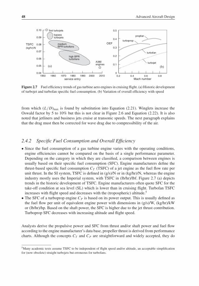
48 Advanced Aircraft Design
turbojet
Mach number
propfan
turbopropOEF
(b)
turbofan
1950 1960 1970 1980 1990 2000 2010
0.10
0.09
0.08
0.07
0.06
0.05
0.04
bypassturbojets
A380engines
high BPRturbofans
mediumBPR turbofans
TSFC(kg/hr)/N
first turbojets
(a)
service entry0.2 0.4 0.6 0.8
0.5
0.4
0.3
0.2
0.1
0
Figure 2.7 Fuel efficiency trends of gas turbine aero engines in cruising flight. (a) Historic developmentof turbojet and turbofan specific fuel consumption. (b) Variation of overall efficiency with speed
from which (L/D)max is found by substitution into Equation (2.21). Winglets increase theOswald factor by 5 to 10% but this is not clear in Figure 2.6 and Equation (2.22). It is alsonoted that jetliners and business jets cruise at transonic speeds. The next paragraph explainsthat the drag must then be corrected for wave drag due to compressibility of the air.
2.4.2 Specific Fuel Consumption and Overall Efficiency
• Since the fuel consumption of a gas turbine engine varies with the operating conditions,engine efficiencies cannot be compared on the basis of a single performance parameter.Depending on the category in which they are classified, a comparison between engines isusually based on their specific fuel consumption (SFC). Engine manufacturers define thethrust-based specific fuel consumption CT (TSFC) of a jet engine as the fuel flow rate perunit thrust. In the SI system, TSFC is defined in (g/s)/N or in (kg/hr)/N, whereas the engineindustry mostly uses the Imperial system, with TSFC in (lb/hr)/lbf. Figure 2.7 (a) depictstrends in the historic development of TSFC. Engine manufacturers often quote SFC for thetake-off condition at sea level (SL) which is lower than in cruising flight. Turbofan TSFCincreases with flight speed and decreases with the (tropospheric) altitude.5
• The SFC of a turboprop engine CP is based on its power output. This is usually defined asthe fuel flow per unit of equivalent engine power with dimensions in (g/s)/W, (kg/hr)/kWor (lb/hr)/hp. Based on the shaft power, the SFC is higher due to the jet thrust contribution.Turboprop SFC decreases with increasing altitude and flight speed.
Analysts derive the propulsive power and SFC from thrust and/or shaft power and fuel flowaccording to the engine manufacturer’s data base, propeller thrust is derived from performancecharts. Although the concepts CT and CP are straightforward and widely accepted, they do
5Many academic texts assume TSFC to be independent of flight speed and/or altitude, an acceptable simplificationfor (now obsolete) straight turbojets but erroneous for turbofans.

Early Conceptual Design 49
not mean the same thing to everybody and their magnitudes are entirely different. Confusionand mistakes can be avoided by the use of the overall engine efficiency (OEF),
ηodef= thrust power developed by the engine
rate of fuel energy added to the engine= T V
mfH(2.23)
The OEF is a dimensionless number which depends on engine technology and flight speed.For gas turbine engines it varies between 0.2 and 0.5 in cruising flight, see Figure 2.7 (b). Theconversion of SFC into OEF is treated in Section 3.2. Another advantage of using OEF insteadof SFC is the unification of flight performance analysis and optimization of aircraft withdifferent propulsion systems. This obviates the separate treatment of jet and propeller aircraftperformances which complies with the evolution of engine technology. Future generationsof very-high bypass ratio turbofans and open rotor engines can be seen as a cross-breed ofjet and propeller propulsion with a mix of genes inherited from both parents. The proposedunification leads to improved understanding of aircraft performance optimization as illustratedby the following example. Chapter 3 offers a more extensive summary of gas turbine engineproperties which will be useful for the aircraft design engineer and analyst.
2.4.3 Best Cruise Speed
When dealing with optimum cruising flight, a distinction should bemade between the optimumcruise condition of a given aircraft and the best aircraft design for a specified cruise condition.
1. The first problem is a classical subject of flight mechanics. It uses the specific range asthe objective for the most fuel-efficient speed and has a straightforward solution. A morerefined analysis is based on minimum direct operating costs (DOC), leading to a higheroptimum cruise speed.
2. The second problem is far more complex since it involves designing the best combinationof airplane and engine for a set of aircraft cruising at different Mach numbers. But even thesolution of the first problem requires careful analysis.
These two cases illustrate the distinction between analysis and synthesis discussed inSection 1.7.Equation (2.11) shows that the specific range in cruising flight is proportional to the range
parameter ηoL/D. Since ηo and L/D are both sensitive to Mach number variation, the rangeparameter ηoL/D is a suitable objective for optimizing the cruise condition and for comparingthe fuel economy of aircraft propulsion systems. For a given combination of airframe andengines in steady level flight, the range parameter is determined by two control variables –typical combinations are altitude and speed or lift coefficient and Mach number. In the caseof a constraint on altitude, speed, or engine rating, only one control variable remains to beoptimized. For historical reasons, this problem first was treated analytically for propelleraircraft, with the classical solution that the cruise speed for maximum range equals theminimum drag speed VMD. The maximum range of jet aircraft was first analyzed duringthe 1940s by assuming constant TSFC and ignoring compressibility drag. A well-knownanalytically derived result was the best flight speed at a given altitude with no limit on thrust

50 Advanced Aircraft Design
12
14
16
18
20
22
L/D
8
7
6
5
4
0.5
0.4
0.3
0.2
turboprop,straight wing
turbofan,swept wing
L/D
L/D
Mach numberMach number0.5 0.6 0.7 0.8 0.90.5 0.6 0.7 0.80.4
wave drag
o
L/D
L/Do
o
o
Figure 2.8 Effects of flightMach number variation on the range parameter for turboprop- and turbofan-powered aircraft flying at optimum altitude
which was found to be 31/4 times VMD. Although this result soon proved to be useless fortransonic (jet) aircraft, it has survived in academic teaching since 1950 (Chapter 12).Figure 2.8 depicts how the range parameter is affected by speed for a short-haul propeller
airplane and a long-range turbofan-powered airliner. Both airplanes are assumed to cruise atthe minimum drag condition for eachMach number, dictating that the altitude is varied in orderto match the varying Mach number. At subsonic Mach numbers, both planes have a constant(L/D)max and the range parameter is governed by the variation of the OEF with speed. Forthe propeller aircraft flying at M > 0.55, aerodynamic and propeller efficiencies deterioratedue to compressibility effects. The OEF of the swept wing turbofan airplane continues toincrease with the Mach number but the drag increases at M > 0.75. As a result, the propellerplane achieves a flat maximum range parameter for Mach 0.55, the jetliner has a pronouncedoptimum at Mach 0.79. This example leads to the following observations.
• The turboprop performs best at low-subsonic speeds, the jetliner achieves a higher rangefactor aboveMach 0.55 due to its higher L/D. If the comparison is made for regional aircraftwith the same design payload and range, the turboprop will probably have a better specificrange, lower fuel consumption and lower cruise speed; the turbofan will have a higher speedand productivity ([14], [21]).
• Transonic aircraft have their best range performance at a speed where drag due to compress-ibility determines the fuel-optimum cruise Mach number.
Between 1960 and 2000, design requirements dictated jetliner cruise speeds between Mach0.75 and 0.85, dependent on range. The urgency of reducing engine emissions is the drivingfactor for recent investigations suggesting that future airliners may have a reduced designcruise Mach number. Notwithstanding an airliner productivity penalty due to the lower blockspeed, the economy may improve since the reduced aircraft acquisition costs and the cost offuel could be the dominant compensating factors.

Early Conceptual Design 51
2.5 Environmental IssuesThe target of a reduction in fuel burn of 50% between 2000 and 2020 is an extremely challengingone which is not achievable without important breakthroughs, both in technology and in conceptsof operation.
—ACARE Strategic Research Agenda, 2002
In view of their effects on community noise and exhaust gas emissions into the atmosphere,engine selection has significant effects on the environment friendliness. The possibility of noiseshielding by positioning engines favourably relative to aircraft components is likely to becomean increasingly important element of conceptual design. On the other hand, the overview ofwhat may be achieved by ‘greener by design’ categorizes the reduction of engine emissions asmore demanding in the long term than the control of noise production around airfields [45].With the exception of the calorific value of fuel, all the factors affecting engine overall
efficiency have improved over the years. Although engine technology development is largelyoutwith the control of the advanced aircraft designer, far-reaching decisions have to be madewhen a new engine generation is introduced to a clean sheet design (Section 3.4). Reductionof engine noise and exhaust emissions is a primary driving factor during the engine selectionprocess (Section 3.5). The bypass ratio of a turbofan is a primary selection variable and theapplication of very high bypass-ratio geared turbofans or open rotor engines will allow amajor step forward in fuel economy but may lead to major complications when designing theairplane’s general arrangement. Since energy efficiency is closely related to aerodynamic andoverall engine efficiency, both figures are of crucial importance for environmental acceptanceand economic competitiveness.
2.5.1 Energy and Payload Fuel Efficiency
The energy efficiency (EEF) of a passenger transport defines the available seat-kilometres perlitre of fuel consumed. A similar characteristic is the payload fuel efficiency (PFE) definingthe available payload-kilometre per unit fuel weight consumed. For a given payload andrange, the accumulated cost of fuel consumed during commercial operations forms a largeproportion of the operating expenses whereas the seat-km or ton-km production represents theincome potential. Energy efficiency can be expressed in terms of parameters which are, to aconsiderable extent, under the control of the advanced designers – Section 8.6 treats payloadfuel efficiency as a figure of merit in the design. Expressed as an instantaneous performance,the EEF is derived from the specific range V/F
EENdef= Ns�R
�Qf= NsV �t
(m/ρ)f �t= ρfgNs
V
F(2.24)
where �Qf is the volume of fuel burn-off per distance flown �R and Ns denotes the numberof cabin seats. Similarly, PFE can be written as
EPFdef= Wpay�R
�Wf= WpayV �t
F�t= Wpay
V
F(2.25)

52 Advanced Aircraft Design
These expressions are clarified by substitution of V/F in horizontal cruising flight accordingto Equation (2.11),
EEN = ρfHNs
Wpayηo
L
D
Wpay
Wand EPF = (H/g)ηo
L
D
Wpay
W(2.26)
Equation (2.26) shows that design drivers are the calorific value of fuel, engine overall effi-ciency, aerodynamic efficiency and the ratio of payload to gross weight, occasionally calledthe structural efficiency. The following examples illustrate that, different from what the namesuggests, energy efficiency is not a dimensionless number between zero and one.
• For a typical payload mass of 95 kg per seat and a fuel energy density of 34.5 MJ perlitre, ρfH Ns/Wpay = 37 seat-km per litre. A jetliner with Wpay/W = 0.20, ηo = 0.35 andL/D = 18 has a range parameter of 6.3 and a PFE of 46.6 seat-km per litre (95.1 seat-nmper gallon).
• The PFE of a cargo aircraft with the same range parameter and a payload fraction of0.25 amounts to 6 850 ton-km per ton fuel (3 700 ton-nm per ton).
The average energy efficiency for a flight is obtained from the integration of the instantaneousvalue along the flight path; see Section 8.6.Energy efficiency is often considered as measure of technical progress in commercial
aviation. Since the introduction of long-range jetliners, it has increased each year with 0.6 seat-km per litre; that is, by a factor 2.5 between 1960 and 2000 (Figure 2.9).6 Wide body passengertransports introduced into service after 2010 achieve EEN values approaching 50 seat-km perlitre. Since the actually realized efficiency depends on the cabin seating arrangement anddistance flown, it varies between different airliner versions, cabin arrangements and operations.Thismakes the clear trend in Figure 2.9 rather coincidental. It is therefore preferable to compareenergy efficiencies based on maximum payload rather than on seating capacity.Figure 2.10 shows the effect on PFE of varying the harmonic range for a family of wide
body airliners with equal MPL, aerodynamic and overall engine efficiency in cruising flight.Long-range aircraft have a disadvantage due to the high MTOW required to carry the largefuel load – indeed, very few existing long-range airliners have a harmonic range longer than10 000 km. For ranges below 3 000 km, the fuel lost during climb and descent forms asignificant fraction of the mission fuel which causes the efficiency to decrease and, in thepresent example, the highest PFE is achieved for approximately 3 500 km range. Most airlineflights are made over shorter distances than the harmonic range, with a take-off weight lessthan the MTOW. Consider an aircraft designed for 10 000 km harmonic range (point D) witha PFE = 6 900 km. If this plane makes a 5 000 km flight with maximum payload (point E),its TOGW is 15% less than the MTOW, and PFE = 7 323 km. However, if the plane weredesigned for a harmonic range of 5 000 km (point F), its empty and fuel weights would belower, resulting in a PFE of 7 900 km – 8% better than point E. Figure 2.10 also shows that,
6The fuel efficiency of a modern airliner is similar to that of a typical middle-class car on the highway. However,airliners travel ten times faster over long distances and achieve a higher load factor. Based on payload-kilometresproduced, airliners achieve a (much) better energy efficiency than cars.

Early Conceptual Design 53
757-200
A320-200
747-400MD-11
767-300
737-300767-200
747-300
DC-9-80
L-1011-500A300-B4
747-SP737-200ADV
727-200ADV
747-200BDC-10-10
L-1011DC-10-30
DC-9-30DC-8-63
727-100
707-320C
707-120B707-320
707-120CV-880
CV-990
Comet 1
1950 1960 1970 1980 1990
50
40
30
20
10
0
entry into service
Figure 2.9 Historic energy efficiency trend for jetliners. Source: NASA
for ranges in excess of the harmonic range, the PFE decreases rapidly due to the replacementof payload by fuel.Since the selection of a long-range design point entails a reduced energy efficiency, it has
been observed that (a lot of) fuel can be saved if long-range flights were covered in two or morestages by medium-range aircraft [40]. This concept is verified in [30] for the Boeing 747 andthe 777 and it is further elaborated in recent publications. According to [36], fuel savings bystaging are possible for trips longer than about 6 000 km. The benefits increase almost linearlywith the flight length, reaching about 13% for the maximum distances that are likely to be
Figure 2.10 Payload fuel efficiency of jetliners with 50 ton payload
54 Advanced Aircraft Design
covered. Since 30% of the global fuel is burned on flights of 6 000 km and above, the stagingof all long-haul flights would save 3% fuel if the same (long-range) aircraft were used, and9% if (optimized) medium-range aircraft were used. However, a long-range transport aircraftis more flexible when an airline network is treated as a system. For instance, an airliner canmake a return flight with two medium-range segments with no intermediate refueling. Thismay be one of the reasons why few customers opt for short/medium-range versions of a basiclong-range airliner. Energy efficiency affects fuel economy as well as engine emissions andit is beneficial to get insight in its importance in the initial design stage. Much of the presentbook is devoted to finding out how selection variables affect these parameters and to whatextent the designer’s freedom of choice is limited. This is a complex matter since the (oftenopposing) effects of design technology are spread all over aircraft components and they arefelt in all technical disciplines contributing to costs.
2.5.2 ‘Greener by Design’
Environmental issues are causing increasing concerns for the aviation community. The IPCCstudy on the global atmosphere [3] assesses radiative forcing7 effects from aircraft in 1992,projects it forward to 2050 and predicts their overall effect to increase by a factor of five.Most effects are associated with engine combustion products. About one-third of the totalradiative forcing stems from CO2, for which fuel burn is the direct measure. Other forcingcomponents are NOx, H2O, contrails, cirrus clouds, sulfate, and soot – the estimated ratings oftheir radiative forcing are mostly qualified as unreliable. Areas of uncertainty are the effectsof the O3 and CH4 created by NOx emissions and the effects of contrails and cirrus clouds.In particular, their dependence on conditions in the engine exhaust, flight altitude, latitude,climate and season are uncertain. Consequently, there are circumstances in which measures toreduce fuel burn may actually increase the overall contribution of engine emissions to climatechange. This applies, for example, to the trade-off between increasing engine pressures andtemperatures in favour of lower SFC and reducing them in order to reduce the generation ofNOx. In spite of these complications, a pertinent recommendation to the aircraft designer is toincrease the energy efficiency of the vehicle by all affordable measures and to treat the cruisealtitude explicitly as an independent design variable.Primary issues driving civil aircraft development were summarized in 2001 by the Advisory
Council for Aeronautics in Europe (ACARE). This organization aims at radical improvementsof the air transport system in order to reduce its environmental impact. In terms of goals to beachieved in 2020–2025, specific measures are summarized as follows:
• Reduce fuel consumption and CO2 emissions by 50%.• Reduce NOx emissions by 80%.• Reduce perceived external noise by 50%.
These requirements are formulated for aviation as a whole and need to be broken down intospecific goals for the individual players. The aircraft and engine industry, operators, air trafficmanagement, certification and safety agencies, and the European Union – all of them takethese goals seriously.
7Radiative forcing expresses the perturbation or change to the energy balance of the Earth’s atmospheric system inwatts per square metre.

Early Conceptual Design 55
In the UK, several organizations representing the manufacturing and air transport sectors aswell as academia have established the Air Travel Greener by Design study group. Focussing onmitigating the environmental impact of aviation, three sub-groups were formed to specificallyconsider operation,market-based options and technology. The technology sub-group addressedairfield noise and local air quality and climate change, with the climate change consideredto be the most important in the long term. The sub-group reported its findings in [40]; thefollowing text is an extract from their recommendations.
In the context of climate change, we consider the following to be key areas of research, study andtechnology validation. Some already benefit from substantial European funding, some are newproposals. All merit support.
• Research into the atmospheric effects of aircraft emissions, including the dependence of theeffects on flight altitude.
• Research and demonstration of engine technology to achieve a substantial reduction in NOx
emissions, particularly at cruise conditions.• Extended in-service trials of hybrid laminar flow control, sufficient to assess the practicabilityof the system.
• Design study of the blended wing-body concept, backed by research and technologydemonstration to eliminate all significant technical doubt.
• Feasibility study of the laminar flying wing.• Total system study of the provision of long distance air travel by medium range aircraft coveringdistances greater than 7 500 km (4 000 nm, eight hours flying time) in two or more stages.
Study of the methodology for designing transport aircraft so as to minimize impact on climatechange per unit thrust. The barrier to the introduction of the identified design and technologyoptions that have the potential to reduce the greenhouse effect is the perceived imbalance betweenthe significant technical and economical risks and the small potential economic benefit.
Increasing environmental acceptability of conventional airliner configurations will eventuallybecome prohibitively expensive and some of the Greener by Design recommendations are notachievable without a radical change of the design concept. The blended wing body (BWB)(Figure 5.3) is an unorthodox but promising concept which has been investigated by manyinstitutions. The less radical configuration depicted on Figure 2.11 features a very high aspectratio laminar flow wing and ultra-high bypass ratio turbofans located above the empennage fornoise shielding. Application of a new generation of airliners appears to promise that a major
Figure 2.11 Will this be the ultimate green aircraft of the future?

56 Advanced Aircraft Design
step forward will be made during the first half of the twenty-first century to reduce the impactof aviation on the Earth’s climate.
Bibliography
[1] Society of Allied Weight Engineers, Introduction to Aircraft Weight Engineering, SAWE Inc., Terminal Annex,Los Angeles, CA, 1996.
[2] Fielding, J.P., Introduction to Aircraft Design, Cambridge University Press, Cambridge, 1999.[3] Intergovernmental Panel on Climate Change, Aviation and the Global Atmosphere, Cambridge University Press,
Cambridge, 1999.[4] Ferreri, D.,Marketing and Management in the High-Technology Sector: Strategies and Tactics in the Commercial
Airplane Industry, Praeger, Westport, CT, 2003.[5] Roux, E., Avions Civils a Reaction: Plan 3 Vues et Donnees Characteristiques, Editions Elodie Roux, Imprime
par lulu.com, 2007.[6] De Florio, Airworthiness: An Introduction to Aircraft Certification, Butterworth-Heinemann, Oxford, 2011.
Initial Orientation
[7] Werner, R.A., and G.F. Wislicenus, ‘Analysis of Airplane Design by Similarity Considerations”, AIAA PaperNo. 68-1017, October 1968.
[8] Caddell, W.E., “On the Use of Aircraft Density in Preliminary Design”, SAWE Paper No. 813, May 1969.[9] Cleveland, F.A., “Size Effects in Conventional Aircraft Design”, Journal of Aircraft, Vol. 3, No. 6, pp. 483–512,
November–December 1970 (also AIAA Paper No. 70-940).[10] Engineering Sciences Data Unit, “Lost Range, Fuel and Time to Climb and Descent: Aircraft with Turbojet and
Turbofan Engines”, ESDU Data Sheet No. 74018, August 1974.[11] Overend, W.J., “Design Criteria for Airline Operations”, AIAA Paper No. 79-1849, August 1979.[12] Smith, H.W., and R. Burnham, “The Outside Has to Be Bigger than the Inside”, Journal of Aircraft, Vol. 18,
No. 6, pp. 463–468, June 1981.[13] Marsh, D.P., “Theory of Transport Aircraft Weight Fractions”, SAWE Paper No. 1452, May 1982.[14] Edlund, U., “Optimum Design Cruise Speed for an Efficient Short Haul Airliner”, ICAS Paper No. 84-4.8.3,
September 1984.[15] Roskam, J., “Rapid Sizing Method for Airplanes”, Journal of Aircraft, Vol. 23, No. 7, 1986, pp. 554–560.[16] Torenbeek, E., “The Initial Calculation of Range and Mission Fuel During Conceptual Design”, TU Delft,
Department of Aerospace Engineering, Report LR 525, 1987.[17] Association of European Airlines, “Requirements for Short/Medium Range Aircraft for the 1980s”, Technical
Affairs Committee, Report G.2110/R2, Third Edition, July 1981. Later edition: December 1989.[18] Oelkers, W., “High Capacity Aircraft”, ICAS Paper No. 92-1.10.3, September 1992.[19] Martınez-Val, R., E. Perez, T. Munoz, and C. Cuerno, “Design Constraints in the Payload-Range Diagram of
Ultra High Capacity Transport Airplanes”, Journal of Aircraft, Vol. 31, No. 6, pp. 1268–1272, November–December 1994.
[20] Arjomandi, M., and N.K. Liseytsev, “A Simplified Method for Estimating the Take-Off Weight for Short-HaulTransports”, Aircraft Design, Vol. 3, No 1, pp. 49–56, 2000.
[21] Richter, H., and S. Menczykalski, “Civil Propulsion of the Future”, Innovative Configurations and AdvancedConcepts for Future Civil Aircraft, Von Karman Institute for Fluid Dynamics, Lecture Series 2005-06, June2005.
[22] Sacco, G., and C. Lanari, “The Three Lifting Surface Configuration Concept and Lessons Learned from thePiaggio P180”, Innovative Configurations and Advanced Concepts for Future Civil Aircraft, Von KarmanInstitute for Fluid Dynamics, Lecture Series 2005-06, June 2005.
[23] Bolsunovsky, A.L., N.P. Buzoverya, B.I. Gurevich, V.E. Denisov, and O.V. Sonin, “Flying-Wing: Problems andDecisions”, Innovative Configurations and Advanced Concepts for Future Civil Aircraft, von Karman Institutefor Fluid Dynamics, Lecture Series 2005-06, June, 2005.

Early Conceptual Design 57
[24] Torenbeek, E., and G. La Rocca, “Civil Transport Aircraft”, Encyclopedia of Aerospace Engineering, R.Blockley and W. Shyy (eds), pp. 4043–4054, John Wiley & Sons, Chichester, 2010.
[25] Torenbeek, E., “Business Aviation”, in Encyclopedia of Aerospace Engineering, R. Blockly, and W. Shyy (eds),John Wiley & Sons, Chichester, UK, October 2010.
[26] Poll, D.I.A., “A First OrderMethod for the Determination of the LeadingMass Characteristics of Civil TransportAircraft”, Aeronautical Journal, vol, 115, No. 1167, pp. 257–272, May 2011.
Energy Efficiency
[27] Poisson-Quinton, P., “Energy Conservation in Aircraft Design and Operational Procedures”, AGARD LectureSeries LS-96, Paper No. 9, October 1978.
[28] Niedzballa, S.M., andD. Schmitt, “Comparison of the Specific EnergyDemand of Aeroplanes andOther VehicleSystems”, Aircraft Design, Vol. 4., No. 4, pp. 163–178, December 2001.
[29] Nangia, R.K., “Efficiency Parameters for Modern Commercial Aircraft”, Aeronautical Journal, Vol. 110, No.1110, pp. 495–510, August 2006.
[30] Creemers, W.L.H., and R. Slingerland, “Impact of Intermediate Stops on Long-Range Jet Transport Design”,AIAA Paper No. 2007–7849, September 2007.
[31] Hahn, A.S., “Staging Airliner Service”, AIAA Paper No. 2007-7759, September 2007.[32] Poll, D.I.A., “The Optimum Aeroplane and Beyond”, Aeronautical Journal, vol, 113, No. 1141, pp. 151–164,
March 2009.[33] Kenway, G.K.W., R. Henderson, J.E. Hicken, N.B. Kuntawala, D.W. Zingg, J.R.R.A. Martins, and R.G. McKe-
and, “Reducing Aviation’s Environmental Impact Through Large Aircraft for Short Ranges”, AIAA Paper No.2010-1015, January 2010.
[34] Lanfhans, S., F. Linke, P. Nolte, and H. Schnieder, “System Analysis for Future Long Range OperationConcepts”, ICAS Paper No. 2010-11.3.4, September 2010.
[35] Martinez-Val, R., E. Perez, C. Cuerno, and J.L. Palacin, “Cost-Range Trade-Off in the Design and Operation ofLong-Range Transport Airplanes”, ICAS Paper No. 2010-1.5.1, September 2010.
[36] Poll, D.I.A., “On the Effect of Stage Length on the Efficiency of Air Transport”, Aeronautical Journal, vol. 115,No. 1167, pp. 273–283, May 2011.
Emissions and Atmospheric Pollution
[37] Haberland, Ch., O. Kranz, and R. Stoer, “Impact of Operational and Environmental Aspects on CommercialAircraft Design”, ICAS-94-1.3.1, Anaheim, 1994.
[38] Deidewig, F., A. Doppelheuer, and M. Lecht, “Methods to Assess Aircraft Engine Emissions in Flight”, ICASPaper No. 96-4.1.4, September 1996.
[39] Szodruch, J., “The Environmental Challenge as Chance for the Next Century Aircraft Design”, ICAS Paper No.98-4.10.3., September 1998.
[40] Green, J.E., “Greener by Design – The Technology Challenge”, Aeronautical Journal, Vol. 106, No. 1056, pp.57–103, February 2002.
[41] Whellens, M.W., and R. Singh, “Propulsion System Optimisation for Minimum Global Warming Potential”,Paper No. 7111, ICAS 2002 Congress, Toronto, September 2002.
[42] Rolls-Royce, “Powering A Better World”, Environment Report, www.rolls-royce.com., 2003.[43] Antoine, N.E., and I.M. Kroo, “Aircraft Optimization for Minimal Environmental Impact”, Journal of Aircraft,
Vol. 41, No. 4, pp. 2100–2109, 2004. (Also AIAA Paper No. 2002-5667, September 2002.)[44] Green, J.E., “Greener by Design”, Innovative Configurations and Advanced Concepts for Future Civil Aircraft,
Von Karman Institute for Fluid Dynamics, Lecture Series 2005–06, June 2005.[45] Green, J.E., “Air Travel – Greener by Design. Mitigating the Environmental Impact of Aviation: Opportunities
and Priorities”, Aeronautical Journal, Vol. 109, pp. 361–416, September 2005.[46] Green, J.E., “Civil Aviation and the Environment: The Next Frontier for the Aerodynamicist”, Aeronautical
Journal, Vol. 110, pp. 469–486, August 2006.[47] Hahn, A.S., “Staging Airliner Service”, AIAA Paper No. 2007-7759, September 2007.

58 Advanced Aircraft Design
[48] Nangia, R.K., “Highly Efficient and Greener Civil Aviation: Step Jump, Why & How”, lecture presented at theRoyal Aeronautical Society, Bristol Branch, RKN-SP-2007-100, October 2007.
[49] Sankrithi, M., “Environmentally Progressive Aircraft Design Leveraging Advanced Technologies”, BoeingCommercial Airplanes, lecture presented to Department of Aerospace Engineering, TU Delft, April 2008.
[50] Shakariyants, S.A., “Generic Methods for Aero-Engine Exhaust Emission Prediction”, doctoral thesis, TUDelft, September 2008.
[51] Gardner, R., “How Green In Your Contrail?”, Aerospace International, pp. 14–17, March 2007.[52] Kenway, G.K.W., R.P. Henderson, J.E. Hicken, N.W. Kuntawala, D.W. Zingg, J.R.R.A. Martins, and R.G.
McKeand, “Reducing Aviation’s Environmental Impact Through Large Aircraft for Short Ranges”, AIAAPaper No. 2010-1015, January 2010.
[53] Rutherford, D., “The Role and Design of a CO2 Standard for New Aircraft”, ICCT, 14 April 2010.[54] Bradley, M.K., and C.K. Droney, “Subsonic Ultra Green Aircraft Research: Phase I Final Report”. NASA/CR-
2011-216847, April 2011.[55] Henderson, R.P., J.R.R.A. Martens, and R.E. Perez, “Aircraft Conceptual Design for Optimal Environmental
Performance”, Aeronautical Journal, Vol. 116, pp. 1–22, January 2012.

3Propulsion and Engine Technology
At 65 cents per gallon, the fuel price was too low to justify the UDF. If fuel were at a buck or so agallon, they’d be clamoring.
—R. Welsh, GE Manager Commercial Operations (1988)
3.1 Propulsion Leading the Way
The history of civil aviation has shown that a prominent contribution to improved energyefficiency and economics stems from advancements in propulsion technology [28]. Sincethe end of the Second World War, gas turbine engines have evolved significantly throughcoordinated development in airplane and engine technology. For instance, the Boeing 707used the evolution from the turboprop to the turbojet engine to fly faster and higher whereasthe need for more range led to the development of bypass engines around 1960. Largerengines with high bypass ratios were developed during the 1960s to meet the high take-offthrust and reduced fuel consumption requirements of wide body airliners. Since 1970, thecontinuous development of turbofans into more efficient and reliable engines has been gradualbut significant. Within half a century, their thermal efficiency has increased from less than0.40 for the straight jet engine to about 0.50 for the modern turbofan engine. The take-offthrust of the largest turbofans has increased from 20 to 45 tons, specific fuel consumption(SFC) decreased by approximately 30%; see Figure 2.7 (a). The greatest improvement camefrom the propulsive efficiency improving from about 0.50 to 0.75. Open rotor turbofans mayimprove this further to 0.90. A new generation of very high bypass ratio engines is emergingand the next step to open rotor technology may mature sooner than expected. The installationof these advanced engines may necessitate a marked change in the general arrangement ofnew airplanes.This chapter gives an overview of the terminology associated with gas turbine engine
technology and performances, covering subjects specifically selected to be applicable to con-ceptual design and performance analysis. For this purpose, the most relevant properties areengine power and thrust, specific fuel consumption and engine efficiencies. Several general-ized performance characteristics will be presented in non-dimensional form for use in cruiseperformance optimization and in engine scaling. Aircraft gas turbines operate on the Brayton
Advanced Aircraft Design: Conceptual Design, Analysis and Optimization of Subsonic Civil Airplanes, First Edition. Egbert Torenbeek.
© 2013 by Egbert Torenbeek. Published 2013 by John Wiley & Sons, Ltd.

60 Advanced Aircraft Design
mf
pema+m f
Ae
ma V ve
p∞ vj
p∞
Figure 3.1 Using the momentum equation to derive turbojet and turbofan thrust
cycle; however, cycle analysis is outwith the scope of this text. Several excellent textbookson gas turbine engine cycles, performance analysis and technology are mentioned in thebibliography.
3.2 Basic Concepts of Jet Propulsion
3.2.1 Turbojet Thrust
The thrust of a straight jet engine is derived from the momentum equation, using the controlsurface as indicated in Figure 3.1. At flight speed V , ambient air with mass flow rate ma
enters the inlet with momentum maV , referred to as ram drag (or inlet momentum drag). Thecompressed air is heated by the injection of fuel with the flow rate mf and then burning it athigh pressure. The hot gas drives the turbine and exits the engine through the nozzle. Its totalmass flow rate is ma(1+ f ), with f denoting the fuel/air mass ratio. Average properties in thenozzle exit with area Ae are velocity ve and pressure pe determinoing the gross thrust,
TG = ma(1+ f )ve + (pe − p∞)Ae (3.1)
where p∞ denotes ambient pressure. The net thrust is equal to gross thrust minus the ram drag,
TN = TG − Dram = ma{ve(1+ f )− V } + (pe − p∞)Ae (3.2)
Engine manufacturers refer to this as the standard net thrust. Since its terms are well definedand accurately measurable, the standard thrust defines the performance of the (uninstalled)engine normally used by the aircraft manufacturer. While expanding to ambient pressurebehind the nozzle exit, the jet efflux mixes with air. This leads to a (small) thrust contributionknown as post-exit thrust. A simplified concept to include post-exit thrust is to assume ahypothetical uniform jet with velocity vj after expansion. Another simplification is to ignorethe fuel mass flow rate relative to the air mass flow ( f � 1). This yields the ideal thrust,
Tid = ma(vj − V ) (3.3)
The difference between standard net thrust and ideal thrust is generally small at subsonicspeeds and is ignored in this text. We consider the thrust T as the net force exerted by theinstalled engine to propel the aircraft. A useful figure of merit for jet propulsion is the specificthrust which relates the thrust to the air throughput for generating it,
T
ma= vj − V (3.4)
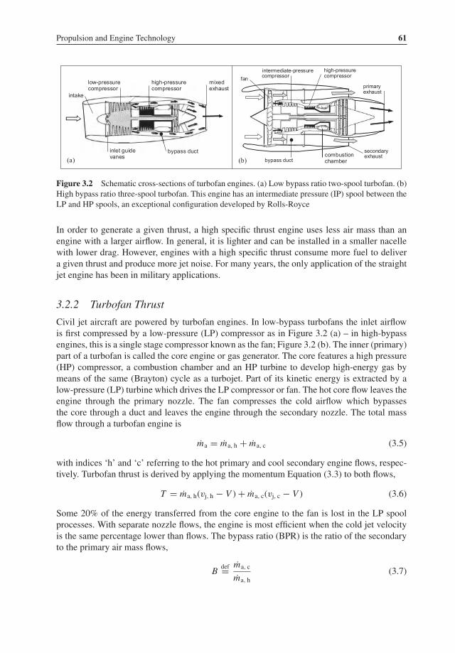
Propulsion and Engine Technology 61
Figure 3.2 Schematic cross-sections of turbofan engines. (a) Low bypass ratio two-spool turbofan. (b)High bypass ratio three-spool turbofan. This engine has an intermediate pressure (IP) spool between theLP and HP spools, an exceptional configuration developed by Rolls-Royce
In order to generate a given thrust, a high specific thrust engine uses less air mass than anengine with a larger airflow. In general, it is lighter and can be installed in a smaller nacellewith lower drag. However, engines with a high specific thrust consume more fuel to delivera given thrust and produce more jet noise. For many years, the only application of the straightjet engine has been in military applications.
3.2.2 Turbofan Thrust
Civil jet aircraft are powered by turbofan engines. In low-bypass turbofans the inlet airflowis first compressed by a low-pressure (LP) compressor as in Figure 3.2 (a) – in high-bypassengines, this is a single stage compressor known as the fan; Figure 3.2 (b). The inner (primary)part of a turbofan is called the core engine or gas generator. The core features a high pressure(HP) compressor, a combustion chamber and an HP turbine to develop high-energy gas bymeans of the same (Brayton) cycle as a turbojet. Part of its kinetic energy is extracted by alow-pressure (LP) turbine which drives the LP compressor or fan. The hot core flow leaves theengine through the primary nozzle. The fan compresses the cold airflow which bypassesthe core through a duct and leaves the engine through the secondary nozzle. The total massflow through a turbofan engine is
ma = ma, h + ma, c (3.5)
with indices ‘h’ and ‘c’ referring to the hot primary and cool secondary engine flows, respec-tively. Turbofan thrust is derived by applying the momentum Equation (3.3) to both flows,
T = ma, h(vj, h − V )+ ma, c(vj, c − V ) (3.6)
Some 20% of the energy transferred from the core engine to the fan is lost in the LP spoolprocesses. With separate nozzle flows, the engine is most efficient when the cold jet velocityis the same percentage lower than flows. The bypass ratio (BPR) is the ratio of the secondaryto the primary air mass flows,
Bdef= ma, c
ma, h(3.7)

62 Advanced Aircraft Design
Exhaust flowmixers improving propulsive efficiency are installed in many low BPR turbofans.If the two flows are mixed with no momentum loss into a uniform jet with velocity
vj = vj, h + Bvj, c
1+ B(3.8)
it appears that Equation (3.3) applies to turbofan thrust as well. Since the BPR varies withoperational conditions, it is commonly specified for the static condition at sea level. Turbofanscan be characterized according to the following tentative scheme:
• Low bypass ratio turbofans (B ≤ 1.5), formerly known as bypass engines, can be found ina few obsolete military aircraft and trainers.
• Medium bypass ratio (1 < B ≤ 4) turbofans are installed in older jetliners and businessjets, most of which do not comply with today’s noise regulations.
• High bypass ratio (4 < B ≤ 10) turbofans constitute the presently dominating category injetliner and business jet applications.
• Very high bypass ratio (B > 10) turbofans will be installed in airliners developed for entryinto service after 2010.
The BPR of a turbofan is closely related to its specific thrust. For a given thrust, increasing theBPR leads to a larger fan diameter, more airflow, reduced specific thrust, and lower jet noise.Many turbofans are offeredwith different values of the fan diameter, BPR and take-off thrust fora basically unchanged core engine. This has the advantage that turbofans with a single commoncore can be matched to the thrust required by different airplane designs. For an entire enginefamily with the same gas generator, development costs are only half as much as developingthree separate engines. Commonality simplifies the manufacturing process and cuts partsinventories to a minimum. For airlines, core commonality translates into simplified inventorymanagement, overall lower propulsion costs and more uniform maintenance procedures for avariety of engines spanning a wide range of thrusts.
3.2.3 Specific Fuel Consumption
The fuel weight flow per unit time burnt by a turbojet or turbofan engine varies approximatelyproportional to its thrust. In order to make ameaningful comparison between different engines,it is customary to use the specific fuel consumption (SFC). The thrust-specific TSFC denotesthe fuel mass flow rate per unit thrust,
CT = mf
T= F/g
T(3.9)
where F denotes the fuel weight flow. A TSFC in SI units has the dimension g s−1 N−1
although it is customary to express TFC in kg h−1 N−1. The TSFC in the SI system differsby a factor g from the value in Imperial units having the dimension lb hr−1 lbf−1. The TSFCbased on fuel weight flow is mostly used in aircraft performance analysis and differs by afactor g from the TSFC based on mass flow. Consequently, the weight-specific SFC in SI unitsis numerically equal to the mass-specific TSFC in Imperial units. Although TSFC is a widely

Propulsion and Engine Technology 63
used parameter, the inexperienced analyst may be confused about its definition since it doesnot mean the same thing to everybody.
3.2.4 Overall Efficiency
In case of doubt, it is recommended to convert SFC into overall efficiency (OEF), also knownas total efficiency,
ηodef= thrust power developed by the engine
rate of fuel energy added to the engine= TV
mfH= TM a
FH/g(3.10)
The (lower) calorific value – or specific energy content – of jet fuel H is the chemical energyconverted into thermal energy on complete combustion in air. The speed of sound is a = asl
√θ ,
with θ denoting the relative atmospheric temperature. Substitution of asl = 340.29 m/s andH/g = 4 350 km for conventional (fossil) gas turbine engine fuel yields the conversion ofTSFC in (kg/h)/N into OEF,
ηo = aslH/g
M√
θ
CT= 0.0287
M
CT /√
θ(3.11)
For TSFC in (lb/h)/lbf this becomes
ηo = aslH/g
M√
θ
CT= 0.2816
M
CT /√
θ(3.12)
Since overall efficiency is a dimensionless quantity between zero and one, it has the samevalue in both systems of units. For given flight conditions, the OEF can be derived from thrustand fuel flow (or SFC) stated in the engine specifications, corrected for installation losses. Forcruising flight near the tropopause at a given Mach number, OEF is (nearly) independent ofthe altitude. The first generation of jetliners flew at M ≈ 0.80 and were powered by straightjet engines with CT ≈ 1.0 (lb/h)/lbf. This complies with an OEF of only 20%which illustratesthe jet’s poor performance.1 A typical CT = 0.56 (lb/h)/lbf for current turbofans installed inlong-range aircraft cruising at M = 0.80 corresponds with an OEF of 35%. It is worth notingthat, even for a 100% efficient propulsion system, there exists a theoretical minimum TSFC;namely, CT = 0.2816 M
√θ . However, a more realistic lower limit is CT = 0.5 M
√θ for
ηo = 0.55. This would require present-day engines to be improved by some 50%.
3.2.5 Thermal and Propulsive Efficiency
The ideal turbofan engine converts the chemical energy contained by the fuel into the max-imum possible kinetic energy which is then converted into propulsive thrust by the largestpossible momentum increment across the engine. Accordingly, the OEF of this process can bedecomposed into several process efficiencies.
1Concorde’s propulsion system achieved an OEF of more than 40% in cruising flight at Mach 2. At the time of writing,this has not been exceeded by any operational subsonic airplane.

64 Advanced Aircraft Design
component efficiency 0.850.7
0.6
0.5
0.4
0.3
0.2
0.1
010 20 30 40 50 60 70
1980sTET (K)
(a)
conventionalpropeller
contra-rotatingopen rotor
high speedpropeller
0.7
0.6
0.5
0.8
0.9
1.0
0.5 0.6 0.7 0.8 0.9
Mach number
2020target
overall pressure ratio
1990s
1970s
1960s
2200
2000
1800
1600
1400turbofan BPR
4
6
8
10
(b)
Figure 3.3 Efficiency trends for several generations of gas turbine engines used in commercial aircraft.(a) Turbofan thermal efficiency affected by cycle parameters. (b) Propulsive efficiency trends. Thegrey-scale curves for propellers and open rotors are performance envelopes
The thermal efficiency (TEF) is a measure of how efficiently the chemical energy containedby the fuel is converted into the kinetic energy increment of the air moving through the engine,
ηth = rate of kinetic energy change across the engine
rate of fuel energy added to the engine=
12 ma(v2j − V 2)
mfH(3.13)
The TEF can be seen as the product of combustion efficiency, thermodynamic efficiency of thegas generator’s Brayton cycle, and efficiency of energy transfer from the gas generator tothe engine air throughput. TEF depends primarily on the core engine’s cycle parameters – itincreases with the overall pressure ratio (OPR) and the turbine entry temperature (TET); seeFigure 3.3 (a). Other important parameters are the efficiencies of the core compressors andturbines. Energy transfer suffers from total pressure losses in the power turbine and the fan andfrom mechanical losses due to gearing.2 TEF increases with decreasing ambient temperatureand increasing flight speed, one reason for airliners to have their best range performanceat high altitudes and Mach numbers. It is expected that the TEF in the year 2020 will beapproaching 55%.The propulsive efficiency (PEF) of an engine is ameasure of the thrust-producingmomentum
change for a given amount of kinetic energy increment of the air throughput,
ηp = thrust power developed
kinetic energy change across the engine= TV
12 ma(v2j − V 2)
(3.14)
Substitution of the thrust Equations (3.3) and (3.4) yields
ηp = ma(vj − V )V12 ma(v2j − V 2)
= 2
1+ vj/V= 2
2+ T/(maV )(3.15)
2Dependent on engine technology, polytropic compression and expansion efficiencies are approximately 90%,combustion and gear efficiencies are close to 99%.

Propulsion and Engine Technology 65
Known as the Froude equation, this formula shows that the PEF is high for engines witha large air throughput producing a low specific thrust with a low-velocity jet. Figure 3.3 (b)illustrates that BPR and flight speed are the primary parameters affecting propulsive efficiency.Increasing the fan diameter – hence, air throughput – for a given core flow translates into higherBPR and increased PEF. For a B = 5 turbofan, a typical uninstalled engine PEF is 0.75 atMach 0.80. In the year 2020 this value may have increased to 0.85.The overall efficiency (OEF) defined by Equation (3.10) is the product of thermal and
propulsive efficiencies,
ηo = ηthηp (3.16)
Engine manufacturers foresee that the typical OEF of 0.35 for present-day turbofans willeventually be improved to 0.45 for open rotor engines. The question is not whether it willhappen but when.
3.2.6 Generalized Performance
Propulsive thrust and fuel consumption of a turbofan engine are functions of its rating, flightspeed, and ambient conditions. The engine rating is characterized by the high pressure (HP)spool rotational speed. Books on gas turbine engine performance derive generalized relation-ships which are useful for matching the engine size to the airframe, engine selection andairplane performance analysis. Thrust, engine air and fuel flow rates are generalized in theform of corrected performances. For example, corrected turbofan thrust is related to flightMach number M and the HP rotor speed N ,
T
δ= fT (M, N/
√θ ) (3.17)
The relative pressure δ and relative temperature θ denote the ambient pressure and temperatureas fractions of sea level values in the standard atmosphere – see Appendix B – and N/
√θ
represents the corrected rotor speed. Fuel weight flow F is generalized as follows:
F
δ√
θ= fF (M, N/
√θ ) (3.18)
Elimination of the rotor speed yields
F
δ√
θ= f3 (M, T/δ) (3.19)
whereas the TSFC is corrected for ambient temperature as
CT√θ
= fF
fT(3.20)
Figure 3.4 depicts a typical generalized performance map of a turbofan engine. Within therange of typical cruise conditions, thrust is affected primarily by Mach number and, to a much

66 Advanced Aircraft Design
Mach number
0.9
0.8
0.7
0.6
0.5
100 120 140 160 180 200
0.08
0.07
0.06
0.05
0.04
10,000N
rpm
T kN
CT
(kg/hr)/N
10,50011,000
10,25010,750
max.climb
max.cruise
Figure 3.4 Generalized altitude performance of a high bypass turbofan
smaller extent, by the engine rating. Within the range of cruise altitudes and Mach numbers,the TSFC can be approximated by an empirical relationship, for instance,
CT /√
θ = C0(1+ CM M) (3.21)
The factors C0 and CM can be derived from the engine manufacturer’s data. For a givenengine, they are affected mainly by the BPR. The OEF is found by substitution intoEquation (3.12),
ηo = 0.0287M
C0(1+ CMM)(3.22)
As opposed to the TSFC, the OEF is independent of the altitude which demonstrates anotheradvantage of its use.
3.2.7 Mach Number and Altitude Effects
In design studies where the engines are scaled up or down by the rubberizing method, thethrust is treated as a fraction of the maximum static take-off thrust (index TO) at sea level (SL)in the ICAO standard atmosphere (ISA). This fraction is known as the thrust lapse rate (TLR).If the corrected thrust is according to Equation (3.17), we obtain the thrust lapse parameter,
τdef= T/p
TTO/psl= T
δ TTO(3.23)
In a rubberizing process it is desirable to eliminate the rotor speed by combining Equations(3.10), (3.17) and (3.18), which yields the OEF in terms of two dimensionless quantities,
ηo = fη(τ, M) (3.24)

Propulsion and Engine Technology 67
Figure 3.5 Rolls-Royce AE 1107: a member of a family of turboshaft and turboprop engines in the6 000 shp (4 474 kW) class for military and commercial applications. The Jet Engine, Rolls RoyceTechnical Publications, Copyright 2013 Rolls-Royce plc
The carpet plot on log-log scale depicted in Figure 12.6 shows that Mach number variationhas much more effect on OEF than the engine rating. For a cruising flight at a given Machnumber, the thrust lapse rate with altitude depends on the engine cycle, in particular, theBPR. However, T/δ is constant in the stratosphere when the Reynolds number effects aredisregarded. Consequently, if for a given engine rating and flight Mach number, a turbofanengine is rubberized, the thrust lapse rate stays practically constant.
3.3 Turboprop Engines
If the BPR efficiency of a turbofan engine is increased tomore than about thirty and the fan ductis deleted, the resulting propulsion system is very similar to a turboprop engine-cum-propeller.In fact, a turboprop engine powers a shroudless propeller acting like a very low FPR. Comparedto turbofan technology, the development of turboprop propulsion has been less spectacular[29]. An example of a modern turboprop engine used in commercial applications is shown inFigure 3.5.
3.3.1 Power and Specific Fuel Consumption
The output of a turboprop engine is the shaft horsepower (SHP) Psh and jet thrust Tjet. Shaftpower is converted into propulsive power by the propeller. Similar to the jet engine, the netjet thrust Tjet of a turboprop is equal to the gross jet thrust minus the ram drag of the inletairflow. Compared to the propeller thrust, the jet thrust is small but not negligible. The totalthrust horsepower (TTHP) available for propulsion is
Pav = ηprPsh + TjetV with propeller efficiency ηprdef= TprV
Psh(3.25)
The TSHP is thus largely dependent on propeller efficiency which varies with the type of pro-peller, engine speed and airspeed. Airplane designers are primarily interested in the availablepower of the complete engine-cum-propeller combination. However, since the turboprop can

68 Advanced Aircraft Design
be equipped with different propellers, the engine manufacturer expresses the available poweroutput in terms of equivalent shaft horsepower (ESHP)
Peq = Psh + TjetV
ηpr(3.26)
where only the (relatively small) second term is affected by propeller efficiency. Note that,for static conditions, velocity and propeller efficiency are both zero and hence the jet thrustcontribution is indefinite. To make allowance for jet thrust, it is assumed that 1 kW SHP gives15 N jet thrust (2.5 lbf/hp).The specific fuel consumption (SFC) of a turboprop engine is mostly referred to the power
delivered. Power specific fuel consumption (PSFC) is then defined as fuel weight flow per unitESHP,
CP = F
Peq= mfg
Peq(3.27)
In the SI system, PSFC has the dimension g s−1 W−1, in British units it is in lb h−1 hp−1.Obviously, the SFC based on shaft power will be higher than the SFC based on equivalentpower. Due to the favourable effect of airspeed on engine thermal efficiency, SFC decreasesslightly with flight Mach number. For engines with SFC based on ESHP, the OEF is computedfrom
ηo = ηprPeqFH/g
= ηpr
CPeq H/g(3.28)
with SFC based on SHP it amounts to
ηo = ηpr + TjetV/PshCPsh H/g
(3.29)
These equations show that the OEF is determined primarily by the propeller efficiency.
3.3.2 Generalized Performance
Turboprop corrected performances are similar to those for jet and turbofan engines.
Shaft power:Psh
δ√
θ= fP (N/
√θ, M) (3.30)
Air flow:ma
√θ
δ= fm(N/
√θ, M) (3.31)
Fuel flow:F
δ√
θ= fF (N/
√θ, M) (3.32)
Gross jet thrust:Tjetδ
= fT (N/√
θ, M) (3.33)
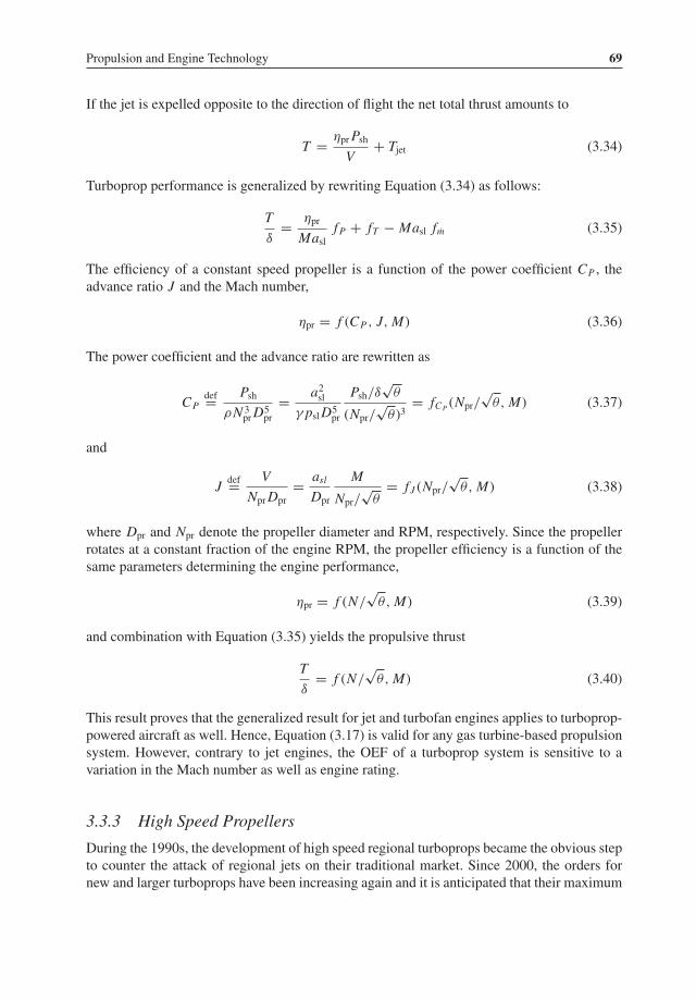
Propulsion and Engine Technology 69
If the jet is expelled opposite to the direction of flight the net total thrust amounts to
T = ηprPshV
+ Tjet (3.34)
Turboprop performance is generalized by rewriting Equation (3.34) as follows:
T
δ= ηpr
MaslfP + fT − Masl fm (3.35)
The efficiency of a constant speed propeller is a function of the power coefficient CP , theadvance ratio J and the Mach number,
ηpr = f (CP , J, M) (3.36)
The power coefficient and the advance ratio are rewritten as
CPdef= Psh
ρN 3prD
5pr
= a2slγ pslD5
pr
Psh/δ√
θ
(Npr/√
θ)3= fCP (Npr/
√θ, M) (3.37)
and
Jdef= V
NprDpr= asl
Dpr
M
Npr/√
θ= f J (Npr/
√θ, M) (3.38)
where Dpr and Npr denote the propeller diameter and RPM, respectively. Since the propellerrotates at a constant fraction of the engine RPM, the propeller efficiency is a function of thesame parameters determining the engine performance,
ηpr = f (N/√
θ, M) (3.39)
and combination with Equation (3.35) yields the propulsive thrust
T
δ= f (N/
√θ, M) (3.40)
This result proves that the generalized result for jet and turbofan engines applies to turboprop-powered aircraft as well. Hence, Equation (3.17) is valid for any gas turbine-based propulsionsystem. However, contrary to jet engines, the OEF of a turboprop system is sensitive to avariation in the Mach number as well as engine rating.
3.3.3 High Speed Propellers
During the 1990s, the development of high speed regional turboprops became the obvious stepto counter the attack of regional jets on their traditional market. Since 2000, the orders fornew and larger turboprops have been increasing again and it is anticipated that their maximum

70 Advanced Aircraft Design
Figure 3.6 The Europrop International TP 400 three-shaft turboprop engine with high-speed propeller.Copyright Europrop International, reproduced with permission
speed will eventually increase to Mach 0.7. This is also the design speed of the Airbus A400Mmilitary freighter which is powered by four of the West’s most powerful Europrop TP400-D6engines each producing 7 830 kW. Their propellers feature eight crescent-shaped compositeblades (Figure 3.6). High speed propellers were studied extensively resulting in the so-calledpropfan. The combination of a gas turbine engine and a propfan is now categorized as an openrotor engine.
3.4 Turbofan Engine Layout
3.4.1 Bypass Ratio Trends
The issue of how to get a step change in propulsion technology is all about (large) increases ofthe BPR and the related key issues of drag, weight, and noise. Installing a bigger fan increasesthe engine’s air mass flow and its BPR with a corresponding reduction in fan pressure ratioand specific thrust. This improves the OEF, leading to lower fuel consumption. Figure 3.7shows the effects of BPR on SFC and OEF for a family of engines with a constant core OPRand TET. Increasing the BPR from today’s value of approximately five to 70 would reduce theTSFC by more than 25% for the ideal cycle with 100% efficient components. With realisticefficiencies, the TSFC is considerably degraded at all BPR levels but the favourable trend of
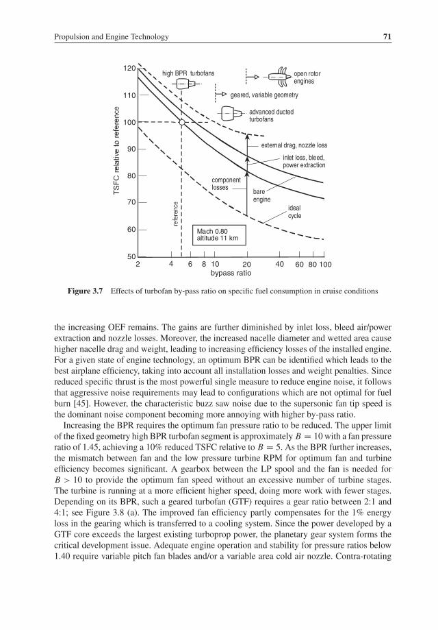
Propulsion and Engine Technology 71
high BPR turbofans
advanced ductedturbofans
open rotorengines
componentlosses
idealcycle
inlet loss, bleed,power extraction
external drag, nozzle loss
geared, variable geometry
120
100
80
60
50
70
90
110
2 4 6 8 10 20 40 60 80 100
Mach 0.80altitude 11 km
bareengine
bypass ratio
Figure 3.7 Effects of turbofan by-pass ratio on specific fuel consumption in cruise conditions
the increasing OEF remains. The gains are further diminished by inlet loss, bleed air/powerextraction and nozzle losses. Moreover, the increased nacelle diameter and wetted area causehigher nacelle drag and weight, leading to increasing efficiency losses of the installed engine.For a given state of engine technology, an optimum BPR can be identified which leads to thebest airplane efficiency, taking into account all installation losses and weight penalties. Sincereduced specific thrust is the most powerful single measure to reduce engine noise, it followsthat aggressive noise requirements may lead to configurations which are not optimal for fuelburn [45]. However, the characteristic buzz saw noise due to the supersonic fan tip speed isthe dominant noise component becoming more annoying with higher by-pass ratio.Increasing the BPR requires the optimum fan pressure ratio to be reduced. The upper limit
of the fixed geometry high BPR turbofan segment is approximately B = 10 with a fan pressureratio of 1.45, achieving a 10% reduced TSFC relative to B = 5. As the BPR further increases,the mismatch between fan and the low pressure turbine RPM for optimum fan and turbineefficiency becomes significant. A gearbox between the LP spool and the fan is needed forB > 10 to provide the optimum fan speed without an excessive number of turbine stages.The turbine is running at a more efficient higher speed, doing more work with fewer stages.Depending on its BPR, such a geared turbofan (GTF) requires a gear ratio between 2:1 and4:1; see Figure 3.8 (a). The improved fan efficiency partly compensates for the 1% energyloss in the gearing which is transferred to a cooling system. Since the power developed by aGTF core exceeds the largest existing turboprop power, the planetary gear system forms thecritical development issue. Adequate engine operation and stability for pressure ratios below1.40 require variable pitch fan blades and/or a variable area cold air nozzle. Contra-rotating

72 Advanced Aircraft Design
reduction gear system
(a) (b)
Figure 3.8 Very high bypass ratio turbofans. (a) Geared turbofan engine layout [46, 47]. (b) Rolls-Royce RB529 project with contra-rotating direct drive fans. Adapted from [31]
fans (CRF) may be favoured for the highest bypass ratios; see Figure 3.8 (b). Application of aBPR between 15 and 25 makes a mechanically complex engine inevitable and complicates itsintegration with the airframe.A properly integrated engine installation forms the best balance between fuel efficiency,
weight, noise production, maintainability, lifetime and cost. Different engine manufacturerscope with this matter in different ways. Pratt & Whitney have taken the lead in twenty-first-century engine technology by offering a GTF family of engines having the potential to cut fuelburn by 12%. Their production GTF is expected to cover the 100–180 kN (22 000–40 000 lbf)thrust range. The engine’s relatively low fan tip speed reduces (accumulative) noise by 30 dBcompared with Stage 3 requirements. In view of the increasing drag and weight of a shroudedturbofan, the radical step to open rotor engine technology is probably unavoidable when theBPR exceeds 30.
3.4.2 Rise and Fall of the Propfan
During the 1970s, NASAmade an ambitious effort to stimulate the development of an advancedturboprop aircraft cruising atMach 0.80 and altitudes up to 30 000 ft that could reduce fuel con-sumption by 30% compared to jetliners. This required the development of advanced high-speedpropellers known as propfans. Proposed in 1975 by propeller manufacturer Hamilton Stan-dard, propfans were introduced with multiple crescent-shaped highly loaded blades designedto maintain at least 80% propulsive efficiency. The company was awarded an advanced bladedevelopment contract and in 1981 began to design the composite blade set of a large single-stage demonstration propfan dubbed SR-7A which was tested in 1986. The complete enginewith an eight-bladed unit flew on a modified Gulfstream II in 1987.Propfan is a portmanteau word coined to describe a propulsion concept which combines
some of the characteristics of a turboprop with those of a turbofan. Although early propfanshad amuch higher disk loadings than a conventional propeller, both were driven by a turboshaftengine via a gearbox. The essential difference with turbofans is the much higher propfan BPRbetween 25 and 40, variable-pitch blades and the absence of a rotor duct. The term propfan wasoriginally applied to a multiple-bladed single rotor; however, since contra-rotation makes nofundamental difference, the term propfan still applies. Contra-rotation of the blades eliminatesmuch of the swirl in the rotor slipstream, making the propulsive efficiency about 7% highercompared to the single-stage layout.

Propulsion and Engine Technology 73
contra-rotation reduction gear
pitch control system
annular exhaust
(b) pusher layout(a) tractor layout
turboprop engine
swept propeller blades
contra-rotation reduction gear
swept propeller blades
turboprop engine
Figure 3.9 General arrangements of propfans with contra-rotating geared open rotors. The output isexpressed as shaft horsepower (SHP) because there is a turboshaft engine and gearbox involved
In the 1980s, all the major airliner manufacturers considered adopting propfan technologyfor clean sheet designs. This required tractor engine arrangements which could be mountedto the wing leading edge or pusher arrangements mounted to the rear fuselage (Figure 3.9).Moving away from the geared propfan trend with the revolutionary unducted fan (UDF)concept, GE concentrated on the tail-mounted pusher configuration to limit cabin noise.Their UDF arrangement dispenses with the gearbox and features a gas generator to powera pair of CR statorless free turbines carrying the rotor blades, as illustrated in Figure 3.10.American airframers were the most active investigators of the propfan. Boeing andMcDonnellDouglas teamed with GE and P & W/Allison to evaluate the technology, culminating in thedemonstrator engines GE 36 and PW 578-D mounted on 727-100 and MD-80 aircraft. InEurope, Rolls-Royce worked along the lines of a geared open rotor in pusher configurationbut did not produce a full-scale demonstrator. The relatively low price of fuel at the timemeant that potential concerns such as noise and reliability problems prevented the promisingpropfan technology from being adopted. The designs studied during the 1980s were at leastthree decennia ahead of their time, except for the Progress D-27 CR propfan which powers the
machinery arrangement
exhaust nozzle
counterrotatingfanblades
turbinebladescowl
coreengine
secondary supportstructure
Figure 3.10 General Electric GE 36 unducted fan (UDF) of the 1980s
74 Advanced Aircraft Design
Antonov AN-70. This military freighter had its public debut in 1997 and is the only applicationof propfans in operational aircraft up to 2010.
3.4.3 Rebirth of the Open Rotor?
After the turn of the twentieth century, with soaring fuel prices and emphasis on reducingenvironmental emissions, the aeronautical industry is showing a renewed interest in the virtuesof propfans. High-speed propellers (Figure 3.6) developed for speeds up to Mach 0.70 arebecoming operational. Their diameter and detailed design are optimized for installation in aspecific airplane. Different from turboprops, propfans are complete systems developed andproduced by gas turbine engine manufacturers featuring variable pitch rotors with pressureratios between 1.05 and 1.40, dependent on BPR. Application of contra-rotating open rotorslead to uninstalled cruise SFC reductions between 25 and 30% with similar noise levelscompared to high BPR turbofans. Due to the varying blade pitch with speed, the gain inpropulsive efficiency is even greater at low speeds; see Figure 2.7 (b). Hence, similar toturboprops, open rotor systems improve low speed performances which makes them especiallyfit for application in short-haul airplanes. However, complex airframe integration issues andacquisition costswill be high since open rotors aremechanicallymore complex than turbopropsas well as turbofans. Major technical concerns exist regarding safety (blade failure), cabinnoise, maintenance costs, reliability and fan efficiency at cruise speeds above Mach 0.75.
3.5 Power Plant Selection
Since 1980, aero engine manufacturers have proposed a large variety of advanced enginedesigns. Table 3.1 is a proposed classification of the propulsion concepts which appear tohave a future of becoming realized. Apart from advanced turboprops, themain stream of enginedevelopment is devoted to direct drive as well as geared (very) high BPR turbofans – these arelikely to be installed in new airliners becoming operational between 2010 and 2020. There isalso a possibility that designing propfan-powered planes might be the right way to replace asubstantial proportion of today’s fleet of narrow body airliners. Engines that come as a logicalchoice might be based on turboprops such as those depicted in Figures 3.5 and 3.6.Figure 3.11 is an overview of the effect on uninstalled and installed TSFC and OEF of the
BPR and the specific thrust of a family of engines with a common core engine. Four candidates
Table 3.1 Classification of gas turbine engine systems
Power generator Primary propulsive device Abbreviation
Turboprop/turboshaft conventional propeller CTPhigh-speed propeller HSTP
Turbofan direct driven ducted fan DDTFgeared ducted fan GTFcontra-rotating ducted fans CRDF
Propfan single stage open rotor SSPFcontra-rotating open rotors CRPF

Propulsion and Engine Technology 75
uninstalled
installedDDTF
GTF
CRDFCRPF
0.040
0.045
0.050
0.055
0.060
0.065
0.070
0.50
0.45
0.40
0.35
0.30
0.25
40 80 120 160 18014010060200
60
50
40
30
20
10
0
BPR
BPR
TSFC (kg/hr)/N
OEF
specific thrust m/s200
core engine:OPR = 40TET = 1550 K
Figure 3.11 Spectrum of aero engine characteristics dependent on specific thrust. Flight conditions:Mach 0.76 at 35 000 ft
of advanced concepts are identified with the potential of reducing uninstalled TSFC between10 and 30% relative to the high BPR turbofan. As indicated, installation effects – nacelle/cowldrag, flow interference drag for propfans, etc. – on system thrust are most important for veryhigh BPR turbofans and open rotor engines (Figure 3.7).
3.5.1 Power Plant Location
The choice of a new propulsion concept has a far-reaching impact on the viability of a newairplane project. It is dictated by many aspects different from fuel economy, such as:
• costs and time to develop the engine to the operational status;• fuel costs as a fraction of the total operating costs, taking into account the fuel price level inthe future;
• the airplane’s general arrangement, in particular the wing-mounted versus fuselage-mountedlocation;
• community noise noise footprint;• cabin noise and effects on acoustic fatigue of the structure;• containment requirements in case of propeller or rotor blade failures, and• acceptance by the airlines, taking into account perceptions of the travelling public, expecta-tions about safety, reliability, maintainability, etc.
The conceptual design stage is used for the process of matching the engine power or thrust tothe airframe and for identifying the best location of the installed engines. High BPR turbofansare likely to be attached in the conventional way to the wing or the rear fuselage. Wing-mounted, very high BPR turbofans may be possible only with a high-set wing (Figure 3.12),
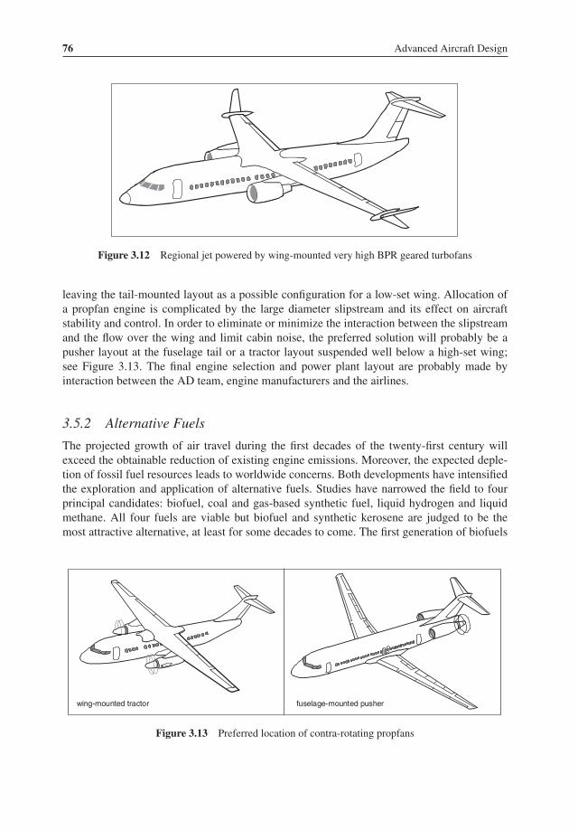
76 Advanced Aircraft Design
Figure 3.12 Regional jet powered by wing-mounted very high BPR geared turbofans
leaving the tail-mounted layout as a possible configuration for a low-set wing. Allocation ofa propfan engine is complicated by the large diameter slipstream and its effect on aircraftstability and control. In order to eliminate or minimize the interaction between the slipstreamand the flow over the wing and limit cabin noise, the preferred solution will probably be apusher layout at the fuselage tail or a tractor layout suspended well below a high-set wing;see Figure 3.13. The final engine selection and power plant layout are probably made byinteraction between the AD team, engine manufacturers and the airlines.
3.5.2 Alternative Fuels
The projected growth of air travel during the first decades of the twenty-first century willexceed the obtainable reduction of existing engine emissions. Moreover, the expected deple-tion of fossil fuel resources leads to worldwide concerns. Both developments have intensifiedthe exploration and application of alternative fuels. Studies have narrowed the field to fourprincipal candidates: biofuel, coal and gas-based synthetic fuel, liquid hydrogen and liquidmethane. All four fuels are viable but biofuel and synthetic kerosene are judged to be themost attractive alternative, at least for some decades to come. The first generation of biofuels
wing-mounted tractor fuselage-mounted pusher
Figure 3.13 Preferred location of contra-rotating propfans
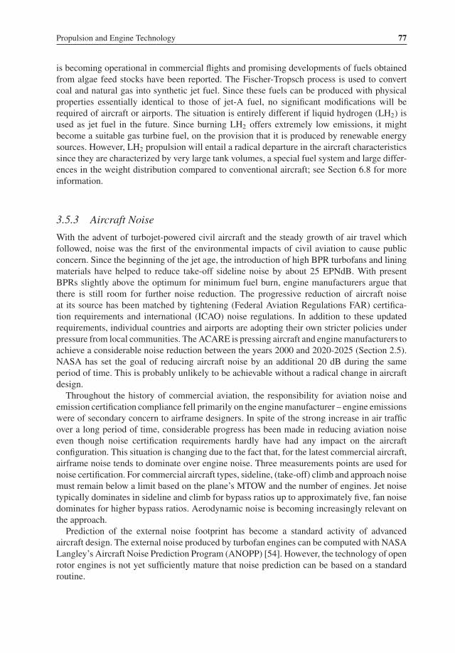
Propulsion and Engine Technology 77
is becoming operational in commercial flights and promising developments of fuels obtainedfrom algae feed stocks have been reported. The Fischer-Tropsch process is used to convertcoal and natural gas into synthetic jet fuel. Since these fuels can be produced with physicalproperties essentially identical to those of jet-A fuel, no significant modifications will berequired of aircraft or airports. The situation is entirely different if liquid hydrogen (LH2) isused as jet fuel in the future. Since burning LH2 offers extremely low emissions, it mightbecome a suitable gas turbine fuel, on the provision that it is produced by renewable energysources. However, LH2 propulsion will entail a radical departure in the aircraft characteristicssince they are characterized by very large tank volumes, a special fuel system and large differ-ences in the weight distribution compared to conventional aircraft; see Section 6.8 for moreinformation.
3.5.3 Aircraft Noise
With the advent of turbojet-powered civil aircraft and the steady growth of air travel whichfollowed, noise was the first of the environmental impacts of civil aviation to cause publicconcern. Since the beginning of the jet age, the introduction of high BPR turbofans and liningmaterials have helped to reduce take-off sideline noise by about 25 EPNdB. With presentBPRs slightly above the optimum for minimum fuel burn, engine manufacturers argue thatthere is still room for further noise reduction. The progressive reduction of aircraft noiseat its source has been matched by tightening (Federal Aviation Regulations FAR) certifica-tion requirements and international (ICAO) noise regulations. In addition to these updatedrequirements, individual countries and airports are adopting their own stricter policies underpressure from local communities. The ACARE is pressing aircraft and enginemanufacturers toachieve a considerable noise reduction between the years 2000 and 2020-2025 (Section 2.5).NASA has set the goal of reducing aircraft noise by an additional 20 dB during the sameperiod of time. This is probably unlikely to be achievable without a radical change in aircraftdesign.Throughout the history of commercial aviation, the responsibility for aviation noise and
emission certification compliance fell primarily on the enginemanufacturer – engine emissionswere of secondary concern to airframe designers. In spite of the strong increase in air trafficover a long period of time, considerable progress has been made in reducing aviation noiseeven though noise certification requirements hardly have had any impact on the aircraftconfiguration. This situation is changing due to the fact that, for the latest commercial aircraft,airframe noise tends to dominate over engine noise. Three measurements points are used fornoise certification. For commercial aircraft types, sideline, (take-off) climb and approach noisemust remain below a limit based on the plane’s MTOW and the number of engines. Jet noisetypically dominates in sideline and climb for bypass ratios up to approximately five, fan noisedominates for higher bypass ratios. Aerodynamic noise is becoming increasingly relevant onthe approach.Prediction of the external noise footprint has become a standard activity of advanced
aircraft design. The external noise produced by turbofan engines can be computed with NASALangley’s Aircraft Noise Prediction Program (ANOPP) [54]. However, the technology of openrotor engines is not yet sufficiently mature that noise prediction can be based on a standardroutine.

78 Advanced Aircraft Design
Bibliography
[1] Torenbeek, E., Synthesis of Subsonic Airplane Design, Chapter 4 and Appendix H, Springer Verlag, Heidelberg,1981.
[2] Kerrebrock, J.L., Aircraft Engines and Gas Turbines, Second Edition, MIT Press, Cambridge, MA, 1992.[3] Hill, P.G., and C.R. Peterson,Mechanics and Thermodynamics of Propulsion, Second Edition, Addison-Wesley,
Reading, MA, 1992.[4] Mair, W.A., and D.L. Birdsall, Aircraft Performance, Chapter 5, Cambridge University Press, Cambridge, 1992.[5] Smith, M.J.T., Aircraft Noise, Cambridge University Press, Cambridge, 1989.[6] Ruijgrok, G.J.J., Elements of Aviation Acoustics, Delft University Press, Delft, 1993.[7] Rolls-Royce plc., The Jet Engine, Fifth Edition, Renault Printing Company Ltd., 1996.[8] Archer, R.D., and M. Saarlas, An Introduction to Aerospace Propulsion, Prentice-Hall, Inc., Englewood Cliffs,
NJ, 1996.[9] Hunecke, K., Jet Engines: Fundamentals of Theory, Design and Operation, Airlife Publishing Ltd., Shrewsbury,
1997.[10] Walsh, P.P., and P. Fletcher, Gas Turbine Performance, Blackwell Science Ltd., Oxford, 1998.[11] Saravanamutto, H.I.H., G.F.C. Rogers, and H. Cohen, Gas Turbine Theory, Fifth Edition, Pearson Education
Ltd., Harlow, 2001.[12] Mattingly, J.D., W.H. Heiser, and D.T. Pratt, Aircraft Engine Design, Second Edition, AIAA, New York, 2002.[13] Cumpsty, N., Jet Propulsion: A Simple Guide to the Aerodynamic and Thermodynamic Design and Performance
of Jet Engines, Second Edition, Cambridge University Press, Cambridge, 2003.[14] Torenbeek, E., and H. Wittenberg, Flight Physics: Essentials of Aeronautical Disciplines and Technology, with
Historical Notes, Chapter 5, Springer, Heidelberg, 2009.
Aero Engine Technology
[15] Jackson, A.J.B., “Some Future Trends in Aero Engine Design for Subsonic Transport”, Journal of Engineeringfor Power, Transactions of the American Society of Mechanical Engineers, Vol. 98, pp. 281–289, April 1976.
[16] Wilde, G.L., “Future Large Civil Turbofans and Powerplants”, Aeronautical Journal, Vol. 82, pp. 281–299, July1978.
[17] Brewer, G.D., et al., “Study of Fuel Systems for LH2 Fueled Subsonic Transport Aircraft”, NASA CR 145369,Lockheed, California, July 1978.
[18] Fishbach, L.H., “Computerized Systems Analysis and Optimization of Aircraft Engine Performance, Weight,and Life Cycle Costs”, AGARD CP 280, Paper No. 26, 1979.
[19] Gatzen, B.S., “Turboprop Design: Now and the Future”, ICAS Paper No. 82-4.5.2., September 1982.[20] Bennett, H.W., “Aero Engine Deveiopment for the Future”, Journal of Power and Energy, Proceedings of the
Institution of Mechanical Engineers, Part A, Vol. 197, pp. 149–157, July 1983.[21] Williams, M.R., “Large Turbofans for the Year 2000”, Aeronautical Journal, January 1984.[22] Blythe, A.A., and P. Smith, “Prospects and problems of Advanced Open Rotors for Commercial Aircraft”,
AIAA Paper No. 85-1191, July 1985.[23] Stuart, A.R., “The Unducted Fan Engine”, AIAA Paper No. 85-1190, 1985.[24] Lange, R.H., “A Review of Advanced Turboprop Transport Aircraft”, Progress in Aerospace Sciences, Vol. 23,
pp. 151–166, 1986.[25] Grieb, H., and D. Eckardt, “Propfan and Turbofan as Basis for Future Economic Propulsion”, 22nd Joint
Propulsion Conference, AIAA Paper No. 86-1474, 1986.[26] Blythe, A., “Potential Application of Advanced Propulsion Systems to Civil Aircraft”, 15th ICAS Congress,
London, Paper No. 86.3.8.3, September 1986.[27] Miller, S.C., and H.W. Bennett, “Future Trends in Propulsion”, ICAS Paper No. 86-86.04, September 1986.[28] Wittenberg, H., “Aircraft Propulsion Leading the Way in Aviation”, Report LR-532, TUDelft, Faculty of
Aerospace Engineering, September 1987.[29] Saravanamuttoo, H.I.H., “Modern Turboprop Engines”, Progress in Aerospace Sciences, Vol. 24, pp. 225–248,
1987.[30] Dunican, M.G., “Installation of Innovative Turbofan Engines on Current Transport Airplanes”, AIAA Paper
No. 87-2921, September 1987.[31] Borradaile, J.A., “Towards the Optimum Ducted UHBR Engine”, AIAA Paper No. 88-2954, July 988.

Propulsion and Engine Technology 79
[32] Gordon, B.J., “The Development of the Unducted Fan”, Aerospace, pp. 22–26, July 1988.[33] Zimbrick, R.A., and J.L. Colehour, “An Investigation of Very High Bypass Ratio Engines for Subsonic Trans-
ports”, AIAA Paper No. 88-2953, July 1988.[34] Skavdahl, H., R.A. Zimbrick, J.L. Colehour, and G.P. Sallee, “Very High Bypass Ratio Engines for Commercial
Transport Propulsion”, ICAS Paper No. 88-4.11.2, September 1988.[35] General Electric, “GE36/UDF, A New Thrust in Aviation”, DGLR Jahrestagung, Darmstadt, Paper 88-011,
1988.[36] Eckardt, D., and G. Brines, “Technology Readiness for Advanced Ducted Engines”, 25th Joint Propulsion
Conference, AIAA Paper No. 89-2479, 1989.[37] Dupslaff, M., P. Wehlitz, and P. Schimming, “Propfan Technology”, in European Forum: The Evolution of
Regional Aircraft Technologies and Certification, organized by DGLR, AAF, RAeS, Friedrichshafen, April 6-7,1989.
[38] Owens, R.E., K.L. Hassel, and D.E. Mapes, “Ultra High Bypass Turbofan Technologies for the Twenty-FirstCentury”, 26th Joint Propulsion Conference, AIAA Paper No. 90-2397, 1990.
[39] Zimbrick, R.A., and J.L. Colehour, “Investigation of Very High Bypass Ratio Engines for Subsonic Transports”,Journal of Propulsion and Power, Vol. 6, pp. 490–496, July-August 1990. Also: AIAA Paper No. 88-2953.
[40] Sieber, J., and H. Jackwerth, “Betriebsverhalten Eines CRISP-Vortriebserzeugers”, No. 91-193, DGLR Jahresta-gung 1991.
[41] Stryker, H.Y., “21st Century Commercial Transport Engines”, RAeS Sidney Branch Lecture, 1992.[42] Saito, Y., M. Endoh, N. Sugahara, and K. Yamamoto, “Conceptual Study of Separated Core Ultra High Bypass
Engine”, AIAA Paper No. 92-3776, July 1992. Associated paper: AIAA Paper No. 92-3776, July 1992.[43] Yaros, S.F., et al., “Synergistic Airframe-Propulsion Interactions and Integrations” White Paper prepared by the
1996-1997 Langley Aeronautics Technical Committee, NASA/TM-1998-207644, March 1998.[44] Birch, N.T., “2020 Vision: the Prospects for Large Civil Airaft Propulsion”, Aeronautical Journal, Vol. 104,
No. 1038, pp. 281–289, August 2000.[45] Richter, H., and S. Menczykalski, “Civil Propulsion of the Future”, Innovative Configurations and Advanced
Concepts for Future Civil Aircraft, Von Karman Institute for Fluid Dynamics, Lecture Series 2005-06, June6-10, 2005.
[46] Kurzke, J, “GasTurb 11 User’s Manual, Design and Off-Design Performance of Gas Turbines”, 2007.[47] Dewanji, D., A.G. Rao, and J.P. van Buijtenen, “Conceptual Study of Future Aero-Engine Concepts”, Interna-
tional Journal of Turbo and Jet Engines, Vol. 26, pp. 263–276, 2009.
Aircraft Noise
[48] Drell, H., “Impact of Noise on Subsonic Transport Design”, SAE Paper No. 700806, October 1970.[49] Kramer, J.J., and R.G. Dorsch, “NASA Aircraft Engine Noise Research”, ICAS Paper no. 72-48, September
1972.[50] Heidmann, M.F., “Interim Prediction Method for Fan and Compressor Source Noise”, NASA TM X-71763,
1979.[51] ICAO, “Aircraft Noise”, International Standards and Practices, Annex 16 to the Convention of International
Civil Aviation, 3rd Edition, 1985.[52] Brentner, K.S., “Aerodynamic Impact on Noise and Emissions”, Session IV of “Potential Impacts of Advanced
Aerodynamic Technology onAir Transportation System Productivity”, NASATechnicalMemorandum 109154,September 1994.
[53] Kennepohl, F., R. Traub, R, Gumicio, and K. Heinig, “Influence of Bypass Ratio on Community Noise ofTurbofans and Single Rotation Ducted Propfans”, AIAA Paper No. 95-0135, June 1995.
[54] Kontos, K.B., B.A. Janardan, and P.R. Gliebe, “Improved NASA-ANOPP Noise Prediction Computer Code forAdvanced Subsonic Propulsion Systems”, Volume 1: ANOPP Evaluation and Fan Noise Model Improvement,1996.
[55] Caves, R.E., L.R. Jenkinson, and D.P. Rhodes, “Development of an Integrated Conceptual Aircraft Design andNoise Model for Civil Transport Aircraft”, ICAS Paper No. 98-6.4.3, September 1998.
[56] Kim, H.D., J.J. Berton, and S.M. Jones, “Low Noise Cruise Efficient Short Take-Off and Landing TransportVehicle Study”, AIAA Paper No. 2006-7738, September 2006.
[57] Hileman, J., “Airframe Design Considerations for a Silent Aircraft”, presentation of work conducted by theSilent Engineering Design Team, Cambridge University Engineering Department, MIT, July 2007.
4Aerodynamic Drag andIts Reduction
It has been noted that transportation is fundamentally 0% efficient as it involves moving massfrom rest at one point to rest at another point, so that the energy of the system is unchanged. Thatit does take energy to accomplish this objective is due to the presence of drag, and the reductionof drag has been the primary focus of aircraft design over the last century.
—I.H. Kroo [72] (2001)
4.1 Basic Concepts
The drag estimation for a new design is not generally a single exercise, but a continuousprocess through its life from the early project study stage through preliminary design anddevelopment. Similar to weight prediction, the fidelity of the drag prediction methodologyused during advanced design (AD) varies with the accuracy required, with the degree ofairplane geometry definition, and with the amount of computed or experimental data available.Initially, predictions are mostly semi-empirical with a gradual shift to quasi-analytical andnumerical methods. A wide variety of handbook methods, computations and wind tunneldata are used as the design proceeds and it is essential to be consistent with the definition ofdrag components. Although aircraft design over the past century has evolved into a processof increasing sophistication, the prediction of aerodynamic drag still poses a formidablechallenge to the AD engineer. Even elemental flow physics driving drag can be quite complex.In addition, there aremyriadways inwhich flowfields around airplane components can interactto produce interference drag which is very difficult to predict accurately. But it is clear thatfull-scale aircraft drag prediction errors of 10 to 20% that have occurred in the past in certaindevelopment programs are outwith the range needed for success [38].
Advanced Aircraft Design: Conceptual Design, Analysis and Optimization of Subsonic Civil Airplanes, First Edition. Egbert Torenbeek.
© 2013 by Egbert Torenbeek. Published 2013 by John Wiley & Sons, Ltd.

82 Advanced Aircraft Design
In spite of the aircraft’s complex shape, the external air force acting on it is traditionallyresolved in the same way as for any other closed body moving through an airflow,1 as follows:
• Drag is a positive force of magnitude D acting in the opposite direction to the airspeedvector �V .
• Lift with magnitude L acts normal to �V in the airplane’s plane of symmetry and is positivein the dorsal sense.
Most objects moving through air experience considerable drag and little or no lift; hence,D/L � 1. Airfoils form a special class of objects since they are designed to generate liftexceeding their drag by an order of magnitude: L/D � 1. Having the potential to generate alift equal to several times the airplane’s gross weight (GW), an airplane wing is classified as astructurally and aerodynamically extremely efficient lifting surface. Tail surfaces are airfoilsdesigned primarily to provide lift for control in dynamic conditions and for stability – they arenot intended for generating much lift in straight and level flight. Decisions taken during allstages of AD can have a major effect on the aerodynamic efficiency L/D; hence, it is essentialto predict the sensitivity of drag to design variables as accurately as possible.
4.1.1 Lift, Drag and Aerodynamic Efficiency
Except for manoeuvres, the flight path angle γ of a passenger plane during climbing anddescending flight normally amounts to less than ten degrees, whereas cruising flight is (nearly)steady and level throughout. Hence, it can be assumed that cos γ = 1 during the completeflight. Accordingly, lift L equals the airplane’s gross weight W and drag follows from
D = W
L/D(4.1)
The L/D ratio enters the performance and design analysis directly since the thrust required isdetermined by the equilibrium of forces along the flight path,
T = D = W
CL/CD(4.2)
Lift and drag coefficients are defined as:
CL = L
q Sand CD = D
q S(4.3)
where the dynamic pressure q is related to the altitude and the flight speed V or the Machnumber M as follows:
q = 1
2ρV 2 = 1
2ρ (Ma)2 = 1
2ρM2 γ RT = 1
2γ p M2 (4.4)
The symbols a, R and γ are the sonic speed, the gas constant and the ratio of specific heats ofair, respectively. Ambient air density, pressure and temperature are ρ, p and T , respectively.
1An airframe can be treated as a closed body by covering engine inlets and exhausts by streamlined nacelle fairings.

Aerodynamic Drag and Its Reduction 83
Drag components are mostly quoted in terms of counts – one drag count is defined as�CD = 0.0001. The standard reference area for lift and drag coefficients is the gross wingarea Sw. This makes their numerical values dependent on the precise definition of the wing areaforwhich no universally accepted standard exists. For example,Airbus andBoeing use differentmethods for including the wing area inside the fuselage whereas wings with a compound taperare sometimes approximated as an equivalent straight-tapered wing. Consequently, the zero-lift drag coefficient and themaximum lift coefficient quoted for different aircraft are not alwayscomparable. However, since Equation (4.2) indicates that the drag in level flight is determinedby the aerodynamic efficiency CL/CD = L/D, it does not depend on the reference area ofboth coefficients. At the time of writing, long-distance airliners achieve maximum values ofL/D between 15 and 20, dependent mainly on their size. This parameter may go up to a valuebetween 20 and 25 in the not too distant future.The aerodynamic efficiency is important to the design engineer since it is a basic parameter
in the engine/aircraft matching process and in flight performance analysis. Fuel consumptionin cruising flight is proportional to the airplane GW and to engine thrust or power and a GWreduction contributes just as much to reducing fuel consumption as increasing the aerodynamicefficiency. Another important flight condition is the climb-out after taking off which is oftena sizing criterion for the engine power or thrust to be installed.
4.1.2 Drag Breakdown and Definitions
Precise definitions of drag and its contributing components are essential for drag prediction andfor an appreciation of drag reduction technology. However, the engineer is often confrontedwith (apparently) different terms for almost the same properties and the terminology foundin the literature may create confusion due to a lack of international standardization.2 Mostof the confusion is associated with the complex task of analyzing and predicting the drag ofa complete aircraft configuration. Dependent on the purpose of the work, the drag may bebroken down according to one of the following basic schemes:
• The body surface exposed to the flow is divided into a large number of panels and the forceon each panel is decomposed into a normal pressure component and a friction componenttangential to it. Their components in the direction of the airflow are added to yield the totaldrag.
• The drag is decomposed in accordance with the physical mechanisms contributing to drag:the viscosity of air, vortical flow and shock waves.
• The drag is subdivided into parasite drag disregarding lift and induced drag caused bylift-generating mechanisms.
Figure 4.1 interrelates these schemes and indicates how flow phenomena, body shape anddimensions have an influence on drag components. The scheme is general since it applies toarbitrary closed bodies surrounded by incompressible as well as compressible (high-speed)flows. The physical mechanisms are fundamental in that they cannot be broken down into
2A comprehensive – but not widely used – set of definitions was drawn up by the British Aeronautical ResearchCouncil [17]; ESDU has produced a more recent overview [40]. It is also noticeable that the scheme in Figure 4.1differs from schemes used in other publications such as [52] and [92].

84 Advanced Aircraft Design
TOTAL DRAG
PRESSURE DRAG
TOTAL DRAG
FRICTION DRAG
INDUCED DRAG
PARASITEDRAG
VORTEX DRAG WAVE DRAG VISCOUS DRAG
FORM DRAG
spanloading
trailing vortices displacement,separation
boundary physical mechanismlayer shear
waves dueto lift
waves dueto volumedue to lift
camber warp slenderness thickness wetted area influential geometry
Figure 4.1 Schemes for decomposing the drag of a closed lifting body. The parasite drag of an airfoilis also known as profile drag
simpler elements. However, the simplicity of the scheme is deceiving since a number ofdrag sources are derived from interactions of fundamental mechanisms. For instance, viscouseffects may affect the lateral variation of trailing vortex strength whereas three-dimensionalnon-viscous flow phenomena may contribute to viscous drag. And interactions between the(throttle-dependent) internal engine flow and the external flow may be the subject of debatebetween airframe and engine manufacturers about the drag accounting methodology.Due to a lack of detailed information in the conceptual design process, the engineer may
be forced to use a drag breakdown based on a simplified representation of the airplane’sgeometry. This leads to a somewhat heuristic approach known as a drag build-up technique,replacing the complex overall shape by individual components such as the wing, fuselage,tail surfaces and engine nacelles. If the result is a mixture of poor bookkeeping, incompatibledrag analysis methods, inaccuracies caused by unforseen flow separations and interactionsand surface imperfections, the reliability of the drag prediction appears to be unsatisfactory.An alternative drag breakdown may be needed during preliminary design by the analyst whouses measured aircraft (model) data to correct them for Reynolds number effects, trim dragand configuration effects.
4.2 Decomposition Schemes and Terminology
4.2.1 Pressure and Friction Drag
The most elemental drag breakdown distinguishes between the two ways in which the aerody-namic force is exerted on the exposed body surface. At each surface element the air pressure

Aerodynamic Drag and Its Reduction 85
exerts a normal force whereas friction between the airflow and the surface due to shear causesa tangential force. Vectorial summation of these forces yields the resulting aerodynamic forceR which is resolved into lift and drag: �R = �L + �D. Accordingly, drag is broken down intopressure drag and skin friction drag. In high speed level flight, pressure and friction drag areof similar magnitude, whereas pressure drag dominates at low speeds.Compared to other breakdowns, the definitions of pressure and friction drag are straightfor-
ward and unambiguous. However, pressure and shear force distributions have to be obtainedby computational fluid dynamics (CFD) methods or measured by experiments in a wind tun-nel or in flight. Since these techniques are very time-consuming and require accurate shapeinformation of the complete airframe, drag predictions for conceptual design are mostly basedon a mixture of alternative schemes for decomposing drag [52]. For instance, insight intovarious forms of drag is gained from a breakdown based on schemes for modelling physicalmechanisms as in the lower part of Figure 4.1. Different forms of energy are left behind theairplane in a trailing vortex sheet, a turbulent wake or a dead air region and, in high-speedflight, in the form of shock waves. The law of energy conservation requires the work producedin overcoming the drag to be equal to the energy increase of the surrounding atmosphere.
4.2.2 Viscous Drag
The viscosity of air leads to the formation of a boundary layer surrounding the body’s surface.Except for a body surrounded by fully separated flow, the greater part of viscous drag is causedby surface friction due to shear stress in the boundary layer. Viscous drag is unique in that itis the only source of drag for which the force-generating mechanism acts tangentially to theexternal surface. For a given flowReynolds number, friction drag is almost entirely determinedby the state of the boundary layer: laminar or turbulent. Behind the body, the boundary layer isshed in the form of a turbulent wake causing a loss of momentum – the mechanical equivalenceof viscous drag. Hence, skin friction drag can be derived from boundary layer analysis or bymeasuring the momentum loss in the wake of a wind tunnel model. As a secondary effect, thedisplacement effect of the boundary layer causes a modified pressure distribution. The resultis a pressure imbalance between the front and rear parts of the body known as form drag, arelatively small component for a streamline body at a low incidence in subcritical flow.Increasing the incidence of a transport or business aircraft leads to flow separation at the
wing trailing edge which gradually spreads forwards. A large dead air region is eventuallyformed when the plane approaches the stall, causing a progressively increasing loss of liftand form drag. However, increasing the incidence of a thin airfoil causes separation at the(sharp) nose and a delta vortex is formed above a highly swept leading edge. Flow separationat the nose causes a loss of leading edge suction and a distinct drag inflation3 when a criticalangle of attack is exceeded. For transport aircraft this type of drag is avoided in normal flightconditions by proper aerodynamic design.
4.2.3 Vortex Drag
The finite span of a lifting surface causes the lower surface flow to move outboard toward thetip while the upper surface flow moves inward toward the centreline. The resulting cross-flow
3Drag inflation may occur at a modest incidence and must not be confused with the stall since it does not necessarylead to loss of lift: a delta vortex increases the lift of a low-aspect ratio wing.

86 Advanced Aircraft Design
velocities at the trailing edges combine with the free-stream flow, leading to the shedding ofvortical flow that is particularly strong near the outboard regions and the tips. The vortexstrength along the span is directly related to the lateral distribution of lift. The trailingvortex sheet contains rotational energy which must be paid for in the form of vortex drag.Since vortex formation is the unavoidable consequence of lift, vortex drag is also known as acomponent of (lift-)induced drag. Its coefficient CDv is derivable for high-aspect ratio straightwings by classical analysis such as L. Prandtl’s lifting line theory which has been availablesince the early days of aeronautics. More general methods such as the vortex-lattice methodand Trefftz plane analysis were derived for swept wings with low and high aspect ratios.Achieving minimal induced drag is a major concern of aircraft designers and remains an areaof research activity [72].Classical theory assumes the vortex sheet to be flat and located in the plane of the undis-
turbed flow. In reality, the vortex sheet is curved and, far behind the wing, the flow is deflecteddownward over the (average) downwash angle ε. In combination with the momentum equa-tion, this flow model forms the basis for an alternative derivation of lift and drag due to lift[14]. It states that the apparent mass flow of air which is deflected downward by the winggenerates lift and experiences a velocity decrement opposite to the direction of flight equalto V (1− cos ε) = 0.5 V ε2. The corresponding momentum loss is interpreted as the induceddrag, which is identical to vortex drag when the flow is subcritical. In order to make sure thatboth concepts lead to the same drag, the apparent mass flow is assumed to be equal to the airmass flow through a circle with diameter equal to the wing span normal to the flow. The weak-ness of the flow model based on the momentum equation is that the sensitivity of the apparentmass flow to the wing shape is very difficult – if not impossible – to identify. The importantexception is that, for given lift, the induced drag appears to be inversely proportional to thewing span squared.
4.2.4 Wave Drag
At high subsonic speeds (beyondMach 0.7) flow expansions create pockets of supersonic flowembedded in the subsonic flow, and the aircraft enters the transonic flight regime. If a flowpocket gains sufficient supersonic speed, it is terminated by a shock wave. A shock wave isa very thin sheet of fluid where the state properties change almost instantaneously. The localvelocity component approaching normal to the shock wave must be at least equal to the sonicvelocity for a shock to exist; behind the shock it is below the sonic velocity. Through a shockwave, flow properties (pressure, velocity vector, density and temperature) change abruptlywith an accompanying total pressure loss. The size of the supersonic pockets and the intensityof the shock waves increase progressively when the flight speed approaches Mach 1.The loss of entropy in shock waves travelling with an aircraft causes wave drag, an important
component of the total drag in high speed flight. Moreover, the severe and adverse surfacepressure gradient at the foot of a strong shock causes thickening and even separation of theboundary layer, resulting in shock-induced form drag. Figure 4.1 makes a distinction betweenwave drag due to volume and wave drag induced by lift. The first of these depends on theprogression of a body’s cross-sectional area perpendicular to the flow, the latter dependsmainlyon the distribution of lift over the wing planform. Consequently, in the transonic regime, theaircraft drag coefficient depends on the Mach number and on the lift coefficient. Wave drag

Aerodynamic Drag and Its Reduction 87
increases progressively when the critical Mach number Mcrit is exceeded. Wave drag canonly be accurately computed by CFD methods. Considering the mixed flow in the transonicregime, an attempt to derive a meaningful analytical expression for wave drag is elusive. Onewill normally resort to experimental data to determine the aerodynamic coefficients accuratelyin this operating regime [6].
4.3 Subsonic Parasite and Induced Drag
Figure 4.1 decomposes total airplane drag alternatively into parasite drag and induced drag.The dotted connections indicate their relationship with the three physical mechanisms of dragand how they are affected by the most influential geometrical properties. The primary aim ofthis breakdown is to make a clear distinction between non-lifting and lifting bodies and toidentify how their drag varies when the altitude and speed change. Many academic texts onaircraft performance apply to flightMach numbers where the flow surrounding the aircraft doesnot contain regions of supersonic flow. In this flight regime, the only contribution to induceddrag is vortex drag. In other words: induced drag and vortex drag are identical and – apartfrom Reynolds number effects – lift and drag coefficients depend only on the angle of attack.Equations (4.2) and (4.4) show that, in steady level subsonic flight, only the variation of
drag with the dynamic pressure q is relevant. Parasite and induced drag are closely related –but not exactly equal – to zero-lift drag and drag due to lift, respectively (Section 4.4).Basically, airplane parasite drag increases proportional to q, whereas induced drag variesinversely proportional to it.4 In the condition of minimum total drag, parasite and induced dragare (approximately) equal. The variation of drag with flight conditions changes markedly attransonic speeds where parasite drag and induced drag are both affected by wave drag. Thedominant parameter in this speed domain is the flight Mach number rather than the dynamicpressure (Section 4.4).
4.3.1 Parasite Drag
Acting on lifting as well as non-lifting airplane components, parasite drag Dp is decomposedinto skin friction drag and a pressure drag term known as form drag. Parasite drag wastraditionally known as profile drag, a term still in use for airfoils. At small incidences to low-speed flow, a relatively thin airfoil or a slender body of revolution has predominantly attachedflow and form drag is an order of magnitude smaller than friction drag. Flow separation athigh incidences increases the form drag of an airfoil considerably, whereas a swept-up aftfuselage can be a source of flow separation and vortical flow, causing significant form drag.Improvement of airfoil characteristics has been the subject of continuous R & D up to thepresent time. A classical overview of theory, test results and design for a large number ofwing sections designed is published in NASA TR 824 – most of this work is available in[1]. Together with an abundance of information in [3], this source has formed a basis forlow-speed airplane wing design up to the 1960s. Aerodynamic research during the 1970s and1980s resulted in design methods based on CFD technology which enable the AD engineer to
4This property differs fundamentally from the air drag of non-lifting objects, such as ground vehicles, since theyexperience only parasite drag.

88 Advanced Aircraft Design
design airfoils specifically adapted for the application. Airframe manufacturers nowadays usehigh-fidelity aerodynamic design tools developed in-house.Although laminar boundary layer friction is much lower, in practical cases the boundary
layer of the airplane components is almost entirely turbulent. The flat plate analogy is widelyused in conceptual design to compute the parasite drag of aircraft components from the frictiondrag of a smooth flat plate at zero incidence in turbulent flow. Classical equations used are theVon Karman-Schoenherr formula
0.242 = √C fi log10 (C fi Re l) (4.5)
or the Prandtl-Schlichting expression
C fi = 0.455
(log10 Re l)2.58(4.6)
with Reynolds numbers referred to the plate length. Since both equations apply to incom-pressible flow (index i) they must be corrected for reduced skin friction due to (subsonic)compressibility. Experimental data on the turbulent flat plate friction coefficient for Reynoldsnumbers between 106 and 108 adjusted to Mach 0.5 can be approximated as follows:
C f = 0.044
Re1/6l(4.7)
The flat plate analogy derives the parasite drag area from
Fpdef= CDp S = �f C f Swet (4.8)
where C f is the skin friction coefficient of a flat plate with the same wetted area Swet andReynolds number as the component.5 Accounting for flow supervelocities and pressure drag,the form factor �f is the ratio between the body’s parasite drag and the skin friction dragof the equivalent plate. The parasite drag area of a body can be interpreted as the area of ahypothetical plate normal to the free stream, having a drag coefficient of 1.0 and the sameparasite drag as the body. This parameter can be seen as a quantitative dimensional valueexpressing the parasite drag of an aircraft configuration. For instance, approximate values areFp = 1.7 m2 for the Fokker 100 and Fp = 7.1 m2 for the B 747-100.Design handbooks might suggest that the prediction method for the friction drag coefficient
and the form factor is highly accurate. In reality, the assumption of a fully turbulent boundarylayer is not necessarily correct whereas the seemingly unambiguous methods for computingform factors are actually based on a specific class of wing sections. One reason is that theonly form factors present in most handbook methods is the thickness ratio and sweep anglefor wings, and the fineness ratio for fuselages. As an alternative, Figure 4.2 compares non-lifting wings and fuselages by relating �f to the ratio of frontal to wetted area. Due to thehigher supervelocities along the wing surface,�f is 15 to 25% higher compared to a fuselage.And since wings mostly have a (much) lower average Reynolds number, their C f is at least
5The wetted (or exposed) area of a body is the external surface which is in contact with the airflow. See Appendix A.

Aerodynamic Drag and Its Reduction 89
1.6
1.4
1.2
0.020 0.04 0.06 0.08 0.10
Sfront/Swet
fuselage
straight wing
1.0
30o swept wing
1.1
1.3
1.5typical values
fФ
Figure 4.2 The form factor derived from experimental data
25% higher. Consequently, the wing’s parasite drag area is significantly higher than that ofa fuselage with the same wetted area. The discussion in Chapter 5 makes it clear that thisobservation is important when different airplane concepts are compared.Aerodynamic design of a wing may require a more accurate drag prediction method than
Equation (4.8). The parasite drag of a lifting surface is then computed by integrating the sectionprofile drag for a number of airfoil sections along the span. Figure 4.3 shows how the sectionprofile drag coefficient is affected by lift and camber. The drag variation with lift is relatedto flow supervelocities and boundary layer thickening at the trailing edge, rather than beinginduced by lift. Profile drag is minimal for the design lift coefficient cld which is proportionalto camber. For positive camber the minimum drag occurs for positive lift. The drag coefficientcan be approximated for normal operating lift coefficients as follows:
cdp = (cdp )d{1+ kl(cl − cld )2} (4.9)
cl
cdp
camberedsection
symmetricalsection
00
friction drag
formdrag
cld
upper surface
lower surface
high-liftsection
cl max
Figure 4.3 Section profile drag coefficient affected by camber and lift

90 Advanced Aircraft Design
The factor kl depends on the section shape, in particular its thickness ratio. Equation (4.9)underestimates the drag at high incidences and loses its validity at the stall, when the liftactually decreases. Using the flat plate analogy should be obviated for low-drag wing sectionsdesigned for natural laminar flow (NLF), for which [23] and [32] are recommended. Anotherapplication of the flat plate analogy is wing area optimization. Variation of the design liftcoefficient is then combined with wing section variation by selecting an optimum camberfor each wing area. For this purpose the (dotted) enveloping curve in Figure 4.3 is used byinserting a modified (reduced) value k l into the wing profile drag coefficient,
CDp = (CDp )L=0(1+ k lC2L ) (4.10)
4.3.2 Monoplane Induced Drag
The present section deals exclusively with flight at subcritical speed where induced drag isidentical to vortex drag (Figure 4.1). Induced drag is generated predominantly by the wing,horizontal tail- and fore-plane surfaces. For an untwisted monoplane with elliptical chord andlift distribution, the classical result from the Lanchester/Prandtl lifting line theory is
Di = L2
πqb2wor CDi = C2
L
π Aw(4.11)
where b is the span measured in the lateral plane and Aw = b2w/Sw denotes the aspect ratio.Equation (4.11) represents the theoretical minimum induced drag of a planar monoplane – itis considered as a reference for aerodynamic wing design. Since the lift distribution of theaircraft as a whole deviates from the elliptical, the induced drag coefficient is usually writtenas follows:
Di = L2
πqb2wevor CDi = C2
L
π Awev(4.12)
The span efficiency factor ev depends on the distribution of lift along the span which is notnecessarily independent of CL . The theoretical span efficiency factor of a planar monoplane isless than or equal to 1.0. However, non-planar systems may achieve ev > 1.0 and their induceddrag can be significantly less than the reference given by Equation (4.11).For a given lift distribution, the span efficiency factor of an symmetrical untwisted wing
can be approximated in terms of the dimensionless lateral centre of lift located at ηc following[72]:
ev = {4.5(πηc)2 − 12πηc + 9}−1 (4.13)
An elliptically loadedmonoplane has the centre of lift atπηc = 4/3 corresponding to ev = 1.0.Dependent on the wing planform and the airplane’s general arrangement, the span efficiencyfactor of a complete aircraft is (significantly) less than one. Figure 4.4 shows examples ofan isolated wing as well as a wing in combination with a fuselage and/or engine nacelles. Awell-designed trapezoidal wing achieves induced drag which is a few percentages above thetheoretical minimum. The lift carry-over across the fuselage body is considered as reducedwing lift which increases induced drag in cruising flight by approximately 5%. Flow interaction

Aerodynamic Drag and Its Reduction 91
0.2 0.4 0.6 0.8 1.00
0.4
0.8
1.2
1.6
0
cl cSb
2y/b
1
1 elliptical loading ev=1.0002 trapezoidal wing ev=0.9763 fuselage interference ev=0.9484 fuselage plus engine interference ev=0.8845 fuselage mounted engine interference ev=0.925
2
3 4 5
Figure 4.4 Lateral lift distribution and the span efficiency factor [38]
between wing and nacelles may lead to a significant modification of the lift distribution, witha drag penalty as indicated.A twisted monoplane at zero lift carries positive lift over some parts of the span and negative
lift over others – trailing vortices are then formed leading to induced drag. Awingwith negativeaerodynamic twist (‘wash-out’) at zero lift carries upward lift on the inboard wing and an equaldownward lift on the outboard wing which reduces the induced drag for a selected range oflift coefficients. Compared to Equation (4.12), the following expression forms a more accuraterepresentation:
CDi = (CL − CLx )2
π Aw ex+ (
CDi
)min (4.14)
where CLx and ex are constants. Even though viscous drag is not included, Equation (4.14)describes an offset parabola which can be expanded into a three-term equation,
CDi = C0 + C1CL + C2 C2L (4.15)
where C0 and C2 are positive and C1 is (normally) negative. The ratio CDi/CL is minimalfor CL = √
C0/C2. Viscosity influences the lift distribution along the span and major inter-actions between viscous and vortex wake flows make an unambiguous decomposition of theassociated drag components problematic. Incidentally, induced drag prediction for an airplaneapproaching the stall is not feasible – and unnecessary – in conceptual design.
4.3.3 Biplane Induced Drag
The induced drag analysis of a biplane system is complicated by the mutual interaction of thelifting surfaces. The aerodynamics of biplanes in combination with the general theorems ofM. Munk [53] have been established in the form of Prandtl’s classical biplane theory [54]. The
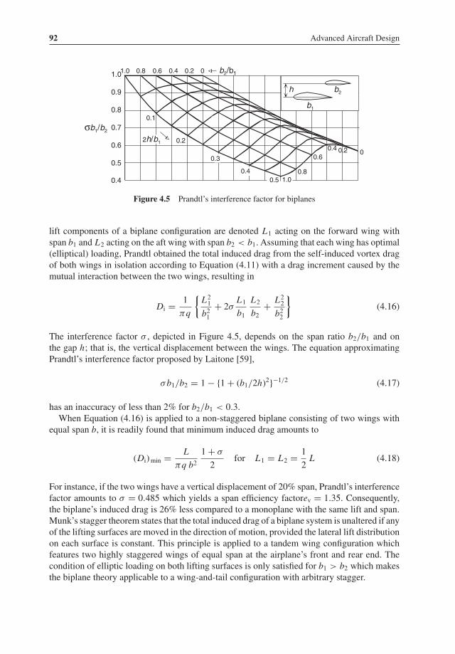
92 Advanced Aircraft Design
1.0
0.9
0.8
0.7
0.6
0.5
0.4
0.2
0.1
0.50.4
0.3
1.00.8
0.60.4
0.81.0 0.6 0.4 0.2
0.2
0
0
b2/b1
2h/b1
h
b1
b2
b1/b2σ
Figure 4.5 Prandtl’s interference factor for biplanes
lift components of a biplane configuration are denoted L1 acting on the forward wing withspan b1 and L2 acting on the aft wing with span b2 < b1. Assuming that each wing has optimal(elliptical) loading, Prandtl obtained the total induced drag from the self-induced vortex dragof both wings in isolation according to Equation (4.11) with a drag increment caused by themutual interaction between the two wings, resulting in
Di = 1
πq
{L21b21
+ 2σ L1b1
L2b2
+ L22b22
}(4.16)
The interference factor σ , depicted in Figure 4.5, depends on the span ratio b2/b1 and onthe gap h; that is, the vertical displacement between the wings. The equation approximatingPrandtl’s interference factor proposed by Laitone [59],
σb1/b2 = 1− {1+ (b1/2h)2}−1/2 (4.17)
has an inaccuracy of less than 2% for b2/b1 < 0.3.When Equation (4.16) is applied to a non-staggered biplane consisting of two wings with
equal span b, it is readily found that minimum induced drag amounts to
(Di)min = L
πq b21+ σ
2for L1 = L2 = 1
2L (4.18)
For instance, if the two wings have a vertical displacement of 20% span, Prandtl’s interferencefactor amounts to σ = 0.485 which yields a span efficiency factorev = 1.35. Consequently,the biplane’s induced drag is 26% less compared to a monoplane with the same lift and span.Munk’s stagger theorem states that the total induced drag of a biplane system is unaltered if anyof the lifting surfaces are moved in the direction of motion, provided the lateral lift distributionon each surface is constant. This principle is applied to a tandem wing configuration whichfeatures two highly staggered wings of equal span at the airplane’s front and rear end. Thecondition of elliptic loading on both lifting surfaces is only satisfied for b1 > b2 which makesthe biplane theory applicable to a wing-and-tail configuration with arbitrary stagger.

Aerodynamic Drag and Its Reduction 93
1.08
1.06
1.04
1.02
0.98
0 0.02
L2/L
relativeinduceddrag
h/b1
1.10
1.00
0.960.04 0.06 0.08-0.02-0.04-0.06-0.08
0.2
0.1
0
b1
b2h
L1
L2
Figure 4.6 Induced drag of a wing-and-tail combination with b2/b1 = 0.3
The nose-plane of a canard configuration has a smaller span than the wing and its trailingvortex field causes the wing lift distribution to be heavily distorted relative to the ellipticloading. For this configuration Munk’s stagger theorem is invalid, especially for a smallvertical displacement between the two planes. Butler [64] and Kroo [63] demonstrated that theinterference between the nose-plane and thewing reduces the induced drag of this configurationrelative to classical biplane theory. They assumed an elliptical lift distribution on the nose-plane and optimized the main wing lift distribution immersed in the nose-plane’s vortex field.The minimum total induced drag is summarized in a modified biplane equation,
Di = 1
πq
{σc
L21b21
+ 2σ L1b1
L2b2
+ L22b22
}(4.19)
with values of σc obtained from [63]. Equation (4.19) is applicable to a wing-and-tail combi-nation (b1 > b2) with σc = 1 as well as to a canard airplane (b1 < b2) with 0 < σc < 1.As an example, Figure 4.6 depicts the induced drag of awing-and-tail combination compared
to the case when all the lift is carried by the wing. For a tail located in the wing plane (h = 0),there is a drag penalty if the tail load is upward or downward.6 A high-set stabilizer maygenerate a modest induced drag reduction if it has an upward lift of about 3% of the totallift; however, even a small tail download causes a considerable drag penalty. Due to the highnose-plane lift inherent to a typical canard configuration its induced drag penalty is relativelyhigh, especially if the classical biplane theory (σc = 1) were used. Figure 4.7 illustrates thatapplying a realistic σc = 0.65 reduces the drag penalty by more than 50%. It can safely beconcluded that the lowest vortex drag of a canard-and-wing combination is obtained when thewing, with its large span, carries the highest possible fraction of the total lift.
6For a given flight condition, the tail load is determined by the airplane’s centre of gravity (CG) location. The tailplaneof a transport aircraft mostly carries negative lift.

94 Advanced Aircraft Design
1.05
0
1.10
1.000.04 0.08
b1
b2
h
L1 L2
0.12 0.16 0.20
1.15
1.20
c=1.0
c=0.65
L1/L
relativeinduceddrag
σ
σ
Figure 4.7 Induced drag of a canard airplane with b1/b2 = 0.4
4.3.4 Multiplane and Boxplane Induced Drag
The induced drag of an optimally loaded triplane is smaller than the minimum induced dragof a biplane with equal span and height. Induced drag approaches a lower limit when thenumber of multiplanes tends to infinity. However, L. Prandtl has proved that the minimuminduced drag of a system of identical parallel lifting surfaces is equal to that of a closed liftingsystem consisting of a biplane interconnected by tip planes. This principle is materialized inthe boxplane concept consisting of a biplane with wings of equal span connected at their tipsby vertical planes. The front view of a boxplane in Figure 4.8 (a) shows that the horizontalsurfaces carry the same lift, with an optimal lift distribution consisting of a constant part andan elliptical one. The circulation on the vertical planes is zero at their midpoint with equal
1.0
0.9
0.8
0.7
0 0.1 0.2 0.3 0.42h/b
0.6
0.50.5
biplane
rela
tive
vort
ex d
rag
boxplane
(a)
b/2
h
(b)
Figure 4.8 Obtainable vortex drag reduction of biplanes and boxplanes. (a) Optimum lift distributionof a boxplane. (b) Minimum vortex drag compared to a monoplane

Aerodynamic Drag and Its Reduction 95
I
III - parasite drag
II - induced drag
CL
(b)
00
maximumCL/CD
00
CD
CL2
(a)
simple parabolicequation
CD0
LCD
mdCL maxCL
true drag polar true drag polar
simple parabolicequation
minCL
mdCD
minCD
CD
zero lift drag
drag due to lift
Figure 4.9 Drag polar for subsonic flight. (a) Breakdown into parasite and induced drag and conditionfor (CL/CD)max. (b) Approximation by a two-term parabola
side force components acting outwards on the upper part and inwards on the lower part. Thevertical planes are effective in reducing the trailing vortices which would appear if the tipswere not jointed. Figure 4.8 (b) depicts the significant reduction in induced drag obtainablewith the boxplane arrangement. For instance, for a height/span ratio of 0.3, the minimuminduced drag is 60% of that for an equivalent monoplane – it reduces to 50% for a height equalto the semi-span. I.M. Kroo has shown in [72] that the boxplane does not have a particularaerodynamic advantage because it is a closed system. Its optimal lift distribution is not uniquebecause one may superimpose a vortex loop with constant circulation on any closed geometryby varying the incidence between the lifting wings. This changes the load distribution but thelift and induced drag are unchanged.
4.4 Drag Polar Representations
Many aircraft are designed to fly at speeds where the flow is subcritical everywhere. If the air-plane configuration and the Reynolds number are specified, lift and drag coefficients are uniquefunctions of the angle of attack:CL = CL (α) andCD = CD(α). In performance analysis α is oflittle significance and can be eliminated. This yields a unique relationship between CL and CD
universally known as the drag polar – a typical example is depicted in Figure 4.9 (a). For theease of performance analysis it is long-established practice to approximate the true drag polarby a polynomial equation. This section demonstrates how a drag polar obtained from compu-tational prediction, wind tunnel or flight tests can be represented by an analytical equation.
4.4.1 Two-term Approximation
The classical representation of the true drag polar consists of two terms,
CD = CD0 + CDL = CD0 + KL C 2L = CD0 + C 2
L
π Aw e(4.20)
defining a parabola which is symmetrical about theCL = 0 axis. This two-term approximationrepresents an artificial breakdown of drag into zero-lift drag and drag due to lift, with coeffi-cients CD0 and CDL , respectively. Such a subdivision does not have a fundamental justification

96 Advanced Aircraft Design
since the quadratic term describes the variation of drag with lift in a simplified manner. Thisuses the airplane efficiency factor e, also called the Oswald factor after W.B. Oswald who firstused it [16].The usual approach to obtain CD0 and KL from a true polar is to make a plot of CD versus
C 2L and approximate it by a linear function as in Figure 4.9 (b). The true polar has a non-symmetrical relation with CL and – since it is obtained by extrapolation of the straight linein this figure – CD0 is (usually) lower than the true CD at zero lift. In spite of this objection,the two-term approximation is mostly accurate in the range of normal operating conditionsand has proven to be of considerable practical value. The Oswald factor accounts for thevortex-induced drag and for the lift-dependent part of the parasite drag. Some insight into itsvalue is obtained by applying Equation (4.10) to the complete airplane,
CDp = CD0 (1+ kLC 2L ) (4.21)
In combination with Equation (4.12) this results in
e = ev1+ kLCD0π Aw ev
(4.22)
The span efficiency factor can be assumed to be equal to ev = 0.95. According to [9] kLvaries between 0.38 for straight wings, 0.40 for 20◦ and 0.45 for 35◦ sweptback wings. Analternative approximation according to [13] is: kLCD0 = 0.007. It is noticeable that Equation(4.22) indicates the Oswald factor to be lower for a high aspect ratio than for a low aspect ratiowing. Trimmed airliners flying in the en-route configuration have an Oswald factor typicallybetween 0.75 for turboprops and 0.85 for jetliners.The two terms of Equation (4.20) may alternatively be obtained from the graphical con-
struction shown in Figure 4.9 (a). The condition for minimum drag (index md) is obtainedby drawing a tangent line from the origin touching the polar curve and reading CLMD and(CL/CD)max. The coefficients CD0 and CDL are then obtained from
CD0 = CLMD
2(CL/CD)maxand π Awe = 2CLMD
(CL
CD
)max
(4.23)
This procedure uses just one point of the true drag polar namely, the minimum drag condition.Equation (4.23) is then very accurate and near this condition, a desirable characteristic forcruise performance analysis.
4.4.2 Three-term Approximation
Figure 4.9 (a) shows that the true polar has its minimum drag coefficient CDmin at the (positive)lift coefficient CLmin . The straight line approximation according to Equation (4.20) ignoresthis asymmetry relative to the CL = 0 axis. Instead, a three-term curve fit increases the CL
range with a close approximation to the true drag polar. For instance, Equation (4.20) can bereplaced by
CD = CDmin + KL(CL − CLmin )2 (4.24)
or
CD = CD0 − 2KL CLmin CL + KL C2L with CD0 = CDmin + KL C2
Lmin (4.25)

Aerodynamic Drag and Its Reduction 97
CL
CD
Re constant
Re level flight
Re increasing
Figure 4.10 Drag polar curves at constant Reynolds number and interpolation for level flight
This equation is especially suitable to represent drag at transonic Mach numbers, for highlycambered wings and for airplanes with deflected high-lift devices. It should, however, benoted that the parameters CD0 and KL in Equation (4.25) are numerically different fromthose in Equation (4.20) since the concept of a constant Oswald factor in the two-termapproximation does not apply to the three-term approximation. An even closer fit might beobtained by replacing a continuous drag polar approximation by two straight-line segments,each representing the angle of attack regionswith different flow characteristics such as attachedand separated flows [40].
4.4.3 Reynolds Number Effects
There exists a large gap between design handbook methods used to rough out a new configura-tion and the initial model testing results used to generate the first true performance prediction.In particular, variations in flight speed and altitude lead to variations in the Reynolds numberaffecting the lift and drag coefficients. For early performance estimates these variations areusually sufficiently small enough to be ignored. During preliminary design this may no longerbe the case, in particular when drag polar curves for different Reynolds numbers measured inthe wind tunnel have to be extrapolated to real flight conditions. The approximation accordingto Equation (4.20) has often been poorly understood as explained in the following commentson Figure 4.10 made by J.H. McMasters [47]:
Unlike the theoretically derivable wing span efficiency factor, the Oswald factor has only quasi-physical meaning since it is one of two parameters in a simple two-term polynomial curve fit toexperimental data. In steady level flight, the Reynolds number (of a wing) varies proportional to1/
√CL . This is not the case in a wind tunnel test, where drag data are usually measured at a
constant Reynolds number. If the drag data show significant variation with Reynolds number, caremust be taken in constructing the correct ‘equivalent flight polar’ from wind tunnel tests.
An airplane may be optimized for a narrow range of lift coefficients, for example, by selectingcambered wing sections and a wing setting angle so that the wing operates in a drag bucket.The simple two-term polynomial curve-fit is symmetrical with respect to the zero-lift conditionand may deviate significantly from the true drag polar. For a point-optimized airplane, this

98 Advanced Aircraft Design
may lead to a surprising value of the Oswald factor very close to or even exceeding e = 1.0whereas an aircraft with a very high aspect ratio wing may be found to have a lower thanexpected Oswald factor.
4.4.4 Compressibility Correction
Compressibility effects are of minor importance when an aircraft flies at a low-subsonic speed.Compressibility drag must be taken into account for speeds in excess of Mach 0.5. Figure 4.1decomposes wave drag into drag due to (wing) lift and drag due to (body) volume. Thefigure does not show the complication that interaction between a strong shock wave and theboundary layer causes boundary layer separation and a wake. Since compressibility drag isdue to a combination of physical mechanisms, its computation is a complex problem. Thedrag coefficient at high-subsonic and transonic Mach speeds are not uniquely determined bythe angle of attack but also by the Mach number,
CL = CL (α, M) and CD = CD(α, M) → CD = CD(CL , M) (4.26)
Figure 4.11 (a) depicts a set of drag polars for several Mach numbers whereas Figure 4.11 (b)is an alternative rendering of the same data. The figure shows that at high-subsonic speedsthere is a noticeable Mach-effect on drag. Dependent on CL , a subdivision can be made inthree regions.
1. The increased stagnation temperature and Reynolds number cause the skin friction drag incompressible flow to decrease with increasing Mach number by up to 5% at Mach 1.0. Thisminor effect is visible for low values of CL in Figure 4.11 (b).
2. When the (CL -dependent) critical Mach number is exceeded, the drag rises slowly due tothe increasing strength of the forward shocks and the gradual thickening of the boundarylayer. Known as drag creep, this process starts at Mach 0.6 for CL = 0.6.
0.10
0.08
0.06
0.04
0.02
CD
CL
(a)0.92
0.900.87
0.850.83
0.810.75
0.650.45
0.10
0.08
0.06
0.04
0.02
CD
M
0.9 0.8 0.70.6
0.5
0.4
0.30.20.1
0.5 0.6 0.7 0.8 0.90.2 0.4 0.6 0.8 1.0
0.79
(b)CL
MMdd
CD/ M=0.1∂ ∂
Figure 4.11 Drag coefficients of a transonic airliner. (a) CD versus CL for different Mach numbers.(b) CD versus M for different lift coefficients
Aerodynamic Drag and Its Reduction 99
3. The drag rises sharply due to strong shocks causing flow separation and a wake whenthe speed exceeds the drag-divergence Mach number Mdd, an important design parameterfor high-speed aircraft. The wing is usually responsible for the major part of the drag rise.Several criteria are in use to indicate when drag divergence begins. The preferable definitionis based on the slope of the drag curve: ∂ CD/∂ M = 0.10. Figure 4.11 (b) shows that Mdd
decreases with increasing CL .
For a given transonic Mach number, the variation of lift is accompanied by a variationin the shock-wave strength and wave drag is interpreted as a component of induced drag.Compressibility drag is a function of CL and M and is mostly accounted for as a correction�CDc of the low-speed drag. The compressibility drag penalty in fuel-optimal cruising flight istypically between five and ten counts; in high speed cruising it may increase to twenty counts.The aerodynamic design of a transonic airplanewing is dominated by the selection ofMdd sinceit is intimately related to the design point for long-range cruising. As shown in Section 10.6,this leads to different combinations of lift coefficient, sweep angle and average thickness ratioenabling optimum cruise performance. Transonic effects form a considerable complication ofthe design process and analytical computation of the compressibility correction is beyond thescope of the conceptual design stage.
4.5 Drag Prediction
Reducing the drag by aerodynamic design requires insight into its sensitivity to variationsof the airplane geometry. The prediction of drag can be approached in several ways: quasi-analytically, numerically (via CFD) and by wind tunnel testing. Since not all of these strategiesadequately recognize the design sensitivity, the selection of a method depends on the develop-ment phase and is influenced by the information available. Examples of drag prediction meth-ods can be found in [7, 8, 9, 19, 21, 31, 39]. Application of most methods is time-consumingand rather than recommending a particular methodology, we discuss some approachesand simplifications useful for quasi-analytical design optimization in the conceptualdesign phase.At the time of writing, no single method is capable of simultaneously predicting all airplane
drag components and no comprehensive method is capable of treating a full aircraft configura-tion. Drag prediction in the conceptual design stage is usually based on a number of methodswith results combined using the classical component build-up technique. This term refers tothe approach of dividing the airframe into basic components and computing the zero-lift dragof each component exposed to the free flow in isolation. It is assumed that these compo-nents have streamline shapes with aerodynamically smooth surfaces. The summation of theircontributions to drag is corrected to account for interacting flow fields around componentsplaced in each other’s vicinity and for the fact that practical airframe surfaces are not perfectlysmooth. Notwithstanding the availability of modern computational drag analysis methods,these do not necessarily produce a better prediction than the component build-up technique.Moreover, high-fidelity CFD methods for drag prediction are very computer-intensive andrequire detailed geometric input which is not always available.

100 Advanced Aircraft Design
4.5.1 Interference Drag
Corrections for the assembly of isolated components into a full configuration allow for wettedarea and other geometric modifications of adjacent components such as fairings to be addedto reduce interference drag (Appendix A). The physical origins of interference drag are notdifferent from the flow phenomena mentioned in Figure 4.1. Significant interference dragmostly arises from the intersection of a lifting surface and a body or the intersection of twolifting surfaces or bodies. Although interference may take myriad forms, in all cases a flowdisturbance is responsible for the drag.
• Interacting body flows. A common form of interference drag can be found with interferingmultiple body or wing-and-body components. A flow disturbance at the wing-to-fuselagejunction may lead to separation and vortex shedding where the weakened viscous layerincreases the probability of flow separation. The problem is aggravated when this formof interference occurs at high speeds where the wing shock pattern is changed. Theseeffects are suppressed by selecting an appropriate wing setting angle relative to the fuselageand by modifying the junction by means of fairings or fillets. For a low-wing high-speedairplane this is effectively a local modification of the external fuselage cross-section shape.However, the use of these provisions leads to a penalty caused by additional wetted area.Flow interaction between the wing and the fuselage body also affects the lift distributionalong the span, leading to a disturbance of the far-field wing wake, with an effect on induceddrag. Similarly, interference drag is often caused by wing-mounted engine nacelles whichis taken into account by modifying the span efficiency factor ev in the design condition(Figure 4.4).
• Trim drag. The basic drag polar is determined for a neutral elevator position. Dependent onthe centre of gravity (CG) location, a tail lift is necessary for trimming the airplane. Theassociated drag correction is primarily affected by the stability margin and by downwash atthe tailplane. Known as trim drag, this correction can be estimated with the help of biplanetheory (Section 4.3). A complication is that, for a given total lift, a download on the tailcauses the wing lift to increase and in the highMach number regime this leads to a significantdrag penalty as demonstrated by Figure 4.12. Trim drag in cruising flight should amount tonot more than a few drag counts.
• Propeller wake effects. Aircraft with tractor propellers have their wing immersed in theirslipstreams. This increases dynamic pressure and changes the lift distribution. The primaryeffects are increased parasite drag and induced drag due to downwash behind the propellers.On the other hand, the swirling wake flow generates an upwash on one side of the propelleraxis and a downwash on the other side and the combined effect on the wing load distributionmay, in theory, reduce the induced drag. In practice, the Oswald factor of propeller transportsmay be reduced by 4%, typically [9].
• Throttle-dependent drag. The nacelle of a turbofan engine is generally designed so thatspillage drag due to reduced intakemass flow is negligible in the cruise condition. Correctionsmay be necessary to account for interference between the flow on which the engines areoperating and the flow around the airframe.
For conventional take-off and landing airplanes, propulsion system interference effects aremostly small. In order to improve low-speed performances, short take-off and landing (STOL)

Aerodynamic Drag and Its Reduction 101
Mach 0.82Mach 0.80Mach 0.78
15 20 25 30 35C.G. position, % MAC
CD - trimCD total
0.08
0.06
0.04
0.02
0
C =0.4L
C =0.3L
Figure 4.12 Percentage change in total drag due to trim for a DC-8-54. Adapted from [60]
airplanes have a large powerplant/airframe interference effect on maximum lift at the cost ofa significant drag penalty. An in-depth analysis can be found in [4].
4.5.2 Roughness and Excrescences
Practical aircraft surfaces are not perfectly smooth. Roughness and excrescence drag mayincrease the zero-lift drag by 15% for large jetliners and up to 30% or more for small propellertransports.7 Information in [48] and [50] can be used to make an estimation of the followingpenalties:
• Surface imperfections such as (protruding) rivets, skin joints, control surface gaps, removablepanels, steps and gaps around windows and doors – alternatively classified as distributedsurface roughness. For a certain type of construction, surface imperfection drag is oftentaken into account by an equivalent sand grain roughness defined as the size of sand grains,distributed uniformly on the surface, which would produce the same skin friction as theoriginal surface with an arbitrary roughness. According to [9], jet transports have an averageequivalent sand grain roughness of 0.0016 inch (0.04 mm) – this is too much for surfacesdesigned for laminar flow.
• Excrescences and protuberances cause a drag penalty that is predictable for each item individ-ually. All transport aircraft are required to have the provisions associated with this category,namely, air data systems, drains, antennas, vents, lights and beacons, auxiliary power unit,and features required for rain dispersal, for ventilation/cooling, for air conditioning, and forfuel systems.
7Some airframe manufacturers characterize this non-ideal drag penalty as the only form of parasite drag. This can beconfusing since parasite drag is widely interpreted as the drag of a nonlifting closed body (Figure 4.1).

102 Advanced Aircraft Design
Additional drag sources may have to be considered such as fuselage upsweep drag or unac-counted drag based on previous experience. Since these drag components are sensitive todetailed design, their estimation during conceptual design is based on statistical data [13].
4.5.3 Corrections Dependent on Operation
Drag is affected by the airplane’s configuration, flight conditions, engine rating and the distri-bution of useful load. In the en-route configuration, drag is subdivided into uncorrected dragand corrections for the trim condition, compressibility and aero-elastic effects. The uncorrecteddrag is represented by a single drag polar for subsonic flight and a representative (variationof) Reynolds number. Engine power effects are often counted as a reduction of the overallefficiency. A compressibility correction accounts for Mach numbers in excess of 0.6 to 0.7.Aero-elastic effects are significant for large airliners flying at a high dynamic pressure. Deflec-tion of high-lift devices, landing gear extension and engine failure also lead to considerabledrag increments.
4.5.4 Estimation of Maximum Subsonic L/D
When different aircraft concepts are compared, the maximum aerodynamic efficiency(L/D)max for the en-route configuration is a useful measure of the aerodynamic design quality.However, it is emphasized that selection of the aircraft shape is the outcome of many com-promises with non-aerodynamic aspects such as structural weight, operational constraints andcost considerations. Moreover, turbofan-powered aircraft cruise optimally at a Mach numberhigher than MMD where compressibility effects increase the drag by up to 5% (Section 2.4).Consequently, when aircraft designs are compared, it cannot be concluded that the one achiev-ing the highest L/D is the best. In spite of these reservations, achieving a high aerodynamicefficiency is an important goal for designing transport as well as business airplanes. In theearly design phase it is therefore safe to assume that the aerodynamic design will be opti-mized during the downstream development process. For example, parasite drag is minimizedby selecting suitably cambered wing sections, application of smooth skin surfaces and byavoiding unnecessary excrescence drag. Major drag components will then approach the lowerlimit of statistical values demonstrated by existing aircraft. The purpose of this section is topresent an approach to a quasi-analytical prediction of the maximum aerodynamic efficiencybased on the classical two-term approximation of the drag polar.For straight and level subsonic flight Equation (4.20) can be written as
CL
CD=
(CD0
CL+ CL
π Aw e
)−1(4.27)
which has its maximum value
(CL
CD
)max
= 1
2
√π Aw e
CD0
for CLMD = √CD0π Aw e (4.28)
Since skin friction is the main contribution to lift-independent efficiency, a simple methodfor estimating CD0 is the equivalent skin friction method. This considers CD0 as the skin
Aerodynamic Drag and Its Reduction 103
friction drag coefficient C feq based on the total airplane’s wetted area CD0 = C feq Swet/Sw. Incombination with Equation (4.28) this yields
(CL
CD
)max
= bw2
√πe
CD0 Sw= bw2
√πe
C feq Swet(4.29)
As explained in the previous sections, the drag coefficient of an aircraft component dependson the Reynolds number, the pressure distribution, the state of the boundary layer, the surfacesmoothness and many other details. The proposed quasi-analytical estimation method is basedon the flat plate analogy. Equation (4.7) is used for the friction drag coefficient of a plate witha fully turbulent boundary layer with the mean full-configuration Reynolds number based onan average wetted plate length,
Redef= V
ν
Swetbw
(4.30)
The uncorrected parasite drag is obtained from Equation (4.8) by multiplying the flat platedrag by the form factor accounting for supervelocities. It is approximated as
�f = 1+ r�
SfrontSwet
(4.31)
Figure 4.2 shows that typical values of r� are 4.8 for a straight wing, 4.1 for a swept wingand 3.5 for a fuselage. The resulting ideal friction drag area (index id) of an aerodynamicallysmooth airframe surface is
C fid S = 0.044Re−1/6(Swet + r� Sfront) (4.32)
where Sfront denotes the frontal area of the airplane excluding the engine air intakes. If detailedinformation is lacking, one may use r� = 4.0 for propeller aircraft and r� = 3.5 for jetaircraft. Although the airplane’s frontal area is much smaller than its surface area, the factorr� magnifies its effect on drag. This makes the values of the wing thickness and the fuselagefineness ratio very influential, an effect that is not visible in prediction methods based on onlywetted areas. The drag increment due to surface roughness, excrescences and other non-ideal(index nid) sources of drag is made by multiplying the parasite drag of the aerodynamicallysmooth airplane by a correction factor knid = C feq /C fid resulting in the lift-independent dragarea
CD0 S = C feq Swet = 0.044 knid Re−1/6(Swet + r� Sfront) (4.33)
In combination with Equation (4.28) this yields
(CL
CD
)max
= 4.2
(e Re1/6
knid
) 0.5bw
(Swet + r� Sfront) 0.5(4.34)
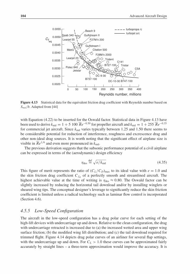
104 Advanced Aircraft Design
Cfeq
Saab 340
Beech 9
Gulfstream II
F27M k 200
Gulfstream ICitation 500
F28M k 2000
Trident
B727-100C141
TristarC5A
B747-100DC-10-30
DC-9-30B737-100
JetstarPotez 840
Learjet 23
Metro
0.0020
0.0030
0.0040
0.0050
0.0055
Reynolds number, millions
0 100 200 300 400
0.0045
0.0035
0.0025
50 150 250 350
Learjet 55
turbopropa /c
turbojet a/c
Figure 4.13 Statistical data for the equivalent friction drag coefficient with Reynolds number based onSwet/b. Adapted from [44]
with Equation (4.22) to be inserted for the Oswald factor. Statistical data in Figure 4.13 havebeen used to derive knid = 1+ 5 100 Re−0.50 for propeller aircraft and knid = 1+ 255 Re−0.35
for commercial jet aircraft. Since knid varies typically between 1.25 and 1.50 there seems tobe considerable potential for reduction of interference, roughness and excrescence drag andother non-ideal drag sources. It is worth noting that the significant effect of airplane size isvisible in Re1/6 and even more pronounced in knid.The previous derivation suggests that the subsonic performance potential of a civil airplane
can be expressed in terms of the (aerodynamic) design efficiency
ηdesdef=
√e/knid (4.35)
This figure of merit represents the ratio of (CL/CD)max to its ideal value with e = 1.0 andthe skin friction drag coefficient C fid of a perfectly smooth and streamlined aircraft. Thehighest achievable value at the time of writing is ηdes ≈ 0.80. The Oswald factor can beslightly increased by reducing the horizontal tail download and/or by installing winglets orsheared wing tips. The conceptual designer’s leverage to significantly reduce the skin frictioncoefficient is limited unless a radical technology such as laminar flow control is incorporated(Section 4.6).
4.5.5 Low-Speed Configuration
The aircraft in the low-speed configuration has a drag polar curve for each setting of thehigh-lift devices with undercarriage up and down. Relative to the clean configuration, the dragwith undercarriage retracted is increased due to (a) the increased wetted area and upper wingsurface friction; (b) the modified wing lift distribution; and (c) the tail download required fortrimmed flight. Figure 4.14 depicts drag polar curves of an airliner for several flap settings,with the undercarriage up and down. For CL > 1.0 these curves can be approximated fairlyaccurately by straight lines – a three-term approximation would improve the accuracy. It is

Aerodynamic Drag and Its Reduction 105
30
25
20
20155
1
3.0 3.52.52.01.51.00.50
0.05
0
0.10
0.15
0.20flap angledegrees
undercarriage up
undercarriage down
CD
CL2
clean
Figure 4.14 Drag polars of a wide body airliner for the low speed configuration
also noticeable that, with flaps down, the drag polar curves have a slightly smaller slope thanwith flaps up. Hence, the Oswald factor in a two-term approximation increases slightly relativeto the value for the clean configuration.A dominant flight condition for sizing the engines is the climb-out after the take-off with
flaps down, undercarriage up, flying at the take-off safety speed V2. For a given flap setting, thelift coefficient is determined by the requirement that the speed must have 20% reserve relativeto the stalling speed: V2 ≥ 1.2 VS. Experimental evidence suggests that the correspondingdrag-to-lift ratio can be linearized for 1.2 < CL 2 < 1.8 as in Figure 4.15:(
CD
CL
)V2
= C0 + CL 2
π AwEwith 1.2 ≤ CL 2 ≤ 1.8 (4.36)
0.20.10 .3 0.40 .5 0.6
take-off flapsV =1.2V2 S
trimmed C L Aw2
0.1
0.2
0.3
0.4
0.7
linearapproximation
flapsup
1
00
1EC0 Aw
CD
CL
2
2Aw
π
π
Figure 4.15 Corrected CD /CL at 1.2VS for a jetliner with CD0 = 0.015 flaps up

106 Advanced Aircraft Design
where C0 = 0.025 accounts for the parasite drag with extended flaps and E = 0.85 is calledthe modified Oswald factor. The drag and lift coefficients are generalized by the factor
√Aw
which makes Figure 4.15 applicable for different aspect ratios. It is emphasized that Equation(4.36) differs from the usual drag polar since it defines conditions at the take-off safety speedfor different flap angles instead of a drag polar for a given flap configuration. This is clarifiedby comparison with the CD/CL ratio for the clean configuration.
4.6 Viscous Drag ReductionSuccessful analysis, prediction, and control of the boundary-layer transition process for improvedaerodynamic efficiency has been the ultimate goal – the Holy Grail – of aerodynamicists since theearliest days of aviation.
—J.R. Chambers [115] (2005)
Figure 4.16 depicts the cruise drag breakdown of a typical wide body transport aircraft givingan alternative view the relative importance of reducing parasite and induced drag. Major com-ponents are skin friction drag and vortex drag induced by lift accounting for about 50% and40%, respectively. Form drag is built up from many small components – typically betweenfive and ten counts – due to flow separations and vortices around the aft fuselage, flowinterference near junctions, surface imperfections, excrescences, protuberances, and miscel-laneous drag. Together they form a significant penalty which should be minimized by careful
roughness
interferenceafter body
100
turbulent
partlylaminar80
60
40
20
0
planar
nonplanar
frictiondrag
parasitedrag
induceddrag
form drag
vortexdrag
wave
Figure 4.16 Example of transport aircraft cruise drag breakdown and drag reduction potential

Aerodynamic Drag and Its Reduction 107
design,8 a subject beyond the scope of the present text.Wave drag at high speed has componentsdue to body volume and lift and is sensitive to Mach number variation. The design conditionin cruising flight is based on a trade-off between the desirability of block fuel conservation andblock time reduction (Chapter 12). Compressibility drag in fuel economical flight is typicallybetween five and ten counts.The minimum drag in straight and level flight is obtained from Equation (4.29),
Dmin = 2W
bw
√C feq Swet
πefor L = W (4.37)
Although cruising flight is not exactly carried out in the minimum-drag condition, this equa-tion clearly shows the relative importance of the design parameters which have a majorinfluence on drag in cruising flight and, hence, on thrust and fuel consumption. The air-plane GW and geometry dominate through the term W/bw and the wetted area Swet, aero-dynamic design quality is apparent in the equivalent skin friction coefficient C feq and theOswald factor.
4.6.1 Wetted Area
The skin friction drag of each aircraft component exposed to the flow is proportional its wettedarea – it is not affected by the aircraft’s gross weight. Since reduction of the wetted areanot only decreases drag but structural weight as well, minimizing the wetted area constantlyneeds the designer’s attention. However, due to practical geometric constraints, feasible wettedarea reductions are normally not spectacular unless major airplane configuration changes areadopted such as foreseen for the blended wing body (BWB, see Chapter 5).
• Fuselage skin area forms a major contributor which is, to a large extent, determined bythe general arrangement of the airplane. It is constrained by cabin comfort and cargo holdvolume requirements and can be minimized by carefully laying out the passenger cabin,baggage and cargo holds and by avoiding unused spaces.
• The wing is the other major contributor to wetted area. Aerodynamic design of a tran-sonic aircraft wing is dominated by the Mach number and the lift coefficient for optimumcruising. Certain combinations of wing area and span, angle of sweep and wing thick-ness ratio lead to maximum aerodynamic efficiency, minimum trip fuel or minimum GW.Reduction of wing area is subject to low-speed performance requirements and a fuel tankvolume constraint.
• Empennage wetted area depends on the size of the horizontal and vertical tail surfaces.Both are normally smaller when wing and/or fuselage wetted areas are reduced in size(Appendix A).
8It may appear easier to obtain a much greater percentage reduction in small drag sources than in the much largercontributions. For example, a 50% aft body drag reduction may be feasible, representing a useful 5% total dragreduction.

108 Advanced Aircraft Design
The traditional airliner configuration with a discrete fuselage – nicknamed tube and wing(TAW) – has a total wetted area between five and six times the wing planform area. Equation(4.34) shows that, for a given span, a 10% smaller wing area leads to roughly 4% wettedarea and Reynolds number reduction, a 0.7% higher equivalent friction drag coefficient anda modest 1.6% improvement of L/D, on the provision that CL is optimized by reducing thealtitude.The wetted area can be reduced significantly by adopting an unorthodox airplane configu-
ration. The most radical mutation is the all-wing aircraft (AWA) which has a wetted area ofabout 2.5 times the gross wing area. For the same aspect ratio and equivalent skin frictioncoefficient, Equation (2.21) predicts the AWA’s aerodynamic efficiency to be at least
√2 times
that of a TAW design, a value confirmed by two TsAGI projects depicted in Figure 2.6. Sincethe AWA planform area is typically twice the TAW gross wing area, its span is a factor
√2
higher – unless the aspect ratio is reduced. In view of the restrictions by the ICAO airfieldclassification, such a large span is probably impractical. A dilemma for the designer of an AWAis therefore how to compare its properties with those of a TAW design. Bearing in mind that‘the outside has to be bigger than the inside’ [75], a realistic approach might be to optimizean AWA with (1) a constraint on the internal volume required to contain the UL, systemsand structure, and (2) an upper limit to the wing span. Such a design should be comparedwith an optimized conventional airplane with the same useful internal volume and wing spanconstraint, the subject of Chapter 5.
4.6.2 Turbulent Friction Drag
Friction drag can be reduced by manipulation of the turbulence structure within the sub-layerof a turbulent boundary layer using micro-structures on the airplane skin. This involves theintroduction of riblets which suppress vortex formation near the wall. Riblets are formed byapplying very fine grooves – a few microns high, about 0.05 mm wide – in the direction offlight, with sharp ridges in between. Riblets can be applied to the aircraft skin in the formof a self-adhesive film. A potential of 7 to 8% drag reduction has been demonstrated withexperiments on flat plates in wind tunnel conditions and research has shown that riblets candeliver up to 2% aircraft drag reduction. This figure has been verified by flight tests with anAirbus A320 fuselage on which some 75% of the wetted surface was covered with 3M ribletfilm, resulting in an airplane drag reduction of the order of 1.5%. Application of riblets tothe wing upper surface, horizontal stabilizer and the upper part of the fuselage (above thewindows) would lead to approximately 1% in fuel burn on a long-haul airliner. The riblet filmhas shown to be durable over a test period of 18 months [85].
4.6.3 Natural Laminar Flow
The friction drag of surfaces with a laminar boundary layer is an order of magnitude lesscompared to a turbulent boundary layer. Delaying the onset of turbulent flow over 50% of theexposed airplane surface leads to a considerable reduction in skin friction drag (Figure 4.17).Natural laminar flow (NLF) is a passive technique that uses optimized pressure gradients tomaintain a laminar boundary layer over large parts of a lifting surface. Transition to turbulenceis a function of several types of instabilities and contamination:

Aerodynamic Drag and Its Reduction 109
Reynolds number
turbulent
laminar
50% laminar
105 106 107 108
0.007
0.006
0.005
0.004
0.003
0.002
0.001
0
Cf
Figure 4.17 Flat plate skin friction coefficient
• Tollmien-Schlichting instability is caused by amplification of streamwise waves which isresponsible for transition when the sweep angle is less than 25◦.
• Cross-flow instability is the first cause of transition at high Reynolds numbers when thesweep angle is more than 25◦.
• Attachment line instability is due to propagation along the wing leading edge of the distur-bance caused by the fuselage boundary layer.
Obtaining NLF is closely connected to the airfoil shape, the leading edge sweep and theReynolds number. The maximum airfoil thickness should be as far aft as possible; however,in high-speed flight this might lead to strong shock waves and high wave drag. Figure 4.18is derived from results obtained in flight tests where transition locations over surfaces with a
0
10
20
30
40
5040302010Reynolds number, millions
L.E
. sw
eep,
deg
rees
decreasingpressure
ALI
CFI
TSI
60
L.E. radius2.5% 1.5%
NLF
LFC
Figure 4.18 Extent of natural laminar flow over swept wings [108]

110 Advanced Aircraft Design
favourable pressure gradient were measured for varying leading-edge sweep. The shaded areaindicates the approximate chordwise extent of laminar flow attainable on a wing with initiallydecreasing surface pressures towards the trailing edge. At relatively low chord Reynoldsnumbers and small leading edge sweep angles, a laminar boundary layer is possible over anappreciable stretch from the leading edge.Present-day construction techniques result in the production of smooth and accurate aero-
dynamic surfaces over which long runs of NLF can be obtained. Stretches of laminar flow upto some 50% of the wing chord have been observed for airplanes featuring lifting surfaceswith less than 18◦ of leading-edge sweepback. The wings of several business aircraft havebeen designed for NLF leading to drag reductions of 5 to 10% – application to high-subsonictransport aircraft leads to savings of a few percent. Consequently, NLF can be appreciated asa proven technique which finds application in business and commuter airplanes flying at sub-sonic speed. These successful applications also justify studies of applying NLF over fuselagesurfaces [80].
4.6.4 Laminar Flow Control
Mid-size and large transport aircraft flying at high subsonic speed attain chord Reynoldsnumbers between 40 and 100 million at the root and between 8 and 20 million at the tip.Accordingly, the only chance of achieving laminar flow over most of the wing is by activecontrol of the boundary layer. Laminar flow control (LFC) concepts using artificialmechanismsto maintain laminar flow over a large region of the wing have to be used. The use of wallsuction is the favourite method of active LFC. This technology uses the continuous removalof a small amount of the laminar boundary layer by applying suction over the exposed surfacethrough porous materials, multiple narrow surface slots or small skin perforations. The effectof suction over the entire airfoil as far back as the eventual transition point is that the laminarboundary layer is stabilized and transition to turbulence is delayed.Active LFC is widely acknowledged to offer the potential for improvements in fuel usage
that far exceed any known single aerodynamic technology. Theoretically, the fuel burnedby transport aircraft might be decreased by up to 30% by applying boundary layer suctionto both sides of the wing and the tail surfaces. A practical fall-back position which stillprovides significant savings is to apply suction control only to the upper wing surfacewhich has the lowest pressures and hence the highest flow velocities and friction drag. Thereduction in lower surface smoothness requirements enables the application of retractableleading edge devices for high lift. It also complies with the presence of inspection hatchesand the higher susceptibility of damage by ground vehicles. Other cases where successfulapplication of LFC must be considered elusive include most (metal) aircraft fuselages withroughnesses such as pitot probes, windshield wipers, doors and windows, and waviness dueto pressurization.LFC of the wing’s upper surface, engines nacelles and the empennage is a well-researched
aerodynamic technology with demonstrated drag benefits. Experience thus far indicates thatlaminar flow can be obtained on modern airfoil sections to mid-chord and beyond. However,a wing featuring LFC over the entire exposed primary structure is mechanically complex –see Figure 4.19 (a) – and costly to produce. The suction concept involves extensive ductingthroughout the internal wing structure, auxiliary power sources or engine bleed air and an

Aerodynamic Drag and Its Reduction 111
(a) structural wing concept (b) perforated leading edge box with Krueger shield
graphite epoxy
graphite epoxy
glassepoxy
electron-beamperforateds kin
0.76 mm
Titanium0.064 mm
0.64 mm
Kruegershield
TKSsystem
fluidspraynozzles
sensorpanel
Figure 4.19 Douglas LFCwing structural concept and leading edge flight test article. Copyright NATOSTO - CSO
additional system to accurately control the suction airflow distribution. There are weight andmaintenance penalties and some uncertainty in structural integrity must be accepted. Sinceresults obtained in airline operation depend on the smoothness of the surface and on eventualcontamination by insects and dust, a system for cleaning the leading edge is a prerequisite.The extension during take-off and landing of a Krueger flap or a shield containing a specialcleaning fluid as depicted in Figure 4.19 (b) has proven to be effective, however, at the cost ofreduced maximum lift.
4.6.5 Hybrid Laminar Flow Control
The hybrid laminar flow control (HLFC) concept integrates natural and active laminar flowtechnologies and avoids most of the objectionable characteristics of both. The leading-edgesweep limitation of NLF is overcome through suction in the leading edge box to controlcross-flow and attachment line instabilities of swept wings. Wing shaping for favourablepressure gradients to suppress Tollmien-Schlichting instabilities allowing NLF over the wingbox region removes the need for in-spar LFC suction and greatly reduces system complexityand cost [108]. Dependent on the wing size, HLFC may be used for long-chord inboardsurfaces in combination with NLF for short-chord outboard surfaces. In 1990, Boeing flighttested the effectiveness of HLFC on a B 757 airplane using a large HLFC glove installed on alarge section of the left wing (Figure 4.20). A titanium skin was used for suction to the frontspar with an ability to reverse flow for purging. Existing manufacturing technology permittedconstruction of the glove to laminar-flow surface quality requirements. A Krueger shield as inFigure 4.19 (b) was installed for insect protection and high lift. All necessary systems requiredfor practicalHLFCwere successfully installed. The flight test results located transition between30 and 50% chord past the end of suction with less suction flow required than anticipated.The primary goals of this experiment – achieving HLFC at Reynolds numbers concurrentwith medium-size transport airplanes and reducing industry risks to acceptable levels – weresuccessfully accomplished [115].

112 Advanced Aircraft Design
HLFC suction panel
x/c %
0102030
50
6560
.79
.80
.81
.82
Mach
40
turbulent flow
laminar flow between spars
extent of laminar flow
Figure 4.20 Transition contours showing the extent of laminar flow obtained on a B 757 test vehiclewith HLFC [115]
4.6.6 Gains, Challenges and Barriers of LFC
Questions regarding long-term operational and reliability characteristics of current conceptsstill remain which must be resolved before a sustained performance of LFC over large areasof the aircraft can be guaranteed. The technologies of each of the three laminar-flow conceptshave different drag reduction potential. LFC allows the aircraft to be sized for a considerablyreduced fuel load and design gross weights, smaller engines and other benefits and this hasthe largest impact for long-range airliners. However, LFC is not a technology to be retrofittedand its application has to be envisaged and investigated in the early conceptual design stage.Figure 4.21 plots the percentage improvement of L/D versus the wing area characterizing
the airplane size. The performance gain due to NLF is now a fact that should not be ignored forbusiness aircraft9 and regional airliners. For a given transitionReynolds number, the percentagechord where laminar flow is obtained and the gain in L/D decrease with wing size. Figure 4.21also shows a large improvement for HLFC compared to NLF, although the decreasing gain inL/D with size is manifest as well. For the largest transports, appreciably larger benefits areobtained with LFC suction position farther aft of the leading edge. Conceptually, even largerlevels of drag reduction may be feasible via synergistic application if active laminarization isapplied to non-conventional aircraft configurations that are especially fit for it.
9Piaggio Aero Industries reports that NLF degradation of their P-180 Avanti wing increases power required for levelflight by 8 to 10%.

Aerodynamic Drag and Its Reduction 113
DC-9, 737 sizeimpr
ovem
ent i
n L/
D, p
erce
nt
727 size
757 size
wing area, m2
100 2000 300 400 500
turbulent dragcoefficient
0.00250.0030
30
25
20
15
10
5
0
noncycled airplaneclean wing
LFC wingsweep = 25 deg.
HLFC wingsweep = 25 deg.LE suction
NLF wingsweep = 20 deg.
Figure 4.21 Improvement in aerodynamic efficiency due to laminar concepts as compared with aturbulent airplane [108]
Aerodynamic performance predictions by researchers indicate that, for a transport aircraftwith laminar flow up to 60% chord on both sides of wing and tail, the fuel burned on long-range flights might decrease by 30% from that of fully turbulent airfoils. The performanceimprovements of HLFC are not as great as LFC, the potential gains are nevertheless substantial.Typical benefits of applying HLFC to a 300-passenger long-range twin engine subsonictransport are reported in [76]. Assuming 50% chord laminar flow over the upper wing surfaceand both surfaces of the empennage, HLFC provides about 15% reduction in mission fuel.Application to the engine nacelles with laminar flow to 40% of the nacelle length has thepotential of at least an additional 1% reduction in fuel burned.Real-world influences upon the operational functionality of LFC surfaces (Figure 4.22)
include surface roughness/waviness, joints and steps, flight through ice clouds and ice pro-tection, acoustic fields caused by the engines and localized vortical flow generation causingclogging effects. Maintaining laminar flow on an airplane wing is possible only with anextremely smooth surface requiring special manufacturing techniques and/or the use of com-posite materials. Research on building porous wing skins for LFC at an acceptable cost andkeeping them free of dirt and insects has shown that composite materials such as graphite-epoxy or fibreglass may provide very smooth surfaces and freedom of waviness required forlaminar flow. The major concern is not whether laminar flow can be obtained but whether itcan be maintained reliably, in an economic fashion.

114 Advanced Aircraft Design
Validation of tools- transition = ?
Application- upper surface- both surfaces
Leading edge devices- krueger- slat- suction effect on CL - max
Technology problems- suction system- leading edge contamination- cleaning- insects contamination- anti-icing / de-icing- surface quality- manufacturing technology
Suction power installation- engine- auxiliary engine or APU- engine location: wing or fuselage?
Maintenance problems- dirt- cleaning (water, soap)- degradation- etc.
Certification- fuel reserves- suction system failure in flight- etc.
Real DOC for airlines?
Figure 4.22 Questions and problems regarding design, certification, operation and reliability of LFCsurfaces. Copyright NATO STO - CSO
4.7 Induced Drag Reduction
4.7.1 Wing Span
The induced drag of a long-range transport at cruise conditions (Figure 4.16) amounts toabout 40% of the total drag, of which wave drag constitutes a small percentage. Reducinginduced drag is therefore of paramount importance. Since induced drag at a given dynamicpressure is proportional to the span loading (W/bw) squared, a span increase is an effectiveway of reducing it. For a given wing area, a 10% larger span increases the aspect ratio by21%, whereas the Oswald factor and the Reynolds number are reduced by 3.3% and 10%,respectively. Equation (4.37) demonstrates that, dependent on the type of aircraft, the resultingimprovement of theminimum drag for a given gross weight is roughly 7.5%. However, induceddrag can have a much greater significance to advanced aircraft design and performance thanmight be inferred from cruise aerodynamics. In particular, induced drag is high at low speedswhere it may account for 80 to 90% of the aircraft’s total drag at a critical take-off conditionwith a failed engine. A mere 1% reduction of induced drag allows the aircraft to take off withalmost the same percentage increasedGW,which can be translated into a useful gain in payloador range. Increasing the span may also be a panacea when downstream of the conceptual phasethe design appears to have performance shortcomings. And a span increment copes effectivelywith the heavier take-off weight of a derivative version in case the engines are sized to theone-engine-out take-off climb gradient.The designer’s freedom to increase the wing span is limited since a larger span requires
more structural material to withstand the increased bending moments. In fact, wing structureweight is even more sensitive to span than induced drag and the problem of improving theaerodynamic efficiency through a span increase is clearly the subject of multidisciplinarydesign optimization (MDO). And a practical upper limit to the wing span – such as the‘80 metre box’ limit – may be a key constraint for large commercial transport aircraft.10 If
10The use of folding wing tips was proposed in several design studies of high-capacity aircraft. However, folding tipsas foreseen for the Boeing 777 during its design stage have not found favour with airlines.

Aerodynamic Drag and Its Reduction 115
increasing the wing span is not an option, the advanced designer can aim to increase the spanefficiency factor ev by using a non-planar wing or by embracing a general arrangement basedon multiple lifting surfaces.
4.7.2 Spanwise Camber
A wing may exhibit a modest induced drag reduction if it produces a non-planar trailingvortex sheet. Dihedral/anhedral and a swept or curved trailing edge are all associated withwake curvature. As a corollary it can be stated that upward wing bending due to lift does notnecessarily increase induced drag. The non-linearities associated with vortex sheet curvaturerequires a more refined analysis than the standard lifting line theory and these effects increasewith incidence and wake roll-up. Relaxing the assumption of classical linear theory thatthe wing sheds a planar vortex sheet provides interesting possibilities to reduce drag. Earlytheoretical analysis was carried out by C.D. Cone Jr. and J.S. Letcher [55, 56]. The greatestincreases in span efficiency occur for configurations which tend to release the major portion ofthe vortexwake over an appreciable vertical area near the tip. This leads to a geometry known asspanwise camber making it possible to get span efficiencies appreciably greater than one [68].
4.7.3 Non-planar Wing Systems
The high span efficiency of non-planar wings appears to accrue from the movement of vorticalflow away from the mid-span line. Multiplane systems distribute the lift vertically as well ashorizontally and each plane should be optimally twisted for minimum induced drag. Someaerodynamic principles of biplanes and boxplanes – see Section 4.3 and Figure 4.8 – wereestablished during the 1920s for low speed aircraft. During the 1970s, the introduction of tran-sonic jetliners stimulated investigations into the transonic biplane and the joined wing. Theseconfigurations may also have desirable non-aerodynamic effects when properly integrated intothe overall airplane general arrangement. For instance, the joined wing geometry is exploredprimarily to improve structural depth when the bending moment on the wing system is high.Radical aircraft configurations based on the multiplane plane concept offer the possibility ofsignificant reductions in induced drag for airplanes with a highly span-constrained wing andmay lead to wetted area reductions or even complete elimination of tail surfaces. In theseapplications, induced drag reduction is just one of many design objectives that have to beinvestigated to obtain a balanced and realistic alternative for the conventional high-aspect ratiocantilever monoplane. A few of these design considerations are surveyed in the next chapters.
Bibliography
[1] Abbott, I.H., and A.E. Von Doenhoff, Theory of Wing Sections: Including a Summary of Airfoil Data, DoverPublications, Inc., New York, 1959.
[2] Lachmann, G.V. (ed.), Boundary Layer and Flow Control, Pergamon Press, Oxford, 1961.[3] Hoerner, S.F., Fluid Dynamic Drag, Hoerner Fluid Dynamics, Bakersfield, CA, 1965.[4] McCormick Jr., B.W., Aerodynamics of V/STOL Flight, Academic Press, New York, 1967.[5] Hoak, D.E., et al., USAF Stability and Control Datcom, Flight Control Division, AFFDL, WPAFB, Ohio,
USA, 1978.

116 Advanced Aircraft Design
[6] McCormick, B.W., Aerodynamics, Aeronautics, and Flight Mechanics, John Wiley & Sons, New York, 1979.[7] Torenbeek, E., Synthesis of Subsonic Airplane Design, Appendices B, F and G, Delft University Press, Delft,
1981.[8] Roskam, J., Airplane Design, Part VI: “Preliminary Calculation of Aerodynamic, Thrust and Power Charac-
teristics”, Roskam Aviation and Engineering Corporation, Lawrence, KA, USA, 1987.[9] Shevell, R.S., Fundamentals of Flight, Chapters 11 and 12, Second Edition, Prentice-Hall, Englewood Cliffs,
NJ, 1989.[10] Eppler, R., Airfoil Design and Data, Springer Verlag, New York, 1990.[11] Mair, W.A., and D.L. Birdsall, Aircraft Performance, Chapters 3 and 10, Cambridge University Press, Cam-
bridge, 1992.[12] Torenbeek, E., and H. Deconinck (eds), Innovative Configurations and Advanced Concepts for Future Civil
Aircraft, von Karman Institute for Fluid Dynamics, Lecture Series 2005-06, June 2005.[13] Obert, E., Aerodynamic Design of Transport Aircraft, Chapter 40, IOS Press, Amsterdam, 2009.[14] Torenbeek, E., and H. Wittenberg, Flight Physics: Essentials of Aeronautical Disciplines and Technology, with
Historical Notes, Chapter 4, Springer Verlag, Heidelberg, 2009.
Theory and Prediction of Drag
[15] Von Karman, T., and J.M. Burgers, “General Aerodynamic Theory: Perfect Fluids”, in Vol. II of AerodynamicTheory, Edited by W.F. Durand, 1935.
[16] Oswald, W.B., “General Formulas and Charts for the Calculation of Airplane Performance”, NACA ReportN0. 408, 1932. TR R-139, 1962.
[17] Aeronautical Research Council, “Definitions to be Used in the Description and Analysis of Drag”, ARCCurrent Paper No. 369, 1958. Also Journal of the Royal Aeronautical Society, Vol. 62, pp. 796–801, 1958.
[18] Hoak, D.E., et al., “The USAF Stability and Control DATCOM”, Air Force Wright Aeronautical Laboratories,TR-83-3048, October 1960 (Revised 1978).
[19] Morrison, W.D., “Advanced Airfoil Design Empirically Based Transonic Aircraft-Drag Buildup Technique”,NASA Contractors Report 137928, January 1976.
[20] Feagin, R.C., and D.W. Morrison Jr., “Delta Method: An Empirical Drag Buildup Technique”, NASA Con-tractors Report 151971, December 1978.
[21] ESDU, “Profile Drag of Axisymmetric Bodies at Zero Incidence for Subcritical Mach Numbers”, Data Item78019, London, 1978.
[22] Shevell, R.S., and F.P. Bayan, “Development of aMethod for Predicting theDragDivergenceMachNumber andthe Drag Due to Compressibility for Conventional and Supercritical Wings”, Stanford University, Departmentof Aeronautics and Astronautics, Report SUDAAR 522, July 1980.
[23] Eppler, R., and D.M. Somers, “A Computer Program for the Design and Analysis of Low-Speed Airfoils”,NASA TM 80210, August 1980.
[24] Young, A.D., J.H. Patterson, and L. Lloyd Jones, “Aircraft Excrescence Drag”, AGARDograph No. 264, July1981.
[25] Jacobs, P.F., “Experimental Trim Drag Values and Flow-Field Measurements for a Wide-Body TransportModel with Conventional and Supercritical Wings”, NASA TP-2071, 1982.
[26] Kroo, I.M., and T. McGeer, “Optimization of Canard Configurations: An Integrated Approach and PracticalDrag Estimation Method”, ICAS Paper No. 82-6.8.1, September 1982.
[27] McGeer, T., and R.S. Shevell, “A Method for Estimating the Compressibility Drag of an Airplane”, StanfordUniversity, Report SUDAAR 535, 1983.
[28] Knaus, A., “ATechnique toDetermine Lift andDrag Polars in Flight”, Journal of Aircraft, Vol. 20, pp. 587–593,July 1983.
[29] Hallstaff, T.H., and G.W. Brune, “An Investigation of Civil Transport Aft Body Drag Using a Three-Dimensional Wake Survey Method”, AIAA Paper No. 84-0614, 1984.
[30] Covert, E.E. (ed.), “Thrust andDrag: its Prediction andVerification”,Progress in Astronautics and Aeronautics,Volume 98, AIAA Education Series, New York, 1985.
[31] Jobe, C.E., “Prediction and Verification of Aerodynamic Drag, Part I: Prediction”, Progress in Astronauticsand Aeronautics, Volume 98, AIAA Education Series, New York, 1985.

Aerodynamic Drag and Its Reduction 117
[32] Drela, M., and M.B. Giles, “ISES:, A Two-Dimensional Viscous Aerodynamic Design Code”, AIAA PaperNo. 87-0424, January 1987.
[33] Slooff, J.W., “Technical Status Review on Drag Prediction and Analysis from Computational Fluid Dynamics:State of the Art”, Foreword and Conclusions, AGARD Advisory Report No. 256, 1988.
[34] Naik, D.A., and C. Ostowari, “An Aerodynamic Comparison of Planar and Non-Planar Outboard WingPlanforms”, ICAS Paper No. 88-4.3.2, September 1988.
[35] Haftmann, B., F-J. Debbeler, and H. Gielen, “Takeoff Drag Prediction for Airbus A300-600 and A-310Compared with Flight Test Results”, Journal of Aircraft, Vol. 25, pp. 1088–1096, December 1988.
[36] Boppe, C.W., “CFD Drag Predictions for Aerodynamic Design”, AGARD Advisory Report No. 256, Lisbon,1988.
[37] Vooren, J. van der, and J.W. Slooff, “CFD-Based Drag Prediction; State-of-the-Art, Theory, Prospects”, lecturenotes prepared for AIAA Professional Development Series on Drag Prediction and Measurement, NLR TP-9047L, August 1990.
[38] Boppe, C.W., “Aircraft Drag Analysis Methods”, AGARD-FDP Special Course on Engineering Methods inAerodynamic Analysis and Design of Aircraft, May 1991.
[39] ESDU, “Estimation of Airframe Drag by Summation of Components: Principles and Examples”, Data Item97016, London, 1997.
[40] ESDU, “Representation of Drag in Aircraft Performance Calculations (with Addenda A to G)”, Data Item81026, London, 1997.
[41] Chao, D.D., and C.P. van Dam, “Airfoil Drag Prediction and Decomposition”, Journal of Aircraft, Vol. 36,pp. 675–681, July–August 1999.
[42] Kriszler, T., “Conceptual Design Methodology to Predict the Wave Drag of a Transonic Wing”, RTO/AVTConference, Ottawa, Canada, 18–21 October 1999.
[43] Dam, C.P. van, “Recent Experience with Different Methods of Drag Prediction”, Progress in AerospaceSciences, Vol. 35, No. 8, pp. 751–798, November 1999.
[44] Es, G.W.H. van, “Rapid Estimation of the Zero-Lift Drag Coefficient of Transport Aircraft”, Journal of Aircraft,Vol. 39, pp. 597–599, July–August 2002.
[45] Vos, J.B., A. Rizzi, D. Darracq, and E.H. Hirschel, “Navier-Stokes Solvers in European Aircraft Design”,Progress in Aerospace Sciences, Vol. 38, No. 8, pp. 601–697, November 2002.
[46] Laflin, K., S.M. Klausmeyer, T. Zickuhr, J.C. Vassberg, R.A. Wahls, J.H. Morrison, et al., “Data Summaryfrom Second AIAA Computational Fluid Dynamics Drag Prediction Workshop”, Journal of Aircraft, Vol. 42,No. 5, pp. 1165–1178, 2005.
[47] McMasters, J.H., private communication, June 2005.[48] ESDU, “Excrescence Drag Levels on Aircraft”, ESDU Data Item No. 94044, November 2007.[49] Filippone, A., “Comprehensive Analysis of Transport Aircraft Flight Performance”, Progress in Aerospace
Sciences, Vol. 44, No. 3, pp. 192–236, April 2008.[50] ESDU, “Examples of Excrescence Drag Prediction for Typical Wing Components of a Subsonic Transport
Aircraft at the Cruise Condition”, ESDU Data Item No. 93032 A, September 2009.[51] Analytical Methods, I., “VSAERO – Integral Methods for Potential and Boundary Layer Flows”, Redmond,
WA, 2009.[52] Gur, O., W.H. Mason, and J.H. Schetz, “Full-Configuration Drag Estimation”, Journal of Aircraft, Vol. 47,
No. 4, pp. 1356–1367, July–August 2010. (Also: AIAA Paper No. 2009-4109.)
Induced Drag
[53] Munk, M.M., “The Minimum Induced Drag of Airfoils”, NACA Report No. 121, 1921.[54] Prandtl, L., “Induced Drag of Multiplanes”, NACA TN-182, March 1924.[55] Cone Jr., C.D., “The Teory of Induced Lift andMinimum Induced Drag of Nonplanar Lifting Systems”, NASA
TR R-139, February 1962.[56] Letcher Jr., J.S., “V-Wings and Diamond Ring Wings of Minimum Induced Drag”, Journal of Aircraft, Vol. 9,
No. 8, pp. 605–607, August 1972.[57] Blackwell, J., “Numerical Method to Calculate the Induced Drag or Optimal Span Loading for Arbitrary
Non-Planar Aircraft”, NASA SP-405, May 1976.

118 Advanced Aircraft Design
[58] Sachs, G., “Minimum Trimmed Drag and Optimum C.G. Position”, Journal of Aircraft, Vol. 15, pp. 456–459,August 1978.
[59] Laitone, E.V., “Positive Tail Loads for Minimum Drag of Subsonic Aircraft”, Journal of Aircraft, Vol. 15,pp. 837–842, December 1978.
[60] Shevell, R.S., “Comment on “Ideal Tail Load for Minimum Drag”, Journal of Aircraft, Vol. 15, pp. 639–640,September 1978.
[61] DeYoung, J, “Minimization Theory of Induced Drag Subject to Constraint Conditions”, NASA CR-3140, June1979.
[62] Laitone, E., “Prandtl’s Biplane Theory Applied to Canard and Tandem Aircraft”, Journal of Aircraft, Vol. 17,pp. 233–237, April 1980.
[63] Kroo, I.H., “Minimum Induced Drag of Canard Configurations”, Journal of Aircraft, Vol. 19, pp. 792–794,September 1982.
[64] Butler, G.F., “Effect of Downwash on the Induced Drag of Canard-Wing Combinations”, Journal of Aircraft,Vol. 19, p. 410, 1982.
[65] Yates, J.E., and C. duP. Donaldson, “A Fundamental Study of Drag and an Assessmant of ConventionalDrag-Due-To-Lift Reduction Devices ”, NASA Contractor Report 4004, 1986.
[66] Henderson, W.O., and B.J. Holmes, “Induced Drag: Historical Perspective”, SAE Paper No. 892341, 1989.[67] Naik, D.A., and C. Ostowari, “Effects of Nonplanar Outboard Wing Forms on a Wing”, Journal of Aircraft,
Vol. 27, No. 2, pp. 117–122, February 1990.[68] Lowson, M.V., “Minimum Induced Drag for Wings with Spanwise Camber”, Journal of Aircraft, Vol. 27, No.
7, pp. 627–631, July 1990.[69] Kroo, I.M., and S.C. Smith, “Computation of Induced Drag with Nonplanar and DeformedWakes”, SAE Paper
No. 901933, 1990.[70] Smith, S.C., “A Computational and Experimental Study of Nonlinear Aspects of Induced Drag”, NASA
TP-3598, 1996.[71] Smith, S.C., “Trefftz Plane Drag Minimization at Transonic Speeds”, SAE Paper No. 971478, 1997.[72] Kroo, I.H., “Drag Due to Lift: Concepts for Prediction and Reduction”, Annual Review of Fluid Mechanics,
Vol. 33, pp. 587–617, January 2001.
Drag Reduction Technology
[73] Hefner, J.N., and D.M. Bushnell, “An Overview of Concepts for Aircraft Drag Reduction”, Special Courseon Concepts for Drag Reduction, Von Karman Institute for Fluid Dynamics, AGARD Report No. 654, PaperNo. 1, June 1977.
[74] Whitcomb, R.T., “Methods for Reducing Subsonic Drag-Due-To-Lift”, Special Course on Concepts for DragReduction, Von Karman Institute for Fluid Dynamics, AGARD Report No. 654, Paper No. 2, June 1977.
[75] Smith, H.W., and R. Burnham, “The Outside Has to be Bigger than the Inside”, Journal of Aircraft, Vol. 17,pp. 463–468, June 1981.
[76] Petersen, R.H., and D.V. Maddalon, “NASA Research on Viscous Drag Reduction”, NASA TM-84518, 1982.[77] Thomas, A.S.W., “Aircraft Drag Reduction Technology”, Improvement of Aerodynamic Performance Through
Boundary Layer Control and High Lift Systems, AGARD Conference Proceedings No. 365, Paper No. 11,1984.
[78] Poisson-Quinton, P, “Parasite and Interference Drag Prediction and Reduction”, Special Course on AircraftDrag Prediction and Reduction, Paper No. 6, Von Karman Institute for Fluid Dynamics, AGARD Report No.23, 1985.
[79] Bushnell, et al., “Turbulent Drag Reduction Research”, Special Course on Aircraft Drag Prediction andReduction, Paper No. 17, Von Karman Institute for Fluid Dynamics, AGARD Report No. 723, 1985.
[80] Dodbele, S.S., C.P. vanDam, P.M.H.W.Vijgen, and B.J. Holmes, “Shaping of Airplane Fuselages forMinimumDrag”, AIAA Paper No. 86-0316, January 1986. Also NASA Contractors Report 3970, 1986.
[81] Wagner, R.D., D.W. Bartlett, and F.S. Collier Jr., “Laminar Flow: The Past, Present and Prospects”, AIAAPaper No. 89-0989, 1989.
[82] Greff, E., “Aerodynamic Design for a New Regional Aircraft”, ICAS Paper No. 90-2.7.1, September 1990.[83] Schmitt, D., “Advanced Technology: Constant Challenge and Evolutionary Process”, Aeronautical Journal,
Vol. 94, pp. 335–340, 1990.

Aerodynamic Drag and Its Reduction 119
[84] Smith Jr., L., “Wake Ingestion Propulsion Benefit”, AIAA Paper No. 91-2007, June 1991.[85] Szodruch, J., “Viscous Drag Reduction on Transport Aircraft”, AIAA Paper No. 91-0685, 1991.[86] Robert, J.P., “Drag Reduction: An Industrial Challenge”, Special Course on Skin Friction Drag Reduction,
AGARD Report 786, Paper No. 2, March 1992.[87] Chioccia, G., and S. Pignataro, “On the Induced Drag Reduction Due to Propeller-Wing Interaction”, Aero-
nautical Journal, Vol. 32, pp. 328–336, October 1995.[88] Thiede, P., “Drag Reduction Technologies”, Proceedings of the CEAS/DRAGNET European Drag Reduction
Conference, Potsdam, Germany, 19–21 June, 2000.[89] Bushnell, D.M., “Aircraft Drag Reduction: A Review”, Journal of Aerospace Engineering, Vol. 217, Part G,
pp. 1–18, 2003.[90] Young, T.M., “Fuel Sensitivity Analysis for Active Drag Reduction Systems”, Aeronautical Journal, Vol. 108,
pp. 215–221, April 2004.[91] Reneaux, J., “Overview on Drag Reduction Technologies for Civil Transport Aircraft”, paper presented at
European Congress on Computational Methods in Applied Sciences and Engineering (ECCOMAS), July2004.
[92] Jahanmiri, M., “Aircraft Drag Reduction: An Overview,” Research Report 2011:02, Chalmers University ofTechnology, Department of Applied Mechanics, 2011.
Laminar Flow Control
[93] Sturgeon, R.F., et al., “Study of the Application of Advanced Technologies to Laminar Flow Control Systemsfor Subsonic Transport Aircraft”, NASA CR 144975 and 133449, May 1976.
[94] Srokowski, A.J., and S.A. Orszag, “Mass Flow Requirements for LFC Wing Design”, AIAA Paper No.77-1222, 1977.
[95] Pfenninger, W., “Laminar Flow Control, Laminarization”, Special Course on Concepts for Drag Reduction,AGARD Report 654, Paper No. 3, June 1977.
[96] Lange, R.H., “Design Integration of Laminar Flow Control for Transport Aircraft”, Journal of Aircraft, Vol. 21,pp. 612–617, August 1984.
[97] Wagner, R.D., D.V. Maddalon, and M.C. Fischer, “Technology Developments for Laminar Boundary LayerControl on Subsonic Transport Aircraft”, Improvement of Aerodynamic Performance Through Boundary LayerControl and High Lift Sysytems, AGARD Conference Proceedings No. 365, Paper No. 16, 1984.
[98] Braslow, A.L., and M.C. Fischer, “Design Considerations for Application of Laminar Flow Control Systemsto Transport Aircraft”, Aircraft Drag Prediction and Reduction, AGARD Report R-723, von Karman Institutefor Fluid Dynamics, 1985.
[99] Saric, W.S., “Laminar Flow Control with Suction: Theory and Experiment”, Aircraft Drag Prediction andReduction, von Karman Institute for Fluid Dynamics, AGARD Report R-723, 1985.
[100] Holmes, B.J., C.J.Obara, G.L. Martin, and C.S. Domack, “Manufacturing Tolerances for Natural LaminarFlow Airframe Surfaces”, SAE Paper No. 850863, 1985.
[101] Wagner, R.D., D.V. Maddalon, and D.F. Fischer, “Laminar Flow Control Leading Edge Systems in SimulatedAirline Service”, ICAS Paper No. 88.3.7.4, 1988.
[102] Redeker, G., et al., “Design of Natural Laminar Flow Glove for Transport Aircraft”, AIAA Paper No. 90-3043,1990.
[103] Arnal, D., “Boundary Layer Transition: Prediction, Application to Drag Reduction”, Special Course on SkinFriction Drag Reduction, AGARD Report 786, Paper No. 5, March 1992.
[104] Bulgubure, C., and D. Arnal, “Dassault Falcon 50 Laminar Flow Flight Demonstrator”, First European Forumon Laminar Flow Technology, Hamburg, March 1992.
[105] Arnal, D., and C. Bulgubure, “Drag Reduction by Boundary Layer Laminarization”, La Recherche Aerospa-tiale, No. 3, pp. 157–165, 1996.
[106] Sawyers, D.M., and R.A.L. Wilson, “Assessment of the Impact of Hybrid Laminar Flow on a Large SubsonicAircraft”, paper presented at Second European Laminar Flow Forum, Bordeaux, June 1996.
[107] Joslin, R.D., “Overview of Laminar Flow Control”, NASA TP-1998-208705, Langley Research Center, Octo-ber 1998.
[108] Braslow, A.L., “A History of Suction-Type Laminar-Flow Control with Emphasis on Flight Research”, Mono-graphs in Aerospace History Number 13, NASA History Division, 1999.

120 Advanced Aircraft Design
[109] Boeing, “High Reynolds Number Hybrid Laminar Flow Control (HLFC) Flight Experiment”, NASA CR-1999-209325 and CR-1999-209326, Boeing Commercial Airplanes Group, April 1999.
[110] Wong, P.W.C., and M. Maina, “Studies of Methods and Philosophies for Designing Hybrid Laminar FlowWings”, ICAS Paper 2.8.2, September 2000.
[111] Schrauf, G., and W. Kuhn, “Future Needs and Laminar Flow Technology”, Fourth Community AeronauticalDays Conference, Hamburg, 29–31 January 2001, Air and Space Europe, Vol. 3, pp. 98–100, 2001.
[112] Young, T.M., and J.P. Fielding, “Potential Fuel SavingsDue toHybrid Laminar FlowControl under OperationalConditions”, Aeronautical Journal, Vol. 105, pp. 581–588, 2001.
[113] Saric, W.S., and H.L. Reed, “Toward Practical Laminar Flow Control: Remaining Challenges”, AIAA PaperNo. 2004-2311, June 2004.
[114] Wong, P.W.C., and M. Maina, “Flow Control Studies for Military Aircraft Operations”, AIAA Paper No.2004-2313, 2004.
[115] Chambers, J.R., “Laminar-Flow Control: The Holy Grail of Aerodynamics”, Innovation in Flight, NASASpecial Paper 2005-4539, 2005.

5From Tube and Wingto Flying Wing
It is logical that the first step in any preliminary study should be the definition of the minimumsize vehicle that can conceivably enclose the required items.
—W.E. Caddell [17] (1969)
5.1 The Case for Flying Wings
Throughout the twentieth century, tailless aircraft and flying wings (FWs) have been continu-ously studied, but only a few have become operational. Between 1925 and 1950, a dedicatedclass of respected designers advocated radical concepts of the FW as the ultimate ideal ofpowered flight. The achievements of I. Cheranovski in the Soviet Union, F. Handley Page andA.V. Roe in the UK have become widely known. In Germany, A. Lippisch worked specificallyon delta-wing research whereas the Horten brothers developed mainly tailless sailplanes [3].However, the most prominent contribution to FW development was made in the USA by thelegendary Jack Northrop.
5.1.1 Northrop’s All-Wing Aircraft
J.K. Northrop began his research on flying wings as early as 1928. In 1940 he convincedthe Army Air Corps that a long-range bomber airplane with an FW configuration would besuperior to itsmore traditionally configured competitor, the Convair B-36. He acquired an orderfor the development of the XB-35 bomber with FW configuration and the development gotunderway in 1941. Northrop completely eliminated fuselage and empennage from his designand buried the engines inside the XB-35 and he called his design an all-wing aircraft (AWA).The XB-35 was powered by four piston engines, each driving two contra-rotating four-bladepusher propellers through a long shaft and gearbox. Although the production contract for thisaircraft was cancelled in 1944, work was continued on testing a single production aircraftwhich flew for the first time in the summer of 1946.
Advanced Aircraft Design: Conceptual Design, Analysis and Optimization of Subsonic Civil Airplanes, First Edition. Egbert Torenbeek.
© 2013 by Egbert Torenbeek. Published 2013 by John Wiley & Sons, Ltd.

122 Advanced Aircraft Design
Figure 5.1 Prototype of the legendary YB-49 strategic bomber (1947). Courtesy of the U.S. Air Force
Towards the end of the Second World War, the turbojet engine had appeared on the sceneand all ten XB-35s that had been built were to be converted to B-49 bombers powered by eightjet engines. The first YB-49 prototype (Figure 5.1) made its maiden flight in October 1947 andimmediately proved to be more promising than its propeller-powered counterpart. Air Forceofficials testified that the aircraft showed considerable promise in speed and altitude, but hadinadequate range. In 1949 the production contract of the B-49 was cancelled in favour of thecompeting piston-powered Convair B-36. The photo reconnaissance version YRB-49A, withsix jet engines, made its first flight in 1950 (Figure 5.1). However, the definite production orderwas eventually granted to Boeing’s revolutionary B-47 which flew considerably faster than theB-49. Shortly after cancellation of the B-49 program in 1950, Jack Northrop withdrew fromairplane development as a disappointed man.For three decades, Northrop refused to discuss why his promising airplane was scrapped
so suddenly. In 1980, he finally admitted that the B-49 order was cancelled because the AirForce wanted the production line set up at Convair in Texas. Northrop was ordered to mergewith the more established and competitive firm under conditions that he considered unfair tohis company. During several decennia the aeronautical mainstream ignored the FW optionuntil the Northrop company revealed in November 1988 that the B-2 (Figure 5.2) would be aflying wing like the B-49. This complex and costly bomber has a very unorthodox layout sinceits external shape was chosen primarily because of its excellent stealth properties rather thanaerodynamic efficiency – its radar cross-section is only about 0.01 m2 compared to 0.5 m2 forthe B-1 [25]. The B-2 became operational in the 1990s and demonstrated the feasibility of amilitary high-speed all-wing aircraft.

From Tube and Wing to Flying Wing 123
Figure 5.2 Northrop B-2 strategic bomber (1988). Courtesy of the U.S. Air Force
5.1.2 Flying Wing Controversy
Under certain assumptions, for wings greater than 12 per cent in thickness, the all-wing versionwill be the optimum envelope aerodynamically, whereas for wings thinner than 12 per cent, thewing-body configuration will be an optimum.
—I.H. Ashkenas, 1948
The flying wing is almost indistinguishable from the worst possible selection of all the wingvolume to fuselage volume ratios that were presented.
—J.V. Foa, 1949
The aerodynamic superiority of appropriate wing-body configurations over the flying wing isgenerally a good deal more impressive than suggested by earlier analyses.
—J.V. Foa, 1983
Other advantages to the all-wing design have been established in recent years that should makeup for the aerodynamic penalty on range expounded by Foa.
—W.R. Sears, 1990
The question whether the FW is the ultimate ideal vehicle for long-range flight initiateda long-lasting technical debate. It can be traced back to the emergence of Northrop’s FW

124 Advanced Aircraft Design
jet-propelled bomberwhen I.H. Ashkenas –whowas involved in the development of theXB-35and the YB-49 – authored a paper onmaximum range performance of jet aircraft [6]. Ashkenasanalyzed themaximum range of various jet propelled aircraft configurations and concluded thatunder certain assumptions the all-wing configuration would be an aerodynamically optimumconcept. The paper was criticized by J.V. Foa [7] who interpreted Ashkenas’ results differentlyand came to the conclusion that the flying wing, when jet propelled, is a poor choice for anaircraft configuration intended to achieve long range. Ashkenas replied ‘. . . with chagrin thatthe ideas I tempted to convey in the paper were so poorly expressed as to result in (Foa’s)conclusions exactly opposite to my own’. Northrop’s YB-49 contract was cancelled a monthafter Foa’s critique was sent in to the Air Force. During the thirty years to come, aviationhistorians have argued about the technical and political aspects of the decision to cancel thepromising B-49 [8]. In his 1983 reconsideration of the flying wing, Foa reconfirmed his earliercritique [9] which was supported by T.S. Schreiber [10].The flying wing controversy was re-animated following the announcement in 1988 of the
Northrop B-2 bomber (Figure 5.2) when Foa claimed that a jet powered flying wing such asthe B-2 would suffer from an inferior range [12]. He repeated his critique on the early paper byAshkenas [6] by emphasizing a mathematical error he found in it. W.R. Sears, Northrop’s chiefaerodynamicist during the B-49 development, replied in [11] and admitted the mathematicalflaw. However, he put it in perspective and repeated that he had never agreed with Foa abouthis conclusions and contended that other advantages of the flying wing had been establishedin favour of the flying wing. Sears revealed that the bending and shear load reduction dueto the favourable lateral mass distribution had proved to be very beneficial to the B-49. In1992 P.J. Torvik published an independent examination of the maximum range problem foraircraft employing high-bypass turbofans [14]. He found a broader range of design parametersfor which the FW produces the best range performance than is the case when a pure jetsystem is used.
5.1.3 Whither All-Wing Airliners?
Perhaps complete dependence on electronics for stability, control, load, and flutter suppressionwill allow the true flying wing as conceived by Jack Northrop over 50 years ago to become apractical alternative to the transport aircraft we know today.
—J.M. Swihart, Wright Brothers Lecture, 1987
The Northrop program of the 1940s demonstrated that the basic stability and control problemsof a FW could be solved even before the days of readily available irreversible controlsand artificial stability. The B-2 came as a surprise and proved the soundness of Northrop’sapproach for applying the concept to a bomber design. The appearance of the B-2 stimulatedinvestigations into the feasibility of an all-wing airliner at aero-industries, research institutesand universities all over the world. Since the mid-1980s, the Russian institute TsAGI hasinvestigated the suitability of the FW layout to very large airliners and freighters and criticaltechnologies with the intention of making them viable [28, 43]. In the USA the investigationsstarted in 1988 and focussed on the revolutionary blendedwing body (BWB) concept originallydeveloped byMcDonnellDouglas under contractwithNASA [39]. Theywere soon followed bypre-competitive research programs conducted in Europe. Although various proposed conceptshave quite different characteristics, they consistently promise a 20 to 25% improvement
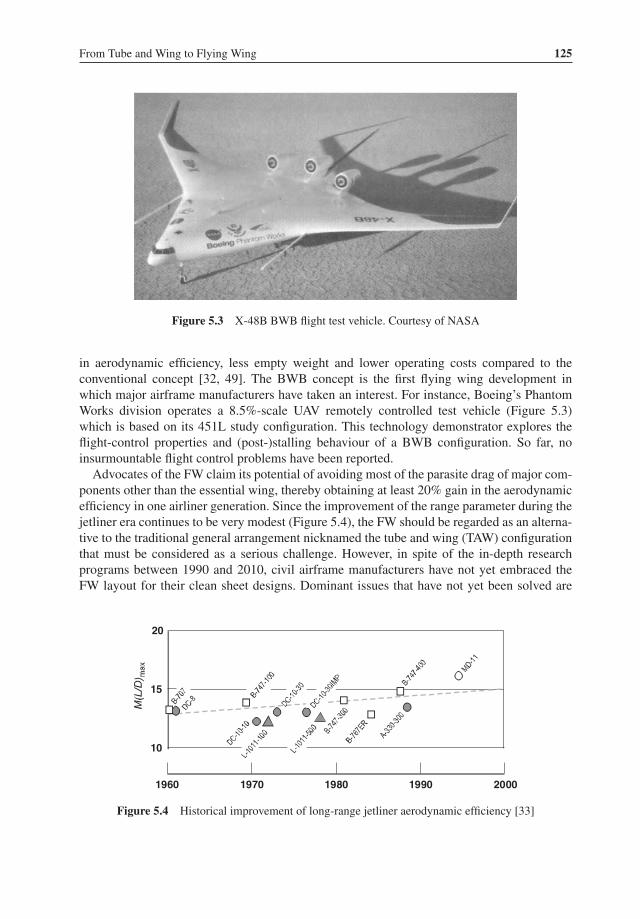
From Tube and Wing to Flying Wing 125
Figure 5.3 X-48B BWB flight test vehicle. Courtesy of NASA
in aerodynamic efficiency, less empty weight and lower operating costs compared to theconventional concept [32, 49]. The BWB concept is the first flying wing development inwhich major airframe manufacturers have taken an interest. For instance, Boeing’s PhantomWorks division operates a 8.5%-scale UAV remotely controlled test vehicle (Figure 5.3)which is based on its 451L study configuration. This technology demonstrator explores theflight-control properties and (post-)stalling behaviour of a BWB configuration. So far, noinsurmountable flight control problems have been reported.Advocates of the FW claim its potential of avoiding most of the parasite drag of major com-
ponents other than the essential wing, thereby obtaining at least 20% gain in the aerodynamicefficiency in one airliner generation. Since the improvement of the range parameter during thejetliner era continues to be very modest (Figure 5.4), the FW should be regarded as an alterna-tive to the traditional general arrangement nicknamed the tube and wing (TAW) configurationthat must be considered as a serious challenge. However, in spite of the in-depth researchprograms between 1990 and 2010, civil airframe manufacturers have not yet embraced theFW layout for their clean sheet designs. Dominant issues that have not yet been solved are
1960 1970 1980 1990 2000
20
15
10
Figure 5.4 Historical improvement of long-range jetliner aerodynamic efficiency [33]

126 Advanced Aircraft Design
(1) how to design a suitable structure for a highly non-cylindrical pressure cabin; (2) how tosettle the stability and controllability which have plagued the class of all-wing airplanes; and(3) how to prove that the radical FW concept can pass the certification process successfully.It cannot be excluded that arguments in favour of or against the FW are often based on
the superficial suspicion against the introduction of new technology. Instead, a satisfactorydecision must be based on a rational investigation of a class of vehicles with various degreesof integration of the payload inside the wing. The aim of this chapter is to embark on a genericapproach to the fundamental question of how the best distribution of the useful load can beestablished in the early conceptual design stage.
5.1.4 Fundamental Issues
The following issues have to be addressed during the early development stage of a new civilaircraft design concept:
• Allocation of useful load (UL) inside one or more fuselage bodies and/or lifting surfaces.• The arrangement and shape of lifting surfaces so that the total lift is generated efficientlyand the aircraft can be trimmed and stabilized in all anticipated operational conditions withlittle trim drag in normal flight.
• How to obtain a well-balanced design by suitably allocating the fuselage (if any), the wing,the power plant, the landing gears, and the horizontal tail or the foreplane (if any) relativeto each other.
Although these issues are far from trivial even for the conventional TAW layout, its designerscan rely on feasible solutions familiar from extensive research and satisfactory applicationsthat have emerged from many decennia of experience. It is therefore unlikely that variationson the traditional arrangement will bring about a step forward unless radically new conceptsand technologies are introduced. However, increasing the energy efficiency significantly byadapting the conventional layout may eventually become prohibitively expensive. The promiseof an unorthodox configuration is primarily associated with increased functionality of majoraircraft components. Anticipated gains can be substantial when this leads to reduced size oreven deletion of some of these components. The main driving force behind the developmentof flying wings has always been the aspiration of designers to conceive an ideal aeronauticalvehicle by removing all components not involved in the generation of lift. Since a wing isneeded for lift – the argument went – the ideal airplane would be that wing and nothing else.The FW is impressive as a simple and elegant concept which, in its most radical form, ischaracterized by the following characteristics:
• The voluminous and pressurized passenger cabin, cargo hold and flight deck, as well asthe power plant, fuel and on-board systems are all contained by the wing hull. Such aconfiguration lacks a fuselage, a horizontal tail and engine nacelles. In spite of the muchbigger wing compared to that of a conventional airplane, the plane’s total wetted area issignificantly smaller.
• It appears obvious that elimination of the horizontal tail results in a useful parasite drag andempty weight reduction. Moreover, the FW has its mass distributed along the wing span insuch a way that bending and shear loads on the structure due to lift are greatly reduced by the

From Tube and Wing to Flying Wing 127
opposing gravity and inertia loading. In spite of the increased wing size, this span loadingeffect yields a significant empty weight saving.
• The inherently lowwing loading obviates the need for complicated high-lift devices requiredfor aircraft of the traditional configuration having the same low-speed performances. Thiswill further reduce wing weight and acquisition cost.
The anticipated overall effect should be a reduced empty weight and up to 30% savings in fuelrequired to fly long distances and, for given design payload/range capability, the take-off grossweight (TOGW) is significantly reduced. Moreover, engines with less thrust or (perhaps) asmaller number of engines can be installed. It is likely that these characteristics will result insubstantially reduced operating costs.The logic behind the FW applies to a strategic bomber such as the B-2 with its compact
military load and equipment. However, a more detailed examination reveals that it may beflawed if applied to a jet airliner where other considerations are essential to achieve overalldesign superiority. In particular, the large cabin volume required and the low thickness ratioof a transonic wing may contribute to the adoption of a wing area that is too large to beaerodynamically efficient. In addition, the wing span of the FW is a design variable whichis subject to the same limitations as for a TAW aircraft and this results in a lower wingaspect ratio. Although the arguments in its favour are difficult to disprove by fundamentalconsiderations, many experienced designers are sceptical of the FW or even dislike it. It is alsofair to point out that the FW gives the deceptive impression of simplicity whereas in realitythe integration of all the major functionalities inside a single lifting hull has far-reachingconsequences. Consequently, the design process of the FW appears to be extremely complexand viable only after committing to a comprehensive R & D program and a highly integrateddesign process.If the strict definition of an FW is adhered to, the designer’s freedom to investigate alter-
natives which may be (more) attractive from the overall system point of view is undesirablynarrowed down. The primary objective of this chapter is therefore to compare the basic geomet-ric, aerodynamic and performance aspects of a conventional layout with those of a ‘pure’ FWand with hybrid configurations retaining some of the FW’s characteristics. The most promisingFW applications might be an airliner with a 500+ passenger capacity and a very large freighteraircraft – the concept is not feasible for airliners carrying less than 200 passengers. Maturetechnological advances in aerodynamic and flight control technology, advanced materials andstructures will be particularly beneficial in materializing this unorthodox concept.
5.2 Allocation of Useful Volume
The flying wing controversy has never been convincingly resolved. The parametric surveypresented in the following sections may serve to clarify the relevance of the FW debate byproviding quantitative guidelines useful in the early conceptual design stage.
The actual size of the required volume changes the answer. Sometimes it is better to put the volumein a distinct fuselage, sometimes not. Thus this has become an interesting configuration issue.As I see it none of the papers to date have provided the answer in a simple, easy to understandanalysis.
—W. H. Mason, www.dept.aoe.vt.edu/mason

128 Advanced Aircraft Design
5.2.1 Integration of the Useful Load
The standard jetliner configuration has the pressurized cabin with payload allocated inside thefuselage, fuel tanks are mostly inside the wing. We refer to this concept as the discrete wing-cum-body (DWB). Although the wetted areas of fuselage and wing are roughly equal, the wingvolume available for useful load is only a fraction of the fuselage volume. On the other hand,if the wing contains all the UL (and perhaps more) it will have a very large planform area andthe optimum flight conditions will be quite different from a conventional design. In particular,it can be expected that an all-wing airliner (AWA) will cruise at a higher altitude and/or lowerspeed than usual and will therefore need a different wing shape and installed thrust.It is anticipated that, for a large airliner and dependent on the design requirements, between
the DWB and the AWA an even better configuration may be conceivable with a sizablepart of the cabin and/or freight hold in the wing and the remaining part in a fuselage ofreduced size. The potential to optimally distribute the UL inside such an integrated wing body(IWB) configuration adds another dimension to the design space: the degree of integration,characterized by the fraction of the UL volume assigned to the wing. This idea will be revealedin the following parametric survey based on [13], followed by practical consequences of thedesign integration applied to some generic hypothetical integrated concepts.
5.2.2 Study Ground Rules
The UL is assumed to be allocated inside the combination of a wing and a streamlined bodyof revolution with an equality constraint on the total useful volume containing the UL. It isassumed that a free exchange is possible of pressure cabin and fuel tank volume between wingand body. A matrix of generic transonic airplane configurations complying with this conditionis depicted in Figure 5.5. The bodies are representative of a conventional airliner fuselage witha cylindrical passenger cabin, the straight-tapered wings are designed for the same cruiseMachnumber. The body and the wing are scaled up and down geometrically similar, although thewing aspect ratio is treated as a design variable. The present family of airplane configurationsdiffers markedly from the blended wing body concept where the fuselage is moulded into alifting body in the form of a very low-aspect ratio airfoil blended into the high aspect ratiooutboard wings. It is interesting for the following reasons:
• Only a (high-aspect ratio) wing generates lift for low induced drag.• A streamlined body of revolution has a better ratio of surface and frontal area to volumeand a lower friction drag coefficient than a wing. Hence, the body has less parasite dragcompared to a wing with the same volume.
• The internal useful volume of every configuration is utilized to the maximum extent – thereis no unused space left. This yields the smallest surface area and empty weight required tocontain the UL.
It may not seem appropriate to fill the available wing volume completely with UL since abigger wing than required for a given useful volume will arguably reduce the induced drag.However, any unused wing volume can be filled by transferring UL from the body to the wing,thereby reducing body size and its parasite drag. The assumption that all the available usefulvolume is filled with payload and fuel is therefore appropriate. Although complete freedom

From Tube and Wing to Flying Wing 129
0.15
0.25
0.50
0.75
0.85
wing volumetotal volume
Aw=8
Figure 5.5 Wing and body configurations with the same total useful volume
in load allocation might be a hypothetical situation, several IWB concepts have been reportedwith part of the cabin and freight hold inside the inboard wing and the remaining part inside abody of reduced size [36]. The present study ground rules are therefore realistic even thoughin the real world they may lead to an objective function response surface which is not perfectlysmooth.
5.2.3 Volume Ratio
The configurations in Figure 5.5 are characterized by their volume ratio, treated as theprimary variable,
X = Qw
Qtot= useful wing volume
total useful volume(5.1)
The useful wing (index w) and body (index b) volumes are
Qw = X Qtot and Qb = (1− X ) Qtot (5.2)
Figure 5.5 shows a progression between a conventional designwith X = 0.15 and an integratedlayout with X = 0.85. The discussion is simplified by relating the volume ratio to the followingclasses of flight vehicles:
• Discrete wing and body (DWB) – 0 < X ≤ 0.2.• Integrated wing body (IWB) – 0.2 < X ≤ 0.9.• All-wing aircraft (AWA) – 0.9 < X ≤ 1.0.

130 Advanced Aircraft Design
In view of the limitations for the aerodynamic loading, a DWB with volume ratio X < 0.1 isnot considered a practical vehicle. An AWAwith X = 1.0 is also known as a pure flying wing.
5.2.4 Zero-Lift Drag
The drag area of the wing and body combination (index bw) is composed of contributions ofexposed body and wing parasite drag,
(CD0 S)bw = (CDpS)b + (CDp S)w (5.3)
Since the allocation of useful volumes inside the airplane forms the subject of this study,parasite drag coefficients are referred to body and wing (volume)2/3 and denoted CDp . Rela-tionships between surface areas and volumes are found in Appendix A. In order to consideruseful volumes rather than gross volumes, a volumetric efficiency factor is introduced,
ηQ = useful volume
gross volume(5.4)
The zero-lift drag coefficient is referred to the gross wing area as follows:
(CD0 )bw = (CDp )w{kbw(X
−1 − 1)2/3 + 1} (5.5)
where the drag parameter1 is defined as
kbwdef=
{(ηQ)w(ηQ)b
}2/3 (CDp )b
(CDp )w(5.6)
The significance of this parameter is clarified by substitution of X= 0.5 into Equation (5.5).It then appears that kbw equals the ratio of body to wing parasite drag for equal volumes andvolumetric efficiencies. A typical value kbw = 0.30 indicates that the tube-like fuselage has aclear parasite drag advantage over the wing. The drag penalty needed to provide stability andcontrollability by means of the empennage is incorporated by factoring the body and wingparasite drag. The size of conventional airplane tail surfaces can be estimated using AppendixA which is based on statistics indicating that a DBW has horizontal and vertical tail areas oftypically 25% and respectively 15% of the wing area. An AWA has no horizontal tail; it mayhave a single vertical tail or winglets with a total area of approximately 10% of the wing area.Between those two configurations the empennage size is accounted for by increasing the bodyparasite drag by 30% and the wing profile drag by 10%. It goes without saying that thesenumbers may have to be adapted to a specific design case. The drag parameter is assumed tobe independent of the volume ratio X although the following reservations are made:
• Parasite drag coefficients are affected by Reynolds number variation. For a variation of Xbetween 0.15 and 1.0 the mean wing chord increases by at least 50% leading to more than7% reduction of its CDp . However, the body’s CDp increases by 12% when its length isreduced by 50%. The net result is slightly in favour of the conventional DWB.
1A similar parameter was introduced byAshkenas [6] who called it the geometric shape parameter kn/kw and proposednumerical values. Other authors [9, 10, 14] use similar parameters without information about numerical values.

From Tube and Wing to Flying Wing 131
• Merging body and wing reduces the net exposed and parasite drag areas. On the other hand,the merging causes unfavourable flow interferences which have to be suppressed by fairingsand local cross-section adaptations resulting in parasite and vortex drag penalties. Althoughanalysis of these drag components is complicated, it is likely that the net effect works out infavour of the AWA.
• It is not immediately obvious whether the volumetric efficiencies of the body and wing areindependent of the volume ratio. The wing of a conventional DWB has a lower volumetricefficiency than the fuselage due to the volume required to install complicated high-liftsystems and controls. However, since a flying wing needs less complicated trailing edgeflaps, it is likely that its volumetric efficiency is higher than that of a conventional wing.
Accounting for these effects leads to considerable analytical complications. Since severaltrends are contradictory, the conclusions from the present simplified analysis probably remainvalid.
5.2.5 Generalized Aerodynamic Efficiency
The power plant installation is not assumed to be integrated into the wing and body airframeand hence the total airplane drag can be decomposed into the airframe drag and engineinstallation drag. The nacelle parasite drag area is proportional (or nearly proportional) to theinstalled thrust. Hence, the nacelle drag has no effect on the optimization since it is equivalentto a percentage reduction of installed thrust and total drag. Consequently, the aerodynamicefficiency derived hereafter refers to the airframe excluding nacelles.The airframe drag coefficient is represented by a two-term parabolic polar,
CD = CD0 + CDL = CD0 + KLC2L (5.7)
The drag due to lift parameter KL is inversely proportional to the wing aspect ratio; seeEquation (4.20). A correction for compressibility is made by increasing the wing profile dragby a few drag counts and the induced drag factor KL by a small percentage. The airframeaerodynamic efficiency is obtained from Equations (5.5) and (5.7),
CL
CD=
(CD
CL
)−1=
[{1+ kbw
(X−1 − 1)2/3 (CDp )w
CL
}+ KLCL
]−1(5.8)
A special case is an AWA in straight and level flight with
CL X=1def= W
q Q2/3tot
Q2/3w
Sw= X2/3CL (5.9)
The termW/(q Q2/3tot ) is the lift coefficient based on the reference area Q2/3
tot and is treated as anindependent design variable representing the flight conditions as determined by the dynamicpressure q = 0.5 γ pM2. The term Q2/3
w /Sw depends on the wing taper, thickness and aspect

132 Advanced Aircraft Design
ratios and can be computed using Appendix A – a typical value for a high-speed wing isbetween 0.07 and 0.08. Equation (5.8) is rewritten after substitution of (5.9) as follows:
CL
CD=
[{X2/3 + kbw(1− X )2/3
} (CDp )wCL X=1
+ KLCL X=1
X2/3
]−1(5.10)
A reference value for L/D is the maximum aerodynamic efficiency achievable for an AWA,
(CL
CD
)ref
def={2√(CDp )wKL
}−1for CL ref =
√(CDp )w
KL(5.11)
This reference configuration is used to define the reduced lift coefficient
Ydef= CL X=1
CL ref
→ CL
CL ref
= X−2/3Y (5.12)
This parameter is substituted into Equation (5.10) to yield the aerodynamic efficiency of ageneral configuration with a given useful volume as a fraction of the maximum achievablevalue for an AWA configuration with the same volume,
CL/CD
(CL/CD)ref= 2
{X2/3 + kbw(1− X )2/3
Y+ Y
X2/3
}−1(5.13)
This expression is treated as a figure of merit of the wing and body configurations considered.Figure 5.6 depicts a contour plot of this FOM as a function of the volume ratio X and thereduced lift coefficient Y .
5.2.6 Partial Optima
The aerodynamic design efficiency as affected by the independent design variables X and Yhas the following partial optima depicted in Figure 5.6 as dotted curves:For given gross weight and flight conditions, the volume ratio resulting in a local optimizer
is obtained from
∂(CL/CD)
∂ X= 0 → Y = X2/3
{1− kbw
(X
1− X
)1/3}1/2(5.14)
For kbw = 0.3 and Y < 0.624, this condition yields two solutions for X . The lowest of thesedefines an IBW with the highest obtainable L/D for given gross weight and flight conditions,the highest defines a local minimum aerodynamic efficiency.2 For Y ≥ 0.624 there exists no
2This is probably the condition referred to by J.V. Foa as the worst possible selection of the volume ratio (Section 5.1).
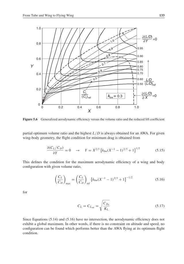
From Tube and Wing to Flying Wing 133
0.20 0.4 0.6 0.8 1.0
1.0
0.8
0.6
0.4
0.2
0
L/D(L/D)ref
Y
0.50
0.60
0.700.750.80
0.85
0.90
0.95
(L/D)Y =0
X
CL
(C )L ref
(L/D)X =0kbw = 0.3
∂∂
∂∂
0.5
0.6
0.7
0.8
0.9
1.0
Figure 5.6 Generalized aerodynamic efficiency versus the volume ratio and the reduced lift coefficient
partial optimum volume ratio and the highest L/D is always obtained for an AWA. For givenwing-body geometry, the flight condition for minimum drag is obtained from
∂(CL/CD)
∂Y= 0 → Y = X2/3
{kbw(X
−1 − 1) 2/3 + 1}1/2 (5.15)
This defines the condition for the maximum aerodynamic efficiency of a wing and bodyconfiguration with given volume ratio,
(CL
CD
)max
=(
CL
CD
)ref
{kbw(X
−1 − 1) 2/3 + 1}−1/2(5.16)
for
CL = CLmd =√
CD0
KL(5.17)
Since Equations (5.14) and (5.16) have no intersection, the aerodynamic efficiency does notexhibit a global maximum. In other words, if there is no constraint on altitude and speed, noconfiguration can be found which performs better than the AWA flying at its optimum flightcondition.

134 Advanced Aircraft Design
5.3 Survey of Aerodynamic Efficiency
The variation of CL/CD illustrated in Figure 5.6 shows that there exists no global optimumvolume ratio for maximum aerodynamic efficiency. The aim of this section is to investigate theeffects of primary design parameter variation on the best obtainable useful volume allocationfor configurations such as those depicted in Figure 5.5. This parametric survey is performed fora hypothetical airliner with 450 metric tons gross weight cruising at Mach 0.85 and altitudesbetween 30 000 and 50 000 ft. It is assumed that the volume ratio can be varied continuouslywith an equality constraint on the total useful volume of 2 000 m3.
5.3.1 Altitude Variation
Equation (5.13) is used to compute the effect of varying the flight altitude for the constantMachnumber on L/D. The lift coefficient for each volume ratio is obtained from the combination ofEquations (5.9), (5.12) and (5.10) which yields the result depicted in Figure 5.7. The followingobservations are made:
• A baseline DWB model with X = 0.18 flying at 35 000 ft altitude attains L/D = 20.5.This performance is close to (L/D)max and is representative of the year 2000 performancepotential of the largest airliner airframes. The highest aerodynamic efficiency at 35 000 ftaltitude is achieved by an IWB with X = 0.35. Its performance (L/D = 22) is not animpressive improvement over the DWB. Due to its low lift coefficient, the AWA does notperform any better than the DWB.
• Significantly higher aerodynamic efficiencies are obtainable at higher altitudes than today’sairliner practice. At 40 000 ft the aerodynamic efficiency is almost constant for X > 0.4. Inother words: any IWB flying at this altitude will be as good as the AWA and significantly
X
L/D
30,000
35,000
40,000
45,000
50,000
AWAIWBDWB
(L/D)max
baseline
kbw= 0.30
Aw = 8
28
26
24
22
20
18
16
altitude ft
0 0.2 0.4
0.40
0.35 0.30
0.25
0.20
0.15
0.6 0.8 1.0
Figure 5.7 Aerodynamic efficiency versus volume ratio and cruise altitude for a large airliner.Data: Q = 2 000 m3; W = 4 500 kN; M = 0.85

From Tube and Wing to Flying Wing 135
better than the DWB baseline flying at 35 000 ft. For instance, a design with X = 0.5 flyingat a modest CL = 0.35 will improve L/D by 12.5% relative to the baseline DWB.
• The AWA’s performance is not impressive at the usual cruise altitudes and achieves its bestperformance at unusually high altitudes. A pure flying wing reaches its full potential inexcess of 50 000 ft.3 The maximum aerodynamic efficiency L/D = 27.5, an improvementof 34% over the baseline DWB, is achieved for CL = 0.39.
Integrated configurations with a substantial fraction of the useful volume in the wing achievesignificantly better aerodynamic performance than the conventional wing body configurationprovided they are designed to fly at a (much) higher altitude than usual.
5.3.2 Aspect Ratio and Span
Variation of the wing aspect ratio is very influential with the primary effect felt in the dragdue to lift parameter KL = (π Awe)−1. Another effect is manifest in Equation (A.2) on p. 437indicating that the wing area required to obtain a specified wing volume is proportional toA1/3w . The following relationships apply if the wing profile drag coefficient is assumed to beindependent of the aspect ratio:4 KL ∝ A−1
w , CL X=1 ∝ A−1/3w and kbw ∝ A−1/3
w . This leads tothe observation that the aerodynamic efficiency of a wing with volume Q carrying a grossweight W at dynamic pressure q has a maximum value for
Aw = (2W/q)6/5{(t/c)/Q}4/5(CDpπe)−3/5(1+ λ)−2/5 (5.18)
This is perhaps an unexpected result since the usual observation is that induced drag continuesto decrease with increasing aspect ratio. The explanation is that increasing the aspect ratioreduces the wing volume unless the wing gets a larger planform area, leading to more wettedarea and higher profile drag. Application of Equation (5.18) to the example wing results in atypical optimum Aw = 8 with the implication that an aerodynamically efficient AWA with aspecified volume does not necessarily have a very high aspect ratio.The parametric survey is now extended with a variation of aspect ratio and wing span for
a constant cruise altitude of 35 000 ft. Equation (5.10) is used to derive the results shown inFigure 5.8 leading to the following observations:
• In spite of its potentially high performance, an AWA offers a disappointingly low L/D withlittle variation for aspect ratios between five and ten.
• Very high L/D values are obtainable for a DWB configuration if there is no constraint onthe wing span. Increasing the baseline aspect ratio from eight to ten requires a fairly modestspan increment and increases L/D by 12.5%, whereas an IWB needs a considerably largerspan for the same improvement.
3Notably, this altitude has been quoted as the best cruising altitude of the Northrop B-49 flying wing bomber.4Aspect ratio variation affects the chord Reynolds number and, hence, the skin friction and profile drag coefficients.This effect is not taken into account in the present analytical approach.

136 Advanced Aircraft Design
span m
L/D
X
110
100
90
80
70
20212223242526
L/DAw
= 0
L/DX
= 0
Aw
0.2 0.4 0.6 0.8 1.00
16
14
12
10
8
6
4
kbw= 0.30
alt. 35,000 ft
baseline
∂∂
∂∂
Figure 5.8 Aerodynamic efficiency versus volume ratio, aspect ratio and span. Data as in Figure 5.7
• For each volume ratio there exists an aspect ratio which maximizes L/D. It is possible toderive this partial optimum analytically but the result is unrealistic and for a span in excessof 110 m there is practically no gain in L/D. Irrespective of the aspect ratio, the optimumvolume ratio occurs at approximately 95 m wing span.
• The partial optima with respect to volume ratio and span are incompatible; hence, thereexists no unconstrained optimum combination.
The present result points to a DWBwith the highest practical wing span to be the configurationyielding the best aerodynamic efficiency at 35 000 ft altitude. Due to the large effect of spanon wing weight, the aspect ratio complying with an overall optimum system is significantlylower than the value for the maximum L/D (Chapter 10).
5.3.3 Engine-Airframe Matching
It has been observed that an airplane with a highly integrated wing body combination has a lowwing loading and, for 35 000 ft flight altitude, its CL is far below the value for maximum L/D.To improve the situation, the altitude of an IWB design should be higher than usual. However,selection of the altitude is closely associated with engine sizing and should not be based onlyon the aim of achieving the highest possible aerodynamic efficiency. The survey will thereforebe augmented with a computation of the required engine size to match the airframe drag inlevel flight.According to Equation (3.17) the corrected thrust T/p of a turbofan operating in the
stratosphere at a fixed rating and Mach number is constant – for instance, equal to the value atthe tropopause. The available thrust is therefore proportional to the ambient pressure and the

From Tube and Wing to Flying Wing 137
28
26
24
22
20
18
16 1312
1110
9
0.1
0.2
0.3
0.4
0.5
0.60.7
0.80.9
1.0(L/D)ref
T/p m2
X
L /D
Aw=8kbw=0.30
baseline
Figure 5.9 Aerodynamic efficiency versus volume ratio and corrected thrust. Data as in Figure 5.7
drag that can be balanced by a given engine thrust in straight and level flight is determined byCD = T/(q Sw). Accordingly, Equation (5.7) defines the achievable altitude andMach numbervia a constraint on the lift coefficient,
CL =(
CD − CD0
KL
)1/2=
{K −1L
(T/p
12γ M2Sw
− CD0
)}1/2(5.19)
Substitution of CD0 according to Equation (5.5) and Sw from Equation (5.9) yields the rela-tionship between CL/CD , T/q and X satisfying the condition T = D. The result is depictedfor the example airplane with Aw = 8 in Figure 5.9 and the following observations are madefrom this carpet plot:
• The obtainable L/D for a DWB with volume ratio between 0.15 and 0.20 is insensitive toengine size for corrected thrust values between 8.0 and 9.5 m2. The highest aerodynamicefficiency for the DWB baseline flying at 35 000 ft is obtained for T/p = 9 m2.
• If engines are installed with T/p = 9 m2, the AWA does not perform any better thanthe baseline design, whereas L/D deteriorates rapidly for lower thrust. Compared withthe baseline, the AWA needs engines with 45% more thrust to reach its full potential ofL/D = 27.5.
• Configurations with X > 0.30 are sensitive to the installed thrust. An IWB with 50% of theuseful volume in the wing achieves a respectable L/D = 24.2 but requires engines with22% more thrust than the baseline DWB.

138 Advanced Aircraft Design
In conclusion, it is essential that the engine-airframe matching condition is included in anyoptimization of IWB configurations. This applies in particular to the pure flying wing.
5.4 Survey of the Parameter ML/D
The previous section has shown that different cruise altitudes can lead to significantly differentappreciations of flying wing compared to conventional configurations if the Mach number isspecified. Arguably, a constraint on the cruiseMach number, although practical for a particulardesign study, might be too restrictive when investigating a radically new concept. This sectiondeals with a simplified analysis of the Mach number variation on the specific range and howit is affected by the volume fraction and the drag parameter.
5.4.1 Optimum Flight Conditions
Chapter 12 shows that, for constant engine TSFC, the specific range of a jet aircraft isproportional to the parameter M L/D. Although in real life this leads to an optimum cruisecondition in the drag!rise, this complication is avoided when the following simplifications areaccepted:
1. For each altitude the achievable Mach number in straight and level flight is determined bya constraint on the available thrust.
2. Engines are scaled up and down for constant cruise rating and the corrected thrust isassumed independent of the Mach number and ambient conditions.
3. The Mach number is below the drag rise so that a single parabolic drag polar can be used.5
Due to these assumptions the accuracy of the analysis is not very high, but the trends arethought to be correct. For a specified T/p the achievable flight Mach number is determinedby the horizontal equilibrium,
M =√
T/p12γ CD S
(5.20)
Hence, the parameter M L/D is proportional to CLC−3/2D S−1/2, whereas the combination of
CL and S determines altitude and speed. The classical partial optimum condition for maximumM L/D is
CL =√
CD0
2KL= CLmd√
2→ M = 21/4Mmd (5.21)
5It is worth noting that all publications in the bibliography on the present subject take the absence of compressibilitydrag for granted.

From Tube and Wing to Flying Wing 139
X0.2 0.4 0.6 0.8 1.00
1.4
1.2
1.0
0.8
0.6
relativevalue
M
T & p
ML/D
L/D k bw =0.3
Figure 5.10 Flight conditions for maximum M L/D
Substitution into Equation (5.20) yields the flight condition
M =√4 T/p
3γ CD0 Sand
CL
CD= 1
3
√2
CD0 KL= 0.9428
(CL
CD
)max
(5.22)
The highest value of M L/D appears to be proportional to (CD0
√S)−1 and substitution of CD0
according to Equation (5.5) yields
M L/D ∝ [X1/3
{1+ kbw(X
−1 − 1)2/3}]−1(5.23)
The example in Figure 5.10 shows that, when more useful volume is allotted to the wing, theoptimum Mach number decreases whereas the altitude and L/D increase. The AWA achievesthe highest aerodynamic efficiency for all values of the volume ratio. However, the parameterM L/D is practically invariable at a level of a few percentage below the AWA for all IWBconfigurations and DWB airplanes with X > 0.15.
5.4.2 The Drag Parameter
The drag parameter kbw is a crucial factor when an FW is compared with the traditional TAWconfiguration. Its value depends on geometrical data such as fuselage fineness ratio, wingtaper, thickness and aspect ratios, and volumetric efficiencies. The following approximationis based on Appendix A and on the assumption of equal volumetric efficiencies for wing andbody:
kbw = 1.20
{t/c
A(1+ λ)
}1/3(5.24)

140 Advanced Aircraft Design
X
ML/D(ML/D)X=1
1.2
1.1
1.0
0.9
0.8
0.70.2 0.4 0.6 0.8 1.00
0.20
0.25
0.30
0.35
0.40
kbw
0.275
Figure 5.11 MaximumML/D affected by the drag parameter
where A, λ and t/c denote the wing’s aspect ratio, taper ratio and thickness ratio, respectively.Equation (5.24) also takes into account that body parasite drag depends on its fineness ratio.Typical values of kbw are between 0.25 and 0.35 leading to the observation that the parasitedrag of a fuselage is between 25 and 35% of the parasite drag of a wing with the same volume.The following conclusions are drawn from Figures 5.10 and 5.11.
• In accordance with [6], a pure flying wing has better specific range than a wing and bodycombination for kbw ≥ 0.275, a wing and body configuration is better for kbw < 0.275.
• Since the best flight Mach number of a pure flying wing is lower than for a wing and bodyconfiguration, a wing section with higher thickness ratio can be selected in the interest of amore efficient passenger accommodation and lower structure weight.
The case for integrated configurations becomes stronger with the (future) introduction of openrotor engines which have their maximum efficiency at Mach numbers between 0.70 and 0.80(Section 3.4). The aerodynamic efficiency increases considerably compared to the traditionalTAW configuration if this speed range were selected as the design condition. It is obviousthat such a radical deviation from the present cruise condition would require a far morecomprehensive investigation than the present analysis.
5.5 Integrated Configurations Compared
The elementary derivation of the achievable aerodynamic efficiency has indicated that twomain roads can be followed to improve the performance of large transport aircraft by meansof a radical mutation.
1. Increasing the wing span is very effective from the aerodynamic point of view but consider-ations such as keeping structural weight within limits tend to dominate. For small tomedium

From Tube and Wing to Flying Wing 141
size airplanes, aspect ratios up to 15 may become an option which requires an increasedthickness ratio, advanced (composite) materials and/or selection of a general arrangementleading to a considerably reduced wing bending load. Examples are strut-braced wings andmulti-body configurations (Chapter 6).
2. Compared to the traditional TAW layout – with constraints on cabin, cargo hold and fueltank volumes and a large empennage – a substantial reduction of wetted area is only feasiblefor a tailless, highly integrated wing body aircraft configuration.
The previous analysis has indicated that it is not necessarily an advantage to adopt an AWAconfiguration for a transonic airliner because its wing area tends to be large, leading to a liftcoefficient (far) below the flight condition for minimum drag. A possible answer is to decreasethe dynamic pressure by increasing the altitude and/or reducing the flight speed. The first optionleads to higher installed engine thrust, the second increases block time. Both options are notin the interest of good economics and in particular the second is likely to be objectionable tothe airlines. This consideration does not necessarily apply to a large (dedicated) freighter forwhich the allocation of cargo in the wing reduces its en route bending moment considerably,allowing a span increase with less wing structure weight penalty than for a conventional design.The integrated configuration may form a viable candidate for this application.The parametric survey in the previous sections is based on combinations of bodies and
straight tapered wings as depicted in Figure 5.5. Although this simplification allows a general-ized analytical approach, a practical integrated design may have a non-cylindrical body and/oran unorthodox wing planform. The survey is therefore not sufficiently flexible to concludewhether an integrated wing body can offer acceptable payload accommodation, operationaland flight characteristics. In this section we compare a large long-range airplane of conven-tional layout with several concepts which have an integrated layout. The airliner designs havethe same cruise speed and total useful volume, the freighter flies at a lower Mach numberand has a larger cargo hold volume. Different from the parametric survey, the engine nacellesare counted as airframe components. Wetted area and drag predictions are based on simplemethods such as those presented in Chapter 4 and Appendix A. Compressibility drag has notbeen taken into account.
5.5.1 Conventional Baseline
The conventional design is a long-range twin-deckMach 0.80 airliner in the category Airbus A380 andBoeing 747. Figure 5.12 (a) andTable 5.1 define its geometry and general arrangement.The wing span is limited to 80 m – the maximum value for ICAO field classification F.Application of Equations (A.5) and (A.2) shows that the fuselage contains 430% of the wingvolume with 12% more wetted area. Empennage area is 35% of the wing area and enginenacelles and pylons surface areas are 10% of the airframe wetted area. Maximum subsonicL/D amounts to 20.6 which is at the upper limit of what is achievable for the largest of theyear 2000 long-range airliners, although a wing span increase to 90 m would increase L/Dby about 9%. Alternatively, a wing area reduction for the same span might be possible if thearea is not constrained by the fuel tank volume required, resulting in reduced wetted areaand parasite drag. However, wing area reduction for the same span entails more complicatedhigh-lift devices and a higher structural aspect ratio, both leading to a higher empty weight. It

142 Advanced Aircraft Design
(a) conventional configuration (b) all-wing airplane
Figure 5.12 Geometries of a large Mach 0.85 airliner of conventional layout and an all-wing aircraft,both accommodating a useful load volume of 2 000 m3
Table 5.1 Design data for a twin-deck airliner with conventional layout
fuselage equivalent diameter 7.5 mlength 75 mgross volume 2 651 m3
gross wetted area 1 570 m2
cabin plus cargo hold volume 1 590 m3
cabin floor area 625 m2
wing span 80 mgross planform area 800 m2
exposed planform area 686 m2
thickness/chord ratios 0.14/0.10exposed gross volume 611 m3
wetted area 1 400 m2
horizontal tail exposed planform area 180 m2
vertical tail exposed planform area 100 m2
engine nacelles wetted area 350 m2
airframe gross volume 3 262 m3
total wetted area 3 852 m2

From Tube and Wing to Flying Wing 143
turns out that there exists an optimum wing size resulting in a practical span and aerodynamicefficiency.
5.5.2 Is a Wing Alone Sufficient?
The AWA is a radical integrated concept which is not simply obtained from a conventionaldesign by removing the empennage. A useful comparison can only be made when both designscarry the same useful load at the same cruising speed with acceptable stability and controlproperties. The AWA depicted in Figure 5.12 (b) has the following characteristics.
• The passengers are accommodated in the central section on a single deck with underfloorbaggage. This section has the same gross volume as the conventional fuselage whereas theoutboard wings together have the same volume as the conventional (exposed) wing.
• The gross planform area of 1 582 m2 is almost twice the conventional wing area. For thesame gross weight and flight conditions, the lift coefficient is reduced by 50% which allowsthe wing to be a few percentage chord thicker than the conventional wing.
• The AWA enables the designer to spread the UL laterally along the wing span ratherthan longitudinally along the fuselage. This reduces the inboard bending and increases thestructural height, allowing a span increase for the same structure weight. In spite of the largespan, the AWA aspect ratio of slightly less than six is unusually low for an airliner.6
• An inherent problem of tailless airplanes is how to achieve high lift and moment equilibriumsimultaneously during take-off and landing. The lowwing loading obviates the need for veryefficient trailing edge flaps. Consequently, the AWA flies at a high angle of attack in lowspeed flight. Slats are applied to the outboard wing to increase the stalling angle of attackand to avoid uncontrollable pitch up during gusts or manoeuvres.
• Several tailless (military) airplanes developed in the past had formidable stability and controlproblems. The principles applied to the present AWA basically comply with the approachused on Northrop’s B-49. Sweepback helps to place outboard control surfaces behind thecentre of gravity (CG) but their lever arm is shorter than that of the conventional tail; hence,more effective controls are required. Pitch and roll control are provided by four elevators atthe centre wing trailing edge and four elevons on each outboard wing. Vertical winglets withdouble-hinged rudders and drag producing split outboard elevons, known as drag ruddervons,provide directional stability and control.
• The allocation of engines close together above the centre wing trailing edge is an attractivefeature of the AWA. This arrangement enhances take-off noise shielding, reduces noisein the cabin, increases passenger safety, and simplifies directional control after enginefailure. However, the arrangement is vulnerable to non-contained engine failure since dis-integration may damage other engines as well. This can make airworthiness certification ashowstopper.
The present layout causes the empty CG and the useful load to be approximately midway inthe primary structure whereas the power plant installation shifts it backward by at least 5% to
6Arguably, a flying wing with 96 m span can be parked inside an 80× 80 m2 box, although this argument may notconvince airlines and airfield operators.
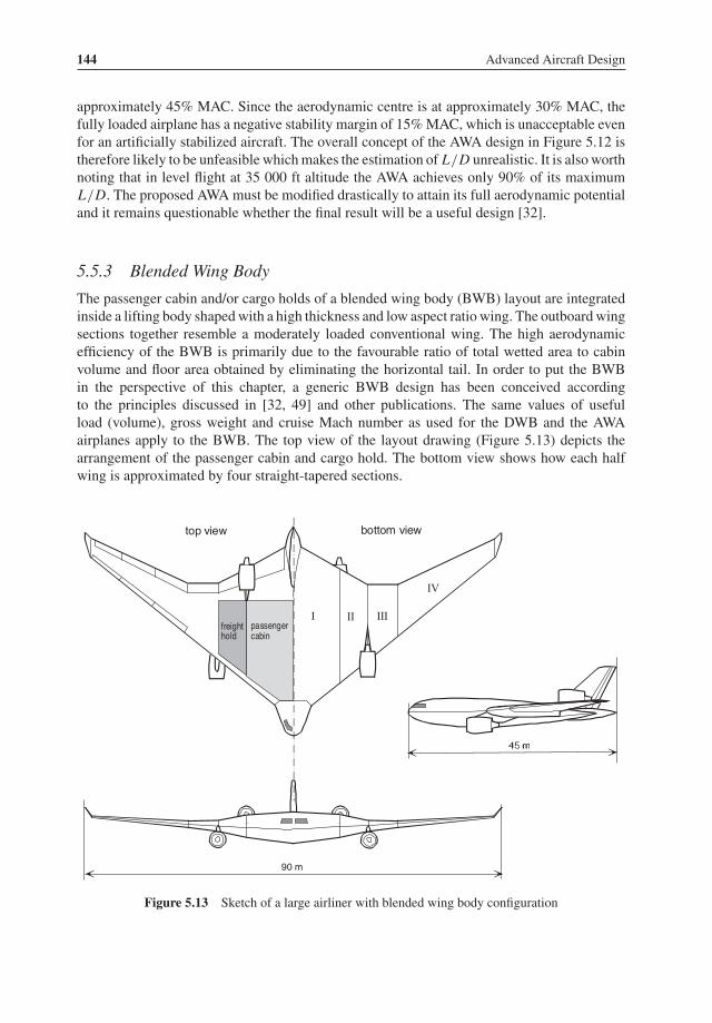
144 Advanced Aircraft Design
approximately 45% MAC. Since the aerodynamic centre is at approximately 30% MAC, thefully loaded airplane has a negative stability margin of 15%MAC, which is unacceptable evenfor an artificially stabilized aircraft. The overall concept of the AWA design in Figure 5.12 istherefore likely to be unfeasible whichmakes the estimation of L/D unrealistic. It is also worthnoting that in level flight at 35 000 ft altitude the AWA achieves only 90% of its maximumL/D. The proposed AWAmust be modified drastically to attain its full aerodynamic potentialand it remains questionable whether the final result will be a useful design [32].
5.5.3 Blended Wing Body
The passenger cabin and/or cargo holds of a blended wing body (BWB) layout are integratedinside a lifting body shapedwith a high thickness and low aspect ratio wing. The outboard wingsections together resemble a moderately loaded conventional wing. The high aerodynamicefficiency of the BWB is primarily due to the favourable ratio of total wetted area to cabinvolume and floor area obtained by eliminating the horizontal tail. In order to put the BWBin the perspective of this chapter, a generic BWB design has been conceived accordingto the principles discussed in [32, 49] and other publications. The same values of usefulload (volume), gross weight and cruise Mach number as used for the DWB and the AWAairplanes apply to the BWB. The top view of the layout drawing (Figure 5.13) depicts thearrangement of the passenger cabin and cargo hold. The bottom view shows how each halfwing is approximated by four straight-tapered sections.
freighthold
passengercabin
90 m
II IIII
IV
top view bottom view
Figure 5.13 Sketch of a large airliner with blended wing body configuration

From Tube and Wing to Flying Wing 145
• The sections I together form the highly tapered central body containing the pressurizedcompartment, the landing gear and an optional underfloor fuel tank between the main gearbays. The aft spar constitutes the rear pressure bulkhead which is available for locatingcabin evacuation doors. For a near-elliptical lift distribution along the span, the large centralwing chord results in a low aerodynamic loading and the three-dimensional character of theflow helps to reduce the supervelocities on top of the body. This allows a thickness ratio toexceed that of a conventional wing by at least 2%. The available internal height allows theaccommodation of a (partly) twin-deck cabin, leading to a favourable ratio of wetted to totalcabin floor area. The inversely cambered central wing section is front loaded in high speedflight and has 17% thickness ratio.7
• Each section II contains a cargo hold and a main landing gear bay. The airfoil sectionsare basically symmetrical, tapering in thickness from 17% inboard to 15% outboard. Thecombined sections I and II of both sides have practically the same gross volume and planformarea as the conventional baseline fuselage.
• The combination of both outboard sections III and IV forms an aspect ratio 6.70 wingcontaining 70% of the conventional baseline’s tank volume. Thickness ratios are 15% at theroot, 13% at the kink, and 11% at the tip. Rear-loaded supercritical sections are used forsection IV.
The situation that the aircraft cannot be certificated in view of the risk that disintegrationof one engine might damage other engines is avoided by using an unorthodox power plantarrangement which also leads to very small effects of thrust variation on longitudinal control.In the interest of avoiding significant trim drag, the plane is inherently unstable in pitch. Twistand camber distribution along the span aims at obtaining a near-elliptic lift distribution in highspeed flight and simultaneously satisfies the condition of self-balancing – that is, trailing-edgecontrols are not deflected in the trimmed condition. The aim is to make trim drag in the cruisecondition negligible which requires the balancing process to have meticulous control over thewing planform geometry and the allocation of systems and equipment. Variations in stabilityat high angles of attack must be carefully assessed to ensure that phenomena such as pitch upor tumbling will not occur [60]. In order to ensure recovery from high angle of attack regimes,the leading edge has a constant sweep angle and features outboard slats [36]. Moreover, a fueltank in the nose for CG control in combination with artificial stabilization and flight envelopeprotection is provided to ensure safe low-speed flight.Table 5.2 compares geometric data and aerodynamic performance of the BWB8 with the
DWB and AWA designs. Compared to the AWA, the span has been reduced from 96 m to amore realistic 90 m, the wing area is 16% smaller. The body-mounted vertical tail with 100 m2
area features a double-hinged rudder to compensate for the small tail arm. Total wetted area is21% less than for the conventional design. In spite of its modest span, the BWB has the highestmaximum aerodynamic efficiency and it achieves 93.5% of this value cruising at the samealtitude and speed as the conventional design. When cruising at a higher altitude, theBWB has the potential to achieve 24% gain in L/D relative to the conventional DWB.
7These characteristics were derived from published design projects. Since they are critical to the feasibility of atwin-deck BWB they must be verified by a CFD method in the conceptual design stage.8Since the BWB differs considerably from the family of wing and body combinations in Figure 5.5, the parametricsurvey in Section 5.3 is not applicable to this configuration without essential modifications.

146 Advanced Aircraft Design
Table 5.2 Geometry and aerodynamic performance for five design concepts. Conditions: Mach 0.85@ 35 000 ft except span loader: Mach 0.80 @ 40 000 ft
Design Qtot m3 S m2 Swet m2 Q2/3tot /Swet maximum L/D CL L/D
Discrete wing & body 3 262 800 3 852 0.0571 20.6 0.47 19.7All-wing aircraft 3 319 1 580 3 562 0.0625 25.7 0.24 23.2Blended wing body 3 025 1 320 3 040 0.0688 26.1 0.28 24.4Hybrid flying wing 3 230 1 050 3 445 0.0634 24.5 0.36 22.7Span loader 6 700 1 995 4 800 0.0740 24.0 0.26 22.1
Its low wing loading makes the BWB more sensitive to gusts but gives it a better high-altitudebuffet margin. Manoeuvre and gust load control are therefore desirable features of a BWB.From the aerodynamic performance point of view the BWB forms a promising alternative forthe presently dominating general arrangement. However, due to its integrated character, thedesign process of a BWB is considerably more complex than usual.
5.5.4 Hybrid Flying Wing
The parametric survey in Section 5.3 shows that allocating more than 30% of the useful loadvolume in the wing can lead to significantly improved aerodynamic performance comparedto both the conventional TAW and the AWA. An integrated wing body (IWB), named byTsAGI a hybrid flying wing (HFW), has a non-lifting body of reduced size (Figure 5.14).Inspired by this design, a generic HFW was conceived based on the same useful load volume,gross weight and cruise Mach number as used for the conventional DWB. The top view inFigure 5.15 depicts the general arrangement of the single deck passenger cabin. The bottomview shows that the wing geometry can be approximated by three straight tapered sections,giving the HFW the following characteristics.
• Sections I are both 20 m wide and 15% thick and form the inhabited parts of the wing.Compared with the BWB, section I has a smaller mean chord and its limited thickness doesnot allow a twin deck configuration.
• Baggage is carried in the belly under the fuselage cabin, main landing gear bays are in thefuselage as well as in wing section I. The same engine installation layout has been adoptedas for the BWB.
Figure 5.14 TsAGI HFW airliner for 750 passengers with twin-deck fuselage. Reproduced from [32].Copyright Elsevier 2001

From Tube and Wing to Flying Wing 147
III
III
90 m
bottom view top view
pass
enge
rca
bin
slats
flaps
drag ruddervonselevator
59 m
Figure 5.15 HFW airliner concept
• The combination of sections II and III is similar to an aspect ratio 7.20 conventional wing.It has thickness ratios 15% at the root, 12% at the kink and 10% at the tip.
• Since its wing loading is halfway between the DWB and AWA designs it is likely that theHFW needs trailing edge flaps for high lift and means to balance the pitching moment dueto their deflection. Elevators at the trailing edge of section I and outboard elevons serve thispurpose. An 80 m2 vertical tail with a double-hinged rudder is mounted to the rear fuselage;directional control is augmented by ruddervons.
Compared to the BWB, the HFW has the same gross volume and wing span. Its gross wingarea is 20% smaller, wetted area is 13% larger and maximum L/D is 6% lower. The HFW hasa 19% higher maximum L/D than the DWB baseline but this gain would largely disappearif the DWB were given the same 90 m wing span. The HFW does not offer a higher L/Dthan the BWB, but the accuracy of the present estimation is too low for a firm conclusion.Moreover, the HFW has the following attractive properties:
• Payload capacity growth can be provided by the traditional expedient of lengthening thefuselage with cylindrical body plugs without the necessity of major wing redesign.
• The emergency evacuation problem is more easily solved, especially in the case of a single-deck configuration. In this respect, the evacuation of the twin-deck cabin is easier than forthe much larger fuselage of a conventional aircraft.
• The cabin floor has no inclination in level flight.
5.5.5 Span Loader
Radical flying wing designs known as span loaders were advocated by NASA [65] andinvestigated by Boeing and Lockheed during the period 1975–1985. By distributing cargoinside the primary structure of a huge prismatic wing along its full span, the concept aimed

148 Advanced Aircraft Design
95 m
bottom view top view
55 m
Figure 5.16 Sketch of a large cargo aircraft with span loader configuration
at the development of very large dedicated freighters for civil and military applications. Allthe cargo of a span loaded freighter can be distributed inside the wing so that a close match isobtained between the aerodynamic and the mass loadings. In such a non-tapered structure, thefront and rear spars run parallel and the cargo hold can be loaded and unloaded through doorsin the wing tips. The span loading concept is primarily aimed at counteracting the negativeeffects of the square cube law [62] by taking advantage of its positive effects. The net bendingmoments and shear forces on the wing structure due to manoeuvre and gust loads are therebysignificantly reduced.In spite of its modest Mach number, a span loader has a swept wing with about half the
aerodynamic loading of a conventional freighter. Since it operates at low lift coefficients inall flight regimes, the span loader can take off with a relatively simple flap system – thiscircumvents the typical problem of trimming a flying wing.9 Moreover, a span loader hasa low geometric aspect ratio and the low aerodynamic loading and Mach number allow ahigh thickness ratio. Thickness ratios between 18 and 20% for transonic application based onGriffith and Goldschmied sections are proposed in [69, 70]. This unorthodox shape allowsa large useful volume in the wing for a given planform area. The lift is concentrated moreoutboard than usual and the circulation distribution along the span is far from elliptical andinduced drag is not ideal. However, due to its large tip chord, a span loader profits fromwingletsmore than a tapered wing. Large winglets increase the aerodynamic aspect ratio considerablyand provide directional stability and control.Dedicated civil freighters will probably be sized to carry 8× 8× 20 ft containers. This
implies that a transonic span loader will have some 3.50 m thickness which requires a chordlength of at least 20 m. The available internal volume is used efficiently with three or four rowsof containers between the main spars. Figure 5.16 depicts a span loaded flying wing designfeaturing a capacity for 48 containers corresponding to a maximum payload of 250metric tons.
9Hybrid span loaders have been proposed with a wing as well as a fuselage containing cargo using a foreplane forlongitudinal control.

From Tube and Wing to Flying Wing 149
For a typical TOGW of 550 metric tons, the plane requires four engines with 350 kN take-offthrust each. It has a favourable ratio of wetted area to volume, whereas the geometric aspectratio amounts to just 4.5 (Table 5.2). The aerodynamic efficiency is estimated by assumingconservatively that two 80 m2 near-vertical winglets increase the aerodynamic aspect ratio by20% to A = 5.4. The estimated maximum aerodynamic efficiency of 24.0 is similar to thevalues for the FW wing airliners described previously. At 40 000 ft altitude the lift coefficientis 0.26 and the actual L/D is less than those of the other FW designs. For a thickness ratioof 0.16 the maximum speed is limited to Mach 0.75. The favourable effect of span loadingon empty weight is the dominant feature of this configuration and it is anticipated that theprismatic structure will be relatively easy to design and manufacture. A major challenge fordesigners of the span loader is to develop a satisfactory landing gear configuration.
5.6 Flying Wing Design
5.6.1 Hang-Ups or Showstopper?
This chapter has demonstrated that a jetliner with the cabin (partly) integrated in the wingleads to a significant increase of the maximum aerodynamic efficiency. However, the analysishas low fidelity and many other aspects have to be considered as well. For example, comparedto the conventional TAW layout, an FW has more surface area that can be treated to obtain alaminar boundary layer. Flying wings therefore have the potential of achieving large surfaceswith a laminar flow, leading to an even greater gain in aerodynamic efficiency compared toan all-turbulent TAW plane. Moreover, a wing with considerably more volume than usualhas more structural stiffness which reduces the effects of aero-elasticity. On the other hand,formidable hurdles have to be fixed before an integrated wing body vehicle can be certifiedand offered to the airlines – some critical aspects are mentioned in Figure 5.17. The increasingsize of airliners leads to major concerns such as taxiway and runway width limits, gate limits,passenger handling, community noise and aircraft separation to avoid wake vortices. Most ofthe operational problems aremagnified for airliners with an integrated configuration since theiraccessibility for loading and unloading will be quite different from conventional airplanes.Provisions for a safe evacuation of 500 up to 1 000 passenger in less than 90 seconds in case
Figure 5.17 Critical development aspects of a flying wing design

150 Advanced Aircraft Design
winglet rudder
drag ruddervons
simple-hingedelevons
centerbody interior cross-sections
three-position slats
Figure 5.18 Structural concept and flight controls of the Boeing BWB-450 baseline. Adapted from [49]
of evacuation from a cabin with many aisles in crosswise arrangement and unusually longdistances to exits may even appear to be an insurmountable problem. Stability and controlproblems inherent to flying wings have to be suppressed by advanced and complex electronictechnologies. Application of the unorthodox flying wing concept can be effective only for thelargest category of airliners, for which the design process is anyhow very complex.
5.6.2 Structural Design and Weight
A major challenge for designers of a FW structure is the integration of the pressure cabin.Boeing’s BWB-450 project (Figure 5.18) features two main structural components: a centrallifting body and two outboard wings. The forward part of the central body containing the cabin,flight deck and cargo hold features thick skin-stringer panels carrying the cabin pressure aswell as the bending loads. Longitudinal internal ribs interconnect the upper and lower surfacesby carrying the pressure load in bending and tension. Fatigue becomes the design condition andit is anticipated that composite material such as CFRP and/or GLARE will be required for themajority of the pressure vessel. Since there is currently little experience of using highly non-circular pressurized structures that have been subjected to many thousands of flight cycles,the detailed design of the lifting central body requires a major technological developmentprogramme.

From Tube and Wing to Flying Wing 151
Table 5.3 Comparison of weight components and fractions for a 480-passenger BWB and aconventional configuration with composite structure [49]
(Lifting) Outboard EmpennageComponent body wings or winglets OEW MTOW
weight ratio BWB/conventional 1.21 0.73 0.18 0.91 0.89weight fraction, BWB 0.128 0.075 0.003 0.472 1weight fraction, conventional 0.094 0.091 0.015 0.462 1
With the box-like pressurized passenger cabin, the central lifting body structure will beheavier than the conventional circular-section fuselage structure. Because of this necessarybeefing-up, the crucial weight advantage due to bending load alleviation of a flying wingwill be negated to some extent. The outboard BWB wings are smaller but structurally similarto that of a conventional transport and the choice of their structural material is a standarddesign procedure. According to [58], fabrication in aluminium will lead to a typical 20%weight penalty compared to composite wings. Table 5.3 presents a comparison of majorweight component and fractions for a BWB project compared with a conventional design withthe same payload/range performance. Although the numbers are sensitive to parameterssuch as wing loading and span, it is noteworthy that the total airframe structure weight andthe empty weight fractions of both designs are nearly equal, with a slight advantage for theconventional design. Consequently, the primary effect on the gross weight reduction stemsfrom the improved aerodynamic efficiency resulting in significantly reduced fuel expenditureand installed engine thrust.
5.6.3 The Flying Wing: Will It Fly?
The systematic case study in Section 5.3 has shown that the pure flying wing achieves itssuperior range performance potential only with a thick airfoil section, at a lower cruisespeed and/or at a higher altitude compared to a conventional configuration. The aerodynamicefficiency of the presently dominant configuration cruising atMach 0.85 is difficult to improve,in particular if its wing aspect ratio can be increased by up to 25%. This observation maynot be valid if the useful load is distributed in a more sophisticated way than assumed inthis parametric survey. In particular, an improved planform shape reduces the central wing’ssurface area for a given useful enclosed volume. This feature is applied in the BWB conceptwhich improves the aerodynamic efficiency by at least 20% relative to the TAW. It has alsobeen stated that the possibility exists to design a BWB for near-sonic speeds up to Mach 0.95[52]. The HFW is a less radical concept with slightly lower aerodynamic performance butwith several advantageous properties. The span loader concept is worth considering for adedicated very large freighter. However, a comparison of merely aerodynamic performance isincomplete in the framework of a realistic design study.When various aircraft concepts are compared, a difficulty arises in relation to their passen-
ger capacity. This is related to the numerous seating accommodations, passenger-cargo andpayload-range combinations that have to be available for large airliners. For example, the Boe-ing 747-400 has typical tri-class cabin for 416 seats and a twin-class cabin for 524 seats – its

152 Advanced Aircraft Design
maximum structural payload varies from 67 to 123 metric tons for the passenger and freighterversions, depending on design range. A comparison between radically different general thearrangements can only be valid when the airplanes are designed for the same accommodationand payload-range performance, information which is of the utmost importance to airlines.Another complication is that radically different cabin layouts with the same seating capacitymay be quite different as regards passenger comfort in terms of available cabin volume andfloor area. For example, the outboard seats in a flying wing are likely to have a lower ceilingand less comfort than in a present-day wide-body airliner. And if a family of designs with dif-ferent capacities is to be developed, the flying wing configuration with its integrated pressurecabin may be a less attractive concept.
Bibliography
[1] Maloney, E.T., Northrop Flying Wings, World War II Publications, Planes of Fame Publishers, Inc., Buena Park,CA, 1975.
[2] Woolridge, E.T., Winged Wonders: The Story of the Flying Wing, Smithsonion Institution Press, Washington,DC, 1993.
[3] Nickel, K., and M. Wohlfahrt, Tailless Aircraft in Theory and Practice, AIAA Education Series, AmericanInstitute of Aeronautics and Astronautics, Inc., Washington, DC, USA, 1994.
[4] Sweetman, Bill, Inside the Stealth Bomber, MBI Publishing, Osceola, WI, 1999.[5] Russell, L., Only the Wing: Reimar Horten’s Epic Quest to Stabilize and Control the All-Wing Aircraft,
Smithsonian Institution Press, Washington, DC, 2011.
Flying Wing Controversy
[6] Ashkenas, I.L., “Range Performance of Turbojet Airplanes”, Journal of the Aeronautical Sciences, Vol. 15,No. 2, pp. 97–101, February 1948.
[7] Foa, J.V., and I.L. Ashkenas, Discussion of [6], in Readers Forum, Journal of the Aeronautical Sciences, Vol. 16,No. 4, pp. 253–254, April 1949.
[8] Gepfert, K., “Northrop Claims AF Scuttled Flying Wing”, Los Angeles Times, December 1980.[9] Foa, J.V., “The Flying Wing Reconsidered”, The George Washington University Technical Report, GWU-TR-
83-FW-2, January 1983. Also: Canadian Aeronautics and Space Journal, Vol. 30, No. 1, pp. 62–65, March1984.
[10] Schreiber, T.S., “Subsonic Airplane Configurations for Maximum Range or Endurance”, AIAA Paper No. 83-2536, October 1983.
[11] Sears, W.R., “Flying Wing Could Stealthily Reappear”, Aerospace America, pp. 16–19, July 1987.[12] Foa, J.V., Letter to the Editor of Defence Science, pp. DS6–DS9, March 1990.[13] Torenbeek, E., “Aerodynamic Performance ofWing-Body Configurations and the FlyingWing”, SAE Technical
Paper No. 911019, April 1991.[14] Torvik, P.J., “On the Maximum Range of Flying Wings”, AIAA Paper No. 92-4223, August 1992.
Flying Wing Design
[15] Northrop, J.K., “The Development of All-Wing Aircraft”, Journal of the Royal Aeronautical Society, pp. 481–510, 1947.
[16] Lee, G.H., “The Possibilities of Cost Reduction with All-Wing Aircraft”, Journal of the Royal AeronauticalSociety, pp. 744–749, November 1965.
[17] Caddell, W.E., “On the Use of Aircraft Density in Preliminary Design”, SAWE Paper No. 813, May 1969.

From Tube and Wing to Flying Wing 153
[18] Davies, S.D., “The History of the AVRO Vulcan”, 14th Chadwick Memorial Lecture, 12 March 1970, TheAeronautical Journal, Vol. 74, May 1970.
[19] Andersen, F., “Northrop, An Aeronautical History”, Northrop Corporation, 1976.[20] Sears, W.R., “Flying Wing Airplanes: The XB-35/YB-49 Program”, AIAA Paper No. 80-3036, March 1980.[21] Begin, L., “The Northrop Flying Wing Prototypes”, AIAA Paper No. 83-1047, March 1983.[22] Volkhausen, R., “Historie und Zukunft von Flugzeugen mit mittragender Nutlastzelle”, DGLR Jahrbuch 1983
II, Paper 83-127, October 1983.[23] Ashkenas, I.L., and D.H. Clyde, “Tailless Aircraft Performance Improvement with Relaxed Static Stability”,
NASAz CR-181806, March 1989.[24] Grellman, H.W., “B-2 Aerodynamic Design”, AIAA Paper No. 90-1802, February 1990.[25] Roskam, J., S.M. Malaek, and W. Anemaat, “AAA (Advanced Aircraft Analysis): A User-Friendly Approach
to Preliminary Aircraft Design”, ICAS Paper No. 90-2.10.2, Stockholm, September 1990.[26] Roskam, J., “The B-2 Bomber: Why?; How?; Is it Affordable?”, paper presented to the Netherlands Association
of Aeronautical Engineers (NVvL) on July 5, 1991.[27] Fremaux, C.M., D.M. Vario, and R.D. Whipple, “Effect of Geometry and Mass Distribution on Tumbling
Characteristics of Flying Wings”, Journal of Aircraft, Vol. 32, No. 2, p. 404, March–April 1995.[28] Denisov, V.E., A.L. Bolsunovsky, N.P. Busoverya, B.I. Gurevich, and L.M. Shkadov, “Conceptual Design of
Passenger Airplanes of Very Large Passenger Capacity in Flying Wing Layout”, ICAS Paper No. 96-4.6.1.September 1996.
[29] Goksel, B., “Conceptual Study for an Advanced Transport Aircraft with Extreme Large Capacity”, EuroaviaNews, pp. 7–11, December 1996.
[30] Denning, R.M., J.E. Allen, and F.W. Armstrong, “Future Large Aircraft Design: The Delta With Suction”, TheAeronautical Journal, Vol. 101, pp. 187–198, May 1997.
[31] Wood, R.M., and S.X.S. Bauer, “Flying Wings/Flying Fuselages”, AIAA Paper No. 2001-0311, 2001.[32] Bolsunovsky, A.L., N.P. Buzoverya, B.I. Gurevich, V.E. Denisov, A.I. Dunaevsky, L.M. Shkadov, O,V. Sonin,
A.Yu. Udzhukhu, and Yu.P. Zhurihin, “Flying Wing: Problems and Decisions”, Aircraft Design, Vol. 4, No. 4,pp. 193–219, December 2001.
[33] Denning, R.M., J.E. Allen, and F.W. Armstrong, “The Broad Delta Airliner”, itshape The Aeronautical Journal,pp. 547–558, September 2003.
[34] Dmitriev, V.G., L.M. Shkadov, V.E. Denisov, B.I. Gurevitch, S.V. Lyapunov, and O.V. Sonin, “The Flying WingConcept: Chances and Risks”, AIAA Paper No. 2003-2887, September 2003.
[35] Martınez-Val, R., and E. Perez, “Medium Sized Flying Wings”, Innovative Configurations and AdvancedConcepts for Future Civil Aircraft, von Karman Institute for Fluid Dynamics, Lecture Series 2005-06, June,2005.
[36] Bolsunovsky, A.L., N.P. Buzoverya, B.I. Gurevich, V.E. Denisov, and O.V. Sonin, “Flying-Wing: Problems andDecisions”, Innovative Configurations and Advanced Concepts for Future Civil Aircraft, von Karman Institutefor Fluid Dynamics, Lecture Series 2005-06, June, 2005.
Blended Wing Body
[37] Callaghan, J.T., and R.H. Liebeck, “Some Thoughts on the Design of Subsonic Transport Aircraft for the 21stCentury”, SAE Paper No. 901987, October 1990.
[38] Liebeck, R.H., M.A. Page, B.K. Rawdon, P.W. Scott, and R.A. Wright, “Concepts for Advanced SubsonicTransports”, NASA CR 4624, September 1994.
[39] Liebeck, R.H., M.A. Page, and B.K. Rawdon, “Evolution of the Revolutionary Blended Wing Body SubsonicTransport”, Transportation Beyond 2000: Technologies Needed for Engineering Design, NASA ConferencePublication 10184, pp. 431–460, February 1996.
[40] M.A. Potsdam, M.A. Page, and R.H. Liebeck, “Blended wing body Analysis and Design”, AIAA Paper No. 97-2317, June 1997.
[41] Liebeck, R.H., “Configuration Control Document CCD-3: Blended Wing Body”, Final Report Under ContractNAS1-20275, NASA Langley Research Center, October 1997.
[42] Liebeck, R.H., M.A. Page, and B.K. Rawdon, “Blended wing body Subsonic Commercial Transport”, AIAAPaper No. 98-0438, January 1998.

154 Advanced Aircraft Design
[43] Denisov, V.E., A.L. Bolunovsky, N.P. Buzoverya, and B.I. Gurevich, “Recent Investigations of the Very LargePassenger Blended Wing Body Aircraft”, ICAS Paper No. 98-4.10.2, September 1998.
[44] Wakayama, S., and I.H. Kroo, “The Challenge and Promise of BlendedWing Body Optimization”, AIAA PaperNo. 98-4736, September 1998.
[45] Wakayama, S., “MultidisciplinaryOptimization of the BlendedWingBody”, AIAAPaperNo. 98-4938, Septem-ber 1998.
[46] Wakayama, S., “Blended Wing Body Optimization Problem Setup”, AIAA Paper No. 2000-4740, September2000.
[47] Smith, H., “College of Aeronautics BWB Development Programme”, ICAS Paper No. 1.1.4, September 2000.[48] Osterheld, C., W. Heinze, and P. Horst, “Preliminary Design of a Blended Wing Body Configuration Using the
Design Tool PrADO”, CEAS Conference on Aircraft Design and Optimization, 25–26 June 2001.[49] Liebeck, R.H., “Design of the Blended Wing Body Subsonic Transport”, 2002 Wright Brothers Lecture, AIAA
Paper No. 2002-0002, January 2002.[50] Mukopadhyay, V., J. Sobieszczanski-Sobieski, I. Kosaka, G Quinn, and C. Charpentier, “Analysis and Opti-
mization of Non-cylindrical Fuselage for Blended Wing Body (BWB) Vehicle”, AIAA Paper No. 2002-5664,September 2002.
[51] Mialon, B, T. Fol, and C. Bonnand, “Aerodynamic Optimization of Subsonic Flying Wing Configurations”,AIAA Paper No. 2002-2931, June 2002.
[52] Gilmore, R., S. Wakayama, and D. Roman, “Optimization of High-Subsonic Blended Wing Body Configura-tions”, AIAA Paper No. 2002-5666, September 2002.
[53] Roman, D., R. Gilmore and S. Wakayama, “Aerodynamics of High-Subsonic Blended Wing Body Configura-tions”, AIAA Paper No. 2003-554, January 2003.
[54] Ko, Y.-Y. A., Leifsson, L.T., J.A. Schetz, W.H. Mason, B. Grossman, and R.T. Halftka, “MDO of a BlendedWing Body Transport Aircraft with Distributed Propulsion”, AIAA Paper No. 2003-6732, November 2003.
[55] Wittmann, R., “Passenger Acceptance of BWB Configurations”, ICAS Paper No. 2.6.0, September 2004.[56] Qin, N., A. Vavalle, A. le Moigne, M. Laban, K. Hackett, and P. Weinerfelt, “Aerodynamic Considerations of
Blended Wing Body Aircraft”, Progress in Aerospace Sciences, Vol. 40, No. 6, 2004.[57] Coppinger, R., “BWB Needs Larger Control Surfaces”, Flight International, p. 42, 13–19 July 2004.[58] Liebeck, R.H., “Design of the BlendedWing Body Subsonic Transport”, Journal of Aircraft, Vol. 41, pp. 10–25,
January–February 2004.[59] Qin, N., A. Vavalle, and A Le Moigne, “Spanwise Lift Distribution for Blended Wing Body Aircraft”, Journal
of Aircraft, Vol. 42, No. 2, pp. 356–365, March–April 2005.[60] Chambers, J.R., “The Blended Wing Body: Changing the Paradigm”, Innovation in Flight: Research of the
NASA Langley Research Center on Revolutionary Advanced Concepts for Aeronautics, NASA SP 2005-4539,August 2005.
[61] Nickol, C.L., and L.A. McCullers, “Hybrid Wing Body Configuration System Study”, AIAA Paper No. 2009-931, January 2009.
Span-Distributed Loading Cargo Aircraft
[62] Cleveland, F.A., “Size Effects in Conventional Aircraft Design”, Journal of Aircraft, Vol. 7, No. 6, pp. 483–512,November–December 1970.
[63] Whitehead, A.H.,“Preliminary Analysis of the Span-Distributed-Load Concept for Cargo Aircraft Design”,NASA Technical Memorandum X-3319, December 1975.
[64] Whitehead, A.H., “The Promise of Air Cargo: Systems Aspects and Vehicle Design”, NASA TMX 71981, July1976.
[65] Whitlow, D.H., and P.C. Whitener, “Technical and Economic Assessment of Span-Distributed Loading CargoAircraft Concepts”, NASA Contractor Report No. 144963, 1976. Also NASA CR-144962 (NASA), CR-145034(Lockheed), and CR-145229 (Boeing).
[66] Jernell, L.S., “Preliminary Study of a Large Span-Distributed-Load Flying-Wing Cargo Airplane Concept”,NASA Technical Paper TP-1158, 1978.
[67] Whitener, P.C., “Distributed Load Aircraft Concepts”, Journal of Aircraft, Vol. 16, No. 2, pp. 72–77, February1979.

From Tube and Wing to Flying Wing 155
[68] Toll, T.A., “Parametric Study of Variation in Cargo-Airplane Performance Related to Progression from Currentto Spanloader Designs”, NASA Technical Paper No. 1625, April 1980.
[69] Goldschmied, F.R., “Thick-Wing Spanloader All-Freighter: A Design Concept for Tomorrow’s Air Cargo”,AIAA Paper No. 90-3198, September 1990.
[70] Chaplin, H.R., “Application of Very Thick BLC Airfoils to a Flying Wing Type Transport Aircraft”, SAE TP901992, October 1990.
[71] Morris, S.J., and W.C. Sawyer, “Advanced Cargo Aircraft May Offer a Potential Renaissance in FreightTransportation”, International Symposium “The Future of Cargo Transport Aircraft”, Strasbourg, France,March25–27, 1993.

6Clean Sheet Design
Prize that which is best in the universe; and this is that which useth everything and orderetheverything.
—Marcus Aurelius (ad 121–180), Meditations, v. 21
6.1 Dominant and Radical Configurations
Designing the general arrangement of a clean-sheet passenger airplane is the most far-reachingof all conceptual design activities.Although a great variety of existing or feasible configurationsmay serve as examples, the superficial appearances of recently developed and projected civilplanes are of such conformity that even experts find it difficult to distinguish between them.Should we therefore conclude that the aeronautical design world has arrived at the end of itscreativity? And if this is not the case, why have alternatives options been rejected?The history of aviation is not a continuous success story. Of the many attempts to move away
from the configuration that was classical in its time only a few were successful, most haveended in failure. The reasons for the failures were not necessary poor technology backgroundor a lack of prospective market understanding. Perhaps the most dramatic example was theConcorde supersonic (Mach 2) airliner which was a brilliant technical achievement of a goodconcept with an initially good order book. However, a mismatch with the world airlinerdemand, unforseen fuel price explosions and a long development time killed the project [6].There are many more not so dramatic stories to tell and the advanced designer’s time iswell spent when getting acquainted with them. Some proposed mutations in the evolution ofairplane concepts are reviewed in this chapter. In addition to radical departures from the tubeand wing (TAW) configuration discussed in Chapter 5, attention is paid to several alternativeconcepts based on unusual combinations of fuselages and lifting systems.
6.1.1 Established Configurations
Conceptual design mostly entails a comparison of an established general arrangement with anunorthodox layout. The relative merits of different proposals are determined by completingthe essential sizing process in accordance with the same technology standards and methodical
Advanced Aircraft Design: Conceptual Design, Analysis and Optimization of Subsonic Civil Airplanes, First Edition. Egbert Torenbeek.
© 2013 by Egbert Torenbeek. Published 2013 by John Wiley & Sons, Ltd.

158 Advanced Aircraft Design
ground rules. The following fundamental questions concerning the topography of majorairplane components have to be answered in the first place.
(a) How should the useful load be distributed over the available internal space?(b) Where to locate lifting surfaces – main wing, horizontal and vertical stabilizer(s) and
controls?(c) How many (propulsion) engines will be used and where will they be installed?(d) How is the aircraft balanced during all likely loading and flight conditions?(e) Where should the landing gears and on-board systems be installed?
Themajority of modern passenger aircraft have been designed with discrete major componentsarranged according to the following principles of the TAW concept.
• Airline passengers, flight deck and cabin crew are allocated inside a pressure cabin. Thewalls of this vessel are formed by the fuselage shell, front and rear pressure bulkheads,wheel bays and a cover for the wing carry through structure. With the exception of a fewlight business jets, the basic shell is cylindrical with a (near-) circular cross-section. Non-pressurized nose and tail sections provide for the required streamline shape. Passenger cabinand freight holds together occupy between 60 and 80% of the gross fuselage volume. Mostof the remaining volume is occupied by the flight deck, bays for electronics and landing gearretraction, wing centre section, auxiliary power unit (APU), and other systems. Long-rangebusiness jets may feature a fuel tank in the rear fuselage, outside the pressure cabin. As arule, unused space is a small fraction of the total fuselage volume.
• The high aspect ratio wing is the main lifting surface located above or below the pressurecabin. The primary structure between the front and rear spars – also known as the wing box –occupies up to 55% of the gross wing volume. A large proportion of the wing box outboardof the wing-to-fuselage attachment contains fuel tanks. Long-range aircraft may also featurefuel tanks inside the central carry through structure. The secondary structure to the fore andaft of the wing box consists of fixed leading and trailing edge structures to which (movable)high-lift devices and flight control surfaces are attached.
• The turbofans of passenger aircraft are installed in nacelles which are attached by meansof pylons to the wing box or to the rear fuselage structure. Triple engine aircraft feature acentral engine inside or above the rear fuselage. Propeller aircraft have turboprop engineswith tractor propellers mostly attached to the fore of the wing box.
• With a total area between 30 and 45%of thewing area, the empennage can be quite large. Thevertical tail plane is nearly always attached to the crown of the rear fuselage. The horizontalplane is attached to the rear fuselage or to the vertical fin. Although the empennage hasa relatively small volume, some airliners feature fuel tanks inside it for centre of gravity(CG) control.
An important property of the presently dominating configuration is that the areas exposed tothe flow of wing and fuselage are of similar magnitude, whereas the useful wing volume isnot more than 20% of the fuselage volume.Since the basic characteristics of the established general arrangements are known in prin-
ciple, its selection offers the advanced design engineer a safe approach yet still allows someleeway to find a competitive design. However, new technologies and conflicting or extreme

Clean Sheet Design 159
design requirements tend to ask for concepts different from the classical ones. For example,new generations of turbofans have ever increasing bypass ratios and fan diameters, whereas theopen rotor engine may eventually appear as the ultimate solution for fuel efficient propulsionbased on the Brayton cycle. However, with increasing engine sizes, the fuel burn reduction isreversed by installation penalties and adverse conditions for the classical low-wing mountedengine pods. Open rotor engines mounted to a high wing or rear fuselage may offer goodalternatives with noise shielding properties; see Chapter 3.
6.1.2 New Paradigms
During the 1980s therewas considerable interest in unusual concepts for application to businessaircraft and small airliners such as the canard configuration with pusher propellers, the joinedwing and biplane systems. But many initially promising projects were eventually cancelled. Itis likely that some crucial development risks could have been avoided by making an advanceinventory of factors that might appear crucial for certification – typical design failures aredocumented in [9]. Although a few innovative designs were actually developed and takeninto production, they did not trigger a revolution in business aviation. Toward the end ofthe 1980s, many experts became concerned that traditional airliner configurations might nolonger offer the best solution to a significant improvement in energy efficiency and operatingcosts. This stimulated a worldwide generation of research and technology programmes aimedat radical departures from the established layouts, creating possibilities for developing moreeconomical and environmentally friendly vehicles. In particular, design studies on flying wing(FW) configurations with large seating capacity were carried out by the Russian instituteTsAGI. At the instigation of NASA, McDonnell Douglas started work on the revolutionaryblended wing body (BWB) concept (Figure 5.3) continued by Boeing after the merger ofthe two companies. These innovative concepts promised considerable (or even spectacular)performance gains and were convincing enough so that funds for in-depth research and applieddesign studies could be raised.Investigation of the BWB configuration has become an on-going technology programme
carried out in cooperation between airframe manufacturers, research institutes and universityteams. The majority of the investigators came to the conclusion that the BWB concept hasconsiderable potential for large long-range airliners. Several pre-competitive investigations ofnew civil aircraft concepts have been subsidized by the European Union. Alternative conceptshave been studied which deserve consideration for specific applications, such as the transonicboxplane, the joined wing and the C-wing. However, up to the present day none of theseconcepts has become the starting point of a for-sale aircraft development programme. Afterall, in an industrial environment novel concepts are only justified when they target a real needin an economically viable manner. Therefore, from the beginning of the design cycle, thedesign problem must be approached in a cooperative effort between designers, manufacturersand operators. Once a design concept and a requirement match, a final decision can be takento embrace the novel concept.
6.2 Morphology of Shapes
A scientist discovers that which exists. An engineer creates that which never was
—Theodore von Karman

160 Advanced Aircraft Design
biplane - 1.36 X-wing - 1.33
branched tips - 1.32end plates - 1.38
box wing - 1.46
V-wing -1.03 vertical winglets -1.41
winglets withend plates -1.20
C-wing - 1.45
joined wing -1.05
height/span=0.2joined wing withwinglets -1.38
C
B
A
Figure 6.1 Front view of lifting systems and their theoretical span efficiency factors for optimal liftdistribution, based on [72, 76, 89]
6.2.1 Classification
Numerous attempts have been made over the past decennia to challenge the classical wing andtail and the TAW design paradigms. In view of the huge variety of existing and imaginableairplane concepts, an effort to make a systematic and complete inventory is doomed to fail.Instead, we will discuss matrices of schematic layouts in front and top views. All conceptsare intended to ensure: (1) a favourable allocation of the useful load inside the airplane hull;(2) trimmed and (preferably inherently) stable flight; and (3) a healthy and light structuralconcept. It is worth noting that, from the aerodynamic point of view, a schematic front view asin Figure 6.1 is most relevant to vortex drag since it depends primarily on the horizontal (span)and the vertical extent of the lifting system. Plan views as depicted in Figure 6.2 are closelyassociated with the plane’s exposed area and skin friction drag. If the front view includes thefuselage, the ratio of frontal to plan view area forms an indication of form drag, mostly arelatively small component.
6.2.2 Lifting Systems
In designing the airplane’s general arrangement, the configuration of its lifting system is themost essential feature. This systemmust ensure that sufficient lift is generated in such away thatthe airplane can be trimmed longitudinally in all flight conditions. The traditional solution is amonoplane combining a planar wing and a (horizontal) tailplane. However, many alternativeconcepts have been used in the past – in particular, the biplane was popular until the 1930s.Although the cantilever monoplane of metal construction became the standard for high-speedflight, continuous attempts have been made to develop more efficient lifting systems based onnon-planar wings, biplanes and even triplanes. Multiplanes are mostly non-coplanar, that is,the lifting surfaces are vertically displaced relative to each other. Obviously, it is importanthow this vertical gap affects parasite and induced drag components and structural weight.Many investigations of the benefits of non-(co)planar lifting systems were made during thesecond half of the twentieth century and they are still continuing. Biplanes distribute the lift

Clean Sheet Design 161
B1 B2 B3
A1 A2 A3
C1 C2 C3
E3
D3
B4
D1D2 D4
E1 E2
C4
E4
A4
Figure 6.2 General arrangement spectrum for civil jet airplanes
vertically as well as horizontally and thereby reduce vortex drag, whereas certain conceptsmay also lead to a significant reduction of wing structure weight.The classification in Figure 6.1 compares the span efficiency factor for several lifting systems
of equal span having a vertical lifting extent of 20% span. Most concepts shown have a higherinterference drag compared to an elliptically loaded planar monoplane.
• Category A – Non-planar monoplanes.In spite of its large dihedral, the V-wing reduces vortex drag by a few percent – verticalwinglets and lifting end plates bring about higher efficiencies. Many intermediate shapesbetween large dihedral and winglets can be obtained. For instance, a wing with branchedtips can achieve a high span efficiency due the large vertical distance between the tips [76].Other related concepts (not shown) are outward canted winglets, wings cambered along thespan and gull wings.
• Category B – Biplanes and boxplanes.Biplanes and boxplanes are classical aerodynamic concepts for reducing vortex drag (Sec-tion 4.3). A highly staggered biplane with wings of approximately equal span is known asa tandem wing (not shown). The rectangle boxplane is a closed system of lifting surfaceswhich forms the ultimate goal of achieving minimum induced drag for given wing span.Its application for high subsonic speed is known as the transonic boxplane. A joined winghas a modest span efficiency factor. It can be considered a boxplane without the verticalelements at the tips. An essential feature of the joined wing is its self-bracing structural

162 Advanced Aircraft Design
concept enabled by the diamond shape in front view as well as in plan view. The X-wingis an exotic concept that should not be confused with an X-shaped system of wings in planview.
• Category C – Hybrid plane systems.A C-wing has large vertical fins at its tips carrying inward-pointing secondary winglets ontop. This yields a span efficiency between a wing with vertical winglets and a boxplane. Thewing with end-plated vertical winglets is effectively a monoplane with tip-mounted T-tailempennages. Its span efficiency is lower than that of the C-wing but this is achieved with amain wing of shorter span. The third concept indicates that the efficiency of a joined wingcan be considerably improved by symmetric inclined winglets.
When some of the radical concepts shown are adopted for a new design concept, it is probablyfound that the design is penalized by a significant parasite drag increment and considerablestructural and aero-elastic complications.
6.2.3 Plan View Classification
Figure 6.2 classifies airplane general arrangements on their lifting system planform and allo-cation of the useful load.
• Category A – Flying wings; see Chapter 5.A1 – All-wing aircraft (AWA) or pure flying wing: carries all the useful load in the wingand lacks a fuselage as well as a tail- or a foreplane. Ideally, the engines are buried insidethe wing.A2 – Blended wing body (BWB): considered as a flying wing since its body functions as alifting surface.A3 – Span loader: large freighter with tip-loaded cargo all along the span of a constant-chordwing with (near-)vertical winglets.A4 – Span loader with end-plated vertical fin at each tip.
• Category B – Planar monoplane, single body.B1 – Wing and tail (WAT) configuration: the general arrangement of the majority of civilairplanes. Alternative empennage: V-tail.B2 – Canard configuration: or tail-first aircraft: uses a foreplane for trimming, stability andcontrol. Existing canard aircraft have wing-mounted pusher propellers.B3 – Three-surface aircraft: (or triplane) has the usualWAT layout augmented by a foreplane.B4 – Tailless aircraft: lacks a horizontal stabilizer but does have a vertical tail.
• Category C – Non(co)planar lifting system, single body.C1 – Tandem wing: highly staggered biplane with two wings of equal span generatingapproximately the same amount of lift.C2 – Joined wing: closed lifting system with a diamond-like shape in planform as well asfront view. The aft-swept front wing with upward V-shape and the forward-swept rear wingwith downward V-shape are jointed at or near the tips.C3 – Boxplane: closed biplane lifting system with wings of equal span and tips connectedby vertical fins. A transonic boxplane has an aft-swept front wing and a forward-swept rearwing.

Clean Sheet Design 163
C4 – C-wing: features vertical fin with inboard pointing winglet at each wing tip. Thesewinglets act as a horizontal stabilizer and pitch control device.
• Category D – Planar monoplane, twin- or multi-body. Examples are twin-fuselage aircraftwithD1 – single horizontal tail,D2 – duplicated empennages,D3 – foreplane between the fuselages,D4 – cabin integrated in two fuselages and the wing centre section.
• Category E – Hybrid configurations combining features of the foregoing concepts.E1 – Hybrid flying wing (HFW): integrated cabin inside the body and the wing.E2 – Joined wing with symmetric inclined winglets.E3 – C-wing combining the characteristics of the HFW, the C-wing and the three-surfacelayout.E4 – Tailless aircraft in lifting fuselage layout featuring elevators at its trailing edge [115].
Figure 6.2 does not show the rhomboidal wing which consists of dual coplanar lifting surfacesof equal span but opposite sweep and horizontal plates connecting their tips – in top view thislayout looks like a joinedwing. Also omitted is awingwith boom-mounted outboard horizontalstabilizers replacing the empennage of the traditional WAT layout, intended primarily toimprove the aerodynamic performance and accessibility for loading and unloading of a smallfreighter or utility aircraft [24].
6.2.4 Strut-Braced Wings
For many years, strut-braced wings (SBWs) were not unusual on low-speed short-rangetransport aircraft such as the Short Skyvan. In the early 1950s the French company HurelDubois developed several aircraft with very high aspect ratio strut-braced wings, whereasW. Pfenninger at Northrop advocated the idea of using a truss-braced wing for very long-range transonic flight. Around 1980, studies of very large military transports with struttedwings were reported by NASA, Lockheed and Boeing. Reference [48] describes more recentNASA-sponsored work done at Virginia Tech which was followed by an industry/universitystudy reported in [50]. Advantages claimed for the SBW embrace several synergistic designfeatures. The strut provides bending load alleviation to the wing and the structural efficiencyof the truss compared to a cantilever structure allows an increased span and/or decreasedthickness and sweep without an increase in wing weight. Consequently, parasite drag and/orinduced are reduced whereas wing sweep may be reduced in order to promote natural laminarflow. The reduced wing thickness may alternatively be used to increase flight Mach number.The reduced gross weight in combination with increased aerodynamic efficiency permits theinstallation of smaller engines. Studies carried out at Virginia Tech [51] point to appreciableweight reductions. For a wide body airliner of the Boeing 777 category, up to 9% MTOWreduction, fuel burn savings between 11 and 16% and more than 20% reduced installed thrustrelative to a cantilever wing design are quoted. Optimum SBW aspect ratios varied between9.7 and 12.2 and aero-elastic problems are not foreseen for a composite wing.The introduction of an SBW design does not necessarily require a radical design paradigm
nor a costly R&D programme and Figure 6.3 illustrates that the overall impression is not

164 Advanced Aircraft Design
Figure 6.3 Concept of a regional aircraft with strut-braced wing and CRPF engines
particularly unaesthetic. However, the following key issues are inherent to the presence ofstruts.
• The airplane is bound to be a high wing configuration, which may be acceptable for afreighter or a commuter aircraft but objectionable for a transonic airliner.
• The presence of the strut may dictate an unfavoured engine location. For example, turbofansmay have to be installed outboard of the strut-to-wing connection, over the wing or at therear fuselage sides.
• Strut bracing increases the number of primary structural parts carrying loads comparable tothe wing leading to more possible failure modes. A mechanism must be found to relieve thecompression load on the strut under negative loads. This leads to additional developmentrisks and increased manufacturing costs.
• Struts add to the number of trailing edges over which the boundary layer passes andmay thuscontribute to increased airframe noise generation. However, in the case of wing-mountedopen rotor engines the noise level will probably not be dominated by airframe noise.
6.2.5 Propulsion and Concept Integration
A realistic attempt to investigate an innovative concept includes consideration of airframe-engine integration – this introduces another degree of freedom not covered by Figure 6.2.Finding a suitable place to install the engines can have a decisive effect on the feasibility of anovel configuration. The following text is devoted to major aspects that need to be consideredwhen an initially favoured general arrangement is developed into a practical design. Insteadof covering a comprehensive variety of complete airplane layouts we will discuss a selectionof basically sound concepts deserving attention for application in the foreseeable future. Thisselection does not cover most of the aggressive synergistic airframe-propulsion interactionsand integration concepts proposed in [31].

Clean Sheet Design 165
In a typical advanced design environment, the characteristics of an unusual configurationmust be analyzed by methods based on first principles rather than empirical and statistics-based methods. Continuing advances in computational capabilities in the major aeronauticaldisciplines combined with MDO technology enable advanced designers to go into consid-erable detail before embarking on a detail design development. Since the desirability of anovel concept depends primarily on the airplane size and critical requirements such as cruiseMach number, range or take-off field length, definite conclusions will not be drawn andrecommendations about specific concepts will not be made in the following text.
6.3 Wing and Tail Configurations
The traditional layout of a planewith aft-mounted tail has established itself as a sound approachto ensure good flying and operational qualities. Its design process is usually straightforward,converging in awell-balanced baseline having the flexibility to generate derivative designswitha high degree of commonality such as (nearly) identical tailplanes. However, installing an afttail entails penalties of roughly 10% parasite drag and 3% empty weight. Since the airplane’sgeneral arrangement has a great impact on the required tail size, design characteristics that aremost influential on the minimum required horizontal tail area have to be carefully selected.Horizontal tail sizing is an essential aspect of the aircraft balancing process involving the
arrangement of major components – wing, body, empennage, landing gears, power plant andother system components – relative to each other so that the centre of gravity (CG) is at alltimes within limits. The loading diagram of a given aircraft specifies CG limits versus the GWfor each useful load in various flight phases – en route, landing/take-off, gear up/down. Mostrelevant are aerodynamic limits derived from stability and control requirements and groundload limits derived from the strength of landing gear components depending on the locationof the undercarriage legs. A typical gear load limit is the maximum ground force acting on thenose gear while taxying, dependent on the GW and the CG location.
6.3.1 Aerodynamic Limits
Although the minimum required tail size is affected by many factors which are outside theconceptual designer’s control, the following derivation enables an initial assessment of majoreffects associated with the airplane’s general arrangement. The required tail area is derivedfrom a schematic model – see Figure 6.4 – of a ‘wing’ (index w) in combination with thehorizontal tail (index h). The ‘wing’ represents the airplane less horizontal tail, including thefuselage, engine nacelles and other bodies exposed to the flow. The X-axis coincides withthe wing’s mean aerodynamic chord (MAC) with length c and has its origin at the leadingedge (LEMAC). The Y-axis is not depicted since no consideration is given of the effects ofthe vertical placement of components relative to each other. The lift Lw on the tail-off aircraftis transferred to the aerodynamic centre (AC) by introducing the pitching moment Mac. Thetail lift is denoted Lh, its pitching moment is neglected. The GW acts in the CG at a distancexcg behind the LEMAC. Figure 6.4 shows the aerodynamic forces and the pitching moment –definitions are in positive direction – for the trimmed condition as well as lift increments dueto an angle of attack disturbance dα. Although lift contributions act normal to the local flow,their pitching moment contributions are computed as if they act normal to the X-axis.

166 Advanced Aircraft Design
x h
xnp
Mac
Lw
dLwdLh
Lh
W
dLw+ dLh
AC
dα
α
α
α
εCG NP
d h
LEMAC
cw
xcg
xac
h hVh
V
MAC
Figure 6.4 Schematic model for deriving stable trimmed flight conditions
In order to illustrate the process of balancing the airplane in combination with horizontaltail design, we consider two basic limits associated with longitudinal flying qualities.
1. Static equilibrium in steady level flight is determined from the pitching moment about theAC,
M = Mac + W (xcg − xac)− Lh(xh − xac) for W = (Lw + Lh) (6.1)
Setting M = 0 leads to the trim capability required expressed in terms of the horizontal tailvolume coefficient
CLhSh lhSw cw
qhq
= CMac + CLxcg − xac
cw(6.2)
where qh/q accounts for the dynamic pressure loss at the tail immersed in the airplane’swake. The tail moment arm lh = xh − xac is assumed to be equal to the distance measuredalong the X-axis between the mean quarter-chord points of the wing and the tail. Theaircraft with deflected high-lift devices has a large nose-down (negative) CMac requiringthe tail to generate a download (Lh< 0) whereas the AC is backward from the en-routeconfiguration. This is usually the dominant condition for the forward CG limit.
2. If the airplane experiences a disturbance of the trimmed flight caused by an increment ordecrement of the angle of attack dα, the wing and tail lift increase or decrease by dLwand dLh, respectively. The resulting lift change acts in the neutral point (NP); its distancebehind the AC derived from the moment equation amounts to lh dLh/ dLw+h. For positive

Clean Sheet Design 167
stability the CG must be in front of the NP. Sufficient inherent stability can be imposed byprescribing a (positive, absolute) stability margin � xsm by locating the CG location at
xcg = xnp − �xsm = xnp + cw dCM/ dCL (6.3)
Substitution in the differential of Equation (6.1) results in the required stabilizing tailcontribution versus the CG location
CLα h (1− dεh/ dα)Sh lhS cw
qhq
= CLαw+hxcg − xac + �xsm
cw(6.4)
whereCLα denotes the lift curve slope and dεh/ dα is the downwash gradient at the tail. Thetail sizing process of large transonic airliners is complicated by the effects of compressibilityand aero-elasticity. High-speed flight is, in general, the dominant condition for the aft CGlimit.
6.3.2 The Balanced Design
A typical tail sizing procedure of an aft-tail passenger plane with powered controls is depictedin Figure 6.5. This example is simplified since in reality more than two CG limits have to beconsidered.
• A crucial forward CG limit is determined by the ability to stall the aircraft with high-liftdevices deployed for landing. In this condition the CG is ahead of the tail-off lift vector;
0.4
0.2
00.10 0.2 0.3 0.4 0.5
Sh/S
xcg/cw
operational range
aerodynamic limits
AC
stabilitymargin
forward aft
NP
optimal balance
LEMAC
Figure 6.5 Tailplane size versus CG limits for a balanced wing and tail configuration

168 Advanced Aircraft Design
hence, moment equilibrium requires a download on the tail. Sufficient elevator power mustbe available for manoeuvring the airplane back to normal flight. Another essential controlrequirement is the take-off rotation for attaining the minimum unstick speed [121]. The taildownload required is then sensitive to the main landing gear location.
• The aft CG limit of an inherently stable airplane is mostly determined by the minimumacceptable longitudinal stability margin in the en-route configuration.
• By increasing the horizontal tail area, the forward and aft CG aerodynamic limits moveforward and backward, respectively, thereby increasing the available CG range. The aerody-namic limits have to be matched in an optimum fashion to the CG travel required for varyingoperational loading conditions.
Figure 6.5 depicts a diagram known as a scissor plot or X-plot. It is obtained by computingthe aerodynamic and the operational CG limits as functions of the tail area. For an unbalancedaircraft the intersections of both forward and aft CG limits yield different tail areas so thateither the forward or the aft limit dominates. The design is balanced by moving the wingforward or backward along the fuselage until the operational CG travel fits neatly between theaerodynamic limits.1 The minimum tail size is assumed to represent the best overall design –more refined optimum conditions are considered in [54].The minimum tail size is found analytically by subtracting the CG limits according to
Equations (6.2) and (6.4) and setting the difference equal to the operational range �xcg. Ifbetween low and high speed flight qh/q is unaltered whereas the AC location changes by adistance �xac, the required tail volume coefficient is determined by
Sh lhSw cw
= −CMac/CLmax + (�xcg + �xac + �xsm)/cw{(1− dεh/ dα)CLα h/CLαw+h − CLh/CLmax
}qh/q
(6.5)
where CMac and CLmax refer to the stall with landing flap setting.
6.3.3 Evaluation
Civil jet aircraft design concepts with inherent stability are compared by applying Equa-tion (6.5) with the following typical input:
• Dynamic pressure ratio: qh/q = 0.85 for low tail, 0.95 for T-tail.• Downwash gradient: dεh/ dα = 0.40 for low tail, 0.30 for T-tail.• Airplane lift gradient: CLαw+h = 1.10 CLαw .• Minimum stability margin: �xsm = 0.02 lh.• Variation of the AC location: �xac = 0.05.• Nose-down pitching moment, flaps/slats down: CMac = − 0.3�CLα=0 .• Maximum tail download: CLh = − 0.80.
1The balancing procedure is described in detail in [1]. The author is grateful to R. Slingerland for pointing to a mistakein Figure 9-19 of that publication where addition of the horizontal tail weight moves the airframe CG forward insteadof backward.

Clean Sheet Design 169
The area ratio Sh/S of existing jet airliners varies between between 0.15 and 0.35; the variationin the tail volume coefficient is smaller but still significant. The statistically determinedexpression Equation (A.7) demonstrates that the required tail size depends not only on thewing size but is equally dependent on fuselage geometry. Equation (6.5) also explains thatmuch of the variation depends on lh/c. The tail arm is increased considerably if the enginesare located to the fore of the wing leading edge and by attaching the stabilizer to the tip ofa sweptback fin – the T-tail. Furthermore, the operational CG variation is small for aircraftwith the cabin centroid close to the empty airplane’s CG, which is the case for wing-mountedengines. Aft-fuselagemounted engines lead to a larger CG travel andmay suffer from high trimdrag due to the tail download, especially in case of a full passenger cabin. Another dominantparameter is the vertical position of the stabilizer. A high-set tail experiences little dynamicpressure loss and the local downwash gradient is less than for a low tail. Since the large CGtravel of an aircraft with engines attached to the rear fuselage is partly compensated by theadoption of a T-tail, its tail area ratio is about average, unless its size must be increased tocope with the deep stall problem. High-α pitch control of several business jets with T-tail hasbeen improved by mounting two ventral strakes in an inverted V arrangement below the rearfuselage.Summarizing, a general arrangement with wing-mounted engines in combination with a
high-set horizontal tail seems hard to beat when minimum tail size is the figure of merit. Forexample, the tail area ratio of the Boeing 747-100 (with low wing and tail) was 1.7 timesthe value for the Lockheed C-5A (with high wing and tail) and its volume coefficient was40% larger.2 It is therefore remarkable that a T-tail has not been adopted on any airliner withengines attached to a low-set wing.
6.3.4 Relaxed Inherent Stability
The traditional airplane concept can be criticized for its property that in most flight conditionsthe tailplane experiences a download causing trim drag and reduced maximum lift. Thesepenalties are reduced by shifting the CG further backward than usual, for instance, by meansof a trim tank in the empennage. The associated reduction of the stability margin can beaccepted when the plane is equipped with a stability augmentation system (SAS). This reducesthe tail download in high-speed flight, whence it follows that the main wing carries all thelift with low induced drag due to its large span. If such a balancing process is based on theapplication of relaxed stability, the wing is shifted forward relative to the fuselage and the tailmoment arm can be increased. Equation (6.5) demonstrates that this results in a reduced tailsize. Consequently, relaxed stability leads to a worthwhile reduction in weight and drag, albeitat the cost of increased system complexity.
6.4 Aircraft Featuring a Foreplane
During the 1980s, several designers of business aircraft as well as NASA and academicresearchers investigated alternative solutions to avoid some of the disadvantages associatedwith the aft-tail layout. Many of these were inspired by the innovative general aviation designs
2The C-5A has a longitudinal stability augmentation system.

170 Advanced Aircraft Design
Figure 6.6 Light business aircraft designs with similar passenger cabin and different arrangement ofthe lifting surface system: wing and tail (left), canard configuration (middle), and three-surface layout(right)
produced during the 1970s by the American designer Burt Rutan [3]. This resulted in thecanard and the three-surface configuration, both featuring a foreplane (Figure 6.6).
6.4.1 Canard Configuration
In view of their successful application to fighter aircraft it is not surprising that the canardconfiguration has its proponents in the civil design world as well. The basic argument quotedmostly goes as follows: The canard layout operates with positive foreplane lift, offering aremedy for the ‘disease’ of a down-loaded tailplane. However, it should be noted that fighterswith a canard layout are short coupled, with the foreplane just in front of and above the wingin order to exploit the favourable aerodynamic interference between the two lifting surfaces atlarge angles of attack. On the other hand, a passenger plane in canard layout generally has itsforeplane attached to the fuselage nose in combination with an aft-located main wing such thatinterference between the two lifting surfaces is minimized. Actually, the main drive behindthe canard in pusher general arrangement is improving cabin comfort. This concept, known asa long-coupled canard, has benefits that are largely ascribed to its layout which allows (a) thewing to be located below the rear end or aft of the passenger cabin with (b) the engines to beplaced in a pusher arrangement above or behind the wing’s trailing edge. As a side effect, theforeplane trims the aircraft with positive lift, in particular when the wing flaps are deployed;hence, for a given total lift, the main wing can be smaller.The scissor plot for balancing a canard configuration is depicted in Figure 6.7. With increas-
ing foreplane area Sc, both CG limits move forwards proportional to Sc but the forward limitis more sensitive to foreplane size than the aft limit. The scissor plot demonstrates that thedesign tends to have a rather large foreplane and a small usable CG shift ahead of the LEMAC.Consequently, designers of a canard aircraft have to copewith several contradictory conditions.
• Different from a tailplane, the foreplane does not operate in the wing downwash whichmakes it an effective de-stabilizer. This problem can be countered by adopting a small, low

Clean Sheet Design 171
0.50-0.5-1.0
LEMAC
optimalbalance
operationalrange
aerodynamiclimits
0.4
0.2
0
Sc/S
xcg/cw
forward
aft
Figure 6.7 Foreplane size versus CG limits for a balanced canard configuration
aspect ratio, sweptback foreplane with a small horizontal stagger between the two liftingsurfaces.
• The inevitable induced drag increment due to foreplane lift (Section 4.3) can be reduced bya selecting a vertical gap and large stagger between the two lifting surfaces and by givingthe foreplane a large span.
• The foreplane’s trailing vortex sheet affects the flow around the main wing in such a waythat its lift distribution is far from elliptical. Interference effects are reduced in high-speedflight when a negative vertical gap is selected so that the foreplane’s trailing vortex sheetpasses below the wing. Since the interference between the two lifting surfaces is complex,its prediction should be validated by wind tunnel experiments.
• Trailing edge (main) wing flaps of a canard configuration tend to be far aft of the CG andtheir extension causes a large nose-down pitching moment. Consequently, the foreplanemust generate a large positive lift for trimming. To obtain the desirable nose-down tendencyin the stall, the foreplane must dump some of its lift at a lower angle of attack than the mainwing without preventing the wing from achieving its maximum lift potential. Recovery fromthe stall requires the elevator to stay effective with separated foreplane flow.
• A large CG shift due to burning fuel will occur if all the fuel tanks are inside the primarywing box.
• The vertical fin moment arm tends to be small and the long fuselage is strongly destabilizingdirectionally.
Different approaches can be taken to resolve the conflicts between these desiderata and require-ments with the usual result of an increase in drag, weight and/or complexity. In order to avoidthe need for a very large foreplane, the canard concept requires a sizing procedure in close

172 Advanced Aircraft Design
harmony with wing size, leaving no margin for last-minute tailoring if a problem with flyingqualities occurs. The CG shift due to burning fuel can be reduced at the cost of extra parasitedrag and empty weight by installing a tank inside a forward wing extension at the root. Analternative would be to accept the complication of a trim tank in the fuselage nose or in theforeplane.This survey leads to the conclusion that the pure canard configuration will not lead to
a viable concept for airliner application. However, the Beechcraft Starship (Figure 6.6) hasdemonstrated that a business airplane with canard layout can be designed, certified and soldto customers. The design was accomplished after flight testing an 85% scale model developedby Rutan which made its maiden flight in 1983. The Starship featured a mechanism forgiving the foreplane variable sweep, an ingenious but costly solution to the stability-versus-controllability conflict. The high aspect ratio foreplane had sweepback for adequate stability inhigh-speed flight and forward sweep for trimming low-speed flight. Large winglets at the tipsof the swept wing replaced the conventional fuselage-mounted vertical tail plane and highlyswept inboard wing leading edges contained fuel tanks. The Starship’s performance and flyingqualities did not appear to be competitive, and production came to an end when 45 planes weredelivered.
6.4.2 Three-Surface Aircraft
Disregarding the Beechcraft 99 with auxiliary stabilizers mounted to the rear fuselage, theonly example of a certified three-surface aircraft blessed with a good market response isthe twin-engine business turboprop Piaggio 180 Avanti; see Figure 6.8 (a). The P 180 II iscapable of carrying seven to nine passengers and one or two pilots with cabin comfort andspeed comparable to that of light business jets. Powered by two P&W PT6A turboprops of635 kW (850 HP), the Avanti attains a maximum cruise speed of 730 km/h and 12 500 mmaximum operating altitude, much faster and higher than existing propeller aircraft such asthe Beech King Air 350. Maximum range with IFR reserves is 2 700 km. The Avanti’s specificrange compares favourably with competing turbofan business jets. Design criteria for a three-surface aircraft and its pros and cons compared with conventional and canard configurationsare discussed in [67]. The P 180’s aerodynamic design is characterized by a high/mid wing
(a) (b)
Figure 6.8 Examples of business aircraft with three-surface layout. (a) Piaggio 180 Avanti. (b) Hypo-thetical small business jet

Clean Sheet Design 173
position aft of the cabin leading to minimum frontal area, wetted area and interference drag.Extensive regions of natural laminar flow (NLF) are obtained over its high aspect ratio straightwing with laminar flow sections and the streamlined fuselage with very smooth skin surfaces.The pusher configuration places all lifting surfaces outside the propeller slipstream leading tolow parasite drag as well as low vibration levels and cabin noise.During the conceptual design phase it was decided that the P 180 would negotiate the
wing position behind the cabin by installing a foreplane but still retaining a conventional afttail for pitch control. Since the foreplane contributes positively to lift, the main wing areacan be reduced for the same total lift. However, the CG is located in front of the LEMACand, compared with the conventional layout, variations of the payload increases the CG shift.On the other hand, the tail sizing process allows more CG variation for a given tail area.Depending on cruise and loading conditions, the configuration may add some lifting surfaceparasite drag with little effect on induced drag. Compared with the pure canard layout, thebalancing problem is reduced since there is adequate space inside the fuselage to install a fueltank above the wing centre section which obviates the need for fuel tanks in leading edgeextensions at the wing root. The flap control system is one of the P 180’s most unconventionalcharacteristics. The remote wing position produces a large pitch-down moment when its flapsare extended. The airplane is balanced by synchronized deployment of the main wing flaps andthe foreplane flaps so that excessive tail download is avoided. Therefore, the foreplane flapsare used exclusively for balancing whereas the tail has elevators for pitch control. The twooutboard main wing flaps are mechanically interconnected by torsional shafts, the two inboardflaps are operated in a similar fashion but they are mechanically independent of the outboardflaps. Similarly, the two foreplane flaps are mechanically independent. Synchronization of flapsurface extensions is provided by an electronic control unit.Figure 6.8 (b) illustrates that the three-surface layout may also be considered for the design
of a small business jet. Forward sweep has been chosen in order to bring the wing carry-through structure aft of the cabin and to promote NLF. The wing has distinct dihedral forpositive lateral-directional stability and its composite structure is tailored to avoid aero-elasticdivergence. In order to avoid the separated flow entering the engine intakes, the wing features asmall leading edge flap. Similar to the P 180 the foreplane flaps serve to trim out the nose-downeffect of deflected main wing flaps, the conventional aft tail is used for pitch control.
6.5 Non-Planar Lifting Systems
6.5.1 Transonic Boxplane
In his analysis of multiplane lifting systems – see Section 4.3 – Prandtl gave no considerationto wing sweep. However, application of the Munk stagger theorem implies that sweeping thewing does not affect vortex drag on the condition that the lift distribution remains constantwhenstaggering the lifting surfaces. This principle is applied in the transonic boxplane consistingof a forward-mounted sweptback lower wing and a rear-mounted forward swept upper wing,connected by swept vertical planes at their tips. The transonic boxplane concept was inventedby L. Miranda of the Lockheed Corporation, who called it the transonic biplane [68]. Thisconfiguration has significantly less vortex drag than a monoplane designed with the samespan and it allows for a constant section fuselage shape while closely matching an ideal areadistribution for cruising at near-sonic Mach numbers. A high-performance boxplane employs
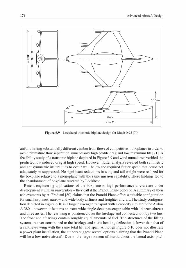
174 Advanced Aircraft Design
71.0 m
18.5 m
Figure 6.9 Lockheed transonic biplane design for Mach 0.95 [70]
airfoils having substantially different camber from those of competitive monoplanes in order toavoid premature flow separation, unnecessary high profile drag and low maximum lift [71]. Afeasibility study of a transonic biplane depicted in Figure 6.9 and wind tunnel tests verified thepredicted low induced drag at high speed. However, flutter analysis revealed both symmetricand antisymmetric instabilities to occur well below the required flutter speed that could notadequately be suppressed. No significant reductions in wing and tail weight were realized forthe boxplane relative to a monoplane with the same mission capability. These findings led tothe abandonment of boxplane research by Lockheed.Recent engineering applications of the boxplane to high-performance aircraft are under
development at Italian universities – they call it the Prandtl Plane concept. A summary of theirachievements by A. Frediani [80] claims that the Prandtl Plane offers a suitable configurationfor small airplanes, narrow and wide body airliners and freighter aircraft. The study configura-tion depicted in Figure 6.10 is a large passenger transport with a capacity similar to the AirbusA 380 – however, it features an extra wide single-deck passenger cabin with 14 seats abreastand three aisles. The rear wing is positioned over the fuselage and connected to it by two fins.The front and aft wings contain roughly equal amounts of fuel. The structures of the liftingsystem are over-constrained to the fuselage and static bending deflection is lower than that ofa cantilever wing with the same total lift and span. Although Figure 6.10 does not illustratea power plant installation, the authors suggest several options claiming that the Prandtl Planewill be a low-noise aircraft. Due to the large moment of inertia about the lateral axis, pitch
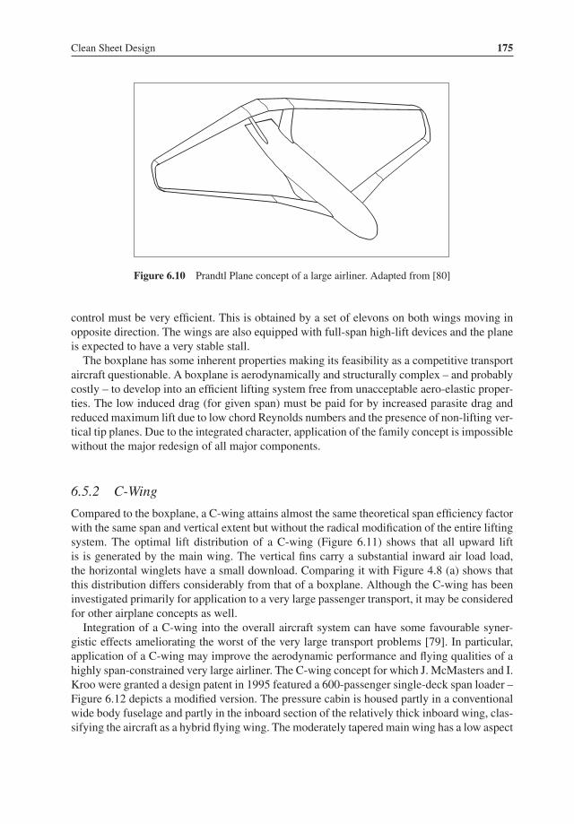
Clean Sheet Design 175
Figure 6.10 Prandtl Plane concept of a large airliner. Adapted from [80]
control must be very efficient. This is obtained by a set of elevons on both wings moving inopposite direction. The wings are also equipped with full-span high-lift devices and the planeis expected to have a very stable stall.The boxplane has some inherent properties making its feasibility as a competitive transport
aircraft questionable. A boxplane is aerodynamically and structurally complex – and probablycostly – to develop into an efficient lifting system free from unacceptable aero-elastic proper-ties. The low induced drag (for given span) must be paid for by increased parasite drag andreduced maximum lift due to low chord Reynolds numbers and the presence of non-lifting ver-tical tip planes. Due to the integrated character, application of the family concept is impossiblewithout the major redesign of all major components.
6.5.2 C-Wing
Compared to the boxplane, a C-wing attains almost the same theoretical span efficiency factorwith the same span and vertical extent but without the radical modification of the entire liftingsystem. The optimal lift distribution of a C-wing (Figure 6.11) shows that all upward liftis is generated by the main wing. The vertical fins carry a substantial inward air load load,the horizontal winglets have a small download. Comparing it with Figure 4.8 (a) shows thatthis distribution differs considerably from that of a boxplane. Although the C-wing has beeninvestigated primarily for application to a very large passenger transport, it may be consideredfor other airplane concepts as well.Integration of a C-wing into the overall aircraft system can have some favourable syner-
gistic effects ameliorating the worst of the very large transport problems [79]. In particular,application of a C-wing may improve the aerodynamic performance and flying qualities of ahighly span-constrained very large airliner. The C-wing concept for which J. McMasters and I.Kroo were granted a design patent in 1995 featured a 600-passenger single-deck span loader –Figure 6.12 depicts a modified version. The pressure cabin is housed partly in a conventionalwide body fuselage and partly in the inboard section of the relatively thick inboard wing, clas-sifying the aircraft as a hybrid flying wing. The moderately tapered main wing has a low aspect

176 Advanced Aircraft Design
Figure 6.11 Distribution of lift over the elements of a C-wing
ratio. The tip-mounted non-planar lifting surface systems are configured as control surfacesreplacing the empennage of a conventional airplane. Each vertical fin has roughly the size of aBoeing 747 vertical stabilizer. The horizontal surfaces are augmented by a foreplane renderingthis configuration effectively into a three-surface aircraft. The following basic features makethe C-wing configuration a possible candidate for a very large transport:
• Thewing span problem associatedwith the 80m box airfield limit is solvedwithout incurringa significant induced drag penalty.
• The single-deck cabin reduces the emergency evacuation problem of a very large airliner.
Figure 6.12 C-wing transport configuration for 600 passengers. Reproduced from [79]. Copyright1998 Elsevier

Clean Sheet Design 177
• Airplane growth can be accommodated by the traditional expedient of lengthening thefuselage with cylindrical body plugs without the necessity of a major wing redesign.
• The trailing vortex field is highly non-planar, a potentially advantageous asset in reducingwake vortex hazards. Much work remains to be done to verify this.
The developers came to the conclusion that, with sufficient further effort, the C-wing con-figuration proposed can probably be made to work. In [79] they compare the characteristicsof the configuration depicted in Figure 6.12 with an optimized conventional WAT airplane.This makes it clear that weight and performance figures of their C-wing giant are inferiorto those of the conventional competitor – a conclusion that may hold only for subsonictransports carrying no more than about 600 passengers in a three-class arrangement. Furtherexplanation is not given but it is likely that some of the problems are similar to those ofthe boxplane. In particular, designers of a C-wing structure are faced with a challenge sinceits concept entails formidable structural dynamics problems. Other sources of concern areprobably the weight of the pressure cabin section in the wing and the drag of the 18% thickinner wing.
6.6 Joined Wing Aircraft
The joined wing configuration has been patented and investigated theoretically and experi-mentally by J. Wolkovitch [82, 83]. A joined wing aircraft (JWA) can be defined as an airplaneconfiguration incorporating two dual wings arranged to form diamond shapes in both plan-form and front view – they are also known as bi-diamond or diamond-ring wings. A singlevertical tail or twin tails may be used to support the centre section of the aft wing. Subjectto aerodynamic and structural optimization, the joints may be located at or inboard of theforward (main) wing tips. The wings can be joined by means of streamline bodies but it is alsopossible to join the wings at their tips by winglets. Advantages claimed for the joined winginclude lightness, stiffness, low vortex drag, low wave drag due to a favourable transonic areadistribution, direct lift and side-force control capability, and high trimmed maximum lift. AJWA would probably be quieter in climb-out and landing approach than conventional aircraft.Most of these claims have been supported by independent studies, design analysis and windtunnel tests described in a comprehensive overview [89], the source of most information inthe present overview.Integration of the joined wing concept into a civil aircraft results in an unorthodox general
arrangement. The example of a hypothetical executive jet in Figure 6.13 shows
• a conventional fuselage with aft-mounted turbofans and a single vertical tail;• a high aspect ratio sweptback front wing with trailing edge flaps;• a forward swept aft wing with trailing edge flaps, with its root attached at the top of thevertical tail(s);
• full-span trailing edge flaps on both wings;• the rear wing’s tips jointed just aft of the front wing’s trailing edge inboard of its tips;• a fairing for the main landing gears which are retracted inside the fuselage structure.

178 Advanced Aircraft Design
Figure 6.13 Concept for a high speed executive jet with joined wings
6.6.1 Structural Principles and Weight
The joined wing differs from a conventional WAT with cantilever wing in its external appear-ance as well as in its internal structure. Figure 6.14 shows how the lift loads on each wing areresolved into components acting normal and parallel to the truss structure formed by the joinedwings. The in-plane components are well resisted by the truss, the out-of-plane componentsbend the wing structures about a bending axis that is tilted at an angle θ to the longitudinalaxis. The primary structure of each wing involves chordwise tapering of the equivalent panelthickness – an essential property of the concept that yields a significant weight advantage.The minimum amount of structural material is needed if bending is resisted by means of abeam with maximum second moment of inertia about the bending axis. This implies that thematerial must be concentrated near the upper front spar cap and the lower rear spar cap, asshown schematically in the lower portion of Figure 6.14. Moreover, it is profitable to use thelargest possible fraction of the airfoil chord with limits set by the space needed for de-icing,
Figure 6.14 Structural principles of the joined wing

Clean Sheet Design 179
high-lift devices and control surfaces. For instance, the joined wing box will typically occupy5 to 75% of the chord length versus 15 to 65% of the cantilever-wing chord.The effective beam depth of a joined wing is determined by the chord of its airfoils – their
thickness is secondary. Hence, thin airfoils may be employedwith less weight and drag than fora cantilevered wing. The torsional stiffness of a joined wing is high since torsion of one wingis resisted by flexure of the other. This yields higher aileron effectiveness and higher flutterspeeds than obtainable with a cantilevered wing of comparable weight. Since under positiveload factors the rear wing is under compression, overall column buckling must be considered.Although rear wing buckling was not found to be a constraint in [88], it was found to be acritical design issue for a JWA in the DC-9 category in [95]. Joined wings are not invariablylighter than aerodynamically equivalent WAT combinations. Weight is saved only if the wingplanform is properly chosen and the internal structure is optimized. By studying awide range ofgeometric parameters, [88] reported some joined-wing configurations realizing weight savingsbetween 20 and 35% of the primary structure weight relative to a WAT configuration. If thereis no constraint on wing span of a joined wing, it has the best inter-wing joint location atapproximately 70% of the semi-span.
6.6.2 Aerodynamic Aspects
Similar to biplane wings of equal span, both tip-jointed wings carry approximately the samelift in order to achieve minimum vortex drag whereas the sensitivity to a non-optimum liftdistribution is low. The span efficiency factor depends primarily on the gap; that is, the verticaldisplacement of the dual wings at their roots. Joined wings together form a closed liftingsystem similar to the boxplane. Nevertheless, since vorticity at the tips is released in a smallarea, its span efficiency factor is only slightly higher compared to the monoplane. Figure 6.15indicates that, for realistic values of the gap/span ratio, the theoretical span efficiency factorev is between 1.05 and 1.10. Hence, the minimum vortex drag of tip-jointed wings is 5 to10% less than the minimum vortex drag of an isolated monoplane with the same span. This
1.0
1.1
1.2
1.3
1.4
1.5
1.6
0.2 0.4 0.6 0.8 1.00d/h
h
b
0.32
0.25
0.17
h/b
d
Figure 6.15 Effect of winglets on the span efficiency factor of a joined wing. Adapted from [89]

180 Advanced Aircraft Design
drag saving falls to a level of only 2–3% for wings with inter-wing joints inboard of the tips.Although the joined wing gains little vortex drag from its non-planarity, it reduces trim dragin cruising flight to less than 1% by exploiting the closed lifting system [81] for its balance.Figure 6.15 also demonstrates that, with symmetric inclined winglets at the tips, the spanefficiency factor approaches that of a boxplane with the same ratio of vertical extent to span.In view of the large number of geometric properties defining a JWA geometry, it is not
feasible to make generally valid statements on parasite drag. The following observations forma liberal interpretation of [89].
• Adverse interferences between the front and aft wings are avoided by using non-overlappingairfoils near the inter-wing joints. The junction of the aft wing with the vertical tail shouldbe filleted properly.
• Due to their smoother area progression, a JWAhas less zero-liftwave drag than a conventionalairplane with comparable leading edge sweep. The application of self-bracing wings permitswings with relatively thin airfoils, giving a further drag saving.
• The lift on each airfoil causes the other airfoil to be immersed in a curved flowfield. Since thiscauses induced flow curvature, airfoils for joined wings should be designed using methodssimilar to those used formulti-element airfoils. The front wing should havemore camber thanthe rear wing and should be washed out towards the tips. The aft wing should have wash-in.
Wind tunnel tests of a joined wing configuration without high-lift flaps indicate that thetrimmed maximum lift coefficient of the joined wing is 4 to 7 percent higher than for aconventional WAT with the same total exposed area. Since the rear wing is immersed in thedownwash of the front wing, the front wing of a statically stable JWA is the first airfoil thatstalls. Although this property provides good stall recovery, it means that the rear wing may beoversized in providing the required trimmed lift for the low speed configuration. Moreover,the high-lift devices are less effective since they occupy a smaller fraction of the chord thanfor a cantilever wing. The following measures will help to increase maximum lift:
• Increase the lift curve slope contribution of the rear wing by increasing its chord and givingit less sweep than the front wing.
• Optimize camber, wash-out and setting angles of both airfoils to achieve a positive pitchingmoment at zero lift.
• Minimize the static margin by moving the CG aft, for instance, by using a trim tank in theempennage.
• Install leading-edge flaps, slats or strakes near the root of the inboard front wing.• Employ maximum trailing-edge flap deflections on the inboard front wing and the outboardaft wing as illustrated in Figure 6.16. Thismakes the zero-lift pitchingmomentmore nose-up.
If these measures appear to be insufficient, a low-aspect ratio foreplane may be employed toprovide appreciable nose-up pitching with little forward AC shift.
6.6.3 Stability and Control
At low angles of attack, the aerodynamic centre (AC) of a JWA configuration is in front of thejoined wing centre of area. The AC moves gradually backwards at moderate and high angles

Clean Sheet Design 181
(a) trimming formaximum lift
(b) directlift control
(c) direct sideforce control
Figure 6.16 Joined wing aircraft lift and control capabilities
of attack below the stall, leading to a pitch-down tendency which can be reduced, if necessary,by proper aerodynamic design. Elevators may be mounted on both the front and rear wings andon the foreplane (if present). If they are deflected by equal angles the resulting lift acts close tothe CG which enables direct lift control (Figure 6.16). A combination of direct lift control andfront elevator deflection facilitates take-off rotation. Figure 6.16 shows that the feasibility ofdirect side force control is inherent to the joined wing configuration due to the large dihedralof the front wing and anhedral of the rear wing which is beneficial for controlling the aircraftin cross-wind landings. In conclusion, a well-designed JWA design is likely to have stabilityand control characteristics as good as or better than a conventional aircraft.
6.6.4 Design Integration
Although it is imaginable to mate a joined wing to the body and vertical tail of an existingairplane, this is not likely to produce the best result. However, the conceptual design of acompletely new JWA airframe involves some novel considerations with regard to fuel tankage,landing gear and wing and body geometry, as well as the load and balance aspect. For instance,a tip-jointed wing would normally carry fuel in both the front and rear wings. Although thevolume of two wings of equal area and geometry would be less than that of a cantilevermonoplane, the larger box chord fractions may compensate for this. And the following aspectsare relevant to fuselage design:
• It appears desirable for minimum weight that the fuselage has a low fineness ratio. Thisis compatible with the aerodynamic requirements of a JWA primarily because it does notrequire a long fuselage to provide a sufficiently large tail moment arm.

182 Advanced Aircraft Design
Figure 6.17 Lockheed design of a very large cargo aircraft with twin-fuselage configuration [103]
• Both wings of a JWA generate upward lift when the aircraft experiences a high upward load.Hence, the fuselage is supported near both ends. By contrast, a conventional wing supportsthe fuselage midway between nose and tail with the tail applying a download. Parts of theJWA fuselage designed to resist the air loads may therefore be lighter than usual. On theother hand, the body must be reinforced where the main landing gears are installed.
• The airliner family concept requires a body that can be stretched or shrunk to suit differentpayload capacities. It would be a challenge to incorporate this flexibility in a JWA withoutmajor design modifications.
The JWA has several inherent advantages over a conventional configuration classifying it as aserious candidate for designing small passenger planes as well as airliners of widely differentcapacities. However, a JWA represents a highly integrated concept with more complex liftingand flight control systems than usual and is probably more costly to manufacture and maintain.
6.7 Twin-Fuselage Aircraft
A twin-fuselage aircraft (TBA) employs the favourable structural effect of span distributedloading (SDL) to reduce wing bending by carrying its payload in two fuselages located atequal distances outboard from the plane of symmetry. SDL leads to a significantly lower wingstructural weight for a given span, resulting in a larger optimum aspect ratio compared to atraditional layout. Figure 6.17 depicts a very large twin-body cargo aircraft conceived by theLockheed Georgia Company. Although a tri-body aircraft with one central and two outboardfuselages is imaginable, it is not likely to offer sufficient advantages to make it a candidate forcivil airplane design.3
Comparison between a conventional airplane and a TBAwith the same payload/range capa-bilities explains that significant empty weight reductions are inherent to the twin-body layout.Most significant is the effect of the unusual SDL illustrated in Figure 6.18. Disregarding thelift losses due to the fuselage(s), the two configurations have a nearly identical distribution oflift along the span and substantially different mass distributions. Both wings experience themaximum bending moment where the wing is connected to the fuselage(s). However, maxi-mum bending moments on a typical twin-fuselage airplane are at least 50% lower than usual
3American designer Burt Rutan used tri-body configurations for his Voyager aircraft that circled non-stop around theworld in 1989 and, more recently, for WhiteKnightTwo, launcher of the sub-orbital Virgin Galactic SpaceShipTwo.

Clean Sheet Design 183
conventional twin-fuselage
lift
mass
bending moment
wing and fuel
fuelage groupand payload
wing and fuel
fuelage groupand payload
Figure 6.18 Distribution along the span of lift, mass and bendingmoment for a twin-fuselage comparedto a conventional aircraft
whereas the bending load between the fuselages decreases rapidly towards the centreline.4 Onthe other hand, torsion constitutes the dominating load on a large portion of the central wing.Overall, the central wing has a significantly lower weight per unit span than the traditionalinboard wing and carry-through structure. Since the area under the bending moment distribu-tion forms an indication for the material required to withstand bending, a considerable weightreduction is obtained for a given span. In view of the sensitivity of fuel weight to induceddrag – hence, wing span – the TBA has a larger optimum span than the traditional airplane.A criterion for sizing a large portion of a cabin shell structure is that it must withstand a
specified number of pressurization cycles. An overpressure �p in a cylindrical cabin withdiameter d causes the skin to experience a tensile force equal to P = 1
2 ld�p (Figure 6.19).The required skin thickness for a given hoop stress σ is t = 1
2 d�p/σ . Hence, skin thicknessis proportional to cabin diameter and the skin weight amounts to
Wskin = π
2ld2ρg
�p
σ= 2Qρg
�p
σ(6.6)
with ρ and Q denoting the material density and cabin volume, respectively. Consequently, theskin weight of a pressure cabin is proportional to its volume. This result can be utilized indifferent ways.
1. A traditional airliner is compared with a TBA having the same total pressure cabin volumeand similar geometry. Equation (6.6) indicates that they have the same skin weight.
2. The TBA cabins are designed to have the same total floor area as the traditional airplanecabin. For similar geometries, each cabin has a length l/
√2, a diameter d/
√2 and a volume
4The bending moment due to lift is zero in the plane of symmetry when the bodies are suspended in the centre ofpressure of each half-wing.

184 Advanced Aircraft Design
PPd
l
t
d
l
single fuselage
twin fuselage
equilibrium of forces
d2
l2
p
volume Q
Q2Δ
Figure 6.19 Weight advantage for the overpressure-sized skins of two fuselages compared to a singlepressure cabin with the same floor area
Q/(2√2) (Figure 6.19). Using Equation (6.6) it is found that the two skins together have a
weight equal to that of the single-body cabin divided by√2, a 29% gain. A similar result
is found for the front and rear pressure bulkheads.
The volume and weight savings of the second option are ascribed to the unused space of a widebody airliner with single-deck cabin – the twin-body layout eliminates this loss. A negativeconsequence is that the total cargo hold volume of the two narrow bodies is reduced relative tothe single-body layout. If this were unacceptable, the twin-body cross-sections would have tobe modified to match the required freight hold capacity. The TBA skin weight saving is thenless than 29%. The reverse argument applies to the volumetric utilization of a twin-deck cabinwhich is better than that of two single-deck cabins with the same total floor area.It is concluded from the previous discussion that two narrow bodies have a smaller total
wetted area and less parasite drag than a wide body with the same total number of cabin seats.Consequently, if the number of seats is in the range of 200 to 400, it appears that the use oftwo fuselages will yield a drag saving. This observation is confirmed by statistical informationon fuselage gross wetted area per cabin seat [112]:
• single deck, single aisle: 2.6 to 2.9 m2;• single deck, two aisles: 3.0 to 3.5 m2;• two decks, four aisles: 2.4 to 2.6 m2.
This confirms that the wetted area of two narrow bodies is 15 to 20% less than that of a singlewide body with an equal number of seats. This difference is augmented by the absence of aflight deck in one of the fuselages of a twin-body airplane. However, this beneficial effect is

Clean Sheet Design 185
Figure 6.20 Medium range airliner design for 250-300 passengers with twin-fuselage configuration[114]
defeated by the scale effect on skin friction drag causing the parasite drag coefficient of a widebody to be less than that of standard body.
6.7.1 Design Integration
Figure 6.20 depicts a clean-sheet airliner design featuring two narrow bodies with a single-aisle cabin [114]. Table 6.1 compares this design with a traditional wide body airliner withthe same passenger capacity designed according to the same ground rules. This shows thatsavings in the design weights, fuel consumed and installed engine thrust are significant. Grossweight reductions between 10 and 16% and improvements of about 20% in fuel efficiencyare suggested in the available literature for medium-sized airliners and even more for largeaircraft. Cost reductions accrue not only from lower empty weight, installed thrust and fuelusage. Several publications have indicated the feasibility of pairing fuselages from existingtransport designs to provide inexpensive bodies [113], [105]. Reduced maintenance costs areassociated with parts commonality in the two fuselages and the empennage(s). Especially
Table 6.1 Characteristics of the design on Figure 6.20 compared with a conventional design withequal payload/range capability
Mass or force Units Conventional Twin fuselage � %
Maximum take-off weight kg 155 000 134 000 −13.5Maximum landing weight kg 128 000 113 000 −11.7Maximum zero fuel weight kg 120 000 106 000 −11.7Operating empty weight kg 84 000 70 000 −16.7Maximum structural payload kg 36 000 36 000 0Mission fuel for 8 000 km range kg 40 715 34 245 −15.9Engine thrust (SL ISA) kN 2×222.5 2×178.0 −20.0

186 Advanced Aircraft Design
for short- to medium-range applications, the TBA concept can be an attractive alternative fordoubling the passenger capacity of narrow body airliners with significantly less than twice theoperating cost. In general, a TBA has the following promising characteristics:
• Different from radical unconventional concepts such as the BWB or the C-wing, the TBAconfiguration is based on conventional technology and offers a low-risk alternative withdistinct advantages. The advantages lie in the general arrangement itself which combinesconventional technology with favourable synergistic effects.
• A TBA needs significantly less installed thrust than a (large) traditional design. This mayfavour application of three engines instead of four with freedom for power plant installationat the central wing enabling application of centreline thrust. The arrangement depicted inFigure 6.20 also has the potential of engine noise shielding.
• The non-swept and relatively thin central wing can be designed as a simple prismaticstructure, an ideal shape for NLF or HLFC and for adapting the wing span to growthversions of the baseline.
• The configuration is ideally suited to the family concept, especially if the wing betweenfuselages is prismatic.
The twin-fuselage concept can be considered for passenger aircraft of any size. However, forvery large aircraft a single twin-deck fuselage may be superior to two single-deck wide body.Since the optimum span of a TBA is larger than the conventional 80 m box span constraint,its performance is degraded more than for the traditional configuration. A configuration withcabins in each outboard fuselage and in the wing-between-fuselages might be considered asan option for a very large passenger transport aircraft – see configuration D4 in Figure 6.2.Due attention must be paid to aero-elasticity, approach and landing flight characteristics andemergency evacuation. Results of several studies ( [113], [104]) lead to the conclusion thataero-elastic behaviour and flight characteristics of a TBA are conventional when moderncontrol technology is applied.There exist several technical unknowns concerning how to configure a clean sheet TBA
design. Efficient ground handling is possible provided two-door loading and unloading facili-ties are available. The emergency evacuation procedure is unconventional and in certain areasbetween the fuselages exits may not be possible. However, safety aspects are not considered asa potential hindrance. In spite of many positive findings, manufacturers have not yet embracedthe TBA concept for their clean sheet or derivative designs. One of their concerns is the expec-tation that lateral displacement of the cabins from the centreline generates an unfavourableopinion about cabin comfort.
6.8 Hydrogen-Fuelled Commercial Transports
In the mid-1950s, NASA successfully flight-tested a B-57 equipped with a liquid hydrogen(LH2) fuel system. The oil crisis of the 1970s brought about a concern that within severaldecades there would be a serious shortage of crude oil resources. This prompted NASA-supported studies by Lockheed and Douglas of aircraft configured to use LH2 as a gas turbineengine fuel. The Russians were the first to use hydrogen on a civil transport with the purposelydeveloped Tupolev Tu-155, which first flew in 1988 and made successful flights with both

Clean Sheet Design 187
Figure 6.21 DASA Cryoplane wide body airliner with LH2 propulsion. Reproduced with permissionfrom Daimler-Benz Aerospace Airbus GmbH
LH2 and liquid natural gas. During the 1990s, DASA in Germany cooperated with Tupolevin cryogenic fuel system technology leading to the Cryoplane project (Figure 6.21). The EU-sponsored Cryoplane research aimed at identifying the feasibility of future application tocommercial aviation [118].
6.8.1 Properties of LH2
The principal benefit accruing from the use of liquid hydrogen is that it is essentially non-polluting. Compared to jet-fuelled engines delivering the same thrust, hydrogen combustionproducts consist of 2.6 times the amount of H2O in contrails contributing less to the greenhouseeffect5 whereas up to 80% NOx can be saved by lean combustion [118]. Hydrogen offers avery high calorific value (H = 120 kJ/g), that is, 280% of current jet engine fuel. Especially forlong-range aircraft, this results in substantial fuel burn and gross weight reductions. The maindisadvantage of LH2 is its low density and its extremely low temperature. In the liquid state,liquid hydrogen has a temperature of about 20 K and a specific mass of only 70.8 kg/m3 Ccompared to 800 kg/m3 for kerosine.6 Consequently, for a given amount of internal energy,
5H2O is a greenhouse gas with a lifetime in the upper atmosphere of only half a year, whereas CO2 emitted by akerosene-burning engine stays aloft for more than 100 years.6When hydrogen vaporizes and the gas is heated to 15◦ C, its density increases to 83.8 kg/m3.

188 Advanced Aircraft Design
Figure 6.22 Hypothetical regional airliner with LH2 propulsion
the storage of LH2 requires a pressurized tank with four times the volume of a normal jet fueltank – far too large to be accommodated in a traditional airplane wing.The result of these characteristics is that a hydrogen-powered aircraft will look quite different
from a conventional fuel-powered aircraft. The main differences are in the use of an unusuallylarge fuselage or in the presence of large wing-mounted streamline bodies to provide the extratankage (Figure 6.22); other solutions are discussed in [121]. In view of the cryogenic fuelproperties, LH2 tanks have to be extensively isolated and pressurized. LH2-fuelled aircraft aretherefore characterized by a relatively low aerodynamic efficiency and increased emptyweight.In spite of it, the large reduction in the aircraft gross weight brings the fuel energy requirementdown by approximately 5 to 20% and the fuel weight by 65 to 70% [116]. Moreover, thereduced take-off gross weight permits smaller engines to be installed.
6.8.2 Fuel System
Although hydrogen fuel systems have been developed for space mission applications, therequirements for aircraft are so different in regard to mission duration, system life, operatingcycles, and safety aspects that entirely different design problems have to be solved. Hydrogencan be used as a fuel for a normal aero gas turbine with minor modifications to the power plantand its systems. The turbo-machinery would be unchanged, the combustor and the fuel controlsystemmust be redesigned and a heat exchanger to vaporize the fuel must be added. Hydrogenmust be stored in liquid form at a temperature of 20.2 to 22.3 K and a pressure of 1.2 to2.0 bar. It is then heated to around 150 K and twice the engine combustor pressure in order todrive the fuel injectors. The heat exchanger has little effect on the engine layout, weight anddrag since it can be wrapped around the gas generator exhaust pipe – utilizing this otherwisewasted heat improves the cycle efficiency compared to conventional fuel. However, the two-phase flow in the fuel system exhibits compressibility. The internal pressure varies continuouslydepending on the balance between the tank insulation characteristics and combustion inlet con-ditions. Consequently, a hydrogen fuel system may exhibit unexpected dynamics and criticalfailure modes.The weight of the large tank(s) is a major issue which requires special attention. In order
to make the insulation light, effective, reliable and damage-tolerant, the tank can be producedfrom foam or super-insulation type multi-layer materials. In the stored condition, there is acontinuous phase change from liquid to gas and vice versa, and some hydrogen will inevitably

Clean Sheet Design 189
be lost due to boil-off when the aircraft is parked between flights. Integration into the aircraftof the pressurized fuel tank(s) is the greatest challenge for hydrogen application. The besttank layout depends on the aircraft category and general arrangement. The fuselage seemssuitable as it is already a pressure vessel, but the presence of passengers next to a hydrogentank might raise public concerns. For wide body transports, the fuel may be stored both foreand aft of the passenger compartment. In order to minimize the CG travel due to fuel burn, thefuselage length/diameter ratio and the tank length can be reduced and/or the engines locatedat the rear end of the fuselage. A three-surface configuration could be a good layout for thistype of aircraft. Special attention should be paid to the risk that a disk burst might lead to anexplosion of the LH2 tank.
6.8.3 Handling Safety, Economics and Logistics
Considering general safety aspects of handling and using hydrogen for aviation, studies haveshown that the overall safety level is at least as high as when using kerosene, on the provisionthat safety procedures are strictly observed [121]. The overall airport layout and procedures donot have to be changed and the aircraft can be serviced at the same positions as kerosene-fuelledaircraft. Although the larger fuel volumes may double refuelling time, this does not necessarilyincrease turnaround time and airport operations will not require significant adaptations to theaircraft itself. However, unless a local LH2 production to fulfil the demand for cryogenic fuelis erected at each airport, a huge and entirely new logistic system would be required for thetransportation, storage and handling of fuel throughout the world. This will prevent the use ofthis radical change in fuelling technology for a long time to come.The results of the Cryoplane project confirmed that LH2, from the technical side, could
be an alternative future fuel; however, the economics of LH2-fuelled aircraft is a differentstory. Although the cryogenic fuel system penalizes the hydrogen aircraft, the technologicalchallenges in the application of hydrogen to aviation aremore related to cheap, environmentallyacceptable and large-scale production of hydrogen than to the adaptation of the aircraft concept.The electrolysis process plus liquefaction to produce LH2 from water requires four to fivetimes the amount of energy produced by burning LH2. Using electricity produced from fossilfuel or gas for the production of hydrogen is several times more expensive than that of jet-Afuel and does not appear the way to conserve energy resources. It seems likely that the missinginfrastructure and the risk and investment of the hydrogen system will stall its implementationuntil cheap, unlimited energy becomes available from fission, fusion, wind or solar resources.
6.9 Promising Concepts
Although the TAW has been under attack from innovative concepts ever since its emergence inthe 1950s, it will continue to be the favoured general arrangement of most clean sheet designs.The cylindrical body shell forms an ideal pressure vessel enabling a passenger cabin withflexible seating arrangements, a high volumetric efficiency and a straightforward realization ofthe family concept. Satisfactory provisions for embarking and disembarking, ground handlingand emergency evacuation are achievable and there exists a wealth of design experience forsafety, reliability, durability and maintenance. The aerodynamics of the high-aspect ratio wingare thoroughly optimized for long-range transonic cruise with maximum efficiencies up to
190 Advanced Aircraft Design
L/D = 20, as well as excellent low speed performance. Balancing the dominant configurationis generally satisfactory with inherent stability and low trim drag in most loading conditions.The choice between improvements obtained from more integration versus discrete major
components is a major issue. Chapters 5 and 6 demonstrate how the presently dominantconfigurations may be improved by unusual or innovative concepts leading to the followingobservations:
• The BWB and the HFW are strong contenders for very large aircraft with seating capacitiesin excess of 600 seats. The BWB is a highly integrated flying wing concept offering anaerodynamic efficiency up to L/D = 25. Its design process is complicated and in spite ofthe considerable effort already expended in research, many aspects remain to be investigatedwhen developing a for-sale aircraft. The span constraint of the 80m box is a serious hand-icap for these very large aircraft, which can be countered by adopting a non-planar wingconfiguration or by using hinged wing tips. Both solutions leads to considerable weightpenalties.
• The twin-fuselage configuration deserves to be considered for short- to medium-rangeaircraft with seating capacities between 200 and 400 seats. The span loading feature enablesa (much) larger wing span resulting in considerably less vortex drag with no increase ofwing structure weight. The twin-fuselage layout offers a good platform for application oflaminar flow and very high bypass ratio turbofans or open rotor engines and does not requirea costly technology development.
• Installing open rotor engines on regional aircraft may lead to higher cruise speeds up toMach 0.75. Strut bracing allows a high-wing airliner to increase its span with little or noweight increase.
• An innovative business jet configuration can be considered if it improves cabin comfortwithout weight and drag penalties. A three-surface layout with a mid wing positionedbehind the cabin may be favoured for a light business jet. Application of a joined wing to along-range executive jet improves its aerodynamic efficiency in cruising flight and reducesthe empty weight.
Anymajor excursion from the dominant configuration requires an all-out overall aircraft systemoptimization, taking into account all the driving factors affecting economy, environmentalissues, operational and safety aspects. Consequently, the advanced designer should be familiarwith multidisciplinary optimization (MDO).
Bibliography
[1] Torenbeek, E., Synthesis of Subsonic Airplane Design, Chapters 2 and 9, Springer Verlag, Heidelberg, 1981.[2] Stinton, D., The Design of the Aeroplane, Granada Publishing Ltd., London, 1983.[3] Downie, D. and J. Downie, The Complete Guide to Rutan Aircraft, Third Edition, Airlife Publishing Ltd.,
Shrewsbury, 1987.[4] Sterk, F.J., and E. Torenbeek, ‘Unconventional Aircraft Concepts’, in Proceedings of a Symposium of the
Netherlands Society of Aeronautical Technology, Delft University Press, 1987.[5] Stinton, D., Flying Qualities and Flight Testing of the Aeroplane, Blackwell Science Ltd., Oxford, 1996.[6] Fielding, J.P., Introduction to Aircraft Design, Cambridge University Presss, Cambridge, 1999.[7] Torenbeek, E., and H. Deconinck (eds), Innovative Configurations and Advanced Concepts for Future Civil
Aircraft, von Karman Institute for Fluid Dynamics, Lecture Series 2005–06, June 2005.

Clean Sheet Design 191
[8] Whitford, R., Evolution of the Airliner, The Crowood Press, Ramsbury, 2007.[9] Roskam, J., Lessons Learned in Aircraft Design, DAR Corporation, Lawrence, Kansas, 2007.
Advanced Concepts and Technology
[10] Black, R.E., and J.A. Stern, “Advanced Subsonic Transports: A Challenge for the 1990’s”, Journal of Aircraft,Vol. 13, No. 5, pp. 321–326, May 1976.
[11] Clay, C.W., and A. Sigalla, “Shape of the Future Long-Haul Airplane”, Journal of Aircraft, Vol. 13, No. 8, pp.551–558, August 1976.
[12] Lange, R.H., and E.S. Bradley, “Parametric Study of Advanced Long Range Military/Commercial CargoTransports”, AIAA Paper No. 77–1221, 1977.
[13] Conner, D.W., and J.C. Vaughan, “Multi-Role Cargo Aircraft Options and Configuration”, NASA TM 80177,October 1979.
[14] Klug, H.G., “Neue Konfigurationen und ihr Beitrag zur Reduzierung der Betriebskosten von Verkehrsflugzeu-gen”, Jahrbuch der DGLR, 1981.
[15] Arata, W.H. Jr., “Very Large Vehicles: Technology Looking for a Need”, Astronautics and Aeronautics, April1982.
[16] Lange, R.H., and J.W. Moore, “Application of Composite Materials and New Design Concepts for FutureTransport Aircraft”, ICAS Paper No. 82–2.7.3, September 1982.
[17] Rosenthal, L., “Nouvelle Architecture des Avions”, L’Aeronautique et l’Astronautique, 1986–1 – No. 116,1986.
[18] Lange, R.H., “A Review of Advanced Turboprop Transport Aircraft”, Progress in Aerospace Sciences, Vol.23, pp. 151–166, 1986.
[19] Lange, R.H., Review of Unconventional Design Concepts”, Journal of Aircraft, Vol. 25, No. 5, pp. 385–392,May 1988.
[20] Roskam, J., “What Drives Unique Configurations”, SAE Technical Paper 881353, October 1988.[21] Kentfield, J.A.C., “Aircraft Configurations with Outboard Horizontal Stabilizers”, Department of Mechanical
Engineering, University of Calgary, January 1990.[22] Roskam, J., and C. Gomer, “Design Developments for General Aviation Aircraft”, SAE Paper No. 911022,
April 1991.[23] Weisshaar, T., and C. Allen, “Design of a Turbofan Powered Regional Transport Aircraft”, AIAA Paper No.
91–3080, September 1991.[24] Kentfield, J.A.C., “Aircraft Configurations with Outboard Horizontal Stabilizers”, Journal of Aircraft, Vol. 28,
No. 10, pp. 670–672, October 1991.[25] Oelkers, W., “High Capacity Aircraft”, ICAS Paper No. 92–1.10.3, September 1992.[26] Bushnell, D.M. (ed.), “Potential Impacts of Advanced Aerodynamic Technology on Air Transportation System
Productivity”, NASA Technical Memorandum 109154, September 1994.[27] Morris, S.J., “Advanced Aerodynamic Configurations and Their Integration into the Airport Environment”,
Session II of [26], September 1994.[28] Kentfield, “Case for Aircraft with Outboard Horizontal Stabilizers”, Journal of Aircraft, Vol. 32, No. 2,
pp. 398–403, March-April 1995.[29] Hefner, J.N., W.L. Sellers III, J.L. Thomas, R.W. Wlezien and R.N. Antcliff, “Challenges and Opportunities
in Fluid Mechanics Research”, ICAS Paper No. 96–2.1.1, September 1996.[30] Peel, C.J., “Advances inMaterials for Aerospace”, The Aeronautical Journal, Vol. 100, No. 1000, pp. 487–503,
December 1996.[31] Yaros, S.F., M.G. Sexstone, L.D. Huebner, J.E. Lamar, R.E. McKinley, A.O. Torres, C.L. Burley, R.C. Scott,
and W.J. Small, “Synergistic Airframe-Propulsion Interactions and Integrations,” White Paper prepared by the1996–1997 Langley Aeronautics Technical Committee, March 1998.
[32] Sandoz, P.L., “The Next Careful Steps in Commercial Aircraft Structures”, Structures Technology; HistoricalPerspective and Evolution, A.M. Noor (ed.), pp. 91–106, American Institute of Aeronautics and Astronautics,1998.
[33] Bushnell, D.M., “Frontiers of the “Responsibly Imaginable” in (Civilian) Aeronautics”, The 1998 DrydenLecture, American Institute of Aeronautics and Astronautics, 1998.
[34] Greitzer, E.M. et al., “N+3 Aircraft Concept Designs and Trade Studies”, Final Report, Volume 1 and 2.,NASA/CR – 2010–216794/VOL1 and VOL2, December 2010.

192 Advanced Aircraft Design
Flying Qualities and Airplane Design
[35] Trubshaw, E.B., “Low Speed Handling with Special Reference to the Super Stall”, Journal of the RoyalAeronautical Society, Vol. 70, pp. 695–704, July 1966.
[36] Sliwa, S.M., “Impact of Longitudinal Flying Qualities Upon the Design of a Transport with Active Controls”,AIAA Paper No. 80–1570, August, 1980.
[37] Sliwa, S.M., “Economic Evaluation of Flying-Qualities Design Criteria for a Transport Aircraft with RelaxedStatic Stability”, NASA Technical Paper No. 1760, December 1980.
[38] Hood, R.V., S.M. Dollyhigh, and J.R. Newsom, “Impact of Flight Systems Integration on Future AircraftDesign”, AIAA Paper No. 84–2459, 1984.
[39] Huber, B., “Center of Gravity Control on Airbus Aircraft – Fuel, Range and Loading Benefits”, SAWE PaperNo. 1843, May 1988.
[40] Roskam, J., “Evolution of Airplane Stability and Control: a Designer’s Viewpoint”, Journal of Guidance,Control, and Dynamics, Vol. 14, pp. 481–491, May-June 1991.
[41] Slingerland, R., “Prediction of Tail Downwash, Ground Effect and Minimum Unstick Speed of Jet TransportAircraft”, doctoral thesis, Delft University of Technology, June 2005.
Airplanes with Strut-braced Wings
[42] Kulfan, R.M., and J.D. Vachal, “Wing Planform Geometry Effects on Large Subsonic Military TransportAirplanes”, AFFDL-TR-78–16, February 1978.
[43] Carrier, G., O. Atinault, S. Dequand, et al., “Investigation of a Strut-Braced Wing Configuration for FutureCommercial Transport”, ICAS Paper No. 1.10.2, September 2012.
[44] Park, P.H., “The Effect on Block Fuel Consumption of a Strutted vs. CantileverWing for a Short-Haul TransportIncluding Strut Aeroelastic Considerations”, AIAA Paper No. 78–1454, August 1978.
[45] Jobe, C.E., and R.M. Kulfan, “Wing Planforms for Large Military Transports”, Journal of Aircraft, Vol. 16,pp. 425–432, July 1979.
[46] Turriziani, R.V., W.A. Lovell, G.L. Martin, J.E. Price, E.E. Swanson, and G.F. Washburn, “Preliminary DesignCharacteristics of a Subsonic Business Jet Concept Employing an Aspect Ratio 25 Strut-BracedWing”, NASACR-159361, October 1980.
[47] Smith, P.M., J. DeYoung, W.A. Lovell, J.E. Price, and G.F. Washburn, “A Study of High-Altitude MannedResearch Aircraft Employing Strut-Braced Wings of High Aspect Ratio”, NASA CR-159262, February 1981.
[48] Grasmeyer, J.M., et al., “Multidisciplinary Design Optimization of a Strut-Braced Wing Aircraft with Tip-Mounted Engines”, Virginia Polytechnic Institute and State University,MADCenter Report 98–01-01, VirginiaTech., January 1998.
[49] Grasmeyer, J.M., et al., “Multidisciplinary Design Optimization of a Strut-Braced Wing Aircraft”, MSc thesis,Virginia Polytechnic Institute and State University, April 1998.
[50] Martin, K.C., and B.A. Kopec, “A Structural and Aerodynamic Investigation of a Strut-BracedWing TransportAircraft Concept”, Lockheed Martin Aeronautical Systems, Report No. LG98ER0431, November 1998.
[51] Gundlach, J.F., et al., “Conceptual Design Studies of a Strut-Braced Wing Transonic Transport”, Journal ofAircraft, Vol. 37, No. 6, pp. 976–983, November–December 2000 (Also: AIAA Paper 2000–0420).
Two-Surface and Three-Surface Airplanes
[52] Anderson, S.B., “Handling Qualities of Canards, Tandem Wings, and other Unconventional Configurations”,SAE Paper No. 830763, April 1983.
[53] Butler, G.F., “Effect of Downwash on the Induced Drag of Canard-Wing Combinations”, Journal of Aircraft,Vol. 19, pp. 410–411, May 10982.
[54] Kroo, I.H., “Tail Sizing for Fuel-Efficient Transports”, AIAA Paper No. 83–2476, October 1983.[55] Butler, G.F., “An Analytical Study of the Induced Drag of Canard-Wing-Tail Aircraft Configurations with
Various Levels of Static Stability”, Aeronautical Journal, Vol. 87, pp. 293–300, October 1983.[56] McGeer, T., and I.M. Kroo, “A Fundamental Comparison of Canard andConventional Configurations”, Journal
of Aircraft, Vol. 20, pp. 983–992, November 1983.

Clean Sheet Design 193
[57] Kendall, E.R., “The Minimum Induced Drag, Longitudinal Trim and Static Longitudinal Stability of Two-Surface and Three-Surface Airplanes”, AIAA Paper No. 84–2164, 1984.
[58] Kendall, E.R., “The Aerodynamics of Three-Surface Airplanes”, AIAA Paper No. 84–2508, 1984.[59] Yip, L.P., “Wind-Tunnel Investigation of a Full-Scale Canard Configuration General Aviation Airplane”,
NASA TP No. 2383, March 1985.[60] Arbuckle, P.D., and S.M. Sliwa, “Parametric Study of a Canard-Configured Transport Using Conceptual
Design Optimization”, NASA TP No. 2400, March 1985.[61] Rokhsaz, K., and B.P. Selberg, “Analytical Study of Three-Surface Lifting Systems”, SAE Paper No. 850866,
April 1985.[62] Selberg, B.P., and K. Rokhsaz, K., “Aerodynamic Trade-Off Study of Conventional, Canard, and Tri-surface
Aircraft Systems”, Journal of Aircraft, Vol. 23, No. 10, October 1986.[63] Muchmore Jr., C.B., “TheEffects ofCanard-WingFlow-Field Interactions onLongitudinal Stability, ERffective
Dihedral and Potential Deep-Stall Trim”, AIAA Paper 88–2514 CP, 1988.[64] Goodrich, K.W., S.M. Sliwa, and F.J. Lallman, “A Closed-Form Trim Solution Yielding Minimum Trim Drag
for Airplanes with Multiple Longitudinal-Control Effectors,” NASA Technical Paper 2907, 1989.[65] Pompeis, R de, P. Cinquetti, and S. Martini, “Development and Certification Flight Test on the Piaggio P.180
Avanti Aircraft: A General Overview”, AIAA Paper No. 911003, April 1991.[66] Middel, J., Development of a Computer Assisted Toolbox for Aerodynamic Design of Aircraft at Subcritical
Conditions with Application to Three-Surface and Canard Aircraft, Doctoral Thesis, Delft University Press,ISBN 90–6275-768–5 / CIP, April 1992.
[67] Sacca, G., and C. Lanari, “The Three Lifting Surface Concept and Lessons Learned from the Piaggio P180”,Innovative Configurations and Advanced Concepts for Future Civil Aircraft, von Karman Institute for FluidDynamics, Lecture Series 2005–06, June 2005.
Aircraft with Non-planar Lifting Surfaces
[68] Miranda, L.R., “Boxplane Configuration: Conceptual Analysis and Initial Experimental Verification”, Lock-heed California Company Report, LR 25180, March 1972.
[69] Miranda, L.R., and G.L. Dougherty, “Transonic Wind Tunnel Testing of a Low Induced Drag Lifting System”,Vols. I and II, Lockheed Aircraft Corp., Burbank, CA, February 1974.
[70] Lange, R.H., J.F. Cahill, et al., “Feasibility Study of the Transonic Biplane Concept for Transport AircraftApplication”, NASA Contractor Report CR-132462, June 1974.
[71] Addoms, R.B., and F.W. Spaid, “Aerodynamic Design of High Performance BiplaneWings”, Journal of Airaft,Vol. 12, pp. 629–630, August 1975.
[72] De Young, J., “Induced Drag Ideal-Efficiency Factor for Arbitrary Lateral-Vertical Wing Forms”, NASAContractor Report 3357, December 1980,
[73] Rhodes, M.D., and B.P. Selberg, “Benefits of Dual Wings over Single Wings for High-Performance BusinessAirplanes”, Journal of Aircraft, Vol. 21, February 1984.
[74] Kroo, I.M., “AGeneral Approach toMultiple Lifting Surface Design andAnalysis”, AIAAPaper No. 84–2507,1984.
[75] Gall, P.D., and H.C. Smith, “Aerodynamic Characteristics of Biplanes with Winglets”, Journal of Aircraft,Vol. 24, pp. 518–522, August 1987.
[76] Kroo, I.H., J. McMasters, and S.C. Smith, “Highly Non-Planar Lifting Systems”, Transportation Beyond 2000:Technologies Needed for Engineering Design, NASA TP 10184, pp. 331–370, 1996.
[77] McMasters, J.H., D.J. Paisley, R.J. Hubert, I. Kroo, K.K. Bofah, J.P. Sullivan, and M. Drela, “AdvancedConfigurations for Very Large Subsonic Transport Airplanes”, NASA CR-198351, October 1996.
[78] Grasmeyer, J., “A Discrete Vortex Method for Calculating the Minimum Induced Drag and Optimal LoadDistribution for Aircraft Configurations with Noncoplanar Surfaces”, Report VPI-AOE-242, January 1997.
[79] McMasters, J.H., and I.M. Kroo, “Advanced Configurations for Very Large Transport Airplanes”, AircraftDesign, Vol. 1, No. 4, pp. 217–242, 1998; also AIAA Paper No. 98–0439.
[80] Frediani, A., “The Prandtl Wing”, in Innovative Configurations and Advanced Concepts for Future CivilAircraft, von Karman Institute for Fluid Dynamics, Lecture Series 2005–06, June 2005.
[81] Kroo, I.H., “Nonplanar Wing Concepts for Increased Aircraft Efficiency”, Innovative Configurations andAdvanced Concepts for Future Civil Aircraft, von Karman Institute for Fluid Dynamics, Lecture Series 2005–06, June 2005.

194 Advanced Aircraft Design
Joined Wing Aircraft
[82] Wolkovitch, J., Joined Wing Aircraft, U.S. Patents 3 942 747 (1976) and[83] Wolkovitch, J., “Principles of the Joined Wing”, Engel Engineering Report No. 80–1, December 1980.[84] Samuels, M.F., “Structural Weight Comparison of a Joined Wing and a Conventional Wing”, Journal of
Aircraft, Vol 19, pp. 485–491, June 1982.[85] Kuhlman, J.M., and T.J. Ku, “Numerical Optimization Techniques for Bound Circulation Distribution for
Minimum Induced Drag of Non-Planar Wings: Computer Program Documentation”, NASA CR-3458, August1982.
[86] Hajela, P., “Weight Evaluation of the Joined Wing Configuration”, Final Report, Department of EngineeringSciences, University of Florida, Gainesville, FL, 1983.
[87] Wolkovitch, J., and W.H. Bettes, “Low-Speed Wind Tunnel on Joined Wing and Monoplane Configurations”,Vol. I: Analysis of Results, Vol. II: Test Data, ACA Report 82–2, 1984.
[88] Miura, H., A. Shyu, and J. Wolkovitch, “Parametric Weight Evaluation of Joined Wings by Structural Opti-mization”, AIAA Paper No. 85–0642, April 1985.
[89] Wolkovitch, J., “The Joined Wing: An Overview”, Journal of Aircraft, Vol. 23, No. 3, pp. 161–178, March1986. (also AIAA Paper No. 85–0274, 1985).
[90] Selberg, B.P., and D.L. Cronin, “Aerodynamic-Structural Optimization of Positive/Negative Stagger JoinedWing Configurations”, AIAA Paper No. 86–2686, October 1986.
[91] Wolkovitch, J., “A Second Look at the JoinedWing”, in Proceedings of the NVvL Symposium “UnconventionalAircraft Concepts”, Delft University Press, 1987.
[92] Gallman, J.W., I.M. Kroo, and S.C. Smith, “Design Synthesis and Optimization of Joined-Wing Transports”,AIAA Paper No. 90–3197, September 1990.
[93] Hashimoto, M., M. Ishikawa, N. Hirose, and T. Ohnuki, “A Computational and Experimental Analysis ofJoined-Wing Aerodynamics”, ICAS Paper No. 90–2.6.1, September 1990.
[94] Gallman, J.W., Structural and Aerodynamic Optimization of Joined Wing Aircraft”, Doctoral Thesis, StanfordUniversity, 1992.
[95] Gallman, J.W., S.C. Smith, and I.M. Kroo, “Optimization of Joined-Wing Aircraft”, Journal of Aircraft,Vol. 30, No. 6, pp. 897–905, November–December 1993.
[96] Gallman, J.W., and I.M. Kroo, “Structural Optimization for Joined Wing Synthesis”, Journal of Aircraft,Vol. 33, No. 1, pp. 214–223, January 1996.
[97] Bagwill, T., and B.P. Selberg, “Aerodynamic Investigation of Joined Wing Configurations for TransportAircraft”, AIAA Paper No. 96–2373, June 1997.
[98] Nangia, R.K., and M.E. Palmer, and C.P. Tillman, “Unconventional High Aspect Ratio Joined-Wing Aircraftwith Aft- & Forward-Swept Wing-Tips”, AIAA Paper No. 2003–0605, January 2003.
Multi-Body and Lifting-Body Aircraft
[99] Lange, R.H., “Trends in Very Large Aircraft Design and Technology”, AIAA Paper No. 80–0902, 1982.[100] Houbolt, J.C., “Why Twin-Fuselage Aircraft?”, AIAA Astronautics and Aeronautics, pp. 26–35, April 1982.[101] Arata Jr., W.H., “Very Large Vehicles: Technology Looking for a Need”, AIAA Astronautics and Aeronautics,
pp. 42–43, April 1982.[102] Moore, J.W., and D.V. Maddalon, “Design Analysis and Benefit Evaluation of Multi-Body Aircraft”, AIAA
Paper No. 82–0810, May 1982.[103] Moore, J.W., E.P. Craven, B.T. Farmer, J.F. Honrath, R.E. Stephens, and R.T. Meyer, “Multibody Aircraft
Study Volume I and II., NASA Contractor Report 165829, July 1982.[104] Grantham, W.D., P.L. Deal, G.L. Keyser Jr., and P.M. Smith, “Simulator Study of Flight Characteristics of a
Large Twin-Fuselage Cargo Transport Airplane During Approach and Landing”, NASA TP-2183, 1983.[105] Nangia, R.K., “Multi-Fuselage Fuel-Efficient Aircraft Concepts (Including Conversions of Existing Types)”,
RKN/AERO/REP 85–09, Issue 2, September 1985.[106] Udin, S.V., and W.J. Anderson, “Wing Mass Formula for Twin Fuselage Aircraft”, Journal of Aircraft, Vol.
29, No. 5, pp. 907–914, September-October 1992.[107] Lauter, C.E. et al., “Design Study: A Global Range Large Subsonic Military Transport”, ICAS Paper 94–1.3.3,
September 1994.

Clean Sheet Design 195
[108] Hahl, R., and J. Katz, “Lifting Fuselage/Wing Aircraft Having an Elliptical Forebody”, U.S. Patent Application08–642997, May 13, 1996.
[109] Spearman, M.L., “A High-Capacity Airplane Design Concept Having an Inboard-Wing Bounded by TwinTip-Mounted Fuselages”, AIAA Paper No. 97–2276, June 1997.
[110] Katz, J., S. Byrne, and R. Hahl, “Stall Resistance Features of Lifting-Body Airplane Configurations”, Journalof Aircraft, Vol. 36, No. 2, pp. 471–474, 1999.
[111] Roskam, J., “Design andEconomicChallenges of 10–22 Passenger, Jet-PoweredRegional Transports”,AircraftDesign, Vol. 3, No 1, pp. 33–48, 2000.
[112] Torenbeek, E., “The Case for Twin-Fuselage Configurations and the H-Cabin”, National Aerospace LaboratoryNLR-TR-2000–095, February 2000.
[113] Schoemaker, F.C., “Aeroelastic Characteristics of Twin-fuselage Configurations”, National Aerospace Labo-ratory NLR-TR-2001–046, July 2001.
[114] Torenbeek, E., and E. Jesse, “Exploratory Design Study of a Transonic Airliner with Twin Fuselage Configu-ration”, National Aerospace Laboratory NLR-TR-2001–309, July 2001.
[115] Kalyguina, G.V., et al., “The Dolphin: A New 100-Seat Aircraft in Lifting-Fuselage Layout”, ICAS 2002Congress, pp. 152.1–152.8, September 2002.
Liquid Hydrogen-Fuelled Aircraft
[116] Brewer, G.D., et al., “Study of Fuel Systems for LH2-Fueled Subsonic Transport Aircraft”, NASA CR 145369,Lockheed California Co., July 1978.
[117] Klug, H.G., “Cryoplane: Quantitative Comparison of Contributions to Anthropogenic Greenhouse Effect ofLiquid Hydrogen Aircraft Versus Conventional Kerosene Aircraft”, EGS XXI General Assembly, Den Haag.May 1996.
[118] Westenberger, A., “Liquid Hydrogen Fuelled Aircraft: System Analysis, Cryoplane”, Final Technical Report,GRD1–1999-10014, submitted to the European Commission, 2003.
[119] Svensson, F., A. Hasselrot, and J. Moldanova, “Reduced Environmental Impact by Lowered Cruise Altitudefor Liquid Hydrogen-Fuelled Aircraft”, Aerospace Science and Technology, Vol. 8, pp. 307–320, 2004.
[120] Svensson, F., “Potential of Reducing the Environmental Impact of Civil Subsonic Aviation by Using LiquidHydrogen”, Ph.D. thesis, Cranfield University School of Engineering, April 2005.
[121] Slingerland, R., “Aircraft with LH2 Propulsion”, Innovative Configurations and Advanced Concepts for FutureCivil Aircraft, Von Karman Institute for Fluid Dynamics, Lecture Series 2005–06, June 6–10, 2005.

7Aircraft Design Optimization
Instead of cutting the engineer out of the picture, optimization puts him squarely in the middle.It is another design tool; one that is particularly applicable when the interaction of more than onevariable is involved.
—W.Z. Stepniewski and C.F. Kalmbach [17] (1970)
7.1 The Perfect Design: An Illusion?
In the early days of aircraft development, conceptual design was based on personal experiencewith previous projects and company tradition. Vehicle weight, flight performances and operat-ing costs were estimated with the help of slide rules or calculators by means of rules of thumband design handbooks. Geometry was defined on paper using drawing boards. Optimizationwas limited to relatively superficial investigations to study the effects of varying a few majordesign parameters. Since this approach allows an experienced designer to generate a newdesign in a short time, handbooks methods are still used in ad hoc studies. However, it hasalways been the engineer’s dream to have all aspects of analysis done in a relatively short timeperiod so that many different configurations can be examined and the best suitable productcan be delivered on time. Although this may still be a dream, actual design turn-around timehas become shorter due to the use of mathematical optimization techniques which have beenintroduced into the design process. How and when to use these techniques is arguably thekey factor for advanced engineering operations [66]. One condition for being successful isthat a proven computer augmented design synthesis program in combination with a suite ofoptimization algorithms is available.Since the 1970s, there has been a tremendous expansion of optimization strategies and
algorithms supporting advanced designers. The introduction of automated optimization hasenabled designers to go intomuch greater in depth andfidelity of analysis than before. Synthesisprograms effectively connecting the inputs and outputs of the functional group disciplines bymeans of an automatic control logic have been developed at aircraft manufacturers, researchestablishments and academia. Sophisticated computer assisted design (CAD) systems fordefining three-dimensional body geometries and computer graphics tools for rapidly preparingparametric surveys are available at a modest cost. System engineering methods have brought
Advanced Aircraft Design: Conceptual Design, Analysis and Optimization of Subsonic Civil Airplanes, First Edition. Egbert Torenbeek.
© 2013 by Egbert Torenbeek. Published 2013 by John Wiley & Sons, Ltd.

198 Advanced Aircraft Design
about a paradigm shift in project development towards integrated product development (IPD)and – at least for traditional designs – this approach is highly refined and widely accepted. Foran unusual aircraft concept, however, existing synthesis programs will have to be thoroughlymodified as the risk of the results being unreliable is high since methods cannot be calibratedwith statistical data. Moreover, advances in the field of practical optimization do not dependexclusively on the availability of fast computers or efficient optimization algorithms but on theoverall company-wide development of computational frameworks geared toward flexibility,automation, and exploitation of high-fidelity analysis systems [93].In spite of these developments, little progress has been made in creating computational tools
to aid in the concept finding and early conceptual design phases. A great challenge to engineerscarrying out this sensitive activity is not necessarily to conceive a realistic clean sheet airplanedesign but to convince project management that the best feasible concept complying withmarket needs is being proposed. Although it is often argued that there exists no substitutefor the expert’s insight based on former projects, widespread effort is devoted to improvingformalized optimization methods. A basic problem is that the choice of a single figure of merit(FOM) defining the design quality is inadequate and even multi-objective optimization is notalways the panacea. At the same time, the availability of sophisticated numerical analysismethods and optimization algorithms running on fast and cheap computers is tempting theinexperienced novice to try exercises generating irrelevant or even misleading results. Inorder to avoid this situation, advanced design managers should have an understanding ofmodern optimization tools for multidisciplinary tasks. The aim of this chapter is to offeran elementary introduction for non-specialists to approaches that have proven effective inconceptual design.
7.2 Elements of Optimization
The techniques for design applications of numerical optimization/search are very challenging.Although an explanation of optimization algorithms is beyond the scope of this book, anoverview of elements and terminology important to advanced design engineers is presented.Textbooks [5, 6, 11] can be consulted for more detailed information. Optimization techniquesfor aircraft design synthesis use the same engineering process described for parametric sur-veys (Section 1.5). The basic difference between parametric and optimization studies lies inthe introduction of an iterative process control system – this is the optimization driver inFigure 1.8 – which interprets numerical results and then iteratively assesses variables to seekthe global optimum of an objective function. In the aircraft design context, the objectivefunction is used to decide which configuration is considered the best combination of designvariables. Typical examples are figures of merit, such as (specific) range, maximum take-offgross weight, energy efficiency and operating costs.
7.2.1 Design Parameters
The results of an optimization effort are largely determined by the problem structure whichis set up to carry out the process. Consequently, it is essential to specify unambiguouslyhow design parameters, defining the values of physical properties and quantities, are to becategorized during the computational process. In particular, the distinction between constants,

Aircraft Design Optimization 199
independent and dependent variables has to be made carefully. The following terminology isused in the context of aircraft design:
• Pre-assigned parameters define properties or quantities which are fixed at the outset to remainconstant during the optimization. Typically, pre-assigned parameters are derived from designrequirements, accepted principles and assumptions regarding the technological state of theart, or previous design experience. In the case of a clean sheet design, for instance, it islikely that the design mission payload and range, properties of structural materials and thegas turbine engine cycle are listed as pre-assigned parameters. And in a design effort wherethe airframe is matched to a specified engine, engine characteristics such as the variationof thrust and fuel consumption with altitude, engine dimensions and weight fall into thiscategory. However, in this particular case, designmission payload and range form the varyingoutcome of the optimization.
• Independent variables are parameters with a range of values in the modification procedureseeking the fittest aircraft for its task. In the context of design, they are are mostly calledselection variables. A further subdivision distinguishes between (1) integer optimizationwhen selection variables are integers – examples are the number of cabin seats and thenumber of propulsion engines; and (2) continuous optimization of selection variables thatcan be defined by any real number in a specific interval. Typical continuous variables areengine take-off power or thrust, wing area and aspect ratio. The number of independentvariables reflects the design freedom and is called the dimensionality of the design space,their upper and lower values limit the boundary domain.
• Dependent variables – also known as behaviour variables – are parameters generated bythe design (optimization) process. Forming the outcome of design analysis, their values arecontrolled by the selection variables. Typical dependent design variables are geometricparameters derived from geometric selection variables, weight and inertia moments ofairframe components, aerodynamic parameters such as lift and drag coefficients and stabilityderivatives, and numbers characterizing the impact on the environment of aircraft operation.
In principle, every combination of selection variables leads to a design analysis resulting ina set of behaviour variables which together represent a unique aircraft design. Addition of anew selection variable will increase the design space by one dimension, that is, another setof designs is generated and included in the optimization process. In spite of the availabilityof powerful computers, the large amount of relationships to be enumerated and the iterativecharacter of the analysis process can easily cause an explosion of computations. The useof analytically derived optima, advanced optimization techniques and efficient programmingsystems will help to avoid this situation. Engineering judgement is a prerequisite in makingpractical assumptions to direct the process.
7.2.2 Optimal Control and Discrete-Variable Optimization
Two fundamentally different types of optimization problems [17] can be distinguished withrespect to aircraft design synthesis in general and optimization in particular.
1. Optimal control problems are encountered in aeronautics when searching for the mostbeneficial process mathematically described by a set of ordinary differential equations. The

200 Advanced Aircraft Design
goal of the problem is usually a requirement to find the optimum variation within a certaininterval of several control parameters, for instance, angle of attack and/or engine controlsetting. The objective is a functional expressing a pay-off quantity – typically, an integralsuch as distance travelled or fuel consumed during a given time interval. Typically, optimalcontrol problems are found in flight mechanics, for example, optimal trajectories for spec-ified range [28, 49] and optimal time-manoeuvres. Another example is finding an airfoilsection shape which minimizes the drag for a given lift. As opposed to design, aircraftflight mechanics and aerodynamics are mono-disciplines based on a well-established set ofequations to be solved without relying on simplifying assumptions. Trajectory optimiza-tion is complicated by the flight dynamics aspect and in principle requires application oftechniques such as the calculus of variations or dynamic programming.
2. Discrete-variable optimization is defined as a process where the objective to be optimizedis expressed as a function of continuously variable parameters. This is done by means of aclosed form analytical expression or by numerical elaboration of a set of linear or non-linearalgebraic equations. The optimum is defined by discrete values of all variables, known asthe optimizer. Most optimizations involved in the design of an aircraft or its componentsbelong to the discrete-variable category. An example is finding a set of characteristics suchas engine take-off thrust, wing area, span, sweep angle, root section thickness/chord ratioand taper ratio resulting in the lowest take-off gross weight.
Introduction of flight path optimization in conceptual design synthesis has been investigatedby several authors [22, 62, 42]. Such a program can be incorporated in the mission analysis(Figure 1.5) which introduces an additional inner loop into the synthesis program. However,this approach complicates the computational system considerably and the rewards are mostlymarginal. In subsonic civil airplane design, the dynamic segments of a flight path can oftenbe ignored or simplified by (quasi-)analytical approximations. For example, in the concep-tual design stage, Breguet’s range equation for cruising flight in combination with analyticalapproximations for non-cruising segments is generally accurate enough to compute the mis-sion range (Chapter 12). The kinematic aspects can then be parameterized which reducesthe problem to discrete optimization. The following discussion applies to discrete-variableoptimization.
7.2.3 Basic Terminology
The topic of non-linear constrained optimization determined by enumeration of constituentequations defining a technical system is treated in many books, e.g [5, 6]. We furnish here abrief summary of the terminology and the basic mathematical formulation of an optimizationproblem.
• The objective function is a scalar function of the design variables that is to be minimizedor maximized during the optimization. Alternative terms are cost function, figure of merit(FOM) and effectiveness criterion.
• Constraints are functions of the design variables representing limitations imposed uponthe design. Based on sound engineering judgement, constraints are derived from top-level

Aircraft Design Optimization 201
requirements, airworthiness regulations, operational rules and other practical or physicalrestrictions. A distinction is made between equality, inequality and side constraints.
• An equality constraint may be imposed on a behaviour variable such as the design missionrange. Such a constraint reduces the number of variables by one and thereby eliminatesone dimension from the design space. Many sizing conditions are translated into equationsacting as equality constraints, although they are not always recognized as such since manyof them are nothing but generic aeronautical relationships. For example, the condition thatin straight and level flight T = D can be interpreted as: ‘In a specified flight condition andcruise rating, engines are sized to deliver the thrust required to balance drag.’
• An inequality constraint is a practical or physical condition that distinguishes feasible fromunfeasible designs. An inequality constraint reduces the size of the design space so thatcertain combinations of independent variables need not be considered. In aeronautics, the setof inequality constraints nearly always contains some complicated and implicit functions ofthe independent variables. Typical examples are upper limits on take-off field length requiredand approach speed and a lower limit on the initial cruise altitude. A typical example of ageometric inequality constraint is the condition that the wing must have enough volume tocontain all the fuel required for a specified long range mission. Depending mainly on wingplanform shape and mean thickness ratio, this constraint leads to a lower limit for the wingarea. Feasible designs are defined as combinations of the selection variables which complywith all the inequality constraints.
• A side constraint on a selection variable can be interpreted as follows: For selection variablex1, consider only the range of values between specified xL and xU .
An active constraint is an equality constraint or an exactly satisfied inequality constraint. Afeasible design is a vector of values for the selection variables that satisfies all the constraints.The complete collection of feasible points is called the feasible region.
7.2.4 Single-Objective Optimization
Many optimization problems in conceptual aircraft design are solved by minimizing a costfunction – such as a component of weight or operating costs – or by maximizing a meritfunction – such as payload or range. This type of problem is called a single-objective opti-mization since a single cost or merit function is considered as representative for the overallquality of the design. The problem formulation is as follows:
Independent variables are represented by a set of N real numbers known as the control vector
�X = (x1, x2, . . . , xn, . . . , xN )T , with xU ≥ xn ≥ xL (7.1)
They are bounded by upper and/or lower side constraints xU and xL , respectively, defining aclosed boundary domain. The optimization task is to find the control vector which minimizesthe objective function F( �X ) which is assumed to be continuous inside the boundary domain.The control vector is subject to a set of inequality constraint functions,
U ≥ gi ( �X ) ≥ L i = 1, 2, . . . , n, . . . , I (7.2)

202 Advanced Aircraft Design
x
F(x)
xA xB xCxL xU
Figure 7.1 Side constraints and optimizers in linear optimization
where U and L denote the upper and lower bounds of the control vector, respectively. Anequality constraint function gn can be specified by setting Un = Ln . In order to avoid theproblem becoming over-constrained, the number of equality constraints must comply withI < N. The optimization thus formulated serves to find the optimum of a convex functionF( �X ). Maximization of a concave function F( �X ) is executed by minimizing −F( �X ) or1/F( �X ) for F( �X ) > 0.
In the application to a design problem, x1, x2, . . . , xn, . . . , xN are selection variables whichcan be interpreted as components of �X defining the N -dimensional Euclidian design space.Their variation results in a set of F( �X ) values which may be represented and visualized by an(N + 1) - dimensional response surface. Chapters 8 through 10 treat examples of optimizationfor problems with two variables in the form of three-dimensional response surfaces. Thefollowing text explains how the geometry of a response surface can be interpreted.The objective function F(x) and the constraint functions g(x) are related to the design
variables through a set of non-linear equations included in the modules of the design sizingprocess. These equations are solved numerically using the dataflow depicted in Figure 1.8.The simple example of a two-dimensional response surface is the result of a linear model asillustrated in Figure 7.1. A local optimizer is a feasible design with an objective function valueat least as good as any other nearby feasible point. A local minimizer of F(x) is xA. The firstderivative ∂ F(x)/∂x is negative to the left and positive to the right of xA and zero in xA; hence,the objective function is convex. The same applies to xC. Since the second derivative of F(x)is positive in A and C, points xA and xC are local minimizers. Point xB is a local maximizersince the second derivative is negative in B where the objective function is concave. A globaloptimizer is a local optimizer that yields at least as good a value for the objective as any otherlocal optimizer in the boundary domain. Point xC in Figure 7.1 is the global optimizer of F(x).
7.2.5 Unconstrained Optimizer
Application of Newton’s theory of extremes is the simplest possible approach to optimizationif there are no inequality constraints on the variables and the objective function is differentiable

Aircraft Design Optimization 203
x2
x1
F/ x 2 =0
F/ x 1 =0
F 1
F 5
2
2
1
1
F 3
F 4
F 2
∂
∂ ∂
∂
Figure 7.2 Optimizers of a two-dimensional objective function
by analysis. If F( �X ) is continuous and differentiable, its partial derivatives can be set equal tozero and the resulting set of equations is solved for the optimizer. The character of the solutionis determined by the sign (positive, negative, or zero) of the second partial derivatives as definedby the Hessian matrix. A local minimizer is obtained if in the immediate neighbourhood ofthe optimizer the objective function everywhere has a higher value.Figure 7.2 depicts the objective functionF( �X ) of a two-dimensional optimization with
independent variablesx1 and x2 varied along orthogonal axes in the plane of the drawing.F( �X ) forms a three dimensional response surface represented by indexed curves connectingpoints with equal values of F . Their projections in the drawing plane visualizes the responsesurface and is known as a contour plot – alternative names are iso-merit plot or thumbprint plot.The example shows the typical hilly character often found in conceptual design optimization.For a given x2, point A defines the partial optimum ∂ F/∂x1 = 0 where the contour hasa horizontal tangent. The collection of points A for variable x1 is denoted by curve O1.Similarly, point B defines ∂ F/∂x2 = 0 in the vertical tangent to an F-contour, with curveO2 forming the collection of these partial optima. The minimizer of F( �X ) is point O whereO1 and O2 intersect. The minimum objective function in a three-dimensional design space isdefined by two zero first derivatives and two positive second derivatives.In the literature on optimization, the situation is sometimes mentioned of an objective
function with a saddle point. In the saddle point shown in Figure 7.3, both partial derivativesare zero, whereas the second derivative is positive for x1 and negative for x2. Althoughthis situation is mathematically well defined, its interpretation in the framework of designoptimization is problematic: a saddle point defines a local maximum and a minimum at thesame time of the same objective function. A unique example of a saddle surface is the response

204 Advanced Aircraft Design
saddlepoint
x1
x2
F(x1,x2) ∂F/∂x2=0
∂F/∂x1=0
Figure 7.3 Objective function with a saddle point
surface of the aerodynamic efficiency L/D in Figure 10.11. The addition of more independentdesign variables increases the dimensionality of the problem to become a hyperspace whichis difficult – if not impossible – to visualize. The global optimizer with respect to all selectionvariables is the intersection in the same point of the partial optimizers O1, O2, . . . ,ON .When partial optimizers do not intersect, they are incompatible with each other. In that sit-
uation there exists no global minimizer and the solution requires introduction of one or moreconstraints. An example of incompatible partial derivatives is experienced when computingthe most fuel-economical cruise speed and altitude of a jet airplane for which the aerodynamicmodel is oversimplified by ignoring the compressibility drag (Chapter 12). Another compli-cation in design optimization occurs when the objective function is obtained via the iterativesolution of a large set of equations, making analytical differentiation unfeasible. Practicalsolutions are the use of calculus-based methods using local (numerically obtained) derivativesor direct search methods based on approximation of response surfaces (Section 7.3).
7.2.6 Constrained Optimizer
In principle, imposing an equality constraint can be treated by adding an additional equationto the system to be solved which effectively reduces the number of independent variables byone. For instance, if J equality constraints are incorporated into the system, the dimensionalityof the problem is reduced to (N -J ). The reduced problem is then formulated as follows:
Minimize the objective function F( �X ′) where the modified control vector of N − J selectionvariables is defined as
�X ′ = (x1, x2, . . . ., xN−J )T (7.3)
subject to inequality constraints
U ≥ gi ( �X ′) ≥ L i = 1, 2, . . . ., (I − J ) (7.4)

Aircraft Design Optimization 205
x1
x2
g1
g1
g2
g2
g3
g3
F5
F4
F3
F2
F1
∂F/∂x2 = 0
∂F/∂x1 = 0
3
2
1
Figure 7.4 Optimizers of an objective function with inequality constraints
Let us assume that the unconstrained problem of Figure 7.2 is augmented by adding severalinequality constraints. Each constraint subdivides the design space into a feasible region andan unfeasible region, as indicated by the shaded curves in Figure 7.4. The feasible region isto the right of constraint g2 and above constraint g3. The new situation leads to the followingobservations:
• Global optimizerO is unfeasible since it is located in the unfeasible region. This invalidatesthe method of intersecting partial optima to find the (feasible) global optimum.
• Constraint g1 is inactive in the complete design domain and its optimizer C1 is unfeasible(and irrelevant).
• Optimizer C2 on constraint g2 is unfeasible since it is not located in the feasible region.• Optimizer C3 on the active constraint g3 is on the boundary of the feasible region. Conse-quently, C3 represents the constrained optimizer of the objective function.
The present example features a global optimizer determined by one active constraint. Inaircraft design optimization it is often found that the best feasible optimizer is found on theintersection of two inequality constraints. On the other hand, a feasible design cannot alwaysbe identified. More explicitly, in the case of very ambitious top-level requirements it may beimpossible to conceive a design that complies with all constraints. If it appears that constraints
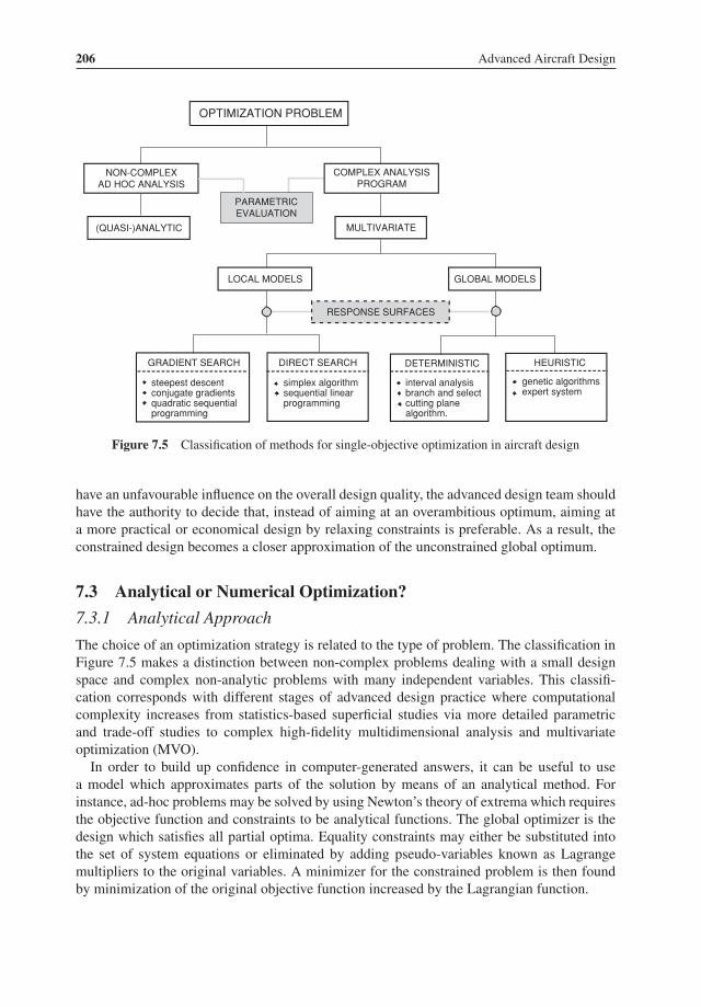
206 Advanced Aircraft Design
GRADIENT SEARCH DIRECT SEARCH HEURISTIC
steepest descentconjugate gradientsquadratic sequentialprogramming
DETERMINISTIC
MULTIVARIATE
COMPLEX ANALYSISPROGRAM
OPTIMIZATION PROBLEM
NON-COMPLEXAD HOC ANALYSIS
PARAMETRICEVALUATION
LOCAL MODELS GLOBAL MODELS
RESPONSE SURFACES
(QUASI-)ANALYTIC
simplex algorithmsequential linearprogramming
interval analysisbranch and selectcutting planealgorithm.
genetic algorithmsexpert system
Figure 7.5 Classification of methods for single-objective optimization in aircraft design
have an unfavourable influence on the overall design quality, the advanced design team shouldhave the authority to decide that, instead of aiming at an overambitious optimum, aiming ata more practical or economical design by relaxing constraints is preferable. As a result, theconstrained design becomes a closer approximation of the unconstrained global optimum.
7.3 Analytical or Numerical Optimization?
7.3.1 Analytical Approach
The choice of an optimization strategy is related to the type of problem. The classification inFigure 7.5 makes a distinction between non-complex problems dealing with a small designspace and complex non-analytic problems with many independent variables. This classifi-cation corresponds with different stages of advanced design practice where computationalcomplexity increases from statistics-based superficial studies via more detailed parametricand trade-off studies to complex high-fidelity multidimensional analysis and multivariateoptimization (MVO).In order to build up confidence in computer-generated answers, it can be useful to use
a model which approximates parts of the solution by means of an analytical method. Forinstance, ad-hoc problems may be solved by using Newton’s theory of extrema which requiresthe objective function and constraints to be analytical functions. The global optimizer is thedesign which satisfies all partial optima. Equality constraints may either be substituted intothe set of system equations or eliminated by adding pseudo-variables known as Lagrangemultipliers to the original variables. A minimizer for the constrained problem is then foundby minimization of the original objective function increased by the Lagrangian function.

Aircraft Design Optimization 207
Table 7.1 Assessment of parametric surveys
AdvantagesTraditional method rooted in industrial practiceRelatively simple programmingDesigner keeps control over decisionsA priori choice of objective function is not requiredSensitivity of the design to off-optimum conditions remains visible
DisadvantagesFew selection variables can be handled – four to five at mostInsufficient to guarantee that (near-)optimum is identifiedMany designs are computed, few are actually usedThe analyst is not encouraged to extend the searchChanges in design (requirements) make most results obsolete
An interesting strategy is geometric programming (GP) which applies to a special categoryof problems based on monomial and posynomial functions. A monomial has the form
f (x) = c xa11 xa2
2 . . . . xann (7.5)
where c > 0 and ai ∈ R. A sum of one or more monomials is called a posynomial function. Anearly publication on GP is found in [1], a recent overview is published in [60]. An applicationof GP to aircraft design is imaginable in the form of minimization of a posynomial consist-ing of weight components derived from regression analysis of statistical data. However, theuse of statistical equations is not always recommended since they may give a false impressionof design sensitivity.Parametric surveys (Table 7.1) are derived from a non-complex and well-organized set of
equations enabling the analyst to compute and visualize response surfaces with constraintsincluded. An example is depicted in Figure 1.9. This approach allows a flexible way of explicitoptimization and decision-making. Compared to automated design which gives little insight,parametric surveys are useful to explain the sensitivity of a design to non-optimal designvariables. They are also useful for investigating the effects of varying design constraints andfor technological or trade-off studies. However, such investigations are feasible only for aproblem with not more than five selection variables.
7.3.2 Multivariate Optimization
Multivariate optimization (MVO) is a powerful tool if the AD team uses a validated computer-assisted design sizing and analysis system. For comprehensive optimization tasks it is necessaryto use amathematical techniquewhich can handle a large range of selection variables – betweenten and thirty, typically. The module containing a suite of available MVO algorithms shouldbe loosely coupled to the design sizing program. The scheme in Figure 7.5 makes a distinctionbetween local and global models.
• Local models proceed in a stepwise manner. They start at an initial guessed point, computea new control vector pointing in a direction which improves the design. A design under

208 Advanced Aircraft Design
Table 7.2 Assessment of multivariate aircraft design optimization
AdvantagesRigorous approach, may potentially lead to improved design qualityMinimum occurrence of biased decisionsThe only viable approach in the case of a non-conventional configurationChanges in the baseline design/requirements are readily accommodated
DisadvantagesProgramming and debugging are complicated and time-consumingConvergence problems may occurThe program may be stuck in a local instead of the global optimumSeveral algorithms may have to be tested before a sensible result is foundThere is no insight in the design sensitivity to primary design variablesInexperienced designers may produce unrealistic results
analysis during this process is called the active point. The search is ended when the objectivefunction becomes stationary in a local optimizer.
• Global models are aimed at identification of local as well as global optimizers. They makedirect evaluations of the objective function of (many) carefully selected designs distributedwithin the closed boundary domain. The processmay proceedwith optimization of a responsesurface approximation or by using a heuristics-based algorithm.
Automatic optimization greatly reduces the number of configurations to be analyzed andavoids the enormous waste of generating configurations that have to be rejected afterwards.Although an abundance of strategies for MVO have been investigated and published, not manyof them have been tested in a realistic aircraft design environment. Introduction of MVO isoften associated with so many computational pitfalls and failures that finding a mathematicallyexact and reliable solution appears elusive. Although the use of automated optimization hasfound applications in many technical design disciplines, including aerospace design, MVOmethods continue to have disadvantages. They are intrinsically difficult to program and debug,the optimization algorithms are not always effective, and convergence problemsmaymean thatno solution is found. Dependent on the computational expense per configuration, the analystmay run into the problem of size which is associated with the large-scale and complexity. Itis concluded from the overview of the pros and cons of MVO in Table 7.2 that a decision toapply MVO to an optimization problem must be thoroughly prepared.Certain complex non-analytic problems are well behaved; that is, the objective function
varies smoothly with each independent variable. In this case, algorithms known as indirect orgradient search are likely to locate the optimum most rapidly. Gradient methods use calculus-based information to find local derivatives of the objective function known as sensitivityinformation. This is used to form a local model of the problem in a region near the activepoint. Local models are low-degree polynomials designed to approximate the true objectiveand constraint functions. They are used to derive the control vector pointing in the directionof the nearest local minimizer. Every step to a new active point is normal to the local contourcurve of the objective function.

Aircraft Design Optimization 209
start
X1
(a) gradient search (b) direct search
X1
X2
start
step taken
step explored
Figure 7.6 Comparison between steepest descent and direct search methods for unconstrainedoptimization
7.3.3 Unconstrained Optimization
Unconstrained optimization using gradients is illustrated in Figure 7.6 (a) showing a stepwisesearch starting at an initial guessed set of independent variables. The explored steps are used tofind the optimizer by means of a local approximation model. Moving along the steepest slopeof the local response surface approximation improves the local objective and is found by one-dimensional probing in the orthogonal directions of the variables. If quadratic polynomials areused to approximate the response surface, its local curvature can be used to derive the Hessianmatrix and the optimal step size. This leads to a more efficient search at the cost of increasedcomputational effort. The process proceeds along steps with continuously varying directionsand step size, until no improvement is obtained. This method is known as the steepest descentalgorithm. To a large extent, the gradient search path is determined by the location of thepartial optima, depicted by the dotted lines.Dependent on the location of the starting point, the gradient search can be a slowly converg-
ing process. The conjugate gradient algorithm uses information from the previous iterationsteps which improves the convergence considerably. In principle, gradient search identifiesan exact solution of the local optimizer. Gradient methods are often applicable in conceptualdesign because many problems are well behaved due to the simple and continuous mathemat-ical models used. In more complex programs, however, indirect search methods may get stuckin a local optimum. It is advantageous to start the gradient search with a design point that isexpected to be feasible. Since a gradient method identifies a local optimizer, it is advisable torepeat the process by starting the search at different points. A more serious problem occurswhen the response surface exhibits kinks or discontinuities caused by a transition betweendifferent design criteria applying in different regions of the design space. Another difficulty iscomputational noise that occurs when complex multidisciplinary computational systems areinvolved. Many engineering optimization problems are of these awkward types, and predicting

210 Advanced Aircraft Design
their behaviour is difficult. In these situations some form of direct search may perform bettersince it uses only (objective) function information to find a global optimum.Direct search methods are useful when local design sensitivity information is lacking since
they do not make use of objective function derivatives. Instead, direct search methods merelygenerate a number of designs and use a direct search algorithm to identify a local optimum.A typical direct method is sequential linear programming (SQL) which approximates theobjective function and the constraints by a first-order Taylor expansion. The resulting linearconstrained problem can be solved with standard methods such as the widely used simplexalgorithm [25]. Figure 7.6(b) shows an example of direct local search with steps taken inorthogonal directions of the independent variables. Starting at the initial guessed point, initialsteps are a line-search in the direction of one axis until the objective is no longer improving. Theline-search then proceeds along the other axis. At the point where the object function becomesstationary, the first variable is no longer on its partial optimum and the next step is resumed inthe original direction. In the present example, the final steps are zigzagging between the twopartial optima, indicating slow convergence. Although direct search methods do not providean exact solution, they are reliable and robust in terms of convergence. However, the directmethod approach needs expensive design analysis for every step of the optimization algorithm.
7.3.4 Constrained Optimization
An efficient method of constrained optimization using gradient search is sequential quadraticprogramming (SQP). A calculus-based algorithm is used to find a local quadratic approxima-tion of the objective function subject to a linear approximation of the constraints (Figure 7.7).SQP uses the gradient method to search for the steepest gradient at the (feasible) active pointS and then performs a line search in that direction. As soon as the active point reaches theunfeasible region of a constraint, the search direction is changed and continued along thelocal constraint function until the design reaches the constrained optimizer C. This processgenerally leads rapidly to the optimizer, provided the starting point is suitably chosen. Animplementation of the SQP code can be found in [38]. Like all gradient methods, SQP is
x2
x1
g
g
Figure 7.7 Geometric interpretation of the SQP method for two independent variables

Aircraft Design Optimization 211
only useful in problems which do not produce discontinuities of the response surface and itsderivatives such as ridges and sharp bends. The method is also sensitive to a computationalnoise error on the derivatives inherent to the solution of complex numerical analysis such asCFD and FEM methods. Applications in aircraft design are reported in [41, 50].Several algorithms try to cast the constrained problem as an unconstrained one and then use
one of the algorithms from that category. They make use of a penalty function which adds apenalty on the objective in the region where constraint violation occurs. A pseudo-objectivefunction created from the original objective by adding the imposed penalty is subsequently opti-mized. This method is known as a sequential unconstrained minimization technique (SUMT).An alternative approach uses the Kreisselmeier-Steinhauser (KS) method to replace the con-straint and objective function boundaries in the design space with a single surface [43]. TheKS method is based on a continually differentiable function,
KS(X ) = 1
ρln�K
k=1 exp{ fk(X )} (7.6)
where fk(X ) is a set of K objective and constraint functions. The parameter ρ controlsthe distance of the KS function surface from the maximum value of this set of functionsevaluated at X . This envelope function formulation effectively converts a constrained problemto an unconstrained single-objective formulation which can also be useful for multileveloptimization to be discussed later.
7.3.5 Response Surface Approximation
Direct methods are used for searching for the global optimizer of the complete design domain.They are not based on a stepwise improvement of active points but evaluate a (usually large)number of design points obtained by carrying out exact analysis. However, since computationof the complete response surface increases exponentially with the size of the problem, it maybe considered (a) to simplify the design analysis model or (b) to simplify the search process.The first option may lead to an inaccurate response surface – which is probably unacceptable –whereas the second option may or may not lead to an inaccurate optimizer, an uncertainty thatmay be acceptable. Therefore, methods have been developed which potentially generate anapproximation of the ‘real optimum’. Compared to integration of the detailed and expensivehigh fidelity analysis into the optimization algorithm, approximation models require a modestnumber of direct and exact evaluations which is computationally inexpensive. By performingthe simulation a priori, the simulationmodel is effectively separated from the surface fitting andoptimization efforts. This enables the analyst to run these processes sequentially andmakes thecomplete procedure versatile. An early example of an application to turbofan engine selectionis found in [26].Approximation models for response surfaces replace the expensive simulation codes in
the analysis process and thereby reduce computational costs. They approximate the trueresponse surface by a simple function of the independent variables. The approximation startsby computing the objective and constraint functions at a number of sample points, carefullyselected by a suitable method of experimental design;1 thereafter, they are all approximatedusing different response surface fits. Approximation models are typically based on low-degree
1In this context, ‘design’ means the method for selecting sample points rather than the original engineering problem.

212 Advanced Aircraft Design
polynomials with coefficients for the terms derived from regression on the true functionvalues. The surface fit is tested by means of statistical evaluation and after its acceptance theoptimization itself proceeds with gradient search on the response surface fit using one of thealgorithms from that category. The global response surfaces identify local as well as globaloptimizers and provide designers with insight into the behaviour of complex phenomena. Forinstance, a screening process can be used to eliminate variables from the design problemwhichappear to have little effect on the objective.
7.3.6 Global Models
Global optimization is the field of mathematics that studies extremal locations of non-convexfunctions which have many different local optima. Due to the high complexity of globaloptimization, its execution is computationally very costly and the method has not yet foundwidespread application to advanced airplane design. Therefore, the following overview issuperficial and concentrates on the two basic classes of algorithms.
1. Deterministicmethods take advantage of the analytical properties of the problem to generatepoints that converge to a global optimizer. Examples are branch and select algorithms,cutting plane algorithm, interval analysis and dynamic programming.
2. Heuristic methods are basically rules of thumb that hopefully will provide a good answer.They have been found to be more flexible and efficient than deterministic methods.
Since the quality of the solution obtained with a heuristic method cannot be guaranteed,application is not advised for problems where good conventional methodologies exist. This isespecially true if the knowledge can be expressed in terms of mathematical models. Neverthe-less, successful applications of heuristic optimization techniques to aircraft design have beenpublished for genetic algorithms and expert systems.Genetic algorithms perform design optimization by using Darwin’s survival of the fittest
model of manipulating long bit strings as the analogy for the genes of replicating individuals.Analogous to a natural population, the starting point is a collection of designs, each witha different set of selection variables mapped into the bit strings. Progress towards a ‘fitterpopulation’ is made by iteratively ‘mating’ promising bit strings to form new bit stringsand by randomly ‘mutating’ bit strings. Genetic algorithms are relatively easy to implementand have the advantage that they do not get stuck in local optima of convoluted responsesurfaces. However, they do not guarantee a global optimum andmay require too many functionevaluations to yield a satisfactory approximate solution. See [9] for a detailed description ofgenetic algorithms and [74] for an application to a supersonic airliner design.An expert system is a method from the field of artificial intelligence (AI) explicitly based
on the problem-solving ability of human experts. Experts systems are based on an amorphousobject-oriented data base known as a rule base or knowledge base2 and on a single modulecalled an inference engine. The inference engine has control over the execution of rulescontaining declarative statements about objects relevant to the application. The relevance ofexpert systems to optimization lies in the potential to manipulate formalized knowledge about
2Expert systems for application in the design field are also known as knowledge-based engineering (KBE).
Aircraft Design Optimization 213
objects. Objects can be physical (aircraft) components, data structures, values of parametersor design procedures. See [94] for an application to aircraft design.
7.4 Large Optimization ProblemsThere is the risk that you gradually expand all your variables and parameters and then find thatmost of them are irrelevant anyhow and that the most important one is somewhere else. It will bea long job to establish the viability of total optimization.
—R. Cockburn [23]
Since the early 1980s, a new field of research has been explored to overcome the challenge ofintegrated analysis and optimization of artifacts represented by complex engineering systems,withmultidisciplinary optimization (MDO) of an aircraft design forming a prominent example.The outcome is inherently compatible with the way engineers cooperate in a design organi-zation with distributed computing capabilities. Prominent contributions to MDO technologyhave been delivered by J. Sobieszczanski-Sobieski and his co-workers at NASA Langley.During the past decennia, MDO has been developed on the basis of a considerable theoreti-cal framework and a multitude of practical applications into a powerful tool in the hands ofdesigner teams. MDO has sparked intense interest from industry as well as the research field.3
MDO has thoroughly changed the way in which design is being organized and it is justified torefer to it as a new engineering discipline [72].Computer simulations of steadily increasing power are becoming available for modelling
a wide variety of physical phenomena. In the advanced design (AD) environment, these sim-ulations enable the engineer/analyst to learn more about the processes and physics involvedthan they have been able to learn from physical experiments. However, in view of their com-plexity, sizing and optimization programs have traditionally been developed and maintainedby specialists in isolation from what is done in other technical fields. As a result, the opti-mization process consisted of sequential disciplinary activities leading to sub-optimization,computational inefficiency and project delays. In today’s state of practice, the methodologyof multidisciplinary analysis and optimization coherently exploits the synergism of mutuallyinteracting computational domains to improve the design of complex engineering systems.
7.4.1 Concept Sizing and Evaluation
Conceptual design involves the exploration of alternate concepts to satisfy vehicle designrequirements. Concept sizing can be described as a program for determining the geometry,weight, performances and other physical characteristics of a design complying with a specifiedmission, including constraints on its feasibility. Basic constituents of a concept sizing programare: (1) a data processing system; (2) contributing disciplinary analysis programs; (3) a userinterface for configuration control and evaluation; and (4) a suite of optimization algorithms.Figure 7.8 illustrates how a broad range of disciplines are interacting in a conceptual sizingprogram. The outcome of the process is defined in terms of flight performances, flying qualitiesand economical figures of merit.
3The steadily growing body of literature on MDO is too large to be completely cited in this chapter’s bibliography.Progress is reported every two years at AIAA/ISSMO conferences.
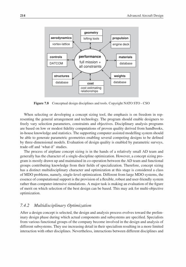
214 Advanced Aircraft Design
performance
full mission +all constraints
propulsion
materials
weights
cost
structures
controls
aerodynamics
geometry
lofting tools
engine deck
database
database
cost estimatingrelationships
database
DATCOM
vortex-lattice
Figure 7.8 Conceptual design disciplines and tools. Copyright NATO STO - CSO
When selecting or developing a concept sizing tool, the emphasis is on freedom in rep-resenting the general arrangement and technology. The program should enable designers tofreely vary selection parameters, constraints and objectives. Disciplinary analysis programsare based on low or modest fidelity computations of proven quality derived from handbooks,in-house knowledge and statistics. The supporting computer assisted modelling system shouldbe able to generate parametric geometries enabling several competing designs to be definedby three-dimensional models. Evaluation of design quality is enabled by parametric surveys,trade-off and ‘what-if’ studies.The process of airplane concept sizing is in the hands of a relatively small AD team and
generally has the character of a single-discipline optimization. However, a concept sizing pro-gram is mostly drawn up and maintained in co-operation between the AD team and functionalgroups contributing knowledge from their fields of specialization. Therefore, concept sizinghas a distinct multidisciplinary character and optimization at this stage is considered a classof MDO problems, namely, single-level optimization. Different from large MDO systems, theessence of computational support is the provision of a flexible, robust and user-friendly systemrather than computer-intensive simulations. A major task is making an evaluation of the figureof merit on which selection of the best design can be based. This may ask for multi-objectiveoptimization.
7.4.2 Multidisciplinary Optimization
After a design concept is selected, the design and analysis process evolves toward the prelim-inary design phase during which actual components and subsystems are specified. Specialistsfrom various functional groups of the company become involved in the design and analysis ofdifferent subsystems. They use increasing detail in their specialism resulting in a more limitedinteraction with other disciplines. Nevertheless, interactions between different disciplines and

Aircraft Design Optimization 215
Table 7.3 Information science and technology associated with MDO based on the discussion bySobieszczanski-Sobieski [72]
Information science Design-orientedand technology multi-disciplinary analysis MDO
product data models mathematical modelling discipline optimizationdata and software standards trading cost vs. accuracy decompositiondata management, storage, smart re-analysis design space searchand visualization sensitivity analysis approximationssoftware engineering practices optimization procedureshuman interface
between disciplines and the total vehicle system remain essential. Multidisciplinary optimiza-tion (MDO) can be described as a methodology for the optimum design of systems where theinteraction between several functional groups must be considered and where a designer in onefunctional group is free to significantly affect the performance in other disciplines [73] and atthe system level. In the design of complex engineering systems such as aircraft, multidisci-plinary interactions are prominent in the organization of integrated product development (IPD)in general and MDO in particular. Subjecting such a system to all-out optimization would leadto an unmanageable data flow and/or a very expensive computational process.Table 7.3 is a taxonomy of theMDO discipline. A prerequisite forMDO is the availability of
parametric product data models (PDMs) forming the basis for the geometry and discretizationmodels that are consistent across the disciplines [76]. In order to integrate MDO programsinto an aircraft design effort, an analysis and optimization process has to be realized thataccounts for the effects of mutual interactions of several engineering disciplines. An essentialfeature required for MDO is that a good system control software exists for communication andtransfer of data between the functional groups involved. In principle, the MDO methodologycan be used at any design stage although its complexity does not justify application in theearly conceptual phase. A great deal of effort is presently being devoted to making MDOmethods utilitarian for preliminary aircraft design by including manufacturing considerationsand constraints, and estimations of cost implications in the analysis.
7.4.3 System Decomposition
The MDO methodology is based on a formal method for analysis and optimization of largeengineering systems by system decomposition introduced in the 1980s [61, 65]. A largeoptimization task is decomposed into a set of smaller (less dependent) subtasks that can besolved concurrently while preserving the interactions between them (Figure 7.9). Dependenton the problem structure, the subtasks are arranged in hierarchical levels with the assembledsystem at the top level. Sub-domain processes are carried out receiving inputs from othersub-domains and optimizing on a local level. The system level process controls the exchangeof object and constraint function information between sub-domains. Decomposition methodsare aimed at identifying the best sequence of disciplinary sub-processes resulting in maximum

216 Advanced Aircraft Design
system level optimization
creation of engineering design directives
mathematicalformulation
engineeringand physicalformulation
mathematicalformulation
sub-domainoptimization
results
sub-domainoptimization
results
sub-domainoptimization
results
parametric survey(sensitivity analysis)
parametric survey(sensitivity analysis)
parametric survey(sensitivity analysis)
optimization specialist
domain specialist domain specialist domain specialist
Figure 7.9 Schematic overview of a large industrial bi-level integrated system optimization process.In reality, the number of sub-domains is much higher than three. Adapted from [80]
computational efficiency through minimizing the number of iteration steps. The principle ofdecomposing enables the analysis and (gradient-based) optimization to be performed concur-rently and independently, accounting for the effects of changing a parameter in one subsystemon parameters of the other subsystem. It turns out that decomposing the optimization problemhas the following advantages:
• enhanced insight into the communications between subsystems;• enhanced insight into the design space and how the optimum is achieved;• functional groups handle optimizers and sensitivity information of subsystems;• flexibility in the choice of dependent and independent variables; and• flexibility in choosing the methods of analysis for each subsystem.
System decomposition is in line with procedures in the industry where collaborative engi-neering is a fact of life and it can be facilitated by using tools from system engineering.The design process of a technical system can be represented by a compact matrix form thatvisualizes and optimizes the flow between subsystems. A well-known representation is thedesign structure matrix (DSM) or N 2 diagram, with N denoting the number of subsystems.As an example, Figure 7.10 depicts a small DSM with subsystems (or design tasks) arrangedon the diagonal. The order of execution of the subsystems is reflected by their position on thediagonal, starting top left and ending bottom-right. Feed-forward relations are characterizedby dots above the diagonal, dotted feedback entries are located below the diagonal. The posi-tion of the subsystems along the diagonal has a significant impact on the effectiveness of thecomputational process. Partitioning algorithms and/or common-sense judgement are used torearrange the positions of the subsystems in order to remove as many feedback relations as

Aircraft Design Optimization 217
S8
S7
S6
S5
S4
S3
S2
S1
1 2 3 4 5 6 7 8
1
2
3
4
5
6
7
8
Figure 7.10 Example of a simple DSM [92]. Subsystem 4 provides input to subsystems 2 and 8, andit receives input from subsystems 5, 6 and 8
possible, thereby minimizing the number of computational iterations. For instance, when thepositions on the diagonal of tasks 6 and 7 are reversed, the feedback is transformed into amore preferable feed-forward. However, real-life design problems can be too complicated tocapture the computational process in a nicely arranged DSM.
7.4.4 Multilevel Optimization
It appears beneficial to separate the design variables and constraints local to a sub-domainfrom those that govern the entire system. Multilevel optimization is a methodology to exploitdisciplinary optimization of a decomposed system. In a collaborative setting, multilevel opti-mization is becoming part of the MDO toolbox aimed at dividing the total optimization intosub-domain optimizations and coordinating them at the system level. This method coordinatesthe information flow from various sub-domains, all having their specific definitions of theobjective function and of the sensitivity of one disciplinary optimum to varying the input fromother disciplines.The number of analysis variables and design variables is adding up with each additional
discipline. Although a single-objective function may be used for each sub-domain optimiza-tion, the entire system optimization requires multiple objectives with an attendant increasein computational expenses. This problem may be further magnified when MDO has to beused at the system level. Consequently, it is not surprising that in the industrial environmentmuch attention is paid to bi-level optimization, featuring a system level that coordinates a setof subsystems which are not decomposed. Examples of bi-level optimization strategies arebi-level integrated system synthesis (BLISS) and collaborative optimization [83, 89].In spite of significant progress made so far, the organizational challenges to realize MDO
optimization in the distributed and highly diversified environment such as the aircraft industryremain formidable. An industrial setting of bi-level optimization as depicted in Figure 7.9taking advantage of interdisciplinary interactions requires specific briefing processes for coor-dination between specialists in the joint disciplines. The basis for any optimization task isa well thought-out problem definition. Such a strategy is needed because the computational

218 Advanced Aircraft Design
multidisciplinary capability is usually difficult to develop and expensive. A clear statementof the design variables and their allowable ranges, constraints and the objective function(s) istherefore necessary. The appropriate strategy depends on such factors as:
• the mix of continuous and discrete variables;• the strength of the interdisciplinary interactions;• separability of the constraints with respect to the design variables;• susceptibility of the analysis tools to algorithmic noise;• computational requirements of the analysis; and• compatibility of the MDO strategy with the existing organizational structure and culture.
7.4.5 Multi-Objective Optimization
In order to reduce design time, conceptual sizing programs (Section 1.5) are equipped withautomated communication between disciplines. Each discipline may select its own set ofdesign objectives and constraints. In such a setting it is unavoidable that conflicts betweenthe interests of different disciplines must be settled. Obviously, this problem has to be solvedat the system level where a suitable weighting method must be conceived. The challengeis to develop a strategy for making a trade-off between different sub-domain optimizationobjectives and simultaneously complying with all constraints applying to these sub-domains.This inherently complicated problem, known as multi-criteria or multi-objective optimization(MOO), is even more difficult to solve when components of the system objective have differentunits of measure. Since it is easier to compare objective values than to compare design vectors,MOO deals with the objective space rather than the design space. Designers must be awarethat aircraft designs optimized for different objectives may have quite different geometric,technical and performance properties.Multi-objective optimization in aircraft design considers all conflicting design objectives
and constraints simultaneously to meet mission requirements and other design drivers, suchas those mentioned in Table 2.1. An approach to this topic is discussed in [45] which includesan application to the conceptual design of a typical wide body transport aircraft. One of thesolutions studied is based on the Kreisselmeier-Steinhauser (KS) function defined by Equation(7.6). Multidisciplinary methods for preliminary design require MOO at the system level totrade off the multiple objectives used in different participating sub-domains [63]. Arguably,adaptation of the KS method to application in MDO appears to be a viable approach [64].Early applications of MOO to pre-conceptual technology assessment are discussed in [32]
and [33]. The second of these publications compares figures of merit such as direct operat-ing costs (DOC) – which emphasizes speed – and acquisition costs which emphasizes emptyweight. These figures are affected in a different way by selection variables such as cruise Machnumber, wing planform parameters and engine thrust. Figure 7.11 depicts a number of designsoptimized for different figures of merit in a two-dimensional objective space with mission fueland life cycle costs (LCC) divided by productivity (PROD) along the axis.What is referred to asa ‘merit trade boundary’ is comparable to the widely known concept of the Pareto front. In thepresent example, two Pareto-optimum designs are at the extreme ends of the trade boundary.Theminimum fuel design has a largewing of very high aspect ratio, cruises at a lowMach num-ber and has a high LCC compared to its productivity. The design with the lowest LCC/PRODratio achieves this at the cost of a 25% penalty in mission fuel and a high thrust/weight ratio.

Aircraft Design Optimization 219
FUEL
weighted penalty
equal penalty
ZERO PENALTY
FUEL(1,000 lb)
dollarston-mile/day
FLYACQ
LCC
LCCPROD
DOC
GW
LCCPROD
200
190
180
170
160
150
110 114 118 122 126 130 134 138
LCC/PROD : FUEL=4:1
FUEL : LCC/PROD=4:1
Figure 7.11 Merit trade boundary with different designs optimized for seven objective functions.Adapted from [33]
Designs optimized for minimum fly-away costs (FLY), acquisition costs (ACQ) and LCCare underpowered, cruise at a low altitude and are far away from the trade boundary of bestdesigns. Designs with the lowest GW and direct operating costs (DOC) are very similar to eachother and have the lowest overall penalty relative to the hypothetical zero penalty design. Thisexample illustrates clearly that multi-objective optimization requires the designer to have agood insight into the various trades. Especially when deciding design technologies, the choiceof a representative (weighted) objective function is of paramount importance.
7.5 Practical Optimization in Conceptual DesignThe most elegant automated optimization procedure is of very limited use to the designer who isnot familiar with setting an objective function and making allowances for uncertainties.
—U. Haupt, AIAA Paper No. 77-1244
7.5.1 Arguments of the Sceptic
In the industrial environment it is often argued that, in automation of a complex optimizationproblem, the danger exists that the designer will lose contact with the basic realities underlyingthe computerized procedures. This may result in failures of judgement and the acceptance ofunsuspected errors, leading in extreme instances to management by – rather than of – thecomputer. However, these kinds of objections made are a direct consequence of the greatestadvantages of rigorous optimization: the ability to deal with a large design space and identifyan optimum design outside the experience of an advanced design group.Automated optimization programs generate the best design for a single objective func-
tion whereas, in general, the designer likes to know more about the design than just the

220 Advanced Aircraft Design
mathematical optimum. For example, if the optimum is highly constrained by some fieldperformance requirement, it makes sense to look at progressively relaxing this constraint,improve the technology level or change some design parameter that has been treated as apre-assigned parameter. One desirable feature is therefore that the computer program allowsvisual inspection of the response surface in the region near the optimum design.
7.5.2 Problem Structure
The design sizing process discussed in Section 1.4 does not provide enough detail to draw upa universally valid sequence of steps according to which synthesis problems can be attacked.The engine-to-airframe matching problem may serve as a typical example.
• If the top-level requirements have to be fulfilled with pre-selected engines of an existing (orprojected) type, the process will proceed differently from the case where study engines canbe varied in power to match the airframe in an optimum fashion.
• In the real world of civil aircraft design, the situation may be a mixture of both cases: a clean-sheet aircraft or a derivative of an existing type is developed alongside existing airliners orbusiness jets which have similar engines installed.
• Aircraft are rarely designed in complete isolation and their engines may be future derivativesof types optimized for existing fleets.
• Airliners may also be offered to the customer with a choice of alternative (competing) enginetypes.
• A study of turbofan engine cycle parameters – for instance, bypass ratio and overall pressureratio – can be carried out in order to generate information for an airplane design conceptstudy.
The concept sizing program should be sufficiently flexible to copewith these and other problemstructures.
7.5.3 Selecting Selection Variables
The number of selection variables increases greatly as the designer goes into more detail. Sincedesigners cannot afford to dissipate their resources on optimization of secondary parameters, ajudicious classification of selection variables is important. To take an example: why optimizewing rib pitch if the wing aspect ratio is still being varied? It appears useful to make adistinction between the selection variables affecting the aircraft’s configuration definition andthe control parameters affecting the operation of a given aircraft. For example, it is temptingto treat the lift coefficient in cruising flight as a selection variable since experienced designersusually have a good feeling for its (optimum) value. This leads to the following considerations.
• Vertical equilibrium in steady level flight requiresW = L = 1/2ρV 2SCL . For a given grossweight, cruise altitude and flight speed, the lift coefficient and wing area are interrelated andcannot be used simultaneously as independent variables.
• Since the take-off gross weight is different for flight profiles deviating from the designmission, there exists no unique cruise lift coefficient.

Aircraft Design Optimization 221
• The gross weight varies with time during the flight.• If ‘the lift coefficient’ is treated as a selection variable, it is not obvious how wing drag andstructure weight are affected by its variation.
Consequently, treating a control parameter as a selection variable may introduce unforeseeneffects if one is not fully aware of the problem structure. A similar argument applies to the(initial) cruise altitude. The present example shows that it is recommendable to consider (gross)wing area and engine thrust available as the primary selection variables.Selection of the cruise Mach number deserves special attention because it can be seen as
a selection variable as well as a control parameter. Treating the cruise Mach number as anindependent design variable has a distinct effect on the design sensitivity information, the(optimum) airframe geometry, the best type of propulsion and the installed engine power. Eco-nomic performances such as DOC and productivity are also sensitive to cruise Mach number.On the other hand, derivation of the best cruiseMach number of a fully specified aircraft is not atrivial task, as demonstrated in Chapter 12. Considering the cruise Mach number as a selectionvariable as well as a control variable adds an additional iteration loop to the synthesis pro-cess increasing computational expenses considerably. This explains why the desirable cruiseMach number is usually selected in the pre-conceptual study phase – henceforth, it is consid-ered a pre-assigned parameter. However, flight performance analysis treats the Mach numberseparately as a control variable which may take different values dependent on the mission.Certain design parameters are not usually selected by means of formal optimization for the
following reasons.
• The design sensitivity to their variation is difficult (or even impossible) to compute.• The impact of their variation on technical/economical quality of the aircraft is negligible.• There is no generally accepted criterion for design quality; hence, a single figure of merit isof no value.
The selection of this category of design parameters is normally based on previous experienceand engineering judgement rather than rigorous computations. A typical example is the wingtaper ratio. Design experience shows that, from the aerodynamic/structural point of view, thetaper ratio usually optimizes at unrealistically low values. Instead of making a considerableeffort to establish the design sensitivities, it makes sense to assign a lower constraint totaper which is likely to avoid premature outer wing stalling or shock stall. Although suchan approach may slightly penalize empty weight and drag, it is unrealistic to expect that, forexample, acceptable stalling behaviour can be incorporated in an analytical objective function.During the first optimization cycle of a civil airliner or business aircraft, the following
parameters are the most appropriate candidates to become selection variables.
• Total engine take-off power Pto or thrust Tto normalized to sea level static (SLS) conditionsin the ICAO standard atmosphere (ISA). Alternatively, thrust-to-weight ratio TTO/WTO orthrust loading WTO/TTO is often used for jet aircraft. The power-to-weight ratio PTO/WTO
or the power loading WTO/PTO is mostly used for propeller aircraft.• Wing area Sw or take-off wing loadingWTO/Sw.• Wing span bw or aspect ratioAw = b2w/Sw.• Wing sweep angle �w.• Wing thickness ratio t/c at the root and at the tip, or a mean value of these.

222 Advanced Aircraft Design
Even if only these five or six parameters are varied with ten values per variable, the designspace will consist of 105 or 106 different designs. It goes without saying that designing andevaluating so many designs – even at the conceptual level – would require an immense effort.It is therefore obvious that alternative approaches are applied such as those introduced in thefollowing chapters.
7.5.4 Design Sensitivity
Optimization is useful only when all the relationships between the design variables and theobjective function affected by these variables are sensitive to the variations in the design duringthe sizing process. Although this condition forms a significant complication to the optimiza-tion process, much can be done to reduce computational expenses. Analysis methods builtinto sizing analysis routines are often of low to medium fidelity but they must be sufficientlydetailed to provide meaningful trade-offs and sensitivities. Although weight prediction meth-ods based on statistics are commonly used in conceptual design, they may be inappropriatefor optimization since the statistical variation of component weights is based on regressionanalysis which is not necessarily functionally related to the selection variables. The use ofstatistics is therefore acceptable only in computations which do not affect the results of theoptimization. For instance, statistics can be used to predict the weight of components suchas cabin furniture, operational items and several on-board system components which are notaffected by variation of the wing shape.Design sensitivity can be defined as the percentage change in a performance measure due
to a percentage change in some parameter. An important output of any synthesis programis sensitivity information permitting an assessment of critical areas. Subsystem inputs toconfiguration optimization must be of sufficient technical depth to accurately reflect the effectsof subsystem changes on geometry and behaviour variables. To take one (admittedly ratherextreme) example: airliner wing structural weight is statistically close to 12% of the MTOW,a simple rule of thumb which can be useful for an initial estimation. Such a rule of thumbdoes, however, not reflect the effects on wing weight of geometry variations such as wingsize, low or high aspect ratio, and thick or thin sections. Wing design optimization demands amuch finer tolerance than statistical equations can guarantee in spite of their proven absoluteaccuracy. Consequently, a weight prediction method which is to be used for optimum wingdesign must be essentially design sensitive. This does not exclude the use of statistics sinceempirical and statistical data are indispensable to calibrate the absolute accuracy to reality.
7.5.5 The Objective Function
The all-important selection of the objective function can be problematic, as illustrated by thefollowing example. Suppose that the designer attempts to reduce the fuel consumption byincreasing the wing span. From the calculations he will conclude that a low wing structuraland empty weight are obtained for a small span. Minimum fuel and empty weight are bothdesirable properties, but since they are conflicting objectives, they cannot be realized in thesame design. The traditional figure of merit in conceptual design has been the MTOW, whichsolves the problem to some extent. Moreover, the MTOW is an essential property which hasto be computed accurately for many purposes other than optimization.

Aircraft Design Optimization 223
During the optimization it will also be observed that the installed engine thrust required andpropulsion system weight follow similar trends as the fuel weight. Minimizing the MTOW is,therefore, rational if mission fuel and empty weight are assumed to be of equal importance.However, the economical importance of engine and fuel weights are different and minimizingtheir sum forms an oversimplification. Therefore, it is more rational to weigh them on thebasis of their contribution to operational costs. This requires a lot more depth of analysis,information and assumptions, and introduces the problem that fuel prices sharply fluctuate intime. And if two dissimilar criteria such as operational economy and atmospheric pollutionare competing, it appears desirable to consider both properties as objective functions. Again,this leads to multi-objective optimization.
Bibliography
[1] Duffin, R., E. Peterson, and C. Zener, Geometric Programming: Theory and Application, Wiley and Sons, NewYork, 1967.
[2] Wilde, D.J., and C.S. Beightler, Foundations of Optimization, Chapter 4, Polynomial Inequalities: GeometricProgramming, Prentice-Hall, Inc., Englewood Cliffs, NJ, 1967.
[3] Fox, R.L., Optimization Methods for Engineering Design, Addison-Wesley Publishing Company, Inc., MenloPark, CA, 1971.
[4] Burley, D.M., Studies in Optimization, Intertext Books, ISBN 0 7002 0248 X, 1975.[5] Gill, P.E., W. Murry, and M.H. Wright, Practical Optimization, Academic Press, New York, 1981.[6] Vanderplaats, G.N., Numerical Optimization Techniques for Engineering Design: with Applications, McGraw-
Hill Book Company, New York, 1984.[7] Box, E.P., and N.R. Draper, Empirical Model-Building and Response Surfaces, John Wiley & Sons, New York,
1987.[8] Farin, G., Curves and Surfaces for Computer Aided Geometric Design: A Practical Guide, Academic Press
Professional, Inc., San Diego, CA, USA, 1988.[9] Goldberg, D.E., Genetic Algorithms in Search, Optimization and Machine Learning, Addison-Wesley, Inc.,
Reading, MA, 1989.[10] Arora, J.S., Introduction to Optimum Design, Second Edition, Elsevier, San Diego, CA, 2004.[11] Horst, R., and P.M. Pardalos, Handbook of Global Optimization, Kluwer Academic Publishers, Dordrecht,
1995.[12] Vanderplaats Research & Development, Inc., DOT User’s Manual, Version 4.20, Colorado Springs, CO, 1995[13] Nocedal, J., and S. Wright, Numerical Optimization, First Edition, Series in Operational Research, Springer
Verlag, New York, 1999.[14] Honlinger, H. (ed.), CEAS Conference on Multidisciplinary Aircraft Design and Optimization, Maternushaus,
Koln, 25–26 June, 2001.
Optimization Techniques
[15] Krzywoblocki, M.Z., von, and W.Z. Stepniewski, “Application of Optimization Techniques to the Design andOperation of V/STOL Aircraft”, in Proceedings of the International Congress of Subsonic Aeronautics”, theNew York Academy of Sciences, NY, April 1967.
[16] Hague, D.S., and C.R. Glatt, “An Introduction to Multivariate Search Techniques for Parameter Optimization”,NASA CR-73200, April 1968.
[17] Stepniewski, W.Z., and C.F. Kalmbach, “Multivariate Search in Aircraft Design Optimisation”, Journal of theRoyal Aeronautical Society, Vol. 74, pp. 419–432, May 1970.
[18] Piggott, B.A.M., and B.E. Taylor, “Application of Numerical Optimization Techniques to the Prelimnary Designof a Transport Aircraft”, Royal Aircraft Establishment Technical TR-71074, April 1971.

224 Advanced Aircraft Design
[19] Kirkpatrick, D.L.I., “Review of Two Methods of Optimising Aircraft Design”, Royal Aircraft EstablishmentTM Aero-1423, June 1972; also AGARD LS-56, Paper No. 12, April 1972.
[20] Kirkpatrick, D.L.I., and D.H. Peckham, “Multivariate Analysis Applied to Aircraft Optimization – Some Effectsof Research Advances on the Design of Future Subsonic Aircraft”, RAE Technical Memorandum Aero 1448,September 1972.
[21] Beale, E.M.L., “Optimization Methods Based on Linear Programming”, Paper No. 2, Symposium on Optimiza-tion in Aircraft Design, The Royal Aeronautical Society, November 15, 1972.
[22] Hague, D.S., C.R. Glatt, and R.T. Jones, “Integration of Aerospace Vehicle Performance and Design Optimiza-tion”, AIAA Paper No. 72-948, September 1972.
[23] Bishop, A.W., “Optimisation in Aircraft Design: the Whole Aircraft” Paper presented at the Symposium onOptimisation in Aircraft Design, Royal Aeronautical Society, November, 1972.
[24] Kirkpatrick, D.L.I., and M.J. Larcombe, “Initial Design Optimisation of Civil and Military Aircraft”, AGARDCP-147, Vol. 1, Paper No. 19, October 1973.
[25] Olsson, D.M., “A Sequential Simplex Program for Solving Minimization Problems”, Journal of Quality Tech-nology, Vol. 6, No. 1, pp. 53–57, January 1974.
[26] Healy, M.J., J.S. Kowalik, and J.W. Ramsey, “Airplane Engine Selection by Optimization on Surface FitApproximations”, Journal of Aircraft, Vol. 12, No. 7, pp. 593–599, July 1975.
[27] Vanderplaats, G.N., “Automated Optimization Techniques for Aircraft Synthesis”, AIAA Paper No. 76-909,September 1976.
[28] Barman, J.F., and H. Erzberger, “Constrained Optimum Trajectories for Specified Range”, Journal of Aircraft,Vol. 30, No. 10, pp. 748–754, October 1976.
[29] Edwards, J.B., “The Use of Computer Based Optimisation Methods in Aircraft Studies”, AGARD CP-280,Paper No. 4, September 1979.
[30] Torenbeek, E. “Some Fundamental Aspects of Transport Aircraft Conceptual Design Optimization”, AGARD-CP-280, Paper No. 5, 1979.
[31] Dixit, C.S., and T.S. Patel, “Multivariate Optimum Design of a Subsonic Jet Passenger Airplane”, Journal ofAircraft, Vol. 17, No. 6, pp. 429–433, June 1980.
[32] Sliwa, S.M., “Use of Constrained Optimization in the Conceptual Design of a Medium-Range Subsonic Trans-port”, NASA Technical Paper 1762, December 1980. Also AIAA Paper No. 80-1095, 1980.
[33] Jensen, S.C., I.H. Rettie, and E.A. Barber, “Role of Figures of Merit in Design Optimization and TechnologyAssessment”, Journal of Aircraft, Vol. 18, No. 2, pp. 76–81, January 1981.
[34] Ashley, H., “On Making Things the Best: Aeronautical Uses of Optimization”, AIAA 44th Wright BrothersLecture in Aeronautics, AIAA Paper No. 81-1738, 1981; also Journal of Aircraft, Vol. 19, No. 1, January 1982.
[35] Collingbourne, J., “Multivariate Optimisation Applied to the Initial Design of Transport Aircraft”, RAE TR84044, 1984.
[36] Haberland, C., J. Thorbeck, and W. Fenske, “A Computer Augmented Procedure for Commercial AircraftPreliminary Design and Optimization”, ICAS Paper 4.8.1, 1984.
[37] Chacksfield, J.E., “Multivariate Optimization as Applied to Aircraft Project Design”, ICAS Paper 4.8.2, 1984.[38] Gill, P.E.,W.Murry,M.A. Saunders, andM.H.Wright, “User’s Guide for NPSOL (Version 4.0): A Fortran Pack-
age for Nonlinear Programming”, Technical Report SOL 86-2, Department of Operations Research, StanfordUniversity, January 1986.
[39] Alsina, J., J.P. Fielding, and A.J. Morris, “Progress Towards an Aircraft Design Expert System”, ComputerApplications in Aircraft Design and Operation, ComputationalMechanics Publications, Springer Verlag, Berlin,1987.
[40] Britton, C.L., and W.W. Jenkinson, “A Computer-Aided Design System for Airplane Configuration”, ComputerApplications in Aircraft Design and Operation, ComputationalMechanics Publications, Springer Verlag, Berlin,1987.
[41] Bil, C., Development and Application of a Computer-Based System for Conceptual Aircraft Design, doctoraldissertation, Delft University of Technology, Delft University Press, 1988.
[42] Simos, D., and L.R. Jenkinson, “Optimization of the Conceptual Design and Mission Profiles of Short-HaulAircraft”, Journal of Aircraft, Vol. 25, No. 7, pp. 618–624, July 1988.
[43] Wrenn, G.A., “An Indirect Method for Numerical Optimization Using the Kreisselmeier-Steinhauser Function”,NASA CR-4220, March 1989.
[44] Takai, M., “A New Architecture and Expert System for Aircraft Design Synthesis”, Stanford PhD thesis, June1990.

Aircraft Design Optimization 225
[45] Dovi, A.R., and G.A. Wrenn, “Aircraft Design for Mission Performance using Non-Linear Multi-objectiveOptimization Methods”, NASA CR-4328, 1990. Also AIAA Paper No. 89-2078.
[46] Jenkinson, L.R., “Regional Fanjet Aircraft Optimization Studies”, Journal of Aircraft, Vol. 30, No. 2, March–April 1993.
[47] Velden,A. van der, “Tools forApplied EngineeringOptimization”, AGARDReport No. 803,AGARD-FDP-VKISpecial Course, April 1994.
[48] Gallman, J.W., R.W. Kaul, R.M. Chandrasekharan, and M.L. Hinson, “Optimization of an Advanced BusinessJet”, AIAA Paper No. 94-4303-CP, September 1994.
[49] Lee, H., “Optimal Aircraft Trajectories for Specified Range”, Report ARC-11282, NASA, 1994.[50] Gage, P.J. “New Approaches to Optimization in Aerospace Design”, NASA Contractor Report 196695, March
1995.[51] Wakayama, S., and I.M. Kroo, “Subsonic Wing Planform Design Using Multidisciplinary Optimization”,
Journal of Aircraft, Vol. 32, No. 4, pp. 746–753, July–August 1995.[52] Cramer, E.J., “Numerical Methods for Aircraft Performance”, AIAA Paper No. 95-3879, September 1995.[53] Anderson, M.B., and G.A. Gebert, “Using Pareto Genetic Algorithms for Preliminary Subsonic Wing Design,”
AIAA Paper No. 96-4023, September 1996.[54] Obayashi, S., Y.Yamaguchi, and T.Nakamura, “Multi-objectiveGeneticAlgorithm forMultidisciplinaryDesign
of Transonic Wing Planform”, Journal of Aircraft, Vol. 34, No. 5, pp. 690–693, May 1997.[55] Roth, G.L., and W.A. Crossley, “Commercial Transport Aircraft Conceptual Design Using a Genetic Algorithm
Based Approach”, AIAA Paper No. 98-4934, 1998.[56] Pant, R.K., and J. Fielding, “Aircraft Configuration and Flight Profile OptimizationUsing SimulatedAnnealing,”
Aircraft Design, Vol. 2, No. 4, December 1999.[57] Jameson, A., “Re-Engineering the Design Process Through Computation”, Journal of Aircraft, Vol. 36, No. 1,
pp. 36–50, January–February 1999.[58] Willcox, K, and S. Wakayama, “Simultaneous Optimization of a Multiple-Aircraft Family”, AIAA Paper
No. 2002-1423, 2002.[59] Buonanno, M.A., and D.N. Mavris, “Aerospace Vehicle Concept Selection Using Parallel, Variable Fidelity
Genetic Algorithms”, paper presented at AIAA/ISSMO Multidisciplinary Analysis and Design Conference,August/September 2004.
[60] Boyd, S., S-J Kim, L. Vandenberghe, and A. Hassibi, “A Tutorial on Geometric Programming”, Optimizationand Engineering, (2007)-8, pp. 67–127, 2007.
Multidisciplinary Design and Optimization
[61] Sobiezczanski-Sobieski, J., “A Linear Decomposition Method for Large Optimization Problems: Blueprint forDevelopment”, NASA TM 83248, 1982.
[62] McCullers, L.A., “FLOPS: Flight Optimization System”, Recent Experience in Multidisciplinary Analysis andOptimization, Part 1, NASA CP-2327, pp. 395–412, April 1984.
[63] Sobiezczanski-Sobieski, J., J-F.M. Barthlemy, and G.L. Giles, “Aerospace Engineering Design by SystematicDecomposition and Multilevel Optimization”, ICAS Paper 84-4.7.3, September 1984.
[64] Sobiezczanski-Sobieski, J., A.R. Dovi, and G.A. Wrenn, “A New Algorithm for General Multiobjective Opti-mization”, NASA TM-100539, March 1988.
[65] Sobiezczanski-Sobieski, J., “Sensitivity Analysis and Multidisciplinary Optimization for Aircraft Design:Recent Advances and Results”, ICAS Paper 88-1.7.3, September 1988.
[66] Abdi, F., H. Ide, M. Levine, and L. Ausrel, “The Art of Spacecraft Design: a Multidisciplinary Challenge”,NASA Langley Research Center, Recent Advances in Multidisciplinary Analysis and Optimization, NASACP-3031, Part 3 pp. 1137–1155, 1989.
[67] Kirkpatrick, D.L.I, and J.S. Smith, “Multidisciplinary Optimisation in Aircraft Design”, ICAS Paper No. 90-2.3.1, September 1990.
[68] Consoli, R.D., and J. Sobiezczanski-Sobieski, “Application of Advanced Multidisciplinary Analysis and Opti-mization Methods to Vehicle Design Synthesis”, ICAS Paper No. 90-2.3.4, September 1990.
[69] Kroo, I., S., S. Altus, R. Braun, P. Gage, and I. Sobieski, “Multidisciplinary Optimization Methods for AircraftPreliminary Design”, AiAA Paper No. 94-4325, September 1994.
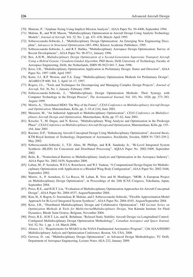
226 Advanced Aircraft Design
[70] Martens, P., “Airplane Sizing Using Implicit Mission Analysis”, AIAA Paper No. 94-4406, September 1994.[71] Malone, B., and W.H. Mason, “Multidisciplinary Optimization in Aircraft Design Using Analytic Technology
Models”, Journal of Aircraft, Vol. 32, No. 2, pp. 431–438, March–April 1995.[72] Sobieszczanski-Sobieski, J., “Multidisciplinary Design Optimization: An Emerging New Engineering Disci-
pline”, Advances in Structural Optimization (483–496), Kluwer Academic Publishers, 1995.[73] Sobieszczanski-Sobieski, J., and R.T. Haftka, “Multidisciplinary Aerospace Design Optimization: Survey of
Recent Developments”, AIAA Paper No. 96-0711, January 1996.[74] Bos, A.H.W., Multidisciplinary Design Optimization of a Second-Generation Supersonic Transport Aircraft
Using a Hybrid Genetic / Gradient-Guided Algorithm, PhD thesis, Delft University of Technology, Faculty ofAerospace Engineering, Delft, the Netherlands, ISBN 90-5623-041-7, June 1996.
[75] Kroo, I.H., “Multidisciplinary Optimization Application in Preliminary Design: Status and Direction”, AIAAPaper No. 1997-1408, April 1997.
[76] Korte, J.J., R.P. Weston, and T.A. Zang: “Multidisciplinary Optimization Methods for Preliminary Design”,AGARD CP-600, Vol. 3, April 14–17, 1997.
[77] Rogers, J.L., “Tools and Techniques for Decomposing and Managing Complex Design Projects”, Journal ofAircraft, Vol. 36, No. 1, January–February 1999.
[78] Sobieszczanski-Sobieski, J., “Multidisciplinary Design Optimization Methods: Their Synergy withComputer Technology in the Design Process”, The Aeronautical Journal, Vol. 103, No. 1026, pp. 373–383,August 1999.
[79] Morris, A., “Distributed MDO: TheWay of the Future”, CEAS Conference on Multidisciplinary Aircraft Designand Optimization, Maternushaus, Koln, pp. 3–18 of [14], June 2001.
[80] Meussen, M., “An Industrial Approach to Multidisciplinary Optimization”, CEAS Conference on Multidisci-plinary Aircraft Design and Optimization, Maternushaus, Koln, pp. 57–62, June 2001.
[81] Kriszler, T., M. Dugas, and N. Kresse, “Multidisciplinary Wing Analysis and Optimization in the PredesignPhase”,CEAS Conference on Multidisciplinary Aircraft Design and Optimization,Maternushaus, Koln, pp. 155–164, June 2001.
[82] Raymer, D.P., “Enhancing Aircraft Conceptual Design Using Multidisciplinary Optimization”, doctoral thesis,KTH-Royal Institute of Technology, Department of Aeronautics, Stockholm, Sweden, ISBN 91-7283-259-2,May 2002.
[83] Sobieszczanski-Sobieski, J., T.D. Altus, M. Phillips, and R.R. Sandusky Jr., “Bi-Level Integrated SystemSynthesis (BLISS) for Concurrent and Distributed Processing”, AQIAA Paper No. 2002-5409, September2002.
[84] Belie, R., “Nontechnical Barriers to Multidisciplinary Analysis and Optimisation in the Aerospace Industry”,AIAA Paper No. 2002-5439, September 2009.
[85] Laban, M., P. Arendsen, W.F.J.A. Rouwhorst, and W.J. Vankan, “A Computational Design Engine for Multidis-ciplinary Optimisation with Application to a Blended Wing Body Configuration”, AIAA Paper No. 2002-5446,September 2002.
[86] Morris, A., P. Arendsen, G. La Rocca, M. Laban, R. Voss and H. Honlinger, “MOB: A European Projecton Multidisciplinary Design Optimisation”, in Proceedings of the 24th ICAS Congress, Yokohama, Japan,September 2004.
[87] Perez, R.E., and H.H.T. Liu, “Evaluation of Multidisciplinary Optimization Approaches for Aircraft ConceptualDesign”, AIAA Paper No. 2004-4537, August/September 2004.
[88] Kim, H., S. Ragon, G. Soremekun, B. Malone, and J. Sobieszczanski-Sobieski, “Flexible ApproximationModelApproach for Bi-Level Integrated System Synthesis”, AIAA Paper No. 2004-4545, August/September 2004.
[89] Kroo, I.H., “Distributed Multidisciplinary Design and Collaborative Optimization”, VKI Lecture Series onOptimization Methods & Tools for Multicriteria/Multidisciplinary Design, Von Karman Institute for FluidDynamics, Rhode Saint Genese, Belgium, November 2004.
[90] Perez, R.E., H.H.T. Liu, and K. Behdinan, “Relaxed Static Stability Aircraft Design via Longitudinal Control-Configured Multidisciplinary Design Optimization Methodology”, Canadian Aerospace and Space Journal,Vol. 52, No. 1, pp. 1–14, March 2006.
[91] Alonso, J.J., “Requirements for MA&O in the NASA Fundamental Aeronautics Program”, 12th AIAA/ISSMOMultidisciplinary Anlysis and Optimization Conference, Reston, VA, USA, 2008.
[92] Gerwen, D. van, “Multidisciplinary Design Optimization”, in Advanced Design Methodologies, TU Delft,Department of Aerospace Engineering, Lecture Notes AEA-232, January 2009.

Aircraft Design Optimization 227
[93] La Rocca, G., and M.J.L. van Tooren, “Knowledge-Based Engineering Approach to Support Aircraft Multidis-ciplinary Design and Optimization”, Journal of Aircraft, Vol. 46, No. 6, pp. 1875–1885, November–December2009.
[94] La Rocca, G., and M.J.L. van Tooren, “Knowledge-Based Engineering to Support Aircraft MultidisciplinaryDesign and Optimization”, Proc. IMechE Vol. 224, Part G: J. Aerospace Engineering, February 2010.
Geometry Representation
[95] Samareh, J.A., “Survey of Shape Parameterization Techniques for High-Fidelity Multidisciplinary Shape Opti-mization”, AIAA Journal, Vol. 39, No. 5, pp. 877–884, May 2002.
[96] Kulfan, B.M., “Universal Parametric Geometry Representation Method”, Journal of Aircraft, Vol. 45, No. 1,pp. 142–158, January–February 2008.
[97] Ciampa, P.D., T. Zill, and B. Nagel, “CST Parametrization for Unconventional Aircraft Design Optimization”,ICAS Paper No. 2010-1.4.3, September 2010.

8Theory of Optimum Weight
Without doubt, weight and weight distribution, or balance, are of more importance in airplanedesign than in any other branch of engineering.
—T.P. Wright, quoted in [4], 1999
8.1 Weight Engineering: Core of Aircraft Design
Nowhere in the industry is the role of weight engineers in the design process as essential as inaircraft design. Weight engineering activities are initiated during the crystal ball phase of con-cept finding and they continue to form an essential part of conceptual, preliminary, and detaildesign. During the manufacturing, testing and certification phases of an aircraft programme,weight information is still being generated and used by all the program participants. Weightengineers are also active in supporting airlines during the operational deployment of deliveredaircraft and they are involved in the development of modifications and derivatives of the basicaircraft. The aircraft industry has traditionally derived relationships for airplane weight esti-mation in the design stage using accumulated statistical data for their validation and regressionmethods for correlating weight components to the most influential design parameters. Semi-empirical methods calibrated by statistics are still in use – they are normally augmented byanalytical relationships between component function, geometry, loads and sizing criteria. Agreat deal of effort has been expended in developing analytical weight prediction methods formajor structural elements, in particular, the wing. Dependent on the design phase, various lev-els of prediction accuracy vary between about 10% standard deviation in the early conceptualphase down to a few percent in the preliminary phase.Weight engineering activities in a new project gear up as soon as configuration details
become available, in particular during the aircraft balancing process. They become mostintensive when the general arrangement of the airplane has been defined and subsystems arein the detail design phase. Information obtained from the complete spectrum of disciplinarygroups involved in the development process are centralized and controlled by the weightmanagement group. A weight problem may appear during the detailed design phase oftenconsisting of excess subsystem weights compared to predictions. Such a situation must beaddressed by means of a comprehensive weight reduction program in which virtually the
Advanced Aircraft Design: Conceptual Design, Analysis and Optimization of Subsonic Civil Airplanes, First Edition. Egbert Torenbeek.
© 2013 by Egbert Torenbeek. Published 2013 by John Wiley & Sons, Ltd.
230 Advanced Aircraft Design
complete organization participates. Although weight engineers usually do not create newaircraft designs, they deliver essential contributions to new aircraft programmes as well as tothe development of derivative versions.Weight prediction is important whenmaking a sound decision on the feasibility of the project
before the costly detail design phase begins and must therefore be accurate. The selection ofthe design characteristics such as the wing geometry and engine power or thrust has a majoreffect on empty weight, fuel consumption, operating costs and other properties contributingto the airplane’s economic effectiveness. This chapter gives an overview of the early weightprediction for a complete civil airplane and demonstrates how a typical initial sizing of thewingand the engines is carried out. For this purpose, design-sensitive empty weight componentsat the system level and simplified relationships for power plant thrust and the total fuel loadare derived. The present approach is unique in that it aims at developing a closed formsolution which enables explicit optimization in the form of response surfaces for significantweights such as the operating empty weight (OEW), useful load (UL) and maximum take-offweight (MTOW). Effects of varying basic selection variables on the weight distribution andanalytic conditions for unconstrained optima are also derived. Finally, conditions are derivedfor achieving maximum energy efficiency of the airplane in cruising flight. The effects ofdesign constraints imposed by low speed performance and other requirements are treated inChapter 9.
8.1.1 Prediction Methods
The writer is convinced after many years of work generating, using, and improving generalizedweight estimating methods that more of the aircraft components are size dependent than loaddependent.
—W.E. Caddell [9]
Weight predictions made during conceptual design must be reasonably accurate at the majorcomponent level but should also provide reliable trends for trade-off and optimization studies.The desired accuracy is ensured by calibration with statistical data. However, the statementcited above implies that the conceptual designer should use geometry of major componentsand design weights as soon as they are sufficiently settled. As soon as a (provisional) three-view drawing becomes available of a configuration which is to be evaluated on its merits, it isrecommended to apply more detailed methods which are sensitive to specific vehicle geom-etry and design requirements. Functional sensitivity is obtained by using first principles forcomponent weight sizing related to major component size, design requirements and conditionssuch as aerodynamic loads and cabin overpressure. Provisional design weights obtained froma Class I method are used as input. For major components such as the wing box and fuselageshell structure, a choice has to be made between a quasi-analytical method and a multiplestation analysis.
• A quasi-analytical approach is based on functional considerations, a schematic structuralmodel and a single load case of the component. The derived expression is often linearizedby means of regression analysis and calibrated with the help of empirical data of certificatedaircraft. For each weight component, the prediction consists of a single term with known
Theory of Optimum Weight 231
accuracy. The method is validated for past or contemporary technology which may have thedisadvantage that its design sensitivity raises doubts. Examples are found in [16] and [27].
• Amultiple station method defines a suitable number of stations along the component length.Design criteria and applied loads are determined at each station and the amount of materialrequired per unit length to resist the dominating load at each station is computed. Integrationof the local material along the length yields the component’s weight. A multiple stationmethod is preferably used for large structures such as the primary structures of fuselagesand wings. It has the potential of being accurate, design sensitive and versatile to cope withunconventional concepts and (local) application of advanced structural materials. Comparedto the quasi-analytical approach, a station analysis method is more elaborate to develop,requires detailed knowledge of the geometry and an extensive data collection for calibration.Examples are found in [13, 28].
The quasi-analytical approach is mostly applied in Class II weight predictions. A multiplestation method requires much more input and is therefore considered a typical Class III weightprediction, applicable in the preliminary design phase.
8.1.2 Use of Statistics
Initial weight estimates are required for starting up airplane sizing and feasibility studies.However, in the early design stage it is impossible to calculate the weight of every pieceof the structure and every airborne system. It takes months of design effort before detaileddrawings become available and enough detailed information is available to make accurateweight predictions. Moreover, there is no point in spending the effort on detailed design ofstructures and systems for an airplane that may never be built. Nevertheless, the empty weightof an airplane must be estimated with sufficient accuracy before a decision can be taken aboutthe project’s feasibility. Careful use of statistics forms a panacea for this dilemma.When developing a weight prediction methodology the engineer may be confronted with
many pitfalls and sources for inaccuracies.
• Methods presented in design handbooksmay contain terms originating from different (indus-trial) sources, leading to an inaccurate result when they are combined.
• Calibration of a quasi-analytical prediction method requires a weight breakdown of past andexisting aircraft – these are not readily available for reasons of proprietorship. Moreover,weight breakdowns do not always indicate the production phase to which they apply.
• Although standardized weight breakdown forms exist, many manufacturers use their ownversion of these standards. For instance, manufacturers may consider an aerodynamic wing-to-fuselage fairing as a wing component, others count it as a body component. This resultsin incomparable weight breakdowns of airframes produced by different manufacturers,although these inaccuracies cancel out when all terms are added to yield the empty weight.
• Weight prediction is also problematic for a design that deviates significantly from existingaircraft if a new technology or an unusual configuration is inaugurated.
Since the use of statistics in conceptual design is inescapable, component weight predictionsmostly have a standard deviation between 5 and 10%. Fortunately, the standard deviation of

232 Advanced Aircraft Design
a full-configuration OEW prediction can be considerably less than the average deviation ofthe constituents [31]. It is generally observed that methods which are calibrated for a specificairplane category are more reliable than general methods drawn up for a large but diffuse datacollection.Simple statistical wing weight prediction formulas exist with a standard deviation up to
10%. If this is not satisfactory, the method can be improved as follows:
1. Increase the number of influential parameters – in particular, wing size, design weights andthe critical load factor.
2. Increase the number of terms decomposing the structure into components designed fordifferent functions – for example, wing box upper and lower panels, shear webs, ribs,secondary structure and non-optimum weight.
Weight engineers have experienced that the first strategy is not always successful, therebyconfirming the statement made as early as 1950: the accuracy of a weight prediction does notnecessarily improve when more influencing parameters are involved [5]. The present authoris not aware of a published rational explanation for this remarkable observation. However,even if the accuracy achieved for a purely statistical wing weight prediction is satisfactory,the sensitivity to variation of the primary design parameters is essential for optimization. Thechoice of selection variables and the objective function must be logical otherwise designershave no guidance in their effort to improve the aircraft’s characteristics. The predictive accuracycan be optimized by using a multiple station method for primary structural components suchas the wing box or the pressure cabin, in combination with a statistics-based method forsecondary structures that are mostly sized by many different functional requirements.
8.2 Design Sensitivity
8.2.1 Problem Structure
The example of sensitivity analysis treated in Chapter 5 explains the influence of useful volumedistribution on aerodynamic performance of an airframe with constant total useful volume.The present chapter deals with the more comprehensive problem of finding an optimumweightdistribution for a jet transportwith a conventional tube andwing (TAW) configuration.Differentfrom the previous case, cabin arrangement and external fuselage geometry are assumed to besettled. Wing loading and initial cruise altitude for the design mission are treated as selectionvariables. Geometry and useful volume of the fuselage are fixed whereas wing area, wingvolume and total airframe useful volume are varying.An investigation of cruising flight and low speed performance capabilities dependent on
wing size and engine thrust forms an essential element of the design synthesis. This activityhas the objective of defining a concept that yields the most economical aircraft within theconstraints imposed by the top level requirements. In accordance with Section 7.2, the designermay structure the problem as follows:
• A choice is made of the design condition defining a scenario for which operational charac-teristics and economics have to be optimized. In optimization jargon, the design condition
Theory of Optimum Weight 233
is specified by pre-assigned parameters. A typical example is a representative combinationof payload, range and cruise speed or Mach number.
• An objective function is selected defining ‘the best aircraft’. Many designers consider theMTOW as the prime figure of merit (FOM) for a commercial aircraft since it affects mostoperational and economical properties. Moreover, the MTOW has to be predicted for sizingthe airframe and recomputed for each design iteration. Another objective of the presentanalytical study is to compare designs optimized for different objective functions. Forexample, the energy efficiency is considered a useful alternative FOM.
• The sensitivity of major design characteristics to the selection variables is established. Inparticular, the variation of aerodynamic drag, installed engine thrust, major componentweights and flight conditions are established. Although wing size and installed engine thrusthave an influence on development, manufacturing and operating costs, these sensitivities aredifficult, if not impossible, to quantify in the early design stage.
• A set of design constraints is derived from top level requirements (TLRs), certificationrules and technological restrictions. The best design is mostly derived from constrainedoptimization.
Solving a constrained design optimization problem, even a relatively basic one such as findingthe best cruise altitude, forms a major effort. Even though the suitability of using a single FOMis disputable, it may be decided that a comprehensive solution does not have a high priorityand that a simplified problem statement is acceptable for getting a quick insight into the majordesign problems and possible solutions.
8.2.2 Selection Variables
The approach of this chapter illustrates an unconstrained optimization based on a quasi-analytical weight prediction – introduction of design constraints is postponed to Chapters 9and 10. The derivation of major weight components and theMTOWuses input that is normallyavailable during early design work. The analysis is illustrated by the example of a hypotheticalmedium range jetliner design depicted on Figure 8.1.In the stage of conceptual wing design a distinction can be made between (1) the (gross)
wing planform area Sw; (2) the wing planform shape in terms of aspect ratio, taper ratio andsweep angle; and (3) variation along the span of airfoil sections and their incidence. Thepresent study concentrates on optimization of the TOGW and the major weight componentsrequired to comply with the design mission – wing shape optimization forms the subject ofChapter 10. The following parameters are selection variables:
1. The (maximum) wing loading WMTO/Sw. It is worth noting that – although the GW of agiven aircraft decreases during the flight – the maximum TOGW is a primary dependentdesign variable.
2. The initial cruise altitude defined by the (relative) ambient pressure δ (Appendix B). Thisaltitude is not a design characteristic of the airplane but it determines the thrust requiredto attain the specified cruise Mach number and, for a specified cruise rating, the take-offthrust to be installed.

234 Advanced Aircraft Design
47.5 m
43.5 m
5.25 m
Figure 8.1 Baseline design of a medium-range airliner with a twin-aisle cabin for 180 to 210 seats.Harmonic range: 7 300 km @ Mach 0.8
The use of these variables allows analysis and optimization resulting in closed-form solutions.However, if a design synthesis program is used for the optimization, it is more appropriateto consider the wing area and the engine take-off thrust as the selection variables. MaximumTOGW and cruise altitude are then dependent variables.
8.3 Jet Transport Empty Weight
The concise weight prediction methodology exposed in this section serves as an illustration ofthe approach used for early sizing and optimization studies. More accurate methods are foundin [1, 2, 16] and in SAWE papers. Although the proposed equations have been calibrated witha (diffuse) database, a high overall prediction accuracy is not claimed. Significant deviationsmay occur when an unusual aircraft configuration, advanced design technology or structuralmaterial is used. The analyst should be alert to verify statistics-based coefficients with in-houseinformation.
8.3.1 Weight Breakdown
In the present context, the design payload/range and cruise Mach number are pre-assignedparameters, the MTOW and the fuel load are dependent variables affected by the aerodynamicefficiency and the overall engine efficiency in cruising flight. The manufacturer’s emptyweight (MEW) is broken down into group weights of airframe structure, power plant, airframesystems, and furnishings and equipment. Addition of the operator’s items (OIs) prepares theaircraft for a condition ready for flight. Figure 8.2 shows how group weights can be furtherdivided into sub-groups.

Theory of Optimum Weight 235
1. AIRFRAME STRUCTURE
10. Wing11. Fuselage12. Horizontal Tailplane13. Vertical Tailplane14. Landing Gear15. Engine Pylons
2. POWERPLANT
20. Equipped Engines (Incl. Nacelles)21. Bleed Air System22. Engine Control System23. Fuel System
30. Auxiliary Power Unit31. Hydraulic and Pneumatic Systems32. Environmental Control System33. De-Icing and Anti-Icing34. Fire Protection35. Flight Controls36. Flight Deck Instruments37. Navigation and Communication38. Electrical and Electronic Systems
3. AIRFRAME SYSTEMS
4. FURNISHING AND EQUIPMENT
40. Thermal and Acoustic Insulation41. Crew Seats42. Flight Deck and Cabin Furnishing43. Fixed Emergency Oxygen44. Lighting45. Water Installation
5. OPERATOR’S ITEMS
50. Standard Items (Incl. Passenger Seats)51. Operational Items
Figure 8.2 Jet transport empty weight breakdown scheme
One should be aware that advancements in technology may not be visible in a componentweight reduction when at the same time design requirements have become more stringent.An example is passenger seat weight which is reduced by application of advanced materialsbut increased by safety provisions and increased comfort. Conservative as well as optimisticassumptions should be avoided because they may lead to cumulative prediction errors. Thepresent approach illustrates how an elementary Class II weight prediction of a jet transportcan be used to develop a sensitivity analysis by linearizing empirical (statistical) equationscontaining terms with non-integer exponents. The item numbers refer to Figure 8.2.
8.3.2 Wing Structure (Item 10)
Trade-off studies and optimization of wing geometry require a structure weight predictionreflecting the influence of design variables such as MTOW, wing area, aspect ratio, thicknessratio and angle of sweep. Chapter 11 describes a Class II wing weight prediction methoddeveloped to be used in the preliminary design stage. Since its application requires knowledgeof design data that are not yet available in the early conceptual stage, the use of a simplifiedversion which correctly reflects the design sensitivities is preferred. The semi-empirical pre-diction method presented in Figure 18.18 of [2] satisfies this requirement. It is approximatedby a two-term equation,
Ww = 0.0013 nult(WMZFWMTO)0.5 η cpbw
bref
Aw(t/c)w(cos�w)2
+ �SSw (8.1)
The factors bref and�S are dependent on structural topography and material(s), geometry andactuation of high-lift devices, scale effects and many other factors. They can be derived frominformation such as [2] and calibrated with in-house data. Values used for the examples in this

236 Advanced Aircraft Design
chapter are bref = 100 m (328 ft) and �S = 210 N m−2 (4.4 lbf/ft2). These numbers apply toa predominantly metal wing.The first term of Equation (8.1) represents the primary structure weight. The ultimate load
factor equals 1.5 times the limit load factor. For MTOW exceeding 50 000 lbf (222.5 kN),nlim = 2.50. If the manoeuvre load exceeds the maximum gust load, the structure is designedfor nult = 3.75 – see Section 11.2. The primary structural components are sized to withstandwing bending, shear and torsion. Bending is resisted by the upper and lower covers withweight proportional to bw; hence, this weight component as a fraction of the MTOW increaseswith wing size. This consequence of the square cube law is defeated by the proper choiceof structural materials and, to a lesser extent, by distributing fuel and engine pods along thespan. The inertia relief due to fuel is represented by using the gross weight (WMZFWMTO)0.5
in Equation (8.1) instead of the MTOW. The dimensionless lateral coordinate of the centre ofpressure can be approximated as a function of the wing taper ratio: η cp = 0.36 (1+λw) 0.5. Thefactor (t/c)w is the average thickness ratio weighted by chord. The term cos2�w allows forthe effect of sweep on the structural span.The second term of Equation (8.1) is the weight of secondary structures: trailing and
leading edge structures, high-lift devices and flight control surfaces, including their supportsand controls. This weight depends primarily on the planform area of these structures andon the complexity of the deflection systems and support structures. For a given design, thespecific weight �S is hardly affected by wing area variation although its magnitude dependsstatistically on the airplane MTOW. The present analysis considers wing area variation forconstant aspect ratio, thickness ratio, taper ratio and sweepback angle, ultimate load factor andthe ratio WMZF/WMTO. The following wing weight fraction follows from Equation (8.1):
μwdef= Ww
WMTO=
(�WSwWMTO
)0.5+ � SSw
WMTO(8.2)
with �W = 30 Nm−2 applying to the baseline design on Figure 8.1.
8.3.3 Fuselage Structure (Item 11)
Fuselage geometry is considered to be independent of wing geometry. Its structure weightestimation is based on first principles resulting in a quasi-analytical expression applying topredominantly metal fuselages,
W fus = C shell d2fus{ lfus + lref} + �fl n 0.5ult dfuslfus (8.3)
where lref = 1.50 m (5 ft). The equivalent diameter (Figure A.1) is defined as dfus =0.5 (w fus+ hfus). Calibration factors for bodies with a single-deck cabin are Cshell = 60 N m−3
(0.38 lbf ft−3) and �fl = 160 N m−2 (3.3 lbf ft−2). The terms of Equation (8.3) are interpretedas follows:
1. The major part of the first term is shell weight which is proportional to pressure cabinvolume. The theoretical ideal Al-alloy skin weight of a hypothetical cylindrical shellequals 25 ld 2 for 0.5 bar overpressure and a tensile stress of 84 MPa for a fatigue-resistant

Theory of Optimum Weight 237
skin. If the weight of stiffeners and longerons is assumed to be equal to 50% of the skinweight and frames weight equal to 20% of the stiffened skin weight, the result is an idealgross shell weight of 45 ld 2. However, nose and tail sections are not cylindrical, additionalskin thickness is required in areas where the overpressure is not the dominant design caseand the gross shell weight must be corrected for cutouts and openings. This explains thestatistically determined ratio 60/45.
2. The second term is the weight of pressure bulkheads which is independent of the cabinlength.
3. The third term summarizes the weight of cabin floors and floor supports, doors, windows,cargo hold structures, wheel bays, the fairing around the wing carry-through structure andattachment structures for the wing, tail and nose landing gear. Attachment structure of aftfuselage mounted engines is not taken into account. Most of these components are closelyrelated to cabin floor area and, to some extent, to the ultimate load factor.
The first and the last terms are of the same order of magnitude, the second one amounts to nomore than 5% of the shell weight.Equation (8.3) illustrates that a large part of the fuselage weight per unit floor area increases
proportional to the body diameter. This is another consequence of the square cube law explain-ing that airplanes get heavier when they get heavier. A twin deck or an alternative cabincross-section is almost unavoidable for cabins with more than ten seats abreast. The squarecube law is defeated by application of shell material with a higher ratio of allowable hoopstress to specific weight. This can be very effective in areas where the tensile stress due tothe combination of stochastic 1.5-g down bending and cabin pressurization-depressurizationcycles results in a fatigue-critical case. A fuselage weight reduction between 5 and 10% isachievable for wide body airliners by replacing Al-alloy skin with fibre metal laminate. It isshown in [40] that the fatigue-critical case mainly occurs in rear panels of the fuselage crown.Although application of Glare 3 reduces their weight by 20 to 30% the weight gain as a fractionof the fuselage weight is modest. A thinner shell with significantly less weight can be realizedwith an all-composite structure.
8.3.4 Empennage Structure (Items 12 and 13)
Al-alloy tail surfaces have a typical specific weight of 250 N per square metre of planformarea. For tail surface areas estimated with Equations (A.7) and (A.8) the empennage weightcan be approximated as
Wemp = W12 + W13 = 250 ( 0.2 S 1.5w + lfus d 2fus)(lhlv)−0.5 (8.4)
An alternative approach considers the horizontal tail weight as a fraction of the wing weightand the vertical tail as a fraction of the fuselage weight,
Wemp = rhWw + rvW fus (8.5)
Typical values are rh = 0.10 and rv = 0.07, subject to calibration with data on similar aircraft.All-composite tail surfaces are up to 20% lighter than metal ones.

238 Advanced Aircraft Design
8.3.5 Landing Gear Structure (Item 14)
Primary undercarriage design criteria are the heat generated during an aborted take-off andthe landing touch-down load. Consequently, the landing gear weight depends on the MTOWas well as on the MLW typically as follows:
Wlg = W14 = 0.025WMTO + 0.016WML (8.6)
with constants based on statistics. The following empirical equation for the landing gear weightfraction of low-wing aircraft can be used if the MLW is not known:
μlgdef= Wlg
WMTO= 0.039
(1+ lfus
lref
)(8.7)
with lref = 1 100 m (3 600 ft). The undercarriage of a high-wing aircraft tends to be heaviercompared to a low wing if the external retraction bay weight is included.
8.3.6 Power Plant and Engine Pylons (Items 2 and 15)
The bare weight of a turbofan engine is approximately proportional to the engine airflow inthe take-off condition. However, since several engine component weights are not affected bythrust variation, there is a favourable scale effect. For example, the weight of one large engineis roughly 15% less than the weight of two engines together delivering the same thrust. Asimilar effect applies to the pylon structure between the engine pod and the airframe which hasa weight of 14% of the power plant weight. Statistics indicate that the total weight of a fullyequipped and installed turbofan engine is proportional to T 0.8
TO . This scale effect on specificengine weight can be taken in to account by linearizing the total power plant weight. It is thenfound that, for thrust per engine between 5 and 50 metric tonnes,
Wpp = W2 + W15 = 0.25 TTO + Neng(Wpp) fix (8.8)
where Neng is the number of installed propulsion engines. The scale effect is quantified by theterm (Wpp) fix which amounts to 8 000 N (1 800 lbf) per engine.
8.3.7 Systems, Furnishings and Operational Items (Items 3, 4 and 5)
The following weight components are approximations of statistical equations in [31], contain-ing the fuselage length and diameter in metres.
Airframe systems:
Wsys = W3 = 270 lfus dfus + 150 lfus (8.9)

Theory of Optimum Weight 239
Table 8.1 Empty weight breakdown for the baseline design in Figure 8.1 derived for an 185-seatcabin. WMTO = 1 100 kN. TTO = 275 kN
Component Method Weight (kN) Symbol
wing structure Equation (8.2) 121 Ww
fuselage structure Equation (8.3) 142 W fus
empennage structure 0.10Ww + 0.07W fus 22 Wemp
landing gear 0.038WMTO 42 Wlg
power plant Equation (8.8) 85 Wpp
systems Equation (8.9) 66 Wsys
furnishings, equipment Equation (8.10) 48 Wfur
operator’s items 400 N per seat 74 Wops
operating empty weight 340 + 0.1955 WMTO + 231Sw 600 WOE
Furnishings and equipment:
Wfur = W4 = 12 lfus dfus(3 dfus + 0.5Ndeck + 1)+ 3 500 (8.10)
where Ndeck denotes the number of cabin decks.
Operator’s items weight per seat is typically as follows:2-class standard body, short/medium range: 350 N.2-class wide body, medium range: 500 N.3-class wide body, long range: 700 N.
8.3.8 Operating Empty Weight: Example
Decomposition of empty weight into fixed and variable components must be adapted to theproblem structure. In the present context the sensitivity to wing area, installed engine thrustand MTOW is made explicit in all weight components. Results of a simplified empty weightprediction are summarized in Table 8.1. This approach may have to be refined and extended ifthe optimization problem requires it. The resulting OEW for the present case is as follows:
WOE = � Wfix + {(1+ rh)μw + μlg
}WMTO + μT TTO (8.11)
The term � Wfix summarizes the weight components related to the body group: fuselage andvertical tail structure, airframe systems, furnishings and equipment, and OIs. The second termsummarizes the weight components that are proportional to the MTOW. The last term is thepower plant weight. The take-off thrust is decomposed into terms related to the cruise thrustrequired to balance wing drag and fuselage drag – see Section 8.5.
8.4 Design Sensitivity of Airframe Drag
Wing area and installed engine thrust are basic selection variables during conceptual sizing.Their variation affects the aerodynamic efficiency in cruising flight, fuel weight, engine weight

240 Advanced Aircraft Design
and TOGW. It is emphasized that wing area variation has a significant effect on the drag polar,an essential element of design optimization. Using the background information of Chapter 4,this section describes the dependence onwing area andflight altitude of the drag polar and thrustrequired in high-speed flight. The variation of installed engine thrust is based on the rubberizingconcept and the engine nacelles are scaled to match the required thrust. Accordingly, the totaldrag is split up into airframe drag D and nacelle drag which is considered a loss of installedthrust and overall efficiency (Section 8.5).
8.4.1 Drag Decomposition
Several methods of decomposing airplane drag are discussed in Chapter 4. For steady levelflight in the en route configuration we use the two-term parabolic approximation of the dragpolar,
CD = CD0 + CDL = CD0 + KL C 2L (8.12)
The drag due to lift of the complete aircraft and the airframe can be assumed to be equal onthe provision that the engine nacelles do not contribute to the lift and its distribution along thespan. Since variation of the wing aspect ratio is not considered in this chapter, the factor KL isconstant; see Equation (4.22). The zero-lift drag area is obtained by adding the parasite dragareas of all N airplane components exposed to the flow,
CD0 Sw = �N1 (CDp S)i (8.13)
The zero-lift drag area is broken down into a variable drag area depending on the wing areaSw and a fixed drag area.
• The wing drag area is proportional to Sw if the profile drag coefficient is constant.• The drag area of the fuselage is constant since its geometry is assumed to be independent ofthe wing geometry.
• The planform areas of horizontal and vertical tailplanes are affected by fuselage and winggeometry (Appendix A). The empennage drag area therefore consists of a constant termdependent on fuselage geometry and a variable term dependent on the wing area. Thissubdivision is simplified by considering the vertical tail (index v) drag as a fixed term relatedto fuselage geometry and the horizontal tail (index h) drag as a variable term related to winggeometry.
• The drag area of the engine nacelles is proportional to the total surface area of all engines.Equation (A.10) shows this to consist of a term proportional to the total engine take-offthrust and a surface area per engine. The first term is translated into a loss of installed thrust,the latter is counted as a (fixed) airframe drag component.
The airframe surface area is less than the total gross surface areas of all components. Althoughfairings are used to minimize interference drag they contribute additional wetted area. Quan-tifying the net effect would require considerable effort. The airframe parasite drag is therefore

Theory of Optimum Weight 241
Figure 8.3 Variation of airframe parasite drag area with wing area
considered as the summation of drag components based on component gross surface areas.This leads to a decomposition of the airframe drag area into a varying term
(CDp S)var = (CDp S)w + (CDp S)h (8.14)
and an invariable term
CDp S = (CDp S)fus + (CDp S)v + (CDp S)eng (8.15)
The (small) term Seng – originating from a linearized expression of the nacelle wetted area –is the second term of Equation (A.10). At first sight, the varying drag areas are proportionalto the wing and horizontal tail areas. However, area variation affects chord Reynolds number,and hence CDp , and the drag areas the appear to be proportional to S 0.92w . Figure 8.3 illustratesthat the drag can be linearized for a limited wing area deviation from the baseline design. Thisis effected by an 8% reduction of the variable wing and tail drag and an increment of the fixeddrag area equal to 8% of the baseline (index base) wing and tail drag area. The total airframedrag area is thus
CD0Sw = CDp Sw + (CDpS)fix (8.16)
where
CDp = 0.92{(CDp )w + (CDp )h Sh/Sw} (8.17)
and
(CDp S)fix = (CDp S)fus + (CDp S)v + (CDp S)eng + 0.08 {(CDp S)w+h}base (8.18)
Fuselage and empennage are mostly designed so that their drag divergence occurs above thecruiseMach number. Compressibility drag is therefore counted as an increment of wing profileand drag due to lift.

242 Advanced Aircraft Design
1718
1920
0.6
0.4
0.2
0
MD
4.5
6.0
7.5
9.0
10.5
12
15
18
altitude km
W/Sw kN/m2
L/D
0.1
0.3
0.5
10
CL ref
tropopause
16
15
14
13
12
1 20 43 98765
δδ
Figure 8.4 Airframe aerodynamic efficiency at Mach 0.80 affected by wing loading and cruise altitudefor the design depicted in Figure 8.1. Aerodynamic data: CDp = 0.008, (CD S)fix = 1.9 m2 and KL = 0.040
8.4.2 Aerodynamic Efficiency
The variation of airframe drag in straight and level flight with given gross weight is derivedfrom Equations (8.12) and (8.16),
L
D=
{CDp
CL+ δ q sl (CDpS)fix
W+ KL CL
}−1(8.19)
where q sl = 0.5 γ p slM2 denotes the hypothetical dynamic pressure when flying with the cruiseMach number at sea level and δ = p/p sl is the relative ambient pressure. Figure 8.4 depictsthe sensitivity of L/D to variation of the selection variables1 for a hypothetical jetliner designflying at given Mach number and gross weight. The following partial optima are relevant:
1. Constant altitude: the maximum L/D occurs for minimum wing-related drag defining apartial optimum lift coefficient and wing loading,
C L ref =√
CDp K −1L and (W/Sw)ref = qsl δ C L ref (8.20)
1The unrealistic range of wing loadings and altitudes in Figure 8.4 serves for illustration – L/D contours are onlyaccurate for modest deviations from the baseline design.

Theory of Optimum Weight 243
For this condition, the wing-related profile drag equals the drag due to lift and the maximumaerodynamic efficiency amounts to
L
D=
{2√
CDp KL + q (CDp S)fixW
}−1(8.21)
Figure 8.4 indicates that the effect of selecting a wing loading up to 20% above or belowthe optimizer has little effect on the airframe aerodynamic efficiency.
2. Constant wing loading: the zero-lift drag coefficient is constant and the conditions forminimum airframe drag are
C LMD =√
CD0K −1L and
L
D=
(2√
CD0KL
)−1(8.22)
corresponding to the altitude for minimum drag determined by
δMD = W
q sl C LMD Sw(8.23)
These two optimizers are incompatible; hence, there exists no unconstrainedmaximumaerody-namic airframe efficiency. Figure 8.4 shows that the achievable L/D is improved by increasingthe flight altitude on the provision that the wing loading is reduced concurrently. For example,the design with optimum wing loading at 11 km altitude has a 12% higher L/D than theoptimum at 9.5 km. However, the higher flying aircraft needs 25% more installed thrust anda 45% bigger wing. The overall system-optimal design has a higher wing loading than thereference value according to Equation (8.20) and flies below the altitude for minimum drag.In other words, the best CL is located between C L ref and C LMD . Even though aerodynamicefficiency contributes significantly to fuel economy, it is not a suitable FOM for overall systemoptimization. These remarks are elaborated in the next sections.
8.5 Thrust, Power Plant and Fuel Weight
Most system design optimization studies aim at reducing airframe structural weight since itamounts to approximately 30% of the MTOW. However, the combination of the power plantand total fuel weighs between 25 and 50% of the MTOW. It is therefore instructive to considerthis as a propulsion weight penalty that should be minimized. Since both weight componentsdepend primarily on the MTOW, this section considers the optimization for fixed MTOW.
8.5.1 Installed Thrust and Power Plant Weight
Except for relatively small (regional) aircraft, it is unusual that off-the-shelf engines will bechosen to be installed in transport aircraft. Instead, engine selection is based on the outcome ofengine-to-airframe matching studies and negotiations between the airframer and engine man-ufacturer(s). In the present study context this implies that engines are subject to variation of

244 Advanced Aircraft Design
performance capabilities. In addition to installed power or thrust, certain engine cycle param-eters may be considered as selection variables. Typical examples are the bypass ratio of aturbofan and the propeller diameter of a turboprop engine (Chapter 3). The following analysisexclusively investigates the variation of installed turbofan thrust by means of the rubberizingconcept which implies that airflow and thrust of a baseline engine are scaled up and downby varying the inlet diameter while keeping operating pressures and temperatures constant.Engine rubberizing requires a set of scaling laws relating basic engine characteristics – diam-eter, cowl length, weight – to take-off thrust. Although engine manufacturers generally usenon-linear scaling laws, linearized relations are considered acceptable for the present study.The installed take-off thrust is selected so that the condition T = D is complied with in
steady level flight at the initial cruise condition (index cr) after reaching the top of climb(TOC). The minimum installed thrust is required when the engines operate at their maximumcruise rating or a specified percentage of it.2 Hence, the required sea level static (SLS) thrust is
TTO = TTOT cr
(W
CD
CL
)cr
(8.24)
The thrust lapse with altitude is derived from the corrected lapse rate defined by Equation(3.10), modified to include nacelle (index nac) drag,
τ = T /δ
TTO= T − Dnac
δ TTO= τ − q sl
(CD S)nacTTO
(8.25)
Since the temperature in the stratosphere is constant, turbofan thrust at a given rating andMachnumber is proportional to the ambient pressure. Consequently, τ as well as τ are independentof the altitude3 and, dependent on the engine cycle, their value in cruising flight is not verydifferent from one. Substitution of Equation (8.25) into (8.24) yields
TTO =(
W
τ δ
CD
CL
)cr
(8.26)
Assuming 2%TOGW fuel burn-off during take-off and climb yields the power plant (index pp)weight
Wpp = μT
(W
τ δ
CD
CL
)cr
+ NengWref (8.27)
with typical values μT = 0.26 and Wref = 8 kN. Equations (8.26) and (8.8) show that theinstalled engine thrust and power plant weight are sensitive to increasing the cruise altitude.
2If engines are sized to comply with a dominating take-off requirement, the cruise rating may be less than themaximum allowed value (Chapter 9).3The corrected thrust lapse rate is not exactly constant in the troposphere, an irrelevant aspect for the presentapplication.

Theory of Optimum Weight 245
8.5.2 Mission Fuel
Similar to τ and ηov, the installed overall efficiency of a turbofan depends on the Mach numberonly,
ηodef= (T − Dnac)V
WfH/g= ηo
(1− Dnac
T
)= ηo
τ
τ(8.28)
The loss of installed efficiency due to nacelle drag is significant for high bypass turbofans attransonic Mach numbers whereas the horizontal equilibrium requires the installed thrust tobe equal to the airframe drag. Hence, the two expressions for the range parameter are equal:ηoL/D = ηoL/D. The symbology used in this chapter is a refinement necessary becauseengines are scaled up and down in size. However, all derived equations are equally valid ifthe traditional terminology – aircraft drag and uninstalled engine thrust – is used instead ofairframe drag and installed thrust.The simplifiedmission fuel weight estimation derived in Section 2.3 is used here in a slightly
modified form by introducing the equivalent range,
Reqdef= (Rmis + Rlost)(1− 0.5Wmisf/WMTO) (8.29)
This concept is used since many detailed computations need not be repeated in the frameworkof optimization. The second bracketed term of Equation (8.29) allows for the continuouslyreducing thrust and fuel flow during cruising due to the reducing gross weight. Near theoptimum condition, this term is practically identical to the value for the baseline design. Thelost range Rlost representing the reduced specific range during take-off, climb and descent,amounts to a few hundred kilometres. This is a relatively minor term for long-range flight;but for short-range flight it may be as much as 10% of the cruise range. The terms Rlost andReq are treated as constants. Mission fuel weight is written as a fraction of the take-off grossweight,
Wmisf
WMTO= Req
ηoH/g
CD
CL(8.30)
Computation of the MTOW uses the harmonic range to be substituted for the mission rangein combination with the maximum payload.
8.5.3 Propulsion Weight Penalty
We define the combination of power plant weight and mission fuel weight as the propulsionweight penalty. It is found by combining Equations (8.12), (8.27) and (8.30),
Wprop
WMTO= Fprop
{CDp
CL+ δ q sl (CD S)fix
WMTO+ KL CL
}(8.31)
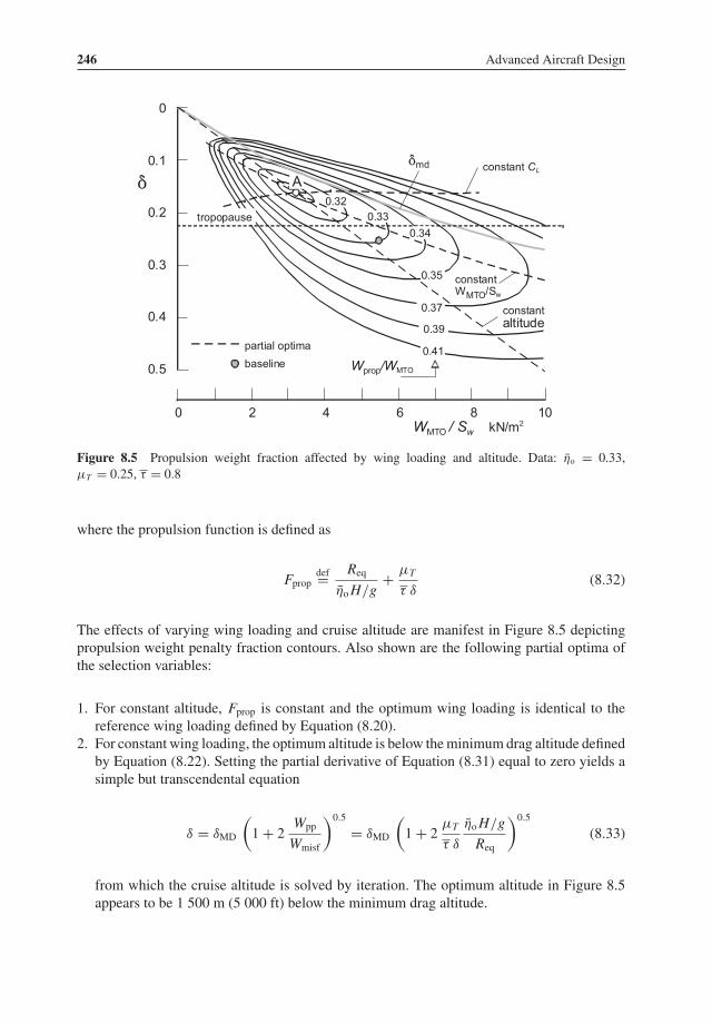
246 Advanced Aircraft Design
Figure 8.5 Propulsion weight fraction affected by wing loading and altitude. Data: ηo = 0.33,μT = 0.25, τ = 0.8
where the propulsion function is defined as
Fpropdef= Req
ηoH/g+ μT
τ δ(8.32)
The effects of varying wing loading and cruise altitude are manifest in Figure 8.5 depictingpropulsion weight penalty fraction contours. Also shown are the following partial optima ofthe selection variables:
1. For constant altitude, Fprop is constant and the optimum wing loading is identical to thereference wing loading defined by Equation (8.20).
2. For constant wing loading, the optimum altitude is below theminimum drag altitude definedby Equation (8.22). Setting the partial derivative of Equation (8.31) equal to zero yields asimple but transcendental equation
δ = δMD
(1+ 2 Wpp
Wmisf
)0.5= δMD
(1+ 2 μT
τ δ
ηoH/g
Req
)0.5(8.33)
from which the cruise altitude is solved by iteration. The optimum altitude in Figure 8.5appears to be 1 500 m (5 000 ft) below the minimum drag altitude.

Theory of Optimum Weight 247
As opposed to the case of aerodynamic efficiency and mission fuel, the partial optima of thepropulsion weight penalty are compatible in the intersection of the two partial optima – pointA in Figure 8.5. This global optimizer is obtained analytically by introduction of the followingconstant terms:• The mission fuel fraction required to overcome the minimum wing-related drag,
μ1def= 2
ReqηoH/g
√CDp KL (8.34)
• The power plant weight fraction required to overcome the invariable parasite drag,
μ2def= μT
τ
q sl(CD S)fixWMTO
(8.35)
Closed-form analytical expressions for the optimizers are found by substitution of μ1 and μ2into Equation (8.31) and setting the derivative with respect to the altitude equal to zero:
wing area: Sw = (CD S)fix2 CDp
√μ1
μ2(8.36)
altitude: δ = μT
τ
ηoH/g
Req
√μ1
μ2(8.37)
thrust:TTO
WMTO= μ2 + √
μ1 μ2
μT(8.38)
The corresponding mission fuel and power plant weight fractions are
Wmisf
WMTO= μ1 + √
μ1 μ2 andWpp
WMTO= μ2 + √
μ1 μ2 (8.39)
The optimum ratio of power plant to mission fuel weight is
Wpp
Wmisf=
√μ2
μ1(8.40)
and theminimumpropulsionweight penalty is defined by the following remarkable expression:
Wprop
WMTO= (√
μ1 + √μ2
)2(8.41)
In spite of their simplicity, these results must be carefully interpreted. For example, Figure 8.5indicates that point A corresponds to a wing loading of only 3 200 N/m2 and an unusually highinitial cruise altitude of 13 000 m. This is reflected in an unpractical large and heavy wing,driving up empty and take-off weights. It is therefore appropriate to extend the optimizationby including wing weight. Due consideration must also be given to constraints on wing andthrust loading, the subject of Chapter 9.

248 Advanced Aircraft Design
AB
C
20 864 10
0
0.1
0.2
0.3
0.4
0.5
WMTO / Sw kN/m2
partial optimum wing loadingpartial optimum altitude
L/D, fuel, fuel + engine
fuel+engine+wing
L/D, fuel, fuel+wingfuel+engine,fuel+engine+wingfuel+wing
global optima
fuel+engine+wingCfuel+wingBfuel+engineA
CL
MDtropopause partial optima
ref
baseline
1 9753
δ
δ
Figure 8.6 Optimum wing loading and cruise altitude treating several weight fractions as the objectivefunction
8.5.4 Wing and Propulsion Weight Fraction
Addition of wing weight according to Equation (8.2) (excluding wing attachment weight) tothe propulsion weight penalty yields
Ww + Wprop
WMTO=
{�W
WMTO/Sw
}0.5+ �S
WMTO/Sw+ Wprop
WMTO(8.42)
where the last term is defined by Equation (8.31). The contours of this weight fraction have ashape similar to Figure 8.5 but they are shifted to significantly higher wing loadings. Partialoptima are summarized in Figure 8.6, leading to the following observations:
• For constant altitude, the optimum wing loading is found by setting the partial derivative ofEquation (8.42) equal to zero resulting in
WMTO
Sw=
(WMTO
Sw
)ref
(1+ 0.5
√�W WMTO/Sw + �S
δ qsl CDp Fprop
)0.5(8.43)
where (WMTO/Sw)ref is defined by Equation (8.20). This equation must be solved by succes-sive iterations. An initial approximation is found by inserting 1.4 times the reference wingloading into the square root term.

Theory of Optimum Weight 249
• Optimum altitude: since wing structure weight is independent of the cruise altitude, thepartial optimum is equal to the altitude for minimum propulsion weight according to Equa-tion (8.33).
8.5.5 Optimum Weight Fractions Compared
Figure 8.6 shows that the three unconstrained optimizers A, B and C define quite differentairplane designs. Associated values of altitude and wing loading are obtained from Equations(8.20), (8.33) and (8.43). Design A (minimum fuel plus power plant weight fraction) isunrealistic since it ignores the effect of the varying wing size on empty weight. DesignB for minimum fuel plus wing weight fraction – not derived explicitly in this text – is amore practical solution. It has a lower optimum altitude and a considerably higher wingloading than design A. Design C for minimum fuel plus power plant plus wing weightfraction is derived from the most complete figure of merit and is representative for the designwith the lowest MTOW. However, design C has a high wing loading and flies at a lowaltitude.The selection of one of these unconstrained optimizers does not necessarily lead to a
good design since wing and thrust loading constraints imposed by low-speed performancerequirements are ignored. This need not be a problem since the combination of propulsionweight penalty and wing weight fractions is not sensitive to non-optimum conditions. Amore serious objection is that the economic impact of wing structure weight variation is lesssignificant than engine thrust and mission fuel weight variation. In principle, this effect canbe incorporated by multiplying the three terms involved by weight factors derived from theireconomic impact.
8.6 Take-Off Weight, Thrust and Fuel Efficiency
The previous optimizations were derived for a given MTOW. In the real world of conceptualdesign the payload and range are usually specified and the MTOW forms the outcome ofadding all the empty weight components and the useful load. The next step is therefore toinvestigate the various optimizers for the case of a specified payload and range capability.Since many empty weight components depend on the MTOW, the objective of the presentquasi-analytical approach is to derive a closed form equation for the MTOW for a specifiedpayload and range capability.
8.6.1 Maximum Take-Off Weight
The equations derived in the previous sections are used to add all empty weight components,payload and fuel. Solving for the MTOW yields
WMTO = Wpay + � Wfix + Fprop δ q sl (CDp S)fix
1− {μresf + μlg + (1+ rh)μw + Fprop (CDp/CL + KL CL )
} (8.44)

250 Advanced Aircraft Design
The propulsion function Fprop is defined by Equation (8.32) and the lift coefficient is propor-tional to the wing loading: CL = (WMTO/Sw)/q . In accordance with Table 8.1, the followingweight component groups are identified in Equation (8.44):
• The numerator summarizes fixed weight components that are (practically) independent ofthe MTOW – they include the design payload, the cabin and its contents, systems, operator’sitems, the fuselage and vertical tail structures, and a small term dependent on the number ofengines. Since fuselage and vertical tail geometry are considered to be independent of winggeometry, their weights are fixed. The term proportional to Fprop represents the mission fueland power plant weight attributed to the thrust required to balance the fuselage and verticaltail drag along the mission distance. It is easy to show that this engine weight componentis independent of the altitude. However, since the associated fuel weight component isproportional to the ambient pressure, it decreases with increasing altitude.
• The denominator summarizes all weight components treated as fractions of the MTOW.Statistics indicate that the reserve fuel load can be considered a fraction of theMTOW: μresf = 0.045. The landing gear weight fraction according to Equation (8.7) isμlg = 0.040, typically. The term rh ≈ 0.10 is a correction factor accounting for the hori-zontal tailplane weight and Equation (8.2) is substituted for the wing weight fraction μw.The term proportional to Fprop represents the propulsion weight penalty attributed to thethrust required to balance the wing and horizontal tail drag along the mission distance. Thefuel weight fraction is independent of the altitude, the engine weight fraction is inverselyproportional to the ambient pressure and increases (significantly) with increasing altitude.Both terms are independent of fuselage geometry.
Equation (8.44) forms a suitable tool for explicit optimization of the wing loading and theinitial cruise altitude – it can readily be adapted to cope with variation of the wing planformgeometry and thickness ratio. Figure 8.7 shows theMTOW to have an unconstrained optimizerfor a wing loading of 7 kN/m2 at 10 000 m altitude initial cruise altitude (design D). Thisoptimum is insensitive to the wing loading, especially if the altitude is optimized for each
Figure 8.7 Effect of wing loading and initial cruise altitude on MTOW. Baseline: Figure 8.1
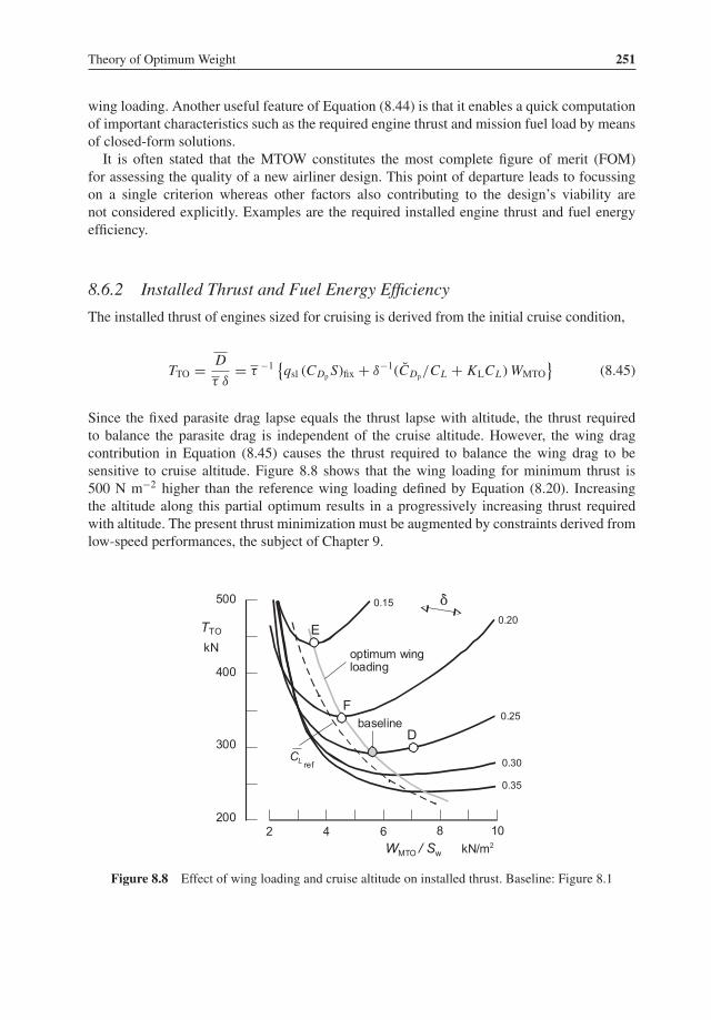
Theory of Optimum Weight 251
wing loading. Another useful feature of Equation (8.44) is that it enables a quick computationof important characteristics such as the required engine thrust and mission fuel load by meansof closed-form solutions.It is often stated that the MTOW constitutes the most complete figure of merit (FOM)
for assessing the quality of a new airliner design. This point of departure leads to focussingon a single criterion whereas other factors also contributing to the design’s viability arenot considered explicitly. Examples are the required installed engine thrust and fuel energyefficiency.
8.6.2 Installed Thrust and Fuel Energy Efficiency
The installed thrust of engines sized for cruising is derived from the initial cruise condition,
TTO = D
τ δ= τ −1 {
qsl (CDp S)fix + δ−1(CDp/CL + KLCL )WMTO}
(8.45)
Since the fixed parasite drag lapse equals the thrust lapse with altitude, the thrust requiredto balance the parasite drag is independent of the cruise altitude. However, the wing dragcontribution in Equation (8.45) causes the thrust required to balance the wing drag to besensitive to cruise altitude. Figure 8.8 shows that the wing loading for minimum thrust is500 N m−2 higher than the reference wing loading defined by Equation (8.20). Increasingthe altitude along this partial optimum results in a progressively increasing thrust requiredwith altitude. The present thrust minimization must be augmented by constraints derived fromlow-speed performances, the subject of Chapter 9.
Figure 8.8 Effect of wing loading and cruise altitude on installed thrust. Baseline: Figure 8.1

252 Advanced Aircraft Design
(a) (b)
Figure 8.9 Effect of wing loading and cruise altitude on propulsion characteristics. (a) Fuel energyefficiency (b) Propulsion weight penalty
The energy efficiency (Section 2.5) is a useful figure for comparing the fuel economy ofdifferent commercial transport aircraft. It can be expressed as an instantaneous performancebut in actual operation it varies during the flight due to the varying GW and the reducedfuel efficiency during non-cruising flight segments. The average fuel energy efficiency for acomplete mission is derived from Equations (2.26) and (8.30),
EEN = E ηoL
D
Wpay
WMTO
RmisReq
(8.46)
with E = ρfHNs/Wpay = 37 seat-km/litre (75.5 seat-nm/gallon). Figure 8.9 (a) demonstratesthat fuel efficiency is sensitive to wing loading and cruise altitude.The propulsion weight penalty is defined as the combined weight of the mission fuel and
the power plant (Section 8.5). Different from expressing it as a weight fraction, Figure 8.9 (b)depicts its absolute value.
8.6.3 Unconstrained Optima Compared
Figure 8.10 depicts three unconstrained optimizers: design D for minimum MTOW, design Efor minimummission fuel and and design F for a minimum propulsion weight penalty. DesignD has a slightly lower MTOW and a much higher wing loading than the other optimizers.Design E achieves 45-seat-km production per litre at 13 500 m altitude for a wing loading of3.6 kN/m2, 12% higher than the fuel efficiency of design D. However, this high fuel efficiencyis achieved at the cost of 47% more installed thrust. The minimum propulsion weight designF is an unconstrained optimum for a wing loading of 4.6 kN/m2 at an initial cruise altitudeslightly above the tropopause. This design has 13% more installed thrust than design D anda few percentage lower fuel efficiency than design E. Design F appears to represent a goodcompromise, provided wing loading and thrust loading comply with low-altitude performance
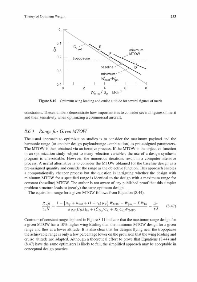
Theory of Optimum Weight 253
Figure 8.10 Optimum wing loading and cruise altitude for several figures of merit
constraints. These numbers demonstrate how important it is to consider several figures of meritand their sensitivity when optimizing a commercial aircraft.
8.6.4 Range for Given MTOW
The usual approach to optimization studies is to consider the maximum payload and theharmonic range (or another design payload/range combination) as pre-assigned parameters.The MTOW is then obtained via an iterative process. If the MTOW is the objective functionin an optimization study subject to many selection variables, the use of a design synthesisprogram is unavoidable. However, the numerous iterations result in a computer-intensiveprocess. A useful alternative is to consider the MTOW obtained for the baseline design as apre-assigned quantity and consider the range as the objective function. This approach enablesa computationally cheaper process but the question is intriguing whether the design withminimum MTOW for a specified range is identical to the design with a maximum range forconstant (baseline) MTOW. The author is not aware of any published proof that this simplerproblem structure leads to (nearly) the same optimum design.The equivalent range for a given MTOW follows from Equation (8.44),
Reqg
ηoH= 1− {
μlg + μresf + (1+ rh)μw}
WMTO − Wpay − �Wfix
δ q sl(CD S)fix + (CDp/CL + KLCL )WMTO− μT
τ δ(8.47)
Contours of constant range depicted in Figure 8.11 indicate that the maximum range design fora given MTOW has a 10% higher wing loading than the minimum MTOW design for a givenrange and flies at a lower altitude. It is also clear that for designs flying near the tropopausethe achievable range is only a few percentage lower on the provision that the wing loading andcruise altitude are adapted. Although a theoretical effort to prove that Equations (8.44) and(8.47) have the same optimizers is likely to fail, the simplified approach may be acceptable inconceptual design practice.

254 Advanced Aircraft Design
Figure 8.11 Achievable range for constant MTOW. Baseline: Figure 8.1
8.6.5 Extended Range Version
A useful application of Equation (8.44) is a first-order weight analysis of a derived versionof a baseline design. Figure 8.12 shows the weight distribution of an extended range (ER)version of the design depicted in Figure 8.1. The harmonic range is increased by 43% from7 000 to 10 000 km. One possibility is to assume that both versions have the same wingarea. This causes the MTOW to increase by 19% from 5.6 kNm−2 to 6.7 kNm−2; the missionfuel increases by 49%. Although the increased fuel weight fraction drives the optimum wingloading down, the penalty of the increased wing loading is negligible due to the flatness ofthe MTOW optimum. Another option is to increase the wing area so that both designs have awing loading of 5.5 kNm−2 and the same initial cruise altitude of 10 500 m. This approachdoes not affect the mission fuel increment of 49% but enables the plane to use the same fieldsfor taking off and landing. In both cases the fuel efficiency decreases from 40 to 36 seat-kmper litre.
8.7 Summary and Reflection
8.7.1 Which Figure of Merit?
A general observation from this chapter is that weight fractions and absolute weights ofthe considered components have different optimum conditions. Also, the absolute weights aremore sensitive to non-optimum conditions than the weight fractions. It is therefore advisableto relate weight components to invariable quantities such as the maximum payload or numberof seats. It is also an open question which weight component should be considered a suitablefigure of merit (FOM) for the aircraft’s sizing process.

Theory of Optimum Weight 255
Figure 8.12 Weight distribution of the baseline design with extended range
The accumulated costs of fuel consumed during the service life of a medium-range commer-cial aircraft is generally of the same magnitude as the aircraft’s first cost; the design missionfuel weight is about 50% of the OEW. On the other hand, the engines’ first cost amounts toabout 20% of the aircraft’s first cost versus a weight of 12% of the OEW, typically. Savingengine weight through reduced installed thrust appears to be as valuable as saving the samefuel weight. On the other hand, it is unlikely that saving the same wing structure weight has acomparable direct effect on the aircraft operating costs, while the indirect effect on fuel con-sumed and thrust required (via wing loading and MTOW) is far more significant. This leads tothe proposition that – to optimize wing loading and initial cruise altitude – the (mission-based)propulsion weight component is a more useful FOM than MTOW.From the economical and environmental points of view, the various weight components
are not equally important. How should their weight be weighed? For example, mission fuelcosts are very substantial and will dominate any design decision, while reserve fuel is seldomconsumed and contributes to costs indirectly through its contribution to gross weight. Fuelburn is responsible for atmospheric pollution since CO2 production is proportional to it. On theother hand, although (gas turbine) engines are very costly, it may turn out that the availabilityof a suitable engine type may be decisive, rather than the installed thrust.4 It is also significantthat the number of engines to be installed has not yet entered the analysis up to now, butthis situation will change in Chapter 9 when design constraints are introduced. And finally,although wing weight considerations dominate the location of the combined optimum, the
4Installed engine costs are often assumed to be proportional to take-off thrust. This assumption is based on statisticalevidence, which may not be valid in actual design practice. In particular, a highly fuel-efficient engine is more costlythan an engine with older technology with the same thrust.

256 Advanced Aircraft Design
costs of designing and building a wing structure are much lower than the costs related toengines and accumulated fuel expenditure. This makes the MTOW a less suitable FOM.
8.7.2 Conclusion
The sensitivity to variations in wing loading and initial cruise altitude of the aerodynamicefficiency, the fuel load, weight and thrust of the installed power plant, wing weight, andthe aircraft gross weight at take-off has been examined. A rational breakdown of drag andweight into contributions from the wing, the engine installation, and (mainly payload-related)invariable items has been proposed in order to derive analytical expressions for the fuel load,power plant and wing structural weight as fractions of the MTOW. Although simplificationswere required to obtain closed-form equations leading to unconstrained optimum values forthe wing loading and the initial cruise altitude, it is concluded that realistic results were foundwithin the validity range of these assumptions.
• The aerodynamic efficiency L/D in cruising flight has partial optimawith respect to thewingloading and the altitudewhich aremutually incompatible to define a combined unconstrainedoptimum for both variables. Although a high L/D is a very important property of an airliner,it is not suitable as a figure of merit for the overall system. The same applies to the missionfuel weight fraction since it is inversely proportional to L/D whereas the overall engineefficiency is independent and practically constant in the stratosphere.
• Installed engine thrust and weight increase significantly when the initial cruise altitude isincreased for the same engine rating. The required cruise thrust at a given altitude has aminimum value which is insensitive to the wing loading for fairly large excursions above orbelow the optimum.
• Optimumvalues for cruise altitude andwing loading have been derived resulting inminimumcombined weight fractions of fuel and engine, referred to as the propulsion contribution.Partial and global unconstrained optima have been expressed as closed-form analyticalexpressions. Since wing weight is excluded from this optimization, the result is a designwith an unrealistically low wing loading.
• Adding the wing and the propulsion weight fractions leads to optimum conditions that differsignificantly from the previous optima. Although the combined weight can be computedreadily, the unconstrained optimum has not been expressed in explicit form.
• The OEW is obtained from addition of invariable – mostly payload-related – weight com-ponents and weight components that are considered proportional to MTOW. The resultingexpression for the MTOW appears to provide a non-iterative solution which is useful forminimizing the MTOW as well as the constituting weight components, in particular, thepropulsion contribution to weight.
• By-products of the MTOW equation were derived and applied to optimize the exampledesign, yielding realistic results. For example, it appeared that the conditions for maximumdesign range for given MTOW and the minimum MTOW for given range were almost –but not exactly – identical. Another property of the quasi-analytical approach is a quickcomputation of the weight distribution of an extended-range version of the baseline design.And finally, the fuel efficiency in terms of productivity delivered per fuel burn rate and itssensitivity to range excursions from the baseline design are readily obtained. It was foundthat fuel efficiency degrades considerably with ranges in excess of about 6 000 km.

Theory of Optimum Weight 257
8.7.3 Accuracy
Several assumptions made in the interest of deriving simplified optimum conditions may havean effect on the accuracy of the results.
• Constraints on the wing area and engine take-off thrust due to low-speed performancerequirements, available fuel tank volume and other practical considerations have not beenconsidered.
• Supercritical compressibility effects on drag have been taken into account formally, but highwing loadings and/or altitudes lead to high cruise lift coefficients. These are feasible onlyin combination with increased wing sweep and/or decreased thickness. Both modificationswill increase wing structural weight, and the best wing loading may be below the presentprediction.
• Overall engine efficiency is assumed to be independent of the stratospheric altitude. Theeffects of the Reynolds number variation can be incorporated readily into the analysis bymeans of numerical solutions. It is likely that more accurate solutions will shift the optima tocruise altitudes slightly closer to the tropopause, where the highest overall engine efficiencyis obtained.
• Increasing the cruise altitude will require a larger cabin pressure differential and this willincrease the fuselage structural weight, as well as several system component weights. Thisis another argument to decrease the design cruise altitude to a sub-optimum value.
The first two points are most essential and will be addressed in Chapters 9 and 10, the otherpoints are worth being studied in any comprehensive optimization study but are beyond thescope of the present book.
Bibliography
[1] Torenbeek, E., Synthesis of Subsonic Airplane Design, Chapter 9 and Appendix D, Springer Verlag, Heidelberg,1981.
[2] Shevell, R.S., Fundamentals of Flight, Chapter 18, Second Edition, Prentice-Hall, Englewood Cliffs, NJ, 1989.[3] Roskam, J., Airplane Design, Part V: Component Weight Estimation, Roskam Aviation and Engineering Cor-
poration, Ottawa, Kansas, 1989.[4] Schatzberg, E.M., Wings of Wood, Wings of Metal: Culture and Technical Choice in American Airplane
Materials, 1914–1945, Princeton University Press, Princeton, NJ, 1999.
Design Sensitivity of Weight
[5] Carayette, J.F., “Aircraft Wing Weight Estimation”, Aircraft Engineering, January pp. 8–11 and April p. 119,1950.
[6] Burt, M.E., “StructuralWeight Estimation for Novel Configurations”, Journal of the Royal Aeronautical Society,pp. 15–30, January 1962.
[7] Kuchemann, H., and Weber, J., “An Analysis of Some Performances of Various Types of Aircraft Designed toFly over Different Ranges at Different Speeds”, Progress in Aeronautical Sciences, Vol. 9, Pergamon Press,1968, pp. 329–456.
[8] Coker, B.B., “Problems in Airframe Development Associated with Weight and Balance Control in HeavyLogistics Transport Vehicles such as the C-5A Transport”, Short Course in modern theory and practice ofweight optimization and control for advanced aeronautical systems, University of Tennessee, November 1968.
[9] Caddell, W.E., “On the Use of Aircraft Density in Preliminary Design”, SAWE Paper No. 813, May 1969.

258 Advanced Aircraft Design
[10] Gerend, R.P., and J.P. Roundhill, “Correlation of Gas Turbine Engine Weights and Dimensions”, AIAA PaperNo. 70-669, June 1970.
[11] Howe, D., “The Prediction of EmptyWeight Ratio and Cruise Performance of Very Large Subsonic Jet TransportAircraft”, Cranfield Report Aero 3, 1971.
[12] Marsh, D.P., “Post-Design Analysis for Structural Weight Estimation”, SAWE Paper No. 936, 1972. (DouglasPaper 6021).
[13] Schneider, W., “Project Weight Prediction Based on Advanced Statistical Methods”, AGARD CP-147 Vol. 1,Paper No. 17, 1973.
[14] Patterson, R.W., “Weight Estimates for QUIET/STOL Aircraft”, SAWE Paper No. 1001, 1974.[15] Waters, M.H., and E.T. Schairer, “Analysis of Turbofan Propulsion System Weight and Dimensions”, NASA
TM X-73199, January 1977.[16] Beltramo, M.N., D.L. Trapp, B.W. Kimoto, and D.P. Marsh, “Parametric Study of Transport Aircraft Systems
Cost and Weight”, NASA CR-151970, April 1977.[17] Storey, R.E., “Dynamic Loads and Airplane Structural Weight”, SAWE Paper No. 1153, 1977.[18] Onat, E., and G.W. Klees, “A Method to Estimate Weight and Dimensions of Large and Small Gas Turbine
Engines”, NASA CR-159481, 1979.[19] Anonymus, “Requirements for Short/Medium Range Aircraft for the 1980s”, Association of European Airlines,
document G.2110/R2, Third Edition, July 1981.[20] Scott, P.W., “Developing Highly Accurate Empirical Weight Estimating Relationships: Obstacles and Tactics”,
SAWE Paper No. 2091, May 1992.[21] Martin, J.F., “Etude Preliminaire d’un Avion de Transport a Reaction”, l’Aeronautique et l’Astronautique,
1992-6, No. 157, pp. 62–70, 1992.[22] Scott, P.W., “Conceptual Estimation of Moments of Inertia”, SAWE Paper No. 2171, May 1993.[23] Schneegans, A., “Weight Analysis of Commercial Aircraft Dependent on Cruising Altitude”, DGLR Jahrbuch
1993, Paper No. 93-03-096, 1993.[24] Read, A., “Stretching an Aircraft: A Case Study”, SAWE Paper No. 2165, May 1993.[25] Giles, G.L. ‘Equivalent Plate Modelling for Conceptual Design’, AIAA Paper No. 95–3945, September
1995.[26] Liebeck, R.H., D,A, Andrastek, J. Chau, R. Girvin, R. Lyon, B.K. Rawdon, P.W. Scott, and R.A. Wright,
“Advanced Subsonic Airplane Design and Economic Studies”, NASA CR-195443, April 1995.[27] Ardema, M.D., M.C. Chambers, A.P. Patron, A.S. Hahn, H. Miura, and M.D. Moore: “Analytical Fuselage
and Wing Weight Estimation of Transport Aircraft”, NASA TM-110392, 1996 (also AIAA Paper No. 96-5583,October 1996).
[28] Schmidt, A., M. Lapple, and R. Kelm, “Advanced Fuselage Weight Estimation for the New Generation ofTransport Aircraft”, SAWE Paper No. 2406, May 1997.
[29] Saeedipour, H.R., and T.N. Stevenson, “The Effects of Small Changes to the Design Specification of a Jet CivilTransport Aircraft”, Aircraft Design, Vol. 1, No. 1, pp. 25–41, 1998.
[30] Shustrov, Y.M., “Starting Mass: A Complex Criterion of Quality for Aircraft On-Board Systems”, AircraftDesign, Vol. 1, No. 4, pp. 193–203, 1998.
[31] Dorbath, F., “Civil Aircraft Mass Analysis (MTOM> 40t): Statistical Mass Estimation”, LTH Mass Analysis,UL-442.0(T), Ausgabe A, DLR-LY/Airbus, 2011.
Structures Technologies and Materials
[32] Lovell, D.T., andM.A. Disotell, “Structural Material Trends in Commercial Aircraft”, AIAA Paper No. 781552,August 1978.
[33] Wissel, W.D., “Advanced Material Application on the European Wide Body Transport Aircraft Airbus”, SAWEPaper No. 1484, 1982.
[34] Lange, R.H., and J.W. Moore, “Systems Study of Application of Composite Materials for Future TransportAircraft”, AIAA Paper No. 82-0812–1982.
[35] Burns, J.W., “Advanced Composites SizingGuide for PreliminaryWeight Estimates”, SAWE Journal, pp. 44–61,Fall 1992.
[36] Giles, G.L., “Equivalent Plate Modeling for Conceptual Design of Aircraft Wing Structures”, AIAA PaperNo. 95-3945, September 1995.

Theory of Optimum Weight 259
[37] Peel, C.J., “Advances in Materials for Aerospace”, The Aeronautical Journal, Vol. 100, No. 1000, pp. 487–503,December 1996.
[38] Anonymous, “Metallic Materials and Processes”, http://www.nap.edu/openbook/0309053900/html/26.html,copyright 1996, The National Academy of Sciences, 2000.
[39] Rudolph, P.K.C., “High-Lift Systems on Commercial Subsonic Airliners”, NASA Contractor Report 4746,September 1996.
[40] Slingerland R., F. van Reijn van Alkemade, and B. Vermeulen, “A Preliminary Prediction Method for the Effectof New Fuselage Materials on Transport Aircraft Weight,” AIAA Paper 2007-2289, April 2007.
[41] Sandoz, P.L., “The Next Careful Steps in Commercial Aircraft Structures”, Structures Technology: HistoricalPerspective and Evolution, A.M. Noor, (ed.), AIAA, pp. 91–106, 1998.
[42] Curran, R., A. Rothwell, and S. Castagne, “Numerical Method for Cost-Weight Optimization of Stringer-SkinPanels”, Journal of Aircraft, Vol. 43, No. 1, pp. 264–274, January–February 2006.
[43] Ciampa, P.D., B. Nagel, and M.J.L. van Tooren, “Global Local Structural Optimization of Transport AircraftWings”, AIAA Paper No. 2010-3098, April 2010.
9Matching Engines and Airframe
The Wright brothers, among their other notable achievements, discovered a design truism stillvalid today: if an aircraft engine is sized to optimum airspeed, pilots will decide that the aircraftis underpowered.
—B.H. Carson, in AIAA Paper 80–1847 (1980)
9.1 Requirements and Constraints
Design sensitivity to variations in wing loading, initial cruise altitude and installed enginethrust was the subject of the previous chapter. The emphasis was on unconstrained optimiza-tion of several basic objective functions: aerodynamic efficiency, mission fuel, fuel plus powerplant weight, and maximum take-off weight (MTOW). It was found that optimization of theseobjective functions results in widely divergent optimum values of the wing area, engine thrustand cruise altitude. In view of the importance of engine selection, the present chapter focusseson design constraints reducing the designer’s freedom of choice. The most relevant constraintsare top level and safety requirements such as available take-off and landing distances and climbor cruise performance with an inoperative engine. Performance constraints are mostly trans-lated into minimum required values of the installed engine thrust and wing area. Engine thrustis irrelevant for constraints imposing a lower limit on wing size, such as the condition that themaximum fuel loadmust be contained inside the primarywing box and the cruise lift coefficientmust be limited to avoid high speed buffet. These constraints are treated in Chapter 10.Modern mature gas turbine engines are extremely reliable – their in-flight shutdown (IFSD)
rates have reduced from about one per 10 000 engine hours for the first generation of turbofansto one per 100 000 hours for current engines. Nevertheless, a fleet with an average yearlyutilization of 4 000 hours per airliner will occasionally experience a significant in-flight poweror thrust reduction or even a complete engine failure. Regardless of the number of propulsionengines installed, a safe continuation of the flight must be possible in such a situation albeit ata reduced performance level. And when the pilot decides to abort the take-off when the plane isstill on the runway, the emergency stop must be a safe event as well. Engine failure is likely tooccur during take-off and initial climb when the engines operate at their maximum rating, but asafe continuation of the flight en route can be equally critical during a flight over water in view
Advanced Aircraft Design: Conceptual Design, Analysis and Optimization of Subsonic Civil Airplanes, First Edition. Egbert Torenbeek.
© 2013 by Egbert Torenbeek. Published 2013 by John Wiley & Sons, Ltd.

262 Advanced Aircraft Design
of its long duration. Airworthiness requirements associated with engine failure are dependenton the operational conditions – field lengths and elevations, ambient temperature and pressure,etc. – for which civil airplanes must comply with one engine inoperative (OEI) requirements.Obviously, the consequences of engine failure on performance are sensitive to the number ofengines to be installed and their position relative to the airframe. Both subjects are consideredoutside the context of this book – the number of installed engines is assumed to be pre-assigned.Top level requirements (TLRs) specify flight performances which dominate the engine to
airframe matching process – the most relevant parameters involved are installed thrust andwing size. Constraints on these selection variables are derived from the following performanceconstraints:
• The cruise speed or cruise Mach number – occasionally in combination with an initial cruisealtitude capability (ICAC) – following the take-off with MTOW, ascending to the top ofclimb (TOC) and acceleration to cruise speed.
• Climb gradients achievable after engine failure for several flight segments and aircraftconfigurations.
• Engine-out altitude capability (EOAC): the altitude achievable in level flight with OEI. Thisrequirement is relevant for airplanes having the capability to cross extensive uninhabitedterrains and oceans.
• The take-off field length (TOFL) required for taking off with engine failure at the criticalspeed.
• The approach speed and/or the landing field length (LFL) required.
Low-speed flight, field performances and cruise speed capabilitymay pertain to standard and/ornon-standard ambient conditions defined by the ICAO standard atmosphere (ISA) defined inAppendix B.
9.2 Cruise-Sized Engines
Having reached the TOC, the airplane accelerates to the initial cruise speed and the ICACis attained when a specified rate of climb (ROC) is achievable with maximum climb rating.The present analysis simplifies this requirement by assuming that, after throttling back frommaximum climb to cruise rating, the engines have sufficient thrust to fly horizontally at theprescribed speed and altitude. A 1 m/s (200 ft/min) ROC is equivalent to a gradient of 0.4%,which requires 8% of the cruise thrust, typically. Hence, if the maximum climb and cruiseratings produce a thrust ratio of 1.08, the two criteria yield the same thrust requirement. Thethrust lapse rate for cruise conditions is used to translate this requirement into an installedtake-off thrust at sea level ISA.
9.2.1 Installed Take-Off Thrust
The matching relationship between engine thrust and airplane drag makes use of the rubber-izing concept explained in Section 8.5. The essential characteristic is the corrected lapse ratedefined by Equation (3.10)
τdef= T/p
TTO/p sl= T/δ
TTO(9.1)

Matching Engines and Airframe 263
which is derived from basic engine performance information. For instance, the corrected cruisethrust lapse is derived from
τ ∗ = T ∗/p∗
TTO/p sl(9.2)
denoting properties at the tropopause by an asterisk. Since the thrust at high (stratospheric)altitudes is (theoretically) proportional to the ambient pressure, the corrected lapse rate dependson the engine cycle and cruise Mach number only. Hence, it is fair to assume a constant τ = τ ∗
for altitudes not too far above or below the tropopause. The relationship between (all-engines)take-off thrust and initial cruise altitude is obtained from Equation (8.45), assuming that theinitial cruise weight is equal to the TOW,
TTO = T/δ
τ= D/δ
τ= 1
τ
[q sl
{(CDp S) fix + CDp Sw
} + KL(WMTO/δ )2
q sl Sw
](9.3)
with q sl = 0.5γ p slM2 and δ denotes the relative ambient pressure at the initial cruise altitude.The installed thrust lapse rate τ , referring to engine thrust minus nacelle drag, and othersymbols are defined in Sections 8.4 and 8.5. Equation (9.3) determines how the requiredthrust/weight ratio varies with the cruise altitude and wing loading at take-off. The presenceof the MTOW is a minor complication which is solved by substitution of Equation (8.44).
9.2.2 The Thumbprint
The design selection chart Figure 9.1 – some designers call it a ‘performance thumbprint’ – isuseful for explicit optimization; an application to high-lift system technology is described in[21]. This diagram depicts the ratio of installed thrust to MTOW versus the take-off wing load-ing. An alternative diagram with installed thrust or power versus wing area has a considerableadvantage if the MTOW is fixed and the design range is considered a figure of merit (FOM)as discussed in Section 8.6. Figure 9.1 depicts the case of unconstrained optimization, thecomplete selection chart to be discussed later visualizes several performance, geometric andaerodynamic constraints in combination with objective functions such as MTOW or missionfuel weight. The following remarks apply to the present example:
• The constant altitude curves are more or less horizontal for usual combinations of wingloading and altitude. Hence, if small excursions are considered from a baseline wing size,the required cruise thrust required needs little or no revision.
• Although wing structure weight has a major effect on the location of the unconstrainedoptimizer (point D), the MTOW is more sensitive to altitude than to wing loading. PointD combines a rather high wing loading with a low initial cruise altitude and low-speedperformance constraints are likely to render design D unfeasible.
• Fixed (fuselage-related) drag decreases with increasing cruise altitude, minimum wing dragis insensitive to altitude. These effects are counteracted by increasing installed engine thrustand weight with increasing cruise altitude. Curve I defines the partial optimum thrust forgiven wing loading.

264 Advanced Aircraft Design
0.50
0.40
0.30
0.205 64 8 10
9,000
10,000
12,000
11,000
13,00014,000
altitude m
WMTO/Sw kN/m2
TTO
WMTO
D
E
F
I
I
II
II
III
III
WMTOkN
73 9
baseline
1,210
1,1601,1401,120
1,100
1,080
Figure 9.1 Design selection chart with MTOW contours for the design in Figure 8.1. Partial optima:I – constant wing loading, II – constant thrust/weight, III – constant altitude
• The optimum wing loading for a given thrust is defined by Curve II. This can be seen as theminimum MTOW for the case of a given engine type.
• The optimumwing loading and thrust loading for a given altitude are defined by Curve III. Itis found that the optimum wing loading decreases with altitude such that the lift coefficientis CL = 0.63. The thrust to be installed increases considerably with the altitude; see alsoFigure 8.8.
Design points E and F in Figure 9.1 are unconstrained optimizers for minimum mission fueland minimum propulsion weight penalty, respectively. Due to its initial cruise altitude ofnearly 13 000 m, design E needs extremely large engines in combination with a large wing,leading to a 6% higher gross weight than aircraft D. Design F with the lowest weight penaltyof two costly items and a mere 2% MTOW penalty might be an attractive compromise.Whether this design satisfies constraints other than the cruise speed requirement remains to beinvestigated.The computation of thrust and wing size effects on MTOW contours in the design selection
chart are derived for the MTOW. However, the performances treated in the following sectionsapply to aircraft gross weights equal to or less than themaximumGW for each case considered.The notations are therefore general: WTO for take-off and WL for landing.
Matching Engines and Airframe 265
9.3 Low Speed Requirements
Critical climb performances of civil aircraft can be categorized as (a) minimum climb gradi-ents available during critical phases of the flight, in particular after failure of an engine, and(b) obstacle clearance requirements for the net flight path, obtained by subtracting gradientdeviations from the gross flight path. Although both performances are subject to safety require-ments for all operations, only certification requirements affect the engine-to-airframematchingprocess. The operational variables involved are the aircraft gross weight (GW), the pressurealtitude and the ambient temperature. The permissible TOGW is the highest GW ≤ MTOWfor which all climb requirements are satisfied. In case of an elevated airfield with higherthan standard ambient temperature, the permissible TOGW may be significantly less thanthe MTOW, resulting in an undesirable reduction of payload or range. Similar arguments forlanding are usually less restrictive. Consequently, engine sizing is often based on ‘hot andhigh’ conditions representative of the most elevated airfields to be served.
9.3.1 Stalling Speed
The safety speeds during and after the take-off and before landing are related to the stallingspeed VS with deflected high-lift devices. The 1-g stalling speed (VS)1−g is derived from levelflight tests duringwhich the airplane decelerates at a rate of 1 kt/s until g-break occurs. The stalldevelops into a descent followed by recovery of the non-stalled condition.1 Reference speedsare based on the minimum speed occurring during the stall or on 0.94 (VS)1−g . Assuming thelatter to be the highest, the (equivalent) stalling speed in flight with TOGW is
VS = 0.94
(2WTO
ρTO SwCL max
)1/2(9.4)
The factor 0.94 is equivalent to accounting for the g-break by using a normal load factorof 0.88 during the take-off manoeuvre.2 Alternatively, the maximum lift coefficient obtainedfrom aerodynamic data can be increased by 13%. The free air safety speed V2 is the speed towhich the airplane accelerates while climbing away after lift-off with one engine inoperative.For jet aircraft this speed must comply with V2 ≥1.20 VS . The safety speed with one engineinoperative at V2 = 1.20 VS amounts to
V2 =(
2WTO
ρTO Sw CL2
)1/2(9.5)
with CL2 = 0.786 CL max. Instead of the (aerodynamic) maximum lift coefficient, the liftcoefficient at V2 can be treated as a basic parameter. The conceptual stage offers the possibilityof optimizing CL2 and V2, a dominating condition for sizing the engines. The flap deflectioncorresponding to the optimum CL2 is one of the design cases of aerodynamic and mechanicalflap design to be settled during the downstream design stages.
1Many airliners have a flight envelope protection system preventing the plane from entering the stalled condition.Nevertheless, the stalling speed is subject to certification.2This effect is ignored when using CL2 = CL max/1.22, leading to a significant error in the stalling speed and thetake-off distance.

266 Advanced Aircraft Design
Table 9.1 Summary of FAR/JAR 25 climb requirements for jet transports. N : number of installedengines. OEI: one engine inoperative; AEO: all engines operating
Phase of flight Airplane configuration Climb gradient%
Flaps uc Eng. rating Flight speed N = 2 N = 3 N = 4
lift-off 1st seg. TO ↓ TO VLOF → V2 0 0.3 0.5take-off 2nd seg. TO ↑ OEI TO V2 ≥ 1.20VS 2.4 2.7 3.0path final seg. ↑ ↑ MC V ≥ 1.25 VS 1.2 1.5 1.7approach climb APP ↑ TO V ≤ 1.5VS 2.1 2.4 2.7landing climb LAND ↓ AEO TO V ≤ 1.3VS 3.2 3.2 3.2
9.3.2 Take-Off Climb
Most pertinent climb requirements for civil transport aircraft reproduced in Table 9.1 pertainto the continued take-off (CTO) after failure of one engine. The flight path after lifting off(LOF) is subdivided into four segments.
• The first segment commences at the moment of lifting off with OEI. Undercarriage retractionbegins at least three seconds after lift-off, the condition of full retraction denotes the end ofthe first segment. Although flight performance during this benefits from ground effect, therequired climb gradient pertains to flying out of ground effect.
• During the second segment, engine rating and flap position are the same as for the firstsegment, but the climb gradient has improved due to the undercarriage retraction. Thissegment lasts until flap retraction begins at a height of at least 400 ft (120 m).
• The third segment (not indicated) is the flight phase during which the aircraft is acceleratedto the flap retraction speed, flaps are retracted and the engine rating is reduced to maximumcontinuous. The speed is finally increased until the flaps-up safety speed is reached.
• The final segment refers to the aircraft in the en route configuration, with the operatingengines at maximum continuous rating.
The minimum take-off (or free air) safety speed is V2 = 1.20VS for most multi-engine aircraft,except for four-engine propeller aircraft and a certain class of jet aircraft; see FAR/JAR25.107 (b). Since the best speed to achieve a high climb gradient VX is higher than 1.20VSthe aircraft improves its climb performance for V2 > 1.20 VS. This overspeed situation isachieved by delaying the rotation. In the design stage, overspeed is not an option since theTOFL requirement is usually a dominant requirement.
9.3.3 Approach and Landing Climb
The climb requirements in Table 9.1 pertain to the approach climb after engine failure and theclimb-out after an aborted landing.
1. Amissed approach is one that is discontinued at or above the decision height; the subsequentflight segment is referred to as the approach climb. The decision to go around is made after

Matching Engines and Airframe 267
engine failure with flaps in the approach setting. At this point undercarriage is retractedand the remaining live engines are set to take-off power or thrust.
2. If after landing touch-down the ground roll is discontinued, the thrust levers off all enginesare advanced to the maximum take-off power position without altering the flap setting.Climbing out after a baulked landing is called the landing climb. It is not likely that thiscase will affect the engine thrust unless the flap angle is very large. In that case the landingflap angle may have to be reduced which obviously increases the stalling speed and thelanding distance.
9.3.4 Second Segment Climb Gradient
The following derivation concentrates on the often critical second segment climb. The climbangle in steady flight at speed V2 with OEI follows from the equations of motion for a smallclimb angle,
γ 2 = (1− N−1eng) TV2
WTO−
(CD
CL
)V2
(9.6)
with TV2 denoting the total thrust of Neng installed engines. Equation (4.36) is substituted toobtain the thrust-to-weight ratio for a specified climb gradient,
TV2
WTO= Neng
Neng − 1(
γ 2 + C0 + CL2
π AwE
)for 1.2 ≤ CL2 ≤ 1.8 (9.7)
Apart from the number of engines, the lift coefficient at V2 and the wing aspect ratio Aware the most influential parameters affecting the required thrust. The take-off thrust requiredis derived from the engine’s thrust lapse with flight speed between the static condition andthe climb-out condition at V2. For standard ambient conditions, the engine thrust lapse ratedepends mainly on the specific thrust (or bypass ratio) and the safety speed. A significantincrease of the required thrust must be applied if the take-off is specified at a ‘hot and high’airfield. This requires information on the flat rating characteristics of the engine; that is, howtake-off thrust varies with ambient temperature and elevation of the field.Equation (9.7) makes it clear that the thrust required is reduced when the climb-out lift
coefficient is low. However, this leads to a high lift-off speed and a long ground run. The nextsection explains how the optimum CL2 is derived for a combined take-off and climb awayperformance analysis.
9.4 Schematic Take-Off Analysis
The required take-off performance capability of a commercial transport aircraft is essentialfor sizing its wing and engines – however, it is the most complicated of all flight performancerequirements. This becomes clear when reviewing definitions and procedures in the relevantairworthiness codes, for example, FAR/JAR 25.103 through 25.121. A detailed explanation ofhow these rules are used in the operation of civil aircraft is found in [4].

268 Advanced Aircraft Design
9.4.1 Definitions of Take-Off Field Length
The required take-off field length (TOFL) for an airliner in operation is prescribed by the flightmanual (FM) which has been derived from certification flight tests on a dry concrete runway –operational take-off characteristics on wet runways are assessed separately. A take-off will besafe when the runway is long enough for the normal situation that all engines are operatingcontinuously and if that engine failure occurs at the most critical speed during the take-off.An airplane may take off if the available runway is long enough to accommodate the longestof the following distances complying with a nominal piloting technique.
1. The distance required for taking off with all engines operating (AEO). Acceleration on therunway from standstill to rotation at speed VR is followed by the lift-off at speed VLOF andclimb to 35 ft (10.7 m) obstacle height. In order to account for technical and operationalvariations from the nominal situation, the runway length required is equal to the regulartake-off distance (RTOD) multiplied by 1.15.
2. The distance required for acceleration on the runway from standstill to the speed at whichone engine fails, followed by a continued take-off (CTO) with OEI. This distance is calledthe continued take-off distance (CTOD).
3. The distance required for acceleration on the runway from standstill to the engine failurespeed VEF followed by deceleration to standstill using maximum braking effort. Duringthis rejected take-off (RTO) the aircraft stays on the ground. The runway length required iscalled the accelerate-stop distance (ASD).
For ensuring a safe take-off from a given airfield, the longest of the three distances mentionedabove is determined (Figure 9.2). Since the second and third depend on VEF, the critical situationoccurs when the CTOD and the ASD are equal. The decision speed V1 is scheduled so thatthe pilot can act appropriately when an engine fails. If during the ground run an engine fails ata speed below V1, the take-off is aborted, otherwise it is continued. The requirement V1 ≤ VRimplies that the take-off must not be rejected once the rotation for taking off has been initiated.The balanced field length (BFL) refers to the situation where the CTOD and the ASD are equal.Take-off analysis in the concept design stage can be complicated by a lack of detailed
aerodynamic data and emergency braking characteristics. Hence, it is often assumed that the
engine failure speed
BFL
V1 VR
1.15 RTOD
AS
dist
ance
D
CTOD
Figure 9.2 Rotation speed, decision speed and balanced field length

Matching Engines and Airframe 269
dist
ance
Figure 9.3 Take-off distances affected by the take-off safety speed
BFL is the dominant requirement for deriving the installed take-off thrust. This is likely tobe correct for twin-engine airplanes since failure of an engine causes the power or thrust tobe reduced by 50%. However, large four-engine jetliners have a long take-off run comparedto the air distance and the 15% take-off distance reserve may well exceed the effect of 25%thrust loss due to failure of one engine. The following take-off analysis applies to a take-offwith engine failure during the take-off run followed by a continued take-off with OEI.
9.4.2 Take-Off Run
The take-off run consists of an acceleration from standstill to VLOF which is about 1.15 VS.The take-off run length LRUN is computed from the energy equation,
LRUN = kinetic energy at lift-off
mean accelerating force= (Ek)LOF
Facc(9.8)
When the plane starts rolling, the accelerating force equals the AEO static thrust TTO minusthe runway friction. The thrust decreases gradually with speed until engine failure occurs atVEF; thereafter it decays rapidly to the OEI thrust. Since V2 is only slightly higher than VLOF,the thrust at lift off TLOF is assumed equal to the thrust at the safety speed TV2 which is treatedas the dominant parameter determining the acceleration during taking off. Aerodynamic dragincreases proportional to V 2, stays relatively small but increases progressively between therotation speed VROT and VLOF. The length of the take-off run is written as
SRUN = W 2TO
ρTO g SwCL2 kTTV2
where kTdef=
(V2
VLOF
)2 FaccTV2
(9.9)
The parameter kT allows for the variation of thrust, friction drag and aerodynamic drag and forthe speed increment after lift-off. Its order of magnitude is 0.85, subject to statistical validation.

270 Advanced Aircraft Design
9.4.3 Airborne Distance
The angle of attack and the lift are building up rapidly during the rotation until the plane liftsoff. During the climb segment the plane follows a curved path with the angle of pitch controlledby the pilot until the steady-state climb angle is reached. Due to the engine-out condition thereis little acceleration. The minimum speed at the obstacle height V2 is 1.2 times the power-off stall speed VS for jet transports and twin-engine turboprops. During airborne flight theremaining failed engine thrust and wind milling drag depend on engine characteristics whichare usually unknown during conceptual design. The yawing moment due to thrust asymmetryis negated by a lateral force on the vertical tail which causes induced drag, whereas landinggear retraction and ground effect lead to another variation of the drag. Accurate analysis ofa CTO after engine failure must be considered elusive during the conceptual design phaseand a quasi-analytical approximation is proposed as an alternative. In particular, it is assumedconservatively that the thrust of the operating engines stays constant and that the failed enginedelivers no thrust after lifting off.The climb segment can be modelled as a manoeuvre with constant rate of pitch [5] or
as a circular path, followed by a steady climb. A typical outcome of the analysis is thatthe air distance equals the distance travelled during a steady climb with gradient γ 2 to areference height hTO which equals twice the obstacle height. Accordingly, the horizontaldistance between lifting off and passing the obstacle derived from Equation (9.6) is written as
LAIR = hTOγ 2
= hTO
{(1− N−1
eng) TV2
WTO−
(CD
CL
)V2
}−1(9.10)
with hTO = 21 m.
9.4.4 Take-Off Distance
The field length required for a CTO is found by adding Equations (9.9) and (9.10) andsubstitution of CD2/CL2 according to Equation (4.36),
LTO = W 2TO
ρTO g Sw CL2 kTTV2
+ hTO
{(1− N−1
eng) TV2
WTO−
(C0 + CL2
π AwE
)}−1(9.11)
This expression makes it clear that the minimum distance required for a CTO is obtainedby making a compromise between a shorter take-off run and a longer air distance when CL2increases. The optimum is found from Equation (9.11) by minimizing with respect to CL2 ,resulting in
CL2
π AwE= (1− N−1
eng) TV2 − C0WTO
WTO + (hTOρTOg π AwE Sw kTTV2 )0.5(9.12)
on the provision that 1.20< CL2 < 1.80. Consequently, the best value of CL2 is high for a highaspect ratio wing, when many engines are installed or when the thrust-to-weight ratio is high.

Matching Engines and Airframe 271
WTO/Sw
TTO
WTO
00
specified λ2
specified LRUN
CLincreasing
2
Figure 9.4 Thrust-to-weight ratio required for taking off with specified lift coefficient at V2
Although the optimum according to Equation (9.12) is not necessarily accurate, the minimumtake-off distance is insensitive to a deviation of CL2 from its (real) optimum.
9.4.5 Generalized Thrust and Span Loading Constraint
Top-level requirements specify an upper constraint on the take-off field length from which theadvanced designer must derive feasible combinations of installed engine thrust and wing area.This forms a typical example of a reverse engineering problem. Several handbook methodsoffer a solution based on statistics by considering the TOFL to be determined by the samecombination of design variables that determine the take-off run distance. This leads to theconclusion that, in order to minimize the thrust required to cope with a given TOFL constraint,CL2 (and CL max) should be high. Although such a method may be valid when CL2 is selectedin the usual range, the inexperienced designer is tempted to try a very high CL max. Indeed,Figure 9.4 shows that the thrust required to lift off within a given runway length is smallwhen CL2 is high but this requires a high thrust to obtain the specified positive climb gradient.Conversely, a low CL2 is favourable to reduce the air distance but leads to a high thrust toreduce the run length. A closed form solution for selecting the correct CL2 is obtained bycombining two terms in Equation (9.11),
kDdef= 1− C0
WTO
TV2
with C0WTO
TV2
� 1.0 (9.13)
and inserting the factor kD into the following dimensionless parameters:
span loading: �def= LTO
hTO
(kD − N−1eng)
kT ρTO g hTO
WTO
b2wπ E(9.14)
thrust-to-weight ratio: �def= LTO
hTO(kD − N−1
eng)TV2
WTO(9.15)
lift coefficient at V2: def= LTO
hTO
CL2
π AwE(9.16)
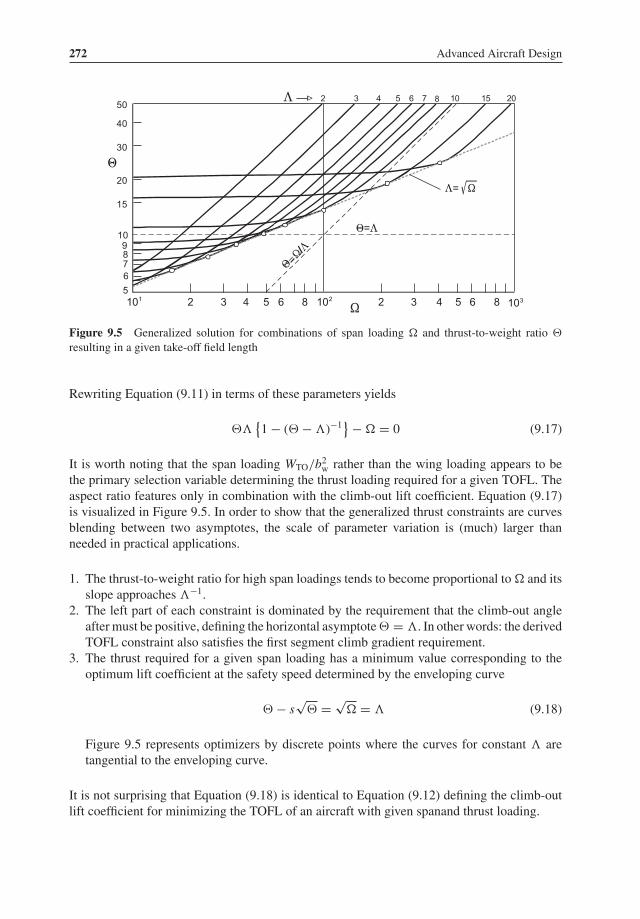
272 Advanced Aircraft Design
Figure 9.5 Generalized solution for combinations of span loading � and thrust-to-weight ratio �
resulting in a given take-off field length
Rewriting Equation (9.11) in terms of these parameters yields
�{1− (� − )−1
} − � = 0 (9.17)
It is worth noting that the span loading WTO/b2w rather than the wing loading appears to bethe primary selection variable determining the thrust loading required for a given TOFL. Theaspect ratio features only in combination with the climb-out lift coefficient. Equation (9.17)is visualized in Figure 9.5. In order to show that the generalized thrust constraints are curvesblending between two asymptotes, the scale of parameter variation is (much) larger thanneeded in practical applications.
1. The thrust-to-weight ratio for high span loadings tends to become proportional to� and itsslope approaches −1.
2. The left part of each constraint is dominated by the requirement that the climb-out angleafter must be positive, defining the horizontal asymptote� = . In other words: the derivedTOFL constraint also satisfies the first segment climb gradient requirement.
3. The thrust required for a given span loading has a minimum value corresponding to theoptimum lift coefficient at the safety speed determined by the enveloping curve
� − s√
� =√
� = (9.18)
Figure 9.5 represents optimizers by discrete points where the curves for constant aretangential to the enveloping curve.
It is not surprising that Equation (9.18) is identical to Equation (9.12) defining the climb-outlift coefficient for minimizing the TOFL of an aircraft with given spanand thrust loading.
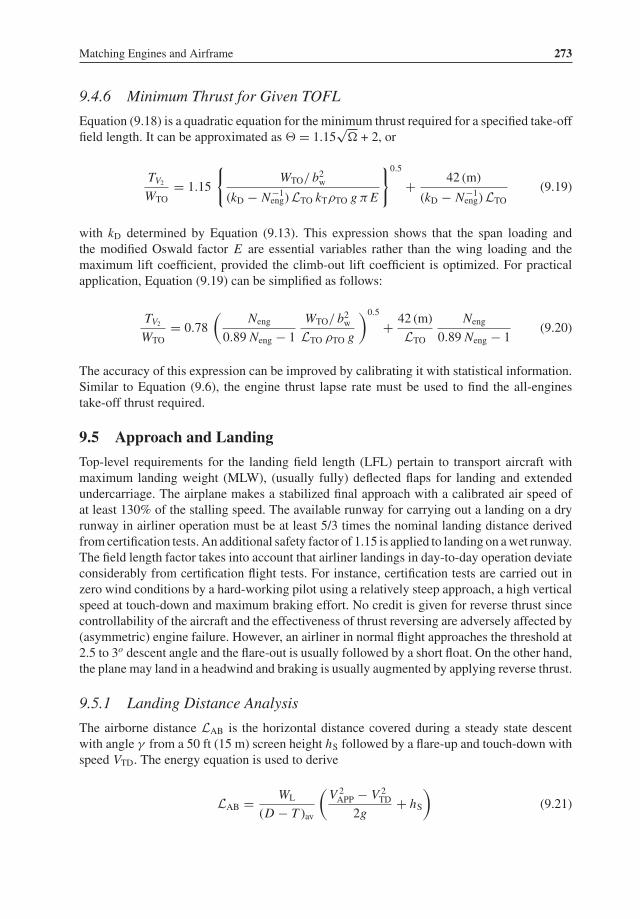
Matching Engines and Airframe 273
9.4.6 Minimum Thrust for Given TOFL
Equation (9.18) is a quadratic equation for the minimum thrust required for a specified take-offfield length. It can be approximated as � = 1.15√� + 2, or
TV2
WTO= 1.15
{WTO/ b2w
(kD − N−1eng)LTO kTρTO g π E
}0.5+ 42 (m)
(kD − N−1eng)LTO
(9.19)
with kD determined by Equation (9.13). This expression shows that the span loading andthe modified Oswald factor E are essential variables rather than the wing loading and themaximum lift coefficient, provided the climb-out lift coefficient is optimized. For practicalapplication, Equation (9.19) can be simplified as follows:
TV2
WTO= 0.78
(Neng
0.89 Neng − 1WTO/ b2wLTO ρTO g
)0.5+ 42 (m)
LTONeng
0.89 Neng − 1 (9.20)
The accuracy of this expression can be improved by calibrating it with statistical information.Similar to Equation (9.6), the engine thrust lapse rate must be used to find the all-enginestake-off thrust required.
9.5 Approach and Landing
Top-level requirements for the landing field length (LFL) pertain to transport aircraft withmaximum landing weight (MLW), (usually fully) deflected flaps for landing and extendedundercarriage. The airplane makes a stabilized final approach with a calibrated air speed ofat least 130% of the stalling speed. The available runway for carrying out a landing on a dryrunway in airliner operation must be at least 5/3 times the nominal landing distance derivedfromcertification tests. An additional safety factor of 1.15 is applied to landing on awet runway.The field length factor takes into account that airliner landings in day-to-day operation deviateconsiderably from certification flight tests. For instance, certification tests are carried out inzero wind conditions by a hard-working pilot using a relatively steep approach, a high verticalspeed at touch-down and maximum braking effort. No credit is given for reverse thrust sincecontrollability of the aircraft and the effectiveness of thrust reversing are adversely affected by(asymmetric) engine failure. However, an airliner in normal flight approaches the threshold at2.5 to 3o descent angle and the flare-out is usually followed by a short float. On the other hand,the plane may land in a headwind and braking is usually augmented by applying reverse thrust.
9.5.1 Landing Distance Analysis
The airborne distance LAB is the horizontal distance covered during a steady state descentwith angle γ from a 50 ft (15 m) screen height hS followed by a flare-up and touch-down withspeed VTD. The energy equation is used to derive
LAB = WL
(D − T )av
(V 2APP − V 2
TD
2g+ hS
)(9.21)

274 Advanced Aircraft Design
The touch-down speed after a (hypothetical) circular flare with constant incremental loadfactor n between the descent and the horizontal runway is
VTD = VAPP√1− γ 2/n (9.22)
The ground run length LGR is the distance required to come from touch-down to a full stopwith an average deceleration aav,
LGR = V 2TD
2aav(9.23)
Addition of Equations (9.21) and (9.23) yields the landing distance
LLD = WL
(D − T )avhS + V 2
APP
2g
{1− γ 2/n
aav/g+ γ 2
n
WL
(D − T )av
}(9.24)
A good prediction for jet transports is obtained forn = 0.10, γ = 0.08 andWL/(D − T )av =10 and substitution of hS yields the factored LFL,
LLF = 250 (m)+ V 2APP
2g
(1.56
aav/g+ 1.07
)(9.25)
Prediction of the average deceleration during the landing run requires knowledge of theeffectiveness of lift dumpers and/or air brakes and the operation and performance of wheelbrakes. If such information is lacking, the use of statistics is unavoidable. A comparison of jetairliner and business jet landing performance reveals that the deceleration depends primarilyon the use of automatic spoilers and on the main landing gear configuration [2]. For jetaircraft with automatic ground spoilers, Equation (9.25) provides a realistic approximation foraav/g = 0.40 for two-wheel trucks, and aav/g = 0.32 for four-wheel trucks.
9.5.2 Approach Speed and Wing Loading
Primary parameters affecting the landing distance are the approach speed and the decelerationduring the braked run. Both are affected by the level of technology.
• For given wing geometry and landing weight, the stalling speed is determined by the maxi-mum lift coefficient with flaps in the landing position. Apart from careful aero-mechanicaldesign, CL max can be increased by applying leading edge high lift devices, multiple trailingedge flap slots and/or large-span flaps.
• Modern commercial aircraft are equipped with anti-skid devices, many also with carbonbrakes. For given total landing gear load, the deceleration is increased by applying brakeson both main and nose landing gears. Lift dumpers increase the main gear load and air dragduring the ground run. Some regional aircraft use aerodynamic speed brakes both in the airand on the ground.
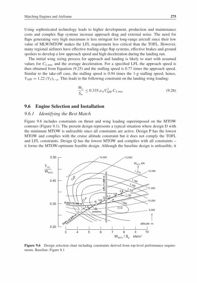
Matching Engines and Airframe 275
Using sophisticated technology leads to higher development, production and maintenancecosts and complex flap systems increase approach drag and external noise. The need forflaps generating very high maximum is less stringent for long-range aircraft since their lowvalue of MLW/MTOW makes the LFL requirement less critical than the TOFL. However,many regional airliners have effective trailing-edge flap systems, effective brakes and groundspoilers to develop a low approach speed and high deceleration during the landing run.The initial wing sizing process for approach and landing is likely to start with assumed
values for CL max and the average deceleration. For a specified LFL the approach speed isthen obtained from Equation (9.25) and the stalling speed is 0.77 times the approach speed.Similar to the take-off case, the stalling speed is 0.94 times the 1-g stalling speed; hence,VAPP = 1.22 (VS)1−g . This leads to the following constraint on the landing wing loading:
WL
Sw≤ 0.335 ρ slV
2APP CL max (9.26)
9.6 Engine Selection and Installation
9.6.1 Identifying the Best Match
Figure 9.6 includes constraints on thrust and wing loading superimposed on the MTOWcontours (Figure 9.1). The present design represents a typical situation where design D withthe minimum MTOW is unfeasible since all constraints are active. Design P has the lowestMTOW and complies with the cruise altitude constraint but it does not comply the TOFLand LFL constraints. Design Q has the lowest MTOW and complies with all constraints –it forms the MTOW-optimum feasible design. Although the baseline design is unfeasible, it
3 4 5 6 7 8 9 10
9,000
10,000
12,000
11,000
13,00014,000
D
QP
WMTO kNTTO
WMTO
WMTO / Sw kN/m2
altitude m
0.50
0.40
0.30
0.20
E
F
1.5
1.71.8
1.9
R 1.6
baseline
Figure 9.6 Design selection chart including constraints derived from top-level performance require-ments. Baseline: Figure 8.1
276 Advanced Aircraft Design
can be improved for the same wing loading by increasing its installed thrust by 7%. It thenbecomes practically identical to designRon the intersection of the ICACandTOFLconstraints.Although designR does not represent the constrainedMTOW-optimizer, its lowerwing loadingallows it to have 8% less thrust than design Q for a small take-off weight penalty. Arguably,design R can be considered the best solution for the present performance requirements sinceits lower wing loading gives it some weight growth potential. Design E with the highest fuelefficiency is not a practical option whereas design F, with the minimum propulsion weightcontribution, does not offer gross weight and thrust advantages over design R.The engine-to-airframe matching chart allocates various constrained and unconstrained
optima and clarifies design sensitivities. It can be enriched by overlaying energy efficiencyand direct operating costs (DOC) contours. Other important design criteria may also be addedsuch as a buffet boundary and the minimum wing size required to contain the maximumfuel volume (Chapter 10). If the best feasible design is penalized by constraints pushingit too far from unconstrained optima, the designer may introduce (more) advanced designtechnology or even an unusual general arrangement. And if a particular requirement appearsto be very dominant, the associated top-level requirement may have to be reconsidered. Whenall requirements are met in what is considered to be a well-tempered design, the choice of asuitable engine and further wing design refinement will be the advanced designer’s next task.The design selection chart is thus a versatile tool for explicit multi-objective optimization.
9.6.2 Initial Engine Assessment
A straightforward approach to initial engine selection is to compare engine types complyingwith the thrust or power requirements within the feasible design space. For example, Fig-ure 9.6 indicates that the installed thrust of each engine should amount to approximately 0.15MTOW. If existing or projected engines with (approximately) this thrust are available, theirmanufacturers will be contacted for basic information to be used for comparing potentialcandidates. The propulsion weight penalty introduced in Chapter 8 is a useful figure of meritfor comparing the effect of different engine options on the airplane’s MTOW.The propulsion system consists of the (dry) propulsion engines, their nacelles, and the
associated systems and accessories. Mission fuel and MTOW are determined by the overallengine efficiency in cruising flight, nacelle drag and power plant weight. These properties arecombined in Section 8.5 to derive the propulsion weight penalty; that is, the combination ofmission fuel and power plant weight. Irrespective of the airframe aerodynamic efficiency, thislarge weight component is proportional to the propulsion function
Fpropdef= Req
ηo H/g+ μT
τ δ(9.27)
with H/g = 4 350 km. The lowest value of Fprop can serve as a criterion for comparingdifferent engines. The propulsion function has a more universal significance if we multiply itby H/g and R−1
eq . The result is the dimensionless engine figure of merit
EFM =(
1
overall efficiency+ H/g
Req
p.p. weight
cruise thrust
) (1− nacelle drag
cruise thrust
)−1(9.28)

Matching Engines and Airframe 277
The usual engine performance parameters are adapted to define the complete installation,nacelles included. The initial cruise condition defines speed, installed thrust and overall effi-ciency. The equivalent range is used in the denominator of the second term. Although the ratioof power plant weight to cruise thrust depends on altitude, the maximum cruise thrust at thetropopause (11 000 m, 36 000 ft) can be used as a standard. Equation (8.25) proves that theratio of nacelle drag to thrust is independent of the altitude since, for a given Mach number,both are proportional to ambient pressure.It is worth noting that the ratio of the second to the first term of Equation (9.28) is identical
to the ratio of power plant weight to mission fuel weight. If the manufacturer of a new enginetype has taken measures to increase the overall efficiency – for instance, by increasing the BPRor the OPR – this will usually be negated by an engine weight increase. The EFM effectivelyweighsup these effects and is useful for the engine selection process and for revealing generaltrends. For example, for engines intended to be applied to short-range aircraft the second termis as important as the first one, which could lead to selecting moderately high values of bypassand/or overall pressure ratios.
9.6.3 Engine Selection
Engines are not only selected for their favourable thrust (or power) delivery and fuel economy.
• If the engine SFC is reduced by increasing the OPR, a penalty has to be paid in the engineprice3 and NOx emissions.
• Very high BPR engine fans are driven by small cores, making it increasingly difficult tomatch the fan and turbine rotational speeds. This problem is solved in the geared turbofan(GTF) by using a gearbox to reduce the fan speed.
• For wing-mounted engines with a very large diameter, the airframe design may be penalizedbecause a longer and heavier landing gear is required to provide enough ground clearance.Moreover, the airflow around thewing is influenced by the engine so that adverse interactionsmay lead to high drag. This problem can be avoided by attaching engines to the rear fuselage.
Selecting a current production engine minimizes the risk associated that engine performancepredictions are overoptimistic so that tight performance guarantees can be made to the cus-tomer. Application of an engine that is already in service is always more attractive thanintroducing a new engine with its added logistics and teething problems. Moreover, airlinesconsider it as an advantage when the engines to be installed are in their inventory.New engine development is a very costly undertaking and the designer of a commercial
aircraft is usually bound to select a suitable engine from only a few candidates. In the caseof a small general aviation aircraft, the engine requirements may be fulfilled by off-the-shelf engines. The engine-to-airframe matching will then proceed differently from the casewhere projected engines can be varied in thrust or power to match the aircraft performancerequirements in an optimum fashion – the case considered in this chapter. The situation inthe civil aircraft design world may be a mixture of these cases. For example, a new aircraftor a derivative of an existing type is developed alongside aircraft which have similar engines
3Statistical information in [3] suggests that for 1% TSFC reduction the engine price will increase by almost 3%.
278 Advanced Aircraft Design
installed. After all, aircraft are rarely designed in complete isolation and their engines may be(derivatives of) existing types. On the other hand, a new airliner generation will probably beoffered with alternative engines of (very) similar thrust.
Bibliography
[1] Torenbeek, E., Synthesis of Subsonic Airplane Design, Chapter 5 and Appendix K, Springer Verlag, Heidelberg,1981.
[2] Shevell, R.S., Fundamentals of Flight, Chapter 15, Second Edition, Prentice-Hall, Englewood Cliffs, NJ, 1989.[3] Jenkinson, L.R., P. Simpkin, and D. Rhodes, Civil Jet Aircraft Design, Chapter 9: Powerplant and Installation,
Arnold, London, 1999.[4] Swatton, P.J., Aircraft Performance Theory for Pilots, Blackwell Science, Oxford, 2000.
Take-Off and Landing Performance
[5] Perry, D.H., “The Airborne Path During Takeoff for Constant Rate-of-Pitch Manoeuvres”, AeronauticalResearch Counsil, CP No. 1042, 1969.
[6] Perry, D.H. “A Review of Methods for Estimating the Airfield Performance of Conventional Fixed-WingAircraft”, RAE Technical Memorandum Aero 1264, 1970.
[7] Torenbeek, E, “An Analytical Expression for the Balanced Field Length.” AGARD Lecture Series 56, Paper 9,April 1972.
[8] Anonymous, “First Approximation to Take-off Field Length of Multi-engined Transport Aeroplanes”, ESDUItem Number 76011, May 1976.
[9] Anonymous, “First Approximation to Landing Field Length for Civil Transport Aeroplanes (50 ft, 15.24 mscreen)”, ESDU Data Item No. 84040, December 1984.
[10] Chandrasekharan, R.M., “Improved Method of Analyzing Takeoff Performance Data”, AIAA Paper No. 88–4509, September 1988.
Matching Engines to the Airframe
[11] Pakendorf, H., “Zur Optimierung der Triebwerksanlage eines Kurzstreckenfleugzeuges, unter BesondererBerucksichtigung der Hoher Bypass Verhaltnisse”, WGLR Jahrbuch, pp. 261–270, 1966.
[12] Whitlow, J.B., and G.A. Kraft, “Optimization of Engines for Commercial Air Transports Designed for CruiseSpeeds ranging from Mach 0.9 to 0.98”, NASA TM X-67906, 1971.
[13] Dugan, J.F., “Engine Selection for Transport and Combat Aircraft”, NASATMX-68009, 1971. Also in AGARDLecture Series No. 56, Paper No. 6, April 1972.
[14] McIntire, W.L., and P.E. Beam Jr., “Engine and Airplane: Will It Be a Happy Marriage?”, SAWE Paper No.910, May 1972.
[15] Healy, M.J., J.S. Kowalik, and J.W. Ramsey, “Airplane Engine Selection by Optimization on Surface FitApproximations”, Journal of Aircraft, Vol. 12, No. 7, July 1975, pp. 593–599.
[16] Bowles, J.V., M.H.Waters, and T.L. Galloway, “Thrust andWing Loading Requirements for Short Haul AircraftConstrained by Engine Noise and Field Length”, NASA TN D-8144, 1976.
[17] Keith Jackson Jr., S., “Propulsion System Sizing . . . No Longer Exists”, Annual Aircraft Design Short Course,University of Dayton, Ohio, August 1977.
[18] Hopps, R.H., and E.C.B. Danforth, “Correlation of Wind-Tunnel and Flight-Test Data for the Lockheed L-1011Tristar Airplane”, AGARD Conference Proceedings No. 242, Paper No. 21, 11–13 October 1977.
[19] D.B. Morden, “Engine/Airplane Performance Matching”, The Aerodynamics of Aircraft Gas Turbine Engines,Chapter 9, AFAPL-TR-78–52, The Boeing Commercial Airplane Company, 1978.
[20] Conlon, J.A., and J.V. Bowles, “Powered Lift and Mechanical Flap Concepts for Civil Short-Haul Aircraft”,Journal of Aircraft, Vol. 15, No. 3, pp. 168–174, March 1978.
[21] Sullivan, R.L., “The Size and Performance Effects of High Lift System Technology on a Modern Twin EngineJet Transport”, AIAA Paper No. 79–1795, August 1979.

Matching Engines and Airframe 279
[22] Loftin Jr., L.K., “Subsonic Aircraft, Evolution and the Matching of Size to Performance”, NASA ReferencePublication 1060, August 1980.
[23] Snyder, J.R., “Advanced Technology Tactical Transport”, AIAA Paper No. 86–2668, October 1986.[24] Lavelle, T.M., R.M. Plencner, and J.A. Seidel, “Concurrent Optimization of Airframe and Engine Design
Variables”, AIAA Paper No. 92–4713, September 1992.[25] Guha, A. D. Boylan, and P. Gallagher, “Determination of Optimum Specific Thrust for Civil Aero Gas Turbine
Engines: A Multidisciplinary Synthesis and Optimization”, Journal of Aerospace Engineering, Proceedings ofthe Institution of Mechanical Engineers, Part G: 0(0) pp. 1–26, March 2012.
Engine Integration
[26] Swan, W.C., and A. Sigalla, “The Problem of Installing a Modern High Bypass Engine on a Twin Jet TransportAircraft”, AGARD CP-124, Paper No. 17, April 1973.
[27] Barche, J., “Tragflugelentwurf am Beispiel des Verkehrsflugzeuges VFW 614”, Zeitschrift fur Flugwis-senschaften, Vol. 22, pp. 101–115, April 1974.
[28] Krenz, G., and B. Ewald, “Airframe-Engine Interaction for Engine Configurations Mounted above the Wing”,AGARD CP-150, Paper 26, 1975.
[29] Smyth, R., “Computer Programs for the Design and Performance of Nacelles for High Bypass-Ratio Engines”,AGARD CP-280, Paper No. 25, 1979.
[30] Reubush, D.E., “Effect of Over-the-Wing Nacelles on Wing-Body Aerodynamics”, Journal of Aircraft, Vol. 16,No. 6, pp. 359–365, June 1979.
[31] Krenz, G., “Engine/Airframe Interference”, AGARD-FDP-VKI Special Course, May 1983.[32] Henderson, W.P., and J.C. Patterson, “Propulsion Installation Characteristics”, AIAA Paper No. 83–0087, 1983.[33] Szodruch, J., and J. Kotschote, “Wind Tunnel Tests of Over-the-Wing Nacelles”, Journal of Aircraft, Vol. 20,
No. 7, pp. 606–611, July 1983.[34] Awker, R.W., “Application of Propfan Propulsion to General Aviation”, AIAA Paper No. 86–2698, October
1886.[35] Mirat, J.J., R. Perin, and C. Castan, “Engine Installation Design for Subsonic Transport Aircraft”, ICAS Paper
No. 90–2.7.4, 1990.[36] Greff, E., K. Becker, M. Karwing, and S. Rill, “Integration of High By-pass Ratio Engines onModern Transonic
Wings for Regional Aircraft”, Paper 91–160, DGLR Jahrbuch 1991.[37] Rossow, C.C., J.L. Goddard, H. Hoheisel, et al., “Investigation of Propulsion Integration Interference Effects
on a Transport Aircraft Configuration”, Journal of Aircraft, Vol. 31, No. 5, pp. 1022–1030, 1992.[38] Bacon, R.J. and J. Roskam, “The 3X Jet: An Advanced Engine Configuration for Two-Engine Aircraft”, AIAA
Paper No. 95–3963, September 1995.[39] Rud, K., and H.J. Lichtfuss, “Trends in Aero-Engine Development, Aspects of Engine Airframe Integration for
Transport Aircraft”, Proceedings of the DLR Workshop, Braunschweig, Germany, 6–7 March 1996.[40] Spreen, J.S., R. Slingerland, and E. Jesse, “The 3X Propulsion Concept Applied to a Business Jet Aircraft:
Integration of Two Dissimilarly Sized Turbofan Engines”, AIAA Paper No. 2007–1047, January 2007.

10Elements of AerodynamicWing Design
The airline is interested in the wing only in so far as it enables it to carry fare paying passengersover the required mission with minimum cost . . . and with adequate safety (as also demanded bythe certification authorities).
—J.A. Jupp [27]
10.1 Introduction
Wings produce the lift generated to sustain flight at the expense ofmajor drag and emptyweightcomponents – they form the primary focus of attention by aircraft designers. A wing designevolves to the unique configuration necessary to satisfy the needs of a particular application,and hence there are no universal ‘best wings’. Even if we restrict ourselves to civil subsonicaircraft, the variety of wing shapes that has been brought forth during the evolution of aircraftis overwhelming. Figure 10.1 depicts a selection of geometric permutations that have beenselected from historical documents. It would be easy to increase the size of this collectionand if we would produce a list of words characterizing wing concepts and descriptors itwould count more than 60 items [11]. However, during conceptual design it is not necessary(or desirable) to consider many details that will characterize the final geometry establishedduring the (downstream) detail design phase. In fact, the main contribution of the wing tothe aerodynamic efficiency L/D in cruising flight is determined to a large extent by two keyparameters: planform area and span or aspect ratio. Both features contribute to achieve a highL/D and they are also helpful to fulfil take-off and landing field length requirements. Wingsfor long-range cruise at high altitudes are characterized by long spans and lots of area. Wingsweep does not contribute directly to L/D but is essential to comply with a requirement ofobtaining a cruise speed exceedingMach 0.7. On the other hand, wing span and area are strongdrivers of structural weight and the best solution is obtained from a compromise between highaerodynamic efficiency and low structural weight.
Advanced Aircraft Design: Conceptual Design, Analysis and Optimization of Subsonic Civil Airplanes, First Edition. Egbert Torenbeek.
© 2013 by Egbert Torenbeek. Published 2013 by John Wiley & Sons, Ltd.
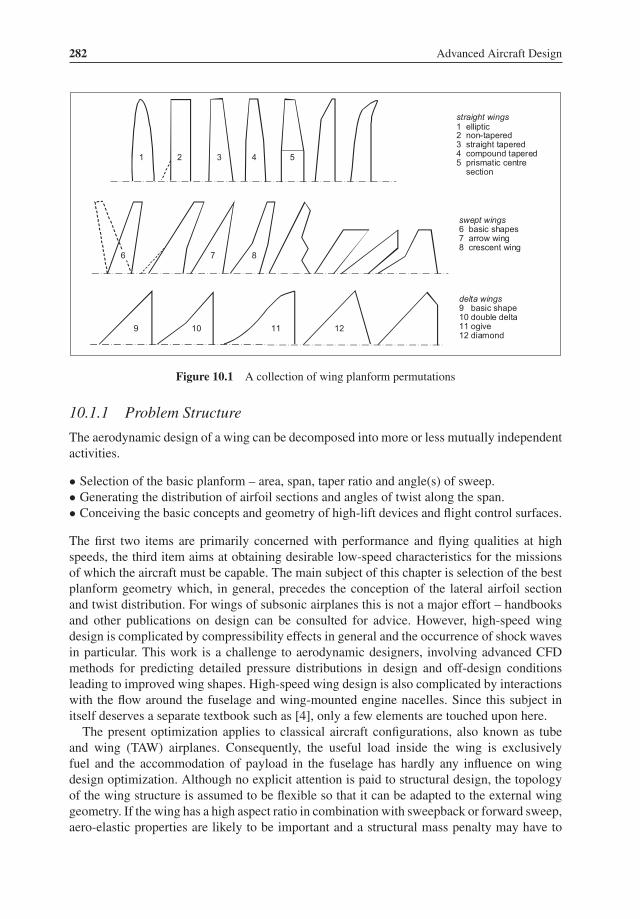
282 Advanced Aircraft Design
Figure 10.1 A collection of wing planform permutations
10.1.1 Problem Structure
The aerodynamic design of a wing can be decomposed into more or less mutually independentactivities.
• Selection of the basic planform – area, span, taper ratio and angle(s) of sweep.• Generating the distribution of airfoil sections and angles of twist along the span.• Conceiving the basic concepts and geometry of high-lift devices and flight control surfaces.
The first two items are primarily concerned with performance and flying qualities at highspeeds, the third item aims at obtaining desirable low-speed characteristics for the missionsof which the aircraft must be capable. The main subject of this chapter is selection of the bestplanform geometry which, in general, precedes the conception of the lateral airfoil sectionand twist distribution. For wings of subsonic airplanes this is not a major effort – handbooksand other publications on design can be consulted for advice. However, high-speed wingdesign is complicated by compressibility effects in general and the occurrence of shock wavesin particular. This work is a challenge to aerodynamic designers, involving advanced CFDmethods for predicting detailed pressure distributions in design and off-design conditionsleading to improved wing shapes. High-speed wing design is also complicated by interactionswith the flow around the fuselage and wing-mounted engine nacelles. Since this subject initself deserves a separate textbook such as [4], only a few elements are touched upon here.The present optimization applies to classical aircraft configurations, also known as tube
and wing (TAW) airplanes. Consequently, the useful load inside the wing is exclusivelyfuel and the accommodation of payload in the fuselage has hardly any influence on wingdesign optimization. Although no explicit attention is paid to structural design, the topologyof the wing structure is assumed to be flexible so that it can be adapted to the external winggeometry. If the wing has a high aspect ratio in combination with sweepback or forward sweep,aero-elastic properties are likely to be important and a structural mass penalty may have to

Elements of Aerodynamic Wing Design 283
be imposed to avoid excessive wing deformation. Moreover, the lateral stiffness distributiondetermines the wing shape – and therefore drag – in the loaded condition, which deviates fromthe jig shape. Since aero-elastic effects are normally covered downstream of the conceptualdesign phase they are considered to be outside the scope of this text.
10.1.2 Relation to Engine Selection
Sizing and selection of the engines to be installed are the subject of previous chapters. Thewing design process can be started as soon as a provisional engine selection has been made.In practical design the situation can be more complicated because engine sizing criteriaand aerodynamic wing design are intertwined. For example, the choice of wing span has asignificant effect on engine thrust required in the case of constrained performances such asa cruise altitude/speed or a take-off distance constraint. It is therefore useful to classify thedesign process according to one of the following approaches:
A. Variations in wing geometry are studied for constant flight performance constraints andengine (cruise) rating. The engine thrust to be installed is adapted to wing design variations,often by adopting the rubberizing concept (Section 8.5). The engine selection is made aftercompletion of the wing design.
B. Wing design is executed for a given engine type with specified power or thrust charac-teristics, weight and geometry. Variations in wing geometry then result in varying flightperformance.
Option A was the subject of previous chapters in which take-off wing loading and the ratioof installed thrust to MTOW were treated as primary selection variables. An example of aselection diagram illustrated how the initial cruise altitude,MTOWand low-speed performanceconstraints affected the best choice of the wing loading and the ratio of thrust to weight. Theexample demonstrated that, for given wing loading, the take-off thrust required is sensitive tothe initial cruise altitude, whereas variation of the wing loading for a given cruise altitude haslittle effect on it. For the present study, the initial operating conditions (altitude and speed) incruising flight are considered to be pre-assigned. The wing shape is subject to optimization,which requires an extension of the sensitivity analysis used for the case discussed previously.Aircraft figures of merit (FOM) to be optimized are mission fuel and MTOW.Option B uses the same sensitivity analysis as option A; however, the optimization is
basically a weight and performance analysis for designs with different drag and weight char-acteristics. The objective function can be (a) MTOW for a given mission fuel and range;(b) mission fuel required for a given range and MTOW; (c) mission range for a given fueland MTOW; or (d) a more elaborate economical figure of merit. The preliminary design stageactivity uses detailed aerodynamic and engine performance information required to comparecompeting engine types and/or fine-tuning the wing design.
10.2 Planform GeometryWhen unusual wings are presented, you can suspect that they were driven by a set of performancespecifications that could not be fulfilled by straightforward means.
—J. Chuprun [11]
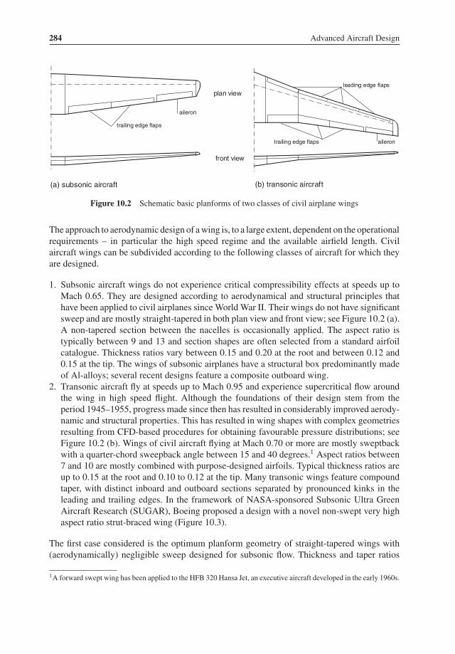
284 Advanced Aircraft Design
plan view
front view
trailing edge flaps
trailing edge flaps
leading edge flaps
aileron
aileron
(a) subsonic aircraft (b) transonic aircraft
Figure 10.2 Schematic basic planforms of two classes of civil airplane wings
The approach to aerodynamic design of awing is, to a large extent, dependent on the operationalrequirements – in particular the high speed regime and the available airfield length. Civilaircraft wings can be subdivided according to the following classes of aircraft for which theyare designed.
1. Subsonic aircraft wings do not experience critical compressibility effects at speeds up toMach 0.65. They are designed according to aerodynamical and structural principles thathave been applied to civil airplanes since World War II. Their wings do not have significantsweep and are mostly straight-tapered in both plan view and front view; see Figure 10.2 (a).A non-tapered section between the nacelles is occasionally applied. The aspect ratio istypically between 9 and 13 and section shapes are often selected from a standard airfoilcatalogue. Thickness ratios vary between 0.15 and 0.20 at the root and between 0.12 and0.15 at the tip. The wings of subsonic airplanes have a structural box predominantly madeof Al-alloys; several recent designs feature a composite outboard wing.
2. Transonic aircraft fly at speeds up to Mach 0.95 and experience supercritical flow aroundthe wing in high speed flight. Although the foundations of their design stem from theperiod 1945–1955, progress made since then has resulted in considerably improved aerody-namic and structural properties. This has resulted in wing shapes with complex geometriesresulting from CFD-based procedures for obtaining favourable pressure distributions; seeFigure 10.2 (b). Wings of civil aircraft flying at Mach 0.70 or more are mostly sweptbackwith a quarter-chord sweepback angle between 15 and 40 degrees.1 Aspect ratios between7 and 10 are mostly combined with purpose-designed airfoils. Typical thickness ratios areup to 0.15 at the root and 0.10 to 0.12 at the tip. Many transonic wings feature compoundtaper, with distinct inboard and outboard sections separated by pronounced kinks in theleading and trailing edges. In the framework of NASA-sponsored Subsonic Ultra GreenAircraft Research (SUGAR), Boeing proposed a design with a novel non-swept very highaspect ratio strut-braced wing (Figure 10.3).
The first case considered is the optimum planform geometry of straight-tapered wings with(aerodynamically) negligible sweep designed for subsonic flow. Thickness and taper ratios
1A forward swept wing has been applied to the HFB 320 Hansa Jet, an executive aircraft developed in the early 1960s.

Elements of Aerodynamic Wing Design 285
Figure 10.3 High span strut-braced folding wing concept described in NASA/CR-2011-216847
are constant and the only selection variables to be optimized are (gross) wing area and spanand it is assumed that the span can be varied without hard constraints. The next case is theoptimum aerodynamic design of transonic wings. This is complicated by the requirement thatthe aircraft has to cruise at a specified Mach number without experiencing a large drag penaltydue to supercritical compressibility of the flow. For a given airfoil technology, the criticalMach number of a wing is affected by the thickness ratio, sweep angle and lift coefficient.Hence, for a given design cruise Mach number, variation of the wing loading has an effect ondrag and weight. This is accounted for in analyzing the design sensitivity.
10.2.1 Wing Area and Design Lift Coefficient
For a conceptual sizing problem, the wing planform area Sw is arguably a primary designparameter.2 Although the wing loading WMTO/Sw is often treated as an independent variable,it is strictly a dependent variable since the MTOW is generally determined by the requirementthat the plane has to carry a given payload over a specified distance. Large weight componentssuch as structure and fuel weight depend on the MTOW which itself results from the additionof many weight contributions. This complicates the sizing and optimization problem, unlessclosed-form design sensitive equations can be derived for design weights. The previous andpresent chapters aim at deriving explicit relationships between the selection variable(s), theMTOW and other weight components that are considered as objective functions. A non-iterative solution of the governing sizing equations allows the designer to compute and visualizethe design space enabling multi-objective optimization.The primary selection variable used in the present chapter is the design lift coefficient
CL = WMTO
q Sw(10.1)
The present chapter treats the dynamic pressure q = 0.5 ρV 2 = 0.5 γ p M2 as a pre-assignedparameter referring to the initial cruise condition. In view of the fuel burnt during the ascentto cruise altitude, the initial cruise GW is 2 to 3% less than the MTOW which is taken into
2Airframe manufacturers use different methods to extend leading and trailing edges to the centreline; hence, thereexists no international standard for defining the gross wing area.

286 Advanced Aircraft Design
account by increasing the actual dynamic pressure by the same percentage. The design liftcoefficient CL is proportional to the wing loading and is a uniquely defined independent designvariable – it forms a demanding condition for the aerodynamic wing design, especially for atransonic airliner.
10.2.2 Span and Aspect Ratio
The wing span bw is a well-defined geometric property; namely, the distance betweenthe wing tips.3 Vortex drag is inversely proportional to the span loading WMTO/b2w and alow span loading results in a low take-off distance (Section 9.4). However, a long wingspan results in a high structure weight unless unconventional measures are taken, such asstrut bracing.Aerodynamic properties such as the aerodynamic efficiency L/D and the lift gradient
dCL/dα are usually expressed in terms of the aspect ratio
Awdef= b2w
Sw(10.2)
Aircraft designers are familiar with the aspect ratio since it is the foremost parameter by whicha wing can be matched to performance requirements in an optimum fashion. Different fromother selection variables, the aspect ratio can often be varied within a fairly wide range withno hard constraints. An exception is due to an upper limit on wing span specified in ICAOairfield classifications.Figure 10.4 depicts a matrix of wing and body combinations representing members of a two-
dimensional design space of planform areas and aspect ratios. All designs have the same body,wing sweepback angle and taper ratio. The angle of sweep and wing size variation suggest thatthese wings could be members of the design space for a large long-range jetliner. In a realisticstudy it is very likely that different airfoil sections and high-lift systems will be matched to therange of cruise lift coefficients and wing loadings. As a starting point, the design space will bestudied without paying attention to practical constraints such as fuel tank capacity. Althoughthe wide variation of wing geometry in Figure 10.4 seems rather unrealistic, it provides agood overview of the global design sensitivity and the penalty due to off-optimum choices.Incidentally, the present design case differs fundamentally from the progression in wing andbody combinations with the same total volume as depicted in Figure 5.5.
10.3 Design Sensitivity Information
For the purpose of realistic optimization, it is imperative to get a grip on the functionalsensitivity of the airplane’s drag and weight to relevant selection variables. The methodologydiscussed in Chapters 8 and 9 forms the basis of the present chapter but the design space isextended with applications to optimize other geometric properties. Different from the previouschapters, the initial cruise altitude remains constant and variation of CL is effected by varyingthe wing loading.
3The definition of span may have to be adapted when winglets are attached to the tips.

Elements of Aerodynamic Wing Design 287
Figure 10.4 Combinations of a fuselage with wings with different areas and aspect ratios
10.3.1 Aerodynamic Efficiency
The airframe drag components essential for the present optimization are profile drag of thewing and horizontal tail, parasite drag of the fuselage and vertical tail and drag due to lift.The variation of drag components with the wing area is discussed in Section 8.4. The profiledrag coefficient CDp according to Equation (8.17) takes into account that the horizontal tailarea is scaled up proportional to wing area. The drag areas of the fuselage and vertical tailare assumed to be fixed; that is, independent of the wing geometry. In view of the variationof installed engine thrust or power, nacelle drag is treated as a reduction of the engine thrust.However, in this chapter, engines are sized for constant cruise altitude and the variation ofengine thrust and nacelle size is small. Although the distinction between aircraft drag andairframe drag can still be made, we refrain from this for simplicity and treat the nacelle dragarea as fixed.The inverse of the aerodynamic efficiency in the design condition according to Equa-
tion (8.19) is rewritten with the drag due to lift factor KL dependent on the aspect ratio,
CD
CL= CD0
CL+ CL
π Awe= CDp
CL+ q
(CDp S)fixWMTO
+ CL
π Awe(10.3)
Section 8.4 explains that CDp is slightly sensitive to wing area variation due to the scale effecton chord Reynolds number and skin friction drag. This becomes more complicated whenboth CL and Aw are design variables – it can be shown that CDp ∝ (CL Aw)1/12. This refine-ment can be handled by numerical analysis but we ignore it for simplification of the present
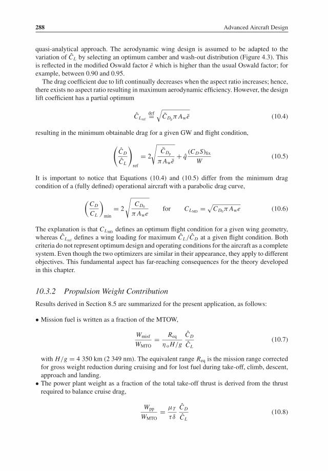
288 Advanced Aircraft Design
quasi-analytical approach. The aerodynamic wing design is assumed to be adapted to thevariation of CL by selecting an optimum camber and wash-out distribution (Figure 4.3). Thisis reflected in the modified Oswald factor e which is higher than the usual Oswald factor; forexample, between 0.90 and 0.95.The drag coefficient due to lift continually decreases when the aspect ratio increases; hence,
there exists no aspect ratio resulting in maximum aerodynamic efficiency. However, the designlift coefficient has a partial optimum
CL refdef=
√CDpπ Awe (10.4)
resulting in the minimum obtainable drag for a given GW and flight condition,
(CD
CL
)ref
= 2
√CDp
π Awe+ q
(CD S)fixW
(10.5)
It is important to notice that Equations (10.4) and (10.5) differ from the minimum dragcondition of a (fully defined) operational aircraft with a parabolic drag curve,
(CD
CL
)min
= 2
√CD0
π Awefor CLMD = √
CD0π Awe (10.6)
The explanation is that CLMD defines an optimum flight condition for a given wing geometry,whereas CL ref defines a wing loading for maximum CL/CD at a given flight condition. Bothcriteria do not represent optimum design and operating conditions for the aircraft as a completesystem. Even though the two optimizers are similar in their appearance, they apply to differentobjectives. This fundamental aspect has far-reaching consequences for the theory developedin this chapter.
10.3.2 Propulsion Weight Contribution
Results derived in Section 8.5 are summarized for the present application, as follows:
• Mission fuel is written as a fraction of the MTOW,
Wmisf
WMTO= Req
η oH/g
CD
CL(10.7)
with H/g = 4 350 km (2 349 nm). The equivalent range Req is the mission range correctedfor gross weight reduction during cruising and for lost fuel during take-off, climb, descent,approach and landing.
• The power plant weight as a fraction of the total take-off thrust is derived from the thrustrequired to balance cruise drag,
Wpp
WMTO= μT
τδ
CD
CL(10.8)

Elements of Aerodynamic Wing Design 289
where μT is the power plant weight per unit take-off thrust. The parameter τ denotes thecorrected thrust lapse rate; that is, the corrected maximum cruise thrust T/δ divided by thetake-off thrust TTO with δ denoting the relative ambient pressure.
• The propulsion weight penalty is the combination of mission fuel and power plant weight,
Wprop
WMTO= Fprop
CD
CL=
(Req
η oH/g+ μT
τδ
){CDp
CL+ q (CD S)fix
WMTO+ CL
π Ae
}(10.9)
For specified cruise conditions, the propulsion function Fprop is a constant which does notdepend on the airframe characteristics.
10.3.3 Wing and Tail Structure Weight
A subsonic wing will generally have a near-zero sweep angle, its thickness ratio has an upperlimit set by the objective to avoid critical compressibility effects.In principle, loading cases for all structural components need to be considered which deter-
mine the material thicknesses, an approach including a number of steps and iterations. Forexample, structural components are sized to withstand several load distributions – combina-tions of fuel and payload, design speeds and altitudes, etc. – in order to find a critical condition.Moreover, the wing structural mass distribution, which is not known a priori, affects the inertiarelief effect. An example of such a methodology is described in Chapter 11. A more refinedmultiple station method is required to take into account that for each element the critical load-ing varies along the span. For components such as the upper and lower box panels a selectionmust be made of skin/stringer configurations and rib distances. Moreover, all major compo-nents of the wing box are subject to sub-optimization and since each wing geometry requiresan adaptation of the structural topology, this approach will entail a laborious computationalprocess. Prediction of the horizontal tail weight requires knowledge of the tail geometry andcritical tail loads and follows the same structural sizing method as for the wing. The entireweight prediction is time-consuming, computer-intensive and degrades the efficiency of theairplane system optimization with no guarantee of improved accuracy.For the present analytical optimization, Equation (8.1) is used as a starting point for com-
puting the wing weight sensitivity. The assumption is made that the manoeuvre load is criticalfor all values of the wing area and the aspect ratio. Horizontal tail weight is closely related towing area; hence, the tail weight is accounted as a fraction of wing weight,
rhdef= Wh
Ww(10.10)
with a typical value rh = 0.10. Substitution into Equation (8.1) yields the wing and horizontaltail weight fraction
μw+hdef= Ww + Wh
WMTO= 1 Aw
√AwCL
+ 2
CL(10.11)

290 Advanced Aircraft Design
The dimensionless weight parameters are defined as
1 = 0.0013 (1+ rh)
√WMZF/q
bref
n ult η cp(t/c)w (cosw)2
(10.12)
with bref = 100 m (328 ft) and
2 = (1+ rh)�S
q(10.13)
Typical values used for the baseline design on Figure 8.1 are: 1 = 0.0020 and 2 = 0.025.
10.3.4 Wing Penalty Function and MTOW
Similar to the propulsion weight penalty, we consider a weight penalty associated with theindispensable wing. The wing penalty function (WPF) is composed of three mutually inde-pendent weight components:
(1) wing and tail structure weight;(2) the engine weight required to balance wing and horizontal tail drag; and(3) the mission fuel weight required to balance wing and horizontal tail drag along the
mission range.
The WPF is found from Equation (10.9) by leaving out the drag due to the fixed drag area andadding the wing and horizontal tail structure weight
Fwpdef= 1 Aw
√AwCL
+ 2
CL+ Fprop
(CDp
CL+ CL
π Ae
)(10.14)
The selection variables CL and Aw are explicit in this equation – a convenient situation forderiving analytical optimizers.The maximum take-off weight (MTOW) is an important figure of merit (FOM) for civil
aircraft and is often used as an objective function in design optimization. The MTOW derivedin Section 8.6 is modified as follows:
(a) nacelle drag is not considered as a thrust loss and τ is replaced by τ , and(b) the fixed drag area (CDp S)fix includes the nacelle drag area.
The resulting expression for the MTOW
WMTO = Wpay + � Wfix + Fprop q (CDp S)fix1− (μresf + μlg + Fwp)
(10.15)
shows that the wing penalty function Fwp is the only term reflecting the variation of CL andAw. Hence, for given cruise altitude and speed, minimization of the WPF yields the sameoptimizers as minimization of the MTOW. In other words: it is appropriate to optimize wingdesign on the basis of the WPF without knowledge of all weight components in the numerator

Elements of Aerodynamic Wing Design 291
of Equation (10.15). This implies that optimum wing area and aspect ratio are independent ofall drag and weight components not included in the WPF. Moreover, the accuracy of optimizersdepends on the prediction accuracy of the WPF only.
10.4 Subsonic Aircraft Wing
10.4.1 Problem Structure
A subsonic wing has mostly a near-zero sweep angle and its thickness ratio has an upper limitset by the objective to avoid critical compressibility effects. The sweep angle and thickness ratioare therefore constant pre-assigned parameters. Optimization of the wing is carried out for con-stant flight condition q . In principle, the MZFW, centre of pressure location and�S are depen-dent variables but their deviations from the baseline values are negligible. Consequently, theparameters1 and 2 determining the wing and horizontal tail weight are treated as constants.The theory is illustrated for a turboprop-powered freighter design depicted in Figure 10.5.
Although the previous analysis is generally applicable, the propulsion function Fprop mustbe adapted to turboprop propulsion. In particular, the overall efficiency η o in the missionfuel weight term equals the product of engine efficiency based on equivalent power Peq andpropeller efficiency ηpr; see Equation (3.28). The power plant weight contribution is definedby the dimensionless constant term
μT
τδ= power plant weight
available cruise thrust= Wpp
T= (Weng + Wnac + Wpr) V
η prPeq(10.16)
60.0 m
50.8 m
15 m
Figure 10.5 Baseline of a propeller-powered cargo aircraft designed to carry 20 tons of payload over4 000 km. Cruise speed 600 km/h @ 9 150 m altitude. Maximum range 6 000 km

292 Advanced Aircraft Design
I
II
II
IIICL
MTOW kN
0.4 0.6 0.8 1.0 1.20.3 0.5 0.7 0.9 1.1CL
P
1.3
missionfuel kN
III
IV
Aw
6
8
10
12
14
16
baseline
CL
I
Figure 10.6 MTOW and mission fuel affected by the design lift coefficient and aspect ratio for thedesign on Figure 10.5
where the index pr denotes the propeller. This section is devoted to deriving conditions for theminimum achievable MTOW and augmented by conditions for minimum mission fuel.
10.4.2 Unconstrained Optima
MTOW contours for the example aircraft are depicted in Figure 10.6. Several optimizers areindicated by curves and points.
1. The optimum design lift coefficient for given aspect ratio (Curve I) is defined by the con-dition ∂ Fwp/∂CL = 0, resulting in a transcendental equation which is identical to Equa-tion (8.43),
CL =√
CDpπ Awe
(1+ 0.51 Aw
√AwCL + 2
CDp Fprop
)0.5(10.17)
Figure 10.6 clearly shows the difference between the present optimumand the lift coefficientCL ref for minimum wing drag. The difference between the corresponding wing loadingsincreases when the aspect ratio increases which is caused by the increasing wing weightrelative to the fuel weight. Since the response surface is flat near the global optimum, the

Elements of Aerodynamic Wing Design 293
MTOW is not very sensitive to off-optimum values. For instance, plus or minus 20% aboveor below the optimum CL penalizes the MTOW by 1.5%.
2. The optimum aspect ratio for given lift coefficient (Curve II) is obtained from∂ Fwp/∂ Aw = 0, resulting in
Aw = C 0.6L
(2Fprop31π e
)0.4(10.18)
Although this aspect ratio increases sensitively for a high CL , the MTOW is insensitive todeviations from the partial optimizer.
3. Unconstrained global optimizer. The intersection of curves I and II (design P) is defined byclosed-form analytical equations for the design lift coefficient
CL = (CDp + 2/Fprop)5/7(1.5π e) 3/7(Fprop/1)
2/7 (10.19)
and the aspect ratio
Aw = (CDp + 2/Fprop)3/7(1.5π e)−1/7(Fprop/1)
4/7 (10.20)
The optimum selection variables are combined into
CL√Aw
=√1.5π e (CDp + 2/Fprop) (10.21)
whereas the optimum ratio of wing and tail structure weight to mission fuel weight is
Ww + Wh
Wmisf= 2 CDp Fprop + 42
5 CDp Fprop + 32(10.22)
The minimum wing penalty function amounts to
Fwp = 3.5
(Fprop1.5π e
)3/7 {1 (CDp Fprop + 2)
}2/7(10.23)
The following observations on these results illustrate their usefulness:
• Since the response surface is quite flat near the global optimum, Fw is accurately approxi-mated if CL and Aw are selected close to the optimum. Equation (10.23) is therefore usefulfor a first prediction of the MTOW if the wing loading and aspect ratio have not yet beenselected.
• The sensitivities of the wing penalty function to various aerodynamic and (wing) weightparameters are readily computed, which offers an effective tool for technology assessment.For example, application of laminar flow control (LFC) to the wing reduces parasite dragsubstantially, and the optimum wing loading and aspect ratio for minimum MTOW will belower than for a conventional wing. This observation is correct even when secondary effectssuch aswingweight increments and suction power requirements are taken into consideration.
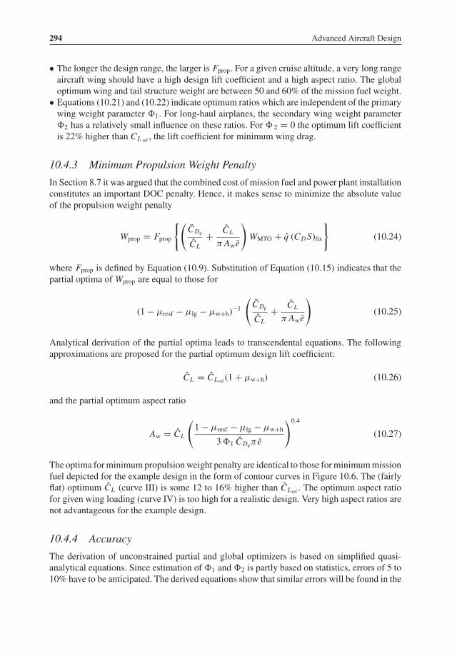
294 Advanced Aircraft Design
• The longer the design range, the larger is Fprop. For a given cruise altitude, a very long rangeaircraft wing should have a high design lift coefficient and a high aspect ratio. The globaloptimum wing and tail structure weight are between 50 and 60% of the mission fuel weight.
• Equations (10.21) and (10.22) indicate optimum ratios which are independent of the primarywing weight parameter 1. For long-haul airplanes, the secondary wing weight parameter2 has a relatively small influence on these ratios. For 2 = 0 the optimum lift coefficientis 22% higher than CL ref , the lift coefficient for minimum wing drag.
10.4.3 Minimum Propulsion Weight Penalty
In Section 8.7 it was argued that the combined cost of mission fuel and power plant installationconstitutes an important DOC penalty. Hence, it makes sense to minimize the absolute valueof the propulsion weight penalty
Wprop = Fprop
{(CDp
CL+ CL
π Awe
)WMTO + q (CD S)fix
}(10.24)
where Fprop is defined by Equation (10.9). Substitution of Equation (10.15) indicates that thepartial optima of Wprop are equal to those for
(1− μresf − μlg − μw+h)−1(
CDp
CL+ CL
π Awe
)(10.25)
Analytical derivation of the partial optima leads to transcendental equations. The followingapproximations are proposed for the partial optimum design lift coefficient:
CL = CL ref (1+ μw+h) (10.26)
and the partial optimum aspect ratio
Aw = CL
(1− μresf − μlg − μw+h
31 CDpπ e
)0.4(10.27)
The optima forminimumpropulsionweight penalty are identical to those forminimummissionfuel depicted for the example design in the form of contour curves in Figure 10.6. The (fairlyflat) optimum CL (curve III) is some 12 to 16% higher than CL ref . The optimum aspect ratiofor given wing loading (curve IV) is too high for a realistic design. Very high aspect ratios arenot advantageous for the example design.
10.4.4 Accuracy
The derivation of unconstrained partial and global optimizers is based on simplified quasi-analytical equations. Since estimation of1 and2 is partly based on statistics, errors of 5 to10% have to be anticipated. The derived equations show that similar errors will be found in the

Elements of Aerodynamic Wing Design 295
optimizers for wing loading and aspect ratio. Although the wing penalty function may have anerror between 1 and 2%, the outcome is still realistic. Wing box weight prediction accuracycan be improved by applying station analysis and/or a finite element method (FEM) whereassecondary structure weight is difficult to predict accurately during the conceptual design stage(Chapter 11). Several published optimization studies simply treat secondary wing weight asa percentage of the primary structure weight. However, if the primary wing weight is 2/3 ofthe total wing weight, 1 is multiplied by 1.5 and 2 = 0, leading to erroneous results for alloptimizers. For instance, the global optimum wing loading and aspect ratio are both reducedby 20 to 35%, wing and tail weight goes down to 40%, mission fuel increases to 60%, althoughthe wing penalty function itself is practically unaffected. An even cruder simplification is tocompute wing weight as a constant specific weight multiplied by wing area. In the presenttheory this means1 = 0, whereas2 increases by a factor of three. In this case the optimumaspect ratio becomes infinite, while for a realistic Aw = 11, the (partial) optimumwing loadingincreases by 25%. Although some of these problems may be avoided by imposing inequalityconstraints, such an artificial remedy degrades the credibility of the results.
10.5 Constrained Optima
The unconstrained global optimum wing area and aspect ratio may be unfeasible due topractical design requirements. In particular, a limit on the take-off distance imposes a constrainton wing area and span. If this becomes an active constraint, the feasible optimum spanloading is affected. Constraints and constrained optima for minimum MTOW are depicted inFigure 10.7. Their position relative to each other and relative to the unconstrained optimumfinally determines the best feasible design. If performance requirements are not too severe and
CL ref
Aw
0.4 0.6 0.8 1.0 1.20.3 0.5 0.7 0.9
6
8
10
12
14
16
CL
fuel tank volume
C1
C1
P
span loading550 N/m2
wing and tail weightfraction 0.15
C2
II
II
I
I C2
baseline
CL ref
1.1
Figure 10.7 Inequality constraints and constrained optima for the design on Figure 10.5

296 Advanced Aircraft Design
design technology is adequate, combination of all constraints indicates a feasible region of thedesign space. An optimum wing design can be identified on every constraint. If none of themsatisfies all constraints, the global optimum is located on the intersection of two constraints.
10.5.1 Take-Off Field Length
Section 9.4 demonstrates that the engine thrust required for taking off from a given airfield isprimarily determined by the span loadingWMTO/b2w. In the present case the installed take-offthrust-to-weight ratio is considered to be known for the baseline aircraft. Hence, a field lengthconstraint is identical to a constraint on the span loading
CL
Aw= WMTO
q b2w(10.28)
is represented by a straight line in the design selection chart (Figure 10.7). The constrainedoptimum is the point of tangency with the local iso-MTOW contour. It is derived analyticallyby substitution of Equation (10.28) into Equation (10.14) and setting its differential equal tozero,
AwC1/3L =
(CDp Fprop + 2
1
)2/3(10.29)
This result is depicted as curve C1 which intersects all partial optimizers in design P.
10.5.2 Tank Volume
For civil aircraft a frequently imposed requirement is that all fuel shall be carried inside thewing. Using a typical relationship between the available and the required tank volume, theavailable fuel tank volume for given average thickness ratio is
Vtank = 0.90 ηtank(t/c)w S1.5w A−0.5w (10.30)
Depending mainly on the wing box planform area as a fraction of the planform area, thevolumetric efficiency ηtank of a completely ‘wet wing’ is approximately 0.55. The tank volumeis a few percentage larger than the total fuel volume required to fly the maximum range RM(Figure 2.3) which follows from the mission fuel and reserve fuel
(Wf)max = (RM)eqη o H/g
{(CDp
CL+ CL
π Aw e
)WMTO + q (CD S)fix
}+ Cresf WMTO (10.31)
with the equivalent range defined by Equation (8.29). If all fuel is to be carried in wing tanks,the upper limit of the take-off wing loading is solved by combining these two equations. Sincewing volume and maximum L/D ratio are both inversely proportional to
√Aw, the wing
loading constraint is insensitive to the aspect ratio. The baseline freighter aircraft design usedas an example is a medium-range aircraft and the wing tank volume constraint appears to beinactive in most of the design space.

Elements of Aerodynamic Wing Design 297
The wing loading constraint varies proportional to W 1/3MTO and the volume constraint can
be problematic for relatively small long-range aircraft. If the resulting weight penalty isobjectionable, an increased cruise altitude can be considered, leading to a larger optimumwing area and less fuel consumed at the cost of more installed engine thrust. Another solutionapplied in several business jets is installation of fuel tanks in the rear fuselage.
10.5.3 Wing and Tail Weight Fraction
The unconstrained optimizer according to Equations (10.19) and (10.20) indicates that opti-mumwing loading and aspect ratio both increasewith increasing range. This is partly explainedby the fact that the optimum wing and tail weight appears to be a certain fraction of the fuelweight. Arguably, since development and production costs are related to empty weight, a largewing is undesirable. If a limit is imposed on the weight fraction μw+h an upper limit on theaspect ratio is derived from Equation (10.11)
Aw ≤ C1/3L
(μw+h − 2/CL
1
)2/3(10.32)
which is depicted in Figure 10.7 for μw+h = 0.15. Application of Equation (10.14) provesthat the constrained optimum is identical to a maximum L/D-ratio for constant wing and tailweight fraction. In other words: the following condition applies to minimum MTOW as wellas minimum fuel weight:
CL =√1.5 CDpπ Awe
(1− 2
1A1.5w C 0.5L
)− 0.5(10.33)
depicted in Figure 10.7 as curve C2. Although the aspect ratio is prominent in this equation,the optimum CL appears to be insensitive to it.
10.5.4 Selection of the Design
The combination of Figures 10.6 and 10.7 is called a design selection chart which is similarto Figure 9.6 but not depicted here. For the cargo aircraft designer, this chart leaves little to bedesired since there exists a convenient feasible region which contains the unconstrained globaloptimum, design P. In the present example the baseline design has a slightly higher aspect ratioand a wing loading 10% below design P. The baseline design needs 2% less mission fuel andhas better field performances than the global optimum, at the cost of a 0.4% higher MTOW.In the more usual situation, the unconstrained optimum is outside the feasible design space orthere exists no feasible design. In the first case, the design point is selected on a constraint or anintersection of two constraints. In the second case it may be necessary to reconsider the engineselection, introduce technology improvements and/or relax the most critical requirement(s)which makes a new design iteration unavoidable.

298 Advanced Aircraft Design
10.6 Transonic Aircraft WingThis work also demonstrates very clearly how much more insight into what really matters maybe obtained from approximate solutions rather than from purely numerical solutions obtained bya computer, where the main trends may be difficult to detect and well hidden and may easily bemissed altogether.
—D. Kuchemann [1] page 419 (1978)
10.6.1 Geometry
The aerodynamic design of a transonic wing requires compressibility effects to be taken intoaccount. This requires variation of the wing geometry dependent on the designMach number incruising flight. Most high-speed wings feature a positive angle of sweep and a kink in the chordand thickness distributions along the span (Figure 10.2). The wing outboard of the kink hasless taper and a smaller thickness ratio compared to the inboard wing. The root thickness ratiois, typically, a factor 1.2 higher. This configuration forms a compromise between conflictingaerodynamic and structural objectives by combining (a) a high thickness ratio at the root, werestructural loads are highest, with (b) a reduced, near-constant thickness ratio of the outboardwing where compressibility effects are more demanding. For conceptual design of a transonicwing, the sweep angle w and the average thickness ratio (t/c)w are additional selectionvariables.
• Instead of the quarter-chord line mostly used for computing low-speed aerodynamic prop-erties, we use the mid-chord line of the outboard wing to define the sweep angle w. Therationale is that the mid-chord line is more representative to characterize the supercriticalpressure distribution of the highly loaded outboard sections.
• The average thickness ratio (t/c)w of a straight tapered wing as depicted in Figure 10.2 (a)is the mean value of the root and the tip thickness ratios. For a complex wing such as shownin Figure 10.2 (b) it is preferable to use the thickness ratio at the leading edge kink.
Apart from the design lift coefficient and the aspect ratio, the sweep angle and thicknessratio are primary selection variables for a transonic civil aircraft wing. This requires a mod-ification of the wing and horizontal tail weight defined by Equations (10.11) and (10.12)as follows:
μw+h = 3
(t/c)w (cosw)2Aw
√AwCL
+ 2
CL(10.34)
with
3 = 0.0013 (1+ rh) η cp n ult
√WMZF/q
bref(10.35)
The design featuring in Figure 8.1 has3 = 0.0002, one order of magnitude smaller than1.
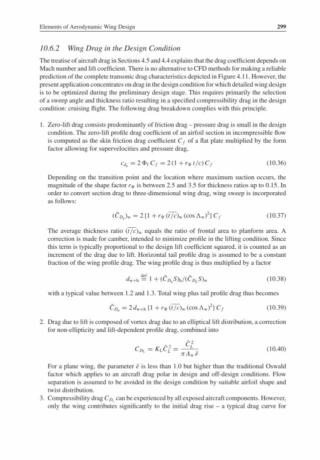
Elements of Aerodynamic Wing Design 299
10.6.2 Wing Drag in the Design Condition
The treatise of aircraft drag in Sections 4.5 and 4.4 explains that the drag coefficient depends onMach number and lift coefficient. There is no alternative to CFDmethods for making a reliableprediction of the complete transonic drag characteristics depicted in Figure 4.11. However, thepresent application concentrates on drag in the design condition for which detailed wing designis to be optimized during the preliminary design stage. This requires primarily the selectionof a sweep angle and thickness ratio resulting in a specified compressibility drag in the designcondition: cruising flight. The following drag breakdown complies with this principle.
1. Zero-lift drag consists predominantly of friction drag – pressure drag is small in the designcondition. The zero-lift profile drag coefficient of an airfoil section in incompressible flowis computed as the skin friction drag coefficient C f of a flat plate multiplied by the formfactor allowing for supervelocities and pressure drag,
cdp = 2f C f = 2 (1+ r t/c)C f (10.36)
Depending on the transition point and the location where maximum suction occurs, themagnitude of the shape factor r is between 2.5 and 3.5 for thickness ratios up to 0.15. Inorder to convert section drag to three-dimensional wing drag, wing sweep is incorporatedas follows:
(CDp )w = 2 {1+ r (t/c)w (cosw)2} C f (10.37)
The average thickness ratio (t/c)w equals the ratio of frontal area to planform area. Acorrection is made for camber, intended to minimize profile in the lifting condition. Sincethis term is typically proportional to the design lift coefficient squared, it is counted as anincrement of the drag due to lift. Horizontal tail profile drag is assumed to be a constantfraction of the wing profile drag. The wing profile drag is thus multiplied by a factor
dw+hdef= 1+ (CDp S)h/(CDp S)w (10.38)
with a typical value between 1.2 and 1.3. Total wing plus tail profile drag thus becomes
CDp = 2 dw+h {1+ r (t/c)w (cosw)2} C f (10.39)
2. Drag due to lift is composed of vortex drag due to an elliptical lift distribution, a correctionfor non-ellipticity and lift-dependent profile drag, combined into
CDL = KLC 2L = C 2
L
π Aw e(10.40)
For a plane wing, the parameter e is less than 1.0 but higher than the traditional Oswaldfactor which applies to an aircraft drag polar in design and off-design conditions. Flowseparation is assumed to be avoided in the design condition by suitable airfoil shape andtwist distribution.
3. Compressibility dragCDc can be experienced by all exposed aircraft components. However,only the wing contributes significantly to the initial drag rise – a typical drag curve for
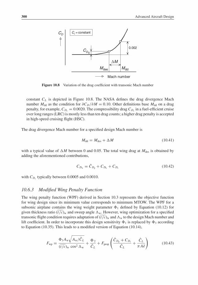
300 Advanced Aircraft Design
Mach number
Mdd
M
0.002
Mdes
CDc
CL = constantCD
Δ
Figure 10.8 Variation of the drag coefficient with transonic Mach number
constant CL is depicted in Figure 10.8. The NASA defines the drag divergence Machnumber Mdd as the condition for ∂CD/∂ M = 0.10. Other definitions base Mdd on a dragpenalty, for example, CDc = 0.0020. The compressibility drag CDc in a fuel-efficient cruiseover long ranges (LRC) is mostly less than ten drag counts; a higher drag penalty is acceptedin high-speed cruising flight (HSC).
The drag divergence Mach number for a specified design Mach number is
Mdd = Mdes + �M (10.41)
with a typical value of �M between 0 and 0.05. The total wing drag at Mdes is obtained byadding the aforementioned contributions,
CDw = CDp + CDL + CDc (10.42)
with CDc typically between 0.0005 and 0.0010.
10.6.3 Modified Wing Penalty Function
The wing penalty function (WPF) derived in Section 10.3 represents the objective functionfor wing design since its minimum value corresponds to minimum MTOW. The WPF for asubsonic airplane contains the wing weight parameter 1 defined by Equation (10.12) forgiven thickness ratio (t/c)w and sweep angle w. However, wing optimization for a specifiedtransonic flight condition requires adaptation of (t/c)w andw to the designMach number andlift coefficient. In order to incorporate this design sensitivity 1 is replaced by 3 accordingto Equation (10.35). This leads to a modified version of Equation (10.14),
Fwp =3Aw
√Aw/CL
(t/c)w cos2 w+ 2
CL+ Fprop
(CDp + CDc
CL+ CL
π Ae
)(10.43)

Elements of Aerodynamic Wing Design 301
This equation has two contributions containing (t/c)w and w:
3Aw
√Aw/CL
(t/c)w cos2 wand CDp = 2 {1+ r (t/c)w (cosw)
2} C f (10.44)
The first term is the primary wing structure weight which decreases when the thickness ratioincreases. The second term representing fuel and power plant weight to balance wing thicknessdrag is reduced when the thickness ratio decreases. Their combination has a minimum valuefor
(t/c)w(cosw)2 = A 0.75
w C 0.25L
√3
2 dw+h r C f Fprop(10.45)
for which the two terms of Equation (10.44) are equal. This ‘optimum thickness ratio’ seemsto be an intriguing result but in practice it is too high to have any practical significance for atransonic airliner. A more realistic design objective is to find the best value of (t/c)w cos2 w
within the limit of acceptable compressibility drag in the cruise condition. The next paragraphsare drawn up to derive wing designs with a drag divergenceMach number at a specified marginabove the design Mach number.
10.6.4 Thickness Ratio Limit
The thickness ratio of a transonic airfoil section has an upper limit determined by the abilityto achieve a very limited amount of compressibility drag at the design Mach number. Aerody-namic wing design technology has a large effect on this limit. During the 1960s, long-rangeairliners and executive aircraft were designed with peaky airfoils which operated with a smallpocket of supersonic flow above the wing nose. The more advanced supercritical airfoilsdeveloped between 1970 and 1990 are representative of the current state of the art. Theseare characterized by a relatively large leading-edge radius, reduced curvature over the middleregion of the upper surface, and substantial camber of the aft surface; see Figure 10.9. Thisgeometry results in a large region of supercritical flow on top closed by a weak shock waveand considerable aft loading in the design condition. The design limit of supercritical sectionscan be quantified by Korn’s equation [20],
Mdd + t/c + 0.10 cl = κ (10.46)
The aerodynamic technology factor κ for supercritical wing sections amounts to approximately0.95. The following modified version of Korn’s equation is based on empirical data of secondgeneration supercritical sections [22]:
Mdd + t/c + 0.10 c 1.5l = M� with M� = 0.935 (10.47)

302 Advanced Aircraft Design
shock wave
sonic line
expansion waves
-1.0
-0.8
-0.6
-0.4
-0.2
0
0.2
0.4
0.6
0.8
1.0.20 .4 .6 .8 1.0
upper surface
lower surface
M= 0.80; cl = 0.613
(c )p soniccp
x/c
(a) schematic flow field
compression wave
(b) chordwise pressure distibution
+ M - MΔ Δ
Figure 10.9 Flow properties for an 11% thick supercritical section near the design Mach number [22]
Equation (10.47) is adapted to three-dimensional airfoils by means of the simple sweep theoryas follows:
Mdd cosw + (t/c)wcosw
+ 0.10{
1.1CL
(cosw)2
} 1.5
= M� (10.48)
The factor 1.1 accounts for the higher than average aerodynamic loading of the outboard wingand the sweep angle refers to the outboard mid-chord line. The upper thickness ratio limitfollows from
(t/c)w (cosw)2 = (cosw)
3(M� − Mdd cosw)− 0.115 C 1.5L (10.49)
Figure 10.10 depicts this relationship and shows that for Mdd ≥ 0.75M� a sweep angle can beidentified for which the term (t/c)w (cosw)2 has a maximum value,
cosw = 0.75M�
Mdd(10.50)
It is worth noting that this characteristic sweep angle is independent of the lift coefficient. ForMach 0.7 or less this condition means that a swept wing is not required to achieve the highestthickness ratio limit. If this condition is inserted in Equation (10.44), the dominant wingweight-related term has a minimum value. This criterion defines the condition of minimumwing penalty function. This is interpreted as a recommendation that for flying at Mdd theMach number component normal to the mid-chord line should be equal to 0.75M�. Indeed, itis confirmed and appears statistically that sweep angles and maximum cruise Mach numberof modern transport and executive aircraft are interrelated as follows: Mdes cosw ≈ 0.70.The optimum sweep angle is thus primarily dependent on the design Mach number and onaerodynamic technology. An advanced aerodynamic wing design corresponds to a high M�
and allows a smaller sweepback angle compared to a less advanced wing. The best thickness

Elements of Aerodynamic Wing Design 303
0.20
0.15
0.10
0.05
0100 20 30 40
0.70
0.75
0.80
0.85
0.90
Mdd
minimumWPF
degrees
t/c cos2
50
Λ
Λ
Figure 10.10 Upper limit of the thickness ratio related to the drag divergence Mach number, forCL = 0.55 and M� = 0.935
ratio is, however, definitely affected by the design lift coefficient. It is therefore rational toselect the sweep angle first and then solve for the highest thickness ratio determined byEquation (10.48).
10.6.5 WPF Affected by Sweep Angle and Thickness Ratio
An interesting illustration of the effects of sweep and thickness ratio variation on the WPF isobtained by adapting the combination of w and (t/c)w to the design lift coefficient CL . Thefollowing observations are based on results for the optimization study in Chapter 8 depictedin Figure 10.11:
• In accordance with previous remarks, the sweep angle resulting in the lowest WPF – line I,w = 31.2◦ – is independent of CL . Selecting a sweep angle a few degrees smaller shouldbe favoured since this affects WPF only slightly whereas low-speed aerodynamic propertiesare improved. Another argument for less sweep is that it allows a higher aspect ratio in caseof an active pitch-up limit.
• The partial optimum CL for minimum Fwp is represented by curve II. Its analytical derivationis discussed in Section 10.7.
• The response surface of wing and tail L/D is a saddle surface. The partial optimum CL
differs little from the MTOW-optimum (curve II) and should be taken seriously. Sensitivityto sweep angle variation is low. Profile drag for zero sweep is low because the wing is verythin; it is low for high sweep angles due to the strong (cosw)2 effect.
• Reference [25] emphasizes the importance of achieving the highest possible cruise liftcoefficient since this results in minimum wing area. The condition for maximum CL isderived from Equation (10.49) by setting the partial derivative w.r.t. the sweep angle equalto zero, which yields
cosw = 3M�
8Mdd
⎧⎨⎩1+
√1− 32 (t/c)w Mdd
9 (M�)2
⎫⎬⎭ (10.51)

304 Advanced Aircraft Design
403020100
0.8
0.7
0.6
0.5
0.4
0.3
0.9
50
24
25
26
26.5
27
2625
26.5
27
0.10 0.12 0.14 0.16
0.08
t/c
(L/D)w+h
WPF
0.38
0.37
0.36
0.355
0.3450.35 0.3350.33
0.34
P
I
II
IIIII
IIIMdd = 0.825Aw = 9.0
I
CL baseline
Λw degrees
Figure 10.11 Wing penalty function and wing/tail aerodynamic efficiency affected by planform geom-etry and lift coefficient. Design: Figure 8.1
depicted by curve III in Figure 10.11. However, complying with this criterion requiresconsiderably more sweepback and higher MTOW compared to Equation (10.50) definingminimum WPF.
These observations clearly illustrate that using a purely aerodynamic criterion as the objectivefunction leads to sub-optimum solutions. The 30◦ sweepback angle of the baseline design isfully justified. The next section demonstrates that the choice of (t/c)w and CL is closely related.
10.7 Lift Coefficient and Aspect Ratio
10.7.1 Partial Optima
Since for transonic aircraft the sweep angle and/or thickness ratio have to be treated as selectionvariables, the wing penalty function optimization must be reconsidered. Equations (10.43) and(10.49) are used to compute the WPF contours in Figure 10.12 which deviate significantlyfrom those in Figure 10.5 for the turboprop freighter design. Figure 10.13 shows that forAw ≥ 6 the partial optimum CL (curve I) is increasingly below the value defined for the case

Elements of Aerodynamic Wing Design 305
0.4 0.6 0.80.3 0.5 0.7 0.9
6
8
10
12
14
16
CL
4
P
I
I
II
II
Mdd = 0.825
w = 30o
WPF
Qpitch-up
Aw
baseline R
0.400.38
0.360.35
0.34
0.335
Λ
Figure 10.12 The WPF in the CL – Aw design space. Conditions: Figure 10.11
Aw
0.4 0.6 0.80.3 0.5 0.7 0.9
6
8
10
12
14
CL
4
P
Fwp/ CL = 0
Fwp/ Aw= 0
constant Mdd
constant t/c
P’
∂
∂ ∂
∂
Figure 10.13 Optima for constant drag rise Mach number compared with those for constant thicknessratio

306 Advanced Aircraft Design
of constant thickness ratio, Equation (10.17). The partial optimum aspect ratio according toEquation (10.18) remains valid provided the wing weight factor 1 is adapted for variationof the sweep angle and thickness ratio with Equation (10.35). The condition ∂ Fwp/∂ Aw = 0results in
Aw = C 0.6L
[2Fprop3π e 3
{(cosw)
3(M� − Mdd cosw)− 0.11 C 1.5L
}]0.4(10.52)
designated as curve II. This solution differs significantly from the subcritical case for CL > 0.6.The global optimum design P’ for the transonic wing has amuch lower wing loading and aspectratio compared with the optimizer for constant thickness ratio.
10.7.2 Constraints
Design limitations such as those mentioned in Section 10.4 apply to subsonic as well astransonic aircraft. However, they have to be modified in order to account for sweep andthickness ratio variation. The span loading constraint indicated in Figure 10.12 is derivedfrom the BFL limit. Attempts to derive an analytical solution for the constrained optimum(design Q) were unsuccessful. The wing box volume available for fuel is sensitive to thicknessratio variation. The volume limit happens to define a design lift coefficient which is almostindependent of the aspect ratio. The corresponding thickness ratio may therefore be assumedto be constant and Equation (10.31) needs no modification.Wing design for transonic flow raises some additional limitations which can be very restric-
tive but difficult to predict accurately.
• Deviations from the equilibrium in cruising flight can occur as a consequence of manoeuvresor a gust upset. The associated variations in incidence and Mach number may lead to shockwaves, shock-boundary layer interactions and a turbulent wing wake impinging on thehorizontal stabilizer. This phenomenon is felt in the aircraft as buffeting. Figure 10.14 showsa typical variation of the lift coefficient for initial buffet onset. Freedom from buffet isnormally required during a manoeuvre load factor of at least 1.30 or a vertical gust velocityof 12.5 m/s from the trimmed condition. Since CL for the buffet onset is difficult to predictduring preliminary design, it is usually derived from wind tunnel and flight tests. For thestudy aircraft the buffet limitation indicated in Figure 10.12 is based on the assumption thatwith the current CFD technology a buffet onset limit of CL = 0.80 can be realized for a 12%thick supercritical wing at the normal Mach 0.81 cruise speed.
• Another off-design requirement is related to handling characteristics at high speed. Inresponse to an increase in incidence, the aircraft should tend to pitch nose-down. If theflow breaks down over the outer wing, this will move the centre of pressure forward andinboard, causing increased downwash at the stabilizer. The resulting pitch-up tendency willbe stronger when the angle of sweep and the aspect ratio are larger. Therefore, a maximumaspect ratio depending on wing sweep and taper is imposed to avoid high speed pitch-upand critical aero-elastic effects. In accordance with current advanced civil aircraft, an aspectratio Aw = 10 is considered to form the pitch-up limitation for a 30◦ sweptback wing.

Elements of Aerodynamic Wing Design 307
Mach number0.6 0.7 0. .9
0.7
0.8
0.9
0.6
0.5
CL
buffet onset
margin
maximumcruise altitude
W/p = constant
8 0
Figure 10.14 Buffet boundary compared with constant altitude cruise
The study design Q (Figure 10.12) has a constrained optimum CL = 0.54 and Aw = 10 – bothfigures are slightly higher than for the baseline design. The preferred modified design R withCL = 0.50 and Aw = 10 promises a useful reduction of the mission fuel at the cost of lessthan 1% MTOW penalty relative to the unconstrained optimum design P.The analytical optima derived in this chapter are intended as guidelines for the initial
selection of the wing geometry. For the present category of aircraft, explicit results such asFigure 10.12 are considered to be more useful than closed-form expressions for the various(partial and global) optima. Although computing iso-merit contours is more labour-intensive,visualization of the design sensitivity to excursions from the baseline and the global optimumis rewarding. The diagrams become even more useful when FOMs such as the propulsionfunction and fuel energy efficiency are shown explicitly.
10.7.3 Refining the Optimization
In this chapter we have treated the wing loading and aspect ratio as the primary selectionvariables. For the optimization of subsonic aircraft the wing was assumed to have zero sweepand constant thickness ratio. For transonic aircraft the sweep angle and thickness ratio wereadditional selection variables associated with obtaining a specified drag-divergence Machnumber. Relatively simple relationships for the WPF according to Equations (10.14) and(10.43) enabled the use of explicit optimization. The two example designs appeared to havea feasible region in which a constrained optimizer could be allocated with modest penaltiesrelative to the unconstrained one. Experienced designers may, however, argue that the situationin the real design world can be more complicated. This is illustrated hereafter for the caseswhere the load factor and the maximum lift coefficient for landing are treated as designparameters or constraints.

308 Advanced Aircraft Design
The ultimate load factor featuring in Equations (10.12) and (10.35) equals 1.5 times of thelimit load factor, the greater of the manoeuvre load factor nman and the gust load factor,
ngust = 1+ 0.5Kg ρ sl UDE VC SwCLα
WMTO(10.53)
For a gust load alleviation factor Kg = 0.8 the manoeuvre load factor is critical for
WMTO
Sw≥ 0.4 ρsl UDE VC CLα
nman − 1 (10.54)
If the wing loading does not comply with this condition, the gust load factor is dominant andthe ultimate load factor is
nult = 1.5+ 0.6 ρsl UdeVC CLα
(WMTO
Sw
)−1(10.55)
In the interest of simplicity it has been assumed that the manoeuvre load factor is dominantso that nult is not affected by wing design. This is justified only if Equation (10.54) is treatedas an inequality constraint. In reality this equation merely represents a limit for the validity ofthe simplified objective function, and there is no valid argument to consider wing loadings notcomplying with Equation (10.54) as unfeasible. Instead, for these wing loadings the gust loadfactor should be treated as dominant. For a given aspect ratio and GW, the structure weightrequired to resist wing bending is then composed of a term proportional to S1.5w and a termproportional to S0.5w , with a dominating first term.The landing wing loading can be constrained by an upper limit of the approach speed to a
lower value than that for minimumweight. As this limit is proportional to CLmax the refinementmay be introduced to treat this coefficient as a design variable. This requires a design-sensitiverelationship between high-lift system design parameters and wing weight. For a given systemconfiguration, it is anticipated that increasingCLmax is possible to a limited extent by increasingflap chords and deflection angles. If this measure is expressed in terms of flap weight, the wingloading constraint can be relaxed. In practice this may be a laborious and complicated exercise.At first sight it seems that the optimization problem has been oversimplified by using the
same expression for the wing penalty function for all combinations of wing loading andaspect ratio. However, the design space can be subdivided into three regions: (1) for low wingloadings nult decreases when the wing loading increases; (2) for intermediate wing loadingsCLmax and nult are constant; (3) for high wing loadings nult is constant andCLmax increases whenthe wing loading increases. Figure 10.15 depicts an example where it can be useful to treat adesign criterion as a borderline between two regions of the design space where the objectivefunction is computed differently. In Figure 10.15 (a) the stall speed constraint is active,making the unconstrained optimum design P unfeasible. The constrained optimum design Qapplies to CLmax = 2.80. The analysis can be refined by relaxing the inequality constraint andconverting it into a borderline with the region where CLmax is variable. In Figure 10.15 (b) anew unconstrained optimum P corresponds to CLmax > 2.80.The wing loading limit for which the load factor is constant is an inequality constraint in
Figure 10.15 (a). Reducing the wing loading below this limit renders the gust load dominant,
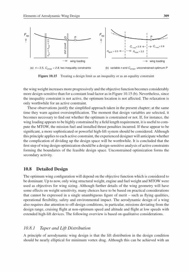
Elements of Aerodynamic Wing Design 309
wing loading
(a) n = 2.5, CLmax = 2.8, two inequality constraints (b) variable n and CLmax, unconstrained optimum P
P
wing loading
P
ngust > 2.5 nman = 2.5
CL > 2.8max
QFwp Fwp
CL = 2.8max
Figure 10.15 Treating a design limit as an inequality or as an equality constraint
the wingweight increases more progressively and the objective function becomes considerablymore design-sensitive than for a constant load factor as in Figure 10.15 (b). Nevertheless, sincethe inequality constraint is not active, the optimum location is not affected. The relaxation isonly worthwhile for an active constraint.These observations justify the simplified approach taken in the present chapter; at the same
time they warn against oversimplification. The moment that design variables are selected, itbecomes necessary to find out whether the optimum is constrained or not. If, for instance, thewing loading appears to be highly constrained by a field length requirement, it is useful to com-pute the MTOW, the mission fuel and installed thrust penalties incurred. If these appear to besignificant, a more sophisticated or powerful high-lift system should be considered. Althoughthis principle applies to each active constraint, the experienced designer will anticipate whetherthe complication of dividing up the design space will be worthwhile. It is concluded that thefirst step of wing design optimization should be a design-sensitive analysis of active constraintsforming the boundaries of the feasible design space. Unconstrained optimization forms thesecondary activity.
10.8 Detailed Design
The optimum wing configuration will depend on the objective function which is considered tobe dominant. Up to now, only wing structural weight, engine and fuel weight andMTOWwereused as objectives for wing sizing. Although further details of the wing geometry will havesome effects on weight sensitivity, many choices have to be based on practical considerationsthat cannot be expressed in a single unambiguous figure of merit – such as flying qualities,operational flexibility, safety and environmental impact. The aerodynamic design of a wingalso requires due attention to off-design conditions, in particular, missions deviating from thedesign range, cruising flight at non-optimum speed and altitude and flight at low speeds withextended high-lift devices. The following overview is based on qualitative considerations.
10.8.1 Taper and Lift Distribution
A principle of aerodynamic wing design is that the lift distribution in the design conditionshould be nearly elliptical for minimum vortex drag. Although this can be achieved with an

310 Advanced Aircraft Design
elliptical planform, (straight) tapered wings are favoured by airplane manufacturers for variousreasons.
• Tapered wings are simpler and cheaper to manufacture.• A highly tapered wing has a more triangular lift distribution, leading to reduced bending atthe (highly loaded) wing root.
• For given planform area and span, the root section is thicker and the wing structure is lighter.• At each lateral station, the structural layout can be better adapted to what is required to copewith the critical local loading case. This results in less non-ideal weight.
• Many sweptback wings have kinks in the leading and/or trailing edge which give themcompound taper. A pronounced trailing edge kink is usually associated with an increasedroot chord length, creating space for retracting landing gears.
If the taper (ratio) is close to the value for minimum induced drag and the twist distributionis correct, the induced drag penalty due to straight taper is very small. A lower limit on theoutboard wing taper ratio is imposed to avoid too high lift coefficients. The lift coefficientinboard of the kink is significantly lower which allows the root section to be thicker – usefulfor reducing wing structural weight.
10.8.2 Camber and Twist Distribution
Figure 10.16 illustrates that in the design (cruise) condition large regions of a supercritical winghave a nearly two-dimensional pressure distribution. The outboard wing is heavily loaded witha region of supersonic flow above the upper surface up to the crest with a plateau of M ≈ 1.20.The highly cambered outboard wing is rear-loaded, resulting in high lift coefficients. A sideeffect of this lift distribution is a nose-down pitching moment that is to be balanced bya horizontal tail download, entailing a trim drag penalty. This disadvantage is reduced bytwisting the inboard wing and applying negative camber near the wing/fuselage junction. Theresulting pressure distribution causes a front loading at the root negating the outboard rearloading; see Figure 10.17. An increased leading-edge sweep of the inboard section will further
Figure 10.16 Pressure distribution of a supercritical wing in the design condition

Elements of Aerodynamic Wing Design 311
+3o
+5o
11.8/6% +1o5-3o
131211109876543210
8380
70064096
chord,millimetres
34002017
1
2
metres
1
2
10.8%
11.6%
15%11.8%
+1 5o
Figure 10.17 Geometry of the Airbus A 310 supercritical wing
reinforce this effect. The peaky pressure distribution is also effective for sweeping back theisobars, thereby minimizing the aerodynamic un-sweeping effect at the root. The variation ofairfoil camber is combined with twist – especially the inboard wing – in order to optimizethe lateral lift distribution and avoid too high outboard wing lift coefficients. Except for thetip region, the outboard wing in Figure 10.17 has little twist in order to approximate thetwo-dimensional pressure distribution as close as possible.4 The net effect of these measuresis a complicated wing geometry, in particular, inboard of the kink.
10.8.3 Forward Swept Wing (FSW)
Sweeping a wing provides an effective means of increasing the drag divergence Mach number,an effect that is obtained regardless of the direction of sweep. However, compared to theaft swept wing (ASW), the outboard section of a forward swept wing (FSW) has a reducedloading and the wing’s centre of pressure is more inboard compared to a forward swept wing(FSW). Comparing an ASW and a FSW for equal planform area, span and lift, the FSWexperiences a reduced bending moment at the structural wing root. Hence, if the FSW span isallowed to increase until the root bending moment equals that of the ASW, the reduced spanloading reduces its induced drag. The FSW tends to stall first at the inboard wing and does notsuffer from pitch up at high angles of attack, an inherent disadvantage of the ASW. It is alsoanticipated that forward sweep favours achievement of NLF since the inboard moving leadingedge flow is not contaminated by the fuselage boundary layer.When a FSW aircraft is manoeuvred at high dynamic pressure, wing bending leads to
increased angle of attack and torsion of the outboard wing at the tips. The FSW tends tosuffer from the aero-elastic phenomenon of structural divergence which cannot be solvedwith a conventional metallic structure without paying an excessive weight penalty. Withcomposite wings, the skin laminates can be tailored to provide favourable deflections atdynamic pressures considerably higher than those previously obtained with conventionalstructures [42]. Advances in the use of composite materials have enabled the elimination ofthe divergence problemwith little or noweight penalty. In spite of their favourable aerodynamicproperties, only a few FSW aircraft have been designed, produced and flown. One notableexample is the HFB 320 Hansa business jet [41], which was marketed (with little commercialsuccess) in the early 1960s.
4Due to aero-elastic deformation, the jig shape built into the structure at the tip of a sweptback wing may differ up toseveral degrees from the desired 1-g loaded shape in flight.

312 Advanced Aircraft Design
Figure 10.18 The winglet concept for drag reduction
10.8.4 Wing-Tip Devices
It has been known since many decennia that addition of wing tip-mounted lifting surfacescan diffuse tip vortex structures and reduce vortex drag. A favoured option is the use ofwinglets – relatively small vertical or outward canted lifting surfaces (Figure 10.18). They areimmersed in the local vortex flow passing from the lower to the upper surface which has aninward velocity component above the wing tip. The winglet acts under an angle of incidenceto this flow and experiences lift. Its component in the direction of flight – the figure indicatesit as a thrust component – balances the winglet’s vortex drag. The trailing vortex sheet isspread out in an upward and outward direction and the wing experiences reduced downwashat the tip. Dependent on the basic wing shape and winglet height, the resulting vortex dragreduction is between 10 and 15%. Wings designed with high outboard lift coefficients aregood candidates for these wing tip devices. The vortex drag reduction is partly offset by thewinglet’s parasite drag and interference between the main wing, whereas the winglet flowmay lead to formation of shock waves at the wing/winglet junction. The blended winglet aimsat reducing these unfavourable effects [64]. Total drag reductions in cruising flight for severalairliners are between 3.5 and 4.5% for winglet heights between 12 and 16% of the semi-span.This compares to a reduction of 5.5% for a 10% wing span increase by means of sheared tips.Especially in the case of a constraint on the wing span, fitting winglets is a favoured option.
In all other cases a fundamental issue is whether or not it is preferable to merely extend thewing tips instead of adding wing-tip devices. A parametric study [50] compared induced dragimprovements achievable with wing tip extension and fitting of optimized winglets, assumingthe same wing root bending moment for both cases. It was found that for almost every tipextension a better performing winglet could be found. Another investigation [55] showedmoremodest advantages. For aircraft with critical engine-out performance at high and hot airfields,a useful induced drag reduction is obtained during the take-off climb, allowing the plane tobe taken off with increased weight. The question whether or not to apply winglets cannot beanswered in general – each configuration must be examined for its net drag reduction, bendingmoment increase, weight penalty and manufacturing costs. Winglets designed as an integral

Elements of Aerodynamic Wing Design 313
wing component are widely accepted as beneficial, as add-on devices they can be detrimental.Aerodynamic tip devices are also introduced on new versions of an existing airliner if thesecan be installed with relatively minor structural modifications.
10.9 High Lift Devices
10.9.1 Aerodynamic Effects
Apart from powered systems such as blown and jet flaps, a high lift system is basically avariable geometry mechanical alteration of the (secondary) structure in front and aft of theprimary box. Civil aircraft feature slotted flaps incorporated at the trailing edge of the inboardwing, many of them have leading edge flaps as well. Deflection of a trailing edge flap on anairfoil section increases its camber which increases the lift. If flap deflection does not extendthe chord, the lift increment�cl is independent of the angle of attack α. Figure 10.19 (a) showsthat, for small flap deflections, �cl is proportional to the flap angle δfl. The flap efficiencydecreases at large deflections due to flow separation above the upper flap surface. For a plainflap (lacking slots), the separation begins at a relatively small flap angle, a single slotted flapis effective to higher deflections and double and triple slotted flaps can cope with deflectionsup to fifty degrees. Slotted flaps, in particular Fowler flaps, move backwards during extension.The increased chord length augments the lift increment proportional to α.A wing with extended slotted flaps can be seen as a series of aerodynamically interacting
airfoils. Each airfoil experiences lift-producing circulation, inducing upwash in the flow aroundthe preceding airfoil and downwash at the following airfoil. The leading airfoil is deflecteddownwards to avoid separation due to the increased local upwash. The nose suction onthe following airfoils acts to energize the trailing edge flow of the preceding one. Theseinteractions postpone separation to higher angles of attack and deflection provided that theairfoils are carefully positioned relative to each other. Figure 10.19 (b) illustrates these effects
fl
fl
cl
number of slots
(a) airfoil trailing edge flap effectivity
0
cL
crit
cLmax
chordextensioneffect
(b) wing lift curves, single slotted flaps and slats
cL
0
0
1
2
Figure 10.19 Effects on lift of extended high lift devices

314 Advanced Aircraft Design
for the lift curve of a three-dimensional wing. The achievable �CLmax of a wing with noleading edge devices is less than �CL at low incidences whereas a slat extends the lift curveto a significantly higher αcrit and has little effect on lift at a given incidence. Multi-slottedpart span Fowler flaps in combination with full span slats can increase the aircraft’s �CLmaxby up to 100% allowing the wing planform area to be selected without compromising highspeed design. For take-off configurations, however, low drag is at least as important as highlift (Section 9.4). References [68, 71, 77] can be consulted for relevant further explanation.
10.9.2 Design Aspects
Application of slats on high speed aircraft with highly swept thin wings is almost unavoidablesince it gives a high maximum lift in combination with a greater freedom to optimize the noseshape for high speed flight. A penalty for extending high lift devices is increased profile dragwhereas part-span flaps increase vortex drag as well. Moreover, trailing edge flaps increasethe wing’s nose-down pitching moment. This effect must be compensated by a tail downloadat the cost of trim drag. Aircraft cruising at speeds below the Mach 0.70 to 0.75 region featurelittle sweepback and fairly thick airfoils. Even without slats they may achieve CLmax up to 3.0with deflected trailing edge devices. Several executive aircraft are optimized to cruise at highaltitudes with a relatively low wing loading, and in combination with the large thrust for take-off their wings can be designed with no leading edge flaps. Avoiding the complication of a slatsystem simplifies the overall aircraft concept and operational properties, forming an invaluablecost saver. An aircraft featuring amodestCLmax should therefore not be dismissed as technicallyinferior. In fact, apart from the application of advanced (composite) structural materials, therehas not been any dramatic advancement in high lift system concepts of today’s generation ofaircraft compared to the historical trend up to 1984 depicted in Figure 10.20. The highest valuein the landing configuration realized for civil transports amounts to CLmax ≈ 3.5 cos0.25 butmany modern airliners do not need this. In association with the superior lifting propertiesof supercritical wings, current trends are towards mechanically simpler systems. These aremostly based on single slotted flaps and slats with increasing emphasis on reducing drag andaerodynamic noise emission by countering the effects of engineering excrescences such as
Figure 10.20 Historical trends in Boeing transport aircraft high lift systems development. CopyrightNATO STO - CSO

Elements of Aerodynamic Wing Design 315
flap and slat tracks. A comprehensive overview of mechanical principles of high lift systemson modern commercial airliners is found in [27] and [82].
Bibliography
[1] Kuchemann, D., The Aerodynamic Design of Aircraft, Pergamon Press, Oxford, 1978.[2] Torenbeek, E., Synthesis of Subsonic Airplane Design, Appendix F, Delft University Press, 1981.[3] Shevell, R.S., Fundamentals of Flight, Chapter 11, Second Edition, Prentice-Hall, Englewood Cliffs, NJ, 1989.[4] Obert, E., Aerodynamic Design of Transport Aircraft, Part 5, Delft University of Technology, Faculty of
Aerospace Engineering, IOS Press, Amsterdam, 2009.
Conventional and Supercritical Wing Design
[5] McRAe, D.M., “The Aerodynamic Development of the Wing of the A300B”, Aeronautical Journal, Vol. 77,pp. 367–379, July 1973.
[6] Whitcomb, R.T., “Review of NASA Supercritical Airfoils”, ICAS Paper No. 74-10, August 1974.[7] Kyser, A.C., “An Elementary Analysis of the Effect of Sweep, Mach Number, and Lift Coefficient on Wing
Structure Weight”, NASA Technical Memorandum 74072, September 1977.[8] Hicks, R., and P.A. Henne, “WingDesign byNumerical Optimization”, Journal of Aircraft, Vol. 15, pp. 407–412,
1978. Also: AIAA Paper No. 77-1247.[9] McGhee, R.J., and W.D. Beasly, “Low-Speed Aerodynamic Characteristics of a 13 Percent-Thick Medium-
Speed Airfoil Designed for General Aviation Applications”, NASA TP-1498, 1979.[10] Henne, P.A., “Inverse Transonic Wing Design Method”, Journal of Aircraft, Vol. 18, No. 2, pp. 121–127,
February 1981. Also: AIAA Paper No. 77-1247. Also: AIAA Paper No. 80-0330.[11] Chuprun, J., “The Evolution of Aircraft Wing Design”, in Proceedings of the Symposium, Dayton, Ohio, March
18 and 19, 1980. Also: AIAA Paper No. 80-3031, 1980.[12] Torenbeek, E., “Fundamentals of Conceptual Design Optimization of Subsonic Transport Aircraft”, TU Delft,
Department of Aerospace Engineering, Report LR-292, August 1980.[13] Summerfield, M., “Transonic Aerodynamics”, in Progress in Astronautics and Aeronautics, Volume 81, Edited
by D. Nixon, Technical papers selected from the Transonic Perspective Symposium,Moffet Field, CA, February1981.
[14] Large, E., “The Optimal Planform, Size and Mass of a Wing”, Aeronautical Journal, pp. 103–110, March 1981.[15] Aronson, M., “Optimum Configuration for a 10 Passenger Business Turbofan Jet Airplane”, AIAA Paper
No. 82-0365, 1982.[16] Rettie, I.H., “Aerodynamic Design for Overall Vehicle Performance”, AGARDReport R-712, Paper No. 6, May
1983.[17] Kroo, I.M., “Design and Analysis of Optimally Loaded Lifting Systems”, AIAA Paper No. 84-2507, 1984.[18] Torenbeek, E., “On the Conceptual Design of Subsonic Transport Aircraft for Cruising Flight Optimized for
Different Merit Functions”, TU Delft, Department of Aerospace Engineering, Report LR-451, December 1985.[19] Drela, M., and M.B. Giles, “ISES: A Two-Dimensional Viscous Aerodynamic Design and Analysis Code”,
AIAA Paper No. 87-0424, January 1987.[20] Boppe, C.W., “CFD Drag Predictions for Aerodynamic Design”, AGARD Advisory Report No. 256, Lisbon,
1988.[21] Mabey, D.G., “Buffeting Criteria for a Systematic Series of Wings”, Journal of Aircraft, Vol. 26, No. 6,
pp. 576–589, 1989.[22] Harris, C.D., “NASA Supercritical Airfoils”, NASA TP 2969, March 1990.[23] Desterac, D., and J, Reneaux, “Transport Aircraft Aerodynamic Improvement by Numerical Optimization”,
ICAS Paper No. 90-6.7.4, September 1990.[24] Goldhammer, M.I., and F.W. Steinle, Jr., “Design and Validation of Advanced Transonic Wings Using CFD and
Very High Reynolds Number Wind Tunnel Testing”, ICAS Paper No. 90-2.6.2., September 1990.[25] Mason, W., “Analytic Models for Technology Integration in Aircraft Design”, AIAA Paper 90-3262, September
1990.

316 Advanced Aircraft Design
[26] Henne, P.A., and R.D. Gregg III, “NewAirfoil Design Concept”, Journal of Aircraft, Vol. 28, No. 5, pp. 300–311,May 1991.
[27] Jupp, J.A., “Wings for Airbus: Examples of Integrated Design”, Material prepared for ECATA Course, Block2, April 1992.
[28] Martınez-Val, R. and Perez, E., “Optimum Cruise Lift Coefficient in Initial Design of Aircraft”, Journal ofAircraft, Vol. 29, No. 4, pp. 712–714, July–August 1992.
[29] Van de Velden, A., “Aerodynamic Shape Optimization”, AGARD R-803, AGARD-FDP-VK1 Special Course,April 1994.
[30] Streshinsky, J.R., and V.V. Ovcharenko, “Aerodynamic Design Transonic Wing Using CFD and OptimizationMethods”, ICAS Paper No. 94-2.1.4, September 1994.
[31] Torenbeek, E, “Optimum Wing Area, Aspect Ratio and Cruise Altitude for Long Range Transport Aircraft”,TU Delft, Department of Aerospace Engineering, Report LR 775, October 1994.
[32] Hoffman, K.W., and P.F.H. Clignett, “Designing the Global Express”, AIAA Paper No. 95-3953, September1995.
[33] Vicini, A., and D. Quagliarella, “A Multiobjective Approach to Transonic Wing Design by Means of GeneticAlgorithms”, RTO/AVT Conference, Ottawa, Canada, Paper 22, October 1999.
[34] Kriszler, T., “A Conceptual Design Methodology to Predict the Wave Drag of a Transonic Wing”, RTO/AVTConference, Ottawa, Canada, Paper 27, October 1999.
[35] Schneider, G., F. van Dalen, T. Barth, H. Hornlein, and M. Stettner, “Determining Wing Aspect Ratio ofa Regional Aircraft with Multidisciplinary Optimisation”, CEAS Conference on Multidisciplinary AircraftDesign and Optimization, Maternushaus, Koln, 25-26 June 2001.
[36] Dalhuijsen, J.L., and R. Slingerland, “Preliminary Wing Optimization for Very Large Transport Aircraft withWingspan Constraints”, AIAA Paper No. 2004-0699, January 2004.
[37] Jameson, A., “Efficient Aerodynamic Shape Optimization”, 10th AIAA/ISSMOMultidisciplinary Analysis andOptimization Conference, Albany, New Jersey, Paper 2004-4369, August–September 2004.
[38] Scholz, D., and S. Ciornei, “Mach Number, Relative Thickness, Sweep and Lift Coefficient of the Wing:an Empirical Investigation of Parameters and Equations”, DGLR Jahrbuch 2005, Paper 122, Friedrichshafen,September 2005.
[39] Berard, A, and A.T. Isikveren, “Conceptual Design Prediction of the Buffet Envelope of Transport Aircraft”,Journal of Aircraft, Vol. 46, No. 5, pp. 1593–1606, September–October 2009.
[40] Morris, A.M., C.B. Allen, and T.C.S. Rendall, “Aerodynamic Shape Optimization of a Modern TransportWing Using Only Planform Variations”, Journal of Aerospace Engineering, Proc. IMechE, Vol.223 Part G,pp. 843–851, 2009.
Forward Swept Wings
[41] Wocke, H., and L.W. Davis, “SweptforwardWings for the HFB 320 Hansa”, Aircraft Engineering, pp. 248–251,August 1964.
[42] Krone, N.J. Jr., “Divergence Elimination with Advanced Composites”, AIAA Paper No. 75-1099, August 1975.[43] Krone, N.J. Jr., “Forward Swept Wing Flight Demonstrator”, AIAA Paper No. 80-1882, 1980.[44] Spacht, G., “The Forward Swept Wing, A Unique Design Challenge”, AIAA Paper No. 80-1885, 1980.[45] Uhuad, G.C., T.M. Weeks, and R. Large, “Wind Tunnel Investigation of the Transonic Aerodynamic Charac-
teristics of Forward Swept Wings”, Journal of Aircraft, Vol. 20, No.3, pp. 195–202, March 1983.[46] Smith, P.R., and A.J. Srokowski, “High Aspect Ratio Forward Sweep for Transport Aircraft”, AIAA Paper
No. 83-1832, 1983.[47] Nangia, R.K., “Subsonic Investigations on Configurations with Forward- and Aft-Swept Wings of High Aspect
Ratio”, ICAS Paper No. 84-2.6.2, September 1984.[48] Redeker, G., and G. Wichmann, “Forward Sweep: A Favourable Concept for a Laminar Flow Wing”, Journal
of Aircraft, Vol. 28, No. 2, pp. 97–103, February 1991.
Winglets, Sheared Tips and Crescent Moon-Shaped Wings
[49] Whitcomb, R.T., “A Design Approach and Selected High Speed Wind Tunnel Results at High Subsonic Speedsfor Wing-Tip Mounted Winglets”, NASA TN D-8260, July 1976.

Elements of Aerodynamic Wing Design 317
[50] Heyson, H.H., G.D. Riebe, and C.L. Fulton, “Theoretical Parametric Study of the Relative Advantages ofWinglets and Wing-Tip Extensions”. NASA TP-1020, September 1977.
[51] Reynolds, P.T., W.M. Gersten, and C.G. Voorhees, “Gates Learjet Model 28/29, the First Longhorn Learjet”,AIAA Paper No. 78-1445, 1978.
[52] Spillman, J.J., “The Use of Wing Tip Sails to Reduce Vortex Drag”, Aeronautical Journal, pp. 387–395,September 1978.
[53] Gilkey, C.D., “Design and Wind Tunnel Results of Winglets on a DC-10 Wing”, NASA CR-3119, April 1979.[54] Van Dam, C.P., and B.J. Holmes, “Effect of Winglets on Performance and Handling Qualities of General
Aviation Aircraft”, AIAA Paper No. 80-1870, August 1980.[55] Jones, R.T.+ and T.A. Lasinski, “Effect of Winglets on the Induced Drag of Ideal Wing Shapes”, NASA TM
81230, 1980.[56] Webber, G.W., and T. Dansby, “Wing-Tip Devices for Energy Conservation and Other Purposes”, Canadian
Aeronautics and Space Journal, Vol. 29, No. 2, p. 105, 1983.[57] Weihs, D., and J. Ashenberg, “Minimum InducedDragCharacteristics ofWingswith Curved Planform”, Journal
of Aircraft, Vol. 21, pp. 89–91, January 1984.[58] Van Dam, C.P., “Induced-Drag Characteristics of Crescent-Moon-Shaped Wings,” Journal of Aircraft, Vol. 24,
No. 2, pp. 115–119, 1987.[59] Burkett, C.W., “Reduction in Induced Drag by the Use of Aft Swept Wing Tips”, The Aeronautical Journal,
Vol. 93, pp. 400–405, December 1989.[60] DeHaan M.A., “Induced Drag of Wings with Highly Swept and TaperedWing Tips”, AIAA Paper No. 90-3062,
1990.[61] Van Dam, C.P., P.M.H.W. Vijgen, and B.J. Holmes, “Experimental Investigation on the Effect of Crescent
Planform on Lift and Drag”, Journal of Aircraft, Vol. 28, No. 11, pp. 713–720, November 1991. Also AIAAPaper No. 90-0300, January 1990.
[62] Rokhsaz, K., “A Brief Survey of Wing Tip Devices for Drag Reduction”, SAWE Paper No. 93-2574, 1993.[63] Kravchenko, S.A., “Wing Tip Lifting Surfaces: Aerodynamic Design and Comparative Analysis”, AIAA Paper
No. 95-3909, 1995.[64] Faye, R., R. Laprete, and M. Winter, “Blended Winglets for Improved Airplane Performance”, Boeing Com-
mercial Airplane Compnay, AERO 16-31, 2007.[65] Verstraten, J.G., and R. Slingerland, “Drag Characteristics for Optimally Span-Loaded Planar, Wingletted and
C-Wings”, Journal of Aircraft, Vol. 46, pp. 962–971, March 2009.
High Lift Systems
[66] Wimpenny, J.C., “The Design and Application of High Lift Devices”, Annals of the New York Academy ofSciences, Vol. 154, Art. 2, pp. 245–1117, November 1968.
[67] McRae, D.M., “Aerodynamics of Mechanical High Lift Systems”, AGARD Lecture Series 43, 1971.[68] Smith, A.M.O., “High-Lift Aerodynamics”, 37th Wright Brothers Lecture, Journal of Aircraft, Vol. 12, No. 6,
pp. 501–530, June 1975. Also AIAA Paper No. 74-939, 1974.[69] Liebeck, R.H., “Design of Airfoils for High Lift”, AIAA Paper No. 80-3034, March 1980.[70] Murillo, L.E., and J.H. McMasters, “A Method for Predicting Low-Speed Aerodynamic Characteristics of
Transport Aircraft”, Journal of Aircraft, Vol. 22, No. 3, pp. 168–174, March 1984.[71] Butter, D.J., “Recent Progress on Development and Understanding of High Lift Systems”, AGARD CP-365,
Paper No. 1, May 1984.[72] Dillner, B., F.W. May, and J.H. McMasters, “Aerodynamic Issues in the Design of High-Lift Systems for
Transport Aircraft”, AGARD-CP-365, Paper No. 9, May 1984.[73] Brune, B.W., and J.H. McMasters, “Computational Aerodynamics Applied to High-Lift Systems”, in Progress
in Aeronautics and Astronautics, Vol. 125, AIAA, 1991.[74] Valarezo, W.O., and V.D. Chin, “Maximum Lift Prediction for MultielementWings”, AIAA Paper No. 92-0401,
January 1992.[75] Valarezo, W.O., and R.J. McGhee, “Multielement Airfoil Performance Due to Reynolds and Mach Number
Variations”, Journal of Aircraft, Vol. 30, No. 5, pp. 689–694, September–October 1993.[76] Flaig, A., andR.Hilbig, “High-Lift Design for Large Civil Aircraft”,High-Lift Systems Aerodynamics, AGARD-
CP-515, September 1993.

318 Advanced Aircraft Design
[77] Obert, E., “Forty Years of High-Lift R&D: An Aircraft Manufacturer’s Experience”, High-Lift Systems Aero-dynamics, AGARD-CP-515, September 1993.
[78] Nield, B., “An Overview of the 777 High-Lift Aerodynamic Design”, CEAS European Forum on High Lift andSeparation Control”, University of Bath, UK, March 29–31, 1995.
[79] Anonymous, “Increments in Aerofoil Lift Coefficient at Zero Angle of Attack and in Maximum Lift Coefficientdue to Deployment of a Double-Slotted or Triple-Slotted Trailing-Edge Flap, with or without a Leading-EdgeHigh-Lift Device, at Low Speeds”, ESDU Item 94031, London, April 1995.
[80] Anonymous, “Maximum Lift of Wings with Leading-Edge Devices and Trailing-Edge Flaps Deployed”, ESDUItem 92031, London, November 1995.
[81] Van Dam, C.P., and R.S. Pepper, “Design Methodology for Multi-Element High-Lift Systems on Subsonic CivilTransport Aircraft”, NASA CR-202365, 1996.
[82] Rudolph, P.K.C., “High-Lift Systems on Commercial Subsonic Airliners”, NASA CR-4746, September 1996.
Variable Camber
[83] Hilbig, R., and H. Wagner, “Variable Wing Camber for Civil Transport Aircraft”, ICAS Paper No. 85-5.2.1.,1984.
[84] Szodruch, J., “The Influence of Wing Camber Variation on the Aerodynamics of Civil Transport Aircraft”,AIAA Paper No. 85-0353, January 1985.
[85] Renken, J.H., “Mission Adaptive Wing Camber Control Systems for Transport Aircraft”, AIAA Paper No. 85-5006, 1985.
[86] Szodruch, J., and R. Hilbig, “Variable Wing Camber for Transport Aircraft”, Progress in Aerospace Sciences,Vol. 25, pp. 297–328, 1988.
[87] Greff, E., “AerodynamicDesign and Integration of aVariable CamberWing for aNewGeneration Long/MediumAircraft”, ICAS Paper No. 88-2.2.3, September 1988.
[88] Greff, E., “The Development and Design Integration of a Variable Camber Wing for Long/Medium RangeAircraft”, The Aeronautical Journal, Vol. 94, No. 939, pp. 301–312, 1990.
11The Wing Structure and Its Weight
The structural weight of wings on swept-wing aircraft is a subject that continues to be widelydiscussed and little understood except in terms of the results of a highly complex design process.
—A.C. Kyser [26] (1977)
11.1 Introduction
The aerodynamic performance and weight of the wing are primary drivers of civil airplaneoptimization. Contrary to the fuselage body, wing design offers a wide range of possibilitiesto minimize aerodynamic drag and structure weight. However, the most effective measures toreduce drag tend to increase wing weight which makes a careful trade-off necessary. Althoughthis observation applies to other airplane components as well, the wing is the most dominant ofthese and its weight prediction is therefore a classical subject of research. Several publicationssuggest that wing weight can be predicted within less than 1 or 2% of inaccuracy by applyinga sophisticated computational programme based on finite elements methods. This may be truefor the advanced stage of preliminary design, optimization of an airplane as a complete systemdoes not allow a prediction which is both very accurate and design-sensitive. Even recentmajor airliner development programmes have proven that, in spite of ‘very accurate weightprediction’ and a radical weight reduction programme, the empty weight of a newly developedaircraft can be significantly higher than guaranteed by the design specification.Wingweight prediction in conceptual design is actuallymore an art than a science, justifying
the dedication of a complete chapter of this book. Since this deals exclusively with the wingstructure, the index ‘w’ of geometric wing parameters – such as area, span, sweep angle, thick-ness, aspect and taper ratio – used in previous chapters have been left out for editorial clarity.
11.1.1 Statistics can be Useful
In the initial design stage, a Class I wing structure weight prediction is based on a statisticalrelationship between the wing weight and few primary influential characteristics (Section 8.1).For instance, if the maximum take-off weight (MTOW) is available, a collection of wingstructure weight data for similar aircraft forms a useful point of departure. It is often found
Advanced Aircraft Design: Conceptual Design, Analysis and Optimization of Subsonic Civil Airplanes, First Edition. Egbert Torenbeek.
© 2013 by Egbert Torenbeek. Published 2013 by John Wiley & Sons, Ltd.

320 Advanced Aircraft Design
that wing weight as a fraction of the MTOW shows little variation with wing size and that, fora given class of aircraft,
Ww ∝ WMTO (11.1)
A weight fraction of 0.115 is typical for jetliners and 0.10 for business jets, with a ballparkaccuracy of about 10%. A design engineer may consider this heuristic estimation to be unsatis-factory since it ignores that wing weight depends on the load factor, geometry, type of high-liftdevices, material properties and many other characteristics. Therefore, an alternative approachcan be tried to find a correlation between the wing weight fraction and a few primary designparameters. Experience teaches that the wing span is the most influential parameter since itaffects the bending load as well as the length of the primary structure whereas the area is lessprominent because it determines mainly the weight of secondary structure. For instance, thefollowing relationship for civil jet aircraft is based on trial and error:
Ww ∝ b2 (S WMZF/WMTO)0.5 (11.2)
where b and S denote the wing span1 and the planform area, respectively, and the statisticallydetermined factor of proportionality is 6.25 N m−3. Even though this equation uses moredetailed input, its standard deviation is 11%, similar to the previous equation.A significant improvement is obtained by applying a trick. Since we have just proposed two
expressions for the same quantity, multiplication and then drawing the square root yields
Ww ∝ b (S WMZFWMTO)0.25 (11.3)
The factor of proportionality amounts to 0.86 N0.5 m−1.5 for jetliners and business jets withMTOWbetween 10 and 600metric tonnes. Surprisingly, even thoughEquation (11.3) uses onlyfour parameters, it has a standard deviation better than 6% and it is accurate for small as well aslarge aircraft. One explanation for this improved accuracy is a partial cancellation of positiveand negative errors of the two previous statistical expressions. Moreover, most airplanes in thecategory considered operate in the same Mach number range leading to similarly optimizedwing designs. Equation (11.3) is therefore sufficiently accurate to be used as a first step to startthe iterative wing weight prediction method derived in this chapter.
11.1.2 Quasi-Analytical Weight Prediction
The sophistication of analysis methods used in advanced design (AD) increases when thedesign progresses through conceptual, preliminary and detail design stages. However, lack oftime and detailed geometric data during the initial design stage often prohibits application ofhigh fidelity CFDmethods for computing aerodynamic loads and FEM for sizing the structure.Nevertheless, even in the initial conceptual phase the designer must use a validated weightprediction method which is design-sensitive and easy to apply – that is, it should not require
1Airplane wings designed with tip extensions such as winglets often have their span defined as the distance betweenthe extended tips.
The Wing Structure and Its Weight 321
a large amount of (guessed) input data and expensive computations. As the computationallysimple quasi-analytical approach proposed in this chapter complies with these requirements,it can be considered as a medium fidelity design tool. Application to several existing airplaneshas shown that their wing weights are realistically predicted although a standard deviationsignificantly better than existing Class II methods is not claimed.Attempts to make an accurate prediction of wing structure weight have been made through
the years. During the 1950s, F.R. Shanley andM.E. Burt publishedmethods based on analyticallift distributions, strength and stiffness considerations and systematic experiments [1, 9]. Theirapproaches paved the way to the (multiple) station analysis method enabling weight engineersto extend the method to components designed to resist different loading cases. A station anal-ysis method is based on a computational procedure by which the amount of material requiredto resist the most significant loads is determined at a number of stations along the span. Thematerial per unit span is integrated numerically to yield the basic (minimum) weight of theprimary (box) structure. Penalties are made to allow for non-ideal structures and practicalrequirements unrelated to the aerodynamic loads, such as non-tapered and minimum gaugeskins, joints, inspection hatches, etc. The significant weight contribution of secondary struc-tures – leading edges, trailing edges, high-lift devices, flight control surfaces, and attachmentstructures for engines and landing gears – is usually obtained from semi-empirical analysis.A Class II weight prediction used in the preliminary design of a modern aircraft wing is
based on the station analysis approach and incorporates modifications required for structureswith a specified lifetime requirement. However, the large amount of detailed data required forsuch a method discourages designers to apply them in conceptual stage. The present approachis based on first principles applying to wing box sizing and statistics for 1-g stress levels andsecondary structure. The method was originally derived in [33] and its application resultedin several improvements and extensions. Primary structure weight is predicted with classicalbeam theory, using analytical integration along the span of material required to resist bendingand shear. Allowances are made for stiffness required to cope with aero-elasticity and reducedstress levels for increasing lifetime. The summary in Section 11.9 describes a straightforwardprocedure for implementing the method. The user may choose between a basic method fora straight tapered wing and a more refined approach applying to a wing with kinked leadingand trailing edges and a central carry-through structure. Another option is offered to selectmaterial properties different fromAl-alloys and to account for winglets at the tips. The methodshould not be used without major modifications to unusual concepts such as boxplanes andthe blended wing body (BWB) concept. In accordance with the SI system, weight componentsare stated in newtons or kN, as indicated by the derived equations. In order to minimize thepossibility of confusion, some statistics-based equations are made more accessible to users ofthe Imperial System by scaling weights and geometry with reference values.
11.2 Methodology
11.2.1 Weight Breakdown and Structural Concept
The wing structure of conventional transport and business aircraft is composed of a largenumber of components classified in Figure 11.1. The primary structure is configured asa closed box beam featuring a multi-rib design concept with integral fuel tanks. Its mainelements are upper and lower stiffened skin panels, a front spar, an aft spar, and ribs. The box

322 Advanced Aircraft Design
wing structure
bending
torsion shear
skins
flanges
stringers
ribs
flight controls
spars leading edge trailing edge
fixed structure
high lift devices
primary structure secondary structure
wing tipsl.g. doorshatchesfairingsfencespaint
ideal weight
non-ideal weight
non-taperjointsmin. gaugereinforcementsattachmentsmanholes
misc. items
webs
panels tip struct.
primary structure
Figure 11.1 Subdivision of functional and hardware components of a civil aircraft wing structure
chord is typically between 45 and 50% of the wing chord for short- and long-range aircraft,respectively. The primary structure of most sweptback wings can be subdivided into inboardand outboard sections and a carry-through structure known as the centre section (CS). Thedominant aerodynamic force is the lift on the exposed wing outboard of the wing/fuselagejunction. Moreover, inertial forces act on the wing structure, its fuel contents and attachedfixed masses. Since they oppose the wing bending due to lift, these forces entail a significantweight reduction which is known as inertia relief.The box beam accommodates aerodynamic, inertia and ground loads acting on the wing
and collects loads from secondary structures as well as wing-mounted items such as engines,nacelles and pylons. The load normal to the wing plane is transferred to the body structureby attachments at the structural root (SR, index sr) consisting of reinforced ribs where theCS is mated to the outboard sections. The in-plane load on the wing is a small fraction ofthe normal load which is ignored in most weight prediction methods – it is demonstratedthat this is not always justified. The combination of all loads results in bending, shear andtorsion of the box beam. Most of its weight is determined by the amount of material requiredto resist the critical loading conditions. Non-ideal weight increments are required to complywith principles of fail-safety, damage tolerance and manufacturing, as well as operationaland maintenance considerations. Ground forces are exerted by landing gears through theirattachment structure.Secondary structure consists of components located to the fore of the front spar and behind
the aft spar. Some components are fixed structures whereas high-lift devices and flight controlsare movable. Depending mainly on the size and complexity of the movable devices andtheir mechanisms and supports, the summation of all secondary weight components forms asubstantial fraction up to 35% of the wing weight. This weight cannot readily be predicted bymeans of first principles; hence, statistics have to be used in the conceptual design stage. Someof them can be viewed as non-ideal primary structures. Inspection hatches are classified as

The Wing Structure and Its Weight 323
non-ideal box structure, flap support fairings are counted as components of flaps and controls.Most manufacturers do not classify a large wing/fuselage fairing as a component of the wingstructure. Although the weight of miscellaneous items is not always considered as a separatecategory, it is mentioned here for completeness.
11.2.2 Basic Approach
The present weight prediction method is applicable to conventional primary structures pre-dominantly made of stressed skin construction. Referring to the functional classification inFigure 11.1 and the terminology in Figure 11.2, the following basic principles are used for ageneric weight prediction methodology:
• The method applies to conventional high aspect ratio cantilevered wings with a primarystructure of predominantly Al-alloy. Guidelines are given to correct for the use of compositematerials.
• The wing is treated as a statically determined rigid structure. A tentative allowance is givento ensure adequate stiffness resisting aero-elastic deformation.
• Loading cases considered are steady manoeuvring and atmospheric gusts, resulting in twoweight predictions from which the critical case is selected. The theoretical minimum weightof the fully-stressed box structure is called the ideal weight.
• Wing bending is absorbed by the top skin compression panels and lower tension panels.Covers plates are stiffened by stringers and spar flanges which are ‘buttered’ with the skins
Figure 11.2 Geometric definitions and nomenclature for a typical high-speed aircraft wing structure

324 Advanced Aircraft Design
to form an equivalent skin thickness (index es). Simple plate theory is used for the analysisof panel cross-section and weight.
• Shear loads are transmitted by stiffened spar webs using an equivalent skin thickness.• Torsion is not taken into account explicitly. Instead, the box weight is corrected to ensuresufficient torsional stiffness.
• Rib weight is estimated by an empirical approach based on first principles.• The emphasis is on accurate prediction of the stiffened panel loads at the wing root wherethe maximum bending moment occurs. The required material is obtained by analyticalintegration of the box weight per unit span.
• Non-ideal weight allows for local reinforcements near attachments introducing discreteforces and penalties due tominimum-gauge skin thickness, splices, joints, manholes, landinggear and engine attachments.
• Secondary structure weight is estimated for each category separately from statistical infor-mation and functional parameters.
11.2.3 Load Factors
The aerodynamic load considered explicitly in wing weight prediction is the normal loaddue to wing lift L causing bending, shear and torsion. The highest lift loads occur duringmanoeuvring and flight into a vertical gust. They are specified in relation to the aircraft grossweight WG (GW) by the load factor,
ndef= L
WG(11.4)
The airframe must be designed to withstand limit and ultimate loads specified in the airworthi-ness requirements relevant for the aircraft category under consideration. The limit load mustnot lead to permanent deformation corresponding to the yield stress. Nowhere in the structure,may the material stress at the ultimate load – which is equal to 1.5 times the limit load –exceed the ultimate stress, leading to failure. Relatively small passenger aircraft with a lowwing loading experience a gust load which is in excess of the manoeuvre load. Consequently,in order to determine the critical loading case, diagrams specifying gust and manoeuvre loadfactors versus equivalent airspeed are drawn up during the preliminary design phase for severalloading conditions and airplane configurations. In the context of wing weight prediction weconsider only loads caused by upward lift for the en-route configuration.Manoeuvre loads (index man) are exerted during steady turns and pull up manoeuvres.
Transport aircraft do not engage in extreme manoeuvres because of passenger comfort. FARChapter 25.337 specifies a positive manoeuvre limit load factor for speeds up to the maximumcruise speed
nman = 2.50 for WMTO ≥ 50 000 (11.5)
or
nman = 2.10 + 24 000
WMTO + 10 000 ≤ 3.8 for WMTO < 50 000 (11.6)

The Wing Structure and Its Weight 325
with forces in lbf. For a given load factor, the normal wing load is highest when the airplaneis flown at its MTOW. However, for a given GW, the zero fuel weight WZF (ZFW) dependson the payload (PL). Section 11.4 shows that the highest wing bending moment occurs whenthe ZFW is taken at its maximum value MZFW; in other words: the aircraft takes off with themaximum allowable payload.Gust loads (index gust) are derived from the assumption that the aircraft flies through a
sharp-edged upward gust with a derived (equivalent) gust speed UDE increasing the angle ofattack – downward gusts are usually not critical for most of the wing structure. The gust loadfactor is computed as follows:2
ngust = 1+ �n = 1+ Kg0.5 ρ sl UDE VEAS S
WG
dCL
dα(11.7)
where ρ sl = 1.275 kg m−3 and EAS denotes equivalent airspeed. Since Equation (11.7) isderived for a quasi-steady gust load condition the empirical gust alleviation factor
Kg = 0.88μg5.3+ μg
with μgdef= 2WG b
ρ gS 2
(dCL
dα
)−1(11.8)
is introduced to correct for dynamic effects – the aircraft pitching and vertical motion and thetime lag during which lift is building.Many wing weight prediction methods assume a priori that manoeuvre loads are more
critical than gust loads. This is not necessarily true for propeller aircraft and business jets withrelatively low wing loading and maximum subsonic speed. Combining Equations (11.7) and(11.8) shows that the manoeuvre and gust load factors are equal for
WG
S= dCL
dα
(0.44
ρ sl UDEVEASnman − 1 − 2.65 ρ g S
b
)(11.9)
The gust load factor exceeds the manoeuvre load factor for wing loadings below this value.This condition increases the sensitivity of wing weight to wing area variation.Gust velocities featuring in discrete gust design criteria are specified in Figure 11.3 as linear
functions of the altitude.3 The highest gust velocity occurs at the design airspeed for maximumgust intensity VB. Lower gust velocities apply to the maximum cruise speed VC and the designdiving speed VD as specified by the aircraft’s flight envelope. The highest gust load factoris determined by the highest value of UDEVEAS dCL/ dα. Since all three parameters of thisproduct are affected by the flight speed and altitude, the critical condition is not immediatelyobvious. A starting point is selecting the design cruise speed VC @ 20 000 ft (6 100 m)altitude where the gust velocity amounts to 15 m/s as the critical condition. A more thoroughapproach requires drawing up the gust envelopes depicted in FAR/JAR Chapter 25.333 for
2The present simple method for computing gust load factors is intended for initial analysis. It is not as complete andaccurate as the method used at large aircraft companies.3Transport aircraft certified before 1990 comply with more stringent gust velocities.

326 Advanced Aircraft Design
Figure 11.3 Derived gust velocities for discrete gust criteria according to FAR 25.341 (a)
several altitudes. The lift curve slope is required for computing themass parameter and the gustload factor. It can be predicted with the DATCOM method [18] for straight-tapered airfoils,
dCL
dα= 2π A{
(tan2 �0.50 + 1− M2)A2 + 4}1/2 + 2rad−1 (11.10)
This equation does not account for transonic lift divergence. The maximum level flight speedof a transonic airliner will occur near the force break where Equation (11.10) underestimatesthe wing lift gradient by 5 to 10%. On the other hand, the lift on the complete aircraft isgenerally less than that of the exposed wing whereas the latter determines the wing load.
11.3 Basic Wing Box
The basic weight analysis is applied to a simplified wing geometry. In particular, the presenceof the fuselage and the carry through structure are ignored, the wing is assumed to haveno leading and trailing edge kinks and tip structures such as winglets and sheared tips areignored. Hence, the wing is schematized into a straight-tapered ruled surface, an acceptablesimplification when the major effects of wing geometry variation are required. Refinementsare discussed in Section 11.8.
11.3.1 Bending due to Lift
Normal bending of the wing is caused by the upward aerodynamic force component normalto the wing plane caused by angle of attack increments. It can be shown that, within the flightenvelope of a civil aircraft, this normal force is only slightly less than the lift. Hence, it isconservative to use the lift instead of the normal pressure force component for computing the
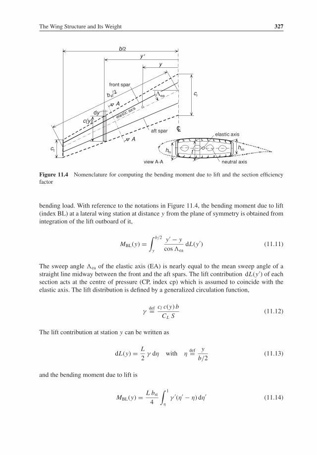
The Wing Structure and Its Weight 327
b/2
y
y
c(y)
dy
aft spar
front spar
elastic axis
neutral axis
thfshas
A
A
view A-A
cr
c t
ea
CL
Λ
Figure 11.4 Nomenclature for computing the bending moment due to lift and the section efficiencyfactor
bending load. With reference to the notations in Figure 11.4, the bending moment due to lift(index BL) at a lateral wing station at distance y from the plane of symmetry is obtained fromintegration of the lift outboard of it,
MBL(y) =∫ b/2
y
y′ − y
cos�eadL(y′) (11.11)
The sweep angle �ea of the elastic axis (EA) is nearly equal to the mean sweep angle of astraight line midway between the front and the aft spars. The lift contribution dL(y′) of eachsection acts at the centre of pressure (CP, index cp) which is assumed to coincide with theelastic axis. The lift distribution is defined by a generalized circulation function,
γdef= cl c(y) b
CL S(11.12)
The lift contribution at station y can be written as
dL(y) = L
2γ dη with η
def= y
b/2(11.13)
and the bending moment due to lift is
MBL(y) = L bst4
∫ 1
η
γ ′(η′ − η) dη′ (11.14)
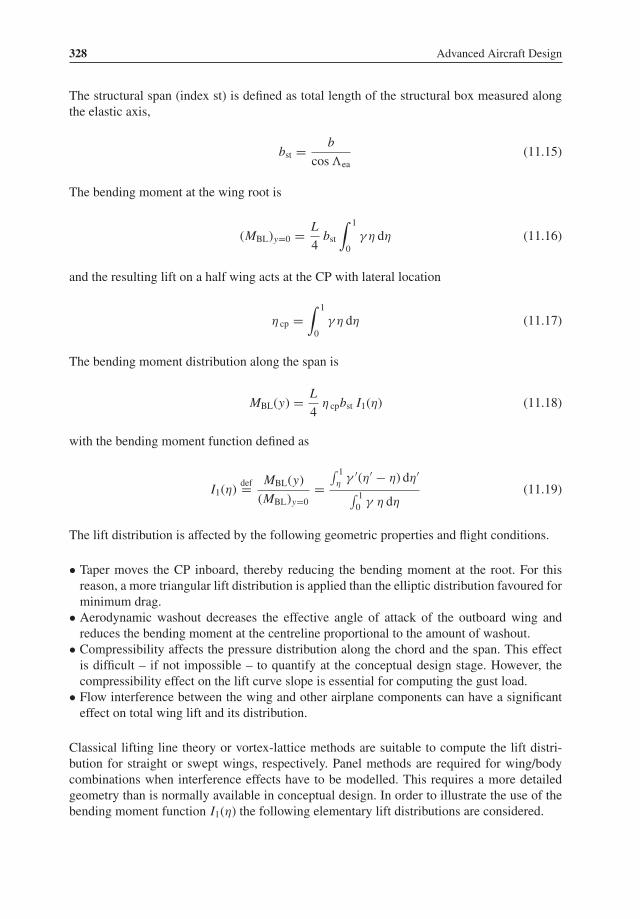
328 Advanced Aircraft Design
The structural span (index st) is defined as total length of the structural box measured alongthe elastic axis,
bst = b
cos�ea(11.15)
The bending moment at the wing root is
(MBL)y=0 = L
4bst
∫ 1
0γ η dη (11.16)
and the resulting lift on a half wing acts at the CP with lateral location
η cp =∫ 1
0γ η dη (11.17)
The bending moment distribution along the span is
MBL(y) = L
4η cpbst I1(η) (11.18)
with the bending moment function defined as
I1(η)def= MBL(y)
(MBL)y=0=
∫ 1η
γ ′(η′ − η) dη′∫ 10 γ η dη
(11.19)
The lift distribution is affected by the following geometric properties and flight conditions.
• Taper moves the CP inboard, thereby reducing the bending moment at the root. For thisreason, a more triangular lift distribution is applied than the elliptic distribution favoured forminimum drag.
• Aerodynamic washout decreases the effective angle of attack of the outboard wing andreduces the bending moment at the centreline proportional to the amount of washout.
• Compressibility affects the pressure distribution along the chord and the span. This effectis difficult – if not impossible – to quantify at the conceptual design stage. However, thecompressibility effect on the lift curve slope is essential for computing the gust load.
• Flow interference between the wing and other airplane components can have a significanteffect on total wing lift and its distribution.
Classical lifting line theory or vortex-lattice methods are suitable to compute the lift distri-bution for straight or swept wings, respectively. Panel methods are required for wing/bodycombinations when interference effects have to be modelled. This requires a more detailedgeometry than is normally available in conceptual design. In order to illustrate the use of thebending moment function I1(η) the following elementary lift distributions are considered.
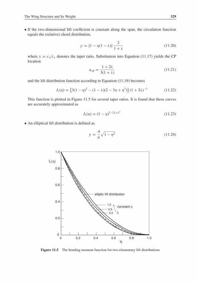
The Wing Structure and Its Weight 329
• If the two-dimensional lift coefficient is constant along the span, the circulation functionequals the (relative) chord distribution,
γ = {1− η(1− λ)} 2
1+ λ(11.20)
where λ = c t/c r denotes the taper ratio. Substitution into Equation (11.17) yields the CPlocation
η cp = 1+ 2λ3(1+ λ)
(11.21)
and the lift distribution function according to Equation (11.19) becomes
I1(η) = {3(1− η)2 − (1− λ)(2− 3η + η3)
}(1+ 2λ)−1 (11.22)
This function is plotted in Figure 11.5 for several taper ratios. It is found that these curvesare accurately approximated as
I1(η) = (1− η)3−2λ+λ2 (11.23)
• An elliptical lift distribution is defined as
γ = 4
π
√1− η2 (11.24)
elliptic lift distribution
1.0
1.0
0.50.2
0.8
0.6
0.4
0.2
01.00.80.60.40.20
constant cl
I (1 )
Figure 11.5 The bending moment function for two elementary lift distributions
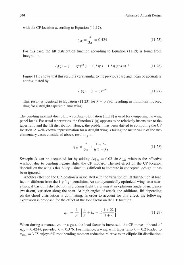
330 Advanced Aircraft Design
with the CP location according to Equation (11.17),
η cp = 4
3π= 0.424 (11.25)
For this case, the lift distribution function according to Equation (11.19) is found fromintegration,
I1(η) = (1− η2)0.5(1− 0.5 η2)− 1.5 η (cos η)−1 (11.26)
Figure 11.5 shows that this result is very similar to the previous case and it can be accuratelyapproximated by
I1(η) = (1− η)2.39 (11.27)
This result is identical to Equation (11.23) for λ = 0.376, resulting in minimum induceddrag for a straight-tapered planar wing.
The bending moment due to lift according to Equation (11.18) is used for computing the wingpanel loads. For usual taper ratios, the function I1(η) appears to be relatively insensitive to thetaper ratio and the lift distribution. Hence, the problem has been shifted to computing the CPlocation. A well-known approximation for a straight wing is taking the mean value of the twoelementary cases considered above, resulting in
η cp = 2
3π+ 1+ 2λ6 (1+ λ)
(11.28)
Sweepback can be accounted for by adding �η cp = 0.02 sin�0.25 whereas the effectivewashout due to bending flexure shifts the CP inboard. The net effect on the CP locationdepends on the wing’s flexibility – since it is difficult to compute in conceptual design, it hasbeen ignored.Another effect on the CP location is associated with the variation of lift distribution at load
factors different from the 1-g flight condition. An aerodynamically optimized wing has a near-elliptical basic lift distribution in cruising flight by giving it an optimum angle of incidence(wash-out) variation along the span. At high angles of attack, the additional lift dependingon the chord distribution is dominating. In order to account for this effect, the followingexpression is proposed for the effect of the load factor on the CP location:
η cp = 1
3n
{4
π+ (n − 1) 1+ 2λ
1+ λ
}(11.29)
When during a manoeuvre or a gust, the load factor is increased, the CP moves inboard ofη cp = 0.4244, provided λ < 0.376. For instance, a wing with taper ratio λ = 0.2 loaded tonULT = 3.75 enjoys 6% root bending moment reduction relative to an elliptic lift distribution.

The Wing Structure and Its Weight 331
11.3.2 Bending Material
The upper and lower stiffened skin panels including spar flanges (Figure 11.4) resist bendingby normal loads leading to tensile and compressive stresses. The variation of stress along thespan for resisting the bending due to lift (index BL) is
| σ (y)| = MBL(y) t(y)
2Iz(y)(11.30)
where the neutral axis has been taken midway between the upper and lower panels. Thebending moment of inertia Iz is obtained by replacing the panels by an equivalent skin withpanel cross-section area A(y) and equivalent thickness δ(y) at an effective mutual distanceηtt(y), with
ηtdef=
√2Iz(y)
A(y) t2(y)(11.31)
This effectiveness factor depends on thewing section shape, the location of the front spar (indexfs) and the aft spar (index as), and on panel geometry where the nomenclature (Figure 11.2)applies to the wing root. Methods for computing ηt in [1] and [22] require detailed inputand apply to obsolete wing sections. Instead, the following first-order estimation is proposedinstead:
ηt =√1+ (hfs/t)2 + (has/t)2
3− tsk/t (11.32)
where tsk/t is the smeared skin thickness as a fraction of the section thickness. A typical valueof this fraction is 0.025. If the section thickness at the spars is not known, the value of ηt maybe assumed to be equal to 0.81 for subsonic and 0.84 for transonic (supercritical) sections.The required panel cross-section area follows from the two previous equations,
A(y) = MBL(y)
ηt(y) | σ (y)| (11.33)
and the total weight of the upper and lower wing box covers is
WBL = 2ρg∫ bst/2
0A(y) dy (11.34)
with ρ denoting the material’s specific density. The maximum bending moment is exertedwhen the lift equals the ultimate load factor times the gross weight WG. Combining Equations(11.18) and (11.33) yields the weight of material required to resist bending due to lift,
WBL = 0.5 nULTWG bstη cp
ηt
bst2 t r
{ρg
σt(y = 0)(I2)t + ρg
σc(y = 0)(I2)c
}(11.35)

332 Advanced Aircraft Design
The indices t and c refer to tension and compression stress, respectively. The integral
I2 =∫ 1
0I1(η)
(σ t)η=0σ (η)t(η)
dη (11.36)
is developed differently for the lower (tension) and upper (compression) panels:
• The theoretical minimum weight of lower panels is obtained by assuming that the tensilestress is constant along the span. The allowed tensile stress is either the (fatigue) stress limitdetermined by the aircraft’s specified lifetime, or the maximum tensile stress of the appliedmaterial. The basic approach assumes a constant thickness ratio along the span; hence, thevariation of thickness taper t(η)/t(η = 0) equals the planform taper. When using the liftdistribution functions discussed previously it is found that (I2)t = 0.36 for most practicaltaper ratios. It is noteworthy that this value is 10% higher than (I2)t = 1/3 for a parabolicvariation of material weight along the span.
• The allowable compressive stress in the upper panels is mostly based on the criterion thatcolumn buckling is to be avoided. The limit is assumed proportional to the square root ofthe local structural index defined as the panel load per unit width divided by the rib distance.For lightly loaded structures the tangent modulus is constant and for constant ratio of boxchord to wing chord and constant rib pitch along the span we have
σc ∝√
MBL(y)
t(y) c(y)(11.37)
with the factor of proportionality depending on the stiffening configuration. The result forconstant section thickness ratio is
(I2)c =∫ 1
0
√I1(η) dη (11.38)
Similar to the lower surface panels, the lift distributions considered do not lead to significantvariation in this integral. A good average value is (I2)c = 0.45. For highly loaded structuresthe compressive stress is not allowed to exceed the maximum compressive stress. SeeSection 11.7 for more details.
Equation (11.35) shows that the weight of material required to resist bending is proportionalto the cantilever ratio, broadly defined as the ratio of the structural semi-span to the maximumbox thickness at the root,
Rcant = bst2t r
= b
2t r cos�ea= A(1+ λ)
4(t/c) r cos�ea(11.39)

The Wing Structure and Its Weight 333
where A = b2/S denotes the aspect ratio. The last term on the right-hand side of Equa-tion (11.39) features in several published wing weight prediction formulas, for instance,Equation (8.1). Introducing Rcant into Equation (11.35) leads to
WBL = (I2)tρg
σrnULTWG Rcant
η cp
ηtbst (11.40)
with the mean stress level at the root defined as
1
σr= 0.5
{1
σt+ 1.25
σc
}(11.41)
Thanks to the relatively crude assumptions made so far, this result seems deceptively simple.However, its application requires knowledge of the distribution of fuel in the wing and allow-able stress levels, subjects treated in Sections 11.4 and 11.7. It is worth noting that, for givenmaterial stresses, load factor and cantilever ratio, Equation (11.40) proves that the bendingmaterial weight fraction increases proportional to the wing span. This important consequenceof the square cube law [15, 16] explains why, especially for large airliners, much effort mustbe spent in reducing wing weight.
11.3.3 Shear Material
The shear force due to wing lift is transferred by spar webs which are assumed to be of thefull-depth type stiffened diagonal tension webs – spar flanges are counted as material resistingbending to which they contribute approximately 5%. Similar to the bending moment, the shearforce due to lift (index SL) at any station is obtained from integration of the lift outboard ofthat station
FSL(y) = nULTWG
2I3(η) (11.42)
where
I3(η)def=
∫ 1
η
γ ′ dη′ (11.43)
The required shear material is assumed to be divided equally over the shear webs. Its areaA(y) is equal to the shear force divided by the (mean) shear stress τ (y),
ASL(y) = FSL(y)
τ (y)(11.44)
For constant shear stress along the span, the total weight of material required to transfer lift tothe wing root is
WSL = 0.5 nULTWG bstρg
τ
∫ 1
0I3(η) dη (11.45)

334 Advanced Aircraft Design
The integral on the right-hand side equals the lateral coordinate of the CP. Similar to thecompressive stress in the top cover panels, the allowable shear stress decreases in outboarddirection. Its mean value is assumed equal to 50% of the mean centreline stress in the upperand lower cover panels. With an additional 20% for web stiffening, the shear material weightamounts to
WSL = 1.20 nULT WGη cp bstρg
σ(11.46)
11.3.4 In-Plane Loads and Torsion
In deriving the ideal basic box weight it was assumed that bending and shear loads due toupward lift determine the material required. In reality, coping with in-plane bending and shearcauses a weight penalty that cannot be ignored.
• In addition to the normal load N , the wing experiences a tangential forward force whichequals the leading edge suction force L sinα minus the wing drag. Its magnitude canbe considerably larger than expected. For instance, at 15◦ angle of attack the in-planeaerodynamic force amounts to roughly 20% of the lift. The resulting in-plane bendingand shear loads entail shear stresses and increased tensile stresses behind and compressivestresses in front of the elastic axis.
• Straight wings experience a positive (nose-up) torsional moment which is caused by thelocation of the CP forward of the EA. Its magnitude is approximately equal to the bendingmoment due to lift divided by the aspect ratio. In addition, wing camber and twist cause a(generally negative) torsion which achieves its highest value at the design diving speed VD.
• Sweepback shifts the CP backwards relative to the root. This causes a negative torsion of theinboard wing counteracting the positive torsional load mentioned for straight wings. The neteffect is zero when the CP coincides with the shear centre at the structural root. This is thecase for a sweepback angle of the order of 10◦. For the more usual sweep angles the exertedtorsion requires the inboard rear spar to be beefed up. The magnitude of this effect is highlydependent on the structural topology.
The present method accounts for these effects by increasing the cover panel loads at the wingroot by 5%.
11.3.5 Ribs
Ribs give shape to the wing section and are designed to fulfil a multitude of functions. Generalribs support and stabilize the skin – in particular compression loaded panels – and transmitdistributed aerodynamic pressure load from the upper and lower panels to the spars. They alsostiffen the wing against torsion and withstand crushing loads due to wing bending. Special ribscollect concentrated loads from high-lift devices, control surfaces, landing gears and enginepods and pass them to the primary elements of the box. Several special ribs act as baffles toprevent the fuel surging around when the aircraft manoeuvres. The bulkheads of the structuralroot transfer the normal loads to the fuselage. The mass of a rib depends on the structural

The Wing Structure and Its Weight 335
topology and, since only a few ribs can be considered as typical, an analytical approach totheir weight prediction is precluded. In the CS of a large airliner, the mass of general ribs isroughly 10 kg m−2, equivalent to a smeared thickness of 3.6 mm – the outboard rib mass isabout half this value. However, special ribs carrying concentrated loads can be two to threetimes heavier.Even if the mass of a typical rib could be predicted accurately, the number of ribs must
be known to compute their total weight. Several authors have attempted to optimize the ribpitch with the aim of minimizing the weight of compression panels plus ribs. The outcome ofthis approach appears to be unrealistic since in practice rib pitches are selected on other thanminimumweight considerations such as the location of flap and engine attachments. Althoughthe rib pitch varies along the span, the average pitch of 0.75 m is not greatly different betweeninboard and outboard sections. The prediction method suggested here applies to the generalrib weight, including the wing-to-fuselage interconnection bulkhead and fuel tank boundaries,but does not include penalties for support structures (Section 11.5). Basic assumptions are:
• The weight per unit of rib area is constant along the span.• For constant rib pitch, the number of ribs is proportional to the span. Rib weight is thenproportional to the product of the mean wing chord, the mean section thickness, and thespan. In other words: rib weight is proportional to wing volume.
• If the rib pitch is proportional to the mean wing thickness the number of ribs per unit spanis inversely proportional to it. Rib weight is then proportional to the mean rib chord timesthe span, that is, wing area.
If the actual rib pitch is determined partly by the first and partly by the second assumption, thegeneral rib weight amounts to
Wrib = krib ρ gS
(tref + t r + t t
2
)(11.47)
including the wing-to-fuselage interconnection and fuel tank bulkheads. Factors to be cali-brated are: krib = 0.5 ×10⁻³ and tref = 1 m.
11.4 Inertia Relief and Design Loads
The B-52 wing was much larger than the B-47 wing and thus had a high volume between thespars. In the B-52 this internal wing volume was used as a fuel tank. There were also large fueltanks in the body. The use of wing fuel saved a lot of wing weight. The B-52 also had relativelysmall outboard wing fuel tank pods.
—G. Schairer, July/August 1989
The inertia forces acting on the wing structure, its contents and attached (engine) massesoppose the lift and lead to a relief of bending and shear loads. The large amount of fuel inthe wing yields a significant load relief when a long-range airplane takes off; however, thisis no longer the case at the end of the flight. Since the payload depends on the mission andfuel varies during the flight, critical loading conditions forming the design case for the wing

336 Advanced Aircraft Design
structure must be identified. The subject of this section is to derive weight-critical loadingconditions and corrections of the ideal box weight derived in the previous section for givengross weight and load factor.
11.4.1 Relief due to Fixed Masses
The resultant of the inertial forces on the aircraft and its contents in flight with a constant loadfactor equals the lift. In the (hypothetical) case of an all-wing aircraft with lift and inertialforces distributed identically along the span, the wing is not subjected to bending and shear.Although this span loading effect is less dominant for realistic designs, it forms an incentivefor allotting as much useful load as possible to the wing (Chapter 5). The fuselage group and itscontents of a conventional TAW configuration are concentrated inboard of the wing/fuselageconnection. The lift required to carry their combined inertial force causes major bending andshear loads on the wing, whereas the inertial relief due to the wing group and its contentsreduces the wing structural weight by a fraction of not more than 20%. The computation ofinertia relief due to components of the empty weight is straightforward. Major relief stemsfrom the wing structure and wing-mounted engines, the effects of wing-mounted landing gearsand system components are usually negligible.The mass of the wing structure, fuel system and local flight control systems is denoted as the
wing group (index wg) mass. Similar to the lift, its weight is distributed between the root andthe tip. Since wing structure weight per unit chord decreases in outboard direction, whereas thelift per unit chord is more or less constant, the resulting inertia relief is concentrated inboardof the CP. The relative bending moment reduction is some 20% less than the wing weightfraction but it is compensated by the inertia relief due to systems inside the wing. The resultis expressed as a relief factor on the root bending moment,
(Rin)wg = ywgWwg
y cpWMTO≈ Ww
WMTO(11.48)
Application of this expression requires knowledge of the wing weight and its distributionwhich happens to be the outcome of the wing structure weight prediction. Consequently,computation of the inertia relief is essentially iterative. A practical approach to avoid iterationis to input a Class I wing weight estimation from a statistical method such as Equation (11.3).A second approximation is then usually not required.A wing-mounted engine (index eng) causes a constant shear force and a linear bending
moment reduction inboard of its attachment. It is found that the inertia relief factor due to oneengine on each side is approximately
(Rin)eng = 3η2eng
η cp
Weng
WMTO(11.49)
where ηeng denotes the dimensionless lateral coordinate of the engine attachment (Figure 11.6)and Weng is the installed weight of one engine including nacelle, thrust reverser and pylon.If two engines are mounted per wing half, their contributions must be added. Typical inertiarelief factors are 0.03 and 0.08 for twin and quadruple wing-mounted turbofans, respectively.

The Wing Structure and Its Weight 337
Figure 11.6 Forces contributing to inertia relief of wing bending due to lift
11.4.2 Weight-Critical UL and Design Weights
The effect of a filled fuel tank on the root bending moment is determined in a way similar tothe bending moment due to lift. The inner tank bulkhead is assumed to coincide with the rootstation (Figure 11.7) and the upward moment due to lift and fuel (index LF) amounts to
(MLF)y=0 = 0.25 bst nULT (η cp WG − ηf Wf) (11.50)
or
(MLF)y=0 = 0.25 η cp bst nULT
{WZF +
(1− ηf
η cp
)W f
}(11.51)
Figure 11.7 Fuel tank geometry

338 Advanced Aircraft Design
The lateral coordinate of the fuel CG in a filled straight tapered tank with taper ratio λft is
η f = yfb/2
= 1+ 2λft + 3λ2ft4(1+ λft + λ2ft)
bftb
(11.52)
For a completely filled full-span tank – the so-called ‘wet wing’ – the tank and wing spansand taper ratios are (nearly) equal and Equations (11.29) and (11.52) show that ηf < ηcp.For a given GW, reduction of the fuel load and its inertia relief is more than the reduction ofthe bending moment due to lift. The highest root bending moment therefore occurs when theaircraft has its maximum payload on board and takes off with MTOW,
(MLF)y=0 = 0.25 η cp bst nULT WMTO
{1− ηf
η cp
(1− WMZF
WMTO
)}(11.53)
The bending material reduction due to the inertia relief of fuel is derived from Equations(11.29), (11.52) and (11.53). If it is assumed that the variation along the span of bendingmaterial due to lift is proportional to the local chord and its reduction due to fuel relief isproportional to the square of the local chord, the solution is mathematically straightforward.However, the exact answer is cumbersome and the following inertia reduction factor for fuelis suggested if the wing and the wing box have the same taper ratios:
(Rin)f = 0.5b fb
(1+ 3λ2
1+ 2λ) (1− WMZF
WMTO
)(11.54)
This equation should be applied so that b f/b complies with the filled tank. It should also benoted that the amount of fuel corresponding to the MZFW is normally (much) less than themaximum fuel capacity. Hence, Equation (11.54) should not be applied to the wet wing sinceit does not represent the critical load condition. It is found that the bending material reductiondue to fuel inertia relief is mostly less than 15% of the material required to withstand lift.Further analysis is required if the inner fuel tank bulkhead is outboard from the wing root.
For a given amount of fuel, this decreases the root bending moment up to the point that thefuel CG coincides with the wing CP. If the fuel tank CG is shifted outboard from the CP, themaximum root bending occurs when the tanks are empty and the wing structure weight mustbe computed for the zero-fuel condition. However, filled outboard tanks reduce wing bendingin 1-g flight which is in the interest of reducing structural fatigue. Some turboprop aircrafthave fuel tanks only outboard of their (wing-mounted) engines. A structural reserve fuel isthen used to select the design condition. The airworthiness rules allow reduced maximum loadfactors; see FAR/JAR Chapter 25.343. From these results it is concluded that inertia relief dueto fuel is important only for the manoeuvre-critical case.
11.5 Non-Ideal Weight
The ideal wing box weight is derived from static bending and shear loads and from allowablestress levels in every cross-section, sometimes referred to as a fully stressed structure. In apractical wing design, allowances are made for non-ideal features such as non-tapered skins,

The Wing Structure and Its Weight 339
main landinggear breakaway
positive manoeuvre
positive manoeuvre
front spar
front spar
rear spar
rear spar
negative dynamicgust (down)
positivedynamicgust (up)aileron
roll
positivesteadymanoeuvre
positive dynamic gust (up)
aileron rollpositive steadymanoeuvre
LOWER SURFACE
UPPER SURFACE
Figure 11.8 Example of panel design conditions for a primary wing structure [27]
partitioning into sub-assemblies, inspection hatches in the lower box cover plates, etc. Typicalspar and panel surface design conditions for a large transport airplane in Figure 11.8 illustratethat several segments of the primary box are sized differently by manoeuvre and gust loads.Moreover, some structural elements are sized by aileron control and landing flap load cases,the landing impact load, dynamic loads, and torsional stiffness requirements to avoid criticalaero-elastic effects.Several publications refer to non-ideal weight penalties as ‘non-optimum weight’. This is
a misnomer because it suggests that non-ideal weight is not necessary and can be avoided ifsufficient attention is paid to computational refinement. However, even if non-ideal weight canbe minimized, it cannot altogether be eliminated. In terms of cost-effectiveness, one mighteven speak of ‘optimum non-ideal weight’. Since most non-ideal weight penalties cannot betreated analytically, they must be derived from statistics and calibrated with data collected formanufactured aircraft. Several prediction methods compute the non-ideal weight by applyinga correction factor to the ideal weight. This suggests that there exists a functional relationshipbetween ideal and non-ideal weight terms. However, the design sensitivity is not properlyrepresented in this way since most non-ideal weight is determined by design variables andsizing criteria conditions different from the ideal weight. The present alternative approachaims at avoiding these traps.
11.5.1 Non-Taper, Joints and Fasteners
Manufacturing constraints and cost considerations do not allow continuous adjustment to thetheoretical optimum along the span of the skin/stringer configuration. For instance, minimumgauge sheet thickness (0.8 mm, typically) is applied in lightly loaded parts near the wing tips.Stepwise skin thickness adjustments can be made by subdividing a panel into sections joined

340 Advanced Aircraft Design
by splices. Theoretically, there is an optimum number of steps for which the combined weightpenalty due to non-tapered sheets and joints is minimized. Compared to constant thicknesssheets, the application of linear sheet tapering and integrally machined panels reduces thenon-taper weight penalty significantly. Penalties also occur where the wing is partitioned intosub-assemblies leading to major production joints and splices in cover panels. Depending onthe wing size and its manufacturing concept, weight penalties add up to between 5 and 10%of the box weight. Since the major part of this non-ideal (index nid) weight is related to thesurface area of the wing box, the following estimation can be made by applying a smearedthickness �δ increment to panel skins and shear webs:
�nidW = δnidρg Sbox ≈ 1.20 δnidρgS (11.55)
with Sbox denoting the total projected area of box panels plus spar webs. For fabricated (built-up) structures based on high-strength fastener technology, a typical value is δnid = 10−3 m.For bonded or integrally machined structures, this penalty can be reduced by 20% or 50%,respectively.
11.5.2 Fail Safety and Damage Tolerance
The ideal shear material weight has to be increased to allow for increased web thickness tocope with shear due to wing torsion and for provisions such as the need for web stiffeners andrib posts. Moreover, an essential requirement for civil aircraft states that the wing must be a failsafe and damage-tolerant structure. In particular, complete failure of a wing spar constitutesa potential hazard that must either be countered by an auxiliary spar or avoided altogether.The provision of crack stoppers is an effective measure to protect a shear web from completefailure, especially when it forms an integral structure. The combined effect of these provisionsis estimated to be a 15% penalty on the basic shear material according to Equation (11.46).
�nidW = 0.18 nULT WGη cp bstρg
σ(11.56)
11.5.3 Manholes and Access Hatches
Cutouts in structures invariably increase its weight because the structure adjacent to a cutoutmust be beefed up to redistribute the load. To allow inspection and maintenance of thestructure and tank condition, the lower box cover features numerous manholes closed byinspection covers (index ic) which can be removed for access.Manholes cause weight penaltiesdepending on the type of access. Inspection hatches in the outer wing are large relative to thechord and are stressed to reduce the weight penalty. Non-stressed hatches are applied mainlyin the inboard and mid-wing sections and the carry-through structure. The weight penalty dueto the reinforcement around manholes is estimated by assuming that: (a) the structural widthof the lower box cover is effectively reduced by the cutout width; (b) the cover is reinforcedby increasing its smeared thickness by the same amount as the cutout material; and (c) theinspection cover’s smeared thickness is equal to the increased cover thickness. This leadseffectively to a cover thickness increment along the structural span equal to the ratio of the

The Wing Structure and Its Weight 341
cutout to the mean box width. If the mean box chord is assumed to be equal to 50% of themean geometric chord, the ideal lower panel weight is corrected by a factor
Ric = 1+ 2wic bstS
(11.57)
with a standard IC cutout width of 10 inch;wic = 0.25 m. Application of this correction yieldsa lower box cover weight penalty between 5% for large and 15% for small airliners. This resultcomplies with the recommendation in [34] that the net weight penalty due to providing for amanhole with inspection hatch amounts to 1.5 times the cutout material weight.
11.5.4 Reinforcements, Attachments and Support Structure
Structural elements are required for mounting engines and landing gears to the wing box andconnecting the wing to the fuselage.
• The installation of engines in pods under the wing leading edge requires pylon attachments,additional ribs, and reinforcements of spars, special ribs and covers. The following weightpenalty is based on scanty statistical data for jet aircraft:
�nidW = 0.015(1+ 0.2Neng)Wpp (11.58)
The number of wing-mounted engines is denoted Neng, the power plant weightWppp includesthe weight of engines, nacelles, thrust reversers and pylons (Section 8.3). An enginemountedto the outboardwing can have an appreciable effect on aero-elastic characteristics.Dependingon the engine location relative to the elastic axis, this may lead to a weight reduction or apenalty.
• The landing impact load absorbed by wing-mounted landing gears requires provisions suchas gear bulkheads, auxiliary spar structures transferring the impact loads to the fuselage, aftspar and rib reinforcements, and wheel well doors. The total non-optimum weight penaltyis a fraction of the MLW, for example
�nidW = 0.006WML (11.59)
depending on the landing impact load which is affected by the impact load factor nland. Ifthe load factor and shock absorbing properties are known, the prediction can be refined to
�nidW = 0.0015 nlandWML (11.60)
This penalty is omitted if the gear legs are attached to the fuselage.• Connecting the wing to the fuselage requires attachment structures, rib reinforcements andother hardware. For a continuous carry through structure this weight penalty amounts to
�nidW = 0.0003 nULTWMTO (11.61)

342 Advanced Aircraft Design
11.5.5 Dynamic Over Swing
The wing of large jetliners is mostly designed by the manoeuvre load which is more criticalthan the gust load. Since during a manoeuvre the lift build-up is gradual, the dynamics willhave little overall effect on the bending and shear loads. For the gust-critical case, however,dynamic effects may become important. As opposed to static gust load factors, the dynamicbehaviour must be analyzed for flight through a standardized gust distribution, accounting forthe degrees of freedom of the elastic structure [2]. Such an analysis needs knowledge of thecomplete structural design and yields the dynamic over-swing deflection for every station alongthe span, an analysis which is outside the scope of the present method. Instead of this, the gustload factor according to Equation (11.7) can be multiplied by a correction factor that shouldbe obtained from past design experience and checked by a dynamic analysis downstream ofthe conceptual design. However, dynamic gust loads are usually concentrated on the outboardwing where extra stiffness is built in to cope with aero-elasticity. It is therefore unlikely thatdynamic gust loads will entail a weight penalty in excess of the one to be treated hereafter.
11.5.6 Torsional Stiffness
In addition to static bending and shear, there may be additional considerations which requirea beef up in the basic structure in specific areas, in particular the wing box in front of theailerons. Some of these weight penalties are very design-specific, others are related to moregeneral conditions. In principle, the need to avoid aero-elastic divergence when flying at a highdynamic pressure may cause a weight penalty depending on general design characteristics.When dealing with the wing lift distribution (Section 11.3), it was mentioned that there existsan interaction between the static air load distribution and wing distortion. Static deflectionsthat tend to shift the lift inboard are found to be a function of the bending stiffness, those thattend to shift the lift outboard are a function of the torsional stiffness. The usual result is thatthere is a small inboard CP shift on sweptback wings and an even smaller outboard shift onstraight wings. Other aero-elastic phenomena relevant to wing weight prediction are primarilyaffected by the sweepback angle and the dynamic pressure.Figure 11.9 forms a qualitative indication of the speeds at which static aero-elastic diver-
gence, bending-torsion flutter and aileron reversal occur dependent on the angle of sweep.
• For (nearly) straight wings, the divergence case is usually covered when the requirementsfor aileron reversal are met; the flutter case must be investigated separately.
• Whereas sweepback has a relieving effect in the flutter and divergence cases resulting fromthe outboard lift relief due to upward bending, aileron reversal usually becomes the criticaldesign case. Some high-aspect ratio swept wings have been problematic with regard toaileron reversal. A solution has been found on the A310 by applying inboard high-speedailerons in combination with spoilers.
• Divergence is a critical condition when designing a forward swept wing. Advanced com-posite construction is most adaptable to control the deflection characteristics by aero-elastictailoring.
For a certain category of high speed airplanes, torsional stiffness requirements may becomedominant and the extra structure required to safeguard against flutter may amount to as muchas 20% of the wing weight. The location of outboard wing-mounted engines relative to the
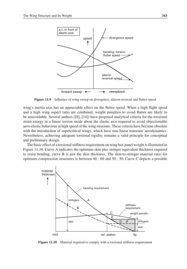
The Wing Structure and Its Weight 343
speed
sweepbackforward sweep
Figure 11.9 Influence of wing sweep on divergence, aileron reversal and flutter speed
wing’s inertia axis has an appreciable effect on the flutter speed. When a high flight speedand a high wing aspect ratio are combined, weight penalties to avoid flutter are likely tobe unavoidable. Several authors ([8], [14]) have proposed analytical criteria for the torsionalstrain energy in a linear torsion mode about the elastic axis required to avoid objectionableaero-elastic behaviour at high speed of the wing structure. These criteria have become obsoletewith the introduction of supercritical wings, which have non-linear transonic aerodynamics.Nevertheless, achieving adequate torsional rigidity remains a valid principle for conceptualand preliminary design.The basic effect of a torsional stiffness requirement onwing box panel weight is illustrated in
Figure 11.10. Curve A indicates the optimum skin plus stringer equivalent thickness requiredto resist bending, curve B is just the skin thickness. The skin-to-stringer material ratio foroptimum compression structures is between 40 : 60 and 50 : 50. Curve C depicts a possible
Figure 11.10 Material required to comply with a torsional stiffness requirement

344 Advanced Aircraft Design
variation along the span of skin thickness which provides the required torsional stiffness. Thestiffness is defined in terms of the strain energy associated with a given torsional deflection.The reference station is usually at 70% semi-span outboard from the root. Since the amount ofinboard wing skin material required to cope with bending exceeds the torsional requirement,the outboard skin thickness can be reduced from curve C to curve D. Adding stringers yieldscurve E, representing a mass distribution satisfying both bending and torsional requirements,with the hatched area defining the associated weight penalty. This penalty may be furtherreduced by increasing the stringer pitch in areas where the stiffness requirement dominates,resulting in modified skin-to-stringer material ratio to, for example, 55 : 45. Another optionis increasing the rib pitch in combination with a skin thickness increment. Basically, thisapproach complies with design experience that a minimum weight penalty due to aero-elasticeffects is obtained by a local increase in skin gauge over the outboard portion of the wing.Apart from skin thickening to comply with aero-elastic requirements, the outboard wing skinmay have to be thickened to comply with a minimum gauge requirement, the transfer ofaileron loads, dynamic gusts, etc. A detailed station analysis is required to find out which caseis critical at any given lateral position.The implementation of stiffness requirements is feasible only if the torsional stiffness
variation along the span and details such as the location of the inertial and flexural axis areavailable. It was concluded from a literature survey that an empirical weight penalty for anAl-alloy box structure will have the following appearance:
�nidW = WrefqDqref
(b cos�0
bref
)3 (t
c
)−2
ref
(1− sin�0.50){1− (MD cos�0.50)2}−0.5 (11.62)
with qref = 30 kNm−2 and bref= 50 m. Leading edge and mid-chord sweep angles are denotedas�0 and�0.50, respectively, and the thickness ratio (t/c)ref refers to the reference wing chordjust inside the aileron (Figure 11.2). The dynamic pressure qD and the Mach number MD atthe design diving speed are obtained from the flight envelope. The calibration factor Wref canbe estimated from previous design information. If this is lacking, a typical Wref= 200 N leadsto a wing weight penalty of about 2% for regional jets up to 5% for wide-body airliners. Thisstiffness correction is most sensitive to the span and the thickness ratio.
11.6 Secondary Structures and Miscellaneous Items
There is little evidence that specific weights of high-lift system components change noticeablywith the size of the aircraft.
—P.K.C. Rudolph in [36]
Even though secondary structure can contribute as much as 35% to the wing weight, publishedmethods treat its prediction superficially due to the difficulty experienced in defining designcriteria. Therefore, weight predictions are mostly based on statistical evidence using basicgeometry and functional parameters as input. Since there is hardly any functional relationbetween secondary weight (components) and the airplane MTOW, statistical prediction meth-ods may use the MTOW to account for the scale effect. On the other hand, it is not necessary

The Wing Structure and Its Weight 345
to vary secondary structure weight (components) to account for minor MTOW variationsduring the design sizing process. This section presents equations for leading and trailing edgestructure weight components and wing tip structures (Figure 11.1) based on first principlesand statistical information.Most presented equations are derived in [31] by regression analysis of some twenty civil
aircraft in operation until the 1980s. Since they apply to basically Al-alloy structures it isrecommended to calibrate component weights with information on recent aircraft, if available.Weight reduction factors obtainable with composite material applications are presented inSection 11.8. Most component weights are expressed in terms of specific weight � referredto the component’s area in plan view – these areas are normalized by Sref = 10 m2. Sincethe basic secondary structures are lifting surfaces with a geometry somewhat similar to awing section, a reference specific weight �ref = 56 N m−2 is defined equal to the hypo-thetical weight of a thin section built up from two Al-alloy skins with one millimetrethickness each.
11.6.1 Fixed Leading Edge
Fixed leading edge (index fle) structure (excluding the de-icing system) is the structure in frontof the primary box remaining when all movable leading edge devices are removed. A typicalfixed leading edge weighs between 4% and 7% of the complete wing. Leading edge surfacepanels are generally not designed to carry any part of the wing box bending and torsion loads.The primary design load is the aerodynamic surface pressure. The following expression forthe specific weight has a standard deviation of about 10%:
�fle = 3.15 kfle�ref
(qDqref
)0.25 (WMTO bstWrefbref
)0.145(11.63)
with qref = 30 kN m−2, Wref = 106 N and bref = 50 m. The specific weight is referred to theleading edge plan view area with high-lift devices removed. Use kfle = 1.0 if the leading edgecarries no slats or Krueger flaps and kfle = 1.3 to account for the strengthening required tosupport slats.
11.6.2 Leading Edge High-Lift Devices
Slats andKrueger flaps are themost frequently applied leading edge high-lift devices. Includingthe panel structure, actuator supports and tracks, their weight is referred to the plan view area inretracted position. Droop noses have been used in the past on a few civil airplanes. Comparedto slats, droop noses are mechanically simple but aerodynamically less effective. Their specificweight is comparable to slats. Slats are primarily stressed to carry normal forces and their nosemust protect the wing from rain erosion and hail damage. Closely spaced slat ribs are requiredto transfer the aerodynamic loads and there are heavy ribs where actuator supports and tracksare located. The tracks are usually made of high strength steel or titanium to react to the highbending loads on the extended slats. A complete slat system weighs typically 5% of the totalwing weight.

346 Advanced Aircraft Design
The specific weight of slats is quite high as indicated by the following correlation whichhas a standard deviation of 14%:
�slat = 4.83�ref
(SslatSref
)0.183(11.64)
This weight is referred to the nested slat area and includes tracks and support but excludes slatactuation. Slats are not always fitted over the full span and their chords are usually between15% and 20% of the wing chord. Krueger flaps are mostly used on the inboard section of asweptback wing. Fixed geometry Krueger flaps are generally made of one piece of material.Their specific weight referred to the planform area in the retracted position amounts to roughlyhalf the specific weight of a slat, but there is a large scatter due to the variety in the retractionmechanism. Variable camber increases the specific weight by about 60%.
11.6.3 Fixed Trailing Edge
The fixed trailing edge (index fte) is the structure aft of the rear spar remaining when trailingedge flaps and controls are removed. Spoilers and lift dumpers hinged and actuated fromthe rear spar are not included. However, moving shroud spoilers and lift dumpers are oftenhighly integrated with the trailing edge structure and the distinction is difficult to make. Inthat case their combined weight has to be considered. Fixed trailing edge weight is of theorder of 8% of the total wing weight. Trailing edge shrouds on large aircraft consists of skinpanels, ribs supporting control surface hinges, intermediate supports and auxiliary beams. Partof the undercarriage support structure may also be integrated in this structure. The specificweight depends primarily on the overhang and on the configuration of flap supports. Thespecific weight based on the plan view area of trailing edge shrouds for single slotted flaps andailerons is
�fte = 2.6�ref
(WMTO bstWrefbref
)0.0544(11.65)
with the reference weight and span used in Equation (11.63). This must be increased by40 N m−2 for structures supporting single slotted Fowler flaps and double slotted flaps or by100 Nm−2 for supporting double-slotted Fowler and triple-slotted flaps. The trailing edge areaexcludes open shroud spoilers and depends to a large degree on the location of the rear spar,the presence of a trailing edge kink and the mechanical design of the flap support.
11.6.4 Trailing Edge Flaps
The aerodynamic effectiveness of high-lift devices at the trailing edge can be expressed as thelift coefficient increase at given angle of attack and deflection angle. It is affected mainly bythe overall flap configuration and actuation, section and planform geometry. Flap loads areproportional to flap size, lift increment and dynamic pressure at the maximum extension speed.Since the complete system of trailing edge flaps weighs up to 20% of the total wing structure,any attempt to reduce flap weight and improve its prediction is worthwhile. A subdivision
The Wing Structure and Its Weight 347
into subgroups – preferably for each flap segment – is essential to achieve the highest weightprediction accuracy. The following is a typical example for transport aircraft.
• Flap surfaces weight is determined by the air load and by the bending moment distribution,the latter being affected by the support structure lay-out. Another factor is the thickness/spanratio of a flap segment. The absolute thickness can be quite small for high speed wing flaps,in particular when they are retracted below the trailing edge shroud.
• Slotted flap supports and vane controls have a weight dependent on the type: fixed hinge,four-bar linkage or track systems. Their weight depends mainly on the chordwise extensionand deflection angle in the fully extended position.
• Support fairings weight is proportional to wetted area.• Shroud doors weight is proportional to projected area.• Flap actuation is not included.
In the conceptual stage many flap system design criteria are still unknown. An attempt todevelop a generalized weight prediction method that takes into account all considerationsmentioned above is likely to result in a complex procedure requiring many input data, butwith a mean prediction error no better than 20%. A more effective method is to use availableinformation on a flap system of similar lay-out and size. The flap element weights are thenscaled up or down to the actual size. If that is not feasible (due to lack of information), it canbe assumed that the flap loads and specific weight are statistically related to the MTOW. Thefollowing specific weight of Al-alloy flaps is based on the plan view area of all flaps in nestedposition:
�tef = 1.7 ksup kslot �ref {1+ (WMTO/Wref)0.35} (11.66)
with Wref = 106 N. The multiplication factors depend on the mechanical properties of the flapsystem:
• The factor ksup represents the complexity of the primary flap motion support. It amountsto 1.0 for simple hinge external supports, 1.2 for link/track end supports, or 1.6 for Fowlerflaps with hooked track external supports. An auxiliary trailing edge hinged flap increasesksup by 0.2.
• The factor kslot represents the number of slots and flap angle variability. It amounts to1.0 for single-slotted flaps, 1.5 for double-slotted flaps with fixed nose vanes, and 2.0 fordouble-slotted flaps with articulating vanes.4
For wings equipped with different flap systems – for example, double-slotted inboard andsingle-slotted outboard – the specific weight and flap area are multiplied for each flap typeseparately. Trailing edge flap chords are between 25% and 35% of the local wing chord,their span is generally between 65% and 75% of the outboard wing span. If no details areavailable, the total nested area of uninterrupted flaps can be estimated at 20% of the wingplanform area, the presence of inboard high speed ailerons brings this down to 16%. It is
4Triple-slotted Fowler flaps were used for the first versions of the Boeing 727, 737 and 747. They are mechanicallycomplex and about 15% heavier than double-slotted systems.

348 Advanced Aircraft Design
noted that Equation (11.66) predicts a flap weight independent of segmentation. In reality,flap surface specific weight is reduced when more flap segments are used, while flap supportand control weight will increase. As explained in [19], the number of flap segments is subjectto optimization. However, an attempt to incorporate this into a practical weight predictionmethod is likely to fail.
11.6.5 Flight Control Devices
The weight of flight control devices includes the control structures, hinges and supports, andbalance weights – it excludes actuators and controls. Similar to high-lift devices, the presenteddata on weight applies to Al-alloy structures. Application of composite materials reducesweight appreciably.Aileron-specific weight depends primarily on the design diving speed, maximum deflection
angles, size and thickness/chord ratio. However, this sensitivity is obscured by large variationsassociated with balancing and activation. For manually activated ailerons with a tab system,there is a substantial weight penalty due to mass balancing and aerodynamic balancing requir-ing large surfaces in front of the hinge. This may bring the total aileron weight up to 3% ofthe wing weight. Tabs and balancing masses are not required for triplex powered ailerons andtheir weight is about 1% of the wing weight, for power-boosted ailerons, this is typically 1.5%.Aileron design criteria and the method of balancing and activation depend on aileron size asreflected in the following empirical expression for total aileron weight:
�ail = 3.0�ref kbal (Sail/Sref)0.044 (11.67)
The area Sail denotes the total planform area behind the hinge line of all ailerons in the neutralposition which may vary between 3% and 5% of the wing area. The factor kbal is 1.0 forunbalanced ailerons, 1.3 for aerodynamic-balanced and 1.54 for mass-balanced ailerons.The spoiler group consists of spoilers, lift dumpers and air brakes fitted to the top surface
of the fixed trailing edge structure. Two or more of their functions can be combined in onedevice. Spoiler weight, comprising control panels and the supporting bracket, is treated insimilar fashion to aileron weight. The scanty available information suggests that
�sp = 2.2�ref (Ssp/Sref)0.032 (11.68)
Total spoiler and lift dumper plan view area Ssp is defined in the retracted controls position.For large jetliners this may amount to about 4% of the gross wing area.
11.6.6 Tip Structures
The complete tip assembly includes the structure, its attachments and provisions for tip lights.The great variety of tip shapes found on existing aircraft makes a statistical prediction ofthis weight component unavoidable. The following equation based on [31] is suggested fortraditional tapered wings:
Wtip = 150
(WMTO
Wref
)0.67(11.69)

The Wing Structure and Its Weight 349
withWref = 106 N. Its standard deviation of 33% is not objectionable for this small component.However, sheared wing tips and winglets are as heavily loaded aerodynamically as the wingitself and, depending on their size, their weight amounts to several percent of the wingweight. Since the structural layout of a tip extension is comparable to the fixed leading edge,Equation (11.63) is adapted to estimate the specific weight of a tip extension with length ltip,
�tip = 2.5�ref
(WMTO ltipWreflref
)0.145(11.70)
where ltip is defined in Figure 11.12 and lref = 5 m. Unfortunately, statistical material availableto check the accuracy of Equation (11.70) is not available. It is also emphasized that tipextensions increase the structural wing box span and therefore its bending load and weight.This effect is discussed in Section 11.8.
11.6.7 Miscellaneous Items
Miscellaneous items represent widely scattered weight components. Their summation dependson structural layout and on the manufacturer’s empty weight breakdown. Typical items arepaint, fuel tank sealant, undercarriage wheel well doors, jacking fittings, rivets, nuts and bolts,fences and flow spoilers, and wing tips. Fairings for wings without wheel wells are oftenrelatively small, weighing less than 1% of the wing weight. Fairings for low wings housingundercarriage wheel wells can be quite large, weighing up to 5% of the wing structure.However, they are generally classified as a fuselage body component. If data is missing a totalmiscellaneous weight can be estimated by increasing the secondary wing weight by 10%.
11.7 Stress Levels in Aluminium Alloys
Structural material selection has a great impact on airliner design and is not just a matterof looking at the highest strength and stiffness values available. In addition to low emptyweight, airplanes have service life requirements which will limit the freedom of choosingmaterials which can be used to perform the function. The allowable stresses for a givenmaterial are often determined by the proven ability to withstand minor damage in servicewithout endangering structural integrity. The ground-air-ground (GAG) load cycle spectrumand gust loading experienced in 1-g flight cause the majority of the damage to transport aircraftstructure. Variation in tension and stress concentrations lead to fatigue of structural material,reducing the operational lifetime and number of flight cycles. Many advanced designersinitially express the allowable tensile stress of the lower box covers’ surfaces in terms of amaximum 1-g stress in steady level flight. More refined analysis is based on the expectednumber of flights to be made during the aircraft’s service life since this largely determines theallowable stress levels.The present method requires knowledge of material properties for computing the material
weight required to resist bending, shear and torsion, assuming that upward normal loads arethe dominating design condition. They are combined in the term ρg/σ at the wing root wheremaximumpanel loads occur. Allowable stress levels depend largely on the type ofmaterial and,for compression panels, on the loading intensity, the structural configuration and fabricationtechnology. The present method is based on high-strength Al-alloys used in aircraft primary

350 Advanced Aircraft Design
structures which are variants of the 2XXX- and the 7XXX-series with a specific weightρg = 2 796 N m−3. Typical yield tensile stresses are:
• 450 MPa for 2024-T3 (Dural) sheet• 520 MPa for 7075-T6• 550 MPa for 7150-T6, and• 620 MPa for 7055-T7 materials.
Further developments of the 2XXX series alloys, such as 2324-T3 for plates and 2224-T3 forextrusions, have approximately 8% improved specific strength while durability and damagetolerance are also higher. These properties can be used to obtain a panel weight reduction,to design for an extended lifetime or both. Although the allowable stress levels mentionedhereafter are realistic, it is recommended to check them with structural design experts.
11.7.1 Lower Panels
Lower box covers are primarily sized to withstand application and relaxation of tensile stressesdue to (static) upward bending. They are skin damage critical and, for this reason, the traditionalmaterial used is 2024-T3 which has good fatigue resistance. In order to cope with combinedtension and shear loading, the ultimate tensile stress of 450 MPa for Dural is reduced by 5%.For an ultimate manoeuvre load factor of 3.75, this would yield a tensile stress in 1-g flight of114 MPa – too high for most applications.To prevent fatigue failure in wing structures of aircraft with a specified service life, an
analysis must be performed dealing with frequency and magnitude of loads. Such a procedureresults in an allowable stress dependent on the structural configuration and type of material[22]. The following recommendations are based on statistical data found in the literature.
• Short-range (regional) airliners must achieve a crack-free structure for more than 50 000flights. For conventional fabricated and riveted skin-stringer panels in 2024-T3 alloy itis recommended to use a 1-g tensile stress no higher than 75 MPa. A stress between80 and 85 MPa can be acceptable for adhesive-bonded structures which eliminate stressconcentrations in rivet and bolt holes. Accordingly, for a gust-critical nULT = 5.0, theallowable tensile stress is between 375 and 425 MPa.
• Long-range airliners achieve a crack-free structure for about 25 000 flights. Integrallymachined structures allow a 1-g stress of 110 MPa. For nULT = 3.75 this corresponds to anallowable tensile stress of about 410 MPa.
If service life and type of fabrication are not known, a conservative approach could be toselect a maximum tensile stress between 375 MPa for a gust-critical and 410 MPa for amanoeuvre-critical wing structure.
11.7.2 Upper Panels
The upper box cover is designed to withstand primarily compression loads and is typicallymade of 7075-T6 alloy stiffened panels. Achievable compressive stress levels are based on thebuckling behaviour of a rib-supported panel. Lightly loaded stiffened panels exhibit bucklingfailure in a flexural instability mode. For traditional skin-and-stringer combinations, a higher

The Wing Structure and Its Weight 351
compressive stress is allowed with increasing loading intensity which is represented by thestructural index (SI), defined as the panel end load L per unit width w divided by the rib pitchr (Figure 11.11). The compressive stress at failure is proportional to the square root of thestructural index,
σc = kF
√Et
Lwr
for σc < 350 MPa (11.71)
where Et is the tangent modulus and kF denotes Farrar’s efficiency factor. The dotted linein Figure 11.11 represents Equation (11.71) for kF = 1.0, with Young’s modulus of 71 GPasubstituted for Et . For a given type of stiffeners, kF has amaximum value depending on stringersize and spacing, rib spacing and other geometric details of the panel’s cross-section. Theobtainable efficiency for integrally stiffened panels with non-flanged stiffeners is no more thankF = 0.75. Factors of 0.88 are obtained for Z-stringers, J-stringers and hat section stringers andefficiencies up to 1.15 are achievable for optimized Y-section stringers. Experiments indicatethat, for stress levels greater than 350 MPa, the structure begins to lose its efficiency withincreasing loading intensity. A yield stress of 440 MPa is considered the limit for avoidingskin buckling. A limit on the compressive stress of 420 MPa is recommended, taking intoaccount a 5% reserve for combined compression and shear. This value applies to a transportaircraft with an MTOW higher than 50 tonnes, typically.The curve recommended for weight prediction in Figure 11.11 is based on kF = 0.85 in
the elastic range and 420 MPa for highly loaded panels. Between 350 and 420 MPa, thecurve is blended between these two values. Applying this curve to the wing root structurerequires knowledge of the local SI. This is obtained from the bending moment according toEquation (11.18) and the effective thickness ηttr as defined by Equation (11.32). Correctingthe bending moment for inertia relief (Section 11.4) by the factor
Rin = 1− {(Rin)wg + (Rin)eng + (Rin)f} (11.72)
0.4 0.6 0.8 1.0 2.0 3.0 4.0 6.0 8.0 10
structural index, MPa
cMPa
800700
600
500
400
300
200
100
use for weight prediction
Al-alloy 7075-T6
yield stressσ
Figure 11.11 Allowable stress in compression structures

352 Advanced Aircraft Design
yields the structural index at the root,
SI = 0.5 nULTWMTORinηcpbstηttrcboxr
≈ 0.2 nULTWMTONrib
trcbox(11.73)
where Nrib is the total number of general ribs. Amore accurate computation requires knowledgeof the structural topology – in particular, the distance between the front and aft spars and therib pitch.
11.7.3 Shear Stress in Spar Webs
Similar to compression structures, the achievable shear stress in spar webs depends on theloading intensity and the type of material – 7075-T6 material can accept about 25% highershear stress than 2024-T3. The loading intensity and the achievable shear stress decreasebetween the wing root and the tip. Accurate prediction of allowable stresses requires detailedinformation on the structural concept which is generally not available. Since shear web weightconstitutes a relatively minor contribution, the conservative assumption has been that the meanshear stress τ in the spar webs amounts to 50% of the average normal stress σ in the coverpanels.
11.8 Refinements
Equation (11.35) was derived analytically for a straight-tapered wing with linearly decreasingwing thickness between the root and the tip, disregarding the presence of the centre sectionbetween the structural roots. In particular for high-speed wings, the prediction accuracy can beimproved by adapting the structural box to account for the carry-through structure connectingthe two wing halves, non-linear lofted wing sections and modifications such as winglets andsheared tips. In principle, these refinements result in a modified lateral lift distribution.
11.8.1 Tip Extensions
Sheared tips and winglets extend the trailing vortex sheet and shift the tip vortices in thedirection of their own tips. This effectively increases the aerodynamic span and reducesinduced drag. Blended winglets improve the flow at their attachment to the main wing andcan be installed as retrofits as well as on clean sheet designs. Apart from their own structureweight, tip extensions have a significant effect on wing box bending load and weight. However,the author is not aware of a published validated method making allowance for this penalty.The following heuristic approach based on first principles is illustrated by Figure 11.12.
• By definition, the sheared wing tip (index tip) is an in-plane tip extension of the basic wing(index bw). Both surfaces are schematized as straight-tapered sections with aerodynamiclift distribution proportional to the local chord. Their lift is denoted Lbw and L tip.
• A winglet is represented by rotating the sheared tip upwards around the basic wing tip overan angle �tip. It is assumed that winglet lift and the CP location are unchanged during thisrotation. This reduces the winglet’s contribution to the total lift.
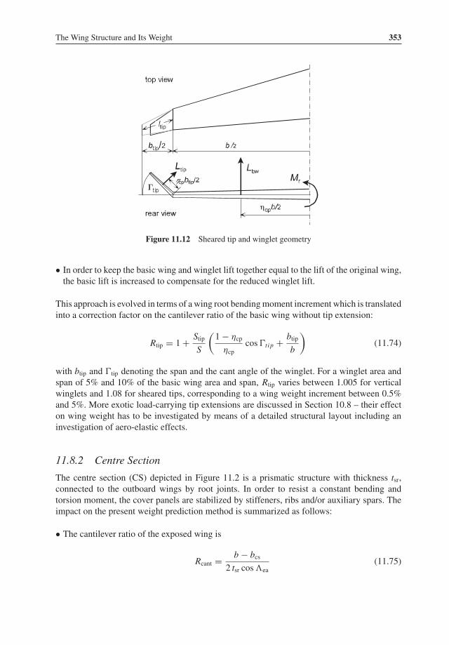
The Wing Structure and Its Weight 353
Figure 11.12 Sheared tip and winglet geometry
• In order to keep the basic wing and winglet lift together equal to the lift of the original wing,the basic lift is increased to compensate for the reduced winglet lift.
This approach is evolved in terms of a wing root bendingmoment increment which is translatedinto a correction factor on the cantilever ratio of the basic wing without tip extension:
Rtip = 1+ StipS
(1− ηcp
ηcpcos�ti p + btip
b
)(11.74)
with btip and �tip denoting the span and the cant angle of the winglet. For a winglet area andspan of 5% and 10% of the basic wing area and span, Rtip varies between 1.005 for verticalwinglets and 1.08 for sheared tips, corresponding to a wing weight increment between 0.5%and 5%. More exotic load-carrying tip extensions are discussed in Section 10.8 – their effecton wing weight has to be investigated by means of a detailed structural layout including aninvestigation of aero-elastic effects.
11.8.2 Centre Section
The centre section (CS) depicted in Figure 11.2 is a prismatic structure with thickness tsr,connected to the outboard wings by root joints. In order to resist a constant bending andtorsion moment, the cover panels are stabilized by stiffeners, ribs and/or auxiliary spars. Theimpact on the present weight prediction method is summarized as follows:
• The cantilever ratio of the exposed wing is
Rcant = b − bcs2 tsr cos�ea
(11.75)

354 Advanced Aircraft Design
• Since the CS is not exposed to the flow, the lift on a low-set wing acts only outboard of thestructural root. For the same lift distribution, the CP of each half-wing moves to a lateralposition 0.5η cp(b − bcs) outboard from the structural root. Application of Equation (11.40)to the exposed wing demonstrates that the weight of its bending material is reduced by afactor (1− bcs/b)2 relative to the wing with the same span but without the CS.
• The CS bending material resisting lift is derived by modifying Section 11.3. It is assumedthat the bending moment and the stress levels are equal to the value at the structural root;hence, I1 = I2 = 1 are substituted in Equation (11.40). The local elastic axis is straight andthe amount of bending material along the CS width is constant.
Application of these principles leads to a modified expression for the panel weight. Sincethe ratio σc/σt appears to have hardly any effect, it is treated as a constant. This yields thefollowing correction factor on the box weight resisting bending due to lift:
Rcs =(1− bcs
b
){1+ bcs
b(2.45 cos�ea − 1)
}(11.76)
For a straight wing, the CS leads to a typical cover weight penalty of 3%. For a 30◦ sweptbackwing the un-sweeping effect of the CS reduces this penalty to almost zero.Although the shear forces due to lift on both exposed wing halves are taken out at the
wing root, shear webs are required in the central wing box to cope with torsion. Therefore,Equation (11.46) can be used without correction on the provision that the structural spanincludes the CS. Disregarding the weight penalty of joints at the wing roots, it is justified toassume that the same value of Rcs applies to shear material and to the wing box as a whole.In accordance with [26] it is concluded that – contrary to what is often suggested – there isno large penalty associated with the sweep break at the wing root, compared to a non-sweptwing with the same structural span. The factor Rcs does not account for the small change ofthe inertia relief due to wing fuel if there is no fuel in the centre section. The factor (Rin)faccording to Equation (11.54) should therefore be applied to the case when there is no fuel inthe wing outboard of the structural root. If the aircraft has a centre section tank5 this is filledonly for long-range flights when the outboard tanks are full – they are the first to be emptied.If (due to a failure) this is not possible, the aircraft is allowed to be manoeuvred to less thanthe limit load factor.
11.8.3 Compound Taper
Most published wing weight prediction methods contain the thickness ratio of the root sectionin the plane of symmetry, the aspect ratio and the taper ratio. Since an internationally acceptednormalization of dimensions such as (gross) wing area and root chord does not exist, thedefinition of these parameters is not always unambiguous. This complicates calibration ofthe weight prediction method and may lead to confusion. In particular, the root chord atthe centreline of a schematic swept wing is based on a somewhat arbitrary extension of theleading and trailing edges to the plane of symmetry. However, the (maximum) thickness of the
5Aircraft with a centre section tank have a zero wing fuel weight limitation (MZWFW) in addition to the maximumzero fuel weight (MZFW).

The Wing Structure and Its Weight 355
structural root is well defined since it equals the CS thickness – the same applies to the wingspan. Consequently, the present method uses the cantilever ratio as defined by Equation (11.39)as the major shape parameter instead of using the root chord thickness ratio.The variation of the chord and thickness along the span is non-linear for most high-speed
airplane wings. In order to approximate an ideal planform, many wings feature one or twokinks in the trailing edge, some have a kinked leading edge as well. The inboard wing hasa pronounced wash-out and its thickness tapers off more rapidly than the outboard wingtaper. The reduced thickness of the outboard wing is in the interest of obtaining high locallift coefficients at the cost of increased panel loads. The weight penalty due to the reducedoutboard thickness ratio and the presence of winglets or sheared tips is taken into account bymodifying the cantilever as follows:
R′cant = Rtip
b − bcs2 tsr cos�ea
{2
3+ (t/c)sr3 (t/c)tk
}(11.77)
The indices sr and tk denote the structural root and the thickness kink, respectively. Equa-tion (11.74) is used for wings with winglets or sheared tips, Rtip = 1 is used for conventionalwing tips. Compared to the basic wing with ruled surfaces, use of the modified cantilever ratiomay lead to 10% of the bending material weight increment.
11.8.4 Exposed Wing Lift
In deriving the primary structure weight it was assumed that the wing lift equals the aircraftlift. In reality, the lift on the aircraft is made up from wing lift – this is the dominating term –and (upward or downward) lift contributions from other exposed components, in particular thefuselage and the horizontal tail. Depending on the CG location, the tail download required formanoeuvring can subtract an appreciable fraction from the total lift. Consequently, wing liftcan be appreciably less or more than airplane lift.Wing lift is generated by the exposed wing surface whereas lift carry-over on the fuselage
is less than the (hypothetical) lift on the wing section covered by the fuselage. Lift losses mustalso be expected where engine nacelles are connected to the wing. If, in the design condition,the exposed wing lift is less than the complete aircraft lift, this may lead to a reduction of thebending and shear loads. This is taken into account by a pro-forma lift correction factor
RL = exposed wing lift
aircraft lift(11.78)
Exposed wing lift and its distribution along the span depend on the load case – manoeuvringor gust – and its computation can be time consuming. If we assume conservatively that thelift carried by the fuselage and – the tail download at the most forward CG location arecompensating, we have RL= 1.0. This assumption may have to be revised for tail-first aircraftwith a relatively large upward lift on the canard.
11.8.5 Advanced Materials
Composites archieve extremely high strength/weight ratios from cloths of carbon, aramid orglass fibres embeddedwithin a thermosetting resin such as epoxy. They offer the best near-term

356 Advanced Aircraft Design
fin torque boxstabilizer torque box
outboard aileron
floorbeams
outboard flap
rudder
elevator
leading and trailingedge panels
wing-to-body fairingflaps
flaperon inboard andoutboard spoilers
engine cowlings
MLG doors
nose gear doors
nose radome
strut fwd and aft fairings
wing fixed leading edge
trailing edge panels
composites
Figure 11.13 Composites application on the Boeing 777. Adapted from [4]
prospect for significantly reducing wing weight. The obtainable weight saving is, however,highly dependent on the application. For more than half a century, composites have been usedfor secondary structures such as trailing edges, flaps, control surfaces, fairings, and wheelwell doors. Since the 1980s, composite tail units and significant parts of the wing structurehave been made of CFC. The application of thermoplastics is increasing as well. The AirbusA320 and A330/340 have all-composite vertical and horizontal tails. Figure 11.13 illustrates atypical example for a modern airliner in which composites are applied in the empennage andin secondary structures. Several airliners have embraced a hybrid material application in thewing box by incorporating CFC for components such as ribs, the carry-through structure orthe outboard wings. In the Boeing 787 and Airbus A350, composites have even become thedominant material in the complete wing structure.Because of their remarkably high specific tensile strength and stiffness, CFCs offer the
potential of weight savings up to 35%. Demonstrated secondary wing weight reductionscollected in Table 11.1 show that actual weight savings are more modest. This applies inparticular to spoilers and lift dumpers since CFC is not applied to their highly loaded supports.A practical wing structure will not completely be made of composites. Various studies haveindicated that a CFC materials usage of approximately 80% is obtainable for wings, resultingin a weight reduction of 28%. Since the primary box of a modern wing features a mixedapplication of several materials, a simple correction factor on all-aluminium wing weight isnot useful. A reliable prediction should be made by a multiple station analysis. This requiresa more detailed knowledge of the structural design features than the elementary procedureexposed in the present prediction method.Fibre composites are not the only advanced materials considered for wing structures. For
instance, aluminium-lithium alloys have become a viable alternative because of the modulusincrease and density decrease. Compared to standard Al-alloys, Al-Li has superior strength,stiffness and fatigue life. A density reduction of 8% to 10% has been achieved, although in

The Wing Structure and Its Weight 357
Table 11.1 Typical achievable secondary weight reductions with CFCrelative to Al-alloy structures
Component Weight reduction (%)
Fixed leading and trailing edge structures 20Trailing edge flaps 15Ailerons 25Spoilers, lift dumpers and air brakes 10Wing/fuselage fairing 20
many wing components Al-Li may not replace conventional materials because of their lowerfracture toughness and higher cost. Another viable replacement for standard Al-alloys is Glare,a hybrid composite built up from layers of Al-alloy with glass fibre composite in between. Thelayers of glass fibres act as crack stoppers and this hybrid material has practically no lifetimerestriction from fatigue. Glare is damage-tolerant and accepts increased tensile stress levels.For example, for fatigue-critical pressure cabin skins and lower wing panels, weight savingsdue to Glare application are comparable to CFC. Moreover, fabrication of Glare componentsis done with similar techniques and tools as with Al-alloys.
11.9 Application
Themain body of this chapter is devoted to deriving the structure weight of a basically straight-tapered Al-alloy wing with constant section thickness ratios. This basic prediction method isalso used as the starting point for the more complex wing of a high-speed aircraft. For thisapplication, the basic weight is modified and augmented by several refinements accountingfor the presence of a central wing box, compound taper, wing-tip extensions and applicationof composite material.
11.9.1 Basic Ideal Structure Weight
As indicated in Figure 11.1, the ideal weight (index id) of the primary wing structure representsthe theoretical minimum amount of structural material required to resist bending, shear andtorque loads. It is obtained by adding the bending material according to Equation (11.40)corrected by 5% for in-plane and torsion, shear material according to Equa-tion (11.46) increased by 10% for damage tolerance and fail safety, and rib weight according toEquation (11.47).The basic ideal structure weight is computed from the ideal box weight and rib weight,
Wid = (Wid)box + Wrib (11.79)
where
(Wid)box = 0.36 nULTRinWGη cpbstρg
σ r
(1.05
Rcantηt
+ 3.67)
(11.80)

358 Advanced Aircraft Design
and
Wrib = ρgkribS
(tref + tr + tt
2
). (11.81)
• The MTOW is substituted for the design gross weight WG and the ultimate load factor nULTis determined according to the directives in Section 11.2. In order to decide which conditionis critical, Equation (11.9) is consulted or the wing weight is be computed for ultimatemaneuver as well as gust loads.
• The inertia relief due to wing, engine and fuel weight (Section 11.4) is
Rin = 1− {(Rin)w + (Rin)eng + (Rin)f} (11.82)
with the various terms defined by Equations (11.48), (11.49) and (11.54). The fuel weightequals MTOW – MZFW.
• The location of the centre of pressure, the section effectiveness factor ηt and the cantileverratio Rcant are obtained from Equations (11.29), (11.32) and (11.39), respectively.
• The structural span bst obtained from Equation (11.15) is measured along the elastic axiswhich can be assumed midway between the front and aft spars or defined at 40% of thechord.
• The specific weight of Al-alloy amounts to ρg = 2 796 N m−3.• The mean stress at the root section is obtained from
1
σr= 1
2
(Ricσt
+ 1.25
σc
)(11.83)
Allowable tensile and compressive stress levels comply with the recommendations of Sec-tion 11.7. The correction factor Ric for manholes – this represents strictly a non-ideal weightpenalty – is defined by Equation (11.57).
• Statistical rib weight coefficients are krib = 0.005 and tref = 1.0 m – calibration with in-housedata is recommendable.
11.9.2 Refined Ideal Structure Weight
If sufficient details are available to make the refinements exposed in Section 11.8 the followingmodifications are applied:
• Sheared tips and winglets are categorized as tip extensions. Their structure weight is derivedfrom Equation (11.70) and the effect on the wing box weight is taken into account by thecorrection factor Rtip on the cantilever ratio according to Equation (11.74).
• The presence of the centre section is taken into account by the correction factor Rcs accordingto Equation (11.76) to the ideal bending material weight.
• The effect of compound taper and varying section thickness ratio along the span is takeninto account by the modified cantilever ratio R′
cant according to Equation (11.77). The inertiarelief due to fuel is computed for fuel outboard of the centre section.

The Wing Structure and Its Weight 359
• If the exposed wing lift and its distribution are known, the pro forma correction factor RLis applied to the ideal box weight according to Equation (11.78), RL = 1 is assumed whendetails are lacking.
• Application of advanced materials to the wing box requires empirical modifications of thespecific mass and/or the factor krib in Equation (11.79) and stress levels in Equation (11.83).This simple approach cannot be expected to give more than a first-order approximation.
Introduction of these refinements in Equation (11.79) yields
W′id = (W
′id)box + W
′rib (11.84)
where
(W′id)box = 0.36 nULTRtip RcsRLWGη cp bst
ρg
σ
(1.05
R′cant
ηt+ 3.67
)(11.85)
and
W′rib = ρg krib S
(tref + tr + tt
2
)(11.86)
11.9.3 Wing Structure Weight
The total wing weight is computed from Equation (11.79) or (11.84) by adding non-idealweight penalties and secondary weight to the ideal box weight,
Wwing = Wid + �Wnid + 1.10 Wsec (11.87)
• Non-ideal penalties (index nid) are specified in Section 11.5, Equations (11.55) and (11.58)through (11.62). Dependent on the specific configuration and availability of data, some ofthese terms may be modified or calibrated with in-house data.
• Secondary weight (index sec) components are specified by Equations (11.63) through(11.68). Each component is computed in terms of its specific weight � multiplied bythe item’s planform area.
• The correction factor 1.10 for miscellaneous items should be improved if better informationis available.
11.9.4 Accuracy
Different from many published methods, the present weight prediction uses a mixture of ratio-nal analysis based on first principles and statistical calibrations and formulas. It demonstratesthe merits and pitfalls of a typical quasi-analytical approach intended to generate a result thatis accurate in the absolute sense as well as sensitive to variations in the design characteristics.Most of the work to be done when using the method is input data collection of design weights,combinations of design speeds and Mach number and about thirty geometric properties. A

360 Advanced Aircraft Design
worked example for the Boeing 747-100 has demonstrated that the method is easy to apply[33]. An prediction error of + 3% was found for the basic method and + 4% for the refinedapproach. The large reduction of the thickness ratio from 13.4% at the root to 8.0% at theouter wing increases the bending material considerably compared to a constant thickness ratioof 13.4%. The use of the modified cantilever ratio according to Equation (11.77) is thereforerecommended provided the wing geometry is well defined.The validation has been extended to three jetliners and a light business jet with maximum
take-off weights between 5 and 350 tonnes. In all cases the prediction error was less than 4%and they were positive as well as negative. These results are encouraging in that the methodappears to predict the size effect adequately even though it has not been calibrated for differentairplane categories. The most influential parameter determining the prediction accuracy is themean stress level at the wing root. In particular, it may be improved when sufficient data areavailable about the airplane’s required lifetime in combination with a typical flight spectrumand the derivation points to several assumptions which can be revisited with the use of in-housedata. In principle, application to non-conventional wing configurations is possible by extendingit to a multiple station analysis with different load cases for each wing station. However, thismay require a disproportional increase of detailed and complicated analysis which does notnecessaryly comply with the character of the conceptual design process.
11.9.5 Conclusion
A comprehensive method has been developed to predict the structural wing weight of transportand business aircraft with the objective of obtaining a design-sensitive method which can bemodified by the user. Accurate information on data such as tensile, compressive and shearstresses at the structural root, lift curve slope and location of the aerodynamic centre can beinput to improve the presented approaches. The method has the following basic characteristics:
• The structure is broken down into functional components (Figure 11.1). Their weights areestimated in analysis based on first principles, where necessary augmented by statisticsbased expressions. Occasionally, missing information on some minor weight componentshas necessitated a heuristic approach.
• The bending and shear loads at the wing root are computed from the lift distribution andinclude inertia relief. The theoretical minimum material required to resist these loads isderived from analytical integration along the span. Effects of variation in thickness ratio andallowable stresses are taken into account.
• Semi-empirical methods are used for the weight of ribs, weight penalties due to non-idealstructural features, and for secondaryweight of leading and trailing edge structures, includinghigh-lift devices and flight controls.
• Considerations are given to select allowable stress levels in the wing box cover panelsand spars, taking into account structural topology, expected lifetime, fail safe and damagetolerance structural design principles.
• The effect of inertia relief due to fixed masses and fuel is included and quantified by meansof elementary equations.
• Refinements are suggested to account explicitly for the presence of tip extensions, carry-through structure, compound taper and advanced materials.

The Wing Structure and Its Weight 361
Advantages and limitations of the method have been clarified: many weight components aresensitive to computations and design decisions to be made downstream of conceptual design.It is therefore unrealistic to expect the method to have a standard deviation less than, say, 5%in the conceptual design phase, unless the wing is a derivative of an existing aircraft version.Although a standard deviation has not been established, application to several existing airplanespoints to an acceptable accuracy.
Bibliography
[1] Shanley, F.R., Weight-Strength Analysis of Aircraft Structures, Second Edition, McGraw-Hill, NY, Reprintedby Dover Publications, 1960.
[2] Hoblit, F.M., Gust Loads on Aircraft: Concepts and Applications, AIAA Education Series, American Instituteof Aeronautics and Astronautics, Inc., Washington, DC, 1988.
[3] Niu, C.Y., Airframe Structures: Practical Design Information and Data, Conmilit Press, Hong Kong, 1988.[4] Niu, C.Y., Composite Airframe Structures: Practical Design Information and Data, Conmilit Press Ltd.,
Hong Kong, 1992.
Weight Prediction Methods
[5] Farrar, D.J., “The Design of Compression Structures for MinimumWeight”, Journal of the Royal AeronauticalSociety, pp. 1041–1052, November 1949.
[6] Carayette, J.F., “Aircraft Wing Weight Estimation”, Aircraft Engineering, January 1950, pp. 8–11, and page119, April 1950.
[7] Ripley, E.L., “A Method of Wing Weight Prediction”, RAE Report Structures 109, May 1951.[8] Broadbent, E.G., “Aeroelastic Problems in Connection with High-Speed Flight”, Journal of the Royal Aeronau-
tical Society, July 1956.[9] Burt, M.E., “Structural Weight Estimation for Novel Configurations”, Paper No. 11220, May 1961.[10] Saelman, B., “Effect of Wing Geometry on Volume and Weight”, Journal of the Aeronautical Sciences,
Vol. 29,No. 11,November 1962, pp. 1390–1392. Further notes inVol. 1, No. 5, pp. 305–306, September–October1964.
[11] Crawford, R.F, and A.B. Burns, “Minimum Weight Potentials for Stiffened Plates and Shells”, AIAA Journal,Vol. 1, No. 4, pp. 879–886, April 1963.
[12] Saelman, B., “Multitapered Wings”, AIAA Journal of Aircraft, Vol. 2, No. 4, pp. 348–349, July–August 1965.[13] Garrock, C.A., and J.T. Jackson, “Estimation of Wing BoxWeight to Preclude Aeroelastic Instabilities”, SAWE
Paper No. 500, May 1966.[14] Sanders, K.L., “A Review and Summary of Wing Torsional Stiffness Criteria for Pre-Design and Weight
Estimations”, SAWE Paper No. 1632, May 1967.[15] Keith-Lucas, D., “Defeating the Square Cube Law”, Flight International, Vol. 94, No. 3106, pp. 440–442,
September 1968.[16] Laser, “Design Probe: Another Look at the Square Cube Law”, Flight International, Vol. 94, No. 3110,
pp. 615–616, October 1968.[17] Roland, H.R., “General Approach to Preliminary Design Weight Analysis and Structural Weight Prediction”,
Short Course in Modern Theory and Practice of Weight Optimization and Control for Advanced AeronauticalSystems, University of Tennessee, November 1968.
[18] Hoak, D.E., et al., “USAF Stability and Control DATCOM”, 45433–0000 (revised), Flight Control Division,AFFDL, Wright Patterson AFB, Ohio, 1968.
[19] Sanders, K.L., “High-Lift Devices, a Weight and Performance Trade-off Methodology”, SAWE Paper No. 761,1969.
[20] Cate, D.M., “A Parametric Approach to Estimate Weights of Surface Control Systems of Combat and TransportAircraft”, SAWE Paper No. 812, May 1969.
[21] Torenbeek, E., “Prediction of Wing Group Weight for Preliminary Design”, Aircraft Engineering, pp. 16–21,July 1971. (Summary in February 1972 issue, pp. 18–19).
362 Advanced Aircraft Design
[22] Schneider,W., “A Procedure for Calculating theWeight ofWing Structures with Increased Service Life”, SAWEPaper No. 1021, May 1974.
[23] Hangartner, R., “Correlation of Fatigue Data for Aluminium Aircraft Wing and Tail Structures”, NationalAeronautical Establishment, Aeronautical Report LR-582, Ottawa, December 1974.
[24] Fritz, R.J., “Method for Determining the Maximum Allowable Stress for Preliminary Aircraft Wing Design”,University of Witwatersrand, School of Mechanical Engineering Research Report No. 72, January 1977.
[25] Anderson, R.D., “Development of Weight Estimates for Lifting Surfaces with Active Controls”, SAWE Journal,Vol. 36, No. 3, April 1977.
[26] Kyser, A.C., “An Elementary Analysis of the Effect of Sweep, Mach Number, and Lift Coefficient on WingStructure Weight”, NASA Technical Memorandum 74072, September 1977.
[27] Ramsey, H.D., and J.G. Lewolt, “Design Manoeuvre Loads for an Airplane with an Active Control System”,20th Structures, Structural Dynamics and Materials Conference, AIAA/ASME/ASCE/AHS, St. Louis, NASACP 1795, pp. 456–464, 1979.
[28] Toll, T.A., “Parametric Study of Variation in Cargo-Airplane Performance Related to Progression from Currentto Spanloader Designs”, NASA Technical Paper No. 1625, April 1980.
[29] York, P., and R.W. Labell, “Aircraft Wing Weight Build-Up Methodology with Modification for Materials andConstruction Techniques”, NASA Contractor Report No. 166173, September 1980.
[30] Fairchild, M.P., “Structural Weight Comparison of a Joined Wing and a Conventional Wing”, AIAA PaperNo. 81–0366, January 1981.
[31] Schaeken, A.H.P.M., “A DetailedWingMass EstimationMethod”, MSc. thesis, Delft University of Technology,Dept. of Aerospace Engineering, June 1983.
[32] Udin, S.V., andW.J. Anderson, “Wing Mass Formula for Subsonic Aircraft”, Journal of Aircraft, Vol. 29, No. 4,pp. 725–727, July–August 1992.
[33] Torenbeek, E., “Development and Application of a Comprehensive, Design-SensitiveWeight PredictionMethodfor Wing Structures of Transport Category Aircraft”, Report LR 693, Department of Aerospace Engineering,Delft University of Technology, September 1992.
[34] Kelm, R., M. Lapple, and M. Grabietz, “Wing Primary Structure Weight Estimation of Transport Aircraft in thePre-Development Phase of a New Aircraft”, SAWE Paper No. 2283, May 1995.
[35] Macci, S.H., “Semi-Analytical Method for Predicting Wing Structural Mass”, SAWE Paper No. 2285, May1995.
[36] Rudolph, P.K.C., “High-Lift Systems on Commercial Subsonic Airliners”, NASA CR-4746, September 1996.

12Unified Cruise Performance
12.1 Introduction
The design of an airliner or a business aircraft inevitably confronts the analyst with one orseveral of the following questions:
1. What are the best cruise altitude and speed from the point of view of minimum fuelconsumed per unit of time elapsed or per unit of distance travelled?
2. How to estimate the total amount of fuel and time required for a specified mission?3. For a given mission range, how to determine the flight profile resulting in minimum fuelconsumed or direct operating costs (DOC) incurred?
The first question can be treated as a point performance problem, with equilibrium of forcesin steady level flight. Most educational texts are, however, focussed on flight at a low Machnumber and treat the engines as if they were pure jets. Consequently, their answers are oflittle use to turbofan-powered aircraft flying at conditions where the compressibility of airaffects the aerodynamic efficiency. The second of the above questions involves integration ofpoint performances to obtain a flight path performance. Take-off gross weight (TOGW) canbe an input for computing the fuel load or a result of the analysis in case the zero fuel weight(ZFW) is specified. Each regular flight consists of a number of segments – take-off, climb,cruise, descent, approach, and landing – and a diversion flight has to be analyzed as well.The computation is usually made by iterations on the TOGW. A rigorous solution of the thirdproblem requires flight mechanics to be treated as a dynamic problem and the optimizationrequires application of the calculus of variations or optimal control theory [26]. Except forvery short-range flights, dynamic optimization leads to marginal fuel savings and the problemis considered to be outside the context of advanced aircraft design.
12.1.1 Classical Solutions
The analysis and optimization of cruise performance have been treated in the extensive liter-ature on flight mechanics [2, 3, 4, 18]. All sources are in agreement that, for specified initial
Advanced Aircraft Design: Conceptual Design, Analysis and Optimization of Subsonic Civil Airplanes, First Edition. Egbert Torenbeek.
© 2013 by Egbert Torenbeek. Published 2013 by John Wiley & Sons, Ltd.

364 Advanced Aircraft Design
altitude and speed, a cruise/climb flight program yields the longest range. Breguet’s equationmodified for jet aircraft is widely accepted as a good representation of a long-range flight.There is, however, little consensus in derivations of the best cruise altitude and speed. Theinexperienced design analyst of a transonic airplane who takes a close look at these solutionsmay become puzzled by remarkable inconsistencies; examples are given in [32]. The confusionis ascribed mainly to one or more of the following issues.
• Classical derivations of the maximum range of a jet aircraft are mostly based on subcriticalflight conditions and they simplify the aerodynamic model by assuming that there is nocompressibility drag. In reality, the optimum cruise condition of a jetliner is dominated bythe fact that there is not a single unique drag polar in the transonic flight regime.
• The numerical model of engine characteristics is mostly oversimplified. In particular, theoften made assumption that specific fuel consumption is independent of speed is invalid athigh speeds.
• Many authors derive the optimum cruise condition by assuming a constraint on altitude,speed or engine rating. Though this may form a practical approach for optimizing anoperational cruising flight of a given aircraft, the designer is also interested in achieving anunconstrained optimum initial design. This is achieved by matching the installed power orthrust to the airframe aerodynamics so that fuel efficiency closely approaches its highestachievable value (Chapter 8).
Classical fixed-wing aircraft performance analysis is based on a different set of equationsfor propeller and jet aircraft. This historical distinction has been made because the output ofpiston engines is specified as a shaft power whereas the performance of (now obsolete) straightjet engines is specified as a thrust. Piston engine shaft power and (straight) jet engine thrustwere roughly independent of airspeed and the same could be said of specific fuel consumption(SFC). Different sets of optimum flight conditions for propeller and jet airplanes can be foundin many textbooks on aircraft performance. However, the presently dominant categories ofairplanes with turboprops and high bypass ratio turbofan engines require a different approach.
12.1.2 Unified Cruise Performance
The evolution of high-speed airliners and business jets has degraded the validity of the classicaltheory of cruise performance. Turboprop engines generate propeller shaft power as well as jetthrust and the available propulsive power and thrust vary considerably with forward speed.Dependent on (mainly) the bypass ratio, turbofan thrust decreases and TSFC increases withspeed. This tendency will become more pronounced with the future introduction of open rotorand ultra-high bypass ratio engines. Arguably, the unification into a single category of gasturbine-powered propulsive devices has made the distinction between jet and propeller aircraftless relevant.The theory of maximum specific range performance published in [25] forms the point of
departure for this chapter which offers a unified approach covering the complete spectrumof gas turbine engine-powered subsonic and transonic aircraft. Overall efficiency rather thanSFC is used to define the fuel flow and drag due to compressibility is taken into account. Foreditorial reasons, the original analysis is simplified by leaving out the usually minor effect of

Unified Cruise Performance 365
engine rating on propulsive efficiency. Several operational flight schedules are analyzed andcompared for given initial and final gross weights. A closed-form solution for the mission fuelrequired to accomplish a flight over a given distance is also included. This analysis showsthat a high accuracy of analytical performance optimization can be obtained with little extracomplication.No effort has beenmade to extend the present approach to low speed flight segments. Effects
of wind on cruise performance [21], special flights such as extended range operations [30] andconditions for minimum direct operating costs (DOC) [33] are not treated. It is emphasizedthat the present chapter focusses on optimization of the cruising flight for a completely definedairplane with known aerodynamic and engine properties. The derivation of optimum cruisealtitude and Mach number is, therefore, not applicable to optimize an airplane design, anexample of analysis versus synthesis problem structure discussed in Section 1.7.
12.1.3 Specific Range and the Range Parameter
The range R is the distance that an airplane can cruise with a given amount of fuel (index f).It is computed by integrating the specific air range (SAR),
V
F= dR
dWf= dR/ dt
mf g(12.1)
The term F = mfg is the fuel weight flow rate. Engine characteristics are introduced in theform of the overall efficiency of propulsion as defined in Section 3.2, Equation (3.10),
η o = thrust power developed by the engine
rate of fuel energy added to the engine= T V
mf H(12.2)
where H denotes the calorific value of the fuel. For a given airplane GW, the SAR is writtenin terms of the range parameter,
P def= W
H/g
V
F= η o
W/δ
T/δ(12.3)
where δ denotes the relative ambient pressure (AppendixB). The range parameter ismaximizedfor quasi-steady level flight with equilibrium conditions
W/δ = L/δ = 1
2γ p slM
2SCL and T/δ = D/δ = 1
2γ p slM
2SCD (12.4)
Different from previous chapters, the wing area S is defined without the index w for wing.The range parameter and specific range in steady level flight are
P = η oCL
CD→ V
F= P H/g
W(12.5)

366 Advanced Aircraft Design
For jet aircraft, the specific range is usually written in terms of the thrust-specific fuelconsumption (TSFC),
V
F= V
CT W
CL
CD= a sl M L/D
W CT /√
θ(12.6)
with symbols defined in Section 3.2 and in Appendix B. Translated into the classical equationfor propeller aircraft, the use of the power-specific fuel consumption (PSFC) is
V
F= ηprop
CP W
CL
CD(12.7)
The relation between overall efficiency and flight conditions is based on knowledge of thefuel flow required to produce a given amount of installed thrust. This accounts for engine andpropeller installation effects such as intake and exhaust losses, bleed air and power off-takes,and propeller slipstream wash.The objective of cruise point optimization is to maximize the product of overall propulsive
and aerodynamic efficiencies. Both are mutually unrelated functions of cruise speed andaltitude. For transonic Mach numbers, their combined optimum does not coincide with themaxima of either η o or CL/CD . Moreover, η o does not always attain an extremal value inthe operational flight regime. In order to introduce the reader to the optimization of thespecific range for high speed flight, the following sections deal with CL/CD , MCL/CD andP separately. The conditions for maximizing the range parameter are explained and appliedto derive the maximum cruise range.
12.2 Maximum Aerodynamic Efficiency
The aerodynamic performance of a transonic airplane is defined by a set of drag polarsdepending on the Mach number (Section 4.4). An example of aerodynamic efficiency curvesderived from these polars is depicted on Figure 12.1. Since several curves are intersecting,this representation is not entirely unambiguous. The preferred rendering of the same data inFigure 12.2 shows contours connecting points with the same aerodynamic efficiency whichenable graphical identification of conditions for minimum drag [17]. Below the critical Machnumber, CD at constant CL decreases slightly with Mach number and CL/CD increasesgradually until the critical Mach number is exceeded and the drag begins to increase. Point Aidentifies the global minimumdrag conditionwithM = 0.675,CL = 0.515 andCL/CD = 18.4.For a given GW this defines a unique combination of pressure altitude and flightMach number,The CL/CD contours become closed in the drag rise where the highest L/D at given Machnumber is identified by a vertical tangent to the contour. Due to the deteriorating aerodynamicefficiency at transonic Mach numbers, the conventional definition of the minimum drag speedhas become irrelevant. Figures 12.1 and 12.2 illustrate the essential message that in thetransonic flight regime the minimum drag condition is defined by a different value of CL foreach Mach number.

Unified Cruise Performance 367
Figure 12.1 Aerodynamic efficiency of a transonic airliner
0.90.80.70.60.5
1.0
0.8
0.6
0.4
0.2
18
14
1210 M
dd
68
18
16
16
1412
10 8 6C /CL D
Mach number1.0
AB
C = 0DCL
0.4
C ML2= 0.30
C /CL D
M
C = 0DM
C = 1DL
C = 1DL
C = 1+0.5CDL DM
C
M
Figure 12.2 Aerodynamic efficiency contours in the CL versus M plane
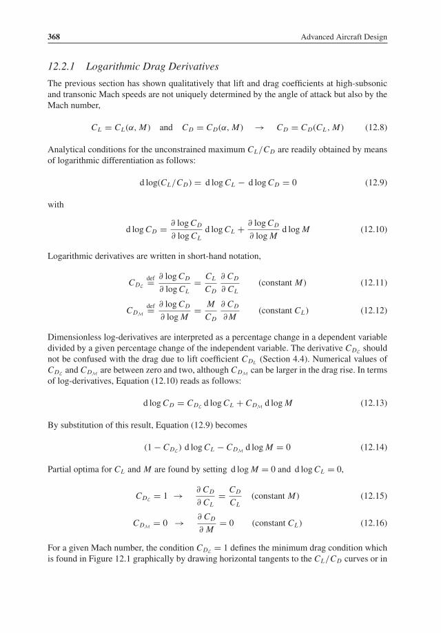
368 Advanced Aircraft Design
12.2.1 Logarithmic Drag Derivatives
The previous section has shown qualitatively that lift and drag coefficients at high-subsonicand transonic Mach speeds are not uniquely determined by the angle of attack but also by theMach number,
CL = CL (α, M) and CD = CD(α, M) → CD = CD(CL , M) (12.8)
Analytical conditions for the unconstrained maximum CL/CD are readily obtained by meansof logarithmic differentiation as follows:
d log(CL/CD) = d logCL − d logCD = 0 (12.9)
with
d logCD = ∂ logCD
∂ logCLd logCL + ∂ logCD
∂ logMd logM (12.10)
Logarithmic derivatives are written in short-hand notation,
CDLdef= ∂ logCD
∂ logCL= CL
CD
∂ CD
∂ CL(constant M) (12.11)
CDMdef= ∂ logCD
∂ logM= M
CD
∂ CD
∂ M(constant CL ) (12.12)
Dimensionless log-derivatives are interpreted as a percentage change in a dependent variabledivided by a given percentage change of the independent variable. The derivative CDL shouldnot be confused with the drag due to lift coefficient CDL (Section 4.4). Numerical values ofCDL and CDM are between zero and two, although CDM can be larger in the drag rise. In termsof log-derivatives, Equation (12.10) reads as follows:
d logCD = CDL d logCL + CDM d logM (12.13)
By substitution of this result, Equation (12.9) becomes
(1− CDL) d logCL − CDM d logM = 0 (12.14)
Partial optima for CL and M are found by setting d logM = 0 and d logCL = 0,
CDL = 1 → ∂ CD
∂ CL= CD
CL(constant M) (12.15)
CDM = 0 → ∂ CD
∂ M= 0 (constant CL ) (12.16)
For a given Mach number, the condition CDL = 1 defines the minimum drag condition whichis found in Figure 12.1 graphically by drawing horizontal tangents to the CL/CD curves or in

Unified Cruise Performance 369
Figure 12.2 by drawing vertical tangents. The condition CDM = 0 forms the lower boundaryof the Mach number region where compressibility degrades the aerodynamic efficiency. Thepartial optima intersect in the global optimizer point A defined by unique values of the liftcoefficient and the Mach number. This defines the most fuel-efficient cruise condition only ifthe overall efficiency of the engines has a stationary value in the same point. In general, thisis not the case for jet aircraft although a (future) propulsion systems such as the open rotorengine may achieve its maximum overall efficiency at a subsonic Mach number.
12.2.2 Interpretation of Log-Derivatives
Dependent on the aircraft design stage, drag polars of different appearance may be used (Sec-tion 4.4). For the purpose of initial performance analysis, the drag polar is often approximatedby a two-term approximation,
CD = CD0 + KLC 2L , with KL
def= dCD/ d(C 2L ) (12.17)
For this case the log-derivative CDL is
CDL = 2KLC 2L
CD0 + KLC 2L
= 2drag due to lift
total drag(12.18)
Conditions for minimum drag are
CLMD =√
CD0
KLand CDMD = 2CD0 →
(CL
CD
)MD
= 1
2√
KLCD0
(12.19)
This is the classical result that the aerodynamic efficiency is maximized for equal zero-liftdrag and drag due to lift. The relationship between CDL and CL is
CDL = 2(CL/CLMD)2
1+ (CL/CLMD)2or
CL
CLMD
=√
CDL
2− CDL(12.20)
The aerodynamic efficiency in relation to its maximum value amounts to
CL/CD
(CL/CD)MD= 2(CL/CLMD)
1+ (CL/CLMD)2= √
CDL(2− CDL) (12.21)
which proves that 0 ≤ CDL < 2. The relationships derived above are depicted in a generalizedform in Figure 12.3.In principle, a two-term drag polar can be used at low as well as high Mach numbers. In the
latter case, Mach number-dependent coefficients have to be used,
CD = CD0 (M)+ KL(M)C2L (12.22)
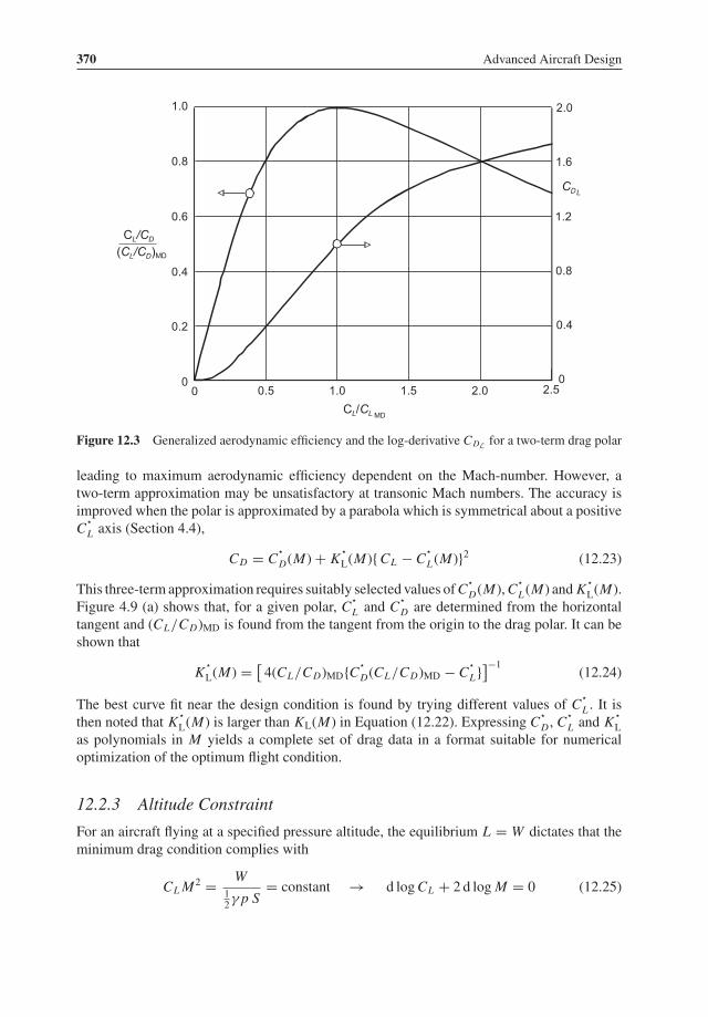
370 Advanced Aircraft Design
Figure 12.3 Generalized aerodynamic efficiency and the log-derivative CDL for a two-term drag polar
leading to maximum aerodynamic efficiency dependent on the Mach-number. However, atwo-term approximation may be unsatisfactory at transonic Mach numbers. The accuracy isimproved when the polar is approximated by a parabola which is symmetrical about a positiveC
�
L axis (Section 4.4),
CD = C�
D(M)+ K�
L(M){ CL − C�
L (M)}2 (12.23)
This three-term approximation requires suitably selected values ofC�
D(M),C�
L (M) and K�
L(M).Figure 4.9 (a) shows that, for a given polar, C
�
L and C�
D are determined from the horizontaltangent and (CL/CD)MD is found from the tangent from the origin to the drag polar. It can beshown that
K�
L(M) = [4(CL/CD)MD{C �
D(CL/CD)MD − C�
L}]−1(12.24)
The best curve fit near the design condition is found by trying different values of C�
L . It isthen noted that K
�
L(M) is larger than KL(M) in Equation (12.22). Expressing C�
D , C�
L and K�
Las polynomials in M yields a complete set of drag data in a format suitable for numericaloptimization of the optimum flight condition.
12.2.3 Altitude Constraint
For an aircraft flying at a specified pressure altitude, the equilibrium L = W dictates that theminimum drag condition complies with
CL M2 = W12γ p S
= constant → d logCL + 2 d logM = 0 (12.25)

Unified Cruise Performance 371
and substitution into Equation (12.14) yields
CDL = 1+ 0.5CDM (12.26)
Visualized in Figure 12.2, this condition is identical to Equation (12.15) below the criticalMach number where CDM≈ 0. The occurrence of high compressibility drag leads to CDM > 0and a constrained minimum drag condition CDL > 1; hence, CL > CLMD . As an example,Figure 12.2 depicts the altitude constraint CL M2 = 0.30 which has a point of tangency to aCL/CD contour in point B, defining the intersection with Equation (12.26). If we had derivedthis condition by intersecting the same altitude curve with CDL =1 the erroneous result wouldbe point C with a much higher Mach number and lower CL than point B.
12.3 The Parameter ML/D
Classical cruise performance optimization of jet aircraft assumes that the TSFC is independentof the flight speed. Overall efficiency is then proportional to Mach number and, according toEquation (12.6), the objective function is MCL/CD , or M L/D. In terms of log-derivatives itsmaximum value is determined from
d logM + d logCL − d logCD = 0 (12.27)
After expansion of d logCD in terms of the lift coefficient andMach number, Equation (12.13)is used to find that
(1− CDL) d logCL + (1− CDM) d logM = 0 (12.28)
where the log-derivatives CDL and CDM are defined by Equations (12.11) and (12.12), respec-tively. The parameter M L/D can be interpreted as the airframe’s contribution to specificrange, an acceptable simplification when aircraft with similar engines are compared withina small range of Mach numbers. However, M L/D should not be used for comparing rangeperformances of aircraft cruising at widely different speeds.
12.3.1 Subsonic Flight Mach Number
The traditional approach to the analysis of optimum cruising flight is based on the assumptionthat there is no drag due to compressibility (CDM = 0). For this case, meaningful results areobtained only by imposing a constraint on some operational parameter limiting the flight speedto a subcritical Mach number.
• For given Mach number, the optimizer according to Equation (12.20) is CDL = 1. Thiscondition defines the altitude where CL = CLMD .
• For given altitude, the productCL M2 is prescribed. Equation (12.28) yieldsCDL = 0.5 whichis identical to maximizing
√CL/CD . For a two-term parabolic polar, Equation (12.20) yields
CL = CLMD/√3, speed 31/4VMD andCD = 4
3 CD0 . This is a classical solution for the optimumcruise speed of a jet aircraft.

372 Advanced Aircraft Design
• For a constant engine rating – this is (nearly) equivalent to a constraint on the correctedthrust T/δ – the equation for horizontal equilibrium yields
CD M2 = 2 T/δ
γ pslS(12.29)
Hence, the term CD M2 is constant, or d logCD + 2 d logM = 0. Substitution into Equation(12.28) yields CDL = 2/3. This condition is identical to maximizing C 2
L /C 3D for which
CL = CLMD/√2, CD = 1.5 CD0 and V = 21/4VMD, another classical solution.
These conditions are incompatible and there exists no unconstrained optimizer.
12.3.2 Transonic Flight Mach Number
The ‘fingerprint’ contours of constant MCL/CD in Figure 12.4 are obtained by multiplyingCL/CD contours (Figure 12.2) by the Mach number. Partial optima are defined as follows:
• The optimum lift coefficient for given Mach number CDL = 1 (curve I) is identical to thatfor maximum CL/CD .
• The optimum Mach number for given lift coefficient obtained from Equation (12.28) is inthe drag rise: CDM = 1 (curve II).
Figure 12.4 Contours of constant MCL/CD . Partial optimizers: I lift coefficient; II Mach number.Constrained optima: III specified altitude; IV specified thrust

Unified Cruise Performance 373
L
00 0
0
M
(a) M1
M6 M5 M4 M3 M2
M1
M2 M3 M4 M5M6(b)
CD CD
Figure 12.5 Graphical construction of the partial optima for M L/D. (a) Optimum lift coefficient forgiven Mach number. (b) Optimum Mach number for given lift coefficient
• The unconstrained maximizer of M L/D id defined by the intersection of curves I and II inpoint A. In the example this flight condition is located just below the drag divergence Machnumber, but it is clearly in the drag rise since the aerodynamic efficiency has decreased to96% of (CL/CD)MD.
Although the unconstrained optimum is illustrated by means of a contour plot, its allocationdoes not require the drawing up of these explicit contours. A direct solution of the solutionis provided by the graphical construction using two representations of drag curves illustratedin Figure 12.5. The partial optimizers CDL = 1 and CDM = 1 are transferred as curves I andII, respectively, to the CL versus M plane (Figure 12.4). Their intersection (point A) definesthe global optimizer. A global optimizer may not be achievable due to one of the followingequality constraints.
• For an equality constraint on the pressure altitude, the optimizer follows from substitution ofd logCL + 2 d logM = 0 into Equation (12.28) resulting in 2CDL =1 + CDM . Depicted ascurve III, this condition is identical to the one found for subsonic Mach speed in the previousparagraph. Curve III bends sharply upwards for M > 0.70 and intersects curves I and II inPoint A. Its intersection with the altitude constraint defines the constrained optimum veryclose to point A.
• For an equality constraint on the corrected thrust, the optimizer follows from substitution ofd logCD + 2 d logM = 0 into Equation (12.28) resulting in CDL = 2 + CDM . Depicted ascurve IV, this condition intersects curves I, II and III in point A. The intersection of curveIV with the thrust constraint defines the constrained optimum above point A.
If the equality constraints on altitude and thrust were treated as inequality constraints allowingto fly at reduced speed and/or altitude, the global optimum flight condition point A wouldbecome the best cruise condition for the present example.Curves I and II are readily obtained without the use of explicit L/D contours. This is shown
in Figure 12.5 where tangents from the origin identify the condition ∂CD/∂CL = CD/CL
and ∂CD/∂ M = CD/M . After transfer to Figure 12.4 the intersecting of these partial optima

374 Advanced Aircraft Design
yields the global unconstrained optimizer. This demonstrates that an unconstrained optimumflight condition for maximum M L/D exists only when compressibility effects are present.Hence, the global optimizer is located in the drag rise. For the example aircraft, the criterion∂ CD/∂ M = CD/M = 0.033 defines a Mach number below the drag divergence Mach numberwith ∂ CD / ∂ M = 0.10. A more accurate criterion for the maximum specific range will bederived below.
12.4 The Range Parameter
The range parameter P defined by Equation (12.5) is a primary characteristic contributing tothe energy efficiency of an airliner. It is obtained from multiplication of the overall efficiencyand the aerodynamic efficiency. As explained in Chapter 3, the overall efficiency η o of a gasturbine-based propulsion system is a function of theMach number and the corrected thrust T/δ
representing the engine rating. Figure 12.6 is an example derived from engine performanceinformation such as Figure 3.4. It shows T/δ made dimensionless with the take-off thrust TTO.Since in steady level flight
T/δ = D/δ = 0.5 γ p slM2CD S (12.30)
the corrected thrust is a function of CD and M . Consequently, the range parameter is fullydetermined by CL and M and the range parameter contours on Figure 12.7 are independentof the plane’s gross weight.
12.4.1 Unconstrained Optima
General conditions for the maximum specific range have been derived in [25]. Since Machnumber variation has a far more significant effect than engine rating, the results have beensimplified by considering only the log-derivative of the overall efficiency with respect to theMach number,
ηMdef= d log η o
d logM= M
η o
dη odM
(12.31)
0.45
0.40
0.35
0.30
0.25
0.5
0.6
0.7
0.8
0.91.0
M
(T/ )/TTO
max. cruise rating
o
Figure 12.6 Overall efficiency of a high bypass ratio turbofan on a logarithmic scale

Unified Cruise Performance 375
Normally, this parameter has a value between zero for constant overall efficiency and one andfor constant TSFC. Conditions for achieving the maximum range parameter are derived bylogarithmic differentiation,
d logP = d log η o CL/CD = d log η o + d logCL − d logCD = 0 (12.32)
which can be expanded in terms of partial derivatives as follows:
(1− CDL) d logCL + (ηM − CDM) d logM = 0 (12.33)
This leads to the following partial optima for CL and M :
CDL = 1 or∂ CD
∂ CL= CD
CL(constant M) (12.34)
CDM = ηM or∂ CD
∂ M= ηM
CD
M(constant CL ) (12.35)
The unconstrained global optimizer (point A) is found by combining these conditions. At sub-sonic and transonicMach numbers, the overall efficiency of a turbofan engine mostly increasesmonotonically with Mach number; hence, Equation (12.35) indicates that the unconstrainedoptimum is in the drag rise. In other words: the best cruise Mach number of a jet airplane
Figure 12.7 Range parameter of a turbofan powered airliner. Partial optima: I lift coefficient; II Machnumber. Constrained optima: III specified altitude; IV specified thrust

376 Advanced Aircraft Design
is in the drag rise. Partial optima for CL and M are indicated in Figure 12.7 as curves I andII, respectively. Although the general shape of this diagram is similar to Figure 12.4 there aresome noticeable differences. In particular, since ηM < 1, the best cruise condition (point A)is located at a lower Mach number than for the case of maximum M L/D – the differenceis approximately M = 0.025 – and the range parameter is less sensitive to flying at anoff-optimum flight Mach number.
12.4.2 Constrained Optima
For an equality constraint on the altitude, the optimum is found by inserting a constant CL M2
into Equation (12.33) which yields
CDL = 1+ 0.5 (CDM − ηM) (12.36)
In Figure 12.7 this condition is represented by curve III, which intersects the specified valueof CL M2 in point B. The optimizer with an equality constraint on the corrected thrust is foundby inserting a constant CD M2 which yields
CDL = 2+ CDM
2+ ηM(12.37)
This condition is represented by curve IVwhich intersects the specified value ofCD M2 in pointC. These results can be simplified for aircraft having a single parabolic drag polar cruising insubcritical flow (CDM = 0) which yields the optimum conditions of Table 12.1. For idealizedjet propulsion (ηM = 1) they are in accordance with classical performance analysis.
12.4.3 Interpretation of ηMThe log-derivative ηM represents the percentage change in overall engine efficiency as afraction of the same percentage change inMach number. In order tomake it a practical concept,this parameter deserves further explanation based on its relation to the corrected TSFC,
ηM = 1− M
CT /√
θ
d(CT /√
θ)
dM(12.38)
The overall efficiency can be expressed as the product of the combustion efficiency ηcb, thermalefficiency ηth and propulsive efficiency ηprop,
η o = η cbη thη prop (12.39)
Table 12.1 Constrained optima for maximum subsonic specific range.
Parameter Altitude constraint Thrust constraint
CDL 1− 0.5 ηM (1+ 0.5 ηM)−1
CL/CLMD {(2− ηM)/(2+ ηM)}1/2 (1+ ηM)−0.5
V/VMD {(2+ ηM)/(2− ηM)}1/4 {(1+ ηM)/(1+ 0.5 ηM)}1/2(L/D)/(L/D)MD (1− 0.25 η 2M)
1/2 (1+ ηM)1/2/(1+ 0.5 ηM)

Unified Cruise Performance 377
Logarithmic differentiation yields
ηM = d log η cb
d logM+ d log η th
d logM+ d log η prop
d logM(12.40)
Thefirst of these terms is close to zero, the second has a small positive value due to the rameffecton the engine pressure ratio. The third term is dominant – it can be associated with the Froudeequation (3.15). This approach can be further evolved resulting in ηM = 1− factor× η propwhere the factor depends on the specific thrust [32]. Since η prop = 0 for M = 0, ηM approaches1.0 for M↓ 0. For subsonic Mach numbers ηM varies typically between 0.8 for low bypassturbofans, 0.5 for high bypass turbofans and 0.3 for very high bypass ratios. The propulsiveefficiency of a turboprop system at cruise conditions varies little with subsonic speed; hence,ηM ≈ 0.Application to cruise performance optimization requires input of a realistic value of ηM.
The following approaches are suggested.
• If engine performance data is available, the corrected TSFC versus Mach number is approx-imated by a linear relationship,
CT /√
θ = C 0 (1+ CM M) → ηM = (1+ CM M)−1 (12.41)
Figure 12.8 shows an example for a typical high bypass turbofan. In the Mach number rangeof interest, the variation of ηM with Mach number is relatively small so that for optimizationpurposes ηM can be considered as constant.
Figure 12.8 Properties of a high bypass turbofan with C0 = 0.3 h−1 and CM = 1.4
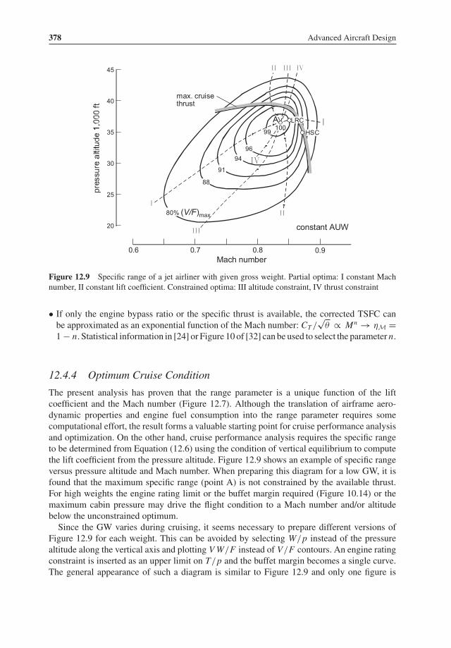
378 Advanced Aircraft Design
Figure 12.9 Specific range of a jet airliner with given gross weight. Partial optima: I constant Machnumber, II constant lift coefficient. Constrained optima: III altitude constraint, IV thrust constraint
• If only the engine bypass ratio or the specific thrust is available, the corrected TSFC canbe approximated as an exponential function of the Mach number: CT /
√θ ∝ Mn → ηM =
1− n. Statistical information in [24] or Figure 10 of [32] can be used to select the parameter n.
12.4.4 Optimum Cruise Condition
The present analysis has proven that the range parameter is a unique function of the liftcoefficient and the Mach number (Figure 12.7). Although the translation of airframe aero-dynamic properties and engine fuel consumption into the range parameter requires somecomputational effort, the result forms a valuable starting point for cruise performance analysisand optimization. On the other hand, cruise performance analysis requires the specific rangeto be determined from Equation (12.6) using the condition of vertical equilibrium to computethe lift coefficient from the pressure altitude. Figure 12.9 shows an example of specific rangeversus pressure altitude and Mach number. When preparing this diagram for a low GW, it isfound that the maximum specific range (point A) is not constrained by the available thrust.For high weights the engine rating limit or the buffet margin required (Figure 10.14) or themaximum cabin pressure may drive the flight condition to a Mach number and/or altitudebelow the unconstrained optimum.Since the GW varies during cruising, it seems necessary to prepare different versions of
Figure 12.9 for each weight. This can be avoided by selecting W/p instead of the pressurealtitude along the vertical axis and plotting V W/F instead of V/F contours. An engine ratingconstraint is inserted as an upper limit on T/p and the buffet margin becomes a single curve.The general appearance of such a diagram is similar to Figure 12.9 and only one figure is

Unified Cruise Performance 379
required to cover different weights. A choice of the initial and final operating conditions –for example, for long-range cruising (LRC) or high speed cruising (HSC) – is necessary forcarrying out the integration of specific range, the subject of the following text.
12.5 Range in Cruising Flight
Different from the point performance problem treated in the previous sections, the distanceattainable in cruising flight is an integrated performance. In order to maximize the range, anoptimal control lawhas to be be derived for the independent variables. Several cruise techniquesleading to closed-form solutions have been reported in the literature; an overview is given in[22]. Solutions for the case of specified initial conditions are accurate on the provision thatthe flight condition does not vary considerably during the flight. However, the optimum initialcruise condition and maximum range are inaccurate if propeller efficiency or engine TSFC areassumed to be invariable with speed and altitude. Computed optimum cruise conditions mayeven be unrealistic when compressibility effects are ignored. The unified cruise performanceanalysis exposed in this section is applied to derive analytical solutions for the cruise rangecorresponding to several control laws. It applies to airplanes powered by any category of gasturbine engines flying at low as well as high airspeeds.
12.5.1 Breguet Range Equation
The widely used expression ascribed to Louis Breguet (1880–1955) for the range obtainedin steady level cruising flight was originally derived for propeller aircraft with piston enginesflying at constant angle of attack. If we denote the engine’s SFC based on shaft horse power(SHP) by CP , propeller efficiency by η pr, the initial GW by Wi and the final GW by We,Breguet’s classical equation reads as follows:
RBr = η pr
CP
CL
CDln
Wi
We(12.42)
This expression can be used for turboprop engines as well, provided SFC is based on equivalentengine power (Section 3.3). When jet engines were introduced during the 1940s, it was notedthat Breguet’s equation can be modified so that it applies to the range of jet aircraft flying withconstant speed and angle of attack,
R = V
CT
CL
CDln
Wi
We(12.43)
Equations (12.42) and (12.43) can be replaced by a single one. The range in quasi-steadycruising flight is obtained from integration of the specific range according to Equation (12.1),
R =∫ Wi
We
V
FdW (12.44)
If V/F were constant during the flight the solution would simply be
R = V
F(Wi − We) = V
FW f (12.45)
380 Advanced Aircraft Design
where Wf denotes the weight of fuel burnt. In reality, the specific range increases during theflight due the decreasing GW. This is taken into account by substitution of Equation (12.5) forthe specific range P ,
R = H
g
∫ Wi
We
η oCL
CD
dW
W= H
g
∫ Wi
We
P dW
W(12.46)
If the angle of attack and the flight speed are controlled so that P is constant during the flight,the integral can be solved analytically,
R = H
gP ln
Wi
We(12.47)
Substitution of the overall efficiency according to Equations (3.12) and (3.28) yields theBreguet range equation for jet and propeller aircraft, respectively. Equation (12.47) representstherefore a unified expression for the range of aircraft with various types of propulsion systemswhen flying with a constant range parameter.The theoretical maximum distance is covered when P stays constant at its maximum value.
For transonic jet aircraft this means that CL and M are constant. Since this is not alwaysfeasible, alternative schedules are investigated using the following notations for frequentlyoccurring combinations of terms:
ζdef= We/Wi = 1− Wf/Wi and y i
def= CL i/CLMD (12.48)
12.5.2 Continuous Cruise/Climb
Aircraft cruising at constant angle of attack andMach number fly at constant L/D and increasetheir altitude so that W/p is constant as well. In the (isothermal) stratosphere the aircraft flieswith constant engine rating, and hence constant corrected thrust and overall efficiency. Thisflight schedule is known as the continuous cruise/climb (index ccc) technique1 for whichintegration of Equation (12.46) yields
Rccc = H
gP ln(1− ζ )−1 (12.49)
If the initial conditions are such that P has its maximum value this equation represents thelongest range theoretically achievable in quasi-steady flight. Although Equations (12.49) and(12.47) are identical, the original Breguet equation was derived for airplanes with constantpropeller efficiency cruising at constant altitude. The continuous cruise/climb technique may,however, not form a practical control law since the continuously varying altitude is consideredobjectionable from the air traffic control (ATC) point of view. Several alternative schedulesare available resulting in slightly shorter ranges than the Breguet range.
1Some extra thrust is required to climb to higher altitude and strictly speaking, there is no equilibrium between thrustand drag. However, having completed the cruising flight, the aircraft descends back to the initial altitude with reducedthrust, thus regaining the range loss during the climb.

Unified Cruise Performance 381
12.5.3 Horizontal Cruise, Constant Speed
Different from the continuous cruise/climb, cruising horizontally at constant speed (indexhccs) leads to a decreasing angle of attack and lift coefficient. The engines must be graduallythrottled back so that the thrustmatches the decreasing drag due to lift. This procedure is readilyaccomplished with modern engine control systems and it is beneficial from the operationalpoint of view. Integration of P for the case of a two-term parabolic drag polar [20] results in
Rhccs = 2H
g(η o)i
(CL
CD
)MD
{ arctan y i − arctan y i (1− ζ )} (12.50)
The difference between the two angles in the parentheses can be evolved by means of gonio-metric equations into a single one. After introduction of the range parameter for the initialcruise condition one finds
Rhccs = H
gPi (y−1
i + y i ) arctan
{ζ
y−1i + y i (1− ζ )
}(12.51)
Since for optimum cruising usually CL i ≤ C LMD (or y i ≤ 1.0) the angle defined by the arctanis small so that it can be approximated by its argument, resulting in
Rhccs = H
gPi ζ
(1− ζ
y2i1+ y2i
)−1(12.52)
This equation overestimates the exact solution by less than 1%. If the initial cruise altitudeis sufficiently high to obtain y i ≈ 1 the constant altitude/speed schedule predicts a slightlyshorter range than the continuous cruise/climb range. If, however, the initial cruise altitudeis constrained by the available engine thrust, Equation (12.52) may predict a significant fuelpenalty for a long range flight. As soon as the engine rating falls below the optimum cruiserating, the overall efficiency begins to deteriorate. The usual operational practice is thereforeto approximate the continuous cruise/climb by executing several horizontal cruise segmentswith intermediate climb segments to increased flight levels. This is known as the steppedcruise/climb.
12.5.4 Horizontal Cruise, Constant Lift Coefficient
The constant incidence schedule has traditionally been used to compute the range of jet aircraft.In subsonic flowCL andCD are constant, speed is reduced steadily and the engines are throttledback so that T/W is constant as well. The following expression is found for constant ηM byintegration of the specific range:
Rhccl = 2H
gP i1− (1− ζ ) ηM/2
ηM(12.53)

382 Advanced Aircraft Design
This equation applies to any value of ηM between zero and one. If the TSFC of a jet engineis assumed independent of speed, ηM = 1 and Equation (12.53) complies with the classicalsquare root range equation,
Rhccl = 2H
gP i (1−
√1− ζ ) (12.54)
The decreasing flight speed reduces the overall efficiency of turbofan engines causing a rangeloss at subcritical Mach numbers. If the flight is initiated in the drag rise, speed reduc-tion improves the aerodynamic efficiency and the range parameter may actually stay nearlyconstant. From the operational point of view, the continuously reducing flight speed is objec-tionable. The overall efficiency of a turboprop system is nearly invariable in high-speed flightand Equation (12.53) applies to propeller aircraft for ηM ↓ 0. It is worth noting that thisoutcome appears to be numerically identical to the Breguet range.
12.6 Cruise Procedures and Mission Fuel
The continuous cruise/climb is the only schedule based on constant overall propulsive andaerodynamic efficiencies. In the absence of an active constraint on altitude or engine rating, thelongest cruising range with a given amount of fuel is thus obtained when the range parameterP has its unconstrained maximum value throughout the flight (Section 12.4). For subsonicas well as transonic Mach numbers this schedule results in the generalized Breguet rangeEquation (12.47). Other cruise techniques lead to a few percentage range penalty, dependenton range.
12.6.1 Subsonic Flight
The case of zero compressibility drag is important mainly for propeller aircraft although jetaircraft may be forced to fly at reduced speed and/or altitude; for example, when engine failurehas occurred [30]. Steady level flight is a practical schedule approximating the cruise/climbrange closely. For this case the mean value of the range parameter should be maximizedinstead of its initial value. In Equation (12.51) this is manifest in the ratio y i = CL i/CLMD . Itsmodification Equation (12.52) defines the optimum initial altitude for given speed as
y i = 1√1− ζ
(12.55)
whereas the best initial speed at given altitude is
y i =√
2− ηM(2+ ηM)(1− ζ )
(12.56)
These optima are identical for (idealized) propeller aircraft with ηM = 0, defining the initialcruise speed to be lower or the altitude to be slightly above the condition for minimum drag(y i > 1). For jet propulsion with ηM > 0, the partial optima are incompatible – this is not

Unified Cruise Performance 383
surprising in view of the findings in Section 12.3. In this case, cruise performance is improvedby flying fast and high until an engine thrust limit is met, forming the ultimate constraint. Thebest range performance is obtained for an initial lift coefficient determined by
y i = 1√(1+ ηM)(1− ζ )
(12.57)
Contrary to what is usually stated in the literature, this equation shows that for long-range flightthe optimal initial lift coefficient is quite close to the minimum drag condition. For example,a fuel fraction of 0.30 for a turbofan powered airplane with ηM = 0.6 yields yi = 0.945. Theinitial flight speed is then only 3% above the speed for minimum drag.
12.6.2 Transonic Flight
The best cruising flight of a transonic jet airplane is executed in the drag rise. Figure 12.10shows an enlarged sector of Figure 12.7 near the maximum range condition (point A) whichyields the unconstrained maximum range in a continuous cruise/climb,
Rmax = (H/g)Pmax ln(1− ζ )−1 (12.58)
Although in the present example the cruise thrust limit allows the aircraft to fly continuously atthis combination of CL and Mach number, the required cruise/climb control law is, in general,not selected in operational practice. With reference to Figure 12.9, long-range cruising (LRC)is executed in a flight condition where the specific range is 98 or 99% of its maximum value,provided the higher cruise speed makes the fuel penalty acceptable in view of the time saved.A larger fuel penalty may be acceptable for short haul flights and the aircraft may be flown
M
CL
buffetboundary
max. thrustmax. cabinpressure
(W/p)i
(W/p)e
100%A
i
CD =1L
C ηD = MM
(a)
(b)
(c)
98%(V/F)max
Figure 12.10 Flight schedules for high speed cruising

384 Advanced Aircraft Design
at a lower altitude with the engines operating at their maximum cruise rating, known as highspeed cruising (HSC).2
As an example we assume that in the initial flight condition – point ‘i’ in Figure 12.10 – theengines are running at the recommended cruise rating and the altitude is above the minimumdrag condition. Several flight schedules can be considered with ranges slightly below theunconstrained maximum.
(a) During a horizontal constant speed cruise, the GW decreases from the initial value Wi tothe final value We, the ambient pressure is constant at p i. The gradually decreasing CL
allows the range parameter to remain close to the partial optimum CDL= 1 and the rangeis longer than for a continuous cruise/climb in point i.
(b) During a horizontal constant CL cruise, the Mach number decreases and the specificrange varies close to the partial optimum CDM= ηM. In contrast with subsonic flight, thisensures good range performance. However, a significant speed reduction during the flightis unlikely to be preferred in commercial operation.
(c) A horizontal constant engine rating cruise penalizes the range significantly because thedrag rise is deeply penetrated. For a reduced (but constant) rating with point i moved tothe left and/or downwards, good range performance is combined with the drawback ofincreasing speed.
(d) In a stepped cruise/climb (not indicated in Figure 12.10) the lift coefficient initially followsschedule (a) in horizontal flight at constant speed. As soon as the gross weight reductionenables a 4 000 ft altitude increment, the plane climbs to the altitude for minimum dragand starts another steady level cruise segment. Dependent on the number of climb steps,the complete flight closely approximates CDL = 1.
The question remains, at what altitude and speed the cruising flight should be commenced.For given Mach number, the specific range is maximum for CDL= 1 but for a level constantspeed cruise CL decreases during the flight and the optimum initial CL is higher. Moreover,the altitude for maximum range may initially not be attainable due to an engine rating or abuffet margin constraint as indicated. The preferred initial cruise condition in Figure 12.10is then at the intersection of the 98% or 99% maximum V/F contour with the criticalconstraint.
12.6.3 Cruise Fuel
The present analysis has resulted in expressions for the range in cruising flight applying toseveral Mach number regimes and flight schedules. The horizontal constant speed schedule ismostly used for short to medium range flights and the stepped cruise/climb is preferred for longdistance flights. Equation (12.52) for horizontal cruising at constant Mach number is thereforeconsidered as representative of operational practice. Although it is derived for the case of atwo-term parabolic drag polar this does not invalidate the result, provided compressibility drag
2Weather conditions may force the pilot to reduce the speed below the theoretical best value in order to improve ridecomfort and to increase the buffet margin.

Unified Cruise Performance 385
is taken into account. The following versatile expression applies to several flight schedulesand has the advantage that it provides the fuel fraction in analytical closed form:
Wf
Wi=
(H/g
RPi + 0.5 fcc
)−1(12.59)
where P = η oCL/CD . Equation (12.52) is approximated by selecting the cruise control factorfcc as follows:
fcc = 1+ R
6Pi H/gcontinuous cruise/climb @ constant CL and M ,
fcc = 1− R
6Pi H/ghorizontal cruise @ constant M .
Using the first of these factors closely approximates the cruise fuel (index crf) based onBreguet’s range equation. The following simple approximation is based on the steppedcruise/climb with fcc = 1:
Wcrf
Wi=
{H/g
RPi + 0.5
}−1(12.60)
with H/g = 4 350 km (2 700 sm). It is worth noting that this result would also be foundfrom Equation (12.45) provided V/F specific range is computed for the mean GW during thecruising flight, W = Wi − 0.5Wf .The following recommendation for the initial cruise condition is based upon the previous
analysis, Section 12.4 in particular.
• Subsonic propeller aircraft: the optimum speed is VMD at the altitude where ηo achieves itsmaximum value, on the provision that there is no engine power constraint.
• Subsonic jets: the fuel-optimum is on the engine cruise rating (corrected thrust) constraint;see Table 12.1.
• High speed propeller and open rotor aircraft: the fuel-optimum is located halfway betweenthe Mach numbers for maximum aerodynamic efficiency and maximum overall efficiency.The best (pressure) altitude is determined by the condition CDL = 1.
• Transonic jet aircraft: The unconstrained maximum V/F should be determined first, as wellas the 98 or 99% contour (Figure 12.10). Its intersection at high speed with the recommendedengine cruise rating defines a good initial cruise condition.
12.6.4 Mission Fuel
The profile of a typical commercial flight is shown in Figure 12.11. Total fuel is subdividedinto block fuel and reserve fuel. Block fuel is equal to mission fuel plus fuel for taxying out.3
3Except for multi-mission operations, reserve fuel may be used for taxying after landing.

386 Advanced Aircraft Design
climb
climb
cruise
MISSION RESERVES
LRC(100 nmi)
appr
oach
and
land
desc
end
to 1
,500
ft
mis
sed
appr
oach
(at
35
ft,ac
cele
rate
to 2
50 k
t at 1
,500
ft
taxi
in (
5 m
in.)
from
res
erve
s
taxi
out
(9
min
.)
take
-off
(to
35 ft
)
clim
b to
1,5
00 ft
, acc
el. t
o 25
0 kt
clim
b to
10,
000
ft at
250
kt
acce
lera
te to
clim
b sp
eed
1.0
hr a
t LR
C(a
t end
cru
ise
altit
ude
and
wei
ght)
appr
oach
and
land
desc
end
to 1
,500
ftde
cel.
to 2
50 k
tde
scen
t to
10,0
00 ft
200 nmi
reserves
still air range
block time, fuel
mission fuel
Figure 12.11 Flight profile for an international flight, with components for the mission and the reserveflight
The mission begins at take-off brake release and ends at standstill after landing. Mission fuelis broken down into fuel for take-off, acceleration and climb to the initial cruise altitude andspeed, cruising flight, descent and deceleration for approach and landing at the destination.Accurate calculation of the total fuel load is possible when detailed data are available in theform of design weights, drag polar curves, engine thrust and fuel flow diagrams or tables,including corrections for bleed air and power take-off for driving on-board systems.In the conceptual stage it may be acceptable to derive the mission fuel weight from the
cruise fuel with estimated corrections to allow for the non-cruising segments. The dominantfactor to be used as input for such a method is the range factorP for the initial cruise condition.The analysis of range performance in Section 12.6 has resulted in expressions for the range incruising flight according to several techniques. These were used to derive Equation (12.60) forfor the cruise fuel fraction. A procedure for mission fuel prediction recommended in [32] is todetermine first the amount of fuel required for a (hypothetical) cruising flight over the requiredmission range Rmis assuming the MTOW to be the initial weight. An amount of fuel is thenadded referred to as lost fuel (Wf)lost. This is not the fuel used in climb but rather the increasein fuel required to take off, climb and acceleration to the cruise altitude and speed compared tocruising the distance covered in climb [24]. The lost fuel is obtained from a simplified energybalance, assuming constant GW. In terms of the energy height at the initial cruise condition,
(he) i = h i + V 2i
2g(12.61)
the lost fuel fraction is determined from the following expression [32]:
(Wf)lostWTO
= (1.1+ 0.5 ηM)(he) i
(ηo) i H/g(12.62)

Unified Cruise Performance 387
The term 1.1 + 0.5 ηM accounts for the factors that are suboptimal in climbing flight: lowerspeed, altitude and engine efficiency. It shows that the higher the bypass ratio – hence, thelower ηM – the smaller the lost fuel fraction. The fuel consumed during descent, approachand landing is conservatively assumed equal to the fuel used during a cruising flight over thesame distance. In other words: lost fuel for this flight segment is ignored. The lost fuel maybe converted into a lost range
Rlost = (1.1+ 0.5 ηM)(CL/CD) i (he) i (12.63)
representing the difference between the actual mission range and the distance travelled incruising flight with the same amount of fuel. The mission fuel fraction is found by adding thelost range to the mission range,
(Wf)misWTO
= Rmis + RlostP i H/g + 0.5 (Rmis + Rlost)
(12.64)
12.6.5 Reserve Fuel
The following reserve fuel requirements are specified in the FAR.141.645 regulation forinternational flights.
1. After completing the mission, flying 10% of the mission time.2. After that, to fly to the most distant alternate airport.3. Thereafter, to fly 30 minutes at holding speed 1 500 ft above the airport.
Reserve fuel requirements for US domestic operations are specified in FAR 121.639 as follows:
1. After completing the mission, to fly to the most distant alternate airport.2. Thereafter, to fly for 45 minutes at normal cruising fuel consumption.
There are important differences between different nations and operations in specificationsof standard reserve fuel. The Association of European Airlines (AEA) specifies a 200 nm(370 km) diversion flight for short and medium range aircraft or a 250 nm (463 km) diversionfor long range aircraft, 30 minutes holding at 1 500 ft (457 m) altitude, and 5% of the missionfuel for contingency reserve [28]. Reserves are less for domestic flights in the USA, forexample 130 nm (241 km) diversion and 30 minutes holding at 1 500 ft (457 m) altitude.Long-range international flights may require an extension of the cruise sector, for exampleone hour at LRC flying. For business aircraft, the total reserves are frequently defined as anextension of the cruising flight by 45 minutes.Statistical values of the total reserve fuel are between 4.5 and 5% MTOW. A more accurate
computation of reserve fuel in the preliminary design stage allows the user to insert the

388 Advanced Aircraft Design
reserve policy specified in the TLRs. This results in the selection of several of the followingallowances:
1. A diversion distance equal to Rdiv flown at the MLW. This fuel weight fraction can beexpressed as a mission range increment of rdivRdiv times the ratio WML/WMTO where rdivaccounts for the fuel penalty due to an aborted landing and the reduced specific range dueto flying at reduced speed and altitude, partly in low-speed configuration.
2. An allowance for a holding period thold flown at the MLW. This reserve fuel weight fractionis considered as a range increment rholdVholdthold times the ratio WML/WMTO where rholdaccounts for the reduced specific endurance during holding relative to cruising.
3. Contingency fuel is accounted as a fraction – for example, 0.05 or 0.10 – of the missionfuel weight.
4. An extension time tcr of the cruising flight, equivalent to a mission range increment ofVcrtcr.
12.7 Reflection
12.7.1 Summary of Results
Comprehensive treatment of high speed cruise optimization requires the availability of dragpolars for different Mach numbers. It is recommended to convert these to contours of constantCL/CD values as depicted in Figure 12.2. Drag polars at transonic Mach numbers can be quitedifferent from those at subsonic speeds and the present theory does not assume them to betwo-term parabolic approximations. Global unconstrained as well as constrained optimizersare derived from contour plots for MCL/CD or ηoCL/CD , as summarized below.
• The lift coefficient and the Mach number are treated as independent control variablesaffecting the drag coefficient. Different from the classical solutions for subsonic airplanes,the aerodynamic efficiency CL/CD has a global unconstrained maximum for a uniquecombination of CL and M referred to as (CL )MD and MMD, respectively. This optimizer isdefined by the intersection of partial optima with respect to the two control variables.
• The parameter M L/D attains a global unconstrained optimizer well into the drag rise ata lift coefficient not much different from (CL )MD. However, the optimum Mach number isdefined by the partial optimum dCD/d M = CD/M which is readily constructed graphically;see Figure 12.5.
• The range parameter P = ηo L/D is a unique function of CL and M and can be visu-alized in a similar contour plot as M L/D; see Figure 12.7. The unconstrained globaloptimizer is defined by the partial optimum d logCD / d logM = dlog ηo/dlogM = ηM. Itis located at a Mach number between MMD and the Mach number for maximum M L/D.The parameter ηM is determined mainly by the engine’s propulsive efficiency and is readilyobtained from engine performance information. Propeller and open rotor engines at highsubsonic speeds have ηM ≈ 0. High-bypass ratio turbofans have ηM ≈ 0.5 at transonic flightspeeds.
• The range in cruising flight is derived for three flight control schedules: continuous cruise/climb, level flight at constant Mach number and level flight at constant lift coefficient.

Unified Cruise Performance 389
An example for high-speed cruising shows that, different from subsonic cruising, theseschedules lead to a few percent shorter range compared to the Breguet range equation. Levelflight at constant altitude is recommendable if the attainable cruise altitude for the initialgross weight is sufficiently high to cruise the minimum drag condition.
• A constraint on the cruise altitude imposed by the available engine thrust may cause asignificant range loss if the aircraft takes off with maximum take-off weight. A steppedcruise/climb is recommendable for long range flights.
• A simple closed-form equation containing a parameter dependent on the flight controlschedule is derived for computing the cruise fuel weight. Analytical approximations formission and reserve fuel are presented which are useful for the quasi-analytical optimizationprocedure treated in Chapters 8 to 10.
Although the mission fuel depends to a large extent on the cruise conditions, there is limitedfreedom to deviate from the global optimum with a small fuel penalty. A penalty of 1 or 2%is accepted on a long-range cruising flight if the increased speed results in a worthwhile timesaving.
12.7.2 The Design Connection
The unconstrained global optimizer for the cruise altitude and Mach number derived in thischapter applies to conditions which lead to maximum range for given fuel or minimum fuelfor a specified range. A constraint on the (initial) cruise altitude may cause a significantrange loss or fuel penalty and the designer may be tempted to increase the installed enginepower or thrust. However, it was found in Chapter 8 that the altitude for minimum MTOWis below the altitude for minimum cruise fuel. This may be the explanation why existingaircraft are equipped with engines that do not allow them to climb to the most fuel-efficientcruise altitude after taking off with MTOW. Chapter 9 showed that installed engine thrustmay have to be increased in excess of the value for minimum MTOW in order to complywith low speed requirements or with the requirement of reducing mission fuel burn-off.An increased installed thrust also helps to fly at a higher Mach number in the interest ofeconomy.Selection of the cruise Mach number for optimum aerodynamic wing design is more critical
than selecting optimum cruise conditions for a given (wing) design. Figure 12.7 illustrates thatthe global optimumMach number is about 0.05 below the drag-divergence valueMach number.It can be argued that for this example the wing is too thin or has too much sweep, resultingin a heavier wing than necessary. This may lead to the decision to reduce the design cruiseMach number. The greatest uncertainty is that airliners are operated by different operators onwidely different missions. The design mission with maximum payload or maximum range istherefore not often flown and the most economical operation should be defined with lowerthan the structural payload over shorter distances than the maximum range.The question may thus arise in the advanced aircraft designer’s mind:Which figure of merit
should I select to optimize my design? The answer cannot be left to the individual designer.The well-tempered airplane is the result of system engineering in which the designer/analystplays a modest but invaluable part on the instrument of advanced optimization.
390 Advanced Aircraft Design
Bibliography
[1] Miele, A., Flight Mechanics: Theory of Flight Paths, Addison-Wesley, Reading, MA, 1962.[2] Hale, F.J., Introduction to Aircraft Performance, Selection and Design, John Wiley & Sons, New York, NJ,
1984.[3] Mair, W.A. and Birdsall, D.L., Aircraft Performance, Cambridge Aerospace Series 5, Cambridge University
Press, Cambridge, 1992.[4] Vinh, N.X., Flight Mechanics of High-Performance Aircraft, Cambridge Aerospace Series 4, Cambridge Uni-
versity Press, Cambridge, 1993.[5] Ojha, S.K.,Flight Performance of Aircraft, Chapters 8 and 9,American Institute ofAeronautics andAstronautics,
Education Series, Washington, DC, 1995.[6] Padilla, C.E.,Optimizing Jet Transport Effeiciency, Performance, Operations & Economics, McGraw-Hill, New
York, 1996.[7] Eshelby, M., Aircraft Performance: Theory and Practice, Chapter 4, Arnold Publishing, London, 2000.[8] Filippone, A.,Flight Performance of Fixed and Rotary Wing Aircraft, Chapter 9, Elsevier Aerospace Engineering
Series, Oxford, 2006.[9] Roux, E., Avions Civils a Reaction: Plan 3 Vues et Donnees Characteristiques, Editions Elodie Roux, ISBNN
978-2-9529380-2-0, 2007.[10] Torenbeek, E., and H. Wittenberg, Flight Physics: Essentials of Aeronautical Disciplines and Technology, with
Historical Notes, Chapters 6 and 9, Springer Verlag, Heidelberg, 2009.
Optimum Cruise Performance and Prediction of Range
[11] Jonas, J., “Jet Airplane Range Considerations”, Journal of the Aeronautical Sciences, Vol. 14, No. 2,pp. 124–128, February 1946.
[12] Ashkenas, I.L., “Range Performance of Turbojet Airplanes”, Journal of the Aeronautical Sciences, Vol. 15,No. 2, pp. 97–101, February 1948.
[13] Edwards, A.D., “Performance Estimation of Civil Jet Aircraft”, Aircraft Engineering, pp. 95–99, April 1950.[14] Pearson, H., “The Estimation of Range of Jet-Propelled Aircraft”, The Aeronautical Quarterly, Vol. II, pp. 167–
182, November 1950.[15] Schairer, G.S. and Olason, M.L., “Some Performance Considerations of a Jet Transport Airplane”, First Turbine
Powered Air Transportation Meeting, Institute of the Aeronautical Sciences, Seattle, Washington, USA, August9–11, 1954.
[16] Backhaus, G., “Grundbeziehungen fur den Entwurf Optimaler Verkehrsflugzeugen”, Jahrbuch der WGLR,pp. 201–213, 1958.
[17] Ward, K.E., “Contour Plotting for the Transonic Flight-Test Drag Polar”, Journal of Aircraft, Vol. 5, No. 2,pp. 191–192, March–April 1968.
[18] Page, R.K., “Range and Radius-of-Action Performance Prediction for Transport and Combat Aircraft”, AGARDLecture Series No. 56, Paper No. 1, March 1973.
[19] ESDU, “Approximate Methods for Estimation of Cruise Range and Endurance: Aeroplanes with Turbo-jet andTurbo-fan Engines”, Data Sheet No. 73019, October 1973.
[20] Peckham, D.H., “Range Performance in Cruising Flight,” Royal Aircraft Establishment Technical Report 73164,March 1974.
[21] Hale, F.J. and Steiger, A.R., “Effects of Wind on Aircraft Performance”, Journal of Aircraft, Vol. 16, No. 6,pp. 382–387, June 1979.
[22] ESDU, “Introduction to Estimation of Range and Endurance”, Data Item No. 73018, Performance, Vol. 6,October 1980.
[23] Bert, C.W., “Prediction of Range and Endurance of Jet Aircraft at Constant Altitude”, Journal of Aircraft,Vol. 18, No. 10, pp. 890–892, October 1981.
[24] ESDU, “Approximate Methods for Estimation of Cruise Range and Endurance: Aeroplanes with Turbojet andTurbofan Engines”, Data Item No. 73019, Revised May 1982.
[25] Torenbeek, E. and Wittenberg, H., “Generalized Maximum Specific Range Performance”, Journal of Aircraft,Vol. 20, No. 7, pp. 617–622, July 1983.

Unified Cruise Performance 391
[26] Sachs, G., and T. Christodoulou, “Reducing Fuel Consumption of Subsonic Aircraft by Optimal Cyclic Cruise”,Journal of Aircraft, Volume 24, No. 9, pp. 616–622, September 1987.
[27] Menon, P.K.A., “Study of Aircraft Cruise”, Journal of Guidance, Control, and Dynamics, Vol. 12, No. 5,pp. 631–639, September–October 1989.
[28] AEA, “Definitions and Input for Range and Direct Operating Cost Calculation”, Appendix;1, G(T) 5656,1990.
[29] Martınez-Val, R. and Perez, E., “Optimum Cruise Lift Coefficient in Initial Design of Jet Aircraft”, Journal ofAircraft, Vol. 29, No. 4, pp. 712–714, July–August 1992.
[30] Martınez-Val, R. and Perez, E., “Extended Range Operations of Two and Three Turbofan Engined Airplanes”,Journal of Aircraft, Vol. 30, No. 3, pp. 382–386, May–June 1993.
[31] Miller, L.E., “Optimal Cruise Performance”, Journal of Aircraft, Vol. 30, No. 3, pp. 403–405, May–June 1993.[32] Torenbeek, E., “Cruise Performance and Range Prediction Reconsidered”, Progress in Aerospace Sciences, Vol.
33, No. 5/6, pp. 285–321, 1997.[33] Isikveren, A.T., “Identifying Economically Optimal Flight Techniques of Transport Aircraft”, Journal of Air-
craft, Vol. 39, No. 4, pp. 528–544, July–August 2002.[34] Cavcar, A., and M. Cavcar, “Approximate Solutions for Range at Constant Altitude: Constant High Speed
Subsonic Flight of Transport Aircraft”, Aerospace Science and Technology, Vol. 8, No. 6, pp. 557–567, 2004.[35] Pargett, D.M., andM.D.Ardema, “Flight PathOptimization at Constant Altitude”, Journal of Guidance, Control,
and Dynamics, Vol. 30, No. 4, pp. 1197–1201, July–August 2007.[36] Rivas, D., and A. Valenzuela, “Compressibility Effects on Maximum Range Cruise at Constant Altitude”,
Journal of Guidance, Control, and Dynamics, Vol. 32, No. 5, pp. 1654–1658, September-October 2009.

Appendix AVolumes, Surface andWetted Areas
The surface area of a fully defined airplane component can be computed by dividing itsexternal surface into a sufficiently large number of nearly-flat panels and adding their areas.Alternatively, a double-curved streamline body (section) can be decomposed into a numberof (thin) disks with easy-to-compute ring shaped external areas. Quicker – but less accurate –analytical approximations are useful for conceptual design. This appendix presents formulasfor the volume and surface area of airplane major components derived in papers mentioned inthe bibliography.
A.1 Wing
The straight-tapered wing of a subsonic airplane can be considered as a linear lofted three-dimensional airfoil. Each half-wing is treated as a truncated pyramid with parallel end planesin the form of airfoil sections. Its volume is related to the planform area Sw by
Qw = kQ (t/c)w√1+ λw
Sw
√SwAw
(A.1)
with the aspect ratio defined as Aw = b2w/Sw. The mean thickness ratio t/c is the ratio offrontal to planform area and the taper ratio λ is the ratio of tip chord to root chord. The volumefactor of a prismatic wing (section) is kQ = 1 – a typical value for a tapered wing is kQ = 0.95.If the surface area is approximated as twice the planform area plus half the frontal area it isrelated to the volume as follows:
(Sw)surf = {2+ 0.5(t/c)w}{
Qw√
Aw(1+ λw)
kQ t/c
}2/3(A.2)
Advanced Aircraft Design: Conceptual Design, Analysis and Optimization of Subsonic Civil Airplanes, First Edition. Egbert Torenbeek.
© 2013 by Egbert Torenbeek. Published 2013 by John Wiley & Sons, Ltd.

394 Appendix A
It is worth noting that the sweep angle does not appear in these equations. However, the wingof many high-speed airplanes features a kink in the leading and/or the trailing edge. Suchwings are composed of distinct inboard and outboard sections. Equations (A.1) and (A.2) arethen used to compute the properties of the combined inboard and outboard sections, treatingboth combinations as a low-aspect ratio wing. Even a blended wing body (BWB) configurationcan be treated in this way.
A.2 Fuselage
The fuselage of passenger aircraft with a pressure cabin is approximated as a slender body ofrevolution with a cylindrical mid section and streamlined nose and tail sections. A fuselagewith overall length lfus and further geometry depicted in Figure A.1 has a frontal area accordingto
(Sfus)front = (π/4)w fushfus = (π/4) d2fus (A.3)
Its volume equals
Qfus = (Sfus)front (lfus − 2 d fus) = (π/4) d2fus lfus(1− 2/λfus) (A.4)
where the fineness ratio is defined as λfus = lfus/d fus. Surface area and volume are interrelatedas follows:
(Sfus)surf = 2 (2πλfus)1/3 Q2/3
fus (1+ 1/λ2fus) ≈ π d fus(lfus − 1.3 dfus) (A.5)
and the ratio of frontal to surface area is approximated as
(Sfus)front(Sfus)surf
= 1
4(λfus − 1.30) (A.6)
This equation can be used for streamlined fuselage bodies with or without a cylindrical mid-section.
wfus
bcwcr
hfus
hfus wfusdfus=
Figure A.1 Fuselage cylindrical mid section and fairing geometry of a low-wing jetliner

Appendix A 395
A.3 Tail Surfaces
The geometry and location of tail surfaces become available downstream of the airplane sizingand balancing process. However, the design analyst may prefer to make a first estimation oftail surface areas using only wing and fuselage dimensions as input. The following equationswere derived with inspiration from [2] and Section 6.3. They predict the empennage area ofpost-1970 jetliners with a standard deviation of less than 10%. Referring to the geometry inFigure A.1 the horizontal tail volume is obtained from
Shlh = 0.2 (Swcw + 2w2fuslfus)
Aw + 2Aw − 2 (A.7)
The term (Aw + 2)/(Aw − 2) accounts for the effect of wing aspect ratio on the downwashat the tail and cw = Sw/bw denotes the mean aerodynamic wing chord. The expectation thatthe reduced downwash at a high-set horizontal tail allows a smaller area is not confirmed bystatistics. This may be ascribed to the tail size required to cope with ‘deep stall’. The verticaltail volume is approximated as
Svlv = 0.03 (Swbw + 10 h2fus lfus) (A.8)
A.4 Engine Nacelles and Pylons
The external surface area of a turbofan nacelle depends primarily on the maximum engineairflow which is determined by the SLS take-off thrust TTO and the specific thrust; that is, thethrust per unit airflow rate. The specific thrust is closely related to the bypass ratio B (BPR).The expression derived in [6] for the nacelle’s surface area uses the engine thrust and the BPRas the basic parameters,
Snac = Sref (1+ B)0.2 (TTO/Tref)0.8 (A.9)
with Sref = 25 m2 and Tref = 100 kN. For take-off thrusts between 50 and 250 kN per enginethe surface area of Neng nacelles is linearized as follows:
Snac = 0.8 SrefNeng(1+ B)0.2 ( TTO/Tref + 0.25) (A.10)
The surface area of engine pylons which amounts to typically 20% of the nacelle area has tobe added.
A.5 Airframe Wetted Area
The analytical methods of this appendix are used to compute gross volumes and surfaceareas of isolated major airplane components – their accuracy may be improved by calibrationwith data for a design under development. The wetted area of the airframe is the net surfacearea obtained after merging of major components and addition of aerodynamic fairings.The resulting airframe surface area is less than the sum of all component gross areas and the

396 Appendix A
combination of the fuselage and the wing needs particular attention. Figure A.1 illustratesa typical fairing which causes a surface area penalty dependent on local wing and bodydimensions according to the following considerations:
• High-speed airliners with a low wing mostly have a sizable fairing covering the wing-to-fuselage intersection. The fairing increases the body volume and surface area by a fewpercent whereas the wing’s wetted area is (considerably) reduced. Some business aircrafthave the wing passing below the pressure cabin resulting in a rather large fairing increasingthe body cross-sectional and surface area over a long stretch.
• The wetted area of a high wing is not much less than its gross surface area since only thelower surface of the carry-through structure is covered by the fuselage. A small fairing isusually sufficient.
• The net (exposed) area of a mid wing is considerably smaller than its gross surface area. Thefuselage area covered by the intersecting wing is small and a fairing has a negligible effecton the wetted area.
Instead of computing exposed areas of al major items, adding them and correcting for fairings,a simple estimation for the airframe (less nacelles) with a near-circular fuselage cross-sectionis obtained from
Swet = πd fus(lfus − 1.3 d fus)+ (Sw)net{2+ 0.5 (t/c)w} + kfair bcwcr + 2 (Sh + Sv) (A.11)
The first term on the r.h.s. is the gross surface area of the fuselage, the second is the surface areaof the exposed wing outboard of the fuselage or the fairing. The net area of a shoulder wingis equal to its gross area reduced by the (small) lower skin surface covered by the fuselage.The third term of Equation (A.11) corrects for the area penalty due to the fairing (Figure A.1)which is proportional to the centre section span bcs and the wing root chord cr. Typical valuesof kfair are 0 for a mid wing, 0.2 for a high wing and 0.3 for a low wing. The total airframewetted area may have to be corrected for miscellaneous items such as winglets, ventral finsand fairings covering landing gear bays, flap tracks and horizontal/vertical tail intersections.
Bibliography
[1] Schmidt, A.H., “A Simplified Method for Estimating the Wetted Area of Aircraft Fuselages”, SAWE PaperNo. 308, 1962.
[2] Morris, J., and D.M. Ashford, “Fuselage Configuration Studies”, SAE Paper No. 670370, April 1967.[3] Caddell, W.E., “On the Use of Aircraft Density in Preliminary Design”, SAWE Paper No. 813, May 1969.[4] Torenbeek, E., “The Computation of Characteristic Areas and Volumes of Major Aircraft Components in Project
Design”, TU Delft, Department of Aerospace Engineering, Memorandum M-188, January 1973.[5] Bullis, R.T., “Geometric Analysis”, SAWE Paper No. 1025, May 1974. Also: SAWE Journal, pp. 19–29,
April/May 1975.[6] Torenbeek, E., and G.H. Berenschot, “De Berekening van het Omspoeld Gondeloppervlak van Enkel- en Dubbel-
stroomstraalmotoren voor Civiele Vliegtuigen” [Computation of the Wetted Area of Turbojet and TurbofanEngines for Civil Aircraft], Memorandum M-445, TU Delft, Department of Aerospace Engineering, January1983.

Appendix BInternational Standard Atmosphere
The International Standardization Organization (ISO) has defined a standard atmosphere basedon the model established by the ICAO in their Document 7488/2, Second Edition, 1964. Thedata in Table B.1 define the state variables at sea level (SL) and the gravitational accelerationat 45◦ northern latitude on which the potential altitude is based. The (absolute) temperaturevaries linearly in the troposphere between SL and 11 km with a gradient of −6.5◦C/km. Thestratospheric layer between 11 and 20 km is isothermal.Instead of absolute quantities, atmospheric state variables are often quoted as fractions of
their SL values as follows:
• relative temperature: θ = T/Tsl• relative pressure: δ = p/psl• relative density: σ = ρ/ρsl
Table B.1 Basic properties of the International Standard Atmosphere (ISA)
Standard values at SLPressure p = 1.013250× 10⁵ Pa (760 mm Hg)Temperature T = 15◦C (288.15 K)Density ρ = 1.2250 kg/m3
Speed of sound a = 340.29 m/sAbsolute viscosity coefficient μ = 1.7894× 10⁻⁵ kg/(ms)Gravitational acceleration g = 9.80665 m/s2
Other standard valuesMolar weight of air M = 28.9644 kg/kmolGas constant of air R = 287.05287 (J/kg)/KRatio of specific heats γ = cp/cv = 1.4Tropopause hpot = 11 000 mTroposphere T = −56.5◦C (216.65 K)
Advanced Aircraft Design: Conceptual Design, Analysis and Optimization of Subsonic Civil Airplanes, First Edition. Egbert Torenbeek.
© 2013 by Egbert Torenbeek. Published 2013 by John Wiley & Sons, Ltd.

398 Appendix B
Table B.2 Properties of the International Standard Atmosphere (ISA) between sea level and 20 kmgeopotential altitude
Standard values at altitudeAlt. (m) T (K) θ a (m/s) p (Pa) δ ρ (kg/m3) σ μ/μsl
0 288.15 1 340.29 101,325 1 1.2250 1 1500 284.90 0.9887 338.37 95,461 0.9421 1.1673 0.9529 0.99121,000 281.65 0.9774 336.43 89,874 0.8870 1.1117 0.9075 0.98231,500 278.40 0.9662 334.49 84,556 0.8345 1.0581 0.8638 0.97352,000 275.15 0.9549 332.53 79,495 0.7846 1.0065 0.8216 0.96452,500 271.90 0.9436 330.56 74,682 0.7371 0.9569 0.7811 0.95563,000 268.65 0.9306 328.58 70,108 0.6919 0.9091 0.7421 0.94653,500 265.40 0.9210 326.58 65,764 0.6490 0.8632 0.7055 0.93754,000 262.15 0.9098 324.58 61,640 0.6083 0.8191 0.6686 0.92834,500 258.90 0.8985 322.56 57,728 0.5697 0.7768 0.6341 0.91915,000 255.65 0.8872 320.53 54,020 0.5331 0.7361 0.6009 0.90995,500 252.40 0.8759 318.48 50,506 0.4985 0.6971 0.5691 0.90066,000 249.15 0.8647 316.43 47,181 0.4656 0.6597 0.5385 0.89116,500 245.90 0.8534 314.36 44,034 0.4346 0.6238 0.5092 0.88187,000 242.65 0.8421 312.27 41,060 0.4052 0.5895 0.4812 0.87247,500 239.40 0.8308 310.17 38,251 0.3775 0.5566 0.4544 0.86288,000 236.15 0.8195 308.06 35,599 0.3513 0.5252 0.4287 0.85328,500 232.90 0.8083 305.93 33,099 0.3267 0.4951 0.4042 0.84369,000 229.65 0.7970 303.79 30,742 0.3040 0.4663 0.3807 0.83399,500 226.40 0.7857 301.63 28,523 0.2815 0.4389 0.3583 0.824110,000 223.15 0.7744 299.46 26,436 0.2609 0.4127 0.3369 0.814310,500 219.90 0.7631 297.27 24,474 0.2415 0.3877 0.3165 0.804411,000 216.65 0.7519 295.07 22,632 0.2234 0.3639 0.2971 0.794412,000 216.65 0.7519 295.07 19,330 0.1908 0.3108 0.2537 0.794413,000 216.65 0.7519 295.07 16,510 0.1629 0.2655 0.2167 0.794414,000 216.65 0.,7519 295.07 14,101 0.1392 0.2268 0.1851 0.794415,000 216.65 0.7519 295.07 12,044 0.1189 0.1937 0.1581 0.794416,000 216.65 0.7519 295.07 10,287 0.1015 0.1654 0.1350 0.794417,000 216.65 0.7519 295.07 8,786 0.0867 0.1413 0.1153 0.794418,000 216.65 0.7519 295.07 7,505 0.0741 0.1207 0.0985 0.794419,000 216.65 0.7519 295.07 6,410 0.0633 0.1031 0.0842 0.794420,000 216.65 0.7519 295.07 5,475 0.0540 0.0880 0.0718 0.7944
ISA properties for potential altitudes up to 20 km are given in Table B.2. The dynamic viscosityis computed with Sutherland’s Equation
μ
μsl=
(T
Tsl
)3/2 Tsl + TS
T + TS
with the Sutherland constant TS = 110 K.

Appendix CAbbreviations
AC aerodynamic centreACARE Advisory Council for Aeronautics in EuropeAD advanced designADS automated design synthesisADSE Aircraft Design and Systems EngineeringAEA Association of European AirlinesAGARD Advisory Group for Aeronautical Research and DevelopmentAI artificial intelligenceAIAA American Institute of Aeronautics and AstronauticsANOPP Aircraft Noise Prediction ProgramAPU auxiliary power unitASD accelerate-stop distanceATC Air Traffic ControlATM air traffic managementATR air traffic controlAUW all-up weightAWA all-wing aircraftBFL balanced field lengthBPR by-pass ratioBWB blended wing bodyCAEP Committee on Aviation Environmental ProtectionCFC carbon fibre compositeCFD computational fluid dynamicsCG centre of gravityCP centre of pressureCRDF contra-rotating ducted fansCRPF contra-rotating propfanCS centre sectionCTO continued take off
Advanced Aircraft Design: Conceptual Design, Analysis and Optimization of Subsonic Civil Airplanes, First Edition. Egbert Torenbeek.
© 2013 by Egbert Torenbeek. Published 2013 by John Wiley & Sons, Ltd.

400 Appendix C
CTP conventional turbopropDAR Design of Aircraft and RotorcraftDDTF direct driven turbofanDOC direct operating costsDPL design payloadDSM design structure matrixDWB discrete wing and bodyEA elastic axisEAS equivalent airspeedEASA European Aeronautical Safety AdministrationECU environmental control unitEEF energy efficiencyEFM engine figure of meritEIS entry into serviceEOAC engine out altitude capabilityEPNdB equivalent perceived noise level dBESDU Engineering Sciences Data UnitESHP equivalent shaft horsepowerFAA Federal Aviation AdministrationFAR Federal Aviation RegulationsFEM finite element methodFM flight manualFOM figure of meritFPR fan pressure ratioGP geometric programmingGTF geared turbofanGW gross weightHFW hybrid flying wingHLFC hybrid laminar flow controlHP high pressureHSC high-speed cruiseHSTP high speed turbopropICAC initial cruise altitude capabilityICAO International Civil Aviation OrganizationICAS International Council of Aeronautical SocietiesICT information and communication technologyIFSD in-flight shutdownIP intermediate pressureIPCC Intergovernmental Panel on Climate ChangeIPD integrated product developmentISA ICAO Standard AtmosphereIWB integrated wing bodyJAR Joint Aviation RegulationsJWA joined wing aircraftKBE knowledge based engineeringLCC life cycle costs

Appendix C 401
LEMAC leading edge of the MACLFC laminar flow controlLFL landing field lengthLH2 liquid hydrogenLOF lifting offLP low pressureLRC long-range cruiseMAC mean aerodynamic chordMDO multidisciplinary design optimizationMEW manufacturers empty weightMLW maximum landing weightMOO multi-objective optimizationMPL maximum payloadMTOW maximum take-off weightMVO multivariate optimizationMZFW maximum zero fuel weightNACA National Advisory Committee for AeronauticsNASA National Aeronautics and Space AdministrationNBAA National Business Aviation AssociationNLF natural laminar flowOEF overall engine efficiencyOEI one engine inoperativeOEW operating empty weightOI operator’s itemOPR overall pressure ratioPAD payload accommodation densityPDM product data modelPEF propulsive efficiencyPFE payload fuel efficiencyPSFC power-specific fuel consumptionROC rate of climbRTO rejected take-offRTOD regular take-off distanceR&T research and technologySAR specific air rangeSAS stability augmentation systemSAWE Society of Allied Weight EngineersSBW strut-braced wingSDL span distributed loadingSEAD Systems Engineering and Aircraft DesignSFC specific fuel consumptionSHP shaft horsepowerSI structural indexSL sea levelSLP sequential linear programmingSLPL space limited payload

402 Appendix C
SPL structural payloadSQP sequential quadratic programmingSR structural rootSSPF single stage propfansTBA twin-body aircraftTEF thermal efficiencyTET turbine entry temperatureTLR thrust lapse rateTLR top level requirementTOC top of climbTOD top of descentTOFL take-off field lengthTOGW take-off gross weightTSFC thrust-specific fuel consumptionTTHP total thrust horsepowerUDF unducted fanUL useful loadVLJ very light jetWAT wing and tailWPF wing penalty function

Index
80 m box, 176, 186
accelerate-stop distance, 268active constraint, 11, 201, 205active point, 208advanced design, 3, 4, 6, 31, 81, 206, 213, 320aerodynamic centre, 165, 180aerodynamic efficiency, 32, 43, 45, 47, 83, 102,
125, 131, 136, 239, 256, 281, 286, 287,366, 388
aerodynamic limit, 16, 165, 168aft spar, 322aileron, 348air brake, 348air traffic control, 380air traffic management, 24airborne distance, 273airborne systems, 24airfoil, 82airframe noise, 77airport compatibility, 35airworthinesscertification, 7code, 12requirement, 32, 39
all engines operating, 268all-wing aircraft, 11, 24, 108, 121, 128, 129, 162alternative fuel, 76ambient conditions, 262ambient pressure, 233analytical optimization, 5approach climb, 266approach speed, 35, 262artificial intelligence, 212
artificial stabilization, 145aspect ratio, 90, 127, 128, 135, 158, 182, 218,
221, 272, 284, 333, 393automated design synthesis, 19automated optimization, 197average deceleration, 274
balanced design, 167, 168balanced field length, 17, 268baseline design, 10, 13, 17bi-level optimization, 217biofuel, 76biplane, 91, 115, 159–161, 179theory, 91
blended wing body, 11, 45, 55, 124, 128, 144,159, 162, 321, 394
blended winglet, 312block fuel, 385boundary domain, 199boundary layer, 85box beam, 321boxplane, 94, 115, 161, 162, 179, 321transonic, 161, 162, 173
Breguet range equation, 43, 379, 385branched tips, 161Brayton cycle, 60buffetboundary, 276margin, 378
buffeting, 306business jet, 34bypass engine, 2bypass ratio, 15, 21, 159, 244, 395ultra-high, 23
Advanced Aircraft Design: Conceptual Design, Analysis and Optimization of Subsonic Civil Airplanes, First Edition. Egbert Torenbeek.
© 2013 by Egbert Torenbeek. Published 2013 by John Wiley & Sons, Ltd.

404 Index
C-wing, 162, 163calculus of variations, 200calorific value, 43, 51, 63, 365canard configuration, 11, 93, 159, 162, 170cantilever ratio, 332, 353cantilevered wing, 179, 323carpet plot, 21centre of gravity, 12, 16, 36, 100, 143, 158, 165centre of lift, 90centre of pressure, 236, 311, 327centre section, 322, 353tank, 354
certification category, 36climb gradient, 262climb rating, 262climb-out performance, 32combustion efficiency, 64, 376community noise, 149competition evaluation, 7component build-up technique, 99composite material, 24compound taper, 310, 354compressibility drag, 49, 98, 107, 241, 299, 301,
364compressive stress, 332, 350computational fluid dynamics, 12, 37, 85computational system, 19computer assisted design, 13, 197conceptdefinition, 10finding, 4, 7, 198sizing, 213
conceptual design, 4, 8, 9, 84, 198concurrent engineering, 5configuration, 10configuration freeze, 9, 13conjugate gradient algorithm, 209constant speed propeller, 69constrained optimization, 200constraint, 21, 25, 200continued take-off, 266, 268continuous cruise/climb, 380continuous optimization, 199contour plot, 203contra-rotating fans, 71control parameter, 220control vector, 201, 208core engine, 61, 62, 74correctedlapse rate, 262
performance, 65rotor speed, 65thrust, 136, 138, 374
cost function, 201critical Mach number, 87, 98, 285, 366cruisealtitude, 25, 26, 232, 233, 256condition, 32, 244Mach number, 221speed, 8, 262
cruise control factor, 385
decision speed, 268dependent design variable, 368dependent variable, 199, 291derivative design, 36designcondition, 26, 232, 299constraint, 8, 233definition, 11diving speed, 334efficiency, 104lift coefficient, 89, 285mission, 14, 42parameter, 197payload, 40range, 40, 45sensitivity, 37, 222space, 21, 25, 199, 202, 218, 285structure matrix, 216synthesis, 31technology, 1validation, 11variable, 19, 47weight, 14, 32, 36, 39, 45
design optimization, 4, 11analytical, 4automated, 5multidisciplinary, 5
design selection chart, 263, 297design variabledependent, 25independent, 14, 25
detail design, 4, 9, 13, 31, 37deterministic method, 212development process, 8direct lift control, 181direct operating costs, 218, 276, 365direct search, 210discrete-variable optimization, 200

Index 405
discrete wing and body, 128, 129diversion distance, 388downwash angle, 86downwash gradient, 167dragarea, 88, 103bucket, 97build-up technique, 84coefficient, 82count, 83, 131, 300creep, 98divergence, 241, 300due to lift, 47, 87, 95, 131, 240, 287, 299inflation, 85parameter, 130, 139polar, 47, 91, 95–97, 100, 105, 240rise, 138, 299, 366
drag area, 130, 240, 241, 287drag-divergence Mach number, 99durability, 36dynamic pressure, 82, 87, 131dynamic programming, 200dynamic viscosity, 398
elastic axis, 327empennage, 158empty weight, 13enabling technology, 7, 22, 31end plate, 161energy efficiency, 32, 51, 159, 230, 233, 252,
374energy height, 386energy transfer efficiency, 64enginecycle, 15failure, 18, 268figure of merit, 276nacelle, 1noise, 71, 77rating, 65rubberizing, 15, 26selection, 7
engine-airframe matching, 138engine-out altitude capability, 262environmental issues, 32, 35equality constraint, 134, 201, 204equivalentpower, 291range, 245, 277, 288, 296shaft power, 68
skin friction, 102, 107skin thickness, 324
exhaust emissions, 51experimental design, 211expert system, 212
fairing, 323fairing geometry, 394fan, 61fatigue, 349feasible design, 201feasible region, 21, 201, 205figure of merit, 19, 198, 200, 214, 233, 251, 254,
263, 283, 290fineness ratio, 88, 394finite element method, 12, 37, 295fixedleading edge, 345trailing edge, 346weight, 42
flat plate analogy, 88, 103flat rating, 267flightenvelope, 145, 325manual, 268profile, 17
flight controldevice, 348system, 12, 24
flow mixer, 62fly-by-wire, 3flying wing, 121, 159controversy, 123, 124, 127hybrid, 146, 163, 175
foreplane, 126, 162, 170form drag, 85, 87, 106, 160form factor, 88, 103forward swept wing, 311freighter, 44friction drag, 106, 128, 299front spar, 322Froude equation, 65, 377fuelenergy efficiency, 307load, 38tank capacity, 39, 286weight, 32, 41weight flow, 62, 65
fuel tankvolume, 107

406 Index
fully stressed structure, 338functional group, 37functional sensitivity, 286fuselage cross-section, 10future projects, 6
geared turbofan, 23, 51, 71, 76, 277genetic algorithm, 212geometric programming, 207global model, 208global optimizer, 204gradient search, 208gross weight, 37, 82, 107gross wing area, 83ground load limit, 165gustalleviation factor, 325load, 236, 325speed, 325
harmonic range, 40, 45, 52, 253, 254heuristic method, 212high speed cruising, 384holding period, 388horizontal tail, 2, 16, 34volume coefficient, 166
hybrid laminar flow control, 111hydrogen fuelled engine, 24
ideal weight, 323, 357inactive constraint, 205inboard profile, 10independent variable, 199, 203, 286, 368induced drag, 24, 86, 87, 114, 128inequality constraint, 201, 204inertia relief, 236, 289, 322, 336, 351, 358inherent stability, 167, 168inoperative engine, 18installed thrust, 240, 244, 251, 255installed thrust lapse, 263integer optimization, 199integratedconfiguration, 11, 24, 135, 140, 149product development, 198, 215
wing body, 128, 129, 141, 146interference drag, 100, 161
joined wing, 115, 159, 161, 162, 177, 178joined-wing aircraft, 177
knowledge-based engineering, 21Korn’s equation, 301Krueger flap, 345
Lagrange multiplier, 206Lagrangian function, 206laminar boundary layer, 108laminar flow control, 24, 104, 110, 293laminar flow technology, 15landingclimb, 267distance, 273field length, 35, 262, 273gear, 16weight, 38
leading edge, 34, 165flap, 313suction, 85
liftcoefficient, 82curve slope, 167, 326dumper, 348, 356gradient, 286
lifting off, 266lifting system, 160limit load, 324factor, 236, 308, 354
liquid hydrogen, 77, 186load and balance, 16load factor, 324loading cases, 323loading diagram, 165localminimizer, 203model, 207optimizer, 132, 202, 208
logarithmic derivative, 368long-coupled canard, 170long-range cruising, 379, 383lost fuel, 44, 288, 386lost range, 44, 46, 245, 387
manhole, 340manoeuvre load, 324manoeuvring, 324manufacturer’s empty weight, 234manufacturing capabilities, 7market analysis, 7mass engineering, 37
Index 407
maximumcruise rating, 244landing weight, 39payload, 253range, 40, 296take-off weight, 230, 290, 319zero fuel weight, 39
mean aerodynamic chord, 165merit function, 201minimum drag, 96minimum drag speed, 366minimum unstick speed, 168miscellaneous items, 323, 349missed approach, 266mission analysis, 17mission fuel, 17, 26, 38, 39, 43, 45, 113, 245,
288, 292, 365, 386mission range, 44modified Oswald factor, 106momentum equation, 60monoplane, 90, 160, 161multi-body configuration, 141multidisciplinary optimization, 114multiplane, 160multiple station method, 231, 232, 289Munk, M., 91Munk stagger theorem, 173
narrow body aircraft, 33natural laminar flow, 24, 90, 108, 163,
173noise footprint, 77noise shielding, 51non-ideal weight, 310, 324nonplanar wing, 11, 24normal force, 85
object-oriented engineering, 21objective function, 25, 27, 129, 198, 200, 203,
222, 232, 233, 283, 285objective space, 218obstacle height, 268open rotor engine, 23, 51, 70, 72, 74,
140, 159, 364, 369operating costs, 2, 12, 32operating empty weight, 37, 230operational research, 7operator’s items, 37optimal control, 199, 379
optimizationalgorithm, 197multi-objective, 198, 214, 218, 223, 276, 285multidisciplinary, 190, 213, 215multilevel, 211, 217multivariate, 206, 207problem structure, 25
optimizer, 200Oswald factor, 47, 96, 105, 114, 299overall efficiency, 15, 32, 43, 45, 49, 63, 65, 102,
245, 276, 277, 291, 364, 369, 374
parametric survey, 5, 21, 128, 134, 198, 207parasite drag, 87, 125, 128, 130, 140, 162, 172,
180, 184, 240, 287Pareto front, 218partial optimum, 203payload, 38, 325accommodation density, 44fuel efficiency, 51versus range diagram, 40
peaky airfoil, 301penalty function, 211pitch up, 145planar wing, 160planform area, 285, 320power loading, 221power plant, 12Prandtl, L., 91Prandtl Plane, 174pre-assigned parameter, 199, 221, 233, 291pre-conceptual study, 7, 221pre-flight fuel, 39preliminary design, 4, 9, 11, 18, 84, 97, 214, 231,
283, 299pressure cabin, 14, 150pressure drag, 85, 299primary structure, 158, 178, 321product data model, 215product development, 8profile drag, 87, 287project go-ahead, 9, 13propellerdiameter, 244efficiency, 291, 379
propfan, 23, 70, 72propulsionfunction, 246, 276, 289, 307weight penalty, 243, 245, 252, 276, 289, 294

408 Index
propulsive efficiency, 59, 64, 74, 376pure flying wing, 130, 138
radiative forcing, 54ram drag, 60range, 40range parameter, 45, 46, 365, 374, 382reduced lift coefficient, 132regional jet aircraft, 33regional propeller aircraft, 33rejected take-off, 268relativedensity, 397pressure, 65, 397temperature, 65, 397
relative ambient pressure, 242relaxed stability, 169reliability, 36reserve fuel, 17, 38, 39, 45, 250, 385response surface, 202, 203, 207, 209, 230resulting aerodynamic force, 85reverse thrust, 273rhomboidal wing, 163rib weight, 324riblets, 108rigid structure, 323rotation speed, 269rubberizing, 66, 240, 244, 262ruddervon, 147drag, 143
saddle point, 203safety speed, 265scale effect, 47scissor plot, 168, 170screen height, 273sea level, 48, 397second segment climb, 267secondary structure, 322, 324selection diagram, 283selection variable, 21, 31, 37, 199, 202, 220, 232,
233, 283, 285, 286sensitivity information, 208sequential linear programming, 210sequential quadratic programming, 210shear load, 324shear stress, 352sheared wing tip, 104, 312, 326, 349, 352shock wave, 86shroudless propeller, 67
side constraint, 201simple sweep theory, 302simplex algorithm, 210single-level optimization, 214single-objective optimization, 201, 206skin friction drag, 47, 85, 98, 160slat, 345slotted flap, 313span distributed loading, 182span efficiency factor, 90, 92, 100, 115, 161, 175,
179span loader, 147, 162span loading, 114, 127, 272, 286, 296, 306, 336spanwise camber, 115specificfuel consumption, 15, 48, 59, 62, 364, 366range, 40, 43, 46, 49, 51, 138, 379thrust, 60, 65, 70, 71, 74, 267, 395
spillage drag, 100spoiler, 348, 356square cube law, 42, 148, 236, 237, 333stability augmentation system, 169stability margin, 100, 167, 169stagger theorem, 92stalling speed, 265standard atmosphere, 66, 262, 397, 398static margin, 180station analysis method, 321steepest descent, 209stepped cruise/climb, 381, 384straight jet engine, 59, 60, 364straight-taper, 284structuralconfiguration, 16divergence, 311efficiency, 52index, 332, 351material, 32payload, 39root, 322span, 328
structuredamage tolerant, 340fail safe, 340
strut-braced wing, 11, 141, 163, 284subsonic aircraft, 284supercriticalairfoil, 301flow, 284technology, 15

Index 409
sweep angle, 88, 221, 298sweepback angle, 284synthesis program, 5, 197, 234, 253system decomposition, 215system engineering, 12, 197, 216
T-tail, 34, 169tail volume coefficient, 168tailless aircraft, 121, 141, 162take-offdistance, 268field length, 32, 35, 262, 268, 273run, 269thrust, 14, 15, 66, 262weight, 37, 39, 127
tandem wing, 162tangential force, 85taper ratio, 221, 236, 329, 393technology assessment, 22tensile stress, 332thermal efficiency, 59, 64, 376thermodynamic efficiency, 64thickness ratio, 88, 140, 221, 236, 298, 301,
393three-surface aircraft, 11, 162, 172, 176thrust, 60, 61gross, 60ideal, 60net, 60propeller, 48standard net, 60
thrust lapse, 244, 263parameter, 66rate, 15, 66, 67, 262, 289
thrust loading, 221tip extension, 352tool development, 6top level requirements, 6, 7, 31, 35, 205,
262top of climb, 262torsion, 324torsional stiffness, 324total fuel, 39total thrust horsepower, 67transonic aircraft, 284transonic biplane, 115transport capability, 40trim drag, 100, 169, 310, 314triplane, 94tropopause, 263
tube and wing, 108, 125, 157, 232, 282tumbling, 145turbofan engine, 34, 61, 375turboprop engine, 33, 67turbulent boundary layer, 108twin-fuselage aircraft, 11, 163, 182type specification, 12, 37
ultimate load, 324factor, 236, 237, 308, 331, 358
ultimate range, 40ultimate stress, 324ultra-high bypass ratio, 364unconstrained optimization, 261unducted fan, 3, 23, 73unfeasible region, 205unity equation, 41, 42, 45useful load, 37, 102, 126, 128, 165, 230, 249,
282useful volume, 128
V-tail, 162V-wing, 161variable weight, 42vertical gap, 160vertical gust, 324vertical tail, 16viscous drag, 85volume ratio, 129, 132, 134volumetric efficiency, 130volumetric payload, 39vortex drag, 86, 106, 160, 161, 173, 299,
312
wake vortex, 149wave drag, 48, 86, 99, 107, 114, 180weightand balance, 10empty, 32engineering, 36fraction, 41growth, 13limit, 39reduction, 37sensitivity, 32statement, 36
well-tempered design, 276, 389wetted area, 47, 71, 107wide body aircraft, 33

410 Index
wingarea, 221bending, 323box, 158loading, 14, 221, 232, 233, 250, 256, 285planform, 10position, 10span, 86, 135, 140, 221, 222, 286, 320
wing and tail, 162, 165wing penalty function, 290, 300
winglet, 24, 48, 104, 148, 161, 162, 172, 180,312, 321, 326, 349, 352
X-wing, 162
yield stress, 324
zero fuel weight, 38, 325zero-lift drag, 87, 95, 101, 130, 240, 299