70

ADOPT DSS - Ocean Environment Modelling for Use in Decision Making support

Heinz Günther, GKSS Research Center Geesthacht, Germany, Heinz.guenther@gkss.de

Ina Tränkmann, OceanWaveS GmbH, Lüneburg, Germany, traenkmann@oceanwaves.de

Florian Kluwe, Hamburg University of Technology, Germany, kluwe@tu-harburg.de

Abstract

The numerical simulation of the ship response for the ADOPT DSS requires a reliable representation

of the sea state, which has to be generated from different available environmental data sources

including wind and wave information. Depending of the application mode of the ADOPT DSS data

sources are: real time measurements onboard for ship operations or hindcast data for design and

training. For the operational mode of the ADOPT DSS sea-state data will be measured by the Wave

Monitoring System (WaMoS II) sensing system by using a X-band nautical radar that was developed

for real-time monitoring of the surrounding ocean wave fields. The full two-dimensional frequency-

direction wave spectrum and sea state parameters such as significant wave height, peak wave period

and direction both for windsea and swell are derived. For the design and training mode long term

hindcast data are used to cover a huge sample of sea states in a consistent way. Special emphasis is

put on the two-dimensional frequency-direction wave spectrum as basic input to the ADOPT DSS to

cover multimodal sea states. A methodology has been developed to calculate two-dimensional wave

spectra according to the different kind of input data and a procedure to create irregular seaways out

of those. The qualities of these data sets are examined and an attempt is made to quantify the related

uncertainties. This paper will present the different data sources, the data flow and handling towards

the ship response simulations module of the ADOPT DSS.

1. Introduction

Detailed knowledge about the environment is necessary to access the risk for a ship with respect to

various hazards like large accelerations, large amplitude motions and related secondary effects.

Besides water depth, winds, and currents the sea surface, represented by the sea state is the most

important quantity to reflect the operational conditions of a vessel.

The research project ADOPT, Tellkamp et al. (2008), aims at developing a concept for a ship specific

Decision Support System (DSS) covering three distinct modes of use (Design - mode 3; Training -

mode 2; Operation - mode 1). For ADOPT, a module is developed, which provides the required

environmental information for the different processing modules. This information includes:

• A representation of the sea surface for the ship motion analyzer and

• The associated uncertainties for the probability calculator

The three modes need different basic data sources. Whereas in operations (mode 3) real time

measured data are necessary in training and design (mode 2 and 1) hindcast data are the appropriate

choice. Therefore the aim is to development a methodology to generate representations of the sea

surface for the ship motion calculations using different environmental input data sets including

measured or modelled wind and wave information. Hence possible input data sets are examined,

focussing on their quality as well as on their availability and are combined to make optimal use of

those for the DSS. The accuracy of the appropriate wave components and wind forces that can be

expected for the ship motion calculations are quantified for the uncertainty modelling in the limit state

formulations.

These data sources are outlined in Chapter 2 and 3. Chapter 4 presents the concept of a module to

combine the different data sources and the associated parameters, which describe the sea state, to a

common product, which is passed to the motion analyzer.

71

2. Hindcast data for design and training mode

Ship design requires the use of realistic and reliable sea state and wind data. Therefore it is of great

importance to have an unrestricted consistent long-term area-wide wave data set as a basic source for

the ADOPT DSS. To achieve that objective a mathematical wave model has to be used. The

approached described in the following is used in the ADOPT project for the North Sea and may serve

as an example for other areas of interest.

2.1. The wave model

The appropriate tool for the computation of a ten years hindcast in the North Sea is the third

generation wave model WAM Cycle 4.5, Komen et al. (1994), Hasselmann et al. (1988). This state-

of-the-art model runs describes the rate of change of the wave spectrum due to advection including

shoaling and refraction, wind input, dissipation due to white capping, nonlinear wave-wave

interaction and bottom friction. The model has been validated successfully in numerous applications

and runs on a global or on regional scales at many institutions worldwide.

The sea state model is set-up for the North Sea between 51° N, 61° N, 3.5° W and 13.5° E. The spatial

resolution of the wave model grid is ∆ϕ * ∆λ = 0.05° * 0.1° (∆x corresponds to 5,38 km at 61° and

6,99 km at 51°, ∆y = 5.5 km). Fig.1 shows the model domain, which includes 17592 sea points, and

the used water depth distribution.

The driving wind fields have been computed at GKSS by the REgional MOdel REMO, Jacob and

Podzun (1997) and are available in a one-hourly time step for the whole 10-years period. At the open

boundaries of the REMO model grid the required information has been extracted from the re-analysis

fields of the global atmosphere forecast system of the National Centres for Environmental Prediction.

At its open boundaries the ADOPT North Sea wave model uses the full two-dimensional spectral

information provided by the SAFEDOR North Atlantic model.

Fig.1: Depth distribution for the ADOPT North Sea wave model grid in metres.

The wave hindcast system is implemented on the supercomputer of the German High Performance

Computing Centre for Climate- and Earth System Research. The current configuration of that

72

computer system includes 24 PVP (Parallel Vector Processing) -nodes (NEC SX-6) equipped with 8

CPUs each. To take advantage of this system a version of the wave model is used that uses the MPI

(Message Passing Interface) software to run the program in parallel. The CPU-time consumption for

the simulation of one year in nature is about 100 CPU-hours.

2.2. Wave model results

The results of the 10-years include 17 integrated wave parameters, which are listed in Table I, at every

model sea point in one-hourly time steps in ASCII code for the time period 1990-01-01 (01 UTC) to

2000-01-01 (00 UTC). The full two-dimensional wave spectra for all active grid points are saved

three-hourly in binary code.

Table I: Integrated parameters included in the final wave data set

PARAMETER UNIT

wind speed metres/second

wind direction degree

windsea mean direction degree

windsea significant wave height metres

windsea peak period seconds

windsea period from 2nd

moment seconds

windsea directional spread degree

swell mean direction degree

swell significant wave height metres

swell peak period seconds

swell period from 2nd

moment seconds

swell directional spread degree

mean direction degree

significant wave height metres

peak period seconds

period from 2nd

moment seconds

directional spread degree

Fig.2: Distribution of significant wave height in the North Sea on 1990-02-28, 00 UTC

73

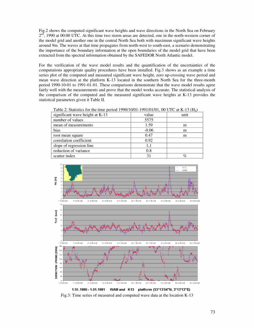
Fig.2 shows the computed significant wave heights and wave directions in the North Sea on February

2nd

, 1990 at 00:00 UTC. At this time two storm areas are detected, one in the north-western corner of

the model grid and another one in the central North Sea both with maximum significant wave heights

around 9m. The waves at that time propagates from north-west to south-east, a scenario demonstrating

the importance of the boundary information at the open boundaries of the model grid that have been

extracted from the spectral information obtained by the SAFEDOR North Atlantic model.

For the verification of the wave model results and the quantification of the uncertainties of the

computations appropriate quality procedures have been installed. Fig.3 shows as an example a time

series plot of the computed and measured significant wave height, zero up-crossing wave period and

mean wave direction at the platform K-13 located in the southern North Sea for the three-month

period 1990-10-01 to 1991-01-01. These comparisons demonstrate that the wave model results agree

fairly well with the measurements and prove that the model works accurate. The statistical analysis of

the comparison of the computed and the measured significant wave heights at K-13 provides the

statistical parameters given it Table II.

Table 2: Statistics for the time period 1990/10/01-1991/01/01, 00 UTC at K-13 (HS)

significant wave height at K-13 value unit

number of values 5575

mean of measurements 1.59 m

bias -0.06 m

root mean square 0.47 m

correlation coefficient 0.92

slope of regression line 1,1

reduction of variance 0.8

scatter index 31 %

Fig.3: Time series of measured and computed wave data at the location K-13

74

3. Real time measurements for operation mode In the operational mode 1 safe and reliable estimates of environmental conditions are essential for the

functionality of a DSS. Within the ADOPT project radar measurement are identified as the most

advanced technique to collect as much information as possible about the wave systems and the winds.

The WaMoS II wave radar was selected as a demonstrator and tested on board of the Tor Magnolia.

A WaMoS II raw data file consists of 32 subsequent radar images. The time interval between two

measurements depends on the antenna repetition time, which was about 2.4s aboard Tor Magnolia.

Each individual image in a sequence has a spatial resolution of 7.5 m, covering a circular area of

approximately 4.2 km in diameter around the antenna position in the centre of the image. The

backscattered radar intensity is digitised in relative units, linearly scaled to one byte. Fig.4 gives an

impression of the appearance of a radar image (recorded on 2005-12-15 at 10:03 UTC). The colour

coding in the figure corresponds to the radar backscatter strength in relative units. Black indicates no

radar return and white maximum return. A circular area of 440 m in diameter in the image centre is

blanked. Due to the measurement set-up, this area is not valuable for the purpose of wave

measurements, as the radar signal will be disturbed by vessel constructions. In the remaining area,

stripe-like wave patterns are clearly visible. These patterns are analysed to derive wave spectra and

sea state parameters. For a standard measurement, this analysis is limited to so called analysis areas

placed within the radar image. The three analysis areas chosen for the Tor Magnolia measurements

are marked with red frames in Fig.4. For these areas, the directional wave spectra and all statistical

sea state parameters are calculated. The spectra of all areas that passed the internal quality control are

averaged, resulting into a mean spectrum representative for the entire area around the vessel.

Fig.4: Analysis areas of WaMoS II for Tor Magnolia (2005-12-15 at 10:03 UTC).

3.1 Quality control

An improved automatic quality control mechanism to exclude unsuitable or corrupted radar raw

images from further analysis was developed to enhance the reliability of data acquisition and prevents

system failures of the DSS. As technical background, each WaMoS II measurement is marked with a

quality control code (‘IQ’) to distinguish between high and low radar raw data quality. A code

number reflects both the nature of a disturbance as well as its impact on the results.

75

Especially for an on board installation of the system two main factors lead to wrong measurements:

1. Parts of the measurements are taken with the radar being operated in ‘long pulse’ mode. In

this pulse setting, the radar images are blurred, making an accurate analysis of the images

impossible [2].

2. In times when the ‘Tor Magnolia’ approaches or leaves a harbour, parts of the coastline or

harbour constructions are visible in the radar images thus disturbing the wave analysis.

In addition, examples of less frequent sources of image disturbances are:

3. Signatures of passing ships within the analysis areas.

4. Heavy rainfall.

The new quality control is based on 14 quality parameters deduced from the grey levels of the radar

images and the wave spectra computed from the images. The evaluations of these parameters are

treated as a classification problem and image disturbances are sorted into 'classes' with defined

properties. The quality control separates these classes by a cluster analysis algorithm. Fig.5 gives an

impression on the overall performance of the algorithm. All measurements with unreliable high

significant wave heights are detected and marked as belonging to one of the error classes. In

particular, the extreme significant wave heights at the beginning and end of data gaps within the time

series, resulting from harbour times of the vessel are indicated correctly. The red colour marks those

data sets that belong to the 'harbour' error class. In addition, disturbances by small objects like ships

are more frequent close to the harbour gaps in the time series, as can be expected. Another indicator

for the good performance of the algorithm is the stability of the peak wave direction within the green

areas.

Fig.5: Result of quality control marked in time series of sea state parameters.

76

3.2 Wind measurements

Usually, wind information is retrieved by sensors aboard a vessel. These measurements are often

influenced by sensor position and the occurring error can be of the same magnitude as the

measurement itself. A measurement technique that allows monitoring the wind on a larger area is a

desirable complement to the standard data product. With such a method the wind measurements

becomes more stable and in addition offers the opportunity to localise spatial variations in the area

surrounding the vessel. Radar images are capable to provide this information, e.g. wind field

measurements over open waters by radar are common practice in satellite remote sensing.

The imaging mechanism of wind signatures is based on the radar signatures of wind generated surface

waves ('ripple waves') with wave lengths of a few centimetres. These waves develop instantaneously

when wind blows over an open water surface. Their amplitude and shape is directly related to the

surface wind speed. As radar sensors are sensitive to the roughness of a water surface, the ripple

waves become visible in radar images. In satellite applications the backscatter is related to the local

surface wind speed by semi-empirical models (e.g. CMOD-4). This measurement principle is

transferred to nautical X-Band radar, because the imaging mechanism of wind is basically the same

for all kinds of radar systems. Differences between satellite radar sensors and nautical X-Band radar

in terms of spatial resolution, observed area, look angles and radar wave lengths prevent a direct

application of the satellite algorithms to nautical radar images. In Dankert and Horstmann (2005) a

neural network approach was used to relate the nautical radar signatures to wind speed and direction.

For the ADOPT project a simplified method is developed.

The new method relates the mean grey levels directly to the wind speed. The mean grey level is the

averaged grey level of 32 successive radar images. Fig.6 shows the correlation between the grey

levels and the wind speeds measured by the standard wind sensor of the Tor Magnolia. The data are

clustered into different wave height regimes. The data cover wind speed up to 30m/s and significant

wave height up to 10m. A correlation of 0.89 reflects the very good agreement of mean image

brightness and wind speed. In addition, the alignment of the data samples is independent on the

significant wave height. In Fig.11, the wind speeds calculated from the radar images are compared to

the wind measurements of the reference sensor. This time series shows only minor deviations and a

standard deviation of 2.2m/s, demonstrating that radar images have the capability to serve as a wind

sensor.

Fig.6: Scatter diagram: Mean Grey value and wind speed.

77

Fig.7: Derived wind speed compared to reference

4. Combination of data for the numerical surface analyzer

The full information about the actual sea state at an arbitrary location at a certain time is given by the

corresponding two-dimensional wave spectrum, but usually the description of sea state is reduced to a

few numbers, e.g. significant wave height, peak period and peak direction. In state-of-the-art weather

forecasting those are the typically distributed data so far. However, from mathematical wave model

hindcasts and forecasts as well as from measurements, such as the wave radar data, a lot more

information, e.g. the detailed energy distribution is available. Therefore the required environmental

input for the DSS can be obtained from different data sets that may include integrated parameters only

or two-dimensional spectra at the best.

One important basis for the DSS is the numerical simulation of the ship response to the actual sea

state. To simulate the seaway required for the numerical motions simulation, the model needs

directional sea state spectra as input data. A representation of the sea surface elevation η at each point

x=(x,y) at a time t can be derived from the amplitudes of a directional spectrum by summing up the

spectral components,

η x,t( )= an

n=1

N

∑ cos knx −ωnt + ϕn( ) (1)

an denotes the spectral amplitude of a plane wave with angular frequency ωn and wave number

kn=(kx,ky).

Fig.8: Flowchart of the environmental data input into the DSS

78

The phases φn have to be generated randomly for each surface realisation. As k and ω are connected

by the dispersion relation for ocean waves, the amplitudes can be expressed as a function of k or

angular frequency ω and direction θ, respectively.

Thus, the directional sea state spectra contain all sea state information required for the simulation and

it was decided to use it as the key data source. Therefore, the main task is to derive the directional

spectra from the various available data sources for the generation of irregular seaways to provide the

input for the ship motion calculations.

Fig.8 summarizes the dependencies between the different data inputs and gives a flowchart to

combine the data. The proposed system is capable to be operated in two different modes:

• Mode 1: calculates directional spectra on a theoretical basis, derived from integrated sea state

parameters.

• Mode 2: uses directly directional spectra from measurement or model computations.

Input data for both input modes can be wave model results or measurements.

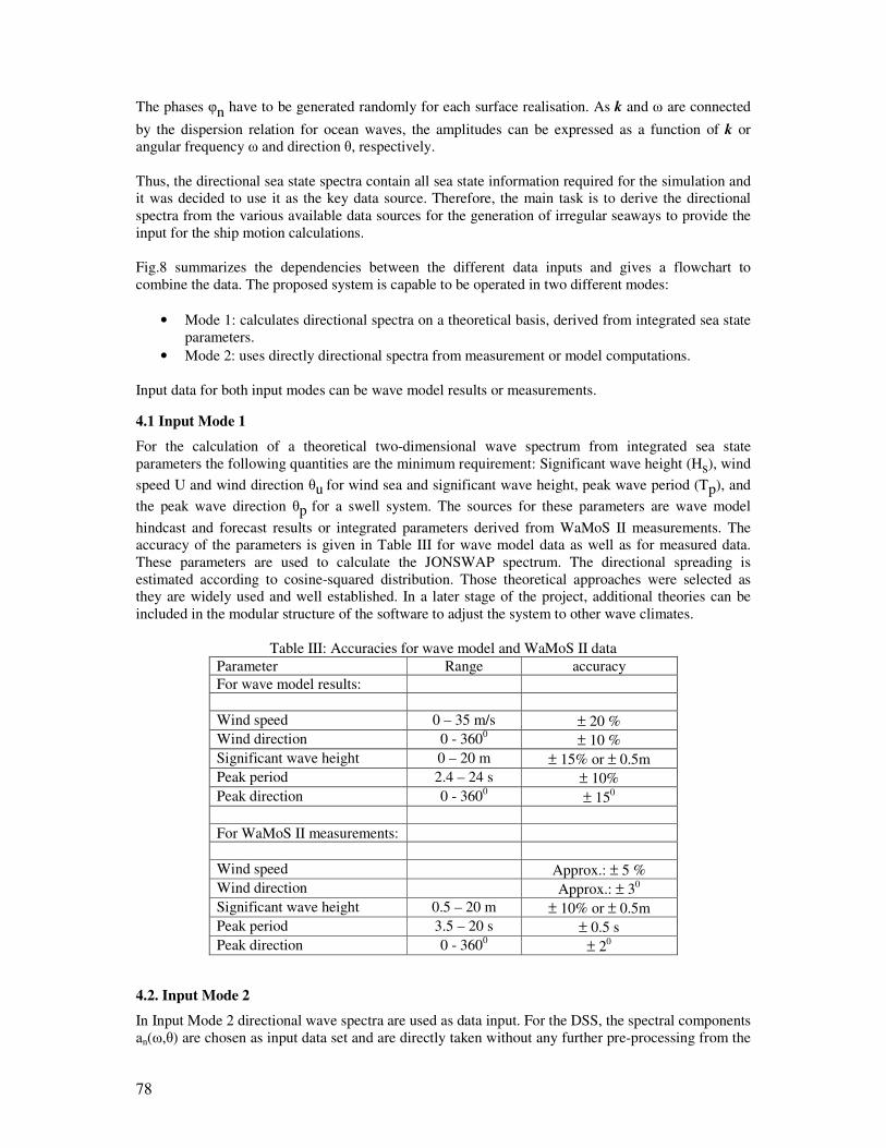
4.1 Input Mode 1

For the calculation of a theoretical two-dimensional wave spectrum from integrated sea state

parameters the following quantities are the minimum requirement: Significant wave height (Hs), wind

speed U and wind direction θu for wind sea and significant wave height, peak wave period (Tp), and

the peak wave direction θp for a swell system. The sources for these parameters are wave model

hindcast and forecast results or integrated parameters derived from WaMoS II measurements. The

accuracy of the parameters is given in Table III for wave model data as well as for measured data.

These parameters are used to calculate the JONSWAP spectrum. The directional spreading is

estimated according to cosine-squared distribution. Those theoretical approaches were selected as

they are widely used and well established. In a later stage of the project, additional theories can be

included in the modular structure of the software to adjust the system to other wave climates.

Table III: Accuracies for wave model and WaMoS II data

Parameter Range accuracy

For wave model results:

Wind speed 0 – 35 m/s ± 20 %

Wind direction 0 - 3600

± 10 %

Significant wave height 0 – 20 m ± 15% or ± 0.5m

Peak period 2.4 – 24 s ± 10%

Peak direction 0 - 3600

± 150

For WaMoS II measurements:

Wind speed Approx.: ± 5 %

Wind direction Approx.: ± 30

Significant wave height 0.5 – 20 m ± 10% or ± 0.5m

Peak period 3.5 – 20 s ± 0.5 s

Peak direction 0 - 3600

± 20

4.2. Input Mode 2

In Input Mode 2 directional wave spectra are used as data input. For the DSS, the spectral components

an(ω,θ) are chosen as input data set and are directly taken without any further pre-processing from the

79

wave spectra. The standard deviation for spectral components an is estimated to 32%, by adapting

theoretical considerations for one-dimensional wave measurements to the WaMoS II temporal and

spatial analysis.

5. Creating irregular seaways for numerical motion simulations from directional spectra

Given a directional spectrum the energy distribution of a certain seaway is dependent on two

variables, namely the wave frequency and the encounter angle of the waves. Fig.9 shows a three

dimensional plot of a directional spectrum. In this case the spectrum consists of two components: One

wind sea component with the wave energy spread over a wide range of angles (here 180 degrees) and

a swell component with a very narrow banded range of encounter angles.

The common and well-established way to generate irregular seaways for numerical motions

simulations is to superpose a finite number n of regular wave components. The superposition principle

is valid as long as linear wave theory is used. This seems to be sufficiently accurate for the prediction

of ship motions, as the error in the surface elevation, which is most important parameter for such kind

of problem, is moderate according to Stempinski (2003). Equation [1] shows the position- and time

dependent wave elevation following the superposition approach.

The individual amplitudes for each component are obtained by dividing the given spectrum is divided

into n strips: either equidistant or in such way that all strips contain the same resulting wave energy

(constant-amplitude approach). When using a relatively small amount of wave components, the latter

approach still provides a good resolution of the peak region of the wave spectrum. In order to avoid a

periodicity of the generated seaway, the frequencies ωn of the wave components are randomly chosen

within the component individual frequency band, assuming a uniform distribution. Besides the

encounter angle and the frequency, the phasing of the wave components is important for the

generation of a natural seaway. The phase shift φn is also randomly chosen for each component due to

the reasons mentioned above.

Fig.9: Bi-modal directional wave spectrum

Fig.10 shows a time series recorded amidships in a ship-fixed coordinate frame for a time interval of

1000 seconds, which is obtained from the wave spectrum shown in Fig.9. The ship speed is equal to

zero in the given example, thus the encounter frequency equals the wave frequency in this case.

80

Fig.10: Time series of wave elevation amidships

6. Conclusions

Different environmental data sets including wind and wave measurements or wave model results are

identified as possible input for the DSS and an attempt is made to quantify the accuracy of those.

Since the two-dimensional wave spectra is the key source for the generation of sea surface

representations, all available spectral data can be used directly whereas the integrated wave data must

be processed to obtain the required spectra. The corresponding algorithms are outlined. The two-

dimensional wave spectra will always be the base for the creation of irregular seaways for the

numerical motion simulations and the method to generate those sea state representations are

presented. Finally, the treatment of the different environmental input data is evident, the chain of all

required steps of the methodology from input via two-dimensional wave spectra to the creation of

irregular seaways is clearly resolved and the related uncertainties are discussed. The methodology

developed and described will be realised and implemented into the ADOPT DSS.

References

DANKERT, H.; HORSTMANN, J. (2005), Wind measurements at FINO-I using marine radar image

sequences, Geoscience and Remote Sensing Symp. IGARSS Proc., Volume 7, pp.4777-4780

HASSELMANN, S.; HASSELMANN, K.; BAUER, E.; JANSSEN, P.A.E.M.; KOMEN, G.J.;

BERTOTTI, L.; GUILLAUME, A.; CARDONE, V.C.; GREENWOOD, J.A.; REISTAD, M.;

ZAMBRESKI, L.; EWING, J. (1988), The WAM model – a third generation ocean wave prediction

model, J. Phys. Oceanogr., Vol. 18, pp.1775-1810

JACOB, D.; PODZUN, R. (1997), Sensitivity studies with the regional climate model REMO, Atmos.

Phys., 63, pp. 119-129

KOMEN, G.J.; CAVALERI, L.; DONELAN, M.; HASSELMANN, K.; HASSELMANN, S.;

JANSSEN, P.A.E.M. (1994), Dynamics and Modelling of Ocean Waves, Cambridge University Press

STEMPINSKI, F. (2003), Seegangsmodelle zur Simulation von Kenterprozessen, Diplomarbeit, TU

Berlin

TELLKAMP, J.; GÜNTHER, H.; PAPANIKOLAOU, A.; KRÜGER, S.; EHRKE, K.C.; KOCH

NIELSEN, J. (2008), ADOPT - Advanced Decision Support System for Ship Design, Operation and

Training - An Overview, 7th COMPIT, Liege, pp.19-32