Adjusting to Capital Account Liberalization

Kosuke Aoki, Gianluca Benigno and Nobuhiro Kiyotaki�

First Version: April, 2006This Version: June, 2009

Abstract

We study theoretically how the adjustment to liberalization of international�nancial transaction depends upon the degree of domestic �nancial development.Using a model with domestic and international borrowing constraints, we showthat, when the domestic �nancial system is underdeveloped, capital account lib-eralization is not necessarily bene�cial because TFP stagnates in the long-run oremployment decreases in the short-run. Government policy, including allowing for-eign direct investment, can mitigate the possible loss of employment, but cannoteliminate it unless the domestic �nancial system is improved.

�London School of Economics, London School of Economics, and Princeton University. Email ad-dresses: k.aoki@lse.ac.uk, g.benigno@lse, and kiyotaki@princeton.edu. We thank Philippe Bacchetta,Alex Berentsen, Fernando Broner, Vasco Curdia, Andrei Levchenko, Omar Licandro, Paolo Pesenti,Lard Svensson and various seminar and conferences participants for their comments. Correspondence:kiyotaki@princeton.edu

1 Introduction

"Capital account liberalization, it is fair to say, remains one of the most controversial

and least understood policies of our day". (Eichengreen, 2002)

This paper is a theoretical study into how an economy adjusts to the liberaliza-

tion of international �nancial transaction � capital account liberalization. Although

most economists agree that trade liberalization generally improves e¢ ciency of resource

allocation, they are sharply divided on the costs and bene�ts of capital account lib-

eralization. According to standard microeconomic theory, the international �nancial

transaction is international trade of goods in di¤erent dates (possibly contingent on the

states of nature), and thus capital account liberalization should have similar bene�ts

with trade liberalization. Why do economists disagree? We think that the intertempo-

ral exchange of present goods and claims to future goods is fundamentally di¤erent from

intra-temporal exchange of di¤erent goods at least in one respect: the intertemporal

exchange requires the commitment that agents will provide goods (or their purchasing

power) in the future, while intra-temporal exchange does not require such commitment.1

If people�s ability to keep their promises is limited, then the equivalence of intertempo-

ral trade and intra-temporal trade no longer holds, and thus we need to investigate the

e¤ects of capital account liberalization taking into account the limitation of commitment.

In this paper, we consider an economy in which the debtor does not keep his promise

to repay unless debt is secured by collateralizable assets �assets he looses if he defaults.

Then, the creditor limits her loan to the debtor so that the debt repayment does not

exceed the value of collateral. Moreover, we consider the case in which the amount of

1Of course, international trade requires some commitment because the order, delivery, payment andconsumption of goods are not simultaneous. But, the degree of commitment is usually more demandingfor international borrowing than trade.

1

collateralizable assets for foreign credits is more restricted than for domestic credits,

because foreign creditors have more di¢ culty in taking over control and utilizing the

collateral assets in a di¤erent country. The extent of assets usable for collateral depends

upon both technology and quality of institution of the economy which a¤ects the devel-

opment of �nancial system. The extent of collateralizable assets for domestic borrowing

a¤ects the overall �nancial depth of the economy. The gap between collateralizable

assets for international borrowing and domestic borrowing � the relative tightness of

international borrowing �a¤ects how much the home economy is �nancially integrated

into the international �nancial market. Our aim is to examine how the adjustment of

the home economy to capital account liberalization depends upon the parameters of

�nancial depth of the domestic economy and the relative tightness of the international

borrowing constraint.

For this purpose, we construct a dynamic model of a small open economy with entre-

preneurs and workers. At each date, some entrepreneurs are productive and others are

not. Entrepreneurs hire workers to produce output in the following period, and they can

borrow domestically against a fraction of future output. The fraction they can borrow

from foreigners is smaller. When domestic �nancial system is underdeveloped, it fails to

transfer enough purchasing power from savers (typically unproductive entrepreneurs) to

investing agents (productive entrepreneurs), so that the unproductive entrepreneurs end

up hiring workers. The productive entrepreneurs are credit constrained, the domestic

interest rate to the savers remains low (symptom of interest rate suppression), and the

total factor productivity (TFP) is low, which leads to low a wage rate (symptom of wage

suppression).2

2Kiyotaki and Moore (1997), Kiyotaki (1998), Aghion, Banerjee and Piketty (1999), and Aghion andBanerjee (2005), for examples, investigate these symptoms of the borrowing constrained economy.

2

The way the economy adjusts to capital account liberalization depends upon the

relative strength of wage suppression versus interest rate suppression. If the wage-

suppression e¤ect dominates the interest rate suppression, then even unproductive en-

trepreneurs may enjoy a higher rate of return on production than the foreign real interest

rate before liberalization. Following capital account liberalization, both productive and

unproductive entrepreneurs borrow from foreigners, causing capital in�ow, which pushes

up the wage rate. But the size and duration of the capital in�ow are limited due to the

poor domestic �nancial system, and TFP may deteriorate after liberalization.

If the interest rate suppression e¤ect dominates the wage-suppression, then the do-

mestic real interest rate faced by the savers (unproductive entrepreneurs) under �nancial

autarky is lower than the foreign interest rate. Following capital account liberalization,

they start lending abroad and reduce their production. With capital out�ows, workers

su¤er from wage reduction and loss of employment until unproductive entrepreneurs stop

producing. Here, capital account liberalization serves as a catalyst to reduce ine¢ cient

production by providing an alternative means of saving, improving TFP over time.

If domestic �nancial system is more advanced than the rest of the world, the produc-

tive entrepreneurial sector has enough borrowing capacity to absorb the domestic saving

so that the domestic interest rate under autarky is higher than the world interest rate.

After liberalization, the productive domestic entrepreneurs will attract foreign funds,

causing capital in�ow and higher investment. With a superior �nancial institution, the

domestic economy can take advantage of cheaper funds possibly induced by �nancial

suppression of the rest of the world.

What emerges from our analysis is that the adjustment of home economy to capital

account liberalization depends not only on the absolute level of development of home

�nancial system, but also on the relative level of development of home institutions com-

3

pared to the rest of the world.

Since capital account liberalization under poor domestic �nancial system leads to a

costly adjustment for workers under �nancial suppression, a natural step would be to

examine the role of government policy. When agents�commitment is limited, tax liability

a¤ects their capacity to borrow. For the economy under �nancial suppression, a subsidy

to production of unproductive entrepreneurs mitigates the loss of the workers following

capital liberalization at the cost of prolonging the transition to e¢ cient production.

Allowing foreign direct investment (FDI), which is considered as a more stable source

of employment compared with private �nancial in�ows, cannot eliminate workers�loss

unless it helps to improve domestic technology and �nancial institutions.

There is an extensive literature that examines theoretically the relationship between

domestic �nancial development and capital account liberalization. Aghion, Bacchetta

and Banerjee (2004) show that an economy with an intermediate level of �nancial de-

velopment may become unstable following capital account liberalization. Caballero and

Krishnamurthy (2004) emphasize the interaction between domestic and international

�nancial constraints in explaining the vulnerability of an economy to a �nancial crisis.

Kim (2001) develops a two-country model of adoption of vintages of technologies, and

shows that, following capital liberalization, the country with better domestic �nancial

system specializes in adopting more recent technology, while the country with poor �-

nancial system ends up with adopting older technologies, leading to a substantial gap in

the TFP between the two.

Concerning the direction of capital �ows, Gertler and Rogo¤ (1990) propose a frame-

work in which capital can �ow from the poor South to the richer North in a context

of a model of international lending under moral hazard. Recent contributions by Ca-

ballero, Fahri and Gourinchas (2006) emphasize the di¤erent �nancial development and

4

di¤erent supply of means of saving, while Mendoza, Quadrini and Rios-Rull (2007) focus

on the di¤erent precautionary saving as determinants for the current pattern of global

imbalances across countries.3,4

While our analysis shares some of the aforementioned features, our distinctive con-

tribution to the literature is to investigate the implications of limited commitment of

private agents against both domestic and foreign creditors, for the entire adjustment

process of the economy following capital account liberalization. In particular we em-

phasize the endogenous adjustment of TFP, pointing out to the existence of a certain

threshold in terms of domestic �nancial development above which a country could bene�t

from a process of capital account liberalization.

3There is a vast empirical literature that has examined the e¤ects of capital account liberalization.For an example, Obstfeld and Taylor (2004) analyzes the evolution of international �nancial integrationfrom the late 19th century. Kose, Prasad, Rogo¤ and Wei (2008) summarizes previous studies of postWWII. experiences to conclude that there is no robust relationship between capital account liberalizationand economics growth.In a subsequent work Kose, Prasad and Taylor (2009) �nd evidence of threshold e¤ects of capital

account liberalization on growth in terms of domestic �nancial developement. By using the ratio ofprivate credit to GDP as a proxy for �nancial depth, they �nd that greater �nancial depth leads to animprovement in the growth e¤ects of �nancial liberalization but only up to a certain level of �nancialdepth.Also, Kose, Prasad and Terrones (2008) provide a comprehensive empirical analysis on the link

between �nancial integration and TFP (see also Bon�glioli (2008) on this). Interestingly they �nd thatthe composition of the underlying capital �ows is crucial for understanding the link between �nancialintegration and TFP growth. Indeed liberalization of FDI and equity tends to improve TFP while thatof external debt liabilities does not (at least for poorly developed domestic �nancial system).

4In a di¤erent strand of literature, Kehoe and Perri (2001, 2004) consider implications of enforcementconstraint between sovereign nations while abstracting from that between private agents. Jeske (2006)and Wright (2006) examine the problem of resident default risk and the implication for governmentintervention on capital �ows.

5

2 Model

2.1 Framework

We consider a small open economy with one homogeneous goods and two types of con-

tinua of in�nitely-lived agents: entrepreneurs and workers. Entrepreneurs hire workers

to produce goods. Workers do not have production technology, simply supplying homo-

geneous labor in order to consume.

The preference of the entrepreneur is described by the expected discounted utility

Et

" 1Xs=t

�s�t log cs

#; 0 < � < 1; (1)

where cs is the consumption at date s; and Et is the expectations conditional on in-

formation at date t. The entrepreneurs have a constant returns to scale production

technology

yt+1 = atlt; (2)

where yt+1 is output at date t + 1, lt is labor input at date t, and at is a productivity

parameter which is known at date t. At each date some entrepreneurs are produc-

tive (at = �); and the others are unproductive (at = 2 (0; �)). Each entrepreneur

shifts stochastically between productive and unproductive states following a Markov

process. Speci�cally, if an entrepreneur is productive in this period he/she may become

unproductive in the next period with probability �; an unproductive entrepreneur in

this period may become productive in the next period with probability n�: The shifts

of the productivity are exogenous and independent across entrepreneurs and over time.

This transition matrix implies that the fraction of productive entrepreneurs is stationary

over time and equal to n=(1 + n), given that the economy starts with such population

6

distribution. We assume that the probability of the productivity shifts is not too large:

� + n� < 1: (3)

This assumption implies that the productivity of each agent is positively serially corre-

lated.

We assume that the production technology is speci�c to the entrepreneur, and that

only the entrepreneur who started the production has the necessary skill to obtain full

amount described by the production function. We also assume that the entrepreneur

cannot precommit to work, always having freedom to withdraw her/his labor. (The

entrepreneur�s human capital is inalienable, following Hart and Moore (1994)). Besides

the entrepreneur, a lead creditor who has been monitoring the production throughout

has a speci�c skill to obtain � (< 1) fraction of full amount of output, if she takes over

the entrepreneur�s production. Although production is divisible, we assume that there

is only one lead creditor for each segment of production, and that only a home resident

can be a lead creditor. All the other (non-lead) outside creditors, home or foreign,

can obtain only �� fraction of full output, where � 2 [0; 1). Knowing this possibility

in advance, the foreign lenders restrict their loan of this period so that the repayment

(b�t+1) does not exceed �� fraction of output in the next period5:

5 Here, we apply Hart and Moore (1994) and Aghion, Hart and Moore (1992) on default andrenegotiation between private parties. We assume the outside creditors have weak bargaining poweragainst the producer and the lead creditor in the renegotiation, (even though the outside creditors aremade to be senior creditors in order to maximize borrowing from them). Unlike Bronner, Martin andVentura (2006) in which there are many domestic creditors who can correct a large fraction of returns,we have only one monopolistic domestic lead creditor for each project. Then the lead creditor paysthe outside creditors �� fraction of full output in order to acquire the outside creditors�right to theproject as senior creditors. When the lead creditor and the producer-debtor negotiate after the outsidecreditors leave, we assume the producer has all the bargaining power. Then, after the producer pays �fraction of maximum output to the lead creditor, the producer is allowed to complete the production toobtain 1� � fraction of maximum output. The resource allocation is e¢ cient ex post. But the ex anteresource allocation may not be e¢ cient because of the credit constraint which arises from the possibility

7

b�t+1 � ��yt+1: (4)

Also, the domestic lead creditor restricts her loan (bt+1) so that the total sum of loans

does not exceed � fraction of output:

bt+1 + b�t+1 � �yt+1: (5)

We take both � and � as exogenous parameters to represent the degrees of devel-

opment of the country�s �nancial institution. We consider the size of � as a domestic

collateral factor, representing the overall �nancial depth of the home economy. The gap

between �� and � re�ects the di¤erence between the outside creditors and the lead cred-

itor in their skills of production and bargaining (being in�uenced by legal protection of

the outside creditors6).

The �ow-of-funds constraint of the entrepreneur is given by

ct + wtlt = yt � bt � b�t +bt+1rt

+b�t+1r�

; (6)

where wt is the real wage rate, rt is the domestic real gross interest rate, r� is the foreign

real gross interest rate, and bt and b�t are domestic and foreign borrowing. Consumption

ct and investment on the wage bill wtlt in the left-hand side (LHS) of this equation are

�nanced by the net worth yt � bt � b�t and the domestic and foreign new borrowing in

the right hand side (RHS). The entrepreneur chooses consumption, labor input, output

and domestic and foreign borrowing�ct; lt; yt+1; bt+1; b

�t+1

�to maximize utility subject to

of the default and negotiation. We assume there is no reputation to enforce debts, because there is norecord keeping of the past defaults.

6See La Porta, Shleifer, Lopez-de-Silanes and Vishny (1997,1998).

8

the constraints of production technology, the �ow-of-funds, and the international and

domestic borrowing constraints.

We now turn to workers. Unlike the entrepreneurs, the workers do not have produc-

tion technology, nor any collateralizable asset in order to borrow either domestically or

internationally. They choose consumption ct, labor supply lt, and domestic and foreign

net borrowings (bt+1 and b�t+1) to maximize the expected discounted utility,

Et

" 1Xs=t

�s�tu (cs � v(lt))

#;

subject to the �ow of funds constraint

ct = wtlt � bt � b�t +bt+1rt

+b�t+1r�

;

and the borrowing constraints, bt+1 � 0 and b�t+1 � 0. We make the standard assump-

tions u0(c � v) > 0; u"(c � v) < 0; and v(0) = 0; v0(l) > 0; v"(l) > 0: We normalize the

population size of workers to be unity.

We �nally assume that there is no constraint on domestic agent�s lending to the

foreigners and that the foreign interest rate r� is exogenous being strictly less than the

time preference rate7

r� < 1=�: (7)

2.2 Equilibrium

We now derive the general properties of the competitive equilibrium. If the domestic

interest rate were strictly lower than the foreign interest rate, the domestic savers would

7The underlying assumption is that the rest of the world is also subject to credit frictions describedabove. As is shown later, the equilibrium interest rate under this environment is lower than ��1.

9

lend to foreigners instead of lending to domestic borrowers while there would be many

agents who want to borrow. This contradicts the market equilibrium. Therefore we

obtain

rt � r�: (8)

The entrepreneur has a few choices of accumulating net worth. Let Rt(at) be the

maximum rate of return on the net worth from date t to date t+1 for the entrepreneur

with productivity at: Then, it is the maximum of all the options as:

Rt(at) =Max

�rt;

atwt;

at(1� ��)

wt � (at��=r�);

at(1� �)

wt � (at��=r�)� [at(1� �)�=rt]

�: (9)

The �rst term in the brackets of RHS is the rate of return on domestic loan. The second

term is the rate of return on production without borrowing. The third term is the rate of

return on production with maximum foreign borrowing. By borrowing from foreigners

secured by �� fraction of output, the entrepreneur can �nance externally at��=r� amount

of unit labor cost. Thus the denominator is the required net worth (downpayment) for

the unit labor input, and the numerator is the output after repaying the debt. The last

term is the rate of return on production with maximum borrowing from both foreigners

and the domestic lead creditor. The denominator is downpayment for hiring unit labor,

when the entrepreneur �nances at��=r� of unit labor cost by borrowing from foreigners,

and �nances at(1 � �)�=rt by borrowing additionally from the domestic lead creditor

at interest rate rt: Note that the entrepreneur prefers to borrow maximum �rst from

foreigners at a lower interest rate.

In the expression of maximum rate of return on net worth (9); each of the last

three rates are strictly higher for the productive entrepreneur than the unproductive

entrepreneur, while the rate of return on domestic loan is the same for both. Thus,

10

in equilibrium the unproductive entrepreneurs lend to productive entrepreneurs, and

produce if and only if their rate of return on production is equal to the domestic interest

rate - otherwise, they specialize in providing loan.8 Therefore the domestic interest rate

and employment of unproductive entrepreneur satisfy9

Rt( ) = rt � (1� ��)

wt � ( ��=r�)and 0 = lt

�rt �

(1� ��)

wt � ( ��=r�)

�: (10)

The productive entrepreneur always borrows to produce, and their rate of return is given

by

Rt(�) =�(1� �)

wt � (���=r�)� [�(1� �)�=rt]� rt:

Given the optimal choice of accumulating net worth, the �ow-of-funds constraint (6)

can be written as

zt+1 = Rt(at)(zt � ct);

where zt � yt � bt � b�t denotes the net worth of the entrepreneur at date t. When

the entrepreneur chooses consumption to maximize his logarithmic utility subject to

this �ow-of-fund constraint, the �rst order condition is given by the Euler equation:

1ct= �Rt(at)Et

�1

ct+1

�. Then we have the explicit consumption function as

ct = (1� �)zt = (1� �)(yt � bt � b�t ): (11)

The productive agents produce with their domestic and international borrowing con-

straints binding if the rate of return on production with maximum leverage exceeds the

8Later, we will show that the workers will not lend nor borrow in the equilibrium.9We note here that as long as rt � r�, the rate of return on production with maximum borrowing

from abroad is at least as great as the rate of return on production without borrowing.

11

domestic interest rate. Thus, from (4)(5)(6); and (11), their employment is given by

lt ��zt

wt � (���=r�)� [�(1� �)�=rt]; (12)

and equality holds if Rt(�) > rt.

Regarding the workers, their labor supply lst is given by wt = v0(lst ); or

lst = Ls(wt); where Ls(w) = v0�1(w):

Thus dLs=dwt > 0: They will decumulate their asset until the borrowing constraint

becomes binding, if the domestic real interest rate is strictly less than the time preference

rate:

rt < 1=�: (13)

We will later verify this inequality holds in the neighborhood of the steady state equi-

librium. Therefore, the aggregate consumption of the workers is equal to the aggregate

wages10

bt = b�t = 0; and ct = wtLs(wt): (14)

Now let us de�ne aggregate variables. Denote aggregate quantities of the productive

entrepreneurs, the unproductive entrepreneurs, and workers of a generic quantity yt

by Yt; Y 0t ; and Y

wt . De�ne B

�t as the aggregate net debt of all the home entrepreneurs

against foreigners matured at date t. Then, aggregate net worth of all the entrepreneurs,

10The workers do not save, not because the workers are impatient relative to the entrepreneurs, butbecause the real interest rate is lower than the time preference rate in equilibrium. The entrepreneursnonetheless save because their rate of return on net worth exceeds the time preference rate when theyare productive. If the workers expect sharp decline of wage in future, then they may save despite of theinterest rate being lower than the time preference rate. Throughout the paper we do not consider suchexpectations.

12

denoted by Zt, is given by

Zt = Yt + Y 0t �Bt �B0

t �B�t : (15)

Furthermore, let st be the share of net worth of all the productive entrepreneurs, so that

stZt is the aggregate net worth of the productive entrepreneurs. Then, because of the

linearity of (12), we derive the aggregate employment of the productive entrepreneurs

as

Lt ��stZt

wt � (���=r�)� [�(1� �)�=rt]; (16)

and the equality holds if Rt(�) > rt. The aggregation of (10) and (14) respectively yields

0 = L0

t

�rt �

(1� ��)

wt � ( ��=r�)

�; (17)

and Cwt = wtLs(wt). The market clearing condition for labor, goods, and domestic credit

are written as

Lt + L0t = Ls(wt); (18)

Ct + C 0t + Cwt = Yt + Y 0t +

�B�t+1

r��B�

t

�; (19)

Bt+1 +B0t+1 = 0: (20)

The term in the bracket of the RHS of equation (19) are the net supply of goods by

the foreigners to domestic agents. In equation (20), the domestic borrowing and lending

should be net out in aggregate, even though the total debts of the domestic agents need

not because of the international borrowing and lending.

The competitive equilibrium is de�ned as a set of prices (rt; wt) and quantities (yt, lt,

ct, bt+1, b�t+1, Yt, Y0t , Lt, L

0t, Ct, C

0t, C

wt , Bt+1, B

0t+1, B

�t+1), which is consistent with the

13

choice of all the individual entrepreneurs and workers as well as the clearing conditions

of markets for labor, goods and domestic credit. Because there is no shocks except for

the idiosyncratic shock to the productivity of each entrepreneur, the agents have perfect

foresight of future prices and aggregate quantities in the equilibrium.

By aggregating the consumption of the entrepreneurs (11) and using (15), market

clearing condition (19) can be written as

wtLs(wt) = �Zt +

B�t+1

r�: (21)

The LHS is gross investment on wage bill by the entrepreneurs, and the RHS is the

sum of gross saving and foreign borrowing of the entrepreneurs. The foreign borrowing

satis�es the international borrowing constraints:

B�t+1 � ��(Yt+1 + Y

0

t+1) = ��(�Lt + L0

t); (22)

where the equality holds if rt > r�.

We take the aggregate net worth of the entrepreneurs (Zt) and the share of the

productive entrepreneurs�net worth (st) as the state variables of the economy at date

t. The law of motion of aggregate wealth is given by

Zt+1 = (1 + xt)rt�stZt + rt�(1� st)Zt (23)

= (1 + stxt)rt�Zt:

where

xt �Rt(�)�Rt( )

Rt( )=

�� wtrt + ��� rt�r�

r�

wtrt � �� � ��� rt�r�

r�: (24)

14

is the extra rate of return of the productive entrepreneur over the unproductive entre-

preneur. Here, the accumulation of wealth depends upon not only the interest rate and

saving rate but also the distribution of wealth, because the saving of the productive

entrepreneurs earns the extra rate of returns. We can also derive the law of motion of

the share of productive entrepreneurs�net worth as

st+1 =(1� �)(1 + xt)rt�stZt + n�rt�(1� st)Zt

(1 + stxt)rt�Zt(25)

=(1� �)st(1 + xt) + n�(1� st)

1 + stxt:

The denominator of RHS of the �rst equation is the aggregate net worth in the next

period. The numerator is the aggregate net worth of productive agents in the next

period, which is the sum of the net worth of those who continue to be productive,

(1��)(1+xt)rt�stZt; and those who shift from unproductive to be productive, n�rt�(1�

st)Zt. The evolution of the economy is characterized by the recursive equilibrium:�Zt+1; st+1; xt; rt; wt; Lt; L

0t; B

�t+1

�that satis�es (16 - 18), and (21 - 25) as functions of

the state variables (st; Zt):

Finally, in the subsequent analysis it would be of interest to see the total factor

productivity (TFP) of the economy. Since labor is the only input, the TFP is de�ned

as the average productivity of labor

At =�Lt + L0t

Lst= (�� )

LtLst+ : (26)

The property that the TFP is an increasing function of the fraction of labor employed

by productive entrepreneurs is a unique feature of our credit constrained economy.

15

3 Steady State under Financial Autarky

Before looking into how the economy adjusts to capital account liberalization, it is useful

to analyze the steady state of the economy before liberalization - the economy which has

no �nancial transaction with foreigners (� = 0). Since goods are homogeneous and labor

is not mobile across the border, the economy becomes autarky. In the steady state, all

the endogenous variables are constant. Let us de�ne X = sx; the product of the share

of net worth and the extra rate of return of productive agents �the importance of extra

return of the productive entrepreneurs. Then, the equilibrium conditions can be written

as

r �

w; and L0(r �

w) = 0; (27)

L � X

(�=r)� w�Z; and the equality holds if

�

r> r: (28)

L+ L0 = Ls(w); (29)

wLs(w) = �Z; (30)

x =(�=r)� w

w � (��=r) ; (31)

1 = �(1 +X)r; (32)

F (X; x) = X2 + [�(1 + n)� (1� �)x]X � n�x = 0; and X � 0: (33)

In the steady state equilibrium of the autarky economy, these seven equilibrium condi-

tions determine (r; w; x;X; L; L0; Z) endogenously. Then, we have the following propo-

sition in which upper script a represents variables under autarky. (Proofs of all the

Propositions are in Appendix).

Proposition 1 The steady state equilibrium of the autarky economy depends upon the

16

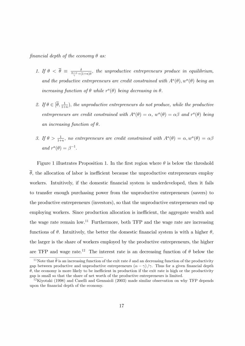
�nancial depth of the economy � as:

1. If � < � � ��� +(1+n)�

; the unproductive entrepreneurs produce in equilibrium,

and the productive entrepreneurs are credit constrained with Aa(�); wa(�) being an

increasing function of � while ra(�) being decreasing in �.

2. If � 2 [�; 11+n); the unproductive entrepreneurs do not produce, while the productive

entrepreneurs are credit constrained with Aa(�) = �, wa(�) = �� and ra(�) being

an increasing function of �.

3. If � > 11+n

; no entrepreneurs are credit constrained with Aa(�) = �;wa(�) = ��

and ra(�) = ��1:

Figure 1 illustrates Proposition 1. In the �rst region where � is below the threshold

�, the allocation of labor is ine¢ cient because the unproductive entrepreneurs employ

workers. Intuitively, if the domestic �nancial system is underdeveloped, then it fails

to transfer enough purchasing power from the unproductive entrepreneurs (savers) to

the productive entrepreneurs (investors), so that the unproductive entrepreneurs end up

employing workers. Since production allocation is ine¢ cient, the aggregate wealth and

the wage rate remain low.11 Furthermore, both TFP and the wage rate are increasing

functions of �. Intuitively, the better the domestic �nancial system is with a higher �,

the larger is the share of workers employed by the productive entrepreneurs, the higher

are TFP and wage rate.12 The interest rate is an decreasing function of � below the

11Note that � is an increasing function of the exit rate � and an decreasing function of the productivitygap between productive and unproductive entrepreneurs (�� ) = . Thus for a given �nancial depth�, the economy is more likely to be ine¢ cient in production if the exit rate is high or the productivitygap is small so that the share of net worth of the productive entrepreneurs is limited.12Kiyotaki (1998) and Caselli and Gennaioli (2003) made similar observation on why TFP depends

upon the �nancial depth of the economy.

17

threshold �, because the interest rate is equal to the rate of returns on production for

the unproductive entrepreneurs (which is a decreasing function of wage rate and �).

In the second region, � 2 [�; 11+n), all the savings are transferred to the productive

entrepreneurs so that aggregate output is at the maximum for a given total employment.

It does not mean the allocation is the �rst best, because individual consumption is not

smooth as the credit constraint is binding for productive entrepreneurs. Since the TFP

is given by �, the wage is given by ��. In this region, the interest rate is increasing

in � because a higher � simply means a larger demand for domestic credit relative to

supply.13

In the third region � � 11+n

where the domestic �nancial system is so well developed

that none is credit constrained. Both the productive and unproductive entrepreneurs

enjoy the same rate of return on saving, behaving similarly, and thus the entrepreneurs

as a whole behave like the representative entrepreneur. The economy achieves the �rst

best allocation.

The autarky interest rate is lower than the time preference rate for � < 1=(1 + n).

This veri�es our conjecture (13).14 Another property of the autarky steady state is that

the interest rate is not monotone with respect to �. It is decreasing in � when � < �� and

is increasing when between �� and 1=(1+n). As is analyzed below, this non-monotonicity

has important implications for the e¤ects of the capital account liberalization.

13In Figure 1, autarky net real interest rate could be negative in the neighborhood of ��: For thosevalues of �; there exists another equilibrium in which intrinsecally useless �at money circulates withvalue and the net real interest rate becomes zero. As long as the net foreign interest rate is positive theexistence of this equilibrium will not change the qualitative features of our analysis of capital accountliberalization.14Because (13) no longer holds for � � 1=(1 + n), workers may not be credit constrained. Also, since

x = 0 (X = 0) we must use (16) instead of (28) in order to characterize the equilibrium. If we rede�neZ as the total wealth of the economy, instead of the aggregate net worth of the entrepreneurs, then theremaining equilibrium conditions are unchanged.

18

4 Adjusting to Capital Account Liberalization

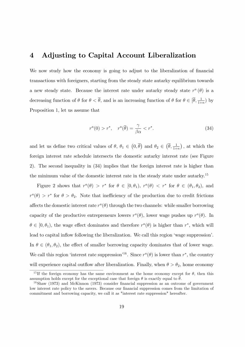
We now study how the economy is going to adjust to the liberalization of �nancial

transactions with foreigners, starting from the steady state autarky equilibrium towards

a new steady state. Because the interest rate under autarky steady state ra (�) is a

decreasing function of � for � < �, and is an increasing function of � for � 2 [�; 11+n) by

Proposition 1, let us assume that

ra(0) > r�; ra(�) =

��< r�: (34)

and let us de�ne two critical values of �, �1 2�0; ��and �2 2

��; 1

1+n

�; at which the

foreign interest rate schedule intersects the domestic autarky interest rate (see Figure

2). The second inequality in (34) implies that the foreign interest rate is higher than

the minimum value of the domestic interest rate in the steady state under autarky.15

Figure 2 shows that ra(�) > r� for � 2 [0; �1), ra(�) < r� for � 2 (�1; �2), and

ra(�) > r� for � > �2. Note that ine¢ ciency of the production due to credit frictions

a¤ects the domestic interest rate ra(�) through the two channels: while smaller borrowing

capacity of the productive entrepreneurs lowers ra(�), lower wage pushes up ra(�). In

� 2 [0; �1), the wage e¤ect dominates and therefore ra(�) is higher than r�, which will

lead to capital in�ow following the liberalization. We call this region �wage suppression�.

In � 2 (�1; �2), the e¤ect of smaller borrowing capacity dominates that of lower wage.

We call this region �interest rate suppression�16. Since ra(�) is lower than r�, the country

will experience capital out�ow after liberalization. Finally, when � > �2, home economy

15If the foreign economy has the same environment as the home economy except for �, then thisassumption holds except for the exceptional case that foreign � is exactly equal to �.16Shaw (1973) and McKinnon (1973) consider �nancial suppression as an outcome of government

low interest rate policy to the savers. Because our �nancial suppression comes from the limitation ofcommitment and borrowing capacity, we call it as "interest rate suppression" hereafter.

19

has more advanced �nancial system than the rest of the world so that ra(�) is higher

than r�, causing capital in�ow. We refer to this region as the �advanced �nancial system�.

Thus the direction of capital �ow crucially depends on the degree of domestic �nancial

development relative to the rest of the world.

While some analytical results are available, it is easier to illustrate transition dynam-

ics based on numerical examples. Given that our model is highly stylized, we do not

intend to calibrate the model to match a particular country. The purpose is the quali-

tative analysis of how a country�s adjustment to liberalization depends on its degree of

�nancial development relative to that of the rest of the world. The parameter values

used in the numerical examples are explained in Appendix E.

4.1 Wage Suppression

Figures 3.1 and 3.2 show the dynamics of the economy under wage suppression for a low

level of domestic �nancial development � = 0:15 < �1. Under wage suppression, the wage

rate is so low that even the unproductive entrepreneurs enjoy a higher rate of return on

production under autarky than the foreign interest rate. Thus both unproductive and

productive entrepreneurs borrow from abroad. However, since the borrowing capacity

is small, capital in�ow is limited. The productive entrepreneurs also borrow from the

unproductive entrepreneurs who become their lead creditors in the domestic credit mar-

ket. Here, the unproductive entrepreneurs serve as �nancial intermediary: they borrow

from the foreigners secured by the fraction of their output at the world interest rate

r�, and, at the same time, extend loan to the productive entrepreneurs in the domestic

credit market as the lead creditors at the domestic interest rate rt. The fact that the

unproductive entrepreneurs act as �nancial intermediary stems from the fact that in-

20

ternational borrowing constraint is tighter than the domestic borrowing constraint (i.e.,

0 < � < 1).17

The dynamics of the wage suppression economy is characterized by a temporary

boom followed by stagnation. Immediately after the liberalization, the unproductive

entrepreneurs expands production by borrowing from abroad at a cheaper interest rate.

The total employment increases with capital in�ow, which pushes up the wages. The

expansion, however, is short-lived. Because the employment by the productive entrepre-

neurs is crowded out with a higher wage, TFP keeps decreasing from autarky level. After

the international borrowing constraint becomes binding, output and wage rate start de-

creasing until the economy converges to its new steady state. The long-run e¤ect on

output is marginal.

4.2 Interest Rate Suppression

Figures 4.1 and 4.2 show the dynamics of the economy under the interest rate suppression

for a medium level of domestic �nancial development � = 0:3 2 [�1; �2]. The adjustment

process under the interest rate suppression is characterized by temporary drop in wages

and employment followed by gradual expansion. Because the unproductive entrepre-

neurs start lending abroad and reduce employment, wage and total employment drop

immediately after liberalization. While total employment and employment of unpro-

ductive entrepreneurs fall, employment of productive entrepreneurs rise due to cheap

wage rate and borrowing rate. As a result, TFP improves. Over time, employment of

productive entrepreneurs increases together with their accumulation of net worth, until

17During the rapid economic growth era after the World War II, Japanese general trading companiesplayed a role of �nancial intermediary, borrowing from abroad against their international collateral andlending to domestic businesses. Possibly, countries like India and China (at least in the early stage)may experience this type of adjustment. Caballero and Krishnamurty (2001) has a similar feature.

21

it absorbs the entire employment. Thereafter, the wage rate and employment start re-

covering. Intuitively the international capital market has a catalyst e¤ect by eliminating

the ine¢ ciency in production in the long run through accumulation of net worth.18

4.3 Advanced Domestic Financial System

When domestic �nancial system is more advanced than the rest of the world, autarky

interest rate is higher than the world interest rate due to large borrowing capacity of the

productive entrepreneurs. After liberalization, the productive domestic entrepreneurs

will attract foreign fund, causing capital in�ow. The unproductive entrepreneurs con-

tinue to specialize in lending. Figures 5.1 and 5.2 show the dynamics of the economy

under advanced domestic �nancial system � = 0:8 > �2. The total employment (which

is equal to employment of the productive entrepreneurs) expands at the beginning and

then stays roughly constant.19

Similar to the analysis by Caballero et al. (2006) and Mendoza et al. (2007) our

framework suggests the existence of �equilibrium imbalances� in which countries with

more developed �nancial system experience capital in�ows as they integrate with less

�nancially developed economies. Intuitively, the home economy can take advantage

of the relatively low interest rate (and the saving glut) of the rest of the world. A

distinguishing feature of our work is that capital in�ow needs not be the result of superior

domestic �nancial system, because it can be a result of wage suppression. But the key

di¤erence among these two types of capital in�ow is that TFP stays high with capital

in�ow induced by a superior �nancial system, while the TFP deteriorates and the boom is

18Perhaps, some Latin American countries experience this type of adjustment, which is characterizedby capital out�ow and the loss of employment of the unproductive sector, which may cultivate theanti-globalization sentiment.19This depends on the elasticity of labour with respect to wage. If labour supply is elastic enough,

then the employment continues to increase.

22

temporary when capital in�ow is caused by the wage suppression with an underdeveloped

domestic �nancial system.

4.4 Steady State after Liberalization

The new steady state after capital account liberalization depends upon the relative level

of domestic �nancial development to the rest of the world as:

Proposition 2 Let r(�) and w(�) be the domestic interest rate and the wage rate in the

steady state equilibrium after liberalization with �nancial depth �.

1. Wage suppression, � < �1: Unproductive entrepreneurs produce and the home

interest rate stays above the foreign interest rate: r� < r(�) < ra(�), w (�) > wa(�),

r0(�) < 0 and w0(�) > 0:

2. Interest rate suppression, � 2 [�1; �2]: Unproductive entrepreneurs do not produce,

and the home and foreign interest rates are equalized: ra(�) � r(�) = r�, A(�) =

� � Aa(�), and w0(�) > 0:

3. Advanced domestic �nancial system, � > �2: Unproductive entrepreneurs do not

produce. The home and foreign interest rates are equalized if �2 < � � e� ��+��[n�+(1=�r�)�1](1+n)�+(1=�r�)�1 2 (�2; 1): The home interest rate stays above the foreign interest

rate if � > e�. In both cases, ra(�) > r(�), w(�) > wa(�); A(�) = � = Aa(�),

r0(�) � 0 and w0(�) > 0:

Note that unproductive entrepreneurs do not produce if the �nancial depth is at least

as high as �1: Thus the economy is more likely to achieve e¢ ciency in production for the

same �nancial depth in the new steady state than autarky. Also, we observe that capital

23

account liberalization does not necessarily leads to the complete �nancial integration of

the home economy with the rest of the world. If the �nancial depth of the economy is

very di¤erent from the rest of the world, either extremely low � < �1 or extremely high

� > ~�; the domestic interest rate stays higher than the foreign interest rate because the

international borrowing constraint is binding. From Proposition 2, we learn wage rate

and total employment are increasing functions of the �nancial depth of the economy �

for the entire range of �.

5 Welfare and Government Policies

5.1 Welfare Analysis

From the analysis of the previous section, we learn that the capital account liberalization

is not necessarily bene�cial, especially when the domestic �nancial system is underdevel-

oped. If the wage suppression is pronounced under �nancial autarky, the liberalization

does not improve the TFP and thus the boom is temporary. If the interest rate sup-

pression is signi�cant, the liberalization causes capital out�ow and decline in wages and

employment during the transition, even though the TFP will improve in the long-run.

A natural question is to what extent capital account liberalization is bene�cial for the

country, and how the costs and bene�ts are distributed among di¤erent groups. To

answer this question, we examine the welfare e¤ects on workers and productive and un-

productive entrepreneurs separately. (We do not use Pareto e¢ ciency criteria of whether

everyone can be better o¤ with suitable redistribution, because it is di¢ cult to enforce

redistribution with limited collateral).

We measure the welfare e¤ect of capital account liberalization by a constant per-

24

productive unproductive workerswage suppression -0.025 -0.025 0.0022interest rate suppression 0.25 0.25 -0.018advanced �nance -0.086 -0.19 0.014

Table 1: Welfare analysis

centage change of steady state autarky consumption that is required to make an agent

indi¤erent between liberalizing capital account and staying in autarky. In computing

this measure, we take into account the e¤ects of the transition dynamics from autarky

to the post-liberalization steady state. Formally, for each entrepreneurs i, we de�ne this

measure of welfare change - called the consumption equivalent �i - as

E0

1Xt=0

�t log�cit�=

1

1� �log�(1 + �i)cia

�(35)

where cit is date t consumption of entrepreneur i after the liberalization at date 0, starting

from the autarky steady state at date �1, and cia is his consumption under autarky

steady state.

The welfare measure of workers is de�ned in a similar way. Assume that the utility

of the workers is logarithmic: u(c� v(l)) = log(c� v(l)) and that the disutility of labor

is constantly elastic: v(l) = 11+(1=�)

l1+(1=�). De�ne �w as

1Xt=0

�t log (ct � v(lt)) =1

1� �[log ca(1 + �w)� v(la)]; (36)

where �w is consumption equivalent for the workers. Here ca and la respectively denote

consumption and labor supply under autarky.

Table 1 reports the welfare e¤ect of capital account liberalization for the cases corre-

sponding to wage suppression, interest rate suppression and advanced domestic �nancial

25

system, using the numerical example of the previous section. The headline of �produc-

tive�implies the group of entrepreneurs who are productive and �unproductive�is the

group who is unproductive at the time of liberalization. Under wage suppression, capital

in�ow is limited and boom is temporary because the borrowing constraint is tight and

as a result the welfare e¤ects of liberalization are small compared to the other two cases.

The workers gain only modestly from the temporary boom and the entrepreneurs lose

modestly from the lower expected rates of return.

Under interest-rate suppression, the economy experiences an initial recession before

improving the TFP in the long-run. The workers tend to lose since the loss from the

lower wages during the initial recession is large compared to the possible long-run gains

in a distant future. The entrepreneurs gain substantially because their rate of return

become higher. The unproductive (savers) obtain better saving opportunities abroad

at the higher world interest rate, and the productive entrepreneurs achieve higher rate

of return due to lower wages. The welfare e¤ects on the entrepreneurs are much larger

than those on workers since changes in the rate of return have compound e¤ects on their

consumption through wealth accumulation.

Finally, in the case of advanced �nancial system, the workers gain due to perma-

nently higher wages. The entrepreneurs lose because they face lower rate of return. In

particular, unproductive entrepreneurs loose substantially because they are savers at the

time of liberalization and their rate of return on saving drops to the world interest rate.

In contrast, productive entrepreneurs do not loose as much because they can expand

production by borrowing at a cheaper world interest rate even though the wage rate is

higher.

From these analysis, we learn that there tends to be con�icts of interests between

workers and entrepreneurs towards the capital account liberalization. The welfare of the

26

workers tend to be more in�uenced by the short-run movement of the aggregate economy

immediately after the liberalization, because the workers do not smooth consumption

due to the binding borrowing constraint. In contrast, the entrepreneurs tend to care more

about the subsequent rates of return which depends upon the long-run performance of

the economy.

From a policy maker�s point of view, the case of interest-rate suppression would be of

particular interest. This is because capital account liberalization of private capital �ows

can eventually eliminate the ine¢ ciency of production, but such process can be painful to

the workers who su¤er from lower wage and employment. Can the government mitigate

the loss of workers during the adjustment to the capital liberalization? One possibility

is redistribution, but the government may face a limited enforcement problem similar

to that of the private agents as long as the domestic �nancial and legal systems are not

developed enough. Therefore, in the next two Sections we consider two di¤erent types

of policy intervention. The �rst one is a simple tax and subsidy policy under balanced

budget constraint, while the second one is to allow foreign direct investment (FDI) �ows

along with private capital �ows in the process of capital account liberalization.

5.2 Tax and Subsidy under Interest Rate Suppression

The reason for which wages drop temporarily under interest-rate suppression is that

the unproductive entrepreneurs lend abroad and shrink their production. In order to

mitigate the drop in wages, we consider a production subsidy to unproductive agents by

imposing taxes on the productive agents. We assume balanced budget, so the budget

constraint of the government sector is given by

�t�1Y0t = � t�1Yt; (37)

27

where �t represents subsidy rate and � t represents tax rate.20

Limited commitment and shortage of collateral have implications for both private

�nance and public �nance. Because the tax liability to the government is considered to

be the most senior debt of the entrepreneur, it a¤ects his domestic and international

borrowing constraints as

� tyt+1 + b�t+1 � ��yt+1; (38)

� tyt+1 + b�t+1 + bt+1 � �yt+1: (39)

The �rst constraint implies that the foreign creditors will limit their loans so that the

sum of the tax liability and the foreign debt repayment does not exceed the value of

collateral for the outside creditors. The second constraint says the domestic lead creditor

restricts her loan so that the sum of all liabilities of the entrepreneur does not exceed

the collateral value of the project to the lead creditor. In what follows, we assume that

the tax liability of the entrepreneur does not exceed the collateral value for the outside

creditors: � tyt+1 � ��yt+1.21 The �ow-of-fund constraint of the productive entrepreneur

becomes

ct + wtlt = (1� � t�1)yt � bt � b�t +bt+1rt

+b�t+1r�

(40)

The unproductive entrepreneur�s �ow-of-fund constraint is similar to (40), term �� t�1

being replaced by �t�1.22 In Appendix D we describe the set of equilibrium conditions.

20The role of public debt as liquidity in an economy under credit constraint is an interesting question.For example, Woodford (1990) considers a model with heterogeneous entrepreneurs who cannot borrow,in order to argue that government can issue public debt to absorb the saving of the unproductiveentrepreneurs and improve the e¢ ciency. See, also, Holmstrom and Tirole (1997). However, a systematicanalysis of public debt under credit-constrained economy is beyond the scope of this paper and is leftfor future research.21This constraint can be an outcome of limited power of government who cannot enforce tax liability

more than the outside creditors.22We assume that the unproductive entrepreneur who receive production subsidy cannot borrow

against the future production subsidy, because the creditor who take over the project may not receive

28

productive unproductive workerswithout government 0.25 0.25 -0.018with government 0.17 0.24 -0.013

Table 2: Welfare with government under interest-rate suppression

Figure 6 shows the dynamics of the economy with government under interest-rate

suppression. Here, subsidy is chosen to set the wage immediately after liberalization as

wt = wa + (1� )wlt;

where wa is wage under autarky steady state and wlt � =r� is wage immediately after

liberalization without government policy. Here is set 0.3. There is a trade-o¤ for

our government policy. On one hand, the unproductive entrepreneurs who receive sub-

sidy employ more workers than the laissez faire economy during transition. As a result

employment is larger with the government policy. On the other hand, taxation on the

productive entrepreneurs decrease their capacity of private borrowing. As a result their

accumulation of net worth and expansion of employment are slower. Thus the transition

to the equilibrium with e¢ cient production takes longer than the laissez faire econ-

omy.23 Eventually, the unproductive entrepreneurs stop producing, and thereafter the

adjustment is identical to the laissez faire economy. Table 2 shows welfare consequences

of the government policy. Not surprisingly, workers�loss is mitigated. The productive

entrepreneur�s gain from liberalization shrinks by the taxation. The unproductive en-

trepreneur�s gain does not change much, because their rate of return is still given by the

foreign interest rate despite of receiving the production subsidy.

the production subsidy from the government.23If subsidy is large enough to maintain the autarky wage, the employment of the productive entrepre-

neurs starts shrinking as their net worth deccumulates. Then the tax rate on output of the productiveagents have to be higher in order to balance the budget, which leads to further deccumulation of theirnet worth. Thus, the large subsidy program is not sustainable in the long run.

29

5.3 Foreign Direct Investment

Another policy intervention which has become increasingly more important is to allow

foreign direct investment (FDI) along with �nancial capital �ows.24 Allowing FDI might

imply smaller distortion than the tax and subsidy policy of the previous section. Also,

it has been argued that FDI tends to be the least volatile type of capital �ows because

it involves relatively irreversible types of investment (physical capital, human capital,

managerial resources)25. Therefore allowing FDI may make countries less vulnerable to

capital out�ow. In this section we are interested in examining whether the FDI is able

to mitigate the losses of workers in the interest rate suppression region.26

We assume that foreign �rms have a similar production technology as domestic en-

trepreneurs:

yt+1 = ��l�t ; (41)

where yt+1 is output of goods at date t + 1, l�t is the labor input at date t, and �� is

constant productivity of foreign �rms. Here we assume that foreign productivity is at

least as big as the productivity level of the productive entrepreneurs, �� � �. Since we

consider a small open economy, when foreigners make their decisions about FDI they

24As documented recently in Prasad and Rajan (2008), the share of foreign direct investment �owshas now become far more important than that of debt in gross private capital �ows to nonindustrialcountries. The share of foreign direct investment in total gross in�ows to emerging markets and otherdeveloping countries has risen from about 25 percent in 1990-94 to nearly 50 percent by 2000-04. Overthe same period, the share of debt in in�ows to emerging markets has fallen from 64 percent to 39percent.25Kose et al. (2006) looks at the volatility of di¤erent types of in�ows, calculated as the cross-country

averages of the standard deviations of di¤erent types of in�ows (measured as ratios to GDP) over theperiod 1985-2004. They �nd that gross in�ows of debt �nancing are substantially more volatile thanFDI or equity in�ows.26A important issue in FDI is technology transfer (see for example Blalock and Gertler (2008) for the

case of Indonesian manufacturing establishment). While it is certainly an important issue we abstractfrom it because our main focus in the paper is to explore how liberalization of international �nancialtransactions a¤ect resource allocation among heterogeneous producers subject to credit constraints. Webelieve we can analyze the role of FDI in this regard without considering the spillover e¤ects.

30

are not subject to borrowing constraints. Therefore the relevant discount factor is the

international interest rate r�:

On the other hand, it seems natural to assume that foreign producers face frictions

in expanding production: In particular, it takes time and cost for the foreign employers

to recruit suitable workers who understand technology and organization of the �rm. We

capture this by search frictions along the line of Mortensen and Pissarides (1994). In

order to hire a suitable worker, a foreign employer maintains an open vacancy at �ow

cost c. A �ow of new worker-employer matches is given by a constant-returns-to-scale

function M(Ht; Vt), where Ht is the number of searching workers and Vt is the number

of vacancies in the economy. Here we assume that all the workers (including the workers

employed by the domestic �rms) can costlessy look for jobs in foreign �rms. Then

given the constant population of workers, Ht is constant. For simplicity, we assume

that workers can supply labor to domestic and foreign �rms simultaneously, and that

each worker supplies one unit of labor when they match with foreign producers, so

that foreign �rms have only extensive margin to adjust labor. Finally, the relationship

between foreign �rm and a worker might end every period with a exogenous separation

rate 1� �.

Total labor force in the FDI sector (Pl�t = L�t ) evolves according to

L�t = �L�t�1 +M(H; Vt); (42)

where the �rst term represents the fraction of employed workers who remain employed

in foreign �rms and the second component represents workers who �nd a job. The

31

matching function is given by

M(H; Vt) = ~�H�V 1��

t = �V 1��t : (43)

The model is completed by the relationship that determines the link between the

value of the vacancy and the value of the job. The recursive equation for the value of

the vacancy is given by

Jvt = �c+ �V ��t Jt +

(1� �V ��t )

r�Jvt+1; (44)

where Jvt is the value of the vacancy, �V��t represents the rate at which the vacancy is

�lled and Jt is the value of the job that evolves accordingly to

Jt =��

r�� wt +

�

r�Jt+1: (45)

In (45), the term ��

r� � wt represents the current net bene�t from the match while the

last term represents the continuation value which depends on the separation rate. We

assume free entry, implying that Jvt = 0 at all times. In contrast to the production

by the foreign �rms, we continue to assume that all the workers are homogeneous and

suitable for the production by the domestic entrepreneurs. Assuming that the foreign

�rms have full bargaining power against the workers, the foreigners will choose the wage

equal to the competitive wage level.

The competitive equilibrium condition in the labor market is now

Lt + L0t + L�t = Ls(wt): (46)

32

Once we use (42), (43) and (44) to substitute out the measure of vacancies, Vt;

the dynamic evolution of the economy is characterized by the recursive equilibrium:�Zt+1; st+1; xt; rt; wt; Lt; L

0t; L

�t ; B

�t+1; Jt

�that satis�es (16), (17), (21 - 25), (42), (45),

and (46) as functions of the state variables (st; Zt; L�t�1):

In the subsequent analysis we focus on the adjustment in the case of interest-rate

suppression when the economy starts from its steady state without international �nancial

transactions but with FDI allowed. Then the economy liberalizes the international

�nancial transaction with the continued presence of FDI. This exercise seems to be

useful for thinking about the experience of some countries, such as China, which is

allowing FDI while keeping strict restrictions on international �nancial capital �ows.

Figure 7 shows how the presence of the FDI changes the adjustment of the �nancially

suppressed economy to the liberalization of international �nancial transactions. The

parameter values used are discussed in Appendix. Solid line and uneven dotted line plot

the dynamic path with FDI. For comparison, even dotted lines plot the adjustment of the

economy without FDI � identical to Figure 4.2. Prior to liberalization of international

�nancial transaction with the presence of the FDI, employment of the unproductive

domestic entrepreneurs is smaller and the TFP is higher than the steady state without

the FDI, because a fraction of workers are employed by productive foreign �rms.27

Immediately after the liberalization of international �nancial transaction, wages fall

as much as the case without the presence of FDI. This is because, as long as the un-

productive entrepreneurs still produce, the unproductive agents are indi¤erent between

producing and lending abroad: =wt = r�. However, because employment of foreign

27Because of our speci�c feature of the domestic entrepreneurial sector (such as constant returns toscale production function, constant turnover rate, and constant saving rate), the FDI does not changethe share of wealth and employment of the productive entrepreneurs within the domestic entrepreneurialsector. Thus the wage rate, total employment and domestic interest rate are not a¤ected by the FDIin the steady state under �nancial autarky.

33

productive unproductive workerswithout FDI 0.2533 0.2533 -0.01815with FDI 0.2532 0.2532 -0.01807

Table 3: Welfare with FDI under interest-rate suppression

�rms expands in addition to that of productive entrepreneurs, it takes less time for the

unproductive production to be eliminated and the wage level recovers more quickly.28

Table 3 reports the welfare e¤ect of capital account liberalization with and without

FDI. Qualitatively, we see that by shortening the initial recession FDI mitigates the

workers�s loss. However under our chosen parameter values the e¤ect is very small.29

The presence of FDI does not have much e¤ect on the welfare of entrepreneurs either

since their rate of return is not directly a¤ected by the presence of FDI. Overall, by

making domestic entrepreneurial employment smaller, the presence of FDI speeds up

the necessary adjustment to the liberalization of the international �nancial transactions.

However, the prices and the distributions among the domestic sectors in the new steady

state are mostly determined by the domestic institution, not directly a¤ected by the

FDI in our framework in which there is no direct spillover e¤ects from the FDI to the

domestic technology and institution.

28At the new steady state again, the presence of the FDI does not a¤ect the distribution of wealthand employment between productive and unproductive domestic entrepreneurs, and thus does not a¤ectwage rate and total employment.29The share of FDI in the initial period (i.e., at the time of liberalization) is important in determining

the quantitative signi�cance of the welfare e¤ect on workers. As is explained in Appendix E we chosethe parameter values such that the share of FDI is about 20%. If the share of FDI is higher, it takesless time for the unproductive production to be eliminated, and the resulting welfare gain is higher.

34

6 Final Remarks

We have developed a model of capital account liberalization under domestic and inter-

national borrowing constraints in which workers and entrepreneurs might not bene�t

from �nancial integration as long as the domestic �nancial system is underdeveloped.

If wage suppression is dominant with underdeveloped domestic �nancial system, then

the liberalization leads to a deterioration of TFP and long-run stagnation. If interest

rate suppression is more pronounced, then the liberalization causes capital out�ow and

signi�cant loss of employment during the adjustment. The reason for which capital ac-

count liberalization generates these costly adjustments is because under underdeveloped

�nancial system funds are used by unproductive entrepreneurs and producers located in

foreign countries rather than productive domestic entrepreneurs.

Our logic might extend to �nancial liberalization across regions or di¤erent segments

of the economy. For example, Guiso, Sapienza and Zingales (2004) �nd that the regions

with better local �nancial system in Italy enjoy better economic performance after the

�nancial liberalization of the mid-1980s as they have more entries of new �rms, smaller

monopoly markup, and higher growth.30

Of course, an important remained question would be to examine how to improve the

domestic �nancial system.

30Reinhart and Rogo¤ (2008) argue that the subprime mortgages could be interpreted as lending todeveloping countries, because those loans are directed to the "under-developed" segment of the U.Seconomy. Then, the �nancial liberalization of this segment may fail to improve the resource allocationin the long-run unless the �nancial system within this segment is improved..

35

Appendix

A Proof of Proposition 1:

From (27) and (28) ; we learn there are three possible types of the equilibrium:

(i) Unproductive entrepreneurs produce (L0 > 0; r = w)

(ii) Unproductive entrepreneurs do not produce and productive entrepreneurs are

credit constrained (r 2� w; �w

�)

(iii) Unproductive entrepreneurs do not produce and none is credit constrained�r = �

w

�Let us now examine each type of equilibrium in turn in order to derive the necessary

and su¢ cient condition on the parameters for such equilibrium to exist.

A.1 Autarky equilibrium with ine¢ cient production:

Because the interest rate is less than the rate of return of production on productive

entrepreneurs:

r =

w<�

w; (A.1)

the productive entrepreneurs are credit constrained. (28) becomes:

L =X

(�=r)� w�Z =

X

�� �Z: (A.2)

For employment of unproductive entrepreneurs to be positive, we need from goods mar-

ket equilibrium condition (30) that:

wL = X

�� �Z < wLs(w) = �Z; or

36

X <��

: (A.3)

From (31) and (A:1) ; we learn x = (�� )=( � ��): Thus, from (33) ; X solves

F (X;��

� ��) = X[X + �(1 + n)]� ��

� ��[(1� �)X + n�] = 0: (A.4)

Because F (0; �� ���) < 0; we know X > 0; which implies from (32) that

r =1

�(1 +X)<1

�:

Thus, we verify the condition (13) that guarantees that workers do not save in the

neighborhood of the steady state equilibrium. Also, we learn the condition for ine¢ cient

production (A:3) holds if and only if; F (�� ; �� ���) > 0; or

� <�

�� + (1 + n)�

� �: (A.5)

From (A:4) ; X and w are increasing functions of �; and r is a decreasing function of �.

A.2 Autarky equilibrium with e¢ cient production and credit

constrained productive entrepreneurs:

Here, because there is no employment by the unproductive entrepreneurs (L0 = 0) and

the productive entrepreneurs are credit constrained, the equilibrium conditions (28) -

(30) imply

Ls =�Z

w= L =

X�Z

(�=r)� w; and

w =�

(1 +X)r= ��:

37

Together with (31) - (33), we learn

X = �1� (1 + n)�

�: (A.6)

Then, we learn the productive entrepreneurs earn extra return X > 0 so that they are

credit constrained, if and only if

� <1

1 + n:

Also we learn r = 1= [�(1 +X)] < 1=�, which veri�es (13).

A.3 Autarky equilibrium in which no one is constrained:

If, � � 1=(1 + n); then we learn

X = 0; r = 1=�; w = ��; and s =n

1 + n

satisfy all the equilibrium conditions of the steady state autarky equilibrium in which

none of the entrepreneurs are credit constrained. (See footnote 13). Concerning the

quantities, we have L0 = 0 and:

L = Ls(��) = Z=�:

Q:E:D: of Proposition 1.

38

B Proof of Proposition 2

From the generic equilibrium conditions, (16) - (18) and (21) - (25), the steady state

equilibrium of the open economy is characterized by (r; w; x;X; L; L0; Z) that satis�es

the conditions (29), (32), (33) and

r � (1� ��)

w � ( ��=r�) ; and�r � (1� ��)

w � ( ��=r�)

�L0 = 0; (B.7)

L =�XZ

(�=r)� w + ���[(1=r�)� (1=r)] ; (B.8)

�Z +��

r�[ Ls(w) + (�� )L] � wLs(w); and (B.9)

(r � r�)

��Z +

��

r�[ Ls(w) + (�� )L]� wLs(w)

�= 0;

x =�� wr + ��� r�r

�

r�

wr � �� � ��� r�r�

r�: (B.10)

B.1 Wage suppression: � < �1

Lemma 3 : r > r� for � < �1:

Proof. Suppose not. Then, from (8), we learn r = r�: Then we have

ra > r� = r; for � < �1;

by construction of �1. Then, from (32) ; we learn

Xa < X:

39

Then from (33), we obtain

xa =��

� ��< x =

�� wr

wr � ��; or

r <

w<

(1� ��)

w � ��=r�:

This contradicts (B:7).

Guess L0 > 0 in (B:7). Then Lemma 3 implies

r = (1� ��)

w � ( ��=r�) ; or

w =

���

r�+1� ��

r

�= � [1 +X + ��(X� �X)] : (B.11)

where 1 +X� = 1=�r�: Then from (B:10) ; we learn

x = (�� )1 + ��X

��X1+X

� ��� (�� )��X��X1+X

:

Thus from (33), we have

eF (X; �; �) � X[X + �(1 + n)]� ��

� ��[(1� �)X + n� + ��(X� �X)(X + n�)] = 0:

Then we see X 0(�) > 0, or r0(�) < 0. Also because eF (X; �; �) < F (X; �� ���) for

X 2 (0; X�); we learn X > Xa, or r(�) < ra(�). Then from (B:11) and Proposition

1, we learn w(�) > wa(�). We can also verify that L0 > 0 from (B.8) and (B.9) under

Lemma 3.

40

B.2 Interest rate suppression: � 2 [�1; �2]

Lemma 4 L0 = 0 for � 2 (�1; �2)

Proof. By de�nition of (�1; �2); we know r(�) � r� > ra (�) for � 2 (�1; �2). Thus

X < Xa, or

x =�� wr + ���

�rr� � 1

�wr � ��� ���

�rr� � 1

� < xa =�� wara

wara � ��� ��

� ��:

Thus < wr � ����rr� � 1

�; or

w >

r+ ���

�1

r�� 1r

�>

�1� ��

r+��

r�

�:

Thus from (17) ; we learn L0 = 0 for � 2 (�1; �2).

Lemma 5 r = r� for � 2 (�1; �2)

Proof. Suppose that r > r�: Then from Lemma 4, (B:8) and (B:9), we learn

�w � ���

r�

�L = �Z =

1

X

��

r� w + ���

�1

r�� 1r

��L; or

w = ��(1 + ��X�)

Then,

x = X1� ��

1� � � �(1� �)X:

Also from (33), we know

x = XX + (1 + n)�

(1� �)X + n�:

41

Therefore we learn

0 = (1� ��) [(1� �)X + n�]� [X + (1 + n)�] [1� � � �(1� �)X]

= (1 +X) f�(1� �)X � � [1� � � n�(1� �)]g , or

X = �1� � � n�(1� �)

�(1� �):

Because from equation (A.6) we know �2 satis�es X� = � 1�(1+n)�2�2

, we learn that

X > �1� �2 � n�2(1� �)

�2(1� �)> X�; for � < �2:

This contradicts r > r� because r = 1�(1+X)

.

Lemma 5 implies X = X� = 1�r� 1. Then from (33) and (B:9), we know

x = X� X� + (1 + n)�

(1� �)X� + n�=

��(1 +X�)� w

w � ���(1 +X�):

Thus

w = ��

�1 +X� � [X

� + (1 + n)�]� �

X� + n�

�= ��[1 +X�k(X�)(� � �2)] = w(�), where

k (X�) � X� + (1 + n)�

X� + n�:

Lemma 4, 5, (B:8) and (29) implies

Z = � [1 + k(X�)(� � �2]Ls (�� [1 +X�k(X�)(� � �2]) :

42

Thus Z is an increasing function of � i¤

wLs0(w)

Ls(w)>

1

X�1�X�k(X�)(� � �2)

1 + k(X�)(� � �2):

where the LHS is the elasticity of labour supply.

B.3 Advanced Domestic Financial System: � > �2

Lemma 6 L0 = 0 for � > �2.

Proof. Suppose L0 > 0. Then we learn

w =

�1� ��

r+��

r�

�:

Thus

x = (�� )1 + ��X

��X1+X

� ��� (�� )��X��X1+X

:

Thus from (33), we learn X > X� for � > �2 > �1. This contradicts r > r� for � > �2.

Lemma 6, (B:8) and (B:9) imply

�Z �X�w � ���

r�

��r� w + ���

�1r� �

1r

��Z; (B.12)

where the strict inequality implies r = r� while r > r� implies the equality.

The equilibrium with r = r� implies

w = �� [1 +X�k(X�)(� � �2)]

43

Then from (B:12) ; r = r� if and only if

� � e� � �2

1� �k(X�)

=� + ��[n� + (1=�r�)� 1](1 + n)� + (1=�r�)� 1 :

If � > e�, we learn r > r� and thus from (B:12) ;

w = ��(1 + ��X�):

Thus we get

x = X1� ��

1� � � � (1� �)Xand

X = �1� � � �(1� �)n

�(1� �);

from (33).

Q:E:D: of the Proposition 2.

C Welfare computation

Since consumption cit is proportional to his net worth of date t, zit, we can write c

it as:

cit = (1� �) zit

= (1� �) �tzi0ri0ri1 � � � rit�1;

where rit is the gross rate of return on saving of entrepreneur i: The level of rit is equal

to rt when he is unproductive, and is equal to (1 + xt) rt when he is productive at date

44

t. Then, we can write the consumption equivalent �i as

log�1 + �i

�= �

1Xt=0

�t�P tRt

�j� �

�(I � �P )�1RA

�j; (C.13)

where

P =

264 1� � �

n� 1� n�

375is the transition matrix for the productivity shift, and

Rt = [log ((1 + xt)rt) ; log rt]0 ;

and

RA =�log�(1 + xA)rA

�; log rA

�are the vectors of the log rate of return for the productive and unproductive entrepreneurs

in the liberalization and in the autarky regimes respectively. Index [�]j denotes the j

column in matrix [�] in equation (C.13) and it identi�es the type of entrepreneurs (j = 1

for productive and j = 2 for unproductive) at t = 0 when the liberalization occurs. Since

entrepreneurs can shift from the productive to the unproductive status, we will need to

distinguish two groups depending on the productivity at the time of liberalization.

For workers we have that since workers�s consumption is equal to wage income (ct =

wtlt = w1+�t ), we can express �w as

log

�1

1 + �+ �w

�= log

�1

1 + �

�+ (1� �)(1 + �)

1Xt=0

�t logwt (C.14)

�(1 + �) logwA

45

D Tax and Subsidy

With production subsidy, the behaviour of the unproductive entrepreneurs is modi�ed

from (10) to:

r� = rt � (1 + �t)

wt; and L0t

�rt �

(1 + �t)

wt

�= 0: (D.15)

Term (1 + �t)=wt represents the rate of return of the unproductive agents without

borrowing, which is the relevant return in the case of interest-rate suppression. The

employment of the productive entrepreneurs is modi�ed from (16) to

Lt ��stZt

wt � � [�� � � t] =r� � [�(1� �)�=rt]; (D.16)

and equality holds if

R (�) =� (1� �)

wt � � [�� � � t] =r� � [�(1� �)�=rt]> rt:

The denominator of RHS is downpayment for unit labor input, when the productive

entrepreneur borrows �(���� t)=r� from foreigners and �(1��)�=rt from domestic lead

creditor for unit labor cost. This expression shows that taxation crowds out investment

because it decreases collateral that can be used for private borrowing.

Since there is no government expenditure and no government bond, the goods market

clearing condition (19) is not a¤ected. The extra rate of return by the productive

entrepreneur is modi�ed from (24) to

xt =R(�)�R( )

R( )=

� [1� ��] =rt + �[�� � � t]=r� � wt

wt � � [�� � � t] =r� � [�(1� �)�=rt]: (D.17)

The competitive equilibrium with government policy is de�ned recursively by (wt, rt, xt,

46

Lt, L0t, � t, st+1, Zt+1, B�t+1) as functions of the state variables (st; Zt; ) that satisfy (18),

(19), (22) (23), (25), (37), (D:15), (D:16), and (D:17), for a given policy �t.

E Parameter Values in Section 4 and 5

We choose our parameters values such that one period in our model corresponds to a

year. The discount factor, �, is set 0.92: this implies that the steady state interest

rate under autarky ranges from 0% to 8.1% depending on the value of � under which

unproductive agents produce. Note that in a credit constrained economy, the steady

state interest rate is lower than the inverse of the time preference rate.

� represents the Frish elasticity of labor supply. Micro studies estimate a low elasticity

ranging from 0.1 to 0.4 (MaCurdi 1981), at 0.7 (Hall, 2009), at 1 (Kimball and Shapiro,

2008) and at 1.5 (Gourio and Noual, 2007) while macroeconomic models usually use

higher values: for instance, King and Rebelo (1999) in their survey of RBC models use

an elasticity of 4 in their basic model and an in�nite elasticity in an extension of their

model. New Keynesian models also use a high elasticity: Rotemberg and Woodford

(1998) and Woodford (2003) use an elasticity close to 9. Since our results are not too

sensitive to �, we set the elasticity to 3 lower than the value typically used in macro

models but higher than what micro studies would suggest.

In order to characterize the gap between the productivity of productive and un-

productive agents we use as a reference microeconometric studies that have measured

�rm-level productivity. Syverson (2004) computes labor productivity measure for 443

four-digit industries using plant-level data from the 1977 Census of Manufactures (CM)

for the U.S. Once we focus on the interquartile range as a proxy for the gap between more

productive and less productive �rm we have that the ratio of labor productivity between

47

the 75th and 25th percentile plants is about 1.3 (Syverson, 2004), slightly higher than

the one that we use to parametrize our economy where we set � = 1:2 and = 1:05.

Parameters n and � are set to 0.1 and 0.15, respectively. This implies that in the

steady state the fraction of the productive agents is equal to n/(1+n)=0.09, and the

expected time that an agent continues to be productive is 1/� = 6.66 years. Finally,

those parameters together imply that the unproductive agents produce in the autarky

steady state when � is less than 0.64

We choose the foreign interest rate to be at 4% on a yearly basis which is a quite

standard in the real business cycle literature (see Schmitt-Grohe´and Uribe, 2003). The

value of the parameter that determines the tightness of the international constraint, �;

is set to 0:5 so that foreigners can obtain half of the output compared to the domestic

lead creditor. In a framework with only international borrowing constraint, Mendoza

(2001) sets � = 0:74 so that his model-economy is likely to hit the borrowing limit. We

choose a lower value so that the possibility of hitting the constraint is reduced but our

analysis is robust to changes in �:

In parametrizing the economy with the FDI sector, we set the curvature of the

matching function � to 0.3, in between the value of 0.24 reported in Hall (2005) and

0.36 estimated in Cooper, Haltiwanger and Willis (2007) and the productivity of the

FDI sector, �� is set to be 1:5 so that foreign productivity is 25% higher than produc-

tivity in domestic �rms, which is a plausible value given the degree of heterogeneity in

productivity even in more industrialized countries. The other parameters c, � and 1��

are chosen as to match the size of the FDI sector in the overall economy to a level of

about 20%. (Lankes and Stern (1999) report that the share of FDI in�ows over GDP

in 1996 for emerging market economies ranges between 1% to 19% so that given the

current expansion of FDI �ows 20% seems a reasonable value for the size of FDI). In

48

doing so we obtain that c = 0:2; � = 0:15 and 1�� = 0:4 which is higher than the value

of 0.1for 1�� estimated by Shimer (2005) for the U.S. economy. The dynamics reported

in Section 5 is robust against changing those parameters. As long as the implied share

of FDI is kept at about 20%, the transition dynamics is very similar.

49

F Reference

Aghion, P., P. Bacchetta, and A. Banerjee. "Financial Development and the Instability

of Open Economy," Journal of Monetary Economics, 51 (2004): 1077-1106.

Aghion, P., and A. Banerjee. Volatility and Growth, Oxford University Press, (2005):

Oxford and New York.

Aghion, P., A. Banerjee, and T. Piketty. "Dualism and Macroeconomic Volatility,"

Quarterly Journal of Economics, 114 (1999): 1321-1358.

Aghion, P., O. Hart, and J. Moore. "The Economics of Bankruptcy Reform," Journal

of Law, Economics and Organization, 8, (1992): 523-546.

Bartelsman, E., J. Haltiwanger and S. Scarpetta "Cross Country Di¤erences in Pro-

ductivity: the Role of allocative E¢ ciency, mimeograph. (2006).

Blalock, Garrick & Gertler, Paul J., 2008. "Welfare gains from Foreign Direct In-

vestment through technology transfer to local suppliers," Journal of International Eco-

nomics, vol. 74(2).

Bebchuk, A. L. "A New Approach to Corporate Reorganization," Harvard Law Re-

view, 101, (1988): 775-804.

Bon�glioli, A. "Financial Integration, Productivity and Capital Accumulation," Jour-

nal of International Economics 76, 337-355 (2008)

Broner, Fernando, Albert Martin and Jaume Ventura. "Sovereign Risk and Sec-

ondary Markets," CREI working paper, (2006).

50

Caballero, R., and A. Krishnamurthy. "International and Domestic Collateral Con-

straints in a Model of Emerging Market Crisis," Journal of Monetary Economics, 48,

(2001): 513-548.

Caballero, R., E. Farhi, and P.O. Gourinchas. "An Equilibrium Model of "Global

Imbalances" and Low Interest Rates," NBER Working Paper 11996, (2006).

Caselli, F., and N. Gennaioli. "Dynastic Management," NBER Working Paper 9442,

(2003) National Bureau of Economic Research, MA.

Cooper, R., J. Haltiwanger and J. L. Willis. "Implications of Search Frictions:

Matching Aggregate and Establishment-level Observations." (2007) NBER Working Pa-

pers 13115.

Diamond, D., and R. Rajan. "Liquidity Risk, Liquidity Creation, and Financial

Fragility: A Theory of Banking," Journal of Political Economy, 109 (2001): 287-327.

Eichengreen, B. "Capital Account Liberalization: What Do the Cross-Country Stud-

ies Tell Us?" The World Bank Economic Review,(March 2002).

Gertler, M. and K. Rogo¤. "North-South lending and endogenous domestic capital

market ine¢ ciencies." Journal of Monetary Economics, vol. 26(2), (1990).

Gourio F. and P.A. Noual. "The Marginal Worker and the Aggregate Elasticity of

Labor Supply", mimeograph, University of Chicago (2007).

Guiso, Luigi, Paola Sapienza, and Luigi Zingales. "Does Local Financial Develop-

ment Matter?" Quarterly Journal of Economics, (2004): 929-969.

51

Hall, Robert. "Job Loss, Job Finding, and Unemployment in the U.S. Economy over

the Past Fifty Years". NBER Macroeconomics Annual, 2005, pp. 101-137.

Hall, Robert. "Reconciling Cyclical Movements in the Marginal Value of Time and

the Marginal Product of Labor", mimeograph, Stanford University (2009).

Hart, O., and J. Moore, "A Theory of Debt Based on the Inalienability of Human

Capital," Quarterly Journal of Economics, 109, (1994): 841-879.

Holmstrom, B. and J. Tirole, "Private and Public Supply of Liquidity", Journal of

Political Economy, vol. 106, n. 1, February 1998, p. 1-40.

Jeske, K. "Private International Debt with Risk of Repudiation", Journal of Political

Economy, 114 (2006): 576-593.

Kehoe, P. and F. Perri, "International business cycles with endogenous incomplete

markets," Econometrica, 69, (2001): 575-598.

Kehoe, P. and F. Perri, "Competitive equilibria with limited enforcement" Journal

of Economic Theory 119 (2004): 184-206.

Kim, Yong. "Borrowing Constraints and Technology Di¤usion: Implications of Intra

Industry Trade," Mimeo, (2001) Revised (2003) University of .Southern California.

Kimball, Miles and Matthew D. Shapiro. "Labor Supply: Are the Income and Sub-

stitution E¤ects Both Large or Both Small?." NBER Working Papers 14208. (2008)

King, Robert G. and Sergio Rebelo. "Resuscitating real business cycles," Handbook

of Macroeconomics, in: J. B. Taylor & M. Woodford (eds.) (1999).

52

Kiyotaki, N. "Credit and Business Cycles," Japanese Economic Review, 49, (1998):

18-35.

Kiyotaki, N. and J. Moore. "Credit Cycles," Journal of Political Economy, 105,

(1997): 211-248.

Kose, A., E. Prasad and A. Taylor. "Thresholds in the Process of International

Financial Integration" (2009) NBER Working Paper 14916.

Kose, A., E. Prasad and M. Terrones. "Does Openness to International Financial

Flows Raise Productivity Growth?" (2008) IMF Working Papers 08/242.

Kose, A., E. Prasad, K. S. Rogo¤and Shang-Jin Wei, 2006. "Financial Globalization:

A Reappraisal," NBER Working Papers 12484.

La Porta, R., Lopez-de-Silanes, A. Shleifer, and R. Vishny. "Legal Determinants of

External Finance," Journal of Finance (1997): 1131-50.

La Porta, R., Lopez-de-Silanes, A. Shleifer, and R. Vishny. "Law and Finance,"

Journal of Political Economy, (1998):1113-1155.

Lankes, H.P., Stern, N. Capital �ows to Eastern Europe. (1999) In: Feldstein, M.

(Ed.), International Capital Flows. University of Chicago Press, pp. 57�110.

Lewis, Arthur. "Economic Development with Unlimited Supplies of Labour." The

Manchester School, 23 (1954): 139-191.

MaCurdi, Thomas. "An empirical model of labor supply in a life-cycle setting."

Journal of Political Economy, 89(6):1059�85, December 1981.

53

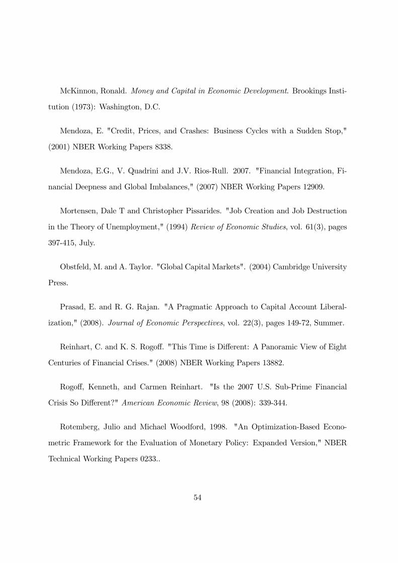
McKinnon, Ronald. Money and Capital in Economic Development. Brookings Insti-

tution (1973): Washington, D.C.

Mendoza, E. "Credit, Prices, and Crashes: Business Cycles with a Sudden Stop,"

(2001) NBER Working Papers 8338.

Mendoza, E.G., V. Quadrini and J.V. Rios-Rull. 2007. "Financial Integration, Fi-

nancial Deepness and Global Imbalances," (2007) NBER Working Papers 12909.

Mortensen, Dale T and Christopher Pissarides. "Job Creation and Job Destruction

in the Theory of Unemployment," (1994) Review of Economic Studies, vol. 61(3), pages

397-415, July.

Obstfeld, M. and A. Taylor. "Global Capital Markets". (2004) Cambridge University

Press.

Prasad, E. and R. G. Rajan. "A Pragmatic Approach to Capital Account Liberal-

ization," (2008). Journal of Economic Perspectives, vol. 22(3), pages 149-72, Summer.

Reinhart, C. and K. S. Rogo¤. "This Time is Di¤erent: A Panoramic View of Eight

Centuries of Financial Crises." (2008) NBER Working Papers 13882.

Rogo¤, Kenneth, and Carmen Reinhart. "Is the 2007 U.S. Sub-Prime Financial

Crisis So Di¤erent?" American Economic Review, 98 (2008): 339-344.

Rotemberg, Julio and Michael Woodford, 1998. "An Optimization-Based Econo-

metric Framework for the Evaluation of Monetary Policy: Expanded Version," NBER

Technical Working Papers 0233..

54

Syverson, C. "Market Structure and Productivity: A Concrete Example," Journal

of Political Economy, December 2004

Shaw, Edward. Financial Deepening and Economic Development. Oxford University

Press (1973): Oxford, UK.

Schmitt-Grohe, S. and M. Uribe, "Closing Small Open Economy Models," Journal

of International Economics, 61, October 2003, Pages 163-185 .

Shimer, R. "The Cyclical Behavior of Equilibrium Unemployment and Vacancies,"

(2005) American Economic Review, vol. 95(1), pages 25-49, March.

Tirole, J. The Theory of Corporate Finance, Chapter 16, Princeton University Press

(2006): Princeton, NJ.

Wright, M. "Private capital �ows, capital controls, and default risk", Journal of

International Economics, vol. 69 (2006): 120-149.

Woodford, M. "Public Debt as Private Liquidity," American Economic Review, 80,

(1990): 382-388.

Woodford, M. "Optimal Interest-Rate Smoothing," Review of Economic Studies, vol.

70(4), (2003).

55

0 0.1 0.2 0.3 0.4 0.5 0.6 0.7 0.8 0.9 10.95

1

1.05

1.1

1.15

θ̄

Figure 1: Interest rate and wages under autarky steady state

inte

rest

rat

e

0 0.1 0.2 0.3 0.4 0.5 0.6 0.7 0.8 0.9 10.95

1

1.05

1.1

1.15

1.2

domestic collateral factor

wag

es

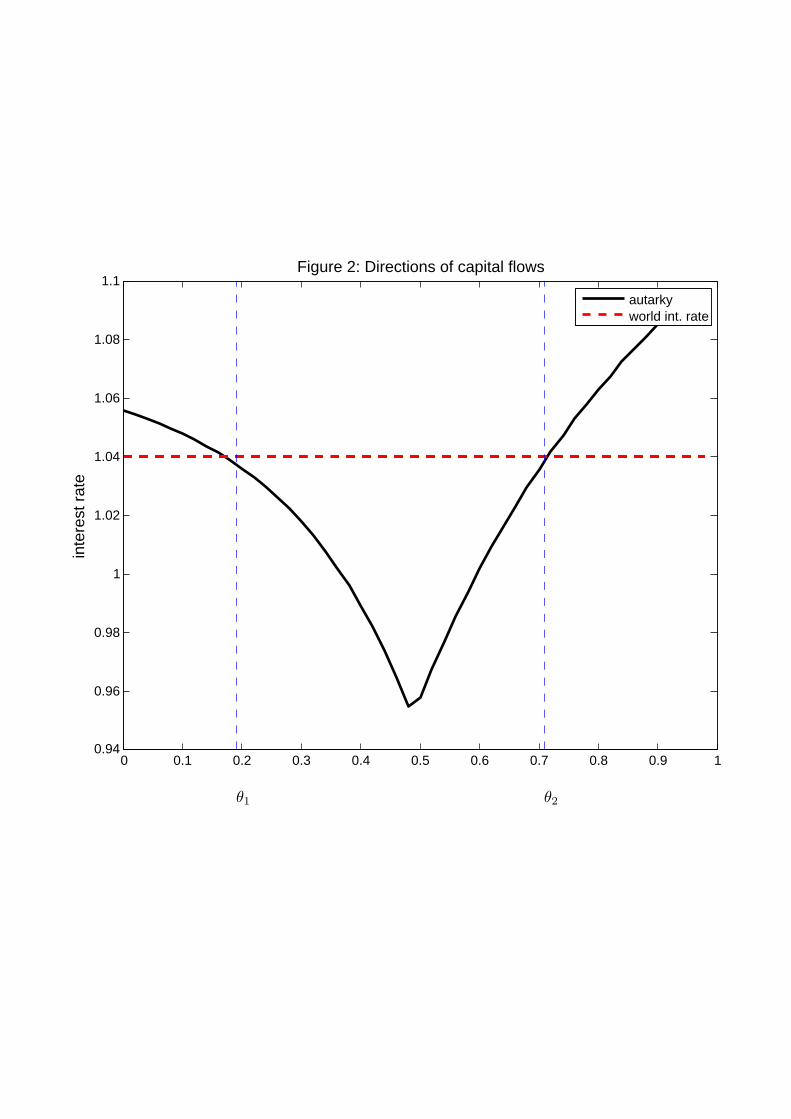
0 0.1 0.2 0.3 0.4 0.5 0.6 0.7 0.8 0.9 10.94

0.96

0.98

1

1.02

1.04

1.06

1.08

1.1

inte

rest

rat

e

Figure 2: Directions of capital flows

θ1 θ2

autarkyworld int. rate

−10 0 10 20 30 40 50 601.04

1.042

1.044

Figure 3.1: Dynamics under wage suppression: θ =0.15

inte

rest

rat

e

−10 0 10 20 30 40 50 60

1.006

1.008

1.01

wag

e

−10 0 10 20 30 40 50 601.1

1.12

1.14

outp

ut

−10 0 10 20 30 40 50 601.09

1.092

1.094

TF

P

time

−10 0 10 20 30 40 50 600.2

0.3

0.4

0.5

0.6

0.7

0.8

0.9

1

1.1

1.2Figure 3.2: Employment under wage suppression: θ =0.15

empl

oym

ent

time

productiveunproductivetotal

−10 0 10 20 30 40 50 601

1.02

1.04

Figure 4.1: Dynamics under interest−rate suppression: θ =0.3

inte

rest

rat

e

−10 0 10 20 30 40 50 601

1.02

1.04

wag

e

−10 0 10 20 30 40 50 601

1.2

1.4

outp

ut

−10 0 10 20 30 40 50 601.1

1.2

1.3

TF

P

time

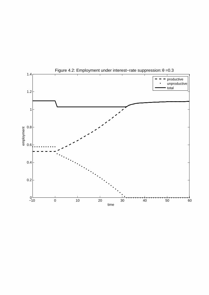
−10 0 10 20 30 40 50 600

0.2

0.4

0.6

0.8

1

1.2

1.4Figure 4.2: Employment under interest−rate suppression: θ =0.3

empl

oym

ent

time

productiveunproductivetotal

−10 0 10 20 30 40 50 601

1.05

1.1Figure 5.1: Dynamics under advanced domestic financyal system: θ =0.8

inte

rest

rat

e

−10 0 10 20 30 40 50 601.1

1.12

1.14

wag

e

−10 0 10 20 30 40 50 601.6

1.7

1.8

outp

ut

−10 0 10 20 30 40 50 600

2

4

TF

P

time

−10 0 10 20 30 40 50 600

0.5

1

1.5Figure 5.2: Employment under advanced domestic financyal system: θ =0.8

empl

oym

ent

time

productiveunproductivetotal

−10 0 10 20 30 40 50 600

0.2

0.4

0.6

0.8

1

1.2

1.4Figure 6 Adjustment with government policy: θ =0.3

empl

oym

ent

time

productive, benchmarkproductive with governmentunproductive, benchmarkunproductive with government

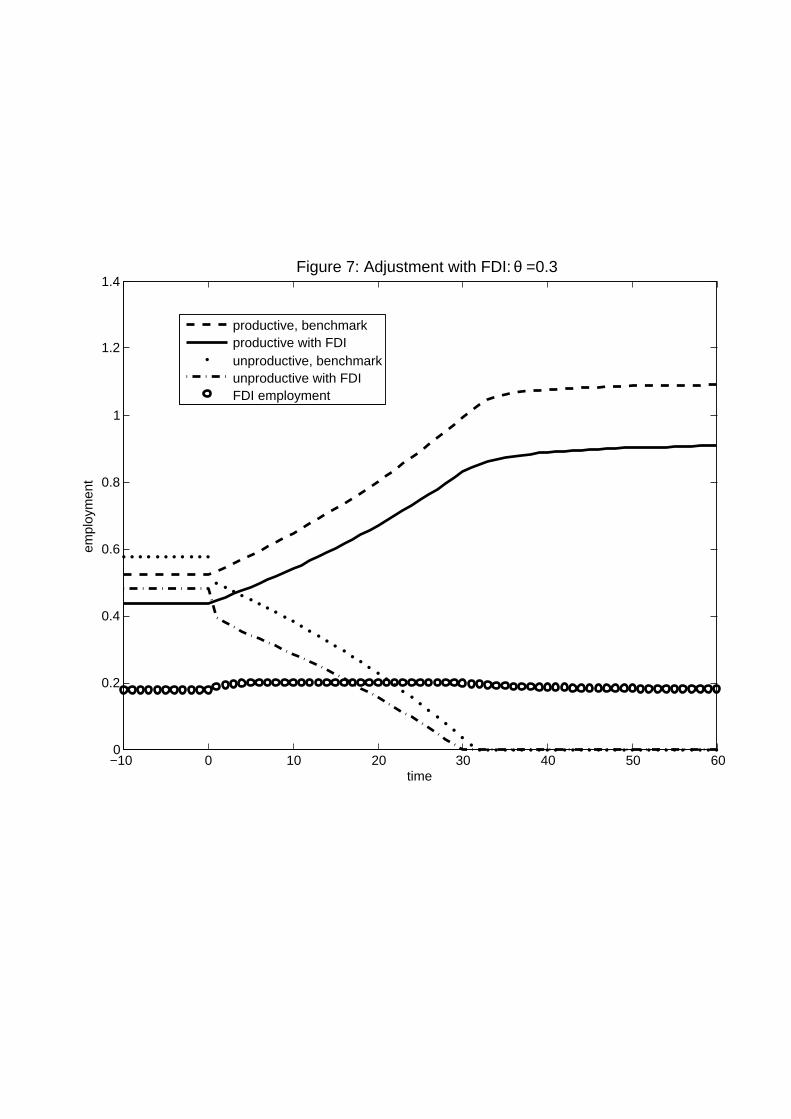
−10 0 10 20 30 40 50 600

0.2

0.4

0.6

0.8

1

1.2

1.4Figure 7: Adjustment with FDI: θ =0.3

empl

oym

ent

time

productive, benchmarkproductive with FDIunproductive, benchmarkunproductive with FDIFDI employment