adjusted functional boxplots for spatio-temporal data ... · outlier detection † ying suna and...

Special Issue Paper Environmetrics

Received: 5 January 2011, Revised: 30 August 2011, Accepted: 6 September 2011, Published online in Wiley Online Library: 24 October 2011

(wileyonlinelibrary.com) DOI: 10.1002/env.1136

Adjusted functional boxplots forspatio-temporal data visualization andoutlier detection†

Ying Suna and Marc G. Gentonb*

This article proposes a simulation-based method to adjust functional boxplots for correlations when visualizing functionaland spatio-temporal data, as well as detecting outliers. We start by investigating the relationship between the spatio-temporal dependence and the 1.5 times the 50% central region empirical outlier detection rule. Then, we propose tosimulate observations without outliers on the basis of a robust estimator of the covariance function of the data. We selectthe constant factor in the functional boxplot to control the probability of correctly detecting no outliers. Finally, we applythe selected factor to the functional boxplot of the original data. As applications, the factor selection procedure and theadjusted functional boxplots are demonstrated on sea surface temperatures, spatio-temporal precipitation and general cir-culation model (GCM) data. The outlier detection performance is also compared before and after the factor adjustment.Copyright © 2011 John Wiley & Sons, Ltd.

Keywords: functional data; GCM data; outlier detection; precipitation data; robust covariance; spatio-temporal data

1. INTRODUCTIONFunctional data analysis is an attractive approach to study complex data in statistics. In many statistical experiments, the observations arefunctions by nature, such as temporal curves or spatial surfaces, where the basic unit of information is the entire observed function ratherthan a string of numbers. There is also an interesting class of applications that can be characterized as random processes evolving in spaceand time in, for instance, environmental science, agriculture, climatology, meteorology and hydrology.

To analyze functional data, many model-based methods have been developed over the years, among which Ramsay and Silverman (2005)provided various parametric methods whereas Ferraty and Vieu (2006) developed detailed nonparametric techniques. For spatio-temporaldata, one can imagine a random field Z.s; t /, .s; t / 2 Rd � R, observed at the space-time coordinates .s1; t1/; : : : ; .sn; tn/. The spatio-temporal variable Z.s; t / could stand for temperature, precipitation, wind speed or atmospheric pollutant concentrations, to name a few.Some recent literature points out the significance of the spatio-temporal modeling approach; see for example Cressie and Wikle (2011) andreferences therein.

Visualization methods can also help to display the data, highlight their characteristics and reveal interesting features. Sun andGenton (2011) proposed an informative exploratory tool, the functional boxplot, and its generalization, the enhanced functionalboxplot, for visualizing functional data as well as detecting potential outliers. The functional boxplot orders functional data by meansof band depth (López-Pintado and Romo, 2009). It allows for ordering a sample of curves from the center outwards and, thus, introducesa measure to define the centrality or outlyingness of an observation. Indeed, one can compute the band depths of all the sample curves andorder them according to decreasing depth values. Suppose each observation is a real function yi .t/, i D 1; : : : ; n, t 2 I, where I is aninterval in R. Let yŒi�.t/ denote the sample curve associated with the i th largest band depth value. Then yŒ1�.t/; : : : ; yŒn�.t/ can be viewedas order statistics, with yŒ1�.t/ being the deepest (most central) curve or simply the median curve, and yŒn�.t/ being the most outlying curve.The implication is that a smaller rank is associated with a more central position with respect to the sample curves. The order statistics inducedby band depth start from the most central sample curve and move outwards in all directions. Thus, it is straightforward to define a centralregion for functional data. More specifically, López-Pintado and Romo (2009) defined the band depth through a graph-based approach. Thegraph of a function y.t/ is the subset of the plane G.y/ D f.t; y.t// W t 2 Ig. The band in R2 delimited by the curves yi1 ; : : : ; yik isB.yi1 ; : : : ; yik /D f.t; x.t// W t 2 I;minrD1;:::;k yir .t/ 6 x.t/ 6 maxrD1;:::;k yir .t/g. Let J be the number of curves determining a band,

* Correspondence to: Marc G. Genton, Department of Statistics, Texas A&M University, College Station, TX 77843-3143,USA. E-mail: [email protected]

a Statistical and Applied Mathematical Sciences Institute, 19 T.W. Alexander Drive, Research Triangle Park, NC 27709-4006, USA

b Department of Statistics, Texas A&M University, College Station, TX 77843-3143, USA

†This article is published in Environmetrics as a special issue on Spatio-Temporal Stochastic Modelling (METMAV), edited by Wenceslao González-Manteiga and RosaM. Crujeiras, University of Santiago de Compostela, Spain.

54

Environmetrics 2012; 23: 54–64 Copyright © 2011 John Wiley & Sons, Ltd.

ADJUSTED FUNCTIONAL BOXPLOTS Environmetrics

where J is a fixed value with 2 6 J 6 n. If Y1.t/; : : : ; Yn.t/ are independent copies of the stochastic process Y.t/ generating the observa-tions y1.t/; : : : ; yn.t/, the population version of the band depth for a given curve y.t/ with respect to the probability measure P is definedas BDJ .y; P /D

PJjD2 BD.j /.y; P /D

PJjD2 P fG.y/� B.Y1; : : : ; Yj /g, where B.Y1; : : : ; Yj / is a band delimited by j random curves.

The sample version of BD.j /.y; P / is defined as BD.j /n .y/ D�nj

��1P16i1<i2<��<ij6n I fG.y/ � B.yi1 ; : : : ; yij /g, where I f�g denotes

the indicator function. Then, the sample band depth of a curve y.t/ is BDn;J .y/DPJjD2 BD.j /n .y/. López-Pintado and Romo (2009) also

proposed a modified band depth that replaces the aforementioned indicator function by a function, which measures the proportion of timethat a curve y.t/ is in a band. This yields a more flexible ordering of the curves in the sample and tends to prevent depth ties.

In the classical boxplot, the box itself represents the middle 50% of the data. By analogy, the 50% central region in the functional boxplotcan be defined by extending the concept of central region introduced by Liu et al. (1999) to functional data. The band delimited by the ˛proportion (0 < ˛ < 1/ of deepest curves from the sample is used to estimate the ˛ central region. In particular, the sample 50% centralregion is

C0:5 D f.t; y.t// W minrD1;:::;dn=2e

yŒr�.t/6 y.t/6 maxrD1;:::;dn=2e

yŒr�.t/g;

wheredn=2e is the smallest integer not less than n=2. The envelope of the 50% central region represents the box in a classical boxplot and isthe analog to the “inter-quartile range” (IQR). It gives useful indication of the spread of the 50% most central curves.

For functional boxplots, based on the center outwards ordering induced by band depth for functional data, the descriptive statistics are:the envelope of the 50% central region, the median curve and the maximum non-outlying envelope. In addition, potential outliers can bedetected in a functional boxplot by the 1.5 times the 50% central region empirical rule, analogous to the rule for classical boxplots. The outerregion (the “fence”) is obtained by inflating the inner region (the “envelope”) by 1.5 times the height of the 50% central region. Any curvescrossing the fences are flagged as potential outliers.

Considering that when each curve is simply a point, the functional boxplot degenerates to a classical boxplot, Sun and Genton (2011)suggested the constant factor 1.5 as in a classical boxplot, but left to the user the possibility of modifying it. However, for functional data,there will be necessarily dependence in time for each curve. And for spatio-temporal data, curves from different locations will be spatiallycorrelated as well. The outlier detection performance may be affected by the dependence in time and space. Therefore, in this article, weinvestigate the relationship between the dependence and the constant factor, and then propose a method to adjust the factor in a functionalboxplot. This leads to an adjusted functional boxplot. Febrero et al. (2007, 2008) also considered outlier detection in functional data by depthmeasures but they did not account for the temporal or spatio-temporal correlation in the data and their method is quite different from thefunctional boxplot approach. In the finite dimensional case, Becker and Gather (1999, 2001) and Hubert et al. (2008) also discussed somemodel-based outlier detection rules for robust estimators.

Classical boxplots were first introduced by Tukey (1970) and Tukey (1977, pp. 39–43) in exploratory data analysis. In a classical boxplot,outliers can be detected by the 1.5 times IQR empirical rule. Here, the constant factor 1.5 can be justified by a standard normal distribution.Let Q1 and Q3 be the first and third quartiles of the standard normal distribution, respectively. The fences determined by L1 DQ1 � 1:5�IQR and L2 DQ3C 1:5� IQR are �2:698 and 2:698. Then, the probability of being detected as an outlier is 0.7%. If we change the factorto 2, then the probability that a value is an outlier is only 0.07%. Therefore, in the functional boxplot, we would like to adjust the value ofthe constant factor on the basis of the dependence such that the probability of detecting no outliers is 99.3%, when actually, no outliers arepresent. It is clear that in a functional boxplot, the factor adjustment is crucial for outlier detection because it determines the percentage ofdetected outliers. However, the adjustment involves a certain amount of computation, thus, it is not necessary if one only wants to visualizeand compare functional or spatio-temporal data.

This article is organized as follows. Section 2 illustrates how the dependence in time and space affects the outlier detection performanceof functional boxplots. Then, the new method to select the constant factor in a functional boxplot is proposed in Section 3. The adjustedfunctional boxplots are demonstrated on applications to space–time datasets in Section 4, and a discussion is provided in Section 5.

2. SIMULATION STUDIESTo illustrate how the dependence in time and space affects the outlier detection performance of the functional boxplots, simulation studiesare conducted under different spatio-temporal covariance models reviewed by Gneiting et al. (2007).

2.1. Data generation

We consider data drawn from a zero-mean, stationary spatio-temporal Gaussian random field Z.s; t /, where .s; t / 2 R2 � R. LetC.h; u/ D covfZ.s1; t1/; Z.s2; t2/g be the covariance function between any two observations whose locations are apart by a vectorh D s1 � s2 and a time span u D jt1 � t2j. Then, C.h; 0/ and C.0; u/ are purely spatial and purely temporal covariance functions,respectively. We aim at seeing how the strength of the correlation in time, in space, or in both, affects the outlier detection performance ofthe functional boxplot with the constant factor F D 1:5. We consider the following isotropic correlation models:

1. A purely temporal correlation function of Cauchy type,

CT .h; u/D .1C ajuj2˛/�1I fhD 0g; (1)

where ˛ 2 .0; 1� controls the strength of the temporal correlation, and a > 0 is the scale parameter in time. We set a D 1 and let ˛ varyfrom 0.1 to 0.9.

Environmetrics 2012; 23: 54–64 Copyright © 2011 John Wiley & Sons, Ltd. wileyonlinelibrary.com/journal/environmetrics

55

Environmetrics Y. SUN AND M. G. GENTON

2. A purely spatial correlation function of the form

CS .h; u/D Œ.1� �/ exp.�ckhk/C �I fhD 0g�I fuD 0g; (2)

where c > 0 controls the strength of the spatial correlation, and � 2 .0; 1� is a nugget effect. We set � D 0:05 and let c vary from 0.1 to 2.3. A space–time separable correlation function of the form

CSEP.h; u/D CS .h; 0/CT .0; u/; (3)

which is the product of the purely temporal correlation function (1) and the purely spatial correlation function (2). Here, we considercombinations of ˛ and c, where each has three levels, ˛ D 0:1; 0:5; 0:9 and c D 0:1; 1; 2.

4. A fully symmetric but generally non-separable correlation function

CFS.h; u/D1� �

1C ajuj2˛

�exp

��

ckhk

.1C ajuj2˛/ˇ=2

�C

�

1� �I fhD 0g

�; (4)

where 0 6 ˇ 6 1 controls the non-separability. It reduces to the separable model (3) when ˇ D 0. Here, we set ˇ D 1, the mostnon-separable version of this model, � D 0:05 and consider the same combinations of ˛ and c as in model (3).

5. A general stationary correlation model

CSTAT.h; u/D.1� �/.1� �/

1C ajuj2˛

�exp

��

ckhk

.1C ajuj2˛/ˇ=2

�C

�

1� �I fhD 0g

�C �

�1�

1

2vjh1 � vuj

C

; (5)

where qC D max.q; 0/ and h1 is the first component of the spatial separation vector h D .h1; h2/0. Here 0 6 � 6 1 controls the

asymmetry. Again, we set a D 1, ˇ D 1 and � D 0:05, then let � D 0:5, v D 0:05 and consider the same combinations of ˛ and c as inmodel (3).

The functional data Xi .t/ D Z.si ; t /, i D 1; : : : ; n, are generated without any outliers from Z.s; t / with each of the correlation modelsabove at nD 100 locations s1; : : : ; sn on a grid of size 10� 10 of the unit square with the grid spacing 1=9 and p D 50 equally spaced timepoints in Œ0; 1�. With 1,000 replications, we compute the proportion of times that functional boxplots with the constant factor F D 1:5 detectno outliers. Thus, a proportion much smaller than 1 is an indication of bad outlier detection performance.

2.2. Numerical results

Tables 1 and 2 summarize the simulation results. In the purely temporal model (1), the larger the value of ˛, the stronger the temporaldependence is when u < 1. For a fixed constant factor F D 1:5 in the functional boxplot, Table 1 shows that the proportion of times that thefunctional boxplot correctly detects no outliers decreases as ˛ increases. In other words, the stronger the correlation in time, the worse theoutlier detection performance is. Similarly, in the purely spatial model (2), the smaller the value of c, the stronger the spatial dependence is.For all the values of c in Table 1, the proportions of correctly detecting no outliers are close to 1. This is an evidence that the constant factor1.5 is too large when spatial correlation exists because usually, spatially correlated curves are more concentrated than independent ones.

Table 2 provides the proportion of times that a functional boxplot with the constant factor F D 1:5 correctly detects no outliers for eachcombination of ˛ and c under the separable, symmetric but non-separable and the general stationary spatial–temporal correlation models.It also shows that the proportion of correctly detecting no outliers decreases as ˛ or the temporal dependence increases. For each value of˛ under different correlation models, because the strongest spatial correlation (c D 0:1) makes curves most concentrated, with the fixedconstant factor F D 1:5 in functional boxplots, the proportions of correctly detecting no outliers for c D 0:1 are always the largest amongthose for c D 0:1; 1; 2. When the dependence in time is relatively large, ˛ D 0:5; 0:9, all the proportions under the separable correlationmodel are greater, hence better outlier detection performance, than those under either the symmetric but non-separable or the general sta-tionary correlation models. This suggests that the interaction or the separability between spatial and temporal dependence has an effect onthe outlier detection performance in a functional boxplot. To investigate the possible effect of the asymmetry in a correlation model, wecompare the proportion of a functional boxplot correctly detecting no outliers under the symmetric but non-separable and the general sta-tionary correlation models. When ˛ D 0:5; 0:9 and c D 1, the two proportions under the symmetric correlation model are larger than thoseunder the general stationary one. However, there are still several cases where the general stationary model shows a better outlier detectionperformance.

It is now clear that the adjustment of the constant factor in functional boxplots is necessary when spatio-temporal correlations exist. Next,we propose a method for selecting the factor F .

3. SELECTION OF THE ADJUSTMENT FACTORThe simulation studies in Section 2 have shown that the constant factor F D 1:5 gives different probability coverages under different spatio-temporal correlation models. In other words, we should choose the value of the factor F by controlling the probability of detecting nooutliers to be 99.3% when, actually, no outliers are present.

To demonstrate the performance of outlier detection in the adjusted functional boxplot, we consider three outlier models, whichhave been studied by Sun and Genton (2011) along with two covariance models from our simulation studies, the purely spatial covari-ance function (2) and the general stationary covariance function (5). For the purely spatial model, we set � D 0:05 and let c D 0:1. For the

56

wileyonlinelibrary.com/journal/environmetrics Copyright © 2011 John Wiley & Sons, Ltd. Environmetrics 2012; 23: 54–64


Table 1. The proportion of times (p) that a func-tional boxplot with the constant factor F D 1:5 cor-rectly detects no outliers under the purely temporaland the purely spatial correlation models with 1,000replications and nD 100 curves

Temporal ˛ 0.1 0.3 0.5 0.7 0.9p 0.998 0.974 0.938 0.839 0.745

Spatial c 0.1 0.5 1 1.5 2p 1 0.999 1 1 1

Table 2. The proportion of times that a functional boxplot with the constant factor F D 1:5correctly detects no outliers under the separable, symmetric but non-separable and the generalstationary spatio–temporal correlation models with 1,000 replications and nD 100 curves

Separable Symmetric Stationary

˛ c 0.1 1 2 0.1 1 2 0.1 1 2

0.1 1 0.997 0.993 0.995 0.990 0.994 0.995 0.994 0.9950.5 1 0.980 0.961 0.956 0.945 0.952 0.957 0.943 0.9500.9 1 0.942 0.908 0.901 0.854 0.836 0.900 0.833 0.844

general stationary model, we set a D 1, ˇ D 1 and � D 0:05, then let � D 0:5, v D 0:05 and consider the worst case in Table 2 where˛ D 0:9 and c D 1. The models with outlying curves are:

1. Model 1 includes a symmetric contamination: Yi .t/ D Xi .t/C ci�iK, where ci is 1 with probability 0.1 and 0 with probability 0.9, Kis a contamination size constant, which is equal to 2 for the purely spatial covariance model and 6 for the general stationary model. �i isa sequence of random variables independent of ci taking values 1 and �1 with probability 1/2;

2. Model 2 is partially contaminated: Yi .t/ D Xi .t/ C ci�iK, if t > Ti and Yi .t/ D Xi .t/, if t < Ti , where Ti is a random numbergenerated from a uniform distribution on Œ0; 1�;

3. Model 3 is contaminated by peaks: Yi .t/D Xi .t/C ci�iK, if Ti 6 t 6 Ti C `, and Yi .t/D Xi .t/ otherwise, where Ti is random froma uniform distribution on Œ0; 1� `� and `D 3=49.

Under the purely spatial covariance model (2), the selected adjustment factor is F D 1:0, whereas F D 2:2 for the general stationary model.To compare with the functional boxplots without adjustment, we consider the distributions of two quantities in Sun and Genton (2011): pc ,the percentage of correctly detected outliers (number of correctly detected outliers divided by the total number of outlying curves), and pf ,the percentage of falsely detected outliers (number of falsely detected outliers divided by the total number of non-outlying curves). Thesimulation results are summarized in Table 3. For the purely spatial covariance model, the adjusted functional boxplots improve the outlierdetection performance by keeping a low false detection rate Opf , whereas increasing the correct detection rate Opc , owing to the smalleradjustment factor F D 1:0 < 1:5. For the general stationary covariance model, the outlier detection performance is improved in the adjustedfunctional boxplots by keeping a high correct detection rate Opc , whereas reducing the false detection rate Opf , owing to the larger adjustmentfactor F D 2:2 > 1:5.

Sharing the same idea as in the simulations, we propose first to estimate the covariance matrix of the data to generate observations withoutany outliers. Then we use the simulations described in Section 2 to choose the constant factor F such that the proportion of times that afunctional boxplot detects no outliers is 99.3%. Finally, we apply this adjusted factor to the functional boxplot on the original data anddetect outliers. When estimating the covariance matrix, robust techniques are needed because outliers may exist in the original data. We usea componentwise estimator of a dispersion matrix proposed by Ma and Genton (2001), on the basis of a highly robust estimator of scale,Qn. This estimator is location-free and has already been successfully used in the context of variogram estimation (Genton, 1998) in spatialstatistics, and autocovariance estimation (Ma and Genton, 2000) in time series. Ma and Genton (2001) only studied the robust estimatorwhen the sample size n > p, but the robust estimator can be also computed for n 6 p because the dispersion matrix is estimated compo-nentwisely. There are also many other robust estimators that could be used; some of which are based on the minimization of a robust scaleof Mahalanobis distances. For example, the minimum volume ellipsoid and minimum covariance determinant estimators (Rousseeuw, 1984,1985). However, their computation can be challenging. Alternatively, a more rapid orthogonalized Gnanadesikan–Kettenring estimator wasproposed by Maronna and Zamar (2002) for high dimensional datasets.

To reduce the computational burden and simplify the covariance matrix estimation, we only generate a small number of curves, nD 100,without any outliers at p time points from the model Z.s; t / D g.s; t / C e.s; t /, with mean g.s; t / D 0, .s; t / 2 R2 � R. Here, e.s; t /


57


Table 3. The mean and standard deviation (in the parentheses) of the percentage Opc and Opf for the functional boxplots, theadjusted functional boxplots under the purely spatial and the general stationary covariance models with 1,000 replications,100 curves for models 1, 2, and 3

Spatial Model 1 Model 2 Model 3F D 1:5 F D 1:0 F D 1:5 F D 1:0 F D 1:5 F D 1:0

Opc 99.9(0.7) 100(0) 85.6(13.9) 96.8(6.6) 34.3(18.3) 75.0(17.6)Opf 0(0) 0.006(0.085) 0(0) 0.003(0.060) 0(0) 0(0)

Stationary Model 1 Model 2 Model 3F D 1:5 F D 2:2 F D 1:5 F D 2:2 F D 1:5 F D 2:2

Opc 100(0) 100(0) 88.2(13.3) 88.2(13.3) 99.9(1.0) 99.7(2.5)Opf 0.143(0.582) 0.012(0.153) 0.146(0.572) 0.007(0.085) 0.001(0.036) 0(0)

is a Gaussian random field with mean zero and covariance function estimated from the standardized original data, hence with marginalvariance 1. For simplicity, we let the trend g.s; t / be 0 and the marginal variance be 1 because they do not affect the values of band depth,hence, the order of these curves. In addition, for spatio-temporal data, to reduce the dimension of the spatio-temporal covariance, we onlyestimate the covariances at certain distances and time lags depending on the simulation design.

4. APPLICATIONS4.1. Sea surface temperatures

A dataset of monthly sea surface temperatures measured in degrees Celsius over the east-central tropical Pacific Ocean was used byHyndman and Shang (2010) and Sun and Genton (2011) to demonstrate the functional bagplot and the functional boxplot, respectively.In this case, each curve represents one year of observed sea surface temperatures from January 1951 to December 2007. The functionalboxplot with the constant factor F D 1:5 in Sun and Genton (2011) detected two potential outliers: the years 1983 and 1997. In addition,the year 1982 from September to December and the year 1998 from January to June were viewed as being part of the maximum envelope.These 57 annual temperature curves show similarity in shape because they share a common mean function. Therefore, we detrend themfirst by subtracting the sample median at each time point and then check the correlations between the curves. Because the correlations arenot statistically significant, we assume that these annual temperature curves are independent copies of each other and estimated the 12� 12covariance matrix in time. In simulations, by generating n D 100 curves at p D 12 time points from a Gaussian process with zero meanand estimated covariance function, the coverage probabilities for different values of the constant factor are listed in Table 4 with 1,000replications. We select the constant factor to be 1.8 because when F D 1:8, the coverage probability is 0.995, close to 99.3%. After adjustingthe constant factor, the functional boxplot still detects two El Niño years as outlier candidates.

4.2. Spatio-temporal precipitation

The functional boxplot can summarize information from complex data, such as space–time datasets. Sun and Genton (2011) illustrated thisaspect by visualizing the observed annual total precipitation data for the coterminous US from 1895 to 1997, provided by the Institute forMathematics Applied to Geosciences (http://www.image.ucar.edu/Data/US.monthly.met/ ). There are 11,918 stations reporting precipitationat some time in this period. The observations are time series with p D 103 yearly precipitation observations, or one curve, at each spatiallocation. Functional boxplots were applied to nine climatic regions for precipitation in the US, defined by the National Climatic Data Centerand the percentages of detected potential outliers for each region were reported. Sun and Genton (2011) noticed that for spatio-temporal data,the precipitation curves are not independent but spatially correlated. Therefore, the percentages of potential outliers might not be correctbecause of the spatial correlations.

By taking the spatio-temporal correlation into account, we adjust the constant factor in the functional boxplots again by simulations. Foreach climatic region, in the simulation, we generate spatio-temporal data from a zero-mean Gaussian random field at nD 100 locations on a

Table 4. The coverage probabilities for different values of the constant factor Fwith nD 100 curves at p D 12 time points and 1,000 replications in simulations forthe sea surface temperatures example

Factor F 1.2 1.3 1.4 1.5 1.6 1.7 1.8 1.9 2.0Coverage 0.768 0.859 0.922 0.956 0.979 0.988 0.995 1.000 1.000

Note: The selected factor is in bold font.

58



grid of size 10� 10 with the grid spacing 1/9 at p D 30 time points. Here, the distance unit is kilometer and the time unit is year. Then, weestimate the 3; 000� 3; 000 covariance matrix from the standardized original data and obtain the coverage probabilities for different valuesof the constant factor with 1,000 replications. The results are summarized for each region in Table 5. Each component of the 3; 000� 3; 000covariance matrix is estimated by the Qn-based procedure of Ma and Genton (2001). To reduce the computational effort, for each combi-nation of time lag and distance, we estimate the covariance element by randomly selecting pairs of the irregularly spaced locations that areclose to the distances on the 10� 10 grid under the assumption of stationarity.

With the concept of central regions, Sun and Genton (2011) generalized the functional boxplot to an enhanced functional boxplot wherethe 25% and 75% central regions are provided as well in addition to the 50% central region. For the spatio-temporal precipitation data, thenine adjusted enhanced functional boxplots in Figure 1 can still reveal information about the different annual precipitation characteristicsfor different climatic regions, but with less potential outliers than previously detected by Sun and Genton (2011). The percentage of detectedoutliers for each region is summarized in Table 6.

4.3. General circulation model

A general circulation model (GCM) is a climate model of the general circulation of a planetary atmosphere or ocean. It uses complex com-puter programs to simulate the earth’s climate system and allows us to look into the earth’s past, present and future climate states. Here, weconsider precipitation data generated from the National Center for Atmospheric Research-Community Climate System Model Version 3.0(Collins et al., 2006, and references therein), which was run given scenarios from the Intergovernmental Panel on Climate Change (IPCC)’sSpecial Report on Emission Scenarios; see IPCC (2000) and Ammann et al. (2010). Functional boxplots can be used to visually comparethe annual precipitation produced by the GCM with the real observations from weather stations considered in the previous section.

For these GCM data, there are 256�128 cells over the whole globe with a resolution of 1:406�1:406 degrees, or around 156�156 km. Theobservations from weather stations are much denser, but only for the coterminous US. To make the weather station observations comparableto the GCM data, we match them by longitude and latitude first, and then average the observations from weather stations within each cell,which leads to 473 cells in total, hence 473 annual precipitation curves for the coterminous US.

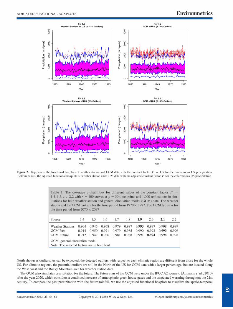
For the coterminous US precipitation, the functional boxplots with the constant factor F D 1:5 for weather station and GCM data areshown in the top panel of Figure 2 with the percentage of detected outliers. Now, we estimate the 3; 000� 3; 000 spatio-temporal covariancematrix from the standardized original data by the same simulation design as in Section 4.2 and the coverage probabilities for different valuesof the constant factor with 1,000 replications are summarized in Table 7 for both weather station and GCM data. The adjusted functionalboxplots with percentage of detected outliers are shown in the bottom panel of Figure 2.

Figure 2 shows that the precipitation data produced by the GCM roughly capture the overall pattern of the US precipitation. The twofunctional boxplots of weather station and GCM data coincide on the median curves, and the maximum annual precipitation for some wetlocations is also on the same level. However, the narrower 50% central region in the functional boxplot of the GCM data indicates that thefirst 50% most representative precipitation curves have less variability, which leads to a relatively large percentage of outliers. Moreover, bothfunctional boxplots are skewed to the right (i.e., to large precipitation), but the one for GCM does not produce as low annual precipitation asthe real observations from weather stations for some dry locations.

The maps of weather station and GCM data where outliers are detected by the adjusted functional boxplots with respect to either the wholeUS or each of the climatic regions are shown in Figure 3. For the whole US, the outliers, denoted by red plus signs, are around the North ofthe US for GCM data, but the only one outlier detected by the functional boxplot is located at the North West for weather station data. The

Table 5. The coverage probabilities for different values of the constant factorF D 1:4; 1:5; : : : ; 2:2 with n D 100 curves at p D 30 time points and 1,000replications in simulations for the precipitation application

Region 1.4 1.5 1.6 1.7 1.8 1.9 2.0 2.1 2.2

NE 0.927 0.951 0.971 0.985 0.987 0.993 0.994 0.995 0.996ENC 0.896 0.941 0.958 0.972 0.985 0.989 0.993 0.994 0.995C 0.926 0.951 0.970 0.984 0.988 0.994 0.995 1.000 1.000SE 0.926 0.948 0.974 0.979 0.988 0.993 0.996 0.999 1.000WNC 0.893 0.944 0.966 0.973 0.984 0.990 0.992 0.995 0.996S 0.902 0.934 0.959 0.976 0.983 0.987 0.989 0.993 0.994SW 0.920 0.948 0.972 0.979 0.987 0.992 0.993 0.995 0.995NW 0.911 0.939 0.962 0.974 0.983 0.987 0.992 0.993 0.995W 0.911 0.949 0.974 0.988 0.993 0.994 0.996 0.999 0.999

NE, North East; ENC, East North Central; C, Central; SE, South East; WNC,West North Central; S, South; SW, South West; NW, North West; and W, West.The selected factors are in bold font.


59


North East (0.14% Outliers)P

reci

pita

tion

(mm

/yea

r)East North Central (0% Outliers) Central (0.12% Outliers)

South East (1.57% Outliers)

Pre

cipi

tatio

n (m

m/y

ear)

West North Central (1.09% Outliers) South (0% Outliers)

South West (1.41% Outliers)

Year

Pre

cipi

tatio

n (m

m/y

ear)

North West (0.2% Outliers)

Year

West (1.72% Outliers)

Year

1895 1920 1945 1970 1995

010

0020

0030

0040

000

1000

2000

3000

4000

010

0020

0030

0040

00

1895 1920 1945 1970 1995

1895 1920 1945 1970 1995

010

0020

0030

0040

000

1000

2000

3000

4000

010

0020

0030

0040

00

010

0020

0030

0040

000

1000

2000

3000

4000

010

0020

0030

0040

00

1895 1920 1945 1970 1995

1895 1920 1945 1970 1995

1895 1920 1945 1970 1995

1895 1920 1945 1970 1995

1895 1920 1945 1970 1995

1895 1920 1945 1970 1995

Figure 1. Adjusted enhanced functional boxplots of observed yearly precipitation over the nine climatic regions for the coterminous US from 1895 to 1997.Dark magenta, magenta and pink denote the 25%, 50% and 75% central regions, respectively, and the outlier rule is the adjusted constant factor times the 50%

central region. The percentage of detected outliers in each climatic region is provided.

Table 6. Comparison of outlier detection percentages for each cli-matic region before and after adjustment of the constant factor

Region NE ENC C SE WNC S SW NW WBefore 0.21 0 0.25 2.52 2.04 0 3.03 2.13 4.04After 0.14 0 0.12 1.57 1.09 0 1.41 0.20 1.72

NE, North East; ENC, East North Central; C, Central; SE, South East;WNC, West North Central; S, South; SW, South West; NW, NorthWest; and W, West.

maps also show that the precipitation data produced by GCM do not capture the characteristics of the observed precipitation from weatherstations well. From weather stations, the West of the US overall has a lower precipitation than the East, and the higher precipitation locationsare along the west coast and the South East. This pattern is hard to see from the GCM, and the higher precipitation locations appear in the

60



Year

Pre

cipi

tatio

n (m

m/y

ear)

F= 1.5 Weather Stations of U.S. (0.21% Outliers)

Year

Pre

cipi

tatio

n (m

m/y

ear)

F= 1.5 GCM of U.S. (3.17% Outliers)

Year

Pre

cipi

tatio

n (m

m/y

ear)

F= 1.9 Weather Stations of U.S. (0% Outliers)

Year

Pre

cipi

tatio

n (m

m/y

ear)

F= 2.1 GCM of U.S. (2.11% Outliers)

1895 1920 1945 1970 1995

010

0020

0030

0040

00

1895 1920 1945 1970 1995

010

0020

0030

0040

00

010

0020

0030

0040

000

1000

2000

3000

4000

1895 1920 1945 1970 1995

1895 1920 1945 1970 1995

Figure 2. Top panels: the functional boxplots of weather station and GCM data with the constant factor F D 1:5 for the coterminous US precipitation.Bottom panels: the adjusted functional boxplots of weather station and GCM data with the adjusted constant factor F for the coterminous US precipitation.

Table 7. The coverage probabilities for different values of the constant factor F D

1:4; 1:5; : : : ; 2:2 with nD 100 curves at p D 30 time points and 1,000 replications in sim-ulations for both weather station and general circulation model (GCM) data. The weatherstation and the GCM past are for the time period from 1970 to 1997. The GCM future is forthe time period from 2070 to 2097

Source 1.4 1.5 1.6 1.7 1.8 1.9 2.0 2.1 2.2

Weather Stations 0.904 0.945 0.968 0.979 0.987 0.993 0.997 0.998 0.999GCM Past 0.914 0.950 0.971 0.979 0.985 0.990 0.992 0.993 0.996GCM Future 0.912 0.947 0.966 0.981 0.988 0.991 0.994 0.998 0.998

GCM, general circulation model.Note: The selected factors are in bold font.

North shown as outliers. As can be expected, the detected outliers with respect to each climatic region are different from those for the wholeUS. For climatic regions, the potential outliers are still in the North of the US for GCM data with a larger percentage, but are located alongthe West coast and the Rocky Mountain area for weather station data.

The GCM also simulates precipitation for the future. The future runs of the GCM were under the IPCC A2 scenario (Ammann et al., 2010)after the year 2020, which considers a continued increase of atmospheric green house gases and the associated warming throughout the 21stcentury. To compare the past precipitation with the future rainfall, we use the adjusted functional boxplots to visualize the spatio-temporal


61


0

1000

2000

3000

4000

F= 1.5Weather Stations of U.S. (0.21% Outliers)

0

1000

2000

3000

4000

F= 1.5GCM of U.S. (3.17% Outliers)

0

1000

2000

3000

4000

F= 1.9Weather Stations of U.S. (0% Outliers)

0

1000

2000

3000

4000

F= 2.1GCM of U.S. (2.11% Outliers)

0

1000

2000

3000

4000

Different F for Each Climatic RegionWeather Stations of U.S. (1.69% Outliers)

0

1000

2000

3000

4000

Different F for Each Climatic RegionGCM of U.S. (5.71% Outliers)

−120 −110 −100 −90 −80 −70

2025

3035

4045

5055

−120 −110 −100 −90 −80 −70

2025

3035

4045

5055

−120 −110 −100 −90 −80 −70

2025

3035

4045

5055

−120 −110 −100 −90 −80 −70

2025

3035

4045

5055

−120 −110 −100 −90 −80 −70

2025

3035

4045

5055

−120 −110 −100 −90 −80 −70

2025

3035

4045

5055

Figure 3. Top panels: the maps of weather station and general circulation model (GCM) data where outliers are detected by the functional boxplots with theconstant factor F D 1:5 for the coterminous US precipitation. Middle panels: the maps of weather station and GCM data where outliers are detected by theadjusted functional boxplots for the coterminous US precipitation. Bottom panels: the maps of weather station and GCM data where outliers are detected bythe adjusted functional boxplots for each climatic region. The colors of each cell denote the averaged annual precipitation (mm/year) and the red plus signs

indicate the detected outliers.

precipitation for the time period from 1970 to 1997 and for the future period from 2070 to 2097. For the past, the functional boxplots ofweather station and GCM data are shown in the top and middle panels of Figure 4. The bottom panels of Figure 4 show the functionalboxplots of GCM data for the future. The future runs of the GCM produce a little wider 50% central region than the past runs do, thus asmaller outlier percentage, but both have narrower 50% central regions hence larger outlier percentages compared with the weather stationdata. We can also see that the median curves of the past and future runs from GCM are higher than that from weather stations, and theminimum precipitation is also higher than the real observations.

5. DISCUSSIONThis article has focused on how to adjust the functional boxplot proposed by Sun and Genton (2011) for correlations to perform functionaland spatio-temporal data visualization and outlier detection. In a functional boxplot, potential outliers can be detected by the 1.5 times the50% central region empirical rule, analogous to the rule for classical boxplots. However, for functional data, there is necessarily dependencein time for each curve. And for spatio-temporal data, curves from different locations are spatially correlated as well. The simulation studiesin Section 2 showed that the outlier detection performance is obviously affected by the dependence in time and space. Therefore, to correctthe outlier detection performance, the constant factor of the empirical outlier rule is important. The factor F D 1:5 in a classical boxplot canbe justified by a standard normal distribution, because it leads to a probability of 99.3% for correctly detecting no outliers. Following this

62



Pre

cipi

tatio

n (m

m/y

ear)

F= 1.5 Weather Stations 1970−1997 (0% Outliers)

Pre

cipi

tatio

n (m

m/y

ear)

F= 1.9 Weather Stations 1970−1997 (0% Outliers)

Pre

cipi

tatio

n (m

m/y

ear)

F= 1.5 GCM 1970−1997 (3.17% Outliers)

Pre

cipi

tatio

n (m

m/y

ear)

F= 2.1 GCM 1970−1997 (2.11% Outliers)

Year

Pre

cipi

tatio

n (m

m/y

ear)

F=1.5GCM 2070−2097 (2.11% Outliers)

Year

Pre

cipi

tatio

n (m

m/y

ear)

F=2.0GCM 2070−2097 (0.42% Outliers)

1970 1975 1980 1985 1990 1995

010

0020

0030

0040

00

1970 1975 1980 1985 1990 1995

010

0020

0030

0040

00

2070 2075 2080 2085

010

0020

0030

0040

00

1970 1975 1980 1985 1990 1995

010

0020

0030

0040

00

2070 2075 2080 2085

010

0020

0030

0040

00

1970 1975 1980 1985 1990 1995

010

0020

0030

0040

00

Figure 4. Top panels: the functional boxplot and the adjusted functional boxplot of weather station data for the coterminous US precipitation from 1970 to1997. Middle panels: the functional boxplot and the adjusted functional boxplot of general circulation model (GCM) data for the coterminous US precipitationfrom 1970 to 1997. Bottom panels: the functional boxplot and the adjusted functional boxplot of GCM data for the coterminous US precipitation from 2070

to 2097 under Intergovernmental Panel on Climate Change A2 scenario.

idea, we proposed a simulation-based method to select this constant factor for a functional boxplot by controlling the probability of detectingno outliers to be 99.3% when actually no outliers are present. Then, how to estimate the covariance function, especially for spatio-temporaldata, is also important, and robust techniques are needed when considering the potential presence of outliers in the original data.

As applications, we used our method to adjust the functional boxplots for sea surface temperatures, spatio-temporal precipitation andGCM data. In fact, all the selected factors were greater than 1.5, which agrees with the simulation results in Section 2. The interpretation is


63


that a positive correlation leads to a larger variability, therefore, the extreme observations may not be outliers but may be due to the positivecorrelation in time and space.

For spatio-temporal data, we have viewed the information as a temporal curve at each spatial location. Sun and Genton (2011) also pro-posed an alternative to treat such data as a spatial surface at each time. In this case, it would lead to a three-dimensional surface boxplotwith similar characteristics as the functional boxplots. Similarly, for outlier detection, the fences are obtained by the 1.5 times the 50%central region rule. Any surfaces crossing the fences are flagged as outlier candidates. Therefore, for the surface functional boxplot in R3,the constant factor can be also adjusted by the simulation-based method described in this article and leads to an adjusted surface functionalboxplot.

AcknowledgementsThis research was partially supported by NSF grants DMS-1007504, DMS-1100492, and Award No. KUS-C1-016-04, made by KingAbdullah University of Science and Technology (KAUST). The authors thank the Guest Editor, two referees and Noel Cressie for helpfulcomments, as well as Caspar M. Ammann for providing the GCM data.

REFERENCES

Ammann CM, Washington WM, Meehl GA, Buja L, Teng H. 2010. Climate engineering through artificial enhancement of natural forcings: magnitudes andimplied consequences. Journal of Geophysical Research 115: D22109. DOI:10.1029/2009JD012878.

Becker C, Gather U. 1999. The masking breakdown point of multivariate outlier identification rules. Journal of the American Statistical Association 94:947–955.

Becker C, Gather U. 2001. The largest nonindentifiable outlier: a comparison of multivariate simultaneous outlier identification rules. Computational Statistics& Data Analysis 36: 119–127.

Collins WD, et al. 2006. The community climate system model version 3 (CCSM3). Journal of Climate 19: 2122–2143. DOI: 10.1175/JCLI3761.1.Cressie N, Wikle C. 2011. Statistics for Spatio-Temporal Data. Wiley: New York.Febrero M, Galeano P, González-Manteiga W. 2007. Functional analysis of NOx levels: location and scale estimation and outlier detection. Computational

Statistics 22: 411–427.Febrero M, Galeano P, González-Manteiga W. 2008. Outlier detection in functional data by depth measures, with application to identify abnormal NOx levels.

Environmetrics 19: 331–345.Ferraty F, Vieu P. 2006. Nonparametric Functional Data Analysis: Theory and Practice. Springer-Verlag: New York.Genton MG. 1998. Highly robust variogram estimation. Mathematical Geology 30: 213–221.Gneiting T, Genton MG, Guttorp P. 2007. Geostatistical space-time models, stationarity, separability and full symmetry. In Statistics of Spatio-Temporal

Systems, Finkenstaedt B, Held L, Isham V (eds). Chapman & Hall/CRC Press; 151–175.Hubert M, Rousseeuw PJ, Van Aelst S. 2008. High-breakdown robust multivariate methods. Statistical Science 23: 92–119.Hyndman RJ, Shang HL. 2010. Rainbow plots, bagplots, and boxplots for functional data. Journal of Computational and Graphical Statistics 19: 29–45.Intergovernmental Panel on Climate Change (IPCC). 2000. Special report on emission scenarios. In A special report of Working Group III of the

Intergovernmental Panel on Climate Change, Nakicenovic N, Swart R (eds). Cambridge Univ. Press: Cambridge, U.K; 612.Liu RY, Parelius JM, Singh K. 1999. Multivariate analysis by data depth: descriptive statistics, graphics and inference. Annals of Statistics 27: 783–858.López-Pintado S, Romo J. 2009. On the concept of depth for functional data. Journal of the American Statistical Association 104: 718–734.Ma Y, Genton MG. 2000. Highly robust estimation of the autocovariance function. Journal of Time Series Analysis 21: 663–684.Ma Y, Genton MG. 2001. Highly robust estimation of dispersion matrices. Journal of Multivariate Analysis 78: 11–36.Maronna RA, Zamar RH. 2002. Robust estimates of location and dispersion for high-dimensional datasets. Technometrics 50: 295–304.Ramsay JO, Silverman BW. 2005. Functional Data Analysis, 2nd ed. Springer: New York.Rousseeuw PJ. 1984. Least median of squares regression. Journal of the American Statistical Association 79: 871–881.Rousseeuw PJ. 1985. Multivariate estimation with high breakdown point. In Mathematical Statistics and Applications, Vol. B, Maddala GS, Rao CR (eds).

Elsevier: Amsterdam; 101–121.Sun Y, Genton MG. 2011. Functional boxplots. Journal of Computational and Graphical Statistics 20: 316–334.Tukey JW. 1970. Exploratory Data Analysis. (Limited Preliminary Edition), Vol. 1, Ch. 5. Addison-Wesley: Reading, MA.Tukey JW. 1977. Exploratory Data Analysis. Addison-Wesley: Reading, MA.

64


adjusted functional boxplots for spatio-temporal data ... · outlier detection † ying suna and...

Documents