D-1

A P P E N D I X D

Additional Performance Measure Discussion and Analysis Procedures

This appendix includes additional discussion and more detailed information about truck bottleneck performance measures and analysis procedures. More specifically, this appendix contains the following four 4) sections with additional details. • Section D.1. Additional Discussion of Performance Measures; • Section D.2. Calculation Procedures for Texas DOT 100 Most Congested Roadways List; • Section D.3. General Calculation Procedures for Truck Bottleneck Analysis; and • Section D.4. Calculation Procedures for Maryland State Highway Administration Freight Fluidity.

D.1 Additional Discussion of Performance Measures The information in this section has been adapted from previous work performed for FHWA on truck

bottleneck analysis methods. (85) Chapter 5 provided information on recommended measures for bottleneck identification and quantification. Below is more detail on these measures as well as additional measures that may be of interest to the analyst.

Congestion and Reliability Measures

For congestion and reliability, performance measures based on travel time are used. The following measures for congestion and reliability can be used for all types of highways. Additionally, they can be calculated only for trucks or for all vehicles. • Total Delay (vehicle-hours and person-hours). Actual vehicle-hours (or person-hours) experienced

in the highway section minus the vehicle-hours (or person-hours) that would be experienced at the reference speed. Total delay is only possible to compute if traffic volumes have been integrated. If not, unit delay (delay per vehicle) is substituted.

• Mean Travel Time Index (MTTI). A dimensionless ratio of the mean travel time over the highway section divided by the travel time that would occur at the reference speed.

• Planning Time Index (PTI). A dimensionless ratio of the 95th percentile travel time to the uncongested travel time.

• 80th Percentile Travel-Time Index (PTI80). A dimensionless ratio of the 80th percentile travel time to the uncongested travel time. (Some wonder why there is a need for both the PTI (based on 95th percentile) and the PTI80. Recent SHRP 2 Research L03 (“Analytical Procedures for Determining the Impacts of Reliability Mitigation Strategies”) found that the PTI (based on 95th percentile) may be too extreme a value to be influenced significantly by operations strategies, but the PTI80 was more sensitive to these improvements. For this reason, both measures are meaningful reliability measures to include. The full report is available here: http://onlinepubs.trb.org/onlinepubs/shrp2/SHRP2_S2-L03-RR-1.pdf.)

D-2

Second Order Performance Measures

Second order performance measures are those that emerge as a direct result of changes in congestion and reliability. They are most commonly used to estimate impacts of bottlenecks and the benefits of improving them. Potential measures to consider are: • Delay Cost. This is the monetized value of delay. It is computed separately for passenger cars and

trucks using the following formulas.

Annual Passenger Vehicle Delay Cost = Annual Passenger Vehicle-Hours of Delay × Value of Person Time × Vehicle Occupancy Annual Commercial Cost = Annual Commercial Vehicle-Hours of Delay × Value of Commercial Time

Where: the annual vehicle-hours of delay is Total Delay above, broken out by passenger and commercial (trucks).

• Reliability Cost. In addition to the cost of typical delay, studies have shown that highway users also

value reliability, or the variability in travel conditions. The valuation of reliability is not nearly as well treated in the literature as that for typical delay. Further, reliability valuation for personal travel has been studied more than for freight travel. One recent study developed a method for computing both typical and reliability portions of congestion costs by using a “travel-time equivalent approach”: (83)

TTIe(VT) = TTI50 + a * (TTI80—TTI50) Where:

TTIe(VT) is the TTI equivalent on the segment, computed separately for passenger cars (personal travel) and trucks (commercial travel);

TTI50 is the median TTI;

TTI80 is the 80th percentile TTI (PTI80); and

a is the Reliability Ratio (VOR/VOT)

= 0.8 for passenger cars

= 1.1 for trucks

• The Reliability Ratio (Value of Reliability/Value of Typical Time) of 1.1 suggests that freight interests value reliability slightly more than typical travel time. In this method, a total equivalent annual weekday delay is computed as a function of TTIe(VT) and a subsequent reliability cost is estimated from the difference between the total delay cost and the recurring delay cost. More details are available elsewhere. See footnote 74. The topic of reliability cost is still evolving. There is no agreed upon methodology for valuing reliability as of this writing. Users are free to incorporate the value of reliability in their analyses but should clearly document the assumptions.

• Fuel Cost is estimated using a simple formula based on fuel efficiency. Alternately, it can be calculated by estimating travel speeds, using a simple linear equation to estimate fuel economy for that speed and applying values to the difference between travel time and fuel consumption in congested versus uncongested conditions. The process is evolving, and the new EPA emissions model (MOVES) has an improved fuel economy algorithm that can be used with relatively simple datasets. The following equation may be used separately for passenger vehicles and trucks:

D-3

Annual Fuel Cost = Annual Vehicle-Hours of Delay × Average Speed for the Time Period Being Analyzed × Average Fuel Economy of Passenger Vehicles or Commercial Vehicles × Fuel Cost Where: Average fuel economy is in gallons per mile (inverse of miles per gallon).

Understanding the type of truck impacted by bottlenecks is important for value of time analysis. Small

trucks are likely to carry goods of lower total value relative to larger trucks and this value of goods carried is a common input into value of delay analyses. Similarly, commodity types can also be used to infer values of goods carried and the impact of delay from bottlenecks.

D.2 Calculation Procedures for Texas DOT 100 Most Congested Roadways List

The following are the methods used by the Texas A&M Transportation Institute to develop the 100 Most Congested Roadways list for the Texas DOT. This bottleneck analysis, which includes a ranking by truck delay, is referenced several times throughout this Guidebook. For the benefit of the interested reader, the analysis procedures and mobility performance measures are included here. The most recent rankings can be found elsewhere. (84)

The Congestion Measure Calculation

The following steps were used to calculate the congestion performance measures and identify the 100 most congested road sections. 1. Obtain TxDOT Roadway-Highway Inventory (RHiNo) traffic volume data by road section; 2. Match the RHiNo road network sections with the traffic speed dataset road sections; 3. Estimate traffic volumes for each 15-minute time interval from the daily volume data; 4. Calculate average travel speed and total delay for each 15-minute interval; 5. Establish free-flow (i.e., low volume) travel speed; 6. Calculate congestion performance measures; and 7. Combine road segments into sections.

The mobility measures require four data inputs:

• Actual travel speed; • Free-flow travel speed; • Vehicle volume (total vehicle and truck); and • Vehicle occupancy (persons per vehicle) to calculate person-hours of travel delay.

The private-sector traffic speed data provides an excellent data source for the first two inputs, actual

and free-flow travel time. The top 100 congestion analysis required vehicle and person volume estimates for the delay calculations; these were obtained from TxDOT’s RHiNo dataset. The geographic referencing systems are different for the speed and volume datasets, a geographic matching process was performed to assign traffic speed data to each TxDOT RHiNo road section for the purposes of calculating the 100 most congested section performance measures.

Process Description

The following sections describe the details for the seven calculation steps and the performance measures that were generated for the determination of the Texas 100 sections. In general, road sections

D-4

were between 3 and 10 miles long. If a major road is less than 3 miles (e.g., a short section of freeway) it was also included in the list.

Step 1. Identify Traffic Volume Data The RHiNo dataset from TxDOT provided the source for traffic volume data, although the geographic

designations in the RHiNo dataset are not identical to the private-sector speed data. The daily traffic volume data must also be divided into the same time interval as the traffic speed data (15-minute intervals). While there are some detailed traffic counts on major roads, the most widespread and consistent traffic counts available are average annual daily traffic (AADT) counts. The 15-minute traffic volumes for each section, therefore, were estimated from these AADT counts using typical time-of-day traffic volume profiles developed from local continuous count locations or ITS data (see section entitled “Estimation of Time Period Traffic Volumes for 100 Most Congested Texas Road Sections” for the average hourly volume profiles used in the measure calculations.

The truck volumes were calculated in the same way by applying the truck-only 15-minute volume profiles to the truck AADTs reported in RHiNo. These 15-minute truck volumes were split into values for combination trucks and single-panel trucks using the percentages for each from RHiNo. These truck-only profiles account for the fact that trucks volumes tend to peak at very different rates and times than do the mixed-vehicle traffic.

Volume estimates for each day of the week (to match the speed database) were created from the annual average volume data using the factors in Table D-1. Automated traffic recorders from the Texas metropolitan areas were reviewed and the factors in Table D-1 are a “best-fit” average for both freeways and major streets. Creating a 15-minute volume to be used with the traffic speed values, then, is a process of multiplying the annual average by the daily factor and by the 15-minute factor.

Table D-1. Day of Week Volume Conversion Factors

Day of Week

Adjustment Factor (to Convert Average Annual Volume

into Day of Week Volume) Monday to Thursday +5% Friday +10% Saturday -10% Sunday -20%

Step 2. Combine the Road Networks for Traffic Volume and Speed Data The second step was to combine the road networks for the traffic volume and speed data sources, such

that an estimate of traffic speed and traffic volume was available for each desired roadway segment. The combination (also known as conflation) of the traffic volume and traffic speed networks was accomplished using Geographic Information Systems (GIS) tools. The TxDOT traffic volume network (RHiNo) was chosen as the base network; a set of speeds from the network used by the private-sector data provider was applied to each segment of the traffic volume network. This will also provide flexibility in later analyses. However, exceptions are possible and the segmentation was made on a case-by-case basis (multiple segments make up a section). The traffic count and speed data for each segment were then combined into section performance measures by TTI.

Step 3. Estimate Traffic Volumes for Shorter Time Intervals The third step was to estimate passenger car and truck traffic volumes for the 15-minute time intervals.

This step and the derivation of the 15-minute traffic volume percentages are described in more detail in

D-5

the last section of Appendix D-2 (“Estimation of Time Period Traffic Volumes for 100 Most Congested Texas Road Sections”). A summary of the process includes the following tasks: • A simple average of the 15-minute traffic speeds for the morning and evening peak periods was used to

identify which of the time-of-day volume pattern curves to apply. The morning and evening congestion levels were an initial sorting factor (determined by the percentage difference between the average peak period speed and the free-flow speed).

• The most congested period was then determined by the time period with the lower speeds (morning or evening); or if both peaks have approximately the same speed, another curve was used. The traffic volume profiles developed from Texas sites and the national continuous count locations are shown in more detail in the last section of Appendix D-2 (“Estimation of Time Period Traffic Volumes for 100 Most Congested Texas Road Sections”).

• Low, medium or high congestion levels – The general level of congestion is determined by the amount of speed decline from the off-peak speeds. Lower congestion levels typically have higher percentages of daily traffic volume occurring in the peak, while higher congestion levels are usually associated with more volume in hours outside of the peak hours.

• Morning or evening peak; or approximately even peak speeds – The speed database has values for each direction of traffic and most roadways have one peak direction. This step identifies the time periods when the lowest speed occurs and selects the appropriate volume distribution curve (the higher volume was assigned to the peak period with the lower speed). Roadways with approximately the same congested speed in the morning and evening periods have a separate volume pattern; this pattern also has relatively high volumes in the midday hours.

• Separate 15-minute traffic volumes for trucks and non-trucks were created from the 15-minute traffic volume percentages shown in the last section of Appendix D-2 (“Estimation of Time Period Traffic Volumes for 100 Most Congested Texas Road Sections”).

Step 4. Calculate Travel Speed and Time The 15-minute speed and volume data were combined to calculate the total travel time for each 15-

minute time period. The 15-minute volume for each segment was multiplied by the corresponding travel time to get a quantity of vehicle-hours.

Step 5. Establish Free-Flow Travel Speed and Time The calculation of congestion measures required establishing a congestion threshold, such that delay

was accumulated for any time period once the speeds are lower than the congestion threshold. There has been considerable debate about the appropriate congestion thresholds, but for the purpose of the Texas 100 list, the data was used to identify the speed at low volume conditions (for example, 10:00 p.m. to 5:00 a.m.). This speed is relatively high, but varies according to the roadway design characteristics. An upper limit of 65 mph was placed on the freeway free-flow speed to maintain a reasonable estimate of delay and the speed limit for each section was used as an upper limit for free-flow speed on all roads.

Step 6. Calculate Congestion Performance Measures Once the dataset of 15-minute actual speeds, free-flow travel speeds and traffic volumes was prepared,

the mobility performance measures were calculated using the equations in Table D-2. For the purposes of the top 100 list, the measures were calculated in person terms. • Total delay per mile of road – One combination of a delay measure and the “indexed” approach is to

divide total section delay (in person-hours) by the road length. So the measure of “hours of delay per mile of road” indicates the level of congestion problem without the different section lengths affecting the ranking. This is the performance measure that best identifies most congested segments.

D-6

• Texas Congestion Index – The TCI is a unitless measure that indicates the amount of extra time for any trip. A TCI value of 1.40 indicates a 20-minute trip in the off-peak will take 28 minutes in the peak. Rider 56 specified the TCI as the performance measure for congestion.

• Total delay – The best measure of the size of the congestion problem is the annual travel delay (in person-hours). This measure combines elements of the TCI (intensity of congestion on any section of road) with a magnitude element (the amount of people suffering that congestion). This combination will prioritize highly traveled sections above those that are less heavily traveled. For example, a four-lane freeway can operate at the same speed (and have the same TCI value) as a 10-lane freeway. But the higher volume on the 10-lane freeway will mean it has more delay and, thus, is a bigger problem for the region.

• Planning Time Index (95th) – The PTI is a travel time reliability measure that represents the total travel time that should be planned for a trip. Computed as the 95th percentile travel time divided by the free-flow travel time, it represents the amount of time that should be planned for a trip to be late for only one day a month. A PTI of 3.00 means that for a 20-minute trip in light traffic, 60 minutes should be planned. The PTI value represents the “worst trip of the month.” This measure resonates with individual commuters and truck drivers delivering goods – they need to allow more time for urgent trips.

• Total delay – The best measure of the size of the congestion problem is the annual travel delay (in person-hours). This measure combines elements of the TCI (intensity of congestion on any section of road) with a magnitude element (the amount of people suffering that congestion). This combination will prioritize highly traveled sections above those that are less heavily traveled. For example, a four-lane freeway can operate at the same speed (and have the same TCI value) as a 10-lane freeway. But the higher volume on the 10-lane freeway will mean it has more delay and, thus, is a bigger problem for the region.

• Congestion Cost – There are several methodologies for estimating the cost of congestion. In particular, private-sector and public-sector methodologies tend to differ. One methodology often used in the public sector includes two cost components are associated with congestion: delay cost and fuel cost. These values are directly related to the travel speed calculations. The cost of delay and fuel in the equation in Exhibit 4 are based on the procedures used in TTI’s 2012 Urban Mobility Report. In 2013, the value of time for a person-hour of time was $17.39 and $89.60 for a truck-hour of time. The 2013 prices for a gallon of gasoline and diesel in Texas was $3.37 and $3.76 respectively.

D-7

Table D-2. Equations for Selected Mobility Measures

INDIVIDUAL MEASURESa

Delay per Mile

𝐷𝐷𝐷𝐷𝐷𝐷𝐷𝐷𝐷𝐷 𝑝𝑝𝐷𝐷𝑝𝑝𝑀𝑀𝑀𝑀𝐷𝐷𝐷𝐷

�𝐷𝐷𝑎𝑎𝑎𝑎𝑎𝑎𝐷𝐷𝐷𝐷 ℎ𝑜𝑜𝑎𝑎𝑝𝑝𝑜𝑜𝑝𝑝𝐷𝐷𝑝𝑝 𝑚𝑚𝑀𝑀𝐷𝐷𝐷𝐷 �=

�𝐴𝐴𝐴𝐴𝐴𝐴𝑎𝑎𝐷𝐷𝐷𝐷

𝑇𝑇𝑝𝑝𝐷𝐷𝑇𝑇𝐷𝐷𝐷𝐷 𝑇𝑇𝑀𝑀𝑚𝑚𝐷𝐷(𝑚𝑚𝑀𝑀𝑎𝑎𝑎𝑎𝐴𝐴𝐷𝐷𝑜𝑜)

− 𝐹𝐹𝑝𝑝𝐷𝐷𝐷𝐷−𝐹𝐹𝐷𝐷𝑜𝑜𝐹𝐹𝑇𝑇𝑝𝑝𝐷𝐷𝑇𝑇𝐷𝐷𝐷𝐷 𝑇𝑇𝑀𝑀𝑚𝑚𝐷𝐷

(𝑚𝑚𝑀𝑀𝑎𝑎𝑎𝑎𝐴𝐴𝐷𝐷𝑜𝑜)� × 𝑉𝑉𝐷𝐷ℎ𝑀𝑀𝐷𝐷𝐷𝐷 𝑉𝑉𝑜𝑜𝐷𝐷𝑎𝑎𝑚𝑚𝐷𝐷

(𝑇𝑇𝐷𝐷ℎ𝑀𝑀𝐷𝐷𝐷𝐷𝑜𝑜) × 𝑉𝑉𝐷𝐷ℎ𝑀𝑀𝐴𝐴𝐷𝐷𝐷𝐷 𝑂𝑂𝐴𝐴𝐴𝐴𝑎𝑎𝑝𝑝𝐷𝐷𝑎𝑎𝐴𝐴𝐷𝐷

(𝑝𝑝𝐷𝐷𝑝𝑝𝑜𝑜𝑜𝑜𝑎𝑎𝑜𝑜𝑇𝑇𝐷𝐷ℎ𝑀𝑀𝐷𝐷𝐷𝐷 ) × ℎ𝑜𝑜𝑎𝑎𝑝𝑝60 𝑚𝑚𝑀𝑀𝑎𝑎𝑎𝑎𝐴𝐴𝐷𝐷𝑜𝑜

𝑅𝑅𝑜𝑜𝐷𝐷𝑅𝑅 𝑀𝑀𝑀𝑀𝐷𝐷𝐷𝐷𝑜𝑜

Texas Congestion Indexb

𝑇𝑇𝐷𝐷𝑇𝑇𝐷𝐷𝑜𝑜 𝐶𝐶𝑜𝑜𝑎𝑎𝐶𝐶𝐷𝐷𝑜𝑜𝐴𝐴𝑀𝑀𝑜𝑜𝑎𝑎 𝐼𝐼𝑎𝑎𝑅𝑅𝐷𝐷𝑇𝑇 =

𝐴𝐴𝐴𝐴𝐴𝐴𝑎𝑎𝐷𝐷𝐷𝐷 𝑇𝑇𝑝𝑝𝐷𝐷𝑇𝑇𝐷𝐷𝐷𝐷 𝑇𝑇𝑀𝑀𝑚𝑚𝐷𝐷(𝑚𝑚𝑀𝑀𝑎𝑎𝑎𝑎𝐴𝐴𝐷𝐷𝑜𝑜)

𝐹𝐹𝑝𝑝𝐷𝐷𝐷𝐷−𝐹𝐹𝐷𝐷𝑜𝑜𝐹𝐹 𝑇𝑇𝑝𝑝𝐷𝐷𝑇𝑇𝐷𝐷𝐷𝐷 𝑇𝑇𝑀𝑀𝑚𝑚𝐷𝐷𝑐𝑐(𝑚𝑚𝑀𝑀𝑎𝑎𝑎𝑎𝐴𝐴𝐷𝐷𝑜𝑜)

Planning Time Index (95th)b

𝑃𝑃𝐷𝐷𝐷𝐷𝑎𝑎𝑎𝑎𝑀𝑀𝑎𝑎𝐶𝐶 𝑇𝑇𝑀𝑀𝑚𝑚𝐷𝐷𝐼𝐼𝑎𝑎𝑅𝑅𝐷𝐷𝑇𝑇(95𝐴𝐴ℎ) =

95𝐴𝐴ℎ 𝑃𝑃𝐷𝐷𝑝𝑝𝐴𝐴𝐷𝐷𝑎𝑎𝐴𝐴𝑀𝑀𝐷𝐷𝐷𝐷 𝑇𝑇𝑝𝑝𝐷𝐷𝑇𝑇𝐷𝐷𝐷𝐷 𝑇𝑇𝑀𝑀𝑚𝑚𝐷𝐷(𝑚𝑚𝑀𝑀𝑎𝑎𝑎𝑎𝐴𝐴𝐷𝐷𝑜𝑜)

𝐹𝐹𝑝𝑝𝐷𝐷𝐷𝐷−𝐹𝐹𝐷𝐷𝑜𝑜𝐹𝐹 𝑇𝑇𝑝𝑝𝐷𝐷𝑇𝑇𝐷𝐷𝐷𝐷 𝑇𝑇𝑀𝑀𝑚𝑚𝐷𝐷(𝑚𝑚𝑀𝑀𝑎𝑎𝑎𝑎𝐴𝐴𝐷𝐷𝑜𝑜)

AREA MOBILITY MEASURESa

Total Delay 𝑇𝑇𝑜𝑜𝐴𝐴𝐷𝐷𝐷𝐷 𝑆𝑆𝐷𝐷𝐶𝐶𝑚𝑚𝐷𝐷𝑎𝑎𝐴𝐴 𝐷𝐷𝐷𝐷𝐷𝐷𝐷𝐷𝐷𝐷(𝑝𝑝𝐷𝐷𝑝𝑝𝑜𝑜𝑜𝑜𝑎𝑎 − 𝑚𝑚𝑀𝑀𝑎𝑎𝑎𝑎𝐴𝐴𝐷𝐷𝑜𝑜) = �

𝐴𝐴𝐴𝐴𝐴𝐴𝑎𝑎𝐷𝐷𝐷𝐷𝑇𝑇𝑝𝑝𝐷𝐷𝑇𝑇𝐷𝐷𝐷𝐷 𝑇𝑇𝑀𝑀𝑚𝑚𝐷𝐷

(𝑚𝑚𝑀𝑀𝑎𝑎𝑎𝑎𝐴𝐴𝐷𝐷𝑜𝑜) −

𝐹𝐹𝑝𝑝𝐷𝐷𝐷𝐷−𝐹𝐹𝐷𝐷𝑜𝑜𝐹𝐹𝑇𝑇𝑝𝑝𝐷𝐷𝑇𝑇𝐷𝐷𝐷𝐷 𝑇𝑇𝑀𝑀𝑚𝑚𝐷𝐷𝑐𝑐

(𝑚𝑚𝑀𝑀𝑎𝑎𝑎𝑎𝐴𝐴𝐷𝐷𝑜𝑜)� × 𝑉𝑉𝐷𝐷ℎ𝑀𝑀𝐴𝐴𝐷𝐷𝐷𝐷 𝑉𝑉𝑜𝑜𝐷𝐷𝑎𝑎𝑚𝑚𝐷𝐷

(𝑇𝑇𝐷𝐷ℎ𝑀𝑀𝐴𝐴𝐷𝐷𝐷𝐷𝑜𝑜) × 𝑉𝑉𝐷𝐷ℎ𝑀𝑀𝐴𝐴𝐷𝐷𝐷𝐷 𝑂𝑂𝐴𝐴𝐴𝐴𝑎𝑎𝑝𝑝𝐷𝐷𝑎𝑎𝐴𝐴𝐷𝐷(𝑝𝑝𝐷𝐷𝑝𝑝𝑜𝑜𝑜𝑜𝑎𝑎𝑜𝑜/𝑇𝑇𝐷𝐷ℎ𝑀𝑀𝐴𝐴𝐷𝐷𝐷𝐷)

Congested Time

Defined as any 15-minute period with a speed less than 75% of the arterial free-flow speed or 80% of freeway free-flow speed.

Congestion Cost

𝐶𝐶𝑜𝑜𝑎𝑎𝐶𝐶𝐷𝐷𝑜𝑜𝐴𝐴𝑀𝑀𝑜𝑜𝑎𝑎𝐶𝐶𝑜𝑜𝑜𝑜𝐴𝐴 = 𝐴𝐴𝑎𝑎𝑎𝑎𝑎𝑎𝐷𝐷𝐷𝐷 𝑃𝑃𝐷𝐷𝑜𝑜𝑜𝑜𝐷𝐷𝑎𝑎𝐶𝐶𝐷𝐷𝑝𝑝

𝑉𝑉𝐷𝐷ℎ𝑀𝑀𝐴𝐴𝐷𝐷𝐷𝐷 𝐶𝐶𝑜𝑜𝑜𝑜𝐴𝐴 + 𝐴𝐴𝑎𝑎𝑎𝑎𝑎𝑎𝐷𝐷𝐷𝐷 𝑇𝑇𝑝𝑝𝑎𝑎𝐴𝐴𝑇𝑇𝐶𝐶𝑜𝑜𝑜𝑜𝐴𝐴

𝐴𝐴𝑎𝑎𝑎𝑎𝑎𝑎𝐷𝐷𝐷𝐷 𝑃𝑃𝐷𝐷𝑜𝑜𝑜𝑜𝐷𝐷𝑎𝑎𝐶𝐶𝐷𝐷𝑝𝑝 𝑉𝑉𝐷𝐷ℎ𝑀𝑀𝐴𝐴𝐷𝐷𝐷𝐷 𝐶𝐶𝑜𝑜𝑜𝑜𝐴𝐴

= �𝐴𝐴𝑎𝑎𝑎𝑎𝑎𝑎𝐷𝐷𝐷𝐷 𝑃𝑃𝐷𝐷𝑜𝑜𝑜𝑜𝐷𝐷𝑎𝑎𝐶𝐶𝐷𝐷𝑝𝑝 𝑉𝑉𝐷𝐷ℎ𝑀𝑀𝐴𝐴𝐷𝐷𝐷𝐷

𝐻𝐻𝑜𝑜𝑎𝑎𝑝𝑝𝑜𝑜 𝑜𝑜𝑜𝑜 𝐷𝐷𝐷𝐷𝐷𝐷𝐷𝐷𝐷𝐷 ×𝑉𝑉𝐷𝐷ℎ𝑀𝑀𝐴𝐴𝐷𝐷𝐷𝐷 𝑂𝑂𝐴𝐴𝐴𝐴𝑎𝑎𝑝𝑝𝐷𝐷𝑎𝑎𝐴𝐴𝐷𝐷

(𝑝𝑝𝐷𝐷𝑝𝑝𝑜𝑜𝑜𝑜𝑎𝑎/𝑇𝑇𝐷𝐷ℎ𝑀𝑀𝐴𝐴𝐷𝐷𝐷𝐷) ×𝑉𝑉𝐷𝐷𝐷𝐷𝑎𝑎𝐷𝐷 𝑜𝑜𝑜𝑜

𝑃𝑃𝐷𝐷𝑝𝑝𝑜𝑜𝑜𝑜𝑎𝑎 𝑇𝑇𝑀𝑀𝑚𝑚𝐷𝐷($17.39/ℎ𝑜𝑜𝑎𝑎𝑝𝑝)

�

+ �𝐴𝐴𝑎𝑎𝑎𝑎𝑎𝑎𝐷𝐷𝐷𝐷 𝐺𝐺𝐷𝐷𝐷𝐷𝐷𝐷𝑜𝑜𝑎𝑎𝑜𝑜 𝑜𝑜𝑜𝑜

𝐸𝐸𝑇𝑇𝐴𝐴𝐷𝐷𝑜𝑜𝑜𝑜 𝐹𝐹𝑎𝑎𝐷𝐷𝐷𝐷 𝐶𝐶𝑜𝑜𝑎𝑎𝑜𝑜𝑎𝑎𝑚𝑚𝐷𝐷𝑅𝑅 𝑏𝑏𝐷𝐷 𝑃𝑃𝐷𝐷𝑜𝑜𝑜𝑜𝐷𝐷𝑎𝑎𝐶𝐶𝐷𝐷𝑝𝑝 𝑉𝑉𝐷𝐷ℎ𝑀𝑀𝐴𝐴𝐷𝐷𝐷𝐷𝑜𝑜

×𝑃𝑃𝑝𝑝𝑀𝑀𝐴𝐴𝐷𝐷 𝑃𝑃𝐷𝐷𝑝𝑝 𝐺𝐺𝐷𝐷𝐷𝐷𝐷𝐷𝑜𝑜𝑎𝑎𝑜𝑜𝑜𝑜 𝐺𝐺𝐷𝐷𝑜𝑜𝑜𝑜𝐷𝐷𝑀𝑀𝑎𝑎𝐷𝐷

($3.37/𝐶𝐶𝐷𝐷𝐷𝐷𝐷𝐷𝑜𝑜𝑎𝑎)�

𝐴𝐴𝑎𝑎𝑎𝑎𝑎𝑎𝐷𝐷𝐷𝐷 𝑇𝑇𝑝𝑝𝑎𝑎𝐴𝐴𝑇𝑇 𝐶𝐶𝑜𝑜𝑜𝑜𝐴𝐴 = � 𝐴𝐴𝑎𝑎𝑎𝑎𝑎𝑎𝐷𝐷𝐷𝐷 𝑇𝑇𝑝𝑝𝑎𝑎𝐴𝐴𝑇𝑇𝐻𝐻𝑜𝑜𝑎𝑎𝑝𝑝𝑜𝑜 𝑜𝑜𝑜𝑜 𝐷𝐷𝐷𝐷𝐷𝐷𝐷𝐷𝐷𝐷 ×

𝑉𝑉𝐷𝐷𝐷𝐷𝑎𝑎𝐷𝐷 𝑜𝑜𝑜𝑜 𝑇𝑇𝑀𝑀𝑚𝑚𝐷𝐷𝑜𝑜𝑜𝑜𝑝𝑝 𝑇𝑇𝑝𝑝𝑎𝑎𝐴𝐴𝑇𝑇𝑜𝑜

($89.60/ℎ𝑜𝑜𝑎𝑎𝑝𝑝)�+ �

𝐴𝐴𝑎𝑎𝑎𝑎𝑎𝑎𝐷𝐷𝐷𝐷 𝐺𝐺𝐷𝐷𝐷𝐷𝐷𝐷𝑜𝑜𝑎𝑎𝑜𝑜𝑜𝑜𝑜𝑜 𝐸𝐸𝑇𝑇𝐴𝐴𝐷𝐷𝑜𝑜𝑜𝑜 𝐹𝐹𝑎𝑎𝐷𝐷𝐷𝐷

𝐶𝐶𝑜𝑜𝑎𝑎𝑜𝑜𝑎𝑎𝑚𝑚𝐷𝐷𝑅𝑅 𝑏𝑏𝐷𝐷 𝑇𝑇𝑝𝑝𝑎𝑎𝐴𝐴𝑇𝑇𝑜𝑜×𝑃𝑃𝑝𝑝𝑀𝑀𝐴𝐴𝐷𝐷 𝑝𝑝𝐷𝐷𝑝𝑝 𝐺𝐺𝐷𝐷𝐷𝐷𝐷𝐷𝑜𝑜𝑎𝑎

𝑜𝑜𝑜𝑜 𝐷𝐷𝑀𝑀𝐷𝐷𝑜𝑜𝐷𝐷𝐷𝐷($3.76/𝐶𝐶𝐷𝐷𝐷𝐷𝐷𝐷𝑜𝑜𝑎𝑎)

�

a “Individual” measures are those measures that relate best to the individual traveler, whereas the “area” mobility measures are more applicable beyond the individual (e.g., corridor, area, or region). Some individual measures are useful at the area level when weighted by PMT (Passenger Miles Traveled) or VMT (Vehicles Miles Traveled). b Can be computed as a weighted average of all sections using VMT or PMT. c Computed as the 85th percentile speed of low-volume conditions (e.g., 10 p.m. to 5 a.m.). Source: The Keys to Estimating Mobility in Urban Areas, A White Paper prepared for the Urban Transportation Performance Measure Study, Texas Transportation Institute, Second Edition, May 2005, available: http://mobility.tamu.edu/resources/related-tti-reports-and-presentations/estimating-mobility/.

D-8

• Commuter Stress Index – Most of the road and public transportation network operates with much more volume or ridership (and more congestion) in one direction during each peak period. Averaging the conditions for both directions in both peaks (as with the Texas Congestion Index) provides an accurate measure of congestion, but does not always match the perception of the majority of commuters. The CSI measure uses the travel speed from the direction with the most congestion in each peak period to illustrate the conditions experienced by the commuters traveling in the predominant directions (for example, inbound from suburbs in the morning and outbound to the suburbs in the evening). The calculation is conducted with the TCI formula, but only for the peak directions.

• Time of Congestion – Providing the time when congestion might be encountered is one method of explaining both the congestion problem and illustrating some of the solutions. The times of day when each road direction speed is below 75 percent of the street free-flow speed or 80 percent of the freeway free-flow speed is shown for each of the 100 most congested sections (for example, below 48 mph on a 60 mph freeway). The times are calculated based on 15-minute increments.

• Excess CO2 – This portion of the methodology was developed using the EPA’s Motor Vehicle Emission Simulator (MOVES) model which takes into account such things as vehicle emission rates, climate data, and vehicle speeds to generate CO2 from mobile sources. The model is run for each 15-minute period for both the measured speed and corresponding free-flow speed to calculate the amount of excess CO2 produced during congestion.

• Excess fuel consumed – based on the relationship between CO2 emissions and fuel usage, the amount of excess fuel consumed in congestion is calculated concurrently when the excess CO2 is calculated by comparing rates at the measured speed and the free-flow speed for each segment.

• Total CO2 produced – annual tons of excess CO2 produced in congestion plus during free-flow driving conditions.

Step 7. Calculate Congestion Performance Measures For Each Road Section Steps 1 through 6 were performed using the short road segments for analysis. The 100 most congested

sections list was intended to identify longer sections of congested road, rather than short bottlenecks. The short road segment values from four measures – delay, congestion cost, excess fuel consumed,

and CO2 produced – can be added together to create a section value. The remaining measures require an averaging process; a weighted average of traveler experience was

used in these cases. Time periods or road segments with more volume should “count for more” than time periods/segments with less volume. The following steps were used: • Delay per mile – The delay from the section was divided by the length of the section • Time of congestion – The segments speeds were averaged to create a section speed for each 15-minute

period. These speeds were used to calculate the time in congestion. • Texas Congestion Index, Planning Time Index and Commuter Stress Index –The 12 time period

values (four 15-minute values for each of the three peak hours) for travel time, speed and delay were summed and divided by the total volume to obtain a weighted average travel time, speed and delay for each peak period. A similar approach was used to calculate the combined morning and evening peak period index values.

Estimation of Time Period Traffic Volumes for 100 Most Congested Texas Road Sections

Mixed-Traffic Methods Typical time-of-day traffic distribution profiles are needed to estimate 15-minute traffic flows from

average daily traffic volumes. Previous analytical efforts have developed typical traffic profiles at the 15-minute level (the roadway traffic and inventory databases are used for a variety of traffic and economic studies). (85, 86) These traffic distribution profiles were developed for the following different scenarios (resulting in 16 unique profiles):

D-9

• Functional class: freeway and non-freeway; • Day type: weekday and weekend; • Traffic congestion level: percentage reduction in speed from free-flow (varies for freeways and

streets); and • Directionality: peak traffic in the morning (AM), peak traffic in the evening (PM), approximately

equal traffic in each peak. Additional work by TTI has generated eight additional truck distribution profiles for the following

different scenarios. (87) • Functional class: freeway and non-freeway; • Day type: weekday and weekend; and • Directionality: peak traffic in the morning (AM), peak traffic in the evening (PM), approximately

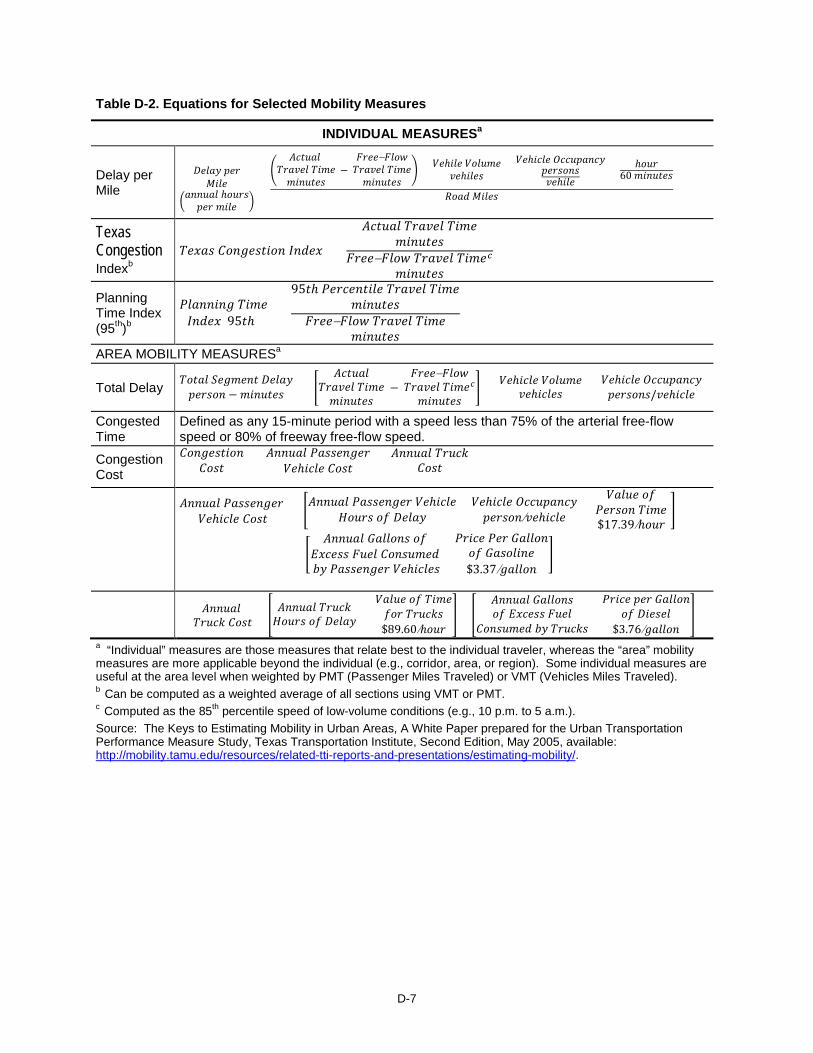
equal traffic in each peak. The 16 mixed-traffic distribution profiles shown in Figures D.1 through D.5 are considered to be very

comprehensive, as they were developed based upon 713 continuous traffic monitoring locations in urban areas of 37 states. TTI compared these reported traffic profiles with readily-available, recent empirical traffic data in Houston, San Antonio and Austin to confirm that these reported profiles remain valid for Texas.

Figure D-1. Weekday Mixed-Traffic Distribution Profile for No to Low Congestion

D-10

Figure D-2. Weekday Mixed-Traffic Distribution Profile for Moderate Congestion

Figure D-3. Weekday Mixed-Traffic Distribution Profile for Severe Congestion

0%

2%

4%

6%

8%

10%

12%

0:00 2:00 4:00 6:00 8:00 10:00 12:00 14:00 16:00 18:00 20:00 22:00

Perc

ent

of D

aily

Vol

ume

Hour of Day AM Peak, Freeway Weekday PM Peak, Freeway Weekday AM Peak, Non-Freeway Weekday PM Peak, Non-Freeway Weekday

D-11

Figure D-4. Weekend Mixed-Traffic Distribution Profile

Figure D-5. Weekday Mixed-Traffic Distribution Profile for Severe Congestion and Similar Speeds in Each Peak Period

D-12

The next step in the traffic flow assignment process is to determine which of the 16 mixed-traffic distribution profiles should be assigned to each speed-network route (the “geography” used by the private-sector data providers), such that the 15-minute traffic flows can be calculated from TxDOT’s RHiNo data. The assignment should be as follows: • Functional class: assign based on RHiNo functional road class. – Freeway – access-controlled highways. – Non-freeway – all other major roads and streets.

• Day type: assign volume profile based on each day. – Weekday (Monday through Friday). – Weekend (Saturday and Sunday).

• Traffic congestion level: assign based on the peak period speed reduction percentage calculated from the private-sector speed data. The peak-period speed reduction is calculated as follows: – 1) Calculate a simple average peak period speed (add up all the morning and evening peak period

speeds and divide the total by the 24 15-minute periods in the six peak hours) for each TMC path using speed data from 6 a.m. to 9:0 a.m. (morning peak period) and 4 p.m. to 7 p.m. (evening peak period).

– 2) Calculate a free-flow speed during the light traffic hours (e.g., 10:00 p.m. to 5:00 a.m.) to be used as the baseline for congestion calculations.

– 3) Calculate the peak period speed reduction by dividing the average combined peak period speed by the free-flow speed.

Speed Average Peak Period Speed Reduction = Free-flow Speed (10 p.m. to 5 a.m.) Factor For Freeways (roads with a free-flow (baseline) speed more than 55 mph): – Speed reduction factor ranging from 90% to 100% (no to low congestion). – Speed reduction factor ranging from 75% to 90% (moderate congestion). – Speed reduction factor less than 75% (severe congestion). For Non-Freeways (roads with a free-flow (baseline) speed less than 55 mph): – Speed reduction factor ranging from 80% to 100% (no to low congestion). – Speed reduction factor ranging from 65% to 80% (moderate congestion). – Speed reduction factor less than 65% (severe congestion).

• Directionality: Assign this factor based on peak period speed differentials in the private-sector speed dataset. The peak-period speed differential is calculated as follows: – 1) Calculate the average morning peak period speed (6 a.m. to 9 a.m.) and the average evening peak

period speed (4 p.m. to 7 p.m.). – 2) Assign the peak period volume curve based on the speed differential. The lowest speed

determines the peak direction. Any section where the difference in the morning and evening peak period speeds is 6 mph or less will be assigned to the even volume distribution.

The final step is to apply the daily adjustment factor to the annual average volume. Table D-3

illustrates the factors for the four different daily periods.

Table D-3. Day of Week Volume Conversion Factors

Day of Week Adjustment Factor

D-13

(to Convert Average Annual Volume into Day of Week Volume)

Monday to Thursday +5% Friday +10% Saturday -10% Sunday -20%

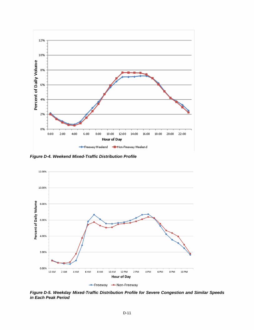
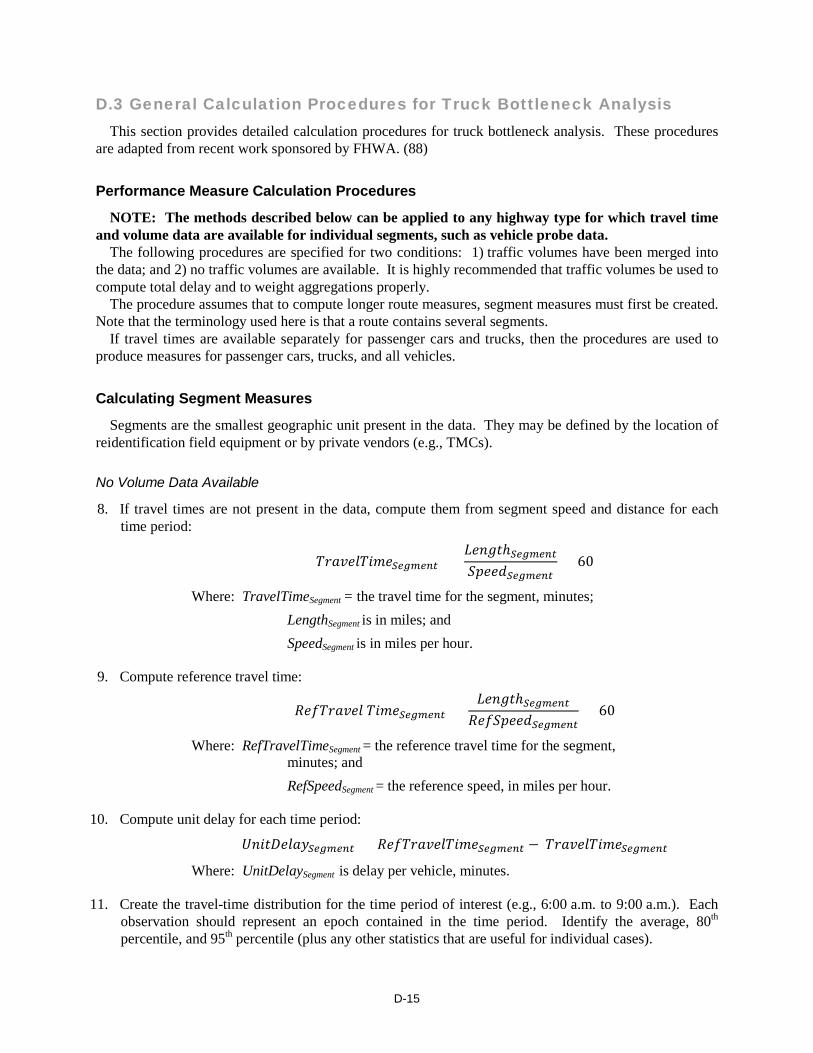
Truck-Only Methods This process is repeated to create 15-minute truck volumes from daily truck volumes However, much

of the necessary information, facility type, day type, and time of day peaking have already been determined in the mixed-vehicle volume process. The eight truck-only profiles used to create the 15-minute truck volumes are shown in Figures D.6 through D.8. There are no truck-only profiles by congestion level.

Figure D-6. Weekday Freeway Truck-Traffic Distribution Profiles

D-14

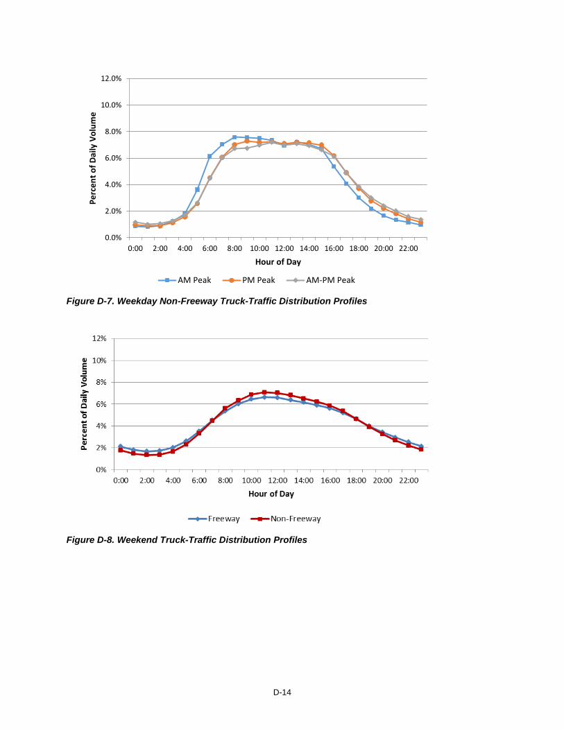
Figure D-7. Weekday Non-Freeway Truck-Traffic Distribution Profiles

Figure D-8. Weekend Truck-Traffic Distribution Profiles

0.0%

2.0%

4.0%

6.0%

8.0%

10.0%

12.0%

0:00 2:00 4:00 6:00 8:00 10:00 12:00 14:00 16:00 18:00 20:00 22:00

Perc

ent o

f Dai

ly V

olum

e

Hour of Day

AM Peak PM Peak AM-PM Peak

D-15

D.3 General Calculation Procedures for Truck Bottleneck Analysis This section provides detailed calculation procedures for truck bottleneck analysis. These procedures

are adapted from recent work sponsored by FHWA. (88)

Performance Measure Calculation Procedures

NOTE: The methods described below can be applied to any highway type for which travel time and volume data are available for individual segments, such as vehicle probe data.

The following procedures are specified for two conditions: 1) traffic volumes have been merged into the data; and 2) no traffic volumes are available. It is highly recommended that traffic volumes be used to compute total delay and to weight aggregations properly.

The procedure assumes that to compute longer route measures, segment measures must first be created. Note that the terminology used here is that a route contains several segments.

If travel times are available separately for passenger cars and trucks, then the procedures are used to produce measures for passenger cars, trucks, and all vehicles.

Calculating Segment Measures

Segments are the smallest geographic unit present in the data. They may be defined by the location of reidentification field equipment or by private vendors (e.g., TMCs).

No Volume Data Available

8. If travel times are not present in the data, compute them from segment speed and distance for each time period:

𝑇𝑇𝑝𝑝𝐷𝐷𝑇𝑇𝐷𝐷𝐷𝐷𝑇𝑇𝑀𝑀𝑚𝑚𝐷𝐷𝑆𝑆𝑆𝑆𝑆𝑆𝑆𝑆𝑆𝑆𝑆𝑆𝑆𝑆 = 𝐿𝐿𝐷𝐷𝑎𝑎𝐶𝐶𝐴𝐴ℎ𝑆𝑆𝑆𝑆𝑆𝑆𝑆𝑆𝑆𝑆𝑆𝑆𝑆𝑆𝑆𝑆𝑝𝑝𝐷𝐷𝐷𝐷𝑅𝑅𝑆𝑆𝑆𝑆𝑆𝑆𝑆𝑆𝑆𝑆𝑆𝑆𝑆𝑆

× 60

Where: TravelTimeSegment = the travel time for the segment, minutes; LengthSegment is in miles; and SpeedSegment is in miles per hour.

9. Compute reference travel time:

𝑅𝑅𝐷𝐷𝑜𝑜𝑇𝑇𝑝𝑝𝐷𝐷𝑇𝑇𝐷𝐷𝐷𝐷 𝑇𝑇𝑀𝑀𝑚𝑚𝐷𝐷𝑆𝑆𝑆𝑆𝑆𝑆𝑆𝑆𝑆𝑆𝑆𝑆𝑆𝑆 = 𝐿𝐿𝐷𝐷𝑎𝑎𝐶𝐶𝐴𝐴ℎ𝑆𝑆𝑆𝑆𝑆𝑆𝑆𝑆𝑆𝑆𝑆𝑆𝑆𝑆𝑅𝑅𝐷𝐷𝑜𝑜𝑆𝑆𝑝𝑝𝐷𝐷𝐷𝐷𝑅𝑅𝑆𝑆𝑆𝑆𝑆𝑆𝑆𝑆𝑆𝑆𝑆𝑆𝑆𝑆

× 60

Where: RefTravelTimeSegment = the reference travel time for the segment, minutes; and

RefSpeedSegment = the reference speed, in miles per hour.

10. Compute unit delay for each time period:

𝑈𝑈𝑎𝑎𝑀𝑀𝐴𝐴𝐷𝐷𝐷𝐷𝐷𝐷𝐷𝐷𝐷𝐷𝑆𝑆𝑆𝑆𝑆𝑆𝑆𝑆𝑆𝑆𝑆𝑆𝑆𝑆 = 𝑅𝑅𝐷𝐷𝑜𝑜𝑇𝑇𝑝𝑝𝐷𝐷𝑇𝑇𝐷𝐷𝐷𝐷𝑇𝑇𝑀𝑀𝑚𝑚𝐷𝐷𝑆𝑆𝑆𝑆𝑆𝑆𝑆𝑆𝑆𝑆𝑆𝑆𝑆𝑆 − 𝑇𝑇𝑝𝑝𝐷𝐷𝑇𝑇𝐷𝐷𝐷𝐷𝑇𝑇𝑀𝑀𝑚𝑚𝐷𝐷𝑆𝑆𝑆𝑆𝑆𝑆𝑆𝑆𝑆𝑆𝑆𝑆𝑆𝑆

Where: UnitDelaySegment is delay per vehicle, minutes.

11. Create the travel-time distribution for the time period of interest (e.g., 6:00 a.m. to 9:00 a.m.). Each observation should represent an epoch contained in the time period. Identify the average, 80th percentile, and 95th percentile (plus any other statistics that are useful for individual cases).

D-16

12. Calculate recommended performance measures for the time period of interest:

𝑇𝑇𝑇𝑇𝐼𝐼𝑆𝑆𝑆𝑆𝑆𝑆𝑆𝑆𝑆𝑆𝑆𝑆𝑆𝑆 = 𝑀𝑀𝐷𝐷𝐷𝐷𝑎𝑎𝑇𝑇𝑝𝑝𝐷𝐷𝑇𝑇𝐷𝐷𝐷𝐷 𝑇𝑇𝑀𝑀𝑚𝑚𝐷𝐷𝑆𝑆𝑆𝑆𝑆𝑆𝑆𝑆𝑆𝑆𝑆𝑆𝑆𝑆

𝑅𝑅𝐷𝐷𝑜𝑜𝑇𝑇𝑝𝑝𝐷𝐷𝑇𝑇𝐷𝐷𝐷𝐷𝑇𝑇𝑀𝑀𝑚𝑚𝐷𝐷𝑆𝑆𝑆𝑆𝑆𝑆𝑆𝑆𝑆𝑆𝑆𝑆𝑆𝑆

𝑃𝑃𝑇𝑇𝐼𝐼𝑆𝑆𝑆𝑆𝑆𝑆𝑆𝑆𝑆𝑆𝑆𝑆𝑆𝑆 = 95𝐴𝐴ℎ 𝑝𝑝𝐷𝐷𝑝𝑝𝐴𝐴𝐷𝐷𝑎𝑎𝐴𝐴𝑀𝑀𝐷𝐷𝐷𝐷 𝑇𝑇𝑝𝑝𝐷𝐷𝑇𝑇𝐷𝐷𝐷𝐷 𝑇𝑇𝑀𝑀𝑚𝑚𝐷𝐷𝑆𝑆𝑆𝑆𝑆𝑆𝑆𝑆𝑆𝑆𝑆𝑆𝑆𝑆

𝑅𝑅𝐷𝐷𝑜𝑜𝑇𝑇𝑝𝑝𝐷𝐷𝑇𝑇𝐷𝐷𝐷𝐷𝑇𝑇𝑀𝑀𝑚𝑚𝐷𝐷𝑆𝑆𝑆𝑆𝑆𝑆𝑆𝑆𝑆𝑆𝑆𝑆𝑆𝑆

𝑃𝑃𝑇𝑇𝐼𝐼80𝑆𝑆𝑆𝑆𝑆𝑆𝑆𝑆𝑆𝑆𝑆𝑆𝑆𝑆 = 80𝐴𝐴ℎ 𝑝𝑝𝐷𝐷𝑝𝑝𝐴𝐴𝐷𝐷𝑎𝑎𝐴𝐴𝑀𝑀𝐷𝐷𝐷𝐷 𝑇𝑇𝑝𝑝𝐷𝐷𝑇𝑇𝐷𝐷𝐷𝐷 𝑇𝑇𝑀𝑀𝑚𝑚𝐷𝐷𝑆𝑆𝑆𝑆𝑆𝑆𝑆𝑆𝑆𝑆𝑆𝑆𝑆𝑆

𝑅𝑅𝐷𝐷𝑜𝑜𝑇𝑇𝑝𝑝𝐷𝐷𝑇𝑇𝐷𝐷𝐷𝐷𝑇𝑇𝑀𝑀𝑚𝑚𝐷𝐷𝑆𝑆𝑆𝑆𝑆𝑆𝑆𝑆𝑆𝑆𝑆𝑆𝑆𝑆

𝑈𝑈𝑎𝑎𝑀𝑀𝐴𝐴𝐷𝐷𝐷𝐷𝐷𝐷𝐷𝐷𝐷𝐷𝑆𝑆𝑆𝑆𝑆𝑆𝑆𝑆𝑆𝑆𝑆𝑆𝑆𝑆 = �𝑈𝑈𝑎𝑎𝑀𝑀𝐴𝐴𝐷𝐷𝐷𝐷𝐷𝐷𝐷𝐷𝐷𝐷𝑆𝑆𝑆𝑆

Where: Subscript e refers to an individual epoch.

Volume Data Available

13. Repeat steps 1 and 2 immediately above. 14. Compute VMT, Vehicle-Hours of Travel (VHT), and total delay (in vehicle-hours) for each epoch.

𝑉𝑉𝑀𝑀𝑇𝑇𝑆𝑆𝑆𝑆𝑆𝑆𝑆𝑆𝑆𝑆𝑆𝑆𝑆𝑆 = 𝑉𝑉𝑜𝑜𝐷𝐷𝑎𝑎𝑚𝑚𝐷𝐷𝑆𝑆𝑆𝑆𝑆𝑆𝑆𝑆𝑆𝑆𝑆𝑆𝑆𝑆 × 𝐿𝐿𝐷𝐷𝑎𝑎𝐶𝐶𝐴𝐴ℎ𝑆𝑆𝑆𝑆𝑆𝑆𝑆𝑆𝑆𝑆𝑆𝑆𝑆𝑆

𝑉𝑉𝐻𝐻𝑇𝑇𝑆𝑆𝑆𝑆𝑆𝑆𝑆𝑆𝑆𝑆𝑆𝑆𝑆𝑆 = 𝑉𝑉𝑜𝑜𝐷𝐷𝑎𝑎𝑚𝑚𝐷𝐷𝑆𝑆𝑆𝑆𝑆𝑆𝑆𝑆𝑆𝑆𝑆𝑆𝑆𝑆 × 𝑇𝑇𝑝𝑝𝐷𝐷𝑇𝑇𝐷𝐷𝐷𝐷𝑇𝑇𝑀𝑀𝑚𝑚𝐷𝐷𝑆𝑆𝑆𝑆𝑆𝑆𝑆𝑆𝑆𝑆𝑆𝑆𝑆𝑆 ×1

60

𝑇𝑇𝑜𝑜𝐴𝐴𝐷𝐷𝐷𝐷𝐷𝐷𝐷𝐷𝐷𝐷𝐷𝐷𝐷𝐷𝑆𝑆𝑆𝑆𝑆𝑆𝑆𝑆𝑆𝑆𝑆𝑆𝑆𝑆= 𝑉𝑉𝐻𝐻𝑇𝑇𝑆𝑆𝑆𝑆𝑆𝑆𝑆𝑆𝑆𝑆𝑆𝑆𝑆𝑆

− �𝑉𝑉𝑜𝑜𝐷𝐷𝑎𝑎𝑚𝑚𝐷𝐷𝑆𝑆𝑆𝑆𝑆𝑆𝑆𝑆𝑆𝑆𝑆𝑆𝑆𝑆 × 𝑅𝑅𝐷𝐷𝑜𝑜𝑇𝑇𝑝𝑝𝐷𝐷𝑇𝑇𝐷𝐷𝐷𝐷𝑇𝑇𝑀𝑀𝑚𝑚𝐷𝐷𝑆𝑆𝑆𝑆𝑆𝑆𝑆𝑆𝑆𝑆𝑆𝑆𝑆𝑆 × 1

60�

15. Create travel time distribution for time period of interest, using VMT as the weight on each observation. That is, the travel times in an epoch are assumed to be the average of all vehicles traveling over that segment in an epoch. Identify the average, 80th percentile, and 95th percentile (plus any other statistics that are useful for individual cases).

16. Repeat step 5 immediately above using the weighted travel time distribution; the reference travel time is the same. Total delay is computed in the same manner as unit delay for the segment (i.e., the sum of the delay in the epochs in the time period of interest).

Calculating Route Measures

No Volume Data Available

17. Create a dataset for travel times over the route for each epoch by either: 1) using the vehicle trajectory method (discussed in Chapter 4); or 2) summing the segment travel times.

18. Compute the reference travel time for the route (RefTravelTimeRoute) as the sum of the segment reference travel times.

19. Compute unit delay for the route for each epoch as the sum of UnitDelay for all segments on the route for the time period of interest.

20. Create the travel time distribution for the time period of interest for the entire route using the data created in Step 1. Each observation should represent an epoch contained in the time period. Identify the average, 80th percentile, and 95th percentile (plus any other statistics that are useful for individual cases.)

D-17

21. Calculate recommended performance measures for the time period of interest:

𝑇𝑇𝑇𝑇𝐼𝐼(𝑅𝑅𝑅𝑅𝑅𝑅𝑆𝑆𝑆𝑆) = 𝐴𝐴𝑇𝑇𝐷𝐷𝑝𝑝𝐷𝐷𝐶𝐶𝐷𝐷𝑇𝑇𝑝𝑝𝐷𝐷𝑇𝑇𝐷𝐷𝐷𝐷 𝑇𝑇𝑀𝑀𝑚𝑚𝐷𝐷𝑅𝑅𝑅𝑅𝑅𝑅𝑆𝑆𝑆𝑆𝑅𝑅𝐷𝐷𝑜𝑜𝑇𝑇𝑝𝑝𝐷𝐷𝑇𝑇𝐷𝐷𝐷𝐷𝑇𝑇𝑀𝑀𝑚𝑚𝐷𝐷𝑅𝑅𝑅𝑅𝑅𝑅𝑆𝑆𝑆𝑆

𝑃𝑃𝑇𝑇𝐼𝐼𝑅𝑅𝑅𝑅𝑅𝑅𝑆𝑆𝑆𝑆 = 95𝐴𝐴ℎ 𝑝𝑝𝐷𝐷𝑝𝑝𝐴𝐴𝐷𝐷𝑎𝑎𝐴𝐴𝑀𝑀𝐷𝐷𝐷𝐷 𝑇𝑇𝑝𝑝𝐷𝐷𝑇𝑇𝐷𝐷𝐷𝐷 𝑇𝑇𝑀𝑀𝑚𝑚𝐷𝐷𝑅𝑅𝑅𝑅𝑅𝑅𝑆𝑆𝑆𝑆

𝑅𝑅𝐷𝐷𝑜𝑜𝑇𝑇𝑝𝑝𝐷𝐷𝑇𝑇𝐷𝐷𝐷𝐷𝑇𝑇𝑀𝑀𝑚𝑚𝐷𝐷𝑅𝑅𝑅𝑅𝑅𝑅𝑆𝑆𝑆𝑆

𝑃𝑃𝑇𝑇𝐼𝐼80𝑅𝑅𝑅𝑅𝑅𝑅𝑆𝑆𝑆𝑆 = 80𝐴𝐴ℎ 𝑝𝑝𝐷𝐷𝑝𝑝𝐴𝐴𝐷𝐷𝑎𝑎𝐴𝐴𝑀𝑀𝐷𝐷𝐷𝐷 𝑇𝑇𝑝𝑝𝐷𝐷𝑇𝑇𝐷𝐷𝐷𝐷 𝑇𝑇𝑀𝑀𝑚𝑚𝐷𝐷𝑅𝑅𝑅𝑅𝑅𝑅𝑆𝑆𝑆𝑆

𝑅𝑅𝐷𝐷𝑜𝑜𝑇𝑇𝑝𝑝𝐷𝐷𝑇𝑇𝐷𝐷𝐷𝐷𝑇𝑇𝑀𝑀𝑚𝑚𝐷𝐷𝑅𝑅𝑅𝑅𝑅𝑅𝑆𝑆𝑆𝑆

𝑈𝑈𝑎𝑎𝑀𝑀𝐴𝐴𝐷𝐷𝐷𝐷𝐷𝐷𝐷𝐷𝐷𝐷𝑅𝑅𝑅𝑅𝑅𝑅𝑆𝑆𝑆𝑆 = �𝑈𝑈𝑎𝑎𝑀𝑀𝐴𝐴𝐷𝐷𝐷𝐷𝐷𝐷𝐷𝐷𝐷𝐷𝑆𝑆

𝑆𝑆

Volume Data Available

22. Repeat Steps 1 and 2 immediately above. 23. Compute total delay for the route for each epoch as the sum of total delay for all segments on the

route for the time period of interest. 24. Create the travel time distribution for the time period of interest for the route using the data created in

Step 1. VMT should be used as the weight on each observation. That is, the travel times in an epoch are assumed to be the average of all vehicles traveling over that segment in an epoch. Identify the average, 80th percentile, and 95th percentile (plus any other statistics that are useful for individual cases).

25. Repeat step 5 immediately above using the weighted travel time distribution; the reference travel time is the same. Total delay is computed in the same manner as unit delay for the route (i.e., the sum of the delay in the epochs in the time period of interest).

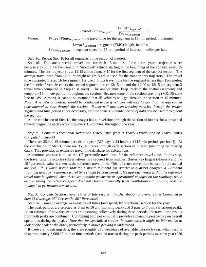
D.4 Calculation Procedures for Maryland State Highway Administration Freight Fluidity

The following provides background and calculation procedures developed by the Texas A&M Transportation Institute for the Maryland State Highway Administration for freight fluidity performance measures. The information below has been adapted to this appendix from a technical memorandum. (89) The discussion begins with background on what “freight fluidity” means for Maryland prior to the calculation procedures.

Background and Application

What is Freight Fluidity?

The concept of a “fluidity indicator” has been popularized by Transport Canada to evaluate the performance of trade corridors and multimodal supply chains. (90, 91) For Transport Canada’s applications, the fluidity indicator measures total transit time and travel time reliability of goods along defined supply chains. There is increasing interest by the Federal Highway Administration (FHWA) to adapt “freight fluidity” in the United States, though a specific documented definition and application of what “freight fluidity” means for the U.S. – and what it might look like – is elusive.

What is clear is that any concept of freight fluidity requires multimodal data across the entire freight network, including information on origins and destinations of freight movements by mode (i.e., supply chains). It includes an understanding of how “fluid” the supply chains are – in terms of mobility,

D-18

reliability, and resiliency. There is also a need for information on the quantity of goods moved (e.g., volume, weight, value – and by commodity type) throughout the network to understand flows and to weight performance measures across the supply chain. The resiliency of the freight network is critical to shippers and carriers and is included as another element within freight fluidity performance. With this information as context and background, TTI proposes this definition of “freight fluidity.”

Freight fluidity is a broad term referring to the characteristics of a multimodal freight network in a geographic area of interest, where any number of specific modal data elements and performance measures are used to describe the network performance (including costs and resiliency) andquantity of freight moved (including commodity value) to inform decision-making.

Just how “fluid” the freight network is can be captured by quantifying performance (including resiliency) and quantity of freight moved. These elements are described in Table D-4. The “geographic area” over which these elements are monitored could be a specific route (e.g., roadway, rail-line, drayage line), supply chain (combination of routes and transload “nodes”), urban area(s), statewide, regional, or global.

Table D-4. The Components of Freight Fluidity (Mind Your Freight Network “Ps and Qs”)

Components Description Selected Suggested Measures/Considerationsa

Performance (“Ps”)

How well are the segments/nodes and network operating? Where are there bottlenecks in the system?

• Mobility (e.g., travel time, total delay, delay per mile, travel time index)

• Reliability (e.g., planning time index) • Costsb (associated with delay, unreliability, wasted

fuel)

How well does the system (infrastructure, users, agencies) react to disruptions (i.e., how resilient is the system)?

• Resiliencyc has 4 aspects: • Robustness (ability to withstand disruption,

measured in time) • Rapidity (time to respond and recover) • Redundancy (alternate route [capacity]

availability/access within a certain travel time) • Resourcefulness (ability and time to mobilize

needed resources)

Quantity (“Qs”) How much freight is moved (and where)?

• Volume (e.g., # of trucks, railcars, twenty-foot equivalent units [TEUs])

• Weight (e.g., pounds, tonnage) • Commodity Value2

a These are selected measures and considerations. These measures are ideally obtained by mode and by commodity for complete freight network evaluation. b Costs in the “performance” component and value in the “quantity” component capture the economic impact of freight fluidity. c Resiliency is an element of the “performance” component because current system resiliency is captured in measures of mobility, reliability and associated costs. Note that the “4 Rs” (robustness, rapidity, redundancy, resourcefulness) of resiliency can typically be expressed in time, and hence, delay and associated cost measures. Resiliency is included in the freight fluidity framework here because it is critical for efficient goods movement during system disruptions. Evaluating and improving transportation system resiliency during disruptions serves to better understand and improve performance during challenging times of goods movement.

Prior to any exercise in computing performance measures, there is a need to understand the application

for the measures. What will the measures be used for? What type of decisions will be made? This can help define any number of important parameters. In this regard, some assumptions are made on the use case prior to providing guidance on the appropriate calculation procedures.

D-19

There are a number of key words in the definition above for “Freight Fluidity” that identify primary parameters that must be considered before computing freight operating characteristics. Table D-5 provides a break-down of these key words, and the assumptions made for the development of the calculation procedures here. The highway mode is the focus for the calculation procedures developed and similar measures and methods could be adapted for other modes.

Table D-5. Calculation Procedure Assumptions Based on Freight Fluidity Definition

Freight Fluidity Definition Phrase

Scoping Questions for Analyst to Ask

“Answers” to Posed Questions for Calculation Procedures Here

“…multimodal…” What freight modes are included? Highway (I-95 and U.S. 40) “…geographic area of interest,…”

What is the geographic scale? From BWI airport and Port of Baltimore to Aberdeen, MD and beyond to the MD/DE State line

“…specific modal data elements…”

What are types of data elements going into the analysis?

Truck volumes, truck vehicle-miles of travel (TMT), speeds (or travel times)

“…network performance…”

What network performance measures are needed? How well are the segments/nodes and network operating? Where are the bottlenecks in the system?

Mobility, reliability, and cost measures

“…quantity of freight moved…”

How much (volume, weight, value) freight is moved (and where)?

Truck volume, vehicle-miles of travel (TMT), truck-miles of travel (VMT)

“….resiliency…” How well does the system react to disruptions?

Not included in demonstration calculation procedures

“...to inform decision-making.”

What decisions do you plan to make with the freight fluidity network characteristics? What is appropriate study scale, measures and study scope to ensure you can impact these decisions with the results?

Planning and programming for highway freight network improvements (based on performance and quantity of freight moved) Identify bottleneck locations.

Data Sources

The initial demonstration is focused on the highway mode. In time, it is the expectation that future data sources providing transit/dwell times and quantity (volume, weight, or value) will become available across modes so freight fluidity characteristics can be estimated on an international scale. For the highway mode demonstration, this section describes the primary travel time and volume data sources.

Travel Time Data Sources

Travel time data are generally available from the following sources: 26. Manual travel time runs; 27. Roadway sensors or road tubes (spot-speeds used to estimate travel times); 28. Reidentification technologies (Bluetooth, toll-tags, pavement sensors, license-plate matching); and 29. Private-company data sources (GPS-based data).

D-20

As stated in Table D-4, the assumed application for these fluidity calculation procedures is for identifying bottleneck locations and planning and programming highway freight network improvements. Because of this, generally ubiquitous and consistently available speed (and volume) data sources are desirable for this planning-level analysis. Because Maryland is a member of the I-95 Corridor Coalition, INRIX day-to-day real-time speed data are available. The Maryland State Highway Mobility Report uses these data to produce performance statistics. These calculation procedures assume the use of data from a source providing data for every time period, every day (as opposed to an annual average value). INRIX real-time data provide such a source for speed (travel time) data. Another source that provides this day-to-day data is the Federal Highway Administration’s National Performance Management Research Data Set (NPMRDS), which also has truck-specific travel time data.

Travel Time Data Source Relationship to Calculation Procedures

Table D-6 provides an overview of three types of calculation procedures as defined by the type of travel time data available. As one moves further down the table, the analysis moves from being “facility-based” to a “trip-based” analysis. In the area of freight mobility analysis, there is a particular interest in not only how the facility is operating (i.e., what segments have bottlenecks), but also the actual point-to-point trips that specific trucks make (i.e., supply chains and routes) to identify the number and location of truck trips.

Option 1 in Table D-6 is based upon using data at the smallest segment level possible (e.g., often traffic message channel [TMC] for GPS-based data). The analysis provides information about that particular segment, but not for specific trips. On the far end of the spectrum is Option 3 where travel time can be directly measured by taking the difference in travel times for a unique vehicle, given its lat/long coordinates along the route of interest. The obtained travel time is a more accurate reflection of exactly what is experienced by the traveler on that roadway. As routes become long, sample sizes can become low as there are fewer trucks traversing the entire route for analysis. In the middle (Option 2), one can use a trajectory method to model vehicles in time and space along the roadway section using the facility-based data (described in Option 1) to estimate the time it takes a vehicle to traverse the route. If data are aggregated to 15 minutes and a traveler takes longer than 15 minutes to traverse the corridor, the next time epoch of 15-minute data would be used for that roadway segment and so on, “tracing” the vehicle trajectory through the entire roadway section. This method is particularly useful on longer sections where sample sizes of trucks traversing the entire corridor are limited.

Table D-6. Overview of Calculation Procedures Based on Type of Travel Time Data Available

Procedure Type Description of Travel Time Data The higher the option number, the closer we get to what the traveler (mover of goods) experiences, and further away from how the infrastructure performs.

Facility-based (Option 1)

Segment-level travel time and speed data used to estimate performance over a roadway section.

“Derived” Trip-based Trajectory (Option 2)

Employing “traces” in time and space using the facility-based (segment) data to estimate performance measures.

Trip-based (Option 3)

Vehicle ID, lat/long and time stamp along route allowing direct measurement of travel time over route taken.

Because of the increasingly ubiquitous nature of GPS-based data, and because Maryland State

Highway Administration and University of Maryland staff have access to INRIX data via the I-95

D-21

Corridor Coalition, the proposed calculation procedures use the “derived” trip-based trajectory (Option 2 in Table D-6).

Benefits of Trip-Based Data (Option 3)

A short discussion of the benefits of trip-based data is justified because they will likely become increasingly available. The primary advantage is that these data allow for the “tracking” of anonymous trucks through the highway network. Consider that performance data over specific segments, such as those currently in the Maryland State Highway Mobility Report, help decision-makers understand the location of bottleneck locations. The trip-based data allows the analyst to develop trip tables between origin-destinations and better understand the “whys” behind the bottleneck locations.

For example, Figure D-9 shows a bottleneck location identified on a hypothetical State Route 1 (SR-3) between SR-1 and SR-2. Trip-based data would allow for more information about the truck trips going between points A, B, C, D, and E. On a regional scale (e.g., Baltimore), and broader scale (Maryland, United States) the trip-based information provides a deeper understanding of system use and supply chains over the network. If trips from many of the origin-destinations use this bottleneck section then it could be identified as a high priority for upgrade for economic viability.

Figure D-9. Illustration of Simplified Roadway Network with an Identified Bottleneck

Volume Data Sources

Volume data (or VMT, TMT) are the “low hanging fruit” to enumerate the quantity component of freight fluidity as described in Table D-4. Volume data are also used in combination with travel time information for delay estimation. Volume data are generally available from the following sources:

30. Manual volume counts; 31. Road tubes; 32. Roadway sensors (including weigh-in-motion, automatic traffic recorders, inductance loops or other

technologies); 33. Statewide inventories and/or FHWA Highway Performance Monitoring System (HPMS); and

D-22

34. Volume estimation techniques (based upon representative local data from similar conditions or even national average day-of-week profiles).

The ideal with volume data is that it be obtained over the same times and locations as the travel time data source. Because this is often not possible due to financial constraints, the analyst must identify the next best sources. This might be using volume counts from similar/adjacent roadways or counts from a different segment of the roadway of interest that may be assumed representative. In some cases, national average day-of-week profile information is used, which is done in the Maryland State Highway Mobility Report or TTI’s Urban Mobility Scorecard. The application determines the appropriate scale of the volume techniques. Generally, for planning and programming applications, such as being discussed here, volume estimation techniques are appropriate and common practice.

Because it is already in use now in the Maryland State Highway Mobility Report, the calculation procedures that follow assume the use of time-of-day volume profiles for needed volume estimates. Of course, if (or as) more complete truck volume data at the temporal and geographic scale become available, these local sources can be incorporated into the methods.

Roadway Network

The geographic scope of the analysis is I-95 and U.S. 40 from the Baltimore (BWI) airport to the Maryland/Delaware state line. Researchers anticipate creating performance measures between the airport (BWI), Port of Baltimore, Aberdeen, MD area and the MD/DE state line. These areas were all chosen as section endpoints because of their relationship to freight movement. Traffic Analysis Zones (TAZ) from the Baltimore Metropolitan Council will be identified as origin-destination locations, thus allowing the fluidity results to inform MPO planning and programming efforts. Note that the word section is used throughout this document for longer “sections” of I-95, whereas “segment” is used for smaller segments of these longer sections (i.e., several segments make up a section).

Calculation Procedures

Key Assumptions and Clarifications

The calculation procedures below use the assumptions described in the previous sections for a highway demonstration of freight fluidity. Some additional assumptions/clarifications are: • Speed data from INRIX GPS-based sources by TMC; • 1-min INRIX speed data are aggregated to 5-minute or 15-minute time periods by TMC (profiles) (for

simplicity, the calculation procedures assume 15-minute time periods) [it is acknowledged that the level of aggregation of the travel time data may be due to volume limitations – i.e., if 5-minute volume can be generated, they can be used];

• Truck volume data from roadway inventory (annual average daily traffic – AADT) or HPMS source; • Time-of-day profile use to convert AADT values to 15-minute volumes throughout the day; • Peak-periods are selected as 6 am to 10 am (morning peak) and 3 p.m. to 7 p.m. (afternoon peak); • “Segment” is the term used for a TMC and “Section” is the term used for a longer route composed of

several TMCs; and • Analysis is for 1 year of data (assuming calendar 2013 data).

Measures

The calculation procedures below estimate the following freight fluidity characteristics for the highway demonstration of freight fluidity:

The Performance (“Ps”) of freight fluidity that are computed in these procedures are as follows: • Travel time (and speed);

D-23

• Planning time index; • Travel time index; • Delay (roadway segments, total section, per trip); • Delay per mile (of section); and • Cost of delay (roadway segment, total section, per truck trip).

The Quantity (“Qs”) of freight fluidity that are computed in these procedures are as follows:

• Section vehicle-miles of travel (VMT) or truck-miles of travel (TMT). The primary product of the freight fluidity demonstration is populated matrices such as the one shown

in Table D-7. The anticipated origin-destinations for I-95 are shown in Table D-7. These matrices can be populated with the performance measures highlighted above.

Table D-7. Anticipated Matrix Output of Freight Fluidity Demonstration Results

Procedures

The following are the high-level steps to compute travel time and associated measures along identified paths:

35. Compute directional travel times through section beginning at each 15-minute period (using trajectories) throughout the year;

36. Compute directional reference travel time from a yearly distribution of travel times computed in Step #1;

37. Compute section travel times of interest from the distribution of travel times computed in Step #1 (average, 95th percentile, 80th percentile);

38. Compute travel time index and planning time index by section with data from Step #3 39. Compute assorted delay measures by directional section; 40. Compute costs of delay; 41. Report “quantity” component of freight fluidity as VMT or TMT per section; and 42. Develop matrices of performance measures by origin-destination (section).

The steps are discussed in more detail in the following sections, including substeps as appropriate. Step 1: Compute Directional Travel Times through Section Beginning at Each 15-minute Period

(Using Trajectories) Throughout the Year Step 1a. Average speed data from 1-minute up to either 5-minute or 15-minute: Speeds from 1-minute

data for a TMC are averaged to 15-minutes. The remainder of this analysis assumes 15-minute data, though the methods also work for 5-minutes.

Step 1b. For all the directional segments (TMCs) in the roadway section of interest, compute the travel time at the segment level for each 15-minute period as:

D-24

𝑇𝑇𝑝𝑝𝐷𝐷𝑇𝑇𝐷𝐷𝐷𝐷 𝑇𝑇𝑀𝑀𝑚𝑚𝐷𝐷𝑆𝑆𝑆𝑆𝑆𝑆𝑆𝑆𝑆𝑆𝑆𝑆𝑆𝑆 = 𝐿𝐿𝐷𝐷𝑎𝑎𝐶𝐶𝐴𝐴ℎ𝑆𝑆𝑆𝑆𝑆𝑆𝑆𝑆𝑆𝑆𝑆𝑆𝑆𝑆

𝑆𝑆𝑝𝑝𝐷𝐷𝐷𝐷𝑅𝑅𝑆𝑆𝑆𝑆𝑆𝑆𝑆𝑆𝑆𝑆𝑆𝑆𝑆𝑆 × 60

Where: 𝑇𝑇𝑝𝑝𝐷𝐷𝑇𝑇𝐷𝐷𝐷𝐷 𝑇𝑇𝑀𝑀𝑚𝑚𝐷𝐷𝑆𝑆𝑆𝑆𝑆𝑆𝑆𝑆𝑆𝑆𝑆𝑆𝑆𝑆 = the travel time for the segment in 15-min period, in minutes

𝐿𝐿𝐷𝐷𝑎𝑎𝐶𝐶𝐴𝐴ℎ𝑆𝑆𝑆𝑆𝑆𝑆𝑆𝑆𝑆𝑆𝑆𝑆𝑆𝑆 = segment (TMC) length, in miles 𝑆𝑆𝑝𝑝𝐷𝐷𝐷𝐷𝑅𝑅𝑆𝑆𝑆𝑆𝑆𝑆𝑆𝑆𝑆𝑆𝑆𝑆𝑆𝑆 = segment speed for 15-min period of interest, in miles per hour Step 1c. Repeat Step 1b for all segments in the section of interest. Step 1d. Estimate a section travel time for each 15-minutes of the entire year: trajectories are

necessary to build a travel time of a “modeled” vehicle starting at the beginning of the corridor every 15 minutes. The first trajectory is at 12:15 am on January 1st for the first segment of the subject section. The average travel time from 12:00 midnight to 12:15 am is used for the trace in this trajectory. The travel time computed in step 1b for segment 1 is used. If the travel time for the segment is less than 15-minutes, the “modeled” vehicle enters the second segment before 12:15 am and the 12:00 to 12:15 am segment 2 travel time (computed in Step 1b is used). The analyst must keep track of the spatial (segment) and temporal (15-minute period) throughout the section. Because some of the sections are long (MD/DE state line to BWI Airport), it cannot be assumed that all vehicles will get through the section in 15-minutes. Note: A sensitivity analysis should be conducted to see if vehicles will take longer than the aggregated time interval to pass through the section. If they will not, then tracking vehicles through the proper segment and time period is not necessary, and the same 15-minute period of data can be used throughout the section.

At the conclusion of Step 1d, the analyst has a travel time through the section of interest for a presumed traveler beginning each section trip every 15-minutes, throughout the year.

Step 2: Compute Directional Reference Travel Time from a Yearly Distribution of Travel Times

Computed in Step #1 There are 35,040 15-minute periods in a year (365 days x 24 hours x 4 [15-min periods per hour]). At

the conclusion of Step 1, there are 35,040 traces through each section of interest (assuming no missing data). This provides an extensive travel time database for calculations.

A common practice is to use the 15th percentile travel time for the reference travel time. In this step, the travel time trajectories (observations) are ordered from smallest (fastest) to largest (slowest) and the 15th percentile value is taken as the reference travel time. This reference travel time is used for the annual analysis. It is worth noting that for a month-to-month (or quarter-to-quarter) analysis, a 12-month “running average” reference travel time should be considered. This approach ensures that the reference travel time is updated when there are possible geometric or operational changes on the roadway, while also ensuring the reference speed does not change drastically from month-to-month, causing possible “jumps” in performance measures.

Step 3. Compute Section Travel Times of Interest from the Distribution of Travel Times Computed in

Step #1 (Average, 95th Percentile, 80th Percentile) Step 3a. Compute average weekday travel times (and speed) by directional section for the year: The peak-periods are selected as 6 am to 10 am (morning peak) and 3 p.m. to 7 p.m. (afternoon peak).

As an estimate of how the sections are operating collectively during these periods, the travel time results from both peaks are combined. Combining both peaks initially provides a planning perspective on overall operations during the peaks. Note that for specialized studies, in some cases it might be informative to look at one peak or the other, particularly if known peaking is understood.

If there are no missing data, there are roughly 250 weekdays of available data each year, which results in approximately 8,000 15-minute time periods (section traces) during the peak periods over the year (250

D-25

weekdays x 8 hours of peak periods x 4 [15-min periods per hour]). The average of these 8,000 values is taken to obtain the average peak period section travel time for the year.

Because travel times are sometimes difficult for all audiences to readily relate to, it is encouraged that these average section travel times be converted to speeds using the equation that follows:

𝑆𝑆𝑝𝑝𝐷𝐷𝐷𝐷𝑅𝑅𝑆𝑆𝑆𝑆𝑐𝑐𝑆𝑆𝑆𝑆𝑅𝑅𝑆𝑆 = 𝐿𝐿𝐷𝐷𝑎𝑎𝐶𝐶𝐴𝐴ℎ𝑆𝑆𝑆𝑆𝑐𝑐𝑆𝑆𝑆𝑆𝑅𝑅𝑆𝑆

𝑇𝑇𝑝𝑝𝐷𝐷𝑇𝑇𝐷𝐷𝐷𝐷 𝑇𝑇𝑀𝑀𝑚𝑚𝐷𝐷𝑆𝑆𝑆𝑆𝑐𝑐𝑆𝑆𝑆𝑆𝑅𝑅𝑆𝑆 × 60

Where: 𝑆𝑆𝑝𝑝𝐷𝐷𝐷𝐷𝑅𝑅𝑆𝑆𝑆𝑆𝑐𝑐𝑆𝑆𝑆𝑆𝑅𝑅𝑆𝑆 = segment speed for 15-min period of interest, in miles per hour 𝐿𝐿𝐷𝐷𝑎𝑎𝐶𝐶𝐴𝐴ℎ𝑆𝑆𝑆𝑆𝑐𝑐𝑆𝑆𝑆𝑆𝑅𝑅𝑆𝑆 = segment (TMC) length, in miles 𝑇𝑇𝑝𝑝𝐷𝐷𝑇𝑇𝐷𝐷𝐷𝐷𝑇𝑇𝑀𝑀𝑚𝑚𝐷𝐷𝑆𝑆𝑆𝑆𝑐𝑐𝑆𝑆𝑆𝑆𝑅𝑅𝑆𝑆 = segment travel time for 15-min period of interest, in minutes

Travel times and speeds can then be reported, and the speeds are often much easier to quickly understand and relate to.

Step 3b. Compute average weekend travel times (and speed) by directional section for the year: Step 3b is the same as Step 3a except that the analysis is for the weekends. For this demonstration, the

same peaks are selected for the weekends, which results in approximately 3,360 15-minute time periods (section trajectories) during the year (105 weekends x 8 hours of peak periods x 4 [15-min periods per hour]). The average of these 3,360 values is taken to obtain the average peak period section travel time for the analysis year. Note that depending upon the analysis, different peak periods might be desired on the weekend for the truck analysis, but the peak periods are kept the same here for consistency and simplicity in this demonstration.

As in Step 3b, it is recommended that the travel times be converted to speeds using the equation above, and that both travel times and speed be reported.

Step 3c. Compute 80th percentile section travel time and 95th percentile section travel time for weekdays for the year:

The approximately 8,000 15-minute travel time trajectories (from Step 3a) are ordered from smallest (fastest) to largest (slowest). The 80th percentile and 95th percentile of these values are computed.

Step 3d. Compute 80th percentile section travel time and 95th percentile section travel time for weekends for the year:

The approximately 3,560 15-minute time traces (from Step 3b) are ordered from smallest (fastest) to largest (slowest). The 80th percentile and 95th percentile of these values are computed.

Note that Step 3 uses data for the entire year in these demonstration calculation procedures. If speed data are complete throughout the year, monthly updates/analyses could be performed. The substeps of Step 3 are the same only a month’s worth of data are used instead of the year of data. The measures in subsequent steps can then be computed as monthly updates to investigate trends over time.

Step 4. Compute Directional Section Travel Time Index and Planning Time Index Using Step #3 Data The travel time index is computed using the results of Steps 2 and 3 and the following equation

(weekdays are most meaningful, but weekends could also be computed).

𝑇𝑇𝑇𝑇𝐼𝐼𝑆𝑆𝑆𝑆𝑆𝑆𝑆𝑆𝑆𝑆𝑆𝑆𝑆𝑆 = 𝐴𝐴𝑇𝑇𝐷𝐷𝑝𝑝𝐷𝐷𝐶𝐶𝐷𝐷 𝑇𝑇𝑝𝑝𝐷𝐷𝑇𝑇𝐷𝐷𝐷𝐷 𝑇𝑇𝑀𝑀𝑚𝑚𝐷𝐷 𝑆𝑆𝑆𝑆𝑐𝑐𝑆𝑆𝑆𝑆𝑅𝑅𝑆𝑆𝑅𝑅𝐷𝐷𝑜𝑜𝐷𝐷𝑝𝑝𝐷𝐷𝑎𝑎𝐴𝐴𝐷𝐷 𝑇𝑇𝑝𝑝𝐷𝐷𝑇𝑇𝐷𝐷𝐷𝐷 𝑇𝑇𝑀𝑀𝑚𝑚𝐷𝐷𝑆𝑆𝑆𝑆𝑐𝑐𝑆𝑆𝑆𝑆𝑅𝑅𝑆𝑆

Where: 𝑃𝑃𝑇𝑇𝐼𝐼𝑆𝑆𝑆𝑆𝑐𝑐𝑆𝑆𝑆𝑆𝑅𝑅𝑆𝑆 = Planning time index for the section

95𝐴𝐴ℎ 𝑃𝑃𝐷𝐷𝑝𝑝𝐴𝐴𝐷𝐷𝑎𝑎𝐴𝐴𝑀𝑀𝐷𝐷𝐷𝐷 𝑇𝑇𝑝𝑝𝐷𝐷𝑇𝑇𝐷𝐷𝐷𝐷 𝑇𝑇𝑀𝑀𝑚𝑚𝐷𝐷𝑆𝑆𝑆𝑆𝑐𝑐𝑆𝑆𝑆𝑆𝑅𝑅𝑆𝑆 = 95th percentile travel time for section (from Step 3c or Step 3d)

𝑅𝑅𝐷𝐷𝑜𝑜𝐷𝐷𝑝𝑝𝐷𝐷𝑎𝑎𝐴𝐴𝐷𝐷 𝑇𝑇𝑝𝑝𝐷𝐷𝑇𝑇𝐷𝐷𝐷𝐷𝑇𝑇𝑀𝑀𝑚𝑚𝐷𝐷𝑆𝑆𝑆𝑆𝑐𝑐𝑆𝑆𝑆𝑆𝑅𝑅𝑆𝑆 = Reference travel time for section (from Step 2)

𝑃𝑃𝑇𝑇𝐼𝐼80𝑆𝑆𝑆𝑆𝑐𝑐𝑆𝑆𝑆𝑆𝑅𝑅𝑆𝑆 = 80𝐴𝐴ℎ 𝑃𝑃𝐷𝐷𝑝𝑝𝐴𝐴𝐷𝐷𝑎𝑎𝐴𝐴𝑀𝑀𝐷𝐷𝐷𝐷 𝑇𝑇𝑝𝑝𝐷𝐷𝑇𝑇𝐷𝐷𝐷𝐷 𝑇𝑇𝑀𝑀𝑚𝑚𝐷𝐷𝑆𝑆𝑆𝑆𝑐𝑐𝑆𝑆𝑆𝑆𝑅𝑅𝑆𝑆𝑅𝑅𝐷𝐷𝑜𝑜𝐷𝐷𝑝𝑝𝐷𝐷𝑎𝑎𝐴𝐴𝐷𝐷 𝑇𝑇𝑝𝑝𝐷𝐷𝑇𝑇𝐷𝐷𝐷𝐷 𝑇𝑇𝑀𝑀𝑚𝑚𝐷𝐷𝑆𝑆𝑆𝑆𝑐𝑐𝑆𝑆𝑆𝑆𝑅𝑅𝑆𝑆

D-26

Where: 𝑃𝑃𝑇𝑇𝐼𝐼80𝑆𝑆𝑆𝑆𝑐𝑐𝑆𝑆𝑆𝑆𝑅𝑅𝑆𝑆 = Planning time index for the section

80𝐴𝐴ℎ 𝑃𝑃𝐷𝐷𝑝𝑝𝐴𝐴𝐷𝐷𝑎𝑎𝐴𝐴𝑀𝑀𝐷𝐷𝐷𝐷 𝑇𝑇𝑝𝑝𝐷𝐷𝑇𝑇𝐷𝐷𝐷𝐷 𝑇𝑇𝑀𝑀𝑚𝑚𝐷𝐷𝑆𝑆𝑆𝑆𝑐𝑐𝑆𝑆𝑆𝑆𝑅𝑅𝑆𝑆 = 80th percentile travel time for section (from Step 3c or Step 3d)

𝑅𝑅𝐷𝐷𝑜𝑜𝐷𝐷𝑝𝑝𝐷𝐷𝑎𝑎𝐴𝐴𝐷𝐷 𝑇𝑇𝑝𝑝𝐷𝐷𝑇𝑇𝐷𝐷𝐷𝐷𝑇𝑇𝑀𝑀𝑚𝑚𝐷𝐷𝑆𝑆𝑆𝑆𝑐𝑐𝑆𝑆𝑆𝑆𝑅𝑅𝑆𝑆 = Reference travel time for section (from Step 2)

Step 5. Compute Assorted Delay Measures by Directional Section Delay measures can only be computed when there is an estimate of volume to go along with the travel

time (speed) information. As mentioned previously, volume from actual counts along the sections of interest are ideal. In the absence of actual volume (truck) counts, estimates can be made. Estimation techniques used by TTI in the Urban Mobility Scorecard and subsequently in the Maryland State Highway Mobility Report use inputs of functional class, peak speeds, peak-speed differential (a.m. peak compared to p.m. peak), and weekday/weekend for profiles to translate AADT values to 15-minute time-of-day volumes to match with the speed data. More information on these methods can be found in either of these reports. (92, 93) Note that the Texas A&M Transportation Institute recently developed “truck-specific” profiles for weekend/weekday and functional classification.

Step 5a. Compute vehicle-miles of travel (VMT) for each segment for a directional section: VMT for each segment for each 15-minute time period is computed as:

𝑉𝑉𝑀𝑀𝑇𝑇𝑆𝑆𝑆𝑆𝑆𝑆𝑆𝑆𝑆𝑆𝑆𝑆𝑆𝑆 = 𝑉𝑉𝑜𝑜𝐷𝐷𝑎𝑎𝑚𝑚𝐷𝐷𝑆𝑆𝑆𝑆𝑆𝑆𝑆𝑆𝑆𝑆𝑆𝑆𝑆𝑆 × 𝐿𝐿𝐷𝐷𝑎𝑎𝐶𝐶𝐴𝐴ℎ𝑆𝑆𝑆𝑆𝑆𝑆𝑆𝑆𝑆𝑆𝑆𝑆𝑆𝑆 It should be noted that Step 7 will use these VMT values summed for the section. It is recommended

that VMT and TMT (truck-miles of travel, if available) be computed for each section for use in Step 7. Note that these are directional computations; therefore, volume is directional. For example, if AADT is being used from HPMS or an available roadway inventory, the analyst requires information about directional traffic split. The assumption of a directional split of 50/50 may be appropriate, and the analyst can divide the AADT by 2. Directional split local knowledge should be used, if available.

Step 5b. Compute VHT for each segment of a directional section: Vehicle-hours of travel (VHT) on each segment for each 15-minute time period is computed as:

𝑉𝑉𝐻𝐻𝑇𝑇𝑆𝑆𝑆𝑆𝑆𝑆𝑆𝑆𝑆𝑆𝑆𝑆𝑆𝑆 = 𝑉𝑉𝑜𝑜𝐷𝐷𝑎𝑎𝑚𝑚𝐷𝐷𝑆𝑆𝑆𝑆𝑆𝑆𝑆𝑆𝑆𝑆𝑆𝑆𝑆𝑆 × 𝑇𝑇𝑝𝑝𝐷𝐷𝑇𝑇𝐷𝐷𝐷𝐷 𝑇𝑇𝑀𝑀𝑚𝑚𝐷𝐷𝑆𝑆𝑆𝑆𝑆𝑆𝑆𝑆𝑆𝑆𝑆𝑆𝑆𝑆 ×1

60

𝑉𝑉𝐻𝐻𝑇𝑇𝑈𝑈𝑆𝑆𝑐𝑐𝑅𝑅𝑆𝑆𝑆𝑆𝑆𝑆𝑈𝑈𝑆𝑆𝑆𝑆𝑈𝑈 = 𝑉𝑉𝑜𝑜𝐷𝐷𝑎𝑎𝑚𝑚𝐷𝐷𝑆𝑆𝑆𝑆𝑆𝑆𝑆𝑆𝑆𝑆𝑆𝑆𝑆𝑆 × 𝑅𝑅𝐷𝐷𝑜𝑜𝐷𝐷𝑝𝑝𝐷𝐷𝑎𝑎𝐴𝐴𝐷𝐷 𝑇𝑇𝑝𝑝𝐷𝐷𝑇𝑇𝐷𝐷𝐷𝐷 𝑇𝑇𝑀𝑀𝑚𝑚𝐷𝐷𝑆𝑆𝑆𝑆𝑆𝑆𝑆𝑆𝑆𝑆𝑆𝑆𝑆𝑆 ×1

60

Step 5c. Compute total delay for each segment of a section: Total delay on the segment for each 15-minute time period is computed in vehicle-hours as:

𝑇𝑇𝑜𝑜𝐴𝐴𝐷𝐷𝐷𝐷 𝐷𝐷𝐷𝐷𝐷𝐷𝐷𝐷𝐷𝐷𝑆𝑆𝑆𝑆𝑆𝑆𝑆𝑆𝑆𝑆𝑆𝑆𝑆𝑆 = 𝑉𝑉𝐻𝐻𝑇𝑇𝑆𝑆𝑆𝑆𝑆𝑆𝑆𝑆𝑆𝑆𝑆𝑆𝑆𝑆 − 𝑉𝑉𝐻𝐻𝑇𝑇𝑈𝑈𝑆𝑆𝑐𝑐𝑅𝑅𝑆𝑆𝑆𝑆𝑆𝑆𝑈𝑈𝑆𝑆𝑆𝑆𝑈𝑈 It is recommended that segment delay be computed as total delay (all vehicles) and also as truck delay

(truck volume only). Note that the truck delay is typically reported in vehicle-hours because the cost values used later are for a truck-hour and total delay is typically reported as person-hours. For person hours, it is recommended that an occupancy value of 1.25 be used (unless there is a better estimate from local knowledge). The 1.25 value is used in TTI’s Urban Mobility Report as a national average.

Total delay is computed for all segments in a section using the equations above. Step 5d. Compute total section delay: Sum the total delay for each segment computed in Step 5c. Note that this is for 24 hours of all days of

the year – a sum of 365 days. The result is the directional total section delay. Step 5e. Compute total section delay per mile: Divide the total directional section delay from Step 5d by the length of the section to obtain the total

directional section delay per mile. This measure is useful when comparing the directional section delays over sections of different length.

Step 5f. Compute delay per vehicle

D-27

This is the difference between the average section travel time computed from Step 3 (in the peaks) and the reference travel time from Step 2. This value is reported in minutes. While this method provides the delay per vehicle for the peaks (as computed in Step 3), certainly other times of day could also be computed.

D-28

Step 6. Compute Costs of Delay Using Delay Measures in Step #5 TTI’s 2012 Urban Mobility Report uses a value of travel time delay of $16.79 per hour of person travel

and $86.81 per hour of truck time (2011 dollars). These values can be adjusted to the analysis year (2013) by adjustment with the Consumer Price Index (CPI).

Each of the following values are multiplied by these hourly delay costs to estimate delay costs (for all vehicles and/or trucks separately): • Total delay for each segment of a section; • Total section delay; • Section delay per mile; and • Delay per vehicle.

Step 7. Report “Quantity” Component of Freight Fluidity as VMT or TMT Per Section As described earlier in this document, freight fluidity encompasses not only the performance measures

but also quantity measures. The quantity of truck traffic on a long section is best represented as VMT or, more specifically, TMT (truck-miles of travel) for trucks.

These values were computed in Step 5b at the segment level. Segments in the section are summed to obtain the section value for reporting.

Step 8. Develop Matrices of Performance Measures by Origin-Destination (Directional Sections) In this step the performance measures are developed into matrices as illustrated in Table D-7. It may also be useful to plot directional profiles of the average and percentile travel time trace measures

to illustrate when (days, months) sectional travel times (and other measures) vary.