Adding Spatially-Correlated Errors Can Mess Up The FixedEffect You Love

James S. Hodges1∗, Brian J. Reich2

1Division of Biostatistics, University of Minnesota, Minneapolis, Minnesota USA 554142Department of Statistics, North Carolina State University, Raleigh, North Carolina USA 27695

∗email: hodge003@umn.edu

March 4, 2010

SUMMARY

Many statisticians have had the experience of fitting a linear model with uncorrelated errors, thenadding a spatially-correlated error term (random effect) and finding that the estimates of the fixed-effect coefficients have changed substantially. We show that adding a spatially-correlated randomeffect to a linear model is equivalent to adding a saturated collection of canonical regressors, thecoefficients of which are shrunk toward zero, where the spatial map determines both the canonicalregressors and the relative extent of the coefficients’ shrinkage. Adding a spatially-correlated ran-dom effect can also be seen as inflating the error variances associated with specific contrasts of thedata, where the spatial map determines the contrasts and the extent of error-variance inflation. Weshow how to restrict the spatial random effect to the orthogonal complement of the fixed effects,which we call restricted spatial regression. We mostly model spatial correlation using an improperconditional auto-regression (ICAR), but briefly show that spatial confounding also arises with so-called geostatistical models and penalized splines, and for the same reason as with the ICAR. Weconsider five proposed interpretations of spatial confounding and draw implications about what, ifanything, one should do about it. For a given problem, the appropriate action depends on whetherthe spatial random effect is merely as a formal device used to implement spatial smoothing, or arandom effect in the traditional sense of, say, Scheffe (1959). For spatial random effects with theformer interpretation, restricted spatial regression should be used, while for the latter interpretationthis is less clear. In the process, we debunk the common belief that adding a spatially-correlatedrandom effect adjusts fixed effect estimates for spatially-structured missing covariates.

Key Words: confounding, missing covariate, random effect, spatial correlation, spatial regression

1

1 Stomach cancer in Slovenia: Where does the fixed effect go?

Dr. Vesna Zadnik, a Slovenian epidemiologist, collected data describing counts of stomach cancersin the 194 municipalities that partition Slovenia, for the years 1995 to 2001 inclusive. She wasstudying the possible association of stomach cancer with socioeconomic status, as measured bya composite score calculated from 1999 data by Slovenia’s Institute of Macroeconomic Analysisand Development. (Her findings were published in Zadnik & Reich 2006.) Figure 1a shows thestandardized incidence ratio (SIR) of stomach cancer for the 194 municipalities; for municipalityi = 1, . . . , 194, SIRi = Oi/Ei, where Oi is the observed count of stomach cancer cases and Ei isthe expected count using indirect standardization. Figure 1b shows the socioeconomic scores forthe municipalities, SEci, after centering and scaling, so the SEci have average 0 and finite-samplevariance 1. In both panels of Figure 1, dark colors indicate larger values. SIR and SEc have anegative association: western municipalities generally have low SIR and high SEc while easternmunicipalities generally have high SIR and low SEc.

Following advice received in a spatial-statistics short course, Dr. Zadnik first did a non-spatialanalysis assuming the Oi were independent Poisson observations with log{E(Oi)} = log(Ei) + α +βSEc, with flat priors on α and β. This analysis gave the obvious result: β had posterior median-0.14 and 95% posterior interval (−0.17,−0.10), capturing Figure 1’s negative association.

Dr. Zadnik continued following the short course’s guidance by doing a spatial analysis usingthe improper (or implicit) conditionally autoregressive (ICAR) model of Besag, York, & Mollie(1991). Dr. Zadnik’s understanding was that ignoring spatial correlation would make β’s posteriorstandard deviation (standard error) too small, while spatial analysis in effect discounts the samplesize with little effect on the estimate of β, just as generalized estimating equations (GEE) adjustsstandard errors for clustering but (in the authors’ experience) has little effect on point estimatesunless the working correlations are very large. As we will see, other people have different reasonsfor introducing spatial correlation.

In the model of Besag, York, & Mollie (1991), the Oi are conditionally independent Poissonrandom variables with mean

log{E(Oi)} = log(Ei) + βSEc + Si + Hi. (1)

The intercept is now the sum of two random effects, S = (S1, . . . , S194)′ capturing spatial clusteringand H = (H1, . . . , H194)′ capturing heterogeneity. The Hi are modeled as independent draws froma normal distribution with mean zero and precision (reciprocal of variance) τh. The Si are modeledusing an L2-norm ICAR, also called a Gaussian Markov random field, which is discussed in detailbelow. The ICAR represents the intuition that neighboring municipalities tend to be more similarto each other than municipalities that are far apart, where similarity of neighbors is controlled byan unknown parameter τs that is like a precision. This Bayesian analysis used independent gammapriors for τh and τs with mean 1 and variance 100, and a flat prior for β.

In the spatial analysis, β had posterior mean -0.02 and 95% posterior interval (−0.10, 0.06).Compared to the non-spatial analysis, the 95% interval was wider and the spatial model fit better,

2

with deviance information criterion (DIC; Spiegelhalter et al 2002) decreasing from 1153 to 1082even though the effective number of parameters (pD) increased sharply, from 2.0 to 62.3. Thesechanges were expected. The surprise was that the negative association, which is quite plain in themaps and the non-spatial analysis, had disappeared. What happened?

This spatial confounding effect, which we reported in Reich, Hodges, & Zadnik (2006), hasbeen reported elsewhere but is not widely known. The earliest report we have found is Clayton,Bernardinelli, & Montomoli (1993), who used the term “confounding due to location” for a lessdramatic but still striking effect in analyses of lung-cancer incidence in Sardinia; they and Wakefield(2007) report a similar-sized effect in the long-suffering Scottish lip-cancer data. This effect is notyet understood; we have seen five proposed interpretations. The interpretations depend on whetherthe random effect S meets the traditional definition of “random effect” given in, for example, Scheffe(1959, p. 238): the levels of a random effect are draws from a population, and the draws are notof interest in themselves but only as samples from the larger population, which is of interest. Forreasons to be discussed later, we describe random effects not meeting this definition as formaldevices to implement a smoother. With this distinction, which Section 3 discusses in more detail,the five interpretations are:

• The random effect S is a formal device to implement a smoother.

– (i) Spatially-correlated errors remove bias in estimating β and are generally conservative(Clayton et al 1993).

– (ii) Spatially-correlated errors can introduce or remove bias in estimating β and are notnecessarily conservative (Wakefield 2007; implicit in Reich et al 2006).

• S is a Scheffe-style random effect.

– (iii) The spatial effect S is collinear with the fixed effect, but neither estimate of β isbiased (David B. Nelson, personal communication).

– (iv) Adding the spatial effect S creates information loss, but neither estimate of β isbiased (David B. Nelson, personal communication).

– (v) Because error is correlated with the regressor SEc in the sense commonly used ineconometrics, both estimates of β are biased (Paciorek 2009).

Except for (v), these interpretations treat SEc as measured without error and not drawn from aprobability distribution.

Our purpose is to examine these interpretations and determine which is appropriate under whatcircumstances. Section 2 describes the mechanics of spatial confounding. We give derivations forthe normal-errors analog to (2); Reich et al (2006) gave some of these derivations and an extensionto generalized linear mixed models. Briefly, adding the ICAR-modeled effect S to the model isequivalent to adding a saturated collection of canonical regressors that are determined solely bythe spatial map. The coefficients of these canonical regressors are shrunk toward zero; their relative

3

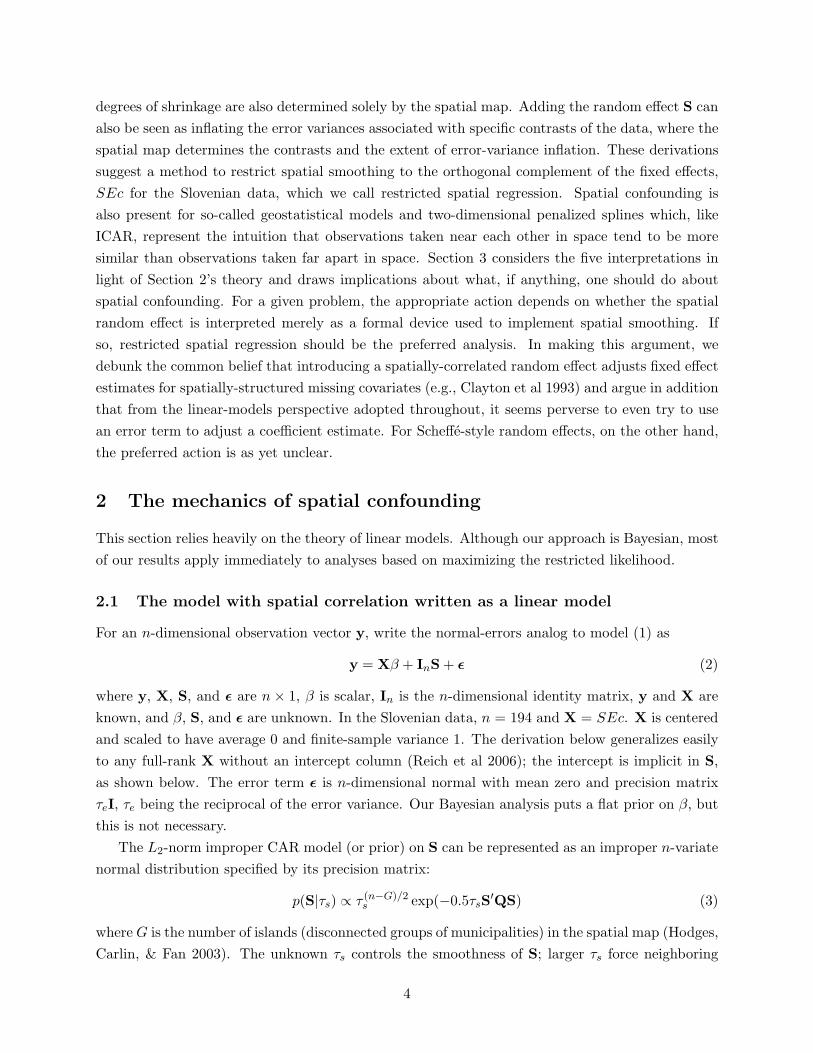
degrees of shrinkage are also determined solely by the spatial map. Adding the random effect S canalso be seen as inflating the error variances associated with specific contrasts of the data, where thespatial map determines the contrasts and the extent of error-variance inflation. These derivationssuggest a method to restrict spatial smoothing to the orthogonal complement of the fixed effects,SEc for the Slovenian data, which we call restricted spatial regression. Spatial confounding isalso present for so-called geostatistical models and two-dimensional penalized splines which, likeICAR, represent the intuition that observations taken near each other in space tend to be moresimilar than observations taken far apart in space. Section 3 considers the five interpretations inlight of Section 2’s theory and draws implications about what, if anything, one should do aboutspatial confounding. For a given problem, the appropriate action depends on whether the spatialrandom effect is interpreted merely as a formal device used to implement spatial smoothing. Ifso, restricted spatial regression should be the preferred analysis. In making this argument, wedebunk the common belief that introducing a spatially-correlated random effect adjusts fixed effectestimates for spatially-structured missing covariates (e.g., Clayton et al 1993) and argue in additionthat from the linear-models perspective adopted throughout, it seems perverse to even try to usean error term to adjust a coefficient estimate. For Scheffe-style random effects, on the other hand,the preferred action is as yet unclear.

2 The mechanics of spatial confounding

This section relies heavily on the theory of linear models. Although our approach is Bayesian, mostof our results apply immediately to analyses based on maximizing the restricted likelihood.

2.1 The model with spatial correlation written as a linear model

For an n-dimensional observation vector y, write the normal-errors analog to model (1) as

y = Xβ + InS + ε (2)

where y, X, S, and ε are n × 1, β is scalar, In is the n-dimensional identity matrix, y and X areknown, and β, S, and ε are unknown. In the Slovenian data, n = 194 and X = SEc. X is centeredand scaled to have average 0 and finite-sample variance 1. The derivation below generalizes easilyto any full-rank X without an intercept column (Reich et al 2006); the intercept is implicit in S,as shown below. The error term ε is n-dimensional normal with mean zero and precision matrixτeI, τe being the reciprocal of the error variance. Our Bayesian analysis puts a flat prior on β, butthis is not necessary.

The L2-norm improper CAR model (or prior) on S can be represented as an improper n-variatenormal distribution specified by its precision matrix:

p(S|τs) ∝ τ (n−G)/2s exp(−0.5τsS′QS) (3)

where G is the number of islands (disconnected groups of municipalities) in the spatial map (Hodges,Carlin, & Fan 2003). The unknown τs controls the smoothness of S; larger τs force neighboring

4

Si to be more similar to each other. Q encodes the neighbor pairs, with diagonal elements qii =number of municipality i’s neighbors, and qij = -1 if municipalities i and j are neighbors and 0otherwise. For the Slovenian data, G = 1 and we specify that municipalities i and j are neighbors ifthey share a boundary. Other specifications of neighbor pairs are possible but this one is common.Model (3) can be re-expressed in the pairwise-difference form

p(S|τs) ∝ τ (n−G)/2s exp(−0.5τs

∑(Si − Sj)2) (4)

where the sum is over unique neighbor pairs (i, j).We have written model (2) with the random effect S having design matrix In to emphasize

that model (2) is over-parameterized and is identified only because S is smoothed or, alternatively,constrained by the ICAR model (3). To clarify the identification issues, re-parameterize (2) asfollows. The neighbor-pair matrix Q has spectral decomposition Q = ZDZ′, where Z is n × n

orthogonal and D is diagonal with diagonal elements d1 ≥ . . . ≥ dn−G > 0 and dn−G+1 = . . . =dn = 0 (Hodges et al 2003). Z’s columns are Q’s eigenvectors; D’s diagonal elements are thecorresponding eigenvalues. Re-parameterize (2) as

y = Xβ + Zb + ε, (5)

where b = Z′S is an n-vector with a normal distribution having mean zero and diagonal precisionmatrix τsD = τsdiag(d1, . . . , dn−G, 0, . . . , 0).

The spatial random effect S thus corresponds to a saturated collection of canonical regressors,the n columns of Z, whose coefficients b are shrunk toward zero to an extent determined by τsD.The smoothing parameter τs controls shrinkage of all n components of b and the di control therelative degrees of shrinkage of the bi for a given τs. Both the canonical regressors Z and the di aredetermined solely by the spatial map through Q. The first canonical coefficient, b1, has the largestdi and is thus shrunk the most for any given τs; for the Slovenian map, d1 = 14.46. The last G bi,bn−G+1, . . . , bn are not shrunk at all because their prior precisions τsdi are zero, so they are fixedeffects implicit in the spatial random effect. The bi with the smallest positive di, dn−G, is shrunkleast of all the shrunken coefficients. For the Slovenian map with G = 1, this is b193, with d193 =0.03, so its prior precision is smaller than b1’s by a factor of about 500 for any τs.

To understand the differential shrinkage of the bi, we need to understand the columns of Z, whichthe spatial map determines. Zn−G+1, . . . , Zn, whose coefficients bn−G+1, . . . , bn are not shrunk atall, span the space of the means of (or intercepts for) the G islands in the spatial map. This is easilyseen from (4): the improper CAR distribution is flat (puts no constraint) on the G island means.Also, Q1n = 0 for any map, so the overall intercept 1n always lies in the span of Zn−G+1, . . . , Zn

and is thus implicit in the ICAR specification. Thus without loss of generality, we set Zn = 1√n1n

so all other Zi are contrasts, i.e., 1′nZi = 0.Based on examples, Zn−G, whose coefficient bn−G has the smallest positive prior precision

τsdn−G, can be interpreted loosely as the lowest frequency contrast in S among the shrunkencontrasts. Figure 2a is a plot of Zn−1 = Z193 for the Slovenian data, where darker and lightercolors indicate higher and lower values respectively. Z193 is “low-frequency” in the sense that it

5

is a roughly linear trend along the long axis of Slovenia’s map. Again based on examples, as thevalue of di increases, the frequency of the corresponding Zi increases as well. Figure 2b shows Z1

for the Slovenian data; it is roughly the difference between the two municipalities with the mostneighbors (the dark municipalities) and the average of their neighbors. For other spatial maps,the interpretations are similar. For the counties of Minnesota (Reich & Hodges 2008, Fig. 6), thecontrast with the least-smoothed coefficient is the north-south gradient, while the contrast with themost-smoothed coefficient is roughly the difference between the county having the most neighborsand the average of those neighbors. For the spatial map representing periodontal measurementsites, the contrast with the least-smoothed coefficient is nearly linear along a dental arch, whilethe contrasts with the most-smoothed coefficients are the difference, on each tooth, between theaverage of the interproximal sites and the average of the direct sites (Reich & Hodges 2008, Fig. 3,which also shows other Zi). For the Scottish lip-cancer data, the contrast with the least-smoothedcoefficient is the north-south gradient, while the contrast with the second least-smoothed coefficientis roughly quadratic along the north-south gradient, high at the northern and southern extremesand low in the middle — just like the much-studied predictor of lip cancer, AFF , which measuresemployment in agriculture, fisheries, and forestry.

2.2 Spatial confounding explained in linear-model terms

For the normal-errors model (2), it is straightforward to show (Reich et al 2006) that the posteriormean of β conditional on the precisions τe and τs is

E(β|τe, τs,y) = (X′X)−1X′y− (X′X)−1X′ZE(b|τe, τs,y), (6)

where E(b|τe, τs,y) is not conditional on β, taking the value

E(b|τe, τs,y) = (Z′PcZ + rD)−1Z′Pcy, (7)

for r = τs/τe and Pc = I−X(X′X)−1X′, the familiar residual projection matrix from linear models.These expressions are correct for full-rank X of any dimension.

In (6), the term (X′X)−1X′y is the ordinary least-squares estimate of β and also β’s posteriormean in a fit without S, using a flat prior on β. Thus the second term −(X′X)−1X′ZE(b|τe, τs,y)is the change in β’s posterior mean, conditional on (τe, τs), from adding S. Note that ZE(b|τe, τs,y)is the fitted value of S given (τe, τs). Thus when S is added to the model, the change in β’s posteriormean given (τe, τs) is -1 times the regression on X of the fitted values of S.

Because X is centered and scaled (so X′X = n− 1) and Z is orthogonal, the correlations ρi ofX and Zi, the ith column of Z, can be written as R = (ρ1, . . . , ρn−G, 0, . . . , 0)′ = (n − 1)−0.5X′Z.Equation (6) can then be written as

E(β|τe, τs,y) = βOLS − (n− 1)1/2R′E(b|τe, τs,y). (8)

(Appendix C gives a more explicit expression.) From (8), adding S to the model induces a largechange in β’s posterior mean if ρi and E(bi|τe, τs,y) are large for the same i. This happens if four

6

conditions hold: X is highly correlated with Zi; y has a substantial correlation with both X andZi; r = τs/τe is small; and di is small. The last two conditions ensure that bi is not shrunk muchtoward zero. These necessary conditions are all present in the Slovenian data: Figure 1 shows thestrong association of y and X = SEc, ρ193 = correlation(SEc, Z193) = 0.72, d193 = 0.03, and S isnot smoothed much (the effective number of parameters in the fit is pD = 62.3).

This effect on β’s estimate is easily understood in linear-model terms as the effect of adding acollinear regressor to a linear model. If S were not smoothed at all — if the coefficients b of thesaturated design matrix Z were not shrunk toward zero — then β would not be identified. Thiscorresponds to setting the smoothing precision τs to 0, so the smoothing ratio r = τs/τe = 0. Ifthe smoothing ratio r is small, β is identified but the coefficients of Zi with small di are shrunkvery little, so if these Zi are collinear with X, the estimate of β is subject to the same collinearityeffects as in linear models.

Consider also how β’s posterior variance changes when the ICAR-distributed S is added to themodel. Reich et al (2006) showed that conditional on τe and τs, adding S to the model multipliesthe conditional posterior variance of β by

[1−

∑ ρ2i

1 + rdi

]−1

, (9)

where the sum is over i with di > 0 and ρi is as above. Expression (9) holds only for single-columnX; Reich et al (2006) give an expression for general full-rank X. In general,

∑ni=1 ρ2

i = 1. BecauseZn ∝ 1n and X is centered, ρn = (n − 1)−0.5X′Zn = 0, so if r = 0, i.e., S is not smoothed,var(β|τe, τs,y) is infinite because

∑ρ2

i /(1 + rdi) =∑n−1

i=1 ρ2i = 1. As r grows from zero, S is

smoothed more and var(β|τe, τs,y) decreases. For given r, the variance inflation factor (9) is largeif ρi is large for the smallest di, as in the Slovenian data. Again, this differs from the analogousresult in linear-model theory only because the bi are shrunk.

2.3 Spatial confounding explained in a more spatial-statistics style

The linear-models explanation above seems odd to many spatial-statistics mavens, who usuallythink of the CAR as a model for the error covariance. We now give a derivation more in line withthis viewpoint.

Begin with the re-parameterized normal-errors model (5) but rewrite it in a more spatial-statistics style as y = Xβ + ψ, where the elements of ψ = Zb + ε are not independent. S does nothave a proper covariance matrix under an ICAR model, so we must proceed indirectly. PartitionZ = (Z(1)|Z(2)), where Z(1) has n−G columns and Z(2) has G columns, and partition b conformablyas b = (b(1)|b(2))′, so b(1) is (n−G)× 1 and b(2) is G× 1. Pre-multiply (5) by Z′, so (5) becomes

Z(1)′y = Z(1)′Xβ + e1, precision(e1i) = τe(rdi)/(1 + rdi) < τe (10)

Z(2)′y = Z(2)′Xβ + b(2) + e2, precision(e2i) = τe

where e1 = b(1) + Z(1)′ε and e2 = Z(2)′ε, so the two rows of (10) are independent, and recall τe isε’s error precision in (5).

7

Suppose G = 1 as in the Slovenian data; G > 1 is discussed below. Then Z(2) ∝ 1n andZ(2)′X = 0 because X is centered, so all the information about β comes from the first row of (10).Fix τs and τe. Without S in the model, β’s posterior precision (the reciprocal of β’s posteriorvariance) is X′Xτe = (n − 1)τe, which is also β’s information matrix (a scalar, in this case). Byadding S to the model, the posterior precision of β decreases by (n− 1)τe

∑n−1i=1 ρ2

i /(1+ rdi), whereas before ρi = correlation(X, Zi) = (n− 1)−1/2X′Zi and r = τs/τe. The information loss is large ifr is small (relatively little spatial smoothing) and ρi is large for i with small di, as in the Sloveniandata. Because the information about β in the different rows of (10) may not be entirely consistent,if row i of (10) differs from the other rows and row i is effectively deleted by the combination oflarge ρi and small di, β’s estimate can change markedly when S is added to the model.

If the spatial map has G > 1 islands, the ICAR model includes an implicit G − 1 degree offreedom unsmoothed fixed effect for the island means, in addition to the overall intercept. Thisisland-mean fixed effect may be collinear with X in the usual manner of linear models even if S issmoothed maximally within islands (i.e., τs is very large).

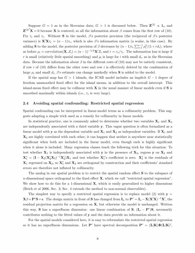
2.4 Avoiding spatial confounding: Restricted spatial regression

Spatial confounding can be interpreted in linear-model terms as a collinearity problem. This sug-gests adapting a simple trick used as a remedy for collinearity in linear models.

In statistical practice, one is commonly asked to determine whether two variables X1 and X2

are independently associated with a third variable y. This vague question is often formalized as alinear model with y as the dependent variable and X1 and X2 as independent variables. If X1 andX2 are highly correlated with each other, it can happen that neither is anywhere near statisticallysignificant when both are included in the linear model, even though each is highly significantwhen it alone is included. Many regression classes teach the following trick for this situation: Totest whether X1 is independently associated with y in the presence of X2, regress y on X2 andX∗

1 = (I − X2(X′2X2)−1X′

2)X1 and test whether X∗1’s coefficient is zero. X∗

1 is the residuals ofX1 regressed on X2, so X∗

1 and X2 are orthogonal by construction and their coefficients’ standarderrors are therefore not inflated by collinearity.

The analog in our spatial problem is to restrict the spatial random effect S to the subspace ofn-dimensional space orthogonal to the fixed effect X, which we call “restricted spatial regression”.We show how to do this for a 1-dimensional X, which is easily generalized to higher dimensions(Reich et al 2006, Sec. 3; Sec. 4 extends the method to non-normal observables).

The simplest way to specify a restricted spatial regression is to replace model (2) with y =Xβ +PcS+ε. The design matrix in front of S has changed from In to Pc = In−X(X′X)−1X′, theresidual projection matrix for a regression on X, but otherwise the model is unchanged. Writtenthis way, S has a superfluous dimension: one linear combination of S, (In − Pc)S, necessarilycontributes nothing to the fitted values of y and the data provide no information about it.

For the spatial models considered here, it is easy to reformulate the restricted spatial regressionso it has no superfluous dimensions. Let Pc have spectral decomposition Pc = (L|K)Φ(L|K)′,

8

where Φ is a diagonal matrix with n− 1 eigenvalues of 1 and one 0 eigenvalue, L has n rows andn− 1 columns, and K has n rows and 1 column, with K proportional to X and K′L = 0. Then fitthe following model:

y = Xβ + LS∗ + ε, (11)

where S∗ is (n−1)-dimensional normal with mean 0 and precision matrix τsL′QL, Q is the neighbormatrix from S’s ICAR model, and ε is iid normal with mean 0 and precision τe.

Using this model in either form and conditioning on (τs, τe), β has the same conditional posteriormean as in the analysis without the ICAR-distributed S, but has larger conditional posteriorvariance (Reich et al 2006, Sec. 3). Thus, restricted spatial regression discounts the sample size toaccount for spatial correlation without changing β’s point estimate conditional on τs and τe.

2.5 Spatial confounding is not an artifact of the ICAR model

Spatial confounding also occurs if, in model (2), S is given a proper multivariate normal distributionwith any of several covariance matrices capturing the intuition that near regions are more similarthan distant. Wakefield (2007), for example, found very similar spatial-confounding effects inthe Scottish lip-cancer data using the ICAR model and a so-called geostatistical model. For theSlovenian data, we considered geostatistical models in which each municipality’s Xi and yi weretreated as being measured at one point in the municipality. For the analyses described belowand in Appendix A, each municipality’s point had east-west coordinate the average of the farthesteast and farthest west boundary points, and analogous north-south coordinate. An example of aproper covariance matrix is cov(S) = σ2

s exp(−δij/θ), with δij being Euclidean distance betweenthe points representing municipalities i and j and θ controlling spatial correlation. Each suchcovariance matrix that we considered had an unknown parameter like θ, which for now we treatas fixed and known. Applying Section 2.2’s approach to such models for S requires only onechange, arising because the precision matrix cov(S)−1 now has no zero eigenvalues: we must addan explicit intercept to model (5). Therefore, holding θ fixed, spatial confounding will occur by thesame mechanism as with the ICAR model for S. (For the Slovenian data, the smallest eigenvalueof cov(S)−1 has eigenvector Z194 which, while not constant over the map as for the ICAR model,nonetheless varies little. We have seen this in other geostatistical models; it explains why theintercept can be poorly identified in such models, but the generality of this intercept confoundingis unknown.)

In the preceding paragraph, we treated as fixed the parameter θ in cov(S). In a non-Bayesiananalysis these parameters are typically estimated, while in a Bayesian analysis they are randomvariables. Thus in applying Section 2.2’s analysis to geostatistical models for S, the canonicalregressors Z depend on the unknown parameter θ of cov(S). However, for at least four commonforms of cov(S) that we explored (Appendix A), as θ varied over a wide range the eigenvectorcorresponding to the second-smallest eigenvalue of cov(S)−1 — the canonical regressor Zi mostlikely to produce spatial confounding — was highly correlated with the analogous eigenvector of theICAR model’s precision matrix τsQ, the canonical regressor that did produce spatial confounding in

9

this dataset. Thus, spatial confounding will occur in the Slovenian data for these four geostatisticalmodels.

Applying the spectral approximation to geostatistical models (Appendix B) is another way tomake the foregoing more concrete. For measurements taken on a regular square grid, the spectralapproximation is closely analogous to Section 2.1’s formulation of the ICAR model as a linearmodel. For this special case, the canonical regressors with least- and most-shrunk coefficients areliterally trigonometric functions that are low- and high-frequency respectively.

Penalized splines are a quite different approach to spatial smoothing; Ruppert et al (2003, ch.13) give a very accessible introduction. However, penalized splines produce the same confoundingeffect in the Slovenian data. In a class project (Salkowski 2008), a student fit a two-dimensionalpenalized spline to the Slovenian data, attributing each municipality’s counts to a point as describedabove. He used the R package SemiPar (version 1.0-2; the package and documentation are athttp://www.uow.edu.au/∼mwand/webspr/rsplus.html) to fit a model in which municipality i’sobserved count of stomach cancers Oi was Poisson with log mean

log{Ei}+ β0 + βSEcSEci + βEEi + βNNi +∑

k

ukbasiski, (12)

where Ei is municipality i’s east-west coordinate, Ni is its north-south coordinate (each coordinatewas centered and both were scaled by a single scaling constant to preserve the map’s shape), basiski

is the default basis in SemiPar (based on the Matern covariance function), the uk were modeledas iid normal, and the knots were SemiPar’s default knots. SemiPar’s default fitting method,penalized quasi-likelihood, shrank the random effect term

∑k ukbasiski to zero but the two fixed

effects implicit in the spline, Ei and Ni, remained in the model and produced a collinearity effectas in an ordinary linear model. Without the spatial spline, a simple generalized linear model fitgave an estimate for βSEc of -0.137 (standard error 0.020), essentially the same as in Zadnik’sBayesian analysis, while adding just the fixed effects Ei and Ni changed βSEc’s estimate to -0.052(SE 0.028). As the spline fit was forced to be progressively less smooth, βSEc’s estimate increasedmonotonically and eventually became positive. (Steinberg & Bursztyn 2004, p. 415, note in passinga similar confounding effect in a different spline.)

Thus, spatial confounding is not an artifact of the ICAR model, but arises from other, perhapsall, specifications of the intuition that measures taken at locations near to each other are moresimilar than measures taken at distant locations.

3 Evaluating the five interpretations; implications for practice

Before we can discuss interpretations of spatial confounding, we need to distinguish two inter-pretations of “random effect”. One is traditional, as in the definition from Scheffe (1959) notedabove: the levels of a random effect are draws from a population, and the draws are not of interestin themselves but only as samples from the larger population, which is of interest. In recent years,

10

“random effect” has come to be used in a second sense, to describe effects that have the mathe-matical form of a Scheffe-style random effect but which are quite different. For these newer-stylerandom effects, the levels are the entire population; or the levels are themselves of interest; or thelevels are in no meaningful sense draws from a population, from which further draws could be made.The Slovenian data is an example in which the levels (municipalities) are the entire population.Hospital quality-of-care studies provide examples in which the levels (hospitals) may be consid-ered draws from a population but are themselves of interest. The mixed-model representation ofpenalized splines (Ruppert et al, 2003) is an example of random effects with levels that are notdraws from any conceivable population. In the simplest case of a one-dimensional penalized splinewith a truncated-line basis, the random effect is the changes in the fit’s slope at each knot, and itsdistribution is simply a device for penalizing changes in the slope. The senselessness of imaginingfurther draws from such random effects is clearest for the examples in Ruppert et al (2003) in whichpenalized splines are used to estimate smooth functions in the physical sciences.

A full discussion of random effect interpretations is beyond the present paper’s scope. Wenote, however, that discussions of spatial random effects are generally either unclear about theirinterpretation or seem to treat them as Scheffe-style random effects. Finally, it is both economicaland accurate to describe all non-Scheffe-style random effects as formal devices to implement asmoother, interpreting shrinkage estimation as a kind of smoothing, so from now on we do so.

3.1 The random effect S is a formal device to implement a smoother

Consider situations in which S is not a Scheffe-style random effect. For these situations, we haveseen two interpretations of spatial confounding.

• (i) Spatially-correlated errors remove bias in estimating β and are generally conservative(Clayton et al 1993).

• (ii) Spatially-correlated errors can introduce or remove bias in estimating β and are notnecessarily conservative (Wakefield 2007; implicit in Reich et al 2006).

It is commonly argued (e.g., Clayton et al 1993) that introducing spatially correlated errorsinto a model, as with S+ ε, captures the effects of spatially-structured missing covariates and thusadjusts the estimate of β for such missing covariates even if we have no idea what those covariatesmight be. Interpretation (i) reflects this view. We have also heard a somewhat different statementof this view, as in: “I know I am missing some confounders, in fact I have some specific confoundersin mind that I was unable to collect, but from experience I know they have a spatial pattern.Therefore, I will add S to the model to try to recover them and let the data decide how much canbe recovered.” In some fields, it is nearly impossible to get a paper published unless a random effectis included for this purpose.

We can now evaluate this view using the results of Section 2, which are a modest elaborationof linear-model theory. Indeed, the only aspect of the present problem not present in linear-model

11

theory is that most of the canonical coefficients bi are shrunk toward 0, although the bi that producespatial confounding are shrunk the least and thus deviate least from linear-model theory.

To make the discussion concrete, consider estimating β using the model y = 1nα + Xβ + ε,where ε is iid normal error, then estimating β using a larger model, either y = 1nα+Xβ +Hγ + ε,where H is a supposed missing covariate, or using model (2), which adds the ICAR-distributedspatial random effect S. Appendix C gives explicit expressions for the adjustment in the estimateof β under either of these larger models, and for the expected adjustment assuming the data weregenerated by the model

y = 1nα + Xβ + Hγ + ε. (13)

We summarize Appendix C’s results here.There is no necessary relationship between the adjustment to β’s estimate arising from adding

S to the model and the adjustment arising from adding the supposed missing covariate H. This ismost striking if we suppose that H is uncorrelated with X, so that adding H to the model wouldnot change the estimate of β. In this case, adding the spatial random effect S does adjust theestimate of β, and in a manner that depends not on H but on the correlation of X and y andon the spatial map. If the data are generated by (13), the expected adjustment in β’s estimatefrom adding S to the model is not zero in general and can be biased in either direction. If thereare no missing covariates, adding S nonetheless adjusts β’s estimate in the manner just describedalthough the expected adjustment is zero. It is fair to describe such adjustments as haphazard.

Now suppose H is correlated with X, so that adding H to the model changes the estimate of β.In this case, the adjustment to β’s estimate under the spatial model is again biased. The bias canbe large and either positive or negative, depending on the degree of smoothing (more smoothnessgenerally implies larger bias) and depending haphazardly on H and on the spatial map. The biascan even be in the wrong direction, so that on average β’s estimate becomes larger when it wouldbecome smaller if H were added to the model.

Therefore, adding spatially correlated errors is not conservative: a canonical regressor Zi thatis collinear with X can cause β’s estimate to increase in absolute value just as in ordinary linearmodels. Further, in cases in which β’s estimate should not be adjusted, introducing spatially-correlated errors will, nonetheless, adjust the estimate haphazardly.

From the perspective of linear-model theory, it seems perverse to use an error term to adjustfor the possibility of missing confounders. The analog in ordinary linear models would be to movepart of the fitted coefficients into error to allow for the possibility of as-yet-unconceived missingconfounders. In using an ordinary linear model, we know that if missing confounders are correlatedwith included fixed effects, variation in y that would be attributed to the missing confounders isinstead attributed to the included fixed effects. We acknowledge that possibility in the standarddisclaimer that if we have omitted confounders, our coefficient estimates could be wrong. In spatialmodeling, the analogy to this practice would be to use restricted spatial regression, so that allvariation in y in the column space of included fixed effects is attributed to those included effectsinstead of being haphazardly re-allocated to the spatial random effect.

12

Therefore, interpretation (i) cannot be sustained and interpretation (ii) is correct, when therandom effect S is interpreted as a mere formal device to implement a smoother. Adding spatially-correlated errors cannot be expected to capture the effect of a spatially-structured missing covariate,but only to smooth fitted values and discount the sample size in computing standard errors orposterior standard deviations for fixed effects. Therefore, in such cases you should always userestricted spatial regression so the sample size can be discounted without distorting the fixed effectestimate. If you are concerned about specific unmeasured confounders, you should add to themodel a suitable explicit fixed effect, not adjust haphazardly by means of a spatially-correlatederror. Finally, conclusions from such analyses should be qualified as in any other observationalstudy, e.g., we have estimated the association of our outcome with our regressors accounting formeasured confounders, and if we have omitted confounders, then our estimate could be wrong.

3.2 S is a Scheffe-style random effect

For these situations, we have seen three interpretations.

• (iii) The spatial effect S is collinear with the fixed effect, but neither estimate of β is biased(David B. Nelson, personal communication).

• (iv) Adding the spatial effect S creates information loss, but neither estimate of β is biased(David B. Nelson, personal communication).

• (v) Because error is correlated with the regressor X in the sense commonly used in econo-metrics, both estimates of β are biased (Paciorek 2009).

Interpretations (iii) and (iv) treat the fixed effect X as measured without error and not oth-erwise drawn from a probability distribution (“fixed and known”), while interpretation (v) treatsX as drawn from a probability distribution. Interpreting spatial confounding therefore depends onwhether X is interpreted as fixed and known or as a random variable. This is a messy business,which seems to be determined in practice less by facts than by the department in which one wastrained. The present authors’ training inclines us to view X as fixed and known as a default, whileeconometricians, for example, seem inclined to the opposite default.

To see the difficulty, consider an example in which the random effect is hospitals selected asa random sample from a population of hospitals, and the fixed effect is an indicator of whether ahospital is a teaching hospital. The present authors’ default is to treat teaching status as fixed andknown. However, if we have drawn 20 hospitals at random, then the teaching status of hospitali is a random variable determined by the sample of hospitals we happen to draw, so X is drawnfrom a probability distribution. But what if, as often happens, sampling is stratified by teachingstatus to ensure that (say) 10 hospitals are teaching hospitals and 10 are not? Now teachingstatus is fixed and known. But what if someone gives us the dataset and we don’t know whethersampling was stratified by teaching status? One might argue that our ignorance disqualifies us fromanalyzing these data, but that argument is not compelling to, for example, people who interpret

13

the Likelihood Principle as meaning they can ignore the sampling mechanism, or to many peoplewho do not have a tenured, hard-money faculty position.

Again, a full discussion of this issue is beyond the present paper’s scope. It is also unnecessaryfor the present purpose, because there are unarguable instances of each kind of fixed effect. Anexample of a fixed and known X could arise in analyzing air pollution measured at many fixedmonitoring stations on each day in a year. The days could be interpreted as a Scheffe-style randomeffect, and the elevation of each monitoring station as a fixed and known X. For an example ofX plainly drawn from a probability distribution, consider the hospitals example just above, wherethe morbidity score for each hospital’s patients is a random variable for the period being studied.

So first assume X is fixed and known. It is then straightforward to show that both (iii) and(iv) are correct and indeed arguably identical, though we think they are worth distinguishing.Interpretation (iv) follows from Section 2.3 and the familiar fact that generalized least squares givesunbiased estimates even when the covariance matrix is specified incorrectly. For interpretation (iii),recall from equation (8) that the estimate of β in the spatial model (which, given τe and τs, is boththe posterior mean and the usual estimate following maximization of the restricted likelihood) is

E(β|τe, τs,y) = βOLS − (n− 1)−1/2R′E(b|τe, τs,y). (14)

By (7), (n−1)−1/2R′E(b|τe, τs,y) can be written as KPcy where K is an appropriate-sized knownsquare matrix. Recalling that Pc = I−X(X′X)−1X′, Pcy = Pc(Zb + ε), which has expectation 0with respect to b and ε. Hence the spatial and OLS estimates of β have the same expectation andare unbiased based on the aforementioned familiar fact about generalized least squares.

Now assume X is a random variable. Paciorek (2009) interprets model (5) as y = Xβ + ψ

where the error term ψ = Zb + ε has a non-diagonal covariance matrix. Because X′Z 6= 0, X iscorrelated with ψ, so by the standard result in econometrics, both the OLS estimate of β and theestimate of β using (5) are biased. Formulating the result this way is more precise than the commonstatement that bias arises when “the random effect is correlated with the fixed effect”, because thedistribution of “the random effect” depends on the parameterization: the random effect b in model(5) is independent of X, but the random effect S in model (2) is not.

The main point of Paciorek (2009), which presumes the spatial random effect S captures amissing covariate, is that “bias [in estimating β] is reduced only when there is variation in thecovariate [X] at a scale smaller than the scale of the unmeasured covariate [supposedly capturedby S]”. We conjecture that this can be interpreted in Section 2.2’s terms as meaning that bias isreduced if X is not too highly correlated with the low-frequency canonical regressors Zi that havesmall di and hence little shrinkage in bi.

Paciorek (2009) concludes that restricted spatial regression is either irrelevant to the issue ofbias in estimating β or makes an overly strong assumption by attributing to X all of the disputedvariation in y. The latter appears to presume that the spatial random effect S captures an unspec-ified missing covariate, which, we have argued, is difficult to sustain. However, this area of researchis just beginning and much remains to be developed.

14

4 Conclusion

The preceding sections laid out the mechanics by which spatial confounding occurs, expanding onReich et al (2006); showed briefly that this is not an artifact of the ICAR model but is far moregeneral; gave an alternative analysis (restricted spatial regression) that removes spatial confounding;and considered proposed interpretations of spatial confounding, concluding that restricted spatialregression should be used routinely when S is a formal device to implement a smoother, a commonsituation.

The literature on spatial confounding is small but it appears many people encounter this problemin practice. Thus although the present paper is not the last word on the subject, it does bringtogether the various approaches to this phenomenon, which should in time yield generally-acceptedadvice for statistical practice.

Our understanding of the mechanics of spatial confounding is underdeveloped in certain respects.In debunking the common belief that spatially-correlated errors adjust for unspecified missingcovariates, our derivation (Appendix C) took the smoothing ratio r = τs/τe as given. Although r’smarginal posterior distribution is easily derived when τe has a gamma prior, it is harder to interpretthan the posterior mean of β so its implications are as yet unclear. However, it should be possible toextract some generalizations which, with the expressions in Appendix C, will permit understandingof the situations in which spatial confounding will and will not occur. We hypothesize this workwill show that whenever both y and X are highly correlated with Zn−G, the canonical regressorwith the least-smoothed coefficient, there will be little smoothing (r will be small) and β’s estimateunder the spatial model will be close to zero. In other words, we hypothesize that in any map, whenboth y and X show a strong trend along the long axis of the map, adding a spatially-correlatederror will nullify the obvious association between y and X as it did in the Slovenian data.

The theory is particularly underdeveloped for the situation in which both S and X can beinterpreted as random in Scheffe’s sense; Paciorek (2009) is a first step in what should be a richarea of research.

Appendix A: A small exploration of spatial confounding in some

common geostatistical models

In Section 2.5, each municipality i was assigned north-south and east-west coordinates. In thecomputations below, each coordinate was centered so it averaged zero across the municipalities,and both centered coordinates were divided by a common scaling constant. The symbols Ni andEi refer to the centered and scaled north-south and east-west coordinates respectively, which hadstandard deviations 0.76 and 1.24 respectively.

We considered four forms of cov(S) determined by combinations of two distance measures andtwo specifications of correlation between municipalities as a function of distance between them.The measures describing distance between municipalities i and j, δij , were Euclidean distance[(Ni−Nj)2 +(Ei−Ej)2]0.5 and maximum distance max(|Ni−Nj |, |Ei−Ej |), for which the largest

15

Table 1: Correlation between eigenvectors corresponding to jth smallest eigenvalues of the ICAR’sQ matrix and of cov(S)−1, for four specifications of cov(S) and various θ.

θ

distance function j 0.5 1.0 1.5 2.0 2.5 3.0 3.5 4.0 4.5 5.0

Euclidean exponential 2 0.89 0.95 0.95 0.96 0.96 0.96 0.96 0.96 0.96 0.963 0.79 0.87 0.88 0.88 0.88 0.87 0.87 0.86 0.86 0.854 0.42 0.20 0.21 0.23 0.24 0.25 0.25 0.26 0.26 0.26

Euclidean linear 2 0.34 0.61 0.88 0.92 0.94 0.95 0.96 0.96 0.96 0.963 0.44 0.60 0.80 0.87 0.88 0.85 0.66 0.28 0.18 0.194 0.25 0.33 0.10 0.15 0.21 0.27 0.28 0.20 0.15 0.13

maximum exponential 2 0.90 0.94 0.95 0.95 0.95 0.95 0.95 0.95 0.95 0.953 0.81 0.86 0.87 0.87 0.87 0.86 0.86 0.85 0.84 0.834 0.17 0.11 0.10 0.10 0.09 0.09 0.09 0.08 0.08 0.08

maximum linear 2 0.36 0.72 0.90 0.93 0.94 0.94 0.95 0.95 0.95 0.953 0.15 0.66 0.83 0.87 0.87 0.87 0.26 0.25 0.26 0.294 0.26 0.36 0.09 0.11 0.14 0.13 0.01 0.03 0.04 0.04

distances between two municipalities were 5.4 and 4.7 respectively. The forms specifying correlationas a function of distance were exponential, exp(−δij/θ), and linear, max[(1− δij/θ), 0].

For each form of cov(S), Table 1 shows the correlation between the eigenvector correspondingto the jth smallest eigenvalue of cov(S)−1 and the eigenvector corresponding to the jth smallesteigenvalue of the ICAR model’s neighbor matrix Q, for a range of values of cov(S)’s tuning constantθ. When this correlation is high for j = 2, the geostatistical specification for cov(S) will producethe same spatial confounding as the ICAR model.

Table 1 shows that generally the correlations between eigenvectors of cov(S)−1 and Q are highfor j = 2 and j = 3, but fall off substantially for j = 4 and for j > 4 (not shown). Results forthe four cov(S) differ somewhat in details. The two distance measures behave similarly. However,while the exponential function of distance gives high correlations for all values of θ shown here forj = 2, 3, the linear function of distance shows smaller correlations for small values of θ, most likelybecause the spatial correlation dies off so quickly for small θ, and for j = 3 for large θ as well.

Appendix B: Spatial confounding with spectral methods

Section 2.2’s results for a discrete spatial domain can be extended to Gaussian process modelsdefined on a continuous spatial domain. Let y(si) = x′iβ+S(si)+εi, where si ∈ R2, εi

iid∼ N(0, τe) ispure error, and S is a spatial process with mean zero, precision τs, and stationary spatial correlationfunction Cor(si, sj) = ρ(si − sj).

16

The spectral representation theorem states that S(s) can be written

S(s) =∫

R2cos(ω′s)db1(ω) +

∫

R2sin(ω′s)db2(ω), (15)

where ω = (ω1, ω2)′ ∈ R2 is a frequency and b1 and b2 are independent Gaussian processes withmean zero, orthogonal increments, and E(|dbj(ω)|2) = F (ω)/τs. The spectral representation formu-lates the spatial process as a convolution of trigonometric basis functions and stochastic processesin the frequency domain with independent increments. The spatial correlation ρ is directly relatedto the spectral density F :

ρ(si − sj) =∫

R2cos[ω′(si − sj)]dF (ω). (16)

The spectral density is often decreasing in ||ω||, for example, F (ω) ∝ exp(−||ω||2/(4φ)) correspondsto the squared-exponential covariance ρ(si − sj) = exp(−φ||si − sj ||2).

Assuming the observations lie on a m × m square grid with distance one between neighbor-ing sites, S’s density can be approximated (Whittle 1954) by a sum over a finite grid of Fourierfrequencies ωl ∈ {2πb−(m− 1)/2c/m, ..., 2π(n− bn/2c)/m}2,

S(s) =2∑

j=1

m2∑

l=1

Zj(s, ωl)bjl (17)

bjl ∼ N(0, τsdl)

where bxc is the smallest integer greater than or equal to x, Z1(s,ω) = cos(ω′s), Z2(s, ω) =sin(ω′s), and τsdl is a precision with dl = 1/F (ωl). In this special case, the Zj are orthogonal, i.e.,∑m2

l=1 Zj(s,ωl)Zk(s′,ωl) = I(k = j)I(s = s′). This approximation may induce edge and aliasingeffects in the spatial covariance, especially for small grids, but the approximation is useful forstudying the fixed effects. This representation is directly analogous to the ICAR model as in (5),so the rest of the analysis applied to the ICAR model follows directly.

Comparing the spectral representation (17) with the ICAR model (5), the trigonometric func-tions Z1 and Z2 are analogous to Section 2.2’s eigenvectors Zj , and the inverse of the spectraldensity 1/F (ω) is analogous to the eigenvalues dj in Section 2.2. Unlike the eigenvectors and eigen-values of the ICAR model, Z1, Z2 and F have explicit forms, so the role of the covariate’s spatialscale is more clear. High-frequency terms (large ||ω||) have small prior variance (small F (||ω||))and are shrunk a great deal, while low-frequency terms (small ||ω||) have large prior variance (largeF (||ω||)) and are shrunk relatively little. In this parameterization, the correlations between acovariate and the Zj clearly describe the covariate’s variation at different spatial scales.

17

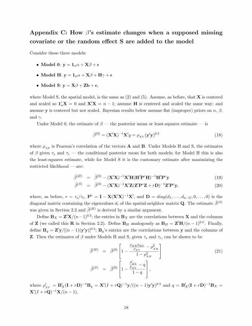
Appendix C: How β’s estimate changes when a supposed missing

covariate or the random effect S are added to the model

Consider these three models:

• Model 0: y = 1nα + Xβ + ε

• Model H: y = 1nα + Xβ + Hγ + ε

• Model S: y = Xβ + Zb + ε,

where Model S, the spatial model, is the same as (2) and (5). Assume, as before, that X is centeredand scaled so 1′nX = 0 and X′X = n − 1; assume H is centered and scaled the same way; andassume y is centered but not scaled. Bayesian results below assume flat (improper) priors on α, β,and γ.

Under Model 0, the estimate of β — the posterior mean or least-squares estimate — is

β(0) = (X′X)−1X′y = ρXY (y′y)0.5 (18)

where ρAB is Pearson’s correlation of the vectors A and B. Under Models H and S, the estimatesof β given τs and τe — the conditional posterior mean for both models; for Model H this is alsothe least-squares estimate, while for Model S it is the customary estimate after maximizing therestricted likelihood — are:

β(H) = β(0) − (X′X)−1X′H(H′PcH)−1H′Pcy (19)

β(S) = β(0) − (X′X)−1X′Z(Z′PcZ + rD)−1Z′Pcy, (20)

where, as before, r = τs/τe, Pc = I − X(X′X)−1X′, and D = diag(d1, . . . , dn−G, 0, . . . , 0) is thediagonal matrix containing the eigenvalues di of the spatial-neighbor matrix Q. The estimate β(S)

was given in Section 2.2 and β(H) is derived by a similar argument.Define BX = Z′X/(n−1)0.5; the entries in BX are the correlations between X and the columns

of Z (we called this R in Section 2.2). Define BH analogously as BH = Z′H/(n − 1)0.5. Finally,define By = Z′y/[(n − 1)(y′y)]0.5; By’s entries are the correlations between y and the columns ofZ. Then the estimates of β under Models H and S, given τs and τe, can be shown to be

β(H) = β(0)

1−

ρXH

ρHY

ρXY

− ρ2XH

1− ρ2XH

(21)

β(S) = β(0)

1−

ρ′XY

ρXY

− q

1− q

,

where ρ′XY

= B′X(I + rD)−1By = X′(I + rQ)−1y/((n − 1)y′y)0.5 and q = B′

X(I + rD)−1BX =X′(I + rQ)−1X/(n− 1).

18

In (21), the expressions in square brackets for β(H) and for β(S) have no necessary relationto each other. For example, if X and H are uncorrelated, so ρXH = 0, then β(H) = β(0) butβ(S) 6= β(0). In particular, β(S) can be larger or smaller than β(H) in absolute value; this dependson how (I+rD)−1 differentially downweights specific coordinates of BX and By. When ρ′

XY≈ ρXY ,

β(S) ≈ 0. This happens if the ith coordinate of BX , the correlation of X and Zi, is large; the ith

coordinate of By, the correlation of y and Zi, is large; and di and r are small, as in the Sloveniandata.

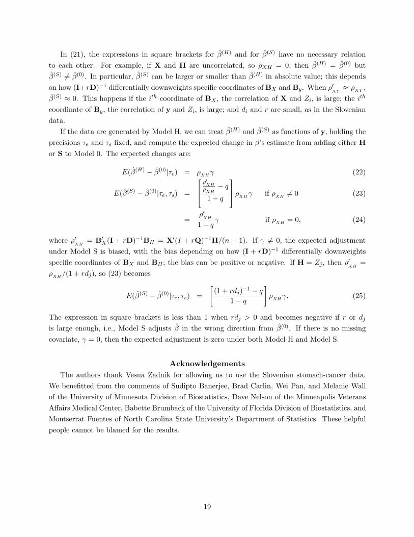
If the data are generated by Model H, we can treat β(H) and β(S) as functions of y, holding theprecisions τe and τs fixed, and compute the expected change in β’s estimate from adding either Hor S to Model 0. The expected changes are:

E(β(H) − β(0)|τe) = ρXH γ (22)

E(β(S) − β(0)|τe, τs) =

ρ′XH

ρXH

− q

1− q

ρXH γ if ρXH 6= 0 (23)

=ρ′

XH

1− qγ if ρXH = 0, (24)

where ρ′XH

= B′X(I + rD)−1BH = X′(I + rQ)−1H/(n − 1). If γ 6= 0, the expected adjustment

under Model S is biased, with the bias depending on how (I + rD)−1 differentially downweightsspecific coordinates of BX and BH ; the bias can be positive or negative. If H = Zj , then ρ′

XH=

ρXH /(1 + rdj), so (23) becomes

E(β(S) − β(0)|τe, τs) =

[(1 + rdj)−1 − q

1− q

]ρXH γ. (25)

The expression in square brackets is less than 1 when rdj > 0 and becomes negative if r or dj

is large enough, i.e., Model S adjusts β in the wrong direction from β(0). If there is no missingcovariate, γ = 0, then the expected adjustment is zero under both Model H and Model S.

Acknowledgements

The authors thank Vesna Zadnik for allowing us to use the Slovenian stomach-cancer data.We benefitted from the comments of Sudipto Banerjee, Brad Carlin, Wei Pan, and Melanie Wallof the University of Minnesota Division of Biostatistics, Dave Nelson of the Minneapolis VeteransAffairs Medical Center, Babette Brumback of the University of Florida Division of Biostatistics, andMontserrat Fuentes of North Carolina State University’s Department of Statistics. These helpfulpeople cannot be blamed for the results.

19

References

Clayton DG, Bernardinelli L, Montomoli C (1993). Spatial correlation in ecological analysis. Int.J. Epi., 22,1193-1201.

Hodges JS, Carlin BP, Fan Q (2003). On the precision of the conditionally autoregressive priorin spatial models. Biometrics, 59, 317-322.

Paciorek CJ (2009). The importance of scale for spatial-confounding bias and precision of spatialregression estimators. Manuscript dated March 12, 2009.

Reich BJ, Hodges JS (2008). Identification of the variance components in the general two-variancelinear model. J. Stat. Plan. Inf., 138, 1592-1604.

Reich BJ, Hodges JS, Zadnik V (2006). Effects of residual smoothing on the posterior of thefixed effects in disease-mapping models. Biometrics, 62, 1197-1206. Errata available fromthe corresponding author.

Ruppert D, Wand MP, Carroll RJ (2003). Semiparametric Regression. New York:Cambridge.

Salkowski NJ (2008). Using the SemiPar Package. Class project, available at URLhttp://www.biostat.umn.edu/∼hodges/SalkowskiRPMProject.pdf.

Scheffe H (1959). The Analysis of Variance, New York:Wiley.

Spiegelhalter DM, Best DG, Carlin BP, Van der Linde A (2002). Bayesian measures of modelcomplexity and fit (with discussion). J. Royal Statistical Society, Ser. B, 64, 583-639.

Steinberg DM, Bursztyn D (2004). Data analytic tools for understanding random field regressionmodels. Technometrics, 46, 411-420.

Wakefield J (2007). Disease mapping and spatial regression with count data. Biostatistics, 8,158-183.

Whittle P (1954). On stationary processes in the plane. Biometrika, 41, 434-449.

Zadnik V, Reich BJ (2006). Analysis of the relationship between socioeconomic factors andstomach cancer incidence in Slovenia. Neoplasma, 53, 103-110.

20

Figure 1: For the Slovenian municipalities, panel (a): Observed standardized incidence ratio SIR =Oi/Ei; panel (b): Centered and scaled socioeconomic status SEc.

(a) SIR (b) SEc

21

Figure 2: Two canonical regressors, columns of the matrix Z; panel (a): Z193, with the smallestpositive eigenvalue d193 and thus the least-shrunk coefficient b193 among the shrunk coefficients;panel (b): Z1, with the largest eigenvalue d193 and thus the most-shrunk coefficient b1.

(a) Z193 (b) Z1

22