adaptive spatiotemporal receptive field estimation in the ... ·...

LETTER Communicated by Dario Ringach

Adaptive Spatiotemporal Receptive Field Estimation in theVisual Pathway

Garrett B. [email protected] of Engineering and Applied Sciences, Harvard University, Cambridge, MA02138, U.S.A.

The encoding properties of the visual pathway are under constant con-trol from mechanisms of adaptation and systems-level plasticity. In allbut the most arti�cial experimental conditions, these mechanisms serveto continuously modulate the spatial and temporal receptive �eld (RF)dynamics. Conventional reverse-correlation techniques designed to cap-ture spatiotemporal RF properties assume invariant stimulus-responserelationships over experimental trials and are thus limited in their ap-plicability to more natural experimental conditions. Presented here is anapproach to tracking time-varying encoding dynamics in the early visualpathway based on adaptive estimation of the spatiotemporal RF in thetime domain. Simulations and experimental data from the lateral genic-ulate nucleus reveal that subtle features of encoding properties can becaptured by the adaptive approach that would otherwise be undetected.Capturing the role of dynamically varying encoding mechanisms is vi-tal to our understanding of vision on the natural setting, where there isabsence of a true steady state.

1 Introduction

In the early visual pathway, each neuron encodes information about a re-stricted region of visual space that is generally referred to as the receptive�eld (RF) of the cell. The dominant paradigm over the past several decadesis that the RF extent and the corresponding temporal encoding propertiesof the neuron are primarily a function of bottom-up processing, and arethus invariant properties of the cell. Overwhelming evidence contradictsthis static construct, pointing toward more complex time-varying encodingmechanisms that result from a variety of dynamic sources. Adaptation andplasticity exist on a number of different timescales ranging from millisec-onds to hours; these mechanisms have been studied for some time, but therole in the encoding process is not yet known. In this article, a new ap-proach to RF estimation is presented that is critical in precisely quantifyingeffects of systems-level plasticity or adaptation and the role they play inencoding information about the visual world. An adaptive implementation

Neural Computation 14, 2925–2946 (2002) c° 2002 Massachusetts Institute of Technology

2926 Garrett B. Stanley

is developed that characterizes the functional nature of the time-varyingproperties that have been explored experimentally but have not yet beenwell quanti�ed in the context of neuronal encoding.

The linear correlation structure between controlled sensory stimuli andthe corresponding recorded neural activity has been shown to reveal a sig-ni�cant amount of information about the underlying functional proper-ties of the neuron. Reverse-correlation techniques, which refer to the cross-correlation between stimulus and response for white noise stimuli, havebeen implemented in a number of systems to characterize the linear compo-nent of the stimulus-response relationship of the cells. In the visual pathway,spatiotemporal white noise stimuli have been used extensively to character-ize the dynamics of neurons in the retina, lateral geniculate nucleus (LGN),and primary visual cortex using the reverse-correlation technique (Jones& Palmer, 1987; Reid, Soodak, & Shapley, 1991; Reid, Victor, & Shapley,1997; Mao, MacLeish, & Victor, 1998). Additionally, in the auditory system,researchers have long since used reverse-correlation techniques for charac-terizing auditory neurons in the periphery (DeBoer & Kuyper, 1968), andothers have recently used reverse-correlation techniques to extract sound-feature selectivity of neurons in the auditory cortex (deCharms, Blake, &Merzenich, 1998). These techniques have been instrumental in developingour understanding of systems-level processing in the early sensory path-ways. One of the major assumptions of the reverse correlation technique isthat the dynamics of the underlying functional mechanisms in the visualpathway are time invariant, resulting in spatiotemporal RF properties thatremain unchanged with time. As early as the retina, however, adaptationmechanisms act on a continuum of timescales to adjust encoding dynamicsin response to changes in the visual environment (Enroth-Cugell & Shap-ley, 1973; Shapley & Victor, 1978). Adaptation mechanisms have also beenidenti�ed in the LGN (Ohzawa, Sclar, & Freeman, 1985) and cortical areaV1 (Albrecht, Farrar, & Hamilton, 1984), and models have been suggestedin which population activity acts in a divisive manner to regulate the cellu-lar response properties (Heeger, 1992). Furthermore, several recent studieshave shown that the spatial and temporal characteristics of visual neuronscan vary drastically over a variety of different timescales (Pei, Vidyasagar,Volgushev, & Creutzfeld, 1994; Gilbert, Das, Ito, Kapadia, & Westheimer,1996; Mukherjee & Kaplan, 1995; Przybyszewski , Gaska, Foote, & Pollen,2000), through neuromodulatory in�uences from other brain regions. Neu-rons throughout the visual pathway have been shown to exhibit temporaland spatial properties that evolve over a continuum of timescales, bring-ing into question the reliability of traditional reverse-correlation techniquesapplied over even short experimental trials. In this article, an adaptive ap-proach for the estimation of spatiotemporal RF properties from single trialsis developed speci�cally to address time-varying dynamics in the visualpathway, and the utility is demonstrated in simulation of geniculate andcortical dynamics, as well as experimental data from the cat LGN. Portions

Adaptive Spatiotemporal Receptive Field Estimation 2927

of these results have been presented elsewhere in abstract form (Stanley,2000b).

2 Receptive Field Estimation

The foundation for much of modern systems neurophysiology is the char-acterization of the relationship between sensory inputs and the correspond-ing evoked neural activity. This relationship is often referred to as the RFand in general encompasses temporal as well as spatial characteristics ofthe underlying sensory map. Temporal estimation is �rst developed here,but is easily extended to complete spatiotemporal maps. Suppose the spiketrain of a neuron is denoted as r (t) D

Pj d (t ¡ tj), with spike event times

t0, t1, t2, . . . on the interval (0, tf ], where d is the Dirac delta function. Thefundamental task lies in the characterization of the relationship between atemporally continuous stimulus and the discrete process of the �ring ac-tivity of the neuron. One approach is to relate the continuous input to the�ring “rate” of the neuron, allowing the quanti�cation of the relationshipbetween the input and its modulatory effects on the rate of action potentialsgenerated.

Let the �ring rate of the neuron be denoted r[k], which represents thenumber of events occurring in the interval ((k¡1)Dt, kDt] normalized by theinterval width, Dt. The rate is also often interpreted as the time-dependentrate of an inhomogeneous Poisson process, which obviously results in dis-crete stochastic event times (Ringach, Sapiro, & Shapley, 1997). Althoughthe transformation to rate does simplify the relationship a great deal, theremaining relationship between the stimulus, which takes on values bothpositive and negative relative to the mean level, and the strictly nonnega-tive �ring rate is nontrivial. Linear models are insuf�cient to capture sucha transformation, and thus generally must be described through a higher-order Wiener kernel expansion. An alternate functional model to describethe relationship between the stimulus and the �ring rate of a neuron is theWiener system, which incorporates a linear (L) system followed by a staticnonlinearity (N), and is therefore often also referred to as an LN system(Movshon, Thompson, & Tolhurst, 1978; Tolhurst & Dean, 1990; Ringach etal., 1997; Chichilnisky, 2001), as shown in Figure 1. The output of the linearelement is expressed as a convolution of the temporal stimulus, s, with the

f( )r

gs

x

X

Figure 1: Wiener system.


�rst-order kernel g, plus an offset m x,

x[k] DL¡1X

mD0

g[m]s[k ¡ m] C m x,

where LDt is the �lter length, which can be interpreted as the temporal in-tegration window of the cell. For white noise inputs, since x is the linearcombination of independent random variables, the process x is approxi-mately gaussian. The �ring rate of the neuron is then a nonlinear functionof the intermediate signal x, so that r[k] D f (x[k]). The inherent rectifyingproperties of neurons can often be described through a simple half-waverecti�cation function, b¢c, resulting in the output r[k] D bx[k]c, which isthen driving an inhomogeneous Poisson process. In contrast to the complexnature of a higher-order Wiener kernel representation, the Wiener systemprovides a relatively simple means for describing the inherent nonlinear-ity in neural encoding. The basic characteristics of the Wiener system havebeen discussed in a variety of studies focused on a number of systems.Several studies have provided algorithms for the identi�cation of Wienercascades (Hunter & Korenberg, 1986; Korenberg & Hunter, 1999), and theconvergence properties of the estimators have also been well characterized(Greblicki, 1992, 1994, 1997). Although these developments were targeted atmore general physiological systems, the utility of these techniques in neuralsystems has been recently demonstrated (Paulin, 1993; Dan, Atick, & Reid,1996;Ringach et al., 1997;Smirnakis, Berry, Warland, Bialek, & Meister, 1997;Chichilnisky, 2001). In the work presented here, an adaptive approach toWiener system estimation is used to capture time-varying characteristics inthe dynamic relationship between visual stimulus and neuronal response.

2.1 Estimation of Time-Invariant Properties. Before the adaptive ap-proach is developed, the framework for the general estimation problemmust �rst be discussed. Let the parameter vector be de�ned ash , [g[0] g[1]¢ ¢ ¢ g[L ¡ 1]]T 2 RL£1 to represent the �rst-order kernel, where T de-notes transpose. The response can then be written r[k] D bx[k]c, wherex[k] D hTQ[k] C m x and Q[k] , [s[k] s[k¡1] ¢ ¢ ¢ s[k¡L C 1]]T is the time his-toryof the stimulus. As is well known and shownfor reference in section A.1,the parameter vector for a �rst-order kernel can be estimated from the cross-covariance between the stimulus and the output of the linear element, nor-malized by the autocovariance structure of the stimulus, or Oh D W¡1

ss wsx,where Wss 2 RL£L is the Toeplitz matrix of the autocovariance of the stim-ulus s, w sx 2 RL£1 is the cross-covariance vector between the stimulus andthe output of the linear block, x, and O¢ denotes estimate. As discussed insection A.2, for gaussian inputs to the static nonlinearity, the only effect isa scaling of the cross-covariance, and the estimate of the parameter vector


0 200 400 600 2

0

2s

Time (msec)

a

0 200 400 6000

200

400

Time (msec)

r (s

pik

es/s

ec) b

0 50 100

0

10

20

Time (msec)

g (

spik

es/s

ec)

c

0 1 2 3 4 200

0

200

Time (sec)r

(sp

ikes

/sec

) d

Figure 2: First-order kernel estimation. The �rst-order kernel was computedfrom (a) the temporal m-sequence and (b) the corresponding �ring rate (in 7.7 msbins) of X cell in the LGN. (c) The temporal kernel at the center of the receptive�eld; band represents § 2SD around estimate (see equation A.1). The actual(positive) and predicted (negative) �ring rates (in 40 msec bins) from the fullspatiotemporal RF model. Approximately 4 minutes of data at a sampling rateof 128 Hz.

can be expressed as a function of the stimulus, s, and response, r,

Oh D W¡1ss wsx D

1C

W¡1ss wsr, (2.1)

where 1C 2 R is a constant of proportionality. As shown in section A.2, for

half-wave recti�cation with gaussian inputs with mean much less than thestandard deviation, this scaling will be approximately 2, which is consistentwith the experimental results presented here. Figure 2 shows the estimateof a low-pass biphasic �rst-order kernel at a single pixel at the center ofthe RF from cat LGN X cell response to a spatiotemporal m-sequence. Asegment of the m-sequence stimulus (at 128 Hz) at the center pixel is shownin Figure 2a, and the corresponding �ring rate (in 7.7 ms bins) is shown inFigure 2b. The kernel estimate for the center pixel computed over the entiretrial is shown in Figure 2c. The band represents two standard deviationsaround the estimator (for a discussion of the kernel estimator statistics, seesection A.4). The uncertainty in the estimation (due to noise and unmodeleddynamics) is an extremely valuable measure, especially when comparingthe encoding properties in different physiological states. Using the completespatiotemporal kernel, the �ring rate of the cell is predicted in Figure 2d;the actual �ring rate is shown in the dark-shaded (positive) region, and thepredicted �ring rate is shown in the gray-shaded region, re�ected about thehorizontal axis for comparison. The cascade of the linear system with the


static nonlinearity is obviously a good predictor of the neuronal responsefor this relatively linear cell.

2.2 Adaptive Estimation. As shown in section A.3, a recursive estimateof the kernel at time t is posed as the least-squares estimate based on infor-mation up to time t:

Oht D arg minh

tX

kDL

(r[k] ¡ bhTQ[k] C m xc)2.

Kernel estimation formulated in this manner has various computational ad-vantages (Stanley, 2000a; Ringach, Hawken, & Shapley, 2002). If this estima-tion is carried out over the entire trial, the resulting kernel will be equivalentto that of the nonrecursive estimate from equation 2.1, but the computationwill be signi�cantly more ef�cient. Perhaps the most bene�cial aspect of therecursive estimation method, however, is the natural extension to adaptiveestimation for neurons whose encoding dynamics vary over time, whichhas not been explored until recently (Stanley, 2000b, 2001; Brown, Nguyen,Frank, Wilson, & Solo, 2001). Many RF properties in the sensory pathwaysvary with time, violating a critical assumption for the reverse-correlationtechnique. Suppose that the recursive �lter estimation (see section A.3) isreformulated as (Ljung, 1987),

Oht D arg minh

tX

kDL

lt¡k (r[k] ¡ bhTQ[k] C m xc)2,

where l 2 [0, 1] is a weighting parameter. Let Ct and P t represent the inputautocovariance and cross-covariance between input and output at time t,respectively, which can be expressed in an adaptive form:

Ct D lCt¡1 C Q[t]QT[t] P t D lPt¡1 C Q[t]r[t]. (2.2)

As shown in section A.3, the estimate of the kernel at time t is �nally writtenas the estimate at time t ¡ 1 plus a correction based on new informationarriving at time t:

Oht D Oht¡1 C update

D Oht¡1 C1

t ¡ L C 1C¡1

t Q[t]µ

1C

r[t] ¡ QT[t] Oht¡1

¶. (2.3)

This estimate therefore downweights past information in an exponentialmanner as controlled by the size of l, which is often called the “forget-ting” factor. As the encoding properties vary over time, the input-outputcovariance obviously changes properties, which is accounted for by a sin-gle weighting parameter, telescoping backward in time; the result is an


exponentially downweighting of past information. Let the time constantof the adaptive estimation t denote the time at which the exponential de-cay reaches 63% of its �nal value, which is t D Dt £ ln(0.37)/ ln(l). Thestatistical properties of the adaptive estimator are discussed in section A.4.

3 Time-Varying Dynamics in Sensory Systems

Although there are computational advantages to the estimation posedabove, the primary advantage in characterizing neuronal encoding is theability to track time-varying characteristics of the cell response proper-ties over a single trial. The importance of the paradigm is well illustratedthrough the following examples involving both simulation and experimen-tally obtained data from the mammalian visual pathway.

3.1 Simulations of Time-Varying Encoding Dynamics in the LGN andCortex. Neurons in the LGN of cats have been shown to exhibit temporaltuning properties that change over time (Sherman & Koch, 1986; Mukherjee& Kaplan, 1995). Over a relatively short time frame of seconds to minutes,the dynamics can change smoothly from a tonically �ring state to a burst-ing state, which is thought to be modulated by neuromodulatory in�uencesfrom the visual cortex and brain stem. Mukherjee and Kaplan analyzed thetransfer function characteristics between the visual input and LGN cell ac-tivity and found that the tonic mode is associated with low-pass temporal�lter characteristics, whereas the burst mode has more of a bandpass na-ture, as shown in Figure 3a. Such nonstationary behavior over experimentaltrials precludes the accurate characterization of encoding properties thatchange over the experimental trial. The adaptive approach presented here,however, is speci�cally designed to capture such phenomena. Consider thefollowing example for which both noise-free and more physiologically re-alistic stochastic simulations are conducted. Let the �ring rate of the neuronsimply be a linear function of a spatially uniform but temporally varyingstimulus, r[t] D

¥hT

t Q[t]¦. Figure 3a shows the temporal frequency char-

acteristics of the neurons in the tonic (low-pass) and bursting (bandpass)states. The system can be transformed to the parameterized form of the�rst-order Wiener kernel,h , where htonic and hburst represent the dynamics ofthe two modes in the time domain, as shown in Figure 3b. The tonic modeis associated with the slower rise to the peak, whereas the burst mode hasa quicker transient and a long inhibitory rebound. In order to simulate thetransition from tonic �ring to bursting and back to tonic, the dynamics ofthe neuron were generated from a time-varying weighted average of thetwo models:

ht D atonic (t)htonic C aburst (t)hburst.

The weighting functions atonic (t) and aburst(t) are shown in Figure 3c. Theadaptive approach was then applied to estimate the time-varying kernel,


10.00s

8.75s

7.50s

6.25s

5.00s

3.75s

2.50s

1.25s

d

0 5 100

0.5

1

Time (seconds)

ctonic burst

100

101

102

0

100

200

Frequency (Hz)

Ma

gn

itu

de

atonic

burst

0 50 100 150 200

0

50

100

Lag (msec)

sp

ike

s/s

ec

b

Figure 3: Adaptive tracking of temporal tuning modulation in LGN. (a) Tem-poral frequency response of tonic and burst �ring modes and (b) associatedkernels, (c) temporal weighting functions for tonic (solid) and burst (dashed)modes, and (d) kernels estimated during the course of the trial (thick line). Thenonadaptive estimate is superimposed for reference (thin line). Kernel lengthwas 175 msec and t was 800 msec.

and the adaptive time constant t was varied to produce the minimal pre-diction error. Figure 3d shows the �rst-order kernel estimate as a functionof time, transitioning from the tonic to burst modes, and then back to thetonic mode over the time course of 10 seconds. For this case, the estimationtime constant was approximately 800 msec. The estimate of the nonadap-tive kernel is superimposed (thin line) for comparison. The transition fromtonic to burst and then back to tonic modes is well captured in the kernelestimate for this noise-free simulation. The same analysis was then per-formed for the case when the recti�ed output of the linear kernel was usedas the time-varying rate of an inhomogeneous Poisson process. A thinningalgorithm was used to ef�ciently produce spike times from this construct(Dayan & Abbott, 2001); a segment of the stimulus and the spike train are


Figure 4: Adaptive tracking of temporal tuning modulation in LGN with noise.Temporal white noise (a) was �ltered with the time-varying linear kernel, recti-�ed, and then used as the rate of an inhomogeneous Poisson process to generatespikes (b). The adaptive algorithm tracked the time-varying kernel, as shownin the image (c), and the kernel evolution (black) in (d) where the nonadaptivekernel (gray) is again superimposed for reference. Bands represent two standarddeviations around the estimate (see equation A.3). Kernel length was 175 msec,and t was approximately 800 msec.

shown in Figures 4a and 4b. The resulting spikes were binned to represent�ring rate again, and the estimation procedure was implemented. An im-age of the kernel evolution over the stimulus trial is shown in Figure 4c,where the prominent peak of the tonic mode is present at the beginning andend of the trial, and the quick transients and inhibitory lobe of the burstmode are present in the middle of the trial. Figure 4d provides anotherview of the progression, again with adaptive estimate (red) and nonadap-tive estimate (black) superimposed for comparison. Bands represent twostandard deviations around the estimate (details of statistical properties arein section A.4). Although the estimate suffers as compared to the noise-free


simulations of Figure 3, the fundamental properties of the two modes arestill extracted from the data set, which is clear from both illustrations. Thenonadaptive estimate essentially averages out the interesting time-varyingdynamics, while the adaptive estimate deviates from this over the 3.75 to7.5 second range. The quick transient of burst mode is especially prominentin the adaptive estimate at 6.25 seconds. The con�dence bands suggest thatthe adaptive estimates are signi�cantly different from the nonadaptive es-timates and also that the apparent evolution of the kernel properties overthe trial is statistically signi�cant.

The spatial RF properties of neurons in the visual cortex have been shownto exhibit plasticity not only over long timescales of days or months, butalso over short timescales of seconds to minutes. It has been proposed that

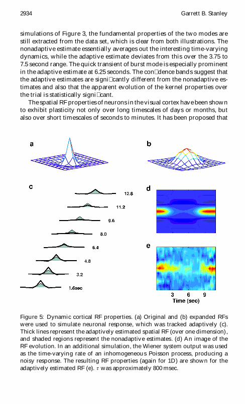
Figure 5: Dynamic cortical RF properties. (a) Original and (b) expanded RFswere used to simulate neuronal response, which was tracked adaptively (c).Thick lines represent the adaptively estimated spatial RF (over one dimension),and shaded regions represent the nonadaptive estimates. (d) An image of theRF evolution. In an additional simulation, the Wiener system output was usedas the time-varying rate of an inhomogeneous Poisson process, producing anoisy response. The resulting RF properties (again for 1D) are shown for theadaptively estimated RF (e). t was approximately 800 msec.


this short-term plasticity plays a role in the continuing process of normaliza-tion and calibration of the visual system (Gilbert et al., 1996). Many corticalneurons exhibit stimulus-dependent RF expansions over relatively shorttime periods. Consider the following example, as illustrated in Figure 5.Concentrated and expanded RF were generated using difference of gaus-sian functions with different spatial extents, as shown in Figures 5a and5b, with essentially instantaneous temporal dynamics. The time-varyingsystem was then generated using the temporal weighting functions of theprevious example, varying from the original to expanded and back to origi-nal RF structure. The response to spatiotemporal white noise was simulated,as previously discussed, resulting in a mean �ring rate at 35 Hz. Figure 5cshows a spatial slice of the adaptively estimated 2D receptive �eld as itevolves over the trial (thick line) with the static RF estimate (shaded) super-imposed for reference. The static RF estimate is essentially the averaged RFover the trial, whereas the actual RF was initially more peaked, followedby a broadening of the tuning, and �nally a return to the peaked tuning atthe end of the trial. The adaptive approach in this case is able to track thesechanges as they evolve over the stimulus trial, as shown in Figure 5d. Ina more realistic simulation, the output of the linear �lter-static nonlinear-ity cascade was used as the rate of an inhomogeneous Poisson process, aswas done in the previous example. An image of the adaptively estimatedRF (again for a 1D slice of the 2D �eld) over the stimulus trial is shown inFigure 5e. As with the previous example, the inherent noise of the Poissonsimulation degrades the estimate, but the essential time-varying character-istics are still well captured.

3.2 Experimental Results from LGN Response to the SpatiotemporalM-Sequence. The above simulations provide insight into the developmentof the methods of adaptive estimation, but the primary target of the ap-proach is experimental. X cells in the cat LGN were stimulated with the

Figure 6: Evolution of adaptation in the LGN. (a) The �rst-order kernel at thebeginning (beg) and end (end) of the 4 minute trial. For comparison, the kernelderived from the entire trial is superimposed (avg). Bands represent two stan-dard deviations around the estimators. (b) An image of the kernel evolutionover the 4 minute trial. t was 7.8 sec.


spatiotemporal m-sequence at 128 Hz and 100% contrast over several min-utes (for details of experimental protocol, see Stanley, Li, & Dan, 1999).Figure 6 illustrates typical results obtained using the adaptive estimationapproach for a single pixel at the center of the RF. Figure 6a shows the�rst-order kernel estimates at the beginning (beg) and end (end) of the trial,with a marked change in temporal dynamics over the 4 minute period.This example was typical among the population from which this cell wasdrawn, undergoing an attenuation over the stimulus trial, consistent withslow adaptation effects related to a step up in contrast at stimulus onset.Also invariant among cells is the temporal compression that results in adecreased latency. The kernel derived from the entire trial (avg) is superim-posed for reference, underscoring the importance of the adaptive approachpresented here; when the kernel is computed from the entire trial, it pro-duces essentially the average dynamics over the trial. Bands represent twostandard deviations around the estimators. The image shown in Figure 6billustrates the evolution of the kernel dynamics over the entire trial, with adecrease in latency and in kernel magnitude over the 4 minute period. Theadaptive time constant t was 7.8 seconds for this example. The sudden shiftin latency is an artifact of the discretization of the kernel at 128 Hz, sincethe average shift in latency was on the order of magnitude of the samplinginterval. The point to emphasize here is that these changes in encodingdynamics would not be discovered through traditional reverse-correlationtechniques that assume a �xed relationship between stimulus and responseover the trial.

4 Discussion

Reverse-correlation techniques have been used extensively in a wide rangeof sensory systems. Characterizing the RF properties of sensory neuronsforms the basis for our current understanding of their functional signi�-cance. The assumption that the spatiotemporal RF properties are static overeven short time intervals, however, is problematic. Systems-level adapta-tion, functional modulation, and plasticity occur on a continuum of time-scales that exist in all but the most arti�cial of experimental conditions.Examples were presented here in which spatiotemporal RF properties ofvisual neurons were adaptively tracked over short time intervals throughboth simulation and experimental trials. Realistic, noisy simulations wereconducted in the development of the adaptive approach, shown throughboth modulation of temporal coding properties in the LGN and modula-tion of spatial properties in the cortex. Furthermore, experimental data wereused to demonstrate the validity of the approach under physiological con-ditions, and it was shown that the evolution of encoding properties could besmoothly tracked over short trials. The kernels showed a marked attenua-tion and temporal compression over a timescale that is consistent with slowforms of contrast and light adaptation. Obviously this could be controlled


for experimentally by allowing the cell to adapt �rst to the high-contraststimulus, but one could argue that this induces an unnatural steady statethat is not relevant ethologically. Statistical properties of both the adap-tive and nonadaptive estimators were derived, providing a more rigorousmeans with which to compare encoding dynamics in different physiolog-ical conditions. It should also be noted that the approach presented heretracks the evolution of spatiotemporal encoding properties over a singletrial, an especially critical point in tracking dynamics that are modulatedby nonstimulus-related activity, and thus may not be possible to repeat.Furthermore, for stimulus-related modulation of encoding dynamics, theapplicability over single trials is important in natural viewing conditions,in which case the eyes saccade across the visual scene, never to invoke thesame trajectory, and therefore stimulus pattern, twice.

In this work, the neuronal response is characterized as the single trial�ring rate of the neuron in question. This simpli�cation obviously ignoresthe precise temporal structure of the underlying point events that may bepresent in sparse coding strategies. However, for some subset of cells inearly sensory systems, much of the information is thought to be coded inthe �ring rate. As is evident in Figure 2, X cells in the LGN are typically rel-atively linear in their response properties and are often well characterizedwith this strategy. The simple model prediction of �ring rate is surprisinglygood, although it may not be capturing subtle features that could be trackedthrough more elaborate strategies. One would expect that the speci�c tech-niques presented here would be less ideal for the sparse coding observedin many cortical cells. The relatively high �ring rate of thalamic neuronsenables the use of an adaptive time constant that is small enough to allowtracking of relatively fast changes in the RF properties. The lower �ring ratesassociated with sparse coding strategies in the cortex would require muchlonger adaptive time constants, thereby limiting the effective bandwidth ofadaptive processes that could be tracked. However, the general approachof adaptive estimation could certainly be applied; adaptive point processestimation techniques have been recently demonstrated in the hippocam-pus (Brown et al., 2001) and represent a promising direction of explorationin this context.

The adaptive approach presented here is based on an exponential down-weighting of past stimulus-response information. This functional form ofthe downweighting was chosen for computational reasons, but could easilybe extended to more complex relationships. However, when this strategywas implemented with other functional forms of the temporal dependence,the results were qualitatively similar. The relevant parameter in each casewas the relative temporal window over which the estimation was performed(the time constant of the adaptive estimate, t ). The shorter window obvi-ously enables one to trackdynamics that change more rapidly over time, butat the expense of the estimator variance; conversely, larger time constantsreduce the variance but make it impossible to detect the nonstationarities.


The time constants used in this study were thus chosen so as to use as littlepast information as possible while still yielding meaningful structure in thekernel estimates.

One of the limitations of the proposed methodology lies in the under-lying assumptions imposed on the model structure. The input to the staticnonlinearity was assumed to be gaussian in nature. However, even with bi-nary inputs, such as that of the m-sequence, the output of the linear block isnearly gaussian for even relatively short �lter lengths. The nonlinearity de-scribed in this work is a simple half-wave recti�cation. This obviously doesnot capture saturation at high �ring rates, but instead assumes that stimuliare suf�ciently small as to avoid driving the cells to saturation. The approachpresented here could certainly be integrated with recent techniques in theidenti�cation of arbitrary nonlinearities in the cascade (Chichilnisky, 2001;Nykamp & Ringach, 2001), in order to capture the phenomena over a largeroperating range. Finally, it was also assumed that the mean of the input tothe static nonlinearity was much smaller than the standard deviation (seesection A.4), which signi�cantly reduced the complexity of several of theestimates. However, as demonstrated in section A.2, this assumption wasreasonable for the experimental data presented.

In summary, time-varying encoding properties may be a ubiquitous char-acteristic of all sensory neurons. Adaptation has been studied for some timeand is known to dramatically affect the temporal and spatial dynamics, andanecdotal evidence of modulatory effects from other brain regions on en-coding properties has been reported for a number of stages in the visualpathway. However, it is not yet known what these phenomena imply forthe coding strategies of the sensory pathway as a whole. The approach pre-sented here is a �rst step toward capturing the evolution of spatiotemporalRF properties over a range of timescales, with the goal of eventually un-derstanding dynamic coding strategies employed by the visual pathway innatural settings, where there is no real concept of steady state.

Appendix

A.1 Time-Domain Estimation. Consider a purely linear system, withzero-mean input s[k], output x[k], and �rst-order kernel g[k] that can beexpressed through the vector h . De�ne a data vector Q,

Q[k] , [s[k] s[k ¡ 1] ¢ ¢ ¢ s[k ¡ L C 1]]T 2 RL£1.

The output can be written x[k] D hTQ[k]. Let the error in the prediction bede�ned as e[k] D x[k] ¡ Ox[k]. The mean square error (MSE) is then de�ned asMSE D Ef(e[k])2g, where Ef¢g denotes statistical expectation. The �rst-orderkernel can then be estimated by minimizing the MSE of prediction:

Oh D arg minh2RL

X

k

»±r[k] ¡hTQ[k]

²2¼

.


Taking the partial of this objective function with respect to h[q] and settingequal to zero yields wsx[q] D

PL¡1mD0h[m]wss[q ¡ m], where wsx is the cross-

covariance between the input and output, and wss is the autocovariance ofthe input. This can be expressed as:

2

66664

wsx[0]

wsx[1]...

wsx[L ¡ 1]

3

77775D

2

66664

wss[0] wss[1] . . . wss[L ¡ 1]

wss[1] wss[0] . . . wss[L ¡ 2]...

.... . .

...wss[L ¡ 1] wss[L ¡ 2] . . . wss[0]

3

77775

2

66664

h[0]

h[1]...

h[L ¡ 1]

3

77775.

Using compact notation reduces the relationship to wsx D Wssh where Wss isthe L £L Toeplitz matrix of the input autocovariance. The �rst-order kernelcan then be estimated as Oh D W¡1

ss wsx. This estimator is the optimal estimatorin the least-squares sense (Ljung, 1987).

A.2 Effect of Static Nonlinearity on Covariance Structure. The cascadeof a linear system with a static nonlinearity is often referred to as a Wienersystem, as shown in Figure 1. It has been shown that the effect of odd staticnonlinearities is a simple scalingof the covariance structure (Bussgang,1952;Papoulis, 1984;Hunter & Korenberg, 1986). Bussgang’s theorem states that ifthe input to a memoryless system r D f (x) is a normal process x(t), the cross-covariance of x(t) with the output r (t) is proportional to the autocovarianceof the input (Papoulis, 1984):

wxr (t ) D Cwxx (t ) where C D Ef f 0[x(t)]g.

For a half-wave recti�cation, we have:

f (x) D

(x for x ¸ 00 else

f 0 (x) D

(1 for x ¸ 00 else

.

The scaling constant C then becomes

C D Ef f 0 (x)g DZ 1

¡1f 0 (x)px (x) dx,

where px (x) is assumed a gaussian probability density function N (m x, s2x ).

We therefore have

C DZ 1

0px (x) dx D

Z 1

¡m xsx

1p2p

e¡z2

2 dz D 1 ¡ Y

³¡m x

sx

´,

where Y (¢) is the standard normal cumulative. The theoretical and observedscalings for varying m x /sx are shown in Figure 7. Gaussian white noiseprocesses with mean m x and variance s2

x were recti�ed; the ratio of cross-covariance to autocovariance, C, is plotted as a function ofm x /sx in Figure 7a.


2 0 20

0.5

1

C

x/

x

a

200 0 200x

b

0 5 101/C

erro

r

c

Figure 7: Effect of recti�cation on correlation structure. (a) Simulated and theo-retical relationships between m x/sx and scaling C. Gaussian white noise signalswith mean m x and variance s2

x were recti�ed, and the ratio of cross-covarianceto autocovariance computed (�). (b) The output of the linear �lter tends to agaussian distribution. The nonscaled estimated kernel underpredicts the exper-imentally observed �ring rate. (c) The 1

C scaling on the kernel that minimizesthe mean squared error is approximately 2, implying a m x ¿ sx , as indicatedin a.

Importantly, data from the cat LGN reveal that the scaling of the kernel, 1/C,which minimizes the error in predicted �ring rate, is approximately 2, asshown in Figure 7c. The combination of these two results suggests that themean of the �lter output is small relative to the standard deviation. Forthe Wiener system shown in Figure 1, it is straightforward to extend thediscussion above to the estimate for the linear block. For an uncorrelatedinput, the output of the linear kernel tends to a gaussian distribution, asshown in Figure 7b. The resulting relationship is wsr D Cwsx, giving, forhalf-wave recti�cation, the estimate

Oh D1C

W¡1ss wsr.

Importantly, data from the cat LGN reveal that the scaling of the kernel,1/C, that minimizes the error in predicted �ring rate is approximately 2, asshown in Figure 7c. The combination of these results suggests that m x ¿ sxwithin this structural framework.

A.3 Recursive Estimation. The recursive kernel estimation problem canbe formulated in the following manner. After presenting a stimulus andobserving the response of the neuron up to time t, the estimation can beexpressed as

Oht D arg minh

tX

kDL

(r[k] ¡ bhTQ[k] C m xc)2,

where the subscript t denotes the time-varying nature of the parametervector h . Using the least-squares technique described previously, the �lter


can be estimated based on information up to time t,

Oht D1C

C ¡1t P t,

where Ct and P t are the stimulus autocovariance Toeplitz matrix and cross-covariance between stimulus and response, respectively, based on data upto time t:

Ct D1

t ¡ L C 1

tX

kDL

Q[k]QT[k]Dt ¡ L

t ¡ L C 1Ct¡1 C

1t ¡ L C 1

Q[t]QT[t]

P t D1

t ¡ L C 1

tX

kDL

Q[k]r[k] Dt ¡ L

t ¡ L C 1P t¡1 C

1t ¡ L C 1

Q[t]r[t].

This gives the �nal expression for the estimate:

Oht D Oht¡1 C1

t ¡ L C 1C¡1

t Q[t]µ

1C

r[t] ¡ QT[t] Oht¡1

¶.

The estimate based on data up to time t¡1 is therefore used in the subsequentestimate based on information up to time t, which results in a recursion forthe �lter estimation (Goodwin & Sin, 1984; Ljung & Soderstrom, 1983).

A.4 Statistical Properties of Estimates. As with the traditional least-squares problem, the statistics of the estimator for the Wiener system canbe characterized in a relatively straightforward manner. It is �rst necessaryto establish the statistical properties of the linear problem, given here forreference. De�ne the following data matrices:

D , [Q[L] Q[L C 1] ¢ ¢ ¢ Q[N]]T 2 R(N¡LC1)£L

y , [x[L] x[L C 1] ¢ ¢ ¢ x[N]]T 2 R(N¡LC1)£1.

The estimate of the parameter vector from section A.1 can then be writtenin a more standard least-squares form,

Oh D C¡1P D (DTD)¡1DTy,

where again C represents the stimulus autocovariance Toeplitz matrix, andP represents the cross-covariance matrix between stimulus and response.This estimator is known to be unbiased, so that E[ Oh ] D h . The covariancecan be written (Westwick, Suki, & Lutchen, 1998)

L Oh D Ef( Oh ¡h )( Oh ¡ h )Tg D (DTD)¡1DTEfeeTgD(DTD)¡1,


where e D [e[L] e[L C 1] ¢ ¢ ¢ e[N]]T 2 RN¡LC1£1 is the noise vector, wheree[k] , x[k] ¡ Ox[k]. If the noise is a white process, with standard deviationse À m e, then EfeeTg ¼ s2

e I, resulting in

L Oh ¼ s2e (DTD)¡1 D

s2e

N ¡ L C 1C¡1 2 RN¡lC1£N¡LC1.

The covariance structure of the estimator Oh could be directly obtained fromthe noise term e[k] D x[k] ¡ Ox[k]. In this case, however, there is obviously noaccess to the intermediate signal x[k]. The unobservable noise term e musttherefore be related to observable noise, which is the difference between theactual �ring rate of the cell r[k] and that predicted by the linear-nonlinearcascade, n[k] D r[k] ¡ Or[k].

In order to understand how the two noise processes relate, it is helpful toconsider �rst the effect of the static nonlinearity on the probability densityfunction. Suppose x is a random variable such that x » N (m x, s2

x ). Let px (x)represent the density function associated with the random variable x. Letr be the output of the static nonlinearity f (¢) such that r D f (x). For thehalf-wave recti�cation, the expectation becomes

m r D Efrg DZ 1

¡1rpr (r) dr D

Z 1

¡1f (x)px (x) dx D

Z 1

0x

1p2p s2

x

e¡(x¡mx )2

2s2x dx.

Letting z D x¡m xsx

, the expression becomes:

Efrg D1p

2p s2x

Z 1

¡ mxsx

(sxz C m x)e¡z2

2 sx dz

D sx

Z 1

0

1p2p

ze¡z2

2 dz C sx

Z 0

¡m xsx

1p2p

ze¡z2

2 dz C m x

Z 1

¡ mxsx

e¡z2

2 dz.

If m x ¿ sx, the expectation becomes:

Efrg D sx

Z 1

0

1p2p

ze¡z2

2 dz Dsxp2p

.

From the sample mean of the output signal r, the variance of the underlyingzero mean noise process can be estimated. For the variance, s2

r D Efr2g¡m 2r ,

where

Efr2g Ds3

xps2

x

Z 1

¡ mxsx

z2 1p2p

e¡z2

2 dz

C 2m xs2

xps2

x

Z 1

¡ mxsx

z1p2p

e¡z2

2 dz Cm 2

xsxps2

x

Z 1

¡ mxsx

1p2p

e¡z2

2 dz.


g

g

x

x

Figure 8: Equivalent noise sources. The top block diagram represents the encod-ing model as observed experimentally, with the source of noise at the point ofmeasurement. The bottom block diagram represents the dynamics assumed inthe adaptive estimation scheme. As detailed in the text, the statistical propertiesof the hidden noise source e can be estimated from the observed “noise” n.

If again m x ¿ sx, this results in

s2r D Efr2g ¡ Efrg2 D

s2x

2¡ s2

x

2pD s2

x(p ¡ 1)

2p.

This result can now be extended to describe the equivalent noise sourcesshown in Figure 8. For the top block diagram,

s2r D s2

Or C s2n D

p ¡ 12p

s2Ox C s2

n Dp ¡ 1

2pkhk2s2

s C s2n .

Similarly, for the bottom system,

s2r D

p ¡ 12p

s2x D

p ¡ 12p

(s2Ox C s2

e ) Dp ¡ 1

2p(khk2s2

s C s2e ),

where k ¢ k is the standard Euclidean norm. Putting the two equations to-gether yields

s2n D

p ¡ 12p

s2e .

This gives the equivalent variance of the two noise sources. Given the ob-served neuronal response r, the statistical properties of the hidden noiseprocess e can be estimated, which is necessary for determining the statis-tics of the least-squares estimate. The estimator remains unbiased, and thecovariance of the estimator can be written as

L Oh D s2e (DTD)¡1 D

s2e

N ¡ L C 1C¡1 D

1N ¡ L C 1

(2p m 2r ¡ khk2s2

s )C¡1, (A.1)


where m r is the mean observed �ring rate and s2s is the variance of the

stimulus. The quantities m r, h , and s2s can obviously be estimated from

data. The uncertainty in the kernel estimate in Figure 2 was computed inthis manner. This argument extends naturally to the recursive estimates, forwhich the covariance becomes

L OhtD

1t ¡ L C 1

(2p m 2r ¡ khk2s2

s )C¡1. (A.2)

Within the adaptive framework, the estimate remains unbiased, as withthe nonweighted estimation problem, but the covariance of the estimatorhas a slightly different form. The previous expression for covariance wasnormalized by the data length used in the estimate. With the adaptive al-gorithm presented here, the normalization depends on the structure of theexponential decay of contributions from the past:

L OhtD

1w

(2p m 2r ¡ khk2s2

s )C¡1t w ,

tX

kDL

lt¡kC1, (A.3)

where w re�ects the exponential downweighting of past information. Notethat if l D 1, the estimator variance matches that of the nonadaptive esti-mator. The uncertainty in the kernel estimate in Figures 4 through 6 werecomputed in this manner.

Acknowledgments

I thankEmery Brown, Roger Brockett, and NickLesica for helpful commentsin thepreparation of this article and Yang Dan for the use of the physiologicaldata.

References

Albrecht, D. G., Farrar, S. B., & Hamilton, D. B. (1984). Spatial contrast adaptationcharacteristics of neurones recorded in the cat’s visual cortex. J. Physiol., 347,713–739.

Brown, E. N., Nguyen, D. P., Frank, L. M., Wilson, M. A., & Solo, V. (2001). Ananalysis of neural receptive �eld plasticity by point process adaptive �ltering.PNAS, 98, 12261–12266.

Bussgang, J. J. (1952). Crosscorrelation functions of amplitude-distorted gaus-sian signals. MIT Res. Lab. Elec. Tech. Rep., 216, 1–14.

Chichilnisky, E. J. (2001). A simple white noise analysis of neuronal light re-sponses. Network, 12, 199–213.

Dan, Y., Atick, J., & Reid, R. (1996). Ef�cient coding of natural scenes in the lateralgeniculate nucleus: Experimental test of a computation theory. J. Neurosci.,16(10), 3351–3362.


Dayan, P., & Abbott, L. F. (2001). Theoretical neuroscience. Cambridge, MA: MITPress.

DeBoer, E., & Kuyper, P. (1968). Triggered correlation. IEEE Trans. Biomed. Eng.,15, 169–179.

deCharms, R. C., Blake, D., & Merzenich, M. (1998). Optimizing sound featuresfor cortical neurons. Science, 280, 1439–1443.

Enroth-Cugell, C., & Shapley, R. (1973). Adaptation and dynamics of cat retinalganglion cells. J. Physiol., 233, 271–309.

Gilbert, C. D., Das, A., Ito, M., Kapadia, M., & Westheimer, G. (1996). Spatialintegration and cortical dynamics. Proc. Natl. Acad. Sci. USA, 93, 615–622.

Goodwin, G. C., & Sin, K. S. (1984). Adaptive �ltering prediction and control. UpperSaddle River, NJ: Prentice Hall.

Greblicki, W. (1992). Nonparametric identi�cation of Wiener systems. IEEETrans. on Inform. Thry., 38, 1487–1493.

Greblicki, W. (1994). Nonparametric identi�cation of Wiener systems by orthog-onal series. IEEE Trans. on Automatic Control, 39, 2077–2086.

Greblicki, W. (1997). Nonparametric approach to Wiener system identi�cation.IEEE Trans. on Circuits and Sys., 44, 538–545.

Heeger, D. (1992). Normalization of cell responses in cat striate cortex. Vis. Neu-rosci., 9, 181–197.

Hunter, I. W., & Korenberg, M. J. (1986). The identi�cation of nonlinear biologicalsystems: Wiener and Hammerstein cascade models. Biological Cybernetics, 55,135–144.

Jones, J. P., & Palmer, L. A. (1987). The two-dimensional spatial structureof simple receptive �elds in cat striate cortex. J. Neurophysiol., 58, 1187–1211.

Korenberg, M. J., & Hunter, I. W. (1999). Two methods for identifying Wienercascades having noninvertible static nonlinearities . Annals of Biomed. Eng.,27, 793–804.

Ljung, L. (1987). System identi�cation:Theory for the user. Upper Saddle River, NJ:Prentice Hall.

Ljung, L., & Soderstrom, T. (1983). Theory and practice of recursive identi�cation.Cambridge, MA: MIT Press.

Mao, B. Q., MacLeish, P. R., & Victor, J. D. (1998). The intrinsic dynamics of retinalbipolar cells isolated from tiger salamander. Vis. Neurosci., 15, 425–438.

Movshon, J. A., Thompson, I. D., & Tolhurst, D. J. (1978). Spatial summation inthe receptive �elds of simple cells in the cat’s striate cortex. J. Physiol., 283,53–77.

Mukherjee, P., & Kaplan, E. (1995). Dynamics of neurons in the cat lateral genicu-late nucleus: In vivo electrophysiology and computational modeling. J. Neu-rophysiol., 74(3), 1222–1243.

Nykamp, D. Q., & Ringach, D. L. (2001). Full identi�cation of a linear-nonlinearsystem via cross-correlation analysis. Journal of Vision, 2, 1–11.

Ohzawa, I., Sclar, G., & Freeman, R. D. (1985). Contrast gain control in the cat’svisual system. Journal of Neurophysiology, 54, 651–667.

Papoulis, A. (1984). Probability, random variables, and stochastic processes (2nd ed.).New York: McGraw-Hill.


Paulin, M. G. (1993). A method for constructing data-based models of spikingneurons using a dynamic linear-static nonlinear cascade. Biol. Cybern., 69,67–76.

Pei, X., Vidyasagar, T. R., Volgushev, M., & Creutzfeld, O. D. (1994). Receptive�eld analysis and orientation selectivity of postsynaptic potentials of simplecells in cat visual cortex. J. Neurosci., 14(11), 7130–7140.

Przybyszewski, A. W., Gaska, J. P., Foote, W., & Pollen, D. A. (2000). Striatecortex increases contrast gain of macaque LGN neurons. Visual Neuroscience,17, 485–494.

Reid, R. C., Soodak, R. E., & Shapley, R. M. (1991). Directional selectivity andspatiotemporal structure of receptive �elds of simple cells in cat striate cortex.J. Neurophysiol., 66, 505–529.

Reid, R. C., Victor, J. D., & Shapley, R. M. (1997). The use of m-sequences in theanalysis of visual neurons: Linear receptive �eld properties. Vis. Neurosci.,14, 1015–1027.

Ringach, D. L., Hawken, M. J., & Shapley, R. (2002). Receptive �eld structurein neurons in monkey primary visual cortex revealed by stimulation withnatural image sequences. Journal of Vision, 2, 12–24.

Ringach, D., Sapiro, G., & Shapley, R. (1997). A subspace reverse-correlationtechnique for the study of visual neurons. Vision Res., 37, 2455–2464.

Shapley, R., & Victor, J. D. (1978). The effect of contrast on the transfer propertiesof cat retinal ganglion cells. J. Physiol, 285, 275–298.

Sherman, S., & Koch, C. (1986). The control of retinogeniculate transmission inthe mammalian lateral geniculate nucleus. Exp. Brain. Res., 63, 1–20.

Smirnakis, S. M., Berry, M. J., Warland, D. K., Bialek, W., & Meister, M. (1997).Adaptation of retinal processing to image contrast and spatial scale. Nature,386, 69–73.

Stanley, G. B. (2000a). Algorithms for real-time prediction in neural systems. Paperpresented at the Annual Meeting of the Engineering in Medicine and BiologySociety, Chicago.

Stanley, G. B. (2000b). Time-varying properties of neurons in visual cortex:Estimationand prediction. Paper presented at the 30th Annual Meeting of the Society forNeuroscience, New Orleans, LA.

Stanley, G. B. (2001). Recursive stimulus reconstruction algorithms for real-timeimplementation in neural ensembles. Neurocomputing, 38–40, 1703–1708.

Stanley, G., Li, F., & Dan, Y. (1999). Reconstruction of natural scenes from ensem-ble responses in the lateral geniculate nucleus. Journal of Neuroscience, 19(18),8036–8042.

Tolhurst, D. J., & Dean, A. F. (1990). The effects of contrast on the linearity ofthe spatial summation of simple cells in the cat’s striate cortex. ExperimentalBrain Research, 79, 582–588.

Westwick, D. T., Suki, B., & Lutchen, K. (1998). Sensitivity analysis of kernel esti-mates: Implications in nonlinear physiological system identi�cation. Annalsof Biomend Eng., 26, 488–501.

Received July 1, 2001; accepted May 13, 2002.

adaptive spatiotemporal receptive field estimation in the ... ·...

Documents