adaptive signal processing class project adaptive interacting multiple model technique for tracking...

Ad

apti

ve S

ign

al P

roce

ssin

gC

lass

Pro

ject

Adaptive Interacting Multiple Model Technique

for Tracking Maneuvering Targets

Viji Paul, Sahay Shishir Brijendra,

Krishnamoorthy Iyer, Meles Gebreyesus

Ad

apti

ve S

ign

al P

roce

ssin

gC

lass

Pro

ject

Outline of the Presentation

• Introduction to the problem

• Multiple Model Technique

• IMM and the models used

• Multiple Target Scenario

• Simulation results

• Adaptive Cancellation of Oscillation Effect

• Simulation results

Ad

apti

ve S

ign

al P

roce

ssin

gC

lass

Pro

ject

Radar site

Observed Position

Predicted Position

Error

Target Tracking Using Surveillance radar

Ad

apti

ve S

ign

al P

roce

ssin

gC

lass

Pro

ject

•In the MM estimation, it is assumed that the possible system behavior patterns, called system modes, can be represented by a set of models.

•A bank of filters runs in parallel at every time, each based on a particular model, to obtain the model-conditional estimates.

•Overall state estimate is a certain combination of these model-conditional estimates.

Multiple Model Estimation

Ad

apti

ve S

ign

al P

roce

ssin

gC

lass

Pro

ject


A Bayesian framework starting with prior probabilities of each model being correct (i.e. the system is in a particular mode) is used.

The model, assumed to be in effect throughout the process, is one of r possible models (the system is in one of r modes)

Ad

apti

ve S

ign

al P

roce

ssin

gC

lass

Pro

ject


The prior probability that is correct (i.e. the system is in mode j) is

j = 1…….r

where is the prior information; and

Ad

apti

ve S

ign

al P

roce

ssin

gC

lass

Pro

ject


The output of each mode-matched filter:

•Mode-conditioned State Estimate

•Associated State Error Covariance Matrix

•Mode Likelihood Function

Ad

apti

ve S

ign

al P

roce

ssin

gC

lass

Pro

ject

Multiple Model Structure

Ad

apti

ve S

ign

al P

roce

ssin

gC

lass

Pro

ject

Output Estimate

After the filters are initialized, they run recursively

on their own estimates.

Their likelihood functions are used to update the

mode probabilities.

The latest mode probabilities are used to combine

the mode-conditioned estimates and covariances.

Ad

apti

ve S

ign

al P

roce

ssin

gC

lass

Pro

ject

Output Estimate

The combination of mode-conditioned estimates is therefore done as follows

And the covariance of the combined estimate is

Ad

apti

ve S

ign

al P

roce

ssin

gC

lass

Pro

ject

Multiple Model Approach for Switching Models

Consider an example with two models, and at time, k =2 one has possible histories.l li ,1 li ,2

1 1 1

2 1 2

3 2 1

4 2 2

Ad

apti

ve S

ign

al P

roce

ssin

gC

lass

Pro

ject

Multiple Model Approach for Switching Models

The mode history – or sequence of models – through

time k is denoted as

where is the model index at time k from history l. It is important to note that number of histories increases exponentially with time.

Ad

apti

ve S

ign

al P

roce

ssin

gC

lass

Pro

ject

Interacting Multiple Model Algorithm

Ad

apti

ve S

ign

al P

roce

ssin

gC

lass

Pro

ject

Steps in IMM

One cycle of the algorithm consists of the following:

Step 1: Calculation of the mixing probabilities.

Step2: Mixing- Calculation of mixed initial conditions

Step3: Mode matched filtering.

Step4: Mode probability update.

Step5: Estimate and covariance combination

jM

Ad

apti

ve S

ign

al P

roce

ssin

gC

lass

Pro

ject

Block Diagram of the Tracking Routine

Model jKalman

Filter

j = 1…r

IMM Block

State estimates for established target

State estimate covariancefor established target

Model probabilities forestablished target

Sensor measurements

Ad

apti

ve S

ign

al P

roce

ssin

gC

lass

Pro

ject

Tracking Maneuvering target

A weaving target track constructed of linked coordinated turns

Ad

apti

ve S

ign

al P

roce

ssin

gC

lass

Pro

ject

IMM

One cycle of the algorithm consists of the following:

Step 1: Calculation of the mixing probabilities.

The probability that mode was in effect at time k-1

given that is in effect at k, conditioned on is:

jM

Ad

apti

ve S

ign

al P

roce

ssin

gC

lass

Pro

ject

IMM Algorithm

The above are the mixing probabilities, which can be written as

Where the normalizing constants are

j = 1,…,r.

Ad

apti

ve S

ign

al P

roce

ssin

gC

lass

Pro

ject

IMM Algorithm

Step 2: Mixing.

Starting with one computes the mixed initial

condition for the filter matched to

j = 1,…,r

Ad

apti

ve S

ign

al P

roce

ssin

gC

lass

Pro

ject

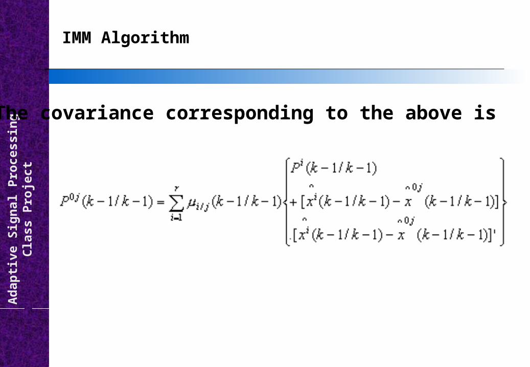
IMM Algorithm

The covariance corresponding to the above is

Ad

apti

ve S

ign

al P

roce

ssin

gC

lass

Pro

ject

IMM Algorithm

Step 3: Mode-matched filtering.

The estimate and covariance are used as input to the

filter matched to which uses

to yield and

The likelihood functions corresponding to the r filters

)(kM j

are computed using the mixed initial condition and the associated covariance

Ad

apti

ve S

ign

al P

roce

ssin

gC

lass

Pro

ject

IMM Algorithm

Step 4: Mode probability update. This is done as follows

Ad

apti

ve S

ign

al P

roce

ssin

gC

lass

Pro

ject

IMM Algorithm

Step 5: Estimate and covariance combination.

Combination of the model-conditioned estimates

and covariances is done according to the mixture

equations

Ad

apti

ve S

ign

al P

roce

ssin

gC

lass

Pro

ject

There are total four targets moving with different kinematics.

Initial Range : Range of the target at time zero.

Initial Theta : Azimuth of the target at time zero.

Split no : Number of splits into which time is partitioned.

No of Scans : Number of scans in each time split.

Start Scan : Starting scan number of each partition of time.

End Scan : Ending scan number of each partition of time.

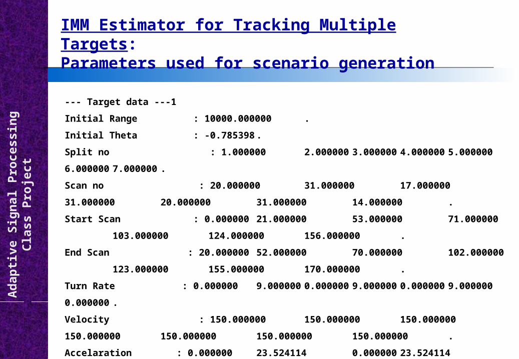
IMM Estimator for Tracking Multiple Targets:Parameters used for scenario generation

Ad

apti

ve S

ign

al P

roce

ssin

gC

lass

Pro

ject

Turn Rate : Amount of course change in degree per second.

Velocity : Velocity in each partition of time.

Acceleration : Acceleration in each partition of time.

Heading : Heading in each partition of time.


Ad

apti

ve S

ign

al P

roce

ssin

gC

lass

Pro

ject

--- Target data ---1

Initial Range : 10000.000000 .

Initial Theta : -0.785398 .

Split no : 1.000000 2.000000 3.000000 4.000000 5.000000 6.000000 7.000000 .

Scan no : 20.000000 31.000000 17.000000 31.000000 20.000000 31.000000 14.000000 .

Start Scan : 0.000000 21.000000 53.000000 71.000000 103.000000 124.000000 156.000000 .

End Scan : 20.000000 52.000000 70.000000 102.000000 123.000000 155.000000 170.000000 .

Turn Rate : 0.000000 9.000000 0.000000 9.000000 0.000000 9.000000 0.000000 .

Velocity : 150.000000 150.000000 150.000000 150.000000 150.000000 150.000000 150.000000 .

Accelaration : 0.000000 23.524114 0.000000 23.524114 0.000000 23.524114 0.000000 .

Heading : -0.785398 1.374447 -0.785398 1.374447 -0.785398 1.374447 -0.785398 .


Ad

apti

ve S

ign

al P

roce

ssin

gC

lass

Pro

ject



Initial Theta : 0.785398 .

Split no : 1.000000 .

Scan no : 170.000000 .

Start Scan : 0.000000 .

End Scan : 170.000000 .

Turn Rate : 0.000000 .

Velocity : 100.000000 .

Accelaration : 0.000000 .

Heading : 0.785398 .


Ad

apti

ve S

ign

al P

roce

ssin

gC

lass

Pro

ject



Initial Theta : -2.356194 .

Split no : 1.000000 2.000000 3.000000 4.000000 .

Scan no : 30.000000 34.000000 31.000000 72.000000 .

Start Scan : 0.000000 31.000000 66.000000 98.000000 .

End Scan : 30.000000 65.000000 97.000000 170.000000 .

Turn Rate : 0.000000 -9.000000 9.000000 0.000000 .

Velocity : 100.000000 100.000000 100.000000 100.000000 .

Accelaration : 0.000000 15.682742 15.682742 15.682742 .

Heading : -2.356194 3.141593 -2.552544 -0.792379 .


Ad

apti

ve S

ign

al P

roce

ssin

gC

lass

Pro

ject



Initial Theta : 2.356194 .

Split no : 1.000000 2.000000 3.000000 4.000000 .

Scan no : 30.000000 34.000000 31.000000 72.000000 .

Start Scan : 0.000000 31.000000 66.000000 98.000000 .

End Scan : 30.000000 65.000000 97.000000 170.000000 .

Turn Rate : 0.000000 -9.000000 9.000000 0.000000 .

Velocity : 100.000000 100.000000 100.000000 100.000000 .

Accelaration : 0.000000 15.682742 15.682742 15.682742 .

Heading : 2.356194 1.570796 2.159845 -2.363176 .


Ad

apti

ve S

ign

al P

roce

ssin

gC

lass

Pro

ject

Maneuvering ModelsConstant Velocity Model

• For small sample intervals T, the following model is commonly used (Blackman & Popoli, Sec. 4.2.2):

k

ky

y

x

x

ky

y

x

x

U

v

p

v

p

T

T

v

p

v

p

1000

100

0010

001

1

Ad

apti

ve S

ign

al P

roce

ssin

gC

lass

Pro

ject

Maneuvering ModelsConstant Acceleration Model

k

kx

x

x

kx

x

x

U

a

v

p

T

TT

a

v

p

100

1021

2

1

Ad

apti

ve S

ign

al P

roce

ssin

gC

lass

Pro

ject

Maneuvering ModelsCoordinated Turn Model

sin (1 cos )1 0

0 cos 0 sin( ) ( 1)

1 cos sin0 1

0 sin 0 cos

T T

T Tx k x k

T T

T T

Ad

apti

ve S

ign

al P

roce

ssin

gC

lass

Pro

ject

Multi Target Scenario

10000

20000

30000

30

210

60

240

90

270

120

300

150

330

180 0

Ad

apti

ve S

ign

al P

roce

ssin

gC

lass

Pro

ject

Variation of Model weights

0 20 40 60 80 100 120 140 1600

0.1

0.2

0.3

0.4

0.5

0.6

0.7

0.8

0.9Fot T1

Constant Velocity

Constant accelerationCoordinated Turn

For Target 1

Ad

apti

ve S

ign

al P

roce

ssin

gC

lass

Pro

ject

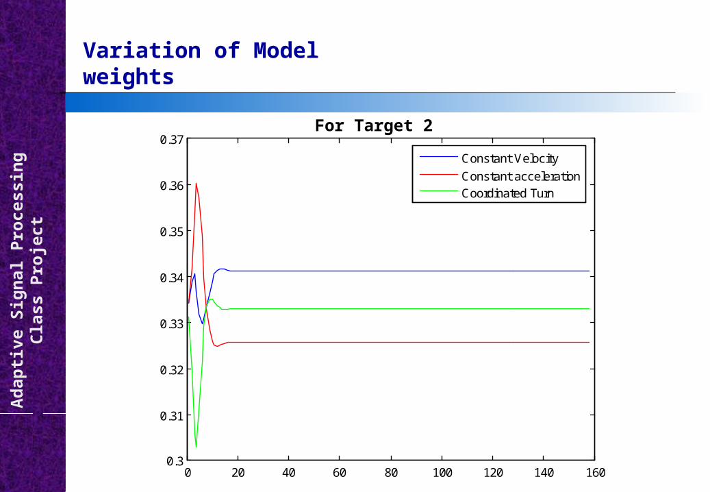
0 20 40 60 80 100 120 140 1600.3

0.31

0.32

0.33

0.34

0.35

0.36

0.37Fot T2

Constant Velocity



For Target 2

Ad

apti

ve S

ign

al P

roce

ssin

gC

lass

Pro

ject


0 20 40 60 80 100 120 140 1600

0.1

0.2

0.3

0.4

0.5

0.6

0.7

0.8

0.9Fot T3

Constant Velocity


For Target 3

Ad

apti

ve S

ign

al P

roce

ssin

gC

lass

Pro

ject


0 20 40 60 80 100 120 140 1600

0.1

0.2

0.3

0.4

0.5

0.6

0.7

0.8

0.9Fot T4

Constant Velocity


For Target 4

Ad

apti

ve S

ign

al P

roce

ssin

gC

lass

Pro

ject

Tracking From Unstable PlatformThe environment strongly impacts radar performance

Ad

apti

ve S

ign

al P

roce

ssin

gC

lass

Pro

ject

Platform Oscillations

•Roll, Yaw and Pitch

•Only Roll has been considered in this simulation.

•All the three motions are sinusoidal or DC shifted sinusoidal.

•At max, frequency of the sinusoid is about 1/10 Hz.

Ad

apti

ve S

ign

al P

roce

ssin

gC

lass

Pro

ject

Physically stabilized beam

Ad

apti

ve S

ign

al P

roce

ssin

gC

lass

Pro

ject

Tracking Maneuvering target

A weaving target track constructed of linked coordinated turns.

Perturbations are seen because of platform motion.

Ad

apti

ve S

ign

al P

roce

ssin

gC

lass

Pro

ject

Target Tracking Data Flow

Estimated State

Target

Sensor(Obsvn Device)

Signal / Data Pre-

Processor

Tracker (State Estimation / Data Association)

Electro Magnetic or Acoustic Energy

Channel Signal / Raw Data

Tracking Algorithm

Data Conversion Decoupling Detection-Subsystem

Typical Target tracking system

Ad

apti

ve S

ign

al P

roce

ssin

gC

lass

Pro

ject

10000

20000

30000

30

210

60

240

90

270

120

300

150

330

180 0

Measurement corrupted by Oscillations

•Increased deterioration at larger ranges.

Ad

apti

ve S

ign

al P

roce

ssin

gC

lass

Pro

ject

0 20 40 60 80 100 120 140 1600

0.1

0.2

0.3

0.4

0.5

0.6

0.7

0.8Fot T1

Constant Velocity


For Target 1

Model weight variations due to Platform Oscillations

Ad

apti

ve S

ign

al P

roce

ssin

gC

lass

Pro

ject

0 20 40 60 80 100 120 140 1600.1

0.2

0.3

0.4

0.5

0.6

0.7

0.8Fot T2

Constant Velocity


For Target 2


Ad

apti

ve S

ign

al P

roce

ssin

gC

lass

Pro

ject

0 20 40 60 80 100 120 140 1600

0.1

0.2

0.3

0.4

0.5

0.6

0.7

0.8Fot T3

Constant Velocity


For Target 3


Ad

apti

ve S

ign

al P

roce

ssin

gC

lass

Pro

ject

0 20 40 60 80 100 120 140 1600

0.1

0.2

0.3

0.4

0.5

0.6

0.7

0.8

0.9Fot T4

Constant Velocity


For Target 4


Ad

apti

ve S

ign

al P

roce

ssin

gC

lass

Pro

ject

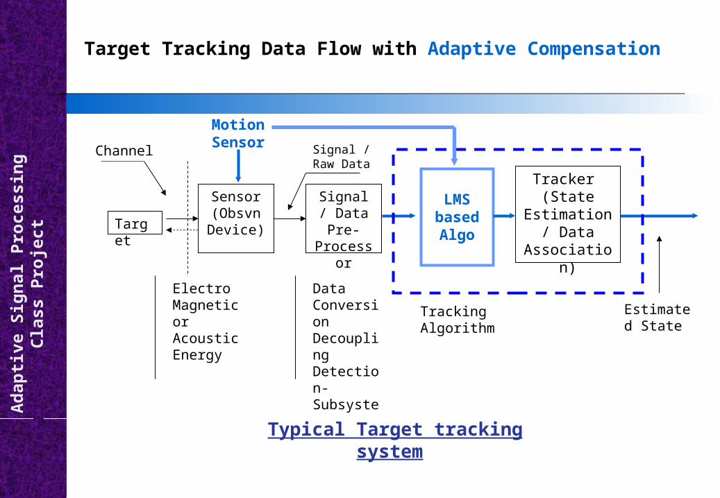
Target Tracking Data Flow with Adaptive Compensation

Estimated State

Target

Sensor(Obsvn Device)

Signal / Data Pre-

Processor

Tracker (State

Estimation / Data

Association)

Electro Magnetic or Acoustic Energy

Channel Signal / Raw Data

Tracking Algorithm

Data Conversion Decoupling Detection-Subsystem

Typical Target tracking system

Motion Sensor

LMS based Algo

Ad

apti

ve S

ign

al P

roce

ssin

gC

lass

Pro

ject

Measurements corrupted by a proportional multiplication of oscillation

50 100 150 200 250 300 350 400 450 500

1.54

1.55

1.56

1.57

1.58

1.59

1.6

Ad

apti

ve S

ign

al P

roce

ssin

gC

lass

Pro

ject

Reminds You of Something ???

Output from the Gyro

Modified form of Gyro output

Signal from the radar

Ad

apti

ve S

ign

al P

roce

ssin

gC

lass

Pro

ject

10000

20000

30000

30

210

60

240

90

270

120

300

150

330

180 0

Compensated for Platform Oscillation

Ad

apti

ve S

ign

al P

roce

ssin

gC

lass

Pro

ject

Its OK in Theory but is the Target a Sitting Duck ?

Operational Solution:

•Sea state does not change drastically.

•Ships are always in formation during an operation.

•During the pre-detection phase, i.e. while approaching the Theatre of Operation, the weights of the Adaptive Filter can be “set” using the LMS Algorithm.

•The same weights can then be used during the Target Detection phase.

Ship with Surv

Radar

Friendly Ship in Compan

y

Ad

apti

ve S

ign

al P

roce

ssin

gC

lass

Pro

ject

0 20 40 60 80 100 120 140 1600

0.1

0.2

0.3

0.4

0.5

0.6

0.7

0.8

0.9Fot T1

Constant Velocity



For Target 1

Ad

apti

ve S

ign

al P

roce

ssin

gC

lass

Pro

ject

0 20 40 60 80 100 120 140 1600.2

0.25

0.3

0.35

0.4

0.45

0.5Fot T2

Constant Velocity



For Target 2

Ad

apti

ve S

ign

al P

roce

ssin

gC

lass

Pro

ject

0 20 40 60 80 100 120 140 1600

0.1

0.2

0.3

0.4

0.5

0.6

0.7

0.8

0.9Fot T3

Constant Velocity



For Target 3

Ad

apti

ve S

ign

al P

roce

ssin

gC

lass

Pro

ject

0 20 40 60 80 100 120 140 1600

0.1

0.2

0.3

0.4

0.5

0.6

0.7

0.8

0.9Fot T4

Constant Velocity



For Target 4

Ad

apti

ve S

ign

al P

roce

ssin

gC

lass

Pro

ject

Conclusion

•Analyzed Multiple Model Technique

•IMM based estimation is implemented

•Generated a Multi Target Scenario

•Applied IMM

•Verified the algorithm

•Introduced Platform Oscillations

•Added LMS based adaptive compensation

Ad

apti

ve S

ign

al P

roce

ssin

gC

lass

Pro

ject

Thank you

adaptive signal processing class project adaptive interacting multiple model technique for tracking...

Documents