adaptive recovery of spars vector

354 IEEE TRANSACTIONS ON SIGNAL PROCESSING, VOL. 62, NO. 2, JANUARY 15, 2014

Adaptive Identification and Recovery ofJointly Sparse VectorsRoy Amel and Arie Feuer, Life Fellow, IEEE

Abstract—In this paper we present a novel approach to thesolution of a sequence of SMV problems with a joint support.This type of problem arises in a number of applications suchas multiband signal reconstruction and source localization. Theapproach we present is adaptive in that it solves it as a sequence ofweighted SMV problems rather than collecting the measurementvectors and solving an MMV problem. The weights are adaptivelyupdated from one instance to the next. This approach avoidsdelays and large memory requirements (at the cost of increasedcomputational load) with the added capability of tracking changesin joint signal supports.

Index Terms—Sparse, multiple measurement vectors (MMV),adaptive, multiband, signal recovery.

I. INTRODUCTION

W E consider in this paper the following problem. A se-quence of measurement vectors, is being

generated and is known to satisfy the model

(1)

where and . We wish to re-cover the vector sequence from the available measure-ments. Since this is obviously an under-determined problem,it does not have a unique solution in general. However, it be-comes feasible when we add the prior of sparsity to the vectors

—only a small number of their entries are different fromzero, the same entries at each time . This type of problem arisesin a number of applications, such as sub-Nyquist sampling ofmultiband signals (see e.g., [2] and [3]) and source localization(see e.g., [4]). To make this more formal, we introduce the no-tion of support of the vector and assumethat there exists a set such thatwhere we refer to as the joint support. We refer the reader toTable I where we summarize some of the notation we use in thispaper.One possible approach would be to solve at each time in-

stance the following optimization problem:

Manuscript received March 06, 2013; revised July 17, 2013 and October 09,2013; accepted October 23, 2013. Date of publication November 05, 2013; dateof current version December 24, 2013. The associate editor coordinating thereview of this manuscript and approving it for publication was Dr. Ruixin Niu.The authors are with the Department of Electrical Engineering, Tech-

nion—Israel Institute of Technology, Haifa, Israel (e-mail: [email protected]; [email protected]).Color versions of one or more of the figures in this paper are available online

at http://ieeexplore.ieee.org.Digital Object Identifier 10.1109/TSP.2013.2288679

TABLE INOTATION

where

(2)

is just the count of the nonzero entries of . The problem for-mulated in is commonly referred to in the literature as theSparse Representation (SR) problem for a Single MeasurementVector (SMV) and has received much attention over the pastfew years (see e.g., [6] or [7] and the many references there).The two main issues are clearly (i) under what conditions does

have a unique solution, and (ii) how can it be found.We quote one result for (i) and for that we need the following:Definition 1 ([7]): The spark of a given matrix , denoted as

, is the smallest number of columns of which arelinearly dependent.Then:Claim 2 ([7] and [8]): If a linear system has a

solution satisfying , then this solutionis necessarily unique for , namely, the sparsest possible.Regarding (ii), a direct solution of is known to be

NP-Hard [7]. However, this problem was well studied, seee.g., [6], [9], [7]. Generally, there exist two main families ofalgorithms which solve under additional assumptions.The first family consists of greedy algorithms (GA), [6] and[7], such as the Orthogonal Matching Pursuit (OMP). The mainidea behind the GA is reducing complexity by finding a seriesof locally optimal single-term updates. The second familycomprises the convex relaxation techniques, for example:FOcal Under-determined System Solver (FOCUSS) [10] andBasis Pursuit (BP) [6], [9], [7], [11]–[13]. In BP the objectivefunction is relaxed to a convex form, the norm, which isknown to be tractable and with polynomial-time complexity[14]. Stated formally:

Going back to our problem and the sequential SMV solutionwe considered, we observe that we have not utilized the common

1053-587X © 2013 IEEE. Personal use is permitted, but republication/redistribution requires IEEE permission.See http://www.ieee.org/publications_standards/publications/rights/index.html for more information.

AMEL AND FEUER: JOINTLY SPARSE VECTORS 355

joint sparsity prior. In an attempt to utilize this prior we consideran alternative solution to our problem. Collect the data as long asit is being generated, say measurement vectors and formulatethe following optimization problem:

where:. This problem

has been addressed in the literature and is commonly referred toas the Multiple Measurement Vector (MMV) problem (see e.g.,[15] or [16]). We quote a uniqueness result for this problem:Claim 3 ([16]): If the set of equations has a solu-

tion satisfyingis the unique solution to the problem.Comparing the conditions in Claims 2 and 3 we readily ob-

serve the benefit of utilizing the joint sparsity prior in a consid-erably less restrictive condition for solution uniqueness in theMMV case. As is also an NP-hard problem there are anumber of alternative algorithms in the literature for solvingit. They too can be grouped into greedy algorithms, such asOMP-MMV (see e.g., [16]) and relaxation algorithms such asthe M-FOCUSS (see e.g., [15]).However, the MMV approach to our problem suffers from a

major drawback—it results in a (potentially large) time delayof samples before the recovered signals are available. In ad-dition, it would involve computations with large dimensionalmatrices and require a significant memory size to store the data.Using adaptive signal processing terminology, we refer to thesesolutions as offline solutions. Motivated by a similar dilemmain the adaptive signal processing literature (see e.g., [17]) wepresent here, what we believe to be a novel adaptive approachwhich is sequential in nature but utilizes the solutions up to timewhen solving for time . As such, there is no time delay, thedata storage requirements are minimal and we have the addedcapability, demonstrated in our simulation, of tracking changesin signal support. We should also add that because of its sequen-tial nature, could be infinitely large in which case it is some-times referred to as IMV (see e.g., [2]).Another interesting consideration for the MMV problem is

the question of how does one define the joint support. Typically,once a non-zero value appears in any entry at any time, the indexof this entry enters the joint support. The question of frequencyof occurrence is never raised. Intuition tells us though that, whenthis happens rarely, the right thing would be to ignore it. Ouradaptive algorithms basically do this—only if a particular entryis consistently nonzero, it will affect the result.The paper is structured as follows: Chapter 2 describes the

setup of the problem. Chapter 3 details an algorithm based onBP and discusses some of its properties. Chapter 4 describes analgorithm based on OMP. In Chapter 5 we present some simu-lation results, where the presented algorithms are also appliedto the multiband signal reconstruction problem and Chapter 6concludes the paper.

II. GENERAL SETUP DESCRIPTION

Let be a stochastic vector process withthe following properties:1) There exists a set of indices such that

(possibly, ) andfor all and all .

2) The sequences are all stationary processeswith pdfs .

Note that we do not assume the to be continuous.Namely, we allow for the possibility thatfor at some (namely, ).The measurement vector is generated via

(3)

We wish to recover the vectors given the matrix(dictionary) and the measurements .

III. ADAPTIVE WEIGHTED BASIS PURSUIT(AW-BP) ALGORITHM

As discussed earlier, our approach is to process the datasequentially, to generate an estimate of at each time .However, we wish to utilize the information acquired up totime when we repeat the process at time . Motivated by[18], where the concept of ‘re-weighting’ is introduced but in atotally different way, we prove the following simple result:Claim 4: Let be the unique solution to

(4)

with the support set , and let

(5)

(6)

where is a diagonal matrix such that

(7)

Then, assuming and wehave

(8)

(For the proof see Appendix)So, our idea is to forward, from time to time , a weight

matrix which carries with it a “soft” form of the support infor-mation. Specifically, we present the Adaptive Weighted BasisPursuit (AW-BP) algorithm.


A. Algorithm Description and Performance

1) Initialize: Choose

(9)

2) At :a) Find

(10)

b) Update by

(11)

c) Calculate by

(12)

d) Find

(13)

3) Use as the estimate of .

In hardware implementation, in Step 2c can be replacedby so that Steps 2a and 2d, which are the time con-suming steps, can be carried out in parallel at the cost of one timeinterval delay in the adaptive learning curve. This is clearly ob-served in our experiment results in Fig. 2.We wish to point out that the matrices are the vehicles

through which we utilize the support information we gained attime to time in a non-greedy way. This is clearly done bythe re-enforcement process described in (11). We have exper-imented extensively in replacing the hard limiter in (12) withother types of limiters, or even taking , but foundthe above choice to work best.Let us next present some performance results for the AW-BP

algorithm. Let , then we have from (11),for all [see (14) at the bottom of the page].Thismeans that are stationary, finite state Markov chains withthe same states, , but different transition probabil-ities, . We prove the following properties for these chains:Claim 5: Consider the Markov chains as defined in (11) with

initial distribution vector (the th row of thedimensional identity matrix). Then for each chain we have:

1) The transition matrix is given by

......

.... . .

......

... (15)

with eigenvalues

(16)

2) The stationary distribution vector as defined by the equa-tion, , is

(17)

where .3) For , the stateprobability distribution vector at time , there exist con-stants so that

(18)

(For the proof see Appendix).Claim 6: Let the process be generated as in (3) and

be defined by (10),

(19)

and

(20)

for the matrix sequence generated by the AW-BP. Then,for all

(21)

and there exist constants such that

(22)

(14)


where , and for all

(23)

and there exist constants such that

(24)

where, again, .

Proof: From the definition of and (12) we have

(25)

(26)

and by Claim 5(2)

(27)

(28)

Then, (22) follows directly from Claim 5(3) with.

Similarly, for we have

and by Claim 5(2)

(29)

(30)

and (24) follows directly from Claim 5(3) withwhich completes the proof.

Claim 7: Let us assume that

(31)

and

(32)

Then, for all as given in (21) is mono-tonically increasing function of and , and

for all as given in (23) is monotonicallyincreasing function of and .

Proof: The proof follows directly from (31), (32), (21) and(23) applied to the derivatives of and .An immediate conclusion from Claim 7 and (12) is that after

some finite time, for sufficiently large , we get almost surelythat for all and for allwhich then by (13) leads to almost surely.

B. Discussion

Wewish to brieflydiscuss here the assumptionsmade inClaim7. First note that these assumptions do not imply that

. Next, in order to test these assumptions we haveconducted extensive simulations the results of which we presenthere. Let and , then we generated a dictionary

with entries (i.e., Gaussianwith zeromean and variance one) and normalized its columns (atoms) tohave norm 1. Keeping constant, for we choserandomly the set so that and generated sothat for and for . Givenand we calculated according to

For each cardinality we repeated this 1000 times and countedthe occurrences , denoted . We used

as estimates of . Fig. 1 shows how

and changed with the cardinality. We clearly

observe that the assumptions we made in Claim 7 hold for allcardinalities up to .Remark 8: The introduction and choice of the integer repre-

sents the trade off between convergence and tracking propertiesof our algorithms. The larger is the better the convergence butthe tracking is slower. This is clearly demonstrated in Fig. 4.Our analysis indicates that the choice of does not affect thealgorithm performance as long as , at least theoretically.

IV. ADAPTIVE WEIGHTED-ORTHOGONAL MATCHING PURSUIT(AW-OMP) ALGORITHM

Another implementation of the adaptive concept we intro-duced is the Adaptive Weighted Orthogonal Matching Pursuit(AW-OMP).

Algorithm Description1) Initialize: Choose

(33)

2) Ata) Find, using OMP

s.t. (34)

b) Update by

(35)

if

if

c) Calculate by0 if1 if

(36)

d) Find, using OMP

s.t. (37)

3) Use as the estimate of


Fig. 1. and as functions of the supportcardinality, .

As the reader can readily note, this is quite similar to theAW-BP we introduced in the previous section. The differenceis in the Steps (2b) and (2d) where BP is replaced by OMP. TheOMP is described in many references, e.g., [6], [7]. In Step (2d)a straightforward modification of the standard OMP is required.Remark 9: Under assumptions similar to those made in

Claims 5, 6 and 7, similar properties can be proved for theAW-OMP.Remark 10: Another modification we have experimented

with is a compromise between the adaptive approach we havedescribed so far and the offline approach most solutions to theMMV problem use. Instead of carrying out the iterations wedescribed at every time step as the data is measured, one canaccumulate a block of data vectors of small size andsolve MMV versions of the BP and OMP at each iteration andcarry the weights to the next block (so, one gets Block versionsof the AW-BP and AW-OMP). The results of our experimentswill be presented in the sequel.

V. SIMULATION RESULTS

To test the algorithms presented above we have conductedextensive simulation of two types of experiments. In the firstwe have used data generated according to the setup in Section 2and tested our algorithms on this data. In the second, we appliedour algorithms to data generated by sampling a multiband signalas described in [2].

A. Simulated Data

We start our experiments by generating data according to thesetup in Section II where we chose , pdfs

and dictionary with entriesand normalized columns. With each support we have

generated 100 measurement vectors on which we applied ouralgorithm1) AW-BP: We start by applying the AW-BP algorithm. To

execute the steps of (10) and (13) we used CVX (see [26]). InFig. 2 we show the convergence results for two support sizes,60 and 80. Each experiment consisted of 100 runs and at eachtime we counted the relative number of perfect support estima-tions. We observe that for a support of cardinality 60, after 25

Fig. 2. Success probability for true recovery as a function of time (also shownis the effect of using instead of ).

Fig. 3. Success probability for true recovery as a function of the support car-dinality.

time steps we get perfect estimation with probability 1 whichwe view as convergence. For support of cardinality 80 conver-gence occurs after 96 steps.In Fig. 3 we present a comparison between the M-FOCUSS

([15]), M-OMP ([16]) and the AW-BP algorithms. We per-formed the simulation with 150 measurement vectors and theperformance is measured in terms of probability for true re-covery of , as a function of the support cardinality. TheM-OMP and M-FOCUSS algorithms use all vectors at oncewhereas the AW-BP processes one vector at a time. The M-FO-CUSS was implemented using as in [15], while for itstermination we used as compared to used in[15]. The parameters of the AW-BP are: . Wehave also experimented with the choice of . Taking differentvalues had very little effect on algorithm performance (seeRemark 8). However, increasing it, at some point we startedto encounter numerical instability. The AW-BP, after conver-gence, seems to outperform the other two algorithms (whichwork off-line). This may seem inconceivable, but one shouldkeep in mind that these are three distinct algorithms neither ofwhich solves directly .In Fig. 4 we present the support change tracking capability of

the AW-BP algorithm. For support cardinality , we have


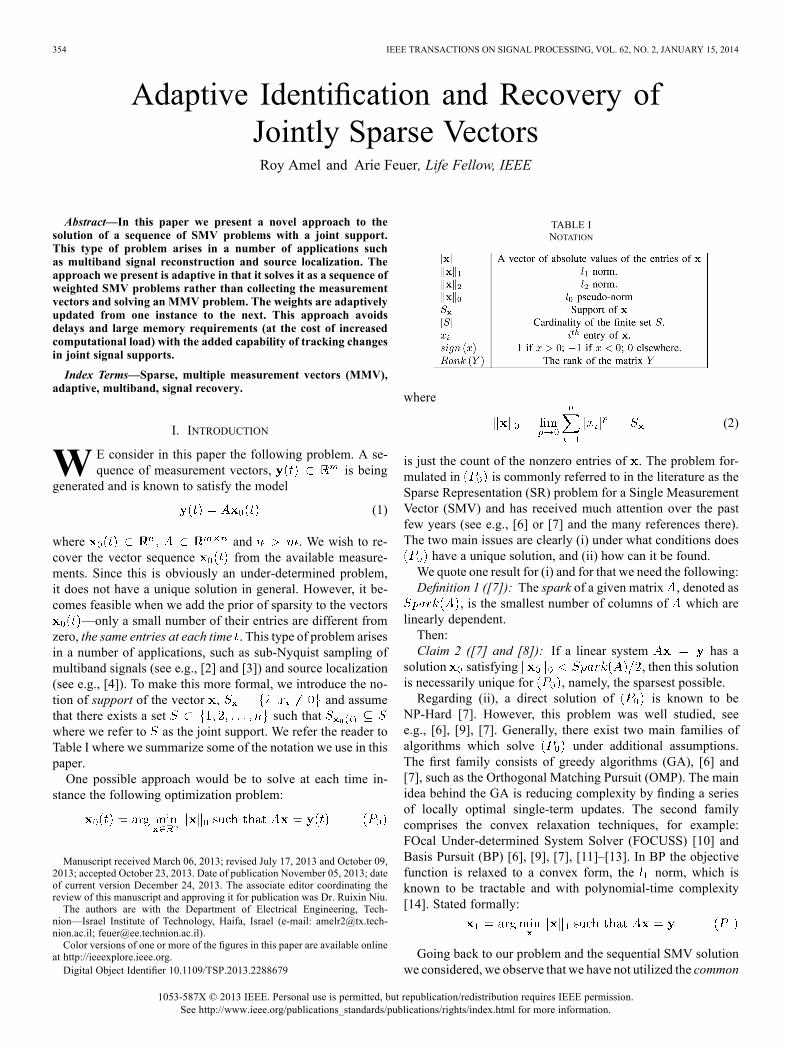
Fig. 4. Demonstration of tracking capability for different values of -successprobability for true recovery as function of time for .

Fig. 5. Performance comparison between the M-OMP and the AW-OMP algo-rithms for sub-block sizes and 100.

changed the support at time and we show the algorithmbehavior for different values of . We clearly observe that forlarger the tracking is slower.2) AW-OMP: Next we applied the AW-OMP on the same

data. Here we have experimented with the block version of theAW-OMP (see Remark 10) and show the results in Fig. 5 wherewe varied the block sizes as well. The M-OMP was applied oneach block independently using different number of measure-ment vectors. It is noticeable that the AW-OMP achieves betterresults than the M-OMP for the same block size. Interestinglyenough, the AW-OMP with block size 10, by , out-performs the M-OMP which is applied to the whole data set

.To get an idea of the computational aspects of the approach

we consider the set-up with andand applied the AW-OMP up to . We counted thenumber operations carried out in the process. Then we appliedthe M-OMP on the collected data set. The comparison is pre-sented in Table II. As anticipated, our approach is computation-ally more demanding. We should point out however, that thisload is not uniform in time. As convergence occurs in our algo-rithms, the computational load goes down significantly as Step2d is reduced to a solution of a set of linear equations.

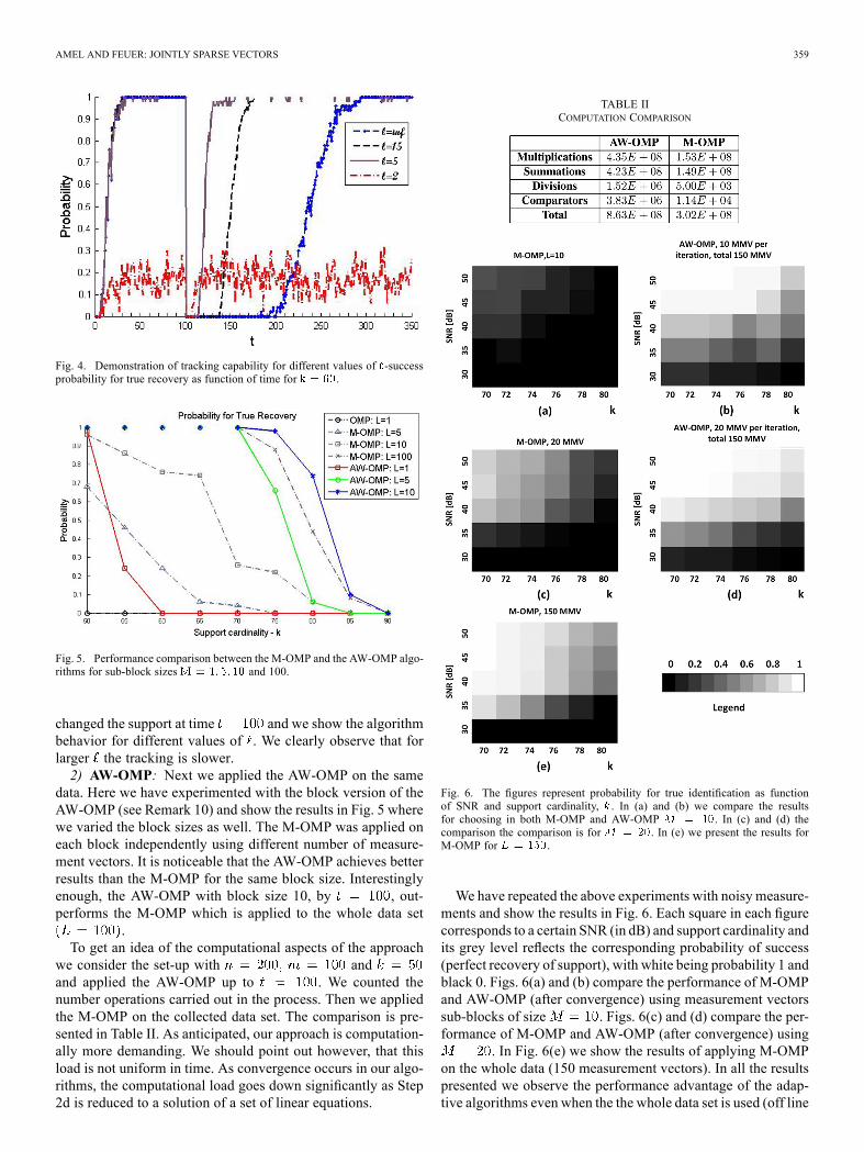
TABLE IICOMPUTATION COMPARISON

Fig. 6. The figures represent probability for true identification as functionof SNR and support cardinality, . In (a) and (b) we compare the resultsfor choosing in both M-OMP and AW-OMP . In (c) and (d) thecomparison the comparison is for . In (e) we present the results forM-OMP for .

We have repeated the above experiments with noisy measure-ments and show the results in Fig. 6. Each square in each figurecorresponds to a certain SNR (in dB) and support cardinality andits grey level reflects the corresponding probability of success(perfect recovery of support), with white being probability 1 andblack 0. Figs. 6(a) and (b) compare the performance of M-OMPand AW-OMP (after convergence) using measurement vectorssub-blocks of size . Figs. 6(c) and (d) compare the per-formance of M-OMP and AW-OMP (after convergence) using

. In Fig. 6(e) we show the results of applying M-OMPon the whole data (150 measurement vectors). In all the resultspresented we observe the performance advantage of the adap-tive algorithms even when the the whole data set is used (off line


Fig. 7. Probability for true recovery of Sub-Nyquist system. (a) Using blockAW-OMP, and 100 measurement vectors total. The results are afterconvergence. (b) Using the reconstruction as described in [2].

processing) and this goes beyond the obvious advantage of theonline processing (smaller or even no delays and less demandon memory).

B. Reconstruction of a Multiband Signal

There are at least two examples in the literature of applica-tions which are cast in the form of the model in (1). One is thesource localization problem in radars with sensor arrays (seee.g., [4]) and the second is the reconstruction of under-sam-pled multi-band signals (see e.g., [2]). We chose to apply ouradaptive approach to the latter and used the example presentedin the work of Mishali and Eldar [2]. They consider a signalwhich consists of disjoint frequency bands at unknown loca-tions, each of width bounded by . The measurement vectorsare generated by an ingenious sampling of that signal, consid-erably below Nyquist rate, as described in detail in [2]. Theyshow that the measured data vectors satisfy the frequency do-main equation where is the DFT of themeasurements vectors is a known matrix and the vector

is sparse for every . To reconstruct the multibandsignal, the support of is found first, which then leads tocalculating and the signal reconstruction. Both the sam-pling and reconstruction described in [2] were thoroughly in-vestigated by Mishali and Eldar who also proceeded to success-fully implement it in hardware.We propose here an alternative approach to the reconstruction

by looking at the time domain version of the above equation,, where are the measurement vectors, as

above and is sparse (same support as ) for all .With this equation we apply our AW-OMP to the same signalas in [2] ((37) and Option A in their Table I).In Fig. 7(a) we show the performance using AW-OMP (after

convergence) and, in Fig. 7(b) the results using the algorithmdescribed in [2]. The rsults seem quite comparable.

VI. CONCLUSION

The set up considered in this paper is of, possibly a largenumber, of measurement vectors being generated sequentiallyfrom a set of jointly sparse signals with a common dictionary.One approach would be to collect all the measurement vectorsand solve an MMV problem with one of the available algo-rithms. This approach has the advantage of low computationalrequirements and takes advantage of all the joint sparsitybenefits (see Claim 3). However, it requires a large memory,introduces a (possibly large) delay in the signal reconstructionand it does not have the capability of tracking a changingjoint sparsity. The other possibility is solving independently anSMV problem each time a new measurement vector becomesavailable. This approach, while having minimal memory re-quirements and no delay, does not make use of the joint sparsityprior. In this paper we introduced a novel approach whichhas the benefits of the two extremes above. It can be viewedas an adaptive method of solution. It is based on a sequentialsolution of (weighted) SMV (or weighted blocked MMV)problems. The resulting signal supports are then carried over,in a non-greedy way via a weighting matrix, from one instanceto the next.Different applications of this concept can be realized by

using different methods of solving the sequence of SMVproblems. In our paper we have chosen two representativeexamples to demonstrate our approach. One is using theBasis Pursuit (BP), resulting in what we termed AW-BP andthe other, the Orthogonal Matching Pursuit (OMP) resultingin AW-OMP. However the method can be applied throughmany other existing algorithms such as: IRLS ([7]), LARS([19]), FOCUSS ([7], [10]), M-FOCUSS ([15]) etc. Clearly,the resulting properties will depend on the actual underlyingalgorithm chosen.All our experiments with the AW-BP and AW-OMP

demonstrated a clear advantage over their sequentialindependent counterparts (both SMV and blocked MMV).While this is not surprising, we also observed a performancesimilar (or even better) to MMV when the whole data set isconsidered. Comparing the performance of the AW-BP to theAW-OMP we observed that the first has a significant advantagein its recovery rate for growing support cardinality, while thelatter is a faster algorithm with significantly lower computa-tional load.

APPENDIXPROOF OF CLAIM 4

Proof: Let

(38)

Clearly and for any we have

(39)


Then, by (7) and (39) we get

So .Let be such that and, then and . On the

other hand

which means that and we can conclude that .This means that there are only three possibilities

and

and

and

We observe that andand and and . By the

claim assumptions and since , we note thatso we readily conclude that

which completes the proof.

PROOF OF CLAIM 5

Proof:1) We readily observe from (14) that the Markov chain has

states, , and the matrix in (15) is adirect consequence of (14). To find the eigenvalues ofwe are interested in the roots of

(40)

Let us denote

......

. . ....

...

(41)

and

......

. . ....

... (42)

Then, using determinant properties and expanding bythe last row and and by the first rows ofthe respective matrices, we get the following relationships:

(43)

(44)

(45)

By straight forward substitutions we get from (43)–(45)

(46)

As is the characteristic polynomial of a tridiag-onal Toeplitz matrix it is known (see e.g., [20]) to have theroots:

(47)

and combined with (46), (16) follows.2) It can be shown (see e.g., [21]) that the Markov chain withthe given results in a stable Markov chain and will con-verge to a steady state distribution. The proof of (17) is bystraight forward substitution.

3) Let be the eigen-values of and the corresponding left eigen-vectors which are linearly independent (as the eigenvaluesare distinct). Note that , the stationary distribu-tion vector. Then we can write

(48)

where

...

(49)


where we note that (a vector of ones). Namely,we can also rewrite

and

(50)

Then we get

or

(51)

where which completesthe proof of the claim.

REFERENCES[1] M. Mishali and Y. C. Eldar, “Blind multiband signal reconstruction:

Compressed Sensing for analog signals,” IEEE Trans. Signal Process.,vol. 57, no. 3, pp. 993–1009, Mar. 2009.

[2] M. Mishali and Y. C. Eldar, “From theory to practice: Sub-Nyquistsampling of sparse wideband analog signals,” IEEE J. Sel. Topics inSignal Process., Special Issue on Compressed Sens., vol. 4, no. 2, pp.375–391, Apr. 2010.

[3] R. Venkataramani and Y. Bresler, “Perfect reconstruction formulas andbounds on aliasing error in sub-Nyquist nonuniform sampling of multi-band signals,” IEEE Trans. Inf. Theory, vol. 46, no. 6, pp. 2173–2183,Sep. 2000.

[4] D. Malioutov, M. Cetin, and A. Willsky, “A sparse signal reconstruc-tion perspective for source localization with sensor arrays,” IEEETrans. Signal Process., vol. 53, no. 8, pp. 3010–3022, Aug. 2005.

[5] D. L. Donoho, “Compressed sensing,” IEEE Trans. Inf. Theory, vol.52, no. 2, pp. 1289–1306, 2006.

[6] A. M. Bruckstein, D. L. Donoho, and M. Elad, “From sparse solutionsof systems of equations to sparse modeling of signals and images,”SIAM Rev., vol. 51, no. 1, p. 34, 2009.

[7] M. Elad, Sparse and Redundant Representations. From Theory to Ap-plications in Signal and Image Processing, 1st ed. New York, NY,USA: Springer, 2010.

[8] M. Elad, “Sparse representations are most likely to be the sparsest pos-sible,” EURASIP J. Appl. Signal Process., pt. Paper No. 96247, 2006.

[9] E. J. Candes and M. B. Wakin, “An introduction to compressive sam-pling,” IEEE Signal Process. Mag., vol. 25, no. 2, pp. 21–30, Mar.2008.

[10] I. F. Gorodnitsky and B. D. Rao, “Sparse signal reconstruction fromlimited data using FOCUSS: A re-weighted minimum norm algo-rithm,” IEEE Trans. Signal Process., vol. 45, no. 3, pp. 600–616, Mar.1997.

[11] Y. Kopsinis, K. Slavakins, and S. Theodoridis, “Online sparse systemidentification and signal reconstruction using projection onto weightedballs,” IEEE Trans. Signal Process., vol. 59, pp. 936–952, Mar.

2011.[12] D. L. Donoho, “For most large underdetermined systems of linear

equations, the minimal ’1-norm near-solution approximates thesparsest near-solution,” Commun. Pure Appl. Math., vol. 59, no. 7, pp.907–934, Jul. 2006.

[13] S. S. Chen, D. L. Donoho, andM.A. Saunders, “Atomic decompositionby basis pursuit,” SIAM Rev., vol. 43, no. 1, pp. 129–159, 2001.

[14] S. Boyd and L. Vandenberghe, Convex Optimization. Cambridge,U.K.: Cambridge Univ. Press, 2008.

[15] S. F. Cotter, B. D. Rao, and K. Kreutz-Delgado, “Sparse solutionsto linear inverse problems with multiple measurement vectors,” IEEETrans. Signal Process., vol. 53, pp. 2477–2488, Jul. 2005.

[16] J. Chen and X. Huo, “Theoretical results on sparse representations ofmultiple-measurement vectors,” IEEE Trans. Signal Process., vol. 53,pp. 4634–4643, Dec. 2006.

[17] A. H. Sayed, Fundamentals of Adaptive Filtering. Hoboken, NJ,USA: Wiley, 2003.

[18] E. J. Candes, M. B. Wakin, and S. P. Boyd, “Enhancing sparsity byreweighted minimization,” J. Fourier Anal. Appl., vol. 14, no. 5, pp.877–905, Dec. 2008.

[19] B. Efron, T. Hastie, I. M. Johnstone, and R. Tibshirani, “Least angleregression,” Ann. Statist., vol. 32, no. 2, pp. 407–499, 2004.

[20] G. D. Smith, Numerical Solutions of Partial Differential Equations.New York, NY, USA: Clarendon, 1978.

[21] C. M. Grinstead and J. L. Snell, Introduction to Probability, 2nd ed.New York, NY, USA: Amer. Math. Soc., 2003.

[22] M. Mishali and Y. C. Eldar, “Reduce and boost: Recovering arbitrarysets of jointly sparse vectors,” IEEE Trans. Signal Process., vol. 56,no. 10, pp. 4692–4702, Oct. 2008.

[23] E. J. Candes, J. Romberg, and T. Tao, “Robust uncertainty principles:Exact signal reconstruction from highly incomplete frequency infor-mation,” IEEE Trans. Inf. Theory, vol. 52, pp. 489–509, Feb. 2006.

[24] J. A. Tropp, “Greed is good: Algorithmic results for sparse approxima-tion,” IEEE Trans. Inf. Theory, vol. 50, no. 10, pp. 2231–2242, Oct.2004.

[25] R. Amel and A. Feuer, “Adaptive algorithm for online identificationand recovering of jointly sparse signals,” in Proc. Sparse 11, 4th Work-shop on Signal Process. Adapt. Sparse Structure Represent., Jun. 2011,p. 113.

[26] M. C. Grant, CVX [Online]. Available: http://cvxr.com/[27] J. A. Tropp, “Algorithms for simultaneous approximation. Part

II: Convex relaxation,” Signal Process. Special Issue, vol. 86, pp.598–602, Apr. 2006.

Roy Amel received the B.Sc. degree in electrical en-gineering in 2009 and the M.Sc. degree in electricalengineering in 2013 both from the Technion—IsraelInstitute of Technology, Haifa.Since 2012, he has been a System Engineer of the

physical layer (include all the blocks from the An-tenna to the bit) of Intel WIFI products.

Arie Feuer (M’76–SM’93–F’04–LF’14) receivedthe B.Sc. and M.Sc. degrees from the Technion—Is-rael Institute of Technology in 1967 and 1973,respectively, and the Ph.D. degree from Yale Uni-versity in 1978. In 2009, he received an honorarydoctorate from the University of Newcastle.He has been with the Department of Electrical En-

gineering, Technion—Israel Institute of Technology,since 1983 were he is currently a Professor Emeritus.From 1967 to 1970, he was in industry working onautomation design and between 1978 and 1983 with

Bell Labs in Holmdel, NJ. In the last 22 years, he has been regularly visiting theElectrical Engineering and Computer Science Department at the University ofNewcastle. His current research interests include: Medical imaging—in partic-ular, ultrasound and CT; resolution enhancement of digital images and videos;3D video and multi-view data; Sampling and combined representations of sig-nals and images.Dr. Feuer served as the president of the Israel Association of Automatic Con-

trol between 1994 and 2002, and was a member of the IFAC Council during2002–2005.

adaptive recovery of spars vector

Documents