University of ConnecticutOpenCommons@UConn

Doctoral Dissertations University of Connecticut Graduate School

6-15-2016

Adaptive Partition Weighted Monte CarloEstimationYu-Bo Wangyu-bo.wang@uconn.edu

Follow this and additional works at: https://opencommons.uconn.edu/dissertations

Recommended CitationWang, Yu-Bo, "Adaptive Partition Weighted Monte Carlo Estimation" (2016). Doctoral Dissertations. 1056.https://opencommons.uconn.edu/dissertations/1056

Adaptive Partition Weighted Monte CarloEstimation

Yu-Bo Wang, Ph.D.

University of Connecticut, 2016

ABSTRACT

This dissertation mainly focuses on the development of new Monte Carlo estima-

tors for marginal likelihood and marginal posterior density with minimal assumption

of a known nonnormalized posterior density and a single MCMC sample from the

posterior distribution. We use the ideas of partitioning the parameter space and as-

signing an adaptive weight to the points of MCMC sample within different partition

subsets. The estimators are shown to be consistent with the targets and their opti-

mal performances in terms of minimizing the variance of estimators can be achieved

by increasing the number of partition subsets. The proposing methods provide effi-

cient ways to the problems including but not limited to Bayesian model or variable

selection, the choices of power prior by empirical Bayes method, and phylogenetic

model selection for a variable topology. Moreover, when multiple MCMC samples are

available from the posterior density and conditional posterior densities, we provide a

hybrid method, which is benefited from the dimension reduction.

Adaptive Partition Weighted Monte CarloEstimation

Yu-Bo Wang

B.S., Statistics, National Chengchi University, Taiwan, 2006

M.S., Statistics, National Chengchi University, Taiwan, 2009

A Dissertation

Submitted in Partial Fulfillment of the

Requirements for the Degree of

Doctor of Philosophy

at the

University of Connecticut

2016

Copyright by

Yu-Bo Wang

2016

APPROVAL PAGE

Doctor of Philosophy Dissertation

Adaptive Partition Weighted Monte CarloEstimation

Presented by

Yu-Bo Wang, B.S. Statistics, M.S. Statistics

Major AdvisorLynn Kuo

Major AdvisorMing-Hui Chen

Associate AdvisorPaul O. Lewis

University of Connecticut

2016

ii

ACKNOWLEDGEMENTS

First, I want to exalt my God through Jesus Christ.

I would like to express my utmost and sincere gratitude to my major advisers

Professor Lynn Kuo and Professor Ming-Hui Chen. With their wisdom, commitment,

enthusiasm, and patience, they inspire and guide me in life and research, and establish

great models of being a great scholar to me. Because of them, I can be what I am

now.

I am grateful to my associate adviser Professor Paul O. Lewis for his kind help and

valuable advice. He enriches my knowledge in phylogeny and programming, which

are so important to me in the whole process of my graduate studies and to my future

research.

I would also like to thank Professor James Grady. Because of him, I can have a

valuable 4-year consulting experience in UConn Health Center. With his guidance

and training, I have accessed to many different projects and become confident.

I would also like to thank Professor Natiee Ting. He enriches my experience in

applied statistics. Through him, I have a deeper understanding about clinical trials,

see the different applications of statistics, and cultivate my another research interest.

Many thanks are to all faculty members and my fellow graduate students. Special

thanks to Tracy Burke and Megan Petsa for their helpful assistance, and to my former

colleagues at UConn Health Center and Boehringer Ingelheim for offering me the

precious opportunities to gain various experiences and continuous support. Lastly,

I want to dedicate this dissertation to my wife, Yi-Chun, and my parents. Their

everlasting love and support always encourage me to achieve my goals.

iii

Contents

Ch. 1. Introduction 1

1.1 Marginal Likelihood Estimation . . . . . . . . . . . . . . . . . . . . . 1

1.2 Marginal Posterior Density Estimation . . . . . . . . . . . . . . . . . 2

1.3 Overview of the Dissertation . . . . . . . . . . . . . . . . . . . . . . . 3

Ch. 2. Marginal Likelihood Estimation 5

2.1 Introduction . . . . . . . . . . . . . . . . . . . . . . . . . . . . . . . . 5

2.2 Preliminary . . . . . . . . . . . . . . . . . . . . . . . . . . . . . . . . 7

2.3 A New Monte Carlo Estimator . . . . . . . . . . . . . . . . . . . . . . 102.3.1 General Monte Carlo Estimator . . . . . . . . . . . . . . . . . 112.3.2 The Optimal Monte Carlo Estimation . . . . . . . . . . . . . . 142.3.3 Construction of the Partition with Subsets A1, . . . , AK . . . . 17

2.4 Extension of the General PWK Estimator . . . . . . . . . . . . . . . 18

2.5 Simulation Studies . . . . . . . . . . . . . . . . . . . . . . . . . . . . 202.5.1 A Bivariate Normal Example . . . . . . . . . . . . . . . . . . 202.5.2 A Mixture Normal Example . . . . . . . . . . . . . . . . . . . 24

2.6 Application of the PWK to Real Data Examples . . . . . . . . . . . . 282.6.1 The Ordinal Probit Regression Model . . . . . . . . . . . . . . 282.6.2 Analysis of ECOG Data . . . . . . . . . . . . . . . . . . . . . 32

2.7 Discussion . . . . . . . . . . . . . . . . . . . . . . . . . . . . . . . . . 38

Ch. 3. Marginal Posterior Density Estimation 41

3.1 Introduction . . . . . . . . . . . . . . . . . . . . . . . . . . . . . . . . 41

3.2 Preliminaries . . . . . . . . . . . . . . . . . . . . . . . . . . . . . . . 45

3.3 The Proposed Method for Estimating Posterior Densities . . . . . . . 483.3.1 Estimating Marginal Posterior Density . . . . . . . . . . . . . 48

iv

3.3.2 Estimating Conditional Posterior Density . . . . . . . . . . . . 52

3.4 Inequality-Constrained Analysis of Variance . . . . . . . . . . . . . . 53

3.5 APT for Bayesian Variable Selection . . . . . . . . . . . . . . . . . . 623.5.1 The Basic Formulation . . . . . . . . . . . . . . . . . . . . . . 623.5.2 The Ordinal Probit Regression Model . . . . . . . . . . . . . . 653.5.3 Analysis of the Prostate Cancer Data . . . . . . . . . . . . . . 68

3.6 Discussion . . . . . . . . . . . . . . . . . . . . . . . . . . . . . . . . . 72

Ch. 4. Marginal Likelihoods of Phylogenetic Models Using a Poste-rior Sample 75

4.1 Introduction . . . . . . . . . . . . . . . . . . . . . . . . . . . . . . . . 75

4.2 Preliminary . . . . . . . . . . . . . . . . . . . . . . . . . . . . . . . . 77

4.3 PWK Estimator in Variable Topology . . . . . . . . . . . . . . . . . . 814.3.1 General Monte Carlo Estimator . . . . . . . . . . . . . . . . . 824.3.2 New Monte Carlo Estimator . . . . . . . . . . . . . . . . . . . 84

4.4 6-taxon rcbL Data Set . . . . . . . . . . . . . . . . . . . . . . . . . . 87

4.5 Results and Discussion . . . . . . . . . . . . . . . . . . . . . . . . . . 89

Ch. 5. Concluding Remarks and Future Work 91

5.1 Concluding Remarks . . . . . . . . . . . . . . . . . . . . . . . . . . . 91

5.2 Future Work . . . . . . . . . . . . . . . . . . . . . . . . . . . . . . . . 93

Bibliography 94

v

Chapter 1

Introduction

In this dissertation, marginal likelihood and marginal posterior density estimation

is the main focus with special discussions on computation of the Bayes factor, the

choice of power prior by empirical Bayes method, dimension reduction when multiple

MCMC samples are available, and the application in phylogenetic models.

1.1 Marginal Likelihood Estimation

Evaluating the marginal likelihood in Bayesian analysis is essential for model selec-

tion. There are existing estimators based on a single Markov chain Monte Carlo

sample from the posterior distribution, including the harmonic mean estimator and

the inflated density ratio estimator. We propose a new class of Monte Carlo estimators

based on this single Markov chain Monte Carlo sample. This class can be thought of

as a generalization of the harmonic mean and inflated density ratio estimators using a

partition weighted kernel (likelihood times prior). We also show that our estimator is

1

2

consistent and has better theoretical properties than the harmonic mean and inflated

density ratio estimators. In addition, we provide guidelines on choosing the optimal

weights. Simulation studies are conducted to examine the empirical performance of

the proposed estimator. We further demonstrate the desirable features of the pro-

posed estimator with two real data sets: one is from a prostate cancer study using an

ordinal probit regression model with latent variables; the other is for the power prior

construction from two Eastern Cooperative Oncology Group phase III clinical trials

using the cure rate survival model with similar objectives.

1.2 Marginal Posterior Density Estimation

The computation of marginal posterior density in Bayesian analysis is essential in that

it can provide complete information about parameters of interest. Furthermore, the

marginal posterior density can be used for computing Bayes factors, posterior model

probabilities, and diagnostic measures. The conditional marginal density estimator

(CMDE) is theoretically the best for marginal density estimation but requires the

closed-form expression of the conditional posterior density, which is often not available

in many applications. We develop an Adaptive Partition weighTed (APT) method to

realize the CMDE. This unbiased estimator requires only a single MCMC output from

the joint posterior distribution and the known unnormalized posterior density. The

theoretical properties and various applications of the APT estimator are examined in

detail. The APT method is also extended to the estimation of conditional posterior

densities. We further demonstrate the desirable features of the proposed method

with two real data sets: one is from a study of dissociative identity disorder patients

3

using an analysis of variance model with constrained inequalities; the other is from

a prostate cancer study, where model selection is investigated using ordinal probit

regression models with latent variables.

1.3 Overview of the Dissertation

This rest of the dissertation is organized as follows:

Chapter 2 reviews some established methods for marginal likelihood. A detailed

development of the proposed Monte Carlo marginal likelihood estimator is presented

and its various properties are examined. We also provide a guideline on how to

implement this method in different types of parameter space. A simulation study of

comparing its performance with other existing methods is illustrated in a bivariate

normal distribution with both unknown mean and covariance matrix. Then a real

data from a prostate cancer study and ECOG data are analyzed to demonstrate the

usefulness of this new method. A sensitivity analysis of this new method is also

included.

Chapter 3 introduces the new Monte Carlo estimator for marginal posterior den-

sity with inspiration from the new method in Chapter 2. Its development and prop-

erties are detailed examined and discussed. In first real data, we empirically show

the precision of this method in an inequality-constrained analysis of variance model.

In second example, the application of this method to computing the Bayes factor is

demonstrated. Besides, the benefit of dimension reduction is empirically shown when

multiple MCMC samples are available.

Chapter 4 proposes the new marginal likelihood estimator for the phylogenetic

4

models with variable topology. It is inspired by the new method in Chapter 2. By

using the concept of working parameter space, the estimator can avoid those topolo-

gies with few or no visiting of MCMC sample, which is a common phylogeny problem

when a variable topology is considered.

Chapter 5 makes conclusions from the established theorems and the results from

the simulation study and real data analysis. Discussions and directions for future

research are also provided.

Chapter 2

Marginal Likelihood Estimation

2.1 Introduction

The Bayes factor quantifying evidence of one model over a competing model is com-

monly used for model comparison or variable selection in Bayesian inference. The

Bayes factor is a ratio of two marginal likelihoods, where the marginal likelihood is

essentially the average fit of the model to the data. However, the integration for the

marginal likelihood is often analytically intractable due to the complex kernel (the

likelihood times the prior) structure. To deal with this computational problem, several

Monte Carlo methods have been developed. They include the importance sampling

(IS) of Geweke (1989), the harmonic mean (HM) of Newton and Raftery (1994) and

its generalization (GHM) of Gelfand and Dey (1994), the serial approaches of Chib

(1995) and Chib and Jeliazkov (2001), the inflated density ratio method (IDR) of

Petris and Tardella (2003) and Petris and Tardella (2007), the thermodynamic inte-

gration (TI) of Lartillot and Philippe (2006), the constrained GHM estimator with

5

6

the highest posterior density (HPD) region of Robert and Wraith (2009) and Marin

and Robert (2010), and the steppingstone sampling of Xie et al. (2011). Under some

mild conditions, they are all shown to be asymptotically convergent to the marginal

likelihood by the ergodic theorem. They vary in using Monte Carlo samples or kernels

in the Monte Carlo integration.

We assume only a single Markov chain Monte Carlo (MCMC) sample from the

posterior distribution, which may be readily available from standard Bayesian soft-

ware, and the known kernel function for computing the marginal likelihood. The HM

and IDR estimators are the two existing ones, which only need these two minimal

assumptions. The main difference between the HM and the IDR estimators lies in the

different weights assigned to the inverse of the kernel function. The former uses the

prior function as a weight, while the latter uses the difference between a perturbed

density and its kernel function. Although the HM estimator has been used in practice

because of its simplicity, it can be unstable when the prior has heavier tails than the

likelihood function and it is known to overestimate the marginal likelihood (Xie et al.,

2011).

While the IDR estimator has better control over the tails of the kernel than the

HM estimator in controlling the tails of the likelihood function, it requires reparam-

eterization, posterior mode calculation, and a careful selection of radius. Under the

aforementioned two minimal assumptions, we extend the HM and IDR methods to

develop a new Monte Carlo method, namely, the partition weighted kernel (PWK)

estimator. The PWK estimator is constructed by first partitioning the working pa-

rameter space (where the kernel is bounded away from zero), and then estimating

the marginal likelihood by a weighted average of the kernel values evaluated at the

MCMC sample, where weights are assigned locally using a representative kernel value

7

in each partition. We show the PWK estimator is consistent and has finite variance.

When the partition is refined enough to make the kernel values in the same region

similar, we can construct the best PWK estimator with the minimum variance. Our

simulation study empirically shows that the proposed PWK estimator outperforms

both the HM and IDR estimators.

The rest of Chapter 2 is organized as follows. Section 2 is a review of the HM,

GHM and IDR methods that motivate the PWK estimator. In Section 3, we develop

the PWK estimator and its theoretical properties. Additionally, in the class of the

general PWK estimator, we find the best (minimum variance) PWK estimator and

provide a spherical shell approach to realize it. In Section 4, an extended general PWK

estimator which is defined on the full support of the kernel function is investigated.

Besides the theoretical properties, we show that the HM and IDR estimators are

special cases in this family. In Section 5, we conduct a simulation study of a bivariate

normal case with the normal-inverse-Wishart prior to compare the performance and

computing time of the HM, IDR and PWK estimators. In Section 6, we compare the

performance of the PWK estimator to the methods by Chib (1995) and Chen (2005b)

for a ordinal probit regression model. Moreover, we apply the PWK estimator to the

determination of the optimal power prior using two ECOG clinical trial data sets.

Finally, we conclude with a discussion in Section 7.

2.2 Preliminary

We review several Monte Carlo methods that only require a known kernel function and

an MCMC sample from the posterior distribution to compute the marginal likelihood.

8

Suppose θ is a p-dimensional vector of parameters and D denotes the data. Then,

the kernel function for the joint posterior density π(θ|D) is q(θ) = L(θ|D)π(θ),

where L(θ|D) is the likelihood function and π(θ) is a proper prior density. Assume

Θ ⊂ Rp is the support of q(θ). The unknown marginal likelihood c is defined to

be∫Θ q(θ)dθ. Due to the complicated kernel structure, the integration is often

analytically intractable.

To estimate the normalizing constant c, Newton and Raftery (1994) suggest the

following equation to motivate the HM method,

1

c=

∫Θ

π(θ)

q(θ)

q(θ)

cdθ. (2.1)

Let θt, t = 1, . . . , T be an MCMC sample from the posterior distribution π(θ|D) =

q(θ)/c. The HM estimator is then given by

cHM =1

1T

∑Tt=1

1

L(θt|D)

, (2.2)

where the prior π(θt) can be viewed as the weight assigned to 1/q(θt). Although it has

the feature of simplicity and has asymptotic convergence to the marginal likelihood,

the finite variance is not guaranteed. Xie et al. (2011) also point out that the HM

estimator tends to overestimate the marginal likelihood.

Gelfand and Dey (1994) suggest the GHM estimator where π(θ) in equation (2.1)

is replaced by a lighter-tailed density function f(θ) compared to q(θ):

cGHM =1

1T

∑Tt=1

f(θt)q(θt)

. (2.3)

9

By proposing a light-tailed density, the ratio f(θt)/q(θt) can be controlled. Conse-

quently, the estimator has finite variance. However, in high dimensional problems,

finding a suitable density f(θ) may be a challenge.

Petris and Tardella (2003) propose the IDR estimator. They use the difference

between a perturbed distribution qr(θ), which is inflated in the center of the kernel,

and the posterior kernel q(θ) as the weight. The perturbed density qr(θ) is defined

as

qr(θ) =

q(0) if ||θ|| ≤ r,

q(w(θ)) if ||θ|| > r,

(2.4)

where r is the chosen radius and w(θ) = θ (1− rp/||θ||p)1/p. It follows,

∫Θqr(θ)dθ =

∫||θ||≤r

qr(θ)dθ +

∫||θ||>r

qr(θ)dθ = q(0)br + c, (2.5)

where br = Volume of the ball θ : ||θ|| ≤ r = πp/2rp/Γ(p/2 + 1). Then, we can

have the following equation,

q(0)br + c

c=

∫Θ

qr(θ)

q(θ)

q(θ)

cdθ, (2.6)

and the IDR estimator is given by

cIDR =q(0)br

1T

∑Tt=1

qr(θt)q(θt)

− 1. (2.7)

Under some mild conditions, the estimator is shown to have finite variance by Petris

and Tardella (2007). However, the method requires a careful selection of radius and

unbounded support of q(θ). Any bounded parameter must be reparameterized to the

10

full real line. Also, in order to have a more efficient estimate, mode finding is essential

and standardization of an MCMC sample with respect to the mode and the sample

covariance matrix is required.

2.3 A New Monte Carlo Estimator

We first modify (2.1) and (2.6) by imposing a working parameter space Ω ⊂ Θ, where

Ω = θ : q(θ) is bounded away from zero to avoid regions with extremely low kernel

values. Then we assume there is a function h(θ) such that∫

Ωh(θ)dθ = ∆ can be

evaluated. Consequently, we have the identity:

∆

c=

∫Ω

h(θ)

q(θ)

q(θ)

cdθ. (2.8)

We next partition the working parameter space into K subsets, where the ratio

of h(θ) over q(θ) has similar values within each subset, to reduce the variance of the

Monte Carlo estimator. The general form of the PWK estimator with unspecified

local weights is essentially a weighted average for the harmonic mean estimator for

q(θ) with the same weights assigned locally to an MCMC sample in a subset.

The working parameter space is essentially the constrained support considered by

Robert and Wraith (2009) and Marin and Robert (2010). However, we do not require

h(θ) to be a density function as in GHM or constrained GHM. Consequently, we

allow a larger class of estimators to be considered.

11

2.3.1 General Monte Carlo Estimator

Suppose A1, . . . , AK forms a partition of the working parameter space Ω, where for

an integerK > 0, w1, . . . , wK are the weights assigned to theseK regions, respectively.

Let the weight function be the step function:

h(θ) =K∑k=1

wk1θ ∈ Ak. (2.9)

Evaluate ∆:

∆ =

∫Ω

h(θ)dθ =K∑k=1

wkV (Ak),

where V (Ak) is the volume of the kth subset in the partition, that is, V (Ak) =∫Ω

1θ ∈ Akdθ.

Using the step function h(.) in (2.9), the PWK estimator for d ≡ 1/c is given by

d =

1T

∑Tt=1

∑Kk=1

wkq(θt)

1θt ∈ Ak∑Kk=1wkV (Ak)

. (2.10)

In order to establish consistency and finite variance of the PWK estimator, we

introduce two assumptions.

Assumption 1: The volume of each region V (Ak) <∞ for k = 1, 2, . . . , K.

Assumption 2: q(θ) is positive and continuous on Ak, where Ak is the closure of

Ak for k = 1, . . . , K.

Theorem 2.3.1. Under Assumptions 1 to 2 and certain ergodic conditions, d in

(2.10) is a consistent estimator of 1/c. In addition, Var(d) <∞.

12

Proof:

limT→∞

1

T

T∑t=1

K∑k=1

wkq(θt)

1θt ∈ Ak

=K∑k=1

wk limT→∞

1

T

T∑t=1

1

q(θt)1θt ∈ Ak

=K∑k=1

wk

∫θ∈Ak

1

q(θ)

q(θ)

cdθ

=dK∑k=1

wkV (Ak),

which implies that da.s.−−→ 1/c. Let qk,min = minθt∈Ak q(θt). Under Assumption 2,

we have qk,min > 0. Write g(θt) =∑K

k=1wk/q(θt)1θt ∈ Ak. Under Assumptions 1

and 2, we have

E[g(θt)]2 =

K∑k=1

E([ wkq(θt)

]1θt ∈ Ak

)2

≤K∑k=1

w2k

qk,minE([ 1

q(θt)

]1θt ∈ Ak

)≤

K∑k=1

w2kV (Ak)

qk,minc<∞, (2.11)

13

which implies that Var[g(θi)] <∞. Using Cauchy–Schwarz Inequality, we obtain

Var[ 1

T

T∑t=1

g(θt)]

=1

T 2Var[ T∑t=1

g(θt)]

=1

T 2

T∑t=1

Var[g(θt)] + 2∑∑t′<t′′

Cov[g(θt′), g(θt′′)]

≤ 1

T 2

T∑t=1

Var[g(θt)] + 2∑∑t′<t′′

√Var[g(θt′)]Var[g(θt′′)]

. (2.12)

Thus, Var(d) <∞ directly follows from (2.12). 2

Remark 3.1: Another property of d in (2.10) is that when a certain full condi-

tional density is available, the computation can be lessened. This is often the case

in the generalized linear model with latent variables or random effects, and in any

Gibbs sampler or its hybrid. To be specific, let (ϑ1,ϑ2) be 2 blocks of parame-

ters, ϑ1 = (θ1, ..., θq)′ and ϑ2 = (θq+1, ..., θp)

′. Assume that a full conditional density,

π(ϑ1|D,ϑ2), is available. Then, the p-dimensional estimation problem can be reduced

to p− q dimensions:

1 =

∫Rp

q(θ)

cdθ

=

∫Rp−q

∫Rq

q(ϑ2)π(ϑ1|D,ϑ2)

cdϑ1dϑ2

=

∫Rp−q

q(ϑ2)

c

∫Rqπ(ϑ1|D,ϑ2)dϑ1dϑ2

=

∫Rp−q

q(ϑ2)

cdϑ2,

where q(ϑ2) =∫Rqq(θ)dϑ1, which has a closed form expression. Therefore, instead

of investigating the kernel q(θ), we can work on the kernel q(ϑ2). In this case, (2.10)

14

becomes

d =

1T

∑Tt=1

∑Kk=1

wkq(ϑ2t )

1ϑ2t ∈ Bk∑Kk=1 wkV (Bk)

,

where B1, ..., BK is a partition of the working parameter space Ω2,Ω2 ⊂ Θ2, which

is the support of q(ϑ2), and V (B1), ..., V (BK) are the corresponding volumes, respec-

tively.

2.3.2 The Optimal Monte Carlo Estimation

Our next step is to find the optimal weight wk in the class of PWK estimators (2.10),

motivated by Chen and Shao (2002).

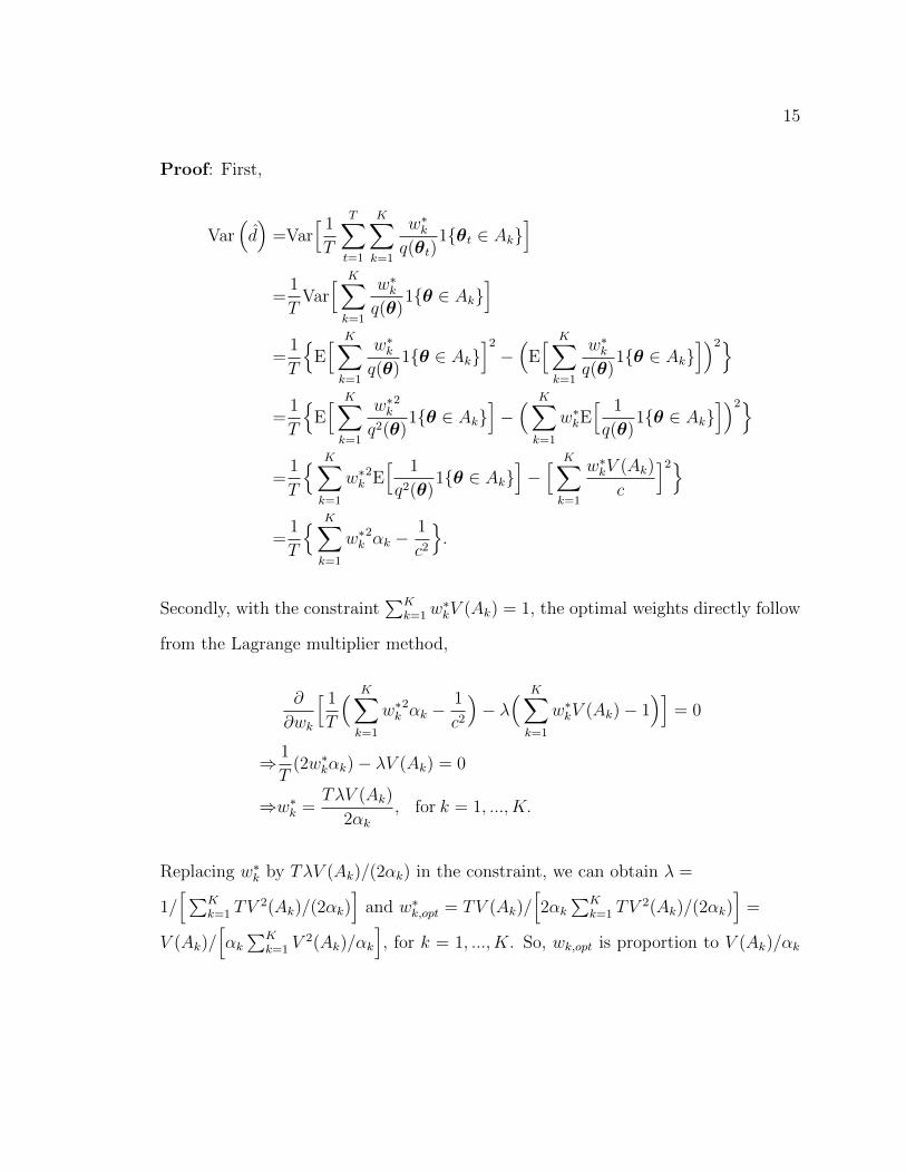
Theorem 2.3.2. Assume θt, t = 1, . . . , T is an MCMC sample from the posterior

distribution π(θ|D), and let w∗k = wk/[∑K

k=1 wkV (Ak)]

and αk = E[(1/q2(θ))1θ ∈

Ak]. Then, Var(d) =(∑K

k=1 w∗k

2αk − 1/c2)/T . Moreover, the optimal variance=

1/[∑K

k=1 V2(Ak)/αk

]− 1/c2

/T , which is obtained by

w∗k,opt = V (Ak)/αk

[ K∑k=1

V 2(Ak)/αk

]

for k = 1, ..., K.

15

Proof: First,

Var(d)

=Var[ 1

T

T∑t=1

K∑k=1

w∗kq(θt)

1θt ∈ Ak]

=1

TVar[ K∑k=1

w∗kq(θ)

1θ ∈ Ak]

=1

T

E[ K∑k=1

w∗kq(θ)

1θ ∈ Ak]2

−(

E[ K∑k=1

w∗kq(θ)

1θ ∈ Ak])2

=1

T

E[ K∑k=1

w∗k2

q2(θ)1θ ∈ Ak

]−( K∑k=1

w∗kE[ 1

q(θ)1θ ∈ Ak

])2=

1

T

K∑k=1

w∗k2E[ 1

q2(θ)1θ ∈ Ak

]−[ K∑k=1

w∗kV (Ak)

c

]2=

1

T

K∑k=1

w∗k2αk −

1

c2

.

Secondly, with the constraint∑K

k=1w∗kV (Ak) = 1, the optimal weights directly follow

from the Lagrange multiplier method,

∂

∂wk

[ 1

T

( K∑k=1

w∗k2αk −

1

c2

)− λ( K∑k=1

w∗kV (Ak)− 1)]

= 0

⇒ 1

T(2w∗kαk)− λV (Ak) = 0

⇒w∗k =TλV (Ak)

2αk, for k = 1, ..., K.

Replacing w∗k by TλV (Ak)/(2αk) in the constraint, we can obtain λ =

1/[∑K

k=1 TV2(Ak)/(2αk)

]and w∗k,opt = TV (Ak)/

[2αk

∑Kk=1 TV

2(Ak)/(2αk)]

=

V (Ak)/[αk∑K

k=1 V2(Ak)/αk

], for k = 1, ..., K. So, wk,opt is proportion to V (Ak)/αk

16

for k = 1, ..., K. Under this setting, the variance can be simplified to

Var(d)

=1

T

1∑Kk=1 V

2(Ak)/αk− 1

c2

. (2.13)

2

Remark 3.2: In practice, it is quite difficult to estimate the second moment αk.

A very large sample size is required in order to obtain an accurate estimate of αk.

However, the results shown in Theorem 2.3.2 sheds light on the choices of A1, . . . , AK

and wk. First, it is only required that wk is proportional to V (Ak)/αk. Second, if

q(θ) is roughly constant over Ak, then αk ≈ V (Ak)/[q(θ∗k)c], where θ∗k ∈ Ak. Thus,

in this case, we can simply choose wk = q(θ∗k) and d in (2.10) reduces to

d =

1T

∑Tt=1

∑Kk=1

q(θ∗k)

q(θt)1θt ∈ Ak∑K

k=1 q(θ∗k)V (Ak)

. (2.14)

Remark 3.3: Followed by the Remark 3.1, when a full conditional density

π(ϑ1|D,ϑ2) is available, the estimator d in (2.10) reduces further to

d =

1T

∑Tt=1

∑Kk=1

q(ϑ∗2)

q(ϑ2t )1ϑ2t ∈ Bk∑K

k=1 q(ϑ∗2)V (Bk)

.

Remark 3.4: In practice, the marginal likelihood is often reported in log scale.

Considering the dependence within the MCMC sample, we use the Overlapping Batch

Statistics (OBS) of Schmeiser et al. (1990) to estimate the Monte Carlo (MC) standard

error of − log(d). Let ηb denote an estimate of the reciprocal of the marginal likelihood

in log scale using the bth batch, θt, t = b, b+ 1, . . . , b+B− 1, of the MCMC sample

17

for b = 1, 2, . . . , T −B + 1, where B < T is the batch size. Then, the OBS estimated

MC standard error of η = − log(d) is given by

√Var(η) =

[ B

T −B

]∑T−B+1b=1 (ηb − η)2

T −B + 1

12, (2.15)

where η =∑T−B+1

b=1 ηb/(T−B+1) and a batch sizeB is suggested to be 10 ≤ T/B ≤ 20

in Schmeiser et al. (1990).

2.3.3 Construction of the Partition with Subsets A1, . . . , AK

In order to make q(θ) roughly constant over Ak, for each k, which is a sufficient

condition for the PWK estimator in (2.14) to be optimal, we provide the following

rings approach for achieving it:

Step 1: Assume Θ is Rp; if not, then a transformation φ = G1(θ) is needed so that

the parameter space of φ is Rp.

Step 2: Use the MCMC sample to compute the mean φ and the covariance matrix

Σ of φ and then standardize φ by ψ = G2(φ) = Σ−1/2(φ− φ).

Step 3: Construct a working parameter space for ψ by choosing a reasonable radius

r such that ‖ψ‖ < r for most of the standardized MCMC sample.

Step 4: Partition the working parameter space into a sequence of K spherical shells

such that Ak = ψ : r(k − 1)/K ≤ ‖ψ‖ < rk/K, with k = 1, . . . , K.

Step 5: Select a ψ∗k in Ak as a representative point, for example, ‖ψ∗k‖ = r[k/K −

1/(2K)].

18

Sept 6: Compute the new kernel value q(ψ∗k) = q(G−11 G−1

2 (ψ∗k))|J |ψ=ψ∗k, where

J = |∂θ/∂φ||∂φ/∂ψ|. Also compute the new kernel value q(ψt), t = 1, . . . , T ,

for the standardized MCMC sample.

Step 7: Estimate d = 1/c by

d =

1T

∑Tt=1

∑Kk=1

q(ψ∗k)

q(ψt)1ψt ∈ Ak∑K

k=1 q(ψ∗k)V (Ak)

, (2.16)

where V (Ak) = (rk/K)p − [r(k − 1)/K]pπp/2/Γ(p/2 + 1).

Remark 3.5: When K is big enough, q(ψt) in (2.16) will be roughly constant over

Ak so that the best PWK estimate will be obtained. Besides, each kernel value q(ψt)

is simply the original kernel value q(θt) multiplied by the absolute value of Jacobian

function.

2.4 Extension of the General PWK Estimator

In this section, we generalize the PWK estimator from the working parameter space

to the full support space and from the locally constant weight function to a general

weight function of θ. We call this class to be variable PWK (vPWK) estimators.

Suppose A1, . . . , AK∗ is a partition of Θ, and wk(θ) is a weight function defined

on Ak. We need the following assumption to define this vPWK class:

Assumption 3 : The weight function wk is integrable, that is,∫|wk(θ)|dθ <∞ for

k = 1, . . . , K∗.

Under Assumption 3, we can extend the general PWK in (2.10) to a variable weighted

19

Monte Carlo estimator of 1/c, which is given by

d∗ =

1T

∑Tt=1

∑K∗

k=1wk(θt)q(θt)

1θt ∈ Ak∑K∗

k=1

∫Akwk(θ)dθ

. (2.17)

Theorem 2.4.1. Under Assumption 3 and q(θ) > 0, then the vPWK estimator d∗

in (2.17) is a consistent estimator of 1/c. In addition, if∫Ak

[wk(θ)2/q(θ)]dθ < ∞

for k = 1, . . . , K∗, then Var(d∗) <∞.

Proof: Under certain ergodic conditions and Assumption 3, the consistency property

can be proven similarly as that in the general PWK estimator in (2.10). Specifically,

we have

limT→∞

1

T

T∑t=1

K∗∑k=1

wk(θt)

q(θt)1θt ∈ Ak

=K∗∑k=1

limT→∞

1

T

T∑t=1

wk(θt)

q(θt)1θt ∈ Ak

=K∗∑k=1

∫θ∈Ak

wk(θ)

q(θ)

q(θ)

cdθ

=dK∗∑k=1

∫θ∈Ak

wk(θ)dθ,

which implies that d∗a.s.−−→ 1/c. 2

Remark 4.1: It is easy to see that d in (2.10) is a special case of d∗ in (2.17). When

K∗ = K + 1 and assigning an MCMC sample in each region with an equal weight,

wk, among which wK∗ = 0, d∗ reduces to d.

Remark 4.2: The HM estimator is another special case of d∗ in (2.17). When using

20

the prior π(θi) as weights, the inverse of d∗ is the HM estimator.

d∗|wk(θ)=π(θ)

=

1T

∑Tt=1

∑K∗

k=1π(θt)q(θt)

1θt ∈ Ak∑K∗

k=1

∫Akπ(θ)dθ

=

1T

∑Tt=1

π(θt)q(θt)

∑K∗

k=1 1θt ∈ Ak∫Θ π(θ)dθ

=1

T

T∑t=1

1

L(θt|D).

Remark 4.3: In addition, d∗ in (2.17) includes the IDR estimator as a special case.

Let K∗ = 2, A1 = θ : ||θ|| ≤ r, w1(θ) = q(0) − q(θ), A2 = θ : ||θ|| > r,

and w2(θ) = qr(θ) − q(θ). We can show that∫A1w1(θ)dθ = q(0)br −

∫A1q(θ)dθ

and∫A2w2(θ)dθ = c −

∫A2q(θ)dθ, implying

∑2k=1

∫Akwk(θ)dθ = q(0)br. Thus, the

inverse of d∗ reduces to the IDR estimator. Note w1(θt) and w2(θt) in IDR are allowed

to be negative.

2.5 Simulation Studies

2.5.1 A Bivariate Normal Example

We apply the PWK estimator for computing the normalizing constant of a bivari-

ate normal distribution with the normal-inverse-Wishart prior. We consider both

location and scale parameters to be unknown. Including the scale parameters makes

computation challenging. Let y = (y1,y2, ...,yn)′ be n observations from a bivariate

normal distribution,

yi|µ,Σi.i.d.∼ N(µ,Σ), i = 1, . . . , n,

21

where µ ∈ R2 and Σ are unknown parameters. The likelihood function is

L(µ,Σ|y) = (2π)−n|Σ|−n/2 exp− 1

2

n∑i=1

(yi − µ)′Σ−1(yi − µ).

The prior for µ and Σ is specified as follows:

µ|Σ ∼ N(µ0,Σ/κ0) and Σ ∼ IWν0(Λ−10 )

with hyperparameters µ0, κ0, ν0, and Λ0. Then, the joint posterior kernel is given by

q(µ,Σ) = L(µ,Σ|y)π(µ|Σ)π(Σ)

= (2π)−n|Σ|−(n+ν0+2)/2−1 1

γexp

− 1

2

n∑i=1

(yi − µ)′Σ−1(yi − µ)

× exp− κ0

2(µ− µ0)′Σ−1(µ− µ0)

exp

− 1

2trace(Λ0Σ−1)

with γ = 2ν0+1πΓ2(ν0/2)|Λ0|−ν0/2κ−1, where Γ2(ν0/2) = π1/2Γ(ν0/2)Γ(ν0/2 − 1/2) is

the bivariate gamma function. Under this setting, the analytical form of the normal-

izing constant is available as follows:

c =1

πnΓ2(νn/2)

Γ2(ν0/2)

|Λ0|ν0/2

|Λn|νn/2(κ0

κn), (2.18)

where Λn = Λ0 +∑n

i=1(yi − y)(yi − y)′ + κ0nκ0+n

(µ0 − y)(µ0 − y)′, κn = κ0 + n, and

νn = ν0 + n. In the scenario, we set the hyperparameters µ0 = (0, 0)′, k0 = 0.01,

ν0 = 3, and Λ0 =

1 0.7

0.7 1

. We generate a random sample y with n = 200 from a

22

bivariate normal distribution with µ = (0, 0) and Σ =

1 0.7

0.7 1

. The correspond-

ing sample mean y is (−0.029, 0.040)′, and the sample variance-covariance matrix S

is

201.987 143.330

143.330 192.365

. Using equation (2.18), the marginal likelihood in log scale is

−507.278. In this example, in order to apply the spherical shell approach in Section

3.3, a transformation of Σ is needed. Here, we use the log transformation for each

variance parameter and the Fisher z-transformation for the correlation coefficient pa-

rameter to have unbounded support for each of them. Then, we standardize each

transformed MCMC sample from its transformed sample mean and standard devia-

tion. In the new parameter space, we construct the working parameter space and its

partition by choosing r = 1.5, 2, or 2.5 and K = 10, 20, or 100. After picking up a

representative point in each spherical shell, we estimate d = 1/c using equation (2.16).

We compare our method to the HM and IDR methods based on M = 1, 000 inde-

pendent MCMC samples with T = 1, 000 or T = 10, 000 in Table 2.1. Let dm be the

estimate of d based on the mth MCMC sample for m = 1, 2, . . . ,M . Then, the simu-

lation estimate (Mean), the MC standard error (MCSE), and the root mean squared

error (RMSE) of the estimates in log scale are defined as log c = 1M

∑Mm=1(− log dm),

1M−1

∑Mm=1(− log dm− log c)21/2, and 1

M

∑Mm=1(− log dm− log c)21/2, respectively.

23

Table 2.1: Simulation results for the bivariate normal case

log c = −507.2776

T=1,000 T=10,000 Time (sec.)

K r Mean MCSE RMSE Mean MCSE RMSE

HM -494.671 0.908 12.639 -495.142 0.762 12.159 0.644

IDR 1.5 -509.064 0.302 1.811 -509.123 0.145 1.851 1.638

2.0 -509.095 0.537 1.895 -509.284 0.387 2.043 1.634

2.5 -508.926 0.710 1.795 -509.216 0.629 2.038 1.621

PWK 10 1.5 -507.260 0.064 0.067 -507.264 0.020 0.025 0.329

2.0 -507.260 0.057 0.059 -507.264 0.018 0.022 0.596

2.5 -507.259 0.057 0.060 -507.264 0.019 0.023 0.784

20 1.5 -507.260 0.064 0.066 -507.264 0.020 0.024 0.327

2.0 -507.262 0.053 0.055 -507.264 0.016 0.021 0.596

2.5 -507.259 0.055 0.058 -507.264 0.018 0.023 0.792

100 1.5 -507.260 0.064 0.066 -507.264 0.020 0.024 0.426

2.0 -507.261 0.052 0.054 -507.264 0.016 0.021 0.660

2.5 -507.260 0.055 0.058 -507.264 0.018 0.022 0.877

Table 2.1 shows the results, where the average computing time (in seconds) per

MCMC sample on an Intel i7 processor machine with 12 GB of RAM memory using

a Windows 8.1 operating system is given in the last column. From Table 2.1, we

see that (i) PWK has the best performance with much smaller MCSE’s and RMSE’s

than HM and IDR under both T = 1, 000 and T = 10, 000; (ii) when T increases, the

MCSE’s and the RMSE’s of the PWK estimator becomes smaller under all choices

of r’s and K’s; (iii) the performance of the HM estimator slightly improves but

the IDR estimator does not when T increases; and (iv) the computing time of the

PWK estimator is comparable to that of the HM estimator while the IDR estimator

requires the most computing time. It is interesting to mention that the MCSE’s and

the RMSE’s of the PWK estimator are very similar for all choices of r’s and K’s

24

under each T , implying the robustness of the PWK estimator with respect to the

specification of the working parameter space and the number of partition subsets.

To evaluate the effect of the vague prior on the precision of the PWK estimator,

we extend our simulation study by considering different values of hyperparameters κ0

and ν0. Note that the value of log c in Table 2.1 is computed under κ0 = 0.01 and

ν0 = 3, which corresponds to a relatively vague prior for (µ,Σ). Table 2.2 shows the

simulation results of the PWK estimators with r = 2 and K = 100 for (κ0, ν0) =

(0.0001, 3), (1, 3), and (1, 10) in addition to (0.01, 3). From Table 2.2, we see that

the MCSE’s under these different values of (κ0, ν0) are almost the same while these

RMSE’s are comparable except the last one with (κ0, ν0) = (1, 10), in which the

RMSE’s are slightly larger.

Table 2.2: Simulation results of PWK estimators for different hyperparameters κ0

and ν0

T=1,000 T=10,000

κ0 ν0 log c Mean MCSE RMSE Mean MCSE RMSE

0.0001 3 -511.883 -511.866 0.052 0.054 -511.869 0.016 0.021

0.01 3 -507.278 -507.261 0.052 0.054 -507.264 0.016 0.021

1 3 -502.682 -502.665 0.052 0.054 -502.669 0.016 0.021

1 10 -512.773 -512.721 0.053 0.074 -512.725 0.016 0.050

2.5.2 A Mixture Normal Example

To further evaluate the performance of the PWK, we consider a two-dimensional

normal mixture in Chen et al. (2006) as follows

π(µ) =2∑j=1

1

2

[ 1

2π|Σj|−1/2 exp

− 1

2(µ− µ0j)

′Σ−1j (µ− µ0j)

], (2.19)

25

where µ = (µ1, µ2)′, µ01 = (0, 0)′, µ02 = (2, 2)′ and Σj =

σ21 σ1σ2ρj

σ1σ2ρj σ22

with

σ1 = σ2 = 1, ρ1 = 0.99, and ρ2 = −0.99. Figure 2.1(a) is a scatter plot of a random

sample with T = 10, 000 generated from (2.19). Based on the random sample, we

apply the PWK to estimate the normalizing constant in (2.19), which is known to be

1. Due to the high but opposite correlations (i.e., ρ1 = 0.99 and ρ2 = −0.99), π(µ)

cannot be homogeneous over a partition ring formed by the spherical shell approach in

Section 3.3. To circumvent this difficulty, we additionally slice (dash lines) the existing

partition rings by dividing equally along the angle from 0 to 360 degrees as shown in

Figure 2.1(b), where the center of circle is the sample posterior mean (denoted as µ).

Now, the heterogeneity of π(µ) over each partition subset is effectively eliminated by

this additional slicing step.

Table 2.3 shows the results of HM, IDR, and PWK estimators based on M = 1, 000

independent random samples with T = 1, 000 or T = 10, 000 from (2.19). For PWK,

we consider different K’s (number of rings × number of slices) and r’s (75%, 90%, or

95% × max1≤t≤T ||µt − µ||). We use the same values of r’s for both IDR and PWK.

From Table 2.3, we see that (i) the RMSE’s of PWK are considerably smaller than

those of HM and IDR; (ii) the performance of PWK improves when the sample size

(T ) or the number of partition subsets (K) increases; and (iii) PWK takes slightly

longer computing time than HM and IDR.

26

−5 0 5

−6

−4

−2

02

46

8

µ1

µ 2

−5 0 5

−6

−4

−2

02

46

8

µ1

µ 2(a) (b)

Figure 2.1: Forming the working parameter space and its partition for a mixturenormal distribution with means (0,0) and (2,2).

Table 2.3: Simulation results for the mixture normal with means equal to (0,0) and(2,2)

log c = 0

T=1,000 T=10,000 Time (sec.)

K r Mean MCSE RMSE Mean MCSE RMSE

HM -2.868 0.685 2.948 -3.069 0.519 3.113 1.647

IDR 5.065 1.879 0.639 1.985 1.706 0.448 1.764 1.680

6.078 2.149 0.650 2.245 1.935 0.485 1.995 1.839

6.415 2.243 0.659 2.337 2.015 0.485 2.073 1.717

PWK 20× 100 5.065 0.001 0.020 0.020 0.000 0.006 0.006 2.167

6.078 0.000 0.025 0.025 0.000 0.008 0.008 2.375

6.415 0.000 0.025 0.025 -0.001 0.008 0.008 2.187

100× 100 5.065 0.000 0.011 0.011 0.000 0.003 0.003 2.933

6.078 0.000 0.011 0.011 0.000 0.004 0.004 3.037

6.415 0.000 0.011 0.011 0.000 0.004 0.004 2.929

27

Next, we consider a more challenging case, where µ02 is replaced by (5, 5)′ so that

the two modes are much far away from each other. Figure 2.2 (a) is a scatter plot of

a random sample with T = 10, 000 and Figure 2.2 (b) shows the partition subsets of

the chosen working parameter space.

−5 0 5 10

−5

05

10

µ1

µ 2

−5 0 5 10

−5

05

10

µ1

µ 2

(a) (b)

Figure 2.2: Forming the working parameter space and its partition for a mixturenormal distribution with means (0,0) and (5,5).

Table 2.4 summarizes the simulation results with the same simulation setting as

before. We see that PWK outperforms both HM and IDR under this more challenging

case. As expected, the RMSE’s in Table 2.4 are larger than those in Table 2.3 for

all three methods. However, the RMSE’s of the PWK estimator are still quite small

when K and T are reasonably large.

28

Table 2.4: Simulation results for the mixture normal with means equal to (0,0) and(5,5)

log c = 0

T=1,000 T=10,000 Time (sec.)

K r Mean MCSE RMSE Mean MCSE RMSE

HM -2.915 0.681 2.993 -3.107 0.500 3.147 1.728

IDR 6.675 2.340 1.586 2.825 2.791 1.695 3.263 1.763

8.011 1.658 1.780 2.429 2.409 1.350 2.760 1.730

8.456 1.568 1.985 2.524 2.216 1.430 2.636 1.822

PWK 20× 100 6.675 -0.001 0.035 0.035 0.000 0.011 0.011 2.277

8.011 0.003 0.060 0.060 0.000 0.019 0.019 2.253

8.456 0.000 0.060 0.060 0.000 0.018 0.018 2.374

100× 100 6.675 0.000 0.018 0.018 0.000 0.006 0.006 3.022

8.011 0.000 0.018 0.018 0.000 0.006 0.006 2.933

8.456 0.000 0.019 0.019 0.000 0.006 0.006 3.114

2.6 Application of the PWK to Real Data Exam-

ples

2.6.1 The Ordinal Probit Regression Model

In the first example, we apply the PWK method to compute the marginal likelihood

under the ordinal probit regression model. Let y = (y1, y2, ..., yn)′ denote the vector

of observed ordinal responses, each is coded as one value from 0, 1, ..., J−1, X denote

the n×p covariate matrix with the ith row equal to the covariate of the ith subject x′i,

and u = (u1, u2, ..., un)′ denote the vector of latent random variables. We consider

29

the following hierarchical model as in Albert and Chib (1993) such that

yi = j, if γj ≤ ui < γj+1

and

ui = x′iβ + εi,

where j = 0, 1, ..., J − 1, β is a p-dimensional vector of regression coefficients, and

εii.i.d.∼ N(0, σ2). Based on the reparameterization of Nandram and Chen (1996), the

cutpoints for dividing the latent variable ui can be specified as −∞ = γ0 < γ1 = 0 ≤

γ2 ≤ · · · ≤ γJ−1 = 1 < γJ = ∞. Under this setting, the likelihood function is given

by in Chen (2005b)

L(θ|D) =n∏i=1

[Φ(γyi+1

− x′iβσ

)− Φ

(γyi − x′iβσ

)],

where θ = (β′, σ, γ2, . . . , γJ−2)′ if J ≥ 4, otherwise, θ = (β′, σ)′, and Φ(.) is the

cumulative standard normal distribution function. Then, we specify normal, inverse

gamma, and uniform priors for the parameters β, σ2, and γ, respectively.

To examine the performance of the PWK estimator under this model, we consider

the prostate cancer data of n = 713 patients as in Chen (2005b). In this data

set, Pathological Extracapsular Extension (PECE, y) is a clinical ordinal response

variable, and Prostate Specific Antigen (PSA, x1), Clinical Gleason Score (GLEAS,

x2), and Clinical Stage (CSTAGE, x3) are three covariates. PECE takes values of 0, 1,

or 2, where 0 means that there is no cancer cell present in or near the capsule, 1 denotes

that the cancer cells extend into but not through the capsule, and 2 indicates that

cancer cells extend through the capsule. PSA and GLEAS are continuous variables

30

while CSTAGE is a binary outcome, which was assigned to 1 if the 1992 American

Joint Commission on cancer clinical stage T-category was 1, and assigned to 2 if the

T-category was 2 or higher.

In this application, J = 3 so that all four cutpoints can be assigned to fixed values:

−∞ = γ0 < γ1 = 0 < γ2 = 1 < γ3 =∞. Then, the prior distribution is specified as

π(θ) = π(β|σ2)π(σ2),

where β|σ2 ∼ N(0, 10σ2I4) and σ2 ∼ IG(a0 = 1, b0 = 0.1), an inverse gamma

distribution with density proportional to (σ2)−(a0+1) exp(−b0/σ2).

The marginal likelihood is not analytically available. Nevertheless, the estimates

of this are obtained in Table 1 of Chen (2005b) using the method proposed by Chen

(called Chen’s method) and the method proposed by Chib (1995) (called Chib’s

method). Chen’s method needs only a single MCMC sample from the joint pos-

terior distribution π(β, σ2|D). However, Chib’s method with two blocks requires an

additional MCMC sample from the conditional posterior distribution π(σ2|β∗, D),

where β∗ is the posterior mean of β. We compare the PWK method with r = 3.327

and K = 100 to these two methods under the same MCMC sample sizes T = 2, 500,

or 5, 000, except Chib’s method doubles them. We have obtained the PWK estimates

log c = −758.70, or −758.70 respectively with corresponding OBS estimated MCSE

to be 0.020, or 0.016. So we observe that the PWK estimates are comparable to that

of the other two methods and the PWK method has the smallest OBS estimated

MCSE among the three methods.

For the PWK, the log transformation of σ2 is needed. Then, after the standard-

ization of the transformed MCMC sample, we consider K = 10, 20, and 100 and

31

r = 0.75√χ2

5,0.95,√χ2

5,0.95, and 1.25√χ2

5,0.95 to investigate robustness of the PWK

estimates with respect to these choices. We note that√χ2

5,0.95 is chosen based on Yu

et al. (2015). Table 2.5 shows the PWK estimates and the corresponding estimated

MCSE (eMCSE) under the MCMC samples with T = 2,500 and 5,000, where eM-

CSE is computed using (2.15) with T/B = 10. We note that we use the same MCMC

sample sizes as in Chen (2005b). The results show the PWK estimators are relatively

robust to the choices of the radius r and number of partitioned subsets K.

32

Table 2.5: The PWK estimates of the marginal likelihood for the prostate cancerdata

r = 0.75√χ2

5,0.95

PWK (K=10) PWK (K=20) PWK (K=100)

T − log d eMCSE − log d eMCSE − log d eMCSE

2, 500 -758.73 0.026 -758.73 0.025 -758.73 0.025

5, 000 -758.70 0.021 -758.70 0.020 -758.70 0.020

r =√χ2

5,0.95 = 3.327

PWK (K=10) PWK (K=20) PWK (K=100)

T − log d eMCSE − log d eMCSE − log d eMCSE

2, 500 -758.70 0.020 -758.70 0.019 -758.70 0.020

5, 000 -758.70 0.016 -758.70 0.016 -758.70 0.016

r = 1.25√χ2

5,0.95

PWK (K=10) PWK (K=20) PWK (K=100)

T − log d eMCSE − log d eMCSE − log d eMCSE

2, 500 -758.69 0.020 -758.69 0.019 -758.69 0.017

5, 000 -758.70 0.018 -758.70 0.015 -758.69 0.014

2.6.2 Analysis of ECOG Data

In this subsection, we apply the PWK estimator to the problem of determining the

power prior based on the historical data for the current analysis. Assume we have

33

conducted two clinical trials for the same objective. A natural way to combine these

two trials is to consider the power prior setting, which allows us to borrow information

from the historical data to construct the prior for the current analysis. Assume

we have an initial prior for the unknown parameters which is determined before

observing the historical data. To quantify the heterogeneity between the current data

and the historical data, the power prior weights the historical likelihood function

by the power a0, where 0 ≤ a0 ≤ 1, to indicate the degree of incorporating the

historical likelihood to the initial prior. Our objective is to find the optimal a0 which

maximizes the marginal likelihood for the current data with respect to the power

prior. Ibrahim et al. (2015) point out the difficulty of finding this solution except

for normal linear regression models. Therefore, they resolve to using the deviance

information criterion (DIC) and the logarithm of pseudo marginal likelihood (LPML)

criterion for constructing the parameter a0 of the power prior in Ibrahim et al. (2012,

2015). To evaluate DIC, we need to plug the MCMC sample into the sum of the

log likelihood over all data points; to evaluate LPML, we need to take the sum of

the log transformation of each CPO, where the ith CPO is the harmonic mean of the

ith likelihood evaluated at the MCMC sample from the posterior distribution based

on the full sample. Both methods yield much less computational burden than the

marginal likelihood method. We will show how the PWK estimator can circumvent

the computational burden in evaluating the marginal likelihood.

The effectiveness of Interferon Alpha-2b (IFN) in immunotherapy for melanoma

patients has been evaluated by two observation-controlled clinical trials: Eastern

Cooperative Oncology Group (ECOG) phase III, E1684, followed by E1690. The

first trial E1684 was conducted with 286 patients randomly assigned to either IFN

or Observation. The IFN arm demonstrated a significantly better survival curve, but

34

with substantial side effects due to high dose regimen. To confirm the results of the

E1684 and the benefit of IFN at a lower dosage, a later trial E1690 was conducted

with three arms: high dose IFN, low dose IFN, and Observation. We use the data

in E1684 as the historical data and a subset (high dose arm and Observation) of the

E1690 trial as our current data. There are 427 patients in this subset.

For n = 427 patients in the current trial (E1690), we follow the model in Chen

et al. (1999). Let yi denote the survival time for the ith patient, νi denote the censoring

status, which is equal to 1 if yi is a failure time and to 0 if it is the right censored,

xi = (1, trti)′ denote the vector of covariates, where trti = 1 if the ith patient received

IFN and trti = 0 if the ith patient was assigned to Observation. Then, the likelihood

function is given by

L(β,λ|D) =n∏i=1

exp(x′iβ)f(yi|λ)

νiexp− exp(x′iβ)F (yi|λ)), (2.20)

where D = (n,y,ν, X) is the observed current data, β = (β0, β1)′, and F (y|λ) is the

cumulative distribution function and f(y|λ) is the corresponding density function.

In (2.20), we use the same piecewise exponential model for F (y|λ) as Ibrahim et al.

(2012), which is given by

F (y|λ) = 1− exp− λj(y − sj−1)−

j−1∑g=1

λg(sg − sg−1),

where sj−1 ≤ y < sj, s0 = 0 < s1 < s2 < . . . < s5 =∞, and λ = (λ1, . . . , λ5)′.

For n0 = 286 patients in the historical trial (E1684), we attempt to extract some

of its information to set up the prior distribution for the current analysis. Similarly,

we let y0i denote the survival time for the ith patient, ν0i denote the censoring status,

35

and x0i = (1, trt0i)′ denote the vector of covariates. So D0 = (n0,y0,ν0, X0) is the

observed historical data. Assume π0(β,λ) is an initial prior. Here, we specify an

initial proper prior N(0, 100I2) for β and Exp(λ0 = 1/100) (λ0: rate parameter) for

each λj, j = 1, . . . , 5, to come close to the flat prior in Ibrahim et al. (2012). To

update the initial prior with the historical data, the power prior is intuitively set as

the initial prior π0 multiplied by the historical likelihood function with power a0 as

follows:

π(β,λ|D0, a0)

∝[ n0∏i=1

exp(x′0iβ)f(y0i|λ)

ν0iexp− exp(x′0iβ)F (y0i|λ))

]a0π0(β,λ), (2.21)

where π(β,λ|D0, a0) is called the power prior and 0 ≤ a0 ≤ 1. In this setting, we

can see when a0 = 0, the power prior is exactly equal to the initial prior, which

integrates to be 1, and when a0 6= 0, the power prior is equal to the right-hand side

kernel function in (2.21) divided by c0 =∫L(β,λ|D0)a0π0(β,λ)dβdλ. Combining the

likelihood function in (2.20) and the power prior in (2.21), the posterior distribution

of β and λ given (D,D0, a0) will be

π(β,λ|D,D0, a0) ∝ L(β,λ|D)π(β,λ|D0, a0). (2.22)

In this framework, we compare the marginal likelihoods of L(β,λ|D)π(β,λ|D0, a0)

for 0 ≤ a0 ≤ 1. The one with the highest marginal likelihood is our final model, and

its corresponding a0 determines the power prior.

However, as we point out earlier, except for a0 = 0, π(β,λ|D0, a0) is known up

to a normalizing constant c0. Hence, a two-step evaluation is needed to obtain the

36

marginal likelihood:

c =

∫L(β,λ|D)π(β,λ|D0, a0)dβdλ

=

∫L(β,λ|D)L(β,λ|D0)a0π0(β,λ)dβdλ∫

L(β,λ|D0)a0π0(β,λ)dβdλ

=c1

c0

=d0

d1

.

We apply the PWK to estimate the numerator, L(β,λ|D)L(β,λ|D0)a0π0(β,λ), and

the denominator, L(β,λ|D0)a0π0(β,λ), respectively.

For each choice of a0 with an increment of 0.1 from 0 to 1, an MCMC sample size is

fixed at 10,000. The log transformation of each λj is needed. After the standardization

of transformed MCMC sample, we choose the maximum radius r = 3.751 and the

number of spherical shells K = 100. By equations (2.16) and (2.15), we can obtain

the marginal likelihood estimate and its eMCSE in each chosen a0. We summarize

the results in Table 2.6. Table 2.6 also includes the PWK estimates under different

choices of r’s and K’s.

37

Table 2.6: PWK estimates for marginal likelihood with different power priors underdifferent choices of r’s and K’s

r = 0.75√χ27,0.95

K=10 K=20 K=100

a0 ln(d0/d1) eMCSE ln(d0/d1) eMCSE ln(d0/d1) eMCSE

0.0 -552.717 0.028 -552.713 0.026 -552.709 0.028

0.1 -523.619 0.055 -523.614 0.051 -523.621 0.053

0.2 -522.091 0.044 -522.078 0.044 -522.073 0.044

0.3 -521.408 0.043 -521.420 0.043 -521.419 0.043

0.4 -521.336 0.046 -521.332 0.047 -521.338 0.045

0.5 -521.201 0.057 -521.229 0.060 -521.229 0.060

0.6 -521.189 0.037 -521.202 0.034 -521.187 0.033

0.7 -521.356 0.050 -521.363 0.044 -521.353 0.044

0.8 -521.553 0.054 -521.558 0.056 -521.576 0.058

0.9 -521.592 0.061 -521.618 0.051 -521.612 0.050

1.0 -521.702 0.052 -521.724 0.055 -521.732 0.050

r =√χ27,0.95 = 3.751

K=10 K=20 K=100

a0 ln(d0/d1) eMCSE ln(d0/d1) eMCSE ln(d0/d1) eMCSE

0.0 -552.732 0.022 -552.707 0.025 -552.708 0.027

0.1 -523.633 0.059 -523.646 0.049 -523.624 0.054

0.2 -522.098 0.052 -522.093 0.050 -522.077 0.045

0.3 -521.433 0.039 -521.432 0.040 -521.417 0.043

0.4 -521.309 0.046 -521.321 0.048 -521.339 0.043

0.5 -521.179 0.062 -521.187 0.059 -521.230 0.059

0.6 -521.186 0.039 -521.174 0.037 -521.187 0.033

0.7 -521.365 0.034 -521.361 0.042 -521.349 0.044

0.8 -521.535 0.055 -521.568 0.056 -521.573 0.056

0.9 -521.627 0.047 -521.613 0.055 -521.613 0.050

1.0 -521.746 0.059 -521.739 0.049 -521.732 0.050

r = 1.25√χ27,0.95

K=10 K=20 K=100

a0 ln(d0/d1) eMCSE ln(d0/d1) eMCSE ln(d0/d1) eMCSE

0.0 -552.740 0.039 -552.719 0.033 -552.708 0.027

0.1 -523.551 0.057 -523.622 0.052 -523.622 0.053

0.2 -522.105 0.045 -522.077 0.044 -522.071 0.045

0.3 -521.427 0.048 -521.422 0.045 -521.421 0.042

0.4 -521.311 0.048 -521.317 0.046 -521.335 0.044

0.5 -521.239 0.052 -521.232 0.057 -521.227 0.059

0.6 -521.186 0.037 -521.171 0.033 -521.184 0.032

0.7 -521.381 0.047 -521.376 0.045 -521.350 0.043

0.8 -521.569 0.067 -521.578 0.063 -521.578 0.057

0.9 -521.597 0.052 -521.621 0.054 -521.609 0.049

1.0 -521.705 0.060 -521.740 0.046 -521.730 0.051

38

Note the marginal likelihood function c can be shown to be continuous in a0.

Therefore, from the results in Table 2.6, we see that the best choice of a0 is between

0.5 and 0.6 under the marginal likelihood criterion. This result is quite comparable

to the result of a0 = 0.4 in Ibrahim et al. (2012) obtained by DIC and LPML criteria,

where a suitable marginal likelihood computation was not accessible to them at the

time. We also observe that the results are quite robust to the different r’s and K’s,

and all point out the best choice of a0 is between 0.5 and 0.6.

2.7 Discussion

The marginal likelihood is often analytically intractable due to the complicated kernel

structure. Nevertheless, an MCMC sample from the posterior distribution is readily

available from Bayesian computing software, for example, MrBayes (Huelsenbeck and

Ronquist, 2001; Ronquist and Huelsenbeck, 2003), Beast (Drummond et al., 2012),

and Phycas (Lewis et al., 2015) in Bayesian phylogenetics. Additionally, the likelihood

values evaluated at the MCMC sample are outputted in a file. Consequently, we can

produce kernel values easily using the output and the prior function. In this chapter,

we propose an easily implemented algorithm PWK for estimating the marginal like-

lihood based on this single chain of the MCMC sample and its corresponding kernel

values. Unlike some existing algorithms requiring knowing the structure of the ker-

nel, which is rare in Bayesain phylogenetics, we only need to know the kernel values

evaluated at the MCMC sample. Therefore, our algorithm can be applied to model

selection in Bayesian phylogenetics with a fixed topology. It may have potential for

the variable topology problems.

39

We extend our PWK to the variable PWK that can handle the parameter space

with full support and we show the HM and IDR are special cases of this vPWK.

We conduct a simulation study from a bivariate normal model with 5 parameters

in a Bayesian conjugate prior inference problem to compare our estimator to HM

and IDR; our results show the PWK has the smallest empirical SE and RMSE. The

computation time for our method is only slightly longer than that for the HM which

indicates our spherical shell partition approach is very efficient.

In real data analysis, we first consider an ordinal probit regression model with

a latent variable structure, and compare our method to that in Chib (1995) and

Chen (2005b). We find the three methods are comparable and our method has the

smallest MCSE. In the second example, we consider a cure rate survival model with

the piecewise constant baseline hazard function and a power prior construction based

on two clinical trial data sets. We obtain the optimal power prior using the marginal

likelihood criterion as opposed to the DIC and LPML methods considered by Ibrahim

et al. (2012). Although we obtain similar results, except we prefer borrowing more of

the historical data, it would be interesting to investigate the effects of the criterion

and the initial prior on the choice of a0. We implemented our methodology using the

R programming language (Team (2014)).

In an unimodal problem, we suggest using the square root of the 95th percentile in

Chi-square distribution with p degree of freedom as the guide value (rGV) of radius r for

constructing the working parameter space of the standardized MCMC sample. This

is because after standardizing the MCMC sample, each parameter can be marginally

viewed as a normal distribution. Although the results are quite robust to the choices

of r’s as shown in simulation and case studies, this way can insure that we can make

use of most of the MCMC sample and avoid the region with posterior density close

40

to 0. For a multimodal problem, we suggest using 95% × max1≤t≤T ||µt − µ|| as

rGV for constructing the working parameter space of the transformed MCMC sample.

Since this approach may include many place with extremely small posterior density in

the working parameter space, we propose an advanced spherical rings approach with

additional slices on the partition rings to assure the homogeneity of the MCMC sample

in each subset. This new partition approach can also be extended to n-dimensional

problem by introducing another n− 2 angular coordinates.

Chapter 3

Marginal Posterior DensityEstimation

3.1 Introduction

Posterior density estimation is one of the most important topics in Bayesian infer-

ence because it provides the complete information about parameters of interest in

the model. Chen (2005a) provides an overview of the usefulness of the posterior den-

sity estimation in computing Bayes factors, marginal likelihoods, and posterior model

probabilities. Posterior density estimation has also been used in various applications,

including selection of the best predictors for the development of AIDS or death using

historical data (Chen et al., 1999) in the AIDS study, the development of compu-

tational algorithms in molecular population genetics (Stephens and Donnelly, 2000),

estimation of the functional Bregman divergence for Bayesian model diagnostics (Goh

and Dey, 2014), and the intensity bias correction in endorectal multi-parametric MRI

41

42

(Lui, 2014; Lui et al., 2015).

When all parameters in the model are of concern, the joint posterior density is

investigated using the unnormalized posterior density, which is the product of the

likelihood function and a joint prior distribution. The normalizing constant, which

is the marginal likelihood when the prior is proper, is often analytically intractable

due to the complicated model structure. In this case, the computational problem

reduces to estimation of the marginal likelihood. For estimating the marginal like-

lihood, many Monte Carlo methods have been developed. An efficient method with

minimal assumptions is the partition weighted kernel (PWK) estimation in Chapter 2.

It requires only a single Markov chain Monte Carlo (MCMC) sample from the poste-

rior distribution and the known unnormalized posterior density, both available from

standard Bayesian software. By assigning a weight to each point of an MCMC sample

adaptively within a working parameter space where the unnormalized posterior den-

sity is bounded away from zero, the PWK estimator is consistent for the reciprocal of

the normalizing constant and of finite variance, and its minimum variance estimator

can be achieved.

In many practical problems, however, investigators may be interested only in

specific parameters rather than all parameters. As a result, the calculation and

display of the marginal posterior density of the focal parameters are of most interest.

Similar to the joint posterior density, the marginal posterior density is not analytically

available for most cases. Hence, several methods in the literature have been developed

for estimating marginal posterior densities using an MCMC sample from the joint

posterior distribution. One common approach is the kernel density estimator (KDE)

proposed by Rosenblatt et al. (1956) and Parzen (1962). KDE is easily implemented,

but leaves room for more efficient estimators that can make use of more of the available

43

information. Another approach is the conditional marginal density estimator (CMDE)

method proposed by Gelfand et al. (1992). This method simply takes the average of

the known conditional posterior density of the interested parameters given the other

parameters from the MCMC sample. The CMDE is most efficient since it is a Rao-

Blackwell estimator. Unfortunately, CMDE requires the closed form of the conditional

posterior density, which is often known only up to an unknown normalizing constant

for many Bayesian problems, especially when the parameter space is constrained.

To overcome this difficulty, Chen (1994) proposed the importance weighted marginal

density estimation (IWMDE) method, which can be viewed as a generalization of the

CMDE and only requires a careful selection of the conditional weight density. Some

other approaches including two block structures of the IWMDE by Oh (1999) and

the Gibbs stopper (GS) estimator by Yu and Tanner (1999) are described in Chen

(2005a). However, when the conditional posterior density is analytically intractable,

the realization of the CMDE still remains an open research problem.

We use ideas motivated by the PWK estimator to compute the marginal posterior

density. We propose a new Monte Carlo method, the Adaptive Partition weighTed

(APT) marginal density estimator, which assumes only the availability of the unnor-

malized posterior density and an MCMC sample from the joint posterior distribution.

The APT method is constructed by first partitioning a subset of the support of the

conditional posterior distribution, and then estimating the marginal posterior density

at a fixed point of the focused parameters. An adaptive weighted average is assigned

to the ratios of the unnormalized posterior density evaluated at the MCMC sam-

ple, except the focused parameters in the numerator are set at this fixed point, where

weights are assigned locally using a representative value of the unnormalized posterior

density in each partitioned subset. Both the partition and the weights change adap-

44

tively at each MCMC sample point. We show that the APT estimator is unbiased,

and most of all, its optimal result is realizable and approximates the CMDE, which is

known to be the best solution but whose widespread use is limited by unavailability

of the conditional posterior density analytically. In addition, we extend the APT

method to estimate the conditional posterior density when an MCMC sample from

the conditional posterior density is available. In our first real data example, where

closed form conditional posterior densities are available, we show that our estimator

produces results similar to the gold standard (CMDE). In our second real data ex-

ample, we demonstrate an excellent performance of the APT method in estimating

Bayes factors. The proposed APT method has the potential to become a powerful

tool for computing posterior densities, Bayes factors, and marginal likelihoods for

complex Bayesian models with a large number of parameters.

The rest of the article is organized as follows: Section 2 is a review of existing

methods and a summary of preliminaries needed for our method. In Section 3, we

develop the APT method for estimating marginal and conditional posterior densities,

and examine its theoretical properties and various applications. In Section 4, we

compare the performances of KDE and APT with the CMDE in the inequality-

constrained analysis of variance model. We use the data set from an amnesia study

of dissociative identity disorder patients to demonstrate the empirical performance

of the APT. In Section 5, we present a novel application of the APT method for

computing the marginal posterior densities in Bayesian model selection. A complete

Bayesian analysis is carried out under an ordinal probit regression model with latent

variables using the real data from a prostate cancer study. To avoid the phenomenon

of the Bartlett’s or Lindley’s paradox (Jeffreys, 1998; Lindley, 1957), we first apply the

PWK estimator to find the best prior distribution in the full model by the empirical

45

Bayes method and we then apply APT to compute the Bayes factors under the best

full model using the same MCMC sample used by the PWK estimator for model

selection. Finally, we conclude the paper with a brief discussion in Section 6.

3.2 Preliminaries

We first introduce some notation. Suppose ζ = (θ, ξ) is a v-dimensional vector of

parameters, where θ is a vector of parameters of interest having length p. Let D

denote the data, L(ζ|D) denote the likelihood function, and π(ζ) denote the prior

distribution for ζ. Then, the joint posterior density is

π(ζ|D) =L(ζ|D)π(ζ)

c=q(ζ)

c, (3.1)

where c is the normalizing constant, and q(ζ) is the unnormalized posterior density.

The equation (3.1) shows that the joint posterior density is known up to a normalizing

constant. Hence, when p = v, the computation problem is the estimation of c. For

this value, the PWK estimator in Chapter 2 can be used. Assume Ω is the support of

π(ζ|D) with Ω′ ⊂ Ω being the working parameter space, and A1, A2, ..., AK forms

a partition of Ω′. If we have an MCMC sample ζt = (θt, ξt), t = 1, 2, . . . , T from

the joint posterior distribution π(ζ|D), the PWK estimator for 1/c is

c−1 =

1T

∑Tt=1

∑Kk=1

q(ζ∗k)

q(ζt)1ζt ∈ Ak∑K

k=1 q(ζ∗k)V (Ak)

, (3.2)

where ζ∗k is a representative point in region Ak, 1ζt ∈ Ak is the indicator function,

and V (Ak) =∫Ω′ 1ζ ∈ Akdζ. As discussed in Chapter 2, q(ζt) in (3.2) can be made

46

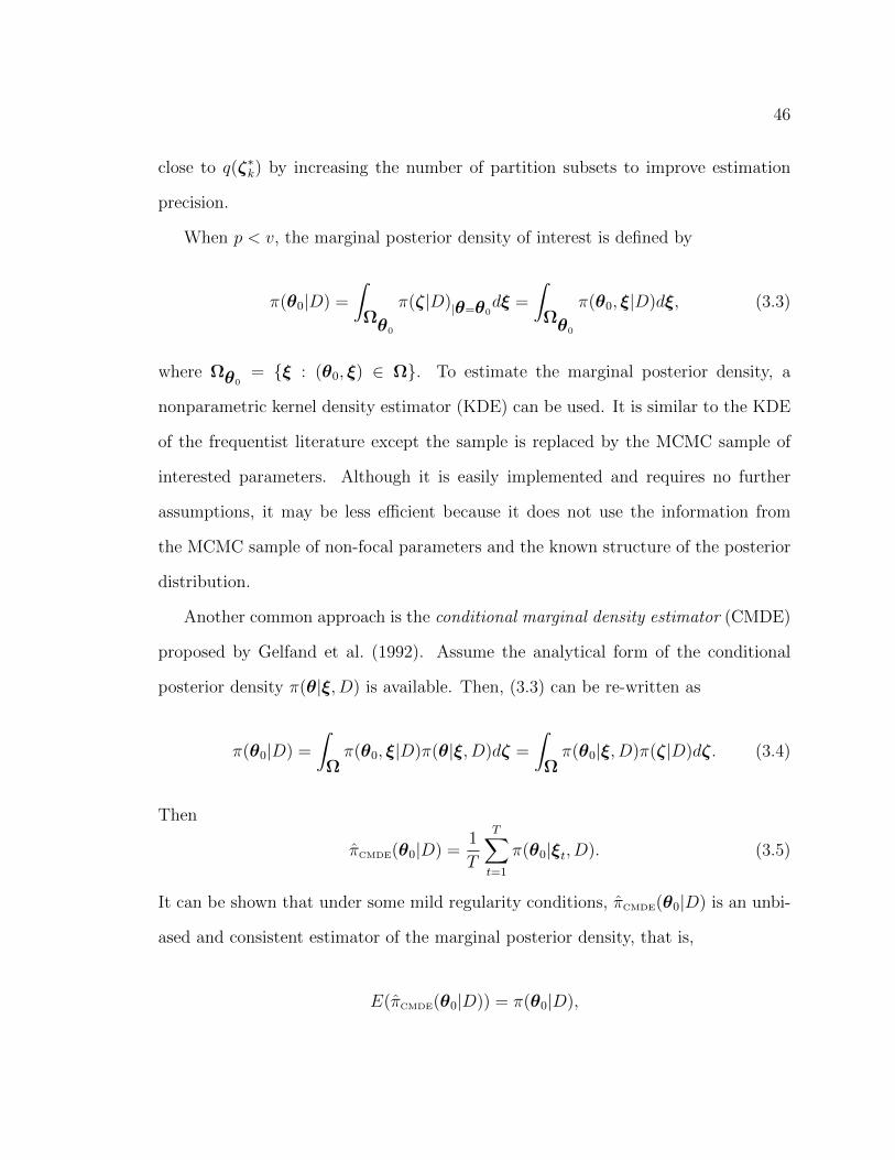
close to q(ζ∗k) by increasing the number of partition subsets to improve estimation

precision.

When p < v, the marginal posterior density of interest is defined by

π(θ0|D) =

∫Ωθ0

π(ζ|D)|θ=θ0dξ =

∫Ωθ0

π(θ0, ξ|D)dξ, (3.3)

where Ωθ0= ξ : (θ0, ξ) ∈ Ω. To estimate the marginal posterior density, a

nonparametric kernel density estimator (KDE) can be used. It is similar to the KDE

of the frequentist literature except the sample is replaced by the MCMC sample of

interested parameters. Although it is easily implemented and requires no further

assumptions, it may be less efficient because it does not use the information from

the MCMC sample of non-focal parameters and the known structure of the posterior

distribution.

Another common approach is the conditional marginal density estimator (CMDE)

proposed by Gelfand et al. (1992). Assume the analytical form of the conditional

posterior density π(θ|ξ, D) is available. Then, (3.3) can be re-written as

π(θ0|D) =

∫Ωπ(θ0, ξ|D)π(θ|ξ, D)dζ =

∫Ωπ(θ0|ξ, D)π(ζ|D)dζ. (3.4)

Then

πCMDE(θ0|D) =1

T

T∑t=1

π(θ0|ξt, D). (3.5)

It can be shown that under some mild regularity conditions, πCMDE(θ0|D) is an unbi-

ased and consistent estimator of the marginal posterior density, that is,

E(πCMDE(θ0|D)) = π(θ0|D),

47

and

limT→∞

πCMDE(θ0|D) = π(θ0|D) a.s .

In addition, the use of the conditional structure of the posterior density makes the

CMDE a Rao-Blackwell estimator so that it is optimal for this estimation problem.

However, the closed form of π(θ|ξ, D) is often not available in many Bayesian prob-

lems. To overcome this difficulty, Chen (1994) proposed the importance weighted

marginal density estimation (IWMDE) method, which can be considered as a gener-

alization of CMDE. Consider the following identity:

π(θ0|D) =

∫w(θ|ξ)π(θ0, ξ|D)

π(ζ|D)π(ζ|D)dζ, (3.6)

where w(θ|ξ) is a proposed conditional density whose support is contained in the

support of π(θ|ξ, D). Using the identity in (3.6), the IWMDE of π(θ0|D) is given by

πIWMDE(θ0|D) =1

T

T∑t=1

w(θt|ξt)π(θ0, ξt|D)

π(θt, ξt|D). (3.7)

The IWMDE method is attractive since it does not require the conditional poste-

rior density to be known, the only requirement is that one needs to choose a good

weight function w(θ|ξ). Under mild regularity conditions, the IWMDE also has the

properties of unbiasedness and consistency to the marginal posterior density.

48

3.3 The Proposed Method for Estimating Poste-

rior Densities

3.3.1 Estimating Marginal Posterior Density

Chen (1994) showed that the optimal weight function minimizing the variance of

(3.7) is π(θ|ξ, D), and in this case the IWMDE in (3.7) reduces to CMDE in (3.5).

However, this optimal weight function is unavailable in most cases, and proposing

a similar one is nontrivial. To circumvent the difficulties, we exploit the main idea

behind the PWK estimator to obtain an approximate distribution of the conditional

posterior density so that the CMDE can be realized for marginal posterior density

estimation.

Let Θξ = θ : q(θ, ξ) > 0 denote the support of the conditional posterior

distribution π(θ|ξ, D) and Θξ be any subset of Θξ such that∫

Θξq(θ, ξ)dθ > 0.

We call Θξ the conditional working parameter space. We also let Ak(ξ), k =

1, 2, . . . , K be the partition of Θξ. We consider a weight function w(θ|ξ) which

satisfies the following two conditions: (i) w(θ|ξ) ≥ 0 and (ii)∫

Θξw(θ|ξ)dθ = 1.

Then, we propose a new estimator of π(θ0|D) using the idea behind PWK:

π(θ0|D) =1

T

T∑t=1

K∑k=1

w(θt|ξt)q(θ0, ξt)

q(θt, ξt)1θt ∈ Ak(ξt). (3.8)

Write

πt(θ0|D) =K∑k=1

w(θt|ξt)q(θ0, ξt)

q(θt, ξt)1θt ∈ Ak(ξt)

49

such that π(θ0|D) = 1T

∑Tt=1 πt(θ0|D). Then, we have

E[πt(θ0|D)] =

∫ ∫ K∑k=1

w(θ|ξ)q(θ0, ξ)

q(θ, ξ)1θ ∈ Ak(ξ)q(θ, ξ)

cdθdξ

=

∫q(θ0, ξ)

c

∫w(θ|ξ)

K∑k=1

1θ ∈ Ak(ξ)dθdξ

=

∫q(θ0, ξ)

c

∫Θξ

w(θ|ξ)dθdξ

= π(θ0|D), (3.9)

which ensures that π(θ0|D) in (3.8) is an unbiased estimator of π(θ0|D). After some

algebra, we obtain

Varwπt(θ0|D) =

∫ [q(θ0, ξ)π(θ0, ξ|D)

∫Θξ

w2(θ|ξ)

q(θ, ξ)dθ]dξ − π2(θ0|D). (3.10)

Now, we establish the following useful result.

Theorem 3.3.1. Let

wopt(θ|ξ) =q(θ, ξ)∫

Θξq(θ, ξ)dθ

, (3.11)

which is the conditional posterior density defined on Θξ. Then, we have

Varwoptπt(θ0|D) =

∫ [q(θ0, ξ)π(θ0, ξ|D)∫

Θξq(θ, ξ)dθ

]dξ − π2(θ0|D) (3.12)

and

Varwoptπt(θ0|D) ≤ Varwπt(θ0|D) (3.13)

50

for any conditional density w(.) defined on Θξ.

The result established in Theorem 3.3.1 is an extension of Theorem 2.1 in Chen

(1994). The proof of this theorem is also similar.

Proof of Theorem 3.3.1. Using the Cauchy-Schwarz inequality, we have

1 =

∫Θξ

w(θ|ξ)√q(θ, ξ)

√q(θ, ξ)dθ

2

≤∫

Θξ

w2(θ|ξ)

q(θ, ξ)dθ

∫Θξ

q(θ, ξ)dθ.

Subsequently, we obtain

1∫Θξ

q(θ, ξ)dθ≤∫

Θξ

w2(θ|ξ)

q(θ, ξ)dθ

⇒∫ [

q(θ0, ξ)π(θ0, ξ|D)1∫

Θξq(θ, ξ)dθ

]dξ

≤∫ [

q(θ0, ξ)π(θ0, ξ|D)

∫Θξ

w2(θ|ξ)

q(θ, ξ)dθ]dξ

⇒ Varwoptπt(θ0|D) ≤Varwπt(θ0|D),

which completes the proof. 2

Remark 3.1: Note that wopt(θ|ξ) in (3.11) is not the conditional posterior den-

sity π(θ|ξ, D) unless Θξ = Θξ. Consequently, πwopt(θ0|D), that is equation (3.8)

with plug-in weights of (3.11), is not the CMDE. From Theorem 3.3.1, we see that

Varwoptπt(θ0|D) decreases when the conditional working parameter space Θξ gets

larger. Once Θξ = Θξ, Varπwopt(θ0|D) is equal to [∫π(θ0|ξ, D)π(θ0, ξ|D)dξ −

π2(θ0|D)]/T and exactly the variance of the CMDE. Thus, the CMDE is the best

among all of the estimators given in (3.8). As discussed in Chen (1994), the CMDE

51

is analytically intractable and thus it is almost impossible to compute the CMDE

in practice for most applications. However, the result established in Theorem 3.3.1

sheds light on how to obtain an estimator of the marginal posterior density, which is

approximately as good as the CMDE.

Although wopt(θ|ξ) is analytically intractable, we can borrow the idea behind

the PWK estimator to obtain an approximate optimal estimator πw(θ0|D) using

discretization. First, we take Θξ such that∫

Θξdθ <∞. Second, we specify w(.) as

wAPT(θ|ξ) =q(θ∗k, ξ)∑K

k=1 q(θ∗k, ξ)V (Ak(ξ))

, θ ∈ Ak(ξ), (3.14)

where θ∗k is a fixed point in Ak(ξ) and V (Ak(ξ)) is the volume of Ak(ξ). Then,

plugging wAPT in (3.8) gives

πAPT(θ0|D) =1

T

T∑t=1

K∑k=1

q(θ∗k, ξt)1θt ∈ Ak(ξt)∑Kk=1 q(θ

∗k, ξt)V (Ak(ξt))

q(θ0, ξt)

q(θt, ξt). (3.15)

We see from (3.15) that the partition Ak(ξt), k = 1, 2, . . . , K changes at each t and,

consequently, the weightq(θ∗k,ξt)1θt∈Ak(ξt)∑Kk=1 q(θ

∗k,ξt)V (Ak(ξt))

adaptively changes with t. Therefore,

we call this the Adaptive Partition weighTed (APT) marginal density estimator.

Remark 3.2: Under very mild conditions, we can show that πAPT(θ0|D) is an

unbiased and consistent estimator of π(θ0|D). In addition, when K → ∞ and

V (Ak(ξ))→ 0, wAPT(θ|ξ)→ wopt(θ|ξ). In this case, πAPT(θ0|D) is the best estimator

for the given subset Θξ. Furthermore, when Θξ → Θξ, K →∞, and V (Ak(ξ))→ 0,

πAPT(θ0|D) → πCMDE(θ0|D). Thus, the proposed APT has a potential to be as good

as the best solution (CMDE).

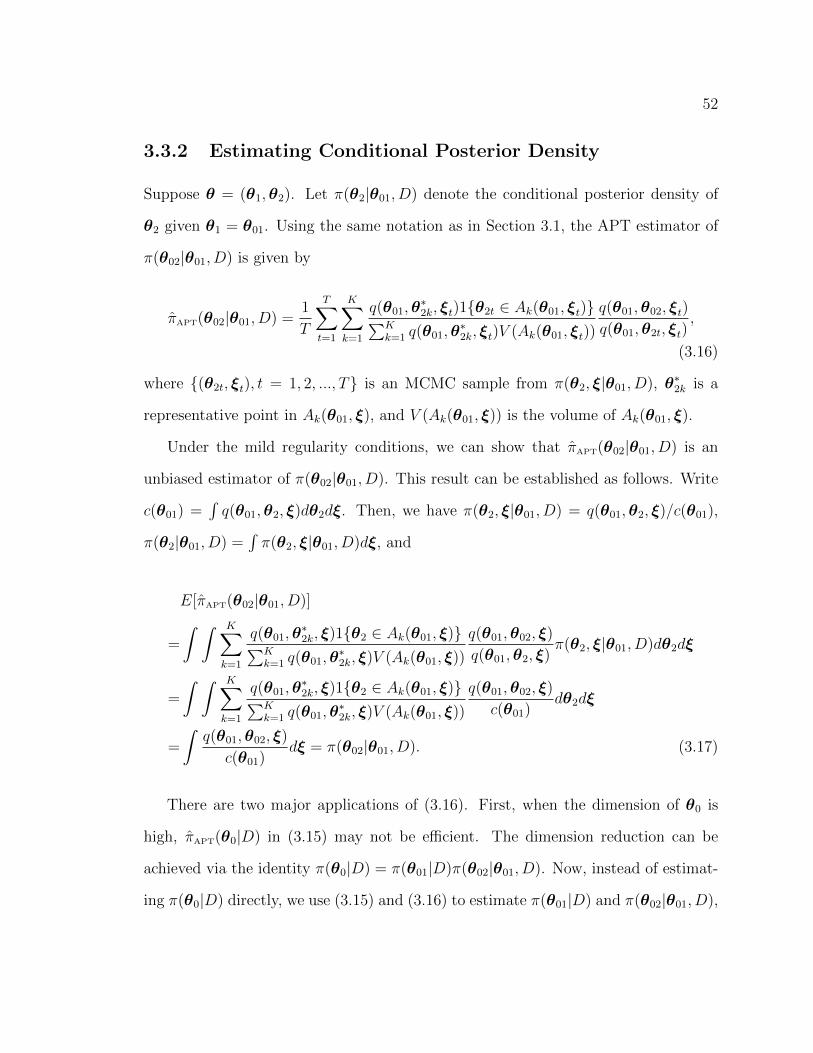
52

3.3.2 Estimating Conditional Posterior Density

Suppose θ = (θ1,θ2). Let π(θ2|θ01, D) denote the conditional posterior density of

θ2 given θ1 = θ01. Using the same notation as in Section 3.1, the APT estimator of

π(θ02|θ01, D) is given by

πAPT(θ02|θ01, D) =1

T

T∑t=1

K∑k=1

q(θ01,θ∗2k, ξt)1θ2t ∈ Ak(θ01, ξt)∑K

k=1 q(θ01,θ∗2k, ξt)V (Ak(θ01, ξt))

q(θ01,θ02, ξt)

q(θ01,θ2t, ξt),

(3.16)

where (θ2t, ξt), t = 1, 2, ..., T is an MCMC sample from π(θ2, ξ|θ01, D), θ∗2k is a

representative point in Ak(θ01, ξ), and V (Ak(θ01, ξ)) is the volume of Ak(θ01, ξ).

Under the mild regularity conditions, we can show that πAPT(θ02|θ01, D) is an

unbiased estimator of π(θ02|θ01, D). This result can be established as follows. Write

c(θ01) =∫q(θ01,θ2, ξ)dθ2dξ. Then, we have π(θ2, ξ|θ01, D) = q(θ01,θ2, ξ)/c(θ01),

π(θ2|θ01, D) =∫π(θ2, ξ|θ01, D)dξ, and

E[πAPT(θ02|θ01, D)]

=

∫ ∫ K∑k=1

q(θ01,θ∗2k, ξ)1θ2 ∈ Ak(θ01, ξ)∑K

k=1 q(θ01,θ∗2k, ξ)V (Ak(θ01, ξ))

q(θ01,θ02, ξ)

q(θ01,θ2, ξ)π(θ2, ξ|θ01, D)dθ2dξ

=

∫ ∫ K∑k=1

q(θ01,θ∗2k, ξ)1θ2 ∈ Ak(θ01, ξ)∑K

k=1 q(θ01,θ∗2k, ξ)V (Ak(θ01, ξ))

q(θ01,θ02, ξ)

c(θ01)dθ2dξ

=

∫q(θ01,θ02, ξ)

c(θ01)dξ = π(θ02|θ01, D). (3.17)

There are two major applications of (3.16). First, when the dimension of θ0 is

high, πAPT(θ0|D) in (3.15) may not be efficient. The dimension reduction can be

achieved via the identity π(θ0|D) = π(θ01|D)π(θ02|θ01, D). Now, instead of estimat-

ing π(θ0|D) directly, we use (3.15) and (3.16) to estimate π(θ01|D) and π(θ02|θ01, D),

53

respectively. These two estimators require one MCMC sample from the full posterior

distribution π(ζ|D) and another MCMC sample from the conditional posterior dis-

tribution π(θ2, ξ|θ01, D). We note that once the sampling code for the full posterior

distribution is readily available, the very same code with minimal changes can be

used to generate an MCMC sample from the conditional posterior distribution.

Second, (3.16) can also be applied to the estimation of the marginal likelihood

through Chib’s identity (Chib, 1995). Suppose we group ζ into G blocks as ζ =

(ζ ′1, ζ′2, ..., ζ

′G)′. Following Chib (1995), we have

c =q(ζ∗)

π(ζ∗1, ζ∗2, ..., ζ

∗G|D)

=q(ζ∗)

π(ζ∗1|D)π(ζ∗2|ζ∗1, D) . . . π(ζ∗G|ζ∗1, ζ∗2, ..., ζ∗G−1, D), (3.18)

where ζ∗ = ((ζ∗1)′, (ζ∗2)′, ..., (ζ∗G)′)′ is a high posterior density point such as the pos-

terior mean or mode of ζ. In (3.18), π(ζ∗1|D) can be estimated by (3.15) using an

MCMC sample from the full posterior density while an estimate of each conditional

density π(ζ∗g|ζ∗1, ζ∗2, ..., ζ∗g−1, D) can be obtained by (3.16) using an MCMC sample

from the conditional posterior distribution π(ζg, ζg+1, . . . , ζG|ζ∗1, ζ∗2, ..., ζ∗g−1, D) for

g = 2, 3, . . . , G. This approach does not require knowing the full conditional posterior

density analytically (i.e., CMDE) or the closed-form expression of the full conditional

density after introducing additional latent variables (namely, the augmented CMDE)

as discussed in Chib (1995).

3.4 Inequality-Constrained Analysis of Variance

In this section, we apply APT to the inequality-constrained analysis of variance model

to find the marginal posterior density. We use the data in Hoijtink et al. (2008)

54

collected to study amnesia in patients with dissociative identity disorder (DID). The

experiment is designed to compare memory performance scores among four groups,

including DID, mimic normal, symptom simulated, and true amnesic subjects. Chen

and Kim (2008) were interested in testing several hypotheses for the mean scores.

Based on their best model, we further investigate the marginal posterior density of

each mean. In each case, the closed form of the conditional posterior density is

available so that the CMDE can be used for comparison. Furthermore, we obtain two

joint marginal posterior densities: the means of the DID and true amnesia groups, and

the means of DID and symptom simulated groups. Note that the conditional posterior

density of the former is analytically available while the latter requires numerical

integration in the process.

The experiment investigates whether a DID patient really suffers from amnesia

when switching from one identity to another. To objectively evaluate the subjective

experience of amnesia in DID patients and avoid the iatrogenic problem (i.e., patients’

behaviors are induced by therapists) or some suggestive influence of media, DID

patients (n1 = 19) were implicitly measured for amnesia in the following procedure:

after being told a brief story and shown some figures, they were asked to change their

identity and then answer recognition questions about the story and figure details. To

avoid the issue of symptom simulation in DID patients, three control groups composed

of normal healthy people were recruited for comparison. The second (first control)

group (n2 = 25) was a normal control group. They were told the story and shown

the figures, and were then asked to answer the questions. Without any intervention,

their performance would be the performance of normal people. The same procedure

was used for the third (second control) group (n3 = 25), but they were extensively

informed about the behaviors of DID in advance and asked to deliberately simulate

55

inter-identity amnesia. They can be viewed as the symptom simulation group. The

fourth (third control) group (n4 = 25) were asked to directly answer the questions

without experiencing the story and graphs. Due to their complete lack of knowledge,

this group represented a true amnesic group.

We model memory performance score yij for the ith subject in group j as an

independent observation from a normal distribution with mean µj and variance σ2

for i = 1, 2, ..., nj and j = 1, ..., J . Let Θ denote the corresponding constrained

parameter space for θ under the hypothesis, for example µ1 < µ2 < ...., and let

D = n,y = ∑J

j=1 nj, y11, y21, . . . , yn11, . . . , y1J , y2J , . . . , ynJJ denote the observed

data. Then, the likelihood function is given by

L(θ|D) = (2πσ2)−n2 exp

− 1

2σ2

J∑j=1

nj∑i=1

(yij − µj)2

,

where θ = (µ, σ2) = (µ1, . . . , µJ , σ2). For this model, a prior distribution in Chen

and Ibrahim (2003) is considered: a power prior based on the prior predictive values

of the performance score is assigned for µ given σ2, and an inverse gamma prior is

assumed for σ2. Specifically, the joint prior is

π(µ, σ2|y0, a0) ∝[(σ2)−

n02 exp

− 1

2σ2

J∑j=1

n0j∑i=1

(y0ij − µj)2]a0

(σ2)−b01−1

× exp

(−b02

σ2

)1(µ, σ2) ∈ Θ,

where y0 = (y01,y02, ...,y0J) with y′0j = (y01j, y02j, . . . , y0n0jj) denotes the prior pre-

dictive values of the response variables, a0 is a scalar parameter determining the

degree of involvement of the prior predictive values in forming the prior distribution,

56

n0 =∑J

j=1 n0j, and b01 > 0 and b02 > 0 are prespecified hyperparameters. Under this

constrained structure, the marginal posterior density of µj is analytically intractable,

but can be evaluated by using an MCMC approach.

Assume∑nj

i=1 y0ij = 0 for j = 1, 2, ..., 4 and b01 = b02 = 0.0001. For comparing

our proposed method with KDE and CMDE, we choose one of the best hypotheses:

Θ = µ2 > (µ1, µ4) > µ3, σ2 > 0 under a0 = 0.01 based on Bayesian analyses by

Chen and Kim (2008), where Bayesian model selection of different hypotheses on

mean scores is carried out with various criteria including L measure, deviance infor-

mation criterion (DIC), the conditional predictive ordinate (CPO) statistic, and the

marginal likelihood or Bayes factor. Under this hypothesis, the CMDE is applicable

in estimating the marginal posterior density of each mean since the closed form of

57

the conditional posterior density is available as follows:

π(µ1|µ(−1), σ2, D,y0, a0) =

√n1+a0n1

2πσ2 exp

(−

(n1+a0n1)[µ1−∑yi1

n1+a0n1]2

2σ2

)Φ

µ2−∑yi1

n1+a0n1√σ2

n1+a0n1

− Φ

µ3−∑yi1

n1+a0n1√σ2

n1+a0n1

,

π(µ2|µ(−2), σ2, D,y0, a0) =

√n2+a0n2

2πσ2 exp

(−

(n2+a0n2)[µ2−∑yi2

n2+a0n2]2

2σ2

)1− Φ

max(µ1,µ4)−∑yi2

n2+a0n2√σ2

n2+a0n2

,

π(µ3|µ(−3), σ2, D,y0, a0) =

√n3+a0n3

2πσ2 exp

(−

(n3+a0n3)[µ3−∑yi3

n3+a0n3]2

2σ2

)

Φ

min(µ1,µ4)−∑yi3

n3+a0n3√σ2

n3+a0n3

,

π(µ4|µ(−4), σ2, D,y0, a0) =

√n4+a0n4

2πσ2 exp

(−

(n4+a0n4)[µ4−∑yi4

n4+a0n4]2

2σ2

)Φ

µ2−∑yi4

n4+a0n4√σ2

n4+a0n4

− Φ

µ3−∑yi4

n4+a0n4√σ2

n4+a0n4

,

where Φ(.) denotes the cumulative standard normal distribution function. To im-

plement APT, we first choose the conditional working parameter space Θµ(−jt),σ2t

of each π(µj|µ(−j), σ2, D,y0, a0) to be Θµ(−1t),σ

2t

= µ3t < µ1t < µ2t, Θµ(−2t),σ2t

=

max(µ1t, µ4t) < µ2t < 15, Θµ(−3t),σ2t

= 0 < µ3t < min(µ1t, µ4t), and Θµ(−4t),σ2t

=

µ3t < µ4t < µ2t, where µjt is the tth MCMC sample point for the jth parame-

ter. Notice that the chosen conditional working parameter space for Θµ(−jt),σ2t, j =

1, 4 is exactly equal to the whole support of the conditional posterior distribution

π(µj|µ(−j), σ2, D,y0, a0), j = 1, 4 since µ1 and µ4 are bounded on both sides. For µ2

and µ3, which are each bounded on one side, we set 15 as the upper bound and 0

58

as the lower bound for each respective parameter such that the working space can

cover most of the MCMC sample. Then, we decide on the number of subsets K in

the conditional working parameter space.

(a) KDE (b) APT (K=20) (c) APT (K=50)

π(µ

1|D

)

0 5 10 15

−1.

0−

0.5

0.0

0.5

1.0

µ10 5 10 15

−1.

0−

0.5

0.0

0.5

1.0

µ10 5 10 15

−1.

0−

0.5

0.0

0.5

1.0

µ1

π(µ

2|D

)

0 5 10 15

−1.

0−

0.5

0.0

0.5

1.0

µ20 5 10 15

−1.

0−

0.5

0.0

0.5

1.0

µ20 5 10 15

−1.

0−

0.5

0.0

0.5

1.0

µ2

π(µ

3|D

)

0 5 10 15

−1.

0−

0.5

0.0

0.5

1.0

µ30 5 10 15

−1.

0−

0.5

0.0

0.5

1.0

µ30 5 10 15

−1.

0−

0.5

0.0

0.5

1.0

µ3

π(µ

4|D

)

0 5 10 15

−1.

0−

0.5

0.0

0.5

1.0

µ40 5 10 15

−1.

0−

0.5

0.0

0.5

1.0

µ40 5 10 15

−1.

0−

0.5

0.0

0.5

1.0

µ4

Figure 3.1: The estimated marginal posterior density curve for each µj with the fixedMCMC sample size T = 1, 000 by (a) KDE, (b) APT (K=20), and (c) APT (K=50).The blue curve is the estimated curve by the corresponding approach, and the red oneis its difference from the estimated curve by the CMDE with a further subtraction of1 to separate the two curves.

Figure 3.1 includes the four estimated curves of KDE in the first column (using

the function, density(.), with the default setting in R software), and APT curves with

K = 20 and K = 50 in the second and third columns, respectively. In each graph,

a blue curve denotes the estimated curve, while a red curve (offset by 1 vertically)

59

denotes the difference of the estimated curve from the CMDE estimated curve. It

shows that KDE deviates from the CMDE for each parameter in the region around

its posterior mode. Whereas, APT can produce results very similar to CMDE even

when the number of partition subsets is small. When K is increased to K = 50, APT

completely overlaps with the CMDE, empirically confirming the results established

in Remarks 3.2 and 3.3.

Next, we examine the performance of APT in the joint marginal posterior density

of µ1 and µ4. As in the one-dimensional problem, the CMDE is applicable because

the closed form for the conditional posterior density is available:

π(µ1, µ4|µ(−1,−4), σ2, D,y0, a0) =

∏j=1,4

√nj+a0nj

2πσ2 exp

(−

(nj+a0nj)[µj−∑i yij

nj+a0nj]2

2σ2

)Φ

µ2−∑i yij

nj+a0nj√σ2

nj+a0nj

− Φ

µ3−∑i yij

nj+a0nj√σ2

nj+a0nj

.

For APT, the conditional working parameter space Θθ(−1t,−4t)is set to be µ3t <

(µ1t, µ4t) < µ2t, then the working parameter space in each dimension is equally

divided into 20 or 50 pieces so that K = 400 or K = 2, 500. Figure 3.2 shows the

estimated joint marginal posterior densities by KDE (using the function, kde2d(.),

with the default setting in R software), APT (K=400), and APT (K=2,500) based on

an MCMC sample of size T = 1, 000. The difference of each from the CMDE estimate

is shown below the estimated density surface (using an offset of -1). Figure 3.2 shows

that KDE is quite different from the CMDE in this two-dimensional problem, while

only minor differences are detectable in the center using APT even with a small

number of partition subsets. These slight differences disappear when K is increased.

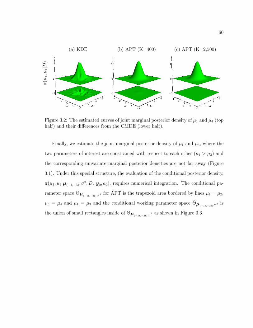
60

(a) KDE (b) APT (K=400) (c) APT (K=2,500)π

(µ1,µ

4|D

)

Figure 3.2: The estimated curves of joint marginal posterior density of µ1 and µ4 (tophalf) and their differences from the CMDE (lower half).

Finally, we estimate the joint marginal posterior density of µ1 and µ3, where the

two parameters of interest are constrained with respect to each other (µ1 > µ3) and

the corresponding univariate marginal posterior densities are not far away (Figure

3.1). Under this special structure, the evaluation of the conditional posterior density,

π(µ1, µ3|µ(−1,−3), σ2, D, y0, a0), requires numerical integration. The conditional pa-

rameter space Θµ(−1t,−3t),σ2 for APT is the trapezoid area bordered by lines µ1 = µ2,

µ3 = µ4 and µ1 = µ3 and the conditional working parameter space Θµ(−1t,−3t),σ2 is

the union of small rectangles inside of Θµ(−1t,−3t),σ2 as shown in Figure 3.3.

61

µ1

µ 3(0,0) µ4 µ2

µ4

µ1=µ3

Figure 3.3: The chosen conditional working parameter space of µ1 and µ3 and itspartition (small rectangles) for APT.

(a) KDE (b) APT (K=590) (c) APT (K=3,725)

π(µ

1,µ

3|D

)

Figure 3.4: The estimated curves of joint marginal posterior density of µ1 and µ3 (tophalf) and their differences from the CMDE (lower half). The red dashed line is theboundary µ1 = µ3 of the constraint µ1 > µ3.

Figure 3.4 shows the performance of KDE (using the function, kde2d(.), with

the default setting in the R software) and APT based on an MCMC sample of size

T = 1, 000. APT performs well even for the smaller number of partition subsets,

K = 590 (190 for green area and 400 for gray area). In contrast, KDE again deviates

62

from the CMDE. Because it does not use the structure of the known unnormalized

posterior density, the KDE has positive values in the area beyond the red dashed line,

where the joint marginal posterior density values are supposed to be 0.

3.5 APT for Bayesian Variable Selection

3.5.1 The Basic Formulation

Suppose there are p regression parameters, β, in the full model M , and β ∈ Rp.

In variable selection, we let β(m) and β(−m) denote the regression parameters in-

cluded in and excluded from the reduced model m, respectively. Then, β(M) = β =

((β(m))′, (β(−m))′)′ holds for all m, and β(−M) = ∅. We further let α denote the

nuisance parameters in the model. Under this setting, two conditions required for

the Savage-Dickey density ratio in Dickey (1971) are given in Chen et al. (1999) as

follows:

Condition I. L(β(m),α|D,m) = L(β(m),β(−m) = 0,α|D,M), where

L(β(m),α|D,m) is the likelihood function under the reduced model m and

L(β(m),β(−m) = 0,α|D,M) is the likelihood function under the full model

evaluated at β(m), β(−m) = 0 and α;

Condition II. π(β(m),α|m) = π(β(m),α|β(−m) = 0,M), where π(β(m),α|m) is the

prior distribution specified under the reduced model m and π(β(m),α|β(−m) =

0,M) is the conditional prior distribution of β(m),α given β(−m) = 0 under the

full model.

63

If both conditions hold, the Bayes factor of the reduced model m over the full model

M can be simplified to

BF =c(D|m)

c(D|M)=π(β(−m) = 0|D,M)

π(β(−m) = 0|M), (3.19)

where c(D|m) and c(D|M) are the marginal likelihoods under the reduced model and

the full model, respectively, and π(β(−m) = 0|D,M) and π(β(−m) = 0|M) denote the

marginal posterior and prior densities evaluated at β(−m) = 0 from the full model,

respectively. It shows that the Bayes factor can be simplified as the function of the

marginal posterior density evaluated at zero values of the parameters excluded from

the reduced model m so that the model comparison can be done by using a single

MCMC sample from the posterior density of the full model. To estimate the marginal

posterior density in (3.19), we can use the APT in (3.15) by assigning θ = β(−m),

θ0 = 0, and ξ = ((β(m))′,α′)′. Since the parameters in the marginal posterior density

are all regression parameters with no constraints, the partition of the conditional

working parameter space can be easily constructed via elliptical rings. Assuming the

dimension of θ is q, the elliptical rings are defined as

Ak(ξ) = Ak = θ : r(k − 1)/K ≤ ‖(θ − θ)′Σ− 1

2‖ ≤ rk/K, k = 1, 2, . . . , K,

where θ and Σ are the posterior mean and the posterior covariance matrix of θ,

respectively, and r is the radius chosen for the conditional working parameter space.

The volume of Ak(ξ) can be calculated as follows

V (Ak) = Vq|Σ|1/2[(rkK

)q−(r(k − 1)

K

)q], (3.20)

64

where |.| is the determinant and Vq = πq/2/Γ(q/2+1) is the volume of a q-dimensional

unit hypersphere for k = 1, 2, . . . , K.

Suppose (β(m)t ,β

(−m)t ,αt), t = 1, ..., T is an MCMC sample from the posterior

distribution under the full model. Let θt = β(−m)t and ξt = ((β

(m)t )′,α′t)

′ for t =

1, 2, . . . , T . Then, we have

πt(θ = 0|D,M) =K∑k=1

q(θ∗k, ξt)1θt ∈ Ak∑Kk=1 q(θ

∗k, ξt)V (Ak)

q(θ = 0, ξt)

q(θt, ξt),

where θ∗k ∈ Ak is a representative point in the kth elliptical ring for k = 1, 2, . . . , K.

Assume that the marginal prior density π(θ = 0|M) is analytically available. Then,

the Bayes factor in log scale is estimated as

log BF APT = log 1

T

T∑t=1

πt(θ = 0|D,M)− log π(θ = 0|M). (3.21)

We use the Overlapping Batch Statistics (OBS) of Schmeiser et al. (1990) to estimate

the Monte Carlo (MC) standard error of log BF APT. Write η = log BF APT. Let ηb

denote an estimate of the Bayes factor in log scale via (3.21) using the bth batch,

(β(m)t ,β

(−m)t ,αt), t = b, ..., b+B− 1, of the MCMC sample for b = 1, ..., T −B+ 1,

where B < T is the batch size. Then, the OBS estimated MC standard error of η is

given by √Var(η) =

[ B

T −B

]∑T−B+1b=1 (ηb − ηOBS)

2

T −B + 1

1/2

, (3.22)

where ηOBS =∑T−B+1

b=1 ηb/(T − B + 1). According to Schmeiser et al. (1990), a

reasonable choice of batch size B is 10 ≤ T/B ≤ 20.

Remark 5.1: A reasonable choice of the representative point in each elliptical ring

65

Ak can be based on the following equation

θ∗k = r∗kΣ12d+ θ, (3.23)

where r∗k = r[k/K − 1/(2K)], and d is a normalized vector, that is ‖d‖ = 1, which

decides the direction of θ∗k. Since the largest eigenvalue of Σ can explain the most

variation of the MCMC sample, we suggest using its corresponding eigenvector for d.

3.5.2 The Ordinal Probit Regression Model

We consider the model selection problem under the ordinal probit regression model,

in which the prior distribution does not satisfy Condition II. Thus, the Savage-Dickey

density ratio does not hold. Under this situation, we show how marginal posterior

density estimation can still be used for estimating ratios of marginal likelihoods be-

tween each reduced model and the full model.

Let y = (y1, y2, ..., yn)′ denote the vector of observed ordinal responses, each is

coded as one value from 0, 1, ..., J − 1, and X denote the n× p covariate matrix with

the ith row equal to the covariates of the ith subject x′i. Let D = (y,X, n). Following

Nandram and Chen (1996), the likelihood function is then given by

L(β, γ, σ|D) =n∏i=1

[Φ

(γyi+1

− x′iβσ

)− Φ

(γyi − x′iβ

σ

)], (3.24)

where γ = (γ2, . . . , γJ−2)′, −∞ = γ0 < γ1 = 0 ≤ γ2 ≤ · · · ≤ γJ−1 = 1 < γJ = ∞

are the cutoff points, β is a p-dimensional vector of the regression coefficients, and

σ > 0 is a scale parameter. The likelihood function in (3.24) is derived based on the

reparameterization of the ordinal regression model with latent variables proposed by

66

Albert and Chib (1993) to accelerate convergence of the Gibbs sampling algorithm.

Another attractive feature of (3.24) is that when J = 3, there are no unknown cutoff

points. The priors of (β, γ, σ2) considered in Chen (2005b) are given by

π(β, γ, σ2) = π(β|σ2)π(σ2)π(γ), (3.25)

where β|σ2 ∼ N(0, τ−10 σ2Ip), σ

2 follows an inverse gamma distribution IG(b01, b02),

γ is assigned a uniform prior on the constrained space of γ, Ip is the p × p identity

matrix, and τ0 > 0, b01 > 0, and b02 > 0 are prespecified hyperparameters. Then, the

resulting posterior distribution is given by

π(β, γ, σ2|D) ∝ L(β, γ, σ|D)π(β, γ, σ2). (3.26)

To carry out Bayesian variable selection under the ordinal probit regression model,

we let (x(m)i , β

(m)) and (x

(−m)i , β

(−m)) denote the pm and p − pm covariates and

the corresponding regression coefficients included in and excluded from the mth re-

duced model, respectively, such that 0 < pm ≤ p, xi = ((x(m)i )′, (x

(−m)i )′)′, and

β = ((β(m)

)′, (β(−m)

)′)′. To ensure that the prior of (β(m), σ2,γ) under the reduced

model m has the same structure as the one given in (3.25) under the full model, we

take

π(β(m), γ, σ2|m) = π(β

(m)|σ2)π(σ2)π(γ), (3.27)

where β(m)|σ2 ∼ N(0, τ−1

0 σ2Ipm), and π(σ2) and π(γ) are defined in (3.25). The

likelihood function L(β(m), γ, σ|D,m) under the reduced model is given by (3.24) with

x′iβ replaced by (x(m)i )′β

(m). For this application, α = (γ ′, σ2)′. Since x′iβ

∣∣∣ ˘β(−m)

=0=

67

(x(m)i )′β

(m), Condition I holds. From (3.25), we have

π(β(m), γ, σ2|β(−m) = 0)

∝(σ2)−p/2 exp− τ0

2σ2(β

(m))′(β

(m))

(σ2)−(b01+1) exp(−b02/σ2),

which is clearly not equal to π(β(m), γ, σ2|m) given in (3.27) when pm < p. Thus,

Condition II is not satisfied. Under this setting, the Bayes factor of the reduced model

m over the full model cannot be calculated using (3.19). To circumvent this problem,

we take the following one-to-one transformations:

β =β√σ2, γj =

γj√σ2, j = 2, . . . , J − 2, and γJ−1 =

1√σ2. (3.28)

The absolute value of the determinant of the Jacobian of the transformations from

(β, γ, σ2) to (β,γ) is γ−(p+J)J−1 . Write γ = (γ2, . . . , γJ−1)′. After the transformations,

the likelihood function of (β,γ) is given by

L(β,γ|D) =n∏i=1

[Φ(γyi+1

− x′iβ)− Φ (γyi − x′iβ)

], (3.29)

and the prior of (β,γ) is given by

π(β,γ) ∝ exp(− τ0

2β′β

)γ−J+2b01+2J−1 exp

(− b02γ

2J−1

), (3.30)

where β ∈ Rp and −∞ = γ0 < γ1 = 0 ≤ γ2 ≤ · · · ≤ γJ−1 < γJ =∞. Now, applying

the Bayesian variable selection procedure to (β,γ) with the likelihood function and

the prior given by (3.29) and (3.30), we can show that both Conditions 1 and 2 are

satisfied. Therefore, we can use the APT via (3.19) to compute the Bayes factor.

68

Although the use of (3.29) and (3.30) leads to easy computation of the Bayes fac-

tor, sampling (β,γ) from the posterior distribution induced by (3.29) and (3.30) is not

as efficient as sampling (β, γ, σ2) from (3.26) (e.g. Nandram and Chen, 1996). Since

the transformations in (3.28) are one-to-one, MCMC samples of (β, γ, σ2) from (3.26),

which can be generated by Nandram-Chen algorithm, can be directly used to obtain

MCMC samples of (β,γ) via (3.28). Therefore, by combining these two settings of

the ordinal probit regression model, we can achieve both convenient implementation

of MCMC sampling and efficient computation of Bayes factors.

3.5.3 Analysis of the Prostate Cancer Data

We apply the ordinal probit regression model to the prostate cancer data (n = 713)

as in Chen (2005b). We examine the relationships between a clinical ordinal re-

sponse variable, Pathological Extracapsular Extension (PECE, y), and three covari-

ates: Prostate Specific Antigen (PSA, x1), Clinical Gleason Score (GLEAS, x2, x3),

and Clinical Stage (CSTAGE, x4). Here, PECE takes values of 0, 1, or 2, where

0 means that there is no cancer cell present in or near the capsule, 1 denotes that

the cancer cells extend into but not through the capsule, and 2 indicates that can-

cer cells extend through the capsule. PSA is a continuous variable while CSTAGE

is a binary outcome, which is assigned to 1 if the 1992 American Joint Commis-

sion on Cancer (AJCC) clinical stage T-category is 1, and assigned to 2 if the T-

category is 2 or higher. As for GLEAS, considering similar biologic behaviors of

tumors (well-differentiated, moderately-differentiated, or poorly-differentiated), it is

trichotomized by two dummy variables: x2 = 1 if GLEAS= 7, otherwise x2 = 0;

x3 = 1 if GLEAS> 7, otherwise x3 = 0. We note that in Chen (2005b), GLEAS was

69

treated as a continuous variable. Since x2 and x3 are defined from the same variable

GLEAS, we either include both x2 and x3 in the model or exclude them together from

the model.

In this example, since J = 3, there are no unknown cutpoints in (3.24). In (3.25),

we take b01 = 1 and b02 = 0.1. Due to lack of historical information about τ0 and

for avoiding the phenomenon of the Bartlett’s or Lindley’s paradox (see Jeffreys,

1998; Lindley, 1957), we first use an empirical Bayes method to find the best prior

setting of τ0 for the full model based on the marginal likelihood criterion. The PWK

estimator was used to calculate the marginal likelihoods under different τ0. Table

3.1 summarizes the marginal likelihood estimate and its Monte Carlo standard error

(MCSE) for each τ0 using an MCMC sample of size T = 10, 000. The MCSE is

calculated by (3.22) with the batch size B = 1, 000.

Table 3.1: Marginal likelihood estimate under different precision τ0

τ0c(D|M) MCSE

0.1 -766.398 0.009

1 -760.791 0.007

10 -756.690 0.011

15 -756.516 0.011

20 -756.641 0.009

30 -757.240 0.005

40 -758.065 0.009

50 -758.928 0.011

From the results in Table 3.1, we choose τ0 = 15 as the best prior under the full

70

model. On this basis, we use the Bayes factor for variable selection. Following (3.28),

we first transform the regression parameters to satisfy the conditions for Savage-

Dickey density ratio. Then, we apply APT to estimate the marginal posterior density

at zero values in (3.19) by constructing an elliptical-ring partition of the working

parameter space with r = 4 and K = 1, 5, or 10. Table 3.2 shows the 95% HPD

interval for each β, Bayes factor estimates of the reduced models over the full model

in log scale, their estimated MCSE’s using (3.22) with the batch size B = 1, 000,

and their relative MCSEs denoted by rMCSEs, each of which is defined as MCSE

divided by its | log BF |. The results are obtained based on an MCMC sample of size

10, 000. From Table 3.2, we see that the full model is preferred because all the values

of logBF are negative. This result is also supported by the 95% HPD intervals, which

do not contain 0. In addition, we observe that each MCSE dramatically drops when

a reasonable number of subsets (K = 5 or 10) is used. The fact that each MCSE is

relatively small compared to the magnitude of logBF empirically demonstrates that

our proposed method is very accurate. Table 3.2 also shows the results for τ0 = 0.1,

where the inconsistency between the Bayes factors and the 95% HPD intervals is

evident. Even though the 95% HPD intervals suggest that all covariates are important

for the case of τ0 = 0.1, the Bayes factor tends to favor the reduced model, which is

known as the Bartlett’s or Lindley’s paradox.

71

Table 3.2: HPD interval and Bayes Factor in log scale when τ0 = 15 and τ0 = 0.1

τ0 = 15 τ0 = 0.1

Variable Mean SD 95% HPD Mean SD 95% HPD

x0 0.573 0.071 (0.434, 0.716) 0.581 0.070 (0.446, 0.718)

x1 0.494 0.103 (0.303, 0.701) 0.512 0.103 (0.322, 0.723)

x2 0.129 0.063 (0.013, 0.257) 0.128 0.062 (0.008, 0.253)

x3 0.241 0.070 (0.108, 0.378) 0.239 0.069 (0.103, 0.373)

x4 0.146 0.064 (0.021, 0.270) 0.145 0.063 (0.027, 0.273)

APT(K=1) APT(K=1)

Model logBF MCSE rMCSE logBF MCSE rMCSE

(x1, x2, x3) -1.035 0.059 5.72% 1.437 0.094 6.52%

(x2, x3, x4) -17.184 0.091 0.53% -15.126 0.191 1.27%

(x1, x4) -4.740 0.092 1.93% 0.424 0.065 15.30%

(x2, x3) -20.023 0.067 0.34% -15.722 0.167 1.06%

(x1) -6.404 0.085 1.33% 1.125 0.080 7.10%

(x4) -28.045 0.126 0.45% -21.985 0.081 0.37%

APT(K=5) APT(K=5)

(x1, x2, x3) -1.033 0.006 0.59% 1.471 0.010 0.70%

(x2, x3, x4) -17.086 0.039 0.23% -15.425 0.060 0.39%

(x1, x4) -4.645 0.024 0.52% 0.330 0.034 10.23%

(x2, x3) -19.848 0.061 0.31% -15.791 0.069 0.44%

(x1) -6.263 0.035 0.56% 1.213 0.053 4.33%

(x4) -27.993 0.047 0.17% -21.902 0.060 0.28%

APT(K=10) APT(K=10)

(x1, x2, x3) -1.034 0.006 0.60% 1.471 0.010 0.69%

(x2, x3, x4) -17.088 0.039 0.23% -15.424 0.057 0.37%

(x1, x4) -4.649 0.023 0.49% 0.327 0.031 9.51%

(x2, x3) -19.844 0.059 0.30% -15.783 0.065 0.41%

(x1) -6.268 0.032 0.51% 1.200 0.048 3.96%

(x4) -27.989 0.046 0.16% -21.893 0.058 0.26%

We also use the KDE with several choices of the kernel function to compute

π(β(−m) = 0|D,M) in (3.19). The KDE estimates and corresponding MCSEs of

logBF for the model (x1, x2, x3) when τ0 = 0.1 are 1.466 and 0.060 under the Gaussian

kernel; 1.475 and 0.059 under the Epanechnikov kernel; 1.446 and 0.069 under the

rectangular kernel; 1.472 and 0.059 under the triangular kernel; 1.473 and 0.058

under the biweight kernel; 1.472 and 0.058 under the cosine kernel; and 1.475 and

0.058 under the optcosine kernel. These MCSEs are larger than 0.010 shown in Table

72

3.2 using APT with K = 5 or K = 10.

To examine empirical performance of the estimates (3.15) and (3.16) for π(θ01 =

0|D) and π(θ02 = 0|θ01 = 0, D) using two MCMC samples, we consider models

(x1, x4) and (x2, x3) when τ0 = 0.1. In order to make a fair comparison, we generate

5,000 MCMC sample points from both the full posterior distribution and the con-

ditional posterior distribution. The resulting values of logBF , MCSE, and rMCSE

are 0.331, 0.021, and 6.42%, respectively, under model (x1, x4), and −15.849, 0.053,

and 0.33%, respectively, under model (x2, x3). In these computations, we fixed r = 4

and K = 10. In both cases, the estimates of logBF using (3.15) and (3.16) for

π(θ01 = 0|D) and π(θ02 = 0|θ01 = 0, D) have smaller MCSEs and rMCSE. These

results empirically demonstrate that the approach based on the dimension reduction

is quite promising in obtaining a more accurate estimate of logBF .

3.6 Discussion

Marginal posterior density estimation provides complete information for the parame-

ters of interest in Bayesian inference. While it is known that the conditional marginal

density estimator is the best (minimizing the variance) in the class of importance

weighted marginal density estimators (Chen, 1994), the method for realizing this es-

timator has not been accessible when the closed form of the conditional posterior

density is not available. To circumvent it, we propose an adaptive partition weighted

(APT) marginal density estimator that requires only the unnormalized posterior den-

sity and an MCMC sample from the joint posterior distribution. Our method is con-

structed by first partitioning the subset of the support of the conditional posterior

73

distribution, and then estimating the marginal posterior density at a fixed point of

the focal parameter vector by assigning a weighted average to the ratios of the unnor-

malized posterior density evaluated at the MCMC sample. The focal parameters in

the numerator are set to this fixed point, and weights are assigned locally using a rep-

resentative value in each partitioned subset. We show that our estimator is unbiased,

and approaches the conditional marginal density estimator when the number of par-

tition subsets is large. We illustrate our method APT with two examples. The first

one is a constrained parameter space problem, where the conditional marginal density

estimator for the parameters of interest can be evaluated. We show our estimator

performs as well as the gold standard (the conditional marginal density estimator)

in this case. The other example involves variable selection under the ordinal probit

regression model. In this example, we demonstrate the usefulness of the marginal

posterior density estimation for computing Bayes factors between the reduced model

with a subset of variables and the full model with all variables using a single MCMC

sample from the posterior distribution under the full model.

As discussed in Section 3 and shown in Section 5, APT is useful not only in

computing marginal posterior densities but also in estimating marginal likelihoods

through Chib’s identity and Bayes factors via the Savage-Dickey density ratio. As

further demonstrated in Section 5, the APT method in conjunction with the con-

ditional posterior density estimate leads to a more efficient estimate, which will be

potentially useful for Bayesian computation problems with high-dimensional param-

eters. Currently, KDE is a standard method for computing and displaying marginal

posterior densities using MCMC samples in existing Bayesian software. As empirically

shown in Sections 4 and 5, APT can be much closer to CMDE and produce a more

accurate estimate of Bayes factor than KDE. Since the proposed method requires only

74

the unnormalized posterior density and an MCMC sample from the joint posterior

distribution, APT has a potential to become a “black-box” algorithm, which can be

implemented in existing software including SAS, OpenBugs (Thomas et al., 2006),

as well as more specialized Bayesian software such as that used in phylogenetics:

MrBayes 3.2 (Ronquist et al., 2012) and BEAST2 (Bouckaert et al., 2014).

Chapter 4

Marginal Likelihoods ofPhylogenetic Models Using aPosterior Sample

4.1 Introduction

In Bayesian phylogenetics model selection, many Monte Carlo (MC) methods have

been developed in recent decades to estimate the marginal likelihood (normalizing

constant) for a fixed tree topology under a substitution model. This constant value

measures a average fit of the model to the data over the prior information for the

specific tree, and hence can be used as a criterion to select the best model. The

available methods include the harmonic mean (HM) method by Newton and Raftery

(1994), the inflated density ratio (IDR) method by Petris and Tardella (2003, 2007),

the thermodynamic integration (TI) method by Lartillot and Philippe (2006), the

stepping-stone (SS) method by Xie et al. (2011), and the generalized stepping-stone

75

76

(GSS) method by Fan et al. (2011). Under certain ergodic conditions, they are all

shown to produce consistent marginal likelihood estimators.

Wu et al. (2014) and Holder et al. (2014) further extend the HM, IDR, SS, and GSS

methods to estimating the marginal likelihood for variable tree topology. This value is

preferred by systematists, since the marginal likelihood is evaluated by summing over

all tree topologies, and hence, models can be compared based on the overall marginal

likelihood rather than being restricted to a certain topology. In the HM method,

the joint prior distribution of the tree and parameters in the substitution model is

used as a weight to the inverse of the joint posterior kernel evaluated at the points of

an Markov chain Monte Carlo (MCMC) sample. For the IDR method, the prior of

topology times a perturbed density, which is based on the conditional posterior kernel

given a topology T , is assigned as the weight. For SS and GSS, the computation

is decomposed into a series of telescoping ratios of two marginal likelihoods using

power posterior kernels, where each ratio requires an MCMC sample from a power

posterior distribution and is estimated by the importance sampling approach. Then,

the overall marginal likelihood estimate is obtained simply by the multiplication of

all these estimated ratios.

The partition weighted kernel estimator (PWK) developed in Chapter 2 can also

be applied to the marginal likelihood calculation for a fixed topology problem. The

PWK estimator is constructed by first partitioning the working parameter space

(where the posterior kernel is bounded away from zero), and in each partition subset,

assigning a local weight to the inverse of the posterior kernel evaluated at an MCMC

sample. This method is essentially a generalization of the HM and IDR methods,

but produces an estimator with smaller variance as shown in Chapter 2. In addition,

compared to SS and GSS, the PWK is more attractive since it only needs a single

77

MCMC sample from the joint posterior distribution. In this chapter, we extend the

working parameter space to the discrete tree topology space and propose the variable-

topology partition weighted kernel (VPWK) estimator for the marginal likelihood.

Furthermore, the use of estimated posterior density of selected tree as a re-weighted

function of this new method also improves the efficiency.

In the rest of this chapter, we first formulize the problem and introduce the existing

approaches in Section 2. In Section 3, we update the PWK estimator to variable tree

topology and examine its theoretical properties. Based on this method, the VPWK

estimator and its related properties are developed. In Section 4, we use the rcbl data

set in Lewis and Trainor (2012) for the real data analysis and compare the results of

VPWK to the VSS and VGSS estimates in the general time reversible plus Gamma

model. Finally, we conclude with a discussion in Section 5.

4.2 Preliminary

Suppose θτ is a pτ -dimensional vector of parameters affiliated with a binary labeled

unrooted tree topology τ on a set of S taxa for τ ∈ Γ = τ1, τ2, ..., τT, where Γ is

the discrete tree topology space, and T is the total number of distinct tree topologies

and equal to (2S − 5)!! = (2S − 5) (2S − 7) . . . (3)(1). Let y denote the data. Also

let f(y|θτ , τ) be the likelihood function and π(θτ , τ) = π(θτ |τ)π(τ) be the prior

distribution for (θτ , τ). Then, the posterior kernel q(θτ , τ) is f(y|θτ , τ)π(θτ , τ) with

support Ω = Γ ×Θτ , where Θτ = θτ : (θτ , τ) ∈ Ω is the support of conditional

posterior function θτ given τ , and the unnormalized conditional posterior function

78

θτ given τ is defined as

q(θτ |τ) = f(y|θτ , τ)π(θτ |τ).

Hence, the conditional marginal likelihood given τ , that is the marginal likelihood for

a fixed topology, is

c(τ) =

∫Θτ

q(θτ |τ)dθτ , (4.1)

and the overall marginal likelihood, that is the marginal likelihood for a variable

topology, is given by

c =∑τ∈Γ

c(τ)π(τ). (4.2)

Although c is a function of c(τ) for τ ∈ Γ, it is impractical to evaluate this summation

by brute-force approach since the size of Γ is often large. To estimate (4.2), Wu

et al. (2014) and Holder et al. (2014) update the HM, IDR, SS, and GSS estimators

originally designed for the marginal likelihood estimation under a fixed tree topology

to a variable tree topology. We examine each approach in the remaining of this

section.

Suppose (θ(n)τ , τ (n)), n = 1, 2, . . . , N is an MCMC sample from the posterior

distribution π(θτ , τ |y) = q(θτ , τ)/c, the HM estimator is given by

cVHM =

[1

N

N∑n=1

1

f(y|θ(n)

τ (n), τ (n))

]−1

. (4.3)

79

Under certain ergodic conditions, it is shown that

cVHM

a.s.→ c.

For the IDR, based on the conditional posterior kernel q(θτ |τ), an perturbed density

qr(θτ |τ) is proposed as

qr(θτ |τ) =

q(0|τ) if ||θτ || ≤ rτ ,

q(w(θτ )|τ) if ||θτ || > rτ ,

where rτ is the chosen radius for each tree topology and w(θτ ) = θτ×

(1− rpττ /||θτ ||pτ )1/pτ . It follows,

∫Θτ

qr(θτ )dθτ =

∫||θτ ||≤rτ

qr(θτ |τ)dθτ +

∫||θτ ||>rτ

qr(θτ |τ)dθτ = q(0|τ)brτ + c,

where brτ = Volume of the ball θτ : ||θτ || ≤ rτ = πpτ/2rpτ/Γ(pτ/2 + 1). Then, the

IDR estimator is given by

cVIDR =1

1N

∑Nn=1

1

q(0|τ (n))bτ(n)

[qr(θ

(n)

τ |τ (n))

q(θ(n)

τ |τ (n))− 1

] . (4.4)

It is also shown that

cVIDR

a.s.→ c.

In the GSS, the power posterior distribution is proposed as

pβ(θτ , τ) =qβ(θτ |τ)πβ(τ)

cβ, (4.5)

80

where 0.0 ≤ β ≤ 1.0,

πβ(τ) = [π(τ)]β[π∗(τ)]1−β,

qβ(θτ |τ) = [qβ(θτ |τ)]β[π∗β(θτ |τ)]1−β,

π∗β(θτ |τ) is a conditional reference prior distribution given τ , and π∗(τ) is a reference

prior distribution for the tree topology. When β = 0, c0 = 1 due to a proper reference

distribution proposed; when β = 1, c1 = c is the overall marginal likelihood. With

this setting, the computation of c is decomposed into

c =H∏h=1

cβhcβh−1

, (4.6)

where βh is often chosen as h/H, h = 1, 2, . . . , H. Given an MCMC sample is available

from pβh−1(θτ , τ), the estimator for uh = cβh/cβh−1

is given by

uVSS,h =1

N

N∑n=1

[q(θ

(n)

τ (n)|τ (n))

π∗(θ(n)

τ (n)|τ (n))

]βh−βh−1

. (4.7)

Then,the overall marginal likelihood is calculated by

cVSS =H∏h=1

uVSS,h. (4.8)

Under certain ergodic conditions,

uVSS,ha.s.→ cβh

cβh−1

,

so that

cVSS

a.s.→ c.

81

For the GSS, it improves the SS method by proposing a reference distribution close

to the posterior distribution. Then, a more efficient estimator is developed since a

smaller value of H is required to fill in the gap of dissimilarity between the posterior

and reference prior densities, or more stable estimates of uh can be obtained given

the same H is used.

In spite of consistency to the overall marginal likelihood for all four estimators,

both HM and IDR estimators are shown being less efficient than the PWK in Chap-

ter 2, and both SS and GSS require MCMC samples from a series of power posterior

distribution so that more computation time is expected. The motivation is initialized

by by these two facts and the PWK. We propose a new estimator, a variable-topology

partition weighted kernel (VPWK) estimator, in next section. This estimator only

requires a known posterior kernel and an MCMC sample from the posterior distri-

bution, and allows us to only focus on few frequently sampled trees rather than all

sampled trees.

4.3 PWK Estimator in Variable Topology

To estimate the marginal likelihood in (4.2), we first derive the PWK estimator in

Chapter 2 for a variable tree topology. We then examine its theoretical properties,

and further develop an improved estimator, variable-topology partition weighted ker-

nel (VPWK) estimator. The proposed method only requires the known posterior

kernel and a single MCMC sample from the posterior distribution. With minimal

assumptions, the VPWK is consistent to the reciprocal of overall marginal likelihood

and has a finite variance. It can be optimalized by increasing the number of partition

82

subsets in each chosen tree. Most of all, this new estimator is free from the curse of

unsampled or seldom-sampled topologies in an MCMC sample, which are common in

a variable-topology problem.

4.3.1 General Monte Carlo Estimator

Suppose Θτ = θτ : q(θτ |τ) > 0 is the working parameter space of Θτ , and

A1(τ), A2(τ), . . . , AKτ (τ) forms a partition of Θτ . Given an MCMC sample

(θ(n)

τ (n), τ (n)), n = 1, 2, . . . , N is available from the posterior distribution π(θτ , τ |y),

we update the PWK estimator for the reciprocal of the marginal likelihood in a

variable-topology problem as follows

1

c PWK

=1

N

N∑n=1

∑t∈Γ

1τ (n) = tKt∑kt=1

1∑Ktkt=1wktV (Akt(t))

[wkt

q(θ(n)t |t)

1θ(n)t ∈ Akt(t)

].

(4.9)

It can be shown that under some mild regularity conditions, 1/cPWK

is consistent to

1/c.

83

Proof: Under certain ergodic conditions, we first have

limN→∞

1

N

N∑n=1

∑t∈Γ

1τ (n) = tKt∑kt=1

1∑Ktkt=1 wktV (Akt(t))

[wkt

q(θ(n)t |t)

1θ(n)t ∈ Akt(t)

]

=∑τ∈Γ

∫Akτ (τ)

∑t∈Γ

1τ = tKt∑kt=1

1∑Ktkt=1wktV (Akt)

wktq(θt|t)

q(θτ , τ)

cdθτ

=∑t∈Γ

Kt∑kt=1

1∑Ktkt=1wktV (Akt(t))

∫Akt (t)

wktq(θt|t)

q(θt, t)

cdθt

=∑t∈Γ

Kt∑kt=1

1∑Ktkt=1wktV (Akt(t))

∫Akt (t)

wktπ(t)

cdθt

=∑t∈Γ

π(t)

c=

1

c

so that

1

c PWK

a.s.→ 1

c.

2

According to Chapter 2, the variance of∑Kt

kt=11∑Kt

kt=1 wktV (Akt (t))

[wkt

q(θ(n)

t |t)1θ(n)

t ∈

Akt(t)]

can be minimized by partitioning Θt into an abundant number of subsets

so that the sufficient condition for the optimality, that is homogeneity of q(θt|t) in

each subset, is satisfied. For each subset, we assign q(θ∗kt |t) as the local weight wkt ,

where θ∗kt is a representative point for the subset Akt(t) , and obtain an approximately

optimal PWK estimator. Based on the same idea, suppose for each τ ∈ Γ, Kτ is large

enough to insure the homogeneity of q(θτ |τ) in each subset, the optimal estimator of

84

(4.9) with minimum variance is given by

1

c PWK

=1

N

N∑n=1

∑t∈Γ

1τ (n) = tKt∑kt=1

1∑Ktkt=1 q(θ

∗kt |t)V (Akt(t))

[q(θ∗kt |t)q(θ

(n)t |t)

1θ(n)t ∈ Akt(t)

]

(4.10)

We see that (4.10) is a consistent estimator to 1/c by the ergodic theorem and ap-

proximates the optimal estimator in the class of estimators in (4.9) when Kτ → ∞

for τ ∈ Γ. Nevertheless, when the number of taxa S increases, the size of Γ increases

dramatically resulting in a huge computation burden from partitioning the working

parameter space for each sampled topology. In addition, the fact that most of the

MCMC sample comprises few dominant topologies motivates us to improve (4.10) by

excluding topologies of low frequency in the MCMC sample. In the next section, we

extend the idea of the working parameter space from continuous parameters to the

discrete tree topology space, and propose the variable-topology partition weighted

kernel (VPWK) estimator to estimate the marginal likelihood in a variable-topology

problem.

4.3.2 New Monte Carlo Estimator

The number of possible tree topology increases dramatically with number of taxa,

which results in the impossibility of constructing the working parameter space and

its partition subset for each tree. Moreover, knowing the fact that few tree topologies

account for most of the MCMC sample, we improve (4.10) by introducing the idea

85

of a subset Ξ of τ, τ = 1, 2, . . . , T. Essentially, it is an extended concept of the

working parameter space in Chapter 2 to a discrete parameter. We show that the

VPWK estimator is also consistent to 1/c. Under certain ergodic conditions and

Assumptions 1 and 2, it is shown to have finite variance.

Suppose Ξ is a subset of Γ, where Ξ excludes any topology with a small value of

π(τ |y). We propose the new estimator as

1

c V PWK

=

1N

∑Nn=1

∑t∈Ξ 1τ (n) = t

∑Ktkt=1

1∑Ktkt=1 q(θ

∗kt|t)V (Akt (t))

[q(θ∗kt ,t)

q(θ(n)

t ,t)1θ(n)

t ∈ Akt(t)]

∑t∈Ξ π(t)

.

(4.11)

In order to establish consistency and finite variance of the new estimator, we

introduce two assumptions.

Assumption 1: The volume of each region V (Akτ (τ)) < ∞ for k = 1, 2, . . . , Kτ ,

and τ ∈ Ξ.

Assumption 2: q(θkτ , τ) is positive and continuous on Akτ (τ), where Akτ (τ) is the

closure of Akτ (τ) for k = 1, . . . , Kτ , and τ ∈ Ξ.

Theorem 4.3.1. Under Assumptions 1 to 2 and certain ergodic (e.g., time-reversible,

invariant, and irreducible) conditions, 1/cV PWK in (4.11) is a consistent estimator

of 1/c. In addition, Var(1/cV PWK) <∞.

86

Proof: Under certain ergodic conditions, we have

1

N

N∑n=1

∑t∈Ξ

1τ (n) = tKt∑kt=1

1∑Ktkt=1 q(θ

∗kt |t)V (Akt(t))

[q(θ∗kt , t)

q(θ(n)t , t)

1θ(n)t ∈ Akt(t)

]a.s.→∑

t∈Ξ π(t)

c.

2

Although (4.11) has most of the desirable properties, we note that the weight as-

signed to q(θ∗kt , t)1θ(n)t ∈ Akt(t)/q(θ

(n)t , t) is π(t)/[

∑Ktkt=1 q(θ

∗kt , t)V (Akt(t))], which

may not be efficient especially when a vague prior distribution of tree topology is

used. To improve (4.11), we multiply this weight by π(t|y)/π(t) so that the VPWK

estimator is given by

1

c V PWK

=

1N

∑Nn=1

∑t∈Ξ 1τ (n) = t

∑Ktkt=1

π(t|y)∑Ktkt=1 q(θ

∗kt,t)V (Akt (t))

[q(θ∗kt ,t)

q(θ(n)

t ,t)1θ(n)

t ∈ Akt(t)]

∑t∈Ξ π(t|y)

,

(4.12)

where π(t|y) =∑N

n=1 1τ (n) = t/N . This re-weighting approach allows an MCMC

sample drawn from the dominant trees have more weights so that increases the ef-

ficiency. Additionally, we note that although both numerator and denominator in

(4.12) need to be estimated, it does not require an extra MCMC sample. Instead,

using the same MCMC sample in both parts is more efficient as proven in Chen et al.

(2008). Also, (4.12) has all desirable properties of that in (4.11).

87

4.4 6-taxon rcbL Data Set

In this section, we use the same rcbL data set as in Lewis and Trainor (2012), where

the survival under desiccation of green algae was investigated in soil collected from

Storrs, Connecticut, in October 1958 and dried for 43 years. Following a series of

long-term studies, in 2001 and 2008, Lewis and Trainor (2012) repeated the growth

experiment on the same soil, and found the presence of the green alga Protosiphon

botryoides from liquid preparations of soil dried for 43 years and its absence from

cultures prepared with soils dried for 50 years.

The rcbL data set includes 6 taxa: Chlamydopodiumvacuolatum (Chlamydo),

Protosiphon FRT2000 (Pspp), and the Protosiphon cultures from UTEX (the Uni-

versity of Texas Culture Collection of Algae): UTEX B99 (PbotB99), UTEX 46

(Pbot46), UTEX 47 (Pbot47), and UTEX B461 (PbotB461), each with the sequence

length equal to 1376. The number of unrooted tree topologies for 6 taxa is 105.

Figure 4.1 shows the majority rule (which equals the most probable tree topology)

and second most probable trees. Around 80% of the MCMC sample are from these

two dominant trees. For this data set, we consider the general time reversible plus

Gamma (GTR+G) model, which involves 18 unknown parameters (9 edge lengths, 3

nucleotide relative frequencies, 5 exchangeabilities, and 1 gamma shape) in θτ . To

examine performance of the VPWK estimator in this variable-topology problem, we

will compare the VPWK marginal likelihood estimate with those estimated using the

variable-topology stepping-stone approach in MrBayes (using the method of Xie et al.

(2011)) and Phycas (using the generalized stepping stone method of Fan et al. (2011)).

Additionally, the sensitivity analysis of the VPWK based on different chosen Ξ’s will

be included. To apply the VPWK to this model, we first transform the MCMC sam-

88

ple of continuous parameters: the log transformation of branch length parameters,

the log-ratio transformation of nucleotide frequency and GTR exchangeability pa-

rameters, and the log transformation of the gamma shape parameter, so that the new

conditional parameter space is Rp. Then, we standardize the transformed MCMC

sample and choose the radius as 5 to form the working parameter space. Note that

the chosen radius is a round-up value of√χ2p=18,0.95, which is a suggested value to

cover the most of an MCMC sample in Yu et al. (2015). On this basis, we apply the

spherical shell approach in Chapter 2 to construct the partitioned subsets of working

parameter space for each chosen tree topology.

Chlamydo

Pspp

PbotB461

Pbot47

PbotB99

Pbot460.01 substitutions/site

Chlamydo

Pspp

PbotB461

Pbot47

Pbot46

PbotB990.01 substitutions/site

(a) (b)

Figure 4.1: (a) is the majority rule tree (around 65% MCMC sample points), and(b) is the second most probable tree (around 15% MCMC sample points). Thoughimpossible to see due to very short edge lengths, Pbot46 is sister to (Pspp, (PbotB461,Pbot47)) in tree (b).

The VSS and VPWK estimates are summarized in Table 4.1 based on an MCMC

sample with size N = 60, 000, where 15 out of 105 trees were visited by the MCMC

89

sample. Table 4.1 provides two estimates based on the two most probable trees and

the ten most probable trees. The former only uses 81.26% of MCMC sample while

the latter uses 99.62% of MCMC sample. We see the results are robust to the size of

Ξ. In both cases, we only need to construct 2 or 10 working parameter spaces and

their partition subsets rather than creating a working parameter space for all 105

possible tree topologies, or all 15 tree topologies included in the MCMC sample. We

also observe that, based on a single MCMC sample from the joint posterior density,

the VPWK can produce comparable results to VSS by MrBayes (Ronquist et al.,

2012) and VGSS by Phycas (Lewis et al., 2015), which requires MCMC samples from

a series of power posterior distributions. Note that H is chosen as 29 and the size of

each MCMC sample from the power posterior distribution is 3, 584 in VSS; while H

is chosen as 30 and N from the power posterior distribution is 1, 000 in VGSS.

Table 4.1: Marginal likelihood estimates of VPWK and VSS in log scale

Method No. of Tree Considered % of the MCMC sample Used Estimate

VPWK 2 81.26% -2682.79

10 99.62% -2682.78

VSS by MrBayes all trees in the MCMC sample 100.00% -2682.79

VGSS by Phycas all trees in the MCMC sample 100.00% -2682.77

4.5 Results and Discussion

In this chapter, we develop a new estimator for a variable tree topology based on the

PWK estimator in Chapter 2. In this particular application, we introduce the concept

of working parameter space to a tree topology space. The computation time is much

lessened by only focusing on frequently sampled trees rather than all trees in the

90

MCMC sample. Additionally, this new estimator is desirable due to only requiring a

single MCMC sample from the posterior density. In addition to theoretical properties

such as consistency to the reciprocal of overall marginal likelihood, finite variance,

and optimization of the VPWK estimator, it also makes use of the estimated posterior

distribution of tree topology as a re-weighted function to increase the efficiency.

In real data analysis, we use the rcbL data set in Lewis and Trainor (2012) and

fit the data with the general time reversible plus Gamma model, where there are 18

parameters involved in. We show that the VPWK estimates are comparable to the

results of VSS and VGSS, both of which require a series of MCMC samples from the

power posterior distributions. We also show that the VPWK estimates are robust to

the choices of the size of Ξ as long as the selected trees contain reasonable size of an

MCMC sample.

At this stage, we are still developing software of the VPWK method for public

use. Besides the GTR+G model, more complicated models such as the GTR+G+I

model will be included.

Chapter 5

Concluding Remarks and FutureWork

5.1 Concluding Remarks

In this research work, a series of Monte Carlo estimators are developed for calculat-

ing the marginal likelihood, marginal posterior density, and marginal likelihood for

a variable tree topology. All methods are inspired by the idea of partitioning the

working parameter space and only require the known posterior kernel function and a

single MCMC sample from the posterior distribution.

The partition weighted kernel estimator is essentially an extension of the harmonic

mean (Newton and Raftery, 1994) and inflated density ratio (Petris and Tardella,

2003, 2007) approaches, but has more desirable properties including but not limited

to consistency, finite variance, optimization. In two simulation studies, we show

the PWK has smaller MCSE and RMSE, and approaches proposed for forming the

91

92

partition subsets of the working parameter space can insure the homogeneity of the

posterior kernel in each subset so that provide stable estimates. In the real data

example, we compare the PWK method with Chen’s (Chen, 2005b) and Chib’s (Chib,

1995) methods. We also show that the PWK produce a smaller estimated Monte Carlo

standard error by Overlapping batch statistics (Schmeiser et al., 1990). In the second

example, we show the usage of the PWK estimator in constructing the power prior

by the empirical Bayes approach using the marginal likelihood as a criterion.

In Chapter 3, we show the adaptive partition weighted estimator can approximate

the gold standard approach, the conditional marginal density estimator, when the

number of subsets increases. In the first real data example, we empirically show

this new method works well in the inequality-constrained analysis of variance. Then,

in the second example, we show the usefulness of this method in Bayesian variable

selection when the conditions for Savage-Dickey density ratio are satisfied.

In Chapter 4, we develop the variable-topology partition weighted kernel estimator

based on the PWK for the overall marginal likelihood calculation. This new method

contains all desirable properties as the PWK. In addition, we use the re-weighted

function to improve the efficiency of the VPWK. In real data example, the general

time reversible plus Gamma model is considered, where there are 18 unknown param-

eters, for this 6-taxon data. We show this new estimator can produce the comparable

results as the VSS and GSS but needs much less computation.

93

5.2 Future Work

Since our new methods only need minimum assumptions, we are developing the open

packages, which can construct the working parameter and its partition subsets by the

default setting based on the input of the posterior kernel function and the MCMC

sample from the investigators, and produce the marginal likelihood and marginal

posterior density estimates.

For Bayesian phylogenetics, we want to make use of the idea of Savage-Dickey

density ratio and develop a method to do the phylogenetics model selection by a single

MCMC sample from the posterior distribution based on the most complicated model

considered. This would be a challenge problem especially for a variable topology.

Additionally, although we have done many sensitivity analyses about the robust-

ness of the methods to the chosen working parameter space and the number of subsets,

we are still interested in developing some measures about the convergent speeds of

the number of partition subsets.

We leave these three interests as our future works.

Bibliography

Albert, J. H. and Chib, S. (1993). “Bayesian analysis of binary and polychotomous

response data.” Journal of the American of Statistical Assocation, 88: 669–679.

Bouckaert, R., Heled, J., Kuhnert, D., Vaughan, T., Wu, C.-H., Xie, D., Suchard,

M. A., Rambaut, A., and Drummond, A. J. (2014). “BEAST 2: a software platform

for Bayesian evolutionary analysis.” PLoS Computational Biology , 10(4): e1003537.

Chen, M.-H. (1994). “Importance-weighted marginal Bayesian posterior density esti-

mation.” Journal of the American Statistical Association, 89(427): 818–824.

— (2005a). “Bayesian computation: from posterior densities to Bayes factors,

marginal likelihoods, and posterior model probabilities.” In Dey, D. and Rao, C.

(eds.), Handbook of Statistics 25, Bayesian Thinking: Modeling and Computation,

437–457. Elsevier.

— (2005b). “Computing marginal likelihoods from a single MCMC output.” Statistica

Neerlandica, 59: 16–29.

Chen, M.-H., Huang, L., Ibrahim, J. G., and Kim, S. (2008). “Bayesian variable

selection and computation for generalized linear models with conjugate priors.”

Bayesian Analysis , 3(3): 585.

94

95

Chen, M.-H. and Ibrahim, J. G. (2003). “Conjugate priors for generalized linear

models.” Statistica Sinica, 13(2): 461–476.

Chen, M.-H., Ibrahim, J. G., and Yiannoutsos, C. (1999). “Prior elicitation, variable

selection and Bayesian computation for logistic regression models.” Journal of the

Royal Statistical Society. Series B, Statistical Methodology , 223–242.

Chen, M.-H. and Kim, S. (2008). “The Bayes factor versus other model selection

criteria for the selection of constrained models.” In Hoijtink, H., Klugkist, I.,

and Boelen, P. (eds.), Bayesian Evaluation of Informative Hypotheses , 155–180.

Springer.

Chen, M.-H., Kim, S., et al. (2006). “Discussion of Equi-energy sampler by Kou,

Zhou and Wong.” The Annals of Statistics , 34(4): 1629–1635.

Chen, M.-H. and Shao, Q.-M. (2002). “Partition-Weighted Monte Carlo Estimation.”

Annals of the Institute of Statistical Mathematics , 54: 338–354.

Chib, S. (1995). “Marginal likelihood from the Gibbs output.” Journal of the Amer-

ican Statistical Association, 90(432): 1313–1321.

Chib, S. and Jeliazkov, I. (2001). “Marginal likelihood from the Metropolis-Hastings

output.” Journal of the American Statistical Association, 96: 270–281.

Dickey, J. M. (1971). “The weighted likelihood ratio, linear hypotheses on normal

location parameters.” The Annals of Mathematical Statistics , 204–223.

Drummond, A. J., Suchard, M. A., Xie, D., and Rambaut, A. (2012). “Bayesian Phy-

logenetics with BEAUti and the BEAST 1.7.” Molecular Biology And Evolution,

29: 1969–1973.

96

Fan, Y., Wu, R., Chen, M.-H., Kuo, L., and Lewis, P. O. (2011). “Choosing among

partition models in Bayesian phylogenetics.” Molecular Biology and Evolution,

28(1): 523–532.

Gelfand, A. E. and Dey, D. K. (1994). “Bayesian Model Choice: Asymptotics and

Exact Calculations.” Journal of the Royal Statistical Society, Series B , 56: 501–

514.

Gelfand, A. E., Smith, A. F., and Lee, T.-M. (1992). “Bayesian analysis of constrained

parameter and truncated data problems using Gibbs sampling.” Journal of the

American Statistical Association, 87(418): 523–532.

Geweke, J. (1989). “Bayesian Inference in Econometric Models Using Monte Carlo

Integration.” Econometrica, 57: 1317–1339.

Goh, G. and Dey, D. K. (2014). “Bayesian model diagnostics using functional Breg-

man divergence.” Journal of Multivariate Analysis , 124: 371–383.

Hoijtink, H., Klugkist, I., and Boelen, P. (2008). Bayesian Evaluation of Informative

Hypotheses . Springer Science & Business Media.

Holder, M. T., Lewis, P. O., Swofford, D. L., and Bryant, D. (2014). “Variable tree

topology stepping-stone marginal likelihood estimation.” In Chen, M.-H., Kuo,

L., and Lewis, P. O. (eds.), Bayesian Phylogenetics: Methods, Algorithms, and

Applications , 95–112. Chapman & Hall/CRC Mathematical and Computational

Biology.

Huelsenbeck, J. P. and Ronquist, F. (2001). “MrBayes: Bayesian inference of phy-

logeny.” Bioinformatics , 17: 754–755.

97

Ibrahim, J. G., Chen, M.-H., and Chu, H. (2012). “Bayesian Methods in Clinical

Trials: a Bayesian Analysis of ECOG Trials E1684 and E1690.” BMC Medical

Research Methodology , 12: 170–183.

Ibrahim, J. G., Chen, M.-H., Gwon, Y., and Chen, F. (2015). “The Power Prior:

Theory and Applications.” Statistics in Medicine.

Jeffreys, H. (1998). The Theory of Probability . OUP Oxford.

Lartillot, N. and Philippe, H. (2006). “Computing Bayes Factors Using Thermody-

namic Integration.” Systematic Biology , 55: 195–207.

Lewis, L. A. and Trainor, F. R. (2012). “Survival of Protosiphon botryoides (Chloro-

phyceae, Chlorophyta) from a Connecticut soil dried for 43 years.” Phycologia,

51(6): 662–665.

Lewis, P. O., Holder, M. T., and Swofford, D. L. (2015). “Phycas: software for

Bayesian phylogenetic analysis.” Systematic Biology , 525–531.

Lindley, D. V. (1957). “A statistical paradox.” Biometrika, 187–192.

Lui, D. (2014). Monte Carlo framework for prostate cancer correction and reconstruc-

tion in endorectal multi-parametric MRI . M.S. Thesis, Department of Systems

Design Engineering, University of Waterloo, Canada.

Lui, D., Modhafar, A., Haider, M. A., and Wong, A. (2015). “Monte Carlo-based noise

compensation in coil intensity corrected endorectal MRI.” BMC Medical Imaging ,

15(1): 1.

98

Marin, J. M. and Robert, C. P. (2010). “Importance Sampling Methods for Bayesian

Discrimination between Embedded Models.” In Chen, M.-H., Dey, D. K., Muller,

P., Sun, D., and Ye, K. (eds.), Frontiers of Statistical Decision Making and Bayesian

Analysis , 513–527. New York: Springer.

Nandram, B. and Chen, M.-H. (1996). “Reparameterizing the generalized linear

model to accelerate Gibbs sampler convergence.” Journal of Statistical Computa-

tion and Simulation, 54: 129–144.

Newton, M. A. and Raftery, A. E. (1994). “Approximate Bayesian Inference by the

Weighted Likelihood Bootstrap.” Journal of the Royal Statistical Society, Series

B , 56: 3–48.

Oh, M.-S. (1999). “Estimation of posterior density functions from a posterior sample.”

Computational Statistics & Data Analysis , 29(4): 411–427.

Parzen, E. (1962). “On estimation of a probability density function and mode.” The

Annals of Mathematical Statistics , 1065–1076.

Petris, G. and Tardella, L. (2003). “A Geometric Approach to Transdimensional

Markov Chain Monte Carlo.” The Canadian Journal of Statistics , 31(4): 469–482.

— (2007). “New Perspectives for Estimating Normalizing Constants via Posterior

Simulation.” Technical report, Universita di Roma ”La Sapienza.”.

Robert, C. P. and Wraith, D. (2009). “Computational Methods for Bayesian Model

Choice.” MaxEnt 2009 Proceedings .

Ronquist, F. and Huelsenbeck, J. P. (2003). “MrBayes 3: Bayesian phylogenetic

inference under mixed models.” Bioinformatics , 19: 1572–1574.

99

Ronquist, F., Teslenko, M., Van Der Mark, P., Ayres, D. L., Darling, A., Hohna,

S., Larget, B., Liu, L., Suchard, M. A., and Huelsenbeck, J. P. (2012). “MrBayes

3.2: efficient Bayesian phylogenetic inference and model choice across a large model

space.” Systematic Biology , 61(3): 539–542.

Rosenblatt, M. et al. (1956). “Remarks on some nonparametric estimates of a density

function.” The Annals of Mathematical Statistics , 27(3): 832–837.

Schmeiser, B. W., Avramidis, T. N., and Hashem, S. (1990). “Overlapping batch

statistics.” In Proceedings of the 22nd Conference on Winter Simulation, 395–398.

IEEE Press.

Stephens, M. and Donnelly, P. (2000). “Inference in molecular population genetics.”

Journal of the Royal Statistical Society: Series B (Statistical Methodology), 62(4):

605–635.

Team, R. C. (2014). “R: A language and environment for statistical computing. R

Foundation for Statistical Computing, Vienna, Austria. 2013.”

Thomas, A., O´Hara, B., Ligges, U., and Sturtz, S. (2006). “Making BUGS open.”

R news , 6(1): 12–17.

Wu, R., Chen, M.-H., Kuo, L., and Lewis, P. O. (2014). “Consistency of marginal

likelihood estimation when topology varies.” In Chen, M.-H., Kuo, L., and Lewis,

P. O. (eds.), Bayesian Phylogenetics: Methods, Algorithms, and Applications , 113–

128. Chapman & Hall/CRC Mathematical and Computational Biology.

Xie, W., Lewis, P. O., Fan, Y., Kuo, L., and Chen, M.-H. (2011). “Improving Marginal

100

Likelihood Estimation for Bayesian Phylogenetic Model Selection.” Systematic

Biology , 60(2): 150–160.

Yu, F., Chen, M.-H., Kuo, L., Talbott, H., and Davis, J. S. (2015). “Confident

difference criterion: a new Bayesian differentially expressed gene selection algorithm

with applications.” BMC Bioinformatics , 16(1): 245.

Yu, J. Z. and Tanner, M. A. (1999). “An analytical study of several Markov chain

Monte Carlo estimators of the marginal likelihood.” Journal of Computational and

Graphical Statistics , 8(4): 839–853.