Adaptive Parallelization

of Model-Based Head Tracking

A Thesis

Presented to

The Academic Faculty

by

Arno Schödl

In Partial Fulfillment

of the Requirements for the Degree

Master of Science in Computer Science

Georgia Institute of Technology

May 1999

ii

Adaptive Parallelization

of Model-Based Head Tracking

Approved:

______________________________Irfan A. Essa, Chairman

______________________________Christopher G. Atkeson

______________________________Karsten Schwan

Date approved __________________

iii

Table of Contents

List of Tables and Illustrations........................................................................................iv

Summary .........................................................................................................................v

1 Introduction ................................................................................................................. 1

1.1 Previous Work ...................................................................................................... 1

1.2 Our Approach ....................................................................................................... 3

2 The Head Tracking Algorithm ..................................................................................... 4

2.1 The Error Function................................................................................................ 4

2.2 Special Case: Rigid Transformation and Perspective Projection ............................ 5

2.3 Model Parameterization with Uncorrelated Feature Sets........................................ 6

2.4 Relationship between Uncorrelated Feature Sets and Preconditioning ................... 8

2.5 Gaussian Pyramid ................................................................................................. 9

2.6 Using OpenGL for Rendering ............................................................................... 9

3 Parallel Implementation ..............................................................................................10

3.1 Parallelization by Parameter Testing .................................................................10

3.2 Minimization Schedule and Generating Test Points ..........................................11

4 System Structure and Implementational Details ..........................................................13

5 Results........................................................................................................................15

5.1 Hardware OpenGL...............................................................................................17

5.2 Intra-Node Parallelism .........................................................................................18

5.3 Network Performance ..........................................................................................20

6 Discussion ..................................................................................................................24

6.1 Reasons For Introducing a New Parallel Convex Minimization Scheme...............24

6.2 Future Work.........................................................................................................25

7 Conclusion..................................................................................................................26

References .....................................................................................................................27

iv

List of Tables and Illustrations

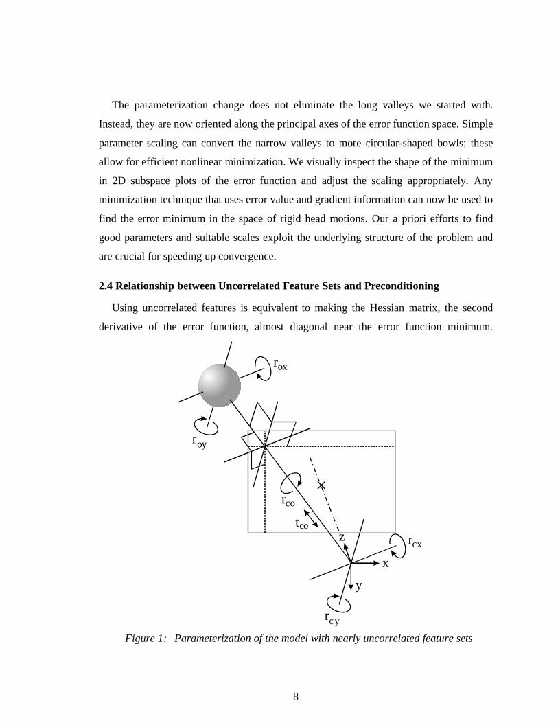
Figure 1: Parameterization of the model with nearly uncorrelated feature sets 7

Figure 2: Overview of the parallel minimization algorithm with adaptive test

point generation.

12

Table 1: The four estimation steps done for every camera frame. 13

Figure 3: The system structure and the flow of data. 13

Figure 4: The average amount of computation time per cluster node per frame. 15

Figure 5: The decomposition of the total time spent on one frame into pyramid

generation, OpenGL, and match computation.

16

Figure 6: Rendering and frame-buffer read speed for various system

configurations.

17

Figure 7: Frame rate depending on the number of participating cluster nodes and

the model of intra-node parallelism.

19

Figure 8: The various models of intra-node parallelism. 19

Figure 9: Frame rate as a function of the number of cluster nodes and the size of

the camera frame (1x = real frame size, 14.4 KB).

21

Figure 10: Delay per frame due to network transport as a function of the number

of cluster nodes and the size of the camera frame.

22

Figure 11: Network throughput as a function of the number of cluster nodes and

the size of the camera frame

23

v

Summary

We describe an implementation of a model-based head tracking system on a

workstation cluster. The system creates a textured model of the user’s head. This model is

rendered and matched with the image of the head by finding the six rotation and

translation parameters. To find these parameters, the system generates a set of test

parameters, which are clustered around the current head position. The test parameters are

generated adaptively from the previous motion of the head. Each cluster node then

evaluates the matching error and its gradient for some number of test parameters. A

central node then pools this information by fitting a quadratic to the matching error data

and thereby computes a new parameter estimate.

1

Chapter 1

Introduction

Computer vision is an area with high computational demands, which naturally lead to

implementations on parallel systems. In this paper we show the parallelization of a head

tracking system on a workstation cluster. Head tracking is an important processing step

for many vision-driven interactive user interfaces. The obtained position and orientation

allow for pose determination and recognition of simple gestures such as nodding and

head shaking. The stabilized image obtained by perspective de-warping of the facial

image according to the acquired parameters is ideal for facial expression recognition [9]

or face recognition applications.

In contrast to scientific numerical computations, head tracking requires real-time

operation. We use a particular algorithm for head tracking that matches a rendered image

of the head with the camera image. We will show how the real-time requirement and the

particular algorithm used affects the chosen strategy of parallelization, and we will show

a new parallel minimization technique particularly suited to our problem.

1.1 Previous Work

Much research effort has been expended on locating and tracking heads and

recognizing pose and facial expressions from video. Face detection is still considered a

2D problem where facial features, facial color, and the shape of the face are obtained

from the image plane for locating the head [14, 15]. To extract 3D parameters, a model

that encodes head orientation and position must be used. All approaches mentioned here

including our own method require some initialization of a model to a face.

Black and Yacoob [4] use a rectangular planar patch under affine transformation as a

face model. Similar patches are attached to the eyebrows and the mouth. They follow the

movements of the underlying facial patch but detect differential movements of their facial

parts. Affine motion, like any 2D model, is limited because it has no concept of self-

occlusion which occurs at the sides of the head and around the nose. Affine

2

transformations also distort the frontal face image when they are used to model larger

rotations.

Azarbayejani et al. [1] use feature point tracking projected on an ellipsoidal model to

track the head position. Feature point tracking has the drawback that tracking fails when

the feature points are lost due to occlusions or lighting variations. New feature points are

acquired, but only at the cost of excessive error accumulation.

Jebara and Pentland [12] also use feature point tracking, but with automatically

located head features like eyes and mouth corners. The 3D position of the feature points

is estimated using a structure from motion technique that pools position information over

the image sequence with an extended Kalman filter. The estimate of the feature point

position is filtered using Eigenfaces [14] to restrict the measurements to match an

expected facial geometry.

Basu, Essa and Pentland [2] couple an ellipsoidal model with general optical flow

computation for tracking. First, optical flow is computed independently of face position

and orientation using a gradient-based method. Then the motion of an ellipsoidal mesh

regularizes the flow. The method’s strengths are also its weaknesses. It copes well with

large head rotations since it does not rely on any fixed features. For the same reason, it

has no means to ground the model to the face, thus the mesh slowly drifts off the face due

to error accumulation.

La Cascia, Isidoro and Sclaroff [5] use a textured cylinder as a head model. The

approach is most similar to ours because it also uses a three-dimensional textured model.

The technique differs from ours in that it uses a cylinder instead of a full head model and

it updates its texture during tracking. The lack of fixed features again leads to error

accumulation although confidence maps are used to minimize this problem.

DeCarlo and Metaxas [6] use a polygonal head model that is hand-positioned on the

subject’s face. While our method uses texture, theirs extracts optical flow at some feature

points and regularizes it by the model movements. The measurements are stabilized using

a Kalman filter. Using optical flow leads to a similar error accumulation as in [2].

3

However, their system additionally uses face edge information to prevent divergence.

This work also extracts face shape and facial expressions.

Parallel computation methods for visual tracking have been used before [13], but there

is no work on parallel high-level tracking for user interfaces, such as head tracking.

1.2 Our Approach

We use a 3D textured polygon model that is matched with the incoming video stream.

This model is manually aligned with the head in the first camera frame and textured with

the facial image of the user. For every camera frame, the color difference between a

rendered image of the model and the video image, in conjunction with the image

gradient, is then mapped to derivatives of our model parameters. They lead to a local

error minimum that is the best possible match between the rigidly transformed model and

the real video image. The technique can be seen as a more sophisticated regularization of

optical flow, similar in principle to the method presented by Black and Anandan in [3].

Our system allows for extraction of all six degrees of freedom of rigid motion, but is

slower than simpler 2D models, which do not account for accurate head shape and hidden

surfaces. We use two methods to improve the speed of our system.

We exploit graphics hardware to perform rendering and hidden surface removal in our

algorithm. While special hardware such as user-programmable DSPs to accelerate vision

applications is still expensive and not present in an ordinary PC, graphics hardware is

ubiquitous. For further speed-up we implemented this system on an 8-node workstation

cluster to achieve real-time performance.

4

Chapter 2

The Head Tracking Algorithm

For initialization, the user’s head in the video stream is manually aligned with a

generic polygonal head model. Our model is a male head from Viewpoint Data Labs,

which we simplified to contain 500 triangles. The model is taken as is and is not

customized to the test user’s head.

The head model is textured with the facial image of the user. Tracking is achieved by

rotating and translating the now textured model so that the rendering of the model

matches the image of the head in the video-stream.

2.1 The Error Function

In this section we derive our algorithm for the case of an arbitrary camera

transformation and arbitrary motion model. For our application, we approximate the

camera transformation with a pinhole model and a rough estimate of the focal length. The

parameter set {αi} is six-dimensional, for the six degrees of freedom of rigid motion.

This specialization of the algorithm for our application will be shown in Section 2.2.

Let {p} be the set of visible points on the 3D head model with an associated texture

intensity M(p), and let I(x) be the intensity at point x in the camera picture. Let the

transformation T represent any motion and projection model, which maps from some

model point p to screen coordinates with a parameter set {αi}. We minimize the sum over

the robust difference between the projected texture points and the corresponding points in

the camera image:

( )E I T Mi= −∑ ρ α( ( ,{ })) ( ){ }

p pp

,

where ρ is the Geman & McClure robust error norm [11] defined as

ρσ

( )xx

x=

+

2

2 .

5

Here, σ controls the distance beyond which a measurement is considered an outlier

[3]. The error function derived with respect to a particular parameter αj is

( )dE

dI T M

dI T

dji

i

jαψ α

αα

= −∑ ( ( ,{ })) ( )( ( ,{ })

{ }

p pp

p,

where ψ designates the derivative of ρ. Expanding the second term to evaluate it as a

linear combination of the image intensity gradients gives

dI T

d

dI T

dT

dT

d

dI T

dT

dT

d

i

j

i x

i x

i x

j

i y

i y

i y

j

( ( ,{ })) ( ( ,{ }))

( ,{ })

( ,{ })

( ( ,{ }))

( ,{ })

( ,{ })

p p

p

p

p

p

p

αα

αα

αα

αα

αα

= ⋅

+ ⋅.

The first factors of the terms are just the image intensity gradient at the position

T(p,{αi}) in the x and y directions, written as Ix and Iy:

dI T

dI T

dT

d

I TdT

d

i

jx i

i x

j

y ii y

j

( ( , { }))( ( ,{ }))

( , { })

( ( , { }))( , { })

pp

p

pp

αα

αα

α

αα

α

= ⋅

+ ⋅.

We use the Sobel operator to determine the intensity gradient at a point in the image.

Note that in this formulation the 3D model, its parameterization, and the 3D to 2D

transformation used are arbitrary provided the model can be rendered onto the screen.

2.2 Special Case: Rigid Transformation and Perspective Projection

For our more specific case we use the transformation matrix, written in homogeneous

coordinates, going from 3D to 2D:

1

0

0

0

1

0

0

0

0

0

0

1 0 0

0 1 0

0 0 1

0 0 0 11f

t

t

tR R R

x

y

zz y x

−

⋅

−−−

⋅ ,

with Rx, Ry, and Rz being rotation matrices around the x, y, and z axis, for some angles

rx, ry, and rz respectively. tx, ty, and tz are translations along the axes. We assume that the

6

focal length f is known, but found that a rough estimate gives good results. Without loss

of generality, we assume that rx=ry=rz=tx=ty=tz=0, which corresponds to a camera at the

origin looking down the positive z-axis. Note that in this case the order of rotations does

not affect our calculations.

Omitting the parameters of I, Ix, and Iy, we obtain as derivatives of the intensity with

respect to our parameters for a particular model point p = (px, py, pz)T

dI

drf

I p p I p p

px

y y z x x y

z

= −+ +( )2 2

2 ,

dI

drf

I p p I p p

py

x x z y x y

z

=+ +( )2 2

2 ,

dI

drf

I p I p

pz

y x x y

z=

−,

dI

dtf

I

px

x

z= − ,

dI

dtf

I

py

y

z= − ,

dI

dtf

I p I p

pz

x x y y

z

=+

2 .

For color video footage we use the Geman & McClure norm on the distance in RGB

space rather than on each color channel separately. σ is set such that anything beyond a

color distance of 50 within the 2563 color cube is considered an outlier. We sum the

results of each color channel to obtain a minimum error estimate.

2.3 Model Parameterization with Uncorrelated Feature Sets

The parameterization given above is not adequate for implementation because the

rotations and translations of the camera used in the parameterization look very similar in

the camera view resulting in correlated feature sets. For example, rotating around the y-

axis looks similar to translating along the x-axis. In both cases the image content slides

horizontally, with slight differences in perspective distortion. In the error function space

7

this results in long, narrow valleys with a very small gradient along the bottom of the

valley. It destabilizes and slows down any gradient-based minimization technique.

A similar problem is translation along and rotation around the z-axis, which causes the

image of the head not only to change size or to rotate, but also to translate if the head is

not exactly in the screen center.

To overcome these problems we choose different parameters for our implementation

than those given in 2.2. They are illustrated in Figure 1.

We again assume that the camera is at the origin, looking along positive z, and that the

object is at some point (ox, oy, oz). Note that the directions of the rotation axes depend on

the position of the head. rcx and rcy have the same axis as rox and roy, respectively, but

rotate around the camera as opposed to around the object. rcx and rox are orthogonal to

both the connecting line between the camera and the head, and to the screen’s vertical

axis. Rotation around rcx causes the head image to move vertically on the screen, but it is

not rotating relative to the viewer and it does not change its horizontal position. Rotation

around rox causes the head to tilt up and down, but keeps its screen position unchanged.

rcy and roy are defined similarly for the screen’s horizontal coordinate. Note that rcy/roy

and rcx/rox are not orthogonal except when the object is on the optical axis. However, the

pixel movement on the screen that is caused by rotation around them is always

orthogonal. It is vertical for the rcy/roy pair and horizontal for the rcx/rox pair.

Rotation around rco causes the head’s image to rotate around itself, while translation

along tco varies the size of the image. Neither changes the head screen position.

The parameterization depends on the current model position and changes while the

algorithm converges. Different axes of rotation and translation are used for each iteration

step.

We now have to find the derivatives of the error function with respect to our new

parameter set. Fortunately, in Euclidean space any complex rotational movement is a

combination of rotation around the origin and translation. We have already calculated the

derivatives for both in section 2.2. The derivatives of our new parameter set are linear

combinations of the derivatives of the naïve parameter set.

8

The parameterization change does not eliminate the long valleys we started with.

Instead, they are now oriented along the principal axes of the error function space. Simple

parameter scaling can convert the narrow valleys to more circular-shaped bowls; these

allow for efficient nonlinear minimization. We visually inspect the shape of the minimum

in 2D subspace plots of the error function and adjust the scaling appropriately. Any

minimization technique that uses error value and gradient information can now be used to

find the error minimum in the space of rigid head motions. Our a priori efforts to find

good parameters and suitable scales exploit the underlying structure of the problem and

are crucial for speeding up convergence.

2.4 Relationship between Uncorrelated Feature Sets and Preconditioning

Using uncorrelated features is equivalent to making the Hessian matrix, the second

derivative of the error function, almost diagonal near the error function minimum.

Figure 1: Parameterization of the model with nearly uncorrelated feature sets

z

y

x

r

r

r

r

r

cx

ox

cy

oy

co

co

t

9

Choosing an appropriate scale for each of the parameters brings the condition number of

the Hessian matrix close to unity, which is the goal of preconditioning in a general

nonlinear minimizer. In our case we use a priori knowledge to avoid any analysis of the

error function during run-time.

2.5 Gaussian Pyramid

To allow larger head motions, a 2-level Gaussian pyramid is used. First, the model is

rendered at a lower resolution, and is compared with a lower resolution camera image.

Once the minimization is completed at this level, the minimizing parameter set is used as

a starting point for the minimization process at full resolution.

2.6 Using OpenGL for Rendering

For each evaluation of the error gradient, two OpenGL renderings of the head are

performed. The first rendering is for obtaining the textured image of the head using

trilinear mipmapping to cope with the varying resolution levels of the pyramid. The

second rendering provides flat-filled aliased polygons. Each polygon has a different color

for visible surface determination in hardware. All transformations into camera and screen

coordinates and the calculations of gradients to compute the parameter derivatives are

done only for visible surfaces of the model.

10

Chapter 3

Parallel Implementation

Using conjugate gradient with adaptive step size as a sequential minimization

algorithm on a single machine we obtain a computation time of .9 frames/s. To get real-

time performance we ported the algorithm to a PC cluster.

3.1 Parallelization by Parameter Testing

We need to exploit the additional computation power to search the six-dimensional

space of rigid head-motions for an error minimum. We parallelize the system by

performing multiple evaluations of the matching error and the gradient in parallel and

pool the information from all evaluations to obtain a better estimate of the error

minimum. This has the advantage of incurring only a single round-trip communication

per evaluation. In addition, all information specific to a single evaluation is local to a

specific node.

We evaluate the error and its gradient at some test points distributed around the

current head position. We then find the test point with lowest error, and estimate the

Hessian at this point by fitting a quadratic to this point and its six nearest neighbors. Let

{(xi, ei, gi) | i=1...7}

be the set of seven test points with lowest error where xi is the ith parameter vector, ei

is the corresponding error and gi is the error gradient, with ei ≤ ej for i ≤ j. We assume

without loss of generality x1 = 0. Then the parameters of the quadratic

xTAx + bTx + c = 0

are c = e1, b = g1 and

11

A w A c e

w A

A E i i i ii

g i ii

= + + −

+ + −

=

=

∑

∑

min x x b x

x b g

T T

2

2

7

2

2

7.

The quadratic matches the error and the gradient of the lowest test point exactly, and

approximates the gradient and error at the rest of the points in a least square sense. By

plotting some slices through the error function we validate that a quadratic is a good fit

for the error function close to the minimum. By matching the error and gradient at the

lowest test point we assure that the quadratic will be an accurate fit around the lowest

point, which is the best indication of the minimum location that we have.

If the minimum of the quadratic is within some distance r from the lowest point, the

position of the minimum is the new error function minimum estimate. If the minimum of

the quadratic is farther away, or does not exist at all because the quadratic is concave, the

lowest point of the quadratic with the distance r is taken as the new minimum. This

corresponds to the trust region approach used for general nonlinear minimization. We use

the hook-step approximation for our implementation [7].

3.2 Minimization Schedule and Generating Test Points

To find an initial estimate of the error minimum, when a new camera frame is

processed, an adaptive method is used to generate the test points. It takes the previous

head position as its starting point and uses an adaptive set of test points that are generated

along the linearly extrapolated path of head motion. If the head motion is faster and the

extrapolated path is longer, more points are generated to keep the distance between test

points approximately equal. As described only the test point with lowest error and the 6

points closest to this one are used for the quadratic interpolation. Figure 2 shows the

position of the generated points and some other algorithm features for an equivalent

scheme in 2D.

To refine the initial estimate, a different point generation method uses the previous

estimate as a starting point. Instead of adaptively selecting test points this method always

12

uses seven test points arranged in a six-dimensional triangle or tetrahedron, with the

previous estimate at the center of gravity. The orientation of the tetrahedron is chosen

arbitrarily. Since there are only seven points all test points are used to fit the quadratic.

For every camera frame, four estimates are obtained. Table 1 shows the distance

between test points (step length) and the level of the Gaussian pyramid that is used for

every step.

Step Starting Point Step Length Pyramid Level Point Generation

1 Estimate of previous frame 4 units low res adaptive

2 Estimate of 1st step 2 units low res tetrahedron

3 Estimate of 2nd step 2 units high res tetrahedron

4 Estimate of 3rd step 1 unit high res tetrahedron

Table 1: The four estimation steps done for every camera frame.

xt+1

xt

^

trust region with fitted quadratic.

new estimatederror minimum

other points definingthe quadratic

test point withlowest error

test points

system state at time t-1: xt-1

Figure 2: Overview of the parallel minimization algorithm with adaptive test point

generation.

13

Chapter 4

System Structure and Implementational Details

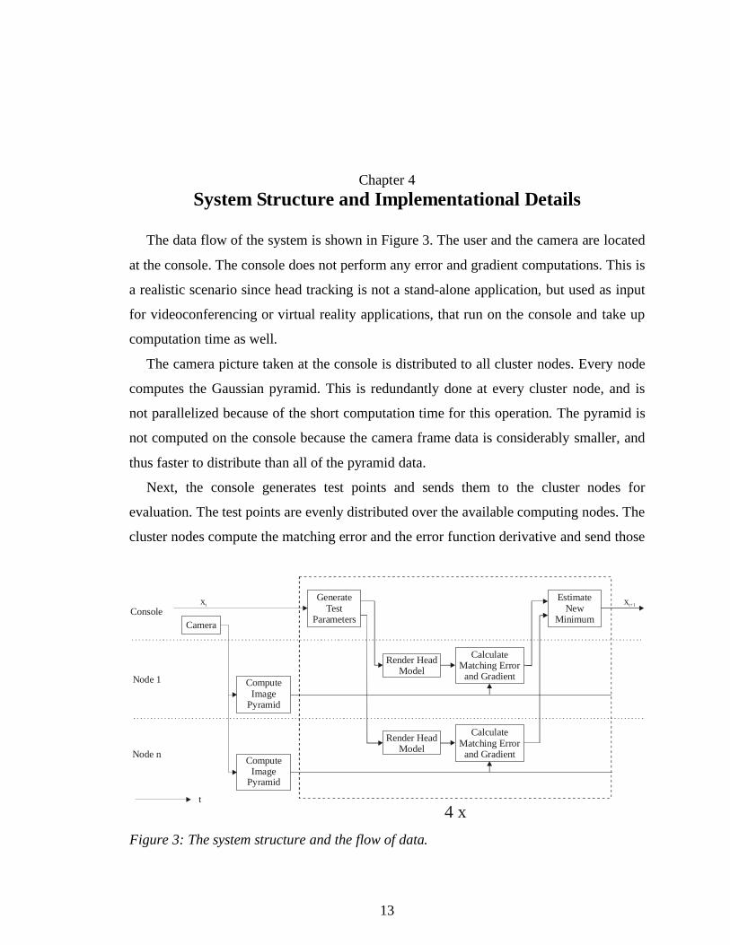
The data flow of the system is shown in Figure 3. The user and the camera are located

at the console. The console does not perform any error and gradient computations. This is

a realistic scenario since head tracking is not a stand-alone application, but used as input

for videoconferencing or virtual reality applications, that run on the console and take up

computation time as well.

The camera picture taken at the console is distributed to all cluster nodes. Every node

computes the Gaussian pyramid. This is redundantly done at every cluster node, and is

not parallelized because of the short computation time for this operation. The pyramid is

not computed on the console because the camera frame data is considerably smaller, and

thus faster to distribute than all of the pyramid data.

Next, the console generates test points and sends them to the cluster nodes for

evaluation. The test points are evenly distributed over the available computing nodes. The

cluster nodes compute the matching error and the error function derivative and send those

Figure 3: The system structure and the flow of data.

Node 1

Node n

Console

t

ComputeImage

Pyramid

Camera

ComputeImage

Pyramid

xtGenerate

TestParameters

Render HeadModel

CalculateMatching Error

and Gradient

Render HeadModel

CalculateMatching Error

and Gradient

EstimateNew

Minimum

xt+1

4 x

14

results back to the console, where the quadratic is fitted into the measured data points and

a new minimum estimate is calculated.

This process is repeated four times, with parameters as shown in Table 1, for every

camera frame. Then a new camera frame is read.

We implemented the system on a 8-node cluster of Pentium Pro 200 Mhz PCs with 4

processors each. The operating system is Windows NT. One node is used as the console,

and one to seven other nodes are used for computation. For message passing we use the

DataExchange system [8] that is implemented on top of the WinSock API, and for

multithreading the NT-native Win32 threads.

We use an image resolution of 80x60 pixels, with a second Gaussian pyramid level of

40x30 pixels. We use both live video feeds and prerecorded sequences. All our footage is

in color.

Our model is a male head from Viewpoint Data Labs, which we simplified to contain

500 triangles. The model is taken as is and is not customized to the test user’s head.

Our implementation uses Microsoft OpenGL under Windows NT for rendering. This

implementation only uses a single processor even on multiprocessor machines. It also

does not allow multiple threads to issue commands to the same OpenGL window.

15

Chapter 5

Results

The system works best on seven processors. The tetrahedron scheme generates seven

test points and is always used for estimation iterations two to four. The adaptive scheme

generates a multiple of seven points, but is only used for the first estimate of every

camera frame. With our test sequence, the adaptive scheme generated 7 points for 40 %

of the frames, 14 for the rest.

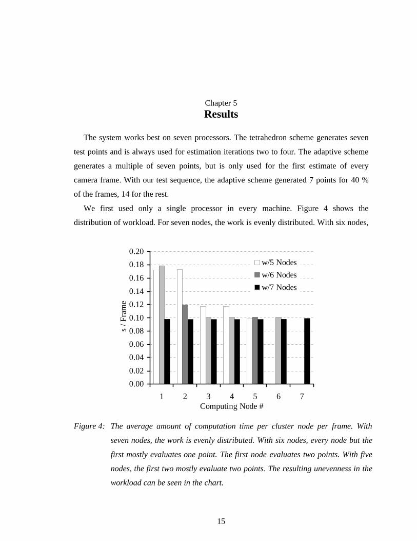
We first used only a single processor in every machine. Figure 4 shows the

distribution of workload. For seven nodes, the work is evenly distributed. With six nodes,

0.00

0.02

0.04

0.06

0.08

0.10

0.12

0.14

0.16

0.18

0.20

1 2 3 4 5 6 7Computing Node #

s / F

ram

e

w/5 Nodes

w/6 Nodes

w/7 Nodes

Figure 4: The average amount of computation time per cluster node per frame. With

seven nodes, the work is evenly distributed. With six nodes, every node but the

first mostly evaluates one point. The first node evaluates two points. With five

nodes, the first two mostly evaluate two points. The resulting unevenness in the

workload can be seen in the chart.

16

for the frequently used tetrahedron scheme the first node always gets two test points to

evaluate, all others get one, and for the tetrahedron scheme, the first two nodes get three

points and the others two. This is clearly visible in the graph. A similar pattern exists for

all node counts, but it is less noticeable for node counts smaller than 5. As a consequence,

the frame rates with five and six nodes are almost equal, and with seven nodes the frame

rate increases sharply.

Figure 5 decomposes the sum of processor time of all the nodes into the time spent on

Gaussian pyramid generation, OpenGL rendering, and the calculation of the matching

error and gradient. Note that the total time is about equal for different numbers of nodes,

for more numbers of nodes it is just more distributed among the nodes. This chart also

does not include network overhead and processor time on the console. The time spent on

Gaussian pyramid generation grows with the number of nodes, because this operation is

done on every node. About 75 % of the total time is spent on OpenGL operations. As part

of our effort to make efficient use of the machine resources, we looked for ways to speed

0.0

0.1

0.2

0.3

0.4

0.5

0.6

0.7

0.8

1 2 3 4 5 6 7# of Computing Nodes

s / F

ram

e

Pyramid GenerationOpenGL

Match Computation

Figure 5: The decomposition of the total time spent on one frame into pyramid

generation, OpenGL, and match computation.

17

up this most expensive part of our algorithm. The Microsoft software implementation of

OpenGL under NT does not make any use of multiprocessing and the use of different

threads to render different tiles of the image seemed unattractive because of the geometry

overhead. A natural way to speed up OpenGL is to make use of hardware acceleration.

5.1 Hardware OpenGL

Instead of using OpenGL for displaying purposes, rendering is used in our system as

part of the computation. After rendering, the image is copied out of the frame buffer into

main memory for further processing using a glReadPixels call. For software OpenGL,

the frame buffer is located in main memory, while hardware solutions only render into

their on-board memory, which our program then reads from.

We use a Diamond FireGL 1000pro PCI with the 3Dlabs Permedia 2 accelerator chip

in one of our cluster nodes. We also tried the AGP version of the same card in a 400 Mhz

Pentium II Xeon, an ATI Rage Pro AGP card in the same machine, and finally an SGI

320 workstation with a 450 MHz Pentium II, representing the state of the art in hardware

Figure 6: Rendering and frame-buffer read speed for various system configurations.

0.0

0.1

0.2

0.3

0.4

0.5

0.6

PPro200 SW

PPro200

FireGLPCI

P2 400 SW

P2 400FireGLAGP

P2 400RagePro

AGP

SGI 320SW

SGI 320HW

s / F

ram

e

glReadPixels

Rendering

18

rendering. All machines are used as a single computation node. For comparison purposes,

we also tested software rendering performance on all machines. Figure 6 shows the time

spent on OpenGL per camera frame.

Hardware rendering is faster than software rendering, except for the ATI Rage Pro

card. Unfortunately, reading the frame buffer for hardware rendering is always slower

than for software rendering and uses up some of the rendering speed increase. The fact

that the data has to go over the I/O bus, whether it is PCI or AGP, seems not to be the

decisive factor. The SGI 320 workstation, which has a UMA architecture, is about as fast

as the FireGL AGP card. Some measurements with the GLPerf benchmark yielded

around 6 Mpixels/s for the FireGL AGP card, much less than the AGP bus bandwidth

allows.

We found an indication that there are inefficiencies in the OpenGL drivers

contributing to the problem. We performed all the hardware speed measurements using

the GL_RGB pixel format. If the Microsoft-proprietary GL_BGR_EXT format is used,

which only differs by a swapped byte order, glReadPixels performance drops by a factor

of 14 for the FireGL, and by a factor of 30 for the SGI 320, making hardware rendering

unusable. The Rage Pro card does not show this anomaly, but glReadPixels is in general

very slow with this card.

Despite the performance flaws, the results show that using hardware OpenGL is worth

doing. The appearance of benchmarks that give more detailed information, like GLPerf,

will hopefully make driver deficiencies more apparent, and encourage video card

manufacturers to deliver consistently performing drivers.

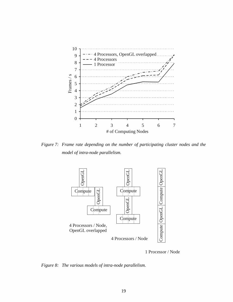
5.2 Intra-Node Parallelism

The second largest part of the computing time is the computation of the matching error

and the gradient. We make use of the four processors per machine to speed up this

computation. We tried two models of parallelism. The first just distributes the match

computation to all n processors by processing the ith scanline of the image by the

19

Figure 7: Frame rate depending on the number of participating cluster nodes and the

model of intra-node parallelism.

Figure 8: The various models of intra-node parallelism.

4 Processors / Node,OpenGL overlapped

4 Processors / Node

1 Processor / Node

Ope

nGL

Ope

nGL

Ope

nGL

Ope

nGL

Ope

nGL

Com

pute

Com

pute

Ope

nGL

Compute

Compute Compute

Compute

0

1

2

3

4

5

6

7

8

9

10

1 2 3 4 5 6 7# of Computing Nodes

Fram

es/s

4 Processors, OpenGL overlapped4 Processors1 Processor

20

(i mod n)th processor. With this scheme the computation time for matching is reduced to a

third on a four-processor machine. We then overlapped this computation with the

OpenGL rendering process to utilize some of the other processor’s time while the single-

thread OpenGL rendering is running. Figure 8 compares the modes of intra-node

parallelism that we used and Figure 7 shows the performance of our system.

The performance gain from switching from one to four processors is as expected. The

benefits of overlapping OpenGL with computation are especially small for seven nodes

because in this case every node mostly calculates a single matching error and gradient.

Overlapping OpenGL is only rewarded when the adaptive scheme generates 14 test

points and every node evaluates two points.

5.3 Network Performance

The system uses the network to distribute frame data and to exchange requests and

answers of data point evaluations. For each of the four estimation iterations a batch of

requests is sent out to every node. For the first evaluation cycle the request batch includes

the new frame data. The cluster nodes send their results back, and once all results have

arrived a new estimate is generated and new batches of requests are sent out.

We tested the influence of network performance on our system. The evaluation request

messages and results are on the order of a hundred bytes. The only sizable messages are

those that distribute the frame among all cluster nodes. A typical frame has 80x60 pixels

resolution with 24 bit color depth, which results in 14.4 KB frame size. We test the

impact of network traffic by using frame sizes of 28.8 KB (2x original), 43.2 KB (3x),

144 KB (10x) and 576 KB (40x). To avoid side effects these frame sizes are tested by

padding the network packets, not by actually using a higher resolution. Besides the frame

rate (Figure 9), we also measured how much the network delays the computation (Figure

10). This measurement is calculated as the time the console spends waiting for the

network minus the longest time any computing node spends on its computation. The

console’s waiting time can sometimes be shorter than the computation time of the longest

computing node. This is because instead of idling the console did some useful work

21

processing results arriving early. This explains the low network delays for five and six

nodes (see Figure 4 and the discussion in chapter 5).

There are two other effects affecting network delay. If less computing nodes do all the

computation and have to send all the answers back to the console, then more time per

node is spent on network operations, which leads to higher network delay. On the other

hand, distributing the frame data takes longer for more nodes, which also leads to higher

network delay. Therefore, disregarding the anomalies for five and six frames, the network

delay graph is U-shaped, with a minimum at three nodes, or at two nodes for 3x frame

size.

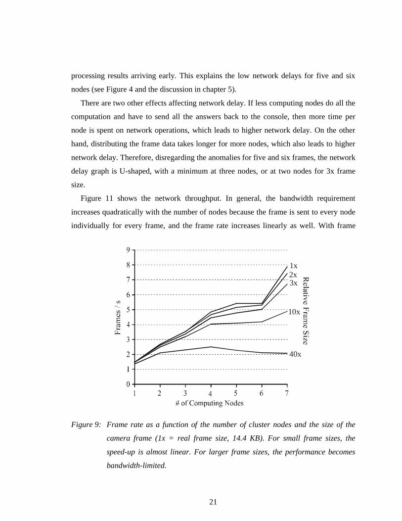
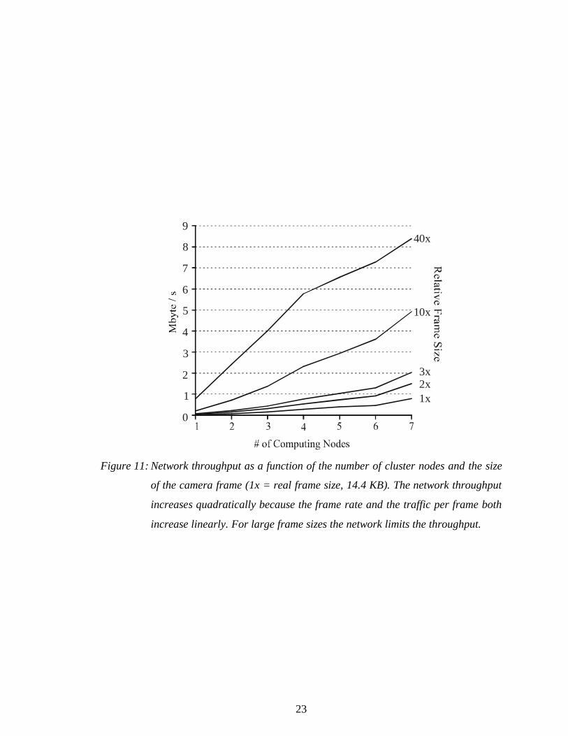
Figure 11 shows the network throughput. In general, the bandwidth requirement

increases quadratically with the number of nodes because the frame is sent to every node

individually for every frame, and the frame rate increases linearly as well. With frame

Figure 9: Frame rate as a function of the number of cluster nodes and the size of the

camera frame (1x = real frame size, 14.4 KB). For small frame sizes, the

speed-up is almost linear. For larger frame sizes, the performance becomes

bandwidth-limited.

40x

10x

2x3x

1x

22

sizes of 10x and larger, though, the 100 Mbit/s bandwidth limitation of the network

becomes apparent. For 40x the original frame size, bandwidth limitations lead to a

decrease in frame rate when more than 4 nodes are used.

Our underlying message library, DataExchange, does not support multicast or

broadcast. Such capabilities could be used to decrease traffic, but the speed-up would be

minor for the regular frame size.

2x

3x

1x

35

30

25

20

15

10

5

0

Figure 10: Delay per frame due to network transport as a function of the number of

cluster nodes and the size of the camera frame (1x = real frame size, 14.4

KB). On one hand, for a small number of nodes a single node has to send

many answers, which increases delay. On the other hand, for more nodes

distributing the frame data takes longer. Therefore, the network delay graph

is in general U-shaped

23

2x3x

10x

1x

0

1

2

3

4

5

6

7

8

940x

Figure 11: Network throughput as a function of the number of cluster nodes and the size

of the camera frame (1x = real frame size, 14.4 KB). The network throughput

increases quadratically because the frame rate and the traffic per frame both

increase linearly. For large frame sizes the network limits the throughput.

24

Chapter 6

Discussion

6.1 Reasons For Introducing a New Parallel Convex Minimization Scheme

The naive way to parallelize convex nonlinear optimization is to stick to a sequential

algorithm, but to parallelize the computation of the gradient. The number of iteration

steps required for convergence remains unchanged. The sequential version of our

algorithm uses conjugate gradient minimization with adaptive step size and requires on

average 42 error and gradient evaluations at the lower resolution and 35 evaluations at the

higher resolution of the Gaussian pyramid to converge. For every camera frame the

image has to be distributed across the cluster. Also, for every iteration step round-trip

message costs are incurred to send out messages to all the cluster nodes and to get the

results back. Using the NetPerf benchmark, we calculated that for a single computation

node the network overhead would be at least 33 ms per camera frame, compared to 6 ms

in practice for our current implementation. Another issue is that OpenGL rendering had

to be parallelized by rendering a tile of the whole frame per node. This does not scale

well, because clipping and geometry transformations have to be done for every cluster

frame. The only exploitable parallelism is the scan conversion. All in all, distributed error

and gradient evaluation is not an attractive option.

In order to obtain more coarse-grain parallelism, common parallel implementations of

convex nonlinear minimization techniques rely on partitioning the problem space into

subspaces of smaller dimensionality. These subspaces are minimized individually on

each node with periodic synchronization between processors. Several variants of this

technique exist; they belong to the class of Parallel Variable Transformation (PVT)

algorithms [10]. These rely on the assumption that the computational load is proportional

to the number of partial derivatives computed. In our case, we have to render the head

model entirely, which takes a large constant amount of time, no matter the dimensions of

the subspace in which the derivative is computed. Also, the number of processors has to

25

be considerably smaller than the number of dimensions. Otherwise, each processor

receives only a trivially small subspace. This would result in each processor spending

much less time on minimization of the subspace than on sequential synchronization

between processors. Unfortunately, in our case the number of dimensions is small since

rigid motion has only six degrees of freedom, which is in the order of the number of

nodes.

6.2 Future Work

Our approach uses efficiently up to 7 cluster nodes, because a quadratic is defined in

6D by a minimum of 7 points. For large head motions, more cluster nodes are adaptively

used if available.

All minimization methods require some model of the error space, and they become

more efficient if a better-suited model is used. Steepest descent is outperformed by

quadratic methods, which again are surpassed by tensor methods. Likewise, to exploit

more parallelism for small-dimensional problems an even better model of the error space

will be necessary to make use of a greater number of parallel gradient evaluations. Future

work may explore self-adjusting models like neural networks. These may be a good

choice for a real-time system similar to the one discussed in this paper that has to do a

large number of minimizations in a similar error space. It can learn how to generate a

good set of test points and to calculate a new estimate of the minimum from the results of

the tests.

Likewise, the performance for less than seven nodes is not satisfactory. The system

should generate a set of test points that is as large as the number of available nodes, pool

the information, and then generate the next suitable test set. This would generate equal

load on all the nodes, and should have the potential to converge faster, because new

information is incorporated into the solution earlier and can influence the location of

subsequent test points.

26

Chapter 7

Conclusion

We believe that real-time speed is a major requirement for successful and usable

vision systems. Unfortunately, for a long time to come, real-time implementations of

some vision systems will be impossible on a single desktop machine. Parallel algorithms

for real-time vision will remain an active area of research.

We presented model-based head tracking as an example of a low-dimensional real-

time minimization problem, and its parallel solution using a test point based minimization

scheme. We looked at some of the factors that influenced our design decisions and

affected the performance of our system. With 9 frames/s on the available hardware, we

achieved our goal of real-time head tracking. Using current OpenGL hardware like the

SGI 320 graphics pipeline, or a consumer-level accelerator like the Riva TNT, we expect

to be able to process up to 30 frames/s. The presented tracking technique is not specific to

heads. By using a different 3D model, it is generally applicable for parallel model-based

rigid as well as non-rigid tracking.

By using OpenGL for rendering we can leverage off the current growth of hardware

rendering acceleration. Currently, graphics performance is growing much faster than

processor speed, so the gap between hardware and software rendering will widen even

more in the future.

27

References

[1] A. Azarbayejani, T. Starner, B. Horowitz, and A. Pentland. Visually controlled

graphics. PAMI, 15(6), 1993.

[2] S. Basu, I. Essa, A. Pentland. Motion regularization for model-based head tracking.

ICPR, 1996.

[3] M. Black, P. Anandan. The robust estimation of multiple motions: parametric and

piecewise-smooth flow fields. TR P93-00104, Xerox PARC, 1993.

[4] M. J. Black, Y. Yacoob. Tracking and recognizing rigid and non-rigid facial motions

using local parametric models of image motions. ICCV, 1995.

[5] M. La Cascia, J. Isidoro, S. Sclaroff. Head tracking via robust registration in texture

map images. CVPR, 1998.

[6] D. DeCarlo, D. Metaxas. The Integration of Optical Flow and Deformable Models

with Applications to Human Face Shape and Motion Estimation. CVPR 1996.

[7] J. E. Dennis, R. B. Schnabel. Numerical Methods for Unconstrained Optimization

and Nonlinear Equations, ch. 6. Prentice-Hall 1993.

[8] Greg Eisenhauer, Beth Plale, Karsten Schwan. DataExchange: High Performance

Communication in Distributed Laboratories. Journal of Parallel Computing, Number

24, 1998, pages 1713-1733.

[9] I. Essa, A. Pentland. Coding analysis, interpretation, and recognition of facial

expressions. PAMI, 19(7): 757-763, 1997.

[10] Masao Fukushima. Parallel Variable Transformation in Unconstrained Optimization.

SIAM J. Optim., Vol. 8. No. 4, pp. 658-672, August 1998.

[11] S. Geman, D. E. McClure. Statistical methods for tomographic image

reconstruction, Bull. Int. Statist. Inst. LII-4, 5-21, 1987.

[12] T. S. Jebara, A. Pentland. Parameterized Structure from Motion for 3D Adaptive

Feedback Tracking of Faces. CVPR 1997.

28

[13] M. Mirmehdi, T. J. Ellis. Parallel Approach to Tracking Edge Segments in Dynamic

Scenes. Image and Vision Computing 11: (1) 35-48, 1993.

[14] A. Pentland, B. Moghaddam, T. Starner. View-Based and Modular Eigenspaces for

Face Recognition. CVPR 1994.

[15] H. A. Rowley, S. Baluja, T. Kanade. Human Face Detection in Visual Scenes.

CVPR 1998.