Adaptive Methods for the Vlasov Equation

Eric Sonnendrucker

IRMA, Universite de Strasbourg and CNRS

projet CALVIINRIA Lorraine

MAMCDP09 Workshop, Paris, 22-23 January 2009

in collaboration with N. Besse, M. Campos Pinto, M. Gutnic,G. Latu, M. Mehrenberger

Outline

1 Application: Controlled Fusion

2 Mathematical modeling of charged particles

3 Important features of the Vlasov equation

4 Grid based methods for the Vlasov equationProblems with grid based methodsMotivation for adaptive gridsHierarchical approximation and local adaptivity

Hierarchical approximation based on interpolationg wavelets

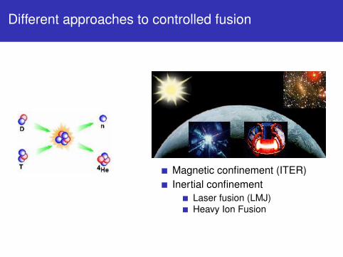
Different approaches to controlled fusion

Magnetic confinement (ITER)Inertial confinement

Laser fusion (LMJ)Heavy Ion Fusion

Heavy Ion Fusion

Kinetic models for plasmas and particle beams

In the sequel we shall consider only the collisionless relativisticVlasov-Maxwell equations

∂fs∂t

+p

msγs· ∇x fs + qs(E(x, t) +

pmsγs

× B) · ∇pfs = 0,

∂tE− c2∇× B = − Jε0, ∇ · E =

ρ

ε0,

∂tB +∇× E = 0, ∇ · B = 0,

where γ2s = 1 + |p|2

m2s c2 and the source terms are computed by

ρ =∑

s

qs

∫fs dp, J =

∑s

qs

ms

∫fs

pγs

dp.

In some cases Maxwell’s equations can be replaced by areduced model like Poisson’s equation.

Invariants of Vlasov-Maxwell system

Invariance along characteristics:

ddt

f (X (t),P(t), t) = 0

where X = Pmγ , P = q(E(X (t), t) + P(t)

mγ × B(X (t), t)).

Energy:∫

f (γ − 1) dx dp + 12(

∫(E2 + B2) dx .

Lq norms:∫

f q dx dp.Phase space volume:

∫V f (x ,p, t) dx dp.

Conservative form of Vlasov equation

∂f∂t

+∇x,p · (Ff ) = 0,

with F = ( pγm ,E + p

γm × B) so that ∇x,p · F = 0.

The backward semi-Lagrangian Method

f conserved along characteristicsFind the origin of the characteristicsending at the grid pointsInterpolate old value at origin ofcharacteristics from known grid values→ High order interpolation needed

Typical interpolation schemes.Cubic spline [Cheng-Knorr 1976,Sonnendrucker-Roche-Bertrand-Ghizzo 1998]Cubic Hermite with derivative transport[Nakamura-Yabe 1999]

Comparison of PIC and Eulerian methods

Particle-In-Cell (PIC) method is the most widely used.Pros:

Good qualitative results with few particles.Very good when particle dynamics dominated by fields whichdo not depend on particles (e.g. in accelerators when selffield small compared to applied field).More efficient when dimension is increased (phase-space =6D).

Cons Hard to get good precision : slow convergence,numerical noise, low resolution at high velocities.

Grid based Vlasov methodsPros High-order method, same resolution everywhere ongrid.Cons Needs huge computer ressources in 2D or 3D.

Problems with grid based methods

Numerical diffusionCurse of dimensionality: Nd grid points needed in ddimensions on uniform grids.Number of grid points grows exponentially with dimension→ killer for Vlasov equation where d up to 6.Memory needed

In 2D, 163842 grid → 2 GBIn 4D, 2564 grid → 32 GBIn 6D, 646 grid → 512 GB

Adaptive algorithm is a must in higher dimensions

A typical beam simulation

Semi-Gaussian beam in periodic focusing channelApplied field ~B = (−1

2B′(z)x , −12B′(z)y , B(z)), with

B(z) = B02 (1 + cos(2πz

s )), with B0 = 2 T and S = 1 m.Semi-Gaussian beam of emittance ε = 10−3,

f0(r , vr ,Pθ) =n0

πa2 exp(−v2r + (Pθ/(mr))2

2v2th

),

where Pθ = mrvθ + mB(z) r2

2 , n0 = Iqvz

, I = 0.05 A andE = 80 MeV so that vz = 626084 ms−1.

Semi-Gaussian beam in periodic focusing channel

Adaptive semi-Lagrangian method

Semi-Lagrangian method consists of two stages :advection and interpolationInterpolation can be made adaptive : approximate f n withas few points as possible for a given numerical error usingnon linear approximation.Construct approximation layer by layer, starting fromcoarse approximation and adding pieces to improveprecision where needed, using nested grids.It is possible to modify hierarchical decomposition so as toexactly conserve mass and any given number of momentseven when grid points are removed.

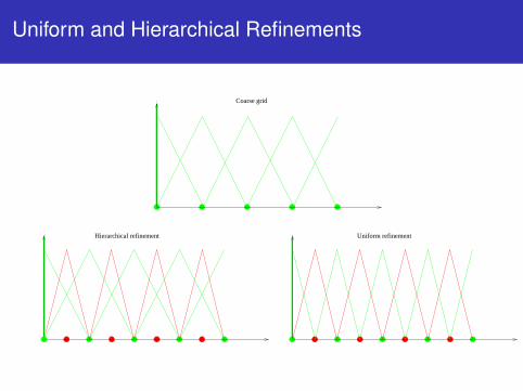
Uniform and Hierarchical Refinements

Coarse grid

Uniform refinement Hierarchical refinement

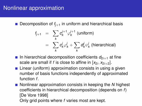
Nonlinear approximation

Decomposition of fj+1 in uniform and hierarchical basis

fj+1 =∑

k

c j+1k ϕj+1

k (uniform)

=∑

k

c jkϕ

jk +

∑k

d jkψ

jk (hierarchical)

In hierarchical decomposition coefficients d2i+1 at finescale are small if f is close to affine in [x2i , x2i+2].Linear (uniform) approximation consists in using a givennumber of basis functions independently of approximatedfunction f .Nonlinear approximation consists in keeping the N highestcoefficients in hierarchical decomposition (depends on f )[De Vore 1998]Only grid points where f varies most are kept.

Localization of points

PIC code non linear approximation

Construction of a hierarchical approximation

Hierarchical approximation is constructed by defining aninterpolation method enabling to go from coarse grid to finegrid.Two methods have been tried:

1 Interpolating wavelets based on Lagrange polynomialinterpolation. Classical wavelet compression technique.Addressed moment conservation issues[Gutnic-Haefele-Paun-Sonnendrucker 2004,Gutnic-Haefele-Sonnendrucker 2006].

2 Hierarchical approximation based on finite elementinterpolants. More local, cell based → simpler andpotentially more efficient parallelization.[Campos Pinto-Mehrenberger 2003].

Hierarchical expression of fj+1 of interpolating wavelets

Consider Gridfunction fj defined by its values c jk on Gj of

step 2−j .

cubicpolynomial

valuepredicted Define dyadic refinement

procedure via interpolationoperator, e.g. Lagrangeinterpolation

Refinement procedure linear with respect to c jk so that on

can introduce basis functions ϕjk defined by infinite

refinement of δk ,n

Basis functions = Scaling functions

linear Lagrange interpolation cubic Lagrange interpolation

Multiresolution Analysis (MRA)

Our ad hoc hierarchical procedure fits into the mathematicalframework of multiresolution analysis (wavelets) [Cohen 2003].

A multiresolution analysis is a sequence of subspaces(Vj)j∈Z of L2(R) verifying the following properties

There exists a function ϕ called scaling function such thatt 7→ ϕ(2j t − k)k∈Z forms a basis of Vj .The spaces Vj are nested Vj ⊂ Vj+1. Hence

ϕ(t) =∑n∈Z

hnϕ(2t − n).

∩jVj = {0} et ∪jVj = L2(R).

Example : the Schauder multiresolution analysis

Scaling function defined by

ϕ(t) = max(0,1− |x |)

The space Vj is the set of functions which are linear oneach of the intervals [k2−j , (k + 1)2−j [.Scaling relation

ϕ(t) =12ϕ(2t + 1) + ϕ(2t) +

12ϕ(2t − 1).

Filter

Multiresolution analysis completely defined by scalingrelation

ϕ(t) =∑n∈Z

hnϕ(2t − n).

Scaling function completely defined by coefficients (hn)n∈Z.

Properties of (hn)n∈Z translate on properties on ϕ.

Express that V0 ⊂ V1, and by change of scale Vj ⊂ Vj+1.

Fourier transform of scaling relation

ϕ(2ω) =12

m(ω)ϕ(ω), where m(ω) =∑n∈Z

hne−inω.

In frequency domain change of scale corresponds tofiltering by filter m.

Case of interpolating wavelets

cubicpolynomial

valuepredicted

Interpolation procedure yields scaling relation.

For Lagrange interpolation, denoting by ϕjk = ϕ(2j · −k),

we get

ϕjk = ϕj+1

2k +N∑

n=1−N

anϕj+12k+1+n.

e.g in case of linear interpolation N = 1, a0 = a1 = 12 .

The supplementary space

It is natural to look for Wj such that Vj+1 = Vj ⊕Wj . Onlyone possibility if orthonality is required, infinitely many else.Wj will be uniquely defined by the projectionPj : V j+1 → V j .One convenient choice is to use the restriction for Pj , i.e.

Pj(f ) =∑

k

f (x jk )ϕj

k (x) =∑

k

〈f , δjk 〉ϕ

jk (x).

V j = span((δjk )k ) defines set of nested space with scaling

relation δjk = δj+1

2k , thus another MRA.

Expression of fj+1 in Vj+1 and Vj ⊕Wj

A basis of Wj will consist of (ϕj+12k+1)k .

Compare fj+1 to its restriction on Gj :equal at even grid pointsdefine d j

k as

d jk = c j+1

2k+1 − P2N−1(xj+12k+1) = c j+1

2k+1 −N∑

n=1−N

anc j+12k+2n.

fj+1 ∈ Vj+1 can be expressed equivalently as

fj+1 =∑

k

c j+1k ϕj+1

k

=∑

k

c jkϕ

jk +

∑k

d jkψ

jk

Biorthogonal wavelets (1)

The interpolating scaling functions (basis of Vj ) and wavelets(basis of Wj ) fit in the framework of biorthogonal wavelets

Introduced by Cohen, Daubechies and Fauveau (1992).Biorthogonal wavelets defined by set of four L2 functionsϕ, ϕ, ψ, ψ called respectively scaling function, dual scalingfunction, wavelet and dual wavelet.ϕ and ϕ are defined by their scaling relations

ϕ(x) =∑n∈Z

hnϕ(2x − n),

ϕ(x) =∑n∈Z

hnϕ(2x − n).

Biorthogonal wavelets (2)

Then ψ and ψ are defined by

ψ(x) =∑n∈Z

gnϕ(2x − n) with gn = (−1)n+1h1−n,

ψ(x) =∑n∈Z

gnϕ(2x − n) with gn = (−1)n+1h1−n.

The following space decompositions are associated to thebiorthogonal wavelets

Vj+1 = Vj ⊕Wj , Vj+1 = Vj ⊕ Wj .

where (ϕ(2j · −k))k span Vj and (ψ(2j · −k))k span Wj .

Biorthogonal wavelets (3)

Bases are biorthogonal:〈ϕ, ϕ(· − k)〉 = δ0,k , 〈ϕ, ψ(· − k)〉 = 0.Projections of f onto Vj and Wj defined by their coefficients

c jk = 〈f , ϕj

k 〉, d jk = 〈f , ψj

k 〉, where ϕjk = ϕ(2j · −k).

fj+1 ∈ Vj+1 can be expressed equivalently as

fj+1 =∑

k

c j+1k ϕj+1

k

=∑

k

c jkϕ

jk +

∑k

d jkψ

jk

Scaling functions and wavelets

ϕ ϕ ψ ψ

Case of interpolating wavelets: ψjk = ϕj+1

2k+1, ϕ = δ.

Thresholding

Consider following expression: fj+1 =∑

k c jkϕ

jk +

∑k d j

kψjk .

Adaptivity introduced by neglecting the terms in thisexpansion such that |d j

k | < εj .Error commited can be easily estimated

‖d jkψ

jk‖Lp = |d j

k |2− j

p ‖ψ‖Lp < εj2− j

p ‖ψ‖Lp .

Moments of fj+1 can be conserved by appropriatelymodifying ψ: taking ψm = ψ −

∑k skϕ(· − k) with (sk )k

chosen such that∫

x lψm(x) dx = 0 for 0 ≤ l ≤ m.→ modifies the supplementary space Wj of Vj in Vj+1.

Computation of sources for Maxwell’s equations

The coupling of Vlasov with Maxwell lies in part on thecomputation of the charge and current densities from thedistribution function

ρ =∑

s

qs

∫fs dp, J =

∑s

qs

ms

∫fs

pγs

dp,

where fs is approximated by its wavelet decomposition.In practice for the computation of ρ, one needs to be ableto compute ∫

φjk (p) dp, and

∫ψj

k (p) dp

→ Straightforward.

Computation of J

A little bit more complicated for J where we need∫φj

k (p)p

γ(p)dp, and

∫ψj

k (p)p

γ(p)dp.

As γ is a non linear function of p, no exact integration.We chose to approximate 1

γ by its polynomial interpolation(of degree 2 or 3), in order to boil down the problem to thecomputation of moments of wavelet and scaling function,which we know how to do.Full algorithm in [Besse, Latu, Ghizzo, S, Bertrand, JCP2008].

The Algorithm for the Vlasov-Maxwell Problem

Initialisation: decomposition and compression of f0.Computation of electromagnetic field from Maxwell.Prediction of the grid G (for important details) at the nexttime step following the characteristics forward. Retainpoints at level just finer.Construction of G: grid where we have to compute valuesof f n+1 in order to compute its wavelet transform.Transport-interpolation : follow the characteristicsbackwards in x and interpolate using waveletdecomposition.Wavelet transform of f n+1: compute the ck and dkcoefficients at the points of G.

Rem: No splitting in this case. Generally done forVlasov-Poisson.

Numerical Analysis of the method

Convergence of finite Volume method in 1D [Filbet 2001]Convergence of semi-Lagrangian method for the 1DVlasov-Poisson for P1 interpolation: [Besse 2004]Convergence of semi-Lagrangian method with high-orderinterpolation schemes:[Besse (preprint) 2004, Besse-Mehrenberger 2004]Convergence of adaptive method based on linearinterpolation: [Campos Pinto-Mehrenberger 2005]

Computer science issues

Multiresolution code a lot harder to make efficient thatuniform grid counterpart.Careful work on data structures and code optimizationneeded.Data structures:

Adaptive grid GDistribution function FWavelet decomposition D

Wall clock time depends mostly on data access speed.Try and make it as fast as possible for code optimization.For cache optimization data needs to be accessed by levelor by physical position in different parts of the algorithm.

Optimization of data structure (2D)

Hash tables efficient for memory reduction and randomaccess, but not for ordered walk through by level withaccess to adjacent levels.Use sparse data structure based on two levels of densearrays instead of hash-table

first array contains all grid points up to some intermediatelevelsecond array which is allocated where needed contains allthe grid points from this intermediate up to the finest levelall grid points can be accessed with at most one indirectionpointer

Computing time decreased by a factor of 3 in 2D

Optimization of data structure (4D)

Data structure based on two levels of dense arrays (usedin 2D code) consumes too much memory for large gridsizes (more than 1284).Data structure based on hexadecatree is used but insteadof storing one level per node, we store two levels per node,i.e. 162 = 256 points.

Parallelization

Two kinds of data locality because wavelet transformaccesses grid points by levels.One single domain decomposition ⇒ complex data shapeaccess.Code was parallelized using OpenMP targeting sharedmemory computers to avoid calling communicationsubroutines.Efficiency on SGI Origin 3800 at 500 MHz for large grid(2D code)

1 proc 16 proc 32 proc 64 proc100% 89% 79% 66%

Comparison dense vs. adaptive

Comparison with optimize solver on uniforme mesh in 2Dphase space for semi-Gaussian beam for different meshsizes (2k × 2k ).

k 10 11 12 13 14mesh size (MB) 8 32 128 512 2048

Loss 2D (s) 0.11 0.44 2.70 24.20 138.60Obiwan 2D (s) 0.33 0.83 2.46 3.70 8.90

Adaptive code becomes faster for very fine grids.Same remark for 4D code. Enables to take grids of 5124

that uniform mesh solver cannot handle.

Transport of a 5 MeV proton beam

Beam parameters:Lattice consists of 60 periods of length L = 1 m. Field givenby

B(z) = α(1 + cos(2πz/L)2), α = 1.12 T .

I = 1.9 A ⇒ K = 10−4, εKV = 10−5πm · rad .σ0 = 2.3 rad per period, σ = 0.45 rad per period ⇒ σ

σ0≈ 0.2

Numerical parameters:512× 512 fine grid. Grid point suppression threshold 10−4.50 time steps per lattice period.

+50% mismatch in all of r , vr and I

0 20 periods 30 periods

40 periods 50 periods 60 periods

Localization of grid points after30 and 60 periods

4D results

100 mA, 5 MeV proton beam in periodic solenoid lattice40 mA, 1 MeV potassium beam in alternating gradientlattice

0.9

0.92

0.94

0.96

0.98

1

1.02

1.04

0 0.5 1 1.5 2 2.5

32^4128^4

0.9

1

1.1

1.2

1.3

1.4

1.5

1.6

1.7

0 0.05 0.1 0.15 0.2 0.25 0.3

32^4128^4

Proton beam in solenoid lattice

Parametric Vlasov-Maxwell instability (1/3)

Parametric Vlasov-Maxwell instability (2/3)

Parametric Vlasov-Maxwell instability (3/3)

Laser wake-field (1/2)

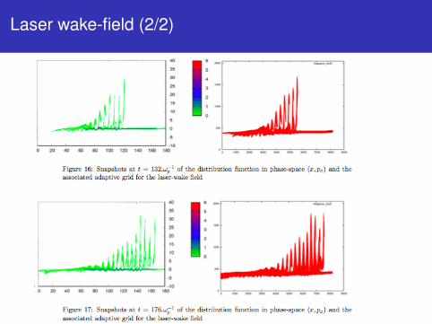
Laser wake-field (2/2)

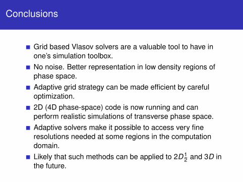
Conclusions

Grid based Vlasov solvers are a valuable tool to have inone’s simulation toolbox.No noise. Better representation in low density regions ofphase space.Adaptive grid strategy can be made efficient by carefuloptimization.2D (4D phase-space) code is now running and canperform realistic simulations of transverse phase space.Adaptive solvers make it possible to access very fineresolutions needed at some regions in the computationdomain.Likely that such methods can be applied to 2D 1

2 and 3D inthe future.

A. Arakawa, Computational Design for Long-TermNumerical Integration of the Equation of Fluid Motion: Twodimensional Incompressible Flow. Part 1.J. Comput. Phys., 1 (1) (1966) pp. 119–143. Reprinted in J.Comput. Phys., 135 (1997) pp. 103–114.

F. Assous, P. Degond, E. Heintze, P. A. Raviart, J. Segre,On a finite element method for solving thethree-dimensional Maxwell equations, Journal ofComputational Physics 109 (1993) pp. 222-237.

Regine Barthelme, Le probleme de conservation de lacharge dans le couplage des equations de Vlasov et deMaxwell, these de l’Universite Louis Pasteur, 2005,specialite Mathematiques.http://www-irma.u-strasbg.fr/irma/publications/2005/05014.shtml

William B. Bateson, Dennis W. Hewett, Grid and particlehydrodynamics: beyond hydrodynamics via fluid elementparticle-in-cell. J. Comput. Phys. 144 (1998), no. 2,358–378.

Besse, Nicolas Convergence of a semi-Lagrangian schemefor the one-dimensional Vlasov-Poisson system. SIAM J.Numer. Anal. 42 (2004), no. 1, 350–382

Nicolas Besse : Convergence of a high-ordersemi-Lagrangian scheme with propagation of gradients forthe Vlasov-Poisson system, Prepublication IRMA (2004),http://www-irma.u-strasbg.fr/irma/publications/2004/04031.shtml

Nicolas Besse, Michel Mehrenberger : Convergence ofclasses of high-order semi-Lagrangian schemes for theVlasov-Poisson system, Prepublication IRMA (2004),

http://www-irma.u-strasbg.fr/irma/publications/2004/04032.shtml

Besse, N.; Sonnendrucker, E. Semi-Lagrangian schemesfor the Vlasov equation on an unstructured mesh of phasespace. J. Comput. Phys. 191 (2003), no. 2, 341–376.

Besse, Nicolas; Segre, Jacques; Sonnendrucker, EricSemi-Lagrangian schemes for the two-dimensionalVlasov-Poisson system on unstructured meshes. TransportTheory Statist. Phys. 34 (2005), no. 3-5, 311–332.

C. K. Birdsall, A. B. Langdon, Plasma physics via computersimulation, Institute of Physics, Bristol (1991) p. 359.

J. P. Boris, Relativistic plasma simulations - Optimization ofa hybrid code, Proc. 4th Conf. Num. Sim. of Plasmas (NRLWashington, Washington DC, 1970) pp. 3-67.

Boris, Jay P.; Book, David L. Flux-corrected transport. I.SHASTA, a fluid transport algorithm that works, J. Comput.Phys. 11 (1973), no. 1, 38–69. Reprinted with anintroduction by Steven T. Zalesak. Commemoration of the30th anniversary {of J. Comput. Phys.}. J. Comput. Phys.135 (1997), no. 2, 170–186.

Boris, Jay P.; Book, David L.; Hain, K. Flux-correctedtransport. II. Generalization of the method, J. Comput.Phys. 18 (1975), 248–283.

Boris, Jay P.; Book, David L. Flux-corrected transport. III.Minimal FCT algorithms, J. Comput. Phys. 20 (1976),397–431.

A. Bossavit, Electromagnetisme en vue de la modelisation,Math. et Applications, Springer, 1993.

M. Campos Pinto and M. Mehrenberger, ”Adaptivenumerical resolution of the Vlasov equation”, in NumericalMethods for Hyperbolic and Kinetic Problems (proceedingsof Cemracs 2003), S. Cordier, T. Goudon, M. Gutnic, E.Sonnendrucker editors, European Mathematical Society2005.

Martin Campos Pinto, Michel Mehrenberger Convergenceof an Adaptive Scheme for the one dimensionalVlasov-Poisson system, Rapport de Recherche INRIA no.5519 (2005),http://hal.inria.fr/inria-00070487

Canouet, Nicolas; Fezoui, Loula; Piperno, Serge A newdiscontinuous Galerkin method for 3D Maxwell’s equationon non-conforming grids. Mathematical and numerical

aspects of wave propagation—WAVES 2003, 389–394,Springer, Berlin, 2003.

C.Z. Cheng, G. Knorr, The integration of the Vlasovequation in configuration space, J. Comput. Phys. 22(1976) 330-351.

Albert Cohen, Numerical Analysis of Wavelet Methods,North-Holland 2003.

G.-H. Cottet, P.-A. Raviart, Particle methods for theone-dimensional Vlasov-Poisson equations. SIAM J.Numer. Anal. 21 (1984), no. 1, 52–76.

J. Denavit, Numerical simulation of plasmas with periodicsmoothing in phase space, J. Comput. Phys. 9, (1972),75-98.

R.A. De Vore, Nonlinear approximation, Acta Numerica 7,1998, 51-150, Cambridge Univ. Press, (1998)

Bengt Eliasson, Numerical modelling of thetwo-dimensional Fourier transformed Vlasov-Maxwellsystem, J. Comput. Phys. 190 (2003) no. 2 , 501 - 522

E. Fijalkow,A numerical solution to the Vlasov equation.Comput. Phys. Communications, 116: (1999) pp. 319–328.

Filbet, Francis Convergence of a finite volume scheme forthe Vlasov-Poisson system. SIAM J. Numer. Anal. 39(2001), no. 4, 1146–1169

Filbet, F.; Sonnendrucker, E. Comparison of EulerianVlasov solvers. Comput. Phys. Comm. 150 (2003), no. 3,247–266.

Filbet, Francis; Sonnendrucker, Eric; Bertrand, PierreConservative numerical schemes for the Vlasov equation.J. Comput. Phys. 172 (2001), no. 1, 166–187.

Moments conservation in adaptive Vlasov solver, NuclearInstruments and Methods in Physics Research Section A,Volume 558, Issue 1 , 1 March 2006, Pages 159-162.Proceedings of the 8th International ComputationalAccelerator Physics Conference - ICAP 2004

M. Gutnic, M. Haefele, I. Paun and E. SonnendruckerVlasov simulations on an adaptive phase-space grid,Computer Physics Communications, Volume 164, Issues1-3, 2004, Pages 214-219

Hesthaven, J. S.; Warburton, T. Nodal high-order methodson unstructured grids. I. Time-domain solution of Maxwell’sequations. J. Comput. Phys. 181 (2002), no. 1, 186–221.

R. Hiptmair. Finite elements in computationalelectromagnetism. Acta Numerica, 11:237–339, January2002.

RW Hockney and JW Eastwood. Computer SimulationUsing Particles. Adam Hilger, Philadelphia, 1988.

Holloway, James Paul Spectral velocity discretizations forthe Vlasov-Maxwell equations. Transport Theory Statist.Phys. 25 (1996), no. 1, 1–32.

Jacobs, G. B.; Hesthaven, J. S. High-order nodaldiscontinuous Galerkin particle-in-cell method on

unstructured grids. J. Comput. Phys. 214 (2006), no. 1,96–121.

A. J. Klimas , W. M. Farrell, A splitting algorithm for Vlasovsimulation with filamentation filtration, Journal ofComputational Physics, v.110 n.1, p.150-163, Jan. 1994

A. J. Klimas , W. M. Farrell, A method for overcoming thevelocity space filamentation problem in collisionless plasmamodel solutions, Journal of Computational Physics, v.68n.1, p.202-226, January 2, 1987

A. B. Langdon, On enforcing Gauss’ law in electromagneticparticle-in-cell codes, Computer Physics Communisations70 (1992) pp. 447-450.

B. Marder, A method for incorporating Gauss’s law intoelectromagnetic PIC codes, J. Comput. Phys. 68 (1987) pp.48-55.

M. Mehrenberger, E. Violard, O. Hoenen, M. Campos Pintoand E. Sonnendrucker, A parallel adaptive Vlasov solverbased on hierarchical finite element interpolation ?ARTICLE Nuclear Instruments and Methods in PhysicsResearch Section A, Volume 558, Issue 1, 1 March 2006,Pages 188-191.

C.D. Munz, R. Schneider, E. Sonnendrucker, U. Voss,Maxwell’s equations when the charge conservation is notsatisfied, C.R. Acad. Sci. Paris, t. 328, Serie I (1999) pp.431-436.

C.-D. Munz, P. Omnes, R. Schneider, E. Sonnendrucker, U.Voss (2000) : Divergence correction techniques for Maxwellsolvers based on a hyperbolic model, J. Comput. Phys.161, no. 2, pp. 484-511.

Takashi Nakamura, Takashi Yabe,

Cubic interpolated propagation scheme for solving thehyper-dimensional Vlasov-Poisson equation in phasespace.Comput. Phys. Communications, 120: (1999) pp. 122–154.

H. Neunzert, J. Wick, The convergence of simulationmethods in plasma physics. Mathematical methods ofplasmaphysics (Oberwolfach, 1979), 271–286, MethodenVerfahren Math. Phys., 20, Lang, Frankfurt, 1980.

Pulvirenti, M.; Wick, J. Convergence of Galerkinapproximation for two-dimensional Vlasov-Poissonequation. Z. Angew. Math. Phys. 35 (1984), no. 6, 790–801.

Robert, R.; Sommeria, J. Statistical equilibrium states fortwo-dimensional flows. J. Fluid Mech. 229 (1991), 291–310.

J. W. Schumer and J. P. Holloway, Vlasov simulations usingvelocity-scaled Hermite representations. J. Comp. Phys,144, (1998), 626-661.

Shoucri, Magdi M.; Gagne, Real R. J. Numerical solution ofa two-dimensional Vlasov equation. J. Computational Phys.25 (1977), no. 2, 94–103.

R. R. J. GAGNE AND M. M. SHOUCRI, A splitting schemefor the numerical solution of a one-dimensional Vlasovequation, J. Comput. Phys., 24 (1977), 445.

Shoucri, Magdi; Knorr, Georg Numerical integration of theVlasov equation. J. Computational Phys. 14 (1974), no. 1,84–92.

E. Sonnendrucker, J. Roche, P. Bertrand, A. Ghizzo,

The Semi-Lagrangian Method for the Numerical Resolutionof Vlasov Equations.J. Comput. Phys. , 149: (1998) pp.201–220.

E. Sonnendrucker, F. Filbet, A. Friedman, E. Oudet andJ.-L. Vay, Vlasov simulations of beams with a moving gridComputer Physics Communications, Volume 164, Issues1-3, 2004, Pages 390-395

H. D. Victory, Jr., Edward J. Allen, The convergence theoryof particle-in-cell methods for multidimensionalVlasov-Poisson systems. SIAM J. Numer. Anal. 28 (1991),no. 5, 1207–1241.

J. Villasenor and O. Buneman, Rigorous chargeconservation for local electromagnetic field solvers,Comput. Phys. Commun. 69 (1992) pp. 306-316.