adaptive methodologies for real-time skin …
TRANSCRIPT
ADAPTIVE METHODOLOGIES FOR
REAL-TIME SKIN SEGMENTATION AND
LARGE-SCALE FACE DETECTION
A THESIS SUBMITTED TO THE UNIVERSITY OF MANCHESTER
FOR THE DEGREE OF DOCTOR OF PHILOSOPHY
IN THE FACULTY OF ENGINEERING AND PHYSICAL SCIENCES
2015
By
Michael Taylor
School of Computer Science

2
Contents
Abstract 11
Declaration 12
Copyright 13
Acknowledgements 14
1 Introduction 15
1.1 Research Overview ............................................................................................. 15
1.2 Research Hypothesis and Objectives .................................................................. 20
1.3 Research Challenges ........................................................................................... 21
1.4 Research Contributions ...................................................................................... 22
1.4.1 Publications .............................................................................................. 23
1.5 Thesis Outline ..................................................................................................... 24
2 Literature Review 25
2.1 Face Detection .................................................................................................... 25
2.1.1 The Viola-Jones Face Detection System .................................................. 32
2.1.2 Recent Detection Advancements .............................................................. 36
2.1.3 Face Detection Enhancement Methods .................................................... 43
2.2 Colour-Based Skin Segmentation ....................................................................... 44
2.2.1 Colour Spaces for Skin Modelling ........................................................... 45
2.2.2 Colour Distribution Modelling Approaches ............................................. 49
2.2.1.1 Explicit Skin Colour Cluster Models .............................................. 49
2.2.1.2 Non-Parametric Skin Colour Modelling ......................................... 50
2.2.1.3 Parametric Skin Colour Modelling ................................................. 52
2.2.4 Skin Colour Model Adaptation................................................................. 53
2.2.4.1 Face Detection-Based Skin Colour Modelling ............................... 55
2.3 Review Summary ............................................................................................... 56

3
3 Adaptive Skin Segmentation via Feature-Based Face Detection 58
3.1 Segmentation Problem Definition ...................................................................... 58
3.1.1 Analysis of Existing Techniques .............................................................. 61
3.1.1.1 Explicit RGB Cluster Model ........................................................... 68
3.1.1.2 Explicit Normalised RG Cluster Model .......................................... 70
3.1.1.3 Explicit HSV Cluster Model ........................................................... 72
3.1.1.4 Explicit YCbCr Colour Model ........................................................ 74
3.1.1.5 Bayes’ Theorem-Based Look-Up Table ......................................... 76
3.1.1.6 Gaussian Distribution Function ...................................................... 81
3.1.2 Results Comparison and Discussion ......................................................... 86
3.2 Segmentation System Design and Development ................................................ 91
3.2.1 Image Sampling ........................................................................................ 92
3.2.1.1 Feature-Based Face Detection ........................................................ 92
3.2.1.2 Sub-Region Sampling ..................................................................... 98
3.2.1.3 Pixel Filtering................................................................................ 100
3.2.2 Skin Colour Distribution Modelling ....................................................... 106
3.2.2.1 Modelling Approach Selection ..................................................... 107
3.2.2.2 Generated Model Validation ......................................................... 111
3.2.3 Segmentation System Application .......................................................... 116
3.2.4 Segmentation System Optimisation ........................................................ 121
3.2.4.1 Mahalanobis Distance-Based Classification ................................. 123
3.2.4.2 Efficiently Discarding Zero-Likelihood Pixels ............................. 125
3.2.4.3 Colour Range-Based Classification .............................................. 131
3.3 Segmentation System Evaluation ..................................................................... 134
3.3.1 Lecture Theatre-Based Imagery .............................................................. 138
3.3.1.1 Discrete Classifier Analysis .......................................................... 138
3.3.1.2 Receiver Operating Characteristic Analysis ................................. 143
3.3.1.3 Precision-Recall Analysis ............................................................. 148
3.3.1.4 Qualitative Analysis of Additional Images ................................... 152
3.3.2 Annotated Arbitrary Image Database ..................................................... 154
3.3.2.1 Complete Dataset Evaluation ........................................................ 156
3.3.2.2 Detection-Facilitating Image Evaluation ...................................... 163
3.3.2.3 Partial Dataset Performance Improvements .................................. 169

4
3.3.3 Adaptive Methodology Comparison ....................................................... 172
3.3.3.1 Adaptive Lecture Theatre Imagery Analysis ................................. 174
3.3.3.2 Adaptive Arbitrary Imagery Analysis ........................................... 178
3.3.4 Segmentation Efficiency Evaluation ...................................................... 180
3.3.4.1 Offline Performance Analysis ...................................................... 180
3.3.4.2 Real-Time Performance Analysis ................................................. 183
3.3.4.3 Interval-Based Face Detection ...................................................... 187
4 Adaptive Framework for Enhanced Large-Scale Face Detection 192
4.1 Framework Design and Development .............................................................. 192
4.1.1 Face Detection Collation ........................................................................ 194
4.1.2 PCA-Based Size Filtering ....................................................................... 196
4.1.2.1 Size Distribution Model Derivation .............................................. 198
4.1.2.2 Sized-Based Detection Elimination .............................................. 202
4.1.3 Retained Detection Consolidation .......................................................... 210
4.1.4 Score-Based Face Candidate Classification ........................................... 217
4.1.5 Colour-Based Face Candidate Classification ......................................... 227
4.2 Framework Evaluation ..................................................................................... 235
4.2.1 Lecture Theatre Imagery Analysis ......................................................... 237
4.2.1.1 Default Configuration Analysis .................................................... 238
4.2.1.2 Precision-Recall Analysis ............................................................. 240
4.2.2 Arbitrary Imagery Analysis .................................................................... 244
4.2.2.1 Default Configuration Analysis .................................................... 245
4.2.2.2 Precision-Recall Analysis ............................................................. 246
4.2.3 Detection Efficiency Evaluation ............................................................. 248
5 Discussion and Conclusions 258
5.1 Synoptic Discussion ......................................................................................... 258
5.2 Itemised Conclusions........................................................................................ 268
5.3 Potential Extensions ......................................................................................... 273
Bibliography 276
Word Count: 77,775

5
List of Tables
3.1 Analysis of RGB segmentations ......................................................................... 69
3.2 Analysis of normalised rg segmentations ........................................................... 71
3.3 Analysis of HSV segmentations ......................................................................... 73
3.4 Analysis of YCbCr segmentations ...................................................................... 75
3.5 Analysis of Bayes segmentations ....................................................................... 80
3.6 Analysis of Gaussian segmentations................................................................... 85
4.1 Specification of face detection parameter configurations ................................. 241

6
List of Figures
1.1 A typical lecture theatre scene .......................................................................... 16
1.2 Detection results achieved by an existing face detector ................................... 17
1.3 Samples of undetected faces ............................................................................. 17
1.4 Detection results achieved using greater sensitivity ......................................... 18
2.1 A knowledge-based face detection scheme ...................................................... 26
2.2 Feature-invariant detection method using an edge map ................................... 27
2.3 Multiscale segmentation approach to face detection ........................................ 28
2.4 Face detection scheme using template-matching ............................................. 29
2.5 A face detector utilising shape and grey-level information .............................. 30
2.6 Approximation of a face using different numbers of eigenpictures ................. 31
2.7 Neural network-based face detection system ................................................... 32
2.8 Examples of Haar-like features used to identify faces ..................................... 33
2.9 A visualisation of the intergral image scheme ................................................. 34
2.10 Haar-like features selected through AdaBoost training .................................... 35
2.11 Attentional cascade classification process ........................................................ 35
2.12 Flexible Haar-like features ............................................................................... 37
2.13 Multi-block LBP detection technique .............................................................. 38
2.14 Fast-training method for boosting processes .................................................... 39
2.15 An example of deformable parts modelling of a face ...................................... 40
2.16 DCNN-based face detection system ................................................................. 41
2.17 Face likelihood heat map generated by a neural network ................................ 42
2.18 Skin colour variation given a range of illuminants........................................... 45
2.19 Representation of the RGB colour space .......................................................... 46
2.20 Representation of the HSV colour space .......................................................... 47

7
2.21 Representation of the YCbCr colour space....................................................... 48
2.22 An HSV skin colour cluster model ................................................................... 49
3.1 An example of a lecture theatre scene with strong illumination ....................... 59
3.2 A second example of a well-illuminated lecture theatre scene ......................... 59
3.3 An example of a poorly illuminated environment ............................................ 61
3.4 Manually annotated skin of Fig. 3.1 ................................................................. 62
3.5 Manually annotated skin of Fig. 3.2 ................................................................. 63
3.6 Segmentations achieved by RGB model .......................................................... 69
3.7 Segmentations achieved by normalised rg model............................................. 71
3.8 Segmentations achieved by HSV model ........................................................... 73
3.9 Segmentations achieved by YCbCr model ....................................................... 75
3.10 Non-skin training samples ................................................................................ 78
3.11 Positive skin training samples .......................................................................... 78
3.12 Segmentations achieved by Bayes model ......................................................... 80
3.13 Segmentations achieved by Gaussian model .................................................... 84
3.14 Quantitative comparison of the achieved segmentations .................................. 86
3.15 Normalised rg representations of skin within input images ............................. 90
3.16 An overview of our proposed skin segmentation system ................................. 91
3.17 Face detection results achieved over a range of sensitivities ............................ 95
3.18 The results of precise face detection ................................................................. 97
3.19 Demonstration of background elimination using sub-regions .......................... 99
3.20 Comparison of intensity distributions of two different sub-regions ............... 103
3.21 Results of luma filtering using different tolerance levels ............................... 103
3.22 Optimisation of the luma filter tolerance ........................................................ 105
3.23 Sample of results of luma filtering ................................................................. 106
3.24 Overview of our sampling and colour modelling process .............................. 110
3.25 Comparison of annotated and sampled colour distributions ........................... 111
3.26 Validation of Gaussian distribution modelling ............................................... 114
3.27 Generation of an intermediary skin likelihood image .................................... 117
3.28 The variation of skin likelihood with mean deviation .................................... 118

8
3.29 Example segmentations using different likelihood thresholds ....................... 120
3.30 Relative process time expenditure comparison .............................................. 122
3.31 The variation of Mahalanobis distance with mean deviation ......................... 124
3.32 The definition of "possible skin" ranges to limit calculations ........................ 128
3.33 Visualisation of the effects of optimisation .................................................... 130
3.34 The use of "possible skin" ranges to classify inputs ....................................... 132
3.35 The relative efficiency of the use of classification ranges .............................. 133
3.36 Segmentations produced by our system over original inputs ......................... 140
3.37 Comparison of our results with those of the existing techniques ................... 142
3.38 ROC analysis of lecture theatre segmentations .............................................. 146
3.39 ROC AUC for lecture theatre segmentations ................................................. 147
3.40 PR analysis of lecture theatre segmentations ................................................. 150
3.41 PR AUC for lecture theatre segmentations .................................................... 151
3.42 Additional lecture theatre segmentations ....................................................... 153
3.43 Samples of annotated arbitrary image dataset ................................................ 157
3.44 ROC analysis of arbitrary image segmentations ............................................ 159
3.45 ROC AUC for arbitrary image segmentations ............................................... 160
3.46 PR analysis of arbitrary image segmentations ................................................ 161
3.47 PR AUC for arbitrary image segmentations ................................................... 162
3.48 Sample arbitrary images with visible but undetectable faces ......................... 164
3.49 ROC analysis of arbitrary face image segmentations ..................................... 165
3.50 ROC AUC for arbitrary face image segmentations ........................................ 166
3.51 PR analysis of arbitrary face image segmentations ........................................ 168
3.52 PR AUC for arbitrary face image segmentations ........................................... 169
3.53 Observed improvements between sets of segmentations ............................... 171
3.54 Segmentations achieved by existing adaptive system .................................... 174
3.55 Comparison of adaptive approach results with those of our system .............. 175
3.56 ROC analysis of adaptive lecture theatre segmentations................................ 176
3.57 PR analysis of adaptive lecture theatre segmentations ................................... 177
3.58 ROC analysis of adaptive arbitrary image segmentations .............................. 179

9
3.59 PR analysis of adaptive arbitrary image segmentations ................................. 179
3.60 Segmentation throughput times achieved over dataset ................................... 182
3.61 Input stream sample frame depicting user interaction .................................... 184
3.62 Frame rates achieved over different image stream sizes ................................ 186
3.63 Frame rates achieved using different face detection intervals ........................ 188
4.1 An overview of our face detection framework ............................................... 193
4.2 A sample input image depicting a lecture theatre ........................................... 194
4.3 Collated high-sensitivity face detection results .............................................. 196
4.4 Results of precise face detection ..................................................................... 198
4.5 Visualisation of results within three-dimensional space ................................. 199
4.6 The first principal component plotted against data points .............................. 201
4.7 The plane derived from our first two principal components .......................... 202
4.8 Collated detections plotted against our planar model ..................................... 203
4.9 Projections of the detections onto the model .................................................. 205
4.10 Optimisation of our size error bounds ............................................................ 207
4.11 Collated detections plotted against error bounds ............................................ 208
4.12 Elimination of detections based upon size ...................................................... 208
4.13 Detections retained after size filtering ............................................................ 209
4.14 Demonstration of simple consolidation .......................................................... 211
4.15 Example of complex consolidation problem .................................................. 211
4.16 Scaling technique to achieve consolidations .................................................. 212
4.17 Problems caused by overly sensitive consolidation ........................................ 215
4.18 Optimisation of detection scaling factor ......................................................... 216
4.19 The results of detection consolidation ............................................................ 217
4.20 The scores assigned to candidates and the distribution of them ..................... 218
4.21 Scores observed given a lower quality input image ....................................... 220
4.22 Optimisation of score threshold for face classification .................................. 222
4.23 Faces identified through score-base classification .......................................... 224
4.24 Low-score candidates retained for further processing .................................... 225
4.25 Candidates retained after elimination of score-of-1 candidates ...................... 226
10
4.26 Skin rating calculated for each candidate ....................................................... 231
4.27 Optimisation of skin rating threshold for face detection ................................ 232
4.28 Faces identified through colour-based classification ...................................... 233
4.29 Final output of our system .............................................................................. 234
4.30 Samples of our lecture theatre imagery dataset .............................................. 238
4.31 Quantitative and qualitative default configuration detection results .............. 239
4.32 PR analysis of lecture theatre detections ........................................................ 242
4.33 PR AUC for lecture theatre detections ........................................................... 243
4.34 Sample images within arbitrary image dataset ............................................... 244
4.35 Quantitative default configuration detection results ....................................... 245
4.36 PR analysis of arbitrary image detections ...................................................... 246
4.37 PR AUC for arbitrary image detections ......................................................... 247
4.38 Dataset detection throughput time comparison .............................................. 249
4.39 Framework component time expenditure comparison ................................... 251
4.40 Throughput times achieved using single cascade for collation ...................... 252
4.41 Comparison of component efficiency using single cascade ........................... 253
4.42 Lecture theatre detection results achieved using single cascade .................... 254
4.43 Arbitrary image detection results achieved using single cascade ................... 256
11
Abstract
ADAPTIVE METHODOLOGIES FOR REAL-TIME SKIN SEGMENTATION
AND LARGE-SCALE FACE DETECTION
Michael Taylor
A thesis submitted to the University of Manchester
for the degree of Doctor of Philosophy, 2015
In the field of computer vision, face detection concerns the positive identification of the faces of people within still images or video streams, which is extremely useful for applications such as counting, tracking, and recognition. When applied in large-scale environments, such as lecture theatres, we have found that existing technology can struggle greatly in detecting faces due primarily to the indiscernibility of their features, caused by partial occlusion, problematic orientation, and a lack of focus or resolution. We attempt to overcome this issue by proposing an adaptive framework, capable of collating the results of numerous existing detection systems in order to significantly improve recall rates. This approach uses supplementary modalities, invariant to the issues posed to features, to eliminate false detections from collated sets and allow us to produce results with extremely high confidence. The properties we have selected as the bases of detection classification are size and colour, as we believe that filters that consider them can be constructed adaptively, on a per-image basis, ensuring that the variabilities inherent to large-scale imagery can be fully accounted for, and that false detections and actual faces can be accurately distinguished between on a consistent basis. The application of principal component analysis to precise face detection results yields planar size distribution models that we can use to discard results that are either too large or too small to realistically represent faces within given images.
Classifying a detection according to the correspondence of its general colour tone to the expected colour of skin is a more complex matter, however, as the apparent colour of skin is highly dependent upon incident illumination, and existing techniques are neither specific nor flexible enough to model it as accurately as we believe possible. Therefore, we propose another system, which will be able to adaptively model skin colour distributions according to the Gaussian probability densities exhibited by the colours of precise face detections. Furthermore, it will be suitable for independent application to real-time skin segmentation tasks as a result of considerable optimisation.
This thesis details the design, the development, and the implementation of our systems, and thoroughly evaluates them with regards to the accuracy of their results and the efficiency of their performances, thereby establishing fully the suitability of them for solving certain types of presented problems.

12
Declaration
No portion of the work referred to in this thesis has been
submitted in support of an application for another degree or
qualification of this or any other university or other institute of
learning.

13
Copyright
i. The author of this thesis (including any appendices and/or schedules to this thesis)
owns certain copyright or related rights in it (the “Copyright”) and s/he has given
The University of Manchester certain rights to use such Copyright, including for
administrative purposes.
ii. Copies of this thesis, either in full or in extracts and whether in hard or electronic
copy, may be made only in accordance with the Copyright, Designs and Patents
Act 1988 (as amended) and regulations issued under it or, where appropriate, in
accordance with licensing agreements which the University has from time to time.
This page must form part of any such copies made.
iii. The ownership of certain Copyright, patents, designs, trade marks and other
intellectual property (the “Intellectual Property”) and any reproductions of
copyright works in the thesis, for example graphs and tables (“Reproductions”),
which may be described in this thesis, may not be owned by the author and may be
owned by third parties. Such Intellectual Property and Reproductions cannot and
must not be made available for use without the prior written permission of the
owner(s) of the relevant Intellectual Property and/or Reproductions.
iv. Further information on the conditions under which disclosure, publication and
commercialisation of this thesis, the Copyright and any Intellectual Property
and/or Reproductions described in it may take place is available in the University
IP Policy (see http://documents.manchester.ac.uk/DocuInfo.aspx?DocID=487), in
any relevant Thesis restriction declarations deposited in the University Library,
The University Library’s regulations (see
http://www.manchester.ac.uk/library/aboutus/regulations) and in The University’s
policy on Presentation of Theses

14
Acknowledgements
Despite being ultimately rewarding, conducting research towards the completion of this
degree has been a journey fraught with trials and tribulations, the likes of which I would
not have been able to overcome without the support of a multitude of people. I would
firstly like to thank my supervisor, Dr. Tim Morris, for his unending guidance and
advice. Without his feedback and the constructive criticism of my work, the results that
my project has yielded would not be nearly as encouraging as they have been.
My sincerest gratitude also goes towards all the members of the faculty, the school,
and the Advanced Interfaces Group that have helped to support my research and my
professional development over the past four years. Furthermore, I would like to thank the
funding bodies that have not only provided me with the resources necessary to carry out
my work, but also afforded me excellent opportunities to travel in order to present my
work and meet numerous experts within the field.
The support of my friends, both those within Manchester and those further afield,
has been invaluable to me, as the stresses and strains put upon me by the rigours of
research would not have been manageable without their help. I would also like to thank
the numerous fellow researchers that I have had the pleasure of sharing an office with
during my time at the school for their geniality, as even the most casual of mid-afternoon
conversations has helped to keep me motivated.
Of course, none of my achievements would have been possible without the continual
support and encouragement of my family, including that of my grandparents, who sadly
passed away before my research could come to its conclusion.
Finally, my everlasting appreciation goes to my beloved Lauren. For the
innumerable and immeasurable sacrifices you have made, I will forever be grateful.

15
Chapter 1
Introduction
As computer systems and electronic devices become increasingly ubiquitous and capable,
the development of more sophisticated and useful human-computer interfaces becomes
significantly more viable. Computer vision, which provides an extremely broad platform
for such interfaces, has been subject to great advancements over recent years, and the
efficacy and accessibility of applications developed within the field has been improved
upon enormously. A fundamental and extremely prominent aspect of these technologies
is face detection, which pertains to the capacity of a machine to positively identify the
existence of faces within still images or video streams. Detecting faces is a critical
precursor to a vast range of applications, including, amongst many others, face
recognition [149], verification and authentication [69], tracking and surveillance [30],
expression analysis [102], and demographic analysis [33]. Developing methodologies
with the capacity to yield accurate face detection results, therefore, is of great importance.
1.1 Research Overview
Given an arbitrary image, it is the objective of a face detection algorithm to ascertain
whether or not any faces are present within it, and, if so, to return information pertaining
to the apparent size and location of each of them [159]. This is not a trivial problem to
solve for computers, because of the extreme variabilities involved in such a process
[165]. Even two separate instances of an individual face can exhibit changes in scale,
illumination, focus, occlusion, location, orientation, and expression, meaning that

16 CHAPTER 1. INTRODUCTION
achieving robust detection can become extremely complex. Of course, approaches to
detection will typically be designed to be invariant to such issues [163], but there will
always be some limit on the extent to which this can be the case. Face detection can
become particularly complex where “large-scale” imagery is concerned, as it will depict
environments within which the presence of large numbers of people is entirely expected.
This is problematic for any ambition to achieve accurate face detection results because
the prevalence of the aforementioned issues, and combinations of them, will often be
significant. A lecture theatre would be an archetypal example of such an environment,
and Fig. 1.1 depicts a typical image of people that may be captured within one.
Figure 1.1: An image taken within a lecture theatre, depicting a large number of people
that exhibit numerous obstacles to successful detection, and constituting a large-scale
problem. This image (and many similar that we will be making use of) was provided by
P. Touloupos [142].
As can be seen, many of the faces within Fig. 1.1 represent examples of the types of
problems we have highlighted, such as partial occlusion, problematic orientation, and a
lack of focus. Some of these issues are inherently particularly prevalent where such
imagery is concerned. For instance, larger numbers of people being depicted will mean
that there are greater numbers of objects to actually cause occlusion, and people being
distributed over large environments will lead to the faces of individuals being great
distances away from the point of image capture, resulting in insufficient resolution and
focus to positively identify them. Numerous specialised technologies have been
developed in efforts to overcome some of these suboptimal circumstances [34,36,138],

CHAPTER 1. INTRODUCTION 17
but we are yet to discover a detection approach flexible enough to account for all that our
large-scale imagery presents. To demonstrate the detrimental effects of the issues we are
concerned with, Fig. 1.2 depicts the results achieved by an off-the-shelf detection system
- the seminal work of Viola and Jones [147], which is implemented using its default
configuration through OpenCV.
Figure 1.2: The result of using the Viola-Jones face detector to identify faces within the
lecture theatre scene depicted by Fig. 1.1 The image contains 44 visible faces, and the
detector has yielded 21 true positives, 4 false positives, and 23 false negatives.
As can be discerned from Fig. 1.2, the detector has failed to positively identify more than
half of the faces within the scene, which cannot be considered a satisfactory result. A
number of the faces that have not been identified in this instance are depicted by Fig. 1.3.
(a) (b) (c) (d) (e)
Figure 1.3: A selection of the faces within Fig. 1.1 that the Viola-Jones face detection
system has failed to positively identify, because of a range of detection-inhibiting issues.
Even though the face samples shown by Fig. 1.3 represent just a fraction of those that the
detector has failed to detect, they strongly indicate how problematic issues such as
18 CHAPTER 1. INTRODUCTION
occlusion and blur can be to successful face detection, as they can severely impact the
discernibility of facial features. Of course, it could be argued that an increase to the
sensitivity of the detector would yield improved results, as it would increase the
probability of “weak” faces (those with weakly expressed features) being identified.
However, as the detector has already generated a number of false positives using its
default configuration, lowering the positive classification threshold is likely to result in
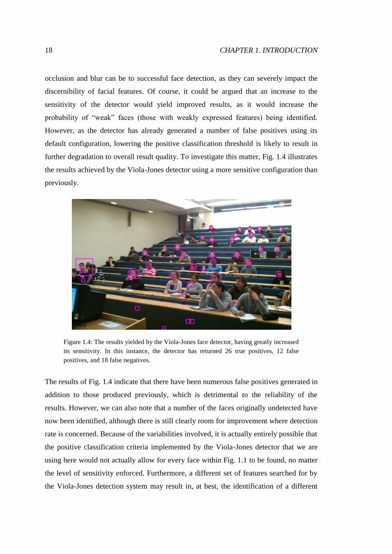
further degradation to overall result quality. To investigate this matter, Fig. 1.4 illustrates
the results achieved by the Viola-Jones detector using a more sensitive configuration than
previously.
Figure 1.4: The results yielded by the Viola-Jones face detector, having greatly increased
its sensitivity. In this instance, the detector has returned 26 true positives, 12 false
positives, and 18 false negatives.
The results of Fig. 1.4 indicate that there have been numerous false positives generated in
addition to those produced previously, which is detrimental to the reliability of the
results. However, we can also note that a number of the faces originally undetected have
now been identified, although there is still clearly room for improvement where detection
rate is concerned. Because of the variabilities involved, it is actually entirely possible that
the positive classification criteria implemented by the Viola-Jones detector that we are
using here would not actually allow for every face within Fig. 1.1 to be found, no matter
the level of sensitivity enforced. Furthermore, a different set of features searched for by
the Viola-Jones detection system may result in, at best, the identification of a different

CHAPTER 1. INTRODUCTION 19
subset of the faces we are attempting to find. Combined, however, these sets of detections
may actually account for a considerable proportion of the faces within the image,
granting us a satisfactory detection rate.
Nevertheless, the results depicted by Fig. 1.4 suggest that using a framework to collate
the results of high-sensitivity feature-based detection processes in such a manner would
produce a set that contains a significant number of false positive results. Whilst features
are extremely strong indicators of the presence of faces [39], the inconsistent
discernibility of them is clearly a prevalent and harmful issue where large-scale imagery
is concerned. If the proposed framework were to consider supplementary modalities,
however, we believe that we could distinguish between the detected faces and the false
positives represented by collated detection sets. This would allow us to ultimately yield
enhanced overall results, consisting of more positively identified faces than any of the
original detection sets would contain as well as smaller numbers of false positives.
There is precedence for the use of alternative visual properties in reinforcing the results
of the Viola-Jones detector [11,93,117,123,125], but the techniques proposed by those
works would not necessarily solve the issues we face with large-scale imagery. The
modalities our framework utilises should allow for consistent differentiation between
face and non-face image regions, and we believe that size and colour are two that could
satisfy this requirement. By verifying face candidates according to their sizes and
colours, we can still confidently identify faces even when their features are expressed
particularly weakly. Where size is concerned, predetermining acceptable detection size
ranges would be failing to adequately consider relevant variabilities, but if we were to
sample input images, we could derive representative face size distribution models, which
could be used to eliminate detections either too large or too small to realistically
represent faces within those images.
With regards to colour, there are a multitude of approaches to modelling skin colour
distributions [145], but the apparent colour of skin is remarkably dependent upon incident
illumination [136], and general lighting conditions are greatly variable where our large-
scale imagery is concerned. Only the adaptive derivation of models, therefore, will allow
us to accurately represent skin colours on a consistent basis. Several adaptive approaches
to skin colour modelling do exist [41,78,92,151], but the specific issues these techniques

20 CHAPTER 1. INTRODUCTION
overcome do not correlate entirely with those that we face. We will, therefore, be
developing our own adaptive skin colour modelling methodology, specifically with the
variabilities of large-scale images in mind. If we can derive the means to intelligently
interpret image samples, we could build representative skin colour models and use them
to determine the skin likelihood of pixels, allowing us to effectively utilise colour as a
discriminator between faces and non-face image regions.
Aside from assisting in the detection of faces, such a system would, in theory, also be
entirely capable of independently performing skin segmentation. Similarly to face
detection, skin segmentation is a process that enables a broad range of computer vision-
based applications [54], so developing an exceptional methodology would have benefits
even beyond the scope of our face detection framework, especially if we were to achieve
real-time performance. We will, therefore, be initially regarding the development of our
skin colour modelling approach as an entirely isolated endeavour, and only during the
subsequent construction of our framework will we be fully exploring its potential to
classify face candidates.
1.2 Research Hypothesis and Objectives
The central hypothesis of our research, which we will be exploring within this thesis, can
be expressed thusly:
The results of existing feature-based face detection approaches can be
consistently improved upon, in terms of both recall and precision, through the
consideration of the supplementary properties of size and colour, without the
introduction of prohibitive computational costs.
The main objectives we will be meeting in order to produce evidence pertaining to this
hypothesis can be summarised by the following:
Develop a methodology capable of adaptively generating representative skin
colour models given images of people within complex lecture theatre scenes.

CHAPTER 1. INTRODUCTION 21
Design a framework that can intelligently filter the results of existing face
detection systems, according to input-specific size and skin colour models, in
order to improve results over large-scale imagery.
Demonstrate the flexibility of our techniques by additionally analysing
performances over generic datasets, and establish the computational
efficiency with which our results are achieved.
1.3 Research Challenges
There are a number of inherent challenges to the type of research we will conduct
towards the meeting of our outlined objectives. Firstly, defining a method for image
sampling requires careful calibration, as we attempt to ensure that we minimise the risk
of false positive samples being generated whilst also trying to maximise the amount of
useful information we obtain. Subsequently using those samples to derive representative
skin colour models is an issue that requires careful consideration of both our choice of
colour space and our choice of modelling approach, as certain combinations of them will
naturally work more effectively than others. This is especially true where our large-scale
images are concerned, as they are liable to exhibit atypically broad distributions of skin
colours. Optimising the application of derived skin colour models to images is also non-
trivial, as it necessitates the precise determination of where time expenditure is most
significant, and the development of creative solutions to the discovered inefficiencies.
Where the construction of our face detection framework is concerned, the main
difficulties to overcome pertain to the calibration of the filters used to discriminate
between faces and non-face regions. Each of the classification processes we develop will,
of course, be applied with some degree of error tolerance, but it would be entirely remiss
of us to use arbitrary tolerances without any real appreciation for the precise effects that
they are likely to have on our sets of data points. If applied error bounds are too
permissive, for instance, false positive detections may not be fully eliminated, but if they
are too strict, actual faces may also be discarded, and it for these reasons that the careful
calibration of our filters is critically important to the efficacy of the system.

22 CHAPTER 1. INTRODUCTION
1.4 Research Contributions
The main contributions we feel we have made to the field of computer vision with our
research can be described by the following:
High-confidence image sampling through the feature-based detection of
large numbers of faces, enabling the adaptive generation of models to be
used for data point classification. (Chapter 3)
The derivation of representative skin pixel sets through subjecting face
detection results to background elimination and luma-based filtering, which
we use to distinguish between skin and non-skin facial features. (Chapter 3)
The use of Mahalanobis distances to define “possible skin” colour ranges for
pixel classification, which can drastically reduce image throughput times by
efficiently discarding zero-likelihood pixels. (Chapter 3)
A skin segmentation system that combines these advancements with other
current techniques in order to achieve levels of accuracy and efficiency that
are superior to those of a broad range of existing approaches. (Chapter 3)
The use of principal component analysis in deriving multidimensional face
size distribution models that can discriminate between faces and non-faces
based upon their sizes and locations. (Chapter 4)
The combination of the results of separate face detection systems in order to
derive overall facial feature discernibility measures for face candidates,
allowing for precise classification. (Chapter 4)
The application of our skin modelling approach to face detection regions in
order to distinguish between actual faces and non-face regions according to
their general colour tones. (Chapter 4)

CHAPTER 1. INTRODUCTION 23
A framework for enhancing the results of face detection systems, which is
achieved by combining initial results to boost detection rates and applying
filters that consider adaptively generated size and colour models to eliminate
false positives. (Chapter 4)
1.4.1 Publications
The research that has been conducted throughout the course of this project has yielded
the following publications:
Abstract accepted for poster presentation
Counting faces for the blind, through skin segmentation and head size
distribution modelling
M. J. Taylor and T. Morris
BMVC 2012 Student Workshop
Peer-reviewed paper accepted for poster presentation
Adaptive skin segmentation via feature-based face detection
M. J. Taylor and T. Morris
SPIE Photonics Europe 2014: Real-Time Image and Video Processing
Peer-reviewed paper accepted for oral presentation
Enhanced face detection: An adaptive cascade-mixture approach for large-scale
detection
M. J. Taylor and T. Morris
BMVC 2014 Doctoral Consortium
It should be noted that the methodologies described by these publications have been
enhanced upon substantially since the times that they were disseminated, and the
evaluations of them made decidedly more comprehensive, and it is these improved
versions of our work that are presented within this thesis.

24 CHAPTER 1. INTRODUCTION
1.5 Thesis Outline
The subsequent chapters of this thesis can be described by the following:
Chapter 2: We present an extensive review of existing face detection and
skin segmentation technology relevant to the problems we are attempting to
solve over the course of this project.
Chapter 3: We analyse the shortcomings of existing skin segmentation
approaches then describe the design, development, and optimisation of our
own adaptive system, the accuracy and efficiency of which is then
thoroughly evaluated.
Chapter 4: We detail the entire developmental process of our adaptive face
detection framework, and then present a comprehensive evaluation that
explores its efficacy and its efficiency.
Chapter 5: In our final chapter, we summarise the research we have
conducted and our findings, and offer a number of suggestions for potential
extensions to our work.

25
Chapter 2
Literature Review
As we discussed in Chapter 1, the research that we will be conducting during the course
of this project pertains to the disciplines of face detection and skin segmentation. In this
chapter, we will be describing the foundations of these fields and examining a broad
range of the existing works relevant to them.
2.1 Face Detection
There exist many different approaches to detecting faces. In 2002, Yang et al. [159]
defined four categories to describe the nature of early detection techniques, although it
should be noted that the specific terminology they used for their definitions is not applied
consistently within the field today, and many of the approaches discussed could be
legitimately ascribed to more than one of the categories. Furthermore, they broke down
the problem of face detection to specify that certain types of systems were somewhat
limited in scope and suitable primarily for localising faces in images known to contain
just one face.
Knowledge-based methods use decision rules that are derived from knowledge
pertaining to human faces in order to classify image regions and localise faces. These
decision rules would be simple to define, and would concern, for instance, the positions
of the eyes, mouth, and nose of a face, and the relative distances between them. A
hierarchical approach was proposed by Yang and Huang [154] that would first apply
26 CHAPTER 2. LITERATURE REVIEW
general faces rules across low resolution versions of inputs in order to identify candidate
regions. These would then be classified at higher resolutions according the edges they
exhibit and the appearance of the features within them. Although this method struggled to
yield high detection rates, its hierarchical nature proved to be rather efficient, and was
built upon by Kotropoulos and Pitas [66], as they initially applied a projection-based
localisation technique [57] to inputs for the purpose of identifying face candidates, which
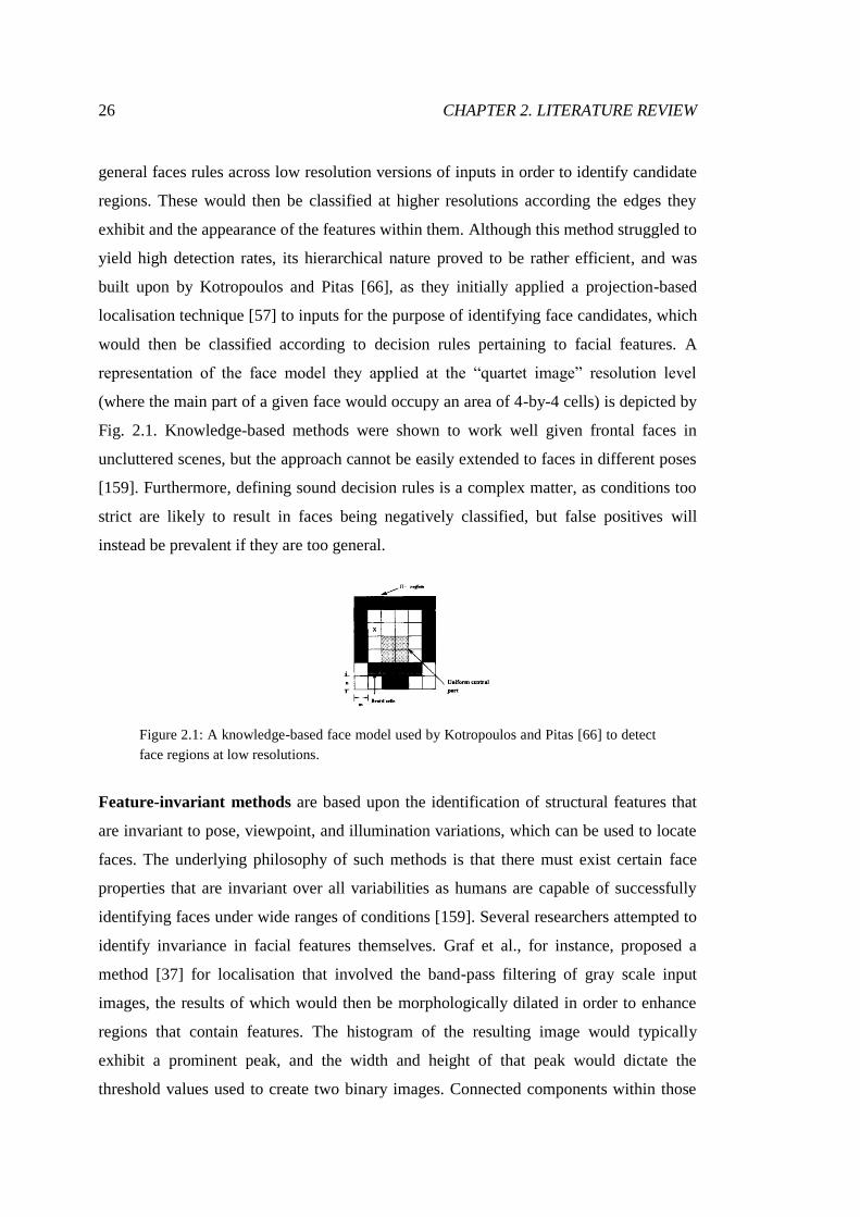
would then be classified according to decision rules pertaining to facial features. A
representation of the face model they applied at the “quartet image” resolution level
(where the main part of a given face would occupy an area of 4-by-4 cells) is depicted by
Fig. 2.1. Knowledge-based methods were shown to work well given frontal faces in
uncluttered scenes, but the approach cannot be easily extended to faces in different poses
[159]. Furthermore, defining sound decision rules is a complex matter, as conditions too
strict are likely to result in faces being negatively classified, but false positives will
instead be prevalent if they are too general.
Figure 2.1: A knowledge-based face model used by Kotropoulos and Pitas [66] to detect
face regions at low resolutions.
Feature-invariant methods are based upon the identification of structural features that
are invariant to pose, viewpoint, and illumination variations, which can be used to locate
faces. The underlying philosophy of such methods is that there must exist certain face
properties that are invariant over all variabilities as humans are capable of successfully
identifying faces under wide ranges of conditions [159]. Several researchers attempted to
identify invariance in facial features themselves. Graf et al., for instance, proposed a
method [37] for localisation that involved the band-pass filtering of gray scale input
images, the results of which would then be morphologically dilated in order to enhance
regions that contain features. The histogram of the resulting image would typically
exhibit a prominent peak, and the width and height of that peak would dictate the
threshold values used to create two binary images. Connected components within those
CHAPTER 2. LITERATURE REVIEW 27
images signify candidate feature regions, and combinations of these areas would be
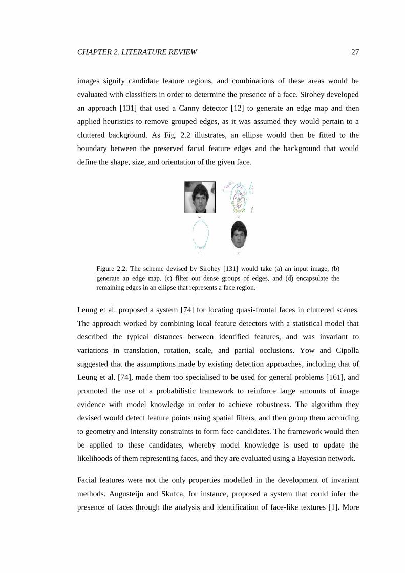
evaluated with classifiers in order to determine the presence of a face. Sirohey developed
an approach [131] that used a Canny detector [12] to generate an edge map and then
applied heuristics to remove grouped edges, as it was assumed they would pertain to a
cluttered background. As Fig. 2.2 illustrates, an ellipse would then be fitted to the
boundary between the preserved facial feature edges and the background that would
define the shape, size, and orientation of the given face.
Figure 2.2: The scheme devised by Sirohey [131] would take (a) an input image, (b)
generate an edge map, (c) filter out dense groups of edges, and (d) encapsulate the
remaining edges in an ellipse that represents a face region.
Leung et al. proposed a system [74] for locating quasi-frontal faces in cluttered scenes.
The approach worked by combining local feature detectors with a statistical model that
described the typical distances between identified features, and was invariant to
variations in translation, rotation, scale, and partial occlusions. Yow and Cipolla
suggested that the assumptions made by existing detection approaches, including that of
Leung et al. [74], made them too specialised to be used for general problems [161], and
promoted the use of a probabilistic framework to reinforce large amounts of image
evidence with model knowledge in order to achieve robustness. The algorithm they
devised would detect feature points using spatial filters, and then group them according
to geometry and intensity constraints to form face candidates. The framework would then
be applied to these candidates, whereby model knowledge is used to update the
likelihoods of them representing faces, and they are evaluated using a Bayesian network.
Facial features were not the only properties modelled in the development of invariant
methods. Augusteijn and Skufca, for instance, proposed a system that could infer the
presence of faces through the analysis and identification of face-like textures [1]. More

28 CHAPTER 2. LITERATURE REVIEW
specifically, these textures would pertain to hair and skin regions. Representations of
textures were derived from the use of co-occurrence matrices over second-order statistics,
and these characteristics would then be subjected to supervised classification through the
usage of a cascade-correlation neural network [23]. The identified textures are then
clustered using a Kohonen self-organising feature map [62]. Although this approach
demonstrated encouraging classification performance, it yielded only the results of
texture classification, rather than actually identified faces.
For the same purpose of detecting faces, many works have explored the potential of
colour to be used as an invariant property [38,88,156,157], and we will fully examine
skin segmentation techniques in Section 2.2. Several approaches to localisation and
detection proposed the combination of different types of invariant features. Typically,
global properties such as colour, size, and shape were used to initially identify face
candidates, and these would then be classified according to the presence of detailed facial
features such as eyes, nose, and mouth. Yang and Ahuja, for instance, developed a
system [157] that would use multiscale segmentation to extract homogeneous regions
within images, as in Fig. 2.3. Subsequently, a Gaussian skin colour model would be
applied in order to identify regions that exhibit compelling skin tones, which are then
grouped into ellipses. A face would then be positively identified if specific facial features
can be detected within an elliptical region.
Figure 2.3: Multiscale segmentation scheme proposed by Yang and Ahuja [157],
whereby an input image (a) will be segmented at a range of homogeneity levels
(b)(c)(d).

CHAPTER 2. LITERATURE REVIEW 29
Wu et al. proposed a method [153] for face detection that utilised fuzzy colour models to
describe the appearance of skin and hair regions. Given an input image, these models are
used to extract potential faces regions, which would then be compared to prebuilt head
shape models through fuzzy pattern-matching in order for face candidates to be derived.
Verification of candidates is then based upon the horizontal edges of facial features. The
main weakness of feature-invariant methods is that the features being considered can be
severely degraded by variations in illumination, noise, and occlusion, and the existence of
shadows can produce strong visual edges that undermine grouping and classification
algorithms [159].
Template-matching methods compare input images to stored patterns of standard whole
faces and facial features in order to achieve both localisation and detection. Correlations
between a given input and the patterns representing whole faces, mouths, noses, eyes, and
other features are determined independently, and classifications are made based upon the
calculated values. Craw et al. proposed a localisation system [18] that would first use a
Sobel filter to extract edges from gray scale inputs, which would then be grouped and
compared to stored patterns. Once the template for a head had been matched, those
relating to facial features could be searched for on smaller scales, whereby successful
matching would result in positive classification. Miao et al. developed a hierarchical
template-matching method [90] that would rotate input images through a range of
orientations, which was intended to account for orientation variations exhibited by faces.
In order to improve efficiency over traditional techniques, the system would make use of
a processing hierarchy, whereby the gravity-centred results of mosaic template-matching
(as in Fig. 2.4) would first be verified according to gray-level checks, and the results of
that process would be subjected to edge-level checks for faces to be classified.
Figure 2.4: Miao et al. [90] proposed a system whereby input images would be rotated
and gravity-centre template matching results would constitute face candidates to be
filtered by gray-level and edge-level checks.
30 CHAPTER 2. LITERATURE REVIEW
Although simple to implement, such methods have been shown to be inadequate for
global face detection as they are incapable of dealing with significant variations in scale,
pose, and shape [159]. Towards solving these issues, many researchers attempted to
utilise deformable templates. For instance, Yuille et al. described features of interest by
parameterised templates [162], and then used an energy function to link edges, peaks, and
valleys in image intensity to properties of the templates. The parameter values of the
templates can then be adjusted in order to minimise the energy function, achieving best
fits through a process of deformation. The derived final values can then be used to
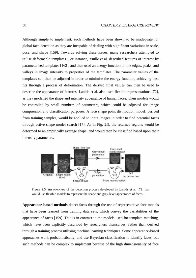
describe the appearance of features. Lanitis et al. also used flexible representations [72],
as they modelled the shape and intensity appearance of human faces. Their models would
be controlled by small numbers of parameters, which could be adjusted for image
compression and classification purposes. A face shape point distribution model, derived
from training samples, would be applied to input images in order to find potential faces
through active shape model search [17]. As in Fig. 2.5, the returned regions would be
deformed to an empirically average shape, and would then be classified based upon their
intensity parameters.
Figure 2.5: An overview of the detection process developed by Lanitis et al. [72] that
would use flexible models to represent the shape and grey-level appearance of faces.
Appearance-based methods detect faces through the use of representative face models
that have been learned from training data sets, which convey the variabilities of the
appearance of faces [159]. This is in contrast to the models used for template-matching,
which have been explicitly described by researchers themselves, rather than derived
through a training process utilising machine learning techniques. Some appearance-based
approaches work probabilistically, and use Bayesian classification to identify faces, but
such methods can be complex to implement because of the high dimensionality of face
CHAPTER 2. LITERATURE REVIEW 31
descriptors. Other appearance-based systems use discriminant functions (in the form of
differentiating hyperplanes or thresholds, for instance) to distinguish between faces and
non-faces and achieve classification using large numbers of parameters. An instance of
the latter type is the use of eigenvectors to recognise human faces, under which
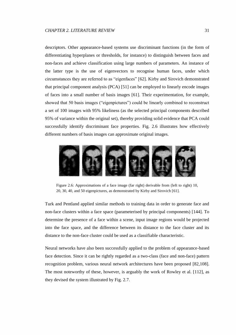
circumstances they are referred to as “eigenfaces” [62]. Kirby and Sirovich demonstrated
that principal component analysis (PCA) [51] can be employed to linearly encode images
of faces into a small number of basis images [61]. Their experimentation, for example,
showed that 50 basis images (“eigenpictures”) could be linearly combined to reconstruct
a set of 100 images with 95% likeliness (as the selected principal components described
95% of variance within the original set), thereby providing solid evidence that PCA could
successfully identify discriminant face properties. Fig. 2.6 illustrates how effectively
different numbers of basis images can approximate original images.
Figure 2.6: Approximations of a face image (far right) derivable from (left to right) 10,
20, 30, 40, and 50 eigenpictures, as demonstrated by Kirby and Sirovich [61].
Turk and Pentland applied similar methods to training data in order to generate face and
non-face clusters within a face space (parameterised by principal components) [144]. To
determine the presence of a face within a scene, input image regions would be projected
into the face space, and the difference between its distance to the face cluster and its
distance to the non-face cluster could be used as a classifiable characteristic.
Neural networks have also been successfully applied to the problem of appearance-based
face detection. Since it can be rightly regarded as a two-class (face and non-face) pattern
recognition problem, various neural network architectures have been proposed [82,108].
The most noteworthy of these, however, is arguably the work of Rowley et al. [112], as
they devised the system illustrated by Fig. 2.7.
32 CHAPTER 2. LITERATURE REVIEW
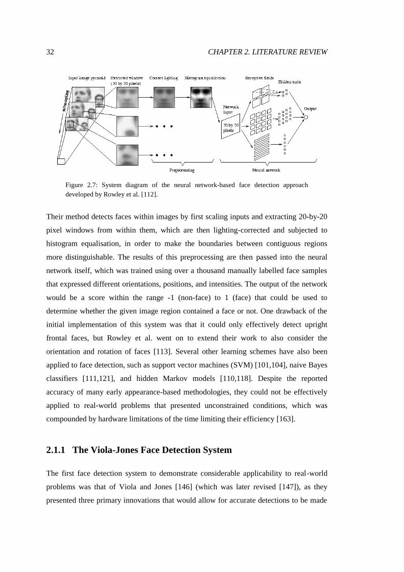
Figure 2.7: System diagram of the neural network-based face detection approach
developed by Rowley et al. [112].
Their method detects faces within images by first scaling inputs and extracting 20-by-20
pixel windows from within them, which are then lighting-corrected and subjected to
histogram equalisation, in order to make the boundaries between contiguous regions
more distinguishable. The results of this preprocessing are then passed into the neural
network itself, which was trained using over a thousand manually labelled face samples
that expressed different orientations, positions, and intensities. The output of the network
would be a score within the range -1 (non-face) to 1 (face) that could be used to
determine whether the given image region contained a face or not. One drawback of the
initial implementation of this system was that it could only effectively detect upright
frontal faces, but Rowley et al. went on to extend their work to also consider the
orientation and rotation of faces [113]. Several other learning schemes have also been
applied to face detection, such as support vector machines (SVM) [101,104], naive Bayes
classifiers [111,121], and hidden Markov models [110,118]. Despite the reported
accuracy of many early appearance-based methodologies, they could not be effectively
applied to real-world problems that presented unconstrained conditions, which was
compounded by hardware limitations of the time limiting their efficiency [163].
2.1.1 The Viola-Jones Face Detection System
The first face detection system to demonstrate considerable applicability to real-world
problems was that of Viola and Jones [146] (which was later revised [147]), as they
presented three primary innovations that would allow for accurate detections to be made

CHAPTER 2. LITERATURE REVIEW 33
with exceptional efficiency. The first of these was the integral image, which was an
image representation scheme that enabled the rapid summation of pixel intensities within
image sub-windows. The process was first proposed for the efficient generation of
mipmaps [19], but Viola and Jones applied it to the computation of Haar-like features.
These simple features, consisting of combinations of rectangular regions, were based
upon Haar basis functions [103], and three different types were used, which are
illustrated by Fig. 2.8.
Figure 2.8: Examples of the three types of Haar-like features used by Viola and Jones,
relative to enclosing detection windows. A and B are two-rectangle features, C is a three-
rectangle feature, and D is a four-rectangle feature
The value of a feature is calculated as the difference between the sum of pixel intensities
within the grey regions and the sum of pixel intensities within the white regions. Given
that a detection window will be moved across the entirety of any given input image
multiple times (at multiple scales), using a traditional method of pixel intensity
summation in order to evaluate feature regions would be extremely time-consuming.
However, using an integral image, feature evaluation can be carried out with remarkable
efficiency. Every location within an integral image ii(x,y) inclusively contains the sum of
the pixels above and to the left of the location within the original image i(x,y), as Eq. 2.1
describes.
𝑖𝑖 𝑥,𝑦 = 𝑖(𝑥′ ,𝑦′)𝑥 ′≤𝑥 ,𝑦′≤𝑦 (2.1)
If every integral image point ii(x,y) contains the sum of the pixels between itself and the
top-left origin, then the evaluation of any given rectangular region within an image can
be carried out by considering the integral image value stored at each of its four corners,
as Fig. 2.9 visualises.

34 CHAPTER 2. LITERATURE REVIEW
Figure 2.9: The value of rectangle D can be calculated by considering the integral image
values at points, 1, 2, 3, and 4. 1 represents the sum of the pixels within A, 2 the sum of
A + B, 3 the sum of A + C, and 4 the sum of A + B + C + D. The value of D, therefore,
can be computed as 4 – 2 – 3 + 1.
The method described by Fig. 2.9 would clearly be more efficient than summing each
and every pixel within the region of interest, as it requires only four array references.
Furthermore, given the nature of the Haar-like features being used, where the regions
being considered will have common corners, a two-rectangle feature will require only six
references, a three-rectangle feature only eight, and a four-rectangle feature just nine. Of
course, the generation of the integral image itself will necessitate a non-zero amount of
computational effort, but this time expenditure will be absolutely minimal in comparison
to the total time saved avoiding the isolated summation of regions.
The second major advancement presented by Viola and Jones was the use of adaptive
boosting (AdaBoost [31]) to construct classifiers by selecting small numbers of
important features. They noted that the exhaustive set of rectangle features that could be
applied across a 24-by-24 pixel detection window would contain more than 180,000 of
them, and even though each could be computed rather efficiently, processing an entire set
of that size would be prohibitive to any sense of real-time application. It was postulated,
however, that a very small proportion of these features could actually be combined to
form an effective classifier, and it was through AdaBoost that these features could be
selected and a classifier trained with them. In its original form, AdaBoost is used to
progressively improve the performance of a weak classifier through the identification of
errors and the adjustment of input weights in order to emphasise and correct those errors.
Viola and Jones modified this procedure so that each stage of the learning process would
return a classifier of just a single feature, and successive stages would identify features
that could minimise remaining error in training data points. Their boosting algorithm,
CHAPTER 2. LITERATURE REVIEW 35
therefore, could be regarded as a feature selection process, and could be utilised to
establish sets of features that optimally describe the appearance of faces, a sample of
which is depicted by Fig. 2.10.
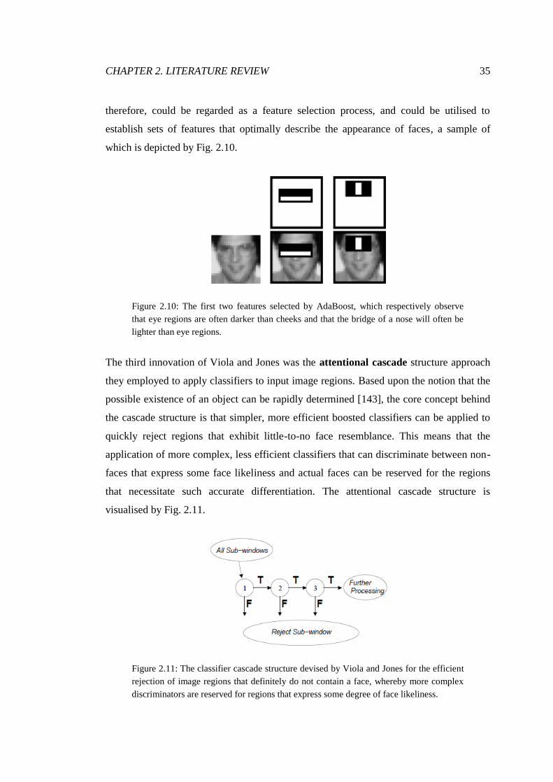
Figure 2.10: The first two features selected by AdaBoost, which respectively observe
that eye regions are often darker than cheeks and that the bridge of a nose will often be
lighter than eye regions.
The third innovation of Viola and Jones was the attentional cascade structure approach
they employed to apply classifiers to input image regions. Based upon the notion that the
possible existence of an object can be rapidly determined [143], the core concept behind
the cascade structure is that simpler, more efficient boosted classifiers can be applied to
quickly reject regions that exhibit little-to-no face resemblance. This means that the
application of more complex, less efficient classifiers that can discriminate between non-
faces that express some face likeliness and actual faces can be reserved for the regions
that necessitate such accurate differentiation. The attentional cascade structure is
visualised by Fig. 2.11.
Figure 2.11: The classifier cascade structure devised by Viola and Jones for the efficient
rejection of image regions that definitely do not contain a face, whereby more complex
discriminators are reserved for regions that express some degree of face likeliness.

36 CHAPTER 2. LITERATURE REVIEW
As can be seen, a negative classification being made by any of the boosted classifiers will
result in the given region of interest being rejected. Given that any typical input image
will be dominated by such regions, avoiding the use of more complex classifiers to
discard them helps greatly in minimising image throughput times. Regions that are
positively identified by a classifier will be retained and processed by the next classifier,
and those that are positively classified by every detector within the given cascade will be
considered faces. In practice, the application of the Viola-Jones detector can result in
certain regions being positively classified multiple times, as the given input image will be
processed across a range of scales in order to find faces of different sizes. Building a set
of output faces, therefore, will involve applying a threshold to the number of positive
detections existing within a neighbourhood. Groups of detections larger in size than the
given applied minimum neighbour threshold will be positively classified, and those
smaller will be discarded.
2.1.2 Recent Detection Advancements
Thanks to the dramatic expansion of storage and computation resources and the
groundwork laid down by Viola and Jones [146], appearance-based methods have
dominated the scene of face detection over recent years [163]. As a methodology,
appearance-based face detection involves the collection of large sets of face and non-face
samples from which representative face models can be derived (through the application
of a machine learning technique) and used for classification. Zhang and Zhang break
down this process to highlight two primary issues that recent works have attempted to
solve: what features to extract from training samples, and what learning approach to
apply [165].
Towards the identification of more generalised and representative feature sets, Lienhart
and Maydt [79] introduced 45-degree rotations to the rectangular Haar-like features used
by Viola and Jones, which were designed to counteract perceived weaknesses of the
original features where orientation variability was exhibited by input images. Li et al.
[77] noted that the original Haar-like feature set was limited where multi-view face
detection was concerned, and proposed a scheme that would allow for flexible
combinations of rectangular regions to be formed, as in Fig. 2.12. It was argued that the

CHAPTER 2. LITERATURE REVIEW 37
non-symmetrical features that this technique could produce would be more effective in
identifying the non-symmetrical features of non-frontal faces.
Figure 2.12: Flexible distances were introduced to Haar-like features by Li et al. [77],
whereby the values of features would be determined through the weighted sums of pixels
within the rectangles.
Jones and Viola themselves went on to suggest improvements to their initial system.
Firstly, they proposed the use of diagonally arranged features to enhance multi-view
detection rates [53], although this differed from the previously proposed rotated features
[80] in that the rectangles themselves would maintain orthogonality. Furthermore, Viola
et al. extended the Haar-like feature set so that it could be applied to the problem of
video-based pedestrian detection [148], where motion information could be combined
with intensity information in order to identify people across consecutive input frames. In
an effort to better represent the complex characteristics of human faces, Mita et al
proposed joint Haar-like features [91], which would be based upon the co-occurrence of
multiple basic Haar-like features and would, they claimed, make it possible to build more
effective classifiers.
By virtue of Haar-like features relating to image region intensities, robustness can be a
serious issue where inputs exhibit extreme lighting conditions [165]. It is for this reason
that numerous other types of features have been proposed and applied to face detection.
A particularly prominent example of these is the local binary patterns (LBP) [96], which
are highly efficient texture operators that consider the neighbourhoods of input pixels,
making them robust to illumination variations [114]. It has been demonstrated that LBPs
can effectively detect faces within images given Bayesian [50] and boosting [167]
(through the image representation scheme illustrated by Fig. 2.13) frameworks. Other
examples of utilised features include anisotropic Gaussian filters [89], local edge

38 CHAPTER 2. LITERATURE REVIEW
orientation histograms [75], histograms of oriented gradients (HoG) [20], and shape-
based techniques that use contour fragments [100,127].
Figure 2.13: The multi-block LBP image representation technique proposed by Zhang et
al. [167], whereby blocks of pixels are averaged before thresholding, which allows for
large-scale structure to be captured.
As Zhang and Zhang alluded to, as well as exploring different types of features to work
with, many researchers have attempted improve upon the learning processes that build
classifiers [165]. An early enhancement to AdaBoost was the development of RealBoost
[119]. This classifier training scheme differed from the original in two key ways. Firstly,
the weak feature classifiers yield likelihood values rather than binary classifications.
Secondly, the selection of successive classifiers is not based upon the performances of
them when considered in isolation, but rather their contributions to the overall
classification system. Whilst this scheme allows for the construction of detectors with
less internal redundancy, more complete datasets are required than would be necessitated
by AdaBoost [16], but RealBoost has been shown to achieve superior results [8,79].
Another noteworthy modification of AdaBoost was Floatboost, as proposed by Li et al.
[77] in conjunction with their flexible features. The primary innovation of this training
technique was the incorporation of floating search methodology [109], whereby the
sequential fashion of feature selection was rejected in order for insignificant features to
be retrospectively removed from sets, supposedly resulting in more optimal classifiers.
To complement attempts to improve upon the efficacy of feature selection processes, a
number of works have developed techniques to increase the efficiency of them, as
training a face detector through boosting can be extremely time-consuming [159].
Brubaker et al., for instance, investigated filter schemes that could reduce the sizes of
possible feature sets prior to boosting by identifying and discarding spurious features [8],
which would prove to be more effective than reducing the number of training examples
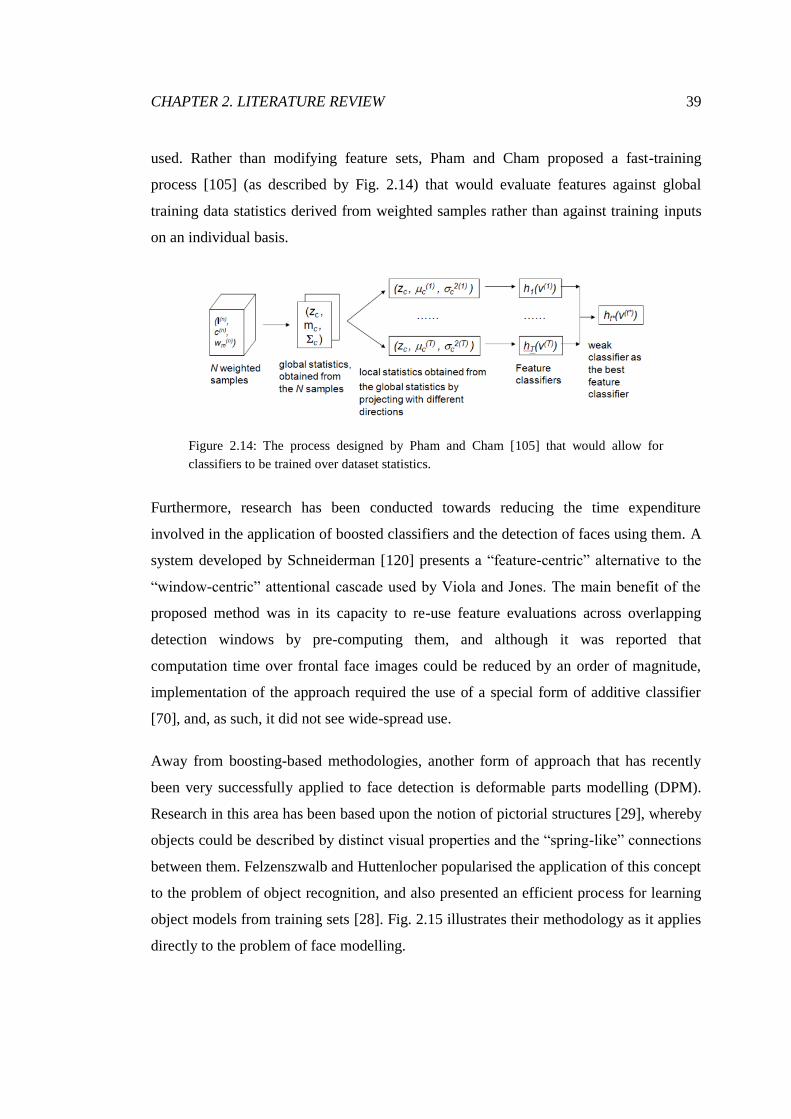
CHAPTER 2. LITERATURE REVIEW 39
used. Rather than modifying feature sets, Pham and Cham proposed a fast-training
process [105] (as described by Fig. 2.14) that would evaluate features against global
training data statistics derived from weighted samples rather than against training inputs
on an individual basis.
Figure 2.14: The process designed by Pham and Cham [105] that would allow for
classifiers to be trained over dataset statistics.
Furthermore, research has been conducted towards reducing the time expenditure
involved in the application of boosted classifiers and the detection of faces using them. A
system developed by Schneiderman [120] presents a “feature-centric” alternative to the
“window-centric” attentional cascade used by Viola and Jones. The main benefit of the
proposed method was in its capacity to re-use feature evaluations across overlapping
detection windows by pre-computing them, and although it was reported that
computation time over frontal face images could be reduced by an order of magnitude,
implementation of the approach required the use of a special form of additive classifier
[70], and, as such, it did not see wide-spread use.
Away from boosting-based methodologies, another form of approach that has recently
been very successfully applied to face detection is deformable parts modelling (DPM).
Research in this area has been based upon the notion of pictorial structures [29], whereby
objects could be described by distinct visual properties and the “spring-like” connections
between them. Felzenszwalb and Huttenlocher popularised the application of this concept
to the problem of object recognition, and also presented an efficient process for learning
object models from training sets [28]. Fig. 2.15 illustrates their methodology as it applies
directly to the problem of face modelling.
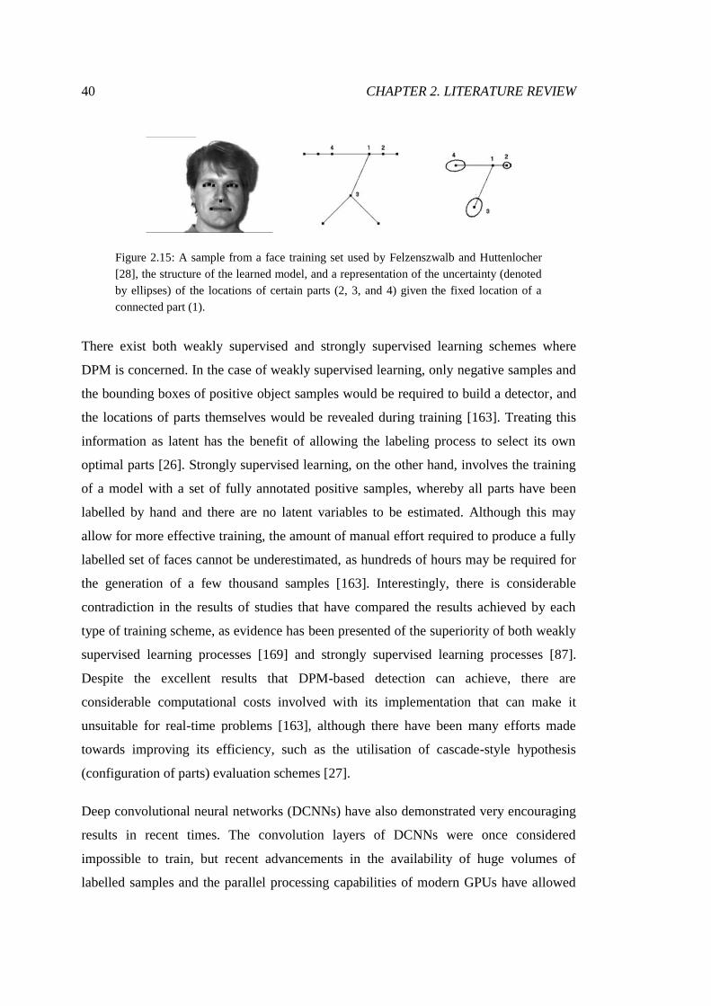
40 CHAPTER 2. LITERATURE REVIEW
Figure 2.15: A sample from a face training set used by Felzenszwalb and Huttenlocher
[28], the structure of the learned model, and a representation of the uncertainty (denoted
by ellipses) of the locations of certain parts (2, 3, and 4) given the fixed location of a
connected part (1).
There exist both weakly supervised and strongly supervised learning schemes where
DPM is concerned. In the case of weakly supervised learning, only negative samples and
the bounding boxes of positive object samples would be required to build a detector, and
the locations of parts themselves would be revealed during training [163]. Treating this
information as latent has the benefit of allowing the labeling process to select its own
optimal parts [26]. Strongly supervised learning, on the other hand, involves the training
of a model with a set of fully annotated positive samples, whereby all parts have been
labelled by hand and there are no latent variables to be estimated. Although this may
allow for more effective training, the amount of manual effort required to produce a fully
labelled set of faces cannot be underestimated, as hundreds of hours may be required for
the generation of a few thousand samples [163]. Interestingly, there is considerable
contradiction in the results of studies that have compared the results achieved by each
type of training scheme, as evidence has been presented of the superiority of both weakly
supervised learning processes [169] and strongly supervised learning processes [87].
Despite the excellent results that DPM-based detection can achieve, there are
considerable computational costs involved with its implementation that can make it
unsuitable for real-time problems [163], although there have been many efforts made
towards improving its efficiency, such as the utilisation of cascade-style hypothesis
(configuration of parts) evaluation schemes [27].
Deep convolutional neural networks (DCNNs) have also demonstrated very encouraging
results in recent times. The convolution layers of DCNNs were once considered
impossible to train, but recent advancements in the availability of huge volumes of
labelled samples and the parallel processing capabilities of modern GPUs have allowed

CHAPTER 2. LITERATURE REVIEW 41
for significant breakthroughs in their application to object classification problems [163],
as demonstrated by a state-of-the-art performance over the ImageNet database [22] by a
DCNN with 60 million parameters, 650,000 neurons, and five convolutional layers,
which was developed by Krizhevsky et al. and dubbed “AlexNet” [68]. Zhang and Zhang
also worked with DCNNs, as they applied the architecture directly to the problem of
multi-view face detection [166]. Their proposed scheme would firstly employ a cascade-
based face detector to identify potential face regions within input images. The results of
this would then be scaled and preprocessed, as in Fig. 2.16(a), with histogram
equalisation, linear lighting removal, and intensity normalisation utilised to prepare
regions of interest for classification through the DCNN. The neural network itself, as
illustrated by Fig. 2.16(b), consisted of three separate branches, each of which was
designed to return classifications on different face properties. The first of these would
yield a face / non-face decision, the second would learn the pose of the face (in terms of it
being frontal, profile, half-profile etc.), and the third would determine the locations of
various facial landmarks, such as eyes, noses, and the corners of mouths. Each of these
branches also made use of the “dropout” technique [40] for reducing network overfitting,
as previously employed for AlexNet [68], which worked by setting the output of hidden
neurons to zero with a probability of 0.5. This would ensure that different architectures
were sampled for each input presented, which would reduce the complex co-adaptation of
neurons. This approach to face detection achieved state-of-the-art detection results over
the FDDB dataset [47].
(a) (b)
Figure 2.16: The face detection approach of Zhang and Zhang [166] would (a)
preprocess image regions of interest before passing them into (b) their DCNN, which
consisted of three separate classification branches.
Farfade et al. [24] also attempted to solve multi-view face detection with DCNNs. They
noted that the requirement of annotating facial landmarks and face poses, and the
necessity to train numerous models to fully capture all face orientations, were large issues
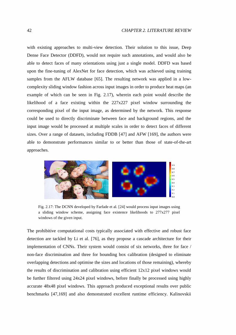
42 CHAPTER 2. LITERATURE REVIEW
with existing approaches to multi-view detection. Their solution to this issue, Deep
Dense Face Detector (DDFD), would not require such annotations, and would also be
able to detect faces of many orientations using just a single model. DDFD was based
upon the fine-tuning of AlexNet for face detection, which was achieved using training
samples from the AFLW database [65]. The resulting network was applied in a low-
complexity sliding window fashion across input images in order to produce heat maps (an
example of which can be seen in Fig. 2.17), wherein each point would describe the
likelihood of a face existing within the 227x227 pixel window surrounding the
corresponding pixel of the input image, as determined by the network. This response
could be used to directly discriminate between face and background regions, and the
input image would be processed at multiple scales in order to detect faces of different
sizes. Over a range of datasets, including FDDB [47] and AFW [169], the authors were
able to demonstrate performances similar to or better than those of state-of-the-art
approaches.
Fig. 2.17: The DCNN developed by Farfade et al. [24] would process input images using
a sliding window scheme, assigning face existence likelihoods to 277x277 pixel
windows of the given input.
The prohibitive computational costs typically associated with effective and robust face
detection are tackled by Li et al. [76], as they propose a cascade architecture for their
implementation of CNNs. Their system would consist of six networks, three for face /
non-face discrimination and three for bounding box calibration (designed to eliminate
overlapping detections and optimise the sizes and locations of those remaining), whereby
the results of discrimination and calibration using efficient 12x12 pixel windows would
be further filtered using 24x24 pixel windows, before finally be processed using highly
accurate 48x48 pixel windows. This approach produced exceptional results over public
benchmarks [47,169] and also demonstrated excellent runtime efficiency. Kalinovskii
CHAPTER 2. LITERATURE REVIEW 43
and Spitsyn similarly proposed a cascade-based neural network scheme [56], noting that
although the approach of Li et al. [76] significantly reduced the computational
complexity of detection, it could not achieve the real-time processing of HD video
streams. Their “compact” system was based upon a number of key concepts: the use of
only three cascade stages; compact network design; asynchronous execution of cascade
stages, whereby the results of the GPU-executed first stage will be immediately passed
on to the CPU-executed subsequent stages; and optimisation through hardware
technologies, such as SIMD expansion of CPUs, CUDA, and OpenCL. Evaluation of this
approach demonstrated levels of detection accuracy comparable to state-of-the-art
techniques over FDDB [47] and AFW [169], and proved that it was capable of processing
4K video streams in real-time (up to 27fps) on mobile platforms.
2.1.3 Face Detection Enhancement Methods
As well as improvements being made to feature-based learning, modelling, and
classification methodologies, a number of researchers have harnessed certain visual
properties of images in the direct enhancement of the capabilities of the Viola-Jones face
detector [147], much in the way we have proposed in Chapter 1. Here, we will highlight a
selection of these works, but also touch upon the general unsuitability of them for solving
the specific problems we are concerned with.
Burgin et al. [11], for instance, combined face detection results with context and depth
information in order to improve human-computer interaction in robots, but this
methodology would not necessarily be applicable to our single-image problem. Nanni et
al. [93] proposed the adoption of a pre-trained colour classifier to filter detections, as well
as the use of a depth map to investigate the unevenness of those regions, creating a
process that takes multiple properties into account in an attempt to improve overall
detection accuracies, but we do not believe this technique would be flexible enough to
account for the variabilities that the inputs we are concerned with are liable to exhibit.
Seguí et al. [123] found that integrating content-based face detection information with
contextual body part information could yield significant improvements to accuracy,
although such information would clearly not be available in the case of our lecture
theatre-based imagery.
44 CHAPTER 2. LITERATURE REVIEW
Employing a different form of approach, Shieh and Hsieh [125] used the IR information
provided by a Microsoft Kinect sensor in order to refine detection results through
structured light analysis. Alternative hardware was also utilised by Ruiz-Sarmiento et al.
[117], as they initially identified face candidates by using the Viola-Jones detector on
intensity data provided by a time-of-flight camera, then filtered the results of that process
according to three-dimensional information, such as region flatness and size-to-distance
ratio. Whilst interesting, these solutions requiring additional pieces of hardware severely
limits their general applicability to problems. Furthermore, the success of the works that
have not made use of external devices leads us to believe that enough information already
exists within typical input images for the issues we have identified to be overcome
without them, given the sound derivation and implementation of models pertaining to
supplementary modalities.
2.2 Colour-Based Skin Segmentation
Systems that can accurately discriminate between skin and non-skin pixels on a
consistent basis are extremely valuable, as the segmentation of skin regions enables many
types of applications, such as face detection [67], face tracking [134], gesture analysis
[6], and content-based image retrieval [126]. It is colour-based methodologies that have
become predominant in the field of skin segmentation, as colour, as a low-level property,
allows for efficient classifications and is invariant to issues concerning rotation, scaling,
and subject occlusion [54].
This is not to say that colour-based approaches do not have their limitations, however, as
the apparent colour of skin within an image is greatly dependent upon a number of
factors, adding complexity to any proposed modelling approach. As well as varying
considerably with the ethnicity of individuals and the characteristics of camera sensors,
illumination will play a near-decisive role in how skin appears [54]. The appearance of
any region of skin can, naturally, tend towards absolute black or absolute white
depending upon the intensity of incident light, but Storring et al. also demonstrated that
the specific correlated colour temperature (CCT) of a light source will also be greatly

CHAPTER 2. LITERATURE REVIEW 45
influential, as even two near-white light sources with different CCTs can lead to entirely
different representations for skin regions [136], as Fig. 2.18 illustrates.
Figure 2.18: Storring et al. [136] demonstrated that light source CCT will greatly
influence the chromaticity of skin regions, even more so than the ethnicity of an
individual.
Because the effects of illumination variability are so significant, they of primary concern
to the development of any colour-based skin classification methodology. There are a
number of considerations to be made when conceptualising a colour-based segmentation
approach capable of accounting for influential factors [54], including the colour space to
be worked with, the means by which colour distributions will be modelled, and the way
in which models will be applied to inputs (including potential adaptation).
2.2.1 Colour Spaces for Skin Modelling
A colour space is a specification for the mathematical representation of colours, whereby
a certain set of parameters will be used to define appearance. A wide variety of spaces
exist, which will have been developed to emphasise certain usage characteristics (such as
efficiency or illumination invariance), and many of them have been applied to the
problem of skin colour modelling [46]. RGB is the most commonly utilised space for
digital image processing, largely because it linearly combines red, green, and blue colour
components (as illustrated by Fig. 2.19), which made it easy to implement for early CRT
technology, giving its usage a considerable historical basis. Its simplicity also means that
it allows for the rapid classification of input pixels, making it attractive for real-time
systems [145], and its use has been investigated by a number of works [5,67,164].

46 CHAPTER 2. LITERATURE REVIEW
Figure 2.19: The RGB colour space linearly combines red, green, and blue colour
components to represent colours. Visualisation courtesy of ArcSoft.
The usage of the RGB colour space in skin classification is not broadly suggested,
however, as it intrinsically associates illumination information with chromatic
information, meaning that even minor changes in lighting conditions can result in
significant changes to colour representation [86], making consistent classification with
RGB models largely infeasible. To overcome this dependency, the space can be
normalised to only consider the proportions of colour components, as in Eq. 2.1, Eq. 2.2,
and Eq. 2.3.
𝑟 = 𝑅
𝑅+𝐺+𝐵 (2.1)
𝑔 = 𝐺
𝑅+𝐺+𝐵 (2.2)
𝑏 = 𝐵
𝑅+𝐺+𝐵 (2.3)
Given that these components would always sum to unity (1), a dimension can be
discarded without any actual loss of information, which is how the normalised rg colour
space comes to be derived. Not only does this conversion provide significant resistance to
variations in illumination intensity, but the reduction in dimensionality makes modelling
and classification processes less complex [145]. Furthermore, it has been demonstrated
that skin colour clusters within the normalised rg space have much lower variance than
distributions within RGB space [155] and that the skin tones of people from various
ethnicities will be tightly clustered [136] (as Fig. 2.18 illustrated), making it a popular
choice for skin classification tasks [7,98,122,134].
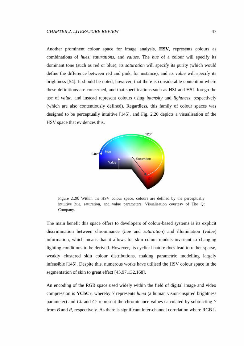
CHAPTER 2. LITERATURE REVIEW 47
Another prominent colour space for image analysis, HSV, represents colours as
combinations of hues, saturations, and values. The hue of a colour will specify its
dominant tone (such as red or blue), its saturation will specify its purity (which would
define the difference between red and pink, for instance), and its value will specify its
brightness [54]. It should be noted, however, that there is considerable contention where
these definitions are concerned, and that specifications such as HSI and HSL forego the
use of value, and instead represent colours using intensity and lightness, respectively
(which are also contentiously defined). Regardless, this family of colour spaces was
designed to be perceptually intuitive [145], and Fig. 2.20 depicts a visualisation of the
HSV space that evidences this.
Figure 2.20: Within the HSV colour space, colours are defined by the perceptually
intuitive hue, saturation, and value parameters. Visualisation courtesy of The Qt
Company.
The main benefit this space offers to developers of colour-based systems is its explicit
discrimination between chrominance (hue and saturation) and illumination (value)
information, which means that it allows for skin colour models invariant to changing
lighting conditions to be derived. However, its cyclical nature does lead to rather sparse,
weakly clustered skin colour distributions, making parametric modelling largely
infeasible [145]. Despite this, numerous works have utilised the HSV colour space in the
segmentation of skin to great effect [45,97,132,168].
An encoding of the RGB space used widely within the field of digital image and video
compression is YCbCr, whereby Y represents luma (a human vision-inspired brightness
parameter) and Cb and Cr represent the chrominance values calculated by subtracting Y
from B and R, respectively. As there is significant inter-channel correlation where RGB is
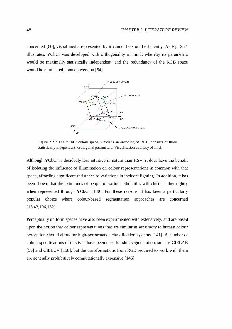
48 CHAPTER 2. LITERATURE REVIEW
concerned [60], visual media represented by it cannot be stored efficiently. As Fig. 2.21
illustrates, YCbCr was developed with orthogonality in mind, whereby its parameters
would be maximally statistically independent, and the redundancy of the RGB space
would be eliminated upon conversion [54].
Figure 2.21: The YCbCr colour space, which is an encoding of RGB, consists of three
statistically independent, orthogonal parameters. Visualisation courtesy of Intel.
Although YCbCr is decidedly less intuitive in nature than HSV, it does have the benefit
of isolating the influence of illumination on colour representations in common with that
space, affording significant resistance to variations in incident lighting. In addition, it has
been shown that the skin tones of people of various ethnicities will cluster rather tightly
when represented through YCbCr [130]. For these reasons, it has been a particularly
popular choice where colour-based segmentation approaches are concerned
[13,43,106,152].
Perceptually uniform spaces have also been experimented with extensively, and are based
upon the notion that colour representations that are similar in sensitivity to human colour
perception should allow for high-performance classification systems [141]. A number of
colour specifications of this type have been used for skin segmentation, such as CIELAB
[59] and CIELUV [158], but the transformations from RGB required to work with them
are generally prohibitively computationally expensive [145].

CHAPTER 2. LITERATURE REVIEW 49
2.2.2 Colour Distribution Modelling Approaches
Even with a sound selection of colour space to work with, the way in which a
representative skin colour model is derived will mean the difference between accurate
and inaccurate segmentations. There exist numerous approaches to modelling, and each
will offer its own set of advantages and potential drawbacks, so the choice of which to
apply will depend upon the requirements of the problem to be solved.
2.2.1.1 Explicit Skin Colour Cluster Models
The colour distributions exhibited by regions of skin can be defined by piecewise linear
decision rules that pertain to the parameters of colour spaces. Such models are derived
manually, based upon observations made of the appearance of skin over large sets of
positive samples. An example of such a model was developed by Sobottka and Pitas
[132], whereby hue and saturation parameters were used to discriminate between skin
and non-skin pixels. The rules they developed are described by Eq. 2.4, where H
represents the hue of the input pixel and S represents its saturation.
𝑝𝑖𝑥𝑒𝑙 = 𝑠𝑘𝑖𝑛, 0 ≤ 𝐻 ≤ 50 𝑎𝑛𝑑 0.23 ≤ 𝑆 ≤ 0.68
𝑛𝑜𝑛 − 𝑠𝑘𝑖𝑛, 𝑜𝑡𝑒𝑟𝑤𝑖𝑠𝑒
(2.4)
As can be discerned, this approach will yield binary discrete classifications, whereby any
pixel that exhibits a hue and saturation within the defined bounds of the model would be
classified as skin, and any that does not would be discarded. This explicit colour cluster
can also be visualised, as in Fig. 2.22.
Figure 2.22: The HSV skin colour model derived by Sobottka and Pitas [132] dictates
that any pixel with a hue and saturation within the shaded cluster will be positively
classified.

50 CHAPTER 2. LITERATURE REVIEW
The primary benefit of using explicit clusters is that they allow for extremely rapid
classifications [145], and since they necessitate no upfront training process, they can be
implemented trivially and potentially save significant amounts of time, which has made
them attractive to a number of works [150,152,160]. There are, however, a number of
issues inherent to such models. Firstly, the empirical nature of the derivation of the
decision rules can result in models being “overfitted” to experimental data [145]. This
may cause issues for adopters if their potential inputs are not adequately represented by
the training samples used, as significant numbers of misclassifications may ensue.
Furthermore, as the appearance of skin is so dependent upon its illumination, explicitly
defined clusters are liable to be inaccurate under weaker lighting conditions [54].
2.2.1.2 Non-Parametric Skin Colour Modelling
Non-parametric modelling approaches estimate the probabilities that certain colours
represent skin through the statistical analysis of large skin and non-skin training sample
sets. A typical form for such a model is a skin probability map, which will attribute skin
likelihoods to colours without the derivation or definition of specific skin colour cluster
parameters [35]. To build such a representation, a colour space must first be quantised
into a certain number of histogram bins, each of which will uniquely correspond to a
specific colour component combination. The number of bins used must be decidedly
upon with care, as too few bins will result in classification oversensitivity and poor
accuracy, but too many can lead to models being overly specific to training samples [52].
In order to derive a simple look-up table, the occurrence of certain colours within a set of
positive skin samples can be tallied according to the defined bins, then normalised
according to the greatest observed frequency [164], but this resulting in an accurate
classifier would require perfectly representative training data to be used.
A more complete representation can be constructed through the application of Bayes’
theorem, whereby individual skin and non-skin probability mass functions (normalised
according to the total numbers of used samples) can be used to build a probability map
that accounts for the colour distribution of non-skin entities. The potential efficacy of this
methodology has resulted in it being adopted by many researchers [13,129,135]. The
calculation of skin likelihoods using this approach is conducted according to Eq. 2.5,
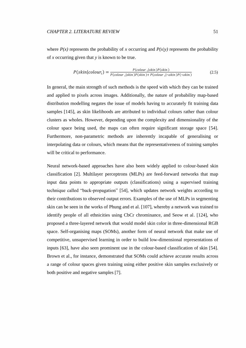
CHAPTER 2. LITERATURE REVIEW 51
where P(x) represents the probability of x occurring and P(x|y) represents the probability
of x occurring given that y is known to be true.
𝑃 𝑠𝑘𝑖𝑛 𝑐𝑜𝑙𝑜𝑢𝑟𝑖 =𝑃 𝑐𝑜𝑙𝑜𝑢𝑟 𝑖 𝑠𝑘𝑖𝑛 𝑃 𝑠𝑘𝑖𝑛
𝑃 𝑐𝑜𝑙𝑜𝑢𝑟 𝑖 𝑠𝑘𝑖𝑛 𝑃 𝑠𝑘𝑖𝑛 + 𝑃 𝑐𝑜𝑙𝑜𝑢𝑟 𝑖 ¬𝑠𝑘𝑖𝑛 𝑃 ¬𝑠𝑘𝑖𝑛 (2.5)
In general, the main strength of such methods is the speed with which they can be trained
and applied to pixels across images. Additionally, the nature of probability map-based
distribution modelling negates the issue of models having to accurately fit training data
samples [145], as skin likelihoods are attributed to individual colours rather than colour
clusters as wholes. However, depending upon the complexity and dimensionality of the
colour space being used, the maps can often require significant storage space [54].
Furthermore, non-parametric methods are inherently incapable of generalising or
interpolating data or colours, which means that the representativeness of training samples
will be critical to performance.
Neural network-based approaches have also been widely applied to colour-based skin
classification [2]. Multilayer perceptrons (MLPs) are feed-forward networks that map
input data points to appropriate outputs (classifications) using a supervised training
technique called “back-propagation” [54], which updates network weights according to
their contributions to observed output errors. Examples of the use of MLPs in segmenting
skin can be seen in the works of Phung and et al. [107], whereby a network was trained to
identify people of all ethnicities using CbCr chrominance, and Seow et al. [124], who
proposed a three-layered network that would model skin color in three-dimensional RGB
space. Self-organising maps (SOMs), another form of neural network that make use of
competitive, unsupervised learning in order to build low-dimensional representations of
inputs [63], have also seen prominent use in the colour-based classification of skin [54].
Brown et al., for instance, demonstrated that SOMs could achieve accurate results across
a range of colour spaces given training using either positive skin samples exclusively or
both positive and negative samples [7].
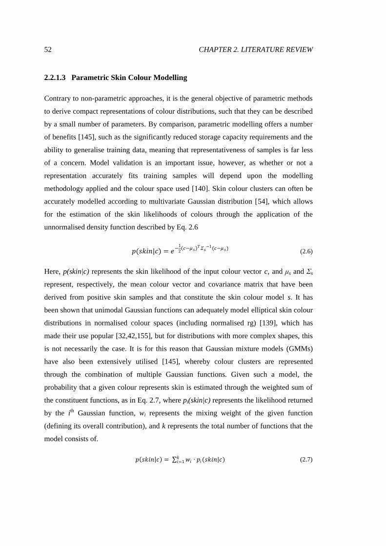
52 CHAPTER 2. LITERATURE REVIEW
2.2.1.3 Parametric Skin Colour Modelling
Contrary to non-parametric approaches, it is the general objective of parametric methods
to derive compact representations of colour distributions, such that they can be described
by a small number of parameters. By comparison, parametric modelling offers a number
of benefits [145], such as the significantly reduced storage capacity requirements and the
ability to generalise training data, meaning that representativeness of samples is far less
of a concern. Model validation is an important issue, however, as whether or not a
representation accurately fits training samples will depend upon the modelling
methodology applied and the colour space used [140]. Skin colour clusters can often be
accurately modelled according to multivariate Gaussian distribution [54], which allows
for the estimation of the skin likelihoods of colours through the application of the
unnormalised density function described by Eq. 2.6
𝑝(𝑠𝑘𝑖𝑛|𝑐) = 𝑒−1
2 𝑐−𝜇𝑠
𝑇𝛴𝑠−1(𝑐−𝜇𝑠)
(2.6)
Here, p(skin|c) represents the skin likelihood of the input colour vector c, and μs and Σs
represent, respectively, the mean colour vector and covariance matrix that have been
derived from positive skin samples and that constitute the skin colour model s. It has
been shown that unimodal Gaussian functions can adequately model elliptical skin colour
distributions in normalised colour spaces (including normalised rg) [139], which has
made their use popular [32,42,155], but for distributions with more complex shapes, this
is not necessarily the case. It is for this reason that Gaussian mixture models (GMMs)
have also been extensively utilised [145], whereby colour clusters are represented
through the combination of multiple Gaussian functions. Given such a model, the
probability that a given colour represents skin is estimated through the weighted sum of
the constituent functions, as in Eq. 2.7, where pi(skin|c) represents the likelihood returned
by the ith Gaussian function, wi represents the mixing weight of the given function
(defining its overall contribution), and k represents the total number of functions that the
model consists of.
𝑝 𝑠𝑘𝑖𝑛 𝑐 = 𝑤𝑖 ∙ 𝑝𝑖(𝑠𝑘𝑖𝑛|𝑐)𝑘𝑖=1 (2.7)

CHAPTER 2. LITERATURE REVIEW 53
The training of a GMM is conducted according to an expectation maximisation
algorithm, but the number of individual functions it will consist of must be defined
beforehand. Similarly to the choice of number of bins used to build a non-parametric
model, the specific number of components to use to build a GMM is extremely important
[54], as too small a number will result in datasets not being effectively represented, and
too large a number may result in overfitting. Results have been reported on the efficacy
of models trained using as few as two functions [158] and as many as 16 functions [52].
Although GMMs have been shown to represent training samples very accurately, the
iterative training processes necessary to build them can be computationally expensive,
and their implementation can also be rather inefficient, as numerous functions must be
evaluated for skin likelihoods to be determined [54]. Lee and Yoo proposed an efficient
alternative to GMMs that they termed “elliptical boundary models” [73]. Although
favourable results, relative to those of a GMM and a unimodal Gaussian function, were
presented over a range of colour spaces, one major drawback of the approach was that it
could not preserve continuous probability information, and could yield only binary
classifications.
2.2.4 Skin Colour Model Adaptation
Whilst colour models that have been derived using the methodologies we have discussed
can certainly be successfully applied in a static context (whereby there is no specific
consideration made for the appearance of individual inputs), several adaptation
techniques exist that are capable of extending the efficacy of models by accounting for
the ever-influential effects of illumination variation at the point of application.
Kakumanu et al. [54] categorised such techniques into two classes: colour constancy-
based approaches; and dynamic adaptation approaches.
One way in which the effects of variable lighting can be negated is through the
consideration of colour constancy, which relates to the capacity for vision systems (be
they natural or artificial) to discount spectral variation and assign constant colours to
objects [84]. Skin segmentation approaches that apply this concept will analyse inputs in
order to estimate the colour and intensity of illuminants, and then transform them through
pixel-wise adjustments in an effort to correct and normalise the colours of skin regions
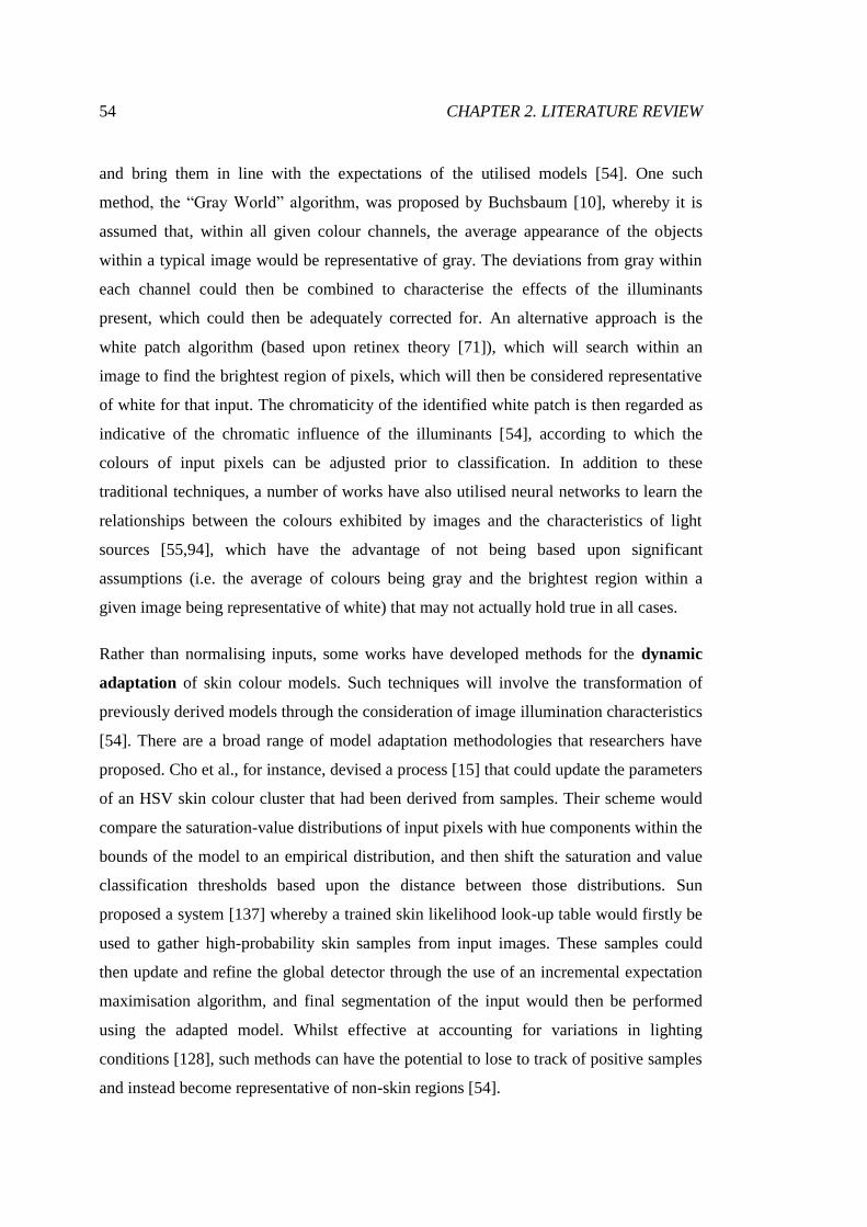
54 CHAPTER 2. LITERATURE REVIEW
and bring them in line with the expectations of the utilised models [54]. One such
method, the “Gray World” algorithm, was proposed by Buchsbaum [10], whereby it is
assumed that, within all given colour channels, the average appearance of the objects
within a typical image would be representative of gray. The deviations from gray within
each channel could then be combined to characterise the effects of the illuminants
present, which could then be adequately corrected for. An alternative approach is the
white patch algorithm (based upon retinex theory [71]), which will search within an
image to find the brightest region of pixels, which will then be considered representative
of white for that input. The chromaticity of the identified white patch is then regarded as
indicative of the chromatic influence of the illuminants [54], according to which the
colours of input pixels can be adjusted prior to classification. In addition to these
traditional techniques, a number of works have also utilised neural networks to learn the
relationships between the colours exhibited by images and the characteristics of light
sources [55,94], which have the advantage of not being based upon significant
assumptions (i.e. the average of colours being gray and the brightest region within a
given image being representative of white) that may not actually hold true in all cases.
Rather than normalising inputs, some works have developed methods for the dynamic
adaptation of skin colour models. Such techniques will involve the transformation of
previously derived models through the consideration of image illumination characteristics
[54]. There are a broad range of model adaptation methodologies that researchers have
proposed. Cho et al., for instance, devised a process [15] that could update the parameters
of an HSV skin colour cluster that had been derived from samples. Their scheme would
compare the saturation-value distributions of input pixels with hue components within the
bounds of the model to an empirical distribution, and then shift the saturation and value
classification thresholds based upon the distance between those distributions. Sun
proposed a system [137] whereby a trained skin likelihood look-up table would firstly be
used to gather high-probability skin samples from input images. These samples could
then update and refine the global detector through the use of an incremental expectation
maximisation algorithm, and final segmentation of the input would then be performed
using the adapted model. Whilst effective at accounting for variations in lighting
conditions [128], such methods can have the potential to lose to track of positive samples
and instead become representative of non-skin regions [54].

CHAPTER 2. LITERATURE REVIEW 55
2.2.4.1 Face Detection-Based Skin Colour Modelling
As well as methodologies for updating existing models based upon the sampling of
images, there are numerous approaches that build skin colour representations directly
from sampled data. The main benefit of this is that applied models can be entirely
specific to given inputs, which maximises the likelihood of accurate segmentation. Image
sampling towards this end can be performed using a face detector, which will allow for
representative regions of skin to be identified on a consistent basis. Here, we will look at
a number of works that make use of face detection technology for skin colour modelling,
but also discuss reasons as to why they make not solve our problems effectively.
Mittal et al. [92] proposed a hand detection approach that involved the combination of the
results of a global, generalised skin detector, with those derived from the Viola-Jones
face detector [147]. The approach then uses spatial information in order to complete the
segmentation. Although they claim segmentation accuracies greater than accepted state-
of-the-art methods, the use of spatial techniques renders the approach rather unsuitable
for real-time applications, as the processing of a single 640x360-pixel image would
reportedly take in the region of two minutes. Wimmer and Radig [151] developed a
system that utilises the same face detector, but uses detection region of interest (ROI)
data to extract a small set of pixels with a skin mask. A skin mask is derived from a
threshold applied to an empirically determined probability map, which has been trained
to estimate the likelihood of specific coordinates of a detected face ROI representing
skin. Extracted pixels are then used to build a parametric colour model to be applied to
the entire image. While interesting, we do not believe that the pixel extraction process of
this approach is ideal, and it may be prone to undersampling in some cases, and
oversampling in others (especially when a subject has hair that may be occluding their
forehead, for instance), both of which are capable of harming the efficacy of any
generated skin colour model.
Again using the Viola-Jones detector, Hsieh et al. [41] developed a system that would
allow for accurate hand detection, by generating skin colour models from detected face
data. Given a square detection region, an inner face region is defined as being a square
centred on the same point, but being only 0.6 of the size of the original in both width and
height (granting a sample of 36% of the pixels of the detection). The pixels within this

56 CHAPTER 2. LITERATURE REVIEW
region are then filtered according to their luminance, whereby the symmetric property of
Gaussian distributions is applied to remove “dark” pixels from the set. The remaining
pixels are then used to build decision rules in the hybrid normalised rg/R (r,g,R) space,
which will simply classify a given pixel as skin if it is within two standard deviations of
the mean value for all three components. Given what we know of the elliptical clustering
of skin colours in the normalised rg space [139], however, we do not believe that
orthogonal, binary decision boundaries are the ideal choice for the accurate segmentation
of skin.
A new face detection algorithm, based upon directional Sobel edges, was developed by
Liao and Chi [78]. Within detected face regions, they sample pixels from a small,
predefined window, the location of which has presumably been empirically derived, in an
effort to consistently extract “good” skin pixels from the right-hand cheeks of subjects. A
histogram of the extracted pixels within the hue domain is then computed, and non-zero
local minima, both greater and smaller than the peak hue, are found. These minima stand
as the upper and lower bounds of skin segmentation, respectively, as every pixel in the
given image is classified according to their hue value. The window used by this approach
samples only 4% of the given detected face, which we believe could cause critical
undersampling in a high proportion of cases. Additionally, we do not believe that hue
alone is sufficient for accurate skin colour modelling in anything but the most ideal
illumination conditions, a belief reinforced by the sheer number of works that have
combined hue information with saturation information at the very least [54].
2.3 Review Summary
In this chapter, we initially examined a large amount of the research conducted within the
field of face detection. Although a wide array of techniques had been proposed that could
demonstrate accurate detection results under constrained conditions, it was not until the
seminal work of Viola and Jones [146] and the dramatic expansion of the capabilities of
electronic devices that face detection systems could be applied effectively to real-world
problems [165]. Because of the high complexity of the problem of face detection, the
number of disparate approaches experimented with in recent years has been vast, with

CHAPTER 2. LITERATURE REVIEW 57
DCNNs and DPMs demonstrating increasingly exceptional performances and the
traditional boosting-based techniques also being improved upon [163]. Furthermore, we
have noted the recent development of systems that enhance the results of existing face
detectors with supplementary information, which we believe is a methodology that could
prove effective where our large-scale detection problem is concerned.
We have also reviewed the field of colour-based skin segmentation. As the apparent
colour of skin is so greatly dependent upon incident illumination [136], accurately and
consistently identifying skin within images is a considerable challenge. The success of a
segmentation system will hinge primarily upon the selection of an appropriate colour
space, the availability of representative training data, the suitability of the applied
modelling methodology, the utilisation of an adaptation algorithm, and the definition of
an effective input classification scheme [163]. Existing works have experimented with
various combinations of options for the above, and demonstrated great success under
certain conditions. More recently, a number of approaches have modelled skin colour
distributions directly from the results of face detectors, which is a concept that may allow
us to consistently achieve accurate segmentations over lecture theatre imagery.

58
Chapter 3
Adaptive Skin Segmentation via
Feature-Based Face Detection
In this chapter, we will explore the deficiencies of a range of existing colour-based skin
segmentation techniques, describe the developmental process of our own adaptive
approach, and then present an extensive evaluation of its capabilities.
3.1 Segmentation Problem Definition
In order for us to successfully incorporate colour-based classification into our face
detection system, we need to use a modelling methodology that meets the requirements
of our input. Although colour is a useful property for us to examine because it is invariant
to many of the issues that degrade feature discernibility, large-scale imagery will often
exhibit illumination that is influenced by numerous light sources, which can have
variable hues, intensities, orientations, and distributions. All of these factors can have
dramatic effects upon the apparent colour of skin within an image [136], which, of
course, could majorly impact the segmentation consistency of certain classifiers when
used over multiple images.
In this section, we will investigate the efficacy of a number of existing segmentation
methodologies when applied to images of lecture theatres, and attempt to ascertain the
reasons for their successes and their shortcomings. We will be using two different sample
images, which have been captured under entirely different circumstances. As well as

CHAPTER 3. ADAPTIVE SKIN SEGMENTATION 59
containing separate sets of people, the images pertain to markedly different
environments, with rather dissimilar illumination tones. What is important to note,
however, is that we believe both images represent fairly favourable circumstances for
segmentation, with each being of high general quality (in terms of focus and resolution)
and exhibiting relatively intense and even illumination. These images can be seen in Fig.
3.1 and Fig. 3.2.
Figure 3.1: Our first input image. It depicts the visible faces of 31 individuals of various
ethnicities, and a number of light sources contributing to a generally even illumination.
Figure 3.2: Our second input image. It contains 37 visible faces of individuals from a
wide range of ethnicities, and has a strong general illumination, which is whiter in tone
than the one depicted by Fig. 3.1.

60 CHAPTER 3. ADAPTIVE SKIN SEGMENTATION
We believe these inputs will prove sufficient in providing us with the information that we
need to successfully incorporate a skin detector into our face detection system. Given the
exposure of a broad range of skin colours to the same illumination conditions, we will be
able to discern the consistency with which individual segmentation methodologies
identify different skin tones. For instance, a detector may generally be more effective at
segmenting Caucasian skin than African skin, and this trait should become apparent
during our experimentation across different illuminations. Additionally, the specific
illumination tones being worked with are important, as it is entirely possible that the tone
of one of our images more closely reflects the illumination present within the training
data of a given classifier, which could have quite a dramatic effect on its segmentation
consistency.
It should be noted that it is critical our sample images are indeed of high quality, as it will
allow us to discern how liable existing techniques are to failure given even advantageous
conditions, giving us the best possible sense of how much room there is for improvement.
Inputs of lesser quality would simply not yield the same amount of information, as the
root causes of failures may not always be obvious. For instance, the failure of a classifier
to properly segment a skin region may be attributed to a lack of intense light incident on
that skin, but the classifier actually being too insensitive may be obfuscated by that
circumstance. Furthermore, multiple classifiers may fail to segment the same poorly
illuminated skin region, but, of course, that does not imply all of them would have been
successful had the lighting conditions been better, so some potential insight into the
differences between those classifiers is lost. For the sake of exemplifying the relative
quality of our two inputs, we present an image of much lower quality, which can be seen
in Fig 3.3.

CHAPTER 3. ADAPTIVE SKIN SEGMENTATION 61
Figure 3.3: An example of a poor quality input. The light sources within the environment
are arranged such that the illumination is extremely uneven. While some individuals are
illuminated rather favourably, many others, especially those near the front, are decidedly
less so.
The illumination presented by Fig. 3.3 being greatly uneven is a particularly problematic
circumstance. While a colour-based classifier could be designed specifically for the
segmentation of skin as it appears under weak illumination, the existence of different
degrees of illumination within the same image is almost certain to result in an
inconsistent performance. The potential for such circumstances to occur further
reinforces the suitability of the images we have chosen to use for this experimentation.
3.1.1 Analysis of Existing Techniques
We will now implement a broad range of the existing colour-based segmentation
methodologies we identified in Chapter 2, and analyse how well they perform when
tasked with segmenting the skin from within our test images. Our segmentation analysis
will be two-fold, as we assess outputs both quantitatively and qualitatively.
With regards to our quantitative analysis, we will be presenting results using a range of
different statistics. Not only will this type of analysis provide us with a wealth of useful
information, it will also allow us to compare the results of different detectors simply and
effectively. This objective analysis will involve the pixel-wise comparison of produced
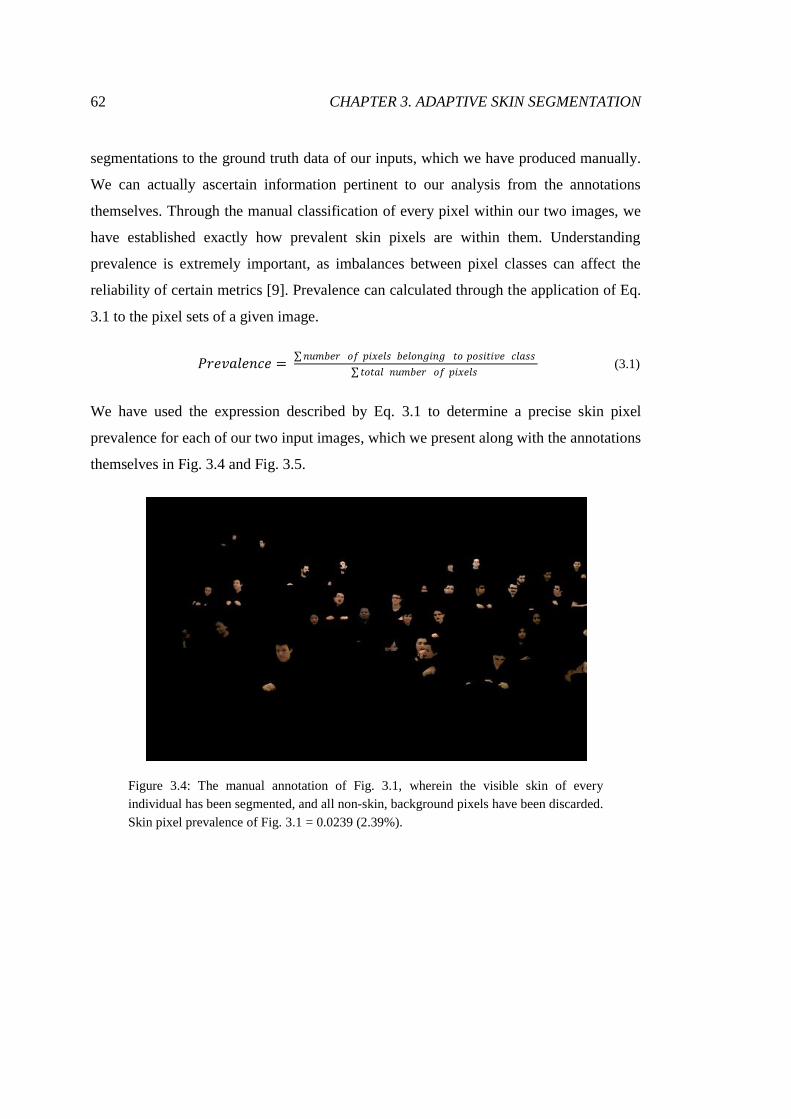
62 CHAPTER 3. ADAPTIVE SKIN SEGMENTATION
segmentations to the ground truth data of our inputs, which we have produced manually.
We can actually ascertain information pertinent to our analysis from the annotations
themselves. Through the manual classification of every pixel within our two images, we
have established exactly how prevalent skin pixels are within them. Understanding
prevalence is extremely important, as imbalances between pixel classes can affect the
reliability of certain metrics [9]. Prevalence can calculated through the application of Eq.
3.1 to the pixel sets of a given image.
𝑃𝑟𝑒𝑣𝑎𝑙𝑒𝑛𝑐𝑒 = 𝑛𝑢𝑚𝑏𝑒𝑟 𝑜𝑓 𝑝𝑖𝑥𝑒𝑙𝑠 𝑏𝑒𝑙𝑜𝑛𝑔𝑖𝑛𝑔 𝑡𝑜 𝑝𝑜𝑠𝑖𝑡𝑖𝑣𝑒 𝑐𝑙𝑎𝑠𝑠
𝑡𝑜𝑡𝑎𝑙 𝑛𝑢𝑚𝑏𝑒𝑟 𝑜𝑓 𝑝𝑖𝑥𝑒𝑙𝑠 (3.1)
We have used the expression described by Eq. 3.1 to determine a precise skin pixel
prevalence for each of our two input images, which we present along with the annotations
themselves in Fig. 3.4 and Fig. 3.5.
Figure 3.4: The manual annotation of Fig. 3.1, wherein the visible skin of every
individual has been segmented, and all non-skin, background pixels have been discarded.
Skin pixel prevalence of Fig. 3.1 = 0.0239 (2.39%).

CHAPTER 3. ADAPTIVE SKIN SEGMENTATION 63
Figure 3.5: The manual annotation of Fig. 3.2, wherein every background pixel has been
discarded, and all skin pixels have been positively classified. Skin pixel prevalence of
Fig. 3.2 = 0.1065 (10.65%).
At this time, we will be evaluating skin segmentation technique performance using five
different (although intrinsically related) metrics, which can be derived from the number
of true positives (TP), true negatives (TN), false positives (FP), and false negatives (FN)
yielded by the process of segmentation. It is vitally important that we do use a range of
different types of statistics, as certain metrics, when used in isolation, can give false
impressions of how a given classifier has actually performed.
Recall (also Sensitivity, True Positive Rate) represents the proportion of all skin pixels
present within the given image that have been segmented by the process of detection, and
can be described by Eq. 3.2.
𝑅𝑒𝑐𝑎𝑙𝑙 = 𝑛𝑢𝑚𝑏𝑒𝑟 𝑜𝑓 𝑠𝑘𝑖𝑛 𝑝𝑖𝑥𝑒𝑙𝑠 𝑠𝑒𝑔𝑚𝑒𝑛𝑡𝑒𝑑
𝑡𝑜𝑡𝑎𝑙 𝑛𝑢𝑚𝑏𝑒𝑟 𝑜𝑓 𝑠𝑘𝑖𝑛 𝑝𝑖𝑥𝑒𝑙𝑠 𝑖𝑛 𝑖𝑚𝑎𝑔𝑒=
𝑇𝑃
𝑇𝑃+𝐹𝑁 (3.2)
Maximising recall is extremely important to any detection system, as it represents the
capacity of the given classifier to actually detect the class of pixels it has been trained to
detect. Without the capacity to achieve high recall rates, the actual usefulness of a given
detection system could potentially be called into question. In isolation, this metric can be
misleading, however, as a skin detector designed to indiscriminately positively classify

64 CHAPTER 3. ADAPTIVE SKIN SEGMENTATION
every pixel within a given image would achieve a recall rate of 100% during any given
trial.
Precision (also Positive Predictive Value) is defined as the proportion of all pixels
positively classified by a detector that actually belong to the skin class, and can be
described by Eq. 3.3.
𝑃𝑟𝑒𝑐𝑖𝑠𝑖𝑜𝑛 = 𝑛𝑢𝑚𝑏𝑒𝑟 𝑜𝑓 𝑠𝑘𝑖𝑛 𝑝𝑖𝑥𝑒𝑙𝑠 𝑠𝑒𝑔𝑚𝑒𝑛𝑡𝑒𝑑
𝑡𝑜𝑡𝑎𝑙 𝑛𝑢𝑚𝑏𝑒𝑟 𝑜𝑓 𝑝𝑖𝑥𝑒𝑙𝑠 𝑠𝑒𝑔𝑚𝑒𝑛𝑡𝑒𝑑=
𝑇𝑃
𝑇𝑃+𝐹𝑃 (3.3)
Achieving a high precision is paramount to building confidence in a classifier, as the
higher the precision of a result, the more likely a positive classification actually
represents a skin pixel. Precision can also give a false impression of the performance of a
classifier, however, as a precision of 100% can be achieved through the positive
classification of only a single pixel, as long as that one pixel does indeed represent skin.
Although this is a scenario that would probably have to be quite specifically engineered,
it does remain a possibility, and implies that recall should always be taken into
consideration in conjunction with precision.
Specificity (also True Negative Rate) is defined as the proportion of non-skin pixels
present within the given image that have been negatively classified, and can be described
by Eq. 3.4.
𝑆𝑝𝑒𝑐𝑖𝑓𝑖𝑐𝑡𝑦 = 𝑛𝑢𝑚𝑏𝑒𝑟 𝑜𝑓 𝑛𝑜𝑛 𝑠𝑘𝑖𝑛 𝑝𝑖𝑥𝑒𝑙𝑠 𝑛𝑜𝑡 𝑠𝑒𝑔𝑚𝑒𝑛𝑡𝑒𝑑
𝑡𝑜𝑡𝑎𝑙 𝑛𝑢𝑚𝑏𝑒𝑟 𝑜𝑓 𝑛𝑜𝑛 𝑠𝑘𝑖𝑛 𝑝𝑖𝑥𝑒𝑙𝑠 𝑖𝑛 𝑖𝑚𝑎𝑔𝑒 =
𝑇𝑁
𝑇𝑁+𝐹𝑃 (3.4)
Achieving a high specificity is the result of successfully avoiding false positive
classifications. This is distinct from precision, which relates specifically to pixels that
have been classified as skin, because it considers all pixels within the given image that
belong to the non-skin class, and, as such, it can be considered the recall rate of non-skin
pixels. Similarly to the previous metrics, specificity alone can mislead if used to assess
the quality of a segmentation or model. For instance, if a skin classifier were to
indiscriminately negatively classify every pixel within a given image, and not segment a
single one, then a specificity of 100% would be achieved.

CHAPTER 3. ADAPTIVE SKIN SEGMENTATION 65
Accuracy quantifies overall segmentation quality, and is defined as the proportion of all
pixel classifications that are actually correct [64]. Accuracy can be described by Eq. 3.5
𝐴𝑐𝑐𝑢𝑟𝑎𝑐𝑦 = 𝑛𝑢𝑚𝑏𝑒𝑟 𝑜𝑓 𝑐𝑜𝑟𝑟𝑒𝑐𝑡 𝑐𝑙𝑎𝑠𝑠𝑖𝑓𝑖𝑐𝑎𝑡𝑖𝑜𝑛𝑠
𝑡𝑜𝑡𝑎𝑙 𝑛𝑢𝑚𝑏𝑒𝑟 𝑜𝑓 𝑝𝑖𝑥𝑒𝑙𝑠=
𝑇𝑃+𝑇𝑁
𝑇𝑃+𝑇𝑁+𝐹𝑃+𝐹𝑁 (3.5)
Accuracy can simply be regarded as the rate of correct classification, so, naturally, it is
strongly related to the general quality and usefulness of a given model or process.
Inherently, the accuracy achieved by a segmentation technique cannot be manipulated
quite as simply as the previous metrics, but its reliability can vary significantly and will
be determined by the nature of the given input [9]. If an input image exhibits a large pixel
class imbalance (that is to say, a large disparity between the number of pixels that should
be positively classified and the number that should be negatively classified, in the case of
binary classification problems), accuracy becomes a less reliable metric for determining
classifier quality [9]. As described by Eq. 3.6 below, accuracy can also be defined as the
weighted sum of the sensitivity and specificity exhibited by a result – weighted by the
prevalence of pixels belonging to the positive class and the prevalence of pixels
belonging to the negative class, respectively.
𝐴𝑐𝑐𝑢𝑟𝑎𝑐𝑦 = 𝑆𝑒𝑛𝑠𝑖𝑡𝑖𝑣𝑖𝑡𝑦 ∙ 𝑃𝑟𝑒𝑣𝑎𝑙𝑒𝑛𝑐𝑒 + 𝑆𝑝𝑒𝑐𝑖𝑓𝑖𝑐𝑖𝑡𝑦 ∙ 1 − 𝑃𝑟𝑒𝑣𝑎𝑙𝑒𝑛𝑐𝑒 (3.6)
It is clear to see, therefore, that accuracy will be skewed by imbalances in the pixel
classes, but this is to be expected as the accuracy relates to overall segmentation success,
and if the negative class is considerably bigger than the positive class, for instance, then it
stands to reason that the segmentation accuracy will be more heavily determined by the
specificity achieved than the sensitivity achieved, as it is the former that represents the
majority of the pixels within the given image. However, skin detection cannot be
considered such a general case, as it is the effective segmentation of pixels belonging to
the positive “skin” class that we are primarily concerned with, but as skin pixels will very
often constitute the minority class of a problem, accuracy will naturally be weighted
towards specificity, placing more emphasis on the class we are, in fact, less interested in.
The inputs we will be experimenting with both exhibit a very low prevalence of positive
skin pixels to be segmented (this is true of Fig. 3.1 in particular, as it demonstrates a
prevalence of skin pixels of only 2.39%, although the prevalence of 10.65% presented by

66 CHAPTER 3. ADAPTIVE SKIN SEGMENTATION
Fig. 3.2 cannot be considered large either), meaning that accuracy alone is insufficient for
determining overall segmentation quality. This is such an extreme case, in fact, that the
concept of the “accuracy paradox” is very much applicable. This states that a model of
zero predictive power (and, hence, no actual value or use) can actually achieve higher
accuracies than those that do actually employ some form of intelligent decision-making
process [9]. For example, if we were to apply a model that simply classified every single
pixel as “non-skin” to Fig. 3.1, it would achieve a remarkable accuracy of 97.61% (with
zero sensitivity and absolute specificity, our accuracy simply becomes equal to 1 –
prevalence, as per Eq. 3.6), or 89.35% if it were applied to Fig. 3.2. However, such a
model is naturally useless, and would have no potential application to any classification
problem. Furthermore, over such inputs, a well-developed model that has some predictive
power – some overall potential to correctly differentiate between skin and non-skin pixels
– will almost certainly yield a lower overall accuracy, but will be infinitely more useful.
Therefore, even though it is far from entirely useless, accuracy alone cannot convey
enough reliable information for us to properly determine the efficacy of the skin
classification approaches we will be looking at when used to detect skin within our low-
prevalence images.
The F-score (also F1-score, F-measure) is the harmonic mean of the achieved precision
and recall for the given segmentation, and conveys the degree of balance between the two
metrics. F-score can be described by Eq. 3.7.
𝐹𝑠𝑐𝑜𝑟𝑒 = 2 ∙𝑃𝑟𝑒𝑐𝑖𝑠𝑖𝑜𝑛 ∙𝑅𝑒𝑐𝑎𝑙𝑙
𝑃𝑟𝑒𝑐𝑖𝑠𝑖𝑜𝑛 +𝑅𝑒𝑐𝑎𝑙𝑙 (3.7)
The F-score of a result can be regarded as another measure of overall accuracy, although
it is clearly derived from values that exclusively relate to the classification of positive
skin pixels. Given the extreme class imbalance present within the images we are
experimenting with at this time, accuracy is an insufficient evaluation metric, but it is
under these circumstances that the F-score of a segmentation becomes extremely useful
[49,85,99]. As the positive class of our binary classification problem (and, therefore, the
more interesting class), metrics that relate specifically to “skin” are of the utmost value,
which is why precision and recall are the foundation of the F-score measure. Whilst
accuracy would be skewed by variations in skin pixel prevalence, by focusing solely on

CHAPTER 3. ADAPTIVE SKIN SEGMENTATION 67
the positive class performance instead of accounting for all pixels within a given image,
the F-score will remain invariant to class imbalance. This can be imagined rather simply,
as the number of true negative results yielded by the segmentation of an image would
clearly have no effect whatsoever on its F-score (regardless of whether they are much
more numerous, or much less), but would play a large role in the determination of its
accuracy. F-score, therefore, will be regarded as our primary metric for measuring overall
segmentation quality during this experiment.
We believe that these statistics will assist greatly in determining the strengths and
weaknesses of the segmentation approaches we will be discussing, and will allow us to
compare them in a straightforward and meaningful manner. As we have established, no
individual metric will provide us with all the information we require, but we believe the
combination of those that we have identified will allow us to draw accurate conclusions
that will assist greatly in the search for our solution.
Furthermore, in addition to the quantitative analysis we have described, we will also be
assessing segmentations visually. Whilst statistics are undeniably useful for gauging
holistic performance, they are insufficient for identifying the root causes of successes and
failures. Through the careful qualitative inspection of results, we will be able to
determine the circumstances under which certain classifiers may have failed to segment
certain regions of skin, for instance, or identify the characteristics of certain non-skin
regions that may have lead to them being positively classified. Through this process, we
hope to ascertain information that will prove useful in the implementation of a skin
segmentation system.
Of course, even though we are primarily concerned with faces, the capacity for a skin
segmentation technique to detect skin pixels will also extend to the segmentation of other
skin regions we could reasonably expect to be on display given a lecture theatre
environment, such as necks and hands. This is of little concern to us at this stage,
however, as our focus is merely upon the accurate classification of pixels that represent
either skin or non-skin.
Our evaluation will concern six different static segmentation techniques. The first four
will utilise explicit cluster models, whereby decision rules that pertain to the parameters

68 CHAPTER 3. ADAPTIVE SKIN SEGMENTATION
of certain colour spaces will dictate whether input pixels are segmented or discarded. We
will then be looking at a non-parametric modelling approach and an instance of a
parametric technique, both of which we will be training using our own datasets.
3.1.1.1 Explicit RGB Cluster Model
The first explicit cluster modelling approach we will be experimenting with is the RGB
model presented by Kovac et al. [67], which is defined by the decision rules of Eq. 3.8,
where R, G, and B represent, respectively, the red, green, and blue colour components of
pixels in the RGB colour space.
𝑝𝑖𝑥𝑒𝑙 =
𝑠𝑘𝑖𝑛, 𝑅 > 95 𝑎𝑛𝑑 𝐺 > 40 𝑎𝑛𝑑 𝐵 > 20 𝑎𝑛𝑑 𝑚𝑎𝑥 𝑅,𝐺,𝐵 − 𝑚𝑖𝑛 𝑅,𝐺,𝐵 > 15 𝑎𝑛𝑑
𝑅 − 𝐺 > 15 𝑎𝑛𝑑 𝑅 > 𝐺 𝑎𝑛𝑑 𝑅 > 𝐵
𝑛𝑜𝑛 − 𝑠𝑘𝑖𝑛, 𝑜𝑡𝑒𝑟𝑤𝑖𝑠𝑒
(3.8)
The results that the RGB model of Kovac et al. [67], as described by Eq. 3.8, has
achieved over our two input images can be seen in Fig. 3.6, and are quantified by Tab.
3.1.
(a)
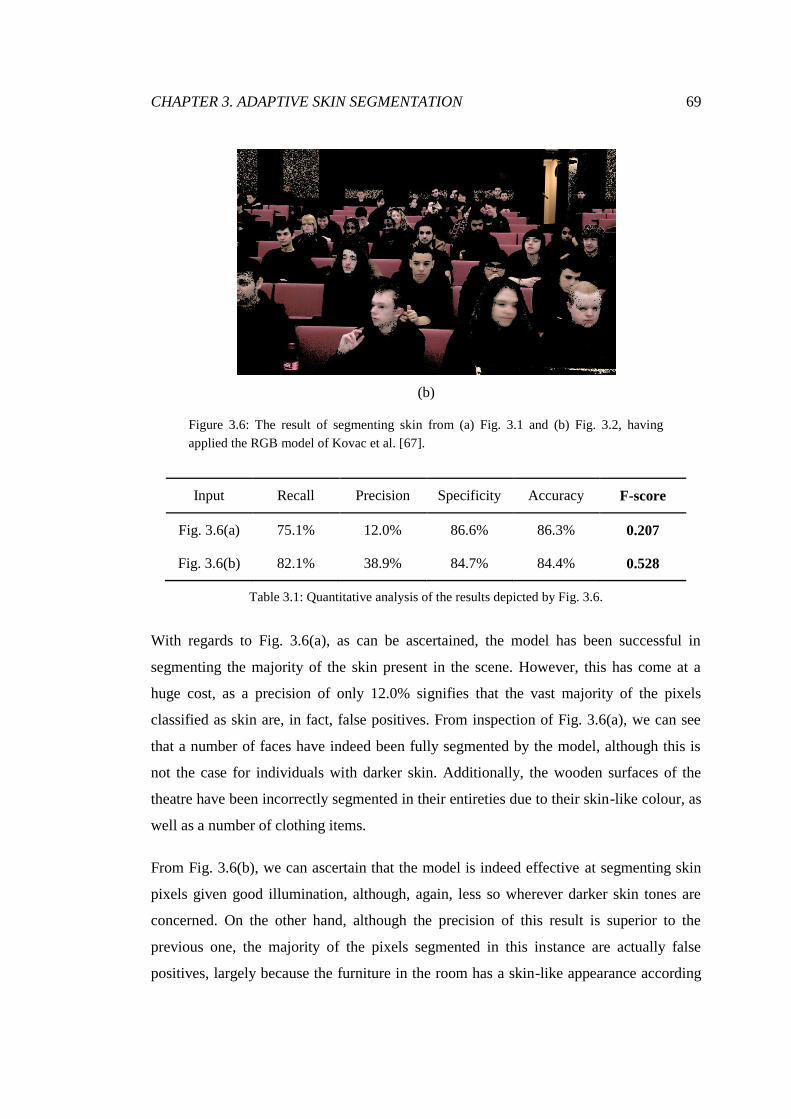
CHAPTER 3. ADAPTIVE SKIN SEGMENTATION 69
(b)
Figure 3.6: The result of segmenting skin from (a) Fig. 3.1 and (b) Fig. 3.2, having
applied the RGB model of Kovac et al. [67].
Input Recall Precision Specificity Accuracy F-score
Fig. 3.6(a) 75.1% 12.0% 86.6% 86.3% 0.207
Fig. 3.6(b) 82.1% 38.9% 84.7% 84.4% 0.528
Table 3.1: Quantitative analysis of the results depicted by Fig. 3.6.
With regards to Fig. 3.6(a), as can be ascertained, the model has been successful in
segmenting the majority of the skin present in the scene. However, this has come at a
huge cost, as a precision of only 12.0% signifies that the vast majority of the pixels
classified as skin are, in fact, false positives. From inspection of Fig. 3.6(a), we can see
that a number of faces have indeed been fully segmented by the model, although this is
not the case for individuals with darker skin. Additionally, the wooden surfaces of the
theatre have been incorrectly segmented in their entireties due to their skin-like colour, as
well as a number of clothing items.
From Fig. 3.6(b), we can ascertain that the model is indeed effective at segmenting skin
pixels given good illumination, although, again, less so wherever darker skin tones are
concerned. On the other hand, although the precision of this result is superior to the
previous one, the majority of the pixels segmented in this instance are actually false
positives, largely because the furniture in the room has a skin-like appearance according

70 CHAPTER 3. ADAPTIVE SKIN SEGMENTATION
to the model used. According for the F-score for the two segmentations, however, the one
achieved for Fig. 3.6(b) is substantially more accurate than the previous one.
3.1.1.2 Explicit Normalised RG Cluster Model
Using the normalised rg space, Soriano et al. [133] developed the skin colour cluster
defined by Eq. 3.9 to segment skin, whereby r and g respectively represent the proportion
of red and the proportion of green in the RGB representation of the colour of the given
pixel.
𝑝𝑖𝑥𝑒𝑙 =
𝑠𝑘𝑖𝑛, 𝑔 < −1.8423𝑟2 + 1.5294𝑟 + 0.0422 𝑎𝑛𝑑
𝑔 > −0.7279𝑟2 + 0.6066𝑟 + 0.1766 𝑎𝑛𝑑
𝑟 − 0.33 2 + 𝑔 − 0.33 2 > 0.004
𝑛𝑜𝑛 − 𝑠𝑘𝑖𝑛, 𝑜𝑡𝑒𝑟𝑤𝑖𝑠𝑒
(3.9)
The results that the normalised rg model of Soriano et al. [133], as described by Eq. 3.9,
has achieved over our two input images can be seen in Fig. 3.7, and are quantified by
Tab. 3.2.
(a)

CHAPTER 3. ADAPTIVE SKIN SEGMENTATION 71
(b)
Figure 3.7: The result of segmenting skin from (a) Fig. 3.1 and (b) Fig. 3.2, having
applied the normalised rg model of Soriano et al. [133].
Input Recall Precision Specificity Accuracy F-score
Fig. 3.7(a) 81.2% 14.3% 88.1% 87.9% 0.243
Fig. 3.7(b) 36.6% 43.6% 94.4% 88.2% 0.398
Table 3.2: Quantitative analysis of the results depicted by Fig. 3.7.
Despite the models defined by Eq. 3.8 and Eq. 3.9 representing markedly different
approaches to skin segmentation, the result illustrated by Fig. 3.7(a) is remarkably similar
to that achieved previously, with a respectable recall rate again coming at huge costs to
classification precision. Although the faces and hands of many individuals have been
extracted almost entirely, some large wooden surfaces have also been segmented by the
normalised rg model, but it has positively classified fewer clothing items than the RGB
model.
Contrary to the result achieved on the previous image, Fig. 3.7(b) demonstrates a
significant difference in the behaviours of the RGB and normalised rg models we are
investigating. Furthermore, this result illustrates how a variation in lighting conditions
can severely degrade the performance of a classifier. Rather than the arguable
oversensitivity of Fig. 3.7(a), we now see a much lower skin pixel recall rate, although a
natural consequence of this is improvements to precision and specificity. Through
inspection, we can see that very few faces are close to being fully extracted, and some are

72 CHAPTER 3. ADAPTIVE SKIN SEGMENTATION
almost entirely negatively classified. In some of these cases, it would seem that the cause
is the model not segmenting large regions of skin because they are tending towards white
in appearance. Even though one would not reasonably expect skin to appear white under
normal circumstances, lighter skin tones can often appear extremely white wherever
strong illumination and specular reflections are present. This can be evidenced especially
well by the faces closer to the camera. Despite this shortcoming, the model has yielded
far fewer false positives than in the previous instance, as the particular colour of the
furniture in the theatre depicted by Fig. 3.2 is not defined as skin by the model described
by Eq. 9. This has resulted in almost half of the segmented pixels actually being skin,
which, while still far from ideal, represents a dramatic improvement, the overall effects
are which are reflected by the increased F-score.
3.1.1.3 Explicit HSV Cluster Model
Using the HSV colour space, Sobottka and Pitas [132] developed the decision rules
described by 3.10 to define the appearance of skin, where H represents hue and S
represents the saturation of the given colour.
𝑝𝑖𝑥𝑒𝑙 = 𝑠𝑘𝑖𝑛, 0 ≤ 𝐻 ≤ 50 𝑎𝑛𝑑 0.23 ≤ 𝑆 ≤ 0.68
𝑛𝑜𝑛 − 𝑠𝑘𝑖𝑛, 𝑜𝑡𝑒𝑟𝑤𝑖𝑠𝑒
(3.10)
The results that the HSV model of Sobottka and Pitas [132], as described by Eq. 3.10, has
achieved over our two input images can be seen in Fig. 3.8, and are quantified by Tab.
3.3.
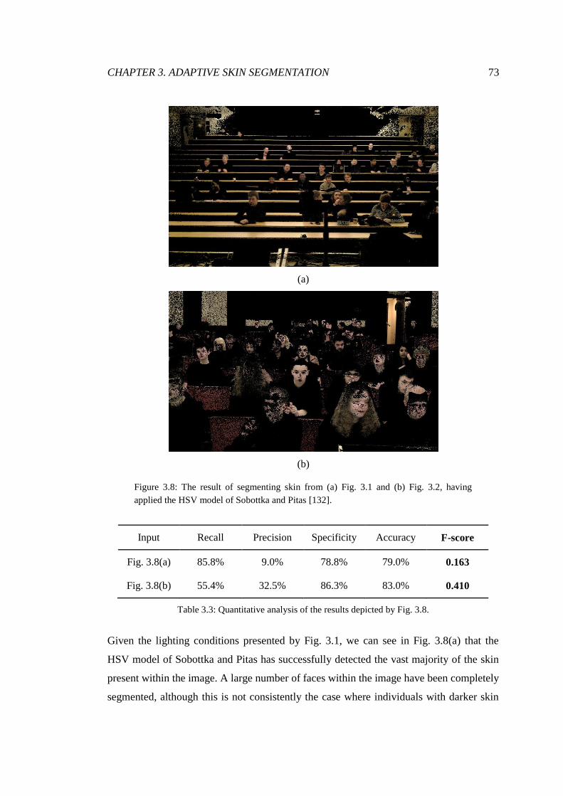
CHAPTER 3. ADAPTIVE SKIN SEGMENTATION 73
(a)
(b)
Figure 3.8: The result of segmenting skin from (a) Fig. 3.1 and (b) Fig. 3.2, having
applied the HSV model of Sobottka and Pitas [132].
Input Recall Precision Specificity Accuracy F-score
Fig. 3.8(a) 85.8% 9.0% 78.8% 79.0% 0.163
Fig. 3.8(b) 55.4% 32.5% 86.3% 83.0% 0.410
Table 3.3: Quantitative analysis of the results depicted by Fig. 3.8.
Given the lighting conditions presented by Fig. 3.1, we can see in Fig. 3.8(a) that the
HSV model of Sobottka and Pitas has successfully detected the vast majority of the skin
present within the image. A large number of faces within the image have been completely
segmented, although this is not consistently the case where individuals with darker skin

74 CHAPTER 3. ADAPTIVE SKIN SEGMENTATION
are concerned. This generally impressive recall rate of 85.8% has come at a significant
cost, as the apparent segmentation of walls, doors, wooden surfaces, and certain items of
clothing has resulted in a precision of merely 9.0%, signifying an extremely high
propensity for generating false positive results.
The output that can be seen in Fig. 3.8(b) signifies large variation in the capacity for the
HSV model to accurately segment skin given a change in illumination conditions. The
recall rate of the technique is significantly lower in this instance, as it has struggled to
fully classify even the lighter skin tones that it competently extracted previously.
Similarly to our findings using the normalised rg model, it would seem that specular
reflections of skin regions are the primary cause of the increased rate of false negatives.
Fig. 3.8(b) represents a significantly improved level of achieved precision, largely
because the colour of the furniture of this lecture theatre is not defined as skin by the
HSV model, although some sections of the rear wall of the room have been incorrectly
segmented.
3.1.1.4 Explicit YCbCr Colour Model
Working with the YCbCr colour space, Hu et al. [43] derived the decision rules described
by Eq. 3.11, where Cb and Cr represent, respectively, the blue and red chroma
components that are generated upon conversion from RGB to YCbCr.
𝑝𝑖𝑥𝑒𝑙 =
𝑠𝑘𝑖𝑛, 137 < 𝐶𝑟 < 177 𝑎𝑛𝑑 77 < 𝐶𝑏 < 127 𝑎𝑛𝑑 190 < 𝐶𝑏 + 0.6𝐶𝑟 < 215
𝑛𝑜𝑛 − 𝑠𝑘𝑖𝑛, 𝑜𝑡𝑒𝑟𝑤𝑖𝑠𝑒
(3.11)
The results that the YCbCr model of Hu et al. [43], as described by Eq. 3.11, has
achieved over our two input images can be seen in Fig. 3.9, and are quantified by Tab.
3.4.
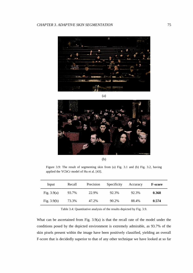
CHAPTER 3. ADAPTIVE SKIN SEGMENTATION 75
(a)
(b)
Figure 3.9: The result of segmenting skin from (a) Fig. 3.1 and (b) Fig. 3.2, having
applied the YCbCr model of Hu et al. [43].
Input Recall Precision Specificity Accuracy F-score
Fig. 3.9(a) 93.7% 22.9% 92.3% 92.3% 0.368
Fig. 3.9(b) 73.3% 47.2% 90.2% 88.4% 0.574
Table 3.4: Quantitative analysis of the results depicted by Fig. 3.9.
What can be ascertained from Fig. 3.9(a) is that the recall rate of the model under the
conditions posed by the depicted environment is extremely admirable, as 93.7% of the
skin pixels present within the image have been positively classified, yielding an overall
F-score that is decidedly superior to that of any other technique we have looked at so far

76 CHAPTER 3. ADAPTIVE SKIN SEGMENTATION
for Fig. 3.1. Although this recall rate has been achieved with a precision of only 22.9%,
we can see that many of the skin-coloured surfaces that have previously been entirely
segmented by other approaches are decidedly less so in this instance. What may also be
observed is that the model has been effective in segmenting darker skin tones almost as
consistently as it has lighter tones.
Not too dissimilarly to the previous image, Fig. 3.9(b) illustrates that the model has been
rather successful in correctly classifying skin pixels, as most faces have been segmented
to a reasonably high degree, regardless of their tone. At 47.2%, the precision of this result
is also considerably higher than many of the previous outputs we have seen, although it is
still far from ideal, as the case remains that the majority of segmented pixels are actually
non-skin. As can be seen, the primary cause of these false positives is the furniture within
the room, with some walls also being partially segmented.
3.1.1.5 Bayes’ Theorem-Based Look-Up Table
Skin colour distributions can be modelled non-parametrically, whereby the probabilities
that certain colours represent skin can be determined by through the statistical analysis of
training datasets. Bayes’ theorem, as described by Eq. 3.12, can be used to perform this
analysis, in order for representative look-up tables to be constructed. Here, P(x)
represents the probability of x occurring and P(x|y) represents the likelihood of x
occurring given that we already know y to be true.
𝑃 𝑠𝑘𝑖𝑛 𝑐𝑜𝑙𝑜𝑢𝑟𝑖 =𝑃 𝑐𝑜𝑙𝑜𝑢𝑟 𝑖 𝑠𝑘𝑖𝑛 𝑃 𝑠𝑘𝑖𝑛
𝑃(𝑐𝑜𝑙𝑜𝑢𝑟 𝑖) (3.12)
According to the law of total probability, we can expand the term P(colouri) to give us
the expression described by Eq. 3.13, which defines the probability of colouri occurring
as the combination of the probability of it occurring when the given pixel represents skin
and the probability of it occurring when the given pixel represents non-skin – a set of
events that are mutually exclusive and jointly exhaustive.
𝑃 𝑐𝑜𝑙𝑜𝑢𝑟𝑖 = 𝑃 𝑐𝑜𝑙𝑜𝑢𝑟𝑖 𝑐𝑙𝑎𝑠𝑠𝑛 𝑛
= 𝑃 𝑐𝑜𝑙𝑜𝑢𝑟𝑖 𝑠𝑘𝑖𝑛 𝑃 𝑠𝑘𝑖𝑛 + 𝑃 𝑐𝑜𝑙𝑜𝑢𝑟𝑖 ¬𝑠𝑘𝑖𝑛 𝑃 ¬𝑠𝑘𝑖𝑛 (3.13)

CHAPTER 3. ADAPTIVE SKIN SEGMENTATION 77
Taking this expanded expression and substituting it into Eq. 3.12 gives us the overall
expression we will be using to build our own probability look-up table, which is
described by Eq. 3.14.
𝑃 𝑠𝑘𝑖𝑛 𝑐𝑜𝑙𝑜𝑢𝑟𝑖 =𝑃 𝑐𝑜𝑙𝑜𝑢𝑟 𝑖 𝑠𝑘𝑖𝑛 𝑃 𝑠𝑘𝑖𝑛
𝑃 𝑐𝑜𝑙𝑜𝑢𝑟 𝑖 𝑠𝑘𝑖𝑛 𝑃 𝑠𝑘𝑖𝑛 + 𝑃 𝑐𝑜𝑙𝑜𝑢𝑟 𝑖 ¬𝑠𝑘𝑖𝑛 𝑃 ¬𝑠𝑘𝑖𝑛 (3.14)
This conditional probability expression is sufficient for the construction of a skin colour
classifier. The term P(skin) is the prior probability of our problem, representing our initial
belief that the given pixel is skin, without any regard for its colour. The value of this
probability can be estimated empirically from training samples, although the accuracy of
that estimation can be considered largely inconsequential [145], as long as the training
sets themselves effectively represent potential inputs and the estimation is not orders of
magnitude away from actuality. Henceforth, we shall be using 0.1 as our prior
probability, which expresses a belief that the likelihood of any arbitrarily selected pixel
being skin in the images we are interested in is 1 in 10.
The terms P(colouri|skin) and P(colouri|¬skin) are further conditional probabilities that
represent how likely colour i is to occur given that the pixel in question is skin or non-
skin, respectively, giving the likelihood of colour i occurring across the entire probability
space. These quantities can be determined for all discretised colour component
combinations i ∈ I of the given colour space through the construction of probability mass
functions that characterise the skin and non-skin training sample sets.
For the purposes of experimentation, we have created our own training data sets, which
pertain directly to the lecture theatre environments we are chiefly concerned with. Our
non-skin sample set consists of images depicting typical clothing of a range of colours,
furniture, and surfaces within rooms, and is made up of a total of 7,029k pixels.
Meanwhile, our skin sample set consists of a large number of skin regions (primarily
foreheads and cheeks) from people of various ethnicities under numerous lighting
conditions, and is made up of a total of 498k pixels. Fig. 3.10 and Fig. 3.11 illustrate the
nature of our non-skin and skin sample sets, respectively.
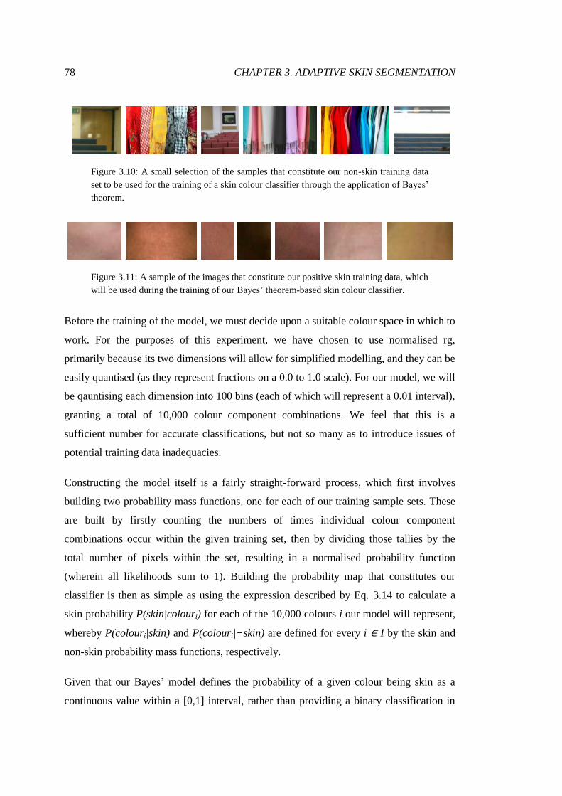
78 CHAPTER 3. ADAPTIVE SKIN SEGMENTATION
Figure 3.10: A small selection of the samples that constitute our non-skin training data
set to be used for the training of a skin colour classifier through the application of Bayes’
theorem.
Figure 3.11: A sample of the images that constitute our positive skin training data, which
will be used during the training of our Bayes’ theorem-based skin colour classifier.
Before the training of the model, we must decide upon a suitable colour space in which to
work. For the purposes of this experiment, we have chosen to use normalised rg,
primarily because its two dimensions will allow for simplified modelling, and they can be
easily quantised (as they represent fractions on a 0.0 to 1.0 scale). For our model, we will
be qauntising each dimension into 100 bins (each of which will represent a 0.01 interval),
granting a total of 10,000 colour component combinations. We feel that this is a
sufficient number for accurate classifications, but not so many as to introduce issues of
potential training data inadequacies.
Constructing the model itself is a fairly straight-forward process, which first involves
building two probability mass functions, one for each of our training sample sets. These
are built by firstly counting the numbers of times individual colour component
combinations occur within the given training set, then by dividing those tallies by the
total number of pixels within the set, resulting in a normalised probability function
(wherein all likelihoods sum to 1). Building the probability map that constitutes our
classifier is then as simple as using the expression described by Eq. 3.14 to calculate a
skin probability P(skin|colouri) for each of the 10,000 colours i our model will represent,
whereby P(colouri|skin) and P(colouri|¬skin) are defined for every i ∈ I by the skin and
non-skin probability mass functions, respectively.
Given that our Bayes’ model defines the probability of a given colour being skin as a
continuous value within a [0,1] interval, rather than providing a binary classification in

CHAPTER 3. ADAPTIVE SKIN SEGMENTATION 79
the manner of the explicit cluster models we have looked at, its application to the pixels
of a given image requires the definition of a probability threshold, which will represent
the minimum skin likelihood required for positive classification. Although using a single
threshold value to assess the performance of a continuous classifier will not fully reveal
its capabilities, we believe it will be sufficient for our current purposes, which are simply
to establish general efficacy. That being said, we will be applying a threshold value of 0.5
in order to achieve segmentations with our Bayes classifier, as any likelihood above that
value will signify that the pixel of that colour is more likely to be skin than not, according
to the model, and vice-versa. Our pixel classification rule, therefore, can be described by
Eq. 3.15.
𝑝𝑖𝑥𝑒𝑙 = 𝑠𝑘𝑖𝑛, 𝑃 𝑠𝑘𝑖𝑛 𝑐𝑜𝑙𝑜𝑢𝑟𝑝𝑖𝑥𝑒𝑙 ≥ 0.5
𝑛𝑜𝑛 − 𝑠𝑘𝑖𝑛, 𝑜𝑡𝑒𝑟𝑤𝑖𝑠𝑒
(3.15)
We can now apply the constructed model to the two lecture theatre images we have used
to test the methodologies we have previously looked at. The achieved results can be seen
in Fig. 3.12, and are quantified by Tab. 3.5.
(a)
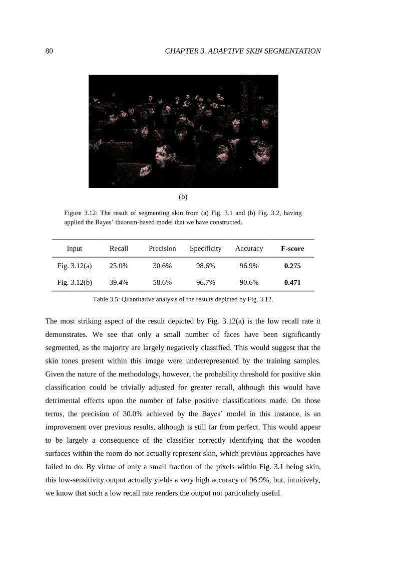
80 CHAPTER 3. ADAPTIVE SKIN SEGMENTATION
(b)
Figure 3.12: The result of segmenting skin from (a) Fig. 3.1 and (b) Fig. 3.2, having
applied the Bayes’ theorem-based model that we have constructed.
Input Recall Precision Specificity Accuracy F-score
Fig. 3.12(a) 25.0% 30.6% 98.6% 96.9% 0.275
Fig. 3.12(b) 39.4% 58.6% 96.7% 90.6% 0.471
Table 3.5: Quantitative analysis of the results depicted by Fig. 3.12.
The most striking aspect of the result depicted by Fig. 3.12(a) is the low recall rate it
demonstrates. We see that only a small number of faces have been significantly
segmented, as the majority are largely negatively classified. This would suggest that the
skin tones present within this image were underrepresented by the training samples.
Given the nature of the methodology, however, the probability threshold for positive skin
classification could be trivially adjusted for greater recall, although this would have
detrimental effects upon the number of false positive classifications made. On those
terms, the precision of 30.0% achieved by the Bayes’ model in this instance, is an
improvement over previous results, although is still far from perfect. This would appear
to be largely a consequence of the classifier correctly identifying that the wooden
surfaces within the room do not actually represent skin, which previous approaches have
failed to do. By virtue of only a small fraction of the pixels within Fig. 3.1 being skin,
this low-sensitivity output actually yields a very high accuracy of 96.9%, but, intuitively,
we know that such a low recall rate renders the output not particularly useful.

CHAPTER 3. ADAPTIVE SKIN SEGMENTATION 81
The recall rate of the segmentation depicted by Fig. 3.12(b) is clearly superior to that
achieved for the previous image, although it remains inferior to the rates other approaches
have yielded. Again, however, we could adjust the probability threshold being used to
improve the recall, but this would be at a cost to specificity. At 58.6%, the precision of
the output has also been drastically improved, to the extent of our Bayes model being
more precise than any other method we have experimented with thus far. It is clear to see
this precision in effect, as numerous skin regions have been segmented rather
extensively, whereas the furniture of the room has not been so consistently extracted. In
contrast with the previous result, we can determine that the specific skin tones on display
in this image have greatly superior representation within the positive training samples,
and that the non-skin training data may also be more suited to this environment.
3.1.1.6 Gaussian Distribution Function
Parametric modelling techniques allow for compact representations of skin colour models
to be derived, such that they can be described by practically efficient numbers of
parameters. In order for us to experiment with parametric methodologies, we will be
building a multivariate Gaussian classifier of our own, the density function of which can
be described by Eq. 3.16.
𝑝(𝑐𝑖 |𝑠𝑘𝑖𝑛) =1
(2𝜋)𝑑/2 𝛴𝑠 1/2 ∙ 𝑒
−1
2 𝑐𝑖−𝜇𝑠
𝑇𝛴𝑠−1(𝑐𝑖−𝜇𝑠) (3.16)
Here, d represents the dimensionality of the problem, ci represents the d-component
colour vector (a particular combination of colour component values) of pixel i, μs and Σs
are the Gaussian distribution parameters (representing the d-component mean colour
vector and the d-by-d covariance matrix, respectively) of skin colour model s. These
parameters are determined through the analysis of the given training data, and |Σs| is the
determinant of the covariance matrix, constituting part of the normalisation factor of the
function, which ensures that the entire volume of the distribution integrates to 1.
Determining the skin likelihoods of pixels cannot be achieved directly through Eq. 3.16,
as it merely returns densities pertaining to the probability of skin pixels being of colour
ci, but from it we can derive an expression that will allow for the calculation of actual

82 CHAPTER 3. ADAPTIVE SKIN SEGMENTATION
skin likelihoods. Eq. 3.17 describes the relationship between p(skin|colour) and
p(colour|skin), as defined by Bayes’ theorem.
𝑝 𝑠𝑘𝑖𝑛 𝑐𝑜𝑙𝑜𝑢𝑟 = 𝑝(𝑐𝑜𝑙𝑜𝑢𝑟 |𝑠𝑘𝑖𝑛 )𝑝(𝑠𝑘𝑖𝑛 )
𝑝(𝑐𝑜𝑙𝑜𝑢𝑟 ) (3.17)
If we were to assume p(skin) and p(colour) being constant, which signifies that all pixels
are equally likely to be skin before we consider their colours and that all colours are
equally likely to occur, then the probability of a pixel representing skin, given its colour,
is directly proportional to the probability of a pixel being of a certain colour, given that it
represents skin, as in Eq. 3.18, where k represents the constant of proportionality.
𝑝 𝑠𝑘𝑖𝑛 𝑐𝑜𝑙𝑜𝑢𝑟 = 𝑘 · 𝑝(𝑐𝑜𝑙𝑜𝑢𝑟|𝑠𝑘𝑖𝑛) (3.18)
If we consider the definition of p(colour|skin) given by Eq. 3.16, we can rewrite the
above expression to give Eq. 3.19.
𝑝 𝑠𝑘𝑖𝑛 𝑐𝑖 = 𝑘 · 1
(2𝜋)𝑑/2 𝛴𝑠 1/2 ∙ 𝑒
−1
2 𝑐𝑖−𝜇𝑠
𝑇𝛴𝑠−1(𝑐𝑖−𝜇𝑠)
(3.19)
The normalisation factor of this expression will be a constant for any given density
function, as it is variant only on the determinant of the covariance matrix and
dimensionality of the given colour model, rather than any individual input colour vector.
If we were to equate the constant of proportionality k to the reciprocal of the
normalisation factor, as in Fig. 3.20, then we could eliminate the constants and derive an
expression to directly calculate the skin likelihoods of input colour vectors, as described
by Eq. 3.21, which would allow for the segmentation of skin.
𝑘 = (2𝜋)𝑑/2 𝛴𝑠 1/2 (3.20)
𝑝(𝑠𝑘𝑖𝑛|𝑐𝑖) = 𝑒−1
2 𝑐𝑖−𝜇𝑠
𝑇𝛴𝑠−1(𝑐𝑖−𝜇𝑠)
(3.21)
As it has been show to perform well given Gaussian representation [139], we will be
using the normalised rg colour space in conjunction with a unimodal function, as we
believe this combination will maximise our likelihood of segmentation success with this
particular methodology, without introducing superfluous degrees of complexity.
Generating a parametric skin colour model necessitates the existence of a set of positive

CHAPTER 3. ADAPTIVE SKIN SEGMENTATION 83
training samples, and we will be reusing the data that was previously used to build the
positive skin probability mass function of the Bayes classifier.
Training the model is a simple process, and requires only the determination of the mean
colour component values and the covariance matrix of the training samples, which will
allow for Eq. 3.21 to be used for classification, when combined with a probability
threshold. Calculating the mean colour vector, which defines the centre point of the
elliptical distribution, can be accomplished through the application of Eq. 3.22 to the
training data, whereby the colour components of every pixel i ∈ I are summarised and
normalised.
𝜇𝑠 = 1
𝑛 𝑐𝑖
𝑛𝑖=1 (3.22)
Here, μs represents the mean colour vector we are interested in ascertaining, ci represents
the colour of the ith pixel in the dataset, and n represents the total number of pixels within
that set.
Generating the covariance matrix for the training data, which will define the shape, size,
and orientation of the distribution, can be achieved through the application of Eq. 3.23,
whereby the deviations of the colours of all pixels i ∈ I from the mean colour vector are
summarised and normalised.
𝛴𝑠 = 1
𝑛−1 𝑐𝑖 − 𝜇𝑠 𝑐𝑖 − 𝜇𝑠
𝑇𝑛𝑖=1 (3.23)
Above, Σs represents the covariance matrix we will be created, μs represents the mean
colour vector of the training samples, ci represents the colour of the ith pixel in the
dataset, and n represents the total number of pixels within that set.
Similarly to the implementation of the Bayes look-up table, classifying pixels using our
trained Gaussian function requires the definition of a probability threshold, which can be
applied to the continuous skin likelihoods that are calculated through the use of Eq. 3.21.
Again, this means that the results we achieve will not be entirely representative of what
our Gaussian classifier has the potential to accomplish, but they will give a strong
indication. In the case of the Bayes classifier, we used a threshold value of 0.5 because it
segregates pixels that are more likely to be skin than not from those for which the
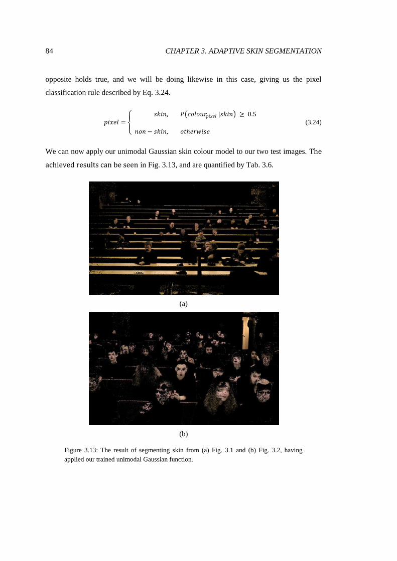
84 CHAPTER 3. ADAPTIVE SKIN SEGMENTATION
opposite holds true, and we will be doing likewise in this case, giving us the pixel
classification rule described by Eq. 3.24.
𝑝𝑖𝑥𝑒𝑙 = 𝑠𝑘𝑖𝑛, 𝑃 𝑐𝑜𝑙𝑜𝑢𝑟𝑝𝑖𝑥𝑒𝑙 |𝑠𝑘𝑖𝑛 ≥ 0.5
𝑛𝑜𝑛 − 𝑠𝑘𝑖𝑛, 𝑜𝑡𝑒𝑟𝑤𝑖𝑠𝑒
(3.24)
We can now apply our unimodal Gaussian skin colour model to our two test images. The
achieved results can be seen in Fig. 3.13, and are quantified by Tab. 3.6.
(a)
(b)
Figure 3.13: The result of segmenting skin from (a) Fig. 3.1 and (b) Fig. 3.2, having
applied our trained unimodal Gaussian function.

CHAPTER 3. ADAPTIVE SKIN SEGMENTATION 85
Input Recall Precision Specificity Accuracy F-score
Fig. 3.13(a) 83.6% 13.2% 86.5% 86.4% 0.228
Fig. 3.13(b) 52.6% 50.1% 93.7% 89.4% 0.513
Table 3.6: Quantitative analysis of the results depicted by Fig. 3.13.
As can be discerned from Fig. 3.13(a), like most of the segmentations of Fig. 3.1 we have
seen previously, our Gaussian function has produced a multitude of false positive results,
leading to a precision of only 13.2%. This has been caused almost entirely by the wooden
surfaces within the lecture theatre, the skin-like colour of which has, seemingly, either
been represented by the training data or interpolated through the derivation of our model.
The recall rate of 83.6% achieved by the classifier is impressive, although it having been
achieved with such a low precision has resulted in a rather low F-score of only 0.228. It
can also be noted the darker skin tones have been segmented almost as effectively as the
lighter tones, reinforcing the notion that unimodal Gaussian functions can sufficiently
model all skin tones given a normalised colour space.
In comparison with the previous result, we have achieved a relatively high precision in
Fig. 3.13(b), with just over half of the pixels segmented actually representing skin.
Although our classifier has avoided segmenting significant portions of the environment,
the skin-like colours of the hair and the clothes of a number of individuals have been
wrongly classified as skin. Demonstrably, however, we have a significantly reduced
recall rate. Although, again, we see a reasonably consistent degree of segmentation across
various ethnicities, there are a number of faces, especially those closer to the point of
capture, that have not been very well segmented, and, given their large relative size, the
overall sensitivity achieved has been significantly impacted by them. It would appear that
the cause of this has again been the misclassification of skin regions that exhibit specular
reflection, as their colours tend towards white to such a degree that they no longer appear
skin-like.

86 CHAPTER 3. ADAPTIVE SKIN SEGMENTATION
3.1.2 Results Comparison and Discussion
Having experimented with a broad range of existing skin segmentation techniques, we
can now compare their results in an effort to draw useful conclusions. Although we have
been able to identify where individual approaches have succeeded and failed, by collating
the results we have produced, we will be able to ascertain information that should pertain
directly to the nature of our inputs, which will help us greatly in finding an adequate
segmentation solution.
For this purpose, we present Fig. 3.14, which illustrates the recall, precision, and F-score
achieved by each detector we have looked at for each of our two images. We have
decided to focus on these three metrics at this time in an effort to more easily interpret
our data, and because it is these statistics relating to the positive skin class that are the
most relevant to us (as we discussed at the start of Section 3.1.1). As we have mentioned
previously, the results of the Bayes and Gaussian classifiers may not represent their most
optimal performances, as thresholds other than 0.5 may have yielded objectively better
results, but we believe that they are close enough that the conclusions we draw from them
can be considered entirely valid.
Figure 3.14: A collation of the segmentation results we have achieved during our
experimentation, presented on a per-approach basis. The three metrics we are concerned
with at this time (recall, precision, and F-score) are represented by their fractional scores.
CHAPTER 3. ADAPTIVE SKIN SEGMENTATION 87
The data presented by Fig. 3.14 is interesting to us in a number of ways. Firstly, we can
note the rather significant lack of consistency with which skin pixels have been recalled
by the classifiers. Kovac et al.’s RGB model [67] is the only one of our six approaches
that has demonstrated a high level of sensitivity for both images. Four of the remaining
five (with the Bayes model being the exception) have demonstrated substantially better
recall rates for Fig. 3.1 than Fig. 3.2, although Hu et al.’s YCbCr model [43] has still
performed rather well on the latter. As we have noted previously, the cause of failure for
a number of techniques on Fig. 3.2 seems to have been the presence of specular
reflections. These have caused skin regions to appear extremely light, and it would seem
many models do not define such white-like colours as skin. Whilst this is not entirely
unreasonable, it is clear that it is indeed a potential scenario given the common presence
of strong, artificial illumination within indoor environments such as lecture theatres, and
so, ideally, would be handled effectively by the skin segmentation approach we will
ultimately be using. The sensitivity demonstrated by our Bayes model for both images is
rather disappointing, and suggests that a positive skin sample set designed to cover the
skin tones of multiple illumination conditions is self-defeating. This is understandable
given the normalisation that a sample set goes through during the training of a Bayes’
theorem-based model, as the probability of skin representation ascribed to a certain
colour will be diminished for every other colour that is present within the set.
Secondly, the lack of consistency in segmentation precision is also clear to see. Every
single one of the classifiers we have experimented with has demonstrated great disparity
in the levels of precision they have achieved over the two images. However, having
achieved a much greater precision in Fig. 3.2 than in Fig. 3.1 is common to all of them,
again suggesting the differing nature of the inputs, and the segmentation approaches’ lack
of adaptation to them, is the cause of the issue. As we have alluded to previously, the
wooden surfaces within the lecture theatre depicted by Fig. 3.1 have been a consistent
and significant source of false positive classifications, and would appear to be the main
reason for the low levels of precision achieved for that image across every methodology.
The most extreme case, however, has been produced by Sobottka and Pitas’ HSV model
[132], which has also positively classified many beige-coloured wall regions and items of
clothing, resulting in the lowest precision of all twelve segmentations. The small number
of skin pixels present within Fig. 3.1 is also a factor where segmentation precision is

88 CHAPTER 3. ADAPTIVE SKIN SEGMENTATION
concerned, as there are many more pixels within the image constituting the skin-like
surfaces than there are belonging to the actual skin regions, which will, inevitably, have
an adverse effect on the precisions achieved. Visually, we can see that the surfaces are
indeed of a similar colour to many of the skin regions visible within the image, but we
believe a model specific enough to the colour of those skin regions would be able to
differentiate between them and the wooden surfaces effectively. Of course, such a model
would only be useful for the image in question (or any other depicting extremely similar
illumination), and would perform poorly given most other images, such as Fig. 3.2.
Although the general precision achieved for Fig. 3.2 is superior, which can be at least
partially attributed to there being a greater proportion of skin pixels to skin-like non-skin
pixels than in Fig. 3.1, there is a rather large degree of variation within those results. It
would seem the primary cause of this is the existence of separate significant non-skin
regions that are markedly different in appearance. Our Gaussian model, for instance, has
segmented a large number of pixels that actually represent hair and clothing, but, a single
region of wall aside, has avoided falsely positively classifying large segments of the
environment itself. Kovac et al.’s RGB model [67], on the other hand, has successfully
refrained from segmenting some of those same regions, but has instead segmented huge
portions of the red furniture and beige walls within the room, and Hu et al.’s YCbCr
model [43] has done similarly, although to a lesser extent.
Since different pre-trained approaches have different, fixed definitions for the appearance
of skin, and will, therefore, be liable to produce false positives from different non-skin
sources, it is clear to see how such an image would yield such inconsistent results. This is
somewhat inevitable where approaches designed to be globally applicable are concerned,
as they must account for broad ranges of potential skin tones. However, as demonstrated
by some of our data, the colours that represent the positive skin tones of one image may
often only represent false positives in another. Dissimilarly to the situation of Fig. 3.1,
the inspection of Fig. 3.2 would indicate that the colour of many of the non-skin regions
falsely segmented is not actually too similar to the colour of the vast majority of the skin
regions within the image. This suggests that a model that could differentiate between
them successfully would not be too difficult to construct. It also reinforces our belief that

CHAPTER 3. ADAPTIVE SKIN SEGMENTATION 89
the methodologies we have been working with define the colour of skin too broadly to be
consistently accurate given our form of inputs.
Finally, while the F-scores themselves cannot offer significant insight into how our
results have come to be, they are very useful for assessing the overall efficacy of the
approaches. As the harmonic mean of recall and precision, the F-score of a given
segmentation represents the balance achieved between the two metrics. A balance
between precision and recall is important, as one can be trivially inflated at the cost of the
other (as we explained at the start of Section 3.1.1), but improving both simultaneously
can speak volumes for the quality of a classifier. As Fig. 3.14 illustrates, every
segmentation approach has, overall, performed significantly better on Fig. 3.2 than on
Fig. 3.1, which is a direct result of the markedly superior precisions achieved for that
image. Having yielded the most impressive results for each image, through a combination
of respectable recall rates and relatively high levels of precision, the YCbCr model of Hu
et al. [43] can be regarded as the best approach for detecting skin within our inputs of
those we have looked at. As we have already discussed, however, the segmentations it
has produced have indicated plenty of room for improvement. The results of the
remaining detectors are relatively similar overall, although it could be noted that the
normalised rg model of Soriano et al. [133] and the HSV model of Sobottka and Pitas
[132] have performed marginally worse than the RGB model of Kovac et al. [67] and the
Bayes and Gaussian models we have trained ourselves.
It would seem that the main issue that the skin segmentation approaches we have looked
at have struggled with is consistency. Although we have seen good individual
segmentations, we have not found a detector that can consistently produce high quality
results even over just the two input images we have been experimenting with so far. To
determine the cause of this, we must look back at the images themselves, and, most
importantly, the skin regions within them. Although both images depict well-illuminated
regions, as we have stressed all along, the general colour tone within each is different,
which means the colour of the skin regions within each is also different. In order to
establish the extent to which this is true, we can compare the colour distributions of the
skin regions of the two images mathematically. To that end, Fig. 3.15 illustrates the
respective distributions of the segmented pixels of Fig. 3.3 and Fig. 3.4 (which represent

90 CHAPTER 3. ADAPTIVE SKIN SEGMENTATION
our manual skin annotations) within the normalised rg colour space. We have chosen the
normalised rg space for analysis at this time because it represents relatively basic
properties of the colours in question (i.e. RGB component proportions), and its low
dimensionality will make comparison of the distributions straightforward.
(a) (b)
Figure 3.15: Colour distributions of the visible skin regions within (a) Fig. 3.1 and (b)
Fig. 3.2, as represented within the normalised rg colour space. NB: These plots visualise
just a small proportion of the entire space in order for the cluster dissimilarities to be
better perceived.
As can be seen, the disparity between the two distributions is rather stark. Whilst both
sets of pixels produce tight, elliptical clusters within the space, the sizes, orientations, and
locations of those clusters differ greatly. In fact, there is virtually no overlap between the
clusters whatsoever, as there are very few skin pixels represented by Fig. 3.15(a) that
have a proportion of red that is less than 0.42, whereas the exact opposite is true of the
distribution depicted by Fig. 3.15(b). This situation is not exclusive to the normalised rg
colour space, though, as similar experimentation with the HSV and YCbCr colour spaces
yielded similar result disparity. It is again important to note that our images are of
relatively high quality, because it emphasises that this phenomenon can be the result of
even non-extreme circumstances. Given all of these points, we can only conclude that the
approaches we have investigated, and any other pre-trained techniques like them, are
inherently incapable of yielding high quality segmentations for our lecture theatre
imagery on a consistent basis.

CHAPTER 3. ADAPTIVE SKIN SEGMENTATION 91
As we discussed in Chapter 2, certain skin segmentation approaches make use of
adaptive methods in order to improve image-to-image consistency. As opposed to the
static models we have looked at so far, adaptive skin detectors will generally be capable
of adjusting certain parameters at run-time, meaning that pixel classification rules can be
tailored to given inputs, and segmentation accuracy can be maximised for any given
image. It would appear that the utilisation of such methodologies is necessary in order for
us achieve accurate results over our lecture theatre imagery.
3.2 Segmentation System Design and Development
Although we highlighted a number of existing adaptive skin colour modelling systems in
Chapter 2, we do not feel that the specific issues they were designed to overcome can be
entirely equated to those that we are trying to solve. Therefore, we will be developing our
own adaptive segmentation system, capable of sampling images in order to generate truly
representative models by which input pixels can be classified. An overview of the system
we are proposing is illustrated by Fig. 3.16.
Figure 3.16: An overview of the adaptive system we will be developing to accurately
segment skin from complex lecture theatre imagery on a consistent basis.
As Fig. 3.16 makes clear, the system we will be constructing consists of a number of
individual components. In brief, our approach will involve sampling images through the
adoption of an existing face detection system, filtering the results to build a set of pixels
that represent the skin within the given image, deriving a unimodal Gaussian model from
that set, then applying the model across the entire image in an attempt to segment skin.
Throughout this section, we will be detailing the implementation of each stage of this
process.

92 CHAPTER 3. ADAPTIVE SKIN SEGMENTATION
3.2.1 Image Sampling
In order for a process to adapt to given inputs, it must employ a method of sampling
those inputs for relevant and useful information. In our case, it is necessary to sample the
skin colours of individuals within a given image. For a colour-adaptive system such as
ours, it stands to reason that we would want to utilise a colour-invariant sampling
method, so that representative samples could be acquired on a consistent basis, regardless
of the circumstances presented by individual inputs. A sampling process based upon
image features would, therefore, be very much suitable. Additionally, it could be asserted
that arbitrary pictures of people are more likely to depict their faces than any other
detectable body part (and even more so where lecture theatre imagery is concerned), and
that human faces themselves are extremely feature-rich, meaning that the detection of
them can be reasonably robust. Therefore, we believe that the reliable sampling of skin
colours could be achieved through the intelligent application of feature-based face
detection methodologies.
3.2.1.1 Feature-Based Face Detection
As we have discussed in Chapter 2, there are numerous previous works that have adopted
feature-based face detection for the purposes of image sampling [41,78,151]. Although
the vast majority of that research pertained to the detection of small numbers of people,
or even individuals, we believe that we can successfully develop a process that is suited
to our larger-scale problem. A common theme amongst the previous works is the
adoption of the face detection framework developed by Viola and Jones [147], which we
believe will also be ideal for our needs. As we previously described, their system
introduced a number of innovations to the computational efficiency of feature-based
detection, without any form of compromise in terms of result accuracy. Additionally, its
open-source implementation as part of the OpenCV function library is extremely
configurable, which will allow us to tailor it to meet our requirements exactly. If our
system is to be adaptive with respect to the colour models it generates, it is important that
the sampling process is also flexible, as there are many potential forms our lecture
theatre-based inputs could take. Being able to configure the sensitivity of the face
detector, therefore, is massively beneficial.

CHAPTER 3. ADAPTIVE SKIN SEGMENTATION 93
We have found that with too high a sensitivity, the detector of Viola and Jones will often
find the majority of faces within our imagery, but will also be liable to produce a number
of false positive detections. It is of great importance that false positives are avoided, as
the sampling of non-skin regions under the false premise of them being skin could have
severely detrimental effects on the representativeness of a subsequently generated colour
model. Conversely, a low enough sensitivity can eliminate false positives entirely, but, of
course, configuring the detector in such a manner can introduce the potential for subject
undersampling. Although it is not necessary to sample the skin of every individual
depicted by a given image to build a skin colour model that represents them effectively
(especially if some form of generalisation or interpolation is used during modelling), if
the sample size is simply too small and too many individuals go undetected, then the
probability of significant skin tones not being sampled can be increased greatly. The
consequence of this would be the generation of models that plainly do not represent the
skin colour of all the individuals they should pertain to. For these reasons, ensuring that
the sensitivity of the face detection process allows us to ascertain as much information as
possible about a given image without introducing any false positives is extremely
important.
It should be noted that none of the previous works we have looked into had any particular
need to configure the sensitivity of the face detector as carefully as we need to. Given the
nature of our problem, we will be attempting to detect multiple small faces, which will
require a greater sensitivity than most typical problems would, as the features of small,
distant faces will naturally be more difficult for a detector to discern than those of a
single large face that is close to the point of image capture, which seemed to be the type
of problem that most of the existing adaptive segmentation approaches were attempting
to solve. Of course, although we require a great enough sensitivity for small faces to be
found reliably, it must still be low enough for false positives to be avoided consistently.
We have extensively experimented with the Viola-Jones detection system in order to find
an optimal sensitivity for our system. This experimentation has involved a much larger
range of lecture theatre imagery than we have used previously, as the utilised dataset
contains 10 images that depict a total of 540 visible faces. The sensitivity of the detection
system can be controlled through the adjustment of a “minimum neighbour” threshold.

94 CHAPTER 3. ADAPTIVE SKIN SEGMENTATION
Typically, individual detections cannot convey enough confidence in order for a positive
face classification to be made, but a certain number of them within close proximity
(“neighbours”) could indeed be used to confidently declare the presence of a face.
Finding an ideal value for this number to use as a threshold is important, as requiring too
many neighbouring detections would reduce overall sensitivity, whereas defining too
small a number of neighbouring detections as a face would lead to an abundance of false
positive classifications.
Our experimentation, therefore, was aimed at the empirical determination of an optimal
minimum neighbour threshold. Through preliminary testing, we found that, where our
inputs were concerned, there was a significant (and potentially harmful) drop-off in
general detection rates when a threshold greater than 10 was used, and a threshold of 0
represents no detection consolidation whatsoever, so we limited our search space for an
optimal value accordingly. Hence, using a broad range of threshold values (1-10), we
processed our dataset with the face detector, and monitored two critical performance
metrics: detection rate; and false discovery rate. The first of these we are familiar with, as
the detection rate (synonymous with “recall”) simply represents the fraction of visible
faces that are positively classified by the detector. The greater the detection rate achieved,
the lesser the likelihood of the skin tones of an image being pivotally undersampled.
However, the second of these metrics, the “false discovery rate”, represents the fraction
of positive classifications that are actually false, and it is not a statistic we used during
our previous skin segmentation work. Although it is simply equivalent to 1 – precision,
we have chosen to present our data using FDR instead at this time as it should allow us to
more easily visualise the expected decrease in the number of false positive classifications
made as a result of the minimum neighbour threshold being increased. Where pixel-wise
classification problems are concerned, such as skin segmentation, such information could
instead be conveyed through a “false positive rate” (defined as 1 – specificity), but since
there exists no real definition of “true negative” where face detection is concerned (as the
label “non-face” could be applied to any number of regions within a given image), this is
not an option for us. However, false discovery rates have the additional benefit of
presenting false positives in terms of their influence on sets of positive classifications,
rather than framing them within a context of all negative samples. This means that the
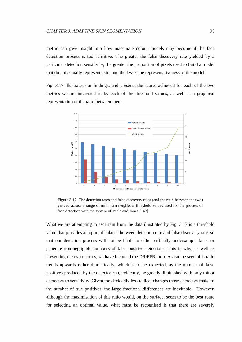
CHAPTER 3. ADAPTIVE SKIN SEGMENTATION 95
metric can give insight into how inaccurate colour models may become if the face
detection process is too sensitive. The greater the false discovery rate yielded by a
particular detection sensitivity, the greater the proportion of pixels used to build a model
that do not actually represent skin, and the lesser the representativeness of the model.
Fig. 3.17 illustrates our findings, and presents the scores achieved for each of the two
metrics we are interested in by each of the threshold values, as well as a graphical
representation of the ratio between them.
Figure 3.17: The detection rates and false discovery rates (and the ratio between the two)
yielded across a range of minimum neighbour threshold values used for the process of
face detection with the system of Viola and Jones [147].
What we are attempting to ascertain from the data illustrated by Fig. 3.17 is a threshold
value that provides an optimal balance between detection rate and false discovery rate, so
that our detection process will not be liable to either critically undersample faces or
generate non-negligible numbers of false positive detections. This is why, as well as
presenting the two metrics, we have included the DR/FPR ratio. As can be seen, this ratio
trends upwards rather dramatically, which is to be expected, as the number of false
positives produced by the detector can, evidently, be greatly diminished with only minor
decreases to sensitivity. Given the decidedly less radical changes those decreases make to
the number of true positives, the large fractional differences are inevitable. However,
although the maximisation of this ratio would, on the surface, seem to be the best route
for selecting an optimal value, what must be recognised is that there are severely

96 CHAPTER 3. ADAPTIVE SKIN SEGMENTATION
diminishing returns on the elimination of false positives, and, after a point, far more true
positives are likely to be lost through further increments to the classification threshold.
The number of false positives eliminated by increasing the threshold from 7 to 10, for
instance, is almost negligible, but there is a 5% decrease in the detection rate achieved.
The threshold value of 7 itself has actually produced an above-trend DR/FDR ratio, and
we, therefore, believe it represents an ideal level of sensitivity for the face detector when
used as part of our system. Again, although we could achieve greater detection rates with
a greater sensitivity, we believe we do not necessarily need to sample a large proportion
of the faces within a given image in order to develop a representative colour model, and,
although the stringent elimination of false positives is extremely important, miniscule
advancements in that regard should not come at much larger costs to true positive
detection rates.
Our selected threshold value of 7 neighbours actually represents a much lower sensitivity
than the default value of the OpenCV implementation of the face detector, as it defines
the presence of only 3 proximal detections to be evidence enough for the existence of a
face, despite our previous suggestion that typical face detection tasks do not necessitate
high sensitivities. We believe this disparity in ideal levels of sensitivity to not only be the
result of the complexity introduced by our sampling requirements, but also a result of
considerations for general image quality, perhaps related to the poor standard of image
capture devices when the OpenCV implementation of the face detector was written. The
lecture theatre images we have collated are generally well-focused, well-exposed, and are
of large resolutions, but we cannot expect every arbitrary image to be of such high
quality, or, therefore, as favourable for successful object detection. Empirically, we have
found that requiring 7 neighbouring detections for a positive classification can actually
lead to rather poor detection rates where images of lesser quality are concerned.
Ideally, however, we do not wish to limit the applicability of our system by making it
overly specialised, especially if accommodation can be made without any compromise to
the meeting of primary objectives. Therefore, we perform face detection in a flexible
manner. For any given input image, we initially attempt to detect faces using our high-
precision, moderate-recall threshold value of 7. Should any faces be found, the results are
accepted and processed. In the event that no faces are found, however, the threshold

CHAPTER 3. ADAPTIVE SKIN SEGMENTATION 97
value is decremented, and detection is performed again. This is repeated until at least one
face is found, or the threshold value is reduced to 1, at which point it is determined that
there are likely to be no actual visible faces within the given image, as any positive
classifications that can only be made using such a low threshold are likely to be false
positives. Through the simple implementation of this process, we can acquire optimal
face detection results on our typically high quality lecture theatre imagery as well as best-
case-scenario detection results for any arbitrary image using just a single system
configuration, making it a globally applicable sampling technique.
Fig. 3.18 depicts the result of detecting faces within Fig. 3.1 using the detection system of
Viola and Jones in conjunction with our optimised threshold value, and serves as an
example of how face detection results are actually presented by the system, and how
effective our threshold value is for yielding desirable results.
Figure 3.18: The result of performing face detection on Fig. 3.1 using the system
developed by Viola and Jones [147] with our high-precision, moderate-recall threshold
value. The faces of 19 individuals have been successfully detected, and zero false
positives have been produced.
The first aspect of the detection results illustrated by Fig. 3.18 that we note is the absence
of any false positive classifications. We have previously discussed how important we
believe the avoidance of such results to be, so a set of positive classifications being
entirely devoid of them is extremely positive. This insurmountable level of precision is
particularly pleasing in this instance because of the excellent detection rate also achieved,

98 CHAPTER 3. ADAPTIVE SKIN SEGMENTATION
with the faces of the majority of the depicted individuals having been successfully
detected. Although these results constitute merely a single demonstration of how
effective the detector, run at an optimal level of sensitivity, can be, we believe they
strongly reinforce the choices we have made regarding image sampling.
3.2.1.2 Sub-Region Sampling
Another aspect of Fig. 3.18 to be noted is the form of the results themselves. As can be
discerned, the regions defined by the detector as “faces” are all perfectly square. This is
reasonable, as the detection windows not necessarily being square could lead to much
greater degrees of computational complexity, at the point of both feature cascade training
and implementation, for very little gain, if any at all. However, it is slightly problematic
where our intentions are concerned. Of course, human faces do not typically resemble the
shape of a square and are generally rounder, more elliptical in appearance. Additionally,
we have found that, in the majority of cases, the detector will overestimate the sizes of
faces, and the detection regions will often be larger than the heads of the individuals they
pertain to. The combination of these factors means that a significant proportion of most
positively classified face regions will not actually be relevant to us, and will instead
represent uninteresting, potentially harmful background information. Given that we
intend to use detected face regions to build skin colour models, ensuring that we can
consistently discard this superfluous information is important.
Our solution to this issue is fairly simple: to define a circular sub-region within each
detection region, located about its centre, within which every pixel is retained for further
processing, and outside of which every pixel will be discarded from the set of samples.
Ideally, the regions we define would be restrictive enough to discard all background
pixels in the vast majority of cases, but still be large enough to retain as many skin pixels
as possible, so as to not limit the amount of useful information we have available for
colour modelling. Just as with the face detection process itself, therefore, we must be
careful that we neither significantly oversample nor undersample our data.
Of course, the sizes of our sub-regions should be relative to the sizes of the detection
regions they pertain to, so that we can achieve representative, consistent sampling.

CHAPTER 3. ADAPTIVE SKIN SEGMENTATION 99
Therefore, simply defining their sizes fractionally would be our best option. Through
experimentation, we found that defining the radius of a given sub-region as 0.4 times the
height of the given detection region yielded satisfying results. Marginally above that
value, we found that there existed some potential for the retention of a non-negligible
number of background pixels. Additionally, we observed that defining sub-regions any
smaller than this would, for the most part, lead to the elimination of large numbers of
actual face pixels for very little further discarding of background information. A circular
sub-region with a radius of 0.4 times the height of a detection region (or, a diameter of
0.8 times the height), yields a pixel retention rate of just over half (50.27%), meaning that
we still have access to the majority of pixels that face detection provided for any given
image, whilst being confident that no significant proportion of them represent detrimental
background information. An unfiltered skin pixel sample set of this size actually
represents a larger sample set than any of the previous works that we have looked at that
use the same face detection method use, which we believe is advantageous.
Fig. 3.19 illustrates the result of our sub-region application to some of the face detection
regions depicted by Fig. 3.18.
Figure 3.19: A graphical representation of our elimination of background pixels within
face detection regions through the definition of inner sub-regions.
As the above results demonstrate, background information can be entirely eliminated
through this simple process of sub-region definition. As can also be seen, although we
have, inevitably, lost some actual skin pixels, our retention of them is generally still
rather high. Furthermore, it can be noted that, as well as eliminating pixels that represent
certain environmental features, we have discarded the pixels pertaining to the hair of

100 CHAPTER 3. ADAPTIVE SKIN SEGMENTATION
many individuals, which is just as beneficial in our attempts to build representative sets
of skin pixels.
3.2.1.3 Pixel Filtering
Although massively advantageous where initial detection is concerned, the major
drawback of faces being so feature-rich is that the features serve to break up skin regions,
making the successful and consistent segmentation of them decidedly more complicated.
In general, facial features will exhibit distinctly different colours to typical skin regions,
which means that they must be removed from pixel sample sets in order for
representative colour models to be built. Unfortunately, unless facial expression,
orientation, and relative detection region size can be guaranteed (which is only likely to
be the case under extremely constrained circumstances), we believe that discarding non-
skin features based upon their presumed locations could lead to inaccurate and
inconsistent results. This is in contrast to the elimination of background information,
which we have shown can be achieved effectively through the assumption that such
pixels will exist almost exclusively around the edges of detection regions.
As we described in Chapter 2, Liao and Chi [78] proposed the use of a small window to
consistently sample skin regions. The location of this window would be predefined and
relative to the given detection region itself, and would, in typical cases, encompass a
small region of skin on the right-hand cheek of individuals. The belief of the researchers
was that this method would allow for expression and orientation variations, because the
window would be so small (covering only 4% of the pixels of a given region) and
specifically located that it would take extreme circumstances for anything other than a
cheek to present itself in that exact location. Although we do not believe this to be too
unreasonable an approach, we do not consider it an ideal solution where our problem is
concerned. Fig. 3.19 demonstrates that even arbitrarily selected faces can exhibit fairly
large degrees of orientation and expression variation, and although we could define very
small regions that would actually represent skin pixels within all three of those samples,
the set of pixels such a selection process would yield would be miniscule, and highly
likely to not be entirely representative. The method proposed by Liao and Chi [78]
seemed to work well for their expected inputs, which would typically exhibit just a single

CHAPTER 3. ADAPTIVE SKIN SEGMENTATION 101
user that would be close to the point of image capture. In that instance, a small region of
skin would actually consist of a reasonably large number of pixels. Where much more
distant individuals and much smaller numbers of pixels are concerned, however, the
likelihood of camera imperfections, image compression artefacts, or other such anomalies
having detrimental effects on the representative of pixel sets becomes much larger.
Wimmer and Radig [151] also proposed a location-based sampling technique, but rather
than predefining the likely location of a region of skin, they presented an empirically
derived probability map. Through applying a threshold to the map, a skin mask could be
generated that would consist of a set of region of interest (ROI) coordinates, which would
define which pixels within a given face detection region have a likelihood of being skin
that is at least as great as the threshold applied. While interesting, and potentially
effective, we do not believe this to be an optimal solution for our problem either.
Although, given the use of a reasonable threshold, this method would yield a larger set of
pixels than the method of Liao and Chi [78], we believe there is still room for
improvement. The introduction of an adjustable threshold adds further complexity to the
sampling process, and it would seem the mask applied to a given face region would still
be rather restrictive unless a particularly permissive threshold were to be used.
Additionally, the technique being based upon location data means that skin probabilities
are somewhat dependent upon facial expressions and orientations, rather than necessarily
invariant to them.
In contrast to the location-based sampling approaches of Liao and Chi [78] and Wimmer
and Radig [151], Hsieh et al. [41] make use of colour information. We concur with the
beliefs of the latter researchers because, although the location of them is largely
indeterminable, non-skin facial features do tend to share a common trait in the colour
domain: extreme intensity. Features such as facial hair, nostrils, eyes, and mouths will
usually tend towards black (low intensity) as they are naturally darker in colour to skin
(especially in the case of facial hair), or are likely to be under the influence of far less
incident light than typical skin regions. Thankfully for the purpose of filtering these
features out and isolating skin pixels, this property should allow for them to be
distinguished and discarded on a reasonably consistent basis. There are a variety of
measures that can be used to express the intensity of colours [58], such as value,
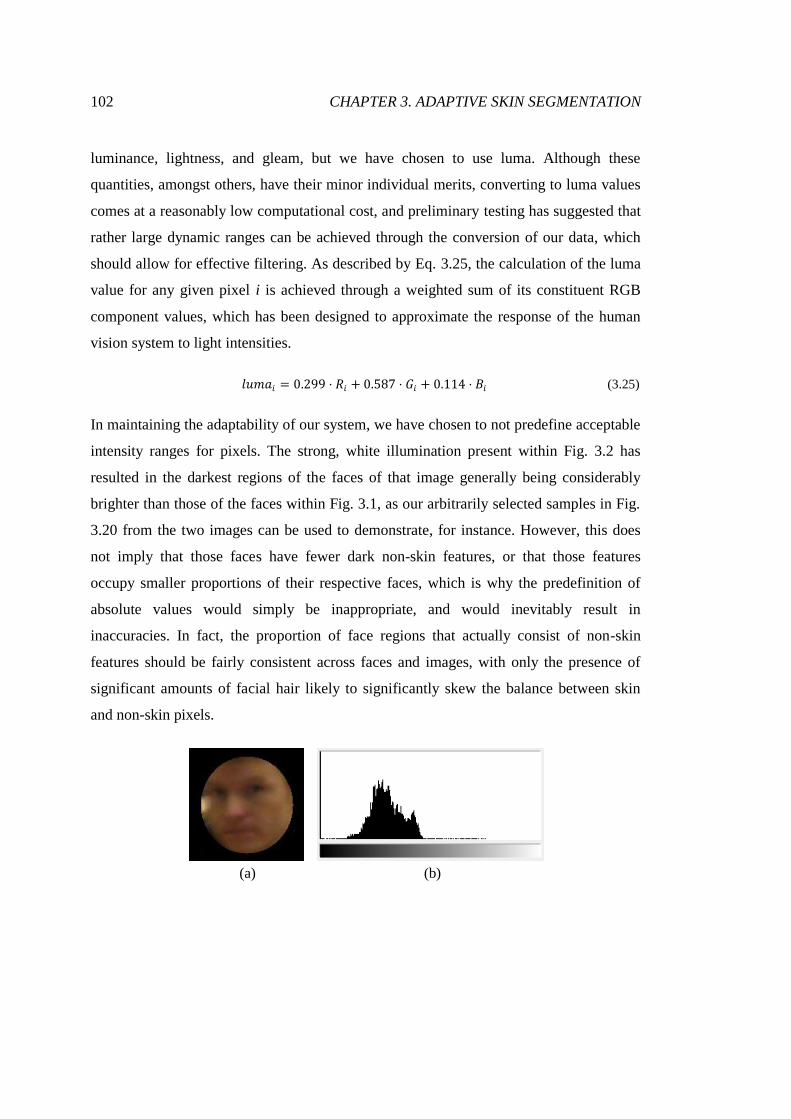
102 CHAPTER 3. ADAPTIVE SKIN SEGMENTATION
luminance, lightness, and gleam, but we have chosen to use luma. Although these
quantities, amongst others, have their minor individual merits, converting to luma values
comes at a reasonably low computational cost, and preliminary testing has suggested that
rather large dynamic ranges can be achieved through the conversion of our data, which
should allow for effective filtering. As described by Eq. 3.25, the calculation of the luma
value for any given pixel i is achieved through a weighted sum of its constituent RGB
component values, which has been designed to approximate the response of the human
vision system to light intensities.
𝑙𝑢𝑚𝑎𝑖 = 0.299 ⋅ 𝑅𝑖 + 0.587 ⋅ 𝐺𝑖 + 0.114 ⋅ 𝐵𝑖 (3.25)
In maintaining the adaptability of our system, we have chosen to not predefine acceptable
intensity ranges for pixels. The strong, white illumination present within Fig. 3.2 has
resulted in the darkest regions of the faces of that image generally being considerably
brighter than those of the faces within Fig. 3.1, as our arbitrarily selected samples in Fig.
3.20 from the two images can be used to demonstrate, for instance. However, this does
not imply that those faces have fewer dark non-skin features, or that those features
occupy smaller proportions of their respective faces, which is why the predefinition of
absolute values would simply be inappropriate, and would inevitably result in
inaccuracies. In fact, the proportion of face regions that actually consist of non-skin
features should be fairly consistent across faces and images, with only the presence of
significant amounts of facial hair likely to significantly skew the balance between skin
and non-skin pixels.
(a) (b) .
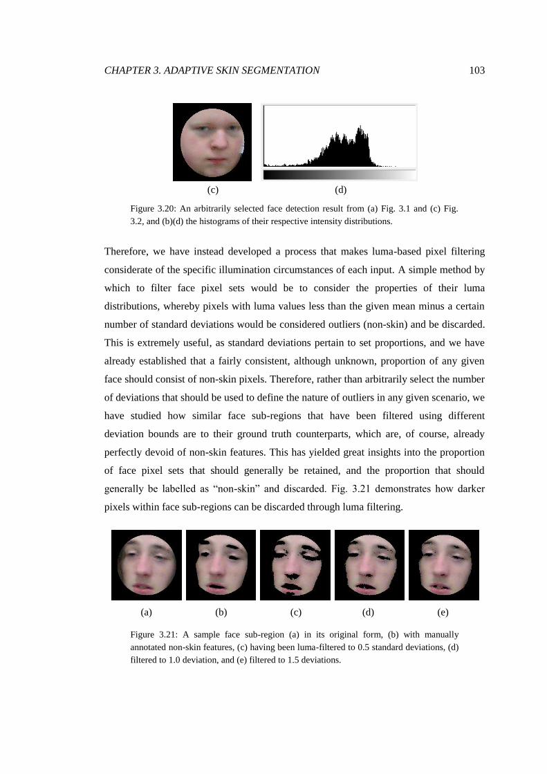
CHAPTER 3. ADAPTIVE SKIN SEGMENTATION 103
(c) (d) .
Figure 3.20: An arbitrarily selected face detection result from (a) Fig. 3.1 and (c) Fig.
3.2, and (b)(d) the histograms of their respective intensity distributions.
Therefore, we have instead developed a process that makes luma-based pixel filtering
considerate of the specific illumination circumstances of each input. A simple method by
which to filter face pixel sets would be to consider the properties of their luma
distributions, whereby pixels with luma values less than the given mean minus a certain
number of standard deviations would be considered outliers (non-skin) and be discarded.
This is extremely useful, as standard deviations pertain to set proportions, and we have
already established that a fairly consistent, although unknown, proportion of any given
face should consist of non-skin pixels. Therefore, rather than arbitrarily select the number
of deviations that should be used to define the nature of outliers in any given scenario, we
have studied how similar face sub-regions that have been filtered using different
deviation bounds are to their ground truth counterparts, which are, of course, already
perfectly devoid of non-skin features. This has yielded great insights into the proportion
of face pixel sets that should generally be retained, and the proportion that should
generally be labelled as “non-skin” and discarded. Fig. 3.21 demonstrates how darker
pixels within face sub-regions can be discarded through luma filtering.
(a) (b) (c) (d) (e)
Figure 3.21: A sample face sub-region (a) in its original form, (b) with manually
annotated non-skin features, (c) having been luma-filtered to 0.5 standard deviations, (d)
filtered to 1.0 deviation, and (e) filtered to 1.5 deviations.

104 CHAPTER 3. ADAPTIVE SKIN SEGMENTATION
Ideally, we would discard the dark pixels from any given sub-region such that it would
match its ground truth counterpart, and Fig. 3.21 demonstrates how this could be
achieved rather accurately through luma distribution-based filtering. However, it also
shows that establishing the correct filter tolerance is critical for the process to be
effective. Fig. 3.21(c), for instance, demonstrates a particularly low tolerance of only 0.5
standard deviations, which has resulted in many more pixels being discarded than have
actually been identified as non-skin in the manual annotation, Fig. 3.21(b). This is
problematic, as it means that actual skin pixels are being discarded, and useful
information lost. Fig. 3.21(e), on the other hand, perhaps illustrates too much tolerance,
as the use of 1.5 standard deviations has resulted in most non-skin features not actually
being fully eliminated, and the colours of unwanted regions being retained. Conversely,
the use of a single standard deviation, as illustrated by Fig. 3.21(d), has yielded a
segmentation that is not too dissimilar from the ground truth, with the mouth, eyes, and
brows of the depicted individual having been discarded to an almost-perfect degree. This
result supports the notion that this process can indeed be implemented effectively.
In an effort to find the optimal filter tolerance to use for our process, we have used a
range of numbers of standard deviations to filter the non-skin pixels from a large number
of faces, and compared the results to the manually annotated data. The range of filter
tolerances we have chosen to investigate is broad: from a rather restrictive 0.5 standard
deviations, which would result in the retention of only 69.1% of pixels, up to an
extremely permissive 3 standard deviations, which would yield 99.9% pixel retention and
virtually have the same effect as applying no filter whatsoever.
Across 41 face sub-regions, we have considered the pixels manually discarded in order to
form the ground truth data as our positive class of pixels, and then calculated the
elimination precision and recall achieved for each one by each filter tolerance in order to
determine elimination F-scores. We regard the F-score to be an extremely useful metric
in this instance for the same reason it has been useful previously: the class we are most
interested in at this time is the significant minority class. The calculated scores can then
be averaged, across all faces, for each number of standard deviations to establish mean F-
scores, which can then be compared simply. The results of this process can be seen in
Fig. 3.22.

CHAPTER 3. ADAPTIVE SKIN SEGMENTATION 105
Figure 3.22: The mean F-score achieved by each filter tolerance across our 41 face sub-
regions, with regards to the elimination of non-skin pixels.
The results illustrated by Fig. 3.22 are interesting, and are largely in line with our
expectations. Firstly, we expected that low tolerances would be overly restrictive, and
result in the elimination of large numbers of skin pixels for little to no gain, yielding
lower precisions and, hence, lower F-scores, and it would seem that this is indeed the
case. Furthermore, as tolerance has been increased, we have seen a steady decline in the
average score achieved, which is again consistent with our expectations. This is a
consequence of smaller numbers of pixels having been discarded, as smaller proportions
of the non-skin regions present within each face have been eliminated, which has resulted
in lower recall rates and lower F-scores. Our results suggest quite strongly that an optimal
filter tolerance of 1 standard deviation exists between these two classes of issues. We
will, therefore, be using it as part of our process to establish positive skin pixel sets from
face sub-regions from this point forward, and an example of the result of its application
can be seen in Fig. 3.23.

106 CHAPTER 3. ADAPTIVE SKIN SEGMENTATION
(a) (b)
Figure 3.23: Applying a filter that discards any pixel with a luma value more than 1
standard deviation away from the mean value for the given sub-region to (a) a set of
inputs will yield (b) high-precision sets of skin pixels.
As Fig. 3.23 demonstrates, discarding any pixel with a luma value that is more than 1
standard deviation lower than the mean value of the given set will yield a pixel retention
rate of 84.1%, meaning that there will be abundant useful information with which to
build colour models after filtering. This result also suggests that the average face sub-
region contains ~16% non-skin pixels, which is a proportion that we believe should be
relatively invariant over any number of input images or face detections. It is for this
reason that the filter tolerance we have identified as optimal should provide consistent
results, with regards to the accurate elimination of non-skin regions, as it simply
represents the proportional relationship between face sub-regions and the skin pixels
within them, and nothing image-specific.
3.2.2 Skin Colour Distribution Modelling
For any given image, the pixel set used as the basis for its skin colour model will simply
be the collation of the pixels retained after the sub-region definition and luma filtering of
every face detected within it. Our image sampling process has been carefully calibrated to
ensure that the skin pixel sets we produce contain as many positive skin pixels as we can
confidently classify without introducing any significant number of false positives. This
ensures that a generated colour model will represent as great a proportion of the skin
within the given image as possible without being skewed at all by non-skin data.

CHAPTER 3. ADAPTIVE SKIN SEGMENTATION 107
3.2.2.1 Modelling Approach Selection
Having produced a set of skin pixels, we are now in a position to build a colour model
that will represent the skin present within the given image. However, the choice of
methodology with which to construct the model is not an entirely trivial one. Parametric
and non-parametric techniques provide us with a wealth of options, but the most
appropriate one for our system can be chosen with a small number of simple
considerations:
We have only positive samples with which to train the model, ruling out any
classifier type dependent upon the existence of negative samples in order to
learn, such as a classifier based upon Bayes’ theorem. As we ran the face
detector at low sensitivity, we cannot be confident that the regions not
returned do not actually contain faces, or other regions of skin.
A given filtered pixel set will, naturally, merely be a subset of all the skin
pixels present within the given image, so being able to interpolate the colours
that are not necessarily being represented by our set, but are very similar to
those that are, would be extremely useful.
A modelling approach that would allow us to calculate continuous skin
likelihoods, rather than providing only binary classifications as typical
decision rule models would, would certainly be preferable, as the potential
for adjustable thresholding would significantly improve the applicability and
usefulness of the system.
The approach to skin segmentation we are developing would ideally be
suitable for real-time systems, so the method by which we model colour
distributions must allow for relatively efficient calculations and
classifications.
Given that we have yet to commit to a specific colour space in which to
operate, we can value highly any particular synergies that may exist between
certain spaces and particular modelling approaches.

108 CHAPTER 3. ADAPTIVE SKIN SEGMENTATION
Thankfully, an option exists that meets all of these criteria: Gaussian modelling. Just as
we demonstrated in Section 3.1.1.6, the development of a unimodal Gaussian function is
straightforward, and requires only the determination of a mean colour vector (through the
application of Eq. 3.22) and a covariance matrix (through the application of Eq. 3.23) for
the given skin pixel set, which can be accomplished using only our positive samples.
Additionally, by generalising our data with such a condensed representation, we are
naturally interpolating skin tones that may have been undersampled by our preceding
face detection and pixel filtering process.
Furthermore, the application of Eq. 3.21 to the pixels of a given image, in order to
determine their skin likelihoods and classify them, will allow for specific thresholds to be
applied for specific results to be obtained. By enabling the trivial adjustment of
classification sensitivity, our approach will be extremely flexible, and capable of meeting
specific end-user needs. If, for instance, a certain segmentation process necessitates that
as much skin as possible is positively identified, without great concern for the co-
existence of some false positives, then the skin likelihood required of a pixel for it to be
positively classified can be lowered accordingly. Alternatively, certain processes may
need to identify pixels that exhibit extremely high skin likelihoods, such as those that
need “seeds” in order to initiate neighbourhood diffusion or skin region growing [116],
and our approach will be equally capable of catering to these demands. The application of
Eq. 3.21 should also prove to be relatively efficient, and will even afford some
opportunity for significant optimisation, which we will be exploring.
Finally, as we have previously highlighted, the elliptical nature of Gaussian models
synergises extremely effectively with the way in which skin colours tend to cluster in
normalised colour spaces [139], which is why we are also electing to use the normalised
rg space for our system. As well as the space providing natural resistance to illumination
variations (through proportion-based representation), the reduction in problem
dimensionality from three (RGB) to two (rg) will serve to reduce computational
complexity, as the distributions we generate will be merely bivariate.
Although the normalised rg cluster model of Soriano et al. [133] was an inconsistent
performer during our initial skin segmentation experimentation in Section 3.1.1.2, we do
not believe those results truly represent the potential for the space to be used to model

CHAPTER 3. ADAPTIVE SKIN SEGMENTATION 109
skin colour distributions as part of a highly effective, adaptive system. As we identified,
given that explicit cluster models are typically inflexible generalisations of large training
data sets, greatly disparate results are inevitable when inputs that are significantly
different in nature are presented, especially when their differences are so extreme that
there exists essentially no overlap between the colour distributions of the skin within
them, as we discussed in Section 3.1.2. Such a situation essentially presents the
possibility of two separate, yet equally undesirable, possibilities when pre-trained models
are being applied: that the moderate levels of recall achieved for each are accompanied
by objectionably low levels of precision; or, although decidedly less likely, that the skin
of one image will be effectively and specifically segmented whilst the skin of the other
will be undetected almost entirely amongst multitudinous false positive classifications.
Either way, the results of broadly applying a single model to inputs that can vary wildly
in nature will inevitably leave great room for improvement.
These issues are entirely alleviated by the adaptive nature of our approach, however.
Since we will be constructing image-specific models, which will be applied to the image
from which they have been derived and no other, the only colours that will ever be
positively classified as skin within any given image will be those that we have identified
with great confidence as being representative of skin within that particular image.
Furthermore, unless there is a significant, unforeseen failure on the part of our adaptive
sampling process, the possibility of the skin of an image not actually being represented
by its respective colour model, and therefore remaining largely undetected after
segmentation, should be all but eliminated.
Although it performed slightly more effectively than the normalised rg model of Soriano
et al. [133], the Gaussian joint-probability distribution model we built in Section 3.1.1.6
was similarly inconsistent in the segmentation of skin from our two lecture theatre-based
inputs. Although constructed specifically from skin samples pulled from those particular
images, and many similar images, the approach failed for the same reasons that the
explicit normalised rg cluster model did. Again, however, the issues that proved the most
detrimental to our pre-trained Gaussian model will be mitigated completely by adaptive
skin colour modelling.

110 CHAPTER 3. ADAPTIVE SKIN SEGMENTATION
In summary, our skin colour distribution sampling and modelling process for any given
input image can be described by the following sequence of steps:
1. Use the face detection system of Viola and Jones in a high-precision,
moderate-recall configuration to detect high-likelihood faces.
2. Define circular sub-regions within each face detection region, about their
centres, in order to eliminate large portions of uninteresting background
information.
3. For each sub-region, calculate the mean and the standard deviation of the
luma values of pixels, and discard those that are darker than the given mean
minus one given standard deviation, as they are likely to represent non-skin
features.
4. Collate the retained pixels of every face detection sub-region to form the
positive skin sample set.
5. Calculate the mean colour vector of the skin sample set according to the
normalised rg colour representations of its pixels.
6. Determine the covariance matrix of the skin sample set as it pertains to the
normalised rg colour space.
The entire sampling and modelling process can also be described by Fig. 3.24, which
illustrates each of its steps and the flow of information from initial input to model
generation.
Figure 3.24: A simplistic overview of our image-specific skin colour sampling and
distribution modelling process.
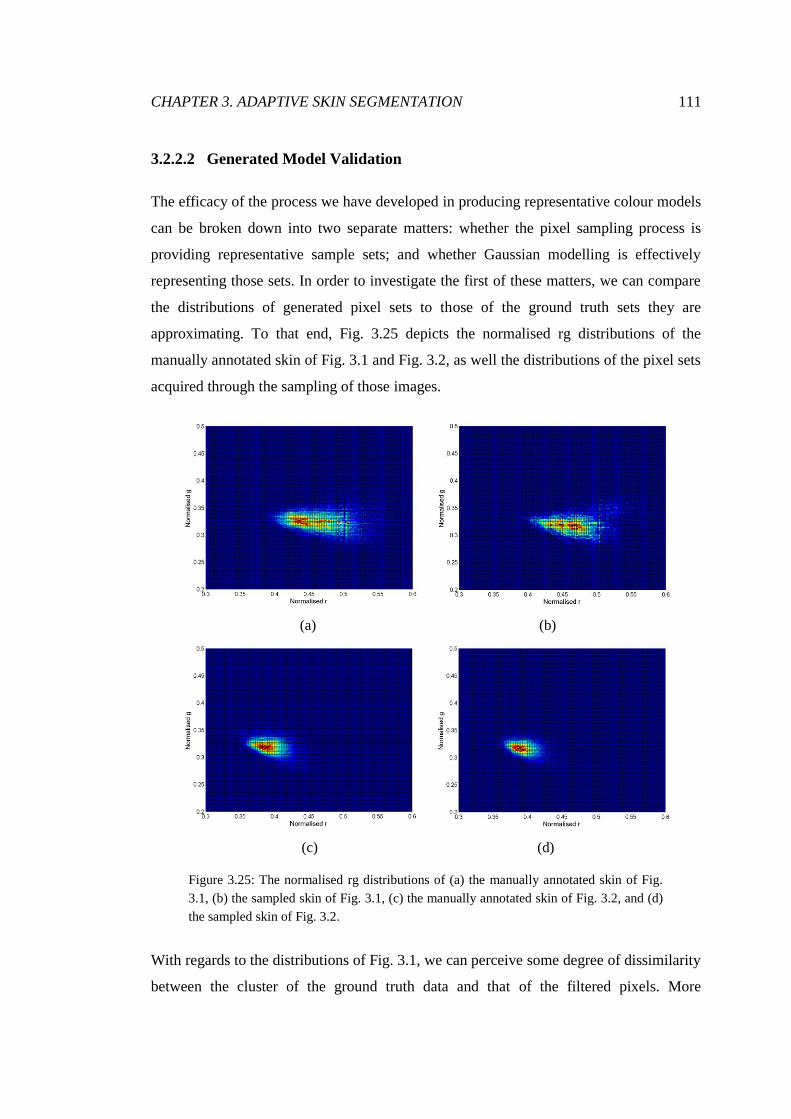
CHAPTER 3. ADAPTIVE SKIN SEGMENTATION 111
3.2.2.2 Generated Model Validation
The efficacy of the process we have developed in producing representative colour models
can be broken down into two separate matters: whether the pixel sampling process is
providing representative sample sets; and whether Gaussian modelling is effectively
representing those sets. In order to investigate the first of these matters, we can compare
the distributions of generated pixel sets to those of the ground truth sets they are
approximating. To that end, Fig. 3.25 depicts the normalised rg distributions of the
manually annotated skin of Fig. 3.1 and Fig. 3.2, as well the distributions of the pixel sets
acquired through the sampling of those images.
(a) (b)
(c) (d)
Figure 3.25: The normalised rg distributions of (a) the manually annotated skin of Fig.
3.1, (b) the sampled skin of Fig. 3.1, (c) the manually annotated skin of Fig. 3.2, and (d)
the sampled skin of Fig. 3.2.
With regards to the distributions of Fig. 3.1, we can perceive some degree of dissimilarity
between the cluster of the ground truth data and that of the filtered pixels. More

112 CHAPTER 3. ADAPTIVE SKIN SEGMENTATION
specifically, we can see less dispersion in the colour distribution of the filtered pixels
(Fig. 3.25(b)), with a greater concentration of data points proximal to centre of the
cluster. This is to be expected, as the pixels that constitute the filtered set are essentially
those of the ground truth set that we can most confidently and most precisely define as
skin. Given that the distributions are otherwise very similar, however, this minor
dissimilarity should prove to be of very little concern. There is even greater similarity
between the clusters of Fig. 3.2., as the naturally slightly greater concentration of the
filtered pixel colour distribution (Fig. 3.25(d)) is made almost imperceptible by the
diminutive size of the clusters themselves.
Given how dissimilar the colour distributions of the skin of the two images are, the fact
that we can sample them and replicate them both so accurately using the exact same
process suggests that our sampling process is indeed highly effective. It should also be
highlighted that the plots depicted by Fig. 3.25 illustrate only a small segment of the
entire normalised rg colour space, which reinforces the notion that the distributions of our
filtered pixel sets are incredibly similar to those that they are supposed to approximate.
As effective as our image sampling process may be, without an equally effective
methodology for building models from skin sample sets, we will not be able to achieve
desirable segmentation results upon the application of said models, which constitutes the
crux of the second of our highlighted matters. In order for us to ascertain the suitability of
Gaussian modelling for our colour distributions, we can compare the models we generate
to the filtered sets they are derived from and the ground truth sets they are estimations of.
Working within the normalised rg colour space, however, our models will essentially be
three-dimensional (r,g,probability), which makes the visual evaluation of them somewhat
problematic, even though a dimensionality this low is the best-case scenario for our
problem in general.
At this time, we can, instead, isolate the normalised r and normalised g dimensions of our
data and consider the means and standard deviations of our models, rather than their
covariance matrices, which will at least give us some visual sense of goodness-of-fit,
which is paramount for establishing model validity and modelling approach suitability. It
should be noted that such a reduction in space dimensionality means that we will only be
looking at our data as it has been regressed onto two individual planes, whilst there are,
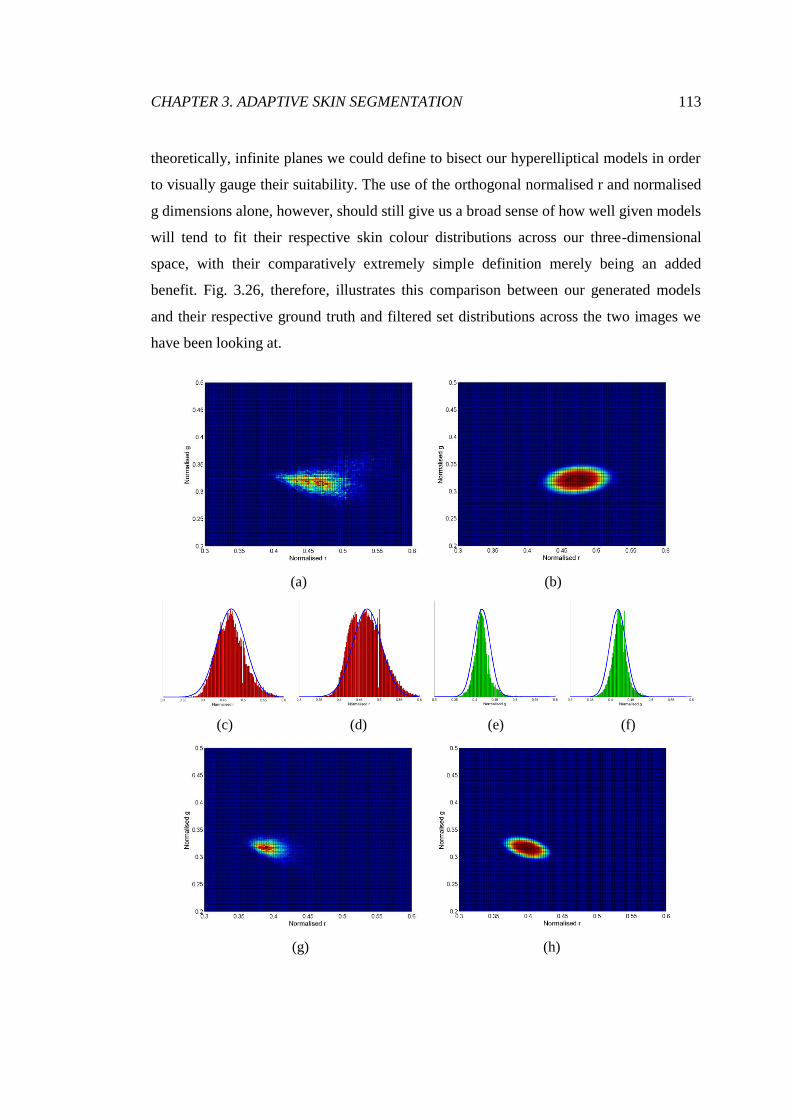
CHAPTER 3. ADAPTIVE SKIN SEGMENTATION 113
theoretically, infinite planes we could define to bisect our hyperelliptical models in order
to visually gauge their suitability. The use of the orthogonal normalised r and normalised
g dimensions alone, however, should still give us a broad sense of how well given models
will tend to fit their respective skin colour distributions across our three-dimensional
space, with their comparatively extremely simple definition merely being an added
benefit. Fig. 3.26, therefore, illustrates this comparison between our generated models
and their respective ground truth and filtered set distributions across the two images we
have been looking at.
(a) (b)
(c) (d) (e) (f)
(g) (h)

114 CHAPTER 3. ADAPTIVE SKIN SEGMENTATION
(i) (j) (k) (l)
Figure 3.26: Comparisons of our Gaussian models with our pixel colour distributions.
We present (a) the normalised rg distribution of the filtered pixels of Fig. 3.1 against (b)
the unimodal joint-probability Gaussian model derived from that pixel set. For that same
image, we then plot the distribution of the model in the normalised r domain (denoted by
the blue bell curve) against the distribution of (c) the filtered pixel r data and (d) the
ground truth r data. We then do similarly with the distribution of the model in the
normalised g domain (again, denoted by the blue bell curve), as it is plotted against (e)
the filtered pixel g data and (f) the ground truth g data. Plots (g), (h), (i), (j), (k), and (l)
respectively depict the same types of data, but with regards to the pixel sets and
Gaussian model of Fig. 3.2.
With respect first of all to the Gaussian model we have generated for Fig. 3.1, which is
depicted by Fig. 3.26(b), we note that the cluster appears to be slightly larger than the
distribution of the pixels themselves. This is not especially unexpected, as the creation of
the model is influenced by every pixel within the set, including those that are not
proximal to the centre of the main cluster of colours. The model being larger is not
particularly detrimental either, as one of the main benefits of using Gaussian models for
skin segmentation is that we can apply threshold values of our choosing in order to obtain
certain forms of results. If we were to apply a high threshold, for instance, we would
identify only pixels with high skin likelihoods, which would be those closest to the centre
of their respective cluster. If we wanted to additionally identify skin pixels with lower
skin likelihoods (more outlying colours), a large model would allow us to apply a low
threshold to accomplish this, even though this would yield an inevitable increase to the
number of false positive classifications being made. The situation is again similar with
regards to Fig. 3.2, as Fig. 3.26(h) illustrates that the model we have generated for that
image is different in size alone from the filtered pixel distribution, with the two clusters
sharing near-identical centre points, shapes, and orientations. Despite the models having
larger sizes than the pixel distributions they have been derived from, we can see that they
still have very little of the colour space in common, which exemplifies that the models
we generate are indeed very much specific to the images that they have been built for.

CHAPTER 3. ADAPTIVE SKIN SEGMENTATION 115
There are a number of interesting aspects to the normalised r and normalised g model
comparison plots we have created. For Fig. 3.1, we can see that, as far as the normalised r
domain is concerned, the model slightly overestimates the filtered pixel set (Fig. 3.26(c))
but slightly underestimates the ground truth data (Fig. 3.26(d)). This suggests that using
the model for classification may result in some lack of sensitivity for the normalised r
values of skin pixels, but the extent of this issue is likely to be very minor. In the
normalised g domain, we note that the model slightly overestimates the distributions of
both the filtered pixels (Fig. 3.26(e)) and the ground truth pixels (Fig. 3.26(f)), with the
situation being marginally less apparent in the case of the latter. The implication of this is
that the model may be slightly overly sensitive with regards to the normalised g values of
skin pixels, but, again, this issue is far from severe, and unlikely to result in significant
segmentation inaccuracies.
Fig. 3.26(i) illustrates that the Gaussian model we have generated for Fig. 3.2 also
overestimates the normalised r value distribution of its respective filtered pixel set, but
does so to a lesser degree where the ground truth data is concerned (Fig. 3.26(j)). As
opposed to the situation of Fig. 3.1, we would expect to see some minor oversensitivity
across the normalised r domain at the point of pixel classification. The model built for
Fig. 3.2 also demonstrates some overestimation of the distributions of the filtered pixels
(Fig. 3.26(k)) and the manually annotated pixels (Fig. 3.26(l)) in the normalised g
domain, but the disparity between these distributions and the generated model is so
minor, especially in the case of the ground truth pixels, that we would not anticipate any
meaningful classification inaccuracy to occur as a result. That our sampling process and
choice of modelling methodology has resulted in such minor distribution misestimations
for two very dissimilar inputs strongly reinforces the choices we have made in the design
of our system to this point.
Although a number of statistical goodness-of-fit tests exist for investigating the
adherence of a set of values to normal distribution, we have found them to be
inappropriate for our situation. Entirely in contrast with our observations, we have found
that the chi-squared test [95], the Kolmogorov–Smirnov test [14], the Lilliefors test [81],
and the Jarque-Bera test [48] all determine the probability of our data samples actually
being from a normal distribution to be infinitesimally small. These tests, and others like
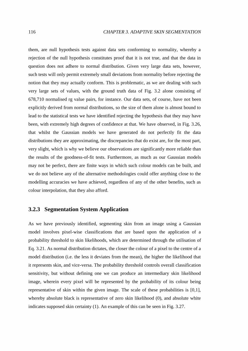
116 CHAPTER 3. ADAPTIVE SKIN SEGMENTATION
them, are null hypothesis tests against data sets conforming to normality, whereby a
rejection of the null hypothesis constitutes proof that it is not true, and that the data in
question does not adhere to normal distribution. Given very large data sets, however,
such tests will only permit extremely small deviations from normality before rejecting the
notion that they may actually conform. This is problematic, as we are dealing with such
very large sets of values, with the ground truth data of Fig. 3.2 alone consisting of
678,710 normalised rg value pairs, for instance. Our data sets, of course, have not been
explicitly derived from normal distributions, so the size of them alone is almost bound to
lead to the statistical tests we have identified rejecting the hypothesis that they may have
been, with extremely high degrees of confidence at that. We have observed, in Fig. 3.26,
that whilst the Gaussian models we have generated do not perfectly fit the data
distributions they are approximating, the discrepancies that do exist are, for the most part,
very slight, which is why we believe our observations are significantly more reliable than
the results of the goodness-of-fit tests. Furthermore, as much as our Gaussian models
may not be perfect, there are finite ways in which such colour models can be built, and
we do not believe any of the alternative methodologies could offer anything close to the
modelling accuracies we have achieved, regardless of any of the other benefits, such as
colour interpolation, that they also afford.
3.2.3 Segmentation System Application
As we have previously identified, segmenting skin from an image using a Gaussian
model involves pixel-wise classifications that are based upon the application of a
probability threshold to skin likelihoods, which are determined through the utilisation of
Eq. 3.21. As normal distribution dictates, the closer the colour of a pixel to the centre of a
model distribution (i.e. the less it deviates from the mean), the higher the likelihood that
it represents skin, and vice-versa. The probability threshold controls overall classification
sensitivity, but without defining one we can produce an intermediary skin likelihood
image, wherein every pixel will be represented by the probability of its colour being
representative of skin within the given image. The scale of these probabilities is [0,1],
whereby absolute black is representative of zero skin likelihood (0), and absolute white
indicates supposed skin certainty (1). An example of this can be seen in Fig. 3.27.
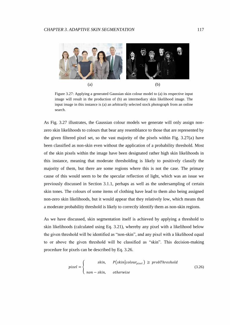
CHAPTER 3. ADAPTIVE SKIN SEGMENTATION 117
(a) (b)
Figure 3.27: Applying a generated Gaussian skin colour model to (a) its respective input
image will result in the production of (b) an intermediary skin likelihood image. The
input image in this instance is (a) an arbitrarily selected stock photograph from an online
search.
As Fig. 3.27 illustrates, the Gaussian colour models we generate will only assign non-
zero skin likelihoods to colours that bear any resemblance to those that are represented by
the given filtered pixel set, so the vast majority of the pixels within Fig. 3.27(a) have
been classified as non-skin even without the application of a probability threshold. Most
of the skin pixels within the image have been designated rather high skin likelihoods in
this instance, meaning that moderate thresholding is likely to positively classify the
majority of them, but there are some regions where this is not the case. The primary
cause of this would seem to be the specular reflection of light, which was an issue we
previously discussed in Section 3.1.1, perhaps as well as the undersampling of certain
skin tones. The colours of some items of clothing have lead to them also being assigned
non-zero skin likelihoods, but it would appear that they relatively low, which means that
a moderate probability threshold is likely to correctly identify them as non-skin regions.
As we have discussed, skin segmentation itself is achieved by applying a threshold to
skin likelihoods (calculated using Eq. 3.21), whereby any pixel with a likelihood below
the given threshold will be identified as “non-skin”, and any pixel with a likelihood equal
to or above the given threshold will be classified as “skin”. This decision-making
procedure for pixels can be described by Eq. 3.26.
𝑝𝑖𝑥𝑒𝑙 = 𝑠𝑘𝑖𝑛, 𝑃 𝑠𝑘𝑖𝑛 𝑐𝑜𝑙𝑜𝑢𝑟𝑝𝑖𝑥𝑒𝑙 ≥ 𝑝𝑟𝑜𝑏𝑇𝑟𝑒𝑠𝑜𝑙𝑑
𝑛𝑜𝑛 − 𝑠𝑘𝑖𝑛, 𝑜𝑡𝑒𝑟𝑤𝑖𝑠𝑒
(3.26)
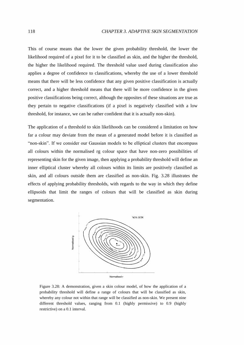
118 CHAPTER 3. ADAPTIVE SKIN SEGMENTATION
This of course means that the lower the given probability threshold, the lower the
likelihood required of a pixel for it to be classified as skin, and the higher the threshold,
the higher the likelihood required. The threshold value used during classification also
applies a degree of confidence to classifications, whereby the use of a lower threshold
means that there will be less confidence that any given positive classification is actually
correct, and a higher threshold means that there will be more confidence in the given
positive classifications being correct, although the opposites of these situations are true as
they pertain to negative classifications (if a pixel is negatively classified with a low
threshold, for instance, we can be rather confident that it is actually non-skin).
The application of a threshold to skin likelihoods can be considered a limitation on how
far a colour may deviate from the mean of a generated model before it is classified as
“non-skin”. If we consider our Gaussian models to be elliptical clusters that encompass
all colours within the normalised rg colour space that have non-zero possibilities of
representing skin for the given image, then applying a probability threshold will define an
inner elliptical cluster whereby all colours within its limits are positively classified as
skin, and all colours outside them are classified as non-skin. Fig. 3.28 illustrates the
effects of applying probability thresholds, with regards to the way in which they define
ellipsoids that limit the ranges of colours that will be classified as skin during
segmentation.
Figure 3.28: A demonstration, given a skin colour model, of how the application of a
probability threshold will define a range of colours that will be classified as skin,
whereby any colour not within that range will be classified as non-skin. We present nine
different threshold values, ranging from 0.1 (highly permissive) to 0.9 (highly
restrictive) on a 0.1 interval.
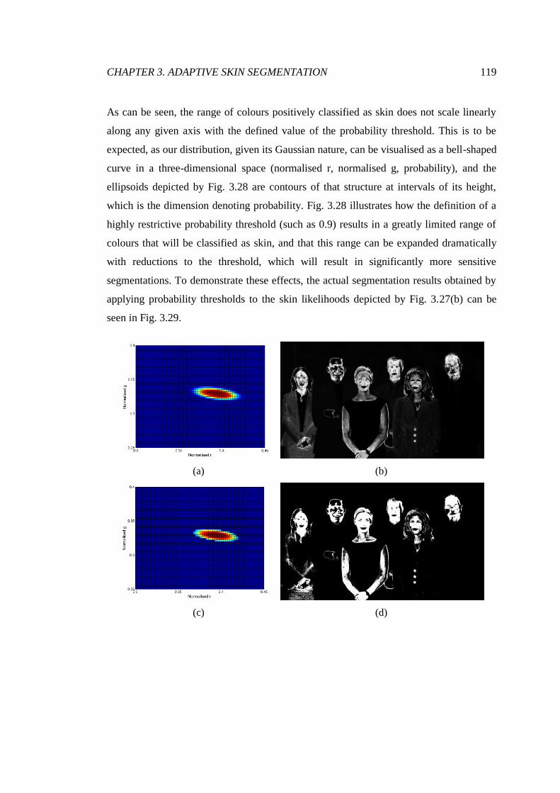
CHAPTER 3. ADAPTIVE SKIN SEGMENTATION 119
As can be seen, the range of colours positively classified as skin does not scale linearly
along any given axis with the defined value of the probability threshold. This is to be
expected, as our distribution, given its Gaussian nature, can be visualised as a bell-shaped
curve in a three-dimensional space (normalised r, normalised g, probability), and the
ellipsoids depicted by Fig. 3.28 are contours of that structure at intervals of its height,
which is the dimension denoting probability. Fig. 3.28 illustrates how the definition of a
highly restrictive probability threshold (such as 0.9) results in a greatly limited range of
colours that will be classified as skin, and that this range can be expanded dramatically
with reductions to the threshold, which will result in significantly more sensitive
segmentations. To demonstrate these effects, the actual segmentation results obtained by
applying probability thresholds to the skin likelihoods depicted by Fig. 3.27(b) can be
seen in Fig. 3.29.
(a) (b) .
(c) (d) .
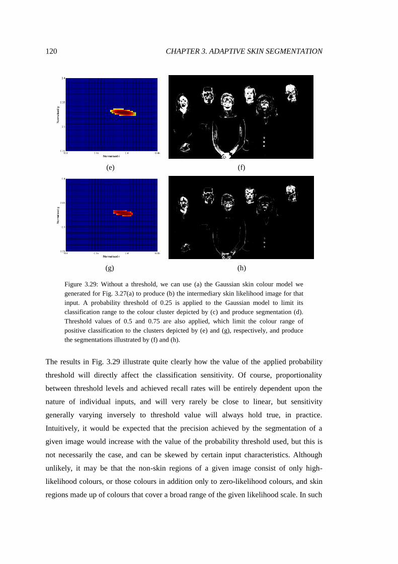
120 CHAPTER 3. ADAPTIVE SKIN SEGMENTATION
(e) (f) .
(g) (h) .
Figure 3.29: Without a threshold, we can use (a) the Gaussian skin colour model we
generated for Fig. 3.27(a) to produce (b) the intermediary skin likelihood image for that
input. A probability threshold of 0.25 is applied to the Gaussian model to limit its
classification range to the colour cluster depicted by (c) and produce segmentation (d).
Threshold values of 0.5 and 0.75 are also applied, which limit the colour range of
positive classification to the clusters depicted by (e) and (g), respectively, and produce
the segmentations illustrated by (f) and (h).
The results in Fig. 3.29 illustrate quite clearly how the value of the applied probability
threshold will directly affect the classification sensitivity. Of course, proportionality
between threshold levels and achieved recall rates will be entirely dependent upon the
nature of individual inputs, and will very rarely be close to linear, but sensitivity
generally varying inversely to threshold value will always hold true, in practice.
Intuitively, it would be expected that the precision achieved by the segmentation of a
given image would increase with the value of the probability threshold used, but this is
not necessarily the case, and can be skewed by certain input characteristics. Although
unlikely, it may be that the non-skin regions of a given image consist of only high-
likelihood colours, or those colours in addition only to zero-likelihood colours, and skin
regions made up of colours that cover a broad range of the given likelihood scale. In such

CHAPTER 3. ADAPTIVE SKIN SEGMENTATION 121
an instance, a high probability threshold would segment the high-likelihood skin as well
as the high-likelihood non-skin, resulting, of course, in a level of precision that is the
proportion of former to the latter. Lowering that threshold would result in the
segmentation of further skin regions, but no additional non-skin, granting an increase to
precision as well as sensitivity. Such a situation arising across arbitrary images would be
rather improbable, but neglecting it as a possibility when we want to consider the
relationship between applied probability threshold values and segmentation results would
be done in error.
3.2.4 Segmentation System Optimisation
Before evaluating the efficacy of our system in accurately segmenting skin from images,
we believe that there are a number of algorithmic improvements we can make in order to
dramatically decrease throughput time at no cost whatsoever to results. In order to
determine where such improvements can be made, and where they can make the most
difference to overall performance, we must first investigate how much time our system
currently expends on its various constituent processes. The time that a certain process
takes for a given input image will depend upon the nature of that image, but the average
fraction of total throughput time dedicated to an individual process over a large number
of images will give us great insight into whether it requires optimisation.
The total time it takes to segment the skin from an image will be largely dependent upon
the resolution of that image, as, naturally, the more pixels there are to process, the more
time processing them all will take. This is why, at a time when we are trying to identify
processes to optimise, it is far more appropriate to consider throughput time proportions
than actual times. Image resolution aside, there are a number of factors that could
theoretically affect the time it takes for individual tasks to be completed, some of which
will have far more effect on certain processes than others. For instance, there being only a
small number of faces detected within a given image, or the faces detected within it being
relatively small, would result in not much time being required to filter pixels and
determine the Gaussian distribution parameters of the yielded filtered set. This would
have no impact, however, on the amount of time required to subsequently classify every
pixel of the image. Alternatively, an image with a high density of features and edges may

122 CHAPTER 3. ADAPTIVE SKIN SEGMENTATION
lead to greater lengths of time being required for face detection windows to be discarded
by the detector, as the existence of certain features within a window may suggest the
presence of a face within it before otherwise-unnecessary evaluations actually confirm
the absence of one. Such a scenario would increase the overall time required to return
face detection results, but would, again, have no impact on subsequent processes.
Figure 3.30 illustrates the average proportion of total throughput time expended by each
major process of our system, which we have defined as the following: face detection;
pixel filtering and skin colour modelling; and skin segmentation. These average values
have been calculated over 20 arbitrary images, which vary greatly in content and are of
numerous sizes.
Figure 3.30: The average proportion of overall throughput time for an image dedicated to
the individual components of our skin segmentation process, with the standard
deviations of the results also labelled.
As Fig. 3.30 makes apparent, the vast majority of the time taken to process a given image
is spent classifying its constituent pixels as either “skin” or “non-skin”. Given that pixel-
wise skin segmentation dictates that our classification algorithm is run for each and every
pixel within a given image, it will often have to be run millions of times before a result is
obtained. This means that even slight algorithmic improvements could yield dramatic
benefits to efficiency, and greatly reduce the amount of time required to process images.
The filtering of pixels and the modelling of them, on the other hand, takes an almost
negligible amount of time to complete, so is of little concern at this stage. Although face
detection takes a decidedly non-negligible amount of time to complete for any given
input image, the face detection system of Viola and Jones that we use has already been

CHAPTER 3. ADAPTIVE SKIN SEGMENTATION 123
incredibly well optimised, so we do not consider it an appropriate target for further
optimisation. It is for these reasons, and our belief that there is significant scope for
improvement, that our efforts to optimise our system will, at this time, be focused upon
the way in which we classify pixels.
3.2.4.1 Mahalanobis Distance-Based Classification
The logical first step towards improving the efficiency of our classification process is to
look further into the method by which we ascertain skin likelihoods. To this point, we
have been using Eq. 3.21 to calculate the probabilities of pixels representing skin, but if
we consider the individual components of that expression, using it in its entirety may
seem unnecessary. The value of the exponent (and, hence, the shape of the distribution
itself) is actually defined by the squared Mahalanobis distance between the given input
colour vector and the given mean colour vector, multiplied by a constant. Mahalanobis
distance itself [83] is a multi-dimensional generalisation of how far a value (or a vector of
values) is from the mean of a distribution, and is expressed by a unitless and scale-
invariant value that measures this distance in terms of standard deviations. Eq. 3.27
describes how the Mahalanobis distance between colour vector ci and distribution s is
calculated.
𝑑𝑖𝑠𝑡𝑎𝑛𝑐𝑒𝑀𝑎𝑎𝑙 (𝑐𝑖 , 𝑠) = 𝑐𝑖 − 𝜇𝑠 𝑇𝛴𝑠
−1(𝑐𝑖 − 𝜇𝑠) (3.27)
Although determining Mahalanobis distances instead of skin likelihoods would reduce
the number of calculations required to classify every pixel within a moderately sized
image by several million, our existing method of classifying pixels is rendered useless, as
we simply cannot apply a probability threshold in the range [0,1] to these distances. If we
could translate our defined thresholds to distances, however, we could indeed classify
pixels based upon their Mahalanobis distances from distributions [106,140]. Thankfully,
this is entirely possible. Since Eq. 3.21 uses a Mahalanobis distance to calculate a
probability, we can rearrange it to yield an expression that will calculate a Mahalanobis
distance given a probability. Eq. 3.28 describes this expression, wherein dM represents
Mahalanobis distance and p represents skin probability.

124 CHAPTER 3. ADAPTIVE SKIN SEGMENTATION
𝑝 = 𝑒 −1
2𝑑𝑀
2
=1
𝑒
12𝑑𝑀
2
𝑒 1
2𝑑𝑀
2 = 1
𝑝 .
𝑑𝑀
2
2= ln 1
𝑝 .
𝑑𝑀2 = 2 ln 1
𝑝 .
𝑑𝑀 = 2 ln 1𝑝 (3.28)
As can be discerned from Eq. 3.28, the mapping of probabilities to Mahalanobis
distances is non-linear. Whereas the probability of a colour representing skin will not
vary linearly, along any axis, with its deviation from the mean of the given distribution
(as illustrated by Fig. 3.28), its Mahalanobis distance from that mean will, of course, vary
linearly with its deviation along every axis. This relationship can be illustrated by Fig.
3.31.
Figure 3.31: The variation of Mahalanobis distance from the centre of a distribution. A
range of Mahalanobis distances are presented, which would cover the vast majority of a
distribution, to demonstrate its linearity.
Although the Mahalanobis distance from the distribution mean along the perimeter of any
of the ellipsoids depicted by Fig. 3.31 is constant, the Euclidean distance, demonstrably,
is not necessarily so. This is because Mahalanobis distance is defined by, and is relative
only to, the covariance matrix of a distribution, rather than the absolute distance between

CHAPTER 3. ADAPTIVE SKIN SEGMENTATION 125
two points in n-dimensional Euclidean space. However, were the dimensions of our space
to be rescaled to have unit variance, then our ellipsoids would become circular, and the
Mahalanobis distances would actually correspond to standard Euclidean distances.
Additionally, although we have illustrated the linearity of Mahalanobis distance variation
using rational values, the distances we use during any pixel classification process are
likely to be irrational, such is the nature of the conversion from probability to
Mahalanobis distance. For instance, a straightforward, meaningful probability threshold
of 0.5 would correspond to a Mahalanobis distance of 1.1774. The actual values of the
distances are of little concern, however, as it is merely whether the Mahalanobis distance
of an input pixel is greater than or less than the given distance threshold that is important.
By using Eq. 3.28, we can determine the Mahalanobis distance dM beyond which any
colour will have a skin likelihood less than the given threshold p, and within which any
colour will have a skin likelihood greater than threshold p. Having now alternated from
probability-based pixel classification to Mahalanobis distance-based pixel classification,
our decision rule for determining whether a given pixel is classified as “skin” or “non-
skin” can now be described by Eq. 3.29.
𝑝𝑖𝑥𝑒𝑙 =
𝑠𝑘𝑖𝑛, 𝑀𝑎𝑎𝑙𝐷𝑖𝑠𝑡𝑝𝑖𝑥𝑒𝑙 𝑐𝑜𝑙𝑜𝑢𝑟 ≤ 𝑀𝑎𝑎𝑙𝐷𝑖𝑠𝑡𝑡𝑟𝑒𝑠𝑜𝑙𝑑
𝑛𝑜𝑛 − 𝑠𝑘𝑖𝑛, 𝑜𝑡𝑒𝑟𝑤𝑖𝑠𝑒
(3.29)
Rather than having a probability threshold to which Mahalanobis distances are compared
after expensive (over vast numbers of pixels) conversions, we now simply convert the
probability threshold itself to a Mahalanobis distance (using Eq. 3.28) at the start of the
pixel classification process, then compare the calculated deviations of pixel colours
directly to that value. This means that the application of this new classification
methodology will yield absolutely identical results to the probability-based decision rule
we used previously (as described by Eq. 3.26), but will do so more efficiently.
3.2.4.2 Efficiently Discarding Zero-Likelihood Pixels
Although classifying pixels using Mahalanobis distances is less computationally
expensive than doing so using probabilities, there is still a non-negligible cost associated
with the classification of any given pixel. For an average arbitrary image, the vast

126 CHAPTER 3. ADAPTIVE SKIN SEGMENTATION
majority of pixels being classified will have skin likelihoods that are essentially zero,
such is the extent of their colours’ deviations from the given model distribution. An
example of this has already been seen in Fig. 3.27(b), wherein the pixels that are not
black (those that actually have non-zero skin likelihoods) are significantly outnumbered
by those that are. In spite of there being virtually no possibility that these pixels would
ever be classified as skin (unless an infinitesimally small, and practically useless,
probability threshold were to be applied), the time currently expended by our pixel
classification process on determining the precise Mahalanobis distance of such a pixel is
exactly the same as the time it would spend for a pixel with a non-zero skin likelihood,
i.e. one for which calculating the Mahalanobis distance will actually determine whether it
is positively or negatively classified, given a practical threshold. What this means is that
the vast majority of the time currently being committed to the classification of pixels is
actually being done so for, essentially, no benefit whatsoever to results. Therefore, an
adequate solution to this issue should yield dramatic improvements to performance.
Devising a method to distinguish zero-likelihood pixels from those with actual
possibilities of being classified as skin, without having to determine their Mahalanobis
distances, would be greatly beneficial, as not having to perform multitudes of matrix-
based calculations for those pixels would save significant portions of the time currently
being spent on pixel classification. We could achieve such pre-emptive distinctions by
defining a range of “possible skin” colours before performing any segmentation. Such a
range could be used to determine, at a low computational cost, whether a given input
pixel would definitely be classified as “non-skin” according to the given skin colour
model, or whether there exists a possibility that it would be classified as “skin”. In this
way, we could ensure that the time being spent on Mahalanobis distance calculations
would only ever be done so for the betterment of results. Given a threshold value, this
methodology could be used to achieve an even greater effect than the elimination of
pixels with near-zero skin likelihoods, as the defined colour range could be calibrated to
also reject pixels that have likelihoods that, while comparatively significant, happen to be
below the threshold, thereby reducing the number of necessary Mahalanobis distance
calculations even further, and improving computational efficiency to an even greater
extent.

CHAPTER 3. ADAPTIVE SKIN SEGMENTATION 127
Defining colour ranges can be done dynamically, on an image-by-image basis, as
parameters can be derived specifically from generated colour models. Given a defined
probability threshold, we can use Eq. 3.28 to determine the Mahalanobis distance from
the given distribution at which colours will have a skin likelihood equal to the threshold.
As we previously have established, any colours with deviations greater than that distance
will have skin likelihoods lower than the threshold, and would, therefore, be classified as
“non-skin”. With regards to either individual dimension of the normalised rg colour
space, the calculated Mahalanobis distance will equate to the maximum number of
standard deviations from the mean that the colour component could exhibit before the
colour itself would definitely be classified as “non-skin”.
Of course, one component of a given colour being within standard deviation bounds does
not guarantee the positive classification of that colour, as the other component must also
be within its respective bounds. Even then, it is still entirely possible that both of the
components of a colour are close enough to their respective limits that the absolute
deviation of the colour is greater than the given Mahalanobis distance threshold, which
would also result in the colour being classified as “non-skin”. This is why, although we
can apply colour bounds to greatly reduce the number of calculations performed during
segmentation, the determination of Mahalanobis distances will always be required to
some extent if we wish to maintain the accuracy of our results. However, by using a
calculated Mahalanobis distance threshold to establish a range of colours for which
calculations are necessary, with all others being outrightly classified as “non-skin”, we
believe we can minimise that extent.
To determine the colour parameter bounds used during the segmentation of a given input,
which consist of lower and upper limits on the normalised r and normalised g component
values of colours, we can use the simple expressions described by Eq. 3.30, Eq. 3.31, Eq.
3.32, and Eq. 3.33, where μi and σi respectively represent the mean and the standard
deviation of colour component i according to the model generated for the given input,
and dM represents the Mahalanobis distance calculated from the defined probability
threshold.
𝑙𝑜𝑤𝑒𝑟𝐿𝑖𝑚𝑖𝑡𝑟 = 𝜇𝑟 − (𝑑𝑀 ∙ 𝜎𝑟) (3.30)

128 CHAPTER 3. ADAPTIVE SKIN SEGMENTATION
𝑢𝑝𝑝𝑒𝑟𝐿𝑖𝑚𝑖𝑡𝑟 = 𝜇𝑟 + (𝑑𝑀 ∙ 𝜎𝑟) (3.31)
𝑙𝑜𝑤𝑒𝑟𝐿𝑖𝑚𝑖𝑡𝑔 = 𝜇𝑔 − (𝑑𝑀 ∙ 𝜎𝑔) (3.32)
𝑢𝑝𝑝𝑒𝑟𝐿𝑖𝑚𝑖𝑡𝑔 = 𝜇𝑔 + (𝑑𝑀 ∙ 𝜎𝑔) (3.33)
With these limits established for a given input image, we ensure that Mahalanobis
distances are only calculated for pixels that have normalised r values and normalised g
values that are both greater than their respective lower limits and less than their
respective upper limits. Any colour not within all four of these bounds will be classified
as “non-skin” without consideration for its actual Mahalanobis distance, as it is certain to
be greater than the given threshold anyway. Were these limits to be any more restrictive,
colours that would actually represent skin according to the given model and threshold
would, inevitably, be falsely negatively classified. Conversely, were the limits to be any
more expansive, then the Mahalanobis distances of colours that would be classified
negatively anyway would also be calculated, which would be detrimental to efficiency.
Basing limits on the Mahalanobis distance threshold itself eliminates the potential for
either of these issues. These concepts can be visualised by Fig. 3.32.
Figure 3.32: The range of colours for which Mahalanobis distances are calculated is
limited according to the Mahalanobis distance threshold itself, and all colours outside of
that range will be classified as “non-skin” without such calculations.
As can be seen, the limits we establish actually form perfect bounding boxes around the
ellipsoids of given Mahalanobis distance thresholds, ensuring that no skin colours are

CHAPTER 3. ADAPTIVE SKIN SEGMENTATION 129
wrongly dismissed as “non-skin” and no unnecessary Mahalanobis distance-based
classifications are performed. What can also be discerned is that, by virtue of the nature
of ellipsoids, there will still be significant ranges of colours within any given bounding
box that will not actually represent skin according to the given model and threshold, and
these must be distinguished through Mahalanobis distance calculation. Given this
modification to our segmentation process, the decision rule for determining whether a
given pixel is classified as “skin” or “non-skin” can now be described by Eq. 3.34.
𝑝𝑖𝑥𝑒𝑙 =
𝑠𝑘𝑖𝑛,
𝑝𝑖𝑥𝑒𝑙 𝑐𝑜𝑙𝑜𝑢𝑟𝑟 ≥ 𝑙𝑜𝑤𝑒𝑟𝐿𝑖𝑚𝑖𝑡𝑟 𝑎𝑛𝑑𝑝𝑖𝑥𝑒𝑙 𝑐𝑜𝑙𝑜𝑢𝑟𝑟 ≤ 𝑢𝑝𝑝𝑒𝑟𝐿𝑖𝑚𝑖𝑡𝑟 𝑎𝑛𝑑𝑝𝑖𝑥𝑒𝑙 𝑐𝑜𝑙𝑜𝑢𝑟𝑔 ≥ 𝑙𝑜𝑤𝑒𝑟𝐿𝑖𝑚𝑖𝑡𝑔 𝑎𝑛𝑑
𝑝𝑖𝑥𝑒𝑙 𝑐𝑜𝑙𝑜𝑢𝑟𝑔 ≤ 𝑢𝑝𝑝𝑒𝑟𝐿𝑖𝑚𝑖𝑡𝑔 𝑎𝑛𝑑
𝑀𝑎𝑎𝑙𝐷𝑖𝑠𝑡𝑝𝑖𝑥𝑒𝑙 𝑐𝑜𝑙𝑜𝑢𝑟 ≤ 𝑀𝑎𝑎𝑙𝐷𝑖𝑠𝑡𝑡𝑟𝑒𝑠𝑜𝑙𝑑
𝑛𝑜𝑛 − 𝑠𝑘𝑖𝑛, 𝑜𝑡𝑒𝑟𝑤𝑖𝑠𝑒
(3.34)
Using Eq. 3.34 to segment skin ensures that the number of calculations required to
accurately classify a pixel is kept to an absolute minimum, as a non-skin pixel will be
classified as such upon the first failure to meet a condition, and, therefore, all conditions
would only ever be evaluated for pixels within the given colour range. It is important to
note that, despite these dramatic changes to the way in which we now perform skin
segmentation, the results this process yields are identical to those that would be produced
using the previous methods. The effect of implementing this system is merely the
acquisition of the same results but with much greater efficiency, thereby improving
system performance at no cost to accuracy whatsoever.
To determine the extent to which applying calculation-limiting colour ranges improves
efficiency, we can repeat the experiment we carried out at the start of Section 3.2.4, and
compare those results to what we can achieve now. Of course, the changes we have made
will have no effect at all on the efficiency of the face detection and colour model-building
processes, so whilst we expect dramatic reductions to the amount of time generally being
expended on the segmentation of skin, the performance of those procedures will remain
unchanged. Fig. 3.33 illustrates the results of our experimentation, having used exactly
the same test parameters as we did during our previous trial. Our findings are presented
in the context of those previous results in order to exemplify how beneficial our
optimisations have been. It should be noted that these results will also reflect the benefits
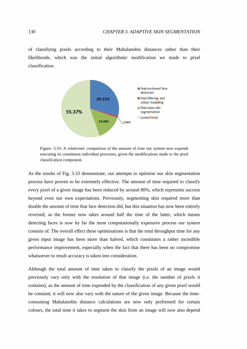
130 CHAPTER 3. ADAPTIVE SKIN SEGMENTATION
of classifying pixels according to their Mahalanobis distances rather than their
likelihoods, which was the initial algorithmic modification we made to pixel
classification.
Figure: 3.33: A relativistic comparison of the amount of time our system now expends
executing its constituent individual processes, given the modifications made to the pixel
classification component.
As the results of Fig. 3.33 demonstrate, our attempts to optimise our skin segmentation
process have proven to be extremely effective. The amount of time required to classify
every pixel of a given image has been reduced by around 80%, which represents success
beyond even our own expectations. Previously, segmenting skin required more than
double the amount of time that face detection did, but this situation has now been entirely
reversed, as the former now takes around half the time of the latter, which means
detecting faces is now by far the most computationally expensive process our system
consists of. The overall effect these optimisations is that the total throughput time for any
given input image has been more than halved, which constitutes a rather incredible
performance improvement, especially when the fact that there has been no compromise
whatsoever to result accuracy is taken into consideration.
Although the total amount of time taken to classify the pixels of an image would
previously vary only with the resolution of that image (i.e. the number of pixels it
contains), as the amount of time expended by the classification of any given pixel would
be constant, it will now also vary with the nature of the given image. Because the time-
consuming Mahalanobis distance calculations are now only performed for certain
colours, the total time it takes to segment the skin from an image will now also depend

CHAPTER 3. ADAPTIVE SKIN SEGMENTATION 131
upon the proportion of pixels within that image that exhibit skin-like colours and
necessitate distance-based classifications.
3.2.4.3 Colour Range-Based Classification
Although we believe we have reached a practical limit on the degree to which our skin
segmentation process can be optimised without any compromises being made to the
accuracy of the results it generates, it would be prudent to explore the potential for minor
compromises that could yield further performance enhancements. We have already
greatly reduced the number of Mahalanobis distance calculations we perform by limiting
them to certain ranges of colours, but it would be interesting to discover how a
classification process that does not necessitate them at all would perform.
If we were to take our updated decision rule (described by Eq. 3.34), and simply remove
the final positive classification condition (stating that the colour of the given pixel must
deviate by less than the given Mahalanobis distance threshold), we would have such a
process. This new segmentation technique would still establish colour ranges through the
same methodology as before, but rather than dictate that pixels with colours that are
within the limits of the given range will be subject to Mahalanobis distance-based
classification, they would now simply be classified as “skin”. The decision rule for this
classification process can, therefore, be described by Eq. 3.35.
𝑝𝑖𝑥𝑒𝑙 =
𝑠𝑘𝑖𝑛,
𝑝𝑖𝑥𝑒𝑙 𝑐𝑜𝑙𝑜𝑢𝑟𝑟 ≥ 𝑙𝑜𝑤𝑒𝑟𝐿𝑖𝑚𝑖𝑡𝑟 𝑎𝑛𝑑𝑝𝑖𝑥𝑒𝑙 𝑐𝑜𝑙𝑜𝑢𝑟𝑟 ≤ 𝑢𝑝𝑝𝑒𝑟𝐿𝑖𝑚𝑖𝑡𝑟 𝑎𝑛𝑑𝑝𝑖𝑥𝑒𝑙 𝑐𝑜𝑙𝑜𝑢𝑟𝑔 ≥ 𝑙𝑜𝑤𝑒𝑟𝐿𝑖𝑚𝑖𝑡𝑔 𝑎𝑛𝑑
𝑝𝑖𝑥𝑒𝑙 𝑐𝑜𝑙𝑜𝑢𝑟𝑔 ≤ 𝑢𝑝𝑝𝑒𝑟𝐿𝑖𝑚𝑖𝑡𝑔 𝑎𝑛𝑑
𝑛𝑜𝑛 − 𝑠𝑘𝑖𝑛, 𝑜𝑡𝑒𝑟𝑤𝑖𝑠𝑒
(3.35)
Given that the condition eliminated from our classification process was designed to
disprove the notion that the colour of a given pixel is representative of skin, as it would
generally be regarded as a positive sample until it could be confidently rejected, the new
method by which we classify pixels will be more permissive. The colour ranges that
would lie within all four parameter bounds but be rejected based upon their Mahalanobis
distances (as can be seen in Fig. 3.32) will no longer be negatively classified, and will
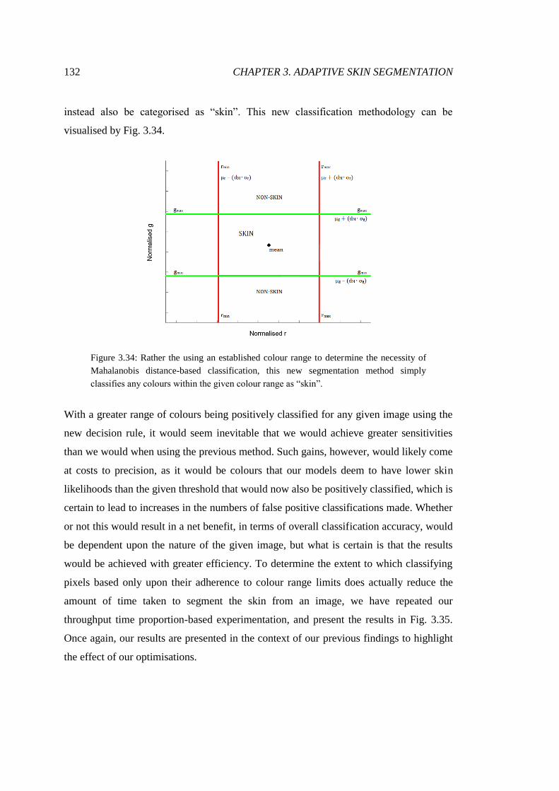
132 CHAPTER 3. ADAPTIVE SKIN SEGMENTATION
instead also be categorised as “skin”. This new classification methodology can be
visualised by Fig. 3.34.
Figure 3.34: Rather the using an established colour range to determine the necessity of
Mahalanobis distance-based classification, this new segmentation method simply
classifies any colours within the given colour range as “skin”.
With a greater range of colours being positively classified for any given image using the
new decision rule, it would seem inevitable that we would achieve greater sensitivities
than we would when using the previous method. Such gains, however, would likely come
at costs to precision, as it would be colours that our models deem to have lower skin
likelihoods than the given threshold that would now also be positively classified, which is
certain to lead to increases in the numbers of false positive classifications made. Whether
or not this would result in a net benefit, in terms of overall classification accuracy, would
be dependent upon the nature of the given image, but what is certain is that the results
would be achieved with greater efficiency. To determine the extent to which classifying
pixels based only upon their adherence to colour range limits does actually reduce the
amount of time taken to segment the skin from an image, we have repeated our
throughput time proportion-based experimentation, and present the results in Fig. 3.35.
Once again, our results are presented in the context of our previous findings to highlight
the effect of our optimisations.

CHAPTER 3. ADAPTIVE SKIN SEGMENTATION 133
Figure 3.35: A relativistic comparison of the amount of time our system expends on each
of its constituent processes, having modified the skin segmentation method to classify
pixels based only upon their adherence to colour bounds.
As can be seen in Fig. 3.35, roughly a third of the time being spent on skin segmentation
after the initial implementation of “possible skin” colour ranges has been saved by our
most recent change in methodology. However, given that the classification of pixels was
no longer the most computationally expensive process our system consisted of, not
classifying pixels based upon their Mahalanobis distances at all only reduces overall
throughput time by around a further 10%, the significance of which will depend upon the
needs of the user. Whilst the amount of time taken to segment the skin from an image
would be dependent upon the nature of the image using the previous classification
methodology, this is not the case for the newly modified process, as the amount of time
expended through determining whether an input pixel colour adheres to the given limits
or not is the same for any given pixel. Therefore, the time expenditure of our
segmentation process would now once again vary only with the size of the given image.
Whilst not as monumental as our previous optimisation, this most recent modification
does yield non-negligible benefits to the performance of our system, but whether or not
these benefits come at only minimal and reasonable costs to segmentation accuracy can
only be determined through evaluation.

134 CHAPTER 3. ADAPTIVE SKIN SEGMENTATION
3.3 Segmentation System Evaluation
In order to determine whether the development of our new skin segmentation system has
been worthwhile, and whether the design decisions we have made throughout the process
have been optimal, we must evaluate it against the very approaches that we have looked
at previously and found to be insufficient for purpose. By discovering the circumstances
under which our approach exhibits superiority over those previous works, we can go a
long way towards establishing its value. In addition, we will also be experimenting with
an existing adaptive methodology. By comparing its achieved results to those of our
system, we can demonstrate that the strengths of our approach are not limited to its
adaptive nature and that its development has not rendered it overly specialised.
The evaluation of our system will be conducted using two separate sets of images. The
first of these is the lecture theatre images we have used previously. The initial impetus
for the development of our system was the inconsistent performance of existing
segmentation techniques when applied to complex lecture theatre imagery. By analysing
how comparatively effective our new approach is at segmenting the skin from those
images, we can assess whether we have found a sufficient solution to our problem.
The second set of images we will be using for classifier evaluation is a large dataset of
arbitrary images. Throughout the development of our system, we have attempted to
maintain algorithmic flexibility, ensuring that the technique will be effective for as broad
a range of inputs as possible. Although it was designed with images depicting large
numbers of people in mind, there have been no specific concessions made that would
render the process unsuitable for images containing only a single face, for instance.
Through demonstrating that our approach can outperform a broad range of existing
methodologies given arbitrary images, its applicability to generic skin segmentation tasks
can be determined.
In Section 3.1.2, we presented a simple quantitative comparison of previous techniques,
which consisted of the evaluation of segmentations using three metrics: recall, precision,
and F-score. These metrics were extremely useful, as their relating exclusively to the
positive “skin” class meant that their reliability was not compromised by the extreme

CHAPTER 3. ADAPTIVE SKIN SEGMENTATION 135
class imbalance of the lecture theatre images, as opposed to that of accuracy, for instance.
Whilst incredibly useful for providing a general sense of how the existing approaches
performed, those metrics did not tell the entire story.
With regards to the pre-trained Bayes and Gaussian classifiers, which are continuous
classifiers (i.e. output likelihoods on the interval [0,1]), we applied a 0.5 probability
threshold based upon the logic that any colour with a likelihood above that value is more-
than-likely to represent skin, and any colour with a likelihood lower than it is more-than-
likely to represent non-skin. Through the application of a single threshold, we essentially
formed a discrete classifier for each methodology, to be evaluated against each other as
well as against the four other discrete, colour space-specific classifiers. This made direct
comparison extremely straightforward, and allowed us to utilise those reliable, highly
informative metrics. The compromise in that instance was that we only explored a single
point on the operational spectrums of the Bayes and Gaussian classifiers, which means
that we were not fully informed on how effective they truly have the capacity to be.
However, given that the system we have developed is also a continuous classifier, and
that we now, naturally, have a much greater need to know precisely how well various
classifiers (including our own) perform than we did during that preliminary testing, our
quantitative analysis at this stage will be significantly more in-depth. This more detailed
study will, of course, also apply to the existing approaches we have been working with,
so any significant misrepresentation of reality the results in Section 3.1.2 yielded (if there
are any at all) can be exposed and corrected.
The first additional evaluatory tool we will be applying to our results is receiver
operating characteristic (ROC) analysis. A ROC curve is a graphical plot that illustrates
how the performance of a binary classification system varies as the probability threshold
applied to its outputs is varied across the entire [0,1] interval [170]. Performance at any
given threshold value is represented by a single point in (FPR,TPR) space. TPR (true
positive rate) is synonymous with recall and sensitivity, and specifies the capacity of a
classifier to segment the samples belonging to the positive class. FPR (false positive rate)
equates to 1 – specificity, and defines the tendency of a classifier to produce false
positive classifications, in terms of the proportion of all negative input samples that have
been positively classified.

136 CHAPTER 3. ADAPTIVE SKIN SEGMENTATION
By specifying a large number of threshold values, a representative ROC curve can be
constructed for any binary continuous classifier. Such a curve will provide significantly
more information about a classifier than condensing it down to a single threshold value
ever could, as the entirety of its performance spectrum will be taken into account. The
curve itself can be a very useful visual aid in the determination of the relative efficacy of
a classifier, as it can reveal to what extent a certain classifier outperforms any other over
the entire range of possible threshold values. Additionally, by minimising the distance
(i.e. the classification error) between the curve and the top-left corner of the graph, which
is the point (FPR=0,TPR=1) and represents perfect classification performance, an optimal
threshold value for a given classifier can be identified, meaning that ROC curves can
actually play a role in the training and optimisation of a classifier [170].
As useful as the visualisation can be, it is often times extremely beneficial to have a
single scalar value that represents the overall performance of a classifier, making
comparison extremely straightforward. Of course, we have previously used the F-score
metric to provide such values, but, as we have established, its scope is limited to only
discrete classifiers. From a ROC graph, however, we can derive a value that represents
the proportion of the entire (FPR,TPR) space that exists between any given plot and the
x-axis, which is referred to as the area under curve (AUC). AUC has been shown to be an
extremely strong indicator of overall efficacy [3,4,44], and it will be an important aspect
of our evaluation process.
In spite of the general usefulness of ROC graphs, there are complications presented by
the nature of our lecture theatre imagery. Just as the reliability of accuracy is lessened by
class skew, so too is that of a receiver operating characteristic. Some researchers argue
that ROC curves are entirely insensitive to class distribution [25], as TPR and FPR relate
exclusively to the positive and negative class, respectively, and so the balance between
them will not be reflected by the appearance of any given curve. Whilst true, this does
mean that ROC curves can yield overly optimistic representations of the performance of a
classifier given evaluation data containing significant class imbalances, and will often not
tell the whole story [21,49]. For instance, when the number of negative samples greatly
outweighs the number of positive samples in an input sample set, large differences in the

CHAPTER 3. ADAPTIVE SKIN SEGMENTATION 137
number of false positives produced by different classifiers will only be reflected by very
small changes to their false positive rates.
It is for this reason that many researchers instead opt to use precision-recall (PR) curves
to evaluate binary classifiers [3,21]. As the name suggests, they are constructed in a two-
dimensional space constrained by the recall and precision metrics we have worked with
previously. The most obviously apparent departure from ROC curves is the lack of regard
for the negative sample class. For our purposes, this is immediately beneficial, as it is the
positive class we eminently more interested in, as we established during our preliminary
testing. The advantages that PR curves hold over ROC curves, therefore, can be
considered similar to those that the F-score metric holds over accuracy.
PR curves are constructed in an identical fashion to ROC curves, with numerous
probability thresholds being used to generate sets of (recall,precision) points for various
classifiers, and they can similarly be represented by individual scalar AUC values.
Despite establishing the rationale for PR curves being considered more reliable and
informative than ROC curves given the nature of our data, we will be making use of both
performance representations throughout our evaluation process, as we believe the more
information we have, the stronger the conclusions we draw will be.
Throughout evaluation, we will be regarding the two forms of our classification system
(hereby denoted by “AGSS”, standing for “Adaptive Gaussian Skin Segmentation”) as
two entirely separate classifiers, which we will be referring to as “AGSS-Mahal” and
“AGSS-Range”. The first of these, AGSS-Mahal, refers to the mode of operation that
ultimately bases pixel classifications on Mahalanobis distances, whereas AGSS-Range is
the form of our system that will classify pixels based only upon their adherence to the
given established range of potential skin colours. It is important that we do regard them
as separate entities, as it is not only whether our system can outperform existing
techniques that is important to us, but also whether the additional optimisations that we
implemented will yield unreasonable costs to accuracy.

138 CHAPTER 3. ADAPTIVE SKIN SEGMENTATION
3.3.1 Lecture Theatre-Based Imagery
As we established, the first stage of our evaluation will be conducted using the lecture
theatre images that we used during our preliminary testing. It is vitally important that we
determine whether our skin segmentation system is capable of solving the issue it was
initially intended to solve. Although our quantitative analysis at this stage will be
restricted to just those two images, we believe that they each contain so much
information, in terms of the numbers and ethnicities of the people within them, and are so
wildly different in nature, in terms of environmental factors that include image capture
point and illumination conditions, that they will still provide us with a very strong
understanding of how our classifier will perform given any image of their type, both in
absolute terms and relatively to those existing methodologies.
However, we will also provide qualitative analysis of a number of other lecture theatre
image segmentations, in order to demonstrate result consistency with the two primary
images. The reason we cannot provide quantitative analysis of a larger number of lecture
theatre images is simple: the production of manual annotations for such complex scenes,
each of which contains dozes of separate skin regions that often encapsulate further non-
skin regions, is extremely time-consuming. It is because of this that we chose the most
dramatically different (although still high quality) images in our large lecture theatre
image set to annotate, as they would allow us to confidently establish approach efficacy
with maximum efficiency, as a result of their great diversity.
3.3.1.1 Discrete Classifier Analysis
Although we have previously outlined the pitfalls of forming discrete classifiers to
represent continuous systems, our initial evaluation will involve the comparison of our
approach to the existing techniques on the same basis that they were compared in Section
3.1.2. This will give us a good sense of how our approach performs in a practical
scenario, and brings to completion that line of evaluation. Therefore, Fig. 3.36 illustrates
the results of segmenting the skin from Fig. 3.1 and Fig. 3.2 using both classification
modes of our system, given a probability threshold value of 0.5.
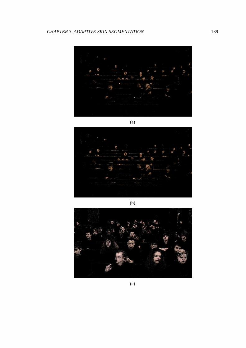
CHAPTER 3. ADAPTIVE SKIN SEGMENTATION 139
(a)
(b)
(c)

140 CHAPTER 3. ADAPTIVE SKIN SEGMENTATION
(d)
Figure 3.36: The results of segmenting the skin from Fig. 3.1 using (a) AGSS-Mahal and
(b) AGSS-Range, and the results of segmenting the skin from Fig. 3.2 using (c) AGSS-
Mahal and (d) AGSS-Range.
In terms of the original configuration of our system (AGSS-Mahal), what may be
immediately noticeable from the results depicted by Fig. 3.36(a) and Fig. 3.36(c) is that
our approach appears to have excelled at avoiding false positive classifications. Whereas
we found many instances of the existing segmentation techniques erroneously classifying
large segments of the environment as skin, the issue is far less prevalent where our
system is concerned. Even the particularly skin-like wooden surfaces visible in Fig. 3.1
have been successfully discarded almost entirely. Of course, what is also apparent is that
these gains have come at some minor costs to recall. This is not an overly severe
situation, however, as a high proportion of skin has been segmented for the vast majority
of individuals across the two images. It would also seem that whatever shortfall exists in
the number of true positive classifications achieved by our system, relative to other
techniques, is greatly outweighed by the reduction in the number of false positive
classifications achieved, which will yield considerably greater levels of precision, and
ensure that a positive classification made by our system is only ever made with a high
degree of confidence.
On first inspection, it may seem as if the results achieved by AGSS-Mahal (Fig. 3.36(a)
and Fig. 3.36(c)) and AGSS-Range (Fig. 3.36(b) and Fig. 3.36(d)) are practically
identical, but there are a number of subtle differences between the outputs that are worthy
of note. In general, it would seem as if AGSS-Range is slightly more sensitive than
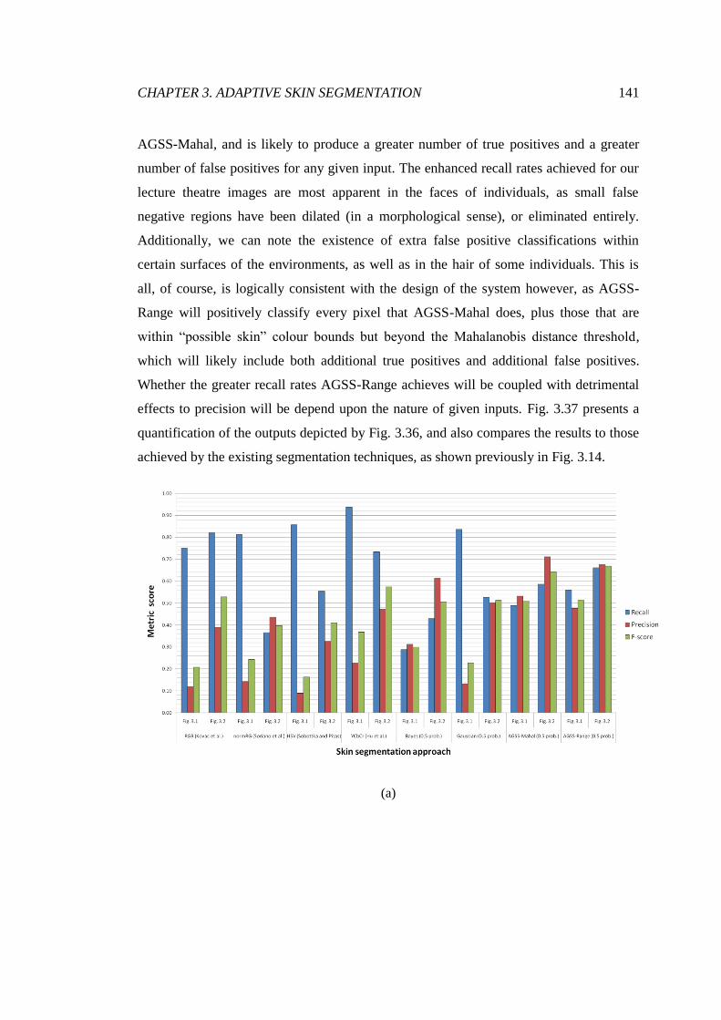
CHAPTER 3. ADAPTIVE SKIN SEGMENTATION 141
AGSS-Mahal, and is likely to produce a greater number of true positives and a greater
number of false positives for any given input. The enhanced recall rates achieved for our
lecture theatre images are most apparent in the faces of individuals, as small false
negative regions have been dilated (in a morphological sense), or eliminated entirely.
Additionally, we can note the existence of extra false positive classifications within
certain surfaces of the environments, as well as in the hair of some individuals. This is
all, of course, is logically consistent with the design of the system however, as AGSS-
Range will positively classify every pixel that AGSS-Mahal does, plus those that are
within “possible skin” colour bounds but beyond the Mahalanobis distance threshold,
which will likely include both additional true positives and additional false positives.
Whether the greater recall rates AGSS-Range achieves will be coupled with detrimental
effects to precision will be depend upon the nature of given inputs. Fig. 3.37 presents a
quantification of the outputs depicted by Fig. 3.36, and also compares the results to those
achieved by the existing segmentation techniques, as shown previously in Fig. 3.14.
(a)
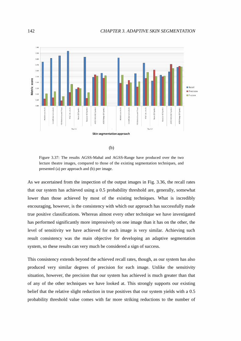
142 CHAPTER 3. ADAPTIVE SKIN SEGMENTATION
(b)
Figure 3.37: The results AGSS-Mahal and AGSS-Range have produced over the two
lecture theatre images, compared to those of the existing segmentation techniques, and
presented (a) per approach and (b) per image.
As we ascertained from the inspection of the output images in Fig. 3.36, the recall rates
that our system has achieved using a 0.5 probability threshold are, generally, somewhat
lower than those achieved by most of the existing techniques. What is incredibly
encouraging, however, is the consistency with which our approach has successfully made
true positive classifications. Whereas almost every other technique we have investigated
has performed significantly more impressively on one image than it has on the other, the
level of sensitivity we have achieved for each image is very similar. Achieving such
result consistency was the main objective for developing an adaptive segmentation
system, so these results can very much be considered a sign of success.
This consistency extends beyond the achieved recall rates, though, as our system has also
produced very similar degrees of precision for each image. Unlike the sensitivity
situation, however, the precision that our system has achieved is much greater than that
of any of the other techniques we have looked at. This strongly supports our existing
belief that the relative slight reduction in true positives that our system yields with a 0.5
probability threshold value comes with far more striking reductions to the number of

CHAPTER 3. ADAPTIVE SKIN SEGMENTATION 143
false positives it produces, which, again, means that positive classifications made by our
system will confer much greater degrees of confidence to users that they are actually true
than those made by any other technique will. It is these significant gains to precision that
have resulted in the F-scores of our system being markedly superior to those of the
existing segmentation approaches, suggesting that the overall performance of our system
is decidedly better than that of any other, as far as these images are concerned.
With respect specifically to the results of AGSS-Mahal and AGSS-Range, the small
differences between them are almost entirely in line with our expectations. Just as we
observed in Fig. 3.36, AGSS-Range does indeed yield marginally greater recall rates than
AGSS-Mahal, and this improvement does seem to be relatively identical across the two
images. We also knew that there was an increase in the number of false positive
classifications made, but without the quantitative results of Fig. 3.37, we could not be
sure whether the balance between them and the additional true positive classifications
would be such that the precision would be improved. Fig. 3.37 confirms that this is not
the case, as, for each image, the precision achieved by AGSS-Range is slightly worse
than that achieved by AGSS-Mahal. Interestingly, it would seem that the superior recall
of AGSS-Range and greater precision of AGSS-Mahal are in almost perfect balance as
far as their F-scores are concerned, as the two classification modes of our system have
almost identical overall performance ratings for both images. By the nature of the design
of our system, however, the results of AGSS-Range have been achieved with slightly
greater efficiency than those of AGSS-Mahal.
3.3.1.2 Receiver Operating Characteristic Analysis
Whilst a useful indicator, Fig. 3.37 cannot tell the whole story of the performance of our
system, as it concerns itself with just a single threshold value. If is for this reason that
ROC analysis has the potential to be a superior gauge of overall success. By producing
segmentation results for a large number of probability thresholds, we can form curves
that will represent how well our system performs across its entire operational spectrum.
We will form a curve for both AGSS-Mahal and AGSS-Range using this method, as well
as for our pre-trained Bayes and Gaussian classifiers. Where curve-based analysis is
concerned, the explicit cluster models we are also comparing our system to represent

144 CHAPTER 3. ADAPTIVE SKIN SEGMENTATION
somewhat of a complication. Since they are inherently discrete classifiers, there exists no
continuous output to which a varying threshold value can be applied, and they can only
ever yield a single point in ROC space. This means that a curve cannot be formed to
represent them in quite the same sense that one can be formed to represent AGSS-Mahal,
for instance. Building curves is very important for our evaluatory process, because they
will subsequently allow us to derive AUC values, which are very powerful performance
indicators [3,4,44].
By applying logic to the (FPR,TPR) ROC space, however, we can simulate curves for the
explicit skin colour cluster models. Firstly, the point (0,0) represents a yield of zero
positive detections, meaning no true positive or false positive classifications whatsoever.
With a sufficiently large probability threshold value applied (such as 1), any given
continuous classifier will produce such a result. If we also apply this notion to discrete
classifiers, we can ascribe an additional point to their performance curves.
Similarly, the point (1,1) represents a yield of zero negative detections, meaning that
every input sample has been indiscriminately positively classified. With a sufficiently
small threshold value applied (such as 0), any given continuous classifier will yield a
result such as this. Again, if this notion is applied to discrete classifiers, a third
performance point can be attributed to them, and curves that are defined across the
entirety of the ROC space can be formed.
It may seem that such curves would overestimate the capabilities of discrete classifiers,
as they would not actually be able to deliver results at any point along them aside from
the three we can specifically define, but the extent of this should not be considerable. By
their very nature, the ROC curves of continuous classifiers will be somewhat convex, as
their performances should improve and then deteriorate as the applied threshold value is
varied over the [0,1] interval. Additionally, a straight line drawn between (0,0) and (1,1)
would represent the result of random guessing (essentially, classifying inputs according
to the flipping of a coin), and the performance of a classifier with any value whatsoever
will always track above this line. Therefore, we would expect the characteristics of the
continuous classifiers to yield larger AUCs than those of the discrete classifiers,
reflecting their greater utility, unless the segmentation results of the latter should happen
to be vastly superior to any individual result of the former.
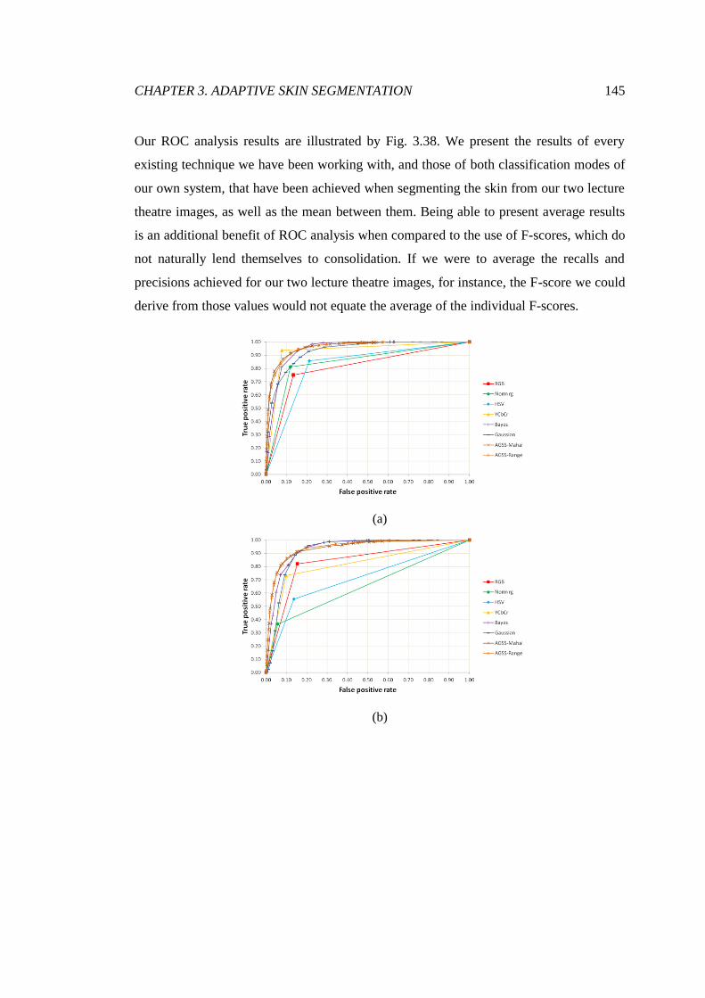
CHAPTER 3. ADAPTIVE SKIN SEGMENTATION 145
Our ROC analysis results are illustrated by Fig. 3.38. We present the results of every
existing technique we have been working with, and those of both classification modes of
our own system, that have been achieved when segmenting the skin from our two lecture
theatre images, as well as the mean between them. Being able to present average results
is an additional benefit of ROC analysis when compared to the use of F-scores, which do
not naturally lend themselves to consolidation. If we were to average the recalls and
precisions achieved for our two lecture theatre images, for instance, the F-score we could
derive from those values would not equate the average of the individual F-scores.
(a)
(b)
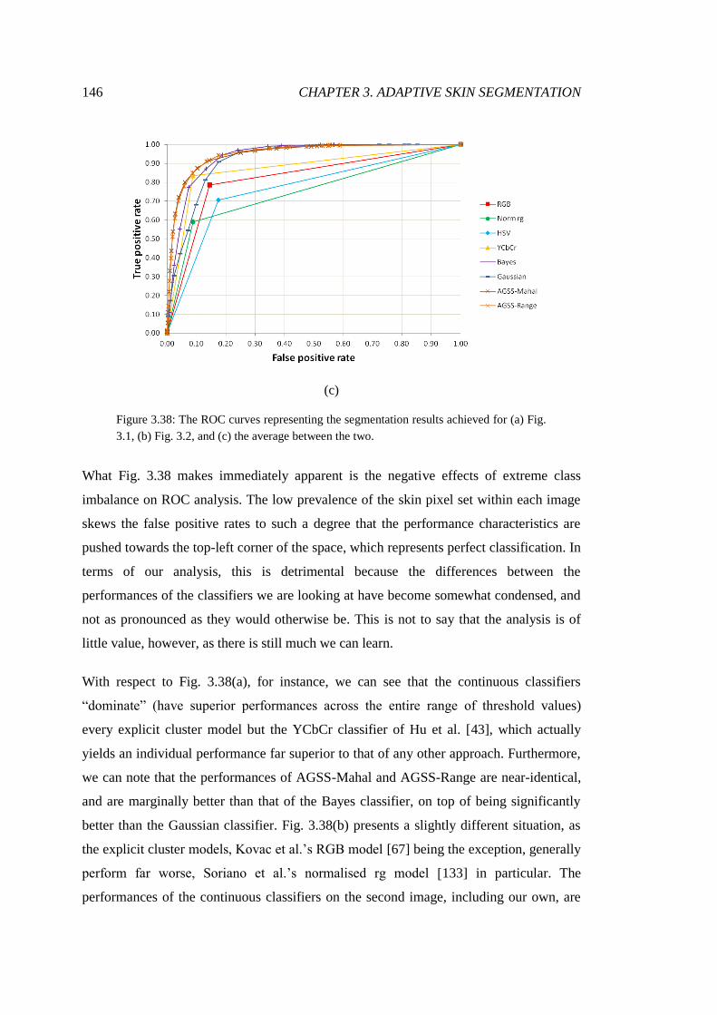
146 CHAPTER 3. ADAPTIVE SKIN SEGMENTATION
(c)
Figure 3.38: The ROC curves representing the segmentation results achieved for (a) Fig.
3.1, (b) Fig. 3.2, and (c) the average between the two.
What Fig. 3.38 makes immediately apparent is the negative effects of extreme class
imbalance on ROC analysis. The low prevalence of the skin pixel set within each image
skews the false positive rates to such a degree that the performance characteristics are
pushed towards the top-left corner of the space, which represents perfect classification. In
terms of our analysis, this is detrimental because the differences between the
performances of the classifiers we are looking at have become somewhat condensed, and
not as pronounced as they would otherwise be. This is not to say that the analysis is of
little value, however, as there is still much we can learn.
With respect to Fig. 3.38(a), for instance, we can see that the continuous classifiers
“dominate” (have superior performances across the entire range of threshold values)
every explicit cluster model but the YCbCr classifier of Hu et al. [43], which actually
yields an individual performance far superior to that of any other approach. Furthermore,
we can note that the performances of AGSS-Mahal and AGSS-Range are near-identical,
and are marginally better than that of the Bayes classifier, on top of being significantly
better than the Gaussian classifier. Fig. 3.38(b) presents a slightly different situation, as
the explicit cluster models, Kovac et al.’s RGB model [67] being the exception, generally
perform far worse, Soriano et al.’s normalised rg model [133] in particular. The
performances of the continuous classifiers on the second image, including our own, are
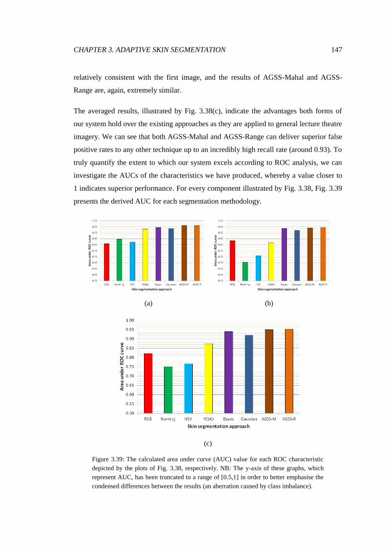
CHAPTER 3. ADAPTIVE SKIN SEGMENTATION 147
relatively consistent with the first image, and the results of AGSS-Mahal and AGSS-
Range are, again, extremely similar.
The averaged results, illustrated by Fig. 3.38(c), indicate the advantages both forms of
our system hold over the existing approaches as they are applied to general lecture theatre
imagery. We can see that both AGSS-Mahal and AGSS-Range can deliver superior false
positive rates to any other technique up to an incredibly high recall rate (around 0.93). To
truly quantify the extent to which our system excels according to ROC analysis, we can
investigate the AUCs of the characteristics we have produced, whereby a value closer to
1 indicates superior performance. For every component illustrated by Fig. 3.38, Fig. 3.39
presents the derived AUC for each segmentation methodology.
(a) (b)
(c)
Figure 3.39: The calculated area under curve (AUC) value for each ROC characteristic
depicted by the plots of Fig. 3.38, respectively. NB: The y-axis of these graphs, which
represent AUC, has been truncated to a range of [0.5,1] in order to better emphasise the
condensed differences between the results (an aberration caused by class imbalance).

148 CHAPTER 3. ADAPTIVE SKIN SEGMENTATION
As we discerned from the ROC curves themselves, the performance of our system is
extremely consistent over the two images, with Fig. 3.39(a) suggesting only very
marginally better results for Fig. 3.1 than for Fig. 3.2. For each image, it would seem that
both AGSS-Mahal and AGSS-Range have outperformed every one of the existing
approaches, albeit to varying degrees. The overall suggestion of these results, as
illustrated by Fig. 3.39(c), is that our system is indeed superior to the alternative
techniques, although the extent to which this may be true is obscured somewhat by the
complications that the extreme class imbalance of our data has introduced to the ROC
analysis.
3.3.1.3 Precision-Recall Analysis
In order to evaluate the results in a manner that is insensitive to the extremely low
prevalence of skin present within our lecture theatre images (which average out to just
0.065), we can employ precision-recall analysis. The important difference between PR
space and ROC space is that the former is constrained only by metrics that relate
exclusively to the positive “skin” class (precision and recall). Although ROC curves and
PR curves are built within different spaces, the metrics they pertain to are intrinsically
related such that the dominance of one classifier over another in ROC space will exist if,
and only if, the first classifier also dominates the second in PR space [21]. This
relationship is extremely encouraging for us, as the characteristics of our system very
nearly dominate those of every existing approach as far as the average results illustrated
by Fig. 3.38(c) are concerned.
Curves in PR space are formed using almost the same procedure as curves in ROC space
are, with only the explicit cluster models presenting somewhat of a complication.
Whereas with ROC curves, we could simply ascribe the points (0,0) and (1,1) to the
performance characteristics of those discrete classifiers to generate a full curve, the
situation is not so straightforward where PR curves are concerned. There does exist a
point to which all characteristics will converge when the applied probability threshold is
0. This point is (1,prevalence), as a threshold value of 0 will result in the positive
classification of every skin pixel within the given image, and a precision that is equal to
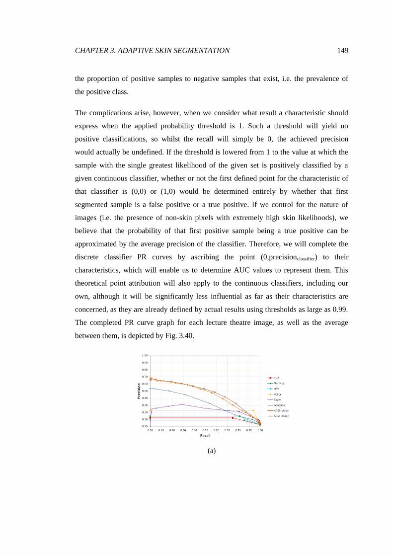
CHAPTER 3. ADAPTIVE SKIN SEGMENTATION 149
the proportion of positive samples to negative samples that exist, i.e. the prevalence of
the positive class.
The complications arise, however, when we consider what result a characteristic should
express when the applied probability threshold is 1. Such a threshold will yield no
positive classifications, so whilst the recall will simply be 0, the achieved precision
would actually be undefined. If the threshold is lowered from 1 to the value at which the
sample with the single greatest likelihood of the given set is positively classified by a
given continuous classifier, whether or not the first defined point for the characteristic of
that classifier is (0,0) or (1,0) would be determined entirely by whether that first
segmented sample is a false positive or a true positive. If we control for the nature of
images (i.e. the presence of non-skin pixels with extremely high skin likelihoods), we
believe that the probability of that first positive sample being a true positive can be
approximated by the average precision of the classifier. Therefore, we will complete the
discrete classifier PR curves by ascribing the point (0,precisionclassifier) to their
characteristics, which will enable us to determine AUC values to represent them. This
theoretical point attribution will also apply to the continuous classifiers, including our
own, although it will be significantly less influential as far as their characteristics are
concerned, as they are already defined by actual results using thresholds as large as 0.99.
The completed PR curve graph for each lecture theatre image, as well as the average
between them, is depicted by Fig. 3.40.
(a)
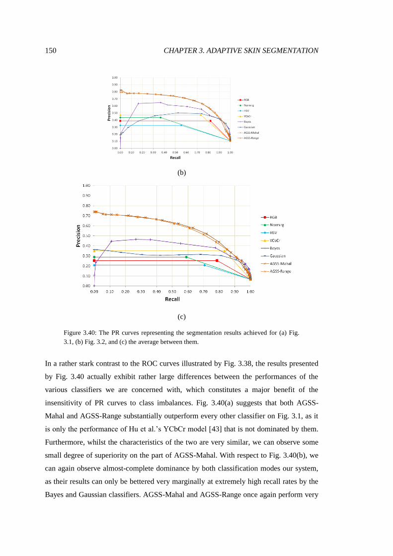
150 CHAPTER 3. ADAPTIVE SKIN SEGMENTATION
(b)
(c)
Figure 3.40: The PR curves representing the segmentation results achieved for (a) Fig.
3.1, (b) Fig. 3.2, and (c) the average between them.
In a rather stark contrast to the ROC curves illustrated by Fig. 3.38, the results presented
by Fig. 3.40 actually exhibit rather large differences between the performances of the
various classifiers we are concerned with, which constitutes a major benefit of the
insensitivity of PR curves to class imbalances. Fig. 3.40(a) suggests that both AGSS-
Mahal and AGSS-Range substantially outperform every other classifier on Fig. 3.1, as it
is only the performance of Hu et al.’s YCbCr model [43] that is not dominated by them.
Furthermore, whilst the characteristics of the two are very similar, we can observe some
small degree of superiority on the part of AGSS-Mahal. With respect to Fig. 3.40(b), we
can again observe almost-complete dominance by both classification modes our system,
as their results can only be bettered very marginally at extremely high recall rates by the
Bayes and Gaussian classifiers. AGSS-Mahal and AGSS-Range once again perform very
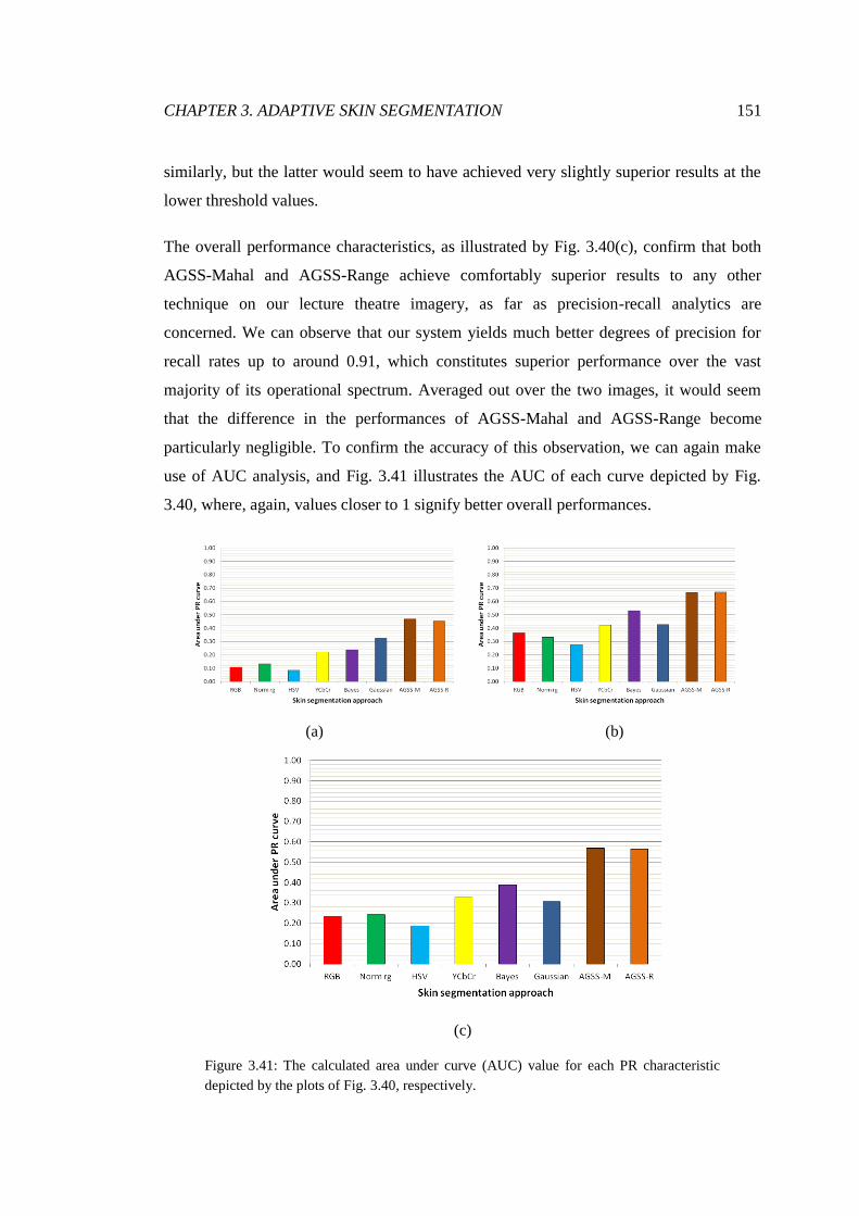
CHAPTER 3. ADAPTIVE SKIN SEGMENTATION 151
similarly, but the latter would seem to have achieved very slightly superior results at the
lower threshold values.
The overall performance characteristics, as illustrated by Fig. 3.40(c), confirm that both
AGSS-Mahal and AGSS-Range achieve comfortably superior results to any other
technique on our lecture theatre imagery, as far as precision-recall analytics are
concerned. We can observe that our system yields much better degrees of precision for
recall rates up to around 0.91, which constitutes superior performance over the vast
majority of its operational spectrum. Averaged out over the two images, it would seem
that the difference in the performances of AGSS-Mahal and AGSS-Range become
particularly negligible. To confirm the accuracy of this observation, we can again make
use of AUC analysis, and Fig. 3.41 illustrates the AUC of each curve depicted by Fig.
3.40, where, again, values closer to 1 signify better overall performances.
(a) (b)
(c)
Figure 3.41: The calculated area under curve (AUC) value for each PR characteristic
depicted by the plots of Fig. 3.40, respectively.

152 CHAPTER 3. ADAPTIVE SKIN SEGMENTATION
We can note from the results illustrated by Fig. 3.41(a) that the performances of the
existing approaches on Fig. 3.1 are rather poor, and are decidedly outclassed by our
system, with only the Gaussian classifier coming close to offering stiff competition. Fig.
3.41(b) suggests that they perform significantly better on Fig. 3.2, with the Bayes
classifier in particular having achieved a marked improvement over its previous result.
Both AGSS-Mahal and AGSS-Range also yield improved results, however, maintaining
their comfortable performance superiority over the alternative techniques. The overall
results of our PR curve analysis for lecture theatre imagery, which are illustrated by Fig.
3.41(c), confirm the outstanding performances of our system, as the AUC both of its
classification modes have achieved are significantly better than those of the previous
approaches over the two images. Whilst there is little to discern between the
performances of AGSS-Mahal and AGSS-Range, it is, again, worth bearing in mind that
the results of AGSS-Range have been achieved with slightly superior efficiency.
3.3.1.4 Qualitative Analysis of Additional Images
As we outlined at the beginning of Section 3.3.1, an unfortunate consequence of the
complexity of our lecture theatre images is that the process of creating manual
annotations to define the presence of skin within them is extremely time-consuming. This
was the reason for our quantitative analysis concerning only a pair of images. We offset
that situation by selecting the most disparate and diverse images in our dataset to
evaluate, but we can reinforce our findings by presenting the qualitative analysis of
additional images. To that end, Fig. 3.42 illustrates the segmentation results our system
has achieved for a further four lecture theatre images. It should be remembered that
producing an actual segmentation using a continuous classification system involves the
definition of a probability threshold, which will yield a single discrete classifier. Just as
our results in Section 3.3.1.1 could not be used to provide complete performance
assessments, the segmentations depicted by Fig. 3.42 can offer only a sense of how
effective our system has the capacity to be.
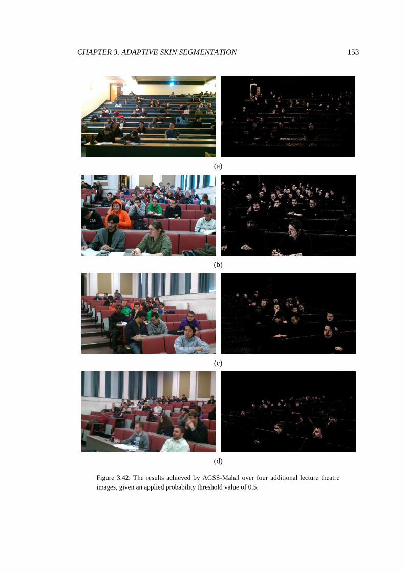
CHAPTER 3. ADAPTIVE SKIN SEGMENTATION 153
(a)
(b)
(c)
(d)
Figure 3.42: The results achieved by AGSS-Mahal over four additional lecture theatre
images, given an applied probability threshold value of 0.5.

154 CHAPTER 3. ADAPTIVE SKIN SEGMENTATION
From first inspection of Fig. 3.42, it would seem that the results we have achieved over
these new images are well in line with those we achieved during our quantitative
analysis. Generally, we see the classification of very few false positives, yielding
excellent levels of precision. The one arguable exception to this observation is depicted
by Fig. 3.42(a), in which a number of skin-coloured surfaces have been segmented to a
non-negligible degree, which is an unfortunate consequence of the particular
circumstances of that environment. Additionally, the illumination present within the
image is far from consistent, with certain regions exhibiting the influence of significantly
stronger incident lighting than other regions, which is problematic for both skin colour
modelling and subsequent segmentation.
Even though the input images of Fig. 3.42 represent a rather diverse range of
segmentation problems, it would be reasonable to suggest that our system has been very
effective at identifying the particular skin tones present within each one, allowing us to
consistently achieve what would appear to be fairly impressive recall rates. Combined
with the generally high levels of precision we have achieved, the overall accuracy of
these segmentations can be considered outstanding. These results, therefore, strongly
reinforce the main conclusion that we drew from our quantitative analysis: that the
adaptive skin segmentation system we have developed is highly effective at modelling
and classifying the skin within lecture theatre-based images, especially in comparison to
number of highly-regarded existing techniques.
3.3.2 Annotated Arbitrary Image Database
Although we have established that our system can comfortably outperform numerous
existing approaches when it comes to the segmentation of skin from lecture theatre
images, it is also well worth investigating how effective it can be where arbitrary images
are concerned. Although the poor performance of those existing techniques specifically
on lecture theatre imagery provided the impetus for us to build our system, its
developmental process has not involved any concession being made for that particular
type of input. Theoretically, therefore, we should also be able to achieve superior results
for any given arbitrary image of people.

CHAPTER 3. ADAPTIVE SKIN SEGMENTATION 155
Rather than construct our own dataset of arbitrary images to evaluate our system against
the existing approaches, we will be making use of the DB Skin annotated skin database
of Ruiz-del-Solar and Verschae [115]. This dataset consists of 103 images of varying
size, quality, environment, and subject, as well as a corresponding manual annotation for
each one. Given the diversity of the segmentation problems the set poses, it will represent
a very strong test of the general-purpose capabilities of the techniques we are interesting
in evaluating.
Our evaluation using the DB Skin dataset will be broken down into two individual
analyses, the first of which will be performed over all 103 images it consists of. A large
majority of the images within the dataset contain detectable faces, but there are a number
that do not, and some of those contain no skin whatsoever. In these latter cases, our
system will be incapable of constructing colour models, and will classify every pixel
within such images as “non-skin”. The results of our system, therefore, may not compare
favourably to those achieved by the existing approaches for the few images that contain
skin but no detectable faces. This shortcoming, however, will be somewhat offset by the
results we achieve for the images that contain no skin at all, as our system will be capable
of correctly identifying the absence of any people, whereas the alternative techniques will
continue to classify pixels without any regard for such higher-level information, and are
liable to produce numerous false positive classifications without the potential to yield a
single true positive.
It should be noted that our overall results will correctly account for these fringe cases, in
terms of their contributions to the average performance metrics. For instance, we will
consider the recall rates achieved for the images containing no skin to be “undefined”,
and simply calculate the average recall of a classifier over the number of images that do
actually contain skin. Similarly, if a classifier were to segment zero pixels from within an
image (which, in practice, should only apply to our own system given an image
containing no detectable faces), we will consider its achieved precision to also be
“undefined”, and eliminate it from further calculations. We will not be applying this rule
to circumstances where a classifier unfairly benefits from its undesirable results being
disregarded, however. For example, the recall rates that our system achieves on the
images that contain skin but no detectable faces will be recorded as 0, and will

156 CHAPTER 3. ADAPTIVE SKIN SEGMENTATION
contributed to its overall results, and the same principle will apply to the levels of
precision achieved by the existing approaches on images that contain no skin whatsoever.
Our second analysis using the DB Skin dataset will involve evaluating segmentation
performances over a 70-image subset. The images that constitute this subset are those
within the dataset that contain at least one detectable face, with the remaining 33
containing no visible faces at all, or being of low enough quality that the detection of the
faces that are visible within them becomes infeasible for the feature-based detector that
we have adopted for our approach. Although we are interested in determining how well
our system performs given any arbitrary image, we are also extremely keen to explore its
relative efficacy when we can control for the visibility of faces within input images. In
this way, we can emphasise how suitable our system may be for solving any problem
where the presence of detectable faces can be guaranteed. Of course, our lecture theatre
images served as practical examples of this suitability, but further demonstration will
allow give us a more comprehensive understanding about the capabilities of our
approach.
For both of these datasets, we will be using ROC analysis and PR analysis to evaluate
classifier performance. We will not, however, be providing any individual discrete
classification results to represent the continuous classifiers. Generating such results made
sense for the evaluation presented by Section 3.3.1.1, as we were operating with such a
small number of input images, but over a much larger and more diverse dataset, where
the segmentations of individual images cannot be taken as reliable indicators of overall
performance, doing so would be decidedly less useful. For the reasons we highlighted at
the beginning of Section 3.3, however, we believe that the quantitative results provided
by ROC and PR analysis will prove to be more than sufficient in allowing us draw
accurate conclusions.
3.3.2.1 Complete Dataset Evaluation
As we outlined, the first stage of our analysis using the DB Skin annotated database will
concern the results achieved over all 103 images it contains. The dataset is extremely
diverse, and should be extremely effective at highlighting the specific circumstances

CHAPTER 3. ADAPTIVE SKIN SEGMENTATION 157
under which the various approaches we will be evaluating excel, and those under which
they struggle. Many of the images contain faces, sometimes numerous but more often
single, a few contain skin but no detectable faces, and a small number contain no skin
whatsoever, and Fig. 3.43 exhibits examples of each of these types of images within the
dataset.
(a) (b)
(c) (d)
Figure 3.43: Samples of the images contained within the DB Skin dataset that contain (a)
multiple detectable faces, (b) individual people with detectable faces, (c) regions of skin
but no visible faces, and (d) no people whatsoever.
Even the few sample images we have provided in Fig. 3.43 strongly support our
suggestion that the DB Skin database consists of an extremely diverse set of images, and
should constitute a rather rigorous test of the segmentation capabilities of the approaches
we will be evaluating. As could be discerned, the images that contain numerous
detectable faces, such as those depicted by Fig. 3.43(a), are likely to be those for which
our system delivers its best results, as the more visible faces there are, the higher the
chances of at least one being found, allowing for a skin colour model to be built and skin
pixels to be segmented. Provided they are of high enough quality, our system should also
comfortably be able to segment the skin from images containing only individual faces,
such as those depicted by Fig. 3.43(b).

158 CHAPTER 3. ADAPTIVE SKIN SEGMENTATION
It is images similar to those within Fig. 3.43(c) that will prove to be most problematic for
our system, as the absence of any detectable faces will mean that we will be unable to
build any colour models, and, therefore, be incapable of segmenting any skin. In terms of
our evaluation, this issue is exacerbated by the fact that the absence of detectable faces
does, of course, not hinder the recall rates of any of the other approaches we are working
with, and they are likely to yield significantly better results for such images, boosting
their overall performance characteristics. Images such as those depicted by Fig. 3.43(d)
represent a stark contrast to that situation, as we would expect our system to successfully
identify the clear absence of any faces, thereby making zero positive classifications and
achieving perfect accuracy. Without regard for such information, however, the existing
techniques are liable to produce significant numbers of false positives, harming their
overall results in the process. The balance between these forms of images within the
dataset could, therefore, play a non-negligible role in determining the relative
performances of the classifiers we will be evaluating.
The first means by which we will be evaluating performance over all 103 images of the
DB Skin database is receiver operating characteristic analysis. Our methodology at
this stage will be identical to that applied during Section 3.3.1.2, which involved the
production of results for the continuous classifiers at various probability threshold values
over the [0,1] interval, which, in turn, can be used to form performance characteristics.
Additionally, we will be applying the same logic to the discrete classifiers as we did
previously, logically ascribing the (FPR,TPR) points (0,0) and (1,1) to their curves in
order to subsequently derive representative AUC values. It should be noted that whilst
the average prevalence of skin within the DB Skin dataset is much greater than the
average present within our lecture theatre images (0.156 as opposed to 0.065), there does
still exist a rather distinct imbalance between the skin pixel class and the non-skin pixel
class. This means that the reliability and usefulness issues we faced previously will still
be present during this analysis, although to a somewhat less extreme extent. The
performance characteristics we have produced for various segmentation techniques,
including our own, over the entire DB Skin dataset can be seen in Fig. 3.44.
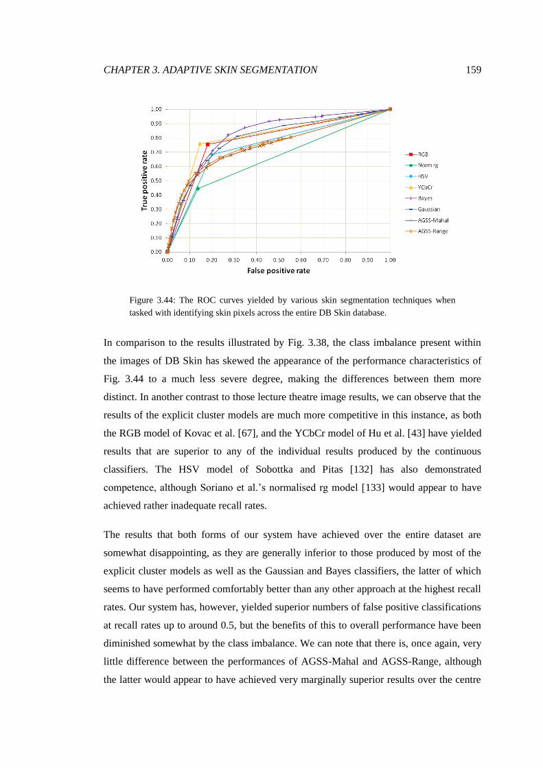
CHAPTER 3. ADAPTIVE SKIN SEGMENTATION 159
Figure 3.44: The ROC curves yielded by various skin segmentation techniques when
tasked with identifying skin pixels across the entire DB Skin database.
In comparison to the results illustrated by Fig. 3.38, the class imbalance present within
the images of DB Skin has skewed the appearance of the performance characteristics of
Fig. 3.44 to a much less severe degree, making the differences between them more
distinct. In another contrast to those lecture theatre image results, we can observe that the
results of the explicit cluster models are much more competitive in this instance, as both
the RGB model of Kovac et al. [67], and the YCbCr model of Hu et al. [43] have yielded
results that are superior to any of the individual results produced by the continuous
classifiers. The HSV model of Sobottka and Pitas [132] has also demonstrated
competence, although Soriano et al.’s normalised rg model [133] would appear to have
achieved rather inadequate recall rates.
The results that both forms of our system have achieved over the entire dataset are
somewhat disappointing, as they are generally inferior to those produced by most of the
explicit cluster models as well as the Gaussian and Bayes classifiers, the latter of which
seems to have performed comfortably better than any other approach at the highest recall
rates. Our system has, however, yielded superior numbers of false positive classifications
at recall rates up to around 0.5, but the benefits of this to overall performance have been
diminished somewhat by the class imbalance. We can note that there is, once again, very
little difference between the performances of AGSS-Mahal and AGSS-Range, although
the latter would appear to have achieved very marginally superior results over the centre

160 CHAPTER 3. ADAPTIVE SKIN SEGMENTATION
of its performance spectrum. In order to more effectively interpret the ROC curves
illustrated by Fig. 3.44, we have derived AUC values to represent them, which are
presented in Fig. 3.45.
Figure 3.45: The calculated area under curve (AUC) value for each of the ROC
characteristics illustrated by Fig. 3.44, which were achieved over the entire DB Skin
database. NB: The y-axis of this graph, which represents AUC, has been truncated to a
range of [0.5,1] in order to better emphasise the condensed differences between the
results(an aberration caused by class imbalance).
The results depicted by Fig. 3.45 confirm the observations we made about the ROC
curves that have been produced using all 103 images of the DB Skin dataset. We note
that the performances of our own system are decidedly mediocre in comparison to those
of several of the existing approaches, with the Bayes classifier in particular having
yielded clearly superior results. Whilst disappointing, however, the inferiority of our
system in this instance was not entirely unexpected, as we were not able to guarantee the
presence of faces throughout the entire set of images. Furthermore, for the reasons we
detailed at the outset of Section 3.3, the class imbalance present within the set has
negatively impacted the degree to which ROC-based results can be considered
representative of true capability.
Just as it did during our lecture theatre image evaluation, we expect that precision-recall
analysis will be able to provide us with highly useful information despite the presence of
a significant class imbalance within the set of images we are using. We will be
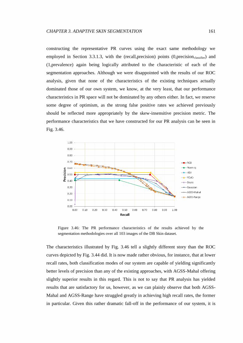
CHAPTER 3. ADAPTIVE SKIN SEGMENTATION 161
constructing the representative PR curves using the exact same methodology we
employed in Section 3.3.1.3, with the (recall,precision) points (0,precisionclassifier) and
(1,prevalence) again being logically attributed to the characteristic of each of the
segmentation approaches. Although we were disappointed with the results of our ROC
analysis, given that none of the characteristics of the existing techniques actually
dominated those of our own system, we know, at the very least, that our performance
characteristics in PR space will not be dominated by any others either. In fact, we reserve
some degree of optimism, as the strong false positive rates we achieved previously
should be reflected more appropriately by the skew-insensitive precision metric. The
performance characteristics that we have constructed for our PR analysis can be seen in
Fig. 3.46.
Figure 3.46: The PR performance characteristics of the results achieved by the
segmentation methodologies over all 103 images of the DB Skin dataset.
The characteristics illustrated by Fig. 3.46 tell a slightly different story than the ROC
curves depicted by Fig. 3.44 did. It is now made rather obvious, for instance, that at lower
recall rates, both classification modes of our system are capable of yielding significantly
better levels of precision than any of the existing approaches, with AGSS-Mahal offering
slightly superior results in this regard. This is not to say that PR analysis has yielded
results that are satisfactory for us, however, as we can plainly observe that both AGSS-
Mahal and AGSS-Range have struggled greatly in achieving high recall rates, the former
in particular. Given this rather dramatic fall-off in the performance of our system, it is
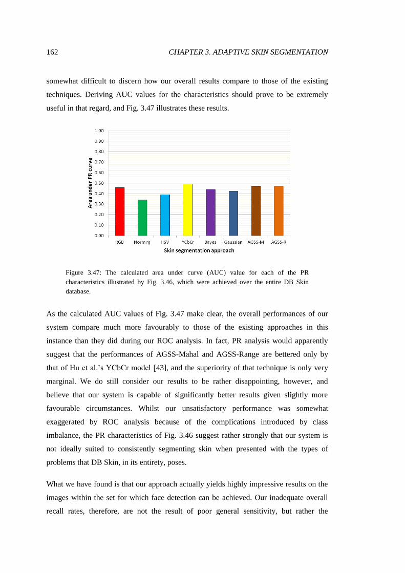
162 CHAPTER 3. ADAPTIVE SKIN SEGMENTATION
somewhat difficult to discern how our overall results compare to those of the existing
techniques. Deriving AUC values for the characteristics should prove to be extremely
useful in that regard, and Fig. 3.47 illustrates these results.
Figure 3.47: The calculated area under curve (AUC) value for each of the PR
characteristics illustrated by Fig. 3.46, which were achieved over the entire DB Skin
database.
As the calculated AUC values of Fig. 3.47 make clear, the overall performances of our
system compare much more favourably to those of the existing approaches in this
instance than they did during our ROC analysis. In fact, PR analysis would apparently
suggest that the performances of AGSS-Mahal and AGSS-Range are bettered only by
that of Hu et al.’s YCbCr model [43], and the superiority of that technique is only very
marginal. We do still consider our results to be rather disappointing, however, and
believe that our system is capable of significantly better results given slightly more
favourable circumstances. Whilst our unsatisfactory performance was somewhat
exaggerated by ROC analysis because of the complications introduced by class
imbalance, the PR characteristics of Fig. 3.46 suggest rather strongly that our system is
not ideally suited to consistently segmenting skin when presented with the types of
problems that DB Skin, in its entirety, poses.
What we have found is that our approach actually yields highly impressive results on the
images within the set for which face detection can be achieved. Our inadequate overall
recall rates, therefore, are not the result of poor general sensitivity, but rather the

CHAPTER 3. ADAPTIVE SKIN SEGMENTATION 163
consequence of a large number of successful segmentations being tarnished by a small
number of instances in which the absence of a detectable face has rendered our system
unable to segment any skin at all. Similarly, the lacklustre degrees of precision achieved
by the existing approaches can be partially attributed to the small number of images
within the DB Skin dataset that contain no skin whatsoever, for which multitudes of false
positive classifications will have been made for no true positives, resulting in zero
precision. It would seem, therefore, that the diversity present across all 103 images of DB
Skin has exposed the weaknesses of every segmentation approach we have investigated,
not only our own.
3.3.2.2 Detection-Facilitating Image Evaluation
Having established that our system will yield overall results that are comparable to those
of the existing techniques when tasked with segmenting skin from an extremely diverse
set of arbitrary input images, we are now interested in determining how well it will
perform when the presence of detectable faces within the input images is controlled. Of
course, it was when face detection yielded no results that our system failed to segment
skin during our previous analysis, so we would expect to see noticeable improvements to
overall performance given exclusively images that facilitate the detection of faces.
This analysis does not simply represent a concerted or contrived effort to generate
favourable results for our system, however, as there are numerous real-world
circumstances under which the presence of detectable faces can be naturally assumed
(such was the case with our lecture theatre images, for instance). It is necessary for us to
understand how our system performs given a broad range of such inputs, so that we can
ascertain just how suitable our approach would be for providing solutions to certain
problems, and determine how widely applicable it could truly be.
In order to establish an appropriate set of images for this analysis, we must discard those
from the DB Skin dataset that do not pose the type of problems we are interested in
solving at this time. This means that the subset of images we will be performing our
evaluation with will not include any inputs that contain no skin at all, and none that do
contain some skin but no visible faces, which rules out the types of images represented
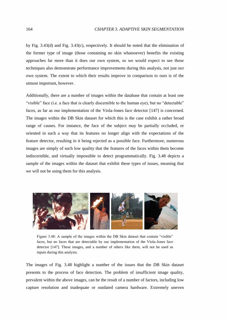
164 CHAPTER 3. ADAPTIVE SKIN SEGMENTATION
by Fig. 3.43(d) and Fig. 3.43(c), respectively. It should be noted that the elimination of
the former type of image (those containing no skin whatsoever) benefits the existing
approaches far more than it does our own system, so we would expect to see those
techniques also demonstrate performance improvements during this analysis, not just our
own system. The extent to which their results improve in comparison to ours is of the
utmost important, however.
Additionally, there are a number of images within the database that contain at least one
“visible” face (i.e. a face that is clearly discernible to the human eye), but no “detectable”
faces, as far as our implementation of the Viola-Jones face detector [147] is concerned.
The images within the DB Skin dataset for which this is the case exhibit a rather broad
range of causes. For instance, the face of the subject may be partially occluded, or
oriented in such a way that its features no longer align with the expectations of the
feature detector, resulting in it being rejected as a possible face. Furthermore, numerous
images are simply of such low quality that the features of the faces within them become
indiscernible, and virtually impossible to detect programmatically. Fig. 3.48 depicts a
sample of the images within the dataset that exhibit these types of issues, meaning that
we will not be using them for this analysis.
Figure 3.48: A sample of the images within the DB Skin dataset that contain “visible”
faces, but no faces that are detectable by our implementation of the Viola-Jones face
detector [147]. These images, and a number of others like them, will not be used as
inputs during this analysis.
The images of Fig. 3.48 highlight a number of the issues that the DB Skin dataset
presents to the process of face detection. The problem of insufficient image quality,
prevalent within the above images, can be the result of a number of factors, including low
capture resolution and inadequate or outdated camera hardware. Extremely uneven
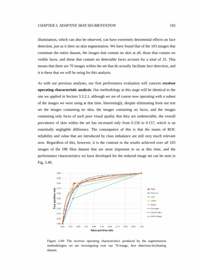
CHAPTER 3. ADAPTIVE SKIN SEGMENTATION 165
illumination, which can also be observed, can have extremely detrimental effects on face
detection, just as it does on skin segmentation. We have found that of the 103 images that
constitute the entire dataset, the images that contain no skin at all, those that contain no
visible faces, and those that contain no detectable faces account for a total of 33. This
means that there are 70 images within the set that do actually facilitate face detection, and
it is these that we will be using for this analysis.
As with our previous analyses, our first performance evaluation will concern receiver
operating characteristic analysis. Our methodology at this stage will be identical to the
one we applied in Section 3.3.2.1, although we are of course now operating with a subset
of the images we were using at that time. Interestingly, despite eliminating from our test
set the images containing no skin, the images containing no faces, and the images
containing only faces of such poor visual quality that they are undetectable, the overall
prevalence of skin within the set has increased only from 0.156 to 0.157, which is an
essentially negligible difference. The consequence of this is that the issues of ROC
reliability and value that are introduced by class imbalance are still very much relevant
now. Regardless of this, however, it is the contrast to the results achieved over all 103
images of the DB Skin dataset that are most important to us at this time, and the
performance characteristics we have developed for the reduced image set can be seen in
Fig. 3.49.
Figure 3.49: The receiver operating characteristics produced by the segmentation
methodologies we are investigating over our 70-image, face detection-facilitating
dataset.
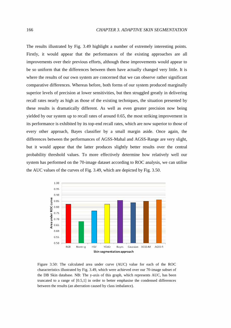
166 CHAPTER 3. ADAPTIVE SKIN SEGMENTATION
The results illustrated by Fig. 3.49 highlight a number of extremely interesting points.
Firstly, it would appear that the performances of the existing approaches are all
improvements over their previous efforts, although these improvements would appear to
be so uniform that the differences between them have actually changed very little. It is
where the results of our own system are concerned that we can observe rather significant
comparative differences. Whereas before, both forms of our system produced marginally
superior levels of precision at lower sensitivities, but then struggled greatly in delivering
recall rates nearly as high as those of the existing techniques, the situation presented by
these results is dramatically different. As well as even greater precision now being
yielded by our system up to recall rates of around 0.65, the most striking improvement in
its performance is exhibited by its top-end recall rates, which are now superior to those of
every other approach, Bayes classifier by a small margin aside. Once again, the
differences between the performances of AGSS-Mahal and AGSS-Range are very slight,
but it would appear that the latter produces slightly better results over the central
probability threshold values. To more effectively determine how relatively well our
system has performed on the 70-image dataset according to ROC analysis, we can utilise
the AUC values of the curves of Fig. 3.49, which are depicted by Fig. 3.50.
Figure 3.50: The calculated area under curve (AUC) value for each of the ROC
characteristics illustrated by Fig. 3.49, which were achieved over our 70-image subset of
the DB Skin database. NB: The y-axis of this graph, which represents AUC, has been
truncated to a range of [0.5,1] in order to better emphasise the condensed differences
between the results (an aberration caused by class imbalance).

CHAPTER 3. ADAPTIVE SKIN SEGMENTATION 167
The AUC values illustrated by Fig. 3.50 confirm many of our observations of Fig. 3.49.
Firstly, we can note that the distribution of the performances of the existing approaches is
virtually unchanged, as they have all yielded slight, but noticeable, improvements over
their performances for the 103-image dataset. It is the improved results of our system that
are made the most apparent by the AUC values, however. Previously, the overall
performances of AGSS-Mahal and AGSS-Range, according to ROC analysis, were
roughly on par with that of the HSV model of Sobottka and Pitas [132], and inferior to
those of a number of other techniques. However, Fig. 3.50 suggests that AGSS-Range is
actually the pre-eminent performer where images containing detectable faces are
concerned, with the results of AGSS-Mahal only being very slightly worse overall,
although also marginally inferior to those of the Bayes classifier. Whilst encouraging, it
should be remembered that these results may not fully represent the reality of the
situation, as the class imbalance within the input images will have skewed the
performance characteristics to some non-negligible degree.
Once again, to overcome the issues that class imbalance can pose, we will be making use
of precision-recall analysis, and the methodology we will be employing to do so will be
identical that which we used in Section 3.3.2.1. During our evaluation with the entire DB
Skin dataset, we observed that PR analysis gave a much more favourable assessment of
the performance of our system than ROC analysis did, due largely to the specific nature
of its results, which were characterised by the generally successful avoidance of false
positive classifications. We would, therefore, expect to see PR analysis yielding an
extremely positive assessment of our system in this instance as well, and the
characteristics that constitute this analysis can be seen in Fig. 3.51.
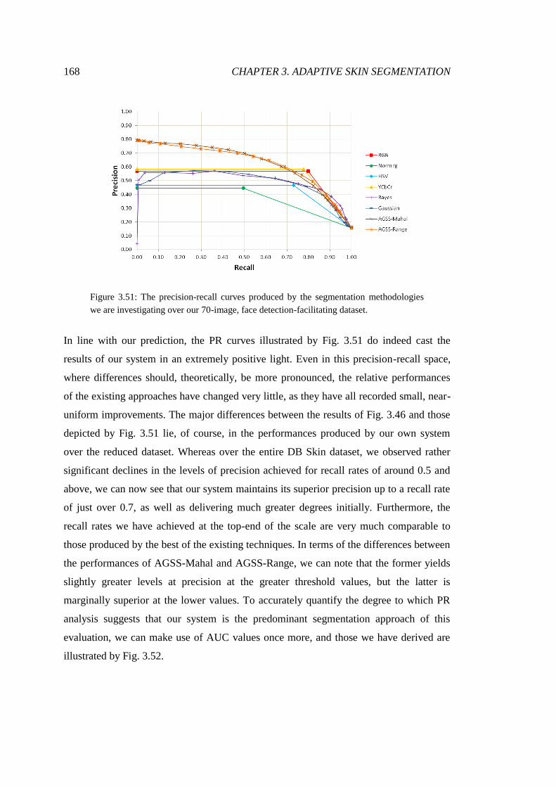
168 CHAPTER 3. ADAPTIVE SKIN SEGMENTATION
Figure 3.51: The precision-recall curves produced by the segmentation methodologies
we are investigating over our 70-image, face detection-facilitating dataset.
In line with our prediction, the PR curves illustrated by Fig. 3.51 do indeed cast the
results of our system in an extremely positive light. Even in this precision-recall space,
where differences should, theoretically, be more pronounced, the relative performances
of the existing approaches have changed very little, as they have all recorded small, near-
uniform improvements. The major differences between the results of Fig. 3.46 and those
depicted by Fig. 3.51 lie, of course, in the performances produced by our own system
over the reduced dataset. Whereas over the entire DB Skin dataset, we observed rather
significant declines in the levels of precision achieved for recall rates of around 0.5 and
above, we can now see that our system maintains its superior precision up to a recall rate
of just over 0.7, as well as delivering much greater degrees initially. Furthermore, the
recall rates we have achieved at the top-end of the scale are very much comparable to
those produced by the best of the existing techniques. In terms of the differences between
the performances of AGSS-Mahal and AGSS-Range, we can note that the former yields
slightly greater levels at precision at the greater threshold values, but the latter is
marginally superior at the lower values. To accurately quantify the degree to which PR
analysis suggests that our system is the predominant segmentation approach of this
evaluation, we can make use of AUC values once more, and those we have derived are
illustrated by Fig. 3.52.
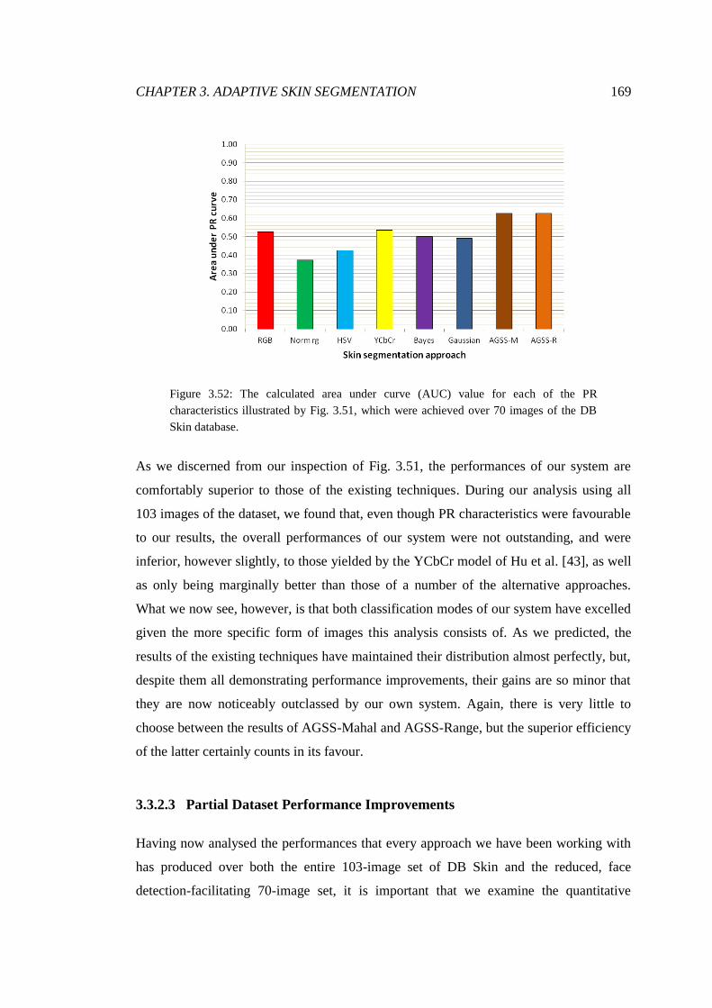
CHAPTER 3. ADAPTIVE SKIN SEGMENTATION 169
Figure 3.52: The calculated area under curve (AUC) value for each of the PR
characteristics illustrated by Fig. 3.51, which were achieved over 70 images of the DB
Skin database.
As we discerned from our inspection of Fig. 3.51, the performances of our system are
comfortably superior to those of the existing techniques. During our analysis using all
103 images of the dataset, we found that, even though PR characteristics were favourable
to our results, the overall performances of our system were not outstanding, and were
inferior, however slightly, to those yielded by the YCbCr model of Hu et al. [43], as well
as only being marginally better than those of a number of the alternative approaches.
What we now see, however, is that both classification modes of our system have excelled
given the more specific form of images this analysis consists of. As we predicted, the
results of the existing techniques have maintained their distribution almost perfectly, but,
despite them all demonstrating performance improvements, their gains are so minor that
they are now noticeably outclassed by our own system. Again, there is very little to
choose between the results of AGSS-Mahal and AGSS-Range, but the superior efficiency
of the latter certainly counts in its favour.
3.3.2.3 Partial Dataset Performance Improvements
Having now analysed the performances that every approach we have been working with
has produced over both the entire 103-image set of DB Skin and the reduced, face
detection-facilitating 70-image set, it is important that we examine the quantitative
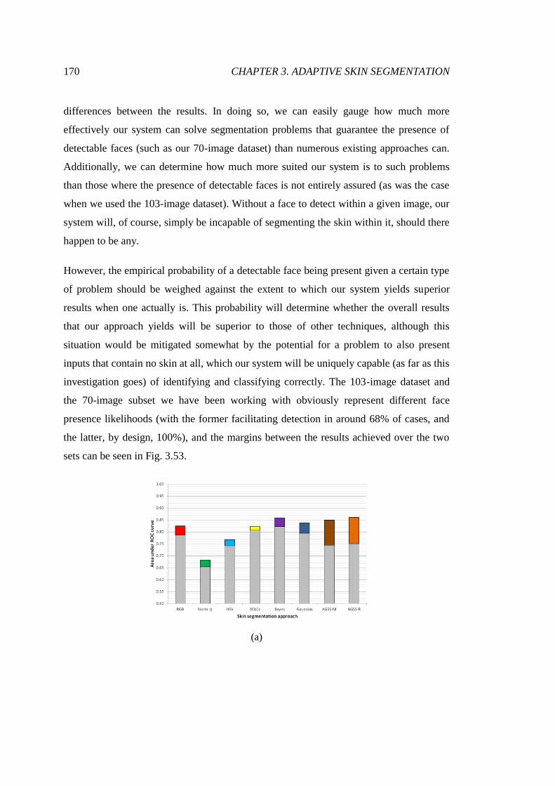
170 CHAPTER 3. ADAPTIVE SKIN SEGMENTATION
differences between the results. In doing so, we can easily gauge how much more
effectively our system can solve segmentation problems that guarantee the presence of
detectable faces (such as our 70-image dataset) than numerous existing approaches can.
Additionally, we can determine how much more suited our system is to such problems
than those where the presence of detectable faces is not entirely assured (as was the case
when we used the 103-image dataset). Without a face to detect within a given image, our
system will, of course, simply be incapable of segmenting the skin within it, should there
happen to be any.
However, the empirical probability of a detectable face being present given a certain type
of problem should be weighed against the extent to which our system yields superior
results when one actually is. This probability will determine whether the overall results
that our approach yields will be superior to those of other techniques, although this
situation would be mitigated somewhat by the potential for a problem to also present
inputs that contain no skin at all, which our system will be uniquely capable (as far as this
investigation goes) of identifying and classifying correctly. The 103-image dataset and
the 70-image subset we have been working with obviously represent different face
presence likelihoods (with the former facilitating detection in around 68% of cases, and
the latter, by design, 100%), and the margins between the results achieved over the two
sets can be seen in Fig. 3.53.
(a)
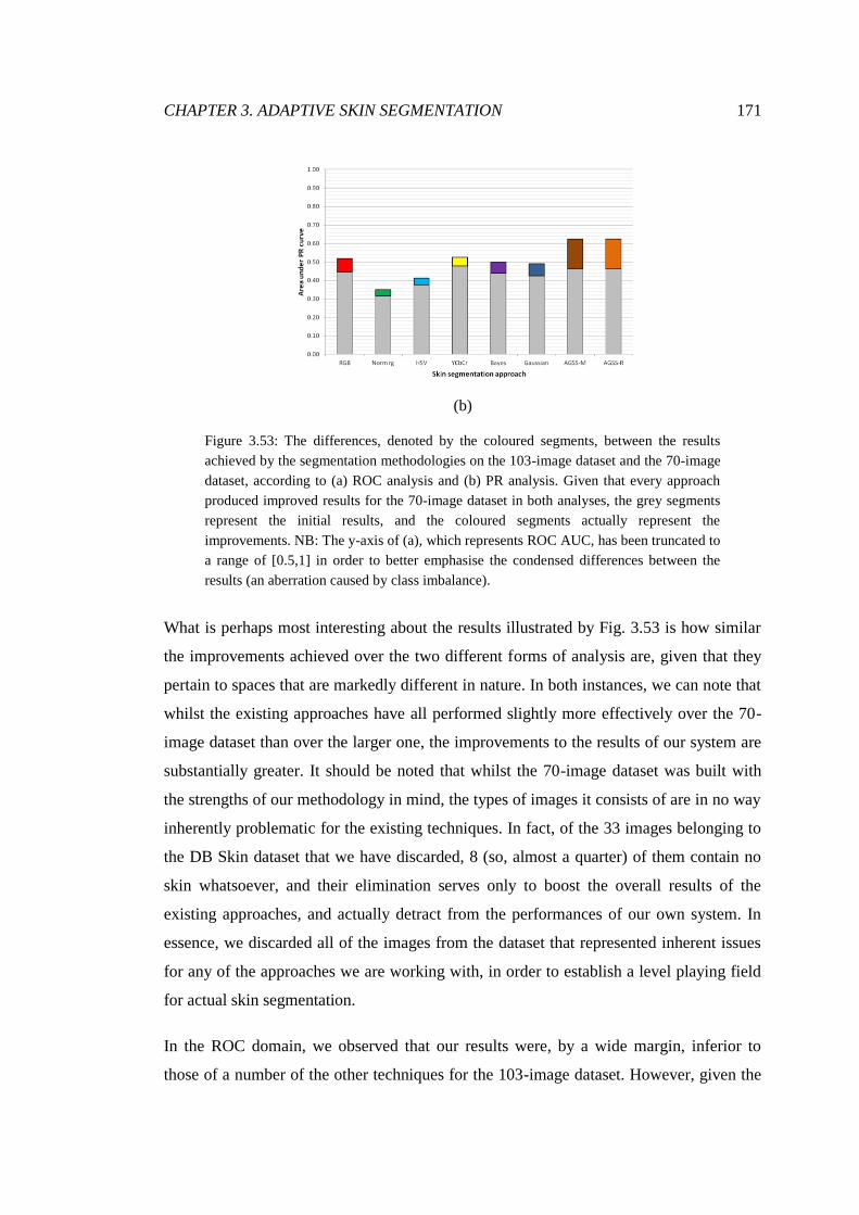
CHAPTER 3. ADAPTIVE SKIN SEGMENTATION 171
(b)
Figure 3.53: The differences, denoted by the coloured segments, between the results
achieved by the segmentation methodologies on the 103-image dataset and the 70-image
dataset, according to (a) ROC analysis and (b) PR analysis. Given that every approach
produced improved results for the 70-image dataset in both analyses, the grey segments
represent the initial results, and the coloured segments actually represent the
improvements. NB: The y-axis of (a), which represents ROC AUC, has been truncated to
a range of [0.5,1] in order to better emphasise the condensed differences between the
results (an aberration caused by class imbalance).
What is perhaps most interesting about the results illustrated by Fig. 3.53 is how similar
the improvements achieved over the two different forms of analysis are, given that they
pertain to spaces that are markedly different in nature. In both instances, we can note that
whilst the existing approaches have all performed slightly more effectively over the 70-
image dataset than over the larger one, the improvements to the results of our system are
substantially greater. It should be noted that whilst the 70-image dataset was built with
the strengths of our methodology in mind, the types of images it consists of are in no way
inherently problematic for the existing techniques. In fact, of the 33 images belonging to
the DB Skin dataset that we have discarded, 8 (so, almost a quarter) of them contain no
skin whatsoever, and their elimination serves only to boost the overall results of the
existing approaches, and actually detract from the performances of our own system. In
essence, we discarded all of the images from the dataset that represented inherent issues
for any of the approaches we are working with, in order to establish a level playing field
for actual skin segmentation.
In the ROC domain, we observed that our results were, by a wide margin, inferior to
those of a number of the other techniques for the 103-image dataset. However, given the

172 CHAPTER 3. ADAPTIVE SKIN SEGMENTATION
consistent presence of detectable faces within the inputs of the 70-image dataset, ROC
analysis, despite still being rather heavily skewed against us due to the nature of our
results and the class imbalance present, now deems our system to be essentially on par
with the best of the existing approaches. Given the existence of that prevailing class
imbalance, however, it would be remiss of us to place too much value in these results, or
draw conclusions from them exclusively.
Despite the strong similarity of the improvements gained over ROC and PR analysis, the
final situations that they present are slightly different. During our initial 103-image
evaluation, although the PR characteristics of our system were decidedly different in
nature to those of the other segmentation methodologies (as we generally yielded greater
precisions, but lower recall rates), the overall AUC values we achieved were very much
comparable to that of the best of the alternatives. As far as PR analysis is concerned then,
the result of our improvements over the 70-image dataset being much greater than those
of the existing approaches is that our system can be considered comfortably superior to
any of them given the assured presence of detectable faces. Given the highlighted issues
of pixel class imbalance, it is the results of our PR analysis that we attribute higher value
to, making its favourable assessment of our system all the more encouraging.
3.3.3 Adaptive Methodology Comparison
As well as comparing our system to established static segmentation approaches, it is
important to explore how well it performs against existing adaptive technology. In doing
so, we can go beyond demonstrating the benefits of adaptive methodologies as a whole,
and express the strengths of our system in particular. Towards this end, we will
experiment with one of the adaptive approaches we identified during our literature
review: the face detection-based system of Hsieh et al [41]. Although this approach is
similar to ours in some regards, there are a number of keys differences, and we hope to
discover the effects on overall performance of the divergent design decisions.
Whilst this analysis should allow for important insights to be made, a noteworthy caveat
is that we have had to write the implementation of the existing approach ourselves, as we
do not have access to the source code of the work. Therefore, although our recreation is

CHAPTER 3. ADAPTIVE SKIN SEGMENTATION 173
as accurate and as truthful as we can achieve given the description offered by the
published article, it should be noted that the results we present may not be entirely
representative of the full capabilities of the methodology. However, given our
understanding of the research, we do not expect any inaccuracy that exists in this regard
to be significant.
Given the structural similarity with our own methodology, we have used our system as a
basis for the implementation of the existing approach, and made a range of modifications,
which can be summarised thusly:
Face sample regions are defined by squares about detection centres that are
60% of the height and 60% of the width of the original detections.
Non-skin pixels are filtered out through the assumption of skin luminance
distribution symmetry, whereby a lower bound is defined by the deviation of
the brightest pixels from the given distribution mean.
Skin colour models consist of the means and standard deviations of the
normalised r, normalised g, and red distributions of filtered skin pixel sets.
Where segmentation is concerned, pixels are classified as skin if their colour
component values all fall within two standard deviations of their respective
model means.
As could be noted, these changes pertain to almost every major component of our
system, which should mean significant differences in the results achieved. The one
exception to this is the process of face detection. Although the work of Hsieh et al.
[41] also made use of the Viola-Jones detector, it was implemented primarily with
individual subjects in mind, for which the research we have conducted towards
determining an optimal detection sensitivity for reliable sampling purposes would be
of no concern. In order to give the existing approach the greatest potential to succeed
over our large-scale imagery, and to emphasise the specific effects of the differences
outlined above, we will be allowing it to benefit from that research and be providing
it with the exact detection results that our system produces.

174 CHAPTER 3. ADAPTIVE SKIN SEGMENTATION
The evaluation itself will be conducted over two datasets we have worked with
previously: the pair of lecture theatre images; and the set of face detection-facilitating
images within the DB Skin dataset. These datasets will be sufficient for demonstrating
that the strengths of our system extend beyond the simple fact that it is adaptive, and that
our detection sampling, model construction, and pixel classification methods are also
sound. Furthermore, for the sake of consistency, the evaluatory methodologies we will be
employing will be identical to those used previously.
3.3.3.1 Adaptive Lecture Theatre Imagery Analysis
We will firstly compare the performance of the existing adaptive approach to that of our
system with respect to our two lecture theatre images. It is the accuracy of results over
these inputs that we originally set out to improve upon, so it is important to fully establish
that our research has paid dividends in this regard. Just as in Section 3.3.1, our initial
evaluatory tool will be discrete classifier analysis, which should provide some
straightforward, if somewhat incomplete, insights. The outputs generated by the adaptive
approach of Hsieh et al. [41] are presented by Fig. 3.54.
(a) (b)
Figure 3.54: The outputs produced by the adaptive approach of Hsieh et al. [41] when
tasked with segmenting skin from (a) Fig. 3.1 and (b) Fig. 3.2.
As can be seen in Fig. 3.54, it would appear that the existing adaptive approach has
consistently segmented large portions of skin throughout both inputs, with lighter skin
tones being identified particularly effectively. The precision demonstrated by these
results would not seem to be as strong, however, as some considerable regions of false
positives have also been segmented, which is an especially large issue where the low skin
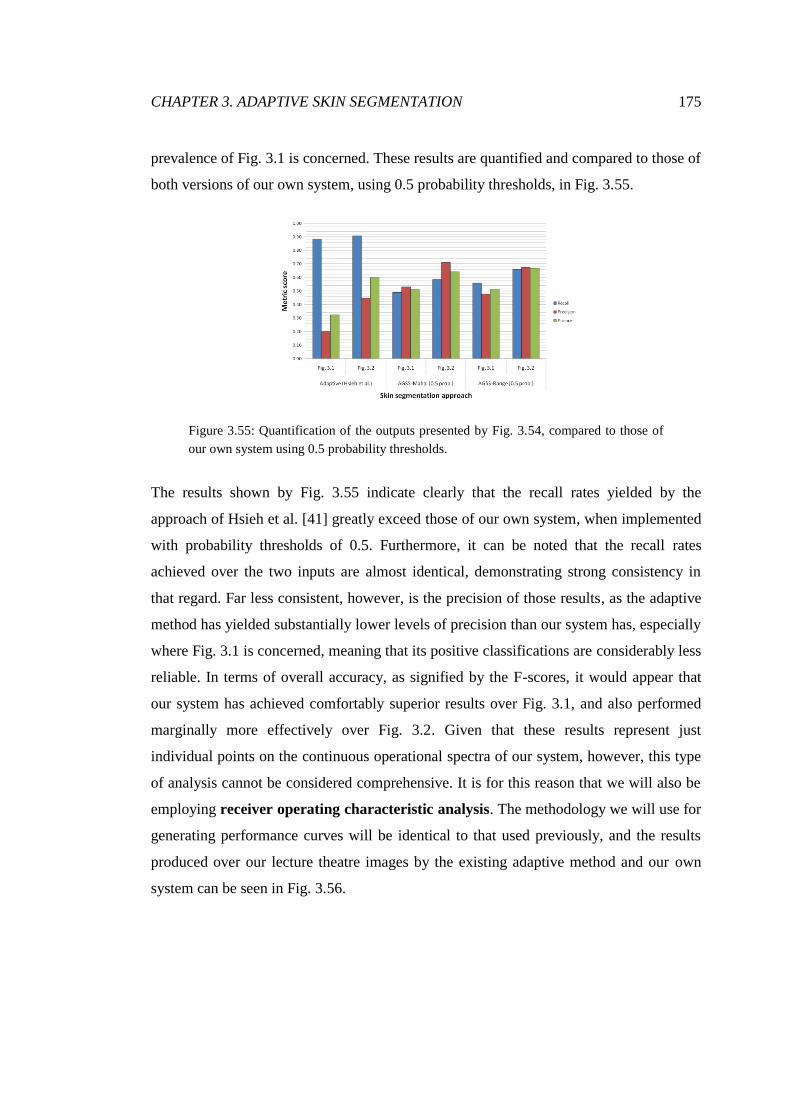
CHAPTER 3. ADAPTIVE SKIN SEGMENTATION 175
prevalence of Fig. 3.1 is concerned. These results are quantified and compared to those of
both versions of our own system, using 0.5 probability thresholds, in Fig. 3.55.
Figure 3.55: Quantification of the outputs presented by Fig. 3.54, compared to those of
our own system using 0.5 probability thresholds.
The results shown by Fig. 3.55 indicate clearly that the recall rates yielded by the
approach of Hsieh et al. [41] greatly exceed those of our own system, when implemented
with probability thresholds of 0.5. Furthermore, it can be noted that the recall rates
achieved over the two inputs are almost identical, demonstrating strong consistency in
that regard. Far less consistent, however, is the precision of those results, as the adaptive
method has yielded substantially lower levels of precision than our system has, especially
where Fig. 3.1 is concerned, meaning that its positive classifications are considerably less
reliable. In terms of overall accuracy, as signified by the F-scores, it would appear that
our system has achieved comfortably superior results over Fig. 3.1, and also performed
marginally more effectively over Fig. 3.2. Given that these results represent just
individual points on the continuous operational spectra of our system, however, this type
of analysis cannot be considered comprehensive. It is for this reason that we will also be
employing receiver operating characteristic analysis. The methodology we will use for
generating performance curves will be identical to that used previously, and the results
produced over our lecture theatre images by the existing adaptive method and our own
system can be seen in Fig. 3.56.
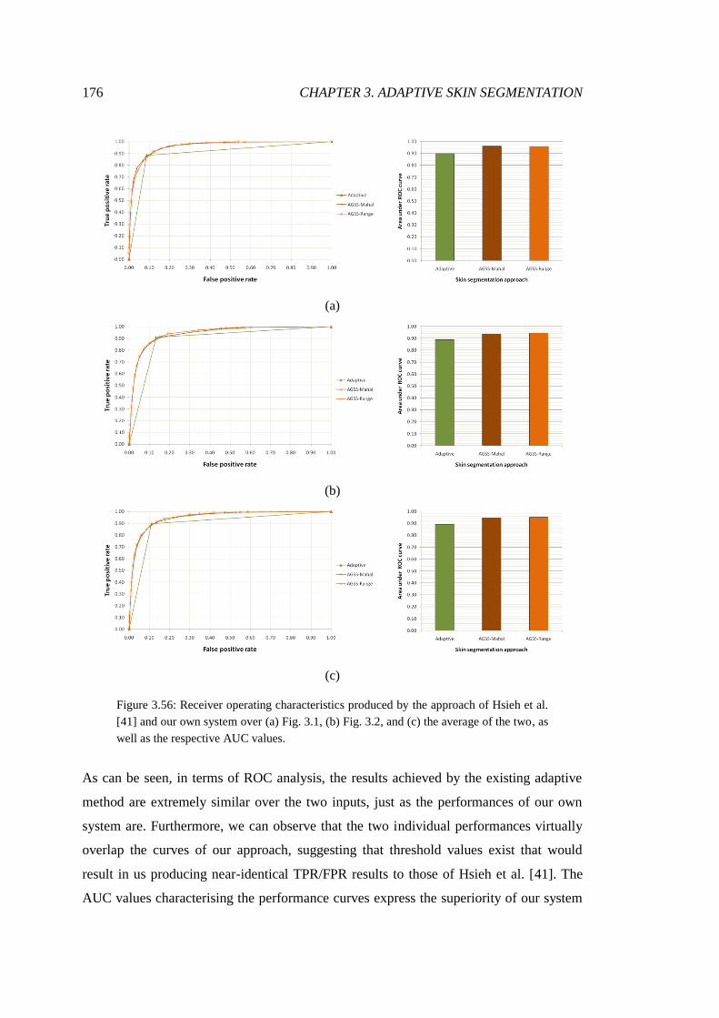
176 CHAPTER 3. ADAPTIVE SKIN SEGMENTATION
(a)
(b)
(c)
Figure 3.56: Receiver operating characteristics produced by the approach of Hsieh et al.
[41] and our own system over (a) Fig. 3.1, (b) Fig. 3.2, and (c) the average of the two, as
well as the respective AUC values.
As can be seen, in terms of ROC analysis, the results achieved by the existing adaptive
method are extremely similar over the two inputs, just as the performances of our own
system are. Furthermore, we can observe that the two individual performances virtually
overlap the curves of our approach, suggesting that threshold values exist that would
result in us producing near-identical TPR/FPR results to those of Hsieh et al. [41]. The
AUC values characterising the performance curves express the superiority of our system
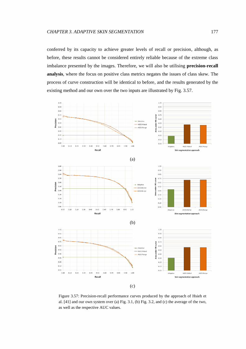
CHAPTER 3. ADAPTIVE SKIN SEGMENTATION 177
conferred by its capacity to achieve greater levels of recall or precision, although, as
before, these results cannot be considered entirely reliable because of the extreme class
imbalance presented by the images. Therefore, we will also be utilising precision-recall
analysis, where the focus on positive class metrics negates the issues of class skew. The
process of curve construction will be identical to before, and the results generated by the
existing method and our own over the two inputs are illustrated by Fig. 3.57.
(a)
(b)
(c)
Figure 3.57: Precision-recall performance curves produced by the approach of Hsieh et
al. [41] and our own system over (a) Fig. 3.1, (b) Fig. 3.2, and (c) the average of the two,
as well as the respective AUC values.

178 CHAPTER 3. ADAPTIVE SKIN SEGMENTATION
Although the results of Fig. 3.57 indicate significantly superior performances by all
approaches over Fig. 3.2 than over Fig. 3.1, we can note that, similarly to before, the
performances of the existing approach overlap the curves of our system almost perfectly,
again suggesting that we could yield very similar outputs, in terms of recall and
precision, given certain threshold values. However, as evidenced by the complete
performance curves, the capabilities of our system exceed those of the approach of Hsieh
et al. [41], as we can achieve greater recall rates and much higher levels of precision, if
configured to do so. The corresponding AUC values quantify this efficacy and flexibility,
as we can plainly note the overall superiority of our system given the lecture theatre
imagery, which indicates that the strengths of our approach are not limited to its capacity
to adapt to inputs.
3.3.3.2 Adaptive Arbitrary Imagery Analysis
As before, to fully assess classifier capabilities, it is important that we analyse the results
achieved over arbitrary images. Although we have already demonstrated that our system
can perform effectively given such images, by comparing the results we achieve to those
of the existing adaptive approach, we can show that there exists no overspecialisation that
was previously compensated for simply by the inherent benefits of adaptation. We will be
utilising the 70-image subset of the DB Skin database that allows for face detection, as
the approach of Hsieh et al. [41] and our own system would perform identically over the
excluded images, which would offer no useful information and serve only to obscure the
performance differences that do exist. Our first form of analysis will concern receiver
operating characteristics, and those produced by the existing approach and both
versions of our own system over the 70-image dataset, using the same methodology as
before, can be seen in Fig. 3.58.

CHAPTER 3. ADAPTIVE SKIN SEGMENTATION 179
Figure 3.58: The receiver operating characteristics produced by the adaptive approach of
Hsieh et al. [41] and our own system over the face detection-facilitating 70-image subset
of the DB Skin database.
Similarly to our analysis over the lecture theatre imagery, Fig. 3.58 indicates that the
performance of the existing adaptive method is near-identical to results that our system
will produce given certain threshold values. Again, when we take the entire performance
characteristics into account, this means that our approach has produced superior overall
results, which is reflected by its greater AUC values. Although the skin prevalence
presented by the set of arbitrary images is greater than that of the lecture theatre images
(0.157 as opposed to an average of 0.065), there still exists enough of a class imbalance
for ROC analysis to be rendered somewhat unreliable. Therefore, we will also be utilising
precision-recall analysis, and the results generated by the existing approach and our own
system over the set of 70 detection-facilitating images can be seen in Fig. 3.59.
Figure 3.59: The precision-recall performance curves produced by the adaptive approach
of Hsieh et al. [41] and our own system over the face detection-facilitating 70-image
subset of the DB Skin database.
Unlike previous results, Fig. 3.59 indicates that the performance of the existing approach
is actually slightly superior to the performances of our system in terms of both recall and

180 CHAPTER 3. ADAPTIVE SKIN SEGMENTATION
precision over a small range of likelihood threshold values. This is comfortably offset by
the remainders of the spectra, however, which demonstrate the capacity of our system to
generate results of either significantly greater recall or significantly greater precision. The
AUC values characterising overall performance express the superiority of both forms of
our system over the approach of Hsieh et al. [41] for the arbitrary image dataset, which
suggests strongly that there exists no overspecialisation in favour of the lecture theatre
imagery we have worked with.
3.3.4 Segmentation Efficiency Evaluation
As well as segmentation accuracy, another key factor in determining whether a classifier
is suitable for solving a certain problem is its efficiency, which considers the amount of
time (or computational energy) that the system expends in the process of generating an
output. How critical a factor this is in the selection process of an ideal solution to a
problem will depend upon the nature of the given task. It is paramount for the potential
applicability of the system we have developed to establish how efficiently it can operate
in comparison to a wide range of existing approaches. Rather than being a mere
afterthought in the pursuit of maximum segmentation accuracy, ensuring computational
efficiency has played a role throughout the development of our approach, and was been
fully considered during the making of decisions pertaining to face detection, pixel
filtering, model building, and pixel classification. This efficiency evaluation will consist
of two separate analyses, which represent two entirely different types of segmentation
problem.
3.3.4.1 Offline Performance Analysis
The first type of problem we will be analysing is “offline” segmentation. Such a task
would typically consist of a large set of images requiring segmentation, with the achieved
results not being yielded immediately after the processing of an image, perhaps instead
being collated with the results of every other image within the given set before being
yielded by the system. We have already presented a practical example of this form of
problem, as all of the quantitative results presented throughout Section 3.3.1 and Section
3.3.2 were generated in an offline fashion. Under typical circumstances, computational

CHAPTER 3. ADAPTIVE SKIN SEGMENTATION 181
efficiency is not overly critical where offline segmentation is concerned, but were the
efficiency of a system to be extremely low, then the parameters of a certain task could
dictate that that approach is not a suitable solution. A system that captures images during
the day and requires them to be processed overnight, for instance, may only consider a
solution adequate if it is efficient enough to guarantee results by the morning.
For this analysis, we will again be making use of the 70-image dataset that we initially
constructed for Section 3.3.2.2. In order to properly establish efficiency, it is extremely
important that we use inputs that we can guarantee will yield successful outputs. As an
example of why this is so critical, our own system would actually be capable of
processing a greater number of images within a given amount of time if they contained
no faces than if they did. In the former case, our system would perform face detection,
determine, rightly or wrongly, that the given image contains no skin, and then
immediately move onto the next image. In the latter case, however, our system would
build a colour model and attempt to segment skin before moving on, which would take a
non-zero amount of computational effort, no matter how small the image or how little
skin it contains. Furthermore, it was the performance of our system over this dataset that
demonstrated its true value, and we feel it would be pertinent to establish its relative
efficiency given a suitable application.
Our evaluation methodology is rather straightforward, as we will simply be measuring
the total amount of time it takes for the various segmentation approaches we are looking
at to process all 70 images of the dataset. Unlike evaluating the accuracy of
segmentations, measuring throughput times is rather non-deterministic, so we will be
repeating the trials numerous times in order to establish an accurate mean value for each
methodology. Furthermore, such an experiment will require the definition of single,
discrete classifiers for sets of segmentations to be generated, so we will be applying a
probability threshold of 0.5 to the four continuous approaches. The achieved results are
illustrated by Fig. 3.60. It should be noted that the value of the threshold will uniquely
affect the amount of time that AGSS-Mahal takes to process images, as lower thresholds
will mean broader ranges of colours necessitate Mahalanobis distance-based
classification, and vice-versa. Conversely, AGSS-Range will only ever establish whether
the colour of a pixel lies within the acceptable range defined for the given image using

182 CHAPTER 3. ADAPTIVE SKIN SEGMENTATION
four conditions, regardless of the boundaries of that range. Given that 0.5 represents the
centre of the [0,1] interval, however, we believe that the results AGSS-Mahal yields will
be strongly representative of its general performance.
Figure 3.60: The mean amount of time taken by each segmentation approach to fully
process our dataset of 70 varyingly sized arbitrary images using an Intel Core 2 Q9550
2.83GHz processer, where shorter throughput times indicate greater levels of efficiency.
As can be discerned from Fig. 3.60, the adaptive nature of our system detriments its
efficiency quite significantly. Despite numerous efforts being made to optimise the
algorithms that constitute our approach, it is clear to see that it still takes around three
times longer for our system to process the entire dataset than it does most of the existing
techniques. As we suggested, however, it would take an extreme degree of inefficiency
for a classifier to be rendered useless for an offline segmentation task such as this, and we
do not believe our results in this instance necessarily constitute extreme inefficiency,
although this would be at the discretion of any potential adopter, of course. What should
also be considered is that, in this scenario, although the results that our system has
achieved have been yielded much more slowly than those of other techniques, our results
are significantly more accurate.
Unlike our approach, the others essentially have flat rates for pixel classification,
meaning that the total throughput times they achieve are, in effect, proportional to the
total number of pixels they are tasked with classifying, as the exact same conditions are
applied to each and every one. This is also true for the Gaussian classifier, it just so

CHAPTER 3. ADAPTIVE SKIN SEGMENTATION 183
happens that its classification rules are so computationally expensive that it takes more
than four times as long as any of the other existing techniques to process the dataset.
Of course, as we discovered during our optimisation in Section 3.2.4, the large majority
of the time our system spends processing a given image is not actually spent on pixel
classification itself. For AGSS-Mahal, roughly two-thirds of the processing time of an
image is taken up by face detection, and this proportion is around three-quarters where
AGSS-Range is concerned. If we consider the results depicted by Fig. 3.60 in the context
of these time proportions, then we can deduce that both forms of our system, AGSS-
Range in particular, actually spend less time classifying pixels than any other approach.
The real problem that the 70-image dataset presents to the efficiency of our system,
therefore, is that it requires face detection to be performed for each individual image.
Whilst this is perfectly understandable, as the DB Skin dataset purposefully consists of an
extremely diverse set of images, it is perhaps not entirely representative of a real-world
problem. Images that have been captured by a stationary camera throughout the day, for
instance, are not likely to exhibit great illumination differences on an image-to-image
basis, although this may be dependent upon certain factors relating to the capture interval.
Given such a scenario, the skin colour model generated for one image through face
detection and pixel filtering may still be adequate for the next image, and then the next x
images after that, so the requirement for a specific model to be generated for each one
results only in unnecessary time expenditure. For every image that undergoes
segmentation without the need for a new skin colour model to be built, the efficiency of
our system will not only improve absolutely, but also relatively to any non-adaptive
method.
3.3.4.2 Real-Time Performance Analysis
The second form of problem that we will be analysing performance over is “real-time”
segmentation. Although the definition of “real-time” is likely to vary from application to
application, the results of real-time segmentation would typically be acted upon
immediately after they are generated, very often in the context of some form of feedback
loop, where future inputs may be influenced in some way by past outputs, making the
type of problem entirely unlike offline segmentation. Under regular circumstances,

184 CHAPTER 3. ADAPTIVE SKIN SEGMENTATION
efficiency is much more critical to real-time systems than it is to offline systems, as any
excessive amount of time being spent on the segmentation of skin from a frame will
result in a delay of feedback to the given user, which would be detrimental to their
experience as well as limiting to what could be achieved through use of the system in any
given period of time.
To carry out this analysis, we will be using image streams from a personal webcam,
which is being interacted with by a user, as the sample in Fig. 3.61 illustrates, which
represents a typical application for real-time skin segmentation, and a potential use-case
for our system. We will define a fixed number of frames to be processed by the various
segmentation methodologies, and measure the amount of time it takes for them to
complete the task in order to determine a mean operating frame rate for each (defined in
frames per second (fps)). Again, because of the non-deterministic nature of such an
experiment, we will be performing numerous trials in order to ensure the accuracy of our
results. Additionally, we will be defining discrete classifiers for the continuous systems
using a probability threshold of 0.5 once more.
Figure 3.61: A sample frame of the image streams we will be using to determine
segmentation methodology frame rates, which consist of a single user interacting with a
personal webcam.
This analysis will actually pertain to two separate image streams. Although we will
control for the content of them to ensure identicality, they will be of different resolutions.
As we have established, the existing approaches exhibit constant pixel classification
rates, so the amount of time it takes them to process an image will simply be a function of
the size of that image, but the performance of our system will also be influenced by the
nature of images, in terms of the presence of features and the prevalence of skin pixels,
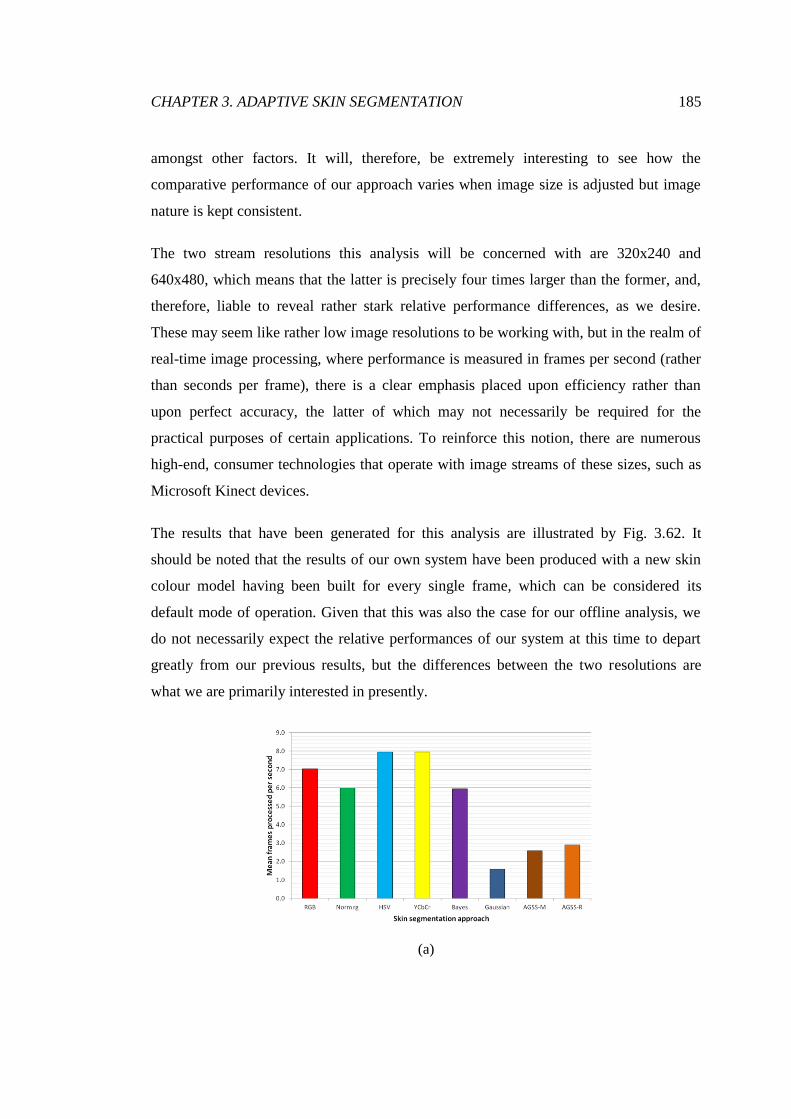
CHAPTER 3. ADAPTIVE SKIN SEGMENTATION 185
amongst other factors. It will, therefore, be extremely interesting to see how the
comparative performance of our approach varies when image size is adjusted but image
nature is kept consistent.
The two stream resolutions this analysis will be concerned with are 320x240 and
640x480, which means that the latter is precisely four times larger than the former, and,
therefore, liable to reveal rather stark relative performance differences, as we desire.
These may seem like rather low image resolutions to be working with, but in the realm of
real-time image processing, where performance is measured in frames per second (rather
than seconds per frame), there is a clear emphasis placed upon efficiency rather than
upon perfect accuracy, the latter of which may not necessarily be required for the
practical purposes of certain applications. To reinforce this notion, there are numerous
high-end, consumer technologies that operate with image streams of these sizes, such as
Microsoft Kinect devices.
The results that have been generated for this analysis are illustrated by Fig. 3.62. It
should be noted that the results of our own system have been produced with a new skin
colour model having been built for every single frame, which can be considered its
default mode of operation. Given that this was also the case for our offline analysis, we
do not necessarily expect the relative performances of our system at this time to depart
greatly from our previous results, but the differences between the two resolutions are
what we are primarily interested in presently.
(a)

186 CHAPTER 3. ADAPTIVE SKIN SEGMENTATION
(b)
Figure 3.62: The mean frame rate of each segmentation approach when tasked with
segmenting skin from an image stream at a resolution of (a) 320x240 and (b) 640x480,
again using an Intel Core 2 Q9550 2.83GHz processer.
There are numerous aspects of the results depicted by Fig. 3.62 that are of interest to us.
Firstly, in line with our expectations, the comparative performances of the existing
approaches have remained almost identical, not just across the two plots seen here, but
also in relation to the results illustrated by Fig. 3.60. This is a result of them all taking an
essentially fixed amount of time to classify any given pixel, as we suggested. Secondly,
in comparison to our offline segmentation analysis, the performance of our system over
the 320x240 image stream (depicted by Fig. 3.62(a)) is notably similar, with the majority
of the existing techniques again operating around three times more quickly than our own,
but this degree of inferiority was also to be somewhat expected.
It is the direct comparison of Fig. 3.62(a) and Fig. 3.62(b) that is the most revealing
aspect of these results, however. We can note that the performances of both AGSS-Mahal
and AGSS-Range are significantly more comparable to those of the existing approaches
where the 640x480 image stream is concerned, suggesting that the larger the given
image, the better the relative performance of our system. As we established during our
offline segmentation analysis, both of our pixel classification processes are actually
quicker than any of the others involved in this evaluation, but, overall, they were greatly
hampered by the necessity to initially perform face detection. What this means is that, in
theory, there will be an image size above which our system will operate more efficiently
than any other, even when face detection is performed for every individual frame.
However, the image resolution required to reach and exceed such a point would likely be

CHAPTER 3. ADAPTIVE SKIN SEGMENTATION 187
unnecessarily large for practical purposes, meaning excessive concessions being made to
frame rates.
3.3.4.3 Interval-Based Face Detection
Rather than image resolution alone, what we must really consider is the necessity for face
detection to actually be run for each and every frame of an image stream. If we take the
320x240 resolution stream, for instance, we note that even when we are performing face
detection for every input frame, we still achieve around 3fps. Given a real-world
scenario, such as that of a user interacting with a webcam, is the illumination of the given
environment likely to be changing at such a rate that a recalibration of the colour model
being used to segment skin is necessary three times every second? Intuitively, such a
requirement would actually appear to be entirely unnecessary. However, the prime
benefit of adaptive methods in general is in their capacity to automatically readjust given
variations in external factors, and continue to produce satisfactory outputs no matter the
circumstances, so abandoning the notion of face detection-based colour model calibration
entirely is out of the question. Between these two extremes, however, there will exist a
recalibration interval large enough to grant our system greater efficiency than any of the
existing approaches, and, given the results we have achieved thus far, we believe that this
interval would be considerably lower than the variations of a typical real-world scenario
would require.
In order to determine what this interval may be, we can experiment with a range of
different values to discover what the mean frame rate of our system would be over them.
Given the flat classification rates of the existing techniques, the curves that characterise
our system in (interval,frame rate) space will intersect them at certain points, the frame
rate coordinates of which will define the face detection intervals over which our system
will yield greater degrees of efficiency. Rather than measuring the interval in frames, we
will be defining it in seconds, as this will establish independence from the frame rate
metric and also more strongly relates to the circumstances of the given real-world
scenario. Additionally, an interval of zero seconds signifies that face detection will be
performed for every frame, mimicking the results depicted by Fig. 3.62. The results we

188 CHAPTER 3. ADAPTIVE SKIN SEGMENTATION
have generated for this experiment, using the same image streams as before, are
illustrated by Fig. 3.63.
(a)
(b)
Figure 3.63: The frame rates achieved by both forms of our system over a range of face
detection intervals against those of the existing approaches, for image streams at
resolutions of (a) 320x240 and (b) 640x480, again using an Intel Core 2 Q9550 2.83GHz
processer.
As can be discerned from Fig. 3.63, there do exist minimum intervals for both forms of
our system that will yield greater levels of efficiency than any other technique can offer
for both image streams. That both AGSS-Mahal and AGSS-Range are capable of offering

CHAPTER 3. ADAPTIVE SKIN SEGMENTATION 189
greater efficiency was not in any doubt, however, as we were already aware that our pixel
classification rates were superior, but these results do reveal that the value of the
minimum interval required to achieve such is somewhat dependent on the resolution of
the image stream in question. In the case of the 320x240 stream, the results for which are
illustrated by Fig. 3.63(a), we can note that AGSS-Range becomes the most efficient
method of segmentation with a face detection interval of just under a second, and
eventually reaches a frame rate almost twice as great as that of any other methodology.
AGSS-Mahal requires a significantly longer interval to achieve greater efficiency over
the existing approaches (around five seconds), and only marginally outperforms them
after that point. As far as AGSS-Mahal is specifically concerned, we previously made
note of the fact that its efficiency is uniquely variable on the value of the given applied
threshold, but, for similar reasons, it is also variable on the prevalence of skin within the
given input. The great similarity in the results of AGSS-Mahal and AGSS-Range
reported by Fig. 3.60 and Fig. 3.62 is largely the result of the burden of per-input face
detection, but with that mode of operation being abandoned, the previously subtle pixel
classification differences between the two have been made rather more apparent.
The 70-image dataset that we used to generate the results depicted by Fig. 3.60 had a
mean skin pixel prevalence of 0.157, but the prevalence within the image stream used for
this experiment is around double that value, as can be discerned from the inspection of
Fig. 3.61. In an average case, this would mean that the rate at which AGSS-Mahal
performs Mahalanobis distance-based classifications would roughly be doubled also,
resulting in greater differences between its performances and those of AGSS-Range,
which is the reason it has trailed so far behind in this experiment. This also means that,
tasked with segmenting skin from inputs exhibiting lower skin prevalences (or, lower
proportions of skin-like pixels in general), the efficiency of AGSS-Mahal would be closer
to that of AGSS-Range, assuming no lower of a probability threshold value. However,
were the prevalence of skin (or any skin-like pixels) within our input stream to be any
greater, the efficiency of AGSS-Mahal may actually become inferior to a number of the
existing approaches, although it should be noted that the prevalence of skin exhibited by
Fig. 3.61, given its nature, could be considered close to the practical limit of skin
prevalence within an image, assuming a real-world problem.

190 CHAPTER 3. ADAPTIVE SKIN SEGMENTATION
The results depicted by Fig. 3.63(b) are rather similar to those yielded for the smaller
resolution stream. AGSS-Range achieves superior efficiency at just over a second for the
640x480 stream, and goes on to far exceed the frame rates that any other approach is
capable of producing. AGSS-Mahal, on the other hand, despite eventually reaching a
point of efficiency very slightly greater than that of any of the existing approaches, takes
a significantly longer period of time to do so, although the differences between its
efficiency and that of Hu et al.’s YCbCr model [43] after an interval of around 10
seconds is practically negligible. Accounting for the error caused by the non-
deterministic nature of the experiment, it would seem that a four-fold increase in the size
of the image being used has approximately resulted in a two-fold increase to the face
detection interval required for each form of our system to achieve levels of efficiency that
are greater than those of the existing approaches.
Another interesting feature of both sets of the results depicted by Fig. 3.63 is the way in
which the levels of efficiency that AGSS-Mahal and AGSS-Range achieve eventually
plateau. As the face detection interval is increased, the proportional amount of time
expended by its execution becomes smaller and smaller, meaning that further reductions
in frequency deliver increasingly diminishing efficiency returns whilst further foregoing
the benefits of adaptive colour model calibration. So, whilst the interval between face
detection processes should not be arbitrarily maximised, it is perhaps advisable that it is
also not minimised simply to the point at which the frame rate of the given classification
mode of our system plateaus for the given input stream.
The reason for this is that face detection at any frequency will introduce some degree of
stutter, as the process will briefly interrupt the output stream in order to recalibrate the
skin colour model being used. Furthermore, the frame rates illustrated by Fig. 3.63 are
simply the mean rates achieved over the entire set of inputs, so do not reflect the
somewhat non-linear (with respect to real-time) fashion in which the frames have been
processed by our system. The lengths of these instances of stutter are not exorbitant
(given the proportion of time that our system spends on face detection when segmenting
skin from any individual image, we can ascertain that they would typically be equivalent
to around two frames for AGSS-Mahal and three frames for AGSS-Range, although the

CHAPTER 3. ADAPTIVE SKIN SEGMENTATION 191
same amount of real-time in both cases, of course), but could detriment the experience of
the user and, therefore, the value of the system, were they to be too frequent.
It is for these reasons that the ideal face detection interval for any given scenario should
simply be dictated by the requirements of that scenario, and the environment it relates to.
For any typical real-world problem, we would not expect the required colour model
recalibration frequency to be anywhere near great enough for the resulting stutter to be
problematic. Even an interval of a minute, for instance, would seem extremely short (as it
would not usually allow for a great deal of environmental change), but yet it would still
allow our system to operate at, essentially, its maximum average frame rate for the given
stream resolution, stuttering for only a couple of frames during any given minute.
Furthermore, defining the interval according to those requirements would also ensure that
the applied recalibration frequency is great enough for any environmental variations to be
adjusted for in a satisfactory timeframe. For any typical real-time segmentation problem,
therefore, our system will be capable of delivering a significantly more efficient
performance than any of the existing approaches can achieve, which, of course, is in
addition to its outputs being decidedly more accurate.

192
Chapter 4
Adaptive Framework for Enhanced
Large-Scale Face Detection
In this chapter, we will fully detail the design and development of our face detection
framework, and then present an evaluation that will explore both its efficacy and its
efficiency.
4.1 Framework Design and Development
As we discussed in Chapter 1, the main obstacle to the successful detection of faces
within large-scale imagery is feature indiscernibility, which can often render faces
undetectable unless positive classification thresholds are lowered and the results of
multiple detection systems are combined. However, identifying weak faces in such a way
will inevitably lead to significant numbers of false positive results, but we believe we can
overcome this issue by introducing adaptive detection classification processes that
consider additional modalities: size and colour. These filters will allow us precisely
eliminate non-face regions from sets of detections and output results that are superior to
those of the systems used initially. An overview of the framework we are proposing is
illustrated by Fig. 4.1.

CHAPTER 4. ENHANCED FACE DETECTION 193
Figure 4.1: An overview of the face detection framework we will be developing, which
uses the properties of size and colour to filter the collated detection results of existing
approaches in an attempt to greatly improve overall accuracies.
As can be seen, the system we are proposing consists of a number of distinct components.
In brief, our methodology will initially collate the detection results of existing face
detectors, and then derive a set of precise samples from the outputs of one of them. These
samples are then used to adaptively construct a size distribution model, which can be
used to discard detections of incongruous sizes. This will yield a set of detections that
consists primarily of duplicates, whereby a great number of them may be associated with
any given face. Therefore, we consolidate groups of detections to form face candidates,
which will have “scores” associated with them that correspond to the number of
detections consolidated in their formation. These scores represent general feature
discernibility, and we outrightly classify candidates with particularly large scores as
faces. Those with scores of just 1 are discarded on the basis that they likely pertain to
non-face regions, but those remaining will be classified according to colour-based
classification. This will involve using our adaptive skin colour modelling methodology to
determine a “skin rating” for each candidate, and those with ratings over a certain
threshold will also be positively classified, and those without will be eliminated. The
final output of our system, therefore, will consists of the union of the score-classified
faces and the colour-classified faces.
In order to visualise the operation of each component of our methodology, we will be
fully processing a sample input image over the course of its development, which will be
the same image we observed the Viola-Jones detector failing to achieve satisfactory
results over in Chapter 1. This input is depicted by Fig. 4.2.

194 CHAPTER 4. ENHANCED FACE DETECTION
Figure 4.2: A sample input image that depicts 44 people within a lecture theatre
environment and presents an archetypal large-scale face detection problem.
Given the complexity of the framework we have designed, there will be numerous
parameters that influence its performance. Due to the nature of a number of them, run-
time definition is entirely infeasible, and, as we hope to prove, somewhat unnecessary
regardless. We will, therefore, be calibrating them prior to the application of our
framework to actual problems. During development, we will be detailing this calibration
as it applies to a number of our processes, establishing sensible and meaningful metrics to
evaluate the performance of filters over broad ranges of possible values, ensuring that
they function optimally and do not limit the potential of our system. Of course, such
calibration requires sample inputs for performance data to be generated, and we will be
using a set of five lecture theatre images to calibrate our processes. Although these will
all pertain to a particular type of face detection problem, there is still great diversity
within the set, and we expect that they will reveal patterns that are consistent with those
exhibited by other types of imagery, which is a notion we intend to fully examine during
the evaluation of our work.
4.1.1 Face Detection Collation
Our process begins with the aforementioned collation of feature-based detections, which
involves performing face detection with any number of existing detection techniques. To
maximise the efficacy of our framework, as much information as possible should be
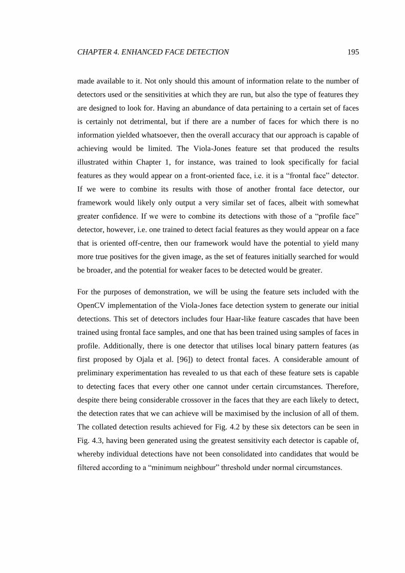
CHAPTER 4. ENHANCED FACE DETECTION 195
made available to it. Not only should this amount of information relate to the number of
detectors used or the sensitivities at which they are run, but also the type of features they
are designed to look for. Having an abundance of data pertaining to a certain set of faces
is certainly not detrimental, but if there are a number of faces for which there is no
information yielded whatsoever, then the overall accuracy that our approach is capable of
achieving would be limited. The Viola-Jones feature set that produced the results
illustrated within Chapter 1, for instance, was trained to look specifically for facial
features as they would appear on a front-oriented face, i.e. it is a “frontal face” detector.
If we were to combine its results with those of another frontal face detector, our
framework would likely only output a very similar set of faces, albeit with somewhat
greater confidence. If we were to combine its detections with those of a “profile face”
detector, however, i.e. one trained to detect facial features as they would appear on a face
that is oriented off-centre, then our framework would have the potential to yield many
more true positives for the given image, as the set of features initially searched for would
be broader, and the potential for weaker faces to be detected would be greater.
For the purposes of demonstration, we will be using the feature sets included with the
OpenCV implementation of the Viola-Jones face detection system to generate our initial
detections. This set of detectors includes four Haar-like feature cascades that have been
trained using frontal face samples, and one that has been trained using samples of faces in
profile. Additionally, there is one detector that utilises local binary pattern features (as
first proposed by Ojala et al. [96]) to detect frontal faces. A considerable amount of
preliminary experimentation has revealed to us that each of these feature sets is capable
to detecting faces that every other one cannot under certain circumstances. Therefore,
despite there being considerable crossover in the faces that they are each likely to detect,
the detection rates that we can achieve will be maximised by the inclusion of all of them.
The collated detection results achieved for Fig. 4.2 by these six detectors can be seen in
Fig. 4.3, having been generated using the greatest sensitivity each detector is capable of,
whereby individual detections have not been consolidated into candidates that would be
filtered according to a “minimum neighbour” threshold under normal circumstances.

196 CHAPTER 4. ENHANCED FACE DETECTION
Figure 4.3: The collated results achieved for Fig. 4.2 by the six face detection cascades
we are working with, operating with maximum sensitivity. There are a total of 3322
detections.
As Fig. 4.3 makes clear, the process of maximum-sensitivity detection collation will yield
huge amounts of noise, as there are false positives of a broad range of sizes scattered
throughout the image. This is of little concern to us, however, as almost every face
visible within the image has at least one detection associated with it, which means that
we have the potential to positively classify it. If our filters are effective at eliminating
false positives, therefore, such results being yielded by the detectors represents an ideal
scenario, as the potential for our approach to output highly accurate results is established.
What can also be noted from Fig. 4.3 is that there are numerous faces that would appear
to have multitudes of detections associated with them. This is entirely in line with our
expectations, as we would anticipate that strong faces would be found by multiple
detectors, and also for any one of the detectors we are using to return the same face
region multiple times, as we have disabled their capacity to filter and consolidate their
detections.
4.1.2 PCA-Based Size Filtering
The first method by which we will be filtering out detections will be classifying them
according to their size. As could be observed from Fig. 4.3, which represented a very
typical result for the type of input we are concerned with, there will be an abundance of

CHAPTER 4. ENHANCED FACE DETECTION 197
detections produced by any usual collation process that have sizes that are completely
incongruous with those of the detections around them and, assuming a reasonably
ordinary distribution of people, quite clearly not all of them can pertain to actual faces. It
is extremely important that this problem is solved in these relative terms, as considering
the solution to be as simple as discarding any detection larger than x or any detection
smaller than y would be completely dismissive of many crucial factors, such as the
distribution of the faces within the given image or the circumstances under which the
image has been captured, each of which is liable to dramatically impact the size that we
would expect any given detection to be were it to actually pertain to a face.
It is for these reasons that we will be generating size models adaptively, as the
distribution of face sizes within any given image will be extremely specific to that image.
In order to build models that can relate image coordinates to face sizes, however, we
require the means by which to sample these distributions. To acquire such samples, we
employ the same methodology that we used in the generation of skin colour models (as
described in Chapter 3), whereby highly precise feature-based face detection results are
considered to be a set of actual faces, from which we can ascertain certain pieces of
information to be used in the creation of representative models. It should be noted than
rather than performing feature-based face detection an additional time, we derive precise
face detections from the results of a single detector used for collation, which involves
detection neighbourhood thresholding and consolidation. The achieved results would be
identical using either technique, but deriving the information from our preexisting results,
and avoiding reprocessing the entire given image, is significantly more computationally
efficient. The set of precise face detections we have constructed for Fig. 4.2 is illustrated
by Fig. 4.4.

198 CHAPTER 4. ENHANCED FACE DETECTION
Figure 4.4: The precise face detection results derived for Fig. 4.2. There are a total of 18
detections, all of which are true positives, meaning 100% precision.
Although the results illustrated by Fig. 4.4 clearly represent only a small subset of all the
faces we ultimately wish to find within Fig. 4.2, the most important aspect of them for
our current intentions is that they are precise, and, in actuality, even the low detection rate
that has been achieved here still far exceeds what we would ever actually need in
practice. Given that we are confident that this sampling process will only very rarely
return false positive detections (as we demonstrated in Chapter 3), we can consider its
results to be representative of the faces present within the image and use them to derive a
size model to be applied to every detection initially collated. The pieces of data acquired
through this approach are the (x,y) coordinates of the centre of each detection and its size,
which is merely considered unidimensional as the detections we have collated using the
feature cascades provided by OpenCV are all square, so an array of (x,y,size) objects
constitute the output of our image sampling process, and the input of our size model
generation process.
4.1.2.1 Size Distribution Model Derivation
Although we have extremely reliable information from which to derive representative
size models, specifying the correct means of doing so is critical for success, as the
implementation of an inappropriate methodology would yield models that are decidedly
less effective than we require them to be. Deriving size distribution models from the sets
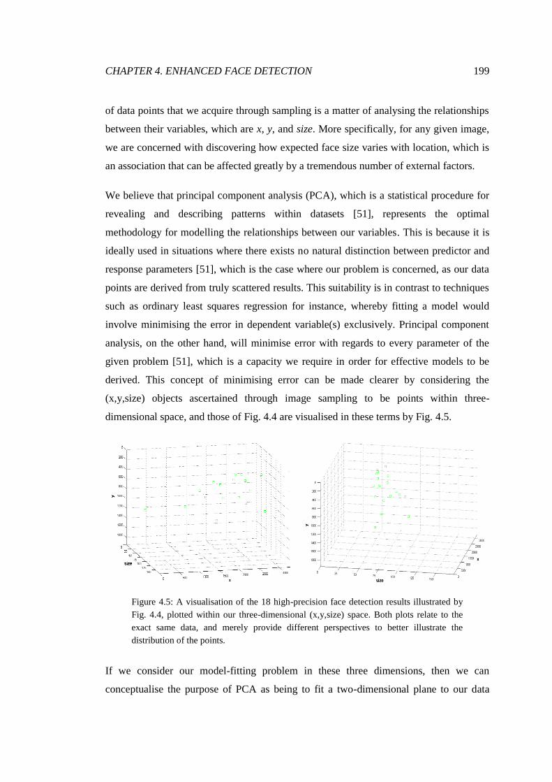
CHAPTER 4. ENHANCED FACE DETECTION 199
of data points that we acquire through sampling is a matter of analysing the relationships
between their variables, which are x, y, and size. More specifically, for any given image,
we are concerned with discovering how expected face size varies with location, which is
an association that can be affected greatly by a tremendous number of external factors.
We believe that principal component analysis (PCA), which is a statistical procedure for
revealing and describing patterns within datasets [51], represents the optimal
methodology for modelling the relationships between our variables. This is because it is
ideally used in situations where there exists no natural distinction between predictor and
response parameters [51], which is the case where our problem is concerned, as our data
points are derived from truly scattered results. This suitability is in contrast to techniques
such as ordinary least squares regression for instance, whereby fitting a model would
involve minimising the error in dependent variable(s) exclusively. Principal component
analysis, on the other hand, will minimise error with regards to every parameter of the
given problem [51], which is a capacity we require in order for effective models to be
derived. This concept of minimising error can be made clearer by considering the
(x,y,size) objects ascertained through image sampling to be points within three-
dimensional space, and those of Fig. 4.4 are visualised in these terms by Fig. 4.5.
Figure 4.5: A visualisation of the 18 high-precision face detection results illustrated by
Fig. 4.4, plotted within our three-dimensional (x,y,size) space. Both plots relate to the
exact same data, and merely provide different perspectives to better illustrate the
distribution of the points.
If we consider our model-fitting problem in these three dimensions, then we can
conceptualise the purpose of PCA as being to fit a two-dimensional plane to our data

200 CHAPTER 4. ENHANCED FACE DETECTION
points. The process to achieve this consists of several stages, the first of which is to
derive the covariance matrix that describes the distribution of our precise face detection
results. The generation of such a covariance matrix is described below, where F, as
described by Eq. 4.1, represents our set of n results, xi, yi, and si define the x-coordinate,
y-coordinate, and unidimensional size of the ith detection, σjk represents the covariance
between parameters j and k, and C represents the covariance matrix itself.
𝐹 =
𝑥1 𝑦1 𝑠1
𝑥2 𝑦2 𝑠2
⋮𝑥𝑛
⋮𝑦𝑛
⋮𝑠𝑛
(4.1)
𝐶 = 1
𝑛𝐹𝐹𝑇 =
𝜎𝑥𝑥 𝜎𝑥𝑦 𝜎𝑥𝑠𝜎𝑦𝑥 𝜎𝑦𝑦 𝜎𝑦𝑠𝜎𝑠𝑥 𝜎𝑠𝑦 𝜎𝑠𝑠
(4.2)
With the covariance matrix of the dataset established, as described by Eq. 4.2, our
objective becomes to determine its eigenvectors. An eigenvector of a square matrix is a
non-zero vector that has a direction invariant under the linear transformation associated
with the given matrix. Where A is a square matrix and λ is a real-valued scalar, any vector
v that satisfies the condition defined by Eq. 4.3 is an eigenvector of matrix A.
𝐴𝑣 = 𝜆𝑣 (4.3)
The scalar λ that completes this condition is known as an “eigenvalue”, and it will define
the factor by which the eigenvector v is scaled when it is transformed by the matrix A,
whereby a negative value would result in its direction being reversed. For a given k-by-k
square matrix that does have eigenvectors, there will exist exactly k linearly uncorrelated
eigenvectors, and an eigenvalue uniquely corresponding to each one. The reason that
finding these vectors is so important to us is that they characterise our original dataset,
and can, therefore, provide us with a model against which our collated data points can be
compared and filtered. The eigenvalue relating to each eigenvector defines the amount of
variance in the dataset that it explains, and the eigenvector with the largest eigenvalue
constitutes the first “principal component” of our representation. This will define a line
through our three-dimensional space that passes through the mean point of our data and
minimises the sum of the squared orthogonal error of every data point, as Fig. 4.6
illustrates.
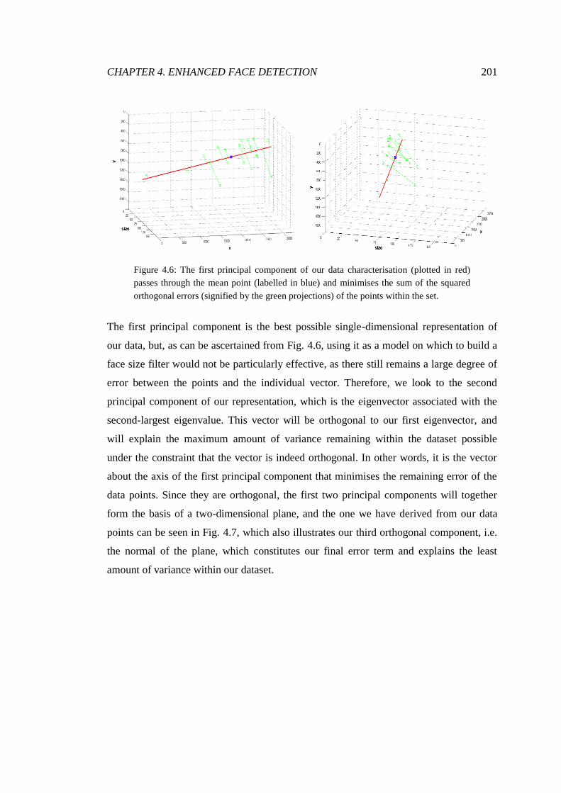
CHAPTER 4. ENHANCED FACE DETECTION 201
Figure 4.6: The first principal component of our data characterisation (plotted in red)
passes through the mean point (labelled in blue) and minimises the sum of the squared
orthogonal errors (signified by the green projections) of the points within the set.
The first principal component is the best possible single-dimensional representation of
our data, but, as can be ascertained from Fig. 4.6, using it as a model on which to build a
face size filter would not be particularly effective, as there still remains a large degree of
error between the points and the individual vector. Therefore, we look to the second
principal component of our representation, which is the eigenvector associated with the
second-largest eigenvalue. This vector will be orthogonal to our first eigenvector, and
will explain the maximum amount of variance remaining within the dataset possible
under the constraint that the vector is indeed orthogonal. In other words, it is the vector
about the axis of the first principal component that minimises the remaining error of the
data points. Since they are orthogonal, the first two principal components will together
form the basis of a two-dimensional plane, and the one we have derived from our data
points can be seen in Fig. 4.7, which also illustrates our third orthogonal component, i.e.
the normal of the plane, which constitutes our final error term and explains the least
amount of variance within our dataset.

202 CHAPTER 4. ENHANCED FACE DETECTION
Figure 4.7: The two-dimensional plane defined by our first two eigenvectors, which are
represented, respectively, by the red and cyan projections through the mean point. Our
third eigenvector, represented by the green projection through the mean point, represents
the normal of the plane, and now constitutes the error term of our data points, the
individual errors of which now project orthogonally onto the plane.
As Fig. 4.7 illustrates, by characterising our data according to a bidimensional model
rather than a unidimensional model, the error terms of our data points have been
significantly reduced, meaning that we have achieved much more accurate representation.
Given that we would usually expect the faces visible within a lecture theatre-based image
to be distributed across a surface of seating, the plane we have constructed can be used to
accurately and reliably model the sizes of faces according to their coordinates, and
therefore has the capacity to discriminate between detections of sizes that we would
expect faces to exhibit and detections that are either too large or too small to reasonably
pertain to actual faces.
4.1.2.2 Sized-Based Detection Elimination
With a representative size model constructed, the issue of filtering out false positive
detections from our collated set becomes one of effective application. For many of the
data points illustrated by Fig. 4.3, it is rather plain to see that their sizes are far beyond
what we would expect actual faces to exhibit, given their locations, and it would,
therefore, be relatively straightforward to discard them. There will be a large number of
false positives, however, with sizes much closer to those that would be exhibited by
actual faces, but are still either too large or too small to realistically be true positives, and
it is these that necessitate our filters being carefully designed. In order to visualise this
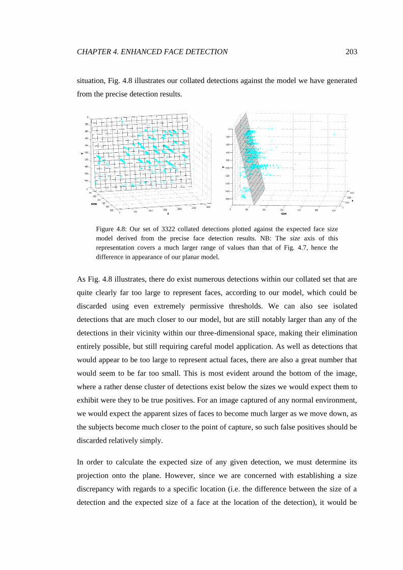
CHAPTER 4. ENHANCED FACE DETECTION 203
situation, Fig. 4.8 illustrates our collated detections against the model we have generated
from the precise detection results.
Figure 4.8: Our set of 3322 collated detections plotted against the expected face size
model derived from the precise face detection results. NB: The size axis of this
representation covers a much larger range of values than that of Fig. 4.7, hence the
difference in appearance of our planar model.
As Fig. 4.8 illustrates, there do exist numerous detections within our collated set that are
quite clearly far too large to represent faces, according to our model, which could be
discarded using even extremely permissive thresholds. We can also see isolated
detections that are much closer to our model, but are still notably larger than any of the
detections in their vicinity within our three-dimensional space, making their elimination
entirely possible, but still requiring careful model application. As well as detections that
would appear to be too large to represent actual faces, there are also a great number that
would seem to be far too small. This is most evident around the bottom of the image,
where a rather dense cluster of detections exist below the sizes we would expect them to
exhibit were they to be true positives. For an image captured of any normal environment,
we would expect the apparent sizes of faces to become much larger as we move down, as
the subjects become much closer to the point of capture, so such false positives should be
discarded relatively simply.
In order to calculate the expected size of any given detection, we must determine its
projection onto the plane. However, since we are concerned with establishing a size
discrepancy with regards to a specific location (i.e. the difference between the size of a
detection and the expected size of a face at the location of the detection), it would be

204 CHAPTER 4. ENHANCED FACE DETECTION
entirely inappropriate for us to use an orthogonal projection. Although these constituted
the final error terms during the derivation of the model, they are not the form of deviation
we are concerned with now. The orthogonal projection of a detection onto the plane
would be a point with entirely different coordinates, yielding the expected size of an
entirely different image location, which would be of no use in the determination of the
nature of that detection. We must project detections directly along the size axis of our
three-dimensional space, and the point at which the vector meets the model will define
the expected face size for that detection. The equation of our plane, which will be
satisfied by every (x,y,size) point that lies upon it, can be described by Eq. 4.4, where μi
represents the ith component of the mean model point, and v3 represents our third
eigenvector, which is the normal of the plane and can be used to independently define it,
given the orthogonal nature of the eigenvectors.
𝑥 𝑦 𝑠 − 𝜇𝑥 𝜇𝑦 𝜇𝑠 ∙ 𝑣3 = 0 (4.4)
Given that the mean point μ and normal v3 will be constants derived from our precise face
detection results, we can rearrange Eq. 4.4 to yield an expression that can be used to
calculate the size component of the point on the plane that corresponds to the input
coordinates x and y. Eq. 4.5 describes this derived expression, where v3j represents the jth
component of the normal vector.
0 = 𝑥 − 𝜇𝑥 𝑦 − 𝜇𝑦 𝑠 − 𝜇𝑠 · 𝑣3 .
= 𝑥 − 𝜇𝑥 𝑣31 + 𝑦 − 𝜇𝑦 𝑣32 + 𝑠 − 𝜇𝑠 𝑣33 .
𝑠 − 𝜇𝑠 𝑣33 = − 𝑥 − 𝜇𝑥 𝑣31 − 𝑦 − 𝜇𝑦 𝑣32 .
𝑠 · 𝑣33 − 𝜇𝑠 · 𝑣33 = − 𝑥 − 𝜇𝑥 𝑣31 − 𝑦 − 𝜇𝑦 𝑣32 .
𝑠 · 𝑣33 = − 𝑥 − 𝜇𝑥 𝑣31 − 𝑦 − 𝜇𝑦 𝑣32 + 𝜇𝑠 · 𝑣33 .
𝑠 = − 𝑥 − 𝜇𝑥 𝑣31 − 𝑦 − 𝜇𝑦 𝑣32 + 𝜇𝑠 · 𝑣33 / 𝑣33 (4.5)
By applying Eq. 4.5 to the coordinates of any detection, we can project it onto the plane
along the size axis, thereby determining the size that a face at its location should exhibit,
according to our model. The size projections of our collated detections are illustrated by
Fig. 4.9.
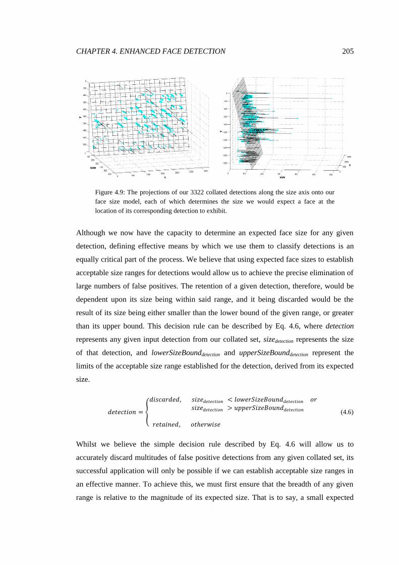
CHAPTER 4. ENHANCED FACE DETECTION 205
Figure 4.9: The projections of our 3322 collated detections along the size axis onto our
face size model, each of which determines the size we would expect a face at the
location of its corresponding detection to exhibit.
Although we now have the capacity to determine an expected face size for any given
detection, defining effective means by which we use them to classify detections is an
equally critical part of the process. We believe that using expected face sizes to establish
acceptable size ranges for detections would allow us to achieve the precise elimination of
large numbers of false positives. The retention of a given detection, therefore, would be
dependent upon its size being within said range, and it being discarded would be the
result of its size being either smaller than the lower bound of the given range, or greater
than its upper bound. This decision rule can be described by Eq. 4.6, where detection
represents any given input detection from our collated set, sizedetection represents the size
of that detection, and lowerSizeBounddetection and upperSizeBounddetection represent the
limits of the acceptable size range established for the detection, derived from its expected
size.
𝑑𝑒𝑡𝑒𝑐𝑡𝑖𝑜𝑛 =
𝑑𝑖𝑠𝑐𝑎𝑟𝑑𝑒𝑑, 𝑠𝑖𝑧𝑒𝑑𝑒𝑡𝑒𝑐𝑡𝑖𝑜𝑛 < 𝑙𝑜𝑤𝑒𝑟𝑆𝑖𝑧𝑒𝐵𝑜𝑢𝑛𝑑𝑑𝑒𝑡𝑒𝑐𝑡𝑖𝑜𝑛 𝑜𝑟 𝑠𝑖𝑧𝑒𝑑𝑒𝑡𝑒𝑐𝑡𝑖𝑜𝑛 > 𝑢𝑝𝑝𝑒𝑟𝑆𝑖𝑧𝑒𝐵𝑜𝑢𝑛𝑑𝑑𝑒𝑡𝑒𝑐𝑡𝑖𝑜𝑛
𝑟𝑒𝑡𝑎𝑖𝑛𝑒𝑑, 𝑜𝑡𝑒𝑟𝑤𝑖𝑠𝑒
(4.6)
Whilst we believe the simple decision rule described by Eq. 4.6 will allow us to
accurately discard multitudes of false positive detections from any given collated set, its
successful application will only be possible if we can establish acceptable size ranges in
an effective manner. To achieve this, we must first ensure that the breadth of any given
range is relative to the magnitude of its expected size. That is to say, a small expected

206 CHAPTER 4. ENHANCED FACE DETECTION
size should yield a small range of acceptable sizes, whereas a larger expected size should
correspond to a larger range. This is extremely important, as it takes into consideration
the potential error involved with any face detection, and the tendency for detectors to
slightly underestimate or slightly overestimate the apparent size of any given face, which
is certainly the case where the Viola-Jones system [147] is concerned, as it scales its
detection window to identify faces of all sizes. The limits of any given expected size
range can, therefore, be calculated using Eq. 4.7 and Eq. 4.8, respectively, where
errorTolerance represents the maximum relative error that we are willing to accept of a
detection before discarding it.
𝑙𝑜𝑤𝑒𝑟𝑆𝑖𝑧𝑒𝐵𝑜𝑢𝑛𝑑𝑑𝑒𝑡𝑒𝑐𝑡𝑖𝑜𝑛 = 𝑠𝑖𝑧𝑒𝑑𝑒𝑡𝑒𝑐𝑡𝑖𝑜𝑛 ∙ (1 − 𝑒𝑟𝑟𝑜𝑟𝑇𝑜𝑙𝑒𝑟𝑎𝑛𝑐𝑒) (4.7)
𝑢𝑝𝑝𝑒𝑟𝑆𝑖𝑧𝑒𝐵𝑜𝑢𝑛𝑑𝑑𝑒𝑡𝑒𝑐𝑡𝑖𝑜𝑛 = 𝑠𝑖𝑧𝑒𝑑𝑒𝑡𝑒𝑐𝑡𝑖𝑜𝑛 ∙ (1 + 𝑒𝑟𝑟𝑜𝑟𝑇𝑜𝑙𝑒𝑟𝑎𝑛𝑐𝑒) (4.8)
Given this requirement of the ranges being relative, what remains is to ascertain how
broad they should actually be. In order to determine appropriate size error tolerances, we
have analysed the results achieved by a number of difference tolerance levels, over 5
images that depict a total of 200 individual faces. These results pertain to the rate at
which detections were eliminated by each filter (calculated as the number discarded over
the number initially collated) and the rate at which actual faces were eliminated, i.e. the
incidence rate of every detection associated with a single face being discarded (calculated
as the number of eliminated faces over the number that had a non-zero number of
detections associated with them prior to the application of the filter). Ideally, we would
like to eliminate as many detections as possible without losing any significant number of
faces, as this would maximise the number of false positive detections that our size filter
can discard without causing any detrimental effects to the overall detection rates of the
system. It should be noted that many of the detections we would expect a given size filter
to eliminate would actually constitute true positives, but they are more than likely to be
some of the overestimates and underestimates that we have previously alluded to, and the
faces they pertain to are almost certain to have vast numbers of detections associated with
them that are more appropriately sized that will not be discarded. Even if the set of
detections eliminated according to their size for a given input image consisted mostly of
true positives, we would expect the false positives also discarded to represent the
majority of the false positives produced for that image during initial detection, and this is
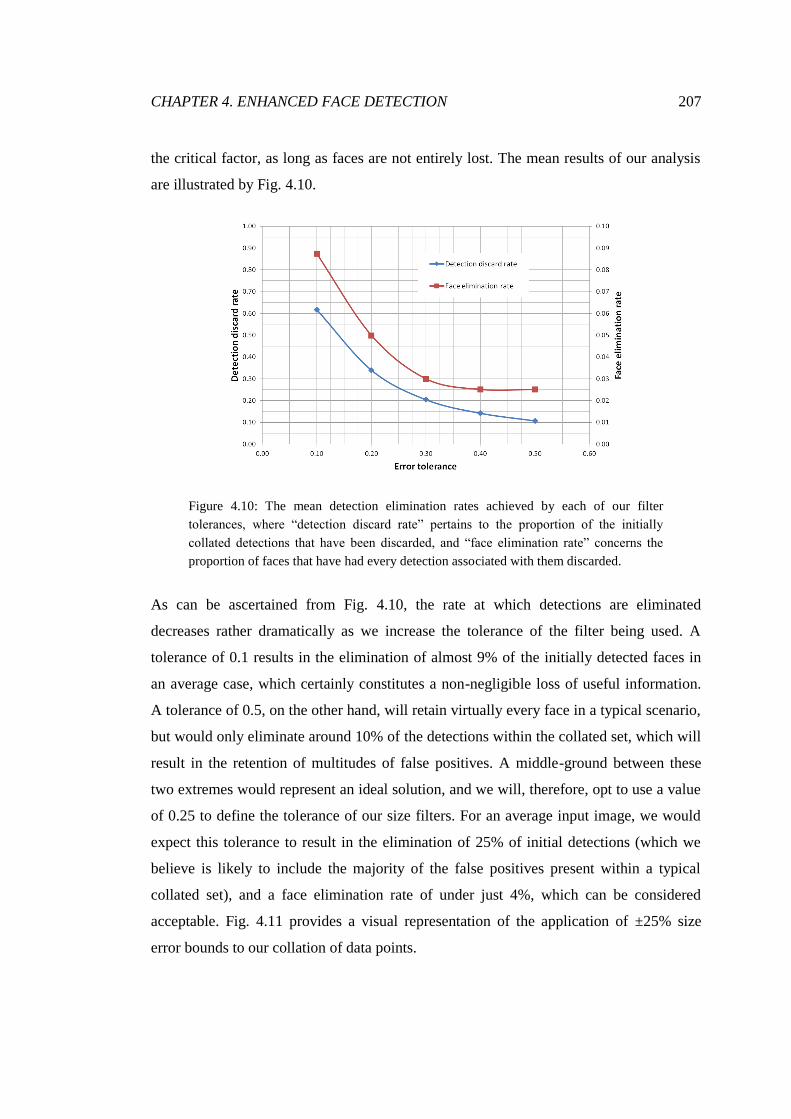
CHAPTER 4. ENHANCED FACE DETECTION 207
the critical factor, as long as faces are not entirely lost. The mean results of our analysis
are illustrated by Fig. 4.10.
Figure 4.10: The mean detection elimination rates achieved by each of our filter
tolerances, where “detection discard rate” pertains to the proportion of the initially
collated detections that have been discarded, and “face elimination rate” concerns the
proportion of faces that have had every detection associated with them discarded.
As can be ascertained from Fig. 4.10, the rate at which detections are eliminated
decreases rather dramatically as we increase the tolerance of the filter being used. A
tolerance of 0.1 results in the elimination of almost 9% of the initially detected faces in
an average case, which certainly constitutes a non-negligible loss of useful information.
A tolerance of 0.5, on the other hand, will retain virtually every face in a typical scenario,
but would only eliminate around 10% of the detections within the collated set, which will
result in the retention of multitudes of false positives. A middle-ground between these
two extremes would represent an ideal solution, and we will, therefore, opt to use a value
of 0.25 to define the tolerance of our size filters. For an average input image, we would
expect this tolerance to result in the elimination of 25% of initial detections (which we
believe is likely to include the majority of the false positives present within a typical
collated set), and a face elimination rate of under just 4%, which can be considered
acceptable. Fig. 4.11 provides a visual representation of the application of ±25% size
error bounds to our collation of data points.
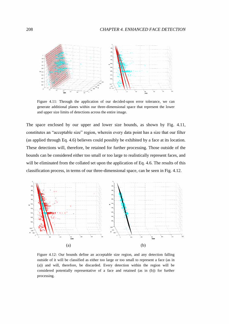
208 CHAPTER 4. ENHANCED FACE DETECTION
Figure 4.11: Through the application of our decided-upon error tolerance, we can
generate additional planes within our three-dimensional space that represent the lower
and upper size limits of detections across the entire image.
The space enclosed by our upper and lower size bounds, as shown by Fig. 4.11,
constitutes an “acceptable size” region, wherein every data point has a size that our filter
(as applied through Eq. 4.6) believes could possibly be exhibited by a face at its location.
These detections will, therefore, be retained for further processing. Those outside of the
bounds can be considered either too small or too large to realistically represent faces, and
will be eliminated from the collated set upon the application of Eq. 4.6. The results of this
classification process, in terms of our three-dimensional space, can be seen in Fig. 4.12.
(a) (b)
Figure 4.12: Our bounds define an acceptable size region, and any detection falling
outside of it will be classified as either too large or too small to represent a face (as in
(a)) and will, therefore, be discarded. Every detection within the region will be
considered potentially representative of a face and retained (as in (b)) for further
processing.

CHAPTER 4. ENHANCED FACE DETECTION 209
If we consider our set of retained detections in the context of the image they pertain to,
we can achieve a greater understanding of how effective our size filtering process has
been at eliminating vast numbers of false positives whilst retaining virtually all useful
information. To that end, Fig. 4.13 depicts the set of retained detections with regards to
our input image.
Figure 4.13: As we have discarded a set of 922 detections, which would appear to
include the vast majority of the false positives initially generated, we have retained
precisely 2400 detections, which will be processed further.
As Fig. 4.13 makes clear, despite discarding almost 28% of the detections within the
collated set, there are still large numbers associated with almost every face that was
initially detected (all of which we have added confidence to by validating their sizes),
which suggests that significant numbers of false positives have been eliminated without
any considerable loss of useful information. The way in which the remaining detections
conform to our generated plane can also be noted, as they generally increase in size as we
move from the top of the image to the bottom and as we move from left to right, although
the latter is decidedly more subtle.
The success of this filtering process can be made even more apparent when Fig. 4.13 is
compared to Fig. 4.3, as the latter illustrated multitudes of false positives detections of all
sizes scattered throughout the image. Now, although there are undoubtedly still false
positives present within our set of detections, the number of them has been drastically

210 CHAPTER 4. ENHANCED FACE DETECTION
reduced. Those that have been retained clearly exhibit face-like sizes, but there do exist
additional means by which they can be identified and discarded.
It should be noted that, due to the nature of principal component analysis, our system will
be unable to process a collated set detections if precise face detection yields fewer than
three results, as this is the minimum number of data points required for a model to be
derived in our three-dimensional space using PCA. In such a scenario, the output of our
framework would simply be the number of precise face detections produced, be it two,
one, or zero.
4.1.3 Retained Detection Consolidation
Although we have demonstrated that our size-filtering process can be successful in
eliminating large numbers of false positives, the set of detections retained cannot be
considered a set of actual faces. Fig. 4.13, for instance, depicts 2400 individual
detections, yet Fig. 4.2 contains merely 44 visible faces, so we must work further towards
deriving an accurate representation of those faces. As can be discerned from Fig. 4.13, it
would seem that the remaining false positives within the detection set account for only a
very small proportion of the number of retained detections. The vast majority, therefore,
constitute duplicate detections of faces, whereby a number of individual faces will have
hundreds of detections associated with them, which will be typical wherever the high-
sensitivity implementation of the Viola-Jones feature cascades is concerned. These
detections are not actually identical, and there will be variation in their sizes and exact
coordinates, but they must be consolidated if we are ever to achieve a number of final
detections that can be considered representative.
The result of successfully consolidating duplicate detections would be a set of face
candidates, and no more than one would correspond to any individual face. In this way,
the final output of our system would never be inflated due to the erroneous counting of
the same face on multiple occasions. The process of consolidation is a matter of
determining whether detections are encapsulated by other detections. Given a scenario in
which we have two detections and one of them is contained entirely within the other, we
would consolidate the two and output a single detection, which would have a size and
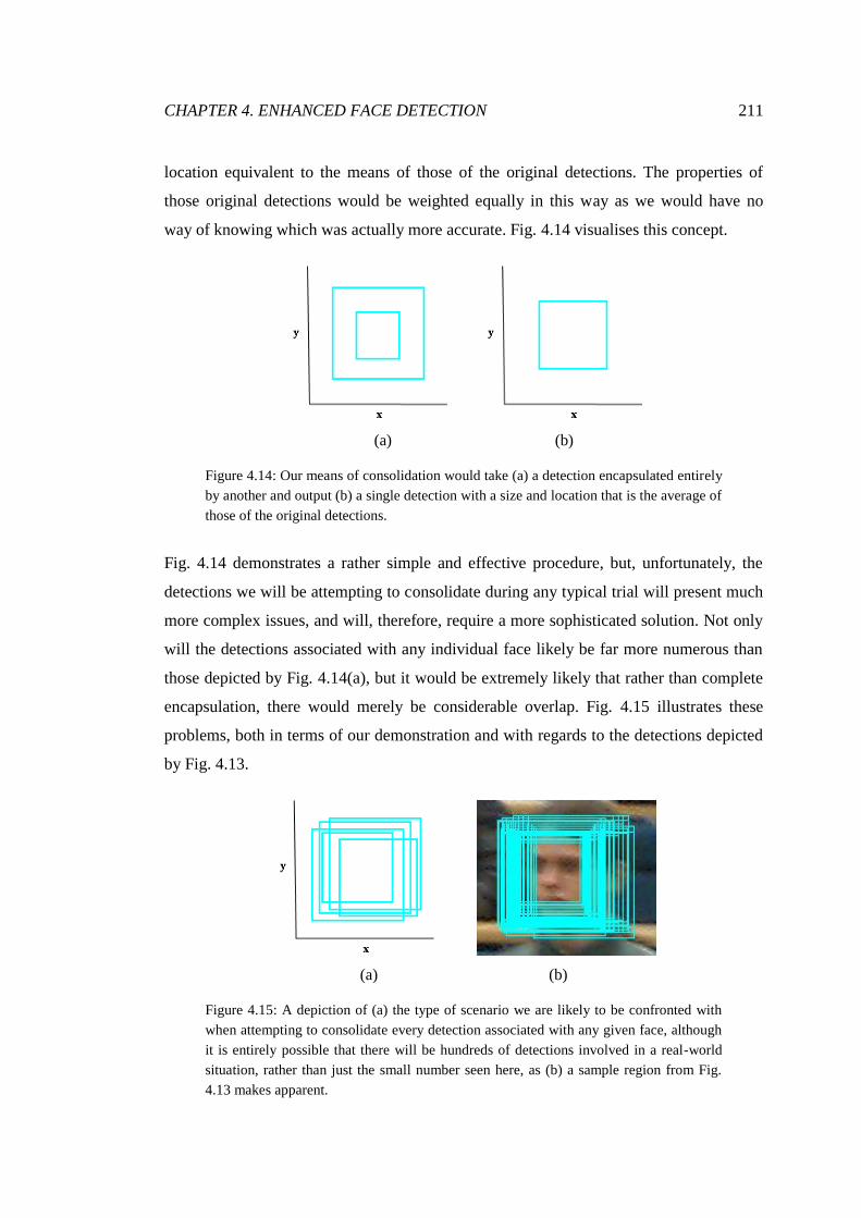
CHAPTER 4. ENHANCED FACE DETECTION 211
location equivalent to the means of those of the original detections. The properties of
those original detections would be weighted equally in this way as we would have no
way of knowing which was actually more accurate. Fig. 4.14 visualises this concept.
(a) (b)
Figure 4.14: Our means of consolidation would take (a) a detection encapsulated entirely
by another and output (b) a single detection with a size and location that is the average of
those of the original detections.
Fig. 4.14 demonstrates a rather simple and effective procedure, but, unfortunately, the
detections we will be attempting to consolidate during any typical trial will present much
more complex issues, and will, therefore, require a more sophisticated solution. Not only
will the detections associated with any individual face likely be far more numerous than
those depicted by Fig. 4.14(a), but it would be extremely likely that rather than complete
encapsulation, there would merely be considerable overlap. Fig. 4.15 illustrates these
problems, both in terms of our demonstration and with regards to the detections depicted
by Fig. 4.13.
(a) (b)
Figure 4.15: A depiction of (a) the type of scenario we are likely to be confronted with
when attempting to consolidate every detection associated with any given face, although
it is entirely possible that there will be hundreds of detections involved in a real-world
situation, rather than just the small number seen here, as (b) a sample region from Fig.
4.13 makes apparent.
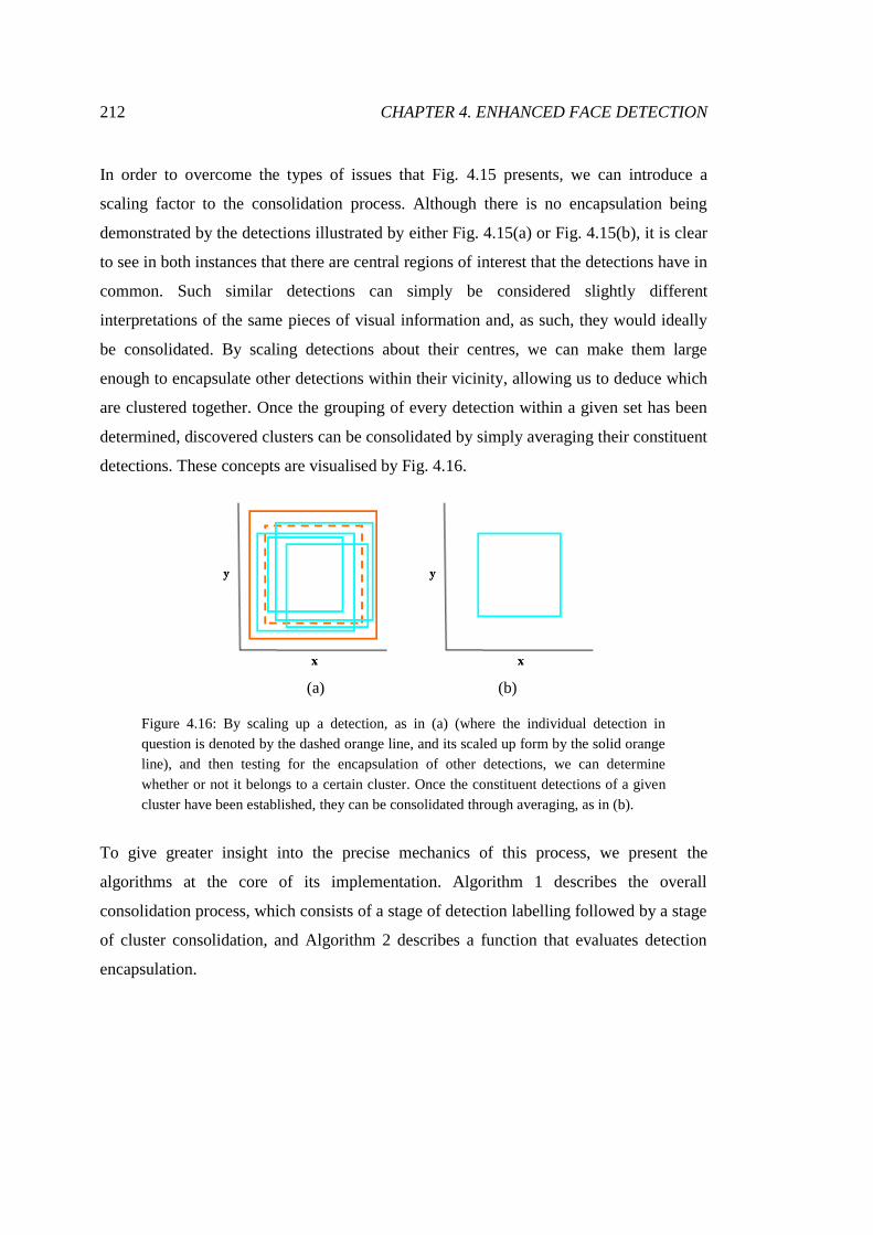
212 CHAPTER 4. ENHANCED FACE DETECTION
In order to overcome the types of issues that Fig. 4.15 presents, we can introduce a
scaling factor to the consolidation process. Although there is no encapsulation being
demonstrated by the detections illustrated by either Fig. 4.15(a) or Fig. 4.15(b), it is clear
to see in both instances that there are central regions of interest that the detections have in
common. Such similar detections can simply be considered slightly different
interpretations of the same pieces of visual information and, as such, they would ideally
be consolidated. By scaling detections about their centres, we can make them large
enough to encapsulate other detections within their vicinity, allowing us to deduce which
are clustered together. Once the grouping of every detection within a given set has been
determined, discovered clusters can be consolidated by simply averaging their constituent
detections. These concepts are visualised by Fig. 4.16.
(a) (b)
Figure 4.16: By scaling up a detection, as in (a) (where the individual detection in
question is denoted by the dashed orange line, and its scaled up form by the solid orange
line), and then testing for the encapsulation of other detections, we can determine
whether or not it belongs to a certain cluster. Once the constituent detections of a given
cluster have been established, they can be consolidated through averaging, as in (b).
To give greater insight into the precise mechanics of this process, we present the
algorithms at the core of its implementation. Algorithm 1 describes the overall
consolidation process, which consists of a stage of detection labelling followed by a stage
of cluster consolidation, and Algorithm 2 describes a function that evaluates detection
encapsulation.

CHAPTER 4. ENHANCED FACE DETECTION 213
Algorithm 1: Detection consolidation
Input:
D : set of size-filtered detections d
S : defined scaling factor
Output:
C : set of consolidated detections c
Phase 1: Detection labelling
Let n be the number of detections in D
Let A be a set of cluster labels, where labels a1,…,n will correspond to detections d1,…,n
Let m be the number of different labels assigned
Assign first detection to first cluster
a1 ← 1
m ← 1
For all other detections
for i = 2 to n do
Until label is assigned, compare to previously labelled detections
for j = 1 to i – 1 and while ai is empty do
Given scaling, if current detection encapsulates previous (Algorithm 2),
then assign same cluster label
if doesEncapsulate(di,dj,S) then ai ← aj
end for
If current detection does not encapsulate any previous under scaling,
then assign new cluster label
if ai is empty then m ← m + 1, ai ← m
end for
Phase 2: Cluster consolidation
For each cluster
for i = 1 to m do
Determine the means (coordinates, size) of all detections with the given
cluster label and assign to the consolidation
ci ← 1
a ∈ A ∶ a = i { dj ∶ aj = i } n
j=1
end for
return C

214 CHAPTER 4. ENHANCED FACE DETECTION
Algorithm 2: Test detection encapsulation under scaling (doesEncapsulate)
Input:
dcur : current detection
dlab : existing labelled detection
S : defined scale factor
Output:
veracity of detection encapsulation under scaling
Let dS be the result of scaling-up current detection dcur
Let xd,p and yd,p respectively represent the x-coordinate and y-coordinate of detection d at
position p, where p = {top-left = tl, bottom-right = br, centre = c} and the origin of the
coordinate system (0,0) is considered to be its top-left corner
Let zd represent half the width of square detection d
Scale up current detection about its centre according to defined scaling factor
xdS,tl ← xdcur,c – ( S · zdcur )
ydS,tl ← ydcur,c – ( S · zdcur )
xdS,br ← xdcur,c + ( S · zdcur )
ydS,br ← ydcur,c + ( S · zdcur )
Test encapsulation of labelled detection according to detection corners
if xdS,tl ≤ xdlab,tl and ydS,tl ≤ ydlab,tl and xdS,br ≥ xdlab,br and ydS,br ≥ ydlab,br then
return true
else
return false
end if
Whether or not these means of detection consolidation will consistently yield accurate
and desirable results will be dependent upon the sound determination of an optimal value
for the applied scaling factor. If we were to set it too small, it is entirely possible that
entire groups of detections would never be consolidated. If we were to use too large a
value, however, the potential for neighbouring groups, which pertain to entirely separate
but nearby faces, to be consolidated into single detections would become considerable.
Not only would this result in individual faces being lost, meaning detection rates would
be diminished, but it is highly likely that the properties of the detections involved would
lead to the output detection, as it is a mean, corresponding to a region of space between
the given faces, and not an actual face. An example of this situation from within Fig. 4.13
is depicted by Fig. 4.17. It is for these reasons that size filtering is performed prior to
detection consolidation, as the presence of even a small number of large false positives
could lead to the erroneous consolidation of multiple groups of detections, which would
be severely damaging to our achieved detection rates.

CHAPTER 4. ENHANCED FACE DETECTION 215
Figure 4.17: Because the scaling factor we have used in this instance is too large, two
separate groups of detections illustrated by Fig. 4.13 have been consolidated into just a
single result, which itself does not entirely pertain to either of the faces involved.
As we would like to avoid the type of result that Fig. 4.17 illustrates, but also
successfully consolidate every group of detections that we generate, we must carefully
derive an optimal value for the scaling factor. In order to do this, we will again be making
use of empirical results, and our analysis will involve the same 5 images we have used
previously. This may not seem like a reliably large sample size, but the images vary
greatly in nature and depict 200 individual faces, which offers vast opportunity for the
issues we have described to manifest. We will be using a broad range of scaling factors to
consolidate our filtered detection set, and measuring the rate at which groups of
detections are not entirely consolidated, which will be contrasted to the rate at which
separate groups are consolidated into single outputs. Both of these rates will be in terms
of the number of faces within each image that have detections associated with them after
size filtering. The optimal scaling factor will be one that can minimise both of these rates,
as they both constitute errors, although one clearly results in system oversensitivity and
the other undersensitivity. The mean results of our analysis are illustrated by Fig. 4.18.
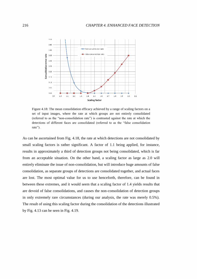
216 CHAPTER 4. ENHANCED FACE DETECTION
Figure 4.18: The mean consolidation efficacy achieved by a range of scaling factors on a
set of input images, where the rate at which groups are not entirely consolidated
(referred to as the “non-consolidation rate”) is contrasted against the rate at which the
detections of different faces are consolidated (referred to as the “false consolidation
rate”).
As can be ascertained from Fig. 4.18, the rate at which detections are not consolidated by
small scaling factors is rather significant. A factor of 1.1 being applied, for instance,
results in approximately a third of detection groups not being consolidated, which is far
from an acceptable situation. On the other hand, a scaling factor as large as 2.0 will
entirely eliminate the issue of non-consolidation, but will introduce huge amounts of false
consolidation, as separate groups of detections are consolidated together, and actual faces
are lost. The most optimal value for us to use henceforth, therefore, can be found in
between these extremes, and it would seem that a scaling factor of 1.4 yields results that
are devoid of false consolidations, and causes the non-consolidation of detection groups
in only extremely rare circumstances (during our analysis, the rate was merely 0.5%).
The result of using this scaling factor during the consolidation of the detections illustrated
by Fig. 4.13 can be seen in Fig. 4.19.

CHAPTER 4. ENHANCED FACE DETECTION 217
Figure 4.19: The multitudes of detections present within Fig. 4.13 have now been
consolidated into 71 face candidates, such that individual faces are now only associated
with single detections and duplicates have been disregarded, which is crucial for the
accuracy of our results.
The results illustrated by Fig. 4.19 indicate that we have greatly successful in our
attempts to disregard the multitudes of duplicate detections present within the set retained
after size filtering. As can be seen, in this instance, we have not produced a single false
consolidation, or a single case of non-consolidation, which is a testament to the
optimality of our settled-upon scaling factor value for this type of problem. This stage of
our face detection process does not inherently confer any confidence to the detections we
did not discard previously, but it does transform the set of data points we have from a set
of mere detections to a set of genuine faces candidates, the properties of which can
henceforth be evaluated in order for us to produce actual positive classifications.
4.1.4 Score-Based Face Candidate Classification
Having generated a set of face candidates from our initially collated set of detections,
through size filtering and then consolidation, we can now begin to examine the
conditions under which regions can be positively classified in order for our output to be
built. The face candidates illustrated by Fig. 4.19 are not the only pieces of information
we have to work with in our attempts to derive a set of actual faces for Fig. 4.2, however.
An exceptionally useful by-product of the detection consolidation process is a set of
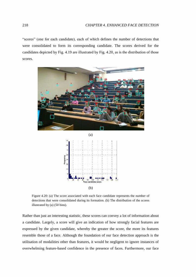
218 CHAPTER 4. ENHANCED FACE DETECTION
“scores” (one for each candidate), each of which defines the number of detections that
were consolidated to form its corresponding candidate. The scores derived for the
candidates depicted by Fig. 4.19 are illustrated by Fig. 4.20, as is the distribution of those
scores.
(a)
(b)
Figure 4.20: (a) The score associated with each face candidate represents the number of
detections that were consolidated during its formation. (b) The distribution of the scores
illustrated by (a) (50 bins).
Rather than just an interesting statistic, these scores can convey a lot of information about
a candidate. Largely, a score will give an indication of how strongly facial features are
expressed by the given candidate, whereby the greater the score, the more its features
resemble those of a face. Although the foundation of our face detection approach is the
utilisation of modalities other than features, it would be negligent to ignore instances of
overwhelming feature-based confidence in the presence of faces. Furthermore, our face

CHAPTER 4. ENHANCED FACE DETECTION 219
candidates were constructed from detections that were retained by the size filter, so their
scores also convey the confidence conferred by the validation of their sizes. It is for these
reasons that we believe classifying candidates that have particularly large scores as faces
would allow us to precisely extract large numbers of actual faces (i.e. without also
extracting non-face regions) from our sets of candidates without the need to further
consider additional candidate properties. This, of course, would not necessarily allow us
to identify every face within a given image, as, although that may be possible, we would
not expect any particularly weak faces to have great enough scores to make them
distinguishable from non-face regions.
In much the same way that attempting to predefine ranges of acceptable detection sizes
would have been greatly inappropriate, establishing a score threshold, above which
candidates would be positively classified as faces, that would be applied in each and
every scenario would also be completely ignorant of numerous critical factors. Firstly,
the score of any given candidate will be highly dependent upon the number of detectors
used during the initial collation of detections. Naturally, no matter the constitution of the
given input, the score associated with any given candidate will be increased
monotonically with the application of additional detectors, so with a sufficient number of
detectors used, every candidate would have a score exceeding any predefined threshold.
Furthermore, a globally applied threshold would give no consideration to the quality of
any given image. Even with a fixed number of detectors, there are a number of variables
associated with the circumstances under which a given image is captured that can
significantly affect the score that candidates are ultimately associated with. Subjects and
features being distant (smaller), the depicted environment being weakly illuminated, and
a lack of general focus, among other factors, can all be detrimental to the initial collation
of detections, and will, therefore, impact the range of scores that a set of candidates
express. If we were to artificially introduce a small degree of blur to Fig. 4.2, for
instance, the candidate scores we would generate would be considerably lower than those
depicted by Fig. 4.20, and there would likely be many fewer candidates, but the
candidates with the largest scores within Fig. 4.20 would still have the largest scores
within the blurred image (which Fig. 4.21 demonstrates), as their relative feature-based
face resemblances would not have changed (were the amount of blur to simulate nothing
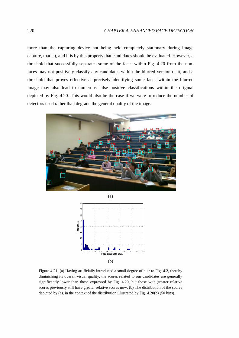
220 CHAPTER 4. ENHANCED FACE DETECTION
more than the capturing device not being held completely stationary during image
capture, that is), and it is by this property that candidates should be evaluated. However, a
threshold that successfully separates some of the faces within Fig. 4.20 from the non-
faces may not positively classify any candidates within the blurred version of it, and a
threshold that proves effective at precisely identifying some faces within the blurred
image may also lead to numerous false positive classifications within the original
depicted by Fig. 4.20. This would also be the case if we were to reduce the number of
detectors used rather than degrade the general quality of the image.
(a)
(b)
Figure 4.21: (a) Having artificially introduced a small degree of blur to Fig. 4.2, thereby
diminishing its overall visual quality, the scores related to our candidates are generally
significantly lower than those expressed by Fig. 4.20, but those with greater relative
scores previously still have greater relative scores now. (b) The distribution of the scores
depicted by (a), in the context of the distribution illustrated by Fig. 4.20(b) (50 bins).

CHAPTER 4. ENHANCED FACE DETECTION 221
It is for these reasons that we must define score thresholds on an image-by-image basis,
and classify candidates in a manner that is relative to the other candidates within the
given set. Our classification rule, therefore, can be described by Eq. 4.9, where candidate
represents any candidate within a given set, scorecandidate represents the score
corresponding to that candidate, and scoreThresholdcandidateSet represents the threshold
defined for the set of candidates that the given candidate belongs to. Rather than
discarding candidates that cannot be confidently classified as faces according to their
scores, we simply draw no conclusions about their nature and retain them for further
processing.
𝑐𝑎𝑛𝑑𝑖𝑑𝑎𝑡𝑒 =
𝑓𝑎𝑐𝑒, 𝑠𝑐𝑜𝑟𝑒𝑐𝑎𝑛𝑑𝑖𝑑𝑎𝑡𝑒 ≥ 𝑠𝑐𝑜𝑟𝑒𝑇𝑟𝑒𝑠𝑜𝑙𝑑𝑐𝑎𝑛𝑑𝑖𝑑𝑎𝑡𝑒𝑆𝑒𝑡
𝑢𝑛𝑑𝑒𝑡𝑒𝑟𝑚𝑖𝑛𝑒𝑑, 𝑜𝑡𝑒𝑟𝑤𝑖𝑠𝑒
(4.9)
Clearly, the success of such a methodology will be dependent upon the appropriate
definition of thresholds, and whether we can suitably adapt them to the aforementioned
variables. To that end, if we assume that the largest score generated for an image pertains
to an actual face, then we can gain an understanding of how strongly expressed the
features of faces within the image have the potential to be, given the circumstances
surrounding the quality of the image and the detectors being used and how dependent
scores are upon them. We believe that this assumption is entirely reasonable given that
we know there must exist at least three faces identifiable using high-threshold detection
within an image for our system to even progress to the stage of score-based classification,
and it would seem extremely unlikely, in any scenario, that a non-face region would exist
that would not only have a greater score than any of those faces, but a greater score than
every single face within the image. It is, of course, this rationale that underpins the entire
concept of score-based classification, and how we can use it to separate a set of faces
from non-face regions.
By using the largest score generated for an input to establish a threshold specific to the
face candidates of it, classifications can be made that account for all of the factors we
have identified. We believe that simply defining the face classification threshold of a
given set of candidate scores as a certain fraction of the largest of those scores would
prove to be effective. The process of determining thresholds in this manner can be
described by Eq. 4.10, where greatestScorecandidateSet refers to the largest score of any

222 CHAPTER 4. ENHANCED FACE DETECTION
candidate within a set, and scoreFraction represents our constant fractional value that
will define the relationship between greatest scores and applied score thresholds.
𝑠𝑐𝑜𝑟𝑒𝑇𝑟𝑒𝑠𝑜𝑙𝑑𝑐𝑎𝑛𝑑𝑖𝑑𝑎𝑡𝑒𝑆𝑒𝑡 = 𝑔𝑟𝑒𝑎𝑡𝑒𝑠𝑡𝑆𝑐𝑜𝑟𝑒𝑐𝑎𝑛𝑑𝑖𝑑𝑎𝑡𝑒𝑆𝑒𝑡 ∙ 𝑠𝑐𝑜𝑟𝑒𝐹𝑟𝑎𝑐𝑡𝑖𝑜𝑛 (4.10)
The efficacy of defining thresholds in this way will be reliant upon the fraction used
being entirely appropriate. We can derive a suitable fraction to use in the definition of
score thresholds empirically, by establishing the frequencies with which certain values
are likely to yield false positives (in terms of false discovery rates, which are equivalent
to 1 – precision) and the rates at which they can positively classify actual faces (in terms
of the proportions of candidates that pertain to faces being positively identified, making
the metric distinct from an overall detection rate). Clearly, it would be desirable for us to
maximise the latter than whilst minimising the former. Having experimented with a range
of values over our five calibration images, the mean results we have achieved are
illustrated by Fig. 4.22.
Figure 4.22: The mean false discovery (FP / (TP + FP)) and positive candidate
identification (TP / (TP + FN)) rates yielded by a range of classification threshold-
defining largest score fractions over our set of system calibration images.
As can be discerned from Fig. 4.22, both our false discovery rate (FDR) and our positive
candidate identification rate (PCIR) decrease rather drastically as we increment the score
fraction used, although the former certainly diminishes at a significantly greater pace. At
a particularly small fraction of 0.01, we can observe an extremely impressive PCIR of

CHAPTER 4. ENHANCED FACE DETECTION 223
90%, but also an FDR of almost 25%, which represents a disappointingly low level of
precision. On the opposite end of the spectrum, we can see that after an applied fraction
of 0.15 or so, the FDRs yielded by thresholds become negligible, but the achieved PCIRs
also become rather low. A fraction of 0.1 would appear to be a reasonable compromise
between these two extremes, as it yields a FDR of only 2%, whilst also delivering a PCIR
of around 66%, and we will, therefore, be using it to define score threshold values from
this point forward. Although this would mean roughly one-third of candidate-associated
faces not being positively identified by our score-based classification methodology in an
average case, what must be remembered is that those faces would have been neither
negatively classified nor discarded, and may very well still be correctly classified as faces
and be represented by our final results. Using a score fraction of 0.1 to define a face
classification threshold for the candidates of Fig. 4.20 using Eq. 4.10 and subsequently
applying Eq. 4.9 to those candidates yields the set of faces depicted by Fig. 4.23.
(a)
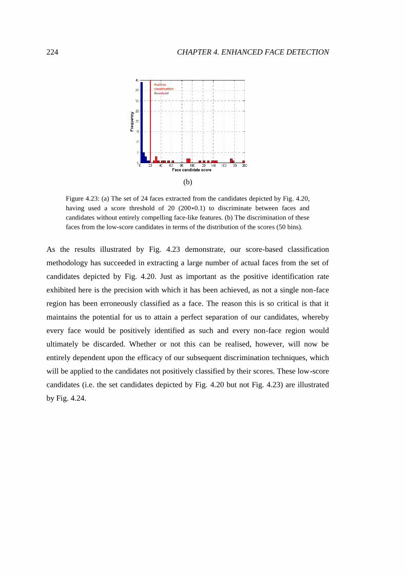
224 CHAPTER 4. ENHANCED FACE DETECTION
(b)
Figure 4.23: (a) The set of 24 faces extracted from the candidates depicted by Fig. 4.20,
having used a score threshold of 20 (200∗0.1) to discriminate between faces and
candidates without entirely compelling face-like features. (b) The discrimination of these
faces from the low-score candidates in terms of the distribution of the scores (50 bins).
As the results illustrated by Fig. 4.23 demonstrate, our score-based classification
methodology has succeeded in extracting a large number of actual faces from the set of
candidates depicted by Fig. 4.20. Just as important as the positive identification rate
exhibited here is the precision with which it has been achieved, as not a single non-face
region has been erroneously classified as a face. The reason this is so critical is that it
maintains the potential for us to attain a perfect separation of our candidates, whereby
every face would be positively identified as such and every non-face region would
ultimately be discarded. Whether or not this can be realised, however, will now be
entirely dependent upon the efficacy of our subsequent discrimination techniques, which
will be applied to the candidates not positively classified by their scores. These low-score
candidates (i.e. the set candidates depicted by Fig. 4.20 but not Fig. 4.23) are illustrated
by Fig. 4.24.

CHAPTER 4. ENHANCED FACE DETECTION 225
Figure 4.24: As the candidates with scores greater than the generated threshold have now
been positively classified as faces, we are left with a set of 47 low-score candidates,
which, rather than simply being discarded, will be classified according to additional
criteria.
Whilst the application of a score threshold to the set of candidates depicted by Fig. 4.20
has segregated the majority of the actual faces represented by that set, Fig. 4.24 makes
clear that there are still a number yet to be positively classified. These weak faces,
however, are vastly outnumbered by candidates that pertain to non-face regions, and the
sheer variety exhibited by those candidates (in terms of their locations, colours, textures,
etc.) is so great that attempting to distinguish the small number of remaining faces from
them using any specific supplementary modality is highly unlikely to yield favourable
results in any typical scenario, and certainly not on any form of consistent basis.
What can also be noted from Fig. 4.24, however, is that the majority of the candidates it
depicts that represent non-skin regions have scores of just 1, whereas most of the actual
faces are associated with scores greater than this. A score of 1 signifies that a region was
related to just a single size-filtered detection, meaning that it only expressed size-
appropriate face resemblance to a single detector at a single scale, which implies that it
could very well be the result of nothing more than a mathematical fluke. We could,
therefore, assume this to be the case for every such candidate, and extend our score-based
classification process by simply discarding any candidate with a score of 1, which would
make the discrimination of faces from non-face regions according to an alternative
property considerably more achievable. Although we have previously stressed the
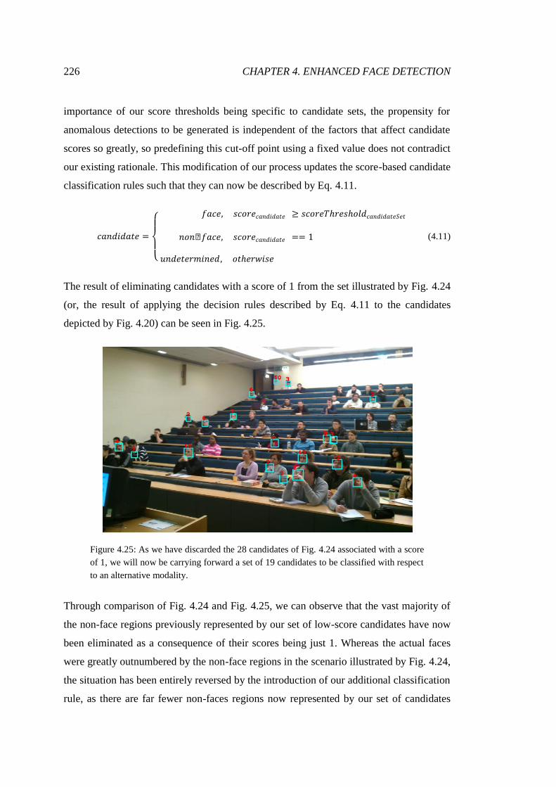
226 CHAPTER 4. ENHANCED FACE DETECTION
importance of our score thresholds being specific to candidate sets, the propensity for
anomalous detections to be generated is independent of the factors that affect candidate
scores so greatly, so predefining this cut-off point using a fixed value does not contradict
our existing rationale. This modification of our process updates the score-based candidate
classification rules such that they can now be described by Eq. 4.11.
𝑐𝑎𝑛𝑑𝑖𝑑𝑎𝑡𝑒 =
𝑓𝑎𝑐𝑒, 𝑠𝑐𝑜𝑟𝑒𝑐𝑎𝑛𝑑𝑖𝑑𝑎𝑡𝑒 ≥ 𝑠𝑐𝑜𝑟𝑒𝑇𝑟𝑒𝑠𝑜𝑙𝑑𝑐𝑎𝑛𝑑𝑖𝑑𝑎𝑡𝑒𝑆𝑒𝑡
𝑛𝑜𝑛‒𝑓𝑎𝑐𝑒, 𝑠𝑐𝑜𝑟𝑒𝑐𝑎𝑛𝑑𝑖𝑑𝑎𝑡𝑒 == 1
𝑢𝑛𝑑𝑒𝑡𝑒𝑟𝑚𝑖𝑛𝑒𝑑, 𝑜𝑡𝑒𝑟𝑤𝑖𝑠𝑒
(4.11)
The result of eliminating candidates with a score of 1 from the set illustrated by Fig. 4.24
(or, the result of applying the decision rules described by Eq. 4.11 to the candidates
depicted by Fig. 4.20) can be seen in Fig. 4.25.
Figure 4.25: As we have discarded the 28 candidates of Fig. 4.24 associated with a score
of 1, we will now be carrying forward a set of 19 candidates to be classified with respect
to an alternative modality.
Through comparison of Fig. 4.24 and Fig. 4.25, we can observe that the vast majority of
the non-face regions previously represented by our set of low-score candidates have now
been eliminated as a consequence of their scores being just 1. Whereas the actual faces
were greatly outnumbered by the non-face regions in the scenario illustrated by Fig. 4.24,
the situation has been entirely reversed by the introduction of our additional classification
rule, as there are far fewer non-faces regions now represented by our set of candidates

CHAPTER 4. ENHANCED FACE DETECTION 227
than there are actual faces within it, as can be ascertained from Fig. 4.25. This is
extremely important, as it means that precisely extracting the remaining faces is now
decidedly more feasible than it was beforehand.
Simply eliminating candidates with a score of 1 is not entirely without its downsides,
however. Empirically, we have found that sets of candidates will occasionally contain
actual (although extremely weak) faces with such scores, and these will, of course, be lost
upon the application of Eq. 4.11 to such sets. An instance of this can actually be observed
between Fig. 4.24 and Fig. 4.25, for example. This is extremely unfortunate, as it means
that detection rates can be negatively impacted, although we would never expect the
extent of this to be particularly significant, as the prevalence of score-of-1 faces is likely
to correlate positively with the total number of visible faces. Nevertheless, it is an
undesirable consequence, but we believe the consistency with which the extension of our
score-based classification rules eliminates large numbers of non-face regions and the
non-negligible improvements to precision that this will generally lead to outweigh the
marginal recall costs we are likely to incur.
Having achieved the precise extraction of numerous actual faces and the elimination of
large numbers of non-face regions from our set of candidates through the application of
score-based classification, we have reached the limit of what can be accomplished
through the isolated consideration of candidate scores, and we must, therefore, examine
different candidate properties in order to accurately determine the natures of those
retained to this point.
4.1.5 Colour-Based Face Candidate Classification
Whilst score-based candidate classification is no doubt capable of being extremely
effective at accurately classifying the majority of the candidates generated for any given
image, be that either positively or negatively, it cannot be used to discriminate between
particularly weak faces and non-face regions that exhibit any non-negligible amount of
face resemblance, as such candidates will be associated with similar scores. Rather than
attempt to further utilise scores, therefore, we will consider an entirely disparate attribute
of our remaining candidates: their colour. The colours expressed by the pixels of any

228 CHAPTER 4. ENHANCED FACE DETECTION
given candidate will be entirely independent from the size of the candidate and how
feature-rich it may be. Therefore, a candidate exhibiting colours that are significantly
skin-like, given that its size and score will have already been validated by virtue of it
being retained to this stage, can be considered compelling evidence of it representing an
actual face. In isolation, the general colour of a region cannot confer sufficient
confidence to it for a positive classification to be made with any particular accuracy, but
through using it to supplement the properties we have already worked with, it most
certainly can.
Of course, classifying candidates according to their colours does not necessarily preclude
the potential for candidates pertaining to non-face regions being erroneously positively
classified, but if we ensure that the skin colour models to which candidates are compared
are extremely specific, then the frequency of such incidents should not be significant.
Furthermore, such specificity of the applied models would also ensure that the probability
of actual face regions being negatively classified is minimised as well. The efficacy of
our colour-based classification process will, therefore, be dependent upon the means by
which skin colour models are generated, and how representative they are. Given the
particularly vast number of variabilities involved with inputs that depict lecture theatres
and like environments, generating models on a per-image basis, using an adaptive
methodology, will maximise the likelihood of accurate candidate classification being
achieved.
To this end, we will be adopting the skin colour modelling approach we detailed the
development of in Chapter 3. This system necessitates the existence of a set of high-
confidence face regions in order for a model to be derived. Conveniently, as we have
already generated a set of such data points during the construction of our size filter, we
are able to produce a skin colour model without the need for additional image sampling.
The derivation of a model, therefore, involves only the detection-wise filtration of sub-
region pixels according to their luma values, and the calculation of the mean colour and
covariance matrix of the resulting set, whereby the normalised rg colour space is used to
represent colours. Once this has been achieved, the model can be used to determine the
likelihood of any given pixel representing skin through the application of an expression
derived from the density function of a Gaussian joint-probability distribution, which can

CHAPTER 4. ENHANCED FACE DETECTION 229
be described by Eq. 4.12, where ci represents the colour vector of input pixel i, and μs and
Σs represent the mean colour vector and covariance matrix of our skin colour model s,
respectively.
𝑝(𝑠𝑘𝑖𝑛|𝑐𝑖) = 𝑒−1
2 𝑐𝑖−𝜇𝑠
𝑇𝛴𝑠−1(𝑐𝑖−𝜇𝑠) (4.12)
Regardless of how effectively we derive skin colour models, the accuracy with which we
can classify candidates according to their colours will be dependent upon the manner in
which we apply Eq. 4.12. Usually, it would be used in conjunction with a threshold to
achieve binary classifications and the segmentation of skin, and we could, in theory, do
this with the pixels of our candidates, then, for instance, calculate the proportion of any
given candidate region that appears to represent skin, then apply a classification threshold
to that value. Although such a process would have the potential to yield accurate results,
making colour-based candidate classification a two-dimensional problem in this manner
(as we would be applying threshold upon threshold) introduces entirely unnecessary
complications, chief among them being that calibration of the process is far more likely
to render it overfitted to the training data used than would otherwise be the case.
Instead, we use Eq. 4.12 to calculate continuous “skin ratings” for candidates, which will
simply be scalars defined on a [0,1] interval. A skin rating will provide a general sense of
how skin-like the colours of a given candidate are according to the given derived model,
and will allow us to classify it using straightforward, unidimensional thresholding,
whereby any candidate with a skin rating greater than the applied threshold will be
positively classified as a face, and any with a rating less than the threshold will be
negatively classified and discarded. This decision rule can be described by Eq. 4.13,
where candidate represents any input from our set of candidates yet to be classified,
SkinRatingcandidate represents the skin rating determined for that input, and
SkinRatingThreshold defines the threshold to be applied to our calculated ratings to
produce classifications.
𝑐𝑎𝑛𝑑𝑖𝑑𝑎𝑡𝑒 =
𝑓𝑎𝑐𝑒, 𝑆𝑘𝑖𝑛𝑅𝑎𝑡𝑖𝑛𝑔𝑐𝑎𝑛𝑑𝑖𝑑𝑎𝑡𝑒 ≥ 𝑆𝑘𝑖𝑛𝑅𝑎𝑡𝑖𝑛𝑔𝑇𝑟𝑒𝑠𝑜𝑙𝑑
𝑛𝑜𝑛‒𝑓𝑎𝑐𝑒, 𝑜𝑡𝑒𝑟𝑤𝑖𝑠𝑒
(4.13)
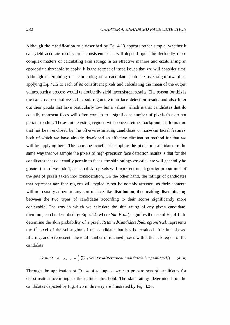
230 CHAPTER 4. ENHANCED FACE DETECTION
Although the classification rule described by Eq. 4.13 appears rather simple, whether it
can yield accurate results on a consistent basis will depend upon the decidedly more
complex matters of calculating skin ratings in an effective manner and establishing an
appropriate threshold to apply. It is the former of these issues that we will consider first.
Although determining the skin rating of a candidate could be as straightforward as
applying Eq. 4.12 to each of its constituent pixels and calculating the mean of the output
values, such a process would undoubtedly yield inconsistent results. The reason for this is
the same reason that we define sub-regions within face detection results and also filter
out their pixels that have particularly low luma values, which is that candidates that do
actually represent faces will often contain to a significant number of pixels that do not
pertain to skin. These uninteresting regions will concern either background information
that has been enclosed by the oft-overestimating candidates or non-skin facial features,
both of which we have already developed an effective elimination method for that we
will be applying here. The supreme benefit of sampling the pixels of candidates in the
same way that we sample the pixels of high-precision face detection results is that for the
candidates that do actually pertain to faces, the skin ratings we calculate will generally be
greater than if we didn’t, as actual skin pixels will represent much greater proportions of
the sets of pixels taken into consideration. On the other hand, the ratings of candidates
that represent non-face regions will typically not be notably affected, as their contents
will not usually adhere to any sort of face-like distribution, thus making discriminating
between the two types of candidates according to their scores significantly more
achievable. The way in which we calculate the skin rating of any given candidate,
therefore, can be described by Eq. 4.14, where SkinProb() signifies the use of Eq. 4.12 to
determine the skin probability of a pixel, RetainedCandidatedSubregionPixeli represents
the ith pixel of the sub-region of the candidate that has be retained after luma-based
filtering, and n represents the total number of retained pixels within the sub-region of the
candidate.
𝑆𝑘𝑖𝑛𝑅𝑎𝑡𝑖𝑛𝑔𝑐𝑎𝑛𝑑𝑖𝑑𝑎𝑡𝑒 =1
𝑛 𝑆𝑘𝑖𝑛𝑃𝑟𝑜𝑏(𝑅𝑒𝑡𝑎𝑖𝑛𝑒𝑑𝐶𝑎𝑛𝑑𝑖𝑑𝑎𝑡𝑒𝑆𝑢𝑏𝑟𝑒𝑔𝑖𝑜𝑛𝑃𝑖𝑥𝑒𝑙𝑖)
𝑛𝑖=1 (4.14)
Through the application of Eq. 4.14 to inputs, we can prepare sets of candidates for
classification according to the defined threshold. The skin ratings determined for the
candidates depicted by Fig. 4.25 in this way are illustrated by Fig. 4.26.

CHAPTER 4. ENHANCED FACE DETECTION 231
Figure 4.26: The skin ratings calculated for the set of low-score face candidates depicted
by Fig. 4.25. Each rating signifies how skin-like the general colour of the given
candidate is, according to the skin colour model generated for the given image.
Through the inspection of Fig. 4.26, we can ascertain that our process of ascribing scalar
values to candidates to describe how skin-like their overall tone is has been rather
successful where the candidates of Fig. 4.25 are concerned. As can be observed, the
candidates that pertain to faces are universally associated with large skin ratings, whereas
those that represent non-skin regions generally have significantly lower ratings.
Interestingly, there would appear to be no significant correlation between the
consolidation scores of these candidates and the skin ratings that have been derived for
them here, as the actual face candidates and non-face region candidates are now
seemingly distinguishable after previously being inseparable, which greatly reinforces
our decision to transition to the analysis of colour-based properties.
Of course, the accurate discrimination that such a range of skin ratings may allow for can
only be realised when we apply a suitable threshold, which we will again be deriving
empirically, using our set of designated calibration images. Unlike the other parameters
we have calibrated during the development of our face detection framework, our derived
skin rating threshold will not be a multiplier for any other element, and the same absolute
value will be applied during any given scenario. The reason for this relates to the nature
of our skin colour modelling process. As our models are adaptively derived and specific
to the characteristics of given input images, the skin rating calculated for any given
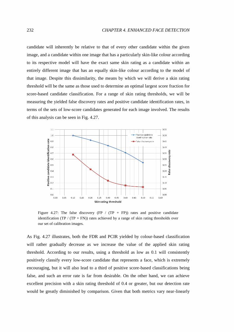
232 CHAPTER 4. ENHANCED FACE DETECTION
candidate will inherently be relative to that of every other candidate within the given
image, and a candidate within one image that has a particularly skin-like colour according
to its respective model will have the exact same skin rating as a candidate within an
entirely different image that has an equally skin-like colour according to the model of
that image. Despite this dissimilarity, the means by which we will derive a skin rating
threshold will be the same as those used to determine an optimal largest score fraction for
score-based candidate classification. For a range of skin rating thresholds, we will be
measuring the yielded false discovery rates and positive candidate identification rates, in
terms of the sets of low-score candidates generated for each image involved. The results
of this analysis can be seen in Fig. 4.27.
Figure 4.27: The false discovery (FP / (TP + FP)) rates and positive candidate
identification (TP / (TP + FN)) rates achieved by a range of skin rating thresholds over
our set of calibration images.
As Fig. 4.27 illustrates, both the FDR and PCIR yielded by colour-based classification
will rather gradually decrease as we increase the value of the applied skin rating
threshold. According to our results, using a threshold as low as 0.1 will consistently
positively classify every low-score candidate that represents a face, which is extremely
encouraging, but it will also lead to a third of positive score-based classifications being
false, and such an error rate is far from desirable. On the other hand, we can achieve
excellent precision with a skin rating threshold of 0.4 or greater, but our detection rate
would be greatly diminished by comparison. Given that both metrics vary near-linearly

CHAPTER 4. ENHANCED FACE DETECTION 233
over the range of thresholds we have experimented with, using these results to determine
an optimal value to apply to future inputs is not entirely straightforward, and will perhaps
be most effectively achieved by simply establishing which value maximises the
proportional difference between the achieved FDR and PCIR, which would be
approximately 0.35. This may seem like a rather low classification threshold, but it
should be remembered just how specific the outputs of our skin colour modelling process
are, and particularly large skin ratings (of 0.8 or above, for instance) will likely be
extremely rare as a result. Using this threshold, we would expect colour-based
classification to yield a positive low-score candidate identification rate of approximately
78% when processing a typical input, as well as a false detection rate within the region of
only 9%, and we believe such performance characteristics represent great success as far
as our development and implementation of the process is concerned. Applied to the
candidate skin ratings illustrated by Fig. 4.26 through the use of Eq. 4.13, a threshold
value of 0.35 will yield the positive classifications depicted by Fig. 4.28.
Figure 4.28: By applying our optimised threshold to the ratings of Fig. 4.26, we have
actually achieved perfect classification, as the output of our colour-based classification
process consists of 12 TPs, 0 FPs, and 0 FNs.
As the results of Fig. 4.28 demonstrate, our colour-based candidate classification
methodology has the potential to discriminate between weak faces and non-skin regions
to a highly accurate degree, as every single candidate within Fig. 4.26 has been correctly
classified, be it positively or negatively. Although score-based classification proved to be

234 CHAPTER 4. ENHANCED FACE DETECTION
extremely effective at correctly determining the true nature of large numbers of
candidates, those that it could not separate have now been successfully categorised by
colour-based classification, which lends great credence to our decision to adopt colour as
a supplementary modality. It should be noted that although we have designed our system
such that the candidates that are indistinguishable to the score-based component have
been passed onto the colour-based component, it could have been implemented in the
opposite fashion just as simply. Empirically, however, we have found that score-based
classification is capable of identifying considerably larger numbers of faces within
candidate sets without also yielding false positives than colour-based classification is,
given typical input images, which is why our finalised framework design dictates that the
latter assumes an auxiliary role. Of course, now that both of our classification processes
have yielded results, we can form the final output of our face detection system, which
will consist simply of the union of the two generated sets of positive classifications. The
overall detection results that we have achieved for Fig. 4.2 are illustrated by Fig. 4.29,
which combines the score-based classification results depicted by Fig. 4.23 and the
colour-based classification results depicted by Fig. 4.28.
Figure 4.29: The face detection results yielded by our system for Fig. 4.2, which
comprise the sets of positively classified candidates generated by our scored-based and
colour-based classification processes. Our results consist of 36 TPs, 0 FPs, and 8 FNs,
granting a recall rate of 0.86, a level of precision of 1.0, and an overall F-score of 0.92.
As Fig. 4.29 demonstrates, the system we have developed certainly has the potential to
yield accurate results where large-scale face detection problems of this type are

CHAPTER 4. ENHANCED FACE DETECTION 235
concerned. Each component of our framework has been calibrated specifically to discard
potential false positive detections, as we apply a number of filters to validate the
properties of data points, whereby a particular lack of conformity to our expectations of
actual faces will result in elimination, and adherence to them will reinforce confidences.
As we have successfully avoided generating even a single false positive in the case of
Fig. 4.2, thereby achieving perfect precision, it would seem that our calibrations have
been extremely effective. Nevertheless, as encouraging as the precision achieved in this
instance may be, it would be rather meaningless if it was simply the result of our system
being generally insensitive. However, as Fig. 4.29 also makes clear, our approach is very
much capable of yielding excellent recall rates, having failed to detect just 8 of the 44
faces visible within Fig. 4.2 using the six facial feature cascades provided by OpenCV,
and each of these face exhibits significant occlusion, problematic orientation, or indeed a
combination of both of these detection-inhibiting factors.
Comparison to the results of the Viola-Jones detection system [147] using its default
configuration (as we presented in Chapter 1) reinforces the quality of our results, as the
recall rate, precision, and overall F-score achieved in that instance have all been
improved upon significantly, by 0.38, 0.16, and 0.31, respectively. Furthermore, in
Chapter 1, we presented a selection of weak faces that, due to a range of issues, had not
been detected during our trial of the Viola-Jones system, and Fig. 4.29 indicates that our
framework has successfully overcome the problems they pose in order to positively
identify all of them. Despite our results being so encouraging here, the output produced
for just a single image can never be considered fully sufficient evidence of its overall
efficacy, and this can only be established through rigorous evaluation.
4.2 Framework Evaluation
Although we are confident that the design and implementation of our framework for
enhanced face detection (henceforth denoted by “EFDF”, standing for “Enhanced Face
Detection Framework”) has been entirely sound, by thoroughly evaluating the results it
can achieve, we can go a long way towards proving whether this is actually the case or
not. Furthermore, we can establish the extent to which our approach is capable of

236 CHAPTER 4. ENHANCED FACE DETECTION
outperforming existing techniques, or reveal the reasons for why it falls short. Our
evaluation will consist of three separate analyses, the first two of which will concern the
detection accuracy of our system when it is used in conjunction with all six of the feature
cascades that we have identified. The final analysis will investigate how efficiently its
results can be achieved when using that set of six cascades, and our findings will then be
contrasted against the efficiency achieved when using just one of them. By evaluating the
performance of our framework so broadly in this manner, we can more effectively assess
its value.
Initially, we will be discovering how effectively our framework can detect faces in a set
of images that pertain to lecture theatres. It is this type of input that exposed the
weaknesses of existing techniques at the outset of this project, so it is imperative that we
assess whether or not the solution we have developed is actually capable of solving the
problems that it poses, and ascertain that the calibration of our process parameters has not
resulted in them being overfitted to the specific images we have used. Subsequently, we
will be working with a set of arbitrary images of people, which will present somewhat
simpler detection problems. Over such images, we would expect the existing detectors to
perform much more capably, and it is important that we verify that our system can still
provide competitive results under such circumstances, thereby demonstrating that it is
sufficiently adaptive, and has not been over-engineered to solve the particular issues
posed by lecture theatre imagery. This is somewhat of a concern to us, as, of course, the
parameters dictating the performance of the various filters that comprise our framework
have been empirically calibrated using exclusively images of people within lecture
theatres, and although we believe that the patterns those images revealed will be
consistent across any images of people, it is important we confirm this to be the case.
The analysis of detection results will firstly involve a simple quantitative comparison of
the outputs generated by each detector operating using its default configuration, which
will be in terms of the recall rates, levels of precision, and F-scores achieved. Such
results are incredibly useful, as they can provide straightforward insight into the expected
performance of a system given its implementation as a solution to a real-world detection
problem. The scope of this type of evaluation is limited, however, as it cannot fully

CHAPTER 4. ENHANCED FACE DETECTION 237
inform on the potential for detection systems to achieve accurate results, as it does not
consider their entire operational spectrums.
It is for this reason that we will also be employing precision-recall (PR) analysis, which
will take into account the results that approaches yield over a broad range of sensitivity
configurations. We will not, however, be utilising receiver operating characteristic (ROC)
analysis, simply because it cannot be applied to the results of face detection systems. The
reason for this is that a “false positive rate” is impossible to reasonably define when the
label of “true negative” could be applied to a practically infinite number of samples
within any given image where faces are concerned. This matters little, however, as it has
been established that the results of PR analysis are more meaningful than those of ROC
analysis when the positive class of a problem is of greater importance and interest than
the negative class [21,49], which is most certainly the case for our problem. The
performance curves that PR experimentation generates can also be quantified according
to the proportions of the precision-recall space that they enclose, which constitutes the
“area under curve” (AUC) metric. This is an extremely strong indicator of the overall
quality of a classification system [3,4,44], and, as such, will allow us to draw strong
conclusions about how successful we have been in meeting our objectives.
4.2.1 Lecture Theatre Imagery Analysis
Our first evaluatory analysis will concern the detection results achieved over a set of
lecture theatre images. These results will include those of our own system as well as
those of the detectors we have used for detection collation, implemented independently of
our framework. By comparing those techniques directly to our own, we can establish the
extent to which our approach can improve upon their results. The lecture theatre image
dataset we will be using for this analysis consists of 18 individual images that depict a
total of 803 faces. A small sample of these images can be seen within Fig. 4.30.

238 CHAPTER 4. ENHANCED FACE DETECTION
Figure 4.30: A selection of the images that our lecture theatre dataset consists of, each of
which depicts a large number of faces under various circumstances, which will fully test
the flexibility of the systems we are working with.
We consider the challenges that this dataset poses to face detection systems to be rather
stern, as the faces it contains are presented at wildly varying scales, orientations, degrees
of occlusion, and levels of illumination, with a number of other factors also needing to be
accounted for. This is highly beneficial, as it means that our system will be rigorously
tested and its potential made apparent. Furthermore, such a diverse set of inputs should
yield a rather broad range of results, allowing us to easily discern between the
performances of the approaches we will be looking at.
4.2.1.1 Default Configuration Analysis
We will firstly be processing our lecture theatre image dataset using the detection
systems in their default configurations. Where our framework is concerned, this means it
will be operating using the parameter values we deemed optimal during its development,
and for the individual feature cascades, the default minimum number of neighbouring
detections required for the presence of a face to be declared (three) will be applied. The
outputs generated will be evaluated in terms of the mean recall rates and levels of
precision achieved, from which we will then derive an overall F-score, which simply
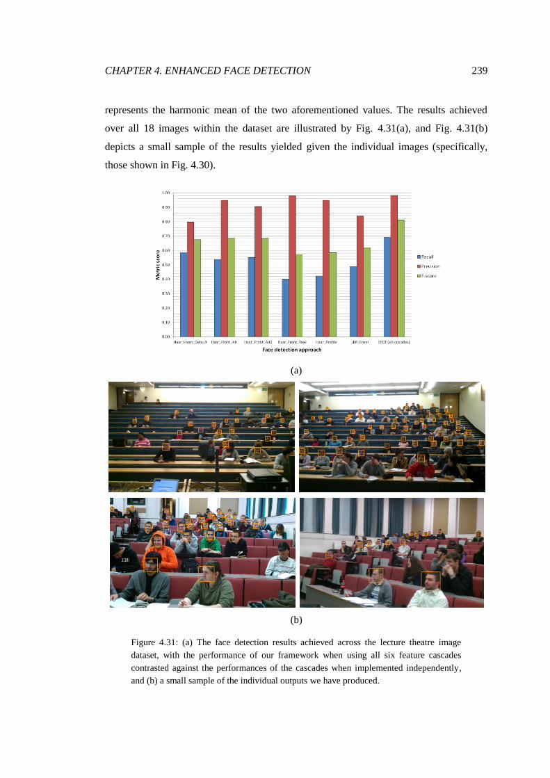
CHAPTER 4. ENHANCED FACE DETECTION 239
represents the harmonic mean of the two aforementioned values. The results achieved
over all 18 images within the dataset are illustrated by Fig. 4.31(a), and Fig. 4.31(b)
depicts a small sample of the results yielded given the individual images (specifically,
those shown in Fig. 4.30).
(a)
(b)
Figure 4.31: (a) The face detection results achieved across the lecture theatre image
dataset, with the performance of our framework when using all six feature cascades
contrasted against the performances of the cascades when implemented independently,
and (b) a small sample of the individual outputs we have produced.

240 CHAPTER 4. ENHANCED FACE DETECTION
As Fig. 4.31(a) shows, the performance of EFDF is comfortably superior to that of any of
the individual detectors it has utilised for this experiment, with an overall F-score of
around 0.81 having been attained. The recall rate we have achieved over the dataset is
roughly 10% greater than that of the next-best detector in that regard, the Default
cascade. Of course, positively identifying around 69% of all faces within the set still
leaves significant room for improvement (as some of the undetected weak faces depicted
by Fig. 4.31(b) confirm), but the potential for our framework to combine and enhance the
results of existing detection systems is strongly evidenced by these results. Furthermore,
whilst the precision of the independent Default cascade was rather poor, that of our own
system is better than that of any of the individually implemented detectors, as almost
99% of the positive classifications we have made are actually correct (in fact, the results
shown by Fig. 4.31(b) consist of 126 TPs and 0 FPs). Not only does this mean that our
classifications have been made with extremely high confidence, but also that there is
substantial room for manoeuver with regards to increasing the sensitivity of our system to
further improve the recall rates we achieve.
4.2.1.2 Precision-Recall Analysis
In order to get a more comprehensive sense of the potential for our framework to improve
upon the results of existing systems, we can employ precision-recall analysis. This form
of evaluation will involve generating precision and recall statistics just as before, but it
will now be done for a range of sensitivity settings for each of the detectors we are
working with. Where the individual cascades are concerned, the adjustment of detection
sensitivity is trivial, requiring merely changes to the discrete minimum neighbour
threshold to be made. Where our framework is concerned, however, the issue is
somewhat more complicated, as the parameters controlling its filters all influence its
overall performance to some degree. Therefore, we will be controlling sensitivity by
making simultaneous marginal adjustments to each of the four major parameters we have
optimised, which will allow us to construct a representative performance curve. In
addition to working with our “optimal” configuration, we will be generating results using
four alternative parameter value sets, designed to induce different levels of sensitivity.
These additional configurations are specified by Tab 4.1.
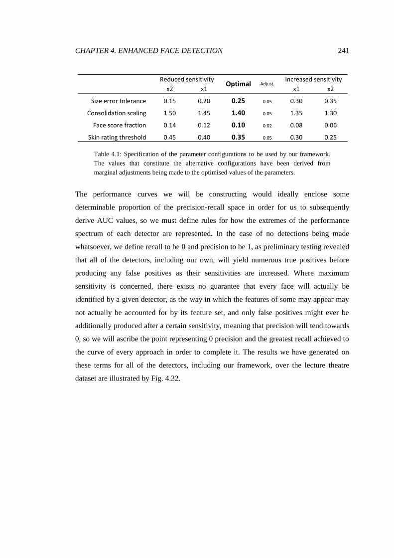
CHAPTER 4. ENHANCED FACE DETECTION 241
Table 4.1: Specification of the parameter configurations to be used by our framework.
The values that constitute the alternative configurations have been derived from
marginal adjustments being made to the optimised values of the parameters.
The performance curves we will be constructing would ideally enclose some
determinable proportion of the precision-recall space in order for us to subsequently
derive AUC values, so we must define rules for how the extremes of the performance
spectrum of each detector are represented. In the case of no detections being made
whatsoever, we define recall to be 0 and precision to be 1, as preliminary testing revealed
that all of the detectors, including our own, will yield numerous true positives before
producing any false positives as their sensitivities are increased. Where maximum
sensitivity is concerned, there exists no guarantee that every face will actually be
identified by a given detector, as the way in which the features of some may appear may
not actually be accounted for by its feature set, and only false positives might ever be
additionally produced after a certain sensitivity, meaning that precision will tend towards
0, so we will ascribe the point representing 0 precision and the greatest recall achieved to
the curve of every approach in order to complete it. The results we have generated on
these terms for all of the detectors, including our framework, over the lecture theatre
dataset are illustrated by Fig. 4.32.
x2 x1 x1 x2
Size error tolerance 0.15 0.20 0.25 0.05 0.30 0.35
Consolidation scaling 1.50 1.45 1.40 0.05 1.35 1.30
Face score fraction 0.14 0.12 0.10 0.02 0.08 0.06
Skin rating threshold 0.45 0.40 0.35 0.05 0.30 0.25
Reduced sensitivity Increased sensitivityOptimal Adjust.
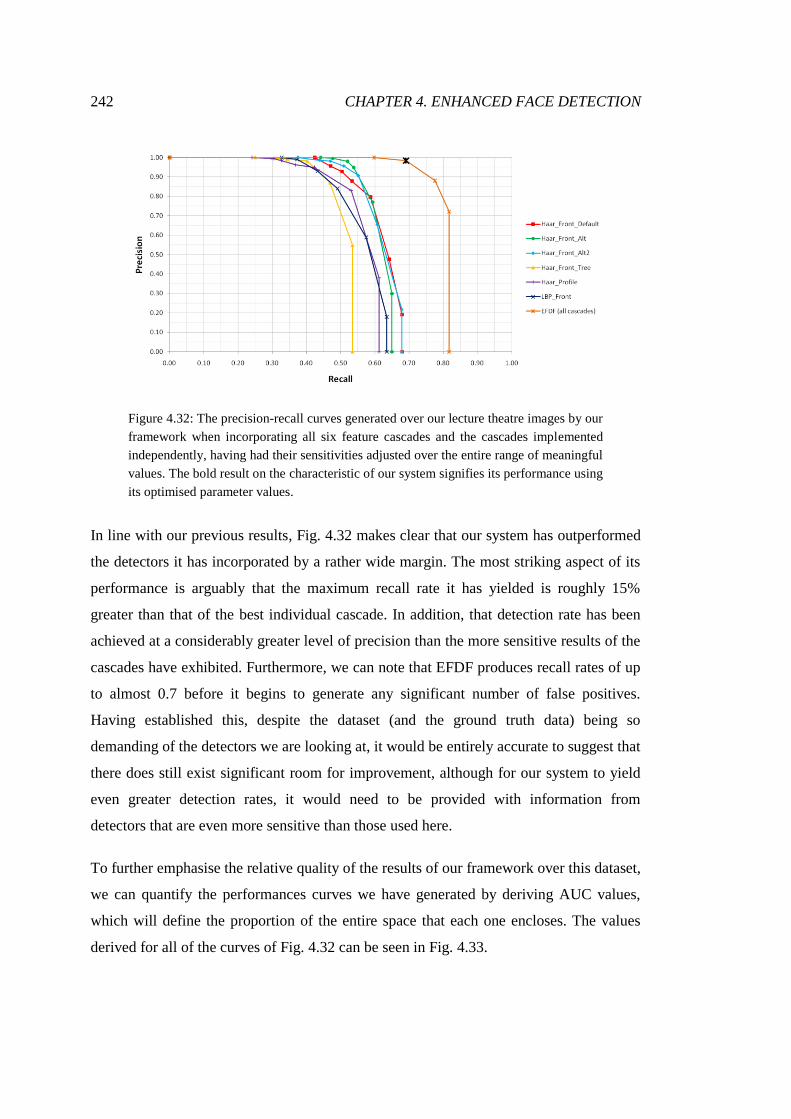
242 CHAPTER 4. ENHANCED FACE DETECTION
Figure 4.32: The precision-recall curves generated over our lecture theatre images by our
framework when incorporating all six feature cascades and the cascades implemented
independently, having had their sensitivities adjusted over the entire range of meaningful
values. The bold result on the characteristic of our system signifies its performance using
its optimised parameter values.
In line with our previous results, Fig. 4.32 makes clear that our system has outperformed
the detectors it has incorporated by a rather wide margin. The most striking aspect of its
performance is arguably that the maximum recall rate it has yielded is roughly 15%
greater than that of the best individual cascade. In addition, that detection rate has been
achieved at a considerably greater level of precision than the more sensitive results of the
cascades have exhibited. Furthermore, we can note that EFDF produces recall rates of up
to almost 0.7 before it begins to generate any significant number of false positives.
Having established this, despite the dataset (and the ground truth data) being so
demanding of the detectors we are looking at, it would be entirely accurate to suggest that
there does still exist significant room for improvement, although for our system to yield
even greater detection rates, it would need to be provided with information from
detectors that are even more sensitive than those used here.
To further emphasise the relative quality of the results of our framework over this dataset,
we can quantify the performances curves we have generated by deriving AUC values,
which will define the proportion of the entire space that each one encloses. The values
derived for all of the curves of Fig. 4.32 can be seen in Fig. 4.33.

CHAPTER 4. ENHANCED FACE DETECTION 243
Figure 4.33: The calculated area-under-curve (AUC) value for each of the precision-
recall performance characteristics depicted by Fig. 4.32, which were achieved over our
lecture theatre image dataset.
The AUC values illustrated by Fig. 4.33 confirm that the overall performance of our
framework over the lecture theatre imagery has been greatly superior to that of any of the
cascades it is has incorporated. It was over such inputs that we were primarily looking to
improve detection results, and this analysis indicates that we have been rather successful
in this regard, as recall rates have been increased considerably while precision has also
been enhanced. It should be noted that there is significant overlap in the feature sets of
some of the cascades, meaning that we could probably have achieved very similar results
using a subset of the six cascades we have used in this instance, but through
incorporating all of them, we have established that our framework can derive outstanding
results from huge sets of supplied detection data points. By virtue of the capacity to
incorporate the detections of any system that can yield simply coordinate and size
information, our system can achieve truly exceptional recall rates, as evidenced by this
analysis. Furthermore, it would appear that the calibration of our adaptive filters has been
so effective that their ability to identify and specifically eliminate false positives is nigh-
on impeccable, only beginning to falter when the parameters controlling them are
artificially adjusted.
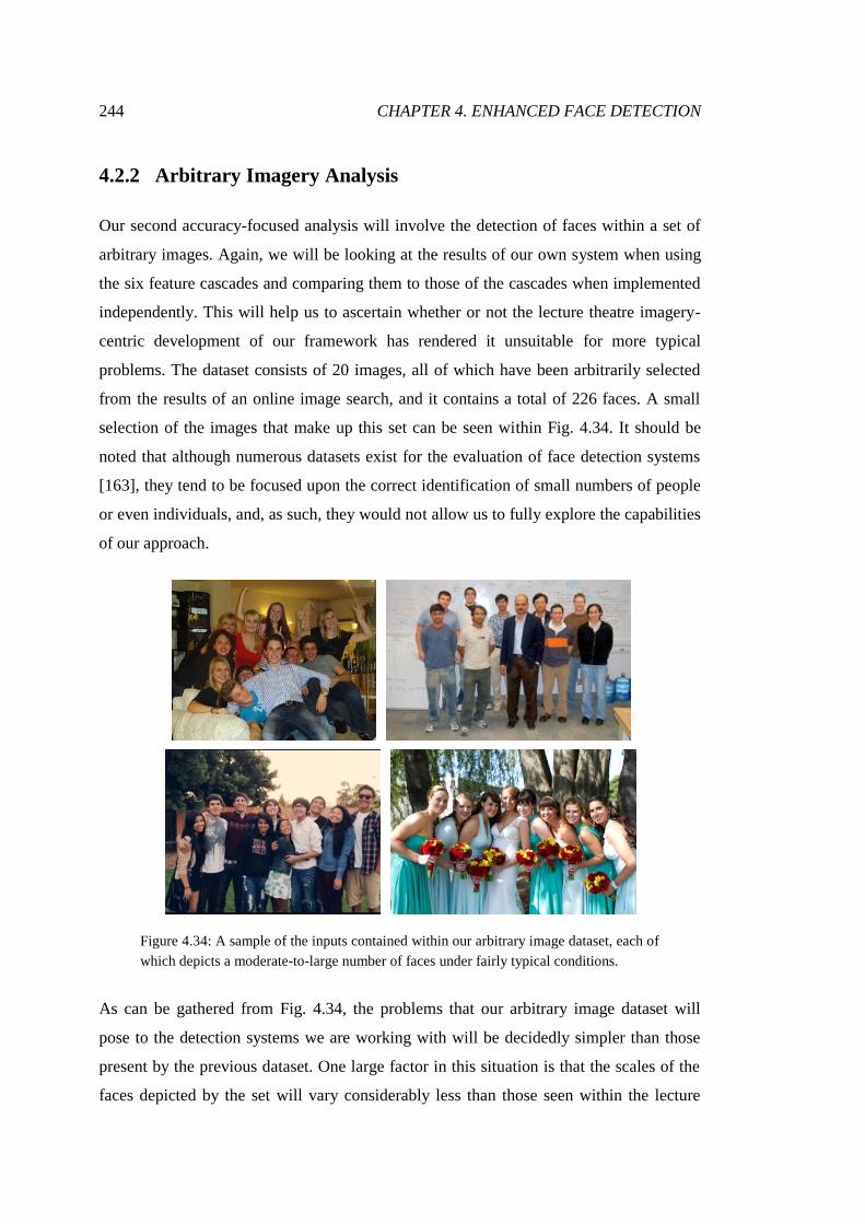
244 CHAPTER 4. ENHANCED FACE DETECTION
4.2.2 Arbitrary Imagery Analysis
Our second accuracy-focused analysis will involve the detection of faces within a set of
arbitrary images. Again, we will be looking at the results of our own system when using
the six feature cascades and comparing them to those of the cascades when implemented
independently. This will help us to ascertain whether or not the lecture theatre imagery-
centric development of our framework has rendered it unsuitable for more typical
problems. The dataset consists of 20 images, all of which have been arbitrarily selected
from the results of an online image search, and it contains a total of 226 faces. A small
selection of the images that make up this set can be seen within Fig. 4.34. It should be
noted that although numerous datasets exist for the evaluation of face detection systems
[163], they tend to be focused upon the correct identification of small numbers of people
or even individuals, and, as such, they would not allow us to fully explore the capabilities
of our approach.
Figure 4.34: A sample of the inputs contained within our arbitrary image dataset, each of
which depicts a moderate-to-large number of faces under fairly typical conditions.
As can be gathered from Fig. 4.34, the problems that our arbitrary image dataset will
pose to the detection systems we are working with will be decidedly simpler than those
present by the previous dataset. One large factor in this situation is that the scales of the
faces depicted by the set will vary considerably less than those seen within the lecture

CHAPTER 4. ENHANCED FACE DETECTION 245
theatre imagery, and there will be dramatically fewer instances of weak faces as a result.
It is for this reason that we would expect to see the independently implemented cascades
perform much more effectively than they did during our previous analysis. This means
that rather than significantly improve upon the results of those detectors, as there may
simply not be much room for improvement, we hope only to see our framework deliver
comparable results.
4.2.2.1 Default Configuration Analysis
The first stage of this analysis will involve generating results using the default
configuration of each detection approach. As before, our own system will operate using
its optimal parameter values, and the cascades will make classifications based upon a
minimum neighbour threshold of three. We will also again be utilising recall, precision,
and F-score to quantify the outputs produced by the various detectors. The results
achieved over our arbitrary image dataset are illustrated by Fig. 4.35.
Figure 4.35: The face detection results achieved across the arbitrary image dataset, with
the performance of our framework when using all six feature cascades contrasted against
the performances of the cascades when implemented independently.
In spite of our hopes to merely remain competitive over this set of relatively typical
images, the results of Fig. 4.35 would suggest that we have still managed to produce non-
negligible improvements to the performances of the individual cascades. The recall rate
of 0.95 that we have achieved over the images is marginally better than that of any of the
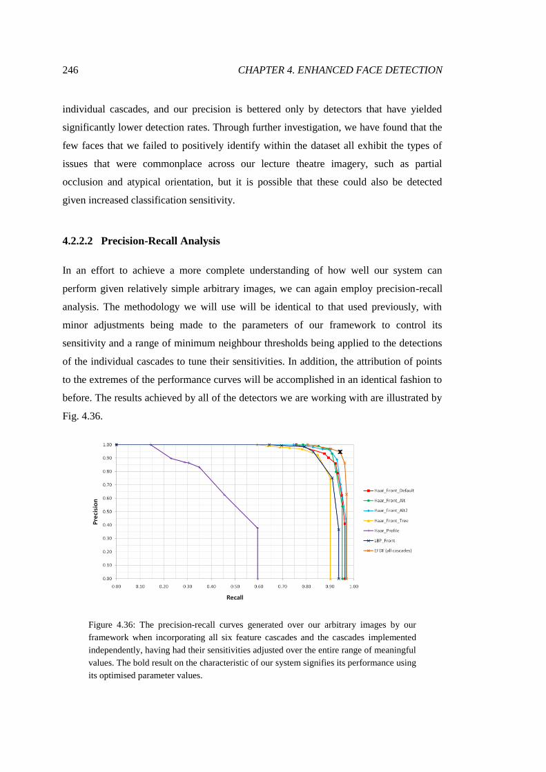
246 CHAPTER 4. ENHANCED FACE DETECTION
individual cascades, and our precision is bettered only by detectors that have yielded
significantly lower detection rates. Through further investigation, we have found that the
few faces that we failed to positively identify within the dataset all exhibit the types of
issues that were commonplace across our lecture theatre imagery, such as partial
occlusion and atypical orientation, but it is possible that these could also be detected
given increased classification sensitivity.
4.2.2.2 Precision-Recall Analysis
In an effort to achieve a more complete understanding of how well our system can
perform given relatively simple arbitrary images, we can again employ precision-recall
analysis. The methodology we will use will be identical to that used previously, with
minor adjustments being made to the parameters of our framework to control its
sensitivity and a range of minimum neighbour thresholds being applied to the detections
of the individual cascades to tune their sensitivities. In addition, the attribution of points
to the extremes of the performance curves will be accomplished in an identical fashion to
before. The results achieved by all of the detectors we are working with are illustrated by
Fig. 4.36.
Figure 4.36: The precision-recall curves generated over our arbitrary images by our
framework when incorporating all six feature cascades and the cascades implemented
independently, having had their sensitivities adjusted over the entire range of meaningful
values. The bold result on the characteristic of our system signifies its performance using
its optimised parameter values.
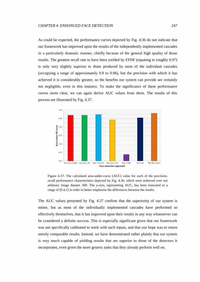
CHAPTER 4. ENHANCED FACE DETECTION 247
As could be expected, the performance curves depicted by Fig. 4.36 do not indicate that
our framework has improved upon the results of the independently implemented cascades
in a particularly dramatic manner, chiefly because of the general high quality of those
results. The greatest recall rate to have been yielded by EFDF (equating to roughly 0.97)
is only very slightly superior to those produced by most of the individual cascades
(occupying a range of approximately 0.9 to 0.96), but the precision with which it has
achieved it is considerably greater, so the benefits our system can provide are certainly
not negligible, even in this instance. To make the significance of these performance
curves more clear, we can again derive AUC values from them. The results of this
process are illustrated by Fig. 4.37.
Figure 4.37: The calculated area-under-curve (AUC) value for each of the precision-
recall performance characteristics depicted by Fig. 4.36, which were achieved over our
arbitrary image dataset. NB: The y-axis, representing AUC, has been truncated to a
range of [0.4,1] in order to better emphasise the differences between the results.
The AUC values presented by Fig. 4.37 confirm that the superiority of our system is
minor, but as most of the individually implemented cascades have performed so
effectively themselves, that it has improved upon their results in any way whatsoever can
be considered a definite success. This is especially significant given that our framework
was not specifically calibrated to work with such inputs, and that our hope was to return
merely comparable results. Instead, we have demonstrated rather plainly that our system
is very much capable of yielding results that are superior to those of the detectors it
incorporates, even given the more generic tasks that they already perform well on.

248 CHAPTER 4. ENHANCED FACE DETECTION
The relatively poor performance of the Profile cascade in this instance is interesting to
note, as it highlights how differently it functions to the other detectors we have been
working with. However, it is actually precisely because of its greatly dissimilar results
that a detector of its nature (i.e. one that looks for atypical features) would be ideally
suited to incorporation into our framework, as it would be able to supplement the results
of a more typical detector to a much greater extent than just another typical detector
would.
Where our lecture theatre imagery was concerned, we suggested that our system could
have yielded roughly equivalent results using a subset of the six cascades it had used to
generate its results. In this instance, we believe we could have achieved virtually the
same results using just one of the better-performing cascades, by maintaining its recall
rate and improving upon its precision through the application of our, demonstrably,
highly effective filters.
4.2.3 Detection Efficiency Evaluation
Although we have presented substantial evidence that our face detection methodology
has the potential to outperform existing approaches, it is important that we discover the
computational costs that our superior results can incur. In doing so, we can go further
towards establishing how suitable our system may be for real-world problems that
necessitate high accuracy, but where efficiency is also somewhat of a concern.
In this analysis, we will be investigating the offline performance of our detection
approach, in relation to the throughput times achieved over the two datasets we have been
interested in. The real-time generation of outputs will often not be critical where offline
processing tasks are concerned, but computational efficiency will always be an important
factor, as a system demonstrating far too little will render itself worthless, depending
upon the requirements of the problem at hand.
Initially, we will be looking at our framework in the context of all six of the feature
cascades we have been working with being incorporated for detection collation, just has
been the case during the generation of the results presented throughout Section 4.2.1 and
Section 4.2.2. Given this, we would expect the throughput times that we achieve to be
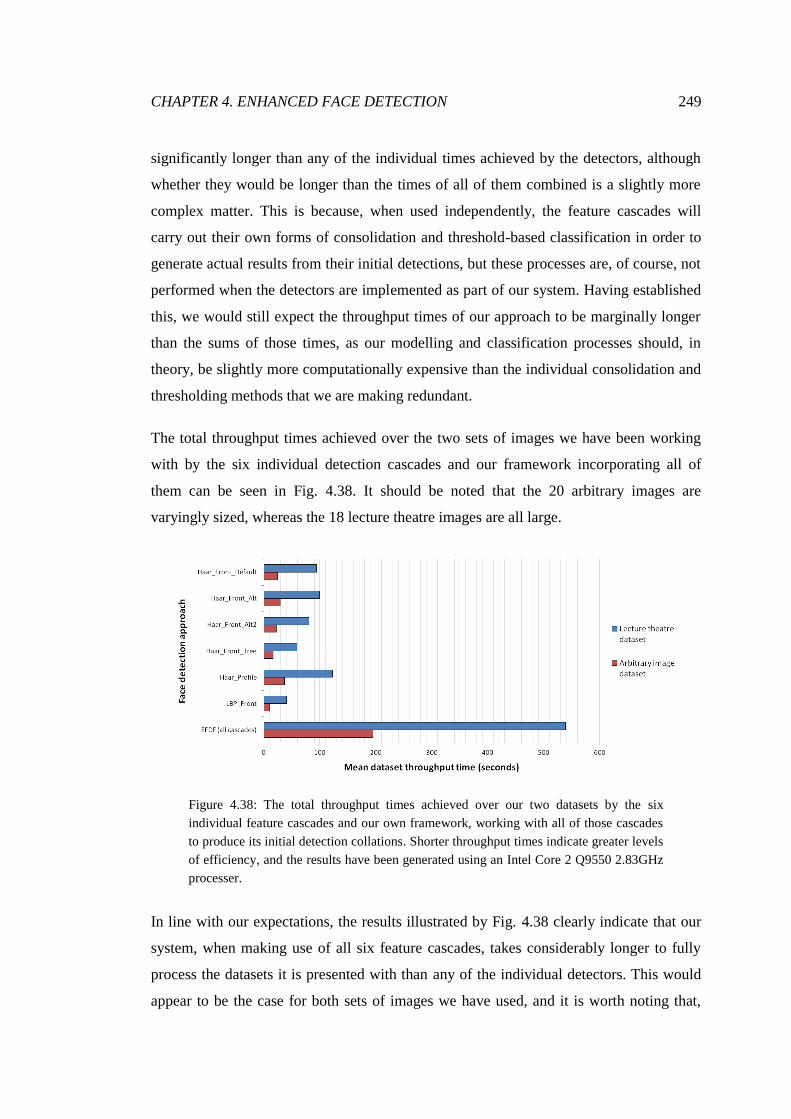
CHAPTER 4. ENHANCED FACE DETECTION 249
significantly longer than any of the individual times achieved by the detectors, although
whether they would be longer than the times of all of them combined is a slightly more
complex matter. This is because, when used independently, the feature cascades will
carry out their own forms of consolidation and threshold-based classification in order to
generate actual results from their initial detections, but these processes are, of course, not
performed when the detectors are implemented as part of our system. Having established
this, we would still expect the throughput times of our approach to be marginally longer
than the sums of those times, as our modelling and classification processes should, in
theory, be slightly more computationally expensive than the individual consolidation and
thresholding methods that we are making redundant.
The total throughput times achieved over the two sets of images we have been working
with by the six individual detection cascades and our framework incorporating all of
them can be seen in Fig. 4.38. It should be noted that the 20 arbitrary images are
varyingly sized, whereas the 18 lecture theatre images are all large.
Figure 4.38: The total throughput times achieved over our two datasets by the six
individual feature cascades and our own framework, working with all of those cascades
to produce its initial detection collations. Shorter throughput times indicate greater levels
of efficiency, and the results have been generated using an Intel Core 2 Q9550 2.83GHz
processer.
In line with our expectations, the results illustrated by Fig. 4.38 clearly indicate that our
system, when making use of all six feature cascades, takes considerably longer to fully
process the datasets it is presented with than any of the individual detectors. This would
appear to be the case for both sets of images we have used, and it is worth noting that,

250 CHAPTER 4. ENHANCED FACE DETECTION
proportionally, the results achieved over the two are very similar, as every detector,
including our own system, has taken roughly three times longer to fully process the set of
lecture theatre images than it has the set of arbitrary images, which suggests that the
general nature of inputs is not likely to significantly influence the relative efficiency of
our approach. It must be remembered, however, that the nature of given inputs will
determine the extent to which our framework can yield superior results. As we
demonstrated in Section 4.2.1, our system can greatly improve overall accuracy when it
is applied to complex imagery that poses challenging, atypical detection problems, and
perhaps its inferior efficiency can be justified in such cases, depending upon the specific
requirements of the given task. However, where more simple inputs are concerned, such
as those worked with in Section 4.2.2, over which the improvements made are less
significant, perhaps the application of our framework using all six feature cascades
simply results in unnecessary computational costs being incurred.
We can also note that sums of the throughput times of the individual cascades are shorter
than the times achieved by our framework, confirming that the consolidation and
thresholding processes of the isolated detectors are not as computationally expensive as
the stages of our system that succeed detection collation, which, again, was very much
expected to be the case. In order for us to fully understand how efficient our system has
the potential to be, it is necessary for us to investigate what proportion of total processing
time each of its major constituent components generally expends, which will reveal
where the most significant computational costs are being incurred. We have broken down
the throughput times achieved over our two datasets to quantify these proportions, and
the results, which represent the averages calculated between the two, are illustrated by
Fig. 4.39. It should be noted that the two sets of proportions we calculated over the
datasets were extremely similar, which is why we simply present the average values in
this instance.

CHAPTER 4. ENHANCED FACE DETECTION 251
Figure 4.39: The mean proportion of total dataset processing times expended by each of
the major components of our face detection framework, when used in conjunction with
all six facial feature cascades.
As Fig. 4.39 makes clear, when all six feature cascades are being utilised, by far the most
computationally expensive process that our approach consists of is detection collation, as
it evidently accounts for the vast majority of the time required for results to be generated.
Precise face detection, which involves the derivation of a set of high-confidence face
detections from the initial detections of a single cascade through consolidation and
thresholding, takes very little time by comparison, as might be expected. Using principal
component analysis to generate a size distribution model using that data then filtering the
collated detections according to that model seemingly takes a negligible amount of time,
but the consolidation of the resulting set of detections into a set of face candidates does
require some effort, albeit not an inordinate amount. The score-based classification of
those candidates is, again, computationally trivial, although colour-based is decidedly
less so, as the derivation of skin colour models and the application of them to candidates
in order to determine their skin ratings takes small, although non-negligible, periods of
time.
Overall, we consider this to be a greatly positive situation, as it means that the overall
efficiency of our framework is significantly more dependent upon the selection of the
incorporated detectors than on its modelling and classification processes, meaning that
those adaptive, non-adjustable components that we have developed are relatively efficient
simply by their design. The importance of this is that any potential adopter of the system
will have almost-complete control over its efficiency, which can, therefore, be adjusted to
meet the specific requirements of the given task in a trade-off against its accuracy. If we
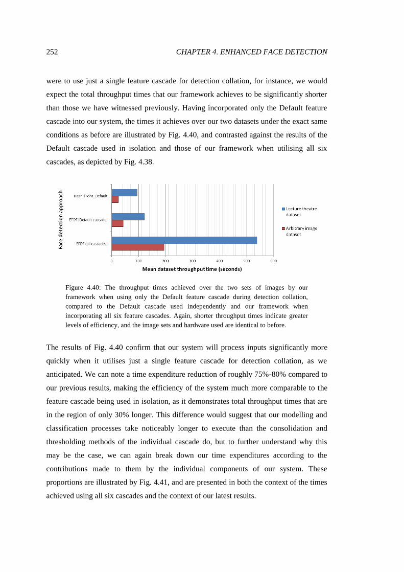
252 CHAPTER 4. ENHANCED FACE DETECTION
were to use just a single feature cascade for detection collation, for instance, we would
expect the total throughput times that our framework achieves to be significantly shorter
than those we have witnessed previously. Having incorporated only the Default feature
cascade into our system, the times it achieves over our two datasets under the exact same
conditions as before are illustrated by Fig. 4.40, and contrasted against the results of the
Default cascade used in isolation and those of our framework when utilising all six
cascades, as depicted by Fig. 4.38.
Figure 4.40: The throughput times achieved over the two sets of images by our
framework when using only the Default feature cascade during detection collation,
compared to the Default cascade used independently and our framework when
incorporating all six feature cascades. Again, shorter throughput times indicate greater
levels of efficiency, and the image sets and hardware used are identical to before.
The results of Fig. 4.40 confirm that our system will process inputs significantly more
quickly when it utilises just a single feature cascade for detection collation, as we
anticipated. We can note a time expenditure reduction of roughly 75%-80% compared to
our previous results, making the efficiency of the system much more comparable to the
feature cascade being used in isolation, as it demonstrates total throughput times that are
in the region of only 30% longer. This difference would suggest that our modelling and
classification processes take noticeably longer to execute than the consolidation and
thresholding methods of the individual cascade do, but to further understand why this
may be the case, we can again break down our time expenditures according to the
contributions made to them by the individual components of our system. These
proportions are illustrated by Fig. 4.41, and are presented in both the context of the times
achieved using all six cascades and the context of our latest results.

CHAPTER 4. ENHANCED FACE DETECTION 253
(a) (b)
Figure 4.41: The mean proportion of total throughput times dedicated to each of the
major components of our system when it uses just the Default cascade during detection
collation, in the context of (a) the times achieved using all six feature cascades and (b)
the times achieved using the single-cascade configuration.
As we discerned from Fig. 4.40, a considerable amount of time was saved by collating
detections using only the Default cascade, but Fig. 4.41(a) suggests that the
improvements to efficiency were not exclusive to the collation process. We can note that
the detection consolidation and colour-based classification components of our system
have also performed much more quickly than previously, and the reason for this is simply
that a reduced number of initial detections will generally result in fewer data points
needing to be processed at these stages. Due to the particular nature of consolidation,
whereby every detection will be compared to every other detection within the given
filtered set, the amount of time it expends will vary polynomially with the number of data
points it processes, and this is why it has seen much greater improvements to efficiency
than colour-based classification, the time expenditure of which, similarly to every other
component of our system, will vary in a much more linear fashion.
Despite the huge reductions in time expenditure, the inspection of Fig. 4.41(b) makes
clear that detection collation is still by far the biggest factor in the overall efficiency of
our framework. Again, this is encouraging, as it confirms that the computational
overheads of the other components of our system are not inherently prohibitive to highly
efficient face detection. It also means that our achieved throughput times could be
reduced even further than they have been already by using a detector that is even more
efficient than the Default feature cascade. As can be seen in Fig. 4.38, of the five other

254 CHAPTER 4. ENHANCED FACE DETECTION
cascades we have been working with, three of them actually achieved even lower
throughput times than the Default cascade, so we would fully expect our framework to
perform even more efficiently using any of them to provide initial detections instead.
However, simply employing the most efficient detector available to provide initial
detections with no concern for the accuracy of the results it can achieve would entirely
undermine the premise of our work. This notion also applies, of course, to our use of the
Default cascade as the only source of initial detections, which will be providing our
system with far less information to work with than the incorporation of all six cascades
would be, thereby degrading our potential to yield highly accurate results. Over our
lecture theatre images, which typically contain numerous weak faces that will not all be
detected by any individual cascade (hence the development of our framework for
detectors designed to identify different sets of features), we would expect that collating
detections using only the Default cascade would result in significantly reduced detection
rates in comparison to the results we presented in Section 4.2.1. To illustrate this, we
have again processed our lecture theatre dataset using our framework in its default
parameter configuration, but only the Default cascade has been used to provide
detections. The results we have achieved, in terms of recall rate, precision, and F-score,
can be seen in Fig. 4.42.
Figure 4.42: The results achieved by our framework over our set of lecture theatre
images using only the Default feature cascade during detection collation, contrasted
against the results it achieves using all six cascades, and the results of the Default
cascade when used independently.

CHAPTER 4. ENHANCED FACE DETECTION 255
As Fig. 4.42 demonstrates, the results we have achieved using only the Default cascade to
provide initial information are decidedly inferior to those we achieved previously. This is
very much as we anticipated, as it is indeed the reduced recall rates that have resulted in
the degradation of the overall F-score, with approximately 10% fewer true positive
classifications being made over the entire dataset, although the high precision of the
previous performance has been largely maintained. The comparison between our new
results and those of the Default cascade used in isolation is very encouraging, however,
as it would appear that our system has managed to greatly reduce the number of false
positive classifications the cascade produces without causing any significant detrimental
effects to its recall rates, resulting in a marked improvement to overall accuracy. This is
particularly positive as we are aware that this has been achieved without an excessive
amount of additional computational effort, as Fig. 4.40 illustrated.
Of course, our lecture theatre images pose very particular, atypical problems for face
detectors, so it is essential that we also investigate the effects of using only the Default
cascade when we are processing arbitrary images. As the analysis we presented in
Section 4.2.2 attests to, the results of the Default cascade when used independently were
much more comparable to those of our system (when using all six cascades) over the set
of arbitrary images than they were over the set of lecture theatre images. This was
primarily because the more strongly expressed features of the faces within the arbitrary
set were discoverable for the Default cascade, which left little room for our framework to
achieve superior detection rates through the incorporation of additional feature cascades.
We did, however, observe a non-negligible difference in precision, with our system
achieving superior overall accuracies as a result. Given this, and the effects of applying
our framework to the detections of the Default cascade depicted by Fig. 4.42, we would
expect that, over the entire arbitrary image set, using only the Default cascade for
collation would achieve very similar detection rates to using the cascade independently,
but yield some improvements to its precision, just as before. To discover whether this
would actually be the case, we have processed the arbitrary image dataset using our
framework in conjunction with only the Default cascade, and the results of this
experimentation are illustrated by Fig. 4.43.

256 CHAPTER 4. ENHANCED FACE DETECTION
Figure 4.43: The results achieved by our framework over the set of arbitrary images
using only the Default feature cascade during detection collation, contrasted against the
results it achieves using all six cascades, and the results of the Default cascade when
used independently.
As Fig. 4.43 elucidates, our expectations of the results were entirely accurate, as we can
firstly note the virtually identical detection rates that we have achieved in this instance
compared to both of the previous cases. Whilst not reducing the number of true positive
classifications made should not be considered success on its own, that this has been
accomplished in conjunction with significant improvements to precision being made is
highly positive, as the yielded results in this instance are essentially no different to those
achieved using all six cascades, but have been generated with much greater efficiency.
Furthermore, we have again demonstrated that we can noticeably improve the results of
an existing detector without incurring inordinate additional computational costs.
Overall, it would seem that the efficiency of our system will largely be determined by the
efficiency of the detectors chosen to be incorporated for the purposes of detection
collation. As we have demonstrated, utilising a broad range of feature cascades will
improve results significantly given complex imagery, but will also result in the system
being relatively inefficient, although this may be considered an acceptable trade-off given
the requirements of the task. Over simpler inputs, the framework will perform just as
inefficiently when using the same set of cascades, but the improvements to accuracy that
it is likely to yield will be significantly reduced, so the trade-off will perhaps no longer be
reasonable, and a smaller set of incorporated detectors may be far more appropriate. The
selection of initial detectors, therefore, should be dictated by the nature and specification

CHAPTER 4. ENHANCED FACE DETECTION 257
of the given problem, and the overall efficiency of our system will then simply be
determined by that choice, in addition to the relatively minor computational costs of our
modelling and classification processes.
It must be remembered that the feature cascades we have used to demonstrate the
capabilities of our framework were not necessarily all required for the results we have
achieved to be as encouraging as they have been. As they were developed to be
implemented independently, there will be considerable overlap in the features that they
look for in order to identify face regions, and it is highly likely that virtually the same
results could have been achieved over the lecture theatre image dataset (the one for which
detection rates were significantly improved) with a smaller number of cascades than we
have been working with, which would have yielded far greater efficiencies. Even though
different detectors are likely to return different results when processing any given input,
there will be diminishing returns as more and more are incorporated for detection
collation, as fewer and fewer faces will remain unfound, so the incurred costs to
efficiency will yield smaller and smaller benefits. However, it was our desire to prove
that our framework could process huge amounts of raw data and still derive highly
accurate detection results from it, and that there would be no upper limit on the number
of detectors that it could incorporate, regardless of how inefficiently the resulting system
may perform.

258
Chapter 5
Discussion and Conclusions
In this chapter, we will summarise and discuss the research we have conducted towards
exploring our hypothesis, present a number of objective conclusions that we have drawn,
and offer suggestions for possible improvements that could be made to our work in the
future.
5.1 Synoptic Discussion
In Chapter 3, we detailed the entire developmental process of our new adaptive skin
segmentation approach, from its inception and design to its implementation, and
concluded with a thorough evaluation, assessing both its accuracy and its efficiency.
Initially, we identified a number of issues with a wide range of existing, and popular, skin
segmentation methodologies when applied to our lecture theatre imagery, even when the
images are of high general quality. These issues related primarily to poor recall rates
under certain circumstances and inadequate degrees of precision under others, and were
strongly linked to the intensity and tone of the illumination present within the inputs. The
overarching problem, however, was the matter of achieving consistency. Over inputs of
different nature, we could not conclude that any of the approaches we had identified were
capable of attaining adequate consistency. This was rather understandable, as the type of
problem we were presenting could be considered somewhat more complex than that of a
typical arbitrary image, but the fact remained that we could not identify a solution.

CHAPTER 5. DISCUSSION AND CONCLUSIONS 259
It was the lack of consistency in the results of the existing techniques that lead to the
realisation that, in order for accurate segmentations to be regularly achieved over such
inputs, we must implement an adaptive approach, capable of segmenting skin according
to the specific conditions exhibited by given inputs. Although a number of adaptive
methodologies for skin segmentation did already exist, we highlighted a number of
reasons why they were not necessarily appropriate answers to our large-scale problem.
Rather than adopting any of them, therefore, we endeavoured to develop our own
adaptive segmentation system.
The first stage of development involved identifying the means by which we could sample
input images, and we found the use of feature-based face detection to be highly effective,
and an ideal fit given the nature of our task. Additionally, we found some precedence for
its successful application to problems such as ours. We proceeded to carefully configure
its implementation and ensure it would perform in a completely beneficial manner, with
an emphasis placed heavily upon the avoidance of false positive detections. We
recognised that the regions returned by the face detector would often contain non-
negligible proportions of background information, so we decided to define circular sub-
regions within the results that would eliminate such data from further consideration, with
the preservation of likely skin pixels also being a major factor in this process.
Furthermore, we found that within the sub-regions we were generating, there were still
considerable numbers of non-skin pixels. These would usually instead pertain to facial
features such as eyes and mouths, but could also represent hair or glasses. Having
identified that these non-skin pixels tended to exhibit low visual intensity, we decided
that an effective method to isolate actual skin pixels from them was to filter them
according to their relative luma values, and applying such a process to every face
detection sub-region for a given image would yield a set of pixels that we could be
confident represented the skin tones present within that image.
Given such a set of pixels, the objective became effectively deriving a representative skin
colour model. There were numerous options available, but by far the most viable and
suitable was Gaussian modelling. Not only would it allow us to construct models from
our positive skin colour samples alone, it would also result in the interpolation of likely
skin colours that may have been undersampled initially, and afford the possibility of

260 CHAPTER 5. DISCUSSION AND CONCLUSIONS
adjustable thresholding due to its continuous nature. Furthermore, by also opting to
operate within the normalised rg colour space, we could take full advantage of skin tones
tending to cluster elliptically within that space. Given a set of sample pixels, the
construction of a representative Gaussian model was trivially simple, and required merely
the determination of the mean colour vector and covariance matrix of the set.
Having derived a skin colour model for a given input image, we would be ready to
segment the skin from within it. By utilising the definition of a joint probability density
function, we could determine the skin likelihood of any given input colour vector. This
alone could not yield any form of segmentation, however, as this would require the
definition of a probability threshold. By applying such a threshold to calculated
likelihoods, we could classify pixels as either “skin” or “non-skin”, thereby achieving an
output – a segmented image. Rather than being content with our system classifying pixels
in this manner, we attempted to optimise it, and ensure that the results it was producing
were being delivered with maximal efficiency. Our first step was to base classifications
directly on Mahalanobis distances, thereby reducing the number of calculations required
to determine the skin likelihoods of pixels. This was only a relatively minor
improvement, however, as having to perform such classifications for every pixel within
any given image was still computationally expensive. We modified the system, therefore,
to limit the number of pixels that necessitated such calculations to an absolute minimum,
by using the given threshold to define a range of possible skin colours for any given
model. Whilst this did drastically improve the performance of our system, we decided
that it would be interesting to discover the effects of going just a step further, and using
the defined ranges themselves to determine the classification of pixels. We expected that
this would further improve performance somewhat, but potentially yield slightly less
accurate results.
The result of our optimisation was two final forms of our system: AGSS-Mahal and
AGSS-Range. Whilst we were extremely confident in the design decisions we had made
to develop them, we could not be sure that they would actually outperform existing
approaches without stringent evaluation. Firstly, we were focused on assessing
segmentation accuracy. Initially, this involved quantifying the results we could achieve
for the lecture theatre imagery, and comparing those results to those yielded by the

CHAPTER 5. DISCUSSION AND CONCLUSIONS 261
existing approaches at outset of this endeavour. Our somewhat rudimentary single-
segmentation results demonstrated that our system was capable of achieving much
greater consistency than any of the existing approaches, but this was far from sufficient
evidence of its superiority. We then applied ROC analysis to our results, and found that it
suggested our system was very marginally better than the others, but the severe class
imbalance of the data greatly limited the amount of information we could ascertain. It
was for this reason that we also applied PR analysis, which is invariant to such issues,
and discovered that our results were actually significantly superior to those of the existing
techniques, leading us to conclude that we had, in fact, solved the problem we had
initially set out to solve.
Despite this success, we were also keen to learn just how applicable our system would be
to more generic segmentation tasks. Therefore, we made use of an existing annotated
database of arbitrary images. We used similar evaluation methodologies to our previous
analysis, and initially found that ROC analysis actually deemed our system to be inferior
to a number of others, although the reliability of these results was somewhat mitigated
again by the presence of class imbalance. The results of PR analysis were more
encouraging, as they suggested that our system was roughly on par with the best of the
existing approaches, but we were still not entirely satisfied. Of course, we knew our
system would not be capable of segmenting any skin from within a given image if it
contained no detectable faces, but the prevalence of such images within the dataset we
were working with was so great that our overall results turned out to be rather
disappointing. We, therefore, formed a subset of the images, all of which would facilitate
face detection, in the hopes that it would allow us to properly emphasise how much more
effectively our system could segment the skin from such images than the existing
approaches. Despite the effects of class skew still being present, ROC analysis reported a
greatly improved performance, determining our overall results to be as good as those of
any other technique. PR analysis, on the other hand, actually indicated that our
performances over the new dataset were substantially superior to any others, suggesting
that both forms of our system were very much capable of delivering excellent
segmentations for generic tasks, assuming the relatively consistent presence of detectable
faces, and that it had not been over-engineered for lecture theatre-based imagery.
Interestingly, we found that the differences in the results of AGSS-Mahal and AGSS-

262 CHAPTER 5. DISCUSSION AND CONCLUSIONS
Range were, for the most part, essentially negligible, which we did not entirely expect,
although could be explained by the extreme specificity of the skin colour models we
generate to the images they pertain to.
In addition to these analyses, we also experimented with an existing adaptive
methodology. This was intended to prove whether or not the strengths of our approach
were limited to its adaptability, and whether there may exist some degree of
overspecialisation with regards to the lecture theatre imagery, which may have been
compensated for by adaptation during our previous arbitrary image analysis. Over both
the lecture theatre images and the set of detection-facilitating arbitrary images, we found
that our overall results were superior to those of the existing approach, especially in the
case of the former. We concluded, therefore, that our system was not overly specialised
and that its strengths extended beyond its capacity to adapt.
Aside from segmentation accuracy, it was paramount for the potential applicability of our
system that we established how efficient it was. Producing even greatly superior
segmentations may not matter if the amount of effort required to produce them
substantially outweighs the requirements of alternative options. Firstly, we were
concerned with performance over an offline segmentation task, which involved
measuring the throughput times achieved by various approaches over a large set of
arbitrary images. We found that our system took considerably longer to complete the task
than most of the existing approaches, but, as it was an offline problem, the extent of this
may not necessarily render it unsuitable. Furthermore, we noted that the majority of the
time our system spent processing any given image was actually committed to face
detection, and that the amount of time it took to classify pixels was actually less than the
amount expended by the existing approaches, which was especially true for AGSS-
Range.
Our second efficiency analysis concerned real-time performance, as we attempted to
establish operating frame rates for the techniques. We used a fixed-resolution image
stream pertaining to a single user interacting with a webcam, and initially found that the
achieved frame rates were in line with the results of our offline analysis. Although this
was to be expected, we identified that, for such a task, performing face detection for each
and every frame was almost entirely unnecessary, as the potential for the environment to

CHAPTER 5. DISCUSSION AND CONCLUSIONS 263
change on an image-by-image basis would be virtually non-existent. We therefore
experimented with different recalibration intervals, and found that even incredibly short
intervals would allow our system to perform at much greater average frame rates than any
of the existing approaches, with AGSS-Range being particularly impressive. We also
identified that frequent recalibrations would introduce output stream stutters, and came to
the conclusion that the ideal face detection interval for a task should simply be dictated
by the requirements of the problem.
Overall, we consider the work that was carried out during the course of Chapter 3 to have
been extremely successful. We initially identified a particular problem, established that a
broad range of existing approaches could not effectively solve this problem, and then set
about developing a solution. Having designed a system that we believed would yield
satisfactory results, we broke down its individual components and ensured they were
implemented optimally. Given our completed system, we rigorously evaluated the
accuracy of its segmentations as well as its efficiency, and found that it could
comfortably outperform the existing techniques in both regards.
In Chapter 4, we described the whole developmental process of our new approach to
large-scale face detection, detailing its conception, design, implementation, and
calibration, and then thoroughly evaluated its detection capabilities and its computational
efficiency.
At the outset, we demonstrated a number of inadequacies with some popular existing
technology (the Viola-Jones detection system [147]) when applied to our atypically
complex lecture theatre imagery. We found that a number of issues were commonplace
where such large-scale inputs were concerned, such as a lack of focus, suboptimal
orientation, and partial occlusion. These problems, amongst others, resulted in the
features of numerous faces being weakly expressed, which was hugely detrimental to the
detection rates of the feature-based detectors. Although we found that simply reducing
the threshold for positive classification would increase the achieved recall rates, doing so
would also produce greater numbers of false positives and degrade overall precision.
We asserted that if provided with the high-sensitivity detection results of numerous face
detection systems, we could apply adaptive filters based upon supplementary modalities

264 CHAPTER 5. DISCUSSION AND CONCLUSIONS
invariant to the highlighted issues in order to achieve exceptional accuracies. These filters
would, in theory, have the capacity to precisely eliminate false positive detections from
generated sets, and each would give us greater confidence that those retained do actually
pertain to faces. The specific properties that we identified as suitable for the basis of
detection classification were size and colour, as we believed we could accurately derive
models to represent them for any given input image through sampling. We had
highlighted a number of previous efforts to reinforce face detection results with
additional modalities, but found the approaches presented to be fundamentally
inappropriate for the type of problem we were attempting to solve.
The first stage of developing our system involved establishing the means by which initial
detections would be collated. As we decided to demonstrate the functioning of our
framework using the feature cascades provided by the OpenCV library, this was a rather
straightforward process. These detectors all return results in the exact same format (a set
of squares with certain sizes and locations) and can be trivially configured for high
sensitivity in the exact same manner. Were we to incorporate different forms of detectors,
specific considerations may need to be made for their results to be appropriately
integrated. We chose to implement every face detection cascade available to us so that we
would have maximal information to process and ensure that we gave our system every
possible opportunity to achieve excellent detection results, even though there would be
significant crossover in the results each would typically return.
No matter the nature of the given input, detection collation will always yield huge
amounts of noise, as the process of high-sensitivity detection will return numerous
regions that bear only the slightest resemblance to a face, and will often be nothing more
than a mathematical fluke. Our efforts to eliminate false positive detections began with
the implementation of a size-based filter. For a number of reasons, we decided that
predefined size thresholds would be entirely unsuitable, as they would fail to account for
several factors relating to the capture of given images, such as the distances from the
people they depict and the sizes of the environments they have been taken within.
Therefore, we developed an adaptive approach, which used principal component analysis
to derive image-specific planar size-coordinate models from high-confidence face
detection data. When combined with appropriate error bounds, we found that filtering

CHAPTER 5. DISCUSSION AND CONCLUSIONS 265
detections according to their size using our generated models to be an extremely effective
method of discarding large numbers of false detections.
As encouraging as the results from our size-based filtering technique were, we found that
the number of retained detections would typically be in the hundreds if not thousands
(when using the six feature cascades), but, clearly, these could not all uniquely represent
a face. In reality, due to the nature of the detection cascades, each face would be
associated with a rather large number of duplicate detections, where the specific number
will correlate with the discernibility of its features, so determining the means to derive
individual candidates from those groups became a necessity, if our final results were to
be in any way accurate. To achieve this, we applied a consolidation algorithm that would
scale individual detections up then assess the encapsulation of other detections, which
would allow us to discover clusters that could be averaged in order to produce face
candidates. The calibration of this process had to be carried out with great precision, as a
scaling factor too great would result in partially occluded faces being lost and a factor too
small would lead to all the detections of faces not being consolidated.
The process of detection consolidation was a preparatory process for actual classification,
and it was through “scores” that we would first begin to classify candidates and produce
actual outputs. These scores represented the number of detections that had been
consolidated to form each candidate, and could be considered a measure of how strongly
candidates expressed facial features. Even though we established that feature
discernibility could not be relied upon exclusively to make accurate classifications, to
ignore the information entirely would have been negligent. Therefore, we decided to
classify every candidate with a compellingly large score as a face. The determination of a
positive classification threshold was not trivial, however, as the scores of candidates were
greatly dependent upon several factors, including image quality and the nature of the
detectors used for detection collation. To solve this issue, we used the greatest score
within any given set as a guideline for the overall effect of those variables, and then
established the positive classification threshold for the given image as a fraction of that
value. We calibrated the specific fraction to be used to maximise the number of true
positives we could produce without also yielding any false positives. Where the
candidates not classified as faces were concerned, those with a score of just 1 were

266 CHAPTER 5. DISCUSSION AND CONCLUSIONS
outright discarded, as empirical evidence suggested that the vast majority of these
pertained to non-face regions, and those that remained were reserved for further
processing.
Although we were able to successfully identify large numbers of faces using our score-
based classification process, it would typically be incapable of finding particularly large
proportions of them within our lecture theatre imagery, due to the natural prevalence of
weak faces. It is for this reason that we turned to colour-based classification, with the
hope that it could distinguish between faces and non-faces in the instances where scores
could not allow us to. We adopted our own adaptive modelling approach to build skin
colour representations specific to given images, as we had already established how
effectively it could overcome the variabilities inherent to the lecture theatre images. We
used these models to calculate skin ratings for the low-score candidates, indicating how
much their general colour tones resembled skin. We could then apply a threshold to these
ratings in order to positively identify additional faces, where the threshold was calibrated
to achieve maximal recall while maintaining impeccable precision. Since the candidates
with skin ratings below the threshold exhibited neither compelling facial features nor
skin-like colour, we discarded them, deeming them to represent only non-face regions.
The union of the score-classified and colour-classified face sets constituted the final
output of our system.
Although we were confident that our system had been developed soundly, we
endeavoured to evaluate it fully to confirm our beliefs. Initially, we used our framework
to detect faces within a set of lecture theatre images, as we considered it extremely
important to provide concrete evidence that we had made significant advances towards
solving the problems that we identified as the basis for our work. We first presented
results generated by our framework and the individual cascades using their default
sensitivities, which demonstrated rather plainly that we had achieved greatly superior
results. These outputs could not represent the entire operational spectrums of the
detection systems, however, which is why we also utilised precision-recall analysis. This
form of evaluation can be considered decidedly more comprehensive, which is why its
extremely positive results were so encouraging for us, and could be considered an
indication of our success in meeting our initial objectives. That being said, the detection

CHAPTER 5. DISCUSSION AND CONCLUSIONS 267
rates we yielded did leave significant room for further improvement, although, where our
framework is concerned, this could only be accomplished through the incorporation of
even more sensitive initial detectors.
To further establish the value and applicability of our work, we decided it was
appropriate to ascertain how well it would perform over a set of arbitrary images. Despite
performing well over the complex lecture theatre imagery, excellent performance over
simpler images was not guaranteed, as the calibration of our system could potentially
have rendered it overly specialised. The results produced during our default sensitivity
analysis were initially encouraging, as they suggested that our framework was at least as
capable as any of the individual cascades, but we again utilised precision-recall analysis
to expand upon them. We found that our overall performance was marginally superior,
but the degree of improvement that our system could offer was limited because the
results of the individual cascades were of rather high quality themselves. Nevertheless,
we demonstrated that our framework could enhance face detection results even when the
inputs were not of the type we primarily designed it for, signifying its flexibility.
The final stage of our evaluatory process involved assessing the relative efficiency of our
system. Firstly, we discovered that the throughput times that our framework (when
incorporating all six of the facial feature cascades) achieved over the image sets were
significantly longer than those of the individually implemented cascades, but this was not
unexpected, as detection collation required each of these detectors to be run before their
results could be processed. Using all six cascades was originally intended to demonstrate
how accurate the results of our system could be, so we felt it necessary to establish how
efficiently it would perform using just one of them. Encouragingly, we found that our
efficiency was still greatly dependent upon that of the detectors chosen to be
incorporated, and that the computational overheads of our framework were minor,
although non-negligible.
Overall, we regard the research that we have detailed within Chapter 4 to have been
greatly successful. We first established the existence of a particular problem and
identified its root causes, and then designed a methodology that we believed could
overcome them. Having soundly implemented every component of our proposed
solution, we provided strong evidence that it could go a long way towards solving our

268 CHAPTER 5. DISCUSSION AND CONCLUSIONS
original problem, and demonstrated that our work could also be successfully applied to
generic tasks.
Throughout our evaluations, we held the reliability of the results we generated in the
highest regard. Where system accuracy was concerned, we ensured that the images,
ground truth data, and metrics used were in no way particularly favourable to our work.
Furthermore, during our efficiency analyses, we fully accounted for the non-deterministic
nature of measuring throughput times and frame rates by extensively repeating our
experiments numerous times and calculating representative mean values. It is for these
reasons that we value our results so highly and draw such encouragement from them.
Further to the results we have presented within this thesis, our skin segmentation system
and face detection framework have also been implemented as fully functional Android
applications. Both of these exhibit the encouraging levels of accuracy and efficiency that
our evaluations have demonstrated, evidencing strongly our belief that our systems would
very much be applicable to real-world problems.
5.2 Itemised Conclusions
The research described by Chapter 3 produced a number of key findings pertaining to the
field of skin segmentation:
Several existing skin segmentation techniques that are commonly applied to
generic problems struggle greatly to yield accurate results on a consistent
basis when applied to complex lecture theatre-based imagery.
Feature-based face detection can be an extremely effective method of
sampling images with the intention of building representative skin colour
models.
By defining sub-regions within face detection regions, uninteresting
background information can be eliminated on a very consistent basis, with
minimal skin pixels being lost.

CHAPTER 5. DISCUSSION AND CONCLUSIONS 269
Regions within detection windows that pertain to non-skin features can be
effectively discarded by filtering them according to their relative luma
values, as they will typically be of lower intensity than the skin pixels around
them.
Skin colour distributions in the normalised rg colour space conform very
strongly to normal distribution, as they tend to form elliptical clusters.
The bivariate Gaussian distribution models that we derive from filtered pixel
sets are highly representative of the skin within the images that have been
built for.
Classifying pixels by applying an adjustable threshold to continuous
likelihood values is an extremely flexible and effective method of
segmenting skin.
By making classifications based directly on Mahalanobis distances rather
than probabilities, calculations can be saved on each and every pixel within a
given image, improving efficiency at no cost to accuracy.
By using the value of the threshold being applied in conjunction with the
given colour model, we can define a range of “possible skin” colours for an
image. In this way, the number of computationally expensive calculations
being performed for any given input can be drastically reduced, again
without accuracy being compromised in any way.
The defined colour ranges themselves could also be used as effective
classifiers, theoretically achieving even greater efficiency at, potentially,
some small costs to accuracy.
Over lecture theatre-based imagery, the system we have developed is
significantly more consistent than any of the existing approaches, capable of
delivering impressive results for inputs of greatly differing nature.

270 CHAPTER 5. DISCUSSION AND CONCLUSIONS
Tasked with segmenting skin from a set of arbitrary images where the
presence of detectable faces is not guaranteed, the overall results of our
system may be inferior to those of other approaches, but this would depend
on how great the proportion of images that do not facilitate face detection is.
When the presence of detectable faces within arbitrary inputs can be assured,
the segmentations that our system produces are markedly superior to those of
any other methodology.
In general, although AGSS-Range does achieve marginally greater recall
rates than AGSS-Mahal, its precision is slightly inferior, but these
differences would appear to cancel out in most circumstances to yield very
similar overall accuracies for the two classification modes.
As it is demonstrably capable of yielding highly precise results, our system
would excel at providing “seed” pixels to a segmentation approach that
involves skin region growing.
As we have demonstrated that our system outperforms an existing adaptive
methodology over both lecture theatre and arbitrary image datasets, we can
conclude that the strengths of our system are not limited to its adaptive
nature, and that it is not overspecialised to the lecture theatre imagery.
For segmentation tasks that necessitate colour models being generated on a
per-image basis, our system will take significantly longer to output results
than most of the existing approaches, although AGSS-Range does perform
more quickly than AGSS-Mahal.
Where real-time segmentation is concerned, establishing an interval on
which to perform face detection and recalibrate the skin colour model being
used, rather than doing so for every input frame, will result in the
performance of AGSS-Range being greatly superior to that of any other
technique, and the performance of AGSS-Mahal being superior to the
existing approaches in most cases, but dependent upon the prevalence of
skin-like pixels.

CHAPTER 5. DISCUSSION AND CONCLUSIONS 271
The research detailed by Chapter 4, which covered our work towards enhancing face
detection, also yielded a number of key findings:
Existing feature-based face detection technology (specifically, the popular
Viola-Jones system [147]) is incapable of producing accurate detection
results over our atypically complex lecture imagery, because of the
prevalence of “weak” faces.
By collating the results of multiple face detection systems (that look for
different properties), we can acquire information on many more apparent
faces than any individual detector can typically provide.
Principal component analysis can be used in conjunction with high-threshold
face detection results to generate highly representative face size distribution
models, which can identify false detections extremely precisely.
The consolidation of near-duplicate two-dimensional data points can be
accomplishing highly effectively by scaling up individual group members
and assessing the encapsulation of other group members.
Detection consolidation “scores” correlate very strongly with feature
discernibility and, as such, can be used to precisely positively identify large
numbers of faces.
If an image region is associated with only a single detection after the
application of six high-sensitivity feature cascades, it is extremely likely that
that region will not pertain to a face.
How skin-like the colour of a face candidate appears to be can be described
by a “skin rating”, which can be established by employing our own adaptive
skin colour modelling approach to derive a model for the given image and
then applying that representation to the constituent pixels of the candidate.

272 CHAPTER 5. DISCUSSION AND CONCLUSIONS
The true nature of regions that express some, but not compelling, feature-
based face resemblance can be determined extremely accurately by applying
a threshold to their calculated skin ratings, separating candidate sets into
“face” and “non-face” classes.
Over complex imagery that presents large-scale problems, our framework
can achieve much greater recall rates than the detectors it uses to provide
initial detection information, as it successfully combines the correct, but
insufficient, positive detections of each to yield a single set of faces.
Where simpler, arbitrary images are concerned, our system will, at the very
least, maintain the high detection rates that the incorporated detectors may
achieve when implemented independently, signifying that it is not
overspecialised for lecture theatre imagery.
As a result of the meticulous calibration of our classification processes, our
system is extremely adept at identifying false positives, and can eliminate
them based upon inordinate size, feature indiscernibility, and unconvincing
general colour.
Even given problems for which detection rates cannot be significantly
improved, our framework can considerably improve upon the levels of
precision achieved by the detectors it incorporates.
The efficiency of our system will be largely determined by the efficiency of
the detectors it employs for detection collation, as the computational costs of
our classification processes will vary with the amount of information
provided, and will almost always be relatively minor.
For the purpose of achieving maximal detection accuracies at optimal
efficiencies, the selection of incorporated detectors should be made to
specifically suit the requirements of the given problem, as simpler tasks will
rarely necessitate the use of a broad range of detectors.

CHAPTER 5. DISCUSSION AND CONCLUSIONS 273
5.3 Potential Extensions
Despite being extremely satisfied with the results we achieved over the course of Chapter
3, it would be entirely fair to suggest that the system we developed is not perfect. Given
its adaptive nature, having a method to sample images in order to build skin colour
models specific to them is a necessity. We chose to adopt the feature-based face detector
of Viola and Jones [147], and found it to be extremely effective, providing plenty of
information from which representative models could be derived. The drawback of this
sampling methodology is, of course, that it will fail should the given input image contain
no detectable faces.
Currently, if our attempts to detect a face within an image return no results, then we
simply conclude that the image contains no skin, and move onto the next input. As we
discovered during our evaluation using the DB Skin dataset, however, the potential for
arbitrary images to contain significant regions of skin but no detectable faces is far from
negligible. This is problematic, as our system is simply incapable of processing such
images, whereas the other segmentation approaches we have looked at do still provide
results of some value, as the absence of detectable face is, of course, of no concern to
them whatsoever.
Given that our implementation of the face detector is already extremely flexible, and it
can be assured that if it returns no results for an image then there exists no configuration
that would allow it to, the only solutions we could attempt to implement would represent
fairly significant departures from our current methodology. Rather than changing our
sampling approach, the simplest, and perhaps the most effective, option might be to
adjust the behaviour of our system in the event that it finds no faces. Instead of coming to
the conclusion that images that contain no detectable faces simply contain no skin, we
could choose to believe that the face detector has failed, and that there is actually skin to
be segmented. In such a scenario, we would have built no skin colour model, so we
would require alternate means by which to classify pixels.
Depending upon the nature of the given problem, there are two options available to us
should we not be able to build a skin colour model for an image. The first of these is

274 CHAPTER 5. DISCUSSION AND CONCLUSIONS
simply to reuse the model we created most recently. This option would be appropriate for
real-time scenarios, whereby the previous model would likely pertain to the same
environment as the one we have just attempted to build. However, over a set of arbitrary
inputs, for instance, where the environment depicted may change on an image-to-image
basis, this solution would be far from effective, as the models our system constructs are,
by design, completely specific to their respective inputs, and could never be considered
globally applicable.
In such a situation, we could instead actually adopt one of the existing approaches. As it
was fairly consistently the best performer of the previous techniques, we could, for
instance, apply the YCbCr model of Hu et al. [43] to images whenever we fail to build a
model due to a lack of detectable faces. Doing so would represent the best of both worlds
as far as segmenting skin from images is concerned, as for the large number of cases
where we can detect a face, build a model, and segment skin, we will achieve the best
results possible, and then in the few images where we cannot do so, we can still yield
results that are considerably better than erroneous “no skin” conclusions. Of course, such
a modification to our system would mean that it would no longer be capable of correctly
identifying situations where the input image really does contain no skin, so the possibility
of such inputs occurring should be weighed against the possibility of images that contain
skin but no detectable faces occurring, which would be dictated by the nature of the given
problem. Over the DB Skin dataset, for instance, there were actually many more
instances of the latter than of the former, so the application of an alternate segmentation
technique would result in a marked improvement to the overall results of our system.
Similarly, although the face detection framework we developed can deliver excellent
detection results given even complex imagery, as we have demonstrated, there are certain
aspects of it that could be improved upon to offer even greater flexibility. For instance,
the existing detectors that we have been using for the purposes of demonstration to
provide initial detection information throughout this chapter (the OpenCV feature
cascades) are very similar in nature, and, running at high sensitivity, can each potentially
return dozens of results pertaining to any single face. Were these results to be collated
with those of a system that would only ever return a maximum of one detection per face
without any consideration for this fact, there would clearly be great imbalance in the

CHAPTER 5. DISCUSSION AND CONCLUSIONS 275
influence that each detector would have over the results produced, where the contribution
of the single-detection system would regularly be negligible. One way to overcome this
issue would be to establish a set of simple calibration images, which would be processed
prior to the collation of detections for any input dataset. In this way, we could determine
the nature of the typical outputs of detectors, and assign weights to them in order to
ensure balanced contributions to the collated detection sets.
Although the issue has never been prevalent during our experimentation, modelling face
size distributions according to individual two-dimensional planes may not always yield
perfect representations of environments, even if the error bounds we apply do allow for
some degree of inaccuracy. If we were to consider, for instance, a semi-circular
auditorium, it is likely that the faces of the people within it would not conform to a planar
distribution and, as such, would be misrepresented by a planar model. We could attempt
to solve this potential issue by generating multiple planes per distribution whenever the
average error expressed by our third principal component (representing residual error in
the given model) exceeds a certain threshold, or we could employ a higher-order
polynomial function to perform our surface modelling, but the necessity for such
complex modifications to be made is questionable when the prevalence of issues caused
by our current system is, evidently, so low.
An aspect of our filters that would almost certainly benefit from some refinement would
be the automatic elimination of face candidates that have a score of just 1, indicating
severely weak feature expression. Empirically, we have found that it is through this
decision rule that most ultimately undetected faces with initial detections associated with
them are lost. We deemed this process to be acceptable during the implementation of our
system, as we discovered that the number of faces that would typically go undetected as a
result of it was seemingly significantly smaller than the number of false positives it
would successfully discard. We currently have no concrete potential solution to this
problem, although we could examine the effects of retaining such candidates for colour-
based classification and weighting their skin ratings according to the precise conformity
of their sizes to the given generated distribution model, exploring further the properties
that we know we can reliably work with.

276
Bibliography
[1] M. F. Augusteijn and T. L. Skujca. Identification of human faces through texture-
based feature recognition and neural network technology. In Proceedings of the
IEEE Conference on Neural Networks, pages 392-398, 1993.
[2] K. K. Bhoyar and O. G. Kakde. Skin color detection model using neural networks
and its performance evaluation. In Journal of Computer Science, 6(9):963-968,
2010.
[3] K. Boyd, K. H. Eng, and C. D. Page. Area under the precision-recall curve: Point
estimates and confidence intervals. In Machine Learning and Knowledge
Discovery in Databases, pages 451-466, 2013.
[4] A. P. Bradley. The use of the area under the ROC curve in the evaluation of
machine learning algorithms. In Pattern Recognition, 30(7):1145-1159, 1997.
[5] J. Brand and J. S. Mason. A comparative assessment of three approaches to pixel-
level human skin-detection. In Proceedings of the 15th International Conference
on Pattern Recognition, 1:1056-1059, 2000.
[6] L. Bretzner, I. Laptev, and T. Lindeberg. Hand gesture recognition using multi-
scale colour features, hierarchical models and particle filtering. In Proceedings of
the Fifth IEEE International Conference on Automatic Face and Gesture
Recognition, pages 423-428, 2002.
[7] D. A. Brown, I. Craw, and J. Lewthwaite. A SOM based approach to skin
detection with application in real time systems. In Proceedings of the 2001
British Machine Vision Conference, 1:491-500, 2001.
[8] S. C. Brubaker, J. Wu, J. Sun, M. D. Mullin, and J. M. Rehg. On the design of
cascades of boosted ensembles for face detection. Georgia Institute of
Technology Technical Report GIT-GVU-05-28, 2005.

BIBLIOGRAPHY 277
[9] T. Bruckhaus. The business impact of predictive analytics. In Knowledge
Discovery and Data Mining, pages 114-138, 2007.
[10] G. Buchsbaum. A spatial processor model for object colour perception. In
Journal of the Franklin Institute, 310(1):1-26, 1980.
[11] W. Burgin, C. Pantofaru, and W. D. Smart. Using depth information to improve
face detection. In Proceedings of the 6th ACM/IEEE International Conference on
Human-Robot Interaction, pages 119-120, 2011.
[12] J. Canny. A computational approach to edge detection. In IEEE Transactions on
Pattern Analysis and Machine Intelligence, 8(6):679-698, 1986.
[13] D. Chai and A. Bouzerdoum. A Bayesian approach to skin color classification in
YCbCr color space. In Proceedings of the 2000 IEEE Region 10 International
Conference (TENCON), 2:421-424, 2000.
[14] I. Chakravarti, R. Laha, and J. Roy. Handbook of Methods of Applied Statistics,
volume 1, John Wiley & Sons, 1967.
[15] K.-M. Cho, J.-H. Jang, and K.-S. Hong. Adaptive skin-color filter. In Pattern
Recognition, 34(5):1067-1073, 2001.
[16] H. Cooper and R. Bowden. Sign language recognition using boosted volumetric
features. In Proceedings of the IAPR Conference on Machine Vision
Applications, pages 359-362, 2007.
[17] T. F. Cootes, C. J. Taylor, D. H. Cooper, and J. Graham. Active shape models:
Their training and application. In Computer Vision and Image Understanding,
61(1):38-59, 1995.
[18] I. Craw, H. Ellis, and J. Lishman. Automatic extraction of face features. In
Pattern Recognition Letters, 5:183-187, 1987.
[19] F. Crow. Summed-area tables for texture mapping. In Proceedings of
SIGGRAPH, 18(3):207-212, 1984.
[20] N. Dala and B. Triggs. Histogram of oriented gradients for human detection. In
Proceedings of the 2005 IEEE Conference on Computer Vision and Pattern
Recognition, 1:886-893, 2005.

278 BIBLIOGRAPHY
[21] J. Davis and M. Goadrich. The relationship between precision-recall and ROC
curves. In Proceedings of the 23rd Internation Conference on Machine Learning,
pages 233-240, 2006.
[22] J. Deng. W. Dong, R. Socher, L.-J. Li, K. Li, and L. Fei-Fei. ImageNet: A large-
scale hierarchical image database. In Proceedings of the 2009 IEEE Conference
on Computer Vision and Pattern Recognition, pages 248-255, 2009.
[23] S. Fahlman and C. Lebiere. The cascade-correlation learning architecture. In
Advances in Neural Information Processing Systems 2, pages 524-532, 1990.
[24] S. S. Farfade, M. J. Saberian, and L.-J. Li. Multi-view face detection using deep
convolutional neural networks. In Proceedings of the 5th ACM International
Conference on Multimedia Retrieval, pages 643-650, 2015.
[25] T. Fawcett. An introduction to ROC analysis. In Pattern Recognition Letters,
27(8):861-874, 2006.
[26] P. F. Felzenszwalb, R. B. Girshick, and D. McAllester. Cascade object detection
with deformable part models. In Proceedings of the 2010 IEEE Conference on
Computer Vision and Pattern Recognition, pages 2241-2248, 2010.
[27] P. F. Felzenszwalb, R. B. Girshick, D. McAllester, and D. Ramanan. Object
detection with discriminatively trained part-based models. In IEEE Transactions
on Pattern Analysis and Machine Intelligence, 32(9):1627-1645, 2010.
[28] P. F. Felzenszwalb and D. P. Huttenlocher. In International Journal of Computer
Vision, 61(6):55-79, 2005.
[29] M. A. Fischler and R. A. Elschlager. The representation and matching of pictorial
structures. In IEEE Transactions on Computers, 22(1):67-92, 1973.
[30] G. L. Foresti, C. Micheloni, L. Snidaro, and C. Marchiol. Face detection for
visual surveillance. In Proceedings of the 12th IEEE International Conference on
Image Analysis and Processing, pages 115-120, 2003.
[31] Y. Freund and R. E. Schapire. A decision-theoretic generalization of on-line
learning and an application to boosting. In Journal of Computer and System
Sciences, 55(1):119-139, 1997.

BIBLIOGRAPHY 279
[32] J. Fritsch, S. Lang, M. Kleinehagenbrock, G. A. Fink, and G. Sargerer.
Improving adaptive skin color segmentation by incorporating results from face
detection. In Proceedings of the 11th IEEE International Workshop on Robot and
Human Interactive Communication, pages 337-343, 2002.
[33] Y. Fu, G. Guo, and T. S. Huang. Age synthesis and estimation via faces: A
survey. In IEEE Transactions on Pattern Analysis and Machine Intelligence,
32(11):1955-1976, 2010.
[34] A. S. Georghiades, P. N. Belhumeur, and D. J. Kriegman. From few to many:
Illumination cone models for face recognition under variable lighting and pose.
In IEEE Transactions on Pattern Analysis and Machine Intelligence, 23(6):643-
660, 2001.
[35] G. Gomez. On selecting colour components for skin detection. In Proceedings of
the 16th International Conference on Pattern Recognition, 2:961-964, 2002.
[36] R. Gopalan, S. Taheri, P. Turaga, and R. Chellappa. A blur-robust descriptor with
applications to face recognition. In IEEE Transactions on Pattern Analysis and
Machine Intelligence, 34(6):1220-1226, 2012.
[37] H. P. Graf, T. Chen, E. Petajan, and E. Cosatto. Locating faces and facial parts.
In Proceedings of the First International Workshop on Automatic Face and
Gesture Recognition, pages 41-46, 1995.
[38] H. P. Graf, E. Cosatto, D. Gibbon, M. Kocheisen, and E. Petajan. Multimodal
system for locating heads and faces. In Proceedings of the Second International
Conference on Automatic Face and Gesture Recognition, pages 88-93, 1996.
[39] H. Hatem, Z. Beiji, and R. Majeed. A survey of feature base methods for human
face detection. In International Journal of Control and Automation, 8(5):61-78,
2015.
[40] G. E. Hinton, N. Srivastava, A. Krizhevsky, I. Sutskever, and R. R.
Salakhutdinov. Improving neural networks by preventing co-adaptation of feature
detectors. In arXiv, arXiv:1207.0580, 2012.
[41] C.-C. Hsieh, D.-H. Liou, and W.-R. Lai. Enhanced face-based adaptive skin color
model. In Journal of Applied Science and Engineering, 15(2):167-176, 2012.
280 BIBLIOGRAPHY
[42] R.-L. Hsu, M. Abdel-Mottaleb, and A. K. Jain. Face detection in color images. In
IEEE Transactions on Pattern Analysis and Machine Intelligence, 24(5):696-706,
2002.
[43] M. Hu, S. Worrall, A. H. Sadka, and A. M. Kondoz. A fast and efficient chin
detection method for 2-D scalable face model design. In Proceedings of
International Conference on Visual Information Engineering 2003, pages 121-
124, 2003.
[44] J. Huang and C. X. Ling. Using AUC and accuracy in evaluating learning
algorithms. In IEEE Transactions on Knowledge and Data Engineering,
17(3):299-310, 2005.
[45] Q. Huynh-Thu, M. Meguro, and M. Kaneko. Skin-color extraction in images with
complex background and varying illumination. In Proceedings of the Sixth IEEE
Workshop on Applications of Computer Vision, pages 280-285, 2002.
[46] N. A. Ibraheem, R. Z. Khan, and M. M. Hasan. Comparative study of skin color
based segmentation techniques. In International Journal of Applied Information
Systems, 5(10):24-38, 2013.
[47] V. Jain and E. G. Learned-Miller. FDDB: A benchmark for face detection in
unconstrained settings. UMass Amherst Technical Report UM-CS-2010-009,
2010.
[48] C. M. Jarque and A. K. Bera. Efficient tests for normality, homoscedasticity and
serial independence of regression residuals. In Economics Letters, 6(3):255-259,
1980.
[49] L. A. Jeni, J. F. Cohn, and F. De La Torre. Facing imbalanced data:
Recommendations for the use of performance metrics. In Proceedings of the
2013 Humaine Association Conference on Affective Computing and Intelligent
Interaction, pages 245-251, 2013.
[50] H. Jin, Q. Liu, H. Lu, and X. Tong. Face detection using improved LBP under
Bayesian framework. In Proceedings of the First IEEE Symposium on Multi-
Agent Security and Survivability, pages 306-309, 2004.
[51] I. T. Jolliffe. Choosing a subset of principal components or variables. Principal
component analysis, Springer New York, pages 92-114, 1986.
BIBLIOGRAPHY 281
[52] M. J. Jones and J. M. Rehg. Statistical color models with application to skin
detection. In International Journal of Computer Vision, 46(1):81-96, 2002.
[53] M. Jones and P. Viola. Fast multi-view face detection. Mitsubishi Electric
Research Laboratories Technical Report TR2003-96, 2003.
[54] P. Kakumanu, S. Makrogiannis, and N. Bourbakis. A survey of skin-colour
modeling and detection methods. In Pattern Recognition, 40:1106-1122, 2007.
[55] P. Kakumanu, S. Makrogiannis, R. Bryll, S. Panchanathan, and N. Bourbakis.
Image chromatic adaptation using ANNs for skin color adaptation. In
Proceedings of the 16th IEEE International Conference on Tools with Artificial
Intelligence, pages 478-485, 2004.
[56] I. Kalinovskii and V. Spitsyn. Compact convolutional neural network cascade for
face detection. In arXiv, arXiv:1508.01292, 2015.
[57] T. Kanade. Picture processing by computer complex and recognition of human
faces, PhD thesis, Kyoto University, 1973.
[58] C. Kanan and G. W. Cottrell. Color-to-grayscale: Does the method matter in
image recognition?. In PLoS ONE, 7(1):e29740, 2012.
[59] S. Kawato and J. Ohya. Automatic skin-color distribution extraction for face
detection and tracking. In Proceedings of the 5th International Conference on
Signal Processing, 2:1415-1418, 2000.
[60] W.-S. Kim, D.-S. Cho, and H. M. Kim. Interplane prediction for RGB video
coding. In Proceedings of the 2004 International Conference on Image
Processing, 2:785-788, 2004.
[61] M. Kirby and L. Sirovich. Application of the Karhunen-Loeve procedure for the
characterization of human faces. In IEEE Transactions on Pattern Analysis and
Machine Intelligence, 12(1):103-108, 1990.
[62] T. Kohonen. Self-organization and associative memory, Springer, 1989.
[63] T. Kohonen. The self-organizing map. In Neurocomputing, 21(1):1-6, 1998.
[64] S. B. Kostiantis. Supervised machine learning: A review of classification
techniques. In Informatica, 31(3):249-268, 2007.

282 BIBLIOGRAPHY
[65] M. Kostinger, P. Wohlhart, P. M. Roth, and H. Bischof. Annotated facial
landmarks in the wild: A large-scale, real-world database for facial landmark
localization. In Proceedings of the 2011 International Conference on Computer
Vision Workshops, pages 2144-2151, 2011.
[66] C. Kotropoulos and I. Pitas. Rule-based face detection in frontal views. In
Proceedings of the International Conference on Acoustics, Speech and Signal
Processing, 4:2537-2540, 1997.
[67] J. Kovac, P. Peer, and F. Solina. Human skin colour clustering for face detection.
In Proceedings of the IEEE Region 8 EUROCON 2003: Computer as a Tool,
2:144-148, 2003.
[68] A. Krizhevsky, I. Sutskever, and G. E. Hinton. ImageNet classification with deep
convolutional neural networks. In Advances in Neural Information Processing
Systems, 25:1097-1105, 2012.
[69] N. Kumar, A. C. Berg, P.N. Belhumeur, and S. K. Nayar. Attribute and simile
classifiers for face verification. In Proceedings of the 12th IEEE International
Conference on Computer Vision, pages 365-372, 2009.
[70] C. H. Lampert. An efficient divide-and-conquer cascade for nonlinear object
detection. In Proceedings of the 2010 IEEE Conference on Computer Vision and
Pattern Recognition, pages 1022-1029, 2010.
[71] E. H. Land and J. J. McCann. Lightness and retinex theory. In Journal of the
Optical Society of America, 61(1):1-11, 1970.
[72] A. Lanitis, C. J. Taylor, and T. F. Cootes. An automatic face identification
system using flexible appearance models. In Image and Vision Computing,
13(5):393-401, 1995.
[73] J. Y. Lee and S. I. Yoo. An elliptical boundary model for skin color detection. In
Proceedings of the 2002 International Conference on Imaging Science, Systems,
and Technology, pages 472-479, 2002.
[74] T. K. Leung, M. C. Burl, and P. Person. Finding faces in cluttered scenes using
random labeled graph matching. In Proceedings of the Fifth IEEE International
Conference on Computer Vision, pages 637-644, 1995.
BIBLIOGRAPHY 283
[75] K. Levi and Y. Weiss. Learning object detection from a small number of
examples: The importance of good features. In Proceedings of the 2004 IEEE
Conference on Computer Vision and Pattern Recognition, 2:53-60, 2004.
[76] H. Li, Z. Lin, X. Shen, J. Brandt, and G. Hua. A convolutional neural network
cascade for face detection. In Proceedings of the 2015 IEEE Conference on
Computer Vision and Pattern Recognition, pages 5325-5334, 2015.
[77] S. Li, L. Zhu, Z. Zhang, A. Blake, H. Zhang, and H. Shum. Statistical learning of
multi-view face detection. In Proceedings of the 7th European Conference on
Computer Vision, pages 67-81, 2002.
[78] W.-H. Liao and Y.-H. Chi. Estimation of skin color range using achromatic
features. In Proceedings of the Eighth International Conference on Intelligent
Systems Design and Applications, 2:493-497, 2008.
[79] R. Lienhart, A. Kuranov, and V. Pisarevsky. Empirical analysis of detection
cascades of boosted classifiers for rapid object detection. In Pattern Recognition,
Springer Berlin Heidelberg, pages 297-304, 2003.
[80] R. Lienhart and J. Maydt. An extended set of Haar-like features for rapid object
detection. In Proceedings of 2002 International Conference on Image
Processing, 1:900-903, 2002.
[81] H. Lilliefors. On the Kolmogorov-Smirnov test for normality with mean and
variance unknown. In Journal of the American Statistical Association, 62:399-
402, 1967.
[82] S.-H. Lin, S.-Y. Kung, and L.-J. Lin. Face recognition / detection by probabilistic
decision-based neural network. In IEEE Transactions on Neural Networks,
8(1):114-132, 1997.
[83] P. C. Mahalanobis. On the generalised distance in statistics. In Proceedings of the
National Institute of Sciences of India, 2(1):49-55, 1936.
[84] L. T. Maloney and B. A. Wandell. Color constancy: A method for recovering
surface spectral reflectance. In Journal of the Optical Society of America,
3(1):29-33, 1986.
[85] C. D. Manning and H. Schutze. Foundations of statistical natural language
processing, MIT Press, 1999.
284 BIBLIOGRAPHY
[86] J. B. Martinkauppi, M. N. Soriano, and M. V. Laaksonen. Behaviour of skin
color under varying illumination seen by different cameras at different color
spaces. In Proceedings of the SPIE Conference on Machine Vision Applications
in Industrial Inspection, 4301:102-112, 2001.
[87] M. Mathias, R. Benenson, M. Pedersoli, and L. Van Gool. Face detection without
bells and whistles. In Proceedings of the 13th European Conference on Computer
Vision, pages 720-735, 2014.
[88] S. McKenna, S. Gong, and Y. Raja. Modelling facial colour and identity with
Gaussian mixtures. In Pattern Recognition, 31(12):1883-1892, 1998.
[89] J. Meynet, V. Popovici, and J.-P. Thiran. Face detection with boosted Gaussian
features. In Pattern Recognition, 40(8):2283-2291, 2007.
[90] J. Miao, B. Yin, K. Wang, L. Shen, and X. Chen. A hierarchical multiscale and
multiangle system for human face detection in a complex background using
gravity-centre template. In Pattern Recognition, 32(7):1237-1248, 1999.
[91] T. Mita, T. Kaneko, and O. Hori. Joint Haar-like features for face detection. In
Proceedings of the Tenth IEEE International Conference on Computer Vision,
2:1619-1626, 2005.
[92] A. Mittal, A. Zisserman, and P. H. S. Torr. Hand detection using multiple
proposals. In Proceedings of the 22nd British Machine Vision Conference, 75:1-
11, 2011.
[93] L. Nanni, A. Lumini, F. Dominio, and P. Zanuttigh. Effective and precise face
detection based on color and depth data. In Journal of Applied Computing and
Informatics, 10(1):1-13, 2014.
[94] A. Nayak and S. Chaudhuri. Self-induced color correction for skin tracking under
varying illumination. In Proceedings of the 2003 International Conference on
Image Processing, 3:1009-1012, 2003.
[95] M. S. Nikulin. Chi-squared test for normality. In Proceedings of the International
Vilnius Conference on Probability Theory and Mathematical Statistics,
2:119:122, 1973.
BIBLIOGRAPHY 285
[96] T. Ojala, M. Pietikainen, and T. Maenpaa. Multiresolution gray-scale and rotation
invariant texture classification with local binary patterns. In IEEE Transactions
on Pattern Analysis and Machine Intelligence, 24(7), 971-987, 2002.
[97] V. A. Oliveira and A. Conci. Skin detection using HSV color space. In
Proceedings of the SIBGRAPI 2009 Workshops, pages 1-2, 2009.
[98] N. Oliver, A. P. Pentland, and F. Berard. LAFTER: Lips and face real time
tracker. In Proceedings of the 1997 IEEE Conference on Computer Vision and
Pattern Recognition, pages 123-129, 1997.
[99] Z. Omary and F. Mtenzi. Machine learning approach to identifying the dataset
threshold for the performance estimators in supervised learning. In International
Journal for Infonomics, 3(3):314-325, 2010.
[100] A. Opelt, A. Pinz, and A. Zisserman. A boundary-fragment-model for object
detection. In Proceedings of the 9th European Conference on Computer Vision,
pages 575-588, 2006.
[101] E. Osuna, R. Freund, and F. Girosi. Training support vector machines: An
application to face detection. In Proceedings of the 1997 IEEE Conference on
Computer Vision and Pattern Recognition, pages 130-136, 1997.
[102] M. Pantic and L. J. M. Rothkrantz. Automatic analysis of facial expressions: The
state of the art. In IEEE Transactions on Pattern Analysis and Machine
Intelligence, 22(12):1424-1445, 2000.
[103] C. Papageorgiou, M. Oren, and T. Poggio. A general framework for object
detection. In Proceedings of the Sixth International Conference on Computer
Vision, pages 555-562, 1998.
[104] C. Papageorgiou and T. Poggio. A trainable system for object recognition. In
International Journal of Computer Vision, 38(1):15-33, 2000.
[105] M.-T. Pham and T.-J. Cham. Fast training and selection of Haar features using
statistics in boosting-based face detection. In Proceedings of the 11th IEEE
International Conference on Computer Vision, pages 1-7, 2007.
[106] S. L. Phung, A. Bouzerdoum, and D. Chai. A novel skin color model in YCbCr
color space and its application to human face detection. In Proceedings of the
2002 International Conference on Image Processing, 1:289-292, 2002.

286 BIBLIOGRAPHY
[107] S. L. Phung, D. Chai, and A. Bouzerdoum. A universal and robust human skin
color model using neural networks. In Proceedings of the 2001 International
Joint Conference on Neural Networks, 4:2844-2849, 2001.
[108] M. Propp and A. Samal. Artificial neural network architectures for human face
detection. In Intelligent Engineering Systems through Artifical Neural Networks,
volume 2, 1992.
[109] P. Pudil, J. Novovicova, and J. Kittler. Floating search methods in feature
selection. In Pattern Recognition Letters, 15(11), pages 1119-1125, 1994.
[110] A. Rajagopalan, K. Kumar, J. Karlekar, R. Manivasakan, M. Patil, U. Desai, P.
Poonacha, and S. Chaudhuri. Finding faces in photographs. In Proceedings of the
Sixth IEEE International Conference on Computer Vision, pages 640-645, 1998.
[111] T. Rikert, M. Jones, and P. Viola. A cluster-based statistical model for object
detection. In Proceedings of the Seventh IEEE International Conference on
Computer Vision, 2:1046-1053, 1999.
[112] H. Rowley, S. Baluja, and T. Kanade. Neural network-based face detection. In
IEEE Transactions on Pattern Analysis and Machine Intelligence, 20(1):23-38,
1998.
[113] H. Rowley, S. Baluja, and T. Kanade. Rotation invariant neural network-based
face detection. In Proceedings of the 1998 IEEE Conference on Computer Vision
and Pattern Recognition, pages 38-44, 1998.
[114] A. Roy and S. Marcel. Haar local binary pattern feature for fast illumination
invariant face detection. In Proceedings of the 2009 British Machine Vision
Conference, LIDIAP-CONF-2009-048, 2009.
[115] J. Ruiz-del-Solar and R. Verschae. Skin detection using neighbourhood
information. In Proceedings of the 6th International Conference on Automatic
Face and Gesture Recognition, pages 463-468, 2004.
[116] J. Ruiz-del-Solar and R. Verschae. SKINDIFF – Robust and fast skin
segmentation. Universidad de Chile Technical Report UCH-DIE-VISION-2006-
01, 2006.
BIBLIOGRAPHY 287
[117] J. R. Ruiz-Sarmiento, C. Galindo, and J. Gonzalez. Improving human face
detection through TOF cameras for ambient intelligence applications. In Journal
of Ambient Intelligence: Software and Applications, 92:125-132, 2011.
[118] F. S. Samaria. Face recognition using hidden markov models, PhD thesis,
University of Cambridge, 1994.
[119] R. Schapire and Y. Singer. Improved boosting algorithm using confidence-rated
predictions. In Machine Learning, 37(3):297-336, 1999.
[120] H. Schneiderman. Feature-centric evaluation for efficient cascaded object
detection. In Proceedings of the 2004 IEEE Conference on Computer Vision and
Pattern Recognition, 2:29-36, 2004.
[121] H. Schneiderman and T. Kanade. Probabilistic modeling of local appearance and
spatial relationships for object recognition. In Proceedings of the IEEE
Conference on Computer Vision and Pattern Recognition, pages 45-51, 1998.
[122] K. Schwerdt and J. L. Crowley. Robust face tracking using color. In Proceedings
of the Fourth IEEE International Conference on Automatic Face and Gesture
Recognition, pages 90-95, 2000.
[123] S. Segui, M. Drozdzal, P. Radeva, and J. Vitria. An integrated approach to
contextual face detection. In Proceedings of the 2nd Internation Conference on
Pattern Recognition Applications and Methods, pages 90-97, 2012.
[124] M.-J. Seow, D. Valaparla, and V. K. Asari. Neural network based skin color
model for face detection. In Proceedings of the 32nd Applied Imagery Pattern
Recognition Workshop, pages 141-145, 2003.
[125] M. Y. Shieh and T. M. Hsieh. Fast facial detection by depth map analysis. In
Mathematical Problems in Engineering, ID: 694321, 2013.
[126] P. Shih and C. Liu. Comparative assessment of content-based face image
retrieval in different color spaces. In International Journal of Pattern
Recognition and Artificial Intelligence, 19(7):873-893, 2005.
[127] J. Shotton, A. Blake, and R. Cipolla. Contour-based learning for object detection.
In Proceedings of the Tenth IEEE International Conference on Computer Vision,
1:503-510, 2005.
288 BIBLIOGRAPHY
[128] L. Sigal, S. Scarloff, and V. Athitsos. Estimation and prediction of evolving color
distributions for skin segmentation under varying illumination. In Proceedings of
the 2000 IEEE Conference on Computer Vision and Pattern Recognition, 2:152-
159, 2000.
[129] L. Sigal, S. Scarloff, and V. Athitsos. Skin color-based video segmentation under
time-varying illumination. In IEEE Transactions on Pattern Analysis and
Machine Intelligence, 26(7):862-877, 2004.
[130] S. K. Singh, D. S. Chauhan, M. Vasta, and R. Singh. A robust skin color based
face detection algorithm. In Temkang Journal of Science and Engineering,
6(4):227-234, 2003.
[131] S. A. Sirohey. Human face segmentation and identification. University of
Maryland Technical Report CS-TR-3176, 1993.
[132] K. Sobottka and I. Pitas. A novel method for automatic face segmentation, facial
feature extraction and tracking. In Signal Processing: Image Communication,
12(3):263-281, 1998.
[133] M. Soriano, B. Martinkauppi, S. Huovinen, and M. Laaksonen. Skin detection in
video under changing illumination conditions. In Proceedings of the 15th
International Conference on Pattern Recognition, 1:839-842, 2000.
[134] M. Soriano, B. Martinkauppi, S. Huovinen, and M. Laaksonen. Using the skin
locus to cope with changing illumination conditions in color-based face tracking.
In Proceedings of the IEEE Nordic Signal Processing Symposium, 38:383-386,
2000.
[135] S. Srisuk and W. Kurutach. A new robust face detection in color images. In
Proceedings of the Fifth IEEE International Conference on Automatic Face and
Gesture Recognition, pages 306-311, 2002.
[136] M. Storring, H. J. Andersen, and E. Granum. Physics-based modelling of human
skin colour under mixed illuminants. In Robotics and Autonomous Systems,
35(3):131-142, 2001.
[137] H.-M. Sun. Skin detection for single images using dynamic skin color modeling.
In Pattern Recognition, 43(4):1413-1420, 2010.
BIBLIOGRAPHY 289
[138] F. Tarres and A. Rama. A novel method for face recognition under partial
occlusion or facial expression variations. In Proceedings of the 47th International
Symposium ELMAR, pages 163-166, 2005.
[139] J.-C. Terrillon and S. Akamatsu. Comparative performance of different
chrominance spaces for color segmentation and detection of human faces in
complex scene images. In Proceedings of the 12th Conference on Vision
Interface, pages 180-187, 2000.
[140] J.-C. Terrillon, M. N. Shirazi, H. Fukamachi, and S. Akamatsu. Comparative
performance of different skin chrominance models and chrominance spaces for
the automatic detection of human faces in color images. In Proceedings of the
Fourth IEEE International Conference on Automatic Face and Gesture
Recognition, pages 54-61, 2000.
[141] M. Tkalcic and J. F. Tasic. Colour spaces: Perceptual, historical and applicational
background. In Proceedings of the 2003 IEEE Region 8 International Conference
(EuroCon), pages 304-308, 2003.
[142] P. Touloupos. Counting students in lectures, MSc dissertation, University of
Manchester, 2011.
[143] J. K. Tsotsos, S. M. Culhane, W. Y. K. Wai, Y. H. Lai, N. Davis, and F. Nuflo.
Modeling visual-attention via selective tuning. In Journal of Artificial
Intelligence, 78(1):507-545, 1995.
[144] M. Turk and A. Pentland. Eigenfaces for recognition. In Journal of Cognitive
Neuroscience, 3(1):71-86, 1991.
[145] V. Vezhnevets, V. Sazonov, A. Andreeva. A survey on pixel-based skin colour
detection techniques. In Proceedings of GRAPHICON 2003, pages 85-92, 2003.
[146] P. Viola and M. J. Jones. Rapid object detection using a boosted cascade of
simple features. In Proceedings of the 2001 IEEE Computer Society Conference
on Computer Vision and Pattern Recognition, 1:511-518, 2001.
[147] P. Viola and M. J. Jones. Robust real-time face detection. In International
Journal of Computer Vision, 57(2):137-154, 2004.
290 BIBLIOGRAPHY
[148] P. Viola, M. Jones, and D. Snow. Detecting pedestrians using patterns of motion
and appearance. Mitsubishi Electric Research Laboratories Technical Report
TR2003-90, 2003.
[149] A. Wagner, J. Wright, A. Ganesh, Z. Zhou, and Y. Ma. Towards a practical face
recognition system: Robust alignment and illumination by sparse representation.
In IEEE Transactions on Pattern Analysis and Machine Intelligence, 34(2):372-
386, 2011.
[150] Y. Wang and B. Yuan. A novel approach for human face detection from color
images under complex background. In Pattern Recognition, 34(10):1983-1992,
2001.
[151] M. Wimmer and B. Radig. Adaptive skin color classificator. In International
Journal of Graphics, Vision and Image Processing, 6:41-46, 2006.
[152] K.-W. Wong, K.-M. Lam, and W.-C. Siu. A robust scheme for live detection of
human faces in color images. In Signal Processing: Image Communication,
18(2):103-114, 2003.
[153] H. Wu, Q. Chen, and M. Yachida. Face detection from color images using a
fuzzy pattern matching method. In IEEE Transactions on Pattern Analysis and
Machine Intelligence, 21(6):557-563, 1999.
[154] G. Yang and T. S. Huang. Human face detection in complex background. In
Pattern Recognition, 27(1):53-63, 1994.
[155] J. Yang, W. Lu, and A. Waibel. Skin-color modeling and adaptation. In
Proeedings of the Third Asian Conference on Computer Vision, 687-694, 1998.
[156] J. Yang and A. Waibel. A real-time face tracker. In Proceedings of the Third
Workshop on Applications of Computer Vision, pages 142-147, 1996.
[157] M.-H. Yang and N. Ahuja. Detecting human faces in color images. In
Proceedings of the IEEE International Conference on Image Processing, 1:127-
130, 1998.
[158] M.-H. Yang and N. Ahuja. Gaussian mixture model for human skin color and its
applications in image and video databases. In Proceedings of the SPIE
Conference on Storage and Retrieval for Image and Video Databases, 3656:458-
466, 1999.

BIBLIOGRAPHY 291
[159] M.-H. Yang, D. J. Kriegman, and N. Ahuja. Detecting faces in images: A survey.
In IEEE Transactions on Pattern Analysis and Machine Intelligence, 24(1):34-
58, 2002.
[160] H. Yao and W. Gao. Face detection and location based on skin chrominance and
lip chrominance transformation from color images. In Pattern Recognition,
34(8):1555-1564, 2001.
[161] K. C. Yow and R. Cipolla. Feature-based human face detection. In Image and
Vision Computing, 15(9):713-735, 1997.
[162] A. Yuille, P. Hallinan, and D. Cohen. Feature extraction from faces using
deformable templates. In International Journal of Computer Vision, 8(2):99-111,
1992.
[163] S. Zafeiriou, C. Zhang, and Z. Zhang. A survey on face detection in the wild:
Past, present, and future. In Computer Vision and Image Understanding, 138:1-
24, 2015.
[164] B. D. Zarit, B. J. Super, and F. K. H. Quek. Comparison of five color models in
skin pixel classification. In Proceedings of the 1999 International Workshop on
Recognition, Analysis, and Tracking of Faces and Gestures in Real-Time
Systems, pages 58-63, 1999.
[165] C. Zhang and Z. Zhang. A survey of recent advances in face detection. Microsoft
Research Technical Report MSR-TR-2010-66, 2010.
[166] C. Zhang and Z. Zhang. Improving multiview face detection with multi-task deep
convolutional neural networks. In Proceedings of the 2014 IEEE Winter
Conference on Applications of Computer Vision, pages 1036-1041, 2014.
[167] L. Zhang, R. Chu, S. Xiang, S. Liao, and S. Z. Li. Face detection based on multi-
block LBP representation. In Advances in Biometrics, Springer Berlin
Heidelberg, pages 11-18, 2007.
[168] Q. Zhu, K.-T. Cheng, C.-T. Wu, and Y.-L. Wu. Adaptive learning of an accurate
skin-color model. In Proceedings of the Sixth IEEE International Conference on
Automatic Face and Gesture Recognition, pages 37-42, 2004.

292 BIBLIOGRAPHY
[169] X. Zhu and D. Ramanan. Face detection, pose estimation, and landmark
localization in the wild. In Proceedings of the 2012 IEEE Conference on
Computer Vision and Pattern Recognition, pages 2879-2886, 2012.
[170] M. H. Zweig and G. Campbell. Receiver-operating characteristic (ROC) plots: A
fundamental evaluation tool in clinical medicine. In Clinical Chemistry,
39(4):561-577, 1993.