European Journal of Operational Research 216 (2012) 346–355

Contents lists available at SciVerse ScienceDirect

European Journal of Operational Research

journal homepage: www.elsevier .com/locate /e jor

Production, Manufacturing and Logistics

Adaptive fuzzy vendor managed inventory control for mitigating the Bullwhipeffect in supply chains

Yohanes Kristianto a,⇑, Petri Helo a, Jianxin (Roger) Jiao b, Maqsood Sandhu c

a Department of Production, University of Vaasa, Finlandb The G.W. Woodruff School of Mechanical Engineering, Georgia Institute of Technology, USAc College of Business and Economics, United Arab Emirates University, United Arab Emirates

a r t i c l e i n f o

Article history:Received 14 May 2010Accepted 28 July 2011Available online 5 August 2011

Keywords:InventoryFuzzy setSupply chain managementSystem dynamics

0377-2217/$ - see front matter � 2011 Elsevier B.V. Adoi:10.1016/j.ejor.2011.07.051

⇑ Corresponding author. Address: Department of PrFabriiki building, PL 700, 65101 Vaasa, Finland. Tel.: +3248467.

E-mail address: ykristiantonugroho@gmail.com (Y

a b s t r a c t

This paper proposes an adaptive fuzzy control application to support a vendor managed inventory (VMI).The methodology applies fuzzy control to generate an adaptive smoothing constant in the forecastmethod, production and delivery plan to eliminate, for example, the rationing and gaming or the Houlihaneffect and the order batching effect or the Burbidge effects and finally the Bullwhip effect. The results showthat the adaptive fuzzy VMI control surpasses fuzzy VMI control and traditional VMI in terms of mitigatingthe Bullwhip effect and lower delivery overshoots and backorders. This paper also guides management inallocating inventory by coordinating suppliers and buyers to ensure minimum inventory levels across asupply chain. Adaptive fuzzy VMI control is the main contribution of this paper.

� 2011 Elsevier B.V. All rights reserved.

1. Introduction on providing demand information through the forecast methods

The Bullwhip effect is an observed phenomenon whereby asmall change in the demand from end customer results in largevariations as it goes upstream. Kaipia et al. (2002) identify twosources for the Bullwhip effect: (1) the supplier delivery lead time(actual replenishment cycle) is far longer than the order fulfillmentcycle (the buyer production and delivery lead times); and (2) theinventory level of the supplier is higher than the normal require-ment of average inventory levels to cover short delivery lead timesand high service levels. These two problems cause a supply chainto generate more capacity to the production system and to increasethe safety stock, which inevitably leads to unrealistic deliveries, aneffect known as the Houlihan effect (Kaipia et al., 2002). Higherproduction capacity raises the level of production ordering andinventory response (Holweg and Bicheno, 2002), which inevitablyrequires higher order batching than the actual demand. This phe-nomenon is also known as the Burbidge Effect (Burbidge, 1991).Consequently, higher levels of production ordering and inventoryresponse causes the sales forces to issue incentives. The incentivesattract customers to order more than they actually require (Chen etal., 1998, 2000; O’Donell et al., 2006). Thus, the Bullwhip effectstarts moving from downstream to upstream.

The importance of mitigating the Bullwhip effect in the supplychains has been well recognized. Dejonckheere et al. (2003) focus

ll rights reserved.

oduction, University of Vaasa,358 46 5949405; fax: +358 6

. Kristianto).

as a necessary decision for managers (Zhang, 2004). Forrester(1961) and Sterman (1989) show that the absence of demand vis-ibility and the existence of information distortion are sources ofexcess delays which require supplier and buyer coordination toshare the demand information (Holweg and Bicheno, 2002). Thiscoordination improves the quality of demand information and fur-ther minimizes the variability of the lead time (Croson andDonohue, 2003; Chatfield et al., 2004). The deficiencies in informa-tion sharing and information quality lead to inefficiencies, such asexcessive inventories, quality problems, higher raw material costs,overtime expenses, shipping costs, poor customer service andmissed production schedules (O’Donell et al., 2006). The mitigationof the Bullwhip effect is also conducive to production and inven-tory control in that it coordinates production systems and channelreduction so as to reduce lead times (Van Ackere et al., 1993). Thekey technical challenges of mitigating the Bullwhip effect can beobserved as follows.

1.1. Technical challenges

1.1.1. Quality of demand informationThe Bullwhip effect can be mitigated by reducing the inventory

variance (Dejonckheere et al., 2002, 2003) which is achievedthrough a non-smoothed demand pattern (Dejonckheere et al.,2004) or a smoothed demand pattern (Yu et al., 2002; Disneyand Towill, 2003a) in the forecast method. Disney and Towill(2003b) provide a resolution of these two contradictory ap-proaches by introducing a lean and an agile supply chain as options

Nomenclature

a smoothing constant used in forecast, inventory anddelivery adjustment

aa the fuzzy weight interval of ‘‘very low’’ab the fuzzy weight interval of ‘‘low’’ac the fuzzy weight interval of ‘‘medium’’ad the fuzzy weight interval of ‘‘high’’ae the fuzzy weight interval of ‘‘very high’’af forecasting constant used in exponential smoothing

forecast af = 1/(1 + Tf)ai smoothing constant used in inventory response

ai = 1/(1 + Ti)aW smoothing constant used in WIP inventory response

aW = 1/(1 + TW)aq smoothing constant used in order response

aq = 1/(1 + Tq)a⁄ the final smoothing constantB the magnitude of the Bullwhip effectBO(t) backorders at time tCcrisp crisp numbers for comparison or ranking purposesd demand changeD demandD(t) demand at time tD set of D e (e, d, X)en(t) forecast error en(t) = D(t) � F(t)F Fischer distributionf(a) the fuzzy membership weightf(aa) the fuzzy membership weight of ‘‘very low’’f(ab) the fuzzy membership weight of ‘‘low’’f(ac) the fuzzy membership weight of ‘‘medium’’f(ad) the fuzzy membership weight of ‘‘high’’f(ae) the fuzzy membership weight of ‘‘very high’’f(a)LE the fuzzy membership weight of ‘‘Lower Expectation’’f(a)MA the fuzzy membership weight of ‘‘Most Acceptable’’

f(a)HE the fuzzy membership weight of ‘‘Higher Expectation’’F demand forecastF(t) demand forecast at time tUW the difference between WIPn(t) and demand D(t)Ui the difference between In(t) and D(t)Uq the difference between qn(t) and D(t), Uq

DIn(t) the required change of product inventory at stage n attime t

In(t) product inventory at stage n and time tK production capacityKn production capacity at stage nk mean value of demandL replenishment timeLd delivery lead timeLp production lead timeln(t) production rate at time t at stage nn stage or echelon of the supply chainX offset that is a set of X e (UW, Ui, Uq)OUT order-up-toP-value The significance value of F distributionr(t) demand volatility at time tTf average age of exponential smoothing forecastTi time to adjust for product inventoryTw time to adjust for WIP inventoryTq time to adjust for orderVMI vendor managed inventoryVout order variability at stage nVin demand variability at stage nWIP work-in-progressWIPn(t + Ld(n)) work-in-progress at time t + Ld at stage nDWIPn(t) the required change of work-in-progress at stage n at

time t

Y. Kristianto et al. / European Journal of Operational Research 216 (2012) 346–355 347

to set the gain on exponential forecasting. However, either lean oragile parameter setting always gives a considerable order up to(OUT) response overshoot, which potentially generates the Bull-whip effect at longer upstream lead times.

Carlsson and Fuller (2000) give the name ‘overshoot’ to the re-sult of non-stationary demand which raises the non-stationaryordering up to the required quantity of the product for meetingthe current demand, which is starting the Bullwhip effect at longerdelivery lead times, and furthermore, motivates the Houlihan ef-fect. Fuzzy logic is then applied to find the accurate demand fore-cast (Zarandi et al., 2008) and OUT level in the distribution supplychains (Wang and Shu, 2005; Petrovic et al., 2008), by developingadaptive fuzzy forecasts to learn about the demand changes(Petrovic et al., 2006; Balan et al., 2009) and to replenish the inven-tory appropriately by using an adaptive replenishment rule (Petro-vic and Petrovic, 2001). In addition, fuzzy forecasts with a learningmechanism is applied by combining the customer and expert fore-casts to predict future demand and establish the confidence asso-ciated with each of the forecasts (Petrovic et al., 2006). Thetechnical challenge here is to provide higher quality informationabout the demand by analyzing multiple criteria (demand changes,forecast error, inventory availability, etc.) so as to minimize theovershoot of the OUT level response (Carlsson and Fuller, 2000,2002; Balan et al., 2009).

1.1.2. Production and distribution coordinationPoor quality demand information leads to poor production and

distribution performance. Some contributions withstand thisdeficiency by proposing a two-level coordinated inventory control

within an integrative supply chain to reduce the ambiguity in fuzzydemands (Yu et al., 2002; Xie et al., 2004). Lin et al. (2010) applyfuzzy arithmetic operations in a VMI supply chain with fuzzy de-mands. The application pays attention to the ordering process andcontrolling the buyer’s target inventory level. Some of the previouscontributions (i.e., Petrovic and Petrovic, 2001; Giannoccaro et al.,2003; Zarandi et al., 2008); Aliev et al. (2007) have applied fuzzycontrol in the distribution chain. Aliev et al. (2007) optimize thefuzzy aggregate planning of production and distribution by holdingthe inventory in the distribution units without allowing an inven-tory allocation in the production units. The contributions pointedout above mention that there are close links between productionand distribution which demands the co-ordination of productionand distribution operations in supply chain systems. Inventory allo-cation covers not only the production and distribution planning,but also production systems and paradigms, such as making to or-der, assembling to order or making to stock (Wikner et al., 2007;Sheu, 2005). It is possible to mitigate the Bullwhip effect by cuttingdown the number of stockholding points and satisfying customerdemands through different production systems.

1.1.3. Supplier buyer coordinationPoor quality demand information motivates either the supplier

or the buyer to behave opportunistically. This situation resemblesa two-stage Stackelberg game in fuzzy demands (Xie et al., 2004).The central demands forecast system (McCullen and Towill, 2000),as first mover, issues information about the demands forecast tothe supply chain (Chen et al., 1998). The buyer and the supplier,acting as the second movers, after analyzing the acts of the first

348 Y. Kristianto et al. / European Journal of Operational Research 216 (2012) 346–355

mover can play according to either a cooperative or a non-cooperative strategy. The technical challenge here is to providean optimal response to maximize the second mover benefits. In adecentralized supply chain, information sharing promises an opti-mal response to demand forecasts (Croson and Donohue, 2003).Thus, information sharing should be available in each supply chainfacility to minimize the imprecision of the demand information(Kumar et al., 2004; Chan and Kumar, 2007).

1.2. Strategy for a solution

While coordinating the production and distribution provides aviable solution to reduce the imprecision of the demand signaland to minimize inventory investment (Thonemann, 2002), auton-omy among facilities must be maintained to attract the coordina-tion of supplier and buyer. Maintaining autonomous coordinationassumes that the customer demand information which is imposedon the end-product inventory is unknown to other facilities in thesupply chain. The suppliers have to have autonomy to decide howmuch to deliver, based on their delivery capacity and how much toproduce, based on their production capacity. Thus, at each stagewithin a supply chain, the facilities for processing work-in-process(WIP) and raw materials receive a centralized demand forecast ofwhat the customer will want in order to properly plan the deliverytime and quantities, the inventory adjustment time, the OUT level,and the demand response time (Towill and Disney, 2003; Wikneret al., 2007).

In the context of non-stationary demand, the demand forecasterrors at all stages are modeled as a fuzzy set (Petrovic et al.,2006). A fuzzy set is applied by considering that the supply chaindynamics are nonlinear (i.e., the production response is basednot only on the offset values between the actual demand and a de-mand forecast, but also the current production rate), in which fuz-zy control seems to be an interesting alternative. Previous geneticalgorithm based on the fuzzy VMI control (Lin et al., 2010) look tothe optimum non-adaptive fuzzy VMI parameters for controllingnonlinear supply chain dynamics at a certain desired service level.However, it is often difficult in practice to assess service levels foran external customer. Managers seem comfortable with the notionof a 100% service level for some ranges of demand; if the demandexceeds the production capacity and available stock, they will haveshortages, unless they can backorder the demand to the next per-iod. Adaptive fuzzy VMI control can always provide 100% servicelevels by adaptively responding to the demand changes accordingto production capacity, available stock and shortages.

The rest of the paper proceeds as follows. Section 2 reviews theliterature on the fuzzy logic in VMI. Section 3 focuses on the fea-tures of supply chain simulation, mainly aiming at mitigating theBullwhip effect and allocating safety stock and it concludes byapplying the VMI to mitigate the Bullwhip effect and the loss ofsales by minimizing the safety inventory. Section 4 simulates thesupply chain model in the previous section. Section 5 analysesthe results of the simulation and finally Sections 6 and 7 suggestsome managerial implications and draw a conclusion and futureresearch directions.

2. Related work

The application of fuzzy sets to coordinated supply chains is di-vided into five areas, namely, inventory management, vendorselecting, transport planning, the planning of production distribu-tion and the planning of procurement, production and distribution(Peidro et al., 2009). Mitigating the Bullwhip effect is the focus areaof inventory management (Carlsson and Fuller, 2000). Selectingvendors optimally provides more demand-responsive supply chain

in terms of quality, service and cost (Kumar et al., 2004; Chan andKumar, 2007; Amid et al., 2006, 2009). Minimizing transportationcost is an application of fuzzy sets in transportation problems(Chanas and Kuchta, 1998; Jimenez and Verdegay, 1999). Further-more, Sakawa et al. (2001) extend the previous application of fuzzyset to a transportation problem to a fuzzy transportation and pro-duction problem. Liang (2008) optimizes the production-distribu-tion planning decisions by finding the production, inventory anddistribution levels at minimum total cost and total delivery times.Torabi and Hassini (2009) exclude the procurement anddistribution lead times from procurement, production and distri-bution planning. The contributions pointed out above assume thatsupply chains are non-autonomous and fully integrated with asingle decision-maker (Peidro et al., 2009; Chanas and Kuchta,1998; Jimenez and Verdegay, 1999).

Applying fuzzy sets to the coordinated and autonomous supplychains are challenging since the facilities in a supply chains (i.e.,downstream, intermediate and upstream) do not need to sharetheir operations data (production capacity, delivery capacity,material order and maximum allowable inventory level). Indeed,the facilities are required to satisfy the demands of the end cus-tomer. In most contexts, this option seems realistic, since eachfacility can optimize its own goal. VMI is then widely applied,not only to provide more accurate forecasting, but also to providebetter logistics control by implementing high integrity demandinformation throughout a supply chains (McCullen and Towill,2000). Moreover, fuzzy sets are introduced to avoid imprecisedeliveries, orders and demands within supply chains and they out-perform traditional VMI in terms of Bullwhip effect and inventoryreductions (Lin et al., 2010).

The Bullwhip effect can be modeled as a nonlinear dynamic sys-tem which receives inputs from offset values between actual de-mands and demand forecasts, available stocks and OUT level,where the relationships between inputs are not linear. Previousnon-fuzzy VMI control models use linear dynamic control systemsto mitigate the Bullwhip effect by assuming that the supply chaindynamic depends solely on a step input of non-stationary demandchanges (Disney and Towill, 2003b; Dejonckheere et al., 2002,2003). Previous fuzzy VMI controls use a linear relationship be-tween the fuzzy service level and fuzzy responsiveness that doesnot depend on demand changes and forecast errors (Lin et al.,2010). The proposed adaptive fuzzy VMI control increases thecoordination of supplier and buyer in terms of the complexityand reliability of the VMI control.

3. Adaptive fuzzy VMI control

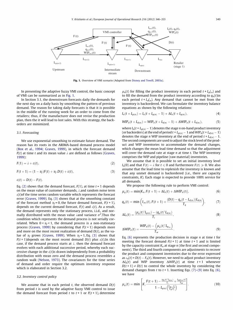
We observe a supply chain with a number of the stockholdingpoints typical of a single-item inventory system, namely, the retai-ler, downstream, intermediate stream and upstream (see Fig. 1).For stage n, the replenishment time, Ln, which comprises produc-tion lead times Lp(n) and delivery lead times Ld(n) is given by:

Ln ¼ LpðnÞ þ LdðnÞ : ð1Þ

We assume that the demand process is non-stationary and stochas-tic, that the OUT level, production and inventory control policy isadaptive and fuzzy and that any demand not satisfied by the inven-tory is backordered. Adaptive fuzzy control is used because the de-mand can differ across periods and the delivery rate will need tochange or adapt over time along with demand. In all periods, itmust be enough to cover the demand over the upcoming Ln. Below,we describe in more detail the forecast model, production and dis-tribution planning to control inventories and present an analysis ofthe model. We introduce additional assumptions as needed.

Downstream

VMI controllerF (t)

D(t)

L(n)

Retailer (stage 1)

Intermediatestream

Upstream

Lp(n+2) Lp(n+1) Lp(n)

L(n+1)L(n+2)

F (t)F (t)

In(t), qn(t), WIPn(t)

In+1(t), qn+1(t),

WIPn+1(t)

In+2(t), qn+2(t),

WIPn+2(t)

Fig. 1. Overview of VMI scenario (Adapted from Disney and Towill, 2003a).

Y. Kristianto et al. / European Journal of Operational Research 216 (2012) 346–355 349

In presenting the adaptive fuzzy VMI control, the basic conceptof VMI can be summarized as in Fig. 1.

In Section 3.1, the downstream forecasts daily the demands forthe next day on a daily basis by smoothing the pattern of previousdemand. The reason for taking daily forecasts is that it is possiblein the middle of the running week for an order to come from theretailers; thus, if the manufacturer does not revise the productionplan, then the it will lead to lost sales. With this strategy, the back-orders are minimized.

3.1. Forecasting

We use exponential smoothing to estimate future demand. Thereason has its roots in the ARIMA-based demand process model(Box et al., 1994; Graves, 1999), in which the forecast demandF(t) at time t and its mean value k are defined as follows (Graves,1999):

Fð1Þ ¼ kþ eðtÞ; ð2Þ

Fðt þ 1Þ ¼ ð1� af ÞFðtÞ þ af :DðtÞ þ eðtÞ; ð3Þ

eðtÞ ¼ DðtÞ � FðtÞ:

Eq. (2) shows that the demand forecast, F(1), at time t = 1 dependson the mean value of customer demands, k;and random noise terme(t)of the time series random variable which represents the forecasterror (Graves, 1999). Eq. (3) shows that at the smoothing constantof the forecast method af = 0, the future demand forecast, F(t + 1),depends on the current demand forecast, F(t) and e(t). As a result,the demand represents only the stationary process, i.i.d., and nor-mally distributed with the mean value kand variance r2.Thus thecondition which represents the demand process is not serially cor-related. When 0 < af < 1, the demand process is a non-stationaryprocess (Graves, 1999) by considering that F(t + 1) depends moreand more on the most recent realization of demand D(t), as the va-lue of af grows (Graves, 1999). When af = 1, Eq. (3) shows thatF(t + 1)depends on the most recent demand D(t) plus e(t).In thiscase, if the demand process starts at k; then the demand forecastevolves with each additional successive period, whereby each suc-cessive change in the e(t)is drawn independently from a probabilitydistribution with mean zero and the demand process resembles arandom walk (Nelson, 1973). The covariances for the time seriesof demand and order require the optimum inventory responsewhich is elaborated in Section 3.2.

3.2. Inventory control policy

We assume that in each period t, the observed demand D(t)from period t is used by the adaptive fuzzy VMI control to issuethe demand forecast from period t to t + 1 or F(t + 1), determine

ln(t) for filling the product inventory in each period t + Lp(n) andto fill the demand from the product inventory according to qn(t)ineach period t + Ld(n). Any demand that cannot be met from theinventory is backordered. We can formulate the inventory balanceequations as shown by the following relations:

Inðt þ LpðnÞÞ ¼ Inðt þ LpðnÞ � 1Þ þ DInðt þ LpðnÞÞ; ð4Þ

WIPnðt þ LdðnÞÞ ¼WIPnðt þ LdðnÞ � 1Þ þ DWIPnðt þ LdðnÞÞ; ð5Þ

where In(t + Lp(n) � 1) denotes the stage n on-hand product inventory(or backorders) at the end of period t + Lp(n) � 1 and WIPn(t + Ld(n) � 1)denotes the stage n WIP inventory at the end of period t + Ld(n) � 1.The second components are used to adjust the stock level of the prod-uct and WIP inventories to accommodate the demand changes,which changes the mean lead time demand so that the adjustmentwill cover the demand rate at stage n at time t. The WIP inventorycomprises the WIP and pipeline (raw material) inventories.

We assume that it is possible to set an initial inventory levelIn(0) and that FðtÞ ¼ k for t 6 0 and furthermore FðtÞP 0. We alsoassume that the lead time to replenish the inventory is known andthat any unmet demand is backordered (i.e., there are capacityconstraints, K). Each stage is expected to provide 100% service forall demands.

We propose the following rule to perform VMI control:

lnðtÞ ¼min½Kn; Fðt þ 1Þ þ DInðtÞ þ DWIPnðtÞ�; ð6Þ

qnðtÞ ¼min IðnÞðtÞ; Fðt þ 1Þ þðDðtÞ � qnðt � LdðnÞÞÞLdðnÞ

Tq

� �; ð7Þ

DInðtÞ ¼ðlnðtÞ

�LpðnÞÞ � ðqnðtÞ�LdðnÞÞ

Ti; ð8Þ

DWIPnðtÞ ¼WIPnðtÞ � lnðtÞ

�LpðnÞ

� �Tw

: ð9Þ

Eq. (6) represents the production decision in stage n at time t formeeting the forecast demand F(t + 1) at time t + 1 and is limitedby the capacity constraint Kn at stage n (the first and second compo-nents). The third and fourth components are adjustments to recoverthe product and component inventories due to the error expressedas en(t) = D(t) � Fn(t). However, we need to adjust product inventoryDIn(t) and WIP inventory DWIPn(t) at time t + 1 wheneverD(t + 1) – D(t) to control the whole inventory by considering thedemand changes from t to t + 1. Inserting Eqs. (7)–(9) into Eq. (6),we have

lnðtÞ ¼min K;Fðt þ 1Þ � ðqnðtÞ�LdðnÞÞ

Tiþ IWIPðnÞðtÞ

TW

1� LpðnÞTW�TiTW Ti

� �24

35: ð10Þ

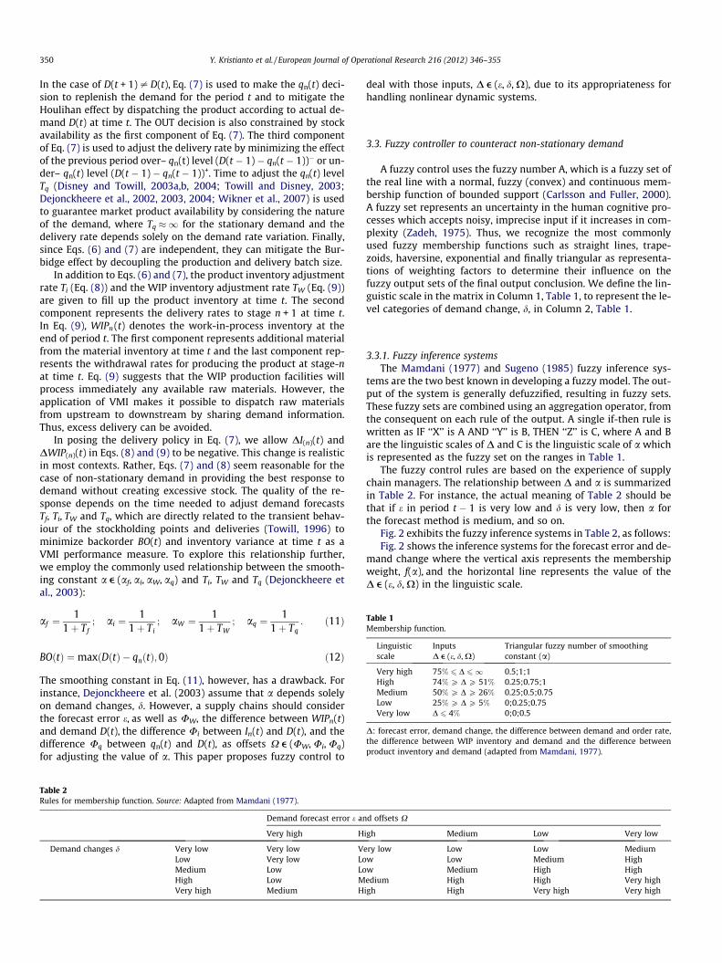
Table 1Membership function.

350 Y. Kristianto et al. / European Journal of Operational Research 216 (2012) 346–355

In the case of D(t + 1) – D(t), Eq. (7) is used to make the qn(t) deci-sion to replenish the demand for the period t and to mitigate theHoulihan effect by dispatching the product according to actual de-mand D(t) at time t. The OUT decision is also constrained by stockavailability as the first component of Eq. (7). The third componentof Eq. (7) is used to adjust the delivery rate by minimizing the effectof the previous period over– qn(t) level (D(t � 1) � qn(t � 1))� or un-der– qn(t) level (D(t � 1) � qn(t � 1))+. Time to adjust the qn(t) levelTq (Disney and Towill, 2003a,b, 2004; Towill and Disney, 2003;Dejonckheere et al., 2002, 2003, 2004; Wikner et al., 2007) is usedto guarantee market product availability by considering the natureof the demand, where Tq �1 for the stationary demand and thedelivery rate depends solely on the demand rate variation. Finally,since Eqs. (6) and (7) are independent, they can mitigate the Bur-bidge effect by decoupling the production and delivery batch size.

In addition to Eqs. (6) and (7), the product inventory adjustmentrate Ti (Eq. (8)) and the WIP inventory adjustment rate TW (Eq. (9))are given to fill up the product inventory at time t. The secondcomponent represents the delivery rates to stage n + 1 at time t.In Eq. (9), WIPn (t) denotes the work-in-process inventory at theend of period t. The first component represents additional materialfrom the material inventory at time t and the last component rep-resents the withdrawal rates for producing the product at stage-nat time t. Eq. (9) suggests that the WIP production facilities willprocess immediately any available raw materials. However, theapplication of VMI makes it possible to dispatch raw materialsfrom upstream to downstream by sharing demand information.Thus, excess delivery can be avoided.

In posing the delivery policy in Eq. (7), we allow DI(n)(t) andDWIP(n)(t) in Eqs. (8) and (9) to be negative. This change is realisticin most contexts. Rather, Eqs. (7) and (8) seem reasonable for thecase of non-stationary demand in providing the best response todemand without creating excessive stock. The quality of the re-sponse depends on the time needed to adjust demand forecastsTf, Ti, TW and Tq, which are directly related to the transient behav-iour of the stockholding points and deliveries (Towill, 1996) tominimize backorder BO(t) and inventory variance at time t as aVMI performance measure. To explore this relationship further,we employ the commonly used relationship between the smooth-ing constant a e (af, ai, aW, aq) and Ti, TW and Tq (Dejonckheere etal., 2003):

af ¼1

1þ Tf; ai ¼

11þ Ti

; aW ¼1

1þ TW; aq ¼

11þ Tq

: ð11Þ

Linguisticscale

InputsD e (e, d, X)

Triangular fuzzy number of smoothingconstant (a)

Very high 75% 6 D 61 0.5;1;1High 74% P D P 51% 0.25;0.75;1Medium 50% P D P 26% 0.25;0.5;0.75Low 25% P D P 5% 0;0.25;0.75Very low D 6 4% 0;0;0.5

D: forecast error, demand change, the difference between demand and order rate,the difference between WIP inventory and demand and the difference betweenproduct inventory and demand (adapted from Mamdani, 1977).

BOðtÞ ¼ maxðDðtÞ � qnðtÞ; 0Þ ð12Þ

The smoothing constant in Eq. (11), however, has a drawback. Forinstance, Dejonckheere et al. (2003) assume that a depends solelyon demand changes, d. However, a supply chains should considerthe forecast error e, as well as UW, the difference between WIPn(t)and demand D(t), the difference Ui between In(t) and D(t), and thedifference Uq between qn(t) and D(t), as offsets X e (UW, Ui, Uq)for adjusting the value of a. This paper proposes fuzzy control to

Table 2Rules for membership function. Source: Adapted from Mamdani (1977).

Demand forecast error e an

Very high H

Demand changes d Very low Very low VLow Very low LoMedium Low LoHigh Low MVery high Medium H

deal with those inputs, D e (e, d, X), due to its appropriateness forhandling nonlinear dynamic systems.

3.3. Fuzzy controller to counteract non-stationary demand

A fuzzy control uses the fuzzy number A, which is a fuzzy set ofthe real line with a normal, fuzzy (convex) and continuous mem-bership function of bounded support (Carlsson and Fuller, 2000).A fuzzy set represents an uncertainty in the human cognitive pro-cesses which accepts noisy, imprecise input if it increases in com-plexity (Zadeh, 1975). Thus, we recognize the most commonlyused fuzzy membership functions such as straight lines, trape-zoids, haversine, exponential and finally triangular as representa-tions of weighting factors to determine their influence on thefuzzy output sets of the final output conclusion. We define the lin-guistic scale in the matrix in Column 1, Table 1, to represent the le-vel categories of demand change, d, in Column 2, Table 1.

3.3.1. Fuzzy inference systemsThe Mamdani (1977) and Sugeno (1985) fuzzy inference sys-

tems are the two best known in developing a fuzzy model. The out-put of the system is generally defuzzified, resulting in fuzzy sets.These fuzzy sets are combined using an aggregation operator, fromthe consequent on each rule of the output. A single if-then rule iswritten as IF ‘‘X’’ is A AND ‘‘Y’’ is B, THEN ‘‘Z’’ is C, where A and Bare the linguistic scales of D and C is the linguistic scale of a whichis represented as the fuzzy set on the ranges in Table 1.

The fuzzy control rules are based on the experience of supplychain managers. The relationship between D and a is summarizedin Table 2. For instance, the actual meaning of Table 2 should bethat if e in period t � 1 is very low and d is very low, then a forthe forecast method is medium, and so on.

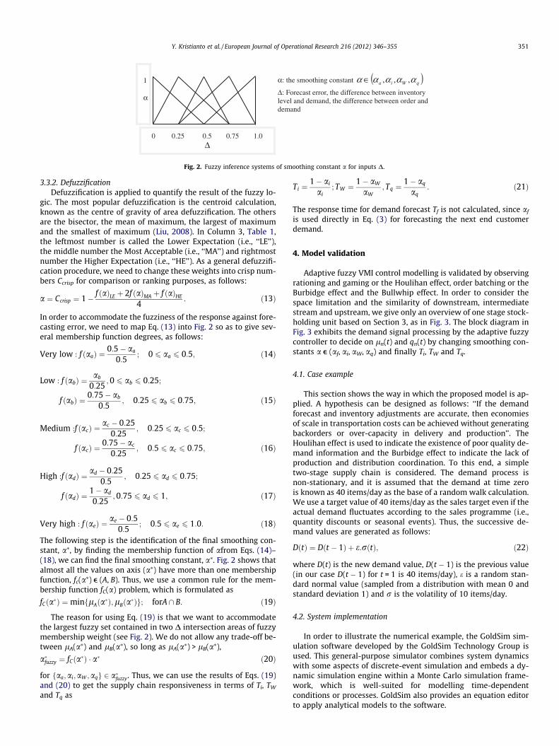
Fig. 2 exhibits the fuzzy inference systems in Table 2, as follows:Fig. 2 shows the inference systems for the forecast error and de-

mand change where the vertical axis represents the membershipweight, f(a), and the horizontal line represents the value of theD e (e, d, X) in the linguistic scale.

d offsets X

igh Medium Low Very low

ery low Low Low Mediumw Low Medium Highw Medium High Highedium High High Very highigh High Very high Very high

1

α

0 0.25 0.5 0.75 1.0 Δ

α: the smoothing constant ( )qWia ααααα ,,,∈Δ: Forecast error, the difference between inventory level and demand, the difference between order and demand

Fig. 2. Fuzzy inference systems of smoothing constant a for inputs D.

Y. Kristianto et al. / European Journal of Operational Research 216 (2012) 346–355 351

3.3.2. DefuzzificationDefuzzification is applied to quantify the result of the fuzzy lo-

gic. The most popular defuzzification is the centroid calculation,known as the centre of gravity of area defuzzification. The othersare the bisector, the mean of maximum, the largest of maximumand the smallest of maximum (Liu, 2008). In Column 3, Table 1,the leftmost number is called the Lower Expectation (i.e., ‘‘LE’’),the middle number the Most Acceptable (i.e., ‘‘MA’’) and rightmostnumber the Higher Expectation (i.e., ‘‘HE’’). As a general defuzzifi-cation procedure, we need to change these weights into crisp num-bers Ccrisp for comparison or ranking purposes, as follows:

a ¼ Ccrisp ¼ 1� f ðaÞLE þ 2f ðaÞMA þ f ðaÞHE

4: ð13Þ

In order to accommodate the fuzziness of the response against fore-casting error, we need to map Eq. (13) into Fig. 2 so as to give sev-eral membership function degrees, as follows:

Very low : f ðaaÞ ¼0:5� aa

0:5; 0 6 aa 6 0:5; ð14Þ

Low : f ðabÞ ¼ab

0:25;0 6 ab 6 0:25;

f ðabÞ ¼0:75� ab

0:5; 0:25 6 ab 6 0:75; ð15Þ

Medium :f ðacÞ ¼ac � 0:25

0:25; 0:25 6 ac 6 0:5;

f ðacÞ ¼0:75� ac

0:25; 0:5 6 ac 6 0:75; ð16Þ

High :f ðadÞ ¼ad � 0:25

0:5; 0:25 6 ad 6 0:75;

f ðadÞ ¼1� ad

0:25;0:75 6 ad 6 1; ð17Þ

Very high : f ðaeÞ ¼ae � 0:5

0:5; 0:5 6 ae 6 1:0: ð18Þ

The following step is the identification of the final smoothing con-stant, a⁄, by finding the membership function of afrom Eqs. (14)–(18), we can find the final smoothing constant, a⁄. Fig. 2 shows thatalmost all the values on axis (a⁄) have more than one membershipfunction, fc(a⁄) e (A, B). Thus, we use a common rule for the mem-bership function fC(a) problem, which is formulated as

fCða�Þ ¼minflAða�Þ;lBða�Þg; forA \ B: ð19Þ

The reason for using Eq. (19) is that we want to accommodatethe largest fuzzy set contained in two D intersection areas of fuzzymembership weight (see Fig. 2). We do not allow any trade-off be-tween lA(a⁄) and lB(a⁄), so long as lA(a⁄) > lB(a⁄),

a�fuzzy ¼ fCða�Þ � a� ð20Þ

for faa;ai;aW ;aqg 2 a�fuzzy. Thus, we can use the results of Eqs. (19)and (20) to get the supply chain responsiveness in terms of Ti, TW

and Tq as

Ti ¼1� ai

ai; TW ¼

1� aW

aW; Tq ¼

1� aq

aq: ð21Þ

The response time for demand forecast Tf is not calculated, since af

is used directly in Eq. (3) for forecasting the next end customerdemand.

4. Model validation

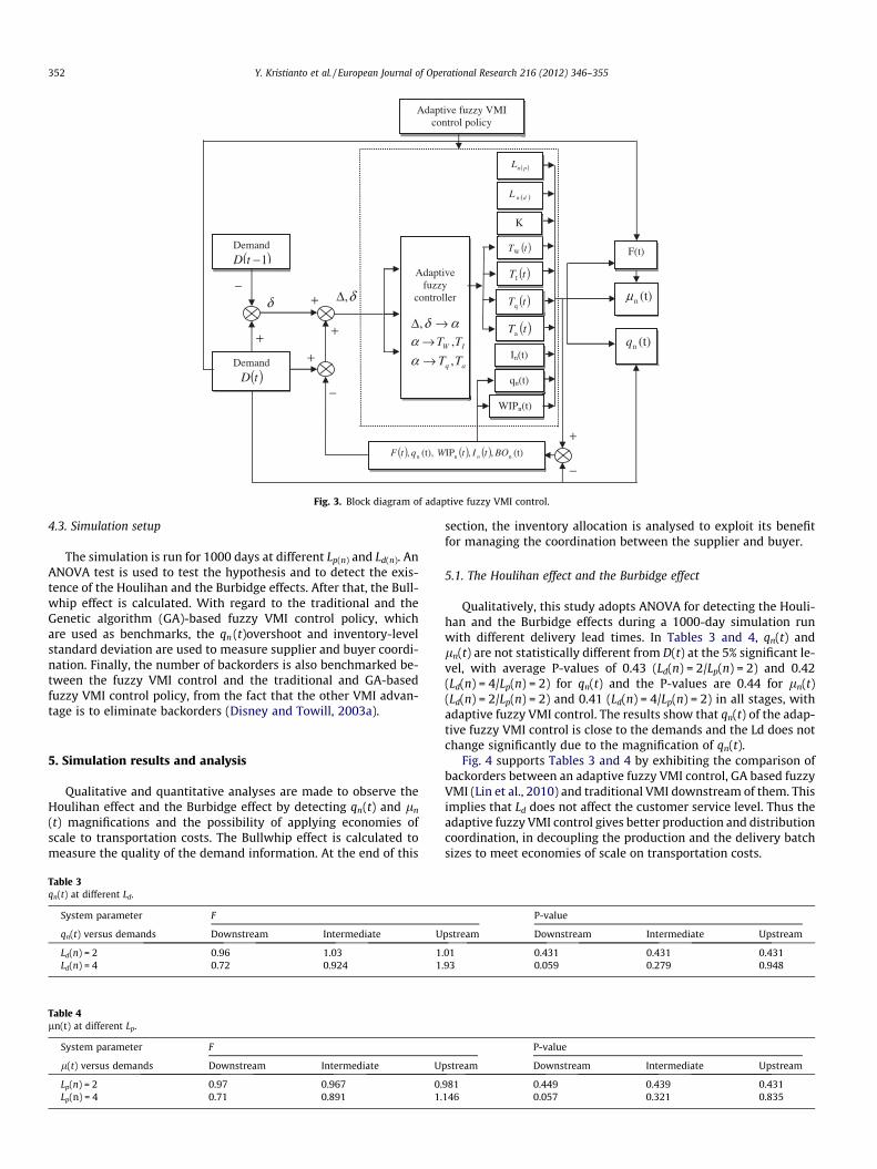
Adaptive fuzzy VMI control modelling is validated by observingrationing and gaming or the Houlihan effect, order batching or theBurbidge effect and the Bullwhip effect. In order to consider thespace limitation and the similarity of downstream, intermediatestream and upstream, we give only an overview of one stage stock-holding unit based on Section 3, as in Fig. 3. The block diagram inFig. 3 exhibits the demand signal processing by the adaptive fuzzycontroller to decide on ln(t) and qn(t) by changing smoothing con-stants a e (af, ai, aW, aq) and finally Ti, TW and Tq.

4.1. Case example

This section shows the way in which the proposed model is ap-plied. A hypothesis can be designed as follows: ‘‘If the demandforecast and inventory adjustments are accurate, then economiesof scale in transportation costs can be achieved without generatingbackorders or over-capacity in delivery and production’’. TheHoulihan effect is used to indicate the existence of poor quality de-mand information and the Burbidge effect to indicate the lack ofproduction and distribution coordination. To this end, a simpletwo-stage supply chain is considered. The demand process isnon-stationary, and it is assumed that the demand at time zerois known as 40 items/day as the base of a random walk calculation.We use a target value of 40 items/day as the sales target even if theactual demand fluctuates according to the sales programme (i.e.,quantity discounts or seasonal events). Thus, the successive de-mand values are generated as follows:

DðtÞ ¼ Dðt � 1Þ þ e:rðtÞ; ð22Þ

where D(t) is the new demand value, D(t � 1) is the previous value(in our case D(t � 1) for t = 1 is 40 items/day), e is a random stan-dard normal value (sampled from a distribution with mean 0 andstandard deviation 1) and r is the volatility of 10 items/day.

4.2. System implementation

In order to illustrate the numerical example, the GoldSim sim-ulation software developed by the GoldSim Technology Group isused. This general-purpose simulator combines system dynamicswith some aspects of discrete-event simulation and embeds a dy-namic simulation engine within a Monte Carlo simulation frame-work, which is well-suited for modelling time-dependentconditions or processes. GoldSim also provides an equation editorto apply analytical models to the software.

( ) ( ) ( ) (t),,IP(t),, nnn BOtItWqtF n

Demand

( )1−tD

(t)nq

(t)nμ

F(t)

( )dnL

( )pnL

Adaptive fuzzy

controller

αδ →Δ,

IW TT ,→α

aq TT ,→α

( )tTI

( )tTW

K

( )tTq

( )tTa

In(t)

Adaptive fuzzy VMI control policy

δ,Δ

Demand

( )tD

δ

+

−+

−

−

+

+

+

qn(t)

WIPn(t)

Fig. 3. Block diagram of adaptive fuzzy VMI control.

352 Y. Kristianto et al. / European Journal of Operational Research 216 (2012) 346–355

4.3. Simulation setup

The simulation is run for 1000 days at different Lp(n) and Ld(n). AnANOVA test is used to test the hypothesis and to detect the exis-tence of the Houlihan and the Burbidge effects. After that, the Bull-whip effect is calculated. With regard to the traditional and theGenetic algorithm (GA)-based fuzzy VMI control policy, whichare used as benchmarks, the qn (t)overshoot and inventory-levelstandard deviation are used to measure supplier and buyer coordi-nation. Finally, the number of backorders is also benchmarked be-tween the fuzzy VMI control and the traditional and GA-basedfuzzy VMI control policy, from the fact that the other VMI advan-tage is to eliminate backorders (Disney and Towill, 2003a).

5. Simulation results and analysis

Qualitative and quantitative analyses are made to observe theHoulihan effect and the Burbidge effect by detecting qn(t) and ln

(t) magnifications and the possibility of applying economies ofscale to transportation costs. The Bullwhip effect is calculated tomeasure the quality of the demand information. At the end of this

Table 3qn(t) at different Ld.

System parameter F

qn(t) versus demands Downstream Intermediate U

Ld(n) = 2 0.96 1.03 1Ld(n) = 4 0.72 0.924 1

Table 4ln(t) at different Lp.

System parameter F

l(t) versus demands Downstream Intermediate U

Lp(n) = 2 0.97 0.967 0.Lp(n) = 4 0.71 0.891 1.

section, the inventory allocation is analysed to exploit its benefitfor managing the coordination between the supplier and buyer.

5.1. The Houlihan effect and the Burbidge effect

Qualitatively, this study adopts ANOVA for detecting the Houli-han and the Burbidge effects during a 1000-day simulation runwith different delivery lead times. In Tables 3 and 4, qn(t) andln(t) are not statistically different from D(t) at the 5% significant le-vel, with average P-values of 0.43 (Ld(n) = 2/Lp(n) = 2) and 0.42(Ld(n) = 4/Lp(n) = 2) for qn(t) and the P-values are 0.44 for ln(t)(Ld(n) = 2/Lp(n) = 2) and 0.41 (Ld(n) = 4/Lp(n) = 2) in all stages, withadaptive fuzzy VMI control. The results show that qn(t) of the adap-tive fuzzy VMI control is close to the demands and the Ld does notchange significantly due to the magnification of qn(t).

Fig. 4 supports Tables 3 and 4 by exhibiting the comparison ofbackorders between an adaptive fuzzy VMI control, GA based fuzzyVMI (Lin et al., 2010) and traditional VMI downstream of them. Thisimplies that Ld does not affect the customer service level. Thus theadaptive fuzzy VMI control gives better production and distributioncoordination, in decoupling the production and the delivery batchsizes to meet economies of scale on transportation costs.

P-value

pstream Downstream Intermediate Upstream

.01 0.431 0.431 0.431

.93 0.059 0.279 0.948

P-value

pstream Downstream Intermediate Upstream

981 0.449 0.439 0.431146 0.057 0.321 0.835

Fig. 4. Step response for GA based fuzzy VMI control and adaptive fuzzy VMIcontrol for Lp = 2 and Ld = 2 during 1000 days with non-stationary demand processrate average of 40 units per day, with 10 items annual volatility.

Fig. 5. Maximum backorders during 1000 days with non-stationary demandprocess rate average of 40 units per day, with 10 items annual volatility.

Y. Kristianto et al. / European Journal of Operational Research 216 (2012) 346–355 353

Quantitatively, Fig. 5 shows the qn(t) overshoot comparison be-tween the adaptive fuzzy VMI control and the GA based fuzzy VMIdownstream. The overshoot is used to measure the Houlihan effectwhich inevitably leads to unrealistic deliveries. Indeed, Fig. 5shows that adaptive fuzzy VMI control surpasses other GA-basedfuzzy VMI control (Lin et al., 2010) in terms of lower qn(t) over-shoot and shorter qn(t) settling time, at a step response. Minimumqn(t) overshoot indicates that the adaptive fuzzy VMI control iscapable of mitigating the Houlihan effect. Shorter settling timeindicates that the production and the delivery batch sizes are notlinearly correlated. A nonlinear relationship between the produc-tion batch size and delivery batch size gives an advantage to themitigation of the Burbidge effect by allowing economies of scalein transportation costs. Thus, the Houlihan and the Burbidge ef-fects are simultaneously mitigated by adaptive fuzzy VMI controland the research hypothesis is accepted.

5.2. Quantification of the Bullwhip effect

BullwhipðBÞ ¼rqn ðtÞðt;tþLdðnÞÞqnðtÞðt;tþLdðnÞÞrDðtÞðt;tþLdðnÞÞDðtÞðt;tþLdðnÞÞ

¼ Vout

Vin: ð23Þ

Table 5Bullwhip effect at different Ld and Lp.

Downstream Intermediate Upstream

Ld = 1Lp = 2 0.98 1.02 1Lp = 3 0.98 1.02 1Lp = 4 0.97 1.04 0.99

Ld = 2Lp = 2 1 1 1Lp = 3 0.98 1.03 1Lp = 4 0.97 1.03 0.99

There are some contributions that quantify the Bullwhip effect indifferent ways. Warburton (2004) calculates the relationship be-tween order rate and demand rate without considering the methodof estimating the mean and standard deviation of the output de-mand. Other quantifications, such as Lee et al. (1997) and Chenet al. (1998), calculate the variance ratio (VR) of order quantityand demand in a way which does not take the lead time varianceinto account. Similarly, Chatfield et al. (2004) also consider VR asthe Bullwhip effect metric, which does take into account the effectof stochastic lead times. However, if for instance the supplier wouldlike to optimize the order batching then the variance of the orderquantity would always be less than the demand. As a result, theBullwhip effect is never detected. In addition, it generates a higherlevel of inventory in the buyer warehouse. Since one of the VMIbenefits is to reduce the inventory level of the supply chain, thenVR creates a conflict between minimizing the inventory and miti-gating the Bullwhip effect.

The Bullwhip effect quantification in Eq. (23) which is calcu-lated in Table 5 Section 5.2 employs the quotient of the demandcoefficient of variation (CV) generated in a given supply chain leveland the demand CV received by the same level (Fransoo andWouters, 2000). The CV is appropriate for implementation in theechelon level of the demand. The reason is that most of the de-mand data in many supply chains are incomplete and not availablein the echelon level (Fransoo and Wouters, 2000). Furthermore, thedemand data at each echelon is not necessarily equal to the de-mand data at the product level. As a result, the magnitude of orderrate is not necessarily equal to the demand rate. Thus, the ratio be-tween the variability of the order rate and demand rate reflects thecapability of the supply chain to respond to the demand. If thisprinciple is applied to the VR then the Bullwhip effect is greatlymagnified.

Whereas the Houlihan and the Burbidge effects are mitigated,Table 5 shows that adaptive fuzzy VMI control supports are appro-priate for mitigating the Bullwhip effect by sharing the demandinformation to avoid multiple forecasting at all stages in the supplychain. Table 5 shows that the imprecision of the demand signal iseliminated to such an extent that variation in the delivery leadtimes has no significant impact on creating demand magnification.This is one more reason to support the mitigation of the Houlihanand the Burbidge effects.

5.3. Inventory allocation across the supply chain

Bullwhip effect mitigation cannot ignore the role of coordina-tion between supplier and buyer. Fig. 6 shows this coordinationin terms of the inventory allocation across the supply chain. TheFigure shows that the downstream causes higher In(t) for the inter-mediate and the upstream echelons. The reason is that the down-stream hedges directly against the demand variability withouthaving the opportunity for dampening the shock. The adaptive fuz-zy VMI control helps to decouple the inventories into In(t) andWIPn(t).Thus, In(t) covers only the demand variability during thedelivery lead times (In(t) standard deviation), while the WIPn(t)

Downstream Intermediate Upstream

Ld = 3Lp = 2 0.98 1.02 1Lp = 3 0.98 1.02 1Lp = 4 0.96 1.04 1

Ld = 4Lp = 2 0.99 1.01 1Lp = 3 0.97 1.03 1Lp = 4 0.97 1.03 1

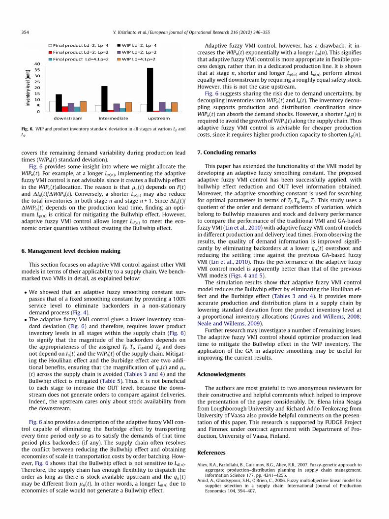
Fig. 6. WIP and product inventory standard deviation in all stages at various Lp andLd.

354 Y. Kristianto et al. / European Journal of Operational Research 216 (2012) 346–355

covers the remaining demand variability during production leadtimes (WIPn(t) standard deviation).

Fig. 6 provides some insight into where we might allocate theWIPn(t). For example, at a longer Lp(n), implementing the adaptivefuzzy VMI control is not advisable, since it creates a Bullwhip effectin the WIPn(t)allocation. The reason is that ln(t) depends on F(t)and DIn(t)/DWIPn(t). Conversely, a shorter Lp(n) may also reducethe total inventories in both stage n and stage n + 1. Since DIn(t)/DWIPn(t) depends on the production lead time, finding an opti-mum Lp(n) is critical for mitigating the Bullwhip effect. However,adaptive fuzzy VMI control allows longer Ld(n) to meet the eco-nomic order quantities without creating the Bullwhip effect.

6. Management level decision making

This section focuses on adaptive VMI control against other VMImodels in terms of their applicability to a supply chain. We bench-marked two VMIs in detail, as explained below:

� We showed that an adaptive fuzzy smoothing constant sur-passes that of a fixed smoothing constant by providing a 100%service level to eliminate backorders in a non-stationarydemand process (Fig. 4).� The adaptive fuzzy VMI control gives a lower inventory stan-

dard deviation (Fig. 6) and therefore, requires lower productinventory levels in all stages within the supply chain (Fig. 6)to signify that the magnitude of the backorders depends onthe appropriateness of the assigned Tf, Ti, TWand Tq and doesnot depend on In(t) and the WIPn(t) of the supply chain. Mitigat-ing the Houlihan effect and the Burbidge effect are two addi-tional benefits, ensuring that the magnification of qn(t) and ln

(t) across the supply chain is avoided (Tables 3 and 4) and theBullwhip effect is mitigated (Table 5). Thus, it is not beneficialto each stage to increase the OUT level, because the down-stream does not generate orders to compare against deliveries.Indeed, the upstream cares only about stock availability fromthe downstream.

Fig. 6 also provides a description of the adaptive fuzzy VMI con-trol capable of eliminating the Burbidge effect by transportingevery time period only so as to satisfy the demands of that timeperiod plus backorders (if any). The supply chain often resolvesthe conflict between reducing the Bullwhip effect and obtainingeconomies of scale in transportation costs by order batching. How-ever, Fig. 6 shows that the Bullwhip effect is not sensitive to Ld(n).Therefore, the supply chain has enough flexibility to dispatch theorder as long as there is stock available upstream and the qn (t)may be different from ln(t). In other words, a longer Ld(n) due toeconomies of scale would not generate a Bullwhip effect.

Adaptive fuzzy VMI control, however, has a drawback: it in-creases the WIPn(t) exponentially with a longer Lp(n). This signifiesthat adaptive fuzzy VMI control is more appropriate in flexible pro-cess design, rather than in a dedicated production line. It is shownthat at stage n, shorter and longer Lp(n) and Ld(n) perform almostequally well downstream by requiring a roughly equal safety stock.However, this is not the case upstream.

Fig. 6 suggests sharing the risk due to demand uncertainty, bydecoupling inventories into WIPn(t) and In(t). The inventory decou-pling supports production and distribution coordination sinceWIPn(t) can absorb the demand shocks. However, a shorter Lp(n) isrequired to avoid the growth of WIPn(t) along the supply chain. Thusadaptive fuzzy VMI control is advisable for cheaper productioncosts, since it requires higher production capacity to shorten Lp(n).

7. Concluding remarks

This paper has extended the functionality of the VMI model bydeveloping an adaptive fuzzy smoothing constant. The proposedadaptive fuzzy VMI control has been successfully applied, withbullwhip effect reduction and OUT level information obtained.Moreover, the adaptive smoothing constant is used for searchingfor optimal parameters in terms of Tf, Tq, TW, TI. This study uses aquotient of the order and demand coefficients of variation, whichbelong to Bullwhip measures and stock and delivery performanceto compare the performance of the traditional VMI and GA-basedfuzzy VMI (Lin et al., 2010) with adaptive fuzzy VMI control modelsin different production and delivery lead times. From observing theresults, the quality of demand information is improved signifi-cantly by eliminating backorders at a lower qn(t) overshoot andreducing the settling time against the previous GA-based fuzzyVMI (Lin et al., 2010). Thus the performance of the adaptive fuzzyVMI control model is apparently better than that of the previousVMI models (Figs. 4 and 5).

The simulation results show that adaptive fuzzy VMI controlmodel reduces the Bullwhip effect by eliminating the Houlihan ef-fect and the Burbidge effect (Tables 3 and 4). It provides moreaccurate production and distribution plans in a supply chain bylowering standard deviation from the product inventory level ata proportional inventory allocations (Graves and Willems, 2008;Neale and Willems, 2009).

Further research may investigate a number of remaining issues.The adaptive fuzzy VMI control should optimize production leadtime to mitigate the Bullwhip effect in the WIP inventory. Theapplication of the GA in adaptive smoothing may be useful forimproving the current results.

Acknowledgments

The authors are most grateful to two anonymous reviewers fortheir constructive and helpful comments which helped to improvethe presentation of the paper considerably. Dr. Elena Irina Neagafrom Loughborough University and Richard Addo-Tenkorang fromUniversity of Vaasa also provide helpful comments on the presen-tation of this paper. This research is supported by FUDGE Projectand Fimmec under contract agreement with Department of Pro-duction, University of Vaasa, Finland.

References

Aliev, R.A., Fazlollahi, B., Guirimov, B.G., Aliev, R.R., 2007. Fuzzy-genetic approach toaggregate production–distribution planning in supply chain management.Information Science 177, pp. 4241–4255.

Amid, A., Ghodsypour, S.H., O’Brien, C., 2006. Fuzzy multiobjective linear model forsupplier selection in a supply chain. International Journal of ProductionEconomics 104, 394–407.

Y. Kristianto et al. / European Journal of Operational Research 216 (2012) 346–355 355

Amid, A., Ghodsypour, S.H., O’Brien, C., 2009. A weighted additive fuzzymultiobjective model for the supplier selection problem under price breaks ina supply Chain. International Journal of Production Economics 121, 323–332.

Balan, S., Vrat, P., Kumar, P., 2009. Information distorsion in supply chain and itsmitigation using soft computing approach. Omega The International Journal ofManagement Science 37, 282–299.

Box, G.E.P., Jenkins, G.M., Reinsel, G.C., 1994. Time Series Analysis Forecasting andControl, 3rd ed. Holden-Day, SanFransisco, CA (Chapter 4).

Burbidge, J.L., 1991. Period batch control (PBC) with GT – the way forward fromMRP. Paper presented at the BPCIS Annual Conference, Birmingham.

Carlsson, C., Fuller, R., 2000. A fuzzy approach to the Bullwhip effect. In proceedingof the 34th Hawaii International Conference of system Science.

Carlsson, C., Fuller, R., 2002. A position paper on the agenda for soft decisionanalysis. Fuzzy sets and systems 131, 3–11.

Chan, F.T.S., Kumar, N., 2007. Global supplier development considering risk factorsusing fuzzy extended AHP-based approach. Omega The International Journal ofManagement Science 35, 417–431.

Chanas, S., Kuchta, D., 1998. Fuzzy integer transportation problem. Fuzzy Sets andsystems 98, 198–291.

Chatfield, D.C., Kim, J.G., Harrison, T.P., Hayya, J.C., 2004. The bullwhip effect-impactof stochastic lead time, information quality, and information sharing: asimulation study. Production and Operations Management 13 (4), 340–353.

Chen, F., Drezner, Z., Ryan, J.K., Simchi-Levi, D., 1998. The Bullwhip effect:managerial insights on the impact of forecasting and information onvariability in a supply chain. In Quantitative Models for Supply ChainManagement, edited by S. Tayur, pp. 418–439.

Chen, F., Drezner, Z., Ryan, J.K., Simchi-Levi, D., 2000. Quantifying the bullwhipeffect in a simple supply chain: the impact of forecasting, lead times, andinformation. Management Science 46 (3), 436–443.

Croson, R., Donohue, K., 2003. Impact of POS data sharing on supply chainmanagement: an experimental study. Production and Operations Management12 (1), 1–11.

Dejonckheere, J., Disney, S.M., Lambrecht, M.R., Towill, D.R., 2002. Transfer functionanalysis of forecasting induced bullwhip in supply chains. International Journalof Production Economics 78, 133–144.

Dejonckheere, J., Disney, S.M., Lambrecht, M.R., Towill, D.R., 2003. Measuring andavoiding the bullwhip effect: A control theoretic approach. European Journal ofOperational Research 147, 567–590.

Dejonckheere, J., Disney, S.M., Lambrecht, M.R., Towill, D.R., 2004. The impact ofinformation enrichment on the Bullwhip effect in supply chains: A controlengineering perspective. European Journal of Operational Research 153, 727–750.

Disney, S.M., Towill, D.R., 2003a. Vendor-managed inventory and bullwhipreduction in a two-level supply chain. International Journal of Operations andProduction Management 23 (6), 625–651.

Disney, S.M., Towill, D.R., 2003b. On the bullwhip and inventory variance producedby an ordering policy. Omega 31 (1), 157–167.

Disney, S.M., Towill, D.R., 2004. Variance amplification and the golden ratio inproduction and inventory control. International Journal of ProductionEconomics 90, 295–309.

Forrester, J.W., 1961. Industrial Dynamics. MIT Press, Cambridge, MA (Chapter 2).Fransoo, J.C., Wouters, M.J.F., 2000. Measuring the bullwhip effect in the supply

chain. Supply Chain Management 5 (2), 78–89.Giannoccaro, I., Pontrandolfo, P., Scozzi, B., 2003. A fuzzy echelon approach for

inventory management in supply chains. European Journal of OperationalResearch 149, 185–196.

Graves, S.C., 1999. A single-item inventory model for a nonstationary demandprocess. Manufacturing and Service Operations Management 1 (1), 50–61.

Graves, S.C., Willems, S., 2008. Strategic inventory placement in supply chains:nonstationary demand. Manufacturing and Service Operations Management 10(2), 278–287.

Holweg, M., Bicheno, J., 2002. Supply Chain Simulation-a tool for education,enhancement and endeavour. International Journal of Production Economics 78,163–175.

Jimenez, F., Verdegay, J.L., 1999. Solving fuzzy solid transportation problems by anevolutionary algorithm based parametric approach. European Journal ofOperational Research 117, 485–510.

Kaipia, R., Holmström, J., Tanskanen, K., 2002. VMI: What are you losing if you letyour customer place orders? Production Planning & Control 13 (1), 17–25.

Kumar, M., Vrat, P., Shankar, R., 2004. A fuzzy goal programming approach forvendor selection problem in a supply chain. Computers and Industrialengineering 46, 69–85.

Lee, H.L., Padmanabhan, P., Whang, S., 1997. Information distortion in a supplychain: The bullwhip Effect. Management Science 43, 543–558.

Liang, T.F., 2008. Fuzzy multi-objective production/distribution planning decisionswith multi-product and multi-time period in a supply chain. Computers andIndustrial engineering 55, 675–694.

Lin, K.P., Chang, P.T., Hung, K.C., Pai, P.F., 2010. A simulation of vendor managedinventory dynamics using fuzzy arithmetic operations with genetic algorithms.Expert Systems with Applications 37, 2571–2579.

Liu, F., 2008. An efficient centroid type-reduction strategy for general type-2 fuzzylogic system. Information Sciences 17, 2224–2236.

Mamdani, E.H., 1977. Application of fuzzy logic to approximate reasoning usinglinguistic synthesis. IEEE Transactions on Computers 26 (12), 1182–1191.

McCullen, P., Towill, D., 2000. Diagnosis and reduction of bullwhip in supply chains.Supply Chain Management: an International Journal 7 (3), 164–179.

Neale, J.J., Willems, S.P., 2009. Managing inventory in supply chains withnonstationary demand. Interfaces 39 (5), 388–399.

Nelson, C.R., 1973. Applied Time Series Analysis for Managerial Forecasting. Holden-Day, SanFransisco, CA (Chapter 1).

O’Donell, T., Maguire, L., McIvor, R., Humphreys, P., 2006. Minimizing the bullwhipeffect in a supply chain using genetic algorithms. International Journal ofProduction Research 44 (8), 1523–1543.

Peidro, D., Mula, J., Poler, R., Luis Verdegay, J., 2009. Fuzzy optimization for supplychain planning under supply, demand and process uncertainties. Fuzzy Sets andsystems 160, 2640–2657.

Petrovic, D., Petrovic, R., 2001. Multicriteria ranking of inventory replenishmentpolicies in the presence of uncertainty in customer demand. InternationalJournal of Production Economics 71, 439–446.

Petrovic, D., Xie, Y., Burnham, K., 2006. Fuzzy decision support system for demandforecasting with a learning mechanism. Fuzzy Sets and Systems 157, 1713–1725.

Petrovic, D., Xie, Y., Burnham, K., Petrovic, R., 2008. Coordinated control ofdistribution supply chains in the presence of fuzzy customer demand.European Journal of Operational Research 185, 146–158.

Sakawa, M., Nishizaki, I., Uemura, Y., 2001. Fuzzy programming and profit and costallocation for a production and transportation problem. European Journal ofOperational Research 131, 1–15.

Sheu, J.B., 2005. A multi-layer demand-responsive logistics control methodology foralleviating the bullwhip effect of supply chains. European Journal of OperationalResearch 161, 797–811.

Sterman, J., 1989. Modelling managerial behavior: Misperception of feeback indynamic decision making experiment. Management Science 35 (3), 321–339.

Sugeno, M., 1985. Industrial applications of fuzzy control. Elsevier Science Pub. Co..Thonemann, U.W., 2002. Improving supply-chain performance by sharing advance

demand information. European Journal of Operational Research 142, 81–107.Torabi, S.A., Hassini, E., 2009. Multi-site production planning integrating

procurement and distribution plans in multi-echelon supply chains: Aninteractive fuzzy goal programming approach. International Journal ofProduction Research 47 (19), 5475–5499.

Towill, D.R., 1996. Industrial dynamics modeling of supply chains. InternationalJournal of Physical Distribution and Logistics 26 (2), 23–42.

Towill, D.R., Disney, S.M., 2003. The effect of vendor managed inventory (VMI)dynamics on the Bullwhip Effect in supply chains. International Journal ofProduction Economics 85 (1), 199–215.

Van Ackere, A., Larsen, E.R., Morecroft, J.D.W., 1993. Systems thinking and businessprocess redesign: An application to the Beer Game. European ManagementJournal 11 (4), 412–423.

Wang, J., Shu, Y.F., 2005. Fuzzy decision modeling for supply chain management.Fuzzy Sets and systems 150, 107–127.

Warburton, R.D.H., 2004. An analytical Investigation of the Bullwhip Effect.Production and Operations Management 13 (2), 150–160.

Wikner, J., Naim, M.M., Rudberg, M., 2007. Exploiting the Order Book for MassCustomized Manufacturing Control Systems with Capacity Limitation. IEEETransactions on Engineering Management 54 (1), 145–155.

Xie, Y., Petrovic, D., Burnham, K., 2004. A heuristic procedure for the two-levelcontrol of serial supply chains under fuzzy customer demand. InternationalJournal of Production Economics 102, 37–50.

Yu, Z., Yan, H., Cheng, T.C.E., 2002. Modelling the benefits of information sharing-based partnership in a two level supply chain. Journal of the OperationalResearch Society 53, 436–446.

Zadeh, L.A., 1975. The concept of a linguistic variable and its application toapproximate reasoning. Information Sciences 1 (8), 199–249.

Zarandi, M.H.F., Pourakbar, M., Turksen, IB., 2008. A fuzzy agent-based model forreduction of bullwhip effect in supply chain systems. Expert Systems withApplications 34, 1680–1691.

Zhang, X., 2004. The impact of forecasting methods on the bullwhip effect.International Journal of Production Economics 88, 15–27.