adaptive finite element method for … finite element method for fractional differential equations...
TRANSCRIPT
ADAPTIVE FINITE ELEMENT METHOD FOR FRACTIONALDIFFERENTIAL EQUATIONS USING HIERARCHICAL MATRICES ∗
XUAN ZHAO † , XIAOZHE HU‡ , WEI CAI§ , AND GEORGE EM KARNIADAKIS¶
Abstract. We develop a fast solver for the fractional differential equation (FDEs) involvingRiesz fractional derivative. It is based on the use of hierarchical matrices (H-Matrices) for therepresentation of the stiffness matrix resulting from the finite element discretization of the FDE andemploys a geometric multigrid method for the solution of the algebraic system of equations. Wealso propose an adaptive algorithm based on a posteriori error estimation to deal with general-typesingularities arising in the solution of the FDE. Through various test examples we demonstrate theefficiency of the method and the high-accuracy of the numerical solution even in the presence ofsingularities.
Key words. Riesz derivative, Hierarchical Matrices, geometric multigrid method, adaptivity,non-smooth solutions, finite element method
AMS subject classifications. 80M10, 65M15, 65M55, 26A33, 41A25
1. Introduction. Numerical methods for differential equations involving frac-tional derivatives either in time or space have been studied widely since they havevarious new scientific applications [5, 27, 28, 30, 31, 33, 34]. However, as the sizeof the problem increases, the time required to solve the final system of equationsincreases considerably due to the nonlocality of the fractional differential opera-tors [4, 9–11, 22, 25, 29, 35, 36, 39, 42]. Generally, there are two main difficulties insolving space fractional problems. First, the discretization matrix obtained by theutilization of the numerical methods is fully populated. This leads to increased stor-age memory requirements as well as increased solution time. Since the matrix is dense,the memory required to store its coefficients is of order O(N2), where N denotes thenumber of unknowns, and the solution of the system requires O(N3) operations ifdirect solvers are used. Second, the solution of a space fractional problem has sin-gularities around the boundaries even with smooth input data since the definitioninvolves the integration of weak singular kernels.
So far good progress has been made on reducing the computational complexityof the space FDEs for uniform mesh discretizations based on the observation thatthe coefficient matrices are Toeplitz-like if a uniform mesh is employed. This resultsin efficient matrix-vector multiplications [16,19,26,37,40], which in conjunction witheffective preconditioners lead to enhanced efficiency [15, 18, 21, 24, 38]. The multigridmethod [7, 17, 26, 46] has also been employed to reduce the computational cost toO(N log(N)). However, to the best of our knowledge, most of the existing fast solversdepend on the Toeplitz-like structure of the matrices, which implies that the under-
∗This work was supported by the OSD/ARO/MURI on ”Fractional PDEs for Conservation Lawsand Beyond: Theory, Numerics and Applications (W911NF-15-1-0562)” .†Division of Algorithms, Beijing Computational Science Research Center, Beijing 100084, P.
R. China, Department of Mathematics, Southeast University, Nanjing 210096, P. R. China,([email protected]; [email protected]).‡Department of Mathematics, Tufts University, Medford, MA 02155 USA,
([email protected]).§Division of Algorithms, Beijing Computational Science Research Center, Beijing 100084, P. R.
China, and Department of Mathematics and Statistics, University of North Carolina at Charlotte,Charlotte, NC 28223-0001, ([email protected]).¶Division of Applied Mathematics, Brown University, Providence, RI 02912, USA,
(george [email protected]).
1
arX
iv:1
603.
0135
8v1
[m
ath.
NA
] 4
Mar
201
6
2 X. Zhao, X. Hu, W. Cai, G.E. Karniadakis
lying meshes have to be uniform. Therefore, the existing efficient solvers cannot bereadily applied when a nonuniform mesh is used, including the important case of non-uniform (geometric) meshes generated by adaptive discretizations employed to dealwith boundary singularities. Another effective approach in dealing with such singu-larities is by tuning the appropriate basis, e.g.. in Galerkin and collocation spectralmethods. For example, the weighted Jacobi polynomials can be used to accommo-date the weak singularity if one has some information about the solution [8, 43–45];the proper choice of the basis results in significant improvement in the accuracy ofnumerical solutions. However, in the current work we assume that we do not haveany information on the non-smoothness of the solution.
H-Matrices [13,20] have been developed over the last twenty years as a powerfuldata-sparse approximation of dense matrices. This representation has been used forsolving integral equations and elliptic partial differential equations [1, 3, 14, 32]. Themain advantage of H-Matrices is the reduction of storage requirement, e.g. whenstoring a dense matrix, which requires O(N2) units of storage, while H-Matricesprovide an approximation requiring only O(Nk log(N)) units of storage, where k isa parameter controlling the accuracy of the approximation.
In this work, instead of using the Topelitz-like structure of the matrices to reducethe computational complexity, we adapt the H-Matrices representation to approxi-mate the dense matrices arising from the discretization of the FDEs. Our H-Matricesapproach does not restrict to the uniform meshes and can be easily generalized to thenon-uniform meshes Therefore, it is suitable for the adaptive finite element method(AFEM) for FDEs. We will show theoretically that the error of such H-Matricesrepresentation decays like O(3−k) while the storage complexity is O(Nk log(N)).Moreover, in order to solve the linear system involving H-Matrices efficiently, we de-velop a geometric multigrid (GMG) method based on the H-Matrices representationsand the resulting GMG method converges uniformly, which implies that the over-all computational complexity for solving the linear system is O(Nk log(N)). Sinceour H-Matrices and GMG methods can be applied to non-uniform meshes, we alsodesigned an adaptive finite element method (AFEM) for solving the FDEs. Similarto the standard AFEM for integer-order partial differential equations, our AFEMalgorithm involves four main modules: SOLVE, ESTIMATE, MARK, and REFINE. Here,the H-Matrices approach and GMG method are used in the SOLVE module to reducethe computational cost. An a posteriori error estimator based on gradient recoveryapproach is applied in the ESTIMATE module. Standard Doflers marking strategyand bisection refinement are employed in the MARK and REFINE, respectively. Thanksto the newly designed algorithm for solving the linear system of equations, the newAFEM for FDEs achieves the optimal computational complexity, while it also obtainsthe optimal convergence order. The key to such AFEM algorithm for FDEs is theoptimal linear solver we developed based on H-Matrices representation and the GMGmethod.
The remainder of the paper is structured as follows. In Section 2, we introducethe FDE considered in this work. Its finite element discretization and H-Matrices rep-resentation are discussed in Section 3. In Section 4, we introduce the GMG methodbased on the H-Matrices representation. The overall AFEM algorithm is discussed indetail in Section 5, and numerical experiments are presented in Section 6 to demon-strate the high efficiency and accuracy of the proposed new method.
Adaptive FEM for FDEs using H-Matrices 3
2. Preliminaries. In this section, we present some notations and lemmas whichwill be used in the following sections.
Definition 2.1. The fractional integral of order α, which is a complex numberin the half-plane Re(α) > 0, for the function f(x) is defined as
(xLIαx f)(x) =
1
Γ(α)
∫ x
xL
f(s)
(x− s)1−α ds, x > xL.
Definition 2.2. The Caputo fractional derivative of order α ∈ (1, 2) for thefunction f(x) is defined as
( CxLD
αxf)(x) = xLI
2−αx
[d2
dx2f(x)
]=
1
Γ(2− α)
∫ x
xL
f ′′(s)
(x− s)α−1ds, x > xL.
Definition 2.3. The Left Riemann-Liouville fractional derivative of order α ∈(1, 2) for the function f(x) is defined as
(RLxLDαxf)(x) =
d2
dx2
[(xLI
2−αx f)(x)
]=
1
Γ(2− α)
d2
dx2
∫ x
xL
f(s)
(x− s)α−1ds, x > xL.
Definition 2.4. The Right Riemann-Liouville fractional derivative of order α ∈(1, 2) for the function f(x) is defined as
(RLxDαxRf)(x) =1
Γ(1− α)
(− d2
dx2
)∫ xR
x
f(s)
(s− x)α−1ds, x < xL.
Definition 2.5. [31] The Riesz fractional derivative of order α ∈ (1, 2) for thefunction f(x) is defined as
Dαxf(x) = − 1
2 cos(απ/2)Γ(2− α)
d2
dx2
∫ xR
xL
|x− ξ|1−αf(ξ) dξ
= − 1
2 cos(απ/2)
[RLxL D
αxf(x) + RL
x DαxRf(x)].
3. Discretization of the problem based on H-Matrices representation.We consider the following fractional differential equation
Dαxu(x) = f(x), x ∈ (b, c), 1 < α < 2, (3.1)
where f ∈ L2([b, c]), subjected to the boundary conditions u(b) = 0, u(c) = 0.Following the Galerkin approach, we solve equation (3.1) projected onto the finite
dimensional space V := span{ϕ1, · · · , ϕN} and V ⊂ H10 ([b, c]), where H1
0 ([b, c]) is thestandard Sobolev space on [b, c] and {ϕi} are standard piecewise linear basis functionsdefined on a mesh b = x0 < x1 < · · · < xN < xN+1 = c with meshsize hi = xi+1− xi,i = 1, 2, · · · , N . We multiply v ∈ V by (3.1) and integrate over [b, c],∫ c
b
Dαxu(x)ϕi(x) dx =
∫ c
b
f(x)ϕi(x) dx. (3.2)
4 X. Zhao, X. Hu, W. Cai, G.E. Karniadakis
By integration by parts, we obtain the following weak formulation of (3.1): findu(x) ∈ V, such that∫ c
b
[1
2c(α)
d
dx
∫ c
b
|x− ξ|1−αu(ξ) dξ
]v′(x) dx =
∫ c
b
f(x)v(x) dx, ∀v ∈ V
where c(α) = cos(απ/2)Γ(2− α).
We rewrite the discrete solution un =∑Nj=1 ujϕj ∈ V and then the coefficient
vector u = (u1, u2, · · · , uN ) is the solution of the linear system
Au = f,
where
Aij :=
∫ c
b
[1
2 cos(απ/2)Γ(2− α)
d
dx
∫ c
b
|x− ξ|1−αϕj(ξ) dξ
]ϕ′i(x) dx, (3.3)
and
fi :=
∫ c
b
ϕi(x)f(x) dx. (3.4)
The matrix A is dense as all entries are nonzero. Our aim is to approximate Aby a matrix A which can be stored in a data-sparse (not necessarily sparse) format.The idea is to replace the kernel S(x, ξ) = |x− ξ|1−α by a degenerate kernel
S(x, ξ) =
k−1∑ν=0
pν(x)qν(ξ). (3.5)
3.1. Taylor Expansion of the Kernel. Let τ := [a′, b′], σ := [c′, d′], τ × σ ⊂[c, d] × [c, d] be a subdomain with the property b′ < c′ such that the intervals aredisjoint: τ ∩ σ = ∅. Then the kernel function is nonsingular in τ × σ.
Lemma 3.1 (Derivative of left/right kernel).
∂νx[(x− ξ)1−α] = (−1)ν
ν∏l=1
(α+ l − 2)(x− ξ)1−α−ν ,
∂νx[(ξ − x)1−α] =
ν∏l=1
(α+ l − 2)(ξ − x)1−α−ν .
Then we can use the truncated Talyor series at x0 := (a′ + b′)/2 to approximatethe kernel and eventually obtain an approximation of the stiffness matrix.
S(x, ξ) :=
k−1∑ν=0
1
ν!
[ν∏l=1
(α+ l − 2)(ξ − x0)1−α−ν
](x− x0)ν (3.6)
:=
k−1∑ν=0
pν(x)qν(ξ), (3.7)
where
pν(x) = (x− x0)ν , (3.8)
qν(ξ) =1
ν!
ν∏l=1
(α+ l − 2)(ξ − x0)1−α−ν . (3.9)
Adaptive FEM for FDEs using H-Matrices 5
3.2. Low rank approximation of Matrix Blocks. If τ×σ is admissible, thenwe can approximate the kernel S in this subdomain by the truncated Taylor seriesS from (3.6) and replace the matrix entries Aij by the use of the degenerate kernel
S(x, ξ) for the indices (i, j) ∈ t× s :
Aij =
∫ c
b
[1
2 cos(απ/2)Γ(2− α)
d
dx
∫ c
b
S(x, ξ)ϕj(ξ) dξ
]ϕ′i(x) dx, (3.10)
in which the double integral is separated into two single integrals:
Aij =
∫ c
b
[1
2 cos(απ/2)Γ(2− α)
d
dx
∫ c
b
k−1∑ν=0
pν(x)qν(ξ)ϕj(ξ) dξ
]ϕ′i(x) dx (3.11)
=1
2 cos(απ/2)Γ(2− α)
k−1∑ν=0
[∫ c
b
p′ν(x)ϕ′i(x) dx
] [∫ c
b
qν(ξ)ϕj(ξ) dξ
](3.12)
Thus, the submatrix A|t×s can be represented in a factorized form
A|t×s =1
2 cos(απ/2)Γ(2− α)CRT , C ∈ Rt×{0,··· ,k−1}, R ∈ Rs×{0,··· ,k−1}
where the entries of the matrix factors C and R are
Ciν :=
∫ c
b
p′ν(x)ϕ′i(x) dx, Rjν :=
∫ c
b
qν(ξ)ϕj(ξ) dξ. (3.13)
3.3. H-Matrix Representation Error Estimate. Now we estimate the errorof the H-Matrix representation. Here we consider the case b′ < c′(i < j) and the cased′ < a′(i > j) follows exactly the same procedure. We first need to rewrite Ciν andRjν using Taylor expansions. For b′ < c′(i < j), using the following Taylor expansionswith hi the length of the element (xi, xi+1), we have
(xi−1 − x0)ν = (xi − x0)ν + ν(xi − x0)ν−1(−hi)
+ν(ν − 1)
2!(ξi − x0)ν−2(−hi)2, ξi ∈ [xi−1, xi],
(xi+1 − x0)ν = (xi − x0)ν + ν(xi − x0)ν−1(hi+1)
+ν(ν − 1)
2!(ξi+1 − x0)ν−2(hi+1)2, ξi+1 ∈ [xi, xi+1],
we have, for ν ≥ 2,
Ciν = −ν(ν − 1)
2!
[(ξi − x0)ν−2hi + (ξi+1 − x0)ν−2hi+1
]. (3.14)
Similarly, using the following Taylor expansions
(xj−1 − x0)3−α−ν = (xj − x0)3−α−ν + (3− α− ν)(xj − x0)2−α−ν(−hj)
+(3− α− ν)(2− α− ν)
2!(ξj − x0)1−α−ν(−hj)2, ξj ∈ [xj−1, xj ],
(xj+1 − x0)3−α−ν = (xj − x0)3−α−ν + (3− α− ν)(xj − x0)2−α−ν(hj+1)
+(3− α− ν)(2− α− ν)
2!(ξj+1 − x0)1−α−ν(hj+1)2, ξj+1 ∈ [xj−1, xj ],
6 X. Zhao, X. Hu, W. Cai, G.E. Karniadakis
we have,
Rjν =1
2!ν!Πνl=1(α+ l − 2)
[(ξj − x0)1−α−νhj + (ξj+1 − x0)1−α−νhj+1
]. (3.15)
Based on (3.14) and (3.15), we can analyze the element-wise error in the followingtheorem.
Theorem 3.2 (Element-wise Approximation Error). Let τ := [a′, b′], σ := [c′, d′],b′ < c′, x0 = (a′ + b′)/2, and k ≥ 2, we have
|Aij − Aij |
≤ 1
8c(α)
k(k − 1)(hi + hi+1)(hj + hj+1)
(|x0 − a′|+ |c′ − b′|)α−1 |x0 − a′|2
[diam(τ) + 2dist(τ, σ)
2dist(τ, σ)
]3 [1 + 2
dist(τ, σ)
diam(τ)
]−k.
(3.16)
where diam(τ) is the diameter of τ and dist(τ, σ) is the distance between the intervals
τ and σ. If dist(τ,σ)diam(τ) ≥ 1, we have
|Aij − Aij | ≤27
64
1
c(α)
k(k − 1)(hi + hi+1)(hj + hj+1)
(|x0 − a′|+ |c′ − b′|)α−1 |x0 − a′|2(3)−k. (3.17)
Proof. Let us consider the case b′ < c′(i < j), according to (3.14) and (3.15), forν ≥ 2, we have
|Ciν | ≤ν(ν − 1)
2(hi + hi+1)|x0 − a′|ν−2,
|Rjν | ≤1
2ν![Πνl=1(α+ l − 2)] (hj + hj+1)
(1
|x0 − a′|+ |c′ − b′|
)ν+α−1
.
Denote r := |x0−a′||x0−a′|+|c′−b′| < 1 and use the fact that
Πνl=1(α+l−2)ν! ≤ 1, we have
|CiνRjν | ≤1
4
(hi + hi+1)(hj + hj+1)
(|x0 − a′|+ |c′ − b′|)α+1
[ν(ν − 1)rν−2
].
Therefore, for k ≥ 2
|Aij − Aij | ≤1
2c(α)|∞∑ν=k
CiνRjν | ≤1
2c(α)
∞∑ν=k
|CiνRjν |
≤ 1
8c(α)
(hi + hi+1)(hj + hj+1)
(|x0 − a′|+ |c′ − b′|)α+1
[ ∞∑ν=k
ν(ν − 1)rν−2
]
=1
8c(α)
(hi + hi+1)(hj + hj+1)
(|x0 − a′|+ |c′ − b′|)α+1
(k − 1)(k − 2)r2 − 2k(k − 2)r + k(k − 1)
(1− r)3rk−2
≤ 1
8c(α)
(hi + hi+1)(hj + hj+1)
(|x0 − a′|+ |c′ − b′|)α+1
k(k − 1)
(1− r)3rk−2
=1
8c(α)
(hi + hi+1)(hj + hj+1)
(|x0 − a′|+ |c′ − b′|)α−1 |x0 − a′|2k(k − 1)
(1− r)3rk
Adaptive FEM for FDEs using H-Matrices 7
Note that r = diam(τ)diam(τ)+2dist(τ,σ) and k ≥ 2, we have
|Aij − Aij |
≤ 1
8c(α)
k(k − 1)(hi + hi+1)(hj + hj+1)
(|x0 − a′|+ |c′ − b′|)α−1 |x0 − a′|2
[diam(τ) + 2dist(τ, σ)
2dist(τ, σ)
]3 [1 + 2
dist(τ, σ)
diam(τ)
]−k,
which gives (3.16).
If dist(τ,σ)diam(τ) ≥ 1, we have diam(τ)+2dist(τ,σ)
2dist(τ,σ) ≤ 32 , 1 + 2dist(τ,σ)
diam(τ) ≥ 3, and then
|Aij − Aij | ≤27
64
1
c(α)
k(k − 1)(hi + hi+1)(hj + hj+1)
(|x0 − a′|+ |c′ − b′|)α−1 |x0 − a′|2(3)−k,
which completes the proof.
In the error estimate (3.16), we can see that the dominating term is[1 + 2dist(τ,σ)
diam(τ)
]−k,
which determines the decaying rate and, thus, the quality of the approximation. Ifdist(τ, σ)→ 0, the approximation will degenerate. However, if we require diam(τ) ≤dist(τ, σ) as in the Theorem 3.2, we can have a nearly uniform bound
|Aij − Aij | = O(3−k),
where c depends on the intervals and α weakly since it is dominated by 3−k. Moreover,
the element-wise error mainly depends on the ratio dist(τ,σ)diam(τ) if we assume diam(τ) ≤
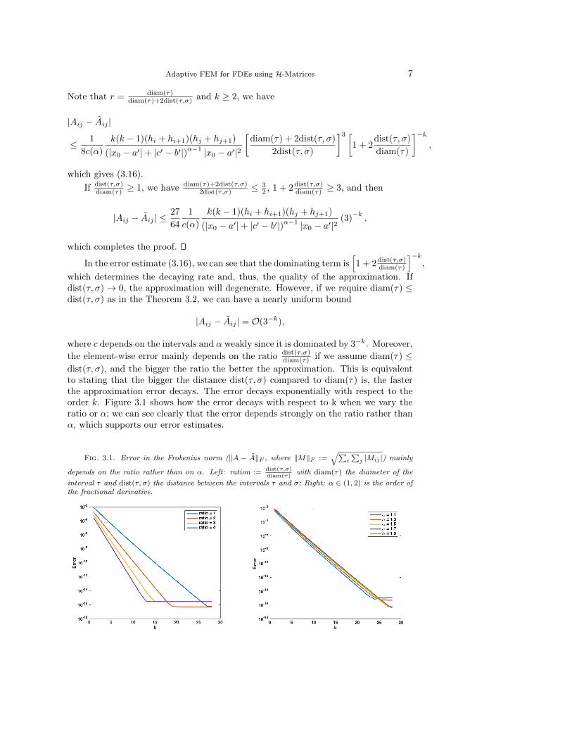
dist(τ, σ), and the bigger the ratio the better the approximation. This is equivalentto stating that the bigger the distance dist(τ, σ) compared to diam(τ) is, the fasterthe approximation error decays. The error decays exponentially with respect to theorder k. Figure 3.1 shows how the error decays with respect to k when we vary theratio or α; we can see clearly that the error depends strongly on the ratio rather thanα, which supports our error estimates.
Fig. 3.1. Error in the Frobenius norm (‖A − A‖F , where ‖M‖F :=√∑
i
∑j |Mij |) mainly
depends on the ratio rather than on α. Left: ration :=dist(τ,σ)diam(τ)
with diam(τ) the diameter of the
interval τ and dist(τ, σ) the distance between the intervals τ and σ; Right: α ∈ (1, 2) is the order ofthe fractional derivative.
8 X. Zhao, X. Hu, W. Cai, G.E. Karniadakis
4. Geometric Multigrid Method based on H-Matrices. In this section, wediscuss how we solve the linear system of equations in the H-Matrix format. Althoughmany existing fast linear solvers based on theH-Matrix format can be applied directly,for example, Hierarchical inversion and H-Matrix LU decomposition (see, e.g. [2]), wewill design the geometric multigrid (GMG) method based on the H-matrix formatand use GMG method to solve the linear system. The reason is the following. Firstly,since we are solving discrete systems resulting from differential equations, the GMGmethod is known to be one of the optimal methods and suitable for large-scale prob-lems. In [17], GMG methods have been introduced to FDEs discretized on uniformgrids. Therefore, it is natural to take advantage of the H-matrices and generalizeGMG methods for FDEs in higher dimensions discretized on non-uniform grids. Sec-ondly, our ultimate goal is to design adaptive finite element methods for solving FDEs,therefore, hierarchical grids are available due to the adaptive refinement procedure(which will be made clear in Section 5); hence, we can use those nested unstruc-tured grids and design GMG methods accordingly. Next, we will present the GMGalgorithms.
As usual, the multigrid method is built upon the subspaces that are defined onnested sequences of triangulations. We assume that we start with an initial grid T0
and a nested sequence of grids {T`}J`=0, where T` is obtained by certain refinementprocedure of T`−1 for ` > 0, i.e.,
T0 ≤ T1 ≤ · · · ≤ TJ = T .
Let V` denote the corresponding linear finite element space based on T`. We thus geta sequence of multilevel spaces
V0 ⊂ V1 ⊂ · · · ⊂ VJ = V.
Note that, a natural space decomposition of V is V =∑J`=0 V` and this is not a direct
sum. Based on these finite element spaces, we have the following linear system ofequations on each level:
A`u` = f`, ` = 0, 1, · · · , J. (4.1)
Correspondingly, we also have their H-Matrix approximation on each level
A`u` = f`, ` = 0, 1, · · · , J, (4.2)
where A` is the H-Matrix representation of A as defined entry-wise by (3.10).In practice, we will solve (4.2) based on the GMG method. Because A` provides
a good approximation to A` on each level `, we can expect that u` provides a goodapproximation to u` on each level ` based on the standard perturbation theory ofsolving linear systems of equations [12]. In order to define the GMG method, we needto introduce the standard prolongation I` on level `, which is the matrix representationof the standard inclusion operator from V`−1 = span{ϕ`−1
1 , ϕ`−12 , · · · , ϕ`−1
N`−1} to V` =
span{ϕ`1, ϕ`2, · · · , ϕ`N`} since V`−1 ⊂ V`, e.g., I` ∈ RN`×N`−1 such that,
(I`)ij = βij , where ϕ`−1j =
N∑i=1
βijϕ`i , j = 1, · · · , N`−1. (4.3)
Now we can define the standard V -cycle GMG method for solving (4.2) by the fol-lowing recursive (Algorithm 1).
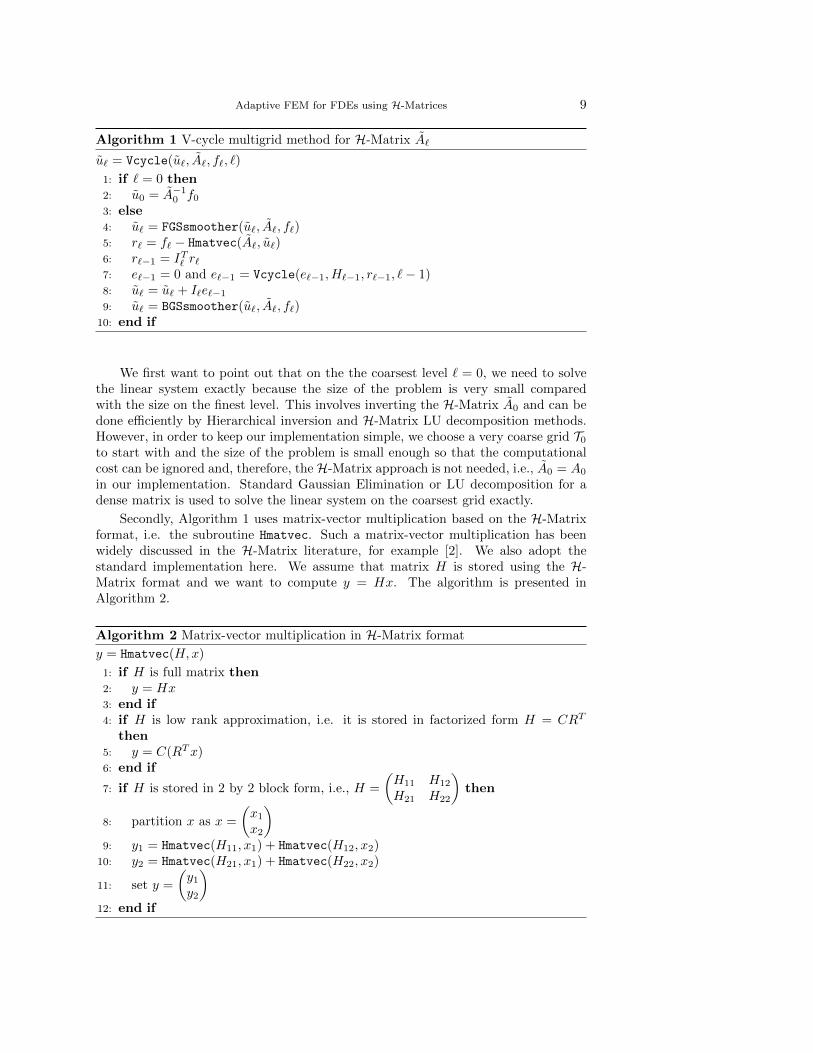
Adaptive FEM for FDEs using H-Matrices 9
Algorithm 1 V-cycle multigrid method for H-Matrix A`
u` = Vcycle(u`, A`, f`, `)
1: if ` = 0 then2: u0 = A−1
0 f0
3: else4: u` = FGSsmoother(u`, A`, f`)5: r` = f` − Hmatvec(A`, u`)6: r`−1 = IT` r`7: e`−1 = 0 and e`−1 = Vcycle(e`−1, H`−1, r`−1, `− 1)8: u` = u` + I`e`−1
9: u` = BGSsmoother(u`, A`, f`)10: end if
We first want to point out that on the the coarsest level ` = 0, we need to solvethe linear system exactly because the size of the problem is very small comparedwith the size on the finest level. This involves inverting the H-Matrix A0 and can bedone efficiently by Hierarchical inversion and H-Matrix LU decomposition methods.However, in order to keep our implementation simple, we choose a very coarse grid T0
to start with and the size of the problem is small enough so that the computationalcost can be ignored and, therefore, theH-Matrix approach is not needed, i.e., A0 = A0
in our implementation. Standard Gaussian Elimination or LU decomposition for adense matrix is used to solve the linear system on the coarsest grid exactly.
Secondly, Algorithm 1 uses matrix-vector multiplication based on the H-Matrixformat, i.e. the subroutine Hmatvec. Such a matrix-vector multiplication has beenwidely discussed in the H-Matrix literature, for example [2]. We also adopt thestandard implementation here. We assume that matrix H is stored using the H-Matrix format and we want to compute y = Hx. The algorithm is presented inAlgorithm 2.
Algorithm 2 Matrix-vector multiplication in H-Matrix format
y = Hmatvec(H,x)
1: if H is full matrix then2: y = Hx3: end if4: if H is low rank approximation, i.e. it is stored in factorized form H = CRT
then5: y = C(RTx)6: end if
7: if H is stored in 2 by 2 block form, i.e., H =
(H11 H12
H21 H22
)then
8: partition x as x =
(x1
x2
)9: y1 = Hmatvec(H11, x1) + Hmatvec(H12, x2)
10: y2 = Hmatvec(H21, x1) + Hmatvec(H22, x2)
11: set y =
(y1
y2
)12: end if
10 X. Zhao, X. Hu, W. Cai, G.E. Karniadakis
Finally, we discuss the smoothers used in the GMG Algorithm 1. We use Gauss-Seidel smoothers in our implementation. The Subroutine FGSsmoother is the imple-mentation of forward Gauss-Seidel method and the subroutine BGSsmoother is theimplementation of backward Gauss-Seidel method. Their implementations are givenby Algorithm 3 and 4, respectively.
Algorithm 3 Forward Gauss-Seidel smoother in H-Matrix format
x = FGSsmoother(H, b, x)
1: r = b− Hmatvec(H,x)2: if H is full matrix then3: get the lower triangular part L of H4: z = L−1r5: x = x+ z6: end if
7: if H is stored in 2 by 2 block form, i.e., H =
(H11 H12
H21 H22
)then
8: partition r as r =
(r1
r2
)9: z1 = FGSsmoother(H11, r1, 0)
10: r2 = r2 − Hmatvec(H21, z1)11: z2 = FGSsmoother(H22, r2, 0)
12: set z =
(z1
z2
)13: x = x+ z14: end if
Algorithm 4 Backward Gauss-Seidel smoother in H-Matrix format
x = BGSsmoother(H, b, x)
1: r = b− Hmatvec(H,x)2: if H is full matrix then3: get the upper triangular part U of H4: z = U−1r5: x = x+ z6: end if
7: if H is stored in 2 by 2 block form, i.e., H =
(H11 H12
H21 H22
)then
8: partition r as r =
(r1
r2
)9: z2 = BGSsmoother(H22, r2, 0)
10: r1 = r1 − Hmatvec(H12, z2)11: z1 = BGSsmoother(H11, r1, 0)
12: set z =
(z1
z2
)13: x = x+ z14: end if
Note that in the Gauss-Seidel smoother algorithms, we do not consider the casethat H is a low rank approximation and is stored in factorized form H = CRT . This
Adaptive FEM for FDEs using H-Matrices 11
is because in the Gauss-Seidel algorithm, only the diagonal entries will be invertedand, in our H-Matrix representation for the FDEs, the diagonal entries are definitelystored explicitly in the full matrix format. Therefore, we consider the cases whereH is stored in either full matrix format or 2 by 2 block format, where the diagonalentries need to be accessed recursively.
Based on Algorithm 2, 3, and 4, the V-cycle multigrid Algorithm 1 is well-defined. It is easy to check that the overall computational complexity of one V-cycleis O(kN` logN`) where N` is the number of degrees of freedom on the level ` and k isthe upper bound of the rank used in the low rank approximation for the H-Matrix.This is because the computational cost of matrix-vector multiplication for H-Matrixis O(kN` logN`) and it is well-known that the Gauss-Seidel method has roughly thesame computational cost as the matrix-vector multiplication. In practice, k � N`usually is a small number and does not depends on N`. Therefore, we can say thatthe computational cost of V-cycle multigrid on level ` is roughly O(N` logN`). Notethat the computational complexity for solving the linear system of equations in theH-Matrix format, such as Hierarchical inversion and H-Matrix LU decompositionmethods, is O(k2N` log2N`) ≈ O(N` log2N`) [2]. Therefore, the GMG approach isslightly better in terms of computational cost, especially for large-scale problems.
5. Adaptive Finite Element Method for Fractional PDEs. In this section,we discuss the adaptive finite element method (AFEM) for solving FDEs. We followthe idea of standard AFEM, which is characterized by the following iteration
SOLVE −→ ESTIMATE −→ MARK −→ REFINE.
Such iteration generates a sequence of discrete solutions converging to the exact one.We want to emphasize that one of the main difficulties of applying the AFEM to theFDEs is the SOLVE step. The AFEM iteration usually generates non-uniform grids,which makes the resulting linear system difficult to solve by existing fast linear solvers.This is because usually the traditional approaches take advantage of the uniform gridand the Toeplitz structure of the resulting stiffness matrices, which is not true for thenon-uniform grid. However, in this paper, by introducing the H-Matrix approach andGMG method, we can efficiently solve the linear system obtained on the non-uniformgrid and, therefore, design an AFEM method for FDEs so that each AFEM iterationhas computational complexity O(kN logN), suitable for practice applications. Next,we will introduce the four modules in the AFEM iterations.
5.1. SOLVE Module. As usual, the SOLVE module should take the current gridas the input and output the corresponding finite element approximation. Note herethat the current grid in general is obtained by adaptive refinement and, therefore,it is an unstructured grid. So, our SOLVE module will use the hierarchical matrixrepresentation mentioned in Section 3 to assemble the linear system of equationsstored in H-Matrix format and solve it by the GMG method discussed in Section 4.The detailed description is listed below.
Let N` denote the number of degrees of freedoms on grid T`. As discussed inSection 3, assembling the H-Matrix on grid T` costs O(kN` logN`) operations andsolving U` by the GMG method also costs O(kN` logN`) operations. Therefore, theoverall cost of the SOLVE module is O(kN` logN`) or O(N` logN`) when k � N`.
5.2. ESTIMATE Module. Given a grid T` and finite element approximation u` ∈V`, the ESTIMATE module computes a posteriori error estimators {η`(u`, τ)}τ∈T` , whichshould be computable on each element τ ∈ T` and indicate the true error. Such a
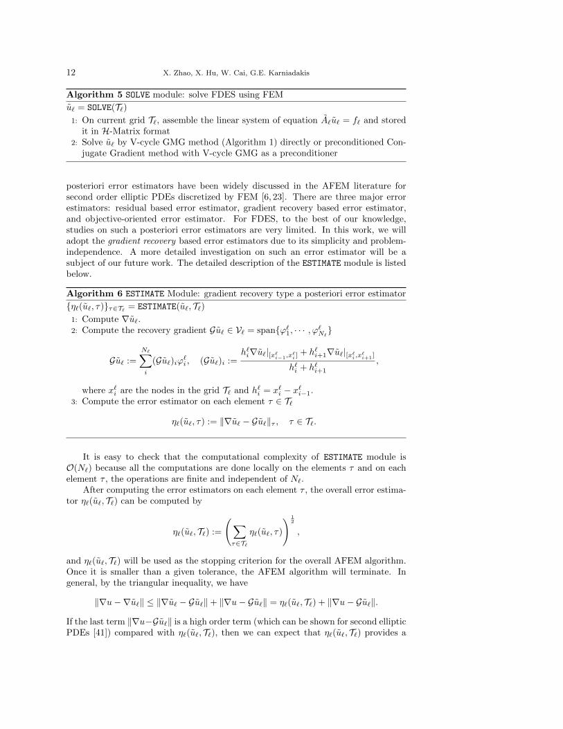
12 X. Zhao, X. Hu, W. Cai, G.E. Karniadakis
Algorithm 5 SOLVE module: solve FDES using FEM
u` = SOLVE(T`)1: On current grid T`, assemble the linear system of equation A`u` = f` and stored
it in H-Matrix format2: Solve u` by V-cycle GMG method (Algorithm 1) directly or preconditioned Con-
jugate Gradient method with V-cycle GMG as a preconditioner
posteriori error estimators have been widely discussed in the AFEM literature forsecond order elliptic PDEs discretized by FEM [6, 23]. There are three major errorestimators: residual based error estimator, gradient recovery based error estimator,and objective-oriented error estimator. For FDES, to the best of our knowledge,studies on such a posteriori error estimators are very limited. In this work, we willadopt the gradient recovery based error estimators due to its simplicity and problem-independence. A more detailed investigation on such an error estimator will be asubject of our future work. The detailed description of the ESTIMATE module is listedbelow.
Algorithm 6 ESTIMATE Module: gradient recovery type a posteriori error estimator
{η`(u`, τ)}τ∈T` = ESTIMATE(u`, T`)1: Compute ∇u`.2: Compute the recovery gradient Gu` ∈ V` = span{ϕ`1, · · · , ϕ`N`}
Gu` :=
N∑i
(Gu`)iϕ`i , (Gu`)i :=h`i∇u`|[x`i−1,x
`i ]
+ h`i+1∇u`|[x`i ,x`i+1]
h`i + h`i+1
,
where x`i are the nodes in the grid T` and h`i = x`i − x`i−1.3: Compute the error estimator on each element τ ∈ T`
η`(u`, τ) := ‖∇u` − Gu`‖τ , τ ∈ T`.
It is easy to check that the computational complexity of ESTIMATE module isO(N`) because all the computations are done locally on the elements τ and on eachelement τ , the operations are finite and independent of N`.
After computing the error estimators on each element τ , the overall error estima-tor η`(u`, T`) can be computed by
η`(u`, T`) :=
(∑τ∈T`
η`(u`, τ)
) 12
,
and η`(u`, T`) will be used as the stopping criterion for the overall AFEM algorithm.Once it is smaller than a given tolerance, the AFEM algorithm will terminate. Ingeneral, by the triangular inequality, we have
‖∇u−∇u`‖ ≤ ‖∇u` − Gu`‖+ ‖∇u− Gu`‖ = η`(u`, T`) + ‖∇u− Gu`‖.
If the last term ‖∇u−Gu`‖ is a high order term (which can be shown for second ellipticPDEs [41]) compared with η`(u`, T`), then we can expect that η`(u`, T`) provides a
Adaptive FEM for FDEs using H-Matrices 13
good estimation of the true error ‖∇u−∇u`‖ and, therefore, guarantees the efficiencyof the overall AFEM algorithm. For FDES, numerical experiments presented belowsuggest that ‖∇u − Gu`‖ is indeed a high order term. A more rigorous analysis onthis topic will be our future work.
5.3. MARK Module. The MARK module selects elements τ ∈ T` whose local errorη`(U`, τ) is relatively large and needs to be refined in the refinement. This module isindependent of the model problems and we can directly use the strategies developedfor second order elliptic PDEs for FDES here. In this work, we use the so-calledDoflers marking strategy [23] with the detailed algorithm listed below (Algorithm 7).
Algorithm 7 MARK Module: Dofler’s marking strategy
M` = MARK(T`, η`(u`, τ), θ)
1: Choose a subset M` ⊂ T` such that
η`(u`,M`) ≤ θη`(u`, T`), (5.1)
where η`(u`,M`) :=(∑
τ∈M`η`(u`, τ)
) 12 .
Here we require that the parameter θ ∈ (0, 1]. Obviously, the choice ofM` is notunique. In practice, in order to reduce the computational cost, we prefer the size of thesubsetM` to be as small as possible. Therefore, we typically use the greedy approachin the implementation of ESTIMATE module. We first order the elements τ accordingto the error indicators η`(U`, τ) from large to small and then pick the element τ ina greedy way so that condition (5.1) will be satisfied with minimal number of theelements.
Based on the above discussion, the ordering could be done in O(N` logN`) opera-tions and picking the elements can be done in O(N`) operations, therefore, the overallcomputational complexity of the ESTIMATE module is O(N` logN`).
5.4. REFINE Module. The REFINE module is also problem independent. It takesthe marked elementsM` and current grid Tk as inputs and outputs a refined grid T`+1,which will be used as a new grid. In this work, because we are only considering the 1Dcase, the refinement procedure is just bisection. Namely, if an element [x`i−1, x
`i ] ∈ T` is
marked, it will be divided into two subintervals [x`i−1, x`i ] and [x`i , x
`i ] by the midpoint
x`i = (x`i−1 + x`i)/2. The detailed algorithm is listed below (Algorithm 8).
Algorithm 8 REFINE Module: bisection refinement
T`+1 = REFINE(T`,M`)
1: for τ ∈M` do2: refine τ using bisection and generate two new elements.3: end for4: Combine all new elements and subset T`\Ml to generate the new grid T`+1.
Obviously, the computational cost of the REFINE module is at most O(N`).
5.5. AFEM Algorithm. After discussing each module, now we can summarizeour AFEM algorithm for solving FDES. We assume that an initial grid T0, a parameterθ ∈ (0, 1], and a targeted tolerance ε are given. The AFEM algorithm is listed inAlgorithm 9.
14 X. Zhao, X. Hu, W. Cai, G.E. Karniadakis
Algorithm 9 Adaptive Finite Element Method for Solving FDES
uJ = AFEM(T0, θ, ε)
1: Set ` = 02: loop3: u` = SOLVE(T`)4: {η`(u`, τ)}τ∈T` = ESTIMATE(u`, T`)5: if η`(u`, T`) ≤ ε then6: J = ` and uJ := u`.7: return8: end if9: M` = MARK(T`, η`(u`, τ), θ)
10: T`+1 = REFINE(T`,M`)11: ` = `+ 112: end loop
Obviously, the overall computational cost of each iteration of the AFEM methodis O(kN` logN`) or O(N` logN`) when k � N`.
6. Numerical Examples. In this section, we present some numerical experi-ments to demonstrate the efficiency and robustness of the proposed H-Matrix repre-sentation, GMG method, and AFEM algorithm for solving the FDES. All the codesare written in MATLAB and the tests are performed on a Macbook Pro Laptop withInter Core i7 (3 GHz) CPU and 16G RAM.
Example 6.1. Solving problem (3.1) with exact solution u(x) = 10x2(1−x2) on[b,c]=[0,1]. The right hand side can be computed as
f(x) =− 10
2 cos(απ/2)
{2
Γ(3− α)
[x2−α + (1− x)2−α]− 12
Γ(4− α)
[x3−α + (1− x)3−α]
+24
Γ(5− α)
[x4−α + (1− x)4−α]} .
It is easy to see that for Example 6.1, the solution u(x) is smooth. Therefore, theadaptive method is unnecessary for this example and we mainly use uniform gridand uniform refinement. The purpose of this example is to show the accuracy of theH-Matrix representation, the efficiency of the GMG method, and the overall optimalcomputational complexity of the proposed approach.
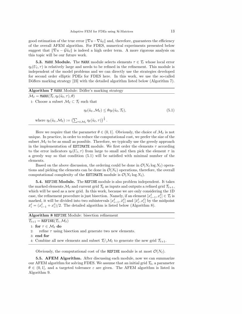
Figures 6.1 and 6.2 present the convergence behavior of the finite element ap-proximations based on full matrix approach and H-Matrix representation for differentvalues of α. For the full matrix approach, we use a direct solver (LU decomposition)to solve the linear system of equations (command “\” in MATLAB) and, for theH-Matrix, we solve the linear system of equations iteratively by the GMG methodpresented in Section 4. The stopping criterion is the relative residual to be less than10−10. The convergence rate of absolute error and L2 error are presented. In all ourexperiments, we use the fact that logE = −r logN + logC which is derived fromE = CN−r, where E denotes error, and then compute the convergence rate r bythe linear polynomial fitting between logE and logN . In all cases, we can see thatusing the H-Matrix representation, the convergence orders are still around 2 whichis optimal as expected. Moreover, in all cases, the errors obtained by the H-Matrixrepresentation are also comparable with the errors obtained by using the full matrix.
Adaptive FEM for FDEs using H-Matrices 15
Fig. 6.1. Example 6.1 (α = 1.2). Convergence comparison between full matrix approach andH-Matrix representation.
Fig. 6.2. Example 6.1 (α = 1.5). Convergence comparison between full matrix approach andH-Matrix representation.
The results show that using the H-Matrix representation can still achieve the optimalconvergence order and the accuracy of finite element approximations is still reliable.
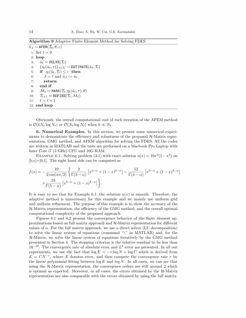
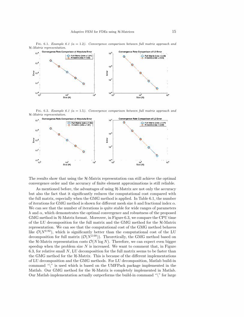
As mentioned before, the advantages of using H-Matrix are not only the accuracybut also the fact that it significantly reduces the computational cost compared withthe full matrix, especially when the GMG method is applied. In Table 6.1, the numberof iterations for GMG method is shown for different mesh size h and fractional index α.We can see that the number of iterations is quite stable for wide ranges of parametersh and α, which demonstrates the optimal convergence and robustness of the proposedGMG method inH-Matrix format. Moreover, in Figure 6.3, we compare the CPU timeof the LU decomposition for the full matrix and the GMG method for the H-Matrixrepresentation. We can see that the computational cost of the GMG method behaveslike O(N0.92), which is significantly better than the computational cost of the LUdecomposition for full matrix (O(N2.68)). Theoretically, the GMG method based onthe H-Matrix representation costs O(N logN). Therefore, we can expect even biggerspeedup when the problem size N is increased. We want to comment that, in Figure6.3, for relative small N , LU decomposition for the full matrix seems to be faster thanthe GMG method for the H-Matrix. This is because of the different implementationsof LU decomposition and the GMG methods. For LU decomposition, Matlab build-incommand “\” is used which is based on the UMFPack package implemented in theMatlab. Our GMG method for the H-Matrix is completely implemented in Matlab.Our Matlab implementation actually outperforms the build-in command “\” for large
16 X. Zhao, X. Hu, W. Cai, G.E. Karniadakis
size N , which is a strong evidence of the efficiency of the GMG method for the H-Matrix.
Table 6.1Example 6.1: number of iterations of GMG method (stopping criterion: relative residual less
than or equal to 10−10)
h = 1/256 h = 1/512 h = 1/1024 h = 1/2048 h = 1/4095α = 1.1 9 9 9 9 9α = 1.3 10 10 10 10 11α = 1.5 11 11 11 12 12α = 1.7 12 12 12 12 13α = 1.9 13 13 13 13 14
Fig. 6.3. Example 6.1 (α = 1.5) CPU time comparison between full matrix (LU decomposition)and the H-Matrix (multigrid)
Example 6.2. Solving model problem (3.1) with right hand side f(x) = 1 +sin(x).
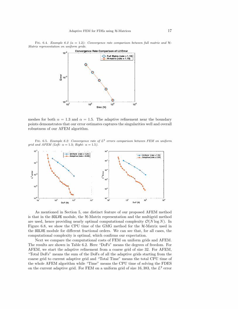
The second example we consider here does not have exact solution. However, dueto the property of the FDES, we expect the solution to have singularities near theboundaries, which leads to degenerated convergence rate in the errors of finite elementapproximations on uniform grids. This is confirmed by the numerical results as shownin Figure 6.4. The convergence rates of the L2 errors for both full matrix and H-Matrix approaches are about 1.2, which reflects the singularity of the solution and thenecessity for the AFEM method. These comparisons show that the AFEM algorithmcan achieve better accuracy with less computational cost, which demonstrates theeffectiveness of the AFEM algorithm for FDES.
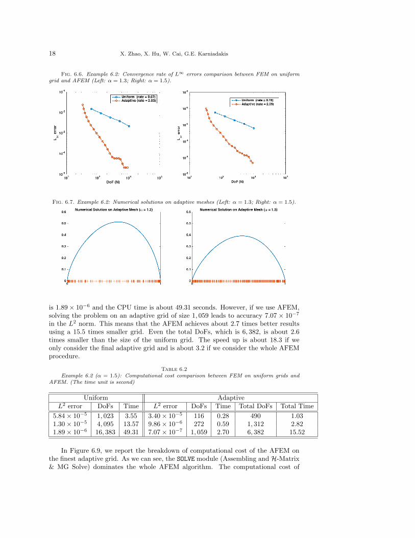
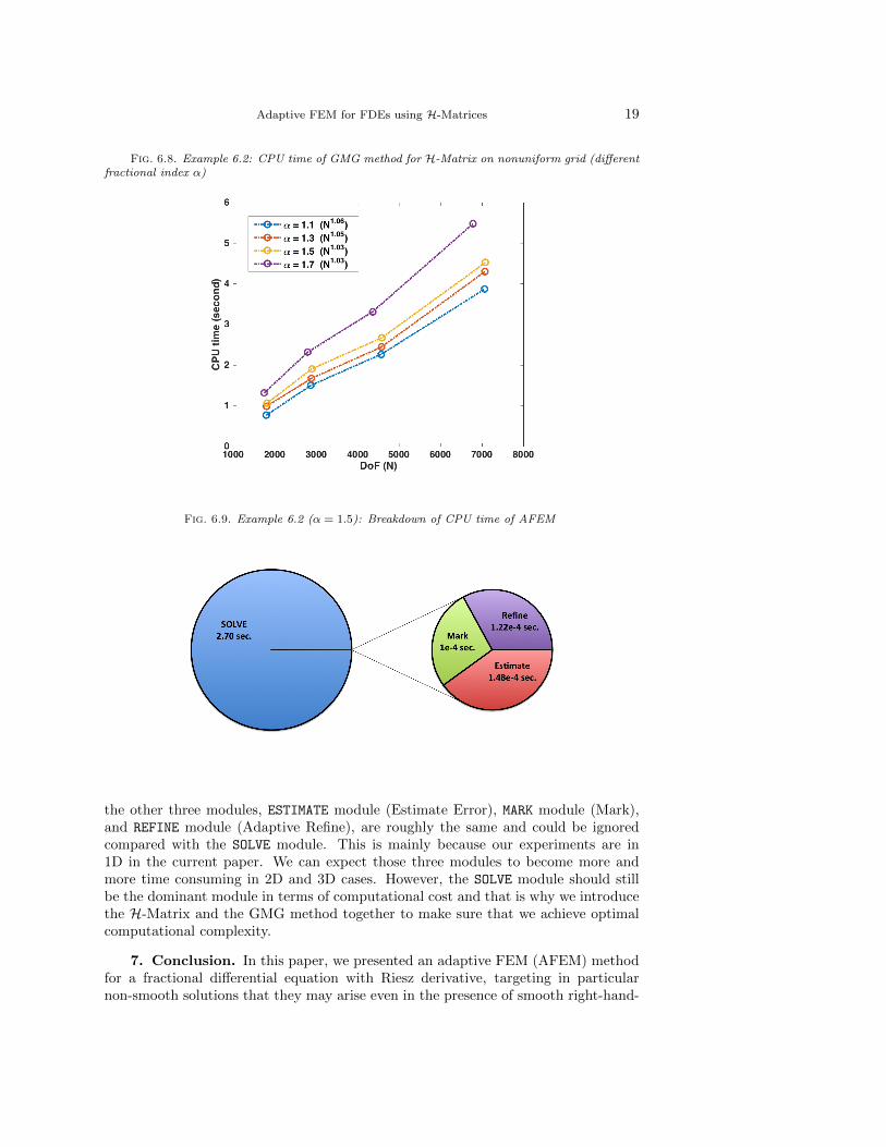
Next we apply the AFEM algorithm (Algorithm 9) to solve Example 6.2. Theresults are shown in Figures 6.5 and 6.6. We can see that, using the AFEM method,the optimal convergence rates of both L2 error and L∞ have been recovered for bothα = 1.3 and α = 1.5. This demonstrates the effectiveness and robustness of theour AFEM methods. In Figure 6.7, we plot the numerical solutions on adaptive
Adaptive FEM for FDEs using H-Matrices 17
Fig. 6.4. Example 6.2 (α = 1.2): Convergence rate comparison between full matrix and H-Matrix representation on uniform grids.
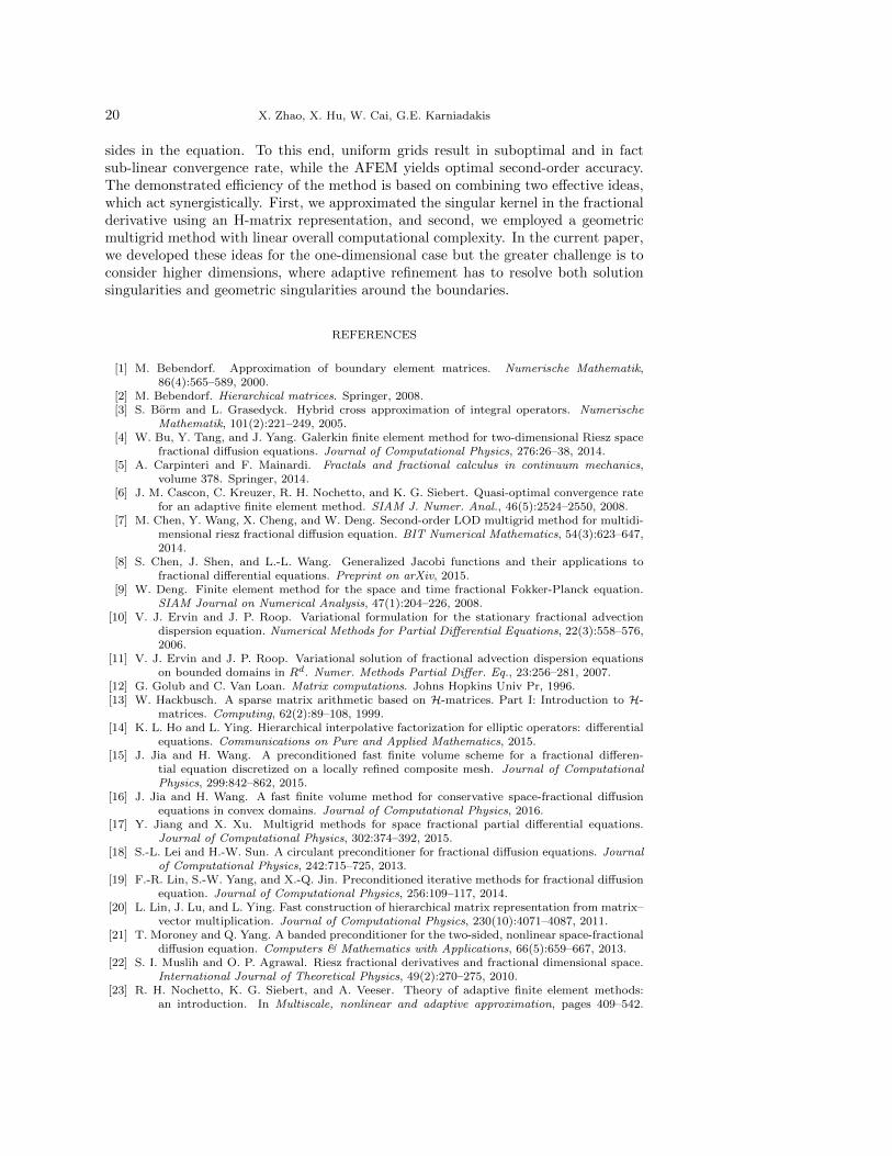
meshes for both α = 1.3 and α = 1.5. The adaptive refinement near the boundarypoints demonstrates that our error estimates captures the singularities well and overallrobustness of our AFEM algorithm.
Fig. 6.5. Example 6.2: Convergence rate of L2 errors comparison between FEM on uniformgrid and AFEM (Left: α = 1.3; Right: α = 1.5).
As mentioned in Section 5, one distinct feature of our proposed AFEM methodis that in the SOLVE module, the H-Matrix representation and the multigrid methodare used, hence providing nearly optimal computational complexity O(N logN). InFigure 6.8, we show the CPU time of the GMG method for the H-Matrix used inthe SOLVE module for different fractional orders. We can see that, for all cases, thecomputational complexity is optimal, which confirms our expectation.
Next we compare the computational costs of FEM on uniform grids and AFEM.The results are shown in Table 6.2. Here “DoFs” means the degrees of freedom. ForAFEM, we start the adaptive refinement from a coarse grid of size 32. For AFEM,“Total DoFs” means the sum of the DoFs of all the adaptive grids starting from thecoarse grid to current adaptive grid and “Total Time” means the total CPU time ofthe whole AFEM algorithm while “Time” means the CPU time of solving the FDESon the current adaptive grid. For FEM on a uniform grid of size 16, 383, the L2 error
18 X. Zhao, X. Hu, W. Cai, G.E. Karniadakis
Fig. 6.6. Example 6.2: Convergence rate of L∞ errors comparison between FEM on uniformgrid and AFEM (Left: α = 1.3; Right: α = 1.5).
Fig. 6.7. Example 6.2: Numerical solutions on adaptive meshes (Left: α = 1.3; Right: α = 1.5).
is 1.89× 10⁻⁶ and the CPU time is about 49.31 seconds. However, if we use AFEM,solving the problem on an adaptive grid of size 1, 059 leads to accuracy 7.07 × 10⁻⁷
in the L2 norm. This means that the AFEM achieves about 2.7 times better resultsusing a 15.5 times smaller grid. Even the total DoFs, which is 6, 382, is about 2.6times smaller than the size of the uniform grid. The speed up is about 18.3 if weonly consider the final adaptive grid and is about 3.2 if we consider the whole AFEMprocedure.
Table 6.2Example 6.2 (α = 1.5): Computational cost comparison between FEM on uniform grids and
AFEM. (The time unit is second)
Uniform AdaptiveL2 error DoFs Time L2 error DoFs Time Total DoFs Total Time
5.84× 10⁻⁵ 1, 023 3.55 3.40× 10⁻⁵ 116 0.28 490 1.031.30× 10−5 4, 095 13.57 9.86× 10⁻⁶ 272 0.59 1, 312 2.821.89× 10−6 16, 383 49.31 7.07× 10⁻⁷ 1, 059 2.70 6, 382 15.52
In Figure 6.9, we report the breakdown of computational cost of the AFEM onthe finest adaptive grid. As we can see, the SOLVE module (Assembling and H-Matrix& MG Solve) dominates the whole AFEM algorithm. The computational cost of
Adaptive FEM for FDEs using H-Matrices 19
Fig. 6.8. Example 6.2: CPU time of GMG method for H-Matrix on nonuniform grid (differentfractional index α)
Fig. 6.9. Example 6.2 (α = 1.5): Breakdown of CPU time of AFEM
the other three modules, ESTIMATE module (Estimate Error), MARK module (Mark),and REFINE module (Adaptive Refine), are roughly the same and could be ignoredcompared with the SOLVE module. This is mainly because our experiments are in1D in the current paper. We can expect those three modules to become more andmore time consuming in 2D and 3D cases. However, the SOLVE module should stillbe the dominant module in terms of computational cost and that is why we introducethe H-Matrix and the GMG method together to make sure that we achieve optimalcomputational complexity.
7. Conclusion. In this paper, we presented an adaptive FEM (AFEM) methodfor a fractional differential equation with Riesz derivative, targeting in particularnon-smooth solutions that they may arise even in the presence of smooth right-hand-
20 X. Zhao, X. Hu, W. Cai, G.E. Karniadakis
sides in the equation. To this end, uniform grids result in suboptimal and in factsub-linear convergence rate, while the AFEM yields optimal second-order accuracy.The demonstrated efficiency of the method is based on combining two effective ideas,which act synergistically. First, we approximated the singular kernel in the fractionalderivative using an H-matrix representation, and second, we employed a geometricmultigrid method with linear overall computational complexity. In the current paper,we developed these ideas for the one-dimensional case but the greater challenge is toconsider higher dimensions, where adaptive refinement has to resolve both solutionsingularities and geometric singularities around the boundaries.
REFERENCES
[1] M. Bebendorf. Approximation of boundary element matrices. Numerische Mathematik,86(4):565–589, 2000.
[2] M. Bebendorf. Hierarchical matrices. Springer, 2008.[3] S. Borm and L. Grasedyck. Hybrid cross approximation of integral operators. Numerische
Mathematik, 101(2):221–249, 2005.[4] W. Bu, Y. Tang, and J. Yang. Galerkin finite element method for two-dimensional Riesz space
fractional diffusion equations. Journal of Computational Physics, 276:26–38, 2014.[5] A. Carpinteri and F. Mainardi. Fractals and fractional calculus in continuum mechanics,
volume 378. Springer, 2014.[6] J. M. Cascon, C. Kreuzer, R. H. Nochetto, and K. G. Siebert. Quasi-optimal convergence rate
for an adaptive finite element method. SIAM J. Numer. Anal., 46(5):2524–2550, 2008.[7] M. Chen, Y. Wang, X. Cheng, and W. Deng. Second-order LOD multigrid method for multidi-
mensional riesz fractional diffusion equation. BIT Numerical Mathematics, 54(3):623–647,2014.
[8] S. Chen, J. Shen, and L.-L. Wang. Generalized Jacobi functions and their applications tofractional differential equations. Preprint on arXiv, 2015.
[9] W. Deng. Finite element method for the space and time fractional Fokker-Planck equation.SIAM Journal on Numerical Analysis, 47(1):204–226, 2008.
[10] V. J. Ervin and J. P. Roop. Variational formulation for the stationary fractional advectiondispersion equation. Numerical Methods for Partial Differential Equations, 22(3):558–576,2006.
[11] V. J. Ervin and J. P. Roop. Variational solution of fractional advection dispersion equationson bounded domains in Rd. Numer. Methods Partial Differ. Eq., 23:256–281, 2007.
[12] G. Golub and C. Van Loan. Matrix computations. Johns Hopkins Univ Pr, 1996.[13] W. Hackbusch. A sparse matrix arithmetic based on H-matrices. Part I: Introduction to H-
matrices. Computing, 62(2):89–108, 1999.[14] K. L. Ho and L. Ying. Hierarchical interpolative factorization for elliptic operators: differential
equations. Communications on Pure and Applied Mathematics, 2015.[15] J. Jia and H. Wang. A preconditioned fast finite volume scheme for a fractional differen-
tial equation discretized on a locally refined composite mesh. Journal of ComputationalPhysics, 299:842–862, 2015.
[16] J. Jia and H. Wang. A fast finite volume method for conservative space-fractional diffusionequations in convex domains. Journal of Computational Physics, 2016.
[17] Y. Jiang and X. Xu. Multigrid methods for space fractional partial differential equations.Journal of Computational Physics, 302:374–392, 2015.
[18] S.-L. Lei and H.-W. Sun. A circulant preconditioner for fractional diffusion equations. Journalof Computational Physics, 242:715–725, 2013.
[19] F.-R. Lin, S.-W. Yang, and X.-Q. Jin. Preconditioned iterative methods for fractional diffusionequation. Journal of Computational Physics, 256:109–117, 2014.
[20] L. Lin, J. Lu, and L. Ying. Fast construction of hierarchical matrix representation from matrix–vector multiplication. Journal of Computational Physics, 230(10):4071–4087, 2011.
[21] T. Moroney and Q. Yang. A banded preconditioner for the two-sided, nonlinear space-fractionaldiffusion equation. Computers & Mathematics with Applications, 66(5):659–667, 2013.
[22] S. I. Muslih and O. P. Agrawal. Riesz fractional derivatives and fractional dimensional space.International Journal of Theoretical Physics, 49(2):270–275, 2010.
[23] R. H. Nochetto, K. G. Siebert, and A. Veeser. Theory of adaptive finite element methods:an introduction. In Multiscale, nonlinear and adaptive approximation, pages 409–542.
Adaptive FEM for FDEs using H-Matrices 21
Springer, Berlin, 2009.[24] J. Pan, R. Ke, M. K. Ng, and H.-W. Sun. Preconditioning techniques for diagonal-times-
toeplitz matrices in fractional diffusion equations. SIAM Journal on Scientific Computing,36(6):A2698–A2719, 2014.
[25] G. Pang, W. Chen, and Z. Fu. Space-fractional advection–dispersion equations by the Kansamethod. Journal of Computational Physics, 293:280–296, 2015.
[26] H.-K. Pang and H.-W. Sun. Multigrid method for fractional diffusion equations. Journal ofComputational Physics, 231(2):693–703, 2012.
[27] I. Podlubny. Fractional differential equations: an introduction to fractional derivatives, frac-tional differential equations, to methods of their solution and some of their applications,volume 198. Academic press, 1998.
[28] A. Rebenshtok, S. Denisov, P. Hanggi, and E. Barkai. Non-normalizable densities instrong anomalous diffusion: beyond the central limit theorem. Physical review letters,112(11):110601, 2014.
[29] J. P. Roop. Computational aspects of FEM approximation of fractional advection dispersionequations on bounded domains in R2. Journal of Computational and Applied Mathematics,193(1):243–268, 2006.
[30] L. Sabatelli, S. Keating, J. Dudley, and P. Richmond. Waiting time distributions in financialmarkets. The European Physical Journal B-Condensed Matter and Complex Systems,27(2):273–275, 2002.
[31] S. Samko, A. Kilbas, and O. Marichev. Fractional integrals and derivatives; theory and appli-cations. Gordon and Breach. Lon don, 1993.
[32] P. G. Schmitz and L. Ying. A fast nested dissection solver for cartesian 3d elliptic problemsusing hierarchical matrices. Journal of Computational Physics, 258:227–245, 2014.
[33] M. Shlesinger, B. West, and J. Klafter. Levy dynamics of enhanced diffusion: Application toturbulence. Physical Review Letters, 58(11):1100, 1987.
[34] H. Sun, W. Chen, and Y. Chen. Variable-order fractional differential operators in anomalousdiffusion modeling. Physica A: Statistical Mechanics and its Applications, 388(21):4586–4592, 2009.
[35] W. Tian, H. Zhou, and W. Deng. A class of second order difference approximations for solvingspace fractional diffusion equations. Mathematics of Computation, 84(294):1703–1727,2015.
[36] H. Wang and T. S. Basu. A fast finite difference method for two-dimensional space-fractionaldiffusion equations. SIAM Journal on Scientific Computing, 34(5):A2444–A2458, 2012.
[37] H. Wang and N. Du. A fast finite difference method for three-dimensional time-dependent space-fractional diffusion equations and its efficient implementation. Journal of ComputationalPhysics, 253:50–63, 2013.
[38] H. Wang and N. Du. A superfast-preconditioned iterative method for steady-state space-fractional diffusion equations. Journal of Computational Physics, 240:49–57, 2013.
[39] H. Wang and K. Wang. An O(n log 2n) alternating-direction finite difference methodfor two-dimensional fractional diffusion equations. Journal of Computational Physics,230(21):7830–7839, 2011.
[40] H. Wang, K. Wang, and T. Sircar. A direct O(n log 2n) finite difference method for fractionaldiffusion equations. Journal of Computational Physics, 229(21):8095–8104, 2010.
[41] J. Xu and Z. Zhang. Analysis of recovery type a posteriori error estimators for mildly structuredgrids. Math. Comp., 73(247):1139–1152 (electronic), 2004.
[42] Q. Yang, F. Liu, and I. Turner. Numerical methods for fractional partial differential equationswith riesz space fractional derivatives. Applied Mathematical Modelling, 34(1):200–218,2010.
[43] M. Zayernouri and G. E. Karniadakis. Fractional spectral collocation method. SIAM Journalon Scientific Computing, 36(1):A40–A62, 2014.
[44] F. Zeng, Z. Zhang, and G. E. Karniadakis. A generalized spectral collocation method withtunable accuracy for variable-order fractional differential equations. SIAM Journal onScientific Computing, 37(6):A2710–A2732, 2015.
[45] X. Zhao and Z. Zhang. Superconvergence points of fractional spectral interpolation. arXivpreprint arXiv:1503.06888, 2015.
[46] Z. Zhou and H. Wu. Finite element multigrid method for the boundary value problem offractional advection dispersion equation. Journal of Applied Mathematics, 2013, 2013.