adaptive collision avoidance using road friction...

348 IEEE TRANSACTIONS ON INTELLIGENT TRANSPORTATION SYSTEMS, VOL. 20, NO. 1, JANUARY 2019

Adaptive Collision Avoidance UsingRoad Friction Information

Yunhyoung Hwang and Seibum B. Choi , Member, IEEE

Abstract— Technical development with the goal of achievingzero accidents and zero fatalities is ongoing. The autonomousemergency braking systems that debuted in the late 2000shave proven their value regarding improved safety. However,the technology still presents many challenges because it is noteasy to ensure that the system will operate as intended in anyenvironment and at any time. Any system that is unaware of itsenvironment is prone to be excessively conservative, which couldadversely affect the efficacy of said system. Situation awarenessis a key to resolving this problem. The present study suggeststhe use of warning braking to gain an awareness of the levelof road friction, which is one of the major uncertainties facedon the road. During warning braking, the tire-road maximumfriction coefficient is estimated in real time, and a threat assess-ment is performed adaptively based on the friction information.Because warning braking is momentary and applied with limiteddynamics due to issues related to human factors, this studydiscusses the major considerations and requirements for thekey parameters related to warning braking. The performanceof the suggested adaptive collision avoidance scheme is verifiedby means of simulation and experiments.

Index Terms— Collision avoidance, threat assessment, situationawareness, autonomous emergency braking.

NOMENCLATURE

W B Warning braking.P B Partial braking.E B Emergency braking.Ab Automated deceleration for threat

assessment [m/s2].Jb Limited jerk of automated braking [m/s3].Td Time delay [s].Jwb Jerk of warning braking [m/s3].Dwb Duration of warning braking [s].Awb Peak deceleration of warning braking [m/s2].th Prediction horizon [s].vego Speed of ego vehicle [m/s].vtar Speed of target vehicle [m/s].vr Relative speed between ego and target

vehicle [m/s].

Manuscript received May 25, 2017; revised December 27, 2017; acceptedFebruary 25, 2018. Date of publication April 23, 2018; date of current versionDecember 21, 2018. This work was supported in part by the Korea Ministryof Science, ICT and Future Planning under Grant R-20160302-003057. TheAssociate Editor for this paper was M. Brackstone. (Corresponding author:Seibum B. Choi.)

Y. Hwang is with the Smart Vehicle Control Centre, Korea AutomotiveTechnology Institute, Cheonan 31214, South Korea (e-mail: [email protected]).

S. B. Choi is with the Mechanical Engineering Department, Korea AdvancedInstitute of Science & Technology, Daejeon 34141, South Korea (e-mail:[email protected]).

Digital Object Identifier 10.1109/TITS.2018.2816947

aego Acceleration of ego(subject) vehicle [m/s2].cet Distance between ego and target vehicle [m].co Minimum required distance [m].Tme Predicted time at which deceleration reaches

Ab [s].Tse Predicted time at which vego becomes zero [s].Tst Predicted time at which vtar becomes zero [s].Teq Predicted time at which vr becomes zero [s].Twb Trigger time of W B [s].Teb Trigger time of E B [s].Tdi f f Time difference between Twb and Teb [s].M Time margin for Dwb [s].μm Tire-road maximum friction-coefficient [−].μx f (r) Longitudinal friction-coefficient of front(rear)

wheels [−].μy f (r) Lateral friction-coefficient of front(rear)

wheels [−].sx f (r) Longitudinal wheel slip of front(rear) wheels [−].m Vehicle mass [kg].G Acceleration due to gravity [m/s2].Clt Load transfer coefficient [kg].hcg Height of center of gravity relative to ground [m].L Vehicle wheelbase [m].L f (r) Distance from center of gravity to front(rear)

axle [m].Fx f (r) Longitudinal tire force of front(rear) wheels [N].Fy f (r) Lateral tire force of front(rear) wheels [N].Fz f (r) Normal tire force of front(rear) wheels [N].Rx Tire rolling resistance [N].Fa Aero-drag force [N].Iw Wheel inertia [kg · m2].ω f (r) Front(Rear) wheel speed [rad/s].re Effective tire radius [m].Tbf (r) Braking torque of front(rear) wheels [Nm].ηb Braking torque distribution ratio [−].Ko Positive tire force observer gain [−].K f Positive tire force estimation gain [−].Fn Friction space with n sub-spaces.�i Friction sub-space of index i .λ Forgetting factor for friction estimation [−].

I. INTRODUCTION

THE intelligent vehicle market is growing quickly becauseof customer demand and the efforts being made by the

industry to improve road safety. In particular, the incorpora-tion of autonomous emergency braking systems is increasingdrastically due to the demands of the New Car Assessment

1524-9050 © 2018 IEEE. Personal use is permitted, but republication/redistribution requires IEEE permission.See http://www.ieee.org/publications_standards/publications/rights/index.html for more information.

Authorized licensed use limited to: Korea Advanced Inst of Science & Tech - KAIST. Downloaded on March 06,2020 at 10:22:12 UTC from IEEE Xplore. Restrictions apply.

https://orcid.org/0000-0003-0533-2031

https://orcid.org/0000-0002-8555-4429

HWANG AND CHOI: ADAPTIVE COLLISION AVOIDANCE USING ROAD FRICTION INFORMATION 349

Program (NCAP) and the regulations of each country. Thus,car makers and suppliers are struggling to perfect their tech-nologies such that products can be offered to the market.

The success of an autonomous emergency braking systemcan be defined technically as whether the system operates atan appropriate time. If this cannot be assured, then the systemwould not be practical and the false reliance of drivers onthe system could lead to unnecessary accidents. Here, threatassessment takes the place of the human brain in identifyingthe appropriate timing.

Threat assessment for collision avoidance has gained theattention of researchers over the past several decades. Theclassical deterministic approach utilizes the kinematics anddynamics of vehicles [1]–[7]. Because both the ego and targetvehicles exhibit uncertainty in their future motion, stochasticapproaches [8], [9] are now popular. Some research [10]integrates threat assessment into the control algorithm. Threatassessment involves predicting the future from data acquiredwith sensors. A problem arises in that uncertainties are intro-duced into this process. Because uncertainty arises mostlyfrom the perception of the environment, precise situationawareness is required to overcome that uncertainty.

The road status is a typical major uncertainty because itsignificantly affects the braking distance and the stability of thevehicle during emergency braking. According to the accidentstatistics for the South Korean rainy season between 2012 and2014 [11], there were a total of 15,862 casualties, while therate of highway fatalities increases by more than 60% on rainydays. Many such accidents could be a result of human driversmisjudging the situation, which is analogous to an autonomoussystem. If a system were to trigger emergency braking withoutany information about the road, the result would vary greatlydepending on the road status. For example, the trigger time ona wet road should be shifted ahead relative to that for a dryroad. In addition, emergency braking on slippery roads couldlead to unnecessary secondary accidents. It is obvious that asituaional awareness of the road would improve the efficacyof autonomous emergency braking systems.

Various techniques for estimating the degree of road frictionhave been introduced in the literature. A common techniqueinvolves utilizing longitudinal dynamics during vehicle accel-eration or deceleration [12]–[15]. The lateral dynamics canalso be harmonized to reinforce the estimation [16], [17].Adaptive threat assessment with a friction estimate was intro-duced in [18]. However, relying on the results of an occasionalestimate cannot guarantee that the result will be valid at theinstant of the threat assessment. For application to autonomousemergency braking, the primary requirements are that the roadfriction information should be available before the triggerof emergency braking and should be homogeneous from itsestimation until the end of the emergency braking.

A. Outline of This Paper

The present study examines the utilization of warning brak-ing to accomplish the goals described above. Warning brak-ing is a kind of haptic measure for collision warning,as recommended in the international standard [19], and has

Fig. 1. Operation cascade concept with the benefit of warning braking.

already been commercialized by some OEM in Europe.In addition, the Euro-NCAP favors the incorporation of awarning braking feature. In the literature [20]–[24], the authorsconsidered the various configurations of warning braking inthe experiments and discussed the results from the perspectiveof human factors, particularly in terms of the coordinationbetween the efficacy and driver’s acceptance. In addition towarning braking being an effective warning measure in itself,the present study additionally focuses on the possibility ofawareness of the road status, immediately before the triggeringof emergency braking. The tire-road friction-coefficient canbe estimated during the warning braking and the system canthen adjust the trigger time according to the results of theestimation. In other words, the system can conduct a moreprecise threat assessment with situation awareness of the roaddue to the application of the warning braking.

Figure 1 depicts a conceptual operation cascade with thebenefit of warning braking for forward collision avoidance.When the ego vehicle, which is the following vehicle equippedwith an autonomous braking system, gets closer to the targetvehicle, warning braking is activated at Twb. Here, T R1 rep-resents the trajectory of the ego vehicle when the emergencybraking is triggered at Teb on a dry road, resulting in collisionavoidance, whereas T R2 is the case where the emergencybraking is triggered on a slippery road, resulting in a collisiondue to the lack of tire-road adhesion. Here, T R3 representsthe trajectory when the time of triggering is shifted to T ∗

ebaccording to the friction estimation during the warning brak-ing, resulting in collision avoidance.

In this paper, we discuss the following five topics. First,when the warning/emergency braking should be triggered(Section II). A classical threat assessment algorithm incor-porating the nonlinear characteristic of the braking systemis introduced in this topic. One of the major parameters ofthe proposed threat assessment algorithm is the road friction.Second, we address how the warning braking should be oper-ated (Section III). The background to the usage, basic require-ments, detailed implementation, and key parameters of thewarning braking are introduced in this topic. Third, we con-sider how the road friction can be estimated (Section IV).A quantized slip-slope method combined with the curve-matching algorithm, which is robust and suitable for collisionavoidance applications, is proposed herein. Fourth, the benefitsof warning braking are verified by experiment (Section V).



Finally, the discussion is extended to some exceptional cases(Section VI). We made the following basic assumptions forthis study,

Assumption 1: The tire-road friction-coefficient is homoge-neous between the warning braking and the subsequentautonomous braking.

Assumption 2: The tire-road friction-coefficient is homoge-neous between the four wheels.

Assumption 3: The operation cascade is composed ofthe warning braking, followed by the emergency braking,as depicted in Fig. 1.

Assumption 4: Straight flat road driving is assumed forsimplicity.

II. THREAT ASSESSMENT USING ROAD INFORMATION

A threat assessment that incorporates road uncertainty andnonlinear vehicle motion is presented in this section. Althoughgeneralized approaches that cover arbitrary collision caseshave been introduced in the literature [3], [4], the algorithmsuggested in the present study is simplified to consider onlya rear-end collision on a straight road, which is a simple butrepresentative case, because the focus of the present study isthe coordination between the threat assessment and the roadfriction information.

A. Vehicle Motion PredictionThe motion prediction is based on the kinematics of the ego

and target vehicles, incorporating the nonlinear brake input ofthe ego vehicle [3], [5] with parameter set pb of the brakesystem as:

pb = [Ab Jb Td ] (1)

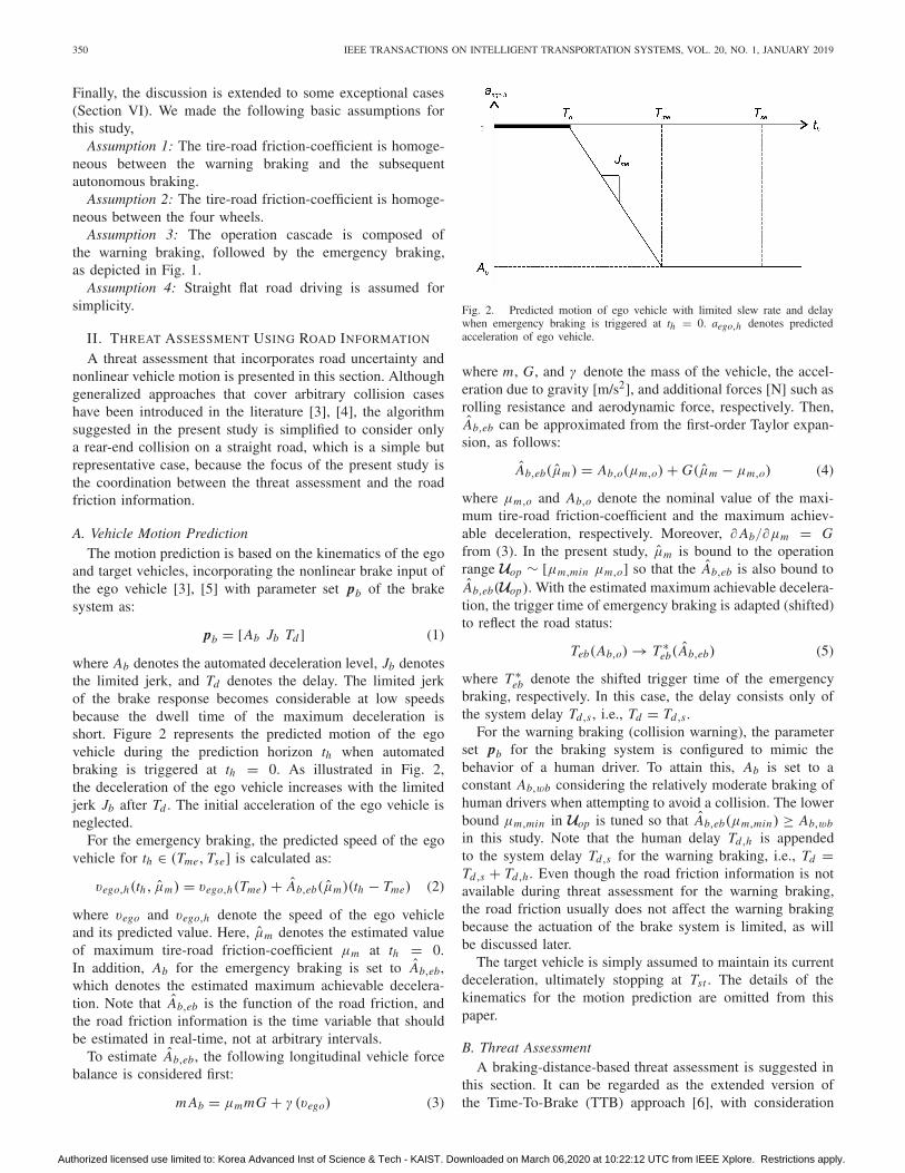
where Ab denotes the automated deceleration level, Jb denotesthe limited jerk, and Td denotes the delay. The limited jerkof the brake response becomes considerable at low speedsbecause the dwell time of the maximum deceleration isshort. Figure 2 represents the predicted motion of the egovehicle during the prediction horizon th when automatedbraking is triggered at th = 0. As illustrated in Fig. 2,the deceleration of the ego vehicle increases with the limitedjerk Jb after Td . The initial acceleration of the ego vehicle isneglected.

For the emergency braking, the predicted speed of the egovehicle for th ∈ (Tme, Tse] is calculated as:

vego,h(th, μm) = vego,h(Tme) + Ab,eb(μm)(th − Tme) (2)

where vego and vego,h denote the speed of the ego vehicleand its predicted value. Here, μm denotes the estimated valueof maximum tire-road friction-coefficient μm at th = 0.In addition, Ab for the emergency braking is set to Ab,eb,which denotes the estimated maximum achievable decelera-tion. Note that Ab,eb is the function of the road friction, andthe road friction information is the time variable that shouldbe estimated in real-time, not at arbitrary intervals.

To estimate Ab,eb, the following longitudinal vehicle forcebalance is considered first:

m Ab = μmmG + γ (vego) (3)

Fig. 2. Predicted motion of ego vehicle with limited slew rate and delaywhen emergency braking is triggered at th = 0. aego,h denotes predictedacceleration of ego vehicle.

where m, G, and γ denote the mass of the vehicle, the accel-eration due to gravity [m/s2], and additional forces [N] such asrolling resistance and aerodynamic force, respectively. Then,Ab,eb can be approximated from the first-order Taylor expan-sion, as follows:

Ab,eb(μm) = Ab,o(μm,o) + G(μm − μm,o) (4)

where μm,o and Ab,o denote the nominal value of the maxi-mum tire-road friction-coefficient and the maximum achiev-able deceleration, respectively. Moreover, ∂ Ab/∂μm = Gfrom (3). In the present study, μm is bound to the operationrange Uop ∼ [μm,min μm,o] so that the Ab,eb is also bound toAb,eb(Uop). With the estimated maximum achievable decelera-tion, the trigger time of emergency braking is adapted (shifted)to reflect the road status:

Teb(Ab,o) → T ∗eb( Ab,eb) (5)

where T ∗eb denote the shifted trigger time of the emergency

braking, respectively. In this case, the delay consists only ofthe system delay Td,s , i.e., Td = Td,s .

For the warning braking (collision warning), the parameterset pb for the braking system is configured to mimic thebehavior of a human driver. To attain this, Ab is set to aconstant Ab,wb considering the relatively moderate braking ofhuman drivers when attempting to avoid a collision. The lowerbound μm,min in Uop is tuned so that Ab,eb(μm,min) ≥ Ab,wb

in this study. Note that the human delay Td,h is appendedto the system delay Td,s for the warning braking, i.e., Td =Td,s + Td,h . Even though the road friction information is notavailable during threat assessment for the warning braking,the road friction usually does not affect the warning brakingbecause the actuation of the brake system is limited, as willbe discussed later.

The target vehicle is simply assumed to maintain its currentdeceleration, ultimately stopping at Tst . The details of thekinematics for the motion prediction are omitted from thispaper.

B. Threat AssessmentA braking-distance-based threat assessment is suggested in

this section. It can be regarded as the extended version ofthe Time-To-Brake (TTB) approach [6], with consideration



Fig. 3. Case I: Ego vehicle stops later than the target vehicle.

given to the nonlinear characteristics of the braking system,as depicted in Fig. 2. Assuming that the autonomous brakingis triggered at this instant, the following condition should besatisfied to enable collision avoidance:

min∀th∈Hse cet,h(th , μm) ≥ co, Hse ∼ (0, Tse] (6)

where cet,h denotes the predicted distance between the egoand target vehicle and co > 0 denotes the minimum distance,which is a tuning parameter. If (6) is not satisfied, the systemtriggers autonomous braking. However, it is computationallydemanding to assess (6) for every sample time. Instead,we consider the following equivalent condition for the threatassessment:

cet,h(Teq , μm) ≥ co (7)

where Teq ∈ Hse denotes the time in the prediction space atwhich the speed of the ego vehicle is predicted to be equalto that of the target vehicle, i.e., the relative speed becomeszero, such that:

vego,h(Teq , μm) − vtar,h(Teq , μm) = 0 (8)

The searching for Teq is divided into two cases, as follows.Only the case of vego > vtar is considered, which is true forthe potential collisions.

1) Case I (Tst ≤ Tse): In this case, the calculation ofTeq is straightforward. This is simply the time at which theego vehicle comes to a stop, i.e. Teq = Tse, as illustratedin Fig. 3. Then, Teq can be found by solving the followinglinear equation:

vego,h(Tme, μm) + Ab(Teq − Tme) = 0 (9)

2) Case II (Tst > Tse): In this case, piece-wise solvingis required to find Teq by solving (8) sequentially for th ∈(Td , Tme] and th ∈ (Tme, Tse). Here, Tse is excluded becauseit contradicts the condition of this case.

If a solution Teq is found, then examine (7) and determinewhether the autonomous braking should be triggered.

Claim 1: If vego > vtar and Tst > Tse, there is always aunique solution to Teq ∈ (0, Tse) in (8).

Proof: Because vego,h(0+) > vtar,h(0+) andvego,h(T −

se ) < vtar,h(T −se ) for T −

se > 0+, a unique solution Teq

always exists in (0, Tse) as illustrated in Fig. 4.Claim 2: If (7) is satisfied and vego > vtar , collision

avoidance is guaranteed for ∀th ∈ Hse.

Fig. 4. Case II: Ego vehicle stops earlier than the target vehicle.

Proof: As illustrated in Fig. 3 for Case I, and in Fig. 4 forCase II, cet,h is the convex function with a minimum at theunique Teq ∈ Hse. Hence, collision avoidance is guaranteedif (7) is satisfied.

III. WARNING BRAKING

A. Basic Considerations

Besides the basic advantages such as congruent stimulus-response mapping and speed reduction, a further possibleadvantage of the warning braking is addressed in this study.That is, real-time tire-road friction estimation could makethe subsequent emergency braking more effective. There aretwo basic considerations for warning braking in terms of themaximum tire-road friction estimation, as follows,

• Securing sufficient vehicle dynamics for accurate frictionestimation.

• Appropriate time in which the friction estimation can becompleted before the triggering of the emergency braking.

The first consideration implies that larger braking dynamicscan enhance the road friction estimation. It is also known thatthe larger braking dynamics ensure better driver responsessuch as the accelerator release time and the stopping dis-tance [24]. However, the braking dynamics for the warningbraking are inevitably limited by the intrinsic considerations,from the perspective of human factors.

B. ParameterizationThe key parameters for the warning braking are the duration

and deceleration (or jerk) level, which are related to the con-siderations discussed in the previous section. Figure 5 showsan illustrative example of the warning braking pulse withparameters:

pwb = [Jwb Dwb] (10)

where Jwb and Dwb denote the jerk and duration of the warn-ing braking, respectively. Increasing the value of pwb wouldresult in larger braking dynamics. However, the parametervalues are inevitably limited, as discussed above. To overcomethis, a strategy is required to secure sufficiently high brakingdynamics with the limited values of pwb. The basic ideapresented in the present study involves measuring the brakingdynamics at the rear wheels. Basically, the purpose of this is toincorporate the load-transfer effect. In addition, the advantageof no interference from the tractive force can be anticipatedby assuming front-wheel drive.



Fig. 5. Illustrative example of warning braking pulse.

Fig. 6. Longitudinal bicycle model. Here, m, L , L f (r), and hcg are allassumed to be known constants.

1) Vehicle Parameters: Before we discuss the warningbraking parameters, we introduce the fundamental vehicledynamics model and parameters in this section [25], [26].From the bicycle model depicted in Fig. 6, the normal tireforce acting on each wheel can be estimated as follows:

Fz f (r) = mGLr( f )

L+ �Fz f (r)

�Fz f = Clt |aego|, �Fzr = −Clt |aego| (11)

where �Fz f (r) denotes the longitudinal load transfer duringdeceleration, and Clt = mhcg/L > 0 denotes the loadtransfer coefficient. The aero-drag force is neglected here forsimplicity. The longitudinal vehicle force balance is given bya generalization of (3), as follows:

maego = Fx f + Fxr − Rx − Fa + γ (12)

The rotational dynamics for each wheel is given as:

Iwω f (r) = −Tbf (r) − re Fx f (r) (13)

where Iw , ω f (r), and re denote the wheel inertia, front (rear)wheel speed, and effective tire radius, respectively. For abraking maneuver, the braking torque of the front (rear) wheelTbf (r) is defined as:

[Tbf

Tbr

]=

[(1 − ηb)Tb

ηbTb

](14)

where 0 ≤ ηb ≤ 1 denotes the braking torque distributionratio.

2) Deceleration (Excitation): The ability to distinguishbetween road surfaces, especially between high and mediumlevels of adhesion, as in the case of dry and wet asphalt,requires sufficient excitation, which refers to the variationin the friction-coefficient during braking. In such a case,a larger excitation statistically guarantees a more reliablefriction estimate [12], [13].

Claim 3: The longitudinal excitation at the rear wheelsduring the warning braking can be approximated by thefollowing inequality equation, provided there is no additionalforce at the rear wheels,

�μxr ≥ �μro + C ltμ

avgxr (15)

where �μxro = (ηb Awb/G)(L/L f ) denotes the excitationwithout any load transfer effect, μ

avgxr denotes the average

friction-coefficient at the rear wheels during the excitation,and C

lt = (Clt /m)(Awb/G)(L/L f ) denotes the normalizedload transfer coefficient.

Proof: The tire-road friction-coefficient at the rear wheelsis defined as:

μxr (t) = Fxr (t)

Fzr (t)(16)

From (16), the excitation at the rear wheels during the warningbraking can be approximated to the following gradient:

�μxr =∫ Dwb

0

(∂μxr

∂ Fxr

d Fxr

dt+ ∂μxr

∂ Fzr

d Fzr

dt

)dt (17)

Because ∂μxr/∂ Fxr = 1/Fzr and ∂μxr/∂ Fzr = −μxr/Fzr

from (16), (17) can be rewritten as:

�μxr =∫ Dwb

0

1

Fzro − |d Fzr |(d Fxr

dt+ μxr

∣∣∣d Fzr

dt

∣∣∣)dt (18)

In (18), Fzr = Fzro − |d Fzr | where Fzro denotes theinitial normal force at the rear wheels at the start of warningbraking, which can be retrieved from (11), and d Fzr denotesthe variation in the normal force at the rear wheels from thestart of warning braking. From the assumption of a monotonicdecrease of Fzr during the warning braking, (18) becomes thefollowing inequality condition:

�μxr ≥ �μxr =∫ Dwb

0

1

Fzro

(d Fxr

dt+ μxr

∣∣∣d Fzr

dt

∣∣∣)dt (19)

where �μxr denotes the lower bound of the excitation level.Finally, from (11), (12), and (13), neglecting the variation oftrivial forces and wheel inertia, �μxr can be rewritten as:

�μxr = 1

Fzro

(mηb Awb + Clt Awbμ

avgxr

)

= Awb

G

L

L f

(ηb + Clt

mμ

avgxr

)(20)

If the average friction-coefficient is defined roughly asμ

avgxr = 0.5�μxr , then the relationship in (15) can be

rearranged as follows:

�μxr ≥ �μxr = �μxro

1 − 0.5C lt

(21)



Fig. 7. Simulation results of excitation for various braking torque distributionratios. Here, Awb,0.4 denotes the required Awb for the excitation at each axlebe 0.4. The solid line represents the values calculated from �μxr in (21).The crosses and circles represent the simulation results for the front and rearaxles, respectively.

Note that the excitation at the rear wheels can be ele-vated with the normalized load-transfer coefficient C

lt asshown in (21). A previous study [13] recommended that theexcitation be larger than 0.4 for the distinction of slip-μ slopesbetween different types of road surfaces. Figure 7 representsthe simulation results of excitation for a range of brakingtorque distribution ratios ηb. The simulation is done withthe veDYNA® commercial high-precision vehicle dynamicsplatform that embodies a sophisticated tire model. The levelof Awb is limited to 0.5G, based on the recommendation givenin the ISO standard [19]. As depicted by the circles in Fig. 7,the simulation results for the rear axle are in good agreementwith the approximation in (21). It is noteworthy that Awb,0.4for the rear axle is only about 0.14G if the warning brakingis applied only to the rear wheels. This fact is important fromthe viewpoint of attaining coordination with the human factorissues. For example, the friction estimate can be reliable witha configuration of ηb = 0.68 for the recommended value ofAwb = 0.2G in [24]. Vehicle parameters L, L f , and Clt inthe simulation are 2.57 m, 1.25 m, and 270.29, respectively.

Based on the above discussion, the autonomous emergencybraking system can be configured in such a way that thebraking torque is concentrated on one axle to attain reliablefriction estimation during warning braking, but distributed toboth axles to attain maximum road adhesion during emergencybraking.

Even though the present study assumed straight roaddriving, it would be useful to investigate how the the lateraldynamics in a normal conflict situation affect the longitu-dinal excitation. Assuming a friction circle, the longitudinalexcitation during warning braking is limited as follows:

M AX (�μxr ) =√

μ2m − μ2

yro (22)

where μyro = Fyro/Fzro is the initial lateral component ofthe friction-coefficient at the start of the warning braking,and the additive excitation of lateral component �μyr duringwarning braking is neglected because the warning braking isa longitudinal maneuver.

According to [27], the 50th and 90th percentile of the lateralacceleration ay for curves with small radii of less than 70 m are

Fig. 8. Simulation of combined excitation in rear wheels for various lateralaccelerations ay for a curve of radius 20m. The solid line with circles denotesthe maximum combined excitation during the warning braking when ay is keptconstant.

around 3 and 5 m/s2. Figure 8 shows the simulation results ofthe combined excitation during warning braking for variouslateral accelerations with reference to [27]. The maximumvalue of combined excitation is observed in the rear wheelswhile the warning braking is triggered with Awb = Awb,0.4,i.e., while the sufficient longitudinal excitation is attained forreliable friction estimation, and ηb is set to 1. In Fig. 8,the combined excitation is about 0.6 if ay is maintainedat 5 m/s2, which is affordable for the friction estimation for thedry or wet road surfaces. This fact implies that the longitudinalexcitation, required for reliable friction estimation duringwarning braking, can be assured in the majority of conflictsituations. If the lateral acceleration is set to an average level,the effect of lateral dynamics becomes insignificant as depictedin Fig. 8. Moreover, warning braking in a normal conflictsituation is usually triggered when drivers are distracted insituations in which the lateral dynamics are relatively gentleand the sensor system has sufficient opportunity to recognizethe hazardous situation.

3) Duration: Another important consideration is that thereshould be a sufficient time margin between the friction esti-mation and the triggering of autonomous braking. This can beinterpreted as a requirement for the duration of the warningbraking, as follows:

Dwb ≤ min{M(μm, vr )|∀μm ∈ Uop, ∀vr ∈ Vop} (23a)

M(μm, vr ) = Tdi f f (vr ) − �Teb(μm , vr ) (23b)

where Tdi f f = Teb − Twb is the time difference between thetriggering of the warning braking and the following emer-gency braking under nominal road conditions, while �Teb =Teb − T ∗

eb is the amount of time by which the emergencybraking is shifted according to the friction estimation results.Here, vr denotes the relative speed, and Vop ∼ [vr,min vr,max ]is the operation range of relative speed, which would be atthe manufacturer’s discretion. The parameters pb and pwb areomitted from (23b). The use of too conservative warning or alack of adhesion would result in the violation of the conditionin (23), such that a collision could occur. However, theproposed method is still effective because the collision speedcan at least be reduced with the estimated friction information,



TABLE I

COLLISION AVOIDANCE STRATEGIES [28]

i.e., the collision can be mitigated. The value of M(μm, vr )depends on the actuation gap, O(μm) = Ab,eb(μm) −Ab,wb ≥ 0. If μm,min is set to O(μm,min ) > , where ∈ Ris a positive small value, the following properties hold:

∂Tdi f f

∂vr>

∂(�Teb)

∂vr> 0,

∂(�Teb)

∂μm< 0 (24)

Thus, from (23b), it follows that:

∂M(·)∂vr

> 0,∂M(·)∂μm

> 0 (25)

That is, M(μm , vr ) is a monotonically increasing functionfor the relative speed vr and μm in this case. Thus, M(μm, vr )is expected to be minimized at the minimum operating valuesof vr,min and μm,min . However, M(μm, vr ) becomes nonlinearat extremely low speeds and reaches a minimum at a certaincritical speed. This is because the speed reduction �vwb bywarning braking becomes dominant. The simulation results,presented later, show that the critical speed is around 12 km/h.On the other hand, if μm,min is set to O(μm,min) ≤ ,the minimum of M(μm .vr ) is approximately a function ofparameters pb and pwb, as follows:

Dwb ≤ M( pb, pwb) ≈ Td,h + �vwb

Ab,wb(26)

where the last term on the right side represents the additionaltime margin resulting from the speed reduction by the warningbraking.

The time margin depends on the characteristics of the asso-ciated threat assessment algorithm and the strategy adoptedfor the operation cascade. Car makers all have their ownstrategies for collision avoidance, as shown in Table I.In Table I, W B , P B , and E B are the abbreviations forwarning braking, partial braking, and emergency braking,respectively. Some car makers utilized warning braking intheir operation cascade. In Table 1, Tdi f f is the time betweenthe collision warning (CW ) and the asterisked autonomousbraking stage in the operation cascade. All the results in Table Iare obtained from a scenario in which an ego vehicle travellingat 100 km/h approaches a slower target vehicle at 60 km/hunder nominal (dry) road conditions.

IV. FRICTION ESTIMATION

A. Slip-Slope Method

The warning braking is momentary and is operated with lim-ited jerk/deceleration, considering the human factors describedin Section III. Thus, we apply a slip-slope based method to

Fig. 9. Friction space for rear wheels.

estimate μm because a better estimation performance can beensured even with the small amount of wheel slip [12], [13].

B. Quantized Friction Estimation

The actuation level of the braking system is adapted accord-ing to the friction estimation results. Some important consid-erations are raised by the use of this configuration. First, thesystem performance should be predictable to the driver andbe robust. Second, the system should be manageable forvarious actuation levels. From these points of view, a quantizedslip-slope method combined with the curve-matching (CM)algorithm is suggested for estimating μm . In the quantizedslip-slope method, the representative slip-slopes are pre-defined for different tire-road adhesion levels. The optimalslip-slope, that is, the one producing the best match with thetrajectory of the samples (sxr,k, μxr,k), is searched in real-time, where a subscript k denotes the k-th sample. Here-after, the subscript represents the rear wheel case. Therefore,the road friction is estimated only for the quantized roadadhesion levels in Uop .

Consider a 2-dimensional friction space Fn ∈ R2 thatconsists of every possible combination of (sxr , μxr ), wheren denotes the number of sub-spaces �i that classifies the levelof tire-road adhesion, giving:

Fn = ∪ni=1�i (Ks,i , δi ) (27)

where �i ∩ � j = ∅ for i �= j , and each sub-space �i ischaracterized with a representative slip-slope Ks,i . In (27),δi denotes the conservativeness factor, which is the gapbetween Ks,i and the boundary of sub-space, as illustratedin Fig. 9. A larger value of δi corresponds to a more conser-vative approach. Here, the term conservative means that thesamples tend to fit a steeper slip-slope. In Fig. 9, Ai denotesthe line of representative slip-slope Ks,i , which defines thelinear relationship between the wheel slip sxr and the roadfriction μxr , and which is defined as:

Ai : Ks,i sxr − μxr = 0 (28)

Furthermore, the distance between each sample point Pk andeach line Ai is defined as the Euclidian distance between Pk



Fig. 10. Friction space with various levels of road adhesion. The hori-zontal length of each sub-space �i indicates the divergence in the observedslip-slopes.

and the projected point P k , as follows:

jd(Ai , Pk) ∼ �Pk − P k�2 (29)

This is an incremental cost obtained from the distance metric.Then, the search for the optimal slip-slope becomes a problemof minimizing the sum of the incremental costs:

Ji =m∑

k=1

λm−k jd(Ai , Pk)2 =

m∑k=1

λm−k �Ks,i sxr,k − μxr,k�2

1 + K 2s,i

(30)

where m denotes the number of samples, and λ denotesthe forgetting factor, which is a tuning parameter. Becausethe distinction between two adjacent slip-slopes improves fora larger excitation, the forgetting factor would enhance theestimation of the slip-slope. This will be verified with theexperimental results, later. Then, the optimal slip-slope Kopt,k

at the current sample time can be obtained as follows:

Kopt,k = Ks,i∗ |i∗ = arg mini

Ji,k (31)

Finally, the μm is determined from Kopt,k . Some previousresearch used linear equations such as μm = c1 Ks + c2to determine the friction-coefficient from the estimated slip-slope. However, the slip-slope varies within a range evenfor the same tire type or the same road surface [12], [13].Thus, a systematic approach based on the quantized slip-slopemethod is suggested as a means of enabling robust frictionestimation. As illustrated in Fig. 10, it is first necessary todivide the friction space Fn into n independent sub-spaces �i ,based on the results of experimental observations. Next, it isnecessary to determine the representative slip-slopes Ks,i bytuning the conservativeness factors δi . The tuning of δi canbe done either statistically or mathematically, according to thedesigner’s choice. For example, the value of δi could be tunedmathematically for consecutive sub-spaces, as follows:

δi >Ks,i+1 + Ks,i

2(32)

This could lead to the obtaining of conservative results.Each sub-space �i matches a specific maximum tire-road

friction-coefficient μm(�i ), as represented by Fig. 10. Thus,μm(�i ) can simply be obtained from a one-dimensionallookup table (LUT) such as,

μm(�i ) = LUT(Kopt,k) (33)

The input to the LUT is Kopt,k , the best-matched Ks,i .

Fig. 11. Hydraulic power unit.

TABLE II

TEST VEHICLE SPECIFICATIONS

Although only the distance metric is considered in thisstudy, additional metrics, e.g., the direction metric [29], canalso be considered to refine the matching process. A directionmetric can be beneficial when there is a bias in the origin.As mentioned above, this quantized approach can be advan-tageous for the collision avoidance application in terms ofsystem management because the system is calibrated only fora few pre-defined actuation levels. In addition, the driver’sacceptance can be improved because the driver can predict theperformance of the system, while the operation characteristicsof the system can easily be tuned with parameters suchas Ks,i and δi .

V. EXPERIMENTS

A. Experiment Set-Up

1) Test Vehicle: As a test vehicle, we used a HyundaiGrandeur HG240. To attain the warning braking function,we developed an auxiliary hydraulic power unit (HPU) andinstalled it in the trunk of the test vehicle as shown in Fig. 11.The HPU mainly consists of an accumulator, motor/pump, andservo-valve. The warning braking is applied by the control ofhydraulic servo-valve. The servo-valve used in the experimentswas a MOOG G761. Table II lists the specifications of the testvehicle. The vehicle was also equipped with an RT3003 iner-tial and GPS navigation system, produced by Oxford TechnicalSolutions, to measure the distance to the target vehicle, andAutoBox, manufactured by dSPACE, for the real-time threatassessment. The longitudinal acceleration and wheel speedsare retrieved via CAN communication to estimate the roadfriction.

2) Warning Braking Parameters: As discussed previously,the braking dynamics should be maximized with limited



actuation levels, given the human factors issue. To maximizethe effect of braking torque distribution, warning braking isapplied only to the rear wheels in the experiments, i.e., ηb = 1during the warning braking. The pwb is set as:

pwb = [−0.32G/s 0.65s] (34)

which results in a speed reduction of about 0.8 m/s. The valuesin (34) are in line with the recommendations produced byfrom the human factors perspective results in [24]. Of course,the values may vary with the characteristics of the algorithmand the strategies. For example, the value of Dwb may bereduced for a smaller time margin. The theoretical expectationof excitation for an HPU-installed test vehicle is about 0.53,as obtained from (21).

3) Estimation of Tire Forces: The tire forces should be esti-mated for the calculation of tire-road friction-coefficient μxr

in (16). The normal tire force Fzr is estimated from (11). Thelongitudinal tire force Fxr can be estimated from the forcebalance in (12) by adopting an observer design, as follows:

m ˙vego = Fxr − Rx − Fa + Ko(vego − vego) (35)

where vego, ˙vego, and Fxr denote the estimated speed of theego vehicle, the derivative of vego, and the estimated longitu-dinal tire force, respectively. The value of Ko in (35) denotesthe positive observer gain. Because warning braking is appliedonly to the rear wheels, the longitudinal tire force at the frontwheels is neglected and vego is obtained from the front wheelspeed while warning braking is being applied. Based on theobserver design described in (35), Fxr is estimated from thefollowing adaptive scheme [14]:

˙Fxr = K f (vego − vego) (36)

where ˙Fxr denotes the derivative of Fxr and K f denotes thepositive force estimation gain. For the experiments, the valuesof Ko and K f were set to 12,000 and 300,000, respectively,which were tuned in the simulations.

Regarding the robustness issue, if there is a difference in thesensitivity to the mass change between the estimated value ofFxr and Fzr , the effect of mass change becomes significant inthe estimation of the friction-coefficient, as discussed in [14].However, as denoted in (11) and (35), the vehicle mass affectsboth Fxr and Fzr in the present study. Thus, it would bereasonable to expect that the friction estimation is robust,regardless of the mass change. Figure 12 shows the resultsof the μxr estimation for a mass change of −20% to 20%relative to the original value, with the simulation settings andparameters as described in Section III. Figure 12 shows thatthe friction estimate is robust to the mass change, which is ingood agreement with the expectation described above.

B. Experiment Results1) Construction of Friction Space: The slip-slopes were

measured for two adhesion levels, dry and wet asphalt,i.e., n = 2. The experiments were conducted with the testvehicle on the low-friction track of the proving grounds ofthe Korea Automobile Testing & Research Institute (KATRI).The specification of μm of wet asphalt lane was 0.7 as shown

Fig. 12. Simulation results of μxr estimation with mass change.

Fig. 13. Wet asphalt lane of KATRI low-friction track.

Fig. 14. Test trials for construction of sub-spaces. (a) Implementation ofwarning braking pulses. The solid line is the reference profile for the warningbraking pulse. (b) μ-slip curves of test trials. The blue lines correspond tothe wet asphalt while the red lines are for dry asphalt.

in Fig. 13. We conducted 50 trials for each road adhesion level,giving a total of 100 trials. Half of the trials conducted foreach road adhesion level, depicted in Fig. 14, were dedicatedto the construction of sub-spaces, while the remaining halfwere used for the tuning of the representative slip-slopes.Table III represents the slip-slope measurements obtained forthe construction of sub-spaces. The top and bottom outliers



TABLE III

RESULTS OF SLIP-SLOPE MEASUREMENTS

Fig. 15. Statistical results obtained from confusion matrix.

were excluded from the statistics. Even though the excitationin the experiments are only estimates, their average is closeto the theoretical value of 0.53, as represented by Table III.

The boundary slip-slope between two sub-spaces was setto 16.8, which is the minimum slip-slope for dry asphalt.Therefore, the overlapped range is truncated at the loweradhesion side. The value of Ks,2 is fixed to the medianvalue of 19.41, and Ks,1 is tuned from the statistical results.Figure 15 represents the statistical results of estimating theroad friction from the confusion matrix defined in Table IVfor different values of conservativeness factor δ1. The precisionand false-positive rate are comparatively flat over δ1. However,the true-positive rate sharply drops at δ1 = 2.0. Consideringthe efficacy of the system, δ1 is thus set to 2.0, which resultsin Ks,1 = 14.8. The forgetting factor λ in (30) was setto 0.91 in the experiments.

In consequence, the friction space F2 can be constructedfrom the experiment results as shown in Fig. 16. The true-positive rate is related to the efficacy of the system, while thefalse-positive rate is related to the driver’s acceptance. Thesystem must be optimized somewhere between these two rates.The estimated maximum friction-coefficients are empiricallyset as μm(�1) ∼ 0.7 and μm(�2) ∼ 1.0 for the wet and dryasphalt, respectively.

Figure 17 shows an experiment result for the friction esti-mation obtained from a sample trial. As shown in Fig. 17(b),the estimated costs are reversed at t = 7.02 s and theestimated maximum tire-road friction-coefficient changes fromthe default value of μm(�1) ∼ 1.0 to 0.7, which is thefinal estimated value. Note that the estimations in the earlystages are not distinguishable between different road adhesion

Fig. 16. Friction space construction (n = 2).

Fig. 17. Experiment results of friction estimation in the time domain.(a) Results of road friction estimation for wet asphalt in time domain. Thesolid and dotted lines represent the estimation results with forgetting factorsof 0.91 and 1.0, respectively. (b) Calculated cost Ji during estimation withforgetting factor of 0.91.

TABLE IV

CONFUSION MATRIX

levels. This is because the slip-slopes for a low excitation arenot distinctive, as depicted in Fig. 14(b). Also note that theestimation is accomplished at an earlier stage if the forgettingfactor is applied, as shown in Fig. 17(a).

2) Threat Assessment With Friction Information: With theconstructed friction space F2, the effect of the friction infor-mation on the threat assessment is verified in the experiments.The experiments were performed on the wet asphalt lane ofKATRI low-friction track. A stopped vehicle scenario is usedfor the experiments. An ego vehicle travelling at 50 km/happroaches an imaginary stopped target on a straight/flat road.



Fig. 18. Simulation results of time margin vs. relative speed.

The imaginary target is placed somewhere in the provingground and the distance to imaginary target cet and vego aremeasured from the RT3003 GPS. The operation cascade iscomposed of the warning braking and the following emergencybraking as Assumption 3. The minimum distance co is set to0.5 m. The value of pwb is set as given by (34) and pb isset as follows, reflecting the characteristics of the test vehiclebraking system:

pb ={

[−0.4G − 2G/s 0.86s], f or W B

[−G − 2G/s 0.2s], f or E B(37)

where the value of Ab for the emergency braking represents thenominal value Ab,o, and Td for the warning braking is the sumof Td,s for 0.2 s and Td,h for 0.66 s. The value of Td,h is basedon the reference report [30], which is the median value of thereaction time of human drivers. Figure 18 shows the resultsof simulating the time margin M(μm, vr ) versus the relativespeed vr for μm ∈ Uop ∼ [0.4 1.0], with parameters pb andpwb of (34) and (37), respectively. From the simulation results,we obtain Tdi f f (vr = 50 km/h) and M(μm = 0.7, vr =50 km/h) values of 1.7 s and 1.49 s, respectively. Of course,the time margin may be made shorter for a more conservativethreat assessment. If the threat assessment for the warningbraking is too conservative to assure a sufficient duration, onepossible means of overcoming this is to reduce the settingof parameter Dwb to a lower value because only a fewhundreds of milliseconds are needed for the friction estimation.However, this requires an increase in the designed jerk Jwb ofthe warning braking, and the decision should be made based ona consideration of the human factors. In Fig. 18, the simulationresult for the case of μm = 0.4 conforms to the discussionin (26).

The test vehicle approached the imaginary stopped targetboth with and without friction estimation. Figure 19(a) rep-resents the experiment results obtained without any frictioninformation. Because the threat assessment is done with thedefault value of maximum adhesion, the collision occurs at areduced speed, that is, the collision is mitigated. On the otherhand, the collision is completely avoided with the frictioninformation, as depicted in Fig. 19(b). The final distance isabout 0.38 m. Comparing this with the results in Fig. 19(a)shows that the emergency braking trigger is shifted forwardas in (5), because the proposed adaptive threat assessment

algorithm is notified of the friction information. Figure 20represents the experiment results for the maximum achievabledeceleration estimation for the case shown in Fig. 19(b).As soon as the warning braking is completed, the maximumtire-road friction-coefficient μm is estimated and Ab,eb(μm) iscalculated from the nominal value of Ab,o, as in (4).

VI. DISCUSSION OF EXCEPTIONAL CASES

A. Split-μ During Warning Braking

In the case of the road adhesion being maintained for boththe left and right wheels during split-μ, the road friction can beestimated for each wheel while attaining the required adhesionfor both sides. Herein, the suggested scheme and discussionalso can be applied to the individual wheels without anymodification based on Assumption 4. Finally, the maximumachievable deceleration Ab,eb that is accounted for the adap-tation of the trigger time for the emergency braking would bedetermined as follows:

Ab,eb = min( Ab,eb,i), i = f l, f r, rl, rr (38)

where Ab,eb,i denotes the estimated maximum achievabledeceleration for each wheel. The strategy described in (38)prevents unstable motion during emergency braking in aprognostic manner, unlike existing stability control systemsthat are aware of the road status only after the emergencybraking is triggered.

Figure 21 shows the results of simulating this case underthe split-μ condition, using the simulation settings given inSection III, ηb = 1, and pwb in (34). In this simulation,the friction space is empirically composed of two sub-spaces,as follows:[

Ks,1

Ks,2

]=

[15.70

18.73

],

[μm(�1)

μm(�2)

]=

[0.7

1.0

](39)

The left wheels of the vehicle are run on the low-μ sidewhile the forgetting factor λ is set to 1.0. As representedin Fig. 21, the road friction of each side of the surface issuccessfully estimated without any loss of adhesion. Becausethe road adhesion is attained on both sides of the split-μduring the warning braking, the yaw-rate remains stablethroughout the actuation of the warning braking, as shownin Fig. 21(c).

If road adhesion is lost for one side of the wheel duringsplit-μ, unstable motion such as yawing must be preventedbecause the warning braking is just the means of hapticwarning for a distracted driver. This can be done by theactive intervention of a system with a higher priority suchas the anti-lock braking or stability control system. Sucha legacy system would regulate the braking force as soonas saturation in the tire force is observed during excitation.Finally, the strategy described in (38) can be applied to preparefor the subsequent emergency braking, with the road frictioninformation estimated before saturation. The estimation of thefriction on extremely slippery surfaces will be described indetail later.



Fig. 19. Experiment results of threat assessment obtained with friction information. (a) Collision mitigation without friction information. (b) Collisionavoidance with friction information. The solid line represents the distance between the ego vehicle and the stopped imaginary target, while the dotted linerepresents the speed of the ego vehicle. The dash-dot and dashed lines represent the triggers for the warning braking and emergency braking, respectively.

Fig. 20. Estimation of maximum adhesion level after warning braking. Thesolid line represents the estimated maximum achievable acceleration, whilethe dotted line represents the actual acceleration of the ego vehicle.

B. Transient-μ During Warning Braking

This is a very rare case because the duration of the warningbraking is only a few hundreds of milliseconds. In this case,the detection algorithm for the surface change should beincorporated. Gustafsson [12] suggests the use of the CUSUMalgorithm for detecting a surface change and issuing a warningto the driver. The covariance matrix of the Kalman filter isadjusted such that the time constant becomes shorter as a resultof detecting the surface change. Choi et al. [16] suggest theuse of the adaptive forgetting factor for the estimation basedon the recursive least square method.

In the present study, the performance of the suggestedscheme in the transient-μ situation is verified using theCUSUM detector for the surface change during warningbraking, as follows [12]:

g0 = 0

gk = gk−1 + ek + ν

gk = M AX (gk, 0) (40)

where ν is a design parameter, and ek denotes the estimationerror for the wheel slip in the current step, which is defined

Fig. 21. Friction estimation for split-μ surface. (a) Calculated costsJi (left axis) and estimated road friction (right axis) for rear-left wheel.(b) Calculated costs Ji (left axis) and estimated road friction (right axis)for rear-right wheel. (c) Yaw-rate during warning braking.

as:

ek = μxr,k K −1opt,k − sxr,k (41)

where the overestimation of slip-slope results in a positivevalue of ek . Here, an adjustment rule for the forgetting factorbased on [12] is suggested, as follows:

i f gk > h

gk = 0; λ = λo − λge−τ−1t (42)

where λo, λg denote the original and marginal values of theforgetting factor, respectively, and h is a positive thresholdvalue.



Fig. 22. Costs with the detection of surface change. (a) Calculated costs Jiduring warning braking. (b) Forgetting factor λ (solid line, left axis) and theestimation error of wheel slip (dotted line, right axis).

Figure 22 represents the simulation results of the cost Ji

with the CUSUM detector during warning braking undertransient-μ conditions. The friction-coefficient of the roadsurface suddenly changes from 1.0 to 0.7 at t = 12.58 s. Thefriction space and simulation parameters are set to the samevalues as in the split-μ case. The values of λo and λg are setto 1.0 and 0.15 in the simulation, respectively. In other words,the forgetting factor is reduced to 0.85 instantaneously andthen reverts back to the original value of 1.0 exponentiallyfor the stable estimation. As represented in Fig. 22, the costsare reset when gk > h and the result of friction estimationis eventually reversed. The ν, h, and τ values are set to0, 0.15, and 0.05 s, respectively, in this simulation.

C. Extremely Slippery SurfacesBecause the slip-slopes of the extremely slippery surfaces,

such as snow or ice, are more easily distinguishable from thenominal higher one, the suggested scheme would perform wellin the low-slip linear region.

However, if the system actuates the braking system uponattaining Awb,0.4 on snowy or icy surfaces without any priorknowledge of the road friction, the longitudinal tire forcewill start to saturate before the excitation reaches the targetvalue. In such a case, the braking force should be regulatedby the operation of the legacy systems as discussed above.At the same time, it is recommended that a decision bemade regarding the road friction, terminating the frictionestimation with the suggested scheme as soon as saturation isdetected. If the friction estimation using the suggested schemeis continued even after saturation, the data samples would befitted to the lowest friction sub-space, which may result in anincreased degree of error. If necessary, further estimation afterthe saturation can be done using popular tire models [16], [17],for example.

Figure 23 shows the simulation results for the μ-slip curveand cost Ji for the rear wheels. The simulation was conducted

Fig. 23. Simulation results of friction estimation for μm = 0.3. (a) μ-slipcurve during saturation. (b) Cost Ji during saturation where Ji represents thecost for �i .

with ηb = 1, λ = 1, and μm = 0.3, where the vehicle triggersa warning braking at with pwb = [Awb,0.4 0.65 s]. The frictionspace is composed of three sub-spaces as follows:⎡

⎣Ks,1Ks,2Ks,3

⎤⎦ =

⎡⎣ 8.56

9.6715.70

⎤⎦,

⎡⎣μm(�1)

μm(�2)μm(�3)

⎤⎦ =

⎡⎣0.2

0.30.7

⎤⎦ (43)

As expected, saturation occurs during the excitation dueto the lack of adhesion, as shown in Fig. 23(a). As shownin Fig. 23(b), the distinction between the slip-slopes is wellmaintained in the low-slip linear region. However, as saturationstarts at about sxr = 0.02, the gap between the costs starts todecrease such that, ultimately, the costs are reversed at aboutsxr = 0.06 (at t = 6.12 s). The simulation results are in goodagreement with the discussion above.

VII. CONCLUSION

The friction estimation in this study was based on the slip-slope method, which uses the slope of the μ-slip curve todetermine the road adhesion level. However, the slip-slope canvary even for the same type of tire or the same road surface.In addition, the system must be easy-to-manage for variousload adhesion levels. Thus, a quantized slip-slope method com-bined with a curve-matching algorithm is introduced in thisstudy. An important feature is that the suggested frameworkand considerations are valid regardless of the limitations in thefriction estimation, while the performance of the system canbe guaranteed using advanced friction estimation technology.Moreover, friction-estimation techniques other than the slip-slope method can be incorporated into the suggested adaptivecollision avoidance scheme.

Future work would include the the reinforcement of the fric-tion estimation to suppress the false-positive and to attain therequired level of performance even on the non-homogeneousroad surfaces, and the extension of the scheme to a wide rangeof conflict scenarios in more detail involving the possibility oflateral evasive maneuvering.



REFERENCES

[1] P. Seiler, B. Song, and J. K. Hedrick, “Development of a collisionavoidance system,” SAE Tech. Paper 980853, 1998.

[2] Y. Seto, T. Watanabe, T. Kuga, Y. Yamamura, andK. Watanabe, “Research on a braking system for reducing collisionspeed,” SAE Tech. Paper 2003-01-0251, 2003.

[3] M. Brännström, E. Coelingh, and J. Sjöberg, “Model-based threatassessment for avoiding arbitrary vehicle collisions,” IEEE Trans. Intell.Transp. Syst., vol. 11, no. 3, pp. 658–669, Sep. 2010.

[4] N. Kaempchen, B. Schiele, and K. Dietmayer, “Situation assessmentof an autonomous emergency brake for arbitrary vehicle-to-vehiclecollision scenarios,” IEEE Trans. Intell. Transp. Syst., vol. 10, no. 4,pp. 678–687, Dec. 2009.

[5] M. Brännstrom, J. Sjöberg, and E. Coelingh, “A situation and threatassessment algorithm for a rear-end collision avoidance system,” in Proc.IEEE Intell. Veh. Symp., Jun. 2008, pp. 102–107.

[6] J. Hillenbrand, A. M. Spieker, and K. Kroschel, “A multilevel collisionmitigation approach—Its situation assessment, decision making, andperformance tradeoffs,” IEEE Trans. Intell. Transp. Syst., vol. 7, no. 4,pp. 528–540, Dec. 2006.

[7] E. Coelingh, A. Eidehall, and M. Bengtsson, “Collision warning with fullauto brake and pedestrian detection—A practical example of automaticemergency braking,” in Proc. 13th Int. IEEE Conf. Intell. Transp. Syst.,Sep. 2010, pp. 155–160.

[8] A. Eidehall and L. Petersson, “Statistical threat assessment for generalroad scenes using Monte Carlo sampling,” IEEE Trans. Intell. Transp.Syst., vol. 9, no. 1, pp. 137–147, Mar. 2008.

[9] G. De Nicolao, A. Ferrara, and L. Giacomini, “Onboard sensor-basedcollision risk assessment to improve pedestrians’ safety,” IEEE Trans.Veh. Technol., vol. 56, no. 5, pp. 2405–2413, Sep. 2007.

[10] A. Gray, M. Ali, Y. Gao, J. K. Hedrick, and F. Borrelli, “A unifiedapproach to threat assessment and control for automotive active safety,”IEEE Trans. Intell. Transp. Syst., vol. 14, no. 3, pp. 1490–1499,Mar. 2013.

[11] S. Wonju, (in Korean). KoROAD, Korea. Accessed: Jun. 23, 2015.[Online]. Available: http://www.koroad.or.kr/kp_web/krPrView.do?board_code=GABBS_050&board_num=131142

[12] F. Gustafsson, “Slip-based tire-road friction estimation,” Automatica,vol. 33, no. 6, pp. 1087–1099, Jun. 1997.

[13] S. Müller, M. Uchanski, and K. Hedrick, “Estimation of the maximumtire-road friction coefficient,” J. Dyn. Syst., Meas., Control, vol. 125,no. 4, pp. 607–617, Jan. 2003.

[14] R. Rajamani, G. Phanomchoeng, D. Piyabongkarn, and J. Y. Lew,“Algorithms for real-time estimation of individual wheel tire-road fric-tion coefficients,” IEEE/ASME Trans. Mechatronics, vol. 17, no. 6,pp. 1183–1195, Dec. 2012.

[15] J. Wang, L. Alexander, and R. Rajamani, “Friction estimation onhighway vehicles using longitudinal measurements,” ASME J. Dyn. Syst.,Meas. Control, vol. 126, no. 2, pp. 265–275, 2004.

[16] M. Choi, J. J. Oh, and S. B. Choi, “Linearized recursive least squaresmethods for real–time identification of tire–road friction coefficient,”IEEE Trans. Veh. Technol., vol. 62, no. 7, pp. 2906–2918, Sep. 2013.

[17] L. Li, F.-Y. Wang, and Q. Zhou, “Integrated longitudinal and lateraltire/road friction modeling and monitoring for vehicle motion control,”IEEE Trans. Intell. Transp. Syst., vol. 7, no. 1, pp. 1–19, Mar. 2006.

[18] K. Yi, M. Woo, S. Kim, and S. Lee, “A study on a road-adaptive CW/CAalgorithm for automobiles using HIL simulations,” Int. J. C, Mech. Syst.,Mach. Elements Manuf., vol. 42, no. 1, pp. 163–170, 1999.

[19] Intelligent Transport Systems—Forward Vehicle Collision WarningSystems—Performance Requirements and Test Procedures,Standard ISO 15623:2013, 2013.

[20] S. B. Brown, S. E. Lee, M. A. Perez, Z. R. Doerzaph, V. L. Neale, andT. A. Dingus, “Effects of haptic brake pulse warnings on driver behaviorduring an intersection approach,” Proc. Hum. Factors Ergonom. Soc.Annu. Meeting, vol. 49, no. 22, pp. 1892–1896, 2005.

[21] M. Lloyd, G. Wilson, C. Nowak, and A. Bittner, Jr., “Brake pulsing ashaptic warning for an intersection collision avoidance countermeasure,”Transp. Res. Rec., vol. 1694, no. 2, pp. 34–41, Nov. 1999. [Online].Available: http://trrjournalonline.trb.org/toc/trr/1999/1694/+

[22] J. Pierowicz, E. Jacoy, M. Lloyd, A. Bittner, and B. Pirson, “Intersectioncollision avoidance using ITS countermeasures,” NHTSA, Washington,DC, USA, Tech. Rep. DOT HS 809 171, Sep. 2000.

[23] B. Riley, G. Kuo, T. Nethercutt, K. Shipp, and M. Smith, “Develop-ment of a haptic braking system as an ACC vehicle FCW measure,”SAE Tech. Paper 2002-01-1601, May 2002.

[24] L. Tijerina, S. Johnston, E. Parmer, H. A. Pham, andM. D. Winterbottom, “Preliminary studies in haptic displays forrear-end collision avoidance system and adaptive cruise control systemapplications,” NHTSA, Washington, DC, USA, Tech. Rep. DOT HS 808,Sep. 2000.

[25] W. Cho, J. Yoon, S. Yim, B. Koo, and K. Yi, “Estimation of tire forcesfor application to vehicle stability control,” IEEE Trans. Veh. Technol.,vol. 59, no. 2, pp. 638–649, Feb. 2010.

[26] R. Rajamani, Vehicle Dynamics and Control . New York, NY, USA:Springer, 2006.

[27] W. Hugemann and M. Nickel, “Longitudinal and lateral accelerations innormal day driving,” in Proc. Inst. Traffic Accident Invest. Conf. (ITAI),2003, pp. 1–8.

[28] C. Gauss et al., “Comparative test of advanced emergency braking sys-tems,” ADAC Internal Test Rep., ADAC Technik Zentrum, Landsberg,Germany, Aug. 2012.

[29] S. Brakatsoulas, D. Pfoser, R. Salas, and C. Wenk, “On map-matchingvehicle tracking data,” in Proc. 31st Int. Conf. Very Large Data Bases,2005, pp. 853–864.

[30] G. Johansson and K. Rumar, “Drivers’ brake reaction times,” Hum.Factors., J. Hum. Factors Ergonom. Soc., vol. 13, no. 1, pp. 23–27,Feb. 1971.

Yunhyoung Hwang received the B.S. degree inelectrical engineering from Hanyang University,Seoul, South Korea, and the M.S. degree from theGraduate School of Automotive Technology, KAIST,Daejeon, South Korea, where he is currently pur-suing the Ph.D. degree in mechanical engineering.He is currently a Senior Research Engineer withthe Smart Vehicle Control Center, Korea AutomotiveTechnology Institute. His current research interestsinclude threat assessment and collision avoidancecontrol for autonomous vehicles.

Seibum B. Choi (M’09) received the B.S. degree inmechanical engineering from Seoul National Univer-sity, Seoul, South Korea, the M.S. degree in mechan-ical engineering from KAIST, Daejeon, South Korea,and the Ph.D. degree in control from the Universityof California, Berkeley, CA, USA, in 1993. From1993 to 1997, he was involved in the develop-ment of automated vehicle control systems withthe Institute of Transportation Studies, University ofCalifornia. In 2006, he was with TRW, Livonia, MI,USA, where he was involved in the development of

advanced vehicle control systems. Since 2006, he has been with the Facultyof the Mechanical Engineering Department, KAIST. His current researchinterests include fuel-saving technology, vehicle dynamics and control, andactive safety systems. He is a member of the American Society of MechanicalEngineers, the Society of Automotive Engineers, and the Korean Society ofAutomotive Engineers.


adaptive collision avoidance using road friction...

Documents