adaptive cellular layout in self-organizing · ploit the flexible sectorization feature in...
TRANSCRIPT


Adaptive Cellular Layout in Self-Organizing
Networks using Active Antenna Systems
Dem Fachbereich 18Elektrotechnik und Informationstechnikder Technischen Universitat Darmstadt
zur Erlangung der Wurde einesDoktor-Ingenieurs (Dr.-Ing.)
genehmigte Dissertation
vonM.Sc. Dereje Woldemedhin Kifle
geboren am 05.12.1983 in Addis Ababa
Referent: Prof. Dr.-Ing. Anja KleinKorreferent: Prof. Dr.-Ing. Thomas KurnerTag der Einreichung: 05.07.2016Tag der mundlichen Prufung: 28.11.2016
D 17
Darmstadter Dissertation


I
Kurzfassung
Die rasch wachsende Nachfrage nach Mobilfunkkapazität stellt die Mobilfunkindustrie
vor immer neue Herausforderungen und verlangt nach neuen Strategien hinsichtlich
des Netzausbaus. Dabei gilt es gerade, das sowohl zeitlich wie auch räumlich sehr
schwankende Verkehrsaufkommen in effizienter Weise zu bewältigen. Traditionell wird
für Bereiche mit höherem Kapazitätsbedarf, als Maßnahme eine Verdichtung der zellu-
laren Struktur in heterogener Weise vorgesehen. Dabei werden sogenannte Pico-Zellen
oder ”small cells” in eine Makrozelle eingebettet und erreicht so durch die dichtere
räumliche Wiederverwendung der Funkressourcen eine Erhöhung der Netzkapazität.
Die Funknetzplanung bedient sich dabei der ”busy hour” Regel, d. h. man stellt so
viele Funkressourcen bzw. so viele kleine Zellen an den entsprechenden Standorten auf,
dass es in der ”Stunde der höchsten Verkehrslast” nicht zu Engpässen kommt. Diese
Überversorgungsstrategie ist jedoch nicht besonders effizient, da zu einem großen Teil
der Betriebszeit viele Netzwerkressourcen ungenutzt bleiben, was für den Netzbetreiber
hohe Investitionen in die Infrastruktur (CAPEX) sowie hohe Betriebskosten (OPEX)
bedeutet. Wünschenswert wäre deshalb ein Netzwerk, dessen Kapazität sich flexibel
an die dynamische Verkehrssituation anpasst und die teure ”busy hour” Strategie mit
maximaler und fixer Ressourcenbereitstellung umgeht.
Neue revolutionäre Basisstationsantennentechnologien, bei der jedes Antennenelement
mit einer aktiven Komponente wie Verstärker kombiniert ist, aktive Antennensys-
teme (AAS) genannt, verspricht die nötige Flexibilität und gewünschte dynamische
Bereitstellungsstrategie für die adaptive Kapazitätsversorgung. Durch die direkte
Phasen- und Amplitudensteuerung jedes einzelnen Antennenelements unterstützt das
AAS eine deutlich verbesserte Beamforming-Funktionalität, die eine neue Art der
”Sektorisierung” mit dynamischer Zellverdichtung ermöglicht. Wird in einer konven-
tionellen Zelle eine Überlastsituation festgestellt, lässt sich die Strahlungskeule der
konventionellen Zelle in zwei neue, kleinere Beams aufteilen, welche als neue Zellen
bzw. Sektoren dienen. Durch die weitere Zellaufteilung (Sektorisierung) werden die
Funkressourcen in diesem Bereich durch die räumliche Wiederverwendung des Frequen-
zspektrums verdoppelt und so die Verkehrslast auf die beiden neuen Zellen verteilt.
Diese Art der dynamischen Gestaltung der zellularen Netzstruktur mittels AAS birgt
aber auch einige Herausforderungen. Durch die zusätzlichen Zellen ergeben sich mehr
Zellgrenzbereiche und somit zusätzlich Areale mit erhöhter Interzellinterferenz, die der
erwarteten Systemkapazitätssteigerung durch Zellverdichtung entgegenwirken. Außer-
dem gilt es den sich zeitlich und räumlich ändernden Verkehr im Blick zu haben, um
gezielt eine Zellverdichtung mittels Sektorisierung vornehmen zu können. Um dieser

II
Aufgabe gerecht zu werden und um mit dieser Methode eine Steigerung der System-
leistung und Optimierung der Dienstgüte beim Endnutzer erreichen zu können, ist ein
automatischer, sich selbstorganisierender Management- und Konfigurationsmechanis-
mus notwendig. Mit einer solchen dynamischen Anpassung der Zellstruktur geht die
Selbstorganisation der Netze in eine neue Dimension, da das zelluläre Netz inklusive der
Funkausbreitungsbedingungen nicht mehr als stationär angesehen werden kann. Um
dies gewährleisten und voll ausnutzen zu können, werden zuverlässige und realistische
Ausbreitungsmodelle benötigt, die die Abhängigkeit der Funkkanalcharakteristik von
der Veränderung der Strahlungskeule abbilden. Dies sowie die komplexen Beziehungen
verschiedener Systemparameter bedingen ein umfassendes systemtheoretisches Model
der AAS-basierten Sektorisierung, um detaillierte Untersuchungen und eine präzise
Auswertung der erwarteten Systemleistungsgewinne zu ermöglichen.
Ein wesentlicher Aspekt der Arbeit ist die Entwicklung eines geeigneten SON Algo-
rithmus, der die gesamte Prozedur der AAS-basierten Sektorisierung automatisiert. Er
steuert die Aktivierung und Deaktivierung von Strahlungskeulen, welche die Zellen
bzw. Sektoren repräsentieren, und ermöglicht somit die verkehrsadaptive Anpas-
sung des sektorbasierten Zellaufbaus mittels Zellteilung und Verschmelzung. Um die
dynamischen Kapazitätsanforderungen durch variierende räumliche Nutzerverteilun-
gen effektiv bereitstellen zu können, überwacht der neu entwickelte SON Algorith-
mus sowohl die Last wie auch die räumliche Verteilung des Datenverkehrs in einer
Funkzelle und adaptiert die darunterliegende Funkzellenabdeckung durch autonome
Sektorisierung in der horizontalen oder vertikalen Ebene. Der Algorithmus verwendet
verschiedene Prozeduren, die von Echtzeitnetzdaten abhängen, welche wiederum aus
Signalmessberichten der Endnutzerterminals gewonnen werden. Eine mögliche Ver-
schlechterung der Systemleistung verhindert der Algorithmus dadurch, dass vor der
Durchführung der Sektorisierung sichergestellt wird, dass die Gleichkanalinterferenz
keinen negativen Einfluss auf die Nutzer hat. Dazu wurde eine Leistungsmetrik ent-
wickelt, die den negativen Einfluss der Gleichkanalinterferenz den erwarteten Gewinnen
durch die Zellverdichtung mit zusätzlichen Funkressourcen gegenüberstellt. Um das
Interzellinterferenzproblem, das durch die AAS-basierte Sektorisierung an den neuen
Zellgrenzen auftritt zu mildern, wird in dieser Arbeit eine weitere neue Methode ent-
wickelt, welche die Datenübertragung in den benachbarten Funkzellen mit Hilfe des
Prinzips der Übertragungsstummschaltung koordiniert. Um sicherzustellen, dass die
partielle Stummschaltung von Ressourcen die Gesamtsystemleistung nicht verringert,
wird der SON Algorithmus dahingehend erweitert, dass auch diese Methode in opti-
maler Weise genutzt wird.
Um die Zellteilung mittels Änderung der Strahlungskeule richtig charakterisieren zu
können, wurde ein neues erweitertes Funkausbreitungsmodell entwickelt, das ein nei-

III
gungsspezifisches Abschattungsmodel (Shadowing) enthält. Entgegen der bestehenden
Shadowing-Modelle, welche eine stationäre neigungsunabhängige Ausbreitungseigen-
schaft in der Elevationsebene haben, wird nun ein neigungsabhängiges Shadowing
Modell vorgeschlagen, das zudem in der Lage ist, die Variabilität des Funkkanals
abhängig von der Höhe der Endnutzer statistisch zu charakterisieren. Für die simu-
lationsbasierte Realisierung der unterschiedlichen Varianten der AAS-basierten Sek-
torisierung, d.h. die schnelle Änderung des Zelllayouts mittels dynamischer Konfigura-
tion der AAS-Parameter, werden vereinfachte 3D-Beamforming Modelle und synthetis-
che Strahlungsmuster entwickelt. Die horizontale und vertikale Sektorisierung sind die
beiden Formen der AAS-basierten zellulären Netzlayoutänderung, die in dieser Arbeit
betrachtet werden. Der ursprünglich Sektor wird durch Generierung von zwei neuen
schmaleren Strahlungskeulen in zwei neue Sektoren aufgespalten, die von einem einzel-
nen AAS gleichzeitig erzeugt werden, was sowohl in der horizontalen wie auch in der
vertikalen Domäne möglich ist.
Die Leistungsfähigkeit des entwickelten AAS-basierten dynamischen Zellverdich-
tungskonzepts und dessen SON-gesteuerte automatische Kontrolle wird mittels System-
Level-Simulationen untersucht. Als Testszenarien werden makrozellulare Netzmodelle
mit Basisstationen verwendet, die mit der Long Term Evolution-Advanced (LTE-A)
Technologie betrieben werden. Die Simulationsergebnisse zeigen, dass der entwickelte
SON Mechanismus das Netzlayout auf die unterschiedlichen Bedingungen anpassen
kann, und sie machen deutlich, wann und wo die Sektorisierung Gewinn bringt bzw.
sie sich nachteilig auf den Endnutzer auswirkt. Ebenfalls wurde die Wechselwirkung
des neuen SON Mechanismus für die adaptive Zelladaptation mit bereits existieren-
den SON Funktionen, wie z.B. Mobility Robustness Optimization (MRO) erforscht,
da diese bislang von einem stationären Zelllayout ausgingen. Die Untersuchungen
ergaben, dass es einer Koordinierung der beiden SON Funktionalitäten bedarf, d.h.
zwischen dem SON Mechanismus für die AAS-basierte Sektorisierung und dem MRO
Betrieb, um unvorhersehbare Leistungseinbußen zu vermeiden und ein reibungsloses
Endnutzererlebnis zu gewährleisten.
Die technischen Konzepte welche im Rahmen dieser Arbeit entwickelt wurden, sind
außerdem in das SON Arbeitspaket für AAS-basierte Netzadaption innerhalb der Ra-
dio Access Network (RAN) Arbeitsgruppe 3 des 3rd Generation Partnership Project
(3GPP) eingeflossen.


V
Abstract
The rapidly growing demand of capacity by wireless services is challenging the mobile
industry with a need of new deployment strategies. Besides, the nature of the spatial
and temporal distribution of user traffic has become heterogeneous and fluctuating
intermittently. Those challenges are currently tackled by network densification and
tighter spatial reuse of radio resources by introducing a heterogeneous deployment
of small cells embedded in a macro cell layout. Since user traffic is varying both
spatially and temporally, a so called busy hour planning is typically applied where
enough small cells are deployed at the corresponding locations to meet the expected
capacity demand. This deployment strategy, however, is inefficient as it may leave
plenty of network resources under-utilized during non-busy hour time, i.e., most of
the operation time. Such over-provisioning strategy incurs high capital investment on
infrastructure (CAPEX) as well as operating cost (OPEX) for operators. Therefore,
optimal would be a network with flexible capacity accommodation by following the
dynamics of the traffic situation and evading the inefficiencies and the high cost of the
fixed deployment approach.
The advent of a revolutionizing base station antenna technology called Active Antenna
Systems (AAS) is promising to deliver the required flexibility and dynamic deploy-
ment solution desired for adaptive capacity provisioning. Having the active radio
frequency (RF) components integrated with the radiating elements, AAS supports
advanced beamforming features. With an AAS-equipped base station, multiple cell-
specific beams can be simultaneously created to densify the cell layout by means of
an enhanced form of sectorization. The radiation pattern of each cell-beam can be
dynamically adjusted so that a conventional cell, for instance, can be split into two
distinct cells, if a high traffic concentration is detected. The traffic in such an area
is shared among the new cells and by spatially reusing the frequency spectrum, the
cell-splitting (sectorization) doubles the total available radio resources at the cost of
an increased co-channel interference between the cells.
Despite the AAS capability, the realization of flexible sectorization for dynamic cell
layout adaptation poses several challenges. One of the challenges is that the expected
performance gain from cell densification can be offset by the ensuing co-channel inter-
ference in the system. It is also obvious that a self-organized autonomous management
and configuration is needed, if cell deployment must follow the variation of the user
traffic over time and space by means of a sectorization procedure. The automated mech-
anism is desired to enhance the system performance and optimize the user experience

VI
by automatically controlling the sectorization process. With such a dynamic adapta-
tion scheme, the self-organizing network (SON) facilities are getting a new dimension
in terms of controlling the flexible cell layout changes as the environment including the
radio propagation characteristics cannot be assumed stationary any longer. To fully ex-
ploit the flexible sectorization feature in three-dimensional space, reliable and realistic
propagation models are required which are able to incorporate the dependency of the
radio channel characteristics in the elevation domain. Analysis of the complex relation-
ship among various system parameters entails a comprehensive model that properly
describes the AAS-sectorization for conducting detailed investigation and carrying out
precise evaluation of the ensuing system performance.
A novel SON algorithm that automates the AAS-sectorization procedure is developed.
The algorithm controls the activation/deactivation of cell-beams enabling the sector-
ization based cell layout adjustment adaptively. In order to effectively meet the dy-
namically varying network capacity demand that varies according to the spatial user
distribution, the developed SON algorithm monitors the load of the cell, the spatial
traffic concentrations and adapts the underlying cell coverage layout by autonomously
executing the sectorization either in the horizontal or vertical plane. The SON algo-
rithm specifies various procedures which rely on real time network information collected
using actual signal measurement reports from users. The particular capability of the
algorithm is evading unforeseen system performance degradation by properly executing
the sectorization not only where in the network and when it is needed, but also only
if the ensuing co-channel interference does not have adverse impact on the user expe-
rience. To guarantee the optimality of the network performance after sectorization, a
performance metric that takes both the expectable gain from radio resource and impact
of the co-channel interference into account is developed. In order to combat the sever-
ity of the inter-cell interference problem that arises with AAS-sectorization between
the co-channel operated cells, an interference mitigation scheme is developed in this
thesis. The proposed scheme coordinates the data transmission between the co-sited
cells by the transmission muting principle. To ensure that the transmission muting is
not degrading the overall system performance by blanking more data transmission, a
new SON algorithm that controls the optimal usage the proposed scheme is developed.
To appropriately characterize the spatial separation of the cell beams being activated
with sectorization, a novel propagation shadowing model that incorporates elevation
tilt parameter is developed. The new model addresses the deficiencies of the existing
tilt-independent shadowing model which inherently assumes a stationary propagation
characteristics in the elevation domain. The tilt-dependent shadowing model is able
to statistically characterize the elevation channel variability with respect to the tilt

VII
configuration settings. Simplified 3D beamforming models and beam pattern synthe-
sis approaches required for fast cell layout adaptation and dynamic configuration of
the AAS parameters are developed for the realization of various forms of AAS-based
sectorization. Horizontal and vertical sectorization are the two forms of AAS-based sec-
torization considered in this thesis where two beams are simultaneously created from
a single AAS to split the underlying coverage layout in horizontal or vertical domain,
respectively.
The performance of the developed theoretical AAS-sectorization concepts and mod-
els are examined by means of system level simulations considering the Long Term
Evolution-Advanced (LTE-A) macro-site deployment within exemplifying scenarios.
Simulation results have demonstrated that the SON mechanism is able to follow the
different conditions when and where the sectorization delivers superior performance
or adversely affects the user experience. Impacts on the performance of existing SON
operations, like Mobility Robustness Optimization (MRO), which are relying on sta-
tionary cell layout conditions have been studied. Further investigations are carried
out in combination with the cell layout changes triggered by the dynamic AAS-based
sectorization. The observed results have confirmed that proper coordination is needed
between the SON scheme developed for AAS sectorization and the MRO operation to
evade unforeseen performance degradation and to ensure a seamless user experience.
The technical concepts developed in this thesis further have impacted the 3rd Genera-
tion Partnership Project (3GPP) SON for AAS Work Item (WI) discussed in the Radio
Access Network (RAN)-3 Work Group (WG). In particular, the observed study results
dealing with the interworking of the existing SON features and AAS sectorization have
been noted in the standardization work.


IX
Contents
1 Introduction 1
1.1 Deployment Trends in Self-Organizing Cellular Networks . . . . . . . . 1
1.2 Active Antenna Systems . . . . . . . . . . . . . . . . . . . . . . . . . . 3
1.3 State of the Art . . . . . . . . . . . . . . . . . . . . . . . . . . . . . . . 5
1.4 Open Issues . . . . . . . . . . . . . . . . . . . . . . . . . . . . . . . . . 7
1.5 Contributions and Outline of the Thesis . . . . . . . . . . . . . . . . . 8
2 System Model 11
2.1 Introduction . . . . . . . . . . . . . . . . . . . . . . . . . . . . . . . . . 11
2.2 Cellular Models of LTE-Advanced Network . . . . . . . . . . . . . . . . 12
2.2.1 3GPP Cellular Model . . . . . . . . . . . . . . . . . . . . . . . . 12
2.2.1.1 Regular Hexagonal Cellular Layout . . . . . . . . . . . 12
2.2.1.2 3GPP Radio Propagation Model . . . . . . . . . . . . 14
2.2.1.3 Antenna Gain and Beam Pattern . . . . . . . . . . . . 15
2.2.1.4 LTE Link Budget . . . . . . . . . . . . . . . . . . . . . 17
2.2.2 Ray-Tracing Based Three-Dimensional Cellular Model . . . . . . 18
2.2.2.1 Realistic Non-Regular Cellular Layout . . . . . . . . . 18
2.2.2.2 Ray-Tracing Based Radio Propagation Model . . . . . 18
2.3 Beam Pattern Design for Active Antenna Systems Based Sectorization 20
2.3.1 Introduction . . . . . . . . . . . . . . . . . . . . . . . . . . . . . 20
2.3.2 Beamforming Technique for Beam Pattern Design . . . . . . . . 21
2.3.3 Beam Pattern Design for Different Types of Sectorization . . . 24
2.3.3.1 Conventional Sectorization . . . . . . . . . . . . . . . . 24
2.3.3.2 Vertical Sectorization . . . . . . . . . . . . . . . . . . 26
2.3.3.3 Horizontal Sectorization . . . . . . . . . . . . . . . . . 29
2.4 Models of Average SINR and Throughput . . . . . . . . . . . . . . . . 31
2.5 Models of User Traffic and Radio Resource Allocation . . . . . . . . . . 32
2.6 Definition of Cell Load and Available Capacity . . . . . . . . . . . . . . 33
2.7 Definitions of Performance Evaluation Metrics . . . . . . . . . . . . . . 34
2.8 Scenario Description and Simulation Parameters . . . . . . . . . . . . . 34
3 Tilt Dependent Shadowing Model 37
3.1 Introduction . . . . . . . . . . . . . . . . . . . . . . . . . . . . . . . . . 37
3.2 Motivation . . . . . . . . . . . . . . . . . . . . . . . . . . . . . . . . . . 37
3.3 Ray-Tracing Data Analysis and Propagation Parameter Extraction . . 39
3.3.1 Introduction . . . . . . . . . . . . . . . . . . . . . . . . . . . . . 39
3.3.2 Empirical Path loss Model . . . . . . . . . . . . . . . . . . . . . 40

X Contents
3.3.3 Extraction of Shadowing Fading Statistics . . . . . . . . . . . . 41
3.4 Analysis of Impact of Tilt on Shadowing . . . . . . . . . . . . . . . . . 44
3.4.1 Modeling Tilt Dependent Shadowing . . . . . . . . . . . . . . . 47
3.4.2 Introduction . . . . . . . . . . . . . . . . . . . . . . . . . . . . . 47
3.4.3 Modeling Shadowing Correlation . . . . . . . . . . . . . . . . . 48
3.4.4 Tilt Specific Shadowing Generation . . . . . . . . . . . . . . . . 49
3.5 Performance of Tilt Dependent Shadowing Model . . . . . . . . . . . . 50
4 Vertical Sectorization 55
4.1 Introduction . . . . . . . . . . . . . . . . . . . . . . . . . . . . . . . . . 55
4.2 Vertical Sectorization Model . . . . . . . . . . . . . . . . . . . . . . . . 56
4.2.1 Vertical Cell Layout and Parameter Settings . . . . . . . . . . . 56
4.2.2 SINR Model for Vertical Sectorization . . . . . . . . . . . . . . 58
4.3 Factors Determining Vertical Sectorization Performance . . . . . . . . . 60
4.3.1 Introduction . . . . . . . . . . . . . . . . . . . . . . . . . . . . . 60
4.3.2 Spatial User Distribution . . . . . . . . . . . . . . . . . . . . . . 61
4.3.3 Beam Parameter Settings . . . . . . . . . . . . . . . . . . . . . 62
4.3.4 Inter-Cell Interference Between Vertical Cells . . . . . . . . . . . 64
4.4 Inter-Cell Interference Coordination Between Vertical Cells . . . . . . . 65
4.4.1 Introduction . . . . . . . . . . . . . . . . . . . . . . . . . . . . . 65
4.4.2 Inter-Cell Interference Impact Analysis . . . . . . . . . . . . . . 66
4.4.3 Enhanced Inter-Cell Interference Coordination (eICIC) Mecha-
nism for Vertical Sectorization . . . . . . . . . . . . . . . . . . . 67
4.4.3.1 Transmission Blanking Pattern of Radio Subframe . . 68
4.4.3.2 Radio Resource Partitioning Strategy with Fixed
Blanking Pattern . . . . . . . . . . . . . . . . . . . . 68
4.4.4 Optimization of Radio Subframe Blanking Pattern . . . . . . . 71
4.5 Supercell Deployment with Vertical Sectorization . . . . . . . . . . . . 72
4.6 Performance Evaluation and Analysis . . . . . . . . . . . . . . . . . . . 75
4.6.1 Performance of Vertical Sectorization without Inter-Cell Inter-
ference Coordination . . . . . . . . . . . . . . . . . . . . . . . . 76
4.6.2 Performance of Vertical Sectorization with Inter-sector Interfer-
ence Coordination . . . . . . . . . . . . . . . . . . . . . . . . . . 79
5 Horizontal Sectorization 83
5.1 Introduction . . . . . . . . . . . . . . . . . . . . . . . . . . . . . . . . . 83
5.2 Horizontal Sectorization Model . . . . . . . . . . . . . . . . . . . . . . 83
5.2.1 Horizontal Cell Layout and Parameters Settings . . . . . . . . . 83
5.2.2 SINR Model for Horizontal Sectorization . . . . . . . . . . . . . 85
5.3 Factors Determining Performance of Horizontal Sectorization . . . . . . 86

Contents XI
5.3.1 Introduction . . . . . . . . . . . . . . . . . . . . . . . . . . . . . 86
5.3.2 Beam Parameter Setting . . . . . . . . . . . . . . . . . . . . . . 87
5.3.3 Inter-Cell Interference Between Horizontal Cells . . . . . . . . . 88
5.4 Performance of Horizontal Sectorization . . . . . . . . . . . . . . . . . . 88
6 SON for Automated Sectorization 95
6.1 Introduction . . . . . . . . . . . . . . . . . . . . . . . . . . . . . . . . . 95
6.2 SON Architecture for Automated Sectorization . . . . . . . . . . . . . . 96
6.3 SON Function for Automated Sectorization . . . . . . . . . . . . . . . . 98
6.3.1 Introduction . . . . . . . . . . . . . . . . . . . . . . . . . . . . . 98
6.3.2 Performance Monitoring . . . . . . . . . . . . . . . . . . . . . . 98
6.3.3 Measurement Data Collection and Analysis . . . . . . . . . . . . 100
6.3.4 SON Algorithm for Sectorization . . . . . . . . . . . . . . . . . 101
6.3.5 Decision . . . . . . . . . . . . . . . . . . . . . . . . . . . . . . . 105
6.4 SON Function for Adaptive Inter-Cell Interference Coordination . . . . 106
6.4.1 Introduction . . . . . . . . . . . . . . . . . . . . . . . . . . . . . 106
6.4.2 Initialization and Resource Status Reporting . . . . . . . . . . . 108
6.4.3 SON Algorithm for Blanking Pattern Adaptation . . . . . . . . 109
6.5 Performance Evaluation and Analysis . . . . . . . . . . . . . . . . . . . 110
6.5.1 Performance Evaluation of SON for Automated Sectorization . . 110
6.5.2 Performance Evaluation of SON for Adaptive Inter-Cell Interfer-
ence Coordination . . . . . . . . . . . . . . . . . . . . . . . . . . 115
7 Impact of Cell Layout Change on Existing Automated Network Op-
erations 119
7.1 Introduction . . . . . . . . . . . . . . . . . . . . . . . . . . . . . . . . . 119
7.2 Impact of Cell Layout Change on Mobility Robustness Optimization . . 120
7.2.1 Intra-RAT Mobility Robustness Optimization . . . . . . . . . . 120
7.2.2 Connection Failures and Performance of MRO . . . . . . . . . 121
7.2.3 Connection Failures Triggered by Cell Layout Change . . . . . . 124
7.2.4 Fast Handover Parameters Reconfiguration . . . . . . . . . . . . 126
7.3 Coordinated Strategies for Dynamic Cell Layout Change . . . . . . . . 127
7.3.1 Handling User Mobility During Sectorization . . . . . . . . . . . 127
7.3.2 Inter-eNB Notification and Information Exchange . . . . . . . . 129
8 Summary and Outlook 133
List of Acronyms 137
List of Symbols 141

XII Contents
List of Own Publications 147
Bibliography 149
Lebenslauf 157
1
Chapter 1
Introduction
1.1 Deployment Trends in Self-Organizing Cellular
Networks
Cellular communication system has been going through a dramatic technological evo-
lution in the past decades. Driven by the rapidly growing data demand and, vari-
ety of service quality and design requirements, different cellular network deployment
strategies are being adopted. A macro cell coverage which is served by a high power
transmitting base station antenna is employed to provision ubiquitous service coverage
over a wide area. Initial macro base station site planing and network dimensioning
are typically carried out to handle a busy hour traffic. Further tuning of different net-
work parameters is performed to a provide the desired network coverage and to ensure
the service quality targets [Hu16]. In practice, the number of network nodes and the
site deployment pattern are highly dependent on the clutter type of the propagation
environment and the spatial distribution of the traffic. For example, denser network
deployment is adopted in urban areas than in sub-urban or rural environment.
Accommodating the influx of the data traffic and addressing the requested capacity are
the key challenges of the mobile industry driving the evolution of various deployment
strategies. Those challenges are currently tackled by denser network configuration and
tighter spatial reuse of radio resources utilizing heterogeneous deployment of small cells
embedded in a macro cell layout [HQ13]. To cope with the rapidly growing capacity
demand, enhancing network capacity with efficient resource utilization has become the
utmost strategy in cellular system design.
Cell sectorization which is realized by using directional antenna also called sector-
antenna is extensively used to increase spectrum utilization efficiency by subdividing
(splitting) a macro cell into smaller cells [Sta01,KC09,Hu16,Zet04]. The sectorization
technique substantially boosts cellular capacity via space division multiplexing (SDM)
scheme where frequency spectrum is heavily reused over the sub-divided cells [KC09,
HOD+10, Cha92]. In the traditional sectorization approach, each cell is served by a
fixed beam generated from a dedicated sector-antenna and the realization of a more
densified cell layout is enabled by increasing the order of sectorization which needs
a higher number sector-antennas to be deployed per site [Hu16]. The typical sector-
antenna widely deployed in today’s network is referred as passive antenna system where

2 Chapter 1: Introduction
vertically stacked antenna elements (array column) and the remote radio head (RRH)
are decoupled in the architecture [Aut16,Ame11]. The conventional cell sectorization
strategy widely deployed is a tri-sector cell layout where three co-sited sector-antennas
are arranged 120 apart in the horizontal direction. It is also a common practice to
further increase the number of cells in the horizontal direction within the base station
serving area by using higher order sectorization, i.e. six-, or tweleve-order sectorizaiton.
The order of sectorizaiton, in this thesis context, refers to the number of cells per site
and the term higher order sectorizatation is used to describe when the number of cells
per site is more than three [Hu16,Zet04].
Despite the increase in the amount available total radio resource, higher order sec-
torization does not proportionally multiply capacity as cell overlap increases and the
ensuing co-channel interference becomes severe thereby limiting the system perfor-
mance [Hu16, WLSSH99, Zet04, Sta01]. In addition, the interference impact can be
exacerbated by the spatial distribution of the user as high traffic concentration around
the cell border is detrimental. Detailed investigation results presented in [WLSSH99]
demonstrated that cell sectorization can effectively increase system capacity if the az-
imuth beam pattern is carefully designed to mitigate the interference leakage between
co-sited cells. The traditional sectorizaiton method yields cells having equal cover-
age width, hence, it is ideally suited for a uniform load distribution [NPK94]. Under
highly nonuniform spatial distribution of the user load, however, the anticipated gain
might not be achieved from such fixed sectorizaiton approach owing to the load im-
balance in the system [NPK94, Cha92]. As indicated in [Zet04], the azimuth beam
width of the employed sector-antenna is determining the shape of the cell layout and
the coverage overlapping between the intra-site cells. Due to the fact that commer-
cially available base station antennas are usually manufactured with a fixed beam
width [Hu16, JMB+16], the flexibility in controlling the shape of cell layout is highly
limited. As a consequence, conventional cell layout remains fixed after sectorization
having static borders between the neighboring cells [LC10,Ame11]. Adapting the cell
coverage layout and optimizing the system capacity requires to change the character-
istics of the cell beam as desired [SAP99].
Base station equipped with multiple columns antenna array and advanced signal pro-
cessing are promising to significantly enhance system capacity, compared to the single
column antenna array transmission, by further exploiting the spatial dimension using
a beamforming technique. With beamforming, a dedicated beam having a desirable
beam characteristics can be formed [SAP99]. Even though the spatial domain is three
dimensional in nature, the existing base station passive antenna supports beamforming
only in the horizontal dimension, i.e. two-dimensional (2D). By reusing the spectral re-
sources over several dedicated horizontal cell-specific beams, transmissions for multiple

1.2 Active Antenna Systems 3
users can be spatially multiplexed. However, for users spatially distributed at differ-
ent elevation angle, passive base station antenna can not exploit the vertical spatial
separation to multiplex transmission as beamforming is not supported in the elevation
dimension. Passive base station antenna rather has only a single beam in the vertical
plane whose boresight is adjusted by varying tilt configuration. Antenna tilt adaptation
technique can be used to effectively control the shape the cell coverage and to reduce
interference leakage to adjacent cells [XSKO03]. However, the supported flexibility in
steering the beam direction in the elevation dimension is limited to a small range of
antenna tilt settings which is supported by mechanical and remote electrical tilting
(RET) operation [Aut16,Ame11].
Since the nature of real traffic distribution in cellular network is getting highly variable
over time and space, it is challenging the traditional cellular deployment paradigm
where the cell layout and system configurations remain fixed and assumed station-
ary. Addressing the variable capacity demand by following the dynamics of the traffic
situation in a cost effective manner requires a flexible deployment solution that can
provision capacity in adaptive manner. Moreover, the intermittent spatial and tempo-
ral variation of the traffic pattern makes system performance monitoring and related
network parameter tuning operations more complex to be handled by manual process
entailing an automated operation.
The co-existence of various cellular radio access technologies (RATs) and the hetero-
geneity of the deployment are increasing the complexity of cellular network making
it impractical to manage the operation by manual intervention [HSS12]. Moreover,
since the number of network parameters and configurations which must be monitored
in multiple RAT network are significantly large, the manual operation will be highly
error-prone and tedious incurring operators high operating cost (OPEX). To address
those challenges, a Self-Organizing Network (SON) feature that can support auto-
mated network operation, configuration and optimization functionalities have been
introduced [SOC08,HSS12]. In SON-enabled network, various types of network opera-
tions can be automated and system performance monitoring can be performed online
based on reliable measurement statistics collected from the network itself.
1.2 Active Antenna Systems
Base station antenna technology has been evolving over years in order to support
various cellular network deployment strategies. The increasing demand in capacity and
the proliferation of new cellular access technologies are challenging the mobile industry

4 Chapter 1: Introduction
by requiring a higher system bandwidth and support for new frequency bands. Those
challenges are driving the integration of advanced signal processing techniques and
more functionality into the base station antenna architecture.
In passive base station antenna architecture, the radio functionality resides in the
remote radio head (RRH) unit and is separated from the antenna array, and the signal
at each column of the antenna array is controlled by only one active transceiver (TRX)
[Ste09]. A typical passive base station antenna diagram comprising phase shifters,
RRH, the RET module and connection with the base band unit (BBU) is illustrated in
Figure 1.1(a). Even though beamforming is possible in such antenna configuration, it is
not highly flexible as it is performed in RF-domain using analogue phase shifters [Ste09].
Figure 1.1. (a) Passive antenna, (b) Active Antenna Systems [Net]
Active Antenna Systems (AAS) is a revolutionized base station platform wherein the
radio functionality is distributed across the antenna array. In AAS, each radiating
element of the antenna array is connected to a separate active transceiver to allow
independent base band control of the phase and amplitude of transmit/receive sig-
nal. Figure 1.1(b) shows a single column AAS configuration consisting of TRX and
common module within the antenna radome. Having multiple distributed transceivers
connected to the array elements enables to perform advanced beamforming in digital
domain providing high flexibility in terms of controlling the shape and orientation of
the generated beam. The 3D beamforming capability is the key components of the
features supported by AAS. Applying 3D beamforming, multiple beams can be formed
from the same AAS and the radiation pattern of each beam can be independently con-
trolled both in the azimuth and elevation domain. Thus, with AAS-enabled cellular
deployment, cell sectorization can be carried out flexibly in the vertical and horizontal

1.3 State of the Art 5
plane. The sectorization flexibility and the number of separate cell beams that can be
simultaneously created depends on the antenna aperture and number of antenna array
elements.
1.3 State of the Art
This section discusses the state of the art of automated cell sectorization strategies
and adaptive cell layout changes. Previous works on adaptive sectorization concept
and related research activities considering the legacy passive anetenna base station
are presented first. Afterwards, available literatures on the flexible sectorization ap-
proach enabled by a more advanced and emerging base station antenna technology are
explored.
In a non-uniform spatial user distribution scenario, automated cell sectorization can
control the cell size and adapt the cell layout according to the distribution of users in
the underlying coverage. With the conventional multi-antenna base station, this can
particularly be achieved by switching different cell beams. In fact, adaptive sectoriza-
tion has become an interesting research topic for many years driven by the advance-
ment in spatial-time signal processing. The study on the feasibility of switched-beam
smart antennas for cellular radio systems and related performance analysis are shown
in [GMV01]. Various studies in [HW16, HSA98, GMV01, SY01] examine the perfor-
mance of adaptive sectorization enabled by switched beam forming. The sectorization
investigations discussed in these literatures relies on the 2D beamforming scheme car-
ried out only in the horizontal dimension limiting the sectorization capability to the
horizontal plane. In [LOp02], an adaptive sectorization algorithm is proposed to auto-
mate the deployment of horizontally sectorized cells. However, the algorithm focuses
rather only on resizing the cell coverages within the conventional three-sector site con-
figuration than dynamically switching between multiple cell-beams.
An emerging more advanced base station antenna platform which has the beamforming
capability both in the horizontal and vertical domain is the enabler technology for the
adaptive cell layout mechanisms this thesis focuses on. Such antenna promises to deliver
a spatial multiplexing capability in the elevation domain supporting a new dimension
for the cell sectorization with additional flexibility of adapting the cell layout. Since the
sectorization in the vertical domain is a relatively new concept, the available literatures
are very limited. Moreover, to the knowledge of the author, a flexible and automated
cell sectorization mechanisms (horizontal and vertical) are not well investigated in the
context of self-organizing networks. The available literatures known by the authors
6 Chapter 1: Introduction
which focus on fixed and SON based vertical sectorization aspects are summarized as
follows.
In [YHH09], a system level performance analysis for vertical sectorization is carried
out for LTE networks considering advanced base station antenna deployment. The
work mainly focuses on the evaluation of the upper bound throughput performance
study and the impact analysis of such novel sectorization strategy in a macro-cell
deployment scenario for various antenna parameter configuration settings. In addition,
However, only the non-realistic uniform user distribution assumption is considered
in the simulation model. Moreover, despite being spatially separated in the elevation
domain, the radio channel with respect to each vertical cell beam is assumed to be fully
correlated and the existing two-dimensional propagation model is directly adopted.
However, these assumptions might not be valid while considering a realistic scenario,
hence, needs to be further examined.
The work in [FWZ+12] studies impact of vertical sectorizaiton on system capacity
and coverage performance by incorporating a novel resource scheduling scheme for a
uniformly distributed user scenario.
Furthermore, the performance of vertical sectorizaiton in real LTE network is evaluated
by conducting a field trial test in [YZXZ14]. The paper does not only show the favorable
system gains from the vertical sectorization, but also highlighted that the inter-cell
interference issue is a critical factor in determining the system performance. In order
to improve user experience, the paper forwards some practical suggestions to mitigate
the impact of the resulting inter-cell interference.
A self-optimizing strategy for vertical sectorization have been explored within a SE-
MAFOUR (self-Management for unified heterogeneous radio access networks) project
where different SON functions and integrated SON management system are stud-
ied [sem17]. The study provides a SON controller for vertical sectorization by flex-
ibly partitioning the available bandwidth and transmit power between the vertical
cells [AZA15a]. However, the considered approach does not guarantee maximum fre-
quency utilization as the spectrum is not fully reused all the time. Besides, changing
the outer cell transmit power may undesirably shift the cell border resulting in unin-
tended load imbalance between cells whose impact on the system performance is not
analyzed. The study develops the SON framework based on realistic deployment sce-
nario, however, the radio propagation conditions for both vertical beams are assumed
to be identical in some cases when analyzing 3GPP based vertical sectorization scenar-
ios [AZA15b]. In addition, the algorithm decision criteria do not explicitly deal with
the impacts of the inter-cell interference for users when traffic hotpots are appearing

1.4 Open Issues 7
on the coverage area close to the new cells’ borders. Therefore, for a realistic and
appropriate SON decision, those issues needs to be properly taken into account.
1.4 Open Issues
Since AAS is an advanced and emerging base station antenna platform, the deployment
options supported, the dynamic sectorization techniques and flexible cell layout design
concepts are new topics and detail theoretical and technical analysis are not available
in literatures. Hence, the thesis work outlines the open issues which are summarized
as follows.
1. How to design a suitable radiation pattern and properly adapt the orientation of
cell-specific beam to carry out the desired form of sectorization?
2. are there deficiencies with the existing two-dimensional propagation model in
characterizing the radio channel to exploit the elevation beamforming capability
of AAS? How does the elevation channel variation for various tilt configuration
can be characterized using propagation shadowing model?
3. How to model enhanced AAS-based sectorization in vertical dimension, vertical
sectorization? how to describe the complex relationship among various related
system parameters?
4. How to combat the ensuing inter-cell interference challenge within the co-channel
operated intra-site cells after AAS sectorization?
5. How to model enhanced AAS-based sectorization in horizontal dimension, hor-
izontal sectorization? how to describe the complex relationship among various
related system parameters?
6. How to design and model a Self-Organizing Network (SON) mechanism in order to
automate the AAS-based sectorizaiton procedure in a self-organized manner and
to provide an adaptive functionalities to support dynamic cell layout changes?
7. what are the impacts of the cell layout change introduced by AAS-sectorization on
the existing automated network operations? does further enhancement required
on the standardized SON use cases?

8 Chapter 1: Introduction
1.5 Contributions and Outline of the Thesis
This section provides the summary of the contributions of the thesis work which address
the open issues described in Section 1.4.
The details of the system model and the description of the scenarios considered for the
purpose of simulative investigation are presented in Chapter 2. This chapter answers
open issue 1. In this chapter, the beamforming model and beam pattern design ap-
proaches required for fast cell layout adaptation and dynamic reconfiguration of the
AAS parameters are provided. Moroever, the beam pattern designs developed to realize
various forms of AAS-based sectorization are presented together with the design crite-
ria including essential aspects specific to the different sectorization types considered in
the thesis, i.e, conventional, horizontal and vertical sectorization.
In Chapter 3, a new propagation shadowing model is developed motivated by the de-
ficiencies of the existing tilt-independent model addressing open issue 2 [KWVK13].
The current shadowing model is derived only to include a two dimensional propagation
scatter behavior, mainly, in the azimuth direction, hence, assumes a stationary prop-
agation characteristics in the elevation domain [Sin15, M.91]. The shadowing model
developed in this thesis introduces elevation tilt angle parameter to capture the effect
of the relative clutter variation that can be experienced while the elevation orientation
of the cell beam is altered in a scatter-rich urban environment [KGW+14]. To ascer-
tain tilt dependency of the shadowing process, a detailed investigation is carried out by
means of statistical analysis of a ray-tracing (RT) based predicted radio propagation
data for a realistic 3D urban environment. Despite being derived from specific scenario
configuration, the irregular site locations within the considered 3D scenario are adopted
from real network planning data. Hence, the employed RT propagation prediction are
able to reflect various clutter experience of real-world propagation effects. The tilt-
dependent model employs statistical correlation predictor function to approximate the
variation of the random shadowing effect with respect to different tilt configuration.
Owing to the diversified nature of the clutter considered in the scenario, the parameter
values introduced in the developed model can be seen as valid and applicable to a wide
range of case scenarios. Throughout the thesis, the tilt dependency of the propagation
shadowing effect is accounted while studying the performance of AAS sectorization.
The overall system model developed for the AAS-based sectorization carried out in the
vertical plane, i.e., vertical sectorization (VS), is presented in Chapter 4 answering open
issue 3. In VS, two beams which are spatially separated in a vertical dimension using
different elevation tilt configuration are created in order to split the conventional cell

1.5 Contributions and Outline of the Thesis 9
vertically into two [KWVK14a,KWVK14b]. The presented model explains the factors
determining the performance of VS and describes the complex relationship among
various related system parameters. This provides a basis for the automated operation
designed to control the corresponding sectorization procedure. Moreover, thorough
analysis for the inter-cell interference problem that countermands the performance of
AAS sectorization, particularly, in VS is carried out. The chapter further addresses
open issue 4 by developing an adaptive interference coordination technique to tackle
the severe impact of the co-channel interference within the intra-site vertical cells to
maximize the system performance [KFW+15].
In Chapter 5, the system model developed for the AAS-based sectorization carried
out in the horizontal plane, i.e., horizontal sectorization (HS) is presented separately
addressing open issue 5. Since the HS procedure completely replaces the wide con-
ventional cell coverage with two narrow cells, it may introduce undesirable cell layout
change considerably altering the border between the neighboring cells. Hence, addi-
tional performance impact analysis particularly focusing on the coverage size, interfer-
ence issue and throughput performance are conducted.
Chapter 6 presents a novel SON mechanism developed to automate the AAS-
sectorization enabling execution of the cell layout adaptation procedure dynamic.
This chapter answers open issue 6. The SON framework for controlling the au-
tomated sectorization mechanism is developed by integrating the AAS-sectorization
models described in Chapter 4 and 5. The framework specifies different procedures
that relies on real time information collected using actual measurement reports from
the network and defines analytical method for the evaluation of the system perfor-
mance [KWVK16]. With the SON based automated AAS-sectorization, a controlled ac-
tivation/deactivation of cell-beams enables to effectively meet dynamic network capac-
ity demand by intelligently monitoring the spatial traffic concentrations and adapting
the underlying cell coverage layout accordingly. The chapter, furthermore, presents the
SON function developed to automate the developed adaptive interference-coordination
mechanism, described in Chapter 4, with the context of SON.
In Chapter 7, the impacts of the cell layout change introduced by the automated sector-
ization is thoroughly investigated. This chapter answers open issue 7.The investigation
mainly analyzes the impacts with respect to user mobility. Detail assessment have
been carried out as well on the performance of the existing standardized automated
Mobility Robustness Optimization (MRO) operation to identify any user Handover
(HO) related problems and open issues that needs to be addressed to support the
AAS-sectorization [KWVK15]. In this chapter, user mobility handling schemes and
HO coordination strategies have been proposed to evade the abrupt connection failure

10 Chapter 1: Introduction
problems that can be experienced by both moving and stationary users while sector-
ization is executed. The proposed schemes and strategies address various open issues
highlighted by 3GPP in response to the request for a potential SON enhancements
that may be necessary to ensure interoperability within the existing features in Re-
lease (Rel.) 12 related to AAS-enabled deployments [3GP14b].

11
Chapter 2
System Model
2.1 Introduction
This chapter presents the system model and the description of the scenarios which are
used to carry out an investigation on automated cell sectorization and adaptive cellular
layout deployments.
A tri-sectorized macro cell layout is traditionally employed in system level simulations
while investigating various system level aspects of a cellular network [3GP13a]. Ac-
cordingly, a cell is served by one of the three co-sited directional antennas using a fixed
cell beam. As the traditional passive base station antenna supports a beamforming
only in the horizontal domain, the study of conventional cell sectorizaiton is limited
to the horizontal only [Hu16]. However, the cell sectorization strategies which this
thesis deals with have got a new dimension by exploiting the elevation domain that
has been omitted in the conventional approach. Therefore, the available system level
simulation framework needs to be adapted to support the appropriate features that are
required to carry out the investigation of such enhanced form of cell sectorization. The
enabler technology that is considered in this thesis is an advanced base station antenna
platform that supports a three-dimensional beamforming. This requires to have the
description of the beam pattern designs and the basic design criteria that needs to be
specified to achieve the desired particular type of sectorization.
Two types of cellular network scenarios are considered assuming the LTE-Advanced
(LTE-A) macro-site deployment. The first type is the 3rd Generation Partnership
Project (3GPP) defined generic and commonly used scenario which is described by a
regular hexagonal cellular model [3GP13a]. This scenario, henceforth referred to as
3GPP-Scenario, is considered to develop the general framework and model for AAS-
sectorization, and to perform baseline analysis of related system performance. The
second one is a realistic scenario wherein a particular urban city area is modeled using
a three dimensional topography map. In this scenario, a Ray-Tracing (RT) based
propagation prediction model is utilized to characterize the corresponding propagation
environment [God01], therefore, is referred to as RT-Scenario throughout the thesis.
Since the ray-tracing model employed in the RT-Scenario inherently accounts various
physical propagation phenomena, it captures and reflects the behavior of a real-world

12 Chapter 2: System Model
propagation environment. Moreover, various studies in [EFL+97, KGI+99, CLW+03]
have demonstrated that ray-tracing prediction provides performance data comparable
to field measurements. For this reason, the RT-Scenario is used as a validation platform
where the developed AAS-sectorization model is applied for further system study and
performance analysis.
This chapter is organized as follows. Details of the considered LTE-A network scenario
and corresponding propagation models including path loss, shadowing and antenna
radiation pattern are presented in Section 2.2. The beam pattern design approaches
together with the description of the 3D beamforming techniques employed in the de-
signing of the pattern suitable for the desired type of AAS-based sectorization are
discussed in Section 2.3. The models for the average SINR and throughput perfor-
mance of a user are presented in Section 2.4. The utilized traffic model and the applied
radio resource allocation scheme are explained in Section 2.5. Section 2.6 introduces
the definition for load and remaining available capacity of a serving cell. Section 2.7
provides the definitions of the performance evaluation metrics that are used through
out the thesis.
2.2 Cellular Models of LTE-Advanced Network
2.2.1 3GPP Cellular Model
2.2.1.1 Regular Hexagonal Cellular Layout
In this section, the regular hexagonal cellular layout of the LTE-A network is presented
as defined by the 3GPP.
The considered LTE-A network is comprised of sectorized sites where a sector-
configuration refers to a physical partition of a coverage area served by a directional
sector-antenna. The sites are deployed in a regular hexagonal grid where adjacent sites
are separated by equal inter site distance (ISD) dISD. Each site has a base station (BS)
equipped with AAS and in total there are Nbs BSs in the network. The index of a BS
is q ∈ Q = 1, 2, . . . , Nbs and the position of each BS is described by a vector Pq.
The total number of AAS being supported by BS q is Nq and the index of each AAS
is a ∈ Na = 1, 2 . . . , Na where Na is the total number of AAS in the network, i.e.
Na =∑q∈Q
Nq. The typical tri-sectorized site and regular cell layout are illustrated in
Figure 2.1 (a) where the index of each sector-antenna a is indicated.

2.2 Cellular Models of LTE-Advanced Network 13
Figure 2.1. (a)Tri-sectorized regular hexagonal cell layout, (b) AAS-enabled BS Site
A cell is defined as a particular service-coverage area that is identified by a physical
cell ID (PCI) in the network where the PCI is broadcast over the desired area using
a cell-specific beam generated from the sector-antenna [HT12]. In the conventional
macro-cell deployment, the sector-antenna supports a single cell called conventional-
cell. However, since AAS provides the capability to flexibly and dynamically create
more beams, the cell count served by a sector-antenna can be proportionally increased
by further splitting the conventional-cell. This scheme is referred as Sectorization (Cell-
splitting). Throughout the thesis, the term Sectorization-OFF is used to describe a
situation where only one cell (conventional-cell) is active per sector-antenna whereas
Sectorization-ON refers to when the conventional-cell is split into two distinct cells. In
this thesis context, the maximum number of cells to be served by a sector-antenna is
restricted to two. The Sectorization-OFF/ON status at sector-antenna a is designated
by la such that la = 0 for Sectorization-OFF and la = 1 for Sectorization-ON. The
index of the cell-specific beam at sector-antenna a is ba ∈ 0, 1, 2 where
ba =
0, for la = 0
1, 2, for la = 1.(2.1)
One of the typical AAS-sectorization realized in vertical domain by activating two
vertical beams is illustrated in Figure 2.1 (b).
The set of cells in the network is given by C = 1, 2, . . . , Nc where Nc = 2 ·Na is the
total number of cells. The cell index c ∈ C is derived as
c = a+ (ba − 1) · la ·Na . (2.2)
The corresponding index of the site and the sector-antenna to which cell c belongs is
mapped by functions Q(c) and A(c) respectively, i.e. q = Q(c) and a = A(c). The
location of UE u on the ground is given by a position vector Pu. The association of

14 Chapter 2: System Model
each UE u to its best serving cell is described by a connection function s(u). The
coverage of cell c designated by Ac is given by the set of all users associated to the
cell, i.e. Ac = u|s(u) = c. Furthermore, the total coverage area served by sector
antenna a is described as the union of the coverage of all cells being served by the same
antenna, i.e.
Aa =⋃
∀c|A(c)=a
Ac. (2.3)
2.2.1.2 3GPP Radio Propagation Model
In this section, the path loss and the shadowing radio propagation models defined by
3GPP are presented. The discussion about the impact of fast fading is excluded from
this section as it has a short-term effect and its impact averages out when observed
over a long time scale. For this reason, it can be omitted while conducting a system
level performance analysis over along period of time [Sin15,Gar07,Bau14,Tur07].
The path loss is the fraction of the loss of signal power in the coarse of propagation and
it depends on the separation distance between the transmitter and receiver receiver.
Given the distance between a BS site serving cell c and UE u by dc,u = |PQ(c)−Pu| inkm, path loss offset Υ in decibel (dB) scale and a path loss exponent , propagation
path loss denoted by Lp(dc,u) is modeled as [3GP14a]
Lp(dc,u) = 10Υ+10··log10 (dc,u)
10 . (2.4)
Shadowing is a slow signal fading process which results from the presence of propagation
obstacles causing a random fluctuation of signal power level in a long-term process
[HZ02,M.91]. The value of the shadowing Suc experienced by a signal transmitted by
cell c and received by UE u is modeled as a log-normally distributed random process,
i.e. Suc = 10Su
c10 where Suc is the shadowing in dB scale and is normally distributed with
mean µs and standard deviation σs. The hat sign () is used to indicate the variable is in
dB. Shadow fading is determined by the propagation characteristics of the environment
depending on where the UE is located with respect to the BS. Thus, Suc is modeled as
a combination of two independent random process components: the first component
called UE-specific term denoted by χu represents the shadowing contribution due to
the propagation obstacles in the vicinity of the UE and the second component χqcalled site-specific term used to include the effect of the obstacles surrounding the
BS site serving cell c, i.e. q = Q(c), [HZ02, M.91]. It has been confirmed in [M.91]
that the shadowing values at u with respect to two different cells are not statistically

2.2 Cellular Models of LTE-Advanced Network 15
independent. The values exhibit some correlation due to the commonality of the UE-
specific term. Therefore, it is essential to incorporate a non-zero cross-correlation
coefficient in the shadowing model to properly include this correlation between any
cell-pair [HZ02]. Given the cross-correlation coefficient by
ρs =E[(Suc1 − µs) · (Suc2 − µs)
]
σ2s
, for c1 6= c2 ∈ C (2.5)
ρs = 1 for Q(c1) = Q(c2), (2.6)
the shadowing model is given by the sum of the UE and site-specific terms as
Suc =√ρs · χu +
√ρs − 1 · χq (2.7)
where
E[χu] = E[χq] = 0, (2.8)
Var[χu] = Var[χq] = σs, (2.9)
Cov[χu, χq] = 0. (2.10)
E[·], Var[·] and Cov[·] are expectation, variance and covariance operators respectively.
Since shadowing is a slow fading process and its effect evolves over distance leading
to a spatially correlated shadowing between any two adjacent UE locations [3GP13a].
The spatial correlation coefficient value drops over distance and is modeled with an
exponential normalized autocorrelation function as
RS(∆d) = e− ∆ddcor , (2.11)
where ∆d is the distance between any two adjacent UE locations and dcor is the
de-correlation distance within which the autocorrelation falls to e−1 [CG03]. For
∆d ≥ dcor, shadowing values are loosely correlated and the shadowing values can be
considered as statistically independent [M.91].
2.2.1.3 Antenna Gain and Beam Pattern
This section describes the antenna gain and 3D beam pattern model defined by 3GPP.
The gain of an antenna in any direction depends on how the antenna is radiating its
energy using the directional beam serving a cell. Beam pattern describes the antenna
radiation pattern using a three dimensional representation of the antenna gain com-
pared to the maximum gain value. Given the boresight of the beam of cell c is tilted

16 Chapter 2: System Model
by Θc in the elevation plane and steering to Φc in the azimuth plane, the antenna-gain
in the direction of UE u is described by Guc (Φc,Θc). The antenna gain is maximum
in the boresight direction of the beam and is denoted by Gmaxc expressed in dBi scale.
Guc (Φc,Θc) is computed from Gmax
c by multiplying the value of the beam pattern which
represents the relative gain reduction in the desired UE direction [Bal05]. The value of
the beam pattern of cell c with respect to UE u located in the angular direction of φucand θuc is described by Bc(Φc,Θc, φ
uc , θ
uc ). Thus, the general expression for Gu
c (Φc,Θc)
becomes
Guc (Φc,Θc) = 10
Gmaxc10 · |Bc(Φc,Θc, φ
uc , θ
uc )|2, (2.12)
where
φuc = ∠(Pq −Pu) (2.13)
θuc = arctan(dqbs
|Pq −Pu|), for q = Q(c). (2.14)
The ideal beam pattern model defined by 3GPP describes a 3D pattern for the main
lobe of a desired cell beam by combining two cross-sectional 2D pattern components in
the azimuth and the elevation plane. In addition, the model specifies the required side
lobe level (SLL) and the attenuation level of the radiation in the backward direction
and the corresponding values in dB scale are described by SLAo and BAo respectively
[3GP13a]. The model allows to set the values of the essential beam parameters such as
azimuth orientation Φc, elevation tilt Θc, half power (3dB) beam width (HPBW) Φc3dB
in azimuth and Θc3dB in elevation plane. Accordingly, the 3D beam pattern is computed
as a product of the 2D patterns: azimuth and elevation plane pattern components
which are denoted by Bhc (Φc,Θc, φ
uc ) and Bv
c (Θc, θuc ) in linear scale and Bh
c (Φc,Θc, φuc )
and Bvc (Θc, θ
uc ) in dB scale, respectively,
Bc(Φc,Θc, φuc , θ
uc ) = minBh
c (Φc,Θc, φuc ) · Bv
c (Θc, θuc ), 10BAo. (2.15)
The azimuth and elevation plane beam pattern components in dB scale are described
as [3GP13a]
Bhc (Φc,Θc, φ
uc ) = 20 · log10(Bh
c (Φc,Θc, φuc )), (2.16)
Bvc (Θc, θ
uc ) = 20 · log10(Bv
c (Θc, θuc )), (2.17)
and
Bhc (Φc,Θc, φ
uc ) = −min12 ·
(φuc − Φc
Φc3dB
)2
, SLAo, ∀Θc ∈ [−90, 90],
Bvc (Θc, θ
uc ) = −min12 ·
(θuc −Θc
Θc3dB
)2
, SLAo.(2.18)

2.2 Cellular Models of LTE-Advanced Network 17
2.2.1.4 LTE Link Budget
In this section, the LTE radio resource block definition and link budget calculation for
LTE downlink is presented.
As LTE downlink employs Orthogonal Frequency Division Multiplexing (OFDM), a
multi-carrier transmission over several narrow bands, the radio resource block is defined
in a time-frequency grid [HT09]. The smallest LTE radio resource unit termed, known
as as Resource Element (RE), is defined per a sub-carrier of 15 · 103 Hz bandwidth in
frequency and a single OFDM symbol in time. The radio resource is allocated in small
chunk of a group of REs called Physical Resource Block (PRB) where a single PRB
spans 12 consecutive sub-carriers in frequency having a bandwidth of ΩPRB = 180 · 103
kHz and 1 ms wide in time which is also called Transmission Time Interval (TTI)
[HT09,HT11].
LTE technology supports a wide range of operating bandwidths and assuming the total
system bandwidth of Ω in [MHz], the the total number of available PRBs for each cell
is
MPRB =
⌊Ω
ΩPRB
⌋. (2.19)
⌊·⌋ is floor operator.
Assuming fixed amount of power of Pa is available for transmission over a single PRB
per sector-antenna a, the transmit power of cell c over a single PRB P txc depends on
the number of cells being simultaneously served by the sector-antenna. The fraction
of Pa transmitted over cell-specific beam is described by αc ∈ [0, 1],
P txc = αc · Pa, where A(c) = a. (2.20)
Assuming an LTE downlink signal transmission and huc (Φc,Θc) is the overall attenua-
tion of the signal incorporating antenna gain, path loss, shadowing and additional loss
experienced due to wall penetration for indoor user Lo given in dB scale where
huc (Φc,Θc) = Guc (Φc,Θc) · 10
Suc +Υ+10··log10 (dc,u)+Lo
10 , (2.21)
the signal power P uc received by UE u from cell c is
P uc = huc (Φc,Θc) · P tx
c . (2.22)
The best serving cell of UE is selected based on the strength of the Reference Signal
Received Power (RSRP) given by RSRP uc measured in downlink by the UE over the

18 Chapter 2: System Model
REs that carry cell-specific Reference Symbols (RSs) [HT09,HT11]. RSRP uc is defined
as a linear average of the signal powers measured from all cell-specific RSs within the
considered measurement frequency bandwidth. Hence, the average RSRP uc value is
computed as the power received over a single RE that carries the RS,
RSRP uc =
ΩPRB
15 · 103· huc (Φc,Θc) · P tx
c . (2.23)
Having the RSRP uc measurements from all cells, the best serving cell of UE u which is
described by a connection function s(u) is the cell with the strongest RSRP measured
value, i.e.
s(u) = argmaxc∈C
RSRP uc . (2.24)
2.2.2 Ray-Tracing Based Three-Dimensional Cellular Model
2.2.2.1 Realistic Non-Regular Cellular Layout
This section presents non-regular cellular layout of a realistic macro-site deployment
scenario utilized for ray-tracing based investigation. The index notations for BS site,
sector-antenna, beam and cell as well as propagation variables defined in Section 2.2.1.1
are still valid and applicable as well for the RT-based cellular model in the same way
unless stated otherwise.
Ray-tracing is a mechanism of approximating signal propagation loss using ray-based
technique in a simplified three dimensional model of a particular environment repre-
senting the real-world clutter behavior. In this thesis work, a 3D-model of a typical
European city is imported into a network-planning tool from available vector database
of the city map and its 3D building structure. Non-regular cellular layout and an ir-
regularly deployed LTE sectorized sites are considered. Due to the fact that each site
locations in this scenario is based on realistic deployment data, the number of sector-
antennas per site is not-necessarily one. Figure 2.2 clearly depicts the irregular pattern
of the site-deployment and the 3D-model representation of the considered propagation
environment.
2.2.2.2 Ray-Tracing Based Radio Propagation Model
This section discusses the type of RT-based propagation prediction technique employed
to characterize the radio channel for the 3D-model scenario.

2.2 Cellular Models of LTE-Advanced Network 19
Figure 2.2. RT-scenario: Cellular layout in a 3D-model
The received signal power level at any point in the outdoor environment is pre-
dicted using a RT-technique. The prediction technique captures the real-world
propagation effects by taking various propagation phenomenon such as reflections,
diffractions, and diffuse scattering into account [YI15, VDEF+15]. Various studies
in [EFL+97,KGI+99,CLW+03] have demonstrated that ray-tracing predictions provide
reliable performance data comparable to field measurements. This makes the ray-
tracing based emulators more suitable for studying radio channel characteristics. The
employed ray tracing method utilizes Dominant Path Prediction Model (DPM) where
the total propagation loss from a transmitting antenna to a desired receiver location
is predicted in the direction of the path taken by single dominant ray which brings
most of the energy to the point of prediction [WRPW, WL]. Despite the fact that
employing several prediction-rays provides possibility to include the effects of multiple
propagation paths, manipulation of huge data with respect to each ray and the result-
ing computational complexity hinder its wide application. DPM,on the other hand,
provides acceptable performance comparable to the several-ray approach with a sig-
nificantly reduced computational effort. Details of the DPM model and performance
analysis can be referred in [Wah11].
Accurate prediction of the propagation loss using RT-approach requires knowing the
radiation pattern of the transmit and receive antenna under consideration [Wah11].
Available measured radiation patterns of real-antennas are used in the RT-scenario at
each BS sector-antenna.
The RT-based propagation prediction is performed in downlink for an LTE system.
The typical conventional sectorization, single cell per sector-antenna, is considered in
the prediction scenario. Each beam serving cell is configured with fixed Φc and variable
Θc settings. The prediction is carried out cell-wise where only one sector-antenna is
transmitting at a time. Each prediction is performed for a specific Θc in a pixel-based
approach where a pixel is considered as a potential spatial location of UE u, i.e., Pu.

20 Chapter 2: System Model
The network area depicted in Figure 2.2 is divided into grid of pixels having equal
spacing dpix. The prediction coverage area denoted by AP is defined as the set of those
pixel points, i.e. AP = u. The value of the received signal power Pu at any outdoor
pixel points is directly obtained using the RT using DPM whereas the indoor values are
estimated from the outdoor values by applying additional post processing. The value
of Pu at the indoor pixels are computed from the strongest ray detected at one of the
outdoor pixels around the 3D model of the considered building. This is performed by
adding a constant wall penetration loss Lo plus an additional attenuation of 0.6 dB/m
for the distance traveled inside the building [KGW+14,E.99,HKS09]. Based on these
approaches, the RT-tool provides a set of tilt-specific received power map of Pc(Θc)
for each cell by collecting all the received power values from the entire grid-of pixels
within the network, i.e., Pc(Θc) = P uc |∀u ∈ AP.
2.3 Beam Pattern Design for Active Antenna Sys-
tems Based Sectorization
2.3.1 Introduction
In a sectorised cellular deployment, the radiation pattern of the sector-antenna deter-
mines the coverage size of each cell. Designing the radiation pattern of the cell-specific
beam aims at achieving the desired beam width, borseight steering angle (Φc,Θc) of
the main lobe and a suppressed side and back lobe levels. Beamfomring is a signal pro-
cessing technique that enable to define the radiation pattern by controlling the relative
phase and amplitude of the input signals at each antenna array element. WIth AAS,
3D beamforming feature is supported that exploits the spatial degree of freedom both
in the azimuth and elevation domain [LC10,Net].
This section provides a simplified beamforming model and beam pattern design ap-
proach that allows to create cell-specific beams suitable for AAS-based dynamic sec-
torization. The beam pattern design criteria used to different types of sectorization,
i.e, conventional, horizontal and vertical sectorization, are provided as well. Section
2.3.2 describes more generic 3D beamforming scheme that can be used to design a
desirable beam pattern considering AAS consisting of planar array arrangement. The
beam pattern design method and specific design criteria are presented for each types
of sectorization in Section 2.3.3.

2.3 Beam Pattern Design for Active Antenna Systems Based Sectorization 21
2.3.2 Beamforming Technique for Beam Pattern Design
This section presents the 3D beamforming technique and specification as a basis for
designing a cell-specific beam pattern.
AAS consisting of a 2D planar array of identical antenna elements arranged in the Y
and Z axis direction with array size of NZ × NY is considered. The array elements
are placed regularly with an inter-array-element spacing of ry and rz in Y and Z axis
direction, respectively. As depicted in Figure 2.3(a), each antenna element in the array
is indicated by (k, i) where k = 1, . . . , NZ and i = 1, . . . , NY . The Cartesian coordinate
(x, y, z) of the (k, i) array element is given by a vector rk,i = [xk,i, yk,i, zk,i]T where
xk,i = 0, yk,i = (i−1) ·ry, zk,i = (k−1) ·rz. [·]T is vector transpose operator. Assuming
large enough spacing between the array elements, the effect of mutual coupling is
neglected [WJ04,Bal05]. Figure 2.3(a) shows a two column AAS array diagram where
a cross polarized antenna element is placed at each (k, i) element position and connected
to its own transceiver (TRX). For the sake of clarity, the spherical coordinate system
adopted throughout the thesis is provided in Figure 2.3(b).
Figure 2.3. (a)Array diagram of AAS (b)Spherical coordinate system
Given the normalized stand-alone pattern of the array element by ν(φ, θ), the response
of each antenna element when a plane wave of wave length λ impinges the array plane
in the direction φ and θ is described by
Vk,i(φ, θ) = ν(φ, θ) · 1√NZ ·NY
· exp(jkTrk,i), (2.25)
where k = 2·πλ
r is the wave vector, and r is a unit vector in the propagation direction
of the incident plane wave, i.e. r = −[cos(φ) cos(θ) sin(φ) cos(θ) sin(θ)]T [God04].

22 Chapter 2: System Model
In beamforming, the responses of all array elements are combined to give the radiation
pattern of the complete array also known as array beam pattern. Unless additional
processing is applied to the input signal at each array element, the direction of the
maximum of the beam pattern remains perpendicular to the 2D planar plane where
the array elements are arranged [God04].
The beam pattern serving cell c whose maximum gain is desired to be in the (Φc,Θc)
direction is formed by adjusting both the amplitude and phase of the input signal
and this is digitally achieved by applying a complex beamforming weight wk,i(Φc,Θc)
[MW99,LW10,Man05]. Thus, the beam pattern described by Bc(Φc,Θc, φ, θ) is derived
as superposition of the individual weighted element’s response
Bc(Φc,Θc, φ, θ) =NZ∑
k=1
NY∑
i=1
w∗k,i(Φc,Θc) · Vk,i(φ, θ). (2.26)
The integration of active elements in the AAS allows dynamic and fast adaptation
of the beam pattern using advanced 3D-beamforming by exploiting the azimuth and
elevation spatial domain [Ame11, Net, LC10]. Besides different base band signals can
be independently transmitted using each AAS array element as several several antenna
input ports are supported with the AAS architecture. This enables to simultaneously
create multiple beams with specific characteristic when it is intended to increase the
number of cells served by a single sector-antenna [LC10].
Given the response of all array elements by array response vector V(φ, θ) ∈ CNZ·NY×1
with elements Vk,i(φ, θ) and the 3D beamforming weight vector Wc ∈ CNZ·NY×1 with
elements wk,i(Φc,Θc), the 3D beam pattern Bc(Φc,Θc, φ, θ) is formulated as
Bc(Φc,Θc, φ, θ) = WHc V(φ, θ), (2.27)
where [·]H denotes the Hermitian transpose of a vector.
Since azimuth orientation Φc and elevation tilt Θc of a cell are essential parameters
to adjust the coverage and tune system performance, steering the boresight of the
beam towards the desired (Φc,Θc) direction is one of the design criteria of the optimal
beamforming weight vector Wc of cell c [Mis15]. In addition, it is required to reduce the
radiation of the antenna power outside the main lobe to mitigate inter-cell interference
and this can be achieved by suppressing the level of the side lobes of the beam pattern
[God04].
While executing sectorization, the 3D beamforming procedure is performed as a com-
bination of horizontal and vertical beamforming applied on a sub-array group in order

2.3 Beam Pattern Design for Active Antenna Systems Based Sectorization 23
to steer and shape the beam with respect to each array dimension. The steering angles
(Φc,Θc) of each cell beam is usually determined a priori and the values can be taken
either from a default or optimized network parameter set. The weight wk,i(Φc,Θc)
applied at each array element is defined as a product of the horizontal and vertical
components given by wi(Φm) and wk(Θm), respectively, [Ste09]. Thus, wk,i(Φc,Θc) is
wk,i(Φc,Θc) = wi(Φc) · wk(Θc). (2.28)
Given the vertical beamforming weight vector applied at each array column by Wvc ∈
CNZ×1 having elements wk(Θc) and horizontal beamforming weight vector for each
array row Whc ∈ CNY×1 consisting of wi(Φc), the 3D beamforming weight vector of
the antenna array can be re-expressed as the Kronecker product of the horizontal and
vertical beamforming vectors [LW10,HSKH13],
Wc = Whc ⊗Wv
c . (2.29)
The 2D array response vector defined in Equation (2.27) can as well be decomposed
into components containing steering vectors in the azimuth and elevation array dimen-
sion.described by Vv(θ) ∈ CNZ×1 and Vh(φ, θ) ∈ CNY×1 composed of elements Vk(θ)
and Vi(φ, θ) respectively, i.e.,
V(φ, θ) = Vh(φ, θ)⊗Vv(θ), (2.30)
where
Vi(φ, θ) = ν(φ) · exp(−j(i− 1) · ry · sin(φ) · cos(θ)) (2.31)
Vk(θ) = ν(θ) · exp(−j(k − 1) · rz · sin(θ)), (2.32)
The element pattern is also can be described in the same manner as the product of its
azimuth and elevation components, i.e, ν(φ, θ) = ν(φ) · ν(θ) [Bal05]. By incorporating
the vertical and horizontal components of the weight and steering vectors shown in
Equation 2.29 and Equation 2.30, a compact expression for Equation (2.26) is redefined
as
Bc(Φc,Θc, φ, θ) = (Whc ⊗Wv
c)H(Vh(φ, θ)⊗Vv(θ))
= ([Whc ]
HVh(φ, θ))⊗ ([Wvc ]
HVv(θ))
= Bhc (Φc, φ, θ) · Bv
c (Θc, θ).
(2.33)
Therefore, the 3D beam pattern value at any angle (φ, θ) can be computed as the
product of its horizontal Bhc (Φc, φ, θ) and vertical Bv
c (Θc, θ) components.
The HPBW of the cell beam main lobe is the other characteristics of that determines the
coverage of a cell. The flexibility in achieving a desirable HPBW values in the azimuth

24 Chapter 2: System Model
and elevation plane, Φc3dB and Θc
3dB respectively, are mainly determined by the size of
the antenna aperture in the respective dimension. This is defined by the size of the
array and the inter-array-element spacing [Rud83]. A single column antenna array con-
figuration is suitable and widely employed to create the typical wide-beam used in the
conventional macro-cell in the traditional tri-sectored site deployment [HH15, LN01].
A higher order sectorization implementation in the horizontal dimension, however, re-
quires creating minimally-overlapped narrower beams having smaller Φc3dB in order to
split the conventional-cell horizontally in to two. Such type of sectorization, as a result,
demands more number of antenna columns approximately proportional to the desired
reduction factor of the HPBW in the azimuth dimension [HH15,FJNC].
2.3.3 Beam Pattern Design for Different Types of Sectoriza-tion
2.3.3.1 Conventional Sectorization
This section describes the beam pattern design approach for conventional sectorization
where a sector-antenna serves only a single cell.
In conventional sectorization mode, cell coverage is maintained by creating a beam
having azimuth beam with the same as that of the with of the individual array element
pattern while the boresight is steered to an intended tilt angle in the elevation plane.
In the traditional macro-cell deployment, the conventional cell type is served by a BS
antenna equipped with one column array configuration [HH15,LN01]. Thus, a single
column array sub-group is chosen from the 2D-array of the AAS for the conventional-
cell beamforming. With such arrangement, having a one-dimensional array sub-group
provides the degree of freedom that allows controlling the beam pattern only in the
array dimension. As a result, only beamforming processing on the vertical antenna
elements is carried out to get the suitable elevation pattern component of the cell
beam whereas the azimuth pattern is solely determined by the azimuth plane pattern
behavior of the array element, i.e. ν(φ). Therefore, the 3D weight vector required to
synthesize the conventional cell beam becomes the same as the vertical beamforming
weight component, i.e,
Wc = Wvc , for bQ(c) = 0. (2.34)
Steering the boresight of the beam main lobe (ML) to a desired orientation angle of
Θc, and reducing the SLL to a minimum level are considered as sufficient beamforming
criteria for designing the cell beam pattern. The beamforming optimization problem is,

2.3 Beam Pattern Design for Active Antenna Systems Based Sectorization 25
therefore, defined as a minimization problem that aims at reducing the total radiated
power at the side lobes (SLs) to achieve a minimum SLL level under SLAo as specified
in the 3GPP model [3GP13a]. The ML region in the elevation plane which determines
the width of the desired cell coverage is represented by set of elevation angles ΘMLc =
∀θ : θ ∈ Θc+[−θMLc , θML
c ] where ±θMLc are offset angles from Θc at which the beam
pattern attains its first minimum point, equivalent to first null of a beam. The set of the
SL angles ΘSLc is defined as well by excluding ΘML
c as ΘSLc = ∀θ : θ ∈ [−90, 90]∧ θ 6∈
ΘMLc . ±θML
c values are computed based on the beam pattern specification defined in
Equation 2.18 by evaluating the ML beam pattern value to SLAo,
θMLc = ±
√SLAo
12·Θc
3dB. (2.35)
Matrix of array response vectors VvML(ΘML
c ) ∈ CNY×NML and VvSL(ΘSL
c ) ∈ CNY×NSL
associated to the ML and SL regions, respectively, are created for the set of sampled
angle values of ΘMLc and ΘSL
c as
VvML(ΘML
c ) = [Vv(θ1), . . . ,Vv(θtML)], for θtML
∈ ΘMLc and tML = 1, . . . ,NML (2.36)
VvSL(ΘSL
c ) = [Vv(θ1), . . . ,Vv(θtSL)], for θtSL
∈ ΘSLc and tSL = 1, . . . , NSL (2.37)
where NML = |ΘMLc | and NSL = |ΘSL
c |.
Including the constraint of maintaining a unity gain at Θc, the beamforming optimiza-
tion problem is defined as
argminWv
c
|| [Wvc ]
HVvSL(ΘSL
c ) ||22 , subject to: [Wvc ]
HVv(Θc) = 1 (2.38)
where || · ||2 is a 2-norm operator. Equation (2.38) is a linearly constrained quadratic
optimization problem having the same form as a minimum variance beamformer
(MVB) [VGL03, JL15, LJLL13]. The optimization problem can be solved efficiently
with Lagrange multiplier technique using the objective function
F (Wvc , ω) = [Wv
c ]HXWv
c + ω · ([Wvc ]
HVv(Θc)− 1)
where X = V(v)SL (ΘSL
c )[V(v)SL (ΘSL
c )]H(2.39)
where ω is the Lagrangian multiplier used with respect to the constraint. The solution
of Equation (2.39) has a well known closed form of solution [LJLL13,J.C05],
Wvc =
X−1Vv(Θc)
[Vv(Θc)]HX−1Vv(Θc)(2.40)
The performance of the applied beamforming is illustrated in Figure 2.4. The elevation
plane beam pattern generated using the optimized beamforming weights Bvc (Θc, θ) are

26 Chapter 2: System Model
θ [°]
-50 -40 -30 -20 0 10 20 30 40
Gain
[dB]
-30
-25
-20
-15
-10
-5
0Elevation Beam Pattern
3GPP Model
Bvc (Θc, θ)
V v(θ)
Antenna Gain (Guc (Φc,Θc)) [dB]
X [m]-1000 -500 0 500 1000
Y [m
]
-1000
-500
0
500
1000 -10
-5
0
5
10
15
20
(b)(a)
Figure 2.4. Conventional-cell: (a) Elevation beam pattern, (b) Antenna gain at groundlevel
depicted together with the elevation component of the array response V v(θ) and the
reference pattern obtained using the 3GPP model for Θc = 0 and SLAo = 20 dB.
The diagram shows the gain values in dB scale, i.e. Bvc (Θc, θ) = 20 · log(Bv
c (Θc, θ))
and V v(θ) = 20 · log(V v(θ)), respectively. As depicted in Figure 2.4(a) effective SLL
suppression is achieved by applying by applying the optimized beamforming weight
with a trade-off of slight broadening of the ML compared to the V v(θ) (without beam
forming weight). However, this can be adjusted to some extent by using the ML angular
range as defined in Equation 2.35 via reducing the offset values of θMLc while monitoring
the SLL. The total antenna gain value, including both horizontal and vertical pattern
effect as defined in Equation 2.33, on the ground plane of down-tilted beams serving
co-sited conventional cells is illustrated in Figure 2.4(b).
2.3.3.2 Vertical Sectorization
This section presents beam pattern design approach for Vertical sectorization (VS)
where the conventional-cell is split into two cells and the sector-antenna serves the two
cells using dedicated vertical beams as demonstrated in Figure 2.1 (b).
In VS realization, two beams ba = 1 and ba = 2 with different elevation tilt angles Θc1
and Θc2, respectively, are simultaneously created from sector-antenna a where each
beam broadcasts its own PCI corresponding to the cell c1, c2 ∈ C and A(c1) = A(c2).
The azimuth HPBW of the vertical beam is configured to be the same as the beam
employed for the conventional cell, i.e., Φc13dB = Φc2
3dB. Such HPBW configuration aims
at minimizing the impacts the VS may introduce on the coverage of the other co-sited or

2.3 Beam Pattern Design for Active Antenna Systems Based Sectorization 27
surrounding neighbor cells. To fulfill this requirement, a single column sub-array group
is maintained for the VS beamforming. This leads to a beam pattern design performed
by applying vertical beamforming on the selected single column array sub-group to
achieve the following design targets.
One of the challenges in VS is the risk of the overlap between the vertical beams in the
elevation plane. The amount of beam overlap determines the severity of the inter-cell
interference problem that may occur. This overlap can be dramatically minimized by
spatially isolating the beams with a higher elevation tilt offset and reduced elevation
HPBW θc13dB configurations. However, θc3dB and θc are sensitive parameters in control-
ling the size of the cell coverage as the performance trade-offs between the coverage and
interference level is highly limiting. Achieving the minimum beam overlap while main-
taining a balanced coverage between the vertical cells is a key aspect that is considered
in the beamforming design criteria, in addition to what is defined by Equation (2.38).
One approach to deal with the interference in the overlap region is to suppress the
SLL peak at the angle ΘIc, c ∈ c1, c2 where the interferer beam has maximum gain.
Enforcing those constraints, the vertical beams are formed by a joint beamforming
scheme combining the optimization problem and beam-specific design criteria. The
joint optimization problem is described by
argminWv
c1,Wvc2
|| [Wvc1]
HVvSL(ΘSL
c1 ) ||22 + || [Wvc2]
HVvSL(ΘSL
c2 ) ||22 (2.41)
subject to: [Wvc1]
HVv(Θc1) = [Wvc2]
HVv(Θc2) = 1, (2.42)
[Wvc1]
HVv(ΘI1) = [Wv
c2]HVv(ΘI
c) = ζ (2.43)
ΘIc = Θtc , c, tc ∈ c1, c2 and tc 6= c, (2.44)
where the constraint at Equation (2.43) is included to ensure that the beam pattern
at the selected angle ΘIc in the overlapped region of the vertical beams is suppressed
to ζ level. Equation (2.41) can be reformulated to derive a combined minimization
problem having the same form as shown in Equation (2.38). Combining the weights,
array response vectors and constraint matrix as described below,
Wv = [Wvc1 Wv
c2]T, (2.45)
VvSL(ΘSL) =
Vv
SL(ΘSLc1 ) 0Nz×NSL
,
0Nz×NSLV
(v)SL (ΘSL
c2 )
. (2.46)

28 Chapter 2: System Model
Vv(Θ) =
[Vv(Θc1) 0Nz×1 Vv(ΘI
c1) 0Nz×1
0Nz×1 Vv(Θc2) 0Nz×1 Vv(ΘIc2)
]and C = [1 1 ζ ζ ]T. (2.47)
The combined joint optimization problem expressed with a well known general form
[VGL03]
argminWv
|| [Wv]HVvSL(ΘSL) ||22 ,
subject to: [Wv]HVv(Θ) = CT.
(2.48)
Since Equation 2.48 is in a form of a linearly constrained quadratic optimization prob-
lem, Lagrangian multiplier technique can be applied as shown in Equation (2.39)
[VGL03, JL15, LJLL13] and the solution for the combined optimized weight vector
becomes
Wv =X−1Vv(Θ)C
[Vv(Θ)]HX−1Vv(Θ)
where X = VvSL(ΘSL)[Vv
SL(ΘSL)]H.
(2.49)
-90 -70 -50 -30 -10 10 30 50 70 90θ [°]
-30
-20
-10
0
Gain[dB]
Elevation Beam Pattern
c1
c2
Antenna Gain [dB]
-1000 -500 0 500 1000
X[m]
-1000
-500
0
500
1000
Y [m
]
-10
-5
0
5
10
15
20
(a) (b)
Figure 2.5. Vertical Beams: (a) Elevation beam pattern, (b) Antenna gain at groundlevel
Figure 2.5(a) depicts the elevation patterns of two vertical cell beams. It can be
observed that adding additional constraint in the overlap region provides a better
suppression of SL peak in the direction of the boresight of the interferer. Figure 2.5(b)
illustrates the total antenna gain map for the co-sited cells after vertical sectorization.

2.3 Beam Pattern Design for Active Antenna Systems Based Sectorization 29
2.3.3.3 Horizontal Sectorization
In this section, a beam pattern design approach is presented for the horizontal sector-
ization (HS) where the conventional-cell is replaced by two new cells which are served
by a dedicated narrow horizontal beams emitted from a single sector-antenna.
The two narrow horizontal beams are created when it is desired to split the
conventional-cell in the azimuth dimension. The HS deals with achieving consider-
ably narrower azimuth HPBW Φc3dB configuration for the beams ba = 1 and ba = 2
serving cell c ∈ c1, c2 ⊂ C, a = A(c) compared to the conventional cell beam. Due
to the fact that creating a beam with reduced azimuth HPBW requires wider antenna
aperture, an array of more than one column is needed [FJNC]. For the HS considered
in this thesis, two columns of the array sub-group are utilized. The parameters of
each horizontal beam are specified as a dedicated azimuth orientation and elevation
tilt settings, Φc and Θc, respectively, in addition to the desirable minimal beam overlap
criteria. Having a two-dimensional sub-array group provides the capability to exploit
the degree of freedom in three-dimensional space enabling flexible adaptation of the
beam pattern by applying 3D-beamfomring technique. The 3D-beamforming proce-
dure, is therefore, performed as a combination vertical and horizontal components as
discussed in Equation 2.29 and the resulting 3D weight vector is computed as
Wc = Whc ⊗Wv
c
=[w1(Φc) · [Wv
c ]T w2(Φc) · [Wv
c ]T]T.
(2.50)
The vertical beamforming weight component allows to adjust the orientation of the
horizontal beams in the elevation plane to the desired respective tilt Θc. In the case of
HS, since the elevation component of the pattern of both beams is not intended to be
affected, it is maintained identical to what is defined for the conventional cell beam,
hence, the beamforming weight solution defined by Equation 2.40 can be directly
adopted.
The general approach of designing the horizontal component of the beam patterns
deals with a joint optimization problem which minimizes the total radiated power
over the SLs with constraints of maintaining the required boresight oreintation and
supressed SL peak at ΦIc in the overlapped region of the beams where ΦI
c = Φtc and
tc 6= c ∈ c1, c2 ⊂ C. The approach employed for VS in Section 2.3.2.1 is applicable
for HS by constructing and replacing the array response vectors and constraints by the

30 Chapter 2: System Model
corresponding values defined in the horizontal array dimension in Section 2.3.1. The re-
sulting joint cost function for the optimization of the combined horizontal beamforming
weight vectors, i.e. Wh = [Whc1 Wh
c2]T, is expressed as
argminWh
|| [Wh]HVhSL(ΦSL) ||22 ,
subject to: [Wh]HVh(Φ) = CT.
(2.51)
The array response vectors’ matrix are constructed as
VhSL(ΦSL) =
VhSL(ΦSL
c1 ) 0NY×NSL
0NY×NSLVh
SL(ΦSLc2 )
(2.52)
Vh(Φ) =
Vh(Φ1,Θc1) 0NY×1 Vh(ΦIc1,Θc2) 0NY×1
0NY×1 Vh(Φc2,Θc2) 0NY×1 Vh(ΦIc2,Θc2)
(2.53)
and C = [1 1 ζ ζ ]T. The set of angles defining the SL region, ΦSLc , and the
corresponding array response vectors’ matrix with respect to each beam, VhSL(ΦSL
c ),
are expressed the same way as explained in Equation 2.35. The ML angular range
±φMLc of the horizontal pattern is computed from the corresponding ideal 3GPP model
horizontal pattern formula described by Equation 2.18
φMLc = ±
√SLAo
12· Φc
3dB, where: ΦMLc = ∀φ : φ ∈ Φc + [−φcML, φ
MLc ] (2.54)
ΦSLc = ∀φ : φ ∈ [−180, 180] ∧ φ 6∈ ΦML
c , (2.55)
and
VhSL(ΦSL
c ) = [Vh(φ1,Θc), . . . ,Vh(φtSL
,Θc)], for φtSL∈ ΦSL
c , tSL = 1, . . . ,NSL, (2.56)
Where NML = |ΦMLc | and NSL = |ΦSL
c |. Solving Equation 2.51 applying Lagrangian
technique, the solution takes the same closed form as shown in Equation 2.49 and it is
given by
Wh =X−1Vh(Φ)C
[Vh(Φ)]HX−1Vh(Φ)
where X = VhSL(ΦSL)[Vh
SL(ΦSL)]H.
(2.57)
The designed azimuth pattern for the horizontal beams are depicted in Figure 2.6(a)
where each beams are oriented with Φc1 = −30 and Φc2 = 30. Moreover, the com-
bined 3D-beam pattern effect is well illustrated using the antenna gain values over the
ground for all co-sited horizontally split cells in Figure 2.6(b).

2.4 Models of Average SINR and Throughput 31
Figure 2.6. Horizontal Beams: (a)Azimuth Beam Pattern, (b)Antenna gain at groundlevel
2.4 Models of Average SINR and Throughput
This section describes the models used to compute the SINR and throughput perfor-
mances.
The average Signal to Interference plus Noise Ratio (SINR) performance of UE u in the
downlink defined over a single PRB when the UE is being served by a conventional-cell
is described by γu,
γu =P us(u)∑
∀c∈Cc 6=s(u)
ςc · P uc + PN
, for lA(s(u)) = 0, (2.58)
where PN is the power of noise in dBm and ςc ∈ [0, 1] is the interference load of cell c
representing the fraction of spectrum being used for data transmission and as a result
is interfering the system.
SINR threshold γthr is defined below which the instantaneous bit error probability
(BEP) is higher than a specified tolerable level, in such cases, the corresponding UE is
declared as in service outage [SA00].
When the conventional-cell is split in to two with either of the sectorization procedure,
VS or HS, the underlying UEs will have to update their association to one of the new
cells. The SINR of UE u after cell-splitting is described by γ′u and its general expression
including the co-channel interference between the new cells served by the same AAS,
i.e.
γ′u =
P us(u)∑
∀c∈Cc 6=s(u)∧lA(c)=0
ςc · P uc +
∑∀c∈C
c 6=s(u)∧lA(c)=1
ςc · P uc + PN
, for lA(s(u)) = 1. (2.59)

32 Chapter 2: System Model
The achievable spectral efficiency of LTE downlink is approximated by means of a mod-
ified Shannon capacity formula incorporating additional correction factors attributed
to the effective bandwidth Ωeff used for data transmission. The signaling overhead
related to the control channels and the SINR efficiency correction factor γeff that re-
sults from the applied Adaptive Coding and Modulation (ACM) scheme are taken into
account [MNK+07]. Accordingly, the expression for the spectral efficiency denoted by
F(γu) is
F(γu) = Ωeff · log2(1 +γuγeff
) [bits/s/Hz] (2.60)
The data throughput achieved in the downlink over a single PRB of bandwidth ΩPRB
given in kHz can, therefore, be expressed as τPRBu
τPRBu = ΩPRB · F(γu) [bps]. (2.61)
Since the radio resource allocation granularity in LTE is on a PRB base, the downlink
throughput performance of UE u designated by τu is determined by the fraction of
resource share assigned to the user, i.e. Ru.
τu = Ru ·MPRB · τPRBu [bps]. (2.62)
2.5 Models of User Traffic and Radio Resource Al-
location
In this section, the type of user traffic model assumed and the employed resource
allocation strategy is discussed.
A full buffer traffic model where the base station have always data to transmit for
all users in the cell is adopted for this study [CLW+15]. With this traffic model
assumption, the whole PRB of a cell is used when there is at least one UE, hence, the
load used for interference calculation is
ςc =
1, ∃u|s(u) = c0, otherwise.
(2.63)
In addition, this traffic model is characterized by having on average a constant num-
ber of UEs in the serving cell where the UEs are competing each other for the radio
resource during scheduling [AWNO+12,CLW+15]. The resource allocation at each cell
is performed in a proportional fair (PF) manner. The PF allocation strategy is ap-
plied in such away that it maximizes the sum of the logarithmic average data rate of

2.6 Definition of Cell Load and Available Capacity 33
all users being served by the cell, i.e.∑u
log(τu) [KH05]. Thus, the resource fraction
set Rc = Ru of the PF scheduler at cell c is obtained from the following resource
allocation problem:
Ru = argmaxRu
∑u
s(u)=c
log(Ru ·MPRB · τPRBu ), subject to :
∑u
s(u)=c
Ru = 1.(2.64)
Solving Equation 2.64 [KH05] [RC09] yields a resource fair allocation strategy that
guarantees equal fraction of resource for each UE. As a result, Ru becomes:
Ru =1
Nuc
, ∀u|s(u) = c (2.65)
where Nuc = |Ac| is the total number of users connected to serving cell c. It has
been demonstrated in [HT09] that a proportional fair allocation, from throughput
perspective, with equal resource scheduling maximizes both the cell and average user
throughput performance.
2.6 Definition of Cell Load and Available Capacity
This section presents the definitions used to describe the load situation of a cell and
the remaining available capacity.
In this thesis, the cell load definition is associated to the percent PRB utilization.
Therefore, the load of cell c Λc ∈ [0, 1] is defined as the sum of the fraction of resources
required to satisfy all the connected UEs with a minimum acceptable target throughput
performance τtarget. In fact the actual PRB utilization of a cell, if there is at least
one UE connected, is always 100% (assuming worst case scenario) and τu defined by
Equation 2.62 is the maximum achievable throughput. This is due to the fact that the
resource-fair based PF scheduler assigns all the available PRBs to the connected UEs
under service. Assuming the minimum fraction of PRB required by UE u to achieve
the defined τtarget is Rminu , Λc is expressed as
Λc =∑
us(u)=c
minRu, Rminu , where Rmin
u =Ru · τtarget
τu. (2.66)
Λc will be used only to describe the capacity of the cell to figure out whether it can
still accommodate additional load while on average satisfying the minimum target
performance.
Having the Λc value, the amount of the remaining cell capacity available at the cell is
evaluated assuming a certain peak load threshold Λpeakc above which cell load should

34 Chapter 2: System Model
not be exceeded, i.e. Λpeakc ≤ 1, is termed as the available capacity (AC) of the cell
that can be used to handle additional traffic [3GP10]. The AC of cell c denoted by
ACc is described as the underutilized fraction of the radio resource and is computed as
ACc = max0,Λpeakc − Λc. (2.67)
2.7 Definitions of Performance Evaluation Metrics
This section discusses the definitions of the performance evaluation metrics used
through out the thesis.
The throughput achieved by a UE or the cell throughput are the key performance
indicators utilized in the analysis of the sectorization performance. In general, the
performance evaluation is carried out based on the analysis of UE throughput (TP)
statistics collected from a particular coverage area A = u described by TA, i.e.
TA = τu|u ∈ A. Given the probability density function (PDF) of τu in TA by
fTPA (τu) and its corresponding cumulative distribution function (CDF) by FTP
A (τu), the
percentile value of the CDF (TP%A ) where ∈ [0, 100], arithmetic mean (TPmean
A )
and harmonic mean (TPHMA ) of the UE throughput metrics are evaluated as
TP%A = infτu ∈ TA|FTP
A (τu) >
100, (2.68)
TPavgA =
1
|TA|·∑
uu∈A
τu, and TPHMA =
|TA|∑u
u∈A
1τu
. (2.69)
2.8 Scenario Description and Simulation Parame-
ters
This section presents the description of the scenarios used for system level simulation
and the parameter settings used in the considered 3GPP and RT-3D cellular models.
A Matalb based discrete event system level simulator is used for the analysis and evalua-
tion of the system performance. The LTE downlink transmission is studied considering
uniform and non-uniform spatial user distribution cases. The deployment layout and
BS site positioning are as shown in Figure 2.1 and 2.2. In the simulation scenarios,

2.8 Scenario Description and Simulation Parameters 35
Table 2.1. Simulation parameter settings
Description Parameter Value
SiteISD 1732 m# Site 7 Tri-sectoredHeight [m] Antenna =30, UE = 1.5
Antenna
Gain[dBi] 19.5/16Φ3dB 62
Θ3dB 5/10
Side and Backward Attenuation 2o dB
PropagationPathloss 128.1 + 37.6 · log10(dc,u)Shadowing Std. 8 dBShadowing corr. b/n horizontal cells. 0.5Shadowing corr. b/n vertical cells. 0.5Penetration Loss 20 dB
UserTraffic
UE Distribution Uniform/Non-uniformTraffic-type Full bufferUE speed: Fast/Slow 60 / 3 km/hTarget data rate (τtarget) 1000 Mbps
Resourceallocation
scheduler proportional-resource fairMax PRB utilization (Λpeak
c ) 0.8Target data rate (τtarget) 1000 Mbps
SystemSetting
RAT-Type LTEFrequency 2 GHzBandwidth 10 MHzOperating Mode Down-Link
MROSettings
MRO Optimization Intra-RAT,Intra-FrequencySimulation time-step 50 msKPI collection period 90 sPing-Pong weight 0.2
Algorithmthresh-olds
load (Λthrc ) 0.8
δa 2.5δc1,δc2 -1Time window (tw) 100 time-steps
both stationary and moving users are considered to properly capture the impact of dy-
namic load variation in the network and investigate mobility related handover aspects.
Two kinds of user mobility are assumed. Some of the users are traveling randomly in
the network while others are moving on streets along a specified path with different
speeds. The street design and traveling paths for the 3GPP model can be referred
in [KWVK15] where as for the RT-scenario, the streets in the 3D model as illustrated
in Figure 2.2 are applied. The employed simulation parameters and the corresponding
settings are summarized and presented in Table 2.1.


37
Chapter 3
Tilt Dependent Shadowing Model
3.1 Introduction
Motivated by the deficiencies of the existing 2D propagation model which assumes a
stationary propagation characteristics in the elevation domain, a new shadowing model
is developed [Sin15]. Considering dynamic beam steering as one of the case-scenarios
of AAS-based deployment, the new shadowing model incorporates elevation tilt angle
to capture the effect of the relative clutter variation that can be experienced while the
elevation orientation of the serving beam is altered in a scatter-rich urban environment.
The investigation to ascertain the tilt dependency of the shadowing is carried out by
means of statistical analysis of RT-based based predicted radio propagation data from
a realistic 3D-urban clutter model described in Section 2.2.2. Based on the analysis,
tilt-dependent shadowing model has been developed which is required for the detailed
studies of dynamic AAS-based deployments.
The organization of this chapter is as follows. The motivation for studying the shadow-
ing model is discussed briefly in Section 3.2. In Section 3.3, the RT-propagation data
analysis and the essential propagation parameter extraction procedures are presented.
The impact of tilt variation on the statistical behavior of the the shadowing effect is
explored and related analysis are provided in Section 3.4. The modeling of the new
tilt-dependent shadowing is presented in Section 3.4.1. The last section of the chapter,
Section 3.5, compares and evaluates the performance of the developed model.
3.2 Motivation
This section discusses the motivation for the study presented in this chapter of the
thesis.
Figure (3.1) illustrates different propagation paths of the dominant (strongest) signal
from a cell beam for two tilt configuration settings assuming a 3D propagation scatter-
ing objects. Although the channel between BS and UE is three-dimensional in nature,
as shown in Figure (3.1), the existing propagation shadowing model omits the channel

38 Chapter 3: Tilt Dependent Shadowing Model
Figure 3.1. Elevation tilt changes and dominant signal paths in 3D model
behavior in the elevation dimension, as shown in Equation (2.7). In Equation (2.7),
the impact of the propagation obstacles in the vicinity of the BS and the user terminal
are considered only as a function of their relative 2D spatial location. Hence, when
the elevation tilt setting Θc of a beam serving cell c ∈ C is changed, the value of the
distance dependent path loss Lp(dc,u) as well as the shadowing Suc with respect to UE
u are assumed to remain constant. The effect of the tilt change is accounted by the im-
pact of the modified beam pattern orientation changing the antenna gain value in the
respective UE direction, Guc (Φc,Θc) [G.11, 3GP13a]. Given ϑc = Θx
c , x = 1, . . . , NΘcis a set of NΘc different tilt settings of cell c where NΘc = |ϑc|, and Θo
c ∈ ϑc is a
reference tilt setting, the overall signal attenuation huc (Φc,Θxc ) after the tilt is altered
from Θoc to Θx
c , according to Equation (2.21), is expressed as
huc (Φc,Θxc ) = Gu
c (Φc,Θxc ) · Lp(dc,u) · 10
Suc
10 , (3.1)
= huc (Φc,Θoc) ·
Guc (Φc,Θx
c )
Guc (Φc,Θo
c). (3.2)
Being modeled only as a location dependent, Suc , in Equation (2.7) assumes that the
behavior of the radio channel with respect to the same UE location is invariant and
the shadowing fading values before and after the tilt change are statistically fully
correlated. As can be seen in Figure (3.1), the assumption of shadowing invariability
with respect to tilt change might be valid in propagation environment characterized by
a low-scattering behavior or in a transmission having a Line-Of-Sight (LOS) situation.
However, this assumption is rather questionable in a typical urban clutter case where
LOS probability is very low. In order to procure certainty whether the shadowing
fading maintains full statistical correlation or not with tilt change ∆Θxc = |Θx
c − Θoc|,
an analysis has been carried out on tilt-specific propagation maps generated in the RT-
based 3D model. Characterizing the shadowing behavior with respect to antenna tilt

3.3 Ray-Tracing Data Analysis and Propagation Parameter Extraction 39
variation is essential in this thesis for the upcoming detailed investigation of network
capacity in AAS-enabled deployments.
3.3 Ray-Tracing Data Analysis and Propagation
Parameter Extraction
3.3.1 Introduction
This section presents the details of the analysis carried out on the tilt-specific propa-
gation maps, Pc(Θxc ), obtained from the RT-scenario and the procedures employed to
extract propagation parameters from the respective maps.
Given P txc is the transmitted power from each sector-antenna to serve cell c during
the prediction in Section 2.2.2, with post-prediction processing on the elements of the
set Pc(Θxc ), the overall signal attenuation huc (Φc,Θx
c ) with respect to each prediction
pixel location u for specific tilt setting Θxc is computed to obtain the set Hc(Θx
c ) of
huc (Φc,Θxc ) from the total prediction area,
Hc(Θxc ) = huc (Φc,Θ
xc ) : huc (Φc,Θ
xc ) =
P uc
P txc
∧ P uc ∈ Pc(Θx
c ). (3.3)
The signal power loss in free space and LOS propagation is determined only by distance
it traveled. In non-LOS (NLOS) case, however, the distance dependent path loss
underlays additional variation owing to the presence of propagation obstacles between
the transmitter and the receiver. In case of beamforming, the radio signal power is
concentrated in a specific direction to achieve additional antenna gain Guc (Φc,Θx
c ).
Since Guc (Φc,Θx
c ) which is defined by the beam pattern, its effect should be excluded
from the huc (Φc,Θxc ) value. Accordingly, the total tilt-specific propagation loss excluding
the antenna gain effect, henceforth, described by LuT(dc,u,Θx
c ) is computed as
LuT(dc,u,Θxc ) =
huc (Φc,Θxc )
Guc (Φc,Θx
c ). (3.4)
Various studies on propagation channel characterization and modeling based on real
measurement statistics have confirmed that the LuT(dc,u,Θx
c ) values for UEs located at
equal distance du,c = d from the BS serving cell c are randomly fluctuating around
a distance dependent local mean value the same as the path loss [E.99, G.11]. This
signal fluctuation is having a log-normal statistical variation and is attributed to the
shadowing phenomenon [G.11]. In the considered RT-scenario, the impact of fast fading

40 Chapter 3: Tilt Dependent Shadowing Model
is not included as multi-path effect does not exist with the employed DPM model and
the prediction pixel points are stationary. The value of LuT(dc,u,Θx
c ) in dB scale, i.e.
LuT(dc,u,Θx
c ) = 10·log10 (LuT(dc,u,Θx
c )) for all UEs located at distance du,c = d, therefore,
follows normal statistical distribution with a mean value the same as the clutter-specific
distance dependent path loss Lup (dc,u) = 10 · log10 (Lup (dc,u)) and standard deviation
equal to that of the shadowing fading. Hence, the PDF of LuT(dc,u,Θxc ) is expressed as
fPL(LuT(d,Θx
c )) =1
σ˜s ·√
2 · π · exp− L
uT(dc,u,Θx
c )− Lup (d)√2 · σ˜s
2
,where (3.5)
Lup(d) = E
[Lc(d,Θx
c )], (3.6)
σ˜
2s = Var
[Lc(d,Θx
c )], (3.7)
Lc(d,Θxc ) =
Lu
T(d,Θx
c ) : ∀u ∈ AP ∧ du,c = d
. (3.8)
Based on the general PDF expression shown by Equation (3.5), and the relationship
defined in Equation (3.1) and Equation (3.4), the tilt-specific shadowing component
of LuT(dc,u,Θx
c ) described by S˜uc (Θ
xc ) is extracted by excluding the distance dependent
path loss component, i.e.
S˜uc (Θ
xc ) = Lu
T(dc,u,Θ
xc )− Lup (dc,u). (3.9)
3.3.2 Empirical Path loss Model
In this section, the modeling of the site-specific path loss to be used to extract the
shadowing fading values from the LuT(dc,u,Θxc ) statistics is presented.
Extracting S˜uc (Θ
xc ) as specified in Equation (3.9) requires accurate approximation of
the distance dependent path loss component. Empirical path loss modeling involves
prediction of the coefficients described by the general path loss model expression in
Equation (2.4). Since the path loss coefficients Υ and are characteristics of the
propagation environment, they reflect the clutter behavior observed between the BS
and the UE [E.99, G.11]. Having a one dimensional distance dependent projection of
LuT(dc,u,Θx
c ), the values of Υ and can be predicted empirically by employing a linear
regression technique. Figure (3.2) illustrates LuT(dc,u,Θx
c ) values for ∀u ∈ AP as a
function of the logarithm of the path loss distance, 10 · log10 (dc,u), for an exemplary
cell c. Υ and are computed as parameters of a best-fitting linear curve to the set of

3.3 Ray-Tracing Data Analysis and Propagation Parameter Extraction 41
Figure 3.2. Total propagation loss statistics and path loss coefficients prediction
LuT(dc,u,Θx
c ) values. The optimal coefficient values minimize the sum of the squares of
the offsets of the points from the fitting curve and the fitting criteria is expressed as
argminΥ,
∑
ΘxcΘxc∈ϑc
∑
uu∈AP
(LuT(dc,u,Θ
xc )− ( Υ + · 10 · log10(du,q) )
)2
. (3.10)
The clutter-specific path loss coefficients Υ and are determined based on the as-
sumption that they depend only on the path loss distance du,c, hence, are valid for the
same cell irrespective of the tilt setting.
3.3.3 Extraction of Shadowing Fading Statistics
This sections explains the shadowing fading statistics extraction scheme and the joint
optimization technique employed to predict the path loss coefficients and antenna ra-
diation pattern parameters.
Having the appropriate path loss characterization model described by Equation (3.10),
the extraction of tilt-specific shadowing fading component, as discussed in Equation 3.9,
needs to exclude the 3D antenna gain pattern effect from huc (Φc,Θxc ) as shown by
Equation (3.4) so that the normal statistical distribution assumption of LuT(dc,u,Θx
c )
described by Equation (3.5) remains valid. Combining Equation (3.4), Equation (3.9)
and Equation (3.10), the shadowing fading statistics extraction is reformulated. Given
huc (Φc,Θxc ) and Gu
c (Φc,Θxc ) are the total propagation loss and antenna gain pattern in
dB scale, the tilt-specific shadowing S˜uc (Θ
xc ) is extracted as
S˜uc (Θ
xc ) = huc (Φc,Θ
xc )− Gu
c (Φc,Θxc )− (Υ + · 10 · log10(du,q)), (3.11)

42 Chapter 3: Tilt Dependent Shadowing Model
A tilt-specific shadow map denoted by Suc (Θxc ) is created for each cell as a set of the
extracted S˜uc (Θ
xc ) values from the whole prediction area, AP, i.e.,
Suc (Θxc ) = S
˜uc (Θ
xc ) : ∀u ∈ u ∈ AP. (3.12)
The antenna gain term, Guc (Φc,Θx
c ), in Equation (3.11), is determined by the respective
3D beam pattern value. As demonstrated in [3D09], the ML pattern can be modeled
analytically using the conventional approach provided by the 3GPP beam pattern
model explained in Section 2.2.1.3. However, the antenna gains in the direction of
the side and back lobes, which in reality are highly impacted by the rooftop or the
surroundings where the BS antenna is mounted, are difficult to predict, hence, typically
approximated with a fixed backward attenuation (BA) factor [EL00]. As a consequence,
it is hardly possible to derive accurate analytical expression of the antenna gain pattern
effect outside the ML region.
3GPP beam pattern model proposes to use average BA value BAo to characterize this
effect as explained in Equation (2.15). Hence, the prediction of the path loss coefficients
from in Equation (3.10) heavily depends on the value of BAo as well, see Equation
(3.4). Furthermore, following the condition that S˜uc (Θ
xc ) is normally distributed, the
beam pattern parameters should yield a shadowing with a mean around zero and
minimum standard deviation, as described in Equation (3.5) and Equation (3.9) [G.11].
Therefore, a joint optimization of BAo, AL,Υ and parameters is applied based on
Equation (3.10) with target of extracting shadowing fading statistics with minimum
standard deviation. The cost function for the optimization problem is described by
Fσs(BAo,Υ, ), where
Fσs(BAo,Υ, ) =√
Var[Suc (Θxc )], (3.13)
argminBAo,Υ,
Fσs(BAo,Υ, ). (3.14)
Even though the value of BAo widely used in system level simulation is 20 dB [3GP13a],
in reality, its different to specific site and the value can vary within ranges depending
on the clutter type between BS and UE.
For the joint optimization, a set of possible values of BAo ∈ B is considered. The
size of the search space in B is limited and very small,hence, a brute-force approach is
employed to determine the global optimal values of BAo, Υ, and using Algorithm 1.
The algorithm iteratively predicts the path loss coefficients for different BAo settings
with the objective of extracting the shadowing values where Fσs(BAo,Υ, ) is evaluated.
The optimal values of (BAo,Υ, ) are the tuples for which Fσs(BAo,Υ, ) is minimum.

3.3 Ray-Tracing Data Analysis and Propagation Parameter Extraction 43
Algorithm 1 :Path loss coefficients prediction and Shadowing fading statistics extrac-tion
1: Initialize: ι← 12: while ι ≤ |B| do3: Compute Gain: Gu
c (Φc,Θxc ) using B(ι)
4: Exclude Gain : LuT(dc,u,Θx
c )← huc (Φc,Θxc )− Gu
c (Φc,Θxc )
5: Regression on⋃
∀Θxc |Θx
c ∈ϑc
Lc(duc,Θx
c ) and find (Υι, and ι)
6: Extract Shadow Map: Suc (Θxc )
7: Compute Shadowing standard deviation: σι =√
Var[Suc (Θxc )]
8: if ι = 1 then9: σ
˜s ← σι10: else11: if σι < σs then12: σ
˜s ← σι13: Υ← Υι
14: ← ι
15: end if16: end if17: end while
In order to validate the proposed path loss coefficients prediction approach and to rely
on the statistical behavior of the extracted shadowing data, the same procedure has
been carried out on propagation map data generated by 3GPP-scenario using path loss
offset and exponent value of 128.1 and 3.76, respectively. As demonstrated in Figure
Cell Index (c)2 4 6 8 10 12 14 16 18 20
Υ
124
125
126
127
128
129
130
131
132
3.4
3.5
3.6
3.7
3.8
3.9
4
4.1
4.2
4.3
4.4
4.5
Predicted path loss offset : Υ
Predicted path loss exponent :
Figure 3.3. 3GPP-Scenario: Predicted Path loss Coefficients
3.3, the applied path loss prediction method has been able to predict the actual values
of the path loss coefficients which have been used to generate the shadowing map. This
can be used as a proof of the concept of the applied path loss parameter prediction
method and shadowing extraction technique. The corresponding predicted values of Υ,

44 Chapter 3: Tilt Dependent Shadowing Model
and for the RT-scenario using Algorithm 1 are depicted in Figure 3.4 for all cells. It
has been observed the predicted coefficients are considerably different even for co-sited
cells depending on the clutter behavior observed in the orientation of the beam serving
the cell.
Cell Index (c)1 5 9 13 17 21 25 29 33 37 41 45 49 53 57 61 65 69 73
Υ
110
113
116
119
122
125
128
131
134
137
140
143
146
149
2
2.4
2.8
3.2
3.6
4
4.4
4.8
5.2
5.6
6 Predicted path loss offset: Υ
Predicted path loss exponent:
Figure 3.4. RT-Scenario: Predicted Path loss coefficients
3.4 Analysis of Impact of Tilt on Shadowing
In this section, the impact of tilt setting variation on the statistical behavior of the
shadowing fading is analyzed based on the tilt-specific shadowing maps Suc (Θxc ) ex-
tracted using Algorithm 1.
As depicted in Figure 3.16 and Figure 3.5, the extracted shadowing values for different
tilt setting seem to remain the same having identical distribution evincing invariable
mean and variance. This is evident that the statistical distribution only is not able to
clearly reflect the impact of the tilt setting change on the shadowing behavior, i.e,
E[Suc (Θx
c )]
= E[Suc (Θo
c)]≈ 0 and, (3.15)
Var[Suc (Θx
c )]
= Var[Suc (Θo
c)]≈ σ˜
2s . (3.16)
In fact, the shadowing effect is not deterministic in its nature rather random. There-
fore, any disparity between the shadowing values with respect to a dedicated UE lo-
cation at two different tilt settings can be captured by investigating their statistical
inter-dependency. Extensive analysis and study results presented by the thesis author
in [KGW+14,KWVK13] reveal that the shadowing values are indeed altered when tilt

3.4 Analysis of Impact of Tilt on Shadowing 45
∆Θxc = 0 ∆Θx
c = 6 ∆Θxc = 9Sector-Antenna
-60
-40
-20
0
20
∆Θxc = 3
Figure 3.5. Extracted tilt-specific shadowing map
Suc (Θ
xc ) [dB]
-15 -10 -5 0 5 10 15
0
0.02
0.04
0.06
0.08
∆Θxc = 0,σs= 5
Suc (Θ
xc ) [dB]
-15 -10 -5 0 5 10 15
∆Θxc = 3,σs= 5
Extracted Shadowing Values
Normal Curve Fit
Suc (Θ
xc ) [dB]
-15 -10 -5 0 5 10 15
∆Θxc = 6,σs= 5
Suc (Θ
xc ) [dB]
-15 -10 -5 0 5 10 15
∆Θxc = 9,σs= 5
Figure 3.6. Extracted shadow fading statistical distribution
configuration is varied. Moreover, the statistical inter-dependency between the shadow-
ing values is found to decrease and becomes loose when the applied tilt difference gets
higher. Such shadowing variability behavior with respect to tilt change ∆Θxc = Θx
c−Θoc
can be measured and characterized by analyzing the statistical cross-correlation prop-
erty of two tilt-specific shadowing maps. Accordingly, for the tilt setting change from
Θoc to Θx
c , the cross-correlation coefficient ρΘxc ,Θ
oc
c of S˜uc (Θ
xc ) and S
˜uc (Θ
oc) is utilized
ρΘxc ,Θ
oc
c =E[S˜uc (Θ
xc ) · S˜
uc (Θ
oc)]
σ˜
2s
(3.17)
In addition to ρΘxc ,Θ
oc
c , the difference of the shadowing values ∆Suc (Θxc ,Θ
oc) evaluated at
each UE location is of interest for further characterization of the shadowing variability.
∆Suc (Θxc ,Θ
oc) is computed as
∆S˜uc (Θ
xc ,Θ
oc) = S
˜uc (Θ
xc )− S˜
uc (Θ
oc). (3.18)
The values of S˜uc (Θ
xc ,Θ
oc) over network wide area are illustrated in Figure (3.7) where
the existence of shadowing variability is evident. The statistical distribution curves of
S˜uc (Θ
xc ,Θ
oc) are shown in Figure (3.8) for different ∆Θx
c where different mean and vari-
ance are reported. Since the distribution of a linearly combined normally distributed
random variables remains normal [Hay12], ∆S˜uc (Θ
xc ,Θ
oc) expressed in Equation (3.18)

46 Chapter 3: Tilt Dependent Shadowing Model
can be modeled as normally distributed whose mean and variance depends on the
amount of the introduced ∆Θxc . This is demonstrated in Figure (3.8).
∆Θxc = 1 ∆Θx
c = 3 ∆Θxc = 6 ∆Θx
c = 9
-30
-20
-10
0
10
20
Figure 3.7. Extracted shadow fading difference values
∆Suc (Θ
xc ,Θ
oc) [dB]
-15 -10 -5 0 5 10 15
0
0.05
0.1
0.15
0.2
0.25∆Θx
c = 1,σ∆s= 2
∆Suc (Θ
xc ,Θ
oc) [dB]
-15 -10 -5 0 5 10 15
∆Θxc = 3, σ∆s= 3
∆Suc (Θ
xc ,Θ
oc) [dB]
-15 -10 -5 0 5 10 15
∆Θxc = 6, σ∆s= 5
∆Suc (Θ
xc ,Θ
oc) [dB]
-15 -10 -5 0 5 10 15
∆Θxc = 9,σ∆s= 5
∆Suc (Θ
xc ,Θ
oc) [dB]
Normal Curve Fit
Figure 3.8. Extracted shadow fading difference distribution
The variance σ˜
2∆s(∆Θx
c ) of ∆S˜uc (Θ
xc ,Θ
oc) can be used to measure the local variation
the random shadowing effect or the de-correlation of the shadowing with respect to
∆Θxc . For 0 < ρΘx
c ,Θoc
c ≤ 1, σ˜
2∆s(∆Θx
c ) value depends not only on the variance of
the shadowing difference itself but also on the covariance property of the shadowing
statistics before and after the tilt change. This is illustrated in Figure 3.8 where the
statistical distribution of ∆S˜uc (Θ
xc ,Θ
oc) confirms a normal distribution with a mean
around zero and a variance that increases proportional to the applied ∆Θxc , i.e. as
the statistical inter-dependency decreases. This can be justified with the following
relationship
σ˜
2∆s(∆Θx
c ) = E[
(S˜uc (Θ
xc )− S˜
uc (Θ
oc))
2]
(3.19)
= 2 · (σ˜
2s − E
[S˜uc (Θ
xc ) · S˜
uc (Θ
oc)]) (3.20)
then,
σ˜∆s(∆Θx) = σ
˜s ·√
2 · (1− ρΘxc ,Θ
oc
c ) (3.21)
Based on Equation (3.21), when statistical correlation level decreases, i.e. higher ρΘxc ,Θ
oc
c ,
the variance value increases. Apart from the correlation coefficient, the severity of the

3.4 Analysis of Impact of Tilt on Shadowing 47
shadowing variability mainly depends on the propagation environment itself which is
characterized by a typical shadowing standard deviation, σ˜s. Consequently, σ
˜2∆s(∆Θx
c )
that describes the shadowing variation with ∆Θxc becomes more critical in a dense
urban scenario which is intrinsically characterized by high σ˜s. This is explained by
Equation (3.21) and clearly illustrated in Figure (3.9). For this reason, the parameters
σ˜∆s(∆Θx) and ρΘx
c ,Θoc
c build the basis for the measure of the statistical variability of the
shadowing fading with respect to tilt setting change.
10987
σs654321000.10.20.30.40.5
ρΘx
c ,Θoc
c
0.60.70.80.91
10
1413121110
5
9876
43
15
2
σ∆s(∆
Θx c)
0
2
4
6
8
10
12
14
Correlation Increases
Figure 3.9. Standard deviation of shadow fading difference
3.4.1 Modeling Tilt Dependent Shadowing
3.4.2 Introduction
Based on the detail analysis carried out in Section 3.43, a new tilt dependent dependent
shadowing model is developed by employing statistical approach. The tilt-dependent
shadowing model, henceforth, described by S˜uc (Θ
xc ) notation predicts the random shad-
owing variable at any new tilt setting Θxc = Θo
c+∆Θxc fulfilling the statistical correlation
with respect to the shadowing at the reference tilt Θoc, i.e. Suc (Θo
c). This requires to
to know the desired ρΘxc ,Θ
oc
c level after ∆Θxc is introduced. Hence, a cross-correlation
coefficient predictor function, to be used in the shadowing modeling, is derived empiri-
cally to approximate the statistical dependency of the shadowing only as a function of
∆Θxc and this is presented in Section 3.4.3. The shadowing model and tilt-dependent
shadowing map generation procedure is discussed in Section 3.4.4

48 Chapter 3: Tilt Dependent Shadowing Model
3.4.3 Modeling Shadowing Correlation
This section presents a function that provides a shadowing cross-correlation coefficient
ρΘxc ,Θ
oc
c that represents the desirable statistical correlation level that has to be main-
tained when a new shadowing value is computed using the proposed tilt-dependent
shadowing model.
The dependency of ρΘxc ,Θ
oc
c with ∆Θxc is derived based on extensive analysis of the
extracted shadowing data. An empirical model for a correlation-coefficient predictor
function described by Fρ(∆Θxc ) is developed to account the tilt-dependent shadowing
variation with a general expression. The model is used to incorporate an estimate of
a statistical correlation drop of the shadowing values with an average ρΘxc ,Θ
oc
c that can
be applied for all sites, i.e.,
ρΘxc ,Θ
oc
c = Fρ(∆Θxc ). (3.22)
∆Θxc
0 1 2 3 4 5 6 7 8 9 10
Correlation
Coeff
cient
0.4
0.5
0.6
0.7
0.8
0.9
1
1.1
Existing Modelc=11c= 20c=33c=72Predcitor: Fρ(∆Θx
c )
Figure 3.10. Shadowing statistics correlation for various ∆Θxc
Figure (3.10) depicts selected plots of the shadowing-correlation as a function of ∆Θxc .
The figure clearly confirms existence of tilt-dependent variation of the correlation level
of the shadowing fading where ρΘxc ,Θ
oc drops approximately linearly with ∆Θx
c . Hence,
Fρ(∆Θxc ) is modeled as a linear predictor function with coefficients ϕ and ξ , i.e.,
Fρ(∆Θxc ) = ϕ+ ξ ·∆Θx
c . (3.23)

3.4 Analysis of Impact of Tilt on Shadowing 49
The predictor coefficients ϕ and ξ of the linear curve displayed in Figure (3.10) are de-
termined empirically from the extracted tilt-specific shadowing maps for different ∆Θx
which corresponds to all sites of the considered network. The approach employs least-
square fitting method that minimizes the sum square errors of ρΘxc ,Θ
oc
c from Fρ(∆Θxc )
evaluated from all cells and for all range of tilt settings, i.e.,
argminϕ, ξ
∑
cc∈C
∑
xΘxc∈ϑc
(ρΘx
c ,Θoc
c − ( ϕ+ ξ ·∆Θxc )
)2
. (3.24)
Coefficient values ϕ = 0.96 and ξ = −0.035 are obtained which are specific to the con-
sidered RT-scenario, i.e., Fρ(∆Θxc ) = 0.96−0.035 ·∆Θx
c . The slop of Fρ(∆Θxc ) indicates
that the shadowing correlation drops by approximately 3.5% per 1 tilt change. In con-
trary, the existing 2D model assumes the shadowing fading effect as tilt independent
thereby proposes full statistical correlation despite a change in the tilt, i.e. ϕ = 1 and
ξ = 0.
Since the irregular site locations adopted in the considered RT-scenario are derived
from real network planning data, the RT propagation maps utilized in the investiga-
tion are able to reflect various clutter experience of the real-world propagation effects.
Therefore, the parameters introduced and derived in the proposed model, for example
the coefficients of the correlation prediction function Fρ(∆Θxc ), can be seen as valid
and applicable to a wide range of case scenarios.
3.4.4 Tilt Specific Shadowing Generation
In this section the developed tilt dependent shadowing model and the procedure how
to apply it to generate a new shadow map for a new tilt setting is discussed.
When the tilt is changed from Θoc to Θx
c , the developed shadowing model estimates a
new shadowing value Suc (Θxc ) that is normally distributed with zero mean and stan-
dard deviation σs. Suc (Θxc ) is generated from the shadowing fading value with respect
to the same UE location at the reference tilt, S˜uc (Θ
oc), while maintaining the desirable
statistical dependency as defined in Equation (3.22). In order to determine Suc (Θxc ),
the model introduces an independent normally distributed random variable described
by Ω(∆Θxc ). Ω(∆Θx
c ) and S˜uc (Θ
oc) are combined in such away that the resulting ran-
dom shadowing, Suc (Θxc ), remains statistically correlated with Suc (Θo
c) with correlation
coefficient given by Fρ(∆Θxc ), i.e.
Suc (Θxc ) = Fρ(∆Θx
c ) · S˜uc (Θ
oc) +
√1− Fρ(∆Θx
c ) · Ω(∆Θxc ) (3.25)

50 Chapter 3: Tilt Dependent Shadowing Model
requiredE[Suc (Θx
c ) · S˜uc (Θ
oc)]
σs · σs
= Fρ(∆Θxc ) (3.26)
E[Suc (Θo
c) · Ω(∆Θxc )]
= 0. (3.27)
As explained in Equation (3.16) and demonstrated as well in Figure (3.6), the new
shadow fading process is expected to have identical statistical distribution with that
of S˜uc (Θ
oc) despite the tilt change. Thus, the variances can be approximated to be the
same, i.e. σs ≈ σ˜s, and the following conditions hold true,
Var[Suc (Θx
c )]
= Var[S˜uc (Θ
oc)], (3.28)
σ2s = Var
[Fρ(∆Θx
c ) · S˜uc (Θ
oc) +
√1− Fρ(∆Θx
c ) · Ω(∆Θxc )]. (3.29)
From the relationship defined in Equation (3.28) and Equation (3.29), the variance for
the independent random variable, σ2Ω, is derived as,
σ2Ω = σ
˜2s · (1 + Fρ(∆Θx
c ), for Fρ(∆Θxc ) 6= 1. (3.30)
As explained in Section 3.3, in addition to achieving statistically correlated shadowing
value after tilt change, as stated by Equation (3.26), the condition with respect to
the variance of the shadowing value difference statistics, σ∆s(∆Θxc ), which characterize
the variability of the shadowing with tilt, as described by Equation (3.21), should be
satisfied. This can be illustrated as follows,
∆Suc (Θxc ,Θ
oc) = Fρ(∆Θx
c ) · S˜uc (Θ
oc) +
√1− Fρ(∆Θx
c ) · Ω(∆Θxc )− S˜
uc (Θ
oc) (3.31)
= (Fρ(∆Θxc )− 1) · S
˜uc (Θ
oc) +
√1− Fρ(∆Θx
c ) · Ω(∆Θxc ), (3.32)
and the variance of ∆Suc (Θxc ,Θ
oc) is described by,
σ2∆s(∆Θx
c ) = 2 · σ˜
2s · (1− Fρ(∆Θx
c )). (3.33)
Equation (3.33) confirms that, the shadowing variability indicated by σ2∆s(∆Θx
c ) in-
creases when the shadowing values gets more de-correlated as the applied tilt change
increases.
3.5 Performance of Tilt Dependent Shadowing
Model
In this section, the statistical behaviors of the extracted shadowing fading values dis-
cussed in the modeling section are presented in detail and compared with the corre-
sponding new values generated by applying the developed model. Furthermore, the

3.5 Performance of Tilt Dependent Shadowing Model 51
considered statistical distribution assumptions considered during the theoretical mod-
eling section are validated.
Employing the new tilt-dependent shadowing model, defined by Equation (3.25), tilt-
specific shadowing maps are reproduced from the existing shadowing map that cor-
responds to the reference tilt Θoc. The statistical dependency between the shadowing
values at Θxc and Θo
c is guaranteed by Equation (3.26) where the correlation coefficient
steers the prediction with respect to ∆Θxc whose approximation is demonstrated in
Figure (3.10).
∆d [m]0 5 10 15 20 25 30 35 40 45 50 55 60 65 70 75 80 85 90 95 100
SpatialAutocorrelation(R
s(∆
d))
0
0.1
0.2
0.3
0.4
0.5
0.6
0.7
0.8
0.9
1
Extracted Statistics
Model: Rs(∆d) : dcor ≈ 38m
Figure 3.11. Model for spatial correlation of shadowing values
Another criterion which has to be satisfied is the inter-pixel spatial correlation char-
acteristics of the shadowing values described by Equation (2.11). For this reason, the
values of the independent random variable Ω(∆Θxc ) introduced in the modeling, in
Equation (3.25), are required to have the same spatial statistical correlation behav-
ior as that of the reference shadow statistics extracted from the RT-based scenario
as illustrated in Figure (3.11). The autocorrelation model which measures the spatial
correlation of the shadowing defined by Equation (2.11) is still valid and applied for
Ω(∆Θxc ). Therefore, Ω(∆Θx) values are generated for each user location point with
spatial de-correlation distance of dcor ≈ 38 m apart whereas the values for other loca-
tion points in between within inter-pixel distance of dcor are assumed to be correlated
and, hence, are computed via interpolation. Figure (3.12) demonstrates the autocor-
relation model that is used to describe the spatial correlation of the shadowing values
over inter-pixel distance. It is evident that both the model and the spatial correlation
for the extracted shadowing values are declining exponentially over distance.
A final statistical analysis examines the distribution of the shadowing maps. Results,
as portrayed in Figure (3.12), confirms that the shadowing maps generated with the

52 Chapter 3: Tilt Dependent Shadowing Model
new model preserves almost identical statistical distribution where the mean, µs, and
the standard deviation, σs, of the shadowing are in the same range irrespective of the
applied tilt change. The plots in Figure (3.12)(a) represents the mean and standard
deviation of the extracted shadowing values for a range of tilts for selected cells where
Θoc = 4. For comparison, the mean and standard deviation values of the corresponding
shadowing map where the shadowing values at any Θxc are generated from the values at
Θoc utilizing the new model, see in Figure (3.12)(b). In Figure (3.12), the non-variability
of the standard deviation is clearly exhibited despite tilt changes.
Θxc []
4 5 6 7 8 9 10 11 12 13 14-2
-1
0
1
2
3
4
5
6
7
8µs
c=11
c=20
c=33
c=72
σs
c=11
c=20
c=33
c=72
Θxc [
]4 5 6 7 8 9 10 11 12 13 14
Values
-2
-1
0
1
2
3
4
5
6
7
8µs
c=11
c=20
c=33
c=72
σs
c=11
c=20
c=33
c=72
(a) (b)
Figure 3.12. Shadowing mean and standard deviation (a) Extracted shadowing values(b) Shadowing values generated with the new model
‘ ∆Suc (Θ
xc ,Θ
oc) [dB]
-15 -10 -5 0 5 10 15
PD
F
0
0.05
0.1
0.15
0.2
0.25∆Θx
c = 1,σ∆S(∆Θxc ) = 1
∆Suc (Θ
xc ,Θ
oc) [dB]
-15 -10 -5 0 5 10 15
∆Θxc = 3,σ∆S(∆Θx
c ) = 3
∆Suc (Θ
xc ,Θ
oc) [dB]
-15 -10 -5 0 5 10 15
∆Θxc = 6,σ∆S(∆Θx
c ) = 4
∆Suc (Θ
xc ,Θ
oc) [dB]
-15 -10 -5 0 5 10 15
∆Θxc = 9,σ∆S(∆Θx
c ) = 4
∆Suc (Θ
xc ,Θ
oc) [dB]
Normal Curve Fit
Figure 3.13. Distribution of ∆Suc (Θxc ,Θ
oc) generated using the new model
Additional validation criterion of the new model is concerning the statistical behavior
of ∆Suc (Θxc ,Θ
oc) defined by Equation (3.31). The statistical distribution presented in
Figure (3.13) matches the expected behavior depicted in Figure (3.8) where σ2∆s(∆Θx
c )
increases proportionally with the amount of the applied tilt change, ∆Θxc . This is
illustrated with an exemplary plots from selected site where ∆Suc (Θxc ,Θ
oc) at different
tilt setting is evaluated. The displayed statistical distribution curves in Figure (3.13)
together with its standard deviation variation clearly manifests that the proposed model
is able to characterize the impact of the tilt using the predicted shadowing value.
Moreover, the observed statistical variability follows the same behavior as what has
been exhibited in the extracted tilt-specific shadowing map illustrated in Figure (3.9).

3.5 Performance of Tilt Dependent Shadowing Model 53
The newly developed tilt dependent shadowing model is applied for the AAS-based
sectorization in terms of SON-based control mechanisms in the following sections per-
formance analysis.


55
Chapter 4
Vertical Sectorization
4.1 Introduction
Dense network configuration and hetrogenous network (HetNet) deployments consist-
ing of small cells have been one of the paradigms of a radio network planning to cope
with the increased traffic load problem and to provide higher capacity at a specific ar-
eas. Due to the fact that the real traffic distribution is varying intermittently over time
and space, such kinds of fixed network densification is unused for a large part of the
network operation time. Therefore, such deployment strategies are not very efficient
and flexible.
AAS-equipped BS supports higher order sectorization where multiple beams are cre-
ated simultaneously from a sector-antenna to split the conventional-cell coverage area
into smaller coverages. By spatially reusing the total frequency spectrum at each
new beam, the cell-splitting scheme with AAS-based sectorization multiplies the total
amount of available radio resources. Through a controlled activation OF the beam(s)
only when required, the AAS sectorization approach can effectively meet dynamic net-
work capacity demand by intelligently tracking the spatial traffic concentrations and
accordingly adapting the cell coverage layout. Unlike to the conventional approach
where only horizontal sectorization is feasible, AAS-based sectorization can be applied
either in the vertical and horizontal dimension depending on how the user traffic is
spatially distributed within the underlying coverage area. This chapter presents the
overall system model developed for the sectorization type in the vertical plane, i.e.
vertical sectorization (VS). In VS the two beams which are separated in a vertical
dimension with different elevation tilt are created splitting the conventional cell verti-
cally in two: inner and outer cell. The model explains in detail the factors determining
the performance of VS and provides the basis for the SON algorithm that control its
optimal usage. The corresponding model for the sectorizatin in the horizontal plane is
discussed separately in the next chapter, Chapter 6.
In this Chapter, the vertical sectorization model is presented in Section 4.2. The
factors which determine the performance of VS are investigated in Section 4.3. In
Section 4.4.1 the analysis for the inter-cell interference which arises due to the VS
and the interference coordination model developed to combat the interference issue are

56 Chapter 4: Vertical Sectorization
discussed. Section 4.5 presents a different VS scheme called Supercell as an alternative
approach proposed for specific-use case scenarios. In the final section, Section 4.6.1,
detailed performance evaluation and analysis are conducted.
4.2 Vertical Sectorization Model
4.2.1 Vertical Cell Layout and Parameter Settings
This section presents the layout of the new cells after VS and discusses the related
system parameter settings.
Assume VS is applied at sector-antenna a and two vertical beams with index ba = 1 and
ba = 2 are activated. The new cells also known as the vertical cells served by ba = 1
and ba = 2 are referred as outer and inner cells, respectively. Figure 4.1 illustrates
VS with two vertical beams and corresponding underlying cell layout. The beams are
spatially separated in the vertical dimension by steering them to different beam-specific
elevation tilt angle of Θc, c ∈ c1, c2 ⊂ C and A(c1) = A(c2) = a, i.e. Θc1 < Θc2.
Maximizing utilization of the available spectrum, the total frequency is fully reused at
the inner and outer cells thereby doubling the total radio resources available over the
area of the conventional cell, i.e. maintaining MPRB at each vertical cell. In order to
mitigate the interference impact that arises from the co-channel operation, the overlap
between the inner and outer vertical beam has to be minimized to a certain level and
this can be carried out by controlling the offset angle Θa2,1 6= 0 between the tilt setting
of each beam, i.e. Θa2,1 = Θc2 −Θc1, in addition to the size of the beam widths.
Figure 4.1. Vertical Sectorization

4.2 Vertical Sectorization Model 57
As described by Equation (2.20), when the secrtorization is carried out, the total
power available per sector-antenna, Pa, is shared among the two cells where each cell
is assigned with αc power fraction,
P txc1 + P tx
c2 ≤ Pa (4.1)
αa,1 + αa,2 ≤ 1. (4.2)
Even though the vertical cells are co-sited and served by the same sector-antenna, as
depicted in Figure (4.1), the overall attenuation, huc (Φc,Θc), experienced by a signal
received by UE u from each cell is different. Incorporating Equation (4.1) into Equation
(2.20) and utilizing the link budget calculation described by Equation (2.22), the link
imbalance κu2,1 between the channel with respect to the inner and the outer cell served
by sector-antenna a is derived as the ratio of the received power level, i.e.,
κu2,1 =αc2 · huc2(Φc2,Θc2)
αc1 · huc1(Φc1,Θc1)=αc2αc1· 100.1·(Gu
2,1+Su2,1), (4.3)
where : Gu2,1 = Gu
c2(Φc2,Θxc2)− Gu
c1(Φc1,Θxc1), (4.4)
Su2,1 = Suc2(Θc2)− Suc1(Θc1), for A(s(u)) = a, (4.5)
where Gu2,1 is determined by the respective cell 3D beam pattern value in the direction
of the UE u and Su2,1 characterizes the variation of the propagation shadowing effect due
to the tilt difference Θ2,1, as discussed in Chapter 3. Considering a non-zero Su2,1 exists,
the VS propagation model accounts the tilt dependent variation of the shadowing with
respect to each cell with correlation coefficient ρΘc1,Θc2.
Since the AAS-based sectorization is intended to operate in a dynamic mode, the terms
VS-activation (VS-ON) and VS-deactivation (VS-OFF) are used interchangeably to
refer to the two specific states of VS executed on demand: vertical sectorization (VS)
and conventional sectorization (CS), respectively. This will be indicated throughput
the thesis by the sectorization status flag, la, defined in the system model Section
2.2.1.1,
la =
0, VS-OFF
1, VS-ON.(4.6)
When VS is activated, UEs served by the conventional-cell being split are associated
to one of the new cells which is dominant over the underlying coverage area as shown
by Equation (2.23). The coverage dominance criterion which is the same as the link

58 Chapter 4: Vertical Sectorization
imbalance described by Equation (4.3), κu2,1, is determined by the relative strength of
the RSRP measured by UE from the respective cell-specific RS,
κu2,1 =RSRP u
c2
RSRP uc1
. (4.7)
The serving cell re-selection and association is, therefore, expressed as,
s(u) =
c1, if κu2,1 ≤ 100.1·χ
hyst
c2, if κu2,1 > 100.1·χhyst .
(4.8)
where χhyst
is a handover hysteresis margin in dB scale used to control the user hand-off
operation between the inner and outer cell [HSS12].
Since cellular coverage layout planning is done carefully with drive test verification, it is
not desirable to cause unintended coverage change and introduce additional interference
on the neighborhood of an optimized network. For this reason, the SON algorithm
which controls the VS activation/deactivation is designed to operate autonomously to
change the cell layout only local to a particular site. As a consequence, the VS model
is subjected to preserving the total coverage area served by the sector-antenna a, Aa,before and after VS, i.e.,
Aa ≈Aco, if la = 0
Ac1⋃Ac2 if la = 1,
(4.9)
where c0 ∈ C refers to the cell index for the conventional-cell and this can typically
be maintained by fixing the RF parameters of the outer cell beam unaltered. The
condition of Equation 4.9 can be satisfied by controlling the cell coverage dominance
through the parameters of the beam serving each cell and the total transmit power P txc1
of the outer cell. The thesis author has related model analysis in [KWVK14a].
4.2.2 SINR Model for Vertical Sectorization
This section provides a model that expresses the achievable SINR performance of a
user after VS in terms of the SINR value with respect to the same user achieved while
being served by the conventional-cell. The relationship derived and presented with this
model are essentially employed in Chapter 7 to estimate the user SINR performance
prior to sectorization decision based on the actual RSRP measurements reported from
the UE.
In fact the SINR performance of a user is changed when VS is activated as its serving
cell and the interference distribution are altered. The general model for the user SINR

4.2 Vertical Sectorization Model 59
after sectorization described by Equation (2.59) can be directly adopted to the VS
case. The total interference power received by UE u denoted by I′u assuming the UE
is connected to either of the vertical cells, i.e. s(u) ∈ c1, c2, can be expressed as
the sum of the interference power coming from conventional-cells and any other split
vertical-cells,
I′u =
∑
∀a∈Qla=0
∑
∀c∈CA(c)=a
ςc · P uc
︸ ︷︷ ︸Conventional cells
+∑
∀a∈Qla=1
∑
∀c∈C,c 6=s(u)A(c)=a∧ba=1
ςc · P uc
︸ ︷︷ ︸Outer cells
+∑
∀a∈Qla=1
∑
∀c∈CA(c)=a∧ba=2
ςc · P uc
︸ ︷︷ ︸Inner cells
. (4.10)
Due to the required steeper tilt setting for inner cell beam, Θc2 > Θc1, the interference
contribution from the inner cells of neighbor-sites where VS is activated has insignif-
icant impact. This is indicated in [KWVK14a] and also will be demonstrated in the
upcoming section. Hence, the interference signal power term from any VS activated
site in Equation (4.10) can be approximated using only the signal power received from
the outer cell.
Furthermore, it is essential that the VS model addresses practical challenges by min-
imizing unintended cell layout changes and the impact of the additional interference
level in the network. In order to limit the undue interference injected into neighbor
cells by the outer cell of the VS and to satisfy the coverage constraint specified by
Equation (4.9), the elevation tilt of the outer cell is fixed to the same setting to that
of its corresponding the conventional cell, the cell before VS. Practically, this can be
managed by a sectorization strategy where only an inner beam corresponding to the
inner cell is activated when VS is intended and the actual beam that has been serv-
ing the conventional-cell will be assigned to the outer cell as discussed by the thesis
author in [KWVK14a]. Consequently, the signal power received by UE u from the
conventional-cell and the outer cell, before and after VS activation, respectively, can
be related as
P uc1 =
αa,1αa,0· P u
c0, for Θc1 = Θc0 ∧ A(c1) = A(c0) = a. (4.11)
The detail analysis for the trade-off between the beam parameter settings and VS
performance will be presented in the subsequent section.
Omitting the impact of the inter-cell interference coming from the inner-cell of neighbor
sites, due to the aforementioned reason, and embodying Equation (4.11) in Equation
(4.10), the SINR γ′u of UE u connected to either of the vertical cells is expressed

60 Chapter 4: Vertical Sectorization
including the interference power from all co-sited cells as
γ′u =
Pus(u)∑
∀a∈Qba=0
∑
∀c∈CA(c)=a
Q(c) 6=Q(s(u))
ςc · P uc · [1− la · (1− αa,1
αa,0)] +
∑
∀a∈Qba=2
∑
∀c∈Cc 6=s(u)A(c)=a
Q(c)=Q(s(u))
la · ςc · P uc + PN
, s(u) = c1
Pus(u)∑
∀a∈Qba=0
∑
∀c∈CA(c)=a
Q(c) 6=Q(s(u))
ςc · P uc · [1− la · (1− αa,1
αa,0)] + ςc1 · P uc1+
∑
∀a∈Qba=2
∑
∀c∈C,c 6=s(u)A(c)=a
Q(c)=Q(s(u))
la · ςc · P uc + PN
, s(u) = c2.
(4.12)
With additional manipulation of Equation (4.12) and incorporating the assumptions
considered in the earlier discussion, SINR model for VS expressing γ′u as a function of
the SINR performance before VS, γu, is derived. Given ψu represents the sum of all
interference power received by UE u from co-sited inner and outer cells normalized to
the serving power of the UE, i.e.
ψu =1
P us(u)
·∑
∀a∈Qba=2
∑
∀c∈C,c6=s(u)A(c)=a
Q(c)=Q(s(u))
la · ςc · P u
c.
(4.13)
Therefore, γ′u is described as
γ ′u =
αa,1·γu
αa,0+αa,1·γu·[κu2,1·ςc2 + ψu]
, if ∀u|s(u) = c1
αa,1·κu2,1·γu
αa,0+αa,1·γu·[ςc1 + κu2,1·ψu]
if ∀u|s(u) = c2
(4.14)
4.3 Factors Determining Vertical Sectorization
Performance
4.3.1 Introduction
Compared to the conventional-cell case, the enhancement in the achievable user
throughput with VS is determined by the amount of radio resource gained and the
change in the SINR performance. In order to decide whether the VS is beneficial for
a particular UE or not, the UE throughput gain designated by ηu is compared to the

4.3 Factors Determining Vertical Sectorization Performance 61
throughput performance achieved before VS, τu. Given the resource share of a UE
after VS by R′u, ηu is described as
ηu =τ ′u − τuτu
=R′u · F(γ′
u)
Ru · F(γu)− 1. (4.15)
R′u is assigned according the employed PF-based resource-fair sharing strategy as de-
scribed by Equation (2.64), i.e,
R′u =
1Nu
c1, if ∀u|s(u) = c1,
1Nu
c2, if ∀u|s(u) = c2,
(4.16)
where Nuc1 = |Ac1| and Nu
c2 = |Ac2|.
Irrespective to which vertical cell the UE is connected, the expectable improvement
in the resource share R′u
Ruwith VS depends on the relative redistribution of the user
load between the inner and the outer cells, i.e. Nuc1 and Nu
c2. In the event of the VS
activation, the number of the UEs that goes to either of the cells is heavily influenced by
the nature of the spatial distribution of the UEs and the size of the coverage dominance
area of the cells which in turn is determined by the link imbalanced κu2,1 measured at
the UE.
In this Section, the factors determining the performance of VS are presented. The
section investigates the impact of various system parameters settings and provides
detail analysis for the trade-off between the settings and the VS performance. Section
4.3.2 discusses the effect of the spatial user distribution and Section 4.3.3 analyzes the
effect of the beam parameter settings. The inter-cell interference between the vertical
cells is investigated in Section 4.4.1
4.3.2 Spatial User Distribution
This section explains the effect of the spatial distribution of users on the performance
of VS.
A load redistribution metric denoted by λa specifies the fraction of user load taken by
the inner cell with respect to the load remaining in the outer cell where both cells are
served by sector-antenna a. In this thesis, λa is defined as the ratio of the number of
connected UEs at each cell,
λa =Nuc2
Nuc1
(4.17)

62 Chapter 4: Vertical Sectorization
From Equation 4.16 and Equation (4.17), the achievable R′u is expressed using the load
redistribution measure parameter λa to derive a vital inter-relationship between the
resource share of a user before and after VS, i.e.,
R′u = Ru ·
1 + λa, if, ∀u|s(u) = c1
1+λa
λa, if, ∀u|s(u) = c2.
(4.18)
Equation (4.18) is illustrated in Figure (4.2) where the dependency of the resource share
gain is explained as a function of λa. Accordingly, the gain from resource increases
proportionally with λa for UEs at the outer cell. On the contrary, the resource gain
diminishes at the inner cell for larger λa as the resource competition gets higher. The
resource gain over both cells is fairly maximized when the load distribution between
the cells is balanced and this is achieved when λa = 1.
λa
0 0.5 1 1.5 2 2.5 3 3.5 4
R′ u
Ru
0
1
2
3
4
5
6
Resource Share Gain: R′u
Ru
Outer cellInner cell
Figure 4.2. Resource share gain with VS
4.3.3 Beam Parameter Settings
This section provides the analysis for the effect of different parameter settings of the
beams serving the vertical cells.
As described in Equations (4.3), (4.7) and (4.8), the elevation tilt Θc and the elevation
HPBW Θc3dB settings of each cell are important radio parameters in determining the
dominance area of the vertical cells through controlling the Gu2,1 value in κu2,1. Since
the azimuth domain beam characteristics are identical, as explained in Chapter 2 VS
beam pattern model, Gu2,1 particularly depends on the pattern of each beam in the
elevation domain. Due to the fact that the maximum antenna gain achieved in the
boresight direction is essentially controlled by the beam width [MHK16], the inverse

4.3 Factors Determining Vertical Sectorization Performance 63
proportional inter-relationship between Gmaxc and Θc
3dB is defined to explain the effect
of the difference in the HPBW setting of each vertical beam as,
Gmaxc2
Gmaxc1
=Θc1
3dB
Θc23dB
(4.19)
Taking Equation (4.19) into account and the 3D beampattern model given by Equation
(2.18), the impact of the beam parameters is demonstrated by deriving an analytical
expression for Gu2,1,
Gu2,1 = −10 · log10 (Ξ) + 12 · (Ξ2 · (θ −Θc1)2 − (θ −Θc1 −Θa
2,1)2
(Ξ ·Θc13dB)2
) (4.20)
where Ξ =Θc2
3dB
Θc13dB
is the relative HPBW of the inner cell beam with respect to the
outer, i.e. when Ξ = 1 both beams have equal elevation HPBW. For the same total
transmitted power per beam, i.e. αa,1 = αa,2, the theoretical inner/outer cell border
where κu2,1 = 1, according to Equation (4.3) and (4.7), is defined at an elevation angle
ΘaVS where the antenna gain from each beam is equal. This is depicted in Figure (4.1).
ΘaVS = θ|
Gu2,1=0
=
Θc1 + 12·Θa
2,1, Ξ = 1
Θc1 + Ξ(Ξ2−1)
·√
(Θa2,1)2 − 0.833 ·Θc1
3dB · (Ξ2 − 1) · log10 (Ξ), Ξ 6= 1.
(4.21)
Therefore, using Equation (4.21), an expression for the inner cell coverage size can
be defined geometrically, as indicated in Figure (4.1), by looking at the distance of
the inner/outer border, dInner, from the BS in the boresight direction. Varying dInner
by adjusting the beam parameters configuration controls the trade-offs on the size of
the inner cell coverage determining the load distribution which in turn impacts the
achievable resource gain. As demonstrated in Figure (4.3), the inner cell coverage
gets smaller for a higher tilt offset ΘaVS. As indicated in Figure (4.3)(b), aggressive
downtilting of the inner beam shrinks its dominance area. Taking dqBS is the mast
height at site q where the BS antenna is mounted, the inner/outer cell border dInner is
computed using the following expression based on the ΘaVS value
dInner = dqbS · tan(90−ΘaVS). (4.22)
Moreover, it has been indicated that unequal setting of Θc3dB where Ξ 6= 1 remarkably
alters the inner cell coverage size by reducing the level of the beam overlapping in the
elevation domain. Despite the fact that Ξ > 1 broadens the inner beam, it does not
provide a better inner cell coverage dominance as the resulting Gmaxc value is deterio-
rated with wider Θc23dB for the reason explained by Equation (4.19). It is demonstrated
that the lower Ξ yields a larger inner cell coverage particularly when small tilt offset

64 Chapter 4: Vertical Sectorization
value is applied between the vertical beams. On the other hand, high Ξ and low Θa2,1
settings causes an undesirably increased beam overlaps, hence, it is required to properly
adjust Θa2,1 setting in order to deliver maximized system performance.
Ξ
1
1.1
1.2
1.3
1.4
1.5
1.6
1.7
1.8
1.9
2
Θa2,1
1 2 3 4 5 6 7 8 9
Inner/Outer Border Elevatoin Angle (ΘaVS)
Θa VS
5.5
6
6.5
7
7.5
8
8.5
9
9.5
Ξ
1
1.1
1.2
1.3
1.4
1.5
1.6
1.7
1.8
1.9
2
Θa2,1
1 2 3 4 5 6 7 8 9
Inner/Outer Border Distance (dInner)
dIn
ner[m
]
180
200
220
240
260
280
300
(a) (b)
Figure 4.3. Impact of Beam parameter settings on cell coverage dominance
4.3.4 Inter-Cell Interference Between Vertical Cells
This section investigates the impact of the ensuing inter-cell interference from the co-
channel operation of the vertical cells.
The system performance gain attributed to the gain from radio resource, i.e. R′u
Ru> 1,
can countermanded by the impact of the resulting inter-cell co-channel interference, as
indicated in Equation (4.15). The extent to which the interference impact is significant
for a particular UE depends on the the relative location where the UE is spatially
located with respect to the inner/outer border region where interference is severe.
Consequently, the level of the SINR degradation is a crucial factor in determining the
overall VS performance. Using the SINR model described by Equation (4.14), the SINR
deterioration with VS can be explained by introducing an expression for the SINR ratioγ′
u
γu. Thus, the SINR change experienced by UE u in dB scale ∆γu = 10 · log10
γ′u
γuis
described as,
∆γu =
−10 · log10(αa,0
αa,1+ γu · [κu2,1 · ςc2 + ψu]), if ∀u|s(u) = c1,
10 ·(
log10(κu2,1)− log10(αa,0
αa,1+ γu · [ςc1 + κu2,1 · ψu])
), if ∀u|s(u) = c2.
(4.23)

4.4 Inter-Cell Interference Coordination Between Vertical Cells 65
108
κu2,1
[dB]
Outer
Inner
64
20
-2-4
SINR Change After VS: ∆γu
-6-8
-101512
γu (SINR VS=OFF)[dB]
96
30
-3-6
15
10
5
-5
-10
-15
-20
0
∆γu[dB]
-20
-15
-10
-5
0
5
Figure 4.4. SINR Change After VS
Figure (4.4) illustrates the variation of ∆γu with γu and the spatial location of the UE
that is characterized by κu2,1. As can be deduced from Equation (4.23) and clearly be
seen in Figure (4.4), the relative SINR deterioration is severe for UEs having high SINR
value, γu, before the VS. Those UEs are mainly located to the center of the conventional
cell coverage and could potentially experience an extreme inter-cell interference after
VS activation as the inner/outer coverage border appearing in the area is characterized
by |κu2,1| → 0 where κu2,1 = 10 · log10 (κu2,1). On the other hand, the lower SINR region
UEs connected to the outer cell are less impacted and are always insensitive ∆γu → 0
for the VS activation because κu2,1 < 0 as the UEs are faraway from the inner/outer
border region. Moreover, at high κu2,1 values, i.e. inner cell is dominant for the UE
residing in the area, the SINR performance is improved because the high received power
resulting from steep downtilt setting yields ∆γu > 0. This is demonstrated in Figure
(4.4).
4.4 Inter-Cell Interference Coordination Between
Vertical Cells
4.4.1 Introduction
The capacity gain in VS attributed to the enhancement in the amount of resource share
is often countermanded by the intra-site inter-cell interference resulting between the
co-channel operated vertical cells. To combat this interference problem, an interference

66 Chapter 4: Vertical Sectorization
coordination mechanism is developed by adopting the enhanced Inter Cell Interference
Coordination (eICIC) scheme which is widely used in LTE HetNet for macro/small
cell deployment scenario [WSP12, 3GP15a]. The newly developed technique called in
this thesis VS-eICIC exploits underutilized radio resources at the inner cell to alleviate
the interference level received by the severely impacted outer cell UEs via applying
a transmission muting principle on selected radio subframes [WSP12, DMW+11]. As
explained in Section , the SINR degradation is more severe for outer cell UEs closer
to the inner/outer border. Consequently, the inner cell is regarded as an aggressive
interferer where the VS-eICIC applies the transmission blanking.
Detailed analysis for the impact of the inter-cell interference is provided in Section
4.4.2. The VS-eICIC scheme developed for the interference coordination is presented
in Section 4.4.3.1 and, in Section 4.4.4, an optimization framework that is used to
adapt the transmission blanking pattern is explained.
4.4.2 Inter-Cell Interference Impact Analysis
This section provides the analysis for the interference level between the vertical cells.
The inter-cell interference is a big challenge with VS due to the aggressive frequency
reuse between the vertical cells. As described by Equation (4.23), the severity of the
level of the inter-cell interference varies at different regions over the coverage layout.
Therefore, the interference problem can be exacerbated by the spatial distribution of the
UEs. This is manifested in Figure (4.4)(a) with a color map of the SINR deterioration
experienced while VS is activated at all cos-sited sector-antenna. It is expected and
also demonstrated that UEs located close to the new inner/outer cell border region are
critically impacted by the interference and experience a significant SINR loss, see ∆γuin Figure (4.4) (a). For this reason, those UEs which have been highly impacted by the
interference are classified as sensitive group of UEs (S-UE) and they are to be treated
as the severely interference affected UEs after VS activation. The notation gu = S is
used to refer to a UE that belongs to S-UEs group. Whereas, the UEs which experience
less SINR loss are classified as non-sensitive (NS-UE) and are denoted by gu = NS.
Within the conventional-cell layout, the coverage region where S-UEs and NS-UEs are
spatially located is illustrated in Figure (4.5) (a) wherein the figure clearly demonstrates
the variation of ∆γu for a VS activated site and the corresponding sensitivity regions
that are referred as sensitive and non-sensitive.

4.4 Inter-Cell Interference Coordination Between Vertical Cells 67
Figure 4.5. (a) SINR Change After VS, (b) FDD-LTE Downlink Radio Frame Structurewith Transmission Blanking
4.4.3 Enhanced Inter-Cell Interference Coordination (eICIC)
Mechanism for Vertical Sectorization
This section describes the principles of the interference coordination scheme to be used
with VS.
The eICIC scheme, being used in controlling the interference level in HetNet environ-
ments relies on muting the data transmission over selected radio subframes [WSP12]
[DMW+11,TZV+14]. In this section, VS-eICIC method is developed adopting the iden-
tical principle where the radio transmissions during βc fraction of the inner cell’s radio
subframes are muted to protect the corresponding outer-cell subframes so that sensitive
region UEs can be scheduled in a better SINR condition [WSP12,DMW+11]. During
the muted subframes, data signal is not transmitted at the inner cell but only critical
system information and Common Reference Signals (CRS). For this reason the muted
subframes are also called Almost Blank Subframes (ABS) and the muting scheme is
referred as transmission blanking [3GP15a]. Figure (4.5) (b) depicts the muted sub-
frames and the time domain transmission coordination using an FDD-LTE downlink
radio frame structure. Such transmission coordination principle yields two types of ra-
dio subframes at the outer cell which are classified based on the interference experience
from the corresponding inner-cell: i) Good-SINR (G) subframes, and ii) Bad-SINR (B)
subframes. In order to identify the UEs to be scheduled over G- or B-subframes, SINR
sesitivity measure is considered. A user sensitivity measure metric Γau is defined that
characterizes the sensitivity of the UE for the inter-vertical cell interference. Given
γ′Gu and γ′B
u are the average SINR values of a UE per PRB on G- and B-subframes,
respectively, Γau is defined as the ratio of the spectral efficiency performance of the UE

68 Chapter 4: Vertical Sectorization
when scheduled on a G-subframe and B-subframe, i.e.,
Γau =F(γ′G
u )
F(γ′Bu )≥ 1, (4.24)
Depending on the sensitivity level distribution at the outer cell, a sensitivity level
threshold ΓThr is applied by the scheduler to categorize the UEs in two groups as
discussed: S-UEs and NS-UEs [KFW+15], where
Nu(S)c1 =
∑
∀u∈Ac1
1Γau ≥ ΓThr, (4.25)
Nu(NS)c1 =
∑
∀u∈Ac1
11 ≤ Γau < ΓThr. (4.26)
4.4.3.1 Transmission Blanking Pattern of Radio Subframe
The amount of mutable resources at the inner cell, also known as the blanking pattern,
is configured based on the load at the inner cell itself as well as the sensitivity dis-
tribution at the outer cell. To create an abstraction for the VS-eICIC aware resource
partitioning, the total amount of radio resources available at the scheduling time with
respect to each vertical cells are analyzed. Apparently, a blanking pattern configu-
ration of βc2 at the inner cell reduces the total resources effectively available at the
inner cell to MPRB · (1 − βc2). On the other hand, the transmission blanking yields
MgPRB = MPRB · βc and Mb
PRB = MPRB · (1 − βc2) amount of resources from G- and
B-subframes, respectively, at the outer cell, i.e. MPRB = MgPRB +Mb
PRB. The VS-eICIC
scheme employs a resource allocation strategy where the radio resources from the G-
and B-subframes are partitioned with a resource share amount that maximizes the
overall system performance over the aggregate coverage area, Aa. The detail resource
allocaiton and paritioniing strategy is presented in Section 4.4.3.2.
4.4.3.2 Radio Resource Partitioning Strategy with Fixed Blanking Pattern
This section presents the resource allocation strategy applied to coordinate the inter-
ference employed by VS-eICIC.
The PF resource allocation strategy aiming at maximizing the sum throughput utility
Uc =∑u
log(τ ′u) of cell c as described in Equation (2.64) is employed to fairly distribute
the radio resources among the UEs at the vertical cells. Similar to what is derived for

4.4 Inter-Cell Interference Coordination Between Vertical Cells 69
the conventional sectorization case in Equation (2.64), the radio resource allocation
objective defined with respect to the inner cell is subjected to a constraint only that
puts a limit on the upper bound of the sum of all assigned resource shares [KFW+15].
The resource allocation set at the inner cell, R′c2 = R′
u|u ∈ Ac2, is given by
argmaxR′
u
∑
u∈Ac2
log(R′u · F(γ′
u)), (4.27)
subject to :∑
u∈Ac2
R′u = 1− βc, R′
u ≥ 0, (4.28)
then,
R′u =
1− βcNuc2
∀u|s(u) = c2. (4.29)
Maximizing the sum∑
log(τ ′u) =
∑log(R′
u · F(γ′u)) +
∑log(MPRB · ΩPRB) is the same
as shown in Equation (4.27) if the second constant term is dropped out. Henceforth,
the utility expression as indicated by Equation (4.27) will be used likewise.
At the outer cell, however, having two group of UEs and two types of resources make
the resource partitioning strategy more complex as the total resource share of an outer
cell UE R′u for gu ∈ S,NS is composed of a resource shares of R′G
u,guand R′B
u,gufrom
G-subframes and B-subframes, respectively, i.e.,
R′u = R′G
u,gu+R′B
u,gu, gu ∈ S,NS ∀u|s(u) = c1. (4.30)
Accordingly, the sum throughput utility of the outer cell Uc1 is described as,
Uc1 =∑
u∈Ac1gu=S
log(R′Gu,gu· F(γ′G
u ) +R′Bu,gu· F(γ′B
u )) +∑
u∈Ac1gu=NS
log(R′Gu,gu· F(γ′G
u ) +R′Bu,gu· F(γ′B
u )).
(4.31)
Having the expression for the composite resource shares R′u, the resource allocation
problem at the outer cell is provided subjected to multiple constraints as shown below,
argmaxR′G
u,S,R′B
u,S,R′G
u,NS,R′B
u,NS
Uc1,
subject to:∑
u∈Ac1gu=S
R′Gu,gu
+∑
u∈Ac1gu=NS
R′Gu,gu
= βc2,
∑
u∈Ac1gu=S
R′Bu,gu
+∑
u∈Ac1gu=NS
R′Bu,gu
= 1− βc2,
∑
u∈Ac1gu=S
R′u,gu
+∑
u∈Ac1gu=NS
R′u,gu
= 1,
R′Gu,S, R
′Gu,NS, R
′Bu,S, R
′Bu,NS ≥ 0.
(4.32)

70 Chapter 4: Vertical Sectorization
The resource allocation strategy at the conventional and inner cell have manifested
that the sum of the logarithm of the throughput is maximized within the same group
of UEs when fairness is achieved with respect to resource. Unless a different type UEs
or resources exist, the resource fairness is maintained when the UEs are assigned with
equal share [KFW+15,TZV+14]. Considering the S-UEs and NS-UEs are characterized
by an average SINR performance, user group-based resource partitioning can be utilized
in order to further simplify the resource allocation problem at the outer cell described
with Equation (4.32) by defining group resource shares that satisfies the following
relationship,
µGS =
∑
∀u∈Ac1gu=S
R′Gu,gu
, µGNS =
∑
∀u∈Ac1gu=NS
R′Gu,gu
, µBS =
∑
∀u∈Ac1gu=S
R′Bu,gu
, µBNS =
∑
∀u∈Ac1gu=NS
R′Bu,gu
,
then, R′Gu,gu
=µGgu
Nu(gu)c1
, R′Bu,gu
=µBgu
Nu(gu)c1
.
(4.33)
Substituting Equation (4.33) in Equation (4.32), the resource allocation problem tar-
gets finding the group resource shares to be assigned to the S-UEs and NS-UEs:
argmaxµG
S ,µBS ,µ
GNS,µ
BNS
∑
∀u∈Ac1gu=S
log(µG
S · F(γ′Gu ) + µB
S · F(γ′Bu )
Nu(S)c1
) +∑
∀u∈Ac1gu=NS
log(µG
NS · F(γ′Gu ) + µB
NS · F(γ′Bu )
Nu(NS)c1
)
subject to: µGS + µG
NS = βR, µBS + µB
NS = 1− βc2,
µGS , µ
BS , µ
GNS, µ
BNS ≥ 0.
(4.34)
In fact the grouping of UEs is applied based on the sensitivity metric to schedule
as many S-UEs as possible in the protected radio subframe while the inner cell data
transmission is muted. Furthermore, the sensitivity threshold ΓThr requires timely cali-
bration depending on the available fraction of G-subframe resources and by monitoring
the nature of the spatial distribution of the UEs in the critically interfered sensitive
region. Thus, a closed form expression can not be easily derived for ΓThr, hence, an it-
erative approach is utilized to select the optimal sensitivity threshold ΓThropt maximizing
the cell utility based on an average statistical behavior over a fixed time window, i.e.
argmaxµG
S,µB
S,µG
NS,µB
NS
Uc1|ΓThr=ΓThropt,
subject to: µGS + µG
NS = βc2, µBS + µB
NS = 1− βc2
µGS , µ
BS , µ
GNS, µ
BNS ≥ 0
(4.35)

4.4 Inter-Cell Interference Coordination Between Vertical Cells 71
4.4.4 Optimization of Radio Subframe Blanking Pattern
This section presents the optimization of the blanking pattern to enable adaptive VS-
eICIC.
A fixed blanking pattern might be suboptimal in terms of the overall system perfor-
mance as the configured blanking pattern βc2 takes usable resources from the inner
cell and brings substantial negative impact. Essentially, the optimal βc2 configuration
requires to properly redistribute the total available radio resources between the verti-
cal cells by taking the load imbalance at the individual cell into account. In order to
overcome this problem and adapt the VS-eICIC according to the cell load situation, a
joint blanking pattern optimization problem is defined which maximizes the combined
utility of the aggregate of the cell described by Ua = Uc1 +Uc2 in a coordinated manner
while satisfying the resource allocation strategy discussed earlier at the outer cell, i.e.:
argmaxµG
S,µB
S,µG
NS,µB
NS
Ua|ΓThr=ΓThropt,
subject to: µGS + µG
NS + µBS + µB
NS = 1
µGS , µ
BS , µ
GNS, µ
BNS ≥ 0,
(4.36)
where the utility at each cell is defined as a function of the unknown group resource
shares of the outer cell as:
Uc1 =∑
∀u∈Ac1gu=S
log(µG
S · F(γ′Gu ) + µB
S · F(γ′Bu )
Nu(S)c1
) +∑
∀u∈Ac1gu=NS
log(µG
NS · F(γ′Gu ) + µB
NS · F(γ′Bu )
Nu(NS)c1
)
(4.37)
Uc2 =∑
∀u∈Ac2
log(1− (µG
S + µGNS)
Nuc2
· F(γ′u)) (4.38)
Having the group resource shares from Equation (4.36), the optimal blanking pattern
to be configured at the inner cell is computed as βc2 = µGS + µG
NS.
The optimization of the blanking pattern can be done in an automated manner based
on the load situation in the network that supports a self-organizing feature. To enable
a VS-eICIC operation with adaptive βc2 configuration, SON based optimization of βc2is developed and presented in the system automation Section of Chapter 7 along with
dynamic sectorization scheme.

72 Chapter 4: Vertical Sectorization
4.5 Supercell Deployment with Vertical Sectoriza-
tion
Motivated by the incursion of the high inter-cell interference when VS is simultaneously
activated at all co-sited sector-antenna, a different sectorization approach in a vertical
dimension is proposed as an alternative options. The section describes the operation
mode of the proposed sectorization type and explains the drawback of the VS approach
that has been being discussed so far.
Yet another deployment variant with respect to the VS is the so-called Supercell,
where a single inner cell called VS-Supercell (VS-S) is created by assigning identical
cell IDs to all co-sited inner cells and transmitting the same signal through them.
This scheme provides a virtually combined sector antenna transmission which acts as
quasi-omni directional operation. The advantages of this configuration are having a
better balanced coverage by having a largerVS-Supercell compared to the normal VS
inner cell and reduced co-channel interference. The Supercell is realized by a simulcast
transmission of identical signals on all three inner cell from the same baseband unit
(BBU) as well as by combining and jointly processing the signals received by each
sector antenna [ADG+96,hp09].
Figure 4.6. Vertical Sectorization: (a)Full VS, (b)VS-Supercell (VS-S)
As can be observed in Equation (4.12) and (4.23), the VS performance is challenged
by the increased intra-site co-channel interference. Particularly, when all co-sited inner
cells are simultaneously activated, the total interference from the co-sited inner cells
indicated by ψu gets worse for the inner cell UEs. This interference impact becomes
severe at the area of the inner cells where the superposition of the radiation from
the side and back lobes of the aggressively down-tilted inner cells’ beams is dominant

4.5 Supercell Deployment with Vertical Sectorization 73
[KWVK14a] [KWVK14b]. Unlike to the full VS which multiplies the radio resource
via a higher order densificaiton, the VS-S operation introduces only one additional
cell, i.e. number of resources is not doubled but increased by 1/3 only. The schematic
cell layout representation for the vertical sectorization with Supercell configuration is
depicted in Figure (4.6) in comparison to the VS approach discussed so far and will be
referred as full VS henceforth.
With the Supercell configuration, the digital base band signal is split up and transmit-
ted through all co-sited sector-antenna and the corresponding RF modulated signal is
sent over the inner cells’ beams that are broadcasting identical cell ID. Consequently,
since a user receives replicas of identical signals from each beam, the total serving sig-
nal power P us(u) becomes the superposition of all the signal received from each cells’s
AAS yielding a better quality of the desired signal power as long as all the replicas
are received within a time delay not longer than the cyclic prefix (CP) of the OFDM
symbol [HT09]. Accordingly, assuming the super-cell is activated at site q, the desired
signal power received by UE u when served by the super-cell, P us(u), is expressed as
P us(u) =
∑
c∈C,Q(c)=qbA(c)=2
P uc . (4.39)
The Supercell coverage dominance criterion and best server cell association of user are
modeled the same way as described in Equation (4.8) but using a new relative signal
power strength measure criterion designated by κu2,1(VS-S). Depending on to which outer
cell side UE u is located in the coverage layout, as depicted in Figure (4.6) (b), the
corresponding κu2,1(VS-S) is computed as,
κu2,1(VS-S) =
∑c∈C,Q(c)=q
bA(c)=2
RSRP uc
RSRP uc1
= κu2,1 +
∑c∈C,Q(c)=q
bA(c)=2,c 6=c2
RSRP uc
RSRP uc1
. (4.40)
Owing to the fact that κu2,1(VS-S) > κu2,1, see Equation (4.40), the Supercell configuration
always guarantees a stronger and an improved service coverage compared to the full
VS for the areas where the inner/inner boundaries are eliminated. In fact the Supercell
implementation intrinsically provides a wider single inner cell coverage comparable to
an outer cell thereby providing better traffic load balance among the co-sited cells unlike
to the full VS where the inner sectors’ coverage span smaller area creating coverage
imbalance and uneven load distribution in the system [KWVK14a].
Besides, since the joint transmission scheme over the Supercell effectively avoids the
interference between the co-sited inner cells, the deployment substantially mitigates
the overall system interference and enhances the SINR performance of UEs located

74 Chapter 4: Vertical Sectorization
SINR Gain with Supercell Configuration: [ 10 · log10(γ ′
u(VS−S)
γ ′u
)]
0
5
10
15dB
Figure 4.7. SINR Improvement with Supercell Configuration
within the vicinity of the the inner cell region. Accordingly, the SINR of UE u served
by the Supercell with VS-S denoted by γ′u(VS-S) is modeled as,
γ′u(VS-S) =
∑c∈C,Q(c)=q
bA(c)=2
P uc
∑
∀a∈Qba=0
∑
∀c∈CA(c)=a
Q(c) 6=Q(s(u))
ςc · P uc · [1− la · (1−
αa,1αa,0
)] + ςc1 · P uc1
. (4.41)
From Equation (4.14) and (4.41), the SINR performance of UE u achieved with the
Supercell configuration can be expressed compared to the γ′u, with
γ′u(VS-S)
γ′u
> 1 as,
γ′u(VS-S)
γ′u
= (1 + ψu) · (αa,0 + αa,1 · γu · [ςc1 + κu2,1 · ψu])αa,0 + αa,1 · γu
. (4.42)
Since ψu > 1, it can be seen from Equation (4.42) that the UE SINR with VS-S is always
improved for those inner cell UEs, moreover, the achieved SINR gain significantly
increases while getting closer to the BS as the value of ψu is gets higher. The SINR
performance comparison achieved with the Supercell configuration compared to the
full VS case is demonstrated in Figure (4.7) for αa,1 = αa,0. As can be observed in
the figure, the SINR of the the inner most region (the Supercell area) is enhanced
substantially.
In real propagation environment, apart from the critical interference problem due to
the denser deployment, the inner most cell coverage region is randomly dominated by
any of the inner cells. This is due to the fact that the side and the back lobes of all
co-sited cells can get randomly dominant causing a fragmented cell coverage thereby

4.6 Performance Evaluation and Analysis 75
Fully Vertical Sectoized Site Supercell Vertical Sectorization
VS-S
Figure 4.8. RT-Scenario: Best Server Map Comparison for Full VS and VS-S
creating more cell boundaries as demonstrated with the best server map plot in Figure
(4.8).
This situation is examined extensively using the ray tracing based 3D model scenario
where real antenna beam pattern data is utilized. The impact of such fragmented
sector boundaries with respect to mobility related network operation is investigated
thoroughly and the related performance evaluations and analysis are examined. The
Supercell deployment study have been carried out to contribute an alternative concept
and approach for the SON-based activation/deactivation operation to be discussed in
later section. Detail performance analysis and results of the Supercell investigation are
documented by the author and can be referred in [KWVK14b].
4.6 Performance Evaluation and Analysis
This section discusses the performance of the vertical sectorization for various system
parameter settings.
The different performance determining factors derived in the developed VS model in
Section 5.3 have been analyzed in detail for diverse spatial user distribution behavior.
The limitation to the VS performance with respect to different behaviors of the spatial
UE distribution, i.e. uniform and non-uniform cases, is demonstrated along with the
achievements of the developed interference-coordination scheme, VS-eICIC, illustrating
the situations when and where the foreseen VS performance can be delivered. For the
aforestated reason, the total transmit power share at the inner/outer cell is considered
equal, i.e. αa,1 = αa,0. The scenario layout and the UE distribution type utilized

76 Chapter 4: Vertical Sectorization
for the performance analysis is presented in Figure 4.9 with the best server map for
inner/outer cells. The various UE distribution cases including traffic hotspot placed
at different spatial location which contains 50% of the total number UEs from the
coverage area served by a sector-antenna Aa is assumed.
The structure of this section is as follows. Section 4.6.1 presents the performance VS
for varies parameter settings without employing the developed interference coordina-
tion scheme. The detail VS performance analysis when the VS-eICIC is integrated is
presented in Section 4.6.2.
4.6.1 Performance of Vertical Sectorization without Inter-CellInterference Coordination
This section discusses the performance of VS without including the developed Inter-Cell
interference coordination scheme.
As described in Equation 4.15, the overall system throughput performance with VS
is determined by the trade-offs between the radio resource gain and the degradation
due to the co-channel interference impact. The primary investigation examines the
impact of the beam paramters’ settings on controlling the inner/outer cell UE load
distribution and the level of the inter-cell co-channel interference utilizing a uniform
spatial UE distribution assumption as shown in Figure 4.9 Case-1.
Case-5
1
6
28
30
Case-3
4
25
Case-2
Case-4
Uniform(Case-1)
Traffic Hotspot
Figure 4.9. Uniform and Non-Uniform Spatial UE Distribution Scenarios
The first study deals with the beam offset setting, Θa2,1, between the beams of the inner
and outer cells while maintaining equal elevation HPBW settings, Θc13dB = Θc2
3dB = 5,

4.6 Performance Evaluation and Analysis 77
i.e. Ξ = 1. The Θa2,1 setting is varied by changing the elevation tilt of the inner cell,
Θc2 ∈ 9, 11, 13, 15, 17, whereas the outer cell elevation tilt setting is fixed to an
optimized value of 5 for aforementioned reason, see [KWVK14a]. The cell throughput
(TP) performance from the individual inner/outer cells and from the aggregate of
the cells (Inner+Outer) are used as evaluation criterion as depicted in Figure 4.10 for
various beam parameter settings. Since the outer cell border is not changing due to the
fixed tilt setting, the inner/outer cell load redistribution is mainly determined by the
relative coverage size of the inner cell. As illustrated in Figure (4.10) (a), the total cell
throughput,∑τu, at the inner cell diminishes as the Θa
2,1 is increased for the fact that
the inner cell coverage size is proportionally reduced, see Figure 4.3. High value of Θa2,1
introduced by adjusting the inner cell tilt dramatically boosts the total throughput
performance of the aggregate of the cells by favoring a better interference situation for
the majority of the outer cell UEs as the corresponding κu2,1 value gets lower.
However, too high Θa2,1 setting significantly degrades the aggregate throughput perfor-
mance as further shrinking the inner cell coverage reduces the number of UEs which
have good throughput performances contributing to the cell throughput. Furthermore,
the inner cell shrinking causes a deterioration of the resource share gain achieved by
the outer cell UEs due to the additional cell load pushed to the outer cell. Based on
the parameter sweeping, the offset Θa2,1 = 6 is found to be a setting that maximizes
both the total and the average user throughput performances over the aggregate area
of the cells and this exhibited in Figure (4.10).
In addition, the vertical HPBW can be seen as a parameter to optimize the coverage
imbalance between the inner and outer sector. As demonstrated in Section 5.3, in
limited cases, wider inner beam promises to yield better resource gain by increasing
the coverage dominance of the inner cell. In conjunction with the tilt change, the
impact of HPBW study is explored for wider inner cell beam setting case at Ξ = 2.
The corresponding results presented in Figure (4.10) (b) illustrate that wide inner beam
maintains the total inner cell throughput performance almost unchanged despite the
tilt change variation. However, the outer cell performance has declined as compared
to Ξ = 1 case for moderate tilt offset, as indicated in Figure (4.10) (b). This is due
to the fact that the co-channel interference level received at the outer cell from the
inner gets worse resulting from the higher beam overlap. As a consequence, larger
offset Θa2,1 is required to isolate the beams and alleviate the impact. An offset setting
Θa2,1 = 10 is found to provide enough cell beam isolation maximizing the system
performance. Figure (4.10) (c) demonstrates the average UE throughput performance
comparison for both HPBW setting cases. It can clearly be seen in Figure (4.10) that
narrower and equal HPBW setting outperforms the unequal (wider inner beam) setting.

78 Chapter 4: Vertical Sectorization
Inner/Outer Sector Beam Tilt Setting
VS=OFF 9/5 11/5 13/5 15/5 17/5
SectorThrough
put[M
bps]
0
5
10
15
20
25
30VS: UE Throughput , Equal HPBW( Ξ =1 )
InnerOuterAggregate (Inner+Outer)
Inner/Outer Sector Beam Tilt Setting
VS=OFF 9/5 11/5 13/5 15/5 17/5SectorThrough
put[M
bps]
0
5
10
15
20
25
30VS: UE Throughput , Different HPBW(Ξ =2)
InnerOuterAggregate (Inner+Outer)
Inner/Outer Sector Beam Tilt Setting
VS=OFF 9/5 11/5 13/5 15/5 17/5
Gain[%
]
05
1015202530354045505560
VS: Average UE Throughput Comparison
Inner Beam WIder (Ξ = 2)Equal HPBW (Ξ = 1)
(a) (b) (c)
Figure 4.10. Impact of Sector Beam Parameters on VS Performance
Moreover, the performance of the later setting is substantially impacted by the inter-cell
interference problem. Consequently, equal narrow HPBW and offset Θa2,1 = 6 setting
are selected as suitable cell beam parameter settings, henceforth, for the remaining VS
investigation.
The other VS study investigates the impact of the spatial distribution of UEs on the
system performance assuming the realistic non-uniform distribution cases, (Case-2 to
Case-5 as illustrated in Figure (4.9). For each UE distribution case of different UE
locations, a fixed inner/outer cell coverage is maintained and the VS performance
while positioning the traffic hotspot at different location is, heavily, impacted by the
level of the experienced SINR degradation.
The hotspot locations at the highly interfered sensitive outer cell regions close to the
inner/outer border, depicted in Case-2 and Case-3, are detrimental. From the UE
performance analysis within the aggregated cell area, i.e. combining the throughout
statistics of all UEs served within the inner and the outer cell, the achieved UE through-
put values corresponding to different CDF percentiles level, ω%, (TPω%) and average
(TPavg) performances are reported in Figure (4.11).
As can be observed in the figure, the VS performance is substantially degraded for
Case-2 and Case-3 due to the critical interference situation where losses of 28% and
22% are recorded, respectively, at the 50%-ile UE throughput CDF level compared
to the VS=OFF case. Moreover, the average UE throughput performances have also
sharply declined that only marginal gains are observed in Case-2 and Case-3 owing
to the very few inner cell UEs having peak throughput. For the Case-4 where the
traffic hotspot is located far away in the non-sensitive region, the the VS gain is less-
significant. On the other hand, the UE distribution situation demonstrated by Case-5

4.6 Performance Evaluation and Analysis 79
Spatial UE Distribution Cases
Uniform(Case-1) Case-2 Case-3 Case-4 Case-5
Gain
[%]
-30-20-100102030405060708090100
VS: UE Throughput Performance
TP5%
TP50%
TP80%
TPavg
Figure 4.11. Impact of spatial UE distribution on VS performance
is a particular scenario in which VS considerably improves the UE throughput at all
CDF percentiles due to the fact that the inner cell accommodates approximately 50%
of the total conventional cell load providing a double the resource share (100% gain)
for all UEs residing in both inner/outer cells. This analysis have indicated that, the VS
performance highly depends on the nature of the spatial user distribution, hence, the
VS activation requires proper analysis and decision prior to executing the sectorization.
4.6.2 Performance of Vertical Sectorization with Inter-sector
Interference Coordination
This section provides the VS performance analysis by employing the VS-eICIC scheme
to coordinate the inter-cell interference.
The developed interference coordination technique, VS-eICIC, is employed to effectively
deal with the impact of the co-channel interference described in the previous sub-
section. For each traffic hotspot scenario shown in Figure (4.9), the UE sensitivity
level Γau is examined over the aggregate coverage area, Aa, and used as a criterion
for sensitivity-based user grouping analysis. The sensitivity CDFs depicted in Figure
(4.12) (a) clearly show that high percentage of the aggregate of the cells’ UEs in Case-2
and Case-3 are critically interfered, hence, are exhibiting high sensitivity values. For
example, 50% of the UEs in Case-2 are reporting a significant sensitivity level while
over 20% are critically interfered experiencing a 50% loss in the spectral efficiency
performance, exhibited on the Γau value.
In contrast, the sensitivity CDF of Case-5 is almost identical to the uniform case, Case-
1, as their corresponding outer cell UEs are uniformly distributed. On the other hand,
since the hotspot in Case-4 is positioned in the non-sensitive region, the sensitivity

80 Chapter 4: Vertical Sectorization
Spatial UE Distribution CasesUniform(Case-1) Case-2 Case-3 Case-4 Case-5
ΓThr
1
1.2
1.4
1.6
1.8
2Optimal Sensitivity Threshold for Fixed βc2 Setting
βc2= 0.1
βc2 = 0.2
βc2 = 0.3
βc2 = 0.4
Sensitivity (Γau)
1 1.2 1.4 1.6 1.8 2 2.2 2.4 2.6 2.8 3
CDF
0
0.2
0.4
0.6
0.8
1Sensitivity (Γa
u) Distribution
Case-1
Case-2
Case-3
Case-4
Case-5
Figure 4.12. VS-eICIC with fixed blanking pattern
level of most of the UEs is very small. As explained in the VS-eICIC modeling section,
Section 5.4, the sensitivity-based user grouping operation is performed by selecting
as many severely interfered UEs as possible depending on the available fraction of
subframes, βR, muted at the respective inner sector.
The value of ΓThropt to be used for categorizing UEs to each sensitivity group is determined
during scheduling time by monitoring the defined cell utility function, as discussed in
Equation (4.25) and Equation (4.35). In order to demonstrate the inter-relationship
between the ΓThr and the blanking pattern, simulation results with sweeping the value
of βc2 ∈ 0.1, 0.2, 0.3, 0.4 are considered for all the five show case scenarios and the
results are presented in Figure (4.12) (b). As expected, lower ΓThr value accommodates
more UEs into the sensitive UE group when the configured βc2 is increased, irrespective
of the UE distribution. As illustrated in Figure (4.12) (b), a rather high ΓThr value
is needed in Case-2 for small blanking setting, βc2 = 0.1, due to the fact that only
few of the critical UEs can be accommodated. The sensitivity threshold drops more as
indicated with an increase of the blanking pattern to βc2 = 0.4. For the non-sensitive
scenario, Case-4, the ΓThr remain more or less the same irrespective of the βc2 setting.
Furthermore, no significant changes are observed in Case-1 and Case-5, due to the
uniformity of their outer cell user distribution.
The optimal βc2 that yields the maximum system performance is adapted based on the
sensitivity level reports which vary according to the underlying spatial distribution of
the UEs. In general, blanking the inner cell brings overall system benefit when the
inner cell is not heavily loaded so that it has a spare radio resources to offer for the
coordination and simultaneously there are classified sensitive UEs at the corresponding
outer cell to be scheduled during the interference protected subframes. Applying the
developed blanking pattern optimization model, discussed in Section 5.4, the optimal
βc2 values are obtained and shown in Figure (4.13). For instance, in Case-1, 40% of

4.6 Performance Evaluation and Analysis 81
the resources of the inner cell (βc2 = 0.4) can be muted to provide 40% good SINR
resources at the corresponding outer cell. Despite the critical situation in Case-2, the
optimal βc2 found is even lower, βc2 ≈ 0.3, due to the high load situation at the inner
cell as is it serving the portion of the hotspot region. Light load situation at the inner
cell and the presence of hotspot UEs at the outer cell drives rather high βc2 values in
Case-3 and Case-4. In contrast, the inner-cell of Case-5 can not afford to blank some
of its resources as it is heavily loaded due to the presence of hotspot traffic, therefore,
the blanking pattern obtained is βc2 ≈ 0.
Spatial UE Distribution Cases
Uniform(Case-1) Case-2 Case-3 Case-4 Case-5
βc2
0
0.1
0.2
0.3
0.4
0.5
0.6
0.7
0.8
0.9
11Optimal Blanking Pattern Settings
Spatial UE Distribution Cases
Uniform(Case-1) Case-2 Case-3 Case-4 Case-5
Gain[%
]
-10
-5
0
5
10
15
20
25
30VS-eICIC: UE Throughput Performance
TP5%
TP50%
TP80%
TPavg
(a) (b)
Figure 4.13. Performance of VS-eICIC with optimal blanking pattern
The performance of VS-eICIC compared to the traditional VS (VS-Only) is analyzed
by examining the achieved UE throughput statistics from the aggregate coverage area
for each UE distribution cases. In Figure (4.13) (b), the performance gain of VS-
eICIC evaluated with respect to the VS-Only case is presented utilizing the various
throughput CDF percentile values as a measure of performance metrics. Except for
scenario in Case-5, the VS-eICIC outperforms the VS-Only by delivering additional
significant performance gain. A marginal gain of around 5% is reported for cell-edge
UEs reflected at the 5%-ile CDF level for Case-1, Case-2 and Case-4 whereas this gain is
significantly higher, 15%, in Case-2, as severely affected hotspot UEs at the inner/outer
sector border are benefiting a lot from the VS-eICIC. Furthermore, the VS-eICIC
provides substantial throughput gains at higher CDF percentile which is manifested in
Case-2 and Case-3 where the hotspot UEs are positioned in the interference sensitive
region. Gains of more than 25% and 15% are achieved at the 50%-ile CDF level for
each cases, respectively. For Case-4, however, since the hotspot is located far in the
non-sensitive area, only minor performance enhancement is obtained from the applied
VS-eICIC. It is worth noting that, in all scenarios but Case-2, the average throughput
performance of the aggregate sector has deteriorated marginally with VS-eICIC and

82 Chapter 4: Vertical Sectorization
this is the price which has to be paid-off as the transmission blanking reduces the
high resource shares of the over-performing UEs of the inner sectors. In overall, the
VS-eICIC utilizes the extra resource shares from the inner sector UEs to enhance the
performance of the sensitive outer sector UEs in order to bring a balanced system
performance over the aggregate sector.

83
Chapter 5
Horizontal Sectorization
5.1 Introduction
With Horizontal Sectorizaiton (HS), the cell count served by a single sector-antenna is
increased by simultaneously creating two horizontally directed beams having narrower
beam width configuration in the azimuth domain compared to the wide beam used for
conventional sectorization. The horizontal beams are spatially separated by control-
ling the orientation of each beam via adjusting the respective azimuth steering angle
settings. This type of sectorization is applicable in a capacity-strapped area where
users are spatially distributed in the horizontal direction over the conventional cell
coverage area. Unlike to VS which can be applied by activating an additional inner
beam corresponding to the inner cell, HS involves replacing the conventional cell with
two new cells having different cell-specific configurations. This chapter presents the
model for HS describing the relationships between the various cell-specific parameter
configurations and explains their impact on the system performance. The performance
analysis of HS is carried out in terms of the introduced coverage layout change, the
intra-site inter-cell interference and its impact on the user’s SINR performance based
on simulation results in conjunction with detailed discussions.
The structure of the Chapter is as follows. Section 5.2 provides the the sectorization
model for the HS presenting the horizontal cell layout and describing the relationship
between the SINR performance of a user before and after HS to be used for further HS
performance study. In Section 5.3, factors which determine the performance of HS are
discussed. In subsequent section, Section 5.4, the performance evaluations and analysis
are presented.
5.2 Horizontal Sectorization Model
5.2.1 Horizontal Cell Layout and Parameters Settings
This section describes the cell layout and parameter settings for the HS.

84 Chapter 5: Horizontal Sectorization
In HS procedure two new cells are formed by simultaneously activating two horizontal
beams designated by index ba = 1 and ba = 2 and, likewise to the VS, each beam
is assigned a unique Cell ID. In fact the coverage overlap between the new cells is
controlled by adjusting the azimuth steering angle Φc, c ∈ c1, c2 ⊂ C, and the
HPBW settings, Φc3dB < Φc0
3dB, where c0 refers to the index of the conventinal cell
being replaced during the HS. Proper beam parameters setting enable to focus the
radiation of the corresponding cell beam towards the desired coverage area and to
reduce the level of interference. Φc can generally be expressed in terms of an offset
angle Φc,c0 that has to be applied with respect to the corresponding conventional cell
orientation Φc0, i.e. Φc = Φc0 + Φc,c0, hence, the total angular separation between
the horizontal beams denoted by Φc1,c2 is described as Φc1,c2 = Φc1,c0 + Φc2,c0. The
illustration for HS is shown with a diagram in Figure 5.1.
Figure 5.1. Horizontal Sectorization
As discussed in the system model section, since the number of array columns employed
for the HS beamforming is twice compared to what is being used for the conventional
case, the resulting HPBW of the horizontal cells in the azimuth domain is reduced by
half, i.e. Φc3dB = 1
2·Φc0
3dB. The two columns array configuration increases the directivity
of the antenna and provides additional 3dB higher antenna gain on Gmaxc .
The total transmit power assigned for each cell can generally be described with the
power sharing scheme defined for the VS case in Equation (2.20). Equal power alloca-
tion maximizes and balances the coverage dominance area of both horizontal cells due
to the fact that the cell beams have identical elevation parameter settings and equal
azimuth HPBW. Therefore it is reasonable to set the relative power split fact αc1 = αc2
yielding equal total transmit power per beam.
While HS is executed, the UEs in the underlying coverage layout are handed over to one
of the new cells which becomes dominant at UE’s location. As the coverage dominance

5.2 Horizontal Sectorization Model 85
of each cell is determined by the strength of the received signal power, likewise to
VS, relative signal power strength criterion denoted by ku2,1 is computed using RSRP
reports to determine the propagation link imbalance between the two new horizontal
cells with respect to the same UE location,
κu2,1 =RSRP u
c2
RSRP uc1
. (5.1)
The value of ku2,1 characterizes not only the relative strength of the serving cell’s signal
power but also expresses the level of interference created between the new cells. The
best serving cell selection and association of UEs is defined in the same manner based
on the ku2,1 criterion as explained in Equation 4.8. In HS ku2,1 is mainly determined by
the azimuth domain radiation pattern characteristics of the beams. Besides, additional
relative signal strength measurement criterion denoted by kuc,c0 is specified in order to
relate the strength of the signal power received from the best serving cell of a UE after
and before HS. This can be expressed as,
κuc,c0 =RSRP u
c
RSRP uc0
∝ Guc (Φc,Θc)
Guc0(Φc0,Θc0)
. (5.2)
5.2.2 SINR Model for Horizontal Sectorization
In this section, the model describing the relationship between the user SINR perfor-
mance before and after HS is explained.
Unlike to the VS case, the inter-cell interference situation with HS is more challenging
as the two new horizontal cells not only interfere each other but also cause addi-
tional interference in the neighborhood. Therefore, the SINR model for HS requires
to properly account any sectorization changes in the network in order to comprise the
interference impacts within the inter-site domain as well. Considering activation of HS
at the sector-antenna of index a, the SINR performance of UE u served by either of
the horizontal cells denoted by γ′u is generally expressed including all the inter- and
intra-site additional interfering signals’ power as
γ′u =
P us(u)∑
∀a∈Qba=0
∑
∀c∈CA(c)=a
ςc · P uc · [1− la] +
∑
∀a∈Qba=1
∑
∀c∈Cc 6=s(u)A(c)=a
la · ςc · P uc +
∑
∀a∈Qba=2
∑
∀c∈Cc 6=s(u)A(c)=a
la · ςc · P uc + PN
(5.3)
The derivation of the relationship between the SINR performance of UE u before
and after HS activation is essential as it enables to estimate or pre-evaluate system

86 Chapter 5: Horizontal Sectorization
performance prior to execution and validation of HS change. From Equation 5.3,
the expression for γ′u as a function of γu is formulated substituting the additional
interference impacts with ku2,1 and kuc,c0 parameters as shown below,
γ′u =
kuc1,c0·γu
kuc1,c0·
(ku
2,1+ψu
)·γu+1
if, κu2,1 ≤ 100.1·χhyst ∧ s(u) = c1
kuc2,c0·γu
kuc2,c0·
(1
ku2,1
+ψu
)·γu+1
if, κu2,1 > 100.1·χhyst ∧ s(u) = c2,
(5.4)
where ψu is the sum of the additional interference signal power received at u attributed
to any sectorization changes occurring in the network normalized to the signal power
of the serving cell, i.e.
ψu =1
P us(u)
·( ∑
∀a∈Qba=1
∑
∀c∈CA(c)=a
A(c)6=A(s(u))
la · ςc · P u
c+∑
∀a∈Qba=2
∑
∀c∈CA(c)=a
A(c)6=A(s(u))
la · ςc · P u
c−∑
∀a∈Qba=0
∑
∀c∈CA(c)=a
ςc · P u
c· la).
(5.5)
5.3 Factors Determining Performance of Horizon-
tal Sectorization
5.3.1 Introduction
The performance of HS is examined by comparing the UE throughput achieved before
and after the sectorization state change. The UE throughput gain evaluation approach
performed for the VS case in Equation (4.15) is similarly employed for the HS as well
to explain the achievable HS performance as a function of both the attainable resource
gain, R′u
Ru, and the experienced change in the SINR performance, i.e. γ′
u
γu.
In addition to the relative coverage size of each horizontal cell, the nature of the
spatial distribution of the users over the underlying coverage area is a crucial factor
in determining the resulting load redistribution between the new cells. Likewise to
what is explained for VS with Equation (4.17), the load redistribution metric specified
in Equation (4.17) is applicable to measure the relative number of connected UEs
associated to each horizontal cells and to estimate the amount of resource fraction to
be allocated.

5.3 Factors Determining Performance of Horizontal Sectorization 87
5.3.2 Beam Parameter Setting
This section discusses the effect of the beam parameter settings in determining the
performance of HS.
The coverage area the horizontal cells can be flexibly controlled by tuning the cell-
specific beam parameters. This provides a mechanism to adjust the inter-cell coverage
boundary as the coverage dominance is decided based on the value of κu2,1. As defined
by Equation (5.1), κu2,1 is proportional to the relative antenna gain difference measured
with respect to each beam, Gu2,1, i.e.
κu2,1 ∝ Gu2,1 = 10 · log10
(Guc2(Φc2,Θc2)
Guc1(Φc1,Θc1)
). (5.6)
Gu2,1 in HS is predominantly determined by the characteristics of the radiation pattern
of the beams in the azimuth plane and its expression using the related beam parameters
is derived from the 3D radiation pattern model described by Equation (2.18),
Gu2,1 = −10 · log10 (Ξ)−
Φc1,c0 − Φc2,c0) ·[2 · (φ− Φc0) + Φc1,c0 + Φc2,c0
Ξ · Φc13dB
(5.7)
where the relative azimuth HPBW of each sector beam is described in similar fashion
like VS with Ξ =Φc2
3dB
Φc13dB
. In contrast to VS, each beam in HS can be flexibly steered
within a wide range of angles in the azimuth domain enabling better control of the
individual beam direction to regulate the coverage dominance area. Accordingly, a cell-
splitting procedure yielding a balanced coverage layout can be performed by adjusting
the azimuth angle ΦHS of the resulting inter-cell boundary where Gu2,1 = 0. A general
expression for ΦHS is derived incorporating the required steering angle offset of each
beam and the azimuth HPBW setting as
ΦHS = φ|Gu
2,1=0, (5.8)
= Φ0 −1
2·(
Ξ · Φc13dB · 10 · log10 (Ξ)
Φc1,c0 − Φc2,c0
+ (Φc1,c0 + Φc2,c0)
). (5.9)
For the considered double column AAS array architecture, the azimuth HPBW of
the horizontal beams are equal as discussed in Section 6.1 and aligning the ΦHS to the
orientation angle of reference conventional cell beam steering angle Φc0, i.e. ΦHS = Φc0,
enables to achieve a symmetrical coverage splitting. This can be achieved by steering
each beams away from Φc0 with the same offset angle, i.e. Φc1,c0 = −Φc2,c0.

88 Chapter 5: Horizontal Sectorization
5.3.3 Inter-Cell Interference Between Horizontal Cells
This section investigates and evaluates the impact of the inter-cell interference that
arises due to HS.
Similar to the VS case, the impact of the co-channel interference resulting between
the two new horizontal cells is analyzed by examining the average SINR performance
change experienced by a user employing the relationship provided with the HS SINR
model described by Equation 5.3. Accordingly, the SINR change is expressed as
∆γu = 10 ·
log10 kuc1,c0 − log10
(kuc1,c0 · (ku2,1 + ψu) · γu + 1
), κu2,1 ≤ 100.1·χ
hyst
log10 kuc2,c0 − log10
(kuc2,c0 · ( 1
ku2,1
+ ψu)· γu + 1
), κu2,1 > 100.1·χ
hyst
(5.10)
The expression for ∆γu indicates that the performance of UE’s SINR with HS is pro-
portional to the values of kuc1,c0 and kuc2,c0 computed at the respective UE location. In
fact high values of kuc1,c0 and kuc2,c0 are achieved within the center of each horizontal
cell coverage where the antenna gain measured from the newly activated cell beam is
higher compared to what is measured with respect to the replaced conventional cell as
described by Equation (5.2). Higher antenna gain value increases the strength of the
desired signal power which potentially enhances the SINR performance. On the other
hand, the area where the coverage of the two new horizontal cells is overlapping is char-
acterized by a low values of kuc1,c0 and kuc2,0c, i.e. kuc1,c0, kuc2,c0 < 1, besides the extreme
inter-cell interference situation. As a consequence, UEs in this overlapping coverage
region are significantly impacted and suffers from substantial SINR degradation, i.e.
∆γu < 0, ∀u|u ∈ Aa,max(kuc1,c0, kuc2,c0) < 1.
Using the described expression, the behavior of ∆γu variation experienced by UE u after
HS is illustrated in Figure (5.2). In contrast to VS where the user SINR performance
is sensitive for new inner beam activation owing to the negative impact caused by
the additional interference, HS may yield SINR improvement for the UEs which are
spatially located away from the critically interfered overlapped coverage region, i.e.
|ku2,1| >> 1, as exhibited in Figure (5.2).
5.4 Performance of Horizontal Sectorization
This section provides the analysis and evaluation of the performance of HS.

5.4 Performance of Horizontal Sectorization 89
-10
κu2,1
[dB]
HS=2
HS=1
-8-6
-4-2
02
SINR Change After HS: ∆γu
46
81015
12
γu (SINR HS=OFF)[dB]
96
30
-3
-10
-5
0
5
15
10
-20
-15
-6
∆γu[dB]
-20
-15
-10
-5
0
5
Figure 5.2. SINR change after HS
The analysis and evaluation of HS performance is carried out by investigating the
impact of the system parameters utilizing the relationship developed in the HS model.
For the purpose of this particular investigation, HS is activated to split the conventional
cell at a single site considering the regular hexagonal cellular network scenario where
users are assumed uniformly distributed. In the analysis, the impact of HS activation
on the SINR performance is inspected for all UEs being served by the conventional cell
undergoing the sectorizaiton and its first tier-neighbor cells.
The antenna gain values corresponding to the beams of the new horizontal cells in
any direction within cells coverage area is shown in Figure 5.4, i.e. computed as
∀u|u ∈ Aa,max(Guc1(Φc1,Θc1), Gu
c2(Φc2,Θc2)).
10
12
14
16
18
20
22
-4
-3
-2
-1
0
1
2
3
4
5
(a) (b)
Figure 5.3. (a)Total antenna gain, (b)Antenna gain value difference after HS
As can be observed in Figure (5.4) (a), due to the narrower azimuth beam width con-
figuration of the horizontal beams, users within each horizontal cell achieve relatively

90 Chapter 5: Horizontal Sectorization
a higher antenna gain in the respective beam boresight direction compared to the re-
placed conventional cell. This is justified in Figure (5.4)(b) where the difference in the
antenna gain values experienced within each serving cell coverage before and after HS
is depicted. This demonstrates that the HS indeed provides an improved antenna gain
performance in the boresight direction. On the contrary, the antenna gain experience
gets worse with HS within the cell coverage close to the inter-cell boundary of the
horizontal cells. As described by Equation(5.2), κuc,c0 is related and proportional to the
antenna gain difference determining the relative strength of the serving signal power
of the new cells with respect to the conventional cell replaced due to HS.
Once HS is activated, the new coverage layout is determined based on the value of
κu2,1 computed using the RSRP value measured with respect to each horizontal cell
and the UEs are associated to their best serving cell which becomes dominant over the
underlying coverage area according to the κu2,1 value. As depicted in Figure (5.2) (a),
unlike to the VS case where unbalanced new cell coverages are created, the coverage
of both cells in HS spans over a wide area and their size is comparable to each other.
In fact the number of UEs connected to each cell is proportional to the size of the cell
coverage area for the typical case scenario where homogeneous spatial user distribution
is considered. Moreover, since the employed PF resource allocation strategy assigns
radio resource according to the total number of UEs connected to the individual cell, the
exhibited coverage balance between the new horizontal cells maximizes the achievable
resource gain from HS within both cells, i.e. R′u
Ru.
-20
-15
-10
-5
0
5
10
15
c=4
c=3
c=1
c=5
c=8
c=2
c=22
(b)(a)
c=19
Figure 5.4. HS: (a) Best server map, (b)Change in SINR value
The comparison of the UE SINR performance achieved after and before HS activation
is conducted by evaluating the SINR difference, ∆γu, for all UEs within the new as well
as within the neighboring cells surrounding the area undergoing the cell layout change.
Figure (5.4) (b) presents the map of the ∆γu values both on the cell that undergoes HS
and its neighboring cells which are indicated by their respective cell index. The ∆γu

5.4 Performance of Horizontal Sectorization 91
behavior explained with the model in earlier section according to Equation (5.10) is
also demonstrated in Figure (5.4) (b) where a significant SINR gain is observed within
the coverage of both horizontal cells. Whereas a substantial degradation of UE SINR
performance is indicated as expected for UEs residing in the cell coverage area close
to the border between the two horizontal cells. Moreover, with the proposed beam
parameter and transmit power setting, the additional interference introduced with HS
to the surrounding neighboring cells has been found to be minimal as illustrated with
small SINR loss observed around the edge of the cells’ coverage.
The throughput performance of a UE with HS, τ ′u, is computed based on the assigned
resource share, R′u, and the new SINR experience, γ′
u, applying Equation (2.62). As
explained with the SINR model, the achievable τ ′u value can significantly vary depend-
ing on where the UE is spatially located within the cell coverage as a result of the
exhibited SINR condition variation. For the performance comparison, the CDFs of the
UE throughput statistics collected from the aggregate coverage area Aa is presented
in Figure (5.4). As can be clearly seen in the figure, the UE throughput performance
is substantially improved with HS and a throughput gain of about 100% is achieved
at the 50%-ile CDF level. For the homogeneous UE distribution scenario, the impact
of the critical SINR degradation that can be experienced around the cell border is
reflected on the throughput CDF with a decline in the throughput performance for
less than 5% of the UEs. It is worth noting that in realistic non-homogeneous UE
distribution the presence of high fraction of UEs in such critically interfered area close
to the inter-horizontal cell border region could potentially cause a deteriorated overall
system performance. This explains the fact that the achievable user throughput per-
formance gain with HS may rather vary considerably depending on the nature of the
UE distribution.
Further analysis has been carried out to assess the impact caused by HS on the through-
put performance of the UEs being served by the surrounding neighbor cells. As demon-
strated in Figure (5.2) (a), the newly activated horizontal cells introduce a coverage
overshoot within the neighboring cells in addition to the incursion of the additional
interference that impacts the UEs’ SINR which is depicted in Figure (5.2) (b). On
the other hand, the coverage map evaluation have shown that only 85% of the conven-
tional coverage area is replaced by the two new horizontal cells after HS activation. The
remaining 15% coverage are taken over by the neighboring cells thereby introducing
coverage change. Accordingly, the impact of HS both due to the introduced coverage
change and the interference on the surrounding neighbors is examined by comparing
the CDFs of the UE throughput statistics at the neighbor cells before and after HS,
and the results are summarized in Figure (5.4). It can be observed in Figure (5.4) that
visible performance degradation has been observed at cell c = 4 where on average 16%

92 Chapter 5: Horizontal Sectorization
UE Throughput [kbps]
0 500 1000 1500 2000 2500 3000 3500 4000 4500 5000
CDF
0
0.2
0.4
0.6
0.8
1
HS=OFFHS=ON
Figure 5.5. HS: UE throughput CDF comparison
throughput loss is recorded. This is due to the fact that cell c = 4 is directly impacted
by the HS as it is located facing towards to the cell that undergoes the sectorization.
To the contrary, the performance at cell c = 8 has achieved up to 14% improvement in
the system throughput at higher CDF percentiles due to a better resource share as the
coverage overshoot caused by the HS takes some of its load. In overall, the performance
impact on the remaining surrounding neighbor cells is seen to be not critical and no
significant deterioration in the system throughput is observed.
Figure 5.6. UE throughput CDF comparison of surrounding neighbor cells after HS

5.4 Performance of Horizontal Sectorization 93
The presented HS model discussion and simulation result analysis demonstrated that,
indeed, HS can significantly enhance system capacity by splitting the conventional cell
coverages in to two cell coverages that are relatively balanced, compared to the VS
case. However, in contrast to VS which can be executed while maintaining its outer
cell and surrounding neighbor coverage border, HS recognizably causes a change in
the coverage border of its own and neighboring cells. For this reason, the decision
on executing HS requires careful attention as it could lead to unprecedented coverage
layout change that might cause undesirable impact on the performance of neighbor
cell(s).


95
Chapter 6
SON for Automated Sectorization
6.1 Introduction
Being intermittently variant overtime and space, the nature of real traffic distribution
in cellular network is challenging the fixed deployment paradigm where the cell layout
and system configurations remain fixed. The particular advantage of AAS-driven sec-
torization is the flexibility to adapt the cell layout to such temporarily and spatially
varying traffic situation by activating/deactivating of new cells only when and where
the extra capacity is needed. The dynamic reconfiguration of the AAS parameters
for the on demand activation/deactivation of the new cells following the timely and
locally varying user traffic is difficult to be handled efficiently by manual operation.
This motivates the development for an automated mechanism in order to manage and
carry out the appropriate sectorization procedures in a self-organized manner.
Driven by the AAS capability, dynamic sectorization has been seen as one of the
AAS-use case scenarios that promises to provide flexible cell layout adaptation and
is being discussed by 3GPP. The 3GPP radio access network (RAN) different work
groups (WGs) have approved AAS related study and work items (SIs and WIs) to ex-
plore the RF and system level requirements to analyze the SON mechanisms for AAS
based deployments.The SIs and WIs also discuss to provide standardized inter-node
communications for automated sectorization (AS) without affecting service quality and
ensuring seamless operation of the existing SON functionalities running in the under-
lying network [3GP12, 3GP13b]. Herein, the basic questions in the development of
the SON framework are to define input triggering conditions and to specify the net-
work informations to be used for network status evaluations with a decision criteria to
yield a reliable SON mechanism. This aspect has been also highlighted in one of the
SON-specific aspects discussed by 3GPP RAN3 SI proposed by [3GP13b].
In this chapter of the thesis, a SON framework that controls automated sectorization
mechanism has been developed by integrating the sectorization models presented in
Chapter 4 and 5. The SON framework specifies different procedures that relies on
real time information collected from the network using actual measurement reports
and defines analytical framework for the evaluation of a decision metric. In addition,
SON-based automated interference-coordination mechanism mainly targeting on the

96 Chapter 6: SON for Automated Sectorization
adaptation of the blanking pattern of radio subframe in the VS-eICIC scheme is pro-
posed particular to the VS case.
The organization of the chapter is as follows. The SON architecture defined for the
automated sectorization is presented in Section 6.2. Section 6.3 presents the SON
function corresponding to the automated sectorization and a brief description of the
different SON functional blocks. In Section 6.4, the SON function responsible for
adapting the blanking pattern configuration in the VS-eICIC inter-cell interference
coordination scheme is explained along with the algorithm description. Finally, the
performance evaluation and analysis carried out using both the 3GPP-Scenario and
RT-Scenario are presented and discussed in detail in Section 6.5.
6.2 SON Architecture for Automated Sectorization
This Section provides the SON architecture considered for the AAS-driven automated
sectorization.
The SON architecture presented in this section describes the structure of the SON
mechanism, the basic functional components of the SON function and the relationship
among the functional blocks. Depending on the desired location to put the role of the
SON mechanism in the network, the SON algorithms and functions can be located ei-
ther inside a central unit in the Operation and Maintenance (OAM) domain or can be
distributed in the radio access network employed in the base station which is equipped
with AAS. As explained in the modeling section of Chapter 5, the AAS-based sector-
ization is intended to dynamically follow the local traffic density variation and capacity
demand of an area served by a particular site and the SON action is intended to be per-
formed without introducing unforeseen interruption of any user connection on own and
on neighboring site. For this reason, a distributed SON-architecture where the local
eNB is responsible for monitoring and decision role is considered. With a distributed
SON architecture design, the SON function including the corresponding algorithm for
the automated sectorization is assumed to be placed inside the eNB. Due to the fact
that the sectorization process involves changing the cellular layout of the network of
its serving area, an interaction mechanism between the SON functions in the eNB and
the central OAM unit and/or other network elements like neighbor eNBS needs to be
specified. The SON-arhitecture defined for the automated sectorizaiton depicting the
required information exchange among the basic network components is presented in
Figure 6.1.

6.2 SON Architecture for Automated Sectorization 97
Figure 6.1. SON Architecture for Automated Sectorization
In Figure 6.1, two SON functions are embedded inside the eNB, i.e. SON-AS and
SON VS-eICIC. The SON-AS is the SON function that controls the automated sec-
torization mechanism. Inside the SON-AS, different modules are defined that are
responsible to carry out specific procedures whose detailed descriptions are provided in
Section 6.3. The other SON function indicated inside the eNB, SON VS-eICIC, is used
to automate the blanking pattern configuration to provide an adaptive interference-
coordination mechanism using the developed VS-eICIC scheme. Further explanations
and discussions for the SON VS-eICIC function is presented in Section 6.4.
According to the described SON architecture, sectorization change request is triggered
based on the load situation at the cells served by the eNB. The triggering action ini-
tiates the data collection procedure where measurement reports are collected from the
UEs residing in the underlying coverage area served by the same eNB. In order to per-
form event-triggered measurement reporting, the UEs needs to be configured with the
required measurement reporting information after triggering, hence, UE configuration
updates is broadcast over the serving coverage area using cell broadcast channel. The
SON functions residing inside the eNB statistically analyze and make use of the col-
lected measurement report data to extract relevant information like the nature of the
spatial distribution of the UEs and to perform pre-evaluation of various performance
metrics. While the final decision is made by the SON-logarithms at the eNB, the recon-
figuration of the AAS parameter is carried out to activate/deactivate the beams of the
desired sectorization type. The default or optimal configuration parameters utilized
to reconfigure the AAS and also the various performance evaluations thresholds used

98 Chapter 6: SON for Automated Sectorization
inside the SON functions are assumed to be provided by the OAM unit. Therefore,
the exchange of these information are specified in the SON architecture configura-
tion options information between the eNB and OAM. For further coordination of the
sectorization changes and their impacts with other running network functions, the de-
cisions of the SON algorithms are assumed to be communicated with the OAM unit
via notification message information. The notification can be implemented either as a
pre-notification where the eNB notifies a priori when the setorization change is planned
after it is triggered or post-notification where the final sectorization decision is notified
after the decision is through and the required action has been executed.
6.3 SON Function for Automated Sectorization
6.3.1 Introduction
The developed SON-AS function has four functional blocks. The first function block is
called Monitoring where cell load condition and defined sectorization triggering criteria
are periodically monitored and desired system parameters information are extracted.
The next function block referred as Probing(Scanning) is responsible for triggering
measurement reports and collection of the required information from the network. In
the Probing(Scanning) stage the collected measurement report statistics are analyzed
to extract essential input data to be used with the SON algorithm that automates
the sectorization procedure. The SON algorithm performs further analysis on the
input statistical data and evaluation of metric value to be used for final decision. The
final SON function component described as Decision block compares the metric value
evaluated in the Algorithm section against with a defined threshold level. The diagram
of the SON-AS function comprising its four functional blocks is illustrated in Figure 6.2.
Detail discussions about each functional blocks of the SON-AS function are provided
in the subsequent sections.
6.3.2 Performance Monitoring
This section explains the monitoring procedures carried out by the SON function.
The sectorization process is designed to be performed on event-driven base. In this
regard, both the activation and deactivation processes require associated triggering

6.3 SON Function for Automated Sectorization 99
Figure 6.2. SON function for automated sectorization (SON-AS)
conditions when fulfilled the respective process is initialized. While the state of sec-
tiorization is OFF, the sector-antenna is serving the conventional cell coverage area
using a single beam. The driving factor to trigger the addition of new cell that calls
the activation process is attributed to the capacity demand stems from an overload
situation at the conventional cell. For an accurate and timely reaction, the SON func-
tion needs to periodically monitor and track the average load level variation over time.
Assuming the instantaneous load of cell c at scheduling time instant t is described by
Λc(t), the average cell load denoted by Λc(t) is computed using an exponential moving
average to smooth out the short-term load fluctuation, i.e.
Λc(t) =
Λc(t), if, t = 1,
ε · Λc(t) + (1− ε) · Λc(t− 1), otherwise,(6.1)
where ε ∈ (0, 1) is a smoothing factor used to weight the previous and current load
information in order to get a smoother statistics of the load. For the triggering action,
cell load threshold level Λthr is defined to indicate the occurrence of an overload situ-
ation. As a result,the conventional cell c is regarded as overloaded and the activation
process is triggered when
Λc(t) > Λthr. (6.2)
For initialization of the deactivation process which merges the activated two cells to
one, a rule is defined based on the presence or absence of UEs within the coverage of
the two cells which are associated to the same-sector antenna. Hence, the deactivation
process is triggered to revert to the conventional cell state if either of the cells are not

100 Chapter 6: SON for Automated Sectorization
serving a single UE for a certain duration of time called here monitoring window time
tmw. Assuming, the number of UEs connected to cell c at time instant t is given by
Nuc (t), the deactivation process is triggered to reconfigure the sector-antenna a where
la = 1 when
Nmwc =
tmw−1∑
ι=0
Nc(t− ι) for, (c ∈ c1, c2 ⊂ C) ∧ (A(c1) = A(c2) = a). (6.3)
6.3.3 Measurement Data Collection and Analysis
This section discusses the approach used to collect data and its analysis after sector-
ization change process has been triggered.
After being triggered, the data collection process is carried out by employing a tech-
nique called cell Probing (Scanning). The Probing ( Scanning) technique refers to the
activation of a beam that can be used to scan over the coverage area of the conventional
cell following a certain pattern in sectorization OFF state. In this regard, the configu-
ration of the probing beam is assumed to be the same as one of the cell beams planned
to be activated if the sectorization activation process is successful. The probing beam
is designed only to broadcast cell-specific reference signal intended to be detected by
UEs and trigger event based measurement reports, i.e. no data is transmitted over
it. Figure 6.3 depicts the probing beam illustrating a certain scanning pattern. Ac-
cordingly, the UEs served by the conventional cell are configured using configuration
update message to make measurement reports from the probing beam. From the UE
perspective, the status of the probing beam will seen seen as a normal cell beam broad-
casting a dedicate cell ID, hence, the normal RSRP measurement reporting procedure
can be carried out.
Figure 6.3. Probing(Scanning) mechanism

6.3 SON Function for Automated Sectorization 101
The analysis of the raw measurement report data is performed at the eNB. The first
stage of the analysis is to determine the number of UEs that has been triggered by the
probing cell beam and reported it as a potential handover target. This involves the
computation of the link imbalance measurement criterion described by ku2,1 by Equation
4.7 and Equation 5.1 in the modeling section of Chapter 5 and 6, respectively. This
eventually provides the estimate for the number of UEs that can be captured by each
cell, Nuc , if sectorization is executed.
The pre-evaluation of the UE SINR foreseeable after the sectorization change is carried
out incorporating the computed ku2,1 and applying the developed SINR models which
provide the relationship between γu and γ′u as described by Equation 4.14 and Equation
5.4. All the analyzed data are provided to the SON algorithm where further analysis
including rule based performance evaluation and decision metric value computation are
executed.
6.3.4 SON Algorithm for Sectorization
In this section the developed SON algorithm employed to control the automation of
the sectorization process is explained.
Once the sectorization process is triggered, the respective SON algorithm is started
by initializing different timers associated to various activities during the algorithm run
time. The SON algorithm is designed to run within a fixed time window described
by tw where tw is defined as the time duration between the triggering and the final
decision. This is illustrated with Figure 6.4 where the activation triggering process
is exemplified using the average cell load variation. Once it is triggered the SON
algorithm runs full cycle for tw duration unless an interrupt criteria is fulfilled. For
instance, the interrupt criteria defined for the activation process which is illustrated
with the diagram in Figure 6.4 is the drop in the average cell load value below the
overload Λthr level. This is specified by introducing a load hysteresis margin Λhys such
that the running SON algorithm will be aborted if Λc(t) < Λthr − Λhys.
The SON algorithm evaluates the system performance by considering the throughput
statistics of all UEs from the coverage area served by the sector-antenna involved in
the triggered sectorization process. This is carried out by a utility-based performance
evaluation where an overall system utility associated to each sector-antenna is ana-
lyzed. The system utility of sector-antenna a denote by Ua is generally defined as the

102 Chapter 6: SON for Automated Sectorization
Figure 6.4. Example: sectorization activation process triggering
logarithmic sum of the throughput of the UEs connected to the cell(s) associated to a,
i.e.
Ua =∑
∀c∈CA(c)=a
∑
∀us(u)=c
log(τu) (6.4)
The decision metric to select the sectorizatin state that yields better system utility is
derived by comparing the utility values evaluated for each sectorization state, i.e. for
la = 0 and la = 1. Accordingly, the a decision metric, henceforth described by ∆a, is
defined as,
∆a = Ua|la=1− Ua|la=0
(6.5)
=∑
u∈Aa
log(R′u
Ru
· F(γ′u)
F(γu)). (6.6)
The expression obtained in Equation 6.5 portrays that the system utility difference
described by ∆a is determined by the achievable resource share gain, R′u
Ru, and the ratio
of the spectral efficiency performance of the UEs with respect to each state, F(γ′u)
F(γu).
Replacing the the resource share gain as a function of the UE redistribution metric
λa and the ratio of the spectral efficiency performance by the sensitivity level metric
defined by Equation 4.24, Equation 6.5 can be re-expressed as
∆a =∑
u∈Ac1
log((1 + λa) ·1
Γau) +
∑
u∈Ac2
log((1 + λaλa
) · 1
Γau), for λa 6= 0 (6.7)
where, Aa = Ac1⋃Ac2, (6.8)
and the coverage of the cells Ac1 and Ac2 are determined in the probing stage of the
SON-AS function. Equation 6.7 can be rewritten as the sum of the logarithm of the
resource gains and a term describing the overall change of the SINR of the UEs at each

6.3 SON Function for Automated Sectorization 103
cell using their sensitivity values, i.e.,
∆a = log
((1 + λa)N
uc1+Nu
c2
λNu
c2a
)− ∑
u∈Ac1
log(Γau) +∑
u∈Ac2
log(Γau)
. (6.9)
Given Γc1 and Γc2 are geometric means of the sensitivity values of the UEs within each
cell, i.e.,
Γc1 =
[ ∏
u∈Ac1
Γau
] 1Nu
c1
, and Γc2 =
[ ∏
u∈Ac2
Γau
] 1Nu
c2
, (6.10)
∆a can be re-described in terms of the average sensitivity values,
∆a = ∆λ −∆Γ, (6.11)
where, ∆λ = log
((1 + λa)N
uc1+Nu
c2
λNu
c2a
), and (6.12)
∆Γ =(Nuc1 · log(Γc1) +Nu
c2 · log(Γc2)). (6.13)
From Equation 6.11, ∆a metric is used to indicate which sectorization state is out-
performing in maximizing the defined system utility, accordingly, sectorization ON is
selected if ∆a > 0 else sectorization OFF state is preferred. As clearly illustrated,
the value of ∆a depends on the balance between the overall system gain from radio
resource share and the degradation experienced in the system SINR, i.e. ∆a > 0 if
∆λ > ∆Γ. Consequently, the region in the performance curve where ∆a > 0 and the
decision boundary for the SON algorithm varies following λa and Γau values within each
cell. For the purpose of illustration, the curve showing the ∆Γ plotted for a range of
average sensitivity values within c1 and c2 when the UE distribution yields different
λa cases are presented in Figure 6.5 assuming typical VS scenario. The figure demon-
strates the SON decision curve where ∆a > 0 is defined based on ∆λ which is evaluated
at the given λa using Equation 6.11. As depicted in Figure 6.5 (a), ∆λ value keeps
increasing as λa increases because it starts to balance the resource gain within each cell
served by the sector-antenna a. It is interesting to see that the value of ∆λ attains its
maximum when the load distribution between the two cells becomes balanced, λa = 1,
in this case, the achieved resource gain on the overall aggregate coverage area is fairly
maximized.
For low λa value, λa = 0.1, the achievable resource gain at the outer cell is minimal
resulting in a very small ∆λ, this puts limitation on the margin of the sensitivity level
that leads to ∆a > 0, see the light color region in Figure 6.5. Accordingly, an average
sensitivity of around Γc1 ≈ 1.5 is seen to be the limit at the outer cell such that if there

104 Chapter 6: SON for Automated Sectorization
are many UEs suffering from the inter-cell interference being in the sensitive region, i.e.
Γc1 > 1.5, the system utility becomes deteriorated resulting in a negative metric value,
∆a < 0, which is indicated by red color in the figure. As demonstrated with the plots
in Figure 6.5 (b-f), the sensitivity boundary at the outer cell exhibits improvement as
λa increases and the corresponding sensitivity range that corresponds to ∆a > 0 is in
balance at both cells when λa = 1. This clearly demonstrates that the decision metric
of the SON inspects not only the number connected UEs within each cell but also the
impact of their spatial concentration by using the average sensitivity level metric value.
Γc11 2 3 4 5 6
Γc2
1
2
3
4
5
6λa = 0.1, ∆λ = 6
-40
-20
0
20
Γc1
1 2 3 4 5 6
Γc2
1
2
3
4
5
6λa = 0.4, ∆λ = 12
-40
-20
0
20
Γc1
1 2 3 4 5 6
Γc2
1
2
3
4
5
6λa = 1, ∆λ = 14
-40
-20
0
20
Γc1
1 2 3 4 5 6
Γc2
1
2
3
4
5
6λa = 2.3, ∆λ = 12.7
-40
-20
0
20
Γc1
1 2 3 4 5 6
Γc2
1
2
3
4
5
6λa = 4, ∆λ = 10
-40
-20
0
20
λa
0 1 2 3 4
R′ u
Ru
1
1.5
2
2.5
3
3.5
4
4.5
5Resource Share
∆λ
0
2
4
6
8
10
12
14
16
c1
c2
∆λ
(a) (b) (c)
(d) (e) (f)
Figure 6.5. SON algorithm decision for VS: UE distribution and sensitivity
Moreover, the trends observed in Figure 6.5 indicates that depending on the average
sensitivity performance of each cell, there exists a limited range of λa that maximizes
the utility. In order to determine the λa range a necessary but not sufficient condition
for sectorization activation decision is defined. From Equation 6.4, fairly maximizing
the overall utility, Ua, is the same as maximizing the utilities of each cell denoted by
Uc1 and Uc2, see their coverage relationship by Equation 6.8. The same way described
by Equation 6.7, the utility performance difference corresponding to each cell is defined
as ∆c1 and ∆c2. Given δc1 and δc2 are the allowable margin of the utility degradation
at each cell, the necessary conditions needs to be fulfilled when ∆a is evaluated are
∆c1 ≥ δc1, and ∆c2 ≥ δc2 (6.14)
With further manipulation of the respective cell utilities, the range of λa that satisfies

6.3 SON Function for Automated Sectorization 105
the necessary condition specified by Equation 6.14 is derived as
eδc1Nu
c1 · Γc1 − 1 ≤ λa ≤1
eδc2Nu
c2 · Γc2 − 1. (6.15)
During every iteration, the SON algorithm evaluates the necessary condition described
by Equation 6.15 by computing λa.
The SON algorithm used to automate the AAS-driven sectorizaion process is presented
in Algorithm 2. In the algorithm, different timers and counters are defined to control
the operation while the full algorithm is run within the time window tw. When acti-
vation process is triggered, activation timer tact is initialized. In each iteration, two
counters t(+)act and t
(−)act are used which are incremented when activation conditions are
fulfilled or failed, respectively. Likewise, deactivation timer tdeact and the counters t(+)deact
and t(−)deact are used for the deactivation process. After the algorithm iteration cycle is
completed, the number of successful and fail conditions are compared by analyzing the
counter values by applying thresholds tthract and tthr
deact which provides hysteresis margin
for the decision boundary. Accordingly, if the count of success is higher than the fails,
a decision flag will be set for the respective process, i.e. flagact or flagdeact, which is
passed to the final decision block of the SON-AS function together with average metric
value ∆a, see Algorithm 2 for details.
6.3.5 Decision
This section describes the final decision block of the SON-AS function.
By examining the status of the decision flag provided by Algorithm 2, the final sec-
torization decision is made according to the value of the decision metric compared
against with threshold δa > 0. δa is introduced to avoid unnecessary frequent activa-
tion/deactivation decision due to a marginal change on the decision metric value. The
decision procedure is described in Algorithm 3.
In practice, the type of sectorization to be executed, HS or VS, is determined by
two factors. The first one is the capability of the employed AAS to support HS, i.e.
whether the antenna array is a single column or multi-column array. If the AAS is
composed of a single column array, the viable option for the sectorization is only VS.
On the other hand, if it is a multi-column array, for instance two column array as
discussed in the system model, both HS and VS are supported. In this regard, either
HS or VS can be executed depending on how the UEs are spatially distributed over the
underlying coverage area which can be captured by analyzing the data collected during

106 Chapter 6: SON for Automated Sectorization
Algorithm 2 : SON Algorithm for Automated Sectorization1: ACTIVATION PROCESS2: if la = 0 then3: if Λc(t) > Λthr then4: tact ← 1 :ACTIVATION TRIGGERED5: t
(+)act ← 1, t
(−)act ← 0
6: while tact 6= 0 And tact ≤ tw do7: if Λc(t) ≥ Λthr − Λhys then
8: if eδc1Nu
c1 · Γc1 − 1 ≤ λa ≤ 1
e
δc2Nu
c2 ·Γc2−1
then
9: t(+)act ← t
(+)act + 1
10: else11: t
(−)act ← t
(−)act + 1
12: end if13: tact ← tact + 114: else15: tact ← 0 :ACTIVATION ABORTED16: t
(+)act ← 0, t
(−)act ← 0
17: end if18: end while19: end if20: end if
each probing pattern. Having decided the type of sectorizatin, the AAS is reconfigured
with the right parameter from the configuration options provided in order to execute
the cell beams with the desired radiation pattern.
6.4 SON Function for Adaptive Inter-Cell Interfer-
ence Coordination
6.4.1 Introduction
The performance and reliability of the inter-cell interference coordination technique
developed for VS highly depends on the blanking pattern configuration. Since the
spatial distribution of the users is dynamically varying, the blanking pattern needs
to be flexibly configured with the a value that yields maximized overall system per-
formance, hence, the blanking pattern optimization is a crucial step in applying the
VS-eICIC. The analytical approach for the blanking pattern configuration optimization
and the respective performance analysis have been presented in Chapter 5. Automati-
cally adapting the configuration requires to timely follow the change in the system load

6.4 SON Function for Adaptive Inter-Cell Interference Coordination 107
21: DEACTIVATION PROCESS22: if la = 1 then23: if Nmw
c1 = 0 Or Nmwc2 = 0 then
24: tdeact ← 1 :DEACTIVATION TRIGGERED25: t
(+)deact ← 1, t
(−)deact ← 0
26: while tdeact 6= 0 & tdeact ≤ tw do
27: if eδc1Nu
c1 · Γc1 − 1 ≤ λa ≤ 1
e
δc2Nu
c2 ·Γc2−1
then
28: t(−)deact ← t
(−)deact + 1
29: else30: t
(+)deact ← t
(+)deact + 1
31: end if32: tdeact ← tdeact + 133: end while34: end if35: end if36: DECISION METRIC EVALUATION37: if (tact 6= 0 And tact = tw) Or (tdeact 6= 0 And tdeact = tw) then
38: if la = 0 And t(+)act > t
(−)act − tthr
act then39: flagact ← 140: end if41: if la = 1 And t
(+)deact > t
(−)deact − tthr
deact then42: flagdeact ← 143: end if
44: ∆a ← 1tw·tw−1∑ι=0
∆a(t− ι)45: end if
Algorithm 3 DECISION: Sectorization-ACTIVATION/DEACTIVATION
1: if flagact = 1 And ∆a ≥ δa then2: la = 1 : ACTIVATE3: flagact ← 04: end if5: if flag
deact= 1 And ∆a < δa then
6: la = 0 : DEACTIVATE7: flagdeact ← 08: end if
and the sensitivity of the UEs to the inter-cell interference level based on their spa-
tial location. Hence, a SON based mechanism that adaptively optimize the blanking
pattern configuration is designed and presented.
The SON function that controls the adaptive VS-eICIC is described by Figure 6.6.
Accordingly, when VS is activated, the blanking pattern can be configured to a default
initial value βint. Two functional blocks are defined for the SON VS-eICIC operation.
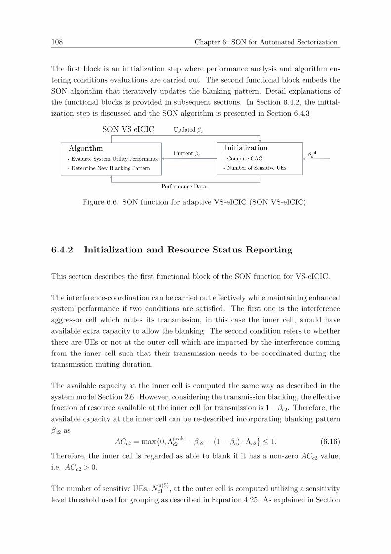
108 Chapter 6: SON for Automated Sectorization
The first block is an initialization step where performance analysis and algorithm en-
tering conditions evaluations are carried out. The second functional block embeds the
SON algorithm that iteratively updates the blanking pattern. Detail explanations of
the functional blocks is provided in subsequent sections. In Section 6.4.2, the initial-
ization step is discussed and the SON algorithm is presented in Section 6.4.3
Figure 6.6. SON function for adaptive VS-eICIC (SON VS-eICIC)
6.4.2 Initialization and Resource Status Reporting
This section describes the first functional block of the SON function for VS-eICIC.
The interference-coordination can be carried out effectively while maintaining enhanced
system performance if two conditions are satisfied. The first one is the interference
aggressor cell which mutes its transmission, in this case the inner cell, should have
available extra capacity to allow the blanking. The second condition refers to whether
there are UEs or not at the outer cell which are impacted by the interference coming
from the inner cell such that their transmission needs to be coordinated during the
transmission muting duration.
The available capacity at the inner cell is computed the same way as described in the
system model Section 2.6. However, considering the transmission blanking, the effective
fraction of resource available at the inner cell for transmission is 1−βc2. Therefore, the
available capacity at the inner cell can be re-described incorporating blanking pattern
βc2 as
ACc2 = max0,Λpeakc2 − βc2 − (1− βc) · Λc2 ≤ 1. (6.16)
Therefore, the inner cell is regarded as able to blank if it has a non-zero ACc2 value,
i.e. ACc2 > 0.
The number of sensitive UEs, Nu(S)c1 , at the outer cell is computed utilizing a sensitivity
level threshold used for grouping as described in Equation 4.25. As explained in Section

6.4 SON Function for Adaptive Inter-Cell Interference Coordination 109
4.4.4, the sensitivity threshold, ΓThr, is determined iteratively based on the inner cell
utility performance evaluated for the configured blanking pattern, i.e.,
Nu(S)c1 =
∑
∀u∈Ac1
1Γau ≥ ΓThr. (6.17)
At initial phase of the algorithm βc2 = βint. Having ACc2 > 0 and Nu(S)c1 > 0 are the
entering conditions for the SON algorithm.
6.4.3 SON Algorithm for Blanking Pattern Adaptation
This sections explains the SON algorithm that automatically adapts the blanking pat-
tern.
The iterative blanking pattern adaptation procedure analyzes the statistics of the UE
throughput performance data collected each scheduling time step. The system utility
Ua computed over the aggregate cell coverage area Aa, i.e. inner plus outer, as ex-
pressed in Section 4.4.4 is employed for performance based adaptation. The average
of the UE throughput performance data within a sliding time window tABS are used in
the system utility computation to provide a reliable comparison between utility per-
formances where variables used for utility computation are indicated in Equation 4.37.
Furthermore, a blanking pattern adaptation step size βstep is defined to be used to
adjust the current blanking pattern in a desired direction, i.e. increase (β++) or de-
crease (β−−). In the SON algorithm, the primary conditions to determine the blanking
pattern update direction, β++ or β−−, are the values of ACc2 and Nu(S)c1 . In this regard,
unless both conditions ACc2 > 0 and Nu(S)c1 > 0 are fulfilled, the blanking pattern is
always decremented if the respective utility performance evaluation is successful and
this can be summarized in pseudo-code 4
Pseudo-code 4 : Blanking pattern update direction
if ACc2 > 0 And Nu(S)c1 > 0 then
β++ Or β−−
elseβ−−
end if
Every iteration step, the adaptation strategy involves the computation of the system
utility from the UE throughput performance data collected within the tABS window
applying three different blanking pattern settings using Equation 4.37: the current

110 Chapter 6: SON for Automated Sectorization
(βc), incremented β+c = βc + βstep and decremented β−
c = βc − βstep blanking pattern
values and the corresponding utility values are denoted by Ua, Ua+ and U−
a , respectively.
During the updating step, the decision whether to increase/decrease βc is performed
by comparing the values of U+a and U−
a with respect to the actual utility performance,
i.e. Ua. The overall adaptive mechanism and algorithm decisions are more elaborated
and presented using the flow chart depicted in Figure 6.7.
Figure 6.7. SON algorithm flowchart for adaptive VS-eICIC
6.5 Performance Evaluation and Analysis
6.5.1 Performance Evaluation of SON for Automated Sector-
ization
The performance evaluation of the SON mechanism developed to automate the AAS-
based sectorization is presented in this Section. The investigation and evaluations

6.5 Performance Evaluation and Analysis 111
have been carried out with system level simulations conducted using the 3GPP and
RT-Scenarios considering a non-homogeneous spatio-temporarily varying UE traffic
distributions.
In the investigation, the initial state of the sectorization is set to the default Conven-
tional sectorization and the SON for AS is let to run network-wide at all BS sites.
Each eNB autonomously monitors the load situation over the coverage area served by
the respective-sector antenna. In this particular exemplary scenario, the automated
vertical sectorization is illustrated where it is prioritized over HS and assumed to be
generally preferred as it can be enabled for both single/multi-column array AAS for
the aforementioned reason. In the simulation, the non-homogeneous UE distribution
variation involving traffic hotspots changing their spatial location periodically over
time. The resulting sectorization status (ON/OFF) for the complete simulation time
period is shown in Figure 6.8. As exhibited in Figure 6.8 the sectorization state at
various sites served by each sector-antenna a is changing overtime and, for this partic-
ular scenario, the sectorization has been activated over the entire network for 24% of
the network operation time, that means, the the SON based automation mechanism
is able to avoid unnecessary sectorization activation over 76% of the time thereby pro-
portionally reducing consumption of network resources, like base band resources and
energy consumption, compared to the always ON sectorizaion case to which a fixed
and dedicated resources are always allocated.
Stimulaiton time Steps200 400 600 800 1000 1200 1400
Sector-an
tennaIndex
(a)
1
3
5
7
9
11
13
15
17
19
21
OFF ON
Figure 6.8. 3GPP-scenario: Sectorization state over time
The performance of the SON-enabled sectorization is further explored by analyzing UE

112 Chapter 6: SON for Automated Sectorization
throughput statistics collected from the coverage area Aa served by different sector-
antennas. The throughput performance of the UEs within coverage Aa for different
cases such as conventional sectorization (VS=OFF), always VS=ON with out SON
and VS with SON are plotted in Figure 6.9. For exemplification, results from three
selected coverage areas served by sector-antenna a = 5, a = 9 and a = 15 where the
UE throughput statistics are collected and evaluated overtime considering a sliding
evaluation time window tev = 100 simulation time steps while tracking the traffic vari-
ation. The evaluation scheme is carried out by comparing the values of TP5%Aa
, TP50%Aa
and TPavgAa
computed from the collected statistical data. As indicated in Figure 6.8 for
a = 5, the applied SON mechanism has activated VS at different times. In compar-
ison, the value of TP5%Aa
achieved with SON-AS is outperforming the always VS=ON
case by 35% maintaining the same performance with VS=OFF during the second time
when VS has been activated. Moreover, it can be clearly seen that the automated
VS mechanism yields performance enhancement similar to the always VS=ON case by
activating the sectorization only when it is worthwhile thereby providing throughput
gain of over 80% at the 50% CDF level of the statistics.
Simulation Time0 500 1000 1500
UETP[kbps]
100
200
300
400
500
600a = 9, TP5%
Aa
Simulation Time0 500 1000 1500
UETP[kbps]
0
500
1000
1500
a = 9, TPavg
Aa
Simulation Time0 500 1000 1500
UETP[kbps]
100
200
300
400
500a = 15, TP5%
Aa
Simulation Time0 500 1000 1500
UETP[kbps]
0
500
1000
1500
a = 15, TP50%Aa
Simulation Time0 500 1000 1500
UETP[kbps]
200
400
600
800
1000
1200a = 15, TP
avg
Aa
Simulation Time0 500 1000 1500
UETP[kbps]
100
150
200
250
300a = 5, TP5%
Aa
Simulation Time0 500 1000 1500
UETP[kbps]
200
400
600
800
1000
1200a = 5, TP50%
Aa
Simulation Time0 500 1000 1500
UETP[kbps]
200
300
400
500
600
700a = 5, TP
avg
Aa
Simulation Time0 500 1000 1500
UETP[kbps]
0
500
1000
1500
2000a = 9, TP50%
Aa
VS= OFF
VS=ON
SON AS
Figure 6.9. SON AS performance comparison for 3GPP-scenario
The adverse impact of always VS=ON case and the need for SON is demonstrated
in Figure 6.9 for a = 9 where deactivating the sectorization averts the significant
performance degradation that could arise from the activated cells. This is evident in
the performance plot that the 50% CDF level throughput performance is enhanced

6.5 Performance Evaluation and Analysis 113
achieving a gain of more than 60% by employing the automation mechanism.
On the other hand, Figure 6.8 shows that for a = 15 the SON strictly decides turning
off the VS at all times as favorable conditions have not been met. This is manifested
in Figure 6.9 where the automated VS performance has been following the VS=OFF
both at the 5% and 50% CDF level which are indicated by TP5%Aa
and TP50%Aa
values,
respectively. In this case, the automated VS is able to provide a gain of up to 37%
and 57% over the always VS=ON approach at the 5% and 50% CDF level respectively.
This clearly demonstrates that the static always VS=ON approach is detrimental and
could lead to significant performance degradation in situations like a = 15 if it is
kept active all the time. It is worth noting that the always VS=ON is unwanted and
costly over-provisioning solution as it keeps the VS always activated irrespective of the
load situation. The presented results show that the applied sectorization automation
mechanism provides a substantial system performance gain by averting the critical
performance deterioration situations that can be caused by keeping the activated cells
all the time ensuring the sectorization state that outperforms is maintained.
Simulaiton time steps500 1000 1500 2000 2500 3000 3500 4000 4500 5000
Sector-an
tennaIndex
(a)
10
20
30
40
50
60
70
OFF ON
Figure 6.10. RT-scenario: Sectorization state over time
The sectorization study has been carried out further by employing the developed SON
based automation scheme in a more realistic RT-scenario wherein the UEs are spa-
tially distributed in a diversified manner to reflect various practical situations. In this
scenario, both indoor and outdoor propagation environments are assumed. Cluster of
UEs which are moving on streets with a constant speed of 3 km/h creating a moving
traffic hotspots are considered to simulate dynamically varying load situation within

114 Chapter 6: SON for Automated Sectorization
the entire network. Accordingly, it can be seen in Figure 6.10 that the sectorization
state is dynamically changing over time tracking the traffic load variation. Compared
to the 3GPP-scenario discussed above, the ON/OFF operations in this particular sce-
nario are significantly noticeable where the ON states are accounting for 40% of the
total simulation time over the entire network while 60% of the time the sectorization
is deactivated.
Similarly, the performance of the automated sectorization is examined by analyzing the
UE throughput statistics while the UEs are being served by a specific sector-antenna
irrespective of the sectorization state. For the purpose of illustration, the throughput
statistics collected from two coverage areas served by sector-antenna a = 53 and a = 60
are presented in Figure 6.11 where in each sub-figure three CDF plots are depicted
comparing the three different sectorization cases discussed earlier. For each coverage
area served by a particular sector-antenna, the throughput statistics within a certain
evaluation time window of tev = 250 are compared and three different time widows are
selected for exemplification to assess the performance while the sectorization state is
being varied over time.
UE TP [kbps]0 1000 2000 3000
CDF
0
0.2
0.4
0.6
0.8
1a = 60, time window = 3
UE TP [kbps]0 1000 2000 3000
CDF
0
0.2
0.4
0.6
0.8
1a = 60, time window = 5
UE TP [kbps]0 1000 2000 3000
CDF
0
0.5
1a = 60, time window = 10
UE TP [kbps]0 1000 2000 3000
CDF
0
0.5
1a = 53, time window = 1
UE TP [kbps]0 1000 2000 3000
CDF
0
0.5
1
a = 53, time window = 3
VS= OFF
VS=ON
SON AS
UE TP [kbps]0 1000 2000 3000
CDF
0
0.5
1
a = 53, time window = 11
Figure 6.11. SON AS performance comparison for RT-scenario
In Figure 6.11, for a = 53 time window 1 refers to the initial phase of the simulation
and apparently the sectorization state if OFF at this stage. In this situations we can
still see the that the throughput CDF corresponding to the SON AS is aligned with

6.5 Performance Evaluation and Analysis 115
the VS=OFF and no significant performance difference is observed. While the simu-
lation time increases, the sectorization state is changed to ON in the third evaluation
time window as exhibited in Figure 6.10 triggered by higher load situation. As can be
observed from the corresponding performance comparison figure, the automated VS
performance is aligned with the always VS=ON case as the sectorization stayed acti-
vated for the whole evaluation time windows and yielding above 51% gain in the system
throughput at the 50% and 80% CDF levels compared to the VS=OFF case. However,
the sectorization state have stayed on ON state only until the beginning of the 11th
evaluation time windows, i.e. t = 2600 simulation time, within this time window the
VS has been deactivated going back to VS=OFF state. The corresponding perfor-
mance plots are evident that the VS=OFF state outperforms the always VS=ON case
for higher CDF percentiles providing more than 35% gain in the average UE through-
put, i.e. TPavgAa
. The same performance trend has been demonstrated for a = 60 over
different evaluation time windows. It is worth noting the performance over time win-
dow 5 that the CDF of the automated VS throughput performance is aligned with
both the VS=OFF case at the lower percentile and the always VS=ON at the higher
percentiles thereby maintaining always the better performance distribution. This is
a clear manifestation of the benefits of the developed SON based automation mech-
anism in ensuring maximized achievable system performance via tracking the traffic
load variation.
The presented performance comparisons and detail analysis have demonstrated that,
indeed, the sectorization process needs to be automated in order to deliver enhanced
system performance based on the actual traffic mix and distribution. As reported
using the displayed exemplary results, the sectorization needs to be activated when
and where there is a demand for the capacity and only when it can bring benefit.
6.5.2 Performance Evaluation of SON for Adaptive Inter-CellInterference Coordination
The performance of the developed adaptive VS-eICIC technique that automatically
optimizes blanking pattern configuration is discussed in this Section.
For this particular investigation, the heterogeneous hotspot-based traffic distribution
model used in the SON-AS study is considered over the entire network coverage are
and the spatial locations of the UEs are assumed to remain invariant with time. In
order to avoid any conflict that might occur between the SON-functions of AS and VS-
eICIC, as SON-function coordination is out of the scope of this thesis, only the SON

116 Chapter 6: SON for Automated Sectorization
for VS-eICIC is let to run while SON-AS is turned off. In this regard, it is valid to
maintain the same sectorization state, for instance VS=ON in this case, for the whole
simulation time as long as the spatial distribution of the UEs remains stationary.
Assuming VS=ON state at all sites, the network wide blanking pattern is initially
configured to a default value βint = 0.2. Then, the SON VS-eICIC is enabled to operate
autonomously at each eNB as explained in Section 6.4 for several simulation time
steps. Each simulation time step, βc can be updated, increased/decreased, based on
conditions by applying a constant step size βstep = 0.05. Figure 6.12 shows how the the
network wide βc behave for different blanking pattern adaptation period, tABS, where
one period corresponds to 90s in the simulation. Despite identical initial configuration,
βc is converged to different values overtime at the inner cells associated to various
sector-antenna where the final converged values are presented in Figure 6.12 (b).
Sector-antenan Index (a)1 2 3 4 5 6 7 8 9 101112131415161718192021
Blankingpattern
(βc)
0
0.1
0.2
0.3
0.4
0.5
0.6
0.7
0.8
0.9
11
Optimized blanking pattern
Blanking pattern adaptation period0 1 2 3 4 5 6 7 8 9 10 11 12 13 14
Blankingpattern
(βc)
0.1
0.2
0.3
0.4
0.5
0.6
0.7
0.8
0.9
11
1
2
3
4
5
6
7
8
9
10
11
12
13
14
15
16
17
18
19
20
21
(a) (b)
Figure 6.12. SON based automated blanking pattern adaptation for VS-eICIC
For example, the inner cell at a = 4 is converged to 0.75 indicating the presence
of high number UEs within the corresponding outer cell which are highly impacted
by the interference coming from the inner cell and the capability of the inner cell to
mute its transmission while maximizing the system utility performance. On the other
hand, the value of βc is converged to a minimum value of 0.15 at a = 7 depicting the
nonavailability of extra capacity the inner cell can offer by blanking. Moreover, it can
be observed that in some cells where the spatial distribution of the UEs behave more
or less uniform, the blanking pattern is moderate and converged fast to around 0.35.
These observations are in agreement with the results of the analytical optimization
approach presented in the modeling section, Section 4.4.4.
The performance of the developed adaptive VS-eICIC is further studied by statistical
analysis of the UE throughput data collected from the respective coverage area Aa.

6.5 Performance Evaluation and Analysis 117
The results are summarized for the entire network and presented in Figure 6.13 where
the values of TP5%Aa
, TP50%Aa
, TP80%Aa
and TPavgAa
are shown for two simulation cases: in
the first case VS-eICIC is disabled, i.e. βc = 0, and in the second simulation case,
the SON enabled VS-eICIC is employed. The gain values indicated in the figure are
evaluated with respect to the corresponding performance while VS is deactivated, i.e.
VS=OFF.
Sector-antenna Index (a)0 1 2 3 4 5 6 7 8 9 101112131415161718192021
Gain[%
]
-30-20-10
0102030405060708090
100TP5%
Aa
Sector-antenna Index (a)0 1 2 3 4 5 6 7 8 9 10 11 12 13 14 15 16 17 18 19 20 21
Gain[%
]
-30-20-10
0102030405060708090
100TP50%
Aa
Sector-antenna Index (a)0 1 2 3 4 5 6 7 8 9 101112131415161718192021
Gain[%
]
-30-20-10
0102030405060708090
100TP80%
Aa
Sector-antenna Index (a)0 1 2 3 4 5 6 7 8 9 10 11 12 13 14 15 16 17 18 19 20 21
Gain[%
]
-30-20-10
0102030405060708090
100TP
avg
Aa
VS=ON, βc = 0VS=ON, SON VS-eICIC
Figure 6.13. Performance of SON enabled adaptive VS-eICIC
The main objective of the proposed VS-eICIC scheme is to combat the impact of the
inter-cell interference that results from the sectorization at a cost of muting data trans-
mission in interferer cell while selectively maximizing the performance of the UEs crit-
ically affected by the interference problem on the interfered cell. This is demonstrated
in Figure 6.13 where the extreme performance degradation with VS=ON at the 5%,
50% and 80% throughput CDF level are significantly mitigated by applying VS-eICIC
technique. Specifically, when the VS-eICIC is employed, up to 23% additional perfor-
mance gain is achieved at the 5% throughput CDF levels, see TP5%Aa
values for a = 1
and a = 9. Moreover, at the 50% CDF level, the VS-eICIC has completely avoided the
performance loss incurred due to VS activation at a = 4 and is able to restore 22% per-
formance as depicted in the plot. In addition, it is worth noting to remember that the
presence of the severe interference at a = 4 is evident from the resulting high blanking
pattern value indicated in Figure 6.12 (b). At a = 7 the performance at all through-
put CDF percentile levels have not been impacted at all, therefore, this justifies that
it is reasonable to maintain the blanking pattern as minimum as possible to prevent

118 Chapter 6: SON for Automated Sectorization
undesirable impacts. Furthermore, it has been discussed in the VS SINR model and
interference analysis that UEs which have high SINR performance during VS=OFF
are more sensitive for VS activation and their impact on the system performance is
reflected at the higher percentiles of the throughput CDF. As a consequence, the values
of TP80%Aa
are compared with and without VS-eICIC. It can be clearly observed that,
indeed, the TP80%Aa
performances are suffering from interference problem at all sites and
negative performance gains up to −18% are reported in Figure 6.13. When VS-eICIC is
enabled, however, all those negative gains have disappeared at all and even additional
gains have been recorded in some cases. This clearly demonstrates that the VS-eICIC
is able to address and resolve the interference problem. Finally, the trade-offs of the
transmission muting to enable the interference coordination is expected to be reflected
on the average performance of the UE throughout, TPavgAa
. Accordingly, a reduction in
the average performance is observed almost at all sites but compared to the achieved
gains, the reduction level is marginal and acceptable, compare TPavgAa
values in in Figure
6.13.
Based on the presented performance results and analysis, it is evident that the SON
enabled VS-eICIC has proved its capability in enhancing the system performance and
providing substantial capacity by adaptively coordinating the interference. As demon-
strated by a diversified network wide heterogeneous spatial distribution scenario, the
SON mechanism developed to automate the coordination scheme has been effectively
able to optimize the blanking pattern according to the underlying traffic situations. In
conclusion, the SON VS-eICIC addresses and averts the critically limiting interference
problem which arises in AAS-enabled vertical sectorization. Moreover, this feature can
be integrated as one of the SON features that can be automatically enabled/disabled.
In real network where SON is enabled, the adaptive VS-eICIC operation can operate in
coordination with other SON functions like SON-AS and the procedure can be carried
out in a self-organized manner.

119
Chapter 7
Impact of Cell Layout Change on ExistingAutomated Network Operations
7.1 Introduction
The various SON mechanisms developed to automate the complicated tasks of radio
network planning and optimization are currently designed to operate in a network
wherein the deployment is not changing frequently and the cell layout remain sta-
tionary [HSS12]. Mobility Robustness Optimization (MRO) is one of the SON use
cases which relies on a cell-pair wise statistical information collected from the network
over a sufficient period of time. The collected statistics is considered as valid as long
as the coverage size/shape of the cells remain static and the neighbor relationships
are maintained [HSS12]. In AAS-driven sectorization, however, the cell layout can be
dynamically changed due to the activation/ deactivation of cell-beams triggered by
momentary local traffic situation. For instance, the introduction of cells via activation
process with a new cell IDs results in a new sets of handover borders altering the exist-
ing cell neighbor relationships. Unless those changes are properly accommodated and
measures are taken, the cell layout change can impair the operation of various SON
mechanisms running in the underlying network.
The impacts of AAS-enabled dynamic sectorizaton on the existing SON functionalities
have been discussed by 3GPP within the SI [3GP15b], and a WI have been approved to
address related ope issues. Future enhancements that might be required on the exist-
ing standardized SON solutions are embodied in the WI to guarantee interoperability
within multi-vendor deployment environment [3GP14b]. This entails a detailed study
and impact analysis of AAS-sectorization with respect to each particular SON use case
as well as identifying the associated issues the resulting cell layout change might cause.
In this chapter, the cell layout change introduced by the automated sectorization is
thoroughly investigated by including user mobility aspects and particularly enabling
MRO operation to optimize the handover performance. The rest of the chapter is
organized as follows. Section 7.2.1 briefly explains the analysis carried out to assess
the impact of the cell layout change on the performance of the existing MRO operation.
Based on the observations from the provided analysis, coordinated strategies for user
mobility handling during the sectorizaiton process are presented in Section 7.3.

120 Chapter 7: Impact of Cell Layout Change on Existing Automated Network Operations
7.2 Impact of Cell Layout Change on Mobility Ro-
bustness Optimization
7.2.1 Intra-RAT Mobility Robustness Optimization
In this section, the performance of the existing MRO operation with respect to the
activation/deactivation process of sectorization is outlined.
MRO is one of the self-optimization features of SON that automatically adjusts mobility
related network parameter configurations by autonomously detecting handover related
connection failures [HSS12]. Intra-RAT MRO particularly deals with handover related
problems occurring between two cells which belong to the same type of Radio Access
Technology (RAT), for example, between two LTE cells. The existing MRO operation
is based on stationary network deployment assumption where handover error statistics
are continuously monitored between cell-pair borders as long as the layout of the cells
and their neighbor relationships are not altered. However, while the cell layout is dy-
namically changing from time to time due to automated sectorization, the existing cell
neighbor relationships might keep varying as neighbor cell(s) could emerge/disappear.
In such cases, the collected mobility event statistics, MRO instances and counter values
associated to the state of the network before the execution of the cell layout change
might not be valid any longer for the new cell layout. As a consequence, the perfor-
mance of the HO parameter optimization operation could be impaired thereby causing
unexpected degradation of user experience.
When a new cell with a different cell border or different cell ID is introduced, new sets of
measurement report statistics are required. This is due to the fact that the propagation
environment with respect to the updated cell layout and the spatial distribution of the
underlying user traffic to be served by each cell are modified. Moreover, new MRO
instances are defined for the new cell-pairs as well. The subsequent sections examines
particularly mobility problems and the performance of MRO by considering VS as a
means to introduce cell layout changes. The objective of the investigation is to address
the following questions.
• How does the existing MRO perform in different sectorization state?
• What HO offset configuration settings can be reused for quick adaptation of
handover parameter after a cell layout is restored?
• How does the MRO statistics collected at specific sectorization state can be han-
dled once cell layout is changed?

7.2 Impact of Cell Layout Change on Mobility Robustness Optimization 121
7.2.2 Connection Failures and Performance of MRO
This section investigates user handover problems and analyzes mobility related con-
nection failures to evaluate the performance of MRO for different sectorization states.
In MRO, mobility related failure types are classified into different groups in order to
be able to precisely identify the root causes of the failures. These different failure
types are termed as Too-Late (TL) HO (HOTL), Too-Early (TE) HO (HOTE) and
HO to Wrong Cell (WC) (HOWC) [HSS12]. In addition, Ping-Pongs(PPs) which are
unnecessary back-and-forth of HO events are also regarded as HO problems as it causes
extra signaling overhead in the system and needs to be addressed by MRO. Such failure
classification enables MRO to take appropriate action via adjusting the Cell Individual
Offset (CIO) values which corresponds to specific HO boundary where mobility failure
is detected.
A mobile user can suffer from connection failure (CoF) from its serving cell due to either
Radio Link Failure (RLF) caused by poor radio condition or a failure to successfully
complete a HO process already initiated which is referred as HO failure (HoF). The
statistics of these failures are categorized and used to study user mobility problems
and the performance of MRO. The total number of CoF NCoF is described as the sum
of the number of HO event failures caused by RLF NRLF and HoF NHoF, i.e. NCoF =
NRLF + NHoF. Given the number of HOTL events by NTL, and the number of HOTE
and HOHoF events as a combination of the count of the corresponding mobility failure
events associated to RLF and HoF by NTE(RLF), NTE(HoF), NWC(RLF) and NWC(HoF),
respectively, the expressions for NRLF and NHoF become
NRLF = NTL +NTE(RLF) +NWC(RLF)
NHoF = NTE(HoF) +NWC(HoF).
(7.1)
In fact the decisions of MRO are made based on observations of HO events and col-
lection of sufficient statistics at each HO cell-pair, i.e. HO-source and HO-target cells.
Hence, MRO convergence depends on the number and behavior of the mobile users
crossing a particular cell border where a specific type of mobility problem is dominant.
In this section, the performance of MRO is illustrated by looking at the statistics of
the HO events collected from the complete network area in cell-pair wise manner, and
the number of all HO events described above in Equation 7.1 represent network-wide
statistics. Therefore, the value of NCoF indicates the reduction of the connection failure
problems and demonstrates the convergence of MRO over time. Besides to CoF, an

122 Chapter 7: Impact of Cell Layout Change on Existing Automated Network Operations
additional performance metric described as mobility failure ratio (MFR) (NMFR) is
defined to express NCoF as a fraction of the total attempted HO events that includes
the statistics of the successful HOs (HOsuc) expressed by Nsuc, i.e.
NMFR =NCoF
NCoF +Nsuc(7.2)
Simulation based MRO performance evaluation has been carried out to inspect HO
event behavior for different cell layout cases. In the simulation, user mobility feature is
integrated within the 3GPP regular hexagonal cellular model wherein users moving at
low speed arbitrary in random direction and at high speed on street along a defined path
direction are considered. The street paths are modeled in such away that UEs cross
through different HO boundaries where the radio condition and underlying coverage
situation are likely impacted by the activation/deactivation of cells. Since developing
the MRO algorithm itself is not within the scope of this thesis, detail information
about the employed intra-RAT MRO algorithm are not presented here, please see
reference [VWLA11]. Furthermore, the simulation parameters and system description
are also provided in Table []. The mobility related connection failures are studied for
two different cell layout cases which correspond to a more challenging and worst case
scenario assumptions as they employ network-wide setups of VS=OFF and VS=ON
sectorization states. The initial handover offset CIOint values with respect to each
source-target cell-pair are set to a default setting, CIOint = 0 dB, and these values are
optimized by MRO overtime by monitoring the local mobility failure events at each
cell border during the simulation run.
MRO period(b)
2 3 4 5 6 7 8 9 10 11 12 13 14 15 16 17 18 19
NM
FR[%
]
02468
101214161820
NMFR Over Simulation Time [%]
VS=OFF
VS=ON
MRO period(a)
2 3 4 5 6 7 8 9 10 11 12 13 14 15 16 17 18 19
Number
ofEvents
[/UE/m
in]
0
0.1
0.2
0.3
0.4
0.5
0.6
0.7
0.8
0.9
11Normalized NCoF and NPP Over Simulation Time
VS=OFF: NCoF
VS=OFF: NPP
VS=ON : NCoF
VS=ON : NPP
HO-Target Cell ID(c)
5 10 15 20 25 30 35 40
HO-Sou
rceCellID
5
10
15
20
25
30
35
40
∆NCoF for Complete simulaiton time
-1
-0.8
-0.6
-0.4
-0.2
0
0.2
0.4
Figure 7.1. (a) Normalized number of MRO events, (b) MFR, (c) ∆NCoF for cell-pair
Figure 7.1 (a) depicts the values of NCoF and NPP normalized to the total number

7.2 Impact of Cell Layout Change on Mobility Robustness Optimization 123
of UEs within the network and the MRO statistics collection period time in minute
for VS=OFF and VS=ON cases. In addition, the corresponding values of NMFR are
presented in Figure 7.1 (b). As can be observed in Figure 7.1(a), MRO is able to
significantly reduce the failures in both VS=OFF and VS=ON cases by over 60% and
their performance stabilizes over time converging to almost same level. Despite the high
number of HO events expected when VS=ON due to the increased number handover
boundaries introduced by the newly activated inner cells, the total number of mobility
failures over the complete network area is lower compared to what is observed when
VS=OFF at each MRO period. This is attributed to the evasion of some of the RLF
problems occurring during UE handover as a result of better service coverage provided
with the denser cell layout with VS=ON. This is demonstrated in Figure 7.1 (b) where
NMFR values are substantially improved (lower) for VS=ON due to the higher number
of successful HO events, Nsuc.
The statistics of the network-wide connection failure problems are further investigated
for each HO source-target cell-pairs by looking at the difference of the normalized total
CoF event counts ∆NCoF collected over the complete simulation time when VS=ON
and VS=OFF described by NONCoF and NOFF
CoF , respectively, i.e. ∆NCoF = NONCoF −NOFF
CoF .
Figure 7.1 (c) illustrates the values of ∆NCoF where the cell ID ranges [1, 21] and
[22, 42] corresponds to the outer and inner cells, respectively. For VS=ON, the new
additional HO events involve inner-outer and outer-inner cell borders unlike to the
only outer-outer cells HO events occurring with VS=OFF. It can be demonstrated
in the figure that the mobility problems attributed to the outer-outer cell HO events
are significantly reduced when VS=ON over several cell boundaries for aforementioned
reason. Despite additional mobility failure counts are recorded, as expected for the new
inner-outer/outer-inner cell borders with VS=ON, the overall CoF statistics illustrates
that the total number of these failures are lower in comparison to the reduction in
the failure rate. Summarizing, the observation from Figure 7.1 evinces the situation
where the cell layout change driven by the AAS-based sectorization, in particular to
VS, does not always lead to mobility problems as expected. It rather enhances the
HO performance by evading the RLF problems as a result of a denser and dominant
service coverage by the activation of the inner cells.
Apart from the CoF, the statistics of HO events that lead to PP are evaluated as well
and reported in Figure 7.1 to study their behavior with respect to the sectorization. As
illustrated in the figure, for VS=OFF, MRO has been able to react on the PP effects,
at the initial MRO periods, even faster than the other mobility failures. However,
when both HOTL and HOTE problems are dominating, MRO algorithm reacts with
higher priority on the cause of those connection failures instead of the PP. Hence, the
PP effects are seen oscillating afterwards over time as MRO stops further reacting on

124 Chapter 7: Impact of Cell Layout Change on Existing Automated Network Operations
it. This is a trade-offs as both the CoF and PP problems can not be always resolved
simultaneously owing to conflicting decisions in adjusting the respective cell border
CIO. With the denser cell layout case, VS=ON, since most of the HOTL causing RLF,
which have been dominating during VS=OFF, are resolved besides PPs are see to be
no longer oscillating as well where their statistics is clearly depicted stabilizing and
converging together with the CoF problems.
7.2.3 Connection Failures Triggered by Cell Layout Change
This section examines more practical case scenarios where the network-wide cell layout
is changed by activating/deactivating all the inner cells simultaneously while MRO is
running.
In reality, cell layout change can be triggered any time and the cell activa-
tion/deactivation process might be executed in a network while MRO operation is
running. The moment the cell layout change is executed, the collected MRO event
statistics and the respective cell border optimized CIO settings can not be representa-
tive for the new cell layout. Hence, the MRO statistics might not be valid any longer
and the CIO values become sub-optimal. These situations are well investigated, in this
section, considering the worst case scenario where the cell activation/deactivation pro-
cedure is carried out suddenly while MRO is operating. In this regard, the practically
challenging aspect becomes how to deal with the MRO instances and the collected HO
event statistics along with the CIO configuration. Two approaches are considered to
deal with those challenges. The first approach assumes no additional reaction is need,
i.e. MRO statistics and CIO configurations are unchanged. In contrary, the second
approach considers to reset the CIO configurations to default settings, CIOint = 0 dB,
and to restart all the MRO instances and event counter values. Henceforth, the terms
NO-RESET and RESET are used to refer to the two approaches, respectively.
Assume VS=OFF state at the beginning and inner cells are activated network-wide
at all sites after MRO stabilizes and the statistics of CoF are converged as illustrated
in Figure 7.2 where the normalized count of mobility events are reported for both
NO-RESET and RESET approaches. In contrast to the stated assumption where the
CIO values might yield sub-optimal performance, the NO-RESET approach exhibits
no significant additional mobility related issues rather demonstrates a stable MRO per-
formance, see Figure 7.2. With CIO RESET approach, however, the optimized CIO
configuration with respect to the handover boundaries of the existing cell borders, i.e.,
outer-outer cells, are reset. This potentially causes high number of mobility failures

7.2 Impact of Cell Layout Change on Mobility Robustness Optimization 125
during the next MRO period right after the cell activation, refer to the curve corre-
sponding to CoF statistics in Figure 7.2. Nevertheless, the performance of MRO for
both approaches are seen later to converge and stabilize to the same level over time.
The PPs statistics are more or less showing not significant deviation from what has
been reported previously in Figure 7.1(a). However, marginal variation is observed due
to the trade-offs in the MRO response towards the abrupt failures in the network. In-
vestigation of the connection failures right after the activation of the inner cells evinces
the dominant mobility failure statistics, in the case of RESET approach, occur between
outer-outer cells while relatively less failures are reported for the NO-RESET case.
MRO period(a)
2 4 6 8 10 12 14 16 18 20 22 24 26 28 30 32 34 36 38 40
Number
ofEvents
[/UE/m
in]
0
0.2
0.4
0.6
0.8
1
MRO period(b)
2 4 6 8 10 12 14 16 18 20 22 24 26 28 30 32 34 36 38 40
Number
ofEvents
[/UE/m
in]
0
0.2
0.4
0.6
0.8
1NCoF: RESETNPP : RESETNCoF: NO-RESETNPP : NO-RESET
Figure 7.2. Normalized MRO Events (a) Activation, (b) Deactivation
For the deactivation case where the VS cells are merged, all the activated inner cells
are turned off while MRO is actively running while in VS=ON state. With such abrupt
deactivation procedure, users those have been connected to the respective inner cells
are eventually be dropped, hence, suffer from RLF problem. Since the CIO values
optimized while VS=ON might not be optimal, additional related handover failures
are likely to occur. This explained using Figure 7.2(b) wherein the sectorization is
changed from ON to OFF state at MRO period 20 applying either RESET and NO-
RESET approaches. As can be observed from the figure, the statistics of COF has
dramatically increased after the deactivation of the inner cells for both deactivation
approaches for the aforementioned reason. In comparison to NO-RESET, the failure
rate is significantly large for the RESET case due to the RLF from all inner cells’ users in
addition to the mobility failures occur between outer-outer cells as the corresponding
optimized CIO configuration is reset to default value. It is worth noting that, the
performance of MRO have demonstrated convergence overtime after being able to react
and resolve the mobility problems in both RESET and NO-RESET approaches.
The simulative investigation and mobility failure statistical analysis presented so far
126 Chapter 7: Impact of Cell Layout Change on Existing Automated Network Operations
have demonstrated that UE mobility related problems can be resolved by the existing
MRO and the failures statistics can be significantly reduced and converged over time.
However, it is clearly observed that a coordinated action between the MRO and the
execution of the cell layout change is essential in order to properly hand-offs users in
the underlying coverage to the appropriate serving cells. The required action enables to
evade unprecedented connection failure during the transition period, otherwise, many
users could experience abrupt connection failures that lead to sudden service disconti-
nuity which eventually deteriorate the user experience.
7.2.4 Fast Handover Parameters Reconfiguration
This section discusses a fast handover offset reconfiguration mechanism during cell
activation/deactivation procedure in order to address connection failure problems and
user service discontinuity caused by a sub-optimal CIOint values.
Depending on how frequent and dynamic the cell activation/deactivation process is
executed, relying on the MRO operation to adjust the CIO values can be sub-optimal
solution as it might take time until the optimization converges to the optimal value, see
Figure 7.2. Unless additional mechanism is applied, the activation/deactivation proce-
dure alone can potentially impact the continuity of user services due to an intermittent
radio link connection with the serving cell as depicted in Figure 7.1. This section, as
a result, introduces a store-and-fetch mechanism where optimized CIO configuration
values, CIOopt, are stored along with additional information to describe and identify
the cell layout prior to a sectorization state is changed. When the same sectorization
or cell layout state is resored CIOopt can be fetched to retrieve back the configura-
tion values and adapt the respective cell-pair CIO concurrently with the sectorization
action.
For illustration purpose, VS with the two particular sectorization states are assumed
to be known as VS=OFF and VS=ON and the respective cell-pair optimal CIO values
are described by CIOOFFopt and CIOON
opt , respectively. Each cell is assumed to be able
to immediately adapt the MRO parameter (e.g CIO values) when the cell layout is
changed via sectorization. When either of the sectorization state is executed for the
first time, MRO algorithm runs to optimize the cell-pair CIOs until it finally converges
as depicted in Figure 7.1. The corresponding optimal CIO values are then stored
along with additional information associated to the respective sectorization state for
later retrieval.By the time the same sectorization sate is executed again, these stored
optimal CIO values are fetched and reconfigured immediately as initial configuration
setting, i.e. CIOint = CIOopt.

7.3 Coordinated Strategies for Dynamic Cell Layout Change 127
MRO period(a)
2 3 4 5 6 7 8
Number
ofEvents
[/UE/m
in]
0
0.2
0.4
0.6
0.8
1
Normalized NCoF Over Simulation Time
VS=OFF: CIOint = CIOOFFopt
VS=OFF: CIOint = CIOONopt
MRO period(b)
2 3 4 5 6 7 8
Number
ofEvents
[/UE/m
in]
0
0.2
0.4
0.6
0.8
1
Normalized NCoF Over Simulation Time
VS= ON: CIOint = CIOOFFopt
VS= ON: CIOint = CIOONopt
Figure 7.3. Store-and-fetch scheme for faster initial CIO reconfiguration
For each sectorizaiton scenario, in Figure 7.3, different CIOint is utilized from previously
optimized CIO. In both VS=OFF and VS=ON cases, the configured CIOint provide
a stable MRO performance where the connection failure rates remain at the value
depicted in Figure 7.1. Irrespective of which initial value is set,CIOOFFopt or CIOON
opt ,
the performance curve have demonstrated the same behavior depicting no significant
additional mobility failures. These results indicate that, unless additional cell layout
change is further introduced, the store-and-fetch scheme is a viable solution for fast
reconfiguration of CIOint. The proposed scheme enables to sustain the performance of
MRO by evading unforeseen failure of UE connection immediately after sectorizaiton
procedure is executed.
7.3 Coordinated Strategies for Dynamic Cell Lay-
out Change
7.3.1 Handling User Mobility During Sectorization
This section discusses user mobility handling mechanisms to address abrupt connection
failure problems occurring during the sectorization procedure and which can not be
tackled by MRO.
One of the challenging aspects of AAS-based sectorization procedure is the abrupt user
connection failures and service discontinuity occurring while the underlying coverage
layout is being changed. Concurrent with the activation/deactivation of new cell(s),

128 Chapter 7: Impact of Cell Layout Change on Existing Automated Network Operations
considerable number of UEs might need to be handed over to a HO target cell within the
new cell layout. Since the existing HO procedure is designed to hand-off UEs through a
step-wise and controllable process, transferring a mass number of UEs simultaneously
might eventually be unsuccessful, for instance, due to Random Access Channel (RACH)
congestion [HT11]. Furthermore, many UEs could suffer from immediate RLF problem
during cell deactivation if the UEs’ serving cell suddenly disappears. Those connection
failure problems are not related to UE mobility itself rather they are attributed to the
alteration of the cell layout, hence, can not be resolved by MRO. This motivates the
need for additional coordinated mechanism to properly handle the HO of group of UEs
to ensure seamless operation of the sectorization process.
In fact, the context of all UEs being served by the same AAS are available at the cor-
responding eNB irrespective of the employed type of sectorization. These information
can be utilized to further coordinate the HO process. Besides, the spatial location of
the UEs can be assumed to remain momentarily stationary when the the underlying
cell layout is changing. Thus, the available timing advance information of each UE
with respect to any of the cell associated to the same AAS used to synchronize data
transmission remains valid during the sectorization process. This avoids the need for
a new RACH procedure to be performed every time the activation/deactivation action
takes place to align the down/up link channel of UEs with respect to a new serving
cell. Moreover, a planned cell layout change and associated cell information (cell-info)
are known a priori by the respective eNB, therefore, the UEs within the underlying
coverage can be pre-configured and prepared in advance so that handing over the UEs
can be handled concurrently with the cell activation/deactivation process.
A user hand-off mechanism that can be processed synchronously for a group of UEs
without performing the normal HO procedure and free of a new RACH request is pro-
posed as a solution. With the RACH-free approach, the group HO can be executed
faster to immediately synchronize UEs with respect to the new cell layout thereby
evading unforeseen connection failures. The RACH-free group HO operation is sum-
marized and illustrated with a diagram in Figure 7.4 which depicts the major message
flow and the coordination functionalities. When an eNB decides to activate/deactivate
a cell, it configures the UEs residing within the coverage area it serves via broadcasting
configuration update messages. The broadcast message includes relevant informations
about the new cell, e.g. Cell ID to be assigned and CIOint that should be used for trig-
gering measurement reports. Based on collected measurement reports, the association
of the UEs to the respective best target cell is prepared at the eNB without additional
procedure because both the source and the possible target cells belongs to the same
eNB. The configuration of the UEs is updated with additional mobility control-info
to prepare them for a timely synchronized group (synch-group) HO. Finally, the eNB

7.3 Coordinated Strategies for Dynamic Cell Layout Change 129
grants physical resources for the handed over UEs, e.g. Physical Downlink Control
Channel (PDCCH) for the UEs, and sends out the synchronization signal immediately
after the HO is completed.
Figure 7.4. RACH-free synch-group HO in AAS-based dynamic sectorization
The presented RACH-free sync-group HO procedure enables not only to combat the
connection failure problems but also provides a standardizable solution. The solution
considers real network deployment aspects where AAS-enabled dynamic sectorization
process is running to further ensure interoperability within vendor specific devices to
address some of the related open issues discussed within the 3GPP WI [3GP14b].
Details of the proposed scheme have been contributed for discussion in the WI and the
inventive concepts are filed and disclosed in [KW15].
7.3.2 Inter-eNB Notification and Information Exchange
In this section, a coordination scheme is proposed to handle the HO of an incom-
ing/outgoing UEs to/from neighboring cells to avoid UE connection failures.
Despite the fact that the sectorization process is designed to be autonomously executed
by an eNB to alter only the local coverage layout, UEs coming from/ going outwards to
neighbor coverage region might be impacted by unforeseen connection failures. Moving
UEs crossing an area undergoing the cell layout change could initiate a normal HO
procedure targeting unstable cell that might be changed in awhile. Unless additional
coordination mechanism is employed between the inter-site eNBs, those UEs might
be admitted while the target cell information is changed before initiating the RACH
procedure. Thus, the incoming UEs may experience a HOF or RLF and such problem
can not be tackled by MRO. Furthermore, re-establishing the UEs’ connection to the
same target cell or any other cell found via cell search after the connection failure might

130 Chapter 7: Impact of Cell Layout Change on Existing Automated Network Operations
not be successfully carried out as the required cell information might not be available.
This demands preparation of the UEs in advance with respect to possible target cells
and configure them with the new cell lay out information.
Dealing with such connection failure issues, this section provides a synchronization
scheme which relies on an inter-eNB signaling through which cell layout change infor-
mation is communicated. The information can be pre- or post-notification messages
that are exchanged before or after the execution of sectorization. If pre-notification
message is used, the eNB planning the sectorization process informs the neighbor cells’
eNBs about the upcoming cell layout change. The message includes informations like
the cell-ID(s), the timing required to synchronize ongoing related activities and further
instructions on how to handle any HO requests during the transition period. With the
post-notification, any HO request from a neighbor eNB serving an incoming UEs can
be handled in two ways. The first approach deals with re-direction of the HO request
to another possible stable cell if the requested HO target cell is about to be changed.
The second approach includes preparation the HO of such UE to multiple cells and
synchronizing its action in time with the sectorization.
Figure 7.5. Coordination with inter-eNB notification and information exchange
A generic message flow diagram is used in Figure 7.5 to illustrate the information
exchange in a typical post-notification case proposed to enable the coordination of the
user mobility to handle aforementioned connection failures. The sectorization process
is carried out at eNB1 and the eNB of a neighbor cell serving moving UE UE2 is denoted
by eNB2. When a normal HO request is sent to eNB1, a cell layout notification message
is replied back to eNB2 indicating the status of the requested HO target cell. In the HO
request reply, additional information (additional-info) and further instructions on how

7.3 Coordinated Strategies for Dynamic Cell Layout Change 131
to proceed with the HO process are included. The coordination scheme proposes first
to redirect the requested HO target to any other possible target cell, for example, the
second strongest HO target cell measured by the UE. In case the HO redirection is not
possible or might not be successful, a fast connection re-establishment option is enabled
by preparing the UE HO in advance with respect to multiple HO target cells. This is
carried out by updating the configuration of the UEs with the additional-info about the
ongoing cell change including the relevant configuration data. The diagram in Figure
7.5 describes only the general inter-eNB message exchange relevant to discuss in this
section and to illustrate the intended coordination mechanism. The detail signaling of
the coordination procedures developed by the author of the thesis is available and have
been disclosed in a filed patent [WKKR17].
In this chapter, the impacts of the cell layout change introduced by AAS-enabled dy-
namic sectorization have been investigated thoroughly. The investigation mainly ana-
lyzes the impacts with respect to user mobility. Detail assessment have been carried
out as well on the performance of the existing standardized automated MRO operation
to identify any HO related problems and open issues that needs to be addressed to
support the AAS-sectorization. The study has indicated that the AAS-sectorization
process should be synchronized properly with other SON functionalities like MRO to
provide a coordinated network operation. Simulative results have demonstrated that
the initial handover offset configurations are crucial in evading some of the UE mobil-
ity related failures at the time of cell activation/deactivation process. This has been
addressed by a store-and-fetch method that quickly adapt the handover offset config-
urations with previously optimized values thereby considerably reducing the failures
attributed to sub-optimal CIO configurations. UE mobility handling schemes and HO
coordination strategies have been proposed to address the abrupt connection failure
problems experienced by UEs while sectorization is executed. The proposed schemes
and strategies provides a solution to address the related open issues highlighted by
3GPP in response to the request for a potential SON enhancements that may be nec-
essary to ensure interoperability within the existing features in Rel.12


133
Chapter 8
Summary and Outlook
This thesis deals with adaptive cellular layout enabled by an automated cell sector-
ization in a self-organizing networks. The developed SON algorithm controls the ac-
tivation/deactivation of cell-beams to effectively meet dynamic network capacity de-
mand by intelligently monitoring the spatial traffic concentrations and adapting the
underlying cell coverage layout accordingly. Moreover, an adaptive enhanced inter-cell
interference coordination scheme is developed to combat the inter-cell interference chal-
lenge between the co-channel operated cells. The scheme adaptively coordinates the
data transmission between the co-sited cells by identifying the users which are severely
impacted by the interference. The proposed SON-based cell sectorization automation
mechanism provides a flexible and efficient deployment solution over the traditional
fixed sectorization paradigm by properly executing the sectorization procedure only
when and where it is needed, and can provide gain.
To exploit the AAS-sectorization flexibility in the elevation domain, a three-dimensional
channel characterization is vital. In Chapter 3, a new tilt-dependent shadowing model
is developed to address the deficiency of the existing shadowing model that considers
the propagation scatter behavior only in the azimuth direction. The model character-
izes the effect of the elevation domain clutter variation with respect to tilt configuration.
A detailed statistical analysis is provided on tilt-specific shadowing values extracted
from a ray-tracing based predicted radio propagation data that are able to reflect
various clutter experience of the real-world propagation environment. The modeling
considers specific scenario configuration consisting of irregular site layout and location
adopted from real network planning data. The proposed model estimates a new shad-
owing value for a new tilt setting by including the expected shadowing variation and
the desirable statistical correlation behavior compared to the reference setting. The
observed performance results and statistical distribution curves have demonstrated
that the proposed model is able to capture the impact of the tilt change. Being derived
based on a scenario having a diversified clutter, the proposed model and the introduced
variable values can be seen as valid and applicable to a wide range of case scenarios.
The system model developed for the AAS-based sectorization are presented in Chapter
4 and 5. The models are employed to carry out detail investigation on the factors which
determine the sectorization performance. The sectorization models describe the com-
plex relationship among various related system parameters to provide a basis criteria

134 Chapter 8: Summary and Outlook
to be used within the automated operation designed to control the sectorization proce-
dure. Simulative based performance analysis have demonstrated the achievable gains
from sectorization with respect to different specific scenarios. Accordingly, different
case scenarios have been identified where and when the AAS-sectorization can bring
the desirable benefit. In addition, thorough analysis has been carried out to study
the resulting inter-cell interference impact that countermands the performance of AAS
sectorization. To address the inter-cell interference issue, Chapter 4 provides analyti-
cal model for the proposed interference-coordination technique and the mathematical
framework to be used while developing the corresponding SON mechanism.
The SON framework designed to automate the AAS-sectorization is presented in Chap-
ter 6. The automation mechanism that mainly controls the sectorization-driven cell
layout changes performs based on real time performance monitoring. Cell beam acti-
vation and deactivation procedures are triggered when the defined cell load criteria are
satisfied. The performance of the proposed automation framework has been evaluated
using system level simulations considering various non-homogeneous user distribution
scenario in the hexagonal-cellular model. Simulation results have clearly demonstrated
that the proposed scheme is able to control the activation/deactivation process thereby
providing a substantial performance gain over the static over-provisioning approach
where the sectorization is always activated. Further performance analysis of the au-
tomated sectorization has been carried out in a more realistic RT-scenario wherein
the users are spatially distributed in a diversified manner to reflect practical situa-
tions. Chapter 6 also provides the adaptive interference-coordination technique that
has been developed to tackle the impact of the co-channel interference between co-sited
cells. The SON mechanism developed for the interference coordination is responsible
for adapting the blanking pattern configuration. Simulation results have demonstrated
that the technique is able to adapt the transmission muting pattern thereby effectively
dealing with the co-channel interference problem and delivering an optimized system
performance.
The impacts of the AAS-enabled dynamic sectorization on the existing SON opera-
tions is analyzed in Chapter 7. In particular, mobility related user connection failure
problems and handover behavior are investigated in combination with the dynamic cell
layout change mechanism. The chapter has focused on a detailed performance assess-
ment on the existing standardized MRO operation and identifying open issues that
has to be addressed within future release. The chapter proposes user mobility han-
dling schemes and HO coordination strategies to evade unforeseen abrupt connection
failure problems triggered by the cell layout change. The result analysis and proposed
concepts have impacted AAS-based related work item and have contributed in the
standardization work.

135
As a future work, the dynamic beam forming and steering capability supported by
AAS can be further exploited by developing an automated sectorization that can steer
cell beams in any sectorizaiton plane. The user- or group of user-specific beam steering
could be more effective in distributing system capacity according to the actual traffic
mix. To support such feature, a fully automated beam steering mechanism can be
designed to track a specific group or user to deliver a desired service with the promised
quality targets. The next-generation massive-array AAS entails further study to fore-
see a new dimension within the upcoming ultra-dense cellular deployment options to
support the proliferation of wireless devices in future networks.


137
List of Acronyms
2D 2 Dimension
3D 3 Dimension
3GPP 3rd Generation Partnership Project
AAS Active Antenna Systems
ABS Almost Blanked Subframe
AC Available Capacity
ACM Adaptive Coding and Modulation
AS Automated Sectorization
BA Backward Attenuation
BBU Base Band Unit
BEP Bit Error Probability
BS Base Station
CDF Commutative Density Function
CIO Cell Individual Offset
CoF Connection Failure
CP Cyclic Prefix
CRS Common Reference Signal
dB decibel
dBi decibel relative to isotropic antenna
DPM Dominant Path Model
eICIC enhanced Inter Cell Interference Coordination
eNB enhanced Node B
HO Handover
HoF Handover Failure
138 List of Acronyms
HO-TE Handover-Too Early
HO-TL Handover-Too Late
HO-WC Handover-to Wrong Cell
HPBW Half Power Beam Width
HS Horizontal Sectorization
ISD Inter Site Distance
LOS Line Of Sight
LTE Long Term Evolution
LTE-A Long Term Evolution-Advanced
MFR Mobility Failure Ratio
ML Main Lobe
MRO Mobility Robustness Optimization
MVB Minimum Variance Beamformer
NLOS Non Line Of Sight
NS-UE Non Sensitive-User Equipment
OAM Operation And Maintenance
OFDM Orthogonal Frequency Division Multiplexing
OPEX Operational Expenditure
PCI Physical Cell ID
PDCCH Physical Downlink Control Channel
PF Proportional Fair
PL Path Loss
PP Ping Pong
PRB Physical Resource Block
RACH Random Access Channel

139
RAN Radio Access Network
RAT Radio Access Technology
RE Resource Element
RET Remote Electrical Tilting
RF Radio Frequency
RLF Radio Link Failure
RRH Remote Radio Head
RS Reference Signal
RSRP Received Reference Signal Power
RT Ray Tracing
SDM Space Division Multiplexing
SINR Signal to Interference plus Noise Ratio
SL Side Lobe
SLL Side Lobe Level
SON Self Optimizing Network
SON-AS Self Optimizing Network function for Automated Sectorization
S-UE Sensitive-Use Equipment
TRX Transmitter
TTI Transmission Time Interval
UE User Equipment
VS Vertical Sectorization
VS-eICIC eICIC for Vertical Sectorization
VS-OFF Vertical Sectorization-enhanced Inter Cell Interference
Coordination
VS-ON Vertical Sectorization-ON

140 List of Acronyms
VS-S Vertical Sectorization-Supercell
WC Wrong Cell
WG Working Group

141
List of Symbols
a Index of sector-antenna
A(c) A mapping function returns index of a sector-antenna serving cell c
Aa Set of users in a coverage area served by sector-antenna index a
AP Set of propagation prediction pixel points
αa,c Fraction of power assigned to cell c from a sector-antenna a
ba Index of cell beam generated from sector-antenna a
BAo Backward attenuation factor
Bc beam pattern of cell c
Bvc Vertical component of beam pattern of cell c in linear scale
Bhc Horizontal component of beam pattern of cell c in linear scale
Bhc Vertical component of beam pattern of cell c in decible scale
Bvc Horizontal component of beam pattern of cell c in decible scale
B-subframe Bad SINR subframe
βc Transmission blanking pattern
βstep Transmission blanking pattern adapt step size
βint Initial Transmission blanking pattern configuration
c index of a cell
C Set of index of all cells
dc,u Path loss distance between user index u and cell c
dcor Shadowing decorrelation distance
dInner Geometrical distance of Inner/Outer cell border in vertical sectoriza-tion
∆a Utility difference value at sector-antenna a
ηu Throughput gain of user u after sectorization compared to conven-tional sectorization
fPL PDF of LuT
Fρ(∆Θxc ) Shadowing correlation coefficient estimate function for ∆Θx
c
Gmaxc Maximum antenna gain in the boresight direction
Guc Direction antenna gain of cell c in the direction of user u in linear scale
G-subframe Good SINR subframe
Guc Directional antenna gain of cell c in the direction of user u in dB scale
Guc2,c1 Difference of the antenna gain of cell c2 and cell c1 at user u
ΓThropt Optimal sensitivity threshold for user grouping
Γau Sensitivity of user u served by a cell from sector-antenna a

142 List of Symbols
Γc Average sensitivity value of the sensitivity of all users served by cell c
γu SINR of user u before sectorization
γ′u SINR of user u after sectorization
γ′u(VS-S) SINR of user u after Super-cell sectorization
huc Total antenna propagation attenuation value
Hc Set of values of huc of all users in the network area with respect to cellc
IISD Site intersite distance
I′u Total interference signal power received at u after sectorization
κuc2,c1 Ratio of the power received from c2 to c1
κuc2,c1(VS-S) Ratio of the power received from c2 to c1 with vertical sectorization
φuc azimuth angle of user u with respect to cell c
Φc3dB Azimuth HPBW of cell c
Φc Azimuth orientation of cell c
φMLc Azimuth angle in the main lobe region of beam pattern of cell c
ΦMLc Set of azimuth angle in the main lobe region of beam pattern of cell c
ΦHS Azimuth angle of the overlap angle of the horizontal beams in HS
θuc Elevation angle of user u with respect to cell c
Θc Elevation tilt of beam of cell c
Θc3dB Elevation HPBW of cell c
Θoc Reference elevation tilt setting of cell c
θMLc Elevation angle in the main lobe region of beam pattern of cell c
ΘVS Elevation angle of the overlap angle of the vertical beams in VS
∆Θxc Difference of elevation tilt configuration values
ϑc Set of elevation angle settings of cell c
la Sectorization state at sector-antenna a
LuT
total propagation loss value in linear scale
LuT
total propagation loss value in dB scale
Lc Average load of cell c
Λc(t) Instantaneous load of cell c at time t
Λpeakc Configured peak load cell c
Λthr Overload triggering threshold of cell c
Λhys Load hysteresis at cell c
λa ratio of the number of users connected either of cell at a after sector-ization
µs Vector of ones

143
µs Vector of ones
µGS Total radio resource share assigned from G-subframe to sensitive user
group
µGNS Total radio resource share assigned from G-subframe to non-sensitive
user group
µBS Total radio resource share assigned from B-subframe to sensitive user
group
µBNS Total radio resource share assigned from B-subframe to non-sensitive
user group
ν Radiation pattern of array element
NY Size of array element in Y direction
NZ Size of array element in Z direction
Na Total number of total number of cells in the network
Nbs Total number of base station sites in the network
Nbs Set of index of base station sites
NML Total number of sample angle of main lobe
NSL Total number of sample angle of side lobe
Ω Total system bandwidth
ΩPRB bandwidth of PRB
Ωeff Bandwith efficiency
Pq Position vector of site q
Pu Position vector of user u
P txc Total transmit power of cell c
PN Thermal noise power
ψu Sum of extra interference power received at u from new activated cells
q Base station site index
Q(c) Mapping function returning site of cell c
Qbs Set of index of base stations
RS Shadowing spatial autocorrelation function
Rc Resource allocation set of cell c
Ru Fraction of assigned resource to u before sectorization
R′u Fraction of assigned resource to u after sectorization
RSRP uc Average RSRP of cell c received at u
R′Gu,NS Resource share assigned to u from G-subframe if categorized as non-
sensitive
R′Bu,NS Resource share assigned to u from B-subframe if categorized as non-
sensitive

144 List of Symbols
ρΘxc ,Θ
oc Correlation coefficient of shadowing values at Θx
c and Θoc
s(u) A connection function reruns index of serving cell of u
Scu Tilt dependent shadowing value with respect to user u and cell c inlinear domain
S˜uc Tilt independent shadowing value of cell c and user u in dB scale
Scu(Θc) Tilt dependent shadowing value with respect to user u and cell c inlinear domain
S˜uc (Θc) Tilt dependent shadowing value of cell c and user u in dB scale
S˜uc (Θ
xc ) Difference of shadowing value of cell c and user u for tilt change in dB
scale
SLAo Side lobe attenuation factor
Sc Set of shadowing values of cell c from all user location,(shadow map)
σs Shadowing standard deviation
∆S˜uc (Θ
xc ) Change in the value of shadowing values with ∆Θx
c
σ∆s(∆Θxc ) Standard deviation of values of ∆S
˜uc (Θ
xc )
σ˜∆s Standard deviation of shadowing values extracted from ray tracing
scenario
tABS Time interval to adapt Transmission blanking pattern
TA Set of user throughput values collected from coverage area ATP%
A Throughput value at of CDF percent of statistics collected fromcoverage area A
TPavgA Average throughput value of statistics collected from coverage area A
TPHMA Harmonic average of throughput statistics collected from coverage area
AΥ Path loss offset
Path loss exponent
U(c) Sum log throughput utility of cell c
β++ Increment Transmission blanking pattern
Vi Elevation component of the element response of antenna of index i
Vk azimuth component of the element response of antenna of index k
Vk,i Total element response antenna of with index (k,i)
VvML matrix of array response vector of main lobe in elevation plane
V(v)SL Matrix of array response vector of side lobe in elevation plane
VhML matrix of array response vector of main lobe in azimuth plane
V(h)SL Matrix of array response vector of side lobe in azimuth plane
Vh matrix of array response vector of antenna array in azimuth plane
Vv matrix of array response vector of antenna array in elevation plane

145
wk,i 3D Beam forming weight applied to an array element at (k,i)
wi Azimuth plane component of wk,i
wk Elevation plane component of wk,i
Wc 3D beamforming weight vector to create beam of cell c
Whc Azimuth plane component of Wc
Wvc Elevation plane component of Wc
χu User-specific component of the random shadowing value
χq Site-specific component of the random shadowing value


147
List of Own Publications
[GKW+14] A. A. Gebremariam, D. W. Kifle, B. Wegmann, I. Viering, andF. Granelli, “Techniques of candidate cell selection for antenna tilt adap-tation in LTE-advanced,” in 20th European Wireless Conference Euro-pean Wireless, 2014.
[KFW+15] D. W. Kifle, F.B.Tesema, B. Wegmann, I. Viering, and A. Klein, “En-hancing vertical sectorization performance with eICIC in AAS basedLTE-a deployment,” in IEEE 82nd Vehicular Technology ConferenceVTC Fall, 2015.
[KGW+14] D. W. Kifle, L. C. Gimenez, B. Wegmann, I. Viering, and A. Klein, “Com-parison and extension of existing 3d propagation models with real-worldeffects based on ray-tracing, a basis for network planning and optimiza-tion,” Springer Jounral of Wireless Personal Communications, 2014.
[KWVK13a] D. W. Kifle, B. Wegmann, I. Viering, and A. Klein, “Impact of antennatilting on propagation shadowing model,” in IEEE 77th Vehicular Tech-nology Conference VTC Spring, 2013.
[KWVK13b] ——, “On the potential of traffic driven tilt optimization in LTE-A net-works,” in IEEE 24th International Symposium on Personal, Indoor andMobile Radio Communications: Mobile and Wireless Networks, 2013.
[KWVK14a] ——, “Mathematical model for vertical sectorization (VS) in AAS basedLTE deployment,” in 11th International Symposium on Wireless Com-munications Systems (ISWCS),, 2014.
[KWVK14b] ——, “Super-cell from inner sectors of active antenna system (AAS) -vertical sectorization,” in IEEE International Conference on Communi-cations (ICC), 2014.
[KWVK15] ——, “Study on impact of vertical sectorization on mobility and exist-ing MRO performance,” in 2015 European Conference on Networks andCommunications (EuCNC),, 2015.
[KWVK16] ——, “Self optimizing network (SON) framework for automated verticalsectorization,” in IEEE 27th International Symposium on Personal, In-door and Mobile Radio Communications: Mobile and Wireless Networks,2016.
[WK15] B. Wegmann and D. W. Kifle, “User handoff mechanism for cell splittingin wireless network,” WO 2015139752 A1, 2015.
[WKKR17] B. Wegmann, K.Krysztof, D. W. Kifle, and R.Waldhauser, “Determina-tion of a re-establishment cell,” WO2016150478 A1, 2017.


149
Bibliography
[3D09] Modeling of 3D Field Patterns of Downtilted Antennas and Their Impacton Cellular Systems, 2009.
[3GP12] 3GPP TSG-RAN WG3, “Study on next generation SON for UTRA andLTE:RP-122037,” 3GPP, Tech. Rep., 2012.
[3GP13a] 3GPP, “TS36.814 technical specification group radio access network:Evolved universal terrestrial radio access (E-UTRA),” 3GPP, Tech. Rep.,2013.
[3GP13b] 3GPP TSG-RAN WG3, “SON for dynamic deployment changes enabledby AAS:r3-130666,” 3GPP, Tech. Rep., 2013.
[3GP14a] 3GPP, “TS36.942 technical specification group radio access network:Evolved universal terrestrial radio access (E-UTRA);,” 3GPP, Tech. Rep.,2014.
[3GP14b] 3GPP TSG RAN, “SON for AAS-based deployments,” 3GPP, Tech. Rep.,2014.
[3GP15a] 3GPP, “Technical specification group radio access network:evolved uni-versal terrestrial radio access (E-UTRA) and evolved universal terrestrialradio access network (E-UTRAN),” 3GPP, Tech. Rep., 2015.
[3GP15b] 3GPP, “TR37.822 technical specification group radio access network:Study on next generation self-optimizing network (SON) for UTRANand E-UTRAN,” Tech. Rep., 2015.
[3GP10] ——, “Lte; evolved universal terrestrial radio access network (E-UTRAN); self-configuring and self-optimizing network (son) use case andsolution,” 3GPP, Tech. Rep., 210.
[ADG+96] S. Ariyavisitakul, T. Darcie, L. Greenstein, M. R. Phillips, and N. K.Shankaranarayanan, “Performance of simulcast wireless techniques forpersonal communication systems,” IEEE Journal on Selected Areas inCommunications, 1996.
[Ame11] G. Americas. (2011) Self-optimizing networks-The benefits of SON inLTE. [Online]. Available: http://www.4gamericas.org/
[Aut16] U. Author, “Active antennas: The next step in radio and ... - comm-scope.com,” Unknown Journal, 2016.
[AWNO+12] P. Ameigeiras, Y. Wang, J. Navarro-Ortiz, P. E. Mogensen, and J. M.Lopez-Soler1, “Traffic models impact on OFDMA scheduling design,”EURASIP Journal on Wireless Communications and Networking 2, 2012.
[AZA15a] A.Tall, Z.Altman, and E. Altman, “Self-optimizing strategies for dynamicvertical sectorization in lte networks,” in IEEE Wireless Communicationsand Networking Conference (WCNC),, 2015.

150 Bibliography
[AZA15b] ——, “Virtual sectorization: Design and self-optimization,” in IEEE Ve-hicular Technology Conference (VTC Spring), 2015.
[Bal05] C. A. Balanis, Antenna Theory: Analysis and Design. John WIley andSons, Inc, 2005.
[Bau14] P. Baudin, Wireless Transceiver Architecture: Bridging RF and DigitalCommunications. Wiley, 2014.
[CG03] X. Cai and G. B. Giannakis, “A two-dimensional channel simulationmodel for shadowing processes,” IEEE TRANSACTIONS ON VEHICU-LAR TECHNOLOGY, 2003.
[Cha92] G. K. Chan, “Effects of sectorization on the spectrum efficiency of cellularradio systems,” IEEE Transactions on Vehicular Technology, Vol. 41,1992.
[CLW+03] D. Chizhik, J. Ling, P. W. Wolniansky, R. A. Valenzuela, N. Costa, andK. Huber, “Multiple-inputŰmultiple-output measurements and modelingin manhattan,” IEEE JOURNAL ON SELECTED AREAS IN COM-MUNICATIONS, 2003.
[CLW+15] T. Chapman, E. Larsson, P. Wrycza, E. Dahlman, S. Parkvall, andJ. Skold, HSPA Evolution: The Fundamentals for Mobile Broadband.ELSEVIER, 2015.
[DMW+11] A. Damnjanovic, J. Montojo, Y. Wei, T. Ji, T. Luo, M. Vajapeyam,T. Yoo, O. Song, and D. Malladi, “A survey on 3GPP heterogeneousnetworks,” IEEE Wireless Communications, 2011.
[E.99] B. J. E., “Propagation prediction models (building penetration). COSTtelecommunications,” COST Telecom Secretariat, Commission of the Eu-ropean Communities, Tech. Rep., 1999.
[EFL+97] V. Erceg, S. J. Fortune, J. Ling, A. J. Rustako, and R. A. Valenzuela,“Comparisons of a computer-based propagation prediction tool with ex-perimental data collected in urban microcellular environments,” IEEEJOURNAL ON SELECTED AREAS IN COMMUNICATIONS, 1997.
[EL00] E.Huemer and K. Lensing, “Practical antenna guide,” KATHREIN, Tech.Rep., 2000.
[FJNC] K. Fujimoto and J. R. James, Mobile Antenna Systems Handbook, 2001ARTECH HOUSE, INC.
[FWZ+12] Y. Fu, J. Wang, Z. Zhao, L. Dai, and H. Yang, “Analysis of verticalsectorization for hspa on a system level: Capacity and coverage,” in IEEEVehicular Technology Conference (VTC Fall), 2012.
[G.11] S. G., Principles of mobile communication. Springer, 2011.

Bibliography 151
[Gar07] V. K. Garg, WIRELESS COMMUNICATIONS and NETWORKING.Elsevier, 2007.
[GMV01] R. Giuliano, F. Mazzenga, and F. Vatalaro, “Adaptive cell sectorizationfor umts third generation cdma systems,” in IEEE VTS 53rd VehicularTechnology Conference, VTC -Spring., 2001.
[God01] L. C. Godara, Handbook of Antennas in Wireless Communications. CRCpress, 2001.
[God04] ——, Smart Antennas. CRC Press, 2004.
[Hay12] A. Hayter, Probability and Statistics for Engineers and Scientists. CEN-GAGE Learning, 2012.
[HH15] S. V. Howard Huang, Constantinos B. Papadias, MIMO Communicationfor Cellular Networks. Springer Science, 2015.
[HKS09] O. H, K. K, and I. S, “Outdoor-to-Indoor Propagation Loss Prediction in800-MHz to 8-GHz Band for an Urban Area,” IEEE TRANSACTIONSON VEHICULAR TECHNOLOGY, 2009.
[HOD+10] H. Huang, O.Alrabadi, J. Daly, D. Samardzija, C. Tran, R. Valenzuela,and S. Walker, “Increasing throughput in cellular networks with higher-order sectorization,” in Conference Record of the Forty Fourth AsilomarConference on Signals, Systems and Computers, 2010.
[hp09] X. S. hui and Z. Z. pei, “Coordinated multipoint transmission systemswith the clustered super-cell structure configuration,” in 5th InternationalConference on Wireless Communications, Networking and Mobile Com-puting(WiCom ’09. ), 2009.
[HQ13] R. Q. Hu and Y. Qian, Heterogeneous Cellular Networks. Wiley, 2013.
[HSA98] M. Ho, G. L. Stuber, and M. D. Austinr, “Performance of switched-beam smart antennas for cellular radio systems,” IEEE Transactions onVehicular Technology, Vol. 47, 1998.
[HSKH13] H. Halbauer, S. Saur, J. Koppenborg, and C. Hoek, “3d beamforming:Performance improvement for cellular networks,” Bell Labs TechnicalJournal, 2013.
[HSS12] S. Hamalanen, H. Sanneck, and C. Sartori, LTE Self-Organizing Networks(SON). Wiley, 2012.
[HT09] H. Holma and A. Toskala, LTE for UMTS - OFDMA and SC-FDMABased Radio Access. Wiley and Sons Ltd, 2009.
[HT11] ——, LTE for UMTS: Evolution to LTE-Advanced. John Wiley andSons, Ltd, 2011.
[HT12] ——, LTE Advanced: 3GPP Solution for IMT-Advanced. Wiley, 2012.

152 Bibliography
[Hu16] F. Hu, Opportunities in 5G Networks: A Research and Development Per-spective. CRC press, 2016.
[HW16] C. Hoymann and B. Wolz, “Adaptive space-time sectorization for inter-ference reduction in smart antenna enhanced cellular WiMAX networks,”Unknown Journal, 2016.
[HZ02] J. M. Holtzman and M. Zorz, Advances in Wireless Communications.Kluwer Academic Publishers, 2002.
[J.C05] J.Capon, “High-resolution frequency-wavenumber spectrum analysis,”IEEE TRANSACTIONS ON SIGNAL PROCESSING, 2005.
[JL15] P. S. Jian Li, Robust Adaptive Beamforming. John Wiley and Sons,2015.
[JMB+16] R. Joyce, D. Morris, S. Brown, D. Vyas, and L. Zhang, “Higher orderhorizontal sectorization gains for 6, 9, 12 and 15 sectored cell sites ina 3GPP/HSPA+ network,” IEEE Transactions on Vehicular TechnologyVol. 65, 2016.
[KC09] J. Kelif and M. Coupechoux, “Cell breathing, sectorization and densifica-tion in cellular networks,” in 7th International Symposium on Modelingand Optimization in Mobile, Ad Hoc, and Wireless Networks, 2009.
[KFW+15] D. W. Kifle, F.B.Tesema, B. Wegmann, I. Viering, and A. Klein, “En-hancing vertical sectorization performance with eICIC in AAS based LTE-a deployment,” in IEEE 82nd Vehicular Technology Conference VTC Fall,2015.
[KGI+99] S.-C. Kim, B. J. Guarino, T. M. W. II, V. Erceg, S. J. Fortune, R. A.Valenzuela, L. W. Thomas, J. Ling, and d J. Don Moore, “Radio propa-gation measurements and prediction using three-dimensional ray tracingin urban environments at 908 mhz and 1.9 ghz,” IEEE TRANSACTIONSON VEHICULAR TECHNOLOGY, 1999.
[KGW+14] D. W. Kifle, L. C. Gimenez, B. Wegmann, I. Viering, and A. Klein, “Com-parison and extension of existing 3d propagation models with real-worldeffects based on ray-tracing, a basis for network planning and optimiza-tion,” Springer Jounral of Wireless Personal Communications, 2014.
[KH05] H. Kim and Y. Han, “A proportional fair scheduling for multicarrier trans-mission systems,” IEEE COMMUNICATIONS LETTERS, 2005.
[KW15] D. W. Kifle and B. Wegmann, “User handoff mechanism for cell splittingin wireless network,” WO 2015139752 A1, 2015.
[KWVK13] D. W. Kifle, B. Wegmann, I. Viering, and A. Klein, “Impact of antennatilting on propagation shadowing model,” in IEEE 77th Vehicular Tech-nology Conference VTC Spring, 2013.

Bibliography 153
[KWVK14a] ——, “Mathematical model for vertical sectorization (VS) in AAS basedLTE deployment,” in 11th International Symposium on Wireless Com-munications Systems (ISWCS),, 2014.
[KWVK14b] ——, “Super-cell from inner sectors of active antenna system (AAS) -vertical sectorization,” in IEEE International Conference on Communi-cations (ICC), 2014.
[KWVK15] ——, “Study on impact of vertical sectorization on mobility and exist-ing MRO performance,” in 2015 European Conference on Networks andCommunications (EuCNC),, 2015.
[KWVK16] ——, “Self optimizing network (son) framework for automated verticalsectorization,” in IEEE 27th International Symposium on Personal, In-door and Mobile Radio Communications: Mobile and Wireless Networks,2016.
[LC10] K. Linehan and R. Chandrasekaran, “White paper :active antennas: Thenext step in radio and antenna evolution,” COMMSCOPE, Tech. Rep.,2010.
[LJLL13] Y. Li, X. J, D. Liang, and Y. Li, “Dynamic Beamforming for Three-Dimensional MIMO technique in LTE-Advanced networks,” InternationalJournal of Antennas and Propagation, 2013.
[LN01] B. Lindmark and M. Nilsson, “On the available diversity gain from dif-ferent,” IEEE JOURNAL ON SELECTED AREAS IN COMMUNICA-TIONS, 2001.
[LOp02] S. H. Lim, S. H. Oh, and J. S. park, “A new adaptive sectorization methodto use maximum capacity base station in wireless networks,” in MobileCommunications, Band 7, 2002.
[LW10] W. Liu and S. Weiss, Wideband Beamforming: Concepts and Techniques,2010.
[M.91] G. M., “Correlation model for shadow fading in mobile radio systems,”Electron. Lett., vol. 27, 1991.
[Man05] D. G. Manolakis, Statistical and Adaptive Signal Processing. ArtechHouse, 2005.
[MHK16] J. D. Matyjas, F. Hu, and S. Kumar, Wireless Network PerformanceEnhancement via Directional Antennas. Tayler and Francis Group, 2016.
[Mis15] A. R. Mishra, Cellular Technologies for Emerging Markets: 2G, 3G andBeyond. Wiley, 2015.
[MNK+07] P. Mogensen, W. Na, I. Z. Kovács, F. Frederiksen, A. Pokhariyal, K. I.Pedersen, T. Kolding, K. Hugl, and M. Kuusela, “LTE capacity com-pared to the shannon bound,” VTC2007-Spring. IEEE 65th VehicularTechnology Conference, 2007.

154 Bibliography
[MW99] V. MADISETTI and D. Williams, Digital Signal Processing Handbook onCD-ROM. CRC Press LLC, 1999.
[Net] N. Networks, “Active antenna systems: A step-change in base station siteperformance,” Nokia Networks, Tech. Rep.
[NPK94] A. F. Naguib, A. Paulraj, and T. Kailath, “Capacity improvement withbase-station antenna arrays in cellular CDMA,” IEEE Transactions onVehicular Technology (Volume 43), 1994.
[RC09] E. Rodrigues and F. Casadevall, “Resource allocation and packet schedul-ing in OFDMA-based cellular networks,” in 4th International Conferenceon Cognitive Radio Oriented Wireless Networks and Communications,2009.
[Rud83] A. W. Rudge, The Handbook of Antenna Design, Band 2. Peter Pere-grinus Ltd, 1983.
[SA00] M. K. Simon and M. Alouini, Digital Communication over Fading Chan-nels(A Unified Approach to Performance Analysis). JOHN WILEY andSONS INC, 2000.
[SAP99] A. Sabharwal, D. Avidor, and L. Potter, “Sector beam synthesis for cel-lular systems using phased antenna arrays,” in IEEE Wireless Commu-nications and Networking Conference, 1999.
[sem17] (2017) Self-management for unified heterogeneous radio access networks(semafour). http://fp7-semafour.eu/en/.
[Sin15] T. L. Singal, Wireless Communications. Tata McGraw Hill, 2015.
[SOC08] SOCRATES. (2008, May) Requirements for self-organizing networks.[Online]. Available: http://www.fp7-socrates.eu
[Sta01] P. Stavroulaki, Third Generation Mobile Telecommunication Systems:UMTS and IMT-2000. Springer, 2001.
[Ste09] S. Stergiopoulos, Advanced Signal Processing: Theory and Implementa-tion for Sonar, Radar, and Non-Invasive Medical Diagnostic Systems.CRC Press, 2009.
[SY01] C. Saraydar and A. Yener, “Adaptive cell sectorization for CDMA,” IEEEJournal on Selected Areas in Communications, 2001.
[Tur07] U. Turke, Efficient Methods for WCDMA Radio Network Planning andOptimization. Deutscher Universitätsverlag, 2007.
[TZV+14] F. B. Tesema, P. Zanier, I. Viering, A. J. Fehske, and G. P. Fettweis,“Simplified scheduler model for SON algorithms of eICIC in heteroge-neous networks,” in 20th European Wireless Conference; Proceedings ofEuropean Wireless, 2014.

Bibliography 155
[VDEF+15] E. M. Vitucci, V. Degli-Esposti, F. Fuschini, J. S. Lu, M. Barbiroli, J. N.Wu, M. Zoli, J. J. Zhu, , and H. L. Bertoni, “Ray tracing rf field pre-diction: An unforgiving validation,” Hindawi International Journal ofAntennas and Propagation, 2015.
[VGL03] S. A. Vorobyov, A. B. Gershman, and Z.-Q. Luo, “Robust adaptive beam-forming using worst-case performance optimization: A solution to thesignal mismatch problem,” IEEE TRANSACTIONS ON SIGNAL PRO-CESSING, 2003.
[VWLA11] I. Viering, B. Wegmann, A. Lobinger, and A. Awada, “Mobility robust-ness optimization beyond doppler effect and WSS assumption,” in Inter-national Symposium on Wireless Communication Systems, 2011.
[Wah11] R. Wahl, “An introduction to the urban dominant path predictionmodel,” AWE Communications GmbH, Tech. Rep., 2011.
[WJ04] J. W. Wallace and M. A. Jensen, “Mutual coupling in mimo wirelesssystems: A rigorous network theory analysis,” IEEE TRANSACTIONSON WIRELESS COMMUNICATIONS, 2004.
[WKKR17] B. Wegmann, K.Krysztof, D. W. Kifle, and R.Waldhauser, “Determina-tion of a re-establishment cell,” WO2016150478 A1, 2017.
[WL] G. Wolfle and F. M. Landstorfer, “Dominant paths for the field strengthprediction,” Unknown Journal.
[WLSSH99] A. Wacker, J. Laiho-Steffens, K. Sipila, and K. Heiska, “The impact ofthe base station sectorisation on wcdma radio network performance,” inIEEE VTS 50th Vehicular Technology Conference ( VTC - Fall)., 1999.
[WRPW] G. Wolfle, R.Wahl, P.Wildbolz, and P. Wertz, “Dominant path predictionmodel for urban scenarios.”
[WSP12] Y. Wang, B. Soret, and K. I. Pederson, “A 3D performance analysis ofenhanced inter-cell interference coordination in LTE-advanced heteroge-neous networks,” in IEEE 75th Vehicular Technology Conference (VTCSpring),, 2012.
[XSKO03] J. Xhou, S. Sasaki, H. Kikuchi, and Y. Onozato, “Cell boundary shiftingwith power ratio control and tilted antenna arrays in a cellular commu-nications,” IEEE Transcations Fundamentsls, 2003.
[YHH09] O. N. C. Yilmaz, S. Hamalainen, and J. Hamalainen, “System level anal-ysis of vertical sectorization for 3GPP LTE,” in 6th International Sym-posium on Wireless Communication Systems, 2009.
[YI15] Z. YUN, , and M. F. ISKANDER, “Ray tracing for radio propagationmodeling: Principles and applications,” IEEE Access, 2015.

156 Bibliography
[YZXZ14] F. Yang, J. Zhang, W. Xie, and X. Zhu, “Field trial results for verti-cal sectorization in lte network using active antenna system,” in IEEEInternational Conference on Communications (ICC), 2014.
[Zet04] P. Zetterberg, “Performance of three, six, nine and twelve sector sites inCDMA - based on measurements,” in IEEE Eighth International Sympo-sium on Spread Spectrum Techniques and Applications,, 2004.

157
Lebenslauf
Name: Dereje Woldemedhin Kifle
Geburtsdatum: 05.12.1983
Geburtsort: Addis Ababa, Ethiopia
Schulausbildung
1996-1998 Meserete Edget, Addis Ababa, Ethiopia
1998-2002 Kolfe Comprehensive, Addis Ababa, Ethiopia
Studium
2002-2007 Bachelor of Science in Electrical Engineeringan der Bahirdar University, Bahirdar, Ethiopia.
2009-2011 Masters of Science in TelecommunicationsEngineering an der University of Trento,Trento, Italy.
Berufstatigkeit
2011-2016 Wissenschaftliche Tatigkeit in der Radio SystemsForschungsabteilung von Bell labs Nokia Networksin Munchen


Erklarung laut §9 der Promotionsordnung
Ich versichere hiermit, dass ich die vorliegende Dissertation allein und nur unterVerwendung der angegebenen Literatur verfasst habe. Die Arbeit hat bisher nochnicht zu Prufungszwecken gedient.
Darmstadt, 28. November 2016,
