adaptive beamforming 6. performing org. report · pdf filesecurity classification of this page...
TRANSCRIPT

SECURITY CLASSIFICATION OF THIS PAGE flWiwi Dmim Enlarmd)
REPORT DOCUMENTATION PAGE t. REPORT NUMBER
SIO REFERENCE 85-23 2. GOVT ACCESSION NO.
4. TITLE (tnd Subtitle)
SELECTIVE REVERBERATION CANCELLATION VIA ADAPTIVE BEAMFORMING
7. AUTHORf*;
Dimitrios Alexandrou
». PERFORMING ORGANIZATION NAME AND ADDRESS
University of California, San Diego, Marine Physical Laboratory of the Scripps Institution of Oceanography, San Diego, CA 92152
II- CONTROLLING OFFICE NAME AND ADDRESS
Naval Sea Systems Command, Department of the Navy, Code 63R, Washington, D.C.. 20362
14. MONITORING AGENCY NAME « AOORESSf//dirr*rwi( /rom Conrro//fn« Otilc*)
16. DISTRIBUTION STATEMENT (ot thit Raport)
READ INSTRUCTIONS BEFORE COMPLETING FORM
3. RECIPIENT'S CATALOG NUMBER
5. TYPE OF REPORT « PERIOD COVERED
Summary
6. PERFORMING ORG. REPORT NUMBER MPL-U-63/85
B. CONTRACT OR GRANT NUMBERr«;
N00024-82-C-6400
10. PROGRAM ELEMENT. PROJECT, TASK AREA » WORK UNIT NUMBERS
12. REPORT DATE
December 1985 13. NUMBER OF PACES
154 pages IS. SECURITY CLASS, (ol Ihit nport)
UNCLASSIFIED
I5«. OECLASSIFI CATION/DOWNGRADING SCHEDULE
Document cleared for public release; distribution unlimited.
17. DISTRIBUTION STATEMENT (ol Ihm mbetraet ttfrad lit Block 30, II dllUrmt from Report)
18. SUPPLEMENTARY NOTES
U. KEY WORDS (Continue on reretee elde II neceeemry end Idenllly by block number)
adaptive beamforming, reverberation cancellation, adaptive algorithm, doppler sonar
20. ABSTRACT (Continue on rav«r>s elde II neceeeery and Identity by 6lock number) ~~"~" "
The central theme of this thesis is the application of the adaptive beamform-
ing concept to the problem of selective reverberation cancellation, with an emphasis
on experimental verification. Oceanic reverberation is often a limiting form of interfer-
enceinecho detection applications. It may also be the "signal" of int.erest conveying
tJD I JAN 73 1473 EDITION OF 1 NOV 65 IS OBSOLETE
S/N 0I02-LF-014-6601 SECURITY CLASSIFICATION OF THIS PAGE (When Dmtm Bnlered)

tKCUMTY CLAMIFICATION OF THIS PAOE fWiM Data Baltm4)
valuable information about the scatterers or physical processes influencing their
dynamical behavior. Because of stringent limitations imposed by the oceanic medium
on the directional characteristics of sonar systems, reverberation is often composite in
nature with two or more unrelated reverberation types contributing to the acoustic
return. In that setting it would be desirable to selectively cancel the unwanted rever-
beration component(s) while preserving the component of interest. This signal process-
ing problem whereby both "signal" and "noise" are constituent components of the -
received reverberation process is the focus of this thesis. The related problem of
extracting reflector echoes from a reverberation backround is also considered.
Significant contributions of this thesis include:
(1) Exposing relevant reverberation properties. It was shown that the spatial
correlation characteristics of volume and boundary reverberation are directly applica-
ble in a reverberation cancellation context.
(2) Critically evaluating a representative cross-section of adaptive algo-
rithmic solutions with special attention to recently developed deterministic least-
squares structures. It was determined, based on theoretical predictions substantiated
by computer simulations, that lattice filters outperform direct tapped-delay-line
implementations and that deterministic least-squares structures are more suitable
than stochastic approximation solutions for reverberation cancellation. In addition,
the multichannel least-squares lattice was shown to offer a significant advantage over
a cascade of scalar filters.
(3) Demonstrating experimentally the feasibility of selective reverberation
cancellation with real and simulated data from a shallow-watec experiment, a near-
surface Doppler sonar deployment and a multibeam bathymetric system. A clear dis-
tinction emerged between adaptive noise cancelling with preformed reference beams
and spatially adaptive beamforming obtained by operating on array elements with a
multichannel joint-process filter. It was shown that significant signal enhancement as
well as selective reverberation cancellation can be achieved through constrained adap-
tive techniques.

LIBRARY RESEARCH REPORTS DIVISION NAVAL POSTGRADUATE SCHOOL MONTEREY. CM IFORNIA 9^940
SELECTIVE REVERBERATION CANCELLATION VIA ADAPTIVE BEAMFORMING
MPL-U-63/85
Dimitrios Alexandrou
Sponsored by the Naval Sea Systems Command Contract N00024-82-C-6400
Code 63R14
Cj*)"
REFERENCE 85-23 f^-
December 1985
Reproduction in whole or in part is permitted for any purpose of the U.S. Government.
Document cleared for public release; distribution unlimited.
MARINE PHYSICAL LABORATORY //
of the Scripps Institution of Oceanography^ iiK
San Diego, California 92152

UNIVERSITY OF CALIFORNIA, SAN DIEGO MARINE PHYSICAL LABORATORY OF THE
SCRIPPS INSTITUTION OF OCEANOGRAPHY SAN DIEGO, CA 92152
SELECTIVE REVERBERATION CANCELLATION VIA ADAPTIVE BEAMFORMING
Dimitrios Alexandrou
Sponsored by the Naval Sea Systems Command Contract N00024-82-C-6400
Code 63R14
SIO REFERENCE 85-23
December 1985
K. M. Watson, Director Marine Physical Laboratory
MPL-U-63/85
111

Table of Contents
vv Page
List of Figures y- List of Tables • Acknowledgements
Xt :::::::::::::::::::::::: I Abstract
Introduction .
I Reverberation in the ocean 4 1.1 Reverberation types/Scatterer identification !.!.."!!^!!^ 5 1.2 The theory of scattering from rough surfaces 5 1.3 The point-scattering reverberation model g 1.4 Spatial correlation of reverberation U
1.4.1 Spatial correlation and selective reverberation cancellation ,4
1.5 Reverberation simulation jr 1.6 Chapter summary ,g
n On optimum adaptive filtering jo 2.1 A historical overview on 2.2 Optimum filtering and prediction oj
2.2.1 The linear MMSE estimation problem 22 2.3 The adaptive noise cancelling (ANC) concept '"''''". 25
2.3.1 Adaptive beamforming via ANC 27 2.3.2 Adaptive beamforming with constraints 28
2.4 Stochastic lattice solutions for optimum filtering OQ 2.4.1 Levinson's algorithm: The Toeplitz recursion ."""''' 30 2.4.2 Lattice properties 01 2.4.3 Alternative lattice solutions 33 2.4.4 The question of modeling 35
2.5 Gradient-based time-recursive solutions 35 2.5.1 The LMS adaptive filter 3y 2.5.2 Summary of the LMS algorithm 33 2.5.3 The gradient lattice filter (GRL) Z'^^""'Z 40 2.5.4 Summary of the GRL algorithm ".."""'.''"'."''' 41
2.6 Deterministic least-squares lattice structures 43 2.6.1 The DLS solution to filtering and prediction 44 2.6.2 The "pre-windowed" DLS lattice 'ZZZZ'" 46 2.6.3 Summary of the LSL algorithm ''!." 48
2.7 Computer simulations ^9 2.7.1 Simulation 1: Eigenvalue spread 53 2.7.2 Simulation 2: Scale change ""''!"'!".' 55 2.7.3 Simulation 3: Multichannel vs cascade 55
2.8 Chapter summary -q

in Boundary reverberation rejection in a shallow water environment 70
3.1 The Dabob Bay environment 72 3.1.1 Experiment description 72
3.2 Adaptive "whitening" of reverberation data 73 3.2.1 Data description 74 3.2.2 Processing results 75
3.3 ANC with fixed, preformed reference beams 75 3.3.1 REVGEN simulation (RS3.1) '...""I!."''."!!l!! 78
3.4 An application of constrained adaptive beamforming 80 3.4.1 Data description 81 3.4.2 Processing with a single constrained reference element 83 3.4.3 Processing with a spatially adaptive cancellation beam 86 3.4.4 REVGEN simulation: symmetric case 87 3.4.5 Volume "feature" interpretation 87
3.5 Vertical reverberation correlation and ANC 88 3.6 Chapter summary gg
IV Surface reverberation interference in upper ocean velocimetry 108
4.1 Experiment description j09 4.2 Velocity estimation procedures HQ 4.3 Data description 122
4.3.1 The Doppler shift of surface reverberation 113 4.3.2 Surface "roughness" vs bubble layer: A hypothesis
based on observation II3 4.4 Sidelobe interference cancellation II5
4.4.1 Spatial aliasing in constrained reference beams 115 4.4.2 Processing results 117 4.4.3 REVGEN simulation 'ZZZ'Z''Z'''. 117
4.5 Chapter summary
V Sea Beam sidelobe interference cancellation 130 5.1 Sea Beam sidelobe interference 131 5.2 Sidelobe interference cancellation 130
5.2.1 REVGEN simulation Z^'Z''''"''''Z. 132 5.3 Chapter summary 134
Conclusions 13g
Appendix 141 A. Levinson's algorithm 141 B. Joint multichannel
complex least squares lattice (JMCLSL) 142
References _ 145
VI

List of Figures
Figure . Page
Chapter I
1.1 Spatial correlation geometry 17
Chapter II
2.1 The noise cancelling concept 60 2.2 Adaptive beamforming via ANC 61 2.3 The lattice filter 62 2.4 Transversal tapped-delay-line (TDL) filter 63 2.5 Simulation 1: Eigenvalue spread 64 2.6 Simulation 2: Scale change 65 2.7 Simulation 2: Scale change 66 2.8 Simulation 2: Scale change 67 2.9 Multichannel vs cascade 68 2.10 Simulation 3: Multichannel vs cascade 69
Chapter III
3.1 Shallow-water experimental geometry 90 3.2 Raytrace: ping EXP3.I 91 3.3 Ping EXP3.1 92 3.4 Adaptive prewhitening results 93 3.5 ANC with preformed reference beams 94 3.6 REVGEN simulation of EXP3.1 95 3.7 Rayrace: ping EXP3.2 96 3.8 EXP3.2 beam patterns 97 3.9 EXP3.2 data Z'^'''Z 98 3.10 Angle vs time of arrival 99 3.11 ANC with single constrained reference element 100 3.12 SRC performance of single constrained reference beam 101 3.13 Adaptive beamforming with 8 constrained reference elements 102 3.14 SRC performance of spatially adaptive reference beam (RS3.2) 103 3.15 SRC performance of spatially adaptive reference beam (RS3.3) 104 3.16 Volume "feature" interpretation 106 3.17 Vertical correlation and ANC 107
Chapter IV
4.1 FLIP experimental geometry 120 4.2 Beam pattern of a single FLIP panel 121 4.3 FLIP orientation during data collection 122 4.4 Representative intensity profiles 123 4.5 Near-range intensity and velocity profiles 124 4.6 The near-range intensity/velocity "anomaly" 125 4.7 Illustration of the " bubble layer" hypothesis 126
VII

Figure Page
4.8 Effect of panel separation on reference beam 127 4.9 ANC results for real FLIP data 128 4.10 ANC results for simulated data 129
Chapter V
5.1 Sea Beam experimental geometry and beam patterns 135 5.2 Sea Beam sidelobe interference 136 5.3 The "tunnel effect" 137 5.4 Sea Beam sidelobe interference cancellation 138
vui

List of Tables
Table Page
Chapter II .
2.1 Summary of Simulation 1 54 2.2 Summary of Simulation 2 55 2.3 Summary of Simulation 3 58
Chapter III
3.1 Steering directions of preformed beam set 73 3.2 Synthetic echo description 74 3.3 REVGEN simulation RS3.1 79
Chapter IV 4.1 REVGEN simulation RS4.1 118
Chapter V 5.1 REVGEN simulation RS5.1 132
IX

ACKNOWLEDGMENTS
I would like to sincerely thank Dr. Hodgkiss for his guidance and unfailing
support throughout this effort. I also thank all members of my commitee for patiently
reviewing this thesis and offering constructive criticism. In addition, I thank Dr. Pinkel
for allowing me to use his Doppler sonar system during several FLIP cruises, Drs.
Spiess and Anderson for sharing their wealth of knowledge and experience through
their student seminar and Dr. Milstein for his constant encouragement and support.
I also thank John Mclnerney for his expert management of the MPLVAX
computer system and Eric Wolin for contributing many useful program modules to the
system software. This work owes much to the excellent signal processing environment
they help maintain. I am grateful to Bob Goddard and Curtis Lacy of the Applied
Physics Lab (University of Washington) for making REVGEN and the associated
beam pattern software available to us. The REVGEN software package has been very
important to this project and a highly educational tool for me.
I am indebted to Steve Beck, Larry Ochiello, Eric Slater, Mike Goldin and
Lloyd Green of the Internal Wave Group for lending their technical expertise and to
the captain and crew of FLIP for their expert seamanship during data collection.
The help of Chris de Moustier in elucidating the operational details of the
Sea Beam system b much appreciated. In addition, I thank Chris de Moustier and Al
Plueddemann for many interesting discussions, Rick Brienzo for painstakingly review-
ing an early draft of this thesis and Allan Sauter, Barbara Sotirin and Robin Williams
for providing me with helpful references.
Special thanks go to Jo Griffith who did the artwork and helped with the for-
matting of the illustrations and to Eleanor Ford who gave me many useful tips on the
finer points of word processing.

This research was supported by the Naval Sea Systems Command, Code 63R14.
XI

VITA
August 23, 1954 — Born — Thessaloniki, Greece.
1976 — B.S. Electrical Engineering, University of Illinois, Champaign/Urbana, Illinois
1976-1978— Teaching Assistant, University of Illinois, Champaign/Urbana, Illinois
1978 — M.S. Electrical Engineering, University of Illinois, Champaign/Urbana, Illinois
1978-1980 — Member of Technical Staff, Bell Telephone Laboratories, Naperville, Illinois
1980-1985 — Research Assistant, Marine Physical Laboratory, University of California, San Diego
1985 — Doctor of Philosophy University of California, San Diego
PUBLICATIONS
D. Alexandrou, "Sea Beam Interference Cancellation" Proc. OCEANS conference, San Diego, Ca., Nov. 1985
W.S. Hodgkiss and D. Alexandrou, "Power Normalization Sensitivity of Adaptive Lat- tice Structures", IEEE Trans. Acous. Speech and Sig. Proc, Vol. ASSP-32, No. 4, pp. 925-928, Aug. 1984
W.S. Hodgkiss and D. Alexandrou, "Sea Surface Reveberation Rejection" IEEE Intl. Conf. on Acoust., Speech, Signal Process., San Diego, CA., pp. 33.7.1-33.7.4, March 1984
W.S. Hodgkiss and D. Alexandrou, "Application of Adaptive Linear Prediction Struc- tures to the Prewhitening of Acoustic Reverberation Data", IEEE Intl. Conf. on Acoust., Speech, Signal Process., Boston, MA, pp. 559-602, 1983.
W.S. Hodgkiss and D. Alexandrou, "Applications of Adaptive Least-Squares Lattice Structures to problems in Underwater Acoustics" , Proc. of the Society of Photo- Optical Instrumentation Engineers, San Diego, CA., pp. 21-26, Aug. 1983
D. Alexandrou and W.S. Hodgkiss, "Complex Adaptive Joint Process Algorithms", MPL TM-351, 22 November 1982, Marine Physical Laboratory, Scripps Institution of Oceanography, San Diego, CA (MPL-U-93/82)
D. Alexandrou and W.S. Hodgkiss, "Application of Adaptive Linear Prediction Struc- tures to the Prewhitening of the ARL/PSU FY80 Field Test Data," MPL TM-346, 27 September 1982, Marine Physical Laboratory, Scripps Institution of Oceanography, San Diego CA (MPL-U-64/82)
D. Alexandrou and W.S. Hodgkiss, "Complex, Adaptive One-Step Linear Predictor Algorithms," MPL TM-341, 23 June 1982, Marine Physical Laboratory, Scripps Insti- tution of Oceanography, San Diego CA (MPL-U-31/82)
xu

D. Alexandrou and W.S. Hodgkiss, "Initial Processing of Selected Segments of the ARL/PSU FY80 Field Test Data: Run ASP 5.2, "MPL TM-340, 1 June 1982, Marine Physical Laboratory, Scripps Institution of Oceanography, San Diego CA (MPL-U- 25/82)
D. Alexandrou and W.S. Hodgkiss, "Initial Processing of Selected Segments of the ARL/PSU FY80 Field Test Data: Run ASP 3.1, "MPL TM-339, 1 June 1982, Marine Physical Laboratory, Scripps Institution of Oceanography, San Diego CA (MPL-U- 24/82)
D. Alexandrou and W.S. Hodgkiss, "Computer Programs for the Initial Processing of the ARL/PSU FY80 Field Test Data," MPL TM-338, 1 June 1982, Marine Physical Laboratory, Scripps Institution of Oceanography, San Diego CA (MPL-U-23/82)
D. Alexandrou and W.S. Hodgkiss, "Preliminary Processing of Selected Segments of the ARL/PSU FY80 Field Test Data," MPL TM-333, 28 December 1981, Marine Phy- sical Laboratory, Scripps Institution of Oceanography, San Diego, CA (MPL-U-85/81)
Xlll

FIELDS OF STUDY
Major Field: Electrical Engineering
Studies in Underwater Acoustics. Professors Victor C. Anderson and Fred N. Spiess
Studies in Digital Signal Processing. Professor William S. Hodgkiss
XIV

ABSTRACT OF THE DISSERTATION
Selective Reverberation Cancellation via Adaptive Beamforming
by , ,
Dimitrios Alexandrou
Doctor of Philosophy in Electrical Engineering ( Applied Ocean Science )
University of California, San Diego, 1985
Professor William S. Hodgkiss, Chairman
The central theme of this thesis is the application of the adaptive beamform-
ing concept to the problem of selective reverberation cancellation, with an emphasis
on experimental verification. Oceanic reverberation is often a limiting form of interfer-
ence in echo detection applications. It may also be the "signal" of interest conveying
valuable information about the scatterers or physical processes influencing their
dynamical behavior. Because of stringent limitations imposed by the oceanic medium
on the directional characteristics of sonar systems, reverberation is often composite in
nature with two or more unrelated reverberation types contributing to the acoustic
return. In that setting it would be desirable to selectively cancel the unwanted rever-
beration component(s) while preserving the component of interest. This signal process-
ing problem whereby both "signal" and "noise" are constituent components of the
received reverberation process is the focus of this thesis. The related problem of
extracting reflector echoes from a reverberation backround is also considered.
Significant contributions of this thesis include:
(1) Exposing relevant reverberation properties. It was shown that the spatial
correlation characteristics of volume and boundary reverberation are directly applica-
ble in a reverberation cancellation context.
XV

(2) Critically evaluating a representative cross-section of adaptive algo-
rithmic solutions with special attention to recently developed deterministic least-
squares structures. It was determined, based on theoretical predictions substantiated
by computer simulations, that lattice filters outperform direct tapped-delay-line
implementations and that deterministic least-squares structures are more suitable
than stochastic approximation solutions for reverberation cancellation. In addition,
the multichannel least-squares lattice was shown to offer a significant advantage over
a cascade of scalar filters.
(3) Demonstrating experimentally the feasibility of selective reverberation
cancellation with real and simulated data from a shallow-water experiment, a near-
surface Doppler sonar deployment and a multibeam bathymetric system. A clear dis-
tinction emerged between adaptive noise cancelling with preformed reference beams
and spatially adaptive beamforming obtained by operating on array elements with a
multichannel joint-process filter. It was shown that significant signal enhancement as
well as selective reverberation cancellation can be achieved through constrained adap-
tive techniques.
XV1

INTRODUCTION
Oceanic reverberation is the composite echo from a large number of sound
scatterers located in the volume and boundaries of the ocean. In the context of signal
detection, reverberation is a form of interference which often presents a serious limita-
tion to the useful operational range of an active sonar. Hence, it would be desirable
to actively reject reverberation while preserving the signal of interest. Although the
view of reverberation as a form of noise is likely to persist, a new outlook has been
developing casting reverberation as an information-bearing signal. It possesses infor-
mation about the nature and distribution of the scatterers and to the extent that the
scatterers are influenced by a fluid process about the process itself. In this light, the
following signal processing problem arises: Extract from a composite reverberation
return the component representing the "signal" of interest. This thesis addresses both
aspects of the reverberation cancellation problem. The proposed solution involves the
application of constrained adaptive beamforming.
The following general approach is taken: First, the theoretical and experi-
mental evidence on oceanic reverberation is reviewed in order to expose properties of
potential relevance in a reverberation cancellation context. Second, the adaptive
filtering problem is studied in detail in order to delineate the operational characteris-
tics of existing adaptive structures with particular attention to some recently
developed algorithms. Having chosen an "optimum" adaptive processor, real and
simulated reverberation data from three active sonar experiments with widely
differing objectives are processed through several adaptive beamforming configurations
in order to establish the feasibility of the selective reverberation cancellation concept.
This thesis is organized as follows: In the first chapter a review is given of the
current state of research on the properties of reverberation. The physical and quasi-
phenomenological approaches are discussed. Some theoretical predictions of the point-

scattering model regarding the spatial correlation characteristics of reverberation are
shown to be applicable in the context of selective reverberation cancellation. A sonar
system simulation program (REVGEN) is described.
In the second chapter, adaptive filtering is set in the proper theoretical
framework. The adaptive noise cancelling (ANC) concept is presented as a special case
of the dual-channel Wiener filtering solution and adaptive beamforming is placed in
the context of ANC. The fundamental difference between stochastic approximation
solutions and the "exact" deterministic least-squares approach is exposed. Three
representative joint-process algorithms are tested through computer simulations.
Their behavior in the presence of power disparities in the reference channel and during
drastic departures from stationarity is examined, in order to identify the algorithm
best suited for reverberation cancellation. An additional simulation demonstrates the
advantages of a true multichannel structure over a cascade of scalar filters.
In the third chapter, the selective reverberation cancellation (SRC) concept is
applied to shallow-water reverberation data. The effect of adaptive "whitening" on
low-Doppler echoes embedded in reverberation is examined. It is shown that significant
signal enhancement can be obtained through adaptive noise cancelling with fixed (pre-
formed) reference beams. Certain ANC model theoretical predictions as well as the
spatial correlation characteristics of reverberation are related to filter performance.
It is shown that SRC can be achieved with constrained adaptive beamforming imple-
mented through a multichannel joint-process filter.
In the fourth chapter, data from a near-surface Doppler sonar deployment
are used to study the effect of surface reverberation interference on upper-ocean
(volume) velocimetry. Based on the intensity/velocity structure of the surface return
a hypothesis is presented involving a thin bubble layer just below the surface. Spatial
aliasing effects in constrained reference beams are shown to be deleterious to SRC. A

3
REVGEN simulation of this experiment is used to show that recovery of volume velo-
city information is possible if the spatial aliasing problem is aleviated.
The fifth and final chapter centers around a REVGEN simulation of the Sea
Beam bathymetric system. It is shown that the sidelobe interference caused by the
near-specular bottom return can be succesfully removed through ANC, pending a
minor modification of the Sea Beam data acquisition system.

CHAPTER I
REVERBERATION EN? THE OCEAN
In the active mode of sonar, the regime of interference which usually limits
system performance is the sound field created by a large number of unwanted echo
returns. The ocean abounds with objects that can intercept and reradiate acoustic
energy. Suspended sediment, organic detritus, air bubbles, plankton, fish and minute
discontinuities in the thermal structure, are all capable of redirecting sound. Irregular-
ities of the sea surface and the ocean floor are also significant contributors to this
reradiation of sound known as scattering. The composite echo from all scatterers is
known as reverberation.
When the objective is signal detection, reverberation is clearly a form of
noise. This consideration is largely responsible for the manner in which reverberation
has been treated in the scientific literature. The overiding concern has been with the
prediction of the reverberation intensity level. This has led to a single-parameter
description of reverberation, the backscattering coefficient which, combined with
geometrical and beam-pattern characteristics gives rise to the reverberation level (RL)
of the well-known sonar equations [Urick, 1975].
Although this view of reverberation as a form of noise will always be valid, a
new outlook has been developing casting reverberation as an information-bearing sig-
nal. It ;>ossesses information about the nature and distribution of the scatterers and
to the extent that the scatterers are influenced by a fluid process, about the process
itself. The information, if properly extracted, may be used to quantify fishery species
of commercial interest [Gushing, 1973; Holliday, 1974], to examine planktonic commun-
ities [Greenblatt, 1980], to monitor pollution in industrial dumping sites [Orr and Hess,
1978], to identify ocean bottom types [de Moustier, 1985b] or for remote sensing of
oceanic fluid processes [Proni et. al., 1978; Fisher and Squire, 1975; Pinkel, 1981].

As reverberation is being reevaluated in terms of its information content, so
must the signal processing techniques used vis-a-vis reverberation be reconsidered. For
instance, rather than indiscriminate reverberation suppression, the situation may call
for the extraction, from a composite reverberation return, of the component created
by the class of scatterers associated with the process of interest. In this scenario,
"signal" and "noise" are both constituent components of the received reverberation
process. This problem has not been previously addressed and is the focus of this thesis.
In the first chapter, we have attempted a brief review of the voluminous
bibliography on the physical properties of oceanic reverberation and the mathematical
methods used to describe it. The relative advantages of the physical versus the quasi-
phenomenological approach are discussed and a simulation program implementing the
latter is described. A direct connection is established between certain model predic-
tions concerning the spatial correlation characteristics of reverberation and the adap-
tive noise cancelling concept.
1.1 Reverberation types / Scatterer identification
Oceanic reverberation is usually classified as volume, surface and bottom
reverberation. The scatterers responsible for volume reverberation are mostly biologi-
cal in nature [Clay and Medwin, 1977]. Inorganic particles are insignificant contribu-
tors and reflections from sound velocity microstructure are effectively masked by bio-
logical scattering [Kaye, 1978]. Zooplankton such as copepods are the dominant source
of volume scattering in the near-surface region. In deeper water, biological scatterers
are often distributed within difl-use Deep Scattering Layers (DSL) consisting of sipho
nophores, copepods, pteropods, euphausiids and fish. The diurnal migrating cycle of
the DSL and its frequency-selective backscattering properties have been studied inten-
sively revealing a complex, multilayered structure [Clarke, 1970; Kampa, 1970; Isaaks,

1974; Hersey, 1962; Gibbs, 1970].
Surface reverberation is generated by the entire spectrum of the rough
air/sea interface and is a function of wind speed and the transmitted frequency.
[Urick and Hoover, 1956; Chapman and Harris, 1962; Garrison et. al., I960]. Specular
reflections from normally inclined wave facets and scattering from an isotropic layer
of bubbles in the near surface have also been suggested as reverberation sources at
high and low grazing angles, respectively [Medwin, 1966; Clay and Medwin, 1964).
Shadowing effects by large-scale surface waves may be significant for low grazing
angles [Gardner, 1973]. ,
Bottom reverberation is an extremely complex phenomenon owing to the
diversity of ocean floor types, lateral inhomogeneity and potential contribution of sub-
bottom layers. The complexity is reflected by the disparity among the reported meas-
urements of bottom scattering strength. It appears that both particle size and bot-
tom relief are important factors [Mc Kinney and Anderson, 1964; Buckley and Urick,
1968]
1.2 The theory of scattering from rough surfaces
The theoretical treatment of reverberation poses a formidable analytical
problem. In principle, the wave equation could be solved if the boundary conditions,
describing the regions where density and sound velocity change discontinuously can be
derived. In the real ocean this is an all but impossible task. In fact, even for the sim-
plest of surfaces, the solution is far from trivial. The theoretical solutions to the prob-
lem of scattering from rough surfaces can be divided into two groups according to
whether deterministic or stochastic surfaces are considered. The scattering of sound
by a sinusoidal surface at normal incidence was first treated by Lord Rayleigh [l945j.
His view of the sinusoidally corrugated surface as a reflection grating led to an

approximate solution consisting of a discrete set of plane waves travelling away from
the surface at angles corresponding to the "orders" of the grating. An exact solution
for the sinusoidal surface was obtained by Uretsky [1965] which was substantiated by
laboratory experiments on sinusoidal cork surfaces [Barnard et.al., 1966]. Other solu-
tions for periodic profiles of a specific type have been obtained [e.g Twersky, 1951]. In
the absence of an exact solution, the Helmholtz formula with the Kirchoff approxima-
tion [Baker and Copson, 1939] has typically been used. This approximation is valid for
"locally flat" surfaces with irregularities whose radius of curvature is large compared
to the wavelength. A good review paper on solutions involving deterministic surfaces
is by Lysanov [1958].
A rough surface is more appropriately described as a stochastic process.
Most methods used to treat random surfaces are generalizations of the methods
developed for deterministic surfaces and are subject to the same restrictive assump-
tions. The randomized Rayleigh approach whereby the surface is described in terms of
random Fourier coefficients was developed by Rice [1951]. Other methods depict a
rough surface as a planar array of objects the size, shape, position and separation of
which are random variables or, alternatively, through the probability distribution of
the slopes of its plane facets [Cox and Munk, 1954]. The Kirchofl' method may be used
to relate the statistics of the surface to the statistics of the scattered field [Eckart,
1953]. By assuming a Gaussian distribution for the surface scatterers, it is i>ossible to
calculate the mean field and mean power scattered in an arbitrary direction. This, in
turn, makes it theoretically pxjssible to solve the inverse problem, that is to determine
the autocorrelation function of the random surface from measurements of the scat-
tered intensity distribution [Horton, Mitchel, Barnard, 1967]. Eckart's high- and low-
frequency solutions were extended to include intermediate frequencies by Proud, Beyer
and Tamarkin [I960]. The question of the appropriate form for the surface covariance

function has been examined by Horton and Muir [1967]. A model for a composite
rough surface consisting of a superposition of independent, stationary random
processes each with its own distribution and covariance function (e.g. "swell", "sea"
"ripple") was suggested by Beckman [1965] and the effect of statistical dependence
between the component roughness processes was studied by Hayre and Kauffman
[1965].
Remarks
This "physical" approach, despite longstanding efforts and the theoretical
elegance of many of the solutions, provides at best an incomplete description of
scattering from the ocean surface (bottom), because of the restricting assumptions
that had to be used in the face of prohibitive analytical difficulties. Only mono-
chromatic incident waves and a single receiver have been considered. The ubiquitous
"locally Bat" assumption limits the range of transmitted frequencies and surface
roughness scales which are amenable to this treatment. In addition, Gaussian statis-
tics with convenient correlation functions must always be used for analytical
expediency. Thus, the direct connection of these solutions to the physical characteris-
tics of the ocean boundaries is rather tenuous in general. Still, useful information such
as roughness and correlation area may be derived through this approach if these
assumptions are satisfied to a sufficient extent. No "physical" solution exists for
volume scattering, however.
1.3 The point-scattering reverberation model
An alternative to the physical approach is to represent reverberation as a
random process constructed by a linear superposition of the individual echoes emanat-
ing from a large number of point reflectors located independently in a homogeneous
medium. The physical equivalent of the independence assumption is the first Born

approximation which states that secondary scattering is negligibly small. This
approach has been developed mainly by Faure [1964], Ol'shevskii [1967] and Middleton
[1967 a,b, 1972 a,b] and is known as the point-scattering or quasiphenomenological
model of reverberation. Specifically, the backscattered signal is represented by
'•(0-Ea,G,(0.[a,(<-t,)]
The returning echo from each scatterer, indexed by i, is delayed by <,, the two-way
travel time between the source and the ith scatterer. The a, and o, are random vari-
ables representing distributions of acoustic cross-section and Doppler factor of the
scatterers, respectively. For a monostatic sonar,
G,(/)=jB,?(r.)/(0
where ; is a system gain factor, B? is the two-way beam pattern sensitivity in the
direction of the ith scatterer and f{t) represents the two-way propagation loss. s{t) is
the transmitted waveform.
Assuming that for a sufficiently large scattering region the mean scatterer
density is constant, the number n of scatterers contributing to the reverberation
return at any given time may be described as a Poisson-distributed random variable.
Based on Poisson statistics, a characteristic function may be derived for the rever-
beration process and the various moments may be obtained by taking appropriate
derivatives. This approach makes it possible to calculate the second order statistics of
reverberation for general experimental geometries, beam patterns and transmitted sig-
nals.
Remarks
Owing to its general construct, the point-scattering model allows the calcula-
tion of some fundamental statistical measures of reverberation for realistic system

10
parameters. However, no direct connection is established by the model between these
measures and the physical characteristics of the scattering region. Any such informa-
tion must be inserted in the model through a dynamical impulse response function
representing the interaction of the incident field and a typical scatterer. Middleton
[1967a] suggests that such knowledge must be derived from experiment but he stops
short of suggesting appropriate experimental procedures.
The simplest approach is to assume that the point scatterers are perfect
point reflectors radiating in all directions and reproducing exactly the incident
waveform. Several investigators [e.g. Plemons et. al., 1972] have shown that even this
simplest of models predicts temporal and spatial correlation values which are in sub-
stantial agreement with experimental estimates, with some interesting deviations.
Such deviations may be caused, for example, by departures from isotropic scattering
due to "patchy" scatterer distributions or they may be a reflection of the
" microroughness" characteristics of a particular scattering region. From an extensive
data set, collected in a variety of environmental conditions, the experimentally
derived reverberation parameters may be categorized into patterns representing dis-
tinct classes of scatterers. Once established with the assistance of independent physi-
cal information such as bottom photographs, wind and wave-height measurements or
plankton sampling, these patterns could be used to classify scatterer distributions
based on reverberation information only. This is the potential solution to the "inverse
problem" offered by the point-scattering model, in this case an empirical one. Modest
steps have already been taken in this direction [Plemons Shooter and Middleton,
1972,a,b; Wilson, 1982; Wilson and Frazer, 1983; Jackson and Moravan, 1983.] The
results tend to support the model predictions on the temporal and spatial covariance
properties of reverberation.

11
No large-scale effort to collect long records of oceanic reverberation data has
been reported thus far. Such a project would require a stable ocean-going platform, a
multichannel data acquisition system and a powerful computing facility to accomo-
date the data validation and parameter estimation procedures for the collected rever-
beration ensembles.
1.4 Spatial correlation of reverberation
Spatial correlation expresses mathematically the fact that returns arriving
from widely separated angular directions tend to add out of phase at spatially
separated receivers. The point-scattering model of reverberation allows the calcula-
tion of the temporal and spatial correlation properties of reverberation independently
of "fine structure" morphological information. Although deviations are to be expected
for real reverberation data, the model does predict accurately the basic structure of
these statistical measures. Based on the predicted structure, good decisions can be
reached on experimental configurations conducive to particular signal processing goals.
In this context, the point scattering model can be of great value. We will show here
that knowledge of the basic spatial correlation structure of the backscattered signal
as predicted by the simplest (point reflector) version of the model, can be used directly
in the context of selective reverberation cancellation.
The following results on the spatial correlation of volume and boundary
reverberation are based the assumptions that the elementary scattered signals repro-
duce the shape of the transmitted pulses and that the reverberation process has been
appropriately stationarized [Ol'shevskii, 1967]. In addition, narrowband (quasi-
harmonic) transmit signals and uniform scatterer distributions are assumed.
The geometry for the volume backscattered return is depicted in Figure 1.1a.
The two receivers /?, and flo are a distance s apart and vertically aligned. Volume

12 -
reverberation arrives from a range of elevation and azimuthal angles determined by
the directional characteristics of the transmitting and receiving arrays. For omni-
directional transmission and reception, the spatial correlation coefficient of volume
reverberation is
Rvi')' ^^ ' (2a)
where
Thus, the spatial correlation coefficient of volume reverberation is a decaying function
and will tend to zero as the transmitted frequency and/or receiver separation
increase.
The geometry for the boundary return is described in Figure 1.1b. The two
receivers lie in the xz plane and the line connecting them forms an angle <f>, with the
X— axis. In this case, for omnidirectional transmission and reception and for ranges
much larger than the receiver separation, the spatial correlation coefficient is given by
RB{«) = J,(kscos4>,) (2b)
where 7, is the modified Bessel function of the first kind. For ^, =0 (horizontal
separation) the result is again a decaying, oscillating function. However for ^ = — ' 2
(vertical separation) we have
Therefore, no loss of spatial correlation is suffered for vertical separation of the
receivers. This can be explained intuitively, in terms of the lack of vertical extent of
the insonified surface patch. The above relations, are similar to some earlier results
on the correlation properties of spatially distributed ambient noise fields (Cron and
Sherman, 1962; Jacobson, 1962].

13
The effect of directional transmission can be readily included. Letting br(9,<l>)
be the beam pattern of the transmitting array, we have for volume reverberation
i ■ ■
HY{') ~ TTT— / JbHS,<P)cos(kst{n<l>)decos4>d4> (3a)
2
where, ' '" *'
w 2 2fr
An.ff '^ J JbHe,(i>)dBcos(t>d<l>
and for boundary reverberation.
j_0 "a
2»
RB{») ~ —^ Jb^(e)cos{kacos4>,sine)d$ (3b)
where,
2»
^e,ff^Jbmde. 0
Equation (3b) indicates that the surface return originating at a thin surface layer, will
continue to be perfectly coherent between vertically separated receivers (^, =—).
However, according to equation (3a), the volume return will become inreasingly corre-
lated with increasing vertical directivity of the transmitting array thus reducing the
correlation disparity between the two reverberation types.
Experimental evidence exists supporting these model predictions. Using
explosive reverberation data, Urick and Lund [1964] have shown varying degrees of
correlation between vertically separated receivers for different reverberation types,
with boundary returns displaying decidedly higher values than the volume component.
The same investigators [Urick and Lund, 1970a,b] have shown that the spatial correla-
tion of composite reverberation in a shallow water environment is substantially higher
in the vertical than in the horizontal. This was confirmed in a more recent experiment

14
involving a pulsed, high frequency sonar and directional receivers [Wilson and Frazer,
1983].
1.4.1 Spatial correlation and selective reverberation cancellation
Provided that the vertical directivities of the transmitting and receiving
arrays are sufficiently low, the predicted disparities in vertical correlation for volume
and boundary reverberation may be exploited in order to achieve selective reverbera-
tion rejection. It can be shown [Jackson and Moravan, 1983] that the vertical correla-
tion of volume reverberation will be zero for receiver separations larger than the verti-
cal dimension of the transmitting array. If directional receivers are used as well, the
"correlation distance" will extend to the sum of the dimensions of the transmitting
and receiving array. On the other hand, surface (bottom) reverberation will be highly
correlated between the same vertically separated receivers, at least for ranges large
relative to the distance of receiver separation. This forms a natural premise for the
application of the Adaptive Noise Cancelling principle (ANC) whereby the correlated
component between two signals is cancelled. In this scenario, boundary reverberation
will be cancelled, while volume reverberation (the uncorrelated component) will be
preserved at the filter output. Therefore, a vertical array is needed for boundary
reverberation rejection.
• The ANC concept will be described in detail in Chapter 2 and this idea will
be tested with real and simulated reverberation data in Chapter III.
Remarks
i. The ocean surface will in general have some vertical extent due to the pres-
ence of surface waves. This will lead to some loss of vertical correlation for
the boundary return and will adversely affect the suggested selective cancel-
lation procedure.

15
ii. If indiscriminate reverberation suppression in the presence of a coherent echo
return is desired, a horizontal conventional array will be much more effective
than a vertical one.
1.5 Reverberation simulation
The point-scattering model of reverberation has the added advantage that it
can be readily implemented in software. Several reverberation simulation software
systems are available [Princehouse, 1977; Chamberlain and Galli, 1983]. REVGEN,
(REVerberation GENerator) [Goddard, 1985] is a direct implementation of the point-
scattering model; returns from a large number of discrete scatterers, distributed ran-
domly throughout the volume and the boundaries, are summed coherently at each
receiver to abtain a reverberation time-series. The REVGEN output is a dual digital
data stream representing the 1 (in phase) and Q (quadrature) components of the
complex-basebanded reverberation signal. A backscattering coefficient for each rever-
beration type and the densities of their Poisson distributions are specified by the user.
Scattering layers, random scatterer motion, platform trajectories, attenuation and
reflection losses, arbitrary (multiple) transmitting and receiving beam patterns and
several transmitted signal types may be specified through appropriate REVGEN
parameters to create realistic experimental settings. In such a controlled environment,
a sonar system concept can be tested prior to actual deployment in the ocean thus
avoiding the cost and operational difficulties associated with oceanic experiments.
REVGEN has undergone an extensive validation process and has been found to be
consistent with the theoretical model predictions regarding spectra and correlation
functions. A favorable independent assessment was made by Hansen [1984] and we
have succesfully repeated the original set of validation tests during the installation of
REVGEN on the MPLVAX computer. The current version of REVGEN has been

16
made available to us by the Applied Physics Laboratory (APL) of the University of
Washington.
The REVGEN software package will be used to simulate three oceanic exper-
iments with widely differing objectives. Comparisons with results from available real
data will be made in order to determine the extent to which the performance of the
adaptive systems in question can be accurately assessed through REVGEN simulated
data. Once a reliable connection is established, new experimental procedures can be
suggested on the basis of simulated results.
It should be noted that such simulations in no way eliminate the need for
further testing through real world experiments as the currently used model is only
weakly related to the actual physical scattering process. Other physical phenomena
such as sound velocity fluctuations and surface waves are not included in the model.
Also not considered are, necessarily, any other unknown factors in the environment of
the actual experiment. Therefore, the simulated results are presented only as a useful
intermediate step in the process of experimental validation of the adaptive techniques.
However, one may conceive a process of continual model update whereby new rever-
beration measurements (e.g. of second order statistics) are incorporated into the model
to eventually produce a more reliable "synthetic" oceanic environment.
1.6 Chapter summary
We have presented a brief survey of the current state of research on the pro-
perties of oceanic reverberation. The fundamental differences between the physical
and quasiphenomenological methods were discussed. A direct connection was esta-
blished between the vertical correlation characteristics of volume and boundary rever-
beration and the adaptive noise cancelling concept. A software implementation of the
point-scattering model was described.

17
b S
Figure 1.1 Spatial correlation geometry (a) volume reverberation, (b) boundary reverberation
( ^, =— for vertical separation.)

CHAPTERn
ON OPTIMUM ADAPTIVE FILTERING
As their name implies, adaptive filters are capable of responding to changing
conditions through a rudimentary "learning" process. The filter parameters adjust
themselves under the guidance of an appropriate cost function and track the evolving
characteristics of the input signal(s). These structures grew out of the demand for sys-
tems capable of operating in uncertain, time-varying environments and were made
possible by the increasing availability of computational power. The general, underly-
ing problem is the one of designing realizable approximations to optimal Wiener filters
when the ensemble of a random process is not available. One is then faced with the
problem of extracting the desired information from a single sample function of the
process. The problem may be approached from a statistical viewpoint by invoking sta-
tionarity and ergodicity and performing time-averaging, or through a deterministic
least-squares formulation. Although the two approaches are fundamentally different,
they lead to basically equivalent results when wide sense stationarity prevails. Both
solutions can be implemented either in a block - processing or a time recursive mode
and both give rise to efficient lattice structures. Nonstationary processes may be
treated as locally stationary by restricting the time interval over which optimization
is performed. This is, essentially, the function performed by an adaptive filter of the
type considered in this thesis. The Wiener problem, or its deterministic counterpart, is
solved over the restricted optimization interval, controlled by an adaptation
coefficient which provides for a "fading" of past information in favor of recent values.
Rather than evolving from this general mathematical premise, the first adap-
tive filters were designed to solve some very specific real-time engineering problems.
The directions defined by these initial applications have created the various regimes of
adaptive filtering and are still evident in current applications, even as a more general
18

19
outlook is developing Among them, linear prediction and high resolution spectral
analysis, adaptive beamforming and adaptive noise cancelling are most commonly
encountered. Central in the development of general adaptive structures has been the
"prototype" linear prediction problem. A large and rapidly expanding body of litera-
ture has been compiled on linear prediction and its application to speech formant
extraction, geophysical signal deconvolution and high-resolution spectral estimation.
The solution to this problem, obtained through a whitening filter in conjunction with
certain modeling schemes for the process of interest, has suggested lattice-form solu-
tions to the more general joint-process problem of which noise-cancelling is a special
case. Of particular interest throughout this thesis is the class of least-squares lattice
filters with exact time-update properties and the potential advantages they enjoy over
"noisy" gradient solutions both of direct form and of the lattice type.
In this chapter, the problem of adaptive filtering is set in the proper theoreti-
cal framework. A brief presentation of both the statistical and deterministic formula-
tions is given and the evolution of the lattice form is discussed. Next, three adaptive
noise-cancelling realizations were chosen to undergo comparison tests through com-
puter simulations. These are the Least-Mean-Square (LMS) algorithm, a direct imple-
mentation with a gradient-search mechanism, the Gradient Lattice (GRL), a lattice
type also with gradient-based adaptation and the Least-Squares Lattice (LSL), an
exact time-update realization not succeptible to "misadjustment" noise. The reported
differences in performance represent a significant contribution of this thesis.
Specifically, the effect of large eigenvalue spread on the performance of the LMS is
shown to extend to its noise-cancelling configuration. In addition, the demonstrated
detrimental effect of a "scale-change" in the reference input to the performance of
both gradient methods is a new result. Finally, the simulation demonstrating the suc-
cessful implementation of the multichannel LSL filter and its advantages over cas-

20
caded processing of individual reference channels is the first reported to the best of
our knowledge. In general, it is hoped that future users will benefit from the the expo-
sition of the operational characteristics of these structures in their noise-cancelling
mode.
2.1 A historical overview
The initial developments on adaptive filtering proceeded independently
within several groups. Howells and Applebaum [1965] designed and built a system for
antenna sidelobe cancellation that used a reference input from an auxiliary antenna
and a simple two-weight filter. Gabor et al. [1969] designed a "learning" machine, a
non-linear adaptive filter implemented as a highly specialized analog computer, capa-
ble of approximating a "target" function by successive adjustment of its variable
coefficients. The term "adaptive filter" has been used [Jakowatz, Shuey and White,
1960] to describe a structure which extracts an unknown signal from noise, when the
signal recurs frequently at random intervals. Davisson [1966] has described an adap-
tive method for estimating an unknown waveform in the presence of white noise of
unknown variance and Glaser [1960] has presented an adaptive system capable of
detecting a pulse signal of a fixed but unknown waveform. Adaptive prediction opera-
tions to fill telemetry "dropouts" were used by Balakrishnan [1962]. An interference
cancelling network using operator-controlled cancellation beams was designed by
Anderson [1968].
The work of Widrow et al. [1960] produced the first generalized adaptive
structure, based on the mathematical method of steepest descent, the LMS algorithm.
The LMS has been used as the central adaptive processor in applications such as
adaptive array processing [ Widrow et al., 1967; Griffiths, 1969; Frost, 1972 ], adaptive
modeling [ Schade, 1971 ], adaptive channel equilization [ Lucky, 1965 ] and adaptive

21
noise cancelling [ Widrow, 1975 ]. The development of lattice adaptive filters superior
in terms of convergence characteristics to direct-form tapped-delay-line (TDL) imple-
mentations such as the LMS, has led to investigations of their performance as the cen-
tral adaptive element. Adaptive lattice structures were used by Satorius and Alex-
ander [1979] in a channel equilization application and by Hodgkiss and Presley [1981]
in frequency tracking simulations. Their potential advantage over the direct form
implementation was clearly demonstrated in both cases. Lattice structures for noise-
cancelling have been suggested [Griffiths, 1978] but this regime of adaptive filtering is
lagging markedly in terms of reported results either simulated or experimental. In par-
ticular, the recently developed deterministic least-squares lattice filters [e.g. Lee 1980 ]
have not yet been seriously considered despite their exact time-update and superior
convergence properties, achieved with only a moderate increase in algorithm complex-
ity. These structures will be examined in detail in Section 2.6.
2.2 Optimum filtering and prediction
The development of the LMS and its successful application in a plethora of
experimental settings, has demonstrated that adaptive structures of considerable
diversity can be realized through a central adaptive estimator which is a practical
implementation of a Wiener filter. The theory of linear Minimum Mean-Square Error
(MMSE) filtering, developed by Kolmogorov [1941] and Wiener [1949], has long been a
integral part of estimation theory. Complete treatments may be found in standard
estimation theory texts [ e.g. Van Trees 1968]. What follows is a statement of the gen-
eral problem and a brief presentation of the relevant results.

22
2.2.1 The linear MMSE estimation problem
Given two discrete-time, complex, vector stochastic processes x(n), d(n) we
want to operate on the first process (data) to obtain an estimate of the second process
(signal). This constitutes the general two-channel (joint-process) filtering problem and
is the focus of our interest. In addition, the one-step prediction problem d(n)^x{n)
has played an important role in the development of lattice-type solutions.
We denote the estimate as d{n) and choose a processor so that, with
£p(n) = rf(n) - i(n), the quantity
is minimized.
Restricting our attention to the class of causal linear processors, we express the esti-
mate as
«*(")= i,F};\n)x{n -,) '
The unique optimum linear MMSE filter may be obtained through the projection
theorem as follows:
equivalently.
E[t^{n)x''(k)) =0, n-^ < Jt<n
E{\d(n) -f,Fl'\n)x[n^)]x"{k)} =0
or
Ri,[n,k)=J:F^'\n)R„(n-<,k) (la)
where R„,Ri, are the autocorrelation and crosscorrelation functions of the received
signal and between the desired and received signals respectively:

23
R«{n,k)=E{x{n)x''{k)}, R^{n,k) = E{ d{n)x«{k)} .
The resulting MMSE is given by
E^n)=Tma[r}E{e,{n)€l!{n)}
= £{€,(n)</»}
or
Ep^n) =^.i(0) -iF(0(„);?2(„_.-,„) (lb)
where R^^ is the autocorrelation of the desired signal.
The well known time-invariant H^iener-/fop/solution, the continuous version of which
was derived by Wiener [1949], is a special case of (l) and holds when wide-sense sta-
tionarity (WSS) prevails and an infinite observation interval (p =oo) is assumed.
Equation (la) may be e.xpressed in matrix notation as
F,^„=R^ (2)
where
^{i:.^\ = [ x''{n),x"{n-l),...,x«{n^) ]
with
and
F/- = [F(°)(n),F(i)(n),...,/'(^)(„)]
The solution to the one-step prediction problem, obtained similarly, is given
by
^»(n,*)=f>lj''(n)fl„(n-.-,*), n-p < ;t <n-l (3a) 1-4
and the corresponding MN'ISE is
24
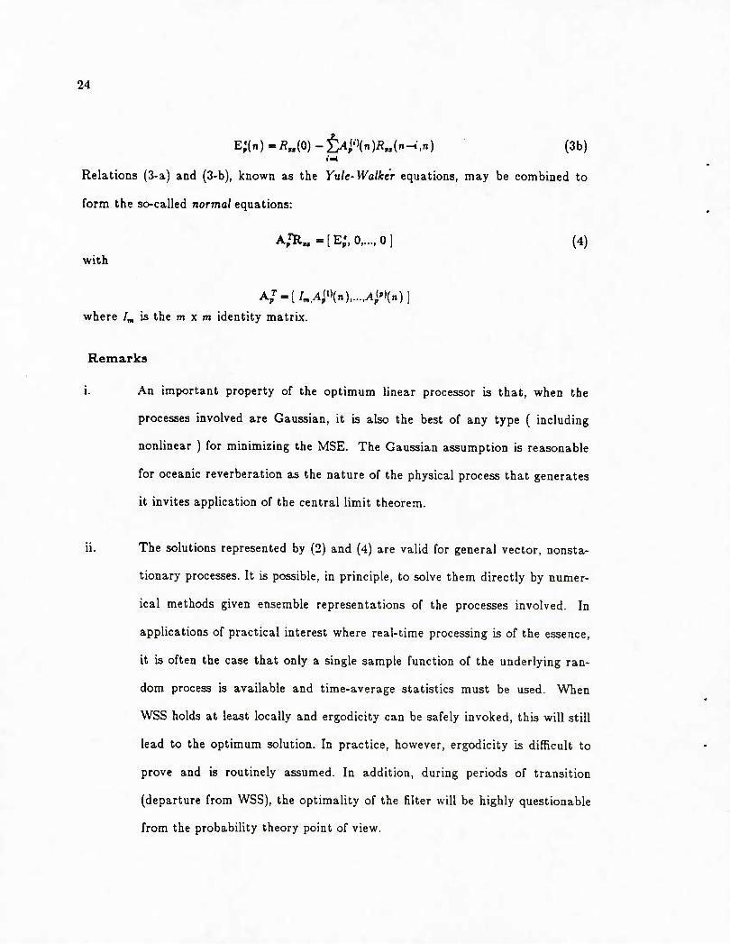
E;{n)^R„{0)-tAl'\n)R„{n^,n) (3b)
Relations (3-a) and (3-b), known as the Yule-Walker equations, may be combined to
form the so-called normal equations:
A,'1I„=[E;,O 0] (4)
with
A/ = [/„A(')(n),...,AW(n)]
where /„ is the m x m identity matrix.
Remarks
An important property of the optimum linear processor is that, when the
processes involved are Gaussian, it is also the best of any type ( including
nonlinear ) for minimizing the MSE. The Gaussian assumption is reasonable
for oceanic reverberation as the nature of the physical process that generates
it invites application of the central limit theorem.
The solutions represented by (2) and (4) are valid for general vector, nonsta-
tionary processes. It is possible, in principle, to solve them directly by numer-
ical methods given ensemble representations of the processes involved. In
applications of practical interest where real-time processing is of the essence,
it is often the case that only a single sample function of the underlying ran-
dom process is available and time-average statistics must be used. When
WSS holds at least locally and ergodicity can be safely invoked, this will still
lead to the optimum solution. In practice, however, ergodicity is difficult to
prove and is routinely assumed. In addition, during periods of transition
(departure from WSS), the optimality of the filter will be highly questionable
from the probability theory point of view.

25
iii. Here we are mainly interested in solving the filtering problem. However, fast
and efficient (lattice-type) solutions for (2) can only be obtained in conjunc-
tion with the solution of the prediction problem. In that sense, (2) and (4) are
intimately related.
2.3 The Adaptive Noise Cancelling (ANC) concept
The set of circumstances which gives rise to the noise cancelling concept is
illustrated in Figure 2.1a. The primary channel consists of the signal », corrupted by a
form of additive noise n, and the reference channel consists of a process ni related in
some unknown way to the primary noise. The key requirement is that the signal be
uncorrelated with both the primary noise and the reference process:
-R«. =0, /?,., = 0.
We then have
which leads to the noise cancelling solution as a special case of the general filtering
problem solution:
^...,(n.*)=fe'(«)fi....(n.*). n-^<k<n. (5)
Thus, solving the filtering problem in this setting is equivalent to producing the best
MMSE estimate of the primary noise process. The ANC output, obtained by subtract-
ing this estimate from the primary input, will consist of the signal component » plus a
residual error n, — n,.
A more detailed model for the noise-cancelling structure is shown in Figure
2.1b. The "mismatch" between the primary and reference inputs is represented by a
linear transfer function H{z). Additional uncorrelated noise components m, and m,
are included in the two channels. This particular model, which is representative of
many situations of practical interest, has been studied in detail by Widrow et.al.

26
[1975]. It was determined that the uncorrelated noise components have a deleterious
effect on cancellation, expressed in z-transform notation [Oppenheim and Schafer,
1975] by the following:
Here, p„,{z) is the signal-to-correlated noise density ratio at the output, p^{z) is the
signal-to-correlated noise density ratio at the primary input and M,{z), A/,(r) are the
ratios of the uncorrelated noise spectrum to the correlated noise spectrum at the pri-
mary and reference channels, respectively. It is apparent from (5a) that the ability of
the ANC system to reduce noise is limited by A/,(z) and Mt(z) when these quantities
are large. When they are small, other factors become important in limiting ANC per-
formance. One such factor is the presence of signal components in the reference chan-
nel. Letting p„/{i) denote the signal-to-correlated noise density ratio at the reference
input and assuming M,{z) =A/,(2) =0, Widrow et. al. show that
/»...{') = —"VT (5b)
Another relation of potential practical significance is the following, regarding the out-
put noise spectrum S„(z).
5„(^) = 5.,.,(z)lp„,(z)llp^.(.)l. (5c)
Equation (5b) indicates that, although the signal components in the reference
input has a detrimental effect on cancellation, it does not render the ANC operation
useless if />„/(«) is held to reasonably low levels. Equation (5c) makes the somewhat
surprising statement that a high signal-to-noise ratio in the primary channel will
result in increased ouput noise power. This can be explained intuitively as follows: If
ppri{z) is low, the filter will be "trained" to cancell the noise rather than the signal
and therefore output noise will be low.

27
2.3.1 Adaptive beamforming via ANC
Conventional arrays are usually designed under the assumption that
unwanted noise is spatially disorganized. These fixed-weight arrays suffer a degrada-
tion of performance in the presence of directional interference possessing some degree
of spatial coherence. Such interference may be due to natural sources, reverberation
returns or jamming signals. Other factors, such as array motion, multipaths and con-
stantly changing interference characteristics, contribute to further deterioration.
Adaptive arrays, on the other hand, are capable of reducing or eliminating directional
noise components and of responding to changing conditions by adjusting their pattern
response according to an appropriately chosen error criterion. In general, adaptive
arrays are in the form of a space-time filter which can be implemented through the
general multichannel filtering structures described in the previous section.
The fields of communications, radar, sonar and geophysics have each contri-
buted to adaptive array development. The exact manner in which control of the
available spatial and temporal degrees of freedom is relegated to the adaptive proces-
sor and the choice of a performance measure, depend largely on the objectives and
priorities of the specific application. For instance, Shor[l966] adjusted the array
coefficients to maximize the signal-to-noise ratio (SNR) at the output. Riegler and
Compton[l973] and Widrow [1967] minimized the mean square of an error signal equal
to the difference between the array output and a reference signal. The total noise
power at the output, in the absence of the signal, was minimized by Lacoss[l968],
while optimum probability of detection for a fixed false alarm rate was the criterion
chosen by Brennan and Reed[l973]. The special case of weak signals in the presence of
strong interference was examined by Zahm[l973]. A good tutorial introduction to the
adaptive array problem is given by Gabriel[l976] and a more complete treatment is by
Monzingo and Miller[l980].

28
Here we are primarily interested in signal extraction and MMSE is the per-
formance measure of our choice. It is flexible enough to encompass many experimental
configurations and it leads to mathematically tractable results. Our objective is to
utilize the general adaptive algorithms which have been derived under this criterion in
conjunction w.th the ANC scheme, .n order to eliminate reverberation interference
entering through the sidelobes and possibly the main lobe of the receiving array. It
will be shown that selective reverberation cancellation may be achieved through con-
strained adaptive beamforming.
2.3.2 Adaptive beamforming with constraints
Of crucial importance m any adaptive array application is the utilization of
all available a priori information concerning the nature of the signal and the .nterfer-
cnce, in order to ensure signal preservation at the output. In the early applications of
adaptive processing to antenna sidelobe cancellation, the effects of signals on the
adapted response were commonly neglected. This was justified by the assumption that
the signals of interest were sufficiently low in power and/or duration so that the adap-
tive control algorithm would not respond to them (e.g. Widrow et. al.[l967].) When
such an assumption is unrealistic, the response of the adaptive array must be expli-
citly constrained to avoid signal cancellation. Constraints may be incorporated into
the adaptive algorithm to maintain a chosen frequency response in a desired direction
(Frost[l972l). This is computationally expensive and operationally inflexible. "Pilot-
signals, simulating actual signals of interest, have also been used to describe a desired
"main" look direction, through a twc^mode adaptation process [Widrow 1967]. How-
ever, accurate replicas of the desired signals are not normally available. An alterna-
tive is to impose preadaptation constraints in the time, space and frequency domains
[Applebaum and Chapman, 1976]. Restrictions may be effected in the time domain by

29
allowing the array to adapt only when no signal is present; in the frequency domain
by allowing adaptation only to energy received outside the signal band. Finally,
preadaptation spatial filtering may be used to remove the signal, whose direction is
presumed known, thus protecting it from cancellation. Such prefiltering may range
from complete conventional beamforming (Figure 2.2a) to simple element-to-element
subtraction (Figure 2.2b). The former can be applied only when the spatial charac-
teristics of the interference, as well as the signal, are known and constant and requires
an external steering mechanism. The latter is more appropriate when the directional
characteristics of the interference are unknown or variable and results in (constrained)
spatially adaptive cancellation beams. These two configurations are compatible with
our objectives and will both be used with attention to their relative advantages.
It is interesting to note that such prefiltering operations, by eliminating the
signal of interest from the reference channel(s), in effect place constrained adaptive
beamforming in the context of ANC and, more generally, of the (vector) Wiener filter-
ing problem. This approach affords us the flexibility of using any efficient solution to
the general filtering problem as the adaptive processor controlling the array element
weights. It will be shown that significant differences in performance exist between
seemingly equivalent algorithmic implementations and that the correct choice is criti-
cal to succesful reverberation cancellation.
2.4 Stochastic lattice solutions for optimum filtering
The optimum linear filters described by (2) and (4) can be determined by
solving the matrix equation directly. In the stochastic approach, the cost is twofold.
First, the needed second order statistics, which are almost always unknown in prob-
lems of practical interest, must be estimated from the data and updated periodically,
since the statistics are in general nonstationary. The second step involves the inver-

30
sion of the autocorrelation matrix R. In general, the p x p correlation matrix can be
inverted by standard methods such as Gaussian elimination and Grout reduction
[Stewart, 1973], or more robust methods making use of the nonnegative definiteness
and/or symmetry properties of R such as Householder transformations or Ghoiesky
decompositions [Lawson and Hanson, 1974]. All of these methods require O(p^) compu-
tations (multiplications of real numbers). The computational requirements can be
substantially reduced when R is characterized by certain shift-invariance properties
which lead to efficient recursive solutions of the lattice or ladder type.
For the remainder of this section, we will restrict our attention to scalar
processes. This was done for the sake of notational simplicity and does not seriously
affect the generality of the presentation.
2.4.1 Levinson's algorithm: The Toepliti recursion
A faster method of inversion, and therefore solution of the normal equations,
exists when R is Toeplitz, i.e. of the form
^=Hi-}% 0<ij<p (6)
It is easy to see that a Toeplitz structure for R is tantamount to the wide-sense sta-
tionarity of the input process. In this case, the shift-invariance and symmetry proper-
ties of R lead to an inversion technique requiring only 0{p'') computations. The pro-
cedure, developed originally by Levinson [1947] and rediscovered by Durbin [1960], con-
sists of using a partial solution and a subsequent correction through a "reversed time"
auxiliary solution. The same concept has been used by Szego [1939] in the different
but mathematically isomorphic problem of polynomial approximation on the unit cir-
cle. Multivariate extensions of the Levinson algorithm have been obtained by Whittle
[1963] and Wiggins and Robinson [1965]. Toeplitz recursions exist for both the filtering
and prediction solutions. The auxiliary Toeplitz recursion solves for the predictors A'"'

31
of (4) and the general Toeplitz recursion solves for the filter coefficients Fj'' of (2).
These recursions give rise to the prediction error and joint process lattice structures,
respectively. Although Levinson, in his original work, was mainly concerned with the
general filtering problem, it was the prediction solution (auxiliary recursion) which has
attracted much attention in recent years, in conjunction with certain modeling
schemes for the input process. The general Toeplitz recursion can only be achieved
through the auxiliary recursion and thus the two procedures are intimately related.
The basic structure for the prediction lattice filter is described by the following rela-
tions (Figure 2.3a with it? =*,!•= *,-.)
«.■(«) "e.-i('«)+*.(n)r,-,(n-l) (7a)
r.(n)=*,*(n)e,_,{n)+r._,(n-l) (7b)
where z(n) is the input signal and e,(n) and ri{n) are the forward and backward pred-
iction error residuals at stage i.
Levinson's algorithm in its original form requires the external calculation of
autocorrelation lags and is sometimes referred to as the "given correlation" algo-
rithm. Alternative stochastic lattice formulations which utilize the input data stream
to directly estimate the lattice coefficients are more suitable for real-time processing.
One such "given data" structure (GRL) will be considered here as a potential candi-
date for our central adaptive processor. The original Levinson's algorithm is included
in Appendix A for the sake of completeness.
2.4.2 Lattice properties
Levinson's algorithm has implications beyond the original intent of a fast
matrix inversion technique. The lattice structures it has created possess properties
summarized below, which can amount to significant operational advantages over
direct TDL implementations.

32
i. Stage-hy-stage decoupling
Each lattice stage is independent of all other stages. Increasing the predictor
order is achieved by adding one more lattice section, without changing any of the pre-
vious sections. Thus, given a lattice implementation of a predictor of order p we have
in fact an implementation of all predictors up to that order. Stated somewhat
differently, the time-variation of the finite-length filter takes on a simple step-function
form in the lattice, whereby each lattice section is turned "on" one at a time. This
decoupling or orthogonalization property is directly responsible for the improved con-
vergence properties of the lattice (see Simulation 1.)
ii. Stability" by inspection" ^
The IIR (inverse) lattice filter is stable if and only if l*,l <i. As a result sta-
bility (or lack thereof) of the inverse ("synthesis") lattice filter is easily established by
examining these reflection or partial correlation (PARCOR) coefficients.
Hi. AR cut-off
For an input AR process of order p, the k^^, i=l,2,... are zero. This pro-
perty can significantly facilitate AR model identification (see Section 2.4.3)
iv. Structural modularity
The lattice forms are built from a cascade of sections with identical struc-
ture, a property attractive from the VLSI implementation point of view.
V. Desirable numerical properties
There is evidence indicating that lattice structures are less sensitive to
roundoff noise [Markel and Gray, 1975; Gray and Markel, 1975] and to quantization
effects [Bruton, 1976; Fettweis, 1974]. _
vi. Physical interpretations

33
The reflection coefficients can be related to parameters of certain models
representing physical processes. In particular, models of wave propagation in a
stratified medium [Thomson, 1950] and of the human vocal tract [Kelly and Loch-
baum, 1962] have been suggested which have lattice-form configurations. The work of
Wakita [1973] established a direct connection between the reflection coefficients and
the cross-sectional area function of the vocal tract, showing that the vocal tract shape
can be estimated directly from the acoustic speech waveform through linear predic-
tion. This parameter estimation technique, coupled with a recent surge of activity in
the area of speech signal processing, can account to a large extent for the predomi-
nance of the linear prediction solution in the literature. On the other hand, the joint-
process lattice solution was largely neglected, leaving direct TDL implementations
(e.g. the LMS) unchallenged in filtering applications such as channel equilization and
noise-cancelling. ^
2.4.3 Alternative lattice solutions
The reflection coefficients t, of the lattice prediction filter can be interpreted
as a measure of the crosscorrelation between e,_i(n) and r,_,(n—1). This idea has
spawned a class of lattice algorithms in which the reflection coefficients are computed
directly from the data and differ only in the manner that this quasi-correlation
coefficient is normalized. Itakura and Saito [1971] used the geometric-mean method of
normalization to compute their PARCOR coefficients. Burg [1975], on the other hand,
chose the harmonic-mean method which satisfied his maximum-entropy criterion. A
more general class of normalization schemes, of which the above are special cases, has
been defined by Makhoul [1977, 1978]. We have chosen the harmonic-mean (maximum
entropy) method for our stochastic lattice implementation (GRL) because its deriva-
tion was based on a well-defined and intuitively pleasing criterion. Morover, it is the

34
method of choice for some widely referenced implementations (e.g. Griffiths [1978],
Satorius [1979]). Thus, we define i, as
Hn) 2^{«.(")r;(n-l)}
where the expectation operator E is approximated in practice by a time average.
Joint-process versions of the given data lattice can be easily derived by con-
sidering the prediction lattice as a practical implementation of Wold's decomposition
theorem jWold 1939]. In essence, the lattice performs a successive orthogonalization, of
the Gram-Schmidt type, on delayed versions of the input signal. The backward residu-
als are orthogonal (£{ r,r,} =*,,^., .-,,■= j ^j ^^^ constitute an innovations
representation of the input signal, forming a natural orthogonal basis which spans the
signal subspace. The dual-channel filtering problem can be solved by estimating the
desired signal with a linear combination of these orthogonal components. A simple
application of the orthogonality principle [Satorius and Alexander 1979] leads to the
optimum set of cross-correlation coefficients */ thus forming the joint-process lattice
structure (Figure 2.3b), suitable for noise-cancelling applications:
L^.. E{cf{n-l)r:(n-l)}
- '^^" ^(lr..(n-l^^} . (9)
These given data structures, by implicitly estimating the second order statis-
tics and by making the error signals available at each stage of the lattice, are more
suitable for real-time processing than the original given correlation Levinson algo-
rithm. In addition, adaptive versions may be easily derived by introducing an exponen-
tial data window and an error gradient criterion. It should be emphasized that these
structures are still based on a stochastic formulation and are fundamentally
equivalent to Levinson's algorithm. They are optimum only when WSS and ergodicity
can be safely assumed. They are, however, precursors to purely deterministic least-

35
squares structures, to be examined in Section 6 of this chapter.
2.4.4 The question of modeling
It is often useful to develop a parametric model for the behavior of a signal
or system. The problem of determining the parameters of a hypothesized mathemati-
cal model given observations of the signal to be modelled is the subject matter of
parameter estimation and system identification. A variety of estimation techiques have
been used in this context, with least-squares methods occupying a prominent position
[Astrom and Eykhoff, 1974; Kailath, 1974; Willsky, 1979].
A very successful application of modeling has led to the development of Kal-
man filters [ Kalman and Bucy, 1961] which have proven to be very useful in control
applications where internal models (or state-space descriptions) are relevant. Parame-
ter identification problems also arise in several digital signal processing applications
where external models ( input/output descriptions) are appropriate, among them
seismic signal processing and the analysis, coding and synthesis of speech. The latter
application, in particular, has received a great deal of attention in the past 10 years [
e.g. Markel and Gray, 1976, Makhoul, 1975]. Modeling, in this context, entails describ-
ing the process of interest in terms of the linear (possibly time-varying) system that
would generate it when driven with white noise. The most general system of this type
is the autoregressive-moving average (ARMA) model, described by the following
difference equation.
$)«.,.:f.-v =£*.,,«»-, n>0,p>0,q>0 hQ)
In z-transform notation [Oppenheim and Schafer, 1975] we have
A{z)X{z)=B(z)U{z) => X{z)=H(z)U{z) (n) where

36
H(z)^B(z)/A{z)
is a rational transfer function. If qM), then x, is known as an autoregressive (AR) pro-
cess and the model is referred to as "all-pole":
■ H(z)^l/A(z).
The "all-zero" filter which will reduce a given AR process of order p to white noise is
known as the inverse or whitening filter and is identical to the prediction error filter of
order p. In fact, paranneter estimation can always be regarded as a mathematical
modeling process, even if the primary goal is not explicitly stated in this form. There-
fore, AR system identification can be effected through the solution of the one-step
prediction problem. This procedure is the basis for most high resolution spectral esti-
mation techniques, where the spectrum of the input process is modeled as an AR
transfer function. In the two-channel filtering problem, on the other hand, it is the
cross-spectrum between the two channels which is modelled as an all-pole transfer
function and must be compensated for by the all-zero filter represented by the lower
section of the joint-process lattice (see Figure 2.1b.) It follows that the optimum choice
of filter order is, in general, quite different for the single-channel (prediction error) and
the two-channel (joint-process) filters.
2.5 Gradient-based time-recursive algorithms
The coefficients of the whitening (prediction) filter, in either its direct or lat-
tice form, can be obtained by operating on a segment of the input time seriesuntil a
white-noise sequence (or as close to white as possible) is produced at its output. In this
block- processing mode, a new set of coefficients (AR model estimates) is derived per
data segment. An alternative approach is to continuously update the coefficients, util-
izing the unbroken stream of data and taking into account each new sample. This
requires the existence of an updating mechanism with a decaying memory, whereby

37
"new" samples are emphasized over "old". The resulting filters are known as time-
recursive or adaptive and can be easily derived from block structures of the given-data
type.
2.5.1 The LMS adaptive filter
The LMS algorithm uses an implementation of the method of steepest des-
cent to provide a time-updating mechanism for the weights of the direct tapped-delay
line (TDL) realization of the linear combiner which can be used either as a predictor
or noise-canceller (Figure 2.4).
The "current" weight vector a(n) (Figure 2.4.b) is set equal to the "past"
weight vector a(n-l) plus a change proportional to the negative gradient of the
mean-square error surface which is a concave paraboloid with a unique minimum.
a(n)=a(n-l)-h/i(-V(n-l)) (12)
where ft is the factor that controls stability and rate of convergence.
Since the true gradient of the true MMS error is not known, it is replaced by
the gradient of the instantaneous error power \e^(n-lp. This "estimated" gradient is
given by Widrow [1975]:
V(n-l)=-2£,V-l)x*(n) (13)
where
£,V)=<'(n)-a^x(n)
x^(n)=[x(n-l), z(n-^)]
and forms the basis for the Widrow-Hofl" LMS algorithm of adaptive weight updating:
a(n)=a(n-l)-|-2/i€(n-l)x'(r.-l) (14)
It has been shown by Widrow [1976] that the expected value of the weight
vector converges to the true Wiener solution. It is also shown that the algorithm will

38
converge in the mean and remain stable as long as
lAm«>P>0 (15)
where X„„ is the largest eigenvalue of the autocorrelation matrix R. In addition, the
time constant for the "learning curve" corresponding to the i'* natural mode of the
signal is related to the i" eigenvalue of R by
r,.-i/4;iX. (16)
Morover, the ratio of the excess noise power due to weight misadjustmcnt over the
estimation error power is given by
A/=ptrR=;.pX.„==i(l-)„, (17)
Relations (16) and (17) portray the major drawback of the LMS. When the
matrix R has a large eigenvalue spread, convergence is controlled by the smallest
eigenvalue and misadjustmcnt by the largest one. The result is slow adaptation cou-
pled with high misadjustment noise. ,
It is convenient to introduce a new parameter 0^^4/5 [Griffiths, 1976] such that
where Eg is the power of the reference sequence x{n). Then (15) becomes
0<QiMS<pE'o/>^u>xx • (18)
Since pEg >X„„ it follows that convergence is always achieved for 0 <aius < 1-
In the algorithm, £g is replaced by the estimate
£5(^)=(l^iJ^^5)£5(^-l)+aiJ^,5lx(^)|2 . (I9)
2.5.2 Summary of the LMS algorithm
The scalar, complex joint-process gradient transversal filter (LMS) algorithm
is summarized as follows (see Figure 2.4a)

39
Initialization (k=0,li--.p)
/»(-!) - 0 (20a)
Eti-l) = (Lus. HMS = EliO) (20b)
x(-*) = i(-p-l) = 0 (20c)
"p^l-l) = 0 ,• (20d)
Time update (n>0 and Jb^,l,...,p)
^*(") = ^*("-^) - m^n ^I-n sV-l)^>-*-l) (20e) (p+1) £:.'(«-1)
•p't") = i;/t(n)x(n^) + d(n) km.
(20f)
£;(n) = (l-QLjw5)£;(n-l) + aiJx(n)|2. (20g)
Slightly simplyfying (20a}-{20g), the one-step forward linear predictor com-
plex gradient transversal filter algorithm can be written as (see Figure (2.4b) )
Initialization (k=4,2,...,p)
«*(-!) =0 (21a)
^.'(-1) = HMS, HUS = ^.'(0) (21b)
z(-*) = x(-p-l) = 0 ^ (21c)
ep(-l) =0 . (2id)
Time uprfafe (n>0 and l:=l,2,...,p) >'
«*(n) = «,(n-l) - y^^^ e,(n-l)x-(„-*-l) (2ie)

40
«,(«) " £«»(")'('«-*) , fl. - 1 (21f) km*
E:(n) ~ {l-ai,,,s)E'.{n-l) + aj,us\'(np. (2lg)
Remarks
Oceanic reverberation is characterized by the rapid onset of comix)nents
differing widely in intensity. The presence of such components will most likely create
this condition of high eigenvalue spread and at the same time the need for extremely
fast adaptation. It has been shown in frequency tracking [Hodgkiss and Presley, 1981]
and adaptive equilization [Satorius, 1979] applications that adaptive forms of the lat-
tice structure possess significant performance advantages over the LMS, resulting
mainly from the orthogonalization and decoupling property between lattice stages. In
effect, each stage of the lattice is asigned to a single mode and adapts independently
of all other stages. It will be the intent of Simulation 1 to confirm this in a noise-
cancelling application.
2.5.3 The gradient lattice filter (GRL)
The same concept of an estimated error gradient may be used to update the
reflection coefficients of a lattice filter. Again, the true gradient with respect to the k
of the sum of the mean square error residuals J?{le,(n)|2-(-lr,(n)l^ is replaced by the
noisy gradient of the sum of the instantaneous square error residuals le,(n)l^-(-|r,{n)l^.
The noisy estimate which can be obtained directly from (8), can be used to estimate
the "next" it, as follows: [Makhoul, 1978; Griffiths, 1977]
ki{n)=k,{n-l)+-^ ■ ^ '' — -, l<i<p-l. (22a)
where /?,('») is computed recursively from
A(n)={l^CRiP.('»-l)+le.-i(n-l)|2+lr,_,(n-2)|2. l<.<p-l (22b)

The product ocsiAln) where 0<O(j«i<l, represents an exponentially averaged esti-
mate of the power level at the •'* stage of the lattice. The normalization by the factor
D,(n) is intended to maintain the same time constant of adaptation at each stage of
the lattice. Thus, the overall convergence rate should be unaffected by the eigenvalue
spread of R.
The optimum set of the "joint-process" coefficients Jb^ may be updated adap-
tively as follov^'s:
>.>(„).>/(„-.) ^'■'-'';'l;-' ■ (23a)
where
G,(n)=(l^c;,JG,(n-l)-hlr,(n-l)l=, l<.<p (23b)
Only preliminary results are available concerning the convergence properties and the
misadjustment noise of the gradient lattice [Griffiths and Medaugh, 1978].
2.5.4 Summary of the GRL algorithm
The scalar, complex, joint-process gradient lattice algorithm (GRL) is sum-
marized as follows (see Figure 2.3b) with it, = it,' = Jt?*).
Initialization (i =0,1,...,p)
it,(-l) = 0 , iVO (24a)
£[(-1) = E^-l) = ijccL . ^Jcai = ^5(0) (24b)
^•(-2) = tjcGL , «Vp (24c)
, e,(-l) = r,(-l) = 0 (24d)
r.(-2) = 0 , iVp . (24e)
KK-l) = 0 (24f)

42
eA-1) - 0
Time update (n > 0)
{24g)
Orrfcr update (i =0,1,..., p)
(24h)
(24i)
*,(n) - *,(„-!) - 2a JCGL
EU(n-2) + £;L,(n-l)
• le,(n-l)r;_,(n-2) + r.'(n-l)e,._,(„-l)| , iVO
e.(n) " e.-ifn) + *.(n)r,_,(n-l) , ijiQ
•".(n) = »-.-j('»-l) + *,'(n)e.H(n) , ,yo
£;L,(n-l) = {l-o,CCi)^;L,(n-2)
+ O^CCLI'-.•-»('»-1)1^ , «V0
£/_,(n) = (1 _ ajcaL)EU{n-\)
eA«) = e/-i(n) + kf{n)r,[n)
Pred»cior5(6/')(„) = a^(ii(„), l=0,l,...,p)
a/')(n) = *,(„)
fl/')(n) = a/'-DCn) + it,(n)aiir^)'(n) , l</<.-l
(24j)
(24k)
(241)
(24m)
(24n)
(24o)
(24p)
(24q)
(24r)
43
2.6 Deterministic least-squares lattice structures
The optimality of the filters discussed in the previous section rests on the
assumptions of stationarity and in the given data case, ergodicity. During transition
periods when the statistics of the signal change drastically, all such solutions are
clearly suboptimal. In addition, the misadjustment noise of the gradient methods is
often a limiting factor on the algorithm convergence speed. An alternative to those
stochastic approximation methods is the deterministic least-squares approach. When
(WSS) stationarity does prevail, the solutions derived through this approach perform
identically to their stochastic (time-average) counterparts. However, they enjoy an
important advantage in that they continue to be optimum (in a deterministic least-
squares sense) even during abrupt changes in the signal statistics. This fact, together
with the "exact" time-update property possessed by one particular realization, contri-
butes to transient behavior superior to the gradient solutions and makes the least-
squares structures an excellent candidate for our choice of adaptive algorithm.
The direct form implementation of the exact least squares algorithm was
first presented by Morf et al [1977]. The lattice recursions were first reported in
[Morf,Lee,Nichols and Viera 1977] and [Morf,Viera,Lee 1977]. A comprehensive presen-
tation of the concept, including Hilbert-space approach derivations, joint process
extensions and computer simulations demonstrating the tracking capability of these
algorithms, is given by Lee [1980]. Satorius and Pack [1979] and Falconer and Ljung
[1978] reported superior performance of the exact least squares algorithms in a
channel-equilization application as did Hodgkiss and Presley [1982] in simulated fre-
quency tracking situations and Nehorai and Morf [1982] in a line-enhancement con-
text. Completely absent from the literature are reports on the performance of these
structures in their noise-cancelling configuration.

44
2.6.1 The DLS solution to filtering and prediction
The deterministic least-squares (DLS) problem is formulated as follows: Given
two dicrete time series
{ i{n),d(n)) , A^, < n <Nf
of dimension m and / respectively, we form the estimate of d(n)
d{n)^tFM{n)T{n-}) ;■•*
^Fp'"(n)x|,,..
and with
«!.,.,/(") = </(") -<i(n) we seek to minimize
where i,f will be specified later (A', < * <Nf , * <f < Nf .)
The deterministic least-squares (DLS) solution to the filtering problem is
obtained through the same arguments used in the stochastic case and is given by:
where
with
F/(«,/)R,.,(.-./)=R^.p(.-,/) (25a)
x,(.-,/) =
x{i) x(/)
x(i-f) ■ ■ ■ x(/-p)
Ri,.p('-/)=d|^/lX;(.-,/)

45
The minimum least-squares error is
E/(i,/)=min{f }(/(.■,/) (25b)
Similarly, the DLS one-step predictor is given by:
A7(.-,/)R..,(.J) = [E;(.-,/),0, ...,0] (26)
where
A;(,-,/) = [/„,A1^)(.J), ...,Aj^H«",/)]
E;(.-,/)=i?,.oo(.-,/)-A;Q,,,(.-,/)
Note that the exact form of Xp(i,/) depends on the choice of i and /. The
following choices are most commonly made, resulting in sample correlation matrices R
with different symmetry and/or shift invariance properties. Such properties are cru-
cial to the development of algorithmic implementations of the above solutions.
(1) Prewindowed case
i=iV,. f =N,
(2) Non windowed case
i=Ni+p, f=Nf
(3) Pre- and postwindowed case
Remarks
An interesting parallelism exists between stationarity conditions in the sto-
chastic formulation and the various windowing schemes in the deterministic least-

46
squares development. For example, pre- and post-windowing results in a sample corre-
lation matrix R which is Toeplitz, in direct analogy with wide-sense stationarity. The
Toeplitz recursion is equally applicable here and is known as the "autocorrelation"
method of linear prediction in the speech processing literature. The non-windowed case
leads to an R which is symmetric but not Toeplitz and is known as the "covariance"
method. (Clearly such characterizations are unjustified from a statistical point of
view.) ;
The prewindowed case is of particular interest. It leads to a matrix R which
is not Toeplitz but "close" to it and has shift properties which lead to an algorithmic
solution with exact time-update. The statistical analogue would be a process which is
not wide-sense stationary but "close" to it, in a sense not explicity defined in standard
probability theory. This creates the possibility of treating processes with various
degrees of stationarity through the same efficient algorithmic solutions once the
appropriate structure for the true autocorrelation matrix has been established.
2.6.2 The "pre-windowed" DLS lattice
In this case, the sample correlation matrix R of order p is of the form
where,
Xp.yv =
i(0) ••• x{p) ■■■' x{N)
0
0 0 2(0) • • • x(N-p)
Note that R^,^ is not Toeplitz but it consists of a product of two (upper- and
lower-triangular) Toeplitz matrices and might be thought of as being " near-Toeplitz".
In fact, it falls within the class of the so-called a-^tationary matrices which can be
expressed as ??
R=T+f:eT,U,U.^ <T, =±1 (27)

47
where T is Toeplitz and the {U,} are upper triangular Toeplitz matrices [Friend-
lander, 1979]. These matrices are also known as "low shift rank" matrices [Morf,
1974]. For such matrices, it is possible to derive generalized Levinson-type recursions.
Specifically in the pre-windowed case, R,,^ is a-,tationary with a = 2 and satisfies the
following recursive identities:
order- and time-update
order-update
R».p(A^) = Rx.oo(A^) Q,,,(7V)
^"PW R..P-4(N-1] (28a)
time-update
wh ere
^sAN) R.,p_(7V) y»^(N)
V.,p(^) R,,,,(/V)
R«,p(^)=R.p(iv-i)+x,^^^^,x,^^^^,
(28b)
(28c)
V..p(^) = E-(n-p)x^_..^,
and all other quantities as previously defined. These identities form the basis for the
exact order- and time-update recursions for the pre-windowed DLS prediction lattice.
The DLS joint-process lattice can be obtained through an embedding technique,
whereby the joint sample correlation matrix R,JN) is defined as
where
Zp(A^) =
d{0) x{0)
0 0
4P) d{N) x{N)
0 x(0) • • • x{N~p)
Then, the filtering normal equations can be re-expressed in terms of R^JN) as follows:

48
F,rR,,,(Ar)„[E/(N),0,...,0] (29)
where
Tr{N)^lI,T^{N)]
R,,, has shift properties similar to R,^. The two sets of recursions can be
combined to concurrently solve the forward prediction, backward prediction and filter-
ing problems, giving rise to the complex, multichannel DLS joint-process lattice. The
needed algebraic manipulations are presented in Lee [1980J and Satorius and Pack
[1979].
Exponential weighting
An adaptive version of the DLS lattice can be easily derived by introducing
an exponential "window" in the error norm. Specifically, one may choose to minimize
where X is a constant <1, so that past errors will have a smaller influence on the esti-
mate. This constant "fade" factor is easily incorporated into the lattice recursions
and allows the algorithm to compensate for time variations in the input signals. The
"effective" number of points used in this case may be defined in terms of a "time con-
stant" as follows:
x(^-)=exp^(^r^)/^^^]
Therefore,
In our implementation X = 1—0^5^.
2.6.3 Summary of the LSL algorithm
The scalar, complex, joint-process, exponentially weighted prewindowed least

49
squares lattice algorithm is summarized as follows (see Figure 2.3b): (The vector ver-
sion is presented in Appendix B). .
Initialization (i =0, 1,... , p)
r, ,(-1) = 0 , .Vp
A,(-i) = 0 , tyo
6i')(-l) = 0 , 0<it<f-l , ,yo, and tVp
7,_i(-l) =0 , iVp
kf{i-l) = 0
Time update (n > 0)
A.(n) = (1 - ai^si) A,(n-1)
k!(n) = A'in) / EU{n) , .yo
*.^n) = A..(n) / Er^(n-l) , .Vo
(30a)
£,^-1) = fj^sL . 'LSi = 0.001 and iVp (30b)
(30c)
(30d)
(30e)
(30f)
«.(") = r,{n) = i{n)
El{n) = £;(„) = (1 _ a,si) £;(n-l) + [^(n)!^ (30^)
'r-i(n) =0
e£,(n) = </(n)
Order update [i =0,1,...^p)
(30g)
(30i)
(30j)
(30k)
(301)
(30m)

so
«.(«) - '.-.(n) + *,1")r,-i(n-l) , iVO (30n)
•".(n) - '■.■H(n-l) + *'(n)e,-i(n) , iVO v* (300)
E:{n) - EU(n) - |A,(n)|2 / £^(n-l) , ,yo (30p)
Er[n) ^ EU(n-l) - \A,{np / EU(n] , .yo (aOq)
%_,(n) - 7.^i(r>) + \rU»p / E;L,(n) , iVO (30r)
\'{n) = (1 - a.sJA/(„-l) - ;^"^;;];| (303)
Predictors
(30u)
^i"!") = *'(") (30w)
fl/')(„) = a/'-^)(n) + *.r(„) 6/1;^)(„-l) (30^.)
i/')(n) = 6/ir^)(n-l) + *,?(„) «/-•)(„) (30y)
The likelihood variable
The parameter which controls the adaptation response of the LSL is 7
defined by
Ti.p ''^lN-p:Ni^7!f'^lN-p:N] (31 )
It can be shown [Lee, 1980] that
7 has an interesting statistical interpetation as the likelihood of deviation of the p

51
succesive samples from a joint Gaussian distribution parameterized by R,,,. [Morf and
Lee, 1978]. It can be expected to be ~ 0 except when the signal statistics undergo
drastic changes, in which case it will approach unity.
Note that in the LSL recursions (Eq. 30s) the "crosscorrelation" quantities
A,- are weighted by a gain factor equal to
l-TT.-i
which replaces the "smoothed" power estimates of the stochastic gradient algorithms.
Clearly, when 7,_, ~ l the algorithm will undergo extremely fast, almost instantane-
ous, adaptation. It is the presence of this optimum gain factor which sets the "exact"
least squares lattice apart from the suboptimum gradient approximations and results
in its superior transient response (see Simulation 2.)
On the choice of adaptation coefRcient
The proper choice of adaptation coefficient can be made by considering the
more general question of resolution vs statistical reliability. If WSS holds for all time,
then Q!=0 is the optimum choice and the time-invariant Wiener-Hopf solution is
obtained. In cases of practical interest, local WSS if more often encountered and the
desired " resolution" is controlled by the time scale of variation of the signal statistics.
By that it is meant that one must refrain from averaging over a number of distinct
statistical events. Therefore the lower limit of the adaptation coefficients (or the
upper limit of the allowable averaging interval) is set by the stationarity properties of
the input process. In the gradient descent algorithms (LMS,GRL) the lower bound of
a is imposed by the misadjustment noise, caused by excessively large steps in the gra-
dient search process (e.g. equation (17)). In the case of the exact deterministic least-
squares solution (LSL), there is no misadjustment error. The lower bound of a
strictly a question of statistical reliability.
LSL IS

52
A complete statistical analysis of the lattice structure has not been pursued
in this thesis. However, insight may be gained by considering the variance of the fol-
lowing crosscorrelation estimate between two bandwidth-limited white noise processes
x{n) and y(n):
ff.,
where,
K, 1D(1 -QLSL)'
The variance of the estimate is given by [Bendat and Piersol, 1971]:
' 'ff
The above indicates that large, spurious crosscorrelation values can be gen-
erated between two uncorrelated processes (R,,(k)^0), for sufficiently small N.^
and/or large autocorrelations within the two processes. Although direct comparison
between this simple result and the behavior of the lattice parameters for arbitrary
signals is not possible, the LSL joint-process filter has been observed to obey this gen-
eral rule. Specifically, the filter has shown a tendency towards cancellation of the pri-
mary channel when the primary and reference channels consisted of independent white
noise sequences, for QJ^SL >0.02. This empirically derived value will be used as the
upper bound for 0^5^ throughout this thesis.
2.7 Computer simulations
The exposition of the theoretical foundation of the LMS, GRL and LSL filters
in the preceding sections of this chapter enables us to make certain conjectures
regarding their operational characteristics. First, one may expect the LMS to be suc-
ceptible to the "eigenvalue spread" condition. On the other hand, a lattice filter (GRL

53
or LSL) should not be affected owing to their orthogonalization (stage-by-stage decou-
pling) property. Secondly, the stochastic approximation solutions (LMS and GRL) are
clearly suboptimum during transient conditions (i.e. departures from WSS). The exact
deterministic LSL solution, on the other hand, remains optimum (in a least-squares
sense, not in a stochastic MKISE sense) during such transient states and may be
expected to perform better. The simulations of this section were intended to provide
support for these mathematical conjectures. They are a representative subset of a
large number of simulations performed during the course of this research project [e.g.
Alexandrou and Hodgkiss, 1982d,e]. Simulations 1 and 2 were designed to bring out
the operational characteristics of the three chosen structures (LMS, GRL, LSL) under
transient conditions and in the presence of the "eigenvalue spread" and "scale
change" effects, respectively; the third to demonstrate the potential advantage of the
multichannel lattice filter over a cascade of single channel filters, when multiple refer-
ence signals are available. The scalar, complex versions of LMS, GRL and LSL as well
as the vector, complex LSL have been programmed in Ratfor [Kernighan, 1975] and
used throughout this work.
For the sake of clarity, simple complex exponentials in additive white noise
were used, which undergo frequency and/or magnitude "steps" at prescribed points
during the iteration. However, the simulated transients do represent conditions which
are likely to be encountered in real reverberation signals. Therefore, these results are
pertinent to the performance of the chosen algorithms in a reverberation cancellation
context. These noise-cancelling simulations have not appeared previously and are a
major contribution of this thesis.
2.7.1 Simulation 1 : Eigenvalue spread
The objective here is to examine the performance of the LMS, GRL and LSL

54
in a noise-cancelling setting, where the reference signal components have widely
separated power levels. Both main (primary) and reference channels consist of a pair
of complex exponentials corrupted by white noise. The reference channel signals
undergo a frequency "step" at iteration number 1536. Table 2.1, below, fully describes
the simulation.
Simulation 1 before step after step
main reference main reference
Wi 8 4 8 8
SNRiidb) 20 10 20 10
CJj 8
IT
8 6ff 8
67r
8
SNR^db) 20 20 20 20
Table 2.1 Summary of Simulation 1
The main and reference channels are displayed in Figure 2.5a and 2.5b
respectively, in the form of a Range-Doppler-Map (RDM) created by taking successive,
50% overlapped FFTs of the two time-series. A filter order of p^ was used and the
adaptation parameters were chosen such that the response of all three algorithms to
the high power sinusoid was similar. The joint-process error outputs produced by
LMS,GRL and LSL are shown in Figures 2.5c,d,e. It is evident that the LMS is lagging
substantially in the cancellation of the lower power sinusoid compared to the two lat-
tice filters. The LSL performs marginally better than the GRL which is consistent
with previous findings in a frequency tracking application [Hodgkiss, 1981.]
Remarks
ce rever- The "eigenvalue spread" condition is likely to exist in a real composite
beration signal since the surface, volume and bottom components are normally
characterized by large intensity disparities. The LMS is therefore a poor candidate for

55
our purposes. *
2.7.2 Simulation 2 : Scale change
The fundamental difference between the stochastic approximation realiza-
tions (e.g. LMS, GRL) and the deterministic least-squares filter (LSL) is the fact that
the latter continues to be optimum within its design even during abrupt changes in
the characteristics of the signal(s). The LMS and GRL are, in such cases, clearly
suboptimum in either the stochastic (MMSE) or the deterministic least-squares sense.
This simulation was intended to bring out the specific consequences of this fact. The
complex exponentials in the reference channel perform, in addition to the frequency
step, undergo instantaneous magnitude "jumps" of 10,20 and 30 db. The simulation is
described in Table 2.2.
Simulation 2 before step after step
main reference main reference
Wi TT
8 _7r_
4 8 jr_
8
SNRi(db) 20 10 20 20,30,40
"2 6ff 8
77r
8 6;r 8 8
SNRJ^db) 20 10 20 20,30,40
Table 2.2 Summary of Simulation 2
The filter outputs for these three cases are shown in Figures 2.6 and 2.7a.
The magnitude plots were artificially " clipped" for display purposes.
The GRL proved to be extremely sensitive to this "scale change" effect and
became increasingly unstable, failing completely to recover from the transient in the
40 db case. The LMS is similarly succeptible although it appears to be considerably
more robust. The LSL was able to adapt immediately to all magnitude jumps. The

56
likelihood variable can be seen (Figure 2.7b) to approach unity as the severity of the
discontinuity inceases. The crosschannel coefficients {k}) of the GRL and the LSL exi-
bit a similar behavior (Figure 2.8).
It is likely that the specific reason for the instability of the gradient filters
lies in the "smoothed" power estimate (Eqs. (19), (22b), (23b)) used to normalize the
coefficients of these filters. This low-pass filtered power estimate does not change fast
enough to compensate for large instantaneous power jumps.
Remarks
The "scale change" condition is also likely to be in effect for real reverbera-
tion signals. For instance, the onset of surface reverberation in a volume reverbera-
tion backround can readily amount to an abrupt increase in intensity of the order of
the simulated magnitude jumps.
2.7.3 Simulation 3: Multichannel V8 cascade v
In situations where spatially adaptive beamforming is in order and direct
control of the spatial transfer function is desirable, the need for the true vector (mul-
tichannel) filter is obvious. If, however, the primary channel interference simply con-
sists of a summation of components each of which can be "tapped" individually, one
might argue that a valid alternative to the multichannel structure is a cascade of
scalar (single-channel) filters where a single interference component is used as the
reference channel at each stage of the cascade (Figure 2.9). This simulation will show
that although this may in fact be the case when the interference components are
mutually uncorrelated, in general the multichannel filter is the better choice because
of Its ability to compensate for interference components correlated between all refer-
ence channels (and not present in the primary channel). In order to clarify this point,
consider the case of a scalar primary process </(n) and a twcvchannel reference signal

57
consider the case of a scalar primary process d{n) and a two-channel reference signal
x(n) =
The matrix form of the solution is (see eq. 2.2)
[=fi(n)
F'"R„ =R « ~ ^*-dt
For the sake of simplicity consider only the 0'* order solution (no time lags involved.)
For that case, we have:
R„=f:{ ri(ny r2(n) x'{n) xiin)]}
and
R^=[£{<f(n)z,(n)} E{d{n)x^n)}]=[R,,l^„,n) R^j^n,n)
F^=[/f /I]
Therefore,
[ ft /I ] ^.jXiC",") R,^J,n,n) = {R^ln,n) R^U,n)
or,
/i«,,..(n,n)+/|/?,^Jn,n) =/?^_(„,„)
f'^^,4n,n)+f^^R,^J^n,n)=R^J^n,n)
Therefore, the two-channel solution has access to the cross-reference channel com-
ponents R,^,^ and R,^^ and has the option of removing them from either reference
channel if they are a major source of output error. This fact can be useful in practice
as it can potentially aleviate the effect of additive noise in the reference channels.

58
described in Section 2.3. :,
In order to confirm this, two reference channels were created each consisting
of a single complex sinusoid in white noise "stepped" in frequency at iteration point
1536 to match the primary input signals. The primary channel of simulation 1 was
also used here. A large white noise component ( 5A7?, «lOdb ) was added to both
reference channels to play the role of the cross-channel interference. The simulation is
fully described in Table 2.3. rv
Simulation 3 before step after step
main refl ref2 main refl rer2
w, 8 4 8 8
SNR^(db) 20 10 20 10
Wo 6>r
8 7K
8 8 6n 8
SNR^db) 20 10 20 10
SNR^idb) 10 10 10 10
Table 2.3 Summary of Simulation 3.
The theoretical evidence (Equation 5a) suggests that the presence of this
large white noise component will render noise-cancelling impossible on a single channel
basis. The multichannel structure, on the other hand should be able to compensate for
such cross-channel noise and proceed with its noise-cancelling task. The simulation
results provide support for this assertion. The single-channel LSL with reference chan-
nel 1 is unable to perform noise-cancelling (Figure 2.10a,b) and therefore cascade pro-
cessing of one channel at a time is not possible in this setting. On the other hand, the
vector (m =2) LSL is successful in eliminating both the cross-channel white noise com-
ponent and the sinusoidal interference from the primary input (Figure 2.10c,d,e)

59
Remarks
This scenario will arise when multiple preformed reference beams are avail-
able. When the beams overlap, any component(s) entering through the overlap region
(more specifically the part of it which is does not intersect the main beam) will serve
as the cross-channel interference components and will have a deleterious effect on can-
cellation via cascade processing.
2.8 Chapter summary
The adaptive filtering problem was set in the proper theoretical framework.
Adaptive beamforming was presented in the context of ANC. The origin of the lattice
structure was examined and the relative advantages of the various implementations
were considered. The basic differences between the stochastic approximation and the
exact deterministic least-squares methods was established. Through computer simula-
tions, the lattice filters were shown to be superior to direct TDL forms in a noise-
cancelling setting. The deterministic least-squares lattice was shown to remain stable
under drastic magnitude transients that drive the gradient algorithms to instability.
Finally, the ability of the multichannel structure to cancel components correlated
between reference channels and thus, its superior performance over a cascade of
single-channel filters, was demonstrated. »

60
a
SIGNAL
NOISE
PRIMARYf CHANNEL'
^
ADAPTIVE FILTER
REFERENCE CHANNEL' ERROR
n
' s
ADAPTIVE NOISE CANCEL LER
ANC 'OUTPUT
PRIMARY CHANNEL
r -^
1 A{z)
7"
1 s
REFERENCE CHANNEL] I
ANC OUTPUT
Figure 2.1 Tht noiee cancelling concept, (a) General structure, (b) Widrow's linear model. Here m, and m, represent uncorrelated additive noise components in the two channels. The "mismatch" between the primary and reference channels, expressed by H{z), must be compensated for by the adaptive filter transfer func- tion A{2).

SENSOR ARRAY
V V V" V
>r . .
CONVENTIONAL BEAMFORMER A
MAIN BEAM
" +
&
•rror fatdback
OUTPUT
'f \f
CONVENTIONAL BEAMFORMER B
\ F(z)
FIXED CANCELLATION BEAM
\ SCAL "T AOAP —^ FILTI
AR TIVE ER
61
SENSOR ARRAY
V V V" V
t i L ©> CONVENTIONAL BEAMFORMER
MAIN BEAM
— + — +
-^T^
F(z)
CONSTRAINED ADAPTIVE CANCELLATION BEAM
MULTICHANNEL ADAPTIVE FILTER
trror fttdback
OUTPUT
Figure 2.2 Adaptive beamforming via ANC. (a) Fixed, preformed reference beam. An external steenng mechanism is required to track the changing directional properties of the mterference. (b) Constrained adaptive beamformer. The multichannel adaptive filter weights the constrained elements to form a spatially adaptive reference beam.

62
a ro(n)
x(n)
r,(n) v,(n)
rp(n)
ep(n) ej(n) epH(n)
d(n)
e,{n) e,(n) e.^(n)
Figure 2.3 TAe /a«iee /i//er. (a) Prediction error (whitening) filter; A? and kf are the forward and backward reflection (PARCOR) coefficients; e,(n) and r,{n) are the i'* order forward and backward prediction error sequences, (b) Joint-process filter; the ri{n) constitute an orthogonal basis for the reference process x(n) and are weighted by the cross-channel coefficients kf to produce an estimate of the pri- mary process d{n).

63
a x(n)
d(n)
-♦— • •
V
d(n)
^
V
elCn)
x(n) ,-1 -t— • • •
_,x{n)
4>- ■*- ep(n)
Figure 2.4 Transvertal tapped-delay-line (TDL) filter, (a) joint-process configuration, (b) one-step forward predictor.

Figure 2.5 Simulation 1: Eigenvalue spread, (a) Primary channel input, (b) reference channel input, (c) LMS output, (d) GRL output, (e) LSL output. Not that the LMS lags significantly in cancelling the weak sinusoid.
on. 4^

stmulatfon 2i scale chongg LMS: joint process error output
stmulatfon 2i scale changg 6RL: joint process error output
1536 1664 1792
sample number
1920 1536 1664 1792
sarple number
1920
Figure 2.8 Simulation 2: Scale change, (a) LMS output (10,20,30 dB jumps) (b) GRL output (10,20,30 dB jumps). Both structures become increasingly unstable as the severity of the scale change increases. (The observed clipping was imposed to facilitate display).
S

sfmulotfon 2i scnle chonge LSL: joinf process error output
b sfmulotfon 2» scole chongB L5L; lilclihiood parameier (gamma)
1536 1664
sample ajmber
1792 1920 1636 1664 1792
sorrple number
1920
Figure 2.7 Simulation 2: Scale change, (a) LSL output (10,10,30 dB jumps) (b) LSL "likelit^ood parameter" (7) (10 20 30 dB
rgL^S:H:L\fadl^;'r:lr:.r^'" ""^^^"^^"-'^ ""^"^" ^" ^-"--^ t.„Si.'r;:^

Bfmulatton 2i scale chonqa GRL: cross-channel coefucient
sfmulotlon 2i scale changB L5L: cross-channel coefficfent
1536 1664 1792
Rnrnple number
1920 1536 1664 1792
sample number
1929
Figure 2.8 Simulation S: Scak change, (a) GRL cross-channel coefficient (kf) and (b) LSL cross-channel coefficient (tf). The instability induced by the power transients is evident in the GRL coefficient, especially for the 30 dB jump. The LSL coefficient exhibits no signs of instability.

e ^ ' ^
F.(z) -^ /
JL F.(z)
7
^
l.Z.-.m
z VM
din)
x,(n)
x^di)
x„(n)
/
F{z)
/
~
•
•
t5H "
Figure 2.9 Multichannel va cascade, (a) Cascade of scalar filters, (b) multichannel joint-process filter.

0)
&1
<s
1536 1664 1792 1920
sonple number
Figure 2.10 Simulation S: Mullichannel va cascade, (a) Single channel LSL joint-process error output and (b) cross-channel coefficient (k^). The scalar filter is unable to compensate for the presence of a large uncorrelated noise com- ponent in the reference channel. On the other hand, the two-channel LSL joint-process error output (c) indi- cates that the multichannel structure can remove the additive noise component common to both reference channels. This is confirmed by the behavior of the two cross-channel coefficients (d,e).

CHAPTERm
BOUNDARY REVERBERATION REJECTION
IN A SHALLOW WATER ENVIRONMENT
In this chapter, the adaptive beamforming concept will be applied to real
reverberation data from a shallow-water active sonar experiment. The shallow-water
environment creates some unique difficulties. As opposed to deep-water settings where
the acoustic paths are few and identifiable, shallow-water reverberation returns arrive
in rapid succession, imposing stringent adaptation requirements on the algorithm and
complicating the performance evaluation process.
Two types of problems will be considered here. The first is the detection of
acoustic signals embedded in a reverberation backround. This is the problem which
may be encountered, for instance, in a fisheries sonar application. The performance of
a horizontally directed sonar deployed from a surface vessel is often reverberation-
limited. Particularly difTicult to detect would be low-Doppler, distributed reliectors
such as fish schools moving slowly and/or at an angle to the sonar beam. It will be
shown that the detectability of such echo returns can be greatly enhanced through
adaptive filtering. The second problem is selective reverberation cancellation (SRC). In
this case, signal and noise are constituent components of the received composite rever-
beration process. Volume reverberation is normally assumed to be the component of
interest with boundary reverberation being the interference.
In Chapter 2 we have shown that the correct choice of adaptive processor is
of critical importance for succesful reverberation cancellation. However, this choice is
not the only factor that merits consideration. Equally important is the decision con-
cerning the filter configuration to be adopted in a particular experiment. In general
this decision .will be influenced by the experimental geometry, the degree of control
70

71
over the spatial characteristics of the system which is afforded by the data acquisition
system, the properties of "signal" and "interference" and the objectives of a particu-
lar deployment. The most appropriate structure for our purposes is a spatially con-
strained adaptive beamformer based on the adaptive noise-cancelling (ANC) principle.
Given the distinctly different scattering mechanisms responsible for the three rever-
beration types, the independence assumptions (see Section 2.3) are readily satisfied. No
further assumptions need to be made about the relative intensity and duration of sig-
nal and interference and no modifications of the algorithm are necessary in order to
impose the constraints. The question remains as to the exact manner in which spatial
constraints are imposed. Spatial prefiltering can range from complete conventional
beamforming designed to encompass the interference and exclude the "signal" com-
ponent from the reference channel to simple element-to-element subtraction followed
by adaptive beamforming controlled by a multichannel algorithm. Both fixed, pre-
formed and spatially constrained adaptive reference beams will be used in this chapter
with attention to their relative advantages. The possibility of applying the results on
the (vertical) spatial correlation characteristics of boundary and volume reverberation
presented in Section 1.4, in conjunction with direct ANC, will also be considered. The
Least-Squares Lattice (LSL) in its scalar and multichannel forms will be exclusively
used as the adaptive processor, based on theoretical considerations and simulation
results presented in Chapter 2.
3.1 The Dabob Bay environment
The experiment was conducted in the deepest part of Dabob Bay, Washing-
ton (maximum depth ~200m). The physical, biological and acoustical properties of
Dabob Bay have been studied intensively [Helton, 1976]. It is characterized by large
fluctuations of temperature and salinity. In addition to the usual seasonal variations

72
in the top ~30m, cellular inhomogeneities exist in the deeper regions, caused by intru-
sions of Pacific Ocean water. Water parcels have been detected with distinctly
different values of temperature and salinity, with thickness of ~40 m and horizontal
extent up to ~1000 m [Ebbesmeyer, 1973), which may remain intact for several weeks
before they dissipate. These transient water masses cause wide fluctuations in the
sound velocity structure and create the need for up-to-date sound velocity profiling
during acoustic experiments. Coring device sampling [Burns, 1962] has shown that the
deep regions of Dabob Bay are covered by silt and mud with some sand and fine
gravel. A harder, highly reflective, layer consisting of glacial till (a dense mixture of
sand, gravel and silt) begins l-15m below the mudline. A maximum bottom back-
scattering coefficient of -20db was measured at ZOkHz. Correspondingly, the surface
backscattering coefficient was found to be in the range of -35 to -25db. Intensive
volume sampling and volume scattering measurements over a period of two years has
revealed multiple scattering layers with substantial seasonal variations [Anderson,
1981]. The maximum measured volume scattering coefficient is ~-60db.
3.1.1 Experiment Description
The sonar system moved with constant velocity along straight line paths. It
carried a transducer array whose elements were combined by a programmable conven-
tional beamformer capable of producing several transmit/receive beam sets. The
overall system geometry is depicted in Figure 3.1. The transmit beam pattern choice
included a "wide" (60° X 60 *) and a "narrow" (15' X 15°) beam. Two receive
beam sets were available. The first (beam set 0) consisted of 9 preformed (15 ° X 15 °)
beams steered in the directions indicated in Table 3.1. In this coordinate system
elevation runs from -90° (up) to 90° (down) and bearing from -180° to 180 ° relative
to broadside (0 °).

73
Beam number 1 2 3 4 5 6 7 8 9
Elevation 0- -7.5- -7.S- -7.5- -7.5' 7.5- 7.5- 7.S- 7.5*
Bearing 0- 15- 7.5- -7.S- -15- IS- 7.5- -7.5 • -15-
Table 3.1 Steering directions of preformed beam set
It may be noticed that beams 3,4,7,8 overlap partially with the center beam (1). This
beam arrangement has good potential as a noise-cancelling configuration. The second
receive set (beam set 1) contains the outputs of 9 row sums comprising the array face
and constitutes a relatively "raw" data set well-suited for multichannel adaptive
beamforming operations. The sonar system transmitted 180ma pulses and recorded
digitally the complex-basebanded reverberation return. Narrowband calibration
returns arriving broadside to the array are occasionally present which are useful "con-
trol" signals valuable in assessing the cancellation results. CTD profiles were recorded
before each experimental run.
34 Adaptive " whitening" of reverberation data
Before we embark on dual-channel ANC operations it would be of interest to
examine the effect of single-channel processing with the prediction-error (whitening)
filter on real reverberation data. Two potential benefits come to mind. First, time
evolving "high resolution" spectral estimates can be obtained or, equivalently, the
appropriate AR model for reverberation can be identified. Second, by adjusting the
adaptation coefficient, the sensitivity of the filter to transient signals off the main
reverberation frequency "ridge" can be substantially reduced. As a result, these sig-
nals may be allowed to "leak" in the error output with considerably improved SNR.
The composite reverberation spectrum has a complex and highly variable
structure. Boundary reverberation has, typically, an abrupt onset. Morover, surface
reverberation is often characterized by Doppler shifts distinctly different from the

74
volume return [Igarashi and Stern, 1970; Swarts, 1971]. It follows that effective whi-
tening of the reverberation ridge cannot be accomplished with a fixed notch filter. On
the other hand, the frequency tracking capability of the adaptive filter should allow it
to be more successful to that end.
3.2.1 Data description
Ping EXP3.1 was chosen to undergo adaptive "prewhitening". During this
run, the sonar depth was 100 m and receive beam set 0 (9 preformed beams) was in
effect. Only the output of the center beam (beam 1 in Figure 3.1b) is considered here.
The sound velocity profile measured prior to this run and the associated ray-tracing
diagram are displayed in Figure 3.2. The received reverberation is highly composite
with both boundaries contributing to the return. Because no real signals are present in
this data set, two synthetic echoes (Tl and T2) were inserted in the vicinity of the
reverberation ridge in order to demonstrate the degree of signal enhancement attained
through adaptive whitening. They are described in Table 3.2 below.
Signal echo Tl T2
Onset time 1.5 5 2.5 s
Duration 180 ms 180 ms
SNR -0 -0
Velocity Om/s 0.375 m/s
Table 3.2 Sythetic echo description
The input waveform is displayed in Figure 3.3. The time series plot was made follow-
ing low-pass filtering and decimation by a factor of 8 in order to facilitate the display
of the time-varying features of the data. The Range Doppler Map (RDM) plot is
intended to show the time-varying character of the ping in the frequency domain. It
was constructed via successive 128-point FFTs of windowed (Kaiser-Bessel, a=2.5)

w
75
data segments with 50% overlap. The (dB) magnitude of each transform corresponds
to a single line in the pseudo-3d plot. The Time-Varying-Gain (TVG) applied to this
ping was designed to compensate for the attenuation factor due to spherical spreading
(~»'"*)- The fact the cylindrical spreading (~r~') is in efifect for most of the return in
the shallow bay explains the observed rising level with range. The main reverberation
ridge occupies the near-DC region, following complex basebanding. The secondary
ridge at w, =0.25 is not physically meaningful and could possibly be the result of alias-
ing suffered during the data acquisition phase. The synthetic signal echoes are well-
concealed by reverberation in both the time and frequency domain.
3.2.2 Processing results
The AR-model order for this ping was determined by making use of the AR-
cutoff property of the lattice filter (see section 2.4.1). The reflection coefficients of ord-
ers (> 7) were found to be virtually equal to zero and therefore p = 6 was accepted as
the appropriate filter order. This is consistent with the findings of Haykin et. al.[l982]
in their investigation of radar clutter, the atmospheric counterpart to reverberation
and of Hansen [1984] in his study of the oceanic reverberation spectrum. Both have
concluded that reverberation (clutter) can be effectively modelled as an AR process of
relatively low order.
- Three whitening runs were made , each with the scalar LSL prediction-error
filter of order p =6 and adaptation coefficients (a^j^) of 0.0002, 0.002 and 0.02 respec-
tively. The results, displayed in Figure 3.4 include the time evolving "high resolution"
spectral estimate and the RDM of the prediction error output for these values of 0^5^.
For ai^sL = 0.0002, the spectral estimate fails to resolve T2 which, as a result, is not
whitened and is preserved at the output with a much improved SNR. For a^si =0.002,
T2 is partially resolved and correspondingly partially removed from the output. For
o'LSL = 0.02, the spectral estimate includes many of the details of the original RDM

76
and to a large extent, tracks its time-varying behavior. Signal T2 is completely
resolved and compensated for. The zero-Doppler signal (Tl) was cancelled every time,
which is to be expected since it resides in the frequency null induced by the reverbera-
tion process.
Remarks
A clear trade-off is evident regarding the choice of adaptation coefficient. If
the objective is enhanced detectability of a transient low-Doppler echo in the vicinity
of the reverberation ridge, then a relatively small 01^1 is in order. In this case, the
effective averaging may be excessive for the spectral modeling objective and may
result in the "smearing" of certain time-varying spectral features. A larger aisi, on
the other hand, will result in a more realistic spectral estimate at the expense of com-
plete elimination of all signals from the output. It should be mentioned that signal
duration is also important with regard to this trade-off. Gradual, persistent echoes
from spatially distributed scatterers are more likely to be whitened than transient
returns from discrete reflectors. Morover, increased signal cancellation will result as
the proximity of the echo to the reverberation ridge is increased. In view of these con-
cerns, the adaptive whitening operation is of limited utility in the context of echo
detection.
3i3 ANC with fixed, preformed reference beams
A more promising alternative, for signal detection in a reverberation back-
round, is dual-channel ANC processing with preformed, fixed reference beams partially
overlapping with the main beam. Signal components common between the main and
the reference beams will be subject to cancellation. On the other hand, echoes arriving
through the angular region covered exclusively by the main beam, will be protected
from cancellation. It follows that such echo returns will be enhanced by an ANC

77
operation between the main and the reference beam. In order to demonstrate this,
the same ping (EXP3.1) will be processed with the multichannel, joint-process LSL
filter, the (multichannel) reference input consisting of the four interior beams of the
multibeam set.
The joint-process error output for p =3 and aisi =0.02 is shown in Figure
3.5. The reverberation backround is reduced substantially, rendering signals Tl and
T2 clearly visible in both the time and frequency domains. Also displayed is a dB-
cancellation curve which is the low-pass filtered ratio of the input signal magnitude
over the output error magnitude and shows the overall character of cancellation
achieved. It is noteworthy that the zero-Doppler echo (Tl) is equally well preserved as
the other low-Doppler echo (T2). In addition, signal duration is no longer an important
factor for signal preservation. The sole requirement is that the echo arrival angles fall
within the protected angular region of the main beam. Therefore, even persistent,
zero-Doppler echoes from distributed scatterers can potentially be extracted through
this process.
Remarks
i. It should be mentioned that in this case the signal echoes are completely
absent from all reference beams. Should a signal component be allowed to
enter one of the reference channels, ANC theory predicts potentially serious
signal cancellation at the output. Therefore, in designing reference beams,
emphasis should be placed in suppressing their sidelobe response in the direc-
tions of high main beam response.
ii. This signal processing technique is likely to be useful in a horizontal fisheries
sonar application. The Doppler structure of a fish school is determined by
varying degrees of systematic and random motion, including rhythmical

78
swimming motions, cruising, short-term accelerations and erratic changes in
speed and direction [Holliday, 1974]. The aspect between the swimming direc-
tion of the school and the main beam axis is also a factor. It follows that the
received waveform will be characterized by varying degrees of net Doppler
shift and with the exception of fish swimming at high speeds along the beam
axis, fish detection with a Doppler sonar is reverberation limited. Reverbera-
tion interfereficfe is particularly severe in shallow-water applications such as
the tracking of migrating species in rivers [Pincock and Easton, 1978; Hen-
dershot and Acker, 1984]. The results of this section indicate that ANC with
appropriately formed reference beams offers the potential for improved fish-
count estimation in such reverberation-limited environments,
iii. The question remains as to the composition of the residual reverberation sig-
nal. It seems unlikely that the particular beam set used is adequate for selec-
tive reverberation cancellation. Since the reference beams do not encompass
all possible directions of arrival of boundary reverberation components enter-
ing the main beam, one may expect the reverberation present at the filter
output to be still highly composite. The following REVGEN simulation was
intended to resolve this question
3.3.1 REVGEN simulation (RS3.1)
Two simulation runs were performed. In the first run, boundary as well as
volume scatterers were placed in the medium. In the second run, only volume scatter-
ers were included in order to create a "desired" signal in the SRC scenario. System
parameters were duplicated to the extent possible. Simplified "pencil" beams were
used and an isovelocity medium was assumed. A summary of the simulation parame-
ters is given in Table 3.3 below.

79
Simulation parameter Symbol Value
Pulse length r 180 ms
Shell thicknesa T 15 m
No. of volume scatterers per slice N;. 100
No. of surface scatterers per slice K 50
No. of bottom scatterers per slice K 50
Layer height H 175
Sound velocity c 1500 m/s
Volume reverberation coefficient «. -70 dB
Surface reverberation coefficient ». -30 dB
Bottom reverberation coefficient "b -20 dB
Table 3.3 REVGEN simulation RS3.1
The approximate number of scatterers per scattering volume and area for volume and
surface (bottom) reverberation respectively, are given by
and
N..=
^./ =
N:.I3CT
N:.i3cT
where fi is the equivalent horizontal receive beam width in radians. The above com-
putations are based on a "wedge" approximation for the receive beam patterns which
is valid at the far ranges, following beam intersection with the boundaries. Here
y9 = 15 ' =0.262ro(i. Substituting, we have
;V„ =0.Z75N;. =37.5 and
N,/ ==0.375iV;, =18.75
Therefore, a sufficiently large number of scatterers contributed for the reverberation

i®
return to "converge" to a Gaussian distribution.
No signal echoes were included in this simulation. The composite reverbera-
tion data were processed identically to the real case and the results are displayed in
Figure 3.6. It can be seen that the ANC output (dotted line) falls between the input
(composite) reverberation process and the "desired" volume reverberation signal.
Therefore, the output is indeed of composite nature. The dB-cancellation curve shows
similar overall cancellation as in the real data case.
3.4 An Application of Constrained Adaptive Beamforming
In this section we focus on SRC. Volume reverberation is the "signal" of
interest. The "interference" consists of surface and bottom reverberation entering ini-
tially through the sidelobes and eventually through the main lobe of the receive beam.
We will examine the possibility of recovering the volume component, normally weak
and completely masked by the boundary return, through adaptive processing.
The feasibility of ANC with fixed, preformed beams depends on the sidelobe
structure of the particular transmit and receive beam patterns. Two different refer-
ence beam sets are in general required for side lobe and main lobe interference cancel-
lation. In constructing a side lobe cancellation beam, great care must be exercised to
closely match the side lobe features of the main beam. This may prove difficult for
beams with complex side lobe structure. The main lobe cancellation beam, on the
other hand, must have a null in the direction of interest in order to protect the
volume signal from cancellation. As the interference arrival angle changes with range,
the fixed null shape may be a serious limitation to cancellation in the far ranges. Mor-
over, an external decision is needed on the appropriate time for switching from side
lobe cancellation to main lobe cancellation mode. The inevitable transient response of
the algorithm to such a discontinuous "step" presents an additional problem.

81
As an alternative, one may allow the adaptive algorithm to directly control
the spatial transfer function of the system, provided that spatially separated receive
elements are independently available and to, in effect, create its own adaptive refer-
ence (cancellation) beam. With appropriatelly constrained reference elements, this
configuration has the potential of cancelling both side lobe and main lobe interference
with a graceful transition between the two modes. In addition, it enjoys a significant
advantage in operational flexibility as it needs little or no a priori information about
the shape of the main receive beam. For these reasons this Constrained Adaptive
Beamforming operation is especially promising for SRC.
3.4.1 Data description
The experimental data set offers an opportunity for application of this con-
cept. Ping EXP3.2 is a good case in point. The same "wide" transmit beam set is in
effect and beam set 1 was used to receive. The latter consists of the individually
recorded outputs of 9 array row sums. These rows will be used as the reference ele-
ments in the adaptive beamforming process. The basic experimental geometry is unal-
tered with the exception of sonar depth which now is 30 m. The velocity profile and
ray tracing diagram for this run are displayed in Figure 3.7.
A REVGEN simulation (RS3.2) was carried out for this scenario. The simula-
tion parameters of Table 3.1 were used and the receive elements were approximated
by rectangular pistons at — spacing.
The main beam was constructed by adding the outputs of the 9 rows. The
simulated beam pattern is shown in Figure 3.8a. In addition, 8 constrained reference
elements were created by pairwise subtraction among the 9 rows, in the manner dep-
icted in Figure 2.2b. The beam pattern of a single constrained element, characterized
by a central null, is the dotted curve in Figure 3.8b.

u
The real and simulated (composite) reverberation signal entering the main
beam are displayed in parallel in Figure 3.9. The first plot is the regular RDM display.
The second plot, an RDM with ~ 90% overlap, provides a liiore detailed view of the
near ranges where boundary reverberation enters through the sidelobes. The data has
been frequency-shifted to compensate for the Doppler shift due to sonar motion.
Clearly visible is the typical "hook" pattern of negative Doppler features in the initial
~ 0.5 s of the ping. This pattern is entirely due to high-angle boundary returns which
are imparted a lesser net Doppler shift by the velocity of the sonar. With increasing
range, as the lower sidelobes and eventually the main lobe become the boundary
reverberation outlets, the pattern merges into the main ridge. This artifact is useful
for identifying sidelobe returns and establishing their cancellation following adaptive
processing. The final plot is the regular time-series diplay.
Although the real and simulated data have similar overall structure, several
differences are apparent. The real data are characterized by a somewhat wider
"hook" which may be an indication that the real beam pattern has an appreciable
side lobe response at a higher angle than the simulated beam or that the actual velo-
city of the sonar was underestimated in the simulation. In addition, the simulated
reverberation is better sustained at long ranges. Two reasons may be cited for this.
First, no decaying function of grazing angle was introduced in the simulation for boun-
dary reverberation. This decay with grazing angle is a well-documented fact [Urick,
1975]. The second reason may be inferred from the raytracing diagram (Figure 3.7)
and the time of arrival vs angle of arrival plot (Figure 3.10). Because of the well-
developed thermocline, a shadow zone is formed in the near surface past a range of ~
500 m. The surface contribution disappears abruptly at that point. In the simulated
case, an isovelocity profile is used and the surface continues to contribute at long
ranges. Finally, a high-Doppler calibration signal can be observed in the real data

83
RDM at <~1.5«. It arrives broadside to the array. This signal was not included in the
simulation.
3.4.2 Processing with a single constrained reference element
A single constrained reference element, created by subtracting one row ele-
ment from another, has a beam-pattern (Figure 3.8b) which at first glance appears to
be well-suited for SRC. Excluding its broadside null, it is nearly omnidirectional in the
vertical, thus covering all possible directions of arrival for boundary reverberation.
One may expect it to be effective in cancelling the sidelobe-born boundary returns and
to some extent main lobe interference, while protecting much of the volume signal in
its null.
Ping EXP3.2 was processed in this manner, using the scalar LSL with p =3
and Qi5i =0.02. The single reference channel consisted of rows (5-6). The results for
both the real and simulated data are displayed in Figure 3.11. Cancellation is gen-
erally low in the near ranges. In addition, the simulated case displays a significant
increase in backround noise level for t < 0.5a. Moderate cancellation was achieved in
both cases for intermediate ranges (l.O < t <2.0) while the behavior in the far ranges
is distinctly different for real and simulated data. For the latter, cancellation contin-
ues to improve with range while little or no cancellation is observed for the former.
The low overall cancellation in the near ranges, is a manifestation of the
ANC theoretical prediction regarding the effect of uncorrelated noise components in
either the primary or the reference channel. This effect, which was outlined in Section
2.2, comes into play here as follows: The transmit beam ensonifies the entire angular
region from -60' to 460°. The reference beam, being nearly omnidirectional in the
vertical, receives reverberation from the entire range with the exception of the near-
broadside. The main beam, on the other hand, has a definite side lobe response which

84
operates on the high angle returns. Each time boundary reverberation arrives through
the nulls between side lobes it is excluded from the primary channel. The same com-
ponents enter the reference channels without being attenuated and in effect cause the
uncorrelated-tocorrelated noise density ratio {M,{z) in Eq. 2.5a ) to increase, resulting
in reduced signal-to-noise ratio at the filter output. This explains the observed rise of
the noise "floor". The somewhat better cancellation Apparent for the high angle
(±60 •) returns in the real vs the simulated data, may be an artifact of the RDM
displays caused by dynamic range differences, unavoidable in view of the necessarily
incomplete model of physical reality which is used in the simulation. The particular
side lobe structure of the real main beam, which may be substantially different from
the simulated beam, could also explain this difference.
The difference in far-range cancellation performance is due to the grazing
angle effect. In the real case, there is simply little boundary reverberation left in the
far ranges and therefore the cancellation potential is low. This effect was not included
in the simulation and as a result significant cancellation was achieved there. Interest-
ingly, there is a clear trend of improving cancellation performance with range, which
is consistent with another ANC theoretical prediction, this one regarding the noise
spectrum at the filter output (relation 2.5c). Specifically, the output noise spectrum
was found to be proportional to the signal-to- correlated noise ratio at the primary
input. In our experimental geometry, this ratio should decrease with range as the
boundary returns begin to enter through the main lobe instead of the side lobes.
Therefore, one may expect the output noise power to decrease and cancellation to
improve. This concept may be tested through the simulated data. Once more, two
separate simulation runs were performed with only volume and only boundary scatter-
ers present, respectively. Thus, "signal" and "interference" were isolated. We have
calculated the volume to boundary reverberation power ratio at the output of the

85
main beam and plotted it together with the dB-cancellation curve in Figure 3.12b. It
is seen that the two curves are nearly mirror images of each other. The decreasing
trend in the main channel SNR corresponds well to the increasing cancellation trend.
In addition, many of the large-scale Ouctuations seem to obey the same relationship.
Figure 3.12a clearly shows that, although cancellation improves with range, this
configuration is inadequate for SRC.
Two additional observations can be made, concerning the real data results.
First, the high-DoppIer "control" signal was virtually unaffected by this processing.
This is an indication that the constraining scheme is effective. Second, a large zero-
Doppler feature was revealed (marked) at t~i.Os. This is probably a volume rever-
beration feature the origin of which will be speculated upon in a later section.
Remarks
u.
m.
Processing with a single constrained reference beam would be more effective
in the side lobe cancellation mode, if the transmit beam were identical to the
main receive beam. In that case, the " uncorrelated noise" effect would not
exist and near-range cancellation would improve.
Regarding the constrained reference cancellation beam, a choice must be
made about the width of thr broadside null. It would be desirable to have a
wide null initially, when interference arrives through the sidelobes and a pro-
gressively narrower null as the main beam begins to intersect the boundaries.
An alternative explanation for the improved cancellation observed in the far
ranges is in terms of the increased spatial coherence of boundary reverbera-
tion predicted by the point-scattering model (Section 1.4.)

8&
3.4.3 Processing with a spatially adaptive cancellation beam
The results of Simulation 3 indicate that the multichannel joint-process filter
can compensate for noise components not present in the primary channel, which are
correlated between the reference channels. Therefore, if the multichannel LSL filter
were to be used in the present case, with the 8 constrained reference elements
comprising the vector reference input, one may expect it to be more effective than the
single channel filter by aleviating the near range "uncorrelated noise" effect.
Equivalently, the multichannel adaptive algorithm should, in theory, form an adaptive
reference (cancellation) beam with the tendency to emulate the side lobe features of
the main beam. This adaptive reference beam will still have the central null according
to the beam pattern product theorem [Urick, 1975] and therefore, the basic constrain-
ing scheme will still be in effect.
The results for the same ping {EXP3.2) processed through the 8-channel LSL
filter are displayed in Figure 3.13. Overall, cancellation is substantially improved over
the single reference element case. As evidenced by the virtual elimination of the
"hook" pattern from the RDM plots, the side lobe boundary interference has been
successfully removed. Somewhat surprising is the dramatic improvement in far range
cancellation. As a result, in the real data case, volume feature Vl is even more clearly
in evidence at t ~ 1.0 s and an additional feature (V2) was exposed at t ~ 1.6 s.
Figure 3.14a shows that the multichannel constrained adaptive beamformer
is generally very successful towards achieving SRC. This is particularly true for
t > 1.0 «. Insight may be gained on the adaptive operation performed by this struc-
ture, by considering the adaptive cancellation beam it creates. Vertical "cuts" of this
beam, at zero bearing, were calculated from each set of 8 cross-channel reflection
coefficients at ~0.024 « intervals and are displayed in a "waterfall" plot (Figure
3.14b). Note that the adaptive cancellation beam still has the central adaptive null,

87
as expected. Morover, it strives to approximate the sidelobe structure of the main
beam in the early ranges of high-angle boundary returns. At longer ranges (t > i.o «)
when the side lobe activity subsides, the adaptive cancellation beam concetrates on
the main lobe boundary returns to the extent allowed by the broadside null.
3.4.4 REVGEN simulation: symmetric case
In order to futher examine the nature of the adaptive cancellation beam, the
same processing was carried out in a more benign symmetric experimental geometry.
In this REVGEN simulation (RS3.3), the overall depth was set to 300 m and the sonar
was positioned at 150 m. The surface and bottom backscattering coeflRcients were
both set equal to -30 db. In the sequence of plots presented in Figure 3.15, it is
apparent that the symmetrical arrangement is beneficial to the SRC performance in
the near ranges. The adaptive cancellation beam is itself symmetric and its behavior
easier to interpret. In its side lobe cancellation mode [t =0.5) it succesfully emulates
the side lobe structure of the main beam. As the main lobe begins to intersect with
the boundaries, the adaptive filter is seen to adaptively alter the effective width of the
broadside null, making it progressively narrower with increasing range (plots for
t =1.0 and t =2.0 in Figure 3.15c). This is intuitively satisfying and explains the
dramatic improvement in far-range cancellation performance achieved by the adap-
tive beamformer over single channel (i.e. fixed null shape) ANC.
3.4.5 Volume " feature" interpretation
A number of hypotheses were considered regarding the origin of the volume
features (Vl and V2) exposed by the adaptive beamforming operation on the real
data. First, the possibility that they are acoustic echoes from schools of fish or cellu-
lar water masses within the angular range of the null was debated. This hypothesis
was rejected based on the processing results for ping EXP3.3 which preceded ping

88
EXP3.2 by ~ 104 seconds. During this time, assumihg they were moving slowly rela-
tive to the sonar, one whould expect the echoes to be at discernably different ranges
for the two pings. This, in fact was not the case; the features appeared at precisely
the same ranges.
Alternatively, the features may be explained by the presence of a strong,
well-defined scattering layer at a shallow depth. Such a layer, consisting mainly of ! I
pre-spawning populations of Pacific herring, has been consistently observed in the
spring months [Friedl, 1970; Anderson, 1981; Frost, 1985]. If, due to refraction effects,
the near broadside rays residing in the null region intersect this layer at appropriate
ranges, they could possibly acount for the features. The high-resolution ray tracing
plot created to provide support for this hypothesis, exposed additional evidence (Fig-
ure 3.16.) Specifically, two caustics are clearly visible at ranges which correspond well
with the feature position. The presence of the caustics in the strong shallow scattering
layer can probably account for the intense scattering which produces the volume
features.
3i5 Vertical reverberation correlation and ANC
As a final step, the theoretical model predictions presented in Section 1.4 on
the vertical correlation characteristics'of reverberation will be tested in the context of
direct ANC. Row 1 will constitute the main channel. Given the width of the transmit-
ting beam pattern, one would expect the volume component to be decorrelated
between row 1 and row 8. A twochannel reference beam will be used, consisting of
rows 8 and 9. The processing results for real and simulated data are shown in Figure
3.17. The behavior of the REVGEN data is consistent with the model predictions.
Cancellation is virtually zero in the early ranges as both volume and boundary rever-
beration have low vertical coherence. The cancellation improves gradually and eventu-
=' -T:

89
ally SRC is achieved as the boundary return becomes increasingly coherent. Cancella-
tion improves with range for the real data as well, although the trend is not quite as
clear. This may be construed as evidence of a degree of departure from the spatial
correlation structure predicted by the simple point-reflector model.
3.6 Chapter summary
A number of adaptive filtering configurations were applied to the problems of
signal detection in a reverberation backround and of selective reverberation cancella-
tion. Adaptive prewhitening, ANC with fixed preformed reference beams and con-
strained adaptive beamforming were used to treat real and simulated shallow-water
reverberation data. It was shown that, although signal enhancement is possible with
other methods, only (spatially) adaptive beamforming, implemented through a mul-
tichannel joint-process structure, is capable of achieving the SRC objective. Certain
model theoretical predictions on ANC performance limitations were shown to be appli-
cable as were the point-scattering model predictions of the spatial correlation charac-
teristics of reverberation. REVGEN simulations were performed to parallel the experi-
mental data and generally good correspondence was observed between the real and
simulated processing results.

90
TRANSDUCER' ARRAY
Figure 3.1 Shallow-water experimental geometry. The surface, volume and bottom contribute to the backscattered return.

91
a Sound VelocltyUi/iec}
1^75.2 iiaB.9 1445.a uw.a
I 0 jw 1-
0 200 400 600 800 1000 1200 1400 1600 1800 2000 2200 2400 2600 2800 3000
Range (n)
JP Sound VelocItyCir/sed
i«e.a 1495 a isea a isas e isia a
0 200 400 600 flOO 1000 1200 1400 1600 1800 2000 2200 2400 2600 2800 3000
Range (m)
Figure 3.2 Raytrace: ping EXPS.l. Velocity profile and corresponding raytrace diagram for real data (a) and REVGEN simulated scenario (b). Both surface and bottom reverberation is produced at all ranees.

92
a
(S
IS si
2 svnthQtfc torggts, (0 »i, 1.5 sec), (60 Hz, 2.5 sac)
Tl-
Figxire 3.3 Pinq EXPS.l: Low-pass time series plot (a) and Range-Doppler-Map (b). The two synthetic echos Tl and T2 are masked by reverberation.

93
!K 9'« ell tV WHiuSoM gp
o «s
3 C a. o.
o «
a A o .2
^ o
I" I
a. ■-
a m
OS ^
fi «-.
V oj o
o w
a. c CO eg 4^
4J .—, fc,
'■S «~ "H.
< p i ^ » o ~ II -
^ a -o
C J2 CO
3 cq •- >- O S a-O .5 « d 4)
e •! 1 «■ 6 K- I fa

94
Figure 3.5 ANC with preformed rcfercr.ce beams. The Range-Doppler-Map (a) and the time-
ZTJV':^ri:[:': ''" ;f--P—/-r outp^, show^L^ynthfticrho des The cSlL n r «"^^'V>''^u^""^ "" '^' reverberation backround sub-
sides. The dB-cancellat.on curve (c) shows cancellation to improve with range.

95
D3 ccncsi ictlcn fmclsl p=3 m=4 alpha=3.22: Tcin(l). ra:{3'37Q)
Figure 3.8 REVGEN simulation of EXPS.l. The LSL joint-process error output (dotted line in (a)) remains much higher than the " desired" volume signal, indicating that fixed, preformed reference beams are not adequate for SRC despite the fact that substantial cancellation is achieved (b).

96
Q Sound VelGcItv<>i/sR:]
H 1 _^ j I 0
0 200 400 600 800 1000 1200 1400 1600 1800 2000 2200 2400 2600 2800 30OO
Range (n)
h Saurti VelocityOn/sK:)
1498.a 1495.2 IbeZ 2 -.525 3 '.SIB 2
200 400 600 800 1000 1200 1400 1600 1800 2000 2200 2400 2600 2800 3000
Range (n)
Figure 3.7 Raytrace: Ping EXP 3.2. Velocity profile and corresponding raytrace diagram for real data (a) and REVGEN simulated scenario (b). Note that in the real data case a shadow zone is formed in the near surface and no surface reverberation is produced at the far ranges. In the simulated case, on the other hand, surface reverberation continues to be produced at the far ranges.

97
.-90.0 -"^.a -60.0 -45.0 -30.0 -15.0 9.0 15.0
Blevotion t0 bearing)
30.9 45.9 60.0 75.0 90.9
Figure 3.8 EXP 3.2 beam patterns, (a) primary beam pattern, produced by adding all 9 rows, (b) single vertical 0 * bearing cuts of the primary beam (solid line) and of a single constrained beam pattern produced by subtracting two rows (dotted line.)

98
Figure 3.9 EXP 3.2 data. Real (LHS) and REVGEN (RHS) primary channel: (a) standard RDM, (b) expanded near-range plot (note the typical "hook" pattern caused by the high-angle boundary reverberation returns) and (c) time-series plot.

99
3 ID
O
a
< a_
m
0.0 0.5 1.0
time of arrival (sec)
1.5 2.0 2.5 3.0 3.5 4.0 4.5
► surface return O bottom return
iime of orrfval (sec)
1.5 2.0 2.5 3.0
H 1—
4.0 4.5
Figure 3.10 Angle vs time of arrival, (a) Real (EXP3.2), and (b) REVGExN (RS3.2) data. These plots were intended to illustrate the origin of the " uncorrelated noise" effect. In the early ranges, the constrained reference beam (dotted line) receives reverberation from angular directions where the primary beam (solid line) has a null response.

100
••5 i.« 1.5 2.e
Figure 3.11 ANC with tingle eonttrained reference element. Ping EXP3.2 (LHS) and REVGEN simulation RS3.2 (RHS): (a) Standard RDM, (b) expanded RDM. Sub- stantial reverberation cancellation is seen for both real and simulated data in the far ranges but near-range performance is marginal. Note increase in noise level in the simulated results, (c) Output time-series and (d) dB- cancellation curve. A volume "signal" (Vl) is exposed in the real data output. Cancellation is seen to improve with range for simulated data, level out for real data.

101
<s
tine (sec)
U REVGEN simulotion of n5P5.2 ping, 100 "^ db-cancellotion and main chanrtel iNR
si
6.
s s
0.5
dB cancellation
^*^main channel SIR
i.e 1
1.5
time (sec)
—I— 2.9 2.5
Figure 3.12 SRC performance of single constrained reference beam (RSS.2). Composite (top solid line), pure volume (bottom solid line) and joint-process error output for single constrained reference beam (dotted line.) Clearly, the SRC objective is not achieved, (b) dB-cancellation curve and Signal-to-interference ratio in the main channel. The two curves are nearly mirror images of each other.

102
Figure 3.13 AdapUvt beamforming with 8 constrained reference elements Ping EXP3 2 (LHS) and REVGEN simulation RS3.2 (RHS): (a) Standard RDM, (b) expanded RDM. Cancellation improves dramatically for both real and simulated data in
. all ranges, (c) Output time-series and dB-cancellation curve. An additional volume signal" (V2) is revealed.

'■■^!iK6<fl«ii*~s5;\3t;(-*-.v--f fA'>
103
adoptive cancellation beam (8 reference elements)
syimrotrtc cosa li kd. 1 alpha=3.02
•(a.a -30.a a.a 3e!a elevation (deg.l
&e.a 90.a
Figure 3.14 SRC performance of spatially adaptive reference beam (RSS.2). (a) Composite (top solid line), pure volume (bottom solid line) and output of 8-channel beam- former (dotted line). With the exception of a near-range region (O.S-l.Oaec), SRC is achieved, (b) "Waterfall" plot of the adaptive reference (cancellation) beam produced by the algorithm. The adaptive beam strives to emulate the sidelobe structure of the primary beam in the near ranges.

104
adaptive cancel lotion beam (8 reference elements)
symmetric case li W. 1 alpho=0.32
.e -&e.3 -30.a 9:a 30.0 elevation (deg.l
&a.0 90.a
Figure 3.15 SRC performance of spatially adaptive reference beam (RS3.S): "Symmetric" ease, (a) SRC performance improves in the near ranges and (b) a symmetric adaptive cancellation beam is produced.

-60 -45 -30 -15 15 30 4b 60
elevation (deg)
-60 -45 -30 -15 0 15 30 45 60
elevrition <deg)
60 -45 -30 -15 0 15 30 45 60
elevotian (deg)
Figure 3.15 (cont.) Vertical "cuts" of the adaptive beam pattern at / =0.5«ec (c), t = l.Oaec (d) and t =2.0see (e) show three stages of the adaptation process. Initially, the reference beam (dotted line) emulates the sidelobe structure of the primary beam (solid line) thus eliminating the near-range "uncorrelated noise" effect. As the high-angle sidelobe returns diminish and boundary reverberation begins to enter through the main lobe, the reference beam progressively narrows its center null to compensate for the near-grazing boundary returns.
O en

106
a 3
<
CD
-20 ■
-40 300 600 900 1200 1500
RANGE (m) 1800 2100
e
X
Ui o
162
300 600 900 1200 1500 RANGE (m)
1800 2100
Figure 3.18 Z±-« /"^-e ,nUrpr.tation. The two volume "signals" exposed in the data ■^: ' ^ adaptive beamforming operation (a), correpond well in range
with two caustics resulting from the sharp velocity gradient in the near-surface The raytrace diagram (b) covers an angular range of ±3 ' which is covered by etu^, . '^Y'^^'l^'^l <=hannel. Therefore, the strong volume reverberation
ZZ^ 7TTII '^"'''' ''^^°"' "' P^°*«^*«^ f^*^"^ cancellation and preserved at the filter output.

107
^ -;
L HbPb.2 cino. 100 D LSL m=2 p=3 alphQ=0.02 main(l*2*. .. *9). ref(a,9)
as
I
si
tine (sec)
Figure 3.17 VerUcal correlat,on and ANC. Real (EXP3.2) (a) and simulated (RS3.2) data (b) The main and reference channels are the outputs of rows 1 and 9 respectively Cancellation improves with range for the simulated data as predicted by the pomt-scattermg model. The real data results are not as conclusive

CHAPTER rV
SURFACE REVERBERATION INTERFERENCE
IN UPPER OCEAN VELOCIMETRY
Doppler sonar systems offer significant operational advantages over mechani-
cal flow meter devices and are becoming increasingly popular within the oceano-
graphic community as remote velocity sensing tools. Typically, they are narrow-beam
sonars which transmit short pulses of sound at carrier frequencies ranging from
several kHz to ~ 10 MHz. The Doppler shift of the volume backscatter has informa-
tion about the relative radial velocity between the platform and the scatterers.
Assuming that the primarily biological scatterers are passive tracers of water motion
and that platform motion is insignificant on the velocity scales of interest, or indepen-
dently measured and compensated for, this estimate may be interpreted as water
mass velocity. Doppler sonars are most frequently categorized into pulse-to-pulse
coherent and incoherent types. In a coherent system the velocity is estimated from the
pulse to pulse variations of the echo phase. In an incoherent system, each return is
considered to be an independent realization (sample function) of a random process and
the velocity determination problen is essentially one of spectral estimation. A
classification of Doppler sonar types is given by Pinkel [1980].
Sidelobe interference from the surface, bottom or a strong scattering layer is
a definite concern during a Doppler sonar experiment; it can distort the volume velo-
city information or completely mask the volume reverberation component. This prob-
lem has been cited explicitly by Pinkel [1980], Lhermitte [1983] and Zedel [1985] and is
very likely to arise during a near-surface deployment of a horizonally directed Doppler
sonar. The near-surface region and the mixed layer in particular, is characterized by
dynamic velocity features which are related to the air-sea interaction process and may
represent important momentum transfer mechanisms [e.g. Pollard, 1970; Weller et.al.,
108

109
1985]. For these reasons, it is a region of great interest to the physical oceanographer.
Currently, limited sampling of the mixed layer velocity field can be obtained by
downward-looking Doppler sonars [e.g. Regier, 1982]. A horizontal sonar would be con-
siderably more efficient for that purpose if not for the surface reverberation interfer-
ence problem which is made more acute by the upward refraction typically encoun-
tered in the mixed layer.
This situation is a potential candidate for SRC. Succesful application of the
adaptive techniques described in the previous sections may significantly extend the
useful operational range of a horizontal Doppler sonar. In this chapter, real and simu-
lated data from a pulse-to-pulse incoherent sonar will be used to examine the poten-
tial of recovering the volume velocity information by eliminating the contamination
due to sidelobe-born surface interference.
4.1 Experiment description
The data were collected in May 1983 off the coast of San Diego, from
Research Platform FLIP and through the pulse-topulse incoherent sonar system of
the Internal Wave Group (SIC). A six-panel array was mounted at a depth of 38
meters on the port side of FLIP's hull, its normal axis forming ~45' angle with the
fore-aft direction. Each trapezoidal panel consisted of 210 transducer elements which
were combined to produce a narrow (~ 2') beam. A maximum of 3 receive channels
was available at 75 khz. Panel A was the transmitting array and panels B,C,D were
used to receive. The experimental geometry and the panel arrangement are depicted
in Figure 4.1. The beam pattern of a single panel, calculated by approximating the
hexagonal transducer elements by circular pistons, is shown in Figure 4.2. It was found
to be in good agreement with the available calibration measurements. Because the
element spacing is somewhat larger than X/2, spatial aliasing occurs giving rise to

110
three families of grating lobes which are ~15 dB down from the main lobe. The upper
two grating lobes (elevation ~37 * and bearing ~ ± 26 *) were expected to let an
amount of surface reverberation in the receive channels during the experiment.
Two data sets were collected, one with the array pointed horizontally (run
12A) and the other with the array rotated up ~ 3' (run 11 A). A pulse length of 20
ms was used. Each transmission was followed by a 2 sec "listen interval" and the
complex basebanded signal, sampled at 500 Hz, was digitally recorded. A step gain of
40 db was applied at ~ 0.3 sec following each transmission in order to preserve the
backscattered return at long ranges.
During data collection, the wind speed was ~25 kn and the sea surface
displayed a large swell with "chop" and "whitecaps." The estimated wave height was
~ 4 m. The diagram in Figure 4.3 shows the orientation of FLIP relative to the wind
direction as recorded during data collection. It is evident that the main lobe axis of
the port horizontal sonar nearly coincides with the direction of the wind.
4.2 Velocity estimation procedures
In the case of a pulse-to-pulse incoherent Doppler sonar, the velocity informa-
tion is embedcfed in the spectrum of the reverberation return. Normally, the entire
spectrum cannot be resolved in the spatial scales of interest. However, much useful
information resides in the first and second moments of the spectrum (mean and spec-
tral width, respectively). Because the autocorrelation and the spectrum are Fourier
transform pairs, these moments may be estimated in the time-domain based on a
well-known transform property. Namely, the spectral moments are equal to the
derivatives of the autocorrelation function evaluated at zero lag. The derivatives may
be determined by evaluating the autocorrelation function at one additional non-zero
lag. This forms the basis for the Spectral Moment Estimation (SME) method
e i

Ill
er [Rummler, 1968; Miller and Rochwarger, 1972] which is widely used in oceanic Doppl
sonar applications [Pinkel, 1980] and will be employed here. Specifically, the first spec
tral moment (mean frequency) is given by:
/--(')-^.a„- ImRitAr) (4.1) Re R(tAr)
where AT is a suitably "small" time lag and R is the reverberation autocorrelation
function. The velocity can then be estimated through:
•■C)-^ (4.2,
where c is the speed of sound in the ocean and /^ is the carrier frequency.
Remarks
i. The SME method will be effective when the Doppler spectrum is unimodal. If
multiple spectral peaks exist, reflecting distinct velocity "events", this
method will produce a meaningless "average" estimate. It is likely that high
resolution AR (or ARMA) spectral estimation techniques may offer significant
advantages over SME by resolving the multiple Doppler features. For exam-
ple, Hansen [1984] has shown that velocity anomalies in the volume signal,
presumably caused by fast-swimming fish, can be detected through AR
- modeling. It may be that surface reverberation can be equally well detected
by such a spectral modeling scheme and the volume and surface velocity
components thus isolated.
ii. Although several different autocorrelation estimators exist, the work of Han-
sen [1984] indicates that they result in essentially equivalent velocity esti-
mates in terms of estimate variance [Theriault, 1981]. Here, the following
estimate will be used:

112
N
where i is the ping (sample function) index.
4.3 Data description
Relative intensity profiles from a representative ~6 min long data segment
are displayed in Figure 4.4. Each profile is a 20 ping average. Two surface reverbera-
tion features are clearly visible in this plot. First, a near-range (~ 65 m) peak is
observed which corresponds well in range with the distance to the surface in the direc-
tion of the upper grating lobes. Evidently, the surface return is strong enough to
overwhelm the volume signal by ~20 dB despite the reduced response of the sidelobes.
As the sidelobe surface hit ends, the volume component reappears until a grazing main
lobe surface hit, probably the result of upward refraction, occurs at ~400-600 m and
dominates the return. The data are significantly difl"erent for the two runs in the far
ranges. It appears that for the horizontal deployment (runl2a) FLIP's motion causes
the beam to periodically miss the surface. This seems to occur with a ~ 1 min period.
The "glitch" at ~300 m is a remnant of the step gain correction.
Expanded intensity plots of the near-ranges (prior to the gain change)
together with the corresponding velocity profiles calculated through SME are
displayed in Figure 4.5. Striking velocity "anomalies" are observed in the vicinity of
the intensity features. They are mostly negative which is consistent with the
downwind orientation of FLIP during the experiment and display a complex, variable
character. The volume velocity estimates are of the order of several em/t as expected.
A substantial increase in the variance of the velocity estimate is observed in the 200-
300 m range which can be attributed to low SNR.

113
4.3.1 The Doppler shift of surface reverberation
Doppler shifts from the ocean surface have been observed in experiments
involving both electromagnetic and acoustic wave transmission. [Crombie and Watts
1967; Pidgeon, 1968; Valenzuela and Laing, 1970; Igarashi and Stearns, 1971; Swarts,
1972]. Most frequently, the mean Doppler frequency of surface reverberation (clutter)
corresponds to the phase velocity of surface waves that satisfy the Bragg resonant
condition (i.e. water waves of wavelength half the transmitted wavelength for grazing
incidence). This "diffraction grating" effect was clearly demonstrated in a laboratory
experiment by Liebermann [1963]. By insonifying a randomly rough surface, he showed
that monochromatic acoustic radiation is preferentially scattered from travelling sur-
face waves with the appropriate wavelength, resulting in Doppler shifts characteristic
of the wave phase velocity. Other possible Doppler shift mechanisms cited in the
literature are orbital velocities associated with gravity waves and "whitecaps" travel-
ling in the direction of the wind [Hicks et. al., I960].
4.3.2 Surface "roughness" vs bubble layer: A hypothesis based on obser-
vation
The single (180 ping average) intensity and velocity estimates plotted
together in Figure 4.7 reveal an interesting discrepancy: The surface velocity "ano-
maly" does not coincide in range with the surface reverberation intensity peak.
Specifically, the velocity feature develops during the second half of the intensity
feature. This may indicate the presence of two distinctly different scattering mechan-
isms at or near the surface. We offer the following hypothesis based on the geometry
of the sidelobe hit (Figure 4.6) and the postulated presence of a layer of bubbles
entrained by turbulence just below the surface. Such a bubble layer has been con-
sistently detected in moderate to high sea states [e.g. Thorpe, 1981] and can cause

114
intense scaUering. If this layer undergoes a random (chaotic) motion it can be
expected to contribute mainly to the broadening of the Doppler spectrum rather than
result in a net Doppler shift. At the same time, a surface insonified "patch" develops
which may cause net Doppler shifts associated with capillary wave velocity or whi-
tecap drift. Initially (aa* in Figure 4.6) the zero-mean spectral broadening due to the
bubble layer return may obscure the surface velocity information. In the latter stages
of the sidelobe hit (bb' in Figure 4.6), on the other hand, the volume component of the
combined return diminishes and the surface return dominates. In that region, the SME
velocity estimate is in the range of 15 to 30 cm/s.
The wavelength of the capillary waves which selectively scatter the 75 kHz
(X -2em) incident acoustic radiation will be, according to the diffraction grating con-
cept:
1.252 em. 2cos9
where 0 is the grazing angle (here ^ZT). The corresponding capillary wave phase
velocity is given, to a linear approximation, by:
"x, jL 2TTY^
2T Lp (4.3)
where T is the surface tension, p is the water density and g is the acceleration of
gravity. Taking T-73.82(fyn/cm and p-1.025 g/em^ [Neuman and Pierson, 1966] we
have,
vi ~ 23.60 em/».
This value is in good agreement with the surface velocity estimate and provides sup-
port for the "diffraction grating" effect.
Further support for the present hypothesis is provided by the velocity esti-
mate in the ranges of the grazing main lobe surface hit. In such a low grazing angle

115
scenario, a subsurface layer of bubbles has often been suggested as the dominant
scattering mechanism. This and the fact that no large velocity "anomalies" were
found in that region are consistent with our hypothesis.
4.4 Sidelobe interference cancellation
An attempt was made to utilize the limited beamforming potential of this
system to create a reference beam suitable for surface reverberation cancellation. A
fixed constrained beam may be produced by subtracting two neighboring panels (e.g. B
and C). Let this be known as configuration Cl. The "uncorrelated noise" effect cited
in Section 3.4.1 will not be present here because the transmit and receive beams are
identical. However, a potential difficulty lies in the large separation distance between
the centers of any two panels which is d = 0.526m or d =26.3X. Panel-to-panel sub-
traction will cause severe spatial "aliasing" resulting in a finely structured "grating
null" pattern which may seriously distort the sidelobe structure of the reference beam.
This may in turn destroy the ANC potential of this particular configuration.
4.4.1 Spatial aliasing in constrained reference beams
In order to quantify the grating null effect, consider two identical omnidirec-
tional transducers spaced a distance d apart and suppose that a signal x(t) impinges
on the two-element array at an angle 8 relative to broadside. The phase delay
between the two elements will be
<t>=2Tr(d/\)sine
and the output of the constrained array formed by subtracting one element from the
other will be
X, =2(0 -x(t)e'*.
In addition to the obvious broadside null corresponding to $=0' (representing the

116
desired constraint), additional "grating" nulls will appear for
rf/Xsinff-n, n -1,2,...
In our case, rf/X-0.526/0.02«26.3 and the first grating null will appear at
*=sin-*(l/26.3)~2.18*. Therefore, according to the beam pattern multiplication
theorem [Urick, 1975], one may expect a large number of closely spaced grating nulls
in the reference beam formed by subtracting the elements of two panels.
The effect of panel separation on the resulting reference beam is illustrated in
Figure 4.8. The first plot (4.8.a) is of a vertical "cut" of the beam pattern produced
by omnidirectional elements separated by ~0.526 m, the distance between two negh-
boring panels. Note the finely structured grating null pattern. The second plot (4.8.b)
displays a 0* bearing cut of the resulting reference beam and shows the broadside null
in the main lobe, representing the desired constraint. The third plot (4.8.c) in the
sequence is of a -26 • cut and shows the original grating lobe to be disected by one of
the grating nulls. Since the preservation of this sidelobe, the main interference outlet,
is crucial for succesful ANC the reference beam created by panel-topanel subtraction
is a poor one for our purpose.
The situation can be remedied by effectively bringing the two arrays closer
together. For instance, by allowing sections of the arrays to overlap, two offset-phase-
center beams may be constructed which are sufficiently close to prevent the formation
of deleterious grating nulls. The series of plots in Figure 4.8.d,e,f demonstrates the
effect of reducing the distance between the array phase centers to ~-. The single
wide broadside null is seen to virtually eliminate the main lobe while leaving the origi-
nal grating lobe undisturbed in the reference beam. This configuration (C2) is nearly
ideal for sidelobe interference cancellation and will be tested through a REVGEN
simulation.

117
4.4.2 Processing results
Segments of the real FLIP data from both experimental runs were processed
with the joint-process LSL filter (p=3, 0^5^ =0.02). The results (Figure 4.9) are con-
sistent with the predictions of the previous section regarding the experimental panel
arrangement (Cl). Although substantial cancellation (~10 dB) is achieved in the range
of the surface sidelobe hit, a large surface reverberation component remains in the
ANC output. Lesser (~ 3 dB) cancellation of the volume signal is observed owing to
the fact that the main lobe is not completely eliminated from the reference beam by
the narrow broadside null. Cancellation improves once more (to ~10 dB) following
the onset of the main lobe grazing surface hit but it is unlikely that SRC is achieved;
this is a situation analogous to the one described in Section 3.4.1 , where the fixed null
width proved to be a serious limitation in maintaining a high interference-tosignal
ratio in the reference channel and consequently achieving SRC.
4.4.3 REVGEN simulation
Two simulations were performed. In the first simulation (RS4.1) the experi-
mental panel arrangement (Cl) was used. In the second (RS4.2) the "ideal"
configuration (C2) was implemented. In both simulations the experimental geometry
was slightly altered in order to contain the computational burden imposed by the nar-
row beam patterns. Specifically, a very high density of scatterers is required to
achieve near-Gaussian reverberation statistics. By moving the arrays deeper, to 240
m, and thus allowing the scattering volume to expand prior to the initial surface hit, a
lower density is required and substantial computational savings are gained. This
alteration does not constitute a serious departure from the experimental setting with
regard to our objective. The volume and surface layers were assigned distinctly
different velocities in order to facilitate the performance evaluation process. The simu-

118
latioD parameters are summarized in Table 4.1
Simulation parameter Symbol Value
Carrier frequency /. 75.0 kHi
Pulse length r 20m8
Sampling rate /. 500 samples/s
Shell slice thickness T 5 m
No. of volume scatterers per slice A'/. 3000
No. of surface scatterers per slice K 1000
Layer height H 260 m
Sound velocity c 1500 m/s
Volume reverberation coefficient «. -70 db
Volume velocity {/i,(T) ". (5,1) cm/s
Surface reverberation coefficient ». -20 dB
Surface velocity {ft,IT) ». (200,20) cm/s
Table4.1 REVGEN simulation (RS4.1)
In addition, the calculated FLIP panel beam pattern was inserted in the simulation.
Intensity and velocity profiles from the simulated data are displayed in Fig-
ure 4.10 a,b. Note that the intensity and velocity surface "events" coincide in range
in the absence of a simulated subsurface zeromean-veiocity layer. The processing
results for Simulation RS4.1 are shown in Figure 4.10 c,d. Marginal intensity cancella-
tion is obtained, similar to the real data results. Virtually no improvement in the velo
city estimate is seen. The results for Simulation RS4.2, shown in Figure 4.10 e,f, are
dramatically different. No evidence of the surface reverberation intensity feature
remains and nearly complete recovery of the volume velocity information is achieved.
Remarks
The "ideal" beam resulting from configuration C2 is not suggested as the
best possible practical implementation of an adequate reference beam for this
application. External transducer elements emulating the sidelobe structure
of the main beam should be equally effective.

119
ii. No.simulations were performed for the main lobe grazing surface hit. The
results of Section 3.4 apply equally well here. SRC can be achieved and there-
fore volume velocity recovered only via spatially adaptive beamforming
implemented through a multichannel joint-process structure.
4.5 Chapter summary
Data from a horizontal pulse-to-pulse incoherent Doppler sonar system were
used to estimate the velocity features of surface reverberation. A hypothesis involving
the presence of a thin layer of bubbles just below the surface was found to be con-
sistent with the observed intensity/velocity structure of the surface return. Spatial
aliasing in constrained reference beams was found to be detrimental to SRC.
REVGEN simulations of this experiment were used to show that SRC and volume
velocity recovery are possible if the spatial aliasing problem is aleviated.

120
SIDELOBC INTERFERENCE (SURFACE REVERBERATION)
-.^MAIN BEAM SIGNAL (VOLUME REVERBERATION
FLif
Figure 4.1 FLIP experimental geometry. Panel A was used to transmit and panels B C D to receive. Surface reverberation entering through the sidelobe contaminates the volume reverberation return.

121
FLIP sonar simuloiion
sfngle pang] beom potigrn
Figure 4.2 Beam pattern of a single FLIP panel. The upper two grating lobes at -37' eleva- tion and ± 26 * bearing are the surface reverberation outlets.

122
^-^
WIND DIRECTION
PORT HORIZONTAL
SONAR
► «?
Figure 4.3 FLIP orientation during data collection. The main lobe axis nearly coincides with the wmd direction.

123
200.0 aee.i 600.0 800.8 1000.0 1200.0 ia00.0 slani ronge (m)
200.0 400.0 600.0 S00.0 1006.0 1200.0 1400.0 sicrt rorqe (™)
Figure 4.4 Repreeentative intensity profiler, (a) run UA, (b) run i2A. Each profile is a 20 ping average. The periodic intensity fluctuations in the far ranges reflect the motion of FLIP.

S8 e 1B8 e IS aw e jse 8 •il(F>t '■arqe (™)
Figure 4.5 Near-range inUnaity and velocity profiler, (a.c) run UA, (b,d) run 12A. A definite velocity "event" can be seen associated with the surface reverberation intensity feature.

125
<s
Lfl
LD
100. e 200.0
slant range (m)
IS Lfl
CD LD
<S
100.0 200.0
slant rtxige (m)
Figure 4.8 The ntar-rangt inUnsity/velocity " anomaly"; (a) run llA, (b) run 12A. The velo city feature is seen to develop during the second half of the intensity feature.

126
MAIN LOBE AXIS
Figiire 4.7 Rluatration of the " bubble layer" hypothesis. Towards the end of the sidelobe sur- face hit the volume part of the combined volume/surface scattering region diminishes, allowing the surface velocity component to emerge.

c en o e
OJ
G3
<S
CS
I
G)
CS
(S
I
<s
s -■ I
(S
. CO
(S
G>
/16.0 -30.0 -15.0 0.0 15.0
elevotion (decj)
30.0 45.0 ^-45.0 -30.0 -15.0 0.0 15.0
elevo^icn (Heg)
30.0 45.0
Figure 4.8 Effect of panel separation on the reference beam. The equivalent omnidirectional beam pattern for configuration Cl (a) is characterized by a multitude of grating nulls; in addition to the desired broadside null (b), more nulls are obtained in the reference beam, one of which disects the original grating lobe (c). The corresponding plots for configuration C2 show the single wide null (d) to completely eliminate the main lobe from the reference channel (e) while leaving the grating lobe unaffected (f).

s
3 ' A """^^^"^^^^^^-.^^
03
v; ' ^''''^'^^^'^=';^-^
<s a ( 1
lee e ^ee.i
slant rcn^ (nO
S
i?we
at 1 1 1 » r
9
s
Vvw\ m s
^'^^'^^^^^'^^^^^
03
^v^ «
O) c/ 1 ( 1 1 -I
slant range (m)
see.e le itont range (m)
i?ee e
Figure 4.9 ANC retults for real FLIP data. (a,b) Run llA, (c,d) nin 12A. Although a degree of cancellation is obtained, SRC is clearly not achieved with the experimental configuration (Cl).

slant ranqe <<•) sitril 'onqe W
Figure 4.10 ANG retuUi for aimvlaled data. Intensity and velocity profiles of simulated data (a,b), data processed with configuration Cl (c,d) and data processed with "ideal" configuration C2 (e,f).
i

CHAPTER V
SEA BEAM SroELOBE INTERFERENCE CANCELLATION
Sea Beam is a system developed by the General Instruments Corporation
which uses time of arrival information obtained through a multibeam echo-sounder to
produce high resolution contoured charts of the ocean floor. It transmits 7 m« pulses
at a carrier frequency of 12.158 kHz with adjustable repetition rate. It employs a 20-
element transmit array mounted along the ship's keel and a 40-hydrophone receive
array which lies athwartships. The resulting transmit beam pattern is wide (54 °)
athwartships and narrow (2 2/3 °) in the fore-aft direction. The opposite is true for
the receive beam (2 2/3° and 20°, respectively). A total of 16 receive beams is
formed by electronically steering at athwartships intervals of 2 2/3 °. An illustration
of the overall system geometry is given in Figure 5.1a. The calculated transmit and
receive beam patterns are displayed in Figures 5.1b and 5.1c, respectively.
Sea Beam is now widely in use within the oceanographic community and has
contributed greatly in advancing the study of sea floor morphology by making large-
scale, detailed surveys possible. It is generally considered to be a highly useful and
reliable scientific tool. However, years of operational experience with the system
installed on the R/V Thomas Washington of the Scripps Institution of Oceanography
(SIO) have revealed a number of artifacts in the Sea Beam output which may be
misinterpreted as seafloor features. Recently, de Moustier [l985aj, using a data
acquisition system developed by the Marine Physical Laboratory (MPL) of SIO, col-
lected the acoustic envelope from all 16 receive channels. Through these data he was
able to identify the underlying causes of artifacts such as the "omega" and "tunnel"
efi'ects. He concluded that the bathymetric artifacts result from echo detection and
processing errors associated with certain characteristics of the sea floor such as a sud-
den change in slope, or caused by interference entering through the sidelobes of the
130

' 131
receive beams.
5.1 Sea Beam sidelobe interference
Sidelobe interference becomes a serious problem when the sea floor surveyed
is relatively flat and highly reflective. In that case, the strong near-specular return
entering the main lobe of the downlooking beam " leaks" through the sidelobes of all
other beams (Figure 5.2a) and is present in all receive channels at levels comparable
to the main lobe backscattered returns. The sidelobe interference "ridge," character-
ized by its simultaneous arrival in all receive channels, can be clearly observed in the
typical Sea Beam acoustic record shown in Figure 5.2b. In certain operational states
the system will track the sidelobe response and interpret it as a synchronous arrival
from all beams. The resulting contoured output is a concave-up half cylinder (Figure
5.3). This is known as the "tunnel efl'ect."
Perhaps a more serious consequence of the sidelobe interference is that it
masks the backscattered acoustic return in the interior (near-vertical) beams. As a
result, it seriously inhibits the process of extracting additional information, beyond
bathymetry, from the Sea Beam acoustic signals. For example, the grazing angle
dependence of -the backscattered intensity may be an important indicator of the sea
floor roughness characteristics. In attempting to estimate this function from Sea
Beam data, de Moustier [1985b] noted that the interior beams were rendered useless
by sidelobe interference. Unless the interference is removed, any potentially impor-
tant information possesed by the interior beams will remain unexplored.
Here, we ofi'er a possible remedy for the sidelobe interference problem
through a simple application of Adaptive Noise Cancelling.

132
5.2 Sidelobe interference cancellation
The same mechanism responsible for creating the sidelobe interference prob-
lem offers the potential for its removal through ANC. Specifically, the downlooking
beam is a natural reference channel which could be used to operate sequentially on
the other 15 beams. Because the interference-to-signal ratio is high in both the main
and reference channels, a substantial improvement in signal-to-interference ratio (SIR)
is predicted by ANC theory (Equations 2.5a,b).
Application of this concept on real Sea Beam data is not currently possible
because only the envelope of the acoustic return is recorded. A modification of the
MPL data acquisition system is under way to allow the collection of amplitude and
phase information through quadrature sampling of all 16 beams.
5.2.1 REVGEN simulation
Preliminary conclusions on the feasibility of this technique may be reached
through a REVGEN simulation. A simulation run (RS5.1) was performed which retains
all known Sea Beam system parameters including the calculated transmit and receive
beam patterns. A summary of this REVGEN run (RS5.1) is given in Table 5.1.
Simulation parameter Symbol Value
Carrier frequency /c 12.158 kHz
Pulse length r 7ms
Sampling rate /. 1000 samples/s
Shell slice thickness T 5 m
No. of volume scatterers per slice Ni. 300
No. of bottom scatterers per slice Ni 300
Layer height H 4000 m
Sound velocity c 1500 m/s
Volume reverberation coefficient «, -90 db
Bottom reverberation coefficient »b -50 db
Table 5.1 REVGEN simulation RS5.1

133
A total of 4 receive beams (steered at 0*, 3', 6* and 9') was deemed sufficient for
the purpose of this simulation. The synthetic Sea Beam record is displayed in Figure
5.4.a. The sidelobe interference pattern b clearly visible and bears close resemblance
to the corresponding real data feature.
The 3 outer beams (3 °, 6 °, 9') were processed through the joint-process
least-squares filter (p=0, a^si =0.02) with the 0° beam serving as the reference chan-
nel. The results (Figure 5.4.b) are promising. The sidelobe interference has been
succesfuUy removed with no evidence of distortion in the remaining signal.
Remarks
i. The emergence of the sidelobe interference "spike" from a backround of
volume reverberation represents an intensity "jump" of ~20-40 dB. Accord-
ing to Simulation 3 (scale change) of Chapter 2, the stochastic approximation
algorithms (i.e. LMS and GRL) would be unsuccessful in this setting. During
exploratory cancellation attempts with the LMS and GRL on the simulated
Sea Beam data, the two filters were driven to instability as predicted by
Simulation 3.
ii. If similar cancellation performance is obtained for real Sea Beam data, the
"tunnel effect" can be eliminated. However, additional simulations are
needed to determine the extent to which recovery of the interior beam back-
scattered return can be achieved.
iii. An alternative operation which may be effective in removing the Sea Beam
sidelobe interference involves the placement of appropriate spatial nulls in all
receive beams. Essentially, an entirely new beamforming scheme must be
implemented; it would require tapping the outputs of all 40 receiver elements
and hence further modification of the current Sea Beam data acquisition sys-

134
tern.
5.3 Chapter summary
It was demonstrated through a REVGEN simulation that the same mechan-
ism responsible for creating the Sea Beam sidelobe interference problem offers the
potential for its removal through ANC, pending a minor modification in the Sea Beam
data acquisition system.

. TRANSMIT *' BEAM PATTERN
Figure 5.1 Sea Beam experimental geometry and beam patterns, (a) A schematic diagram showing the relationship between the transmit beam and tlie sixteen receive beams. The calculated transmit and receive beam patterns are displayed in (b) and (c) respectively.
Cn

136
-20- SIDE LOBE
INTERFERENCE
-20 -10 0 10 ATHWARTSHIPS, d «g.
I
20 30
10 T
SIDE LOBE xp BOTTOM
RETURNS
'•eoad. 6-6 S'S
Figure 5.2 Sta Beam sidelobe interference, (a) Generating mechanism: The near-specular return entering the main lobe of the downlooking beam (solid line), "leaks" through the sidelobe structure of an outer beam (dotted line), (b) A typical Sea Beam record displaying the characteristic sidelobe interference " ridge" (from de Moustier, 1985a).

« t
Figure 5.3 The " tunnel effeeC. As a result of sidelobe interference, the contoured output of Sea Beam resembles a trough approximately centered on the ship's track (from de Moustier 1985a).
e«

138
SEA BEAM Simulation
sec
60 T
o 3
O 4
CD
40--
Figtire 6.4 Sta Beam sidelobe intcrferenee cancellation, (a) RETVGEN simulated data and (b) ANC processing results. By using the downlooking (0') beam as the reference channel, the sidelobe interference ridge is successfully removed from the outer beams of this simulated Sea Beam record.

CONCLUSIONS
The central theme of this thesis has been the application of the adaptive
beamforming concept to the problem of selective reverberation cancellation. We have
exposed relevant reverberation properties, evaluated a representative cross-section of
adaptive algorithms and demonstrated experimentally the feasibility of selective
reverberation cancellation through real and simulated data from three active sonar
experiments.
The spatial correlation properties of reverberation predicted by the point-
scattering model were shown to be directly applicable in a reverberation cancellation
context. Specifically, the predicted disparities in vertical correlation between the
boundary and volume returns provide a natural mechanism for the separation of the
two components through adaptive noise cancelling.
Based on theoretical considerations substantiated by computer simulations, it
was shown that lattice joint-process filters have superior convergence properties over
direct tapped-delay-line implementations in the presence of power disparities in the
reference channel. In addition, deterministic least-squares solutions were shown to per-
form better than stochastic approximation (gradient) solutions during drastic power
transients in the reference channel.
Real and REVGEN-simulated composite reverberation data from a shallow-
water experiment were used to determine the degree of cancellation obtainable
through adaptive processing. It was shown that significant SNR enhancement can be
achieved, for echoes embedded in a reverberation backround, through ANC with fixed,
preformed reference beams. Morover, it was shown that the weak volume reverbera-
tion component can be extracted from a composite process through boundary rever-
beration cancellation obtained via constrained adaptive beamforming.
139

140
Data from a near-surface deployment of a Doppler sonar revealed an
interesting "anomaly" in the intensity/velocity structure of surface reverberation
which led to a hypothesis involving the presence of a thin layer of bubbles immediately
below the surface. In addition, it was demonstrated through a REVGEN simulation
that recovery of the volume velocity signal is possible through ANC if appropriate
reference beams are constructed.
A REVGEN simulation of the Sea Beam bathymetric system was used to
demonstrate that the sidelobe interference problem giving rise to the "tunnel effect"
artifact can be aleviated through adaptive processing.
There are several directions in which the results developed here can be
extended. Experimental measurements of the spatial correlation characteristics of oce-
anic reverberation under a variety of environmental conditions, would be very useful
in assessing the reverberation cancellation potential of a given experimental arrange-
ment. In addition, it would be of interest to pursue further the promising simulation
results of Chapter III. If an appropriate reference beam can be constructed, it may
indeed be possible to recover volume velocity information by selective removal of the
surface reverberation component. Morover, significant potential benefits may be
gained from the application of the sidelobe interference cancellation scheme suggested
in Chapter IV to real Sea Beam data, pending a minor modification in the Sea Beam
data acquisition system to allow the collection of both amplitude and phase informa-
tion. Finally, recently developed algorithms based on the more general ARMA model
(Morf and Lee, 1978; Lee, 1980] offer the potential for better representation of the
reverberation process and may lead to improved cancellation performance.

APPENDIX
A. Levinson's algorithm
This algorithm is an efficient solution of the linear prediction problem (Equa-
tion 2.4), when the autocorrelation matrix RJ, is Toeplitz. We begin with,
\L.Ai') A^'')R!,=[E;,O,....,O] (A.i)
The unknowns are the {AJ')} and E^. The aim is to determine E'^^ and {A^^} in a
way that takes maximum advantage of the previous computations made to find E'
and { AJ')} .
The method starts by trying an "obvious" solution, assuming that adding a
zero to the previous solution may work. It would work if in the resulting equation
\L ^i" >l^',0]RJ,-« = [£;,0,...,0,a,] (A.2)
the term
af=RL^+'§,Al')RSr
is zero. Since this will not happen in general, we have to find a way of forcing a to
zero. For this we introduce the auxiliary (reversed) equations
[o,B('),...,S''">lRi',-*' = [^ ,O,...,O,E;] (A.3)
Next, we form a weighted combination of A.2 and A.3
[/„ A (1) + k-BM, ..., A;]RX,-« = [E; + k^0^ ,0 a, + k^E;]
from which it is easy to see that choosing
gives a solution of the extended equation, i.e.
[LA^i, . . . ,A(^+»)1 =[/„,A('), . . . ,Ai'),0] +it-[0,SW,...,S('),7J. .
141

1^
Similarly, with the help of
we can update the {5/''} as
The recursions for E^ and E^ are * '' ,,.'
R;^ =E;-a^[E;]^0^
E;^=E;-0^[E;ra^
This concludes the multichannel prediction-error Levinson algorithm.
m- Joint multichannel complex least squares lattice (JMCLSL)
The multichannel least squares lattice algorithm is summarized as follows:
Initialization (i =0, 1,... , p)
r,(-l) = 0 , tVp
E.r(-i) = a„ , .Vp
A,(-l) = 0 , .>0
7,-,(-l) = 0 , ,yp
K.^.-l) = 0
Time update (n > 0)
(Ba)
(Bb)
(Be)
(Bd)
(Be)

143
e,(n) - r.(n) - x(n) ^BQ
E.'(n) - E;(n) - (1 - OJCLSL) E;(n-1) + x(n)x''(n) ' (Bg)
T-i(") = ° (Bh)
ei,(n) = d(n)
Order update (i =0,1,-••,?)
Lattice
A,(n) = (1 - OJCLSL) A.(n-l)
e,_i(n)r,^(n-l)
K?(n) = A.^(n)E.-!,(n) , ,yo
K,r{n) = A,(n)E,-:,(n-l) , ,V0
«.(") = e,-i(n) + K,^n)r,_4(n-1) , ,yo
(Bi)
(Bj)
(Bk)
(Bl)
(Bm)
(Bn)
E/(n) = E.L,(n) - A,(n)E.:ri(n-l)A,^(n) , ,^0 , (Bo)
E,r(n) = E.Un-l) - A.^(n)E.r^(„)A,(„) , ,yo (Bp)
tUn) = lUn) + r!U)(n)EUn)TUn) , tVO (Bq)
A.^n) = (1 - a,^,,,)A.^„-l) - ^-^^"^^'^j"; .gf) 1 - 7,M(«) i*"^^

144
. Kfin) = Af{n)Er{n) ■ (gs)
Predictors
B(')(„) = K/(«) (3^^
Ai''(n) = Ai'--)(„) + K.r(n) Bi'Jl')(„-l) (Bw)
1<A<»-1
Bi'Hn) = Bi'J5')(n-l) + K?(n) Ai'-')(n) (Bx)

REFERENCES
Alexandrou, D. and W.S. Hodgkiss (1981). "Preliminary processing of selected seg- ments of the ARL/PSU FY80 field test data," Marine Physical Laboratory, Scripps Institution of Oceanography, San Diego, Ca., MPL TM-333.
Alexandrou, D. and W.S. Hodgkiss (1982a). "Initial processing of selected segments of the ARL/PSU FY80 field test data: Run ASP 3.1," Marine Physical Laboratory, Scripps Institution of Oceanography, San Diego, Ca., MPL TM-339.
Alexandrou, D. and W.S. Hodgkiss (1982b). "Initial processing of selected segments of the ARL/PSU FY80 field test data: Run ASP5.2," Marine Physical Laboratory, Scripps Institution of Oceanography, San Diego, Ca., MPL TM-340.
Alexandrou, D. and W.S. Hodgkiss (1982c). "Application of adaptive linear prediction structures to the prewhiteniing of the ARL/PSU FY80 field test data," Marine Phy- sical Laboratory, Scripps Institution of Oceanography, San Diego, Ca MPL TM- 346.
Alexandrou, D. and W.S. Hodgkiss (1982d). "Complex adaptive one-step linear predic- tor algorithms," Marine Physical Laboratory, Scripps Institution of Oceanoerachv San Diego, Ca., MPL TM-341. & H j,
Alexandrou, D. and W.S. Hodgkiss (1982e). "Complex adaptive joint-process algo rithms," Marine Physical Laboratory, Scripps Institution of OceanoKranhv San Diego, Ca., MPL TM-351. f yj,
Anderson, V.C. (1969). "DICANNE, a realizable adaptive process," Jour. Acous Soc Am. 45, no .2, 398-405.
Anderson, V.C. and P. Rudnick (1969). "Rejection of a coherent arrival at an array " Jour. Acous. Soc. Am. 45, no. 2, 406-410.
Anderson, W.B. (July 1981). "Volume reverberation characteristics of NUWES ranges," NUWES Report 1542.
Applebaum, S.P. and D.J. Chapman (Sept. 1976). "Adaptive arrays with main beam constraints, IEEE Trans. Antennas Propag. AP-24, 650-662.
Baker BE and E.T. Copson (1939). The mathematical theory of Huyghens principle (Oxford Univ. Press, London).
Balakrishnan, A.V. "An adaptive non-linear data predictor," 1962 National Telemetry Conf. Proc, paper 6-5.
Balakrishnan, A.V. (Sept. 1964). "Effect of linear and non-linear signal processine on signal statistics," J. Res. NBS 68-D, 953-965.
Barnard, G.R., C.W. Horton, M.K. Miller, and F.R. Spitznogle (1966). "Underv^rater sound reflection from a pressure-release sinusoidal surface," Jour. Acous. Soc. Am. 39, 1162-1169.
145

146
Beckmann, P. (1965). "Scattering by composite rough surfaces," Proc. IEEE S3, 1012-
Bendat, JS and A.G. Piersol (1971). Random data: Analysis and measurement pro- cedures (Wiley-Interscience, New York, N.Y.).
Brennan, L.E. and I.S. Reed (March 1973). "Theory of adaptive radar," IEEE Trans Aerosp. Elec. Sys. AES-9 No. 2, 237-252. li^-c-C' irans.
^7rl°r;'T r'^fi.r'^ PTtJ*"«^°^"-P°P^ (•^""\i976). "Synthesis of digital lattice filters from LC filters, IEEE Trans. Circ. Sys. CAS-23, no. 6, 395-402.
Buckley, J.P and R J. Urick (1968). "Backscattering from the deep sea bed at small grazing angles. Jour. Acous. Soc. Am. 44 No. 2, 648-650.
^T''-i^'^il^^"lmv,'"rf''^u''-^*^fl'"'"^''^'''" '" «"»«^^ *«■//-/"* embayed estuaries of the Pacific Nothwest (Ph.D. Thesis, University of Washington, Seattle).
Chamberlain, S.G. and J.C. Galli (1983). "A model for numerical simulation of nonsta- tionary sonar reverberation using linear spectral prediction," IEEE Jour. Ocean £t>ng. OE-8, 21-36.
^t"o^us'Soc^ Am'49,'6r^^^^^ "^ "^^ ^'^^ °^ ^^^^^^^ "^^ P~-" ^^ur.
Chapman, R.P. and J.H. Harris (1962). "Surface backscattering strengths measured with explosive sound sources, Jour. Acous. Soc. Am. 34, 1592-1597.
Clarke, G.L. (1970). "Light conditions in the sea in relation to the diurnal vertical migrations of animals, in Proceedings of an international symposium on biological sound scattering m the ocean, edited by G.B. Farquhar, pp. 41-48.
Clay, C.S. and H. Medwin (1964). "High frequency acoustical reverberation from a rough sea surface. Jour. Acous. Soc. Am. 36 (11), 2131-2135.
Clay, C.S. and H. Medwin (1977). Acoustical Oceanography (Wiley, New York, N.Y.).
Cox C. and W. Munk (1954). "Measurement of the roughness of the sea surface from photographs of the sun's glitter," Jour. Opt. Soc. Am. 44, 838.
^'y^^'^' ?-^- ^^'^ ^■^- '^^"^ (^^^^)- "Observations of coherent backscatter of '>-10 MHz radio surface waves from the sea," Deep-Sea Res. 15, 81-87.
Cron, B.F. and QH. Sherman (Nov. 1962). "Spatial correlation functions for various noise models, Jour. Acous, Soc. Am. 34, No.ll, 1732-1736.
Gushing, D.H. (1973). The detection offish (Pergamon Press, New York, N.Y.).
^ TS"; n?i2^97-lJo^^^' "^ ^^'°'^ °^ ^'^^''^'^' filtering," IEEE Trans. Information

147
Durbin, J. (1960). "The fitting of time series models," Rev. Inter. Statist. Inst. 28, J J3-244.
Ebbesmeyer, C.C. (1973). Some observations of medium scale water parcels in a fjord- Dabob Bay, Washington (Ph.D. Thesis, University of Washington, Seattle).
Eckart, C. (1953). "The scattering of sound from the sea surface," Jour Acous Soc Am. 25, 566-570.
Falconer, D.D. and L. Ljung (Oct. 1978). "Application of fast Kalman estimation to adaptive equilization, IEEE Trans. Communications COM-28, 1439-1446.
Faure, P. (1964). "Theoretical model of reverberation noise," Jour. Acous Soc Am 36, 259-266.
Fettweis A., H^Levin, and A. Sedlmeyer (1974). "Wave digital lattice filters," Int Jour. Circuit Theory Appl. 2, 203-211.
Fisher, F.H and E.D. Squier (1975). "Observation of acoustic layering and internal 737^1317 ^ ""^^^-b^^"™ 87.5-kH2 echo sounder," Jour. Acous. Soc. Am. 58,
Fortuin, L. (1970). "Survey of literature on reflection and scattering of sound waves at the sea surface, Jour. Acous. Soc. Am. 47, 1209-1228.
Friedl, W.A. (1970). "Sonic scattering and its probable causes in two areas of Pueet Sound, in P'°<:^^dingsofan international symposium on biological sound scattering tn the ocean, edited by G.B. Farquhar, pp. 527-548.
^t;''l\"t'^"' ^'l^-fi^^'^' I- ^^''^i^'.^^d L. Ljung (1979). "New inversion formulas for matrices classified in terms of their distance from Toeplitz matrices," Linear algebra and its applications 27, 31-60. i-mear
^ No'!8,"829l8y^"^^ ^^^^^' "^^"'" ^""' ^^^ ^^'P'^'' processing," IEEE Proc. 70,
^n^reHiJ?nrYH^-^f r '°t^. Woodcock (July 1960). "A universal non-linear filter
ITE ^Londo^^^o^!^aK ^ ''--' '^ ^ ^^--^^ p---•• ^--^-^s
Gabr^iel, W.F. (Feb. 1976). "Adaptive arrays - An introduction," IEEE Proc. 64, 239-
Gardner, R.R (1973). "Acoustic backscattering from a rough surface at extremely low grazing angles," Jour. Acous. Soc. Am. 53 No.3, 848-857 ^iremeiy low
Garrison, G.R S.R. Murphy, and D.S. Potter (1960). "Measurements of the back- sc^termg of underwater sound from the sea surface," Jour. Acous. Soc. Am 32,
Gibbs, R.H. and C.F.E Roper (1970). "Ocean Acre preliminary report on vertical dis- tribution of fishes and cephalopods," in Proceedings of an international sympoJZ

148
on biological sound scattering in the ocean, edited by G.B. Farquhar, pp. 119-133.
Glaser, E.M. (April 1961). "Signal detection by adaptive filters," IRE Trans Informa- tion Theory IT-7, 87-98.
Glover, J.R. Jr. (Dec. 1977). "Adaptive noise cancelling applied to sinusoidal interfer- ences," IEEE Trans. Acous. Speech Sig. Proc. ASSP-25, no.6, 484-491.
Goddard, R.P (1985). "REVGEN, high-fidelity simulation of sonar signals," Applied Physics Laboratory, University of Washington, Seattle., APL-UW 8805.
Gray, A.H. Jr. and J.D. Markel (1975). "A normalized digital filter structure," IEEE Trans. Acous. Speech Sig. Proc. ASSP-23, no, 3, 268-277.
Greenblatt, P.R. (1980). Observations of zooplankton patchiness using a high frequency sonar and a multiple sample plankton net (Ph.D. thesis, University of California San Diego).
Griffiths, L.J. (Oct. 1969). "A simple adaptive algorithm for real-time processine in antenna arrays," IEEE Proc. 57, No. 10, 1696-1704.
Griffiths, L.J. (April 1975). "Rapid measurement of digital instantaneous frequency" IEEE Trans. Acous. Sp. Sig. Proc. ASSP-23, 207-222.
Griffiths, L.J. (May 1977). "A continuously adaptive filter implemented as a lattice structure, Proc. IEEE Int. Conf. Acous. Sp. Sig. Proc, 683-686.
Griffiths, L.J. (1978). "An adaptive lattice structure for noise-cancelling applications" IEEE Int. Conf. on Acous., Speech and Signal Proc, 87-90.
Hansen, D.S. (1984). Considerations in upper ocean Doppler velocimetry (Ph D thesis University of California, San Diego).
Haykin, S., B.W. Carrie, and S.B. Kessler (1982). "Maximum entropy analysis of radar clutter," Proc. IEEE 70, 953-962.
Hayre, H.S. and D.E. KaufiTman (1965). "Plane-wave scattering from a rough surface with correlated large and small scale orders of roughness," Jour. Acous Soc Am 41, 599-603.
Helton, R.A. (Nov. 1976). " Ocenographic and acoustic characteristics of the Dabob Bay range," NAVTORPSTA Report 1300.
Hendershot, R.G. and W.C. Acker (1984). "Doppler techniques applied to fisheries hydroacoustics," Proc. OCEANS 84 conf., 15-20.
Hersey, J.B., R.H. Backus, and J. Hellwig (1962). "Sound scattering spectra of Deep Scattering Layers in the Western North Atlantic Ocean," Deep Sea Res. 8, 196-210.
Hicks, B.L., N. Knable, J.J. Kovaly, G.S. Newell, J.P. Ruina, and C.W. Sherwin (March 1960). "The spectrum of X-band radiation backscattered from the sea sur- face," Jour. Geophys. Res. 65, no. 3, 825-837.

149
Hodgkiss, W.S. and J.A. Presley (June 1981). "Adaptive tracking of multiple sinusoids whose power levels are widely separated," IEEE Trans. Circuits Syst. CAS-28 550-561.
Holliday, D.V. (June 1974). "Doppler structure in echoes from schools of pelagic fish," Jour. Acous. Soc. Am. 55, No. 8, 1313-1322.
Horton, C.W., S.K. Mitchell, and G.R. Barnard (1967). "Model studies on the scatter- ing of acoustic waves from a rough surface," Jour. Acous. Soc. Am. 41, 635-643.
Horton, C.W. and T.G. Muir (1967). "Theoretical studies on the scattering of acoustic waves from a rough surface," Jour. Acous. Soc. Am. 41, 627-634.
Howells, P. "Intermediate frequency sidelobe canceller," U.S. Patent 2 202 990 Aue 24 1965. ' ^'
Igarashi, Y. and R. Stern (1971). "Observation of wind-wave-generated Doppler shifts in surface reverberation," Jour. Acous. Soc. Am. 49, 802-809.
Ill, O.L. Frost (Aug. 1972). "An algorithm for linearly constrained adaptive array pro- cessing," IEEE Proc. 60, No. 8, 926-935.
Isaacs, J.D., S.A. Tont, and G.L. Wick (1974). "Deep scattering layers: vertical migra- tion as a tactic for finding food.," Deep-Sea Res. 21, 651-656.
Itakura, F. and S. Saito (1971). "Digital filtering techniques for speech analysis and synthesis," Proc. 7th Int. Cong. Acous., 261-264.
Jackson, D.R. and K.Y. Moravan (Feb. 1984). "Horizontal spatial coherence of rever- beration," Jour. Acous. Soc. Am. 75 no.2, 428-436.
Jacobson, M.J. (July 1962). "Space-time correlation in spherical and circular noise fields," Jour. Acou. Soc. Am. 34, No. 7, 971-978.
Jakowatz, C.V., R.L. Shuey, and G.M. White (Sept. 1960). "Adaptive waveform recog- nition," m 4 th London Symposium on Information Theory (Butterworths, London) pp. 317-326. "
Kailath, T. (March 1974). "A view of three decades of linear filtering theorv " IEEE Trans. Inf. Th. IT-20, No. 2, 146-181.
Kampa, E. M. (1970). "Photoenvironment and sonic scattering," in Proceedings of an international symposium on biological sound scattering in the ocean, edited by G B Farquhar, pp. 51-58.
Kaye, G.T. (April 1978). "Backscattering from discrete targets at 87.5 kHz" Jour Acous. Soc. Am. 64 no.2, 556-562. '
Kelly, J.L. Jr. and C.C. Lochbaum (1962). "Speech synthesis," Proc. 4th Int Coneress Acous., 1-4. °

150
Kernighan, B.W. (1975). "RATFOR - A preprocessor for a rational fortran," Vol. 5, in Software - Practice and experience, pp. 395-406.
Kolmogorov, A.N. (April 1962). "Interpolation and extrapolation of stationary random sequences," Bull. Acad. Sci. USSR Ser. Math. 5.
Lacoss, R.T. (May 1968). "Adaptive combining of wideband array data for optimal reception," IEEE Trans. Geosc. Elec. GE-8, No. 2, 78-86.
Lawson, C.L. and R.J. Hanson (1974). Solving least squares problems (Prentice-Hall Englewood Cliffs, N.J.).
Levinson, N. (Jan. 1947). "The Wiener rms (root-mean-square) error criterion in filter design and prediction," Jour. Math. Phys. 25, 261-278.
Lhermitte, R. (Jan. 1983). "Doppler sonar observation of tidal flow," Jour Geoohvs Res. 88, no. Cl, 725-742. ^ ^ '
Liebermann, L.N. (1963). "Analysis of rough surfaces by scattering," Jour Acous Soc Am. 35, 932.
Lippmann, B.A. (1953). "Note on the theory of gratings," Jour. Opt. Soc. Am. 43, 408.
Lucky, R.W. (April 1965). "Automatic equalization for digital communication" Bell Sys. Tech. Journal 24, 547-588.
Lysanov^ Y.P. (1958). "Theory of the scattering of waves at periodically uneven sur- faces," Sov. Physics - Acoustics 4, 1-10.
Makhoul, J. (April 1975). "Linear prediction: A tutorial review," Proc. IEEE 83, 561- 580.
Makhoul, J. (Oct. 1977). "Stable and efficient lattice methods for linear prediction" IEEE Trans. Acous. Sp. Sig. Proc. ASSP-25, 423-428.
Makhoul, J. (Aug. 1978). "A class of all-zero lattice digital filters: Properties and applications, IEEE Trans. Acous. Sp. Sig. Proc. ASSP-26, No. 4, 304-314.
Markel, J.D. and A.H. Gray, Jr. (1975). "Roundoff noise characteristics of a class of orthogonal polynomial structures," IEEE Trans. Acous. Speech Sie Proc ASSP-23 473-486. K 6- •
Markel, J.D. and A.H. Gray, Jr. (1978). Linear prediction of speech (Springer-Verlag Berlin). '
McKinney, CM. and CD. Anderson (1964). "Measurements of backscattering of sound from the ocean bottom," Jour. Acous. Soc. Am. 36 No.l, 158-163.
Medwin, H. (1966). "Specular scattering of underwater sound from a wind-driven sur- face," Jour. Acous. Soc. Am. 41 No,6, 1485-1495.

151
Middleton, D. (1967a). "A statistical theory of reverberation and similar first-order scattered fields, part I: Waveforms and the general process," IEEE Trans. Informa- tion Theory IT-13, 372-392.
Middleton, D. (1967b). "A statistical theory of reverberation and similar first-order scattered fields, part II: Moments, spectra and special distributions," IEEE Trans. Information Theory IT-13, 393-414.
Middleton, D. (1972a). "A statistical theory of reverberation and similar first-order scattered fields: part III: Waveforms and fields," IEEE Trans. Information Theory IT-18, 35-67.
Middleton, D. (1972b). "A statistical theory of reverberation and similar first-order scattered fields: part IV: Statistical models," IEEE Trans. Information Theory IT- 18, 68-90.
Miller, K.S. and M.M. Rochwarger (Sept. 1972). "A covariance approach to spectral moment estimation," IEEE Trans. Inform. Theory IT-18, no. 5, 588-596.
Morf, M., D.T. Lee, J.R. Nichols, and A. Viera (April 1977). "A classification of algo- rithms for ARMA models and ladder realizations," Proc. IEEE Conf. on Acous. Speech and Sig. Proc, 13-19.
Morf, M., A. Viera, and D.T. Lee (Dec. 1977). "Ladder forms for identification and speech processing," Proc. IEEE Conf. D&C, 1074-1078.
Morf, M., B. Dickinson, T. Kailath, and A. Viera (Oct. 1977). "Efficient solution of covariance equations for linear prediction," IEEE Trans. Acous. Speech Sig Proc ASSP-25, no. 5, 429-433.
Morf, M. and D.T. Lee (Jan. 1978). "Recursive least-squares ladder forms for fast parameter tracking," Proc. IEEE Conf. Decision and Control, 1326-1367.
Moustier, C. de and M.C. Kleinrock (1985a). "Bathymetric artifacts in Sea Beam data: hovir to recognize them, what causes them," Jour. Geophys. Res. (in press).
Moustier, C. de (1985b). "Beyond bathymetry: mapping acoustic backscattering from the deep seafloor with Sea Beam," Jour. Acous. Soc. Am. (submitted).
Moustier, C.P. de (1985). "Inference of manganese nodule coverage from Seabeam acoustic backscattering data," Geophysics 50, 989-1001.
Ol'shevskii, V.V. (1967). Characteristics of sea reverberation (Colsultants Bureau New York, N.Y.). ^
Oppenheim, A.V. and R.W. Schafer (1975). Digital signal processing (Prentice-Hall Englewood Cliffs, N.J.). '
Orr, M.H. and F.R. Hess (1978). "Remote acoustic monitoring of industrial chemical waste released at Deep Water Dumpsite 106," Jour. Geophys. Res. 83, 6145-6154.

152
Acous. Soc. Am. 52 No.5 (part 2), 1487-1502. ^"aa^on ol the data, Jour.
Piemons, T.D., J.A. Shooter, and D Middleton riQ79^ "TTr,^^
Princehouse, D.W. (1977) "REVGFN a rod f.-^ L • ITTITT? T„f o r K ' .^'^^'^^i^' a real time reverberation eenerator" Prr^n IEEE Int. Conf. on Acoustics, Speech and Signal Processing., 827-835 '
Proni, J.R., F. Ostapoff, and RL Sellers riQTS^ "A^^..of u
RayLigh, J.W. Strutt, Lord (1945). Theory ojsmnd (Dover, New York, N.Y.).
"'retLon!-- lEEE^of.r^l/js'^""^ "'''' '•^" '^^^"^ "-^ '- '""'"-ce
''".Tr?'"R.TT i"S**- "J'";°''""'°" °' ' ■"" «='™"°' f<" ''locity spectral parame SHI 5 """ '■''--"'"«. Wk'PP^y. New Jersey, Technical MerS"^:
'tct:fy?.e^°VeJ'JlNVs^c7'lS; "''"' ^^""^ '^'^'■^ ^'«"i''-." N-a,

153
Satorius, E.H. and S.T. Alexander (June 1979). "Channel equalization using adaptive lattice algorithms," IEEE Trans. Communications COM-27, NO. 6, 899-905.
Schade, CM. (Aug. 1971). "Optimal regulation of physiological systems via real-time adaptive model synthesis," SEL-71-003. Stanford Electronics Laboratories, Stanford University.
Shor, S.W.W. (Jan. 1966). "Adaptive technique to discriminate against coherent noise in a narrow-band system," J. Acoust. Soc. Am. 39, 74-78.
Stewart, G.W. (1973). Introduction to matrix computations (Academic Press, London).
Swarts, R.L. (1972). "Doppler shift of surface reverberation," Jour. Acous Soc Am 52, No.l, 457-461.
Szego, G. (1939). "Orthogonal polynomials," Amer. Math. Soc. Colloq. Publ. 23.
Theriault, K.B. (1981). "Bounds on pulsed-Doppler current profiler performance " Bolt Benarek and Newman, Cambridge, Mass., Technical Memo 634.
Thomson, W.T. (Feb. 1950). "Transmission of elastic waves through a stratified solid medium, Jour. Applied Physics 21, 80-93.
Thorpe, S.A. (1982). "On the clouds of bubbles formed by breaking wind-waves in deep T^r^^^r. *^^"' '°^^ '" ^''"^^^ 8^^ transfer," Phil. Trans. R. Soc. London A304 155-210. '
Twersky, V. (1951). "On the nonspecular reflection of sound from planes with absor- bent bosses. Jour. Acous. Soc. Am. 23, 336-338.
^o?^^'oo^^J^^^5?- '"^^^ scattering of plane waves from periodic surfaces," Ann Phys. 33, 400-427. '
Urick, R.J. and R.M. Hoover (1956). "Backscattering of sound from the sea surface- its measurement, causes and application to the prediction of reverberation leve'ls " Jour. Acous. Soc. Am. 28, 1038-1042.
Urick, II.J. and G.R. Lund (Nov. 1964). "Vertical coherence of explosive reverbera- tion. Jour. Acous. Soc. Am. 36 No.ll, 2164-2170.
Urick, RJ. and G.R Lund (1970). "Horizontal coherence of explosive reverberation " Jour. Acous. Soc. Am. 47 No,3 (part 2), 909-911.
Urick, R.J. and G.R. Lund (1970). "Vertical coherence of shallow-water reverbera- tion, Jour. Acous. Soc. Am. 47 No.l (part 2), 342-349.
Urick, R.J. (1975). Priciples of underwater so«n<f (McGraw-Hill, New York, N.Y.)
Valenzuela, G.R. and M.B. Laing (Jan. 1970). "Study of Doppler spectra of radar sea echo. Jour. Geophys. Res., 551-563.

154
Van Trees, H.L. (1968). Detection, estimation and modulation theory, part I (John Wiley, New York, N.Y.).
Wakita, H. (Oct. 1973). "Direct estimation of the vocal tract by inverse filtering of acoustic speech waveforms," IEEE Trans. Audio Electroacoustics AU-21, 417-427.
Weller, R.A., J.P. Dean, J. Marra, J.F. Price, E.A. Francis, and D.C. Boardman (1985). "Three-dimensional flow in the upper ocean," Science 227, 1552-1556.
Whittle, P. (1963). "On the fitting of multivariate autoregressions and the approxi- mate canonical factorization of a spectral density matrix," Biometrica 50, 129-134.
Widrow, B. and M. Hofl", Jr. (1960). "Adaptive switching circuits," IRE WESCON Conv. Rec, pt 4, 96-104.
Widrow, B., P.E. Mantey, L.J. Griffiths, and B.B. Goode (Dec. 1967) "Adaptive antenna systems," IEEE Proc. 55, 2143-2159.
Widrow, B., J.R. Glover, J.M. McCool, J. Kaunitz, C.S. Williams, R.H Hearn JR Zeidler, E. Dong, Jr., and R.C. Goodlin (Dec. 1975). "Adaptive noise cancelling- Principles and applications," IEEE Proc. 63, No. 12, 1692-1716.
Widrow, B., J.M. McCool, M.J. Larimore, and C.R. Johnson, Jr. (Aug. 1976). "Station- ary and nonstationary learning characteristics of the LMS adaptive filter " IEEE Proc. 64, No. 8, 1151-1162.
Wiener, N. (1949). Extrapolation, interpolation and smoothing of stationary time series with engineering applications (Technology Press and Wiley, New York).
Wiggins, R.A. and E.A. Robinson (April 1965). Jour. Geophys. Res. 70, 1885-1891.
Wilson, G.R. (Dec. 1982). "Comparison of the measured covariance of surface rever- beration for horizontal and vertical arrays," Jour. Acous. Soc. Am. 72 No. 6, 1905-
Wilson, G.R. and M.E. Frazer (March 1983). "Horizontal covariance of surface rever- beration: Comparison of a point-scatterer model to experiment," Jour. Acous Soc Am. 73 No.3, 749-760.
Wold, H. (1938). A study in the analysis of stationary time series (Almqvist and Wiksell Uppsala, Sweden). '
Zahm, C.L. (March 1973). "Application of adaptive arrays to suppress strong jammers in the presence of weak signals," IEEE Trans. Aerosp. Elec. Sys. AES-9. No 2 260-271. ^
Zedel, L.J. (1985). Evaluation of an acoustic Doppler profiler and its application to the study of stratified flow in a fjord (M.S. thesis , University of Victoria, Canada).

ONR/MPL GENERAL DISTRIBUTION LIST
Chief of Naral Research Department of the Navjr ArIiii(tOD, Virginia 22217
Code 12, 122(2), 102C 111, 112,113, 1122PO, 425-AC, 460
ONRDET NSTL Station Bay St. Loais, Miaaiuippi 39529
Code 112, 1121, 1122CS, 422CB, 1122PO, 112SGG
Director Office of Naral Ruearch Branch Office 1030 Ea«t Green Street Paiadena, California SllOl
Commander Naral Sea Sjratema Command Waahington, D. C. 20382
Code 83, 83R, 83R-23
Defenae Adranced Rea. Proj. Agency TTO - Tactical Technology Office 1400 Wilaon Boulerard Arlington, Virginia 22209
Atten: CDR Kirk Erana
Commander Naral Air Systems Command Waahington, D. C. 20381
Code 370
Commander Naral Ship Res. St Der. Center Bethesda, Maryland 20084
Director Strategic Systems Proj. Ofc. (PM-1) Department of the Nary Washington, D. C. 20381
Code NSP-2023
Commander Naral Surface Combat Systems Center White Oak Silrer Spring, Maryland 20910
Commanding Officer Ciril Engineering Laboratory Naral Conatruction Battalion Center Port Hueneme, California 93043
Code L40, L42
Director of Research U.S. Naral Research Laboratory Waahington, D. C. 20375
Code 2820, 2827, 5000, 5100, 5800
Commanding Officer Naral Ocean Research and
Derelopment Actirity (NORDA) NSTL Station Bay. St. Louis, Mississippi 39529
Code 100, 110, 300, 330, 340, 350, 380, 500
Commander U.S. Naral Oceanographic Office NSTL Station Bay St. Louis, Mississippi 39522
Bill Jobst
Commander Submarine Derelopment Group ONE Fleet Poet Office San Diego, California 92152
Commander Naral Wafare Systems Command Waahington, D. C. 20360
Code PME-124, 320A
Commanding Officer U.S. Naral Air Derelopment Center Attention: Tim Howard Warminister, Pennsylrania 18974
Executire Secretary, Naral Studies Board
National Academy of Sciences 2101 Constitution Arenue, N.W. Washington, D.C. 20418
Commander Naral Ocean Systems Center San Diego, California 92152
Code 00, 01, 18, 94, 531 . 5301, 71, 72
Commanding Officer Naral Underwater Systems Center Newport, Rhode Island 20844
John D'Albora
Officer in Charge Naral Underwater Systems Center New London Laboratory New London, Connecticut 06320
Code 900, 80S, 910, 930, 960
Assistant Secretary of the Nary (Research Engineering & Systems) Department of the Navy Waahington, D. C. 20350
Commanding Officer Naral Coaatal Systems Laboratory Panama City, Florida 32401
Director Defense Documentation Center (TIMA), Cameron Station 5010 Duke Street Alexandria, Virginia 22314
Institute for Defense Analyses 400 Army-Nary Drire Arlington, Virginia 22202
Chief Scientist Nary Underwater Sound Reference Dir. U.S. Naral Research Laboratory P.O. Box 8337 Orlando, Florida 32806
Supreme Allied Commander U.S. Atlantic Fleet ASW Research Center, APO New York, New York 09019
Via: ONR 100 M, CNO OP092D1, Secretariat of Military, Information Control, Committee
Director College of Engineering Department of Ocean Engineering Florida Atlantic Unirersity Boca Raton, Florida 33431
Director Applied Research Laboratory Pennsylrania State Unirersity P.O. Box 30 State College, Pennsylrania 16802
Director Lamont-Doherty Geological Obserrstory Torrey Cliff Palisades, New York 10964
Director The Unir. of Texas at Austin Applied Research Laboratory P.O. Box 8029 Austin, Texas 78712
Director Woods Hole Oceanographic Institution Woods Hole, Massachusetts 02543
National Science Foundation Washington, D. C. 20550
STOUC Battelle Columbus Laboratoriea 505 King Arenue Columbus, Ohio 43201
National Oceanic & Atmospheric Administration
Ocean Engineering Office 8001 Executire Boulerard Rockrille, Maryland 20852
Superintendent U.S. Naral Postgraduate School Monterey, California 93940
Director Institute of Marine Science Unirersity of Alaska Fairbanks, Alaska 99701
Director Applied Physics Laboratory Johns Hopkins Uhirersity Johns Hopkins Road Laurel, Maryland 20810
Atten: J. R. Austin
Director Marine Research Laboratories c/o Marine Studies Center Unirersity of Wisconsin Madison, Wisconsin 53708
Director Applied Physics Laboratory Unirersity of Washington 1013 East 40th Street Seattle, Waahington 98105
Director Inst. of Ocean Science Engineering Catholic Unirersity of America Washington, DC. 20017
Office of Naral Research Resident Representative c/o Unir. of California, San Diego La Jolla, California 92093
Unirersity of California. San Diego Marine Physical Laboratory Branch Office La Jolla, California 92093
December 1985

U22A585