AD-ALS5 080 BELL TECHNICAL OPERATIONS TEXTRON TUCSON AZ F/B 17/2.1DCS/ACC PACI FIC EW SURVIVABILITY STUDY. SECTION 111. ENGINEERIN--ETC(U)JUL al DAEAS-78-6-0025

UNCLASSIFIED NL'"EIIIIIIIEIIEIIIIIIIIIIIIIIEIIIIIIIIIIIIlI/I/Ill/lID/I/lIgEgggggEggEEIIIIIIIIIIIIIIIffllfllf

IEIIEEEIk

H .0..L9. 1- _ IIH~

111115li, il

MI(RNOL (Y P11, I U I ( HA

~k'~'1~Th p

V. "~44 '~ . . -

'9~~$ jt~

79 .. , -

{ S-f

~>' ~ $ ~9t4~t r ~'tA>

J 9' ~ ~' "2'~ -. 4

C 4~'~~'~' -2 '

9'w~ -~.

2' '9>( ft ~ ~

RI" ASURVIVAPL*tY1 :~. "~ -

4 9, 2'S

4 ~ ~

.......................~ A.

4~>~ ~9't~42g..,7 I" "'~

'kg.~2 T ~

sv,27 StAY Ifli it.~.. 4w~,

.tj' Sit r~ 2's.

PZCt...~$

~ 2

'p t't~Wi'~999.99-

9~~~ - 9 ~..;. .'4v~~r' '~ ' * ~

9j-. ~x4

,Y.. A~~*

2 £%~V> '&## ''9

4.4

'9',4,47

' -'. a ~ ~j9.9Z**99 N

9 Ii' ~* t

92~49'~9'Zj r2

'- 9'

A 't,5*t.,r 2~ 794

~: ,~.

~. . - . - -. -

A

FOREWORD

Bell Technical Operations Textron, Tucson, Arizona, assisted in the prep-

aration of this document under contract DAEAl8-78--G-0025/OO0l.

lot.I

TABLE OF CONTENTS

Page

PART 1 - LINK AVAILABILITY

1.1 Introduction .................................................... 1-1

1.2 LOS Links ....................................................... 1-1

1.2.1 Fade Outage Statistics ................................... 1-1

1.2.2 Availability Equations ................................... 1-81.2.3 Failure Threshold ........................................ 1-121.2.3.1 DCA LOS Link Availability Criterion .................... 1-121.2.3.2 Required Jamming Margin ................................ 1-121.2.3.3 Required Processing Gain ............................... 1-131.2.4 Sample Calculations ...................................... 1-131.2.4.1 Baseline Link Availability ............................. 1-131.2.4.2 Link Availability in Presence of Jamming ............... 1-141.2.4.3 Failure Threshold ...................................... 1-151.2.4.4 Required Jamming Margin ................................ 1-151.2.4.5 Required Processing Gain ............................... 1-16

1.3 Troposcatter ana Diffraction Links .............................. 1-16

1.3.1 Fade Outage Statistics ................................... 1-161.3.2 Availability Equations ................................... 1-181.3.2.1 Baseline Link Availability ............................. 1-181.3.2.2 Link Availability in the Presence of Jamming ........... 1-291.3.3 Failure Threshold ........................................ 1-291.3.3.1 DCA Troposcatter and Diffraction Link Availability

Criterion .............................................. 1-301.3.3.2 Required Jamming Margin ................................ 1-301.3.3.3 Required Processing Gain ............................... 1-301.3.4 Sample Calculations ...................................... 1-301.3.4.1 Baseline Link Availability ............................. 1-311.3.4.2 Link Availability in the Presence of Jamming ........... 1-331.3.4.3 Failure Threshold ...................................... 1-34

1.4 Satellite Links ................................................. 1-36

1.4.1 Satellite Link Availability Equation ..................... 1-361.4.2 Baseline Link Availability ............................... 1-371.4.3 Link Availability in the Presence of Jamming ............. 1-381.4.4 Failure Thresholds ....................................... 1-391.4.4.1 DCA Satellite Link Availability Criteria ............... 1-391.4.4.2 Required Jamming Margin ................................ 1-39

1.4.4.3 Required Processing Gain................................1-391.4.5 Sample Calculations ...................................... 1-391.4.5.1 Baseline Link Availability ............................. 1-391.4.5.2 Link Availability in the Presence of Jamming ........... 1-411.4.5.3 Failure Threshold ...................................... 1-431.4.5.4 Required Jamming Margin ................................ 1-431.4.5.5 Required Processing Gain ............................... 1-43

lii

TABLE OF CONTENTS (CONT)

Page

PART 1 - LINK AVAILABILITY (CONTI

1.5 Atmospheric Absorption ............................................ 1-43

1.5.1 Absorption by Water Vapor and Oxygen ....................... 1-431.5.2 Sky-Noise Temperature ...................................... 1-441.5.3 Attenuation by Rain ........................................ 1-441.5.4 Attenuation in Clouds ...................................... 1-44

1.6 Digital Considerations ............................................ 1-44

PART 2 - LINK QUALITY

2.1 Introduction ...................................................... 2-12.2 Quality of Voice Circuits ......................................... 2-12.3 Quality of Data and Teletypewriter Circuits ....................... 2-12.4 Quality of Digital Radio Links .................................... 2-12.5 Probability of Error Equations .................................... 2-6

PART 3 - NETWORK TRAFFIC

3.1 Introduction ...................................................... 3-13.2 Network Traffic Analysis .......................................... 3-13.3 Network Traffic Equations ......................................... 3-6

PART 4 - EQUIPMENT CHARACTERISTICS

*4.1 Introduction ...................................................... 4-1

4.2 Radio Systems ..................................................... 4-1

4.2.1 Line-of-Sight (LOS) Radio Systems .......................... 4-14.2.1.1 Analog Radio Systems ..................................... 4-14.2.1.2 Digital Radio Systems .................................... 4-1

4.2.2 Troposcatter and Diffraction Radio Systems ................. 4-14.2.2.1 Analog Radio Systems ..................................... 4-14.2.2.2 Digital Radio Systems .................................... 4-14.2.3 Satellite Terminal Radio Systems ........................... 4-6

............ ...................................................................... 4-6

4.3.1 Analog Multiplexers ........................................ 4-64.3.2 Digital Multiplexers ....................................... 4-6

4.4 Data Modems and Telegraph Multiplexers ............................ 4-6

4.4.1 Data Modems ................................................ 4-64.4.2 Telegraph Multiplexers ..................................... 4-6

iv

TABLE OF CONTENTS (CONT)

Page

PART 4 - EQUIPMENT CHARACTERISTICS (CONT)

4.5 Passive Reflectors .............................................. 4-6

4.5.1 Introduction ............................................. 4-64.5.2 Passive Reflector Gain ................................... 4-134.5.3 Sample Calculation ....................................... 4-154.5.4 Propagation Loss ......................................... 4-17

PART 5 - REFERENCES

Bibliography ......................................................... 5-1

LIST OF FIGURES

Figure

1-1 Definitions of L and fade duration ............................. 1-21-2 Representative values of terrain factor ........................ 1-31-3 Terrain factor calculations .................................... 1-41-4 Climate factor ................................................. 1-51-5 Frequency factor ............................................... 1-71-6 Availability equations - LOS ................................... 1-101-7 Availability equations - tropo and diffraction ................. 1-191-8 Minimum monthly surface refractivity values referred to mean

sea level ............... .................. ................... 1-221-9 Scatter volume and path geometry ............................... 1-23

1-10 Aperture-to-medium coupling loss ............................... 1-251-11 Diffraction geomctry ........................................... 1-271-12 Surface values Y and y of absorption by oxygen and

water vapor ............ ..... ............... .................. 1-451-13 Effective distances r and r for absorption by oxygen

eo ewand water vapor, 00 = 0, 0.01, 0.02 ............................ 1-46o

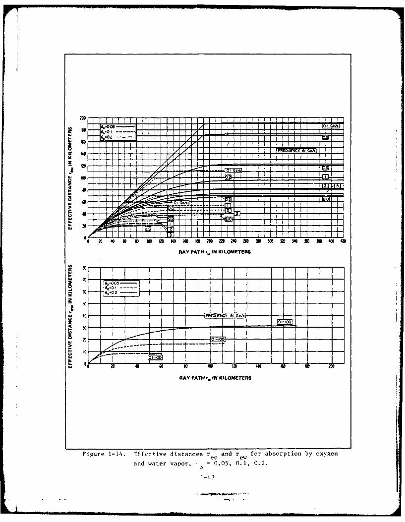
1-14 Effective distances r and r for absorption by oxygeneo ew

and water vapor, 00 = 0.05, 0.1, 0.2 ........................... 1-470

1-15 Effective distances r and r for absorption by oxygeneo ew

and water vapor, 0 W 0.5, 1, R/2 .............................. 1-480

2-1 Articulation score versus noise interference ................... 2-22-2 Probability of error versus signal-to-interference ratio for

noncoherent FSK modulation ..................................... 2-32-3 Probability of error versus signal-to-interference ratio for

PCM (polar), PSK, or QPSK modulation............................ 2-42-4 Probability of error versus signal-to-interference ratio for

3LPR modulation................................................ 2-52-5 Probability of error versus signal-to-interference ratio for

QPR modulation ............ .................................... 2-7

v

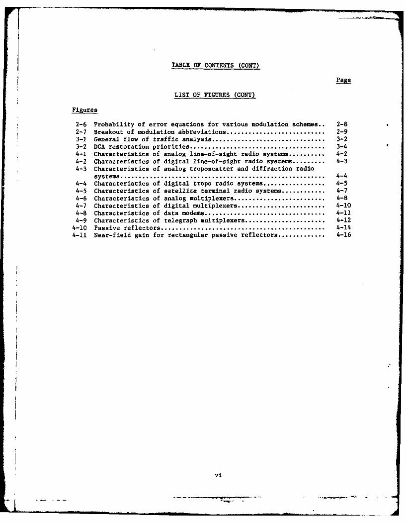
TABLE OF CONTENTS (CONT)

Page

LIST OF FIGURES (CONT)

Figures

2-6 Probability of error equations for various modulation schemes.. 2-8

2-7 Breakout of modulation abbreviations ........................... 2-9

3-1 General flow of traffic analysis ............................... 3-23-2 DCA restoration priorities ..................................... 3-44-1 Characteristics of analog line-of-sight radio systems .......... 4-24-2 Characteristics of digital line-of-sight radio systems ......... 4-34-3 Characteristics of analog troposcatter and diffraction radio

systems ........................................................ 4-44-4 Characteristics of digital tropo radio systems ................. 4-54-5 Characteristics of satellite terminal radio systems ............ 4-74-6 Characteristics of analog multiplexers ......................... 4-84-7 Characteristics of digital multiplexers ........................ 4-104-8 Characteristics of data modems ................................. 4-114-9 Characteristics of telegraph multiplexers ...................... 4-12

4-10 Passive reflectors ............................................. 4-144-11 Near-field gain for rectangular passive reflectors ............. 4-16

vi

PART I - LINK AVAILABILITY

1.1 Introduction.' LOS, tropo, diffraction, and satellite links all experi-

ence signal variations as a function of time and RF signal path length,

commonly referred to as fading. Fading occurs when microwave signals arrive

simultaneously at a receiving antenna over more than one path and result from

the fact that at certain times these signals will be out of phase, cancelling

each other. Fading is caused by a combination of climatic and terrain factors;

therefore, it is difficult to predict the frequency and depth of fades that

can occur over a given path. The discussions which follow delineate the

methods used to predict the probability of a fade and the fade outage statis-tics which have a bearing on the performance of a particular link. Themethods are derived for LOS, tropo, diffraction, and satellite links. In

addition, failure thresholds for these types of links are discussed, which

permit the calculation of required processing gain (antijam) for ECCM appli-

cations. Sample calculations are also provided for typical LOS, tropo, andsatellite links The methodology described in the subsequent paragraphs isderived from reerences 1 through 5, part 5, this section.

1.2 LOS Links

1.2.1 Fade Outage Statistics

a. The probability distribution of the signal envelope voltage (V) for

LOS paths is given by the equation:

P(V<L) rL2 (1)

where

P = probability, or fraction of time, T, that V is < L

L = the normalized algebraic value of envelope voltage (see fig. 1-1)

r = the multipath occurrence factor for heavy fading months

b. The factor r is given by:

r = ab D3 10- 5 (2)

or

r a x b x 2.5 x 10-6 x f x D3 (3)

where

a = terrain factor (numeric) which takes into account the terrain roughness

for three climatic conditions. The terrain factor may be either arepresentative value (see fig. 1-2) or a calculated value (see fig. 1-3)

from path profiles

b - climate factor (numeric), which accounts for the effect of climate on

fading (see fig. 1-4)(Text continued on page 1-6)

1-1

o 0o

I I V

1 001 ~VKr.OL DAJ~lU UP 1UAo

44a

14

ala La

tmuI NIHMdAN0AS3

1-21

Terrain Terrain. Factor, aTerrain Roughness Coastal Average Dry

Type (ft) climate Climate Climate

smooth 20 6.6 3.3 1.6

Normal 50 2.0 1.0 0.3

Rough 140 1.6 0.5 0.1

Figure 1-2. Representative values of terrain factor.

1-3

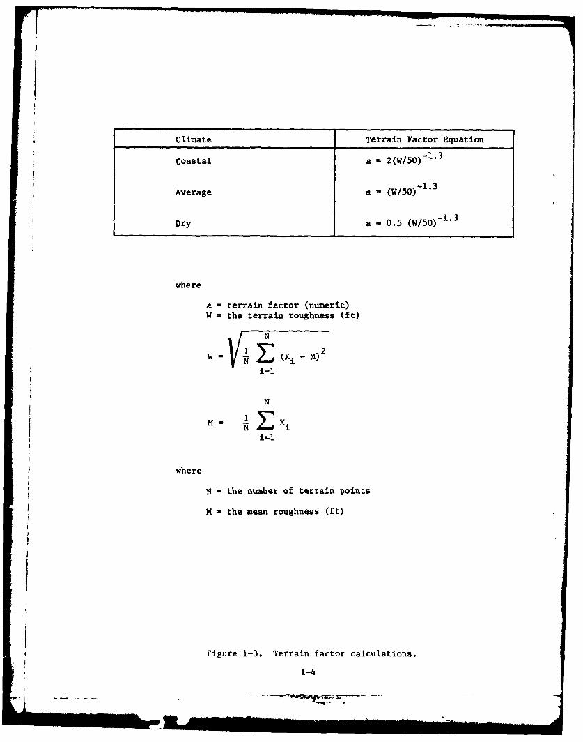
Climate Terrain Factor Equation

Coastal a - 2(W/50)- "3

Average a - (W/50)-1.3

Dry a - 0.5 (W/50)- 1.3

where

a = terrain factor (numeric)W = the terrain roughness (ft)

N

W= I (X - M)2i l

N

where

N - the number of terrain points

N - the mean roughness (ft)

Figure 1-3. Terrain factor calculations.

1-4

Climate Climate Factor, b

Gulf coast, or similar hot, 0.5humid areas

Normal interior temperate, 0.25or northern

Mountainous, or very dry 0.125

Figure 1-4. Climate factor.

1-5

V.

f - frequency (GHz)

D = path length (statute miles)

c. The relationship of the link fade margin (F) to L is given (fromfig. 1-1) by:

F - -20 log L (4)

hence,

L 2 = 1 0-F/l0 (5)

Since P(V<L) is really the probability of a fade outage (P) -- that is, the

probability that V will be less than the threshold level, L - then equation1 can be rewritten, in terms of fade margin, as:

P axbx 2.5 x 10-6 x f x D3 x F/ (6)0

d. However, equation 6 does not consider the effects of diversityoperation. Diversity can be accounted for by an improvement factor (I).

(1) For frequency diversity, the improvement factor (Ifd) isgiven by:

Ifd c (-L)x OF/10 (7)

where

c = the frequency factor (see fig. 1-5)

Af - the frequency diversity spacing (GHz)

Equations 6 and 7 can be combined so that P may be calculated for the fre-quency diversity condition by:

-6 2 o-2F/10

a xbx2.5 x 10-6 xf xl 2P (fd)- c x Af (8)

(2) For space diversity, the improvement factor (Isd) is given by:

d 7xl- 5 xfxS 2 i0 F/1Osd (9), D

where

S - the vertical antenna spacing between centers (ft)

F the fade margin (dB) associated with the second antenna, or the smaller

of the two fade margins

1-6

4.8-JV x

1-7I

Equations 6 and 9 can be combined so that P may be calculated for the spacediversity conditions by: 0

P 0(sd) b a xx3.57 x 10- 2 xD 0 F/ (10)S2 x F/10

For practical reasons in this study, the difference between the two fade

margins was considered to be negligible and, hence, F was considered to be

equal to F(F=F).

Therefore, equation 10 can be rewritten as:

3.57 x 10-2 x 4x(sd) = axx3n)10~o $2

(3) For quadruple (quad) diversity, the improvement factor (Iqd)is given by:

Iqd I fd x Isd

-7 x 10 . 5 x fFx 2x (17xO x /F10 (12)

Hence, P for the quad diversity condition is given by:0

-2 D 4lO 1 0 0P (qd) x b x3.57 x 10- 2 x f x D4x 03/0()

P0(qd) a-- 7lO~(13)cx~fxS

where F = F, as with the space diversity condition.

1.2.2 Availability Equations

a. Availability - General. Link availability is the fraction of time(T) that the signal envelope voltage (V) will be above threshold, L. Hence,link availability (A) is defined as:

A= 1- P (14)0

(1) Link availability for the nondiversity condition is given by:

A(nd) 1- a x b x 2.5 x 106 x f x x 1 0 (15)

(2) Link availability for the frequency diversity condition isgiven by:

A(fd) I / a x b x 2.5 x 10-6 xf 2 x x (6)cx Af

1-8

(3) Link availability for the space diversity condition is given by:

-2 4 -2F/10A(sd) = I- a x b x 3.57 x 2 0 (17)

(4) Link availability for the quad diversity condition is given by:2 D4 103F/10

b 3.57 x 102 x f x xA(qd) 2 f D X (18)

c x Af x S2

(5) For convenient reference, the availability equations are pre-sented in summary form in figure 1-6.

b. Baseline Link Availability

(1) The baseline link availability (As) is the link availability

when no Jamming is present. It is calculated using the appropriate availa-bility equation (fig. 1-6) and appropriate link parameters. The link fademargin, with no jamming present, is the difference between the received sig-nal level, SRE C (dBm), and the required signal level, SREQ (dBm), that is -

FS = SREC - SREQ (dB) (19)

(2) SRE C (dBm) is calculated using the equation:

S = P +G + R-L -L -L (dBm) (20)

where

PT = transmitter output power (dBm)

GT = transmitter antenna gain (dB)

CR = receiver antenna gain (dB)

LT = transmitter antenna system losses (dB)

LR = receiver antenna system losses (dB)

LS = propagation path loss (dB)

(3) Propagation path loss (LS) is calculated for LOS links bythe equation:

Ls 97.0 + 20 log f + 20 log D + Aa (21)

where

1-9

1. Nondiversity:

A =1 - (a x b x 2.5 x 10- 6 x f x D3 x 10

-F/10)

2. Frequency Diversity:

A =1- (a x b x 2.5 x 10- 6 x f2 x D3 x 10 -2F/1

0 )

c x Af

3. Space Diversity:

A = 1 - (a x b x 3.57 x 10- 2 x D4 x 10-2F/1

0 )S 2

4. Quad Diversity:

-2 4 -3F/10A =1 ( a x b x 3 .57 x 10 xfx D x 1 )

c x Af x S2

where

A = availabilitya = terrain factor (numeric)b = climate factor (numeric)c = frequency factor (numeric)f = frequency (GHz)D = path length (statute miles)F = fade margin (dB) (Note: In the case of space diversity,

the fade margin associated with the first antenna, or thelarger of the two fade margins)

Af= the frequency diversity spacing (GHz)S = vertical antenna spacing between centers (ft)

Figure 1-6. Availability equations - LOS.

1-10

f = frequency (GHz)

D = path length (statute miles)

A = absorption by water vapor and oxygen (dB) - discussed in morea detail in paragraph 1.5.1

(4) SREQ (dBm) is calculated by the equation:

SREQ -138.6 + 10 log T + 10 log B + NF + S/NREQ (22)

where

T = system operating temperature in degrees Kelvin (for LOS linksT - 290 0K)

B = receiver IF 3-dB bandwidth (11Hz)

NF = receiver system noise figure (dB)

S/N = signal-to-noise ratio required to produce acceptable systemREQ output (dB) (for LOS systems, S/NREQ = 10 dB)

c. Link Availability in the Presence of Jamming

(1) The link availability when jamming is present (A ) is calcu-lated using the appropriate equation of figure 1-6. The link fade margin inthe presence of jamming (F ) is the difference between S (dBm) and the

received jamming signal level, JREC (dBm), that is:

Fj = SREc - JREC (dB) (23)

(2) JREC (dBm) is calculated by the equation:

JE ERP + -L - L + 10 log B - 10 log B (24)

~REC J RJ R J

where

ERPJ = jammer effective radiated power (dBm)

G1 = receiver antenna gain in the direction of the jammer (dB)

Bi jammer 3-dB emission bandwidth (MHz)

L = = propagation path loss between jammer and link receiver (dB)

1-ii

(3) Propagation path loss for the jammer (LK) is calculated by

the equation:

Lj W 9 7 .0 + 20 log f + 20 log Dj + Aa (25)

where

ji path length between jammer and link receiver (statute miles)

1.2.3 Failure Threshold. The failure threshold is the value of fade marginbelow which the link is considered to be below the DCA availability criterion.

1.2.3.1 DCA LOS Link Availability Criterion. The availability criterion valuefor DCS LOS links is 0.99996, as given in TR-12-76. This criterion value is

denoted AC for the purposes of this study.

1.2.3.2 Required Jamming Margin. The fade margin required in the presence

of jamming (Fc), is the signal-to-jamming ratio (S/J) in dB required to

restore the link to the DCA availability criterion (AC) . The calculation of

FC for LOS is dependent upon the types of diversity operation employed by the

specific system.

a. For nondiversity operation:

Fc(nd) = 0 log (26)a xb x 2.5 x 10- x f xD

b. For frequency diversity operation:

C~~~ .jll& lAC ) (C xAf)F(fd)a x x 2.5 x 10-6 x f2 x2 (27)

c. For space diversity operation:

- A Co ) S

Ca x b x 3.57 x 10- 2 xD

d. For quad diversity operation:

C 2 11Fcq)= - i04]o3 (29)

a x b x 3.57 x 10 x f x D

1-12

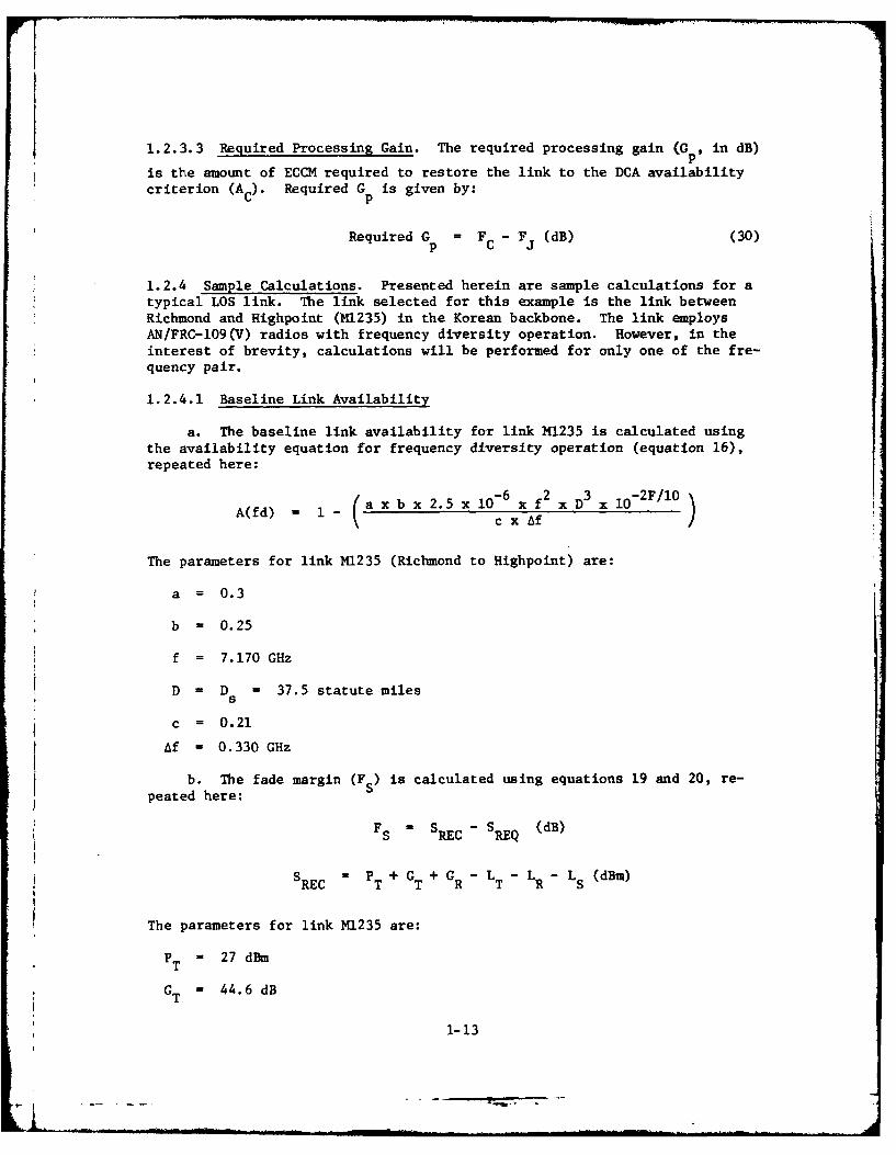
1.2.3.3 Required Processing Gain. The required processing gain (G p, in dB)

is the amount of ECCM required to restore the link to the DCA availabilitycriterion (Ac). Required Gp is given by:

Required Gp = F C - Fj (dB) (30)

1.2.4 Sample Calculations. Presented herein are sample calculations for atypical LOS link. The link selected for this example is the link betweenRichmond and Highpoint (H1235) in the Korean backbone. The link employsAN/FRC-109(V) radios with frequency diversity operation. However, in theinterest of brevity, calculations will be performed for only one of the fre-

quency pair.

1.2.4.1 Baseline Link Availability

a. The baseline link availability for link M1235 is calculated usingthe availability equation for frequency diversity operation (equation 16),

repeated here:-6 25 2 D3 o-2F/10

A(fd) = a x x 2.x 10-6 x x x

c x Af

The parameters for link M1235 (Richmond to Highpoint) are:

a = 0.3

b = 0.25

f = 7.170 GHz

D = D = 37.5 statute miless

c = 0.21

Af = 0.330 GHz

b. The fade margin (F S ) is calculated using equations 19 and 20, re-

peated here:

FS M S - S (dB)RC REQ

S P +G+ G - L L -L (dBm)REC T T R T R S

The parameters for link N1235 are:

PT = 27 dBm

TT = 44.-61dB

' 1-13

- ---- ---

CR = 44.6 dB

LT = 2.3 dB

LR = 1.7 dB

LS = 146.5 db

SREC = 27 + 44.6 + 44.6 - 2.3 - 1.7 - 146.5

- - 34.9 dBm

The SREQ for the AN/FRC-109(V) for M1235 is -77 dBm and, thus, the fade

margin (F s) is:

FS = - 34.9 - (- 77) - 42.1 dB

c. The baseline availability can now be calculated as follows:

As(fd) 1 ( 0.3 x 0.25 x 2.5 x 10 - 6 x 7.170) 2 x (37.5)3 x 84 2/

s 0.21 x 0.330

[ 0.3 x 0.25 x 2.5 x 10- 6 x 51.4 x 52,734 x 3.8046 x 10 - 9

A s(fd) - 1 - 2.7901 x 10- 8

A s(fd) - 0.9999999

1.2.4.2 Link Availability in Presence of Jamming

a. Consider link M1235 operating in the presence of a hypothetical air-borne noise jammer at a distance of 10 miles from the receiver at Highpoint.The same availability equation (equation 16) is used:

A(fd) M - a x b x 2.5 x 10 - f x D x 1 0 -cx Af

However, the availability will be denoted A and the fade margin, Fj.

b. The fade margin is calculated by equation 23:

Fj = SREC - JREC (0)

SREC is calculated by equation 24:

3REC i ERPj + GRj L R - Lj - 10 log B 10 log B

1-14

'-

The parameters used are:

ERPj = 70 dBm

GFU = 24.6 dB

R - 1.7 dB

Li = 134.4 dB (from equation 25) for a distance of 10 miles

B = 20 MHz

Bj M 20 M z

Thus, JREC is calculated as:

JRE =70 + 24.6 - 1.7 - 134.4 + 13.0 -13.0REC

- - 41.5 dBm

and

Fj = - 34.9 - (-41-5) - 6.6 dB

c. The Aj is thern e.Alculated as:

(fd) = 1 - 0.3 k 0.25 x 2.5 x 10 6 x (7.170) x (37.5) 3 x 10 - 13 2 / 10

j 10.21 x 0.33

(0.3 x 0.25 x 2.5 x 10-6 x 51.4 x 52,734 x 4.7868 x 10-2 .A3 (fd) l 1-(03x02 2. o 0066c 2 )k 0. 0696/

Aj(fd) f 1 - 0.3495353

A (fd) i 0.6504646

1.2.4.3 Failure Threshold. Comparison of the calculated Aj to the DCA

availability criterion (Ac) reveals that the link is vulnerable to this

jammer, that is, Aj = 0.6504646 and AC = 0.99996, hence Aj < AC .

1.2.4.4 Required Jamming Margin. The required Jamming margin (Fc) is then

calculated by equation 27:

Fc(fd) -0 log [ . )(c 2I a x b x 2.5 x 10- 6 x f2 x D 3

1-15

Thus, for link M1235, F C is calculated as:

F (fd) = -10 log (1-0.99996) -6.2 2.3)/C 0.3 x 0.25 x 2.5 ( 0.21 x 07.33) 2x(75

1077 x (7170-67*)

F (fd) [-10 log (-~2x l ]/2C5.0822 x 10 - 1 /

Fc(fd) 10 log (5.4542 x 10-6) /2

F c(fd) f 26.3 dB

Hence, a fade margin of 26.3 dB is required to maintain the criterion avail-ability of 0.99996.

1.2.4.5 Required Processing Gain. The processing gain required to restorelink M1235 to the DCA availability criterion (AC = 0.99996) is then calculated

by equation 30:

RequiredG = F - Fp r J

Required G = 26.3 - 6.6p

Required G = 19.7 dBp

Therefore, 19.7 dB of processing gain must be achieved by employing theavailable ECCM techniques, either singly or in combination, to restore thelink to the DCA availability criterion.

1.3 Troposcatter and Diffraction Links

1.3.1 Fade Outage Statistics

a. The probability distribution of the signal envelope voltage (V) fortroposcatter and diffraction links is given by the Rayleigh formula from

Barnett (ref 1, part 5):

P(V<L) = 1 - eL (31)

1-16

Since P(V<L) is really the probability of a fade outage (P ), and theo

relationship of L to the fade margin (F) is F = -20 log L, equation 31 canbe expressed as

P = 1 - exp (-I0 -F/IO) (32)

b. Equation 31 does not consider the diversity combining techniquesemployed by tropo and diffraction systems. Combining is performed at oneof two states in the receiver system: (1) before detection (predection),combining the individual signals before detection; and (2) after detection(post-detection), combining the individual signal inputs after detection atthe baseband level. There are various means in which combining may beaccomplished, whether pre- or post-detection is used. There are threecommon types of combiners:

(1) Selection Combiner: The selection combiner determines thelarger received input signal and applies this signal to the receiver output.

(2) Equal-gain Combiner: The equal-gain combiner adds the inputsignals and applies the sum to the receiver output.

(3) Maximal-ratio combiner: The maximal-ratio or ratio-squarecombiner squares the input signals before addition and then applies the sumto the receiver output.

c. The probability of fade outage (P ) for tropo and diffraction paths

can be estimated for the three types of combiners (selection, equal-gain, andmaximal-ratio).

(1) For selection combining:

0 = - exp - (33)

where

P 0f= the probability of fade outage0

F = the fade margin (dB)

M = the number of diversity channels

NOTE: M = 1, for non-diversity

= 4, dual-diversity (frequency or space)

f 8, quad-diversity

(2) For equal-gain combining:

1-17

.. . .. . .- . ..L .. i1 . . . . . . . .. ...- f 1 -

. ., . .i i , iu - -" -. . . .

P = 10-MY/10 (34)o = (2M)!

(3) For maximal-ratio combining:

=10

o M! (35)

1.3.2 Availability Equations

a. Link availability is the fraction of time (T) that the signalenvelope voltage (V) will be above threshold L. Hence, link availability(A) is defined as:

A = 1 = P (36)0

(1) Link availability for selection combiners is given by:

A = 1 [ exp(10F/1) M (37)

(2) Link availability for equal-gain combiners is given by:

A =2) 1- 10 J0 (38)(2M)!

(3) Link availability for maximal-ratio combiners is given by:

A = 1[ (39)

For convenient reference, the availability equations are presented in summaryform in figure 1-7.

1.3.2.1 Baseline Link Availability

a. As with LOS links, the baseline link availability (As) is the link

availability when no jamming is present. It is calculated with the appropriateavailability equation (see fig. 1-7) and appropriate link parameters. The linkfade margin, with no jamming present (FS) is the difference between SREC (dBm)

and SREQ (dBm); that is, from equation 19:

F S = S - S (dB)REC REQ

1.-18

I

1. Selection combiner:

[ M

A 1- [ 1- exp (-Io-F/IO)J

2. Equal-gain combiner:

(2M)!

3. Maximal-ratiocombiner:

A = I M! ]

where:

A - link availabilityF - fade margin (dB)M = the number of diversity channels

1, non-diversityM = 4, dual-diversity

8, quad-diversity

Figure 1-7. Availability equations - trono and diffraction.

1-19

20:

where. The received signal leeS RC dBmn), is calculated using equationS REC = P T + G T + G R L LT - L R - L S (dBm)

where

P T = transmitter output power (dBm)

GT = transmitter antenna gain (dB)

GR = receiver antenna gain (dB)

LT = transmitter antenna system losses (dB)

LR = receiver antenna system losses (dB)

LS = propagation path loss (dB)

c. Propagatic oath loss (L S) for tropo and diffraction links iscalculated as follow :

(1) For troposcatter links:

LS 30 log f - 20 log D + F(OD) + L (40)

where

f = frequency (MHz)

D = path length (km)

F(OD) = the attenuation function (dB)

0 = the angular distance, the angle between horizon rays in thegreat circle plane, and is the minimum diffraction angle, orscattering angle unless antenna beams are elevated (radians)

L = medium-to-aperture coupling loss (dB)c

A = absorption by water vapor and oxygen (dB) -- discussed ina detail in paragraph 1.5.1.

F(O) is calculated by first determining 0 by:

D + 0 + 0 (41)a et er

where

a = the effective earth's radius (km)

1-20

IkA

a 1i - 0.04665 exp (0.005577 N)]

h - hts dLt0et d Lt 2a(42)

0 hLr rs dLr (43)eer d dLr 2a (3

NS the value of N at the surface.of the earth

N 0 exp (-0.1057 hs )

I N 0 exp (0.1057 hst) + N0 exp (-0.1057 hsr)J /2 (44)

a 6370 km0

N 0 surface refractivity reduced to sea level (see fig. 1-8)

h = elevation of the surface of the ground above mean sea level (km)s

hst hs of the transmitter site (km)

h = h of the receiver site (km)sr s

hLt height of the transmitter horizon obstacle above mean sea level(km)

hLr = height of the receiver horizon obstacle above mean sea level (km)

hts height of transmitter antenna above mean sea level (kin)

h = height of receiver antenna above mean sea (kin)rs

dLt great circle distance from the transmitter antenna to its horizon(km)

dLr great circle distance from the receiver antenna to its horizon(km)

Figure 1-9 shows the scatter volume and path geometry. F(OD) can then becalculated as follows:

For 0.01 < OD < 10:

F(eD) = 139.5 + 0.06 N - 2.4 x 10-4 NS2 + 0.34 OD + 30 log (OD) (45)

For 10 < OD < 70:

(Text continued on page 1-24)

1-21

L ' " "

i ='" =id= . i " ' ' S ON =

2 2 2 ~zo 0 2 0

A ERRR a t -XI a m 1

/j. r

- -4 -4

oo

~4

-4

0 -4

1-22j

(a) SCATTER VOLUME (TROPO LINKS)

TRANSMITTER RCIE

NOTE- DISTANCES ARE MEASURED

(b) PATH GEOMETRY (TROPO AND DIFFRACTION LINKS)

Figure 1-9. Scatter volume and path geometry.

1-23

F(OD 140.7 + 0.06 Ns - 3.2 x 10 - 4 Ns ~ 2 (46)

+ OD (3.925 + 3.3 x 10- 3 N - 1.9 log N S)

+ (22.5 + 0.05 N ) log (OD)s

For OD > 70:

F(OD) = 123.6 - 0.008 Ns + 0.158 OD + 44 log (OD) (47)

The medium-to-aperture coupling loss (Lc) can be determined from figure 1-10.

To convert the scatter angle (G) from radians to degrees, multiply by 57.29578.To calculate the antenna 3-dB beamwidth (BW), use the following equation:

BW = 68,70O (48)f x d

where

BW = antenna 3-dB beamwidth (degrees)

f - frequency (MHz)

d = diameter of parabola (ft)

(2) For diffraction links, the propagation loss (L ) is given by:

Ls = 97 + 20 log f - 20 log D + A + Aa (49)

where

f = frequency (GHz)

D = path length (statute miles)

AD = the attenuation due to diffraction (dB)

A = absorption by water vapor and oxygen (d)a (discussed in detail in paragraph 1.5.1)

(a) The attenuation due to diffraction, with no groundreflections, can be determined by first calculating the parameter, V:

V = ± 2.583 0I(fdld 2 )/D (50)

where

f = frequency (MHz)

dI = the distance from the obstacle to the transmitter (km)

d2 = the distance from the obstacle to the receiver (km)

1-24

ANTENNA SEAMWVIDTH(DEGREES)

SCATTER ANGLE(DEGREES) .

0-4.APERTURE TO

30-. MEDIUM COUPLING 3LOSS (DB) _

066

60- 0.2 3.0

.0.7

-J0.90. 2.0

La1.35

I-7

L*

ISO 1.

ul 1.94 2. I

320016 0.5

-2I3

isIs

3.0

300 2

31104.0

4004.3

56 1 .0

Figure 1-10. Aperture-to-medium coupling loss.

1-25

D = path length (km)

(b) The geometry for knife-edge and rounded obstacle diffrac-

tion is shown in figure 1-11.

(c) For the case of a single isolated knife-edge obstacle, AD

can be determined by calculating A(V,O) (AD=A(V,O):

For -i < V<0:

A(V,O) = 2.78 V 2 + 9.95V + 6.17 (51)

For 0 < V < 3:

A(V,O) = 6.08 - 0.005 V4 + 0.159 V3 - 1.7 V2 + 9.3V t2)

For V > 3:

A(V,O) - 12.953 + 20 log V (53)

(d) For the case of a single isolated, rounded obstacle,

AD is expressed by the following equation:

AD = A(V,O) + A(O,p) + U(Vp) (54)

where

A(V,O) = the diffraction loss for a knife-edge obstacle (dB), as shown

above (equations 51 through 53)

A(Op) = the diffraction loss for 0 = 0 over a rounded obstacle (dB)

U(V,p) = the diffraction parameter which accounts for values of 0 other

than zero (dB)

(e) To calculated AD, the parameter, p, must first be

determined by:1/2

p = 0.676 rl/3 f! 6 [D/ (r 1 r 2 )] (55)

where

p = the index of curvature for the crest radius of the rounded obstacle

r = the crest radius of the rounded obstacle (km)

r = the distance from the transmitter to the rounded obstacle (km)

r2 = the distance from the receiver to the rounded obstacle (km)

NOTE: For all practical purposes rlr 2 may be replaced by dId 2 .

1-26

TRANSMITTER CL 0 RECEIVER

_dj d2

dit O d

D

(b) RONDFEED OTCL FCTIONN

1-27

(f) The crest radius (r) may be calculated by:

2 DH dst dsr (56)

0 st + d sr2

where

D = great circle distance between transmitter and receiver horizons (km)H

DH - D- dLt - dLr (57)

dst f distance between the transmitter antenna horizon and the crossoverof horizon rays as measured at sea level (kin)

dst = D 0oo /0- dLt (58)

d - distance between the receiver antenna horizon and the crossover ofsr horizon rays as measured at sea level 0km)

dsr o - dLr (59)

h -ha D + rs rs (60)oo 2a et D

D rs tr00 a + 0 er- + D(61)

(g) With the p calculated, A(O,p) may then be calculated as:

A(O,p) 5.86 + 1.49 p + 1.46 p + 6.49 p (62)

NOTE: An average allowance for terrain foreground effects may be made byadding a term 10 exp (-2.3 p) to A(O,p). This term gives a correction whichranges from 10 dB for p = 0 to 1 dB for p = 1. A more detailed discussionon the effects of ground reflections may be found in reference 2, part 5.

(h) And, finally, U(V,p) may be calculated; for Vp < 2:

U(V,p) = (43.6 + 23.5 Vp) log (1 + Vp) - 6 - 6.7 Vp (63)

for Vp > 2:

U(V,p) = 22 Vp - 20 log (Vp) - 14.13 (64)

(4) SRE (dBm) can be calculated by equation 22:

SREQ = - 138.6 + 10 log T + 10 log B + NF + S/NREQ

1-28

where

T - system operating temperature in degrees Kelvin (for tropo anddiffraction links T - 290*K)

B - receiver IF 3-dB bandwidth (MHz)

NF - receiver system noise figure (dB)

S/NRE Q signal-to-noise ratio required to produce acceptable systemoutput (dB), (for tropo and diffraction links S/NRE 10 dB).

REQ

1.3.2.2 Link Availability in the Presence of Jamming

a. A is calculated using the appropriate equation of figure 1-8. The

link fade margin in the presence of Jamming (F) is the difference between

SREC(dBm) and JREC (dBm), that is, per equation 23:

Fj M SRE C - JREC (dB)

b. JREC (dBm), is calculated by equation 24:

JREC = ERPj + GRJ - LR - Lj + 10 log B - 10 log B

where

ERPj jammer effective radiated power (dBm)

receiver antenna gain in the direction of the jammer CdB)

B = jammer emission 3-dB bandwidth (MHz)

Lj = propagation path loss between jammer and link receiver (dB)

c. L is calculated by equation 25:

Li = 97 + 20 log f + 20 log D + Aa

where

f = frequency (GHz)

D = Dj = the path length between jamner and link receiver (.statute

miles)

A= absorption by water vapor and oxygen (dB) -- discussed in morea detail in paragraph 1.5.1.

1.3.3 Failure Threshold. The failure threshold is the value of fade marginbelow which the link is considered to be below the DCA availability criterion.

1-29

1.3.3.1 DCA Troposcatter and Diffraction Link Availability Criterion. Thecriterion availability value for DCS tropo and diffraction links is 0.99985,as given in TR-12-76. This criterion value is denoted AC for the purposesof this study.

1.3.3.2 Required Jamming Margin. The fade margin required in the presence

of Jamming (Fc) is the S/J in dB required to restore the link to the DCA

availability criterion (AC). The calculation of FC for tropo and diffraction

links is dependent upon the type of combining employed by the specific system.

a. For selection combining:

M

where

M = the number of diversiLy channels

AC = the DCA link availability criterion

b. For equal-gain combining:

=C 10 log(I - A (66)

C (2M)M )c. For maximal-ratio combining:

Fc 0 log [1/!7(1 -A CJ (67)

1.3.3.3 Required Processing Gain. The required processing gain (G , in dB)

is the amount of ECCM required to restore the link to criterion AC . Required

G is given by equation 30:p

Required Cp M FC - Fj (dB)

1.3.4 Sample Calculations

* a. Presented herein are sample calculations for a typical tropo link.The tropo link selected for this example is link T1225 between Yaedake,Okinawa, and Chiran, Japan.

b. Tropo link T1225 between Yaedake and Chiran employes the NEC modelTO-2G120-2A transmitters and RO-2GA60-lA receivers with frequency diversityoperation and selection combining. However, in the interest of brevity,calculations will be performed for only one of the frequency pair on thelink from Chiran to Yaedake.

1-30

_Woo

1.3.4.1 Baseline Link Availability

a. The fade margin (F S) was calculated using equations 19 and 20:

FS = S RC- SRQ(dB) l

S P + G + G - L - L - L dmRC T T R T R Lsd )

(1) The parameters for link T1225 operating at 1.752 GHz are:

P T= 73.0 dBm

G 82d

GR = 48.2 dB

LT = 0.9 dB

LR = 0.9 dB

LS = 236.9 dB

S REC m 73 + 48.2 + 48.2 - 0.9 - 0.9 - 236.9

-- 69.3 dflm

(2) The LSwas calculated by equation 40:

LS = 30Olog f -20log D+ F(OD) +L A

(3) The parameters for link T1225 are:

f = 1752 Mz

D - 360 miles = 579 km

0 = 0.0467 radians = 2.68 degrees

h = 1625 ft - .5kmst

h sr= 1368 ft -0.42 km

BW = 0.63 degrees

N - 305

(4) Since OD =27, F(OD) is calculated by equation 46:

1-31

F(OD) = 140.7 + 0.06 N - 3.2 x 10 - 4 N 2s s

+ OD (3.925 + 3.3 x 10 - 3 N - 1.9 log N)S s

+ (22.5 + 0.05 N ) log ODS

F(OD) f 140.7 + 0.06 (305) - 3.2 x 10-4 (305)2

+ (27 (3.925 + 3.3 x 10- 3 (305) - 1.9 log 305)

+ (22.5 + 0.05 (305)) log 27

F(OD) = 140.7 + 18.3 - 29.8 + 0.225 + 52.9

F(SD) = 182.3 dB

(5) The medium-to-aperture coupling loss (L c) is obtained from

figure 1-10, where 0 = 2.68 degrees and BW = 0.63 degrees. Hence, L =c

12 dB.

(6) Absorption by water vapor and oxygen (Aa) is calculated using

the methods of paragraph 1.5.1. For this link, A = 0.6 dB.a

(7) The propagation path loss can now be determined, using equation40:

Ls = 30 log (1752) - 20 log (579) + 182.3 + 12 + 0.6

L = 97.3 - 55.3 + 182.3 + 12 + 0.6s

L = 236.9 dB5

(8) The SREQ for the RO-2GA60-IA receiver was estimated to be

-89 dBm, by equation 22:

SREQ = -138.6 + 10 log T + 10 log B + NF + S/NR

S = -138.6 + 10 log (290) + 10 log (5) + 8.5 + 10REQ

SREQ = -138.6 + 24.6 + 7.0 + 8.5 + 10

S = 88.5 -- 89 dBmREQ

(9) The fade margin (F s is now calculated by equation 19:

FS = SREC - SREQ (dB)

F s = -69.3 - (-89)

FS = 19.7 dB

1-32

. ... ... -r- -4

b. Since the RO-2GA60-1A uses selection combining at baseband (post-detection), the baseline availability can be calculated by the first equation

of figure 1-7: A - [ x 0 F/0

in this case M 4,A 1- [ ( 1097 0]

A s= 1- -Fl ex, (0010716)]

A = 1- (1 -0.98934) 4

5

A 1 - 1.2913 x 10-8S

A =0.99999995

1.3.4.2 Link Availability in the Presence of Jamming

a. Consider link T1225 operating in the presence of a hypothetical air-borne noise jammer at a distance of 10 miles from the receiver at Yaedake.

b. The fade margin is calculated by equation 23:

Ji = REC - JREC(0

C. The received jamming signal level, JRE (dBm), is calculated by

equation 24:

J RC =ERP J+0 -J L R L J+l10log B- 0log B

The parameters used are:

ERP 70 dBm3

GP' 28.2 dB

=R 0.9 dB

L J 122.0 dB at 1.752 0Hz

B -B = 5 MHz

1-33

Thus,

JREC = 70 + 28.2 - 0.9 - 122.0 + 7.0 - 7.0

J REC = 24.7 dBm

d. The fade margin (F) is:

Fj = SREC- JREC

Fj = -69.3 - (-24.7)

Fj = -44.6 dB

e. The availability in the presence of jamming (A ) is calculated by

the same equation as for the baseline availability for this link:

1M

AJ =I [1 _exp 1-J1

= 1_ 1_ oe] 10- (44.6)/10)

4

A1 = I_ 1_ex _1o o46 )]4

Aj = 1 - [ l-exp (28840)1

Aj = 1- (l - 0)4

Ai = 0

1.3.4.3 Failure Threshold

a. Comparison of the calculated A to the DCA link availability criterionJ

(Ac) reveals that link T1225 is vulnerable to this jammer; that is, Aj = 0

and AC 0.99985, hence AJ < AC .

b. The r-iuired jamming margin (F C ) for link T1225 is calculated using

equation r or selection combining:

1-34

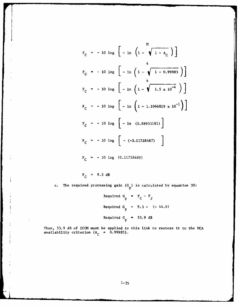
FC = -l10log [ in (1i- i-AC)

4

FC = - 10 iog [ in (I i-.98)

4

Fc = - 10 log [ In (1 l .5 x10 4

FC = - i0 log [ n - 1i - 1.1066819 x 10-1)

FC = - i0 log [-in (0.88933181)]

FC = -10 iog [-(-0.11728487) ]FC = - 10 iog (0.11728489)

FC = 9.3 dB

c. The required processing gain (G ) is calculated by equation 30:

Required G = F- F

Required G = 9.3 - -44.6)

Required C =53.9 dB

Thus, 53.9 dB of ECQC1 must be applied to this link to restore it to the DCAavailability criterion (AC 0.99985).

1-35

1.4 Satellite Links

1.4.1 Satellite Link Availability Equation

a. Satellite links are not subjected to the same terrain, climate, andfading conditions as terrestrial LOS, tropo, or diffraction links. Fadingis usually on the order of 6 dB, at worst case; hence, satellite links aredesigned for a 6-dB fade margin to account for multipath and scintillationloss variations. Since a satellite link is really a non-diversity LOS linkwith one terminal at an extremely high elevation, the non-diversity availa-bility equation for LOS links was modified to permit calculation of satellitelink availability. The non-diversity LOS availability equation (equation 15)is given as:

A =1- (a x b x 2.5 x 10-6 x f xD 3 xlOF/lO

where

A = the link availability, or probability that the mean received signallevel (S REC) will be above the required signal level (SREQ )

a = terrain factor

b = climate factor

2.5 x 10 -6 _ a constant which accounts for the worst LOS fading periodof the year

f = frequency (GHz)

D = distance (statute miles)

F = the fade margin (dB)

b. The expression in parenthesis in equation 15 is the probability ofa fade outage (P ). This expression must be modified so that P may be cal-

culated for satellite links, as follows:

(1) The satellite threshold conditions must be defined in terms ofthe maximum allowable P and the expected depth of fade. For satellite links,

0

the expected fade depth is 6 dB.

(2) Since factors a and b and the constant 2.5 x 10- 6 do not applyto satellite links, a new constant, z, replaces them in the P equation, hence:

0

3 -F/10P =z x f xD x (68)0

(3) To determine the value of z, equation 68 must be rewritten,solving for z:

PD3 o -F/l0 (69)

f1 x

1-36

(4) To account for threshold conditions, some of the terms areredefined and equation 69 is rewritten to provide a general solution of z:

PZoc (70)

f x D3 x 10- Du1

where

P = the threshold, or criterion, P

FD = the expected fade depth (dB), normally 6dB

c. The general availability equation for satellite links can now bewritten as:

A = 1 - (z x f xD 3 x l F/1 (71)

(1) Equations 70 and 71 can be combined:

A = I - [( D oc f xD 3 x 1 F/1) (72)

o,[f x Dx 10

or,

_ 0F/10 F D/10

A = 1- P x 10 x 10 (73)oc

where

A = the link availability, or probability that S will be above SREC REQ

Poc = the criterion probability of fade outage (P )

F = the calculated fade margin (dB)

F = the expected fade depth (dB)D

1.4.2 Baseline Link Availability. The baseline link availability (AS) is the

link availability when no jamming is present. It is calculated using equation

73 and the following procedure:

a. The link fade margin, with no jamming present (Fs), is calculated

using equation 19:

FS W S REC - S REO

b. The received signal level (SREC ) is calculated using equation 20:

1-37

. . .. . . . ...I. . . . .. . . .. .. . .. . . ." r.. . . ... . . . I I i I

SREC = PT + GT + G -L - LR - LS (dBm)

c. Propagation path loss (L is calculated, for satellite links, by

the equation:

L = 98.7 + 20 log f + 20 log D + A (74)

d. SREQ can be calculated, using equation 22:

S = -138.6 + log T + 10 log B + NF + S/NREQ (dBm)

where

T = system operating temperature in degrees Kelvin for satellite links:

(1) Uplink (satellite receiver; nominal T = 777 0 K; worst-caseT = 1227OK

(2) Downlink (ground terminal receiver); nominal T - 424*K;

worst-case T = 4406K

B = receiver IF 3-dB bandwidth (MHz)

NF = receiver system noise figure (dB)

S/NREQ signal-to-noise ratio required to produce acceptable system output(dB) (for satellite systems S/NREQ = 10 dB)

1.4.3 Link Availability in the Presence of Jamming

a. The link availability when jamming is present (Aj) is calculated, usingequation 73.

b. The link fade margin in the presence of Jamming (Fj) is calculated,using equation 23:

F = S -J (dB)J REC REC

c. The received jamming signal (J is calculated using equation 24:

JREC = ERPj + GRJ - LR - Lj + 10 log B - 10 log B

d. Propagation path loss for the jammer (Lj) is calculated by equation25:

Lj M 97.0 + 20 log f + 20 log D + Aa

1-38

where

D = path length between jammer and link receiver (statute miles)

1.4.4 Failure Thresholds. The failure threshold is the value of fade marginbelow which the link is considered to be below the DCA availability criterion.

1.4.4.1 DCA Satellite Link Availability Criteria. The criterion availabilityvalue for DCS satellite links is 0.999, as given in TR-12-76. This criterionvalue is denoted AC for the purposes of this study.

1.4.4.2 Required Jamming Margin. The fade margin required in the presenceof jamming (Fc), is the S/J, in dB, required to restore the link to the DCAavailability criterion (Ac). The equation to calculate FC for satellitelinks is:

FC = FD (dB) (75)

where

FD = the expected fade depth (dB)

FC = the fade margin (dB), between the received signal level (SREc) and

the received jamming signal level (JREc), required to maintain the criterion

availability.

1.4.4.3 Required Processing Gain. The required processing gain (CG p, in dB)

is the amount of ECCM required to restore the link to the DCA availabilitycriterion (AC). The required Cp is calculated by equation 30:

Required Gp = FC - Fj (dB)

1.4.5 Sample Calculations. Presented herein are sample calculations for atypical satellite link. The link selected is the downlink between the WesternPacific (WPAC) satellite and the AN/MSC-46 terminal at Song So, Korea, linkS2194.

1.4.5.1 Baseline Link Availability

a. The baseline link availability for the downlink of link S2194 iscalculated using equation 73, at a frequency of 7.425 GHz.

b. The fade margin (FS) is calculated using equations 19 and 20:

FS M SREC - SREQ (dB)

S = P + G + G - LT -L L (dBm)REC T T R T RLSdm

The parameters for link S2194 (downlink) are:

1-39

TT

P T = 43 dBm

GT = 30 dB

GR = 56.9 dB

LT = 0 dB

LR = 0 dB

LS = 203.2 dB

LS is calculated by equation 74:

LS = 98.7 + 20 log f + 20 log D + Aa (dB) (74)

The parameters for link S2194 are:

f - 7.425 GHz

D = 22,300 statute miles

A = 0.1 dB, as calculated by the method described in paragraph 1.5.1a

LS = 98.7 + 20 log (7.425) + 20 log (22,300) + 0.1

LS = 98.7 + 17.4 + 87.0 + 0.1

Ls = 203.2 dB

Hence,

SR = 43 + 30 + 56.9 - 0 - 0 - 203.2

SREC = - 73.3 dBm

S is calculated using equation 22:4 REQ

SREQ-- 138.6 + 10 log T + 10 log B + NF + S/N (dBm)REQ

The parameters for link S2194 (downlink) are:

T = 440oK

B = 40 MHz

NF = 16.5 dB

S/N = 10 dB

Hence,

1-40

SREQ - - 138.6 + 10 log (440) + 10 log (40) + 16.5 + 10.0

SREQ = - 138.6 + 26.4 + 16.0 + 16.5 + 10.0

SREQ = - 69.7 - - 70 dBm

However, the AN/MSC-46 receiver has a parametric amplifier between the RFand IF stages which has a gain of 30 dB. Therefore,

S = - 100 dBm

REQ

The fade margin can now be calculated as:

FS REC - SREQ

F S M - 73.3 - (-100.0)

FS - 26.7 dB

c. The baseline link availability (AS) for S2194 (downlink) is calcul-

ated per equation 73 as:

A - 1 _ P xi 0- F /10 x 10 FD/10)

for this DCS link:

P = I - A = 1-0.999 = 0.001oc

D u 6 DB

FS = 26.7 dB

As 1 - (0.001 x 10-26.7/10 x 10 6/10

A s = 1 - (0.001 x 0.069252 x 3.9808)

As M 1- 2.7567 x 10- 4

As = 0.9997243

1.4.5.2 Link Availability in the Presence of Jamning

a. Consider link S2194 (downlink) operating in the presence of a hypo-thetical airborne noise jamer at a distance of 10 miles from the AN/MSC-46ground terminal at Song So. The same availability equation (equation 73)is used. However, the link availability in the presence of Jamming (A j)replaces AS '

H e n c e ,-F / 0F I

AHn, 1 - Poc x 10 x 10

1-41

b. The fade margin (F 3) is calculated by equation 23:

Fj S RC- JRC(dB)

3 E is calculated by equation 24:

3 E = ERP + G J- L -L +l10log B-10log B

The jamming parameters are:

ERPJ 70.0 dBm

GP- 16.9 dB

LR 0 dB

B B =40 MHz

L is calculated by equation 25:

L - 97.0 + 20logf + 2 0log D j+A a

where

f -7.425 GHz

Di 10 miles

A =0.1 dB, calculated by the method described in paragraph 1.5.1a

Li = 97.0+ 17.4+ 20.0 +0.1

Li 134.5 dB

Hence,

3 RE 70.0 + 16.9 - 0 - 134.5 + 16 - 16

3 =E -47.6 dBm

F is then calculated as:

3j = - 73.3 - (-47.6)

Fj = - 25.7 dB

The link availability in the presence of Jamming (A3) is then calculated as:

Ai = 1 - (0.001 x 10-(-25.7/10) x 10 6/10)

Aj = 1 - (0.001 x 371.45 x 3.9808)

1-42

Aj = 1 - 0.3643181

Aj - 0.6356819

1.4.5.3 Failure Threshold. Comparison of the calculated A to the DCA

availability (AC ) reveals that the downlink is vulnerable to the Jamer

(0.63561819 < 0.999).

1.4.5.4 Required Jamming Margin. The required Jamming margin (Fc) is deter-mined by equation 75:

FC - FD = 6 dB (75)

1.4.5.5 Required Processing Gain. The processing gain required to restorelink S2194 (downlink) to the DCA availability criterion (Ac = 0.999) is cal-culated by equation 30:

Required Gp = FC - Fj

Required G -- 6 - (-25.7)p

Required G - 31.7 dBp

Therefore, 31.7 dB of processing gain must be achieved by employing the avail-able ECCM techniques, either singly or in combination, to restore the downlinkto the DCA availability criterion.

1.5 Atmospheric Absorption. Atmospheric absorption may seriously affectLOS, tropo, diffraction, and satellite links, particularly at frequenciesabove 1 GHz. Atmospheric absorption is comprised of several differentfactors which variously influence link performance. These factors are (1)absorption by water vapor and oxygen, (2) sky-noise temperature, (3) attenu-ation by rain, and (4) attentuation in clouds. Since only absorption by watervapor and oxygen was considered in this study, for the sake of simplicity, itwill be treated in some detail in paragraph 1.5.1 The remaining factors willbe discussed briefly in subsequent paragraphs. Details on these factors may

be found in reference 2, part 5.

1.5.1 Absorption by Water Vapor and Oxygen. Absorption by water vapor andoxygen affects radio links over a range of frequencies from 100 MHz to 100GHz and may be calculated by the equation (from reference 2, part 5):

a Yoo eo Ywo ew(dB) (76)

where

A = absorption by water apor and oxygen (dB)a

Yo 0 = the differential absorption for oxygen (dB per Kin)

Ywo = the differential absorption for water vapor (dB per km)

1-43

r = the effective distance for absorption by oxygen in the atmosphere (km)eor = the effective distance for absorption by water vapor in the atmos-

LW phere (kin)

Yoo and Ywo can be determined for a given frequency (GHz) from figure 1-12,and r and r can be obtained for a given path length (km) and angle of

eo ew

elevation above the horizontal, 0 (radians), from figures 1-13 through 1-15.Figures 1-12 through 1-15 were extracted from reference 2, part 5.

1.5.2 Sky-Noise Temperature. The nonionized atmosphere is a source of radionoise, with the same properties as a reradiator that it has as an absorber.This reradiation is primarily due to oxygen and water vapor over the frequencyrange from 100 MHz to 100 GHz. Details are given in reference 2, part 5.

1.5.3 Attenuation by Rain. The attenuation of radio waves above 2 GHz bysuspended water droplets and rain often exceeds the combined absorption bywater vapor and oxygen. Water droplets in fog or rain will scatter radiowaves in all directions, regardless of whether the drops are less than orequal to the wavelength. Attenuation is a function of rainfall rate andheight above the surface of the ground. Details are given in reference 2, part 5.

1.5.4 Attenuation in Clouds. Cloud droplets are those water or ice parti-cles having radii smaller than 100 microns (0.01 cm). Attenuation in cloudsshould be considered for links operating above 6 GHz in mountainous terrain.Details are given in reference 2, part 5.

1.6 Digital Considerations

a. The previous discussion of fade margin in terms of signal-to-threshold and signal-to-jamming ratios are applicable to digital as well asanalog systems. Digital systems are often discussed in terms of signalenergy per bit-to-noise power density ratio (E,,/N ) or signal energy per

bit-to-jamming energy per bit ratio (Eb/E ). Hence, the following equations

will permit conversion of the generalized parameters to the digital case,or vice versa.

b. Eb/N received, in dB, and SREC (dBm), can be obtained by the

equations:

Eb/NO REc (dB) = SREC - i0 log R + 228.6 - 10 log T - NF + 10 log B (77)

or

SREC = E b/N (dB) + 10 log Rb - 228.6 + 10 log T + NF - 10 log B (78)

b REC

where

(Text continued on page 1-49)

1-44

PRESSURE 760mm HgTEMPERATURE 200C

WATER VAPOR DENSITY iog/rn

20

5

02

0.0

S0.5

S 0.21

z

S0.052

0 .0

.00

S0.02

-J 0.01.. ..

1-4

0

0

. W

z 20

IL I

40 c

0 0 a m a 0 a 0 a5 a4 m4 m1 a 4W 40

RAY PATH r. IN KILOMETERS

an wae vpr 0.0000, .2A 40 0

J-4-6

20160

- 2/Iso -- --,--I-oO2 . . . '

-M 2 I.

oA AT o NKIOETR

6 100

12 - CA -

U tooz2 5

>- ----

40 -7

iU I

0 11 1ILIIj1- F0 20 40 So so I00 120 140 ISO 10 200 220 240 260 21 300 20 34 U 3 50 400 43

RAY PATH ro IN KILOMETERS

o60 ew02

- 50 - -- - -- -

r =

zo

3 0

-'4

20 -- -

In -- 1 1....

II..0 20 a0 60 a 1 140 ... Is*

RAY PATH ro IN KILOMETERS

Figure 1-14. Effertive distances r eoand r eWfor absorption by oxygen

and water vapor, -1 = 0.05, 0.1, 0.2.

1 -47

30 1

8a 80 -fHi Ir

20 ~FIIEUENCY ING

-1 -02 0 -5

z> --- --

02 ---- - --- 1 -

* 4 6 0 1 14 8 4 0 2 r8 30 II 32 36i-- 9 0 4 4 46 4 0 5

RAY PATH r. IN KILOMETERS

0 08'1-48

- 80,1 ---

Eb = signal energy per bit [milliwatts per bit (mW/b)]

N = noise power density [milliwatts per Hz (mW/Hz)]

E.D/No (dB) = 10 log EbINo (mW)

SREC = mean received signal level (dBm)

Rb =the link data rate (b/s)

T = system operating temperature (degrees, Kelvin)

NF = receiver noise figure (dB)

B = receiver IF 3-dB bandwidth (Hz)

c. Eb/No required, in dB, and SRE q (dBm), can be calabulted by the

equation:

Eb N0REQ (0) = SREQ - i0 log R + 228.6 - 10 log T - NF (79)

+ 10 log B

or

SRE Q = b/NOREQ + i0 log R - 2 2 8. 6 + 10 log T (80)

+ NF - 10 log B

d. The fade margin (Fs), in terms of energy per bit, can be calculated by:

Fs = Eb -E/N (dB) (81)S Eb / NO REC Eb/NOREQ

e. Ej/N received, in dB, and JREc(dBm) can be obtained by the euqations:

Ej/NREC (dB) J REC - 10 log Rb + 2 2 8 .6 - 10 log T - NF (82)

+ 10 log B

or

REC I NREc (d) + 10 log Rb - 228.6 + 10 log T (83)

+ NF - 10 log B

where

1-49

JREC = the received jamming signal level (dBm)

Ej = jamming signal energy per bit (mW/b)

N = noise power density (mW/Hz)0

E /No(dB) = 10 log Ej/N° (mW)

f. The fade margin (F ), in terms of energy per bit, can be calcuated by:

Fj tN -E/ (dB) (84)

= /OREc - jNREC

which is E /E- ().E

1-50

PART 2 - LINK QUALITY

2.1 Introduction. Discussed herein are the parameters used to measure thequality of the information transferred over a radio link and the quality of thelink itself. Information quality is expressed in articulation score (AS) forvoice circuits (channels) and probability of error for teletypewriter and datacircuits. Link quality is expressed in terms of link availability (as discussedpreviously) for both analog and digital radio links and probability of error(P e) in the mission, or aggregate, bit stream, for digital links.

2.2 Quality of Voice Circuits

a. The measure of voice quality most widely used is the AS. This is ameasure of the percentage of phonetically balanced words in a test message cor-rectly interpreted by a team of trained listeners. In practice, team memberslisten and respond to recordings of the test message derived from the outputof a test channel into which interference has been injected. After all lis-teners have responded, the responses are computer-processed to determine themean and standard deviation for the listeners.

b. A representative curve of AS versus noise interference, in terms ofsignal-to-interference ratio, S/I (dB), is provided in figure 2-1. This curvewas used in the estimation of voice circuit quality in this study and is con-sidered a good approximation of actual voice quality over the DCS links whichwere evaluated. Of course, actual measured values may vary somewhat from theseestimates, but the estimated values provide a good indication of the magnitudeof voice channel degradation.

2.3 Quality of Data and Teletypewriter Circuits. A measure of data or tele-typewriter quality widely accepted is the P . P is a function of signal-to-

e enoise ratio (S/N) or S/I and the type of modulation employed to transfer thedata or teletypewriter message over the radio link. The majority of datamodems and teletypewriters in use in the DCS employ FSK modulation and, hence,the curve in figure 2-2 was used in this study to estimate the level of degra-dation of data and teletypewriter circuits.

2.4 Quality of Digital Radio Links

a. The quality of digital radio links is determined by the P in thee

aggregate or mission bit stream (sometimes referred to as the baseband bitstream). P is a function of S/N or S/I and the type of modulation employed

eby the radio system. The most common modulation schemes employed (or plannedfor) in the DCS are pulse code modulation (PCM), phase-shift keying (PSK),three-level partial response (3LPR), quadrature partial response (QPR), andquadrature phase shift keying (QPSK).

b. Curves of P versus S/I are provided for the most common digital mod-e

ulation schemes as follows:

(I) PCM, PSK or QPSK, figure 2-3.

(2) 3LPR, figure 2-4.(Text continued on page 2-6)

2-1

9e

---

U CURVE IS BASED ON A MESSAGE LENGTHOF 1000 PHONETICAL LY-BALANCED WORDS

. 60 -- iRANSMITTED OVER A 3--kHz VOICE CHANNEL,Z WITH NOISE INTERFERENCE (FROM REFERENCE 6)

0

z

o40

30

-15 -10 -5 0 5 10 15 20 25 30 35 40 45 50 55

SIGNAL-TO-INTERFERENCE RATIO (S/I, IN dB)

Figure 2-1. Articulation score versus noise interference.

2-2

~Io-4'

cc

0-

X I2-3

100

T

0 -

0cc

0-

SIONAL-O-INTEPHiEll RATI iSI IN.l

IC (1la) PS, or 1PS modulation.1

11HIII~i~ HillI 2-4

0-

-2

0

I i T

i NATONTR RE E TAI ISI IN I

ESTIMATEDFiue240 rbblt ferrvrsssga-oitreec ai o

3LPR 1111 moua ion 1 I H 111~ k l2-5IT

(3) QPR, figure 2-5.

2.5 Probability of Error Equations. Equations for the calculation of Pe for

the modulation schemes discussed in paragraphs 2.3 and 2.4, and for other mod-ulation schemes which may be encountered, are provided in terms of S/I (S/I,actual ratio, not in dB) in figure 2-6. It should be noted that for baselinecalculations (no interference or jamming) S/I can be replaced by S/N. For jam-ming calculations, S/I can be replaced by S/J. It should also be realizedthat the equations will provide the theoretical Pc' and that actual measuredP values may vary from the theoretical values. Figure 2-7 provides a break-e

out of the abbreviations for the modulations shown in figure 2-6.

2-6

0-2

I

10-

0-

-> 1 02 04

IGALOINTERFERIENCE RAI SIII I I I

ILIATD

Figue 25. robbiliy o eror ersu sinalto-ntererece ati fo

QPR modulation. Il21-71 1 ! ; 1 1 1 1 1 M 1 1

C-4

44;p C O

0~

cn N -

-1 -41 0

4)) C:_ LW0 .LM Lt M L LM..... - M

C: I

-. -1 4 0 m wlow -A 0)r-~~4 '- _LA4-

*r 00 >CO)

4) 0. 0. 04. V .,4

4.44 -. 44. C4~ 5. .'l

4j0 ) )0 0 '4.4 1

Cc,0 03 V01

., 14) w) 4 4J 00 0 M

04 0. 04 L4 04 0. 4j04) 11 u00 4 0

PC = If 0 01 0 4__ _ 0) 0 C: 0 0-Mwxtoz 0

44~~4.U C a. w..0 C, 0(n Qx

N 1.i 0 4-8

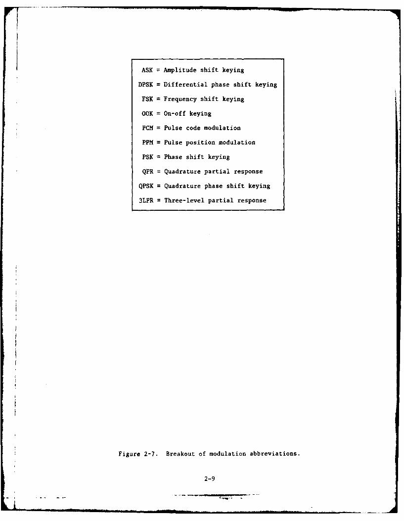
ASK = Amplitude shift keying

DPSK = Differential phase shift keying

FSK = Frequency shift keying

OOK = On-off keying

PCM = Pulse code modulation

PPM = Pulse position modulation

PSK = Phase shift keying

QPR = Quadrature partial response

QPSK = Quadrature phase shift keying

3LPR = Three-level partial response

Figure 2-7. Breakout of modulation abbreviations.

2-9

PART 3- NETWORK TRAFFIC

3.1 Introduction

a. Traffic within the DCS networks consists of a wide variety of circuitsprovided to subscribers via several types of access. Circuit types are: (1)voice, (2) secure voice, (3) teletypewriter, (4) data, (5) facsimile, and (6)television. A subscriber is provided connection to another subscriber by thetwo methods--common user access lines via switchboards or excharig's and directlines (patched directly through the switch).

b. In the case of common-user lines, many subscribers must compete for alimited, or finite, number of lines (trunks, in telephone parlance) at a switch-

board, or exchange. During a busy period, a subscriber faces an increased prob-ability of receiving an all-trunks-busy signal and, hence, must hang up and tryagain at a later time. This probability is also called the probability of alost calL, or the probability of blocking--that is, the call is lost or blockedfrom completion. The probability of a lost call during the busy period is re-ferred to in the DCS as the grade-of-service (GOS). The DCA has establishedzriteria for acceptable GOS within the DCS network.

c. In the case of direct-access lines, a subscriber has direct access toanother subscriber with no blocking of calls. Actually, several subscribers mayuse the same telephone, but this factor has no impact on the network, since noblocking occurs within the system. Since there is no blocking within the sys-tem, no GOS can be calculated.

d. A network traffic analysis usually consists of (1) determining the num-ber of circuits between telecommunications facilities (such as switches, switch-boards, or exchanges); (2) the traffic load offered to these circuits (usuallyduring the busy hour, or 2-hour period); and (3) determining the resultant GOSfor both the baseline (original) and alternate routing situations. However,

traffic statistics such as busy-hour offered load and average holding time werenot available for this study. Therefore, the network analysis was performedfor Korea and Okinawa in terms of channels (circuits) lost due to rerouting of

traffic (on those links affected by ECM) over alternate routes when circuit res-

toration priorities (RP's) were considered. In addition, the reduction in GOSwas determined for common-user circuits. The following paragraphs describe the

methodology employed to accomplish this network traffic analysis.

3.2 Network Traffic Analysis

a. As previously stated, the methodology developed for this study was theresult of the unavailability of traffic statistics for the DCS in the Pacific

area in the form of busy-period load and average holding time. The traffic

analysis for this study was performed using the procedure shown in the flowdiagram of figure 3-1, and described in the following paragraphs.

b. The network traffic analysis for this study depends upon the resultsof the ECM and ECCM analyses. The link subjected to ECM is first evaluated to

determine whether the ECM is effective in disrupting the traffic on that link.

If it is not effective, there is no impact on the network traffic. If the ECM

3-1

ECM NO

EFFECTIVE

ES

ALO NOECCM NO IMPACTEFFECTIVE ON NETWORK

YES

SCHANNEL NCAPACITY N

FYES

T PART OF

REROUTED OVER

ALTERNATE ROUTES

DETERMINEPOSSIBLE DETERMINE NUMBER OFALTERNATE ROUTES CIRCUITS LOST ON AFFECTED

LINK AND ALTERNATE ROUTE LINKS

IDETERMINE BESTALTERNATE ROUTESALTERATE RUTESFOR SWITCHES AND SWITCH BOARDS,

DETERMINE REDUCTION IN

1 GRADE -OF -SERVICE DUE TOIDETERMINE SPARE ALTERNATE ROUTINGCHANNEL CAPACITIESON ALTERNATE

ROUTE LINKS

DETERMINE RESTORATION PRIORITIESAND TYPES OF CIRCUITS ON

AFFECTED LINK AND ALTERNATEROUTE LINKS

PERFORM ALTERNATE ROUTINGOF TRAFFIC CONSIDERING

RESTORATION PRIORITIES. TYPES

OF CIRCUITS, AND SPARE CAPACITIES

Figure 3-1. General flow of traffic analysis.

3-2

is effective, appropriate ECCM techniques are applied to the link and an eval-

uation is made to determine whether the ECCM is effective in restoring the linkto DCA availability standards. If it is not effective, all of the traffic onthat link must be rerouted over alternate routes. If the ECCM is effective, adetermination is made as to whether or not the link must operate at reducedchannel (circuit) capacity. If the channel capacity is not reduced, there isno impact on the network traffic. If the channel capacity is reduced, thatportion of the traffic which cannot be accommodated on the link must be reroutedover alternate routes.

c. Before traffic from the affected link can be rerouted, the best alter-nate routes must be determined from those available in the network. Alternateroutes are selected on the basis of their overall channel capacity, spare chan-nel capacity, and the type of circuits, by RP, traversing these routes. The RP'sof the circuits which must be rerouted must then be compared to the RP's of likecircuits on the alternate routes. Rerouting is then accomplished by loading thereroute circuits on the alternate routes in the following order:

(1) Alternate route spare channels are loaded with reroute circuitsin descending order of RP.

(2) Alternate route circuits are preempted in ascending order of RPand loaded with reroute circuits in descending order of RP. That is, RPOO cir-cuits on the alternate routes would be preempted by RP1A circuits from theaffected link, and so on. A list of RP's used by DCA is provided in figure 3-2.

d. After the traffic on the affected link has been rerouted over the alter-nate routes, the number of circuits (channels) lost due to preemption and/or in-sufficient channel capacity is determined for the affected link and the alternateroute links.

e. For common-user circuits between switches, switchboards, or exchanges,the reduction in GOS is determined by the following procedure:

(1) Determine the total number of circuits between the two terminalsof interest. For example, there is a total of 17 circuits between the overseasswitch (OSS) at Seoul, Korea, and the AUTOVON switch (SCA) at Fuchu, Japan.

(2) Determine the traffic capacity for the total number of circuitsbetween the two terminals for the DCA criterion GOS, using the GOS performanceobjective (PO) from reference 7, part 5, and the Erlang B trunk tables from ref-erence 8, part 5. For example, the traffic capacity for the 17 circuits betweenSeoul OSS and the Fuchu SCA for a GOS of 0.1 (10 percent overflow) is 525 hun-dreds of call seconds (CCS) for the busy period.

(3) Determine the resultant number of circuits between the two termi-nals after alternate routing is accomplished. As a hypothetical example, alter-nate routing resulted in a reduction in circuits between Seoul OSS and Fuchu SCAfrom 17 circuits to 5 circuits.

(4) Using the capacity determined in paragraph 3.2e(2) as the offeredload, the probability of a lost call (GOS) can be calculated using the ErlangB formula:

3-3

Restoration Priority (RP) Ranking

1A Highest1B'CID1E1F1G2A2B2C2D2E2F2G2H213A3B3C4A4B00 Lowest

Figure 3-2. DCA restoration priorities.

3-4

0

n.P (LC) ()

0 2 !n

where

P(LC)= the probability of a lost call, for high-usage trunks (circuits)where a subscriber receiving a busy signal is cleared from the system(i.e., he must hang up and try later).

to=the offered load, in erlangs = (the number of CCS)/36

n =number of trunks (circuits)

For example, in the case where the number of trunks (circuits) between the SeoulOSS and the Fuchu SCA is reduced from 17 to 5, the GOS can be calculated by in-serting to 525 CCS = 14.58 erlangs and n = 5 as follows:

14-58 5

5!P(LC) = ______________________ __

1+14.58 + 14.58 2 + 14.58 3 14.58 4 14.58 5

2! 3! 4! 5!

658,922.7

120P(LC)=

1 1.5 + 212.6 3099.7 + 45,193.6 658,922.72 + 6 24 + 120

5491.0

15.58 + 106.3 + 516.6 + 1883.1 + 5491.0

P(LC)5491.0P(LC) = 8012.58

P(LC) = 0.6852973 0.685

3-5

This means that 68.5 percent of calls attempted during the busy period will belost (receive a busy signal). The GOS has been reduced 58.5 percent through

the increase in P(LC) from 0.1 to 0.685.

3.3 Network Traffic Equations

a. Generalized traffic equations which permit calculation of probability

of a lost call (blocking) for a variety of situations encountered within theDCS are provided herein.

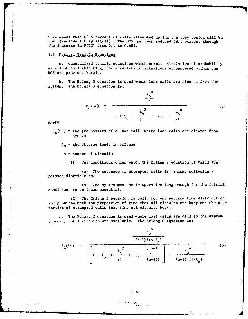
b. The Erlang B equation is used where lost calls are cleared from thesystem. The Erlang B equation is:

n

n!

P (LC) = (2)B2 n

0 o_++ 0-- + ... + -

where 2! n!

PB(LC) = the probability of a lost call, where lost calls are cleared fromsystem

to = the offered load, in erlangs

n = number of circuits

(1) The conditions under which the Erlang B equation is valid are:

(a) The sequence of attempted calls is random, following a

Poisson distribution.

(b) The system must be in operation long enough for the initial

conditions to be inconsequential.

(2) The Erlang B equation is valid for any service time distribution

and provides both the proportion of time that all circuits are busy and the pro-portion of attempted calls that find all circuits busy.

c. The Erlang C equation is used where lost calls are held in the system

(queued) until circuits are available. The Erlang C equation is:

n0

(n-l)!(n-Zo )

Pc(LC) = 2 (3)S2 n-I 2n

1+. + o + 0 +S 2! (n-l)! (n-l)!(n-o)

3-6

where

Pc(LC) the probability of a lost call, where lost calls are held in the sys-tem until circuits are available

to and n are as defined in paragraph 3.3b

(1) The conditons under which the Erlang C equation is valid are:

(a) The seqxence of attempted calls is random, following aPoisson distribution.

(b) The system must be in operation long enough for the initialconditions to be inconsequential.

(c) Service times are exponentially distributed.

(d) The offered load (in erlangs) is less than the number ofcircuits (Y 0 < n). This means that the rate of attempted calls cannot exceedthe average rate of call completions.

(2) The average waiting time for any order of service, for the con-

ditional case (excluding those calls that don't wait for service) is:

th

t = (4)1-(o/n)

and for the unconditional case (including those calls that don't wait for ser-

vice) is:

th

tw - PC(LC) (5)/- n)0

where

tw = the average waiting time (s) for service to begin

th = the average holding time (s) for all calls

(3) Equations 3, 4, and 5 are valid for any order of service of wait-ing calls.

d. The Poisson equation is used where calls which are not immediately ser-viced at the first attempt are held in the system for a period not exceeding theaverage holding time (th) of all calls, and are thereafter cleared from the sys-tem. The Poisson equation is:

n -£

£ e0

Pp(LC) = (6)

3-7

where

Pp(LC) = the probability of a lost call, where lost calls are held for aperiod (t < th), and then, if not serviced, are cleared from system

to and n are as defined in paragraph 3.3b

The conditions under which the Poisson equation is valid are:

(1) The sequence of attempted calls in random, following a Poisson dis-

tribution.

(2) The system must be in operation long enough for the initial conditionsto be inconsequential.

3-8

PART 4 - EQUIPMENT CHARACTERISTICS

4.1 Introduction. Presented herein are the equipment characteristics for the

DCS in the Pacific. Radio and multiplexer equipment characteristics are pro-vided for both the existing and planned LOS, tropo, and satellite systems. Inaddition, characteristics are provided for those data modems and telegraph multi-plexers identified in the DCS-Pacific station profiles. The characteristics for

the equipment now in, or planned for, the Pacific were obtained from varioussources, including technical manuals, DCS Applications Engineering Manual DCAC-

370-185-1 (dated May 1968, no longer published), open literature and periodicals,DCS Europe Vulnerability to Jamming RADC-TR-79 (dated July 1979), and ThreatAssessment Report MILSATCOM (dated October 1978).

4.2 Radio Systems

4.2.1 Line-of-Sight (LOS) Radio Systems

4.2.1.1 Analog Radio Systems. Characteristics for the analog LOS radio systems

in the DCS-Pacific are presented in figure 4-1. The characteristics include (1)nomenclature or model of the equipment; (2) frequency range, in MHz; (3) outputpower in watts and dBm; (4) 3-dB emission bandwidth, in MHz; (5) modulation

scheme employed at RF and baseband; (6) VF channel capacity; (7) receiver sensi-tivity, in dBm; (8) receiver noise figure, in dB; (9) IF 3-dB bandwidth, in M4Hz;(10) required signal level, in dBm; (11) type of combiner used; and (12) types

of diversity employed.

4.2.1.2 Digital Radio Systems. Characteristics for the digital LOS radio sys-tems in the DCS-Pacific are presented in figure 4-2. The characteristics in-clude (1) nomenclature or model of the equipment; (2) frequency range, in MHz;

(3) output power, in watts and dBm; (4) 3-dB emission bandwidth, in MHz; (5)modulation scheme employed at RF and baseband; (6) mission bit stream (MBS)

data rate, in Mb/s; (7) VF channel capacity; (8) receiver sensitivity, in dBm;

(9) receiver noise figure, in dB; (10) IF 3-dB bandwidth, in Mz; (11) requiredsignal level in dBm; (12) type of combiner used; and (13) types of diversityemployed.

4.2.2 Troposcatter and Diffraction Radio Systems

4.2.2.1 Analog Radio Systems. Characteristics of the analog tropo and dif-fraction radio systems in the DCS-Pacific are presented in figure 4-3. Thecharacteristics include (1) nomenclature or model of the equipment; (2) fre-quency range, in MHz; (3) output power, in watts and dBm; (4) 3-dB emission

bandwidth, in MHz; (5) modulation scheme employed at RF and baseband; (6) VF

channel capacity; (7) receiver sensitivity, in dBm; (8) noise figure, in dB;(9) IF 3-dB bandwidth, in MHz; (10) required signal level, in dBm; (11) typeof combiner used; and (12) types of diversity employed.

4.2.2.2 Digital Radio Systems. Characteristics for the digital tropo systems

in the DCS-Pacific are presented in figure 4-4. The characteristics include

(1) nomenclature or model of the equipment; (2) frequency range, in Mz; (3)

output power, in watts and dBm; (4) 3-dB emission bandwidth, in MHz; (5) mod-

ulation scheme employed at RF and baseband; (6) MBS data rate, in Mb/s; (7) VF

channel capacity; (8) receiver sensitivity, in dBm; (9) noise figure, in dB;

(Text continued on page 4-6)

4-1

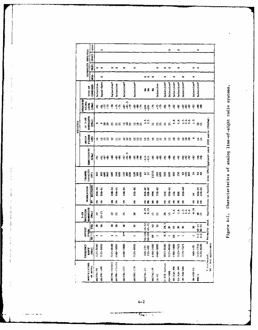
q 4 a Cc a * 4 0 0 4 04

- 00 0 00 0 000 004~ 00 00 W 00000 0

T. I T a I, I~ TI T T T

41 -c -c - .-0 - -

;:a 0 II 00 Coco0

- .0~ 0 .in . a 1. al" -1 co vnii 0 N N N N N

ina 00 cc ccO in 9-,8 cccc0 c

0 0 . . c

In Nw % N W N 0 .4 N N N) N6 W 0 0 o

- h-C

twwm :1 ll I =

4-2I-

x x

- a.

t Z

. . . . . . . . . . . . .4

c4 0 w0000000w0000000000

Inc U U U U J C UJUUJU

Wi ~ u ~ E wa ~ e~m@1 ~c cc.~ll~mm4mm 0.~m ccCc

Itii~lU~UIWU OOllO~tm~ oC

416O

'-I

aoi 00 w - - - - - -0-lsZ'. NN.INN7.4 ~-g~4~NNS *

0000000 0000000000

g w-2 U ) u u Ku 0iiu uNi . . l u- uu uN07

z ~ ~ ~ 0 m KK .KKK KNNKK

00

z N 0.N ~ a. NK- .0 NK- s0- NK. .

Z Z

4-3)

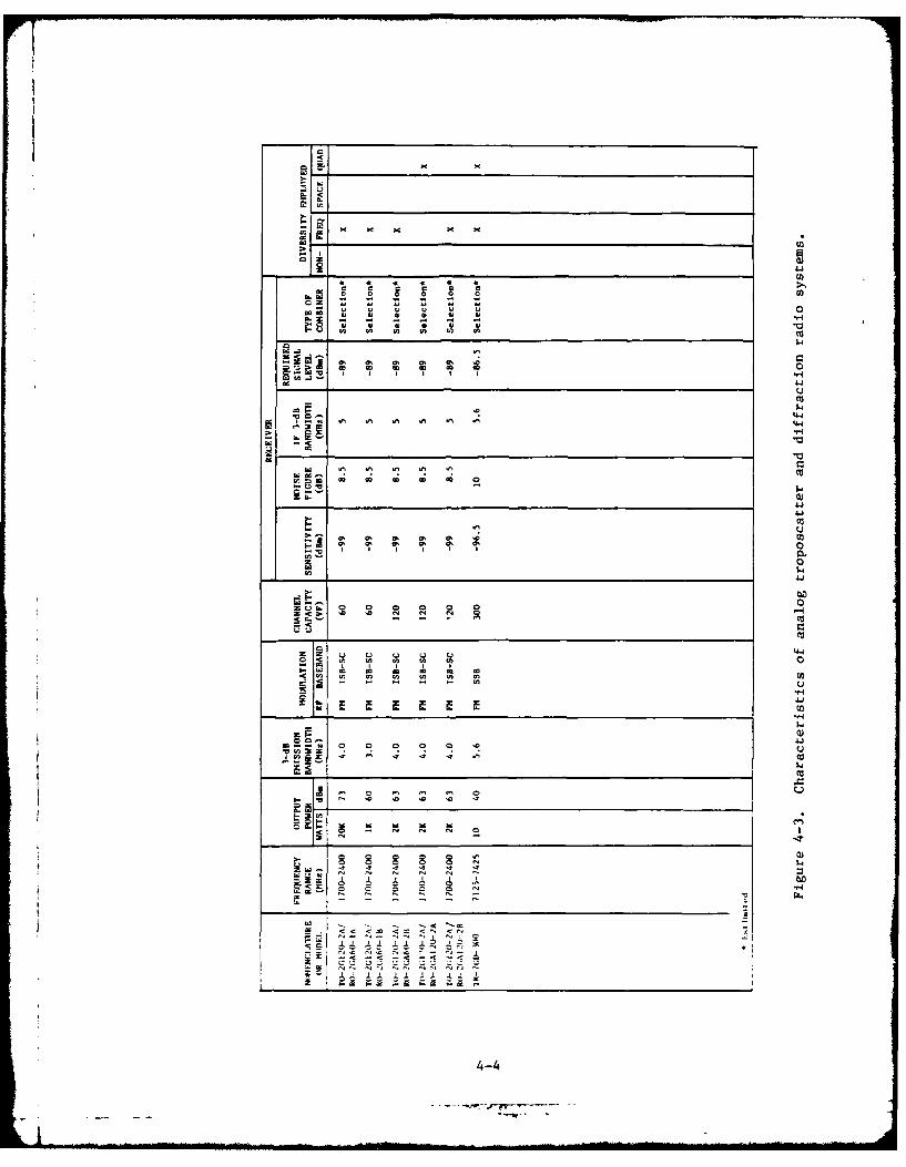
1'1~ U: P%

1 A.

4-b

o 0 0 0

z-z ~ i

I z 4 I-4U) Jto

03

C! C! 4-

U:4-4

II

C. u

"z -

- -aC-

0'0

0

00

LS a

0

W.~

4-

(10) IF 3-dB bandwidth, in MHz; (11) required signal level, in dBm; (12) type

of combiner used; and (13) types of diversity employed.

4.2.3 Satellite Terminal Radio Systems. Characteristics for the satellite

terminals in the DCS-Pacific are presented in figure 4-5. The characteristicsinclude (1) nomenclature of the terminal; (2) frequency range, in MHz; (3) out-

put power, in watts and dBm; (4) 3-dB emission bandwidth, in MHz; (5) modulation

scheme employed at RF and baseband; (6) receiver sensitivity, in dBm; (7) noisefigure, in dB; (8) IF 3-dB bandwidth, in MHz; (9) required signal level, in dBm;

(10) antenna diameter, in feet; and (11) antenna gain, in dB, and beamwidth, in

degrees, for midband transmit and receive frequencies.

4.3 Multiplexers

4.3.1 Analog Multiplexers. Characteristics for the analog multiplexers in the

DCS-Pacific are presented in figure 4-6. The characteristics include (1) no-menclature or model; (2) type of multiplexing employed; (3) modulation used;(4) channel capacity; (5) baseband frequency range, in kHz; and (6) input andoutput levels, in dBm per channel.

4.3.2 Digital Multiplexers. Characteristics for the digital multiplexers inthe DCS-Pacific are presented in figure 4-7. The characteristics include (1)

nomenclature or model; (2) type of multiplexing; (3) number of inputs; (4) max-imum output data rate in b/s; (5) input and output modulations employed; and

(6) data modes capable of being handled (asynchronous or synchronous).

4.4 Data Modems and Telegraph Multiplexers

4.4.1 Data Modems. Characteristics for the data modems in the DCS-Pacific are

presented in figure 4-8. The characteristics include (1) nomenclature or model;(2) minimum and maximum data rate, in b/s; (3) modulation scheme used; (4) du-

plex mode capability (half or full); and (5) data modes capable of being handled

(asynchronous or synchronous).

4.4.2 Telegraph Multiplexers. Characteristics of the telegraph multiplexers

in the DCS-Pacific are presented in figure 4-9. The characteristics include(1) nomenclature or model; (2) number of teletypewriter channels multiplexed;(3) number of VF channels into which the indicated number of teletypewriter

channels are multiplexed; (4) modulation scheme used; (5) multiplex scheme used;(6) maximum speed in bauds; (7) frequency deviation per channel, in Hz; (8) in-put and output VF signal levels, in dBm per channel; and (9) types of diversity

employed.

4.5 Passive Reflectors

4.5.1 Introduction. Passive reflectors are employed on a number of LOS links

in the Pacific area to overcome obstructions, reduce the number of active re-

peaters, or in the case of tower-mounted reflectors, reduce the length of wave-

guide runs, thus reducing line losses. Two basic types of passive reflectors are

employed in the Pacific, (1) the periscope system which is a small passive re-

flector mounted on the same tower (usually above and within the near-field) as

the parabolic antenna and (2) the large billboard reflector which may be in-

stalled anywhere between the distant station antennas and may, or may not, be

(Text continued on page 2-13)

4-6

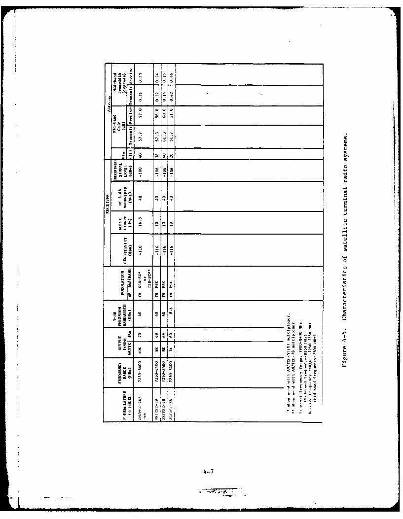
*1 10

r! ,,

0IrI

41

rCA4

0

0 000

,1-

=~I)

0 000s

Go w+ .0

4-7

I- "

Z 0 0n 0 0 U,) 'T- 00401 " I + + ~ -

z

r. + + +

zI. _D____ ____U -- 4

Z~cl '0 '0'0 '0 0 0 '0 U,'0 '.z bd .-I -T coC4 - o 0 -I 00-4 IT - co 10 -D' T0 -

0

04 40C e'0 D 00 0 0 4 0 C 00 0l J.J 0 ' 0

CD 00 0e TJ 0 0 C 00 0CD ID 0 04j 0 00 00 0

C,4 -4 %0 100

C)C

0-44

0C)

00

-.

> ~ >

%01- C-") 01

E ,(' -4 E- H- I

-~~ -0 zN ('. z,. ' - N -?

4-8

-4 1A

W ~uZ-- o ~C

go .4 4 C14 - C1 II II I I z z

-4

~ w E-

r. 0 + +++ I + z Z

W 1 1 0 -T 0 -- T

z~~ Cod 0 000' 0 Nu

0000 04 T C '.00 0N 00'. C14

I I I. -. ~.0. '. '. ' -4 ' L

0 C C4ciC %1 0 C) C- C-4 e4C'c'.J C' .J0 J- - -H_ _

< - - 0. ocl or

U U,

-~~ Q) N -. U C)

U) W In V) n I n V) U) )

0 n 0- V3j W W U j4 U

0 0 Cl

z w

0 x- -4

a)) w

CL. 0-4 ra.a )4P L 41-4 0

00

col -4

0) :D

00 Ct0 "Z

K ~CW W ,

H L) > ~ V) 4z I: .1

4-9

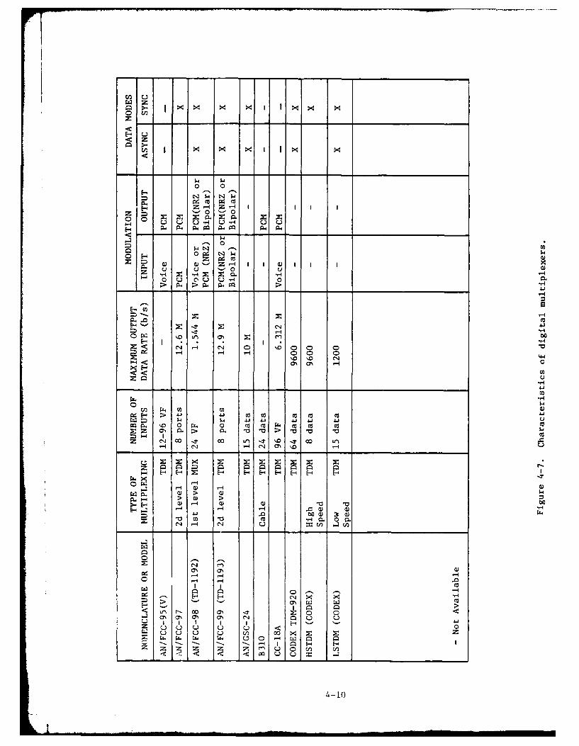
0 En ~ X~

0 0~

0 P4

1- -1 Z 10 0

0'~ '-'0a- U U U-H --4 U UE-4 P A 0 A q P L

,. 0

0 E-4 0 N p

Q) ) Z I IJ u '-0 C)

z Z - Z 0. .-H -40 u W u u " 0 P

E- a)

r--4

-4 -

E I 0*-H-

C'4 -4 ' , 0 000 0

'41

P4 E-4 0> 0 c 0 ca co coA. ' 0.~ 0x 0 co Cf 44 0y w co 1

C-4 e' .4 c' 7% ~ ,

E- H -4 H H- H- H H-

-44 > a) >4

E.~~ Q)- ) w" a0-4 -4 = a) -H

0

C'

W' a

0r - 00 (ON '-

-Z (a' a' a% as C140

Z U Un U U U

4-10

w- Z

Sx Ixxx.< 11X ix x I

z

cicn

94 .z- m 0

0 pq 0

0 -4 CLU)-)MP

.14

cci,0 0 C) 0 C)

-- - O M M -4C4 c

liii coo Lt)0C0mV Z0400 0 1 N 0 z

Cl)4- 14 t

I I I I I 1 0. 0 0 0 0 0 0 1 0 0 I I I II I I I I cn C z Z z z Z Z in I 0r z Z I I I I

I I+ + +

::3 o 0lz A 4.j 4j

C) (D0II c I C 0 C) I I I I I

<-C

cj) 0 0 0 0 0 0 0 0 0 0"~ ". 4. 4j .4 .4 .4- 4a 4.4

> 1 n Vr, 'D 'o 'D0 'D Ln I I C C U UI I I I

-- a

'n r' C-4 .f n C1, C r'C r C

N T N 7 No N1 N 11 m I C cn I I+ 1-I+1 +1 1I 1I +1 +1 +-!

m___ _ _____4t 00

('4

-4

E- m-

- CH

-31

CO F- Zi 9L Cf 0 i D / (I0 -.r 10 lo x ~ (fl (c w J c ( w / I

C1 C

c 'r- 0- - - -- - I

w~~~ -ju u u uz I 1 I

C'44

C Zt 7 4 7 Z - Z 0o

+4 1

within the near-field of one or the other. In some instances, because of pecu-

liar path geometry, double billboard reflectors are employed. The method of

calculating gain for passive reflectors is the same for either the periscope

system or the billboard system. The two basic passive reflector configurationsare shown in figure 4-10.

4.5.2 Passive Reflector Gain. The gain of a passive reflector is determined

by the following procedure:

a. Determination of the effective area of the reflector:

a2 = A cos a (1)

where

a 2 = the effective area of the reflector (ft2)

A = the actual area of the reflector (ft2)

a = the angle of incidence--the angle between the boresight of the parobolicantenna and the normal to the surface of the passive reflector (degrees)

b. Determination of the wavelength:

A = 0 .98 36 /fGHz (ft) (2)

c. Determination as to whether the passive reflector is in the near-field

of the parabolic antenna:

ird (3)k 20 4a2

where

k° = parameter used to determine whether passive reflector is in the near-

field of parabolic antenna

d = distance between antenna and passive reflector (ft)

If ko > 2.5, the passive reflector is not in the near-field, and the gain is cal-

culated as follows:

G = 20 log (dB) (4)GPR2

4-13

• -- " -" ' |ra m II I I I - I

R4

REFLECTOR

d Ci -45o

\ PARABOLA

(a) PERISCOPE SYSTEM (SIDE VIEW)

REFLECTOR

D2

(bi BILLBOARD SYSTEM (OVERHEAD VIEW)

WHERE:R - LARGEST DIMENSION OF PASSIVE REFLECTOR (FEET)d - DISTANCE BETWEEN ANTENNA AND PASSIVE REFLECTOR (STATUTE MILES)o - DIAMETER OF PARABOLIC ANTENNA (FEET)0a - ANGLE OF INCIDENCE (DEGREES)

Figare 4-10. Passive reflectors.

4-14

f

where

GPR = gain of the passive reflector (dB)

If ko < 2.5, the passive reflector is in the near-field, and the gain is deter-mined by first calculating the parameter, ro:

rO D D /4a2 (5)

where

r° = parameter used in calculating near-field gain of passive reflector

D = diameter of parabolic antenna (ft)

The near-field gain is then determined from figure 4-11, using parameters kand rO .

4.5.3 Sample Calculation

a. To illustrate the method of determining passive reflector gain, a sam-ple calculation is provided. The example is LOS link M1085 between Kadena andNaha, in Okinawa. The Kadena terminal employs a periscope system, with an 8by 12 foot rectangular reflector mounted 47 feet above a 6 foot parabolic an-tenna. Although the link employs frequency diversity, only one frequency isused in the following calculations in the interest of brevity.

b. The effective area of the reflector from equation 1 is:

a2 A cosa

where

A = 8 x 12 ft = 96 ft2

a = 450

and

a2 96 cos (45) = 67.9 ft2

c. The wavelength at the frequency of interest, 4.712 GHz is:

Xfi 0.98361fGHz

X= 0.9836/4.712

X = 0.209 ft

4-15

+6 - ALL CURVES ASYMPTOTIC TO 20 LOG4

-,o-O.4

+31---.+ +

ro- 0.8 6 :

T ro " 10 !t't:

Hil

0 . L . I

. .- -1 4111

-3 Zz -,n.TI ~~ ~ I ' C4:::

-4 ~ ~~~ 1 L. ,,H

-5~~ 0 ::'

i0

-7 . . .

-12 " " : :i: + :

0.1 0.2 0.3 0O4 0.5 0.6 0.7 1.0 2.0 3.0

0.8 0.9k,

Figure 4-11. Near-field gain for rectangular passive reflectors.

d. To determine whether the reflector is in the near-field of the para-

bolic antenna, calculate ko:

d 9(0.209)(47) 30.9k - .- -0.11

0 4a2 4(67.9) 271.6

Since ko < 2.5, the passive reflector is in the near-field.

e. To determine the near-field gain, first calculate ro:

ro = D ;7/4a2

ro = 6 jf /271.6

ro = 0.65

f. The near-field gain is determined from figure 4-11 for ko = 0.11 and

ro = 0.65 --

(1) Finding ko = 0.11 along the abscissa of the graph.

(2) Finding the curve for ro = 0.65--actually by interpolating be-tween the curves for ro = 0.6 and ro = 0.8.

(3) Determining the gain, G (dB), on the ordinate--GpR f + 0.6 dB(by interpolation) which was rounded of to 1 dB for this study.

4.5.4 Propagation Loss. Calculation of propagation path loss for links usingpassive reflectors depends upon the type of configuration used. In the case ofthe periscope system, only the propagation path loss between the distant termi-nals is used, since the reflector is in the near-field of the parabolic antenna.In the case where a billboard passive reflector is in the near-field of one par-abolic antenna, only the propagation loss between the billboard and the distantantenna (far-field distance) is used. In the case where the billboard reflectoris in the far-field of both antennas, the propagation path loss between thebillboard and each antenna must be calculated. Propagation loss (Ls) for thefar-field condition is calculated by:

Ls = 97 + 20 log f + 20 log D (dB) (6)

where

f = frequency (GHz)

D = path length (statute miles)--use dI and/or d from figure 4-10(b)

4-17

PART 5 - REFERENCES

(Section III only)

1. W. T. Barnett, "Multipath Propagation at 4, 6, and 11 GHz," Bell SystemTechnical Journal, Volume 51, Number 2, February 1972.

2. Technical Note 101, "Transmission Loss Predictions for Tropospheric Commu-nications Circuits," P. L. Rice, A. G. Longley, K. A. Norton, and A. P. Barsis,National Bureau of Standards, May 7, 1965.

3. A. Vigants, "Space-Diversity Engineering," Bell System Technical Journal,Volume 54, Number 1, January 1975.

4. "Engineering Considerations for Microwave Communications Systems," GTE

Lenkurt, Inc., 1972.

5. A. B. Crawford, D. C. Hogg, and W. H. Kummer, "Studies in TroposphericPropagation Beyond the Horizon," Bell System Technical Journal, Volume 38,Number 5, September 1959.

6. ESD-TR-75-013, "Communications/Electronics Receiver Performance Degradation

Handbook (Second Edition)," published jointly by the Frequency Management Support

Division, Office of Telecommunications, U.S. Department of Commerce, and the DoDElectromagnetic Compatibility Analysis Center, August 1975.

7. DCAC 310-130-2, "Communications Requirements, Defense Communications System

Management Thresholds (MT) and Performance Objectives (PO)," Defense Communi-cations Agency, 13 February 1979.

8. FM 11-486-2, "Telecommunications Engineering Traffic," Department of theArmy, January 1978.

5-1

DAT

Fl, ILMI

p T