AD-A243 473IIiiI !, !!1 !ESL-TR-90-44

FEASIBILITY OF A 6-INCH SPLIT HOPKIN-

SON PRESSURE BAR (SHPB)

* E. L. JEROME

*', :SVERDRUP TECHNOLOGY, INC. .SP. 0. BOX 1935

EGLIN AFB FL 32542

JANUARY 1991

FINAL REPORT

MAY 1989 - JULY 1990

APPROVED FOR PUBLIC RELEASE: DISTRIBUTIONUNLIMITED

91-17540

AIR FORCE ENGINEERING & SERVICES CENTER

ENGINEERING & SERVICES LABORATORYTYNDALL AIR FORCE BASE, FLORIDA 32403

NOTICE

PLEASE DO NOT REQUEST COPIES OF THIS REPORT FROM

HG AFESC/RD (ENGINEERING AND SERVICES LABORATORY),

ADDITIONAL COPIES MAY BE PURCHASED FROM:

NATIONAL TECHNICAL INFORMATION SERVICE

5285 PORT ROYAL ROAD

SPRINGFIELD, VIRGINIA 22161

FEDERAL GOVERNMENT AGENCIES AND THEIR CONTRACTORS

REGISTERED WITH DEFENSE TECHNICAL INFORMATION CENTER

SHOULD DIRECT REQUESTS FOR COPIES OF THIS REPORT TO:

DEFENSE TECHNICAL INFORMATION CENTER

CAMERON STATION

ALEXANDRIA, VIRGINIA 22314

UNCLASSIFIED

SECURITY CLASSIFICAT:ON OF THIS PAGE

Form ApprovedREPORT DOCUMENTATION PAGE OMB No. 0704-0188

la. REPORT SECURITY CLASSIFICATiON lb RESTRICTIVE MARKINGS

UNCLASSIFIED

2a. SECURITY CLASSIFICATION AUTHORITY 3, DISTRIBUTION/AVAILABILITY OF REPORTApproved for public release

2b DECLASSIFiCATION/DOWNGRADING SCHEDULE Distribution unlimited

4 PERFORMING ORGANIZATION REPORT NUMBER(S) 5. MONITORING ORGANIZATION REPORT NUMBER(S)

TEAS-SAA-891014 ESL-TR-90-44

6a. NAME OF PERFORMING ORGANIZATION 6b OFFICE SYMBOL 7a. NAME OF MONITORING ORGANIZATION(If applicable)

Sverdrup Technology, Inc. Air Force Engineering and Services Center

6c. ADDRESS (City, State, and ZIPCode) 7b ADDRESS(City, State, and ZIP Code)

P.O. Box 1935 HQ AFESC/RDCMEglin AFB, FL 32542 Tyndall Air Force Base, Florida 32403-6001

Ba. NAME OF FUNDING/SPONSORING 8b OFFICE SYMBOL 9 PROCUREMENT INSTRUMENT IDENTIFICATION NUMBERORGANIZATION (If applicable)

F08635-86-C-0116

8c. ADDRESS (City, State. and ZIP Code) 10 SOURCE OF FUNDING NUMBERS

PROGRAM PROJECT TASK WORK UNITELEMENT NO. NO NO ACCESSION NO.

11. TITLE (Include Security Classification)

Feasibility of a 6-Inch Split Hopkinson Pressure Bar (SHPB)

12. PERSONAL AUTHOR(S)

Jerome, Elisabetta L.

13a. TYPE OF REPORT 13b. TIME COVERED 14. DATE OF REPORT (Year, Month, Day) 15 PAGE COUNT

Final FROM May 89 TOJuly 90 January 199116. SUPPLEMENTARY NOTATION

Availability of this report is specified on reverseof front cover.

17. COSATI CODES 18. SUBJECT TERMS (Continue on reverse if necessary and identify by block number)

FIELD GROUP SUB-GROUP

Split Hopkinson Pressure Bar

19 ABSTRACT (Continue on reverse if necessary and identify by block number)

The objective of this study was to assess the feasibility of a 6-Inch Split Hopkinson

Pressure Bar (SHPB) using a mathematical and a numerical analysis. It was shown how by

increasing the input pulse duration by the same amount as the diameter change, the wave

propagation problem remains mathematically the same. This study also suggests a way to

correct for friction and inertia effects.

20 DISTRIBUTION/AVAILABILITY OF ABSTRACT 21 ABSTRACT SECURITY CLASSIFICATION

(3 UNCLASSIFIEDIUNLIMITED 0 SAME AS RPT C: DTIC USERS UNCLASSIFIED

22a NAME OF RESPONSIBLE INDIVIDUAL 22b TELEPHONE (Include Area Code) 22c OFFICE SYMBOL

Capt. S. T. Kuennen (904) 283-4932 HQ AFESC/RDCM

DIO Form 1473, JUN 86 Previous editions are obsolete SECURITY CLASSIFICATION OF THIS PAGE

i(The reverse of this page is blank.) UNCLASSIFIED

EXECUTIVE SUMMARY

The main objective of this study was to assess the

feasibility of a 6-inch Split Hopkinson Pressure Bar, SHPB, to

test cementitious materials at high rates of loading. There is a

need to do non-destructive tests on concrete structures, but the

current SHPB's are only 2 to 3 inches in diameter and therefore

they are not able to test material samples 6-inches in diameter

which is the typical size of concrete specimens cored in the

field.

This effort included a thorough mathematical analysis in

parallel with numerical calculations. The study focused on the

SHPB system, the assumptions made, their validity in a larger

apparatus, and the problems and issues associated with a size

change.-

It was shown how by increasing the input pulse duration by

the same amount as the diameter change, the wave propagation

problem remains mathematically the same. However, the larger

SHPB will differ from the existing smaller ones in the treatment

of the specimen. Friction and inertial effects cannot be

neglected any longer. This study suggests a way to correct for

these effects in the data analysis phase.

The results of this study indicate that mathematically a

pressure bar system can be scaled up or down to any degree,

without affecting particle motion. A 6-inch SHPB is thus

feasible if one can produce an input pulse of the required

duration. The results also point out the potential errors in

such a large system because of specimen friction and inertia.

iii

Recommendations for further work include more numerical

calculations, especially needed to fully understand the effects

of the specimen. Also, it is worth considering more innovative

methods of data collection and pressure input, still maintaining

the basic, well proven SHPB approach.

iv

PREFACE

This report was prepared by Ms. E. Jerome, Sverdrup, Inc.,Technical Engineering Acquisition Support (TEAS) Group, P.O. Box1935, Eglin AFB, Florida. The work was conducted for the AirForce Engineering and Services Center, Engineering and ServicesLaboratory, Air Base Structural Materials Branch, HQ AFESC/RDCM,Tyndall Air Force Base, Florida 32403-6001. The work wasconducted under TEAS Task Order No. SAA-891014 for MSD/SAA, EglinAFB, FL 32542-5000. Mr. J. A. Collins served as the programtechnical manager for MSD/SAA. Capt. S. T. Kuennen served as theprogram technical manager for HQ AFESC/RDCM. This reportsummarizes work conducted between 1 May 1989 and 31 July 1990.

This report has been reviewed by the Public Affairs Officeand is releasable to the National Information Service (NTIS). AtNTIS it will be available to the general public, includingforeign nationals.

This report has been reviewed and is approved forpublication.

T. KUENNEN, CAPT, USAF NEIL H. FRAVEL, Lt Col, USAFProject Officer Chief, Engineering Research

Division

LOREN M. WOMACK, GM-14, DAF FRANK P. GAL GHER I I, Colonel, USAFChief, Air Base Structural Director, gineeri a and ServirpqMaterials Branch Laborat ry

Z

( r.....e o. ...... ...

ii

V,. -

(The reverse of this page is blank)

TABLE OF CONTENTS

Section Title Page

INTRODUCTION......................................... 1I

A. OBJECTIVE.......................................1IB. BACKGROUND...................................... 2C. APPROACH........................................ 3

II MATHEMATICAL ANALYSIS............................... 4

A. SHPB ASSUMPTIONS................................ 4B. EQUATIONS OF MOTION............................. 6C. SOLUTIONS OF FREQUENCY EQUATION................ 8D. TRANSIENT BEHAVIOR............................. 16E. NUMERICAL ANALYSIS............................. 17F. COMPROMISES..................................... 18

III DISCUSSION.......................................... 20

A. DISCUSSION OF ANALYSES......................... 20B. CORRECTIONS..................................... 23C. NUMERICAL RESULTS.............................. 25

IV CONCLUSIONS/RECOMMENDATIONS........................ 31

REFERENCES...........................................33

APPENDIX

A WAVEFORM COMPARISON FOR BARS OF THREE............. 36

DIFFERENT DIAMETERS

vii(The reverse of this page is blank)

LIST OF FIGURES

Figure Title Page

1 Pochhammer-Chree Solutions ....................... 11

2 Cross-Sectional Displacement ..................... 11

3 Longitudinal Stress and Strain at Center ........... 27

4 Longitudinal Stress and Strain at the Surface .... 28

5 Stresses at the Center of Bar .................... 29

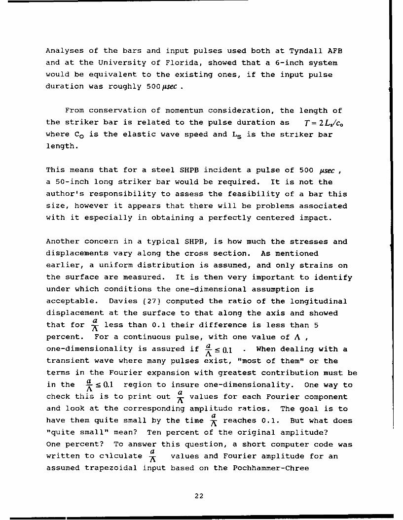
6 Stresses at the Surface .......................... 30

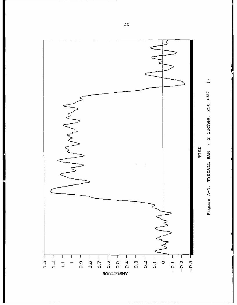
A-1 Tyndall Bar (250 microseconds) ...................... 37

A-2 Tyndall Bar (160 microseconds) ...................... 38

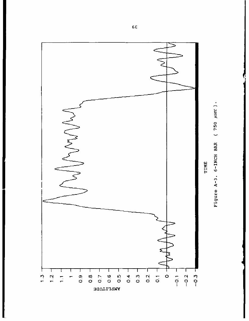
A-3 6-inch Bar (750 microseconds) ....................... 39

A-4 6-inch Bar (500 microseconds) ....................... 40

A-5 6-inch Bar (200 microseconds) ....................... 41

ix(The reverse of this page is blank)

SECTION I

INTRODUCTION

A. OBJECTIVE

The objective of this study is to determine whether a 6-inch

SHPB is feasible, whether the assumptions made in a typical

2-to-3 inch system still apply, and what major changes, problems

and issues would be associated with a system that size.

The Split Hopkinson Pressure Bar, SHPB, is used to study

materials at high strain-rates both in tension and in

compression. An SHPB system consists of a specimen sandwiched

between and in contact with two elastic bars - incident and

output bar. The incident bar is impacted by a striker bar at a

known velocity causing a pressure pulse to travel down the bar.

This wave is partially reflected at the incident bar/specimen

interface, partially reflected at the specimen/output bar

interface, and the remainder is transmitted to the output bar.

Two strain gages usually record the response of the reflected,

transmitted, and incident pulse. From these data stresses,

strains and strain-rates in the specimen can be computed as a

function of time.

Although different sizes of SHPB have been built, the largest

existing one is 3 inches in diameter. There are reasons behind

this size limitation: it is generally assumed the wave

propagation is one-dimensional, implying a high length to

diameter ratio. This apparatus has been around since the late

1940s when techniques and instrumentations were not as

sophisticated as they are today. Furthermore, there really never

was a need to test a material specimen larger than 3 inches in

diameter. The Air Force has been interested in concrete

structures for years and the only concrete specimens it can test

today at the strain rates typical of weapon's blast pressures are

in the 2-to-3 inch diameter range. Unfortunately, these

1

specimens cast in a laboratory are significantly different from

the type of concrete found on runways, shelters and other

structures. The major difference is the aggregate size.

Therefore, to obtain reliable results, full-scale destructive

tests usually need to be performed. This is both time consuming

and costly. There is then a need to use an SHPB type apparatus

to test concrete specimens, usually about 6 inches in diameter,

cored or cast directly in the field.

B. BACKGROUND

The mechanical behavior of concrete and other cementitious

materials at high rates of loading has been the subject of many

investigations in recent years. Understanding how the mechanical

properties of these materials depend on the rate at which

stresses are applied is essential to improve the design of

protective structures subjected to non-nuclear weapons effects.

The SHPB has proven to be a very effective and useful tool to

conduct material response studies since Kolsky [1] described its

use in 1949. Detailed discussions of how a typical system works

can be found in numerous papers including Hauser, Simmons and

Dorn [2], Lindholm [3], Malvern and Ross [4], Robertson, Chou,

and Rainey [5] and many others.

Because of the inherent difficulties associated with a system

of this kind, an idealized one-dimensional wave theory is

commonly assumed, where stress is uniformly applied over each

cross section, plane cross sections remain plane during motion

and stress and strain are uniform throughout the length of the

specimen. The above assumptions are adequate if the length of

the bar greatly exceeds the diameter to insure no end effects,

but factors like radial and axial inertia effects and friction

between the specimen and the bars can cause erroneous results if

care is not used in either conducting the experiment or analyzing

the data.

2

Approximate corrections for the calculated one-dimensional

stress have been formulated to account for inertial and

frictional effects. Kolsky [6] introduced a correction for

radial inertia. Davies and Hunter [7] discussed both friction

and inertia effects. Other papers of interest on this subject

are those by Rand [8], Dharan and Hauser [9], Samanta [10],

Jahsman [11], Chiu and Neubert [12], and Young and Powell [13].

The original SHPB apparatus was devised to study materials in

compression. More recently it was modified to also test

specimens in both tension and torsion. Examples of these

techniques are discussed by Nicholas [14], Lawson [15], Baker and

Yew [16], Jones [17], Okawa [18], Rajendran and Bless [20], and

Ross [21].

Follansbee and Frantz [22] used the Pochhammer-Chree

frequency equation to correct the recorded pulses for dispersion

as they travel down the bar assuming only the first vibrational

mode is excited.

C. APPROACH

An analysis of the implications of increasing the dimensions

in a SHPB, requires a thorough understanding of how the system

works, what has been done and assumed in the past, and what

equations govern its operation. This effort will include a

review of past studies on the subject, followed by a mathematical

analysis. Due to the complexity of the governing equations

numerical analysis will be conducted to gain insight of the

system's total response.

3

SECTION II

MATHEMATICAL ANALYSIS

A. SHPB ASSUMPTIONS

As discussed earlier, a one-dimensional wave theory is

generally assumed in the analysis of an SHPB. The

one-dimensional theory assumes longitudinal spatial variations

only. Applying Newton's law for a displacement u in the x

direction of the diagram below, the equation of motions for an

elastic system can be written as:

aaax

-uA +(a+ -dr) =pAdr-- ax a A

or au a2U au (la)

ii

where a is the stress, E is Young's modulus, E is strain, t is

time and P is the density of the material. Equation (la) can be

rewritten as follows:

-/ - (lb)

where E/pis the familiar elastic wave speed squared, or E/p=c2

The general solution to (ib) is of the form

u = f(x - Cot) + g(x + cot)

4

corresponding to forward and backward propagating waves.

Assuming u = g(x - cot) only, differentiate u and obtain

au = and a -cog

g' denotes differentiation of the function w.r.t. the argument

(x-c0 t). Solving for g' from each expressing then

au auat = C-C " - Co

strains are measured in an SHPB experiment at some distance from

the specimen. To obtain the displacements, the strains are

integrated directly over time, or

u = fo- cE i - -r) & and u2 - CoEdt

Where the subscripts i,r, and t indicate incident, reflected and

transmitted. Ui and u2are the specimen's displacements at the

input and output bars interfaces respectively. Let L be the

length of the specimen, from the above equation the strain in the

specimen isEs= (ut-U2)/L

and from the assumption of equal forces on each end of the

specimen Et = Ei + er

The specimen strain becomes ES =(-2cILfErdt

and the specimen strain rate ise, =-2 c"IL) E,

Using Hooke's law, the stresses on either face of the specimen

are

orz = E (A/A, ) Et and E =E(A/A )(i + Er)

where A/As is the ratio of the bar and specimen areas.

5

The problems with such a simplified one-dimensional theory

are numerous, even for long, slender rods, and are accentuated

for larger and shorter systems. First, longitudinal waves are

dispersive, (wave speed is a function o" frequency), even in the

fundamental mode; that means what is recorded at a distance from

the specimen is not the same waveform that actually arrives at

the specimen. Wave dispersion can be corrected for, but it is

time consuming and is not exact. The one-dimensional theory also

neglects stress and displacement variations across the cross

section. Since strains are measured only at the surface, this

can lead to errors.

B. EQUATIONS OF MOTION

To assess the validity of this simple theory, turn to the

equations of motion that govern a generalized SHPB. The equation

of motion is given as

d d2 UV-T+pb =p* (2)

T is the stress tensor, b are the body forces (which are usually

safely neglected), and d is the acceleration term. In

cylindrical coordinates, equation (2) becomes

a2U, -af+ ~- US 0 1 + au-0

at, ar r r

a3ue _ a 9 + 1 ae0 + a'g z + Gdr r W 9z r (3)

a2 - 1a + -r

at 2 ar W r z r

6

F/ds

L dO leo

Cyhndrical cooraW

Assuming axisymmetric conditions, so that the solution is

independent of theta, and using the elastic Hooke's law

relationships between stresses and displacements, thetwo-dimensional governing equations that need to be solved in anSHPB problem, can be obtained. Specifically, using the

constitutive relations,

Uff=¢ + 2u) -r + A +--u,

( ( Uz)u,

S - + - )(4)

Uz = (I + 2p) a-, + A + a --

where I and /u are Lame's constants, the following is obtained:

PI= (,I + 2p + + aZatr 82U, r ru.C 7

r2U Sr r2 H I-ia[ , u,] ___o n, 5

r r r

7

The boundary conditions require no stress at the surface or

arr=O and cr=O atr=a

where a is the radius of the bar. Also at a free end, orz= 0

and u=0 and at a rigid end, ciz=0 u z = 0

The initial conditions can be in the form of a step change in

pressureaz = -PH (t), arz = 0

where P is a uniform pressure and H(t) is the function of time,

or as a harmonic displacement of Uz =sin wt and a = 0.

Equations (5) have been solved by Pochhammer and Chree [6, 23,

27, 29] for a sinusoidal excitation. It is called the frequency

equation and has the form

2y- a J0 (ha) (2y2' - )J(Ka)f_0J2 p to =0 (6)

2u iJo (ha)- + 2 /- Jo (ha) 2#y -JI(Ka)

where h 2 = (2/A )2 (pc2/y+2$ 1) and K 2r/A )2 (pc 2/ _1)

A = wavelength , y = 2 and J0, and I are the zero and first order Bessel functions

C. SOLUTIONS OF FREQUENCY EQUATION

There are an infinite number of solutions to Equation (6),

each corresponding to a unique mode of vibration. The solutions

are exact only for an infinitely long cylinder; although, for a

cylinder whose length greatly exceeds its diameter the errors are

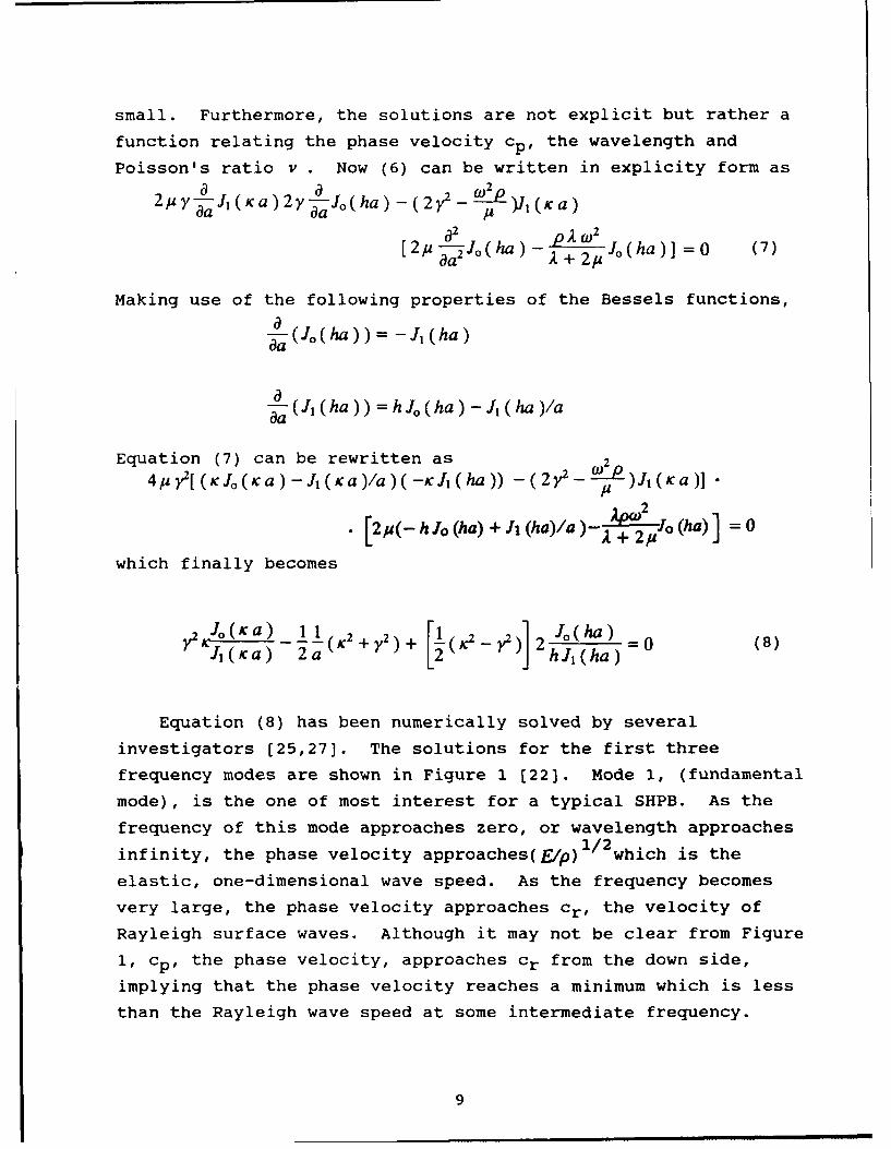
small. Furthermore, the solutions are not explicit but rather a

function relating the phase velocity Cp, the wavelength and

Poisson's ratio V . Now (6) can be written in explicity form as2y__IKa yIJ(a 22 W0 op)JI(Ka)

[2,u-4aJo(ha)- A (2Jo(ha)] =0 (7)

Making use of the following properties of the Bessels functions,

- ( J, ( ha ) ) = - J, ( ha)

--"( JI ( ha ) ) = h J, ( ha )-J, ( ha )1aa

Equation (7) can be rewritten as 24ju,[ (KxJ ( xa ) -J"icta )/a)( -K JI(ha )) -(2 y - a-- P).1(Kxa )] •

[2(-h Jo (ha) +J (ha)/a)-j+ Jo(ha)] =0

which finally becomes

J,(Ka)- (K2 +Y2)+ (2-)) 2h J(ha) =0 (8)

7(Ka) 2a [(I IJhJ(h)

Equation (8) has been numerically solved by several

investigators [25,27]. The solutions for the first three

frequency modes are shown in Figure 1 [22]. Mode 1, (fundamental

mode), is the one of most interest for a typical SHPB. As the

frequency of this mode approaches zero, or wavelength approaches

infinity, the phase velocity approaches(E/p) /2which is the

elastic, one-dimensional wave speed. As the frequency becomes

very large, the phase velocity approaches Cr, the velocity of

Rayleigh surface waves. Although it may not be clear from Figure

1, Cp, the phase velocity, approaches cr from the down side,

implying that the phase velocity reaches a minimum which is less

than the Rayleigh wave speed at some intermediate frequency.

9

Also, notice that the parameter h for mode 1 is always

imaginary since for all frequencies cp < cd where cd is the

dilatational wave speed in an infinite medium. Recall that

P tP

h2 = (2r/A) 2 (pc 2/A.+2# - l ) and K 2 =(2;/A) 2 (pc 2 / -)

aFor very low frequencies K is real, but past roughly 7.

0.65, when cp becomes less than ct, it too is imaginary. This

means that at low frequencies (a/A< 0.65), the displacement is

mainly transverse since the set of dilatational waves exists only

as a surface disturbance. At high frequencies the total

displacement becomes increasingly like a pure surface

disturbance.

Mode 2 and higher may be of interest in a "larger" SHPB and

at high frequencies. These modes have what are called cut-off

frequencies, i.e., frequencies at which the phase velocity

becomes infinite. From equation (8) this implies either that 7 =

0.0 or that Jl(Ka) 0.0. If y 0.0, equation (8) becomes

1(._ )2- ( = 2 Jo(ha)2 ct) ca 2t) hJ, (ha)

which can be rewritten as

(oo

2 /

Cd (Cd W i (a)Cd

10

1 .4

2 - +2Pu1.2-------------------- Cd

Cd(/C a

0 MODE 3 2=

o Cr= RAYLEIGH VELOCITYMODE 22

MODE 1 Co=-Ct/cop

----------------------

Cr / c

0.4

0.0 0.5 1.0 1.5 2.0

a/AFigure 1. Pochharnmer-Chree Solutions for First Three Modes.

1.0

I0.-z w dw7AQ

a_/ct) I/

N

0Az

1 0 0

r/a

Figure 2. Longitudinal Cross-Sectional DisplacementFor Various values of d

S025.

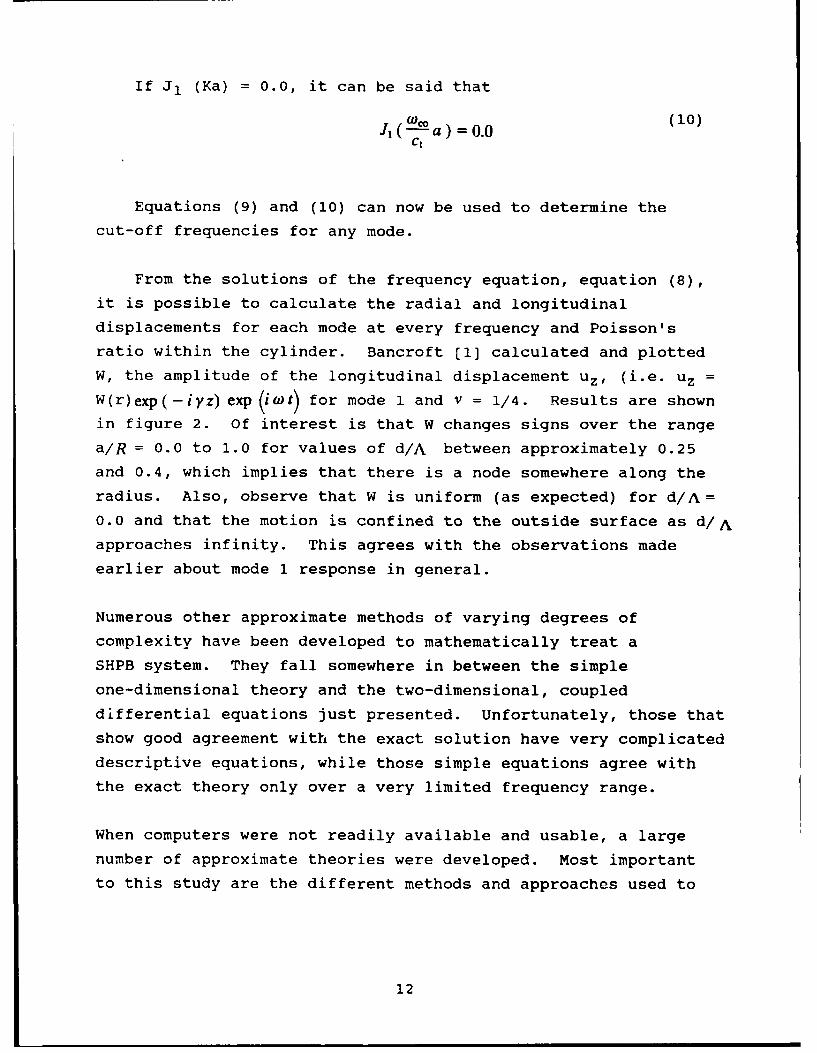
If Jl (Ka) = 0.0, it can be said that

S( a) = 0.0 ()Ct

Equations (9) and (10) can now be used to determine the

cut-off frequencies for any mode.

From the solutions of the frequency equation, equation (8),

it is possible to calculate the radial and longitudinal

displacements for each mode at every frequency and Poisson's

ratio within the cylinder. Bancroft [1] calculated and plotted

W, the amplitude of the longitudinal displacement uz, (i.e. uz =

W(r)exp(-iyz)exp(iWt) for mode 1 and V = 1/4. Results are shown

in figure 2. Of interest is that W changes signs over the range

a/R = 0.0 to 1.0 for values of d/A between approximately 0.25

and 0.4, which implies that there is a node somewhere along the

radius. Also, observe that W is uniform (as expected) for d/A=

0.0 and that the motion is confined to the outside surface as d/A

approaches infinity. This agrees with the observations made

earlier about mode 1 response in general.

Numerous other approximate methods of varying degrees of

complexity have been developed to mathematically treat a

SHPB system. They fall somewhere in between the simple

one-dimensional theory and the two-dimensional, coupled

differential equations just presented. Unfortunately, those that

show good agreement with the exact solution have very complicated

descriptive equations, while those simple equations agree with

the exact theory only over a very limited frequency range.

When computers were not readily available and usable, a large

number of approximate theories were developed. Most important

to this study are the different methods and approaches used to

12

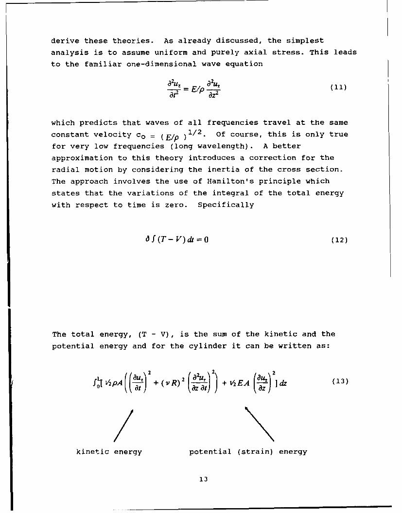
derive these theories. As already discussed, the simplest

analysis is to assume uniform and purely axial stress. This leads

to the familiar one-dimensional wave equation

atu a (11)

aZ'

which predicts that waves of all frequencies travel at the same

constant velocity c0 = (E/p )1/2. Of course, this is only true

for very low frequencies (long wavelength). A better

approximation to this theory introduces a correction for the

radial motion by considering the inertia of the cross section.

The approach involves the use of Hamilton's principle which

states that the variations of the integral of the total energy

with respect to time is zero. Specifically

6 f(T- V)& =O (12)

The total energy, (T - V), is the sum of the kinetic and the

potential energy and for the cylinder it can be written as:

2 V2 / 2 -"'(13

fy~pA (() +(vR) + V2 EA 1dz (13)

kinetic energy potential (strain) energy

13

where L is the length of the cylinder, R is the radius of

gyration about the z-axis, is Poisson's ratio, and the

velocities in the z and r directions are respectively

au '. an au ,- and atrat a

au,But Ur can be assumed to be of the form (-vr--) so that

au, a2

at az at

The result of substituting Equation (13) into (12) and solving

the integration by parts is as follows:

p ~az2 (4

This equation gives a better approximation to the exact theory

than Equation (11) at low frequencies. However, for short waves

the errors become considerable.

A third approximate theory developed by Love [29] is based on the

exact characteristic Equation (8), where the Bessels functions

are expanded in power series. If a, the radius of the cylinder,

is small enough to that ha and Ka are small compared to unity,

then powers of ha and Ka higher than the second can be neglected.

That is

JO(Ka) = 1 - 1/4 (Ka)2

Jl(Ka) = 1/2 (Ka)

14

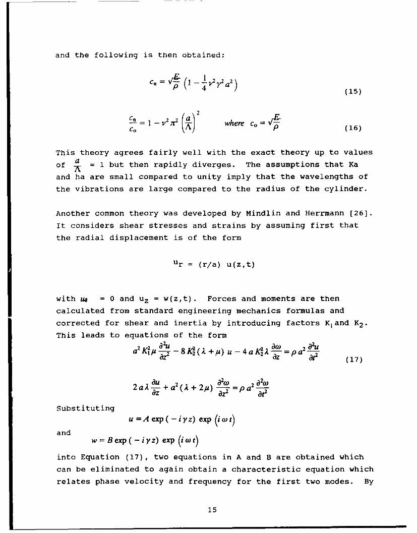
and the following is then obtained:

P 4 i±~~2 (15)

2

C V (X) w (16)

This theory agrees fairly well with the exact theory up to values

of a 1 but then rapidly diverges. The assumptions that Ka

and ha are small compared to unity imply that the wavelengths of

the vibrations are large compared to the radius of the cylinder.

Another common theory was developed by Mindlin and Herrmann [26].

It considers shear stresses and strains by assuming first that

the radial displacement is of the form

Ur = (r/a) u(z,t)

with u = 0 and uz = w(z,t). Forces and moments are then

calculated from standard engineering mechanics formulas and

corrected for shear and inertia by introducing factors K1 and K2.

This leads to equations of the form2U 2K 2 82 ua2i#( -- - 8 KI (A +,u ) u - 4 a I2 l- =p a -(7

(+u u. 4t (17)

2aA a -+ a 2( A + 2,u) --f pa 2 -

Substituting

u =A exp(-iyz) exp (i Wt)

and w=B exp( - iyz) exp (i Wt)

into Equation (17), two equations in A and B are obtained which

can be eliminated to again obtain a characteristic equation which

relates phase velocity and frequency for the first two modes. By

15

adjusting Kzand K1 , a very good approximation can be obtained for

mode 1. Mode 2 on the other hand shows considerable deviation

from the exact theory.

Many other theories have been developed and, in general,

their complexity is directly proportional to their accuracy.

These analyses are important because of the insight they give

into the response of a cylinder subjected to impulsive loading.

Knowing how stresses and displacements are distributed is crucial

to the study of wave propagation and SHPB systems.

D. TRANSIENT BEHAVIOR

So far, the discussion has been limited to continuous waves

or at least with pulses more than just a few cycles in length.

However, in an SHPB experiment a very short pulse is propagated

through the cylinder, giving rise to a transient behavior which

cannot be completely determined from the continuous theories;

therefore, a different approach must be taken. One way to tackle

the transient problem is to use Fourier analysis. By decomposing

the pulse into its continuous components, continuous wave theory

can be used on each component at any point down the bar and the

new pulse can be obtained by adding the pieces together again.

This method is not exact but it does give a close approximation,

especially at some distance from the source.

Choosing a mathematical function which describes the input pulse

and which can be represented by a reasonably simple Fourier

series is very difficult. Davies [27] used a trapezoidal pulse

while Kolsky [28] assumed an error function. In both cases the

Pochhammer and Chree curves are used to obtain the phase velocity

for each pulse. To calculate the new shape of the wave-forms,

only the fundamental mode is assumed to be excited.

16

Another approach taken by some investigators in studying

transient behavior is based on the concept of "dominant groups"

and the method of stationary phase. The idea is that if at the

beginning everything is in phase, any time after that all waves

are out of phase and, therefore, interfere destructively. When

the combined effects of all these waves are studied, the main

contribution comes from a small "dominant" group whose phase

velocities, periods and wavelengths are almost the same. By

focusing on this special group, one can obtain approximate

propagation of longitudinal, flexural and torsional waves in a

cylinder.

In this study the Fourier analysis approach was employed. It is

straightforward and can be easily simulated numerically.

E. NUMERICAL ANALYSIS

Due to the complexity of even the solutions to a

two-dimensional wave propagation problem, numerical methods must

be employed to fully describe the response of an SHPB system.

Over the past 20 years many investigators have tried

numerically to solve the governing equations of an SHPB system.

The various finite-difference schemes are straightforward but

tedious to derive. It seems pointless to start a numerical

analysis from scratch. After having understood the physics and

problems associated with a finite-difference approach, it does

appear worthwhile to look and make use of available computer

codes that were written specifically for this task. Considerable

time and effort were spent in identifying and trying to obtain

some of these programs. Two types of codes are available for

this type of problems. The first specifically addresses the

propagation of waves in a bar. The two most used are Toody [32]

and Hemp which were written for a SHPB and could easily be

adapted to the present needs. Unfortunately, they are quite old,

hard to find, and not be as sophisticated and efficient as they

17

could be. The second group is of a more general kind; from these

we could extract the modules ot interest to this study, examples

include Epic [31] and Hull [30].

Within the numerical arena contains is another worthwhile

aspect of this study. Specifically, one can compute, solve, and

present the Pochhammer and Chree solutions directly along the

length of the bar. If their solution is correct, these results

ought to match those of the governing equations numerical

solutions.

Both numerical representations can tell us what the wave

propagation looks like within the bar, and an analysis and

feasibility assessment of a larger SHPB will be possible. What

is of interest is the distribution of radial stresses and strains

at different stations along the bar to decide whether a

one-dimensional analysis is still reasonable or not.

Furthermore, the effects of friction and specimen inertia and

their relationship to the specimen size can be studied.

Because of the enormous complexity of the analytical

solutions, the computational approach is not only a valuable but

an indispensable tool. A comparison and analysis of the exact

solutions, and of the finite difference solution of the governing

equations will give a complete look at and understanding of an

SHPB system, and recommendations will be possible regarding a

"larger" bar.

F. COMPROMISES

Looking beyond the general equations of wave propagation in a

long cylindrical bar, focus is placed on the SHPB system.

Understanding the mathematical background makes it apparent that

the analyst must make many compromises. One problem may be

minimized and another may be magnified to reach some basic

assumption, and an important part of the system may be ignored.

18

For example, to minimize inertia the material specimen to be

tested should be as short as possible. To minimize friction, the

lenSth-to-diameter ratio of the specimen should be high. When

the material is concrete, a length-to-diameter ratio close to one

should be used in order to have the same number of aggregates in

both directions. This poses a problem for the experimenter who

must choose in essence which errors will be introduced in the

system. By minimizing friction, inertia will play an important

role; the reverse is also true. To properly test concrete,

neither friction nor inertia can be minimized. In the system as

a whole, it has been shown that to minimize dispersion the

diameter should be much less than the wave length, that is the

duration of the input pulse should be long compared to the time

taker for the pulse to travel a distance equal to the radius.

Also, the duration of the pulse should be much greater than

the transit time through the specimen. This last restriction

arises from momentum considerations, amd goes back to the basic

SHPB assumption of conversq'ion of momentum across the specimen.

The Pochhammer and Chree equaLidon sl. w that the longitudinal

stresses and displacements will vary radially and their

distribution along the cross section is directly dependent on the

frequency of the pulse. Since measurements in an SHPB are made

on the surface and assumed constant throughout the radial

distance, large errors could be introduced depending on the

specific conditions.

Radial inertia has also been addressed by several investigators,

it is probably due to the kinetic energy but its effects are

unknown.

Finally, it has always been assumed that only the fundamental

mode of vibration is excited in a typical SHPB. This appears

true for the conditions in the experimental setup, and analyses

based on mode 1 only have shown good correlation to experimental

data.

19

SECTION III

A. DISCUSSION

The particle motion in a bar is governed by the equations of

motion. Pochhammer and Chree independently solved these

equations for the propagation of a sinusoidal wave. The

solution, discussed in section II.A is the so called frequency

equation; it has an infinite number of solutions, one for each

mode, and results in a function relating Cp, Ap and v [wave

speed, wave length and Poisson's ratio]. These solutions are

valid and exact for infinitely long bars. If the bar is long

enough to eliminate end effects (10 diameter lengths) and if the

interest is in the transient pulse in its first passage, then the

infinite assumption is pretty good.

The Pochhammer and Chree solutions can be plotted in

non-dimensional form as shown in Figure 1. It is interesting toa _a an hsaC apnote that since A=c T, then a - a and t Co _ a

then if a is multiplied by a certain factor and T is also

multiplied by that same factor, then VS will notC o

change. What this means is that mathematically, under the

assumptions made, if the diameter is increased to 6 inches and

simultaneously the duration of the input pulse is increased bythe same factor, then the solution is the same. This applies to a

sinusodial, continuous input where the wavelength is constant,

and thus, it will travel at only one wavespeed relative to the

bar radius: a long wave in a large bar will have the same waveaspeed as a short wave in a small bar. As long as a stays

constant, nothing changes.

What happens if the input is a transient pulse? A simple

mathematical function can be chosen to describe this type of

input and it can be represented by a Fourier series. A transient

pulse is composed of a spectrum of frequencies; the higher

20

frequency components travel more slowly than the lower frequency

components, and thus lag behind and cause the initial sharp pulse

to spread. This spreading is called dispersion. The Pochhammer

and Chree solutions give the velocity of each wave depending onits frequency, and thus one can correct for dispersion by

calculating how far each frequency component has traveled in a

certain time, and then reassemble the pulse. This task basically

amounts to correcting for phase changes within each term of the

Fourier series. It is important to be able to correct for

dispersion since the strain gages recording the pulse are

typically 30 to 60 inches from the specimen. Interest is in the

response at the specimen itself but in many cases a gage cannot

be physically placed there. The dispersion correction technique

allows one to predict the shape of the pulse as it travels from

the strain gage to the specimen.

Further, following the same kind of reasoning as for the

continuous wave case, a Cp _ a

7%C nAtc,

can be written where n is the number of points taken to rep-esent

the transient pulse and At is the time interval between them.aIn essence nAt is the period of the transient pulse, and if

stays constant, the case is analogous to the continuous case, as

long as the radius and the pulse width are increased or decreased

by the same amount, the problem will not change.

This fact is important to this study because the main concern

is the feasibility of a 6-inch SHPB system. What the Por.hhammer

and Chree equations show is that if the incident pulse is of

large enough duration then, at least as far as the longitudinal

waves are concerned, there is mathematically no difference

between a 2-, 3-, 6- or 60-inch diameter SHPB. One must then

determine what pulse duration would be needed to make a new

6-inch system equivalent to the existing 2- and 3-inch bars and

whether a pulse that long can be produced. The answer to the

question of pulse period needed is fairly straightforward.

21

Analyses of the bars and input pulses used both at Tyndall AFB

and at the University of Florida, showed that a 6-inch system

would be equivalent to the existing ones, if the input pulse

duration was roughly 5001sec .

From conservation of momentum consideration, the length of

the striker bar is related to the pulse duration as T=2 L/cowhere Co is the elastic wave speed and Ls is the striker bar

length.

This means that for a steel SHPB incident a pulse of 500 psec ,

a 50-inch long striker bar would be required. It is not the

author's responsibility to assess the feasibility of a bar this

size, however it appears that there will be problems associated

with it especially in obtaining a perfectly centered impact.

Another concern in a typical SHPB, is how much the stresses and

displacements vary along the cross section. As mentioned

earlier, a uniform distribution is assumed, and only strains on

the surface are measured. It is then very important to identify

under which conditions the one-dimensional assumption is

acceptable. Davies [27] computed the ratio of the longitudinal

displacement at the surface to that along the axis and showed

that for a less than 0.1 their difference is less than 5

percent. For a continuous pulse, with one value of A

one-dimensionality is assured if A<0.1 When dealing with a

transient wave where many pulses exist, "most of them" or the

terms in the Fourier expansion with greatest contribution must be

in <0.1 region to insure one-dimensionality. One way toAnth reiotA - acheck this is to print out 7V values for each Fourier component

and look at the corresponding amplitude ratios. The goal is toahave them quite small by the time s reaches 0.1. But what does

"quite small" mean? Ten percent of the original amplitude?

One percent? To answer this question, a short computer code wasa

written to cilculate X values and Fourier amplitude for an

assumed trapezoidal input based on the Pochhammer-Chree

22

solutions. This allowed one to look at the values for the

existing systems at the University of Florida and at Tyndall AFB;

it was found that the amplitudes of the Fourier components hada

fallen to 5-9 percent of the original value by the time -N

reached 0.1. Therefore, a good value to use for the proposed

6-inch system is about 10 percent. This would assure the

one-dimensionality of the response. Notice that it does not

matter at which component a reaches 0.1, but rather the value

of the amplitude at that point. If it is at the 10th or the

100th term in the Fourier series it makes no difference.

As a check, calculations were made for a 6-inch bar and 500 usec

input pulse, and, as predicted from our earlier discussion, the

amplitude of the Fourier components drop off to 8 percent of

their original value before becomes 0.1. This is shown inTable A-1 in the Appendix for three bars, nominally a 2-inch, a

3-inch and a 6-inch bar, for an assumed trapezoidal input of

normalized amplitude of 1. Also included in the appendix is the

comparison of corrected waveforms for a 2-inch bar with a 250 psec

pulse and a 6-inch bar with a 750 1Ssec pulse, to show the

similarity, while a 6-inch bar with a 200 jsec pulse clearly

shows the deviation from one-dimensionality.

B. CORRECTIONS

Up to this point the aspects of wave propagation in a

cylindrical bar have been discussed. It has been established

that by choosing a pulse of a certain duration, the conditions of

a typical SHPB can be reproduced in a 6-inch diameter system. It

was shown that dispersion corrections can still be made assuming

only mode 1 vibrations and that the one-dimensional assumption is

still valid. The only provision is for the bar to be long enough

to avoid end effects.

23

A SHPB has, by definition, a specimen in between and in

contact with the input and the output bars. The specimen will

contribute inertia to the problem as well as errors due to

friction. As discussed in section II, there are ways to minimize

the effects of friction and/or inertia. To minimize friction a

good rule of thumb is to maintain 1d << 1. The values of u

are not quite known, and certainly not constant for any one case,

but from this the radius and the length of the specimen should be

a minimum, be of the same order of magnitude. Keeping that in

mind, we turn our attention to inertia; radial inertia is assumed

to cause a larger stress than that which would have resulted in

its absence. Davies and Hunter (7] calculated the contribution

of inertia based on the kinetic energy due to both axial and

radial motions. Their result is

L! _q g)dp2_ (18)

where ab is the measured stress, subscript s pertains to the

specimen and 'L and v24! are the axial and radial inertia6 S8

contributions respectively.

The length and the diameter of the specimen can be chosen so that

the second part of Equation 18 vanishes; thus the effects of

inertia and minimized. That is

L 2 2d 2

which leads to L _V (19)d 2- VS

For concrete, as an example, vs is roughly .22 and thus oneL ~would want an .2.

d

24

This result is consistent with the friction considerations, but

unfortunately not with the testing procedures for concrete. A

very impoi :ant factor in this material is aggregate size and

number. To properly test concrete the number of aggregates must

be the same in both directions; thus an L/d of one is usually

recommended. Therefore, both for a 2-inch as well as for a

6-inch SHPB, inertia effects cannot be cancelled. Therefore,

inertia effects cannot be cancelled for either a 2- or 6-inch

SHPB.

For a large system, like the one proposed, the inertia effects

cannot be ignored and the analyst would have to calculate the!Econtributions, based on the measured & , and add it to the

measured stress. Because quantities are known, this should not

be difficult.

Additionally, several investigators have calculated the effects

of radial friction and an additional contribution due to inertia

from the convective portion of the material derivative. Both

were found to be insignificant in a typical SHPB. This is

believed to hold true for a 6-inch system because the diameterdappears in the equation as d ratio, which is kept to about one

in all cases.

C. NUMERICAL RESULTS

The Lagrangian module in the hydrocode Hull [ ] was exercised

to numerically solve the equations of motion in a 6-inch elastic

bar subjected to a step input pressure. The enormous amount of

calculations in the code requires many hours of CPU time for just

a few microseconds of calculations.

25

The goal of this exercise was to answer two questions. Is

the motion one-dimensional and is it uniform in the radial

direction? These questions are important because they can

validate the conclusions made in the mathematical analysis and

thus reinforce the allegations of feasibility of a 6-inch system.

Figures 3 and 4 show the longitudinal stresses and strains at the

surface and in the center of the bar. Figures 5 and 6 show all

the stresses at those same points. All output was calculated

roughly 50 inches (1.27 m) from the impacted end, and the problem

was run for a millisecond. Figures 3 and 4 confirm the fact that

the stresses do not vary appreciably along the cross section,

while Figures 5 and 6 confirm the one-dimensionality of the

response, as all but Tyy, the longitudinal stress, are quite

insignificant.

These results are a direct outcome of the finite differencing

of the actual governing equations, and, as such, provide a

reliable tool to compare results obtained via approximate

solutions and other simplifying assumptions.

26

S300

I,0 STA= 1 XO = I900E I VAX = 2-810E+002 40 Y0 = 9980E MIN =-2 709E400

1.80V

1.20 /6.00' 1

-6.00x1

0.00 0 10 0 20 0.30 140 0.50 060 0 70 080 090 1.00T (MSEC)

SPLIT HOPKINSON BAR - 0.4CM ZONING Problem 1.1000

80.10-lSTA- 1 XO = 1.900E-01 MAX = 1.260E-03

1.50x10 "' Y0 = 9.980E-01 MIN =-I 195E-03

1 .20x10-'

9.00x 10"-

3.00x 10 '

0.00

-3 00x10-'

-6.00x 10-

-g.00x 10-

- I 20x 10"0.00 0.10 020 0.30 0.40 0.50 0.60 0.70 0.80 090 1.00

T (MSEC)SPLIT HOPKINSON BAR - 0.4CM ZONING Problem 1.1000

Figure 3. Longitudinal Stress and Strain at the Center.

27

2.50STA- 2 XO 71410.O MAX - 2.422E+00

2 00 Yo = 9.980 0=-2 388E+00

.50

1 .00

S5,00x10'

0.00

-5.00-10'

-1,00

SPLIT.1 0,20 0.30 - 0.40 0.50 0.60 070 0.80 0.90 1.00

1.80x 10-1STA- 2 XO - 7.410E+00 MAX 1.001E-03

,0xo YO = 9-980Ei-01 MIN =-9.882E-04

I .20x10'

9-00X 10-1

6,00x 10-

3.O0X 10

0.00

-3 O0XiO-

-6.O0x 10"

-9 0Ox 1 0-

- 1.20x 1010.00 0.10 0.20 0.30 0.40 0.50 0.60 0.70 0.80 0.90 1-00

r (USEC)SPLIT HOPKINSON BAR -0.4CM ZONING Problem 1.1000

Figure 4. Longitudinal Stress and Strain at the Surface.

28

3.00STA= 1 XO = 1.900E-01 MAX = 1,947E-02

Y: = 9.980E + MIN =-1.407E-02

"o I2 40

-180

20

-300x

PL -O6.00x 10-B .

20

- 80

-2.40

T (MSEC)SPLIT HOPKINSON BAR - 0.4CM ZONING Problem 1.1000

Figure 5. Stresses at the Center of Bar.

29

2.50STA= 2 XO 7-410E+" MAX = 9.377E-03

YO =990 MIN =-1.163E-02

2.00

.50

1 00

-. 00i-

-1,30

SECTION IV

CONCLUSIONS/RECOMMENDATIONS

The major question to be answered in this effort was whether

a 6-inch SHPB is feasible, do the assumptions for a 3-inch system

still apply and what are the problems and issues associated with

a system of that size.

The author believes that, because of the form of the

equations involved, a pressure bar system can be scaled up or

down to any degree, without affecting particle motion. It was

shown that a pulse 500 usec in duration in a 6-inch bar is

mathematically identical to a 250 usec pulse in a 3-inch bar.

This does not mean the response is perfectly one-dimensional,

nor does it exactly follow the Pochhammer-Chree solutions. What

it does imply, however, is that since the existing 2- and 3-inch

SHPB have been shown to give reliable results, and thus

validating the basic assumptions made, then the proposed 6-inch

system will be just as accurate and useful.

Where a larger system will differ from a smaller one is in

the treatment of the specimen. In compression the specimen is

not attached to the main bars, and thus friction and inertia

contribute some errors to the analysis. It seems logical that

the heavier the specimen the greater kinetic energy it will have;

so, in a 2-inch system where friction and inertia are probably

negligible, in a 6-inch system they are not. This study proposes

a way to correct for inertia as discussed in section IIIA. It

further appears from experimental results, that the strain rate

eventually levels off to a quasi - steady state value, so that

its derivative with respect to time which appears in Equation

(18), may eventually go to zero, thus minimizing inertia effects

automatically.

31

One could also argue about the difficulty in having a striker bar

over 4 feet long and 6 inches in diameter. Although not in the

scope of this study, two suggestions come to mind. A sleeve or

barrel could be manufactured to guide the striker bar and assure

a centered impact. Secondly there are other means of inputting a

pressure pulse in a bar other than from a bar's impact. A

little creativity may bypass a lot of complications associated

with scaling up existing methods.

Finally, more numerical calculations could prove useful in

studying the effects of radial constraints and friction, and give

a better understanding of stress/strain distributions in a large

diameter SHPB.

32

REFERENCES

1. Kolsky, H., "An Investigation of the Mechanical Propertiesof Materials at Very High Rates of Loading," Proceedingsof the Physics Society, Vol. 62, 1949.

2. Hauser, F.E., Simmons, J.A., and Dorn, J.E., "Response ofMetals to High Velocity Deformation," Proceedings of theMetallurgical Society Conference, Vol. 9, 1960.

3. Lindholm, U.S., "Some Experiments with the Split HopkinsonPressure Bar," Journal of the Mechanics and Physics ofSolids, Vol. 12, 1964.

4. Malvern, L.E., and Ross C.A., "Dynamic Response of Concreteand Concrete Structures," Final Technical Report, AFOSRContract F49620-83-K007, May 1986.

5. Robertson, K.D., Chou, S. ar Rainey, J.H., "Design andOperating Characteristics ot a Split Hopkinson Pressure BarApparatus," Technical Report AMMRC TR 71-49, November 1971.

6. Kolsky, H., Stress Wave in Solids, Dover Publications, NewYork, 1963.

7. Davies, E.D.H., and Hunter, S.C., "The Dynamic CompressionTesting of Solids by the Method of the Split HopkinsonPressure Bar," Journal of the Mechanics and Physics ofSolids, Vol. 11, 1963.

8. Rand, J.L., U.S. Naval Ordnance Laboratory Report,NOLTR67-156, 1967.

9. Dharan, C.K.H. and Hauser, F.E., Experimental Mechanics,Vol. 10, pp. 370, 1970.

10. Samanta, S.K., Journal of the Mechanics and Physics ofSolids, Vol. 19, pp. 117, 1971.

11. Jahsman, W.E., "Re-examination of the Kolsky Technique forMeasuring Dynamic Material Behavior," Journal of AppliedMeghan__s, Vol. 38, 1971.

12. Chiu, S.S. and Neubert, V.H., Journal of the Mechanics andPhysics of Solids, Vol. 15, pp. 177, 1967.

13. Young, C. and Powell, C.N., "Lateral Inertia Effects on RockFailure in Split Hopkinson-Bar Experiments," 20th U.S.Symposium on Rock Mechanics, 1979.

14. Nicholas, T., "An Analysis of the Split Hopkinson BarTechnique for Strain-Rate-Dependent Material Behavior",Journal of Applied Mechanics, March 1973.

33

15. Lawson, J.E., "An Investigation of the Mechanical Behaviorof Metals at High Strain Rates in Torsion," Ph.D. Disserta-tion, Air Force Institute of Technology, June 1971.

16. Baker, W.E. and Yew, .H., "Strain-Rate Effects in thePropagation of Torsional Plastic Waves", Journal of AppliedMechanics, Vol. 33, 1966.

17. Jones, R.P.N., "The Generation of Torsional Stress Waves ina Circular Cylinder", Quarterly Joural of Mechanics andApplied Mathematics, Vol. 12, 1959.

18. Okawa, K., "Mechanical Behavior of Metals Under Tention-Compression Loading at High Strain Rate", AeronauticalEngineering, Kyoto University, Kyoto, Japan 606, 1984.

19. Ross, C.A., Nash, P.T., Friesenhahn, G.H., "Pressure Wavesin Soils Using a Split-Hopkinson Pressure Bar", FinalTechnical Report, ESL-TR-81-29, July 1986.

20. Rajendran, A.M. and Bless, S.J., "High Strain Rate MaterialBehavior", Technical Report, AFWAL-TR-85-4009, December1985.

21. Ross, C.A., "Split Hopkinson Pressure Bar Tests," FinalTechnical Report, ESL-TR-88-82, March 1989.

22. Follansbeen, P.S. and Frantz, C., "Wave Propagation in theSplit Hopkinson Pressure Bar", ASME Journal of EngineeringMaterials and Technology, Vol. 105, 1983.

23. Bertholf, L.D. and Karnes, C.H., "Two-dimensional Analysisof the Split Hopkinson Pressure Bar System," Journal of theMechanics and Physics of Solids, Vol. 23, 1975.

24. Karal, F.C., "Propagation of Elastic Waves in a Semi-infinite Cylindrical Rod Using Finite DifferenceMethods," Journal of Sound Vibration, Vol. 13, 1970.

25. Bancroft D., The Velocity of Longitudinal Waves inCylindrical Bars, Physical Review, Vol. 59, April 1941.

26. Mindlin, R.D. and Herrmann G., A One-Dimensional Theoryof Compressional Waves in an Elastic Rod, Pro. 1st U.S. Nat.Gong. App. Mech., Chicago, 187-191, 1951.

27. Davies, R.M., 1948, A Critical Study of the HopkinsonPressure Bar, Philosophical Transactions Royal Society A240,375-457.

28. Kolsky, H., 1956, The Propagation of Stress Pulses inViscoelastic Solids, Phil. Mag. 1, 693-710.

29. Love, A. E. H., 1927, The Mathematical Theory of Elasticity,Dover Publications, New York.

34

30. Hull, Finite Difference Code, Orlando Technology, Inc.,Box 855, Shalimar, Florida 32579.

31. Epic, Elastic Plastic Impact Calculation, G. R. Johnson,R. A. Stryk, Honeywell, Inc., Armament Systems Division,7225 North Land Drive, Brooklyn Park, Minnesota 55428.

32. Toody IV, A Computer Program for Two Dimensional WavePropagation, J. W. Swegle, Computational Physics andMechanics Division 1-5162, Sandia Laboratoiies, Albuquerque,New Mexico 87185.

35

APPENDIX A

TABLE A-I. AMPLITUDES AND RADIUS OVER WAVELENGTH VALUESFOR 2, 3, AND 6 INCH BARS

Duration -- > 250 ysec 250 ysec 1000 Usec

Bar Diameter -- > 2-inch 3-inch 6-inch

an An/Ao A

1 -.635 .0105 .0154 .00762 .2116 .0316 .0464 .02283 -.1263 .0528 .0776 .0384 .0895 .0741 .1092 .05335 -.0689 .0956 .1418 .06866 .0556 .1174 .08417 -.0463 .1397 .0997

8 .0394 .11549 -.0340 .1314

10 .0297

36

LE0

If)

C.,'

z>4

-4

r~J - ~- a3 N ~ ~ ii v- 0 N '000000 00 00

I I I3Qfllr~dUN

0%D

E-4

U)

-4

(N

H 1

0p

Pri

ci c 0* i ci 0' 0

aciru rica)

IL'

zH

1Z4

r~j N ~ iir~ I- 7 -7N r

0F

0 0 0

TI __<____

E-4

10 . r')N M ,-,W toN to -tH

c 0'0' 0 6 ' 0'ci 0* i ,

aclfL ir-'-4