actuarial mathematics and life-table statisticsslud/s470/bookchaps/actuchp2.pdfactuarial mathematics...
TRANSCRIPT

Actuarial Mathematics
and Life-Table Statistics
Eric V. SludMathematics Department
University of Maryland, College Park
c©2006


Chapter 2
Theory of Interest andForce of Mortality
The parallel development of Interest and Probability Theory topics continuesin this Chapter. For application in Insurance, we are preparing to valueuncertain payment streams in which times of payment may also be uncertain.The interest theory allows us to express the present values of certain paymentstreams compactly, while the probability material prepares us to find andinterpret average or expected values of present values expressed as functionsof random lifetime variables.
This installment of the course covers: (a) further formulas and topics inthe pure (i.e., non-probabilistic) theory of interest, and (b) more discussionof lifetime random variables, in particular of force of mortality or hazard-rates, and theoretical families of life distributions.
2.1 More on Theory of Interest
The objective of this subsection is to define notations and to find compactformulas for present values of some standard payment streams. To this end,newly defined payment streams are systematically expressed in terms of pre-viously considered ones. There are two primary methods of manipulatingone payment-stream to give another for the convenient calculation of present
25
26 CHAPTER 2. INTEREST & FORCE OF MORTALITY
values:
• First, if one payment-stream can be obtained from a second one pre-cisely by delaying all payments by the same amount t of time, thenthe present value of the first one is vt multiplied by the present valueof the second.
• Second, if one payment-stream can be obtained as the superposition oftwo other payment streams, i.e., can be obtained by paying the totalamounts at times indicated by either of the latter two streams, thenthe present value of the first stream is the sum of the present values ofthe other two.
The following subsection contains several useful applications of these meth-ods. For another simple illustration, see Worked Example 2 at the end of theChapter.
2.1.1 Annuities & Actuarial Notation
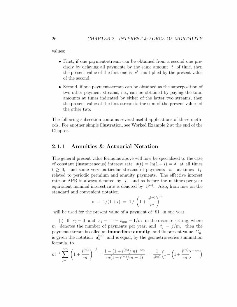
The general present value formulas above will now be specialized to the caseof constant (instantaneous) interest rate δ(t) ≡ ln(1 + i) = δ at all timest ≥ 0, and some very particular streams of payments sj at times tj,related to periodic premium and annuity payments. The effective interestrate or APR is always denoted by i, and as before the m-times-per-yearequivalent nominal interest rate is denoted by i(m). Also, from now on thestandard and convenient notation
v ≡ 1/(1 + i) = 1 /
(
1 +i(m)
m
)m
will be used for the present value of a payment of $1 in one year.
(i) If s0 = 0 and s1 = · · · = snm = 1/m in the discrete setting, wherem denotes the number of payments per year, and tj = j/m, then thepayment-stream is called an immediate annuity, and its present value Gn
is given the notation a(m)n⌉ and is equal, by the geometric-series summation
formula, to
m−1
nm∑
j=1
(
1 +i(m)
m
)−j
=1 − (1 + i(m)/m)−nm
m(1 + i(m)/m − 1)=
1
i(m)
(
1−(
1+i(m)
m
)
−nm)

2.1. MORE ON THEORY OF INTEREST 27
This calculation has shown
a(m)n⌉ =
1 − vn
i(m)(2.1)
All of these immediate annuity values, for fixed v, n but varying m, areroughly comparable because all involve a total payment of 1 per year.Formula (2.1) shows that all of the values a
(m)n⌉ differ only through the factors
i(m), which differ by only a few percent for varying m and fixed i, as shownin Table 2.1. Recall from formula (1.4) that i(m) = m{(1 + i)1/m − 1}.
If instead s0 = 1/m but snm = 0, then the notation changes to a(m)n⌉ ,
the payment-stream is called an annuity-due, and the value is given by anyof the equivalent formulas
a(m)n⌉ = (1 +
i(m)
m) a
(m)n⌉ =
1 − vn
m+ a
(m)n⌉ =
1
m+ a
(m)
n−1/m⌉(2.2)
The first of these formulas recognizes the annuity-due payment-stream asidentical to the annuity-immediate payment-stream shifted earlier by thetime 1/m and therefore worth more by the accumulation-factor (1+i)1/m =1 + i(m)/m. The third expression in (2.2) represents the annuity-due streamas being equal to the annuity-immediate stream with the payment of 1/mat t = 0 added and the payment of 1/m at t = n removed. The finalexpression says that if the time-0 payment is removed from the annuity-due,the remaining stream coincides with the annuity-immediate stream consistingof nm − 1 (instead of nm) payments of 1/m.
In the limit as m → ∞ for fixed n, the notation an⌉ denotes thepresent value of an annuity paid instantaneously at constant unit rate, withthe limiting nominal interest-rate which was shown at the end of the previouschapter to be limm i(m) = i(∞) = δ. The limiting behavior of the nominalinterest rate can be seen rapidly from the formula
i(m) = m(
(1 + i)1/m − 1)
= δ · exp(δ/m) − 1
δ/m
since (ez − 1)/z converges to 1 as z → 0. Then by (2.1) and (2.2),
an⌉ = limm→∞
a(m)n⌉ = lim
m→∞
a(m)n⌉ =
1 − vn
δ(2.3)

28 CHAPTER 2. INTEREST & FORCE OF MORTALITY
Table 2.1: Values of nominal interest rates i(m) (upper number) andd(m) (lower number), for various choices of effective annual interest ratei and number m of compounding periods per year.
i = .02 .03 .05 .07 .10 .15
m = 2 .0199 .0298 .0494 .0688 .0976 .145
.0197 .0293 .0482 .0665 .0931 .135
3 .0199 .0297 .0492 .0684 .0968 .143
.0197 .0294 .0484 .0669 .0938 .137
4 .0199 .0297 .0491 .0682 .0965 .142
.0198 .0294 .0485 .0671 .0942 .137
6 .0198 .0296 .0490 .0680 .0961 .141
.0198 .0295 .0486 .0673 .0946 .138
12 .0198 .0296 .0489 .0678 .0957 .141
.0198 .0295 .0487 .0675 .0949 .139
A handy formula for annuity-due present values follows easily by recallingthat
1 − d(m)
m=(
1 +i(m)
m
)
−1
implies d(m) =i(m)
1 + i(m)/m
Then, by (2.2) and (2.1),
a(m)n⌉ = (1 − vn) · 1 + i(m)/m
i(m)=
1 − vn
d(m)(2.4)
In case m is 1, the superscript (m) is omitted from all of the annuitynotations. In the limit where n → ∞, the notations become a
(m)∞⌉ and
a(m)∞⌉ , and the annuities are called perpetuities (respectively immediate and
due) with present-value formulas obtained from (2.1) and (2.4) as:
a(m)∞⌉ =
1
i(m), a
(m)∞⌉ =
1
d(m)(2.5)
Let us now build some more general annuity-related present values out ofthe standard functions a
(m)n⌉ and a
(m)n⌉ .

2.1. MORE ON THEORY OF INTEREST 29
(ii). Consider first the case of the increasing perpetual annuity-due,
denoted (I(m)a)(m)∞⌉ , which is defined as the present value of a stream of
payments (k + 1)/m2 at times k/m, for k = 0, 1, . . . forever. Clearly thepresent value is
(I(m)a)(m)∞⌉ =
∞∑
k=0
m−2 (k + 1)(
1 +i(m)
m
)
−k
Here are two methods to sum this series, the first purely mathematical, thesecond with actuarial intuition. First, without worrying about the strictjustification for differentiating an infinite series term-by-term,
∞∑
k=0
(k + 1) xk =d
dx
∞∑
k=0
xk+1 =d
dx
x
1 − x= (1 − x)−2
for 0 < x < 1, where the geometric-series formula has been used to sumthe second expression. Therefore, with x = (1 + i(m)/m)−1 and 1 − x =(i(m)/m)/(1 + i(m)/m),
(I(m)a)(m)∞⌉ = m−2
( i(m)/m
1 + i(m)/m
)
−2
=
(
1
d(m)
)2
=(
a(m)∞⌉
)2
and (2.5) has been used in the last step. Another way to reach the same resultis to recognize the increasing perpetual annuity-due as 1/m multiplied by
the superposition of perpetuities-due a(m)∞⌉ paid at times 0, 1/m, 2/m, . . . ,
and therefore its present value must be a(m)∞⌉ · a(m)
∞⌉ . As an aid in recognizing
this equivalence, consider each annuity-due a(m)∞⌉ paid at a time j/m as
being equivalent to a stream of payments 1/m at time j/m, 1/m at(j + 1)/m, etc. Putting together all of these payment streams gives a totalof (k+1)/m paid at time k/m, of which 1/m comes from the annuity-duestarting at time 0, 1/m from the annuity-due starting at time 1/m, upto the payment of 1/m from the annuity-due starting at time k/m.
(iii). The increasing perpetual annuity-immediate (I(m)a)(m)∞⌉ —
the same payment stream as in the increasing annuity-due, but deferred bya time 1/m — is related to the perpetual annuity-due in the obvious way
(I(m)a)(m)∞⌉ = v1/m (I(m)a)
(m)∞⌉ = (I(m)a)
(m)∞⌉
/
(1 + i(m)/m) =1
i(m) d(m)

30 CHAPTER 2. INTEREST & FORCE OF MORTALITY
(iv). Now consider the increasing annuity-due of finite duration
n years. This is the present value (I(m)a)(m)n⌉ of the payment-stream of
(k + 1)/m2 at time k/m, for k = 0, . . . , nm− 1. Evidently, this payment-
stream is equivalent to (I(m)a)(m)∞⌉ minus the sum of n multiplied by an
annuity-due a(m)∞⌉ starting at time n together with an increasing annuity-
due (I(m)a)(m)∞⌉ starting at time n. (To see this clearly, equate the payments
0 = (k + 1)/m2 − n · 1m
− (k − nm + 1)/m2 received at times k/m fork ≥ nm.) Thus
(I(m)a)(m)n⌉ = (I(m)a)
(m)∞⌉
(
1 − (1 + i(m)/m)−nm)
− na(m)∞⌉ (1 + i(m)/m)−nm
= a(m)∞⌉
(
a(m)∞⌉ − (1 + i(m)/m)−nm
[
a(m)∞⌉ + n
] )
= a(m)∞⌉
(
a(m)n⌉ − n vn
)
where in the last line recall that v = (1 + i)−1 = (1 + i(m)/m)−m and
that a(m)n⌉ = a
(m)∞⌉ (1 − vn). The latter identity is easy to justify either
by the formulas (2.4) and (2.5) or by regarding the annuity-due paymentstream as a superposition of the payment-stream up to time n − 1/m andthe payment-stream starting at time n. As an exercise, fill in details of asecond, intuitive verification, analogous to the second verification in pargraph(ii) above.
(v). The decreasing annuity (D(m) a)(m)n⌉ is defined as (the present
value of) a stream of payments starting with n/m at time 0 and decreasingby 1/m2 every time-period of 1/m, with no further payments at or aftertime n. The easiest way to obtain the present value is through the identity
(I(m)a)(m)n⌉ + (D(m)a)
(m)n⌉ = (n +
1
m) a
(m)n⌉
Again, as usual, the method of proving this is to observe that in the payment-stream whose present value is given on the left-hand side, the paymentamount at each of the times j/m, for j = 0, 1, . . . , nm − 1, is
j + 1
m2+ (
n
m− j
m2) =
1
m(n +
1
m)

2.1. MORE ON THEORY OF INTEREST 31
2.1.2 Loan Amortization & Mortgage Refinancing
The only remaining theory-of-interest topic to cover in this unit is the break-down between principal and interest payments in repaying a loan such as amortgage. Recall that the present value of a payment stream of amount cper year, with c/m paid at times 1/m, 2/m, . . . , n− 1/m, n/m, is c a
(m)n⌉ .
Thus, if an amount Loan-Amt has been borrowed for a term of n years,to be repaid by equal installments at the end of every period 1/m , at fixednominal interest rate i(m), then the installment amount is
Mortgage Payment =Loan-Amt
m a(m)n⌉
= Loan-Amti(m)
m (1 − vn)
where v = 1/(1 + i) = (1 + i(m)/m)−m. Of the payment made at time (k +1)/m, how much can be attributed to interest and how much to principal ?Consider the present value at 0 of the debt per unit of Loan-Amt lessaccumulated amounts paid up to and including time k/m :
1 − m a(m)
k/m⌉
1
m a(m)n⌉
= 1 − 1 − vk/m
1 − vn=
vk/m − vn
1 − vn
The remaining debt, per unit of Loan-Amt, valued just after time k/m,is denoted from now on by Bn, k/m. It is greater than the displayed presentvalue at 0 by a factor (1 + i)k/m, so is equal to
Bn, k/m = (1 + i)k/m vk/m − vn
1 − vn=
1 − vn−k/m
1 − vn(2.6)
The amount of interest for a Loan Amount of 1 after time 1/m is (1 +i)1/m − 1 = i(m)/m. Therefore the interest included in the payment at(k + 1)/m is i(m)/m multiplied by the value Bn, k/m of outstanding debtjust after k/m. Thus the next total payment of i(m)/(m(1− vn)) consistsof the two parts
Amount of interest = m−1 i(m) (1 − vn−k/m)/(1 − vn)
Amount of principal = m−1i(m)vn−k/m/(1 − vn)
By definition, the principal included in each payment is the amount of thepayment minus the interest included in it. These formulas show in particular

32 CHAPTER 2. INTEREST & FORCE OF MORTALITY
that the amount of principal repaid in each successive payment increasesgeometrically in the payment number, which at first seems surprising. Noteas a check on the displayed formulas that the outstanding balance Bn,(k+1)/m
immediately after time (k + 1)/m is re-computed as Bn, k/m minus theinterest paid at (k + 1)/m, or
1 − vn−k/m
1 − vn− i(m)
m
vn−k/m
1 − vn=
1 − vn−k/m(1 + i(m)/m)
1 − vn
=1 − vn−(k+1)/m
1 − vn=
(
1 −a
(m)
(k+1)/m⌉
a(m)n⌉
)
v−(k+1)/m (2.7)
as was derived above by considering the accumulated value of amounts paid.The general definition of the principal repaid in each payment is the excessof the payment over the interest since the past payment on the total balancedue immediately following that previous payment.
2.1.3 Illustration on Mortgage Refinancing
Suppose that a 30–year, nominal-rate 8%, $100, 000 mortgage payablemonthly is to be refinanced at the end of 8 years for an additional 15 years(instead of the 22 which would otherwise have been remaining to pay itoff) at 6%, with a refinancing closing-cost amount of $1500 and 2 points.(The points are each 1% of the refinanced balance including closing costs,and costs plus points are then extra amounts added to the initial balanceof the refinanced mortgage.) Suppose that the new pattern of payments isto be valued at each of the nominal interest rates 6%, 7%, or 8%, dueto uncertainty about what the interest rate will be in the future, and thatthese valuations will be taken into account in deciding whether to take outthe new loan.
The monthly payment amount of the initial loan in this example was$100, 000(.08/12)/(1− (1+ .08/12)−360) = $733.76, and the present value asof time 0 (the beginning of the old loan) of the payments made through the
end of the 8th year is ($733.76) · (12a(12)8⌉
) = $51, 904.69. Thus the presentvalue, as of the end of 8 years, of the payments still to be made under theold mortgage, is $(100, 000− 51, 904.69)(1 + .08/12)96 = $91, 018.31. Thus,if the loan were to be refinanced, the new refinanced loan amount would be
2.1. MORE ON THEORY OF INTEREST 33
$91, 018.31 + 1, 500.00 = $92, 518.31. If 2 points must be paid in order tolock in the rate of 6% for the refinanced 15-year loan, then this amountis (.02)92518.31 = $1850.37 . The new principal balance of the refinancedloan is 92518.31 + 1850.37 = $94, 368.68, and this is the present value at anominal rate of 6% of the future loan payments, no matter what the term ofthe refinanced loan is. The new monthly payment (for a 15-year duration) ofthe refinanced loan is $94, 368.68(.06/12)/(1 − (1 + .06/12)−180) = $796.34.
For purposes of comparison, what is the present value at the currentgoing rate of 6% (nominal) of the continuing stream of payments underthe old loan ? That is a 22-year stream of monthly payments of $733.76,as calculated above, so the present value at 6% is $733.76 · (12a
(12)22⌉
) =$107, 420.21. Thus, if the new rate of 6% were really to be the correctone for the next 22 years, and each loan would be paid to the end of itsterm, then it would be a financial disaster not to refinance. Next, supposeinstead that right after re-financing, the economic rate of interest would bea nominal 7% for the next 22 years. In that case both streams of paymentswould have to be re-valued — the one before refinancing, continuing another22 years into the future, and the one after refinancing, continuing 15 years
into the future. The respective present values (as of the end of the 8th
year) at nominal rate of 7% of these two streams are:
Old loan: 733.76 (12a(12)22⌉
) = $98, 700.06
New loan: 796.34 (12a(12)15⌉
) = $88, 597.57
Even with these different assumptions, and despite closing-costs and points,it is well worth re-financing.
Exercise: Suppose that you can forecast that you will in fact sell yourhouse in precisely 5 more years after the time when you are re-financing. Atthe time of sale, you would pay off the cash principal balance, whatever itis. Calculate and compare the present values (at each of 6%, 7%, and 8%nominal interest rates) of your payment streams to the bank, (a) if youcontinue the old loan without refinancing, and (b) if you re-finance to geta 15-year 6% loan including closing costs and points, as described above.

34 CHAPTER 2. INTEREST & FORCE OF MORTALITY
2.1.4 Computational illustration in Splus or R
All of the calculations described above are very easy to program in any lan-guage from Fortran to Mathematica, and also on a programmable calculator;but they are also very handily organized within a spreadsheet, which seemsto be the way that MBA’s, bank-officials, and actuaries will learn to do themfrom now on.
In this section, an Splus or R function (cf. Venables & Ripley 2002)is provided to do some comparative refinancing calculations. Concerningthe syntax of Splus or R, the only explanation necessary at this point isthat the symbol <− denotes assignment of an expression to a variable:A <−B means that the variable A is assigned the value of expression B.Other syntactic elements used here are common to many other computerlanguages: * denotes multiplication, and ∧ denotes exponentiation.
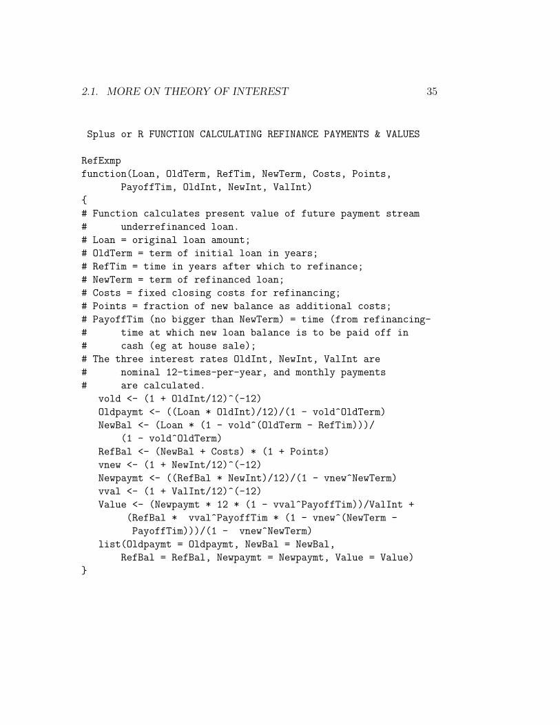
The function RefExmp given below calculates mortgage payments, bal-ances for purposes of refinancing both before and after application of ad-ministrative costs and points, and the present value under any interest rate(not necessarily the ones at which either the original or refinanced loans aretaken out) of the stream of repayments to the bank up to and including thelump-sum payoff which would be made, for example, at the time of sellingthe house on which the mortgage loan was negotiated. The output of thefunction is a list which, in each numerical example below, is displayed in‘unlisted’ form, horizontally as a vector. Lines beginning with the symbol #are comment-lines.
The outputs of the function are as follows. Oldpayment is the monthlypayment on the original loan of face-amount Loan at nominal interest i(12) =OldInt for a term of OldTerm years. NewBal is the balance Bn, k/m offormula (2.6) for n = OldTerm, m = 12, and k/m = RefTim, and therefinanced loan amount is a multiple 1+ Points of NewBal, which is equalto RefBal + Costs. The new loan, at nominal interest rate NewInt, hasmonthly payments Newpaymt for a term of NewTerm years. The loan is tobe paid off PayoffTim years after RefTim when the new loan commences,and the final output of the function is the present value at the start of therefinanced loan with nominal interest rate ValInt of the stream of paymentsmade under the refinanced loan up to and including the lump sum payoff.
2.1. MORE ON THEORY OF INTEREST 35
Splus or R FUNCTION CALCULATING REFINANCE PAYMENTS & VALUES
RefExmp
function(Loan, OldTerm, RefTim, NewTerm, Costs, Points,
PayoffTim, OldInt, NewInt, ValInt)
{
# Function calculates present value of future payment stream
# underrefinanced loan.
# Loan = original loan amount;
# OldTerm = term of initial loan in years;
# RefTim = time in years after which to refinance;
# NewTerm = term of refinanced loan;
# Costs = fixed closing costs for refinancing;
# Points = fraction of new balance as additional costs;
# PayoffTim (no bigger than NewTerm) = time (from refinancing-
# time at which new loan balance is to be paid off in
# cash (eg at house sale);
# The three interest rates OldInt, NewInt, ValInt are
# nominal 12-times-per-year, and monthly payments
# are calculated.
vold <- (1 + OldInt/12)^(-12)
Oldpaymt <- ((Loan * OldInt)/12)/(1 - vold^OldTerm)
NewBal <- (Loan * (1 - vold^(OldTerm - RefTim)))/
(1 - vold^OldTerm)
RefBal <- (NewBal + Costs) * (1 + Points)
vnew <- (1 + NewInt/12)^(-12)
Newpaymt <- ((RefBal * NewInt)/12)/(1 - vnew^NewTerm)
vval <- (1 + ValInt/12)^(-12)
Value <- (Newpaymt * 12 * (1 - vval^PayoffTim))/ValInt +
(RefBal * vval^PayoffTim * (1 - vnew^(NewTerm -
PayoffTim)))/(1 - vnew^NewTerm)
list(Oldpaymt = Oldpaymt, NewBal = NewBal,
RefBal = RefBal, Newpaymt = Newpaymt, Value = Value)
}

36 CHAPTER 2. INTEREST & FORCE OF MORTALITY
We begin our illustration by reproducing the quantities calculated in theprevious subsection:
> unlist(RefExmp(100000, 30, 8, 15, 1500, 0.02, 15,
0.08, 0.06, 0.06))
Oldpaymt NewBal RefBal Newpaymt Value
733.76 91018 94368 796.33 94368
Note that, since the payments under the new (refinanced) loan are herevalued at the same interest rate as the loan itself, the present value Value ofall payments made under the loan must be equal to the the refinanced loanamount RefBal.
The comparisons of the previous Section between the original and refi-nanced loans, at (nominal) interest rates of 6, 7, and 8 %, are all recapitulatedeasily using this function. To use it, for example, in valuing the old loan at7%, the arguments must reflect a ‘refinance’ with no costs or points for aperiod of 22 years at nominal rate 6%, as follows:
> unlist(RefExmp(100000,30,8,22,0,0,22,0.08,0.08,0.07))
Oldpaymt NewBal RefBal Newpaymt Value
733.76 91018 91018 733.76 98701
(The small discrepancies between the values found here and in the previoussubsection are due to the rounding used there to express payment amountsto the nearest cent.)
We consider next a numerical example showing break-even point for refi-nancing by balancing costs versus time needed to amortize them.
Suppose that you have a 30-year mortage for $100,000 at nominal 9% ( =i(12)), with level monthly payments, and that after 7 years of payments yourefinance to obtain a new 30-year mortgage at 7% nominal interest ( = i(m)
for m = 12), with closing costs of $1500 and 4 points (i.e., 4% of the totalrefinanced amount including closing costs added to the initial balance), alsowith level monthly payments. Figuring present values using the new interestrate of 7%, what is the time K (to the nearest month) such that if bothloans — the old and the new — were to be paid off in exactly K years afterthe time (the 7-year mark for the first loan) when you would have refinanced,

2.1. MORE ON THEORY OF INTEREST 37
then the remaining payment-streams for both loans from the time when yourefinance are equivalent (i.e., have the same present value from that time) ?
We first calculate the present value of payments under the new loan.As remarked above in the previous example, since the same interest rate isbeing used to value the payments as is used in figuring the refinanced loan,the valuation of the new loan does not depend upon the time K to payoff.(It is figured here as though the payoff time K were 10 years.)
> unlist(RefExmp(1.e5, 30,7,30, 1500,.04, 10, 0.09,0.07,0.07))
Oldpaymt NewBal RefBal Newpaymt Value
804.62 93640 98946 658.29 98946
Next we compute the value of payments under the old loan, at 7% nominalrate, also at payoff time K = 10. For comparison, the value under theold loan for payoff time 0 (i.e., for cash payoff at the time when refinancingwould have occurred) coincides with the New Balance amount of $93640.
> unlist(RefExmp(1.e5, 30,7,23, 0,0, 10, 0.09,0.09,0.07))
Oldpaymt NewBal RefBal Newpaymt Value
804.62 93640 93640 804.62 106042
The values found in the same way when the payoff time K is successivelyreplaced by 4, 3, 3.167, 3.25 are 99979, 98946, 98593, 98951. Thus, thepayoff-time K at which there is essentially no difference in present valueat nominal 7% between the old loan or the refinanced loan with costs andpoints (which was found to have Value 98946), is 3 years and 3 monthsafter refinancing.
2.1.5 Coupon & Zero-coupon Bonds
In finance, an investor assessing the present value of a bond is in the samesituation as the bank receiving periodic level payments in repayment of aloan. If the payments are made every 1/m year, with nominal couponinterest rate i(m), for a bond with face value $1000, then the paymentsare precisely the interest on $1000 for 1/m year, or 1000 · i(m)/m.For most corporate or government bonds, m = 4, although some bonds
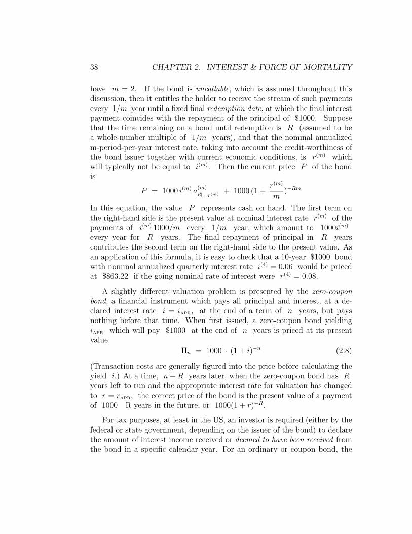
38 CHAPTER 2. INTEREST & FORCE OF MORTALITY
have m = 2. If the bond is uncallable, which is assumed throughout thisdiscussion, then it entitles the holder to receive the stream of such paymentsevery 1/m year until a fixed final redemption date, at which the final interestpayment coincides with the repayment of the principal of $1000. Supposethat the time remaining on a bond until redemption is R (assumed to bea whole-number multiple of 1/m years), and that the nominal annualizedm-period-per-year interest rate, taking into account the credit-worthiness ofthe bond issuer together with current economic conditions, is r(m) whichwill typically not be equal to i(m). Then the current price P of the bondis
P = 1000 i(m) a(m)R⌉ , r(m)
+ 1000 (1 +r(m)
m)−Rm
In this equation, the value P represents cash on hand. The first term onthe right-hand side is the present value at nominal interest rate r(m) of thepayments of i(m) 1000/m every 1/m year, which amount to 1000i(m)
every year for R years. The final repayment of principal in R yearscontributes the second term on the right-hand side to the present value. Asan application of this formula, it is easy to check that a 10-year $1000 bondwith nominal annualized quarterly interest rate i(4) = 0.06 would be pricedat $863.22 if the going nominal rate of interest were r(4) = 0.08.
A slightly different valuation problem is presented by the zero-couponbond, a financial instrument which pays all principal and interest, at a de-clared interest rate i = iAPR, at the end of a term of n years, but paysnothing before that time. When first issued, a zero-coupon bond yieldingiAPR which will pay $1000 at the end of n years is priced at its presentvalue
Πn = 1000 · (1 + i)−n (2.8)
(Transaction costs are generally figured into the price before calculating theyield i.) At a time, n−R years later, when the zero-coupon bond has Ryears left to run and the appropriate interest rate for valuation has changedto r = rAPR, the correct price of the bond is the present value of a paymentof 1000 R years in the future, or 1000(1 + r)−R.
For tax purposes, at least in the US, an investor is required (either by thefederal or state government, depending on the issuer of the bond) to declarethe amount of interest income received or deemed to have been received fromthe bond in a specific calendar year. For an ordinary or coupon bond, the

2.2. FORCE OF MORTALITY & ANALYTICAL MODELS 39
year’s income is just the total i(m) · 1000 actually received during the year.For a zero-coupon bond assumed to have been acquired when first issued,at price Πn, if the interest rate has remained constant at i = iAPR sincethe time of acquisition, then the interest income deemed to be received inthe year, also called the Original Issue Discount (OID), would simply bethe year’s interest Πn i(m) on the initial effective face amount Πn of thebond. That is because all accumulated value of the bond would be attributedto OID interest income received year by year, with the principal remainingthe same at Πn. Assume next that the actual year-by-year APR interestrate is r(j) throughout the year [j, j + 1), for j = 0, 1, . . . n − 1, withr(0) equal to i. Then, again because accumulated value over the initialprice is deemed to have been received in the form of yearly interest, the OIDshould be Πn r(j) in the year [j, j + 1). The problematic aspect of thiscalculation is that, when interest rates have fluctuated a lot over the timesj = 0, 1, . . . , n − R − 1, the zero-coupon bond investor will be deemed tohave received income Πn r(j) in successive years j = 0, 1, . . . , n − R − 1,corresponding to a total accumulated value of
Πn (1 + r(0)) (1 + r(1)) · · · (1 + r(n − R − 1))
while the price 1000 (1 + r(n − R))−R for which the bond could be soldmay be very different. The discrepancy between the ‘deemed received’ accu-mulated value and the final actual value when the bond is redeemed or soldmust presumably be treated as a capital gain or loss. However, the presentauthor makes no claim to have presented this topic according to the viewsof the Internal Revenue Service, since he has never been able to figure outauthoritatively what those views are.
2.2 Force of Mortality & Analytical Models
Up to now, the function S(x) called the “survivor” or “survival” functionhas been defined to be equal to the life-table ratio lx/l0 at all integer agesx, and to be piecewise continuously differentiable for all positive real valuesof x. Intuitively, for all positive real x and t, S(x) − S(x + t) is thefraction of the initial life-table cohort which dies between ages x and x+ t,and (S(x)− S(x + t))/S(x) represents the fraction of those alive at age xwho fail before x + t. An equivalent representation is S(x) =
∫
∞
xf(t) dt ,

40 CHAPTER 2. INTEREST & FORCE OF MORTALITY
where f(t) ≡ −S ′(t) is called the failure density. If T denotes the randomvariable which is the age at death for a newly born individual governed bythe same causes of failure as the life-table cohort, then P (T ≥ x) = S(x),and according to the Fundamental Theorem of Calculus,
limǫ→0+
P (x ≤ T ≤ x + ǫ)
ǫ= lim
ǫ→0+
∫ x+ǫ
x
f(u) du = f(x)
as long as the failure density is a continuous function.
Two further useful actuarial notations, often used to specify the theoret-ical lifetime distribution, are:
tpx = P (T ≥ x + t |T ≥ x ) = S(x + t)/S(x)
and
tqx = 1 − tpx = P (T ≤ x + t |T ≥ x ) = (S(x) − S(x + t))/S(x)
The quantity tqx is referred to as the age-specific death rate for periodsof length t. In the most usual case where t = 1 and x is an integerage, the notation 1qx is replaced by qx, and 1px is replaced by px. Therate qx would be estimated from the cohort life table as the ratio dx/lx ofthose who die between ages x and x+1 as a fraction of those who reachedage x. The way in which this quantity varies with x is one of the mostimportant topics of study in actuarial science. For example, one importantway in which numerical analysis enters actuarial science is that one wishesto interpolate the values qx smoothly as a function of x. The topic called“Graduation Theory” among actuaries is the mathematical methodology ofInterpolation and Spline-smoothing applied to the raw function qx = dx/lx.
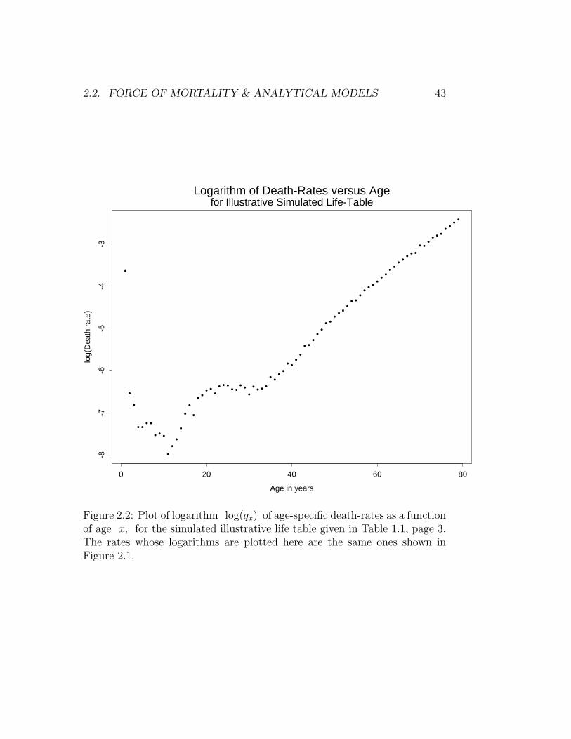
To give some idea what a realistic set of death-rates looks like, Figure 2.1pictures the age-specific 1-year death-rates qx for the simulated life-tablegiven as Table 1.1 on page 3. Additional granularity in the death-rates canbe seen in Figure 2.2, where the logarithms of death-rates are plotted. Aftera very high death-rate during the first year of life (26.3 deaths per thousandlive births), there is a rough year-by-year decline in death-rates from 1.45per thousand in the second year to 0.34 per thousand in the eleventh year.(But there were small increases in rate from ages 4 to 7 and from 8 to9, which are likely due to statistical irregularity rather than real increases

2.2. FORCE OF MORTALITY & ANALYTICAL MODELS 41
in risk.) Between ages 11 and 40, there is an erratic but roughly linearincrease of death-rates per thousand from 0.4 to 3.0. However, at agesbeyond 40 there is a rapid increase in death-rates as a function of age.As can be seen from Figure 2.2, the values qx seem to increase roughlyas a power cx where c ∈ [1.08, 1.10]. (Compare this behavior with theGompertz-Makeham Example (v) below.) This exponential behavior of theage-specific death-rate for large ages suggests that the death-rates picturedcould reasonably be extrapolated to older ages using the formula
qx ≈ q78 · (1.0885)x−78 , x ≥ 79 (2.9)
where the number 1.0885 was found as log(q78/q39)/(78 − 39).
Now consider the behavior of ǫqx as ǫ gets small. It is clear that ǫqx
must also get small, roughly proportionately to ǫ, since the probability ofdying between ages x and x + ǫ is approximately ǫ f(x) when ǫ getssmall.
Definition: The limiting death-rate ǫqx/ǫ per unit time as ǫ ց 0 iscalled by actuaries the force of mortality µ(x). In reliability theory orbiostatistics, the same function is called the failure intensity, failure rate, orhazard intensity.
The reasoning above shows that for small ǫ,
ǫqx
ǫ=
1
ǫS(x)
∫ x+ǫ
x
f(u) du −→ f(x)
S(x), ǫ ց 0
Thus
µ(x) =f(x)
S(x)=
−S ′(x)
S(x)= − d
dxln(S(x))
where the chain rule for differentiation was used in the last step. Replacingx by y and integrating both sides of the last equation between 0 and x,we find
∫ x
0
µ(y) dy =(
− ln(S(y)))x
0= − ln(S(x))
since S(0) = 1. Similarly,
∫ x+t
x
µ(y) dy = ln S(x) − ln S(x + t)

42 CHAPTER 2. INTEREST & FORCE OF MORTALITY
•
• • • • • • • • • • • • • • • • • • • • • • • • • • • • • • • • • • • • • • • • • • • • • • • • • • • • • ••• • • •
•••••••• •
• •
•
•••
•
•
•
•
Age-Specific Death Rates for Illustrative Life Table
Age in Years
Age
-Spe
cific
Dea
th R
ate
0 20 40 60 80
0.0
0.02
0.04
0.06
0.08
Figure 2.1: Plot of age-specific death-rates qx versus x, for the simulatedillustrative life table given in Table 1.1, page 3.
2.2. FORCE OF MORTALITY & ANALYTICAL MODELS 43
•
•
•
• • • •
• • •
••••
•••
• •• •
•• • • • •
• ••• • • •
• •• •
• •••• •
•• •
• •• • • •
• ••• • • • • • • •
• • • • •• • • • • •
• • • •
Logarithm of Death-Rates versus Age
Age in years
log(
Dea
th r
ate)
0 20 40 60 80
-8-7
-6-5
-4-3
for Illustrative Simulated Life-Table
Figure 2.2: Plot of logarithm log(qx) of age-specific death-rates as a functionof age x, for the simulated illustrative life table given in Table 1.1, page 3.The rates whose logarithms are plotted here are the same ones shown inFigure 2.1.

44 CHAPTER 2. INTEREST & FORCE OF MORTALITY
Now exponentiate to obtain the useful formulas
S(x) = exp{
−∫ x
0
µ(y) dy}
, tpx =S(x + t)
S(x)= exp
{
−∫ x+t
x
µ(y) dy}
Examples:
(i) If S(x) = (ω−x)/ω for 0 ≤ x ≤ ω (the uniform failure distributionon [0, ω] ), then µ(x) = (ω−x)−1. Note that this hazard function increasesto ∞ as x increases to ω.
(ii) If S(x) = e−µx for x ≥ 0 (the exponential failure distribution on[0,∞) ), then µ(x) = µ is constant.
(iii) If S(x) = exp(−λxγ) for x ≥ 0, then mortality follows the Weibulllife distribution model with shape parameter γ > 0 and scale parameter λ.The force of mortality takes the form
µ(x) = λ γ xγ−1
This model is very popular in engineering reliability. It has the flexibilitythat by choice of the shape parameter γ one can have
(a) failure rate increasing as a function of x ( γ > 1 ),
(b) constant failure rate ( γ = 1, the exponential model again),or
(c) decreasing failure rate ( 0 < γ < 1 ).
But what one cannot have, in the examples considered so far, is a force-of-mortality function which decreases on part of the time-axis and increaseselsewhere.
(iv) Two other models for positive random variables which are popularin various statistical applications are the Gamma, with
S(x) =
∫
∞
x
βα yα−1 e−βy dy /
∫
∞
0
zα−1 e−z dz , α, β > 0
and the Lognormal, with
S(x) = 1 − Φ( ln x − m
σ
)
, m real, σ > 0

2.2. FORCE OF MORTALITY & ANALYTICAL MODELS 45
where
Φ(z) ≡ 1
2+
∫ z
0
e−u2/2 du√2π
is called the standard normal distribution function. In the Gamma case,the expected lifetime is α/β, while in the Lognormal, the expectation isexp(µ + σ2/2). Neither of these last two examples has a convenient orinterpretable force-of-mortality function.
Increasing force of mortality intuitively corresponds to aging, where thecauses of death operate with greater intensity or effect at greater ages. Con-stant force of mortality, which is easily seen from the formula S(x) =exp(−
∫ x
0µ(y) dy) to be equivalent to exponential failure distribution, would
occur if mortality arose only from pure accidents unrelated to age. Decreas-ing force of mortality, which really does occur in certain situations, reflectswhat engineers call “burn-in”, where after a period of initial failures due toloose connections and factory defects the nondefective devices emerge andexhibit high reliability for a while. The decreasing force of mortality reflectsthe fact that the devices known to have functioned properly for a short whileare known to be correctly assembled and are therefore highly likely to have astandard length of operating lifetime. In human life tables, infant mortalitycorresponds to burn-in: risks of death for babies decrease markedly after theone-year period within which the most severe congenital defects and diseasesof infancy manifest themselves. Of course, human life tables also exhibit anaging effect at high ages, since the high-mortality diseases like heart diseaseand cancer strike with greatest effect at higher ages. Between infancy andlate middle age, at least in western countries, hazard rates are relatively flat.This pattern of initial decrease, flat middle, and final increase of the force-of-mortality, seen clearly in Figure 2.1, is called a bathtub shape and requiresnew survival models.
As shown above, the failure models in common statistical and reliabilityusage either have increasing force of mortality functions or decreasing force ofmortality, but not both. Actuaries have developed an analytical model whichis somewhat more realistic than the preceding examples for human mortaltyat ages beyond childhood. While the standard form of this model does notaccommodate a bathtub shape for death-rates, a simple modification of itdoes.
46 CHAPTER 2. INTEREST & FORCE OF MORTALITY
Example (v). (Gompertz-Makeham forms of the force of mortality). Sup-pose that µ(x) is defined directly to have the form A + B cx. (The Bcx
term was proposed by Gompertz, the additive constant A by Makeham.Thus the Gompertz force-of-mortality model is the special case with A = 0,or µ(x) = Bcx.) By choice of the parameter c as being respectivelygreater than or less than 1, one can arrange that the force-of-mortalitycurve either be increasing or decreasing. Roughly realistic values of c forhuman mortality will be only slightly greater than 1: if the Gompertz(non-constant) term in force-of-mortality were for example to quintuple in20 years, then c ≈ 51/20 = 1.084, which may be a reasonable value exceptfor very advanced ages. (Compare the comments made in connection withFigures 2.1 and 2.2: for middle and higher ages in the simulated illustrativelife table of Table 1.1, which corresponds roughly to US male mortality ofaround 1960, the figure of c was found to be roughly 1.09.) Note that inany case the Gompertz-Makeham force of mortality is strictly convex (i.e.,has strictly positive second derivative) when B > 0 and c 6= 1. TheGompertz-Makeham family could be enriched still further, with further ben-efits of realism, by adding a linear term Dx. If D < −B ln(c), with0 < A < B, c > 1, then it is easy to check that
µ(x) = A + B cx + Dx
has a bathtub shape, initially decreasing and later increasing.
Figures 2.3 and 2.4 display the shapes of force-of-mortality functions (iii)-(v) for various parameter combinations chosen in such a way that the ex-pected lifetime is 75 years. This restriction has the effect of reducing thenumber of free parameters in each family of examples by 1. One cansee from these pictures that the Gamma and Weibull families contain manyvery similar shapes for force-of-mortality curves, but that the lognormal andMakeham families are quite different.
Figure 2.5 shows survival curves from several analytical models plotted onthe same axes as the 1959 US male life-table data from which Table 1.1 wassimulated. The previous discussion about bathtub-shaped force of mortalityfunctions should have made it clear that none of the analytical models pre-sented could give a good fit at all ages, but the Figure indicates the rathergood fit which can be achieved to realistic life-table data at ages 40 andabove. The models fitted all assumed that S(40) = 0.925 and that for lives

2.2. FORCE OF MORTALITY & ANALYTICAL MODELS 47
aged 40, T − 40 followed the indicated analytical form. Parameters for allmodels were determined from the requirements of median age 72 at death(equal by definition to the value tm for which S(tm) = 0.5) and probability0.04 of surviving to age 90. Thus, all four plotted survival curves have beendesigned to pass through the three points (40, 0.925), (72, 0.5), (90, 0.04).Of the four fitted curves, clearly the Gompertz agrees most closely with theplotted points for 1959 US male mortality. The Gompertz curve has param-eters B = 0.00346, c = 1.0918, the latter of which is close to the value1.0885 used in formula (2.9) to extrapolate the 1959 life-table death-ratesto older ages.
2.2.1 Comparison of Forces of Mortality
What does it mean to say that one lifetime, with associated survival functionS1(t), has hazard (i.e. force of mortality) µ1(t) which is a constant multipleκ at all ages of the force of mortality µ2(t) for a second lifetime withsurvival function S2(t) ? It means that the cumulative hazard functions areproportional, i.e.,
− ln S1(t) =
∫ t
0
µ1(x)dx =
∫ t
0
κ µ2(x)dx = κ(− ln S2(t))
and therefore that
S1(t) = (S2(t))κ , all t ≥ 0
This remark is of especial interest in biostatistics and epidemiology whenthe factor κ is allowed to depend (e.g., by a regression model ln(κ) = β ·Z )on other measured variables (covariates) Z. This model is called the (Cox)Proportional-Hazards model and is treated at length in books on survival dataanalysis (Cox and Oakes 1984, Kalbfleisch and Prentice 1980) or biostatistics(Lee 1980).
Example. Consider a setting in which there are four subpopulations of thegeneral population, categorized by the four combinations of values of twobinary covariates Z1, Z2 = 0, 1. Suppose that these four combinations have

48 CHAPTER 2. INTEREST & FORCE OF MORTALITY
Weibull(alpha,lambda)
Age (years)
Haz
ard
0 20 40 60 80 100
0.0
0.00
50.
010
0.01
50.
020
0.02
5
alpha=1alpha=0.7alpha=1.3alpha=1.6alpha=2
Gamma(beta,lambda)
Age (years)
Haz
ard
0 20 40 60 80 100
0.0
0.00
50.
010
0.01
50.
020
0.02
5
beta=1beta=0.7beta=1.3beta=1.6beta=2
Figure 2.3: Force of Mortality Functions for Weibull and Gamma ProbabilityDensities. In each case, the parameters are fixed in such a way that theexpected survival time is 75 years.

2.2. FORCE OF MORTALITY & ANALYTICAL MODELS 49
Lognormal(mu,sigma^2)
Age (years)
Haz
ard
0 20 40 60 80 100
0.0
0.00
50.
010
0.01
50.
020
0.02
5
sigma=0.2sigma=0.4sigma=0.6sigma=1.6sigma=2
Makeham(A,B,c)
Age (years)
Haz
ard
0 20 40 60 80 100
0.0
0.00
50.
010
0.01
50.
020
0.02
5
A=0.0018, B=0.0010, c=1.002A=0.0021,B=0.0070, c=1.007A=0.003, B=0.0041, c=1.014A=0.0041, B=0.0022, c=1.022
Figure 2.4: Force of Mortality Functions for Lognormal and Makeham Den-sities. In each case, the parameters are fixed in such a way that the expectedsurvival time is 75 years.

50 CHAPTER 2. INTEREST & FORCE OF MORTALITY
Plots of Theoretical Survival Curves
Age (years)
Sur
viva
l Pro
babi
lity
40 50 60 70 80 90 100
0.0
0.2
0.4
0.6
0.8
• • • • • • • • • • • • • • • • • • • • • ••
••
••
••
••
••
••
••
••
•
Plotted points from US 1959 male life-table
Lognormal(3.491, .246^2)Weibull(3.653, 1.953e-6)Gamma(14.74, 0.4383)Gompertz(3.46e-3, 1.0918)
Figure 2.5: Theoretical survival curves, for ages 40 and above, plotted aslines for comparison with 1959 US male life-table survival probabilities plot-ted as points. The four analytical survival curves — Lognormal, Weibull,Gamma, and Gompertz — are taken as models for age-at-death minus 40,so if Stheor(t) denotes the theoretical survival curve with indicated parame-ters, the plotted curve is (t, 0.925 · Stheor(t − 40)). The parameters of eachanalytical model were determined so that the plotted probabilities would be0.925, 0.5, 0.04 respectively at t = 40, 72, 90.

2.2. FORCE OF MORTALITY & ANALYTICAL MODELS 51
respective conditional probabilities for lives aged x (or relative frequencies inthe general population aged x)
Px(Z1 = Z2 = 0) = 0.15 , Px(Z1 = 0, Z2 = 1) = 0.2
Px(Z1 = 1, Z2 = 0) = 0.3 , Px(Z1 = Z2 = 1) = 0.35
and that for a life aged x and all t > 0,
P (T ≥ x + t |T ≥ x, Z1 = z1, Z2 = z2) = exp(−2.5 e0.7z1−.8z2 t2/20000)
It can be seen from the conditional survival function just displayed that theforces of mortality at ages greater than x are
µ(x + t) = (2.5 e0.7z1−.8z2) t/10000
so that the force of mortality at all ages is multiplied by e0.7 = 2.0138 forindividuals with Z1 = 1 versus those with Z1 = 0, and is multiplied bye−0.8 = 0.4493 for those with Z2 = 1 versus those with Z2 = 0. The effecton age-specific death-rates is approximately the same. Direct calculationshows for example that the ratio of age-specific death rate at age x+20 forindividuals in the group with (Z1 = 1, Z2 = 0) versus those in the group with(Z1 = 0, Z2 = 0) is not precisely e0.7 = 2.014, but rather
1 − exp(−2.5e0.7((212 − 202)/20000)
1 − exp(−2.5((212 − 202)/20000)= 2.0085
Various calculations, related to the fractions of the surviving population atvarious ages in each of the four population subgroups, can be performedeasily . For example, to find
P (Z1 = 0, Z2 = 1 |T ≥ x + 30)
we proceed in several steps (which correspond to an application of Bayes’rule, viz. Hogg and Tanis 1997, sec. 2.5, or Larson 1982, Sec. 2.6):
P (T ≥ x+30, Z1 = 0 Z2 = 1|T ≥ x) = 0.2 exp(−2.5e−0.8 302
20000) = 0.1901
and similarly
P (T ≥ x + 30 |T ≥ x) = 0.15 exp(−2.5(302/20000)) + 0.1901 +

52 CHAPTER 2. INTEREST & FORCE OF MORTALITY
+ 0.3 exp(−2.5 ∗ e0.7 302
20000) + 0.35 exp(−2.5e0.7−0.8 302
20000) = 0.8795
Thus, by definition of conditional probabilities (restricted to the cohort oflives aged x), taking ratios of the last two displayed quantities yields
P (Z1 = 0, Z2 = 1 |T ≥ x + 30) =0.1901
0.8795= 0.2162
2.
In biostatistics and epidemiology, the measured variables Z = (Z1, . . . , Zp)recorded for each individual in a survival study might be: indicator of a spe-cific disease or diagnostic condition (e.g., diabetes, high blood pressure, spe-cific electrocardiogram anomaly), quantitative measurement of a risk-factor(dietary cholesterol, percent caloric intake from fat, relative weight-to-heightindex, or exposure to a toxic chemical), or indicator of type of treatment orintervention. In these fields, the objective of such detailed models of covari-ate effects on survival can be: to correct for incidental individual differencesin assessing the effectiveness of a treatment; to create a prognostic index foruse in diagnosis and choice of treatment; or to ascertain the possible risks andbenefits for health and survival from various sorts of life-style interventions.The multiplicative effects of various risk-factors on age-specific death ratesare often highlighted in the news media.
In an insurance setting, categorical variables for risky life-styles, occupa-tions, or exposures might be used in risk-rating, i.e., in individualizing insur-ance premiums. While risk-rating is used routinely in casualty and propertyinsurance underwriting, for example by increasing premiums in response torecent claims or by taking location into account, it can be politically sen-sitive in a life-insurance and pension context. In particular, while genderdifferences in mortality can be used in calculating insurance and annuitypremiums, as can certain life-style factors like smoking, it is currently illegalto use racial and genetic differences in this way.
All life insurers must be conscious of the extent to which their policyhold-ers as a group differ from the general population with respect to mortality.Insurers can collect special mortality tables on special groups, such as em-ployee groups or voluntary organizations, and regression-type models like theCox proportional-hazards model may be useful in quantifying group mortal-ity differences when the special-group mortality tables are not based upon

2.3. EXERCISE SET 2 53
large enough cohorts for long enough times to be fully reliable. See Chapter6, Section 6.3, for discussion about the modification of insurance premiumsfor select groups.
2.3 Exercise Set 2
(1). The sum of the present value of $1 paid at the end of n years and$1 paid at the end of 2n years is $1. Find (1+ r)2n, where r = annualinterest rate, compounded annually.
(2). Suppose that an individual aged 20 has random lifetime Z withcontinuous density function
fZ(t) =1
360
(
1 +t
10
)
, for 20 ≤ t ≤ 80
and 0 for other values of t.
(a) If this individual has a contract with your company that you mustpay his heirs $106 · (1.4−Z/50) at the exact date of his death if this occursbetween ages 20 and 70, then what is the expected payment ?
(b) If the value of the death-payment described in (a) should properly bediscounted by the factor exp(−0.08 · (Z − 20)), i.e. by the nominal interestrate of e0.08 − 1 per year) to calculate the present value of the payment,then what is the expected present value of the payment under the insurancecontract ?
(3). Suppose that a continuous random variable T has hazard rate function(= force of mortality)
h(t) = 10−3 ·[
7.0 − 0.5t + 2et/20]
, t > 0
This is a legitimate hazard rate of Gompertz-Makeham type since its mini-mum, which occurs at t = 20 ln(5), is (17−10 ln(5)) ·10−4 = 9.1 ·10−5 > 0.
(a) Construct a cohort life-table with h(t) as “force of mortality”, basedon integer ages up to 70 and cohort-size (= “radix”) l0 = 105. (Give thenumerical entries, preferably by means of a little computer program. If youdo the arithmetic using hand-calculators and/or tables, stop at age 20.)

54 CHAPTER 2. INTEREST & FORCE OF MORTALITY
(b) What is the probability that the random variable T exceeds 30, giventhat it exceeds 3 ? Hint: find a closed-form formula for S(t) = P (T ≥ t).
(4). Do the Mortgage-Refinancing exercise given in the Illustrative on mort-gage refinancing at the end of Section 2.1.
(5). (a) The mortality pattern of a certain population may be described asfollows: out of every 98 lives born together, one dies annually until thereare no survivors. Find a simple function that can be used as S(x) for thispopulation, and find the probability that a life aged 30 will survive to attainage 35.
(b) Suppose that for x between ages 12 and 40 in a certain population,10% of the lives aged x die before reaching age x+1 . Find a simple functionthat can be used as S(x) for this population, and find the probability thata life aged 30 will survive to attain age 35.
(6). Suppose that a survival distribution (i.e., survival function based ona cohort life table) has the property that 1px = γ · (γ2)x for some fixed γbetween 0 and 1, for every real ≥ 0. What does this imply about S(x) ?(Give as much information about S as you can. )
(7). If the instantaneous interest rate is r(t) = 0.01 t for 0 ≤ t ≤ 3, thenfind the equivalent single effective rate of interest or APR for money investedat interest over the interval 0 ≤ t ≤ 3 .
(8). Find the accumulated value of $100 at the end of 15 years if the nominalinterest rate compounded quarterly (i.e., i(4) ) is 8% for the first 5 years, ifthe effective rate of discount is 7% for the second 5 years, and if the nominalrate of discount compounded semiannually (m = 2) is 6% for the third 5years.
(9). Suppose that you borrow $1000 for 3 years at 6% APR, to be repaidin level payments every six months (twice yearly).
(a) Find the level payment amount P .
(b) What is the present value of the payments you will make if you skipthe 2nd and 4th payments ? (You may express your answer in terms of P . )
(10). A survival function has the form S(x) = c−xc+x
. If a mortality tableis derived from this survival function with a radix l0 of 100,000 at age 0,

2.3. EXERCISE SET 2 55
and if l35 = 44, 000 :
(i) What is the terminal age of the table ?
(ii) What is the probability of surviving from birth to age 60 ?
(iii) What is the probability of a person at exact age 10 dying betweenexact ages 30 and 45 ?
(11). A separate life table has been constructed for each calendar year ofbirth, Y , beginning with Y = 1950. The mortality functions for thevarious tables are denoted by the appropriate superscript Y . For each Yand for all ages x
µYx = A · k(Y ) + B cx , pY +1
x = (1 + r) pYx
where k is a function of Y alone and A, B, r are constants (with r > 0).If k(1950) = 1, then derive a general expression for k(Y ).
(12). A standard mortality table follows Makeham’s Law with force ofmortality
µx = A + B cx at all ages x
A separate, higher-risk mortality table also follows Makeham’s Law withforce of mortality
µ∗
x = A∗ + B∗ cx at all ages x
with the same constant c. If for all starting ages the probability of surviving6 years according to the higher-risk table is equal to the probability ofsurviving 9 years according to the standard table, then express each of A∗
and B∗ in terms of A, B, c.
(13). A homeowner borrows $100, 000 at 7% APR from a bank, agreeingto repay by 30 equal yearly payments beginning one year from the time ofthe loan.
(a) How much is each payment ?
(b) Suppose that after paying the first 3 yearly payments, the homeowner
misses the next two (i.e. pays nothing on the 4th and 5th anniversaries of
the loan). Find the outstanding balance at the 6th anniversary of the loan,figured at 7% ). This is the amount which, if paid as a lump sum at time
56 CHAPTER 2. INTEREST & FORCE OF MORTALITY
6, has present value together with the amounts already paid of $100, 000 attime 0.
(14). A deposit of 300 is made into a fund at time t = 0. The fund paysinterest for the first three years at a nominal monthly rate d(12) of discount.From t = 3 to t = 7, interest is credited according to the force of interestδt = 1/(3t + 3). As of time t = 7, the accumulated value of the fund is574. Calculate d(12).
(15). Calculate the price at which you would sell a $10, 000 30-year couponbond with nominal 6% semi-annual coupon (n = 30, m − 2, i(m) = 0.06),15 years after issue, if for the next 15 years, the effective interest rate forvaluation is iAPR = 0.07.
(16). Calculate the price at which you would sell a 30-year zero-coupon bondwith face amount $10, 000 initially issued 15 years ago with i = iAPR = 0.06,if for the next 15 years, the effective interest rate for valuation is iAPR = 0.07.
2.4 Worked Examples
Example 1. How large must a half-yearly payment be in order that the streamof payments starting immediately be equivalent (in present value terms) at6% interest to a lump-sum payment of $5000, if the payment-stream is tolast (a) 10 years, (b) 20 years, or (c) forever ?
If the payment size is P , then the balance equation is
5000 = 2P · a(2)n⌉ = 2 P
1 − 1.06−n
d(2)
Since d(2) = 2(1 − 1/√
1.06) = 2 · 0.02871, the result is
P = (5000 · 0.02871)/(1 − 1.06−n) = 143.57/(1 − 1.06−n)
So the answer to part (c), in which n = ∞, is $143.57. For parts (a) and(b), respectively with n = 10 and 20, the answers are $325.11, $208.62.
Example 2. Assume m is divisible by 2. Express in two differ-ent ways the present value of the perpetuity of payments 1/m at times1/m, 3/m, 5/m, . . . , and use either one to give a simple formula.

2.4. WORKED EXAMPLES 57
This example illustrates the general methods enunciated at the beginningof Section 2.1. Observe first of all that the specified payment-stream isexactly the same as a stream of payments of 1/m at times 0, 2/m, 4/m, . . .forever, deferred by a time 1/m. Since this payment-stream starting at 0
is exactly one-half that of the stream whose present value is a(m/2)∞⌉ , a first
present value expression is
v1/m 1
2a
(m/2)∞⌉
A second way of looking at the payment-stream at odd multiples of 1/mis as the perpetuity-due payment stream ( 1/m at times k/m for allk ≥ 0) minus the payment-stream discussed above of amounts 1/m attimes 2k/m for all nonnegative integers k. Thus the present value has thesecond expression
a(m)∞⌉ − 1
2a
(m/2)∞⌉
Equating the two expressions allows us to conclude that
1
2a
(m/2)∞⌉ = a
(m)∞⌉
/
(1 + v1/m)
Substituting this into the first of the displayed present-value expressions, andusing the simple expression 1/d(m) for the present value of the perpetuity-due, shows that that the present value requested in the Example is
1
d(m)· v1/m
1 + v1/m=
1
d(m) (v−1/m + 1)=
1
d(m) (2 + i(m)/m)
and this answer is valid whether or not m is even.
Example 3. Suppose that you are negotiating a car-loan of $10, 000. Wouldyou rather have an interest rate of 4% for 4 years, 3% for 3 years, 2% for2 years, or a cash discount of $500 ? Show how the answer depends uponthe interest rate with respect to which you calculate present values, and givenumerical answers for present values calculated at 6% and 8%. Assume thatall loans have monthly payments paid at the beginning of the month (e.g., the4 year loan has 48 monthly payments paid at time 0 and at the ends of 47succeeding months).
The monthly payments for an n-year loan at interest-rate i is 10000/
(12 a(12)n⌉ ) = (10000/12) d(12)/(1 − (1 + i)−n). Therefore, the present value

58 CHAPTER 2. INTEREST & FORCE OF MORTALITY
at interest-rate r of the n-year monthly payment-stream is
10000 · 1 − (1 + i)−1/12
1 − (1 + r)−1/12· 1 − (1 + r)−n
1 − (1 + i)−n
Using interest-rate r = 0.06, the present values are calculated as follows:
For 4-year 4% loan: $9645.77
For 3-year 3% loan: $9599.02
For 2-year 2% loan: $9642.89
so that the most attractive option is the cash discount (which would makethe present value of the debt owed to be $9500). Next, using interest-rater = 0.08, the present values of the various options are:
For 4-year 4% loan: $9314.72
For 3-year 3% loan: $9349.73
For 2-year 2% loan: $9475.68
so that the most attractive option in this case is the 4-year loan. (The cashdiscount is now the least attractive option.)
Example 4. Suppose that the force of mortality µ(y) is specified for exactages y ranging from 5 to 55 as
µ(y) = 10−4 · (20 − 0.5|30 − y|)Then find analytical expressions for the survival probabilities S(y) for exactages y in the same range, and for the (one-year) death-rates qx for integerages x = 5, . . . , 54, assuming that S(5) = 0.97.
The key formulas connecting force of mortality and survival function arehere applied separately on the age-intervals [5, 30] and [30, 55], as follows.First for 5 ≤ y ≤ 30,
S(y) = S(5) exp(−∫ y
5
µ(z) dz) = 0.97 exp(
−10−4(5(y−5)+0.25(y2−25)))
so that S(30) = 0.97 e−0.034375 = 0.93722, and for 30 ≤ y ≤ 55
S(y) = S(30) exp(
− 10−4
∫ y
30
(20 + 0.5(30 − z)) dz)

2.4. WORKED EXAMPLES 59
= 0.9372 exp(
− .002(y − 30) + 2.5 · 10−5(y − 30)2)
The death-rates qx therefore have two different analytical forms: first, inthe case x = 5, . . . , 29,
qx = S(x + 1)/S(x) = exp(
− 5 · 10−5 (10.5 + x))
and second, in the case x = 30, . . . , 54,
qx = exp(
− .002 + 2.5 · 10−5(2(x − 30) + 1))
60 CHAPTER 2. INTEREST & FORCE OF MORTALITY
2.5 Useful Formulas from Chapter 2
v = 1/(1 + i)
p. 26
a(m)n⌉ =
1 − vn
i(m), a
(m)n⌉ =
1 − vn
d(m)
pp. 27–27
an⌉m = v1/m an⌉m
p. 27
a(∞)n⌉ = an⌉∞ = an =
1 − vn
δp. 27
a(m)∞⌉ =
1
i(m), a∞⌉m =
1
d(m)
p. 28
(I(m)a)(m)n⌉ = a
(m)∞⌉
(
a(m)n⌉ − n vn
)
p. 30
(D(m)a)(m)n⌉ = (n +
1
m) a
(m)n⌉ − (I(m)a)
(m)n⌉
p. 30
n-yr m’thly Mortgage Paymt :Loan Amt
m a(m)n⌉
p. 31

2.5. USEFUL FORMULAS FROM CHAPTER 2 61
n-yr Mortgage Bal. atk
m+ : Bn,k/m =
1 − vn−k/m
1 − vn
p. 32
tpx =S(x + t)
S(x)= exp
(
−∫ t
0
µ(x + s) ds
)
p. 40
tpx = 1 − tpx
p. 40
qx = 1qx =dx
lx, px = 1px = 1 − qx
p. 40
µ(x + t) =f(x + t)
S(x + t)= − ∂
∂tln S(x + t) = − ∂
∂tln lx+t
p. 41
S(x) = exp(−∫ x
0
µ(y) dy)
p. 44
Unif. Failure Dist.: S(x) =ω − x
ω, f(x) =
1
ω, 0 ≤ x ≤ ω
p. 44
Expon. Dist.: S(x) = e−µx , f(x) = µe−µx , µ(x) = µ , x > 0
p. 44

62 CHAPTER 2. INTEREST & FORCE OF MORTALITY
Weibull. Dist.: S(x) = e−λxγ
, µ(x) = λγxγ−1 , x > 0
p. 44
Makeham: µ(x) = A + Bcx , x ≥ 0
Gompertz: µ(x) = Bcx , x ≥ 0
S(x) = exp
(
−Ax − B
ln c(cx − 1)
)
p. 46
174 CHAPTER 2. INTEREST & FORCE OF MORTALITY

Bibliography
[1] Bowers, N., Gerber, H., Hickman, J., Jones, D. and Nesbitt, C. Actu-arial Mathematics Society of Actuaries, Itasca, Ill. 1986
[2] Cox, D. R. and Oakes, D. Analysis of Survival Data, Chapman andHall, London 1984
[3] Feller, W. An Introduction to Probability Theory and its Ap-plications, vol. I, 2nd ed. Wiley, New York, 1957
[4] Feller, W. An Introduction to Probability Theory and its Ap-plications, vol. II, 2nd ed. Wiley, New York, 1971
[5] Gerber, H. Life Insurance Mathematics, 3rd ed. Springer-Verlag,New York, 1997
[6] Hogg, R. V. and Tanis, E. Probability and Statistical Inference,5th ed. Prentice-Hall Simon & Schuster, New York, 1997
[7] Jordan, C. W. Life Contingencies, 2nd ed. Society of Actuaries,Chicago, 1967
[8] Kalbfleisch, J. and Prentice, R. The Statistical Analysis of FailureTime Data, Wiley, New York 1980
[9] Kellison, S. The Theory of Interest. Irwin, Homewood, Ill. 1970
[10] Larsen, R. and Marx, M. An Introduction to Probability and itsApplications. Prentice-Hall, Englewood Cliffs, NJ 1985
[11] Larson, H. Introduction to Probability Theory and StatisticalInference, 3rd ed. Wiley, New York, 1982
175

176 BIBLIOGRAPHY
[12] Lee, E. T. Statistical Models for Survival Data Analysis, LifetimeLearning, Belmont Calif. 1980
[13] The R Development Core Team, R: a Language and Environment.
[14] Splus, version 7.0. MathSoft Inc., 1988, 1996, 2005
[15] Spiegelman, M. Introduction to Demography, Revised ed. Univ. ofChicago, Chicago, 1968
[16] Venables, W. and Ripley, B. Modern Applied Statistics with S, 4thed. Springer-Verlag, New York, 2002