ACTIVE POWER CONTROL

RESPONSE FROM LARGE

OFFSHORE WIND FARMS

A thesis submitted in partial fulfilment for the degree of Engineering Doctorate

This research programme was carried out in collaboration with GE Energy’s Power Conversion business

by Dominic Banham-Hall

Supervised by Dr Gareth Taylor

Brunel Institute of Power Systems, Department of Electronic and Computer Engineering, Brunel University, UK

March 2012

ii

Abstract

The GB power system will see huge growth in transmission connected wind farms over

the next decade, driven by European clean energy targets. The majority of the UK’s wind

development is likely to be offshore and many of these wind farms will be interfaced to

the grid through power converters. This will lead to a loss of intrinsic inertia and an

increasing challenge for the system operator to keep grid frequency stable. Given this

challenge, there is increasing interest in understanding the capabilities of converter control

systems to provide a synthesised response to grid transients. It is interesting to consider

whether this response should be demanded of wind turbines, with a consequential

reduction in their output, or if advanced energy storage can provide a viable solution.

In order to investigate how large offshore wind farms could contribute to securing the

power system, wind turbine and wind farm models have been developed. These have been

used to design a patented method of protecting permanent magnet generator’s converters

under grid faults. Furthermore, these models have enabled investigation of methods by

which a wind turbine can provide inertial and frequency response. Conventionally inertial

response relies on the derivative of a filtered measurement of system frequency; this

introduces either noise, delay or both. This research proposes alternative methods, without

these shortcomings, which are shown to have fast response. Overall, wind farms are

shown to be technically capable of providing both high and low frequency response;

however, holding reserves for low frequency response inevitably requires spilling wind.

Wind’s intermittency and full output operation are in tension with the need of the power

system for reliable frequency response reserves. This means that whilst wind farms can

meet the technical requirements to hold reserves, they bid uncompetitive prices in the

market. This research shows that frequency response market prices are likely to rise in

future suggesting that the Vanadium Redox Flow Battery is one technology which could

enter this market and also complement wind power. Novel control incorporating fuzzy

logic to manage the battery is developed to allow a hybrid wind and storage system to

aggregate the benefits of frequency response and daily price arbitrage. However, the

research finds that the costs of smoothing wind power output are a burden on the store’s

revenue, leading to a method of optimising the combined response from an energy store

and generator that is the subject of a patent application. Furthermore, whilst positive

present value may be derived from this application, the long payback periods do not

represent attractive investments without a small storage subsidy.

iii

Acknowledgements

I would like to start by thanking my industrial supervisor, Dr Chris Smith, for guiding this

project into interesting areas and providing me with opportunities to present this work at

many levels within the company. Dr Gary Taylor, my principle academic supervisor has

been a source of interesting ideas, new contacts and experience to ensure this project stays

relevant and that I stay abreast of wider developments in power engineering, I am in your

debt. I would also like to thank Professor Malcolm Irving, who as second supervisor has

had disproportionate involvement in the less interesting task of paper reviews, but has

always provided useful insight.

I acknowledge here the contribution of the Brunel University Environmental Technology

Engineering Doctorate centre. In particular I would like to recognise the contribution of

the research office at Brunel University. This office has always been prompt in dealing

with admin and practical matters, for which I particularly thank Janet Wheeler.

I would also like to thank the directors and staff of GE Energy for their support of this

research, particularly the Modelling team, the Drives development team, Derek Grieve,

the External Communications team, the Energy business and those who were once in the

Renewables department. The input to my project from across the company has

undoubtedly shaped it and made it a far more enjoyable experience.

I would particularly like to thank National Grid’s Jonathan Horne, Helge Urdal and Neil

Rowley for fielding endless Grid Code questions and then, when they had dried up,

starting all over again to field endless Electricity Markets questions. Jonathan and Helge’s

input to progress meetings has contributed significantly to the shape of the research.

The project has been financially supported by The Engineering and Physical Sciences

Research Council (EPSRC) and GE Energy, this support is gratefully acknowledged here.

Personally I would like to thank my wife, Katharine, for supporting me not only at the

start of this research but throughout. Finally, I would like to thank my daughter, Emma,

for providing me with an expensive reason to hurry up and finish!

iv

Contents

ABSTRACT.................................................................................................................... II

ACKNOWLEDGEMENTS ............................................................................................. III

CONTENTS................................................................................................................... IV

LIST OF FIGURES.......................................................................................................VII

LIST OF TABLES..........................................................................................................XI

LIST OF ABBREVIATIONS.........................................................................................XIII

MATHEMATICAL NOTATION .....................................................................................XV

EXECUTIVE SUMMARY............................................................................................XVII

Challenges for Wind Power and the Power System........................................... xvii Energy Storage to Complement Wind Power.................................................... xviii Aims and Objectives ......................................................................................... xviii Contributions to Knowledge ................................................................................ xix Publications ........................................................................................................ xxi

1 INTRODUCTION................................................................................................. - 1 -

1.1 OVERVIEW............................................................................................... - 1 - 1.2 WIND POWER DEVELOPMENT IN THE UK ............................................ - 1 - 1.3 AN OPPORTUNITY FOR ENERGY STORAGE? ...................................... - 2 - 1.4 RESEARCH OBJECTIVES ....................................................................... - 3 - 1.5 CONTRIBUTIONS TO KNOWLEDGE....................................................... - 4 - 1.6 ENGD SCHEME........................................................................................ - 5 - 1.7 THESIS OVERVIEW ................................................................................. - 6 -

2 WIND POWER AND THE GB GRID ................................................................. - 10 -

2.1 INTRODUCTION..................................................................................... - 10 - 2.2 THE GROWTH OF THE WIND POWER INDUSTRY .............................. - 10 - 2.3 THE UK WIND INDUSTRY...................................................................... - 12 - 2.4 WIND FARM DEVELOPMENT................................................................ - 14 -

2.4.1 Wind Turbine Development ............................................................... - 15 - 2.4.2 Grid Connection................................................................................. - 21 -

2.5 CHANGING GENERATION CHARACTERISTICS .................................. - 24 - 2.5.1 Conventional Synchronous Plant ....................................................... - 24 - 2.5.2 Grid Faults......................................................................................... - 27 - 2.5.3 Grid Inertia......................................................................................... - 27 - 2.5.4 Grid Frequency.................................................................................. - 28 -

2.6 A CHALLENGE FOR THE GB GRID....................................................... - 28 - 2.6.1 The UK’s Offshore Wind Farms ......................................................... - 28 - 2.6.2 The Grid’s Frequency Challenge ....................................................... - 29 - 2.6.3 Power System Oscillation .................................................................. - 31 -

2.7 POTENTIAL APPLICATION OF ENERGY STORAGE? .......................... - 31 - 2.8 SUMMARY.............................................................................................. - 34 -

3 MODELLING OF FULL CONVERTER WIND TURBINES ................................ - 35 -

3.1 INTRODUCTION..................................................................................... - 35 - 3.2 AERODYNAMICS ................................................................................... - 35 -

3.2.1 Wind Modelling .................................................................................. - 36 - 3.2.2 Blade Modelling ................................................................................. - 38 -

3.3 DRIVE TRAIN.......................................................................................... - 39 - 3.3.1 Geared .............................................................................................. - 40 - 3.3.2 Direct-drive ........................................................................................ - 41 -

3.4 ELECTRICAL SYSTEM........................................................................... - 42 -

v

3.4.1 Park and Clarke’s Transforms ........................................................... - 42 - 3.4.2 Induction Generator ........................................................................... - 44 - 3.4.3 Permanent Magnet Generator ........................................................... - 47 - 3.4.4 Converter........................................................................................... - 48 -

3.5 CONTROL SYSTEM ............................................................................... - 51 - 3.5.1 Converter........................................................................................... - 51 - 3.5.2 Wind Turbine ..................................................................................... - 55 - 3.5.3 Wind Farm......................................................................................... - 60 -

3.6 SOFTWARE............................................................................................ - 62 - 3.6.1 Matlab-Simulink ................................................................................. - 62 - 3.6.2 DIgSILENT PowerFactory.................................................................. - 63 -

3.7 VALIDATION........................................................................................... - 64 - 3.7.1 Wind Model ....................................................................................... - 65 - 3.7.2 Shaft Model ....................................................................................... - 66 - 3.7.3 PMG Model ....................................................................................... - 67 - 3.7.4 Converter Control .............................................................................. - 68 -

3.8 SUMMARY.............................................................................................. - 69 -

4 GRID CONNECTION OF FULL CONVERTER WIND TURBINES .................... - 70 -

4.1 INTRODUCTION..................................................................................... - 70 - 4.2 GRID FAULT RIDE-THROUGH............................................................... - 71 -

4.2.1 Grid Code Requirements ................................................................... - 71 - 4.2.2 Fully Fed Induction Generator ........................................................... - 72 - 4.2.3 Model Validation ................................................................................ - 74 - 4.2.4 Fully Fed Permanent Magnet Generator............................................ - 78 - 4.2.5 Choppers and Brake Resistors .......................................................... - 83 - 4.2.6 Reduced Order Model ....................................................................... - 89 -

4.3 FREQUENCY RESPONSE ..................................................................... - 91 - 4.3.1 Grid Code Requirements ................................................................... - 92 - 4.3.2 Control Methods for Frequency Response......................................... - 96 - 4.3.3 Frequency Response Capability ...................................................... - 101 -

4.4 SYNTHETIC INERTIA ........................................................................... - 107 - 4.4.1 Grid Code Developments................................................................. - 107 - 4.4.2 Control Methods for Providing Inertia............................................... - 108 - 4.4.3 Inertial Response Capability ............................................................ - 112 -

4.5 SUMMARY............................................................................................ - 117 -

5 ENERGY STORAGE DEVELOPMENT........................................................... - 119 -

5.1 INTRODUCTION................................................................................... - 119 - 5.2 ENERGY STORAGE TECHNOLOGIES................................................ - 120 -

5.2.1 Pumped Hydro................................................................................. - 120 - 5.2.2 Compressed Air Energy Storage ..................................................... - 121 - 5.2.3 Conventional Batteries..................................................................... - 122 - 5.2.4 Advanced Redox Flow Batteries...................................................... - 125 - 5.2.5 Thermal Storage Systems ............................................................... - 128 - 5.2.6 Flywheels ........................................................................................ - 128 - 5.2.7 Supercapacitors............................................................................... - 129 - 5.2.8 Superconducting Magnetic Energy Storage..................................... - 129 - 5.2.9 Hydrogen......................................................................................... - 130 -

5.3 ENERGY STORAGE ECONOMICS...................................................... - 130 - 5.3.1 Power Costs .................................................................................... - 130 - 5.3.2 Energy Costs................................................................................... - 131 - 5.3.3 Economic Comparison..................................................................... - 132 -

5.4 VANADIUM REDOX FLOW BATTERY DEVELOPMENT...................... - 135 - 5.4.1 Historic Development....................................................................... - 135 - 5.4.2 Present Application.......................................................................... - 137 - 5.4.3 Future Advances ............................................................................. - 137 -

vi

5.5 SUMMARY............................................................................................ - 138 -

6 MODELLING OF VANADIUM REDOX FLOW BATTERIES ........................... - 139 -

6.1 INTRODUCTION................................................................................... - 139 - 6.2 VRFB ELECTROCHEMICAL MODEL ................................................... - 140 -

6.2.1 Fully Detailed................................................................................... - 140 - 6.2.2 Fully Simplified ................................................................................ - 141 - 6.2.3 Power System ................................................................................. - 141 -

6.3 ELECTRICAL SYSTEM MODEL ........................................................... - 144 - 6.3.1 Step-up Converter ........................................................................... - 145 - 6.3.2 Power Converter Model ................................................................... - 146 - 6.3.3 Ancillaries ........................................................................................ - 147 - 6.3.4 Wind Farm....................................................................................... - 147 -

6.4 MODEL VALIDATION ........................................................................... - 148 - 6.4.1 Software .......................................................................................... - 148 - 6.4.2 Flow Battery Voltage........................................................................ - 149 - 6.4.3 Round Trip Efficiency....................................................................... - 151 -

6.5 CONVERTER CONTROL SYSTEM...................................................... - 152 - 6.5.1 Converter Control Scheme .............................................................. - 153 - 6.5.2 Grid Fault Ride-through Simulations ................................................ - 155 -

6.6 WIND FARM AND VRFB SYSTEM CONTROL..................................... - 157 - 6.6.1 Output Smoothing............................................................................ - 159 - 6.6.2 Frequency Response....................................................................... - 160 - 6.6.3 State of Charge ............................................................................... - 166 - 6.6.4 Arbitrage.......................................................................................... - 169 - 6.6.5 Integrated Controller ........................................................................ - 169 -

6.7 SUMMARY............................................................................................ - 172 -

7 FREQUENCY RESPONSE ECONOMICS ...................................................... - 173 -

7.1 INTRODUCTION................................................................................... - 173 - 7.2 ECONOMIC MODELLING METHODOLOGY........................................ - 174 -

7.2.1 Electricity Market Structure .............................................................. - 176 - 7.2.2 Scenario Analysis ............................................................................ - 177 - 7.2.3 Energy Store Capacity..................................................................... - 179 - 7.2.4 Discounted Cash Flow Analysis....................................................... - 180 - 7.2.5 Market Reform................................................................................. - 181 -

7.3 ECONOMIC DATA ................................................................................ - 182 - 7.3.1 Renewable Obligation Certificates ................................................... - 182 - 7.3.2 Energy Price and System Price Data............................................... - 182 - 7.3.3 Imbalance........................................................................................ - 184 - 7.3.4 Frequency Response Market........................................................... - 185 - 7.3.5 Arbitrage Scheduling ....................................................................... - 188 - 7.3.6 VRFB Costs..................................................................................... - 190 - 7.3.7 Discount Rate and Sensitivity Analysis ............................................ - 190 -

7.4 ENERGY STORAGE REVENUES ........................................................ - 191 - 7.4.1 Integrated Energy Store Revenues.................................................. - 192 - 7.4.2 Independent Energy Store Revenues .............................................. - 196 - 7.4.3 Affiliated Energy Store Revenues .................................................... - 197 - 7.4.4 Arbitrage Impacts ............................................................................ - 200 -

7.5 NET PRESENT VALUE......................................................................... - 201 - 7.5.1 Integrated Energy Store................................................................... - 201 - 7.5.2 Optimal Power Rating...................................................................... - 204 - 7.5.3 Optimal Energy Rating..................................................................... - 205 - 7.5.4 Affiliated Energy Store Revenues .................................................... - 207 - 7.5.5 Discount Rate Sensitivity ................................................................. - 208 -

7.6 ALTERNATIVES TO STORAGE ........................................................... - 208 - 7.6.1 Curtailment of wind power ............................................................... - 209 -

vii

7.6.2 Interconnection ................................................................................ - 210 - 7.6.3 Conventional Generation ................................................................. - 210 -

7.7 SUMMARY............................................................................................ - 214 -

8 CONCLUSIONS AND FURTHER WORK ....................................................... - 216 -

8.1 MODELLING OF WIND TURBINES...................................................... - 216 - 8.2 GRID CONNECTION OF WIND TURBINES ......................................... - 217 - 8.3 VANADIUM REDOX FLOW BATTERY ENERGY STORAGE ............... - 219 - 8.4 FREQUENCY RESPONSE FROM WIND AND ENERGY STORAGE... - 220 - 8.5 FUTURE WORK.................................................................................... - 221 -

9 APPENDICES................................................................................................. - 224 -

9.1 WIND MODELLING............................................................................... - 224 - 9.1.1 Ziggurat Algorithm ........................................................................... - 224 -

9.2 FULL ENERGY STORAGE COMPARISON .......................................... - 225 - 9.2.1 Pumped Hydro................................................................................. - 225 - 9.2.2 Compressed Air Energy Storage ..................................................... - 225 - 9.2.3 Lead Acid ........................................................................................ - 226 - 9.2.4 Nickel Cadmium .............................................................................. - 226 - 9.2.5 Sodium Sulphur ............................................................................... - 227 - 9.2.6 Sodium Metal Halide (Zebra) ........................................................... - 227 - 9.2.7 Lithium Ion....................................................................................... - 228 - 9.2.8 Metal Air .......................................................................................... - 228 - 9.2.9 Vanadium Redox ............................................................................. - 229 - 9.2.10 Zinc Bromine ................................................................................... - 229 - 9.2.11 Polysulphide Bromine ...................................................................... - 230 - 9.2.12 Superconducting Magnetic Energy Store......................................... - 230 - 9.2.13 Supercapacitors............................................................................... - 230 - 9.2.14 Flywheels ........................................................................................ - 231 - 9.2.15 Thermal ........................................................................................... - 231 -

10 REFERENCES................................................................................................ - 232 -

List of Figures Figure 1.1: National Grid's 'Gone Green' capacity projections for 2020/2021 (right)

compared to 2010/11 (left).......................................................................................- 1 - Figure 1.2: National Grid's [3] Projections for Reserve Requirements ...........................- 2 - Figure 1.3: Energy Research Partnership's [4] assessment of the scale of challenges facing

the power system and the solutions that energy storage systems offer....................- 3 - Figure 2.1: Global Installed Wind Power Growth .........................................................- 11 - Figure 2.2: Wind Markets by Installed Capacity ...........................................................- 11 - Figure 2.3: North Sea Gas Reserves according to DECC [8] statistics .........................- 12 - Figure 2.4: UK Continental Shelf Water Depth according to DBERR[9].....................- 13 - Figure 2.5: European Offshore Wind Resources, Copyright © 1989 by Risø National

Laboratory, Roskilde, Denmark, used with permission.........................................- 13 - Figure 2.6: Pöyry’s [11] Assessment of the Impact of Wind Generation on the UK in 2030

................................................................................................................................- 14 - Figure 2.7: Typical Offshore Wind Farm Arrangement (Photos courtesy of GE Energy

Power Conversion).................................................................................................- 15 - Figure 2.8: Market Share of the Different Wind Turbine Types (from Hansen and Hansen

[12], with modified legend)....................................................................................- 16 - Figure 2.9: Fixed Speed Induction Generator Wind Turbine ........................................- 16 - Figure 2.10: Variable Speed Induction Generator Wind Turbine..................................- 17 - Figure 2.11: Doubly Fed Induction Generator Wind Turbine .......................................- 18 - Figure 2.12: Fully Fed Synchronous Generator Wind Turbine .....................................- 19 -

viii

Figure 2.13: Fully Fed Induction Generator Wind Turbine...........................................- 20 - Figure 2.14: Fully Fed Permanent Magnet Generator Wind Turbine............................- 20 - Figure 2.15: Offshore Wind Farm with AC Connection ...............................................- 22 - Figure 2.16: Offshore Wind Farm with DC Connection ...............................................- 23 - Figure 2.17: A map of the offshore supergrid from Offshore Grid [26]........................- 24 - Figure 2.18: Synchronous Generator and Single Phase Equivalent Circuit...................- 24 - Figure 2.19: Synchronous Machine Vector Diagrams...................................................- 25 - Figure 2.20: Phasor Diagram under Normal (left) and Suppressed (right) Voltage ......- 27 - Figure 2.21: Effect of Frequency Decrease on Load Angle and Torque .......................- 28 - Figure 2.22: GB System Frequency 27th May 2008......................................................- 30 - Figure 2.23: National Grid’s [33] Projection for Requirement for Frequency Response

(The solid line represents the typical requirement, with maximum and minimum requirements shown by the dashed lines)...............................................................- 32 -

Figure 2.24: Wind Output During Periods of Peak System Demand according to National Grid [38].................................................................................................................- 33 -

Figure 3.1: Full Converter Wind Turbine Model Elements...........................................- 35 - Figure 3.2: Wind Model Structure .................................................................................- 37 - Figure 3.3: Typical Wind Turbine Performance Curve .................................................- 38 - Figure 3.4: Wind Turbine Drive Train System ..............................................................- 40 - Figure 3.5: Clarke’s Transform abc-αβγ ........................................................................- 43 - Figure 3.6: Park’s Transform αβγ to dq0 .......................................................................- 44 - Figure 3.7: Induction Machine Equivalent Circuit (left) and Field Oriented Control (right)-

45 - Figure 3.8: Permanent Magnet Generator Equivalent Circuit (left) and Vector Diagram

(right)......................................................................................................................- 47 - Figure 3.9: Two Level Power Converter........................................................................- 49 - Figure 3.10: Simplified Representation of the Power Converter...................................- 49 - Figure 3.11: Network Bridge Equivalent Output Circuit (left) and Vector Diagram (right) -

50 - Figure 3.12: Basic Conventional Power Converter Control Strategy............................- 52 - Figure 3.13: Control Block diagram for the DC link .....................................................- 52 - Figure 3.14: Alternative Power Converter Control Strategy .........................................- 54 - Figure 3.15: Rotor speed to power look-up table...........................................................- 56 - Figure 3.16: Direct Speed Control Overview ................................................................- 57 - Figure 3.17: Direct Speed Controller (A hill climbing approach) .................................- 58 - Figure 3.18: Direct Speed Control Torque Swings........................................................- 58 - Figure 3.19: Shaft Damping Controller Added to Maximum Power Tracker ...............- 59 - Figure 3.20: Pitch Controller for Indirect Speed Controlled turbine .............................- 60 - Figure 3.21: Wind Farm Controller, aggregating wind turbine availability and dispatching

real and reactive power or voltage set-points to the individual turbines ...............- 62 - Figure 3.22: Wind Speed Time Series Comparison (Top: Developed model, Bottom:

Aalborg Model)......................................................................................................- 65 - Figure 3.23: Wind Model Power Spectral Density Function Comparison (Top: Developed

model, Bottom: Aalborg Model)............................................................................- 66 - Figure 3.24: Generator, shaft and blade oscillations (Top) and model validation (Bottom) -

67 - Figure 3.25: PMG Regulation plots from machine designers (left) and PMG model (right)-

68 - Figure 3.26: Converter Control Validation Plot.............................................................- 68 - Figure 4.1: International Fault Ride-through Requirements Comparison according to

Ausin, Gevers and Andresen [77] ..........................................................................- 71 - Figure 4.2: FFIG Reversed Converter Control for Fault Ride-through .........................- 74 -

ix

Figure 4.3: FFIG Machine Bridge Fault Ride-through Validation Plot (Site data is shown in blue, modelled predictions in red) .....................................................................- 76 -

Figure 4.4: FFIG Network Bridge Fault Ride-through Validation Plot (Site data is shown in blue, modelled predictions in red) .....................................................................- 77 -

Figure 4.5: PMG Conventional Converter Control for Fault Ride-through...................- 79 - Figure 4.6: PMG Vector Diagram with Pseudo-Field Weakening ................................- 80 - Figure 4.7: PMG Fault Ride-through without a Chopper or Brake Resistor .................- 82 - Figure 4.8: Fault Ride-through of a PMG with Fully Rated Chopper ...........................- 83 - Figure 4.9: Simplified Shaft System ..............................................................................- 85 - Figure 4.10: Composition of a Ramped-Step Function .................................................- 86 - Figure 4.11: Amplitude of shaft oscillations following a ramped reduction in torque ..- 87 - Figure 4.12: Converter Control for a Ramped Chopper ................................................- 87 - Figure 4.13: Fault Ride-through of a PMG with Ramped Chopper...............................- 88 - Figure 4.14: Reduced Order Model Design ...................................................................- 90 - Figure 4.15: Fault Ride-through Simulation Comparison of PMG (Right) and Reduced

Order (Left) Models ...............................................................................................- 91 - Figure 4.16: GB Requirement for Droop Control from National Grid [78] ..................- 93 - Figure 4.17: Implementation of Frequency Response with an Intermittent Resource taken

from National Grid [78] .........................................................................................- 94 - Figure 4.18: Frequency Response Types .......................................................................- 96 - Figure 4.19: Primary Frequency Response by Pitch Control.........................................- 98 - Figure 4.20: Primary Frequency Controller Using Converter Power Reference ...........- 99 - Figure 4.21: Frequency Response Controller for Temporary Over-production ..........- 100 - Figure 4.22: High Frequency Response Comparison under low wind (left) and high wind

(right)....................................................................................................................- 102 - Figure 4.23: Low Frequency Response Comparison under low wind (left) and high wind

(right)....................................................................................................................- 103 - Figure 4.24: High Frequency Response in Variable Wind (available power shown in red,

with output power in blue) ...................................................................................- 104 - Figure 4.25: Low Frequency Response in Variable Wind with GB Requirements

(available power shown in red, with output power in blue).................................- 105 - Figure 4.26: Low Frequency Response in Variable Wind with Delta Requirements

(available power shown in red, with output power in blue).................................- 106 - Figure 4.27: Inertial Control by Frequency Derivative................................................- 109 - Figure 4.28: Inertial Control by Speed Control ...........................................................- 110 - Figure 4.29: Inertial Control by Synthetic Load Angle ...............................................- 112 - Figure 4.30: Inertial response to a high frequency step ...............................................- 114 - Figure 4.31: Inertial response simulation to 27th May 2008 frequency profile (low wind) .. -

115 - Figure 4.32: Expanded view of Figure 4.31.................................................................- 115 - Figure 4.33: Inertial response simulation to 27th May 2008 frequency profile (high wind). -

116 - Figure 5.1: Indicative Range of Power Capacity Costs for Energy Storage Technologies .. -

131 - Figure 5.2: Installed Energy Capacity Costs................................................................- 132 - Figure 5.3: Energy Storage Technologies' Cycle Life and Efficiency.........................- 133 - Figure 5.4: Effective Generation Cost of Storage........................................................- 134 - Figure 5.5: Generation Costs from Parsons Brinckerhoff [125], [126] .......................- 134 - Figure 5.6: The VRFB System.....................................................................................- 136 - Figure 6.1: Summary of VRFB Integration .................................................................- 140 - Figure 6.2: Mathematical Model of VRFB from Blanc [134] .....................................- 142 - Figure 6.3: VRFB Physical Model...............................................................................- 144 -

x

Figure 6.4: VRFB Power Converter Interface .............................................................- 145 - Figure 6.5: VRFB Boost Converter Performance from Gray and Sharman [130].......- 146 - Figure 6.6: Simplified Model of the Boost Converter and IGBT SVC .......................- 147 - Figure 6.7: Integrated VRFB and Wind Farm Single Line Diagram...........................- 148 - Figure 6.8: VRFB Voltage according to Bindner et al. [137] (Top) and Model (Bottom)... -

149 - Figure 6.9: Energy Store System Round Trip Efficiency according to Binder et al. [137]

(Top) and Model (Bottom)...................................................................................- 151 - Figure 6.10: Power Converter Control for VRFB........................................................- 153 - Figure 6.11: Low Voltage Ride-through Controller ....................................................- 155 - Figure 6.12: GFR of Energy Store as a Load...............................................................- 156 - Figure 6.13: GFR of Energy Store as a Generator .......................................................- 157 - Figure 6.14: VRFB Integration with a Wind Farm......................................................- 158 - Figure 6.15: Wind Farm Main Controller with Integrated Storage .............................- 160 - Figure 6.16: Controller for Shared Frequency Response Capability between a Wind Farm

and an Energy Store .............................................................................................- 161 - Figure 6.17: Fast Frequency Response from VRFB ....................................................- 161 - Figure 6.18: High Frequency Response from a Wind Farm and VRFB......................- 162 - Figure 6.19: Generator Control for Low Frequency Response....................................- 163 - Figure 6.20: Load Control for Low Frequency Response............................................- 164 - Figure 6.21: Bipolar Control for Low Frequency Response........................................- 165 - Figure 6.22: Frequency Response and Power Smoothing ...........................................- 166 - Figure 6.23: Integrated Fuzzy Logic Based Wind Farm and Store Controller ............- 167 - Figure 6.24: Degree of Membership of the Input (Top & Centre) and Output (Bottom)

Functions ..............................................................................................................- 168 - Figure 6.25: Integrated Power Smoothing and Frequency Response Control including, top

to bottom, inertial response, droop response, state of charge management, forecasting and wind smoothing .............................................................................................- 170 -

Figure 6.26: Performance of Integrated Wind Farm and VRFB Controller ................- 170 - Figure 7.1: Economic Modelling Methodology...........................................................- 175 - Figure 7.2: Electricity Market Structure according to National Grid [144].................- 176 - Figure 7.3: Horns Rev Wind Speed Data Subset Comparison, histogram of forecast errors

for an hour ahead FPN (the x axis shows the % error in forecast to actual output as a percentage of total wind farm rating)...................................................................- 178 -

Figure 7.4: Wind Speed Scenarios ...............................................................................- 179 - Figure 7.5: Average System Buy and Sell Prices for March 2010 to February 2011..- 183 - Figure 7.6: Mandatory Frequency Response Market Price Evolution over a 3 year period

March 2008-February 2011) ................................................................................- 186 - Figure 7.7: Mandatory Frequency Response Market Price to Holding Volume

Relationship .........................................................................................................- 187 - Figure 7.8: Comparison of Arbitrage and Frequency Response Revenues, the first hour

represents charging in the cheapest half-hour period and discharging into the single peak half hour period, with longer charge/discharge periods shown moving right on the x axis ..............................................................................................................- 189 -

Figure 7.9: Oxera, 2011 discount rates today and 2020 for typical low carbon sources- 191 -

Figure 7.10: Traded Energy Revenues, excluding frequency response, for the different power capacities considered.................................................................................- 192 -

Figure 7.11: Low Case - Incremental Revenue............................................................- 193 - Figure 7.12: Mid Case - Incremental Revenue ............................................................- 194 - Figure 7.13: High Case - Incremental Revenues .........................................................- 194 -

xi

Figure 7.14: Incremental Revenues (Excluding ROCs) in £ for different power and energy rating batteries......................................................................................................- 195 -

Figure 7.15: Comparison of revenues from an independent energy store and a store operating with a wind farm (under the “Mid” scenario) ......................................- 196 -

Figure 7.16: Grid Frequency Distribution for 2008 courtesy of National Grid ...........- 197 - Figure 7.17: Optimal control of wind and energy storage in tandem ..........................- 199 - Figure 7.18: Optimal Charging Rate of an Energy Store with a Wind Farm...............- 200 - Figure 7.19: Potential Annual Arbitrage Revenues - Dependence on Round Trip

Efficiency .............................................................................................................- 201 - Figure 7.20: Net Present Value of VRFB over 20 year life under Low scenario ........- 201 - Figure 7.21: Net Present Value of VRFB over 20 year life under Mid scenario.........- 202 - Figure 7.22: Net Present Value of VRFB over 20 year life under High scenario........- 202 - Figure 7.23: Comparison of VRFB's Benefit to a 300MW Wind Farm (Mid Case) ...- 204 - Figure 7.24: Net Present Value (20 year lifetime) of Different Power and Energy Rating

Stores under Low Economic Case .......................................................................- 205 - Figure 7.25: Net Present Value (20 year lifetime) of Different Power and Energy Rating

Stores under Mid Economic Case ........................................................................- 206 - Figure 7.26: Net Present Value (20 year lifetime) of Different Power and Energy Rating

Stores under High Economic Case.......................................................................- 206 - Figure 7.27: NPV Comparison of the Different Storage Integration Options (75MW, 3

hour store over 20 years)......................................................................................- 207 - Figure 7.28: Plot of hourly electricity demand to percentage served by wind from Sinden

[163] (red elements are superimposed and show the curtailment of energy if wind were curtailed at 50% of demand and 33GW were installed on the GB system, rather than Sinden’s 25GW)...........................................................................................- 209 -

Figure 7.29: Frequency Response Instructions Distribution from Pearmine [164] .....- 210 - Figure 7.30: NOx and CO Emissions from CCGT Plant According to Tauschitz and

Hochfellner [165] .................................................................................................- 211 - Figure 7.31: Part Load Efficiency of CCGT Plant According to Tauschitz and Hochfellner

[165] .....................................................................................................................- 211 - Figure 9.1: Ziggurat Algorithm Implementation .........................................................- 224 -

List of Tables Table 3.1: Comparison of Geared and Direct-drive Shaft Parameters (Approximate to

protect commercial sensitivity) ..............................................................................- 42 - Table 3.2: Matlab-Simulink Wind Turbine Models Developed ....................................- 63 - Table 5.1: Advantages and Disadvantages of Pumped Hydroelectric Storage............- 121 - Table 5.2: Advantages and Disadvantages of CAES...................................................- 122 - Table 5.3: Advantages and Disadvantages of Lead Acid Batteries .............................- 123 - Table 5.4: Advantages and Disadvantages of Nickel Cadmium Batteries...................- 123 - Table 5.5: Advantages and Disadvantages of Sodium Sulphur Batteries....................- 124 - Table 5.6: Advantages and Disadvantages of Sodium Metal Halide Batteries............- 124 - Table 5.7: Advantages and Disadvantages of Lithium Ion Batteries...........................- 125 - Table 5.8: Advantages and Disadvantages of Metal Air Batteries ..............................- 125 - Table 5.9: Advantages of Redox Flow Batteries compared to conventional batteries - 126 - Table 5.10: Advantages and Disadvantages of the Bromine Polysulphide Redox Flow

Battery..................................................................................................................- 126 - Table 5.11: Advantages and Disadvantages of the Zinc-Bromine Redox Flow Battery- 127

- Table 5.12: Advantages and Disadvantages of Vanadium Redox Flow Batteries.......- 127 - Table 5.13: Advantages and Disadvantages of Thermal Storage Systems ..................- 128 - Table 5.14: Advantages and Disadvantages of Flywheels..........................................- 129 -

xii

Table 5.15: Advantages and Disadvantages of Supercapacitors..................................- 129 - Table 5.16: Advantages and Disadvantages of SMES.................................................- 130 - Table 5.17: Advantages and Disadvantages of Hydrogen ...........................................- 130 - Table 5.18: VRFB Performance Metrics (* with membrane replacement at 10 years) . - 137

- Table 6.1: Integrated Fuzzy Logic Controller..............................................................- 168 - Table 7.1: Energy Store Power and Energy Ratings....................................................- 180 - Table 7.2: Economic Scenarios....................................................................................- 187 - Table 7.3: Cost Scenarios for the VRFB......................................................................- 190 - Table 7.4: VRFB Deployment Payback Periods (x = Not paid back within 20 years) - 203 - Table 7.5: Integrated Energy Store NPV Sensitivity to Discount Rate .......................- 208 - Table 7.6: Independent Energy Store NPV Sensitivity to Discount Rate....................- 208 - Table 7.7: Optimal Energy Store and Wind Farm NPV Sensitivity to Discount Rate - 208 - Table 7.8: Carbon Intensity of Electricity Generation in the UK ................................- 212 - Table 9.1: Pumped Hydroelectric Characteristics........................................................- 225 - Table 9.2: Compressed Air Energy Storage Characteristics........................................- 226 - Table 9.3: Lead Acid Battery Characteristics ..............................................................- 226 - Table 9.4: Nickel Cadmium Battery Characteristics....................................................- 227 - Table 9.5: Sodium Sulphur Battery Characteristics.....................................................- 227 - Table 9.6: Sodium Nickel Chloride (Zebra) Battery Characteristics...........................- 227 - Table 9.7: Lithium Ion Battery Characteristics............................................................- 228 - Table 9.8: Metal Air Battery Characteristics ...............................................................- 228 - Table 9.9: Vanadium Redox Flow Battery Characteristics..........................................- 229 - Table 9.10: Zinc Bromine Flow Battery Characteristics .............................................- 229 - Table 9.11: Polysulphide Bromine Flow Battery Characteristics................................- 230 - Table 9.12: Superconducting Magnetic Energy Store Characteristics.........................- 230 - Table 9.13: Supercapacitor Characteristics..................................................................- 230 - Table 9.14: Flywheel Characteristics...........................................................................- 231 - Table 9.15: Thermal Energy Store Characteristics ......................................................- 231 -

xiii

List of Abbreviations

AC Alternating Current AVR Automatic Voltage Regulator AFE Active Front End CAES Compressed Air Energy Storage CCGT Combined Cycle Gas Turbine CCL Capped Committed Level CIGRE International Council on Large Electric Systems Cp Coefficient of Performance d-axis Direct axis DBERR Department of Business, Enterprise and Regulatory Reform DBR Dynamic Brake Resistor DC Direct Current DCF Discounted Cash Flow DECC Department of Energy and Climate Change DFIG Doubly Fed Induction Generator DTI Department for Trade and Industry EMF Electro-motive Force EngD Engineering Doctorate ENTSO-E European Network of Transmission System Operators for Electricity EPRI Electric Power Research Institute ESA Electricity Storage Association FFIG Fully Fed Induction Generator FFPMG Fully Fed Permanent Magnet Generator FFSG Fully Fed Synchronous Generator FPN Final Physical Notification FSIG Fixed Speed Induction Generator FSM Frequency Sensitive Mode GFR Grid Fault Ride-through GWEC Global Wind Energy Council HVAC Heating, Ventilation and Air Conditioning HV High Voltage HVDC High Voltage Direct Current IGBT Insulated Gate Bipolar Transistor KE Kinetic Energy LFSM Limited Frequency Sensitive Mode LV Low Voltage MEL Maximum Export Limit MV Medium Voltage NPV Net Present Value OFTO Offshore Transmission Owner 3p Three times the blade rotational frequency PI Proportional-Integral PLL Phase Locked Loop PMG Permanent Magnet Generator pu Per Unit PWM Pulse Width Modulation q-axis Quadrature axis ROC Renewable Obligation Certificate ROCOF Rate Of Change Of Frequency

xiv

RPM Revolutions Per Minute SMES Superconducting Magnetic Energy Storage SBP System Buy Price SoC State of Charge SSP System Sell Price STOR Short Term Operational Reserve SVC Static VAR Compensator TSO Transmission System Operator TSR Tip Speed Ratio UPS Uninterruptible Power Supply VRFB Vanadium Redox Flow Battery VRIG Variable Resistance Induction Generator

xv

Mathematical Notation

General Notation Conventions

X Scalar Quantity, X X Vector, X

X Peak value of X

X~

Root mean square (RMS) value of X

∠X Y Angle between vectors X and Y

|X| Magnitude of the vector X X Per unit value of X Xd d-axis component of X Xq q-axis component of X Xm, Xmag Magnetising branch value of X

Xr Rotor side value of X

Xs Stator side value of X

Xt Total air-gap value of X

Xw Wind side value of X Xgrid Grid side value of X

Xgen Generator side value of X

XDC DC link side value of X

Xref Set-point value of the controlled variable, X

YX ⋅ Multiplication of X and Y YX • Dot product of X and Y

YX × Cross product of X and Y

Specific Notation Used β Blade Pitch Angle (º) δ Generator Load Angle (º) Φ cos Φ is the power factor η Efficiency in % ρ Air density in kg/m3

λ Tip speed ratio of the wind turbine blades θ Angle (rad) Ψ Magnetic flux linkage (Vs) π, Π Revenue is £ ω Rotational frequency in rad/s A Swept area of the blades in m2 B Magnetic Field in Wb Cdc DC link capacitance in F Cp Coefficient of performance D Mechanical damping component in Nms/Rad E Electromotive force in V E

o Electrochemical Potential in V f Frequency in Hz H Per unitised moment of inertia in s I,i General Current in A Ichop Chopper current in A J Moment of inertia in kgm2

KE Kinetic Energy in J Kshaft Shaft Stiffness in Nm/rad

xvi

Kp Proportional Gain Ki Integral Gain L Inductance in H m Mass of Air in kg ngear Gearbox ratio ncycles Life time of energy store in cycles N Number of turns p Pole pairs P Power in W R Resistance in Ω Rb Blade radius in m Rdbr Dynamic Brake Resistor in Ω S Apparent Power in VA s Induction Generator slip t Time in s T, Tq Torque in Nm U Terminal Voltage in V vmean Average effective wind speed in m/s vw Instantaneous effective wind speed in m/s V General Voltage in V X General Reactance in Ω

xvii

Executive Summary

Introduction Widespread offshore wind power development is fundamental to meeting the UK’s share

of the European target of generating 20% of all energy renewably by 2020. Large offshore

wind farms will be connected to the transmission system and will displace conventional

generation at times of high output. Concurrent with this development will be the

replacement of the UK’s nuclear fleet, potentially with fewer, larger individual generators.

Historically sudden loss of a major generator, such as a nuclear station trip, has been

covered by frequency response reserve, held as a contingency, on large, mainly fossil

fuelled, power stations. However, the displacement of traditional generation by wind

power challenges this model.

Challenges for Wind Power and the Power System

Conventional synchronous generators provide an inherent reactive power in-feed to

system voltage disturbances such as grid fault events, helping to trigger protection devices

and secure system voltages. Modern wind turbines connect to the grid through voltage

source power electronic converters. Power electronic converters permit the use of new

machine topologies such as the direct-drive permanent magnet generator, which in turn

simplifies the wind turbine design for the offshore environment. The control of these

converters has extended to providing a reactive current in-feed to low grid voltages from

full converter wind turbines, with this in-feed limited to the current rating of the power

converter. These voltage events, characterised by real power output reduction within a

mains cycle, can however, cause significant electrical and mechanical transients. These

transients present a particular challenge to direct-drive permanent magnet generator wind

turbines owing to a relatively high shaft mechanical resonant frequency and the fact that

the rotor field can not be weakened if the generator exceeds its nominal speed, leading to a

tendancy for over-voltage.

One of the main benefits of a power converter is that it controls the turbine to operate at

variable speed, maximising energy yield. But this inherently also decouples the rotating

inertia of the blades and generator from the grid. Conventional generators’ rotational

inertia acts as an energy buffer to the grid, ensuring that supply and demand imbalances

do not lead to large frequency changes on the power system. Removing inertia from the

system at a time when larger single nuclear generators are proposed therefore threatens to

lead to decreased frequency stability.

xviii

The power converter also adds flexibility and controllability to the wind turbines, which

allows them to meet increasingly advanced Grid Codes. Given the potential impact of

rising levels of wind power on the GB system, it is of increasing interest to establish

whether the control of the wind turbine and power converter can be modified to support

the system frequency.

Energy Storage to Complement Wind Power

The challenges presented by wind power’s intermittency and optimal output tracking may

well find their natural solution in advanced energy storage technologies. Energy storage

offers the prospect of allowing wind to be dispatchable as well as being capable of holding

reserves for securing the power system’s frequency. However, whilst the intuitive link

between energy storage and wind power is obvious, the technical integration is more

complex. Control of the energy store has to consider intermittent charging in the context

of finite energy capacity and provision of frequency response may still have to account for

the variable power capacity of the energy store required for wind smoothing. Furthermore,

adding equipment and complexity to the wind farm would increase cost, so a return is

necessary.

The challenge with energy storage is to identify the right technology to operate in tandem

with a wind farm and establish whether it can be integrated into the power system in a

manner that is economically viable. Frequency response offers a high value application for

technology with a fast dynamic response, whilst energy time-shifting offers further benefit

to technologies with high energy capacities at low cost, but can the two be integrated?

Aims and Objectives

The current trend in GB Grid Code development is to mandate technical capabilities, in

line with the inherent behaviour of conventional synchronous plant, regardless of

technology, and ensure compliance through type-testing and commissioning. This places a

burden of technical requirements on all new technologies connecting to the grid, including

wind power. Research into grid connection of renewable generators generally focuses

exclusively on the development of control algorithms and techniques to provide a

particular service to the power system. This research aims to distinguish itself in the

following ways:

• Addressing the implications of Grid Code requirements on direct-drive permanent

magnet generator based power trains and highlighting how the Grid Code

requirements influence the design of the physical system.

xix

• Extending the techniques used in wind turbines to emulate a synchronous

machine’s fast frequency response by considering the controllability of the power

converter.

• Investigating the technical and economic status of different emerging and

traditional energy storage technologies in order to assess the best technology to

complement wind power.

• Developing control techniques for aggregating benefits of energy storage and wind

power, whilst ensuring that the combined system can meet the Grid Code

frequency response requirement in the place of the wind farm alone.

• Assessing the economic viability of providing frequency response services and

determining whether an integrated energy storage system would offer a genuine

benefit over a stand alone wind farm.

Contributions to Knowledge

The research has developed four main key findings supported by a number of subsidiary

results.

Grid Fault Ride-through of Permanent Magnet Generator based Wind Turbines

Direct-drive Permanent Magnet Generators (PMGs) are typically characterised by:

• Stiff shaft systems with higher resonant frequencies than conventional wind

turbines.

• Intrinsically linked speed and open-circuit voltage owing to the fixed rotor flux

provided by the magnets.

• High stator reactance to protect the magnets under short circuit conditions.

These three factors contribute to the conclusion that it is essential for direct-drive PMG’s

power converters to be equipped with choppers and brake resistors in order to ride-

through low voltage grid events. Under grid faults these absorb the stator magnetic energy

as well as prevent excitation of the shaft and acceleration of the generator. However, as a

patented alternative to using a fully rated chopper to ride-through the complete grid fault,

this work presents a novel technique of controlling the power converter to minimise

chopper use. The energy capacity of this chopper and brake resistor can be significantly

reduced by controlling the generator’s maximum torque ramp rates to match the resonant

period of the shaft system. This minimises mechanical excitation and avoids converter DC

link over-voltage.

xx

Fast Frequency Response from Wind Turbines

Research on synthetic inertial response from wind turbines has focussed mainly on

methods that rely on a measurement of the derivative of system frequency. System

frequency is a noisy signal and taking the derivative either increases noise, thereby

reducing controller robustness, or else requires filtering, thereby increasing controller

delay. Integration of synthetic inertia with the power converter control capability has

allowed two alternative methods of inertial provision to be identified. Either the

magnitude of the frequency deviation can be used to modify the speed set point of the

turbine through a speed control loop, which offers tuneable inertial response. Or

alternatively, the integral of the frequency error can be used to derive an angle analogous

to a synchronous machine’s load angle change. This offers fast, noise insensitive response

in line with a conventional generator. However, the work also confirms that fast inertial

and primary response from wind turbines in low wind conditions inevitably leads to

mechanical speed changes, which in turn lead to periods of reduced power output as the

turbine recovers. This recovery period threatens to limit the true usefulness of wind farms’

inertial and frequency response capability.

Energy Storage for Wind Power

An appraisal of the status of energy storage technologies shows that, for the specific

requirements of frequency response provision with intermittent wind power, the

Vanadium Redox Flow Battery is an attractive option. This conclusion is helped by the

flow battery’s long cycle life, fast response and cheap energy capacity. Such an energy

storage system could be readily integrated with power converter based reactive power

compensation equipment for AC connected wind farms. A novel incremental

improvement is made to the control of a flow battery connected to the grid through a boost

converter and IGBT SVC. This adaptation allows the battery to support the power

converter’s DC link voltage through extreme low voltage events so that a continuous

reactive current output can be maintained.

Application of energy storage with wind power for frequency response under current GB

regulations requires that the store first smoothes the wind output. This means that the

control of the energy store must manage the battery’s state of charge as well as provide

frequency response capability and energy time shifting. An innovative fuzzy logic

controller has been developed to manage the state of charge of the battery, whilst the

reference state of charge level can be scheduled to manage energy time-shifting thereby

presenting aggregation of multiple benefits alongside frequency response.

xxi

Economics of Frequency Response

The GB Grid Code mandates core technical requirements on plant, but it is the prices set

in the separate frequency response market that ultimately determines whether that

capability is used. The increasing requirement for primary and secondary frequency

response is likely to lead to increased prices for frequency response services by 2020.

Integration of energy storage with a wind farm for frequency response is disadvantaged by

the Grid Code requirement to regulate relative to a fixed output. Revenues from increased

output firmness do not compensate for the reduced capacity available for frequency

response. Nevertheless, sharing high frequency response capacity with the wind farm,

whilst the store is charging, permits the energy store to offer greater frequency response

capacity and thereby increases revenues. The frequency response revenues are the

dominant source of income as round trip energy losses in the flow battery offset arbitrage

gains. If the energy store offers frequency response services, with the wind farm only

offering high frequency balance control, the revenues can be maximised by a method that

is the subject of a patent application.

Discounted Cash Flow analysis shows that present prices are insufficient to lead to a

positive present value from an energy store; however, likely price trends suggest this will

change before 2020. Even with positive present value, the payback periods are unlikely to

be short enough to represent an attractive investment. Nevertheless, only a small subsidy

would be needed to change this and the Electricity Market Reform may deliver this

through a potential capacity mechanism.

Publications

Conference Papers

1. D. D. Banham-Hall, C. A. Smith, G. A. Taylor, M. R. Irving. “Grid Connection

Oriented Modelling of Wind Turbines with Full Converters.” In Proc. 44th

Universities Power Eng. Conf. (UPEC), Glasgow, UK, 1-4 Sept. 2009.

The associated presentation won the ‘Best Presentation’ award at the conference.

2. D. D. Banham-Hall, C. A. Smith, G. A. Taylor, M. R. Irving. “Grid Connection

Oriented Modelling for Simulation of Frequency Response and Inertial Behaviour

of Full Converter Wind Turbines.” In Proc. 8th Int. Workshop on Large Scale

Integration of Wind Power into Power Syst., Bremen, Germany, Oct. 2009.

xxii

3. D. D. Banham-Hall, C. A. Smith, G. A. Taylor, M. R. Irving. “Grid Connection

Oriented Modelling of Wind Farms to Support Power Grid Stability.” In Proc. the

21st Int. Conf. on Syst. Eng. (ICSE), Coventry, UK, Sept. 2009.

4. D. D. Banham-Hall, C. A. Smith, G. A. Taylor, M. R. Irving. “Towards Large-

scale Direct Drive Wind Turbines with Permanent Magnet Generators and Full

Converters.” In. Proc. IEEE Power and Energy Soc. General Meeting,

Minneapolis, USA, July 2010, doi: 10.1109/PES.2010.5589780.

5. D. D. Banham-Hall, C. A. Smith, G. A. Taylor, M. R. Irving. “Investigating the

Limits to Inertial Emulation with a Large-scale Wind Turbines with Direct-Drive

Permanent Magnet Generators.” In Proc. UKACC Control 2010 Conference,

Coventry, UK, Sept. 2010.

6. D. D. Banham-Hall, C. A. Smith, G. A. Taylor, M. R. Irving. “Investigating the

Potential Contribution of Future Offshore Wind Turbines to Frequency Stability

During Major System Disturbances.” In Proc. IET ACDC 2010 Conf., London,

UK, 19-22 Oct. 2010, doi: 10.1049/cp.2010.1004.

7. D. D. Banham-Hall, C. A. Smith, G. A. Taylor, M. R. Irving. “Frequency Control

Using Vanadium Redox Flow Batteries on Wind Farms.” In Proc. IEEE Power

and Energy Soc. General Meeting, Detroit, USA, 24-29 July 2011, doi:

10.1109/PES.2011.6039520.

Patent Applications

1. D. D. Banham-Hall, C. A. Smith, G. A. Taylor. Generator torque control methods.

European Patent Application no. EP10006961.1 filed 06/07/2010.

2. D. D. Banham-Hall, C. A. Smith, G. A. Taylor. Frequency reserves from an

Energy store and a generator. European Patent Application no. EP10007692.4 filed

26/09/2011.

Journal Articles

1. D. D. Banham-Hall, C. A. Smith, G. A. Taylor, M. R. Irving. “Meeting Modern

Grid Codes With Large Direct-Drive Permanent Magnet Generator Based Wind

Turbines – Low Voltage Ride-through.” Accepted for publication in Wind Energy.

2. D. D. Banham-Hall, C. A. Smith, G. A. Taylor, M. R. Irving. “Meeting Modern

Grid Codes With Large Direct-Drive Permanent Magnet Generator Based Wind

xxiii

Turbines – Frequency and Inertial Response.” Submitted and under revision for

publication in Wind Energy.

3. D. D. Banham-Hall, C. A. Smith, G. A. Taylor, M. R. Irving. “Flow Batteries for

Enhancing Wind Power Integration.” Accepted for publication in IEEE

Transactions on Power Systems.

- 1 -

1 Introduction

1.1 Overview

This section is intended to act as an introduction and a reader’s guide to the thesis. The

widespread deployment of wind power on the GB transmission system together with the

technological advance of energy storage are highlighted as the motivation behind

investigating future active power control from large offshore wind farms. The key

research objectives and findings are introduced.

1.2 Wind Power development in the UK

The UK government [1] has enacted a legally binding commitment to reduce Carbon

Dioxide and associated greenhouse gas emissions by 80% by 2050, relative to 1990 levels.

To achieve this, it is likely that emissions will have to be cut by 34% by 2020. In order to

achieve these goals the electricity sector, which accounts for a third of emissions and is

the largest single source, must see rapid and extensive decarbonisation. Indeed the

Department of Energy and Climate Change’s (DECC) [2] own roadmap foresees a central

scenario where over 30GW of wind power is added to the GB power system by 2020.

Furthermore, offshore wind power alone is projected to exceed 40GW from 2030. This

trajectory is reinforced by National Grid’s [3] projections for the transmission level

connected generating capacity on the power system in 2020, given the right incentives, as

shown in Figure 1.1.

2010/11 GW, Percentage

28.2, 33%

0, 0%

10.8, 13%

31.9, 38%

3.4, 4%

2.7, 3%

3.8, 4%

3.3, 4%

1.1, 1% 0, 0%

0, 0%

Coal

Coal (CCS)

Nuclear

Gas

Oil

Pumped Storage

Wind

Interconnectors

Hydro

Biomass

Marine

2020/2021 GW, Percentage

14.5, 14%

0.6, 1%

11.2, 11%

34.7, 34%

0, 0%

2.7, 3%

26.8, 27%

5.8, 6%

1.1, 1%

1.6, 2%

1.4, 1%

Figure 1.1: National Grid's 'Gone Green' capacity projections for 2020/2021 (right) compared to

2010/11 (left)

The large scale development of wind, which is inherently an intermittent resource, will

have a significant impact on the operation of the power system. Balancing supply and

demand in real time will become increasingly challenging due to wind’s intermittency.

- 2 -

Furthermore, power electronic interfaced wind turbines with low inherent inertia will

replace conventional high inertia rotating generators, thereby removing a stabiliser from

the grid system. Additionally, large offshore wind farms and nuclear power stations will

present a larger potential single loss of generation than the current largest in-feed loss on

the system (Sizewell B, 1200MW approx.). These factors combined lead to an increased

requirement for reserves and response on the power system, with National Grid’s [3]

estimates shown in Figure 1.2.

Figure 1.2: National Grid's [3] Projections for Reserve Requirements

Figure 1.2 clearly illustrates that the requirements for many types of response and reserve

are likely to grow significantly over the current decade. Large offshore wind farms are

likely to be the dominant source of new transmission connected wind generation. Active

power control from large offshore wind farms will therefore be increasingly important, but

can wind contribute to securing the power system as well as supply clean energy.

1.3 An opportunity for energy storage?

The challenges of integrating high levels of wind energy into the GB power system may

represent a significant opportunity for energy storage. Storage’s flexibility to operate as

dynamic generation or demand could help to alleviate the power swings associated with

intermittent wind power. Furthermore, advanced battery technologies can offer fast

response to the power system to meet the requirements for increased response. The

Energy Research Partnership [4] has shown how the diverse range of developing energy

storage technologies can meet many of the challenges posed by a grid served by

renewable power in 2020, this is shown in Figure 1.3.

- 3 -

Figure 1.3: Energy Research Partnership's [4] assessment of the scale of challenges facing the power

system and the solutions that energy storage systems offer

Conventional energy storage, in the form of pumped hydroelectric power, has supported

the power system for decades. Today, the scale of the challenges facing the power system,

combined with the advance of energy storage technologies, suggests it may be time for

new technologies to emerge to assist with active power control from large offshore wind

farms.

1.4 Research objectives

Planning for the security of the GB power system in 2020 must incorporate a considered

assessment of the behaviour of widespread, intermittent wind power. To address this, the

general research area considers the differences between conventional generators and

modern wind turbines, particularly in view of the turbines’ power electronic interface to

the grid and then develops control methods for wind plant to emulate the behaviour of the

conventional plant. This research specifically addresses modern wind turbines equipped

with full rating converters and either induction or permanent magnet generators. It aims to

assess their capability to control active power in response to transient changes on the

power grid, investigating both low voltage events and frequency changes. This contributes

to the technical capability of modern wind farms to provide for the increasing reserve

- 4 -

services required by the grid. Can wind power provide reserves and response to help

secure the power system in 2020?

Historically, different generation technologies have always offered different dynamic

performance capabilities and varying capacity factors. However, today’s approach to

provision of dynamic response is based on requiring mandatory basic performance

through compliance with Grid Code technical requirements. Whilst it is important to

understand the technical capabilities of wind plant to meet these requirements and offer

ancillary services, it is worth considering whether this capability may become redundant

in the face of energy storage technologies that are advancing both economically and

technically. The research therefore also aims to investigate the integration of energy

storage with wind power to offer reserve services to the power system in terms of both

their potential control schemes and their financial viability. Does energy storage provide a

better means of offering frequency response services than relying on spilling wind and

limiting a free, but intermittent resource?

1.5 Contributions to knowledge

The trend in wind turbine design, particularly for offshore, is leading to ever larger

machines and designs which simplify the drive train through use of multi-pole permanent

magnet generators. Such machines offer lower maintenance and potentially higher

efficiency; however, the permanent magnets mean that the rotor flux is fixed. The lack of

control over rotor flux leads to potential over-voltage in the event of turbine over speed or

loss of load under a grid fault. In chapter 4 and Banham-Hall et al. [80] a modification to

the control technique of the power converter is proposed to address low voltage ride-

through with permanent magnet generator based wind turbines. This control forces a

ramped reduction of generator torque at a rate determined by the fundamental frequency

of the mechanical shaft system. The energy from the generator is diverted to a brake

resistor on the power converter’s DC link; however, this resistor need not be rated for the

full turbine energy for the duration of the fault. Furthermore, the appropriate torque ramp

rate ensures that mechanical oscillations of the wind turbine shaft are avoided, thereby

minimising the transient over-voltages from the permanent magnet generator that could

result from grid faults.

The trend to ever larger turbines with permanent magnet generators is also part of a move

towards power electronic converter interfaced wind farms, whether they are turbine level

converters or DC connected wind farms. This implicitly implies a decoupling of the

physical rotating inertia from the power output of the wind farm. Conventional approaches

- 5 -

to imposing inertial response from converter interfaced wind plant rely on taking a

measurement of the derivative of power system frequency. This inherently introduces

noise or delay to the response as the initial frequency measurements are noisy and

therefore either the increased noise of the derivative must be tolerated or a low pass filter

must be applied, thereby slowing down the response. Chapter 4 and Banham-Hall et al.

[87] propose methods that allow a wind turbine to offer inertial response without relying

on taking the frequency’s derivative; these offer a means to fast response more akin to a

conventional generator.

Whilst the thesis demonstrates key methods of providing frequency response from a stand

alone wind farm, it moves on to develop novel methods of providing this service from a

wind farm equipped with a Vanadium Redox Flow Battery. Chapter 6 begins by

developing a simplified model of a Vanadium Redox Flow Battery and power converter

for interface to the grid. Chapter 6 and Banham-Hall et al. [138] then explore the control

methods that can be used to regulate the battery’s state of charge, whilst also offering

reserve for frequency response and smoothing of the wind farm’s output power. These

control methods depend on a novel fuzzy logic controller, which manages the energy store

and wind farm’s power output and also allows the energy store to offer some daily price

arbitrage. The flow battery is shown to be technically capable of being integrated with a

wind farm to offer combined frequency response services.

Ultimately, the provision of frequency response reserves on the GB power system depends

on selection in the market. Whilst stand alone wind farms and those potentially equipped

with energy storage could offer these services to the grid, either solution would have to

compete with conventional plant. Chapter 7 therefore analyses the economics surrounding

the deployment of energy storage on the power system for frequency response. It

highlights the importance of using wind’s capability to provide high frequency response in

conjunction with energy storage’s capability to provide low frequency response and daily

arbitrage. Whilst it ultimately finds that the economic case alone is not sufficient to justify

Vanadium Redox Flow Batteries, it concludes by illustrating that storage would offer

environmental benefits and argues in favour of a subsidy, which could see this application

become an economically viable application for energy storage.

1.6 EngD Scheme

Brunel and Surrey Universities have offered an “Environmental Technology” Engineering

Doctorate since near the inception of the scheme in 1993. The Engineering Doctorate

(EngD) scheme itself is a four year research degree where the researcher is based in

- 6 -

industry in order to tackle industrially relevant research problems. The EngD is supported

by a series of professional development modules covering a range of environmental and

technology matters.

It is expected that an EngD should be of at least the same quality as the traditional PhD

and commensurate with 4 years of study. Nevertheless, the EngD differs from a PhD both

in its industrial location and its focus on innovation as opposed to scientific discovery. As

such an EngD may be developed as a portfolio, where it is the synthesis of the portfolio

itself that presents the key contribution to knowledge. In this vein, whilst this thesis

presents specific new control methods for both wind turbines and energy storage systems;

these alone do not define the contribution of the EngD. Over-arching these specific

contributions this thesis aims to question whether securing the power system, particularly

system frequency, with ever more onerous requirements on wind turbines, is necessarily

desirable.

This EngD has been sponsored by GE Energy’s Power Conversion business and located

within the Modelling and Simulation team of the Central Engineering department. In

addition to the sponsorship from GE Energy’s Power Conversion business, National Grid

has provided regular input to the project by attending and hosting some project progress

meetings.

It should be noted that GE Energy bought Converteam, the original sponsors of this work,

in 2011 and Converteam became GE Energy’s Power Conversion business. Converteam

were a supplier of power conversion equipment to a wide range of wind turbine

manufacturers including Siemens Wind Power. However, GE Wind historically internally

supplied their own power converters. When this thesis refers to GE Energy’s technology,

it is referring to the technology derived from Converteam and associated with multiple

wind turbine manufacturers and not that of GE Wind.

1.7 Thesis overview

Chapter 1: Introduction

This section begins by providing the foundational knowledge regarding active power

control on the GB transmission system and from offshore wind farms. The section aims to

provide a readers guide to the thesis, highlighting the research approach, the key

contributions to knowledge and the over-arching structure of the thesis as a whole. It also

sets the project within the field of Environment Technology.

- 7 -

Chapter 2: Wind Power and the GB Grid

Chapter 2 forms a technical introduction to the changes in power generation

characteristics on the GB transmission system. After reviewing the exponential growth in

the wind industry globally, it shows that the UK is likely to lead globally in the

development of offshore wind resources. Alongside the industry’s growth has come

technology development that will mean that the GB system faces a rapidly increasing

share of generation that is connected via a power converter. This power converter

interface is highlighted as providing both flexibility and a significant change from

conventional synchronous plant.

Chapter 3: Modelling of Full Converter Wind Turbines

The principle research method applied within this thesis is modelling and simulation. This

chapter reviews the existing literature covering modelling of wind turbines and develops

individual modules to represent the key aerodynamic, mechanical, electrical and control

systems. The chapter includes a comprehensive comparison of the two alternative power

converter control strategies for use with a full converter wind turbine as well as an

introduction to simplified representation of the wind turbine and wind farm controllers for

use in power system simulations. The two software packages used for dynamic simulation

throughout this research project are introduced. Finally, key sub-system models are

validated, as independent modules, against real world data and test bench data, which in

turn permitted the development of a suite of different full converter wind turbine models.

Chapter 4: Grid Connection of Full Converter Wind Turbines

Grid Codes place an increasing technical burden on wind turbines; this section reviews

three areas of present and future compliance: Grid fault ride-through, frequency response

and inertial response. It reviews the existing and developing codes, defines control

schemes to meet their requirements and presents validation results for a full wind turbine

model against a grid fault. The particular challenges of riding-through grid faults with a

permanent magnet generator and full converter are introduced leading to the development

of a novel control scheme that meets this requirement whilst only using a minimally rated

chopper to avoid fundamental drive-train oscillations. The existing requirement to provide

frequency response is reviewed and further control is developed for application with a

control strategy from a wind turbine manufacturer proposing an alternative turbine control

methodology. Finally, against a background of regulatory uncertainty, innovative control

methods are presented for providing fast acting inertial response, whilst minimising

- 8 -

sensitivity to frequency noise. Whilst the chapter shows the technical capabilities of wind,

it is against a backdrop of uncertain reserves from a fickle resource.

Chapter 5: Energy Storage Development

This chapter acts as a bridge between the work on wind turbines and that on energy

storage. It shows that at a time when regulations are mandating wind farms have the

capability to provide frequency response, increasing numbers of energy storage

manufacturers are taking an interest in the economic viability of meeting this requirement

from storage technology. Furthermore, the chapter highlights the complementary nature of

wind and storage for smoothing power output and shifting power generation to times of

high demand. As such there appears to be a potential market for storage if only suitable

aggregation of energy storage’s benefits can be realised. The chapter therefore critically

reviews the technical and economic status of electrical energy storage systems for this

application and concludes that the Vanadium Redox Flow Battery offers great potential.

Chapter 6: Modelling of Vanadium Redox Flow Batteries

In many ways this chapter parallels chapters 3 and 4, but for an energy store, beginning by

building up a model of the Vanadium Redox Flow Battery, validating it and then

developing control methodologies for meeting the rigours of Grid Codes. The developed

model of the flow battery is innovative for both its simplicity and its accurate

representation of output voltage and energy efficiency. This flow battery model is

integrated with the grid via a power converter for which a novel adaption allows the grid

fault ride-through control to enhance the operation of the power converter at low voltage.

Finally, a new integrated controller is developed that manages the battery’s state of charge

whilst also aggregating several different benefits of the storage technology in conjunction

with the capabilities of an offshore wind farm.

Chapter 7: Frequency Response from Wind in 2020

The first half of the thesis advanced control methods for frequency response from wind

power, demonstrating the technical capabilities of power converter interfaced plant.

However, it also identified the challenge of providing reliable frequency response from an

intermittent resource. Therefore, chapters 5 and 6 introduced the advances in energy

storage technologies and the potential of the Vanadium Redox Flow Battery, in particular,

to complement wind power. Ultimately, the direction the power system takes will be

dictated by the economic merit of the different solutions. This chapter investigates the

frequency response market, attempting to establish a value for this service, and then

- 9 -

conducts a scenario analysis to investigate the economics of wind power and storage

acting in tandem. It is a chapter that applies the models developed in chapters 3, 4 and 6

with real wind data to assess the frequency response market. It also introduces a concept

of operation for holding frequency response on a wind farm and an energy store that

optimises their combined operation.

Chapter 8: Conclusions and Further Work

This chapter summarises the contribution of the thesis in the context of the transmission

system, equipment manufacturers and academia. It restates the key contributions to

knowledge and demonstrates how they contribute to the thesis as a whole. As with any

research project, this thesis has raised many more areas that are worthy of further research

and these are addressed here.

- 10 -

2 Wind Power and the GB Grid

2.1 Introduction

This chapter will demonstrate that the development of large scale wind power is likely to

run contrary to the historic development practises of the Great Britain transmission

system. Furthermore, the technology behind wind turbines and wind farms is advancing

rapidly. This chapter introduces the technological challenges that arise when emulating

synchronous machines’ fault and frequency response behaviour.

Section 2.4 follows the trends in electrical systems at both the wind farm and wind turbine

level. It highlights the increasing use of power converter technology, at both the

transmission scale and the wind turbine scale, to meet the challenges of optimising wind

farm yield and meeting modern grid codes.

Section 2.5 introduces, mathematically, the behaviour of the conventional synchronous

machine under both voltage and frequency disturbances. This section highlights how the

inherent fault and inertial behaviour of such generators, which currently provide the

mainstay of the UK's power industry today, acts as an automatic stabiliser to the grid.

The grid of 2020 is likely to include many new offshore wind farms and section 2.6

introduces two consequential challenges. First the challenge to the UK’s offshore wind

farms to provide the same service as synchronous generators whilst presenting a power

electronic interface to the grid. Second the challenge to the grid of providing the same

security of supply with changing generation characteristics.

2.2 The Growth of the Wind Power Industry

Mankind has been harnessing natural power, to do work, for centuries, with the first

conclusive evidence of windmills attributable to Persia in the 10th century. Carlin, Laxson

and Muljadi [5] assert that electricity generation from the wind has been developing since

at least 1888, when the ‘Brush Wind Turbine’ in Cleveland, U.S. produced up to 12kW

peak power output. However, they also show that the grid connection of wind farms was

not an option until the 1970’s.

The oil price shock of the 1970’s combined with air pollution and other environmental

concerns, led to a surge of development of Wind Turbines in the 1980s. By the late 1980s

machines such as NASA’s MOD-5 had peak power generation ratings of over 1MW.

Growing machine ratings led to economies of scale and a gradual decrease in the cost of

wind power.

- 11 -

The improving economics of wind power combined with the increasing cost of fossil fuels

has driven market growth for nearly two decades. Figure 2.1 and Figure 2.2 have been

compiled from the Global Wind Energy Council’s (GWEC) [6] annual statistics digests.

Figure 2.1 shows that there was exponential growth in annual installations until 2010,

when installations fell slightly. Whether 2010 comes to be seen as a blip, as a result of the

global financial crisis, or supply chain issues; or else the end of wind power’s accelerating

growth remains to be seen. However, over this period, the development of wind has seen

it become a mainstream energy source.

0

50000

100000

150000

200000

250000

1996

1997

1998

1999

2000

2001

2002

2003

2004

2005

2006

2007

2008

2009

2010

Year

Tota

l In

sta

lled C

apacity

(MW

)

0

5000

10000

15000

20000

25000

30000

35000

40000

Annual In

sta

llation (

MW

)

Global Installed Capacity(GW)

Annual Installed Capacity(GW)

Figure 2.1: Global Installed Wind Power Growth

0

10000

20000

30000

40000

50000

60000

70000

80000

90000

100000

2002 2003 2004 2005 2006 2007 2008 2009 2010

Year

US

, E

uro

pe a

nd C

hin

a Insta

lled

Capacity (

MW

)

0

1000

2000

3000

4000

5000

6000

UK

Insta

lled C

apacity (

MW

)

UK (MW)

US (MW)

China (MW)

Europe (MW)

Figure 2.2: Wind Markets by Installed Capacity

- 12 -

Figure 2.2 shows the growth in wind power installations in the UK in comparison to the

three key wind power markets: China, Europe and the USA. Europe’s historic role in the

early development of wind energy can be seen by the high number of installations pre-

dating 2004. Whilst Europe continued to see significant growth in the wind industry since

2004, the USA showed an increasing appetite for clean energy sources in the last decade

to become a second key market. The third key market resulted from China’s fast growth

rate, which has led it from relative insignificance in 2004 to being the principal market

globally today. In comparison, the UK is a relatively small contributor to the wind market

as a whole, but with a relatively small islanded grid system could see very high

proportions of energy derived from wind.

2.3 The UK Wind Industry

There are two underlying drivers of the UK’s wind industry: concerns surrounding climate

change and concerns regarding security of the energy supply. International concern about

the impact of rising atmospheric Carbon Dioxide levels has led to European legislation

from the Commission of the European Communities [7] targeting a European-wide 20%

contribution to energy supply from renewables by 2020. Additionally, the UK has

historically depended on North Sea fossil fuel reserves to provide security of supply.

However, Department of Energy and Climate Change (DECC) statistics [8] show that the

North Sea gas output has been in long term decline owing to resource depletion, as shown

in Figure 2.3. This decline has already made the UK a net importer of oil and gas and will

lead to decreasing security of supply.

Figure 2.3: North Sea Gas Reserves according to DECC [8] statistics

The UK’s relatively shallow continental shelf has traditionally aided the North Sea

industries and also provides a significant advantage for offshore wind power deployment.

- 13 -

Shallow waters, close to shore, typically permit simpler foundations and less costly

connection to the onshore electricity network. The UK has a relative abundance of such

sites, as shown in Figure 2.4 from the Department of Business, Enterprise and Regulatory

Reform (DBERR) [9].

Figure 2.4: UK Continental Shelf Water Depth according to DBERR[9]

Landscape protection interests are cited by Toke [10] as a barrier to widespread onshore

wind power development in the UK. However, he finds the UK has significant strengths

including a central planning regime for offshore wind developments and the historic

development of offshore energy assets. Overall Toke concludes that the UK is very likely

to receive 20% of its electrical energy from wind power by 2020, but that distinctively,

much of this power will come from offshore wind development.

Figure 2.5: European Offshore Wind Resources, Copyright © 1989 by Risø National Laboratory,

Roskilde, Denmark, used with permission

- 14 -

Figure 2.5 illustrates that the UK has the best offshore wind resource in Europe, which,

coupled to the relatively shallow continental shelf makes it favourable for offshore

development. As such, the Crown Estate has operated three rounds of leasing for

development of offshore wind farms, using a zone based approach. These leases have a

maximum cumulative capacity of 40GW, with single zones of up to 9GW.

The mass development of wind power in the UK is expected to have a significant impact

on the operation of other generators. Figure 2.6, compiled by Pőyry Consulting [11] based

on real demand and wind output data, shows that wind’s intermittency will even require

that base load generators be sufficiently flexible to reduce power output in periods of high

wind. Meanwhile, in low wind periods, the back-up of gas fired plant would be critical.

However, in a grid where wind could instantaneously supply upwards of 75% of demand,

it is essential to understand the technology behind wind power plants and how it behaves

in grid connected applications.

Figure 2.6: Pöyry’s [11] Assessment of the Impact of Wind Generation on the UK in 2030

2.4 Wind Farm Development

The offshore wind farms that will provide a significant proportion of the UK’s energy

supply are likely to consist of hundreds of turbines, each individually connected to the

wind farm’s collector network. Figure 2.7 shows a typical wind farm arrangement, with

individual turbines in series and ‘strings’ of turbines connected in parallel, however,

overall, the power is collected and connected to the onshore grid at a single interface

point. Often reactive power compensation is then required at the onshore substation such

- 15 -

as Insulated Gate Bipolar Transistor (IGBT) based Static VAR Compensators (SVCs).

From a power system perspective, when the UK is subject to good wind conditions, these

wind farms will dominate the power system and will need to provide some of the ancillary

services that help to maintain a secure grid today.

The behaviour of the turbines is therefore critical to the operation of the wind farm as a

whole. Additionally, the technology used in the wind farm’s grid connection will affect

the interface that the grid sees with the wind farm. These two aspects are explored in this

section.

Figure 2.7: Typical Offshore Wind Farm Arrangement (Photos courtesy of GE Energy Power

Conversion)

2.4.1 Wind Turbine Development

Hansen and Hansen [12] categorises wind turbines by two independent metrics, power

control and speed control type. This work identifies the evolution of four distinct types of

wind turbine, 1, 2, 3 & 4, these will be introduced in detail in sections 2.4.1.1 to 2.4.1.4.

Figure 2.8, taken from this work, shows the gradual decline in importance of Type 1 and 2

wind turbines and the increasing use of later designs relying on power electronics, pitch

control and variable speed generators. This is a trend which has only continued since

2005.

- 16 -

Figure 2.8: Market Share of the Different Wind Turbine Types (from Hansen and Hansen [12], with

modified legend)

2.4.1.1 Type 1: Fixed Speed Induction Generator

The synchronous machine is the natural generator choice for conventional power stations;

however, its rigidly fixed speed is not ideal for wind applications where rotational speed

has a critical influence of energy yield. Soter and Wegener [13] have shown that instead,

the induction generator, with a narrow range of speed determined by the slip, provides a

slight improvement. This meant that most early turbines consisted of induction generators

directly coupled to the grid, however, their limited speed range still led to them becoming

known as Fixed Speed Induction Generator (FSIG) type turbines.

Figure 2.9: Fixed Speed Induction Generator Wind Turbine

Figure 2.9 shows the key components of an FSIG turbine. The grid’s 50Hz, combined

with a typically 4 pole induction generator mean that the high speed side of the gear box

spins at around 1500 revolutions per minute (rpm). A high ratio, multi-stage, gear box

would then step this down to around 20rpm blade speed for a large scale wind turbine.

The induction machine’s reactive power consumption necessitates power factor correction

capacitors connected across the machine’s terminals, to avoid drawing excess reactive

- 17 -

power from the grid. The blades are designed to aerodynamically stall when the wind

speed exceeds the rated speed for the turbine, thus limiting power capture.

The fixed speed induction generator’s simple design and low cost made it successful in

the early development of the wind industry. However, it suffered from several drawbacks;

first the fixed speed limited its capacity to capture all of the available wind power.

Second, the machines tended to trip under large voltage disturbances, which whilst

acceptable when wind was a small percentage of generation, became unacceptable as the

industry advanced. Further, wind gusts led to both mechanical stresses on the turbine and

power fluctuations into the grid.

2.4.1.2 Type 2: Variable Resistance Induction Generator

In order to improve on the FSIG’s energy yield and reduce mechanical stress, the Variable

Resistance Induction Generator (VRIG) was developed. This uses a wound rotor induction

generator, with a switchable rotor resistance, allowing the turbine to be operated at

variable speed. This design is shown in Figure 2.10. With a power electronic component

switching the three phase rotor resistance, reasonable control over the torque-slip

characteristic can be achieved. This meant that power quality improved and noise reduced.

Figure 2.10: Variable Speed Induction Generator Wind Turbine

The VRIG still has drawbacks, however, as the range of speeds that the turbine can

operate over is typically still narrow at around 10% of the rated speed according to

Muljadi et al. [14]. This means that it is not possible to operate the turbine at the optimal

aerodynamic point in all conditions. Further, the switchable rotor resistance is inherently

high loss and the wound rotor induction generator is more complex and expensive than the

equivalent squirrel cage machine would be.

- 18 -

2.4.1.3 Type 3: Doubly Fed Induction Generator

Given the additional expense of the wound rotor induction generator, combined with the

falling costs of power electronics, the natural successor to the VRIG was the Doubly Fed

Induction Generator (DFIG). In this design, the rotor of the induction generator is fed with

a back to back power converter. Hansen and Michalke [15] have suggested this power

converter only needs to be sized at 20-30% of the rating of the machine. This power

converter rectifies the output of the generator to DC before inverting it back to AC. This

means that, within the limits of the power converter, the rotational speed of the turbine

blades is completely decoupled from the electrical grid frequency. This typically permits a

±30% speed range relative to synchronous and this decoupling allows optimal

aerodynamic performance over the vast majority of the turbine’s operating range.

The DFIG has many other advantages, as the power electronics can compensate the

reactive power requirement of the generator and allow output operation at a range of

power factors. However, the direct grid connection of the stator can cause high rotor

currents and voltages during grid disturbances, the rotor could then feed these directly to

the power converter, which is not designed for high over currents or over voltages. This

sometimes necessitated the use of a crowbar, which short circuits the rotor to protect the

power converter during faults. This increases significantly the control complexity of the

turbine during grid voltage disturbances.

Figure 2.11: Doubly Fed Induction Generator Wind Turbine

2.4.1.4 Type 4: Full Converter

An alternative approach to achieving variable speed operation is to fully decouple the

generator from the grid via a power electronic converter. Chen, Guerrero and Blaabjerg

[16] conclude that such decoupling gives the advantage that they are less complicated to

control and can provide active grid support during faults, without the drawback of DFIG

- 19 -

protection schemes. Three different generator types can be used under this scheme, which

are outlined here.

• Fully Fed Synchronous Generators (FFSG)

The early full converter wind turbines were developed around synchronous generators of

the so called ‘Enercon-concept’. The use of a full converter allows excellent grid side

control, whilst the familiar synchronous generator has the benefits of rotor excitation

control and fully decoupled speed. However, Jauch [17] has shown that such systems

require active damping of the mechanical system as a result of this decoupling.

Furthermore, Jauch asserts that grid codes have become more comprehensive requiring

wind turbines such as FFSGs to provide more grid services such as power system

damping.

Figure 2.12 shows the arrangement of a FFSG, either a single stage gearbox with medium

speed generator, or even no gearbox with a low speed generator is possible. The direct-

drive version benefitting from gear box elimination and hence reduced maintenance, but at

the expense of a very large diameter machine. However, the rotor requires electrical

excitation and the power electronics required can be expensive.

Figure 2.12: Fully Fed Synchronous Generator Wind Turbine

• Fully Fed Induction Generators (FFIG)

An alternative full converter wind turbine concept was proposed by Peña et al. [18]

comprising an induction generator with back to back converters. The simple, low cost of a

squirrel cage induction generator, together with control to operate at optimal speeds

therefore promised an improvement in turbine economics.

Molinas et al. [19] have shown that this type of turbine could meet the requirements of

low voltage ride-through and other challenges of grid codes in the same way that the

FFSG could. However, the rotor still requires excitation, increasing the stator currents and

losses even in low wind conditions. Furthermore, this design typically requires a

- 20 -

multistage gearbox to increase the generator’s rotor speed. Hence, a lighter machine is

traded off against a more complex gearbox in comparison to the FFSG.

Figure 2.13: Fully Fed Induction Generator Wind Turbine

• Fully Fed Permanent Magnet Generators (FFPMG)

Permanent Magnet Generators (PMGs), despite being considered for wind power

applications for years, were only appearing in Megawatt class turbines from 2005

onwards, with GE and Siemens leading the way according to Akhmatov [20]. The

magnetic rotor excitation offers the promise of higher efficiency, particularly at low loads.

Further, high pole number machines can be designed to eliminate the need for a gearbox,

whilst the power converter maintains the decoupling from the grid frequency. Figure 2.14

shows the key components of a PMG wind turbine system and highlights that gear boxes

for this scheme are optional.

Figure 2.14: Fully Fed Permanent Magnet Generator Wind Turbine

Despite the PMG’s many advantages, it still suffers two significant shortcomings; first the

rotor excitation is fixed, meaning that the power converter must be designed carefully to

match a specific machine. Second, for direct-drive designs, as the wind turbine blade

diameters increase, their rotational speed falls; this means that multi-pole machines must

have ever higher pole numbers. Hence, large PMG designs are likely to lead to rising

generator diameters and masses.

2.4.1.5 Future Advances

In order to address the problem of the increasing mass of direct-drive turbines, high

temperature superconducting generators for wind turbines have been proposed by Lewis

and Műller [21]. This type of generator is estimated to lower the mass of the generator,

compared to a standard PMG, by around 50%, whilst also potentially allowing further

- 21 -

efficiency gains through the use of superconducting wires. However, currently the costs of

superconducting wires prohibit the uptake of these designs.

An alternative approach also aimed at reducing mass and volume is to integrate the power

electronic converter with the stator of the generator, creating an advanced DC generator.

Loddick [22] asserts that such a machine is particularly suited to wind power’s torque-

speed characteristic for low speed direct drive applications. Further, he proposes the

integration of this technology with DC networks as a step forward for wind farms as a

whole.

The common feature of proposed advances in wind turbine technology is the increasing

integration of sophisticated power conversion technology with the generators. These

power converters offer excellent controllability and flexibility but present inherently

different characteristics to the grid to a conventional synchronous power plant.

2.4.2 Grid Connection

The changing electrical technology in wind turbines is not the only area that is affecting

wind farms’ integration with the grid. The UK’s moves to offshore wind power will

necessitate new transmission connections. Djapic and Strbac [23] identify that of the UK

offshore wind farms allocated during the Crown Estate’s licensing, some will be AC

connected and some DC connected, whilst there are also some opportunities for

interconnection of the various wind farm zones.

2.4.2.1 AC Connection

All of the round one offshore wind farms in UK waters were close to shore in shallow

waters. This meant that AC connection remained the preferred grid connection option,

with a variety of different voltage levels either available or in development for offshore

applications. Morton et al. [24] looked at the possible configurations for Round Two

developments, which are further from shore and generally in deeper water and concluded

that all but two of these were likely to still be using a standard 132kV AC connection to

shore with little or no redundancy.

Figure 2.15 shows that the AC connection of offshore wind farms is a simple design with

a synchronous link either connecting into a distribution network at 132kV or being

stepped up and connected into the transmission network at 275 or 400kV. The differences

to an onshore wind farm’s electrical system are two-fold, first additional power factor

correction equipment is necessary at the point of connection to the grid to compensate for

the offshore cable. Second, distribution network connected wind farms and small

- 22 -

installations of less than 50MW are not subjected to many of the regulatory requirements

of Grid Code. Whilst most onshore wind farms avoid this burden, the majority of new

offshore wind farms will not.

Figure 2.15: Offshore Wind Farm with AC Connection

Under the regime set up to deliver the offshore wind farm grid connections, the Offshore

Transmission Owner (OFTO) would be responsible for delivering a connection from the

HV side of the onshore step up transformer to the LV side of the offshore transformer on

the offshore platform. Under such a scheme, the offshore generator can be considered as

an extension to the GB onshore transmission network, albeit a remote one.

2.4.2.2 DC Connection

The use of a DC connection has the benefit of reducing the number of expensive subsea

cables required for connection to shore. Further, over long distances AC connections

require periodic voltage compensation and additional capacitive charging current,

therefore suffering from higher losses. These effects mean that over long distances DC

transmission is preferable to AC transmission.

Round three wind farms are again further offshore than the previous two rounds of Crown

Estate licenses. This means that there is significant scope for DC grid connection. This

removes the need for onshore power factor correction equipment owing to the four

quadrant capability of the link’s onshore inverter. Typically the offshore AC grid is still

maintained as an AC grid at 50Hz owing to the standardised equipment for this

- 23 -

application. However, this offshore grid is decoupled from the onshore grid through high

voltage power electronics (either conventional thyristor based or modern IGBT based).

Under this regime, the OFTO’s scope of ownership would include the DC connection and

associated converter equipment as shown in Figure 2.16. The control of real power

remains the responsibility of the wind farm, whilst reactive power becomes the

responsibility of the onshore High Voltage Direct Current (HVDC) converter owned by

the OFTO. This effectively means that the offshore wind farm operates as an island

isolated from the onshore network, with only control schemes linking the two, but the

wind farm must still have appropriate real power control.

Figure 2.16: Offshore Wind Farm with DC Connection

2.4.2.3 Future Advances

The move towards HVDC transmission of offshore wind farms’ power has led some, such

as Zhan et al. [25] to propose DC collector networks for the offshore wind farm as well.

Such a scheme claims higher efficiency, availability and power density than the existing

AC collector networks. The offshore wind farm, as in the DC connected case, is largely

isolated from the onshore grid and reliant on control schemes to provide the necessary real

power control.

2.4.2.4 European Supergrid

The widespread development of wind power has led to the proposal, originally by

Airtricity, that a pan-European HVDC grid could lower the costs of integrating renewable

energy into the grid. This concept has now been developed into a more detailed design.

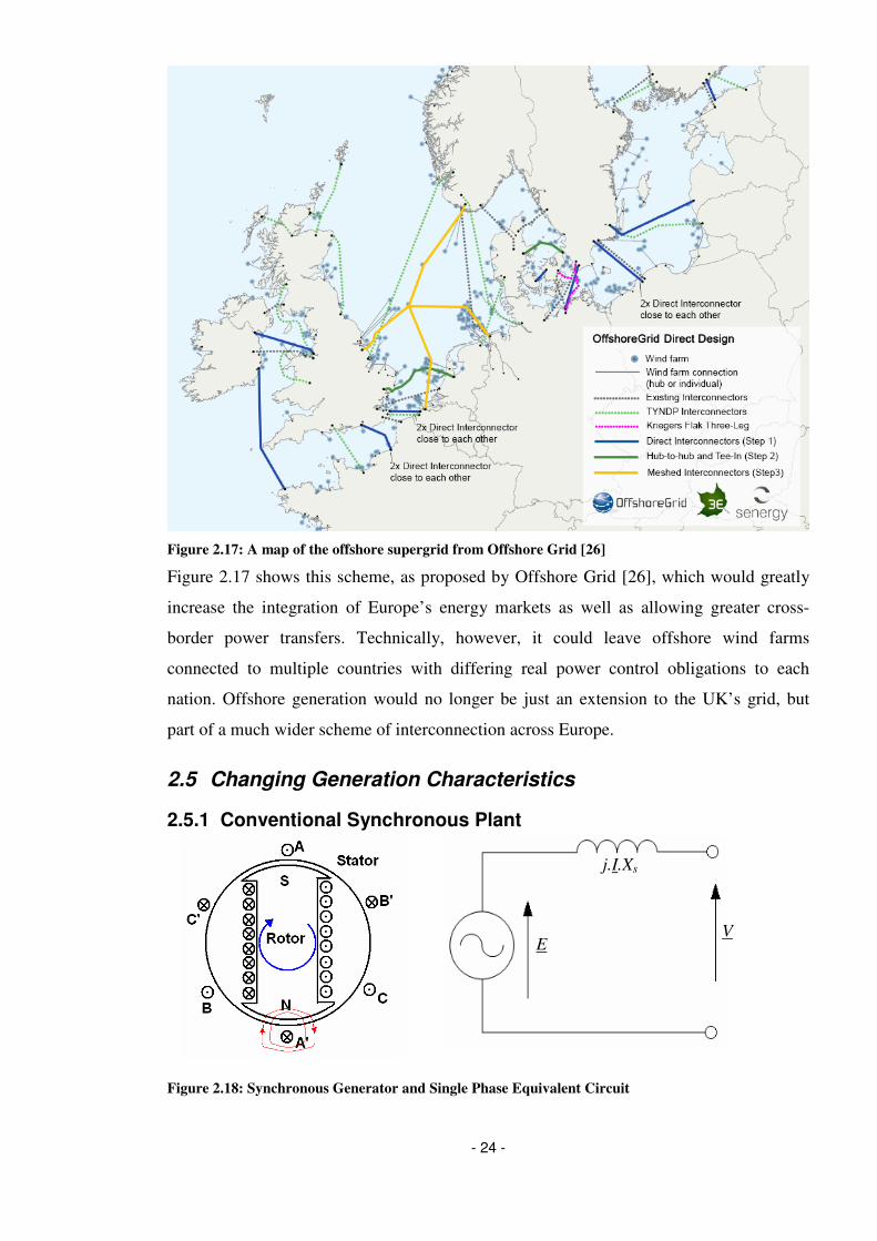
- 24 -

Figure 2.17: A map of the offshore supergrid from Offshore Grid [26]

Figure 2.17 shows this scheme, as proposed by Offshore Grid [26], which would greatly

increase the integration of Europe’s energy markets as well as allowing greater cross-

border power transfers. Technically, however, it could leave offshore wind farms

connected to multiple countries with differing real power control obligations to each

nation. Offshore generation would no longer be just an extension to the UK’s grid, but

part of a much wider scheme of interconnection across Europe.

2.5 Changing Generation Characteristics

2.5.1 Conventional Synchronous Plant

Figure 2.18: Synchronous Generator and Single Phase Equivalent Circuit

E V

j.I.Xs

- 25 -

The majority of the UK’s conventional power plants use steam or gas turbines to drive

synchronous generators directly coupled to the electric grid. As the synchronous machine

has provided the mainstay generator for the UK’s power grid, understanding its basic

behaviour is fundamental to understanding the changes that wind farm technology will

bring to the grid. Some of the key grid interactions of these plants can be understood by

considering an idealised synchronous machine as shown in Figure 2.18 and considering a

single phase representation of the machine, which assumes that the system is balanced.

The three-phase grid voltage drives the current in the stator windings to produce a

magnetic field in the machine’s air gap that rotates at a speed (ωs) defined by the grid

frequency (fgrid) and the machine’s pole pairs (p). This is shown in Equation 2.1 and

Equation 2.2.

Equation 2.1 p

fgrid

s

⋅⋅=

πω

2

Equation 2.2 tBBsss⋅⋅= ωcosˆ

The rotor of a synchronous machine is fed with a DC current which sets up a fixed

magnetic field, in effect as a dipole magnet. Careful design of the rotor windings ensures

that the rotor field is sinusoidally distributed round the air gap. When this rotor is driven

to rotate, either motored by the stator field or by the action of a prime mover, then the

dipole rotates, setting up a second sinusoidally rotating component of magnetic field in the

machine’s air gap as in Equation 2.3. The rotor and stator magnetic fields rotate

synchronously, ensuring that the total field also rotates with a sinusoidal distribution.

Equation 2.3: ( )θω −⋅⋅= tBBrrr

cosˆ

Figure 2.19: Synchronous Machine Vector Diagrams

The total rotating air gap magnetic field, comprised of both the stator and the rotor

components, leads by Faraday’s law (dt

dNE

ψ⋅−= ), to a back Electromotive Force

(EMF) induced in the stator windings, E, as given in Equation 2.4.

Br

Bs

Bt

∠BrBs = α

O

Et

V j.I.Xs

O

I

∠I V = ϕ ∠Et V = ∠BrBt= δ ∠I (j.I.Xs) = 90°

- 26 -

Equation 2.4 ( )δω +⋅⋅= tEEr

cosˆ

Figure 2.19 shows the magnetic field (left) vector diagram for the case of a rotor field

lagging the stator field, alongside the phasor diagram for the machine (right).

The magnetic torque acting on the rotor can be defined according to the equation for the

magnetic moment acting in a magnetic field, BmT ×= . Hence the torque can be seen to

be given by Equation 2.5 where D is a constant.

Equation 2.5 αsinˆˆ ⋅⋅⋅=sr

BBDT

By considering that from the vector diagram δα sinˆsinˆ ⋅=⋅ts

BB

Equation 2.6 δsinˆˆ ⋅⋅⋅=rt

BBDT

The implication of this is that the torque produced by the synchronous machine is

dependent upon the angle between the rotor magnetic field and the total magnetic field,

also known as the load angle. Hence, for steady torque production, this angle must be

constant and the rotor and stator must be rotating synchronously. Furthermore, the torque

from the synchronous machine varies in a sinusoidal relationship with the load angle.

This can also be deduced by considering the phasor diagram, the back EMF is defined as

in Equation 2.7.

Equation 2.7 s

XIjVE ⋅⋅+=

The real power output from the machine can then be defined by Equation 2.8.

Equation 2.8 φω cos3~~

⋅⋅⋅=⋅= IVTPs

By considering the phasor diagram trigonometric relationships:

Equation 2.9 ( ) φφδ cos90sinsin ⋅⋅=−⋅⋅=⋅ss

XIXIE

So φδ

cossin

⋅= IX

E

s

from Equation 2.9 and hence:

Equation 2.10

s

sX

EVTP

δω

sin3

⋅⋅⋅=⋅=

So the torque can be expressed as:

Equation 2.11 δω

sin3

⋅⋅

⋅⋅=

ssX

EVT

- 27 -

Equation 2.11 shows that the generator torque is critically dependent on the angle between

the generator’s internal EMF and the network voltage.

2.5.2 Grid Faults

The phasor diagram of Figure 2.20 shows the effect of a grid voltage that is transiently

suppressed from its nominal rating. The rotor field windings initially continue to be fed

with the same DC current, so the rotor magnetic field is unaffected, supporting the internal

EMF. However, to compensate for the reduced grid voltage, an increased reactive current

is drawn from the machine, dropping voltage across the stator reactance and closing the

phasor triangle. An Automatic Voltage Regulator (AVR) could then act to control to

voltage or reactive power fed into the grid, but there is still an initial current increase. This

current in-feed helps to trip protection devices in the event of a grid fault.

Figure 2.20: Phasor Diagram under Normal (left) and Suppressed (right) Voltage

2.5.3 Grid Inertia

Equation 2.11 considers the torque dependency on the machine’s load angle, but this

inherently assumes constant frequency behaviour of both the rotor and the stator. A

reduction in grid frequency has the effect of gradually changing the angle between the

stator and rotor magnetic fields, and therefore increasing the load angle of the machine.

This relationship between the machine’s frequency and torque means that falling grid

frequency automatically increases the torque, provided it does not exceed the maximum

torque at 90°. This torque increase draws kinetic energy ( 2

2

1ω⋅⋅= JKE ) from the rotor

and accompanying spinning mass. Given that the machine’s rotor must ultimately remain

synchronous to the grid’s frequency, the power output from the machine can be

approximately found by differentiating the rotor’s stored kinetic energy with respect to

time as shown in Equation 2.12. This means that the power output of a synchronous

machine has been shown by Morren, Pierik and de Haan [27] to be broadly proportional to

the rate of change of frequency, acting as an automatic stabiliser to rapid frequency

changes.

Et

j.I.Xs O

∠I V = ϕ ∠Et V = δ ∠EtI = 90°

Et

V j.I.Xs O

I

I

V

- 28 -

Equation 2.12 dt

dJ

dt

dJ

dt

KEd ωω

ωω ⋅⋅=⋅⋅⋅= 2

2

1)(

-1.5

-1

-0.5

0

0.5

1

1.5

-200 -150 -100 -50 0 50 100 150 200

Load Angle (δ) (º)

Pe

r U

nit

To

rqu

e

Figure 2.21: Effect of Frequency Decrease on Load Angle and Torque

Specifically, however, the machine’s output will be dependent on the change in torque,

which is in turn dependent on the change in load angle. The torque will follow the

sinusoidal load profile as the load angle increases or decreases as shown in Figure 2.21. A

frequency difference between the rotor and stator fields creates the change in load angle.

This acts to smooth out the inertial contribution to rapid frequency deviations as the

torque does not step from one level to another.

2.5.4 Grid Frequency

Grid frequency changes result from imbalance between generation and demand, and

whilst the inertia of synchronous machines helps to arrest rapid deviations, ultimately the

imbalance must be eliminated before the frequency can be brought back to target. With a

synchronous generator, this is achieved through governor action, whereby a generator will

increase or decrease its output in proportion to the magnitude of the frequency excursion,

through increased steam raising or boiler action.

2.6 A Challenge for the GB Grid

2.6.1 The UK’s Offshore Wind Farms

Section 2.4.1 highlighted the move in wind turbine technology towards increasing use of

power electronics. These power converters involve extremely fast control loops that are

flexible to react rapidly to desired changes. Fast control is also essential because of power

electronic switches’ sensitivity to over current and the need to rapidly reduce currents in

the event of a fault on the output. The impact of the fast control of a power converter is to

limit the in-feed current in the case of a fault to a much lower level than might be the case

with a traditional synchronous generator.

Generating

Motoring Effect of frequency decrease

- 29 -

The power converters are also deliberately designed to decouple the rotational frequency

of the blades from the grid frequency so as to maximise the energy capture from the wind.

Yet this removes the inertia to frequency changes that synchronous machines inherently

provide to stabilise the grid. A frequency change on the grid side is rectified to DC and

not automatically seen by the machine side. Hence, the kinetic energy of the blades does

not automatically stabilise the grid.

In response to supply shortfalls causing a frequency change, a wind turbine’s output is

limited by the available wind power. Whereas a conventional synchronous plant could

increase its output by burning more fuel or steam raising, the wind turbine has no

equivalent extra resource. This means that for a wind turbine to provide low frequency

response, it would have to deliberately operate at a reduced output. This involves spilling

wind energy in order to hold a margin and have the potential to increase its output in

response to a falling frequency, but does not have associated fuel savings.

These three differences, which are inherent to the design of wind turbines, and provide

them with exceptional controllability, mean that power converter interfaced wind turbines

behave very differently to grid disturbances to the familiar synchronous generators.

Section 2.4.2 highlighted the trends in grid connection which will further distance

offshore wind farms from the grid of today. The increasing use of DC transmission and

potentially distribution will lead to isolation of the offshore wind farms from the

behaviour of the onshore grid. This provides not only technical challenges, to ensure the

continued security of the GB grid, but also regulatory ones.

Today the effects of rising wind power levels are already beginning to be felt, with the

National Grid having to act to constrain wind in 2011 to ensure the security of the GB

system according to the Renewable Energy Foundation [28]. With ever growing levels of

wind power, the challenges of managing the system will continue to grow and challenges

other than constraints will emerge. These challenges, combined with the technological

differences of wind farms will mean that the grid in 2020 with 33GW of offshore wind is

likely to have to look very different to the grid of today. The challenge is to deliver this

whilst protecting the security of supply and grid stability experienced today.

2.6.2 The Grid’s Frequency Challenge

Major frequency deviations on a power system usually occur as the result of a large

generator or load tripping and disconnecting. Such events are currently extremely rare;

however, the GB grid was shown to be susceptible to sizeable frequency deviations by the

- 30 -

events of 27th May 2008. On this occasion, the UK’s largest nuclear plant, Sizewell B,

tripped offline shortly after a coal plant of 345MW. This led to a supply shortfall of

around 1582MW having to be picked up by responsive generators. This is just within the

1600MW maximum loss that the GB grid is typically secured against.

Figure 2.22: GB System Frequency 27th May 2008

After the loss of these two generators, the subsequent frequency fall, whilst initially

arrested, then accelerated again and was ultimately only stopped by the activation of

automatic demand disconnection at 48.8Hz. This further frequency fall is not totally

explained, however, the official report, from National Grid [29], found that “The

unexpected loss of a significant amount of small embedded generation resulted in a total

loss of some 1993MW in 3.5 minutes”. This embedded generation was outside of the

scope of the transmission system Grid Code and therefore was subject to G59, which the

National Grid [30] review found at the time set recommended frequencies at which

generation should trip; this is the reverse philosophy to that applied in Grid Code. It

brought forward the activation of automatic demand disconnection.

Immediately after the loss of each generator, the inertia of the large number of

synchronous machines on the system helped to slow the Rate of Change of Frequency

(ROCOF) such that the maximum ROCOF was 0.073Hz. This provided time for other

plant to increase their output powers to compensate for the lost plant and prevented the

level of demand disconnection being worse. This event demonstrates the importance of

synchronous machines’ inherent inertia in securing the grid.

- 31 -

In the run up to 2020 the UK may have single generation connections of 2GW as a result

of the offshore wind development plans. Partly as a consequence of this, the power system

will be secured against a loss of 1.8GW by National Grid [31] and will also have to deal

with connections from wind turbine technologies with very different grid interfaces to

conventional generation. In a small islanded system, where frequency can already see

significant deviations, this thesis addresses what future offshore wind farms can do to

support the grid’s frequency stability and whether energy storage is ready to provide a

more robust solution.

2.6.3 Power System Oscillation

Ashton et al. [32] have shown that the UK transmission system currently experiences a

number of power system events due to circuit switching as well as a significant major

oscillation between the generators of Scotland and those of England and Wales. Currently

limited capacity across the North/South boundary does not help this situation. Figure 2.5

shows that the UK’s best wind resources are located in the North, beyond the constraint

boundary. Development of these resources will lead to increased stress of the system and

is part of the cause of National Grid’s installation of a wide area monitoring system based

on phasor measurement unit installations at some substations.

The installed monitoring system has been shown by Ashton to have measured the time

delay as a large frequency deviation rippled through the system following a loss of a

generator. A time delay of 0.65s was observed between the frequency deviation occurring

at the closest substations to the lost generator and those furthest away. The monitoring

system provides a large amount of real time data which will in future enhance the system

operator’s visibility of events such as that in Figure 2.22, the challenge will be to use that

data to secure the system’s stability in the face of these multiple challenges.

2.7 Potential Application of Energy Storage?

Concurrent with the development of large scale offshore wind power, National Grid’s

“Gone Green” scenario anticipates a renewed development of Nuclear Power in the UK.

These two factors contribute to National Grid’s [33] projections that the GB system

requirements for frequency response reserves will be significantly increased before 2020,

as outlined in Figure 2.23. This increase in low frequency response requirement, to cover

loss of generation, together with the high price that wind power would require to provide

such services, suggests that the value of frequency response will inevitably significantly

increase in the coming decade.

- 32 -

Figure 2.23: National Grid’s [33] Projection for Requirement for Frequency Response (The solid line

represents the typical requirement, with maximum and minimum requirements shown by the dashed

lines)

The increasing importance of providing balancing services to transmission systems is not

a phenomenon specific to the GB system. Walawalker, Apt and Mancini [34] investigated

the economics of frequency regulation services in New York and concluded that there

were “significant opportunities” for the application of flywheels to frequency regulation in

New York state. They also noted the developments of Beacon Power towards commercial

application of frequency response services with flywheels in both California and New

York states. Alongside Beacon Power, other energy storage manufacturers, such as A123

Systems, according to Vartanian and Bentley [35], have been investigating the frequency

response market as a potential opportunity for their products.

Oudalov, Chartouni and Ohler [36] of ABB Ltd. have had a detailed look at the potential

for energy storage solutions to provide primary frequency control (i.e. short time-scale

only) on part of the European transmission system. Their comparison of Vanadium Redox

Flow, Sodium Sulphur, Lead Acid and Nickel Cadmium batteries concluded that Lead

- 33 -

Acid is viable for this application, in conjunction with dump resistors for accommodating

high frequency response when the battery is fully charged. However, their analysis was

limited to primary frequency control and therefore considered only relatively short

timescales. Nevertheless, this further demonstrates the increasing interest that

manufacturers are taking in the frequency response markets.

Despite the growing interest of manufacturers, Beacon Power, who backed by a US

government loan guarantee program built their 20MW flywheel based frequency

regulation plant in New York State, have recently filed for bankruptcy according to Hals

and Hampton [37]. Their brief exploration of this opportunity showed that the commercial

environment for application of flywheels to frequency response is not viable yet in the

U.S.A.. Their ultimate failure could be put down to technology, timing or both; but they

have perhaps pointed to a possible future for power systems; with generators providing

bulk energy and energy storage systems providing balancing services.

Figure 2.24: Wind Output During Periods of Peak System Demand according to National Grid [38]

In addition to the potential opportunity for energy storage to contribute to system

balancing, there are longer timescale opportunities emerging for energy storage. Figure

2.24, from National Grid [38], shows a typical wind turbine output power profile against

wind speed, superimposed on the graph are the measured wind speeds during the top five

annual power demand periods for the years 1985 to 2008. The y-axis represents both the

year and the power output from a typical wind turbine. It highlights that in the 25 year

period considered, the average wind speed during the five half-hour periods with highest

demand was never above 10m/s. Based on the typical wind turbine’s power production

curve this illustrates that it would be likely that during peak demand periods wind would

- 34 -

be operating at less than 50% of its capacity. This illustrates the need for firm power

capacity.

The broad correlation between low wind speeds and high system demand, during winter

anti-cyclones in the UK, illustrates the need that the UK has for firm capacity to provide

for the power system’s peak demands. This is an area where longer term energy storage

may become increasingly technically and economically necessary.

One of the most comprehensive analyses of the application of energy storage in power

systems is by Eyer and Corey [39] of Sandia National Laboratories. Their work identifies

the need to aggregate different energy storage applications in order to develop “Value

Propositions” that are economically viable. One of the eight value propositions they

investigate is “Renewables Energy time-shift plus Electric Energy Time-shift plus Electric

Supply Reserve Capacity”. This value proposition is the only complementary application

including supplying reserve power to the power system. It involves using an energy store

to provide reserve power at night, whilst charging, and then dispatching that energy into

the peak demand periods, such as those of Figure 2.24. By charging at night the store can

not only take advantage of typically cheap night time power prices, but can also offer

greater capacity for fast reserves as it can revert from charging to discharging.

In the context of this application, the next section will explore the capabilities of different

storage technologies to contribute to solving these challenges as wind power deployment

grows.

2.8 Summary

The development of the wind industry in the UK is likely to see significant offshore

deployment. The technology for both offshore turbines and offshore grid connection is

developing towards solutions that decouple the generators from the onshore grid through

power electronics incorporating interim DC stages. This means that these offshore wind

farms do not provide some of the inherently stabilising actions that a conventional

synchronous machine would. This will lead to challenges for the control of offshore wind

farms in order to maintain the frequency stability of the onshore grid and to provide fault

in-feed currents. These are challenges that the rest of the thesis sets out to address.

- 35 -

3 Modelling of Full Converter Wind Turbines

3.1 Introduction

The growth in wind power on power systems has necessitated development of wind

turbine models that are appropriate for the study of grid interactions. Slootweg et al. [40]

have characterised the key elements that require modelling for power system studies. This

chapter therefore covers the development of a suite of full converter wind turbine models

appropriate for power system studies. Figure 3.1 illustrates the key elements of such a

model, which allows studies from the raw wind input to the grid electrical output.

Figure 3.1: Full Converter Wind Turbine Model Elements

Sections 3.2 to 3.4 cover modelling of physical elements of the system, from the blades to

the output of the power converter into the grid. Section 3.5 then covers the control of the

wind turbine components and system, this section starts at the level of the power converter

control and progresses to cover both the wind turbine control and then the control schemes

that have been used with large scale wind farms. Section 3.7 then covers the validation of

the component parts that make up the wind turbine models.

3.2 Aerodynamics

The available power in the wind can be calculated by considering the kinetic energy of the

air passing through the swept area of the blades. Consider that the kinetic energy (KE) of a

mass of air is given by:

Equation 3.1 2

2

1w

vmKE ⋅⋅= where m is the mass of the air and vw, the wind speed.

The power output is given by the differential of the kinetic energy with respect to time.

- 36 -

Equation 3.2 dt

vmd

Pw

w

⋅⋅

=

2

2

1

Now the mass flow rate of the air is given by:

Equation 3.3 w

vAdt

dm⋅⋅= ρ where A is the blades’ swept area and ρ is the air density.

Hence, the total power available in the wind, Pw, is proportional to the cube of the wind

speed, as shown in Equation 3.4:

Equation 3.4 3

2

1ww

vAP ⋅⋅⋅= ρ

However, the power captured by the wind turbine, P, will only be a proportion of this,

dependent on a performance coefficient Cp. It has been shown by Burton et al. [41] that

the limit on Cp, known as the Betz Limit, is 59.3%. Equation 3.5 illustrates that there are

two key aspects of the aerodynamics which must be modelled in order to accurately

reflect a wind turbine’s output: The prevailing wind speed and the wind turbine’s

coefficient of performance.

Equation 3.5 3

2

1wp

vACP ⋅⋅⋅⋅= ρ

3.2.1 Wind Modelling

Sorensen et al. [42] have shown that accurate wind power output modelling requires

simulations of long slow wind variations that are not typically included in standard

turbulence models. Sorensen also shows that individual large offshore wind farms can

suffer from greater power fluctuations than would be the case for the onshore fleet. This is

caused by the correlation of wind fluctuations at individual turbines being much higher

than would be the case for distributed onshore turbines, due to an offshore wind farm’s

geographical concentration.

This work therefore takes two approaches to modelling the wind: first, when individual

wind turbine component design is considered, a single turbine turbulence model is used

and fed with extreme wind speed conditions. Second, several months’ power output data

from the Horns Rev offshore wind farm have been provided by Hugh Sharman at

Incoteco. This allows accurate simulation of the output power from an entire wind farm,

without the need for this work to investigate detailed farm level wind models.

- 37 -

Sorensen, Hansen and Carvalho-Rosas [43] have presented wind models that are

segregated between the wind farm model which provides a hub wind speed reference to a

separate wind turbine level turbulence model. Sorenson’s model provides a good wind

model structure and details of the transfer functions of the output stage filters. IEC 61400

[44] contributes further by recommending the use of independent turbulence in the

fundamental, 3p horizontal and 3p vertical elements. The structure of an appropriate wind

model is shown in Figure 3.2.

Figure 3.2: Wind Model Structure

In order to implement this wind model with maximum simulation speed, the white noise

generators have been implemented according to the Ziggurat algorithm presented by

Marsaglia and Tsang [45]. The implementation of this can be found in appendix 9.1.1.

The rational filter approximations to the Kaimal spectra are taken from Diop et al. [46],

whose work demonstrates the application of Von Karman and Kaimal filters to meet the

requirements of IEC 61400. The application here considers only the component normal to

the blades’ swept area. The Kaimal filter, as specified by the IEC standard, therefore

reduces to:

- 38 -

Equation 3.6 ( ) ( ) ( )( ) ( ) ( )161616

16164

42

31

+⋅⋅⋅⋅+⋅⋅⋅⋅+⋅⋅

⋅+⋅⋅⋅⋅+⋅⋅⋅⋅⋅=

sTmsTmsT

sTmsTmTsH

Where: m1, m2, m3, m4 = 0.745, 0.152, 0.05, 0.0028; T = 170.1m/vmean; vmean is the

mean wind speed (m/s).

3.2.2 Blade Modelling

The derivation of the power output from a wind turbine in the introduction to section 3.2

showed that aerodynamically the power available from a wind turbine is critically

dependent on the wind speed and the coefficient of performance. Wind turbine

performance coefficient relationships are normally manufacturer specific and

commercially sensitive. However, differences between curves are usually small and Heier

[47] is one of a number of authors presenting a model for a typical coefficient of

performance curve as outlined in Equation 3.7 and Equation 3.8.

Equation 3.7 ( ) ( )βλββ ,54321

6cx

p ecccccC ⋅−⋅−⋅−⋅= , where β is the pitch angle of the

blades of the turbine and λ is the tip speed ratio defined as the ratio of speed of the tip of

the blade to the prevailing wind speed w

b

v

R⋅=

ωλ .

5.01 =c , i

cλ

1162 = , 4.03 =c , 04 =c , 55 =c and

i

cλ

216 = where iλ is given as:

Equation 3.8 1

035.0

08.0

113 +

−⋅+

=ββλλi

Figure 3.3: Typical Wind Turbine Performance Curve

- 39 -

It should be highlighted that Heier’s representation of the blades of a wind turbine is a

static approximation to a dynamic system. As such its use represents an approximation of

the true case and is a significant simplification in comparison to a dynamic model using

dedicated software such as Bladed.

Figure 3.3 shows the impact of the tip speed ratio and pitch angle on the wind turbine’s

performance curve. It can be clearly seen that the optimal power capture occurs for a

single ratio of the blade speed to the wind speed at any given pitch angle. This is the

foundation of the benefit of variable speed machines over fixed speed machines, as the

wind speed increases the rotational speed of a variable speed machine can also increase to

optimise the tip speed ratio and maximise power capture. The plot also illustrates that the

coefficient of performance can be reduced by changing the angle of attack of the blades or

‘pitching’. Hence, turbines equipped with blades that can be pitched can exercise fine

control over power output. This is the subject of section 3.5.2.3.

The controller of a variable speed wind turbine has two primary aims. First, to optimise

the rotational speed of the blades so as to maximise the coefficient of performance, second

to minimise the effects of loads due to wind turbulence. These aims, at least in part are

mutually exclusive as minimising loads in turbulent wind normally requires acceleration

or deceleration of the blades away from the optimal operating point so that the torque

acting on the drive train is smooth.

3.3 Drive Train

Figure 3.3 shows that the optimal tip speed ratio for a wind turbine is typically around 8.

The tip speed ratio is defined as w

v

R⋅=

ωλ and for a typical 2.5MW rating the blade

length, R, would be approximately 50m. Further, such a turbine would start up in wind

speeds of 4m/s and reach rated power output in wind speeds of around 14m/s. Hence, to

operate at the optimal coefficient of performance, the optimal blade speed would be:

rpmsradR

vw 6/64.0

50

481 ==

⋅=

⋅=

λω in low wind conditions up to a maximum of

rpmsradR

vw 4.21/24.2

50

1482 ==

⋅=

⋅=

λω in high wind conditions.

However, typical electrical generator frequencies are around 1500rpm. Hence to deal with

such low mechanical frequencies, the drive train either requires gearing or to be connected

to a multi-pole generator with high pole number, or possibly a combination of the two

approaches.

- 40 -

3.3.1 Geared

The level of detail required to represent the drive train of a traditional geared drive-train

has been the subject of much debate. Ramtharan et al.[48] compared two and three mass

models under transient faults, whilst Muyeen et al.[49] investigated 2, 3, transformed 3

and 6 mass models but both ultimately led to an equivalent two-mass model that

represents the fundamental resonant mode of the shaft system. Such a two mass system

considers a lumped mass broadly representing the inertias of the three blades, hub and low

speed part of the gearbox, connected via a spring and damper system to a second inertia

representing the generator and high speed side of the gearbox, referred to the low speed

shaft. This is illustrated in Figure 3.4.

Figure 3.4: Wind Turbine Drive Train System

Ignore the damping and external torques and consider the torque in the spring acting on

the inertias alone:

Equation 3.9 shaft

gen

gen

blade

bladeT

dt

dJ

dt

dJ =⋅−=⋅

ωω

Now consider the rate of change of the shaft torque:

Equation 3.10 dt

dT

K

shaft

shaft

bladegen⋅=−

1ωω leading to

dt

dT

K

shaft

shaft

bladegen⋅+=

1ωω

Hence substituting back into Equation 3.9:

Equation 3.11 dt

dt

dT

Kd

JT

shaft

shaft

blade

genshaft

⋅+

⋅−=

1ω

Simplifying to 2

21

dt

Td

KJ

dt

dJT

shaft

shaft

gen

blade

genshaft⋅⋅−⋅−=

ω

And given Equation 3.9 gives blade

shaftblade

J

T

dt

d=

ω, substitute into Equation 3.11:

- 41 -

Equation 3.12 2

21

dt

Td

KJT

J

JT

shaft

shaft

genshaft

blade

gen

shaft⋅⋅−⋅

−= which rearranges to give:

Equation 3.13 2

2

dt

TdT

J

Kshaft

shaft

eff

shaft=⋅− where

genbladeeffJJJ

111+=

Equation 3.13 solves to give:

Equation 3.14 tj

shafteTT

⋅⋅−⋅= ω

max with eff

shaft

J

K=ω

Hence there is a natural resonant mode within the shaft system that may be excited by

either electrical or mechanical torque steps. Hansen and Michalke [50] have shown that

this natural resonant mode is inherently unstable in variable speed wind turbines, owing to

the decoupling of the speed of the generator from the grid frequency, which removes the

inherent damping in FSIG wind turbines. They highlight the need to implement active

damping controllers to remove oscillations in the drive train. This will be covered further

in section 3.5.2.3.

3.3.2 Direct-drive

Direct-drive systems allow the generator to be directly coupled to the blades of a wind

turbine, with the low mechanical speed stepped up to a higher electrical frequency through

the use of a high pole number generator. The removal of the gearbox can increase the

physical shaft stiffness significantly, whilst the effective inertia of the system is reduced.

These two factors tend to increase the mechanical resonant frequency of the shafts of

direct-drive wind turbines. However, opposing this improvement in the stability of the

shaft system, Akhmatov [51] has shown that the shaft stiffness is effectively reduced by

the pole number of the generator, such that smaller mechanical oscillations are amplified

by the electrical system.

Parameter Geared Direct-Drive Blade Inertia (Jblade) (kgm2) 2.5 x 107 2.5 x 107

Generator Inertia (Jgen’) (kgm2) 200 90000 Gearbox ratio (ngear) 120 1

Effective Inertia (kgm2) '2

111

gengearbladeeffJnJJ ⋅

+= 2.6 x 106 89700

Shaft Stiffness (Kshaft) (Nm/rad) 3 x 108 1.3 x 109

Generator’s number of pole pairs 2 60

Mechanical Resonant Frequency eff

shaft

resJ

Kf ⋅

⋅=

π2

1 1.7 19

- 42 -

Table 3.1: Comparison of Geared and Direct-drive Shaft Parameters (Approximate to protect

commercial sensitivity)

Table 3.1 shows a comparison of the mechanical parameters of the shaft systems of a

geared and a direct drive generator, both machines are rated identically, with a multi-MW

rating. Despite the lower inertia of the low pole number generator, compared to that of the

multi-pole generator, the high gearing ratio leads to an effectively higher inertia for the

geared shaft than for the direct-drive shaft, as the geared generator’s inertia is referred to

the low speed side (a ratio of ngear2). Further, the geared shaft has significantly lower shaft

stiffness. It can be seen that this leads the mechanical resonant frequency of the direct

drive shaft to be an order of magnitude higher than that of the geared shaft. However,

according to Akhmatov’s work, it is important still to represent the shaft system with a

second order model in direct-drive models, owing to the amplifying effect of the

generator’s high pole number.

3.4 Electrical System

The mechanical shaft system model includes a representation of the generator’s rotor

inertia. The output of this mechanical model drives the generator at a set rotational speed

whilst the generator exerts an electrical torque on the mechanical shaft model. Section

2.4.1.4 highlighted that three different full converter configurations are possible,

consisting of induction generators and both electrically excited and permanent magnet

synchronous generators. The trends in wind turbine configuration, alongside GE Energy’s

Power Conversion business’s experience and commercial involvement, have led this work

to concentrate on the FFIG and FFPMG.

3.4.1 Park and Clarke’s Transforms

Much of the analysis and control of three phase rotating machinery depends on the ability

to transform the three phase vectors into an equivalent stationary two axis form (Clarke’s

transform) or an equivalent synchronously rotating two axis reference frame (Park’s

transform), this derivation is based on Adkins and Harley [52]. These are introduced here

as they underpin much of the subsequent analysis of both induction machines and

permanent magnet machines. Clarke’s method transforms the ABC three phase system

into an αβγ reference frame. The α axis is typically aligned with the A phase, with the β

axis lagging by 90°, the γ axis is then analogous to an unbalanced DC offset to this pair,

which for simplicity means it is zero for balanced systems. Figure 3.5 shows the

relationship of these axes. The transform can then be derived by resolving the components

of the ABC system into α and β components. First consider the α component:

- 43 -

Equation 3.15 ( )

−

⋅+⋅⋅+

−

⋅−⋅⋅+−⋅⋅= δ

πωδ

πωδωα 3

2cosˆ

3

2cosˆcosˆ tItItII

Equation 3.16 ( )

−

⋅+⋅⋅+

−

⋅−⋅⋅+−⋅⋅= δ

πωδ

πωδωβ 3

2sinˆ

3

2sinˆsinˆ tItItII

Figure 3.5: Clarke’s Transform abc-αβγ

By aligning the α axis with phase A, the angle between the α axis and the A phase

becomes zero and the transform reduces in matrix form to (the factor of two thirds is from

conservation of power between the axes):

Equation 3.17

−

−−

⋅=

C

B

A

I

I

I

I

I

2

3

2

30

2

1

2

11

3

2

β

α

The inverse transform can be derived by inverting this and is given as:

Equation 3.18

−−

−=

β

α

I

I

I

I

I

C

B

A

2

3

2

12

3

2

101

Park’s transform is in many ways an extension of Clarke’s transform which aids with the

analysis of rotating machinery as it transforms the three phase equations onto a

synchronously rotating reference frame. This in turn allows the AC quantities to be

considered as DC components and controlled as such. This is shown in Figure 3.6, where

again the three phase system is considered balanced and the d axis is rotating

synchronously (speed, ω) at an angle, θ, to the A phase.

β

α

( )δω −⋅⋅= tIIA

cosˆ

−

⋅+⋅⋅= δ

πω

32

cosˆ tIIB

−

⋅−⋅⋅= δ

πω

3

2cosˆ tII

C

- 44 -

Once again the transform can be derived by resolving the components of the three phase

currents onto the dq axes.

Equation 3.19 ( )

⋅+⋅+

⋅−⋅+⋅=

3

2cos

3

2coscos

πθ

πθθ

CBAdIIII

Equation 3.20 ( )

⋅+⋅+

⋅−⋅+⋅=

3

2sin

3

2sinsin

πθ

πθθ

CBAqIIII

Figure 3.6: Park’s Transform αβγ to dq0

These transforms, when power is invariant, in matrix form are then given as:

Equation 3.21

( )

( )

+

−

+

−

⋅=

C

B

A

q

d

I

I

I

I

I

3

2sin

3

2sinsin

3

2cos

3

2coscos

3

2π

θπ

θθ

πθ

πθθ

The inverse transform can be derived by inverting this and is given as:

Equation 3.22

( ) ( )

+

+

−

−=

q

d

C

B

A

I

I

I

I

I

3

2sin

3

2cos

3

2sin

3

2cos

sincos

3

2

πθ

πθ

πθ

πθ

θθ

3.4.2 Induction Generator

Park’s transforms greatly help with the analysis of a squirrel cage induction machine.

Which can be considered with a reference frame rotating synchronously to machine speed

and the d axis aligned with rotor flux as is considered here.

The squirrel cage induction machine was originally the dominant generator technology in

fixed speed wind turbines. Hence, the upgrade path to develop a variable speed wind

turbine with FFIG is an appealing option. The equivalent circuit of the induction generator

is shown in Figure 3.7, with the magnetising branch resistance assumed infinite.

q d

( )δω −⋅⋅= tIIA

cosˆ

−

⋅+⋅⋅= δ

πω

32

cosˆ tIIB

−

⋅−⋅⋅= δ

πω

3

2cosˆ tII

C

θ ω

- 45 -

Figure 3.7: Induction Machine Equivalent Circuit (left) and Field Oriented Control (right)

It is desirable to be able to independently control the generator’s torque and flux in order

to achieve fast transient performance. With this aim Bose [53] provides a synopsis of the

current capabilities of vector control for induction machines and highlights the parallel

that can be drawn to a DC machine when an induction machine is controlled in a field

oriented manner, as in Figure 3.7. The fundamentals of this technique are outlined here.

Consider the current through and voltage across the magnetising and other branches:

Equation 3.23

m

Lrr

m

r

r

mqmdm

X

XIj

X

s

RI

IjII⋅

⋅+⋅

=⋅+=

Hence the rotor circuit current can be defined by considering the d-axis component:

Equation 3.24

r

mmd

r

mmd

rR

XIs

s

R

XII

⋅⋅=

⋅=

But by definition, Ir must be in the q-axis to be purely torque producing, therefore, the

total q-axis current is (by Kirchoff’s law):

Equation 3.25

m

Lr

r

mmd

r

mmd

m

Lrr

r

mmd

rmqqX

XR

XIs

R

XIs

X

XI

R

XIsIII

⋅⋅⋅

+⋅⋅

=⋅

+⋅⋅

=+=

This can be rearranged to give the q-axis stator current in terms of the magnetising branch

current:

Equation 3.26 ( )

rmd

r

Lrmmd

qTIs

R

XXIsI ⋅⋅⋅=

+⋅⋅= ω where the rotor time constant is

given by the equation ( )

r

Lrm

rR

LLT

+= . Furthermore, the d-axis stator current must equal

the d-axis magnetising branch current as Ir has been shown to be in the q-axis.

Iqs

Ids

ωe

Ψr_pk

- 46 -

Equation 3.27 mdd

II =

The real power and resistive losses in the rotor circuit can be derived by considering the

referred rotor resistance as a pure resistance (r

R ) in series with the torque producing

resistance (s

sR

r

−⋅1

) and considering the mechanical power to be equal to the three phase

electrical power.

Equation 3.28

−⋅

⋅⋅⋅=⋅=

s

sR

R

XIsTP

r

r

mmd

rq

13

2

ω

This simplifies to:

Equation 3.29 ( )r

mmd

rqR

XIssT

22

13⋅⋅

−⋅=⋅ω

And substituting for the rotor frequency (( )

p

sfr

−⋅⋅⋅=

12 πω , p is machine pole pairs):

Equation 3.30 ( ) ( ) ( )

r

mmd

qR

LIss

p

sfT

22

1312 ⋅⋅⋅

−⋅=−⋅⋅⋅

⋅ωπ

Equation 3.31

r

mmd

qR

LIspT

22

3⋅⋅⋅

⋅⋅=ω

Substituting in Imd from Equation 3.26 and recognising Equation 3.27, gives torque in

terms of the q and d-axis stator currents:

Equation 3.32

rm

m

qdqLL

LIIpT

+⋅⋅⋅=

2

3

Rearranging to give the q-axis current gives:

Equation 3.33 p

L

L

TI m

r

r

q

q⋅

+

⋅Ψ

=3

1

where dmr

IL ⋅=Ψ

Equation 3.26 taken together with Equation 3.33 shows how the induction machine can be

controlled in the manner of a DC machine, through independent control of d and q-axis

stator currents, where the d-axis is aligned with the rotating rotor flux vector. This

independent control of the torque and flux allows fast torque response to transients, but

also allows fine control over the rotor flux. This has the advantage that the field can be

weakened when the rotor speed is high so that the generator’s output voltage is lower, so

- 47 -

called “field weakening”. In a wind turbine application, where instantaneous gusts can

cause acceleration of the blades and generator, field weakening is a useful feature, as it

ensures that the voltage seen by the full converter can be kept within its voltage ratings

across a relatively wide speed range.

There are two drawbacks of the induction machine, however, first the machine must be

charged with the d-axis (magnetising) current even in relatively low winds. This can mean

that it is relatively inefficient at the light loads that are common in wind turbine

applications. Second, as blade diameters have increased, in order to maintain a constant

tip speed ratio, the blade rotational frequency has fallen. This reduction in blade rotational

frequency has necessitated increased gearbox ratios; which have come at the expense of

increasing gearbox torques.

3.4.3 Permanent Magnet Generator

The twin challenges of FFIG wind turbines’ poor low speed efficiency and gearbox

failures are two of the drivers behind many manufacturers developing Permanent Magnet

Generator based wind turbines. Troedson [54] finds that all of the top three wind turbine

manufacturers are developing new FFPMG based solutions, with part load efficiency,

reliability, maintainability and grid compatibility raised as the key advantages over

induction generator solutions.

As with the FFIG, it is desirable to independently control the torque on the PMG in a wind

turbine application. Figure 3.8 shows the equivalent circuit of the PMG alongside a vector

diagram which considers the PMG in the rotor flux oriented reference frame. Here a

multi-pole design with equal d and q-axis stator reactance is considered.

Figure 3.8: Permanent Magnet Generator Equivalent Circuit (left) and Vector Diagram (right)

Considering the rotor flux oriented reference frame of Figure 3.8, the real power can be

seen to be given by:

EInternal =

ω.Ψmag UStator

Ψmag

ωLiq

id = 0

iq

δ

iqR

- 48 -

Equation 3.34 δω cos2

3⋅⋅⋅=⋅=

StatorqUiTP This is equivalent to:

Equation 3.35 magq

iT Ψ⋅⋅⋅= ω2

3 (Ignoring the stator resistance)

Hence, the torque is directly controlled by the q-axis current in this reference frame.

Implementation of a non-zero d-axis current varies the q-axis stator voltage and allows

control over the total voltage seen by the power converter. However, in contrast to the

induction machine it cannot change the rotor flux (Ψmag), as this is fixed by the permanent

magnets. This means that as the machine tends to higher speeds, the open circuit voltage

of the permanent magnet generator will tend to increase linearly. The equations of the

PMG can be written to assess the voltages on the terminals of the PMG and converter.

These are shown in Equation 3.36 and Equation 3.37 and highlight the voltage

dependency on speed.

Equation 3.36 dt

dILLIRIU d

ssqdd⋅+⋅⋅−⋅= ω

Equation 3.37 dt

dILLIRIU

q

smagsdqq⋅+Ψ⋅+⋅⋅+⋅= ωω

The inability to field weaken is a limitation of the PMG in comparison to a conventional

induction or synchronous generator. It has led Michalke, Hansen and Hartkopf [55] to

consider what is the most appropriate reference frame for the control of a PMG in order to

minimise the risk of transient over-speeds causing excessive voltages which damage the

power converter. This problem has also led Li and Chen [56] to suggest optimising the

selection of PMGs based on their rated speed for specific wind speed sites.

3.4.4 Converter

The power converter for a modern wind turbine relies on the application of IGBT

technology. It has been in large part the technical and economic advancement of IGBT

devices that has enabled the widespread deployment of variable speed wind turbines.

Today most wind turbine converters are two level designs, incorporating six IGBT devices

per bridge, as shown in Figure 3.9. Each bridge can act as a passive three phase rectifier;

converting the three phase AC voltage to DC through the anti-parallel diode bridge, or as

an Active Front End (AFE) by switching the IGBTs to synthesise a three phase voltage

based on Pulse Width Modulation (PWM) of the DC voltage.

The generator AC voltage, which is usually Low Voltage (LV), below 690V according to

GE Energy [57], is actively rectified to DC by the machine bridge, which raises the DC

- 49 -

voltage above the peak of the AC waveform. This DC level is then inverted back to AC

again to connect into the grid at around 690V, before being stepped up by a transformer to

typical levels of 11kV or 33kV.

Figure 3.9: Two Level Power Converter

Portillo et al. [58] highlighted as early as 2006 that the continued advance in power

electronic component cost and performance was making 3 level power converters a

potentially better option for high power wind turbine applications. The increased number

of levels improves harmonics, raises the operating voltage and increases the efficiency of

the power converter. These advantages will continue the increase in power device count in

wind turbines.

In both two and three level converters, the switching frequency of the IGBTs is typically

over 1 kHz, with low order harmonics generally very low level. The modelling of a power

converter including switching cycles and devices is computationally demanding, all the

more so with increasing numbers of devices in the power converter.

Figure 3.10: Simplified Representation of the Power Converter

Given the high switching frequencies involved and the desire for a model that is effective

for power system studies, an idealised model using ideal voltage and current sources has

been used to represent the power converter. Figure 3.10 shows how this simplification is

- 50 -

achieved with power balances between ideal three phase AC voltage systems and ideal

current sources on the DC link. The use of ideal current sources feeding the DC link

allows any major disturbances in DC link voltage to be observed.

In the real converter, the DC link applies a natural limit to the AC side voltages that can

be generated by the IGBT bridges as the peak of the AC waveform cannot exceed the DC

voltage. However, this natural limit must be replaced by synthetic modulation depth limits

in the control layer that take into account the voltage on the DC link and consequently

limit the maximum AC voltage. Furthermore, the passive three phase rectifier of the anti-

parallel diodes is not represented, meaning that this representation is not appropriate for

converter start-up studies, where DC link precharge is necessary.

Figure 3.11: Network Bridge Equivalent Output Circuit (left) and Vector Diagram (right)

The network bridge can be controlled in a synchronous reference frame as with the PMG.

Figure 3.11 shows how the control of the bridge voltage magnitude and phase controls the

d and q-axis currents, which in turn set the network bridge’s real and reactive power

outputs.

3.4.4.1 Without Chopper

Under load large steps or severe voltage disturbances, transients on the AC sides of the

system can lead to increased DC link voltages. The peak allowable DC voltage is set by

the lower of the DC voltage rating of the IGBTs (which may differ between passive

rectification and active switching) and the capacitor’s voltage rating. The capacitor

typically has a time constant of just a few milliseconds and this voltage must not be

exceeded, hence high bandwidth control is necessary to ensure that the DC link voltage

stays within safe margins. The FFIG does not include or require the use of a DC link

chopper, in part because its ability to field weaken ensures generator side speed transients

can be protected against in isolation from the DC link.

Ugrid

Vbridge

RI

I

j.X.I

Iq

Id

- 51 -

3.4.4.2 DC Choppers and Brake Resistors

Figure 3.9 shows that it is possible to use an additional IGBT switch connecting a resistor

across the DC link. This allows power to be sent to the Dynamic Brake Resistor (DBR) in

the event of an over-voltage on the DC link. Typically such events are brief transients,

allowing the resistor to be rated at the kW level, whilst thermally absorbing occasional

transients in the MW level. Normally chopper control is a simple threshold controller,

where the IGBT is switched on as soon as the voltage exceeds a preset level. Figure 3.10

shows that the chopper has been modelled in the simplified model as an anti-parallel

current source drawing current from the capacitor in the event of a DC link over voltage.

3.5 Control System

Three layers of control exist within a typical wind farm, with the wind farm controller

providing set points to the wind turbine controller, which in turn provides set points to the

turbine’s power converter. This section covers the implementation of these controllers.

3.5.1 Converter

In 2009, Hansen and Michalke [59] proposed two possible broad methods of controlling

the power converter of a wind turbine. What they proposed as a novel method was in fact

the method that had already been deployed to meet the rigours of grid codes in GE

Energy’s power converters. The control scheme that is classified as a ‘classical’ control

scheme is outlined in section 3.5.1.1 whilst section 3.5.1.2 covers the method used in most

of GE Energy’s Power Conversion business’ wind turbine converters.

3.5.1.1 Conventional Control Scheme

Figure 3.12 shows the conventional method of controlling a power converter as

implemented in the wind turbine model. The machine side bridge, which acts as a

rectifier, receives two set points. One set point controls the torque by controlling the q-

axis current in accordance with either the PMG or the Induction machine vector control

(note an unusual convention is used for dq axes in GE Energy’s Power Conversion

business). A second reference for either the flux or the maximum stator voltage is used as

the set point for the d-axis current and controls the machine’s magnetisation and

ultimately the voltage which is seen at the power converter terminals.

Two set points are also provided to the network bridge, one for the AC supply voltage

(shown), power factor or reactive power output (both not shown), this set-point is attained

by means of a Proportional-Integral (PI) controller setting the d-axis current reference. A

second reference is the target DC link voltage. The machine bridge pushes power onto the

- 52 -

DC link according to the machine’s speed and the torque set point. The network bridge

responds through a PI regulator which sees an increase in machine power as an increase

DC link voltage and controls the network bridge’s q-axis current reference so as to

increase power output to the grid.

Figure 3.12: Basic Conventional Power Converter Control Strategy

This cascade control scheme uses fast inner current controllers, which control the d and q-

axis voltages to ensure that the d and q-axis currents follow their set points. Also of note

from the control scheme, the grid angle and frequency are tracked by a Phase Locked

Loop (PLL), which acts to ensure the network bridge’s dq reference frame is synchronous

to the grid. The modulation depth limits incorporated into the control scheme compensate

for the use of ideal voltage sources in place of IGBT switch models.

Figure 3.13: Control Block diagram for the DC link

- 53 -

Seok, Lee and Lee [60] have developed tuning techniques for a permanent magnet

generator’s converter which incorporates a neat method of automatically setting the gain

for a PI controller where the plant is an integrator. Their method can be applied to the DC

link voltage controller to automatically set the PI controller gains here.

Figure 3.13 shows the block diagram, and if the current controller is assumed to have a

very high bandwidth, relative to the DC link voltage controller, its phase delay and gain

can be ignored. Hence an approximate open loop transfer function can be seen to be:

Equation 3.38 ( )2

1

sC

KsK

sCs

KKsG

dc

ip

dc

i

p⋅

+⋅=

⋅⋅

+=

Now if we desire a DC link controller bandwidth of ω rad/s at the gain cross-over point

the phase margin (φ ) can be considered (Bandwidth and Phase Margin Assignment

Method):

Equation 3.39 )tan(φω

=⋅

i

p

K

K

Equation 3.40 ( )

124

22

=⋅

+⋅

dc

ip

C

KK

ω

ω

Now the proportional gain can be substituted for in Equation 3.40 by rearranging Equation

3.39 to give:

Equation 3.41 24

22

24

2

2

))(tan1(1

)tan(

dc

i

dc

i

i

C

K

C

KK

⋅

+==

⋅

+

⋅

⋅

ω

φ

ω

ωω

φ

So rearranging Equation 3.41 allows the integral gain to be assigned by selection of an

appropriate phase margin and then the proportional gain can be found from Equation 3.39.

Equation 3.42 ))(tan1( 2

2

φ

ω

+

⋅= dc

i

CK

Automatic tuning of the DC link controller provides benefits when setting up new variants

of the wind turbine power converter models as it is the DC link which couples the two

IGBT bridges. Therefore, automatic gain setting to ensure that the DC link voltage

controller has reasonable stability and hence allows the other controllers to be tuned

without interference from the modulation depth limit.

3.5.1.2 Reversed Control Scheme

The classical converter control scheme suffers from two shortcomings, first the network

bridge’s control over the DC link voltage is not ideal for a generating application. The

- 54 -

tendency is for grid transients to lead to the DC link controller running into current limits.

This in turn can cause the DC link voltage to increase as the machine bridge continues to

generate into the DC link. The second shortcoming is a commercial block, in that General

Electric historically held a US patent by Richardson and Erdman [61] on torque

controlling an induction machine with vector control. Hence, Converteam UK Ltd., prior

to being taken over by General Electric, developed a control scheme patented by Jones et

al. [62], that avoided this patent but relied on DC link control on the machine bridge.

Figure 3.14: Alternative Power Converter Control Strategy

Under this alternative control strategy, the DC link voltage is used to set the machine

bridge’s q-axis current reference, thereby indirectly controlling the generator’s torque in

order to maintain a constant DC link voltage. The network bridge is provided with a

power set point which sets the network bridge’s q-axis current reference. Hence, power is

drawn off the DC link and the DC link controller responds by increasing the generator’s

torque. This method has the advantage that it makes it simpler to control a converter to

- 55 -

avoid the need for a chopper and DBR. Figure 3.14 shows the overall control strategy of

the power converter under this scheme.

The challenge with this control scheme is that it requires a power set point rather than a

generator torque set point. This is a slight difference from classical wind turbine controller

reference setting, but has the advantage that it ultimately leads to power output

optimisation from the machine to the grid, rather than purely of the machine and machine

bridge.

Whichever control strategy is selected, it must interface to the wind turbine controller

which provides two of the power converter set points. Whereas the DC link voltage and

maximum generator side voltage are for the power converter supplier to control, it is

desirable for the wind turbine to control the real and reactive power to the grid.

3.5.2 Wind Turbine

The wind turbine controller interfaces with the power converter controller by setting the

converter’s real power output reference and either a voltage set point, power factor or a

reactive power set point. The wind turbine controller may receive a signal from the power

converter during a grid fault, to indicate a loss of power output.

The aims of the wind turbine controller are broadly two-fold, first to maximise the energy

yield of the turbine and second to ensure the speed of the turbine and the structural loads

exerted on the turbine stay within design limits. Section 3.2.2 showed that the optimal

coefficient of performance is achieved at a single ratio between the tip speed and the wind

speed. Hence, under turbulent wind conditions, the rotational speed of the turbine would

have to continuously vary to optimise the power capture and energy yield.

There are two possible approaches to optimising the energy yield which are covered in

Camblong et al. [63]: “Indirect Speed Control” and “Direct Speed Control”. The direct

approach is shown to be more flexible to follow the optimal rotational speed as it is not

restricted by the inertia of the turbine. Whilst they recommend the direct approach, they

also acknowledge the higher torque and electrical power oscillations that result.

3.5.2.1 Indirect Speed Control

Leithead and Connor [64] illustrate that there is no such thing as a single wind speed, for

use in the turbine controller, as the wind varies across the swept area of the blades. Hence,

it is not possible to optimise the turbine through use of a wind speed input. Further, they

highlight four goals for the wind turbine controller, which are summarised here:

- 56 -

• Limit mechanical loads

• Limit and smooth power output

• Damping the shaft system

• Optimising power capture and hence energy yield

They highlight the dynamic stability of a controller that tracks the optimal coefficient of

performance by controlling the torque to follow the optimal Cp curve. Whilst Leithead

and Connor propose complex controllers that are ideal for tracking the maximum power

point, for power system applications these can be approximated with a look-up table

defining either the generator torque or power dependent on the rotor speed of the turbine.

Such a look-up table is graphically illustrated in Figure 3.15. Stability can be intuitively

understood as follows; an increase in wind speed causes an increase in aerodynamic

torque, which in turn accelerates the blades. The higher rotational speed of the blades

leads to an increase in the power reference (from A to B) sent to the power converter. This

increase in power reference leads to an increase in the electrical torque to counteract the

increased aerodynamic torque and hence stable operation at a new, higher operating speed

and output power.

Figure 3.15: Rotor speed to power look-up table

This approach to optimising the energy yield of the turbine implicitly helps to smooth

structural loads; sudden generator torque steps are avoided and gusts and lulls in the wind

speed are filtered by the blades’ inertia, resulting in only small changes in the rotor speed

of the blades. However, the inherent use of the blades’ inertia means that the optimal Cp

Increased wind speed Increased rotor speed Increased power reference

- 57 -

curve can only be tracked slowly, resulting in lower than optimal yield particularly in

turbulent wind conditions.

This maximum power tracking method achieves a good trade-off between optimising the

turbine’s energy yield and minimising the structural loads. It is therefore a reasonable

approximation to the conventional choice for a full converter wind turbine application.

3.5.2.2 Direct Speed Control

Burton et al. [65] have highlighted that closer tracking of the optimal Cp curve than

Indirect Speed Control permits could allow an increase in the energy yield of a wind

turbine by around 1-3%. This is a sufficient incentive that a new entrant to the wind

turbine market proposed using a direct method of controlling the wind turbine’s speed in

2009. This method is described here.

Figure 3.16 provides an overview of the salient features of the controller. A key feature is

the measurement of output power to the grid and the subsequent setting of a new speed set

point based on this, which is a reversal of the indirect method. The pitch controller

therefore has to act to limit power output and the turbine controller provides a speed

reference to the machine side converter.

Figure 3.16: Direct Speed Control Overview

The speed set point is set according to an adaptive algorithm that can be seen in Figure

3.17. Essentially, if the power output increases when the speed reference has been

increased then the controller sets a new higher speed reference until such a time as the

power output decreases. This results in a ‘hill-climbing’ controller. Conversely, if the

power output decreased when the speed reference had been increased then the controller

- 58 -

would set a new lower speed reference. By this means the controller should always look to

maintain the optimal speed and therefore the optimal Cp.

Figure 3.17: Direct Speed Controller (A hill climbing approach)

As the direct speed control method results in a speed reference output, it is necessary to

implement a speed controller in order to give a torque reference output to interface with

the drive controller. It is the dynamic performance of this speed controller, rather than the

rotational inertia, which sets limits on how closely the optimal Cp point is tracked in

turbulent wind conditions. A simple PI controller is the traditional means of providing

speed control and this gives a torque reference which is modified by the maximum and

minimum torque limits. The maximum torque is set by the limit on the drive train torque,

whilst the minimum torque is likely to be zero or more as it would be unacceptable to

motor the blades.

Figure 3.18: Direct Speed Control Torque Swings

Figure 3.18 illustrates the key challenge with direct speed control. Following a sudden

increase in the wind speed there could be a significant torque transient, potentially to zero

torque, whilst the blades accelerate to the new optimal speed. Given that the blades cannot

be motored and the allowable torque is limited, the high inertia of the blades means that

the controller can take a significant period of time to reach the new optimal point. The

torque swings associated with keeping the wind turbine operating at the optimal Cp point

- 59 -

lead to unnecessary wear and tear on the drive train and difficulty achieving the

theoretical gains from this strategy.

3.5.2.3 Shaft System Damping

Section 3.3 highlighted that wind turbines can have natural resonant modes between the

shaft and the generator that can become unstable in variable speed applications owing to

the loss of the grid’s stabilising effect. This necessitates active damping of the shaft,

which can be achieved in three ways:

• Use of the pitch controller to aerodynamically damp the speed oscillations of the

blade. This is limited by the rate at which the pitch actuators can adjust the blades

and consequently is the least effective method according to Muyeen et al. [66].

• Add a damping term directly to the torque controller of the machine bridge. This is

rapid and effective according to Hansen and Michalke [50] but requires the

oscillation energy to be stored in the DC link of the converter. This oscillation

energy results in higher voltages on the DC link and would necessitate a higher

rated and more expensive capacitor.

• The third option is to add a damping term to the converter’s power reference; this

method has also been shown to be effective but has the side effect of causing a

degree of ripple in the power to the grid whenever the mechanical mode is excited.

The third option is the preferred option here as it has the lowest impact on the design

requirements for the power converter and wind turbine. It can be implemented by

augmenting the power reference derived from the wind turbine’s maximum power

tracking algorithm and using a damping controller that is similar in structure to that

proposed by Hansen and Michalke. This is shown in Figure 3.19, however, it should be

noted that the phase delay due to the machine bridge DC link control of the power

converter makes the phase lag greater than that seen by Hansen and Michalke’s controller,

necessitating careful tuning of the phase compensator.

Figure 3.19: Shaft Damping Controller Added to Maximum Power Tracker

3.5.2.4 Pitch Angle Control

- 60 -

Figure 3.1 and Figure 3.16 highlighted the need for pitch angle control of the wind

turbine’s blades in order to limit the speed and power output of the turbine respectively.

The representation of the pitch controller used here ignores the fine tuning of pitch angle

that occurs to optimise Cp in below rated wind speeds. For the power system models

developed here, it is appropriate to concentrate on the primary function of the controller:

limiting power or blade speed in above rated wind conditions. As the focus is on large,

full converter wind turbines, the pitch strategy considered here is pitch-to-feather owing to

the high structural loads that a pitch-to-stall strategy would incur and the more common

deployment of pitch-to-feather according to Muljadi and Butterfield [67].

Bossanyi [68] has shown that modern large scale wind turbines have complex pitch

controllers fulfilling multiple objectives, including smoothing out tower shadow torque

pulsations using individual blade pitch angle control. For the purposes of representing the

electrical characteristics of a wind turbine it is not necessary to model the pitch controller

in such detail, however, it should be noted that the representation of the pitch controller

used in this work is a significant simplification compared to a full controller.

A standard PI controller can be augmented with anti-wind-up control to account for the

physical limit on the extent and rate at which the blades can pitch. Muljadi and Butterfield

have also shown that slower pitch systems of 4°/s experience significant speed

fluctuations and hence wind-up, whilst faster systems (they consider 8°/s) can lead to

significantly smoother output. Figure 3.20 shows the key elements of the pitch controller.

It can be noted that the modelled pitch controller does not act when the rotor speed is

below the rated rotor speed. Thereafter, the pitch angle increases to bring the turbine

speed back to target.

Figure 3.20: Pitch Controller for Indirect Speed Controlled turbine

3.5.3 Wind Farm

The wind turbine’s controller is responsible for optimising the power output and

behaviour of the wind turbine by controlling the pitch of the turbine’s blades and the set

points of the power converter. In individual installations or small wind farms this is

- 61 -

sufficient functionality to operate, however, Christiansen [69] has shown the complexity

involved in larger scale offshore wind farms which are captured by the requirements of

Grid Codes. Under large scale schemes it is necessary to have some control of the

individual turbines centrally in order for the wind farm to operate in the manner of a

conventional power plant.

Gjengedal [70] has detailed fourteen different means by which centralised wind farm

control may be necessary in order to replicate the behaviour of conventional plant. These

reasons may be summarised as:

• Reactive power control for voltage stability and variable power factor operation in

steady state.

• Reactive power control to feed fault current contributions in transient states.

• Real power control to meet ramping and maximum power limits in steady state.

• Real power control to meet frequency control requirements under transient states.

• Black start and islanding control.

Such control can be implemented by communicating with the individual wind turbine

controllers and acting as a system aggregator. Banham-Hall et al. [71] have shown a

typical scheme where the wind turbines provide the central wind farm controller with a

measure of their individual available power. The central controller then dispatches real

power and voltage operating points to the individual wind turbines. This ensures that the

wind farm operates as a single power plant to meet the requirements of modern Grid

Codes, which will be discussed further in chapter 4.

Figure 3.21 considers the case where frequency is centrally controlled, with power set-

points sent to each individual turbine. Conversely, the voltage (potentially reactive power

or power factor) is controlled locally to the turbines. However, this combination is not

unique, alternatively the frequency controller could exist at each turbine, with a central

supervisor; or else the control of voltage could be exercised centrally, with a reactive

current demand dispatched to each turbine. Overall, however, the central controller has to

maintain a supervisory function.

- 62 -

Figure 3.21: Wind Farm Controller, aggregating wind turbine availability and dispatching real and

reactive power or voltage set-points to the individual turbines

3.6 Software

3.6.1 Matlab-Simulink

Matlab-Simulink is an ideal environment for development of control systems and single

wind turbine models. Iov et al. [72] have released a standard library for wind turbine

modelling, however, this was developed in the era before the prominence of full converter

wind turbines and hence focussed largely on DFIGs and FSIGs. Further, the power

converter control systems deployed were not in keeping with the control system used in

GE Energy’s converter. The library is also restricted to academic and non-commercial

use, hence whilst it has provided useful insights, new blocks and models have been

developed.

GE Energy use Matlab-Simulink for modelling of the full converter, importing the drive

code and wrapping it in s-functions. This modelling includes switching patterns, full

internal drive features, such as alarms and protection, and full modelling of the DC link.

This model is appropriate for short time scale studies that require absolute detail, such as

fault ride-through modelling of single turbines. However, at the outset of this project the

simulation times associated with this model were of the order of an hour per fault ride-

through study. This demonstrated that it was unfeasibly complex for longer time-scale

studies or for multiple turbine studies.

- 63 -

This project has therefore developed a suite of models for use in multiple turbine or longer

time-scale studies. These models have in common that they are full converter type wind

turbines, but beyond that incorporate different generators, shaft topologies, converter

control strategies and maximum power point tracking methods. The range of different

models is summarised in Table 3.2.

As can be seen from Table 3.2, the variety of models developed allows comparison

between many of the different control techniques and technologies deployed with full

converter wind turbines. Often wind turbines with full converters are classified as a single

type, this work reveals the variety that can exist within type 4 wind turbines and highlights

the risk of assuming generic properties of full converter wind turbines without

understanding the underlying technologies.

Model

Number

Capacity

(MW)

Geared Generator

Type

Converter

Voltage (V)

DC Link

Chopper

and DBR

Converter

Control

Strategy

Turbine

Speed

Control

1 2.3 Yes Induction 690 No Reversed Indirect

2 3.6 Yes Induction 690 No Reversed Indirect

3 3.3 Yes Permanent Magnet

690 Yes Reversed Indirect

4 3.0 No Permanent Magnet

900 Yes Conventional Direct

5 3.0 No Permanent Magnet

900 Yes Reversed Indirect

6 Variable Either N/A 690 Yes Reversed Indirect

Table 3.2: Matlab-Simulink Wind Turbine Models Developed

3.6.2 DIgSILENT PowerFactory

Matlab-Simulink does not lend itself to studies of a wind farm’s interaction with the wider

power system and grid connection studies. DIgSILENT PowerFactory is fast becoming

the standard industry tool for transmission system studies and for analysing the impact of

integration of renewable energy into the power grid. National Grid is currently

transferring their in-house modelling capability onto DIgSILENT. As such it was

appropriate to ensure that the modelling capability in Matlab-Simulink was transferred

into PowerFactory for analysis of larger wind farms and integration with the power

system.

Hansen et al. [73] have released a description of wind turbine models in PowerFactory.

However, it suffers from the same restrictions and limitations as the Matlab library.

Therefore, a new model of a full converter wind turbine has been developed in

- 64 -

PowerFactory. As the use of the model was geared towards power system application, this

model is a generic full converter model in the same style as model 6 from the Matlab-

Simulink suite. Further details of this model are given in section 4.2.6. The DigSilent

PowerFactory model, whilst introduced and validated here, is only extensively used in

chapter 7 where larger systems and longer timescales are considered.

3.7 Validation

Validation of wind turbine models is critical to ensuring the reliability of any studies

based on them. Transmission system operators have increasingly required provision of

validated wind turbine and wind farm models for use in their power system studies. This

has increased the formality of model validation and led Martin, Purellku and Gehlhaar

[74] to develop and present software which conducts a formal validation analysis on wind

turbine site and model data.

Amongst wind turbine manufacturers, model validation is rigorous but less formalised,

typically relying on comparing the outputs from network related fault ride-through events

with modelled predictions. Nielsen et al. [75] have shown how this typically relies on the

use of data from a fault ride-through test facility and involves complete faults with 0%

retained volts and partial faults with retained voltage above zero. As the manufacturers’

models are for application in wider power system modelling, the relevant parameters are

typically:

• Voltage at the turbine terminals.

• Real power exported to the grid.

• Reactive power exported to the grid.

• d and q-axis current to the grid.

• Speed of the wind turbine.

The models developed as part of this EngD are used for power system studies and hence

this level of validation is applicable. However, they are also used internally for addressing

the impact of the wind turbine’s operation on the generator and power converter system.

This additional use is particularly true for the Permanent Magnet Generator wind turbine

models where much of the use of the models has been geared towards design impacts for

prototype systems. Hence the validation process applied to the models developed as part

of this EngD has been two-fold; first, where possible individual subsystem models (for

example the drive train) have been validated independently. Second, a complete wind

- 65 -

turbine model of an FFIG has been validated against site data in the manner previously

described by Nielsen et al. The individual subsystem validation is covered in this section,

whilst the second stage grid fault ride-through validation is included in section 4.2.3,

following the detailing of grid fault ride-through control and modelling.

3.7.1 Wind Model

The adaption to the wind model presented by Sorenson has been compared to the released

model in the Matlab-Simulink library from Aalborg University [72]. The comparison of

the power spectral density functions and two time series from the different models can be

seen in Figure 3.22 and Figure 3.23.

Figure 3.22: Wind Speed Time Series Comparison (Top: Developed model, Bottom: Aalborg Model)

The time series comparison confirms that the fundamental component of turbulence

associated with wind peaks and troughs has been exaggerated in the developed model.

This brings the developed model into line with the IEC 61400 standard [44] for extreme

events and is therefore appropriate for individual extreme loadings, but is less

representative of real wind farm conditions. This was desirable for assessing extreme

- 66 -

speeds of PMGs as a result of gusts and turbulence and consequently to assess peak

voltages experienced by the machine side rectifier under open circuit conditions.

Comparing the power spectral density functions of Figure 3.23 illustrates that the

developed model has a higher power spectral density at low frequency, leading to the

higher 0p fluctuations. The 3p component is still clearly in evidence in the developed

model, but with a slightly narrower peak.

Overall, the developed wind model is appropriate for investigating individual turbine

behaviour under extreme conditions. This is particularly true when considering the

variation in wind power available over periods of seconds to minutes as is the case when

assessing worst case peak speeds and voltages of PMG based wind turbines. When

considering whole wind farms, the Horns Rev actual output data is more applicable.

Figure 3.23: Wind Model Power Spectral Density Function Comparison (Top: Developed model,

Bottom: Aalborg Model)

3.7.2 Shaft Model

The shaft model has been validated against data provided from a customer’s higher order

wind turbine direct-drive PMG shaft model. Figure 3.24 shows a comparison between the

oscillations predicted by the developed second order shaft model and those of the higher

order shaft system. In both cases there is no active damping, so the resonance is a result of

free oscillations in the shaft, the only limit on the resonance is provided by the torque

limits of the generator. Being a direct-drive system, it also highlights the higher frequency

of oscillation that is possible with direct drive shafts.

- 67 -

From a mechanical system perspective, the internal shaft torque is the critical parameter as

this determines design loads. However, from a power system modelling perspective, the

generator’s oscillation is the critical parameter as this directly affects the model’s

electrical output. Both of these parameters show excellent agreement with the real data.

This provides confidence in the shaft model for a wider range of systems.

Figure 3.24: Generator, shaft and blade oscillations (Top) and model validation (Bottom)

3.7.3 PMG Model

GE Energy’s PMG designers’ provide a plot of expected volts against current at a specific

power factor, at rated speed for each PMG product. This is a steady state validation as it

excludes the effects of changing currents on terminal volts; however, it can provide partial

validation of the accuracy of the PMG model. Figure 3.25 shows the projected regulation

curve from the machine design for models 4 and 5 on the left, with the model’s measured

output on the right.

To generate this measured model plot also partially validates the PMG control

methodology as it relies on constant power factor control in a stator voltage oriented

reference frame. These measurements at all points are within 3% of that projected by the

machine designers. This is well within the error band of voltage for variation between

different machines. The magnets within PMGs can vary in strength leading to variations

in voltage between machines that are greater than the error margin in model accuracy.

Furthermore, the representation of the machine assumes that the magnets are operating at

their design temperature, as this can have a further significant impact on the internal EMF

and output voltage. One point to be aware of, however, is that the model slightly

underestimates the peak voltage of the PMG at this power factor (1.5%), illustrating the

need to keep a safe headroom margin for converter control.

- 68 -

Model Stator Voltage Against Current at Rated Speed

0

200

400

600

800

1000

1200

0 500 1000 1500 2000 2500Current (A)

Lin

e-L

ine

Volta

ge

(V

)

Figure 3.25: PMG Regulation plots from machine designers (left) and PMG model (right)

3.7.4 Converter Control

GE Energy has a 750kW test bench at their converter manufacturing facility with back to

back converters. This allows one converter to synthesise grid disturbances whilst the

response of the other converter can be measured. This has allowed the dynamic behaviour

of the network bridge to be validated against the test bench.

Figure 3.26: Converter Control Validation Plot

Figure 3.26 shows the results from the network bridge model and the test bench under a

voltage disturbance. The agreement between the model’s output and the test bench data is

excellent, demonstrating that the dynamic performance of the model is good. However,

this validation process does highlight the limitations of using a fundamental voltage

source model, with the magnitude of the fastest transients on the current controllers

underestimated. The fundamental voltage source model is limited by the bandwidth of the

current controllers to less than 200Hz. However, the switching frequency of the PWM

- 69 -

cycle would typically be around 1.0-2.5kHz. The underestimation in fast transients would

be a concern if the model were intended for detailed studies of the power converter,

however, for power system study use it is adequate as all transients of 10ms or longer are

well represented.

3.8 Summary

The key contribution of this chapter was the development of validated models of full

converter wind turbines, permitting wind to grid analysis.

This chapter has covered the development of a suite of full converter wind turbine models

in Matlab-Simulink, with a key model also created in DIgSILENT PowerFactory. It has

illustrated the diversity in technology and control techniques within this single class of

wind turbines. The sub-system models developed have been validated independently to

allow confidence in hybrid models using different model combinations.

Whilst the development of these models has depended on the existing literature, it has also

extended it. A new wind model, which is appropriate for extreme wind condition

scenarios has been developed, this allows assessment of the extreme speeds, leading to

extreme voltages that can be seen on generators. This is particularly crucial for PMGs,

where it has been shown that their inability to field weaken presents a design challenge

with regard to the stator and converter voltage levels. PMGs with direct-drive shafts are

also shown to have potentially higher frequency resonant mechanical modes than would

be the case with geared solutions.

The full converter induction generator has not been extensively covered by those

modelling full converter wind turbines, who typically focus on either conventional

synchronous generators or PMGs. These same modellers have historically focussed on

only conventional control of the back-to-back IGBT bridge, but here the modelling

includes the newer reversed control scheme, which provides benefits in generating

applications. The interface of this converter controller to the wind turbine controller is

also shown, owing to renewed commercial interest in applying direct speed control to

wind turbines in place of the classical indirect control scheme.

The suite of models is built on a fundamental voltage source representation of the

converter, which includes power balancing to replace the requirement to physically model

the devices and switching patterns. This allows the model to be more appropriate to

multiple turbine and longer time-scale studies.

- 70 -

4 Grid Connection of Full Converter Wind Turbines

4.1 Introduction

As the scale and number of large offshore wind farms increases, it is anticipated that

increasingly they will be connected directly to the GB transmission system, or possibly

even a European Super-grid. As such, it is important that these wind farms interact with

the power system in a manner that supports the grid’s stability. The approach that the GB

Grid Code has taken is one where all generation is required to fulfil a specific set of

technical requirements. Urdal and Horne [76] have shown that this approach is technology

neutral and encompasses much more than just Grid Fault Ride-through behaviour. They

have identified six key areas where Grid Codes impact on wind farm systems: “Fault Ride

Through (FRT), Reactive Range, Voltage Control, Frequency Range, Frequency Response

and Modelling”.

This chapter concentrates mainly on two key areas of Grid Code compliance. First, section

4.2 considers the GFR requirements and their impact on full converter wind turbines. It

begins with the FFIG, showing how field weakening can contribute to controlling machine

voltage during a fault. It also presents validation results from the derived model and site

tests. Section 3.4.3 highlighted that PMG rotor flux is essentially fixed, which places key

limits on a FFPMG’s ability to replicate this. This leads to new and specific challenges for

the FFPMG under GFR which are explored in more detail in section 4.2.4. Section 4.2.5

then contributes new control methods that allow the FFPMG to ride-through grid faults

with small choppers and dynamic brake resistors whilst also protecting the wind turbine

mechanical system.

Second, section 4.3 considers the frequency response requirements placed on wind farms

and the methods that wind farms can use to emulate the behaviour of conventional

generators. It specifically explores different methods of providing short term frequency

support and compares different control methods for providing response, extending

existing knowledge in this area. Section 4.4 then considers in detail the challenge of

providing very fast inertial response to rapid grid frequency changes and proposes new

control methods that provide a synthetic inertial response without taking the derivative of

grid frequency.

- 71 -

4.2 Grid Fault Ride-through

Grid faults may be caused by damage to lines causing single phase, two phase or three

phase faults either phase to phase or phase to ground. The most severe case is usually a

three-phase to ground fault, which may lead to a complete loss of a wind farm’s ability to

export power to the grid. It is important that under such faults the transmission system’s

protection devices operate as intended and that the system subsequently recovers stably.

As such Grid Codes have developed specific requirements on generators connected to the

transmission system to ensure the secure operation of the system.

The transient nature of grid faults typically leads to a thorough test both of the physical

wind turbine system, due to a step change in electrical and mechanical behaviour, and

wind turbine models, which try to predict the behaviour of a wind turbine under a specific

grid fault.

4.2.1 Grid Code Requirements

GFR requirements are typically specified in terms of an envelope of potential faults for

which a wind farm must stay connected to the system and transiently stable. The wind

farm usually classifies a voltage of less than 90% of nominal as a fault. Ausin, Gevers and

Andresen [77] have provided a worst case envelope from studying several different

nation’s Grid Codes, which is shown in Figure 4.1. The solid green region is the region for

which a wind farm must stay connected. In a worst case, this requires a wind farm to ride-

through a zero voltage fault lasting 180ms at the wind farm’s connection point.

Alternatively, a fault that led to a suppression of the voltage to 50% would require the

wind turbine to stay connected and transiently stable for up to 1.8s.

Figure 4.1: International Fault Ride-through Requirements Comparison according to Ausin, Gevers

and Andresen [77]

- 72 -

Section 2.5.2 showed that under a transient voltage suppression such as GFR a

synchronous machine would inherently provide a high reactive current output. This

reactive current output contributes to supporting the voltage at the machine’s terminals

and triggering any necessary protection devices. Hence, in addition to riding through the

fault, it is typical for Grid Codes to mandate that wind turbines output reactive power

according to their power converter’s current limit for the duration of the fault. This

necessitates a priority change for the power converter from outputting real power prior to

the fault to outputting reactive power during the fault and back to real power following

fault clearance and can contribute to significant mechanical load changes on the turbines.

Following the restoration of voltage to normal, national Grid Codes place different

requirements on generators depending on their system characteristics. The relatively

small, islanded system of the GB grid prioritises the restoration of real power in order to

avoid a subsequent frequency problem. This leads to a requirement on GB connected wind

farms to recover their real power output to within 90% of the pre-fault level within 0.5s of

system voltage recovering to within 90% of nominal according to National Grid [78].

Such a requirement effectively mandates a fast ramped increase in the wind turbine’s

output following a fault. Conversely, the large and interconnected Eon Netz system in

Germany prioritises the recovery and stabilisation of system voltage following a fault,

with reactive power taking priority for the first 500ms following fault clearance.

Furthermore, active power is only required to recover at a rate of 20%/s or faster [79]

which is much slower than the effective 180%/s rate that National Grid apply.

Typically wind turbines are designed to withstand the combined worst case scenario, such

that GFR performance is satisfactory for any market internationally.

4.2.2 Fully Fed Induction Generator

Under a severe grid fault the power output to the grid is instantaneously lost; however, the

aerodynamic input power to the blades is initially unchanged. Consequently, initially the

machine will tend to continue generating into the power converter’s DC link. Without

additional control, in the case of the conventional control strategy of section 3.5.1.1, this

would lead to the DC link voltage rising beyond its design rating. Conversely, under the

reversed strategy, outlined in section 3.5.1.2, the DC link voltage controller would reduce

the torque and hence power generated in response to the DC link voltage rise. However,

this response to a 100% step in output power may be too slow to stop excessive power in

feed to the DC link due to the limited energy storage capacity of the optimally sized

capacitors (which have a time constant of around 5ms).

- 73 -

Given the risk of over-voltage on the power converter’s DC link, the control strategy has

to be modified to protect the DC link capacitors. This is done by first calculating the real

current output capacity of the grid (Iq_lim) according to Equation 4.1, where the d-axis

current is set in line with the requirement of the relevant grid code according to Equation

4.2 (kGrid_Code is typically 1 to 1.5 in per unit terms). The current output limit and the

instantaneous fault voltage can then be used to estimate the power capacity of the grid

(Pff) in per unit, according to Equation 4.3. This power capacity then acts as a feed-

forward to the machine bridge, where it limits the power output of the machine and

improves the dynamic response of the converter to a grid fault (see Figure 4.2).

Equation 4.1 )( 22

lim_ dratingqIII −= Where Irating is the converter nominal rating.

Equation 4.2 )(_ VVkInomCodeGridd

−⋅= Where |Vnom| and |V| are the nominal grid voltage

and instantaneous faulted grid voltage magnitudes.

Equation 4.3 lim_2

3qff

IVP ⋅⋅=

Rapidly reducing the torque on the generator has a two-fold effect, first the machine

begins to accelerate as a result of the unrestrained torque from the blades. Second, the

torque step would be liable to excite the mechanical shaft resonance discussed in section

3.3. Hence, the GFR strategy leads to activation of the shaft damping controller discussed

in section 3.5.2.3 and blade acceleration may lead to activation of the pitch controller

discussed in section 3.5.2.4.

The typical pitch controller has a finite response time and a limited pitch rate, meaning

that it cannot instantaneously limit the acceleration of the turbine. Hence, the speed of the

generator will typically increase due to the slow blade acceleration and the transient

oscillations of the shaft. The field weakening strategy of the induction machine therefore

has to act to counteract the speed oscillations and to ensure that the consequent voltage

oscillations seen at the power converter terminals are within safe operating limits. The

vector control of the induction machine allows this to be achieved straightforwardly with a

stator voltage limiter modifying the d-axis current reference on the machine bridge, which

is shown in Figure 4.2.

The final modification to the steady-state control to provide for GFR is to switch from a

steady state voltage controller derived Id reference on the Network Bridge to that defined

in Equation 4.2, according to the instantaneous voltage and the relevant Grid Code. This

- 74 -

change in Id set-point is designed to ensure that the grid voltage support is activated

rapidly at the onset of a fault.

Figure 4.2: FFIG Reversed Converter Control for Fault Ride-through

4.2.3 Model Validation

The severity of GFR, combined with the fact that it activates many of the wind turbine

controllers and that there is a requirement for wind turbines to undergo GFR type testing

means that it provides ideal data for validation of complete wind turbine models. As such

Figure 4.3 and Figure 4.4 show the outputs from a large FFIG wind turbine undergoing

type testing against the GFR requirement. Under this specific test the turbine was

subjected to a three-phase to ground voltage fault with 50% retained voltage, lasting for

1.8s. This section discusses the degree of agreement between the models and the type tests

and identifies the causes for any differences.

Figure 4.3 shows the key parameters of the machine bridge under this GFR scenario. It

should be noted at the outset, that the large spike on Wr at the onset of the fault suggests

some high frequency noise coupled onto the measured site data, as clearly a speed change

such as this is non-physical.

The top sub-plot shows the rapid change in real power on the machine bridge that is

achieved as a result of the feed-forward power limit from the network bridge. The initial

- 75 -

spike in power prior to the fault is due to the demagnetisation of the converter’s main

reactor, whilst the spike at the point of fault recovery is due to the release of the power

limit and a transient as the DC link voltage controller recovers control. During the fault,

the full current capacity is deployed to fulfil the d-axis current requirement and then to

maximise real current output, within the limits of the converter. This means that the shaft

damping controller is inactive until the post-fault period, whereupon it superposes the

decaying sinusoidal damping term on the DC power level. The profile of the power plot

and damping show excellent agreement, with the only significant differences due to the

model’s simplified ideal voltage source behaviour not representing the fastest switching

dynamics.

The second to fifth sub-plots show the dq-axes’ set-point and feedback currents. The q-

axis plots show good agreement again between the modelled data and the site data, as well

as between the set-points and feed-back values. The q-axis, aligning with torque and

resulting from the DC link controller, closely follows the behaviour of the machine bridge

real power.

The d-axis currents show reasonable agreement between the site data and modelled data,

with the stator voltage limiter acting to sinusoidally modulate the flux in order to maintain

a smoother voltage output. This helps to ensure the q-axis current is also smoother.

However, there are two noteworthy differences in the d-axis current. First, the sinusoidal

component begins to loose synchronism between the modelled data and the site data

following the end of the fault. This is because of differences in the performance of the

damping controller between the ideal modelled case and the site case. The second

difference in the d-axis current can be seen on the peaks of the sinusoids with the model

showing a double peak in current for two periods following fault clearance. This is

because the q-axis current is given priority over the current limits following the fault and

the total current runs into the converter’s design limit at the peak of the Id curve; hence the

reference is reduced causing the double peak. This double peak is more pronounced than

the site data infers, and is largely due to the modelled damping controller superposing a

larger sinusoid on the q-axis current reference in the model than the site data, which in

turn leads to the faster damping discussed above. Overall, however, the model shows very

good agreement with the site current measurements.

The sixth sub-plot shows the DC link voltage. Here, the spike at the onset of the fault is

assumed to be noise in the measurement as further investigation has shown it appears and

disappears within a couple of switching cycles. With the exception of that spike, the plot

- 76 -

shows the success of the feed-forward power limit in maintaining the DC link voltage

within limits. Slight transients can be seen at the beginning and end of the fault, which are

larger on the site data than the model data, but the broad shape of the responses at these

points are similar.

Finally, the last sub-plot shows the generator speed, where the undamped shaft

oscillations can be seen to build up during the fault and then are damped down in the post

fault period. The unknown wind conditions of the site test led the turbine to initially be

operating slightly above rated speed and this is assumed to be the reason for the slight

steady state deceleration in the measured generator speed which is not replicated in the

model. However, this discrepancy is small and the mechanical oscillations due to the shaft

are seen to be in phase and similar in magnitude throughout the simulation.

Figure 4.3: FFIG Machine Bridge Fault Ride-through Validation Plot (Site data is shown in blue,

modelled predictions in red)

- 77 -

Figure 4.4 shows the key parameters for validating the network bridge model. The top

sub-plot shows the voltage profile for the fault, with the sharp fault edges indicating the

scale of challenge that GFR sets wind turbines. The fault is applied downstream of the

turbine transformer, with the top plot representing the measured voltages on the LV side.

Hence, the reactive power output of the converter ensures that the measured voltage is

slightly above the 50% retained voltage at the fault site. The simplified grid representation

used in the model means that the fast voltage oscillations on fault recovery do not

represent those of the network under site tests.

Figure 4.4: FFIG Network Bridge Fault Ride-through Validation Plot (Site data is shown in blue,

modelled predictions in red)

The second plot shows the power into the network during the grid fault, with the ramped

post-fault recovery of power evident, prior to the damping controller activating. The

agreement in power output levels, ramping rates and damping is good. It should be noted,

- 78 -

however, that the damping here reduces the power output below the 90% level 0.5s after

the fault is cleared, this test was not for GB grid code. This suggests that under GB grid

code, the damping contribution would either have to be reduced, or the interpretation of

the Grid Code relaxed slightly.

The third to sixth plots represent the converter current set-points and feedback values. The

magnitudes, ramp rates and oscillations are all broadly in agreement between the model

and the site data. It is noteworthy from here, however, that the q-axis current during the

fault is non-zero, being limited only by the d-axis current and converter current limits.

This means that at the point of voltage recovery, the q-axis current is discontinuous, with a

step decrease, in order that the output power (second plot) is continuous.

Overall, Figure 4.3 and Figure 4.4 show very good agreement between the site data and

the modelled data. This provides further confidence in the models derived in chapter 3.

This validation and verification process underpins much of the next section, as at the time

of writing, whilst GE Energy have equipped several PMGs which have been operating

since 2008, none have yet been type-tested against the GFR requirements. However, the

converter control, which represents the fastest dynamics, is only modified between the

two cases by changes to the machine bridge vector control. Hence, there is high

confidence that the models provide an adequate basis for investigating the FFPMG

further.

4.2.4 Fully Fed Permanent Magnet Generator

The following two sections of the thesis have been combined and written up as a peer

reviewed journal article in Wind Energy by Banham-Hall et. al. [80]. The new Chopper

control method is the subject of a patent application [81].

The validated wind turbine model deployed a FFIG with a reversed control scheme for the

power converter, whereby the machine bridge is responsible for the control of the DC

link. However, GE Energy’s Power Conversion business were approached in 2008 by a

company wishing to deploy Direct Speed Control of a PMG wind turbine (see section

3.5.2.2), which necessitated speed control on the machine bridge. This speed controller

feeds a torque reference to the vector controller of the machine bridge as seen in Figure

4.5. This necessitated a conventional power converter control strategy with DC link

voltage control on the network bridge.

Figure 4.5 shows the control strategy for GFR with a conventional converter control

strategy. The key difference to Figure 4.2 is in the formulation of the feed-forward that

- 79 -

acts to limit torque on the machine bridge. In the former case the feed-forward acted only

to accelerate the natural response of the DC link controller. However, with conventional

control the machine bridge’s natural response is to continue to generate according to the

torque reference whilst the DC link controller on the network bridge winds up. Without

additional control the torque reference would tend to eventually increase as and when the

turbine blades accelerate leaving the DC link voltage being pumped up by the generator

until the fault clears. To avoid this, the power feed-forward between the bridges is

modified. The grid power limit is calculated as Equation 4.1 to Equation 4.3 describe but

in addition, the wind up of the DC link controller is also used in the feed-forward so that

as it winds up the machine bridge power limit is reduced. This reduction in the machine

bridge power limit leads to a reduction in the power fed into the DC link and a subsequent

fall in the DC link voltage. As the DC link voltage falls the wind up is reduced and the

power limit is correspondingly reduced until a balance is reached between the two

bridges. Hence, responsibility for DC link control is shared between the two bridges

during the fault.

Figure 4.5: PMG Conventional Converter Control for Fault Ride-through

The GFR behaviour of the FFIG showed the benefits of true field weakening control over

the generator’s magnetic field. However, a PMG effectively has fixed rotor flux leading to

- 80 -

new challenges. Fernandez, Garcia and Jurado [82] have proposed that pseudo-field

weakening can still occur with a PMG using reactive power to change the voltage across

the stator winding reactance and this is true under normal conditions. The machine

bridge’s d-axis current can still act to reduce the terminal voltage of the PMG under

normal conditions. This is shown in Figure 4.6, ignoring the stator resistance. However,

the governing equations, repeated below, must be considered.

Figure 4.6: PMG Vector Diagram with Pseudo-Field Weakening

Equation 3.36 dt

dILLIRIU d

ssqdd⋅+⋅⋅−⋅= ω

Equation 3.37 dt

dILLIRIU

q

smagsdqq⋅+Ψ⋅+⋅⋅+⋅= ωω

Under normal operating conditions, the power converter maintains control over the PMG

current and can act as a four quadrant converter that sources or sinks reactive power to the

generator. However, following a converter trip, the IGBT devices inhibit switching and

the converter control over the reactive power exchange with the generator is lost. Current

flows into the DC link through the converter anti-parallel diodes whenever the peak of the

generator voltage exceeds the DC link voltage. Hence, the machine bridge acts as an

uncontrolled rectifier. This means that the generator will pump power into the DC link of

the converter until the DC voltage is high enough that the diode bridge becomes

continuously reverse biased. All currents are then zero, so that Equation 3.36 and

Equation 3.37 show the terminal voltage would then become equal to the open circuit

voltage of ω.Ψmag. Hence, any field weakening used to suppress the PMG voltage is lost

and voltage ultimately rises to the open circuit EMF.

In the FFIG field weakening was used to suppress the generator voltage when the

generator speed exceeded the nominal rating. However, the discussion above shows that

this is not sufficient to ensure the correct operation of the PMG, because in a trip situation

EInternal =

ω.Ψmag UStator

Ψmag

ωLiq

id ≠ 0

iq

δ

ωLid

- 81 -

the voltage would rise, rather than fall, and could cause an excessive voltage on the

converter terminals.

There are two further challenges for the FFPMG system when designing for GFR. First,

the higher mechanical resonant frequency of the shaft described in section 3.3.2 could lead

to high oscillatory over speeds shortly after the onset of the fault, this in turn would lead

to a rise in the open-circuit voltage of the PMG which could cause transients to exceed the

converter’s voltage rating. Second, the magnetic materials used to manufacture PMGs

have to be protected against excessive heat to ensure their magnetic performance.

Generator design protects against excessive heating from stator short circuits by using a

high stator reactance to limit short circuit currents. This means that the magnetic energy of

the stator windings must be considered during a GFR situation. Ultimately, as Equation

4.4 shows, this magnetic energy will be converted into electrostatic energy in the DC link

capacitor, hence this increase in DC link voltage must be considered for the GFR case.

Equation 4.4 [ ]( )222

2

1

2

1DCDCDCS

VVVCIL −∆+⋅⋅=⋅⋅

Expanding this gives:

Equation 4.5 ( )2222 2DCDCDCDCDCS

VVVVVCIL −∆+∆⋅⋅+⋅=⋅

Assuming the change in DC voltage is small compared to the absolute link voltage gives:

Equation 4.6 DCDCS

VVCIL ∆⋅⋅⋅≈⋅ 22

From which the change in link voltage can be found to be approximately:

Equation 4.7

DC

S

DCV

I

C

LV

2

2

1⋅⋅≈∆

Figure 4.7 shows the simulation of a three phase to earth fault with 0% retained voltage on

the MV side of the turbine transformer. The fault lasts for 140ms, which is the maximum

specified in GB Grid Code, before recovering. The grid power profile (Pgrid) sees a step

reduction at the onset of the fault, which is followed by a slower reduction in the

generator’s power (Pgen). The feed-forward demands a faster power reduction response

from the PMG than is achieved. This is due to the magnetic energy of the PMGs stator

reactance discussed above.

In order to rapidly reduce the current of the PMG there must be sufficient voltage margin

on the power converter to incur a high dI/dt as shown in Equation 3.36 and Equation 3.37.

However, the typical power converter design does not have sufficient margin on the

modulation depth of the DC link to achieve this, hence, the generator continues generating

- 82 -

into the DC link as the PMG current is reduced at the fastest rate the converter can

achieve. This increases the DC link voltage (Vdc) which in turn creates headroom for the

PMG voltage to increase (Vpmg). However, both the peak DC link voltage and the peak

PMG voltage are well beyond typical design limits here.

Figure 4.7: PMG Fault Ride-through without a Chopper or Brake Resistor

Despite the slow reduction in torque on the machine bridge, it is still sufficiently fast to

appear as a near-step change to the shaft system. This leads to the initiation of high

frequency speed oscillations of the generator. These fast oscillations are superposed onto a

slower acceleration of the generator as the blades increase speed through the fault.

Depending on the specific PMG design, these speeds must be designed to stay inside the

rated speed to ensure that the open circuit voltage of the PMG does not exceed the power

converter’s rating.

Banham-Hall et al. [83] have investigated the specific details of GFR with the FFPMG

and concluded that normally all direct-drive PMG would require a Chopper and DBR in

- 83 -

order to act both to avoid the mechanical shaft oscillations and to absorb the magnetic

energy stored in the PMG’s stator windings.

4.2.5 Choppers and Brake Resistors

4.2.5.1 Fully Rated

Conroy and Watson [84] have shown how the use of DBRs and choppers across the DC

link of a power converter can suppress otherwise excessive voltages. Their work compares

the case of a PMG with and without a fault resistor, but in each case the generator’s power

is unaffected through the fault, either pumping up the DC link voltage or being diverted to

the brake resistor.

Figure 4.8: Fault Ride-through of a PMG with Fully Rated Chopper

Michalke and Hansen [85] also consider choppers and brake resistors for PMG wind

turbines but focus specifically on their benefit in terms of avoiding exciting the shaft

resonance. The brake resistor sits across the DC link, switched in or out by an IGBT that

- 84 -

is triggered by a simple threshold controller. The threshold controller works such that the

IGBT is on whenever the DC link voltage exceeds a predefined level. The IGBT is then

switched off when the voltage falls below a second level, which is set to ensure some

hysteresis. This controller is shown to work well to avoid the mechanical shaft oscillations

that are present from a grid fault without a brake resistor.

Neither Michalke and Hansen nor Conroy and Watson consider the importance of brake

resistors to direct-drive PMG wind turbines in order to avoid generator over-voltages and

over-speeds. Furthermore, they model resistors that are rated sufficiently to absorb all the

generator energy during a fault. Figure 4.8 shows a simulation of the FFPMG model with

a full rating chopper and Dynamic Brake Resistor (DBR). The generator power (Pgen),

Speed (Wgen) and Voltage (Vpmg) can be seen to be generally unaffected by the grid

fault as the generator power is diverted by the chopper (Pchop) and dissipated as heat by

the brake resistor (DBR Energy).

The problem with using a full chopper and brake resistor is the total energy dissipation.

The resistor must be sized to absorb 0.25pu.s; which means it must be capable of heating

sufficiently to absorb full power output from the generator for ¼s for a zero voltage fault,

this in turn can extend to over 1s for a worst case fault of greater retained voltage but also

longer fault duration. The resistor does not have to be continuously rated for full power,

which would result in an unfeasibly large and expensive solution, but must be sufficiently

sized to survive worst case grid faults whilst absorbing energy as heat. This typically leads

to designs with a continuous rating of tens of kW. However, informal discussions around

Grid Codes have suggested that it may be necessary in future for turbines to ride-through

successive faults caused by auto-reclosure of faulted transmission lines. This would mean

that the DBR would have to be resized to allow ride-through of multiple faults within a

specified period as the under-rated resistors have long thermal time constants leading to

long cooling periods before they can be reused. This necessitates an increase in energy

rating, size and cost.

4.2.5.2 Partially Rated

The analysis of the PMG without a chopper showed that the voltage rise at the onset of the

fault is of key concern to the power electronic system. Additionally fast changes in torque

led to mechanical oscillations in the shaft system. However, use of a fully rated chopper

and brake resistor necessitates a relatively large resistor, which may in future need to be

increased to allow GFR of multiple faults. As an alternative to a fully rated chopper, it is

- 85 -

possible to consider using a partially rated chopper with ramped reduction in machine

torque; however, the ramp would ideally be designed to avoid mechanical resonance.

The mechanical response of the generator to a ramped change in torque can be found by

considering the blades fixed as in Figure 4.9. This is a reasonable approximation since the

blade inertia is typically more than an order of magnitude higher than the generator. As

the shaft damping is low, in a typical direct-drive application, this can be considered

negligible to simplify the mathematics further. Hence the differential equation governing

the angular response of the generator to applied torque is then given in Equation 4.8.

Figure 4.9: Simplified Shaft System

Equation 4.8 ( ) ( )tKtJtTshaftgen

θθ ⋅−⋅=⋅⋅

)(

Now the response of this system to a ramped reduction in torque can be found by setting

T(t) = Trated(t/tramp) where tramp sets the ramp rate.

Equation 4.9 ( ) ( )tKtJt

tTtT

shaftgen

ramp

ratedθθ ⋅−⋅=⋅=

⋅⋅

)(

The homogenous equation for this is then:

Equation 4.10

gen

shaft

J

Km −= 20 so that

n

gen

shaft

J

Km ω=±=

So the solution of the complementary function is given as (C1 and C2 are constants):

Equation 4.11 ( ) ( )tCtCnncf⋅⋅+⋅⋅= ωωθ cossin 21

Now try a particular integral of the form (A.t+B)

Equation 4.12 BtApi

+⋅=θ

By comparing coefficients:

Equation 4.13 ( )BtAJ

K

t

t

J

T

gen

shaft

rampgen

rated +⋅⋅=⋅ AtK

T

rampshaft

rated =⋅

− and B=0

So the overall response of the shaft to an infinite ramp is given as:

Equation 4.14 ( ) ( ) ( ) ttK

TtCtCt

rampshaft

rated

nn⋅

⋅−⋅⋅+⋅⋅= ωωθ cossin 21

Now considering that at t = 0, θ = 0 gives that C2 = 0 as all other terms would be zero.

Jgen

Kshaft θ, dθ/dt, d2θ/dt2

- 86 -

Then consider that at t = 0, dθ/dt = 0:

Equation 4.15 ( )rampshaft

rated

nntK

TC

⋅−⋅⋅⋅= 0cos0 1 ωω so that

rampshaftn

rated

tK

TC

⋅⋅=

ω1

Hence the general solution giving the response of the shaft to an infinite ramp in torque is

given as:

Equation 4.16 ( )

−⋅⋅⋅

⋅= tt

tK

Tn

nrampshaft

rated ωω

θ sin1

In order to find the response of the shaft to a finite ramped-step function, it is possible to

consider two opposing ramp functions offset in time as shown in Figure 4.10. Hence, the

solutions to the two opposing ramps can be superposed.

Figure 4.10: Composition of a Ramped-Step Function

Equation 4.17 [ ]( ) [ ]

−−−⋅⋅⋅

⋅

−=

ramprampn

nrampshaft

rated tttttK

Tω

ωθ sin

12

Hence, the overall response is given as:

Equation 4.18 ( ) [ ]( )

−−⋅−⋅⋅⋅

⋅=

ramprampnn

nrampshaft

rated

Ttttt

tK

Tωω

ωθ sinsin

1

And in order to minimise the oscillations, it is desirable to avoid oscillations in dθT/dt:

Equation 4.19 ( ) [ ]( )( )rampnn

rampshaft

rated

TTttt

tK

T−⋅−⋅⋅

⋅== ωωωθ coscos

From standard trigonometric relationships this can be re-written as:

Equation 4.20

⋅⋅

⋅−⋅⋅⋅

⋅

⋅−=

2sin

2

2sin

2 rampnrampnn

rampshaft

rated

T

ttt

tK

T ωωωω

To avoid sinusoidal oscillation in ωT, the stationary points provide the speed maxima by

differentiating Equation 4.19:

Equation 4.21 ( ) [ ]( )( )rampnn

rampshaft

ratednT

Tttt

tK

T

dt

d−⋅−⋅⋅

⋅

⋅−== ωω

ωωα sinsin

This can again be simplified by standard trigonometric relationships:

Tq

t

Trated

tramp

T1(t) = Tratedt/tramp

T2(t) = -Trated(t-tramp)/tramp

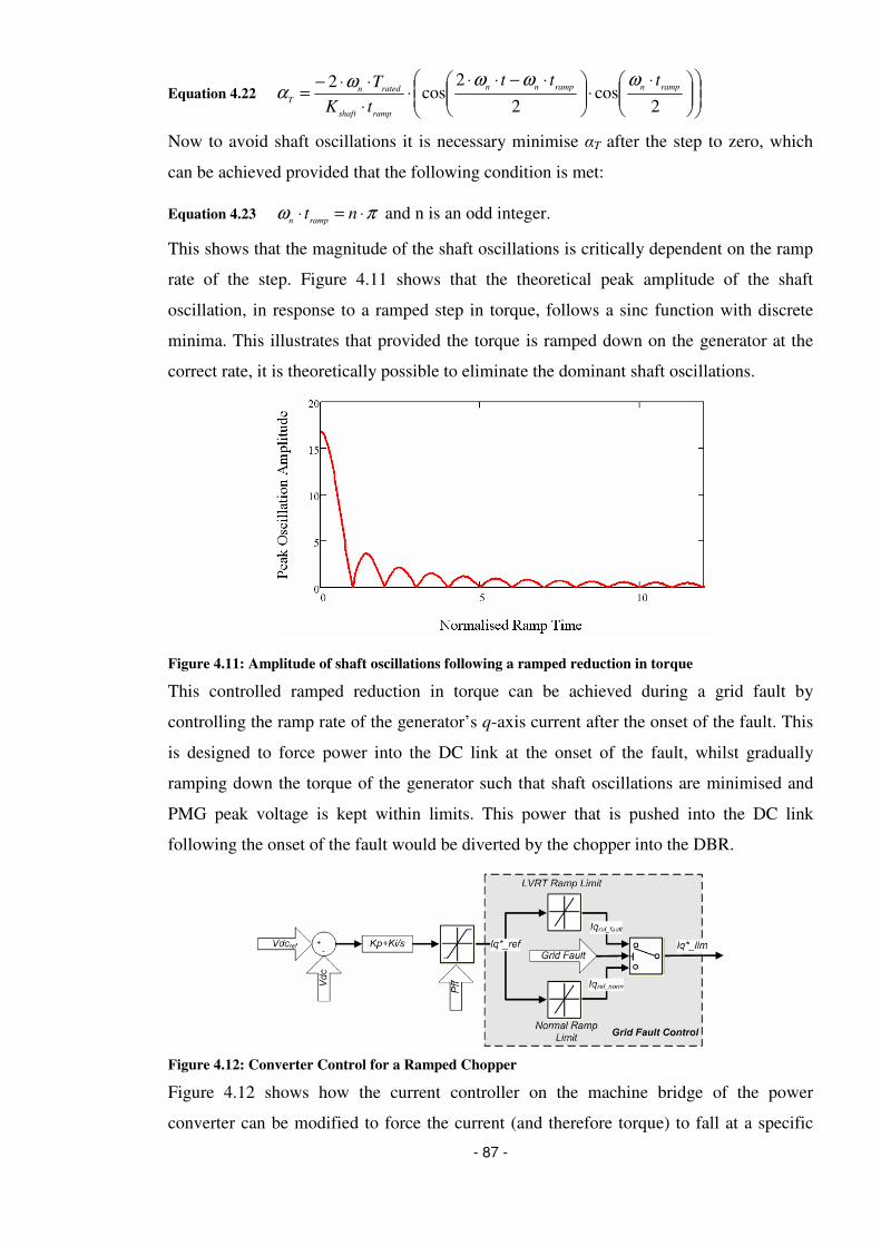
- 87 -

Equation 4.22

⋅⋅

⋅−⋅⋅⋅

⋅

⋅⋅−=

2cos

2

2cos

2 rampnrampnn

rampshaft

ratedn

T

ttt

tK

T ωωωωα

Now to avoid shaft oscillations it is necessary minimise αT after the step to zero, which

can be achieved provided that the following condition is met:

Equation 4.23 πω ⋅=⋅ ntrampn

and n is an odd integer.

This shows that the magnitude of the shaft oscillations is critically dependent on the ramp

rate of the step. Figure 4.11 shows that the theoretical peak amplitude of the shaft

oscillation, in response to a ramped step in torque, follows a sinc function with discrete

minima. This illustrates that provided the torque is ramped down on the generator at the

correct rate, it is theoretically possible to eliminate the dominant shaft oscillations.

Figure 4.11: Amplitude of shaft oscillations following a ramped reduction in torque

This controlled ramped reduction in torque can be achieved during a grid fault by

controlling the ramp rate of the generator’s q-axis current after the onset of the fault. This

is designed to force power into the DC link at the onset of the fault, whilst gradually

ramping down the torque of the generator such that shaft oscillations are minimised and

PMG peak voltage is kept within limits. This power that is pushed into the DC link

following the onset of the fault would be diverted by the chopper into the DBR.

Figure 4.12: Converter Control for a Ramped Chopper

Figure 4.12 shows how the current controller on the machine bridge of the power

converter can be modified to force the current (and therefore torque) to fall at a specific

- 88 -

ramp rate. The grid fault causes the feed-forward power limit and the DC link controller to

work together to rapidly reduce the torque reference on the machine bridge, however,

slower ramp limits are applied during the fault than during normal operation. This ramp

limit is set according to the idealised ramp time described in Equation 4.23 and as Iq*_ref

is reduced much faster than this limit, the set-point sent to the current controller (Iq*_lim)

is limited to change at the specified ramp rate.

This modification to the control method has been implemented in the wind turbine

converter model and simulated. Figure 4.13 shows the results. The energy absorbed by the

DBR is reduced by 60% compared to the case with a fully rated DBR. This improvement

would permit existing turbine designs to ride-through multiple consecutive faults, or for a

smaller DBR and chopper to be used in future designs that only have a single fault

requirement.

Figure 4.13: Fault Ride-through of a PMG with Ramped Chopper

- 89 -

The ramped DBR method has also made considerable improvements to the magnitude of

the speed oscillations, which are around 0.015pu peak to peak during the fault and

0.045pu peak to peak in the worst case after the fault. This is compared to amplitude of

0.19pu peak to peak without a DBR and chopper. Hence, the oscillations are negligible

compared to the case without a chopper. In fact the shaft is near transient free following

the ramped reduction in torque at the onset of the fault, with the majority of shaft

oscillations being excited by the release of the DC link controller to higher ramp rates as

the fault clears. As the DC link controller regains control there is a rapid 0.15pu change in

the generator torque (see Pgen plot at 61.14s). This slight step is also visible on the plot

showing power through the chopper switch (Pchop), however, the power to the chopper

broadly follows the intended profile, by absorbing the power imbalance between the

network and machine bridges. The slight step in torque when the grid recovers is primarily

responsible for the excitement of the shaft and it may be possible to improve on this

response. The transient spike in output power that coincides with the fault recovery (Pgrid

at 61.14s) draws power from the DC link causing it to fall suddenly at the same time that

the DC link controller is released from the ramp limits. This transient therefore causes the

transient in torque and removing this would allow an even smoother response from the

machine bridge and shaft.

The result of minimising the speed oscillations and gradually reducing torque on the PMG

is to significantly reduce the transient voltages that the power converter has to control on

the generator side (Vpmg). This is achieved by reducing the peak speed and thereby

reducing the rate of change of generator flux, which reduces the open circuit EMF of the

generator.

Overall, this novel control adaption makes a contribution to improving the performance of

direct-drive PMG systems under grid faults. The initial outcome of this work has been

implementation of a generic design rule for new direct-drive PMG systems to ensure that

they are equipped with chopper rated for full power for at least ½s. However, further work

in this area would include verifying the control performance when a wind turbine reaches

type testing. Additionally, the control strategy could be investigated further in the context

of other mechanical modes rather than just the fundamental shaft oscillation.

4.2.6 Reduced Order Model

One of the side effects of deploying a chopper and DBR is to improve the decoupling

between the machine bridge and the grid. The chopper ensures that the machine does not

have to be exposed to any fast transients caused by grid events and that the DC link stays

- 90 -

within its target limits. This has led Conroy and Watson [86] to show that models of wind

turbines with PMGs, full converters and choppers can be simplified. Their approach is

only for transient studies and hence the machine side power can be represented as fixed by

a constant current source feeding the DC link. The control and modelling of the network

side bridge remains unchanged, thus ensuring the correct grid behaviour is represented.

However, this approach is not appropriate for longer timescale studies where wind

variability is relevant.

Figure 4.14: Reduced Order Model Design

Here Conroy and Watson’s simplified approach has been built upon. The fast dynamics of

the machine bridge are no longer relevant, hence it is not necessary to represent the

machine or the inner current loops of the machine bridge. Instead, it can be noted from

Figure 4.2 that the DC link voltage controller directly controls the q-axis current, which in

turn aligns with torque. Ignoring fast dynamics, this DC link voltage controller is therefore

indirectly, but proportionately controlling the generator torque. Hence, in a per unitised

model, the per unit q-axis current reference is numerically identical to the per unit

electromagnetic torque exerted by the generator on the shaft. Hence, the machine and

much of the machine bridge control can be removed to leave a hybrid simplified model

that retains sufficient fidelity for fast timescales whilst removing some of the complexity

associated with the machine bridge. This is shown in Figure 4.14.

Figure 4.15 shows the comparison of the full model, which includes the machine model

and machine bridge representation, and the simplified model discussed above. It is evident

from these two plots that the grid side outputs of the simplified model are near identical to

the more detailed model case. However, it should be repeated that this is only true for the

case with a chopper and DBR decoupling the two bridges.

- 91 -

This hybrid reduced order model is often used in subsequent sections that address

frequency response and inertia. Whilst even simpler models are possible for frequency

response studies, this model accurately reflects speed changes which might otherwise

influence PMG voltage, particularly with fast inertial response.

Figure 4.15: Fault Ride-through Simulation Comparison of PMG (Right) and Reduced Order (Left)

Models

4.3 Frequency Response

The instantaneous balance between supply and demand on the transmission system is

maintained through the system frequency. Conventional steam turbine synchronous

generator based power plants provide a fast response to changing frequency by releasing

or storing energy in their rotational inertia and steam drum before their slower governor

and boiler action increases or decreases their output power to return system frequency to

its target.

Full converter wind turbines are specifically designed to vary machine frequency

independently to network frequency so that the blades can be rotated at the optimal

aerodynamic speed rather than being fixed to the system frequency. However, this acts to

decouple their physical inertia from the grid and means that frequency response capability

must be built into their control systems to compensate.

Conventionally, if system demand exceeds supply then the system frequency falls and a

synchronous generator would release an inertial contribution as its rotational kinetic

energy falls, thus aiding the stability of the system. Conversely, if the system supply

- 92 -

exceeds demand then the system frequency rises above nominal and energy is stored in

the synchronous generator’s rotational inertia. This intrinsically stabilising contribution of

synchronous generators helps to ensure that major deviations in system frequency are

extremely rare.

Severe frequency disturbances, such as that illustrated in Figure 2.22, are usually the

consequence of one or more large power stations tripping. Unscheduled power station

trips cause a sudden generation shortfall which has to be rapidly covered by other power

stations on the system, or else by flexible demand. Given that power electronic interfaced

wind turbines do not intrinsically provide the same service as conventional generators, the

subject of frequency response is of interest to system operators globally.

4.3.1 Grid Code Requirements

Parts of the following two sub-sections of the thesis, covering frequency response and

synthetic inertia, have been written up for Wind Energy by Banham-Hall et. al. [87]. This

article is currently being updated following review.

The GB transmission system is a comparatively islanded system with a high credible loss

of generation due to large individual nuclear generators. Furthermore, with plans to meet

the greater part of the UK’s 2020 targets with large offshore wind farms, it is unsurprising

that the GB Transmission System Operator (TSO) has been at the forefront of

investigations into the capability and impact of wind turbines on system frequency.

The approach National Grid [78] has taken is in line with their general principle of

treating all generators connecting to the grid equally. Hence, wind farms connecting to the

transmission system must be technically capable of providing the same service as

conventional generators. This technical capability is checked for compliance when the

wind farm is commissioned, by a series of compliance tests.

4.3.1.1 Droop

The key frequency response related requirement currently mandated in GB Grid Code is

the requirement to provide droop response and is shown in Figure 4.16. A wind farm must

be capable of operating such that it can regulate up or down its output power in direct

proportion to the magnitude of the deviation in system frequency from the nominal 50Hz

target. This response should be directly proportional with only a limited dead-band

permitted around the 50Hz nominal frequency. A droop of 3-5% should be attainable,

which in turn relates back to the speed of a synchronous generator. A droop of X%

implies that a hypothetical 100% load step on that generator would cause a change in

- 93 -

speed of X%. Hence a 3-5% droop implies a change in power of between 40-66% per

Hertz deviation from the nominal frequency.

Figure 4.16: GB Requirement for Droop Control from National Grid [78]

Clearly, a wind farm cannot indefinitely increase its power output in line with a droop

requirement unless it is operating at an output power lower than the available wind power.

Additionally, it would be economically undesirable to operate wind farms at lower than

their maximum output just to provide frequency response, when other power plants can

provide this capacity. Therefore the requirement of Figure 4.16 is only relevant when a

generator is selected for Frequency Sensitive Mode (FSM). When a generator, such as a

wind farm, is not selected for FSM it can operate under the less stringent requirements for

Limited Frequency Sensitive Mode (LFSM). Under LFSM, the wind farm is only required

to regulate down its output in response to a frequency above 50.4Hz. It is thereby allowed

to operate at the maximum available power unless there is a major system over-frequency

event.

The split in requirements between FSM and LFSM highlights a key difference between

the GB regulatory framework and the economic reality. Wind farms being built have to be

technically capable of providing FSM operation and are tested for it; however, they

typically price themselves out of providing this service and invariably operate under

LFSM.

The technical requirement to provide droop response from a wind farm has to be enhanced

to take into account the variable nature of the wind resource. In contrast to a conventional

generator, which would operate at a fixed output under normal operation, a wind farm

would operate according to the variable available wind power. Figure 4.17, from National

Grid [78], shows the GB Grid Code requirement on wind farms providing frequency

response, this requires that when they are selected for FSM, they reduce their output

- 94 -

below the variable available power (Pavail) to a lower fixed output, known as the Capped

Committed Level (CCL), and regulate according to system frequency from that level. The

generator must also then supply a discretely updated measure of the maximum available

power, known as the Maximum Export Limit (MEL), which informs National Grid of the

magnitude of the (varying) level of reserve held by the wind farm.

Figure 4.17 shows that with variable wind speed it is understood that the available power

could drop sufficiently to compromise response. This is shown on the dark blue output

between about 17 minutes and 24 minutes, where the output reverts to tracking the

maximum available power. This highlights a distinct feature of the implementation of the

GB droop response requirement; it is based on a variable reserve approach, but ideally

targets a fixed output.

Figure 4.17: Implementation of Frequency Response with an Intermittent Resource taken from

National Grid [78]

The Danish approach to providing frequency response capacity is the reverse of the GB

case, the Danish system operates a fixed reserve, variable output requirement [88]. This is

typically known as “Delta-control” and requires a generator to operate at a fixed margin or

“Delta” below their maximum available power. The droop response then operates relative

- 95 -

to the varying output of the wind farm. This type of response is illustrated, compared to

the GB approach, in the FSM period of Figure 4.18 (Pdelta).

4.3.1.2 Response Types

The droop requirement dictates the magnitude of the steady state change in power output

that a wind farm should provide in response to a frequency deviation. However, following

a major loss of generation the speed of response is also critical. As such the market, from

which FSM services are procured, is divided into three different types of response. Of

these three, “Primary” and “Secondary response” govern the increase in power output in

response to a reduction in grid frequency and “High response” governs the reduction in

power output in response to a rise in grid frequency.

Primary response is the fastest type of frequency response currently procured for the GB

grid. The magnitude of response is measured 10 seconds after a frequency deviation and

should be maintained for 30 seconds according to National Grid [78]. Although the

measurement is made at 10 seconds it would usually be expected that a generator would

start to provide additional power output within 2 seconds of the frequency deviation. The

aim of primary response is to stabilise the frequency within operational limits.

Secondary response is slower response that is measured according to the minimum

increase in power supplied between 30 seconds and 30 minutes after a frequency

deviation. Its purpose is to start the process of restoring system frequency whilst allowing

time for the TSO to modify generation profiles to make up for the generation shortfall.

Both primary and secondary response would be expected to be supplied relative to a fixed

output level.

High frequency response is the response to a system over-frequency event and is

measured 10 seconds after the frequency event. In contrast to Primary and Secondary

response, High frequency response has no time limit specified, however, it would usually

only be required for a maximum of half an hour before National Grid’s Balancing

Mechanism adjusted generation profiles to compensate for the imbalance. Also in contrast

to the low frequency response capabilities, the High frequency response controller must be

active at all times, albeit it would only respond when frequency is significantly above

target when in LFSM. When operating in LFSM, the wind farm’s output would be

variable, therefore, but if the frequency exceeds the limit (50.4Hz) and High response is

required, the wind farm would regulate its output relative to its power output immediately

prior to the frequency exceeding 50.4Hz. This control is known as Balance control and is

- 96 -

illustrated alongside the other types of control discussed here in Figure 4.18. It should be

noted from this illustration that in the event that the available wind power falls, excess

response may be provided by the wind farm, which would revert to tracking the (lower)

available power.

In addition to the frequency response controllers, it is possible National Grid may

constrain the output of a given wind farm to a maximum level. This is typically an

expensive option for National Grid, and generates negative headlines such as The

Telegraph’s [89] “Wind farm paid £1.2 million to produce no electricity”. This was due to

the constraint payments made to Scottish wind farms for not producing power.

Nevertheless, the control, known as “Absolute Limit” control is implemented in the

frequency controller and shown in Figure 4.18.

Overall, methods of providing frequency response have been implemented by wind farm

operators, which have been successfully tested against the compliance tests of GB Grid

Code by Horne [90]. Different control methods that can be used to provide frequency

response are discussed in section 4.3.2.

Figure 4.18: Frequency Response Types

4.3.2 Control Methods for Frequency Response

In order for a wind turbine to hold power reserve for frequency response, it is ultimately

necessary to reduce the aerodynamic power from the blades. Figure 3.3 shows that in

order to achieve this, for a given wind speed; a wind turbine controller must either change

the pitch angle, or else change the speed of the blades. Whereas the pitch angle to

coefficient of performance relationship is a monotonically decreasing function for any

given Tip Speed Ratio (TSR); both acceleration and deceleration of the blades, relative to

the optimal speed, leads to a decrease in power output. However, deloading a turbine by

Time

Pdelta

Pout Pavail Pref Frequency Pmax

10s

High Response

10s

Primary Response

Selected for FSM LFSM operation only

Balance Control

Absolute Limit Control

- 97 -

deliberately slowing the blades down below the optimal speed would lead to slow

response times due to the slow acceleration of the wind turbine required to return the

turbine to the optimal operating point. It is therefore desirable to either operate on the

right hand side of the peak in Figure 3.3 or to use the blade pitch to control output.

Holdsworth, Ekanayake and Jenkins [91] were the first to consider the provision of

inertial and frequency response from wind turbines in depth. Their analysis compared the

capabilities of an FSIG with a DFIG, showing the natural inertial response of the FSIG

and comparing it with the lack of inherent response from the DFIG. They then proceed to

demonstrate how inertial response and frequency control can be added to the wind turbine

controller. Their contribution to synthetic inertia will be considered in section 4.4.1. Here,

however, their proposals for provision of frequency response are considered. They

propose a frequency response strategy that applies droop control on the converter torque

set-point which is matched by a second droop characteristic that trims the minimum pitch

angle of the blades. This range of pitch angle variation is shown to give a maximum 20%

change in power output and is demonstrated through various different, but constant, wind

speed simulations.

Section 3.5.2.2 showed that the direct speed controlled wind turbine optimised power

capture by controlling the wind turbine blades to the optimal rotational speed. Therefore,

in order for a direct speed controlled wind turbine to hold margin for frequency response it

is necessary to deload the turbine through a change in pitch angle. This can be achieved

with the wind turbine controller shown in Figure 4.19.

For this method of frequency control it is necessary to ensure that the power output of the

wind turbine changes, but that the speed stays close to optimal. This allows the wind

turbine to respond to a frequency deviation with all its power reserve whilst only changing

the blade pitch angle and not speed. Hence, the controller of Figure 3.17 must set the

optimal speed, when in FSM only, according to the estimated available power rather than

the measured output power. This means that the margin held by the wind turbine when in

frequency responsive mode is subject to the same error as the estimated available power.

This error would be partially reduced by averaging many turbines’ output.

Under this method of frequency response, the pitch controller acts to regulate the

measured power output of the wind turbine to the set-point by using a PI controller (rather

than the droop method used in Holdsworth, Ekanayake and Jenkins). The power reference

is taken from the estimate of the available wind power and modified to hold a reserve and

respond to any changes in frequency. For example if the available power in the wind is

- 98 -

2MW, a turbine is to hold a 300kW margin and the system frequency is 50Hz, the pitch

angle controller will increase the pitch angle until the measured output power is 1.7MW.

The capability to provide primary frequency response by pitch control is considered

further by modelling and simulation in section 4.3.3.

Figure 4.19: Primary Frequency Response by Pitch Control

The simple droop control of pitch angle proposed by Holdsworth, Ekanayake and Jenkins

works under steady wind conditions and the control of pitch angle for frequency response

is necessary for the direct speed controlled turbines. However, under intermittent wind

conditions, neither technique is ideal for meeting the fixed output, variable reserve

requirements of the GB Grid Code. Furthermore, the pitch controller has to deal with the

continuously variable aerodynamic power.

An alternative approach, which works well with indirectly speed controlled wind turbines,

is to modify the power generated directly. Section 3.5.2.1 showed how the rotor speed of a

wind turbine could be used to set the optimal power or torque set-point for the generator.

This torque (see Figure 3.12) or power (see Figure 3.14) set-point is then fed to the power

converter controller.

Ekanayake, Jenkins and Strbac [92] have shown that frequency response reserves can also

be attained by directly modifying the torque set-point of a DFIG or full converter wind

turbine. This is done by subtracting a term from the optimal torque or power set-point. In

Figure 4.20 this is shown as a modification to the Pavail reference point. Pdelta is the margin

held for response. The sample and hold block is triggered to hold whenever the frequency

- 99 -

exceeds the nominal limit (50.4Hz in LFSM) so that “Balance control” can be

implemented. Otherwise, the power reference to the power converter is modified by the

available power, response holding and any deviation in frequency. Note that in order to

meet the specific requirements of GB Grid Code with regulation from a fixed output level,

the controller’s Pavail signal is held constant for a settlement period (30 minutes) based on

a forecast; whereas under a “Delta control” arrangement it continuously varies.

A change in the power reference of the power converter leads to a change in the torque on

the generator. This in turn leads to a change in the speed of the generator and blades. If the

wind turbine is operating in rated wind speeds or higher, this change in speed will lead

onto a change in the blade pitch angle of the turbine.

This frequency control method has the advantage that response times are only limited by

the dynamics of the power converter and the ability to accurately measure system

frequency. Given that system frequency measurement typically provides a noisy signal,

the frequency controllers are equipped with low pass filtering on that frequency

measurement, but given the response requirement of 2 seconds, this filter does not pose a

problem for primary response. The disadvantage of this method from a commercial

perspective is a patent by Delmerico and Miller [93], of General Electric, covering some

of the necessary components and pre-dating Converteam’s acquisition by GE.

Figure 4.20: Primary Frequency Controller Using Converter Power Reference

The power converter control operates to implement the required torque on the generator. It

does this regardless of the aerodynamic effect any speed change is having. Conroy and

Watson [94] have shown, with work that included an inertial controller, that drawing too

much power from the blades, which leads to an excessive deceleration, can cause unstable

- 100 -

operation and ultimately contribute to a frequency collapse. Even if collapse in the speed

of the turbine is avoided, Tarnowski et al. [95] have shown that the recovery periods

following periods of significant over-production can be of long duration and require

significant power reductions.

Operation of a power converter interfaced wind turbine, with a power reserve for

frequency response, in below rated wind conditions can lead to an acceleration of the

blades to a higher than optimal TSR. Tarnowski’s starting point was a turbine operating at

the optimal rotational speed, such that over-production leads to worsening TSRs.

However, a plant operating in FSM according to Figure 4.20 can store additional energy

as kinetic energy under below rated wind speed conditions, thus potentially avoiding the

under-production recovery periods associated with frequency response from an optimal

starting speed. This has been investigated by Banham-Hall et al. [96] and Teninge et al.

[97].

Figure 4.21 shows a one-shot controller to provide additional power output from stored

rotor kinetic energy. First the estimated available power is used to provide an estimate of

the optimal speed of the turbine. Tarnowski’s [95] research, in conjunction with Vestas,

derives the available power estimate from an estimate of the prevailing wind speed as is

done here. The energy stored in the rotor can then be calculated for the current operating

speed (ωb) and the optimal operating speed (ωopt). The difference between these two

values is the energy available for over-production, which can contribute to an additional

power response for the Primary response period (Tprim). This additional power capacity is

sampled and held in the event of frequency falling below a fixed level (ftarget) and added to

the power converter’s set-point to release a one-shot power increase.

Figure 4.21: Frequency Response Controller for Temporary Over-production

- 101 -

4.3.3 Frequency Response Capability

Figure 4.22 shows a comparison of the high frequency response of wind turbines, using

the pitch and power regulation strategies, under constant wind conditions. The left hand

plot shows a case with low wind speed. The right hand plot considers the case where the

wind speed is above rated, but the wind farm is operating in FSM and therefore holding a

margin for both high and low frequency response. In both cases the response to a 0.5Hz

frequency step at t=80s is evaluated, which corresponds to one of the more severe

compliance tests for the GB Grid Code.

In both cases it can be seen that the frequency response method that directly adjusts the

power converter set-point leads to an instantaneous and proportional change in the power

output (Pturbine). The power response from the pitch regulated turbine is slightly slower,

as it depends on the dynamics of pitching mechanism; however, a stable new power

output level is achieved within 2 seconds.

In the low wind case, the power reserve held on the power reference regulated case has led

to the turbine operating at above optimal rotational speed; furthermore, the pitch controller

has intervened to ensure turbine speed does not exceed the design rating. However, the

rapid reduction in the converter’s power reference in response to the frequency change

allows the turbine to accelerate (Wr), as the generator torque is lower than the blade

torque in both cases. The change in blade pitch angle is then slow to catch up, as the

turbine’s acceleration is slow. In contrast, the pitch regulated turbine is operating at

optimal speed throughout both scenarios. In order to maintain the optimal speed and

provide the required power reduction, the pitch controller has to change the blade pitch

much faster and is limited initially by the maximum pitch rate of the turbine. The pitch

controller is slightly under-damped to optimise the speed of response in this

implementation.

A side effect of operating the direct speed controlled turbine at optimal speed throughout

the scenario is that the corresponding PMG voltage is lower, as the open circuit voltage of

the PMG is reduced. Furthermore, the PMG is not exposed to the slight voltage transient

that occurs for the power reference regulated case under high wind conditions, which is

due to a sudden torque reference change.

Figure 4.23 shows the comparison of these turbine controllers, plus the one-shot

additional energy controller, under a low frequency deviation. This time the frequency is

ramped down by 0.8Hz over a 10 second period, again reflecting a severe test under the

GB Grid Code.

- 102 -

Figure 4.22: High Frequency Response Comparison under low wind (left) and high wind (right)

As with the high frequency response case, when the frequency response is driven by the

pitch controller it is unsurprisingly somewhat slower than the power converter driven

response. The response settles some 2.5 seconds later in the low wind case. The one-shot

controller is activated right at the start of the frequency deviation and leads to a step

increase in output power from the wind turbine (Pturbine) that lasts for 20 seconds.

For the low wind speed case, the direct speed controlled turbine, with pitch regulated

power output, operates throughout the scenario at the optimal rotational speed for the

wind speed. This is in contrast to the deceleration of the power reference regulated

turbines, which start at an above optimal speed. In the case with the one-shot controller,

the turbine decelerates back to the optimal speed much more quickly, as the kinetic energy

stored in the blades is being actively used in the additional power output contribution. The

standard power reference regulated case experiences a slower deceleration as power

output only exceeds the power capture due to the relatively smaller deviation in Cp from

optimal.

The one-shot controller is not applicable to the high wind case as the rotor will be

operating at rated speed and therefore is below the optimal rotational speed and at rated

torque. In this scenario the direct speed controlled turbine’s constant speed approach can

be seen to be of some value. The faster power response of the power regulated case comes

- 103 -

at the expense of a significant blade speed transient. The power difference between the

power reference regulated case and the pitch reference regulated case has to be supplied

from the kinetic energy of the blades, leading to a 6% drop in turbine speed. This sub-

optimal speed recovers as a result of an undershoot in pitch angle, which allows the

turbine speed to be restored to target. For different wind conditions, however, this speed

transient could lead to a period of under-production, compromising the turbine’s

frequency response.

Figure 4.23: Low Frequency Response Comparison under low wind (left) and high wind (right)

Figure 4.24 shows a longer timescale study which includes variable wind speed for

investigating the high frequency response performance of a wind turbine using the power

reference regulated approach. This scenario demonstrates the behaviour of the absolute

power limit (set at 0.95pu) and the balance controller. The scenario wind speed has been

selected such that it varies around the rated wind speed (13m/s) of the wind turbine. The

frequency is ramped up by 1Hz at t=200s.

From this variable wind speed study the smoothing effect of the rotor’s inertia can be seen

on the power output from the turbine. The turbulent wind field leads to much slower

variations in the turbine’s speed. These slow variations in turbine speed slowly move the

turbine’s operating point according to Figure 3.15, effecting a change in the power output.

When the turbine is operating at rated speed and the wind speed rises, the turbine pitch

- 104 -

controller responds to limit the blade rotational speed. This pitch response is filtered by

the slowly varying rotational speed too.

Figure 4.24: High Frequency Response in Variable Wind (available power shown in red, with output

power in blue)

In this example, the turbine is operating only in LFSM, and hence only responds when the

frequency has exceeded 50.4Hz with a “Balance control” response. Prior to the frequency

deviation the wind turbine is tracking the available power (red) and outputting the

maximum power possible. At the moment that the grid frequency rises, the wind turbine

output is at 0.95pu, the Balance controller samples and holds this power output value and

deloads relative to it to 0.8pu. The wind turbine’s power output cannot now exceed 0.8 pu

unless the frequency falls. However, when the available power drops below 0.8pu, the

wind turbine can revert to tracking the available power in the wind, such as occurs in the

simulation at around 260 seconds. This reversion to tracking available power cannot

compromise the response but may lead to additional response, which helps to restore

system frequency.

Figure 4.25 shows the challenges of providing low frequency response from a fixed output

level. The wind farm is initially deloaded to a fixed output level (0.6pu), however, the

available power varies sufficiently to cause the farm controller to have to revert to

- 105 -

tracking the available power for a period (around t = 100s). Furthermore, although the

frequency response to the low frequency step at t = 200s leads to a predominantly smooth

output from the wind farm, over the period considered here, the wind varies sufficiently to

reduce the response for a period. The response is actually briefly eliminated by the

reduction in available power at t = 390s.

Figure 4.25: Low Frequency Response in Variable Wind with GB Requirements (available power

shown in red, with output power in blue)

This shows the particular challenge of providing a firm response margin for secondary

response time scales when the wind speed is close to the turbine’s ratings. Small

fluctuations in the wind speed cause significant changes in the output power, greatly

affecting and potentially compromising the margin available for response. To compensate

for this, the wind farm would have to deload itself by a greater margin prior to any

frequency event, thereby incurring a greater economic penalty.

The alternative “Delta control” approach does not have this drawback, as shown in Figure

4.26. Under this control strategy the wind farm can track the available power with a fixed

margin prior to the frequency deviation. Then, following the frequency fall, the wind farm

can be increased up to a maximum of the available power. The wind farm then reverts to

tracking the available power to provide maximum output.

- 106 -

Figure 4.26: Low Frequency Response in Variable Wind with Delta Requirements (available power

shown in red, with output power in blue)

In this scenario the wind speed rises and therefore the effect of wind intermittency is to

contribute to meeting the generation gap. The problem with this control method would be

highlighted by falling wind speed. In that event, the additional power provided by the use

of the Delta margin could be offset by a loss of power due to reduced available power in

the wind. Overall therefore, Delta control solves the challenge of predicting the necessary

deload for reliable frequency response, that the GB requirements lead to, but potentially

causes a further problem for system operators as real response capacity depends on the

variability of the prevailing wind conditions.

Despite the differences between delta control and the GB requirement to regulate power

output from a fixed level, it can be seen that the wind turbine control systems themselves

can be modified to allow wind farms to hold power reserves. These power reserves can be

delivered within the timescales required for primary response, although the mechanical

systems of the wind turbine may continue responding for a considerable time afterwards.

Wind farms can also contribute high frequency response and a balance controller has been

presented that ensures optimal response from a wind farm in LFSM. The technical

- 107 -

challenges of providing droop type response from directly or indirectly speed controlled

turbines can be met with appropriate control strategies.

Whilst this section has shown that it is technically feasible for wind farms to hold

frequency response reserves, it has only touched on the economic implications. Holding

reserves for low frequency response implies spilling wind energy and incurs a significant

opportunity cost. Whereas today’s conventional generators can benefit from significant

fuel savings whilst holding reserves, there is no such compensation for wind power.

Hence, the economic viability of wind for this application, on all but a few high wind

occasions per year, is likely to be questionable.

The Grid Code requirements for provision of frequency response currently incur a

technical burden on wind farms. They have to meet the technical requirements of the

code. However, given the questionable economic implications of providing frequency

response from wind power, it is worth considering what other options are available in

order to meet the frequency response requirement. The second half of this thesis will

address this issue.

4.4 Synthetic Inertia

Section 4.3 has shown that the frequency response capability of power converter

interfaced wind turbines differs substantially from conventional synchronous generators.

Along with section 2.5, it has been shown that the inertial response of grid connected

generation could substantially change in the coming years. The frequency response

capability of wind turbines and wind farms to provide primary, secondary and high

frequency response has been investigated in the previous section and is already clearly

mandated in the GB Grid Code with specific guidelines that cover technical requirements

on wind farms. This section specifically covers the initial inertial response to changing

frequency.

4.4.1 Grid Code Developments

It is notable that the procurement mechanism for frequency response of the GB TSO only

considers time periods of 10 seconds and longer. This is reflective of the inherent inertial

effect that conventional plant’s synchronous generators and rotating machinery provides

to the grid today, arresting the rate of change of frequency and helping stabilise the

system. As the future grid is likely to incorporate more power electronic interfaced

equipment, it is unsurprising that specification of an inertial component was considered in

- 108 -

the first draft of the European harmonised Grid Code [98] from the European Network of

Transmission System Operators for Electricity (ENTSO-E).

Thus far only Hydro-Quebec [99] have implemented a Grid Code requirement for a

synthetic inertial response, requiring manufacturers to have an equivalent H constant of at

least 3.5 seconds.

The capability of wind turbines to provide inertial response has been the subject of

consultation between National Grid [100] and manufacturers. Concern centred on the

recovery period of wind turbines after they have provided an inertial response and whether

the measurement of system frequency could be accurate and fast enough to provide the

desired response. Perhaps as a result of these uncertainties, the latest working copy of the

European code has removed this requirement according to ENTSO-E [101]. In its place

ENTSO-E has proposed a faster response (6 seconds) from primary response, with the aim

of avoiding the need for synthetic inertial response. It is in the context of this regulatory

uncertainty that this work explores the capability of wind turbines to provide a synthetic

inertial response.

4.4.2 Control Methods for Providing Inertia

An analysis of the change in kinetic energy of a synchronous machine’s rotor in response

to a frequency change led to Equation 2.12, which showed that power released by that

synchronous machine would be broadly proportional to the derivative of frequency. On

this basis Holdsworth, Ekanyake and Jenkins [91], Morren et al. [102] and Morren, Pierik

and de Haan [103] considered the kinetic energy of DFIG wind turbines and proposed a

control strategy based on emulating this. These papers inform the general derivation here.

The kinetic energy of the rotating parts of a wind turbine is given as:

Equation 4.24 2

2

1ω⋅⋅= JKE

Differentiating the kinetic energy with respect to time provides the power output profile

from energy stored in the rotor according to:

Equation 2.12 dt

dJ

dt

dJ

dt

KEd ωω

ωω ⋅⋅=⋅⋅⋅= 2

2

1)(

Additionally, an inertial constant can be defined according to the turbine’s kinetic energy

and rated apparent power. This inertial constant determines the time for which a generator

can supply rated power purely from its kinetic energy.

- 109 -

Equation 4.25 S

JH

⋅

⋅=

2

2ω which can be rearranged to

2

2

ω

HSJ

⋅⋅= and substituted into

Equation 2.12:

Equation 4.26 dt

dHSP

inertia

ωω

ω⋅⋅

⋅⋅=

2

2 which naturally simplifies in per unit terms to:

Equation 4.27 dt

dH

dt

dHP

inertia

ωωω ⋅⋅≈⋅⋅⋅= 22

Hence, the inertial controller derived from an analysis of the release of kinetic energy of

the wind turbine has to respond to the rate of change of grid frequency. A controller that

uses this strategy is shown in Figure 4.27 and adds a term to the turbine’s power

reference. This approach of modifying the power (or torque) reference of the turbine

means that it is suited to use with the classical indirect speed control of turbines.

It is notable that the controller has to include some additional components other than the

gain and frequency derivative. Any measure of grid frequency is subject to noise owing to

voltage distortion, harmonics, poor PLL performance or voltage transients. Given that the

measurement of grid frequency is subject to noise, the frequency derivative will be subject

to spurious transient peaks in response to frequency measurement noise. To prevent these

transients leading to transitory impulse power demands on the wind turbine, the measured

frequency has to be pre-filtered by a low pass filter. Additionally, if this inertial controller

were continually active it would add a stochastic term to the wind turbine’s maximum

power tracker, thereby potentially having a negative impact on wind turbine yield.

Therefore, a dead band is also included, which in conjunction with the low pass filter,

helps to ensure that the inertial controller is only sensitive under large sustained frequency

changes.

Figure 4.27: Inertial Control by Frequency Derivative

A comparison of the different inertial control methods presented here is conducted in

section 4.4.3. Nevertheless it should be considered that the low pass filter and dead band

combination have to be specifically introduced to avoid an overly sensitive response

owing to noise on the frequency derivative and so that the controller only responds under

large frequency deviations. Furthermore, whilst this control is suitable for the common

- 110 -

indirect speed controlled turbine, it would not be directly applicable to any future direct

speed controlled versions.

A synthetic inertial controller can be derived for the direct speed controlled turbine by

considering that the aim of an inertial controller is to release the kinetic energy from the

rotating equipment as it slows down to a new operating point. Hence, the synthetic inertial

controller can modify the speed set-point of the turbine, dependent on the magnitude of

the frequency error, to invoke an inertial response. This would de-optimise the energy

capture slightly, although even a frequency change to 49Hz would only lead to a 2%

change in speed, so this effect is negligible. The benefit of this control approach is that the

inertial set-point change is initiated by the magnitude of the frequency deviation and not

by the rate of change of frequency. Hence the controller is less sensitive to frequency

measurement noise. Furthermore, the speed of response is dependent on the dynamics of

the speed controller rather than the bandwidth of the low pass filter used to filter the

frequency in the derivative case. However, this controller still requires a dead band to

ensure that small frequency fluctuations do not continually lead to transient power swings

from the turbine as the speed controller’s set-point changes.

Figure 4.28: Inertial Control by Speed Control

Whilst the speed control method solves the problem of avoiding noise sensitivity to the

frequency derivative, it can only be directly applied to the directly speed controlled

turbine. Furthermore, its response is dependent on the bandwidth of the speed controller.

It is shown in Figure 4.28.

A new alternative approach can be developed by considering the approach to providing

inertia from an energy store described in Larsen and Delmerico [104]. Under their

approach, an inertial controller directly modifies an energy store converter’s firing angle,

thereby modifying power output. However, a feedback loop effectively takes a derivative

of frequency and filters it with a first order low pass filter, thereby indirectly taking a

frequency derivative.

- 111 -

The controller developed here takes Larsen and Delmerico’s approach of generating an

angle from the system frequency but applies it instead to model a synchronous machine’s

response. The feedback loop is replaced by a model of the blades’ deceleration. Section

2.5.3 suggested that changes in grid frequency actually caused the inertial response from a

synchronous machine by leading to a load angle change. This load angle change in turn

leads to a change in torque, which follows a sinusoidal path, according to section 2.5.1.

Hence instead of taking the frequency derivative, an inertial controller can be developed

by generating a synthetic change in load angle. This change in load angle is calculated by

integrating the error between the nominal frequency and the instantaneous system

frequency (note fnom would normally be 1):

Equation 4.28 ( )∫ ⋅−⋅=∆ dtffnomgridnominertia

ωδ

This change in load angle has to be taken relative to an initial synthetic starting load angle

(δnom), which is here taken to be π/4, although this value is somewhat arbitrary (see Figure

2.21). Hence, a new operating load angle is:

Equation 4.29 ( )∫ ⋅−⋅+= dtffnomgridnom

ωπ

δ4

This new synthetic load angle would lead to a relative change in torque, from the initial

load angle (δnom) to the new load angle (δ), of:

Equation 4.30

nom

outTq

TqqT

δ

δ

sin

sin

1

2 ==

This ratio can then act as a torque (or power) reference multiplier, increasing the output of

the turbine as and when the frequency falls and decreasing it when the frequency is high.

This leads to the “Torque Multiplier” output in Figure 4.29.

Thus far this approach has considered a hypothetical machine angle change between the

nominal frequency and the instantaneous system frequency. In a synchronous machine,

this angle change is stopped by the acceleration or deceleration of the machine such that

its rotational frequency returns to matching the grid frequency. In order to emulate this

part of a synchronous machine’s behaviour, it is possible to model the turbine’s speed

response to the torque change and use this to form the feedback loop.

Equation 4.31 dt

dHqT

ω⋅⋅= 2

Hence, the change in speed of the turbine can be modelled as:

- 112 -

Equation 4.32 tdqTH∫ ⋅⋅

⋅=∆

2

1ω

This modelled change in the speed of the turbine then modifies the frequency reference

point and closes the feedback loop. In parallel with this integral feedback is a small

proportion gain contribution which improves the stability of the loop. Now, in the event of

a frequency change, the controller estimates a change in a synthetic load angle and

modifies the torque (or power) reference to the power converter. The power converter

responds fast by changing the generator torque. The modelled speed of the turbine (in the

inertial controller) then decreases and modifies the frequency reference until the load

angle closes and the torque rebalances to its original value. Note that the real turbine

speed is not used owing to unpredictable speed behaviour due to wind speed changes.

Figure 4.29 shows this inertial response controller.

Figure 4.29: Inertial Control by Synthetic Load Angle

4.4.3 Inertial Response Capability

Figure 4.30 shows a comparison of the three different inertial methods in response to the

0.5Hz step increase in frequency. Whilst a step response would not be a realistic physical

scenario on the power system, it serves to distinguish the response of the different control

methods by highlighting the filter and derivative effects. The top plot shows the measured

frequency after the PLL but before the low pass filtering stages of the controllers,

however, the actual frequency applied was a pure step at t = 80s. The wind conditions

were constant and below the rated wind speed. In all three cases, the droop controller was

also active.

The transient power to the grid (Pgrid) shows the benefits and shortcomings of the

different control methods. The method relying on the frequency derivative shows both a

noisy response and a slight delay of around 150ms before the inertial response is initiated.

The delay is partly induced by the low pass filter, whilst the noise is a response to the

overshoot in measured frequency from the PLL, which to an extent persists even after

filtering. Given the fast change in frequency measured, the response is sharp and short

- 113 -

lived from this controller, effectively only achieving a slight improvement over a fast

droop response.

The speed controller method achieves a faster response than the frequency derivative

method and is clearly less noisy. However, the power output profile is solely determined

by the dynamics of the speed controller, so the inertial response lasts for only around

300ms before the inertial contribution is finished and the power profile follows the droop

response. This droop response is only provided at the slower rate at which the blade pitch

mechanism can respond, leaving a time lag between the end of the inertial response and

the droop response reaching the same level.

The response of the synthetic load angle controller is extremely promising, responding

with no time lag and showing little noise sensitivity. The high rate of change of frequency

leads to an overshoot, relative to the steady state droop response, before the feedback loop

closes the synthetic load angle and brings the inertial response contribution back to zero.

The frequency derivative controller and the synthetic load angle controller both effect

rapid changes in power output whilst leaving the slower turbine dynamics to respond. This

change in power output leads to the generator torque being reduced and the blades

gradually accelerating. As the blades reach the maximum speed the pitch controller begins

to increase the blade pitch angle in order to decrease Cp. This is in contrast to the speed

controlled approach, where the pitch controller and speed controller work together to

change the turbine operating point which then leads onto a change in the output power.

This difference means that the speed controlled turbine continues to operate at the optimal

speed, but the other two methods accelerate to a higher than optimal rotational speed.

Figure 4.31 shows the inertial response (no droop) to the GB system event discussed in

section 2.6.2. Here, the response of the synthetic load angle controller and the frequency

derivative controller appear similar, with the speed controller slower. However, close

inspection of the frequency derivative output shown in Figure 4.32 shows the improved

noise rejection of the synthetic load angle method. The frequency measurement noise,

combined with a finite update rate of the power control on the power converter leads to

significantly less smooth power output from the power regulated control.

It is also notable, that the inertial response causes a speed change from the power

reference and synthetic load angle regulated turbines. This speed change in turn leads onto

a reduction in the turbine’s power reference (Po/p) (which then has the inertial term

added) according to the cubic relationship of Figure 3.15. This change in operating point

- 114 -

reduces the inertial response and eliminates it prior to the frequency stabilising. This

ultimately leads into the recovery period, which can be seen as the turbines slowly regain

speed for up to half a minute after the frequency deviation. Whilst this recovery period

can be delayed (by triggering the balance controller on falling rate of change of

frequency), this serves to highlight the concerns that National Grid have had over the

recovery of wind turbines following an inertial response contribution.

Figure 4.30: Inertial response to a high frequency step

The speed controller modifies the speed set-point for as long as the grid frequency is low;

the speed recovery in this case is much slower, matching the frequency recovery of the

grid. However, the dynamics of the speed controller ensure that the inertial response is

also delivered slightly slower. Nevertheless, following delivery of the inertial power

contribution, the controller only recognises a change in speed of the turbine as a slight de-

optimisation of Cp across the flat peak of Figure 3.3 instead of the cubic outcome of the

other two controllers. This ensures that the power recovery period is insignificant

compared to the other two cases.

- 115 -

Figure 4.31: Inertial response simulation to 27

th May 2008 frequency profile (low wind)

In this scenario the wind speed was deliberately modelled at constant speed, but slightly

below the rated wind speed of the turbine. This ensured that the speed changes of the

turbine occur at the steepest part of the operational curve in Figure 3.15, maximising the

differences in the performance of the controllers.

Figure 4.32: Expanded view of Figure 4.31

- 116 -

Figure 4.33: Inertial response simulation to 27

th May 2008 frequency profile (high wind)

In contrast to the case with the wind speed just below rated, the inertial response to the

frequency change at 210 seconds with above rated wind conditions is shown in Figure

4.33 and this illustrates that under high wind conditions the recovery period is eliminated.

The response is not compromised by a change in the available power as the pitch angle

controller responds to the slight change in turbine speed by reducing the pitch of the

blades, thereby temporarily increasing Cp and allowing the turbine speed to recover to

rated rotational speed.

The inertial response simulations have shown the benefit of using a synthetic load angle

approach to providing inertial response. This offers fast response with less noise

sensitivity than the traditionally proposed frequency derivative method. There are several

other alternative methods of providing inertial response. Manufacturers such as Enercon

[105] have proposed one shot controllers that output either a set percentage increase in

power output (i.e. 10% extra for 10 seconds above the varying output) or a set power

output (i.e. 100% output for 10 seconds). Others such as Vestas [106] have proposed

controllers that follow the frequency derivative method.

- 117 -

Initial GB TSO engagement with manufacturers, to address inertia, raised two concerns;

first the recovery periods of wind turbines and second the sensitivity and design of

controllers reliant on taking the derivative of a noisy frequency signal. This work has

shown that it is possible to devise inertial controllers that are less sensitive to frequency

noise whilst offering a fast response. To complete the evaluation of this controller’s

capabilities it would be necessary to address National Grid’s first concern and investigate

the recovery period of multiple different turbines from different manufacturers when

providing this service. National Grid [100] has consulted with manufacturers, whilst

considering the system needs, on limitations and capabilities of wind turbines’ inertial

emulation. This is perhaps a better forum for addressing aspects that depend on

manufacturer specific designs.

4.5 Summary

A novel converter control adaptation has enabled full converter PMG wind turbines to ride

through grid voltage transients with only a minimally rated chopper, whilst a modification

to the wind turbine controller has permitted demonstration of response to grid frequency

transients with a noise insensitive synthetic inertial response.

This chapter has covered the development of control schemes for wind turbines with full

converters to meet the requirements of modern Grid Codes. It has illustrated the challenge

presented by grid faults and used type test data to validate a complete wind turbine model.

This validated wind turbine model then forms the basis for further investigation of the

impact of grid events on turbine behaviour. Section 4.2.4 looks specifically at the fully fed

direct-drive Permanent Magnet Generator identifying its speed-voltage relationship and

high stator reactance as new challenges for GFR compliance. The developed models are

then applied to improving this GFR behaviour, leading to a novel ramped chopper control

scheme in section 4.2.5. This control scheme allows PMGs to ride-through grid faults with

minimal shaft oscillation and stator over-voltage, whilst permitting a smaller chopper and

brake resistor than conventional schemes.

Beyond the challenges of GFR, the chapter moves on to examine the frequency response

capabilities of wind turbines. It shows the key requirements in Great Britain in section

4.3.1 and highlights how these have been applied in the context of the intermittent wind

resource. Section 4.3.2 builds on and extends existing knowledge to develop control

strategies for conventional indirect speed controlled turbines and then novel strategies for

direct speed controlled turbines. Further it shows how wind turbine’s rotors can store

- 118 -

some kinetic energy for short term additional response when operating with a power

reserve in low winds. The operation of these controllers is demonstrated in section 4.3.3.

Synthetic inertial response is one area not currently covered by GB Grid Code, however,

as section 4.4.1 shows; there are developments on a European and international scale

which may see it included. Concern has been raised over the ability of a synthetic

controller to be sufficiently fast and noise insensitive when driven by a noisy frequency

signal, therefore alternative approaches are taken offering better performance than

straightforward derivative based controllers. This is presented alongside an inertial

controller for the directly speed controlled turbine in section 4.4.2, with simulations of

these controllers demonstrating the new controllers’ improved behaviour in section 4.4.3.

- 119 -

5 Energy Storage Development

5.1 Introduction

Chapters 2 to 4 have covered the large scale development of wind power on the GB power

system. They have addressed the emerging challenges for the power system, the

development of models for further power system study and the technical capabilities of

wind turbines and farms to meet some of the requirements of Grid Codes. Chapters 6 and

7 will address the complementary capabilities of Vanadium Redox Flow Batteries to wind

farms and the economics of their development. This chapter acts as a bridge between these

two subjects, highlighting the opportunities, technologies and applications of energy

storage on the power system.

Wind farms have been shown to be capable of complying with the requirements of

frequency response under Grid Codes. However, this technical capability comes at a

significant economic cost owing to spilt wind. Section 2.7 explores whether this

dichotomy between capability and cost will lead to a split in power system development

between generators providing bulk energy and energy storage systems providing

balancing services. There is a strong intuitive link between increasing intermittent power

providers, such as wind farms, and a perceived need for energy storage, so this section

introduces the question of whether energy storage would be a better provider of balancing

services than wind farms.

In view of the potential opportunities for energy storage technologies to be applied as

wind power scales up, section 5.2 explores the different energy storage options. A critical

evaluation of the energy storage technologies addresses the strengths and weaknesses of

each technology. This is followed by an economic analysis of the typical costs of different

storage systems in section 5.3, which breaks down the technologies based on their power

costs and energy costs. The technical and economic comparisons identify that the

Vanadium Redox Flow Battery (VRFB) has the potential to be complementary to wind

power in power system applications.

Given the interest in the VRFB, section 5.4 introduces the technology, its historical

development and further details surrounding its potential application to the power system.

- 120 -

5.2 Energy Storage Technologies

Chapter 4, in part, addressed the frequency response requirements placed on wind farms.

It showed how wind farms could meet the technical requirements of the code, but also

briefly highlighted the economic implication of spilling wind to provide frequency

response reserves. This cost, which could be placed on wind farms, presents a potential

opportunity for energy storage systems. There are a multitude of energy storage

technologies available with different strengths and weaknesses, this chapter therefore sets

out to find the correct technology to address this market need.

As a result of the array of different technologies there are many reviews from academic

sources such as Chen et al. [107] or Ibrahim, Ilinca and Perron [108] as well as from

government sources illustrating the range of interested parties:

• The UK’s Department of Trade and Industry (DTI) [109]

• The US’s Electric Power Research Institute (EPRI) [110]

• The International Council on Large Electric Systems [111]

• The European Parliament’s committee on Industry, Research and Energy (ITRE)

[112].

The Electricity Storage Association [113] takes an advocacy role in promoting the

benefits of all different storage technologies on the power system. These sources, plus

technology specific references inform the analysis of different technology options which

is included in this chapter. Further numerical data, which underpins the technology

comparison, is shown in appendix 9.2, which also lists the references from which the data

was sourced.

5.2.1 Pumped Hydro

Pumped hydroelectric storage takes advantage of specific geographical locations where

natural or artificial reservoirs exist with a significant height difference. Energy is stored in

the potential energy of water pumped into the upper reservoir. In a market based system

pumping typically takes place during low demand and low price periods, with the system

generating during peak demand hours. Typical round trip efficiency of these schemes is

around 75% or less, meaning that significant price differentials must exist in order to

allow economically viable operation purely from energy time-shifting.

The GB system is supported by a significant facility at Dinorwig in Wales, rated at

1.8GW. The greater part of all the energy storage on the GB grid is found at Dinorwig,

- 121 -

which has been running since 1981. It has impressive dynamic properties for such a large

system, being able to reach full output power in only 16 seconds from a spinning start or

75 seconds from a standing start. This allows it to earn revenue from the market for Short

Term Operating Reserves.

Pumped hydroelectric storage is a mature technology with many large scale, long duration

plants in long term operation around the world. Nevertheless, the highly site specific

nature of this storage type has been shown to lead to highly variable economics according

to Deane, Gallachóir and McKeogh [114]. There are some opportunities for further

development of pumped hydroelectric storage in Europe, however, due to the specific

geological features required, these developments are limited.

Pumped hydroelectric projects are typically expensive undertakings, whilst their long

lives, of upwards of 50 years, ultimately ensure that they payback, it has been suggested

by Kazempour et al. [115] that newer technologies such as Sodium Sulphur batteries may

represent better investment opportunities. Furthermore, the long payback periods

associated with pumped hydroelectric may deter new investment.

Advantages Disadvantages

Very high power ratings (GW) possible Limited locations possible

Large energy capacity (GWh) possible High capital cost

Good economics in the right sites May require land use change

Long cycle life Very low energy density

Moderate round trip efficiency

Table 5.1: Advantages and Disadvantages of Pumped Hydroelectric Storage

5.2.2 Compressed Air Energy Storage

Like pumped hydroelectric storage, Compressed Air Energy Storage (CAES) requires

specific geological features, such as salt caverns. Energy is stored as a pressure increase of

gas within a sealed cave or feature and is usually then pre-heated by natural gas prior to

expansion. Operation is typically similar to pumped hydroelectric, with off-peak

compression of gas for use during peak periods; however, the slightly lower efficiency

(~70%) of CAES requires a greater price differential. Furthermore, often caverns suitable

for CAES are also ideal for natural gas storage for the gas network, limiting GB

development opportunities.

- 122 -

Advantages Disadvantages

High power ratings (100’s MW) possible Specific geological sites only

Moderately high storage capacity (100’s MWh)

Sites compete with natural gas storage

Proven at large scale Low energy density

Long cycle life Poor round trip efficiency

Table 5.2: Advantages and Disadvantages of CAES

Two large scale CAES facilities have been developed, 100MW at McIntosh, U.S.A. and

290MW at Huntorf, Germany. These have been operating for two and three decades

respectively, showing that CAES plants typically have longer lifetimes than battery

technologies. This also shows that CAES is a relatively mature technology and is the only

storage technology, other than pumped hydroelectric, to offer GW and GWh scale

technology today.

5.2.3 Conventional Batteries

There are multiple traditional cell batteries, based on different chemistries, with varying

strengths and weaknesses. Divya and Østergaard [116] have addressed the specific

features of cell battery technologies and flow batteries (see section 5.2.4) for application

in the power system and concluded that batteries such as Vanadium redox batteries are

more likely to be used on a large scale than traditional lead acid batteries. Dufo-López,

Bernal-Agustín and Domínguez-Navarro [117] have also looked at these technologies for

application in conjunction with Spain’s wind power and concluded that there would need

to be a subsidy for batteries to become viable in that context, but that Sodium Sulphur

batteries represent the best technology choice. With such differing views, this section

outlines the different battery types.

5.2.3.1 Lead Acid

Lead acid is the oldest of the battery technologies for utility scale energy storage, having

been around for over 140 years. Following the Californian renewable energy boom of the

1970s, there was much interest in Lead Acid batteries for system support. That interest re-

emerged for renewable power smoothing in the late 1990’s. However, the major advances

in higher power and energy density batteries, due in part to the need for portable power in

the communications industry, have led to Lead Acid batteries being technologically

surpassed.

- 123 -

Advantages Disadvantages

Mature technology Limited depth of discharge

Lower capital cost than other batteries Very limited cycle life

Low specific energy

Poor round trip efficiency

High environmental cost

Power and energy ratings inter-linked

Table 5.3: Advantages and Disadvantages of Lead Acid Batteries

5.2.3.2 Nickel Cadmium

Nickel Cadmium is the most common Nickel based battery chemistry, having been

developed in the early 20th century. It was a common rechargeable battery type until being

overtaken by Nickel Metal Hydride in the 1990’s and then by Lithium based batteries.

Cadmium is a toxic and heavy metal with a significant environmental impact. Recent

changes to EU environmental legislation have outlawed the use of Nickel Cadmium

batteries in all but a few specific applications. As such Nickel Cadmium batteries are

unlikely to be deployed further in EU power systems.

Advantages Disadvantages

Mature technology High capital cost

High charge and discharge rates achievable Limited cycle life

Low maintenance Power and energy ratings inter-linked

High environmental impact

Poor round trip efficiency

Table 5.4: Advantages and Disadvantages of Nickel Cadmium Batteries

5.2.3.3 Sodium Sulphur

Sodium Sulphur batteries are one of the leading technologies seeing deployment in power

systems today and have been pioneered since 1983 by Tokyo Electric Power Corporation

and NGK in Japan. These batteries use a molten salt technology, whereby a high

temperature (typically >300°C) is necessary for battery operation. This technology can

achieve improved round trip efficiency compared to older battery technologies, however,

the battery must be continually heated, leading to some self-discharge losses even when

not in use. Additionally, the batteries typically have a long warm up time if they are to be

activated from cold and there are health and safety concerns owing to battery temperature.

Sodium Sulphur batteries do offer high energy density and a very high short term overload

capability. Advertised round trip efficiencies are typically approaching 90%, however,

- 124 -

Xcel Energy’s Himelic and Novachek [118] have reported on the recent trial of a Sodium

Sulphur battery in the U.S.A. and found round trip efficiency varied from 68 to 79%.

Advantages Disadvantages

Very high energy density Continuous heating required

High theoretical round trip efficiency Limited cycle life

High short term overload capability Power and energy ratings inter-linked

Rapidly approaching maturity in large scale

Table 5.5: Advantages and Disadvantages of Sodium Sulphur Batteries

5.2.3.4 Sodium Metal Halide

Sodium metal halide batteries are an alternative form of molten salt battery, again

requiring high temperatures for operation. The most common form is the Sodium Nickel

Chloride battery (also known as the Zebra battery), owing to its operation at 245°C versus

around 400°C for other variants. General Electric moved into the development of this type

of battery following their acquisition of Beta. They have recently developed a facility with

a target to supply up to 900MWh of these batteries per year meaning that this battery type

is moving rapidly towards maturity for commercial applications. It is yet to be seen

whether this technology will be deployed for power system applications as there is a

significant market for telecommunications infrastructure.

Compared to Sodium Sulphur batteries, Sodium Metal Halide is safer under over-charge

or over-discharge conditions but it does not achieve as high energy or power density.

Advantages Disadvantages

High energy density Continuous heating required

High theoretical round trip efficiency Limited cycle life

Short term overload capability Power and energy ratings inter-linked

Rapidly approaching maturity in large scale

Table 5.6: Advantages and Disadvantages of Sodium Metal Halide Batteries

5.2.3.5 Lithium Ion

Small scale Lithium ion batteries have developed rapidly over the last two decades, due

mainly to the rapidly expanding communications industry and the consequent need for

portable power sources. Their high energy density makes them ideal for such applications.

However, safety issues, particularly if the cells are over-charged, punctured or deeply

discharged, and difficulty dealing with heating and life times when scaled up means that

their use for large utility scale systems has developed more slowly. Nevertheless, 2011

- 125 -

saw the deployment of a Lithium Ion based battery storage facility by UK Power

Networks at Hemsby, Norfolk, UK according to Lang et al. [119]

Advantages Disadvantages

High energy density Significant safety risks associated

Very high round trip efficiency Expensive

Difficult to scale

Limited Lithium supplies

Technology development driven by communications and potentially automotive

industries Power and energy ratings inter-linked

Maturing – commercial trials started

Table 5.7: Advantages and Disadvantages of Lithium Ion Batteries

5.2.3.6 Metal Air

Metal air batteries have long held the promise of extremely high energy density, making

them ideal for mobile applications and were investigated by militaries in the 1960s.

Typically air provides oxygen for the cathode reaction contributing to their high energy

density when compared to cells that contain all electrolytes. IBM are developing a Metal

Air battery but don’t anticipate commercialisation until 2020.

Advantages Disadvantages

Very high energy density Very limited cycle life

Very high power density Difficulty with electrical recharging

Low round trip efficiency

Immature technology

Table 5.8: Advantages and Disadvantages of Metal Air Batteries

5.2.4 Advanced Redox Flow Batteries

Ponce de León et al. [120] distinguish redox flow batteries from conventional cells by the

nature of the energy stored. Conventional cell batteries store energy within the battery’s

electrode structure, whilst flow batteries store energy in the form of reduced and oxidised

species which are then circulated through the reaction cell. Fuel cells are different again,

storing energy in the reactants that are external to the cell. This section looks at the

various different redox flow battery types considered by Ponce de León et al.

In general redox flow batteries have the following advantages and disadvantages

compared to conventional batteries:

- 126 -

Advantages Disadvantages

Less mature technology Independently variable power and energy ratings Lower energy density

Longer cycle life

High efficiency

Capable of fast mechanical recharge

Modularity

Table 5.9: Advantages of Redox Flow Batteries compared to conventional batteries

5.2.4.1 Bromine Polysulphide

Bromine Polysulphide flow cells were the basis for the technology demonstrator by

Regenesys at Little Barford in the UK and are based on the following redox couple.

Equation 5.1 −−− ↔⋅−⋅ 323 BreBr where Eo = 1.09V

Equation 5.2 −−− ⋅↔⋅+ 22

24 22 SeS where Eo = -0.265V

Unfortunately, as the demonstrator and subsequent review by the Department of Trade

and Industry [DTI] [121] proved, it was very difficult to avoid membrane breakdown and

cross-contamination of the active species. In this redox flow cell the electrical balance is

achieved by transfer of Sodium ions across a selective membrane. The relatively similar

size of the Sodium ions to the other electro-active species in this reaction cell mean that it

is highly prone to cross-contamination. This cross-contamination in turn necessitates

complete replacement of the chemicals and punctured membrane.

Advantages Disadvantages

Risk of H2S (gas) evolution UK experience gained through Little Barford demonstrator Cross-contamination almost inevitable

Low cost chemicals Sulphur deposition on electrodes

Poor round trip energy efficiency

Table 5.10: Advantages and Disadvantages of the Bromine Polysulphide Redox Flow Battery

5.2.4.2 Zinc-Bromine

The Zinc Bromine flow cell is another flow cell system to have received widespread

research and development interest. It relies on the following redox couple:

Equation 5.3 −−− ↔⋅−⋅ 323 BreBr where Eo = 1.09V

Equation 5.4 ZneZn ↔⋅+ −+ 22 where Eo = -0.76V

The many advantages of this redox couple have been outweighed by practical experience

with unbalanced rates of reaction leading to system polarisation and breakdown as well as

- 127 -

Zinc deposition on the electrodes during charging. These practical difficulties have left

Zinc Bromine systems some way short of theoretical potential. Nevertheless, ZBB Energy

Corporation has been developing these systems and is now marketing systems up to

125kW.

Advantages Disadvantages

Good energy density Low cycle life

Highly reversible High self-discharge

Low cost reactants High cost electrodes

Higher cell voltage Poor energy efficiency

Table 5.11: Advantages and Disadvantages of the Zinc-Bromine Redox Flow Battery

5.2.4.3 All Vanadium

Concerns resulting from the difficulty of avoiding cross-contamination of electrolytes in

other flow battery systems have led to a significant focus on the Vanadium Redox Flow

Battery (VRFB). This type of flow battery uses the same chemicals, Vanadium dissolved

in Sulphuric Acid, on both sides of the cell stack, and this means it is relatively robust

against cross-contamination. Furthermore, the fast kinetics of the Vanadium reactions

leads to higher efficiency than other flow cells. The redox reaction is based on the

following couple:

Equation 5.5 ++−+ ⋅+↔−+ HVOeOHVO 222

2 where Eo = 1.00V

Equation 5.6 +−+ ↔+ 23

VeV where Eo = -0.26V

Prudent Energy has been involved in the commercialisation and sale of VRFBs, deploying

GE Energy’s power conversion business’ power converters, including projects in China

and California.

Advantages Disadvantages

Long cycle life Low energy density

Membrane failures aren’t catastrophic

High efficiency

Membrane costs currently high but falling fast

Can be mildly over-charged

Fast response time

Energy capacity cost is linked to Vanadium cost

Table 5.12: Advantages and Disadvantages of Vanadium Redox Flow Batteries

5.2.4.4 Others

In addition to the utility scale flow batteries mentioned, there are Zinc-Cerium and Iron-

Chromium systems. Zinc-Cerium offers the promise of an environmentally benign system

with higher voltage and current density than other flow cell systems. This system is being

- 128 -

developed by Plurion in Scotland and is at an early stage of development. Further Deeya

Energy is developing energy dense Iron-Chromium flow cells but targeting them at

smaller scale applications, such as telecommunications and defence, rather than utility

power use.

5.2.5 Thermal Storage Systems

An alternative to storing potential energy or chemical energy is to store energy thermally

either in a cryogenic store, or a hot thermal store. Many such systems are in use in order to

displace Heating, Ventilation and Air Conditioning (HVAC) loads at times of peak

demand, but these typically do not convert the stored heat energy back to electricity for

use. Resistance heating or refrigeration are used to heat or cool the store and a heat engine

can be used to recover the energy. The bulk storage medium can typically be a low cost

material ensuring that the underlying cost of materials in a thermal energy store is low.

Thermal storage systems normally have limited round trip energy efficiency although

Isentropic [122] claim to have improved upon typical efficiency levels with a hot gravel

storage system designed to achieve efficiencies in excess of pumped hydroelectric.

However, self-discharge is typically higher than battery storage systems.

Advantages Disadvantages

Long cycle life Low round trip efficiency

Potentially low cost Requires extreme temperature stores

Scalable

Environmentally Inert

Relatively immature for power grid applications

Table 5.13: Advantages and Disadvantages of Thermal Storage Systems

5.2.6 Flywheels

Flywheels store energy as kinetic energy in a rotating mass. Composite materials permit

high speeds allowing greater kinetic energy storage; however, overall energy capacities

are limited. Flywheels are well suited to power applications where high specific power

and peak output capacity are key parameters. High self-discharge means that flywheels are

not suited to storing energy for long time periods.

Beacon Power’s flywheels were amongst the first of the ‘new’ energy storage

technologies to be deployed on the grid, with projects in New York and California in the

USA according to Lazarewicz and Ryan [123]. The 20MW project in New York State is

one of the biggest power quality applications of storage in the world. However, it is likely

that flywheels will be limited in scope to the short time-scale frequency regulation market,

- 129 -

where in time they will be overtaken by other energy storage technologies that provide a

wider range of services to the grid.

Advantages Disadvantages

High specific power Low specific energy

Economically mature High self-discharge

High cycle life Small unit capacities

High round trip efficiency

Environmentally benign

Fast response time

Table 5.14: Advantages and Disadvantages of Flywheels

5.2.7 Supercapacitors

Supercapacitors store energy in the form of an electrostatic field. They offer very high

specific power, but very low specific energy in comparison to other energy storage

technologies. However, they have been proposed by Muyeen et al. [124] to smooth power

fluctuations from wind power due to their high speed of response and low standby losses.

For very short term power smoothing, the high specific power allows a compact and cheap

system, whilst the low specific energy is not a constraining factor. For longer term storage

Supercapacitors are not an option, due to their low energy density and high self-discharge.

Advantages Disadvantages

Very high specific power Very low specific energy

Very high cycle life Moderate self-discharge

Excellent round trip efficiency Power and energy ratings inter-linked

Fast response time Wide operational voltage range

Table 5.15: Advantages and Disadvantages of Supercapacitors

5.2.8 Superconducting Magnetic Energy Storage

Superconducting Magnetic Energy Storage (SMES) stores energy in a magnetic field

created by high circulating currents in infinitely low impedance high temperature

superconducting materials. The lack of moving or chemical components promises very

long cycle lives. However, cryogenic cooling of the superconducting components ensures

that these devices have a significant ancillary load causing low round trip efficiency. The

high cost of superconducting wire and associated ancillaries ensures that the energy

capacities of these systems are typically low.

- 130 -

Advantages Disadvantages

Very high specific power Very low specific energy

Very high cycle life Moderate self-discharge

Excellent round trip efficiency

Fast response time

Table 5.16: Advantages and Disadvantages of SMES

5.2.9 Hydrogen

A study of energy storage would be incomplete without reference to the alternative

viewpoint of using hydrogen as the energy vector in place of electricity. Hydrogen’s

energy density, along with the gradual advance of fuel cells, is particularly attractive for

vehicular applications due to the high specific energy capacity. The challenge in these

applications is ensuring the successful and safe storage of hydrogen at high pressures.

A key challenge facing hydrogen for power system applications is that when electrolyser

fuel cell efficiencies are taken into account, the round trip efficiency of a hydrogen based

system is currently too low (<50%). Such a low round trip efficiency means that it cannot

be economically viable in all but a few niche applications. Furthermore, currently the bulk

of Hydrogen is created by steam reforming Methane, with associated CO2 emissions.

Advantages Disadvantages

High specific energy Very low round trip efficiency

Potentially environmentally benign Requires high pressure storage

High capital cost

Hydrogen currently derived from fossil sources

Table 5.17: Advantages and Disadvantages of Hydrogen

5.3 Energy Storage Economics

The success or failure of different energy storage options will ultimately come down to

their commercialisation and economics. This section relies on the data available in

appendix 9.2 in order to compare the different economic strengths and weaknesses of the

different energy storage options.

5.3.1 Power Costs

Figure 5.1 shows the comparative cost of installed power capacity. As expected, high

power density technologies such as flywheels, SMES and supercapacitors can be seen to

have favourable costs per installed kW. These technologies are well suited to applications

- 131 -

where a short duration pulse of energy is required, but owing to high self-discharge and

very low energy density are not applicable to longer timescale applications. It is notable

that the high power density storage technologies can offer a lower cost of installed

capacity than the mature energy storage technologies of CAES and pumped hydroelectric.

0 500 1000 1500 2000 2500 3000 3500 4000

Hydro

CAES

Lead Acid

Nickel Cadmium

Sodium Sulphur

Sodium Nickel Chloride

Lithium Ion

Metal Air

Zinc-Bromine

Bromine PolySulphide

Vanadium I

SMES

Flywheel

Thermal

SupercapsB

attery

Flo

wB

attery

Oth

er

Tech

no

log

y

Installed Power Cost ($/kW) Figure 5.1: Indicative Range of Power Capacity Costs for Energy Storage Technologies

Amongst the technologies that have moderate or high energy density, the Sodium Nickel

Chloride battery is shown to have a favourable power cost of the commercialised

technologies. Thermal energy storage can also be seen to hold the potential of low cost

power capacity, however the principle developers of these systems (e.g. Highview Power,

Isentropic Ltd.) appear to be at an earlier stage of development than the other technologies

considered here.

5.3.2 Energy Costs

Figure 5.2 compares the cost of the different energy storage technologies for increased

energy storage capacity. This highlights one of the shortcomings of the three power dense

technologies (SMES, flywheels, supercapacitors) in that they have the highest installed

energy costs of all the technologies considered. Furthermore, their low energy density

would lead to unfeasibly large systems for long duration energy storage applications.

- 132 -

10 100 1000 10000

Hydro

CAES

Lead Acid

Nickel Cadmium

Sodium Sulphur

Sodium Nickel Chloride

Lithium Ion

Metal Air

Zinc-Bromine

Bromine PolySulphide

Vanadium I

SMES

Flywheel

Thermal

Supercaps

Battery

Flo

wB

attery

Oth

er

Tec

hn

olo

gy

Installed Energy Cost ($/kWh)

Figure 5.2: Installed Energy Capacity Costs

Once again thermal energy storage can be seen to hold promise, with a relatively low cost

of installed energy capacity that is anticipated to be competitive with CAES and

Hydroelectric systems. Metal air batteries, which are similarly experimental, can be seen

to offer a low cost of energy capacity but are hindered by their very short cycle life

capacities.

CAES and pumped hydroelectric systems can be seen to typically have installed energy

costs that are lower than the various commercialised battery technologies. Depending on

site geology, the installed energy costs of CAES and pumped hydroelectric can be

significantly lower than all but the projected cost of thermal energy storage.

5.3.3 Economic Comparison

The capital cost of an energy storage system is defined by its installed cost of power

capacity and installed cost of energy capacity. The capital cost of a system does not,

however, define the economic merit or otherwise of a system. Different technologies have

significantly different lifetimes and efficiencies, which directly affect the revenue they can

expect to earn and recover the capital costs from. Figure 5.3 shows a comparison of the

different technologies’ round trip efficiencies and shows that cycle life expectations vary

from just a couple of hundred cycles (Metal air batteries) to around 100,000 or more

(SMES, supercapacitors, flywheels).

- 133 -

100.0

1000.0

10000.0

100000.0

1000000.0

Hydro

CA

ES

Lead A

cid

Nic

kel

Cadm

ium

Sodiu

mS

ulp

hur

Sodiu

mN

ickel

Lithiu

m Ion

Meta

l A

ir

Zin

c-B

rom

ine

Bro

min

eP

oly

Sulp

hid

e

Vanadiu

m I

SM

ES

Fly

wheel

Therm

al

Superc

aps

Battery Flow Battery Other

Technology

Min

imu

m C

ycle

Lif

e

0.0%

20.0%

40.0%

60.0%

80.0%

100.0%

120.0%

Ro

un

d T

rip

Eff

icie

ncy

Minimum cycle Life (no. cycles)

Round Trip Efficiency (%)

Figure 5.3: Energy Storage Technologies' Cycle Life and Efficiency

In order to reasonably compare the different technologies it is possible to consider the

capital cost spread over the cycle life of the system. This provides a comparable metric to

the cost of generation from an alternative source and is a method used by the Electricity

Storage Association (ESA).

Equation 5.7

triproundcycles

installedkWh

effectiven _

_

η⋅

Π=Π where ΠkWh_installed is the capital cost of installed

energy capacity (£/kWh), Πeffective is the effective generation cost (£/kWh), ηround_trip is the

efficiency and ncycles is the storage technology’s cycle life.

This effective generation cost from an energy store can be compared to the typical costs of

generating from conventional power plants. Parsons Brinckerhoff [125] in 2006 produced

a report “Powering the Nation” detailing the typical range of power generation costs in the

UK, Parsons Brinckerhoff [126] then provided an update to that report in 2010 to bring

the costs into line with recent experience. A comparison of the different effective

generation costs from energy storage technologies is shown in Figure 5.4. The estimated

costs from conventional generation are shown in Figure 5.5. It should be noted that the

effective generation cost is a simple calculation and does not discount the value of future

revenue, whilst the “Powering the Nation” reports considered a 10% discount rate. The

high capital cost of storage systems, combined with their reliance on future revenue,

would undoubtedly have less favourable costs on a discounted basis. However, without

knowing the application of the energy store, its lifetime can not be assessed, therefore an

- 134 -

appropriate discounting strategy can not be defined. Nevertheless, it can be seen, that

when the effective generation cost is considered, some energy storage solutions can be

seen to potentially offer competitive costs. Furthermore, in chapter 7 a full economic

analysis of the VRFB battery in a specific application with a wind farm is considered.

This does apply a discounting strategy and therefore extends the analysis conducted based

on reasonable lifetime assumptions.

0.001 0.01 0.1 1 10

Hydro

CAES

Lead Acid

Nickel Cadmium

Sodium Sulphur

Sodium Nickel Chloride

Lithium Ion

Metal Air

Zinc-Bromine

Bromine PolySulphide

Vanadium I

SMES

Flywheel

Thermal

Supercaps

Battery

Flo

wB

atte

ryO

ther

Te

ch

no

log

y

Effective Generation Cost ($/kWh)

Figure 5.4: Effective Generation Cost of Storage

0.001 0.01 0.1 1 10

Tidal

Offshore Wind

OCGT (5% Duty Cycle)

OCGT (20% Duty Cycle)

Coal IGCC

Biomass

CCGT

Onshore Wind

Nuclear

Ge

nera

tors

Tech

no

log

y

Effective Generation Cost ($/kWh)

Figure 5.5: Generation Costs from Parsons Brinckerhoff [125], [126]

- 135 -

Amongst the different energy storage technologies, CAES and pumped hydroelectric still

stand out as the best options economically. However, their requirement for specific

geological sites limits their further development. The power dense technologies (SMES,

flywheels, supercapacitors) are competitive for power applications but would be

unfeasibly large for high energy capacity projects. This leaves the VRFB competing with

thermal energy storage for widespread adoption. The VRFB holds a commercialisation

advantage with a number of systems already in deployment, particularly in Japan.

Amongst the conventional battery technologies, the two high temperature technologies

(Sodium Nickel Chloride and Sodium Sulphur) lead the way. However, their effective

generation cost is increased by their currently limited lifetimes. Overall it is worth

tracking the developments in thermal energy storage systems as large scale prototypes are

developed and following high temperature batteries’ life time developments. Nevertheless

the Vanadium Redox Flow Battery will be considered further and in particular for

application in conjunction with wind power in section 5.4.

5.4 Vanadium Redox Flow Battery Development

5.4.1 Historic Development

The invention of the Vanadium Redox Flow Battery (VRFB) is attributed to the work of

Skyllas-Kazakos et al. [127] at the University of New South Wales, Australia. Kear, Shah

and Walsh [128] have recorded the development of the VRFB in detail since then,

showing that whilst the technology originated in Australia, developments since have

focussed on Japan. Sumitomo Electric Industries hold the license for Japan and have

developed at least 16 installations of up to 4MW, 6MWh capacity. Japan’s battery

facilities have benefitted from access to the national feed-in-tariff for renewable energy

generation.

Kear, Shah and Walsh also show that recently research interest has increased in China

following Prudent Energy’s purchase of VRB Power Systems in 2009. China itself has

burgeoning wind and solar sectors which Prudent will undoubtedly try to complement.

Furthermore, Chinese transmission grids are operating at greater than 95% capacity in

many urban areas.

- 136 -

Figure 5.6: The VRFB System

Beyond transmission level applications, Cellstrom GmbH (Austria) markets a smaller

scale VRFB for Uninterruptible Power Supply (UPS) applications. In the UK, Renewable

Energy Dynamics Technology Ltd. (REDT) is marketing VRFB systems in the range

30kW to 150kW.

A typical VRFB consists of two tanks, the cathode tank where V4+ and V5+ ions are stored

in a solution of mild Sulphuric acid, and the anode tank where V2+ and V3+ are stored,

again in Sulphuric acid solution. When the system is primed for operation, these solutions

are pumped continuously through the stack. If the system is to be shutdown for a

significant period of time, the stack is prepared and the pumps switched off. The two

solutions are separated in the stack by semi-permeable membranes. These membranes are

permeable to hydrogen ions but not the other soluble ions. The flow of current is

controlled by the DC voltage applied across the stack. Application of a voltage below the

equilibrium voltage will discharge the VRFB, whilst higher voltages charge it. The basic

chemistry will be explored in more detail in chapter 6. Figure 5.6 provides an overview of

the VRFB system and highlights that the four different Vanadium ion solutions have

different colours. Here the picture illustrates a fully charged system just beginning to

discharge.

Cathode Tank

Anode Tank

V5+ (yellow) V2+ (lilac)

Bipolar Electrode Felt-Membrane-Felt

V4+ (Blue) V3+

(Green)

Pumps

Stack

- 137 -

Typical VRFB performance characteristics are given in Table 5.18, based on appendix

9.2.9. Key to the VRFB’s economic merit is its capability for a high cycle life, which is a

critical precursor to application in frequency response services.

Characteristic Low range High range

Energy Density (kWh/kg) 0.02 0.04

Cycle Life (No. of full cycles) >12,000

Age (years) 10 20*

Round Trip Efficiency (%) 70 85

Power Cost ($/kW) 600 2500

Energy Cost ($/kWh) 200 400

Table 5.18: VRFB Performance Metrics (* with membrane replacement at 10 years)

5.4.2 Present Application

Prior to the financial crisis, Tapbury Management Ltd. et al. [129] were planning a large

scale VRFB deployment on the Sorne Hill wind farm in Ireland. The purchase of VRB

Power Systems by Prudent Energy in 2009 appears to have ended this interest; however, it

shows an underlying interest in storage technologies. Furthermore, Ireland’s grid with low

interconnection capacity and increasingly high wind power penetration is perhaps a

microcosm of where the mainland GB grid is heading.

Elsewhere, Prudent Energy and GE Energy Power Conversion recently deployed a

500kW, 2MWh battery in China according to Gray and Sharman[130].They also have a

large scale industrial project in California, showing the rising international interest in flow

batteries and energy storage in general. The challenge is to advance the technology to

megawatt scale deployments.

5.4.3 Future Advances

One of the limiting factors of the VRFB today is that it has relatively low energy density.

This means that tanks must be large and that pumps have to run at higher speed to ensure

that the electrolyte circulation is sufficient to support high powers. This higher pump

speed in turn leads on to higher ancillary loads and lower round trip efficiency. In recent

years the VRFB’s originators, Skyllas-Kazacos et al. [131], have turned their attention to

solving these twin problems. They propose using Vanadium Bromide in both half cells,

which has the potential to almost double the energy density, opening up mobile

applications.

Alongside development of alternative chemistry, Skyllas Kazakos et al. have also been

investigating the performance of the original VRFB with lower cost membrane material.

- 138 -

The round trip efficiency of 80% reported suggests that this research is proving effective.

Both research streams suggest the continued development of the VRFB towards

widespread commercial application.

5.5 Summary

The Vanadium Redox Flow Battery has been shown to be well suited to meeting the

requirements of smoothing wind output, time shifting energy and providing fast frequency

response services.

Chapter 4 showed the technical control methods that allow wind farms to contribute to

frequency control of the National Grid. However, despite the technical capabilities in this

area, the economic case is unfavourable. Section 2.7 showed that this could present an

opportunity for energy storage. The expected increase in required GB frequency response

holdings combined with the loss of responsive plant is anticipated to lead to a significant

shortfall which could be filled with energy storage. Furthermore, this section shows that

there are a number of storage companies looking at the opportunities that frequency

response markets will provide globally. Nevertheless, realistic commercial application of

energy storage is likely to depend on aggregation of benefits and this section suggests the

combined aggregation with providing energy time shift to peak demand periods.

Section 5.2 then critically analyses the different energy storage technologies available,

leading on to an economic comparison in section 5.3. This shows that high power density

energy storage technologies (SMES, flywheels, supercapacitors) offer a competitive

solution in low energy applications, but that in higher energy capacity applications the

optimal solutions are the Vanadium Redox Flow Battery and thermal energy storage

systems.

Section 5.4 shows that the VRFB has been widely applied today, but also that there is

significant research that may lead to improvements in its commercial viability in future.

As such it is worthy of detailed consideration.

- 139 -

6 Modelling of Vanadium Redox Flow Batteries

6.1 Introduction

Chapters 3 and 4 of this thesis developed models and control strategies that enhanced full

converter wind turbines’ capability to meet the requirements of Grid Codes. This work

included control methods allowing a wind turbine to provide frequency response reserves

and power regulation up and down in response to system frequency changes. However,

they also illustrated that the margin for low frequency response, from intermittent wind

resources, is critically dependent on the prevailing wind conditions. Furthermore, whilst

improved control methods to allow synthetic inertial response were presented, there

remain concerns over the capacity of wind turbines to recover following a period of

temporary over-production.

The limitation on the capability of wind power to secure the frequency stability of the GB

transmission system potentially presents an opportunity for energy storage. Chapter 5

therefore explored the different energy storage technologies available and their

applicability to providing frequency response services and operating with wind power. It

highlighted the potential of the Vanadium Redox Flow Battery (VRFB) to operate across

different time-scales and compliment wind power and the power system, whilst being a

commercially favourable option. Chapter 6 therefore focuses on the VRFB and its

integration into the power system.

First, a model of the VRFB, appropriate for power system representation, is developed in

section 6.2. A model of the power electronics representing the interface between the

VRFB and the grid is then developed in section 6.3. The representation of the VRFB is

shown to be valid by comparison with published data in section 6.4, whilst simulations are

used to demonstrate the effectiveness of the VRFB controller in section 6.6. Overall, the

chapter presents a novel simplified model of a flow battery for use in power system

applications. Incremental changes to the power converter grid fault control schemes are

then developed based in part on knowledge from the grid integration of wind turbines, but

novel in application with energy storage. Finally, the controller, developed for

management of the VRFB state of charge and frequency reserves, shows how energy

storages’ many potential applications can be managed in a single controller.

- 140 -

6.2 VRFB Electrochemical Model

VRFB energy storage would be integrated with the grid through a power electronic

interface as illustrated in Figure 6.1. Therefore to a first approximation, from a power

system perspective, the energy store can be considered to be an ideal current source

behind an inverter. However, this would neglect the VRFB’s round trip efficiency, state of

charge or finite energy storage and power capacities, which are critical to the economic

provision of frequency response reserves. In order to accurately assess the VRFB’s

capability for operation with a wind farm it is necessary to develop a model of the VRFB

which simply represents these features for power system application. Section 6.2.1

investigates the typical level of detail in a full representation of a VRFB before section

6.2.3 extends the existing literature on simplified models in order to meet the minimal

requirements for the power system model.

Figure 6.1: Summary of VRFB Integration

6.2.1 Fully Detailed

The University of Southampton has long been at the forefront of the UK’s interest in flow

batteries and in conjunction with Brunel University were involved in the Regensys project

discussed in section 5.2.4. Shah, Watt-Smith and Walsh [132] from this group have

presented the first significant work on modelling the fundamental behaviour of a VRFB.

Their work aimed to provide a model that assisted commercialisation of flow batteries by

minimising the required laboratory tests associated with long term effects such as

membrane fouling and electrolyte stability.

In order to investigate these effects, their model relies on fundamental chemical behaviour

and equations and was validated against a small scale VRFB. However, it relies on a

- 141 -

complex representation of the transport and circulation of the charge carriers, focussing on

the relationship between the coupling of fluid dynamics and electrochemical phenomena.

As such, this approach to modelling of the VRFB is unnecessarily complex for a power

system representation. However, Shah, Watt-Smith and Walsh’s work does demonstrate

that the chemistry defining a VRFB’s electrical behaviour is ultimately governed just by

the two reaction equations:

Equation 5.5 ++−+ ⋅+↔−+ HVOeOHVO 222

2 where Eo = 1.00V

Equation 5.6 +−+ ↔+ 23VeV where Eo = -0.26V

This work has been replicated by You, Zhang and Chen [133] and described as a simple

model, however, it leads to a model that is applicable to a single cell, with voltage of

approximately 1V and negligible energy storage capacity. For power system application,

typically at least fifty cells are stacked in series in order to give a reasonable output power

level with a higher voltage whilst the current is kept lower. Consequently, this model is

inappropriate for a power system model, but does demonstrate that a simple approach just

representing the electrical output, but based on the underlying chemical equations, but

assuming ideal fluid dynamics, ought to be possible.

6.2.2 Fully Simplified

When considering an energy store, modelled to the simplest possible degree, it may be

considered to be a high value capacitance connected to the grid through a power electronic

converter. The capacitor may have maximum and minimum permissible voltage levels

which set the maximum and minimum state of charge. Any energy stored or discharged

from the capacitor then causes a change in voltage owing to the underlying Equation 6.1.

Equation 6.1 2

2

1VCE ⋅⋅=

Such an approach is useful where the technology of the energy storage medium is

irrelevant to the simulations being conducted. However, it is at best limited to a static

representation of a system’s round trip efficiency and therefore is not appropriate for

applications where the energy losses are of interest. As the VRFB efficiency is

considerably lower than unity and is also dependent on the power output, a more detailed

model for representing the VRFB is beneficial.

6.2.3 Power System

Blanc [134] has studied the modelling of VRFBs extensively and in his thesis builds up

the complex chemical theory in chapter 2 before developing a simplified model in chapter

- 142 -

3. His model depends only on the physical parameters of the system and outputs the

voltage across the VRFB; it depends on the following parameters:

• The initial electrolyte and acid concentrations.

• The tank volumes.

• Electrolyte flow rate.

• Ambient temperature.

• The number of series cells.

• The system current.

This makes it more relevant to power system application, particularly if the flow rate and

temperature are constant. Figure 6.2 shows the outline of the structure of Blanc’s model.

Figure 6.2: Mathematical Model of VRFB from Blanc [134]

This model structure can be readily understood in conjunction with the physical system

shown in Figure 5.6.

• First, the “Tank concentrations” of the Vanadium ions can be derived directly from

the current and initial ion concentrations. This is done according to the general

formula in Equation 6.2, where the concentration of V2+ and V5+ rise with positive

current (charging) whilst the concentration of V3+ and V4+ fall and vice versa for

negative current (discharging).

Equation 6.2 [ ] [ ] ∫ ⋅⋅±= ++dtI

FVV

stackinit

x

tc

x 1

This equation uses the current integral to calculate the change in charge based on

the law Q = It. [Vx+] represents the concentration of the x+ Vanadium ions, []tc

represents the instantaneous tank concentrations and []init initial values; F is the

Q - Electrolyte flow rate (l/s) Ccell - Electrolyte cell concentration (mol/l) Istack - Cell current (A) SoC - State of charge Ctank - Electrolyte tank concentration (mol/l) CH+ - Hydrogen ion concentration (mol/l) T - Ambient temperature (K) Uloss - Internal voltage loss (V) Ustack - Output voltage (V) E - Open circuit potential (V)

- 143 -

Faraday number, which is in C/mol and converts the change in individual charge

numbers (Q) to a change in molar concentration; finally, Istack is the VRFB current.

• The tanks contain the vast majority of the entire electrolyte in the system for a

large VRFB; hence, measurement of the concentration of the Vanadium ions in the

tanks allows a reasonably accurate measurement of the system’s state of charge. In

practice this information can be inferred from the voltage of an open-circuit test

cell connected across the tanks, however this measurement can directly use

calculated concentrations in the power system model. Hence, the “State of charge”

(SoC) block calculates the charge level according to Equation 6.3 and as the

membrane is assumed ideal, both half cell SoC’s should balance.

Equation 6.3 [ ]

[ ] [ ][ ]

[ ] [ ]++

+

++

+

+=

+=

54

5

32

2

VV

V

VV

VSoC

• The actual “Vanadium concentrations” in the stack will differ from the tank

concentrations, as beyond the physical input point of the pumped electrolytes to

the stack, the reaction will be proceeding and ion concentrations changing. To a

first approximation the stack (or reaction) concentrations can be modelled as the

mean of the input (≡ Tank) and output concentrations. The change in Vanadium

concentration through the stack is itself a function of the fluid flow rate and the

VRFB current according to Equation 6.4.

Equation 6.4 [ ]QF

INV stackcellx

⋅

⋅=∆ + where Ncell is the number of series cells and Q is

the fluid flow rate in mol/s.

Hence, the stack concentration can be represented as:

Equation 6.5 [ ] [ ]

⋅

⋅±⋅⋅= ++

QF

INVV stackcell

tc

x

s

x 22

1 where []s is the average stack

concentration.

• Equation 5.5 shows that as the VRFB is charged, H+ ions are liberated, pushing up

the “Protons concentration” and hence acidity of the electrolyte. This in turn

influences the equilibrium voltage of the cells. However, this equation shows that

the acid concentration climbs linearly with the increase in [V5+], meaning that the

acid concentration can be readily calculated from its initial condition and the

concentration change in [V5+].

• The “Nernst potential” calculates the electrode potential of the reaction under

equilibrium conditions according to the effective stack concentrations of the

- 144 -

participating ions and the standard potential. This potential is multiplied up by the

number of cells in series according to Equation 6.6.

Equation 6.6 [ ] [ ]

[ ][ ][ ]

⋅

⋅⋅

⋅+⋅=

+

+

+

++

3

2

4

5

lnV

V

V

HV

F

TRENE

std

cells

Estd is the standard potential produced by this reaction under equilibrium

conditions. R is the gas constant (8.31J/K.mol) and T the ambient temperature,

which is here assumed to be constant at 293K owing to the likelihood that large

installations would be temperature controlled.

• The reaction in a VRFB will be driven away from equilibrium by the stack

voltage; this is dealt with in Blanc by the “Internal losses” block. This block

modifies the equilibrium electrode potential according to the various internal

resistances (membrane, electrodes and bulk fluid) and the activation over-

potentials associated with the energy of activation of the reaction and the

circulation of ions. Rather than mathematically calculating these losses, here these

losses have been modelled in the resistance and diode elements of the physical

model as shown in Figure 6.3, these values have then been tuned to match the

output voltage profile and round trip efficiency characteristics.

Figure 6.3: VRFB Physical Model

This electrochemical model represents the combined output of the VRFB, which itself

consists of a number of series cells. This feeds into a DC-DC boost power electronic

converter for connection to the DC link of an inverter and through to the grid.

6.3 Electrical System Model

Equation 5.5 and Equation 5.6 show that under standard conditions, the potential across a

VRFB is only around 1.3V. Figure 5.6 also showed that bipolar electrodes may be used in

the cell stack, effectively allowing multiple cells to operate in series. This series operation

permits the VRFB’s voltage to reach around 200V today with a target to double this,

E Vdrop_discharge

Vdrop_charge

Rdischarge

Rcharge

Istack

- 145 -

leading to lower currents for power applications. Nevertheless, this voltage is DC, not AC,

and too low for optimal grid integration.

Arulampalam et al. [135] have proposed the integration of a battery energy store onto the

DC rail of a STATCOM for power quality improvement on a wind farm. According to

Smith, Hayward and Lewis [136] some wind farms require STATCOMs in order to meet

the reactive power requirements at the grid connection point, this option therefore

provides an optimised solution for the integration of energy storage with wind power.

However, as Arulampalam et al. were focussed on the stability improvement of the wind

farm, they did not consider the voltage requirements for connecting the battery onto the

DC rail or else may have considered higher voltage battery technologies.

6.3.1 Step-up Converter

Figure 6.1 shows that the VRFB is connected through a DC-DC converter, which raises

the DC voltage level, before supplying the DC link of an inverter. Use of this DC-DC

converter allows connection to the grid with the same power converter topology as is used

for a wind turbine. This in turn permits minimal modification in order for the VRFB’s

power converter to be compliant with the rigours of Grid Codes.

Figure 6.4: VRFB Power Converter Interface

Figure 6.4 shows the configuration of the network side inverter and the boost converter. It

illustrates that the standard two-level converter used for wind power applications can have

the ‘machine bridge’ reconfigured such that the three IGBT phases act in parallel through

independent smoothing reactors to supply the controlled voltage across the VRFB. This

parallel operation of the IGBT phases allows the high current, low voltage operation of the

VRFB to be met as it turns the circuit from a three phase rectifier into a single phase boost

converter with current capacity three times that of a single IGBT. Note, however, a

smoothing capacitor is required across the VRFB to ensure the controlled voltage quality.

- 146 -

There are, however, limitations of this circuit including the high device count, owing to

the paralleled operation of IGBTs within the boost converter. This is currently necessary,

owing to the low operating voltage (~200 to 400V) of the largest VRFB systems, as the

IGBTs are limited by current capacity. Additionally, the three parallel IGBTs have to be

matched by three parallel smoothing inductors, leading to a hardware system that uses

standard components but is not topologically optimal. The typical AC side voltage is

~400V, necessitating a step up transformer for connection to the grid.

Figure 6.5: VRFB Boost Converter Performance from Gray and Sharman [130]

Figure 6.5 shows the output voltage and current from a VRFB and is taken from Gray and

Sharman’s [130] presentation on a Prudent Energy and GE Energy development in China.

This shows that the ripple in the output voltage is minimal and is at a high frequency

compared to the VRFB’s response time. The current output can be seen to have a slight

residual ripple from the three phase displaced currents through the smoothing inductors

despite the smoothing capacitor, but again this is minimal and does not adversely affect

the VRFB’s operation.

Overall, as VRFBs currently represent bespoke project developments, there is a need to

avoid new product development and this circuit has been shown to permit the minimal

modification of a wind turbine converter and reuses a hardware system that has been

extensively proven in the field.

6.3.2 Power Converter Model

As with a wind turbine, representing the DC-DC boost converter, common DC link and

network side inverter with switching models of the IGBTs would lead to a slow and

- 147 -

cumbersome model. Therefore, as in that case, it is proposed to use ideal voltage source

representation of the IGBT bridges and to couple them mathematically using power

balance calculations. This representation is shown in Figure 6.6 and allows a significantly

faster simulation model than full detail would permit.

Figure 6.6: Simplified Model of the Boost Converter and IGBT SVC

6.3.3 Ancillaries

The VRFB has a significant ancillary load predominantly providing power to the pumps

that circulate the electrolyte through the stack. These pumps represent a significant

constant power drain on the VRFB as the low energy density of the electrolytes means

that they must be circulated at relatively high flow rates to ensure the ion concentrations in

the stacks are optimal. Additionally power must be provided to the associated control

circuits. The development described by Gray and Sharman [130] had a 500kW power

rating so was of significant size compared to earlier demonstration work, the ancillary

load provided a constant power draw of approximately 1/6th of the total rating. This value

is used here for the ancillary loading as it is anticipated that larger installations will exceed

this performance and hence it provides a conservative middle-ground between the high

ancillary loads of current small installations and the potential to lower this with very large

installations.

6.3.4 Wind Farm

Connecting energy storage with wind farm level reactive power compensation equipment,

as proposed by Arulampalam et al. [135], presents one obvious location for energy storage

within a wind farm. Such a scheme might be configured as in Figure 6.7, with a VRFB

operating at an improved 400V DC and connecting to the grid at 690V. The example

presented represents an offshore wind farm, as these wind farms will certainly be large

- 148 -

enough to be captured by the frequency response requirements of Grid Code (these

offshore wind farms are typically greater than 50MW capacity or even larger) according

to National Grid [78].

Figure 6.7: Integrated VRFB and Wind Farm Single Line Diagram

6.4 Model Validation

As with the wind turbine model, new components of the flow battery model have been

validated. Bindner et al. [137] have conducted an extensive long-term practical evaluation

of a small scale (15kW, 120kWh) VRFB by Prudent Energy and published significant

results. Some of the key results presented there are used to validate the VRFB model

developed here. As the VRFB systems are modular systems, relying on modules of this

size to build larger systems, validation of the electrochemical stacks model against this

data gives a good approximation to likely performance of much larger systems.

6.4.1 Software

The flow battery model has been implemented in both DIgSILENT PowerFactory and

Matlab-Simulink. The Matlab-Simulink model is better suited to modification and tuning

of the power converter and state of charge control loops, however, it is too slow to allow

long time scale studies with a high energy capacity VRFB. As an alternative, the model

has also been implemented in DIgSILENT PowerFactory which allows longer time-scale

studies and ready integration with the earlier developed model of a wind turbine to

represent a complete wind farm with energy storage. The model outputs have been

400k

33kV

690V

Transmission Grid

IGBT SVC and VRFB

132k

33kV

Wind Turbine Model

Offshore Cable

690V

132k

33kV

Collector Cable

- 149 -

compared to confirm that they match and the validation plots shown here are from the

DIgSILENT model.

6.4.2 Flow Battery Voltage

145

150

155

160

165

170

175

180

185

190

-40 -20 0 20 40 60 80 100 120

State of Charge (%)

EM

F (

V)

Figure 6.8: VRFB Voltage according to Bindner et al. [137] (Top) and Model (Bottom)

Figure 6.8 shows the DC open circuit voltage across the VRFB at various different state of

charge levels. The top plot shows the reported results from Bindner et al. The maximum

and minimum states of charge (SOC) reported here are outside of the nominal operating

range (<0% and >100%) representing a load level beyond that of the battery’s normal

operational limits. Bindner et al. state that this is due to the difference between the SOC

- 150 -

reported by the battery (which is an interpolation of various data points and is shown in

the plot) and the theoretical state of charge as calculated from the state of the battery.

The application of the VRFB to providing frequency response services with a wind farm

is likely to involve repeated charge and discharge cycles, as such; it is not acceptable to

allow the state of charge of the flow battery to exceed the nominal operating range as this

would rapidly degrade the VRFB’s lifetime. Furthermore, as the voltage drops, the

constant power current increases, hence at low states of charge the current for rated power

would be at a maximum. The power converter would be optimally sized for rated power

capacity at the lowest nominal state of charge; hence, at the low end of the range the

power converter’s current limit would lead to reduced output power. Hence, the battery’s

reported state of charge would be used in order to ensure operation within the designed

limits of SOC. This means that the model needs only replicate the voltage profile in the

nominal state of charge operating range and not the extended range.

As a result of some of the underlying assumptions in simplifying the VRFB model, the

physical molar concentrations of Vanadium ions do not directly correspond to the

concentrations applied in the Nernst equation to calculate the open circuit potential. As a

result, the five underlying concentrations (four Vanadium ion concentrations and the acid

concentration) have been tuned to optimise the match between the VRFB output and the

model output; this is a quick manual process that only affects the initial concentrations

and not the magnitude of changes in concentration of the various ions. Figure 6.8 shows

the result of a tuned electrochemical model across the normal state of charge range for the

VRFB. The validation plot shows that the slight non-linearity in the voltage profile has

been replicated and that at all states of charge the open circuit voltage is well within 3% of

the expected value and is normally within 1.5%.

This voltage to state of charge profile also highlights the current output variation that can

be expected from the VRFB. As the power converter will operate to ensure that the battery

provides a constant power output, the boost converter current will increase by more than

10% as the battery state of charge drops from its rated level.

The non-linearity in the voltage profile also helps to show the benefits of a limited

operating range. As the SoC approaches full charge, the voltage increases more steeply,

hence the power converter voltage rating would have to increase significantly to provide a

limited additional capacity for operation at higher states of charge. Conversely, as the SoC

reaches the lowest nominal level, the voltage drops more severely, indicating that the

power converter’s current rating would have to increase substantially to provide limited

- 151 -

additional power capacity from lower states of charge. Overall, the optimal system will be

developed and the model agreement has been shown to be acceptable based on less than

3% difference in the model and output voltage across the entire operating range.

6.4.3 Round Trip Efficiency

0

10

20

30

40

50

60

70

80

90

100

0.0 20.0 40.0 60.0 80.0 100.0

Power (% of Capacity)

Ro

un

d T

rip

Eff

icie

ncy

(%

)

VRFB Stacks

Full System

Figure 6.9: Energy Store System Round Trip Efficiency according to Binder et al. [137] (Top) and

Model (Bottom)

The top plot in Figure 6.9 shows the practical efficiencies achieved with constant power

charge and discharge cycles. The two plots’ x axes have been approximately aligned to

allow quicker cross referencing. The gold coloured plot shows the round trip efficiency

from the electrochemical part of the flow battery system (stacks, membrane and stack

concentration changes). This agrees well with the modelled round trip efficiency, shown

- 152 -

by the blue line in the lower plot. This validates the efficiency of the electrochemical part

of the model.

Bindner et al. noted the low efficiency of the power converter in their installation (<85%

round trip). This in part is due to its smaller scale (15kW) when compared to the systems

typically supplied for commercial applications. However, their power converter also

suffered very poor response times, suggesting that the design was poor. Furthermore, the

total auxiliary load on the 15kW system represented a higher proportion of rated output

than would be the case for a larger scale system. As a result the electrical model represents

the typical commercial system, with the ancillary load set according to that experienced

for real applications where the load was approximately 1/6th of the rated power. This leads

to a higher round trip efficiency for the full system model of a large scale VRFB (lower

plot, magenta) than the measured round trip efficiency on the small scale demonstrator

(top plot, blue). This is in line with claims that the efficiency of VRFB systems will

improve with scale but is still lower than the average 70-85% range projected in Table

5.18, which is the range widely predicted in the literature.

The overall round-trip efficiency plot illustrates the need to consider the dynamic

efficiency. The non-linearity in efficiency means that in a real world application,

particularly in conjunction with an intermittent resource such as wind power, the

instantaneous losses will vary widely. Overall, this representation of round trip efficiency

will provide an accurate projection of likely VRFB commercial performance.

6.5 Converter Control System

Parts of the following two sub-sections of the thesis, covering control of energy storage

and wind farms, have been written up as a peer reviewed journal article and accepted for

publication in IEEE Transactions on Power Systems by Banham-Hall et. al. [138].

The electrical interface to the grid has been shown to use the same hardware, but in a

different topology, as a full converter wind turbine. However, whereas a wind turbine

operates only as a generator, a flow battery can operate either as a generator or as a load.

Furthermore, the flow battery has a finite energy capacity which must be managed in

order to avoid over-charging or under-charging the battery. These differences mean that,

whilst there is some cross-over with the control scheme of a wind turbine, some parts of

the power converter control software must be modified.

- 153 -

6.5.1 Converter Control Scheme

Figure 6.10: Power Converter Control for VRFB

It has already been discussed in section 6.3 that the VRFB would be connected to the DC

link of a power converter. This power converter in turn could be essential for meeting a

wind farm’s reactive power control requirement. As such, the network bridge must be

capable of operating independently of whether the battery is charging or discharging or

even connected. This means that the network bridge controller must follow the

conventional control scheme from section 3.5.1.1. The network side converter must be

responsible for controlling the power converter’s DC link voltage as well as the grid’s

reactive power requirement in order to ensure that the DC link stays within operational

limits. This is clear in Figure 6.10 as the general structure of the network bridge control

part is identical to the wind turbine application. Furthermore, by avoiding using the VRFB

to control the DC link voltage, micro cycles and voltage noise will not lead to battery

- 154 -

degradation as the battery will only charge or discharge according to an external set-point

and not grid disturbances.

The DC boost converter receives a single control reference as a power set-point from the

battery controller. The controller in Figure 6.10 then converts this power reference set-

point into a current reference for the flow battery and controls the VRFB voltage. By

controlling the voltage relative to the chemical equilibrium voltage of the flow battery (see

Figure 6.8) the current can be controlled. This power to/from the VRFB will be supplied

to/from the common DC link, leading the network bridge’s DC link controller to modify

the power to or from the grid in order to maintain a constant DC link voltage.

Whilst it is necessary to control the DC link voltage from the network, the VRFB offers

the potential to support the reactive power compensation capability of the network bridge

under certain situations. With a conventional IGBT based SVC, when the grid voltage is

very low (<15% of rated) the IGBT SVC is unable to draw sufficient real power from the

grid to compensate the converter’s ancillary load and switching losses, owing to the

IGBTs’ current limit. This means that the converter’s reactive current capacity is reduced

as a greater proportion of the converter’s current rating is used for real power import to

compensate losses. A typical example of this limitation would be the ability of the power

converter to continuously supply reactive power into a severe low voltage fault (until the

fault is isolated). The losses of the converter would lead to a falling DC link voltage until

the converter’s modulation depth limit is reached and it could no longer supply reactive

current into the fault.

If an IGBT based SVC is equipped with an energy store the operational envelope of the

power converter can be extended to allow supply of rated current at all voltages below

unity with the energy store compensating for converter losses at low voltage. In order to

achieve this, control of the DC link must pass from the network bridge to the boost

converter under low voltage conditions.

Figure 3.13 shows the DC link controller block diagram, this controller typically works

because an approximation can be made between the DC current and the AC q-axis current

because of the per unit power balance between the AC and DC sides of the bridge, the

inaccuracy in the approximation is then covered by the integral gain of the controller:

Equation 6.7 dcdcql

IVIV ⋅=⋅⋅3

Equation 6.8 dcq II ≈ as the modulation depth is nearly 1.

- 155 -

However, under grid faults, this power balance no longer stands as the AC side voltage is

reduced and the modulation depth is very much less than unity. The power is reduced by a

factor of (in per unit terms):

Equation 6.9

f

f

V

V−1

So, if the error in the DC link controller is scaled by the inverse of Equation 6.9 then the

power balance will approximately hold.

This can be achieved with the feed-forward shown in Figure 6.11, which acts to modify

the VRFB current reference. The feed-forward operates on Iq_lim, the DC link controller

wind up, and scales it such that at very low voltages the feed-forward is greater (Vf is the

fault voltage). By operating on the wind-up of the DC link controller, the network bridge

continues to maintain some control over the DC link voltage, within the bounds of the

current limit of the power converter.

Figure 6.11: Low Voltage Ride-through Controller

6.5.2 Grid Fault Ride-through Simulations

Figure 6.12 shows the response of the system to a zero voltage grid fault on the primary

side of the VRFB system’s transformer, with the retained voltage (Vg) measured across

the secondary. Prior to the grid fault the energy store was charging and therefore acting as

a load. At the onset of the fault (t=16s) the power output (P) of the system is rapidly

reduced to zero as the entire current capacity of the network bridge is provided for

reactive current output. Note in this example that the base power used is the power rating

of the VRFB, which itself is rated at half the apparent power rating of the IGBT SVC. The

network bridge reactive current (Id) therefore increases to rated current at the onset of the

fault. The suppressed network voltage means that the total reactive power (Q) provided is

well below the rated limit. The successful operation of the DC link control feed-forward

can be seen as the VRFB stops charging (Pvrfb) and discharges slightly to compensate the

ancillary load thus helping to maintain control over the DC link (Vdc). The fast response

- 156 -

of the VRFB means that the transient change in DC link voltage is minimised and would

not cause a problem for the power converter.

When the fault recovers, a significant transient is seen in reactive power owing to the

increase in voltage and rated current output before the reactive current reference is

reduced. This in turn leads to a transient in the real power output as the current controller

regains control over the d and q axis currents. However, overall the VRFB when operating

as a load is shown to ride-through the fault and ramps power back to its original state once

the system has recovered from the fault, but the control is slightly under-damped.

The fault simulated is well beyond Grid Code limits (4s as opposed to 140ms), but it

serves to illustrate the benefit that the DC link control provides to the operation of the

power converter. Full reactive current output is maintained through the fault and the DC

link voltage is controlled. The energy store is therefore acting to supply the converter’s

losses and prevent a DC link voltage fall.

Figure 6.12: GFR of Energy Store as a Load

Figure 6.13 shows that the VRFB system also successfully rides through this fault when

the flow battery is initially operating as a generator rather than a load. The performance of

the system can be seen to be near identical, with only the DC link voltage transients

- 157 -

showing a significant deviation from the previous case, as the VRFB reduces its output

but remains supplying the power converter through the fault.

The control strategy of the power converter has been shown to offer excellent dynamic

control. The enhanced DC link control allows the power converter to provide reactive

power through even the most severe faults, by transferring DC link control to the flow

battery’s boost converter. This would provide a further benefit over an independent IGBT

based reactive power compensation device.

Figure 6.13: GFR of Energy Store as a Generator

6.6 Wind Farm and VRFB System Control

Figure 6.14 shows that the natural arrangement for connection of a VRFB with a large,

transmission level AC connected, wind farm. This arrangement has also been proposed by

Wang et al. [139] who consider a wind farm of FF-PMG type wind turbines with a VRFB

for power smoothing. As is the case in their application, the power converter offers both

real and reactive power support to the grid. However, Wang et al. do not consider the

control of the battery state of charge and show only the simulation of a smooth output

power profile over a relatively short time period, furthermore, they do not consider the

frequency response capability.

- 158 -

This configuration of wind farm and VRFB allows the store to aggregate several benefits:

• The VRFB can be used to smooth wind power output and compensate for forecast

errors to ensure that the wind farm meets its production target.

• The VRFB can offer frequency response services to the grid on behalf of the wind

farm, thus earning additional revenue and avoiding the need for the wind turbines

to offer this service.

• The energy generated by the wind farm can be stored at times of low demand and

price and released at times of high price (arbitrage).

To take advantage of these opportunities, the control scheme must be designed in such a

way as to ensure that the Grid Code requirements for frequency response, the market

requirements for energy trading and the battery’s state of charge are all optimally

controlled.

Figure 6.14: VRFB Integration with a Wind Farm

For the purposes of modelling the VRFB a single typical offshore wind farm design has

been modelled with a VRFB in DIgSILENT PowerFactory, according to the diagram in

Figure 6.7. The wind farm is sized at 300MW and is represented by a single lumped

turbine model, which is driven by real wind speed data from the large Horns Rev offshore

wind farm. A variety of different power and energy rating VRFBs have then been

modelled at the onshore connection point. This model forms the basis for simulations of

the energy store behaviour in this chapter and in the multiple scenarios run as part of an

economic analysis in chapter 7.

- 159 -

6.6.1 Output Smoothing

Section 3.5.3 described the role and purpose of a wind farm main controller and described

how such a scheme can help to ensure that a large scale wind farm can offer the functions

of a conventional power plant. Such a centralised controller acts as an aggregator of the

wind turbines’ output, receiving a measure of their available power and dispatching real

and reactive power (or voltage) operating points to the turbines. In normal operation such

a scheme would typically track the available power for the whole wind farm to maximise

output. The wind farm’s intermittency is then typically accommodated by the electricity

supplier with the wind farm holding a power purchase agreement for the whole wind

farm’s output [140]. The electricity supplier currently then balances wind’s intermittency

with other generators, however, as wind power’s contribution to the UK grid expands this

may become impossible and wind generators will themselves become exposed to the cost

of their imbalance.

If the wind farm is equipped with an energy store, such as a VRFB, its control can be

integrated with the wind farm main controller to minimise the imbalance between forecast

output and actual output. In this work, the wind farm main controller generates a simple

persistence forecast, whereby the output at a certain time in the future is assumed to be the

average of the output over the recent past, as in Equation 6.10, according to the method of

Bludszuweit, Dominguez-Navarro and Llombart [141]. This method is comparable to

more complex forecasting techniques over short time horizons.

Equation 6.10 ∑−

=

∆⋅−⋅=+1

0

)(1

)|(n

i

forecasttitP

TtktP where T is the total time period

averaged, k the time into the future that the forecast is for, ∆t is the time step of the

samples and n the number of discrete power measurements to be averaged.

Based on the forecast output the wind farm would then have a contracted output power

profile for a given half-hour settlement period. Thus the wind farm can be dispatched to

track the available power whilst the VRFB is dispatched to output the difference as shown

in Figure 6.15 according to Equation 6.11.

Equation 6.11 ∑=

−=N

n

navailforecastVRFBrefPPP

1

,_

The VRFB would not be likely to be sized to accommodate a 100% error in forecast

output. In fact the natural limit on the VRFB size could be affected by the power

converter, which for meeting reactive power requirements at the wind farm’s connection

point would have a maximum apparent power rating equivalent to 33% of the wind farm’s

- 160 -

real power rating. Hence there will be times when the VRFB is operating at maximum

charge or discharge rate and the wind farm is still subject to imbalance, nevertheless

overall imbalance would be significantly reduced.

Figure 6.15: Wind Farm Main Controller with Integrated Storage

6.6.2 Frequency Response

One of the key purposes of providing output power smoothing would be to comply with

the requirements for offering frequency response, as outlined in section 4.3.1. These

requirements mandate that a generator operating in FSM must regulate their output from a

fixed output level (the CCL). Discussions with National Grid have highlighted that this

level, in future, would be likely to be updated each settlement period (currently 30

minutes). Without an energy store, a wind farm in FSM would be required to spill wind in

order to hold a margin for frequency response but would only be likely to receive

balancing mechanism payments equivalent to their firm, reliable holding, else National

Grid could dispatch an alternative supplier for an economic advantage. Wind farm

operators set their acceptable prices for offering such services when they bid into the

market. If National Grid had few alternatives, as wind dominates the system, then this

would likely lead to significantly higher balancing costs as the system operator would

have to compensate the wind farm for lost Renewable Obligation Certificates (ROCs) at

times when wind power dominates supply.

By contrast to the stand alone wind farm, for a wind farm with an energy store, the output

of the combined farm could be controlled to a constant output based on the persistence

- 161 -

forecast of Equation 6.10 for a period of half an hour. The power capacity of the energy

store can then be used for providing frequency reserve and for achieving a constant output

power for a given settlement period.

Figure 6.16: Controller for Shared Frequency Response Capability between a Wind Farm and an

Energy Store

In addition to the requirement to regulate power output under FSM from a fixed output,

section 4.3.1 also showed that whilst low frequency response can only be applied up to the

available reserve held, the high frequency requirements aren’t limited in this manner. The

wind farm could effectively be required to regulate its output down to zero under a high

frequency event, as they typically have no minimum operating level equivalent to the

level at which a conventional plant would trip. Clearly a partially rated VRFB could not

absorb all the wind farm’s power and therefore the typical frequency controller of Figure

4.20 has to be modified such that if the charging power limit of the VRFB is reached

owing to a high frequency event, the output of the wind farm is regulated down instead.

This modification is shown in Figure 6.16.

Figure 6.17: Fast Frequency Response from VRFB

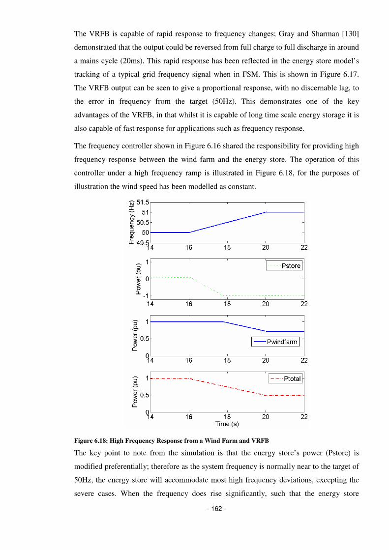
- 162 -

The VRFB is capable of rapid response to frequency changes; Gray and Sharman [130]

demonstrated that the output could be reversed from full charge to full discharge in around

a mains cycle (20ms). This rapid response has been reflected in the energy store model’s

tracking of a typical grid frequency signal when in FSM. This is shown in Figure 6.17.

The VRFB output can be seen to give a proportional response, with no discernable lag, to

the error in frequency from the target (50Hz). This demonstrates one of the key

advantages of the VRFB, in that whilst it is capable of long time scale energy storage it is

also capable of fast response for applications such as frequency response.

The frequency controller shown in Figure 6.16 shared the responsibility for providing high

frequency response between the wind farm and the energy store. The operation of this

controller under a high frequency ramp is illustrated in Figure 6.18, for the purposes of

illustration the wind speed has been modelled as constant.

Figure 6.18: High Frequency Response from a Wind Farm and VRFB

The key point to note from the simulation is that the energy store’s power (Pstore) is

modified preferentially; therefore as the system frequency is normally near to the target of

50Hz, the energy store will accommodate most high frequency deviations, excepting the

severe cases. When the frequency does rise significantly, such that the energy store

- 163 -

reaches its maximum charging rate, the wind farm’s power output (Pwindfarm) begins to

be regulated down but this action would very rarely be required. The overall response

(Ptotal) is a seamless ramp of constant gradient, which itself was defined by the

controller’s droop setting. (Note the base powers of the VRFB and wind farm are different

leading to the different gradients on their individual plots).

Incorporating an energy store for this particular application will have increasing benefit in

avoiding having to spill wind power as the proportion of wind power on the GB system

increases.

Operation of the VRFB to provide low frequency response services can take several

different forms. Figure 6.19 to Figure 6.21 illustrate the behaviour of the energy store,

providing frequency response services but without responsibility for smoothing the wind

farm’s output. In each case the energy store would add a fixed margin to the variable

output of the wind farm, thereby creating a “Delta Control” response (see section 4.3.1)

from the combined wind farm and energy store. Whilst this combined response would not

be in line with the present specifics of GB Grid Code, these three simulations are

illustrative of the way that energy storage and wind power can work in tandem to provide

frequency response services.

Figure 6.19: Generator Control for Low Frequency Response

Figure 6.19 shows the case where the energy store is holding equal high and low

frequency response margin. In this case, when the frequency is close to the target of 50Hz,

- 164 -

the energy store idles, neither charging nor discharging. Both high and low frequency

response reserves are equal to the rating of the VRFB. When the frequency falls, as it does

in this scenario, the VRFB can increase its output (Pstore), from zero, up to the maximum

rating of the battery. This increases the combined plant’s output, but that output is still

variable. Furthermore, the battery will begin to discharge, so the energy stored must be

sufficient to provide for a continuous output until the system frequency is restored or other

plant can come online (i.e. to last at least to the end of the half hour balancing period).

Figure 6.20: Load Control for Low Frequency Response

An alternative approach is shown in Figure 6.20, which could be used when an energy

store is charging. In the event that the system frequency falls, the charging rate of the

energy store could be reduced, thereby helping the system balance by reducing the total

load. A by-product of this control method is that the VRFB can offer twice its rated output

capacity as low frequency response whilst it charges. However, in order to offer high

frequency response the wind farm output would have to be put at risk of being spilt as the

VRFB cannot accommodate a reduction in power output by charging faster.

Figure 6.21 illustrates a greater frequency deviation, where the capability of the VRFB to

swing from acting as a load on the system, to generating is illustrated. Once again

however, it must be reiterated that in order to offer any high frequency response margin,

the wind farm’s output must be put at risk.

- 165 -

Figure 6.21: Bipolar Control for Low Frequency Response

The GB regulations for frequency response stipulate that the output variation must be

relative to a fixed power output level. Figure 6.22 therefore shows the behaviour of this

frequency controller when the smoothing controller of section 6.6.1 is active. As can be

seen, prior to the frequency deviation, the VRFB power (Pstore) absorbs the fluctuations

in the wind power output (Pwindfarm) allowing a constant output power to the grid

(Ptotal). When the frequency falls, the mean of the VRFB output increases so that the total

grid power increases.

This example illustrates the challenge of operating from a constant power output. Towards

the end of the scenario (t>230s), the wind falls sufficiently far that the total output power

from the wind farm and energy store combined is no longer flat. This illustrates that whilst

the initial output is flat, the reserve margin held would be variable dependent on the

prevailing wind conditions. Furthermore, as a consequence of the smoothing power, the

state of charge variation is not predictable, meaning that it must be independently

controlled to ensure that the battery does not exceed its state of charge limits.

- 166 -

Figure 6.22: Frequency Response and Power Smoothing

6.6.3 State of Charge

It has been highlighted that the state of charge of the VRFB will have to be controlled.

Yoshimoto, Nanahara and Koshimizu [142] have developed a controller for regulating the

state of charge of a VRFB installed to smooth a wind farm’s output in Japan, although

without frequency response capability. This is the largest installation of a VRFB globally

and the VRFB effectively acts such that the output of the combined system is low pass

filtered compared to the raw wind power so the VRFB absorbs fast fluctuations. However,

whilst this state of charge control is effective, it is essentially a continuous time

modification to the power output of the combined system. If this were applied here, this

would lead to a variable power output within a settlement period, which would contravene

the GB frequency response requirement to regulate from a fixed output level, and lead to

consequent imbalance.

As an alternative to continuous time management of the state of charge of the VRFB, it is

proposed to manage the state of charge by updating the power output profile (or Final

Physical Notification, FPN) for the next settlement period to be submitted. This FPN has

to be submitted an hour ahead of the relevant half hour settlement period. It is therefore

proposed to use a fuzzy logic supervisor to control the battery’s state of charge by

modifying the forecast output for the wind farm and VRFB for a given settlement period

an hour ahead. Use of fuzzy logic for controlling energy storage on a wind farm was

- 167 -

proposed in Brekken et al. [143], however, there the energy store was purely for

smoothing wind output and had no other purpose, hence the state of charge reference was

constant and the controller was continuous acting. The controller proposed for this more

complex situation is shown in Figure 6.23.

The fuzzy logic controller is designed such that it depends on both the state of charge

itself and the planned change in the state of charge reference. Hence, if the battery is

scheduled to charge or discharge for arbitrage purposes, the controller accounts for this. In

total each input variable is defined to have three states.

• The state of charge is defined as either low, near to its target value or high; where

near to target is defined by a range of ± 20% relative to the target value.

• The rate of change of the state of charge reference is defined to be discharging,

charging or holding; where holding corresponds to a planned change in SOC of

less than 5% per hour.

Figure 6.23: Integrated Fuzzy Logic Based Wind Farm and Store Controller

The membership functions of the normalized input and output variables are shown in

Figure 6.24 and the inference table, Table 6.1, shows the fuzzy rules. These nine rules are

a consequence of the two, three-state inputs. The outputs have been defuzzified according

to Mamdani’s centre of gravity approach. It should be noted that different input

combinations have different rules but potentially the same output. For example, if the state

of charge was near to its target but the planned change in that state of charge target is

negative (to discharge), then the rule states that this should lead to a slow discharge.

Likewise, if the state of charge was high, but the planned change in the state of charge was

to stay constant, then the rule also states that this should lead to a slow discharge of the

VRFB.

The controller has been designed with a view to ensuring that there is sufficient energy

capacity in the battery to absorb significant over or under-production from the wind farm.

- 168 -

Hence, if the battery becomes over-charged relative to the reference, and the reference is

set to hold energy, it will attempt to slowly discharge to ensure there is sufficient energy

margin to absorb a high wind period.

The state of charge controller is only permitted to use 80% of the power capacity of the

VRFB, thus guaranteeing some power capacity margin for frequency response. Further,

by capping the average rate of charge and discharge, the VRFB can be operated more

efficiently by minimizing Ohmic losses as can be seen from Figure 6.9.

SoC Low Near

Target High

Discharge N: Neutral SD: Slow Discharge

FD: Fast Discharge

Hold SC: Slow Charge

N: Neutral SD: Slow Discharge

Planned SoC

Change Charge FC: Fast Charge

SC: Slow Charge

N: Neutral

Table 6.1: Integrated Fuzzy Logic Controller

Figure 6.24: Degree of Membership of the Input (Top & Centre) and Output (Bottom) Functions

- 169 -

6.6.4 Arbitrage

It can be desirable to charge the VRFB at times of low prices and to sell at times of high

prices, or in essence to provide arbitrage services. The state of charge controller has

therefore been designed in order to accommodate a changing state of charge reference. As

the state of charge is based on the integral of the power output of the VRFB, power

exchange for arbitrage can be scheduled by varying the state of charge reference of the

VRFB. When charging the change in the state of charge reference should be defined as:

Equation 6.12 ( )∫ ⋅⋅⋅=∆ dtPPE

SoCechech

rated

ref argarg

1η where Erated is the rated energy

capacity of the storage system, Pcharge is the desired charging power and η(Pcharge) is an

estimate of the one way efficiency of the VRFB at the selected charging power. This

means that an a priori estimate of the efficiency profile for the VRFB is required, but this

can be obtained from the data behind Figure 6.9.

The case is similar for when the VRFB is to be scheduled to discharge, although now the

state of charge reference would be scheduled to reduce. This is illustrated in Equation

6.13. Errors in the open loop setting of the state of charge schedule are then covered by

the fuzzy logic state of charge controller.

Equation 6.13 ( )∫ ⋅⋅−⋅=∆ dtPPE

SoCedischedisch

rated

ref argarg

1η

6.6.5 Integrated Controller

The integrated control of the wind farm and energy store is illustrated in Figure 6.25 for

providing the range of control functions outlined in section 6.6.1 to section 6.6.4.

By scheduling the state of charge reference point (SoCref), the planned energy stored in the

battery can be indirectly controlled, whilst allowing power fluctuation smoothing to take

priority. A forecast is used to predict the wind farm’s output (Pforecast) during the next

balancing period to be submitted. The state of charge controller then alters the next FPN

to be submitted, in order to schedule a charge, discharge or neither (∆PSoC), to maintain

the battery’s state of charge near target. Any deviations between this modified power

production schedule (PFPN) and the actual wind farm output (PWF_Grid) are then combined

with any power demands from the frequency controller (∆Pfreq) to set the power demand

for the VRFB (PVRB_Ref). However, if the battery’s power demand exceeds the maximum

charging rate (1pu) then the wind farm reference (PWF_Ref) is modified as well.

- 170 -

Figure 6.25: Integrated Power Smoothing and Frequency Response Control including, top to bottom,

inertial response, droop response, state of charge management, forecasting and wind smoothing

Figure 6.26: Performance of Integrated Wind Farm and VRFB Controller

Figure 6.26 shows the operation of the integrated controller for the wind farm equipped

with a 25% (75MW) store rated for 6 hours output at maximum power. The plots’ x axes

are defined in terms of the settlement periods (1/2 hour periods, hence 48 per day). From

- 171 -

the top plot, it can be seen that the SoC control clearly operates well, with the SoC broadly

following the reference set for it. The SOC does not track perfectly as the battery uses

power capacity to smooth the wind farm’s output and reduce its imbalance of actual

power output to scheduled power output.

The second plot compares the output of the wind farm with a store, with that of a wind

farm alone (P). The wind farm attempts to maintain a constant output in each half-hour

balancing period, with a 1 minute ramp between periods. This is in order to additionally

provide a stable base power output for frequency response, however, extreme gusts and

lulls can still lead to some imbalance (albeit at a reduced level) as shown in the third plot

(Imbalance). This imbalance is undesirable from a power system perspective and would

be penalised by having to be covered by the wind farm operator purchasing the shortfall at

above the typical market rate or selling an excess at reduced price. Nevertheless, this

penalty does not necessitate sizing an energy store to cover any possible imbalance, as this

would lead to a store of equal capacity to the wind farm, with much of that capacity rarely

used.

The store is scheduled to charge at night (SoC ref increases), which is reflected in the

lower output from the combined wind farm and store during this period when compared to

the wind farm alone. This stored energy is then released during the morning and evening

peaks, by scheduling the SoC reference to fall.

Finally, the fourth plot down shows the maximum power reserves (Pres) available at any

given time for either high or low frequency response. During the periods when the energy

store is discharging, to take advantage of the day-night price differential, little or no low

frequency response capability is available. However, during these periods the system

typically has higher inertia due to more synchronized plant and the requirement for

frequency response reserve is lower and more marginal plant would be online.

Conversely, at night time, the margin for high frequency response capability is lower, as

the store is charging and therefore does not have margin to regulate the plant output

downwards. However, the ability of the energy store to swing from charging to

discharging means that significant low frequency response capability is held. As the

response capability is specified against a fixed output level, the volume of response

available can be seen to continuously vary as the wind speed varies.

Overall, the figure illustrates that the innovative integrated controller presented here can

be used to aggregate some of the multiple benefits of an energy store. The novel state of

charge controller can also be seen to correctly manage the battery capacity and

- 172 -

successfully time shift energy from night to day time peaks. Meanwhile the smoothing

capacity of the battery is used to meet the GB frequency response technical requirements

as the combined system holds a variable reserve for increasing or decreasing combined

output power.

6.7 Summary

This chapter revolves around the development of an integrated controller for the operation

of a VRFB in tandem with a wind farm to provide frequency response services, energy

time shifting, wind smoothing and battery state of charge management.

This chapter began (in section 6.2) by developing a simple electrochemical model of a

Vanadium Redox Flow Battery, that model has sufficient accuracy to represent output

voltage and round trip efficiency, whilst avoiding the complexity of a full representation

of the fluid dynamics of a flow battery. This flow battery must be integrated with the grid

through a boost converter and an inverter. The modelling techniques for representing these

components are drawn from earlier modelling work on wind turbines and adapted for use

with the energy store.

This modelling work led to a simple energy store model that is applicable to power

systems study whilst allowing the viability of the VRFB to be assessed. The model has

been validated against published data in section 6.4.

The energy store’s power converter control is principally drawn from a wind turbine

application but is further developed in order to enhance the response to grid faults, by a

novel feed-forward in section 6.5. This allows the energy store to ride-through grid faults

when generating or consuming power and also support the reactive power capability of the

inverter supplying the grid.

Finally, an innovative controller is developed that allows an energy store to aggregate the

benefits of operating with a wind farm, providing frequency response services and time-

shift of the renewable energy output to peak price periods. At the heart of this control is a

novel fuzzy logic controller for managing the state of charge of the VRFB. The

performance of this controller is verified with simulations using real wind speed data and

the previously validated models.

- 173 -

7 Frequency Response Economics

7.1 Introduction

The power system modelling work described in previous chapters has led to validated

models of wind turbines and Vanadium Redox Flow Battery energy storage systems. This

in turn led to the development of control methods for providing frequency response from

stand alone wind farms or wind farms equipped with flow battery energy storage. These

chapters had a particular focus on the technical capabilities of these technologies to

provide fast response to frequency changes on the power system. Nevertheless, whilst

they addressed the technical capabilities, both applications were left with key questions.

Would the cost of curtailing wind to provide reliable frequency response be too high?

Would the revenues from a flow battery energy store ever be sufficient to provide an

attractive return given their additional capital cost?

This chapter attempts to bridge this gap and to address the economic aspects of providing

frequency response from wind power and energy storage. A series of wind scenarios, as

described in section 7.2, are used by the DIgSILENT model of a 300MW wind farm with

a variety of different capacity VRFB energy stores associated. Section 7.2 also describes

how the outputs from this power system model interface with MathCAD and Excel

models and data which when combined create an economic model in order to assess the

revenues and returns provided by the store.

Whilst the electricity market structure is introduced in section 7.2, its functions and

markets, which impact on frequency response revenues, are described in greater detail in

section 7.3. This section also describes the key calculations in the MathCAD model that

provide the assessment of revenues from the wind farm and energy store. These

calculations ultimately provide the revenue inputs to a discounted cash flow analysis and

the range of appropriate discount rates is considered here.

The financial impact of adding an energy store to a wind farm’s revenues is discussed in

section 7.4, as well as the relative contribution of the different revenue streams. A novel

method of maximising the revenues from an energy store providing frequency response,

whilst putting a wind farm’s output at minimal risk is introduced. This contributes to a

discussion of the advantages and disadvantages of integrating the energy store with the

wind farm by comparing the revenues to the case of an independent energy store. These

revenue calculations lead into the net present value assessment of such energy storage

projects in section 7.5. Finally section 7.6 considers the implications of this analysis and

- 174 -

what the alternatives for frequency response provision are, whilst linking energy storage

to its potential environmental benefits.

7.2 Economic Modelling Methodology

The economic model depends on the outputs from the DIgSILENT model of a 300MW

wind farm enhanced by energy stores with a variety of different ratings. This power

system model is supplied with a series of ten different wind scenarios, each covering a

single day, the selection of these scenarios is described in more detail in section 7.2.2.

These wind inputs lead onto a persistence forecast, as described in section 6.6.1, which is

modified for battery state of charge management and such that the wind farm is scheduled

to hold a (variable) frequency response power reserve. This modified output forms the

basis for the power output forecast (FPN) which is used later in the economic model,

alongside actual output power, to assess imbalance.

The raw wind speed data drives the power system model of the wind farm and energy

store, resulting in a power output profile. This model also provides a profile of the spare

power capacity of the generator to regulate up or down power output, primarily through

modifying the energy store’s charge rate. Hence, overall the power system model passes

three main outputs to the economic model: the contracted (or forecast) power profile, the

actual output power profile and the reserve capacity for high and low frequency response.

The interconnection of this model with the economic model is shown in Figure 7.1.

The economic model draws in data from Microsoft Excel as well as the power system

model. Electricity market price data, balancing mechanism prices and frequency response

market prices have all been collated in Excel spreadsheets. Historical data has been used

to inform three different economic scenarios based on low, mid and high forecasts for the

different prices. The data sources and projections used are described in detail in sections

7.3.2 to 7.3.4.

The economic model itself draws on the outputs of these ten different wind scenarios from

the power system model, together with the three different price scenarios for power

system revenues. It independently calculates the different revenue (and cost) streams for

traded energy, imbalance, frequency response and ROCs before conducting a net present

value analysis based on three different projections for possible costs of the flow battery

installation.

- 175 -

By incorporating three different economic scenarios the uncertainty associated with the

projection is accounted for through the range of possible different economic

developments.

Figure 7.1: Economic Modelling Methodology

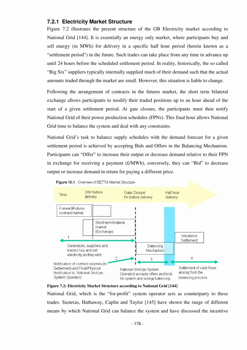
- 176 -

7.2.1 Electricity Market Structure

Figure 7.2 illustrates the present structure of the GB Electricity market according to

National Grid [144]. It is essentially an energy only market, where participants buy and

sell energy (in MWh) for delivery in a specific half hour period (herein known as a

“settlement period”) in the future. Such trades can take place from any time in advance up

until 24 hours before the scheduled settlement period. In reality, historically, the so called

“Big Six” suppliers typically internally supplied much of their demand such that the actual

amounts traded through the market are small. However, this situation is liable to change.

Following the arrangement of contracts in the futures market, the short term bilateral

exchange allows participants to modify their traded positions up to an hour ahead of the

start of a given settlement period. At gate closure, the participants must then notify

National Grid of their power production schedules (FPNs). This final hour allows National

Grid time to balance the system and deal with any constraints.

National Grid’s task to balance supply schedules with the demand forecast for a given

settlement period is achieved by accepting Bids and Offers in the Balancing Mechanism.

Participants can “Offer” to increase their output or decrease demand relative to their FPN

in exchange for receiving a payment (£/MWh), conversely, they can “Bid” to decrease

output or increase demand in return for paying a different price.

Figure 7.2: Electricity Market Structure according to National Grid [144]

National Grid, which is the “for-profit” system operator acts as counterparty to these

trades. Susteras, Hathaway, Caplin and Taylor [145] have shown the range of different

means by which National Grid can balance the system and have discussed the incentive

- 177 -

scheme by which National Grid retains a share of profit made through being incentivised

to optimise the balancing services, or can be punished for any losses. Whilst there are

other options than the Balancing Mechanism available to National Grid, they highlight

that these represent only a minority of operations in comparison to the bids and offers.

This balancing mechanism should ensure that at the start of a given settlement period the

supply schedule meets the forecast demand level. As well as ensuring the match between

forecast supply and demand, the balancing mechanism is also used to ensure that there is

sufficient headroom and footroom on frequency responsive plant to meet the requirements

of Figure 2.23.

During each settlement period, active frequency responsive plant ensures the continuous

match between actual supply and demand outturns. Any significant forecast errors or

supply shortfalls are then met over longer time-scales through use of Short Term

Operational Reserves (STOR) and fast starting units. Following the conclusion of a

settlement period the system operator then retrospectively settles the imbalance payments.

7.2.2 Scenario Analysis

A scenario based approach has been used to assess the economic benefit of adding a

VRFB to a wind farm. Under this approach it is necessary to ensure that the scenarios

tested cover the true range of expected operating conditions. The wind data, which in turn

sets the power output from the power system model, has been extracted from several

months of measured data from Horns Rev offshore wind farm. Analysing the complete

data set would have required excessive simulation time from the power system model;

therefore a subset has been used. However, the subset is reflective of the underlying data

set, particularly for the following parameters:

• Overall Capacity Factor: appropriate selection of data led to an equivalent

estimation of the wind farm’s energy yield.

• Power Output Fluctuation: the scenarios analysed reasonably represent the

variability of the power output that the full wind farm produced.

The capacity factor is relatively straightforward to compare by finding the average output

of the complete dataset and comparing it to the average output of the scenarios chosen.

This comparison shows a capacity factor of 0.43 for the complete dataset, versus a

capacity factor of 0.42 for the sub set, which is well within the bounds of variability in

capacity factor found between different wind farms. This high capacity factor is indicative

of an excellent offshore wind resource.

- 178 -

The subset consists of data from ten periods of one day selected from the complete

dataset. Using a smaller subset inherently means that the histogram of power fluctuations

is not as consistent for the scenarios subset as for the full dataset. However, Figure 7.3

shows the comparative histograms of five minute power ramping incidents for the full

data set and the subset, with the subset appropriately scaled to reflect its lower number of

data points. These histograms are broadly comparable, with the extremes of ramping

reflected reasonably well (i.e. the worst case scenarios will be represented in the analysis).

However, it should be noted that these scenarios have a slightly higher representation of

rapid reduction in output power compared to the original dataset, and a lower

representation of extremely fast increases in power output. Nevertheless, overall the

scenarios selected are reasonably reflective of the range of operation that an offshore wind

farm and energy storage system would encounter.

1

10

100

1000

10000

100000

X<-95% -75%<X<-65%

-45%<X<-35%

-15%<X<-5%

15%<X<25% 45%<X<55% 75%<X<85%

Fre

qu

en

cy

Full data set

Scenarios

Figure 7.3: Horns Rev Wind Speed Data Subset Comparison, histogram of forecast errors for an hour

ahead FPN (the x axis shows the % error in forecast to actual output as a percentage of total wind

farm rating)

The different wind scenarios used are shown in Figure 7.4, and illustrate that there are

prolonged periods with both high and low wind speeds as well as a range of scenarios

with high levels of turbulence reflected in the output power profiles (for example days 3

and 5). Additionally, some start the 24 hour period at very low output and ramp up

considerably (day 2), whilst others do the opposite (day 1 and day 6), thereby challenging

the output scheduling.

- 179 -

-0.2

0

0.2

0.4

0.6

0.8

1

1.2

0 5 10 15 20

Time of Day (hr)

Rela

tive P

ow

er

Outp

ut (p

u) Day 1

Day 2

Day 3

Day 4

Day 5

Day 6

Day 7

Day 8

Day 9

Day 10

Figure 7.4: Wind Speed Scenarios

7.2.3 Energy Store Capacity

Bludszuweit and Dominguez-Navarro [146] suggest that sizing an energy store to cover

wind farm forecast errors can be done probabilistically. Essentially they propose

calculating the required energy capacity by integrating the error between historic forecasts

and actual power output, whilst allowing a certain proportion of “unserved energy”.

However, this methodology is only applicable to compensating for forecast errors.

Korpaas, Holen and Hildrum [147] consider instead a mixed probabilistic approach

combined with scenarios to test the sizing of the store, additionally they incorporate the

effects of a varying electricity market spot price on the storage operation. However, their

work does not consider diurnal pricing leading to arbitrage opportunities and considers

short term power regulation, such as for frequency response, as a cost. These differences

are primarily due to its focus on the Nordpool market, which has significant hydroelectric

resources and a different market structure.

Brekken et al. [143] have proposed sizing a Zinc-Bromine flow battery energy store using

a scenario approach. In their work they consider power and energy ratings at 0.1pu steps

relative to the wind farm rating, before increasing the resolution of their study to find the

optimal solution. Their work was focussed purely on avoiding imbalance penalties in the

Bonneville Power Authorities’ region of western U.S.A. and whilst the optimal sizes

depend on different economics the general approach of using different energy store sizes

is useful.

In order to assess the different possible sizes of energy store, six different power ratings

have been selected and for each different power rating, four different discharge times have

- 180 -

been simulated. The power ratings have been selected as a varying proportion of the wind

farm’s output power. The smallest rating considered is 10% of the wind farm’s output,

which is the minimum size to meet the frequency response requirement of GB Grid Code.

The largest size considered is 33% of the wind farm’s power, which equates to the largest

conceivable size of the wind farm’s IGBT SVC and therefore the point at which the power

electronic interface cost would start to significantly increase. 33% corresponds to the Grid

Code mandated reactive power capacity to achieve a ±0.95 power factor at the grid

connection point.

The four energy ratings have been defined according to a number of hours discharge at

full power output. This means the energy rating for the 1 hour discharge case with a 20%

store is twice that of the 10% case. The relative energy ratings of the store can be seen in

Table 7.1.

Discharge Time at Full Power

No Store 1 hour 3 hours 6 hours 10 hours No Store 0 N/A

10% 0.1 0.3 0.6 1 15% 0.15 0.45 0.9 1.5 20% 0.2 0.6 1.2 2 25% 0.25 0.75 1.5 2.5 30% 0.3 0.9 1.8 3

Store Power Rating

33%

N/A

0.33 1 2 3.3

Table 7.1: Energy Store Power and Energy Ratings

The wind farm itself is considered to be 300MW (to be of similar size to UK round 2

offshore projects). Hence, energy store power ratings vary from 30MW to 100MW. The

size of the wind farm and consequently the energy stores are reflective of the fact that

providers of frequency response in the UK must offer a minimum of 10MW response to

access the market. It is anticipated, however, that any demonstrations or prototype projects

would have to be significantly smaller.

7.2.4 Discounted Cash Flow Analysis

As the primary cost of an energy storage facility would be the initial capital cost of the

technology, whilst the revenue would accrue over time, it is appropriate to consider the

economic case on the basis of a Discounted Cash Flow (DCF) analysis. This allows the

future revenues to be converted to a Net Present Value (NPV) using an interest rate to

accommodate money’s time value and to a lesser extent, risk. The NPV of a future year’s

revenue (πn) is given in Equation 7.1, where i is the percentage interest rate applied and n

is the number is years into the future.

- 181 -

Equation 7.1 n

n

NPVi

ππ ⋅

+=

)100(

100

Where the scenario analysis implicitly assumes that the future revenues will be equal in

any given year, the total revenue over a period of N years can be calculated from the sum

of a geometric series according to Equation 7.2.

Equation 7.2

+−

+−⋅

==Π ∑=

)100(

1001

)100(

10011

1

i

i

n

N

n

NPVNPV

π

π

As the expected life of a VRFB is around 20 years, with a membrane replacement after 10

years, this is the time frame used for the DCF. The interest rate used strongly influences

the outcome of a DCF analysis and this rate in turn may depend on several factors

according to Aston [148]:

• The prevailing bank interest rate.

• The return an equivalent investment could make.

• Returns to shareholders.

• A premium for a project’s risk.

The interest rates applied, along with the costs of operating a VRFB are discussed further

in section 7.3.

7.2.5 Market Reform

The widespread deployment of wind power on the GB power system could have a

significant impact on the electricity market. James Cox [149] of Pöyry Consulting has

highlighted the significant price volatility that could be seen during periods of high and

low wind. Periods of low wind and high demand could lead to particular stress on the

system, leading to a particular concern for DECC over the market’s structure. As the

electricity market currently operates as an energy only market, there is a perceived risk

that it is not sufficiently flexible to provide a return on investments in peaking capacity

which may be used only rarely to cover low wind, high demand periods.

Owing to the concerns that the GB electricity market will not deliver security of supply,

DECC [150] have been consulting on modifying the existing market through the addition

of a capacity mechanism. This would act as an additional revenue stream for providers of

firm capacity, such as energy storage. Hence, whilst this work attempts to estimate the

- 182 -

revenue that an energy store could earn under today’s market arrangements, it should be

recognised that due to proposed reforms these estimates are subject to some uncertainty.

7.3 Economic Data

7.3.1 Renewable Obligation Certificates

The UK wind industry is currently supported through the Renewables Obligation

Certificate (ROCs) scheme, where a power supplier must source a rising share of

electricity from renewable sources. Wind farms are issued with these certificates for each

MWh of energy produced. These certificates can then be traded in a market and the

typical revenue, per MWh generated, is often higher for this revenue source than for a

wind farm’s traded energy.

Equation 7.3 _____

0

ROC

Tt

t

gridROCdtP π⋅

⋅=Π ∫

=

=

Where ΠROC is the total revenue and _____

ROCπ is a

long term average price for ROCs, both in £/MWh.

The challenge when assessing the revenue ROCs generate is not in the mathematical

assessment, which is shown in Equation 7.3, but in understanding the regulations as to

what is and what is not eligible for ROCs, and therefore the impact an energy store would

have.

For an offshore wind farm, the ROCs are metered offshore and the energy store would be

likely to be located onshore, hence any energy transferred to and from the store is

independent of the ROCs regime. This has benefits as it is simple and the round trip losses

of the energy store do not lead to ROC losses. This is inline with the present definitions of

ROCs which are only available for specific, named, technologies, and this list excludes

storage.

The onshore case is less clear as the ROCs could be metered either side of the energy

store’s connection. When the energy store is included, this means that any round trip

energy losses would lead to lost ROCs and therefore have a negative impact on the wind

farm’s overall revenue. Owing to the lack of clarity around what is and isn’t eligible for

ROCs, whilst they are included in the economic assessment, two different cases are

assessed: including ROCs at 1ROC/MWh and excluding them.

7.3.2 Energy Price and System Price Data

In order to assess the revenue from the energy yield of the wind farm, a simplifying

assumption has been made, that the energy is traded at the average of the system buy and

- 183 -

system sell price. This is the same underlying assumption used by Collins, Parkes and

Tindal [151] in assessing the value of advanced forecasting techniques for British power

markets. This assumption implicitly assumes that the economic penalty for over or under-

estimation of the wind power forecast is equal and that the system prices are reflective of

the actual market price paid in the forward/futures market (see Figure 7.2). If this

assumption is not made, the high probability of wind power missing its production

schedules, relative to that of a dispatchable fossil fired plant, means bidding strategies

would become important for maximising revenues thereby significantly complicating

matters.

These system buy and sell prices for every settlement period can be downloaded from the

Elexon reporting website (www.bmreports.com). One year’s data from March 2010 to

February 2011 has been collated and has been approved for use here by Elexon.

Figure 7.5 shows the annual price averages and variation across the settlement periods,

with settlement period 1 corresponding to 00:00 to 00:30 each day. This price profile

clearly illustrates the impact of energy use on the price. During the night hours energy use

is low, leading to lower system price, however, as the day begins energy use and the

corresponding price ramps up. The price stays high during the morning work hours before

declining in the afternoon. The biggest peak of the day is seen during the evening peak, as

domestic demand for heat, light and appliances leads to high demand. Following this

peak, demand gradually declines.

Average System Price: March 2010 - February 2011

0.00

10.00

20.00

30.00

40.00

50.00

60.00

70.00

80.00

0 5 10 15 20 25 30 35 40 45

Settlement Period

£/M

Wh

Yearly Average System Prices (£/MWh) (LowCase) System Sell Price

Yearly Average System Prices (£/MWh) (LowCase) System Buy Price

Yearly Average System Prices (£/MWh) (LowCase) System Average Price

Figure 7.5: Average System Buy and Sell Prices for March 2010 to February 2011

- 184 -

The revenue from traded energy is derived by assuming that the forecast will be perfect

and therefore the entire forecast energy yield is sold. The price is derived as the average of

the system buy and sell prices and revenue is calculated as shown in Equation 7.4.

Equation 7.4 ∑ ∫=

=

+⋅

⋅=Π

48

1

__________min30

02SP

SPSSPSPSBP

t

cclsalesdtP

ππ Where Pccl is the power

production schedule (MW), _____

SPSBPπ is the long term average system buy price for the

settlement period SP and _____

SPSSPπ is likewise the long term average system sell price for a

particular settlement period.

The error in the power production forecast is accounted for by the separate imbalance

calculation(see next section). Furthermore, the scheduling of the battery state of charge

inherently takes account of day-night arbitrage, as Pccl will be modified to be higher

during the periods with higher prices.

OFGEM [152] have presented an analysis of projected development in electricity costs up

to 2025, called “Project Discovery”. According to their analysis electricity prices are

likely to rise by approximately 14% under a central projection or 24% under a worst case.

Today’s system prices form the basis of the “Low” case for the economic forecast, with

these rates of increase being used to adapt the system price profile to give “Mid” and

“High” priced alternative scenarios for comparison.

7.3.3 Imbalance

The costs associated with deviating from a contracted FPN during a settlement period fall

on a wind farm through the System Buy Price (SBP) and System Sell Price (SSP). If the

wind farm is short of its projected output then it must pay for the energy shortfall at the

(usually higher) SBP. If the wind farm overproduces relative to the forecast then it will

only receive the lower SSP. Bathurst and Strbac [153] have shown how using an energy

store to avoid these costs and maximise revenue can lead to added value for a wind farm,

however, their analysis focuses on revenues and not costs nor the likelihood that a system

would pay back.

The revenue associated with the imbalance payments is calculated according to Equation

7.5 for periods where the wind farm’s output is above the contracted level and Equation

7.6 when it is below.

- 185 -

Equation 7.5 ( )∑ ∫=

=

⋅

⋅−=Π

48

1

_____min30

0SP

SSPSP

t

cclgridSSPdtPP π

Equation 7.6 ( )∑ ∫=

=

⋅

⋅−=Π

48

1

_____min30

0SP

SBPSP

t

cclgridSBPdtPP π

The total revenue/cost associated with the imbalance of the wind farm is therefore the sum

of these two components as in Equation 7.7.

Equation 7.7 SBPSSPbalance

Π+Π=Π Im

7.3.4 Frequency Response Market

7.3.4.1 Balancing Mechanism Payments

As indicated in section 7.2.1, the balancing mechanism is used by National Grid to avoid

constraints and match the planned balance between scheduled supply and forecast demand

on the power system. It may also be used to adjust the FPN of plant to create “headroom”

for low frequency response or “footroom” for high frequency response. Hence, even with

a system where supply and demand are scheduled to balance during a settlement period,

National Grid may end up accepting bids on some plant and equal offers on others in

order to ensure that their frequency response margins (see Figure 2.23) are met.

The offer price relates to an increase in generation and therefore needs to cover additional

fuel use plus profit; hence, the offer price is typically loosely tied to the cost of marginal

plant on the system. Bids relate to a reduction in power output and therefore ought to lead

to fuel savings. However, the bids will be made at a level less than the contracted price

that the supplier has received, such that they typically recover their profit, whilst

accounting for fuel savings. Hence, whilst offers are only ever positive values, a bid may

be negative, implying that a generator requires a net payment to reduce its output. Overall

the balancing mechanism prices, which are updated for each settlement period an hour

ahead of delivery, add a cost to the provision of frequency response that is reflective of the

short term market conditions.

The cost of the balancing mechanism payments made to change the output on frequency

responsive plant are available through National Grid’s [154] market information data on

commercial (or “Firm”) frequency response. This data has been collated over a twelve

month period (March 2010 to February 2011) and averaged to find the incremental cost of

frequency response attributable to the balancing mechanism. This can be seen in Table

7.2.

- 186 -

Incorporating the bid and offer data into the calculation of energy store revenue,

introduces an element of value, rather than revenue. Currently an energy store, would not

require a deload to provide frequency response services and therefore would only directly

access the holding payments. However, it is assumed that it could tender higher holding

payment prices and still be selected in the market as that would lead to an overall

optimisation of the response holding.

7.3.4.2 Holding Payments

The balancing mechanism reflects near real time frequency response pricing, but only

covers plant which require an FPN change in order to create headroom or footroom. In

addition to the revenue from the balancing mechanism, there is a separate market for

frequency response which operates monthly covering all relevant plant. Participants in this

market indicate the price (£/MWh, where a MWh here is a measure of potential to deliver

energy, not actual energy delivered) that they require in order to hold margin for primary,

secondary or high frequency response. National Grid [155] publishes details of the

monthly prices paid for plant to hold frequency response.

0

2

4

6

8

10

12

0 5 10 15 20 25 30 35 40

Month

£/M

Wh

Average PrimaryHolding Price(£/MWh)

AverageSecondaryHolding Price(£/MWh)Average HighHolding Price(£/MWh)

Figure 7.6: Mandatory Frequency Response Market Price Evolution over a 3 year period March

2008-February 2011)

As the development of the frequency response market is a result of the relatively recent

deregulation of the electricity industry, prices are still evolving. Figure 7.6 attempts to

illustrate the trend in these prices over time. This shows a strong negative trend for high

frequency response, until, towards the end of the period for which data was available,

prices stabilised and perhaps even slightly increased. The development in price for

primary and secondary response is less dramatic, with prices little changed over the

period.

- 187 -

1.5

2.5

3.5

4.5

5.5

6.5

7.5

8.5

9.5

10.5

11.5

150 250 350 450 550 650 750

Total Reserve Holding (GWh)

Ave

rag

e P

ric

e P

aid

(£

/MW

h)

Primary

Secondary

High

Figure 7.7: Mandatory Frequency Response Market Price to Holding Volume Relationship

Figure 7.7 shows that the prices paid for response have not just developed over time, there

is a correlation between the holdings that National Grid purchase for a given month and

the price paid on average. This is particularly relevant because the projected increase in

requirement for primary and secondary response (Figure 2.23) would therefore suggest a

developing trend towards higher prices.

7.3.4.3 Response Payments

Provision of response, whether reduction in power output in response to a high grid

frequency, or increase in power output following a frequency fall would lead to a change

in the fuel usage of a conventional fossil fuel fired power station. As a result, frequency

responsive plant is compensated, retrospectively, according to its response energy to

frequency deviations. However, these response payments are typically small in

comparison to the payments previously discussed and typically average out to nearly zero.

Hence, the contribution of response payments to the economic case has been ignored with

National Grid’s confirmation that this is a reasonable simplification.

Balancing Mechanism (£/MWh)

Frequency Response Holding Prices (£/MWh) Scenario

System Prices

Bids Offers

ROCs (£/MWh)

Primary Secondary High Low As today 5.4 2.2 45 3.0 2.0 7.0 Mid +14% 6.2 2.5 50 4.0 2.5 7.0 High +24% 6.7 2.7 55 4.5 3.0 7.5

Table 7.2: Economic Scenarios

Table 7.2 illustrates the three different scenarios that have been considered for the

economic analysis of the energy store. The “Low” case takes prices that are approximately

- 188 -

the same as today, whilst developments in the energy market and frequency response

market are modelled separately in the three scenarios owing to differing impacts of wind’s

deployment.

Equation 7.8 to Equation 7.10 show how the revenues from frequency response are

calculated based on the margins held and the different pricing mechanisms.

Equation 7.8 ( ) ( )OfferhighHold

t

selcclHighdtPP ππ +⋅

⋅−=Π ∫

=

_

min30

0

Where Psel is the minimum

possible combined output (MW), which may be negative; πHold_high is the payment for

holding power available to withdraw MWh of energy as needed (£/MWh); πOffer is the

system wide average offer payment required to create the footroom for high response

(£/MWh).

Equation 7.9 ( ) ( )BidHoldprimHold

t

cclmelLowdtPP πππ ++⋅

⋅−=Π ∫

=

sec__

min30

0

πHold_prim and πHold_sec

are the payments for holding power available to deliver MWh of energy as needed

(£/MWh) within primary and secondary timescales; πBid is the system wide average bid

payment required to create the headroom for low response (£/MWh).

Equation 7.10 LowHighFR

Π+Π=Π

7.3.5 Arbitrage Scheduling

Figure 7.5 illustrates that there is a significant potential revenue opportunity from buying

energy at the low night time prices and selling it into the day time peak periods. Figure 7.8

represents a simplified analysis of the absolute maximum revenue that could be derived

from arbitrage, capacity firming and frequency response combined under today’s prices.

The frequency response payments have been derived from the residual power margin held

for either low or high frequency response after the arbitrage charging or discharging takes

priority. The arbitrage revenues been generated by ordering the settlement periods by

average system price and assuming if only 1 hour is allocated to arbitrage that buying

would take place (at the SSP) in the lowest priced settlement period and selling in the

highest (at the SBP). The use of the system buy and sell prices implicitly incorporates the

maximum benefit from capacity firming.

For an energy store with 6 hours capacity, buying would take place in the 12 lowest priced

settlement periods and selling in the 12 highest. Where the efficiency is less than 100%,

the number of settlement periods that the energy store can sell into profitably is reduced.

- 189 -

This places a rough upper limit on the amount that can be earned from different energy

store ratings through arbitrage. Also on the plot is again a rough estimate for the combined

value of frequency response without arbitrage, illustrating that in the 60-75% round trip

efficiency band, as this plot shows the maximum combined revenue, arbitrage may only

add incrementally to the frequency response revenues.

Dependent on the energy storage capacity of the VRFB under consideration, the arbitrage

scheduler uses this plot, in conjunction with the ordered settlement period prices to

generate a schedule as to whether to use capacity for buying selling or holding energy.

This introduces some imperfection into the controller as Figure 7.8 is based on

approximate values and relies on long term average system prices, but this is reflective to

some extent of real world operation.

10.00

15.00

20.00

25.00

30.00

35.00

1 2 3 4 5 6 7 8 9 10 11 12 13 14 15 16 17 18 19 20 21 22 23 24

Time (Hours)

Reven

ue (

£/M

W i

ns

talle

d/h

ou

r)

10.00

15.00

20.00

25.00

30.00

35.00

η = 100%

η = 90%

η = 80%

η = 70%

η = 60%

FR

Figure 7.8: Comparison of Arbitrage and Frequency Response Revenues, the first hour represents

charging in the cheapest half-hour period and discharging into the single peak half hour period, with

longer charge/discharge periods shown moving right on the x axis

Figure 7.8 includes many assumptions and was generated to assess whether the aggregated

benefits of different revenue streams from the energy store could produce meaningful

revenue. It provides an upper bound on the possible revenue from arbitrage as the full

differential between the minimum system sell price and the maximum system buy price is

unlikely to be realised. Overall, it indicates that aggregating benefits in this manner is

likely to provide some improvement over a single purpose energy store, even with limited

round trip efficiency. The scenario analysis provides a more accurate assessment of the

potential aggregated revenues.

- 190 -

7.3.6 VRFB Costs

The principle costs associated with the VRFB are the capital costs, both the energy cost

($/kWh) and the power capacity cost ($/kW). Figure 5.1 provided the indicative range of

costs of power capacity according to current literature, whilst Figure 5.2 provided the

indicative range of current energy capacity costs, again based on the available literature.

Lewis and Sharman [156] have presented on the costs of VRFBs highlighting their

benefits for longer term energy storage. Their analysis of Prudent Energy and GE

Energy’s system estimated the power cost at around $1700/kW and the energy cost at

$300/kWh. These form the central estimate for costs as outlined in Table 7.3, with the

higher and lower estimates based around this central projection.

Kear, Shah and Walsh [157] have conducted an extensive analysis of VRFBs considering

commercialisation and current costs. Their analysis estimates that a typical VRFB

installation would require a membrane refurbishment after 10 years operation and that this

cost would be in the order of 15% of the initial capital cost.

Scenario Power Cost ($/kW) Energy Cost ($/kWh)

Low 1200 200

Mid 1700 300

High 2200 400

Table 7.3: Cost Scenarios for the VRFB

Kear, Shah and Walsh [157] include a significantly higher estimate of operations and

maintenance costs than Bindner [137], whose installation has required no maintenance

over several years operation. Here an operations and maintenance cost of the VRFB is

assumed to be around 0.5% of the capital cost per year.

7.3.7 Discount Rate and Sensitivity Analysis

Under a DCF analysis, the discount rate used significantly affects the results of the study.

Oak Ridge [158] have conducted a study on deploying used batteries in power systems,

under their central case a discount rate of 4% has been used. This is low compared to a

typical discount rate but reflects current low interest rates and a relatively low risk project.

As the analysis here includes scenarios covering low, mid and high end estimates of

revenues, it is reasonable that the discount rate should not include a significant risk

component, as this is reflected in the different scenarios; instead basing it on alternative

returns is reasonable. However, this is still based on an American project and should be

compared to the discount rates appropriate for renewable energy generation projects in

- 191 -

general in the UK. Oxera [159] have conducted an extensive survey of discount rates that

are applicable to low carbon power generation projects. Furthermore, they estimate that

appropriate policy support could lead to discount rates that are 2-3% lower by 2020 for

supported technologies. Figure 7.9 illustrates the range of discount rates that are typical

today and are expected to be typical in 2020 with appropriate government support.

In view of these typical rates, and recognising that the risk weighting is largely reflected

in the different scenarios addressed, 4% can be seen as a reasonable low end estimate for

use in the analysis, where the realistic time frame for deployment of large scale energy

storage is closer to 2020. However, a sensitivity analysis is included where rates of 8%

and 12% have been used to stress test the results under significantly higher rates of

interest.

0 2 4 6 8 10 12 14 16 18 20

CCGTHydro ROR

Solar PVDedicated Biogas (AD)

Onshore WindBiomass

Nuclear (New build)Offshore WindWave (Fixed)Tidal Stream

Tidal BarrageCCS, coalCCS, gas

Wave (Floating)CCGT

Hydro RORSolar PV

Dedicated Biogas (AD)Onshore Wind

BiomassNuclear (New build)

Offshore WindWave (Fixed)Tidal Stream

Tidal BarrageCCS, coalCCS, gas

Wave (Floating)

To

da

y20

20

Tech

no

log

y

Discount Rate (%) Figure 7.9: Oxera, 2011 discount rates today and 2020 for typical low carbon sources

7.4 Energy Storage Revenues

This section considers the benefits that an energy store can bring to a wind farm purely in

terms of its impact on revenues. It begins by considering the case where the energy store

is integrated with the wind farm and therefore responsible for smoothing the wind power

in order to meet the requirement to provide frequency response from a stable output level.

It then moves on to considering the case where the energy store is entirely independent of

the wind farm before introducing an optimal arrangement.

- 192 -

7.4.1 Integrated Energy Store Revenues

The annual (undiscounted) revenues from the wind farm with an energy store can be

compared to the case without a store. This allows an assessment of the incremental

revenue that the energy store provides over and above that of the wind farm alone. The

resulting incremental annual revenues for the three economic scenarios are plotted in

Figure 7.11 through Figure 7.13. The finite number of scenarios considered in the analysis

means that the results for each different store size do not provide totally smooth plots,

which would be possible only with a very large scenario pool. The intermittency and

variability of the wind, combined with different arbitrage capabilities of each of the

different energy ratings, mean that the power profile of the energy store varies

significantly between the various store sizes, even under the same wind profile.

40

45

50

55

60

65

Low Mid High

Economic Scenario

Annual W

ind F

arm

Energ

y S

ale

s (

exc. R

OC

s)

(Mill

ion £

)

0%

10%

15%

20%

25%

30%

33%

Figure 7.10: Traded Energy Revenues, excluding frequency response, for the different power

capacities considered

As the efficiency of the VRFB varies depending on the power input/output; this leads to

significantly different energy losses between the different scenarios. These energy losses

lead to lost sales and may lead to lost ROCs, which can only be compensated for by

selling the remaining energy at a higher price. However, as Figure 7.10 illustrates, the

time shifting of energy to higher prices and the increased certainty of delivery are

insufficient economic levers in any of these scenarios to compensate for the lost energy in

the energy store. This is because the VRFB’s round trip efficiency of around 65% (an

approximate average) is insufficient, at today’s typical power price variation and

imbalance penalties, to operate purely for arbitrage and power smoothing. Frequency

response revenues become the critical revenue stream. However, the capacity of the

- 193 -

energy store to provide frequency response is limited because much of the power capacity

is required to provide wind smoothing, which in turn leads to a loss owing to the round

trip losses.

It can be seen from Figure 7.11 through Figure 7.13 that the ROCs have a significant

impact on the outcome of the analysis. If the energy store were located ‘behind the meter’

then any round trip energy losses would also lead to lost ROCs and therefore lost

revenues. However, if the energy store is independent, such as for an onshore energy store

with an offshore wind farm, the ROCs would still be allocated to the wind farm and the

only loss is due to the lower traded energy sales.

Overall, the addition of an energy store can be seen to normally increase the revenue from

a large wind farm even under the low case. However, these results suggest that the greater

the power capacity of the energy store the better the revenues, owing to the increased

proportion of the power capacity available for frequency response and arbitrage over

power smoothing. This suggests that an independent energy store may be preferable as all

its power capacity could be used for the higher value applications of arbitrage and

frequency response.

-6.00%

-4.00%

-2.00%

0.00%

2.00%

4.00%

6.00%

8.00%

10.00%

12.00%

14.00%

1 3 6 10 1 3 6 10 1 3 6 10 1 3 6 10 1 3 6 10 1 3 6 10

10.00% 15.00% 20.00% 25.00% 30.00% 33.00%

Power and Energy Ratings (% and hr)

% R

evenue Incre

ase

Including Lost ROCs

Excluding Lost ROCs

Figure 7.11: Low Case - Incremental Revenue

- 194 -

-4.00%

-2.00%

0.00%

2.00%

4.00%

6.00%

8.00%

10.00%

12.00%

14.00%

16.00%

1 3 6 10 1 3 6 10 1 3 6 10 1 3 6 10 1 3 6 10 1 3 6 10

10.00% 15.00% 20.00% 25.00% 30.00% 33.00%

Power and Energy Ratings (% and hr)

% R

evenue

Incre

ase

Including Lost ROCs

Excluding Lost ROCs

Figure 7.12: Mid Case - Incremental Revenue

-4.00%

-2.00%

0.00%

2.00%

4.00%

6.00%

8.00%

10.00%

12.00%

14.00%

16.00%

18.00%

1 3 6 10 1 3 6 10 1 3 6 10 1 3 6 10 1 3 6 10 1 3 6 10

10.00% 15.00% 20.00% 25.00% 30.00% 33.00%

Power and Energy Ratings (% and hr)

% R

even

ue Incre

ase

Including Lost ROCs

Excluding Lost ROCs

Figure 7.13: High Case - Incremental Revenues

- 195 -

0

2

4

6

8

10

12

14

16

18

20

1 3 6 10 1 3 6 10 1 3 6 10 1 3 6 10 1 3 6 10 1 3 6 10

30 45 60 75 90 100

Power Rating (MW) and Energy Rating (hrs)

Incre

menta

l R

eve

nue (

£m

illio

n/y

r)

Low Case

Mid Case

High Case

Figure 7.14: Incremental Revenues (Excluding ROCs) in £ for different power and energy rating

batteries

As a very simple comparison, the results above suggest that the addition of an energy

store would ultimately lead to an increase in annual revenue of at a minimum £1.7million

for a 30MW store. Likewise a £17.6million increase for a 100MW store is possible. This

is equivalent to a yield of around £57/kW/yr to £176/kW/yr. As Figure 7.10 shows that the

energy trading actually leads to a net loss, this incremental revenue is entirely ascribable

to the value derived from frequency response.

It is possible to provide a quick validation that the results here are of the right order by

considering the comparison to the published value of frequency response from electric

vehicles derived by Ricardo and National Grid [160]. The annual value of an electric

vehicle for providing frequency response, which is assumed to be not available during

peak periods, is estimated to be £600 for a 3kW system to £8000 for a 50kW system. This

equates to £160/kW/yr to £200/kW/yr, and this is for a system that is assumed to be

unavailable during rush hour, which is typically close to peak power demand periods.

Conversely, Short [161] looked into the economic value of providing frequency response

from dynamic demand in 2004 and concluded a 50W system would provide a benefit of

around £3 per year, which equates to £60/kW/yr.

This shows that the results of this study are inline with the dynamic demand case and are

also of a similar order to those from electric vehicles. In fact the estimates are perhaps on

the low side, which is in part due to conservative projections and in part owed to the

- 196 -

specifics of operating with a wind farm which will be covered further in subsequent

sections.

7.4.2 Independent Energy Store Revenues

The previous section has demonstrated the difficulty of incorporating a VRFB energy

store with a wind farm, owing to the low revenue that is earned for providing a

predictable, flat output, which is a pre-requisite for providing frequency response.

Therefore, this section assesses whether it would be viable to use a VRFB in isolation

purely for the purpose of providing frequency response. Using an energy store in isolation

has the advantage that it can offer its full power capacity for frequency response without

having to smooth the wind. Conversely, it has the disadvantage that it cannot be used in

conjunction with the wind farm’s high frequency response capability to offer greater

combined response.

The revenue from an independent energy store is much more readily calculated than that

from a store integrated with a wind farm, as its output is not compensating for wind’s

variability. Payments are dependent only on the average frequency response payments and

the cost of power to supply the ancillaries of the VRFB.

0

2

4

6

8

10

12

14

16

30 45 60 75 90 100

Store Rating (MW)

Incre

menta

l A

nn

ual R

evenu

e (

Mill

ion

£) Store Only

Store & Wind

Figure 7.15: Comparison of revenues from an independent energy store and a store operating with a

wind farm (under the “Mid” scenario)

Figure 7.15 shows the comparative revenues of a VRFB operating in tandem and

independently from a wind farm, the comparison uses the “Mid” scenario, with 3 hours

capacity. It is clear from this plot that at low size relative to the wind farm, the store is

better off as an independent entity, as the power required for smoothing the wind output

- 197 -

reduces the capacity available for frequency response. However, as the wind farm’s store

becomes relatively larger, the revenues approach those of the independent store; the cost

of smoothing the wind is compensated for by the increased frequency response payments

and the ability to use the wind farm’s capacity to offer greater high frequency response

capacity.

This shows that under some circumstances there is an economic advantage to being able

to combine wind power’s high frequency response capability with the energy store’s

ability to provide low frequency response and simultaneously charge up under low price

periods for later high price dispatch. This fits in with the fact that Figure 7.8 suggests that

even for a relatively inefficient energy store, the combined total revenues including

arbitrage are greater than the frequency response revenues for some settlement periods.

However, when the wind farm is integrated with the energy store, the cost of smoothing

the wind output to meet the frequency response technical requirements typically

diminishes this benefit. The next section therefore considers how an energy storage

system and wind farm could operate to maximise mutual benefits, whilst avoiding the

challenge of having to smooth the wind.

7.4.3 Affiliated Energy Store Revenues

This optimisation of the operation of a combined energy store and wind farm is the

subject of a patent application [162].

0

1

2

3

4

5

6

7

8

<49.

5

49.5

<f<4

9.6

49.6

<f<4

9.7

49.7

<f<4

9.8

49.8

<f<4

9.9

49.9

<f<5

0.0

f=50

50.0

<f<5

0.1

50.1

<f<5

0.2

50.2

<f<5

0.3

50.3

<f<5

0.4

50.4

<f<5

0.5

50.5

<f

Frequency Band (Hz)

Lo

g(T

ime in

Ban

d)

Figure 7.16: Grid Frequency Distribution for 2008 courtesy of National Grid

Section 7.4.1 demonstrated that an energy store could increase the revenue from a wind

farm. However, the round trip losses of the VRFB and the typically low differential

between system prices combined meant it could not provide increased revenue from

- 198 -

power smoothing, which itself was a prerequisite of providing frequency response

services. Section 7.4.2 therefore considered whether an independent energy store would

have higher revenues, as it would have no requirement to provide wind smoothing. Whilst

it was found that this was the case under some circumstances, it also found that the

frequency response revenues were diminished as the energy store could not use the wind

farm’s capacity to offer additional high frequency response services. This section

considers an optimal configuration of a wind farm and energy store, here called an

“affiliated” energy store.

Figure 7.16 shows the distribution of the power system’s frequency during the year 2008.

Noting the logarithmic axis, it highlights that the frequency spends the vast majority of the

time very close to the target of 50Hz. Figure 4.16 illustrated that the response to a

deviation in frequency, from 50Hz, by a frequency responsive plant should be

proportional to the magnitude of the frequency deviation. Hence, the vast majority of the

time, the limits of the frequency response reserve are not used. Whilst Figure 7.8

suggested that for several settlement periods each day an energy store could earn higher

revenue from combining arbitrage with frequency response provision. It is possible to

provide both arbitrage and margin for frequency response; during the time period that the

VRFB is charging it has the capacity to offer low frequency response equivalent to

Equation 7.11, whilst the high frequency response would be capped by Equation 7.12. The

corollary of this is that when the store is discharging into peak demand periods, it could

offer no response, but would be earning higher revenues from the value of its energy.

Equation 7.11 RatedeChLow

PPP += arg where PRated is the energy store’s rated power, PCharge

the charging power and PWindfarm is the wind farm’s output.

Equation 7.12 ( )WindfarmeChRatedHigh

PPPP +−= arg where ( )eChRated

PP arg− is the “residual

capacity” of the VRFB to charge at a faster rate.

Operating the VRFB in this manner would put the wind farm output at risk of being

spilled, if high frequency response greater than the residual capacity of the VRFB is

required, then the wind farm would have to reduce its output. Reducing the wind farm’s

output would lead to lost revenue, primarily through the loss of ROCs. Therefore, when

charging an energy store for later dispatch, there can be an economic gain from providing

frequency response (through the frequency response payments) which must be traded off

against the risk of lost ROCs revenue should high frequency response by required.

- 199 -

Figure 7.17: Optimal control of wind and energy storage in tandem

There is an optimal charging rate where the arbitrage and frequency response revenues are

balanced against the risk of losing ROCs. This trade off is illustrated by Figure 7.17, when

the frequency is exactly 50Hz, the combined output tracks below the available wind

power and the energy store charges. If the frequency falls, the energy store can reduce its

charge rate or even discharge, such that the total output power is the available wind power

plus the energy store’s rated power. If there is a small positive frequency deviation, the

energy store would increase its charging rate, however, for a large positive frequency

deviation, the wind farm would have to activate its balance controller and spill wind as

well. The frequency distribution of frequency shows though that such high frequency

events resulting in spilt wind are rare (the right plot in Figure 7.17 is a simplification of

Figure 7.16).

Figure 7.18 considers the overall revenue that would accrue to a wind farm and affiliated

energy store as a result of the increased frequency response payments from putting more

of the wind farm’s output ‘at risk’. The left hand side of the peak shows a near linear

initial rate of increase of revenue with increased charging rate, reflecting the very low

probability of a high frequency event ever leading to spilt wind. However, the fall off in

revenue as the charging rate exceeds the peak is rapid as the loss of ROCs dominates the

increased frequency response revenues.

- 200 -

0

20

40

60

80

10

0

0.05

0.2

0.35

0.5

0

2

4

6

8

10

12

14

16

18

Net Revenues

Initial charging rate (%)

Storage Size (% of Wind Farm Rating)

Figure 7.18: Optimal Charging Rate of an Energy Store with a Wind Farm

Figure 7.18 suggests that the optimal charging rate for maximum revenues is around 70%

to 80% of the rated power capacity of the energy store. This leaves relatively little power

capacity available for the high frequency response margin from the energy store before

wind must be spilled; therefore it illustrates the steepness of the frequency distribution in

Figure 7.16.

It should be noted, that this increase in frequency response capacity is only available

whilst the energy store is charging. Owing to the finite capacity of energy storage, it will

have a period of reduced frequency response capacity during its discharge period.

However this period still generates high revenue as the store takes advantage of the energy

price differential instead.

7.4.4 Arbitrage Impacts

Figure 7.19 illustrates the critical importance of round trip efficiency to the revenues from

arbitrage of an independently operated energy store with 3 hours storage capacity. The

practical round trip efficiency from today’s VRFBs is around the breakeven point from

arbitrage. However, this is well short of the theoretical efficiency possible from the VRFB

(see Table 9.9) of around 85% for the full system. Hence, the results shown here are

highly sensitive to small technological improvements to the VRFB’s practical efficiency.

- 201 -

-£150.00

-£100.00

-£50.00

£0.00

£50.00

£100.00

£150.00

£200.00

£250.00

£300.00

£350.00

£400.00

0.5 0.55 0.6 0.65 0.7 0.75 0.8 0.85 0.9 0.95

Average Round Trip Efficiency (pu)

Annual A

rbitr

age R

evenue (

Thousand £

/MW

inst

alle

d)

Figure 7.19: Potential Annual Arbitrage Revenues - Dependence on Round Trip Efficiency

7.5 Net Present Value

7.5.1 Integrated Energy Store

Incorporating the costs of the VRFB into the analysis allows the viability of this

application to be assessed. Hence the Net Present Value (NPV) over a 20 year period with

a 4% discount rate has been calculated for the various energy store capacities under the

three economic scenarios.

-£300

-£250

-£200

-£150

-£100

-£50

£0

0 5 10 15 20 25 30 35

Power Rating (% of Wind Farm's Rating)

NP

V (

Mill

ion

£)

1 hour

3 hours

6 hours

10 hours

Figure 7.20: Net Present Value of VRFB over 20 year life under Low scenario

- 202 -

-£120

-£100

-£80

-£60

-£40

-£20

£0

£20

£40

£60

0 5 10 15 20 25 30 35

Power Rating (% of Wind Farm's Rating)

NP

V (

Mill

ion £

)

1 hour

3 hours

6 hours

10 hours

Figure 7.21: Net Present Value of VRFB over 20 year life under Mid scenario

-£40

-£20

£0

£20

£40

£60

£80

£100

£120

£140

0 5 10 15 20 25 30 35

Power Rating (% of Wind Farm's Rating)

NP

V (

Mill

ion £

)

1 hour

3 hours

6 hours

10 hours

Figure 7.22: Net Present Value of VRFB over 20 year life under High scenario

The results are shown in Figure 7.20 to Figure 7.22. This illustrates that under current

system prices and frequency response prices (Low scenario); the VRFB cannot provide an

economically viable service, when in conjunction with a wind farm, as all NPVs are

negative. However, under the forecasts for expected price increases (Mid scenario) or high

price increases (High scenario), some of the high power, low energy rating systems show

a significantly positive NPV.

Figure 7.8 demonstrated that the average differential price achieved with arbitrage

decreases for longer term energy stores. This is due to there only being few peak price

- 203 -

settlement periods in each day (see Figure 7.5). Furthermore, in order to provide primary

and secondary frequency response the energy store only needs to be rated for sufficient

energy capacity to charge or discharge at full power for a single settlement period. Hence

a store rated for full power for a single hour is sufficient (assuming it starts a settlement

period at 50% SOC) to meet frequency response needs. Adding energy capacity is

expensive and offering frequency response capacity accesses most of the value. This is the

reason for low energy rating stores outperforming longer term stores; however, higher

round trip efficiency would preferentially improve the economics of higher energy

capacity stores by improving arbitrage economics.

The comparative benefit of higher power rating of the energy store is again owed to the

relatively low benefit that can be derived from smoothing the wind power output. Higher

power rating stores can dedicate a greater proportion of their energy capacity to providing

frequency response reserves.

Payback Period (years) Power Rating (% of Wind farm MW rating)

Power Rating (MW)

Energy Rating (hrs) Low Mid High

1 x x 15 3 x x 15 6 x x 13

10.00% 30

10 x x 16 1 x x x 3 x x 9 6 x x 16

15.00% 45

10 x x 17 1 x x x 3 x x 15 6 x x x

20.00% 60

10 x x 16 1 x x 10 3 x x 13 6 x x 17

25.00% 75

10 x x 17 1 x 14 6 3 x 19 9 6 x x 14

30.00% 90

10 x x 17 1 x 13 6 3 x 15 7 6 x x 10

33.33% 100

10 x x 17

Table 7.4: VRFB Deployment Payback Periods (x = Not paid back within 20 years)

The negative NPVs of the low case, even with this low discount rate, indicate that

developing a project today would be extremely high risk and likely to deter investors.

Even under the central scenario the returns are modest at best. As development of such a

storage project would be highly capital intensive it is also of interest to compare the

payback periods, which are shown in Table 7.4. These are discounted payback, rather than

- 204 -

simple payback periods, but the lack of a short term payback under the central scenario

suggests that this would not represent a desirable investment. Whilst some ratings promise

relatively short payback periods under the high scenario, this is likely to be insufficient to

prove attractive unless price rises are at the upper end of forecasts.

7.5.2 Optimal Power Rating

Figure 7.23 shows the effect that increasing power capacity has on the total revenues of a

combined wind farm and energy store. The broad trend is not a linear one, with increasing

power capacity leading to greater revenue benefit for larger stores. This connects with the

assertion that the storage facility would be better deriving revenue from frequency

response and arbitrage, rather than through avoiding imbalance penalties. This in turn also

corroborates the payback periods shown in Table 7.4, where the higher power capacity

energy stores are the ones achieving the shorter payback periods.

The optimal power rating of an energy store, if it must be operated in conjunction with the

wind farm, can be found by considering the traded energy sales. Figure 7.10 shows that

under each of the 3 scenarios, the highest energy sales were achieved with an energy store

rated at 25 to 30% of the wind farm’s rating, aside from the case with no storage. Given

the high capacity factor of the wind farm considered here, the lower of these values is

therefore recommended as an approximate guide.

0.00%

2.00%

4.00%

6.00%

8.00%

10.00%

12.00%

14.00%

16.00%

0.00% 5.00% 10.00% 15.00% 20.00% 25.00% 30.00% 35.00%

Power Capacity as % of Wind Farm's Rating

% In

cre

ased

Reven

ue

1 hour

3 hours

6 hours

10 hours

Figure 7.23: Comparison of VRFB's Benefit to a 300MW Wind Farm (Mid Case)

- 205 -

7.5.3 Optimal Energy Rating

Figure 7.24 through Figure 7.26 show the Net Present Value (NPV) of various different

storage ratings assessed over 20 years, under the three economic scenarios. This illustrates

the optimal energy store size, as the lower power ratings (10-20%) typically have higher

(less negative) NPV at 3 to 6 hour ratings, whilst the larger power ratings typically have

higher NPV at 1 to 3 hours. This is a consequence of the greater proportion of revenue

derived by larger stores from frequency response services, which require only limited

energy capacity. The high energy ratings at high power ratings are rarely required, whilst

the high energy ratings at lower power ratings are frequently required for wind smoothing.

This is because wind gusts and lulls of greater than 30% magnitude lasting an hour or

more are orders of magnitude rarer than wind gusts or lulls of 10% magnitude lasting an

hour (note the exponential scale of Figure 7.3). Large unforecast peaks and troughs in

wind output tend to be transient in nature.

Overall, the trends of Figure 7.24 to Figure 7.26 suggest that the optimal energy rating of

a VRFB in conjunction with a wind farm is likely to be around 3 hours or less at full

power output. This is likely to shift to higher energy capacities as and when the round trip

efficiency of these batteries improve, as lower differential market prices would become

profitable for arbitrage. However, this corroborates Prudent Energy and GE Energy’s

modular system size which, whilst expandable, currently typically has a two hour rating as

a base point.

-£300

-£250

-£200

-£150

-£100

-£50

£0

0 2 4 6 8 10 12

Energy Rating (hr)

Net P

resent V

alu

e (

Mill

ion £

)

10% Store

15% Store

20% Store

25% Store

30% Store

33% Store

Figure 7.24: Net Present Value (20 year lifetime) of Different Power and Energy Rating Stores under

Low Economic Case

- 206 -

-£120

-£100

-£80

-£60

-£40

-£20

£0

£20

£40

£60

0 2 4 6 8 10 12

Energy Rating (hr)

Net P

resent V

alu

e(M

illio

n £

)

10% Store

15% Store

20% Store

25% Store

30% Store

33% Store

Figure 7.25: Net Present Value (20 year lifetime) of Different Power and Energy Rating Stores under

Mid Economic Case

-£40

-£20

£0

£20

£40

£60

£80

£100

£120

£140

0 2 4 6 8 10 12

Energy Rating (hr)

Net P

resent V

alu

e(M

illio

n £

)

10% Store

15% Store

20% Store

25% Store

30% Store

33% Store

Figure 7.26: Net Present Value (20 year lifetime) of Different Power and Energy Rating Stores under

High Economic Case

From the analysis, it is clear that 6 or 10 hours of storage capacity is unlikely to be viable

in the near future, owing to the very low average differential price from arbitrage and the

significantly higher capital cost of such a large capacity. However, it should be noted that

a significant benefit of flow battery solutions is that the energy capacity can be adapted by

addition or enlargement of the tanks of electrolyte at a comparatively low cost. This is

achievable at a significantly lower cost than implementing a completely new system, as

whilst the power cost of the VRFB is high compared to other technologies, the energy cost

is comparatively low (see Figure 5.1 and Figure 5.2).

- 207 -

7.5.4 Affiliated Energy Store Revenues

Figure 7.27 shows the comparative NPVs of a 75MW VRFB, with 3 hours capacity, based

on whether the energy store is fully integrated with the wind farm, as in section 7.4.1,

fully independent as in section 7.4.2, or merely affiliated to a particular wind farm as in

section 7.4.3. This shows the benefits of the affiliated method, which combined arbitrage

with providing higher volumes of frequency response by offering additional high

frequency response from the wind farm. This scheme offered a slight improvement over

the independent energy store case, which in turn was significantly improved over the case

where the energy store was integrated with the wind farm.

This plot illustrates that under the central projection, both the independent and the

affiliated energy store have positive NPV, indicating that they would represent

investments that would payback. However, none of the options offers a positive NPV

under the low projection, raising the level of risk of developing such a project and

deterring investment. This highlights the problem identified by the Electricity Market

Reform; the capital cost of investing in storage or other assets for peak load operation is

not supported by the energy only market. However, there is a new capacity mechanism

proposed to solve this problem. Given that the NPVs, under the low projection, of the

independent and affiliated energy stores are relatively small negative values, it is entirely

possible that the capacity mechanism may provide sufficient support to energy storage to

make such projects viable in the medium term.

-100

-50

0

50

100

150

Fully integrated with wind Fully independent Partially integrated with wind

NP

V (

Mill

ion £

)

NPV after 20 years Low

NPV after 20 years Mid

NPV after 20 years High

Figure 7.27: NPV Comparison of the Different Storage Integration Options (75MW, 3 hour store over

20 years)

- 208 -

7.5.5 Discount Rate Sensitivity

Table 7.5 to Table 7.7 show the sensitivity of the NPV calculations to discount rates. The

three tables are all for a 75MW, 3 hour store but for the three applications of the energy

store: integrated with a wind farm, totally independent and affiliated with a wind farm. As

expected, the NPVs are highly sensitive to the discount rates applied, however, owing to

the nature of compound interest, those cases with short payback periods suffer less than

those with longer payback periods. This means that the cases with attractive payback

periods of significantly less than 10 years only see a lengthening of payback period of 1-2

years with the higher discount rates. However, high discount rates do mean that the

independent and affiliated energy stores would not pay back under central projections.

Net Present Value (Million £) Payback Period (years) Discount

Rate (%) Low Mid High Low Mid High

4 -85.9 -21.5 36.0 x x 13

8 -105.0 -50.0 6.2 x x 15

12 -117.2 -63.1 -12.7 x x x

Table 7.5: Integrated Energy Store NPV Sensitivity to Discount Rate

Net Present Value (Million £) Payback Period (years) Discount

Rate (%) Low Mid High Low Mid High

4 -24.6 43.3 105.1 x 14 7

8 -59.0 1.6 58.0 x 20 7

12 -80.9 -24.7 28.2 x x 9

Table 7.6: Independent Energy Store NPV Sensitivity to Discount Rate

Net Present Value (Million £) Payback Period (years) Discount

Rate (%) Low Mid High Low Mid High

4 -8.6 61.4 124.9 x 12 6

8 -47.1 15.3 72.9 x 16 7

12 -71.4 -14.0 39.9 x x 7

Table 7.7: Optimal Energy Store and Wind Farm NPV Sensitivity to Discount Rate

7.6 Alternatives to Storage

The preceding analysis used reasonable projections for the cost of a VRFB, likely

revenues in the energy and frequency response markets and appropriate discount rates to

assess the NPVs of VRFB energy storage on the GB system. It has found that under the

central projection, energy storage is likely to have positive net present value for providing

- 209 -

frequency response and arbitrage when operating as an independent store. This positive

NPV can be improved if the energy store can affiliate itself to a wind farm and use the

wind farm’s capability for providing high frequency response to offer greater frequency

response capacity when charging up for arbitrage.

The challenge for the VRFB is that the payback periods, combined with the lack of a

guaranteed payback under worst case projections suggest that it may remain too risky an

investment for this application alone. This assessment considered the open markets from

which a storage owner could presently earn a return. The Electricity Market Reform may

lead to higher payment for storage’s firm capacity, which could in turn tip the economics

in favour of storage. Failing this, a VRFB owner would have to be able to accrue the

revenue from other benefits it could provide, such as constraint management or grid

capacity upgrade deferral. These revenue streams are less accessible to an independently

owned storage operator, however.

In view of the questionable economics of storage to provide frequency response services,

it is worth briefly considering the alternatives.

7.6.1 Curtailment of wind power

Figure 7.28: Plot of hourly electricity demand to percentage served by wind from Sinden [163] (red

elements are superimposed and show the curtailment of energy if wind were curtailed at 50% of

demand and 33GW were installed on the GB system, rather than Sinden’s 25GW)

If energy storage does not provide frequency response services on behalf of a wind farm,

it is likely that at times of high wind and low demand; the wind farm may have to provide

the service instead. This implies a level of spilt wind as the turbines regulate output down

in order to hold the margin required for frequency response. Sinden [163] has conducted

- 210 -

an extensive analysis using 33 years of wind data from 66 weather stations and compared

this with demand data so as to assess the correlation between the two. He has shown that

wind power has a weak positive correlation with demand in the UK, such that wind

power’s capacity factor during peak demand hours is around 30% higher than the annual

average. Sinden has considered the case where the UK has 25GW of installed wind

capacity and a peak demand of 60GW; he has shown the percentage of hourly energy

served by wind, which is shown in Figure 7.28.

Sinden’s work was based on 25GW of wind development in the UK. If this were scaled up

to 33GW (see section 2.6.1) and Sinden’s limit of wind power providing 50% of demand

remained, then wind power plants could have to spill wind energy approximately 8% of

the time to ensure their output does not exceed 50% of supply. This would lead to an

annual energy loss of around 3%. This in turn would put a significant additional cost on

wind farms, demonstrating the potential additional value of storage for managing this

form of constraint.

7.6.2 Interconnection

Section 2.4.2 showed the ambition of the European Union to move to a more

interconnected grid for Europe, to allow both a free market in electricity and to

accommodate greater renewable energy deployment. In theory such interconnectors could

provide the frequency response services required by the GB grid. However, the current

operation of interconnectors is based almost entirely on the energy price differential

between different countries. It would require an improvement in the economics of

provision of frequency response in order for interconnectors to hold capacity purely for

the purposes of frequency response margin. Such an improvement in these economics

would in turn lead to a more favourable return on any energy storage developments as

well.

7.6.3 Conventional Generation

Figure 7.29: Frequency Response Instructions Distribution from Pearmine [164]

- 211 -

Frequency response is presently provided by part loaded conventional generation,

traditionally predominantly coal fired as illustrated in Figure 7.29. However, as Coal

plants are decommissioned due to the Large Combustion Plant Directive and concerns

over CO2 emissions, the principle conventional generation source that could fill the

frequency response gap is Combined Cycle Gas Turbines (CCGT).

Figure 7.30: NOx and CO Emissions from CCGT Plant According to Tauschitz and Hochfellner [165]

Figure 7.31: Part Load Efficiency of CCGT Plant According to Tauschitz and Hochfellner [165]

Tauschitz and Hochfellner [165] have shown that the typical efficiency of CCGT is

significantly affected by operating at part load. Typically a CCGT can regulate its output

power down to around 50% before the non-linear increase Nitrous Oxide (NOx) and

- 212 -

Carbon Monoxide (CO) emissions reach environmental limits. This is shown in Figure

7.30. Hence, in order for a typical CCGT to offer equal high and low frequency response

capacity it would be regulated down to around 75% of maximum output.

Figure 7.31 illustrates that if a CCGT is regulated down to around 75% of its rated output

it would reduce in efficiency by around 3%. Furthermore, according to Pearmine [164],

such a fossil fuel plant could only be relied on to deliver 55% of its frequency response

holding. Here the net effect on emissions is considered.

First, for simplicity it is assumed that CCGTs are operated to provide 600MW of low and

high frequency response, based on Figure 2.23. Based on delivery of only 55% of this, the

frequency response holding would have to be:

Equation 7.13 MWPFR

109055.0

600== where PFR is the frequency response holding.

Assuming the CCGTs are operated at 75% output, this holding would be distributed

across:

Equation 7.14 MWPTot

436075.01

1090=

−= of plant.

The Department of Energy and Climate Change [166] has created estimates of the Carbon

Intensity of power generation in the UK, which is shown in Table 7.8.

Source Carbon Intensity (χ) (kgCO2/MWh)

CCGT 380 UK Average 550

Table 7.8: Carbon Intensity of Electricity Generation in the UK

Initially, prior to deloading to hold a low frequency response margin, the CCGT plant will

have a CO2 output of:

Equation 7.15 htonnesPmCCGTTotCO

/165738043602

=⋅=⋅= χ

However, after the deload instruction, the frequency response holding would have to be

replaced on the system. Here we consider two conditions, either that this is replaced by

more CCGT plant coming online, or that the shortfall is picked up across all generators,

thereby incurring the average Carbon intensity of the power system. Either way the total

Carbon emissions are given as:

- 213 -

Equation 7.16 ( )

χχη

⋅+⋅−

=FRCCGT

CCGT

FRTot

COP

PPm

'

2

where ηCCGT is the CCGT relative

efficiency at that load from Figure 7.31.

If we assume CCGT plant fills the gap created by deloading this plant, the total CO2

emissions now become:

Equation 7.17 ( )

htonnesmCCGT

CO/16953801090380

97.0

109043602

=⋅+⋅−

=

Or if we assume an average mix of current power stations fills the gap, the total CO2

emissions become:

Equation 7.18 ( )

htonnesmMix

CO/18815501090380

97.0

109043602

=⋅+⋅−

=

So the Carbon Intensity of providing 600MW of high and low frequency response holding

can be calculated as:

Equation 7.19 ( )

MW

mmm

COCOFR

CO 60022

2

' −=

For the CCGT only, and average power mix cases, this translates to a Carbon Intensity for

holding frequency response equivalent to:

Equation 7.20 ( )

MWhkgCOMW

FR

CCGT/63

600

165716952=

−=χ

Equation 7.21 ( )

MWhkgCOMW

FR

Mix/373

600

165718812=

−=χ

This shows that providing frequency response from storage as opposed to deloaded CCGT

plant could lead to substantial CO2 savings. These savings are between 17% and 98% of

the emissions saved from renewable energy displacing each MWh generated by CCGTs in

the generation mix.

Currently onshore wind power receives 1 ROC per MWh and each MWh typically

displaces a MWh from a CCGT plant thereby saving 380kg of CO2. Offshore wind, a less

mature technology although arguably more mature than flow battery storage, receives 2

ROCs per MWh with the same effect on total emissions. This analysis suggests that ROCs

targeted at storage for frequency response could have a beneficial effect on total Carbon

emissions.

The analysis shows a significant environmental benefit to providing frequency response

from energy storage rather than conventional plant. It does not consider the environmental

benefit of providing arbitrage from storage, thereby avoiding the need to have polluting

peaking plants running during peak periods and hence reducing the average Carbon

- 214 -

intensity of UK generation. Instead, this final section is intended to promote discussion.

On the basis of this analysis a targeted subsidy could both act to make storage

economically viable and prove to be an effective means of reducing emissions. A Brunel

Institute of Power Systems M.Sc. project will investigate this further.

7.7 Summary

This chapter has shown that VRFBs are close to being commercial viability for

application on wind farms for frequency response.

This chapter has used the models and techniques described in the preceding chapters in

order to assess the economics of providing frequency response from energy storage and

wind power. Section 7.2 introduced the different scenarios that were to be applied to the

power system models in order to generate power output and power reserve profiles from a

wind farm with VRFB energy store. It also showed how this power system data integrated

with an economic model reflecting the behaviour of the electricity market to generate

revenue data from the power data.

Section 7.3 introduced the financial data behind the calculation of the different revenue

streams, including frequency response, imbalance and traded energy market data. It also

presented the different cost scenarios for the VRFB and introduced the discounted cash

flow analysis scenarios that are used later in the chapter. Three different scenarios: low,

mid and high, were introduced to reflect differing economic conditions.

Section 7.4 discussed the potential increase in revenues from the energy store,

demonstrating that excluding the effect of lost ROCs (if applicable) the energy store could

increase the total revenue of the wind farm in most scenarios. However, it also showed

that integrating it with a wind farm led to lower revenues than independent operation

owing to round trip losses in the VRFB outweighing reduced imbalance penalties from

improved predictability. Against this it showed the advantage of being able to share

responsibility for high frequency provision with the wind farm through access to higher

holding payments. Hence, the concept of an affiliated energy store was developed which

promised incrementally improved revenues.

The revenues from the energy store led into an assessment of the present value of different

storage developments in section 7.5. Whilst this found that some cases produced positive

present value under the central projection, none achieved this under the low revenue

projection and payback periods were shown to be typically too long for an attractive

investment under the central and high revenue projections.

- 215 -

If storage cannot provide frequency response, then it must be provided elsewhere and

section 7.6 explores this. It shows that if wind farms are to provide frequency response

then there will be a small but significant impact on energy yields. Furthermore, the section

introduces the reasons why if conventional CCGT plant is increasingly the source of

frequency response provision this leads to a negative environmental impact and higher

CO2 emissions. This illustrates that storage for frequency response can save CO2 and

should perhaps have a specific support mechanism to bring it to commercial maturity.

- 216 -

8 Conclusions and Further Work

8.1 Modelling of Wind Turbines

The UK has set itself ambitious targets to reduce the carbon intensity of the power

generation sector over the coming decades. The specifics of the UK’s subsidies, seabed

geology and conservative approach to development mean that these targets are in large

part likely to be met with widespread deployment of offshore wind farms. The

development of the offshore wind resource is likely to present significant challenges to the

power system’s frequency stability owing, in part, to wind’s intermittency.

Advances in both Grid Codes and power electronics have driven the wind industry

towards increased use of full converter interfaced wind turbines. The power electronic

interface decouples the generator from the grid system, offering flexibility through

control, but removing the generator’s natural inertial response from the grid. Active power

control from large offshore wind farms is therefore an area of increasing importance to

ensure the power system’s future stability. The use of full converters in wind turbines

permits a range of different control philosophies and physical systems as outlined below:

• In-direct speed control of the turbine (conventional) versus direct speed control

(subject to some renewed commercial interest).

• Blade pitch control as a speed controller versus a power controller.

• Real power control on the grid side inverter versus real power control on the

generator side rectifier.

• Permanent magnet generators versus electrically excited generators.

• Synchronous or asynchronous generators.

• Direct-drive or geared shaft systems.

This project has therefore delivered a suite of validated full converter wind turbine

models. These have been used to investigate the implications of moving to direct-drive

permanent magnet generator based wind turbines, and the effect of directly speed

controlling a wind turbine, on the grid interface.

Direct speed control of the wind turbine, which offers a potential means of incremental

improvement to the wind turbine’s energy yield, is shown to require increased torque

swings in order to improve the tracking of the optimal power coefficient. Furthermore, the

- 217 -

dynamic response is shown to largely depend on the torque limit and the speed controller

performance.

Use of permanent magnet excitation in generators leads to an intrinsic link between speed

and open circuit voltage, meaning that over-speed of a permanent magnet generator based

wind turbine risks leading to excess voltages on the power converter. Whilst it is shown

that voltage can be controlled by a pseudo field-weakening approach when the rectifier is

switching with four quadrant operation, this control method is insufficient to protect the

power converter from over-voltage in the event of a drive trip leading to uncontrolled

diode bridge rectification. Furthermore, direct-drive shafts are shown to be at risk from

mechanical oscillations at higher frequencies than the conventional geared shafts.

Excitation of this mechanical resonance would risk imposing a transiently high generator

speed with a corresponding over-voltage transient on the power converter.

The requirement to equip a PMG based wind turbine with a chopper and dynamic brake

resistor has led to a decoupling of machine and grid dynamics. This led to the

development of a simplified model of this type of wind turbine where the DC link

controller on the machine bridge directly effected a torque on the shaft model. This

removed the need to represent the generator and the majority of the machine bridge

control thus increasing computational efficiency for longer time scale modelling.

8.2 Grid Connection of Wind Turbines

The mechanical resonance of a PMG shaft combined with its intrinsic voltage dependence

on speed and high stator reactance are shown to lead to particular challenges under grid

faults. An electrically excited machine can rely on field weakening to reduce terminal

voltage and thereby avoid the power converter’s maximum voltage limits under grid

faults. However, the magnetic energy in the PMG’s stator reactance must transfer to the

power converter’s DC link in order for the PMG’s torque to be reduced during a fault; this

inherently drives up the DC link voltage. With direct drive permanent magnet generators,

this increase in DC link voltage has the potential to exceed the rated DC link voltage for

the power converter. Furthermore, the rapid torque reduction could excite the shaft

mechanical resonance and lead to a transient over-voltage on the power converter’s stator

connection. This demonstrates the importance of choppers and dynamic brake resistors for

protecting the power converter of a PMG under grid faults.

Banham-Hall et al. [80] and section 4.2.5 described a novel, patented, adaptation to the

generator bridge control in order to drive a ramped reduction in a PMG’s torque under a

- 218 -

grid fault. This method, using a specific ramp rate, is shown to significantly reduce the

amplitude of the resulting mechanical resonance. Furthermore, as the generator’s torque is

eventually removed, the brake resistor need only be rated at a reduced energy rating

compared to a full chopper and brake resistor system.

The presence of a dynamic brake resistor, to slow the transient torque changes of a PMG

wind turbine down, has been shown to permit a significant simplification of the model of

a full converter PMG. The machine and rectifier can be removed, with the DC link voltage

controller, which would normally set the rectifier’s per unit real current reference, being

used directly to set the per unit torque to the shaft model. This simplification produces a

model that is faster in simulations and therefore beneficial for frequency response studies,

which require a longer time-scale.

The GB Grid Code has implemented a requirement that necessitates all large (>50MW),

transmission connected, wind farms to be capable of a proportional droop response to grid

frequency disturbances. The power converter can deliver this response extremely quickly

and with direct proportionality, however, the change in power output can then lead to

slower mechanical changes from the wind turbine. Alternatively, the pitch control can be

modified such that changes in the aerodynamic blade performance filter through to a

change in turbine output power. This method offers slower response, but with no residual

mechanical transients. Furthermore, the flywheel effect of the blades can be used to store

energy when the wind turbine is operating in low wind speeds, this energy can then be

used for temporary over-production following a frequency fall. These control methods

were explored in section 4.3.

GB and European transmission system operators have floated the prospect of a

requirement on transmission connected wind farms to provide a synthetic inertial

response. This would require the turbine controller to restore the link between generator

rotational kinetic energy and system frequency. Conventional approaches to providing a

synthetic inertial response typically rely on a measurement of the power systems rate of

change of frequency. However, frequency is typically a noisy signal and the inertial

response therefore has to be either filtered, introducing delay, triggered, removing

linearity, or accepted as subject to noise, which reduces its benefit as a stabilising

influence. Banham-Hall et al. [87] and section 4.3 therefore propose alternatives based on

speed controlling the wind turbine, or generating a synthetic load angle, which offer the

potential of a fast inertial response that is not as sensitive to noise on the power system’s

- 219 -

frequency. These controllers are shown to be tuneable and potentially advantageous over

the predominant controller that relies on a frequency derivative.

8.3 Vanadium Redox Flow Battery Energy Storage

The importance of frequency response from wind farms is growing as the wind industry

grows and as National Grid increases the holding requirement to accommodate potential

larger single generation losses. However, whilst the Grid Code has ensured that technical

solutions are found so that wind farms can participate in frequency control, it does not

address the economic case. Energy storage and battery manufacturers are increasingly

looking to base business cases for energy storage on the ancillary service markets,

including frequency response. As such, the increasing GB requirement for this service,

along with high levels of wind power generation and an islanded system, may present an

opportunity for energy storage on the GB system.

A review of the available energy storage technologies in chapter 5 has found that the high

cycle life, relatively low energy capacity cost, and design flexibility of the Vanadium

Redox Flow Battery makes it a favourable technology for integration with wind power

and combined provision of frequency response. The freedom to independently optimise

the flow battery’s energy and power ratings, together with its higher round trip efficiency

make it preferable to the nearest competitor of thermal energy storage.

A simplified power system representation of the VRFB has been developed and validated,

with accurate representation of battery voltage, round trip efficiency and state of charge.

Furthermore, this model has been integrated onto the DC link of a model of an IGBT

SVC, as these are often already required to provide dynamic reactive power compensation

for large AC connected offshore wind farms. As with the wind turbine, the power

electronic interface offers fast response to grid transients. An adaptation to the wind

turbine grid fault ride-through control is presented in Banham-Hall et al. [138] and section

6.5. This modification allows the battery to be used to support the IGBT SVC’s DC link

during a grid fault and thus ensure continued reactive power delivery to the grid even in

the event of an extended duration severe voltage dip.

Banham-Hall et al. [138] and section 6.5 also explore the control of a VRFB, in

conjunction with a wind farm, to offer frequency response capability to the power system.

A novel fuzzy logic controller is developed which manages the battery’s state of charge

by modifying the planned future energy trades with the power system. Furthermore, the

integrated controller can be scheduled to perform daily arbitrage and wind smoothing,

- 220 -

thereby aggregating multiple different revenue streams for the single storage facility. This

controller is shown to successfully control the battery’s state of charge even in the

presence of significant unexpected wind turbulence. Furthermore, the scheduling of daily

arbitrage is shown to increase the combined frequency response capability of the wind

farm and energy store during the hours when the store is charging. The battery is also

shown to be capable of extremely fast response, with a complete current reversal possible

in a couple of mains cycles. In conjunction with the direct proportional response that the

power converter can achieve with a droop controller, this successfully demonstrates that

the VRFB potentially offers a technically excellent solution to the problem of securing the

grid’s frequency stability with rising levels of wind power.

8.4 Frequency Response from Wind and Energy Storage

Developing the technical potential of wind farms, with or without energy storage, to

provide frequency response services is only one part of the solution. Ultimately the GB

frequency response reserves are selected and optimised through an ancillary services

market. This market based approach means that a particular provider will only be selected

to hold and provide frequency response if they are an economically viable option.

Assessment of the historic trends in frequency response prices, combined with the

projected increase in holding volumes required, suggest that prices for frequency response

are likely to rise in future.

GB technical requirements for provision of frequency response currently require

regulation from a fixed output level. For an intermittent resource, such as wind, this means

that the plant holds a variable reserve margin and excess wind energy is either spilt or

diverted to the energy store. It is found that the round-trip energy losses of the VRFB are

not adequately compensated for by the higher energy price that can be achieved through

reduced imbalance when meeting this requirement. This contributes to the conclusion that

a VRFB’s business case would be damaged if it had to accommodate wind’s variability.

Wind farms have excellent capability to offer high frequency response without continuous

spilling of wind energy. It has been shown, in section 7.4.3, that an energy store combined

with a wind farm can offer increased frequency response reserves whilst the battery

charges (typically at low night time prices) with very little risk of the wind having to be

spilt. Therefore, during periods of battery charging, greater frequency response revenues

could be earned, whilst the stored energy can be released at times of higher price

(typically day time peaks) to maximise revenues. This offers improved revenues over both

- 221 -

an isolated energy store and one fully incorporated with a wind farm. This method is the

subject of a patent application.

Overall, discounted cash flow analysis has shown that a VRFB store can achieve positive

net present value with modest price increases from today. This NPV is worst when the

energy store has to compensate for the wind’s variability, is improved by operating the

energy store entirely independently but is best if the energy store can share high frequency

response capability with the wind farm. Nevertheless, the payback periods associated with

any of these energy store configurations are too long, even under best case projections, to

offer an attractive return to investors. Hence, whilst energy storage looks like it is close to

competitive for provision of frequency response, it is not sufficiently advantageous to

break into the market.

Given that energy storage is unlikely to offer a commercially viable frequency response

solution for the imminent future without targeted subsidy, it is likely that available

conventional CCGT plant will be required to offer this service instead. However,

operating CCGTs at part load has implications for their efficiency and therefore Carbon

emissions. Analysis here suggests that energy storage would be justifiable receiving ROCs

at a rate of at least 0.17ROCs/MWh for providing a frequency response service alone.

This would save emissions and could well tip energy storage towards commercial viability

for this application.

8.5 Future Work

This thesis has concentrated on active power control from large offshore wind farms that

are AC connected to the GB transmission system and consist of full converter interfaced

wind turbines. Whilst this represents a significant proportion of the UK’s likely offshore

wind development, it is not representative of the totality. Indeed whilst chapter 3 focussed

on the development of models of full converter wind turbines, it ignored advances towards

DC generation and distribution. In that context, system frequency has no meaning and

hence frequency response would be entirely dependent on the control system of the wind

farm. Furthermore, delivery of response could be complicated by multi-terminal

connection to different power systems. This is an important area for research as wind

farms are located in deeper water, further from shore.

This project has focussed on the UK’s wind power development and the GB power

system, which is appropriate given that the UK has an advanced de-regulated industry

where ancillary services, such as frequency response, are technically and commercially

- 222 -

well defined. However, frequency response services and requirements differ globally and

it would be of interest to understand whether there are global opportunities for wind or

energy storage to provide ancillary services.

The novel control method of the chopper and brake resistor under grid faults, covered in

section 4.2.5, considers the removal of the primary torsional resonant mode of the drive

shaft. This method could be extended by investigation of other mechanical modes of the

wind turbine system. Currently prototype PMG based wind turbines are on long term

tests, but these do not have to meet the Grid Codes and this method will need to be proven

by site tests as Grid Code testing is conducted. Furthermore, whilst this method offers a

means to minimise the DBR under a single fault there is increasing interest in ensuring

that turbines can ride-through multiple grid faults caused by auto-reclosure of faulted

transmission lines. This would lead to thermal stress to the chopper switch and DBR

which is worthy of further investigation as Grid Code requirements develop.

The development of methods to provide inertial response from wind turbines focussed on

finding control methods that did not require taking the derivative of system frequency.

However, there are two parallel questions worthy of consideration, first, efforts to provide

synthetic inertia have largely focussed on emulating synchronous generators’ behaviour.

However, is this the best method from a power system perspective? Second, it is

understood that with wind speed below rated, inertial response to a low frequency event

would lead to over-production from the turbine and slowing of the rotor. It is known that

this leads onto a period of underproduction as the turbine recovers. This under recovery

has been the subject of a National Grid consultation with industry and it is largely through

an industry consensus that the true value of wind’s inertial contribution can be understood.

However, there is further work to be done here and it is also worth considering the inertial

capability from a wind farm where many turbines are operating under different conditions

and therefore offering different inertial recovery periods.

Chapter 5 compared many different energy storage technologies and concluded that the

VRFB had significant potential across many different time-scales, including for frequency

response applications. However, there is significant investment and innovation in energy

storage suggesting that it is worth tracking developments in the field. Of particular interest

are advancements in high temperature batteries, thermal energy storage and any advances

in the VRFB’s round trip efficiency, any of which could have a significant impact on the

commercial viability of energy storage.

- 223 -

Whilst it has been highlighted that provision of frequency response from wind power

would involve spilling wind energy and therefore incur a cost. Chapter 7 referenced work

considering wind curtailment as a proportion of demand, but still there is no

comprehensive study on the likely practical requirement for wind farms to provide

frequency response services as wind power grows.

The commercial analysis of energy storage and wind focussed on the economics under the

current market structures. It is anticipated that, when finally formulated, the capacity

mechanism introduced by the electricity market reform will significantly alter the

financial landscape. Such a scheme could well create a favourable environment for storage

projects and thereby accelerate commercial deployment.

A brief analysis in chapter 7 showed that energy storage for frequency response could

offer potential Carbon savings over the use of gas plants. However, energy storage could

potentially offer Carbon benefits in a greater range of applications through ensuring that

the power system operates with the least Carbon intensive plants. Such a study ought to

form the basis of a critical appraisal of the level of specific subsidy support that would be

appropriate in order to incentivise the energy storage industry.

Chapter 4 onwards has highlighted that operation of wind to provide frequency response

from a fixed output power has a significant hidden cost. National Grid take a significantly

different perspective on the technical requirements of frequency response to many other

system operators, who prefer the delta control requirement. There is significant scope for

quantifying whether National Grid’s approach would truly lead to more reliable reserve or

whether it will just shut wind power out of offering this service.

Finally, this thesis has to a large extent focussed on the situation in Britain, however,

some other small islanded networks, with extensive wind deployment, may reach

commercial viability for storage earlier. Ireland is one such example. Further work

addressing such systems may well prove fruitful.

- 224 -

9 Appendices

9.1 Wind Modelling

9.1.1 Ziggurat Algorithm

Figure 9.1: Ziggurat Algorithm Implementation

function [output,rand1,rand2,rand3,sign4] = fcn(u1,u2,u3,s4,ki,wi,r) % This block calculates the output according to a linear congruential

generator % The constants for the generator are from the Numerical Methods

generator m = 2^32; a = 1664525; c = 1013904223; % Initialise dummy variables temp = u1; temp2 = u2; temp3 = u3; temp4 = 10; temp5 = 1; temp6 = s4; gen = 0; % Initialise variables according to previous values to ensure they are

set on all executions rand_out = u1; rand1 = temp; rand2 = temp2; rand3 = temp3; % Determine output's sign s_int = a*temp6+c; temp6 = mod(s_int,m); s_rand = uint32(temp6); s_bit = bitget(s_rand,17); if s_bit ==1 sign = 1; else sign = -1; end sign4 = temp6; while gen == 0 int = a*temp+c; temp = mod(int,m); rand1 = temp; rand_temp = temp; % Use the top 32 bits of Java's LCG index_int = bitand(uint32(rand_temp),uint32(255));

- 225 -

index = double(index_int)+1; % Use the eight MSBs as the

index if rand_temp < ki(index) rand_out = rand_temp*wi(index); % Set x output inside Ziggurat

rectangle gen = 1; elseif index == 1 x = 2; while temp5 < temp4 int2 = a*temp2+c; int3 = a*temp3+c; temp2 = mod(int2,m); temp3 = mod(int3,m); x = (-log(temp2/2^32))/r; y = -log(temp3/2^32); temp4 = x^2; temp5 = 2*y; end rand_out = x; gen = 1; end rand2 = temp2; rand3 = temp3; end output = 5*sign*rand_out; % Set the output on a unitary

scale

9.2 Full Energy Storage Comparison

9.2.1 Pumped Hydro

Source CIGRE Deane Ibrahim Kazempour EU ESA Chen Averages

Energy Cost ($/kWh Low) 40 5 22.5

Energy Cost ($/kWh High) 200 100 150

Power Cost ($/kW Low) 500 627 667 187 600 600 530.2

Power Cost ($/kW High) 2896 800 907 3000 2000 1920.6

O & M Cost (% of initial capital) 6.0% 6.00%

Cycle Life 20000 20000

Maximum Age (years) 50 50 50

Specific Energy (kWh/kg) 0.001 0.001

Specific Power (kW/kg)

Round Trip Efficiency (%) 77.5% 72.5% 67.0% 77.5% 76.0% 74.10% Self Discharge

(%/month) 0 0.00%

Response Time (ms)

Table 9.1: Pumped Hydroelectric Characteristics

9.2.2 Compressed Air Energy Storage

Source Ibrahim EPRI DTI EU ESA Chen Averages

Energy Cost ($/kWh Low) 0.1 30 2 10.7 Energy Cost ($/kWh High) 30 534 100 50 178.5

Power Cost ($/kW Low) 350 500 224 500 400 394.8

Power Cost ($/kW High) 660 1000 800 820.0

- 226 -

O & M Cost (% of initial capital)

Cycle Life 7000 15000 11000.0

Maximum Age (years) 30 25 30 28.3 Specific Energy (kWh/kg) 0.045 0.045

Specific Power (kW/kg) Round Trip Efficiency (%) 70.0% 75.0% 74.0% 73% Self Discharge (%/month) 0 0.0%

Response Time (ms) 2000 2000.0

Table 9.2: Compressed Air Energy Storage Characteristics

9.2.3 Lead Acid

Source Divya Ibrahim Dufo-Lopez CIGRE DTI EU ESA Chen Averages

Energy Cost ($/kWh Low) 66.7 160 150 305 200 200 180.3 Energy Cost ($/kWh High) 200 334 200 707 1100 400 490.2

Power Cost ($/kW Low) 350 300 325.0

Power Cost ($/kW High) 800 600 700.0

O & M Cost (% of initial capital) 2.5% 2.5%

Cycle Life 1500 1055 1000 500 750 961.0 Maximum Age

(years) 10 10.0 Specific Energy

(kWh/kg) 0.025 0.022 0.043 0.035 0.025 0.045 0.033 Specific Power

(kW/kg) 0.5 0.19 0.19 0.293 Round Trip

Efficiency (%) 75.0% 90.0% 72.5% 80.0% 78.0% 74.0% 78.3% Self Discharge

(%/month) 3.5% 2.5% 2.5% 3.5% 6.0% 3.6% Response Time

(ms) 3 3.0

Table 9.3: Lead Acid Battery Characteristics

9.2.4 Nickel Cadmium

Source Divya Ibrahim Dufo-Lopez CIGRE DTI EU ESA Chen Averages

Energy Cost ($/kWh Low) 267 934 600 267 700 800 594.7 Energy Cost ($/kWh High) 800 1001 2000 1500 1325.3 Power Cost ($/kW Low) 600 500 550.0 Power Cost ($/kW High) 2000 1500 1750.0

O & M Cost (% of initial capital) 0.0% 0.0%

Cycle Life 3000 1850 2500 1500 1500 2250 2100.0 Maximum Age

(years) 15 15.0 Specific Energy

(kWh/kg) 0.063 0.05 0.075 0.07 0.05 0.063 0.1 Specific Power

(kW/kg) 0.1 0.225 0.225 0.2 Round Trip

Efficiency (%) 75.0% 75.0% 70.0% 70.0% 63.0% 70.6%

- 227 -

Self Discharge (%/month) 12.5% 12.5% 12.00% 12.3%

Response Time (ms)

Table 9.4: Nickel Cadmium Battery Characteristics

9.2.5 Sodium Sulphur

Source Divya Dufo-Lopez Kazempour CIGRE EPRI DTI EU ESA Chen Averages

Energy Cost ($/kWh Low) 133 250 192 227 200 300 217.0

Energy Cost ($/kWh High) 400 350 585 1000 500 567.0

Power Cost ($/kW Low) 1535 300 250 1000 1000 817.0

Power Cost ($/kW High) 3003 300 2500 3000 2200.8 O & M Cost (% of initial

capital) 3.0% 2.6% 6.0% 3.9%

Cycle Life 2500 5700 2500 2500 3500 3000 2500 3171.4

Maximum Age (years) 20 15 15 12.5 15.6

Specific Energy

(kWh/kg) 0.1 0.4 0.195 0.195 0.125 0.195 0.202 Specific Power

(kW/kg) 0.16 0.19 0.175 Round Trip Efficiency

(%) 89.0% 80.0% 90.0% 89.0% 84.0% 90.0% 75.0% 87.0% 85.5% Self

Discharge (%/month) 600.00% 600.0%

Response Time (ms) 4 4.0

Table 9.5: Sodium Sulphur Battery Characteristics

9.2.6 Sodium Metal Halide (Zebra)

Source Ibrahim CIGRE DTI Chen Averages

Energy Cost ($/kWh Low) 150 100 125.0

Energy Cost ($/kWh High) 800 200 500.0

Power Cost ($/kW Low) 150 150.0

Power Cost ($/kW High) 300 300.0 O & M Cost (% of initial

capital)

Cycle Life 2500 2500 2500.0

Maximum Age (years) 12 12.0

Specific Energy (kWh/kg) 0.11 0.125 0.11 0.115

Specific Power (kW/kg) 0.02 0.145 0.175 0.113

Round Trip Efficiency (%) 90.0% 90.0%

Self Discharge (%/month) 450.00% 450.0%

Response Time (ms)

Table 9.6: Sodium Nickel Chloride (Zebra) Battery Characteristics

- 228 -

9.2.7 Lithium Ion Source Divya Ibrahim CIGRE DTI EU ESA Chen Averages

Energy Cost ($/kWh Low) 934 780 200 700 600 642.8

Energy Cost ($/kWh High) 1335 1333 334 3000 2500 1700.4

Power Cost ($/kW Low) 1500 1200 1350.0

Power Cost ($/kW High) 3500 4000 3750.0

O & M Cost (% of initial capital)

Cycle Life 3000 5000 4000 5500 4375.0

Maximum Age (years) 10 10.0

Specific Energy (kWh/kg) 0.14 0.15 0.175 0.125 0.125 0.14 0.143

Specific Power (kW/kg) 0.1 0.26 0.23 0.197

Round Trip Efficiency (%) 100.0% 100.0% 95.0% 95.0% 96.0% 97.2%

Self Discharge (%/month) 1.0% 1.0% 6.0% 2.7%

Response Time (ms)

Table 9.7: Lithium Ion Battery Characteristics

9.2.8 Metal Air

Source Divya CIGRE EU ESA Chen Averages

Energy Cost ($/kWh Low) 67 20 10 32.3

Energy Cost ($/kWh High) 268 60 60 129.3

Power Cost ($/kW Low) 950 100 525.0

Power Cost ($/kW High) 2000 250 1125.0 O & M Cost (% of initial

capital)

Cycle Life 125 200 125 200 162.5

Maximum Age (years)

Specific Energy (kWh/kg) 0.55 0.265 0.3 1.6 0.679

Specific Power (kW/kg)

Round Trip Efficiency (%) 50.0% 50.0% 47.0% 49.0%

Self Discharge (%/month) 0.00% 0.0%

Response Time (ms)

Table 9.8: Metal Air Battery Characteristics

- 229 -

9.2.9 Vanadium Redox

Source Divya Dufo-Lopez

Ponce de León CIGRE EPRI DTI EU EPRI 2 ESA Chen Averages

Energy Cost ($/kWh Low) 480 267 500 100 210 150 284.5 Energy Cost

($/kWh High) 1335 1800 410 300 1000 969.0

Power Cost ($/kW Low) 425 1250 600 600 718.8

Power Cost ($/kW High) 700 1708 2300 2500 1500 1741.6 O & M Cost (% of initial

capital) 4.0% 0.5% 0.0

Cycle Life 10000 2700 12000 14000 15000 2500 12000 9742.9 Maximum

Age (years) 15 10 15 10 12.5 Specific Energy

(kWh/kg) 0.04 0.025 0.02 0.02 0.02 0.025 Specific Power

(kW/kg) Round Trip Efficiency

(%) 85.0% 70.0% 72.0% 70.0% 79.0% 85.0% 60.0% 79.0% 0.8 Self

Discharge (%/month) 0.0% 0 0.0 Response Time (ms) 10 10.0

Table 9.9: Vanadium Redox Flow Battery Characteristics

9.2.10 Zinc Bromine

Source Divya Dufo-Lopez DTI EU ESA Chen Averages

Energy Cost ($/kWh Low) 480 254 150 294.7

Energy Cost ($/kWh High) 1335 334 900 1000 892.3

Power Cost ($/kW Low) 600 700 650.0

Power Cost ($/kW High) 2500 2500 2500.0

O & M Cost (% of initial capital) 6.0% 6.0%

Cycle Life 1710 2000 2500 2000 2052.5

Maximum Age (years) 10 8 9.0 Specific Energy

(kWh/kg) 0.07 0.06 0.037 0.02 0.04 0.045

Specific Power (kW/kg) Round Trip Efficiency

(%) 75.0% 77.0% 70.0% 75.0% 79.0% 75.2% Self Discharge

(%/month) 0 0.0%

Response Time (ms)

Table 9.10: Zinc Bromine Flow Battery Characteristics

- 230 -

9.2.11 Polysulphide Bromine

Source Divya Ponce de

León EPRI DTI ESA Chen Averages

Energy Cost ($/kWh Low) 480 65 150 150 211.3

Energy Cost ($/kWh High) 1335 120 1800 1000 1063.8

Power Cost ($/kW Low) 150 600 700 483.3

Power Cost ($/kW High) 300 2500 2500 1766.7 O & M Cost (% of initial

capital) 2.2% 2.2%

Cycle Life 400 400.0

Maximum Age (years) 15 15 12 14.0

Specific Energy (kWh/kg) 0.02 0.0

Specific Power (kW/kg)

Round Trip Efficiency (%) 75.0% 67.0% 62.5%

68.0% 68.1%

Self Discharge (%/month) 0.0% 0 0.0%

Response Time (ms) 100 100.0

Table 9.11: Polysulphide Bromine Flow Battery Characteristics

9.2.12 Superconducting Magnetic Energy Store

Source Ibrahim CIGRE EU Chen Averages

Energy Cost ($/kWh Low) 1000 1000.0

Energy Cost ($/kWh High) 10000 10000.0

Power Cost ($/kW Low) 200 200.0

Power Cost ($/kW High) 467 300 383.5 O & M Cost (% of initial

capital)

Cycle Life 100000 100000.0

Maximum Age (years) 20 20.0

Specific Energy (kWh/kg) 0.0025 0.003

Specific Power (kW/kg) 1.25 1.250

Round Trip Efficiency (%) 95.0% 95.0% 97.0% 95.7%

Self Discharge (%/month) 375.00% 375.0%

Response Time (ms) 100 100.0

Table 9.12: Superconducting Magnetic Energy Store Characteristics

9.2.13 Supercapacitors

Source Ibrahim CIGRE EPRI EU ESA Chen Averages

Energy Cost ($/kWh Low) 6000 300 3150.0

Energy Cost ($/kWh High) 10000 2000 6000.0

Power Cost ($/kW Low) 350 210 267 100 100 205.4

Power Cost ($/kW High) 708 1335 800 300 785.8 O & M Cost (% of initial

capital) 1.5% 1.5%

Cycle Life 100000 300000 30000 100000 132500.0

Maximum Age (years) 10 20 15.0

Specific Energy (kWh/kg) 0.01 0.06 0.015 0.008 0.023

Specific Power (kW/kg) 1.4 2.75 2.075

Round Trip Efficiency (%) 95.0% 93.0% 91.5% 98.0% 94.4%

Self Discharge (%/month) 150.0% 900.00% 525.0%

Response Time (ms) 5 5.0

Table 9.13: Supercapacitor Characteristics

- 231 -

9.2.14 Flywheels

Source Ibrahim EPRI ESA Walawalker Chen Averages

Energy Cost ($/kWh Low) 80 2000 2200 1000 1320.0

Energy Cost ($/kWh High) 231 4000 3000 5000 3057.8

Power Cost ($/kW Low) 189 200 550 250 297.3

Power Cost ($/kW High) 410 600 750 350 527.5

O & M Cost (% of initial capital) 7.5% 3.8% 5.7%

Cycle Life 100000 100000 25000 100000 20000 69000.0

Maximum Age (years) 15 15.0

Specific Energy (kWh/kg) 0.01 0.01 0.02 0.013

Specific Power (kW/kg) 0.95 0.950

Round Trip Efficiency (%) 85.0% 75.0% 94.0% 84.7%

Self Discharge (%/month) 1200.0% 3000.00% 2100.0%

Response Time (ms) 5 5.0

Table 9.14: Flywheel Characteristics

9.2.15 Thermal

Source Chen

Aquifers Chen

Cryogenic

Chen Molten

Salt Averages

Energy Cost ($/kWh Low) 20 3 30 17.7

Energy Cost ($/kWh High) 50 30 60 46.7

Power Cost ($/kW Low) 200 200.0

Power Cost ($/kW High) 300 300.0 O & M Cost (% of initial

capital)

Cycle Life

Maximum Age (years) 15 30 10 18.3

Specific Energy (kWh/kg) 0.1 0.2 0.14 0.1

Specific Power (kW/kg) 0.02 0.0

Round Trip Efficiency (%) 40% 0.4

Self Discharge (%/month) 15.00% 15.00% 0.2

Response Time (ms)

Table 9.15: Thermal Energy Store Characteristics

- 232 -

10 References [1] UK Government. “Climate Change Act 2008.” [Online] Available at:

http://www.legislation.gov.uk/ukpga/2008/27/section/1 [Accessed 26 Jan.

2012].

[2] Department of Energy and Climate Change. “UK Renewable Energy

Roadmap.” [Online] Available at:

http://www.decc.gov.uk/assets/decc/11/meeting-energy-demand/renewable-

energy/2167-uk-renewable-energy-roadmap.pdf [Accessed 26 Jan 2012].

[3] National Grid. “‘Operating the transmission networks in 2020 – Update June

2011.” [Online] Available at:

http://www.nationalgrid.com/NR/rdonlyres/DF928C19-9210-4629-AB78-

BBAA7AD8B89D/47178/Operatingin2020_finalversion0806_final.pdf

[Accessed 01 Feb. 2012].

[4] Energy Research Partnership. “The future role for energy storage in the UK

main report.” [Online] Available at:

http://www.energyresearchpartnership.org.uk/tiki-index.php?page=page12

[Accessed 31 Oct. 2011].

[5] P. W. Carlin, A. S. Laxson, E. B. Muljadi. “The History and State of the Art of

Variable-Speed Wind Turbine Technology.” Wind Energy, vol. 6, no. 2, pp.

129-159, Apr. 2003.

[6] Global Wind Energy Council (GWEC). Apr. 2011. “Global Wind Report

2010” [Online] Available at: http://www.gwec.net/index.php?id=180

[Accessed Sept. 13 2011].

[7] Commission of the European Communities. Jan. 2008. “20 20 by 2020:

Europe’s Climate Change Opportunity”, [Online] Available at:

http://www.energy.eu/directives/com2008_0030en01.pdf [Accessed Sept. 22

2011].

[8] Department of Energy and Climate Change. 2011. “UK Energy Sector

Indicators 2011”, [Online] Available at:

http://www.decc.gov.uk/assets/decc/11/stats/publications/indicators/3327-uk-

energy-sector-indicators-2011.pdf [Accessed Oct. 31 2011]

- 233 -

[9] Department for Business, Enterprise and Regulatory Reform. Apr. 2008.

“Atlas of UK Marine Renewable Energy Resources.” [Online] Available at:

http://www.renewables-

atlas.info/downloads/documents/Renewable_Atlas_Pages_A4_April08.pdf

[Accessed Oct. 31 2011]

[10] D. Toke. “The UK offshore wind power programme: A sea-change in UK

energy policy?”, Energy Policy, vol. 39, no. 2, pp526-534, Feb. 2011.

[11] Pöyry. Jul. 2009. “Impact of Intermittency: How wind variability could change

the shape of the British and Irish electricity market.” [Online] Available at:

http://www.poyry.com/linked/group/study [Accessed Mar. 4 2011]

[12] A. D. Hansen, L. Hansen. “Wind Turbine Concept Market Penetration over 10

years (1995-2004).” Wind Energy, vol. 10, no. 1, pp. 81-97, Jan. 2007.

[13] S. Soter, R. Wegener. "Development of Induction Machines in Wind Power

Technology." In IEEE Electric Machines & Drives Conf., Antalya, Turkey,

2007, vol.2, pp.1490-1495.

[14] E. Muljadi, N. Samaan, V. Gevorgian, L. Jun, S. Pasupulati. "Short circuit

current contribution for different wind turbine generator types." In IEEE

Power and Energy Soc. General Meeting, Minneapolis, MN, U.S.A., 2010,

doi: 10.1109/PES.2010.5589677.

[15] A. D. Hansen, G. Michalke. “Fault ride-through capability of DFIG wind

turbines.” Renewable Energy, vol. 32, no. 9, pp. 1594-1610, Jul. 2007.

[16] Z. Chen, J. M. Guerrero, F. Blaabjerg. “A Review of the State of the Art of

Power Electronics for Wind Turbines.” IEEE Trans. Power Electron, vol. 24,

no. 8, pp. 1859-1875, Aug. 2009.

[17] C. Jauch. “Transient and Dynamic Control of a Variable Speed Wind Turbine

with Synchronous Generator.” Wind Energy, vol. 10, no. 3, pp247-269, May

2007.

[18] R. Peña, R. Cardenas, R. Blasco, G. Asher, J. Clare. "A cage induction

generator using back to back PWM converters for variable speed grid

connected wind energy system." In Ind. Electron. Soc. Ann. Conf., IECON '01,

Denver, CO, U.S.A., 2001, vol.2, pp.1376-1381.

- 234 -

[19] M. Molinas, B. Naess, W. Gullvik, T. Undeland. “Cage induction generators

for wind turbines with power electronics converters in the light of the new grid

codes”, Presented at the European Conf. Power Electron. and Applicat.,

Dresden, Germany, 2005.

[20] V. Akhmatov. “Modelling and ride-through capability of variable speed wind

turbines with permanent magnet generators.” Wind Energy, vol. 9, no. 4,

pp.313–326, Jul. 2006.

[21] C. Lewis, J. Muller. "A Direct Drive Wind Turbine HTS Generator." In IEEE

Power and Energy Soc. General Meeting, Tampa, FL, U.S.A., 2007, doi:

10.1109/PES.2007.386069.

[22] S. Loddick. "Active stator, a new generator topology for direct drive

permanent magnet generators," Presented at the 9th IET Int. Conf. on AC and

DC Power Transmission, ACDC, London, UK, 2010.

[23] P. Djapic, G. Strbac. “Grid Integration Options for Offshore Wind Farms.”

Department for Trade and Industry (DTI). URN 06/2133. Dec. 2006.

[24] A. B. Morton, S. Cowdroy, J. R. A. Hill, M. Halliday, G. D. Nicholson. "AC or

DC? economics of grid connection design for offshore wind farms." Presented

at the 8th IEE Int. Conf. on AC and DC Power Transmission, ACDC, London,

UK, 2006.

[25] C. Zhan, C. Smith, A. Crane, A. Bullock, D. Grieve. "DC transmission and

distribution system for a large offshore wind farm," Presented at the 9th IET

Int. Conf. on AC and DC Power Transmission, ACDC, London, UK, 2010.

[26] Offshore Grid. Oct. 2011. “Offshore Grid Direct Design Map.” [Online]

Available at: http://www.offshoregrid.eu/ [Accessed Nov. 3 2011].

[27] J. Morren, J. Pierik, S. W. H. de Haan. “Inertial Response of Variable Speed

Wind Turbines.” Electric Power Syst. Research, vol. 76, no.11, pp980-987,

Jul. 2006.

[28] Renewable Energy Foundation. Jun. 2011. “Scottish Wind Power Constraint

Payments Update.” [Online] Available at:

http://www.ref.org.uk/publications/239-scottish-wind-power-constraint-

payments-update [Accessed Oct. 31 2011].

- 235 -

[29] National Grid. 2009. “Report of the National Grid Investigation into the

Frequency Deviation and Automatic Demand Disconnection that occurred on

27th May 2008”, [Online] Available at:

http://www.nationalgrid.com/NR/rdonlyres/E19B4740-C056-4795-A567-

91725ECF799B/32165/PublicFrequencyDeviationReport.pdf [Accessed Mar.

24 2010]

[30] National Grid. Jan. 2010. “Working Group Report: Small Embedded

Generation Working Group Report.” [Online] Available at:

http://www.nationalgrid.com/NR/rdonlyres/AAD8BBAB-82E3-4C02-9D35-

D2575331609F/39699/pp10_01Workinggroupreportv1018Jan2010.pdf

[Accessed Oct. 31 2011].

[31] National Grid. Aug. 2011. “Summary of Latest Simulation Results.” [Online]

Available at: https://www.nationalgrid.com/NR/rdonlyres/D06C6209-24B4-

4BA4-84F5-551FA87B2FA6/49693/SimResultsAugust2011.pdf [Accessed

Oct. 31 2011]

[32] P. M. Ashton, G. A. Taylor, M. R. Irving, A. M. Carter, M. E. Bradley.

“Prospective Wide Area Monitoring of the Great Britain Transmission System

using Phasor Measurement Units.” Accepted for the IEEE Power and Energy

Soc. General Meeting, San Diego, CA, U.S.A., July 2012.

[33] National Grid. “Future Balancing Services Requirements: Response.” [Online]

Available at: http://www.nationalgrid.com/NR/rdonlyres/0F82BB0B-98E9-

4B02-A514-3C87A85E60D8/42696/Future_Balancing_Services_Requirement

s_Response1.pdf [Accessed 17 Jun. 2010]

[34] R. Walawalkar, J. Apt, R. Mancini. “Economics of electric energy storage for

energy arbitrage and regulation in New York.”, Energy Policy, vol. 35, no. 4,

pp. 2558-2568, Apr. 2007.

[35] C. Vartanian, N. Bentley. "A123 systems' advanced battery energy storage for

renewable integration." In IEEE Power Syst. Conf. and Exposition (PSCE),

Phoenix, Az, U.S.A., 2011, doi: 10.1109/PSCE.2011.5772569.

[36] A. Oudalov, D. Chartouni, C. Ohler. "Optimizing a Battery Energy Storage

System for Primary Frequency Control." IEEE Trans. on Power Syst., vol.22,

no.3, pp.1259-1266, Aug. 2007.

- 236 -

[37] T. Hals, R. Hampton. “Beacon Power bankrupt, had U.S. backing like

Solyndra.” Oct. 31 2011, Reuters, [Online] Available at:

http://www.reuters.com/article/2011/10/31/us-beaconpower-bankruptcy-

idUSTRE79T39320111031 [Accessed 28 Nov. 2011]

[38] National Grid. “Initial Consultation: Operating the Electricity Transmission

Networks in 2020.” [Online] Available at:

http://www.nationalgrid.com/uk/Electricity/Operating+in+2020 [Accessed 19

Jun. 2009]

[39] J. Eyer, G. Corey. “Energy Storage for the Electricity Grid: Benefits and

Market Potential Assessment Guide.” Sandia National Laboratories,

SAND2010-0815, Feb. 2010.

[40] J. G. Slootweg, S. W. H. de Haan, H. Polinder, W. L. Kling. “General model

for representing variable speed wind turbines in power system dynamics

simulations.” IEEE Trans. on Power Syst., vol.18, no.1, pp. 144-151, Feb.

2003.

[41] T. Burton, D. Sharpe, N. Jenkins, E. Bossanyi. Wind Energy Handbook.

Chichester, UK: Wiley, 2001, pp. 45.

[42] P. Sørensen, N. A. Cutululis, A. Vigueras-Rodríguez, L. E. Jensen, J. Hjerrild,

M. H. Donovan, H. Madsen. “Power Fluctuations From Large Wind Farms”,

IEEE Trans. on Power Syst., vol. 22, no. 3, pp. 958-965, Aug. 2007.

[43] P. Sorensen, A. D. Hansen, P. A. Carvalho Rosas. “Wind models for

simulation of power fluctuations from wind farms.” J. of Wind Eng. and Ind.

Aerodynamics, vol. 90, no. 12-15, pp. 1381-1402, Dec. 2002.

[44] Wind Turbines: Design Requirements, BS EN 61400-1, British Standards

Institute, 2005.

[45] G. Marsaglia, W. W. Tsang. “The Ziggurat Method for Generating Random

Variables”, [Online] Available at: http://www.jstatsoft.org/v05/i08/paper

[Accessed Apr. 21 2010].

[46] A. D. Diop, E. Ceanga, J-L. Rétiveau, J-F. Méthot, A. Ilinca, A. “Real-time

three dimensional wind simulation for windmill rig tests”, Renewable Energy,

vol. 32, no. 13, pp2268-2290.

- 237 -

[47] S. Heier, Grid Integration of Wind Energy Conversion Systems. 2nd Ed,

Chichester, UK: Wiley, 2006, pp. 44.

[48] G. Ramtharan, N. Jenkins, O. Anaya-Lara, E. Bossanyi. “Influence of rotor

structural dynamics representations on the electrical transient performance of

FSIG and DFIG wind turbines.” Wind Energy, vol. 10, no. 4, pp. 293-301, Jul.

2007.

[49] S. M. Muyeen, Md. Hasan Ali, R. Takahashi, T. Murata, J. Tamura, Y.

Tomaki, A. Sakahara, E. Sasano. “Comparative study on transient stability

analysis of wind turbine generator system using different drive train models”,

IET Renewable Power Generation, vol. 1. no. 2, pp. 131-141, Jun. 2007.

[50] A. D. Hansen, G. Michalke. “Modelling and Control of Variable Speed Multi-

pole Permanent Magnet Synchronous Generator Wind Turbine.” Wind Energy,

vol. 11, no. 5, pp. 537-554, Sept. 2008.

[51] V. Akhmatov. “Analysis of dynamic behavior of electric power systems with

large amount of wind power”. PhD Thesis, Ørsted DTU, Denmark, 2003, pp.

115.

[52] B. Adkins, R. G. Harley. The General Theory of Alternating Current

Machines. London, UK: Chapman and Hall Ltd., 1975, pp61-65.

[53] B. K. Bose. Modern Power Electronics and AC Drives, Upper Saddle River,

New Jersey, USA: Prentice Hall PTR, 2002, pp.357-380.

[54] A. Troedson, “PM Generator and Full Power Converter – The New Drive

Train Standard.” [Online] Available at:

http://www.ngusummitapac.com/media/whitepapers/The_Switch_NGUAPAC.

pdf [Accessed Oct. 04 2011].

[55] G. Michalke, A. D. Hansen, T. Hartkopf. “Control strategy of a variable speed

wind turbine with multipole permanent magnet synchronous generator.” In

European Wind Energy Conf., EWEC '07, 2007. [Online] Available at:

http://www.ewec2007proceedings.info/ [Accessed Mar. 17 2009].

[56] H. Li, Z. Chen. “Design optimization and site matching of direct-drive

permanent magnet wind power generator systems.” Renewable Energy, vol.

34, no. 4, pp. 1175-1184, Apr. 2009.

- 238 -

[57] Converteam. “MV3000 Full Power Wind Converters Low Voltage.”, [Online]

Available at: www.converteam.com [Accessed Oct. 31 2011].

[58] R. C. Portillo, M. M. Prats, J. I. Leon, J. A. Sanchez, J. M. Carrasco, E.

Galvan, L. G. Franquelo. “Modelling Strategy for Back-to-Back Three-Level

Converters Applied to High-Power Wind Turbines.” IEEE Trans. on Ind.

Electron., vol.53, no.5, pp.1483-1491, Oct. 2006.

[59] A. D. Hansen, G. Michalke. "Multi-pole permanent magnet synchronous

generator wind turbines' grid support capability in uninterrupted operation

during grid faults." IET Renewable Power Generation, vol.3, no.3, pp.333-

348, Sept. 2009

[60] J-K. Seok; J-K. Lee; D-C. Lee. "Sensorless speed control of nonsalient

permanent-magnet synchronous motor using rotor-position-tracking PI

controller." IEEE Trans. on Ind. Electron., vol.53, no.2, pp. 399- 405, Apr.

2006.

[61] R. D. Richardson, W. L. Erdman. “Variable Speed Wind Turbine.” U.S. Patent

5,083,039, Jan. 21 1992.

[62] R. Jones, P. Brogan, E. Grøndahl, H. Stiesdal. “Power Converters.” G.B.

Patent 2432267, Nov. 13 2006.

[63] H. Camblong, I. Martinez de Alegria, M. Rodriguez, G. Abad. “Experimental

evaluation of wind turbines maximum power point tracking controllers.”

Energy Conversion and Manage., vol. 47, no. 18-19, pp. 2846-2858, Nov.

2006.

[64] W. E. Leithead, B. Connor. “Control of variable speed wind turbines: Design

task.” Int. J. of Control, vol. 73, no. 13, pp. 1189-1212, Nov. 2000.

[65] T. Burton, D. Sharpe, N. Jenkins, E. Bossanyi. Wind Energy Handbook.

Chichester, UK: Wiley, 2001, pp. 471-483.

[66] S. M. Muyeen, M. H. Ali, R. Takahashi, T. Murata, J. Tamura. “Damping of

Blade-shaft torsional oscillations of wind turbine generator system.” Electric

Power Components and Syst., vol. 36, no. 2, pp195-211, 2008.

- 239 -

[67] E. Muljadi, C. P. Butterfield. "Pitch-controlled variable-speed wind turbine

generation." IEEE Trans. on Ind. Applica., vol. 37, no.1, pp.240-246, Jan/Feb

2001.

[68] E. A. Bossanyi. “Further load reductions with individual pitch control.” Wind

Energy, vol. 8, no. 4, pp.481–485, Oct. 2005.

[69] P. Christiansen. “A Sea of Turbines.”, Power Engineer, vol. 17, pp.22-24, Feb.

2003.

[70] T. Gjengedal. “Large-scale wind power farms as power plants.” Wind Energy,

vol. 8, no. 3, pp. 361-373, Jul. 2005.

[71] D. D. Banham-Hall, C. A. Smith, G. A. Taylor, M. R. Irving. “Grid

Connection Oriented Modelling of Wind Turbines with Full Converters.” In

44th Universities Power Eng. Conf., CD-ROM, 2009.

[72] F. Iov, A. D. Hansen, P. Sorensen, F. Blaabjerg. 2004. “Wind Turbine

Blockset in Matlab/Simulink - General Overview and Description of the

Models.” [Online] Formerly Available at:

http://www.iet.aau.dk/Research/research_prog/wind_turbine/

Projects/SimPlatformPrj/ [Accessed 8 July 2008].

[73] A. D. Hansen, C. Jauch, P. Sorensen, F. Iov, F. Blaabjerg. Dec. 2003.

“Dynamic Wind Turbine Models in Power System Simulation Tool

DIgSILENT.” [Online] Available at:

http://www.digsilent.es/Software/Application_Examples/ris-r-1400.pdf

[Accessed 12 Jun 2009].

[74] F. Martin, I. Purellku, T. Gehlhaar. “Modelling of and Simulation with Grid

Code validated Wind Turbine Models.” In 8th

Int. Workshop on Large Scale

Integration of Wind Power into Power Syst., Bremen, Germany, 2009, USB.

[75] J. N. Nielsen, V. Akhmatov, J. Thisted, E. Grondahl, P. Egedal, M. N.

Frydensbjerg, K. H. Jensen. “Modelling and Fault-Ride-Trough Tests of

Siemens Wind Power 3.6 MW Variable-speed Wind Turbines.” Wind Eng.,

vol. 31, no. 6, pp. 441-452, December 2007.

[76] H. Urdal, J. Horne. “2GW of wind and rising fast – Grid Code compliance of

large wind farms in the Great Britain transmission system.” Presented at the

Nordic Wind Power Conf., NWPC’2007, Roskilde, Denmark, 2007.

- 240 -

[77] J. C. Ausin, D. N. Gevers, B. Andresen. “Fault Ride-through Capability Test

Unit for Wind Turbines.” Wind Energy, vol. 11, no. 1, pp3-12, January 2008.

[78] National Grid. Sept. 2008. “Guidance Notes for Power Park Developers.” No.

2, [Online] Available at:

http://www.nationalgrid.com/uk/Electricity/Codes/gridcode/associateddocs/

[Accessed 10 October 2008]

[79] Eon Netz. 2006. “Grid Code – High and Extra-high Voltage.” pp. 18-19

[Online] Available at:

http://www.pvupscale.org/IMG/pdf/D4_2_DE_annex_A-

3_EON_HV_grid__connection_requirements_ENENARHS2006de.pdf

[Accessed 10 October 2008]

[80] D. D. Banham-Hall, C. A. Smith, G. A. Taylor, M. R. Irving. “Meeting

Modern Grid Codes with Large Direct-Drive Permanent Magnet Generators:

Low Voltage Ride-through.” Wind Energy, in press.

[81] D. D. Banham-Hall, C. A. Smith, G. A. Taylor. “Generator torque control

methods.” European Patent Application no. EP10006961.1 filed 6 Jul. 2010.

[82] L. M. Fernandez, C. A. Garcia, F. Jurado. “Operating capability as a PQ/PV

node of a direct-drive wind turbine based on a permanent magnet synchronous

generator.” Renewable Energy, vol. 35, no. 5, pp.1308-1318, Jun. 2010.

[83] D. D. Banham-Hall, C. A. Smith, G. A. Taylor, M. R. Irving. “Towards Large-

scale Direct Drive Wind Turbines with Permanent Magnet Generators and Full

Converters.”, In IEEE Power and Energy Soc. General Meeting, Minneaspolis,

MN, U.S.A., 2010, doi: 10.1109/PES.2010.5589780.

[84] J. Conroy, R. Watson. “Low voltage ride-through of a full converter wind

turbine with permanent magnet generator.” IET Renewable Power Generation,

vol. 1, no. 3, pp. 182-189, Sept. 2007.

[85] G. Michalke, A. D. Hansen. “Modelling and control of variable speed wind

turbines for power system studies.” Wind Energy, vol. 13, no. 4, pp.307-322,

May 2010.

[86] J. Conroy, R. Watson. “Aggregate modelling of wind farms containing full-

converter wind turbine generators with permanent magnet synchronous

- 241 -

machines: transient stability studies.”, IET Renewable Power Generation,

vol.3, no.1, pp.39-52, Mar. 2009.

[87] D. D. Banham-Hall, C. A. Smith, G. A. Taylor, M. R. Irving. “Meeting

Modern Grid Codes with Large Direct-Drive Permanent Magnet Generators:

Frequency Response and Inertia.” Wind Energy, awaiting revisions.

[88] C. Bjerge, J. R. Kristoffersen. “How to run an offshore wind farm like a

conventional power plant.” Modern Power Syst., vol. 27, no. 1, pp31-33, Jan.

2007.

[89] E. Malnick, R. Mendick. “Wind farm paid £1.2 million to produce no

electricity.” The Telegraph (Sept. 17 2011), Earth Section.

[90] J. Horne. “Wind Farms can provide Frequency Response – Experience of the

Great Britain Transmission System Operator.”, In 7th

Int. Workshop on Large

Scale Integration of Wind Power into Power Syst., Madrid, Spain, 2008, USB.

[91] L. Holdsworth, J. B. Ekanayake, N. Jenkins. “Power System Frequency

Response from Fixed Speed and Doubly Fed Induction Generator based Wind

Turbines.” Wind Energy, vol. 7, no. 1, pp. 21-35, Jan. 2004.

[92] J. B. Ekanayake, N. Jenkins, G. Strbac. “Frequency Response from Wind

Turbines.” Wind Eng., vol. 32, no. 6, pp573-586, Dec. 2008.

[93] R. W. Delmerico, N. W. Miller. “System and Method for Utility and Wind

Turbine Control.” U. S. Patent 7,345,373, Mar. 18 2008.

[94] J. Conroy, R. Watson. “Frequency Response Capability of Full Converter

Wind Turbine Generators in Comparison to Conventional Generation”, IEEE

Trans. on Power Syst., vol. 23, no. 2, pp649-656, May 2008.

[95] G. C. Tarnowski, P. C. Kjaer, P. E. Sorensen, J. Ostergaard. "Variable speed

wind turbines capability for temporary over-production." In IEEE Power and

Energy Soc. General Meeting, Calgary, AB, Canada, 2009, doi:

10.1109/PES.2009.5275387.

[96] D. D. Banham-Hall, C. A. Smith, G. A. Taylor, M. R. Irving. “Grid

Connection Oriented Modelling of Wind Farms to Support Power Grid

Stability”, In 21st Int. Conf. on Syst. Eng., Coventry, U.K., 2010, CD-ROM.

- 242 -

[97] A. Teninge, C. Jecu, D. Roye, S. Bacha, J. Duval, R. Belhomme. “Contribution

to frequency control through wind turbine inertial energy storage.” IET

Renewable Power Generation, vol.3, no.3, pp.358-370, Sept. 2009.

[98] H. Urdal, Private Communication, Dec. 17 2010.

[99] Hydro-Quebec. “Transmission Provider Technical Requirements for the

Connection of Power Plants to the Hydro-Quebec Transmission System.” Feb.

2006.

[100] National Grid. Dec. 20 2010. “Frequency Response Working Group Minutes.”

[Online] Available at: http://www.nationalgrid.com/NR/rdonlyres/E71D0100-

4FD7-4056-896C-0A72FB480D94/49130/Meeting15Minutes.pdf [Accessed 4

Jan. 2011].

[101] European Network of Transmission System Operators for Electricity [ENTSO-

E], Mar. 22 2011, “ENTSO-E Draft Requirements for Grid Connection

Applicable to all Generators.” [Online] Available at:

https://www.entsoe.eu/fileadmin/user_upload/_library/news/110322_Pilot_Net

work_Code_Connections.pdf [Accessed 12 June 2011]

[102] J. Morren, S. W. H. de Haan, W. L. Kling, J. A. Ferreira. “Wind Turbines

Emulating Inertia and Supporting Primary Frequency Control.” IEEE Trans.

on Power Syst., vol. 21, no. 1, pp. 433-434, Feb. 2006.

[103] J. Morren, J. Pierik, S. W. H. de Haan “Inertial response of variable speed

wind turbines.” Electric Power Syst. Research, vol. 76, no. 11, pp. 980-987,

Jul. 2006.

[104] E. V. Larsen, R. W. Delmerico. “Battery Energy Storage Power Conditioning

System.” U. S. Patent 5,798,633, Aug. 25 1998.

[105] S. Wachtel, A. Beekmann. “Contribution of Wind Energy Converters with

Inertial Emulation to Frequency Control and Frequency Stability in Power

Systems.” In 8th Int. Workshop on Large Scale Integration of Wind Power into

Power Syst., Bremen, Germany, 2009, USB.

[106] G. C. Tarnowski, P. Carne Kjær, P. E. Sørenson, J. Østergaard. “Study on

Variable Speed Wind Turbines Capability for Frequency Response.” In Proc.

of the European Wind Energy Conf., EWEC 2009. [Online] Available at:

- 243 -

http://www.ewec2009proceedings.info/allfiles2/636_EWEC2009presentation.p

df [Accessed 23 Nov. 2009]

[107] H. Chen, T. N. Cong, W. Yang, C. Tan, Y. Li, Y. Ding. “Progress in electrical

energy storage system: A critical review.” Progress in Natural Sci., vol. 19,

no. 3, pp. 291-312, Mar. 2009.

[108] H. Ibrahim, A. Ilinca, J. Perron. “Energy Storage Systems – Characteristics and

comparisons.” Renewable and Sustainable Energy Reviews, vol. 12, no. 5, pp.

1221-1250, Jun. 2008.

[109] Department of Trade and Industry. “Review of electrical energy storage

technologies and systems and of their potential for the UK.”

DG/DTI/00055/00/00, Jul. 2004.

[110] Electric Power Research Institute. “Comparison of Storage Technologies for

Distributed Resource Applications.” 1007301, Feb. 2003.

[111] International Council on Large Electric Systems. “Electric Energy Storage

Systems.” Working Group C6.15, Apr. 2011.

[112] European Parliament’s committee on Industry, Research and Energy. “Outlook

of Energy Storage Technologies.” IP/A/ITRE/FWC/2006-087/Lot 4/C1/SC2,

Feb. 2008.

[113] Electricity Storage Association. 2008. [Online] Available at:

http://www.electricitystorage.org/about/welcome [Accessed 01 Dec. 2011].

[114] J. P. Deane, B. P. Ó Gallachóir, E. J. McKeogh. “Techno-economic review of

existing and new pumped hydro energy storage plant.” Renewable and

Sustainable Energy Reviews, vol. 14, no. 4, pp. 1293-1302, May 2010.

[115] S. J. Kazempour, M. P. Moghaddam, M. R. Haghifam, G. R. Yousefi. “Electric

energy storage systems in a market-based economy: Comparison of emerging

and traditional technologies.” Renewable Energy, vol. 34, no. 12, pp. 2630-

2639, Dec. 2009.

[116] K. C. Divya, J. Østergaard. “Battery energy storage technology for power

systems – An overview.” Electric Power Syst. Research, vol. 79, no. 4, Apr.

2009.

- 244 -

[117] R. Dufo-López, J. L. Bernal-Agustín, J. A. Domínguez-Navarro. “Generation

management using batteries in wind farms: Economical and technical analysis

for Spain.” Energy Policy, vol. 37, no. 1, pp. 126-139, Jan. 2009.

[118] J. Himelic, F. Novachek. “Sodium Sulphur Battery Energy Storage And Its

Potential To Enable Further Integration of Wind.” Xcel Energy Contract #

RD3-12, Jul. 2010.

[119] P. Lang, N. Wade, P. Taylor, P. Jones, T. Larsson. “Early Findings of an

energy storage practical demonstration”, Presented at the 21st Int. Conf. on

Electricity Distribution, Frankfurt, Germany, 2011.

[120] C. Ponce de León, A. Frías-Ferrer, J. González-García, D. A. Szánto, F. C.

Walsh. “Redox flow cells for energy conversion.” J. of Power Sources, vol.

160, no. 1, pp. 716-732, Sep. 2006.

[121] Department of Trade and Industry. “Regenesys Utility Scale Energy Storage.”

URN 04/1048, 2004.

[122] Isentropic. “The advantages of our system.” [Online] Available at:

http://www.isentropic.co.uk/ [Accessed 01 Dec. 2011]

[123] M. L. Lazarewicz, T. M. Ryan. “Integration of Flywheel-Based Energy

Storage for Frequency Regulation in Deregulated Markets.” In IEEE Power

and Energy Society General Meeting, Minneapolis, MN, U.S.A., 2010, doi:

10.1109/PES.2010.5589748.

[124] S. M. Muyeen, R. Takahashi, T. Murata, J. Tamura. “A New Control Method

of Energy Capacitor System in DC-Based Wind Farm.” In IEEE Energy

Conversion Congr. and Exposition (ECCE), San Jose, CA, U.S.A., pp. 1619-

1625.

[125] Parsons Brinckerhoff, 2006, “Powering the Nation: A review of the costs of

generating electricity”, [Online] Available at:

http://www.pbworld.co.uk/index.php?doc=528 [Accessed 30 June 2008]

[126] Parsons Brinckerhoff, 2010, “Powering the Nation Update 2010”, [Online]

Available at:

http://www.pbworld.com/pdfs/regional/uk_europe/pb_ptn_update2010.pdf

[Accessed 30 November 2010]

- 245 -

[127] M. Skyllas-Kazacos, M. Rychcik, R. G. Robins, A. G. Fane, M. A. Green.

“New All-Vanadium Redox Flow Cell.” J. of the Electrochemical Soc., vol.

133, no. 5, pp.1057-1058, May 1986.

[128] G. Kear, A. A. Shah, F. C. Walsh. “Development of the all-vanadium redox

flow battery for energy storage: a review of technological, financial and policy

aspects.” Int. J. of Energy Research, In press.

[129] Tapbury Management Ltd. “VRB ESSTM Energy Storage & the development

of dispatchable wind turbine output.” [Online] Available at:

http://www.seai.ie/Publications/Renewables_Publications/VRB-ESS-Energy-

Storage-Rpt-Final.pdf [Accessed 06 Dec. 2011].

[130] S. Gray, H. Sharman. “Report on the commissioning of Prudent Energy’s 500

kW, 2000 kWh battery and recent projects.” Presented at the Int. Flow Battery

Forum, Edinburgh, Scotland, 2011.

[131] M. Skyllas-Kazacos, G. Kazacos, G. Poon, H. Verseema. “Recent advances

with UNSW vanadium-based redox flow batteries.” Int. J. of Energy Research,

vol. 34, no.2, pp.182–189, Feb. 2010.

[132] A. A. Shah, M. J. Watt-Smith, F. C. Walsh. “A dynamic performance model

for redox-flow batteries involving soluable species.” Electrochemica Acta, vol.

53, no. 27, pp. 8087-8100, Nov. 2008.

[133] D. You, H. Zhang, J. Chen. “A simple model for the vanadium redox battery.”

Electrochemica Acta, vol. 54, no. 27, pp. 6827-6836, Nov. 2009.

[134] C. Blanc. “Modelling of a Vanadium Redox Flow Battery Electricity Storage

System”, PhD Thesis, École Polytechnique Fédérale do Lausanne,

Switzerland, 2009.

[135] A. Arulampalam, M. Barnes, N. Jenkins, J. B. Ekanayake. “Power quality and

stability improvement of a wind farm using STATCOM supported with hybrid

battery energy storage.”, In IEE Generation, Transmission and Distribution,

vol. 153, no. 6, pp.701-710, Nov. 2006.

[136] C. A. Smith, N. Hayward, E. A. Lewis. “Use of Statcom for offshore wind

farm stability and grid compliance.” Presented at the European Offshore Wind

Conf., Stockholm, Sweden, 2009.

- 246 -

[137] H. Bindner, C. Ekman, O. Gehrke, F. Isleifsson. “Characterisation of

Vanadium Flow Battery.” Risø-R-Report 1753, [Online] Available at:

http://130.226.56.153/rispubl/reports/ris-r-1753.pdf [Accessed 05 Jan. 2011].

[138] D. D. Banham-Hall, C. A. Smith, G. A. Taylor, M. R. Irving. “Flow Batteries

for Enhancing Wind Power Integration.” Accepted for publication in IEEE

Trans. on Power Syst.

[139] W. Wang, B. Ge, D. Bi, D. Sun. “Grid-Connected Wind Farm Power Control

using VRB-based Energy Storage System.” In IEEE Energy Conversion

Congr. and Exposition (ECCE), Atlanta, GA, U.S.A., 2010, pp. 3772-3777.

[140] D. Newbery. “Contracting for Wind Generation.” University of Cambridge

Electricity Policy Research Group Working Paper, [Online] Available at:

http://www.econ.cam.ac.uk/dae/repec/cam/pdf/cwpe1143.pdf [Accessed 06

Jan 2012].

[141] H. Bludszuweit, J. A. Dominguez-Navarro, A.Llombart. "Statistical Analysis

of Wind Power Forecast Error." IEEE Trans. On Power Syst., vol.23, no.3,

pp.983-991, Aug. 2008.

[142] K. Yoshimoto, T. Nanahara, G. Koshimizu. "New Control Method for

Regulating State-of- Charge of a Battery in Hybrid Wind Power/Battery

Energy Storage System." In IEEE PES Power Syst. Conf. and Exposition,

PSCE, Atlanta, GA, U.S.A., 2006, pp.1244-1251.

[143] T. K. A. Brekken, A. Yokochi, A. von Jouanne, Z. Z. Yen, H. M. Hapke, D. A.

Halamay. “Optimal Energy Storage Sizing and Control for Wind Power

Applications.” IEEE Trans. on Sustainable Energy, vol. 2, no. 1, pp. 69-77,

Jan. 2011.

[144] National Grid, 2006, “British Electricity Trading and Transmission

Arrangements – 2006 7 year statement”, [Online] Available at:

http://www.nationalgrid.com/uk/sys_06/default.asp?action=mnch10_2.htm&s

Node=1&Exp=N [Accessed 12 Feb. 2011].

[145] G. L. Susteras, G. Hathaway, J. Caplin, G. Taylor. “Experiences of the

Electricity System Operator Incentives Scheme in Great Britain”, In Int.

Congr. on Electricity Distribution, CIDEL, Buenos Aires, Argentina, 2010.

- 247 -

[146] H. Bludszuweit, J. A. Dominguez-Navarro. "A Probabilistic Method for

Energy Storage Sizing Based on Wind Power Forecast Uncertainty." IEEE

Trans. on Power Syst., vol.26, no.3, pp.1651-1658, Aug. 2011.

[147] M. Korpaas, A. T. Holen, R. Hildrum. “Operation and sizing of energy storage

for wind power plants in a market system.” Int. J. of Elect. Power & Energy

Syst., vol. 25, no. 8, pp. 599-606, Oct. 2003.

[148] J. Aston. “Financial Management.” Brunel University, Uxbridge, Nov. 2011,

Lecture.

[149] J. Cox (Pöyry Consulting). “Impact of Intermittency: How wind variability

could change the shape of the British and Irish electricity markets.” Jul. 2009.

[150] DECC. “Electricity Market Reform – Capacity Mechanism.” [Online]

Available at: http://www.decc.gov.uk/assets/decc/11/consultation/cap-

mech/3883-capacity-mechanism-consultation-impact-assessment.pdf

[Accessed 16 Jan. 2012].

[151] J. Collins, J. Parkes, A. Tindal. “Forecasting for utility-scale wind farms – The

power model challenge.” In 2009 CIGRE/IEEE PES Joint Symp. on

Integration of Wide-Scale Renewable Resources Into the Power Delivery Syst.,

Calgary, AB, Canada, CD-ROM.

[152] OFGEM, 2009, "Project Discovery; Energy Market Scenarios", pp7-8.

[153] G. N. Bathurst, G. Strbac. “Value of combining energy storage and wind in

short-term energy and balancing markets.” Electric Power Syst. Research, vol.

67, no. 1, pp. 1-8, Oct. 2003.

[154] National Grid. “Firm Frequency Response Market Information.” [Online]

Available at: www.nationalgrid.com/uk/Electricity/Balancing/services/freque

ncyresponse/ffr/ [Accessed 30 Apr. 2011].

[155] National Grid. “Mandatory Frequency Response: Frequency Response

Reports.” [Online] Available at:

http://www.nationalgrid.com/uk/Electricity/Balancing/services/frequencyrespo

nse/mandatoryfreqresp/ [Accessed 20 Apr. 2011].

- 248 -

[156] E. A. Lewis, H. Sharman. “Implementation of high capacity energy storage

systems using high power inverters and advanced flow cells.” Presented at

Energy Storage Solutions, London, UK, 2009.

[157] G. Kear, A. A. Shah, F. C. Walsh. “Development of the all-vanadium redox

flow battery for energy storage: a review of technological, financial and policy

aspects.” Int. J. of Energy Research, In press.

[158] Oak Ridge National Laboratory. “Economic Analysis of Deploying Used

Batteries in Power Systems.” [Online] Available at:

http://www.ms.ornl.gov/Physical/pdf/Publication%2030540.pdf [Accessed 16

Jan. 2012].

[159] Oxera. “Discount rates for low carbon and renewable generation technologies.”

[Online] Available at:

http://hmccc.s3.amazonaws.com/Renewables%20Review/Oxera%20low%20ca

rbon%20discount%20rates%20180411.pdf [Accessed 16 Jan 2012]

[160] Ricardo, National Grid. “Bucks for Balancing: Can plug-in vehicles of the

future extract cash – and carbon – from the power grid?” [Online] Available at:

www.ricardo.com/Documents/Downloads/White%20Paper/Plug%20In%20Ve

hicle%20of%20Future/Bucks%20for%20balancing%20-%20can%20plug-

in%20vehicles%20of%20the%20future%20extract%20cash%20%E2%80%93

%20and%20carbon%20%E2%80%93%20from%20the%20power%20grid.pdf

[Accessed 23 Aug 2011].

[161] J. Short. “Dynamic Demand Control: What is its financial value?” [Online]

Available at: http://www.dynamicdemand.co.uk/pdf_economic_case.pdf

[Accessed 8 Mar 2011].

[162] D. D. Banham-Hall, C. A. Smith, G. A. Taylor. Frequency reserves from an

Energy store and a generator. European Patent Application no. EP10007692.4

filed 26/09/2011.

[163] G. Sinden. “Characteristics of the UK wind resource: Long-term patterns and

relationship to electricity demand.” Energy Policy, vol. 35, pp.112-127, Jan.

2007.

- 249 -

[164] R. Pearmine. “Review of Primary Frequency Control Requirements on the GB

Power System Against a Background of Increasing Renewable Generation.”

PhD Thesis, Brunel University, UK, 2006, pp. 24.

[165] J. Tauschitz, M. Hochfellner. ‘State of the combined cycle power plants.’ In

Energy efficiency conf., Vienna, Austria, 2004.

[166] Department of Energy and Climate Change. “The UK Power Sector: Trends

and Targets.” [Online] Available at:

http://www.publications.parliament.uk/pa/cm201011/cmselect/cmenergy/523/5

2305.htm [Accessed 18 Jan. 2012].