active load control during rolling maneuvers - nasa · nasa technical paper 3455 active load...
TRANSCRIPT
NASA Technical Paper 3455
Active Load Control During Rolling Maneuvers
Jessica A. Woods-Vedeler
Langley Research Center • Hampton, Virginia
Anthony S. Pototzky
Lockheed Engineering & Sciences Company • Hampton, Virginia
Sherwood T. Hoadley
Langley Research Center • Hampton, Virginia
National Aeronautics and Space AdministrationLangley Research Center • Hampton, Virginia 23681-0001
October 1994
https://ntrs.nasa.gov/search.jsp?R=19950010982 2018-06-15T09:07:39+00:00Z

The use of trademarks or names of manufacturers in this
report is for accurate reporting and does not constitute an
official endorsement, either expressed or implied, of such
products or manufacturers by the National Aeronautics and
Space Administration.
This publication is available from the following sources:
NASA Center for AeroSpace Information
800 Elkridge Landing Road
Linthicum Heights, MD 21090-2934
(301) 621-0390
National Technical Information Service (NTIS)
5285 Port Royal Road
Springfield, VA 22161-2171
(703) 48%4650
Contents
Abstract ................................... 1
Introduction ................................. 1
Symbols and Abbreviations .......................... 2
RMLA Design Concept ............................ 5
Active Flexible Wing Program ......................... 5
Background ................................ 5
Wind Tunnel Model ............................. 6
Construction ............................. 6
Control surfaces ............................ 6
Instrumentation ............................ 7Tip ballast stores ............................ 7
Sting mount .............................. 7
Digital Controller .............................. 7
Plant Equations ............................... 8
Plant Equations of Motion .......................... 8Nonlinear model ............................ 9
Linear model ............................. 9
Effect of Pendulum Term on Plant Equations of Motion ............ 10
Design-Model Equations of Motion ..................... 10
Plant Output Equations .......................... 10
RMLA Control Law Synthesis ........................ 11
Synthesis Procedure ............................ 12
Synthesis Steps .............................. 12
Evaluate control surface load effectiveness ................ 13
Determine potential control law form .................. 13
Determine control law gains ...................... 14
Determine control system stability and robustness ............ 15
Wind Tunnel, Test Procedures_ and Data Reduction for RMLA Performance
Evaluation ................................ 16
Wind _nnel ............................... 16
Test Procedures ............................. 16
Data Reduction for RMLA Performance Evaluation .............. 17
Results and Discussion ........................... 18
Experimental Results ........................... 18
Time history comparisons of incremental loads .............. 18
Typical load alleviation results ..................... 19
Overall analysis of experimental results ................. 19
Summary of experimental results .................... 21
Comparison of Experimental and Analytical Results .............. 21
Multiple-Function Control Law Performance Results .............. 21
Concluding Remarks ............................ 22
°o°111

Appendix A--Aeroelastic Analysis and Parameter Identification ......... 24
Appendix B--Calculation of Mass Eccentricity Effects .............. 28
References ................................. 30
Tables ................................... 31
Figures .................................. 37
iv
Abstract
A rolling maneuver load alleviation (RMLA) system has been
demonstrated on the Active Flexible Wing (AFW) wind tunnel model
in the Langley Transonic Dynamics Tunnel (TDT). The objective
was to develop a systematic approach for designing active control
laws to alleviate wing loads during rolling maneuvers. Two RMLA
control laws were developed that utilized outboard control-surfacepairs (leading and trailing edge) to counteract the loads and that
used inboard trailing-edge control-surface pairs to maintain roll per-
formance. Rolling maneuver load tests were performed in the TDT at
several dynamic pressures that included two below and one 11 percent
above the open-loop flutter dynamic pressure. The RMLA system
was operated simultaneously with an active flutter suppression system
above open-loop flutter dynamic pressure. At all dynamic pressuresfor which baseline results were obtained, torsion-moment loads were
reduced for both RMLA control laws. Results for bending-moment
load reductions were mixed: however, design equations developed in
this study provided conservative estimates of load reduction in allcases.
Introduction
Without the use of active control laws, passive solutions must be provided to suppress
unfavorable aeroelastic response. These solutions result in increased structural stiffness of
the wing; and thus, in increased weight. In the past 20 years, the use of active controls has
been investigated extensively as a means to control the aeroelastic response of aircraft. Gust
load alleviation by using active control laws has been successfully implemented on aircraft such
as the Lockheed L.1011 (ref. 1) and the Airbus A320 (ref. 2). Flutter suppression has been
demonstrated through wind tunnel tests of a variety of aircraft (refs. 3 and 4) and validated in
flight tests on such aircraft as the B-52 (ref. 5) and the F-4F (ref. 6). Until recently, however_ the
use of active control laws has not been successfully developed to alleviate wing loads generated
during rolling maneuvers. Consequently, aircraft wings are still designed to support the increased
loads generated during rolling maneuvers through added structural stiffness. The resultant
increase in wing weight may be unnecessary if active control law technology was available t.o
alleviate loads. Some past research has indicated the feasibility of using active control laws for
rolling maneuver load alleviation.
During early tests of the Active Flexible Wing (AFW), maneuver load control systems were
demonstrated for longitudinal motion (ref. 7). The concepts reduce wing-root bending moment
during pitch maneuvers through the use of angle-of-attack feedback, scheduled wing cambering
by control surface deflections, and bending-moment strain gauge feedback. Significant reductions
in bending moment were achieved. Because of this success, the possibility of designing a control
law to actively reduce wing loads during rolling maneuvers was considered feasible. During this
test, an active roll control system (ARC) was developed to maneuver the model to a commanded
roll angle position at a specified roll rate. While evaluating this control law, the potential
for using active controls to redistribute wing loads during rolling maneuvers was recognized;
however, a systematic approach for designing these control laws was not developed.
The intent of the current research was to develop rolling maneuver load alleviation (RMLA)
control laws that would reduce dynamic wing loads with digital active controls during fast rolling
maneuvers. In this paper, a systematic synthesis approach that involves three steps is defined
for developing RMLA control laws. The first step analytically evaluated the ability of each

control surface to affect loads during fast rolling maneuvers and required developing analyticalevaluation procedures. The next step established effective control surface combinations and a
feedback control law form that could potentially reduce dynamic loads. The third step iterated
control system gains for the various control surface combinations to determine a set of gains thateffectively reduces dynamic loads during specified rolling maneuvers while maintaining adequate
stability margins. With this approach, two RMLA control laws, which differ in selection of
control surface pairs, were developed for the AFW wind tunnel model shown in figures l(a)
and 1 (b). These two control laws were experimentally evaluated by performing controlled rolling
maneuvers of the AFW wind tunnel model in the Langley Transonic Dynamics Tunnel (TDT).
Experimental load alleviation results are presented in this paper and compared with analytically
predicted load reductions from an experimentally determined plant model. Results from rollingmaneuvers performed at dynamic pressures above the open-loop flutter boundary in which a
flutter suppression control law was operating in conjunction with an RMLA control law are alsopresented. Appendix A explains the development of the experimentally determined plant model
equations. Appendix B provides the details of a study conducted to determine the effect of mass
eccentricity on the plant model.
Symbols and Abbreviations
A
AD
AFW
AP
ARC
B
Be
BMI
BMO
b
C
c.g.
D
DA
DCS
DOF
DSP
E
F
FSS
G
g
C1, G2, G3
state-space form system coefficient matrix
analog to digital
Active Flexible Wing
array processor
active roll control
state-space form control coefficient matrix
matrix representing coefficient of nonlinear pendulum term
bending moment inside
bending moment outside
reference wing span
state-space form output system coefficient matrix
center of gravity
state-space form output control coefficient matrix
digital to analog
digital controller system
degrees of freedom
digital signal processor
steady-state load
controller state matrix
flutter suppression system
controller transfer matrix
acceleration due to gravity, in/sec 2
load effectiveness control system gains
2

H
I
Kcom, KTEI, KTEO, KLEO
kTt
L
L
L_
LEO
l
g
M
.AdrT_
.Ad_
m
max
q
RMLA
RRTS
RTS
RVDT
S
8
TDT
TEI
TEO
TMI
TMO
t
tF
u
_C
plant transfer matrix
identity matrix
roll moment of inertia (256.872 in-lb-sec 2)
control system feedback gains
gain margin
rolling moment
diagonal gain and phase change matrix
rolling moment due to roll rate, in-lb-sec
rolling moment due to deflection of control surface i
leading-edge outboard
distance between model c.g. and roll axis, in.
index
moment, in-lb
integral over time of pendulum contribution to total rollingmoment
integral over time of control surface contribution to total
rolling moment
model mass lb-sec2/in.
maximum
dynamic pressure, lb/ft 2
rolling maneuver load alleviation
roll rate tracking system
roll-trim system
resistance variable distance transducer
wing area
Laplace variable
transfer function
Langley Transonic Dynamics Tunnel
trailing-edge inboard
trailing-edge outboard
torsion moment inboard
torsion moment outboard
time
time to maneuver through 90 °, sec
input vector
nonlinear pendulum variable, sin 6

V
x,_
Y
z
6
_d
Subscripts:
b
e
com
f
I
i
L
L
l
g
Load
m
min
O
P
R
88
t
tB
tF
5
0 °
90 °
Superscript:
T
free-stream velocity
vector of state variables and its time derivative
output vector
sensor output
control surface deflection, deg
maximum singular value
roll angle and its time derivatives
frequency, rad/sec
bending
control
command
feedback
inboard
control surface index
left wing
peak, or limiting, value
linearized
index
parameter identification load
mass
minimum
outboard
roll rate
right wing
steady state at 90 ° (roll brake of[ condition)
torsion
break time after which command held constant
time to maneuver through 90 °
control surface
steady state at 0 ° (roll brake of[ condition)
steady state at 90 ° (roll brake of[ condition)
matrix transpose
4

RMLA Design Concept
Theobjectiveof theresearchpresentedin thispaperwasto developanactiveRMLA controllawsdesignthat wouldattempt to alleviateboth bending-momentand torsion-momentwingloadsduringfast rolling maneuvers.Specifically,theconceptreportedhereininvolvesdesigningcontrollawsthat minimizethe peakdeviationfrom the steady-statevalueof the wing loadsduringa rollingmaneuver.Partial motivationfor choosingthepeakdeviationfrom the steady-state valueasbasisof loadreductionwasthe largeartificially inducedstatic loadsthat resultfromthemodelbeingconstrainedto roll aboutasting in thewindtunnel. Thiswouldnotoccurto anaircraft in flight. The basisfor RMLAdesignin that casecouldbe, for example,the loadsaboutthe loadpoint inducedby gravity.However,the systematicsynthesisapproachdefinedinthis paperfor developingRMLA controllawswouldbe thesame.
The deviationof a loadfrom its steady-statevalueis referredto asan incrementalloadandis illustratedin figure2. The actualloadduringa rolling maneuveris shownin figure2(a)asafunctionof time. Thesteady-stateload,whichis definedto be the loadat thebeginningof themaneuver,andthe incrementalload,definedto be the differencebetweenthe actualloadandthesteady-stateload,areshown.Figure2(b) showsthemagnitudeof the incrementalloadasafunctionof time. Thedot in thefigureindicatesthemaximumabsolutedeviationdefinedhereinasthe peakincrementalload. It is the peakincrementalbending-momentandtorsion-momentloadswhichthe RMLA controllawsdescribedhereinwereattemptingto reduce.In additionto reducingpeak incrementalloads,the control lawsweredesignedto meetspecified"time-to-roll" performancerequirementsandcertainstability-marginrequirements.Also includedinthe controllaw designwasthe requirementthat the controllawsbe implementedby a digitalcontroller.Sincediscretizationof continuoustime-domaincontrollawsintroducesdiscretizationerrorsandphaselags,theeffectofdiscretizationoncontrollawperformancehadto beconsideredin the design.
To evaluateload reduction, it is necessaryto compareloadssustainedduring a rollingmaneuveremployingan activeRMLA controllaw with thoseof a baselinerolling maneuverhavingthe sametime-to-roll performance.Consequently, a baseline control law had to be
designed which met the same time-to-roll performance and stability-margin requirements as
the RMLA control laws. The baseline control law_ described in this paper, was used to calculate
load reductions achieved by each of the RMLA control laws for specific rolling maneuvers.
Active Flexible Wing Program
Background
The AFW was developed at Rockwell International Corporation in the mid-1980's (ref. 7).
This concept exploited, rather than avoided, wing flexibility to provide weight savings and
improved aerodynamic performance. Weight savings were realized in two ways: (1) a flexible
wing and (2) no horizontal tail.
In an AFW wing design, large amounts of aeroelastic twist are permitted to provide improved
maneuver aerodynamics at several design points (subsonic, transonic, and supersonic). However,
degraded roll performance (in the form of aileron reversal) over a significant portion of the flight
envelope is a direct result of large amounts of twist in the wing. In a typical aircraft design,
a differential horizontal tail control would be added to provide acceptable roll performance.
However, in an AFW design, multiple leading- and trailing-edge wing control surfaces are used
in various combinations, up to and beyond reversal, to provide enhanced roll performance.
Additional weight savings can be achieved by the use of active controls to suppress unfavorable
aeroelastic responses. Alone or in combination, flutter suppression, gust load alleviation, and

maneuver load alleviation all have the potential for reducing vehicle weight. The payoff foremploying an actively controlled AFW would be decreased wing structural weight that would
ultimately decrease aircraft gross takeoff weight by 15 percent (refs. 7 and 8).
To demonstrate the AFW, Rockwell International built a wind tunnel model in the mid-
1980's that has been evaluated extensively. In cooperation with the USAF and NASA, the AFW
model was tested in the Langley Transonic Dynamics Tunnel in 1986 and 1987 to demonstrate
the application of digital active-controls technology. In 1989 and 1991, the model, with some
modifications to move its flutter boundary into the operating envelope of the TDT, was tested
at NASA to further demonstrate aeroelastic control (consistent with the AFW concept) againthrough the application of digital active-controls technology.
The research documented in this report stems from tests performed during the 1991 evaluationof the AFW wind tunnel model.
Wind Tunnel Model
This section outlines the basic components of the AFW wind tunnel model. The AFW
model was a full-span, aeroelastically-scaled representation of a fighter aircraft configuration.Figure 1 (a) is a photograph of the model, as configured for the wind tunnel tests in 1989 and 1991.
It had a low-aspect ratio wing with a span of approximately 8.67 ft. The model was supportedalong the wind tunnel test section centerline by a sting mount specifically constructed for this
model. This sting utilized an internal ball bearing to allow the model freedom to roll about the
sting axis. Figure 1 (b) is a multiple-exposure photograph showing the model at four different rollpositions. The fuselage was connected to the sting through a pivot so that the model could be
remotely pitched from an angle of attack of approximately -1.5 ° to 13.5 °. Figure 3(a) shows thefuselage skin removed to reveal the model's internal structure and instrumentation. Figure 3(b)
shows the basic dimensions of the model, control surfaces, and sting mount. Additional detailsof the AFW model are included in references 7 and 8.
Construction. The wing of the model is constructed from an aluminum-honeycomb core,cocured with tailored plies of graphite-epoxy composite material. The plies were oriented to
permit desired amounts of bending and twist under aerodynamic loads. To provide the airfoil
shape without significantly affecting the wing stiffness, the surfaces of graphite-epoxy material
were covered by a semirigid polyurethane foam. The rigid fuselage of the model was constructedof aluminum bulkheads and stringers with a fiberglass skin, which was designed to provide a
basic aerodynamic shape.
Control surfaces. The shaded areas in figure 3(b) indicate the location of each control
surface. There were two leading-edge and two trailing-edge control surfaces on each wing. Each
control surface was designed so that the chordwise dimension was 25 percent of the local wing
chord and the spanwise dimension was 28 percent of the wing semispan. The control surfaces
were constructed of polyurethane foam cores with graphite-epoxy cloth skins.
The control surfaces were connected to the wing by hinge-line-mounted, vane-type rotary
actuators powered by an onboard hydraulic system. Deflection limits of -10 ° to 10° wereimposed on the control surfaces to avoid exceeding allowable hinge-moment and wing-load limits.
Two actuators each were used to drive all of the control surfaces except the outboard, trailing-
edge control surfaces, which were each driven by one actuator. As detailed in figure 4, the
actuators were connected to the wing structure by cylindrical rods, which were fitted by titanium
inserts into the wing. This arrangement was designed to meet shear and torsion requirements
placed on the wing-to-control surface connections and to allow for bending freedom of the wing.The contribution of the control surfaces to the wing stiffness was also minimized with this
arrangement.

Instrumentation. The AFW wind tunnel model was instrumented with several types of
sensors. Strain gauges measured bending and torsion moments and a gyro measured roll rate.
Placement of bending- and torsion-moment strain gauges is shown in figure 3 and shown in detail
in figure 5. Primary (1) and secondary (2) strain gauges of each type were positioned at four
stations located inboard and outboard of each wing. Secondary sensor signals were available if
primary sensors failed. The roll-rate gyro was located at an inboard location on the left side of
the model as shown in figure 3(a). The model was also instrumented with accelerometers and a
roll potentiometer, none of which were used by the RMLA control laws described herein.
Tip ballast stores. Because the model was used to evaluate flutter suppression control
laws, the original AFW model was modified before the wind tunnel test in 1989 to move its
flutter boundary into the operating envelope of the TDT. This modification consisted of adding
a ballast store to each wing tip, as shown in figures 1 and 3. A detailed drawing of the tip store
is shown in figure 6. The store was basically a thin, hollow, aluminum tube with internal ballast
distributed to lower the wing flutter boundary to a desired dynamic pressure range. Instead of
a hard attachment, the store was connected to the wing by a pitch-pivot mechanism. The pivot
allowed freedom for the store to pitch relative to the wing surface. When testing for flutter, an
internal hydraulic brake held the store to prevent this rotation. This configuration was called
the coupled tip-ballast-store configuration. In the event of a flutter instability, this brake was
released. In the released or decoupled configuration, the pitch stiffness of the store was provided
by an internal spring element, shown in figure 6. The reduced stiffness of the spring element
(when compared with the hydraulic brake arrangement) significantly increased the frequency of
the first torsion mode of the wing. The change in frequency moved the flutter condition to higher
dynamic pressures. This behavior was related to the decoupler pylon as discussed in reference 9.
The automatic decoupling of the tip ballasts from the wing structure to rapidly increase the
flutter speed of the model during tests in which a flutter instability occurred provided a safety
mechanism that prevented damage to the model and the wind tunnel.
Sting mount. The model was supported in the wind tunnel by a sting mount that was
constructed expressly for tests of the AFW model. An internal ball bearing allowed the model
a roll degree of freedom about the sting and an hydraulic braking system inhibited this degree
of freedom. The hydraulic braking system engaged automatically to prevent the umbilical
cables running through the sting mount from snapping during rolling maneuvers exceeding 135 °or - 135 °.
Digital Controller
The control laws presented in this document were implemented during wind tunnel tests
by using a digital controller system (DCS) (ref. 10). The DCS was a real-time, multiple-
function, multi-input/multi-output digital controller developed by NASA as part of the AFW
test program. A schematic in figure 7 shows how the system was integrated with tile AFWmodel.
The DCS, as used in the 1991 wind tunnel tests, consisted of a workstation, which housed
three separate special purpose processing units: an integer digital signal processor (DSP), a
floating-point DSP with two microprocessors, and an array processor (AP). A high-speed integer
DSP controlled all the real-time processing including control law execution, data acquisition, and
storage. Actual control law computations were performed with the floating-point DSP. High-
speed direct memory access for the DCS was provided by the AP. In addition, the AP provided
vectorized floating-point processing and served as a backup for the DSP during single-functioncontrol law tests.

The DCS was designed to be highly flexible in the structure and the dimension of controllaws to be implemented and in the selection of sensors and actuators used. Simultaneous
implementation of control laws was possible. A flutter suppression system (FSS) could be tested
in conjunction with the roll-trim system (RTS), the roll rate tracking system (RRTS) or theRMLA system.
Additional DCS hardware included two analog-to-digital (AD) converters that transformed
up to 64 analog voltage signals from the model instrumentation into digital form and two digital-
to-analog (DA) converters that converted up to 16 controller output signals to analog form.
The interface electronics box shown in figure 7 filtered the analog signals being received from
the model or sent to the model by the digital controller. The box contained antialiasing filters
with either a 25-Hz or 100-Hz break frequency and first- or fourth-order roll-off characteristics.
Notch filters were also contained in the box and employed by some FSS control laws to provideadditional analog filtering of either input or output signals. The RMLA control laws did not use
notch filters, but low pass filters were included analytically.
Plant Equations
The ARC system was designed to minimize control-surface deflections during rolling maneu-
vers and was experimentally evaluated during the wind tunnel test of the AFW in 1987 (ref. 11).In that study, the frequency of the commanded input was assumed to be well below the fre-
quency of the first flexible mode; consequently, the flexible modes would not be excited by themotion of the control surfaces used by the ARC system for roll control. Only rigid-body motion
was used in the design of the ARC system and analytical and experimental results compared
well with the previous study. Consequently, the RMLA control laws presented herein used only
the rigid-body roll equation and load equations in the design model.
Plant Equations of Motion
The rigid-body roll equation of motion for the open-loop wind tunnel model used in both
this study and that of reference 11 is described as follows:
Izx'¢ - Lp¢ ÷ mgl sin ¢ =
6
E L_Sii=1
(1)
Many of the coefficients and variables used in the equation are defined in reference 12. However,
equation (1) differs in two ways from the equation in reference 12: the control-surface ratederivatives have been neglected and the quantity rngl sin ¢, referred to herein as the pendulum
term, has been added. This pendulum term is necessary because the center of gravity of the windtunnel model is a distance 1 below the roll axis of the model. This term is not representative
of a real aircraft and causes equation (1) to be nonlinear. The nonlinear term can be linearized
for small roll angles by the fact that sine _. ¢ (¢ in radians); however, for the large roll
angles experienced during wind tunnel tests, the small angle assumption is violated. Withthis approximation, the pendulum term is 57 percent too large at ¢ = 90°. Nevertheless, this
assumption was still considered reasonable to obtain estimates of behavior with a linearizedmodel that includes the pendulum effect. To simplify the design of control laws, a linearized
model of the plant was desired. To this end, three sets of plant equations were developed. The
first set was composed of linearized state-space equations with the nonlinear pendulum termincluded explicitly. The second set included a linearized pendulum term in the linearized state-
space equations. The third set was a linearized state-space design model, which contained no
pendulum term. The first two sets were simulation models used for evaluation of analyticalresults; the last set was used for the actual RMLA control law design. A discussion of the
8

techniquesusedto identify parametersfor the plant equationsfrom experimentallyobtaineddataarepresentedin appendixA. A studyof therelativemomentcontributionof the pendulumtermwith respectto the momentdueto control-surfacedeflectionswasperformedto justify theexclusionof thependulumterm in thedesignmodel.The detailsof this studyarepresentedinappendixB, but resultsfrom thestudyarepresentedlater in this section.
Nonlinear model. Equation (1) can be expressed in state-space form as
zk = Ax + Bu + Beue (2a)
Ue = sin ¢ (2b)
where
x-= {6 ¢}T
_TEO L
°10
LOLEOL
B= I_x
0
5TEI L 5LEO R 6TEO R 6TEI R }T
L6TEOL LSTEIL L6LEOR L6TEOR L6TEIR
Ixz Izx Izx Izx Izx
0 0 0 0 0
mgl ]Be = -_xz
0
and equation (2b) includes the nonlinear pendulum term explicitly.
An iterative, variable step Kutta-Merson method was used to solve this system analytically.
This integration process is based conceptually on the discretization of the differential equationsthat represent the model. In this method, an initial value for ue is assumed, and equation (2a) is
then solved for _ and ¢ for the next value of t. The value of 0 is then used in (2b) to define thenext value of ue. The process is repeated for successive values of t over the time interval desired.
Simulations were performed with this process in the MATRIXx/SystemBuild simulation tooldeveloped by Integrated Systems, Inc., and described in reference 13.
Linear model. Equations (2a) and (2b) are linearized by assuming sin 0 _ ¢, which resultsin the following linearized model:
mgl ,
:_ = Ax + Bu - /-_zO (3)
By combining the pendulum term with the term Ax of equation (2a), a linearized state-spacerepresentation may then be written as
± = A/x + Bu (4)

where
A l =Lp mgl ]Ixx Ixx
1 0
and x, u, and B are defined as for equations (2a) and (2b).
Effect of Pendulum Term on Plant Equations of Motion
Because the pendulum effect due to mass eccentricity is not representative of free-flying
airplanes and to establish a synthesis process that is consistent with free-flying airplane equations
of motion, it was desirable to remove the pendulum term from the design model equations used
for control law synthesis. An analytical study was performed to quantify the pendulum effect
relative to the effect of control-surface deflections during rolling maneuvers. This study was
designed to determine the relative contribution of each term to the total rolling moment defined
by equation (1). Simulations were performed with a preliminary set of equations to represent
the AFW wind tunnel model described by equations (2a) and (2b), and the control law structure
illustrated in figure 8, which allowed all control surfaces to be commanded by a single ramp-
on/hold input. Details of this study are discussed in appendix B, and the results of the various
terms contributing to total rolling moment are shown in figure 9. The integrals over time of
the pendulum contribution, Mm, relative to control-surface deflection contribution, Ad_, are
shown in figure 10. The effect of the pendulum contribution is small relative to the effect of
control-surface deflections for rolling maneuvers (t F < 1 sec). To summarize, this study showed
that the contribution to total rolling moment of the pendulum term relative to control-surface
deflections was not significant during fast (less than 1 sec) rolling maneuvers of the AFW windtunnel model.
Design-Model Equations of Motion
Based on the results of the pendulum-effect study described in the previous section, and the
desire to simplify the control law synthesis procedure, the pendulum term was removed from
equation (2a) to form the design-model equations of motion in state-space form
= Ax + Bu (5)
where x, u, A, and B are defined in the same way as for equations (2a) and (2b). Furthermore,
the wind tunnel model was rolled during tests at moderate to fast speeds (t F < 1 sec) to
minimize the pendulum contribution. However, the evaluation models used to generate the
analytical results, which are compared with wind tunnel test results, include either the nonlinear
or linearized pendulum term.
Plant Output Equations
Besides defining the roll angle and roll rate as output quantities in the equations of motion,
additional outputs of interest for RMLA control law design are the torsion and bending moments,
Mtj and Mbj. Equations (6a) and (6b) define the basic load equation for each of these loads
OMtj¢ OMtjMtj - + --Kj- + M% + i-1 -- iOMt (6a)
OMbj OMb OMb Mbj -- 0¢ _) + --_J ¢ + MOb_ + E _i 6i
i=1
(6b)
10

whereMtj and Mbj are loads computed at the locations of the torsion- or bending-moment
strain gauges. Subscript j may be LI (left inboard), LO (left outboard), RI (right inboard),
or RO (right outboard). The quantity _i is one of six control surfaces: _LEOL , _TEOL , _TEIL ,
6LEOR , 6TEOR , or 6TEIR. Inertial loads were not modeled.
These equations, along with roll angle and roll rate, are expressed in linearized state-space
output equations describing the roll rate, roll angle, and model loads experienced during rolling
maneuvers by equation (7)
y = Cx + Du + E (7)
or more explicitly,
where
o T1[i2] 1y= = x+ u+YLoad J CLoad DLoad J ELoad
YLoad={MtLi _ItLo MtR! ]VItRo MbLI
:]
°°/CL°ad = O)1g
J
g =tLi, tLO, tRI, tRO, bLI, bLo, bRI, bRo
0=[0 0 0 0 0 0]
OMtL1 OMtLO OMtRI OMtRo OMbuDLoad ---- O_ i O_i 0(5i -0_ i O_ i
i = LEOL, TEOL, TEIL, LEOR, TEOR, TEI R
MbLo Mbp_ Mb_o}r
O]_IbLO OMbaI 0t_1bRo ] T
--0-_ -O-_i 06i J
ELoad = { MOtEl _/[OtLO /¥lot R I MOrRo MObLI ll'IfObL 0 MObR I _1ObRo }T
The terms in ELoad are either a steady-state torsion moment or bending moment at one of the
inboard or outboard locations of the left or right wing.
Equation (7) defines the plant output equations for both the evaluation and design models.
The experimentally derived parameters for these equations are shown in equations (A6) and (A7).
RMLA Control Law Synthesis
In this study the RMLA control laws were developed by observations of how incremental
loads varied during simulated rolling maneuvers and how control-surface deflections affected
these loads. The linear design model described by equation (5) was the basis of the RMLA
design. Additionally, output equations described by equation (7) formed the basis of the load
calculations. However, for the design model, the steady-state loads, _10j, were assumed to be
0 (E = 0), which means the incremental loads were assumed to equal the output loads. For other
elements in the design model, the experimentally derived parameters defined in appendix A wereused.
The basic design objective for RMLA control laws was to reduce incremental loads generated
during a rolling maneuver with no roll performance penalty. As mentioned in the section entitled
11

"RMLA DesignConcept,"this meantdevelopingactiveRMLA controllawsthat wouldattemptto alleviateboth bending-andtorsion-momentwingloadsduringfast rolling maneuvers.Somepreliminarystudiesthat usedresultsof control-surfaceroll and loadeffectivenessfrom earlier1989wind tunnel tests showedthe trailing-edgeinboardpair of control surfacesgeneratedthe largestrolling moments. However,the outboardcontrol surfacesdemonstrateda moresubstantialability to affectincrementalloadsduring rolling maneuvers.Thesestudiesimpliedthat the outboardsurfacescouldbedeflecteda limitedamountduringa maneuverto alleviateloads,andanyroll performancelostbecauseof this actuationof outboardcontrolsurfacescouldbe regainedby increaseddeflectionsof the trailing-edgeinboardcontrolsurfaces.Frominitialsimulationstudies,it wasfoundthat bending-andtorsion-momentloadswerecoupledto eachotherandto the angulardeflectionsof the controlsurfaces.Resultsof thecontrolsurfaceloadeffectivenessevaluations,describedlaterin thissection,verifytheseinitial studies.Thiscouplingof the loadsindicatedthat simplifyingthecontrolobjectivebytargetingthereductionof asingletypeof loadwasplausible.Resultsof anothersimulationstudy,summarizedin figure11,showedthat whenthe inboardcontrolsurfaceswereused,torsion-momentpeakincrementalloadsweresignificantlylarger relativeto their steady-statevaluesthan the respectivebending-momentloads.Basedon thesepreliminaryresults,the originalRMLA objectivewasmodifiedto targetreductionsof only the peakincrementaltorsionmomentsrather than thoseof both the torsionandbendingmoments.This modificationstill met the intent of the originalresearchobjective.However,by designingcontrol lawsto reduceonly thesekey loads,makesthe designeffortsignificantlysimpler,althoughcaremustbetakenthat the trade-offs(in this case,increasesinthe peakincrementalbendingmoments)arenot too severe.
Thus,theRMLAcontrollawswereformulatedto usethetrailing-edgeinboardcontrolsurfacepair for maintainingroll performanceof thevehiclewhileoutboardcontrolsurfaces(leadingortrailing edge)wereusedto reducepeakincrementaltorsion-momentloads.
Synthesis Procedure
The RMLA control law synthesis procedure used herein involves four steps, which are outlinedbelow.
1. Evaluate control-surface load effectiveness
Evaluate the ability of each control surface to affect change in roll and loads during fast
rolling maneuvers.
2. Determine potential control law form
Establish effective control-surface combinations and a feedback control law form that can
potentially reduce dynamic loads.
3. Determine control law gains
Iterate control system gains for the various control-surface combinations to determine a set
of gains that effectively reduces dynamic loads during specified rolling maneuvers.
4. Determine control system stability and robustness
Check whether the stability margins are adequate after iterating for a set of control system
gains.
Synthesis Steps
The following section describes the development of the particular RMLA control laws whichare described herein.
12

Evaluate control surface load effectiveness. A qualitative procedure was established to
evaluate the ability of each outboard control surface to change incremental loads generated
during a rolling maneuver; in other words, the load effectiveness of each outboard control was
evaluated. This method provided sufficient information to determine which direction the leading-
edge outboard and trailing-edge outboard control-surface pairs should be deflected during rolling
maneuvers to produce decreases in the incremental loads. For this evaluation, the experimentally
determined plant equations defined in appendix A for dynamic pressure q = 150 psf was used.
Simulations were performed with the same control law structure as the mass eccentricity
study, which allowed all surfaces to be commanded by a single external ramp-hold input (fig. 8).
Right and left control surfaces were deflected differentially with a positive deflection of a control-
surface pair being defined as the left control surface deflected upward (negative) and the right
downward (positive).
The systematic procedure used to define operation of the outboard control was straight-
forward. The procedure was simply to apply specified positive and negative outboard control-
surface (differential) deflections during simulated rolling maneuvers while the trailing-edge
inboard control surfaces were used to maintain a constant performance.
Five sets of incremental-load time histories were obtained. Figure 12 shows the time histories
of the incremental outboard bending moment obtained for each of these simulations. The first set
corresponds to a rolling maneuver performed with the trailing-edge inboard control surfaces only
(baseline) to achieve a rolling performance of 90 ° to 0 ° in 0.75 sec. The maneuver was performed
to determine baseline incremental outboard bending moment. The second set of incremental-
load time histories corresponds to a maneuver performed with a 2 ° differential deflection of
the leading-edge outboard control-surface pair (-+-LEO) while the trailing-edge inboard control-
surface pair was deflected a sufficient amount to maintain the roll performance of 90 ° to 0 ° in
0.75 sec. The third set of incremental-load time histories was obtained in a similar manner except
that the leading-edge outboard control surface was deflected -2 ° (-LEO) during the maneuver.
The fourth and fifth sets of incremental-load time histories were obtained by performing the
same rolling maneuvers with the leading-edge outboard control-surface deflections held at 0 ¢
and the trailing-edge outboard control-surface deflections specified to be 2 ° and -2 ° during two
separate rolling maneuvers, (+TEO and -TEO, respectively). The dashed line indicates the
time at which the simulated rolling maneuvers passed 0°.
By plotting the five sets of incremental loads, it can be seen how outboard control-surface
deflections affect the incremental outboard bending moment. As can be seen in figure 12,
negative deflections of both outboard control-surface pairs were found to cause decreases in
outboard incremental bending loads. Similar results were obtained for the inboard incremental
bending loads and inboard incremental torsion loads; however, decreases in outboard incremental
torsion loads resulted only from negative deflections of the outboard trailing-edge control
surfaces. A summary of the qualitative results of this study is shown in table 1. Increase
or decrease indicates whether the peak incremental loads increased or decreased when compared
with the peak incremental loads of the baseline maneuver. Control-surface differential deflection
is also indicated. Based on these results, the most effective control surfaces for reducing all
incremental loads would most likely be the outboard trailing-edge control-surface pair.
Detem_ine potential control law form. Since the rolling maneuvers were defined in terms
of time to roll, it was determined that the command to roll would be proportional to roll
rate. It was also observed during the simulations that the incremental loads tended to be
(linearly) proportional to the roll rate. Thus, direct feedback of the roll rate to control surfaces
could reasonably be used to counteract the incremental loads, as well as to roll the model.
The trailing-edge inboard control surfaces were chosen to maintain roll performance while the
13

outboard control surfaces were used to reduce incremental loads. In summary, the RMLA control
laws described herein were designed to (1) actuate the trailing-edge inboard control surfaces in
the positive direction differentially (left upward, right downward) to effect roll, (2) actuate
the leading-edge outboard and/or trailing-edge outboard control-surface pairs in the negative
direction differentially (left downward, right upward) to reduce loads, and (3) adjust all thecontrol-surface deflections based on the roll rate.
Based on the above reasons, the RMLA control law structure illustrated in figure 13 wasselected as the basic RMLA control law form to be used. The structure includes roll-rate feedback
to the trailing-edge inboard, leading-edge outboard, and trailing-edge outboard control-surface
pairs. Left and right wing control surfaces in each pair are deflected differentially. In addition to
the roll-rate feedback, the roll-rate command describing the desired roll-rate performance is alsosent to the trailing-edge inboard control-surface pair. Outboard control surfaces are commanded
only by roll-rate feedback.
Since the first flexible mode frequency was above 7 Hz, a 8.75-Hz low-pass filter defined by
4.65(105 )
Tsi = s3 + 206.71s2 + 14804s + 4.65(105) (8)
was included in each loop of the system to minimize the effect of the RMLA control laws on theflexible modes that would be present during tests and to smooth the input command.
The RMLA control laws can be expressed in linearized state-space form as
±c = Fcxc + G fz f + Gcom¢com /
Iu = [DcHc]xc + Efzf + Ecom¢com(9)
where
Ecom=[Kcom 0 0 0] T
Ef = [0 KTE I KTE O KLE O]T
and Xc represents the controller states, zf the feedback control input ¢, and ¢com the commandedroll rate.
Determine control law gains. Initial gains were chosen from the information determined
during the control-surface effectiveness study and the RMLA control law structure defined in
figure 13. The most important aspect of the RMLA control law design was that the control lawsproduce outboard control-surface deflections during a rolling maneuver to counteract incremental
loads. In addition, it was necessary that the control laws produce reasonable control-surface
deflections and rates that did not saturate the actuators at dynamic pressure ranges of 150 to250 psf. A target rolling maneuver performance criterion of 90 ° to 0 ° in 0.75 sec was selected
for the RMLA design. The input gain Kcom and feedback gains KTEI, KTEO, and KLE O were
then iterated until the model met its target performance while reducing analytically predicted
peak incremental loads and meeting robustness design objectives analytically.
Three control laws, referred to herein as A, B, and baseline, were developed with exper-
imentally derived equations of motion and equations of plant output. Each control law was
designed to meet test objectives at a design q = 150 psf and a corresponding Mach number
of 0.33. The control laws were then also evaluated for the design model at q = 250 psf and
14

Mach number of 0.44. Control law A was defined by roll-rate feedback to the trailing-edge in-
board control-surface pair and from the trailing-edge outboard control-surface pair (KLE O ---- 0).
Control law B was defined by roll-rate feedback to the trailing-edge inboard control-surface pair
and to the leading-edge outboard control-surface pair (KTE O = 0). Finally, the baseline control
law was defined by roll-rate feedback from the trailing-edge inboard control-surface pair only
(KTE O = 0 and KLE O = 0). A summary of control system gains is listed in table 2.
Determine control system stability and robustness. System stability was determined
analytically for each closed-loop system at the two design conditions, q = 150 and 250 psf,
with each of the three control laws defined previously. The system stability was determined by
performing an eigenvalue analysis on the linearized state-space model of the closed-loop system
for each control law. For these analyses, the plant was defined by equations (10), where _ is the
only output used for the RMLA feedback control law
= Ax+Bu ]
fz] = Cfx(lO)
where x, u, A, and B are defined by equation (5) and
For the stability analyses discussed herein, the experimentally defined models described in
appendix A were used for the equations, and the roll-rate command 0corn was assumed to be 0.
Each of the three control laws presented were stable. Table 3 shows the eigenvalues of the
closed-loop system for each of the RMLA control laws at q = 150 psf that correspond to the
model parameters defined in equation (A6) and those values for q = 250 psf that correspond to
model parameters defined in equation (A7). Note that all eigenvalues have negative real parts
with zero imaginary parts and therefore lie in the left complex plane, which implies a stable
closed-loop system. The eigenvalues for the baseline system are not shown.
Once system stability is established, stability margins can be determined with the method
described in reference 14. The stability margins for each of the designed RMLA control laws was
predicted in terms of simultaneous gain and phase changes in each of the loops of a multiloop
system. The universal gain and phase margin diagram shown in figure 14, which is based on
figure 2 in reference 14, provides a mechanism for predicting regions of guaranteed stability in
an operating frequency range. Reference 14 shows that the stability of the perturbed system is
guaranteed provided the minimum singular value of the linear system return difference matrixis greater than _ = L-1 _ I.
To determine the stability margins in a multiloop system, the system return-difference matrix
at the plant input must be determined and the minimum singular values calculated. This matrix
is defined by [I + GH(iw)], where
G = -[DcHc(Is - Fc)-lGf + Eli
is the controller transfer matrix and
(11)
n = [Cf(Is - A)-IB] (12)
is the plant transfer matrix. The closer the minimum singular value is to 0 at any frequency,
the less robust the system is to modeling errors. The stability margins were determined for
15

the q = 150 psf design model. For this model, the closed-loop system with the baseline control
law implemented was determined analytically to have a minimum singular value of 0.49. The
closed-loop systems, with control laws A and B implemented, were determined to have singular
values of 0.79 and 0.77, respectively. In figure 14, a horizontal line drawn at ami n = 0.79and intersecting the 20° phase line at -4.2 dB and 12.8 dB indicates that control law A has a
guaranteed minimum gain margin of -4.2 dB and 12.8 dB with at least a 20° phase perturbationmargin in all loops. This process illustrates the use of the diagram to determine gain and phase
margins for control law A. The RMLA control law B and the baseline control law have guaranteed
minimum gain margins of -4 dB and 11 dB and -2 dB and 5 dB, respectively, with 20 ° phase
perturbation margin in all loops. For other phase margin perturbations, different gain marginscould be achieved.
Wind Tunnel, Test Procedures, and Data Reduction for RMLA PerformanceEvaluation
Wind Tunnel
The Langley Transonic Dynamics Tunnel (TDT) is a closed-circuit, continuous flow wind
tunnel with a 16-ft-square test section with cropped corners. It operates at stagnation pressuresfrom near vacuum to slightly above atmospheric pressure and at Mach numbers to 1.2. Tunnel
Mach number may be varied simultaneously or independently with dynamic pressure. Either air
or a heavy gas can be used as the test medium. During the current investigation, air was usedas the test medium. The TDT is equipped with hydraulic bypass valves, which may be openedrapidly to reduce test section dynamic pressure and Mach number when flutter is encountered.
A more detailed description of the TDT is presented in reference 15.
Test Procedures
Initially, control laws A and B and the baseline control law were tested at tunnel test
conditions of q = 150, 200, and 250 psf and Mach numbers of 0.33, o.39, and 0.44, respectively.The model was configured for each of these tests so that open-loop flutter would not be incurred.
Each rolling maneuver controlled by RMLA commenced with the model positioned at a roll angle
of 90 ° and was terminated shortly after the model rolled through 0 °. Maneuvers at q = 150and 200 psf were performed with the tip ballast coupled; however, those at q = 250 psf were
performed with the tip ballast deeoupled to raise the open-loop flutter dynamic pressure abovethe test dynamic pressure. Figure 15 shows the operating envelope in air for the TDT. The test
points at which single-function RMLA control laws (no flutter suppression control law active)
were tested with the tip ballasts coupled are indicated by solid circles, and the test point withthe tip ballasts decoupled is indicated by a solid square. The open-loop flutter point is also
identified. Table 4 summarizes the conditions for single-function RMLA control law tests.
Rolling maneuvers were also performed above the open-loop flutter dynamic pressure atq = 250 and 260 psf with the tip ballast coupled. These test points are identified with open
circles in figure 15. For these maneuvers, RMLA control law B was implemented simultaneouslywith an active flutter suppression system (FSS) by using the control law described in reference 16.
During these multiple-function maneuvers, the rolling maneuvers commenced with the model
positioned at 70 ° roll angle instead of 90 ° and were terminated as the model rolled through -20 °because at 90 ° the measured dynamic loads were too close to the preselected load limits of the
trip system for the wind tunnel model. This adjustment of the rolling maneuver starting point
and termination point allowed less interruptions of the test because the multifunction rolling-
maneuver tests could be conducted in a dynamic load range where the trip system was less likelyto trigger the tunnel bypass system. Table 5 summarizes conditions for this multiple-functionRMLA + FSS test.
16

Figure16 is a descriptionof howthe RMLA controllerswerecommandedduring testsandhowthe roll-ratecommandswereimplementedon the digital controller. The modelwasfirstrolled to andheldat its initial roll positionwith the RTS.Whenreadyfor a rolling maneuver,controlof the modelwasswitchedto the RMLA control systemwithin the digital controller,andcontrolof themodelbytheRTSwasdiscontinued.At this point, control-surfacecommandsweredeterminedby a specifiedRMLA controllaw (controllaw A or B, or the baselinecontrollaw). As shownin figure 16, the roll rate wascommandedby a ramp-on/holdinput duringthe maneuver.Differentroll ratescouldbespecifiedto achievedesiredtime-to-rollperformancerequirements.A ramp-off roll-rate commandwasusedto terminatethe maneuverafter themodelpassedthroughtheterminationroll angle.Whenthemodelroll ratewasbelow5deg/sec(denoted &cap in the figure), digital control of the model was switched from RMLA back to RTS
once again. To simplify the control law design process, the rolling-maneuver load control laws
were only designed to reduce loads for the portion of the maneuver prior to the point where theroll-rate commands were ramped off. This point is referred to as the time to roll, identified as
t F in figure 16. The comparison of the results described herein are for the design region from 0to t F.
For both the single-function RMLA tests and the multiple-function tests, rolling maneuvers
were repeated at each test point for several different roll-rate commands defined by a scale factor
times a nominal command input to assure that data obtained were in the performance range ofinterest. These scale factors ranged from 0.8 to 1.4 and are listed in figure 17.
Data Reduction for RMLA Performance Evaluation
Before describing the results obtained from wind tunnel tests, a brief discussion of the
data reduction method used to evaluate the RMLA performance is necessary. First, peak
incremental loads had to be extracted from test data for each rolling maneuver performed.
Four incremental loads were examined: outboard incremental bending moment AMbo , inboardincremental bending moment AMbI, outboard incremental torsion moment AMto , and inboardincremental torsion moment AMtI. These incremental loads were defined to be one-half theright wing incremental load (with respect to the initial steady-state load value) minus one-half
the corresponding left wing incremental load, respectively for each load as described by
(13)
where j = O or I and the terms with ss as a subscript represent the corresponding steady-state
values. The steady-state loads at the start of each rolling maneuver are summarized in table 6
for each dynamic pressure. Table 7 shows corresponding static load limits for each type of loadto provide a reference level for each load.
Peak incremental loads equal to the maximum absolute value of the incremental loads that
occurred during each rolling maneuver were computed by
= maxt AMbj(t) }= max A._ltj (t)
(14)
where j = O or I.
17

Results and Discussion
In this section, incremental-load time histories obtained during RMLA-controlled rolling
maneuvers are compared to baseline loads, and the reduction in peak incremental loads are
presented. The resulting load alleviation achieved with RMLA control law A and control law B
are presented and the performance of the two control laws are also compared. Finally, an
evaluation of the multiple-function performance of RMLA control law B implemented with a
flutter suppression control law is presented.
Experimental Results
Results were calculated with equations (13) and (14) for all RMLA-controlled rolling
maneuvers and the baseline rolling maneuvers. The resulting incremental loads and peak
incremental loads for all maneuvers and test conditions are too numerous to discuss and compare
in this paper; however, typical results are shown and comparisons are made in the subsection
entitled "Time History Comparisons of Incremental Loads." Discussion of incremental-load
reductions and summaries of results are presented in subsections entitled "Typical Load
Alleviation Results" and :'Overall Analysis of Experimental Results," respectively.
Time history comparisons of incremental loads. Some typical time history results
obtained during wind tunnel evaluation for RMLA control laws A and B are shown in figures 18
and 19, respectively. In both of these figures, the incremental loads obtained during a rolling
maneuver controlled by the specified RMLA control law and a corresponding baseline maneuver
having nearly the same performance time to roll 90 ° are compared. Since the performance times
are nearly the same, a comparison can be made between the actual RMLA and the baseline load
time histories, rather than comparing only the RMLA-controlled peak incremental loads with
interpolated peak values from baseline rolling maneuvers. The rolling maneuver was a 90 ° to
0 ° roll at q = 200 psf with a performance time t F of 0.66 sec for control law A, 0.645 sec for
control law B, and 0.65 sec for the baseline control law. Roll-rate and roll-angle time histories
are shown in parts (a) and (b), respectively, of figures 18 and 19. The vertical dashed line
indicates the approximate point in time at which the RMLA-controlled rolling maneuver was
considered terminated, and the roll-rate command ramped off. Since the following discussion
can generally be applied to the results shown for both controllers, only results of control law B
corresponding to figure 19 will be discussed in further detail, but the results of control law A
(fig. 18) are presented for completeness.
Decreases in incremental torsion moments are shown in figures 19(c) and 19(d) for most of
the rolling maneuver from 90 ° to 0 °. There is a substantial decrease in peak incremental torsion
moments. The outboard and inboard torsion moments of 495.1 and 1565 in-lb, respectively, at
0.49 sec for the baseline control law decrease to 265.6 and 885.8 in-lb, respectively, at 0.4 sec for
control law B. This substantial reduction in peak incremental torsion moments is typical of all
the RMLA-controlled rolling maneuvers.
Similar comparisons for the incremental bending moments, figures 19(e) and 19(f), indicate
increases in the peak incremental load for the outboard and inboard bending moments, but all
the peak incremental loads are more nearly the same for the RMLA-controlled maneuver. One
incremental load that is approximately three times larger than all the others for the baseline
maneuver, namely the inboard torsion moment, is brought within the same level of load as all
the others. Since the design criteria did not include the peak incremental bending moments, it
is not surprising to see an increase in these as a result of lowering the peak incremental torsionmoments.
Figure 18 shows similar decreases and increases in incremental loads for control law A;
however, the significance of the load increases to the severity of trade-off between decreases
18

andincreasesin incrementalloadsis still to bedetermined.Thenext two sectionsaddressthisissuein moredetail.
Typical load alleviation results. Table 8 summarizes the percent changes in peak
incremental loads shown in figures 18 and 19 for both control laws A and B, and bar graphs of
these changes are shown in figure 20. Figure 20(a) summarizes the changes for control law A
in peak incremental loads relative to the baseline. The figure shows that the peak outboard
incremental torsion moment is reduced by 27.4 percent relative to the baseline case and peak
inboard incremental torsion moment is reduced by 52.3 percent. There is a 14.7 percent increase
in the peak value of inboard incremental bending moment. Peak outboard incremental bending
moment for control law A, however, is shown to increase by approximately 2.5 times with respectto the baseline.
Figure 20(b) illustrates similar results from the tests of RMLA control law B. As before,
reductions in incremental torsion moments were achieved. Peak outboard incremental torsion
moment was reduced by 46.4 percent and peak inboard incremental torsion moment was reduced
by 43.4 percent. Increases, however, are seen in both outboard and inboard incremental bending-
moment peak values of 39.7 percent and 16.0 percent, respectively.
To gauge the significance of these results for each load, a comparison can be made between
changes in peak incremental loads and the static load limits_ which are listed in table 7. For
instance, the increase over the baseline of 16.0 percent in peak inboard incremental bending
moment shown in figure 20(b) is less than 0.3 percent of the minimum inboard bending-moment
static load limit. Similarly, the percentage increase in peak outboard incremental bending
moment represents less than 2.1 percent of the minimum outboard bending-moment static load
limit. On the contrary, the percentage decreases in peak outboard and inboard incremental
torsion moments represent larger percentages (16.1 percent and 7.6 percent) of their respectiveminimum torsion-moment load limits.
Table 9 summarizes the percent changes in incremental loads relative to minimum static load
limits for both control laws. In both of these cases, the changes in the outboard torsion moment
are significant since the amount of load alleviation because of implementation of the RMLA
control law represents a substantial portion of the capacity of each wing to support outboard
torsion moments. The small percentage increases in the bending moments because of control
law B are considered to be an inconsequential trade-off for the significant percentage decreases in
torsion moments relative to the minimum static load limits. Note that the 12.8 percent increase
in peak incremental outboard bending moment relative to the minimum static load limits for
control law A might indicate a significant trade-off penalty for the decreases in torsion-moment
peak incremental loads, warranting further investigation.
Overall analysis of experimental results. This section provides an analysis of the results
of all the rolling maneuvers performed in the TDT with the two RMLA control laws described
herein and the baseline control law. The same trends indicated in the previous comparisons
occurred between all the RMLA-controlled maneuvers and the baseline maneuvers. The peak
incremental loads were calculated from the experimental data with equations (14) for all the
rolling maneuvers performed and these results are presented in table 10. The RMLA-controlled
rolling maneuvers had different performance times from the baseline maneuvers. Test time did
not permit performing additional maneuvers to obtain the same performance times. Because
it was necessary to compare the RMLA maneuvers with baseline maneuvers with the same
performance times, peak incremental loads obtained for baseline maneuvers were interpolated
as a function of performance time to correspond to performance times equal to those achieved
during RMLA-controlled maneuvers. These calculations are presented in table 11, and the
interpolated values were used for all the results discussed subsequently.
19

The results in table 11 show that the peak incremental torsion moments are decreased in
every case for both control laws. This is consistent with the control law design criteria. Since
the results for bending moments are mixed, and in some cases might represent too great a trade-
off penalty, it is necessary to evaluate these results with other criteria. The relative importanceof the peak incremental change in load can be compared with either the average of the initial
steady-state loads at a 90° roll angle and a 0 deg/sec roll rate of both wings or the minimumstatic load.
Figure 21 shows graphically the percent changes in the peak incremental loads between all
RMLA-controlled maneuvers and the baseline maneuvers with respect to the average steady-
state loads for the three dynamic pressures: q = 150, 200, and 250 psf. The percent changes areplotted with respect to t F. Each percentage shown in figure 21 is in terms of its respective initialsteady-state load value so that relative importance of the change with respect to the initial load
can easily be assessed. Increasing time implies slower rolls and less incremental change. For
control law A and control law B, the rolling maneuvers produced both positive and negativepercentage changes. A negative percentage indicates a decrease in the incremental load fromthe peak baseline incremental loads for either control law.
For control laws A and B, load reductions for all cases of the inboard and outboard torsion
moment ranged from about 21 percent at q = 150 psf for control law A to as much as 140 percentat q = 250 psf for control law B (fig. 21). In general, the reductions tend to increase with
increased dynamic pressure. In most cases, for all three dynamic pressures of q = 150, 200,and 250 psf, rolling the model slower resulted in decreased reductions in the peak incremental
torsion moments. It can be seen from figure 21 that the reductions for outboard torsion moment
are greater for control law B, which used the outboard leading-edge control surfaces for load
reduction, and those for inboard torsion moment were greater for control law A, which used theoutboard trailing-edge control surfaces for load reduction. Furthermore, the combined reductions
in peak incremental torsion moments outweigh the combined increase in peak incrementalbending moments in all cases for both control laws.
Still to be resolved is whether the increase in peak incremental outboard bending moment
represents too severe a trade-off penalty. Thus, percent changes relative to correspondingminimum static load limits were calculated. These results are compared in table 12 with the
percent changes relative to the peak incremental baseline load and the initial steady-state loads.
The results tend to indicate that in the case of control law A, in which peak incremental bendingmoments decidedly increase, the increase is not significantly large with respect to the load limits.
To verify this further, a comparison of the peak incremental baseline load, peak incrementalRMLA-controlled load and the initial steady-state load relative to the static load limits was
performed. Table 13 summarizes these results. The results for control law A at q = 200 psf
are shown in figure 22. Those for control law B are shown in figure 23. These figures depictthe relative percent difference between the RMLA-controlted loads and the baseline in terms of
the load limit percentages for all the loads. The percentage of steady-state load relative to the
static load limit is shown as a dark vertical bar. The percentage change in peak incrementalload relative to the static load limit is added to each of these bars. In each case, the RMLA-
controlled load is plotted to the right of the baseline load. As can be seen from these figures,the only increase in incremental load because of RMLA control of significant interest is that for
outboard bending moment for control law A shown in figure 22(c). It can be seen that the total
load change is less than 50 percent of the static load limit. In fact, the total load is less than
50 percent for all RMLA-controlled loads for this dynamic pressure. Furthermore, very little
change in inboard bending moment occurs from use of either leading- or trailing-outboard edgecontrol surfaces.
2O

Summary of experimental results. In general, control law B, which used the leading-edge
outboard control-surface pair, resulted in greater reductions in outboard incremental torsion
moments than control law A. The reverse is true for the inboard incremental torsion moments.
This suggests that, for the AFW wind tunnel model, the leading-edge outboard control-surface
pair is more effective at reducing the outboard incremental torsion moments than the trailing-
edge outboard control-surface pair. Likewise, the trailing-edge outboard control-surface pair is
more effective in decreasing inboard incremental torsion moments. In both cases, the targeted
design goal, namely, reducing peak incremental torsion moments, was substantially met.
Control law A and control law B differed more significantly in how peak incremental bending
moments were affected during rolling maneuvers. It can be observed from table 12 that peak
values of incremental bending moments increased 285 percent relative to a baseline maneuver
for maneuvers controlled by control law A and less than 42 percent increases for comparable
maneuvers controlled by control law B; however, these increases proved to be only 56.6 percent
increase with respect to the initial loads, and only 17.6 percent with respect to the minimum
static load limit. Furthermore, it was demonstrated that in all cases, the RMLA-controlled load
plus the corresponding initial steady-state load does not exceed 57 percent of the static loadlimit.
In general, control law B demonstrated the better overall RMLA characteristics relative to
the limit loads. (Compare fig. 23 with fig. 22.) The percent changes for bending-moment
loads with respect to the steady-state loads were shown to be small. These results confirm
initial perceptions that only torsion moment need to be targeted for load reduction in designing
an RMLA control law, a,s stated in the RMLA Design Concept section. With control law B,
substantially large reductions were achieved in both inboard and outboard incremental torsion
moments without significant increases in incremental bending moments. A significantly higherreduction was achieved in outboard torsion moment with control law B than for either the
inboard or outboard torsion moments for control law A. Since the reductions relative to static
load limits are most significant for outboard torsion moments, control law B is considered to be
the more effective of the two for rolling-maneuver load alleviation.
Comparison of Experimental and Analytical Results
To evaluate how well the analytical models could be used to predict load reduction during
controlled rolling maneuvers, simulated maneuvers were performed on the computer at dynamicpressures of q = 150 and 250 psf and at performance times of 0.65 and 0.75 sec with the non-
linear equations of motion (2a) and (2b) and the output equation (7). Experimentally derived
parameters defined by equations (A6) and (A7) were used in the equations. Figure 24 shows
the percent changes between simulated and experimental peak incremental torsion moments ob-
tained during RMLA-controlled maneuvers relative to those obtained during baseline-controlled
maneuvers with the same performance times. Dashed lines indicate analytical results and the
solid lines show the experimental results. Figures 24(a) and 24(c) show results for control law A,
and 24(b) and 24(d) for control law B.
As can be seen from figure 24, the analytical model, in general, predicts the trends in reduction
for the incremental torsion moments; however, the analytical model is conservative in predictingthe absolute value of reduction in all cases.
Multiple-Function Control Law Performance Results
Successful rolling maneuvers 6 percent and 11 percent above the open-loop flutter dynamic
pressure were achieved in tests with RMLA control law B and a flutter suppression control law
implemented simultaneously oil the digital controller (ref. 16). Flutter did not occur during the
maneuvers, which implies that the flutter suppression control law was suppressing the instability
21

during roll. It was not possible to quantify incremental load reduction since time did not allow
baseline data at the same dynamic pressures with the AFW model in the tip-ballast-coupledconfiguration to be obtained. Thus, a qualitative evaluation of load reduction could not be
made above open-loop flutter. However, based on comparisons of incremental loads with the
FSS control law operating at subcritical dynamic pressures for which comparable baseline data
were available, namely q -- 150 and 200 psf, it is likely that incremental load reduction occurred.
Since rolling maneuvers had to be ramped off quickly to avoid exceeding the roll angle of the
model on the sting, load trip limits were incurred during the ramp-off portion of the rolling
maneuvers in some cases. However, trip limits based upon static load limits were incurred only
when the roll command was ramped off. Since the RMLA control laws were not designed toreduce loads during the ramp-off portion of the roll command, and trip limits were not incurred
during the ramp-on/hold portion of the rolling maneuvers, it can be stated that control law B
did not induce excessive incremental loads during rolling maneuvers above the open-loop flutterdynamic pressure.
By observing control surface deflection time histories during a rolling maneuver, it was seen
that the RMLA and flutter suppression control laws operated simultaneously without significantinterference. Figure 25 shows control surface deflections during a roll which occurred in 0.63 sec
at q --- 250 psf with simultaneous operation of RMLA and FSS. The time histories are for rightwing control surfaces only. The dashed lines indicate the point in time at which the roll was
terminated. The leading-edge outboard and the trailing-edge inboard control-surface deflections
due to RMLA are shown in figures 25(a) and 25(b). Trailing-edge outboard control-surface
deflection is due to the flutter suppression control law and is shown in figure 25(c). Figure 25(c)
shows that the trailing-edge outboard control surface was oscillating at about 9.5 Hz. This
frequency of oscillation was due to the FSS control law for flutter suppression, during and afterthe rolling maneuvers.
Thus, it was demonstrated that the RMLA and flutter suppression control laws can be
implemented simultaneously on the AFW digital controller and operate effectively together
during rolling maneuvers at dynamic pressures 11 percent above the critical flutter dynamic
pressure.
Concluding Remarks
This report provides a systematic synthesis methodology to design RMLA feedback controllaws. Two relatively simple RMLA control laws, referred to herein as A and B, were designed and
implemented on a digital control computer. Control law A used trailing-edge surfaces and control
law B used leading-edge surfaces to alleviate loads. These control laws were experimentallyevaluated and shown to effectively and reliably reduce incremental torsion loads on the AFW
wind tunnel model in the Transonic Dynamics Tunnel (TDT). In addition, it was demonstrated
through wind tunnel tests that a digital control computer can be used with great versatilityto perform a multifunction task such as suppressing flutter and reducing loads during rolling
maneuvers. The analytical model provided conservative estimates of peak incremental loadreduction.
Load alleviation during controlled rolling maneuvers of a model in the wind tunnel was
demonstrated. Leading-edge and trailing-edge control surfaces were actively employed by digitalcontrol to accomplish this objective.
Torsion moment reduction was targeted as the design objective, and experimental evaluationof two RMLA controllers showed up to a 61.6 percent reduction in peak incremental torsion
moments when compared with those generated by corresponding baseline rolling maneuversat equivalent dynamic pressures with the same time-to-roll performance. Incremental bending
moments were evaluated. Results varied, but in general showed relatively small load changes
22

when compared with static load limits during the same rolling maneuver. The maximum increase
was a peak incremental outboard bending moment of 17.6 percent relative to the static load limit
for control law A; however, the resulting combined steady-state and peak incremental load of
less than 60 percent of the static load limit was within load limit margins.
Control law B showed at least 14 percent greater reduction capability of the outboard torsion
moment and at least a 31 percent reduction in inboard incremental torsion moment relative to
a baseline rolling maneuver than control law A. This was achieved with less than a 2 percent
increase in peak incremental bending moments relative to static load limits. This comparison
demonstrates that the use of outboard leading-edge control surfaces may be more effective for
reducing outboard torsion loads during rolling maneuvers than outboard trailing-edge controls
while still significantly reducing inboard torsion loads with relatively little penalty from increases
in incremental bending moments. These results confirm initial perceptions that only torsion
moment need to be targeted for load reduction in designing an RMLA control law for thismodel.
It was demonstrated by experiment that the RMLA and flutter suppression control laws
could be implemented simultaneously and operate effectively together during rolling maneuvers
at dynamic pressures 11 percent above the open-loop flutter dynamic pressure.
NASA Langley Research CenterHampton, VA 23681-0001August 8, 1994
23

Appendix A
Aeroelastic Analysis and Parameter Identification
Equations of motion were developed during tests to have a state-space representation of AFW
loads suitable for RMLA control law design and evaluation. System equations were defined byeither equations (2), (4), or (5), depending upon how the pendulum term was included. The
output equations were defined by equation (7). Equations were developed to model the plant
at both q = 150 and 250 psf with experimental data to define the parameters in the linearized
equations. For q -- 250 psf, which is above the open-loop flutter dynamic pressure for thetip-ballast-coupled configuration, the experimental data were acquired only for the decoupled
configuration. Time did not allow data for the coupled configuration to be obtained. Since
decoupled data were the best that could be obtained for the higher dynamic pressure test
condition prior to RMLA control law design, decoupled equations were used only to perform
evaluations, not control law design. To be consistent with control law design for free-flyingaircraft, and in light of the results of the study on the effect of mass eccentricity, the center of
mass was assumed to be on the roll axis (l = 0) for the RMLA control law design. Since this
assumption implies the pendulum term is 0, only the remaining linearized equations were usedfor the design models. Evaluation models included either the nonlinear or linear pendulum term.
Test procedures used to acquire the necessary experimental data to identify the parameters inthe linearized equations are identified below.
Data Acquisition
In order to identify the moment and load coefficients due to roll and roll rate, experimental
data were acquired from rolling maneuvers in which control-surface deflections were 0, that is, byperforming free-fall maneuvers of the AFW model at q -- 150 and 250 psf. More specifically, at
each dynamic pressure, the model was positioned at a roll angle of 90 ° with the roll-trim system
(RTS). The model was then released (control surfaces were set to 0) and the model was allowed
to return to its equilibrium position at or near a roll angle of 0° without control-surface actuation
during the maneuver. The restoring force acting on the model was due solely to eccentricity ofthe model-mass c.g. below the roll axis.
Additional experimental load data were obtained during tests to determine the rolling and
moment coefficients due to control-surface deflection by holding the model at a roll angle of 0 °
with the sting-mounted braking system, and then deflecting each control surface, 6i, one at atime, at the rate of 5 deg/sec from 0 to 10°.
Damping-Coefficient Parameter Identification
With data obtained during the free-fall maneuvers, values for the parameters in the state-
space equations were estimated in the following manner.
To determine the damping-in-roll element of A, namely,
Lp
Ixx
equation (2) was used. Since all the _i -- 0 in free fall, and the pendulum term was defined
for the model, the only undetermined value for these simulations was the damping-in-roll term.Consequently, analytical simulations of free fall were performed with this model in which the
damping-in-roll coefficient was varied until the peak roll rate matched that observed in the test
data. Figure 26(a) shows the actual free-fall experimental data at q -- 150 psf with the finalsimulated curve superimposed.
24

Load Parameter Identification
Total loads during rolling maneuvers are defined by
YLoad = CLoadX + DLoadU + ELoad (A1)
where
YLoad : {AItLI, AftLO, AItRI, -hftRO, MbLI, _-fbLO, AJbRI, AIbRO }T
CLoaO = [C1 : C2]
cl = {OM+
g = tLi , tLO, tRI, tRO, bLI, bLo, bRI, bRo
Since there was no control-surface actuation during the free-fall maneuver, the load equations
during these maneuvers are completely defined by the matrices CLoad and ELoad and can be
determined from free-fall data. To identify elements of these matrices, it was first assumed
that each load, M, acting on the model during roll could be described by the following linear
equation,
OM . OM¢M = ---:-0 + + M0 (A2)0¢ oO
Inertial loads were not modeled.
Next the elements of ELoad , defined by the elements, /_I0, were evaluated by averaging the
total loads for short intervals of time after the model reached its equilibrium position when
and O are both 0.
The elements of C2 in the partitioned matrix CLoad were determined by estimating the
coefficient of 0 in equation (A2) for each load M. This term results from the fact that a
variation in steady-state loads existed in the data between the model at 90 ° and 0° roll angles.
Since steady-state load values for roll-angle positions between 90 ° and 0° were not available,
a straight line approximation was made so that the experimental models matched steady-state
wind tunnel loads at 90 ° and 0 ° roll angles, and the partial of .hi with respect to 0 was defined
as the constant slope,OM mgo o - Moo
-- (A3)0¢ 90 °
The coefficient of 0 in equation (A2) defining the element of C1 corresponding to load M in
the partitioned matrix CLoad , was rewritten in terms of known quantities as follows:
03I (M- OM'_- 3Io)_ "-'0_-'_
00 + (a4)
Each term in equation (A4) is a function of time; hence, division by the roll rate implies division
by time-correlated values of the numerator and denominator. Because the acceleration is zero
at the peak roll rate, it was assumed that the unmodeled inertial load would also be zero at this
point because of its proportional relationship with acceleration. Thus, to obtain C1, the average
25

of equation(A4) is takenovera small intervalof time correspondingto the occurrenceof peakroll rate for eachload.Theseaveragedconstantvaluesdefine0M. for each load.
a¢
Rolling-Moment Coefficients Due to Control Surface Deflections
The elements of B describe the rolling moments due to control surface deflection. These
values were identified from AFW static tests at the same tunnel conditions used in this study.
Essentially, these values of the rolling moments per deflection angle were obtained from a load
balance located in the sting to which the wind tunnel model was attached. During the static
tests, several component moments and forces were measured from the balance as each control
surface was statically deflected at various angles.
Load Coefficients Due to Control Surface Deflections
The elements of D are the loads due to control surface deflection. Load data obtained during
tests with the model fixed at 0 ° roll angle were used to identify these elements. Loads were
recorded for a 0 ° to 10 ° deflection at a rate of 5 deg/sec of each control surface as a function
of time. The load data were then approximated with a straight line, and the slope was then
divided by the 5 deg/sec rate of change of control surface position to obtain the change in load
due to the change in control surface deflection,
OM OM 08_-- " (A5)
c95e Ot Ot
Figures 26(a)through 26(j) compare time histories of roll rate, roll angle, and several loads
generated during a free fall at q = 150 psf, with load generated during simulations by using
equations (2) and (7) with parameters in A, B C, D, and E defined as
A=[ -5.800 ] in-lb-sec/rad1.0 in-lb/rad
B = [-80"51934.420064.420011.0400 -36.5100 -61.370]0 in-lb/rad
c=F103 62_2537_20 995.17_979100797.7911 121 inlbsecjrad[0 !
1 -226.8 6.286 -342.6 44.7 752.1 123.4 597.1 126.7 J in-lb/rad
D
0 0 0 0 0 0
0 0 0 0 0 0
-746.05 -8417.37 9542.74 31.52 155.51 -49.28
-977.54 -939.72 -785.01 78.50 13.18 105.43
108.87 24.70 424.02 -1009.63 -11058.90 -12176.25
56.73 110.02 56.14 -863.51 -185.65 -390.21
-2701.69 11339.67 15287.64 -352.97 30.25 1719.00
267.02 3140.04 1104.17 -9.05 21.49 128.35
287.65 813.66 706.51 -2616.32 9912.90 14359.38
0.27 106.98 34.32 211.15 3730.23 1409.58
in-lb/rad
E = [-1215.7 143.90 -1223.1 267.60 4411.4 461.30 3657.0 566.20] Tin-lb
(A6)
26

The nonlinear pendulum term was included in these evaluations, and the simulations were
performed with the Kutta-Merson method of solution. Simulated quantities are indicated by
the smooth lines. Each curve approximates the mean of the experimental data fairly well over
the time interval of interest. Flexible modes and noise were not modeled since they were not
considered necessary for RMLA design; consequently, oscillations about the mean were not
predicted. Similar comparisons were obtained for the model at q = 250 psf. The linear equation
parameters for q = 250 psf are defined as
D
A=r725:]in, secjr dk 1.0 in-lb/rad
B = f-2540 17.80 70.70 25.40 -17.70
L 0 0 0 0 0
C = [1 0 -83.43 -26.19 -376.6 105.3
/ 0 1 -209.6 7.11 -393.2 48.6
0 0 0
0 0 0
-531.46 -10801.62 -14027.04
-1879.67 -2175.05 -1900.64
-34.57 237.39 -327.01
38.49 61.60 208.23
-6968.83 9974.21 19969.62
-137.35 4291.77 1388.95
326.04 153.28 1581.48
412.10 -26.70 218.43
E = [-1962.6 199.94 -1883.6 408.69
-7_'70 ] in_lb/rad
- 198.5 20.2 964.4
840.0 131.0 576.4
0 0
0 0
12.95 747.54
-3.53 13.40
-844.95 -12582.51
-1572.71 1306.21
-593.00 -1527.04
101.88 -177.40
-4136.95 10 291.65
372.45 5410.84
6929.0 755.91 5812.4
165.8 1T in-lb-sec/rad
134.2 J in-lb/rad
0
0
-94.89
134.25
-19258.53
in-lb/rad-1192.41
4302.66
730.00
18 753.14
1935.02
903.66]rin-lb
(A7)
Design-Model Simulation Matrices
The coefficient matrices in equations (5) and (7), defining the design-model plant, equations,
are defined in equation (A6) for q -- 150 psf and equation (A7) for q = 250 psf where
x={O o) r
u = { _LEOL 6TEOL (_TEIL (_LEOR _TEOR
y={0 0 A/'t LI 5ItLo -_ift R i _ftRO MbL I
_TEI R }T
]llbLo _,lbRi AJbtto }T
27

Appendix B
Calculation of Mass Eccentricity Effects
Separating equation (1) into four moment contribution terms, the relative importance of each
rolling moment contribution can be assessed. The four moment contributions are inertial rollingmoment induced roll acceleration
Mxx -- Ixx¢ (B1)
the aerodynamic rolling moment induced by roll rate
kip = Lpcp (B2)
the pendulum rolling moment due to mass eccentricity
Mm = mgl sin ¢ (B3)
and the aerodynamic rolling moment due to control surface deflections
A_I5 = E LSi _i (B4)i=1
Initially, simulations used a preliminary set of equations to represent the AFW wind tunnel
model described by equations (2a) and (2b) were performed with a control law structure that
allowed all surfaces to be commanded by a single external ramp-hold input 6c (i.e., each 5/= 5c)-
The control structure is illustrated in figure 8. Right and left control surfaces were deflected
differentially. For individual control surfaces, it was assumed that downward deflection was
positive. The convention for pairs of control surfaces used in the RMLA development and
design was that a positive (differential) deflection caused the left control surface to be deflected
upward and the right downward (positive). Different _c commands resulted in various time-to-
roll-90 ° performance times tF ranging in value from 0.5 sec to 3 sec. The parameters used in the
equations of motion for this mass eccentricity study are defined in table B1. The roll angle ¢(t)
was determined from the simulation by using the variable step Kutta-Merson method, and each
of the terms defined by equations (B1) through (B4) were plotted. Figure 9 shows the results of
two of these simulations at q = 150 psf for two different performance times. Figures 9(a) and (9c)
show the time histories of the roll angle and roll rate, 0 and ¢, in terms of degrees and deg/sec,
respectively. Figures 9(b) and (9d) show Mxx, Mp, Mm, and M 6 for each tF, respectively. The
performance time to roll from 90 ° to 0° for figures 9(a) and (9b) is tF = 0.58 sec, as indicated
in figure 9(a). For figures 9(c) and (9d), t F = 1.8 sec, as indicated in figure 9(c). By comparing
the magnitudes of Mm, and M6 for 0 < t < tF, for each tF, it can be seen that IMml is small
relative to IM_I during the faster rolling maneuver (t F = 0.58 sec) once the control surfaces
are deflected. However, IMml is significantly larger relative to tM_I during the slower rolling
maneuver (t F = 1.8 sec). In fact, tMml is larger than ]M_t during the first 1.2 sec.
To better quantify the tota] pendulum effect, integrals of the magnitudes of the pendulum
rolling moment and the aerodynamic rolling moment were generated as functions of the timerequired to roll from 90 ° to 0 °.
t=t F t=t F
J_4m= / Ill'Ira[tit= / Imglsin¢(t)ldt (B5)
t=o t=o
28

and
t=tF:j t/F L L_i_ i dtMe = _ IMaldt = (B6)
t=0 t '---"0 Ii=1
Figure 10 shows the results of these integral calculations over a range of performance times from0.5 to 3 see for the same model described above at q = 150 psf in which the _i were control surface
commands that achieved the specified times to roll. The points corresponding to t F = 0.58 sec
and tF = 1.8 see are identified on the plot. It can be seen that Mm is small relative to M6
during fast rolling maneuvers (t F < 1 see); however, Adrn is large relative to .M_ during slow
rolling maneuvers (t F > 1 see), which provides a significant restoring force that aids the rollingmaneuver.
This same trend in relative sizes of .Mm and 2td, could be seen in simulations at other
dynamic pressures and other combinations of control surface deflections, including closed-loop
simulations. Rolling faster reduces the contribution of the pendulum rolling moment to the totalrolling moment relative to the aerodynamic rolling moment due to control surface deflections.
Table B1. Mass Eccentricity Simulation Model
rngl, lb-in ...................... 1329.5
Ixz, lb-in-sec 2 ..................... 256.9
Lp, lb-in-see ..................... 1184.4
L_LEO.L, lb-in/deg ................... -2188
L6TEO.L, lb-in/deg .................... 8841
L_TEU, lb-in/deg .................... 16501
L_.Eo,R, lb-in/deg .................... 2836
L6TEOR, lb-in/deg ................... -9378
LbTFJ.R, lb-in/deg ................... - 15764
.,lI_, lb-in-see, at-
t F = 0.58 see ..................... 2.34
tF = 0.96 sec ..................... 1.54
tF = 1.80 sec ..................... 0.724
MTr,, lb-in-see, ar-
t F = 0.58 see ..................... 0.567
tF -- 0.96 sec ..................... 0.884
tF = 1.80 see ..................... 1.425
29

References
1. O'Connell, R. F.: Design, Development and Implementation of an Active Control System for Load Alleviation
for a Commercial Transport Airplane. AGARD-R-683, Feb. 1980. (Available from DTIC as AD A082 959.)
2. Rollwagen, G.; Ellgoth, H.; and Beuck, G.: Identification of Dynamic Response, Simulation and Design of a
Highly Nonlinear Digital Load Alleviation System for a Modern Transport Aircraft. ICAS Proceedings--1990,
Sept. 1990, pp. 427-433. (Available as ICAS-90-1.3.4.)
3. Sandford, Maynard C.; Abel, Irving; and Gray, David L.: Development and Demonstration of a Flutter-
Suppression System Using Active Controls. NASA TR R-450, 1975.
4. Noll, T. E.; and Huttsell, L. J.: Wing Store Active Flutter Suppression--Correlation of Analyses and Wind-
Tunnel Data. J. Airer., vol. 16, no. 7, July 1979, pp. 491-497.
5. Roger, Kenneth L.; Hodges, Garold E.; and Felt, Larry: Active Flutter Suppression--A Flight Test Demonstra-
tion. J. Aircr., vol. 12, no. 6, June 1975, pp. 551-556.
6. Sensburg, O.; Honlinger, H.; Noll,
J. Alter., vol. 19, no. 5, May 1982,
7. Miller, Gerald D.: Active Flexible
(Available from DTIC as AD B131
T. E.; and Huttsell, L. J.: Active Flutter Suppression on an F-4F Aircraft.
pp. 354-359.
Wing (AFW) Technology. AFWAL-TR-87-3096, U.S. Air Force, Feb. 1988.
204.)
8. Perry, Boyd, III; Cole, Stanley R.; and Miller, Gerald D.: A Summary of the Active Flexible Wing Program.
A Collection of Technical Papers--AIAA Dynamics Specialist Conference, Apr. 1992, pp. 1-10. (Available as
AIAA-92-2080-CP and NASA TM-107655.)
9. Reed, Wilmer H., III; Foughner, Jerome T., Jr.; and Runyan, Harry L., Jr.: Decoupler Pylon: A Simple, Effective
Wing/Store Flutter Suppressor. J. Aircr., vol. 17, no. 3, Mar. 1980, pp. 206 211.
10. Hoadley, S. T.; and McGraw, S. M.: The Multi-Input/Multi-Output Multi-Function Digital Controller System
for the AFW Wind-Tunnel Model. A Collection of Technical Papers -AIAA Dynamics Specialists Conference,
Apr. 1992, pp. 30-38. (Available as AIAA-92-2083 and NASA TM-107600.)
11. Perry, Boyd, III; Dunn, H. J.; and Sandford, Maynard C.: Control Law Parameterization for an Aeroelastic
Wind-Tunnel Model Equipped With an Active Roll Control System and Comparison With Experiment. A
Collection of Technical Papers, Part 1--AIAA/ASME/ASCE/AHS 29th Structure, Structural Dynamics and
Materials Conference, Apr. 1988, pp. 41 56. (Available as AIAA-88-2211.)
12. Etkin, Bernard: Dynamics of Flight. John Wiley & Sons, Inc., 1959.
13. MATRIXx/SystemBuild User's Guide. Version 2.04X, Integrated Systems, Inc., 1990.
14. Mukhopadhyay, V.; and Newsom, J. R.: A Multi-loop System Stability Margin Study Using Matrix Singular
Values..1. Guid., Control, gJ Dyn., vol. 7, no. 5, Sept.-Oct. 1984, pp. 582-587.
15. Yates, E. Carson, Jr.; Land, Norman S.; and Foughner, Jerome T., Jr.: Measured and Calculated Subsonic and
Transonic Flutter Characteristics of a 45 ° Sweptback Wing Planform in Air and in Freon-12 in the LangleyTransonic Dynamics Tunnel. NASA TN D-1616, 1963.
16. Mukhopadhyay, Vivek: Flutter Suppression Digital Control Law Design and Testing for the AFW Wind-T)annel
Model. A Collection of Technical Papers-AIAA Dynamics Specialist Conference, Apr. 1992, pp. 156-161.
(Available as AIAA-92-2095-CP.)
3O
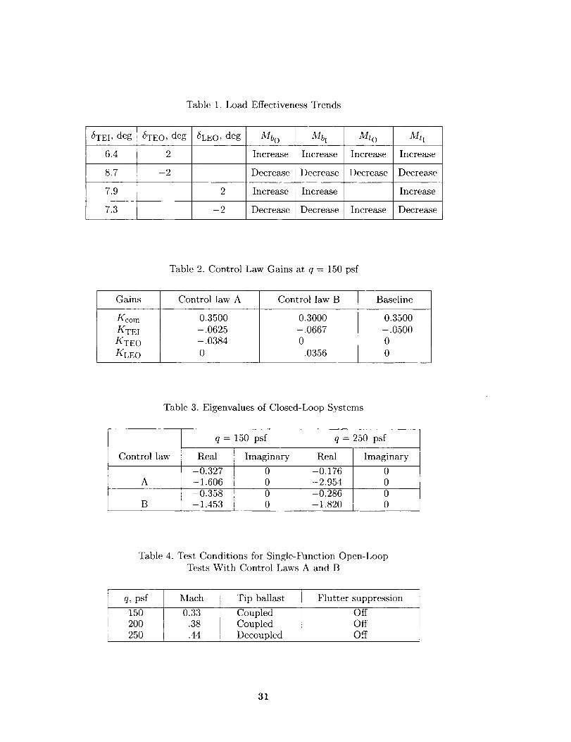
Table 1. Load Effectiveness Trends
5TEI, deg 6TEO, deg _LEO, deg Mbo _lbi A.fto ]Ilti
6.4 2 Increase Increase Increase Increase
8.7 --2 Decrease Decrease Decrease Decrease
7.9 2 Increase Increase Increase
7.3 -2 Decrease Decrease Increase Decrease
Table 2. Control Law Gains at q = 150 psf
Gains Control law A Control law B Baseline
_com
KTEI
KTEO
KLEO
0.3500
-.0625
-.0384
0
0.3000
-.0667
0
.0356
0.3500
-.0500
0
0
Table 3. Eigenvalues of Closed-Loop Systems
q = 150 psf q = 250 psf
Controllaw Real Imaginary Real Imaginary
-0.327 0 -0.176 0
A -1.606 0 -2.954 0
B-0.286 0
-1.820 ] 0
Table 4. Test Conditions for Single-Function Open-LoopTests With Control Laws A and B
q, psf Mach Tip ballast Flutter suppression
150 0.33 Coupled Off200 .38 Coupled Off
250 .44 Decoupled Off
31

Table 5. Test Conditions for Multiple-Function TestsWith Control Law B
q, psf
250260
Mach
0.44.45
Tip ballast
CoupledCoupled
Flutter suppression
On
On
Table 6. Steady-State Loads at Start of Rolling Maneuvers (90 ° )
Dynamicpressure, psf Wing TMO, in-lb TMI, in-lb BMO, in-lb BMI, in-lb
150 Left 69.6 - 1932.9 800.8 6207.3
Right 377.3 - 1261.1 789.9 4555.3Average magnitude 223.4 1597.0 795.4 5381.3
200 Left 54.5 - 2378.7 964.2 7394.6
Right 415.0 - 1585.1 948.7 5434.0Average magnitude 234.8 1981.9 956.5 6414.3
250 Left 40.4 -2712.3 1052.2 8401.5Right 469.7 - 2016.0 1155.1 6322.4
Average magnitude 255.1 2364.2 1103.7 7362.0
Table 7. Static Load Limits
Load limits for--
Wing TMO, in-lb TMI, in-lb BMO, in-lb BMI, in-lb
Left 1627.0 8929.0 4099.0 20 965.0
Right 1425.0 9434.0 3546.0 18 084.0Minimum 1425.0 8929.0 3546.0 18 084.0
Table 8. Percent Change in Peak Incremental Loads Relative to Baseline Load Limits
for Control Laws Having Nearly the Same Performance Time at q = 200 psf
Time to roll
90 ° , see
Peak incremental loads for--
TMO, in-lb TMI, in-lb BMO, in-lb BMI, in-lb
Baseline 0.65 495.1 1565.0 185.7 352.2RMLA A 0.66 359.6 747.1 638.0 403.8
Percent change from baseline -27.4 -52.3 243.6 14.7RMLA B 0.645 265.6 885.8 259.5 408.6
Percent change from baseline -46.4 -43.4 39.7 16.0
32

Table 9. Percent Change in Peak Incremental Loads Relative to Minimum Static Load
Limits for Control Laws Having Nearly the Same Performance Time at q = 200 psf
Time to roll
90 °, see
Peak incremental loads for--
TMO, in-lb
495.1Baseline 0.65
RMLA A 0.66 359.6 747.1
Percent change relative to limit -9.5 -9.2RMLA B 0.645 265.6 885.8
Percent change relative to limit - 16.1 - 7.6
TMI, in-lb
1565.0BMO, in-lb BMI, in-lb
185.7 I 352.2638.0 403.8
12.8 0.3
259.5 408.62.1 0.3
Table 10. Peak Incremental Loads From Experimental Data for Baseline
Dynamic
pressure, psf
150
150
150
200
200
200
250
250250
250
Control
law
Baseline
Baseline
Baseline
Baseline
BaselineBaseline
Time to roll
90 °, sec
0.670
.705
.825
0.575
.650
.805
Peak incremental loads for--
TMO, in-lb
391.6
343.7
304.3
580.0
495.1
394.1
TMI, in-lb
1206.0
1102.0
988.9
1829.0
1565.0
1256.0
I
BMO, in-lb
180.9
164.9
118.1
282.1
185.7
130.8
BMI, in-lb
313.6
342.2
413.0
423.3
352.2
459.9
BaselineBaseline
Baseline
Baseline
0.555
.645
.665
.795
719.1
636.2544.4
506.7
2239.0
1803.0
1617.01497.0
312.5
269.0
244.8168.4
414.7
363.1
460.4429.1
150 A 0.675 308.4 679.5 493.8 313.3
150 A .695 300.7 699.5 488.4 361.8
150 A .805 263.4 523.2 415.4 279.2
200 A 0.635 376.3 628.5 731.1 442.7
200 A .660 359.6 747.1 638.0 403.8
200 A .770 302.1 570.6 551.3 341.2
250 A 0.600 405.0 776.0 915.4 560.0250 A .640 394.4 741.1 825.2 590.6
250 A .735 335.2 615.9 696.8 486.6
150 B 0.650 251.1 858.1 250.8 334.6
150 B .675 225.6 787.2 234.4 307.6
150 B .780 178.0 684.7 164.8 455.7
200 B 0.615 279.0 1064.0 294.3 450.1
200 B .645 265.6 885.8 259.5 408.6
200 B .740 205.1 772.9 217.7 547.3
250 B 0.630 293.4 909.1 328.0 366.2250 B .740 218.0 821.1 230.1 498.4
250 B .770 226.4 700.4 240.5 531.0
33

Table 11. Peak Incremental Loads for RMLA Control Laws With
Interpolated Baseline Maneuver Loads
(a) RMLA control law A
Dynamic
pressure, psf
150
150
150
200
200
200
25O
250
25O
Time to roll
90 °, sec
0.675
.695
.805
0.635
.660
.770
0.600
.640
.735
TMO, in-lb
Peak incremental loads for--
TMI, in-lb BMO, in-lb
A Baseline a Control
178.6 493.8
169.5 488.4
125.9 415.4
205.0 731.1
182.2 638.0
143.2 551.3
290.8 915.4
271.4 825.2
203.7 696.8
BMI, in-lb
A Baseline a Control A
317.7 313.3
334.0 361.8
401.2 279.2
366.4
359.1
435.6
388.9
366.0
443.5
Baseline a Control
384.8 308.4
357.4 300.7
310.9 263.4
512.1 376.3
488.6 359.6
416.9 302.1
677.7 405.0
640.8 394.4
i 524.1 335.2
A iBaseline a Control
1191.1 679.5
1131.7 699.5
1007.8 523.2
1617.8 628.5
1545.1 747.1
1325.8 570.6
2021.0 776.0
1827.2 741.1
1552.4 615.9
442.7
403.8
341.2
560.0
590.6
486.6
(b) RMLA control law B
Dynamic
,pressure, psf
150
150
150
200
20O
200
25O
250
25O
a Interpolated.
Time to roll
90 °, sec
0.650
.675
.780
0.615
.645
.740
0.630
.740
.770
TMO, in-lb
Baseline a Control
419.0 251.1
384.8 225.6
319.1 178.0
534.7 279.0
500.8 265.6
436.5 205.1
650.0 293.4
522.7 218.0
514.0 226.4
Peak incremental loads for--
B
TMI,
:Baseline a
1265.4
1191.1
1031.3
1688.2
1582.6
1385.6
in-lb
Control B
858.1
787.2
684.7
1064.0
885.8
772.9
BMO, in-lb BMI,Baseline a Control B Baseline a
1875.7
1547.8
1520.1
909.1
821.1
700.4
190.0 250.8
178.6 234.4
135.7 164.8
230.7 294.3
192.1 259.5
153.8 217.7
276.2 328.0
200.7 230.1
183.1 240.5
297.3
317.7
386.5
385.4
356.9
414.7
371.7
442.3
435.1
in-lb
Control B
334.6
307.6
455.7
450.1
408.6
547.3
366.2
498.4
531.0
34

c.
, ._,"
I 'I
I'g_g_Nr
I
F-" ,
E-
¢3_
_7
_ _:_ _ i __ m
._ ,g.
.7.
i __q _
li_ _ " _ _ I_ " I_ "i
I I f
I
I I I.ill
__ ._
35

_0 _ C_.I i_ _ ",_ C"_,1 _ Le_ i_ ¢_C_,_,.,,_!,,,_ _ _ !,-.,_ '_'_ _
._"_ ._1.: ,_,_ .,:__ _ _ _ ,,,-_ _,--_ .,-,-_ !",_5_'._ ',_ _ _ _ _I,.--_ ,,,--_ _
L
©
m
_'_'_'__'_
© _,_,_,__,_
._-_.__'_'_ _o'_
..,..C
o , .,o , .,o . .ro . .0 . .,0 . .
C_
36

ORIGINAL PAGE:
BLACK AND WHITE PHOTOGRAPN
I
L-89-12442
(a) AFW model mounted in the Langley TDT prior to tests.
L-89-12446
(b) Multiple-exposure photograph showing the model at four different roll positions.
Figure 1. Photographs of the AFW model modified for the 1989 and 1991 wind tunnel tests and mounted in
the Langley Transonic Dynamics Tunnel.
37

-dO
,d
800
600
4OO
2OO
-2OO
-4OO
-600
-800
ssi
II |ii I
I
0
l',
i I %%
,l "'".,
i I I
I'" I..| I,• |
I" I'lI 11 iii
IP "..l_,
L7--_ Incremental load at to ," dy-state 1
°,,..°ol'"h.' j°
WI'I
J
fIb
II
I iI
' , I'"'.... I
, I',.' I I
to .25 .50 .75
Time, sec
1.00
(a) Load during rolling maneuver.
._e-6
--5¢-¢D
E_9
q_
800
600
400
200
to .25 .50 .75
Time, sec
(b) Incremental load during rolling maneuver.
Figure 2. Wing-load time history illustrating incremental load.
remental load
.Incrmen*a 1.00
38

control
Y
Trailing-edge outboard Sting mount
control surface
6 DOF force balance control surface_
Trailing-edgeinboard ] /,_" __x
Roll potentiometer
Accelerometer
Wingtipballast
Leading-edgecontrol surface
Leading-edge inboard
RVDT
Strain gauge pairs
(a) AFW model control surface locations and instrumentation.
X = 94.404
',X=87"141 ] X=98.682[] Control surface area _ Y = 51.962
Y = 49.462
Y = 34.645Wind tunnel
station X = 49.050[ __ 0_5c 7 IX= 113.867
65ft3.74in. Y=20.O00_' I [ I ' 1X=117.187X =-14.1671 X = 0.000 / ' v-_an,_l _1
xX = 66.667
X -- 66.097Z = 3.200
Z = 4.500
Z = 0.000
(b) Physical dimensions of AFW model with control surfaces delineated.
Figure 3. Schematics of AFW model control surface locations and instrumentation. All dimensions are in inchesunless otherwise specified.
39

L-90-12024
Figure4.Photographof actuatorandattachmentto wing.
Y = -10.0
f----" TMRI 1
Y = 0.00 //-----_ BMRI 1 13Strain gauge
[ II f--- BMRI2
Y=32.375 "_ Y[10.0 , f/f_fiTMRl2
Figure 5. AFW strain gauge locations. All dimensions are in inches. (From ref. 7.)
4O

Added
/-- Springballast / element
HU "li l-D
Hydraulic/ iL Pivot Added/actuator --" ballast---/
mechanism
Figure 6. Tip-ballast decoupler pylon.
AFWsimulation
Operator'sconsole
HostcPu
INTEGERDSP
(Real-TimeExecutor)
FloatingpointDSP
(Control lawprocessor)
Arrayprocessor(Backup
I-,Iooooooo18g °Ioistatus display
Filter box
Digital controllersystem
Figure 7. Schematic of AFW digital controller.
Interfaceelectronics
41

v
&rEo
AFW
plantmodel
Figure 8. Analysis structure for load effectiveness study.
3oL_____---..<i:--?'-....
9o \-210 L I ""r- _ I
0 .2 .4 .6 .8 1.0Time, sec
(a) t£ = 0.58 sec.
12°L.
40t _ , /
0 .4 .8 1.2 1.6 2.0Time, sec
(c) t F = 1.8 sec.
(_, ¢_,loadsr
2000
0
_-2000
0
-4000
r........................ ._.. --,. Mm
11.
'., Mxx .,.-" .............................
/ xf
/
Mp-6000 ----_--_ i i _____ i
0 .2 .4 .6 .8 1.0Time, sec
(b) Moment contributions for time to roll 90 ° oftF = 0.58 sec.
2000 _ ...................._ I000 " Mm
0¢)
EO ' '
r , /'
- 1000 I//, Mp
.2000 I _ .0 .4 .8 1.2
Time, sec
/
1.6 2.0
(d) Moment contributions for time to roll 90° oftF ----1.8 sec.
Figure 9. Simulated roll angle, roll rate, and moments for q = 150 psf with mass eccentricity.
42

e"N
3.0
2.0
1.0
x 103
'e
' "', Mm_
I I
0 1 2 3
tF, sec
Figure 10. Simulated pendulum rolling moment and control-surface rolling moment integral values at,
q = 150 psf.
35
30
25¢,.)
20,,_r
=_.- 15
10
//[_! Peak incremental• [] Steady load
, L/ /0
BMO BM1 TMO
Load
TMI
Figure 11. Design model steady load plus peak incremental load.
500 i
:_ 400e-
;- 300
-- = 200,-=¢d
100¢.)¢-
I
I
I
I
l- +TEO
I +LEO
--_ BASE
,_-- -TEOI
I
I
J I I
0 .5 1.0 1.5Time, sec
Figure 12. Incremental outboard bending moment generated during rolling maneuvers.
43

-__-J_'-I passfi,terI --/ _______.2Low I _EO__
pass filter ] "-
Low-pass filter
M t , M b
AFWplantmodel
Figure 13. RMLA control law structure.
v
r
i
II
ila
7
7,
1.8F_ I,,
t x_,\\ '_"-__-___
.4 19 °
.2
0 / I I _,/ I , A I-6.0 -2.0 0 2.0 6.0 10.0 14.0
Gain margin, kn, dB
I
18.0
Figure 14. Universal diagram for multiloop gain-phase margin evaluation. (Based on fig. 2 from ref. 14.)
44

e,.,
.d
E.
5OO
400
300
200
100
9O
8O
70
60
5o
40
30
2o
235 rpm limit(low speed windin_
1 i235 rpm limit, vane angle -- 2 °(low speed windings)
I lOpen-loop flutter q.
ballast coupled
• RMLA test point with tip ballast coupled
• RMLA test point with tip ballast decoupled
O RMLA test point with tip ballast coupledand FSS operating simultaneously
' r 1--26.1 mW (10 min time limit above)
I I I10.5 mW rotor limit mW (power limit) __
(High speed windings)
;,470 rpm limit (high speed windin
470 rpm limit, vane angle = 2_
0 .2 .3 .4 .5 .6 .7 .8 .9 1.0
Mach number
Figure 15. TDT flight envelope in air with RMLA test points identified.
1.1 1.2 1.3
45

ra,ocommand,
• !_com%apV :
RTS holds model at
initial trim angle
eL Peak hold roll rate
CLon and CLoff Ramp rates (slopes) for roll-rate command
t B
Ramp-on/holdcommand with
slope = _Lon
atF
!
! Ramp-off command
n!with slope = _Lof f
RMLA controller active
tcap
v
RTS active
_c = ¢cap
Figure 16. Roll-rate command structure. (From ref. 10.)
Roll-rate
command,
_)com
1.4
1.2
1.0 (nominal)
0.8
Figure 17. Command input scale factors.
46

.... Baselinecontrolled-- RMLAcontrolled- - Termination of control law
,=
50
0
-50
- 100
-150
-200
-250
i I i
II " " I " " --I
'_, I"t I
'k I'l I
'\ I"1 I• I
' I /'
,j.., [
.5 1.0 1.5
Time, sec
100
_0
._ 50A
0
-5O
I
I
o .; 1'.o 1.5Time, sec
200
._ 0e-_
C
_-200=E
_-400
(a) Roll rate.
-6000
' I I
_, /\/"J./'
i I _0.5 1. 1.5
Time, sec
1000
o.- 0
_E_o_E
. -lOOO
-200O
(b) Roll angle.
7- I T
I
0 .5 1.0 1.5
Time. sec
(c) Incremental outboard torsion moment. Peak
RMLA = 359.6 in-lb; Peak baseline = 495.1 in-lb.
1000
.¢z ..e_" 5O0
_2_ 0
g._=_ -5oo
- 1000
(d)
i i
_.. f-I -_
II
0 _ I '0• 1. 1.5 0
Time, sec
_& 500
.5_ 0
. .--
-5oo¢,.
Incremental inboard torsion moment. Peak
RMLA = 747.1 in-lb Peak baseline = 1565.0 in-lb.
1000 T I v
• . . , -
I
.s IL/___ .... ',,_/'1' 'l
II
- 1000.5 1.0 1.5
Time, sec
(e) Incremental outboard bending moment. Peak
RMLA = 638.0 in-lb Peak baseline = 185.7 in-lb.
(f) Incremental inboard bending moment. Peak
RMLA = 403.8 in-lb; Peak baseline = 352.2 in-lb.
Figure 18. RMLA control law A controlled-maneuver loads compared with baseline loads at q = 200 psf.
47

5O
0
_9
-50
-10o
= -150O
-200
-2500
400
"¢1 ,.t__-v 200_.--.
_= o
,_.£
_ -400
-6000
.5
I'
1.0 1.5
Time, sec
(a) Roll rate.
I
I
I
.\ i i
"'_. /.\flit_.�
I
.;' l'.OTime, sec
.5
.... Baseline controlled-- RMLA controlled- - Termination of control law
_D
0d
e-.
o
e,,
100
5O
0
-5O
i [
I
0 .5 ' l:0 1.5
Time, sec
(b) Roll angle.
1000
._ s: 500_'7
o.- 0
-5oo. -1oooo_ 1500
-20000
u I i
I
• I iI ¢'
_,. I ¢
"'-...__ It,.!I
i I i
.5 1.0 1.5
Time, sec
(c) Incremental outboard torsion moment. PeakRMLA = 265.6 in-lb; Peak baseline = 495.1 in-lb.
600
_ 200
e-,
o
._ -2oo
(d)
n i
[i( "
I
I r
1.0 1.5
Time, sec
Incremental inboard torsion moment. Peak
RMLA = 885.8 in-lb Peak baseline =1565.0 in-lb.
1000
._ 800
_=- 600
4oo__200
_.._ 0
-400 J -2000 .5 0
I /
hh ¢',
• t "_
I "1
[ \t
.;' l:0 1.5Time, sec
(e) Incremental outboard bending moment• PeakRMLA -- 259.5 in-lb; Peak baseline -- 185.7 in-lb.
(f) Incremental inboard bending moment. PeakRMLA = 408.6 in-lb; Peak baseline = 352.2 in-lb.
Figure 19. RMLA control law B controlled-maneuver loads compared with baseline loads at q -- 200 psf.
48

E_
e_
1000 -
0
• Baseline
[] RMLA A
243.6%
14.7%
TMO TMI BMO BMI
(a) t F --- 0.66 sec using control law A.
¢0"_
.zz_9
rt_
2000
1000
/
I 39.7%
TMO TMI BMO BMI
• Baseline
[] RMLA B
16.0%
(b) tF -- 0.645 sec using control law B.
Figure 20. Change in peak incremental loads for two RMLA-controlled maneuvers with performance times
similar to the baseline control law at q = 200 psf.
49
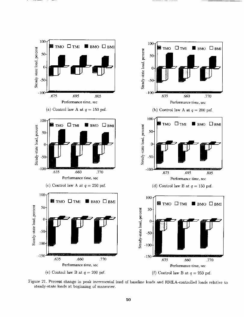
100-TMO []TMI • BMO []
.675 .695 .805Performancetime,sec
(a) ControllawA at q -- 150 psf.
TMO ['].TMI • BMO I--]BMI
.635 .660 .770
Performance time, sec
(b) Control law A at q = 200 psf.
TMO [] TMI roll BMO [] BMI]
.635 .660 .770
Performance time, sec
(c) Control law A at q = 250 psf.
100-
o O-
TMO []TMI • BMO []BMI
.675 .695 .805
Performance time, sec
(d) Control law B at q = 150 psf.
H
e-_
O
B TMO []TMI II BMO []BMI
.635 .660 .770
Performance time, sec
(e) Control law B at q = 200 psf.
100-
-150
IITMO []TMI • BMO []BMI
.635 .660 .770
Performance time, sec
(f) Control law B at q --- 250 psf.
Figure 21. Percent change in peak incremental load of baseline loads and RMLA-controlled loads relative to
steady-state loads at beginning of maneuver.
50

60
5O
40_9
_9
.-_Z30E
.4
20
10
/q
[] Control law peak incremental load[] Baseline peak incremental load
• Steady load
.615 .645 .740 .615 .645 .740
Performance time, sec Performance time, sec
(a) Torsion moment outboard. (b) Torsion moment inboard.
60 /
50 _-
'_ 40 _-
-_ 30 *-
I
220v
10 ,--
50-
40 -
e-,
•_ 30 - ,
q 20 - ,
10 - '
.615 .645 .740 .615 .645 .740
Performance time, sec Performance time, sec
(e) Bending moment outboard. (d) Bending moment inboard.
Figure 22. Steady load plus peak incremental relative to static load limits for baseline control law and control
law A at q = 200 psf.
51

60 _i
I50 -
40 -
.C 30 -
_20 _-1
10 -
6O
50
40
-=" 30.E_
2o
I0
/
dl
[] Control law peak incremental load[] Baseline peak incremental load
• Steady load
.615 .645 .740 .615 .645 .740
Performance time, sec Performance time, sec
(a) Torsion moment outboard. (b) Torsion moment inboard.
6O
5O
/
"_ 40 _-
•_ 30 _-._.
820 ;-.a
I
10 _-
o
50-
40 -
¢)" 30
.-,,
2 20 -
I0-
o,d.615 .645 .740 .615 .645 .740
Performance time, sec Performance time, sec
(c) Bending moment outboard. (d) Bending moment inboard.
Figure 23. Steady load plus peak incremental relative to static load limits for baseline control law and control
law B at q = 200 psf.
52

0
-2Oe-
(D
d -40¢13e.-
¢-
-60
-80
.55
_- i i _ I _ _ _ _ --D
.)
I I
.65 .75 .85
Performance time, sec
(a) Control law A, torsion moment outboard.
-20
¢,1
-40
e.-
e-.
-60
- 150 psf, experimental
# 250 psf, experimental
- - o. - - 150 psf, analytical
- -_ - - 250 psf, analytical
-80 I I
.55 .65 .75 .85
Performance time, sec
(b) Control law B, torsion moment outboard.
-2O
a..
-40
e-
-60
-80
.55
A
I I
.65 .75 .85
Performance time, sec
(c) Control law A, torsion moment inboard.
-20
e-
¢3
co
_'. -40 -¢J
e-
-60
¢. -O
-80. ! I
.55 .65 .75 .85
Performance time, sec
(d) Control law B, torsion moment inboard.
Figure 24. Analytical and experimental incremental load reductions.
53

©rrl
.2
2.0
0
-2.0
-4.0
-6.0
-8.0
I
_ v ix
0 .5 1.0 1.5 2.0
Time, sec
(a) LEO control surface deflection commanded by RMLA control law B.
_9
t_J
4"
6.0
4.0
2.0
0
-2.0
-4.0
-6.0
-8.00 .5 1.0 1.5 2.0
Time, sec
(b) TEI control surface deflection commanded by RMLA control law B.
eu0_9
©;zd
.3
.2
.1
0
-.1
-.2
-.3
-.4
0I I I
.5 1.0 1.5 2.0
Time, sec
(c) TEO control surface deflection commanded by flutter suppression control law.
Figure 25. Control surface activity during rolling maneuver with simultaneous implementation of RMLA andFSS control laws.
54

¢9
_9
E
0
l0
0
-10
-20
-30
-40
-500
?" -- Free fallI I i I I
1 2 3 4Time, sec
(a) Comparison of simulated roll rate with experi-
mental free-fall roll rate at q = 150 psf.
100
8O_303"_ 60_d
40
-- 200
_" 0
-200
I , I , I ,
1 2 3 4
Time, sec
(b) Comparison of simulated roll angle with experi-
mental free-fall roll angle at q = 150 psf.
0-moo"
"_,.__ -1200
7. -14oo
_-1600
,..3 -1800
--- Simulated
C/°
-2000 0 . I . I . i ,1 2 3 4
Time, sec
(c) Comparison of simulated left inboard torsion mo-ment with experimental free-fall inboard torsion
moment at q = 150 psf.
220e,,,,o 200
18o
,- 160
{i 140120
100-20.,_ _
0
-- Free fall, I , I , I ,
I 2 3 4
Time, sec
(d) Comparison of simulated left outboard torsion
moment with experimental free-fall outboard tor-
sion moment at q = 150 psf.
-1000e,-,
0
"_ .m -1200
•= -1400
-_ - 1600
-= -1800
-200(
--- Simulated
I , I , I ,
1 2 3 4
Time, sec
400e-
©
_ 360
-=.__. 320a.
28oO
._ _ 240
.__,v
--- Simulated-- Free fall
0"<;" , I , I , I ,
0 1 2 3 4
Time, sec
(e) Comparison of simulated right inboard torsionmoment with experimental free-fall inboard tor-
sion moment at q = 150 psf.
(f) Comparison of simulated right, outboard torsionmoment with experimental free-fall outboard tor-
sion moment at q -- 150 psf.
Figure 26. Comparison of simulated and flee-fall data.
55

5000Cat)
--= 5600
_--_ 5200
.e _ 4800¢" 0
__ E 4400
,d0_
0
_ ---- Simulated
1 2 3 4
Time, sec
(g) Comparison of simulated left inboard bendingmoment with experimental free-fall inboard bend-
ing moment at q = 150 psf.
800e,-,
_ 700
"- 600O
_E 5000
oE400
0 _0
I I , I ,
l 2 3 4
Time, sec
(h) Comparison of simulated left outboard bend-
ing moment with experimental free-fall outboard
bending moment at q = 150 psf.
5OOO
e-.
= x_ 4500a)-7
e-_
i 4000
--_ 3500e¢
0_0
--- Simulated
-- Free fall
I I , I ,
1 2 3 4Time, sec
900O1)e-
o=__ 80o
;_._- 700
= 600
--_ 500
0 _-0
--- Simulated-- Free fall
, I _ I , I ,
I 2 3
Time, sec
(i) Comparison of simulated right inboard bend-
ing moment with experimental free-fall outboard
bending moment at q = 150 psf.
(j) Comparison of simulated right outboard bend-
ing moment with experimental free-fall outboard
bending moment at q = 150 psf.
Figure 26. Concluded.
56


Form ApprovedREPORT DOCUMENTATION PAGEOMB No. 0704-0188
Public reporting burden for this collection of information is estimated to average 1 hour per response, including the time for reviewing instructions, searching existing data sources.gathering and maintaining the data needed, and completing and reviewing the collection of information Send comments regarding this burden estimate of any other aspect of thiscollection of information, including suggestions for reducing this burden, to Washington Headquarters Services, Directorate for Information Operations and Reports. 1215 JeffersonDavis Highway, Suite 1204, Arlington, VA 22202-4302, and to the Office of Management and Budget, Paperwork Reduction ProJect (0704-0188), Washington, DC 20503
1. AGENCY USE ONLY(Leave blank) 12. REPORT DATE 3. REPORT TYPE AND DATES COVERED
October 1994
4. TITLE AND SUBTITLE
Active Load Control During Rolling Maneuvers
6. AUTHOR(S)
Technical Paper
!S. FUNDING NUMBERS
WU 505-63-36-01
Jessica A. Woods-Vedeler, Anthony S. Pototzky, and Sherwood T. Hoadley
7. PERFORMING ORGANIZATION NAME(S) AND ADDRESS(ES)
NASA Langley Research Center
Hampton, VA 23681-0001
g. SPONSORING/MONITORING AGENCY NAME(S) AND ADDRESS(ES)
National Aeronautics and Space Administration
Washington, DC 20546-0001
8. PERFORMING ORGANIZATION
REPORT NUMBER
L-17053
10. SPONSORING/MONITORING
AGENCY REPORT NUMBER
NASA TP-3455
11. SUPPLEMENTARY NOTES
Woods-Vedeler and Hoadley: Langley- Research Center, Hampton, VA; Pototzky:Sciences Company, Hampton VA.
Lockheed Engineering &
12a. DISTRIBUTION/AVAILABILITY STATEMENT
Unclassified Unlimited
Subject Category 05
12b. DISTRIBUTION CODE
13. ABSTRACT (Maximum 200 words)
A rolling maneuver load alleviation (RMLA) system has been demonstrated on the Active Flexible Wing
(AFW) wind tunnel model in the Langley Transonic Dynamics Tunnel (TDT). The objective was to developa systematic approach for designing active control laws to alleviate wing loads during rolling maneuvers. Two
RMLA control laws were developed that utilized outboard control-surface pairs (leading and trailing edge) to
counteract the loads and that used inboard trailing-edge control-surface pairs to maintain roll performance.Rolling maneuver load tests were performed in the TDT at several dynamic pressures that included two
below and one 11 percent above the open-loop flutter dynamic pressure. The RMLA system was operated
simultaneously with an active flutter suppression system above open-loop flutter dynamic pressure. At alldynamic pressures for which baseline results were obtained, torsion-moment loads were reduced for both RMLA
control laws. Results for bending-moment load reductions were mixed; however_ design equations developed inthis study provided conservative estimates of load reduction in all cases.
14. SUBJECT TERMS
Aircraft; Rolling maneuver; Wind tunnel; Dynamic loads; Control system
17. SECURITY CLASSIFICATION
OF REPORT
Unclassified
NSN 7540-01-280-5S00
18. SECURITY CLASSIFICATION 19. SECURITY CLASSIFICATION
OF THIS PAGE OF ABSTRACT
Unclassified Unclassified
15. NUMBER OF PAGES
59
16. PRICE CODE
A04
20. LIMITATION
OF ABSTRACT
Standard Form 298(Rev. 2-89)Prescribed by ANSI Std Z39_18298-102
