active control for very flexible aircraft an ... · active control for very flexible aircraft an...
TRANSCRIPT

Active Control for Very Flexible AircraftAn Aeroservoelastic Modeling and Control Study
®:�9'õfvå;®ß6Ä/
Hugh H.T. Liu⇠”õ
University of TorontoInstitute for Aerospace Studies
Flight Systems and Control Laboratory
August 5, 2014
UTIAS
Introduction
Toronto ON Canada
• ⇢&⇢/†ˇ'â'e�Ññú�P=(â'eV�⌫∏ÑWâ'e0:⇥1
• ⇢&⇥∫„æ2,790,060�:†ˇ'�'Œ⇥�¶Öäù†Â⇣:⌫é,4'Œ⇥⇥
• �L⌦�'Ñ—ç-√K�⇥˝E'∫„, Õœ⇢C��49%Ñ∫„/(†ˇ'Â�fi�. ⇢&⇢S0ÑN® N‘∫„⇢æ€A⌥�¯S醡'h˝¶~⌃K�Ñ∫„⇥
1http://zh.wikipedia.org/Liu (UTIAS.FSC) www.flight.utias.utoronto.ca 05-Aug-2014 2 / 100

Introduction
University of Toronto⇢&⇢'f
f!Àé1827tÒ˝Tª€�Å⇤Ñá∂™‡�/ñ⌘ˆ„⌦†ˇ'�È˙ÀÑÿIfú⇥(f/ vπb�⇢&⇢'f�Ù⌅éÜHMn⇥vœ9�P>�˝∂YàVy�v˙Hœ œfœÜ:†ˇ'Kñ⇥É髪��™Ñ;Å!.⇧Ï—∞õ r∆fi�—�5Pw✏h�⇢πÊßÄ/�5P>Æ\��6T∆fi�fiLXc� —∞ñ*œ8¡Ñ—�⇥⇢&⇢'f/é˝'fO⇢≈$�(é˝,��⇣XK�⇥'fc∑˙�VÑYà∫p/†ˇ'�⇢Ñ⇥⇢&⇢'fœt—hÑ—∫ápœ(⌫é≈!é»['f��(pœME�LMî⇥
Liu (UTIAS.FSC) www.flight.utias.utoronto.ca 05-Aug-2014 3 / 100
Introduction
U of T Facts
67,000 undergraduate students (10,000 international), 16,000graduate students (2,500 international)China: 6,047Faculty Members: 12,500Research Funds: $1.2B530,000 alumniInternational Institution Ranking (2013): 20 (Times Higher Ed), 28(SJTU), 17 (QS World), and 8 (NTU)
Liu (UTIAS.FSC) www.flight.utias.utoronto.ca 05-Aug-2014 4 / 100

Introduction
!À (’⇢� Â�Yà)
Ì8��z®õf∂�-˝$9��CÀ
±���-˝∞„õf�î(pf`˙∫�-˝—fbbÎ�⌦w'f!�
ó∂ÿ�õf∂�î(pf∂�-˝—fb�MbÎ�MAfl° �˚∆¶‚⌃∫—U⇧
̘�Frederick Banting ��—;��õ —∞⇧�1923t˙��⌃f�;fVó;
}Bi�Norman Bethune �;fZÎ�∫S;I⇧�˝E;I⇧Úy�John Charles Fields �pf∂�ÚyV�À⇧p+·Ú—�Jeffrey Skoll �eBayl¯ñ˚;¡'q�Mark Henry Rowswell �W�(NíSŒ⇢∫Xó◊≤�~�!
HéÑ�ô/ Â,LK�X�✏Ù∂
N�w�ô/X
N◊ı�ô/X
Liu (UTIAS.FSC) www.flight.utias.utoronto.ca 05-Aug-2014 5 / 100
Introduction
U of T Engineering
5,241 undergraduate students, 1,933 graduate students238 faculty membersresearch funds: $63.5MTimes Higher Education World University Rankings forEngineering and Technology: 22nd (2014)Academic Departments, Divisions and Institutions
Institute for Aerospace Studies (UTIAS)Institute of Biomaterials and Biomedical Engineering (IBBME)Department of Chemical Engineering and Applied Chemistry(ChemE)Department of Civil Engineering (CivE)Division of Engineering ScienceDivision of Environmental Engineering and Energy SystemsDepartment of Electrical and Computer EngineeringDepartment of Mechanical and Industrial EngineeringDepartment of Materials Science and Engineering
Liu (UTIAS.FSC) www.flight.utias.utoronto.ca 05-Aug-2014 6 / 100

Introduction
UTIAS: Excellence in Research and Education
Recently awarded the Pioneer Award from the Canadian Air &Space Museum for its part in the rescue of Apollo 13Faculty have won numerous national and international awards,including three Members of the Order of CanadaGraduates play an important role in Canada’s aerospace sectorUniversity of Toronto Engineering Faculty ranked 18th in world in2013-14 (Times Higher Education: Engineering and Technology)UTIAS ranked among top 5 public aerospace departments inNorth America
Liu (UTIAS.FSC) www.flight.utias.utoronto.ca 05-Aug-2014 7 / 100
Introduction
UTIAS: Academic Unit in Aerospace Science andEngineering
19 full-time faculty membersUndergraduate teachingAerospace Option of Engineering ScienceProgram ( 35 graduating students)Graduate program (2013-14)56 M.A.Sc., 66 Ph.D., 25 M.Eng. studentsAeronautical Engineering
aircraft flight systems, propulsion,aerodynamics, computational fluiddynamics, and structural mechanics,sustainable aviation
Space Systems Engineeringspacecraft dynamics and control, space(mobile) robotics and mechatronics,and microsatellite technology
first human-powered ornithoptor
MOST microsatellite (2003)
Liu (UTIAS.FSC) www.flight.utias.utoronto.ca 05-Aug-2014 8 / 100

Introduction
Personal Experience
University EducationPh.D. (June 1998) University of TorontoM.A.Sc. (March 1994) Beihang University (BUAA)B.A.Sc. (July 1991) Shanghai Jiao Tong University
Experiences1998-2000, Systems Engineering/Lead, Honeywell Canada2000-05, Assistant Professor, UTIAS2006-12, Associate Professor, UTIAS2007, Visiting Professor, BUAA2006-07, Honeywell Engines and Systems2006-07, Visiting Scholar, Univ. of Michigan2006-07, Senior Research Fellow, City University of Hong Kong2008 - present, Associate Director, Graduate Studies, UTIAS2013 - present, Professor, UTIAS2009-15, Guest Professor (status only), BUAA2011-16, Guest Professor (status only), SJTU
Liu (UTIAS.FSC) www.flight.utias.utoronto.ca 05-Aug-2014 9 / 100
Introduction
Research Interests
Systems Modelling, Simulation and Control
• Fail-Safe Flight Control• Flexible Wing, Active Control• Landing Gear Systems (MBD)• Systems Sim., Integration
Multi-Vehicle Systems Estimation and Control• Motion-Sync Formation Flight• Vision-based Tracking• Wild Fire Monitoring
Autonomous UVS Applications• Localization and Mapping• Soaring and Surveillance• Border Patrolling
Liu (UTIAS.FSC) www.flight.utias.utoronto.ca 05-Aug-2014 10 / 100
Introduction
Today’s Talk: Outline
1 Introduction
2 Aircraft Flight Dynamics
3 Highly Flexible Wing with Active Control
4 Control Integrated MDO
5 Fault Tolerant Flight Control of Damaged Aircraft
6 Active Flutter Suppression
7 Integrated Flight Control and Simulation
Liu (UTIAS.FSC) www.flight.utias.utoronto.ca 05-Aug-2014 11 / 100
Aircraft Flight Dynamics
2. Aircraft Flight Dynamics I
An inertial Earth Surface Frame is defined with its originsomewhere on the surface and near the vehicle as much aspossible (so that a flat surface might be assumed in simplifyingdynamics analysis); axis z
~E directed vertically down; x
~E points
north, and y
~E east.
The air-trajectory reference frame is also called the wind axessystem. It has origin fixed to the vehicle (usually at the center ofmass), and x
~W is directed along the velocity vector v
~of the vehicle
relative to the atmosphere. The axis z
~W lies in the plane of
symmetry of the vehicle. If the atmosphere is at rest, then OWwould trace out the trajectory of the vehicle relative to the Earth,and x
~W would be always tangent to it.
Liu (UTIAS.FSC) www.flight.utias.utoronto.ca 05-Aug-2014 12 / 100
Aircraft Flight Dynamics
2. Aircraft Flight Dynamics II
Any set of axes fixed in a rigid-body is a body-fixed referenceframe (and the angular velocity of the frame is the same as that ofthe body). In flight vehicles, the origin is usually chosen at thecenter of mass, the axes x
~,z~
are chosen in the plane of vertical
symmetry, where z
~is directed downwards.
Liu (UTIAS.FSC) www.flight.utias.utoronto.ca 05-Aug-2014 13 / 100
Aircraft Flight Dynamics
The Vehicle Euler Angles I
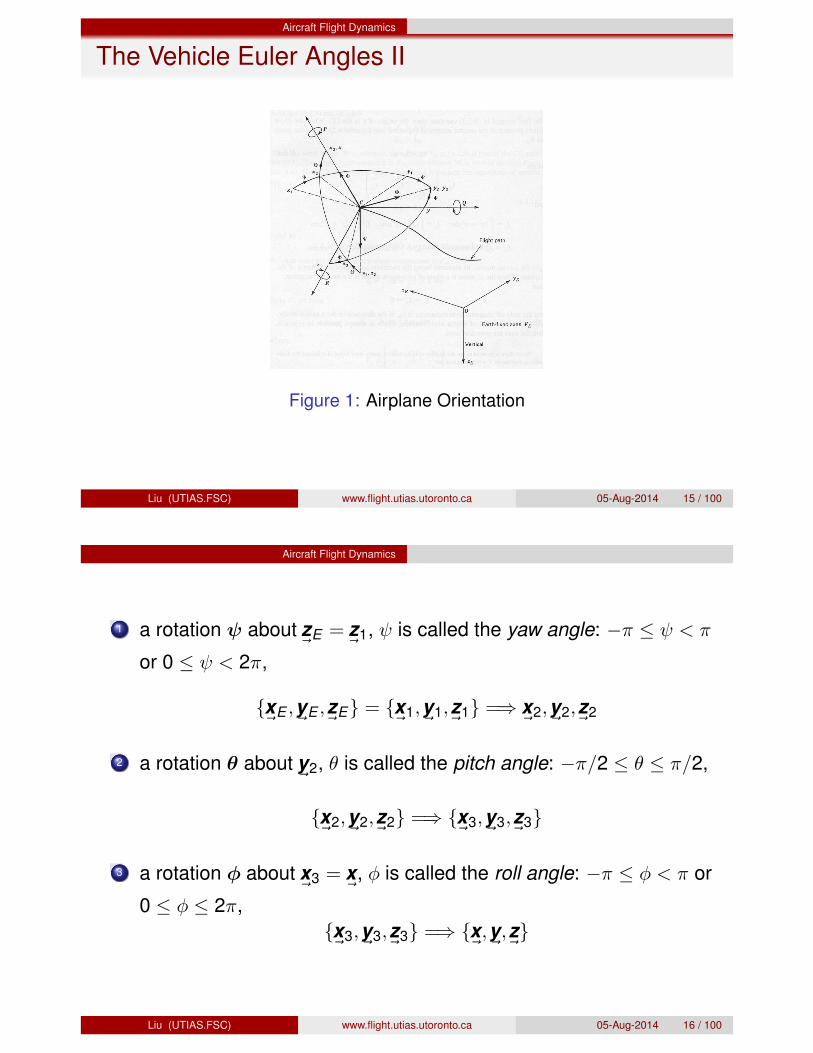
In flight dynamics, the Euler angles used are those which rotate theearth-surface frame FE into coincidence with the relevant axis system(frame), usually either FB or FW , denoted by ( , ✓,�) and (µ, �,�)respectively. Figure 1 shows the sequence of rotations.
Liu (UTIAS.FSC) www.flight.utias.utoronto.ca 05-Aug-2014 14 / 100
Aircraft Flight Dynamics
The Vehicle Euler Angles II
Figure 1: Airplane Orientation
Liu (UTIAS.FSC) www.flight.utias.utoronto.ca 05-Aug-2014 15 / 100
Aircraft Flight Dynamics
1 a rotation about z
~E = z
~1, is called the yaw angle: �⇡ < ⇡
or 0 < 2⇡,
{x
~E ,y~
E ,z~
E} = {x
~1,y~
1,z~
1} =) x
~2,y~
2,z~
2
2 a rotation ✓ about y
~2, ✓ is called the pitch angle: �⇡/2 ✓ ⇡/2,
{x
~2,y~
2,z~
2} =) {x
~3,y~
3,z~
3}
3 a rotation � about x
~3 = x
~, � is called the roll angle: �⇡ � < ⇡ or
0 � 2⇡,{x
~3,y~
3,z~
3} =) {x
~,y~,z~}
Liu (UTIAS.FSC) www.flight.utias.utoronto.ca 05-Aug-2014 16 / 100

Aircraft Flight Dynamics
The rotation matrix from FE to FB is given by
F~ B
= C
¯BEF~ E
(1)
where C
¯BE = C
¯1(�)C
¯2(✓)C
¯3( )
2
4
cos ✓ cos cos ✓ sin � sin ✓sin� sin ✓ cos � cos� sin sin� sin ✓ sin + cos� cos sin� cos ✓cos� sin ✓ cos + sin� sin cos� sin ✓ sin � sin� cos cos� cos ✓
3
5
(2)and C
¯EB
2
4
cos ✓ cos sin� sin ✓ cos � cos� sin cos� sin ✓ cos + sin� sin cos ✓ sin sin� sin ✓ sin + cos� cos cos� sin ✓ sin � sin� cos
� sin ✓ sin� cos ✓ cos� cos ✓
3
5
(3)
Liu (UTIAS.FSC) www.flight.utias.utoronto.ca 05-Aug-2014 17 / 100
Aircraft Flight Dynamics
Similarly, the rotation matrix from FE to FW is given by
F~W
= C
¯WEF
~ E(4)
where C
¯WE = C
¯1(µ)C
¯2(�)C
¯3(�).
1 a rotation � about z
~E = z
~1, � is called the heading angle,
{x
~E ,y~
E ,z~
E} = {x
~1,y~
1,z~
1} =) x
~2,y~
2,z~
2
2 a rotation � about y
~2, � is called the flight path angle,
{x
~2,y~
2,z~
2} =) {x
~3,y~
3,z~
3}
3 a rotation µ about x
~3 = x
~, µ is called the bank angle,
{x
~3,y~
3,z~
3} =) {x
~,y~,z~}
Liu (UTIAS.FSC) www.flight.utias.utoronto.ca 05-Aug-2014 18 / 100
Aircraft Flight Dynamics
The rotation matrix from FE to FB is given by
F~W
= C
¯WEF
~ E(5)
where C
¯WE = C
¯1(µ)C
¯2(�)C
¯3(�)
2
4
cos � cos� cos � sin� � sin �sinµ sin � cos� � cosµ sin� sinµ sin � sin� + cosµ cos� sinµ cos �cosµ sin � cos� + sinµ sin� cosµ sin � sin� � sinµ cos� cosµ cos �
3
5
(6)and C
¯EW
2
4
cos � cos� sinµ sin � cos� � cosµ sin� cosµ sin � cos� + sinµ sin�cos � sin� sinµ sin ✓ sin� + cosµ cos� cosµ sin ✓ sin� � sinµ cos�
� sin ✓ sinµ cos ✓ cosµ cos ✓
3
5
(7)
Liu (UTIAS.FSC) www.flight.utias.utoronto.ca 05-Aug-2014 19 / 100
Aircraft Flight Dynamics
The angular velocity of FB relative to the inertial frame FE is denotedby !
~B and is expressed by !
¯B = [p q r ]T . The angular velocity vector
following the Euler rotations are
!~
= z
~1 + ✓y
~2 + �x
~3 (8)
= [x~
3 y
~2 z
~1]
2
4
�
✓
3
5 (9)
Transform axes z
~1,y~
2,x~
3 to body frame axes x
~,y~,z~
, one obtains
x
~3 = x
~= [x~
y
~z
~]
2
4
100
3
5 (10)
y
~2 = y
~3 = cos�y
~� sin�z
~= [x~
y
~z
~]
2
4
0cos�
� sin�
3
5 (11)
Liu (UTIAS.FSC) www.flight.utias.utoronto.ca 05-Aug-2014 20 / 100
Aircraft Flight Dynamics
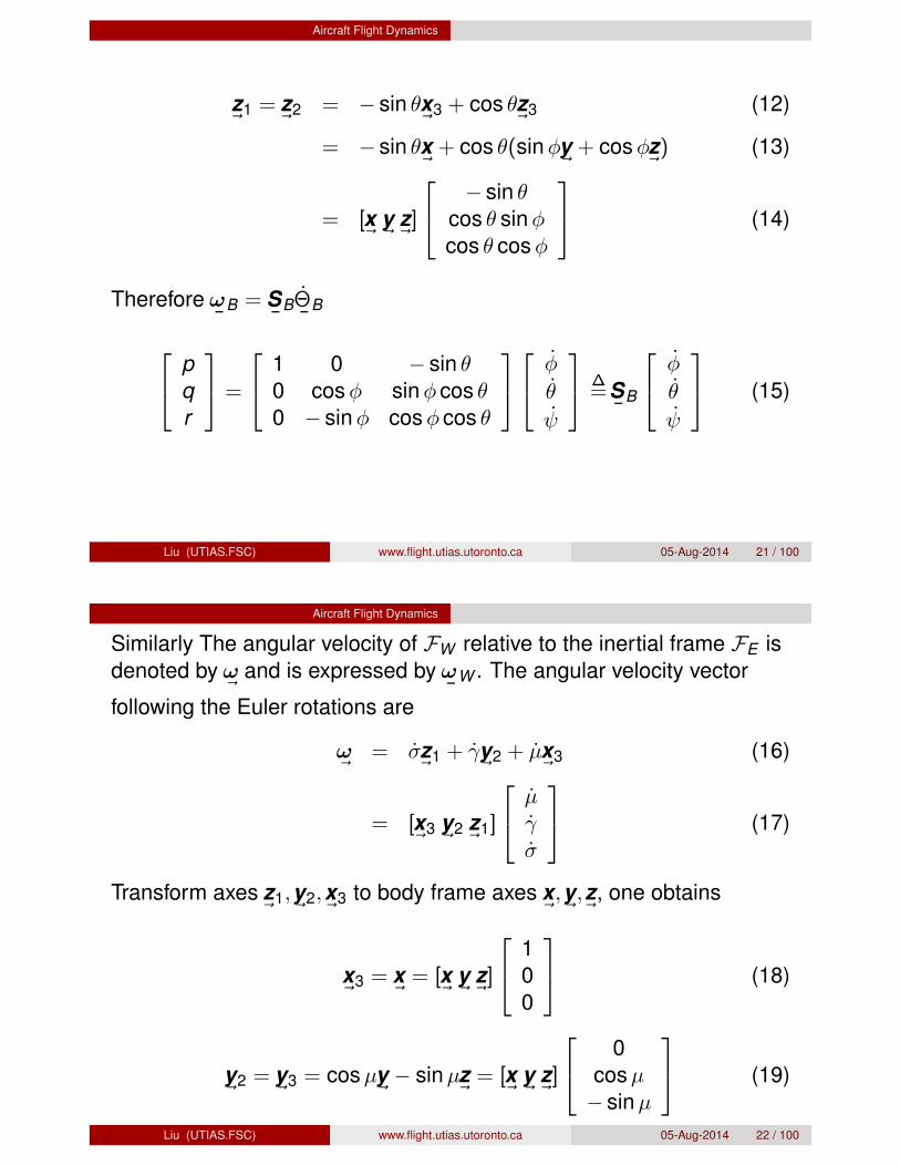
z
~1 = z
~2 = � sin ✓x
~3 + cos ✓z
~3 (12)
= � sin ✓x~+ cos ✓(sin�y
~+ cos�z
~) (13)
= [x~
y
~z
~]
2
4
� sin ✓cos ✓ sin�cos ✓ cos�
3
5 (14)
Therefore !¯
B = S
¯B⇥¯
B
2
4
pqr
3
5 =
2
4
1 0 � sin ✓0 cos� sin� cos ✓0 � sin� cos� cos ✓
3
5
2
4
�
✓
3
5
�=S
¯B
2
4
�
✓
3
5 (15)
Liu (UTIAS.FSC) www.flight.utias.utoronto.ca 05-Aug-2014 21 / 100
Aircraft Flight Dynamics
Similarly The angular velocity of FW relative to the inertial frame FE isdenoted by !
~and is expressed by !
¯W . The angular velocity vector
following the Euler rotations are
!~
= �z
~1 + �y
~2 + µx
~3 (16)
= [x~
3 y
~2 z
~1]
2
4
µ��
3
5 (17)
Transform axes z
~1,y~
2,x~
3 to body frame axes x
~,y~,z~
, one obtains
x
~3 = x
~= [x~
y
~z
~]
2
4
100
3
5 (18)
y
~2 = y
~3 = cosµy
~� sinµz
~= [x~
y
~z
~]
2
4
0cosµ
� sinµ
3
5 (19)
Liu (UTIAS.FSC) www.flight.utias.utoronto.ca 05-Aug-2014 22 / 100
Aircraft Flight Dynamics
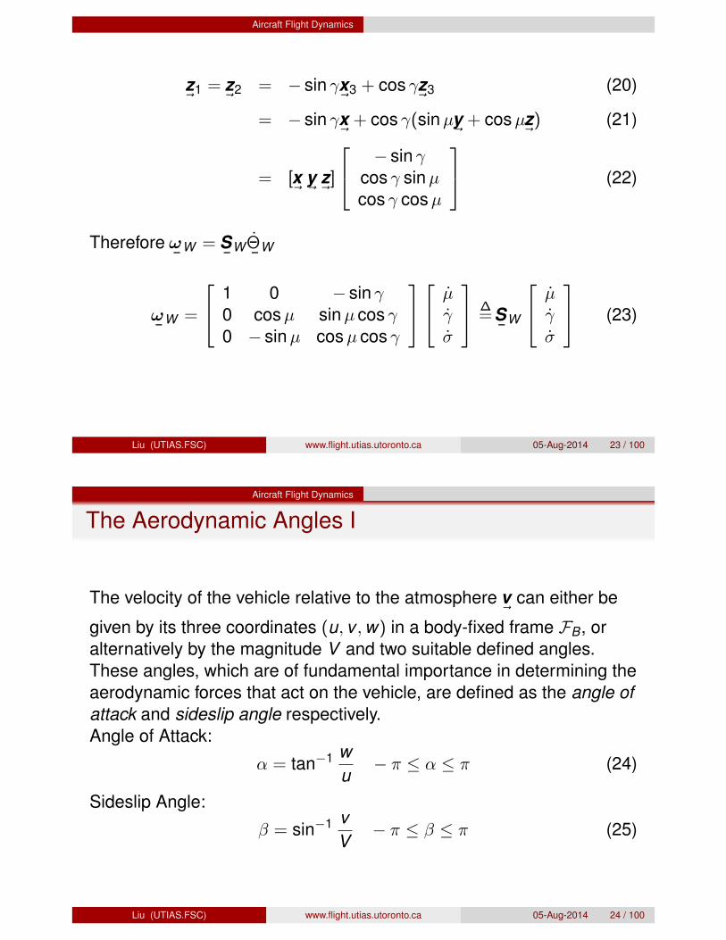
z
~1 = z
~2 = � sin �x
~3 + cos �z
~3 (20)
= � sin �x
~+ cos �(sinµy
~+ cosµz
~) (21)
= [x~
y
~z
~]
2
4
� sin �cos � sinµcos � cosµ
3
5 (22)
Therefore !¯
W = S
¯W⇥
¯W
!¯
W =
2
4
1 0 � sin �0 cosµ sinµ cos �0 � sinµ cosµ cos �
3
5
2
4
µ��
3
5
�=S
¯W
2
4
µ��
3
5 (23)
Liu (UTIAS.FSC) www.flight.utias.utoronto.ca 05-Aug-2014 23 / 100
Aircraft Flight Dynamics
The Aerodynamic Angles I
The velocity of the vehicle relative to the atmosphere v
~can either be
given by its three coordinates (u, v ,w) in a body-fixed frame FB, oralternatively by the magnitude V and two suitable defined angles.These angles, which are of fundamental importance in determining theaerodynamic forces that act on the vehicle, are defined as the angle ofattack and sideslip angle respectively.Angle of Attack:
↵ = tan�1 wu
� ⇡ ↵ ⇡ (24)
Sideslip Angle:� = sin�1 v
V� ⇡ � ⇡ (25)
Liu (UTIAS.FSC) www.flight.utias.utoronto.ca 05-Aug-2014 24 / 100

Aircraft Flight Dynamics
The Aerodynamic Angles II
It follows that the velocity components in the body-fixed frame arerepresented by
u = V cos� cos↵ (26)v = V sin� (27)w = V cos� sin↵ (28)
This relationship reveals the rotation matrix from FW to FB by thefollowing Euler rotation sequence: (��,↵, 0), i.e.
F~ B
= C
¯BWF
~W(29)
Liu (UTIAS.FSC) www.flight.utias.utoronto.ca 05-Aug-2014 25 / 100
Aircraft Flight Dynamics
The Aerodynamic Angles III
where
C
¯BW = C
¯1(0)C
¯2(↵)C
¯3(��)
=
2
4
cos↵ 0 � sin↵0 1 0
sin↵ 0 cos↵x
3
5
2
4
cos� � sin� 0sin� cos� 0
0 0 1
3
5
=
2
4
cos↵ cos� � cos↵ sin� � sin↵sin� cos� 0
sin↵ cos� � sin↵ sin� cos↵
3
5 (30)
Obviously, the velocity of the vehicle relative to the atmosphere v
~expression under FW is v
¯W = [V 0 0]T , and the formulas 26 - 28 can
be obtained by v
¯B = C
¯BWv
¯W .
Liu (UTIAS.FSC) www.flight.utias.utoronto.ca 05-Aug-2014 26 / 100

Aircraft Flight Dynamics
Force Equations in Trajectory Frame
Fromf
~= Wz
~E + Tx
~B � Dx
~W � Lz
~W (31)
one obtains
T � D � W sin � = mV (32)L cosµ � W cos � = mV � (33)
L sinµ = mV � cos � (34)
Liu (UTIAS.FSC) www.flight.utias.utoronto.ca 05-Aug-2014 27 / 100
Aircraft Flight Dynamics
Equations in Body-Fixed Frame I
Given the expressions under body-fixed frame FB : {x
~,y~,z~}:
f
¯B = [X Y Z ]T (35)
!¯
B = [p q r ]T (36)
v
¯B = [u v w ]T (37)
one gets the following force equation expressions:
f
¯B = m(v
¯B + !
¯Bv
¯B) (38)
Liu (UTIAS.FSC) www.flight.utias.utoronto.ca 05-Aug-2014 28 / 100

Aircraft Flight Dynamics
Equations in Body-Fixed Frame II
leading to
X = m(u + qw � rv) (39)Y = m(v + ru � pw) (40)Z = m(w + pv � qu) (41)
Given the expressions in Body-Fixed Frame FB:
⌧¯
cmB = [L M N]T (42)
I
¯B =
2
4
Ixx Ixy IxzIyx Iyy IyzIzx Izy Izz
3
5 (43)
According to⌧¯
B = !¯
BI
¯B!¯
B + I
¯B!¯
B (44)
Liu (UTIAS.FSC) www.flight.utias.utoronto.ca 05-Aug-2014 29 / 100
Aircraft Flight Dynamics
Equations in Body-Fixed Frame III
L = Ixx p + Ixy (q � pr) + Ixz(r + pq) + Iyz(q2 � r2) � (Iyy � Izz)qrM = Iyy q + Iyz(r � pq) + Iyx(p + qr) + Izx(r2 � p2) � (Izz � Ixx)prN = Izz r + Izx(p � qr) + Izy (q + pr) + Ixy (p2 � q2) � (Ixx � Iyy )pq
Liu (UTIAS.FSC) www.flight.utias.utoronto.ca 05-Aug-2014 30 / 100
Highly Flexible Wing with Active Control
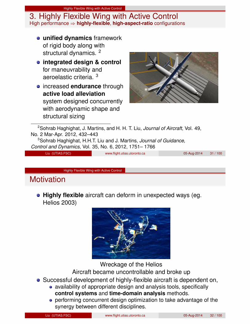
3. Highly Flexible Wing with Active ControlHigh performance ) highly-flexible, high-aspect-ratio configurations
unified dynamics frameworkof rigid body along withstructural dynamics. 2
integrated design & controlfor maneuvrability andaeroelastic criteria. 3
increased endurance throughactive load alleviationsystem designed concurrentlywith aerodynamic shape andstructural sizing
2Sohrab Haghighat, J. Martins, and H. H. T. Liu, Journal of Aircraft, Vol. 49,No. 2 Mar-Apr. 2012, 432–443
3Sohrab Haghighat, H.H.T. Liu and J. Martins, Journal of Guidance,Control and Dynamics, Vol. 35, No. 6, 2012, 1751– 1766
Liu (UTIAS.FSC) www.flight.utias.utoronto.ca 05-Aug-2014 31 / 100
Highly Flexible Wing with Active Control
Motivation
Highly flexible aircraft can deform in unexpected ways (eg.Helios 2003)
Wreckage of the HeliosAircraft became uncontrollable and broke up
Successful development of highly-flexible aircraft is dependent on,availability of appropriate design and analysis tools, specificallycontrol systems and time-domain analysis methods.performing concurrent design optimization to take advantage of thesynergy between different disciplines.
Liu (UTIAS.FSC) www.flight.utias.utoronto.ca 05-Aug-2014 32 / 100

Highly Flexible Wing with Active Control
Aeroservoelastic formulation
Rc
R
r
d
dm
FB
FI
R = Rc + r + d,V = R = Vc + ! ⇥ (r + d) + v.
Structural displacement and velocity expressed using shape functions,d = �
r
⇠ ) d = �r
⌘Liu (UTIAS.FSC) www.flight.utias.utoronto.ca 05-Aug-2014 33 / 100
Highly Flexible Wing with Active Control
Nonlinear equations of motion
2
4
mI3⇥3 X T1 S1
⇤ J S2 + X2⇤ ⇤ Mee
3
5
8
<
:
Vc!⌘
9
=
;
=
�
2
4
m! !X1T 2!S1
!X1 !J + J + VcX1T ! (S2 + X2)
�ST1 !
T R
� ⇢�rT !r T
d� 2R
� ⇢�rT !�rd� + Cee
3
5
8
<
:
Vc!⌘
9
=
;
�
2
4
O3⇥3 O3⇥3 O3⇥nO3⇥3 O3⇥3 O3⇥nOn⇥3 On⇥3
R
� ⇢�rT !2�rd� + Kee
3
5
8
<
:
Rc✓⇠
9
=
;
+
2
4
mCbiX1CbiST
1 Cbi
3
5
�
g
+
8
<
:
FMfe
9
=
;
S1 =R
� ⇢�rd�, S2 =R
� ⇢r�rd�Constant terms that depend on the shape functions and the rigid-bodymass distribution.
X1 =R
� ⇢g�r⇠d�, X2 =
R
� ⇢g�r⇠�rd�
Time-dependent terms that vary as the aircraft structure deforms.
R
� ⇢�Tr !
2�rd�Geometric stiffening, accounts for the coupling between the transverseand the axial deformations and the rigid-body rotational velocity.
J =R
� ⇢
g�r⌘⇣
r + f�r⇠⌘T
+⇣
r + f�r⇠⌘
g�r⌘T�
d�
Liu (UTIAS.FSC) www.flight.utias.utoronto.ca 05-Aug-2014 34 / 100

Highly Flexible Wing with Active Control
Nonlinear equations of motion
2
4
mI3⇥3 X T1 S1
⇤ J S2 + X2⇤ ⇤ Mee
3
5
8
<
:
Vc!⌘
9
=
;
=
�
2
4
m! !X1T 2!S1
!X1 !J + J + VcX1T ! (S2 + X2)
�ST1 !
T R
� ⇢�rT !r T
d� 2R
� ⇢�rT !�rd� + Cee
3
5
8
<
:
Vc!⌘
9
=
;
�
2
4
O3⇥3 O3⇥3 O3⇥nO3⇥3 O3⇥3 O3⇥nOn⇥3 On⇥3
R
� ⇢�rT !2�rd� + Kee
3
5
8
<
:
Rc✓⇠
9
=
;
+
2
4
mCbiX1CbiST
1 Cbi
3
5
�
g
+
8
<
:
FMfe
9
=
;
Liu (UTIAS.FSC) www.flight.utias.utoronto.ca 05-Aug-2014 35 / 100
Highly Flexible Wing with Active Control
Challenges in controlling a highly flexible aircraft
Traditional aircraft control: rigid-body tracking is performedseparately from structural control, and the interaction is avoided byusing notch filters.
1 A unified controller needs to address both rigid-body motion andthe aircraft flexibility.
2 Structural flexibility results in a time delay between the controlinput deflections and the rigid-body motion of the aircraft.,! Non-minimum phase system
3 High frequency structural modes are very lightly damped whichmakes the design of a state observer challenging.,! Filter’s transient response can adversely affect theclosed-loop stability and performance.
Liu (UTIAS.FSC) www.flight.utias.utoronto.ca 05-Aug-2014 36 / 100
Highly Flexible Wing with Active Control
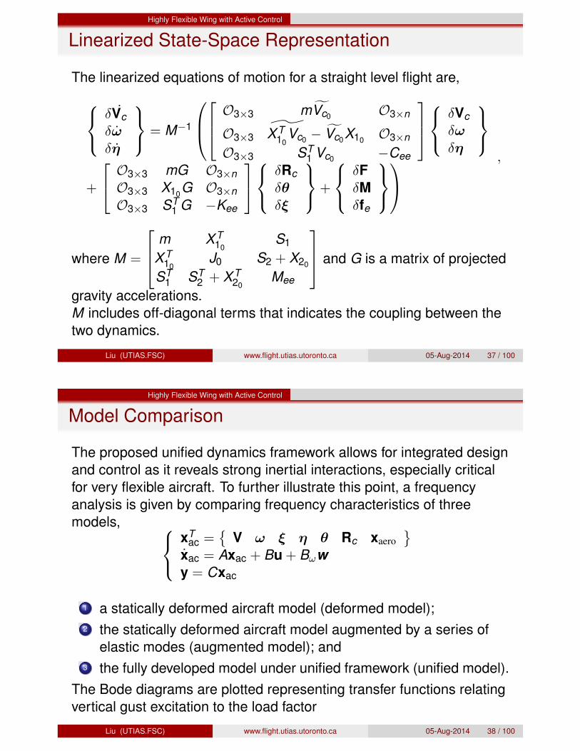
Linearized State-Space Representation
The linearized equations of motion for a straight level flight are,
8
<
:
�Vc�!�⌘
9
=
;
= M�1
0
B
@
2
6
4
O3⇥3 m fVc0 O3⇥n
O3⇥3 X T10
Vc0 � fVc0X10 O3⇥n
O3⇥3 ST1 Vc0 �Cee
3
7
5
8
<
:
�Vc�!�⌘
9
=
;
+
2
4
O3⇥3 mG O3⇥nO3⇥3 X10G O3⇥nO3⇥3 ST
1 G �Kee
3
5
8
<
:
�Rc�✓�⇠
9
=
;
+
8
<
:
�F�M�fe
9
=
;
1
A
,
where M =
2
6
4
m X T10
S1X T
10J0 S2 + X20
ST1 ST
2 + X T20
Mee
3
7
5
and G is a matrix of projected
gravity accelerations.M includes off-diagonal terms that indicates the coupling between thetwo dynamics.
Liu (UTIAS.FSC) www.flight.utias.utoronto.ca 05-Aug-2014 37 / 100
Highly Flexible Wing with Active Control
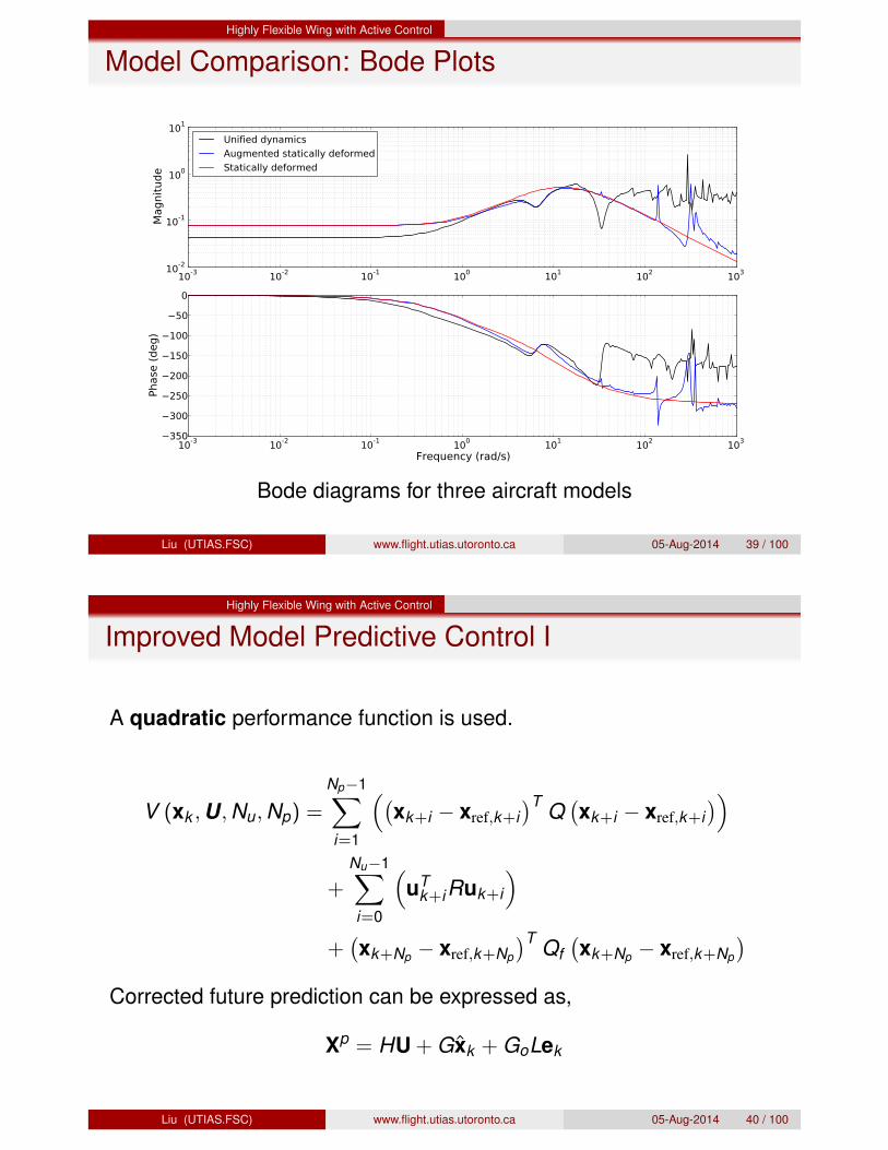
Model Comparison
The proposed unified dynamics framework allows for integrated designand control as it reveals strong inertial interactions, especially criticalfor very flexible aircraft. To further illustrate this point, a frequencyanalysis is given by comparing frequency characteristics of threemodels,
8
<
:
xTac =
�
V ! ⇠ ⌘ ✓ Rc xaero
xac = Axac + Bu + B!w
y = Cxac
1 a statically deformed aircraft model (deformed model);2 the statically deformed aircraft model augmented by a series of
elastic modes (augmented model); and3 the fully developed model under unified framework (unified model).
The Bode diagrams are plotted representing transfer functions relatingvertical gust excitation to the load factor
Liu (UTIAS.FSC) www.flight.utias.utoronto.ca 05-Aug-2014 38 / 100
Highly Flexible Wing with Active Control
Model Comparison: Bode Plots
Bode diagrams for three aircraft models
Liu (UTIAS.FSC) www.flight.utias.utoronto.ca 05-Aug-2014 39 / 100
Highly Flexible Wing with Active Control
Improved Model Predictive Control I
A quadratic performance function is used.
V (xk ,U,Nu,Np) =
Np�1X
i=1
⇣
�
xk+i � xref,k+i
�T Q�
xk+i � xref,k+i
�
⌘
+Nu�1X
i=0
⇣
uTk+iRuk+i
⌘
+�
xk+Np � xref,k+Np
�T Qf�
xk+Np � xref,k+Np
�
Corrected future prediction can be expressed as,
Xp = HU + Gxk + GoLek
Liu (UTIAS.FSC) www.flight.utias.utoronto.ca 05-Aug-2014 40 / 100

Highly Flexible Wing with Active Control
Improved Model Predictive Control II
Plantref
xk
uk
x
k+1
= Ad
x
k
+Bd
uk
+ L (xk
� x
p
k
)+
X = HU+Gx
k
+Go
Lek
min V (x0
,U, Nu
, Np
)w.r.t U
s.t. F.U c
yk
Linear/Nonlinear
Future state prediction
x
pk
Future inputoptimization
V (xk ,U,Nu,Np) = UT⇣
HT QH + R⌘
U
+ 2⇣
xTk GT + eT
k LT GTo � X
ref
⌘
QHU.
The developed controller is well suited to perform gust loadalleviation, an integral part of the aeroservoelastic optimization.
Liu (UTIAS.FSC) www.flight.utias.utoronto.ca 05-Aug-2014 41 / 100
Highly Flexible Wing with Active Control
Compact form matrices
H =
2
6
6
6
6
6
6
6
6
6
6
6
4
CdBdCdAdBd CdBd
... . . .CdANu�1
d Bd CdANu�2d Bd . . . CdBd
CdANud Bd CdANu�1
d Bd . . . CdAdBd... . . . ...
CdANp�1d Bd CdANp�2
d Bd . . .PNp�Nu
i=0 CdAidBd
3
7
7
7
7
7
7
7
7
7
7
7
5
, G =
2
6
6
6
4
AdA2
d...
ANpd
3
7
7
7
5
GTo =
h
I ATd Ad
2T · · ·i
F =
2
6
6
4
INu⇥m�INu⇥m
M�M
3
7
7
5
, c =
2
6
6
4
Umax�Umin
�Umax + b��Umax � b
3
7
7
5
, with M =
2
6
6
6
4
I�I I
. . . . . .�I I
3
7
7
7
5
and
bT =�
uk�1T 0 · · ·
Liu (UTIAS.FSC) www.flight.utias.utoronto.ca 05-Aug-2014 42 / 100

Highly Flexible Wing with Active Control
Gust Profile
For discrete gust evaluation, a (1 - cos) gust profile of the followingform is used:
wg =wg
2
✓
1 � cos2⇡Vt
Lg
◆
where wg is the maximum gust velocity, and Lg is the gust length.For continuous gust modelling, the Dryden model is used to createstochastic gust excitations. A gust filter is used to generate thenumerical values of gust,
Gw (s) = wg
r
L⇡V
1 +p
3Lv s
�
1 + LV s
�2 , Gq (s) =sV
�
1 +� 4b⇡V
�
s�Gw (s)
The parameter L represents the gust scale and V represents theaircraft flying speed.In this work, wg is set to 5 m/s for both continuous and discrete profiles.
Liu (UTIAS.FSC) www.flight.utias.utoronto.ca 05-Aug-2014 43 / 100
Highly Flexible Wing with Active Control
Stress-level reduction for the different controllersLg (s) 1.0 0.5 0.25MPC with PE 45.4% 43.9% 42.9%MPC 41.6% 37.7% 29.3%LQR 44.5% 37.9% 26.7%
Load factor and rigid-body parameters (Lg = 0.25s)Liu (UTIAS.FSC) www.flight.utias.utoronto.ca 05-Aug-2014 44 / 100
Highly Flexible Wing with Active Control
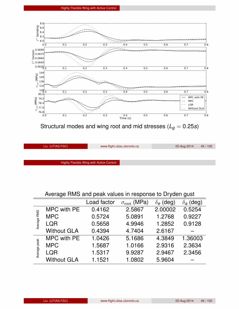
Structural modes and wing root and mid stresses (Lg = 0.25s)
Liu (UTIAS.FSC) www.flight.utias.utoronto.ca 05-Aug-2014 45 / 100
Highly Flexible Wing with Active Control
Average RMS and peak values in response to Dryden gustLoad factor �
root
(MPa) �e (deg) �a (deg)
Aver
age
RM
S MPC with PE 0.4162 2.5867 2.00002 0.5254MPC 0.5724 5.0891 1.2768 0.9227LQR 0.5658 4.9946 1.2852 0.9128Without GLA 0.4394 4.7404 2.6167 –
Aver
age
peak MPC with PE 1.0426 5.1686 4.3849 1.36003
MPC 1.5687 1.0166 2.9316 2.3634LQR 1.5317 9.9287 2.9467 2.3456Without GLA 1.1521 1.0802 5.9604 –
Liu (UTIAS.FSC) www.flight.utias.utoronto.ca 05-Aug-2014 46 / 100
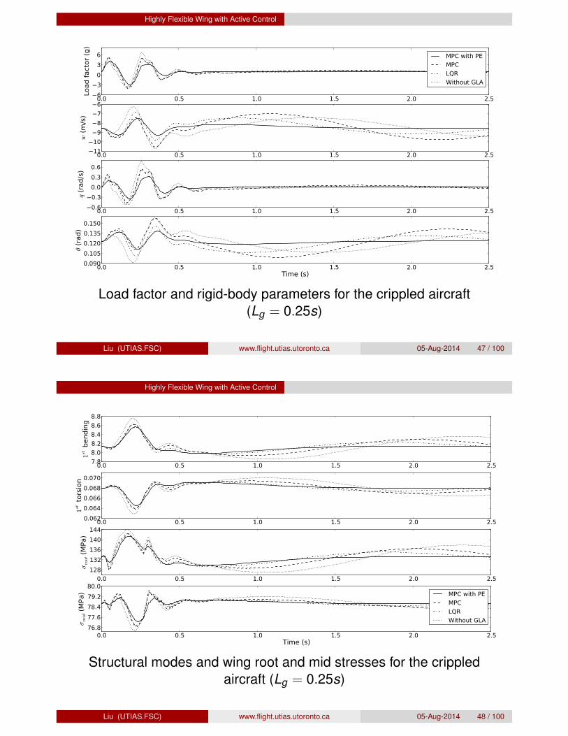
Highly Flexible Wing with Active Control
Load factor and rigid-body parameters for the crippled aircraft(Lg = 0.25s)
Liu (UTIAS.FSC) www.flight.utias.utoronto.ca 05-Aug-2014 47 / 100
Highly Flexible Wing with Active Control
Structural modes and wing root and mid stresses for the crippledaircraft (Lg = 0.25s)
Liu (UTIAS.FSC) www.flight.utias.utoronto.ca 05-Aug-2014 48 / 100

Highly Flexible Wing with Active Control
Average RMS and peak values in response to Dryden gust for crippledaircraft
Load factor �root
(MPa) �e (deg) �a (deg)Av
erag
eR
MS
MPC with P.E. 0.7128 4.9537 3.4353 1.4580LQR 0.9821 8.9246 2.5772 3.3027
Aver
age
peak
MPC with P.E. 1.9363 1.0473 7.6642 3.6368LQR 2.6036 2.0225 6.1842 7.6825
Haghighat et al., Journal of Guidance, Control, and Dynamics (2012)
Liu (UTIAS.FSC) www.flight.utias.utoronto.ca 05-Aug-2014 49 / 100
Highly Flexible Wing with Active Control
MPC Stability
Stabilizability and detectability + standard LQ infinite horizonoptimal control ) optimal stabilizing controller.A linear finite horizon model predictive controller with a quadraticperformance index is not asymptotically stabilizing in general.An LQ model predictive controller is stable if and only if the pair(A,B) is stabilizable, the pair
�
A,Q1/2� is observable, and the costmonotonicity condition, V (xk ,U⇤,N + 1) V (xk ,U⇤,N), issatisfied.
Terminal equality constraintsTerminal set constraintsTerminal penalty function
The first two approaches are very restrictive and reduce thefeasibility region.The terminal penalty approach is used,Qf � Q + K T RK + (Ad � BdK )T Qf (Ad � BdK )for some K 2 Rm⇥n.
Liu (UTIAS.FSC) www.flight.utias.utoronto.ca 05-Aug-2014 50 / 100

Highly Flexible Wing with Active Control
MP Controller Applied to a Non-minimum PhaseSystem
One of the difficulties of controlling a non-minimum phase systemis the internal instability problem.When a high performance level is of interest, the controller isforced to contain an implicit approximate inverse of the systemmodel.For non-minimum phase systems, this leads to the cancellation ofunstable poles and zeros causing internal instability.If no control and state constraints are considered, the optimalcontrol sequence can be calculated as follows,
U =⇣
HT QH + R⌘�1
HT Q (Gxk � Xref
)
If the control effort is not penalized (R = O), and the predictionand the control horizon are equal (H is a square matrix),U⇤ = H�1 (Gxk � X
ref
)Substituting the optimal control sequence into compact form )cancellation of unstable poles with unstable zeros that causes theinternal instability.Penalizing the control effort and also the application of a longerprediction horizon than the control horizon (tall H matrix) havebeen reported to avoid the internal instability.
Liu (UTIAS.FSC) www.flight.utias.utoronto.ca 05-Aug-2014 51 / 100
Highly Flexible Wing with Active Control
2-DOF control architecture
Kff
Kfb
Wg
!g
A/C
Ms
w
y
e
s
u
Ws
refu
�
�
y�
u�
Me
Ws
Wref
�
Wu
err
Wu, Wref
, We, and Ws are the frequency-domain weighting parameters
Liu (UTIAS.FSC) www.flight.utias.utoronto.ca 05-Aug-2014 52 / 100
Highly Flexible Wing with Active Control
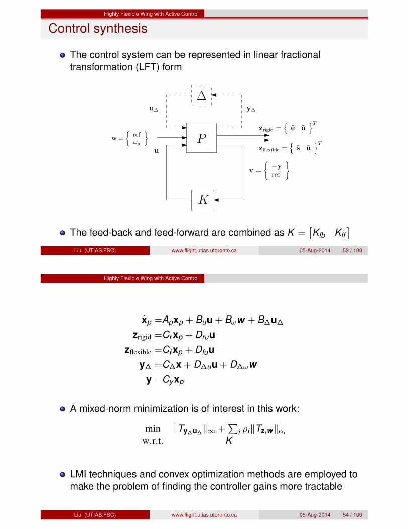
Control synthesis
The control system can be represented in linear fractionaltransformation (LFT) form
Pw =
⇢
ref!g
�
u
v =
(
�y
ref
)
y
�
K
z
flexible
=n
s u
oT
�u
�
z
rigid
=n
e u
oT
The feed-back and feed-forward are combined as K =⇥
Kfb Kff⇤
Liu (UTIAS.FSC) www.flight.utias.utoronto.ca 05-Aug-2014 53 / 100
Highly Flexible Wing with Active Control
xp =Apxp + Buu + B!w + B�u�
zrigid
=Cr xp + Druuz
flexible
=Cf xp + Dfuuy� =C�x + D�uu + D�!w
y =Cyxp
A mixed-norm minimization is of interest in this work:
min kTy�u�k1 +P
i ⇢ikTzi wk↵i
w.r.t. K
LMI techniques and convex optimization methods are employed tomake the problem of finding the controller gains more tractable
Liu (UTIAS.FSC) www.flight.utias.utoronto.ca 05-Aug-2014 54 / 100
Highly Flexible Wing with Active Control
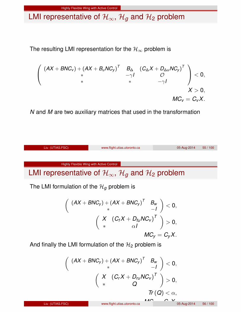
LMI representative of H1, Hg and H2 problem
The resulting LMI representation for the H1 problem is
0
@
(AX + BNCv ) + (AX + BuNCy )T B� (C�X + D�uNCy )
T
⇤ ��I O⇤ ⇤ ��I
1
A < 0,
X > 0,MCv = Cv X .
N and M are two auxiliary matrices that used in the transformation
Liu (UTIAS.FSC) www.flight.utias.utoronto.ca 05-Aug-2014 55 / 100
Highly Flexible Wing with Active Control
LMI representative of H1, Hg and H2 problem
The LMI formulation of the Hg problem is
✓
(AX + BNCy ) + (AX + BNCy )T Bw
⇤ �I
◆
< 0,✓
X (Cf X + DfuNCv )T
⇤ ↵I
◆
> 0,
MCy = CyX .
And finally the LMI formulation of the H2 problem is
✓
(AX + BNCy ) + (AX + BNCy )T Bw
⇤ �I
◆
< 0,✓
X (Cr X + DruNCv )T
⇤ Q
◆
> 0,
Tr (Q) < ↵,
MCv = Cv X .Liu (UTIAS.FSC) www.flight.utias.utoronto.ca 05-Aug-2014 56 / 100

Highly Flexible Wing with Active Control
Optimal control problem
The control design problem can be casted as follows,
min. � +P
i ⇢i↵iw.r.t. X ,Ns.t. LMIs
The X and N matrices are found by solving the above problem,the M matrix can be found by solving MCy = CyXThe controller gain has the following form,
K = NM�1
The above LMI problems are casted in semi-definite programmingform and solved using CVXOPT
Liu (UTIAS.FSC) www.flight.utias.utoronto.ca 05-Aug-2014 57 / 100
Highly Flexible Wing with Active Control
Uncertainty modelling
A = Ao + A1�v + A2�2v where �V = V�Vo
0.2Voand �V 2 [�1, 1]
The actual plant dynamics:
xac =⇣
A +P2
i=1 �iv Ai
⌘
xac +⇣
B +P2
i=1 �iv Bi
⌘
u +⇣
B!
+P2
i=1 �iv B
! i
⌘
w
y = Cxac
Using singular value decomposition (SVD)
xac = Axac + Bu + B!w
+⇥
B�1 B�2⇤
u�z }| {
�vIr1
�2vIr2
�
C�1 D�u1 D�w1
C�2 D�u2 D�w2
�
8
<
:
xacuw
9
=
;
| {z }
y�
where ri = rank
�⇥
Ai Bi B! i⇤�
.Liu (UTIAS.FSC) www.flight.utias.utoronto.ca 05-Aug-2014 58 / 100

Highly Flexible Wing with Active Control
Altitude maneuver results (V = 80 m/s)
0 5 10 15 20 25 30 35 40�0.8
0.0
0.8
1.6
2.4
3.2Lo
adfa
ctor
(g)
H2
H2/H1
0 5 10 15 20 25 30 35 40Time (s)
�30
0
30
60
90
120
Alti
tude
(m)
Liu (UTIAS.FSC) www.flight.utias.utoronto.ca 05-Aug-2014 59 / 100
Highly Flexible Wing with Active Control
Altitude maneuver results (V = 80 m/s)
0 5 10 15 20 25 30 35 40Time (s)
�6000000
�3000000
0
3000000
6000000
Mro
ot(N
m)
0 14(b/2) 1
2(b/2) 34(b/2) b/2
Span position
0
100
200
300
400
500
Max
.Stre
ss(M
Pa)
H2
H2/H1
Liu (UTIAS.FSC) www.flight.utias.utoronto.ca 05-Aug-2014 60 / 100
Highly Flexible Wing with Active Control
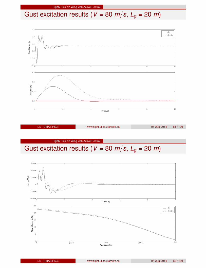
Gust excitation results (V = 80 m/s, Lg = 20 m)
0 2 4 6 8 10�3.0
�1.5
0.0
1.5
3.0
4.5Lo
adfa
ctor
(g)
H2
H2/H1
0 2 4 6 8 10Time (s)
0.0
0.2
0.4
0.6
Alti
tude
(m)
Liu (UTIAS.FSC) www.flight.utias.utoronto.ca 05-Aug-2014 61 / 100
Highly Flexible Wing with Active Control
Gust excitation results (V = 80 m/s, Lg = 20 m)
0 2 4 6 8 10Time (s)
�600000
�300000
0
300000
600000
900000
Mro
ot(N
m)
0 14(b/2) 1
2(b/2) 34(b/2) b/2
Span position
0
50
100
150
200
250
Max
.Stre
ss(M
Pa)
H2
H2/H1
Liu (UTIAS.FSC) www.flight.utias.utoronto.ca 05-Aug-2014 62 / 100

Highly Flexible Wing with Active Control
Altitude maneuver results (V = 96 m/s)
0 5 10 15 20 25 30 35 40�1
0
1
2
3Lo
adfa
ctor
(g)
H2
H2/H1
0 5 10 15 20 25 30 35 40Time (s)
�30
0
30
60
90
120
Alti
tude
(m)
Liu (UTIAS.FSC) www.flight.utias.utoronto.ca 05-Aug-2014 63 / 100
Highly Flexible Wing with Active Control
Gust excitation results (V = 68 m/s, Lg = 20 m)
0 2 4 6 8 10Time (s)
�4000000
�2000000
0
2000000
4000000
Mro
ot(N
m)
0 14(b/2) 1
2(b/2) 34(b/2) b/2
Span position
0
80
160
240
320
400
Max
.Stre
ss(M
Pa)
H2
H2/H1
3AIAA GNC 2011Liu (UTIAS.FSC) www.flight.utias.utoronto.ca 05-Aug-2014 64 / 100

Control Integrated MDO
4. Control Integrated MDOBaseline geometry
X
0
10
20Y
-30
-20
-10
0
10
20
Z
0
2
High aspect ratio UAV
Property ValueFuselage length 26.4 mWing span 58.6 mWing area 196 m
2
Wing taper ratio 0.48HT span 18 mHT area 53.5 m
2
HT taper ratio 0.7VT span 4 mVT area 8.9 m
2
VT taper ratio 0.81A NACA 4415 airfoil is used.Chord-wise location of the spar is set to 45% of the chordThe optimization is performed for a cruise speed of 80 m/s
Liu (UTIAS.FSC) www.flight.utias.utoronto.ca 05-Aug-2014 65 / 100
Control Integrated MDO
Multidisciplinary Design Optimization of a HighlyFlexible Aeroservoelastic Wing
x
0,7!1:Optimization
6 : x 2 : Swing
, AR, �i
3 : Swing
, AR, ti
5 : ⇢rigid
, ⇢elastic
7:Endurance,C
l,max
, �i
6:Function
evaluations
1,4!2:MDA
2 : ⇠target
L/D⇤ 6 : L/D
2:
3 : fe
5 : ↵o
, �e
o
W ⇤ 6 : W 4 : ⇠
3:
e1
e2
e3
t1
t2
t3
u1
u2
u3
X2
X1
d2
d1
5 : ⇠o
K⇤ 6 : A,B,C,D,K
5:
Kff
Kfb
Wg
!g
A/C
Ms
w
y
e
s
u
Ws
refu
�
�
y�
u�
Me
Ws
Wref
�
Wu
err
Liu (UTIAS.FSC) www.flight.utias.utoronto.ca 05-Aug-2014 66 / 100

Control Integrated MDO
Aerodynamic modelling
A three-dimensional unsteady aerodynamic panel code is used toobtain aerodynamic loads.The lifting surfaces are discretized using source and doubletpanels and the wake elements are represented by doublet panels.The combination of the Volterra theory with an eigensystemrealization algorithm is used to construct a ROM.Fidkowski et al. showed that, for a transport aircraft, gustencounters at typical flight conditions can be reasonablymodelled using quasi-steady aerodynamics assumption.
F
aero
=X
j
pj nj�Aj ,
M
aero
=X
j
r�
pj nj�
�Aj ,
f ei =X
j
�i |j pj nj�AjLiu (UTIAS.FSC) www.flight.utias.utoronto.ca 05-Aug-2014 67 / 100
Control Integrated MDO
ERA Algorithm
The recorded pulse responses, are the Markov parameters(Yk = CAk�1B) that are required by the ERA technique toreconstruct the state matrices.The algorithm is based on forming the r · p ⇥ s · m generalizedHankel matrix as,
Hrs (k � 1) =
2
6
6
6
4
Yk Yk+t1 . . . Yk+ts�1
Yk+j1 Yk+j1+t1 . . . Yk+j1+ts�1...
...Yk+jr�1 Yk+jr�1+t1 . . . Yk+jr�1+ts�1
3
7
7
7
5
where
ji (i : 1 ! r � 1) and ti (i : 1 ! s � 1) are arbitrary integers.Using singular value decomposition (SVD), Hrs (0) can bedecomposed into the following form, Hrs (0) = U⌃V T ,The size of the reduced order model can be determined using therank of Hrs (0) (number of singular values, ⌃, that are greater thanthe desired accuracy).A minimum realization,⇥
⌃�1/2UT Hrs (1)V⌃�1/2, ⌃1/2VEm, ETp U⌃1/2⇤ where
ETm =
⇥
Im Om · · · Om⇤
and ETp =
⇥
Ip Op · · · Op⇤
.
Liu (UTIAS.FSC) www.flight.utias.utoronto.ca 05-Aug-2014 68 / 100

Control Integrated MDO
Structural modelling
In the co-rotational formulation :A local coordinate system that translates and rotates with theelement to represent rigid-body motion.The local nodal variables represent the element’s strainingdeformations with respect to the local frame .This approach the geometric nonlinearities are captured throughthe rigid-body motion of the local frame and are shown in form oftransformation matrices.
X
12
14
16
Y
0
5
10
15
20
25
30
Z
0
2
4
Liu (UTIAS.FSC) www.flight.utias.utoronto.ca 05-Aug-2014 69 / 100
Control Integrated MDO
Co-rotational axes systems
e
1
e
2
e
3
t
1
t
2
t
3
u
1
u
2
u
3
X
2
X
1
d
2
d
1
E =⇥
e1 e2 e3⇤
is the local coordinate system .e1, is placed along the line that connects the first node to thesecond node.T =
⇥
t1 t2 t3⇤
and U =⇥
u1 u2 u3⇤
are the nodalcoordinates connected to the elements two end-nodes androtate as the element deforms.
Liu (UTIAS.FSC) www.flight.utias.utoronto.ca 05-Aug-2014 70 / 100

Control Integrated MDO
The local and global nodal variables
The local nodal variables for a 2-node 3-dimensional beam,
pTl =
�
ul ✓Tl1 ✓T
l2
ul represents the element elongation and is defined as ul =ln2�lo2
ln+lo✓
l1 and ✓l2 are pseudo-vectors that represent the rotation
transformation from the element coordinate, E , to the nodalcoordinates T and U
The global nodal variables are,
pTl =
�
dT1 ↵T dT
2 �T
↵T and �T are pseudo-vectors that represent the rotationtransformation from the inertial frame to the nodal coordinates Tand U
Liu (UTIAS.FSC) www.flight.utias.utoronto.ca 05-Aug-2014 71 / 100
Control Integrated MDO
Stiffness matrix derivation
pl = f (p,E)
Through differentiation of the above equation the variation of thelocal and global nodal variables can be related as follows:�pl = F�p where F T =
⇥
f1 f2 · · · f7⇤
Virtual work is equal in both frames,qi = F T qil
The local internal force is related to the local displacementthrough element stiffness matrix�qil = Kl�pl
Differentiating the force equation,�qi = F T �qil + �F T qil = (Ktl + Kt�) �p
where Ktl = F tKlF and Kt��p =P
j qil (j) �fj
Liu (UTIAS.FSC) www.flight.utias.utoronto.ca 05-Aug-2014 72 / 100

Control Integrated MDO
Aerostructural trim calculation
All derivatives and ! are set to zero, yielding,
Faero
+ Fprop
+ mCbig = 0M
aero
+ Mprop
+ X1Cbig = 0
�Kee (⇠) ⇠ + (S1)T Cbig + fe = 0
↵o
, �e
o
, ⇠o
Ltarget
MDA
1
6!22
2 : ⇠target
↵trim
, �e
trim
Aerodynamics(Trim calculator)
2
33 : f
e
⇠trim
6 : ⇠
NonlinearStructures
(Co-rotationalframework)
6
3
4
5! 4
4 : �(ST
1
Cbi
g + fe
)
5 : ⇠n+1
Internal solver(updates
displacement)
4
5
1
Aerostructural iterative solverLiu (UTIAS.FSC) www.flight.utias.utoronto.ca 05-Aug-2014 73 / 100
Control Integrated MDO
Optimization results
Optimization results with and without load alleviation system.Load alleviation Off OnSref (m2) 219.18 191.47 14.5% smallerAR 13.98 14.03L/D 34.29 34.37qelastic 1499.95 1499.88qrigid 90.63 75.71Wing mass (kg) 13,378 7,817 41.5% lighterEndurance factor 31.90 38.83 21.7% higher
Liu (UTIAS.FSC) www.flight.utias.utoronto.ca 05-Aug-2014 74 / 100

Control Integrated MDO
Thickness and twist distribution
0 14(b/2) 1
2(b/2) 34(b/2) b/2
0.02
0.04
0.06
0.08
0.10
t spa
r(m
)
Load Alleviation: ONLoad Alleviation: OFF
0 14(b/2) 1
2(b/2) 34(b/2) b/2
Span position
�8
�6
�4
�2
0
2
�(d
eg)
Liu (UTIAS.FSC) www.flight.utias.utoronto.ca 05-Aug-2014 75 / 100
Control Integrated MDO
Stress and maneuver constraints
0 1 2 3 4 5Time (s)
�2
�1
0
1
2
3
Load
fact
or(g
)
Load Alleviation: ONLoad Alleviation: OFF
0 14(b/2) 1
2(b/2) 34(b/2) b/2
Span position
0.0
0.6
1.2
1.8
2.4
3.0
Gus
t�m
ax(P
a)
⇥108
0 5 10 15 20 25 30 35 40Time (s)
1800
2100
2400
2700
3000
Alti
tude
(m)
0 14(b/2) 1
2(b/2) 34(b/2) b/2
Span position
0.0
0.6
1.2
1.8
2.4
3.0
Man
euve
r�m
ax(P
a) ⇥108
Liu (UTIAS.FSC) www.flight.utias.utoronto.ca 05-Aug-2014 76 / 100
Control Integrated MDO
Contributions
Developed a unified dynamics framework for modeling andsimulating highly flexible aircraft that has the following capabilities,
Independent of the structural representation.The framework allows for integrated control synthesis.
Developed two control techniques adept at controlling highlyflexible aircraft control.Applied the framework to two design cases: 1) control systemsimply worked towards achieving or maintaining a target altitude,2) control system was also performing load alleviation.
For a HALE UAV, the use of the active load alleviation systemresulted in a 21.7% improvement in the endurance.Load alleviation system in flying wing design optimization reducedpower by 2.4%, and the structural weight is lowered by17.4%.
Liu (UTIAS.FSC) www.flight.utias.utoronto.ca 05-Aug-2014 77 / 100
Fault Tolerant Flight Control of Damaged Aircraft
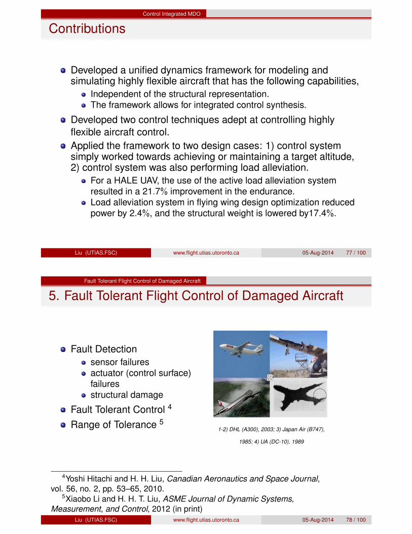
5. Fault Tolerant Flight Control of Damaged Aircraft
Fault Detectionsensor failuresactuator (control surface)failuresstructural damage
Fault Tolerant Control 4
Range of Tolerance 51-2) DHL (A300), 2003; 3) Japan Air (B747),
1985; 4) UA (DC-10), 1989
4Yoshi Hitachi and H. H. Liu, Canadian Aeronautics and Space Journal,vol. 56, no. 2, pp. 53–65, 2010.
5Xiaobo Li and H. H. T. Liu, ASME Journal of Dynamic Systems,Measurement, and Control, 2012 (in print)
Liu (UTIAS.FSC) www.flight.utias.utoronto.ca 05-Aug-2014 78 / 100
Fault Tolerant Flight Control of Damaged Aircraft
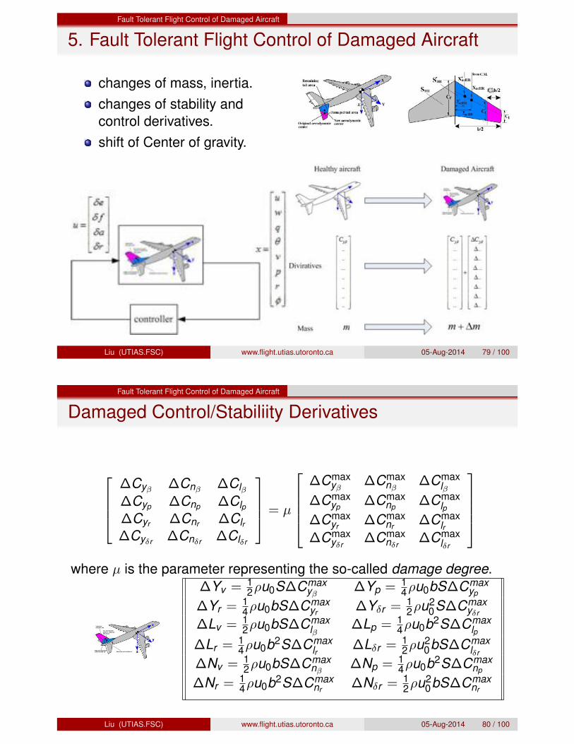
5. Fault Tolerant Flight Control of Damaged Aircraft
changes of mass, inertia.changes of stability andcontrol derivatives.shift of Center of gravity.
Liu (UTIAS.FSC) www.flight.utias.utoronto.ca 05-Aug-2014 79 / 100
Fault Tolerant Flight Control of Damaged Aircraft
Damaged Control/Stabiliity Derivatives
2
6
6
4
�Cy� �Cn� �Cl��Cyp �Cnp �Clp�Cyr �Cnr �Clr�Cy�r �Cn�r �Cl�r
3
7
7
5
= µ
2
6
6
6
4
�Cmaxy� �Cmax
n��Cmax
l��Cmax
yp �Cmaxnp �Cmax
lp�Cmax
yr �Cmaxnr �Cmax
lr�Cmax
y�r�Cmax
n�r�Cmax
l�r
3
7
7
7
5
where µ is the parameter representing the so-called damage degree.�Yv = 1
2⇢u0S�Cmaxy� �Yp = 1
4⇢u0bS�Cmaxyp
�Yr =14⇢u0bS�Cmax
yr �Y�r =12⇢u2
0S�Cmaxy�r
�Lv = 12⇢u0bS�Cmax
l� �Lp = 14⇢u0b2S�Cmax
lp�Lr =
14⇢u0b2S�Cmax
lr �L�r =12⇢u2
0bS�Cmaxl�r
�Nv = 12⇢u0bS�Cmax
n��Np = 1
4⇢u0b2S�Cmaxnp
�Nr =14⇢u0b2S�Cmax
nr �N�r =12⇢u2
0bS�Cmaxnr
Liu (UTIAS.FSC) www.flight.utias.utoronto.ca 05-Aug-2014 80 / 100

Fault Tolerant Flight Control of Damaged Aircraft
Modeling of Damaged Aircraft
Linear parameter dependent model:Define x(t) =
⇥
u w q ✓ v p r �⇤0 and
u(t) =⇥
�e �f �a �r⇤0
Healthy Aircraft:x(t) = Ax(t) + Bu(t)
Damaged aircraft:
x(t) = (A � µA)x(t) + (B � µB)u(t), µ 2 [0, 1]
where µ is the damage degree, which is related to the percentage oftail loss.
µ = 0 represents un-damaged caseµ = 1 represents the complete loss of vertical tail0 < µ < 1 represents partial loss of vertical tail
and look for the maximum tolerable damage degreeLiu (UTIAS.FSC) www.flight.utias.utoronto.ca 05-Aug-2014 81 / 100
Fault Tolerant Flight Control of Damaged Aircraft
Quadratic stabilizationPerformance requirement: maintain stabilityIn theory, a linear parameter-dependent system can be written as a polytopic system.Polytopic description:
x(t) = Ai x(t) + Bi u(t) 8 i = 1, 2, · · · ,N.
The N systems (45) can be quadratically stabilized, if there exists a positive definite matrix Q(Q > 0) and Y such that the following LMIs are satisfied(Boyd1994),
Ai Q + QA0i + Bi Y + Y 0B0
i < 0 8 i = 1, 2, · · · ,N.
controller isK = YQ�1
The aircraft system of our study can be treated in an N = 2 polytopic format to present healthyand faulty dynamics respectively,
A1 = A, A2 = A � µA, B1 = B, B2 = B � µB.
In order to set limits to control surfaces, the following LMI conditions with respect to Q and Y(Boyd1994) are also included
Q � W (45)
Q Y 0
Y ⇢2I
�� 0 (46)
where W = x(0)x(0)0 reflects the upper bound of the initial states, and ⇢ represents the actuatorlimits. Liu (UTIAS.FSC) www.flight.utias.utoronto.ca 05-Aug-2014 82 / 100
Fault Tolerant Flight Control of Damaged Aircraft
Bisection algorithm
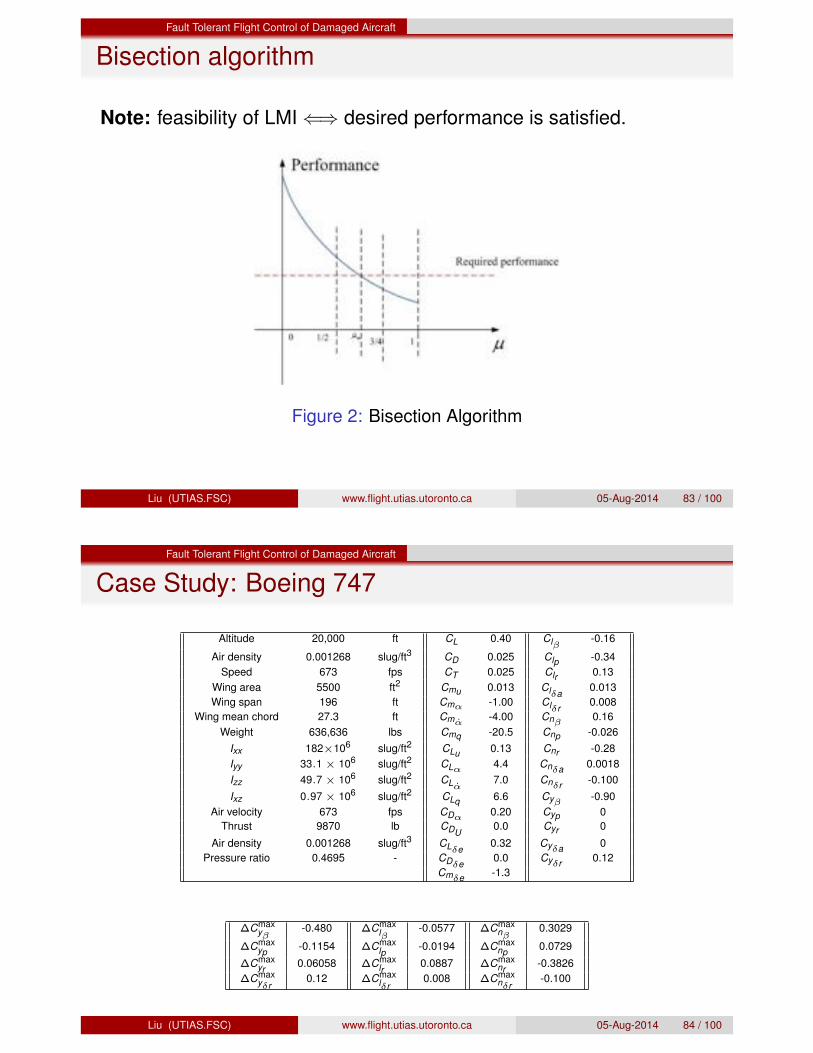
Note: feasibility of LMI () desired performance is satisfied.
Figure 2: Bisection Algorithm
Liu (UTIAS.FSC) www.flight.utias.utoronto.ca 05-Aug-2014 83 / 100
Fault Tolerant Flight Control of Damaged Aircraft
Case Study: Boeing 747
Altitude 20,000 ft CL 0.40 Cl�
-0.16
Air density 0.001268 slug/ft3 CD 0.025 Clp -0.34Speed 673 fps CT 0.025 Clr 0.13
Wing area 5500 ft2 Cmu 0.013 Cl�a 0.013
Wing span 196 ft Cm↵
-1.00 Cl�r 0.008
Wing mean chord 27.3 ft Cm↵
-4.00 Cn�
0.16Weight 636,636 lbs Cmq -20.5 Cnp -0.026
Ixx 182⇥106 slug/ft2 CLu 0.13 Cnr -0.28Iyy 33.1 ⇥ 106 slug/ft2 CL
↵
4.4 Cn�a 0.0018
Izz 49.7 ⇥ 106 slug/ft2 CL↵
7.0 Cn�r -0.100
Ixz 0.97 ⇥ 106 slug/ft2 CLq 6.6 Cy�
-0.90Air velocity 673 fps CD
↵
0.20 Cyp 0Thrust 9870 lb CDU
0.0 Cyr 0Air density 0.001268 slug/ft3 CL
�e 0.32 Cy�a 0
Pressure ratio 0.4695 - CD�e 0.0 Cy
�r 0.12Cm
�e -1.3
�Cmaxy�
-0.480 �Cmaxl�
-0.0577 �Cmaxn�
0.3029
�Cmaxyp -0.1154 �Cmax
lp-0.0194 �Cmax
np 0.0729�Cmax
yr 0.06058 �Cmaxlr
0.0887 �Cmaxnr -0.3826
�Cmaxy�r
0.12 �Cmaxl�r
0.008 �Cmaxn�r
-0.100
Liu (UTIAS.FSC) www.flight.utias.utoronto.ca 05-Aug-2014 84 / 100
Fault Tolerant Flight Control of Damaged Aircraft
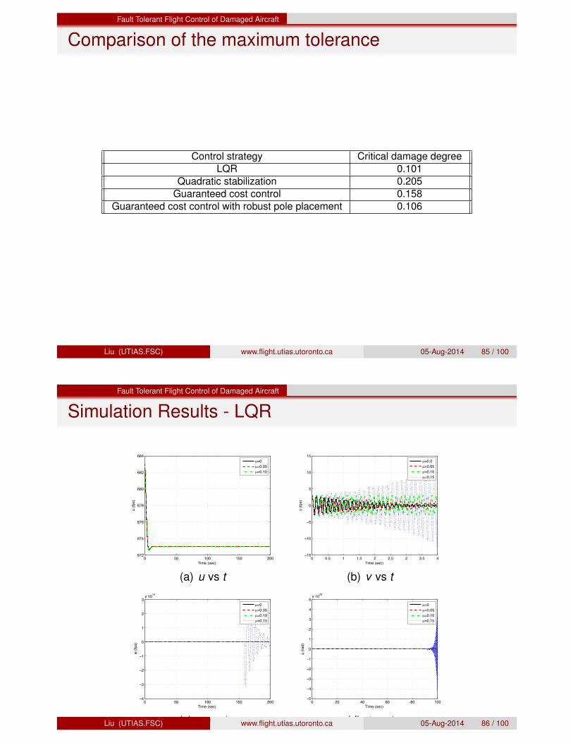
Comparison of the maximum tolerance
Control strategy Critical damage degreeLQR 0.101
Quadratic stabilization 0.205Guaranteed cost control 0.158
Guaranteed cost control with robust pole placement 0.106
Liu (UTIAS.FSC) www.flight.utias.utoronto.ca 05-Aug-2014 85 / 100
Fault Tolerant Flight Control of Damaged Aircraft
Simulation Results - LQR
0 50 100 150 200672
674
676
678
680
682
684
Time (sec)
u (
fps)
µ=0
µ=0.05
µ=0.10
(a) u vs t
0 0.5 1 1.5 2 2.5 3 3.5 4−15
−10
−5
0
5
10
15
Time (sec)
v (
fps)
µ=0.0
µ=0.05
µ=0.10
µ=0.15
(b) v vs t
0 50 100 150 200−4
−3
−2
−1
0
1
2
3x 10
16
Time (sec)
w (
fps)
µ=0
µ=0.05
µ=0.10
µ=0.15
(c) w vs t
0 20 40 60 80 100−5
−4
−3
−2
−1
0
1
2
3
4
5x 10
29
Time (sec)
! (
rad
)
µ=0
µ=0.05
µ=0.10
µ=0.15
(d) � vs tLiu (UTIAS.FSC) www.flight.utias.utoronto.ca 05-Aug-2014 86 / 100
Fault Tolerant Flight Control of Damaged Aircraft
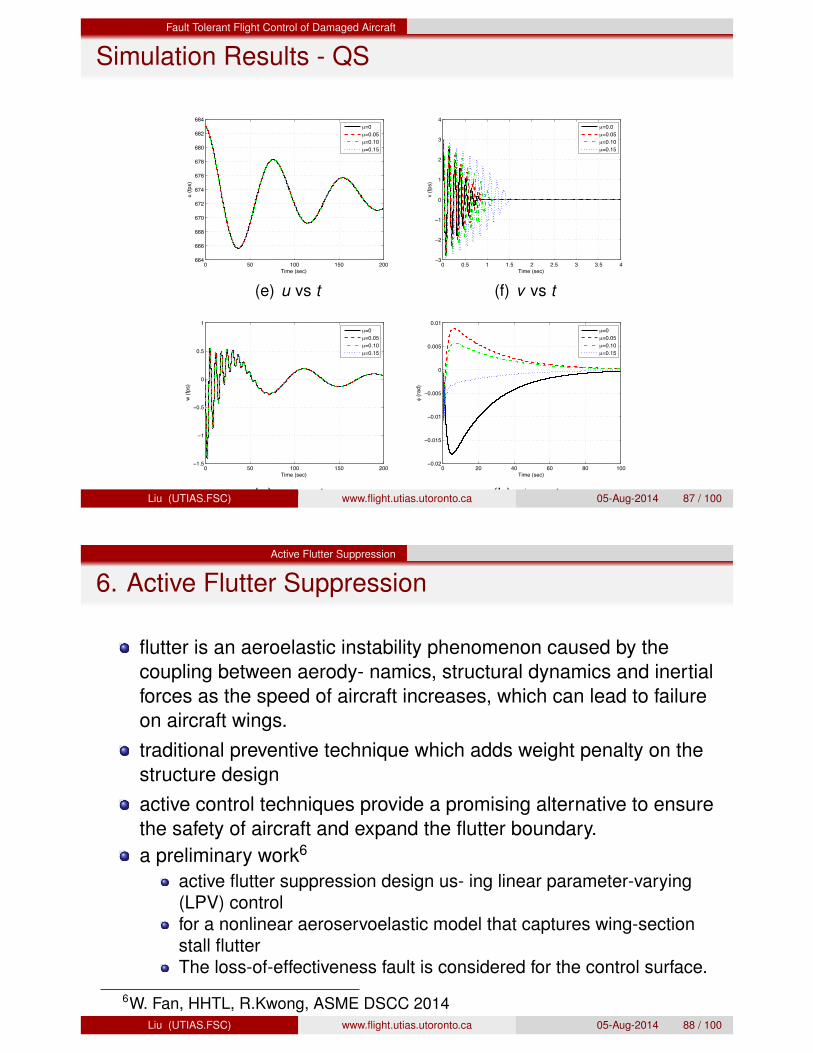
Simulation Results - QS
0 50 100 150 200664
666
668
670
672
674
676
678
680
682
684
Time (sec)
u (
fps)
µ=0
µ=0.05
µ=0.10
µ=0.15
(e) u vs t
0 0.5 1 1.5 2 2.5 3 3.5 4−3
−2
−1
0
1
2
3
4
Time (sec)
v (
fps)
µ=0.0
µ=0.05
µ=0.10
µ=0.15
(f) v vs t
0 50 100 150 200−1.5
−1
−0.5
0
0.5
1
Time (sec)
w (
fps)
µ=0
µ=0.05
µ=0.10
µ=0.15
(g) w vs t
0 20 40 60 80 100−0.02
−0.015
−0.01
−0.005
0
0.005
0.01
Time (sec)
! (
rad
)
µ=0
µ=0.05
µ=0.10
µ=0.15
(h) � vs tLiu (UTIAS.FSC) www.flight.utias.utoronto.ca 05-Aug-2014 87 / 100
Active Flutter Suppression
6. Active Flutter Suppression
flutter is an aeroelastic instability phenomenon caused by thecoupling between aerody- namics, structural dynamics and inertialforces as the speed of aircraft increases, which can lead to failureon aircraft wings.traditional preventive technique which adds weight penalty on thestructure designactive control techniques provide a promising alternative to ensurethe safety of aircraft and expand the flutter boundary.a preliminary work6
active flutter suppression design us- ing linear parameter-varying(LPV) controlfor a nonlinear aeroservoelastic model that captures wing-sectionstall flutterThe loss-of-effectiveness fault is considered for the control surface.
6W. Fan, HHTL, R.Kwong, ASME DSCC 2014Liu (UTIAS.FSC) www.flight.utias.utoronto.ca 05-Aug-2014 88 / 100

Active Flutter Suppression
Wing-Section Model
• the plunge motion h, the pitch motion✓ and the trailing-edge flap deflection�, which is used as the control sur-face.
• two linear spring constants are de-noted by kh and k✓ respectively.
• the points P, C, and Q denote theelastic center, the center of mass,and the aerodynamic center, respec-tively.
• the dimensionless parameters e anda represent the respective locationsof the points C and P from the beamreference line.
Liu (UTIAS.FSC) www.flight.utias.utoronto.ca 05-Aug-2014 89 / 100
Active Flutter Suppression
Equations of Motion
m mbx✓mbx✓ Ip
�
h✓
�
+
kh 00 k✓
�
h✓
�
=
�LT0 � L�
MT0 + M�
�
where m is the airfoil mass, Ip represents the moment of inertia aboutthe elastic axis, x✓ = e � a is the dimensionless distance between thecenter of mass and elastic axis. To account for the dynamic stall, theONERA model is used. The corrected unsteady lift and momentbecome
LT0 = ⇢U20 bCl0 + L0 + ⇢UT�L � CdUT (h + ab✓ � �0)
MT0 = 2⇢U20 b2Cm0 + M0 + 2⇢UT b�M
Aerodynamic lift and moment generated by the deflection of thetrailing-edge control surface � are
L� = 2⇡⇢bc1U2
M� = (12+ a)bL� + 2⇡⇢b2c2U2�
Liu (UTIAS.FSC) www.flight.utias.utoronto.ca 05-Aug-2014 90 / 100

Active Flutter Suppression
LPV Control
H2 gain-scheduled state-feedback control is designed for the LPVmodel subject to dynamic disturbances and control surfaceeffectiveness loss. Consider the following LPV system
x = A(U)x + B(✏)u + B1d
y = Cx
where d is exogenous disturbance signal, B1 = I , C = I . Let X (U, ✏)denote a parameter-dependent Lyapunov matrix. The H2 norm of theclosed-loop system is less than a prescribed value � if there existX = X
T and W = W
T satisfying
X (U, ✏) + AT
clX (U, ✏) + X (U, ✏)Acl X (U, ✏)BclBT
clX (U, ✏) �I
�
< 0
X (U, ✏) CT
clCcl W
�
> 0
Trace(W ) < �2
Liu (UTIAS.FSC) www.flight.utias.utoronto.ca 05-Aug-2014 91 / 100
Active Flutter Suppression
Simulation Results
NACA 0012 airfoil is chosen for study in this paper. The first LCOsare observed to emerge at U = 10.6m/s, which is lower than thelinearly estimated flutter point U = 11m/s.An LPV controller is synthesized over a grid region of schedulingparameters. The grid points are taken at speeds 10, 11, 12, 13, 14and 15m/s and control surface effectiveness factors 1, 0.8 and0.5. The bound of speed variation rate ⌫ = 1m/s
2. The LMIs aresolved for these grid points simultaneously. The resulting H2performance index is � = 8.207.Control input constraint is considered with the limit of controlsurface deflection set at ±15�.
Liu (UTIAS.FSC) www.flight.utias.utoronto.ca 05-Aug-2014 92 / 100

Active Flutter Suppression
0 2 4 6 8 10 12 14 16 18 20−0.5
0
0.5
1
Plun
ge (m
)
Closed−loop Open−loop
0 2 4 6 8 10 12 14 16 18 20−0.5
0
0.5
1
Pitc
h (ra
d)
Closed−loop Open−loop
0 2 4 6 8 10 12 14 16 18 20−10
0
10
Time (s)Flap
Def
lect
ion
(deg
)
Plunge and pitch responses at U=10.8 m/s when ✏ = 1.0
Liu (UTIAS.FSC) www.flight.utias.utoronto.ca 05-Aug-2014 93 / 100
Active Flutter Suppression
0 2 4 6 8 10 12 14 16 18 20−0.2
00.20.4
Plun
ge (m
)
Designed controller LQR controller
0 2 4 6 8 10 12 14 16 18 20−0.2
00.20.4
Pitc
h (ra
d)
Designed controller LQR controller
0 2 4 6 8 10 12 14 16 18 20−5
0
5
Time (s)Flap
Def
lect
ion
(deg
)
Plunge and pitch responses at U=12.6 m/s when ✏ = 0.5
Liu (UTIAS.FSC) www.flight.utias.utoronto.ca 05-Aug-2014 94 / 100
Active Flutter Suppression
0 2 4 6 8 10 12 14 16 18 20−0.5
00.5
11.5
Plun
ge (m
)
Designed controller LQR controller
0 2 4 6 8 10 12 14 16 18 20
0
0.5
1
Pitc
h (ra
d)
Designed controller LQR controller
0 2 4 6 8 10 12 14 16 18 20
−10
0
10
Time (s)Flap
Def
lect
ion
(deg
)
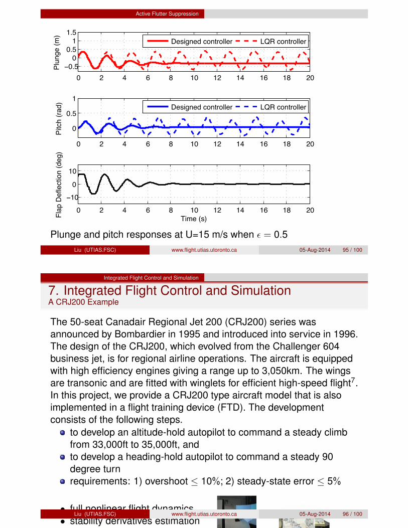
Plunge and pitch responses at U=15 m/s when ✏ = 0.5Liu (UTIAS.FSC) www.flight.utias.utoronto.ca 05-Aug-2014 95 / 100
Integrated Flight Control and Simulation
7. Integrated Flight Control and SimulationA CRJ200 Example
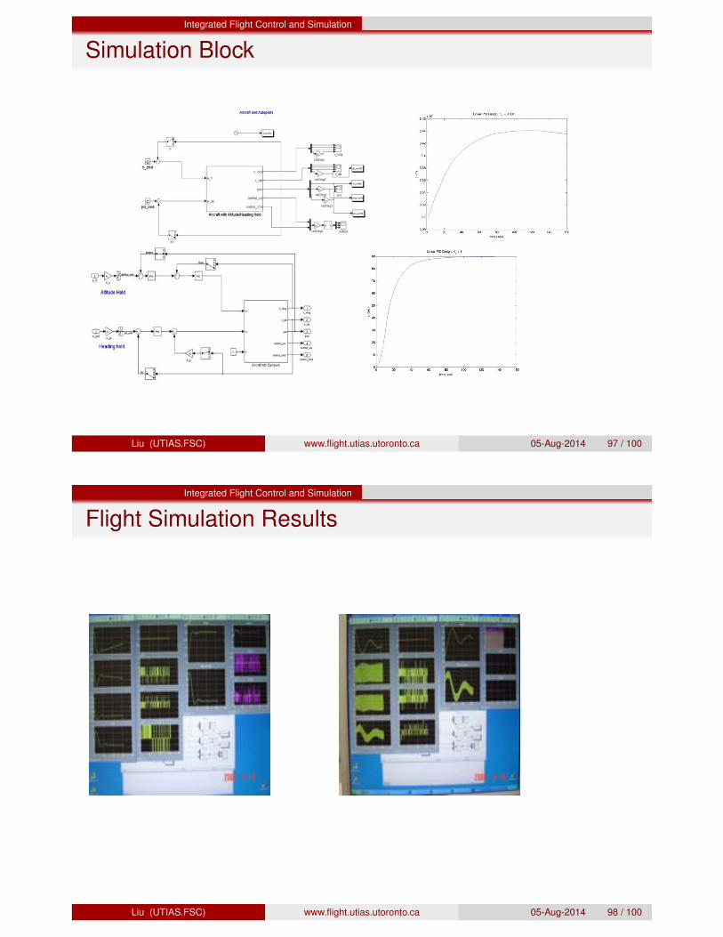
The 50-seat Canadair Regional Jet 200 (CRJ200) series wasannounced by Bombardier in 1995 and introduced into service in 1996.The design of the CRJ200, which evolved from the Challenger 604business jet, is for regional airline operations. The aircraft is equippedwith high efficiency engines giving a range up to 3,050km. The wingsare transonic and are fitted with winglets for efficient high-speed flight7.In this project, we provide a CRJ200 type aircraft model that is alsoimplemented in a flight training device (FTD). The developmentconsists of the following steps.
to develop an altitude-hold autopilot to command a steady climbfrom 33,000ft to 35,000ft, andto develop a heading-hold autopilot to command a steady 90degree turnrequirements: 1) overshoot 10%; 2) steady-state error 5%
• full nonlinear flight dynamics• stability derivatives estimation• linearization and control de-
sign• nonlinear simulation• flight training, cockpit checklist• flight simulation7www.aerospace-technology.com/projects/crj200/
Liu (UTIAS.FSC) www.flight.utias.utoronto.ca 05-Aug-2014 96 / 100
Integrated Flight Control and Simulation
Simulation Block
Liu (UTIAS.FSC) www.flight.utias.utoronto.ca 05-Aug-2014 97 / 100
Integrated Flight Control and Simulation
Flight Simulation Results
Liu (UTIAS.FSC) www.flight.utias.utoronto.ca 05-Aug-2014 98 / 100

Acknowledgement
Acknowledgement
Dr. Sohrab Haghighat (PhD 2012)Research Staff, MRI, Boston
Dr. Xiaobo Li (PDF 2011)
Dr. Ruben Perez (PhD 2007)Assist. Professor, RMC
Dr. Anton de Ruiter (PhD 2005)Assist. Professor, Ryerson U.
Ms. Wen Fan (PhD Candiate 2013 - )
Ms. Yan Zhang s (BUAA, Visiting 2009)
Dr. Peng Zhang O (HIT, Visiting 2009-11)
Liu (UTIAS.FSC) www.flight.utias.utoronto.ca 05-Aug-2014 99 / 100
Acknowledgement
Thank You
Prof. Hugh H.T. LiuUniversity of TorontoInstitute for Aerospace Studies4925 Dufferin StreetToronto, OntarioCANADA M3H 5T6Tel: 416-667-7928Email: [email protected]
Liu (UTIAS.FSC) www.flight.utias.utoronto.ca 05-Aug-2014 100 / 100